targeting core sampling with machine learning: case …

AEGC 2018: Sydney, Australia 1

TARGETING CORE SAMPLING WITH MACHINE LEARNING: CASE STUDY FROM THE SPRINGBOK SANDSTONE, SURAT BASIN Oliver Gaede * Mitchell Levy Queensland University of Technology Queensland University of Technology School of Earth, Environmental and Biological Sciences School of Earth, Environmental and Biological Sciences GPO Box 2434, Brisbane, QLD, 4001 GPO Box 2434, Brisbane, QLD, 4001 [email protected] [email protected] *presenting author asterisked

SUMMARY We show how clustering algorithms can ensure that the core intervals that are pertinent to specific objectives of a sampling campaign are actually sampled. We also show how clusters can be validated prior to sampling with auxiliary data not used for the cluster analysis. We chose to target our core sampling to ensure that both clay poor and clay rich intervals of the Springbok Sandstone are sampled. The clay phases in the Jurassic Springbok Sandstone generally do not exhibit a prominent gamma ray signature and are therefore poorly defined in wireline logs. Similar, hydrogeological properties of the Springbok Sandstone are not well defined through wireline logs. This introduces uncertainty to groundwater models of the Springbok Sandstone. Hence, a better understanding of the clay distribution is thought to be a key to improve the definition of the hydrogeological properties of the Springbok Sandstone. We applied our sample targeting approach to five study wells from the Surat Basin in Queensland. We tailored the application of the cluster analysis to our working hypothesis that the variability of hydrogeological properties of the Springbok Sandstone is controlled by the presence and type of clays, rather than compaction. This informed our choice of wireline logs to include in the clustering (nuclear logs) and of logs to be used for control purpose (resistivity logs, spontaneous potential). We show that identification of five clusters was the most useful number towards our sampling objectives. This allowed for example to exclude coal and siderite layers from sampling for clay analysis and to focus on the differentiation of the clastic sediments in the formation. Further, we show that certain clusters correlate with resistivity and spontaneous potential log signatures. The correlation between the categorical clusters based on nuclear logs and continuous wireline logs not used in the cluster analysis allowed us to interpret the meaning of the clusters in the context of our project and target our sampling to ensure that all clusters are represented in our sample set. Key words: Machine Learning, Cluster Analysis, Wireline Data, Clays, Surat Basin

INTRODUCTION This contribution is part of a larger project that aims to link wireline data, laboratory based clay characterisation and porosity and permeability measurements to build an integrated petrophysical model of the Springbok Sandstone. Coal seam gas production from the Walloon Coal Measures, Surat Basin, does necessitate a better understanding of the hydrogeological properties of the overlying Springbok Sandstone. The Late Jurassic Springbok Sandstone is a formation in the Surat Basin, Queensland (Power and Devine, 1968). According to the definition reference (Exon, 1976) “[t]hroughout the basin the sequence consists mainly of sandstone, with some interbedded siltstone and mudstone and a few thin seams of coal.” The type section in BMR Mitchell 3 (38m to 50m) consists mostly of feldspathic sublabile to lithic sandstones. Occurrence of interbedded siltstones and mudstones is described as minor (Green, 1997). Indeed, classical lithofacies identification based on density (RHOB) and natural gamma ray (GR) cutoffs results in rather homogenous classification of the formation as sandstone (e.g. Hamilton et al., 2014). Applying these cutoffs to the study wells of this contribution will lead to >80% of the formation being classified as sandstone (see Levy and Gaede, this conference volume). Further, the Springbok Sandstone is one of the predominant host stratigraphic units of the Adori-Springbok Aquifer, which in turn is one of five major aquifers of the Great Artesian Basin (Ransley et al., 2015). In this context Ransley et al. (2015) classify the Springbok Sandstone as a partial aquifer. Recent groundwater modelling studies refer to the Springbok Sandstone either as a major aquifer (e.g. OGIA, 2016) or as a moderate aquifer (Underschultz et al., 2016). However, recent exploration activity and testing has led to a growing appreciation of the Springbok’s heterogeneity in regard to lithology (e.g. Gallagher, 2012) and hydrogeological properties (e.g. OGIA, 2016). The Underground Water Impact Report for the Surat Cumulative Management Area 2016 (OGIA, 2016, page 44) states that “The Springbok


Sandstone is highly variable in nature. At some locations it is an important aquifer but in other places it is highly compacted and has very low permeability.” This statement suggests that the hydrogeological properties of the Springbok are primarily controlled by compaction. In our project, we will test the hypothesis that the hydrogeological properties, especially permeability, are primarily controlled by lithology (i.e. clay content and type). For completeness it should be noted that this hypothesis is also considered in the Underground Water Impact Report for the Surat Cumulative Management Area 2016 (OGIA, 2016, page 34): “The Springbok Sandstone and the Walloon Coal Measures show a particularly high degree of variability. At many locations, the Springbok Sandstone has a very high content of mudstone and siltstone with very low permeability. This tends to locally isolate groundwater contained in the formation.” In order to build a petrophysical model of the Springbok Sandstone that addresses clay content and type it is necessary to sample and analysis a representative set of constituency lithologies. Towards this end we are utilizing a multi-sensor, multi-well dataset for electrofacies classification based on k-means clustering (MacQueen, 1967). We identified five clusters based on four nuclear logs available in all study wells to guide the sample selection. Identification of five clusters was the most useful number towards our sampling objectives. This allowed for example to exclude coal and siderite layers from sampling for clay analysis and to focus on the differentiation of the clastic sediments in the formation. Further, we show that certain clusters correlate with resistivity and spontaneous potential log signatures. The correlation between the categorical clusters based on nuclear logs and continuous wireline logs not used in the cluster analysis allowed us to interpret the meaning of the clusters in the context of our project and target our sampling to ensure that all clusters are represented in our sample set.

METHOD AND RESULTS Available Data The sampling campaign is part of a study to investigate the clay content and distribution as well as the porosity and permeability of the Springbok Sandstone. For these purposes 100 samples for clay analysis and 50 samples for porosity and permeability analysis had to be chosen from five study wells. The available core is shown in Figure 1. Close to 350 meters of core are available and as stated above clay poor and clay rich parts of the Springbok Sandstone are not easily distinguished in the natural gamma ray logs. Further, identification of clay rich intervals by core logging is time consuming and can be subjective. In this contribution we show how we used cluster analysis to identify sample locations that are suitable for the project objectives.

Figure 1: Springbok interval in the five study wells with natural gamma ray (GR) log and available core (black vertical lines).


Wireline logs were acquired over the entire Springbok interval for all five study wells. The following four nuclear logs were acquired in all study wells: natural gamma ray radiation (GR), bulk density (RHOB), photoelectric effect factor (PEF) and thermal neutron porosity (TNPH). Thermal neutron porosity was processed for limestone matrix in all five wells. Further, spontaneous potential, resistivity logs and sonic logs (various types) are available in all wells. Elemental logs (Lithoscanner) and dielectric logs are available in one study well only (StudyWell-1 hereafter). All study wells were drilled using water-based mud with KCl as a mud additive.

The first objective of our study is to identify the dominant clay phases and delineate their distribution in the Springbok Sandstone. Hence, enabling a more detailed differentiation of the lithofacies in the formation. We have chosen to use the four nuclear logs that are available in all five wells (GR, RHOB, PEF and TNPH) as the features for the cluster analysis. These four nuclear logs are commonly used for clay quantification either from individual logs or cross-plots (see for example Ellis and Singer, 2007, chapter 22). Elemental logs have the potential to be a powerful clay-typing tool but they are only available in StudyWell-1. The correlation between the clusters and the interpreted

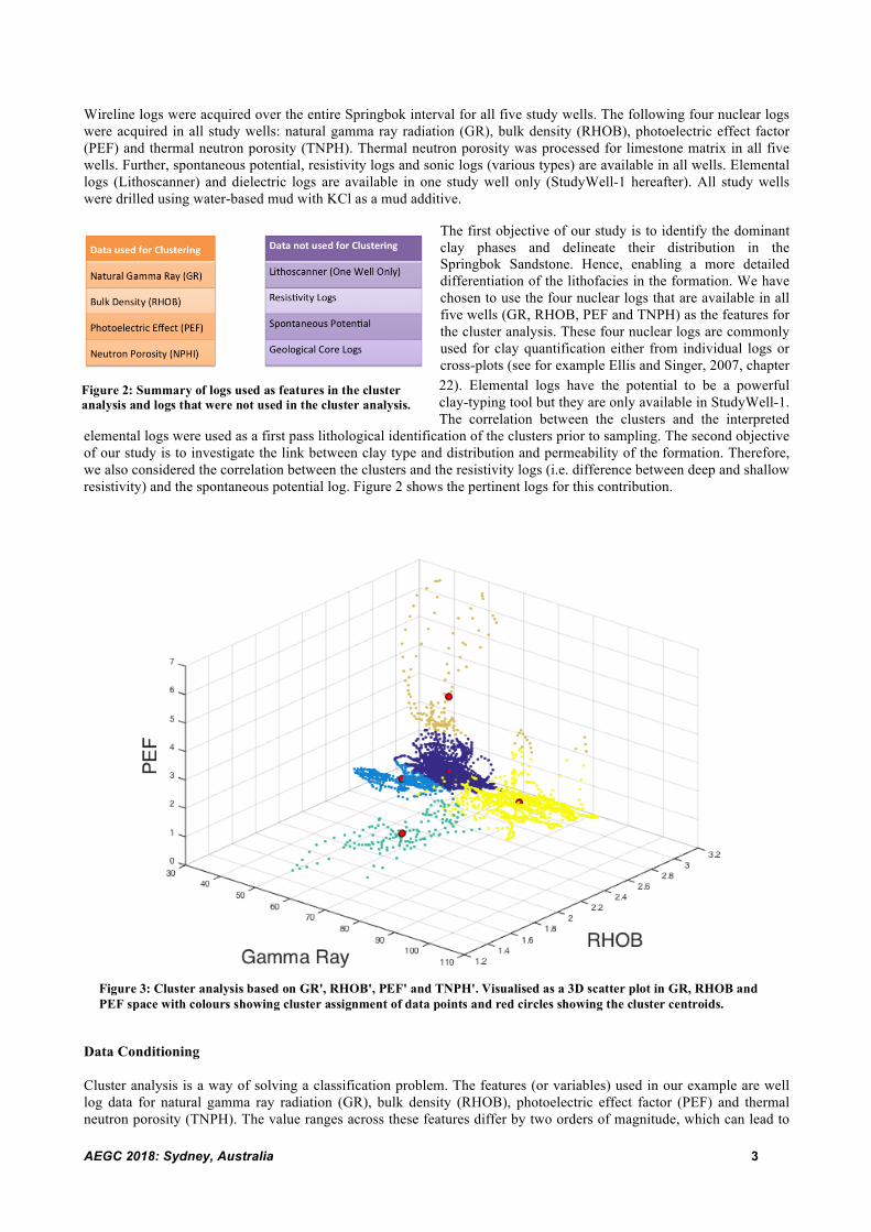
elemental logs were used as a first pass lithological identification of the clusters prior to sampling. The second objective of our study is to investigate the link between clay type and distribution and permeability of the formation. Therefore, we also considered the correlation between the clusters and the resistivity logs (i.e. difference between deep and shallow resistivity) and the spontaneous potential log. Figure 2 shows the pertinent logs for this contribution.

Data Conditioning Cluster analysis is a way of solving a classification problem. The features (or variables) used in our example are well log data for natural gamma ray radiation (GR), bulk density (RHOB), photoelectric effect factor (PEF) and thermal neutron porosity (TNPH). The value ranges across these features differ by two orders of magnitude, which can lead to

Figure 2: Summary of logs used as features in the cluster analysis and logs that were not used in the cluster analysis.

Figure 3: Cluster analysis based on GR', RHOB', PEF' and TNPH'. Visualised as a 3D scatter plot in GR, RHOB and PEF space with colours showing cluster assignment of data points and red circles showing the cluster centroids.


the feature with the broadest value range to dominate the classification. Further, some of the underlying optimizations algorithms used for the classification (e.g. gradient descent) will converge faster for a set of scaled features. In order to address these problems we use mean normalisation to scale the original features x

𝑥! = 𝑥 − 𝑥𝜎

where 𝑥! is the scaled feature, 𝑥 is the mean of the feature values and σ is the standard deviation of the feature values. Cluster Analysis Cluster analysis aims to subdivide a dataset into so-called "clusters" based on a similarity criterion. In this contribution, we use the k-means clustering algorithm, which employs a similarity criterion based on Euclidian distance. The feature space X for our application is four-dimensional with the mean normalised nuclear logs (GR’, RHOB’, PEF’ and TNPH’) as coordinate axis. The number of clusters k is in principle arbitrary and only limited by the number of data points (or observations) m, so that k<m. Each cluster has a cluster centroid 𝜇!, 𝜇!,… 𝜇!. The cluster centroids are initialised at the beginning of the clustering algorithm. The initial set of cluster centroids 𝝁 can be chosen by various methods, such as random selection of k observations from X. We used the k-means ++ algorithm to seed the cluster centroids (Arthur and Vassilvitskii, 2007). Given the initial set of cluster centroids 𝝁, the k-means algorithm aims to minimise the squared sum of the Euclidian distances between data points x and centroid location for each cluster Ci, summed over all clusters:

min ∥ 𝒙 − 𝜇! ∥!

!"!!

!

!!!

This is achieved by an iterative two-step process:

1. Each data point (i.e. observation) is assigned to the “nearest” cluster centroid, by applying the Euclidian distance similarity criterion.

2. The centroids are moved or “updated” by calculating the mean of each cluster. Applied to the same data set multiple times, the k-means algorithm can return different cluster centroid locations and thereby assign some data points to different clusters. This can be due to poor choice of the set of initial cluster centroid locations or the fact that the minimisation found a local minimum instead of a global minimum. This can be circumvented by running k-means repeatedly and choosing the set of clusters with the lowest squared sum of Euclidian distances between data points and centroid locations summed over all clusters. We have run 50 repeats for our cluster analysis, although a number of 5 repeats seems to be sufficient to obtain persistent centroid locations for this data set. Choice of Number of Clusters k The number of clusters can be freely chosen and should be guided by the objectives of the analysis. For our sampling campaign we had two practical considerations:

1. Improve wireline-based differentiation of the bulk of clastic sedimentary rocks of the Springbok interval in comparison to cut-off based techniques (e.g. GR cut-offs).

2. Automatically identify rare or “outlier” lithology (in this case coal and siderite). Figure 3 shows the wireline data for StudyWell-1 as a 3D scatter plot in GR, RHOB and PEF space. The colours represent cluster assignment of data points and red circles show the cluster centroids. The bulk of the data points (>90%) lie within the following intervals 2.1 g/cm3 < RHOB < 2.6 g/cm3, 45 GAPI < GR < 100 GAPI and 2.0 < PEF < 4.0. This bulk of the data cloud is subdivided into three clusters. Using only 4 clusters in total will reduce the differentiation of this “bulk of data”, in particular the differentiation between Cluster 1 and 5 (see below for cluster description). The “outlier” lithologies can be easily seen as the low-RHOB branch (turquoise) and the high-PEF branch (beige) of the point cloud and are subsequently labelled as Cluster 4 (turquoise) and Cluster 2 (beige).


Correlation of Clusters and Continuous Log Data not used during Cluster Analysis We visualise the correlation of the categorical clusters and the continuous log data not used in clustering with the help of box plots (Figures 4 and 5). The boxes depict the data range with the bottom and top of the box representing the first and third quartile and the red vertical line representing the second quartile or median. The “whiskers” (vertical lines extending from the box) represent the highest and lowest data point still within the 1.5 x IQR or interquartile range. Outliers beyond 1.5 x IQR are represented as red crosses. The bottom panels in Figures 4 and 5 show the amount of data points assigned to each cluster. The clusters are sorted by descending cluster size. The total amount of data points differs between Figures 4 and 5, as the sampling intervals of the tools we are correlating to the clusters are different. Two measures are used as proxies for formation permeability: (i) the difference between the deep and shallow resistivity logs and (ii) the spontaneous potential log. We did not attempt to interpret these two measures in absolute terms and focused on the relative changes between the clusters. As can be seen in Figure 4 Cluster 1 stands out in this context. In regard to the difference between shallow to deep resistivity the median value of the data points assigned to Cluster 1 is 4.26 Ω m and have maximum value of 14.48 Ω m. The median and mean values for the entire Springbok Sandstone are 0.21 Ω m and 1.15 Ω m, respectively. The median spontaneous potential value for Cluster 1 is -144.5 mV, whereas median and mean values for entire formation are -168.5 mV and Mean -167.3 mV, respectively.

Figure 5: Box plot showing correlation between the five clusters and the interpreted dry weight fractions of coal, siderite and cobined illite and kaolinite.

Figure 4: Box plot showing correlation between the five clusters and the difference between shallow and deep resistivity as well as spontaneous potential


In StudyWell-1 an elemental log (Lithoscanner) was acquired as well. We use the interpreted mineralogy form this elemental log to obtain as first pass lithological interpretation for the clusters. It has to be noted that the interpreted mineralogy is model based and dependents on the model assumptions (e.g. for StudyWell-1 there seems to be the assumption that there are two clay phases: Kaolinite and Illite). Further, this interpretation is based on a proprietary algorithm that was not available to the authors. Figure 5 shows the correlation of the clusters to the interpreted coal, siderite and combined illite and kaolinite dry weight fractions. Cluster 4 shows a strong correlation to coal (median value of 0.37) with the other cluster containing virtually no coal. At the same time Cluster 4 is void of siderite. Cluster 2 shows the strongest correlation to siderite (median value of 0.06) with Clusters 1 and 5 containing some siderite, albeit at very low weight fractions (median values of 0.01 and << 0.01, respectively). Considering the bulk of the data points, the following clusters have descending median values of combine illite and kaolinite dry weight fractions: Cluster 3 (0.45), Cluster 5 (0.32) and Cluster 1 (0.17). Cluster 2 has a median value of combine illite and kaolinite dry weight fractions of 0.45 as well, but it should be noted that the data points assigned to this cluster are just 4% of the data points in StudyWell-1 for the Springbok interval. Cluster Interpretation and Distribution Based on the signatures of the nuclear logs and the correlation with other logs as shown above we arrived at a preliminary interpretation (i.e. prior to sampling) of the clusters:

• Cluster 1: Clastic rock with prominent mud invasion and distinct spontaneous potential signature (possible high permeability rock), low natural gamma ray signature, low clay content

• Cluster 2: Rock with significant siderite mineralization or siderite concretions

• Cluster 3: Clastic rock with limited to no mud invasion, relatively high natural gamma ray

signature, high clay content

• Cluster 4: Intervals with coal bands

• Cluster 5: Clastic rock, in terms of mud invasion and clay content intermediate to Clusters 1 and 3, low natural gamma ray signature

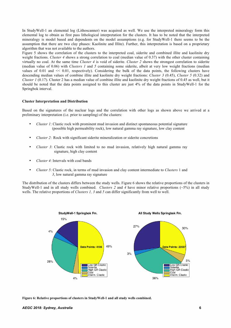
The distribution of the clusters differs between the study wells. Figure 6 shows the relative proportions of the clusters in StudyWell-1 and in all study wells combined. Clusters 2 and 4 have minor relative proportions (~5%) in all study wells. The relative proportions of Clusters 1, 3 and 5 can differ significantly from well to well.

Figure 6: Relative proportions of clusters in StudyWell-1 and all study wells combined.


CONCLUSIONS

We used the k-means clustering algorithm to subdivide our dataset into five clusters. This cluster analysis incorporates information from four different wireline logs in contrast to cut-off based methods that usually rely on one or two wireline logs. This allowed us to achieve the main objectives of our cluster analysis. Firstly, the bulk of the data points from the Springbok interval is subdivided into three clusters. This would not have been possible with a classical cut-off based method or a smaller number of clusters. Secondly, siderite and coal rich intervals can be easily identified. The cluster analysis allowed us to sample and eventually analysis a representative set of constituency lithologies of the Springbok Sandstone. The differentiation between Clusters 1 and 5 is particular helpful and not possible with four cluster or a GR / RHOB cut off. For example Cluster 5 is a somewhat ‘unremarkable’ cluster in terms of the nuclear wireline log responses, yet 30% of the data points in the five study wells are assigned to this cluster and the hydrogeological indictors show considerable spread. Moving forward, our analysis will “ground truth” our preliminary cluster interpretation in regard to the total clay content and shed light on the influence of the actual clay type on hydrogeological properties.

REFERENCES Arthur, D., and Vassilvitskii, S., 2007, k-means++: the advantages of careful seeding: Proceedings of the eighteenth annual ACM-SIAM symposium on Discrete algorithms. Society for Industrial and Applied Mathematics, Philadelphia, PA, USA. pp. 1027–1035. Ellis, D.V. and Singer, J.M., 2007, Well logging for earth scientists (Vol. 692). Dordrecht: Springer. Exon, N.F., 1976, Geology of the Surat Basin in Queensland., Bureau of Mineral Resources, Australia. Bulletin, 166 Gallagher, V. 2012, Reservoir Characterisation of Jurasic Springbok Sandstone, Surat Basin, Queensland, Honours Thesis, University of Adelaide. Green P. M. ed. 1997, The Surat and Bowen Basins South-East Queensland. Queensland Minerals and Energy Review Series. Queensland Department of Mines and Energy, Brisbane.

Hamilton, S.K., Esterle, J.S. and Sliwa, R., 2014, Stratigraphic and depositional framework of the Walloon Subgroup, eastern Surat Basin, Queensland. Australian Journal of Earth Sciences, 61(8), pp.1061-1080. Levy, M. and Gaede, O. , 2018, Identification Of Clay Minerals Within The Springbok Formation, Surat Basin, AEGC 2018 conference volume. MacQueen, J., 1967, Some methods for classification and analysis of multivariate observations. Proc. Fifth Berkeley Symp. on Math. Statist. and Prob., Vol. 1 (Univ. of Calif. Press, 1967), 281--297. OGIA, 2016, Underground Water Impact Report for the Surat Cumulative Management Area. Office of Groundwater Impact Assessment, Department of Natural Resources and Mines, Brisbane Queensland Power, P.E., Devine, S.B., 1968, Some ammendments of the Jurassic stratigraphic nomenclature in the Great Artesian Basin., Queensland Government Mining Journal, 69(799), p194-201 Ransley, T.R., Radke, B.M., Feitz, A.J., Kellett, J.R., Owens, R., Bell, J., Stewart, G. and Carey, H. 2015, Hydrogeological Atlas of the Great Artesian Basin. Geoscience Australia, Canberra. http://dx.doi.org/10.11636/9781925124668 Underschultz, J.R., Pasini, P., Grigorescu, M. and de Souza, T.L., 2016, Assessing aquitard hydraulic performance from hydrocarbon migration indicators: Surat and Bowen basins, Australia. Marine and Petroleum Geology, 78, pp.712-727

targeting core sampling with machine learning: case …

Documents