RL-TR-95-294 Final Technical Report February 1996

MULTICHANNEL SIGNAL PROCESSING EXTENSIONS

Kaman Sciences Corporation

Robert Vienneau

APPROVED FOR PUBL/C RELEASE; DISTR/BUT/ON UNL/M/TED.

19960425 025 xmo qpAum INSPECTED i

Rome Laboratory Air Force Materiel Command

Rome, New York

This report has been reviewed by the Rome Laboratory Public Affairs Office (PA) and is releasable to the National Technical Information Service (NTIS). At NTIS, it will be releasable to the general public, including foreign nations.

RL-TR-95- 294 has been reviewed and is approved for publication.

APPROVED: /

JAMES H. MICHELS, Ph.D. Project Engineer

FOR THE COMMANDER: U JLA D.^&^^i

GARY D. BARMORE, Major, USAF Deputy Director of Surveillance & Photonics

If your address has changed or if you wish to be removed from the Rome Laboratory mailing list, or if the addressee is no longer employed by your organization, please notify Rome Laboratory/ ( OC SM), Rome NY 13441. This will assist us in maintaining a current mailing list.

Do not return copies of this report unless contractual obligations or notices on a specific document require that it be returned.

Porm Approved OMB No. 0704-0188 REPORT DOCUMENTATION PAGE

Pt^raoonrgbLroWitetrtaeofcatrtof WonwftriiiMtTsadtoamgii Hxtam fgirm. iTdu*nqtt-»itT»>otm—i-grinon», i—u i yongd« i B«lTirr^irijn'MiMtufr,o^r»»i«drtccrH*«rQ»T^«»i«^»»colto^of >^^ =<*aian of rfamtfon rxLct-g ajggMO» fa mdLCt-s ** buowv to W«rtno£n H««*|L«rt«» s«r*«* DN^™'w WamBlon 0pw«*T« ir«lR«x«» 1215 J«ff»«Ti 0»»»HltfT»my Sdt» liMMmV« JCTB-tTra ra to If» Oflte» of Mngvnart »id BtilB* P«»w0,,< "«Aatan Pro)U (0704-01 Ml. Wn-r-^on. DC 20501

1. AGENCY USE ONLY <L»«v« Blank) 2 REPORT DATE

February 1996

a REPORT TYPE AND DATES COVERED

Final Apr 94 - Aug 95

4. TITLE AND SUBTITLE

MULTICHANNEL SIGNAL PROCESSING EXTENSIONS & AUTHOR(S)

Robert Vienneau

& FUNDING NUMBERS

C - F30602-94-C-0101 PE - 61102F PR - 2304 TA - E8 WU - PC

7. PERFORMING ORGANIZATION NAME(S) AND ADDRESSES) Kaman Sciences Corporation 258 Genesee Street Utica NY 13502-4627

a PERFORMING ORGANIZATION REPORT NUMBER

N/A

9. SPONSORING/MONfTORING AGENCY NAME(S) AND ADDRESSES) Rome Laboratory/OCSM 26 Electronic Pky Rome NY 13441-4514

10. SPONSORING/MONITORING AGENCY REPORT NUMBER

RL-TR-95-294

11. SUPPLEMENTARY NOTES

Rome Laboratory Project Engineer: James H. Michels, Ph.D./0CSM/(315) 330-4432

12a. DISTRIBimON/AVAILABIUTY STATEMENT

Approved for public release; distribution unlimited.

12b. DISTRIBUTION CODE

1a ABSTRACT (M«*run 200» This effort extends the signal processing capabilities of the Multichannel Signal Processing Simulation System (MSPSS), including:

- the analysis of a signal detection algorithm for a constant magnitude signal of unknown amplitude in white or colored noise;

- the addition of a capability to generate Weibull-distrlbuted noise or clutter;

- the implementation of the representative model that provides user-control over statistical properties of simulated space-time data, as calculated from certain parameters characterizing the phased-array radar platform, the clutter environment, signals, and jammers; and

- additional diagnostic capabilities.

The MSPSS was developed to assess the performance of multichannel signal processing algorithms for detection and estimation analyses. Specific emphasis has been given to the implementation of multichannel parametric model-based methods.

14. SUBJECT TERMS Multichannel, Detection, Estimation, Non-Gaussian, Weibull

IS NUMBER Of PACES 108

1» PRICE cooe

17. SECURfTY CLASSIFICATION OF REPORT

. UNCLASSIFIED NiN7*Wfl1-2BMSOD """"

1 a SECURfTY CLASS8TCATTON OfTHSPAGE

UNCT.ASST7TF.T)

19. SECURTTY CLASSIFICATION Of ABSTRACT

TTWPT.AggTT?T1iT>

2a UMITATION OF ABSTRACT

J£L 'it^3ö^5~fl»-» ■ ** PrwatMO Oy ANSi %ia i*-i 2M-1Q2

TABLE OF CONTENTS

1. OVERVIEW 1/2 1.1 Objective i/2

1.2 Background 1/2

1.2.1 The Multichannel Signal Processing Simulation System 3'4

1.2.2 Detection of Unknown Amplitude Signal 3'^ 1.2.3 Weibull Distribution 6 1.2.4 Representative Model 6 1.2.5 Diagnostics 7

1.3 Overview of Report 7

2. THE MULTICHANNEL SIGNAL PROCESSING SIMULATION SYSTEM 8 2.1 Signal Detection and Statistical Hypothesis Testing 8 2.2 A Model-Based Approach 8 2.3 Diagnostics 10 2.4 Signal Detection 10

3. NEW CAPABILITIES 11 3.1 A Signal with Unknown Amplitude 11

3.1.1 Clutter Synthesis 11 3.1.2 Synthesis of the Deterministic Signal 13 3.1.3 Amplitude Estimation 13

3.1.3.1 The Sample Covariance Matrix 13 3.1.3.2 Time/Space Averaged Estimator 14 3.1.3.3 Time/Space Averaged Estimator with Time Clipping 15 3.1.3.4 Estimating the Amplitude 16 3.1.3.5 Inverting the Covariance Matrix 17

3.1.4 Filtering 17 3.1.4.1 Innovations for White Noise 17 3.1.4.2 Innovations for Temporally Correlated Clutter 18 3.1.4.3 Innovations for a Constant Signal in Clutter 18

3.2 Weibull Clutter Synthesis 19 3.2.1 Weibull SIRP White Noise 19 3.2.2 An AR Process with Weibull Driving Noise 23

3.3 The Representative Model 24 3.3.1 Signal 24

3.3.1.1 Constant Magnitude Signal 24 3.3.1.2 Random Signal 24

3.3.2 Clutter 26 3.3.3 Interference 28

3.3.3.1 Direct Path White Noise Interference Model 28 3.3.3.2 Direct Path Partially Correlated Noise Interference Model 29

3.4 A Two-Dimensional FFT of Clutter Covariance Matrix 30 3.5 Calculation of State Space Parameters 32

3.5.1 State Space Closed Form Method 34 3.5.2 AR Recursion Method 36

3.6 Sixteen Channels 36

4. IMPLEMENTATION 37 4.1 A Signal with Unknown Amplitude 37

4.1.1 Covariance Matrix and Amplitude Estimation 37 4.1.2 Subtraction Filter Routine 42 4.1.3 Constant Signal Analysis Routines 42

4.2 Weibull Clutter 48 4.3 Representative Model 51 4.4 Two-Dimensional FFT 56 4.5 State Space Capabilities 61

5. REFERENCES 64

Appendix A: NOTATION AND ACRONYMS 66 A.l Notation 66 A.2 Acronyms 71

Appendix B: THE WEIBULL DISTRIBUTION 72

Appendix C: THE REJECTION METHOD 73 C.l A Simple Version 73 C.2 A Sophisticated Version 74 C.3 An Application 76

C.3.1 A Triangular Distribution 76 C.3.2 Another Triangular Distribution 78 C.3.3 The Parameters of the Triangular Distribution 80

Appendix D: MATRIX NORMS 82

Appendix E: THE EQUIVALENCE OF TWO METHODS 84 E.l Some Useful Formulas 85 E.2 The Proof 86

ii

Appendix F: AN EXAMPLE FOR THE STATE SPACE MODEL 92 F.l True System State Space Parameters 92 F.2 The Scientific Studies Algorithm with Exact Order 93 F.3 The Scientific Studies Algorithm with Higher Order 96

XXI

LIST OF FIGURES

Figure 1-1: Invoking a Fortran Program from the Menu-Based System

Figure 1-2 Figure 2-1 Figure 2-2 Figure 3-1 Figure 3-2 Figure 3-3 Figure 4-1

The Signal Detection Algorithm Synthesis of an AR Process Innovations Representation of a State Space Model The Linear Filter for White Noise The Linear Filter for an AR Process The Linear Filter for Signal and Clutter Synthesizing a Constant Magnitude Signal in White Noise

Figure 4-2 Figure 4-3 Figure 4-4 Figure 4-5 Figure 4-6 Figure 4-7 Figure 4-8 Figure 4-9 Figure 4-10: Figure 4-11: Figure 4-12: Figure 4-13: Figure 4-14: Figure 4-15: Figure 4-16: Figure 4-17: Figure 4-18: Figure 4-19: Figure 4-20: Figure 4-21: Figure 4-22: Figure 4-23: Figure 4-24: Figure 4-25: Figure 4-26: Figure C-l: Figure C-2 :

Real Part of a Constant Magnitude Signal Imaginary Part of a Constant Magnitude Signal Estimating the Covariance Matrix and Amplitude Estimating the Covariance Matrix and Amplitude (Cont.) Routine for Subtracting the Estimated Signal Unknown Amplitude Analysis Sequences The Signal Detection Algorithm for a Constant Signal Amplitude Estimation Results

Amplitude Estimation Results (Cont'd) Amplitude Estimation Results (Cont'd) Synthesizing Weibull Noise Ozturk Test for Weibull Distribution Representative Model Synthesis Representative Model Synthesis (Continued) Representative Model Synthesis (Continued) Representative Model Synthesis (Continued) Real Part of Sum For the Three Channels An FFT Example Graph of Correlation Function Dolph-Chebychev Filtering of Correlation Function Graph of FFT Logarithm of Magnitude of FFT A State Space Example A State Space Example (Cont'd) A State Space Example (Cont'd)

Triangular Functions More Triangular Functions

5 6 9 10 18 18 19

38 39 40 41 42 43 43 44 45 46 47 49 50 51 52 53 54 55 56 57 58 59 60 61 62

63 77 79

IV

1. OVERVIEW This document is the final report for Multichannel Signal Processing Extensions, an

effort conducted by Kaman Sciences Corporation (KSC) under Rome Laboratory's Broad Agency Announcement (BAA) number 93-07. This effort was performed for

Dr. James H. Michels Rome Laboratory

RL/OCTM Griffiss AFB, NY 13441

(315) 330-4432

1.1 Objective

The objective of this effort was to extend the signal processing capabilities of the Multichannel Signal Processing Simulation System (MSPSS), including:

• The analysis of a signal detection algorithm for a signal with constant but unknown amplitude in (white or colored) noise

• The addition of a capability to generate Weibull-distributed noise or clutter

• The implementation of the Representative Model which provides user-control over statistical properties of simulated space-time data, as calculated from certain parameters characterizing the phased-array radar platform, the clutter environment, signals, and jammers

• Additional diagnostic capabilities.

1.2 Background

Dr. James Michels' ongoing research program investigates an original approach in multichannel signal processing (Michels 89, 90a, 90b, 91, 92a, 92b), including the sponorship of related work (e.g. Rangaswamy 92 and Roman 93). This research program has developed:

• A synthesis procedure for simulating multichannel Autoregressive (AR) processes in which intertemporal and interchannel correlations are controlled parametrically.

• Extensions to this synthesis procedure to handle non-Gaussian Spherically Invariant Random Processes (SIRPs) for K distributions.

• Diagnostics for examining statistical properties of synthesized processes.

• A multichannel signal detection algorithm based on a generalized loglikelihood ratio using an innovations approach, including ratios for Gaussian processes and K-distributed SERPs.

• A Kaiman filter structure for a state-space version of the signal detection algorithm.

• A sensor fusion application of the signal detection algorithm.

• A Monte Carlo approach for exploring the performance of the signal detection algorithms.

• An extension of the Monte Carlo approach for calculating thresholds for given false alarm rates based on approximating the tail of a distribution by a Pareto distribution.

1/2

1.2.1 The Multichannel Signal Processing Simulation System

Kaman Sciences Corporation has designed and implemented the Multichannel Signal Processing Simulation System (MSPSS) to support Dr. Michels' research program. The system architecture was defined early, and capabilities were added over a series of projects (Kaman 91a, 92a, 92b and Vienneau 93 and 94).

The MSPSS is comprised of two major subsystems, a menu-based subsystem and the User Front-end Interface (UFI) based subsystem. The menu-based subsystem interacts with the user by a series of menus and prompts that can be displayed on a line-oriented "glass terminal." It is implemented as a collection of Fortran programs providing the desired signal processing capabilities. Multichannel data is passed between these programs by user-defined files. The menus themselves are Unix C-shells where the bottom-level menu automatically compiles, links, and executes the desired program. Figure 1-1 shows an example of the invocation of a Fortran program from the menu-based subsystem.

The structure of the menu-based subsystem provides the user with a great deal of analytical flexibility. The individual Fortran programs provide certain analytical capabilities, but minimal constraints are imposed on the order in which the user can invoke these functions. A number of diagnostic capabilities are provided, including parameter estimation for certain models, correlation function estimation, and graphical display of data. Thus the user is provided with a system that supports an exploratory style of analysis.

The UFI-based subsystem is designed for more repetitive analyses characteristic of the determination of detection probabilities for given false alarm probabilities and given algorithms. In such analyses, the user needs to invoke certain signal processing synthesis and analysis functions in a predetermined order with certain parameters. The UFI-based subsystem supports this need by allowing the user to construct an "experiment" specified by various algorithms and parameters. Once an experiment has been completely described, a computer program for performing an experiment is automatically generated, compiled, and executed. Since these are simulation experiments, the generated program can run for quite some time. Typically, a single experiment will be used to analyze the performance of the signal detection algorithm in terms of the false alarm probability and the probability of detection. A detailed example of the use of this subsystem is provided in the Software User's Manual for the Multichannel Signal Processing Simulation System (Kaman 92a).

1.2.2 Detection of Unknown Amplitude Signal

The signal detection algorithm, illustrated in Figure 1-2, is quite general. The radar returns x(n) are entered into two parallel filters. The structure of the filters is based on models of the returns with and without a signal. If no deterministic signal is present, the output of the null hypothesis filter, v0(n ), will be a white noise error signal. If a deterministic signal is present, the output of the alternative hypothesis filter, v^/i), will be a white noise error signal. The statistic A is used to determine which filter output provides the minimum white noise error signal. If it is above some threshold value, a signal is determined to be detected. Filters with different structures correspond to models of different clutter environments and different signals. A variety of parameter estimation algorithms may exist for a given model. The appropriate loglikelihood statistic differs between Gaussian and non- Gaussian noise.

3/4

The user invokes the menu-based isaiah.1-52% mchan multichannel system from the Unix shell.

Multi-Channel Detection Algorithm

MAIN MENU

Single Channel Multichannel Ml ~ Process Synthesis Ml 1 - Process Synthesis M2 - Filtering Methods M12 -- Filtering Methods M3 ~ Diagnostics M13 - Diagnostics

LI - List data hies L2 - show the change log Enter a command or Q to quit mil The user chooses a submenu.

MULTI-CHANNEL (M/Q PROCESS SYNTHESIS MENU

MO - Gaussian noise M2 ~ Method 2 (MC2) synthesis Ml - Method 1 (MCI) synthesis M3 - Representative model M4 -- Method 2 unconstrained quadrature process synthesis M5 - State space synthesis M6 - Apply Levinson-Wiggins-Robinson algorithm M7 - Display Multi-Channel (M/Q signal stats M8 - Plot M/C data M9 - Perform Nuttall-Strand or Vieira-Morf estimation MIO - Perform Yule-Walker estimation Ml 1 ~ Estimate AR parameters for each channel M12 - Estimate covariance matrix M13 -- Estimate state space parameters M14 - Estimate state space parameters from exact covariance matrix M15 -- Estimate amplitude of constant signal M16 - Perform M/C correlation (temporal) M17 ~ Perform M/C correlation (ensemble) M18 - Split a M/C input M23 - Join inputs M19 - Add M/C signals M24 ~ Subtract M/C signals M20 ~ Convert AR parameters to state space M21 - Display complex data M25 — Display coefficient file M22 ~ Catenate M/C signals M26 ~ Sum channels

LI - List data files L2 — show the change log

Enter a command or Q to return to the MAIN menu: m3 The user invokes and interacts with a Fortran program.

Figure 1-1: Invoking a Fortran Program from the Menu-Based System

x(n)

Null Hypothesis vjin)

Filter F0

it

' '

Model Parameter Estimates

Calculate Loglikelihood

Statistic

A

1 - . it

► Alternative Hypothesis VjW

Filter F,

Figure 1-2: The Signal Detection Algorithm

Not all instantiations of this signal detection algorithm have been implemented in the MSPSS. Recently, capabilities were added to analyze the detection of a constant magnitude signal, assuming its amplitude is known (Vienneau 94). Dr. Michels has extended the detection algorithm to a model of a signal with constant but unknown amplitude. Capabilities for analyzing this case were added under this effort.

1.2.3 Weibull Distribution

Clutter and noise have been modeled as stochastic processes. For example, capabilities exist in the MSPSS to synthesize the clutter as an AR process. Driving noise for AR processes and white noise were first implemented as Gaussian noise. Recent research at Syracuse University and Rome Laboratory has investigated non-Gaussian processes known as Spherically Invariant Random Processes (SIRPs). SIRPs can be used to model many probability distributions (Rangaswamy 91, 92, 93a, and 93b). A K-distribution was the only non-Gaussian SIRP synthesized by the MSPSS prior to this effort. Now a capability exists for synthesizing Weibull SIRPs in the MSPSS.

1.2.4 Representative Model

The Representative Model is closely related to the synthesis procedure existing in the MSPSS at the start of this effort. The Representative Model provides control over statistical properties of simulated space-time data, as calculated from certain parameters characterizing the phased-array radar platform, the clutter environment, signals, and jammers. The Representative Model differs from the Physical Model in that it provides greater control over statistical properties of the simulated radar returns. The radar is described at a higher level of abstraction, while the Physical Model simulates specific radars, signals, and jammers.

The Representative Model, parameters determine "shaping functions" used to calculate block covariance matrices for the clutter, signal, and interference. The block covariance matrices, in turn, are used to find either a Cholesky decomposition of the block covariance

matrix, or Autoregressive (AR) coefficients used in simulating the radar returns. The simulated radar returns are appropriate for testing the performance of a signal detection algorithm, examining the performance of estimation algorithms, passing through a Fast Fourier Transform (FFT), etc.

An interesting question is the performance of the signal detection algorithm analyzed by the MSPSS when applied to data characterized by the Representative Model. The Representative Model was implemented in the MSPSS under this effort. This implementation permits the use of diagnostics to characterize data synthesized by the Representative Model, but does not support convenient examination of the performance of the signal detection algorithm applied to Representative Model data.

1.2.5 Diagnostics

The MSPSS implemented certain signal processing diagnostic capabilities before the start of this project. More were added. A previous effort added a capability to estimate the parameters of a state space model (Vienneau 94). This capability is difficult to test since estimated matrices may differ from theoretical values by a basis transformation of the state space and since statistical variation may combine with numerical effects to yield inaccurate estimates. A capability was added under this project to calculate a theoretically exact block covariance matrix for an AR process, which in turn is used to estimate the state space parameters.

Certain capabilities existed at the start of this effort for estimating correlation functions. Insight into the underlying processes can be obtained by examining the spectrum of correlation functions. Accordingly, this effort included the addition of a capability to calculate a two dimensional Fast Fourier Transform (2D-FFT).

The radar system simulated by the Representative Model can contain up to 14 channels. Therefore, the number of channels in processes synthesized and analyzed by the MSPSS was increased from the previously existing bound of four channels, namely to 16 channels.

1.3 Overview of Report

This section consists of an introduction and an overview of the remainder of the report.

Section 2 provides a brief description of the signal detection problem and an overview of the approach that can be analyzed by the MSPSS.

Section 3 defines new capabilities added to the MSPSS during this effort. Subsections present the analysis of the detection of a signal with unknown amplitude, the synthesis of a Weibull SIRP, the representative model, the calculation of state space parameters, and a two dimensional Fast Fourier Transform (2D-FFT).

Section 4 discusses implementation details for the new capabilities. Examples of how the new capabilities are invoked are provided.

Section 5 provides references, while appendices describe notation, acronyms, and certain mathematical details.

2. THE MULTICHANNEL SIGNAL PROCESSING SIMULATION SYSTEM The Multichannel Signal Processing Simulation System (MSPSS) was developed by

Kaman Sciences to support RL/OCTM research. This section briefly describes the signal processing problems that can be analyzed with the MSPSS and the use of the MSPSS.

2.1 Signal Detection and Statistical Hypothesis Testing

The primary purpose of the MSPSS is to analyze the performance of a signal detection algorithm. Signal detection can be thought of as a problem in statistical hypothesis testing. Let x denote a multichannel vector stochastic process representing the radar returns. Radar returns consist of a time series of complex vectors, where the dimension of the vectors is the number of radar elements (channels). Let s denote a signal, c denote the clutter, and n denote white noise. Consider deciding between the null hypothesis

• H0: x =c + n

and the alternative hypothesis

• Hi', x = s + c + n.

Deciding that a signal is present is to accept the alternative hypothesis.

The Neyman-Pearson theory of statistical hypothesis testing provides control over probabilities of making an erroneous decision. The significance level, a, of a statistical test is the probability that a decision rule will accept the alternative hypothesis when the null hypothesis is true:

a = Pr (Accept Hx I H0 true ). (2.1-1)

Since to accept the alternative is to decide a signal is present, the significance level is the probability of false alarm in the signal detection problem.

Another type of erroneous decision is possible. A decision rule can result in a decision that no signal is present when, in fact, a signal exists. The probability of this mistake, known as a Type II error, is usually denoted by ß. The power of a test denotes the probability of correctly deciding in favor of the alternative hypothesis. The power is related to the probability of a Type II error, as shown by Equation 2.1-2:

1 - ß = Pr (Accept Hx I //, true ). (2.1-2)

In signal detection, the power of a test is known as the probability of detection.

2.2 A Model-Based Approach

The MSPSS supports the analysis of a model-based approach to signal detection. In other words, both the synthesis and the analysis of radar returns are based on certain parameterized models. (Non-model based approaches are also known as non-parametric approaches.) Synthesis models currently implemented in the MSPSS include:

• Multichannel Gaussian, K-distributed, and Weibull noise

• Spherically Invariant Random Processes (SIRPs) in which each realization is Gaussian but the distribution of a time sample across realizations is K-distributed or Weibull.

• Autoregressive (AR) processes with driving noise from SIRP or white noise

• Autoregressive Moving Average (ARMA) models implemented as the sum of AR models and white noise

• A state space model

• Multipath processes

These models are implemented in an innovations representation. The output process is formed by modifying a driving noise term. The filters in the signal detection algorithm in Figure 1-2 are designed to produce estimates of the innovations process of the model corresponding to the appropriate hypothesis. A different filter structure corresponds to each different model structure. The corresponding loglikelihood statistic is designed to determine which filter output more closely resembles the modeled process.

For example, Figure 2-1 shows the system structure for synthesizing an AR process. The input process v(n) is white noise uncorrelated both in time and across channels. The operator T adds correlation across channels to produce e(n). The remainder of the structure adds correlation in time and modifies the correlation across channels. The appropriate filter to estimate the innovations for this AR model has a tapped delay line structure.

Figure 2-1: Synthesis of an AR Process

A state space model (Figure 2-2) provides another powerful example of an innovations model. In this model, an internal process, a(n), is used to inject intertemporal correlation. In this case, a Kaiman filter provides the appropriate structure for estimating the innovations process.

The MSPSS provides instantiations of the signal detection algorithm shown in Figure 1- 2. An instantiation is constructed by combining a synthesis model, parameter estimation algorithms, filters for estimating innovations, and an appropriate test statistic. The MSPSS allows the user to analyze the resulting algorithm. Thresholds can be calculated for given false alarm probabilities, and then a corresponding probability of detection can be determined.

*(n)

F

a(n)

V z-'

HH K

i

v(n) T

e(n) j + L

Figure 2-2: Innovations Representation of a State Space Model

2.3 Diagnostics

Synthesis procedures in the MSPSS provide user-control over characteristics of the synthesized processes, such as temporal and cross-channel correlation. Since these are stochastic processes, the synthesized radar returns exhibit a range of random variability. Diagnostics provide the user a number of ways to examine radar processes.

The MSPSS provides a graphing capability integrated from Khoros (Rasure 92). Graphical displays can be rotated, annotated, otherwise manipulated, and printed. Statistical routines are provided for means, variances, correlation functions, parameter estimation, distribution identification and testing, periodograms, and Fast Fourier Transforms of spectra. Additional capabilities include various filters and data manipulation capabilities such as adding processes, combining channels, and splitting channels.

2.4 Signal Detection

The User Front-end Interface (UFI) based subsystem provides powerful capabilities for analyzing the signal detection algorithm. Analysis sequences allow the user to specify the model parameters. A Monte Carlo approach is used to estimate filter parameters, thresholds for given false alarm probabilities, probabilities of detection, and variability in thresholds and probabilities of detection. The extreme value method (Chakravarthi 92 and Vienneau 94) gives efficient estimates of thresholds for extremely small false alarm probabilities.

The MSPSS allows the user to determine how the probability of detection varies with false alarm probabilities and characteristics of the radar returns such as signal to noise ratios. Different parameter estimation algorithms and different filtering structures can be explored. In short, the MSPSS allows the user to explore the robustness of the signal detection algorithm under a wide range of instantiations and circumstances. Published results using this system are positive so far (Michels 94 and 95).

Section 4 describes the use of the MSPSS for the capabilities added under this effort. General user information is provided in (Vienneau 93) and (Vienneau 94). (Kaman 92a) describes how to use the User Front-end Interface (UFI) based subsystem. Procedures for adding additional capabilities are discussed in (Vienneau 93).

10

3. NEW CAPABILITIES Kaman Sciences has implemented and enhanced the Multichannel Signal Processing

Simulation System (MSPSS) over a series of contracts. The MSPSS was extended under this effort to include the following capabilities:

• The analysis of the detection of a signal with constant but unknown amplitude in clutter

• The synthesis of a Weibull-distributed Spherically Invariant Random Process (SIRP)

• The synthesis of the Representative Model, originally designed for the Rome Laboratory Space-Time Adaptive Processing Algorithm Development Tool (RLSTAP/ADT)

• The estimation of state space model parameters from a theoretically exact block covariance matrix for an AR process

• A two-dimensional Fast Fourier Transform (2D-FFT)

• The extension of all capabilities to 16 channels.

This section defines the capabilities implemented under this effort.

3.1 A Signal with Unknown Amplitude

A new model-based signal detection analysis capability was added. The signal detection analysis capabilities allow the user to determine the false alarm probability and probability of detection for specific algorithms under controlled conditions. These signal detection algorithms are based on models of the signal, clutter, and noise. In this case, the algorithm decides between the null hypothesis:

//„: x(n)-v(n), n = 1.2 N, (3.1-1)

and the alternative hypothesis:

//,: x(n) = s(n)+y(n), n - 1.2 N. (3.1-2)

The radar return, x(n), is a /-element complex vector, v (n ) represents clutter, while s (n) is the signal.

3.1.1 Clutter Synthesis

The clutter process, y O ). is modeled as an Autoregressive (AR) process with white driving noise:

y („) = -£ AH(k)y(n -*) + E(/I), (3-1_3) k - 1

where y (n ) and e(n ) are /-element complex column vectors and AH (1), AH (2), ..., AH (p) are /x/ AR matrix coefficients for an AR process of order p.

The driving noise process, tin), is uncorrelated in time, but possibly correlated across channels. The correlation across channels is expressed by the JxJ covariance matrix I,,:

Lz = E[E(n)E"(n)]. (3.1-4)

The driving noise process is synthesized based on one of three decompositions of the covariance matrix. The Cholesky decomposition is specified by Equation 3.1-5:

11

z*-ctc?. (3.1-5)

where CE is a lower triangular complex matrix. The LDU decomposition is specified by Equation 3.1-6:

l^ = LzD,Ll, (3.1-6)

where LE is a lower triangular complex matrix with unity along the principal diagonal and £>E

is a diagonal matrix. For a correlation matrix the Singular Value Decomposition (SVD) reduces to the unitary similarity transformation and is given by Equation 3.1-7:

^-O.Mtf. (3.1-7)

where AE is a diagonal matrix whose elements are eigenvalues of 2^. The columns of QE are the corresponding right hand eigenvectors:

^(Ge)., =(Ae),,,(Qe),. (3.1-8)

The rows of Q" are the left hand eigenvectors:

(Ö^),.£e = (Ae)lV(Q?),. (3.1-9)

Since 2^ is Hermitian, the Hermitian transpose of QE is also the inverse of Qz.

The driving noise is generated based on either CE, LE and £>e, or QE and AE. For each time sample in the driving noise term, the /-element complex column vector ve(«) is generated. ve(n) is from a K-distributed Spherically Invariant Random Process (SIRP), a Weibull SIRP, or a Gaussian distribution. ve(n) is uncorrelated across channels and across time. If the user chose a Cholesky decomposition, the jth channel of vE(n) has a variance of unity. If the user specifed a LDU decomposition or SVD, the jth channel has a variance of (D^j or (AJ^, respectively. The driving noise term is then given by Equation 3.1-10:

E(«)-reve(«), (3.1-10)

where Te is either CE, LE, or QE.

The driving noise covariance matrix 2; and the AR coefficients AH (1), AH (2) AH (p ) are determined based on a "shaping function" approach (Michels 94). The correlation matrix for the AR process for the kth lag is defined by Equation 3.1-11:

Ry(k) = E[y(n)yH(n-k)], (3.1-11)

where Ry (k) is JxJ. By definition, Equation 3.1-12 follows:

Ry(-k) = RyH(k). (3.1-12)

The correlation matrix and the AR parameters are related by the Yule-Walker equations. For example, the Yule-Walker equations for three lags, p = 3, are given by Equation 3.1-13:

Ry(0) Ry(l) Ry(2) Ry(3) Ry(-l) Ry(0) Ry(l) Ry(2) Ry{-2) Ry(-l) Ry(0) Ry(l) Ry(-3) Ry(-2) /?,(-!) Ry(0)

The values of Ry (k) are determined by either a Gaussian or Exponential shaping function, and the Yule-Walker equations are solved to obtain the AR parameters. The synthesis of clutter as an AR process was already implemented when this project began. See (Vienneau 93) for further details, including the specification of the shaping functions.

12

/ AH(l) AH(2) AH (3) 2; o o o (3.1-13)

3.1.2 Synthesis of the Deterministic Signal

The deterministic signal, s (n ), is modeled by Equation 3.1-14:

■*o.i(" )

s (n ) = as0(n ) = a

■*o,2(" )

(3.1-14)

s0J(n )

where a is a complex constant equal across all channels and

>2n(i-l)£sin(e,) j2Mn-l)fdTsm(9t)

The complex amplitude is specified as

a = A e J*o

(3.1-15)

(3.1-16)

In synthesizing the signal, the user specifies the constant real. magnitude A, the normalized

Doppler fdT, the normalized element spacing —, and the angle of arrival 0^ of the signal.

The phase <j)0 is a random real number between 0 and In. This number is fixed for each realization, but varies across realizations.

3.1.3 Amplitude Estimation

A program was written to estimate the amplitude a of the signal. The parameters of the steering vector s0(n ) are assumed known. These known parameters-consist of

• The number of time samples N

• The number of channels /

• The normalized Doppler fd T

• The normalized element spacing —

• The angle to the signal 65

In addition to the signal amplitude, the AR parameters of the clutter are assumed unknown.

Amplitude estimation proceeds in two stages. In the first stage, one of three methods is used to estimate the covariance matrix of the clutter from data generated from the null hypothesis; that is, with just clutter and noise. In the second stage, the amplitude is estimated from the estimated covariance matrix and data generated from the alternative hypothesis. Data from the alternative hypothesis consists of the sum of signal, clutter, and noise.

3.1.3.1 The Sample Covariance Matrix

Suppose K realizations of the interference process are observed. Let yk (1), y*(2), ..., y* (N) be the interference for the kth realization, where y* (n ) is a J-element complex column vector, J is the number of channels, and N is the number of time samples. The concatenated J N column vector yk is formed as in Equation 3.1-17:

13

/(I) /(2)

y*- (3.1-17)

yciv)

The covariance matrix is estimated as the sample covariance matrix given in Equation 3.1-18:

Equation 3.1-18 can be expressed in block matrix form:

?i(0) r,(-l) . . . r\(l-N)

W) r2(0) . . . r2(2-N)

fN(N -I) rN(N -2) rN(0)

where

(3.1-18)

(3.1-19)

(3.1-20)

3.1.32 Time/Space Averaged Estimator

In a stationary process, it seems reasonable that estimates of the same lagged correlation matrix based on different time samples, e.g. fni(l) and r„,(/), should be close in some sense. For nonnegative lags, time averaged estimates are found by averaging over time samples:

for biased estimates, and

'r(0 = ^ £ yk(n)[yk(n-l)]H (3.1-21)

(3.1-22)

for unbiased estimates. Equation 3.1-23 can be used to estimate lagged correlation matrices for negative lags:

r'H-n = [rHn]H (3.1-23)

The time averaged estimates of the lagged correlation matrices can now be averaged over many realizations of the clutter. Since in practice these realizations will correspond to different range cells, this step is known as space averaging. The time/space averaged estimators of the correlation matrices are given by Equation 3.1-24:

fa(0-^ £#(/). (3.1-24)

14

The time/space averaged estimate of the covariance matrix is a block matrix formed from the time/space estimates of the lagged correlation matrices:

L =

ris(O)

rn(N-D rjsiN-l) . /Vs(0)

(3.1-25)

This matrix estimate has block Toeplitz form. However, we emphasize that this estimate is not necessarily positive definite.

3.1.3J Time/Space Averaged Estimator with Time Clipping

More data is available for lower lags in calculating time/space averaged estimators of the lagged correlation matrices. Estimates of lagged correlation matrices for high lags will be less accurate and show more variation than those for lower lags. Time clipping (Huang 88) is a modification to the time/space averaged estimators intended to correct for this effect. For nonnegative lags /, the biased time averaged estimate with time clipping of the lagged correlation matrices is given by Equation 3.1-26:

&</).. =^ £ yHn)[yf(n-nT-^ "-' + 1 £ .rfOi)[tf(n)r

(3.1-26)

n ml + 1

The unbiased estimate for nonnegative lags is given by Equation 3.1-27:

ricd) tj'ir-i E yt(n)[yf(n-l)]'^ "-' + I £ y?(n )[yf(n)]'

(3.1-27)

n -/ + 1

For negative lags, the biased estimate with time clipping is given by Equation 3.1-28:

N Lyt(n)[yf(n)Y /fe(')(,-i I yHn-\i\)ly!(n)]'-^

"«-'"♦! £ yHn)[yf(n)Y (3.1-28)

i/i + i

The unbiased estimate for negative lags is given by Equation 3.1-29:

[frei I) N LyHn)[yf(n)r

u-TTTTTT S ytin-innyfin)]'^ (3.1-29) £ yt(n)[yf(n)Y

n -1/ 1 + 1

The remainder of the algorithm closely resembles the time/space averaged estimate. The time/space averaged estimate with time clipping is found by averaging the time averaged estimate with time clipping over many realizations of the clutter:

15

foe </)--£: T,r%(l).

The estimate of the covariance matrix is formed in the usual way:

foc(O) foc(-D • • • r„c(l-JV)

focd) foc(O) . . . r^c(2-N)

t =

tjx(N-l) rjsciN -2) . foc(O)

(3.1-30)

(3.1-31)

3.1.3.4 Estimating the Amplitude

The amplitude a consists of a magnitude A and phase $0.

a = Aej*° (3.1-32)

Given a realization of the sum of signal and clutter, the amplitude a can be estimated as in Equation 3.1-33:

a = cH v-1 sSZTls0

(3.1-33)

where A; is a JN -element complex vector formed by concatenating together the radar returns for each time sample:

X ss

*(1) x(2)

lx(N).

(3.1-34)

The radar returns are assumed to be the sum of signal and clutter in estimating the amplitude. s0 is the (known) J N -element complex steering vector:

S0'

MD *o(2)

(3.-1-35)

s0(N)

and s0(n ) is given by Equation 3.1-15.

The phase <j>0 can be estimated if the magnitude A of the amplitude is known. The estimator is

where

2 P/ (3.1-36)

16

*,*]*-■*£-. (3-1-37)

If the covariance matrix is known, the actual value £ may be used instead of an estimate in Equations 3.1-33 and 3.1-37.

3.1.3.5 Inverting the Covariance Matrix

The inverse of the estimate of the covariance matrix is used in Equations 3.1-31 and 3.1-37. Since i can be a large matrix, numerical problems may arise in calculating an inverse. A clever method of inverting i is based on an SVD decomposition. Let

t = UAVH, (3.1-38)

where A is a diagonal matrix of singular values, the columns of U are the corresponding left singular vectors, and the columns of V are the right singular vectors. Consider the product:

tl = (u A vH r1 - (vH r1 A-1 f/-1. (3.1-39)

Since U and V are unitary matrices:

V" =V~l (3.1-40)

and

f/w=(/-1 (3.1-41)

Thus,

tx-V(\TlUH (3.1-42)

For a positive definite Hermetian matrix I, U = V so that the SVD reduces to the eigen decomposition:

£ = QAQW. (3.1-43)

where A now contains the eigenvalues of L and Q = U = V. The problem of finding an inverse for the estimated covariance matrix has then been reduced to an SVD and finding the inverse of a diagonal matrix.

3.1.4 Filtering

Prediction error" filters are provided to transform the radar returns to white noise uncorrelated in time and across channels. The results of these transformations are estimates of the innovations process for the models upon which the filters are based.

3.1.4.1 Innovations for White Noise

A simple special case arises when the clutter is white noise uncorrelated in time, but possibly correlated across channels. This case can be regarded as a special case of the AR process described in Section 3.1.1, where the order p is zero. If the radar returns consist solely of clutter modeled by white noise, then Equation 3.1-44 holds:

x(n)=y(n) = E(n) = Tv(n). n = 1,2 N,. (3.1-44)

where some subscripts have been dropped. The corresponding linear filter is defined by Figure 3-1 or Equation 3.1-45:

v(n) = r-lx(n). n=1.2 N. (3.1-45)

17

v(n) e(n) I"1

*

Figure 3-1: The Linear Filter for White Noise Multiplying the radar returns by the inverse of T removes correlation between channels, where T is formed from the decomposition of the JxJ covariance matrix for the noise. In practice, the covariance matrix must be estimated. A procedure for estimating the (zero-lag) covariance matrix already existed at the start of this effort. The linear filter in Figure 3-1 was previously implemented as well.

3.1.4.2 Innovations for Temporally Correlated Clutter

The more general case of clutter, or the sum of clutter and noise, modeled as an AR process also already existed. If the radar returns consist solely of such an AR process, the linear filter shown in Figure 3-2 removes correlation in time and across channels. The tapped delay line structure implements Equation 3.1-46:

*(n) x(n-P)

z-'

"

A"(P)

' '

•o- e(n) r'

y(n)

Figure 3-2: The Linear Filter for an AR Process

s(n)=x(«)+ £ A" (k)x(n -k). n = 1.2 ,V . k - 1

(3.1-46)

Cross-channel correlation is removed by Equation 3.1-47:

v(n) = r-1£(«)> n =1.2 N . (3.1-47)

AR parameters can be estimated by the Yule-Walker, Nuttal-Strand, or Vieira-Morf algorithms (Marple 87).

3.1.4.3 Innovations For a Constant Signal in Clutter

A new filter was written to estimate the innovations in the model given by Equation 3.1- 2. In this model, the radar returns consist of a signal with constant but unknown amplitude in clutter modeled as an AR process. The corresponding filter is shown in Figure 3-3. The first

18

part of the filter, given by Equation 3.1-48, removes the signal:

v (n ) = x (n ) - äs0(n ), n = 1,2,...,N . (3.1-48)

The linear filter F0 corresponds to the filter for the null hypothesis as shown in either Figure 3-1 or Figure 3-2. The outputs from the null hypothesis filter F0 and the alternative hypothesis filter, Fx shown in Figure 3-3, are used to calculate a generalized loglikelihood statistic used in signal detection..

*(n) + "^ x(n)-äs1(n) Linear

Filter F0 \

v(n)

i

&(n) Estimate Amplitude

Figure 3-3: The Linear Filter for Signal and Clutter

3.2 Weibull Clutter Synthesis

This effort included the addition of a capability to synthesize Weibull-distributed Spherically Invariant Random Processes (SIRPs). Weibull SIRPs are useful for modeling terrain clutter. Time samples from a given range bin might follow a Gaussian distribution, but a given time sample might be Weibull-distributed across range bins (Rangaswamy 91).

3.2.1 Weibull SIRP White Noise

Let H>(1), w(2), ..., w(N) be white noise uncorrelated in time but possibly correlated across channels. Each time sample w(n) is a / element (column) vector, where J is the number of channels. The cross-channel correlation is specified by the J x J covariance matrix L* defined in Equation 3.2-1:

£, -£[w(n)wH («)]. (3.2-1)

wH (n ) denotes the Hermitian transpose of w (n ). Equation 3.2-1 implies that the covariance matrix £„ is Hermitian.

The user of the MSPSS has the option of either specifying the covariance matrix £„ directly or the Cholesky, LDU, or Singular Value Decomposition of the covariance matrix. The Cholesky decomposition is given by Equation 3.2-2:

19

where Cw is a lower diagonal complex matrix. The LDU decomposition is

**w = '-•w L)w Lw ,

(3.2-2)

(3.2-3)

where L^ is a lower triangular matrix with unity along its diagonal and Dw is a diagonal matrix.

Since E* is Hermetian, the Singular Value Decomposition (SVD) of I«, is given by Equation (3.2-4):

Z*-<LKQZ. (3.2-4)

Aw is a diagonal matrix whose elements are the singular values of £«,. In this case, the singular values are also the eigenvalues of the matrix L„. The columns of Qw are right hand eigenvectors of L*, and the rows of Q" are left hand eigenvectors. Furthermore, Q" is the inverse of Qw.

The decomposition of the covariance matrix allows for the control of cross channel correlation of white noise. Let

w(n ) = Twv(n ), (3.2-5)

where Tw is either Cw, L^, or Qw, depending on which decomposition is chosen by the user. v(«) is a white noise process uncorrelated both in time and across channels. If the Cholesky decomposition is chosen, each channel of v(n) has a variance of unity. If the LDU decomposition is desired, the variance of the jth channel of v(n ) is the corresponding element along the principal diagonal of Dw. Finally, if a SVD is chosen, the channel variances are the diagonal elements of Aw. Equation 3.2-5 then ensures that the resulting white noise process w (n) has the desired cross channel correlations and autocorrelations.

Formerly, the MSPSS supported the generation of Gaussian and K-distributed Spherically Invariant Random Processes (SIRPs). Under these synthesis procedures, v(n) is synthesized from the desired distribution, either Gaussian or a K-distributed SIRP. The resulting process is then transformed to introduce cross-channel correlation.

The MSPSS now supports the synthesis of Weibull distributed SIRPs. Appendix B describes the Weibull distribution. The generation of SIRPs is most easily explained by first considering the special case in which the channel variances are unity and no correlation exists either across channels or in time. Accordingly, let ^(1), ^(2), ..., %(N) be a Weibull- distributed SIRP with a mean of zero and identity as the correlation matrix. Each time sample, %(n), in the SIRP is a J element column vector:

§(«)-

&0»)

(3.2-6)

where / is the number of channels. The entire process can be expressed as a J N element column vector formed by concatenation:

20

'§(1) §(2)

5- (3.2-7)

The distribution of a SIRP is completely specified by the mean, correlation matrix, and a certain quadratic form, q. Let M be the block-structured correlation matrix:

M-E[l;t?]. (3.2-8)

In the special case considered here, the correlation matrix is the identity matrix. The quadratic form q is then defined as follows:

q-fMS. (3.2-9)

If the SIRP under consideration is complex, the Probability Density Function (PDF) of the quadratic form q is given by:

where r( ) is the Gamma function. For Weibull-distributed SIRPs,

Jk-l K-

A =00* ,

Bk= E (-D' ffl ■ 1

o^.-i- i

fitWi ir

I J i-O 1 2 "'J e •> 2 /- i

1 ft , 2 1 1 + T = i.

a

(3.2-10)

(3.2-11)

(3.2-12)

(3.2-13)

(3.2-14)

a2 is the variance of the Weibull distribution. The parameter b, 0 < b <. 2, is specified by the user, while a is set such that the variance is unity. If the SIRP is real, then Equation 3.2-10 is replaced by Equation 3.2-15:

SJ

2 2 r

l NJ

t>Nj(q) . q >0. (3.2-15)

The generation of Weibull-distributed SIRPs relies on the properties of a generalized spherical transformation of the SIRP. This coordinate transformation expresses the SIRP as a function of the JN random variables R, 0, <&,„, n = 1, 2, ..., N; j - 1, 2, ..., / if n < N, j = 1, 2, ..., / — 2 if n = N. The generalized spherical transformation is given by Equations 3.2-16 through 3.2-21:

5,(l)-*cos(<J>,.,). (3.2-16)

21

^(D-Äcosf*;,,/rising). y=2-3 J- (3.2-17) * -1

§;(«)-* cos(*;„) nsin^J II 11 sin(<DM) , ;=1 /./i-2 JV-1, (3.2-18) l J *1 - lk2m '

§>(Ar)-Äcos(<D>A) nsin(*^) n n'sinC^,^) , 7 =1.2 7-2 (3.2-19) n n!sin(*M2) t, - 1*2- 1

&_,(tf)-ÄCOS(0) / -2 nsin(4>tJV)

km 1

&(#)-* sin(0) y-2 nsin(*tJV) t-i

Jt, - u:- 1

n n'sin(oiiJtj

(3.2-20)

(3.2-21)

The random variable R is the distance of the Spherically Invariant Random Vector from the origin in the generalized spherical coordinate system. Its distribution does not depend on the other generalized spherical coordinates. This independence is the defining property of Spherically Invariant Random Vectors and SIRPs.

Note that Equation 3.2-22 holds for the special case of a SIRP in which the correlation matrix M is identity:

R2 = !?$ = q. (3.2-22)

When the SIRP is complex, the distribution of R is: r2NJ - 1

/*<r> = W^ 2NJ~1r(NJ)

When the SIRP is real, the distribution of R is: rNJ -\

f*(r) = -WTL

NJ

h2NJ(r2).

hNJ(r2).

(3.2-23)

(3.2-24)

Note that hNJ(r2) is only defined for even N J. Either the number of channels or the number of time samples in a real Weibull SIRP must be even.

This brief discussion of some of the properties of SIRPs provides some indication of the theory underlying the algorithm for generating Weibull-distributed SIRPs that is implemented in the MSPSS:

• Step 1: Generate a white Gaussian process z (1), z (2), ..., z (N) with a mean of zero and a correlation matrix of identity. The Gaussian process should be complex or real, depending on whether the synthesized SIRP is complex or real, respectively. Each element of the Gaussian process z (n) should have J channels.

• Step 2: Calculate the norm RG of the generated Gaussian process. The norm is defined by Equation 3.2-25:

" ; - 1 n - 1

(3.2-25)

22

• Step 3: Generate a single realization of the random variable R. R has the distribution given by the PDF in Equations 3.2-23 or 3.2-24. R is generated by the rejection method, as described in Appendix C.

• Step 4: Generate the white SIRP £(n ):

s{n)mli!rR' (3-2_26)

In the general case, each channel of v(n) may have different variances, each of which may differ from unity. The process v(n) is generated from $(n) by use of Equation 3.2-27:

v, (« ) = Ov.Sj (n ), ; = 1,2 J;n = 1,2 N , (3.2-27)

where av. is the standard deviation of the jth channel of v(n). Cross-channel correlation is then added using the decomposed covariance matrix as in Equation 3.2-5.

The MSPSS generates a user-specified number of trials of white noise. The user is given the option of generating each trial as a single realization of the SIRP or generating each time sample within the white noise process as a separate realization of the SIRP. Furthermore, separate channels can be a single realization of the SIRP, or each channel can be generated independently. These options leave the user with four choices, only three of which are possible for real processes:

• The white noise process is a single realization of the SIRP. Each element ^ («) appears as a Gaussian process within a single realization of the white noise. (Either the number of channels or the number of time samples must be even in a real SIRP.)

• The white noise process is generated as / realizations of the SIRP with each channel generated separately. (The number of time samples must be even in a real SIRP.)

• Each time sample is generated as a separate realization of the SIRP with J channels. (The number of channels must be even in a real SIRP.)

• Each channel and each time sample is generated as a separate realization of the SIRP. In effect, each element ^ (n) is generated from a Weibull distribution. (This option is not possible in a real SIRP.)

These options affect the appropriate values to use for the number of channels and the number of time samples in the synthesis procedure defined above.

3.2.2 An AR Process with Weibull Driving Noise

Capabilities were added to use Weibull SIRPs as driving noise terms in various models with temporal correlation. These capabilities were added by modifying previously implemented models. For example, consider a clutter process, y(n), modeled as an AR process as in Equation 3.2-38:

p

I km 1

y(n) = -ZA"(lc)y(n-lc) + Tv(n), (3.2-28)

where T is either C, L, or Q in the Cholesky, LDU, or Singular Value Decomposition, respectively, of the driving noise covariance matrix £. v(n) can be a Weibull SIRP synthesized as described in Section 3.2.1.

23

3.3 The Representative Model

A capability for synthesizing "Representative Model" processes was added to the MSPSS under this effort. Multichannel radar returns x(n) are synthesized in the Representative Model as the sum of signal, clutter, and interference processes:

je(n) = j(n) + c(n) + /(n), (3.3-1)

where J {n) is the signal, c (n ) is the clutter, and / (n) is the interference. One can think of each realization of the Representative Model as representing the radar returns from another range bin.

3.3.1 Signal

The signal can be modeled as a constant magnitude signal or a random signal. Let N denote the number of time samples in the radar returns, and let M be the number of channels. Then each time sample in the signal is a M-element vector, as shown in Equation 3.3-2:

*\(n)

s2(n )

*(«) =

*M(«)

(3.3-2)

33.1.1 Constant Magnitude Signal

The constant magnitude signal model is given by Equation 3.3-3:

Un)^^"''^'^'-'^^^^^.^!^ tf;»«1.2 M,(3-3"3)

where

• a is the amplitude

• — is the normalized element spacing

• fdP T is the normalized platform Doppler center frequency

• fjs T is the normalized signal Doppler center frequency

• <(>j is the angular direction to the signal (in radians)

• 9 is the initial phase.

The initial phase can be either user-specified or a random variable. If the initial phase is random, 0 is from a uniform distribution on [0, 2 K]. When random, 9 is constant for each realization of the signal process, but varies from realization to realization.

3.3.1.2 Random Signal

The random signal model is specified by transforming a one-channel stochastic process, i' (re ), to a multichannel process, as shown by Equation 3.3-4:

2itVrf(m _i)lsi„(A ) n 3-41 sm(n) = s'(n)e x , n=l,2,...,N; m=\,2,...,M. ^ H>

This model assumes that the process s'(n) contains all the temporal correlation. The signal

24

amplitude is the same for all channels but is phase-shifted across channels.

The autocorrelation of the process s' (n ) is controlled by a "shaping function" approach. The lagged autocorrelation function for the process is defined by Equation 3.3-5:

RSU,) = E[s'(n)s'\n -/,)], (3.3-5)

where s'* (n ) is the complex conjugate of s' (n ). In the shaping function approach, the lagged autocorrelation function is specified as in Equation 3.3-6:

Rs (I, ) = W(/, )e 2x*:ill(fdPT+fllsT)sin($s) (3.3-6)

where Ff(lt) is a temporal "shaping function," either Gaussian or exponential. Equation 3.3-7 defines the Gaussian temporal shaping function:

W,) = (Mt)'-

The exponential temporal shaping function is defined by Equation 3.3-8:

F/(/,) = (ur)"''.

The covariance matrix is constructed from the individual lags as in Equation 3.3-9:

MO) MD • • • R,(P) ' M-l) MO) . . . Rs(P-\)

(3.3-7)

(3.3-8)

*,=

RA-P) R,(-P + D ■ MO)

(3.3-9)

The one-channel stochastic process s' (n) is synthesized by either a block procedure or as an AR process. In the block procedure, a Cholesky decomposition is found for the covariance matrix:

Ä.-QC* (3.3-10)

where Cs is a lower triangular matrix. The desired process s' (n ) is found by transforming a zero-mean, unit variance process v (n ):

s'(l) *'(2)

s' (P )

= C,

v(l) v(2)

Lv(p)

(3.3-11)

s'(n)= f, (C,)pJv(n +j -p), n=p + \,p +2,...,N, (3.3-12)

where v(n) is uncorrelated in time. The user is given the option of choosing v(«) from a Gaussian distribution, K-distributed SIRP, or Weibull-distributed SIRP. Equation 3.3-11 shows how to generate the first p elements of s' (n ). Theoretically, the order p of the covariance matrix should be set equal to the number of time samples N. The user, however, is given the option of choosing an order p less than N, in which case Equation 3.3-12 is used to synthesize the last N -p time samples.

25

In synthesizing s'(n) as an AR process, the Levinson-Wiggins-Robinson algorithm is used to solve the Yule-Walker equations shown in Display 3.3-13:

1 fl,(D a,(2) os(p)

*i(0) Ä,(l)

*,(-D Rs(0) ■ Rs(p-i)

a.2 0 ... 0 (3.3-13)

Rs(-P) R,(-P + D ■ ■ ■ R,(0)

The process s' (n ) is synthesized as the AR process shown in Equation 3.3-14:

s'(n) = - X as'(k)s'(n -* ) +v(n ), k = I

(3.3-14)

where v(«) is a zero mean process uncorrelated in time. The variance of v(n) is <sj, and the user is given the option of choosing v(« ) from a Gaussian distribution, K-distributed SIRP, or Weibull-distributed SIRP.

3.3.2 Clutter

The spatial and temporal properties of the clutter do not separate so elegantly. The clutter model is specified by controlling the block covariance matrix for the clutter, shown in Equation 3.3-15:

Rr =

Rc(0) MD *c(0)

Rc(-P) Rc(-p + l)

Rc(P)

RC(P-I)

/?c(0)

(3.3-15)

where

Rc(l,) = E[c(n)cH(n -/,)], (3.3-16)

and c (n) is the clutter process. Since the radar is assumed to have M channels, each time sample in the clutter process is an M -element vector. Therefore each entry in the block covariance matrix Rc is itself an MxM matrix. Equation 3.3-17 shows an expansion of one matrix:

Rcd,) =

Äl.l(/») *I.2<U • • • *!*(/,)

*2,l(/,) Rl.2(lt) ■ ■ ■ RTMUI)

(3.3-17)

WO *«,2(0 ■ • • RMMU.)

Block covariance matrix elements are controlled by the function in Equation 3.3-18:

Rij(lt) = ciaJF,(lA)FsUB)e2K^'^Sin^)e2^'^TS"'^\ (3.3-18)

where

26

• a, and a; are the standard deviations of the two channels

• F,(lA) and Fs(lB) are temporal and spatial shaping functions, respectively

• — is the normalized element spacing A.

• <j>0 is the angular beam direction

• fdP T is the normalized platform Doppler center frequency.

The spatial index is the difference of two channels:

l,=j-i. (3.3-19)

The indices lA and lB represent a rotation of the spatial and temporal indices to account for platform rotation:

where

u Cos a -Sin a

V Sin a Cos a

a = Tan~l fdpT dlX

I, (3.3-20)

(3.3-21)

The temporal shaping function, F, (lA), can be a Gaussian, exponential correlation, or exponential power spectrum temporal shaping function. The Gaussian temporal shaping function is defined by Equation 3.3-22:

F,(lA ) = *'*, (3.3-22)

where n, is the one-lag temporal correlation parameter. Equation 3.3-23 defines the exponential correlation temporal shaping function:

F,(/A) = u,"*' (3.3-23)

Equation 3.3-24 defines the exponential power spectrum temporal shaping function

C2

F,HA) = ¥ + (2n)2lA< 2/2 0.1 <£. (3.3-24)

The spatial shaping function, Fs (lB), can be a Hanning, Hamming, Blackman-Harris or Gaussian spatial shaping function. The Hanning, Hamming, and Blackman-Harris spatial shaping functions are special cases of the function defined by Equation 3.3-25:

/rJ(/fl)=iß + (l-ß)Co5

7t/fl

(N - 1 )sina + (7 - 1 )coscc >Cos2($0) (3.3-25)

The Hanning function results when ß = 0.5, the Hamming when ß = 0.543478261, and the Blackman-Harris when ß = 0.53856. The Gaussian spatial shaping function is defined by Equation 3.3-26:

M/fl) = ^flCos^(<|>o) (3.3-26)

As with the Representative Model of the signal, both a block procedure and an AR process model are provided for synthesizing the clutter. The block procedure is based on a Cholesky decomposition of the block covariance matrix:

27

RC=CC CCH, (3.3-27)

where Cc is a lower triangular matrix, which can be thought of as a block matrix also. The clutter is synthesized as defined by Equations 3.3-28 and 3.3-29:

c(l)

c(2)

Lc (p )J

= c.

v(l) v(2)

v(p).

(3.3-28)

c(«)= £ (Q)P,;V(n +j -p), n =p + l,p +2 TV, (3.3-29)

where (Cc )pJ is the (/>,) )th element of the matrix Cc.

The AR process model is based on the solution to the Yule-Walker equations given in Display 3.3-30:

/ AcH(l) AC

H(2) Acw(p)

Re(0) RC(D ■ ■ • Rcip)

ReH) Kc(0) • ■ ■ Re(p-D

Rc(-P) Rci-P + V Rc(0)

= [zc 0 . . . o] (3.3-30)

The solution is found by the Levinson-Wiggins-Robinson algorithm. The clutter process c (n ) is synthesized as in Equation 3.3-31:

c(n) = - £ Ac"(k)c(n -k) + Tv(n), k = l

(3.3-31)

where T is either C, L, or Q in the Cholesky, LDU, or Singular Value Decomposition of the driving noise covariance matrix Zc. v (n ) is a zero-mean process uncorrelated both temporally and spatially. Channel variances of v(n ) are unity for the Cholesky decomposition, and v(« ) can be synthesized from a K-distributed SIRP, Weibull-distributed SIRP, or Gaussian distribution.

3.3.3 Interference

Two models are provided for interference, a direct path white noise interference model and a direct path partially correlated noise interference model. Capabilities exist in the MSPSS for adding together several synthesized processes. Thus, the user can synthesize interference for several jammers separately, and then add the results together.

3.3.3.1 Direct Path White Noise Interference Model

The direct path interference model is defined by Equation 3.3-32:

/.(«)-r(«)«2""=r("-,)*a^)e*Cr-^,-+'*r)Ä^>.B-l,2 JV; »=1.2....... (3-3-32)

where /' (n ) is a zero-mean white noise process with variance a,2. Other parameters consist of:

28

• — is the normalized element spacing

• <j>; is the angular direction to the jammer (in radians)

• fdP T is the normalized platform Doppler center frequency

• fdl T is the normalized interference Doppler center frequency

The user is given the option of choosing /'(«) from a Gaussian distribution, K-distributed SIRP, or Weibull-distributed SIRP.

3.3.3.2 Direct Path Partially Correlated Noise Interference Model

The direct path partially correlated noise interference model closely resembles the random signal model, with a difference of a factor of two in some terms. The interference is found by transforming a one-channel partially correlated noise process f (n), as shown in Equation 3.3-33:

Im(n) = l'(n)e x , n=l,2,...,N; m=l,2 M. V-S-M)

Intertemporal correlation of /' (n ) is controlled by the function defined in Equation 3.3-34:

x'Ein(fdpT+fdlT)Sm($,) (3.3-34) R,(ll) = E[r(n)l"(n)]=<J?F!V,)e

where F/(/, ) is either a Gaussian or exponential temporal shaping function. The Gaussian temporal shaping function is defined by Equation 3.3-35:

Flit,)" (M(',2). (3.3-35)

where n, is the one-lag temporal correlation parameter. The Exponential temporal shaping function is defined by Equation 3.3-36:

F/(/,) = (u,)"'21.

The covariance matrix for the interference is constructed from the individual lags:

Ä/(0) i?/(l) ... R,(P)

R,(-\) R,(0) . . . R,{p -1)

R, =

(3.3-36)

Rii-P) R,{-P + 1) R,(0)

(3.3-37)

Both a block procedure and an AR model are provided for synthesizing the one-channel stochastic process /' (n ). A Cholesky decomposition of the block covariance matrix is used in the block procedure. The Cholesky decomposition is defined by Equation 3.3-38:

Rl = C,Cf, (3.3-38)

where C, is a lower triangular matrix. The desired process /' (n) is found by transforming a zero-mean, unit variance process v(/i):

29

'/'(I)' "v(D" /'(2)

= Q

v(2)

./' (p ). -V(p).

(3.3-39)

/'(«)= S (C/)P.yV(« +y -/>). n =p + l,p +2,...,/V, (3.3-40)

where v(n) is uncorrelated in time. The user is given the option of choosing v(n) from a Gaussian distribution, K-distributed SIRP, or Weibull-distributed SIRP. The first P time samples in r(n) are synthesized as in Equation 3.3-39, while the remaining N-p time samples, if any, are synthesized by Equation 3.3-40.

The synthesis process for /'(n) as an AR process begins by using the Levinson- Wiggins-Robinson algorithm to solve the Yule-Walker equations shown in Display 3.3-41:

[l a/d) a/i '(2) • aiip)

R,(0)

R,(-l) Rid)

Ä/(0)

R,ip)

R,(P-D

of 0 . o] (3.3- 41)

RiirP) RK-P + D ■ ■ ■ R,(0)

The process /' (n ) is synthesized as the AR process shown in Equation 3.3-42:

/'(") = - £ a,'(k)I'(n-k) + v(n), k = \

(3.3-42)

where v(n) is a zero mean process uncorrelated in time. The variance of v(n) is a/, and the user is given the option of choosing v(n ) from a Gaussian distribution, K-distributed SIRP, or Weibull-distributed SIRP.

3.4 A Two-Dimensional FFT of Clutter Covariance Matrix

A capability was added to graph a two-dimensional Fast Fourier Transform (FFT) of the covariance matrix for the Representative Model clutter (Section 3.3.2). This covariance matrix is not estimated, but is determined using the shaping functions.

The clutter covariance matrix, Rcc, can be represented as in Equation 3.4-1:

r«(l-y,l-AO r«(l-;,2-JV) . . . rcc (1 -J,N - 1)"

r„(2-7,l-/V) rcc(2-J,2-N) . . . rcc(2-J,N - I)

Rcc -

rcc(y-l,l-AO rcc(y-l,2-;V) . . . rcc(J-l,N-\)

Each element of the 2y - l x 2N - 1 matrix Rcc specifies a correlation:

ree(l„l,) = E[cj<Ln)c;2(n -I,)]

where

(3.4-1)

(3.4-2)

30

l,=h-ji, 7.-72= 1.2 J, (3.4-3)

and J is the number of channels. The spatial correlation is assumed to depend only on the difference between channels, not the particular pair of channels selected. Using the shaping function approach, the elements of the covariance matrix are specified by Equation 3.4-4:

^(/„u-^c/^F^/.)^'*^^^"^1-*^. (3.4-4)

where

• a is the channel standard deviation (assumed constant across channels)

• F,(lA ) and Fj(/fi) are temporal and spatial shaping functions, respectively, as specified in Equations 3.3-22 through 3.3-26

• — is the normalized element spacing

• <t>o is the angular beam direction

• fdP T is the normalized platform Doppler center frequency.

The indices lA and lB are found by rotating the spatial and temporal lags, as given by Equations 3-3-20 and 3-3-21. Equations 3.3-20 and 3.3-21 are repeated for convenience as Equations 3.4-5 and 3.4-6:

(3.4-5)

(3.4-6)

V Cos a -Sin a V J'. Sin a Cos a .'*.

a = Tan~l fdpT dlX

The covariance matrix Rcc is first windowed before applying a two-dimensional FFT. The window is created by using the Dolph-Chebychev weights given by Equation 3.4-7:

Wk (p ) = - \S + 2 £ Tp _ , P [ n =\

ZQCOS nn

P cos

2itn

P k -

p + \

where a

S = 1020

•, k = 1,2 p, (3.4-7)

(3.4-8)

a is the sidelobe level (in decibels),

K=1

ÜJii p odd

*— — 1, p even 12

Zo = cosh cosh-'(S) p-\

and

ip-i (z) \cos[(p - \)Cos-\z)] if lz I < 1

[cosh[(/7 - 1)COS/J-'(Z)] iflzl<l'

(3.4-9)

(3.4-10)

(3.4-11)

The Dolph-Chebychev weights for the temporal dimension are given by Equation 3.4-12:

31

Q.T =

Cü,_W 0

0 (!>,_„

(3.4-12)

0 0 ... (Oft, _|

where

(ü„=Wn+N(2N -[), n = 1 -iV, 2-N,..., N - 1. (3.4-13)

The Dolph-Chebychev weights for the spatial dimension are given by Equation 3.4-14:

co,_y 0 ... 0

0 C02_y . .

ßc =

0

(3.4-14)

0 0 . . . COy_|

where

(üj = wj+j(2J -i), j = i-y,2-y,...,y-i,

The window is formed as in Equation 3.5-15:

R'cc = &S Rcc &T

(3.4-15)

(3.4-16)

A two dimensional FFT is the applied to R'cc. The particular implementation used in the MSPSS is based on the algorithm used in Khoros.

3.5 Calculation of State Space Parameters

State space synthesis and analysis capabilities were implemented in the MSPSS under a previous effort (Vienneau 94). These capabilities included a fairly complex algorithm for estimating the parameters of an innovations representation of a state space process based on the block covariance matrix. The block covariance matrix is estimated from realizations of the process. The state space parameter estimates are often difficult to validate due to the possibility of a basis transformation of the state vector. Thus, it is difficult to test the estimation algorithm.

A capability was implemented under this effort for determining state space parameters from a block covariance matrix calculated analytically. The covariance matrix used as input to the state space estimation algorithm no longer contains statistical variation, unlike those estimated from a synthesized process. This capability is intended to simplify the testing of the estimation algorithm. The block covariance matrices are limited to those corresponding to an Autoregressive (AR) process.

A stationary state space process can be described by the innovations representation given in Equations 3.5-1 and 3.5-2:

a(n + l) = Fa(n) + K£(n), (3.5-1)

x(n) = HHa(n ) + £(«). (3.5-2)

<x(n ) is an m element (column) vector representing the state variables, where m is the order of

32

the process, x (n ) is a y element (column) vector denoting the process output. The m xm matrix F determines how the state variables evolve through time and is known as the system dynamics matrix. K is an mxJ matrix known as the Kaiman gain, and H is the mxJ observations matrix. The J element (column) vector e (n ) denotes driving noise, and is called the innovations process. The covariance matrix for the innovations process is defined by Equation 3.5-3:

£ = E[t(n)EH (n )]. (3.5-3)

Many of the capabilities provided by the MSPSS relate to AR models. A p th order AR model is defined by Equation 3.5-4:

*(«) = - £ AH (k)x(n-k) + e(n). k = 1

(3.5-4)

This AR process can be cast into an innovations representation of a state space process. The p J state variables consist of the first p lagged values of the process:

x(n -l)

x(n -2)

a(n) =

.x(n -p ).

The system dynamics matrix for an AR process is given by Equation 3.5-6:

(3.5-5)

F =

-Aw(l) -Aw(2) / 0 0 /

0 0

The Kaiman gain is shown in Equation 3.5-7:

-AH(p -1) -AH(p)

0 0

0 0 (3.5-6)

K =

0

(3.5-7)

The Hermitian transpose of the observation matrix is shown in Equation 3.5-8:

H" =[-AH(l)-AH (2) ■■■ -AH(p)] (3.5-8)

Throughout the MSPSS, AR processes are specified by the parameters of shaping functions for a block covariance matrix. The block covariance matrix for an order p AR process is given by Equation 3.5-9:

33

R =

Ä(0) *(U Ä(0)

Rip) R{p -1)

Ä(0)

(3.5-9)

.*(-/>) /? (-/7 + 1) . .

where ä (/) is given by Equation 3.5-10:

Ä(/) = £[jt(n )*"(«-/)]. (3.5-10)

Lagged covariance matrices need only be determined for positive lags. Covariances for negative lags can be found from Equation 3.5-11, which follows from Equation 3.5-10:

/?(-/) = /?"(/). (3.5-11)

Two shaping functions are provided for the capability of estimating state space parameters from a known covariance matrix. The Gaussian shaping function for the cross-channel correlation function (between channels i and j) is given by Equation 3.5-12:

X [(* ~'i.J)2]

RiJ(k) = KiJ ''' ri ^ e2«*rk^t -<;.

v'.y <hS)

(3.5-12)

where Kitj is a magnitude which relates to the cross-channel correlation, A,,,, is the one-lag temporal cross-channel correlation parameter, /,,, is the lag at which the function peaks, <|> is the Doppler shift, and T is the sampling period. The shaping function is constructed to ensure Equation 3.5-13 holds:

Ri,j(k) = RjJ*(-k), i >j.

Equation 3.5-14 defines the exponential shaping function:

(3.5-13)

(3.5-14)

The AR parameters are determined using the Levinson-Wiggins-Robinson algorithm to solve the Yule-Walker equations, which are based on the block covariance matrix of the same order as the AR process. Equation 3.5-15 shows an example of the Yule-Walker system of equations, for an AR process of order three:

/ A"(l) AH(2) A"(3)

Ä(0) R(l) R(2) /?(3) R(-l) R(0) R(\) R(2)

R(-2) R(-l) Ä(0) R(l) R(-3) R(-2) Ä(-l) R(0)

Z 0 0 0 (3.5-15)

Notice that when Equations 3.5-12 or 3.5-14 are used to generate the lagged covariance matrices, such a set of parameters may not correspond to an AR process exactly for any order. In those cases, the AR model obtained via the Yule-Walker equations is a minimum mean square model.

3.5.1 State Space Closed Form Method

A capability to test the state space Canonical Correlations algorithm (Roman 93 and Vienneau 94) was implemented under this contract. The Canonical Correlations algorithm estimates the state space parameters F, K, H, and Z from the block covariance matrix. The

34

Canonical Correlations algorithm estimates the state space model order, and the block covariance matrix input into the algorithm may be larger than the order of the state space model.

The Gaussian and Exponential shaping functions are used to determine the elements of the block covariance matrix up to the order of the AR process. But how should theoretically exact elements of the covariance matrix be determined for higher orders? Two methods were implemented for answering this question, the State Space Closed Form and the AR Recursion Method. Appendix E shows that these two methods are theoretically equivalent when the correlation functions describe the AR process exactly. This section describes the State Space Closed Form Method, while the next section describes the AR Recursion Method.

The State Space Closed Form Method begins with the values of the state space parameters F, K, H, and I for the correct order. For an AR process, these parameters are as in Equations 3.5-6, 3.5-7, and 3.5-8, where the AR coefficients and I are found by solving the Yule-Walker equations. The outputs of the State Space Closed Form Method are the values of the lagged covariance matrices R (0), R (l), R (2), ... R (m ), where p < m.

Intermediate matrices P and r are used in the State Space Closed Form Method. P is the solution of Equation 3.5-16:

P=FPFH +KZKH, (3.5-16)

while r is found from Equation 3.5-17:

r = FPH +KI, (3.5-17)

Equation 3.5-16 defines P, but does not give a closed form solution that can be used in an algorithm. The solution to Equation 3.5-16 can be found as the limit of a matrix series:

P= lim P(k), (3.5-18)

where

P(0) = / (3.5-19)

and

P(k + l) = F P(k)FH + KZKH . (3.5-20)

The program implementing the State Space Closed Form Method sets P (0) to the identity matrix, as in Equation 3.5-19. Successive values of P (k ) are calculated as in Equation 3.5-20 until the spectral radius of the difference in successive values is below some appropriate small bound. As is summarized in Appendix D, this condition imposes a lower bound on all "natural norms" of the difference in successive values of P {k).

The final results of the State Space Closed Form Method, lagged covariance matrices are calculated as in Equations 3.5-21 and 3.5-22:

R(0) = HH PH + 2 (3.5-21)

R(l) = HH F' " ' r, / = 1, 2 m . (3.5-22)

In the cases where the lagged covariance matrices used to obtain the AR parameters do not correspond to a true AR process of order p, the lags generated via Equations 3.5-21 and 3.5- 22 for / = 0, 1, ..., p will be different from the lags used at the start of the procedure.

35

3.5.2 AR Recursion Method

The AR Recursion Method is more straightforward. The first p lagged covariance matrices, where p is the order of the AR process, are found from the shaping function. These are the lagged covariance matrices used in the Yule-Walker Equations to determine the AR coefficients and driving noise covariance matrix. Lagged covariance matrices for higher order lags are found by the recursion relationship shown in Equation 3.5-23:

M

/?(/) = - 2 AH(k)R (/-*), l=P + l,P +2 m. (3.5-23) * = i

However, with this method there will be a model inconsistency in the cases where the shaping function lags for / =0, 1, ..., p do not correspond exactly to a true AR process of order p. This is likely to be the case more often than not because the lagged products from the shaping functions are not analytically related to an AR process. In contrast, once the state-space model parameters F, K, H, I, P, and r are calculated and covariance lags are generated using Equations 3.5-21 and 3.5-22, such a set of covariance lags corresponds exactly to an AR process.

3.6 Sixteen Channels

The MSPSS imposes a maximum limit to the number of channels in all radar signals to be synthesized or analyzed. This limit was four channels at the start of this effort. It was increased to 16 under this effort. The FFT described in Section 3.4 uses a matrix where one of its dimensions is determined by number of spatial lags. The limit for the number of spatial lags in the FFT capability is 32.

36

4. IMPLEMENTATION

Section 3 describes new capabilities implemented under this effort. These capabilities were implemented as a combination of programs under the menu-based subsystem, modifications to existing programs, and new analysis sequences under the UFI-based system. Two new menu-based programs and four analysis sequences provide capabilities for analyzing a constant magnitude signal with unknown amplitude. Existing synthesis programs were modified to provide for the synthesis of Weibull SIRPs. The Representative Model was implemented as a single program under the menu-based subsystem. A new program for the menu-based subsystem provides the capability of estimating state space parameters from the AR parameters of a specified correlation function, and some subroutines were modified to correct a bug in the program for estimating state space parameters for a synthesized process. A two dimensional FFT of the Representative Model correlation function was implemented as a single program under the menu-based subsystem. The maximum number of channels was raised to 16 through a global change to the MSPSS, in both the menu-based and UFI-based subsystems.

4.1 A Signal with Unknown Amplitude

Two new routines were written in the menu-based system to implement the functionality needed for the analysis of a constant magnitude signal with unknown amplitude in interference. One of the existing menu-based synthesis routines was modified. Four new sequences were added to the UFI-based MSPSS subsytem.

The use of the modified menu-based synthesis routine is illustrated in Figure 4-1. This figure shows the creation of a file containing five realizations of the sum of signal and white noise. User inputs are shown in boldface; all values are chosen for illustrative purposes only. The real and imaginary parts of the synthesized process are graphed in Figures 4-2 and 4-3. Both the real and imaginary parts of each channel vary sinusoidally, but the magnitude of each channel is two. The two new menu-based routines are for

• Estimating the covariance matrix for the interference and the unknown amplitude of the signal

• Subtracting the estimated signal from the radar returns as described in Figure 3-3.

4.1.1 Covariance Matrix and Amplitude Estimation

The use of the amplitude estimation routine is shown in Figures 4-4 and 4-5. The names of two files must be input by the user. The first file should have data synthesized under the null hypothesis so that no signal is present. The second file contains data from which the signal amplitude is estimated. The radar returns in these files should contain the same number of time samples, but the number of realizations can vary between the two files. The data from the first file is used to estimate the covariance matrix. The user can choose to see the covariance estimate from each realization, or, as in the example, only the average covariance matrix estimate. The covariance matrix estimate used in amplitude estimation is found by averaging over all the realizations in the first file. Once all the data in the first file is processed, the amplitude is estimated for each trial in the second file. Thus, the second file is treated as if each realization contains the sum of signal and clutter, where the signal is modeled as described in Section 3.1.2. Note that this program can estimate the phase of a constant magnitude signal with known magnitude, as well as the unknown amplitude estimate shown in Figures 4-4 and 4-5.

37

MULTI-CHANNEL (M/C) PROCESS SYNTHESIS MENU

MO - Generate Gaussian noise Ml ~ Method 1 (MCI) process synthesis M2 - Method 2 (MC2) process synthesis

Choose appropriate synthesis option from submenu

Enter a command or Q to return to the MAIN menu: m2 Linking program msirp, please stand by ... f77 -O -C -pipe -cg89 sun4/msirp.o -Lsun4 -lmc -Ivec -Imat -Imc -L/home/marlin/tom/lib/sun4 -lfsl -o MSIRP - Multichannel AR Process Generation with SIRPs Version 1.16 Do you want to set the pseudo random generator seeds (y/n) [N] ? Number of channels ? 3 Boxed values are defaults Number of points to be generated and saved ? 200 Enter the number of trials to be generated ? 1 Add a signal component (y/n) [Y] ? y ENTER PARAMETERS FOR THE SIGNAL. Describe the signal Do you want a Deterministic, Generalized deterministic or an AR process (d/g/a) [D] ? d Enter the magnitude of the amplitude ? 2.0 Enter the normalized Doppler (fd T) ? 0.01 Enter the normalized element spacing ? 0.083333333 Enter the angle to the signal in radians ? 1.570796327 Amplitude magnitude: 2.00003400 Normalized Doppler f(d) T: 1.0000e-02 Normalized element spacing: 8.3333e-02 Angle to the signal: 1.5708e+O0 Initial phase PHI is random. Initial phase is constant within each trial. Are these parameters okay (y/n) [Y] ? Add a clutter component (y/n) [Y] ? n Add a white noise component (yM) [Y] ? n Total output file name ? rlv Title of this dataset ? Constant magnitude signal Signal output file name ? No file name entered, is this okay ? y ok?

Figure 4-1: Synthesizing a Constant Magnitude Signal in White Noise

38

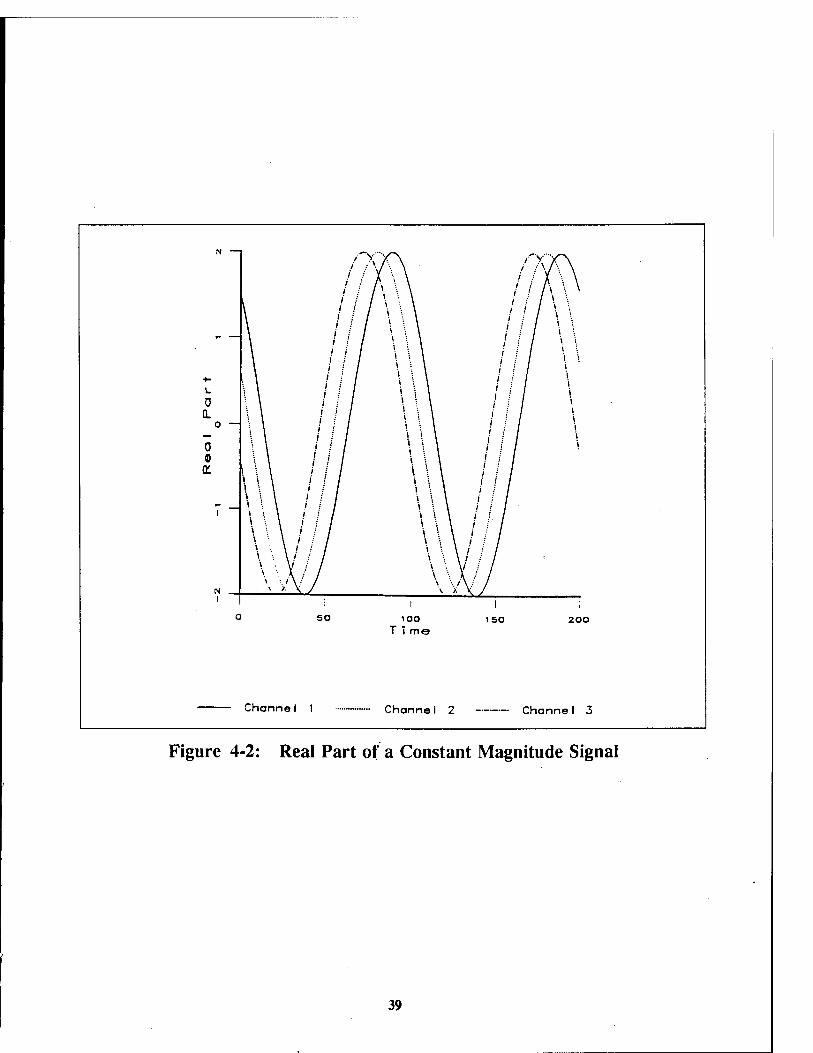
N —

//A\\ ;

>"W\ i ••' Y \

'ihx - -

1 i i i

/ / \ \ \ / * \ / '* ''■ \

i * \

i i i i i

i / \ '■ / ' ■ / / \ ;

/ / \ '■■

+■

i i i

■ / 1 : \ / l : \

/ / t \

i i i / 1.

L / ' : \ i / i

0 i / ' ' \ i / '• Q. 1 ;

1 l 1 i i / 1

o — / ' \ i

/ 1 — i / / ' \ / l

0 i : / ' \ i ! / 1

0 1 / ' "' \

i j

£ \ \ \ / / / ; / * M \ \ \

i j ,

i —

\ \ \ \ \ \ \ \ ' \ \ ' * • \ ' \ \ 1 \ '. \ / \ • \ ;' \ ■ V

' ■ 1 i ; 1 ! 1

i \ i \ i \ \ \ \ \ \ \ \

» \ \ i \ \ i \ '• \ ;' * V

1 j 1

N

\ I \ •■. /' \ •• \ >. \

\ A \ '■. /'\

1

0

i

so 1

lOO

1 1 so

1 200

1

T i me

Chorine 1 2 Chonno1 3

Figure 4-2: Real Part of a Constant Magnitude Signal

39

N —

V '■■ \ A \ \ / \ \

i \ > \ \ '• \

/ /

/' / / i .-: / : / /

•' ■ 1

,- — \ \ \ ///

i I ■♦-

/ / \ ■ j J

L U j /

0 Q. \ \ \ II ]

\ • ■ • /

>> \ \ \ 1 i 1 .

1 i I i 1 \ \ / / /

>- C

\ '• \ i \ i 1

i / \ 11 i— 1 i \ •' i / \ 1 0) 0 E

\\

i I i i i

jl _ 1 \ / j I i i 1

\\ ■

{ J : J

N

\\V/ \\v 1 . 1

(

1 3 SO

1 lOO

i ISO

i 200

T 1 me

Channe 1 1 - — Channel 2 Channe1 3

Figure 4-3: Imaginary Part of a Constant Magnitude Signal

40

Linking program mamp, please stand by ... f77 -O -C -pipe -cg89 sun4/mamp.o -Lsun4 -lmc -lvec -lmat -lmc -L/home/marlin/tom/lib/sun4 -Ifsl MAMP - Estimates amplitude of multichannel constant signal in clutter. Version 1.14 Null hypothesis input file name ? rlvO Already existing noise file with 2 time samples Title: Gaussian noise, covariance matrix is identity Alternate hypothesis input file name ? rlvl Sum of signal and noise Title: Signal + Noise. Amplitude 1.25. Doppler 0.0. Spacing 0.125 Angle 90o Amplitude estimates output file name ? rlva Amplitude file is created Title of this dataset ? Amplitude estimates Help is available Estimation: sample Matrix, time/space Average, time Clipping(m/a/c) [M] ? ? Enter "m" to use sample covariance matrix estimate. Enter "a" to use the time/space averaged estimator for the correlation matrix. Enter "c" to use the time/space averaged estimator with time clipping. Estimation: sample Matrix, time/space Average, time Clipping(m/a/c) [M] ? a Use biased estimate (y/n) [N] ? y Enter the normalized Doppler (fd T) ? 0.0 Enter the normalized element spacing ? 0.125 Enter the angle to the signal in radians ? 1370796327 Is the magnitude of the amplitude known (y/n) [N] ? Display covariance estimates for each trial (y/n) [N] ? Mean value for 10000 trials.

Noise was synthesized with Identity covariance

(-8.681035e-03.-3.323868e-03) (1.006634e+00.0.000000e+OO) (-6.401982e-03.4.316789e-03) (-4.838127e-03.-9.185376e-O4)

Average covariance matrix: Columns 1 through 2

(9.921660e-01.0.000000e+00) (-8.681035e-03,3.323868e-03) (3.554484e-03.-1.095882e-03) (-3.996205e-03,-3.282540e-03)

Columns 3 through 4 (3.554484e-03.1.O95882e-03) (-3.996205e-03.3.282540e-03) (-6.401982e-03.-4.316789e-03) (-4.838127e-03.9.185376e-O4) (9.921660e-01.0.000000e+00) (-8.681035e-03.-3.323868e-03) (-8.681035e-03,3.323868e-03) (1.006634e+0O,0.0O0000e+O0)

Inverse of average covariance matrix: Columns 1 through 2

(l.O08024e+OO.0.OOO000e-t<X)) (8.688107e-03.-3.324494e-03) (-3.545582e-03,1.096502e-03) (4.019544e-03,3.300156e-03)

(8.688107e-03.3.324494e-03) (9.935789e-01 .-2.576044e-09) (6.415665e-03.-4.301259e-03)

(4.840136e-03.8.89914 le-04)

Figure 4-4: Estimating the Covariance Matrix and Amplitude

41

Columns 3 through 4 (-3.545597e-03.-1.096502e-03) (4.019544e-03.-3.300156e-03) (6.415665e-03.4.301277e-03) (4.840136e-03.-8.899141e-04) (1.008057e+O0.4.493454e-09) (8.709729e-03.3.317986e-03) (8.709729e-03.-3.317978e-03) (9.935464e-01,-1.200157e-08)

Trial: 1 Amplitude Estimate: (1.5886e+00.1.2140e+00) Magnitude: 1.9994e-fO0

display: Next trial. All trials, or Quit (n/a/q) [N] ? a Trial: 2 Amplitude Estimate: (-1.0848e+00,-8.5688e-01)

Magnitude: 1.3824e+O0 Trial: 3 Amplitude Estimate: (-5.6062e-01,-1.3987e+00)

Magnitude: 1.5069e-+O0

Trial: 9998 Amplitude Estimate: (-3.373le-OU.2878e+00) Magnitude: 1.3312e+O0

Trial: 9999 Amplitude Estimate: (1.0322e-01,-9.3869e-01) Magnitude: 9.4435e-01

Trial: 10000 Amphtude Estimate: (1.8662e-01,8.7653e-01) Magnitude: 8.9618e-01

Mean value for 10000 trials. Average amplitude estimate: (1.3166e-02,2.2880e-03)

Variance: 1.8137e-tOO Average magnitude: 1.3018e+O0 Actual magnitude was 1.25

Variance: 1.1894e-01 ok?

Figure 4-5: Estimating the Covariance Matrix and Amplitude (Cont.)

4.1.2 Subtraction Filter Routine

Figure 4-6 shows the subtraction filter routine. The input consists of two files. The first file contains the radar returns from which the estimated signal is to be subtracted. The second file contains the estimated amplitudes produced by the amplitude estimating routine. There should be one amplitude estimate for each realization of the radar returns in the first file. Optionally, the user can specify a single amplitude to be used for all realizations. The output is an estimate of the clutter, formed by subtracting the estimated signal from the inputs. The output is suitable for use in a signal detection algorithm, or for diagnostics. For example, mean descriptive statistics over the 10,000 trials in the output from the subtraction filter can be calculated. The sample variance along the two channels is 1.027 and 1.001, respectively. The sample estimates can be compared with the theoretical value for these innovations, unity in this case.

4.1.3 Constant Signal Analysis Routines

Four new analysis sequences were written in the UFI-based system for the analysis of constant magnitude signals with unknown amplitudes. Figure 4-7 shows the UFI menu for choosing one of these analysis sequences. The first sequence is used to examine the performance of the covariance matrix and amplitude estimation algorithms. The other three sequences are used to analyze the signal detection algorithm illustrated in Figure 4-8.

42

Linking program msubfil, please stand by ... f77 -O -C -pipe -cg89 sun4/msubfil.o -Lsun4 -lmc -lvec -lmat -Imc -L/home/marlin/tom/lib/sun4 -lfsl -o MSUBFIL -- Filters input by subtracting constant signal Version 1.5 Input file name ? rlvl Title: Signal + Noise. Amplitude 1.25. Doppler 0.0. Spacing 0.125 Angle 90o Output file name ? rlvsub Title of this dataset ? Estimated noise Enter amplitude or read from File (ef) [F] ? File containing amplitude estimates ? rlva Title: Amplitude estimates Enter the normalized Doppler (fd T) ? 0.0 Enter the normalized element spacing ? 0.125 Enter the angle to the signal in radians ? 1.570796 Filtered 10000 trials. ok?

Figure 4-6: Routine for Subtracting the Estimated Signal

Select a constant magnitude signal sequence with unknown amplitudes

BACK) ? 1

? } Test covariance matrix and amplitude estimation

?} Unknoun amplitude signal detection analysis in SIRP noise )

? ) Unknoun amplitude signal detection analysis in SIRP clutter }

? ) Unknoun amplitude signal detection analysis in SIRP clutter and noise j

Figure 4-7: Unknown Amplitude Analysis Sequences

43

y(n)

Estimate r

Estimate Filter

Parameters

*(n)

*(n)

t<

Linear Filter F0

v0(n)

L,

^0 x(n)-äs^(n) Linear Filter F0

v,W|

SIRP Loglikelihood

&s^(n)

0 sa(n)

x(n) Estimate Amplitude

Figure 4-8: The Signal Detection Algorithm for a Constant Signal

The analysis sequence for analyzing the amplitude estimation algorithm is fairly straightforward. The user is asked to enter the number of trials used in synthesizing clutter and the number of trials used in synthesizing the sum of signal and clutter. Synthesized clutter is used in estimating the block covariance matrix. The sum of clutter and the signal is used to estimate the amplitude. The user enters AR process parameters for the clutter and parameters for the constant magnitude signal. The clutter is an AR process with Gaussian, K- distributed SIRP, or Weibull SIRP driving noise. The covariance matrix and the amplitudes are estimated as in the menu-based routines. Estimates of the covariance matrix and the amplitude are sent to the output file. Figures 4-9, 4-10, and 4-11 show a sample output of this analysis sequence.

44

Set random number seeds Set random number generator seed : n Get number of channels. Number of channels : 2 Get some common parameters for signal, clutter, and noise. Length of the generated process in points : 3 Enter the number of points to be generated before saving data : 500 Get AR process parameters with SIRP driver Order of the AR process : 3 Gaussian, K-distributed SIRP, or Weibull SIRP driving noise (g/k/w) : k Do you want S to vary within each realization/trial (y/n) : y Do you want the diagonal elements of S to all be equal (y/n) : y Specify Cholesky or L-D-U decomposition (c/1) : c Driving noise: real only, imaginary only, or complex (r/i/c) : c Noise Alpha, the shape parameter for Gamma distribution of S : 0.5 Noise B, a parameter for the distribution of V : 1.0 Use Gaussian or Exponential shaped function (g/e) : g Enter the amplitude matrix for the AR process : 1.0,0.0 0.0,1.0 Enter the intertemporal correlation matrix for the AR process : 0.1,0.0 0.0,0.1 Enter the matrix of lag values for the AR process : 0,0 0,0 Reference doppler frequency for the AR process : 0.0 Enter the sample interval for the AR process : 0.01 Intertemporal correlation coefficients: R(0)=( 1.0000e+00,0.0000e+00) (0.0000e+00,0.0000e+00)

(0.0000e+00,0.0000e+00) (1.0000e+00,0.0000e+00)

R( 1 )=( 1 .OOOOe-01,0.0000e+00) (O.0000e+O0,0.0000e+O0) (0.0000e+00,0.0000e+00) (1.0000e-01,0.0000e+00)

R(2)=( 1.0000e-04,0.0000e+00) (0.0000e+00,0.0000e+00) (0.0000e+00,0.0000e+00) (1.0000e-04,0.0000e+00)

R(3)=( 1.0000e-09,0.0000e+00) (0.0000e+00,0.0000e+00) (0.0000e+00,0.0000e+00) (1.0000e-09,0.0000e+00)

Determinants of principle minors: (l.aXXte+«)A000(te+O0)(l.(^^ Coefficients for the AR process: a(l)= (-1.0101e-01,0.0000e+00) (0.0000e+00,0.0000e+00)

(0.0000e+00,0.0000e+00) (-1.0101e-01,0.0000e+00)

a(2)= (1.0101e-02,0.0000e+00) (0.0000e+00,0.0000e+00) (0.0000e+00,0.0000e+00)(1.0101e-02,0.0000e+00)

a(3)= (-1.0000e-03,0.0000e+00) (0.0000e+00,0.0000e+00) (0.0000e+00,0.0000e+00) (-1.0000e-03,0.0000e+00) ;

Figure 4-9: Amplitude Estimation Results

45

Covariances: (9.8990e-01,0.0000e+00) (0.0000e+00,0.0000e+00) (0.0000e+00,0.0000e+00) (9.8990e-01,0.0000e+00)

Correlations: (9.9494e-01,0.0000e+00) (0.0000e+00,0.0000e+00) (0.0000e+00,0.0000e+00) (9.9494e-01,0.0000e+00)

CONSTOP - Reads constant magnitude signal parameters from user Amplitude of constant magnitude signal : 1.25 Normalized Doppler of constant magnitude signal : 0.0 Normalized element spacing : 0.125 Angle to the signal in radians : 1.5708 MCOVP - Asks the user to enter covariance matrix estimation options Estimation: sample Matrix, time/space Average, time Clipping(m/a/c) : a Use biased estimate (y/n) : y Output each covariance matrix estimate (y/n) : n ACOV0P - Asks user for info about average covariance matrix estimate Output the average covariance matrix estimate (y/n) : y MAMPOP - Ask user whether amplitude estimates should be output Output each amplitude estimate (y/n) : n Is the amplitude magnitude known (y/n) : n Mean value for 10000 trials.

Average covariance matrix: Columns 1 through 2

(9.739912e-01,0.000000e+00) (2.712762e-03,-5.375063e-03) (6.350853e-02,5.04961 le-03) (-8.788312e-04,2.111209e-03) (-2.587584e-03,-7.809592e-06) (-8.176130e-04,2.022152e-04)

(2.712762e-03,5.375063e-03) (9.901970e-01.0.OOOOOOe+OO)

(-2.736679e-03,-7.572205e-03) (6.849832e-02,9.498819e-04) (-8.939112e-04,-1.153310e-03)

(-3.452280e-04,1.530773e-03)

Columns 3 through 4 (6.350853e-02,-5.04961 le-03) (-2.736679e-03,7.572205e-03) (9.739912e-01,0.000000e+00) (2.712762e-03,-5.375063e-03) (6.350853e-02,5.04961 le-03) (-8.788312e-04,2.111209e-03)

Columns 5 through 6 (-2.587584e-03,7.809592e-06) (-8.939112e-04,1.153310e-03) (6.350853e-02,-5.04961 le-03) (-2.736679e-03,7.572205e-03) (9.739912e-01,0.000000e+00) (2.712762e-03,-5.375063e-03)

(-8.788312e-04,-2.111209e-03) (6.849832e-02,-9.498819e-04) (2.712762e-03,5.375063e-03) (9.901970e-01,0.000000e+00)

(-2.736679e-03,-7.572205e-03) (6.849832e-02,9.498819e-04)

(-8.176130e-04,-2.022152e-04) (-3.452280e-04,-1.530773e-03) (-8.788312e-04,-2.111209e-03) (6.849832e-02,-9.498819e-04) (2.712762e-03,5.375063e-03) (9.901970e-01,0.000000e+00)

Figure 4-10: Amplitude Estimation Results (Cont'd)

46

Variances: Columns 1 through 4

l.543065e+OO 9.388222e-01 9.388222e-01 2.419760e-01 2.206363e-01 1.050504e-01 1.063162e-01

1.547744e+00 2.341915e-01 2.381257e-01 1.100442e-01 1.076555e-01

2.419760e-01 2.341915e-01 1.543065c+00 9.388222e-01 2.419760e-01 2.206363e-01

2.206363e-01 2.381257e-01 9.388222e-01 1.547744e+00 2.341915e-01 2.381257e-01

Columns 5 through 6 1.050504e-01 1.100442e-01 2.419760e-01 2.341915e-01 1.543065e+O0 9.388222e-01

1.063162e-01 1.076555e-01 2.206363e-01 2.381257e-01 9.388222e-01 1.547744e+00

Inverse of average covariance matrix: Columns 1 through 2

(1.031222e+00,0.000000e+00) (-3.135458e-03,6.307013e-03) (-6.778821e-O2,-5.359376e-03) (1.331642e-03,-3.049985e-03) (7.148132e-03,7.088222e-04) (6.700754e-04,1.828000e-04)

Columns 3 through 4 (-6.778820e-02,5.359375e-03) (3.187418e-03,-8.721530e-03) (1.035732e+O0,1.429922e-09) (-3.431261 e-03,7.086784e-03) (-6.778634e-02,-5.365778e-03) (1.310989e-03,-3.038183e-03)

Columns 5 through 6 (7.148176e-03,-7.088184e-04) (5.463175e-04,-2.309680e-05) (-6.778634e-02,5.365772e-03) (3.181983e-03,-8.725822e-03) (1.031291 e+O0,-9.782253e-10) (-3.096640e-03,6.345086e-03)

(-3.135458e-03,-6.307036e-03) (1.014910e+00,1.124075e-08) (3.187418e-03,8.721530e-03)

(-7.064067e-02,-8.784747e-04) (5.463213e-O4,2.312660e-05) (5.255580e-03,-1.441172e-03)

(1.331642e-03,3.049985e-03) (-7.064067e-02,8.784608e-04) (-3.431246e-03,-7.086769e-03) (1.019806e+00,-8.951288e-09) (3.181972e-03,8.725807e-03)

(-7.064237e-02,-8.721282e-04)

(6.70079 le-04,-1.828074e-04) (5.255580e-03,1.441169e-03) (1.310974e-03,3.038183e-03) (-7.064235e-02,8.721200e-04) (-3.096633e-03,-6.345093e-03) (1.014843e+00,-8.683358e-10)

Mean value for 10000 trials. Average amplitude: (-2.0039e-02,8.3590e-03) Variance: 1.7575e+00 Average magnitude: 1.291 le+00 Variance: 9.1017e-02 Actual magnitude 1.25

Figure 4-11: Amplitude Estimation Results (Cont'd)

47

The remaining sequences estimate the threshold and the probability of detection for user-specified false alarm probabilities. Variances in these estimates are calculated. In all three cases discussed here, the signal is a constant magnitude signal, as described in Section 3.1.2. The three sequences vary among the null hypotheses in which no signal is present. In one case, the clutter is modeled as K-distributed SIRP white noise uncorrelated in time. In this case, the filter F0 merely decorrelates the input across channels, as in Figure 3-1. In the second case, the clutter is modeled as an AR process with K-distributed SIRP driving noise. In the third case, the clutter is modeled as the sum of an AR process and white noise. In both of these cases, the filter F0 decorrelates the input across time and across channels, as in Figure 3-2.

These sequences begin with an a priori estimation phase. Many realizations of the clutter y(n) are used to estimate the covariance matrix I and the filter parameters. When the clutter is modeled as white noise, the filter has only one parameter, related to the 7x7 zero-lag covariance matrix. Otherwise, AR coefficients and the driving noise covariance matrix are estimated.

The next step is to synthesize many realizations of the radar returns x (n) under the null hypothesis of no signal. These realizations are used to determine the loglikelihood statistic A for given false alarm probabilities. The statistic is calculated for each realization, as shown in Figure 4-8. The null hypothesis innovations v0(« ) are estimated by the appropriate linear filter, Figure 3-1 or Figure 3-2. The signal amplitude is estimated for each realization based on the 'a priori' estimate of the covariance matrix and the known steering vector. The user has the option of specifying the amplitude magnitude as known, in which case only the phase is estimated. The amplitude estimate is used to subtract the estimated signal from the radar returns, and the result is then filtered by F0 to produce the alternative hypothesis innovations v,(n). These innovations are used to calculate the appropriate loglikelihood statistic for a K- distributed SIRP. An estimate of the probability distribution for A under the null hypothesis is found from the many realizations of the loglikelihood distribution. This allows the program to calculate the statistic value (threshold) for the tail probability given by the false alarm probability.

Another set of realizations of the radar returns are used to estimate the probability of detection. This set of realizations contains the constant magnitude signal, as well as clutter. The signal is resynthesized for each realization, allowing the signal phase to vary randomly across realizations. The same signal detection algorithm (Figure 4-8) is used to calculate the loglikelihood statistic for each realization. If it is above the threshold determined before by an user-specified false alarm probability, the algorithm decides that a signal is present. The detection probability is estimated as the ratio of the number of realizations in which a signal is decided to be present to the total number of realizations.

The user can specify that this process of a priori estimation, threshold determination, and probability of detection estimation be repeated a number of times. The different results of these repetitions are used to estimate the variance in the estimates of the threshold and the probability of detection.

4.2 Weibull Clutter

A number of subroutines were modified, both in the menu-based subsystem and in sequences in the UFI-based subsystem, to implement the synthesis of Weibull-distributed Spherically Invariance Random Processes (SIRPs). Figure 4-12 shows an invocation of this

48

MULTI-CHANNEL (M/C) PROCESS SYNTHESIS MENU

M2 -- Method 2 (MC2) process synthesis

Enter a command or Q to return to the MAIN menu: m2 Linking program msirp, please stand by ... 'bin/sun4/msirp' is up to date. MSIRP -- Multichannel AR Process Generation with SIRPs Version 1.14 Do you want to set the pseudo random generator seeds (y/n) [N] ? y Enter an integer seed value ? 4 Enter an integer seed value ? 6 Enter an integer seed value ? 8 Enter an integer seed value ? 1 Number of channels ? 1 Number of points to be generated and saved ? 100 Enter the number of trials to be generated ? 10 Add a signal component (y/n) [Y] ? n Add a clutter component (y/n) [Y] ? n Add a white noise component (y/n) [Y] ? y ENTER PARAMETERS FOR THE NOISE. Gaussian, K SIRP, or Weibull SIRP noise (g/k/w) [G] ? w Do you want R to vary within each realization/trial (y/n) [Y] ? y Do you want R to be constant across channels (y/n) [Y] ? y Specify Cholesky, L-D-U, or SVD (c/l/s) [C] ? c Do you want the noise to be real, imaginary, or complex (r/i/c) [C] ? c Enter Noise B, a parameter for the Weibull distribution ? 1.0 Do you want the Cholesky decomposition matrix C to be identity (y/n) [Y] ? y Complex Weibull-distributed SIRP noise will be generated. SIRP random variable R varies across time samples. R will be constant across channels. B for the SIRP: 1.0000e+00 Correlations: (1.0000e+00,0.0000e+00) Are these parameters okay (y/n) [Y] ? y Total output file name ? rlv Title of this dataset ? White noise, magnitude is Weibull Noise output file name ? No file name entered, is this okay ? y Note: the following IEEE floating-point arithmetic exceptions occurred and were never cleared; see ieee_flags(3M): Inexact; Underflow; Overflow; Invalid Operand; Sun's implementation of IEEE arithmetic is discussed in the Numerical Computation Guide.

ok? Warning message is common

Figure 4-12: Synthesizing Weibull Noise

49

capability. In this case, temporally uncorrelated white noise is generated. Each time sample is a complex one-channel SIRP with another realization of the spherical distance from the origin R. From Equations 3.2-23 and 3.2-11 through 3.2-14, one can show the distribution of the magnitude of the process is the Weibull distribution given by Equation 4.2-1:

(4.2-1) fR(r) = ab r b-\e-arb >0.

Since the user specifies b to be equal to unity in the example, both the scale and shape parameters of this Weibull distribution are unity. (See Appendix B.)

The synthesized process can be analyzed by any capabilities provided in the MSPSS. For example, Figure 4-13 shows the results of applying Ozturk's algorithm (Ozturk 90) to the magnitude of the first realization of the processes synthesized in Figure 4-12. The hypothesis that the magnitude is Weibull-distributed, with a shape parameter of unity, should be rejected if the endpoint of the curve corresponding to the sample falls outside the double circles. In this case, Ozturk's statistic leads to the acceptance of a Weibull distribution. So this case illustrates a test showing the Weibull-synthesis capability functions correctly.

o

K)

o

Ozturk's Statistic

I.I.I

>

O

O

0

,90% Confidence Interval

. 99% Confidence Interval

Weibull Distribution Expected Value

Transformed Sample

-o .2 -o. 1 o.o U

o. 1 0.2

Figure 4-13: Ozturk Test for Weibull Distribution

50

Some difficulties arose in implementing the Weibull distribution. Appropriate parameters for the triangular distributions described in Appendix C were found numerically. The synthesis process can be quite slow for Weibull SIRPs with a large number of time samples. Procedures to remove these limitations should be investigated.

4.3 Representative Model The Representative Model was implemented as one routine in the menu-based subsystem.

Figures 4-14 through 4-17 illustrate the use of this routine. The user enters parameters describing the signal, the clutter, and interference. Two models are provided for both the signal and the interference. The synthesized process need not contain signal, clutter, and interference. Any of the three can be absent. The user is able to save each to a separate file, as well as any AR parameters that have been calculated for the respective models. Only the sum of signal, clutter, and interference is saved in the illustrated example. Figure 4-18 shows a graph of the real part of the synthesized process. In this case, the synthesized process consists of two periods of three channels of a phase-shifted sine wave (for the signal), with the addition of clutter and interference.

STAP — Synthesizes multichannel representative model processes Version 1.13 Do you want to set the pseudo random generator seeds (y/n) [N] ? Number of channels ? 3 Describe radar. Number of points to be generated and saved ? 100 Enter the number of trials to be generated ? 100 Enter the normalized element spacing ? 0.25 Enter the normalized platform Doppler center frequency ? 0.014142136

Channels/elements: 3 Time samples: 100 Realizations/trials: 100

Radar parameters: Normalized element spacing: 2.50000e-01 Normalized element spacing: 1.41421e-02

Are these parameters okay (y/n) [Y] ? Add a signal component (y/n) [Y] ? Describe signal. ENTER PARAMETERS FOR THE SIGNAL. Do you want a Constant amplitude or Random signal (c/r) [C] ? c Enter the normalized signal Doppler center frequency ? 0.014142136 Enter the angular direction to signal ? 0.785398163 Enter the magnitude of the signal ? 1.5 Do you want to specify the initial phase (y/n) [Y] ? Enter the initial phase ? 0.0 Constant amplitude signal parameters:

Normalized signal Doppler center frequency: 1.41421e-02 Angular direction to the signal: 7.85398e-01 Magnitude: 1.50000e+00 Initial phase: 0.00000e+00

Are these parameters okay (y/n) [Y] ?

Figure 4-14: Representative Model Synthesis

51

Add a clutter component (y/n) [Y] ? Describe clutter. ENTER PARAMETERS FOR THE CLUTTER. Enter the angular beam direction ? 0.0 Do you want the clutter to be real, imaginary, or complex (r/i/c) [C] ? Gaussian, K-distributed SIRP, or Weibull SIRP driving noise (g/k/w) [G] ? Constant clutter standard deviation across channels (y/n) [Y] ? Enter the channel standard deviation ? 0.5 Do you want to use the Block procedure or an AR process (b/a) [A] ? a Enter the number of points to be generated before saving data ? 1000 Enter the order of the AR process ? 4 Specify Cholesky, L-D-U, or SVD decomposition (c/l/s) [C] ? c Gaussian, exponential Correlation, or exponential Power temporal shaping [G] ? g Enter the one lag temporal correlation parameter ? 0.90 Gaussian or Hanning/hamming/blackman-harris spatial shaping function (g/h) [G] ? g Enter the one lag spatial correlation parameter ? 0.9 Clutter parameters:

Angular beam direction: 0.00000e+00 Driving noise is complex. Cholesky decomposition is used in synthesizing driving noise. Clutter has Gaussian driving noise. Channel standard deviations:

5.00000e-01 5.00000e-01 5.00000e-01 Clutter will be synthesized as an AR process. Points to prime the clutter process: 1000 Order of the AR process: 4 A Gaussian temporal shaping function will be used. One lag temporal correlation parameter: 9.00000e-01 A Gaussian spatial shaping function will be used. One lag spatial correlation parameter: 9.00000e-01

Are these parameters okay (y/n) [Y] ? y

Block covariance matrix for lag 0 2.500000e-01 2.250000e-01 1.640250e-01 2.250000e-01 2.500000e-01 2.250000e-01 1.640250e-01 2.250000e-01 2.500000e-01

The program calculates the block covariance matrix.

Block covariance matrix for lag 4 4.632548e-02 4.169293e-02 3.0394l5e-02 4.169293e-02 4.632548e-02 4.169293e-02 3.039415e-02 4.169293e-02 4.632548e-02

Figure 4-15: Representative Model Synthesis (Continued)

52

Coefficients for the AR process: A(l):

-2.698014e+00 -1.227813e-03 -2.500378e-03 -2.694599e+O0 4.966523e-04 -2.732538e-03

The program calculates the AR coefficients.

1.968449e-05 -2.502176e-03

-2.697129e+00

A(2): 3.308810e+00 6.143676e-03 -1.290442e-03

2.801777e-03 3.300308e+O0 6.827475e-03

5.090439e-05 6.123936e-03 3.306435e+O0

A(3): -2.186008e+00 -6.042001e-03 1.349216e-03

-2.527904e-03 -2.177529e+O0

-6.845814e-03

-1.548294e-04 -5.998279e-03

-2.183456e+O0

A(4): 6.564693e-01 2.379417e-03 -5.674362e-04

9.012222e-04 6.530809e-01 2.756119e-03

1.044273e-04 2.352715e-03 6.553717e-01

Driving noise covariance matrix: 4.342771e-03 3.905334e-03 3.907508e-03 4.342770e-03 2.840573e-03 3.901698e-03

2.844440e-03 3.907157e-03 4.340220e-03

Decomposed driving noise covariance matrix: 6.58997 le-02 0.000000e+00 O.000000e+O0 5.929477e-02 2.875588e-02 0.000000e+00 4.310448e-02 4.680183e-02 1.708250e-02

Figure 4-16: Representative Model Synthesis (Continued)

53

Add interference (y/n) [Y] ? y Describe interference. ENTER PARAMETERS FOR THE INTERFERENCE. Direct path White noise or partially Correlated noise (w/c) [W] ? w Enter the normalized interference Doppler center frequency ? -0.014142136 Enter the angular direction to jammer ? 0.523598776 Do you want the interference to be real, imaginary, or complex (r/i/c) [C] ? c Gaussian, K-distributed SIRP, or Weibull SIRP driving noise (g/k/w) [G] ? g Enter the shaping function standard deviation ? 0.707106781 Direct path white noise interference parameters:

Normalized interference Doppler center frequency: -1.41421e-02 Angular direction to the jammer: 5.23599e-01 Driving noise is complex. Cholesky decomposition is used in synthesizing driving noise. Interference has Gaussian driving noise. Standard deviation:

7.07107e-01 Are these parameters okay (y/n) [Y] ? y Total output file name ? rlv Save synthesized results. Title of this dataset ? Rep. Model signal + clutter + interference Signal output file name ? No file name entered, is this okay ? y Clutter output file name ? No file name entered, is this okay ? y Clutter output coefficient file name ? No file name entered, is this okay ? y Interference output file name ? No file name entered, is this okay ? y ok?

Figure 4-17: Representative Model Synthesis (Continued)

54

Figure 4-18: Real Part of Sum For the Three Channels

55

4.4 Two-Dimensional FFT

A two-dimensional FFT of the covariance matrix for the Representative Model clutter was implemented as one routine in the menu-based subsystem. The 2-D FFT algorithm was based on that implemented under Khoros. A 2-D FFT is implemented in Khoros as a combination of C and Fortran source code. The C source code was translated to Fortran under this effort. Figures 4-19 through 4-23 show an invocation of the two-dimensional FFT capability. The user enters parameters describing parameters of the correlation function for the Representative Model clutter. The 2-D FFT must be run under X Windows. A new window appears at various points in the program for displaying graphs. These displays use the Khoros program Xprism. Xprism allows the user to manipulate, rotate, and annotate the results.

Performs 2-D FFT on Representative Model Covariance Matrix. Version 1.14 Number of channels ? 12 Number of time samples ? 12 Enter the normalized element spacing ? 0.5 Enter the normalized platform Doppler center frequency ? 0.5 Enter the angular beam direction ? 0.0 Enter the channel standard deviation ? 2.0 Gaussian, exponential Correlation, or exponential Power temporal shaping [G] ? Enter the one lag temporal correlation parameter ? 0.9975 Gaussian or Hanning/hamming/blackman-harris spatial shaping function (g/h) [G] ? Enter the one lag spatial correlation parameter ? 0.54 Do you want to do Dolph-Chebychev filtering (y/n) [Y] ? y Sidelobe level (in decibels relative to peak) ? 40.0

Channels/elements: 12 Time samples: 12 Normalized element spacing: 5.0000000e-01 Normalized platform Doppler: 5.0000000e-01 Angular beam direction: 0.0000000e+00 Channel standard deviations: 2.0000000e+00 A Gaussian temporal shaping function will be used. One lag temporal correlation parameter: 9.9750000e-01 A Gaussian spatial shaping function will be used. One lag spatial correlation parameter: 5.4000002e-01 Dolph-Chebychev filtering will be performed. Sidelobe level: 4.0000000e+01 Are these parameters okay (y/n) [Y] ? Plotting covariance matrix... Displays graph in Figure 4-20 Complex data conversion: Real, Imaginary, Magnitude, or Angle [R] ? Plotting covariance matrix... Displays graph in Figure 4-21 Complex data conversion: Real, Imaginary, Magnitude, or Angle [R] ? r Plotting FFT of covariance matrix... Displays graph in Figure 4-22 Complex data conversion: Real, Imaginary, Magnitude, or Angle [R] ? m Plotting FFT of covariance matrix... Displays graph in Figure 4-23 Complex data conversion: Real, Imaginary, Magnitude, or Angle [R] ? ok?

Figure 4-19: An FFT Example

56

Correlation Function

12 Channels, 12 Time Lags Normalized element spacing: 0.5 Normalized platform Doppler: 0.5 Angular beam direction: 0.0 Channel standard deviation: 2.0

L 0 Q.

0 0

Gaussian temporal and spatial shaping functions Temporal correlation: 0.9975 Spatial correlation: 0.54

Figure 4-20: Graph of Correlation Function

57

Correlation Functio with Dolph-Chebychev Filtering

n

Sidelobe level: 40.0

o o 0

o Q.

0

Figure 4-21: Dolph-Chebychev Filtering of Correlation Function

58

Figure 4-22: Graph of FFT

59

Fast Fourier Transform • 6

Logarithm

Doppler

Spatial Frequency

Figure 4-23: Logarithm of Magnitude of FFT

60

4.5 State Space Capabilities

Figures 4-24, 4-25, and 4-26 illustrate the use of the new state space routine added under this effort. The user enters parameters for a "shaping function" defining the block covariance matrices for lags equal to the user-selected order of an AR process. The Levinson-Wiggins- Robinson algorithm is used to solve the Yule-Walker equations to find the AR parameters. Block covariance matrices for a larger number of lags are found through either the State Space Closed Form Method (Section 3.5.1) or the AR Recursion Method (Section 3.5.2). This block covariance matrix is used to find state space parameters by the canonical correlations algorithm. (Previously, the block covariance matrix needed to be estimated from a synthesized process, thus introducing statistical variation.) As the example illustrates, the resulting state space estimates can exhibit a basis transformation.

SSC2 - Estimates state space model parameters by Scientific Studies algorithm Version 1.8 Number of channels ? 2 Order of the AR process ? 2 Use Gaussian or Exponential shaped function (g/e) [G] ? Enter row 1 of the amplitude matrix: Enter a row ? 1.995, 0.0 Enter row 2 of the amplitude matrix: Enter a row ? 0.0,1.995 Enter row 1 of the intertemporal correlation matrix: Enter a row ? 0.9, 0.0 Enter row 2 of the intertemporal correlation matrix: Enter a row ? 0.0, 0.9 Enter row 1 of the lag matrix: Enter a row ? 0,0 Enter row 2 of the lag matrix: Enter a row ? 0,0 Reference doppler frequency ? 0.0 Enter the sample interval ? 0.01 An AR( 2 ) process will be analyzed. Gaussian shaped function. Amplitude matrix:

1.995000e+00 0.000000e+O0 0.000000e+00 1.995000e+00

1 -lag Temporal Correlation Matrix: 9.000000e-01 0.000000e+00 0.000000e+00 9.000000e-01

Lag matrix: 0 0 0 0

Reference doppler frequency: 0.0000e+00 Hz. Sample interval: 1.0000e-02 seconds. Are these parameters okay (y/n) [Y] ? Intertemporal correlation coefficients:

Figure 4-24: A State Space Example

61

R(0): 1.995000e+00 0.000000e+00

O.OOOOOOe+00 1.995000e+00

R(l ): 1.795500e+00 0.000000e+00

O.OOOOOOe+OO 1.795500e+00

R(2): 1.308919e+OO 0.000000e+00

O.OOOOOOe+OO 1.308919e+00

Coefficients for the AR process: The program A(l):

-1.6290O0e+00 0.000000e+00 0.000000e+00 -1.629000e+00

calculates AR parameters

A(2): 8.099999e-01 0.000000e+00

O.OOOOOOe+OO 8.099999e-Ol

Driving noise covariance matrix: 1.303554e-01 0.000000e+00 0.000000e+00 1.303554e-01

Output file name for parameter estimates ? No file name entered, is this okay ? y Upper bound, L, on size of state space block vector ? 3 State space closed Form or AR recursion method (f/a) ? a Covariance matrix for lag 0

1.995000e+00 0.000000e+00 0.000000e+00 1.995000e+00

Covariance matri> 1.795500e+O0 0.000000e+00

: for lag 1 O.OOOOOOe+00 1.795500e+00

Covariance matrix for lag 2 1.308919e+00 O.OOOOOOe+00 O.OOOOOOe+00 1.308919e+00

Covariance matrix 6.778746e-01 O.OOOOOOe+00

L for lag 3 O.OOOOOOe+OO 6.778746e-01

Covariance matrix 4.403305e-02 O.OOOOOOe+OO

. for lag 4 O.OOOOOOe+OO 4.403305e-02

Figure 4-25: A State Space Example (Cont'd)

62

Covariance matrix for lag 5 -4.773485e-01 0.000000e+00 0.000000e+00 -4.773485e-01

Covariance matrix for lag 6 -8.132674e-01 0.000000e+00 0.000000e+00 -8.132674e-01

MODEL ORDER MENU 0 - Enter the model order directly 1 - Use the canonical correlations to calculate the model order 2 - Use the normalized running sum of the canonical correlations 3 - Use the squares of the canonical correlations 4 - Use the normalized running sum of squares 5 - Use the log parameters 6 - Use the normalized mutual information parameters Model order calculation method ? 1 The program can find the model order Upper bound on canonical correlations ? 0.05 Display diagnostic information (y/n) ? n Intermediate calculations could have been displayed Canonical correlations: 9.79406 le-01 9.794056e-01 6.698955e-01 6.698954e-01 1.653733e-07 1.066407e-07 Order: 4 System Dynamics matrix F:

8.740377e-01 3.144643e-15 3.874717e-01 -3.395807e-09 9.068543e-16 8.740378e-01 -3.395813e-09 -3.874718e-01 -3.874723e-01 3.395806e-09 7.549624e-01 9.210561e-15 3.395801e-09 3.874724e-01 -1.060677e-14 7.549620e-01

Hermetian transpose of Observation matrix H: 1.363761e+00 -9.999875e-09 2.536587e-01 2.253127e-09 9.999872e-09 1.363760e+00 2.253115e-09 -2.536590e-01

Kaiman Gain: 1.001023e+00 2.130526e-09 -2.130539e-09 1.001017e+O0 1.040161e+00 -3.170894e-08 -3.170937e-08 -1.040140e+00

Covariance matrix for innovations: 1.303552e-01 -3.080869e-15 -3.080869e-15 1.303568e-01

Matches theoretical value

ok?

Figure 4-26: A State Space Example (Cont'd)

63

5. REFERENCES (Burden 81) Richard L. Burden, J. Douglas Faires, Albert C. Reynolds, Numerical Analysis, Second Edition; Prindle, Weber & Schmidt; 1981.

(Chakravarthi 92) Prakosh R. Chakravarthi, "On Determining the Radar Threshold for Non- Gaussian Processes from Experimental Data," Ph. D. Thesis, Syracuse University, 1992.

(Huang 88) X. Huang et. al., "A Method for Upgrading the Estimates of the Model Parameters of a Signal When Given a Truncated Measurement," Fourth Annual ASSP Workshop on Spectrum Estimation and Modeling, Minneapolis, MN, 3-5 August 1988.

(Hogg 78) Robert V. Hogg and Allen T. Craig, Introduction to Mathematical Statistics, Fourth Edition, Macmillan, 1978.

(Kaman 91a) Kaman Sciences Corporation, Man Machine Interface Experiment, January 23, 1991.

(Kaman 91b) Kaman Sciences Corporation, User Front-End Interface Knowledge Base (UFIKB) Builders' Guide, February 1991.

(Kaman 92a) Kaman Sciences Corporation, Software User's Manual for the Multichannel Signal Processing Simulation System, May 30, 1992.

(Kaman 92b) Kaman Sciences Corporation, Enhancement of Multichannel Signal Processing Simulation System, December 3, 1992.

(Marple 87) S. Lawrence Marple, Jr., Digital Spectral Analysis, Prentice-Hall, Inc., 1987.

(Michels 89) James H. Michels, A Parametric Detection Approach Using Multichannel Processes, Rome Air Development Center, RADC-TR-89-306, November 1989.

(Michels 90a) James H. Michels, Synthesis of Multichannel Autoregressive Random Processes and Ergodicity Considerations, Rome Air Development Center, RADC-TR-90-211, July 1990.

(Michels 90b) James H. Michels, Multichannel Linear Prediction and Its Association with Triangular Matrix Decomposition, Rome Air Development Center, RADC-TR-90-226, November 1990.

(Michels 91) James H. Michels, Multichannel Detection Using the Discrete-Time Model-Based Innovations Approach, Rome Laboratory, RL-TR-91-269, August 1991.

(Michels 92a) James H. Michels, Multichannel Detection of Partially Correlated Signals in Clutter, Rome Laboratory, RL-TR-92-332, December 1992.

(Michels 92b) James H. Michels, Considerations of the Error Variances of Time-Averaged Estimators for Correlated Processes, Rome Laboratory, RL-TR-92-339, December 1992.

(Michels 94) James H. Michels, Pramod K. Varshney, and Donald D. Weiner, "Synthesis of

64

Correlated Multichannel Random Processes," IEEE Transactions on Signal Processing, Vol. 42, No. 2, February 1994, pp. 367-375.

(Michels 95) James H. Michels, Pramod K. Varshney, and Donald D. Weiner, "Multichannel Signal Detection Involving Temporal and Cross-Channel Correlation," IEEE Transactions on Aerospace and Electronic Systems, Vol. 31, No. 3, July 1995, pp. 866-879.

(Ozturk 90) A. Ozturk and E. J. Dudewicz, A New Statistical Goodness-of-Fit Test Based on Graphical Representation, Technical Report no. 53, Department of Mathematics, Syracuse University, 1990.

(Rangaswamy 91) M. Rangaswamy, D. D. Weiner, and A. Ozturk, "Simulation of Correlated Non-Gaussian Interference for Radar Signal Detection," Proceedings of Twenty fifth Asilomar Conference on Signals and Computers, Pacific Grove, CA, 1991.

(Rangaswamy 92) M. Rangaswamy, D. D. Weiner, and J. H. Michels, "Innovations Based Detection Algorithm for Correlated Non-Gaussian Random Process," , 1992.

(Rangaswamy 93a) Muralidhar Rangaswamy, Donald Weiner, and Aydin Ozturk, "Computer Generation of Correlated Non-Gaussian Radar Clutter," unpublished manuscript, April 8, 1993.

(Rangaswamy 93b) M. Rangaswamy et. al., Signal Detection in Correlated Gaussian and Non-Gaussian Radar Clutter, Rome Laboratory, May 1993.

(Rasure 92) Rasure and Mark Young, "An Open Environment for Image Processing Software Development," 1992 SPIEIIS&T Symposium on Electronic Imaging, SPIE Proceedings Vol. 1659, 14 February 1992.

(Roman 93) Jaime R. Roman and Dennis W. Davis, State-Space Models for Multichannel Detection, RL-TR-93-146, Rome Laboratory, July 1993.

(Taylor 80) Angus E. Taylor and David C. Lay, Introduction to Functional Analysis, Second Edition, John Wiley & Sons, 1980.

(Vienneau 93) Robert L. Vienneau, David Dekkers, and Sue Eilers, Generalized Multichannel Signal Detection, RL-TR-93-154, Rome Laboratory, July 1993.

(Vienneau 94) Robert L. Vienneau, Fusion of Correlated Sensor Observations, RL-TR-94- 134, Rome Laboratory, August 1994.

65

Appendix A. NOTATION AND ACRONYMS

A.l Notation

A (1) The amplitude in the constant magnitude signal model. (2) A constant used in defining the Probability Density Function for the quadratic form q. (3) A matrix.

A An estimate of the amplitude in the constant magnitude signal model.

AH (k) An AR coefficient.

A*{k) An AR coefficient for the Representative Model clutter.

Bk A constant used in defining the Probability Density Function for the quadratic form q.

Cu C2 Some sets.

C, The Cholesky decomposition of the covariance matrix R,.

C The vector space consisting of n-dimensional complex vectors.

Cc The Cholesky decomposition of the covariance matrix Rc.

Ck A constant used in the rejection method.

C, The Cholesky decomposition of the covariance matrix Rs.

Cw The Cholesky decomposition of the covariance matrix i^.

Ce The Cholesky decomposition of the covariance matrix 1^.

Dw The diagonal matrix in the LDU decomposition of the covariance matrix I».

De The diagonal matrix in the LDU decomposition of the covariance matrix 1^.

F System dynamics matrix in state space model.

F0 The null hypothesis filter.

F{ The alternative hypothesis filter.

H The observations matrix in the state space model.

H0 The null hypothesis.

Hi The alternative hypothesis.

/ (n ) An interference process.

/'(«) A single-channel process which is transformed to form the interference process.

/ The number of channels (elements) in a radar return.

K (1) The number of realizations of a process. (2) Kaiman gain matrix in state space model. (3) Amplitude matrix in a shaping function.

LH, The lower triangular matrix in the LDU decomposition of the covariance matrix L„.

Lt The lower triangular matrix in the LDU decomposition of the covariance matrix I*.

66

M (1) A block covariance matrix related to the quadratic form q. (2) The number of channels in a radar return.

N The number of time samples in a radar return.

P A matrix used in the State Space Closed Form Method.

P (k) A sequence of matrices used in the State Space Closed Form Method.

Q The matrix of eigenvectors in the SVD of i, an estimated block covariance matrix.

Qw The matrix of eigenvectors in the SVD of L„.

Q€ The matrix of eigenvectors in the SVD of l^.

R (1) A coordinate in a generalized spherical transformation of a SIRP. (2) A block covariance matrix

Ra The norm of a Gaussian process.

/?, The covariance matrix for interference in the Representative Model.

Rc, Rcc The block covariance matrix for the clutter in the Representative Model.

Rs The covariance matrix for the signal in the Representative Model.

Ry (k) The kth lagged correlation matrix for the AR process y (n ).

T (1) Either the Cholesky, LDU, or Singular Value Decomposition of I*. (2) A linear operator. (3) The sampling period in a shaping function.

Te Either the Cholesky, LDU, or Singular Value Decomposition of L,,.

Tc Either the Cholesky, LDU, or Singular Value Decomposition of Lc.

Tw Either the Cholesky, LDU, or Singular Value Decomposition of L*.

Ui A random variable used in the rejection method.

X (1) A random variable from a Weibull distribution. (2) A vector space.

Y A random variable from a Weibull distribution.

a (1) A parameter of a Weibull distribution. (2) An amplitude of a signal.

a' A constant used in the rejection method.

a,*(it) An AR coefficient for the signal in the Representative Model.

b A parameter of a Weibull distribution.

b' A constant used in the rejection method.

c (1) A clutter process. (2) A parameter in a linear transformation of a Weibull-distributed random variable. (3) A constant used in the rejection method.

c (n) A clutter process.

d A constant used in the rejection method.

dx A constant used in the rejection method.

— Normalized element spacing in a phased array radar. A,

67

fd T The normalized Doppler of a constant magnitude signal.

fdi T Normalized interference/jammer Doppler center frequency.

fdP T Normalized platform Doppler center frequency.

fdS T Normalized signal Doppler center frequency.

/ A channel index.

j A channel index.

k (1) A index for lags in an AR process. (2) A constant used in the rejection method.

/ A matrix of lag values at which a shaping function for a block covariance matrix peaks.

lA A transformation of a spatial and temporal lag index.

lB A transformation of a spatial and temporal lag index.

lp (n) A normed vector space.

/, A spatial lag index.

/, A temporal lag index.

m A channel index.

n (1) A time index; (2) A noise process.

p The order of an AR process.

q A quadratic form used in the definition of SIRPs.

r A realization of the random variable R resulting from a generalized spherical coordinate transformation of a SIRP.

f„ (/) An estimate of the 1th lag of a covariance matrix.

r-r(l) Time averaged estimate of the /th lag of a covariance matrix from the kth realization of the clutter process.

?TC (I) Time averaged estimate of the / th lag of a covariance matrix with time clipping, from the kth realization of the clutter process.

fjs (/) Time/space averaged estimate of the /th lag of a covariance matrix.

r-rsc (O Time/space averaged estimate of the /th lag of a covariance matrix with time clipping.

s (1) A signal process. (2) A constant used in the rejection method.

s(n) A signal process.

/ («) A process used in synthesizing the representative model signal.

s0, s0(n) The normalized constant magnitude signal. s0 is a block vector formed by concatenating the time samples s0(n ).

j0,i (n) A channel in the normalized constant magnitude signal.

sm(n) A channel in a signal process.

ui, u2 Realizations of random variables used in the rejection method.

68

w(n) Weibull-distributed white noise.

x (1) Radar returns, x is a block vector formed by concatenating the time samples x(n). (2) A realization of the Weibull-distributed random variable X. (3) A vector in a vector spce.

x(n) Radar returns.

v (1) A clutter process, y is a block vector formed by concatenating the time samples y (n ). (2) A vector in a vector spce.

y (n) A clutter process, either white noise or a stochastic process correlated across time (e.g. an AR process).

yk, yk(n) The kth realization of a clutter process, y* is a block vector formed by concatenating the time samples y* («).

z A vector in a vector space.

z (n) A unit-variance zero-mean Gaussian process.

0 A coordinate in a generalized spherical transformation of a SIRP.

r A matrix in the State Space Closed Form Method.

A (1) The loglikelihood statistic. (2) The diagonal matrix of eigenvalues in the SVD of £, an estimated block covariance matrix.

Aw The diagonal matrix of eigenvalues in the SVD of Z„.

Ae The diagonal matrix of eigenvalues in the SVD of I*.

E The covariance matrix for the innovations in the innovations representation of the state space model.

t Estimated block covariance matrix.

Lc The driving noise covariance matrix for the Representative Model clutter

1^, The covariance matrix for weibull noise w (n ).

L,, The covariance matrix for the driving noise e(n ) in an AR process.

<t>; „ A coordinate in a generalized spherical transformation of a SIRP.

a (1) A significance level, that is, the probability of erroneously accepting an alternative hypothesis. In radar, the probability of false alarm. (2) An angle. (3) A scalar.

a' (1) A tail probability. (2) An unknown complex amplitude to modify a steering vector. (3) An angle in the Representative Model of the clutter.

o(« ) State variables in state space model.

ß (1) The probability of erroneous accepting a null hypothesis. In radar, 1 minus the probability of detection. (2) A parameter of a spatial shaping function.

E (1) A driving noise term in an AR process, e is a block vector formed by concatenating the time samples E(/I ). (2) The innovations in the innovations representation of the state space model.

69

C A parameter of the exponential power spectrum temporal shaping function.

6 The initial phase.

6j Angle to the signal.

A. (1) An eigenvalue. (2) A matrix of intertemporal one-lag correlation parameters in a shaping function.

M# The mean of the random variable X.

RK The mean of the random variable Y.

M» One lag spatial correlation parameter.

H< One lag temporal correlation parameter. v<n) A wnite noise process uncorrelated both in time and across channels. ve(« ) A white noise process uncorrelated both in time and across channels. vo(") The innovations output of the null hypothesis filter. vi (n) The innovations output of the alternative hypothesis filter.

^ A Weibull-distributed Spherically Invariant Random Process (SIRP). § is a block vector formed by concatenating the time samples £(n ).

7i A constant; the ratio of the circumference of a circle to its diameter.

o The standard deviation of a Weibull distribution.

°i A standard deviation for interference in the Representative Model.

°x The standard deviation of the random variable X.

°r The standard deviation of the random variable Y. ai Standard deviation for the ith channel.

CTj A standard deviation. CTv, The standard deviation of the jth channel of the process v (n).

<|> The Doppler shift in a shaping function.

<t>o Angular beam direction.

<t»/ Angular direction to interference/jammer.

<I>J Angular direction to signal.

II II A norm mapping a vector into the real numbers. II llp The l"{n) norm.

II II» The/M(/i) norm. Fldt) A temporal shaping function for interference. Ff( ) A temporal shaping function for the signal process. M ( ) An event used in the rejection method.

/ ( ) A Probability Density Function.

f* ( ) The Probability Density Function of the random variable R.

70

fu ( ) The Probability Density Function of the random variable £/,.

fu .u,( ) A joint Probability Density Function.

/, ( ) The Probability Density Function of the quadratic form q.

g ( ) (1) A Probability Density Function. (2) A function.

h ( ) (2) A triangular function.

hsj ( )» hiNJ ( ) A. function used in defining the Probability Density Function for the quadratic form q.

r ( ) A standard mathematical function.

p ( ) The spectral radius of a matrix.

A.2 Acronyms

AR Autoregressive

ARMA Autoregressive Moving Average

BAA Broad Agency Announcement

CDF Cumulative Distribution Function

COTS Commercial Off The Shelf

FFT Fast Fourier Transform

GUI Graphical User Interface

KSC Kaman Sciences Corporation

MSPSS Multichannel Signal Processing Simulation System

PDF Probability Density Function

RL Rome Laboratory

RLSTAP/ADT Rome Laboratory Space-Time Adaptive Processing Algorithm Development Tool

SERP Spherically Invariant Random Process

STAP Space-Time Adaptive Processing

SVD Singular Value Decomposition

UFI User Front-end Interface

71

Appendix B. THE WEIBULL DISTRIBUTION

Let X be a random variable from the Weibull distribution. The Probability Density Function (PDF) for X is:

f(x)=abxb-lExp[-axb ,0£x. (B-l)

The Cumulative Distribution Function (CDF) is:

F (x) = 1 - Exp -a xb ,0<Zx. (B-2)

The mean of X is ab r >4 2

and the variance is ab r ■♦! -r2 H •

The PDF of a Weibull distribution is often written in a slightly different form. This alternate expression is defined by a scale and shape parameter. In the above expression, am is the scale parameter and b is the shape parameter. These parameters can be set so as to control the mean of the Weibull distribution. Equation B-3 ensures the mean is unity:

lb 1

-i (B-3)

A linear transformation of a Weibull distribution is also Weibull. Let the random variable Y be formed from a linear transformation of X:

Then Y has the following PDF:

g(y) =

Y =cX.

by"-1 Exp a Tb

The means of X and Y are related as follows:

v >0.

(B-4)

(B-5)

HK = - Ux (B-6)

? 1 2 (B-7)

For example, if the mean of X is unity, then X should be multiplied by — to obtain a Mr

Weibull distribution with the indicated mean. The variance will be transformed as well.

72

Appendix C. THE REJECTION METHOD

The synthesis of Weibull-distributed Spherically Invariant Random Process (SIRP) clutter relies on the distribution of a random variable R. The Probability Density Function (PDF) for R is quite complicated, and the corresponding Cumulative Distribution Function (CDF) cannot be found in closed form. Consequently, the generation of R from the appropriate distribution cannot be found by a simple transformation of an uniformly distributed random variable.

C.l A Simple Version

The rejection method provides a Monte Carlo technique for generating random variates from a distribution with a known PDF fR(r). The more complicated and efficient method that was implemented can best be understood by first considering a simpler version of the rejection method. Let V be such that

v lfR(r)drzU (C-l)

and c be such that

c = max/Ä (r ). (C-2)

The rejection method then proceeds as follows:

• Step 1: Generate «j from a distribution uniform on (0, b').

• Step 2: Generate u2 from a distribution uniform on (0, c), where ux and u2 are stochastically independent.

• Step 3: If u2zfR(ux), setR to uv Otherwise, reject ux and return to Step 1.

The proof of the rejection method is based on the theory of conditional probability. A basic definition is that the conditional probability of an event C2, given the event Cb is the ratio of the probability of the intersection of the events and the probability of Cx.

Define the event M (U^) as follows:

M(Ul) = {(ul,u2)\0£ulZUlandO£u2ZfR(uO}- (C-4)

The rejection method generates uu given (uuu2) is in M{V). What needs to be shown to guarantee the rejection method works is that a conditional probability associated with this procedure is as desired:

Pr[Q<Lux£Ul\{ux,u2)isinM(b')} = J/Ä (u^rfu,. (C-5)

Proof: By the definition of conditional probability,

Pr[(uuUo)is inM(Ui)] ,„ „ Pr [0 £ u, £ £/, I (K,.II2) is in M (b')] = \) '' \ . (C-6)

Pr [(uuu2) is in M (b')]

Since u^ and u2 are realizations of stochastically independent uniform random variables, the probability of the location of (uuu2) is equally distributed on the rectangle { (ultu2) I 0 £ «! £ V and 0 £ u2 <* }. The area of this rectangle is f c. The area of the set M (Ui) is the

73

integral f fR (u,) du,. Hence,

^[(ü„«2)«/nM((/1)] = ^j/Ä(ÜI)^1. (C-7)

Or

1 "" \fR(ux)dux b1c Pr[0^ul^Ui\(ul,u2)isinM(b')] = - . (C"8)

Equation C-8 implies Equation C-5, which was to be shown.

C.2 A Sophisticated Version

The simple version of the rejection method will reject a large proportion of the uniform variates generated. A more efficient method is available to reduce the number of rejected variates.

Let R have PDF fR(r). No special restrictions are imposed on fR. Let ur have PDF /ü,(«i) where there exists an rf greater than zero such that

«'/«("l) */£/,(«!)• (C-9)

Define g («,) by Equation C-10:

where fVx("\) is strictly positive. Notice that over the region in which g (ux) is defined,

*(«i)£l. (C-ll)

The rejection method is then defined by the following algorithm:

• Step 1: Generate u{ from the distribution given by fv (ux).

• Step 2: Generate u2 from a distribution uniform on (0, 1), where ux and u2 are stochastically independent.

• Step 3: If u2 <; g (ux), set R to ux. Otherwise, reject uY and return to Step 1.

Before proving that this method generates a variate from the desired distribution, it seems advisable to demonstrate the simple version is a special case of the more sophisticated version of the rejection method. Accordingly, assume there exists a f and c such that Equations C-l and C-2 hold. Let u{ be uniformly distributed on (0, b') for this special case. Notice that Equation C-12 holds:

Y^fR^x)^fuSu0- (C-12)

In other words Equation C-9 holds with a! set to -rj—. Then g (ux) is defined as o c

g(ul) = jfR(ul). O^u^f. (C-13)

74

Let c «2 be uniform on (0, c). The simple version of the rejection method accepts ux if c u2 £ fR (ui). This rule is equivalent to accepting u{ if u2 £ g (ui). So the simple version is indeed a special case of the more sophisticated version of the rejection method.

The proof of the sophisticated version in its full generality relies on the theory of conditional probability. Define the event M (Ux) by Equation C-14:

M(Ul) = {(uuu2)\ Uy&UxandOZUiZglui)}. (C-14)

The rejection method ensures (uuu2) will be in M (°°) when u, is accepted. Equation C-15 is what needs to be shown for the rejection method to work:

Pr[ ux Z U x\ (uuu2) is in M (<*>)] = \fR{ux)dux = FR ({/,). (C-15) — 00

where FR is the CDF for R.

Proof: By conditional probability,

Pr[(uuii2) is in M (Ui)] ,_ „ „ Pr [ux £ Ux I (ux,u2) is in M («)] = lv ' v " . C-16)

Pr [(ux,u2) w '« A/(°°)]

Since ux and u2 are stochasically independent, the joint PDF of (ulfM2) is the product of their individual PDFs:

/</„£/2("l."2) =/£/,("!). 0£«2£l. (C-17)

The probability that (ux,u2) is in M (£/,) is found as follows:

?r[(ii,.H2)wi«ilf(^i)]- J f /u„C/2(«i.«2)^"2^i. (C_18) — 00 0

fr[(«|.«2)ÜiB*f(l/|)]- J f fu^Ux)du2dux. (C-19)

Pr[(w„a2) isinAf (£/,)]- f /"«/, C«1) f </M"L (C-20) — 00 0

Pr[(ux,u2)isinM(Ux)] = f /<, («,)g (ux)dux, (C-21)

t/>

/»r[(ii,.«i2)« in Af (£/!>]- [/„(u//''"''^!, (C-22) Jo JU,\ul)

Pr[(ux,u2)isinM(Ux)) = a' f fR(ux)dux, (C-23) -■'00

/»r[(«,.ii2)w in M(C/1)]=a'/fi ([/,)• (C-24)

75

Hence,

a'FR(UO Pr [«, £ Ul I (III.IIJ) « i« M (co)] = _£__!_ = FR ({/I)%

*FR(») (C-25)

which was to be shown.

C.3 An Application

The rejection method is used in the synthesis of Weibull-distributed SIRPs. Specifically, it is used to generate a random variable R with the PDF given by Equation C-26:

r2NJ - I

where 2NJ-lT{N J)

h2Nj(r2) = (-2?J Z,Bk^rrikb-2NJ>Exp(-Arb),

A =ao*.

•"-{

**- £ (-1)" m - 1

-f NJ -1 n

■ -0

m ö - i

The parameter 0 < b £ 2 is specified by the user, and a is chosen such that a is unity:

a = -i

(C-26)

(C-27)

(C-28)

(C-29)

(C-30)

(C-31)

For small values of b and N J, the PDF either monotonically decreases for all positive values or peaks very close to the origin. For larger values, the PDF first increases and then decreases. In the first case, the PDF can be bounded by a triangle with a right angle at the origin. In the second case, the PDF can be bounded by a differently shaped triangle.

C.3.1 A Triangular Distribution

Consider the PDF fR(r) for small values of b and Ny. Suppose the PDF always lies below the triangular function h(r) shown in Figure C-l in the region (0, d). The parameter d is chosen such that the probability that R exceeds d is negligible, h (r) is defined by:

h(r) =

f r 1

s I1-') 0, else.

,0£r <>d (C-32)

76

Figure C-l: Triangular Functions h{r) is not a PDF since the area under the triangle exceeds unity. But consider the function fu^iui) defined as follows:

ful(ui) = -r-h(ul) =

1- 0£r <>d (C-33)

0. else.

fa (ux) is a PDF. Furthermore, the inequality given by Display C-9 is satisfied for the PDF in Equation C-26 and

2

Hence,

d =

S(«i) =

ds

A(«i)

(C-34)

(C-39)

The random variable U{ can be generated based on the following transformation:

77

tf,«d(l-Vt/). (C-40)

where U is from a uniform distribution on (0, 1).

In summary, a variate is generated from the PDF given by Equation C-26 as follows:

• Step 1: Generate u from a distribution uniform on (0, 1).

• Step 2: Transform to the triangular distribution with PDF fU{(,uO using Equation C-40.

• Step 3: Generate u2 from a distribution uniform on (0, 1). u and u2 are stochastically independent.

• Step 4: If u2 £ g («i), where g is given by Equation C-39, set R to ux. Otherwise, reject «! and return to Step 1.

C.3.2 Another Triangular Distribution

Now consider the PDF fR(r) for larger values of b and N J. In this case, suppose the PDF for R is bounded above by the triangular function h (r) redefined by Equation C-41:

A(r)-1 s(d-r) (C-41)

d,<.r £d. (d-dO

The function h {r) is shown in Figure C-2. Once again, define the PDF fut(uO as follows:

2

/£,,(«i) = ^7A(«i)= 2W-II,) dd.

'(!!,()£ Uj £rfi

(C-42)

did-do %dx£ux<.d.

The inequality given by Display C-9 remains true for cf as defined in Equation C-34, and g (uO is redefined by Equation C-35 in terms of the redefined function h(uO-

The random variable Ux can be generated based on using the inverse of the CDF to transform a uniform variate. The CDF for Ul is:

FVl(uO=-

«? .0^«! £dx

The inverse of the CDF is:

Fü[(u)=-

ddx

u± (ul-d)(ul-dQ d " d(d-dO

di

(C-43) .di^ui^d.

•<iddlu ,0£u £

d -yjd2- [ddx + d{d-dOu], -4 Zu <. 1. a

(C-44)

78

Figure C-2: More Triangular Functions

In summary, a variate is generated from the PDF given by Equation C-26 in this case as follows:

• Step 1: Generate u from a distribution uniform on (0, 1).

• Step 2: Transform to the triangular distribution with PDF /u, («i):

uimFü\(u). (C-45)

where F{j\ is given by Equation C-41.

• Step 3: Generate u2 from a distribution uniform on (0, 1). u and u2 are stochastically independent.

• Step 4: If u2 £ g («!), where g is given by Equation C-39, set R to ux. Otherwise, reject «! and return to Step 1.

79

C.3.3 The Parameters of the Triangular Distribution

The above algorithm presumes that the parameters d,du and s of the triangular functions h (r) are known, d is chosen such that almost all the probability for R is concentrated on (0, d). Since the Weibull SIRP is used for false alarm analysis, the tail of R needs to be closely approximated for very large values of R.

Let a' denote the tail (false alarm) probability that is to be approximated. To ensure that R is synthesized such that this tail probability is accurate, points further out on the tail need to be synthesized. Accordingly, R is synthesized on the space (0, d) where

Pr(R >d) = jfR(r)dr (C-46)

and

a** k a' (C-47)

The constant k should be selected to be much less than unity. A default value of k = 0.01 is appropriate.

Equation C-46 defines d implicitly. Further progress requires the calculation of the integral on the right hand side of Equation C-46. Let Ck be defined by Equation C-48:

Ck = (-2rj A" ^ 2(-irjAk *

2NJ-lT(NJ) k k\ (NJ -l)\k\ Jtt (-1)" NJ -1 n

i -0

m b - i

The PDF of R is then

NJ

fK(r)= ZCkr bk -1„-Ar°

k .1

Equation C-46 can be rewritten as follows:

Pr(R >d)= f £ Ckrbk-le-Ar"dr

■U L. _ I

Pr

NJ

L ■Uk m I

NJ (R>d)=YdCk\r

kml a

bk-le-Arbdr.

Let* =rb. Then,

NJ

* - 1 jb

Kifc - I „-Ax dx.

One can prove by induction the formula for the integral given in Equation C-53:

J xk-le-Ax dx=- £ *"' (*-!)! Jt - (° — 1 0-A X

,-To (k-i-l)lA i + 1 • it = 1.2.3.

Hence,

1 NJ

Pr(R ></)---£■ IQ 0 k m 1

(*-l)! k - 1

.-ToOk-i-DM''*1 _* — i - 1 £-A Jf

(C-48)

(C-49)

(C-50)

(C-51)

(C-52)

(C-53)

(C-54)

80

Pr{R >d) = { £Ct 0 k ml

(Jt-D! k - 1

.■toOt-i-DM' +1 c/( t -i - 1 )6 -A<*°

Or,

1 NJ

a = - Z Ck ° k - 1

* - 1 (*-!)! ,fo(*-'-l)!>l' + 1

So d is found numerically such that i NJ

b 1.1

* -1 (*-l)! i -0 (it -i - 1)M' + 1

j(* -1-1)6

J(t -.-1)6

-Ad»

-Ad"

(C-55)

(C-56)

(C-57)

di is set equal to the point that maximizes the PDF for r. This value is found numerically by using the bisection method to find the value of r for which the derivative of the PDF is equal to zero. The maximum value 5 of the triangular function is found by stepping off the r axis in small increments. The smallest value of s ensuring that the PDF never exceeds the triangular function is thereby determined empirically.

81

Appendix D. MATRIX NORMS

The State Space Closed Form algorithm for calculating the block covariance matrix corresponding to an AR process uses an iterative procedure to calculate an intermediate matrix P. This iterative procedure is said to converge when the norm of the difference between successive iterations is less than some small value. Thus, the implementation of this algorithm requires a decision on the. most appropriate method for calculating matrix norms. This appendix briefly reviews the appropriate theory for matrix and vector norms.

Intuitively, a norm is the length of a vector. A vector is an element of a vector space, where a vector space is a set with addition and scalar multiplication operations and a certain formal structure (Taylor 80). The definition of a vector space generalizes and axiomatizes the intuitive concept of n dimensional real vectors. The space of all matrices of a specified size satisfies the needed properties. Consequently, a matrix can be thought of as a vector, and can have a norm.

A norm on a vector space X is a function II II mapping a vector into the real numbers. The function II II must have the following properties:

• For all vectors * and y, ll*+yll£ll*ll + llyll (triangle inequality)

• For all vectors * and scalars a, IIax II £ I al 11* II.

• For all vectors x, 11*11^0.

• 11 x 11 = 0 if and only if x is the zero vector.

The lp (n ) spaces are probably the most obvious examples of norms. Consider the vector space C, the space of n dimensional complex vectors. Let z = ( zu z2 z„ ) denote an element of that space. Then the lp (n) norm is defined by:

yip II*II„- (D-l)

-1

The l2(n ) norm is also known as the Euclidean norm. The l°°(n ) norm is defined by

11 r IL = max I z,• I. (D-2)

A matrix can be thought of as a basis-specific representation of a linear operator mapping one vector space into another. If X and Y are normed vector spaces, a norm can be defined on the space { T I T: X -» Y } by Equation D-3:

117-11= sup 117*11= sup WTxWm sup M,fx„" (D-3) iixiisi iixir-i iixirii 11*11 y '

where sup denotes the least upper bound (supremum) of a set. Any matrix norm induced by a vector norm on an nxn matrix is known as a natural norm (Burden 81).

Each lp («) induces a natural matrix norm. The norm induced by the Euclidean (vector) norm is of particular interest. This norm is related to the spectral radius of a matrix. The spectral radius p (A ) of the matrix A is defined by Equation D-4:

pM)-maxlJU. (D-4)

where A. is an eigenvalue of A. The matrix norm induced by the Euclidean norm is defined by Equation D-5:

82

WA H2 = [pC4wA)]"2. (D-5)

The spectral radius of a matrix is related to all natural norms by Equation D-6:

piA)Z\\AU. (D-6)

for any natural norm II II.

These mathematical facts suggest two alternatives for choosing a norm in a specific numerical algorithm. One could select a matrix norm induced by a V (n) norm. Values of p = 1, 2, and °° are the obvious candidates. The l2(n ) norm is easily implemented. Since AH A is Hermitian, the singular values of A" A, as found in a Singular Value Decomposition (SVD), are also eigenvalues of AHA. Or one could consider the spectral radius of a matrix A. Minimizing this quantity is equivalent to minimizing a lower bound on all natural norms of the matrix A. This second choice was used in the State Space Closed Form algorithm for calculating the block covariance matrix corresponding to an AR process.

83

Appendix E. THE EQUIVALENCE OF TWO METHODS

Two methods have been given for finding lagged covariance matrices for an AR process past the order m of the process. The State Space Closed Form Method is based on considering an AR process as a special case of an innovations representation of a state space process. Covariance matrices are then found for the state space representation. The AR Recursion Method proceeds more directly by considering certain properties of an AR process.

Assuming the solution of the State Space Closed Form Method is unique, these two methods are equivalent when the correlation functions describe the AR process exactly. This appendix demonstrates this proposition. They may, however, have different numerical stability results.

The AR process is defined by the AR coefficients AH (1), A" (2), .... AH (m) and driving noise covariance matrix L. The lagged covariance matrices for lags -m, -m +1, ..., 1, 0, 1, ..., m are related to the AR coefficients through the Yule-Walker equations. The AR Recursion Method calculates block covariance matrices for larger lags by use of Equation E-l:

/?(/)=- £ AH(k)R(l -k), / -m + l,m +2, k -1

(E-l)

The innovations representation of a state space process is defined by certain block covariance matrices - the system dynamics matrix F, the Kaiman gain K, and the observation matrix H. For an AR process, the system dynamics matrix, the Kaiman gain, and the observation matrix are given by Equations E-2, E-3, and E-4:

F =

-AH{\) -AH(2) I 0 0 /

-AH(m-l) -AH(m) 0 0 0 0

(E-2)

K (E-3)

H =

-*(1) -A (2)

(E-4)

The State Space Closed Form Method makes use of two intermediate matrices P and r. P is found by an iterative algorithm to solve Equation E-5:

84

P =F P K" +KLKf (E-S)

r is defined by Equation E-6:

r = FPH+KZ (E-6)

The State Space Closed Form Method uses Equations E-7 and E-8 to find covariance matrices for all nonnegative lags:

R(0) = HHPH +£ (E-7)

R(l) = HH F'~lr, I = 1,2. (E-8)

The remainder of this appendix shows that covariance matrices that satisfy the Yule-Walker equations and Equation E-l will also satisfy Equations E-7 and E-8.

E.1 Some Useful Formulas

The relationship between the parameters of an AR process and the corresponding correlation functions is expressed by Display E-9:

Ä(0) Ä(l) . . . R(m) Ä(-l) Ä(0) . . . R(m -1)

I AH (I) . . . A" (m) L0...0 (E-9)

.R(-m) R(-m + l) . . . R(0)

The last m columns of this system of equations can be written as in Equation E-10:

Or,

/?(/) + £ AH(k)R(l -k) = 0. / = 1.2. ••• ,m.

R(D=- £ AH(k)R(l-k), I = 1.2. ■■■ .m. kml

(E-10)

(E-ll)

The AR Recursion Method extends Equation E-ll to all strictly positive /. Thus, Equation E- 12 holds for R (I) satisfying the AR Recursion method:

R(D = - £ AH(k)R(l -k). I =1.2.3. k - 1

(E-12)

The Hermitian transpose of the Yule-Walker equations is given by Display E-13:

Ä(0) Ä(l) Ä(-D Ä(0)

. . R(m)

. . R(m - 1) /

-4(1)

R(-m) R(-m +1) . . . Ä(0) \ lA(m)

The first row of this system yields Equation E-14:

- £ A(k)R(k) = R(0)-L. k -1

The remaining rows yield Equation E-15:

(E-13)

(E-14)

85

Ä (-/)»- ^ A(k)R (k -/), / = 1,2, ■■■ ,m k m 1

(E-15)

E.2 The Proof

The proof of the equivalence of the two methods for the special case of AR processes is presented here by means of a succession of lemmas. The first lemma relates P to the covariance matrices:

Lemma E-l: Let P be the solution of Equation E-16:

P =FPKH +K ZKH (E-16)

where F, K, and £ are as in the state space representation of an AR process of order m. Then P is given by Equation E-l7:

P =

Ä(0) Ä(l) . . j?(m -1) Ä(-l) Ä(0) . . Ä(m -2)

./?(-m + 1) R(-m +2) . . . R (0)

(E-17)

Proof: Assume the solution to Equation E-16 is unique. The proof proceeds by showing that when the conjectured value for P is plugged into the right hand side of Equation E-16, the desired left hand side results. To begin, calculate F P:

-AH(l) -AH(2) . . I 0 . . 0 / . .

FP =

-AH(m-l) -AH{m) 0 0 0 0

Ä(0) Ä(l) Ä(-D Ä(0) R(-2) Ä(-l)

Ä(-m + l) Ä(-m+2)

R(m-l) R(m-2) R(m-3)

R(0)

(E-18)

Thus,

FP =

-£Aw(*)Ä(l-jt) -XAw(Ä:)Ä(2-it)

Ä(0)

Ä(-l) Ä(l) Ä(0)

Ä(-m+2) Ä(-m+3)

Using Equation E-ll, one obtains Equation E-20:

. -£AH(k)R(m-k) k-l

R(m-l) R(m-2)

Ä(l)

(E-19)

86

F P =

R(l) R(2) R(3) . . R(m) R(0) R(D R(2) . . R(m - 1) R(-l) R(0) R(D . . R(m -2)

R(-m +2) R(-m +3) R (-m +4) . Ä(l)

The next step is to determine F P FH.

FPFH =

R(l) R(0)

R(2) Ä(l)

Thus,

R(-m +3) R(-m +4) R(-m +2) R(-m +3)

-£A(*)Ä(it) k -1

Ä(m) Ä(/n -1)

Ä(2)

-A(l) -4(2)

/ 0

FPFH =

-ZA(k)R(k-l) k -1

Ä(0)

-4(m - 1) 0 . . • / -A(m) 0 . . . 0

Ä(2) . . . R(m -1)

Ä(D Ä(m -2)

- £ A (Jt)Ä (Jt -m +1) Ä(-/n +2) R(-m +3) . . Ä(0) * -1

Equations E-14 and E-15 yield Equation E-23:

Ä(0)-£ Ä(l)

FPFH =

/?(-!) Ä(0) Ä(2)

.Ä(-m +1) R(-m +2) R{-m +3)

. Ä(/n - 1)

. R(m -2)

Ä(0)

(E-20)

(E-21)

(E-22)

(E-23)

Finally, one needs to calculate K LKH to complete the evaluation of the right hand side of Equation E-16:

KJLK" =

0

L 0 J

L / 0 . . . 0 (E-24)

87

£ 0 0 0

. 0

. 0

KUK" = (E-25)

0 0 .

Therefore,

FPF" +KJLK" = H

R(0) Ad) Ä(0)

R(m - 1) R(m -2)

(E-26)

.R(-m +1) R(-m +2) . . . Ä (0)

Equation E-26 shows that when the claimed value of P is substituted in Equation E-16, equality holds. This completes the proof of the lemma.

The block column vector r is used in the State Space Closed Form method to calculate covariance matrices with positive lags. The following lemma gives r explicitly:

Lemma E-2: Let r be defined by Equation E-27:

r = FPH +KL, (E-27)

where F, H, K, P, and I are as in the state space representation of an AR process of order m. Then r is given by Equation E-28:

r =

R(0) Ä(-l)

_R(-m + 1)

Proof: Using Equation E-20,

/?U) Ä(0)

F PH =

R(2) Rim) R(m - 1)

.R(-m +2) R(-m +3) . R(i) J l-A(m)

-A(l) -A (2)

(E-28)

(E-29)

88

FPH =

-2>(*)Ä(jt) t.\

-Y,A(k)R(k-l) kml

From Equations E-14 and E-15,

- J^A(.k)R(k -m +1) i-1

R(0)-Z

FPH =

Therefore,

LR(-m +1)

Ä(0)

FPH +KL =

R(-m + 1). So the lemma is proved.

Another useful lemma follows:

Lemma E-3:

F'-Ir =

where F and r are as in Lemma E-2.

Ä(Z-l) R(l-2)

.R{1 -m)

. / =1.2,3,

(E-30)

(E-31)

(E-32)

(E-33)

Proof: (by induction) The case / = 1 is a trivial corollary of Lemma E-2. Accordingly, assume the theorem for / - 1:

F'"2r =

R(l-2) RV-3)

R(l-m - 1)

(E-34)

Consider the case of /:

89

P-T-F(F'--T) '-2l (E-35)

F'-1r =

-AH(l) -AH(2) . . . -AH{m-l) -AH{m) I 0 . . . 0 0 0 / . . . 0 0

0 0

Ä(/-2)

Ä(/-3) Ä(/-4)

0 /?(/ -m - 1)

F'-'r-

- £ 4w(Jt)Ä(/-l-it)

Ä(/-2)

(E-36)

(E-37)

Ä(/-/n)

The lemma follows from Equation E-12.

The above lemmas allow a proof of the equivalence of the State Space Closed Form and AR Recursion Methods.

Theorem E-l: Let H, P, and E be as in the state space representation of an AR process. Then Equation E-38 holds:

R(0) = HH PH +£ (E-38)

Proof:

HHP = -/*"(!) -AH{2) . . . -AH(m)

R(0) R(l)

/?(-!) R(0) R(m-l) R(m-2)

_R(-m+l) R(-m+2) . . . R(0)

HHP =

By Equation E-ll,

Thus,

-YlA"(k)R(l-k) -Y,AH{k)R(2-k) . . . -£AH(k)R(m-k) k-l kml i-1

H"P = R{\) R(2) . . . R(m)

HHPH = R(l) R(2) . . . R(m)

-A(l) -A (2)

l-A(m)

(E-39)

(E-40)

(E-41)

(E-42)

90

By Equation E-14,

Theorem 1 follows.

HH PH = - £ A(k)R(k) k m 1

H" PH = R(0)-L

(E-43)

(E-44)

Theorem E-2: Let H, F, and r be as in the state space representation of an AR process. Then Equation E-45 holds:

R(l) = H" F'-lr, I = 1.2.3.

Proof: Using Lemma E-3,

(E-45)

H«F'-lr- -AH(l) -AH(2) . . . -AH(m)

Ä(Z-l) RU-2)

R(l -m)

. / = 1.2,3, (E-46)

Or,

By Equation E-12,

HH F'-1T = -ftAH(k)R(l -k), / = 1,2,3, •■

H" F'-lr = R(l). I = 1.2.3.

(E-47)

(E-48)

The proof of Theorem 2 is complete. Theorems 1 and 2 state that the State Space Closed Form Method follows from the AR Recursion Method.

91

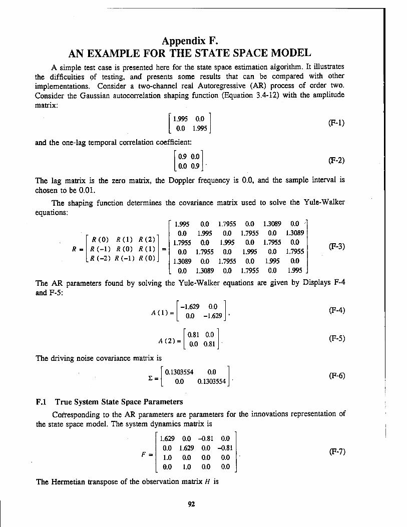
Appendix F. AN EXAMPLE FOR THE STATE SPACE MODEL

A simple test case is presented here for the state space estimation algorithm. It illustrates the difficulties of testing, and presents some results that can be compared with other implementations. Consider a two-channel real Autoregressive (AR) process of order two. Consider the Gaussian autocorrelation shaping function (Equation 3.4-12) with the amplitude matrix:

1.995 0.0 0.0 1.995

and the one-lag temporal correlation coefficient:

0.9 0.0 0.0 0.9

(F-l)

(F-2)

The lag matrix is the zero matrix, the Doppler frequency is 0.0, and the sample interval is chosen to be 0.01.

The shaping function determines the covariance matrix used to solve the Yule-Walker equations:

R

The AR parameters found by solving the Yule-Walker equations are given by Displays F-4 and F-5:

" 1.995 0.0 1.7955 0.0 1.3089 0.0 0.0 1.995 0.0 1.7955 0.0 1.3089

R(0) Ad) /?(2) 1.7955 0.0 1.995 0.0 1.7955 0.0 K(-D R(0) R(D = 0.0 1.7955 0.0 1.995 0.0 1.7955 R(-2) Ä(-l) Ä(0). 1.3089 0.0 1.7955 0.0 1.995 0.0

. 0.0 1.3089 0.0 1.7955 0.0 1.995

(F-3)

A(l) = -1.629 0.0

0.0 -1.629

A (2) = 0.81 0.0 0.0 0.81

The driving noise covariance matrix is

0.1303554 0.0 0.0 0.1303554

(F-4)

(F-5)

(F-6)

F.l True System State Space Parameters

Corresponding to the AR parameters are parameters for the innovations representation of the state space model. The system dynamics matrix is

1.629 0.0 -0.81 0.0 0.0 1.629 0.0 -0.81 1.0 0.0 0.0 0.0 0.0 1.0 0.0 0.0

The Hermetian transpose of the observation matrix H is

(F-7)

92

H» = 1.629 0.0 -0.81 0.0 0.0 1.629 0.0 -0.81

(F-8)

The matrix r is

r =

1.995 0.0 0.0 1.995

1.7955 0.0 0.0 1.7955

(F-9)

The Kaiman gain matrix is

K =

1.0 0.0 0.0 1.0 0.0 0.0 0.0 0.0

(F-10)

And the covariance matrix for the innovations is the covariance matrix for the driving noise in the AR model.

These true system parameters can be used for this test case to test any algorithm for estimating state space parameters. Such an algorithm may introduce a basis transformation of the state space, but the innovations covariance matrix should remain unchanged.

The AR parameters (and the state-space model parameters derived from them) are a minimum-mean-square fit to the matrix lags R (0), R (1), and R (2) in Equation F-3. Thus, in order to have a numerically exact true model, the matrix lags R (0), R (1), and R (2) must be recalculated using the state-space relations:

R(0) = HHPH +L (F-ll)

Ä(m) = //wFm-Ir. m =1.2 (F-12)

where P is the steady-state covariance matrix of the true system state vector. Matrix P is calculated as the solution to the following equation:

P = FPFH +KLK" . (F-13)

For a simple low-order system, matrix P can be obtained analytically. For high-order systems a numerical recursion is preferred. The matrix lags generated in this manner correspond exactly with the state space model and the AR model.

F.2 The Scientific Studies Algorithm with Exact Order

This appendix presents step-by-step results of the Scientific Studies algorithm for estimating state space parameters. This test case shows the results when the upper bound on the matrix order of the state space model matches the actual value, two. The inputs to the algorithm are past block correlation matrix, the future block correlation matrix, the block Hankel matrix, and the column-shifted block Hankel matrix, shown in displays F-14, F-15, F- 16, and F-17, respectively:

93

Rn =

Rp =

HLJ.-

HLh =

R(0) /?(1) R(-D R(0)

R(0) /?(-l) R(l) R(0)

R(l) R(2) R(2) R(3)

R(2) /?(3) R(3) R(4)

1.995 0.0 1.7955 0.0 0.0 1.995 0.0 1.7955

1.7955 0.0 1.995 0.0 0.0 1.7955 0.0 1.995

1.995 0.0 1.7955 0.0 0.0 1.995 0.0 1.7955

1.7955 0.0 1.995 0.0 0.0 1.7955 0.0 1.995

1.7955 0.0 1.3089 0.0 0.0 1.7955 0.0 1.3089

1.3089 0.0 0.6778 0.0 0.0 1.3089 0.0 0.6778

1.3089 0.0 0.6778 0.0 0.0 1.3089 0.0 0.6778

0.6778 0.0 0.04403 0.0 0.0 0.6778 0.0 0.04403

(F-14)

(F-15)

(F-16)

(F-17)

Notice that in this example the past and future block correlation matrices are equal to each other. This is not true in general.

The higher lag covariance matrices R (3) and R (4) were found by the AR Recursion Method. These matrices could have been calculated equivalently using the Closed-Form Method based on the state-space parameters. For this example, they work out to be the least significant numerals in a difference, suggesting that nemerical difficulties can arise here as the order increases.

The singular value decomposition of the past and future block covariance matrices is given by display F-18:

(F-18) i' i' 3.7905/ 0.0 '£' *'' 1.995/ 1.7955/

*' -M 0.0 0.1995/

[*' M 1.7955/ 1.995/

Accordingly, the square root of the past and forward block covariance matrices are:

Rj* = Rp =

The inverse of the square root of these block covariance matrices is:

The matrix A is calculated as:

A-Rf^H^R?»2

1.196787/ 0.750133/ 0.750133/ 1.196787/

1.37625/ -0.86262/ -0.86262/ 1.37625/

0.7973/ 0.5169/ 0.5169/ -0.4879/

(F-19)

(F-20)

(F-21)

At least one significant digit is lost in some of the components of A. Since A is calculated

94

from the Hankel matrix, and numerical precision problems can arise in calculating the covariance sequence lags comprising the Hankel matrix, these numerical difficulties may be compounded. A Singular Value Decomposition of A is:

A = UA SA V? = 0.9431/ -0.3323/ 0.3323/ 0.9432/

0.9794/ 0 0 0.67/

0.9431/ 0.3323/ 0.3323/ -0.9432/

(F-22)

Equation F-22 shows the SVD used in the computer program and further calculations here.

The past and future transformation matrices are:

The matrix A is:

The matrix ZH is

The matrix Zr is

TP =VJlRp-m =

Tr-UZRF«2

A - TF H T? =

1.0113/ -0.3562/ 1.2710/ -1.5847/

1.0113/ -0.3562/ -1.2710/ 1.5847/

0.8560/ 0.3142/ -0.3142/ 0.5054/

ZH = <//«, Tl!)l:2A.A = [ 1.350/ 0.2079/

Zr = ( Tf HLj, )j:4,1:2 - 1.3496/

-0.2079/

(F-23)

(F-24)

(F-25)

(F-26)

(F-27)

These matrices allow one to finally determine the state space parameters. The system dynamics matrix is:

F=Srll2ÄS7ll2 = 0.874/ 0.388/ -0.388/ 0.754/

The Hermetian transpose of the observations matrix is:

H" =ZH5A-"2= 1.36/ 0.254/

The backward observation matrix r is:

r = sA-"2zr

The state space correlation matrix is:

1.364/ -0.254/

0.9794/ 0 0 0.67/

(F-28)

(F-29)

(F-30)

(F-31)

The driving noise covariance matrix is:

CI = R(0)-HHTIH = 0.1304/ (F-32)

The calculation of Q results in the loss of one significant digit in this case. The Kaiman gain matrix is:

95

K =(r-Fn//)£}-» = 0.999/ 1.04/ (F-33)

The state space algorithm has introduced a transformation of the basis for the state vector. An element of the state space associated with the model parameters in Equations F-7 through F- 10 is transformed to the state space associated with the parameters in Equations F-28 through F-33 by premultiplying it by the matrix T, where

7 = 0.999/ -0.315/ 1.04/ -1.50/ (F-34)

F.3 The Scientific Studies Algorithm with Higher Order

This test case shows the results when the upper bound on the matrix order of the state space model exceeds the actual value. In this case, the upper bound is three, while the matrix order of the model is two. The inputs to the algorithm, the past block correlation matrix, the future block correlation matrix, the block Hankel matrix, and the column-shifted block Hankel matrix, are shown in displays F-35 through F-38:

Äp =

R*

HLJ.-

R(0) Ä(l) Ä(2) Ä(-l) Ä(0) /?(1) /?(-2) R(-l) R(0)

Ä(0) R(-l) /?(-2) R(l) Ä(0) R(-l) Ä(2) Ä(l) Ä(0)

Ä(l) Ä(2) Ä(3) Ä(2) Ä(3) Ä(4) Ä(3) Ä(4) R(S)\

1.995/ 1.7955/ 1.3089/ 1.7955/ 1.995/ 1.7955/ 1.3089/ 1.7955/ 1.995/

1.995/ 1.7955/ 1.3089/ 1.7955/ 1.995/ 1.7955/ 1.3089/ 1.7955/ 1.995/

1.7955/ 1.3089/ 0.6779/ 1.3089/ 0.6779/ 0.04403/ 0.6779/ 0.04403/ -0.4773/

(F-35)

(F-36)

(F-37)

Ä(2) Ä(3) Ä(4) #Li= Ä(3) Ä(4) Ä(5)

.Ä(4) Ä(5) Ä(6)

(More significant digits were used in working out this example than are shown.)

The singular value decomposition of the past and future block covariance matrices is

1.3089/ 0.6779/ 0.04403/ 0.6779/ 0.04403/ -0.4773/ 0.04403/ -0.4773/ -0.8133/

(F-38)

0.5589/ -0.7071/ 0.4331/ 0.6125/ 0/ -0.7904/ 0.5589/ 0.7071/ 0.4331/

5.2717/ 0 0 0 0.6861 / 0 0 0 0.02725/

0.5589/ 0.6125/ 0.5589/ -0.7071/ 0/ 0.7071/ 0.4331/ -0.7904/ 0.4331/

1.995/ 1.7955/ 1.3089/ 1.7955/ 1.995/ 1.7955/ 1.3089/ 1.7955/ 1.995/

Accordingly, the square roots of the past and forward block covariance matrices are:

'1.1624/ 0.7296/ 0.3341/ Rjl2 = RF

ll2= 0.7296/ 0.9646/ 0.7296/ .0.3341/ 0.7296/ 1.1624/.

The inverse of the square root of these block covariance matrices is:

(F-39)

(F-40)

%

The matrix A is calculated as:

1.8761/ -1.9247/ 0.6688/ -1.9247/ 3.9480/ -1.9247/ 0.6688/ -1.9247/ 1.8761/

(F-41)

0.7522/ 0.4829/ 0.7522/ 0.4829/ -0.0902/ -0.2647/ 0.2272/ -0.2647/ -0.3525/

Some of the elements of A in the corresponding computer print out are only accurate significant figures, already having lost some precision. An SVD of A is

0.9157/ 0.3941/ 0.0779/ -0.3211/ 0.6015/ 0.7315/ 0.2415/ -0.6949/ 0.6774/

0.9157/ 0.3211/ -0.2415/ 0.3941/ -0.6015/ 0.6949/ 0.07792/ -0.7315/ -0.6774/

0.9794/ 0 0 0 0.6699/ 0 0 0 3.1^10"*/

(F-42)

to four

(F-43)

The past and future transformation matrices are:

" 1.0115/ -0.3564/ -5.6xl(T7

Tp=VgRfll2= -1.2709/ -1.5847/ lAxlCT6

[ 2.2435/ -4.5119 2.7697

USR;1*-

The matrix Z is

The matrix ZH is:

The matrix Zr is:

z =

z„ =

Zr =

1.0115/ -0.3564/ -5.6xl0-7

1.2709/ -1.5847/ 4.4* 10"6

-2.2435/ 4.5119 -2.7697

0.8560/ -0.3139/ 0.3139/ 0.5057/

1.3496/ -0.2076/

1.3496/ 0.2076/

The system dynamics matrix is:

F=SA-1/2ZSA-"2 = 0.8740/ -0.3874/ 0.3874/ 0.7550/

The Hermetian transpose of the observations matrix is:

HH = ZH Sä m = [ 1.3638 / -0.2537 /

The backward observation matrix r is:

r-5A-wZr-

The state space correlation matrix is:

n-sA

The driving noise covariance matrix is:

1.3638/ 0.2537/

0.9794/ 0 0 0.6699/

(F-44)

(F-45)

(F-46)

(F-47)

(F-48)

(F-49)

(F-50)

(F-51)

(F-52)

97

a = Ä(0)-//Hn// =0.1304/

The Kaiman gain matrix is:

K =(r-Fn//)fl-' = 1.0010/

-1.0402/

(F-53)

(F-54)

These values are close to the values obtaining when the upper limit on the state space order matches the actual order.

»U.S. GOVERNMENT PRINTING OFFICE:

98 1996-710-126-20111