Adam Ouorou

A Proximal Cutting Plane Method Using ChebychevCenter for Nonsmooth Convex Optimization

April 2006

Abstract An algorithm is developped for minimizing nonsmooth convex functions. This algortithm extends

Elzinga-Moore cutting plane algorithm by enforcing the search of the next test point not too far from the

previous ones, thus removing compactness assumption. Our method is to Elzinga-Moore’s algorithm what

a proximal bundle method is to Kelley’s algorithm. As in proximal bundle methods, a quadratic problem

is solved at each iteration, but the usual polyhedral approximation values are not used. We propose some

variants and using some academic test problems, we conduct a numerical comparative study with three

other nonsmooth methods.

Mathematics Subject Classification (2000) 90C30, 90C25, 65K05

Keywords nonsmooth optimization, subgradient, proximal bundle methods, cutting plane methods,

convex programming.

1 Introduction

Consider the convex problem

minx∈Rn

f(x), (1.1)

where f : Rn → R is a nonsmooth closed proper convex function. We assume that the optimal set X∗ =

Arg minx∈Rn

f(x) is non empty and denote by f∗ the optimal value of problem (1.1). Suppose that the points

z1, z2, . . . , zk ∈ Rn, have been generated and the function values f(zi) and subgradients gi ∈ ∂f(zi) have

France Telecom, Division R&D, CORE-MCN, 38-40 rue du General Leclerc, 92794 Issy-Les-Moulineaux cedex 9,France. E-mail: adam.ouorou@francetelecom.com until May 31, 2006; adam.ouorou@orange-ft.com from June1st, 2006

2

been computed for each zi through an oracle as usual. We can build the polyhedral approximation (model)

of f defined by

fk(x) = maxi∈Ik

f i(x), (1.2)

where f i(x) = f(zi) + 〈gi, x − zi〉 for i ∈ Ik = {1, . . . , k}. The piecewise linear function fk is an under-

estimate of f i.e. fk(x) ≤ f(x), ∀x ∈ Rn. At the points z1, z2, . . . , zk, we have fk(zi) = f(zi) and

gi ∈ ∂fk(zi), i = 1, . . . , k. Given an upper bound fku to (1.1), the following localization set

Xk ={(r, x) ∈ R × R

n : r ≤ fku , f

i(x) ≤ r, i ∈ Ik}

contains the optimal set {f∗} ×X∗.

The basic issue in solution methods for (1.1) is how to choose the next iterate where to query the

oracle so as to shrink the localization set. Assuming the linear approximation represents correctly the

true function f , cutting plane algorithms, such as Kelley-Cheney-Goldstein [6,13], consists in computing

the next iterate as a minimizer of fk; and this turns out to be a linear programming problem. But those

approachess need to bound the feasible region and in addition, cutting planes are inherently unstable. Their

convergence is known to be rather slow in practice. Some proposals to accelerate cutting plane algorithms

by good separation procedures can be found in [2,3]. To overcome the instability of cutting planes and the

boundedness assumption, other methods propose regularization. Proximal bundle methods [12,17,21,22]

approximate the objective function by a regularized cutting plane model made of fk and a quadratic term.

Other regularization mecanisms rely on centers related to Xk. Among the possible centers, the analytic

center is a good concept that has a number of advantages and exploited to design the analytic center cutting

plane method (ACCPM) [10]. This center can be computed through interior point methods which are now

efficient and robust. Another center used as query point is the center of the largest sphere contained inXk. It

is a point of Xk which the farthest from the exterior of Xk, see [5]. The cutting plane algorithm proposed by

Elzinga and Moore [7] is built on this center whose computation amounts to solving a linear problem. Using

central point does not remedy the compactness problem. Moreover, the linear approximation often turns

out to be a poor representation of the problem far away from the search points [22]. We thus investigate in

this paper a regularized version of Elzinga-Moore algorithm, convinced that a quadratic stabilizing term will

result in a substantial benefit (it has been shown to improve the performance of ACCPM, see [1,25]). Our

approach appears then to be to Elzinga-Moore’s algorithm what a proximal bundle method is to Kelley’s

algorithm.

The paper is organized as follows. In Section 2, we derive the algorithm and establish its convergence

in Section 3. In Section 4 we deal with some practical implementation aspects. The extension to linearly

3

constrained problem and two possible variants are sketched in Section 5. Some numerical results are reported

in Section 6 before a conclusion section.

We use the following notation. The symbol 〈., .〉 denotes the usual scalar product while the Euclidean

norm is denoted by ‖.‖. ∂ǫf(z) = {g : f(x) ≥ f(z) + 〈g, x − z〉 − ǫ ∀x ∈ Rn} is the ǫ-subdifferential of f

at z.

2 Derivation of the algorithm

Given a bounded polyhedron P = {x : a⊤i x ≤ bi, i ∈ I}, the center of the largest ball inside P is called

Chebychev center [5]. Nemhauser and Widhelm [24] showed that the problem

max σ

s.t. a⊤i x+ σ‖ai‖ ≤ bi, i ∈ I, (2.1)

gives the radius σ and the Chebychev center of the polyhedron P . Indeed, the sphere {x + u : ‖u‖ ≤ σ}

centered at x with radius σ lies in P if and only if

sup{〈ai, x〉 + 〈ai, u〉 : ‖u‖ ≤ σ} ≤ bi, i ∈ I,

that is,

〈ai, x〉 + σ‖ai‖ ≤ bi, i ∈ I.

Hence, finding the centre of the largest sphere inside P , amounts to solving the linear program (2.1). For

the localization set Xk, the problem is expressed as

max σ

s.t. r + σ ≤ fku ,

f i(x) − r + σ√

1 + ‖gi‖2 ≤ 0, i ∈ Ik,

σ, r ∈ R, x ∈ Rn.

(2.2)

Elzinga and Moore [7] used this centre as test point in their cutting plane algorithm. To accelerate the

method, it is proposed in [4] to use an objective cut deeper that the original one. Elzinga-Moore method is

not hard to implement when compared to Kelley’s method and has even shown to outperform the latter on

some min-max problems, see [28,30]. Our motive is to further improve it, based on the fact that the current

model function fk approximates the objective function in the neighborhood of the search points and this

approximation is unlikely to be reliable far away from these points. It is therefore reasonable to enforce the

search of the next test point not too far from the previous ones, in the spirit of bundle and proximal-like

methods. We use a positive parameter µk to enforce the next test point to be closed to the best test point

found so far.

4

Instead of (2.2), we consider the problem

max σ − µk

2‖x− xk‖2

s.t. r + σ ≤ f(xk),

f i(x) − r + σ√

1 + ‖gi‖2 ≤ 0, i ∈ Ik,

σ, r ∈ R, x ∈ Rn,

(2.3)

where xk is some proximal point to be specified later, and µk > 0 is a penalty parameter. Note that, for

Elzinga-Moore to be applicable, the localization sets must be bounded. This assumption is now eliminated

by our approach since the quadratic term guarantees compactness.

From the subgradient inequality, we have f i(x∗) = f(zi) + 〈gi, x∗ − zi〉 ≤ f(x∗) ≤ f(xk). Thus

(0, f(x∗), x∗) is feasible to problem (2.3). Therefore σk is positive.

Proposition 2.1 At optimality, the constraint r + σ ≤ f(xk) in (2.3) is tight.

Proof. Using KKT optimality conditions to (2.3) w.r.t. σ and r, we get

1 − u0 −k∑

i=1

ui

√1 + ‖gi‖2 = 0, u0 =

k∑

i=1

ui, ui ≥ 0,

where ui, i = 0, . . . , k, are respectively the dual multipliers associated to the constraints of (2.3). The above

conditions imply that ui > 0 for some i and then u0 > 0. The constraint r + σ ≤ f(xk) is then tight at

optimality from the complementarity slackness conditions.

�

We can thus eliminate variable r and the constraint r + σ ≤ f(xk), and rewrite the problem as

max σ − µk

2‖x− xk‖2

s.t. 〈gi, x− xk〉 − αki + σ

(1 +

√1 + ‖gi‖2

)≤ 0, i ∈ Ik,

σ ∈ R, x ∈ Rn,

(2.4)

where αki = f(xk) − f i(xk) = f(xk) − [f(zi) + 〈gi, xk − zi〉] ≥ 0 is the linearization error between zi and

xk. Let ν be the opposite of σ and denote γi = 1 +√

1 + ‖gi‖2 for i ∈ Ik, we obtain the following problem

equivalent to (2.4)

min ν +µk

2‖x− xk‖2

s.t. 〈gi, x− xk〉 − αki ≤ ν, i ∈ Ik,

ν ∈ R, x ∈ Rn,

(2.5)

where gi = γ−1i gi, and αk

i = γ−1i αk

i , for i ∈ Ik are respectively the scaled subgradients and scaled

linearization errors. This problem appears to be of the same the type of subproblems in bundle and

proximal-like methods [18,8,12]. But here, gi and αki are used in place of the “ordinary” subgradient

gi and linearization errors αki , and ν does not represent fk-values.

5

Denote by λi, i ∈ Ik, the Lagrange multipliers of problem (2.4). The Lagrangian function is

L(x, ν, λ) = (1 −k∑

i=1

λi)ν +µk

2‖x− xk‖2 −

k∑

i=1

λiαki +

k∑

i=1

λi〈gi, x− xk〉

Its minimization w.r.t. primal variables (ν, x) implies 1 −k∑

i=1

λi = 0 and x = xk − µ−1k

k∑i=1

λigi. Plugging

this into the Lagrangian, we obtain the dual problem of (2.5) as

min

{1

2µk

‖k∑

i=1

λigi‖2 +

k∑

i=1

λiαki : λ ∈ Λk

}, (2.6)

where Λk = {λ ∈ Rk :

k∑i=1

λi = 1, λ ≥ 0} is the unit simplex of Rk. Let λk

i denote its optimal solution

and denote by dk and αk respectively the aggregate scaled subgradient dk =k∑

i=1

λki g

i and aggregate scaled

linearization error αk =k∑

i=1

λki α

ki . Due to convexity, there is no duality gap beteween the problem (2.5) and

its dual. Hence, the solutions of problems (2.4) and (2.5) are given by

σk = −νk = µ−1k ‖dk‖2 + αk, zk+1 = xk − µ−1

k dk. (2.7)

Remark 2.2 Let ψk be the convex function ψk(x) = maxi∈Ik

ψi(x), where ψi(x) = 〈gi, x − xk〉 − αki . Then

(2.5) is equivalent to

minx∈Rn

{ψk(x) +

µk

2‖x− xk‖2

}. (2.8)

Bundle methods use a similar quadratic subproblem but with the polyhedral approximation fk in place of

ψk. Note however that ψk is not a model for f . The solution in r of (2.3) is given by rk = f(xk) − σk =

f(xk) + νk and by construction, rk ≥ f i(zk+1) + σk√

1 + ‖gi‖2 ≥ f i(zk+1) for each i ∈ Ik. In other words,

rk ≥ fk(zk+1) and therefore,

ψk(zk+1) = νk = rk − f(xk) ≥ fk(zk+1) − f(xk). (2.9)

�

Proposition 2.3 For any k, we have η−1k dk ∈ ∂η

−1

kαkf(xk) where ηk =

k∑i=1

λki γ

−1i .

Proof. Using the subgradient inequalities, we have for all x ∈ Rn

γ−1i λk

i f(x) ≥ γ−1i λk

i f(xk) + 〈λki g

i, x− xk〉 − λki α

ki , i ∈ Ik,

Summing over i ∈ Ik, we get

ηkf(x) ≥ ηkf(xk) + 〈dk, x− xk〉 − αk.

6

Thanks to dual feasibility, ηk > 0. Then

f(x) ≥ f(xk) + 〈η−1k dk, x− xk〉 − η−1

k αk, (2.10)

or equivalently, η−1k dk ∈ ∂η

−1

kαkf(xk).

�

Remark 2.4 From (2.8) dk ∈ ∂ψk(zk+1) while η−1k dk ∈ ∂η

−1

kαkf(xk). In bundle methods, the aggregate

subgradient dk has the property that dk ∈ ∂fk(zk+1) and dk ∈ ∂bekf(xk), where zk+1 is the next trial point,

xk the proximal point and ek the aggregate linearization error; see [12]. �

Observe that, since∑

i∈Ik

λki = 1 and γi ≥ 2 for each i ∈ Ik, we have 0 < ηk =

∑i∈Ik

λki γ

−1i ≤ 1

2 and then

2 ≤ η−1k <∞. Recall that σk ≥ 0 for any k ≥ 1. If σk = 0, then (2.7) implies dk = αk = 0 and 0 ∈ ∂f(xk),

hence xk minimizes f , proving the following proposition.

Proposition 2.5 If σk = 0, then xk minimizes f .

As a consequence, we may use the same stopping criterion as in Elzinga-Moore algorithm. We note that for

all x ∈ Rn, f(xk) ≤ f(x) + 〈η−1

k dk, xk − x〉 + η−1k αk. Using Cauchy-Schwartz inequality, we get

f(xk) ≤ f(x) + η−1k ‖dk‖‖xk − x‖ + η−1

k αk. (2.11)

Suppose that for some ε ≥ 0, we have

η−1k ‖dk‖ ≤ ε and η−1

k αk ≤ ε. (2.12)

Then xk is ε-optimal in the sense that f(xk) ≤ f(x) + ε‖x− xk‖ + ε for all x ∈ Rn. Along this line, since

σk = µ−1k ‖dk‖2 +αk, we have η−1

k αk ≤ η−1k σk and ‖dk‖2 ≤ µkσ

k i.e. η−1k ‖dk‖ ≤ η−1

k (µkσk)

1

2 , so that (2.11)

yields the following optimality estimate

f(xk) ≤ f(x) + η− 1

2

k

(µkη

−1k σk

) 1

2 ‖xk − x‖ + η−1k σk. (2.13)

Now, let us decide when we are going to change the proximal point. Reasonably, this point should

approximate a minimum point of f . The natural rule

xk+1 = zk+1 if f(zk+1) < f(xk) (descent step), xk+1 = xk otherwise (null step),

can lead to many descent steps without significant improvement in the objective value. The management

of the proximal point in bundle methods relies on a nominal decrease i.e. a positive number giving an idea

of the gain f(xk)− f(zk+1) to be expected from xk to the next iterate zk+1. The usual nominal decrease in

bundle methods is f(xk)−fk(zk+1). We cannot use this nominial decrease here since, as already pointed out,

we dot not have explicitely fk(zk+1) except in the following special context of Proposition 2.6. Computing

fk(zk+1) from (1.2) would require storing all the zi, i ∈ Ik, which is a drawback.

7

Proposition 2.6 For any k, fk(zk+1) ≤ f(xk) + γki(k)ν

k where i(k) = argk

mini=1

γi. If λki(k) > 0, then

fk(zk+1) = f(xk) + γki(k)ν

k.

Proof. Since (νk, zk+1) is the solution to (2.5), for each i ∈ Ik, 〈gi, zk+1 − xk〉 − αki ≤ νk, or equivalently

f i(zk+1) ≤ f(xk) + γiνk. As νk < 0, we get γiν

k ≤ γki(k)ν

k, and then fk(zk+1) ≤ f(xk) + γki(k)ν

k. Because

λk ∈ Λk, there exists at least one i ∈ Ik such that λki > 0. If λk

i(k) > 0, then f(xk) + γki(k)ν

k = f i(k)(zk+1)

from the complementarity slackness conditions. But f i(k)(zk+1) ≤ fk(zk+1), so fk(zk+1) = f(xk)+γki(k)ν

k.

�

This proposition shows that if λki(k) where always strictly positive, γk

i(k)σk could play the role of a

nominal decrease. In case λki(k) = 0 there is no guarantee that f(xk)− f(zk+1) ≤ γk

i(k)σk which is necessary

to avoid negligible improvement. The following lemma allow us to obtain a nominal decrease without the

explicit knowledge of fk(zk+1).

Proposition 2.7 Let δk = η−1k σk where λk ∈ Λk solves (2.6). Then,

f(xk) − f(zk+1) ≤ f(xk) − fk(zk+1) ≤ δk. (2.14)

Proof. The first inequality comes from the fact that fk(x) is an under-estimate of f(x). Now, by definition,

fk(x) ≥ f i(x) = f(xk) + 〈gi, x− xk〉 − αki , i ∈ Ik, ∀x ∈ R

n.

Multipliying these relations by λki γ

−1i and summing over i ∈ Ik, we have

ηkfk(x) ≥ ηkf(xk) + 〈dk, x− xk〉 − αk,

or equivalently,

fk(x) ≥ f(xk) + 〈η−1k dk, x− xk〉 − η−1

k αk. (2.15)

Taking x = zk+1 in (2.15), we get

fk(zk+1) ≥ f(xk) − δk.

�

Based on Proposition 2.7, we consider δk as the nominal decrease predicted by (2.5) and we decide whether

enough progress is made if the actual reduction in the objective value is within a fraction of δk. We thus

use the following rule to manage the proximal point:

xk+1 = zk+1 if f(zk+1) ≤ f(xk) − κδk (descent step), otherwise xk+1 = xk (null step), (2.16)

where κ is some positive parameter κ < 1. Observe that, since 2 ≤ η−1k , the nominal decrease δk is greater

than the diameter of the ball centered at (zk+1, rk) with radius σk. δk involves the primal solution σk as

8

well as the optimal multipliers λki , i ∈ Ik but its computation poses no problem. Most of the quadratic

solvers for the type of subproblems (2.5) solve the dual (2.6), see [8,18].

Assuming defined the sequence {µk}, we now have all the necessary ingredients to state our algorithm.

Algorithm 1 Proximal Chebychev Center Cutting Plane Algorithm (pc3pa)

0. ǫ, x1 = z1 ∈ Rn, f1

u = f(z1), g1 ∈ ∂f(z1), k = 1.

1. If gk = 0, terminate.

2. Solve (2.5) to get (σk, zk+1). If σk ≤ ǫ, terminate.

3. Compute f(zk+1) and gk+1 ∈ ∂f(zk+1). Update the proximal point xk+1 (see (2.16)).

Increase k by 1 and loop to Step 1.

It is reasonable sometimes to use the scale-invariant stopping criterion

σk ≤ ǫ(1 + |f(xk)|).

Another stopping criterion follows (2.12), using two tolerances ǫg, ǫf > 0 homogenous respectively to norms

of scaled subgradients and objectives values and stop the algorithm when

η−1k ‖dk‖ ≤ ǫg and η−1

k αk ≤ ǫf .

From (2.13), δk = η−1k σk is an optimality measure, so we can also use the following stopping criterion

δk ≤ ε,

which will be considered in our computational experiments. Finally, note that as in bundle methods, we do

not need the trial point zi for updating the scaled linearization errors αk+1i in case of descent step:

αk+1i = αk

i + γ−1i [f(xk+1) − f(xk)] − 〈gi, xk+1 − xk〉.

3 Convergence

From Proposition 2.5, if we manage to prove that the sequence {σk} converges to 0 and xk → x∗ ∈ X∗,

then 0 ∈ ∂f(x∗) by the continuity of the subdifferentiable function. The closeness of our approach to bundle

methods allow a convergence analysis using identical ideas and techniques as presented in [15,17,12]. In the

following, we denote by K the set of descent steps (k ∈ K ⇔ xk+1 = zk+1, k /∈ K ⇔ xk+1 = xk).

Proposition 3.1 With the above notations, we have∑

k∈K

δk ≤ 1κ

(f(x1) − f∗

)and

∑k∈K

σk ≤ 12κ

(f(x1) − f∗

).

9

Proof. The descent test (2.16) gives δk ≤ κ−1(f(xk) − f(xk+1)

). If k′ is the next descent step after k, we

have δk′ ≤ κ−1(f(xk′

) − f(xk′+1))

= κ−1(f(xk+1) − f(xk′+1)

). Hence, summing over k ∈ K and using

the fact that f(xk) − f(xk+1) = 0 if k /∈ K, we get

0 ≤∑

k∈K

δk ≤ κ−1∞∑

k=1

(f(xk) − f(xk+1)

)= κ−1

(f(x1) − f∗

).

The fact that 2σk ≤ δk = η−1k σk (because η−1

k ≥ 2) completes the proof. �

As a consequence, we have the following classical result in the framework of bundle methods.

Proposition 3.2 If∑

k∈K

µ−1k = ∞ then 0 is a cluster point to the sequence {dk}k∈K.

Proof. From (2.7),

0 ≤∑

k∈K

µ−1k ‖dk‖2 ≤ 1

2κ

(f(x1) − f∗

)<∞. (3.1)

If∑

k∈K

µ−1k = ∞, {‖dk‖}k∈K cannot be bounded away from 0. �

A second consequence which follows (2.7) is that,

∑

k∈K

αk ≤ 1

2κ

(f(x1) − f∗

). (3.2)

Proposition 3.3 Suppose that µk ≥ µ for some µ > 0. Then, the sequence {xk}k∈K is bounded.

Proof. For any x ∈ X , we have

‖x− xk+1‖2 = ‖x− xk‖2 + 2〈x− xk, xk − xk+1〉 + ‖xk − xk+1‖2.

From (2.10)

〈x− xk, xk − xk+1〉 ≤ µk

(ηk[f(x) − f(xk)] + αk

).

Also, ‖xk − xk+1‖2 = µ−2k ‖dk‖2. Hence,

‖x− xk+1‖2 ≤ ‖x− xk‖2 + 2µ−1k

(ηk[f(x) − f(xk)] + αk + µ−1

k ‖dk‖2),

and using the definition of σk,

‖x− xk+1‖2 ≤ ‖x− xk‖2 + 2µ−1k ηk[f(x) − f(xk)] + 2µ−1

k σk.

As X∗ is nonempty by assumption,

there exists x∗ ∈ Xsuch that f(x∗) ≤ f(xk) for all k. (3.3)

Since ηk > 0, it follows that

‖x∗ − xk+1‖2 ≤ ‖x∗ − xk‖2 + 2µ−1k σk.

10

Summing these inequalities, over i ∈ K, i ≤ k, we obtain

‖x∗ − xk+1‖2 ≤ ‖x∗ − x1‖2 + 2∑

i∈K,i≤k

µ−1i σi ≤ ‖x∗ − x1‖2 + 2µ−1

∑

i∈K

σi.

The results follows from Proposition 3.1.

�

Proposition 3.4 Suppose that |K| = ∞. If {µk} is bounded above and µk ≥ µ for some µ > 0, then

{xk}k∈K has a cluster point which is optimal.

Proof. From (2.13), for all x ∈ Rn we have,

f(xk) ≤ f(x) + η− 1

2

k (µkδk)

1

2 ‖x− xk‖ + δk ≤ f(x) + γ1

2

L (µkδk)

1

2 ‖x− xk‖ + δk,

where L is the Lipschitz constant of f on a bounded set containing {xk} and γL = 1 +√

1 + L2 ≥ η−1k .

Using Propositions 3.1 and 3.3, and taking subsequence if necessary, we get f(x) ≤ f(x) for all x ∈ Rn,

where x is a cluster point of the sequence {xk}k∈K.

�

The above proposition shows that if there are infinitely descent steps, then we are done: the sequence

{xk}k converges to an optimal solution of the problem. The next result fix the case when the proximal

point stops at some xk0 . We show that in this case, the radius {σk} tends to 0 and prove optimality of xk0 .

Proposition 3.5 Suppose that K is finite and let k0 be the last descent step performed by Algorithm 1. If

{µk} is bounded above and µk ≥ µk−1 for all k ≥ k0 + 1, then {σk} tends to 0.

Proof.

i) Note that zk+1 = xk0 − µ−1k dk for k ≥ k0 + 1, so for any x ∈ R

n,

‖x− xk0‖2 = ‖x− zk+1‖2 + 2〈zk+1 − xk0 , x− zk+1〉 + ‖zk+1 − xk0‖2

= ‖x− zk+1‖2 − 2µ−1k 〈dk, x− zk+1〉 + ‖zk+1 − xk0‖2.

This together with the definition of ψk implies for any x ∈ Rn,

νk +µk

2

(‖x− zk+1‖2 + ‖zk+1 − xk0‖2

)= ψk(zk+1) +

µk

2

(‖x− xk0‖2 + 2µ−1

k 〈dk, x− zk+1〉)

= ψk(zk+1) + 〈dk, x− zk+1〉 +µk

2‖x− xk0‖2

From Proposition 4.1, ψk(zk+1) + 〈dk, x− zk+1〉 ≤ ψk(x), and then

νk +µk

2

(‖x− zk+1‖2 + ‖zk+1 − xk0‖2

)≤ ψk(x) +

µk

2‖x− xk0‖2. (3.4)

11

ii) Taking x = zk+2 in (3.4) yields

νk +µk

2

(‖zk+2 − zk+1‖2 + ‖zk+1 − xk0‖2

)≤ ψk(zk+2) +

µk

2‖zk+2 − xk0‖2

Since xk = xk0 for k > k0, by definition, ψk(x) ≤ ψk+1(x) for any k > k0 and x ∈ Rn. Hence,

ψk(zk+2) ≤ ψk+1(zk+2). By definition ψk+1(zk+2) = νk+1, so we get

νk +µk

2‖zk+1 − xk0‖2 +

µk

2‖zk+2 − zk+1‖2 ≤ νk+1 +

µk

2‖zk+2 − xk0‖2

≤ νk+1 +µk+1

2‖zk+2 − xk0‖2,

as µk+1 ≥ µk by hypothesis. But,

νk+1 +µk+1

2‖zk+2 − xk0‖2 = min

x∈Rn

{ψk+1(x) +

µk+1

2‖x− xk0‖2

}≤ ψk+1(xk0) ≤ 0.

Letting ςk = ψk(zk+1) +µk

2‖zk+1 − xk0‖2 = νk +

µk

2‖zk+1 − xk0‖2, we get

ςk +µk

2‖zk+2 − zk+1‖2 ≤ ςk+1 ≤ 0. (3.5)

Consequently, ςk converges to some ς ≤ 0 and ‖zk+2− zk+1‖ → 0. We get from zk+1 = xk0 −µ−1k dk and

(2.7), ςk = − 1

µk

‖dk‖2 − αk +1

2µk

‖dk‖2 = − 1

2µk

‖dk‖2 − αk =νk

2− αk

2. Therefore,

νk ≤ ςk ≤ νk

2≤ 0. (3.6)

iii) Taking x = xk0 in (3.4), we get

ςk +µk

2‖zk+1 − xk0‖2 ≤ ψk(xk0 ) ≤ 0.

Since for any k ≥ k0, −ςk+1 ≤ −ςk and µk ≥ µk−1,

‖zk+1 − xk0‖2 ≤ −2ςk

µk

≤ −2ςk0

µk0

. (3.7)

The sequence {zk}k>k0is then bounded.

iv) There is no descent step for all k > k0, so −κδk < f(zk+1)−f(xk0), that is −κη−1k σk < f(zk+1)−f(xk0),

which combined with σk ≤ f(xk0 ) − fk(zk+1) (cf (2.9)) yield

(1 − κη−1k )σk ≤ f(zk+1) − fk(zk+1)

= f(zk+1) − f(zk) + fk(zk) − fk(zk+1) (we use f(zk) = fk(zk))

≤ 2L‖zk+1 − zk‖,

(3.8)

where L is the Lipschitz constant of f on the ball B(xk0 ,−2ςk0

µk0

), see (3.7). Let γL = 1 +√

1 + L2.

Then γL ≥ η−1k and (1 − κγL)σk ≤ (1− κη−1

k )σk. Taking limit in (3.8), we get f(zk+1)− fk(zk+1) → 0

and σk → 0 provided κ ≤ γ−1L [≤ 1

2 ] in the latter case. Since νk = −σk, we also have from (3.6), ςk → 0

and then zk+1 → xk0 .

�

12

4 Practical aspects

We discuss important questions for an efficient implementation of pc3pa, widely based on the ideas by

Kiwiel [14,17,21] for the penalty parameter µk and the management of the number of subgradients in the

quadratic subproblem (2.5).

4.1 Choice of the penalty parameter µk

The parameter µk controls the strength of the quadratic term in (2.5) and its choice is a difficult task. We

need to test when µk is too large or too small. A large µk leads to small νk and keep zk+1 closed to xk,

while a small µk yields large νk and tends to keep zk+1 away from xk. Clever update strategies have been

proposed in the literature, see [17,32,21,9,31]. We adapt the proximity control proposed by Kiwiel in [17].

For a given k, we conclude that µk is too large when

f(zk+1) ≤ f(xk) − κ′δk (4.1)

for some 1 > κ′ > κ > 0 and use

µk+1int = 2µk

[1 +

f(zk+1) − f(xk)

δk

](4.2)

to update the next penalty parameter. Note that if κ′ > 12 then µint < µk. Still taking inspiration from [17],

we check if

αkk+1 > max

{η−1

k

(‖dk‖ + αk

), 10δk

}, (4.3)

to conclude that µk is too small. Let i1u = 0, µmin a small positive constant, say µmin = 10−10 and ǫ1ν = ∞.

We replace η−1k

(‖dk‖ + αk

)in (4.3) by ǫkν . Our heuristic procedure to update the penalty parameter, which

is an adaptation of Procedure 2.2 in [17], is as follows (initially µ = µk).

Procedure (Update of the penalty parameter)

1. If xk+1 = xk go to Step 5.

2. If (4.1) holds and iku > 0, set µ = µk+1int and go to Step 4.

3. If iku > 3 set µ = µk/2.

4. Set µk+1 = max{µ, 0.1µk, µmin}, ǫk+1ν = max{ǫkν, 2δk} and ik+1

u = max{iku + 1, 1}.

If µk+1 6= µk set ik+1u = 1 and exit.

5. Set ǫk+1ν = min

{ǫkν , η

−1k

(‖dk‖ + αk

)}. If αk

k+1 > max{ǫk+1ν , 10δk

}and iku < −3, set µ = µk+1

int .

Set µk+1 = min{µ, 10µk} and ik+1u = min{iku − 1, −1}. If µk+1 6= µk set ik+1

u = −1 and exit.

13

4.2 Limiting the size of the quadratic subproblem

The number of constraints of the quadratic subproblem (2.5) increases with the number of iterations and

the computational effort per iteration grows rapidly. Therefore, it is clear that the size of this subproblem

should be kept at a reasonable size. The constraint deletion rules proposed in [7] cannot be applied here,

since they are based on the fact that the radius is decreasing at each iteration. Fortunately, since the

quadratic subproblem (2.5) resembles the subproblems in bundle methods, we adapt Kiwiel’s aggregate

subgradient technique [14,15] to limit its size. Define the aggregate piece

ψk(x) = ψk(zk+1) + 〈dk, x− zk+1〉.

Proposition 4.1 For the aggregate piece ψk, we have

ψk(x) ≤ ψk(x) and ψk(x) = 〈dk, x− xk〉 − αk.

Proof. Since zk+1 solves (2.8), we have dk = µk(xk − zk+1) ∈ ∂ψk(zk+1) and then ψk(x) ≥ ψk(zk+1) +

〈dk, x − zk+1〉 using subgradient inequality. Now, 〈dk, x − zk+1〉 = 〈dk, x − xk〉 + 〈dk, xk − zk+1〉. But

〈dk, xk − zk+1〉 = µ−1k ‖dk‖2 = −νk − αk = −ψk(zk+1) − αk, and the result follows.

�

We can see that the aggregate piece is a convex combination of pieces in problem (2.5) and can be

incorporated to this problem with no harm. Now, suppose that at iteration k, we have the (k − 1)th

aggregate piece ψk−1 with scaled subgradient and linearization error dk−1 and αk−1 (we define d0 = g1 and

α0 = α11 = 0), and append the corresponding aggregate constraint to (2.5) to get the following subproblem

min r +µk

2‖x− xk‖2

s.t. 〈dk−1, x− xk〉 − αk−1 ≤ r,

〈gi, x− xk〉 − αki ≤ r, i ∈ Ik,

r ∈ R, x ∈ Rn.

(4.4)

In other words, we replace ψk by ψk = max{ψk, ψk−1} in (2.8). Its solution is given by νk = −µ−1k ‖dk‖2 −

αkd, zk+1 = xk − µ−1

k dk where

dk =∑

i∈Ik

λki g

i + λkdd

k−1, αkd =

∑

i∈Ik

λki α

ki + λk

dαk−1,

and λki ≥ 0, i ∈ Ik, λ

kd ≥ 0 are the dual optimal multpliers of (4.4). Note that

∑i∈Ik

λki + λk

d = 1. We define

the next aggregate piece as

ψk(x) = ψk(zk+1) + 〈dk, x− zk+1〉.

14

From Proposition 4.1, we can see that ψk =∑

i∈Ik

λki ψ

i + λkdψ

k−1. Let Imax be the maximum number of

pieces ψi we want to keep. If we take Ik as any subset of Ik such that |Ik| ≤ Imax − 1, then we can use

Ik+1 = Ik ∪ {k + 1} and ψk+1 = max{ψk+1, ψk} for the next iteration. In case of descent step, we update

αk+1i = αk

i + γ−1i [f(xk+1) − f(xk)] − 〈gi, xk+1 − xk〉, for i ∈ Ik, and αk+1

k+1 = 0,

αk = αkd + ηk[f(xk+1) − f(xk)] − 〈dk, xk+1 − xk〉, with ηk =

∑i∈Ik

λki γ

−1i

and in case of null step,

αk+1i = αk

i , for i ∈ Ik, αk+1k+1 = γ−1

k+1[f(xk) − f(zk+1)] − 〈gk+1, xk − zk+1〉, and αk = αkd.

In theory, Imax ≥ 1 but if Imax is too small, the convergence can be slow.

5 Extension and variants

Algorithm 1 can be extended with no harm if the problem involves linear constraints. Assume that variable

x is constrained by x ∈ X ={x ∈ R

n : 〈aj , x〉 ≤ bj, j = 1, . . . , J}, where aj ∈ R

n and bj ∈ R, j = 1, . . . , J

(this includes box constraints l ≤ x ≤ u). The quadratic problem (2.5) in this case, is

min ν +µk

2‖x− xk‖2

s.t. 〈gi, x− xk〉 − αki ≤ ν, i ∈ Ik,

〈aj , x〉 ≤ bj , j = 1, . . . , J,

ν ∈ R, x ∈ Rn.

(5.1)

Let λi, i ∈ Ik, and βj , j = 1, . . . , J be the Lagrange multipliers of this problem. The Lagrangian function

is

L(ν, x, λ, β) = (1−k∑

i=1

λi)ν +µk

2‖x− xk‖2 −

k∑

i=1

λiαki + 〈

k∑

i=1

λigi +

J∑

j=1

βjaj , x− xk〉+

J∑

j=1

βj [〈aj , xk〉 − bj ]

Proceeding as above, we get the dual problem

min

1

2µk

∥∥∥∥∥

k∑

i=1

λigi +

J∑

i=1

βjaj

∥∥∥∥∥

2

+

k∑

i=1

λiαki +

J∑

j=1

βj [bj − 〈aj , xk〉] : λ ∈ Λk, β ∈ RJ , β ≥ 0

. (5.2)

Let λk, βk be its optimal solution and set

pk =

k∑

i=1

λki g

i, sk =

J∑

i=1

βkj a

j , α(k) =

k∑

i=1

λki α

ki , βk =

J∑

j=1

βkj [bj−〈aj , xk〉], dk = pk +sk, αk = α(k)+βk.

The solution of (5.1) is given by,

νk = −µ−1k ‖dk‖2 − αk, zk+1 = xk − µ−1

k dk. (5.3)

15

Compared to the unconstrained case, sk can be viewed as a correction to the direction pk to maintain

primal feasibility. Note that xk ∈ X , hence βk ≥ 0 and νk ≤ 0. From complementary slackness conditions,

βkj [bj − 〈aj , zk+1〉] = 0, j = 1, . . . , J . Hence,

βk =

J∑

j=1

βkj 〈aj , zk+1 − xk〉 = −µ−1

k 〈sk, dk〉.

Note also that, for any x ∈ X ,

〈sk, x− zk+1〉 = 〈sk, x〉 − 〈sk, zk+1〉 =

J∑

j=1

βkj 〈aj , x〉 −

J∑

j=1

βkj bj =

J∑

j=1

βkj [〈aj , x〉 − bj ] ≤ 0.

But 〈sk, x−zk+1〉 = 〈sk, x−xk〉+µ−1k 〈sk, dk〉 = 〈sk, x−xk〉−βk. Then, adding the following inequalities

(the first one comes from the subgradients inequalities as above, and ηk =k∑

i=1

λki γ

−1i > 0 where λk is the

optimal solution of (5.2))

f(x) ≥ f(xk) + 〈η−1k pk, x− xk〉 − η−1

k α(k),

0 ≥ η−1k 〈sk, x− xk〉 − η−1

k βk,

we get

f(x) ≥ f(xk) + η−1k 〈dk, x− xk〉 − η−1

k αk. (5.4)

Again, Proposition 2.5 holds. We can observe that the linear constraints do not cause major difficulties (in

theory).

We now sketch some possible variants of pc3pa. In (2.4), we can interpret the term σ as the dualization

of a constraint σ = ρk for some target radius ρk. In other words, an alternative to (2.4) could be

min 12‖x− xk‖2

s.t. 〈gi, x− xk〉 − αki + ρk ≤ 0, i ∈ Ik,

x ∈ Rn,

(5.5)

that is, we look for the sphere of radius ρk which center zk+1 is the closest to xk. Following the level method

[20], the target radius is determined as ρk = τσk from some target parameter 0 < τ ≤ 1 and the radius

σk of the largest sphere inscribed in Xk found by solving (2.2). We thus need Xk to be bounded as for

Elzinga-Moore algorithm. The first possible variant to pc3pa is the following called target radius method.

Algorithm 2 Target Radius Algorithm (tra)

0. ǫ > 0, τ ∈]0, 1], z1 ∈ Rn, f1

u = f(z1), g1 ∈ ∂f(z1), k = 1.

1. If gk = 0, terminate.

2. Set xk = Argk

mini=1

f(zi) and solve (2.2) to get σk. If σk ≤ ǫ, terminate; otherwise set ρk = τσk.

16

3. Solve (5.5) to get zk+1. Compute f(zk+1) and gk+1 ∈ ∂f(zk+1).

Set k := k + 1 and loop to Step 1.

The feasible set Sk of the projection problem (5.5) is non empty since it contains the optimal set of problem

(2.2). Note also that xk /∈ Sk unless at optimality (i.e σk = 0). Indeed, ρk > 0 and xk ∈ Sk result into the

contradiction ρk ≤ 0. The algorithm is thus well-defined. The difficulty of tuning the proximal parameter µ

is resolved but at the cost of solving the linear program (2.2) in addition to (5.5). We give no convergence

proof, its applicability seems to be limited as we will see in Section 6.

Another possible variant can be obtained by interpreting the quadratic term in (2.4) as the dualization

of the constraint

1

2‖x− xk‖2 ≤ 1

2ρ2

k

for some parameter ρk. A second alternative to (2.4) is the following problem with a quadratic constraint

max σ

s.t. 〈gi, x− xk〉 − αki + σ ≤ 0, i ∈ Ik,

‖x− xk‖ ≤ ρk,

σ ∈ R, x ∈ Rn.

The compactness assumption is not needed in this variant. However, there is a need to develop special-

purpose quadratic programming algorithms for the above type of subproblems, and a careful tunning of the

parameter ρk. This variant is left for future research.

6 Numerical experiments

We implemented pc3pa and tra in C language using CPLEX 9.0 routines with its default settings to solve

the auxilliary problems. Note that specialized QP codes for the type of problem (2.5) exist [18,8] and are

preferable. After some preliminary experiments we set, τ = 0.7 as level parameter in tra, and for pc3pa we

take κ = 0.1 and κ′ = 0.4 (cf (2.16) and (4.1)). The first guess of the penalty parameter in pc3pa is taken

as µ1 = γ−11 ‖g1‖ where γ1 = 1+

√1 + ‖g1‖2, so that ‖x1− z1‖ = 1. We use the stopping criteria δk ≤ 10−6

and σk ≤ 10−6 respectively for pc3pa and tra.

For comparison, we implemented the cutting plane algorithms by Elzinga-Moore (em) and Kelley (kelley),

and a proximal bundle method (bm), using again CPLEX for the corresponding subproblems. Kelley’s algo-

rithm needs also the localization set to be bounded, and uses the subproblem

min r

s.t. f(xi) + 〈gi, x− xi〉 ≤ r, i ∈ Ik,

r ∈ R, x ∈ Rn,

17

which optimal solution rk provides a lower bound on the optimal solution. The stopping criterion used in

em is σk ≤ 10−6 and fk − rk ≤ 10−6 for kelley, where fk = mini∈Ik

f(xk). The proximal bundle method uses

the following quadratic subproblem

min r +µk

2‖x− xk‖2

s.t. 〈gi, x− xk〉 − αki ≤ r, i ∈ Ik,

r ∈ R, x ∈ Rn,

to determine the trial point zk+1, and the proximal point is updated according to the rule

xk+1 = zk+1 if f(zk+1) ≤ f(xk)−0.1[f(xk)− fk(zk+1)] (descent step), xk+1 = xk otherwise (null step).

The stopping criterion used is f(xk) − fk(zk+1) ≤ 10−6. We follow [17] for updating the parameter µk. Its

first guess is equal to the norm of the first subgradient and the parameter mR in [17], which corresponds

to κ′ in (4.1) is set to mR = 0.5.

All the runs are made in double precision. Since we based our comparison on the number of calls to the

oracle, we do not include the constraints delation rules (for em, bm and pc3pa; kelley has no such clear

rule, it needs to keep all the constraints) and limit the number of oracle calls to 1000.

6.1 Test problems

We used some standard nondifferentiable problems [19,23] listed in Table 6.1, which serve as test problems

for various methods (whenever it is known, we give the optimal value in column “f∗”). These problems

are all described in [23], except Badguy, Ury100 and TSPn which are described for instance in [20] and

reported below.

Badguy. This is a problem illustrating worst-case behaviour. It is constructed such that the gap, after

kn calls to the oracle where n is the dimension of the problem, cannot be reduced by more than the

factor 23k+1. The number of variables here is n = 30 and the feasible set is the box [−512, 512]. The

starting point is x1 = 0.

Ury100. This is a convex problem with 100 variables, in which the function is the sum of a piecewise

linear function and a quadratic problem. The variables are restricted to x ∈ [−0.2, 0.2]. The starting

point is x1 = 0.

TSPn. It’s the dual of a traveling salesman problem following the 1-tree relaxation of Held and Karp [11]

where the function to be minimized is the maximum of a very large number of affine functions. We use

datasets1 with n = 29, 120, 442, 1173 and 3038. The starting point is x1 = 0 in any case.

1 available from http://elib.zib.de/pub/Packages/mp-testdata/tsp/tsplib/tsp/index.html for TSP442,TSP1173 and TSP3038 in files pcb442.tsp, pcb1173.tsp and pcb3038.tsp. The problem data for TSP29, TSP120and TSP442 have been communicated by C. Lemarechal.

18

We used the Fortran code (test19.for) from Luksan homepage 2 for the functions and gradients evalua-

tions. This routine also provides the starting point for each problem. Claude Lemarechal provided Fortran

routines for Badguy, Ury100 and TSPn.

Table 6.1 Academic test problems

Problem Name n f∗

1 CB2 2 1.9522242 CB3 2 23 DEM 2 -34 QL 2 7.2

5 LQ 2 -√

26 Mifflin1 2 -17 Mifflin2 2 -18 Rosen-Suzuki 4 -449 Shor 5 22.60016210 Maxquad 10 -0.84140811 Maxq 20 012 Maxl 20 013 TSP29 29 -901514 Badguy[20] 30 -204815 TR48 48 -63856516 Goffin 50 017 MxHilb 50 018 L1Hilb 50 019 Ury100[20] 10020 TSP120 120 -1606.312521 TSP442 442 -50499.522 TSP1173 1173 -56351 [22]23 TSP3038 3038 -136587.5[22]

6.2 Comments

It is of course impossible to have for each of the algorithms bm, pc3pa and tra, one set of parameters that

perform well for all the test problems, and it is not also acceptable to tune these parameters for each problem

separately (no such setting exist in em and kelley). Hence, the above settings are fixed as described in the

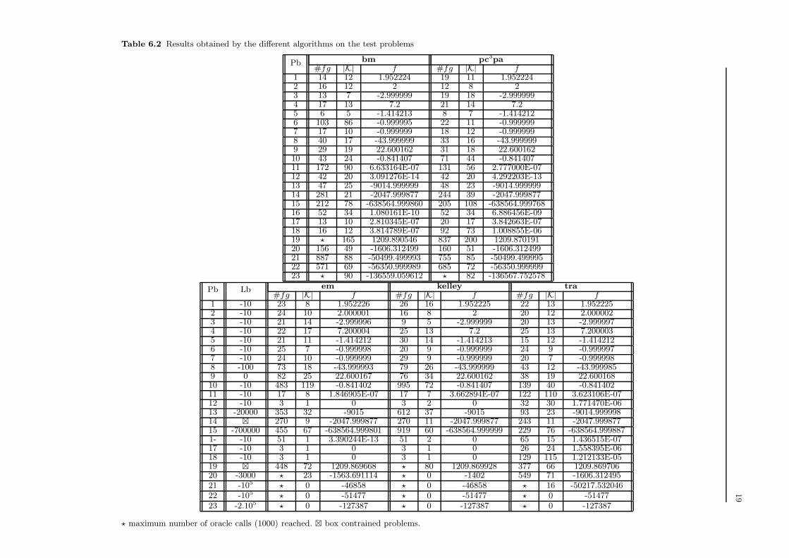
begining of Section 6. The results are given in Table 6.2. The column headed “#fg” displays the number of

oracle calls and the column “|K|” the number of descent steps (for em, kelley and tra, it corresponds to

the number of times the upper bound has been improved). The column “f” contains the optimal objective

produced by the different algorithms, there is no rounding on these values to have a better view on the

quality of the solutions. To deal with the compactness assumption for em, kelley and tra, we give a lower

bound (column “Lb”) on the optimal value when necessary.

Kelley’s algorithm confirms its theoritical default, that is, it is not a reliable method requiring sometimes

an excessive number of calls to the oracle, but often it may be very efficient. Elzinga-Moore’s algorithm

2 http://www.cs.cas.cz/∼luksan/test.html

19

Table 6.2 Results obtained by the different algorithms on the test problems

bm pc3paPb#fg |K| f #fg |K| f

1 14 12 1.952224 19 11 1.9522242 16 12 2 12 8 23 13 7 -2.999999 19 18 -2.9999994 17 13 7.2 21 14 7.25 6 5 -1.414213 8 7 -1.4142126 103 86 -0.999995 22 11 -0.9999997 17 10 -0.999999 18 12 -0.9999998 40 17 -43.999999 33 16 -43.9999999 29 19 22.600162 31 18 22.60016210 43 24 -0.841407 71 44 -0.84140711 172 90 6.633164E-07 131 56 2.777000E-0712 42 20 3.091276E-14 42 20 4.292203E-1313 47 25 -9014.999999 48 23 -9014.99999914 281 21 -2047.999877 244 39 -2047.99987715 212 78 -638564.999860 205 108 -638564.99976816 52 34 1.080161E-10 52 34 6.886456E-0917 13 10 2.810345E-07 20 17 3.842663E-0718 16 12 3.814789E-07 92 73 1.008855E-0619 ⋆ 165 1209.890546 837 200 1209.87019120 156 49 -1606.312499 160 51 -1606.31249921 887 88 -50499.499993 755 85 -50499.49999522 571 69 -56350.999989 685 72 -56350.99999923 ⋆ 90 -136559.059612 ⋆ 82 -136567.752578

em kelley traPb Lb#fg |K| f #fg |K| f #fg |K| f

1 -10 23 8 1.952226 26 16 1.952225 22 13 1.9522252 -10 24 10 2.000001 16 8 2 20 12 2.0000023 -10 21 14 -2.999996 9 5 -2.999999 20 13 -2.9999974 -10 22 17 7.200004 25 13 7.2 25 13 7.2000035 -10 21 11 -1.414212 30 14 -1.414213 15 12 -1.4142126 -10 25 7 -0.999998 20 9 -0.999999 24 9 -0.9999977 -10 24 10 -0.999999 29 9 -0.999999 20 7 -0.9999988 -100 73 18 -43.999993 79 26 -43.999999 43 12 -43.9999859 0 82 25 22.600167 76 34 22.600162 38 19 22.60016810 -10 483 119 -0.841402 995 72 -0.841407 139 40 -0.84140211 -10 17 8 1.846905E-07 17 7 3.662894E-07 122 110 3.623106E-0712 -10 3 1 0 3 2 0 32 30 1.771470E-0613 -20000 353 32 -9015 612 37 -9015 93 23 -9014.99999814 ⊠ 270 9 -2047.999877 270 11 -2047.999877 243 11 -2047.99987715 -700000 455 67 -638564.999801 919 60 -638564.999999 229 76 -638564.9998871- -10 51 1 3.390244E-13 51 2 0 65 15 1.436515E-0717 -10 3 1 0 3 1 0 26 24 1.558395E-0618 -10 3 1 0 3 1 0 129 115 1.212133E-0519 ⊠ 448 72 1209.869668 ⋆ 80 1209.869928 377 66 1209.86970620 -3000 ⋆ 23 -1563.691114 ⋆ 0 -1402 549 71 -1606.31249521 -105 ⋆ 0 -46858 ⋆ 0 -46858 ⋆ 16 -50217.53204622 -105 ⋆ 0 -51477 ⋆ 0 -51477 ⋆ 0 -5147723 -2.105 ⋆ 0 -127387 ⋆ 0 -127387 ⋆ 0 -127387

⋆ maximum number of oracle calls (1000) reached. ⊠ box contrained problems.

20

has a better behaviour and confirms its efficiency when compared to Kelley’s algorithm, see [28,30]. It is

not hard to implement and should be considered as an interesting alternative when there is no problem of

compactness. The more difficult test problems TSPn, n = 120, 442, 1173, 3038 show the limitations of the

two methods and the benefit of regularization mecanisms. On TSP120, Elzinga-Moore’s algorithm behaves

better since it improves the initial solution but on the last three problems the two algorithms completely

fail, no improvement has been obtained from the initial solution. The alternative algorithm tra shows a

certain efficiency in terms of oracle calls, but it also fails on the last three TSP problems (it improves

the initial solution on TSP442). It also suffers from the compactness assumption and requires solving two

problems at each iteration. The gain when compared to em is not so significant to recommand it. We can

also observe from the above results, that MxHilb and L1Hilb are false difficult test problems, they are easily

solved by kelley and em.

The compactness weakness of Elzinga-Moore’s algorithm is now overcome by pc3pa which takes benefit

of the efficiency of Elzinga-Moore’s algorithm to be a valuable alternative to a proximal bundle method.

The two algorithms bm and pc3pa appear to be the most efficient. They solve all the test problems within

the maximum number of oracle calls allowed, except the very challenging problem TSP3038 (and Ury100 for

bm). Our adaptation of Kiwiel heuristic [17] for the choice of µk, shows a certain efficiency when compared

to the fixed parameter µk = 1 as shown in Table 6.3 for the first twenty test problems (it fails within the

1000 oracle calls to solve test problems 13-16). Table 6.4 illustrates the behaviour of pc3pa (we elimiated

TSP3038 for these tests) to reach accuracies 10−4, 10−5 and 10−7; recall that the results for 10−6 are given

on Table 6.2. In general it does not require a great number of oracle calls to reach an additional digit of

tolerance.

Although no firm conclusion can be drawn from these numerical experiments, they are encouraging for

our method. Its efficiency needs to be confirmed on much larger problems such as multicommodity flows

ones and in other context.

7 Conclusion an extensions

We proposed a new approach for nonsmooth optimization, extending Elzinga-Moore cutting plane algo-

rithm. This method uses the same ingredients as bundle methods and appears to be a valuable alternative

to the later. Its extension to separable programming through convex multicommdoity flow problems is under

study [29]. An interesting direction to investigate is the replacement of the Euclidean norm by stabilizers

of the form1

2〈x− xk, Hk(x− xk)〉, where Hk is a n× n symmetric positive definite matrix.

Acknowledgements I’m thankful to C. Lemarechal and L. Luksan for the nondifferentiable test problems androutines used in Section 6. I’m indebted to the authors of references [12,15] which are source of inspiration.

21

Table 6.3 Results by pc3pa with µ = 1 fixed

Pb #fg |K| f1 15 10 1.9522242 13 11 23 34 32 -2.9999994 36 30 7.2000015 9 7 -1.4142126 33 23 -0.9999987 23 16 -0.9999998 27 19 -43.9999999 28 19 22.60016210 52 39 -0.84140711 408 321 1.025418E-0612 529 507 1.665431E-0917 593 590 3.838654E-0418 221 202 1.838589E-0519 572 236 1209.96936820 657 529 -1606.312499

Table 6.4 Results by pc3pa

ε = 10−4 ε = 10−5 ε = 10−7

Pb#fg |K| f #fg |K| f #fg |K| f

1 13 8 1.952264 15 9 1.952228 21 12 1.9522242 11 7 2.000004 11 7 2.000004 13 9 23 14 13 -2.999915 17 16 -2.999995 21 20 -34 17 11 7.200053 19 13 7.200004 24 17 7.25 7 6 -1.414201 8 7 -1.414212 9 8 -1.4142146 16 8 -0.999938 20 10 -0.999997 25 12 -17 14 9 -0.999991 16 10 -0.999995 19 13 -18 25 12 -43.999939 29 14 -43.999995 38 17 -449 24 15 22.600197 27 17 22.600164 34 20 22.60016210 54 36 -0.841357 61 39 -0.841403 76 48 -0.84140811 101 45 2.900605E-05 119 50 3.603576E-06 142 60 4.160684E-0812 42 20 4.292203E-13 42 20 4.292203E-13 42 20 4.292203E-1313 48 23 -9014.999999 48 23 -9014.999999 48 23 -9014.99999914 244 39 -2047.999877 244 39 -2047.999877 244 39 -2047.99987715 205 108 -638564.999768 205 108 -638564.999768 205 108 -638564.99976816 52 34 6.886456E-09 52 34 6.886456E-09 52 34 6.886456E-0917 16 13 3.848038E-05 18 15 5.290344E-06 22 18 9.464784E-0818 66 54 8.429472E-05 81 65 8.665879E-06 93 74 7.209591E-0719 837 200 1209.870191 837 200 1209.870191 837 200 1209.87019120 155 46 -1606.312422 157 48 -1606.312493 161 52 -1606.31249921 752 83 -50499.499934 754 85 -50499.499995 755 85 -50499.49999522 677 68 -56350.999905 682 70 -56350.999988 687 74 -56350.999999†

† With more significant numbers, the f -value is −56350.9999999419 to be compared with −56350.9999993438 forε = 10−6.

References

1. F. Babonneau, C. Beltran, A. Haurie, C. Tadonki, J.-Ph. Vial, “Proximal-ACCPM: a versatile oracle basedoptimization method”, Computational Management Science, to appear.

2. W. Ben Ameur, J. Neto, “A constraint generation algorithm for large scale linear programs using multiple pointsseparation”, Mathematical Programming, 107(3), pp. 517-537, 2006.

3. W. Ben Ameur, J. Neto, “Acceleration of cutting plane and column generation algorithms: applications tonetwork design”, Networks, to appear.

4. B. Betro, “An accelerated central cutting plane algorithm for linear semi-infinite programming”, MathematicalProgramming, 101, pp. 479-495, 2004.

5. S. Boyd, L. Vandenberghe, Convex optimization, Cambridge University Press, 2004.6. E. Cheney, A. Goldstein, “Newton’s method for convex programming and Tchebycheff approximations, Nu-

meriche Mathematik, 1, pp. 253-268, 1959.

22

7. J. Elzinga, T.G. Moore, “A central cutting plane algorithm for the convex programming problem”, MathematicalProgramming, 8, pp. 134-145, 1975.

8. A. Frangioni, “Solving semidefinite quadratic problems within nonsmooth optimization algorithms”, Computers& OR, vol 23(11), pp. 1099-1118, 1996.

9. A. Frangioni, Dual-ascent methods and multicommodity flow problems Ph.D. Thesis, Universita di Pisa, Italy,1997.

10. J.-L. Goffin, J.-Ph. Vial, “Convex nondifferentiable optimization: a survey focused on the analytic center cuttingplane method”, Optimization Methods and Software 17(5), pp. 805-867, 2002.

11. M. Held, RM. Karp, “The traveling-salesman problem and minimum spanning trees: Part II”, MathematicalProgramming, 1, pp. 6-25, 1971.

12. J.-B. Hiriart-Urruty, C. Lemarechal, Convex Analysis and Minimization Algorithms, Springer-Verlag, Berlin,1993.

13. J.E. Kelley, “The cutting plane method for solving convex programs”, Journal of the Society for Industrial andApplied Mathematics 8, pp. 703-712, 1960.

14. K.C. Kiwiel, “An aggregate subgradient method for nonsmooth convex minimization”, Mathematical Program-ming, 27, pp. 320-341, 1983.

15. K.C. Kiwiel, “Methods of descent for nondifferentiable optimization”, Lecture Notes in Mathematics, Springer-Verlag, 1985.

16. K.C. Kiwiel, “An ellipsoid trust region bundle method for nonsmooth convex minimization”, SIAM Journal onControl and Optimization, 27(4), pp. 737-757, 1989.

17. K.C. Kiwiel, “Proximity control in bundle methods for convex nondifferentiable minimization”, MathematicalProgramming, 46(1), pp. 105-122, 1990.

18. K.C. Kiwiel, “A Cholesky dual method for proximal piecewise linear programming”, Numerische Mathematik68(3), pp. 325-340, 1994.

19. C. Lemarechal, R. Mifflin, “A set of nonsmooth optimization test problems”, in Nonsmooth Optimization C.Lemarechal and R. Mifflin eds, Pergamon Press, Oxford, pp. 151-165, 1978.

20. C. Lemarechal, A. Nemirovskii, Y. Nesterov, “New variants of bundle methods”, Mathematical Programming B,69(1), pp. 111-147, 1995.

21. C. Lemarechal, C. Sagastizabal, “Variable metric bundle methods: From conceptual to implementable forms”,Mathematical Programming, 76, pp. 393-410, 1997.

22. C. Lemarechal, “Lagrangian relaxation”, in: Computational Combinatorial Optimization M. Juenger and D.Naddef (eds.) Lecture Notes in Computer Science 2241, pp 112-156, Springer Verlag, 2001.

23. L. Luksan, J. Vlcek, “Test problems for nonsmooth unconstrained and linearly constrained optimization”,Technical report 798, Institute of Computer Science, Academiy of Sciences of the Czech Republic, January2000.

24. G.L. Nemhauser, W.B. Widhelm, “A modified linear program for columnar methods in mathematical program-ming”, Operations Research, 19, pp. 1051-1060, 1971.

25. Y. Nesterov, “Complexity estimates of some cutting plane methods based on the anlytic center”, MathematiclProgramming, 69(1), pp. 149-176, 1995.

26. Y. Nesterov, Introductory Lectures on Convex Programming: Basic Course, Kluwer Academic Publishers, 2003.27. A. Ouorou, “Epsilon-proximal decomposition method”, Mathematical Programming, 99(1), pp. 89-108, 2004.28. A. Ouorou, “Robust capacity assignment in telecommunications”, Computational Management Science, to ap-

pear.29. A. Ouorou, “Solving nonlinear multicommodity flow problems by the proximal Chebychev center cutting plane

algorithm”, Technical Report, France Telecom R&D Division, 2006.30. G. Petrou, C. Lemarechal, A. Ouorou, “An approach to robust network design in telecommunications”, submit-

ted.31. P.A. Rey, C. Sagastizabal, “Dynamical adjustment of the prox-parameter in variable metric bundle methods”,

Optimization, 51(2), pp. 423-447, 2002.32. H. Schramm, J. Zowe, “A version of the bundle idea for minimizing a nonsmooth function: conceptual ideas,

convergence analysis, numerical results”, SIAM Journal on Optimization, 2(1), pp.121-152, 1992.