Evolution of new regulatory functions on biophysically

realistic fitness landscapes

Tamar Friedlander*, Roshan Prizak*, Nicholas H. Barton

Gasper Tkacik

* - equal contribution

Institute of Science and Technology Austria, Am Campus 1, A-3400

Klosterneuburg, Austria

September 28, 2018

Abstract

Gene expression is controlled by networks of regulatory proteins that interact specifically with

external signals and DNA regulatory sequences. These interactions force the network compo-

nents to co-evolve so as to continually maintain function. Yet, existing models of evolution mostly

focus on isolated genetic elements. In contrast, we study the essential process by which regula-

tory networks grow: the duplication and subsequent specialization of network components. We

synthesize a biophysical model of molecular interactions with the evolutionary framework to

find the conditions and pathways by which new regulatory functions emerge. We show that spe-

cialization of new network components is usually slow, but can be drastically accelerated in the

presence of regulatory crosstalk and mutations that promote promiscuous interactions between

network components.

1

arX

iv:1

610.

0286

4v2

[q-

bio.

PE]

27

Feb

2017

Introduction

Phenotypes evolve largely through changes in gene regulation [1, 2, 3, 4], and such evolution may

be flexible and rapid [5, 6]. Of particular importance are mutations affecting affinity and specificity

of transcription factors (TFs) for their upstream signals or for their binding sites, short fragments of

DNA that TFs interact with to activate or repress transcription of specific target genes. Mutations in

these binding sites or at sites that alter TF specificity are crucial because of their ability to “rewire”

the regulatory network—to weaken or completely remove existing interactions and add new ones,

either functional or spurious. Emergence of novel functions in such a network will usually be

constrained to evolutionary trajectories that maintain a viable pattern of existing interactions. This

raises a fundamental question about the effects of such constraints on the accessibility of different

regulatory architectures and the timescales needed to reach them.

The case that we focus on here is the divergence of gene regulation, which can give rise to a

variety of new phenotypes, e.g., via expansion in TF families. A regulatory function previously

accomplished by a single (or several) TF(s) is now carried out by a larger number of TFs, allow-

ing for additional fine-tuning and precision, or, alternatively, for an expansion of the regulatory

scope [7, 8, 9, 10, 11, 12, 13, 14, 15, 16, 17]. The main avenue for such expansions are gene dupli-

cations [18, 19, 20, 21], which generate copies of the TFs and thus provide the “raw material” for

evolutionary diversification. Subsequent specialization of TFs often involves divergence in both

their inputs (e.g., ligands) and outputs (regulated genes) [22, 3]. Examples range from repressors in-

volved in bacterial carbon metabolism that arose from the same ancestor via a series of duplication-

divergence events [23], and ancestral TF Lys14 in the metabolism of S. cerevisiae, which diverged

into 3 different TFs regulating different subsets of genes in C. albicans [24], to many variants of

Lim and Pou-homeobox genes involved in neural development across different organisms [25]. In

some systems the ligand sensing and gene regulatory functions are distributed across two or more

molecules, as for bacterial two-component pathways [26] and eukaryotic signaling cascades [27];

here, too, specialization can occur by a series of mutations in multiple relevant components.

Immediately following a duplication event, molecular recognition between TFs, their input sig-

nals, and their binding sites is specific but undifferentiated between the two TF copies. Under

selection to specialize, recognition sequences and ligand preferences of the two TFs can diverge,

but only if some degree of matching between TFs and their binding sites is continually retained

to ensure network function. Binding sites are thus forced to coevolve in tandem with the TFs, yet

little is known about the resulting limits to evolutionary outcomes and their dependence on impor-

2

tant parameters: the number of regulated genes, the length and specificity of the binding sites, the

correlations between the input signals, and so on.

Theoretical understanding of TF duplication is still incomplete, with existing models predom-

inantly belonging to two categories. The first category of gene duplication-differentiation models

studies subfunctionalization of isolated proteins (e.g., enzymes) that do not have any regulatory

role [28]. When cis-regulatory mutations that control the expression of the duplicated gene are in-

cluded [29, 30, 31, 32, 33], this is done in a simplified fashion, e.g., by a small number of discrete

alleles that represent TF binding sites appearing and disappearing at fixed rates [32, 33]. Because

this approach ignores the essentials of molecular recognition, it cannot model co-evolution between

TFs and their binding sites—the topic of our interest.

The second category of studies tracks regulatory sequences explicitly and uses a biophysical

description of TF-BS (binding site) interactions, properly accounting for the fact that TFs can bind a

variety of DNA sequences with different affinities [5, 35, 36]. In conjunction with thermodynamic

models of gene regulation [1, 38, 39, 40], this approach has been used to study the evolution of bind-

ing sites given a single TF [41, 4, 36, 43, 44], while mostly overlooking the issue of TF duplication

and subfunctionalization (but see [45, 46]).

Here we synthesize these two frameworks—the biophysical description of gene regulation and

the evolutionary modeling of TF specialization—to construct a realistic description of the funda-

mental step by which regulatory networks have evolved. A biophysical model of this setup gives

rise to complex fitness landscapes that are markedly different from simple forms considered pre-

viously; in what follows, we show that realistic landscapes exert a major influence over the evolu-

tionary outcomes and dynamics.

Results

A biophysically realistic fitness landscape

In our model, nTF transcription factors regulate nG genes by binding to sites of length L base pairs;

for simplicity, we consider each gene to have one such binding site. The specificity of a TF for any

sequence is determined by the TF’s preferred (consensus) sequence; sequences matching consensus

are assigned lowest energy, E = 0, which corresponds to tightest binding, and every mismatch

between the consensus and the binding site increases the energy by ε; this additive “mismatch”

model has a long history in gene regulation literature [3, 2, 4, 5].

3

The equilibrium probability that the binding site of gene j (j = 1, . . . , nG) is bound by active

TFs of any type i (i = 1, . . . , nTF) is a proxy for the gene expression level and is given by the

thermodynamic model of gene regulation [1, 49]:

pjm({kij}, {Ci(m)}) =

∑i Ci(m)e−εkij

1 +∑i Ci(m)e−εkij

, (1)

whereCi(m) is dimensionless concentration of active TFs of type i in conditionm, kij is the number

of mismatches between the consensus sequence of the i-th TF species and the binding site of the

j-th gene, and ε is the energy per mismatch in units of kBT . Concentration Ci(m) of active TFs de-

pends on condition m, which can represent either time or space (e.g., during developmental gene

expression programs) or a discrete external environment (e.g., the presence/absence of particular

chemical signals). The simplest case considered here assumes the existence of two such signals that

can be either present or absent, in any combination, for a total number of 4 possible environments

(m = 00, 01, 10, 11), occurring with probabilities αm; an important parameter will be the correla-

tion, −1 ≤ ρ ≤ 1, between the two signals. Each TF has two binary alleles, σi ∈ [00, 01, 10, 11],

determining its specificity for the two signals. If the TF i is responsive to a signal and that signal is

present in environment m, then its active concentration Ci(m) = C0; otherwise, Ci(m) = 0. Given

constants C0, ε, and the genotype D—comprising TF consensus and binding site sequences as well

as TF sensitivity alleles σi—the thermodynamic model of Eq. (4) fully specifies expression levels

for all genes in all environments (Supplementary Notes Section 1).

Fig 1A illustrates this setup for a simple case nTF = nG = 2, assuming that the two copies of the

TF emerged through an initial gene duplication event and are fixed in the population. The original

TF regulates two downstream genes by binding to their binding sites. It is sensitive to both external

signals, which can be present with a varying degree of correlation (Fig 1B). After duplication, three

types of mutation can occur, as shown in Fig 1C: point mutations in the binding sites (rate µ),

mutations in the TF coding sequence that change TF’s preferred (consensus) specificity (rate rTFµ)

and mutations in the two signal-sensing alleles (rate rSµ), which can give each TF specificity to

both signals, to one of them, or to neither. An example in Fig 1D shows the state of the system

after several mutations have affected the degree of (mis)match between the TFs and the binding

sites, kij ; an especially important quantity that tracks the overall divergence of the TF specificity is

denoted as M , the match between the two TF consensus sequences.

4

TF duplication

?mutations

(expressed

at different

time/space) time/space

M=2

signals

TF

CGGTA TGTCC

binding sites

ρ = −1

(anti-correlated)

CGGTA

CTGTA

−1 < ρ < 1

(partially correlated)

ρ = 1

(fully correlated)

BS

mutation

k22

=2

(TF-TF match)

kij: TF-BS

mismatches

k11

=1 k21

=3 k12

=4

BS

(μ)

TF

consensus

sequence

mutation

(rTF

μ)

sensing

domain

mutation

(rSμ)

... ...

σ1 = 11 σ

2 = 01

A

B

C D

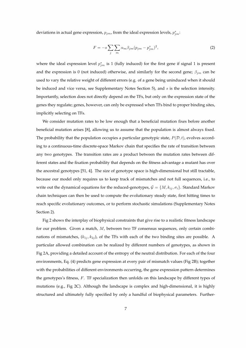
Figure 1: Schematic of the model. (A) TF, initially responsive to two external signals (red andgreen “slots”) and regulating two genes, duplicates and the additional copy fixes in the population.Immediately after duplication, the two copies are undifferentiated. (B) A crucial parameter that willdetermine the fate of the duplicate is the correlation, ρ, of the two signals that activate or induceexpression of the TFs. The signals can correspond to different time periods in development, spatialregions in the organism or tissue, or external conditions / ligands. (C) Various mutation types thatcan occur post-duplication with their associated rates. (D) After accumulating several mutations,the pattern of mismatches between TF consensus sequences and the binding sites is reflected innew values of {kij}, which determine the activation levels of the two genes according to Eq. (4). M ,the number of matches between the consensus sequences of the two TFs (with a value between 0and L), keeps track of the overall divergence of the TF specificities. For a list of model parametersand baseline values see Supplementary Notes Table 1.

5

α00

α10

α01

α11

0 1 2 3 4 5

012345

0 1 2 3 4 5

012345

0 1 2 3 4 5

012345

k1j

k2j

k2j

k2j

0 1 2 3 4 5

012345

012345

012345

012345

k1j

k2j

k2j

k2j

k2j

M=0

M=3

M=5

...

...

0 0.5 1p

jm

AGGTA

CGGTA

TGATC

TGTCC

M

k12

k11

GT G

M

k11

k12

2 1

1 2

4 4

0 1 2 3 4 5k: # of TF-BS mismatches

0

0.25

0.5

0.75

1

strong

binding

S: k<=2weak

binding

W: k>2

bin

din

g p

rob

ab

ilit

y

A

C

D

B

Figure 2: Biophysical and evolutionary constraints shape the genotype-phenotype-fitness mapafter TF duplication. (A) Match, M , between transcription factor consensus sequences (here, oflength L = 5), constrains the possible mismatch values, k1j , k2j , between the gene’s binding siteand either TF. For example, when the two TFs are identical (M = L = 5, bottom left), they musthave equal mismatches with all genes (k1j = k2j). Some combinations of mismatches are impossi-ble given M (white), while others are realized by different numbers of genotypes (grayscale). (B)Expression level (color) for a regulated gene given all mismatch combinations, k1j , k2j , at M = 3.Impossible mismatch combinations are white. Each of the four panels shows expression levels infour possible environments, m = 00, 10, 01, 11. Fitness F depends on the structure of mismatches(A), the biophysics of binding (B), and the frequencies of different environments, αm. Here wechoose α so that the marginal probability of each input signal is always 1

2 but the correlation can bevaried, and assign weight βjm = 1 whenever the gene should be induced but is not, and βjm = 1

2when it should not be induced but is. (C) A single point mutation, e.g. a change in one TF’s bind-ing specificity from T to G, can simultaneously affect the match, M , and either increase, decrease,or leave intact the mismatches, k11 and k12, that determine fitness. (D) TF-BS interactions with mis-match k that is low enough to ensure a high binding probability (p > 2/3) are assigned to a “strongbinding” phenotype (solid link); conversely, p < 1/3 is a “weak binding” phenotype (dotted link).

To complete the evolutionary model, a fitness function is required. We assume selection for

the genes to acquire distinct expression patterns in response to external signals, and thus define

this fully specialized state as having the highest fitness in our model. Specifically, we penalize the

6

deviations in actual gene expression, pjm, from the ideal expression levels, p∗jm:

F = −s∑j

∑m

αmβjm(pjm − p∗jm)2, (2)

where the ideal expression level p∗jm is 1 (fully induced) for the first gene if signal 1 is present

and the expression is 0 (not induced) otherwise, and similarly for the second gene; βjm can be

used to vary the relative weight of different errors (e.g. of a gene being uninduced when it should

be induced and vice versa, see Supplementary Notes Section 5), and s is the selection intensity.

Importantly, selection does not directly depend on the TFs, but only on the expression state of the

genes they regulate; genes, however, can only be expressed when TFs bind to proper binding sites,

implicitly selecting on TFs.

We consider mutation rates to be low enough that a beneficial mutation fixes before another

beneficial mutation arises [8], allowing us to assume that the population is almost always fixed.

The probability that the population occupies a particular genotypic state, P (D, t), evolves accord-

ing to a continuous-time discrete-space Markov chain that specifies the rate of transition between

any two genotypes. The transition rates are a product between the mutation rates between dif-

ferent states and the fixation probability that depends on the fitness advantage a mutant has over

the ancestral genotypes [51, 4]. The size of genotype space is high-dimensional but still tractable,

because our model only requires us to keep track of mismatches and not full sequences, i.e., to

write out the dynamical equations for the reduced-genotypes, G = {M,kij , σi}. Standard Markov

chain techniques can then be used to compute the evolutionary steady state, first hitting times to

reach specific evolutionary outcomes, or to perform stochastic simulations (Supplementary Notes

Section 2).

Fig 2 shows the interplay of biophysical constraints that give rise to a realistic fitness landscape

for our problem. Given a match, M , between two TF consensus sequences, only certain combi-

nations of mismatches, (k1j , k2j), of the TFs with each of the two binding sites are possible. A

particular allowed combination can be realized by different numbers of genotypes, as shown in

Fig 2A, providing a detailed account of the entropy of the neutral distribution. For each of the four

environments, Eq. (4) predicts gene expression at every pair of mismatch values (Fig 2B); together

with the probabilities of different environments occurring, the gene expression pattern determines

the genotypes’s fitness, F . TF specialization then unfolds on this landscape by different types of

mutations (e.g., Fig 2C). Although the landscape is complex and high-dimensional, it is highly

structured and ultimately fully specified by only a handful of biophysical parameters. Further-

7

more, because of the sigmoidal shape of binding probability as a function of mismatch k [Eq. (4)], it

is possible to assign phenotypes of “strong” and “weak” binding to every TF-BS interaction, allow-

ing us to depict network interactions graphically, as shown in Fig 2D, and to classify the possible

macroscopic evolutionary outcomes, as we will show next.

Evolutionary outcomes in steady state

Evolutionary outcomes in steady state are determined by a balance between selection and drift.

The steady state distribution over reduced-genotypes is [9]

PSS(G) = P (G, t→∞) = P0(G) exp(2NF (G)), (3)

where P0 is the neutral distribution of genotypes and N is the population size. Eq. (3) is similar to

the energy/entropy balance of statistical physics [11], with fitness F playing the role of energy and

logP0 the role of entropy; in our model, both of these quantities are explicitly computable, as is the

resulting steady state distribution.

Understanding the high dimensional distribution over genotypes is difficult, but classification

of individual TF-BS interactions into “strong” and “weak” ones, as described above, allows us to

systematically and uniquely assign every genotype to one of a few possible macroscopic outcomes,

or “macrostates,” graphically depicted in Fig 3A and defined precisely in Supplementary Notes

Section 1. Thus, in the No Regulation state, input signals are not transduced to the target genes,

either because TF-BS mismatches are high and there is no binding or because TFs themselves lose

responsiveness to the input signals; in the One TF Lost state, a single TF regulates both genes

(as before duplication), while the other TF is lost, i.e., its specificity has diverged so far that it

does not bind any of the sites; the Specialize Binding state corresponds to each TF regulating

its own gene without cross-regulating the other but the signal sensing domains are not yet signal

specific, as they are in the Specialize Both, the state which we have defined to have the highest

fitness. Finally, the Partial macrostate predominantly features configurations where each of the

TFs binds at least one binding site, but one of the TFs still binds both sites or retains responsiveness

for both input signals; functionally, these configurations lead to large “crosstalk,” where input

signals are non-selectively transmitted to both target genes.

Ultimately, these macrostates are the functional network phenotypes that we care about. The

number of genotypes in each macrostate, however, can vary by orders of magnitude; for example,

the No Regulation state is larger by ∼ 104 relative to the high-fitness Specialize Both state,

8

for our baseline choice of parameters (L = 5, ε = 3). Selection can act against this strong entropic

bias, and the distribution of fitness values across genotypes within each macrostate is shown in

Fig 3B. Clearly, the mean or median fitness within each macrostate is a poor substitute for the de-

tailed structure of fitness levels that depend nonlinearly on TF-BS mismatches and the degeneracy

of the sequence space. Unlike the entropic term in Fig 3A, fitness also depends on the statistics of

the environment, αm, and in particular, the correlation ρ between the two signals. For example,

when the signals are strongly correlated, the Initial state right after duplication or the One TF

Lost state can achieve quite high fitnesses, since responding to the wrong signal or having a high

degree of crosstalk will still ensure largely appropriate gene expression pattern in all likely environ-

ments. In contrast, at strong negative correlation, many genotypes in Specialize Binding and

Initial states will suffer a large fitness penalty because their sensing domains are not specialized

for the correct signals, while the Specialize Both state will have high fitness regardless of the

environmental signal correlation.

9

102 104 106 108

#genotypes

1010

Specialize Binding

No Regulation

Initial

Specialize Both

One TF Lost

Partial

1012

Ns

-1

-0.75

-0.5

-0.25

0

0.25

0.5

0.75

1

ρ

0 10 20 30 40 5025

+Strong selection and

non correlated signals

lead to specialized TFs

PS

S

k11

k21

M

PS

S

0 0.5 1

analytical s

imu

lati

on

-50

-20

-5

-1

-0.1

-0.01

0

ρ = -0.8ρ = 0.8

NF

0

0.2

0.4

0.6

0.8

1

Ns=25Ns=0

0

0.2

0.4

0.6

0.8

1

0 1 2 3 4 5

A B

C D

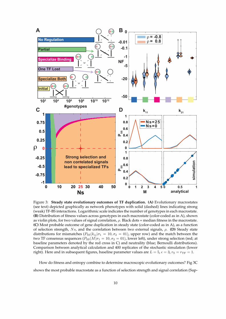
Figure 3: Steady state evolutionary outcomes of TF duplication. (A) Evolutionary macrostates(see text) depicted graphically as network phenotypes with solid (dashed) lines indicating strong(weak) TF-BS interactions. Logarithmic scale indicates the number of genotypes in each macrostate.(B) Distribution of fitness values across genotypes in each macrostate (color-coded as in A), shownas violin plots, for two values of signal correlation, ρ. Black dots = median fitness in the macrostate.(C) Most probable outcome of gene duplication in steady state (color-coded as in A), as a functionof selection strength, Ns, and the correlation between two external signals, ρ. (D) Steady statedistributions for mismatches (PSS(kij |σ1 = 10, σ2 = 01), upper row) and the match between thetwo TF consensus sequences (PSS(M |σ1 = 10, σ2 = 01), lower left), under strong selection (red; atbaseline parameters denoted by the red cross in C) and neutrality (blue; Bernoulli distributions).Comparison between analytical calculation and 400 replicates of the stochastic simulation (lowerright). Here and in subsequent figures, baseline parameter values are L = 5, ε = 3, rS = rTF = 1.

How do fitness and entropy combine to determine macroscopic evolutionary outcomes? Fig 3C

shows the most probable macrostate as a function of selection strength and signal correlation (Sup-

10

plementary Notes Section 3). At weak selection, specific TF-BS interactions cannot be maintained

against mutational entropy and the system settles into the most numerous, No Regulation state.

Higher selection strengths can maintain a limited number of TF-BS interactions in Partial states.

Beyond a threshold value for Ns, the evolutionary outcome depends on the signal correlation:

when signals are anti-correlated or weakly correlated, the TFs reach the fully specialized state,

whereas high positive correlation favors losing one TF and having the remaining TF regulate both

genes and respond to both signals. As signal correlation increases, so does the selection strength

required to support full specialization.

The map of evolutionary outcomes is very robust to parameter variations. The energy scale

of TF-DNA interactions is that of hydrogen bonds: ε ∼ 3 (in kBT units), consistent with direct

measurements. The scale of C0 is set to ensure that consensus sites are occupied at saturation

while fully mismatching sites are essentially empty. The only remaining important biophysical

parameter is L, the length of the binding sites. As expected, increasing L expands the regions of

No Regulation and Partial at low Ns, due to entropic effects. Surprisingly, however, one can

demonstrate that the important boundary between the Specialize and One TF Lost states is

independent of L; furthermore, the map in Fig 3C is exactly robust to the overall rescaling of the

mutation rate, µ, and even to separate rescaling of individual rates rS, rTF.

We compare the steady-state marginal distributions of TF-BS mismatches and the match, M ,

between the two TFs, under strong selection to specialize (Ns = 25) vs neutral evolution (Ns = 0).

Mismatch distributions for k11 and k21 in Fig 3D display a clear difference in the two regimes:

strong selection favors a small mismatch of the BS with the cognate TF, sufficient to ensure strong

binding but nonzero due to entropy, and a large mismatch with the noncognate TF, to reduce

crosstalk. Surprisingly, however, the distribution of matches M between two TF consensus se-

quences shows only a tiny signature of selection, with both distributions peaking around 1 match.

As a consequence, inferring selection to specialize from measured binding preferences of real TFs

might not be feasible with realistic amounts of data.

11

0

23

k12

k11

k21

k22

5

σ1

σ2

M

0

23

5

0

23

5

10-2 10-1 100 101

time (μ-1 generations)

Specialize Both One TF Lost Partial

Specialize Binding No Regulation Initial

0.04

0.04

0.0

5

0.050.05

0.05

0.0

6

0.06

0.1

0.2

0.2

0.2

0.2

0.2

0.20

.50

.50.5

+ρ

0.1

0.1

0.1

-1

-0.75

-0.5

-0.25

0.25

0.5

0.75

1

0

0.2

0.2

0.2

0.2

0.2

0.2

0.5

0.5

0.5

0.5

0.5

0.5

1

1

1 1

1.5

1.51.5

1.7 1.71.7

1.7

ρ +

-1

-0.75

-0.5

-0.25

0.25

0.5

0.75

1

0

0.2

0.2

0.2 0

.2

0.2

0.2

0.5

0.5

0.5

1

1

1

1.75

1.75

1.75

1.7

5

1.751.75

10

10

10

1000

1000

ρ

+

-1

-0.75

-0.5

-0.25

0.25

0.5

0.75

1

0

10-3 10-2 10-1 100 101

-1

-2

5

3

2

0

-3

-4

-5

-6

MNF

Initial

One TF

Lost

Partial

Specialize

Both

τslow

τfast

10-2 μ−1

10-1 μ−1

100 μ−1

101 μ−1

Slow

Fast

10

1

2

5

20

503 4 5 6 7 L

0.1 0.3 1 3 10

rTF

rS

A C

B

D

E

0.2

0.2

0.2

0.2

0.2

0.2

0.5

0.5

0.5

1

1

11

1

11.5

1.51.5

10

10

10

1000

1000

0 10 20 30 40 50

Ns

-1

-0.75

-0.5

-0.25

0.25

0.5

0.75

1

ρ +

25

0

τslow

τfast

101 μ−1

12

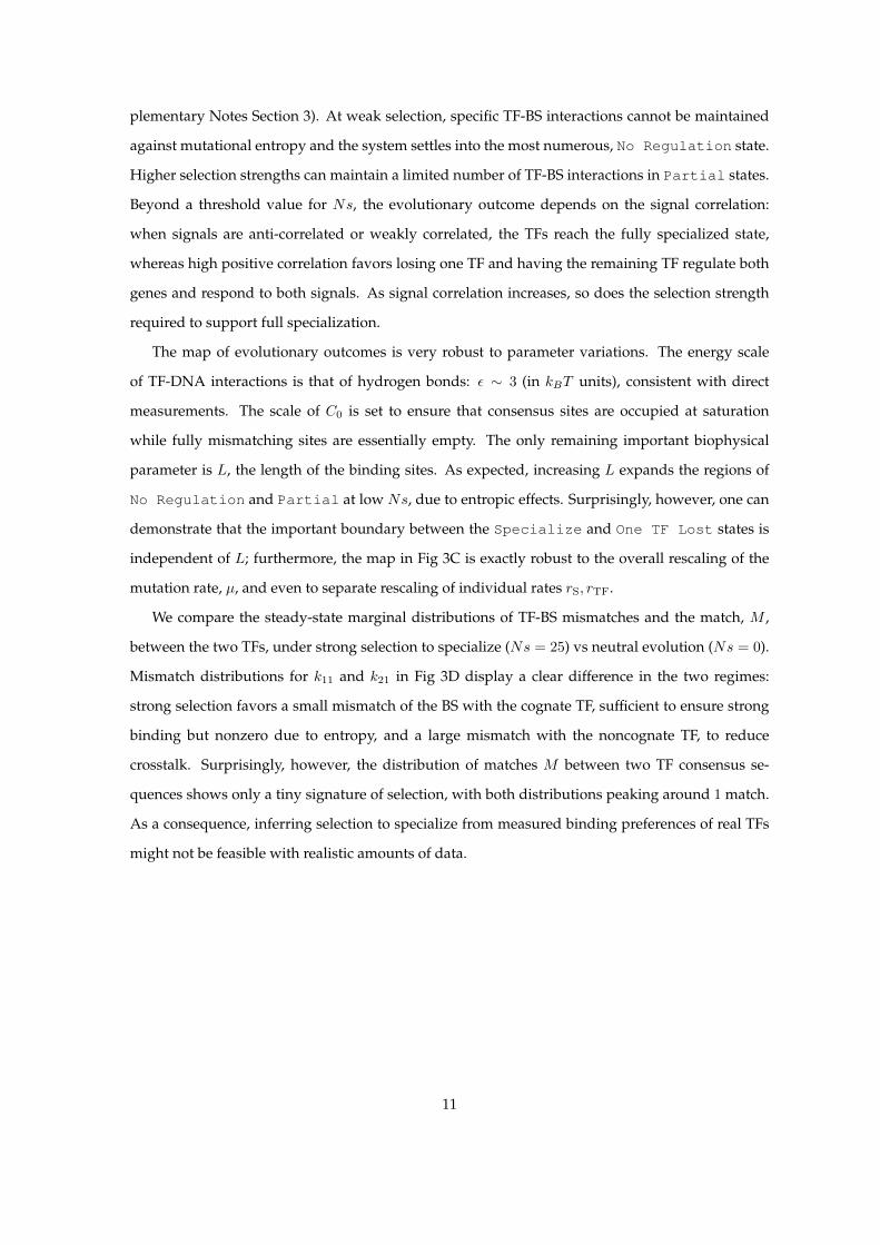
Figure 4: Slow and fast pathways to TF specialization. (A) Temporal traces of TF-TF matchM (top), and TF-BS mismatches kij (middle: TF1, bottom: TF2) with the corresponding signalspecificity mutations denoted on dashed lines, for one example evolutionary trajectory at baselineparameters. Macrostates are color-coded as in the top legend and Fig 3. (B) Average dynamicsof fitness NF (blue, left scale) and TF-TF match M (red, right scale). For every timepoint, thedominant macrostate is denoted in color. (C) Snapshots of dominant macrostates (at increasing timepost-duplication as indicated in the panels), shown for different combinations of selection strengthNs and signal correlation ρ as in Fig 3. Contours mark dwell times in the dominant macrostates(in units of µ−1). Red cross = baseline parameters. (D) Schematic of the two alternative pathwaysto specialization. τslow and τfast are the total times to specialization for the “slow” and the “fast”pathway, respectively. (E) Relative duration of the two pathways, as a function of binding sitelength L (gray line, top axis), TF consensus sequence mutation rate rTF (red), and signal domainmutation rate rS (blue, bottom axis). Pie charts indicate the fraction of slow (pink) and fast (green)pathways at each parameter value.

Evolutionary dynamics and fast pathways towards specialization

Next, we focus on evolutionary trajectories and the timescales to reach the fully specialized state

after gene duplication. An example trajectory is shown in Fig 4A: the two TFs start off identical

(with maximal match, M = L = 5) until, as a result of the loss of specificity for both signals,

TF1 starts to drift, diverging from TF2 (sharply decreasing M in One TF Lost state) and losing

interactions with both binding sites. Subsequently TF1 reacquires preference to the red signal,

which drives the reestablishment of TF1 specificity for one binding site during a short Specialize

Binding epoch, followed quickly by the specialization of TF2 for the green signal at the start of

Specialize Both epoch of maximal fitness.

Dynamics of the TF-TF match, M , and the scaled fitness, NF , become smooth and gradual

when discrete transitions and the consequent large jumps in fitness are averaged over individual

realizations, as in Fig 4B. Importantly, we learn that the sequence of dominant macrostates leading

towards the final (and steady) state, Specialize Both, involves a long intermediate epoch when

the system is in the One TF Lost state. We examine this sequence of most likely macrostates in

detail in Fig 4C, and visualize it analogously to the map of evolutionary outcomes in steady state

shown in Fig 3C. High Ns and correlation (ρ) values favor trajectories passing through the One TF

Lost state, while intermediate Ns (5 . Ns . 20) and low correlation values enable transitions

through Partial macrostate; along the latter trajectory, the binding of neither TF is completely

abolished. Typical dwell times in dominant states, indicated as contours in Fig 4C, suggest that

specialization via the One TF Lost state should be slower than through the Partial state, which

is best seen at t = 1/µ, where specialization has already occurred at intermediate Ns and low, but

not high, ρ values.

It is easy to understand why pathways towards specialization via the One TF Lost state are

13

slow. As the example in Fig 4A illustrates, so long as one TF maintains binding to both sites and

thus network function (especially when signals are strongly correlated), the other TF’s specificity

will be unconstrained to neutrally drift and lose binding to both sites, an outcome which is en-

tropically highly favored. After the TF’s sensory domain specializes, however, the binding has to

re-evolve essentially from scratch in a process that is known to be slow [44] unless selection strength

is very high. In contrast to this “Slow” pathway, the “Fast” pathway via the Partial state relies

on sequential loss of “crosstalk” TF-BS interactions, with the divergence of TF consensus sequences

followed in lock-step by mutations in cognate binding sites. Specifically, the likely intermediary of

the fast pathway is a Partial configuration in which the first TF responds to both signals but only

regulates one gene, whereas the second TF is already specialized for one signal, but still regulates

both genes.

The fast and the slow pathways are summarized in Figs 4D. A detailed analysis (Supplementary

Notes Section 4) reveals how different biophysical and evolutionary parameters change the relative

probability and the average duration (Fig 4E of both pathways. For example, increasing the length,

L, of the binding sites favors the slow pathway as well as drastically increases its duration, lead-

ing to very slow evolutionary dynamics. In contrast, time to specialize via the fast pathway is

unaffected by an increase in L. Increasing the rate of TF-specificity-affecting mutations, rTF, has

a qualitatively similar effect, while increasing the mutation rate affecting the sensory domain, rS,

favors the fast pathway. Indeed, in the limit when rS is much larger than the other two mutation

rates, the sensing domain specializes almost instantaneously, making the complete loss of binding

by either TF very deleterious and thus avoiding the One TF Lost state; the adaptation dynamics

is initially rapid, with binding sites responding to diverging TF consensus sequences, and subse-

quently slow, when TF consensus sequences further minimize their match, M , in a nearly neutral

process.

Promiscuity-promoting mutations

Typically, each TF must regulate more than one target gene. As the number of regulated genes per

TF (nG/nTF) increases, intuition suggests that the evolution of the TF’s consensus sequence should

become more and more constrained: while a mutation in an individual binding site can lower the

total fitness by increasing mismatch and thereby impeding TF-BS binding, a single mutation in the

TF’s consensus has the ability to simultaneously weaken the interaction with many binding sites,

leading to a high fitness penalty. Our analysis of the biophysical fitness landscape confirmed that

14

the landscape gets progressively more frustrated as the number of regulated genes per TF increases,

due to the explosion of constraints that TFs have to satisfy to ensure the maintenance of functional

regulation (Supplementary Notes Section 7). Consequently, one can expect extremely long times to

specialization. How can it nevertheless proceed at observable rates?

A BAAAAA

AAAAG

CAAAA

AAAAG

CAAAA

CAAAG

∗AAAA

AAAAG

∗AAAA

CAAAG

TF

promiscuous

BS

TF

TF

BS

1.5%

3%

9.5%

13%

89%

84%

deleterious neutral

beneficial

wit

ho

ut

pro

mis

cu

ity

wit

h

pro

mis

cu

ity

20

2

Ns

without

promiscuity

with

promiscuity

τ, t

ime

to

sp

ec

ializa

tio

n

10

5

1n

G=2

nG=4

nG=8

0 15050 100

100

50

Ns0 15050 100

15

.43

.51

.7

sp

ee

du

p d

ue

to

pro

mis

cu

ity

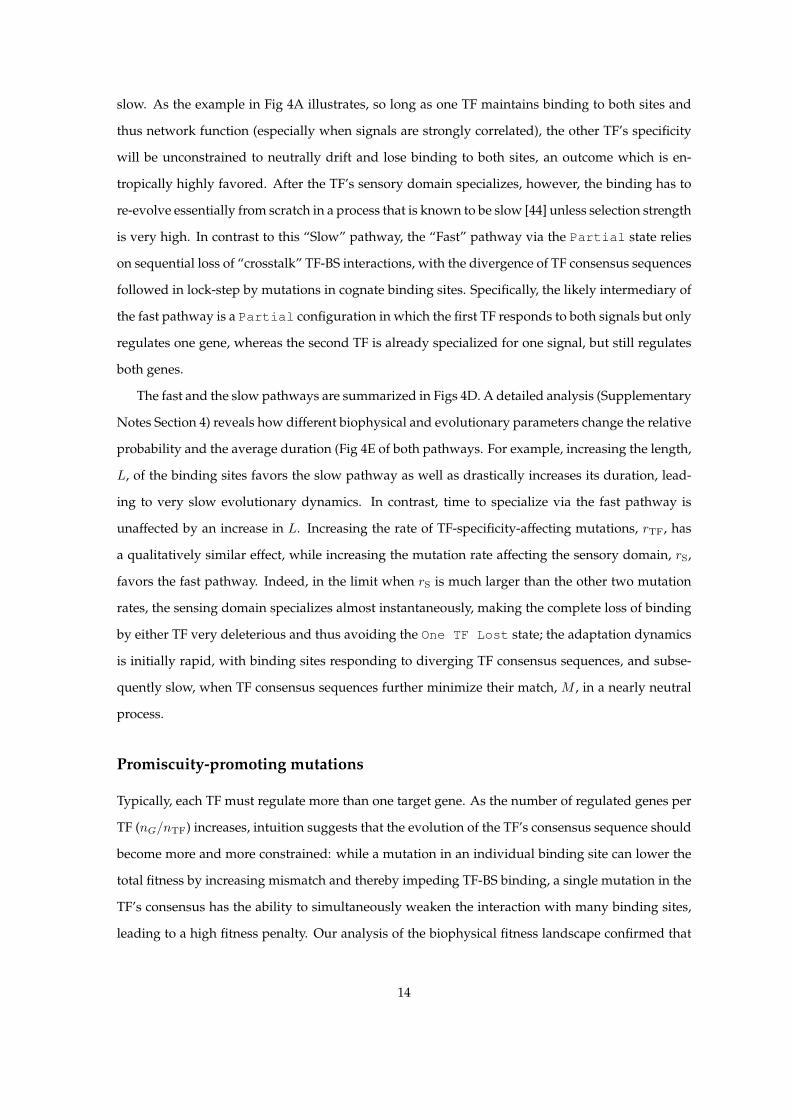
Figure 5: Promiscuity-promoting mutations speed up specialization with multiple regulatedgenes per TF. (A) In the absence of promiscuity-promoting mutations, a compensatory series ofpoint mutations in the TF’s consensus (upper sequence) and its binding site (lower sequence) isneeded to maintain TF-BS specificity (top; light red). Alternatively, in the presence of promiscuity-promoting mutations in the TF consensus, a position in the TF’s recognition sequence (marked bya star) can lose and later regain sequence specificity (middle; light yellow). Promiscuity decreasesthe fraction of deleterious mutations along typical pathways to specialization (bottom, computedusing baseline parameters). (B) Time to specialization as a function of selection strength, Ns, with-out (left) and with (right) promiscuity promoting mutations in the TF, for different numbers ofregulated genes per TF, nG (color).

Energy matrices for many real TFs display “promiscuous” specificity where, at a particular

position within the binding site, binding to multiple nucleotides is equally preferable. We won-

dered how our findings would be affected if consensus sequence specificity of the TFs could pass

through such intermediate promiscuous states. Fig 5A shows how TF consensus sequence and the

corresponding binding site can co-evolve using point mutations, or using the new “promiscuity-

promoting” mutation type for the TF: promiscuity-promoting mutation renders one position in the

recognition sequence of the TF insensitive to the corresponding DNA base in the binding site (Sup-

plementary Notes Section 8). Evolutionary pressure on the binding sites is therefore temporarily

relieved, until the specificity of the TF is reestablished by a back mutation. Without promiscuity-

promoting mutations, TF-BS co-evolution must proceed in a tight sequence of compensatory mu-

15

tations; with promiscuity-promoting mutations, such a precise sequence is no longer required, al-

though one extra mutation is needed to reestablish high TF-BS specificity. With promiscuity, the

fraction of deleterious mutations along the evolutionary path towards specialization is reduced,

an effect that grows stronger with increasing L. As shown in Fig 5B, this has drastic effects on

the time to specialization. Without promiscuity, increasing the selection strength, Ns, decreases

the required time when each TF regulates one gene, as expected for a landscape with large neutral

plateaus but with no fitness barriers. For nG > 2, however, the landscape develops barriers that

need to be crossed, and evolutionary time starts increasing with Ns. In contrast, promiscuity en-

ables fast emergence of TF specialization even with multiple regulated genes in a broad range of

evolutionary parameters (although there are also costs due to high promiscuity).

Discussion

The role that the shape of a fitness landscape plays for the dynamics and the final outcomes of evo-

lution has been appreciated in population genetics for a long time. This has stimulated a large body

of theoretical research into evolution on toy model landscapes [54, 55], as well as motivated efforts

to map out real, small-scale landscapes experimentally. For limited classes of problems, mostly

those involving molecular recognition, biophysical constraints are informative enough to permit

computational exploration of complex landscapes. Such is the case for the secondary structure

of RNA [56], antibody-antigen interactions, protein-protein interactions, and transcription factor-

DNA binding, explored here. We exploit this prior knowledge to construct a fitness landscape for a

more complicated evolutionary event, the specialization of two TFs after duplication, a key evolu-

tionary step by which gene regulatory networks expand. The biophysical model naturally captures

a number of essential features, without having to introduce them “by hand”: the fact that special-

ization is driven by avoidance of regulatory crosstalk; the importance of the mutational entropy;

the dependence on number of downstream genes; the existence of transient network configurations

preceding specialization, which crucially impact dynamics; and the importance for evolutionary

outcomes of the statistical properties of the signals that TFs respond to. Importantly, the expres-

sive power of our framework does not come at increased modeling cost: while complex, the fitness

landscape is still determined only by a few, mostly known, parameters, and an exponentially large

space of genotypes can be systematically coarse grained to a small set of functional network phe-

notypes. This combination of biophysical and co-evolutionary approaches is applicable generally

to the evolution of molecular interactions, e.g., in protein interaction networks.

16

In steady state, our results robustly identify correlation between the environmental signals that

drive TFs as a key determinant for specialization, as shown in Fig 3C. Unless the new signal, for

which a post-duplication TF can specialize, is sufficiently independent (uncorrelated) from the ex-

isting signals that the regulatory network processes, one TF copy will be lost due to drift. As a

consequence, the effective dimensionality of environmental signals dictates the complexity of genetic

regulatory networks [57], reminiscent of information-theoretic tradeoffs in sensory neuroscience;

in evolutionary terms, selection to maintain complex regulation needs to withstand the muta-

tional flux into vastly more numerous but less functional network phenotypes. Recently, it has

been shown that finite biochemical specificity also limits the complexity of genetic regulatory net-

works [12]; an interesting direction for future research is to understand how the balance between

regulatory crosstalk, environmental signal statistics, and evolutionary constraints ultimately deter-

mines the number of TFs that can be stably maintained. A related question concerns the expected

match between pairs of TFs in a large network as a signature of selection for specialized function;

for an isolated pair of TFs, our results in Fig 3D predict only a tiny deviation from neutrality.

Timescales and pathways to specialization are completely shaped by the properties of the bio-

physical fitness landscape, and thus cannot be captured by simple allelic models that ignore the

topology of the sequence space (Supplementary Notes Section 6). We show that the fast pathway

to specialization transitions through Partial states where neither of the two TFs completely loses

binding. Interestingly, it is exactly the existence of crosstalk interactions that permits fast adapta-

tion via these transient states, by maintaining the network function through one TF, while the other

is free to diverge in a series of mutations to the TF and its future binding site [59]. Crosstalk thus en-

ables some amount of network plasticity during early adaptation, yet is ultimately selected against,

when TFs become fully specialized [60, 61]. In the protein-protein-interaction literature, Partial

states are sometimes referred to as promiscuous states, and they have been suggested as evolution-

arily accessible intermediaries that relieve the two interacting molecules of the need to evolve in

a tight (and likely very slow) series of compensatory mutations [62]. In contrast to the fast path-

way, the slow pathway involves a complete loss of TF-BS binding interactions; the long timescale

emerges from long dwell times while the TF and the binding sites evolve in a nearly neutral land-

scape before TF-BS specificity is reacquired. Long binding sites and (perhaps counter-intuitively)

fast TF mutation rates favor the slow pathway, while fast sensing domain mutation rates favor the

fast pathway.

The situation changes qualitatively when each TF regulates more genes [63]. On the one hand,

entropy makes pathways that pass through the One TF Lost state dynamically uncompetitive,

17

as multiple binding sites would have to emerge de novo to reestablish interactions with a diverged

TF. This would favor fast pathways through Partial states. On the other hand, the biophysical

fitness landscape develops frustration (or sign epistasis) as nG > 2 and the timescales to special-

ization lengthen with increasing selection strength when passing through Partial states. We

demonstrate that frustration is relieved by promiscuity-promoting mutations in the transcription

factor, enabling fast emergence of specialization even with multiple regulated genes.

Taken together, our results paint a picture of TF specialization that most likely proceeds through

intermediate states with high crosstalk, in which one TF has already specialized for its input signals

but not yet for the target genes, while the other TF is not yet specialized for the input signals but

only regulates one gene. In addition, these intermediate states are likely to be more promiscuous,

binding different sites with the same affinity, with the promiscuity reverting to specific binding

towards the end of specialization. This picture is qualitatively different from the paradigmatic

idea of a simple and sequential progression of compensatory mutations in the TF and its binding

sites [64, 45]. It depends fundamentally on the biophysical model of TF-BS interactions, predicts

significantly faster specialization times, as well as the existence of promiscuous TF variants that are

starting to be observed in genomic analyses of duplication-specialization events [14, 15].

Acknowledgments We thank the People Programme (Marie Curie Actions) of the European

Union’s Seventh Framework Programme (FP7/2007-2013) under REA grant agreement Nr. 291734

(T.F.), ERC grant Nr. 250152 (N.B.), and Austrian Science Fund grant FWF P28844 (G.T.).

References

[1] King MC, Wilson AC (1975) Evolution at two levels in humans and chimpanzees. Science

188(4184):107–116.

[2] Gilad Y, Oshlack A, Smyth GK, Speed TP, White KP (2006) Expression profiling in primates

reveals a rapid evolution of human transcription factors. Nature 440(7081):242–245.

[3] Wray GA (2007) The evolutionary significance of cis-regulatory mutations. Nature Reviews

Genetics 8(3):206–216.

[4] Carroll SB (2005) Evolution at Two Levels: On Genes and Form. PLoS Biol 3(7):e245.

[5] Yona A, Frumkin I, Pilpel Y (2015) A Relay Race on the Evolutionary Adaptation Spectrum.

Cell 163(3):549–559.

18

[6] Madan Babu M, Teichmann SA, Aravind L (2006) Evolutionary Dynamics of Prokaryotic Tran-

scriptional Regulatory Networks. Journal of Molecular Biology 358(2):614–633.

[7] Kacser H, Beeby R (1984) Evolution of catalytic proteins: On the origin of enzyme species by

means of natural selection. Journal of Molecular Evolution 20(1):38–51.

[8] Simionato E et al. (2007) Origin and diversification of the basic helix-loop-helix gene family in

metazoans: insights from comparative genomics. BMC Evolutionary Biology 7:33.

[9] Larroux C et al. (2008) Genesis and Expansion of Metazoan Transcription Factor Gene Classes.

Molecular Biology and Evolution 25(5):980–996.

[10] Hobert O, Carrera I, Stefanakis N (2010) The molecular and gene regulatory signature of a

neuron. Trends in neurosciences 33(10):435–445.

[11] Achim K, Arendt D (2014) Structural evolution of cell types by step-wise assembly of cellular

modules. Current Opinion in Genetics & Development 27:102–108.

[12] McKeown A et al. (2014) Evolution of DNA Specificity in a Transcription Factor Family Pro-

duced a New Gene Regulatory Module. Cell 159(1):58–68.

[13] Baker CR, Tuch BB, Johnson AD (2011) Extensive DNA-binding specificity divergence of a

conserved transcription regulator. Proceedings of the National Academy of Sciences 108(18):7493–

7498.

[14] Sayou C et al. (2014) A Promiscuous Intermediate Underlies the Evolution of LEAFY DNA

Binding Specificity. Science 343(6171):645–648.

[15] Pougach K et al. (2014) Duplication of a promiscuous transcription factor drives the emergence

of a new regulatory network. Nature Communications 5:4868.

[16] Nadimpalli S, Persikov AV, Singh M (2015) Pervasive Variation of Transcription Factor Or-

thologs Contributes to Regulatory Network Evolution. PLOS Genet 11(3):e1005011.

[17] Arendt D (2008) The evolution of cell types in animals: emerging principles from molecular

studies. Nature Reviews Genetics 9(11):868–882.

[18] Ohno S (2013) Evolution by gene duplication. (Springer Science & Business Media).

[19] Magadum S, Banerjee U, Murugan P, Gangapur D, Ravikesavan R (2013) Gene duplication as

a major force in evolution. Journal of Genetics 92(1):155–161.

19

[20] Andersson DI, Hughes D (2009) Gene Amplification and Adaptive Evolution in Bacteria. An-

nual Review of Genetics 43(1):167–195.

[21] Yona AH et al. (2012) Chromosomal duplication is a transient evolutionary solution to stress.

Proceedings of the National Academy of Sciences 109(51):21010–21015.

[22] Wittkopp PJ, Kalay G (2012) Cis-regulatory elements: molecular mechanisms and evolution-

ary processes underlying divergence. Nature Reviews Genetics 13(1):59–69.

[23] Nguyen CC, Saier MH (1995) Phylogenetic, structural and functional analyses of the LacI-GalR

family of bacterial transcription factors. FEBS Letters 377(2):98–102.

[24] Perez JC et al. (2014) How duplicated transcription regulators can diversify to govern the

expression of nonoverlapping sets of genes. Genes & Development 28(12):1272–1277.

[25] Hobert O, Westphal H (2000) Functions of LIM-homeobox genes. Trends in Genetics 16(2):75–

83.

[26] Parkinson JS (1993) Signal transduction schemes of bacteria. Cell 73(5):857–871.

[27] Bowler C, Chua NH (1994) Emerging themes of plant signal transduction. The Plant Cell

6(11):1529–1541.

[28] Innan H, Kondrashov F (2010) The evolution of gene duplications: classifying and distinguish-

ing between models. Nature Reviews Genetics 11(2):97–108.

[29] Force A et al. (1999) Preservation of Duplicate Genes by Complementary, Degenerative Muta-

tions. Genetics 151(4):1531–1545.

[30] Lynch M, Force A (2000) The Probability of Duplicate Gene Preservation by Subfunctionaliza-

tion. Genetics 154(1):459–473.

[31] Lynch M, O’Hely M, Walsh B, Force A (2001) The Probability of Preservation of a Newly Arisen

Gene Duplicate. Genetics 159(4):1789–1804.

[32] Force A et al. (2005) The Origin of Subfunctions and Modular Gene Regulation. Genetics

170(1):433–446.

[33] Proulx SR (2012) Multiple Routes to Subfunctionalization and Gene Duplicate Specialization.

Genetics 190(2):737–751.

20

[34] Maerkl SJ, Quake SR (2007) A Systems Approach to Measuring the Binding Energy Land-

scapes of Transcription Factors. Science 315(5809):233–237.

[35] Wunderlich Z, Mirny LA (2009) Different gene regulation strategies revealed by analysis of

binding motifs. Trends in Genetics 25(10):434–440.

[36] Payne JL, Wagner A (2014) The Robustness and Evolvability of Transcription Factor Binding

Sites. Science 343(6173):875–877.

[37] Shea MA, Ackers GK (1985) The OR control system of bacteriophage lambda: A physical-

chemical model for gene regulation. Journal of Molecular Biology 181(2):211–230.

[38] Kinney JB, Murugan A, Callan CG, Cox EC (2010) Using deep sequencing to characterize the

biophysical mechanism of a transcriptional regulatory sequence. Proceedings of the National

Academy of Sciences 107(20):9158–9163.

[39] Sherman MS, Cohen BA (2012) Thermodynamic State Ensemble Models of cis-Regulation.

PLoS Comput Biol 8(3):e1002407.

[40] He X, Samee MAH, Blatti C, Sinha S (2010) Thermodynamics-Based Models of Transcriptional

Regulation by Enhancers: The Roles of Synergistic Activation, Cooperative Binding and Short-

Range Repression. PLoS Comput Biol 6(9):e1000935.

[41] Berg J, Willmann S, Lassig M (2004) Adaptive evolution of transcription factor binding sites.

BMC Evolutionary Biology 4:42.

[42] Lassig M (2007) From biophysics to evolutionary genetics: statistical aspects of gene regula-

tion. BMC Bioinformatics 8(6):1–21.

[43] Lynch M, Hagner K (2015) Evolutionary meandering of intermolecular interactions along the

drift barrier. Proceedings of the National Academy of Sciences 112(1):E30–E38.

[44] Tugrul M, Paixao T, Barton NH, Tkacik G (2015) Dynamics of Transcription Factor Binding

Site Evolution. PLoS Genet 11(11):e1005639.

[45] Poelwijk FJ, Kiviet DJ, Tans SJ (2006) Evolutionary potential of a duplicated repressor-operator

pair: simulating pathways using mutation data. PLoS computational biology 2(5):e58.

[46] Burda Z, Krzywicki A, Martin OC, Zagorski M (2010) Distribution of essential interactions

in model gene regulatory networks under mutation-selection balance. Physical Review E

82(1):011908.

21

[47] Von Hippel PH, Berg OG (1986) On the specificity of DNA-protein interactions. Proceedings of

the National Academy of Sciences 83(6):1608.

[48] Gerland U, Moroz JD, Hwa T (2002) Physical constraints and functional characteristics of tran-

scription factorDNA interaction. Proceedings of the National Academy of Sciences 99(19):12015–

12020.

[49] Bintu L et al. (2005) Transcriptional regulation by the numbers: models. Current Opinion in

Genetics & Development 15(2):116–124.

[50] Desai MM, Fisher DS (2007) Beneficial MutationSelection Balance and the Effect of Linkage on

Positive Selection. Genetics 176(3):1759–1798.

[51] Kimura M (1962) On the Probability of Fixation of Mutant Genes in a Population. Genetics

47(6):713–719.

[52] Gillespie JH (2004) Population Genetics: A Concise Guide. (The Johns Hopkins University Press),

2nd edition.

[53] Sella G, Hirsh AE (2005) The application of statistical physics to evolutionary biology. Proceed-

ings of the National Academy of Sciences of the United States of America 102(27):9541–9546.

[54] Kauffman S, Levin S (1987) Towards a general theory of adaptive walks on rugged landscapes.

Journal of Theoretical Biology 128(1):11–45.

[55] Kryazhimskiy S, Tkacik G, Plotkin JB (2009) The dynamics of adaptation on correlated fitness

landscapes. Proceedings of the National Academy of Sciences 106(44):18638–18643.

[56] Schuster P, Fontana W, Stadler PF, Hofacker IL (1994) From Sequences to Shapes and Back: A

Case Study in RNA Secondary Structures. Proceedings of the Royal Society of London B: Biological

Sciences 255(1344):279–284.

[57] Friedlander T, Mayo AE, Tlusty T, Alon U (2015) Evolution of bow-tie architectures in biology.

PLoS Comput Biol 11(3):e1004055.

[58] Friedlander T, Prizak R, Guet CC, Barton NH, Tkacik G (2016) Intrinsic limits to gene regula-

tion by global crosstalk. Nature Communications 7:12307.

[59] Shultzaberger RK, Maerkl SJ, Kirsch JF, Eisen MB (2012) Probing the Informational and Regu-

latory Plasticity of a Transcription Factor DNABinding Domain. PLoS Genetics 8(3):e1002614.

22

[60] Rowland MA, Deeds EJ (2014) Crosstalk and the evolution of specificity in two-component

signaling. Proceedings of the National Academy of Sciences 111(15):5550–5555.

[61] Eldar A (2011) Social conflict drives the evolutionary divergence of quorum sensing. Proceed-

ings of the National Academy of Sciences 108(33):13635–13640.

[62] Aakre C et al. (2015) Evolving New Protein-Protein Interaction Specificity through Promiscu-

ous Intermediates. Cell 163(3):594–606.

[63] Sengupta AM, Djordjevic M, Shraiman BI (2002) Specificity and robustness in transcription

control networks. Proceedings of the National Academy of Sciences 99(4):2072–2077.

[64] de Vos MGJ, Dawid A, Sunderlikova V, Tans SJ (2015) Breaking evolutionary constraint with a

tradeoff ratchet. Proceedings of the National Academy of Sciences 112(48):14906–14911.

23

Evolution of new regulatory functions on biophysically realistic fitness landscapesSupporting Information

Tamar Friedlander, Roshan Prizak, Nicholas H. Barton and Gasper Tkacik

September 28, 2018

Contents

1 Model description and parameters 261.1 Biophysical model . . . . . . . . . . . . . . . . . . . . . . . . . . . . . . . . . . . . . . . 261.2 Evolutionary model . . . . . . . . . . . . . . . . . . . . . . . . . . . . . . . . . . . . . . 271.3 Putting the pieces together . . . . . . . . . . . . . . . . . . . . . . . . . . . . . . . . . . 281.4 Space of reduced-genotypes . . . . . . . . . . . . . . . . . . . . . . . . . . . . . . . . . 291.5 Classification of genotypes into “macrostates” . . . . . . . . . . . . . . . . . . . . . . 30

2 Methods 332.1 Markov chain formulation . . . . . . . . . . . . . . . . . . . . . . . . . . . . . . . . . . 332.2 Steady state after duplication . . . . . . . . . . . . . . . . . . . . . . . . . . . . . . . . 342.3 Evolutionary dynamics . . . . . . . . . . . . . . . . . . . . . . . . . . . . . . . . . . . . 352.4 Stochastic simulations . . . . . . . . . . . . . . . . . . . . . . . . . . . . . . . . . . . . 36

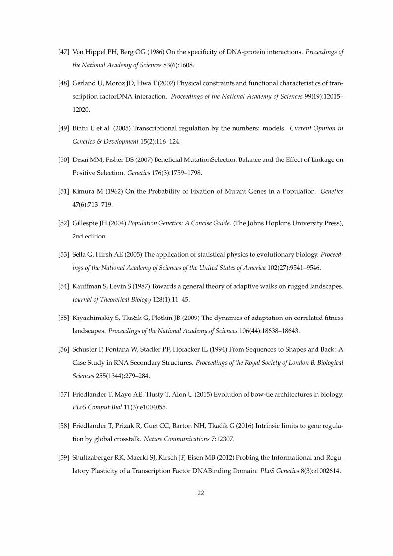
2.4.1 Gillespie Simulation - main model . . . . . . . . . . . . . . . . . . . . . . . . . 362.4.2 Alternative model - fixed signal sensing domain . . . . . . . . . . . . . . . . . 37

3 Steady state 373.1 Distribution of M for neutral and adaptive cases . . . . . . . . . . . . . . . . . . . . . 383.2 Probabilities of major macroscopic outcomes - losing a TF and specializing . . . . . . 383.3 Asymmetric signal occurrence biases final outcomes . . . . . . . . . . . . . . . . . . . 39

4 Evolutionary dynamics 404.1 Evolutionary pathways - first model variant . . . . . . . . . . . . . . . . . . . . . . . . 404.2 Evolutionary pathways - second model variant . . . . . . . . . . . . . . . . . . . . . . 424.3 Time to specialization . . . . . . . . . . . . . . . . . . . . . . . . . . . . . . . . . . . . . 43

5 Role of βX , the relative fitness penalty on crosstalk interactions 445.1 Steady state before duplication . . . . . . . . . . . . . . . . . . . . . . . . . . . . . . . 455.2 Steady state after duplication . . . . . . . . . . . . . . . . . . . . . . . . . . . . . . . . 465.3 Evolutionary dynamics . . . . . . . . . . . . . . . . . . . . . . . . . . . . . . . . . . . . 46

6 Comparison between biophysically-realistic model and simple models 48

7 Multiple genes regulated by each TF post-duplication 507.1 Steady state after duplication . . . . . . . . . . . . . . . . . . . . . . . . . . . . . . . . 507.2 Evolutionary dynamics . . . . . . . . . . . . . . . . . . . . . . . . . . . . . . . . . . . . 52

7.2.1 Frustration of fitness landscape . . . . . . . . . . . . . . . . . . . . . . . . . . . 527.2.2 Evolutionary pathways . . . . . . . . . . . . . . . . . . . . . . . . . . . . . . . 537.2.3 Time to specialization . . . . . . . . . . . . . . . . . . . . . . . . . . . . . . . . 55

24

8 Promiscuity-promoting mutations 568.1 Steady state after duplication . . . . . . . . . . . . . . . . . . . . . . . . . . . . . . . . 598.2 Evolutionary dynamics . . . . . . . . . . . . . . . . . . . . . . . . . . . . . . . . . . . . 60

8.2.1 Time to specialization . . . . . . . . . . . . . . . . . . . . . . . . . . . . . . . . 608.2.2 Typical trajectory . . . . . . . . . . . . . . . . . . . . . . . . . . . . . . . . . . . 61

25

1 Model description and parameters

1.1 Biophysical model

Consider a transcription factor (TF) that activates nG (≥ 2) downstream genes. The starting pointof our evolutionary model is a duplication event of the TF, where the duplicate is fixed in thepopulation. Gene regulation is accomplished by the binding of either TF (original or duplicate) to ashort DNA sequence of length L associated with the gene (abbreviated below as ’BS’: binding site).For simplicity we assume each gene has only a single BS. We describe the DNA-binding preferenceof each TF by its (unique) consensus sequence - the L-base-pair sequence to which it binds withhighest affinity. We begin by assuming that each TF has only a unique consensus sequence andlater on relax this assumption (see Section 8). In our simple model, a gene is activated when its BSis bound by an activating TF. The probability that the binding site of gene j is bound by either TFis calculated using the thermodynamic model of gene regulation [1, 2]:

pjm({kij}, {Ci(m)}) =

∑i Ci(m)e−εkij

1 +∑i Ci(m)e−εkij

, (4)

where {kij}2i=1 is the number of sequence mismatches between the consensus sequence of thei-th TF species and the binding site of the j-th gene and ε is the energy per mismatch. We considermultiple environmentsm that differ in TF concentrations: Ci(m) is the dimensionless concentrationof the i-th TF in environment m. Associated with each TF i is an associated (complex) allele σi thatdetermines the TF concentrationCi(m) in different environments. Eq. (4) assumes that all base pairshave equal and additive contributions to the binding energy, such that the binding probability onlydepends on the number of mismatches kij [3, 2, 4, 5].

Together, the TF consensus sequences, the BS sequences and the complex alleles σi composethe genotype. Genotypes come from the space of all possible genotypes D, and they completelydescribe the regulatory activity of the system in different environments.We study two variants of the model, depending on whether σi is evolvable or not.

Main model

In this model variant, which is described in the main text, transcription factors are equipped withan evolvable signal sensing domain (captured by σi). The original TF senses two distinct externalsignals. Each of the downstream genes is suitable to respond to only one of the two signals. Be-fore duplication the genes are constrained to follow the only TF available which responds to bothsignals. The extra TF formed in the duplication event offers an additional degree of freedom in reg-ulating these genes, if the TFs specialize such that each of them senses only one of the two signalsand regulates only a subset of the genes.

This model variant is applicable to more general pathway architecture than a TF that imple-ments both signal sensing and gene regulation in the same molecule. Often these two functions aresplit between different components of the same pathway; for example, a separate upstream com-ponent senses the signal(s) and consequently activates the TF (e.g. by phosphorylation or anothermodification). Additionally, TF production is also regulated. One can also think of the evolution ofthe regulatory sequences of the gene coding for the TF in terms of our model. Since our model isdefined in very general terms, it can capture such situations as well.

26

Alternative model

In the alternative model, which we explore in the SI, transcription factors have no explicit evolvablesignal sensing domain (no complex allele σi associated with them), but can be expressed at differenttime or location as determined by Ci(m). Before duplication the genes are constrained to followthe only TF available, and are thus expressed at the same time or location. After TF duplication,the two copies immediately specialize to be active at different time slots (different parts of the cellcycle, different phases of developmental process) or space (different tissues), and as such enabledistinct expression patterns for the downstream genes. This variant is a limiting case of the mainmodel, with the main difference being the lack of an evolvable TF signal sensing domain. It alsoacts as an approximation when the signal sensing domain evolves very quickly, resulting in a quickdivergence of TF expression patterns.

Gene birth can occur via different biological mechanisms, some of them allowing for the emer-gence of slightly modified copies of original genes or allowing for different regulation of the samecoding sequence. One such mechanism is called ’retroposition’: creation of duplicate gene copiesin new genomic positions through the reverse transcription of mRNAs from source genes (alsoknown as RNA-based duplication or retroduplication) [6]. These newly formed genes often lackregulatory elements of the parental gene and may also be slightly modified due to transcriptionerrors (that are significantly more common than DNA-duplication errors). It was shown that tran-scription of these so-called ’retrogenes’ is very common and often relies on regulatory elements ofneighboring genes [7].

1.2 Evolutionary model

We define fitness such that the specialized genotypes have higher fitness compared to the initialnon-specialized genotypes. The fitness of a genotype equals the squared deviation of the actual ex-pression pjm from the ideal one p∗jm, summed over all genes j and averaged over all environmentsm:

F = −s∑j

∑m

αmβjm(pjm − p∗jm)2, (5)

where s denotes the selection intensity and αm is the frequency of the m-th environment. Wedefine environments by the presence or absence of the signals, which result in different activeTF concentrations depending on their signal responsiveness. βjm is the penalty for each type ofdeviation from the ideal expression level, allowing for diverse penalties for different genes or atdifferent environments. For example, a gene which is not expressed when needed can incur ahigher penalty than the expression of a gene that is not necessary in a given environment. Tocapture these latter interactions, which we call crosstalk interactions, we exploited βjm to tunethe fitness penalty in Section 5. Expression levels pjm for a genotype are calculated using (4) byobtaining the dimensionless concentrations of the TFs, Ci(m), from their signal sensing alleles σi,and the mismatches, kij , from the TF consensus sequences and the BS sequences.

Note that the fixation probability in (6) below, depends, via the fitness, and in turn via thebinding probabilities, directly on the TFs’ signal sensing alleles σi, and the mismatches kij of theBS sequences with the TF consensus sequences, but not onM , the match between the TF consensussequences. But, as shown in Fig. 2A of the main text, the set of possible kij ’s is constrained by M ,and hence, there is implicit selection onM . Also, importantly, selection does not directly depend on

27

the TFs and BSs, but only via their biophysical interaction to result in appropriate gene regulation,thereby requiring concerted evolution of TFs and BSs.

The evolutionary process proceeds via three types of mutations: The BS of each downstreamgene can acquire point-mutations at rate µ; the consensus sequence of each TF can have point-mutations at rate rTFµ. These two mutation types can modify the (mis)match values M and kij . Athird type of mutation exists in the first model variant: the signal-sensing domain of each TF hastwo components, each of them can alternate between two alleles (sensitive/ non-sensitive to oneof the two signals) at rate rsµ. Owing to the faster time-scales over which gene regulation evolves,we consider only these types of mutations on the BSs and TFs. In particular, we assume no changein the coding regions of the downstream genes themselves, only in their regulation.

1.3 Putting the pieces together

In our main model, we consider nG = 2 downstream genes (models considering larger sets ofdownstream genes are explored in Section 7), each of which is equipped with a binding site oflength L, and two signals, with the presence/absence of the first (second) signal requiring theexpression/silencing of the first (second) gene. In other words, information should be passed fromthe first signal to the first gene and from the second signal to the second gene.

The presence (’1’) or absence (’0’) of these two signals defines the different environments m ∈{00, 01, 10, 11} that are possible, with αm denoting the frequency of environment m. The frequencyof each signal can be obtained as f1 = α10 + α11 and f2 = α01 + α11. Assuming that both signalsappear at equal frequencies, f1 = f2, and that each signal is present (or absent) half of the time,f1 = f2 = 0.5, we obtain the following relations between ρ, the correlation between the signals, andαm:

α00 = α11 =1

4(1 + ρ)

α10 = α01 =1

4(1− ρ).

Thus when the signals are uncorrelated (ρ = 0), we have α00 = α10 = α01 = α11 = 1/4. Whenthe signals are fully correlated (ρ = 1) we obtain α00 = α11 = 0.5 and α10 = α01 = 0 and vice versafor anti-correlation (ρ = −1). We explore asymmetric environments in Section 3.3.

The information transmission between signals and genes is mediated by TFs which containa signal-sensing domain and a DNA-binding domain. TFs, on sensing a signal, become activeand can induce the expression of a gene by binding to its binding site. We define each TF i by itsconsensus sequence, the sequence of lengthL for which the TF has the highest affinity, and its signalsensing allele σi ∈ {00, 01, 10, 11}, which describes its responsiveness to the two signals. If a TF iis responsive to a signal and that signal is present in environment m, then its active dimensionlessconcentration Ci(m) = C0, and Ci(m) = 0 otherwise. For simplicity, we assume only these twoconcentration levels.

The regulatory network is described by its genotype, D, consisting of the consensus sequencesand the signal sensing alleles of the two TFs, and the BS sequences of the (two) genes. As describedin Eq. (4) and Eq. (1) of the main text, the probability pjm that the binding site of gene j is boundin environment m depends on, apart from ε, the mismatches kij (which can be obtained from thegenotype sequences) between the consensus sequence of TF i and the BS of gene j, and the signalsensing alleles σi which determine the active concentrations Ci(m).

In Eq. (5) and Eq. (2) of the main text, we define the fitness of a genotype by considering the

28

deviation of the actual expression levels pjm from the ideal expression levels p∗jm. We define theideal expression level of gene j in environment m, p∗jm, such that p∗jm = 1 if signal j is presentin environment m and p∗jm = 0 if signal j is absent in environment m. We consider the penaltyβjm = 1 if gene j is required in environment m and βjm = βX (βX ∈ [0, 1]) if gene j is not requiredin environment m. βX quantifies the relative penalty on crosstalk interactions between signals andgenes, compared to functional interactions. We explore the role of βX in Section 5. In Table 1 welist the model parameters and their baseline values used in calculations (unless stated otherwise).

With the fitness of genotypes and the mutations between them defined, we consider an evo-lutionary framework to study the evolutionary dynamics of this regulatory system. We assumemutation rates to be low enough such that a beneficial mutation fixes before an additional muta-tion (beneficial or not) arises. The condition under which this assumption is valid was found byDesai and Fisher [8] and reads log(4N∆F )

∆F � 14Nµb∆F . ∆F is the fitness advantage of the beneficial

mutant, N is the population size and µb is the rate of beneficial mutations.Under this condition the population is almost always fixed (monomorphic), and its evolution-

ary trajectory is captured by a series of discrete transitions between different genotypes. Conse-quently, when a new mutation emerges, it competes with only one other genotype. The fixationprobability of a new mutation that alters the genotype from y to x equals

Φy→x =1− exp(−(F (x)− F (y)))

1− exp(−2N(F (x)− F (y))), (6)

where the fitness F is defined by (5) given the frequencies of the various environments αm and thedesired expression pattern of the genes p∗jm at each. (6) applies to a diploid population in whichthe mutant x appears in a single copy over a uniform background of the other genotype y. Fordiploids, the fitness difference ∆F = F (x) − F (y) refers to the fitness difference between the twohomozygotes or to twice the selective advantage of the heterozygote (one copy of the mutant) overthe prevailing homozygote genotype [9]. The overall rate of substitution from genotype y to x isgiven by [4]:

rxy = 2NµxyΦy→x, (7)

where µxy denotes the mutation rate from genotype y to x. We illustrate the evolutionary modelfurther in Section 2.

1.4 Space of reduced-genotypes

The size of the genotype space is huge, |D| = 44L+2 ≈ 1013.25 for L = 5, which makes it hardto analytically track the evolutionary model. Since the fitnesses of genotypes depend only on themismatches kij and the signal sensing alleles σi, and the mutations only alter kij , σi and the TFconsensus sequences’ match M , we consider the space of ”reduced-genotypes”, G = {M,kij , σi},keeping track of only these reduced features of the genotype. The size of the reduced-genotypespace is |G| < 16(L + 1)5 ≈ 105.09 for L = 5, which is tractable. Hence, for analytical calculations,we treat the regulatory network in the reduced-genotype space G, and for simulations, we treat theregulatory network in the full genotypic spaceD. Note that the reduced genotype representation inour model framework is not an approximation, but is an exact solution of the full genotype model,with the tractability gained due to clever bookkeeping of states in the sequence space.

29

1.5 Classification of genotypes into “macrostates”

Since our interest is in the biological function implemented by the network, we further coarse-grainthe space of reduced-genotypes G, and classify these reduced-genotypes into six possible macro-states,M = {No Regulation, Initial, One TF Lost, Specialize Both, Specialize Binding,

Partial}, by distinguishing only between ”strong” and ”weak” interactions. We set a thresholdkT and consider an interaction as weak, kij ∈ W , if kij > kT , and strong, kij ∈ S, if kij ≤ kT . In thebasic version of the model where both TFs have same biophysical properties (in particular same L)kT is the same for all TF-BS interactions (but see the extension in Section 8). The threshold kT foreach TF-BS pair ij is set such that for mismatches k < kT , pjmi

≥ 0.5 and for k > kT , pjmi< 0.5

when only TF i is present and other TF(s) are absent, Ci(mi) = C0.Tje full genotypic space D is a union of sequences belonging to different macrostates z:

D =⋃z∈M

Sz, (8)

where Sz is the set of all genotypes that belong to macrostate z. We apply the following classi-fication rules.

No Regulation

The No Regulation macrostate consists of all genotypes in which there is no regulation of anyform (no information transmitted from the signals to genes). This can happen if both the TFs eitherdo not sense any signal or do not bind well to any binding sites.

x ∈ SNo Regulation if ∀i(

(∀j kij ∈ W) OR (σi = 00))

(9)

Figure 6: Typical genotypes in No Regulation macrostate. In the left genotype, even thoughboth TFs sense some signals, they do not bind well to either of the binding sites, hence preventingany information transmission. In the right genotype one TF binds both the binding sites but doesnot sense any signal and the second TF does not bind any binding site even though it senses bothsignals. This way or the other no information is transmitted between the signals and the genes.

Initial

The Initial macrostate consists of all genotypes in which there is complete regulation with noform of specificity: both the TFs sense both signals and bind both binding sites. This is the typicalinitial state right after duplication.

x ∈ SInitial if ∀i(

(∀j kij ∈ S) AND (σi = 11))

(10)

30

Figure 7: Initial macrostate genotypes. In these genotypes, both TFs sense both signals andbind both binding sites.

One TF Lost

The One TF Lost macrostate consists of all genotypes in which one of the TFs is not involvedin any regulation while the other is involved in some regulatory activity (namely, one TF doesnot sense any signal or does not bind well to any of the binding sites). This is equivalent to thegenotypes before duplication, except that there is a “lost TF”.

x ∈ SOne TF Lost if∣∣∣i :

((∀j kij ∈ W) OR (σi = 00)

)∣∣∣ = 1 (11)

Figure 8: Typical genotypes in One TF Lost macrostate. In the left genotype, only the first TFis involved in regulation as it senses both signals and binds to both binding sites. The secondTF senses the green signal but does not bind any of the binding sites, hence it is not involved inregulation and is “lost”. In the right genotype, again only the first TF is involved in regulation asit senses the red signal and binds both binding sites. The second TF not involved in any regulationbecause it does not sense any signal, although it binds the first binding site.

Specialize Both

The Specialize Both macrostate consists of all genotypes in which there is correct specializa-tion of TFs with respect to both signal sensing and binding sites specificity. In these genotypes, oneTF senses only the first signal and binds only to the first binding site, while the other TF senses onlythe second signal and binds only to the second binding site.

x ∈ SSpecialize Both if

(k11, k22 ∈ S AND k12, k21 ∈ W AND σ1 = 10 AND σ2 = 01)

OR (k12, k21 ∈ S AND k11, k22 ∈ W AND σ1 = 01 AND σ2 = 10) (12)

31

Figure 9: Genotypes in Specialize Both macrostate. Both genotypes have specific paths fromthe signals to the genes. In the left genotype, while the first TF senses the red signal and bindsthe first (correct) binding site, the second TF senses the green signal and binds the second (correct)binding site. Hence, the first TF mediates the red signal to first gene pathway while the second TFmediates the green signal to second gene pathway. In the right genotype, the TFs exchange roles.The first TF mediates the green signal to second gene pathway while the second TF mediates thered signal to first gene pathway.

Specialize Binding

In contrast, the Specialize Binding macrostate consists of all genotypes in which there is spe-cialization of TFs with respect to binding site specificities, but not with respect to the signal sensingdomains.

x ∈ SSpecialize Binding if (∀i σi 6= 00) AND(((k11, k22 ∈ S AND k12, k21 ∈ W) AND ¬(σ1 = 10 AND σ2 = 01)

)OR

((k12, k21 ∈ S AND k11,k22 ∈ W) AND ¬(σ1 = 01 AND σ2 = 10)

))(13)

Figure 10: Typical genotypes in Specialize Binding macrostate. In both genotypes, the firstTF binds the first binding site and the second TF binds the second binding site, but they have notcorrectly specialized in their signal sensing domains. In the left genotype, while the second TF hasspecialized correctly to sense only the green signal, the first TF still senses both the signals. Hence,while the red signal pathway is established properly, the green signal pathway is not - both genesare activated in the presence of green signal. In the right genotype, the TFs have specialized insignal sensitivities, but opposite to the desired response pattern.

Partial

The Partialmacrostate consists of all genotypes which do not belong in any of the other macrostatesmentioned above. It contains a mixture of different regulatory architectures: both TFs regulate onlyone gene with the other gene unregulated, one TF regulates both genes while the other TF regu-

32

lates only one gene or both TFs bind both binding sites but at least one TF has specialized in signalsensing.

Figure 11: Typical genotypes in Partial macrostate. In the left genotype, both TFs regulate onlythe first gene while the second gene is unregulated. In the middle genotype, the first TF regulatesboth genes while the second TF regulates only the second gene. In the right genotype, both TFsregulate both genes but, unlike the Initial macrostate, here the first TF does not mediate anyinformation from the green signal.

Role of L in macrostate classification

Keeping ε and C0 constant while changing L keeps the threshold mismatch kT constant. Hence,the number of mismatches |S| in the strong binding class remains the same while the number ofmismatches |W| in the weak binding class increases. Hence, as L increases, the number of geno-types in all macrostates except Initial increase. The volume of macrostates with a larger num-ber of weak mismatches increase more than the volume of macrostates with a smaller number ofweak mismatches. For instance, No Regulation increases more than Specialize Binding.As One TF Lost and Specialize Binding have the same number of weak mismatches, theratio of the number of genotypes in them stays the same for different L.

2 Methods

2.1 Markov chain formulation

As explained in Section 1, we assume that the time between the emergence and fixation of a ben-eficial mutation is much shorter than the time until the emergence of the next beneficial mutation.Hence, by neglecting the times between emergence and fixation (or loss) of mutations the popula-tion can be captured at any time by a single genotype. This so-called “fixed state assumption” letsus describe the state of the population as a probability distribution over the possible genotypes,P (D, t) or as a probability distribution over the possible reduced-genotypes, P (G, t). This can beobtained via a continuous-time discrete-space Markov chain defined over the genotype space D orthe reduced-genotype space G = {M,kij , σi}. The transition rate between y and x, where eitherx, y ∈ D are genotypes, or x, y ∈ G are reduced-genotypes, is the rate of substitution [4]:

rxy = 2NµxyΦy→x (14)

where N is the population size, µxy is the mutation rate from (reduced-) genotype y to (reduced-)genotype x, and Φy→x is the probability of fixation of a single copy of x in a population of y ((6)). Asthe probability of fixation Φy→x depends on x and y only via their fitness values F (x) and F (y), andµxy can be obtained analytically for reduced-genotypes, it is sufficient to consider the Markov chain

33

on the space of reduced-genotypes G = {M,kij , σi} rather than on the whole genotype space D.Each reduced-genotype x = (M,kij , σi) can be realized by multiple genotypes (DNA sequences),whose number is given byNseq(kij |M) ((17) and (18)) below. Now, the evolution of the probabilitydistribution P (G, t) is captured by

∂P (G, t)∂t

= RP (G, t), (15)

where R is the transition rate matrix of the underlying Markov chain where each entry rxy denotesthe rate of transition from y to x.

2.2 Steady state after duplication

The probability distribution at steady state, PSS(G) = P (G, t → ∞), is the non-trivial solution ofRPSS(G) = 0. It is also possible to obtain PSS(G) by invoking the set of detailed balance conditions,rxyPSS(y) = ryxPSS(x), ∀x, y. This results in an elegant expression

PSS(G) = P0(G) exp(2NF (G)), (16)

where P0 is the neutral distribution of reduced-genotypes and N is the population size.To calculate the neutral distribution P0 of the reduced-genotypes, we begin by enumerating the

number of possible BS sequences j that have mismatch values (k1j ,k2j) with respect to two TFs thatmatch each other at M out of L consensus positions. This number equals:

Nseq(k1, k2|M) =

jmax0∑

j0=jmin0

(M

j0

)3M−j0

(L−M

L− j0 − k1

)(j0 + k1 −ML− j0 − k2

)2k1+k2+2j0−L−M

jmin0 = max(max(0,M −min(k1, k2)), dL+M − k1 − k2

2e)

jmax0 = min(M,L−max(k1, k2))

(17)

where for brevity we write k1, k2 instead of k1j , k2j , and dxe is the ceiling function, which maps xonto the nearest integer larger than or equal to x. Now, the neutral distribution is (up to propor-tionality constant)

P0(x) ∼ Nseq(k11, k21|M)Nseq(k12, k22|M)

(L

M

)3L−M . (18)

From Eq. (16) we obtain the steady state distribution over the macrostate space. For everymacrostate z ∈ M the probability to be in this macrostate at steady state equals the sum of proba-bilities of being in all reduced-genotypes x that are assigned to that macrostate

QSS(z) =∑x∈Sz

PSS(x). (19)

34

Dominant macrostate

We denote the the most probable macrostate at steady state by

z∗SS := arg maxz∈M

QSS(z). (20)

2.3 Evolutionary dynamics

We obtain the evolutionary dynamics of P (G, t) in units of generation time tg by numerically inte-grating the Markov chain in time-steps corresponding to one generation:

P (G, t+ tg) = (I + Rtg)P (G, t). (21)

We define A = I + Rtg as the transition probability matrix in this time-unit. From P (G, t), weobtain the macrostate dynamics ((15)) Q(M, t). For every z ∈M,

Q(z, t) =∑x∈Sz

P (x, t). (22)

Dominant macrostate

To follow the macrostate dynamics in a more compact way, we refer to the most probable macrostateat each time-point t

z∗(t) := arg maxz∈M

Q(z, t) (23)

as the dominant macrostate at that time.

Time to reach a particular macrostate

We compute the mean first hitting time, TS←x, to any subset of reduced-genotypes, S, from anyother reduced-genotype x, by using the following recursive equation.

TS←x = tg +∑y

ayxTS←y, (24)

where ayx are elements of the transition probability matrix A. We consider subsets Sz of geno-types that belong to a particular macrostate z, and compute the mean first hitting times, TSz←x,to this macrostate. In particular, we compute the mean first hitting times to Specialize Both,which we refer to as the “time to specialization”, τ(x).

Dwell times

For every macrostate z, we also compute the dwell time, tdwell(z), which is the mean time to “es-cape” from that macrostate into any other macrostate z′. For every genotype x in Sz , the mean timeto escape from Sz is by definition TS′

z←x, the mean time taken to hit S′z = G−Sz , the complementaryset of Sz . We define the dwell time in macrostate z as

tdwell(z) := 〈TS′z←x〉x∈Sz

(25)

35

2.4 Stochastic simulations

In addition to analytical solutions of the Markov chain formulation we also used stochastic simula-tions of TF and BS evolution to validate our analytical solution and also to test additional cases thatwere not analytically solvable, such as the case where each TF post-duplication regulates multiplegenes.

2.4.1 Gillespie Simulation - main model

We use the Gillespie Stochastic Simulation Algorithm [10] to track the evolutionary trajectories ofthe system. Since we employ the fixed-state assumption, the time to fixation of each mutation issmall compared to the waiting time between mutations and we neglect it in the calculations. Ateach simulation run we obtain a temporal series, s0, s1, s2, . . . , of genotypes (DNA sequences of TFconsensus sequence and binding sites, along with signal sensing alleles), and a corresponding se-quence of times, t0 = 0, t1, t2, . . . , at which substitutions between consecutive genotypes occurred.Here, s0 is the initial DNA sequence with which we start the simulation. We construct s0 by sam-pling a genotype from the steady state before duplication (with only 1 TF). For every i, from ti

to ti+1, the DNA sequence of the system is si, from which there is a substitution event to si+1 atti+1. We obtain si+1 by appropriately sampling substitutions available from si, which can occurvia TF consensus sequence mutations, or TF sensing domain mutations, or BS sequence mutations.We also draw ti+1− ti (the waiting time) from the appropriate exponential distribution in the Gille-spie framework. For each DNA sequence si, one can obtain the reduced-representation (M,kij , σi).From this, we obtain, for each simulation run r, the time trajectories of reduced-genotypes, xr(t),starting from xr(t = 0) = xr0. By running multiple times and computing the fractions of runswith each reduced-genotype x at each t, we obtain the dynamical trajectory of the probability dis-tribution of reduced-genotypes, P sim(G, t), and the steady state distribution, P simSS (G). Groupingthe reduced-genotypes into macrostates, we also obtain the dynamical trajectory of the probabilitydistribution of macrostates, Qsim(M, t) and steady state distribution of macrostates, QsimSS (M).

The simulations enable us to compute non-trivial path-dependent quantities relating to an ensem-ble of trajectories {xr(t)}, as well as to provide full distributions of quantities of interest. One suchexample is the mean hitting time to some macrostate z, conditioned on not hitting some other par-ticular macrostate on the way. While it is possible in principle to compute such a path-dependentquantity exactly, in practice this requires too much numerical effort and Gillespie simulation be-comes be the method of choice.

Time to specialization, dependent on pathway

As explained in the main text, for a single trajectory (population), there are two main paths fromInitial to Specialize Both, each with a different dominant “transient state”. One pathway isfast and predominantly goes via genotypes in Partial macrostate, and the other is slow and pre-dominantly via genotypes in One TF Lost macrostate. In each simulation run r, we calculate thetime to specialization, and also record the dominant transient state. By running many simulations,we have a set of times to specialization that go via the fast pathway of Partial {τfast}, and thosevia the slow pathway of One TF Lost {τslow}. Using these, we obtain the empirical distributionsof τslow and τfast, their means (τslow = 〈τslow〉 and τfast = 〈τfast〉); we also record the fraction ofpathways proceeding via the slow and fast alternatives.

36

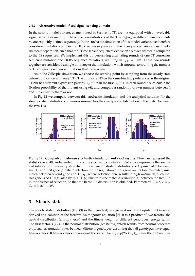
2.4.2 Alternative model - fixed signal sensing domain

In the second model variant, as mentioned in Section 1, TFs are not equipped with an evolvablesignal sensing domain σi. The active concentrations of the TFs, Ci(m), in different environmentsm, are explicitly defined separately. In the stochastic simulation of this model variant, we thereforeconsidered mutations only in the TF consensus sequence and the BS sequences. We also assumed atimescale separation, such that the TF consensus sequences evolve on a slower timescale comparedto the BS sequences. We implement this by performing alternating rounds of one TF consensussequence mutation and 50 BS sequence mutations, resulting in rTF = 0.02. These two roundstogether are considered a single time step of the simulation, which amounts to counting the numberof TF consensus sequence mutations that have arisen.

As in the Gillespie simulation, we choose the starting point by sampling from the steady statebefore duplication with only 1 TF. The duplicate TF has the same binding preferences as the originalTF but has different expression pattern C2(m) than the first C1(m). In each round, we calculate thefixation probability of the mutant using (6), and compare a randomly drawn number between 0

and 1 to either fix them or not.In Fig 12 we compare between this stochastic simulation and the analytical solution for the

steady state distributions of various mismatches the steady state distribution of the match betweenthe two TFs.

k11

0 1 2 3 4 5 6 7 8

ste

ad

y s

tate

dis

t.

0

0.2

0.4

0.6

0.8

selection to bind 1st TF; low mismatch.

simulationanalytical

(a)

k21

0 1 2 3 4 5 6 7 8

ste

ad

y s

tate

dis

t.

0

0.2

0.4

selection not to bind 2nd TF; high mismatch.

simulationanalytical

(b)

M

0 1 2 3 4 5 6 7 8

ste

ad

y s

tate

dis

t.

0

0.1

0.2

0.3

0.4

No selection; neutral distribution.

simulationanalytical

(c)

Figure 12: Comparison between stochastic simulation and exact results. Blue bars represent thestatistics over 400 independent runs of the stochastic simulation. Red curve represents the analyt-ical solution for the steady state distribution. We illustrate distributions of k11 mismatch betweenfirst TF and first gene (a) where selection for the regulation of this gene incurs low mismatch; mis-match between second gene and TF k21 where selection here results in high mismatch, such thatthis gene is NOT regulated by this TF. (c) illustrates the match distribution M between the two TFsin the absence of selection, so that the Bernoulli distribution is obtained. Parameters: L = 8, ε = 3,C0 = 3.269× 105.

3 Steady state

The steady state distribution (Eq. (3) in the main text) is a general result in Population Genetics,derived as a solution of the forward Kolmogorov Equation [9]. It is a product of two factors: theneutral distribution (entropy term) and the fitness weight of different genotypes (energy term).The first factor, P0(G), is the neutral distribution (see below) which results from neutral processesonly, such as mutation rates between different genotypes, assuming that all genotypes have equalfitness values. If fitness values are unequal, the second factor, exp(2NF (G)), biases the probabilities

37

of attaining different genotypes accordingly. For a more comprehensive discussion and relation tostatistical physics see Ref. [11].

3.1 Distribution of M for neutral and adaptive cases

In Fig. 3 of the main text we compared the steady state distribution of M (match between thetwo TFs) in the neutral case to the distribution of M if selection to diverge applies. Parametersused were L = 5, Ns = 25, resulting in hardly distinguishable distributions. Here we repeat thiscalculation with different parameter values that emphasize the difference between these cases: astronger selection Ns = 500 and a longer binding site L = 8. A stronger selection depletes thehighest match values compared to the neutral (Bernoulli) distribution. Even under these moreextreme values the difference between the two distributions is modest, as shown in Fig 13. As aconsequence, using distributions of M as estimated from genomic data may provide insufficientstatistical power to detect selection pressure on TFs to diverge.

k11

0 2 4 6 8

ste

ad

y s

tate

dis

t.

0

0.2

0.4

0.6

0.8

Ns = 500

Ns = 0

(a)

k21

0 2 4 6 8

ste

ad

y s

tate

dis

t.

0

0.2

0.4

Ns = 500

Ns = 0

(b)

M

0 2 4 6 8

ste

ad

y s

tate

dis

t.

0

0.1

0.2

0.3

0.4Ns = 500

Ns = 0

(c)

Figure 13: The steady state distributions of match, M , between TF consensus sequences whenthere is selection on the TFs to diverge is very similar to the neutral distribution. We presentanalytically calculated steady state distribution of k11 (a), k21 (b) andM (c) forNs = 0 (no selection,blue) and Ns = 500 (strong selection, red). The neutral distributions are always the Bernoulli dis-tributions which here are peaked at k = 6 and M = 2. Selection to diverge biases the distributionto have a lower match than expected under neutrality. The difference between neutrality and se-lection becomes obvious only when looking at the distributions of k, the mismatches between BSsand TFs. Under neutrality the probability for match is low and the distribution is peaked aroundhigh mismatch values. When there is selection on the TF to remain functional it must preserve alow mismatch with at least one of the genes. Parameters: L = 8, ε = 3, C0 = 3.269× 105.

3.2 Probabilities of major macroscopic outcomes - losing a TF and specializing

In the main text we illustrate only the most probable macrostate for each parameter combination.Other macrostates are still possible, albeit with lower probability. Here we illustrate the proba-bility to obtain either ’One TF Lost’ or ’Specialize Both’ macrostate at each parameter combina-tion, as described in Section 2. As shown in Fig. 14, the steady state probability of specializationQSS(Specialize Both) is high at large Ns and intermediate ρ, and it decreases as selectionstrength decreases or signal correlation increases. The probability of having QSS(One TF Lost)

at steady state is significant only when selection is not too weak and signals are highly correlated.Although for these parameter values it is the dominant macrostate its probability is only ∼ 0.5,such that other macrostates are not negligible. In contrast, for parameter values where ’Specialize

38

Both’ dominates its probability is close to 1.

z = Specialize Both

0 10 20 30 40

Ns

-1

-0.75

-0.5

-0.25

0.25

0.5

0.75

1z = One TF Lost

0 10 20 30 40 50

Ns

0

0.1

0.2

0.3

0.4

0.5

0.6

0.7

0.8

0.9

1

ρ 0

25 25

QSS

(z)

Figure 14: Steady state probabilities of ’Specialize Both’ (left) and ’One TF Lost’ (right)macrostates for different values of selection intensity Ns and correlation between the signalsρ. The probability of either macrostate QSS(z) is illustrated using a color code (blue = 0, yellow =1). Intersection of the red dashed lines denotes the baseline parameters values.

3.3 Asymmetric signal occurrence biases final outcomes

In the main text, we assume symmetry between the occurrences of the two signals, namely their fre-quencies f1 = f2 = 0.5, where f1 = α10+α11 is the frequency of the first signal, and f2 = α01+α11 isthe frequency of the second. Here we explore the effect of asymmetry in signal occurrence (f1 6= f2)on the final evolutionary outcomes and in particular on the probability to fully specialize. In Fig 15we plot the most probable macrostate as a function of the signal frequencies f1, f2 for different val-ues of selection intensitiesNs. When both signals are rare, f1, f2 � 1, No Regulation macrostatedominates, as selection on both pathways is weak. When one of the signals is frequent whilethe other is rare, f1 � f2, only the frequently used pathway is maintained, and the dominantmacrostate is Partial. Only when both signals are frequent and selection is not too weak, special-ization occurs. Hence, a signal-gene pathway is maintained only if it is required often enough, andthe threshold for this (boundary between Partial and Specialize Both) depends on selectionstrength Ns. As selection strength Ns increases, this threshold moves to lower f1 and f2. As thefrequencies of both signals increase, the dominant macrostate Specialize Both is replaced bySpecialize Binding, where sensing one signal is a good proxy for the other signal as well, andlater by One TF Lost when one TF is sufficient to transduce both signals.

39

0 0.25 0.75 1

f1

0

0.25

0.75

1

0 0.25 0.75 1 0 0.25 0.75 1

f1

f1

f2

0.5

0.5 0.5 0.5

Ns = 10

Partial

Specialize Both

Specialize Binding

Ns = 100Ns = 25

No R

egulatio

n

One TF Lost

only signal 2

to gene 2

pathway

only signal 1

to gene 1

pathway

on

ly s

ign

al 2

to

ge

ne

2 p

ath

wa

y

only signal 1 to gene 1 pathway

Figure 15: Under medium to strong selection specialization occurs under a broad range of signalfrequencies. Under weak selection specialization occurs only if signal frequencies are suffi-ciently high. Phase plots of the most probable macrostate at steady state as a function of signalfrequencies f1 and f2, at three different selection strengths Ns = 10, 25, 100. The intersection be-tween the red dashed lines, f1 = f2 = 0.5, denotes the baseline parameters used anywhere else inthis work.

4 Evolutionary dynamics

Evolutionary trajectories between the post-duplication unspecialized configuration (’Initial’) to fullspecialization (’Specialize Both’ macrostate) are multi-step processes that require several mutationsand transiently pass through various macrostates. Here we describe the various trajectories for thisfunctional transition.

4.1 Evolutionary pathways - first model variant

In Fig. 16 we detail the different pathways to specialization. The pathways proceeding via One TF Lost

are slow compared to the pathways proceeding via Partial which are faster. The mutation initi-ating the process in all pathways is neutral and hence the ratio between rS (signal sensing domainmutations rate) and rTF (TF mutation rate) determines which pathway is more likely to occur - seeFig. 17.

Along the slow One TF Lost pathway, typically, first a TF consensus sequence mutation oc-curs that weakens the binding of one TF to both binding sites. Once binding is lost, further mu-tations cause the TF consensus sequence to neutrally drift away. Meanwhile, the lost TF gains asensing mutation such that it senses only one of the two signals. Next, a BS mutation in one ofthe binding sites flips its TF preference such that the system moves into Specialize Binding

macrostate. This is a beneficial mutation as one of the signal-BS pathways becomes specific. Thisinvolves evolving a TF-BS link essentially from scratch; the lost TF consensus sequence is a ran-dom number of mismatches away from the binding site sequence, and the beneficial BS mutationcan occur only when the TF consensus sequence, by chance, becomes close enough to the BS se-quence. From Specialize Binding, another beneficial sensing mutation leads the system tofull specialization (BS and signal).

40

There are multiple routes in the Partial pathway. In one of the routes, first a neutral TFconsensus sequence mutation occurs such that the TF loses binding to only one of the two bindingsites resulting in Partial macrostate. This is different from the first mutation in One TF Lost

pathway where the TF loses binding to both binding sites. From here, a sensing domain mutationspecializes one of the signal-BS pathways, making this mutation beneficial. Further, a neutral BSmutation brings the system to Specialize Binding, from where a beneficial sensing domainmutation leads the system to specialization.

In the second and third routes via the Partial macrostate, first a neutral sensing domain mu-tation occurs. Next, either a beneficial TF consensus sequence mutation can bring the system ontothe previous route or if the sensing domain mutation rate is high, another neutral sensing domainmight occur first. From here, a beneficial TF consensus sequence mutation and a beneficial BSmutation again lead to full specialization.

TF

TF

S

TF

BS

BS

S

S

S

Initial

One TF Lost One TF Lost Specialize Binding

Specialize Binding

Specialize Both

Partial Partial

Partial

S

Partial

S

PartialTF

BS

rS >> Lr

TF

FAST

SLOW

rS << Lr

TF

rS ~ Lr

TF

rS ~ Lr

TF

TF TF

large neutral

landscape

re-evolve

from scratch

beneficial

deleterious

neutral

state with one

beneficial

mutation

state with two

beneficial

mutations

*

**

Figure 16: Pathways to specialization differ in the order and nature of mutations. Here we detailthe various mutations occurring along the different pathways to specialization. For each mutation,we show the type of mutation (in text on the arrows): TF consensus sequence mutation (TF), bind-ing site sequence mutation (BS), TF signal sensing domain mutation (S) and whether it is beneficial,(nearly) neutral or deleterious (style of the arrows). We also illustrate the macrostates along eachpathway using the same color code in the background as in the main text. The number of benefi-cial mutations in each macrostate relative to the Initial macrostate is depicted by box style (seelegend). Text in red indicates the conditions on mutation rates that favor the different pathways.Note that from the One TF Lost state marked with a star, the “lost” TF can actually take up newfunctions (by sensing and binding to signals and binding sites other than those considered in ourmodel), leading to “neo-functionalization”. Also, the Partial state marked with two stars actsas the initial condition in the alternative model variant, with the TFs already specialize in signalsensing immediately post-duplication.

41

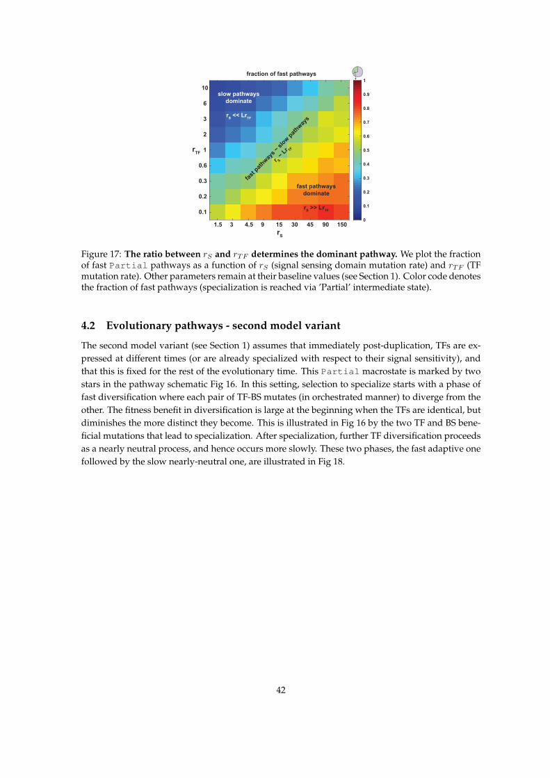
1.5 3 4.5 9 15 30 45 90 150

rS

0.1

0.2

0.3

0.6

1

2

3

6

10

rTF

0

0.1

0.2

0.3

0.4

0.5

0.6

0.7

0.8

0.9

1

fraction of fast pathways

fast pathways

dominate

rS >> Lr

TF

slow pathways

dominate

rS << Lr

TF

fast

pat

hway

s ~

slow

pat

hway

s

r S ~

Lr TF

Figure 17: The ratio between rS and rTF determines the dominant pathway. We plot the fractionof fast Partial pathways as a function of rS (signal sensing domain mutation rate) and rTF (TFmutation rate). Other parameters remain at their baseline values (see Section 1). Color code denotesthe fraction of fast pathways (specialization is reached via ’Partial’ intermediate state).

4.2 Evolutionary pathways - second model variant

The second model variant (see Section 1) assumes that immediately post-duplication, TFs are ex-pressed at different times (or are already specialized with respect to their signal sensitivity), andthat this is fixed for the rest of the evolutionary time. This Partial macrostate is marked by twostars in the pathway schematic Fig 16. In this setting, selection to specialize starts with a phase offast diversification where each pair of TF-BS mutates (in orchestrated manner) to diverge from theother. The fitness benefit in diversification is large at the beginning when the TFs are identical, butdiminishes the more distinct they become. This is illustrated in Fig 16 by the two TF and BS bene-ficial mutations that lead to specialization. After specialization, further TF diversification proceedsas a nearly neutral process, and hence occurs more slowly. These two phases, the fast adaptive onefollowed by the slow nearly-neutral one, are illustrated in Fig 18.

42

time

(# of TFs mutations that have arose)

100 101 102 103 104

ma

tch

be

twe

en

TF

s M

(t)

0

5

F(t)

-1

-0.5

0

(a)

100 101 102 103 104

1

2

3

4

5

6

7

8

<F(t)>

-1.4

-1.2

-1

-0.8

-0.6

-0.4

-0.2

0

av

era

ge

ma

tch

be

twe

en

TF

s <

M(t

)>

time

(# of TFs mutations that have arose)

(b)

Figure 18: In the second model variant (TFs specialized in the signal sensitivities or expressiontimes immediately post-duplication) a significant proportion of evolutionary time is spent inneutral evolution phase. Selection only works in the beginning of the evolutionary trajectory toexert diversification, but a significant part of TF diversification occurs almost neutrally with only amodest fitness benefit involved. We illustrate dynamical trajectories of the match between TFs, M ,and the fitness, F , obtained in stochastic simulations. (a) shows a single trajectory and (b) showsan average over 400 independent repeats of the simulation. Each time unit is a simulation iterationin which a mutation in one of TFs occurs, but does not necessarily fix (see Section 2.4.2).

4.3 Time to specialization

In Fig. 19, we plot the average time to specialization via slow and fast pathways for various valuesof L, rTF and rS . The ratios of these times are plotted in Fig. 4E of the main text. Increasing eithermutation rate by changing rTF or rS speeds up specialization via both pathways because mutationsoccur faster. Increasing L slows down the slow One TF Lost pathway because of an increase insize of the neutral landscape; strikingly, increasing L does not lengthen the fast pathway throughPartial states.

43

101

100

10-1

3 4 5 6 7 3 4 5 6 7

0.1 0.3 1 3 10

rTF

, rS

0.1 0.3 1 3 10

rTF

, rS

L L

τslow

τfast

tim

e t

o s

pe

cia

liza

tio

n

(in

1/μ

ge

ne

rati

on

s)

(via One TF Lost) (via Partial)

rTF

rS

L

Figure 19: Time to specialization via different pathways for different parameters. We plot themean times to specialization, τslow and τfast, via the slow (left panel) and the fast (right panel)pathways, while varying L (grey curve, top axis), rTF (red, bottom axis) and rS (blue, bottom axis)separately. Other parameters remain at their baseline values. We find opposite dependence of thetime to specialize on the binding site length L in the distinct pathways. While for pathways goingvia ’One TF Lost’ (left panel) time increases with L due to increase in the sequence space, it mildlydecreases with L for pathways going via ’Partial’. For all pathways time decreases if mutation ratesincrease.

5 Role of βX , the relative fitness penalty on crosstalk interactions

Transcription factors often bind weak secondary binding sites besides their primary target(s). Thiscan lead to spurious activity of genes called crosstalk, i.e., deleterious activation of genes that doesnot happen via their primary regulatory pathway. For example, in our model a gene can be acti-vated even if the signal to which it should respond is absent only because of (weak) binding of atranscription factor responding to another signal to its binding site. Previously, we studied the ef-fect of crosstalk interference on gene regulation, and showed how it can place global constraints onthe gene regulatory system [12]. Here, we explore the potential role of such crosstalk interactionsin shaping the evolutionary trajectories of TF specialization.

The fitness of each reduced-genotype x ∈ G depends on the difference between the actual ex-pression pattern the genotype generates and the ideal expression pattern as defined in (5).

F (x) = −s∑j

∑m

αmβjm(pjm − p∗jm)2. (26)

Here, βjm weigh the penalties on different deviations from the desired expression level p∗jm. In acertain environment m some genes should be active, p∗jm = 1, while others should remain inactive,p∗jm = 0. In our model, we allow for different penalties in either case. We penalize deviations fromdesired activity p∗jm = 1 by setting βjm = 1. We consider deviations from desired inactivity p∗jm = 0

44

as less crucial and penalize them to a lesser extent βjm = βX , βX ∈ [0, 1]. At the two extremes, ifβX = 0, no penalty on these crosstalk terms applies, while if βX = 1, penalties on all deviations areequally important. In the main text, we used an intermediate value of βX = 0.5. In this section weexplore the role of βX on the steady state distribution prior to and after TF duplication and on theevolutionary dynamics of specialization.

5.1 Steady state before duplication

A steady state distribution is attained before duplication, when only a single TF regulates all genes.In Fig 20 we illustrate the most probable macrostate prior to duplication for different values ofcross-interaction penalties βX . The macrostates possible before duplication are Initial (bothgenes regulated), No Regulation (none regulated) and some (but not all) variants of Partial- see Fig 20A for illustration. For βX ' 1, the fitness penalty on mistakenly activating a geneis comparable to the fitness penalty on not fully inducing genes when needed, resulting in net-work configurations in which only one of the two genes is regulated (corresponding to Partial

macrostate immediately after duplication for most ρ < 0). This is because, while configurationswith only one gene regulated have one functional interaction and no crosstalk interactions, config-urations with both genes regulated have two functional interactions and two crosstalk interactions.As βX decreases, the selection against crosstalk interactions becomes weaker, resulting in config-urations in which both genes are regulated (Initial macrostate immediately after duplication)even when ρ < 0.

Initial (both genes regulated)

Partial(both genes regulated)

Partial(one gene regulated)

No Regulation(no genes regulated)

-1

-0.5

0

0.5

1

-1

-0.5

0

0.5

1

0 10 20 30 40 50 0 10 20 30 40 50 0 10 20 30 40 50

ρ

Ns NsNs

βX = 1 β

X = 0.75

βX = 0.1 β

X = 0

βX = 0.5

βX = 0.25ρ

0 0.25 0.5 0.75 1-1

-0.8

-0.6

-0.4

-0.2

0

0.2

0.4

0.6

0.8

1

βX

ρ +

Ns = 25

B C

A

Figure 20: Dominant macrostate at steady state before duplication depends on βX (crosstalkinteraction penalty). (A) Illustration of the different macrostates when only a single TF exists.Macrostates before duplication are defined in terms of the macrostate they would result in, if a du-plication occurred on those genotypes. (B) Most probable macrostate at steady state before dupli-cation, as a function of selection strength, Ns, and the correlation between the two external signals,ρ, for different values of βX , the relative weight of fitness penalties corresponding to crosstalk in-teractions. (C) The most probable macrostate at steady state before duplication, as a function of βXand ρ at Ns = 25.

45

5.2 Steady state after duplication

We proceed to observe the effect of varying βX on the steady state after duplication, analogous toFig. 3C of the main text where we assumed βX = 0.5. In Fig. 21, we show the phase plot of the mostprobable outcome of duplication at steady state for different values of βX . The qualitative featuresof this phase plot are invariant to changes in βX , as long as βX > 0. For ρ not too close to 1, weobtain transitions from No Regulation to Partial and to Specialize Both as Ns increases.For large enough Ns, as ρ increases, there is a shift from Specialize Both to One TF Lost,via Specialize Binding, the width of which increases as βX decreases. This is because thereis reduced selection pressure on avoiding crosstalk interactions as βX decreases. For small βX , asρ increases, it is sufficient that one of the TFs senses both signals while the TFs are still specializedin binding. As ρ increases even further, it is sufficient to have one TF mediating both pathways,marking the shift to the One TF Lost macrostate. These transitions occur very prominently forvery small βX ≈ 0, where One TF Lost is the most probable outcome for all ρ values. Manymodels of duplication do not consider crosstalk interactions in their fitness function, and hencedeal with the case of βX = 0, making it important for comparison to our results.

-1

-0.5

0

0.5

1

-1

-0.5

0

0.5

1

0 10 20 30 40 50 0 10 20 30 40 50 0 10 20 30 40 50

ρ

Ns NsNs

βX = 1 β

X = 0.75

βX = 0.1 β

X = 0

Specialize Both One TF Lost PartialInitialSpecialize Binding No Regulation

βX = 0.25

βX = 0.5

ρ

0 0.25 0.5 0.75 1-1

-0.8

-0.6

-0.4

-0.2

0

0.2

0.4

0.6

0.8

1

βX

Ns = 25

+ρ

A B

Figure 21: Dependence of steady state after duplication on βX , the fitness penalty on cross-interactions. (A) The most probable macrostate at steady state after duplication, as a function ofselection strength, Ns, and the correlation between the two external signals, ρ, is plotted for sixdifferent values of βX . (B) The most probable macrostate at steady state after duplication, as afunction of βX and ρ at Ns = 25. An increase in βX has a a similar effect to an increase in selectionintensity on all interactions by varying Ns.

5.3 Evolutionary dynamics

To understand how βX affects the evolutionary dynamics of specialization, we first obtained thedynamics of the most probable macrostate as a function of ρ and βX for fixed selection intensityNs = 25 (baseline parameters). In Fig. 22, we plot a few snapshots of the phase diagram of the mostprobable macrostate at different time-points after duplication, starting from t = 0 (immediatelyafter duplication), to t = ∞ (steady state after duplication). Specialization is faster for smaller ρbecause the fitness benefit of eliminating crosstalk interactions is larger. Likewise, specialization isfaster for larger βX as the selection strength against crosstalk interactions is higher. A huge regionof the (βX , ρ) plane corresponding to small βX or large ρ, most of which starts at Initial andspecializes via the slow pathway of One TF Lost.

46

Specialize Both One TF Lost PartialInitialSpecialize Binding No Regulation

0 0.25 0.5 0.75 1-1

-0.5

0

0.5

1

βX

+ρ +

0 0.25 0.5 0.75 1

βX

+

0 0.25 0.5 0.75 1

βX

+

0 0.25 0.5 0.75 1

βX

+

0 0.25 0.5 0.75 1

βX

+

0 0.25 0.5 0.75 1

βX

+

0 0.25 0.5 0.75 1

βX

time (1/μ generations)

0 0.05 0.1 0.5 1 10 ∞immediately

after duplicationsteady state

after duplication

Figure 22: Snapshots of the most probable macrostate at different time-points post-duplication.The most probable macrostate as a function of signal correlation, ρ, and βX , the relative weight offitness penalties corresponding to crosstalk errors, for Ns = 25. The left-most phase plot corre-sponds to the time-point immediately after duplication, and the right-most phase plot correspondsto the steady state after duplication. For other parameters, the baseline values have been used.βX = 1 corresponds to equal-magnitude selection strengths on functional as well as crosstalk in-teractions; βX = 0 corresponds to no selection against crosstalk interactions. In the main text, wechoose βX = 0.5 as the baseline parameter value.

0 0.1 0.25 0.5 0.75 1

0.3

0.4

0.5

0.75

1

2

3

4

5

7.5

10

15

1

2

3

4

5

7.5

10

βX

t slow/tfast

tslow

89% 83% 78% 79% 80% 72%

tfast

Figure 23: How do the slow and fast pathways to specialization depend on βX? For large βX ,the time to specialization shortens for all pathways and the fraction of trajectories to specializationtaken via fast pathways (through Partial macrostate) increases. Pie charts illustrate the fractionof slow (lavender) and fast (green) trajectories for different values of βX . The black line (right y-axis) shows the ratio between average specialization times, which does not significantly changewith βX . For other parameters, the baseline values were used. βX = 1 corresponds to equal-magnitude selection strengths on functional as well as crosstalk interactions; βX = 0 correspondsto no selection against crosstalk interactions. In the main text, we choose βX = 0.5 as the baselineparameter value.

Next we sought to understand which pathways are taken towards specialization for differentβX by running many repeats of simulations at each βX . For each βX , we found the most probable

47

genotype at steady state before duplication and ran many repeats of the simulation starting fromthat genotype. In Fig. 23, we explore the dependence on βX of fraction of the two pathways tospecialization (slow via One TF Lost and fast via Partial), and also the corresponding timesto specialization. First of all, specialization becomes quicker as βX increases from 0 to 1. This isbecause stronger selection against the crosstalk interactions eliminates them faster. Secondly, therelative speed of the fast pathway (compared to the slow pathway) depends only very weakly onβX . Thirdly, about 80% of trajectories follow the slow pathway, and this depends only very weaklyon βX , till βX = 0.75. In contrast, for βX = 1, the fast pathways via Partial become predominant.This occurs because the steady state before duplication (which acts as the initial condition for thetrajectories) flips from Initial to Partial.

6 Comparison between biophysically-realistic model and simple

models

Gene duplication literature often studies models with a small number of discrete alleles, for exam-ple, binary alleles informing whether TF-BS binding occurs. Throughout this work we employ adifferent approach by including a biophysical description of TF/DNA interactions. Consequently,a large number of different genotypes can often realize each functional architecture (macrostate),capturing naturally the important effects of neutral processes (mutational entropy). Our frame-work reduces to biallelic models at L = 1 and alphabet size D = 2 (and multiallelic version withD = 4), so we can directly study the relationship between the results for a biophysically realis-tic fitness landscape and various common simplifications. We refer to these simpler models withL = 1 here as the biallelic-like model. The biallelic-like model cannot reproduce some of the resultsobtained with the biophysically-realistic model of the main text. In particular, certain importantmacrostates do not exist in the biallelic-like model. We also find an opposite dependence on time tospecialization for the different pathways (One TF Lost vs. Partial). In Fig. 24 we plot the dom-inant macrostate at steady state for two values of D. For D = 4 (right panel of the figure), manyqualitative features are retained from the more realistic main text model: for instance, the changefrom No Regulation to Partial to Specialize Both as Ns increases, and the change fromSpecialize Both to Specialize Binding to One TF Lost as ρ increases. For D = 2, wehave Partial macrostate dominating at Ns = 0, because its entropy is larger than that of theNo Regulation macrostate. Also, at large Ns and large ρ, Partial dominates via the genotypesin which all TF-BS links are strong but the signal sensing domain is not specialized.

48

0 10 20 30 40 50

Ns

0 10 20 30 40 50

-1

-0.75

-0.5

-0.25

0.25

0.5

0.75

1

ρ

Ns

D = 2 D = 4

0

25 25

Figure 24: Dominant macrostate at steady state for biallelic-like models. Here we plot the dom-inant macrostate at steady state as a function of Ns and ρ for biallelic-like models with alphabetsize D = 2 (left panel) and D = 4 (right panel). Color code used to indicate different macrostates isthe same as in the main text.

Certain variants of Partial that exist in the general model do not exist in the biallelic-likemodel, as shown in Fig. 25. These states have intermediate fitness and they arise in the fastPartial pathway of the main text model, where they form a bridge between the Initial and theSpecialize Both macrostates. Hence, in biallelic models, fast Partial pathways do not existand instead, passing through Partial entails either losing a BS or specializing very fast in the sig-nal sensing domain. These states have low fitness in the biallelic-like model and hence Partialpathway is actually slow. This is plotted in Fig. 26.

Figure 25: This type of Partial macrostate is absent in biallelic-like models. In biallelic-likemodels, strong TF-BS link means an exact match between TF and BS. Hence, the description ofPartial states of the kind shown here is impossible.

In summary, biallelic-like models and the biophysically realistic model share a few similari-ties but also differ in certain important aspects. Biallelic-like models, while being very simplistic,still capture a few key qualitative features of the steady state distribution, for example, the transi-tions of dominant macrostates along the ρ and Ns axes. On the other hand, biallelic-like modelspaint a completely different picture of evolutionary dynamics and timescales. Because they do notconsider intermediate-fitness Partial states, unlike in the biophysically realistic model, time tospecialization through Partial becomes slower than through One TF Lost.

49

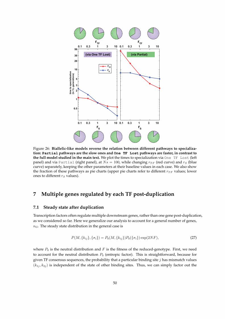
1

10

2

3

5

0.5

20

50

30

0.1 0.3 1 3 10

rS

0.1 0.3 1 3 10

0.1 0.3 1 3 10

rTF

0.1 0.3 1 3 10

rTF

rS

tim

e t

o s

pe

cia

liza

tio

n

(in

1/μ

ge

ne

rati

on

s)

(via One TF Lost) (via Partial)

rTF

rS

Figure 26: Biallelic-like models reverse the relation between different pathways to specializa-tion: Partial pathways are the slow ones and One TF Lost pathways are faster, in contrast tothe full model studied in the main text. We plot the times to specialization via One TF Lost (leftpanel) and via Partial (right panel), at Ns = 100, while changing rTF (red curve) and rS (bluecurve) separately, keeping the other parameters at their baseline values in each case. We also showthe fraction of these pathways as pie charts (upper pie charts refer to different rTF values; lowerones to different rS values).

7 Multiple genes regulated by each TF post-duplication

7.1 Steady state after duplication

Transcription factors often regulate multiple downstream genes, rather than one gene post-duplication,as we considered so far. Here we generalize our analysis to account for a general number of genes,nG. The steady state distribution in the general case is

P (M, {kij}, {σi}) = P0(M, {kij})P0({σi}) exp(2NF ), (27)

where P0 is the neutral distribution and F is the fitness of the reduced-genotype. First, we needto account for the neutral distribution P0 (entropic factor). This is straightforward, because forgiven TF consensus sequences, the probability that a particular binding site j has mismatch values(k1j , k2j) is independent of the state of other binding sites. Thus, we can simply factor out the

50

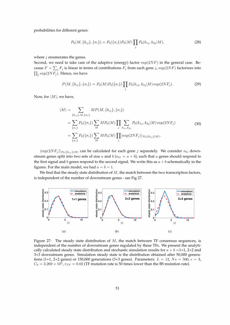
probabilities for different genes:

P0(M, {kij}, {σi}) = P0({σi})P0(M)∏j

P0(k1j , k2j |M), (28)

where j enumerates the genes.Second, we need to take care of the adaptive (energy) factor exp(2NF ) in the general case. Be-cause F =

∑j Fj is linear in terms of contributions Fj from each gene j, exp(2NF ) factorizes into∏

j exp(2NFj). Hence, we have

P (M, {kij}, {σi}) = P0(M)P0({σi})∏j

P0(k1j , k2j |M) exp(2NFj). (29)

Now, for 〈M〉, we have,

〈M〉 =∑

{kij},M,{σi}

MP (M, {kij}, {σi})

=∑{σi}

P0({σi})∑M

MP0(M)∏j

∑k1j ,k2j

P0(k1j , k2j |M) exp(2NFj)

=∑{σi}

P0({σi})∑M

MP0(M)∏j

〈exp(2NFj)〉P0({kij}|M).

(30)

〈exp(2NFj)〉P0({kij}|M) can be calculated for each gene j separately. We consider nG down-stream genes split into two sets of size a and b (nG = a + b), such that a genes should respond tothe first signal and b genes respond to the second signal. We write this as a+ b schematically in thefigures. For the main model, we had a = b = 1.

We find that the steady state distribution ofM , the match between the two transcription factors,is independent of the number of downstream genes - see Fig 27.

M

0 5 10

ste

ad

y s

tate

dis

trib

uti

on

0

0.1

0.2

0.3

1+1 genes

simulationanalytical

(a)

M

0 5 10

ste

ad

y s

tate

dis

trib

uti

on

0

0.1

0.2

0.3

2+2 genes

simulationanalytical

(b)

M

0 5 10

ste

ad

y s

tate

dis

trib

uti

on

0

0.1

0.2

0.3

3+3 genes

simulationanalytical

(c)

Figure 27: The steady state distribution of M , the match between TF consensus sequences, isindependent of the number of downstream genes regulated by these TFs. We present the analyti-cally calculated steady state distribution and stochastic simulation results for a + b =1+1, 2+2 and3+3 downstream genes. Simulation steady state is the distribution obtained after 50,000 genera-tions (1+1, 2+2 genes) or 150,000 generations (3+3 genes). Parameters: L = 12, Ns = 500, ε = 3,C0 = 3.269× 105, rTF = 0.02 (TF mutation rate is 50 times lower than the BS mutation rate).

51

7.2 Evolutionary dynamics

7.2.1 Frustration of fitness landscape

Each TF needs to simultaneously regulate a subset of the genes while avoiding regulation of theremaining ones. This increasing number of constraints, relative to the nG = 2 case, incurs a di-minishing number of feasible evolutionary trajectories. The fitness change due to a TF consensussequence mutation is assessed according to its effect on the binding affinities of this TF with allexisting genes. Hence, for each TF, as nG increases, the number of constraints also increases. Thislimits the number of possible substitutions a TF can access via fewer beneficial and neutral muta-tions. In contrast, for each binding site, the number of constraints does not change because it is onlyconstrained by the two TFs and not by other binding sites. To demonstrate how extra constraintsarising for nG > 2 genes affect evolutionary trajectories, we classified in Fig 28 the effects of all TFmutations on fitness for various numbers of downstream genes a+ b.

time

101

102

103

104

be

ne

fic

ial

0

0.05

0.1

0.15

0.2

0.25

0.3

1+1

2+1

2+2

3+2

3+3

(a)

time

101

102

103

104

ne

utr

al

0

0.05

0.1

0.15

1+1

2+1

2+2

3+2

3+3

(b)

time

101

102

103

104

de

lete

rio

us

0.6

0.7

0.8

0.9

1

1+1

2+1

2+2

3+2

3+3

(c)

Figure 28: The fitness landscape becomes more frustrated when nG > 2 (i.e., when each TFpost-duplication regulates more than 1 gene). At every time point in the stochastic simulation weanalyze all possible TF consensus sequence mutations and classify them according to their effect onfitness as beneficial (a) neutral (b) or deleterious (c). With increasing number of downstream genes,nG = a+ b, regulated by each TF (different curve colors, see legend), the fractions of beneficial andneutral mutations decrease and the fraction of deleterious mutations increases. This is because TFsbecome more constrained as nG increases, resulting in fewer potential mutations that are beneficialor neutral.

With increasing numbers of downstream genes, evolutionary trajectories are more often stuckin local fitness peaks. We demonstrate this effect in Fig 29, where we classified at each time pointin the simulation all possible TF mutations, and determined that a particular point is a fitness peakif all possible TF mutations from that point are strictly deleterious. Evolution can still continuethanks to the binding sites mutations which are much less constrained.

52

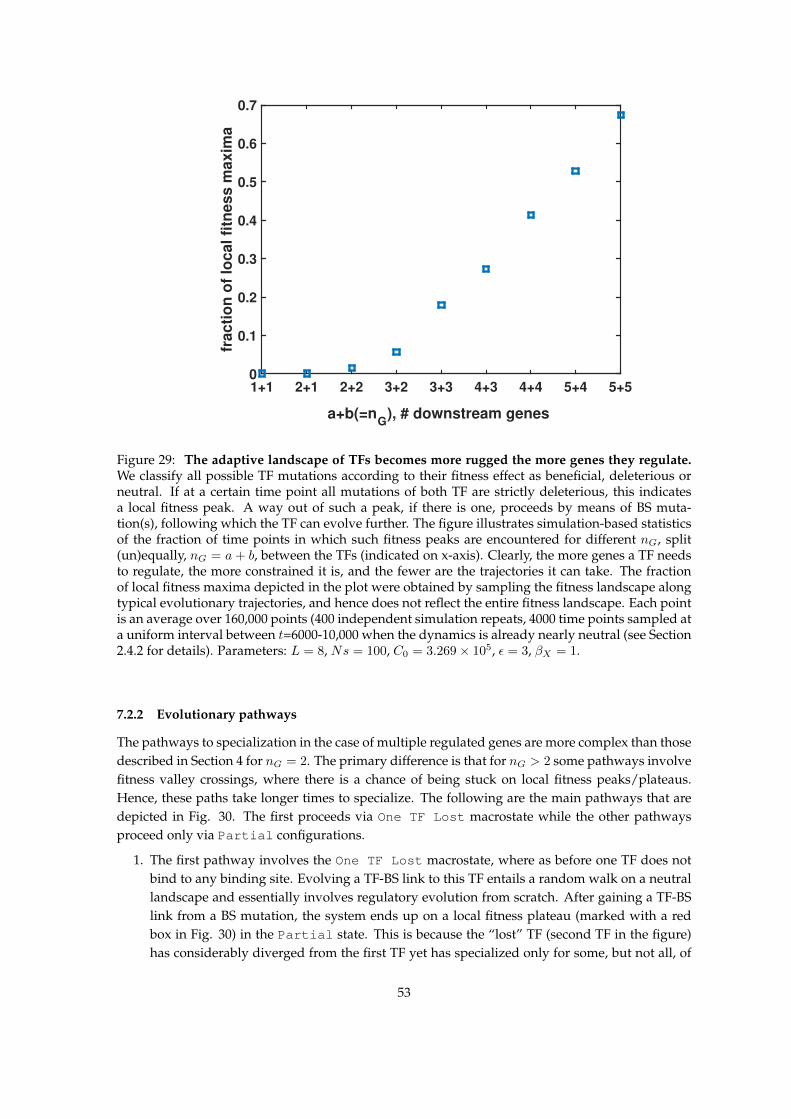
a+b(=nG

), # downstream genes

1+1 2+1 2+2 3+2 3+3 4+3 4+4 5+4 5+5

fra

cti

on

of

loc

al

fitn

es

s m

ax

ima

0

0.1

0.2

0.3

0.4

0.5

0.6

0.7

Figure 29: The adaptive landscape of TFs becomes more rugged the more genes they regulate.We classify all possible TF mutations according to their fitness effect as beneficial, deleterious orneutral. If at a certain time point all mutations of both TF are strictly deleterious, this indicatesa local fitness peak. A way out of such a peak, if there is one, proceeds by means of BS muta-tion(s), following which the TF can evolve further. The figure illustrates simulation-based statisticsof the fraction of time points in which such fitness peaks are encountered for different nG, split(un)equally, nG = a+ b, between the TFs (indicated on x-axis). Clearly, the more genes a TF needsto regulate, the more constrained it is, and the fewer are the trajectories it can take. The fractionof local fitness maxima depicted in the plot were obtained by sampling the fitness landscape alongtypical evolutionary trajectories, and hence does not reflect the entire fitness landscape. Each pointis an average over 160,000 points (400 independent simulation repeats, 4000 time points sampled ata uniform interval between t=6000-10,000 when the dynamics is already nearly neutral (see Section2.4.2 for details). Parameters: L = 8, Ns = 100, C0 = 3.269× 105, ε = 3, βX = 1.

7.2.2 Evolutionary pathways

The pathways to specialization in the case of multiple regulated genes are more complex than thosedescribed in Section 4 for nG = 2. The primary difference is that for nG > 2 some pathways involvefitness valley crossings, where there is a chance of being stuck on local fitness peaks/plateaus.Hence, these paths take longer times to specialize. The following are the main pathways that aredepicted in Fig. 30. The first proceeds via One TF Lost macrostate while the other pathwaysproceed only via Partial configurations.

1. The first pathway involves the One TF Lost macrostate, where as before one TF does notbind to any binding site. Evolving a TF-BS link to this TF entails a random walk on a neutrallandscape and essentially involves regulatory evolution from scratch. After gaining a TF-BSlink from a BS mutation, the system ends up on a local fitness plateau (marked with a redbox in Fig. 30) in the Partial state. This is because the “lost” TF (second TF in the figure)has considerably diverged from the first TF yet has specialized only for some, but not all, of

53

the genes associated with the green signal, but not for all of them. All of the TFs and BSs areconstrained to maintain match beyond some minimal level.

Hence specialization can only occur if one of the strong TF-BS links weakens. Such weakeningdecreases the fitness, and hence incurs crossing a fitness valley. This pathway is consequentlyvery slow.

2. The remaining pathways do not involve One TF Lost macrostate and go only via Partialmacrostate. In the second pathway, first, a TF consensus sequence mutation and a signalsensing mutation (either can occur first) lead the system to a Partial state with some of thesignal-BS pathways specialized. Then, an additional TF consensus sequence mutation pushesthe TFs further apart. This, together with BS mutations, brings the system to the local fitnessplateau (in the Partial macrostate) described in the previous pathway. This pathway is alsoslow, because of the fitness valley crossing described above.

3. In the third pathway also, first, a TF consensus sequence mutation and a signal sensing mu-tation (either can occur first) lead the system to a Partial state with some of the signal-BSpathways specialized. From here, no additional TF consensus sequence mutations occur thatpush the TFs away. Hence, there are paths for the BSs to realign their binding preferences(to the other TF) such that fitness is always maintained and does not involving crossing anyfitness valleys. Hence, this pathway is fast.

4. In the fourth and the fifth pathways, the first two mutations are signal sensing mutationsthat specialize the TFs’ signal sensing domains. From here, a TF mutation and subsequent BSmutations can specialize without going through fitness valleys. Hence, this is a fast pathway.For a given genotype (specifying the TF and BS sequences), this fourth pathway is eitherpossible or not. If it is not possible, then the only resort is the fifth pathway.

5. The fifth pathway comes into play when the fourth pathway is not possible. This happenswhen any TF mutation loses some signal-BS pathways, hence dropping the fitness consider-ably. The TFs cannot diverge at all, and this involves crossing a fitness valley. Hence, this is aslow pathway.

54

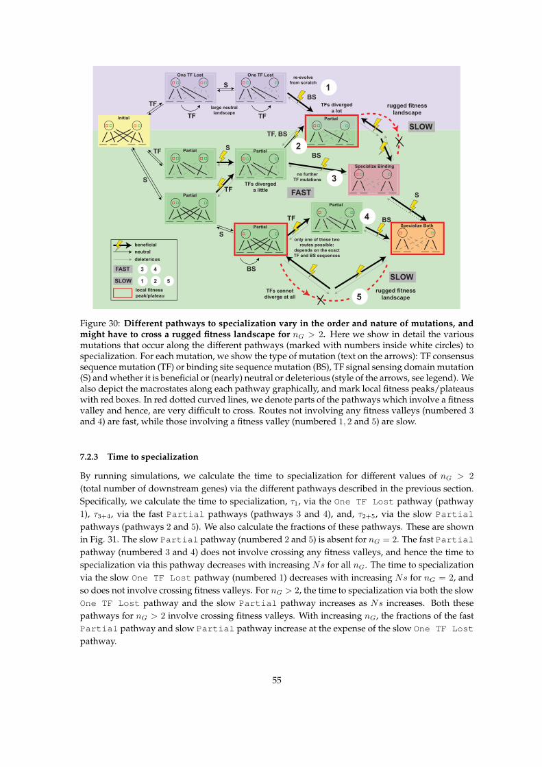
TF

TF

S

TF

BS

Initial

S

FAST

SLOW

TF TF

large neutral

landscape

re-evolve

from scratch

One TF Lost

Partial

One TF Lost

TFs diverged

a lot

Specialize Binding

Specialize Both

Partial PartialS

Partial S

TF, BS

BS

no further

TF mutationsTFs diverged

a little

Partial

S

Partial

TF BS

BS

TFs cannot

diverge at all

rugged fitness

landscape

rugged fitness

landscape

only one of these two

routes possible:

depends on the exact

TF and BS sequences

beneficial

deleterious

neutral

FAST 3 4

SLOW 1 2 5

local fitness

peak/plateau

SLOW

1

3

4

5

2

Figure 30: Different pathways to specialization vary in the order and nature of mutations, andmight have to cross a rugged fitness landscape for nG > 2. Here we show in detail the variousmutations that occur along the different pathways (marked with numbers inside white circles) tospecialization. For each mutation, we show the type of mutation (text on the arrows): TF consensussequence mutation (TF) or binding site sequence mutation (BS), TF signal sensing domain mutation(S) and whether it is beneficial or (nearly) neutral or deleterious (style of the arrows, see legend). Wealso depict the macrostates along each pathway graphically, and mark local fitness peaks/plateauswith red boxes. In red dotted curved lines, we denote parts of the pathways which involve a fitnessvalley and hence, are very difficult to cross. Routes not involving any fitness valleys (numbered 3and 4) are fast, while those involving a fitness valley (numbered 1, 2 and 5) are slow.

7.2.3 Time to specialization

By running simulations, we calculate the time to specialization for different values of nG > 2

(total number of downstream genes) via the different pathways described in the previous section.Specifically, we calculate the time to specialization, τ1, via the One TF Lost pathway (pathway1), τ3+4, via the fast Partial pathways (pathways 3 and 4), and, τ2+5, via the slow Partial

pathways (pathways 2 and 5). We also calculate the fractions of these pathways. These are shownin Fig. 31. The slow Partial pathway (numbered 2 and 5) is absent for nG = 2. The fast Partialpathway (numbered 3 and 4) does not involve crossing any fitness valleys, and hence the time tospecialization via this pathway decreases with increasing Ns for all nG. The time to specializationvia the slow One TF Lost pathway (numbered 1) decreases with increasing Ns for nG = 2, andso does not involve crossing fitness valleys. For nG > 2, the time to specialization via both the slowOne TF Lost pathway and the slow Partial pathway increases as Ns increases. Both thesepathways for nG > 2 involve crossing fitness valleys. With increasing nG, the fractions of the fastPartial pathway and slow Partial pathway increase at the expense of the slow One TF Lost

pathway.

55

50 100 150

102

101

100

10-1

Ns Ns Ns

tim

e t

o s

pe

cia

liza

tio

n

(in

1/μ

ge

ne

rati

on

s)

nG = 2 n

G = 4 n

G = 8

2 5

3 4

1

τ2+5

(slow Partial)

τ1

(One TF Lost)

τ3+4

(fast Partial)

25 50 100 15025 50 100 15025

Figure 31: Times to specialization via different pathways for various numbers of downstreamgenes. Shown are the times to specialization via different pathways as a function ofNs for differentvalues of nG. We plot the times for the slow One TF Lost pathway (numbered 1, yellow), the slowPartial pathway (numbered 2 and 5, red), and the fast Partial pathway (numbered 3 and 4,blue). Plotted as pie charts also are the fraction of various pathways for different nG values as piecharts; these fractions depend only very weakly on Ns. In general, the higher the nG, the larger thefraction of fast trajectories (3 and 4) and the longer the time needed to specialize. Pathways whosetime lengths withNs, which are the slow Partial pathway (red) and the One TF Lost pathway(yellow) for nG > 2, involve crossing fitness barriers.

8 Promiscuity-promoting mutations

So far we considered the ”mismatch-energy model” for TF-BS specificity, where each position inthe TF and the binding site contributed equally to the total binding energy, depending on whetherthe position has a mismatch between the TF consensus sequence and the BS sequence. Let the TFconsensus sequence be s∗ and the binding site sequence be s, both of length L. In general, we have

E =∑i

Ei (31)

where i runs over all the positions of the binding site. For each specific position i, the contributionis Ei = 0 if si = s∗i (match) and Ei = ε if si 6= s∗i (mismatch).

Experiments on TF-BS specificity, however, suggest that some TF (and binding site) positionsdominate while others only have minor energetic contributions. In this section we study a simplegeneralization of the mismatch-energy model, where we allow for two levels of contribution: somepositions are specific (favor a unique nucleotide) and have large energetic contribution while others

56

are non-specific or promiscuous (all nucleotides are equally favorable) and have a smaller energeticcontribution. For each specific position i, the contribution Ei is, as in the mismatch-energy model,ε if there is mismatch between the TF consensus sequence and the BS sequence in that position,and 0 if there is a match. On the other hand, for each promiscuous position i, the contribution isEi = εP (typically 0 ≤ εP ≤ ε), independent of si. Hence, for a TF with LP < L promiscuouspositions in total, and k mismatches in the remaining L − LP specific positions, the total bindingenergy would be E = εPLP + kε. The different possible energy levels for specific and promiscuousTFs are illustrated in Fig. 32.

εP = ε/3

εP = ε/2

εP = 2ε/3

promiscuity mutation (r Pμ)

consensus sequence mutation,

binding site mutation

consensus sequence

mutation

E =

εPL

P+εk

0

ε

2ε

3ε

4ε

5ε

0 1 2 5

LP (#promiscuous sites)

k (#TF-BS mismatches)

k=0

k=1

k=2

k=3

k=4

k=5

Figure 32: Total TF-DNA binding energies depend on number of mismatches as well as on thenumber of promiscuous TF positions. We plot the different energy levels depicting the TF-BSbinding energy, E = εPLP + εk, for TFs with varying number of promiscuous positions LP and kmismatches between the TF and BS in the remaining L − LP specific positions. Note that lower Ecorresponds to tighter TF-BS binding. We illustrate this for three different values of εP , the energycontribution per promiscuous position (different colors). Increasing line thickness of the energylevels represents higher mismatch values k. While promiscuity-promoting mutations increase LPby converting a specific position to a promiscuous one, regular TF mutations that hit a promiscuousposition can convert it to be specific and decrease LP .

We also introduce an additional type of mutation, called “promiscuity-promoting” mutation,

57

that occurs at rate rPµ. As illustrated in Fig. 5A of the main text, these mutations convert a specificTF position in the consensus sequence to a promiscuous one. A promiscuous position can return tobe specific again if it is hit by a consensus TF mutation (regular TF mutations we considered untilnow, happening at rate rTFµ).

Promiscuity entails a cost in terms of TF-BS binding. To elucidate this cost, we consider thedependency of the free (dimensionless) concentration, C0, of a TF, on the binding preferences ofthe TF. For a TF with no promiscuous positions, C0 can be calculated in the chemical potentialframework as

C0(LP = 0) =C

GS(ε, L) +∑n

exp(−En), (32)

where C is the copy number of the TF, G is the number of sites on the DNA where the TF canbind in a sequence-specific manner, n enumerates other possible energy configurations of the TFthat are sequence-independent (residing in the free solution, or nonspecific binding to DNA), andEn is the free energy in configuration n. S(ε, L) = 〈e−εk〉P (k) is the similarity between bindingsites defined in [12], with GS(ε, L) acting as the Boltzmann factor for all possible specific bindingconfigurations. This term captures the sequestration of TFs on the DNA due to spurious binding.Assuming that the DNA sequence is random, P (k) ∼ B(L, 3/4) is the Binomial distribution for thenumber of mismatches that a random DNA sequence has with a given TF consensus sequence.For a promiscuous TF with LP promiscuous positions, we have,

C0(LP ) =C

Ge−εPLP S(ε, L− LP ) +∑n

exp(−En)

= C0(LP = 0)

GS(ε, L) +∑n

exp(−En)

Ge−εPLP S(ε, L− LP ) +∑n

exp(−En)

= C0(LP = 0)1 +A

e−εPLPS(ε,L−LP )S(ε,LP ) +A

,

(33)

where A =∑

n exp(−En)

GS(ε,L) is an effective parameter that captures the relative contribution of theBoltzmann factor corresponding to spurious specific binding on the DNA, compared with all otherBoltzmann factors. We have assumed that A = 0.1 is fixed in our calculations, and the results wepresent are fairly robust to the value of A. The probability that a binding site is bound by a TF withLP > 0 promiscuous positions and k mismatches with respect to the binding site in the remainingL− LP positions, assuming no other TF type is present, is

p =C0(LP )e−εk−εPLP

1 + C0(LP )e−εk−εPLP. (34)

This probability is plotted in Fig 33 for various k and Lp values. While C0(LP ) can be greater orlesser than C0(LP = 0) depending on the value of εP , we have C0(LP )e−εPLP < C0(LP = 0).Hence, as the number of promiscuous positions, LP , in the TF increases, the binding probabilitydecreases.

58

For instance, consider a TF with consensus sequence AAAAA (see Fig. 33). This TF is specificforA’s in all five positions of the binding site sequence. Each mismatch in the binding site sequence(green positions in the sequences in Fig. 33) with respect to AAAAA decreases the binding affinity,and thereby decreases the binding probability. Now consider a promiscuous TF with consensussequence A ∗ AAA, where ∗ denotes a promiscuous position. The second position, independentof the bp in the BS sequence (purple positions in the sequences in Fig. 33), decreases the bindingaffinity, but by a lesser amount than a specific position mismatch (green positions). Hence, thebinding probabilities of the promiscuous TF to AAAAA, AGAAA, ATAAA or ACAAA are equal,and higher than the binding probability of the specific TF to CAAAA or AGAAA or other single-mismatch BS sequences.

k: # of TF-TFBS mismatches

0

0.25

0.5

0.75

1

0 1 2 3 4 5

bin

din

g p

rob

ab

ilit

y

increasing LP

(# promiscuous

positions)

LP = 0

LP = 1

LP = 2

CAAAA

...

AGAAA

AAAAA

AA

AA

A

A*A

AA

AAAAA

AGAAA

CAAAA

C

A

mismatch in

specific position

promiscuous

position

Figure 33: Binding probability of the TF to DNA decreases the more promiscuous it is. The TF-BS binding probability is plotted as a function of the number of TF-BS mismatches k among theL−LP specific positions for different values of LP , the number of promiscuous positions in the TF.We list, as an example, different sequences that are consistent with given (LP , k).

8.1 Steady state after duplication

In the presence of promiscuity-promoting mutations, we obtain the steady state distribution overthe genotypic space analytically, from which we obtain the dominant macrostate at steady state fordifferent ρ and Ns values (Fig. 34). The inclusion of promiscuity-promoting mutations does notsignificantly change the dominant macrostate phase plot except for a slight increase in the range ofOne TF Lost macrostate.

We also plot the mean number of promiscuous positions at steady state in Fig. 35. This numberdecreases with selection intensity, because promiscuous positions decrease the TF binding proba-bility (see Fig. 33) making them less favorable once specialization has occurred.

59

0 10 20 30 40

Ns

-1

-0.75

-0.5

-0.25

0.25

0.5

0.75

1

ρ 0

25 50

No

Re

gu

lati

on

Pa

rtia

l

Specialize Both

One TF Lost

Figure 34: Most probable macrostate in the presense of promiscuity-promoting mutations. Weplot the most probable macrostate at steady state, z∗SS , for different ρ and Ns, for nG = 2 andrelative mutation rate rP = 3, keeping other parameters at their baseline values. We choose rP = 3so that at each position, a specific bp has equal effective mutation rate towards a promiscuous stateor another specific bp.

0 10 20 30 40

Ns

-1

-0.75

-0.5

-0.25

0.25

0.5

0.75

1

ρ 0

25 50

1.7

1.8

1.9

2

2.1

2.2

2.3

2.4

2.5

2.6

2.7

<LP>

Figure 35: Mean number of promiscuous TF positions at steady state decreases with selectionintensity. We plot the mean number of promiscuous positions at steady state, 〈LP 〉 (out of L = 5),for different values of signal correlation ρ and selection strength Ns. Steady state values of 〈LP 〉are within a relatively small range. As selection strength increases, 〈LP 〉 decreases, yet still remainsabove zero. Parameter values: nG = 2, rP = 3; other parameters are at their baseline values.

8.2 Evolutionary dynamics

8.2.1 Time to specialization

In general, promiscuity-promoting mutations accelerate specialization, as shown in Fig. 36. Thespeedup of the fast Partial pathway (3 and 4) is not very large, but the speedup of the slowPartial (2 and 5) and the slow One TF Lost (1) pathways is considerable, an effect that in-creases with increasing Ns (see Fig. 30 for details of the pathways). Promiscuity-promoting mu-tations act by converting deleterious BS mutations into neutral or beneficial ones. By that they

60

effectively lower or even remove fitness barriers. This effect is more significant with a large num-ber of downstream genes, where more constraints on TF evolution exist. The fraction of differentpathways does not change much if promiscuity-promoting mutations are present. Note that asa function of Ns, the fraction of fast Partial pathways does not change considerably, but thefraction of slow Partial pathways decreases while increasing the fraction of slow One TF Lost

pathways.

50 100 150

102

101

100

10-1

Ns Ns Ns

tim

e t

o s

pe

cia

liza

tio

n

(in

1/μ

ge

ne

rati

on

s)

nG = 2 n

G = 4 n

G = 8

2 5

3 4

1

τ2+5

(slow Partial)

τ1

(One TF Lost)

τ3+4

(fast Partial)

25 50 100 15025 50 100 15025

without

promiscuity-promoting

mutations

with

promiscuity-promoting

mutations

Figure 36: Promiscuity-promoting mutations accelerate specialization. We plot the times to spe-cialization via different pathways that are depicted in Fig. 30, as a function of Ns for differentvalues of nG (the number of downstream genes per TF), in the absence (solid lines) and presence(dotted lines) of promiscuity-promoting mutations. Specialization times are shown for the slowOne TF Lost pathway (numbered 1, yellow), the slow Partial pathway (numbered 2 and 5,red), and the fast Partial pathway (numbered 3 and 4, blue). In general, promiscuity-promotingmutations shorten evolutionary specialization times. This effect is particularly marked for the slowpathways (One TF Lost and slow Partial) and for large numbers of downstream genes nG.The pie charts illustrate the fraction of the various pathways at each nG value. For nG = 8, we plotthe pie charts for the different Ns values marked on the x-axis.

8.2.2 Typical trajectory

Promiscuity-promoting mutations play different roles in different phases of the evolutionary tra-jectory. While after specialization they are less favorable (because they lower binding affinity andpotentially destabilize the specialized state), during adaptation they can facilitate fitness valleycrossing. In Fig. 37, we plot the trajectory of the average number of promiscuous TF positions asa function of time. Starting with no promiscious positions in the Initial state, the number ofpromiscuous positions increases during the transient One TF Lost state, and then decreases toreach its steady state value after reaching the Specialize Both state. The speedup of evolution

61

is mainly during the transient One TF Lost phase, where the number of promiscuous positionspeaks.

10-4

0

1

2

10-3 10-2 10-1 100 101

time (in 1/μ generations)

av

era

ge

#p

rom

isc

uo

us

po

sit

ion

s

<LP(t)>

Initial One TF Lost Specialize Both

Figure 37: Number of promiscuous positions transiently peaks during adaptation and relaxesafter specialization to an intermediate steady state value. We plot the average number of promis-cuous positions 〈LP (t)〉 as a function of time for L = 5, nG = 4, Ns = 250 and rP = 10; otherparameters are at baseline values. Solid black arrow indicates the increase in the number of promis-cuous positions in the transient One TF Lost phase, while the dotted black arrow indicates theirdecrease after specializing. The red dotted line indicates the steady state value of 〈LP 〉.

62

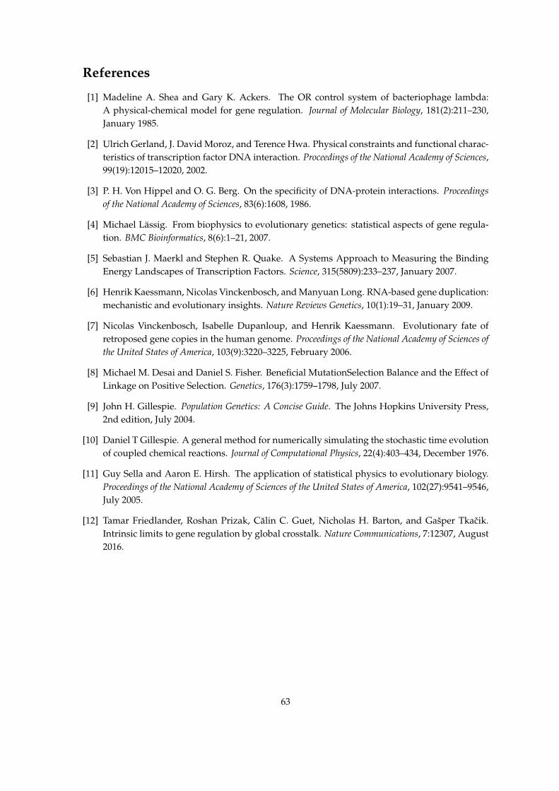
References

[1] Madeline A. Shea and Gary K. Ackers. The OR control system of bacteriophage lambda:A physical-chemical model for gene regulation. Journal of Molecular Biology, 181(2):211–230,January 1985.

[2] Ulrich Gerland, J. David Moroz, and Terence Hwa. Physical constraints and functional charac-teristics of transcription factor DNA interaction. Proceedings of the National Academy of Sciences,99(19):12015–12020, 2002.

[3] P. H. Von Hippel and O. G. Berg. On the specificity of DNA-protein interactions. Proceedingsof the National Academy of Sciences, 83(6):1608, 1986.

[4] Michael Lassig. From biophysics to evolutionary genetics: statistical aspects of gene regula-tion. BMC Bioinformatics, 8(6):1–21, 2007.

[5] Sebastian J. Maerkl and Stephen R. Quake. A Systems Approach to Measuring the BindingEnergy Landscapes of Transcription Factors. Science, 315(5809):233–237, January 2007.

[6] Henrik Kaessmann, Nicolas Vinckenbosch, and Manyuan Long. RNA-based gene duplication:mechanistic and evolutionary insights. Nature Reviews Genetics, 10(1):19–31, January 2009.

[7] Nicolas Vinckenbosch, Isabelle Dupanloup, and Henrik Kaessmann. Evolutionary fate ofretroposed gene copies in the human genome. Proceedings of the National Academy of Sciences ofthe United States of America, 103(9):3220–3225, February 2006.

[8] Michael M. Desai and Daniel S. Fisher. Beneficial MutationSelection Balance and the Effect ofLinkage on Positive Selection. Genetics, 176(3):1759–1798, July 2007.

[9] John H. Gillespie. Population Genetics: A Concise Guide. The Johns Hopkins University Press,2nd edition, July 2004.

[10] Daniel T Gillespie. A general method for numerically simulating the stochastic time evolutionof coupled chemical reactions. Journal of Computational Physics, 22(4):403–434, December 1976.

[11] Guy Sella and Aaron E. Hirsh. The application of statistical physics to evolutionary biology.Proceedings of the National Academy of Sciences of the United States of America, 102(27):9541–9546,July 2005.

[12] Tamar Friedlander, Roshan Prizak, Calin C. Guet, Nicholas H. Barton, and Gasper Tkacik.Intrinsic limits to gene regulation by global crosstalk. Nature Communications, 7:12307, August2016.

63