tabula rasa: model transfer for object category …vgg/publications/2011/aytar11/aytar...tabula...

Tabula Rasa: Model Transfer for Object Category Detection

Yusuf Aytar Andrew ZissermanDepartment of Engineering Science

University of Oxford{yusuf,az}@robots.ox.ac.uk

AbstractOur objective is transfer training of a discriminatively

trained object category detector, in order to reduce thenumber of training images required. To this end we pro-pose three transfer learning formulations where a templatelearnt previously for other categories is used to regularizethe training of a new category. All the formulations resultin convex optimization problems.

Experiments (on PASCAL VOC) demonstrate significantperformance gains by transfer learning from one classto another (e.g. motorbike to bicycle), including one-shotlearning, specialization from class to a subordinate class(e.g. from quadruped to horse) and transfer using multi-ple components. In the case of multiple training samples itis shown that a detection performance approaching that ofthe state of the art can be achieved with substantially fewertraining samples.

1. Introduction

There has been considerable progress recently in objectcategory detection: the task of determining if one or moreinstances of a category are present in an image and, if theyare, localizing them [6]. Indeed, for certain types of objectcategories and images (e.g. compact objects, typical view-points), discriminatively trained template part-based detec-tors perform very well, and source code is freely avail-able for training and development [9]. The negative thoughis that current methods require training the detector fromscratch for each new category – a costly procedure whichrequires an adequate supply of positive and negative anno-tated data. For challenges like ImageNet [2] and beyond,where the goal is thousands of categories, this procedure isnot scalable for object category detection.

One solution to this problem is to represent object cat-egories indirectly by their attributes, and to learn to de-tect attributes that can be applied across multiple cate-gories [10, 12, 13, 7, 19, 29]. The benefits are that eachattribute can be learnt from multiple classes, so training datais plentiful, and that the attribute representation can be ap-

(a) (b) (c)Figure 1. The benefit of transfer learning. The learnt HOG de-tector template for a motorbike (a) is used as the source for learn-ing a bicycle template together with the samples shown in (b). Theresulting learnt bicycle HOG detector template (c) clearly has theshape of a bicycle. Note, here and in the rest of the paper we onlyvisualize the positive components of the HOG vector.

plied to classes that were not used in the training, so it isscalable. However, currently almost all attribute recognitionis for image classification (not detection) and even for clas-sification (a simpler task than detection) the performance isinferior to direct discriminative training.

An alternative solution, that we investigate in this pa-per, is to benefit from category detectors that have previ-ously been learnt for similar categories by transferring in-formation to a new target category. In particular, our objec-tive is to apply transfer learning to the SVM discriminativetraining framework for HOG template models of Dalal &Triggs [1] and Felzenszwalb et al. [9]. The key intuitionis that the learnt template records the spatial layout of pos-itive and negative orientations. Classes that are geometri-cally similar (e.g. a horse and a donkey) – those that canbe ‘morphed’ into one another by local deformations – willhave correspondingly similar HOG templates. To achievethis transfer in the target detector training, the previouslylearnt template is introduced as a regularizer in the costfunction. As illustrated in figure 1, this enables a detectorto be learnt for the target category using substantially fewersamples than tabula rasa.

To this end, we introduce and compare three models,including a novel cost function for rigid template transferand a geometric transfer model where the template is de-formed using local flow. All three models are defined byconvex optimization problems. We also show that the se-lection of training samples is critical but can be determined

by the source category for best results in the case of one-shot learning.

Related work. Model based transfer learning, originallydeveloped in the machine learning literature as adapta-tion [14, 27], has been applied to computer vision primar-ily for image classification [17, 22, 23, 27], rather thandetection. The work closest to ours is that of Tomassi etal. [22, 23] who also use a discriminative SVM framework(though with a quadratic loss), and include the previouslylearnt model as a regularizer. We extend their work bydeveloping new models and also by considering the morechallenging detection problem. We also extend their modelby applying local flow algorithms on the classifier template.Others have investigated transfer learning from multipleclasses [18, 26] though again for classification. The moregeneral task of reducing training requirements by incorpo-rating prior models has also been considered by Fei-Fei etal. [8] for one shot learning, metric-learning by Fink [11],and hierarchical classification by Zweig and Weinshall [30].Stark et al. [21] consider a more geometric based transferbetween models, though this is manual at the moment.

There is another school of transfer learning where clas-sifiers are transferred between domains [3, 4, 20, 28], forexample by learning feature distributions for the source andtarget domains, but we are not concerned with this type ofdomain transfer problem here.

In the next section we define the problem, and then intro-duce two new model transfer methods building on an exist-ing model transfer method of [14, 27]. In the experiments(section 4) we compare transfer learning models for bothone-shot learning and multiple samples in the case of trans-ferring from one category to another; and also investigatethe case of specialization from a class to a subordinate class.

2. Model Transfer Support Vector MachinesSuppose that we wish to detect an object category of in-

terest, which will be referred as the target category, andassume that we have a well trained detector for a visuallysimilar source category. Then, the goal is to learn an objectdetector for the target category by transferring knowledgefrom the source category detector with the guidance of afew available samples of the target category.

We are concerned here with detection using a slidingwindow classifier in the manner of [1]. The classifier islinear and is specified by a template vector w, with a scor-ing function wTx, where x is the feature vector. Then thetask is to learn w for the target category using a few positivetraining instances xi, and the source category detector ws.

In the remainder of the section we introduce and moti-vate model based transfer learning for support vector ma-chines (SVM). Three variants will be defined: AdaptiveSupport Vector Machines (A-SVM), a direct application ofthe classifier transfer of [14, 27]; Projective Model Transfer

Figure 2. Visualization of the projection of the vector w onto ws,and onto the separating hyperplane orthogonal to ws.

SVM (PMT-SVM) which relaxes the transfer of the A-SVMmodel; and Deformable Adaptive SVM (DA-SVM), wherethe source template ws is geometrically transformed duringthe learning.2.1. Adaptive SVM (A-SVM)

The idea, originally introduced by [14, 27], is to learnfrom the source model ws by regularizing the distance be-tween the learned model w and ws. As usual, xi are thetraining samples, yi ∈ {−1, 1} the corresponding labels,and l(xi, yi;w, b) = max

(0, 1− yi(wTxi + b)

)the hinge

loss. The objective function is:

LA = minw,b‖w − Γws‖2 + C

N∑i

l(xi, yi;w, b) (1)

where Γ controls the amount of transfer regularization, Ccontrols the weight of the loss function, and N the numberof samples.

Discussion. We present a brief analysis of A-SVMs tomotivate our second model. Intuitively transfer regulariza-tion for an A-SVM is like a spring between Γws and w, andis equivalent to providing training samples from the sourceclass. The transfer can also be understood by expanding theregularization term. Assume that ws is l2 normalized to 1then

‖w − Γws‖2 = ‖w‖2 − 2Γ‖w‖cosθ + Γ2 (2)

where ‖w‖2 provides the ‘normal’ SVM margin maximiza-tion and −2Γ‖w‖cosθ induces the transfer by maximizingcosθ, i.e. by minimizing the angle θ between the ws and was shown in figure 2. Note, that the transfer term ‖w‖cosθis maximized (and thus the cost minimized) when θ = 0.

However, the term −2Γ‖w‖cosθ also encourages ‖w‖to be larger (as this reduces the cost) and this prevents mar-gin maximization. Thus Γ, which should define the amountof transfer regularization, becomes a tradeoff parameter be-tween margin maximization and knowledge transfer.

2.2. Projective Model Transfer SVM (PMT-SVM)

Rather than transfer by maximizing the transfer term‖w‖cosθ, we can instead minimize the projection of w ontothe seperating hyperplane orthogonal to ws (and thereby re-duce θ, see again figure 2). In this approach, we can in-crease the amount of transfer (Γ) without penalizing margin

maximization. The objective function for Projective ModelTransfer SVM (PMT-SVM) is:

LPMT = minw,b‖w‖2 + Γ‖Pw‖2 + C

N∑i

l(xi, yi;w, b)

st : wTws ≥ 0 (3)

where P is the projection matrix P = I − wswsT

wsTws, Γ con-

trols the amount of transfer regularization, and C controlsthe weight of the hinge loss. ‖Pw‖2 = ‖w‖2sin2θ is thesquared norm of the projection of the w onto the source hy-perplane. wTws ≥ 0 constrains w to the positive halfspacedefined by ws. As Γ → 0, (3) becomes a ‘classical’ SVMobjective. Note that the formulation is convex and can beminimized using quadratic optimization.

2.3. Transferring from a deformable source

Transfer regularization can also be performed by usinga deformable source template, where small local deforma-tions are allowed for a better fit of the source template to thetarget. For instance, the wheel part of a motorbike templatecan be increased in radius and reduced in thickness for abetter fit to a bicycle wheel (see figure 1). These small de-formations provide more flexible regularization. Local de-formations are implemented by the flow of weight vectorsfrom one cell to another, as described in more detail in sec-tion 3. The deformation is governed by the following flowdefinition:

τ(ws)i =

M∑j

fijwsj ,

where τ denotes the flow transformation, wsj is the jth cell

in the source template, the flow parameters fij define theamount of transfer from the jth cell in the source templateto the ith cell in the transformed template. Note that onesource template cell can contribute to multiple transformedtemplate cells.

To generalize from the rigid A-SVM to deformabletransfer formulation,ws in (1) is replaced with τ(ws) whichgives the following Deformable Adaptive SVM (DA-SVM)objective:

LDA = minf,w,b

‖w − Γτ(ws)‖2 + C

N∑i

l(xi, yi;w, b)

+λ

M,M∑i 6=j

f2ijdij +

M∑i

(1− fii)2d

(4)

where dij is the spatial distance between the ith cell andjth cell, d is the penalization for the additional flow fromthe ith source cell to the ith target cell, and λ the weight ofthe deformation.

Again, the hyper-parameter Γ controls the amount oftransfer. The additional parameter λ controls the deforma-bility: high values of λ make the model more rigid so thatthe solution of (4) approaches that of (1), conversely smallvalues allow a very flexible source template with less regu-larization ability.

Discussion. The DA-SVM objective (4) defines a con-vex optimization problem. Even though the term ‖w −Γτ(ws)‖2 may appear to be non-convex (due to the prod-uct of the terms in fij and wk), a short calculation showsthat the Hessian matrix is positive definite.

2.4. Introducing latent variables

In a similar manner to [9], latent variables can be in-troduced that specify the position and scale of the detec-tion ROIs relative to the annotation ROIs. As demonstratedin [9] the introduction of latent variables boosts the perfor-mance of the detector, because the training is no longer ad-versely affected by variations in the annotation and can useeach training sample more fully. The disadvantage is thatthe complete optimization problem is no longer convex.

In more detail, the optimization problem becomesLlatent = minz∈Z(X) L, where L can be any of the modeltransfer objectives, Z(X) defines all possible bounding boxpositions and scales of positive and negative samples, and zselects from these sets. In brief, for positive samples z de-fines a better alignment and for negative samples it definesthe boxes that are more confused with positives and harderto classify as negative. Even though Llatent is not convex,it becomes a convex objective function when z is fixed, asall the transfer model objectives are convex.

3. Implementation detailsHOG features. The features used are HOG [1] with theextensions proposed by [9] and using their source code.Each HOG cell is represented by a 32 dimensional vector.The feature vector x thus has dimension 80× 32. As in [9]we use a 8 × 10 arrangement of HOG cells. The transferexperiments are based only on the root filter of [9] withoutparts. Most of the experiments use a single component, butmultiple components are used in section 4.1.3.

Flow. The weight vector w corresponds to the grid ofM = 80 HOG cells tiled in a rectangle, with each cell rep-resented by a D = 32 dimensional vector (so w has dimen-sion M × D). Write hj for the D dimensional part of wcorresponding to the HOG cell j (so that w is a concatena-tion of M vectors hj , j = 1 . . . D). The flow is restrictedto act on the entire vectors hj , as

∑j fijhj i.e. it does not

mix components of the cell vectors. This is a simplificationthat could be removed if necessary.

Training. We are provided with a training set of anno-tated images with tight bounding boxes around each posi-tive instance (see section 4). During training, we switch be-tween optimizing latent variables (bounding box positionsand scales of positive and negative samples) and SVM ob-jectives. The SVMs are trained either via quadratic pro-grammig using the MOSEK [15] optimization toolkit, or viastochastic gradient descent using the VLFeat library [24]. In

Figure 3. Bicycle classifiers learned using a motorbike classifier as the source and with an increasing number of samples (1,3,6,9,20) fromleft to right. Note the transition from a template that looks like a motorbike (left) to one that looks like a bicycle (right). A-SVM methodis used for learning.

Figure 4. The benefits of transfer learning. The three types ofperformance improvement aspirations from transfer learning. Thex-axis is the number of training samples for the target class. (figurefrom [16, 23]).

other respects (alternating for latent variables etc) the train-ing follows that of [9], and in section 4 we show that weobtain a similar performance to [9].

4. ExperimentsTransfer learning can provide three types of performance

improvements over learning from the target class alone (seeFigure 4) [16, 23]: (1) higher start: the initial perfor-mance is higher, (2) higher slope: performance grows morequickly, (3) higher asymptote: the final performance is bet-ter. The experiments are designed to see which of these areachieved by the model transfer methods.

There are two types of experiments: (i) inter-class trans-fer where the transfer is from one category to another; and(ii) specialization where the transfer is from superior classto subordinate (e.g. from a generic quadruped category to aspecific category).

The evaluations are performed on the PASCAL VOC2007 dataset [5]. The training and validation sets are usedto learn the detector, and the performance is reported asaverage precision (AP) on the test set using the standardPASCAL procedure and evaluation software. For efficiencypurposes, we also select a smaller test subset referred asPASCAL-500 which consists of all the positive samples ofthe target class and a random selection of other imagesup to 500. The complete test set is referred as PASCAL-COMPLETE.

For most of the experiments we restrict the training toside views of the categories horse, sheep, cow, motorbike,and bicycle. These are obtained directly from the VOC datausing the pose attributes provided in the annotations. In thetraining only side facing objects are used and the obtainedfilter is always facing left (i.e right facing samples are mir-

Categories #pos. samples Felz. [9] Base. SVMtrain testhorse 45 53 40.1% 44.6%sheep 45 43 30.7% 37.1%cow 38 41 24.9% 21.5%bicycle 62 76 50.1% 59.0%motorbike 36 57 38.1% 33.8%

Table 1. The comparison of the average precision (AP) results ob-tained from baseline SVM and Felzenszwalb et. al. [9] withoutparts for the pascal-side-only object detection task on PASCAL-COMPLETE test set.

rored before training). Table 1 gives the number of side fac-ing positives in the training and test sets for each class. Insection 4.1.3 we lift the restriction of side view samples anduse all the views for training multiple component models.

Evaluations are performed using two different proce-dures: (i) pascal-default, and (ii) pascal-side-only. Thepascal-default case is the PASCAL VOC [5] evaluation pro-cedure including all views. In pascal-default evaluations,while obtaining detections we also use the mirrored versionof the side facing detector. In the pascal-side-only case,only the left side view ground truth of test samples is usedfor evaluation and true detections of other poses belongingto the target class are not counted towards AP computation.

The hyperparameters C, Γ and λ are learned on the vali-dation set. C is fixed to 0.002 for all the experiments.Baseline detectors. The baseline detectors are SVM clas-sifiers trained directly on positive samples without anytransfer learning. These classifiers provide the source mod-els in the transfer experiments, and also establish the perfor-mance that can be achieved for the target class if all the pos-itive samples of that class are used for training. Other thanthe learning procedure, the baseline is essentially the sameas the discriminatively trained detector of [9] with only theroot filter (no parts), and we compare to this method us-ing the code provided by the authors. As shown in table 1the baseline has very similar performance to [9] (if not bet-ter). This establishes the state of the art performance for thisdataset.

4.1. Between category transfer

In these experiments we investigate two cases: learninga bicycle classifier by transferring from the motorbike clas-sifier, and learning a horse classifier by transferring from

the cow classifier. We discuss first one shot learning, i.e.learning from a single positive sample of the target class,and then multiple shot learning.

4.1.1 One Shot Learning

The one shot learning scenario investigates the higher startaspect of transfer learning benefits (see figure 4). Givena single positive target class sample, we compare fourlearning methods: learning from the given positive sam-ple only (baseline SVM), rigid transfer using A-SVM andPMT-SVM, deformable transfer using DA-SVM. Evalua-tions are conducted on the PASCAL-500 test set using thepascal-side-only evaluation procedure. The experiments areperformed for each training sample of the target class sepa-rately.

We explore the scenario where many samples of the tar-get class are available, and we wish to pick the best one inorder to gain the maximum performance from single shotlearning. In order to see how these four methods respondto varying the quality of the samples, the training samplesare ranked using the source classifier. A few examples fromhigh ranked, medium ranked and low ranked bicycle imagesare displayed in figure 5.

The results for one shot learning are presented in tables 2and 3. The APs are averaged over the samples from eachquality group, namely: high ranked, medium ranked andlow ranked. For all the samples, model transfer methodssignificantly improve over the baseline SVM which showsthat the transfer models enjoy the high start benefit. For thehigh ranked samples, model transfer methods improve ap-proximately 15% over the baseline SVM on both the bicycleand horse detection tasks. The improvement over baselineSVM is around 20% for medium ranked samples in bothtasks. On the low ranked samples the baseline SVM is in-creased from 7% to 21% in horse detection, and 14% to42% in bicycle detection.

For high ranked samples both PMT-SVM and A-SVMhave similar performances. For medium ranked samplesPMT-SVM outperforms A-SVM. In general we expectPMT-SVM to outperform A-SVM, as argued in section 2.Experimentally, classical SVMs tend to have a very small‖w‖ for one positive sample models. But we observe thatA-SVM models trained with one positive sample have rel-atively larger (almost ten times larger) w vectors. This isdue to the transfer term which doesn’t let w reduce fur-ther after a certain value. This problem is rectified in thePMT-SVM model. Note, that PMT-SVM performs muchbetter using some of the medium ranked samples than usinghigh ranked samples. The explanation is that probably thesemedium ranked samples are closer to the target hyperplane,and this contributes more to the learning procedure than thehigh ranked ones. For the low ranked samples, which areeither highly occluded, blurred or distorted, A-SVM clearly

Figure 5. Examples of ranked bicycle samples using the motor-bike detector. Top row: examples from the high ranked (top 15)samples which are generally not occluded, clean and clearly sidefacing; middle row: the middle ranked (other than top or last 15)samples which are mainly clear, might have small occlusion andviewpoint distortions; and bottom row: the low ranked (last 15)samples which are either highly occluded, blurred or not good rep-resentatives of side facing class.

Ranks Base. SVM A-SVM DA-SVM PMT-SVM01-15 40.5 ± 07.2 53.9 ± 04.2 53.7 ± 04.3 53.5 ± 05.716-30 33.0 ± 13.5 52.5 ± 08.3 51.9 ± 08.8 54.7 ± 05.731-45 26.4 ± 13.3 47.1 ± 07.3 47.1 ± 07.6 48.5 ± 08.746-60 14.0 ± 09.3 42.4 ± 03.7 42.5 ± 04.2 27.8 ± 11.3Source: motorbike(44.7%), Target: bicycle(70.1%), Test-set: PASCAL-500,

Test-procedure: pascal-side-onlyIn all the tables, test configuration information is given similar to the line above, thevalues for the source and target are the AP scores of the source(i.e. motorbike) and

full target(i.e. bicycle trained with all available samples) detectors on the target task.

Table 2. Average Precision (AP) comparison of baseline andtransfer SVMs on the one shot learning task. Models arelearned using one sample of bicycle class and the motorbike clas-sifier as the source. The top row displays the average AP resultsusing one of the top 15 (high ranked) samples ranked by the sourceclassifier. Next rows display the next 15 in the ranking. Note thetremendous boost obtained by the transfer method compared to thebase SVM (without transfer).

outperforms PMT-SVM. We conclude that PMT-SVM ishighly sensitive to bad (low ranked) samples. DA-SVM per-forms very similarly to A-SVM for all the samples.

To our knowledge there is no previous work on how toselect or weight samples of the target class while perform-ing transfer learning. Under the assumption that the sourceclass is visually similar to the target class, ranking sampleswith the source detector provides an idea about the qual-ity of available samples. Note, the ranking of samples usingthe source and full target (i.e. trained with all available sam-ples) classifier has 50% overlap in the top 15 samples, and66% overlap for the last 15 samples. This source rankingcan help during the sample selection or weighting of thesamples for transfer learning. Since bad samples clearly de-teriorate the performance (see table 2 and 3), low scoredsamples either should be removed or at least should be as-signed small weights.

Ranks Base. SVM A-SVM DA-SVM PMT-SVM01-15 15.0 ± 08.0 30.2 ± 04.0 30.3 ± 03.5 30.1 ± 05.416-30 07.2 ± 04.1 27.0 ± 04.2 27.0 ± 04.3 27.7 ± 07.131-45 07.2 ± 08.2 24.1 ± 06.0 23.8 ± 05.9 11.9 ± 10.3

Source: cow(26.1%), Target: horse(60.2%), Test-set: PASCAL-500,Test-procedure: pascal-side-only

Table 3. AP comparison of baseline and transfer SVMs on theone shot learning task. Models are learned using one sample ofhorse class and the cow classifier as the source.

# Base. SVM A-SVM DA-SVM PMT-SVM1 05.2 ± 05.6 23.6 ± 02.9 24.1 ± 03.2 22.7 ± 12.12 09.0 ± 07.7 32.3 ± 03.9 32.4 ± 04.9 34.3 ± 07.33 18.9 ± 10.9 34.7 ± 05.5 35.0 ± 04.7 36.0 ± 10.54 24.7 ± 12.2 37.1 ± 04.5 37.7 ± 04.0 35.0 ± 05.65 28.7 ± 09.5 37.7 ± 06.6 37.9 ± 06.4 34.8 ± 06.9

Source: cow(26.1%), Target: horse(60.2%), Test-set: PASCAL-500,Test-procedure: pascal-side-only

(a)

# Base. SVM A-SVM DA-SVM PMT-SVM1 26.9 ± 11.2 51.3 ± 04.5 49.9 ± 05.1 54.9 ± 04.02 48.4 ± 05.0 55.5 ± 05.8 55.2 ± 05.1 55.4 ± 06.03 46.9 ± 11.0 54.2 ± 07.1 54.1 ± 06.7 56.4 ± 06.94 48.2 ± 09.5 56.0 ± 08.5 55.4 ± 07.3 54.2 ± 06.05 52.5 ± 09.1 58.1 ± 06.5 58.7 ± 05.6 56.8 ± 06.4

Source: motorbike(44.7%), Target: bicycle(70.1%), Test-set: PASCAL-500,Test-procedure: pascal-side-only

(b)

# Base. SVM A-SVM DA-SVM PMT-SVM1 26.9 ± 11.2 06.0 ± 09.4 06.2 ± 09.3 27.8 ± 08.12 48.4 ± 05.0 26.4 ± 05.0 27.8 ± 05.4 50.0 ± 06.03 46.9 ± 11.0 33.3 ± 12.7 33.5 ± 12.5 51.4 ± 12.94 48.2 ± 09.5 36.3 ± 14.7 36.0 ± 14.3 51.1 ± 12.75 52.5 ± 09.1 45.4 ± 13.0 45.5 ± 13.4 56.0 ± 09.3Source: horse(00.9%), Target: bicycle(70.1%), Test-set: PASCAL-500,

Test-procedure: pascal-side-only

(c)Table 4. AP results of baseline SVM and model transfer meth-ods. Transfers are performed (a) from cow to horse, (b) from mo-torbike to bicycle, and (c) from horse to bicycle (negative transfer).Leftmost column displays the number of positive samples used forlearning. In this, and all the following tables and figures, the ex-periments are performed five times with different randomized or-derings of the positive samples.

4.1.2 Multiple shot learning

For the experiments we use a fixed (but random) order-ing for four learning methods: target samples only, trans-fer from the rigid source template using A-SVM and PMT-SVM, and transfer from the deformable source template us-ing DA-SVM. Each experiment is repeated 5 times witha different random order. The APs are averaged for eachnumber of samples. The average removes any idiosyn-crasies due to particularly good or bad samples turning upearly in the training. These fluctuations in AP can be seenin the standard deviations of the results given in table 4. Thetransition of the learned template is illustrated in figure 3.

As is clear from table 4, transfer from the source classusing A-SVM, DA-SVM and PMT-SVM performs signifi-cantly better than the baseline SVM, especially for a smallnumber of positive samples. Note that the standard devi-ations of all three methods are smaller than the baselineSVM, showing that the idiosyncrasies due to good and badtraining samples are better tolerated. As the number ofpositive samples increases, the improvements from transferlearning methods over the baseline decreases.

As can be seen from table 4, PMT-SVM works better fora small number of samples (1-2-3). In table 4(a), one sam-ple PMT-SVM appears worse than A-SVM. In fact, this iscaused by one of the orderings where a bad sample is intro-duced. When we remove that ordering and average the other4 orderings, for the one sample case, PMT-SVM clearlyoutperforms A-SVM, with performance 28.12% to 24.64%,respectively. This incident also shows that PMT-SVM isgood for one shot learning but it is highly sensitive to sam-ple quality. PMT-SVM also doesn’t perform well with largenumber of samples, probably caused by the introduction ofbad samples.

In addition to positive transfer experiments, we alsocompared the transfer methods in a negative transfer casewhere we learn a bicycle classifier using a horse classifier asthe source. As can be seen from table 4(c) A-SVM and DA-SVM perform worse than the baseline. Since horse is nota suitable class for transfer learning of a bicycle class, thedeterioration of A-SVM and DA-SVM is expected. How-ever PMT-SVM still manages to perform some boost overthe baseline SVM, which shows that this weaker model cantransfer at the coarse (objectness) level as well.

As another type of baseline for the transfer experiments,we include the performance of the source classifier (withouttransfer) for detecting the target category. This measuresthe confusion between the two categories. As shown in ta-ble 4, if more than 1 positive sample is used then the transfermethods outperform the source classifier for the target cat-egory detection.

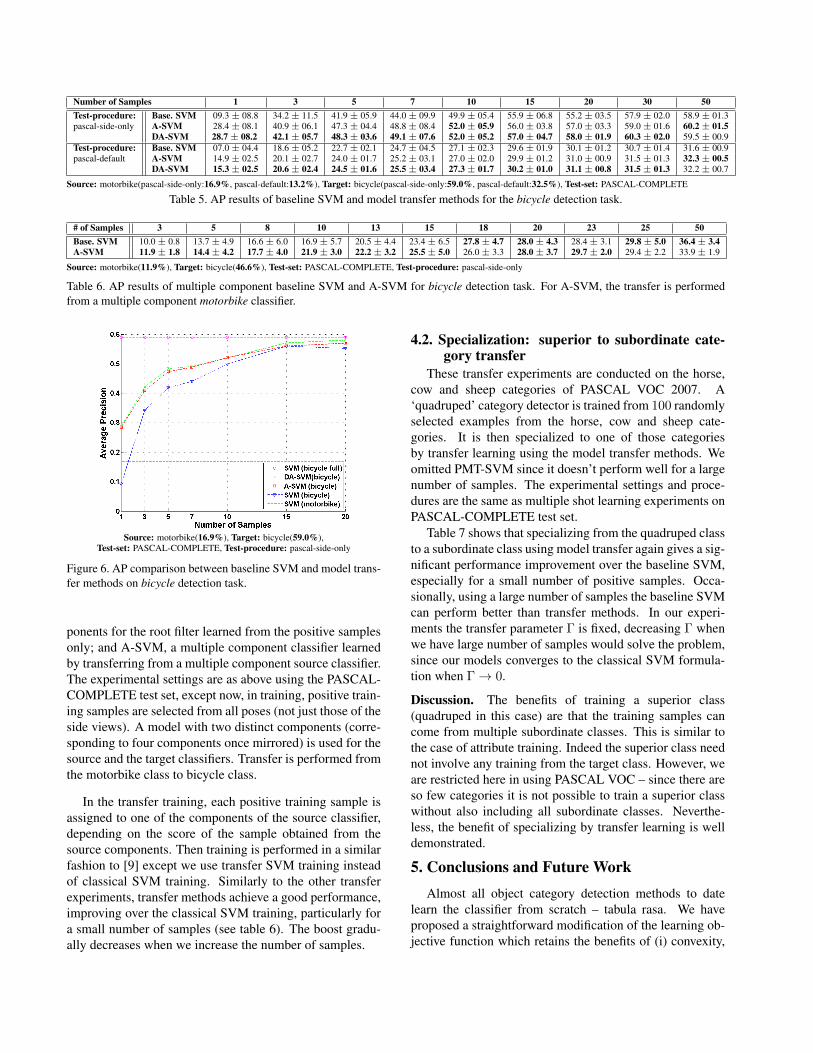
We also evaluated A-SVM and DA-SVM using a largerscale of positive samples on the PASCAL-COMPLETE testset (see table 5 and figure 6). In all the cases A-SVM andDA-SVM perform better that the baseline SVM. DA-SVMis superior to A-SVM except for the 50 samples case.

In summary, the results show a significant improvementthrough transfer learning in terms of higher start and higherslope (refer to figure 4).

4.1.3 Multiple shot learning with multiple components(aspects)

These experiments are conducted on classifiers trained withmultiple components (aspects) (similar to [9]). We comparetwo methods: baseline SVM, a classifier with multiple com-

Number of Samples 1 3 5 7 10 15 20 30 50Test-procedure: Base. SVM 09.3± 08.8 34.2± 11.5 41.9± 05.9 44.0± 09.9 49.9± 05.4 55.9± 06.8 55.2± 03.5 57.9± 02.0 58.9± 01.3pascal-side-only A-SVM 28.4± 08.1 40.9± 06.1 47.3± 04.4 48.8± 08.4 52.0± 05.9 56.0± 03.8 57.0± 03.3 59.0± 01.6 60.2± 01.5

DA-SVM 28.7± 08.2 42.1± 05.7 48.3± 03.6 49.1± 07.6 52.0± 05.2 57.0± 04.7 58.0± 01.9 60.3± 02.0 59.5± 00.9Test-procedure: Base. SVM 07.0± 04.4 18.6± 05.2 22.7± 02.1 24.7± 04.5 27.1± 02.3 29.6± 01.9 30.1± 01.2 30.7± 01.4 31.6± 00.9pascal-default A-SVM 14.9± 02.5 20.1± 02.7 24.0± 01.7 25.2± 03.1 27.0± 02.0 29.9± 01.2 31.0± 00.9 31.5± 01.3 32.3± 00.5

DA-SVM 15.3± 02.5 20.6± 02.4 24.5± 01.6 25.5± 03.4 27.3± 01.7 30.2± 01.0 31.1± 00.8 31.5± 01.3 32.2± 00.7

Source: motorbike(pascal-side-only:16.9%, pascal-default:13.2%), Target: bicycle(pascal-side-only:59.0%, pascal-default:32.5%), Test-set: PASCAL-COMPLETE

Table 5. AP results of baseline SVM and model transfer methods for the bicycle detection task.

# of Samples 3 5 8 10 13 15 18 20 23 25 50Base. SVM 10.0± 0.8 13.7± 4.9 16.6± 6.0 16.9± 5.7 20.5± 4.4 23.4± 6.5 27.8± 4.7 28.0± 4.3 28.4± 3.1 29.8± 5.0 36.4± 3.4A-SVM 11.9± 1.8 14.4± 4.2 17.7± 4.0 21.9± 3.0 22.2± 3.2 25.5± 5.0 26.0± 3.3 28.0± 3.7 29.7± 2.0 29.4± 2.2 33.9± 1.9

Source: motorbike(11.9%), Target: bicycle(46.6%), Test-set: PASCAL-COMPLETE, Test-procedure: pascal-side-only

Table 6. AP results of multiple component baseline SVM and A-SVM for bicycle detection task. For A-SVM, the transfer is performedfrom a multiple component motorbike classifier.

Source: motorbike(16.9%), Target: bicycle(59.0%),Test-set: PASCAL-COMPLETE, Test-procedure: pascal-side-only

Figure 6. AP comparison between baseline SVM and model trans-fer methods on bicycle detection task.

ponents for the root filter learned from the positive samplesonly; and A-SVM, a multiple component classifier learnedby transferring from a multiple component source classifier.The experimental settings are as above using the PASCAL-COMPLETE test set, except now, in training, positive train-ing samples are selected from all poses (not just those of theside views). A model with two distinct components (corre-sponding to four components once mirrored) is used for thesource and the target classifiers. Transfer is performed fromthe motorbike class to bicycle class.

In the transfer training, each positive training sample isassigned to one of the components of the source classifier,depending on the score of the sample obtained from thesource components. Then training is performed in a similarfashion to [9] except we use transfer SVM training insteadof classical SVM training. Similarly to the other transferexperiments, transfer methods achieve a good performance,improving over the classical SVM training, particularly fora small number of samples (see table 6). The boost gradu-ally decreases when we increase the number of samples.

4.2. Specialization: superior to subordinate cate-gory transfer

These transfer experiments are conducted on the horse,cow and sheep categories of PASCAL VOC 2007. A‘quadruped’ category detector is trained from 100 randomlyselected examples from the horse, cow and sheep cate-gories. It is then specialized to one of those categoriesby transfer learning using the model transfer methods. Weomitted PMT-SVM since it doesn’t perform well for a largenumber of samples. The experimental settings and proce-dures are the same as multiple shot learning experiments onPASCAL-COMPLETE test set.

Table 7 shows that specializing from the quadruped classto a subordinate class using model transfer again gives a sig-nificant performance improvement over the baseline SVM,especially for a small number of positive samples. Occa-sionally, using a large number of samples the baseline SVMcan perform better than transfer methods. In our experi-ments the transfer parameter Γ is fixed, decreasing Γ whenwe have large number of samples would solve the problem,since our models converges to the classical SVM formula-tion when Γ→ 0.

Discussion. The benefits of training a superior class(quadruped in this case) are that the training samples cancome from multiple subordinate classes. This is similar tothe case of attribute training. Indeed the superior class neednot involve any training from the target class. However, weare restricted here in using PASCAL VOC – since there areso few categories it is not possible to train a superior classwithout also including all subordinate classes. Neverthe-less, the benefit of specializing by transfer learning is welldemonstrated.

5. Conclusions and Future WorkAlmost all object category detection methods to date

learn the classifier from scratch – tabula rasa. We haveproposed a straightforward modification of the learning ob-jective function which retains the benefits of (i) convexity,



DA-SVM 11.3± 04.5 14.2± 03.4 13.6± 03.0 15.3± 03.0 16.2± 01.7 16.1± 02.7 17.6± 01.0 19.8± 01.9 20.8± 00.4Source: quadruped(pascal-side-only:15.4%, pascal-default:07.9%), Target: horse(pascal-side-only:44.6%, pascal-default:22.3%), Test-set: PASCAL-COMPLETE



DA-SVM 10.6± 02.5 10.3± 03.7 08.7± 02.7 09.6± 03.3 09.7± 02.5 10.6± 01.8 11.1± 01.6 11.5± 00.6 13.3± 00.0Source: quadruped(pascal-side-only:08.1%, pascal-default:07.1%), Target: cow(pascal-side-only:21.5%, pascal-default:14.9%), Test-set: PASCAL-COMPLETE

Table 7. AP results of baseline SVM and specialization using model transfer methods for the horse and cow detection tasks.

(ii) optimization methods honed to the special structure ofan SVM, and also brings the benefit of learning with fewertraining samples. The model transfer methods can act as a‘power-boost’ plug-in to any SVM training scheme.

There are a number clear extensions to the model: (i) Sofar the transfer learning has been applied to the root filterand multiple component scenario of [9], the next step is toextend it to multiple parts. (ii) So far a single feature typehas been used, but the model can also be extended to multi-ple features, such as are used in [25].Acknowledgements. We are very grateful to AndreaVedaldi for insightful discussions and the VLFeat li-brary [24]. Financial support was provided by the RoyalAcademy of Engineering, Microsoft, and ERC grant Vis-Rec no. 228180.

References[1] N. Dalal and B. Triggs. Histogram of Oriented Gradients for Human

Detection. In Proc. CVPR, 2005.[2] J. Deng, W. Dong, R. Socher, L.-J. Li, K. Li, and L. Fei-Fei. Ima-

geNet: A Large-Scale Hierarchical Image Database. In Proc. CVPR,2009.

[3] L. Duan, I. Tsang, D. Xu, and S. Maybank. Domain transfer svm forvideo concept detection. In Proc. CVPR, 2009.

[4] L. Duan, D. Xu, I. Tsang, and J. Luo. Visual event recognition invideos by learning from web data. In Proc. CVPR, 2010.

[5] M. Everingham, L. Van Gool, C. K. I. Williams, J. Winn, andA. Zisserman. The PASCAL Visual Object Classes Challenge 2007(VOC2007) Results, 2007.

[6] M. Everingham, L. Van Gool, C. K. I. Williams, J. Winn, and A. Zis-serman. The pascal visual object classes (voc) challenge. IJCV,2010.

[7] A. Farhadi, I. Endres, D. Hoiem, and D. Forsyth. Describing objectsby their attributes. In Proc. CVPR, 2009.

[8] L. Fei-Fei, R. Fergus, and P. Perona. A Bayesian approach to un-supervised one-shot learning of object categories. In Proc. ICCV,2003.

[9] P. F. Felzenszwalb, R. B. Grishick, D. McAllester, and D. Ramanan.Object detection with discriminatively trained part based models.IEEE PAMI, 2010.

[10] V. Ferrari and A. Zisserman. Learning visual attributes. In NIPS,2007.

[11] M. Fink. Object classification from a single example utilizing classrelevance metrics. In NIPS, 2004.

[12] N. Kumar, A. Berg, P. Belhumeur, and S. Nayar. Attribute and simileclassifiers for face verification. In Proc. ICCV, 2009.

[13] C. Lampert, H. Nickisch, and S. Harmeling. Learning to detectunseen object classes by between-class attribute transfer. In Proc.CVPR, 2009.

[14] X. Li. Regularized Adaptation: Theory, Algorithms and Applica-tions. PhD thesis, University of Washington, USA, 2007.

[15] Mosek: Optimization Toolkit. http://www.mosek.com, 2010.[16] E. Olivas, J. Guerrero, M. Sober, J. Benedito, and A. Lopez. Hand-

book Of Research On Machine Learning Applications and Trends:Algorithms, Methods and Techniques. 2009.

[17] F. Orabona, C. Castellini, B. Caputo, A. Fiorilla, and G. Sandini.Model adaptation with least-squares svm for adaptive hand prosthet-ics. In Proc. ICRA, 2009.

[18] A. Quattoni, M. Collins, and T. Darrell. Transfer learning for imageclassification with sparse prototype representations. In Proc. CVPR,2008.

[19] M. Rohrbach, M. Stark, G. Szarvas, I. Gurevych, and B. Schiele.What helps where – and why? semantic relatedness for knowledgetransfer. In Proc. CVPR, 2010.

[20] K. Saenko, B. Kulis, M. Fritz, and T. Darrell. Adapting visual cate-gory models to new domains. In Proc. ECCV, 2010.

[21] M. Stark, M. Goesele, and B. Schiele. A shape-based object classmodel for knowledge transfer. In Proc. ICCV, 2009.

[22] T. Tommasi and B. Caputo. The more you know, the less you learn:from knowledge transfer to one-shot learning of object categories. InProc. BMVC., 2009.

[23] T. Tommasi, F. Orabona, and B. Caputo. Safety in numbers: Learn-ing categories from few examples with multi model knowledge trans-fer. In Proc. CVPR, 2010.

[24] A. Vedaldi and B. Fulkerson. VLFeat: An open and portable libraryof computer vision algorithms. http://www.vlfeat.org/, 2008.

[25] A. Vedaldi, V. Gulshan, M. Varma, and A. Zisserman. Multiple ker-nels for object detection. In Proc. ICCV, 2009.

[26] G. Wang, D. Forsyth, and D. Hoiem. Comparative object similarityfor improved recognition with few or no examples. In Proc. CVPR,2010.

[27] J. Yang, R. Yan, and A. Hauptmann. Adapting svm classifiers to datawith shifted distributions. In ICDM Workshops 2007, 2007.

[28] J. Yang, R. Yan, and A. Hauptmann. Cross-domain video conceptdetection using adaptive svms. In ACM Multimedia, 2007.

[29] X. Yu and Y. Aloimonos. Attribute-based transfer learning for objectcategorization with zero/one training example. In Proc. ECCV, 2010.

[30] A. Zweig and D. Weinshall. Exploiting object hierarchy: Combiningmodels from different category levels. In Proc. ICCV, 2007.

tabula rasa: model transfer for object category …vgg/publications/2011/aytar11/aytar...tabula...

Documents