systems approach to the flexible pavement design problem · a systems approach to the flexible...
TRANSCRIPT

A SYSTEMS APPROACH TO THE FLEXIBLE PAVEMENT DESIGN PROBLEM
By
F. H. Scrivner Research Engineer
W. M. Moore
Associate Research Engineer
W. F. McFarland
Assistant Research Economist
and
G. R. Carey
Research Associate
Research Report Number 32-11
Extension of AASHO Road Test Results
Research Study ~umber 2-8-62-32
Sponsored by
The Texas Highway Department In Cooperation with the
U. s. Department of Transpor£ation Federal Highway Administration
Bureau of Public Roads
October, 1968
TEXAS TRANSPORTATION INSTITUTE Texas A&M University
College Station, Texas
--- - --- - - - - - - - - - - - - -


Page CHAPTER 1 - INTRODUCTION • . . . . . . . 1
CHAPTER 2 - PHYSICAL VARIABLES • . . . . 3
2.1- Design Variables 4
2.2 -Deflection Variables .. 6
2.3 - Traffic Variables .. 8
2.4 - Performance Variables 10
2.5 - Summary of Definitions. . . . 19
CHAPTER 3 - MATHEMATICAL RELATIONSHIPS ASSUMED TO EXIST BETWEEN THE VARIABLES. · · . . 22
3.1- Discussion of Equations . . . . . . . . 23
3.2 - The Deflection Equation • 25
3.3 -The Traffic Equation. • 26
3.4 - The Performance Equation. . 27
3. 5 - Predictions From The Equations. 28
CHAPTER 4 - EVALUATION OF STRENGTH COEFFICIENTS. 31
4.1 - Mathematical Basis for Coefficient Determinations 32
4.2 - Procedure for Estimating The Subgrade Coefficient 33
4.3 -Procedure for Estimating The Coefficient of a Base Material • . . • . • • • . • . . • • . . . 35
4.4 - Estimating The Coefficient of a Subbase Material. 37
CHAPTER 5 - EVALUATION OF SWELLING CLAY PARAMETERS 38
CHAPTER 6 - COSTS USED IN THE COMPUTER PROGRAM • 39
6.1 ~ Cost of Initial Construction . · .. • • . 41
i

6.2 - Annual Routine Maintenance Costs .
6.3 - Overlay Construction Cost ••
6.4- Seal Coat Costs ..• 44
6.5 - Traffic Cost of Overlay •• 46
6.6 - Analysis Period and Salvage Value ••••• 72
6.7- Interest Rate •. • • • • • • • 'It 74
CHAPTER 7 - INPUT/OUTPUT OF THE COMPUTER PROGRAM 75
7.1- Inputs to Computer Program. 75
7.2 -Outputs of Computer Program. . . . . . . . 78
CHAPTER 8 - THE OP!IMIZATION MODEL. 79
8.1 ~ Initial Construction • 81
8.2 - Overlay Optimization 83
APPENDIX 1 - INPUT DATA REQUIREMENTS. 86
ii

LIST OF FIGURES
Figure
1 A pavement section of n layers . . • •
2 Position of Dynaflect sensors and load wheels·
3 Typical deflection basin • · • . · · · • • · · ·
4 Typical traffic curves
5 A pavement performance curve
6 Effect of foundation movements in the absence of traffic for P 2 ' = 1.5 . . . . . . . . . . . . . . . .
7 Effect of foundation movernen ts in the absence of traffic for P2 ' = 0 . . . . . . . . . . .
8 Performance and serviceability 1oss curves
9 Effect of overlay construction on serviceability loss
10
11
12
13
14
15
16
17
18-29
curves • . • •
Effect of a on performance period length.
Speed profile for vehicles stopped during overlay .
Speed profile for vehicles not stopped but slowed during over lay . . . . • • . • .
Method I. Traffic routed to shoulder .
Method II. Alternating traffic in one lane
Method III. Two lanes merge, non-overlay direction not affected • • • . . • • . • • .
Method IV. Overlay direction traffic routed to non-over lay lanes • • . . • . . • • . . • . . •
Method V. Overlay direction traffic routed to frontage road or other parallel route . • . • . . • •
Input formats, data cards 1 through 28 + NM
iii
5
7
7
9
11
. 12
12
14
14
18
49
51
58
58
58
59
59
88


LIST OF TABLES
Table
1 District Temperature Constants ••••••.• . 17
2 Prediction of 20-Year Performance Curve for a
3
4
5
6
7
8
9
10
Heavy Design •••.•.•.•.•••••••••.•.• 29
Prediction of 20-Year Performance Curve for a Light Design . . •••••••
In Situ Subgrade Coefficients •••
In Situ Base Material Coefficients
Cost of -Speed Change - Rural Roads
Cost of Speed Change - Urban Roads
Operating and Time Costs at Uniform Speeds
Operating and Time Cost of Delay •
Capacity Table . •
iv
30
. 34
• • 36
53
• • 54
• 55
• • • 56
67

ACKNOWLEDGEMENTS
The authors owe special thanks to the following individuals of the
Texas Highway Department:
The District Engineers and project contact men of all 25 districts,
for their cooperation and assistance during the routine field testing
program carried out over the past several years.
Messrs. Joseph G. Hanover and J. C. Roberts, District Engineers at
Bryan and Abilene, respectively, for their assistance in a special field
testing program devbted to the measurement of material strength coefficients.
Mr. James 1. Brown, Senior Designing Engineer, of the Department's
Austin office, for his many helpful suggestions made during the development
stages of the computer program.
The authors also wish to acknowledge the valuable assistance of
Mr. Chester Michalak, Research Assistant, Texas Transportation Institute,
who helped in the analysis work and M. B. Phillips, Assi~tant Research
Geologist, Texas-Transportation Institute, who assisted in the preparation
of the report.
The opinions, findings, and conclusions expressed in this publication
are those of the authors and not necessarily those of the Bureau of Public
Roads.
v

CHAPTER 1 - INTRODUCTION
This report stems from research performed in Project 2-8-62-32,
"Application of AASHO Road Test Results to Texas Conditions." Its
purpose is to make available to the Texas Highway Department a rec
ommended procedure for the design of flexible pavements. The proce
dure takes into account both physical and cost variables, and provides
a means for making design. decisions based on probable overall costs,
rather than on initial construction costs alone.
Physical variables .. ar;e treated in terms of how they affect the
serviceability-time curve of the pavement. Means for evaluating them
in any given locality are presented.
Cost variables considered are the following: initial construction,
routine maintenance, periodic seal coating, overlay construction, user
costs due to traffic delays during overlay construction, and salvage
value. All future costs, discounted to present value, are added to
initial construction costs to form the overall cost.
Because of the number of variables involved, and the need to
investigate all possible designs meeting selected criteria, initial
attempts to prepare the usual curves or nomograms for the designer's
use were quickly abandoned. The solution of the design equations, and
the search for the least-cost design, are made in a computer. The com
puter program, and a brief description of what it contains, are included
in this report.
In writing the computer program, the attempt was made to provide for
ease of change, so that as new findings are made in flexible pavement
- 1 -

research, they can be incorporated in to the program with a minimum 'of
effort. Me.anwhile, the program is recominended as an aid not only to
the design engineer but also to the research engineer in establishing
where emphasis should be placed in pavement research.
In order to shorten the report for the convenience of the design
engiLu~er, to whom it is addressed, practically all supporting data and
documentation have been excluded: these will be treated in later reports.
- 2 -

CHAPTER 2 - PHYSICAL VARIABLES
There :is a large group of physical variables associated with mate
rials, construction, traffic and environment that affect pavement perfor
mance. Of these, a few have been <quantified and their effect on pavement
performance has been established, at least approximately. This chapter
defines the physical variables of the latter group considered in this
design method; and describes, qualitatively, their effect on pavement
performance.
- 3 -

2.1 Design Variables
The sketch in Figure 1 represents a pavement composed of n layers
above the sub grade level. The material in each of these layers, and in
the foundation layer, is characterized by a strength coeffi~ient, a., 1.
where the subscript, i, identifies the position of the layer in the
structure. Layers are numbered consecutively from the top downward;
thus, i = 1 for the surfacing layer, and i = n + 1 for the foundation
layer, which is considered to be of infinite thickness. The thickness
of any layer above the foundation is represented by the symbol, Di.
Measured in situ values of the strength coefficient, a, range from
about 0.17 for a wet clay to about 1.00 for a strongly stabilized base
material. No way has been found for predicting these values with suit-
able accuracy from laboratory tests. For the present the strength coef-
ficient of a material proposed for use in a new pavement in a particular
locality must be estimated from deflection measurements made on the same
type of material in an existing pavement located in the same general area.
Details of the procedure will be given later.
- 4 -

LAYER
LAYER 2
LAYER
LAYER n
FOUNDATtON {LAYER n+l)
PAVEMENT SURFACE
0· I
On+l Dn+l =oo
I
Figure 1:, A pavement section of n layers above the subgrade level.
-5-

2. 2 Deflection Variables
An important feature of this design procedure is the use of the
Dynaflect* for measuring deflections on existing highways. Descriptions
of the instrument and examples of its use in pavement research have been
published previously(])(~)(~). Suffice it.to say here that a dynamic
load of 1000 lbs, oscillating sinusoidally with time at 8 cps, is applied
through two steel load wheels to the pavement, as indicated in Figure 2.
Five sensors, resting on the pavement at the numbered points shown in the
figure, register the vertical amplitude of the motion at those points in
thousandths of an inch (or mils).
A deflection basin of th~ type illustrated in Figure 3 results from
the Dynaflect loading. The symbol w1 represents the amplitude--or deflec
tion--occurring at Point 1, w2
is the deflection at Point 2, etc.
A deflection variable important to this design procedure is the
surface curvature index, S~ shown in Figure 3 and defined by the equation,
S = w1 - w2 • The value of S for a proposed design can be predicted with
reasonable accuracy from the deflection equation to be given in a later
chapter, provided that the values of the design variables are known. Two
designs are assumed to be physically equivalent if they have the same
value of S, and the same swelling clay parameters. (Swelling clay pa
rameters are discussed in a later section). Of two designs with differing
values of S, but with the same swelling clay parameters, the design with
the lower value of Sis assumed to be the better (longer lived).
*Registered Trademark; Dresser Industries,- Inc., Dallas, Texas
- 6 -

:Figure 2: Position of Dynaflect sensors and load wheels during test. Vertical arrows represent load wheels. Points numbered 1 through 5 indicate location of sensors •
. A B ORIGINAL SURFACE
' . 24·--... \=- ----~DEFLECTED SURFACE
DEFLECTION (W1 ) \ \
Figure 3:
' ·· INDEX (5 = w, .... w, )
c + w
Typical deflection basin reconstru·cted from Dynaflect readings. Only half of basin is measured •. S is the deflection variable used to represent the design.

2.3 Traffic Variables
In describing traffic, it i$ first necessary to select the total
period of time following construction that is of interest to the design
engineer. This is usually in the order of 20· to 40 years, and is termed
the analysis period; its length is represented by the symbol, C. Defini-
tions of the other traffic variables follow.
t = time, years. t = 0 at the time of initial construction.
r = the ADT, in one direction, when t = o. 0
r = the ADT, in one direction, when ti =c. c
N = the total number of . equivalent applications of an
18-kip single axle load (computed by the standard
AASHO method) that will have passed over the pavement
in one direction at any time, t.
N = N at t = C. c
It is assumed that the design engineer can obtain the values of r 0 ,
rc and Nc from the Planning Survey Division of the Highway Department for
any particular location. The relationship between N and t will be given
in a later chapter, and will be referred to as the traffic equation.
Typical plots of N versus t for light, moderate and heavy traffic are
shown in Figure 4.
An assumption made with regard to traffic on multi-lane highways is
that commercial vehicles use the outer lane.
- 8 -

--
!
10.0 HEAVY TRAFFIC
........ r o = 33,000 Ul.
rc =51, 000 z 0 Nc = 11,249,000 _J _J
5.0 -~ -z
0
1.0
-U) . MODERATE TRAFFIC z
0 ro = 2,100 _J 0.5 ..J rc = 3,750 ~ Nc= 860,000
z
0
0.08
- LIGHT TRAFFIC U) 0.06 r0 = 175 z 0 rc = 350 ...J 0.04 Nc= 67,000 ...J
~ - 0.02 z
0 0 2 4 6 8 10 12 14 16 18 20
T I M E , t (YEARS)
Figure 4: Typical traffic curves.
- 9 -

2.4 Performance Variables
The serviceability index (P) versus time (t) curve for a pavement
is referred to as the performance curve of the pavement. A performance
variable is any variable describing, or in any way affecting, the per-
formance curve. Obviously the design, deflection and traffic variables
discussed above are also performance variables.
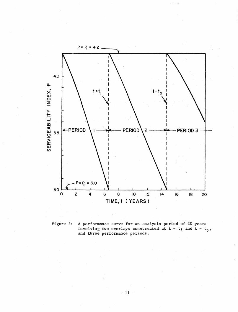
Figure 5 is ·a-~ computed ·~performance- curve-· for-a flexible_ pavement
to which two overlays have been applied within an analysis period of
20 years. A performance period is defined as the time, in years, from
the completion of initial or overlay construction, when P = P1, to the
time when the serviceability index next reaches a predetermined value,
P2
. Performance periods are numbered in chronological order, Period 1
being the first.
Except in the computation of user costs due to traffic delays--to
be discussed later in the report--the time required to construct an overlay
is neglected. th The value of t at the end of the k period, or at the begin-
ning of the next period, is represented by the symbol, tk.
An important phenomenon affecting the performance curve is that of
uneven volumetric expansion and contraction of materials in the foundation.
This effect is illustrated in Figure 6, which portrays the computed service-
ability history of four pavements constructed on foundation materials of
four different types. These performance curves represent pavements Q2!
subjected to traffic: only the effect of foundation movements issshown.
In the case of the three lower curves in Figure 6 the variable, P,
approaches an ultimate value, P2 ', taken here as 1.5.· The variable, b1 ,
- 10 -
a.. .. X UJ 0 z
>t_, m <(
4.0
P= P. = 4.2---
I
I I I I
t = t I I I
~ I I I I I
I I t I I I
t=t2 :
~ I I I I I
~ 3.5 •rc: -----i.L.....-· -PERIOD 3 --+--1
> 0: w (/)
I I I
3.0 .._......._._,._ __ ..ol-. _ _,l,__._ _ _._ __ ~ _ _.... __ ._.......___, __ _._ _ ___,.,~
0 2 4 6 8 10 12 14 16 18 20
TIME;t ( YEARS)
Figure 5: A performance curve for an analysis period of 20 years involving two overlays constructed at t = ti and t = t 2 , and three performance periods.
- 11 -
--
1

a..
a.
4.0
3.0
·2.0
1.0
0
b1=o b, =0.02
p~ = I. 5
0 2 4 6 8 10 12 14 t6 18 20
TIME, t (YEARS)
Figure 6: Four performance curves illustrating the effect of foundation movements in the absence of traffic. These curves approach an assumed lower limit of p = 1.5.
4.0·
3.o·
2.0
1.0
0 0
b, = 0.02
bj=0.32
2 4 6 8 10 12 20
TIME, t (YEARS)
Figure 7: Same as Figure 6,. but. the curves here have a lower limit of P = 0.
- 12 -

represents the relative rate at which P approaches its ultimate value.
Thus, the curve labeled "b1 = .02" approaches the 1.5 serviceability
level much more slowly than the curve la~e=lletl.' ''o1 = . 32."
Not much is known about the quantity P2 '.; since the relevant
serviceability index data are not available. The ultimate value of P
in the absence of traffic may be greater or less than the value of 1.5
used in Figure 6. For comparison with Figure 6, performance curves in
the absence of traffic for P2 ' = 0 are shown in Figure 7.
If P2 ' is fixed at an assumed value, b1
can be estimated from
serviceability index data on new pavements which have not been opened
to traffic but nevertheless have roughened due to swelling clays. Very
limited data of this type have indicated an upper limit of approximately
0.3 for h1 when P2 ' is assumed to be zero. The theoretical lower limit
of bl is zero, for any value assigned to P2'.
No data being available for estimating Pz', a value of zero has been
assumed for the present.
In the development of a relationship between performance variables
based on AASHO Road Test data, it was necessary to define a serviceability
loss function, Q, as follows:
Q = Is - P - Is - P 1
where P and P1
are as previously defined, and the constant, S, is the
the ore tical upper limit of P. With P1
! fix~d, i (a:~ colll11l(i)n:ly~~ us~d,Lvallilet;::is:-:
4.2), Q increases as the serviceability index, P, decreases, as shown
in Figure 8. In this figure we have replotted one of the performance
curves given in Figure 7, and have also plotted the corresponding curve
- 13 -

a.
0
4 b, =0.08
3
2
0.5
p' =0 2 Q~= I. 3 4 1.2
o.a ·a
0.4
TIME , t (YEARS)
Figure 8: A performance curve and its corresponding service- , ability loss curve, with no traffic operating.
b, =0.04
o'2 :; t.34
6 10 t2
TIME, t (YEARS)
b2=0.025 Q~= 1.34
14 16 18 20
Figure 9: The assumed effect on the serviceability loss curve of the construction of an overlay at Point A. The slope of the curve at A and B is the same; both branches approach the same asymptote.
- l4 -

for Q. We refer to the Q versus t curve as the serviceability loss
curve, to distinguish it from the P versus t curve already defined
as the performance curve. The P'and Q curves approach ultimate values
of zero and 1.34 respectively (Pz' = 0; Q2 ' = 1.34).
As previously indicated the serviceability loss or Q-curve of
Figure 8 is taken to represent a pavement which has carried no traffic.
It was necessary to form an hypothesis as to how the placement of an
overlay would affect such a Q-curve. The hypothesis adopted was simply
this: (1) the slope of the curve at t = tk is the same before and after
placement of an overlay, and (2) the ultimate value, P2 ', of the service
ability index remains unchanged. The graph shown in Figure 9, wherein
the slope of the Q-curve is the same at points A and B, illustrates
this hypothesis.
The adoption of the hypothesis requires the computation of a new
value of b at the beginning of each performance period, based on the
value applicable to the preceding period. Thus, for the Q-curve shown
in Figure 9, the value of b1 assigned to the first period is .04,
while the computed value of b2 applying to the second period is .025.
Both branches of this Q-curve would, if extended, approach an ultimate
value of 1.34 (Q2 ' = 1.34) corresponding to P2 ' = 0.
One other performance variable must be mentioned, a daily temperature
constant, a, and its effective value over one year, a. This variable arose
during an analysis of the AASHO Road Test data; and is believed to represent
an increased susceptibility of asphaltic concrete to cracking under traffic
in cold weather. The daily constant, a, is defined as the average of the
maximum and minimum daily temperature, less 32°F. The change in the loss
- 15 -

function, Q, occurring as the result of one day's traffic depends in
part on the value of a. for that day. By summing the daily changes in
Q, a single equivalent value of a, designated ?!; can be used to estimate
the change in Q for a full year.
For use in the computer program a value of a has been computed for
each District, based on mean values of the high _and low daily temperatures
averaged over a ten year period. Values are given in Table 1.
It can be seen from Table 1 that the District values of a vary
from a minimum of 9° in District 4 to a maximum of 38° in District 21.
Figure 10 illustrates the effect of a on the performance curve.
The performance equation relating the variables discussed in
this section, and the effect on the computed performance curve of
the design and traffic variables, will be discussed late:r in the
report.
-16-

TABLE 1 - ·DISTRICT TEMPERATURE CONS'I'.t\.lf£S
Temp. Temp. Temp. Temp. Temp. Const. Con st. Cons t. Cons t. Cons t.
Dist. (rr) Dist. (a) Dist. (c£) Dist. fr£) Dist. (a)
1 21 6 23 11 28 16 36 21 38
2 22 7 26 12 33 17 30 22 31
3 22 8 26 13 33 18 26 23 25
4 9 9 28 14 31 19 25 24 24
5 16 10 24 15 31 20 32 25 19
-17-

0..
4.0
2
b, = .02 Pz = 0 s = .4
4
b = .02 I
P2 = 0 s :1 • 4
a=9 I I I I
10 r2
TIME, t (Years)
ii= 38
14
.0168 0 .3
16
I
t8 20
ll_b2 = .0145
Pa= 0 1-·s = .3 I I I I I
3.00 4 6 8 l2 14 -t6 ... 20
TIME , t ( Y e a r s)
Figure 10: Performance periods are lengthened by an :rncrease in a, as illustrated here for the extreme values in Texas.
18

2.5 Summary of Definitions of Physical Variables
For the convenience of the reader in examining the equations to
be given in the next chapter, we repeat below, in a more concise form,
the definitions previously given. Also included in the list are a few
additional symbols not previously defined but appearing in the equations.
Design Variables -
a. = the strength coefficient of the ith layer of a pavement, 1.
i = 1, 2, .. n + 1.
Di = the thickness of the ith layer in inches.
Deflection Variables -
D n+l
co
w j
th the deflection sensed by the j sensor of the Dynaflect.
r· J
distance~ in inches, from the point of application of
. h D fl 1 d h 'th e1.t er yna ect oa , to t e J sensor.
Traffic Variables -
t time (years) since initial construction.
N total number of equivalent applications of an 18-kip
axle that will have been applied in one direction during
the time, t. N is expressed in millions.
c length in years of the analysis period.
N = N c when t c.
Nk N when t tk (defined below).
ro ADT (one direction) when t = 0.
rc = ADT (one direction) when t c.
- 19 -

Performance Variables -
P = the serviceability index at time, t.
pl = the expected maximum value of p~ occurring only immediately
after initial or overlay construction.
P2 = the specified value of P at which an overlay will be applied.
P2 ', a swelling clay parameter = the assumed value of P at
t = oo, in the absence of traffic. In general, 0 ~ P2
' ~ P1 •
bk is a swelling clay parameter applying to the kth performance
period. A value between zero and 0. 3 must be specified
for h1, depending on the expected activity of foundation
clays.
tk = the value of t at the end of the kth performance period,
or the beginning of the next period. t 0 = 0.
Q, the serviceability loss function = Is - P - Is - P1 .
Q2 = Q when P
Q ' =Is - P ' 2 2 .
a, a daily temperature constant = 1/2 (maximum daily temperature
+ minimum daily temperat~re) - 32°F.
a = the effective value of a for a typical year in a given
locality, defined by the formula for the harmonic mean--
n
m i-1. i
where n is the number of days in a year, and a. is the ~
- 20 -

1 f f h .th d f h va ue o a or t e 1 ay o t e year. To obtain an
approximate value of a for this report, the formula was
used with n = 12, and a. = the mean value of a for the 1
.; th m· ·onth d t · d L average over a en year per1o •
- 21 -


CHAPTER 3 - MATHEMATICAL RELATIONSHIPS ASSUMED . TO EXIST BETWEEN THE PHYSICAL VARIABLES
In this chapter are presented a set of empirical equations relating
the physical variables previously treated. As indicated in Chapter 1,
the data upon which they are based, and the procedures followed in their
derivation, will be the subject of future reports.
- 22 -

3.1 Discussion of Equations
The mathematical relationships assumed to exist between the variables
discussed in Chapter 2 are expressed in the form of three empir~cal equations--
a deflecti.on equation, a traffic equation and a performance equation. The
deflection equation relates the deflection variable S to the design vari-
ables ai and Di. The traffic equation relates the traffic variable N
to the traffic variables C, r0
, rc, Nc and t. The performance equation
relates the serviceability loss function Q to the deflection variable S,
the performance variables a, Q2 ' and bk' and the traffic variables Nand
t. To facilitate discussion, the three equations can be written in ab-
breviated notation as follows:
Deflection Equation: S
Traffic Equation: N
Performance Equation: Q = F(S, ct., Q2 ' , bk, N, t)
where the symbol F is read "a known function of. 11
To illustrate how these equations would be used to solve a simple
design problem involving only physical variables, suppose that it is
desired to calculate the length, t 1 , of the first performance period
for a pavement of known design. In addition to the design parameters
ai and Di, values of the following quantities must be known to obtain a
solution: C, r0
, rc, Nc, Q2 , Q2 ' and b1 .
To clarify the procedure to be followed in solving this problem we
rewrite the three equations as follows with the known variables underscored:
s = F(ai, Di)
N = F(C, ro, rc, Nc, tl) - -
Q2 = F(S, a, Q2 ' bl' N, tl) '
- 23 -

On examining the preceeding equations we see at once that of the
three unknowns, one of them--the variable S--can be computed directly
from the first equation. The computed value of S is then substituted
in the third equation. At this stage we have two equations (the second
and third) involving two unknowns, N and t1
• These two equations are
then solved simultaneously for N and t1: the value of t 1 so obtained
is the quantity we set out to find.
The computing procedure indicated above is but one of many included
in the computer program. It was used here simply to illustrate one way
in which the assumed relationships between the physical variables are
used in this design procedure. Further discussion of the computer
program will be reserved for a later chapter.
- 24 -

3.2 The Deflection Equation
The empirical equation used in this method for estimating the surface
curvature index S from the design variables ai and Di was developed from
deflection data gathered on the A&M Pavement Test Facility located at
Texas A&M University's Research Annex near Bryan. A description of the
facility is contained in Research Report 32-9 (i). The equation, not
previously published, is given below:
where
co = 0.891,
c1 4.503,
c2 = 6.25,
a = D = 0, 0 0
1 k-1 2
+ c ..... o: a. D1·) '"'- i=O ~
and the other variables are as previously defined.
(1)
The documentation of this equation will be the subject of a later
report.
- 25 -

3.3 The Traffic Equation
The Traffic Equation was furnished by Mr. James Brown of the Texas
Highway Department and is given below in the form used in this method.
N 1_,2rtk+(r -r)tk1-N = c o c o ( 2) k C(r + r ) C
. 0 c
where the symbols are as previously defined.
- 26 -

3.4 The Performance Equation
The empirical relationship between the performance variables used in
this method was developed from AASHO Road Test data and then modified to
include the swelling clay variables, bk and P2 ', previously discussed.
It is given below in the form it is used in the computer program •
....
+ q2 • (1 - e~bk(i:k ~ tk~l>J (3)
where the variables are as previously defined.
The second term in the brackets was added to represent the effect
of swelling clays.
This equation applies to the kth performance period. Documentation
of the equation will be the subject of a later report.
- 27 -

3.5 Predictions From The Equations·
Using the computing procedure outlined in Section 3.1, a numberccif
examples have been worked out and the results recorded in Tables 2 and
3 for the purpose of illustrating the predicted effect of some of the
variables on performahce period length.
Table 2 is concerned with a fairly heavy initial design (4"-of
asphaltic concrete on 20" of base material) to which successive l-inch
overlays are added as necessary. Three levels of traffic (heavy, moderate,
light) and seven levels of the swelling clay parameter, b1
, are considered.
Table .3 treats a lighter design (2" of asphaltic concrete on 12'' of
base material) to which successive 2-inch overlays are added when required.
Two levels of traffic (moderate, light) and seven levels of b1
are con
sidered.
Each of the tables serves to illustrate the strong effect of the
swelling clay parameter as it ranges from zero to 0.32. In fact, for
b1 > .04 in either table, the effect of foundation movements appears to
overshadow the effect of large changes in traffic.
- 28 -

N 1.0
TABLE 2: PREDICTIONS OF 20-YEAR PERFORMANCE CURVE FROM DEFLECTION, PERFORMANCE AND TRAFFIC EQUATIONS FOR A SELECTED INITIAL DESIGN, AND SUCCESSIVE ONE-INCH OVERLAYS
(~ = 25, other variables as shown below)
FROM FROM PERFORMANCE AND TRAFFIC EQUATIONS: TRAFFIC PERFORMANCE* DESIGN PARAMETERS DEFLECTION Elapsed Time, t (years), to End of Performance
(See Figure 4) PERIOD Strength Coefficients Layer Thickness ~in) EQUATION: Period For Pz' = 0 and bl = the value indicated for Qarameters) NO. a± a2 a D D2 S ~mils2 b 1=0 b2=.01
Heavy 1 .75 .60 Jo 4 20 .108 20.0 ' 0.0 2 • 75 .60 .20 5 20 .092 3 .75 .60 .20, 6 20 .080 4 • 75 .60 .20 7 20 .070 5 .75 .60 .20 8 20 .062
(3.61) (2.99)
Moderate 1 .75 .60 .20 4 20 .108 20.0 20.0 2 • 75 .60 .20 5 20 .092 3 .75 .60 .20· 6 20 .080 4 • 75 .60 .20 7 20 .070 5 .75 .60 .20 8 20 .062
(4 .16) (3.6.6)
Light 1 .75 .60 .20 4 20 .108 20.0 20.0 2 • 75 .60 .20 5 20 .092 3 .75 .60 .20 6 20 .080 4 .75 .60 .20 7 20 .070 5 .75 .60 .20 8 20 .062
(4.20) (3.70)
* A performance period begins with the serviceability index, P, at 4.2 and ends either when P has dropped to 3.0, or when the end of the 20-year analysis period has been reached.
** Figures in parenthesis are values of P at the end of the 20-year analysis period.
bl=.02 bl=.04 b]=.08 b~=.16 bl=.32 14.0 9~0 5.0 3.0 1.5 20.0 20.0. 12.5 7.5 4.0
20.0 14.5 s.o 20.0 14.0
20.0 (3.83) (3.11) (3.37) (3.55) (3.41)
20.0 12.0 6.0 3.0 1.5 20.0 15.5 8.0 4.0
20.0 16.0 8.0 20.0 14.5
20.0 (3 .. 16) (3.69) (3. 85) (3. 83) (3.57)
20 .. 0 12 .• 0 6.0 3.0 ~.5 20.0 15.5 8.0 4.0
20.0 16.0 8.0 20.0 14.5
20.0 (3.21) (3. 70) (3. 86) (3. 84) (3.57)

w 0
TABLE 3:- PREDICTIONS OF 20...;YEAR PERFORMANCE CURVE FROM DEFLECTION, PERFORMANCE AND TRAFFIC EQUATIONS FOR A SELECTED INITIAL DESIGN, AND SUCCESSIVE TWO-INCH OVERLAYS.
(a= 25, other variables as shown below)
FROM FROMiPERFORMANCE AND TRAFFIC EQUATIONS: TRAFFIC PERFORMANCE* DESIGN PARAMETERS DEFLECTION Elapsed Time, t (years), to End of Performance
(See Figure 4) PERIOD Strength Coefficients Layer Thickness ~in~ EQUATION: Period for P2 ' = 0 and b] = the value indicated for par~meters) NO. -~--- a') _a_L__ DJ D S (mils) b 1=0 b 1=.01 b]=.02 !4=.04 b,==_.0_8 b1=.16 b 1 =. 32
Moderate 1 .75 .60 .20 2 12 .482 20.0 16.0 12.0 8.0 5.0 3.0 1.5 2 • 75 .60 .20 4 12 • 303 20.0 20.0 20.0 12.5 7.5 4~0 3 .75 .60 .20 6 12 .199 20.0 15.0 8.0 4 .75 .60 .20 8 12 .137 20.0 14.5 5 .75 .60 .20 10 12 .100 20.0
(3.25) (4.03) (3.71) (3.04) (3.45) (3.69) (3. 17)
Light 1 .75 .60 .20 2 12 .482 20.0 20.0 20.0 12.0 6.0 3.0 1.5 2 .75 .60 .20 4 12 .303 20.0 15.5 8.0 4.0 3 .75 .60 .20 6 12 .199 20.0 16.0 8.0 4 • 75 .60 .20 8 12 .137 20.0 14.5 5 • 75 .60 .20 10 12 .100 20.0
(4.14) (3.63) (3.12) (3.69) (3 .·69) (3.83) ( 3. 57)
* A performance pe·riod begins with the serviceability index, P, at 4. 2 and ends either when P has dropped to 3.0, or when the end of the 20-year analysis period has been reached.
** Figures in pa.renthesis are values of P at the end of the 20-year analysis period.


CHAPTER 4 - EVALUATION OF STRENGTH COEFFICIENTS
It was mentioned in Chapter 2 that the strength coefficient of a
material proposed for use in a new pavement in a particular locality
must be estimated from deflection measurements made on the same type of
material in an existing pavement in the same general area. This Chapter
explains how the deflection equation can be used for calculating values
of coefficients, and gives recommended testing procedures.
- 31 -

4.1 Mathematical Basis for Coefficient Determinations
It has been found that the deflection equation (Equation 1, Section 3. 2)
can be used in conjunction with a Dynaflect test to estimate the coefficients,
a1
and a2 , of a simple two-layer structure. Since such simple structures
rarely exist, the following assumptions must be made when real pavements
are considered: (1) all the layers above subgrade level are assumed to
form~· layer having a composite coefficient, a1
, and a thickness equal
to the total pavement thickness; and (2) all the material below subgrade
level is assumed to have a composite coefficient, a2
•
For this case the deflection equation can be written in generalized
form for wl and w2 as follows:
w1 =,F (al, a2' Dl, rl) ---
w2 = F (al, a2' Dl, r2) -
where the known quantities are underlined. Here, n1 is the total pavement
thickness at the point where the Dynaflect test is made while w1 and w2
a~ measured values of deflection. The symbols r 1 and r 2 have been pre
viously defined. These two equations can be solved for the two coefficients,
al and a2.
If the pavement above subgrade level consists of only two layers....:-a
surfacing and a base layer--and if the surfacing layer is relatively thin--
say less than 10% of the base thickness--then the composite coefficient a 1
obtained in this manner may be taken as a fair estimate of the in situ
coefficient of the predominate base material. On the other hand, the
value of the subgrade coefficient, a2
, is believed to.be largely inde
pendent of the makeup of the pavement, and ~UB· can be taken as a
fair estimate of the subgrade strength regardless of the composition of
the overlying layers. - 32 -

4.2 Procedure For Estimating The Subgrade Coefficient
The recommended procedure for estimating the coefficient of the
subgrade of a proposed rtew pavement is given below:
1. Select an existing pavement, near the proposed new location,
having a foundation similar to that of the proposed new
pavement.
2. At selected test points uniformly spaced at 100 feet or
more, make Dynaflect tests in the outer wheel path; two
tests should be made near each test point, spaced about
five feet apart.
3. At or near each test point drill a four to six-inch hole,
measure material thicknesses and record descriptions of the
materials encountered. Record total pavement thickness, and
explore the subgrade to the depth necessary to confirm its
similarity to the subgrade of the proposed new pavement.
4. Using the special computer program, "In Situ Material Coefficients
From Dynaflect Data," supplied to the Texas Highway Department
with this report, compute the composite pavement coefficient a1 ,
and the foundation coefficient a2
, for each Dynaflect test.
5. From the computer listing, select values of a2 for use in
design. As a factor of safety it is recommended that the
mean value of a2 , less one standard deviation, be used as
the design value.
A list of typical subgrade coefficients measured in District 17 is
given in Table 4.
- 33 -

TABLE 4 - IN SITU SUBGRADE COEFFICIENTS
District 17
Sec. Test No. Coefficient Date County Highway No. _ ]-fa ter;!.al_~--- _ Points 'rests ____ R_a!1ge Avg. Std. Dev. c. v. (%)
5-21-68 198 us 190 15 Red. Sandy Clay 1-5 10 .218 - .226 .222. .003 1.4
5-21.-68 21 FM 1687 2 Silty Black Clay 4 2 .222 - .225 .223 .002 0.9
5-21-68 21 FM 1687 2 1-3 6 5-21-68 21 FM 1687 2 Brown Clay 5 2 .217 - .246 .227 .008 3.5 5-21-68 21 FM 1687 16 1-5 10
5-21-68 26 FM 1361 5 Tan Sandy Clay 1-3 6 .219 - .242 .233 .009 3.9
5-21-68 239 SH 36 12 Black Clay 1-5 10 .231 - .245 .239 .005 2.1
5-21-68 21 FN 2818 1 1-5 10 5-21-68. 21 FM 2776 4 Grey Sandy Clay 1-5 10 .224 - .263 .240 .010 ~.2 5-21-68 21 FM 974 17 1-5 10
5-21-68 26 FM 1361 5 Brown Sandy Clay 4-5 4 • 238· - • 248 .241 .005 2.1
5-21-68 21 FM 1687 3 Sand and Clay 2 & 5 4 .253 - .264 .258 .006 2.3
5-21-68 21 FM 1687 3 Grey and Brown Sand 1 2
5-21-68 21 FM 1687 3 Grey and Brown Sand 3-4 4 .255 - .263 .~59 .003 1.2

4.3 Procedure for Estimating the Coefficient of a llase Material
The recommended procedure for estimating the coefficient of a material
to be used as the second layer (base) of a proposed pavement is given
below:
1. Select an existing pavement located in the general area of
the proposed pavement, and having (a) a relatively thin
surfacing material, (b) a base similar to the material
proposed for the new pavement, and (c) no subbase.
2,3. Test and drill the pavement as described in Steps 2 and 3
of Section 4.2.
4. Compute coefficients as in Step 4 of Section 4.2.
5. From the computer listing select values of a1
for use in
design. As a factor of safety it is recommended that the
mean value of a 1 , less one standard deviation, be used as
the design value.
A list of typical base coefficients measured in District 17 is
given in Table 5.
- 35 -

TABLE 5 - IN SITU BASE MATERIAL COEFFICIENTS
District 17
Sec. Test No. Coefficient Date County Highv1ay lli?..=_ Material Points Tests Range Avg. Std.Dev. c. v. (%)
5-21-68 239 SH 36 12 Sandstone 1-5 10 • 361 - • 434 .388 .022 5.7
5-21-68 21 FM 1687 3 Red Sandy Gravel 1-5 10 .460 - .568 .514 . 029 5.6
5-21-68 21 FM 1687 2 Mixture (Base & Subbase) 1-5 10 .483 - .578 .521 .028 5.4
5-21-68 26 FM 1361 5 Lime Stab. Sandstone 1-5 10 .478 - .850 .609 .149 24.5
5--21-68 21 FH 2776 4 Asphalt Stab. Gravel 1-5 10 .523 - • 853 .631 .113 17.9
5-21-68 21 FM 974 17 Iron Ore Gravel 1-5 10 .594 - . 85 7 .69] .OR3 12.0
5-21-68 21 FM 2818 1 Mixture (Base & Subbase) 1-5 10 .668- .801 .708 .042 5.9
5-21-68 198 us 190 15 Cement Stab. Limestone 1-5 10 .763- 1.029 .877 • 094 10.7
5-21-68 21 FM 1687 16 Asph. Ernul. Stab. Gravel 1-5 10 .820 - .940 • 882 .041 4.6

4.4 Estimating the Coefficient of a Subbase Material
The problem of estimating the coefficient of a material proposed
for use as the subbase of a new pavement is the same as that of finding
the coefficient of a base material if the material has previously been
used as the base in a simple pavement structure of the kind described
in Section 4.3. If it has not been so used, a coefficient will, for
the present, have to be assigned to the material on the basis of
engineering judgement. Meanwhile, a computer program and testing
procedure for estimating the coefficients of a three-layer system is
under development and should be available soon.
- 37 -


CHAPTER 5 - EVALUATION OF SWELLING CLAY PARAMETERS
Until future research provides a link between laboratory swell tests
and the performance curves of pavements, the designer will be compelled
to rely upon experience and judgement in assigning values to the swelling
clay parameters, P!' and bl· Meanwhile the following guide lines are
offered-_,as an aid in evaluating these parameters.
Since, as mentioned previously (Section 2.4), little or-no data yet
exists on which to base a judgement of what value PQ' should have, it is
recommended that P2' be assigned the value of zero for the present. Then,
with P2' fixed at zero, the following table may help in selecting a value
for b 1 to represent a given area.
Past Experience In Area
The accumulated effect of subgrade movements barely noticeable 12 to 15 years after construction
The accumulated effect of subgrade movements noticeable 3 to 6 years after construction
Severe heaving of subgrade noticeable within 1 year of construction
Value of b1
.02
.08
.32
The value b 1 = 0 is excluded since it is inconceivable that no subgrade
movements whatever will occur during the life of a pavement.
- 38 -


CHAPTER 6 - COSTS USED IN THE COMPUTER PROGRAM
There are a number of cost considerations associated with the investment
in a pavement. Other than initial construction, this investment is accumulated
throughout the life of the structure in the form of different types of
maintenance charges. At the end of the analysis period, the pavement will
usually have some salvage value (although this may be a negative value).
A complete list of these cost considerations may be outlined as follows:
I. Initial construction cost
II. Future costs
A. Overlay costs
1. Overlay construction costs
2. User costs due to traffic delays
B. Annual routine maintenance costs
C. Seal coat costs
III. Salvage value
The purpose of this chapter is to describe how each of these costs is computed.
Since the majority of these costs will be accrued in the future, their
present values must be obtained for determining the present value of the total
cost of the pavement.
The present value of the total cost may be computed as
TC ::. 1C + MC + OC + SC - SV
where TC the present value of the total cost.
IC the cost of initial construction.
MC = the sum of the present values of annual routine maintenance cost.
OC = the sum of the present values of overlay construction and user costs.
- 39 -

SC =the sum of the present valu~s of seal coat costs.
SV ~ the present value of salvage value at the end of the analysis period.
A description of how each of these quantities is calculated will be given in
------
1
following sections. The cost of each of the above quantities will be in terms
of cost per square yard of pavement.
- 40 -

6.1 Cost of Initial Construction
The cost per compacted cubic yard in place for each material must be input
into the computer program. The program will then determine the in-place cost
per square yard per inch thickness by simply dividing by 36. The cost of
initial construction can then be computed as
rc
where n : number of layers above the subgrade.
D.= depth of the jth layer (inches). J
n
D·C· J J
Cj= in-place cost/sq. yd./in. of the material used in the jth layer.
- 41 -
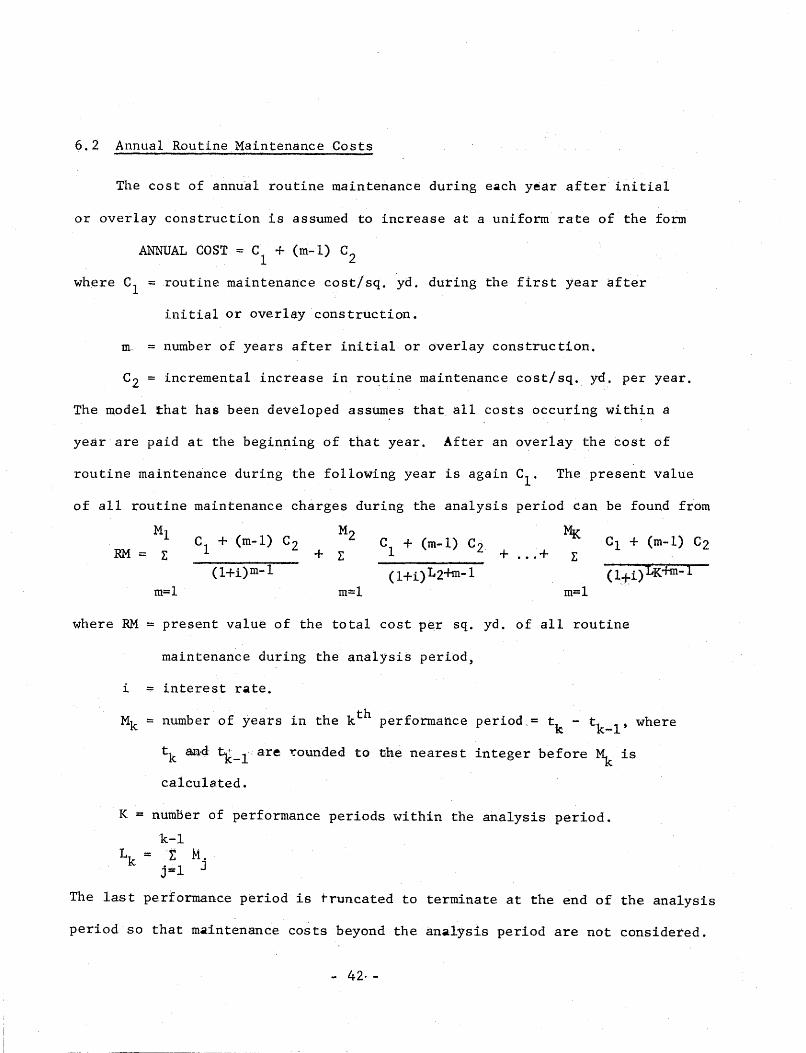
6.2 Annual Routine Maintenance Costs
The cost of arinu~l routine maintenance during e~ch year after ~nitial
or overlay construction is assumed to increase at a uniform rate of the form
ANNUAL COST = c1
+ (m-1) c2
where c1 = routine maintenance cost/sq. yd. during the first year after
initial or overlay construction.
m = number of years after initial or overlay construction.
c2 incremental increase in routine maintenance cost/sq. yd. per year.
The model that has been developed assumes that all costs occuring within a
year are paid at the beginning of that year. After an overlay the cost of
routine maintenance during the following year is again c1
. The present value
of all routine maintenance charges during the analysis period can be found from
Ml c1
+ (m-1) c2 M2
c1 + (m-1) c2 Mr< c1 + (m-1)
RM = 1: + 1: + ... + I: (l+i)m-1 < 1 +i) Lz+m-1 (l+i)tK+m-1
m=l m=l m=l
where RM = present value of the total cost per sq. yd. of all routine
mainteriance during the analysis period,
i = interest r~te.
Mk = number of years in the kth performance period_= tk - tk-l' where
tk c:tn·d tk-r are r.ounded to the nearest integer before ~ is
calculated.
K number of performance periods within the analysis period.
k-1 }':
j=l M.
J
c2
The last performance period is truncated to terminate at the end of the analysis
period so that maintenance costs beyond the analysis period are not considered.
- 42·-

6.3 Overlay Construction Cost
Calculation of the overlay construction cost amounts to no more than
computing the present value of all future overlays. In general, it is assumed
that overlays will be constructed from asphaltic concrete. It is also
assumed that an overlay must be at least 1/2 inch thick, and that all overlays
greater than 1/2 inch must be in even increments of a half inch.
The final assumption is that each time an overlay in constructed,
there is an additional charge equal to the cost of one inch of overlay.
This additional charge is included as a level-up cost.
is
The present value of the total cost attributed to overlay construction
K-1 c1ok+e1 oc I:
k=l (l+i) tk
where K-1 number of overlays constructed in analysis period (there are K
performance periods).
c1
cost/sq. yd/inch of asphaltic concrete.
Ok overlay thickness, not including the level-up ineh, applied at
th the end of the k performance period.
t th k = time (rounded to the nearest year) at the end of.the k perforreance
period, as previously defined.
- 43 -

6.4 Seal Coat Costs
The model for the application of seal coats assumes that the design
engineer will specify the cost per lane mile of applying a seal coat and
a schedule of (1) the time in years before the first seal coat, T1 , and
(2) the time in years between subsequent seal costs, T2
• These two times
may be identical without loss of generality. This schedule is to
initiate after initial construction and after each overlay.
It is ass~med that a seal coat does not affect the serviceability index
of the pavement. It is also assumed that a seal coat will not be
applied within one year prior to an overlay.
The computer program first converts the seal coat cost to cost/sq. yard
of pavement. The determination of the present value of all seal coats is
actually rather simple to describe but rather complicated to formulate
mathematically. The basic idea is that of taking the following sum
sc NUM sec l: (l+i)YJ·
j=l
where SC = present value per sq. yard of all future seal coats,
sec = cost/sq. yard of a seal coat,
i = interest rate,
NUM = total number of seal coats,
Yj = year in which the jth seal coat is applied.
To be more specific:
sc = K Jk sec l: E (l+i)x k=l j=l
-44-

where SC present value per square yard of all future seal coats,
sec cost per sq. yard of a single seal coat,
i interest rate,
K = number of performance periods (which is equal to one plus the number of overlays within the analysis period)
x = [t + 't + (j-1) 't J , where t 1 is the number of .years, after k-1 1 1 . 2 h . 1 k:- b f h b . . - h 1n1t1a construct1on, t at e apse e ore t e eg1nn1ng oi t e
kth performance period, with t 0 =0; and 'tl and 't2 are as previously defined, and
th Jk = the number of seal coats in the k performance period,
and where:
J = k
0 , otherwise.
The reason the one is subtracted from the numerator of the first part
of the above equation is because of the assumption that no seal coat
is applied within one year prior to an overlay. The quantity Jk as
calculated is rounded down, i.e., truncated, to integer form.
-45-

6.5 Traffic Cost of Overlay
The purpose of this section is to describe the procedure for
calculating users' (or motorists') increase in costs due to overlaying
operations. These costs include those associated with delay (time),
vehicle operation, and accidents. Only delay and vehicle operating costs
are considered at this time since there is little information on how
accident rates are affected by overlaying. The purpose of the section
is to give formulas for calculating these traffic costs and to indicate
what inputs must be provided by the program user for a specific job.
Although five methods of handling traffic are discussed, only the first
method has been written in the computer program; the other four methods
will be written in four subroutines which will be added to the computer
program in the next year of the project. A~so it is expected that the
same general method will be used for evaluating the traffic cost associated
with applying seal coats.
This section is divided into four sub-sections, the first of which
describes the assumed speed profiles of vehicles in the vicinity of the
overlay operation. The second sub-section gives the time and operating
costs associated with the different movements described by the speed
profiles. In the third sub-section the five methods of handling traffic
are described and equations are given for calculating the proportion
of vehicles stopped and the average time stopped for conditions where
traffic congestion arises because of the overlay operation. The final
sub-section gives formulas for calculating total user cost and total
user cost per square yard of pavement.
- 46 -

6.5.1 Speed Profiles
It is assumed that all vehicles approach the overlay area at the
same speed, called the "approach speed." It is further assumed that there
is a "restricted area," the length of which is L (in miles), through s
which vehicles travel at a reduced speed. For some methods of handling
traffic this reduced speed may be the same for vehicles traveling in both
directions but for other methods it may be different for each direction;
it is assumed to always be the same for all vehicles going in the same
direction. Generally, the vehicles traveling in the "overlay direction"
will have their speed reduced as much or more than will those traveling
in the "non-overlay direction."
The length L of the restricted area generally will be longer than s
the length L of the actual overlay operation. The amount by which L 0 s
is longer than L will be determined by the road geometries and the method 0
of handling traffic. This is discussed more fully below in the section
on methods of handling traffic.
As was mentioned above it is assumed that vehicles approach the
restricted area at an "approach speed" denoted by SA. Ifthere were no
overlay taking place then the vehicles would travel through the area
which is restricted during overlay at the "approach speed." During over-
lay, however, most vehicles travel through the restricted area at a
rPduced speed called the "through speed, overlay dirP-ctionrr denoted by
SO or the "through speect1 non-overlay direction" denoted by SN. It is
assumed that vehicles maintain these "through speeds" all the way through
the restricted area.
- 47 -

A proportion (called POl in the overlay direction and PN1
in the non
overlay direction) of aJl vehicLes will be ~topped as they approach the
restricted area. It is assumed that these vehicles stop and then accelerate
back to the through speed which is reached at the moment they enter the
restricted area of length L ; the vehicles then travel at the reduced s
speed (SO or SN) through the restricted area for a distance of L and as ~
soon as they leave the restricted area they return to a speed which is the
same as their approach speed.
Figure 11 shows the speed profile for such a vehicle which is stopped.
The letters along the horizontal axis denote points where speeds are changed.
The vehicle approaches the restricted area at a speed of SA, begins deceler-
ating at point A and is stopped by the time it reaches point B, remains
stopped for a time (no1
in the overlay direction and DN1
in the non-overlay
direction) at point B, then accelerates back to the through speed SO or
SN which is reached at point C which is the beginning of the restricted
area of length L , then travels from point C to point D at the through s
speed, and at point D begins accelerating back to the approach speed which
is reached at point E.
Vehicles which do not stop are slowed down when they pass through
the restricted area and it is assumed that their deceleration is such that
they reach the through speed (SO or SN) at the moment they enter the
restricted area. The proportion of vehicles which do not stop equals
one minus P01
for the overlay direction and one minus PN1
for the non
overlay direction.
- 48 -

s
A 8 c 0 E
DISTANCE (MILES)
Figure 11: Speed profile for vehicles which are stopped during overlay.
* This speed is SO in the pverlay direction but would be SN in the nonoverlay direction. L is length of overlay work; L is length of re.stric ted ,area. 0
· 8
- 49 -

Figure 12 shows the speed profile for a vehicle which is not stopped
but is slowed by the overlay operation. The letters along the horizontal
axis denote points where speeds are changed. The vehicle ·approaches
the restricted area'at a speed of SA, begins decelerating at point A,
decelerates to" -the [~rough speed SO or SN which is reached at point B
which is the beginning of the restricted area of length 1 , continues at s
the through speed from point B to point C which is at theeend of the
restricted area, then at point C begins accelerating back to the approach
speed which_is reached at point D.
Because of overlav operations, veh~cles will travel through the over-
lay area with speed profiles as shown in Figures 11 and 12. In the absence
of overlay operations they would have traveled at the approach speed
through the overlay area. The excess traffic costs due to overlay
include the excess time and operating costs due to reducing from the
approach speed to a stop (from A to B in.Figure 11) and returning back to
that speed (from B to C and from D toE in Figure 11), the excess time
and operating (idling) costs due to being stopped (at point B in Figure
11), the excess time and operating costs due to reducing from the approach
speed to the through speed (from A to B in Figure 12) and returning to
the approach speed (from C to D in Figure 12), and the excess time and
operating costs due to traveling a distance L (from C to D in Figure 11 s
and from B to C in Figure 12) at a reduced speed (SO or SN) instead of
traveling at the approach speed (SA). The excess costs of the afore-
mentioned types are discussed in the next section.
- 50 -

c UJ lJJ a.. en
SA.,___ ___ _
sc!
*
A B c 0
DISTA-NCE (MILES)
Figure 12: Speed profile for vehicles which are not stopped but are slowed during overlay~
This speed is SO in the overlay direction but would be SN in the nonoverlay direction. L is length of overlay work; L is length of restricted area. 0 8
- 51 -

6.5.2 Time and Operating Costs
The excess user costs because of an overlay include the excess cost
of stopping and slowing down, the cost of delay while stopped, and the
excess cost of traveling at a reduced speed through the restricted area.
The infonnation needed for calculating these costs are given in Tables
6 through 9. The program·user must stipulate whether the overlay operation
is in an urban or rural area and this determines which tables or which
columns in the table are used. The difference between the urban and
rural costs is the vehicle distributions used to derive the costs. The
operating costs for different types of vehicles were taken from a
publication by Winfrey (5), and this same source was used for the excess
time of making speed changes. The values of time used in calculations
were based on information in studies by the Stanford Research Institute (6),
Lisco (7), and Adkins {8). The proportions of vehicles of different types
for urban and rural areas in Texas is taken from proportions for 1966 given
in a study by the Planning Survey Division of the Texas Highway Department (9).
The reason that the costs are higher for rural areas than for urban areas
is that there is a higher proportion of trucks in rural areas and their
costs are higher than those for passenger cars.
TQbles 6 and 7 give the excess time and operating costs for stopping
(in the first columns) and for slowing down (in the other columns). Table
8 gives the time and operating costs for operating at a uniform (constant)
speed. Table g gives the time and operating costs of delay (or idling}.
- 52 -

Initial Speed
MPH
10
20
30
40
50
60
TABLE 6: DOLLARS OF EXCESS OPERATING AND TIME COST OF SPEED CHANGE CYCLES - EXCESS COST ABOVE
CONTINUING AT INITIAL SPEED, FOR.RURAL ROADS IN TEXAS
DOLLARS PER 1000 CYCLES, BY SPEED REDUCED TO AND RETURNED FROM (MPH2
0 10 20 . .lQ. . '; 40
8.473
18.200 9.413
31.550 21.491 11.354
50.360 39.609 28.422 15.795
77.932 66.233 53.917 39.941 22.612
120.546 106.979 92.482 76.022 56.405
-53-
50
32.485

Initial Speed
MPH
10
20
30
40
50
60
TABLE 7 : DOLLARS OF EXCESS OPERATING AND TIME COST OF SPEED CHANGE CYCLES - EXCESS COS'i' ABOVE
CONTINUING AT INITIAL SPEED, FOR URBAN ROADS IN TEXAS
DOLLARS PER 1000 CYCLES, BY SPEED REDUCED TO AND RETURNED FROM {MPH2
0 10 20 30 40
5.869
11.769 5.602
19.500 12.857 6.501
30.·030 22.933 15.976 8.607
45.002 37.338. 29.610 21.448 11.856
67.868 58.992 49.114 40.242 29.360
-54-
2Q_
16.432

TABLE (i~ DOLLARS OF OPERATING AND TIME COST PER 1000 VEHICLE MILES AT UNIFORM SPEEDS IN TEXAS
UNIFORM SPEED,
MPH
5 10 15 20 25 30 35 40 45 50 55 60
DOtLARS PER 1000 MILES -RURAL URBAN
- ROAns--- - ROADS
$750.20 393.47 274.15 214.53 . 179.13 156.05 -_ 140.18 129.03
.121.06 115.51 111.94 110.16
- 55 -
$692.06 362.43 252.21 197.06 164.16 142.57 127.58 116.84 108.98 103.24
99.18 96.73

TABLE 9: DOLLARS OF OPERATING AND TIME COST OF DELAY (OR IDLING) PER 1000 VEHICLE HOURS, FOR TEXAS
TYPE OF DELAY
COST
Operating Time Total
DOLLARS PER 1000 HOURS RURAL URBAN ROADS ROADS
$ 132.22 3,367.54 3,499.76
-56-
$ 122.89 3,140.22 3,263.11

6.5.3 Methods of Handling Traffic
There are several-methods of handling traffic during an overlay
operation. The method used depends mainly on highwaygeometr;ics,
expecially the number 0£ lanes, the type of median (if any), and the
presence or absence of pavement shoulders, frontage roads, or other
alternate routes. In the two following subsections are described the five
methods of handling traffic which are mo.st commonly.used and the way of
caluclating average delay and proportion of vehicles stopped for each method.
The five methods. The first two methods of handling traffic are
for two-lane roads (with or without shoulders) artd the other three methods
are for roads with four or more lanes. Figures 13 through 17 depict in
a general way the five situations. In each figure L and L are shown. 0 s
L is the amount of road which is overlayed at any one time - not the 0
total overlay job length. L is the distance over which traffic is slowed s
down by the overlay operation at any·one time. In the situations depicted
in Figures 13, 14, and 15, 1 is only slightly longer than 1 by say one-s 0
tenth of a mile, .but in the situations depicted in Figures 16 and 17, L s
may be considerably longer than 1 . L and L are job variables provided 0 s 0
by the program user and should be "expected" average values. If L and 0
L are not constant then the total overlay should be divided into several s
1 and L sections and the traffic costs should be calculated separately for 0 s
each; the program, nevertheless, assumes they are constant. In the figures,
the "overlay direction" is always to the left (or westward).
Method I (see Figure 13). For two-lane roads with shoulders, one
lane of traffic can be diverted onto a shoulder~ Traffic going nwest"
-57-
-~

. ,.. L •t t L s . ·j . .
~·· ·.·. :· ·. · ........ ·. ·.· .. ·.·.·.·.· •.J,·.··: ,··. ··;· ... ·;. · ... · .... · ....... ·. ~·.·· ..•... · .· .............. ;f.·.·.·.:· .. ·.· ..... ·.· .. ·:.·.·:-::·:::·'
::::?::~::~:::~· .. ll!ii"fi.fi:Ii!l:IIi:l:;~::.~:~=::;:.;~: Figure 13: Method I. Traffic routed to shoulder.
Figure 14: Method II. Alternating traffic in one lane ..
I.. Ls ~1
l ~LQ4 1 ••••···••.·••·•• ....................... j.., .... ~ ...... ,.. . .... .. .. . ' ..... ·.·.. . •.• ......... · ................. •'t ....... ·(.' .. ··· ·. ·.· ·.. .. . ·.· ..... ~ .. . . ...... · ............ •.' ... · ......... '· ··:· · · ... ; ... ,.. · ~.·~····· · · · ~ ·. · ··. · · · ··~g·.· ··· ·.·.· i·····rYirJ~fr~i · ·.~. ·:.·;.:.; · ··· · ·.i· • ..... · :·· ·; .;·. · ··• • · • ·•·•· ..... h· • • • • ...
-:.--. _-:--"X ,fu~itfi.z=---:---· ----:-.. ..
-·------·-· -----------------· --------.. ..
Figure 15: Method III. Two lanes merge, non-overlay direction not affected,
- 58 -

~~--------Ls--------~1
I l I ,.. La i
_. ~-.· Figure 16: Method IV. Overlay direction traffic routed to non-overlay
lanes,
..._I ----Ls-------..1
lr-......_ --L0 -.-------...!-; I
Figure 17: Method V. Overlay direction traffic routed to frontage road or other parallel route.
- 59 -
I I
I

in the "overlay direction" can be diverted.onto the shoulder as shown
in Figure 13 and such traffic will generally be slowed down. Traffic in
the non-overlay direction proceeds as usual but also must slow down
though probably not by as much as the traffic going in the overlay
direction. Another version of this method is to divert the traffic in
the non-overlay direction onto their shoulder and divert the traffic
going in the overlay direction into the eastward lane. In addition
to the delay due to traveling at a reduced speed, traffic may be
additionally delayed by having to stop due to movement of overlay
personnel and equipment in the overlay area and by the inability to
overtake other traffic in the overlay area.
Method II (See Figure 14). For two-lane roads without shoulders,
it is sometimes necessary to post flagmen at each end of the overlay
operation and to stop traffic in one direction while traffic from the
other dirPction proceeds through the overlay area. The flagmen determine
from which dire~tion traffic is let through the overiay area at any one
time. The vehicle arriving first usually has priority. If an additional
vehicle arrives while other vehicles going in the same direction are
proceeding through the overlay area then this additional vehicle usually
may also proceed through the area, except that it will be stopped when the
vehicles in the queue from the other direction are af a number or have
been waiting a time which justifies priority for them. Traffic from
each direction travels through the overlay area at a reduced speed. Some
vehicles from each direction are stopped to give way to vehicles from
the opposite direction, or because of the movement of overlay personnel
and equipment in the overlay area, or because vehicles do not have the
ability to overtake other vehicles in the overlay area. Generally
-- 60 -

speaking, the proportion of traffic·Stopped to give way to vehicles from
the opposit~ direction will be higher the longer is L .and the larger s
is the traffic volume.
Method III (See Figure 15). For roads with two or more lanes in
each direction and with a non-transversable median, it is assumed that
traffic in only one direction will be affected by the overlay operation.
It is also assumed that at least one lane in the overlay direction remains
open for traffic. For low traffic volumes the effects on traffic in
the overlay direction will be that of reduced speed through the area,
stops due to movement of overlay personnel and equipment, and inability
to overtake other vehicles as easily. For higher volumes for which the
flow of traffic is above the capacity of the restricted roadway, a
queue will result upstream of the overlay operation and will lead to
vehicles being stopped due to congestion.
Method IV (See Figure 16). For roads with two or more lanes in each
direction and with no medians or with medians which can be crossed at
any point or which have median openings, it may sometimes be desirable
to block all lanes in the overlay direction and divert the overlay-
direction traffic to non-overlay-direction lanes. Figure 16 depicts
the situation for a road with median openings; the difference between
this situation and those with either no median,or situations for which
it is intended that traffic will cross the median immediately in front
and behind the overlay job1is that L8
in these latter two cases would
bear approximately the same relation to L as is the relation in Figures· 0
13, 14; and 15 instead of being the distance between median openings at
each end of the overlay job as is depicted in Figure 16. For these
- 61 -

situations both lanes of traffic will be affected,and the method of
calculating average delay and proportion of vehicles stopped is the same
as that used for Method Ill, but in Method.IV traffic going in both
directions is affected.
Method V (See Figure ·17). In some situations traffic in the overlay
direction is diverted to an alternate route such as a frontage road or
some other parallel road or street.
Average delay and Proportion of Vehicles Stopped. The delay to
traffic due to overlay is of four basic types which are related to vehicles~
(1) traveling at a reduced "uniform" speed in the restricted area,
(2) not having the ability to overtake and pass other vehicles
traveling in the same direction,
(3) having to stop because of the movement of overlay personnel
and equipment in the overlay area, and
(4) having to stop because of congestion when the traffic demand
exceeds the capacity of the restricted area.
The delay per vehicle due to traveling at a reduced speed equals
the travel.time at the reduced speed through the restricted area minus
the travel time vehicles would have had through the restricted area had
it not been restricted.
The delay due to· vehicles not having the ability to overtake and
pass other vehicles traveling in the same direction because of the overlay
operation may result both in the restricted area and outside the restricted
area. This delay when it occurs in the restricted area is included in
the delay discussed in the preceding paragraph if accurate estimates
of speeds through the restricted area are used. The delay due to the
- 62 -

inability to pass outside the restricted area because of the overlay is
a more complicabed,-:' calculation and is probably l~rgest in the cases
where the capacity of the restricted area is smaller than the demand
(or input) for use of the area. I.n such cases --.whe-rem demand exceeds
capacity there will be congestion and queueing of vehicles. These queues
must disperse after leaving the restricted area and before such dispersion
occurs there probably will be some inability to pass outside the
restricted area. Such effects probably will be small in all cases except
Method II with considerable queueing. If the length of the restricted
area is fairly long and/or the traffic volumes are fairly large, then
in Method II there will arise fairly long queues of vehicles. Such queues
arise in one direction while vehicles are traveling through the restricted
area from the other direction; then, when this queue is allowed to
proceed through the restricted area it will emerge as a moving queue,
sometimes of considerable length, and extra delay will result outside
the restricted area until the queue disperses. The rate of dispersion
of this moving queue will depend ~inly upon the amount of traffic from
the opposite direction, the road geometries, and the type of vehicles
in the queue. This moving queue will also impede passing by traffic
from the opposite direction; however, there will be a considerable
length of road in front of this queue in which there will be no (or
very few) vehicles which will somewhat offset the effects of the moving
queue on traffic in the opposite direction, Since the type of delay
discussed in this paragraph probably is small in most cases and since
it is difficult to calculate, it is ignored (i~e., assumed to be zero).
The third type of delay, that result1ng from vehicles having to
stop because of the movement of overlay personnel and equipment in the
- 63 -

overlay area, is calculated by mult~plying the number of vehicles stopped
by the excess delay of stopping. The program user must estimate (1)
P02
and PN2 , the proportion of vehicles stopped due to the movement of
overlay personnel and .equipment and (2) no2
and DN2
, the average time that
each vehicle stopped (because of such movement) remains stopped. It is
expected that the overlay operation will be conducted in a way such that
the number of vehicles stopped due to the movement of overlay personnel and
equipment will be small. Therefore, in the absence of information on
the number of such stops, the program user probably should estimate that
number to be near or equal to zero.
The last type of delay (denoted by 001
in the overlay direction and
by DN1
in the non-overlay direction) results when a proportion of vehicles
(denoted by P01 in the overlay direction and PN1
in the non-overlay direction)
have tQ stop because of congestion which results when traffic demand or
input per hour (Q) exceeds the hourly capacity or output (0) of the restricted
area.
When Method I of handling traffic is used, this type of delay should
be almost nonexistent and is assumed to be zero; i.e., no1 = DN1 = 0 and
P01 = PN1 = 0 for Method I.
When Method II of handling traffic is used, it is assumed that the
hourly traffic is evenly divided between directions. It is also assumed
that vehicle arrivals from each direction are Poisson. The proportion
of vehicles stopped due to congestion from each direction (P01 or PN1)
is estimated by the following equation:
-64-

where;
a = the time that it takes a vehicle to travel through the restricted area, in hours, and
Q the number of vehicles arriving at the overlay area per hour in the overlay direction.
An equation for estimating the average delay per stopped vehicle (Do1
or
DN1) for Method II is developed from equations formulated by Tanner (10)
and given by:
where a, Q and P01
are as previously defined.
When Method III or V is used, both PN1
and DN1
will equal zero. When
Method III, IV, or V is used to handle traffic D01 for all three methods
and DN1 for Method IV are calculated using the following equation developed
and verified by the California Division of Highways (11) :
where;
H(Q- f})(R- Cb) 2Q P01 (R-Q)
0
if Q > 0
if Q i (j
H = the number of hours per day that overlay construction takes place,
R the recovery rate in vehicles per hour,
0 the restricted output rate in vehicles per hour,
and Q and P01
are as previously defined.
It is assumed that the input rate Q is the same for directions of
travel and equals 6 percent of average daily traffic in rural areas and
-65-

5 percent of average daily traffic in urban areas. The output rate 0
and recovery rate R are taken from the California study (11) c'and are
given in Table 10. The California study also gives the number of
vehicles which will be stopped at the time when recovery begins, i.e.,
when all lanes are reopened for travel, and this number equals H(Q-~).
The average number of vehicles which will be stopped at any one time
during overlay will be H(Q-~)/2. By assuming that each vehicle which
is stopped stays stopped for some average amount of time D, which is
assumed to equal 1/12 hour, not including the time stopped after recovery
begins, and assuming that no vehicles are stopped after recovery begins,
the total number of vehicles stopped can be estimated as H2 (Q-~)/2D if
Q > Q and is zero if Q ~ ~. Thus, for Method III, 1V, or V, the proportion
of vehicles stopped P01 (and also PN1 for Method IV) is estimated by
dividing the total number of vehicles stopped by the total input of
vehicles during overlay (H x Q):
PO = H(Q - ~) if Q > ~ 1 2DQ
POl = 0 if Q 2 ~'
with the constraint that: if this value exceeds 1.0, it is assigned a
value of 1.0.
More research, including field observations, needs to be done on
the precise number of stops under stop-anq-go operation which results
from congestion. Use of the above formulas gives reasonably accurate
estimates of hours of delay but may underestimate the vehicle operating
costs associated with stop-and-go operation.
-66-

TABLE 10 - CAPACITY TABLE
(Input rates greater than the output rates listed w norma _y res u t 1.n t e ormat1.on o a queue. ill 11 1 h f f )
No. of Lanes One Direction Percent (Normal Operation) 2 3 4
No. of Lanes One Direction Trucks (Restricted Operations) 1 2 3
Output Rate C/J 1400 2800 4500 0 - 10 (Urban) Recovery Rate R 3000 4700 6400
Output Rate C) 1350 2700 4350 Over 10 (Rural) Recovery Rate R 3000 4500 6200
Note: The rates as listed above are veh/hr in one direction.
-67-

·b.5.4 User Cost Equations
The formula used for computing the total user cost TUC for an entire
overlay operation is, prior to discounting to present value:
TUC =zvfro1 (C01 +COz+C03)+( l-Po1) (C03+CO~+POz (C05)
+PN1 (CN1-K:N2-K:N3)+( l·PN1) (CN3-K:N4)+PN2 (CN5) r where the variables with an rro" refer to the overlay direction and with
an "N" refer to the non-overlay direction and where:
v is the number, of vehicles affected by the overlay in either the
overlay direction or the non-overlay direction which are equal because
of the assumption of an equal directional split of traffic
(See the formula for V below}.
P01 and PN1 are the proportions of traffic which are stopped due to the
capacity of the restricted section being less than the demand for
it, i.e., the proportions stopped because of congestion.
P02 and PN2 are the proportions of traffic which are stopped due to the
movement of overlay personnel and equipment in the restricted area.
co1 and CN1 are the excess costs per vehicle of stopping from the
approach speed and are the values given in the first columns of
Tables 6r and 7, divided by 1000 • co1
= CN1
in all cases.
co2
and CN2
are the costs per vehicle of idle time for vehicles stopped
and are derived by multiplying no1
and DN1
by -total tdl.ing ·cast:
from Table 9, divided by 1000.
co3 and CN3 are the excess costs per vehicle of traveling through the
restricted area of length Ls at a reduced speed and are equal to
Ls multiplied by the difference between' the cost '·of operating at
the reduce'd spe~·d :so · (or:.?S)l) and the-· ccos t of operating at the
·-68-

approach speed SA, both taken from Table 8 and divided by 1000.
co4 and CN4
are the excess costs per vehicle of slowing from the
approach speed SA to through speed SO or SN and returning to
the approach speed and these costs are costs taken from Tables
6 and 7 divided by 1000.
co5 and CN5
are the excess costs per vehicle of stopping from the
through speed SO or SN taken from Tables 6 and 7, and divided
by 1000, plus the cost of idling while stopped due to the move
ment of overlay personnel and equipment which is obtained by
multiplying D02 and DN2
by appropriate values from Table 9 and
dividing by 1000.
The computer program determines, from values given in Tables 6
through 9 and from inputs provided by the program user, values for costs
co1
, C02 , co3 , co4 , co5 . CN1
, CN2 , CN3 , CN4
, and CN5 and also POl and PN1.
The program user must provide P02 and PN2 in the above equation but must
also provide certain inputs (SA, SO, SN, no2 and DN2) for calculating
the costs and for calculating V as is described below. SA is the speed
at which vehicles approach the overlay area, SO is the reduced speed at
which vehicles pass through the restricted area in the overlay direction,
SN is the reduced speed at which vehtcles pass through the restricted
area in the non-overlay direction, no2 is the average length of delay
for vehicles which are stopped in the restricted area because of the
movement of-overlay personnel and equipment, and DN2 is analogous to
no2
bdt for the non-overlay direction.
- 69 -

The number of vehicles affected by the overlay operation in one direction
is calculated using this equation:
V = NL ·~ T P(PS) Hrt Lo
where
NL is the total number of traffic lanes to be overlaid in one di'rec tion,
Lr is the total length of the road to be overlaid, in miles.
Lo is the length of road being overlaid at any one time, in miles.
T is the length of time, in days (or proportion of a day), that it
takes to make one overlay pass of two or less inches thickness of
length L0
•
P is the proportion of average daily traffic, rt, that will pass through
the overlpy area during each hour of the day that overlay takes
place and is assumed to be .06 for rural areas and .055 for urban
areas.
PS is the number of overlay passes made and is calculated in the computer
program.
H is the number of hours per day that overlay construction takes place
(and probably is between 6 and 12 hours).
rt is the average daily traffic at time t, where t is the time o£ overlay
a·s computed internally by the computer program, and is calculated
within the program from inputs r0
, rc, and G .. which are provided by
the program user as inputs for the "traffic equation" described
in a previous chapter.
The program user must provide Ni , LT, L0 , T, and H8 P is an assumed
value. PS is calculated internally in the computer program. rt is also
-70-

calculated internally by the computer program from r , r , and C 0 c
(which are provided by the program user as discussed in a previous chapter)
and t which is calculated in the program and depends on several variables
previously discussed. The equation. for rt is linear with respect to
time, the assumption being that average one-way daily traffic is initially
r and increases linearly to r at the end of the analysis period which 0 c
is C years long:
+ t(r -r ) c 0
c
The total user cost per square yard TUCSY is calculated by dividing
total user cost TUC by the total square yards TSY where TUC is as
previously defined and TSY is given by:
TSY,'«P 2N L L__ (52. 80) L T ~W-
9
where N1 and LT are as previously defined and LW is the width of one
traffic lane, in feet.
-71-

6.6 Analysis Period and Salvage Value
The analysis period is the period of time over which costs are
computed. Ideally the artalysis period should end when the road is
expected to be abandoned or when it is expected that major reconstruc
tion work will be done on the road. It is possible to have an analy~is
period longer or shorter than.this but si1.1ce a ~9nger period brings
several complications into the analysis it should be avoided.
In practice, it is best to use an analysis period such that the
program inputs can be reasonably estimated during that period. The
period probably should be at least 15 years but usually not more than
30 years.
The salvage value of a pavement at the time it is abandoned or has
major reconstruction work done on it is the value of the useable mater
ials in the pavement less the cost of making them useable or disposing
of them. If major changes in vertical and horizontal alignment are made
at the time of reconstruction, then the salvage value probably will be
less than it would have been otherwise. The salvage value will be negative
if materials must be removed and their value in their new use is less
than the cost of their removal; it is expected, however, that this usually
will not be the case for asphaltic pavements.
Although most previous pavement comparisons have used very low
salvage values even for relatively short analysis periods, there seems
to be little justification for this. The salvage value at the end of short
- 72 -

ana.t1sis oeriods such as 15 or 20 years orobably exceeds .JO percent much
of the time. S"ince the salvage value deoends on circumstances which are
different for different roads, it is left to the program user to stipulate
the percent that salvage value is of the cost of initial construction and
overlay construction. Salvage value~~: oer sauare yard, SV, is then calculated
using the following equation:
where:
sv ::i: p ' s~ .. __ _;_
100
n K-1 L 1 n . c . + kr c
1o j; Jf . J J =l L'-
(l+i)c
P = the oercent that salvage value is of the cost of initial SV' construction and overlay construction.
Dj = the depth of the jth layer of material.in the initial construction.
Cj =the cost per square yard/inch of theftlaterial in the jth layer.
c~. = the cost uer souare yard/inch of overlay construction. I
Ok = the denth in inches of the kth over.tay.
n = the number of layers of pavement in the initial construction.
the number of performance periods (and K-1 is the number of overlays,)i;'
K
C = the length of the ana.tysis period.
"-73-

6.7 Interest Rate
In the computer program, pavement designs are compared on.the basis
of the present value of total costs. Future costs and salvage value are
discounted to the present to obtain their present value. A review·o~
interest rates reveals that most interest rates which are used or are
recommended for use are from 3 to 7 percent. Although some people have
used a zero interest rate in pavement comparisons, their usage of this
zero rate usually was based on the fact that they "did not borrow the
money so no interest should be charged." Whether money is borrowed should
have no effect on using an interest rate. The use of an interest rate
is to show that funds used for pavement have alternative uses and bhe
interest rate should give an indication of the rateof return in
these alternative uses.
The program user must specify an interest rate.
-74-

CHAPTER 7 - INPUT/OUTPUT OF THE COMPUTER PROGRAM
A list of the computer program's inputs and outputs discussed
previously is given below.
7.1 Inputs to Computer Program
1. Number of construction materials available.
2. Funds (per sq. yd.) available for initial construction.
3. Length of analysis period in years (C).
4. Interest rate (i).
5. Lane width in feet (L ) • w
6. Performance variables:
a. District temperature constant (a).
b. Maximum serviceability index (P1)
c. Minimum serviceability index (P2).
d. No-traffic lower bound on serviceability index (P2 ').
e. Swelling clay rate parameter for first performance period (b1).
7. Traffic variables (one direction)
a. Initial ADT (r ). 0
b. ADT at the end of analysis period (r ). c
c. Number of 18-kip axle applications accumulated inC years (N ). c
8. Minimum time considerations (years)
a. Minimum time to first overlay. (t1
)
b. Minimum time between overlays.
c. Time to first seal coat after initial or overlay construction.
d. Time between seal coats.
9. User cost variables
a. Number of lanes in each direction (N.__ )~ L
b. Total length of project (miles) (LT).
- 75 -

c. Average length of overlay strip (one lane) (L0 ).
d. Average time to overlay this strip with 2" or less (days) (T).
e. Proportion of ADT passing through overlay zone during each
hour that overlay construction takes place (P).
f. Hours/day that overlay construction takes place (H).
g. Class of highway (rural or urban).
h. Proportion of average daily traffic ~topped in the overlay direction
because of mov~ment of overlay personnel and equipment in the
overlay area (POz).
i. Average delay per vehicle stopped in the overlay direction becaus.e
of movement of overlay personnel and equipment in the overlay
area (DOz).
j. Proportion of average daily traffic stopped in the non-overlay
direction because of movement of overlay personnel and equipment
in the overlay area (PN2).
k. Average delay per vehicle stopped in the non-overlay direction
because of movement of overlay personnel and equipment in the
overlay area (DN2).
1. Average traffic approach speed (mph) (SA).
m. Average speed through restricted area in overlay direction (mph)(SO).
n. Average speed through restricted area in non-overlay direction
(mph) (SN)
o. Average length of restricted area (miles)(Ls).
p. Type of traffic model (1,2,3,4, or 5).
10. Routine maintenance cost (per lane mile)
a. Routine maintenance cost during first year after initial
or overlay construction.
· b. Annual incremental increase in routine maintenance cost.
11. Cost of seal coat (per lane mile)
-76-

12. User cost variables taken from Tables 6 through 10
a. Cost of changing speed/1000 cycles ..
b. Cost of driving at reduced speed/1000 vehicle miles.
c. Cost of delay/1000 vehicle hours.
d. Output and recovery rates.
13. For each material above. natural sub grade
a. Name of material.
b. Strength coefficient.
c. Cost per compacted cubic year in place.
d. Minimum thickness allowed in initial construction (inches).
e. Maximum thickness allowed in initial construction (inches). I
14. Strength coefficient of natural subgrade.
15. Percentage that salvage val~e of value ~f structure existing at
end of analysis period.
16. Total thickness allowed in initial construction (inches).
-77-

7.2 Outputs of Computer Program
1. For each possible combination of materials ~
A. Design with least overall cost
a. Materials used.
b. Initial construction thickness of each material (inches).
c. Life of initial construction (years)~
d. Overlay schedule
(1) overlay thicknesses
(2) overlay times (years)
~. Seal coat -sched~l~ (years) •.
f. Initial construction cost.
g. Total routine maintenance cost.
h. Total overl~y ~onstruction cost.,
i. Tota+ user cost.
j . Total seal coat- cost.
k. Salvage value.
1. Total overall cost.
B. Next cheapest design
(Same information as above)
2. Summary of designs in order of increasing overall cost.
- 78 --
CHAPTER 8 ~ THE.· OPTIMIZATION MODEL
Now that the prinicipal physical equations and a number of cost rela
tionships have been developed-, the analysis is carried one step further.
These equations and costs have been-used as a basis for·thedevelopment of
a model for the optimization of- flexible pavement -des.ign. Briefly, the
objective of this model is to use available data· and parameters to select
the initial and overlay construction policies which result in minimum cost
over an analysis period. This selection, however, is bounded by many
restrictions, such as the minimum allowable time to the first overlay, the
minimum allowable thickness of a material in initial construction, etc.,
as may be seen by reference to the program inputs listed in Chapter 7. It
is these restrictions that force the model to yield solutions that are
physically realistic. At the same time every attempt has been made to
make the model as flexible arid as general as possible.
This section of the report contains a brief description of the model.
A computer program has beenwrittenwhich utiliz~s these concepts. This
program is written in the FORTRAN IV language for the IBM 360/65 digital
computer and has been forwarded to the Texas Highway Department under
separate cover. Since the model is still conceptually new, an attempt
has been made to design the optimization technique into modules so that
sections may be revised with minimum effort as the need arises.
The optimization plan to determine the most economical design requires
several steps. Each of these steps will be discussed. It should be empha
sized at the outset that the intent of the discussion is not to show how
the optimization is mathematically carried out but rather to give an under
standing of the logical development of the model. In this sense, a verbal
description of how the optimization works will be given rather than the
actual development of the model.
-79-

Consider that some number of dollars are available for the entire
cost of the project (this number is not actually known; it is only used
for explanation). This would include the cost of the initial construction
as well as all future costs. This available amount may be split up in
many ways between these two considerations. A very weak pavement might
be initially constructed in which case the future costs of maintaining
the pavement would be rather expensive. On the other hand, a strong
initial design would require very little in the way of future cost.
For this reason the overall optimization plan has been divided
into these two stages: (1) optimization with respect to initial design
and (2) optimization with respect to the overlay policy. It can be seen,
however, that these two optimization problems are interrelated since the
optimal overlay policy is dependent upon the initial design.
-so-~

8.1 Initial Construction
It is assumed that a number of materials are available for initial
construction. Each material has an associated.strength coefficient along
with a cost per compacted· cubic yard, and restrictions on thickness in
the initial construction. Thus, there are a number of combinations of
materials that may be· used· for initial construction. The design with one
layer above the subgrade would naturally consist of asphaltic concrete.
Designs of two layers above the subgrade could also be enumerated by
combining asphaltic concrete with each of the other materials. Other
multiple layer designs can also be enumerated in the same manner.
The remainder of the optimization plan that follows must be carried
out for each of these combinations of materials. As a result, the final
solutions will be in the form of a set· of optimal designs - one for each
combination of materials.
Attention will next be turned to the actual optimization model for
initial design. This model utilizes a branch and bound algorithm as the
tool of optimization. This fact in itself is important from a theoreti
cal point of view but is not of particular importance from the standpoint
of being able to use the computer program. In other words, it is important
to discuss what the technique does but not how it is done.
The important key to determining the optimal initial design is the
deflection equation (1) which relates the design parameters and layer
thicknesses to the surface curvature index of the pavement. This equation
along with the available data for the in-place cost/sq. yd. inch of thickness
for each material are all that is required to do this optimization.
-81-

Since each type of material has a lower limit on the thickness that
will be constructed, there is a minimum design thickness for each com
bination of materials. The cost of this minimum design can easily be
calculated by summing the products of each minimum depth times the in
place cost/sq. yd./inch of depth for each material used. The amount
to be invested in initial construction will be allowed to vary in the
increments of $0.01 from the minimum on up to a prescribed maximum.
For each of these amounts, the actual problem to be solved is that of
determining the depths of each layer that will minimize the surface
curvature index, S. Thus, the optimization process obtains the
strongest design (in terms of S) for each of the possible amounts that
can be invested in initial construction. The deflection variable, S,
for each of these designs can next be used in the performance equation
(3) to determine the number of equivalent 18-kip single axles, N1 , that
the pavement is expected to withstand before the serviceability index
is reduced to its lower limit, P2 . From the traffic equation (2), which
relates traffic to time, the length of time (in years) can be computed
for each of these designs. This is the time, t 1 , at which the first
overlay is required (unless, of course, this time is longer than the
analysis period, C). This completes the first stage of the optimization.
-82-

8.2 Overlay Optimization
The second stage of the optimization is one of determining the optimal
overlay policy for each design. Here, again, there are a number of possible
alternatives. A thick overlay might carry the pavement through the remainder
of the entire analysis period. It would, however, generally be more economical
to construct a thin overlay on the pavement and plan another overlay later
in the analysis period. This latter policy would have the advantage of
deferring the second overlay cost so that the present value of this cost
would be reduced. This policy would have the disadvantage, however, of
increasing the user cost because of the traffic increase at that later
time. Other possibilities are also available. In fact, all of the over-
lay possibilities can be graphically represented as a tree. Each branch
of the tree would reprP.sent an individual overlay policy. Determination
of the optimal overlay policy forms the second optimization problem.
Even though sophisticated optimization-· techniques are . possible, the
problem has· not been formulat·ed as such because experience has showtl
that the actual, number· of bl;'anches· in bhe tree is relatively small.
It is faster and easier to actually enumerate the pos-sible·
ovw·rlay policies. For example, assume that it is found that t1 years
after the initial construction of a certain pavement, the serviceability
index is down to P2 • There are several overlay possibilities available.
A one inch overlay might last until time t 2 in which case an additional
overlay of one inch at that time might carry the pavement through the
remainder of the analysis period. It, however, might be found that a
two inch overlay laid at time t 1 will also carry the pavement through
the analysis period. The answer as to which of these alternatives is
-83-

most economical depends on the overlay cost as well as other cost factors.
The determination of the user cost, annual routine maintenance cost,
overlay construction cost, seal coat cost, and salvage value have been
discussed in Chapter 6. The present worth of each of these costs must
be added (salvage value is treated as a negative cost) to obtain the
total cost associated with each overlay policy. The most economical
policy can then be selected. This cost is added to the cost of the
initial design to determine the overall cost associated with that design.
These overall costs are then scanned to determine (1) the design with
minimum cost, and (2) the next cheapest design as an alternative. These
two designs are determined for each combination of materials.
-84-

LIST OF REFERENCES
1. Scrivner, F. H.; Swift, Gilbert; and Moore, W. M. "A New Research Tool for Measuring Pavement Deflection," Highway Research Record No. 12 9, Highway Research Board, Washington, D. C., pp. 1~11, 1966.
2. Scrivner, F. H. ; Poehl, Rude 11; and Moore, Wm. M. "Detecting Seasonal Changes in Load-Carrying Capabi 1:1. ties of Flexible Pavement," An NCHRP Report in Press, Highway Research Board, Washington, D. C.
3. Pace, George M. "Evaluation of the Dynaflect for the Non-Destructive Testing of Portland Cement Concrete Pavements," Technical Report No. 4-61, Department of the Army, Ohio Division Laboratories, Corps of Engineers, Cincinnati, Ohio, i967.
4. Scrivner, F. H. and Moore, W. M. "Some Recent Findings in Flexible Pavement Research," Research Report 32-9, Te:x:as Transportation Institute, Texas A&M University, College Station, Texas, 1967.
5. Winfrey, Rob ley "Motor Vehicle Ru!ui.ihg Costs for Highway Economy Studies," published by author, Arlington~ Virginia, November, 1963.
6. Haney, Dan G. and Thomas, Thomas C. 11,bl Value of Time for Passenger Cars," Standford Research Institute, Menlo Park, California, May, 1967.
7. Lisco, Thomas E. "The Value of Connnuters' Travel Time: A Study in Urban Transportation," presented at the 48th Annual Meeting of the Highway Research Board, Washington, D. C. , January, 1968.
8. Adkins, W. G.; Ward, A. W. and McFarland, W. F. "Values of Time Savings of Conunercial Vehicles," NCHRP Report 33, Highway Research Board, Washington, D. ·C., 1967.
9. "Truck Weight and Vehicle Classification, State of Texas, 1966;,'" Texas Highway Department, Planning Survey Division, Austin, Texas.
10. Tanner, J. C. "A Problem of :J:ftt;~rff(ii!Ultt~griS~J;;we'~ifn'!ftReQ~S\lt!s ,UJ ~~~l!l~t:~~~a, Volume~40, Parts 1 and 2, June, 1953, pp. 58-69.
11. Smith, Walter, P., Jr. "Delay to Traffic Due to Future Resurfacing Operations,'' Traffic Bulletin No. 7, Department of Public Works, Division of Highways, Sacremento, California, November, 1963.
-85-.

APPENDIX 1 - INPUT DATA REQUIREMENTS
The purpose of this section is to provide the program user with all
the necessary instructions to properly input the required data. This is
accomplished by providing graphical illustrations of the various input
data card fields and the type of information they are to contain.
The required data for an example has been used to illustrate the use of
these cards. Forwarded under separate cover is a complete listing of the
computer program along with the output for the example problem. Comment
cards inserted in the computer listing will also aid the programmer in the
use of this program.
It is felt that the first 7 data cards need no additional explanation.
The next three sets of data, however, might be difficult to interpret.
These sets describe the excess operating and time costs of
1. reducing to and returning from a reduced speed in a rural area
2. reducing to and returning from a reduced speed in an urban area
3. driving at a uniform reduced speed
Each set contains 6 data cards. First consider the first two sets. The
first card in each set assumes that the approach speed is 10 MPH, the
second assumes an approach speed of 20 MPH, etc. The third set of data
is similar; the first .card assumes at reduced speed of 10 MPH, the
second a reduced speed of 20 MPH, etc.
Finally the last set of data is for. the available construction
materials (one card for each). In attempting to combine these materials
into the possible initial designs there is only one restriction. This
is that the order in which the cards are input determines the arrangements
in which these materials will be used. For example, if the card for lime
-86-

treated gravel is placed above the card for crushed gravel,their order will
be preserved. That is to say that in all combinations involving these two
materials, lime treated gravel will always be above crushed gravel,never
below. This may be somewhat restrictive but it is felt that this is the best
way to restrict the combinations to a logical sequence of materials (it
would be undesirable to have asphaltic concrete as a subbase material).
In any event, it is probably most logical to input the materials in the
order of decreasing strength.
-87-

C::lo~ C)~
c=oj!e c::lll::: c=oj! c=oJC C)~
c:::tl=! -~. C),::
c::liJi!! -= -= c::tl;i c::tS c=om C)~ c::tl;l c::t:OI c::lll:iO c::t;J c::t:rl c::t:ll c::tfi; dll c::t:R Ct~ c::t~
-:. -~ --s o: C)~ c::t!; c::tW c::t~ c::t:J CtQ c::t~ c::t:i c::t'T
fZ4 c::tJt
~ c::tJII c::t::; c:::tlll
5 C)~
c::ll;f; c:::ts:l
~ -:::~
~ c::tl=; c::lllil
5 --= c:::tll: c::liS:;j
c:::tl'= a c:::tlQ
-~ c:::t;::
! c~ _,_ Clll<: bt! c::tS c:::t!:::
u c:::l!!! c:::t¥:!
i cs C::! Ct:! c::: c~
2 Ct• --c ...
~ c-c:» .... c. c:::l ...
c:::t ... c:::t ...
Data Card 1
Salvage percent of structural value at the end of the analysis period, PSVGE Format F 10. 2, · _ _ _ _ _ 2 2 ..:.. .2. .2.
Lane width (feet), XLW
Format F 10. 2, _ _ _ __ 1. ~ ..:.. _Q .Q
Interest rate or time value of money, RATE
Format FlO. 2, ____ 2..:..00
Length of the analysis period, CL
Format F 10 • 2, 2 0 . 0 0 -- -·---Maximum number of dollars available for initial construction, CMAX
Format Fl0.2, ______ ~..:.. _Q .Q
Number of materials available, NM
Format IlO, ___ _ 5
Figure 18: Input format for miscellaneous variables
-88-
C7Ji1'1 en: enlJ en!; enw eno en$ en:: en~ en; en:J en111 enJII enf;; enlll en:q en~ ens:! enR en~=;
crllll cnt:~ cnJS en$; en~~: cntQ en~ en;3 enJ::I enf:l en~! cnt! cntl cnc:: en!!! en II! ens
·crto ens:~
crt~ !! en.., il'i
::::I en• en"' en • en .. crt ... en-
-

2: a 5 ~
~
5 a
~ 0 0
i 2
~ .....
c:::tl: COl!! ell! cs::: CJI! Clll! Cl;'t c:»l:! QJ::! Cll=:: Cl~ == c: Cllit c: cia c:; cog ctt co;; c:ofi: c:o:: c~ C(j; c:»:ll c:»:R c:»;K c:ag esc
Data Card 2
~i----·--~----•·•••-,~----~--··•··-·-•""'~'--w·----:: Swelling clay parameter, BONE• .. =~ _, -~ c~ =0 =~ c:o: =~ CJI: ell! c::; c:::llll cl!l' =~ cR c:t::l
-" -c:t!Q c:::tl!l Cl~ CIQ c:::tlQ c:>;t Cl~ a::: C) 1'0
c C!!
=· c:::at:: O!! Cl-111 c:r: ca c::tt:! c::t ;: c:::a_ -.. c::t-c ... c::t-Qon -.. Cl ...
c:t ....
Format FlO. 4,
The no- traffic.:-elower bound on the serviceability index, P2P
Format Fl0.2, 0.:...2..2 ---------·--··-------·--··------·---
Servieaabi'li ty index at time ~~-, ·1?2
Format FlO. 2, ______ .2. .:. .2. .Q.
Serviceability index at time T1 , Pl
Format FlO. 2, ____ _
District temperature constant, ALPHA
Fonnat FlO. 2, _____ 1 2.:. ..Q ..Q
-· enj!! en II! c:ns::: en II! enll! cn;t en!:! enJ::! en!::: en lit en& c:n:a -" en. -= en(£
-~ en:.t en;; en a enS: en :I cnli; c:n:R
-~ en a&; eng cn:;c
cn8t en~ en :I! en!; cn:t -· en~ eno c:nfill en:o: ···--o;-.. -enl!l en Ill ens;; -· cnl!l en ;It cnR cns=c
... 9P..&.
-~ cn!Q enJ: -~ en!Q enlQ en;t c:n1=3
-~ -~
cnse cnt! -· en~:
en:! en Ill en:t cnl:t en a en;: en- i en .. ~
::• -en .. en .. en .. en ..
c:t ...
=-~-----------------------------------------......,._----------~----
Figure 19: Input format for performance variables
-89-

t'%j ..... OQ ~ t1 ro N 0
H ~
"'0 ~ rt
1-h 0
~· I Ill \0 rt 0 I t-h
0 t1
rt t1 lll t-h t-h t-'· ()
<: ~ t1 1-'· ~ 0" ....... ro CIJ
l
INPUT FORMAT COLUMN IDENTIFICATION
OOODOOOOO~lOOOOOOOOO~OOOOOOOO~OOOOOOOOOOOOOOOOOOOOOOBfO~OOJOOOODOOOOOOOOOOOOOOOO t23451711~nuuM~K»~~~nnu~Kna~~~»~~~·n~~~~~a~~~u~u~~U~M~~~~9MhU~M~H~HH~nnnH~nnnnu
hj NO t'%j 0 hj 0 0 0~ 0 ~ 0 ~
g ro g ro ~ ro '<: I I I
~ ro o. Ill 0. ~ 0.. rt Ill ..... rt ....... rt 1-'•
t1 t1 .. t1 t1 hj rn ro ro t:Ej ro ........ .. () 1-J:j () ........ ()
0 rt ....... rt 0 rt . 2 s· 0 ..... . 1-'• 0 . 0 0 0
0~ 0 ~ .. ~ .. ~
I ~ I ~ () () t-l I t-l g I
I I
~ ~ 00 ~ rt
I rt
....... I (J"'' Ill 0" ro
rt ro I l:f 0 ro I OQ 0.
0. 1-'• IW 0 IN § lln
0 rt lo
t-h ·0 t1 1-'•
I·O Ill lo ~ ~
0 t-h OQ lo ::s
t-h lo
~ . 1-'• 0 ........ ()
I· t-h t· "<
rJ)
~ ~ ..... t-h ~ rJ)
rt Ill ro ...... "'0 t1 "< ro
rJ) t1 t-'· 1-'· rJ) 0
0. "'0 .. ro t1 ~ t-'• 0 0. .. ~
~ 9 9 9 9 9 9 9 9 919 9 9 9 9 9 9 9 9 919 9 9 9 9 9 9 9 9 919 9 9 9 9 9 9 9 9 9 9 9 9 9 9 9 9 9 9 9 9 9 9 9 9 9 9 9 9 9 9 9 9 9 9 9 9 9 9 9 9 9 9 9 9 9 9 9 9 9 t23451719~nnu~BKuwa~nnuaanaa»~»~~~•n•~~~u~~~-u~u~~R~MB~~M"~hU~M~u~un~nnnu~nnnnu
-soe1.
t::l ~ rt ~
0 ~ t1 0.
w
J

INPUT FORMAT COLUMN IDENTIFICATION
~ooooooooornooooooooonoooooooo~ooooooooo~oooooooooooooooooooooooooooooooooooooooo \23451litantiUM~~n~~~nnn~~~na~~~»~~~X»~H~UUU~U~~~"~~~UM~Wg~9~h~UMeMVMH~nnnM~~nnnH
~ ~ :s: ~ :s:
I ~ ~
1-
1-rj ~ 1-'• 0 1-'• 0 1-'• 0 1-'• 0 1-'· OQ ~ ~ ~ ~ a :::1 ~ ~ ~ I-'• 1-'• 1-'•
l 1-'•
ti Ill ~ Ill
~ Ill
~ Ill E ([) rt rt
I rt rt a ~ I ~
a N H H ~ ~ rt ~ rt ~ rt ~ rt 0 1-'• 0 1-'• 0 1-'• 0 1-'• a .. s . s I . s (t) ro ~ ro l ~ ro H I I ! .. i .. ::s
I rt
I 0"'
I rt I I
0"' "0 0 ro 0 ro ~
I I rt
I I rt
rt rt ~ rt ~ I
::r' I
ro I
::r' I
ro t:::l t-h ro ro ro ro Ill 0
I I ~
I I ::s
rt I ~ t-h t-h Ill \.0 I
1-'• I
0 I
1-'• I
en. ~ OJ ti < l ti ro
0 rt en. ro
I
en. Ill Ill I l rt I ti I rt I 1-'· ti t-h
I 1-'
I 0.. 0 I 0 Ill en. I (} ti
I < I ~
(Vi ro
lw 0 +:--m Cl) Ill Ill a ti .. 1-' rt 1-'• lVI ~ lVI
~ I· I• en.
~ Ill (} .. 1-'· ~ l lo 0 lo
~ .. Ill ~ 0 rt
~ ; .. t/)
t (") rt
I ~ t-'• 0 a C/) ro (")
<: OJ ti 1-'• Ill 0"' 1-' ro en.
l \ ~ ' ~ i ;99999999999999999999999999999999999999999999999999999999999999999999999999999999 \t 214 517 I 91 t11213141518171111 2223242521V2121381.!S23U4l5ll3731l9~414243~U4147~4i5051525lM55515151159H61&263&4S511171111·10nnn74757Sn717tl0 ' .. aoe . r .

O:i Ole ole ot::: Oj!!
oil! o;!: OJ:! cJ:! Cl!::
OJ<! o:: o:z Oil; oa Ol!l o;,; Ol:l o:;:; OIG C)~ o:: c::.t::C ot;; Oll o:R CD ;It c::.t::l otl o;;;; c::r--;r o:r 0 ·~
C)~
C)*
C)~
o:; 01:/
Cl~ o:;;: o:;
:z: OJ:
s =~ o::; OM
!a olfl' Clllj
0 OR .... Ol::;
~ C);:;
~..:
L1 =~ Oil: 01:;
w Ole a Olll Cl;!; =::::
~ =~ C>J::;
=2 c::t~
=• 0 o::::
u Ct!!! Ct .¥1 0:1 c::tt! c::tl:! C)::;
=~ -.. Q.
c:::t ... Ct .. c:::t ... c::t ..
c::t ... Q N = ~
Data Card 5
·Type of road under consideration, !TYPE
Fonnat 110, _________ _!,
Avg. number of hours/day that overlay takes place, HPO
Format F 10. 1, ______ .!. 1 .!. .2
Avg. proportion of ADT passing through overlay zone during each hour that overlay takes place, PROP
Fonna t FlO .1, _______ i .!. .2
Time {in days) to overlay a strip XLO in length, TLO
Fonnat FlO. 2, ______ .!. .!. .Q .Q
Average length (in miles) of pavement that will be overlayed at one time (one lane), XLO
Fonna t Fl 0. 2, _ _ _ ___ .Q .!. 1 2
Total length of the project (in miles), TLEN
Fo nna t F 10. 2, ______ 2 .!.. .Q .2
Number of lanes in each direction, XNLANE
Format FlO.O, ________ .!_.!..
Figure 22: Input format for the parameters used in determining the user cost
-92-
----· ente en~
en I:: en:e en II! enilt en!:! en~ ..... ~:::
..... ~ en~ en# en:; en~ en!:J en:r en:;t en# en; en:~
en-= enJII cnt:o enM en~ en~ ens:r en~
en Ill en~Q
cnJ: ens;; enJ: entQ cn:t en;! en~ O'lf'i enliil en~ -· cnc: en~e
en Ill ens en a ent:~
en;
::1 ::::I en • en ... en .... en .. en.., 0'1-
-

eli: 0~
OJ! o~=:
Ol! call! o;t ol:! 0~
Data Card 6
0~ . ~---~--~-------------·--------·-··~-----------~--~-·
om o:: oto o:: cam o;s; caQ
Type of model to be used for the traffic situation, MODE£
or: Format IlO, 1 :~;'-----------.;;......-...-.-... o--.--.. --···--·-·-··-·• "'~· . o:J: oil or;; oil o:R oa O:;l
-~ Olft
o::
Length of overlay zone which affects traffic (distance in miles between barricades), XLS
Format FlO. 2, ____ .2.:..12
Average speed through the overlay zone in the non-overlay direction, ASN
Format FlO.l,
~------------.. ·--·---~--0$ ---------·---·----------.. - ... ---· ....... . or:: Oil! o:;; OJil c=i~ 0~
ol=l o:::t Ctl=i
Average speed through the overlay zone in the overlay direction, AS0
Format FlO.l, ______ 1 .Q..:. .Q
Average approach speed, AAS
Format FlO.l,
:;-----.,-------·~-----·----------------·•· ,,,.,,__, __ _,.,__~•·•••· ,-.•' • -.< _.,.,_ •••·-~----,.--, .. ~--·-·~OM"''--·-·-"
:: Proportion of vehicles stopped in the non-overlay :; direction due to overlay construction, PSN. a~
Ct:t
: : Format FlO. 0, _______ 2. ..:.. .Q
~a crtft! crt~! en~=:
enJ! en I(! en;t en,:! en~ en~ -·--en en a cn:J en Iii en a cn:B en:S en :a en:;~
enu; en~ en:J: en :Ill enc;
~cniR crt :X c:nQ cn:;c Cft:ii en :X c:n~ enfl en:;: enfl c:n!Q crt# en~ en~ c:n• ·c:n·s-enl!l crt Ill en(:; mill en~ en~ enj:l en!=!
en~ en~ crt!:; enlfil en¥l crt~ crtl:l c:n~ enF;; ... - -- c;; -~r .... en I! en I! c:nt:: en$! en~
enx eno entt ens:: ~!! -·---· ------------------------------- ·--------------------------~0~ eft:! Cl. =.
c.-a .. con e:::, .. = ~ = ... = ..
Proportion of vehicles stopped in the overlay direction due to overlay construction, PS0
Fonna t F 10. 1, ______ .! .Q ..:.. .Q
:::I en • en.,. en • en,.. en ... ..,_
. -----------------, Figure 23: Input format for the remainder of the
user cost parameters
-93-

Cll,i CIJ!! ole Clj:: Clj!! CIJ(! Cl;!t C)~
CIJ;:! C)!':::
o,:! o: Cl:l Cit; o:s Cll'l o: C)~
Cl!;: o:. Cl:i o:Jl o:x or;; Cl:ll c~ Cl;l C)~
Cl!;l Clift oSt C)~
o:: or; ow C)~
Cl:l c:ttl C)~ Cl:i C)~
:24 o:e:
0 C)~ .... =~ C)~
!< CIJ:l' o·.,;
s C)~
C)~
~ C);;:;
CIJ::
~ Cll!: Cl5:<
~ Clll!l
~ Cll(l o;t C;:l
~ a:::: C)""
= Cl!!! Cll2
0 C) t::
0 CJ !12 c::Jll!
i Cl;! CIC =~ o::: o_
2 0.
=-C)~
0 ..
o ... =. C) ...
C) N
C) ...
Data Card 7
Cost per lane mile of a seal coat, SC
Format FlO. 2, _ .... _ 1 .2. Q Q ~ Q .Q
Annual incremental increase in cast per lane mile for routine maintenance, CM2
Format Fl0.2,
Cost per lane mile for routine maintenance during first year after initial or overlay construction,
Format Fl0.2, ____ _ 1 Q.:. Q .Q
Figure 24: Input format for the costs of routine maintenance and seal coats
-94-
the CMl
en a enJ! en~
en~:
en I!! ente en;t en!=! enJ;:! en" c:nji! en: en:z c:nQ; en I cn:IJ cn;s en~ en:;, enJ;; en :I en:J: enS enr;; en:~~ en :II en;l en:;:r cntc enlft cn='! cn~ en:: enr; cn~ en~ en¥ en~ eft~ en; en~ en:=: en~ cns:; enM en~
en" enR ens:t
enc:: enll! en!(! en;! ent:! cnt:~
cn = -· en .. ~
:;: I en• cn,.. en ... en ... cn .. en-

~ ...... OQ
f:! li ro
N Ln .. H ::1
"0 f:! rt
H-1 0 ...... g
::1 Ill I li rt \.0 f:! V1 li H-1 I Ill 0
t-'li
Ill () li 0 ro m Ill rt
0 H-1
()
::r' Ill ::1
()Q ...... ::1
()Q
Cll "0 ro ro 0.. (/)
INPUT FORMAT COLUMN IDENTIFICATION
OOOOOOOODDIODOOOOOOOOjDDOOOOOOOOOOOOOOOOODOOOOOOOOO~OOOOOOOOO~OOOOOOOOOOOOOODOODOO t2345,JII~nnnM~~n•R~nnnu~ana3~nnu~~•n••~uqu~u•~•u,~u~M~M~Y"l~~QM~Mvuemnnnu~~nnn~
0 0 Cll rt
0 H-1
Cll rt 0
"0 "0 ...... ::1
OQ
C")
0 Cll rt
0 H-1
li ro 0.. c () ...... ::J
OQ
Cll "0 ro ro 0..
rt 0
t-' 0
~~
C") 0 Cll rt
0 H-t
li ro 0.. c () ...... ::1
()Q
Cll "0 ro ro 0..
rt 0
N 0
~-::z::
999999999!999999999~999999999 t2345171san~DM~Mn~~~nnnu~anaa
-&oat
n 0 Cll rt
0 H-t
li ro 0.. f:! () ...... ::1
()Q
Cll "0 ro ro 0..
rt 0
w 0
~ ::z::
I I o l a I o I o 1 ~ ! ~ I 0 H-t
li ro 0.. f:! () ...... ::1
()Q
Cll "0 ro ro 0..
rt 0
<S ~ ::z::
l ! I l I
0 H-t
li ro 0.. c () ...... ::1
()Q
Cll "0 ro ro 0..
rt 0
Ln 0
~ ::z::
l I I l I I
l I
I
I I I l
- i
> t-' t-'
H-1 0 g Ill rt Cll
Ill li ro
~ 1-' 0 . N
rt:;;d ::r'ro ro H-1 Cll ro ro 11
() rt Ill 0 li 0.."0 Cll Ill •OQ
ro
00 Ln
H-1 0 li
Ill ::J
ro X
"0 t-' Ill ::J Ill rt t-'• 0 ::1
0 Hl
rt ::r' ro Cll (I) rt c
"0
0 H-1
i I : 9 9 9 s s 9 9 9 9 9Js 9 9 9 s 9 9 s 9 9l9 s s 9 9 9 9 9 9 sls s s 9 9 s s 9 9 9 9 9 9 9 9 9 9 9 9 9 ,~nu~~•~•u1uqu~u•~•u~~U~M~•~MH~~unM~•v•uMnnnM~nnnn•
t:1 Ill rt Ill
n Ill li 0.. Cll
00
F} l'i 0 f:!
()Q
::r' t-' w

h:j ......
()Q c: 1'1 ro
N (j\ .. H ::s "0 c rt
Hl 0 ....... s
::s Q> I rt
\.0 c: (j\ 1'1 Hl I o'O
Q> 1'1 ::s
(') Q> 0 1'1 rtJ ro rt Q> 0
1-h
(')
::r' Q>
::s ()Q ...... ::s
()Q
rtJ "0 ro ro 0.. rtJ
t
INPUT FORMAT COWMN IDENTIFICATION
0 0 0 0 0 0 0 0 0 0 0 0 0 0 0 0 0 0 0 0. 0 0 0 0 0 0 0 0 0 010 0 0 0 0 0 0 0 0 010 0 0 0 0 0 0 0 0 OlD 0 0 0 0 0 0 0 0 0t 0 0 0 0 0 0 0 0 0 0 0 0 0 0 0 0 0 0 0 0 t2J45171111nnuM~Kn~~~nnnN~anaa~~»~~~•n•n~~~Q~~~~~u~~u~M~~n~H~~~uMeHv"eMnnnu~nnnnu
. f ' I j I I
i • l
C":) '! C":) C":) C":) C":) I C":) I ll> 0 0 0 0 0 0 I-' rtJ Cll rtJ rtJ rtJ rtJ I-' rt rt rt rt rt rt
0
I 0 0 ! 0 0 0
Hl 0 Hl Hl Hl l Hl 1-h 1-h s I rn 1'1 1'1 I 1'1 1'1 1'1 Q>
rt ro ro ro CD ro rt 0 0... 0.. 0.. 0.. 0... (/) "0 c c I c c: c "0 (') (') (') (') (') Q> ...... ...... 1-'• ...... ...... I-'•
I 1'1 ::s ::I ::I ' ::I ::I ::I ro OQ OCI OQ ! OQ ()Q OCI l
~ . h:j til (/)
{ Cll Cll rtJ I-' "0 "0 "0 "0 "0
1 0 ro CD Ct> ro ro .
ro ro ro ro
I ro N
0... 0.. 0... 0... 0...
rt rt rt rt rt 0 0 0 0 0
I-' N w ..p-. l 0 0 0 0 I ~ ~
l ~ ~ ~ l ::c: ::c: ::c: ' ::c: ::c:
I
rtJ :::0 ro ro rtl-h c ro
"0 1'1
0 rt HlO
rt"' ::r'a> CDOQ rtJ CD ro
00 n VI Q> 1'1 Hl o..o rtJ 1'1
Q>
::s ro ~
"0 I-' Q> ::s Q> rt 1-'• 0 ::s 0 1-h
rt ::r' ro
i ~ ~ I ' 9 9 9 9 9 9 9 9 9 9 9 9 9 9 9 9 9 9 9 9 9 9 9 9 9 9 9 9 9 919 9 9 9 9 9 9 9 9 9 9 9 9 9 9 9 9 9 9 9 9 9 9 9 9 9 9 9 9 9 9 9 9 9 9 9 9 9 9 9 9 9 9 9 9 9 9 9 9 123451719~lnauo•an••~•unu~anaa•·~~MUX»XH O~U*U*~*U >RUMBS.MftJOUUMUMOUM•nnnM~MnKnM -~ , l I ~
t1 Q> rt Q>
C":) Q> 1'1 0.. (/)
I-' +'-rt ;:T 1'1 0 c
OQ ::r'
I-' \.0
J

=:11 =!!! =!!! CIS:: Clj!!
=IC Cl;!:
=!:! Cll:! Cl!'::
=!e == =:I Cit;; =• cr.: =: Cll;! Cll;:
Data Cards 20 through 25
Refer to page 85 for an explanation of the setup of the c~rds
All formats are Fl0.2
en a en~ en lie ens:: enj!! en!(! en ;It en!:! en~ en,:: cnJ! en: en :I en Iii; en• enQ en;l eng en~
'"IE ::;~:.;-------------------·----------~---·-- ·--------·-'l:n-· =:!: =:t O!ii =:t c:t:H os -~ c:tri:
Excessive cost of driving at a uniform speed of 60 MPH
..;:::;;:...;;iir----·-~----··-"·~·"'··-·····--~ <H ~·--~----.'>~--'"~'''<' - • o:: ==t Clf;: o=r 0~
=~ 0~
=~
Excessive cost of driving at a unifortn speed of 50 MPH
en:!: en:,; eng en:R en:R enS en :a cn&1 c:n;;; en5t en:: cn=t en:; en# c:n!lJ en~ en~ c:n:;j!
.5iL.L-.--·--··------·--·-----·---·----c:t!i!
. _______ ..;,.__ __________________ , ____ . ·----:; o ~ Excessive cost of driving at a uniform speed OIIC =::; of 40 MPH c:tlll =A' o:s; c:t~ c:t::; : r---~ ·--·-·-~·~··~-~·-· .... ~~~-.. --~~-·,..._ .. _ ..... --···-· ·--·--.-· ____ ._,_. ___ ..... _,_. ___ ..__ . .,.._,._._. ___ ... ..._.. ________ ,.. ____ _ c:t~ Oli!l 01::;
c:tlf:l ot: c::J·~
0~
Excessive cost of driving at a uniform speed of 30 MPH
en 'I eniiC c:nR c:niiC en~ en;f; en~ en!:: en
o~ en~ :;. ~~-~------ ···-··-·····-·---·--·---~-·----···-------------(i,-~-= ~ Excessive cost of driving at a uniform speed :: o ~ of 20 MPH en e: ~~ ~~ ~-~
c:tll! c:s: Cs:! c:tt!
..liS~=:-;--------~----------~~--------·-='!!
en\!! ens ens:! en~
en= --~
0-
=Clr-0-Con
c• c .. C) N
Excessive cost of driving at a uniform speed of 10 MPH
en"';:;;
::1 en • en ... en ... en ... en .. en-,;;;=;.._.---------------·-·---,------------------------------;
Figure 27: Input format for excessive cost of driving at a uniform reduced speed
-97-

t'%j ..... OQ r= li CD
N <X>
H ::1 "0 r= rt
Hl 0 g I» rt
I \0 Hl 'CO 0 I li
0 0 en rt
0 Hl
p.. ro 1-" Ill
'-4
INPUT FORMAT COLUMN IDENTIFICATION
ooooooooo~ooooonoooo~oooooooooooooooooooonoooooooooooooooooooooooooooooooooooooo t234Slltt~nnuwB~n•~~n~u~anaH~~uu~~•n•~~~QQ~~~~~u~MUUM~~~K9R~~~MeMflMH~nnnMannnn~
t%j (") t%j (") 0 0 0 0 a Cf.l g Cf.l
rt rt I» I» rt 0 rt 0
Hl Hl t%j t%j 1-' 0. 1-' 0. 0 CD 0 CD ·- 1-' . 1-' N Dl N Dl .. "< .. ~
"0 "0 ([) ro li li
1-' 1-' 0 0 0 0 0 0
< < ([) ([)
::r ::r ..... ..... 0 0 1-' 1-' ro ro ::r ::r 0 0 r= r= li li Cf.l Cf.l
t-'• ...... ::1 ::1
li r= r= li t1 C"' ru ru 1-' ::1
Dl I» li li ro ro I» I»
999tt9999fl9999999999l999999999999999999f9999999999999999999999999999999999999999 ttJ451las~nnuM•nn•ftm~nnN~ana~•~n~~~•n••~~~~~e•~~u~AUUM~K~M~~~~UMMM~u•~nnnM~nn~n~
-soe
'=' Dl rt I»
(") ·ru li 0..
N 0'\

Data cards 27 through 28 + NM
c,::: enJ::: o;e,.---·-----..--- ·- ---··-·-····· -~··---··- --·-···-- ··---·-- -------·····--·- ·-····~·--········ . ···a;·Jf ell c:J CliO ell
Maximum allowable thickness in initial construction 0tS O't. en Iii; cnll cr>\2 en;s
=-:?.------·E_<;>_tma._t __ E8._2 ... ·--------------------··-··-----------·-·····------- _________________ .. ________ :-+ Minimum allowable thickness in initial construction
enu; en$ Ot:J: en~ enw; cnlfl
Format F8 ·-~--------- .. - __________________ .. _______________________ -----.. ·--·-·-·· ····--·-··-·------~}-
Strength- coef.f.i:cien t of the material
Fonnat F8.2
Blank
In-place cost per compacted cubic yard
Fonnat F8. 2
en:;l en fa enr;; en :ill
en~ en:
"==-~---------------------.,.,~---~---~---~-~--~-----, -----:ienrii~ Name of the type of material
-Fonnat 7A4
~-=--------1B!t'tl""!tann-tr----___,;----·-----------~-----·-·· ·
Figure 29: Input format for material specifications
-99-
en~~: cnt:~ en(:;; en~ en~ en:t .en 1::3 cn~ cn ,_. en til cnt! en• en I: cn!f! cnta cn::t ent::t en a en= en ° i en;;; 5:
::• en • en"' en,. cn ... en;.-en-
