Electronic copy available at: http://ssrn.com/abstract=2346606

Systemic risk and the solvency-liquidity nexus of banks

Diane Pierret1

March 2015

Abstract: This paper highlights the empirical interaction between solvency and liquidity risks

of banks that make them particularly vulnerable to an aggregate crisis. In line with the litera-

ture explaining bank runs based on the quality of the bank’s fundamentals, I find that banks lose

their access to short-term funding when markets expect they will be insolvent in a crisis. This

solvency-liquidity nexus is found to be strong under many robustness checks and to contain useful

information for forecasting the short-term balance sheet of banks. The results suggest that capital

does not only act as a loss-absorbing buffer; it also ensures the confidence of creditors to continue

to provide funding to the banks in a crisis.

Keywords: capital shortfall, funding liquidity risk, short-term funding.

JEL Classification: G01, G21, G28.

1Faculty of Business and Economics (HEC Lausanne), University of Lausanne, CH-1015 Lausanne,Switzerland, email: diane.pierret@unil.ch, phone: +41 21 692 61 28.

I am extremely grateful to Viral Acharya, Luc Bauwens, Robert Engle and Christian Hafner for theirexcellent guidance and continuous support. I thank Tobias Adrian (discussant), Sophie Béreau, StephenCecchetti (discussant), Stephen Figlewski, Harrison Hong, Eric Jondeau, Andres Liberman, Matteo Luciani,Matthew Richardson, Anthony Saunders, Philipp Schnabl, Sascha Steffen, David Veredas, Charles-HenriWeymuller (discussant), research seminar participants at the Bank of Canada, the Bank of England, theBoard of Governors of the Federal Reserve, Bonn University, the Federal Reserve of Boston, HEC Lausanne,Warwick Business School, as well as participants of the 6th Annual Volatility Institute Conference, thejoint Banque de France – ACPR – SoFiE conference, EFA 2014, AEA 2015, and the 2014 Annual ResearchConference of the International Journal of Central Banking for helpful comments. I also thank Rob Capellinifor providing me with V-Lab’s measures of systemic risk. I gratefully acknowledge financial support from theSloan foundation, BlackRock, Deutsche Bank, and supporters of the Volatility Institute of the NYU SternSchool of Business. All remaining errors are my own.

Electronic copy available at: http://ssrn.com/abstract=2346606

“A more interesting approach would be to tie liquidity and capital standards together byrequiring higher levels of capital for large firms unless their liquidity position is substantiallystronger than minimum requirements. This approach would reflect the fact that the marketperception of a given firm’s position as counterparty depends upon the combination of itsfunding position and capital levels. [...] While there is decidedly a need for solid minimumrequirements for both capital and liquidity, the relationship between the two also matters.Where a firm has little need of short-term funding to maintain its ongoing business, it isless susceptible to runs. Where, on the other hand, a firm is significantly dependent on suchfunding, it may need considerable common equity capital to convince market actors that it isindeed solvent. Similarly, the greater or lesser use of short-term funding helps define a firm’srelative contribution to the systemic risk latent in these markets.” - Remarks by Daniel K.Tarullo, Member of the Board of Governors of the Federal Reserve System, Peterson Institutefor International Economics, May 3, 2013.

1 Introduction

The main function of banks is to provide liquidity by offering funding (deposits) that is

more liquid than their asset holdings (Diamond and Dybvig (1983)). This liquidity mis-

match, part of their business model, makes banks vulnerable to runs as creditors can de-

mand immediate repayment when the bank faces asset shocks. The rationale for studying

the solvency-liquidity nexus of banks is based on the literature explaining bank runs based

on the strength of the bank’s fundamentals. In Allen and Gale (1998), banking panics are

related to the business cycle where creditors run if they anticipate that the bank’s asset val-

ues will deteriorate. Similarly, Gorton (1988) shows that bank runs are systematic responses

to the perceived risk of banks.

Theoretical models on the two-way interaction between solvency and liquidity have been

more recently developed. Diamond and Rajan (2005) show that bank runs, by making banks

insolvent, exacerbate aggregate liquidity shortages. In Rochet and Vives (2004), there is an

intermediate range of the bank assets value for which the bank is still solvent but can fail if

too many of its creditors withdraw, and the range of the interval decreases with the strength

of the bank’s fundamentals. Then, Morris and Shin (2008) explain that bank runs come

1

Electronic copy available at: http://ssrn.com/abstract=2346606

from both the bank’s weak fundamentals and the “jitteriness” of its creditors. Therefore, the

failure region of the bank would be smaller if both the bank and its creditors held more cash.

An implication of this literature is that systemic risk is likely to play a key role in the

solvency-liquidity nexus through the liquidation costs caused by fire sales in a crisis. If the

firm fails in isolation, its illiquid assets can be liquidated for a price close to their value in

best use (Shleifer and Vishny (1992)).1 In a systemic crisis, however, potential buyers will be

unable to find funding to buy the assets of the distressed firm. Creditors will consequently

run from banks that are vulnerable to an aggregate shock as they anticipate these banks will

not be able to repay them in a crisis.

While the solvency-liquidity nexus has been well studied theoretically in the economic

literature, the interaction between solvency and liquidity risks tends to be omitted in the

new capital and liquidity regulatory standards. The liquidity coverage ratio (LCR) of Basel

III imposes that financial firms hold a sufficient amount of high-quality liquid assets to cover

their liquidity needs over a month of stressed liquidity scenario.2 However, the liquidity

needs according to this standard are essentially a function of the funding mix of the bank

and do not depend on other bank’s fundamentals, in particular, on its capital adequacy and

asset risks.3

The solvency-liquidity nexus of banks has also not been the center of empirical studies1Other fire-sale papers also relying on the Shleifer and Vishny (1992) insight include Allen and Gale

(1998, 2000a,b, 2004); Acharya and Yorulmazer (2008); Acharya and Viswanathan (2011); Diamond andRajan (2005, 2011).

2Next to the LCR, Basel III also introduces a Net Stable Funding Ratio (NSFR). The NSFR is the ratioof available stable funding to required stable funding over a one year horizon. The required stable funding isdetermined based the institution’s assets and activities (Basel Committee on Banking Supervision (2011)).

3Funding liquidity risk is only likely to play a modest role via the interconnectedness measure usedto derive the additional capital requirement for globally systemically important financial institutions (G-SIFIs). The systemic importance measure is the equally-weighted average of the size, interconnectedness,lack of substitutes for the institution’s services, global activity and complexity (Basel Committee on BankingSupervision (2013b)). Interconnectedness is itself based on three indicator measures: intra-financial systemassets, intra-financial system liabilities, and securities outstanding. Alternatively, some supervisory stresstest models explicitly feature funding liquidity feedbacks from the deterioration of the banks’ fundamentalsas in the risk assessment model for systemic institutions (RAMSI) of Aikman et al. (2009) used at the Bankof England.

2

investigating funding liquidity risk of the financial sector.4 In this paper, I fill this gap in

the literature and test whether the solvency-liquidity nexus of banks empirically holds by

examining the short-term balance sheet of 50 U.S. bank holding companies over 2000-2013.

Short-term debt mainly consists of Fed funds purchased and repurchase agreements (repos),

uninsured deposits and other short-term borrowings. Short-term assets include cash, Fed

funds sold and reverse repos, and short-term debt securities.

The difference between short-term debt and short-term assets is used in this paper as a

proxy for the exposure of a firm to funding liquidity risk. Funding liquidity risk arises when a

financial firm cannot roll-over its existing short-term debt and/or raise new short-term debt.

When the bank’s short-term funding starts drying up, the firm needs a sufficient amount

of liquid assets that can be converted into cash to repay creditors. The gap between its

short-term debt and short-term assets is called the liquid asset shortfall. A negative liquid

asset shortfall (liquidity excess) represents the amount of liquid assets that would be left if

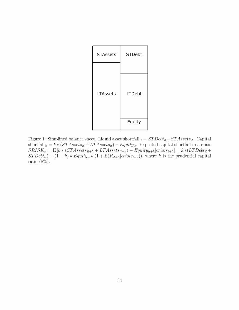
the bank lost its complete access to short-term funding (see Figure 1 for a simplified view of

the balance sheet of a bank).

I test for the solvency-liquidity nexus using several measures of solvency risk: regulatory

capital ratios, market measures of risk (realized volatility, market beta), and a measure

of the expected capital shortfall (SRISK) of the bank under aggregate stress defined by

Acharya et al. (2010, 2012) and Brownlees and Engle (2011). According to SRISK, a firm

is adequately capitalized to survive a crisis if its ratio of market capitalization to total assets

remains larger than 8% when the market index falls by 40% over the next six months. This

measure is an alternative to the capital shortfall estimates of regulatory stress tests that is4Related empirical studies include Das and Sy (2012) who document the trade-off between solvency and

liquidity; banks with more stable funding and more liquid assets do not need as much capital to get thesame stock return. Gorton and Metrick (2012) find that increases in repo rates are correlated to higheraggregate counterparty risk, whereas increases in repo haircuts are correlated to higher uncertainty aboutcollateral values. Afonso et al. (2011) study the Fed funds market and find increased sensitivity to bank-specific counterparty risk during times of crisis (both in the amounts lent to borrowers and in the cost ofovernight funds).

3

purely based on publicly available market data (and therefore available at a higher frequency

than stress tests outcomes).

I document three important results. First, I find that the bank’s capital shortfall under

stress (SRISK) determines how much short-term debt it can raise. This result supports the

models of Allen and Gale (1998); Diamond and Rajan (2005), etc. explaining bank runs based

on the strength of the bank’s fundamentals. The consequences of this solvency-liquidity nexus

are particularly severe for banks that are reliant on private short-term funding, in line with

the introductory quote of D. Tarullo and some previous evidence that firms with more matu-

rity mismatch have a larger contribution to systemic risk (Adrian and Brunnermeier (2010)).

Figure 2 illustrates well the solvency-liquidity nexus where capital-constrained banks (i.e.

banks with a positive SRISK) had a larger average exposure to liquidity risk (measured by

the difference between short-term debt and short-term assets) than adequately capitalized

banks before the financial crisis. The average liquidity shortfall of capital-constrained banks

reached a maximum of $133 billion in the third quarter of 2007. This exposure made them

particularly vulnerable to the sudden freeze of short-term funding markets that followed.

Second, I show that not all solvency risk measures predict the short-term debt level of

banks. The expected capital shortfall SRISK interacts well with the level of short-term

funding of the bank compared to other measures of solvency risk because (i) it is a measure

of the bank’s exposure to aggregate risk, and (ii) it combines both book and market values.

Relating to the model of liquidation costs of Shleifer and Vishny (1992), result (i) suggests

that a bank with higher solvency risk in isolation does not necessarily get restricted access

to short-term funding. What matters most for the suppliers of short-term funding is the

vulnerability of the bank to an aggregate crisis. When this crisis occurs, result (ii) suggests

that ’pure’ solvency risk (measured by the Tier 1 leverage ratio), amplified by market shocks,

explains the bank’s access to short-term funding.

Third, the stressed solvency risk measure interacts with the bank’s profitability (measured

4

by its net income divided by total assets) in determining its short-term balance sheet. While

a more profitable bank has a larger access to short-term funding and does not hold as much

liquid assets, profitability does not have this beneficial effect on its short-term balance sheet

when the bank is expected to be capital-constrained in a crisis. For example, the positive

net income of $2 billion of Citigroup in the third quarter of 2007 did not prevent the bank

from losing 18% of its short-term funding (-$172 billion) the next quarter, as Citigroup

was also highly undercapitalized according to SRISK ($51 billion expected capital shortfall

in 2007Q3). Therefore, maintaining a certain level of capitalization of the banking sector

reduces systemic risk not only by addressing solvency risk problems of banks in a crisis; it

also attenuates the solvency-liquidity nexus that makes banks particularly vulnerable to an

aggregate crisis.

Finally, the solvency-liquidity nexus appears to be strong under many robustness checks

(controlling for government interventions and common factors). Furthermore, out-of-sample

forecasting results during the European sovereign debt crisis show that the solvency-liquidity

interaction helps improve the forecasts of the short-term balance sheet of banks. Omitting

SRISK in the model increases the forecasting errors of the liquid asset shortfall considerably,

and particularly for capital-constrained banks.

Overall, the results of this paper suggest that the solvency-liquidity nexus should be

accounted for when designing liquidity and capital requirements. The paper gives empirical

support to the approach advanced by Tarullo (2013) to tie liquidity and capital requirements

together by requiring banks with a large exposure to short-term funding to hold an additional

capital buffer. The liquid asset buffer of the LCR might be a sufficient requirement from a

microprudential perspective. However, the sudden drop in short-term funding for a bank that

has a perfectly maturity-matched securities book (including repos and reverse repos) may

also result in fire sales and increases the risk of contagion by transferring funding liquidity

risk to the bank’s customers. The supplementary capital buffer is a preemptive measure that

5

would give the confidence to creditors to continue to provide funding to the bank in a period

of aggregate stress.

The rest of the paper is structured as follows. In Section 2, I describe the short-term

balance sheet of banks and their solvency risk measures. I test the solvency-liquidity nexus

in Section 3. I comment on the out-of-sample forecasting results in Section 4, and conclude

in Section 5.

2 Short-term balance sheet and solvency risk measures

I define solvency risk and (funding) liquidity risk from the simplified representation of a

bank’s balance sheet in Figure 1. A bank will be considered insolvent if it is not sufficiently

capitalized to absorb future asset shocks. Solvency risk regulation defines the fraction of

assets to be funded with equity such that a bank has a large enough equity capital buffer to

absorb asset losses when asset values deteriorate. As a result, a measure of solvency risk is

usually defined as a measure of the bank’s equity capital relative to a measure of its assets.

Next to solvency risk, funding liquidity risk is defined in Drehmann and Nikolaou (2013)

as “the possibility that over a specific horizon the bank will become unable to settle obliga-

tions with immediacy.” Funding liquidity risk typically arises when the bank does not hold

enough liquid assets that can be easily converted into cash to repay short-term creditors

when they decide to withdraw. Liquidity regulation therefore ensures that the bank has a

large enough liquid asset buffer to cover all funding outflows over a given horizon.

Funding liquidity risk is related to the maturity mismatch of a bank that invests short-

term funding in long-term assets (see . For the bank depicted in Figure 1, a proxy for its

maturity mismatch is the difference between its short-term debt and its short-term assets.

The gap between the short-term debt and the short-term assets of a bank is called its liquid

asset shortfall throughout, as I expect a bank with a larger maturity mismatch to be more

6

exposed to funding liquidity risk. On the liability side, short-term creditors will be the first

creditors to run as they can simply decide not to roll over their short-term funding contracts.

On the asset side, short-term assets are potentially the largest source of cash of the balance

sheet.5

2.1 Long-term vs. short-term balance sheet and the liquid asset

shortfall

The sample considered in this paper is a panel of 49 publicly traded U.S. bank holding

companies (BHC) reporting their regulatory accounting data over 13 years from 2000Q1 until

2013Q1 (i.e., 53 quarters). This sample of banks corresponds to the intersection between

the NYU Volatility Laboratory (V-Lab) sample for its global systemic risk analysis (that

will be introduced in the next section), and the bank holding companies reporting under the

FR Y-9C schedule (equivalent to the Call Reports of Condition and Income of commercial

banks). The names of the BHCs and their market capitalizations are reported in the online

appendix (Appendix E).

I construct the short-term debt and short-term asset variables of these BHCs based on

items extracted from their FR Y-9C reports from the SNL Financial database. The short-

term debt is constituted of uninsured time deposits of remaining maturity of less than a year,

securities sold under agreements to repurchase (repos), Federal funds purchased, and other

borrowed money of remaining maturity of less than a year. The short-term assets include

debt securities of remaining maturity of less than a year, interest-bearing bank balances

(cash), securities purchased under agreements to resell (reverse repos), and Federal funds5Short-term assets will serve in this chapter as a proxy for liquid assets due to the lack of historical data

for the assets included in the high-quality liquid assets (HQLA) definition of Basel III. High quality liquidassets include cash, reserves at central banks, treasury bonds, and non-financial corporate bonds and coveredbonds with the highest ratings. Additional assets like highly-rated RMBS, non-financial corporate bonds andcovered bonds with [A+, BBB-] rating, and common equity shares can be included in the HQLA stock withthe appropriate haircuts specified in the LCR revision of 2013 (Basel Committee on Banking Supervision(2013a)).

7

sold. The components of short-term debt and short-term assets are described in Appendix

A.

As the panel data set is unbalanced, I will restrict the following analyses to a smaller

sample of 44 banks for which the time series dimension is larger than 30 observations.6 I

test the stationarity of the balance sheet quantities (in logarithms) in Appendix B, using

the panel unit root test robust to cross-sectional dependence of Pesaran (2007). This test

indicates that the permanent impact of a shock on the size (measured by total assets) of

a bank comes from shocks in the long-term balance sheet (where the unit root hypothesis

is not rejected), whereas the short-term balance sheet shocks revert to a trend level.7 This

result is consistent with the long-term balance sheet being the core business of the traditional

bank that invests insured deposits (part of the long-term debt) in loans (long-term assets).8

The evolution of the average balance sheet of banks is shown in Figure 3. The average

size of the balance sheet (total assets) triples (from $85 billion to $280 billion) over the

sample period and follows an increasing trend in the long-term balance sheet. Over this

period, and particularly during the financial crisis, salient events include the acquisition of

out-of-sample banks by in-sample banks; Golden West Financial sold to Wachovia in May

2006, Bear Stearns sold to J.P.Morgan in March 2008, Countrywide to Bank of America

in July 2008, Washington Mutual to J.P.Morgan and Merrill Lynch to Bank of America in

September 2008, and the acquisition of in-sample banks by other in-sample banks; National

City Corp. sold to PNC and Wachovia to Wells Fargo in the last quarter of 2008.

For the purpose of testing the solvency-liquidity nexus, this paper focuses on the short-

term part of the balance sheet. The acquisition of two major investment banks (Bear Stearns6This restriction excludes Goldman Sachs and Morgan Stanley from the sample as they obtained the

status of bank holding company at the end of 2008. The restriction also excludes American Express, CITGroup, and Discover Financial Services.

7The trend stationarity of the short-term balance sheet allows estimating a dynamic panel data modeldirectly on the levels in Section 3, by applying standard estimation and inference techniques.

8The long-term debt (resp. assets) is the difference between total liabilities (resp. assets) and short-termdebt (resp. assets).

8

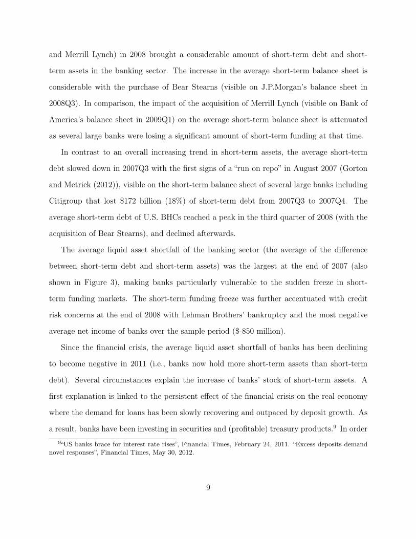
and Merrill Lynch) in 2008 brought a considerable amount of short-term debt and short-

term assets in the banking sector. The increase in the average short-term balance sheet is

considerable with the purchase of Bear Stearns (visible on J.P.Morgan’s balance sheet in

2008Q3). In comparison, the impact of the acquisition of Merrill Lynch (visible on Bank of

America’s balance sheet in 2009Q1) on the average short-term balance sheet is attenuated

as several large banks were losing a significant amount of short-term funding at that time.

In contrast to an overall increasing trend in short-term assets, the average short-term

debt slowed down in 2007Q3 with the first signs of a “run on repo” in August 2007 (Gorton

and Metrick (2012)), visible on the short-term balance sheet of several large banks including

Citigroup that lost $172 billion (18%) of short-term debt from 2007Q3 to 2007Q4. The

average short-term debt of U.S. BHCs reached a peak in the third quarter of 2008 (with the

acquisition of Bear Stearns), and declined afterwards.

The average liquid asset shortfall of the banking sector (the average of the difference

between short-term debt and short-term assets) was the largest at the end of 2007 (also

shown in Figure 3), making banks particularly vulnerable to the sudden freeze in short-

term funding markets. The short-term funding freeze was further accentuated with credit

risk concerns at the end of 2008 with Lehman Brothers’ bankruptcy and the most negative

average net income of banks over the sample period ($-850 million).

Since the financial crisis, the average liquid asset shortfall of banks has been declining

to become negative in 2011 (i.e., banks now hold more short-term assets than short-term

debt). Several circumstances explain the increase of banks’ stock of short-term assets. A

first explanation is linked to the persistent effect of the financial crisis on the real economy

where the demand for loans has been slowly recovering and outpaced by deposit growth. As

a result, banks have been investing in securities and (profitable) treasury products.9 In order9“US banks brace for interest rate rises”, Financial Times, February 24, 2011. “Excess deposits demand

novel responses”, Financial Times, May 30, 2012.

9

to obtain secured short-term funding, banks also need to hold more short-term liquid assets

than before due to stricter collateral requirements (higher haircuts). Then, higher liquid

asset holdings by banks respond to precautionary concerns by banks (protecting against

anticipated interest rate increase) and the regulator. Banks are encouraged by regulation

to hold more short-term liquid assets to comply with both liquidity requirements (Basel

III liquidity coverage ratio) and capital requirements (as holding short-term assets usually

involves low regulatory capital requirements).

2.2 Solvency risk measures

2.2.1 Regulatory capital ratios

The regulator usually employs capital ratios to assess the solvency risk of a bank. Figure

4 displays the average regulatory capital ratios: the Tier 1 common capital ratio (T1CR)

and the Tier 1 leverage ratio (T1LV GR). The Tier 1 common capital ratio is the ratio

of Tier 1 common equity capital to risk-weighted assets, whereas the Tier 1 leverage ratio

is the ratio of Tier 1 capital to total assets. The upward shift in regulatory capital ratios

in the fourth quarter of 2008 indicates a healthier banking system, and coincides with the

launch on October 14, 2008 of the Capital Purchase Program (CPP) and the Temporary

Liquidity Guarantee Program (TLGP) under the Trouble Asset Relief Program (TARP). By

purchasing assets and equity from troubled banks from October 2008 on, the TARP led to

a significant increase in the average capital ratios. For example, Treasury bought $25 billion

of preferred shares of Citigroup in October 2008, and another $20 billion in November 2008

under the CPP.10

10See http://www.treasury.gov/initiatives/financial-stability/reports/Pages/TARP-Tracker.aspx.

10

2.2.2 Expected capital shortfalls in a crisis

Acharya et al. (2012) define the systemic risk contribution of a firm i to the real economy

at time t as “the real social costs of a crisis per dollar of capital shortage(t)⇥ Probability

of a crisis(t) ⇥ SRISKit”, where SRISKit represents the expected capital shortfall of the

firm in a crisis, i.e. when the market equity index drops by 40% over the next six months.

In these market conditions, SRISK is based on the assumption that the book value of the

(long-term) debt Dit of the bank will remain constant over the six-month horizon while its

market capitalization MVit will decrease by its six-month return in a crisis, called the long-

run marginal expected shortfall (LRMES). The expected capital shortfall in a crisis of bank

i at time t is defined by

SRISKit = Et[k(Dit+h +MVit+h)�MVit+h|Rmt+h �40%] (1)

= kDit � (1� k) ⇤MVit ⇤ (1� LRMESit)

where Rmt+h is the return of the market index from period t to period t + h (h = 6

months), k is the prudential capital ratio (8% for U.S. financial firms), and LRMESit =

�Et(Rit+h|Rmt+h �40%). Compared to other market-based measures of systemic risk like

the CoVaR of Adrian and Brunnermeier (2010) or the Distress Insurance Premium (DIP)

of Huang et al. (2012), an interesting feature of SRISK is that it is a function of size and

leverage, which are two characteristics that the regulator finds particularly relevant when

measuring solvency risk of banks. SRISK can be written as a function of size, leverage and

risk

SRISKit = MVit {k(Lvgit � 1)� (1� k)(1� LRMESit)} (2)

where Lvgit is the quasi-market leverage defined as the ratio of quasi-market assets to market

capitalization (Lvgit = (MVit + Dit)/MVit). Therefore, the capital shortfall of a bank will

11

be large if the bank is large, highly leveraged, and highly sensitive to an aggregate shock as

measured by LRMESit.

These measures (SRISK and LRMES) are available from the V-Lab website developed

at NYU Stern School of Business.11 In the global systemic risk analysis of V-Lab, LRMES

is extrapolated from its short-term counterpart MES, which represents the daily return of

the bank conditional on a 2% decline in the daily return of a global market index. The MES

is derived from a time-varying beta estimated with the Dynamic Conditional Beta model of

Engle (2012) that accounts for asynchronous trading around the world when measuring the

comovement of bank returns with a global market index.

By definition, SRISK can be negative when a bank is expected to have a capital excess

in a crisis. In Figure 4, we find two different regimes for the average SRISK of banks. Banks

were in excess of capital in average (negative SRISK) before 2007. The average SRISK

was the lowest in the third quarter of 2006, then started to increase in 2007. SRISK became

positive in the fourth quarter of 2007, and reached a maximum average capital shortfall of

$16 billion in the first quarter of 2009. The average capital shortfall has remained positive

since the financial crisis (reflecting a low market-to-book ratio), and bumped several times

afterwards, in particular in the heat of the European sovereign debt crisis in 2011.

3 Testing the solvency-liquidity nexus of banks

As liquidity risk concerns both sides of the balance sheet, I test for factors affecting both

the short-term debt and short-term assets of the bank. I use an autoregressive model for

the logarithm of the short-term balance sheet as panel unit root tests indicate that the

variables yit = ln(STDebtit) and zit = ln(STAssetsit) are trend stationary (see Appendix

B). Based on in-sample fit criteria, the model for both elements of wit = (yit, zit)0 is an11See http://vlab.stern.nyu.edu/.

12

autoregressive process of lag order one with bank dummies, and heterogeneous trend and

dynamic parameters

wit = ↵i + �i � wit�1 + ✓it+ �

0xit�1 + "it (3)

where ↵i, �i and ✓i are (2 ⇥ 1) vectors of parameters specific to bank i, xit is a (K ⇥ 1)

vector of stationary bank characteristics (including solvency risk measures), and � is the

Hadamard product.12 Bank-specific parameters mainly reflect different business models,

and the resulting differences in aversion for funding liquidity risk.

The solvency-liquidity nexus may appear in different forms; I test for the direct effect

of solvency risk on funding liquidity using SRISK (Section 3.1) and alternative solvency

risk measures (Section 3.2), and for the interaction between profitability and solvency risk

in predicting the short-term balance sheet (Section 3.3). Then, I test the robustness of the

solvency-liquidity nexus in Section 3.4.

3.1 Testing the solvency-liquidity nexus using SRISK

The estimates of the interaction parameters (�) of equation (3), where xit = SRISKit/TAit,

are reported in Table 1 (Panel A). This Table reveals the Granger causality of solvency risk

on the short-term balance sheet, where banks with a larger expected capital shortfall hold

less short-term debt in the next quarter; the estimates suggest that a positive unit shock on

the ratio of SRISK to total assets produces a -1.102% shock on the short-term funding of

the bank.

This result supports the theoretical literature explaining bank runs based on the strength12The parameters of eq. (3) are estimated by ordinary least squares. Judson and Owen (1999) report severe

negative bias for the autoregressive parameters of dynamic panel regressions due to the small time seriesdimension even when T = 30. The potential negative bias of autoregressive parameters has implicationsfor the stationarity of the endogenous variables of the panel regression. Running the regressions in firstdifferences does not, however, qualitatively change the results on the � parameter estimates.

13

of the banks fundamentals (Allen and Gale (1998); Diamond and Rajan (2005), etc.), and

describing the interaction between liquidity and solvency problems of banks (Diamond and

Rajan (2005); Morris and Shin (2008); Rochet and Vives (2004)). The results also give

empirical support to the recent speeches by Carney (2013) and Tarullo (2013) explaining

that the repair of banks’ balance sheet (i.e. higher capital levels) gives the confidence to

investors and creditors to continue to provide funding to banks.

From Table 1, we also note that short-term assets do not react to solvency risk or short-

term funding shocks, suggesting that banks are not able to adjust their stock of short-term

assets to solvency risk or short-term funding conditions in a timely fashion. It also reflects

a liquidity hoarding tendency of banks where banks prefer to sell long-term assets to repay

short-term creditors. Banks prefer to hold the short-term assets for precautionary reasons

or for investing in fire sale assets of other financial institutions that are expected to generate

high future returns (Acharya et al. (2009)).

“Reverse causality” tests (in Appendix C) indicate that a higher exposure to short-term

debt has a positive impact on the capital shortfall SRISK. Therefore, the interaction

between solvency and the short-term balance sheet is asymmetric; higher solvency risk limits

the access of the firm to short-term funding, but a firm with more short-term debt has a

higher risk of insolvency in a crisis. The second finding is however harder to interpret as a

causal relationship as short-term debt is more likely to be endogenous than solvency risk. I

therefore concentrate on the first finding; banks with higher solvency risk are penalized by

the market in their access to short-term debt.

3.2 Testing alternative solvency risk measures

I report the tests of alternative measures of solvency risk to predict the short-term balance

sheet (yit and zit) in Table 2, controlling for the market-to-book ratio as the regression

includes both accounting and market variables. The columns (1) to (5) show the individual

14

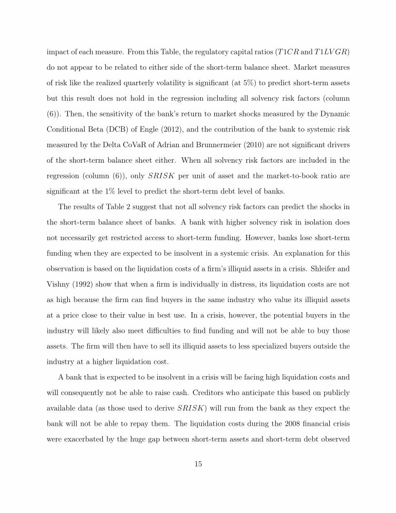
impact of each measure. From this Table, the regulatory capital ratios (T1CR and T1LV GR)

do not appear to be related to either side of the short-term balance sheet. Market measures

of risk like the realized quarterly volatility is significant (at 5%) to predict short-term assets

but this result does not hold in the regression including all solvency risk factors (column

(6)). Then, the sensitivity of the bank’s return to market shocks measured by the Dynamic

Conditional Beta (DCB) of Engle (2012), and the contribution of the bank to systemic risk

measured by the Delta CoVaR of Adrian and Brunnermeier (2010) are not significant drivers

of the short-term balance sheet either. When all solvency risk factors are included in the

regression (column (6)), only SRISK per unit of asset and the market-to-book ratio are

significant at the 1% level to predict the short-term debt level of banks.

The results of Table 2 suggest that not all solvency risk factors can predict the shocks in

the short-term balance sheet of banks. A bank with higher solvency risk in isolation does

not necessarily get restricted access to short-term funding. However, banks lose short-term

funding when they are expected to be insolvent in a systemic crisis. An explanation for this

observation is based on the liquidation costs of a firm’s illiquid assets in a crisis. Shleifer and

Vishny (1992) show that when a firm is individually in distress, its liquidation costs are not

as high because the firm can find buyers in the same industry who value its illiquid assets

at a price close to their value in best use. In a crisis, however, the potential buyers in the

industry will likely also meet difficulties to find funding and will not be able to buy those

assets. The firm will then have to sell its illiquid assets to less specialized buyers outside the

industry at a higher liquidation cost.

A bank that is expected to be insolvent in a crisis will be facing high liquidation costs and

will consequently not be able to raise cash. Creditors who anticipate this based on publicly

available data (as those used to derive SRISK) will run from the bank as they expect the

bank will not be able to repay them. The liquidation costs during the 2008 financial crisis

were exacerbated by the huge gap between short-term assets and short-term debt observed

15

in Section 2. As a result, banks had no choice but to sell illiquid assets to repay creditors

when losing access to short-term funding.

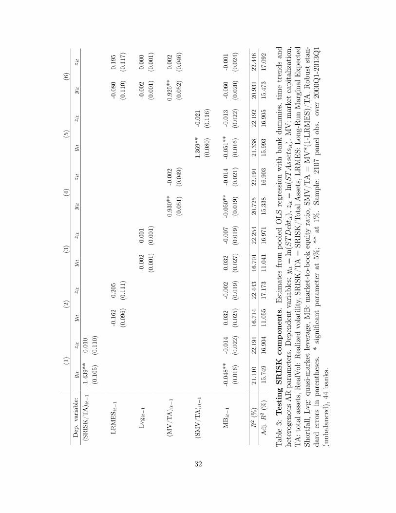
In-sample fit criteria show the higher performance of SRISK in Table 3 (first column) in

predicting short-term funding; the adjusted R

2 is 15.7% compared to an adjusted R

2 around

11% for the regressions with the alternative solvency risk measures of Table 2.13 In order to

identify what works so well in SRISK to predict the short-term funding of banks, Table 3

also reports the estimates of the different components of SRISK highlighted in eq. (2). The

Table shows that the improvement in in-sample fit rather comes from the ratio of market

capitalization to total assets (MV/TA) than from the long-run marginal expected shortfall

(LRMES) or the quasi-market leverage (Lvg). The main difference between Lvg and the

ratio MV/TA is a different combination of book and market values; the ratio MV/TA is the

product of the book leverage ratio (T1LV GRit) and the market-to-book ratio (MVit/BVit)

MVit

TAit=

BVit ⇤⇣

MVitBVit

⌘

TAit' T1LV GRit ⇤

✓MVit

BVit

◆,

whereas Lvgit = 1 + DitMVit

is not a function of the book leverage ratio. Market values are

expected to reflect liquidity problems of banks as they incorporate information about both

solvency and liquidity risks. Therefore, any measure based on market values is not a “pure”

solvency risk measure. The fact that the ratio MV/TA is a function of the book leverage

ratio (T1LV GRit) — a “pure” solvency risk measure — appears to be a crucial element

in predicting short-term funding; it makes this ratio significant in the solvency-liquidity

interaction compared to other solvency risk measures like the distance-to-default which is an

inverse function of market leverage (Lvg) and firm assets volatility. The results of Table 3

indeed suggest that both the book leverage ratio — informing about “pure” solvency risk —

and the market-to-book ratio — informing about how fast the market values fall compared13Note that all reported R2 are on the first differences (wit �wit�1). The R2 of levels (wit) are very high

(around 90%) given the bank specific constant, trend and autoregressive parameters.

16

to book values — are important factors explaining banks’ access to short-term funding. The

ratio MV/TA is highly correlated to the book leverage ratio (0.91) and less correlated to

the market-to-book ratio (0.44); solvency risk, amplified by market shocks, explains banks’

access to short-term funding, and neither the market-to-book or the leverage ratio taken

separately, nor their linear combination predict short-term funding.

The modest improvement in fit due to the downside risk of the bank in a crisis LRMES

(0.66% increase of adjusted R

2 from column 4 to column 5, Table 3) is consistent with the

sample period that contains several episodes of market stress. In a crisis, all is already

function of the aggregate shock. However, measuring the downside risk is important pre-

emptively; I find increasing out-of-sample forecasting errors when MV/TA is employed in eq.

(3) instead of SRISK/TA for predicting the short-term balance sheet of banks during the

European sovereign debt crisis (especially with the dynamic forecasting exercise of Section

4).

3.3 Interaction between solvency and profitability

In Perotti and Suarez (2011), both liquidity risk and profitability are increasing functions

of the short-term debt level of the bank. A bank will indeed demand more short-term

funding when it finds profitable investment opportunities. Its liquidity risk will also increase

as its short-term debt will be invested in long-term profitable assets. The impact of the

profitability of the bank measured by its net income divided by total assets is found to be

positive on short-term debt and negative on short-term assets in Table 1 (Panel B), but

these parameters are not significant at the 5% level.

The parameters of eq. (3) are however expected to vary with the state of the bank and/or

the aggregate liquidity conditions. In good times, short-term funding and short-term assets

are the result of management decisions and are driven by demand factors. As mentioned,

banks with profitable opportunities will demand more short-term funding. In bad times,

17

supply factors determine how much short-term debt a bank can raise and the short-term

assets adjust accordingly. One way to disentangle supply and demand effects on the bank

characteristics is to augment equation (3) with a state variable

wit = ↵i + �i � wit�1 + ✓it+ �

0xit�1 + �

0xit�1 ⇤ st�1 + !st�1 + "it (4)

where the state variable st could be a bank characteristic or a common factor. For example,

Cornett et al. (2011) use the TED spread (the difference between 3-month LIBOR rate

and the T-bill rate) to reflect the change in the management of liquidity risk exposures of

banks during the financial crisis.14 In Table 1 (Panel C), I show that a good candidate

for the state variable is simply a dummy variable equal to one when SRISK is positive

(sit = 1{SRISKit>0}), i.e. when the bank is expected to have a capital shortfall in a crisis.

This distinction between states where SRISK is positive or negative appears to be

important when measuring the effect of the profitability of the bank on its short-term balance

sheet. Indeed, a bank with a higher net income has a larger access to short-term funding

while it does not hold as much liquid assets. In Table 1, this beneficial effect of the bank’s

profitability on its short-term balance sheet appears to be true only when the bank’ SRISK

is negative, i.e. when the bank is adequately capitalized to survive a crisis (sit = 0). When

the bank is expected to be capital-constrained in a crisis (sit = 1), the effect of profitability

on its balance sheet disappears (� + � ' 0), and only solvency risk predict the short-term

debt of the bank. Therefore, the solvency-liquidity nexus appears to be exacerbated for

capital-constrained banks; for these banks, only solvency risk explains access to short-term

debt.14The TED spread is however not significant to predict the short-term balance sheet for the sample

considered in this paper (cf. Appendix D).

18

3.4 Robustness of the solvency-liquidity nexus

3.4.1 Robustness to the TARP

On October 14, 2008, the U.S. government announced a series of measures — the Trou-

bled Asset Relief Program (TARP) — to restore financial stability. Under the TARP, the

Treasury Department launched the Capital Purchase Program (CPP) and the Federal De-

posit Insurance Corporation (FDIC) launched the Temporary Liquidity Guarantee Program

(TLGP). Treasury injected $205 billion capital into banks under the CPP by buying war-

rants, common shares, and preferred shares.15 Under the TLGP, the FDIC allowed financial

institutions to retain and raise funding by giving a guarantee on existing noninterest-bearing

transaction accounts and certain newly issued senior unsecured debt. Data on the amount

and maturity of total unsecured debt issued by banks and guaranteed by the FDIC are

publicly available.16

It is possible to derive the hypothetical amount of short-term debt a bank would have

had if it did not have benefited from government guarantees. The solvency-liquidity nexus

estimates hardly change when TLGP funding is not taken into account. It is however difficult

to project this scenario on the other variables (SRISK and short-term assets) as it requires

knowing where TLGP funding was invested and how markets would have reacted in this

scenario.

3.4.2 Robustness of the solvency-liquidity nexus to common factors

The short-term balance sheets of firms are expected to co-move according to the aggregate

liquidity conditions. To capture these common effects, I consider the macroeconomic and

financial factors that are used in Fontaine and Garcia (2012) to relate to their factor mea-15http://www.treasury.gov/initiatives/financial-stability/TARP-Programs/bank-investment-

programs/cap/Pages/overview.aspx16See http://www.fdic.gov/regulations/resources/TLGP/index.html

19

suring the value of funding liquidity. The sensitivity of the short-term balance sheet to the

common factors is tested in Appendix D.

I test the robustness of the solvency-liquidity nexus to the presence of common factors in

wit = ↵i + �i � wit�1 + ✓it+ �

0git�1 + �

0ft�1 + "it (5)

where wit = (yit, zit)0, git is a ((2 ⇤K + 1)⇥ 1) vector stacking xit, xit ⇤ sit and sit in a single

column, � is a ((2 ⇤ K + 1) ⇥ 2) vector containing the �, � and ! parameters, and ft is a

vector of macroeconomic and financial factors.17

Chudik and Pesaran (2013) propose an alternative modeling strategy based on the Com-

mon Correlated Effects (CCE) of Pesaran (2006), where the unobserved common factors are

proxied by the cross-sectional averages of the dependent variable and the regressors

wit = ↵i + �i � wit�1 + ✓it+ �

0git�1 +

1X

l=0

'

0lwt�l +

0gt�1 + "it (6)

where wt�l = N

�1PN

i=1 wit�l and gt = N

�1PN

i=1 git.

The estimation results of eq. (5) and eq. (6) are reported in Appendix D (Table 4). The fit

improves considerably when common factors are included. The best in-sample performance

is found with the CCE model for all elements of wit. However, the CCE model counts a

contemporaneous factor (average of the dependent variable), while the model with macro

and financial factors only includes lagged factors. The macro-financial model is therefore

more convenient for forecasting and the loss of in-sample fit is relatively small compared to

the CCE model.

The solvency-liquidity nexus holds when I control for cross-sectional dependence. The

interaction term between the profitability and SRISK is however not as important (not17Note that common factors do not necessarily need to be lagged but this allows for the derivation of

one-step ahead forecasts for wit without specifying a model for the common factors.

20

significant at the 5%).

3.4.3 Short-term debt components and fixed effects

The different components of short-term debt (repos, uninsured deposits, commercial papers,

etc.) have very different characteristics and may not react to solvency risk with the same

magnitude. Table 5 in Appendix D reports the parameter estimates of eq. (3) where the

dependent variable in each column is a different component (in logarithm) of the short-term

debt available from FR 9-YC reports. SRISK predicts most of the components of the

short-term debt; it is significant at the 1% level for wholesale funding (Fed funds, repos,

and commercial papers), and at the 5% level for retail funding (uninsured time deposits and

foreign office deposits).

Finally, an important result is that SRISK is only related to the short-term part of the

balance sheet and does not predict long-term leverage. Table 6 in Appendix D shows that the

long-term balance sheet is not sensitive to SRISK. The long-term debt only reacts to short-

term assets and the flows in long-term assets. Other robustness checks (not reported in this

paper) show that the interaction between solvency and liquidity remains with homogenous

dynamic parameters (�i = �, 8i), homogenous trend parameters (✓i = ✓, 8i), without trend

(✓i = 0, 8i), and when a break in 2008Q4 is included in the trend. These results tend

to confirm the robustness of the solvency-liquidity nexus. In the next section, I test for

the out-of-sample forecasting performance of the solvency-liquidity nexus in predicting the

short-term balance sheet of banks.

4 Forecasting the short-term balance sheet

To test for the out-of-sample predictive performance of the solvency-liquidity nexus, I con-

duct two forecasting exercises. Both exercises are based on a fixed estimation period from

21

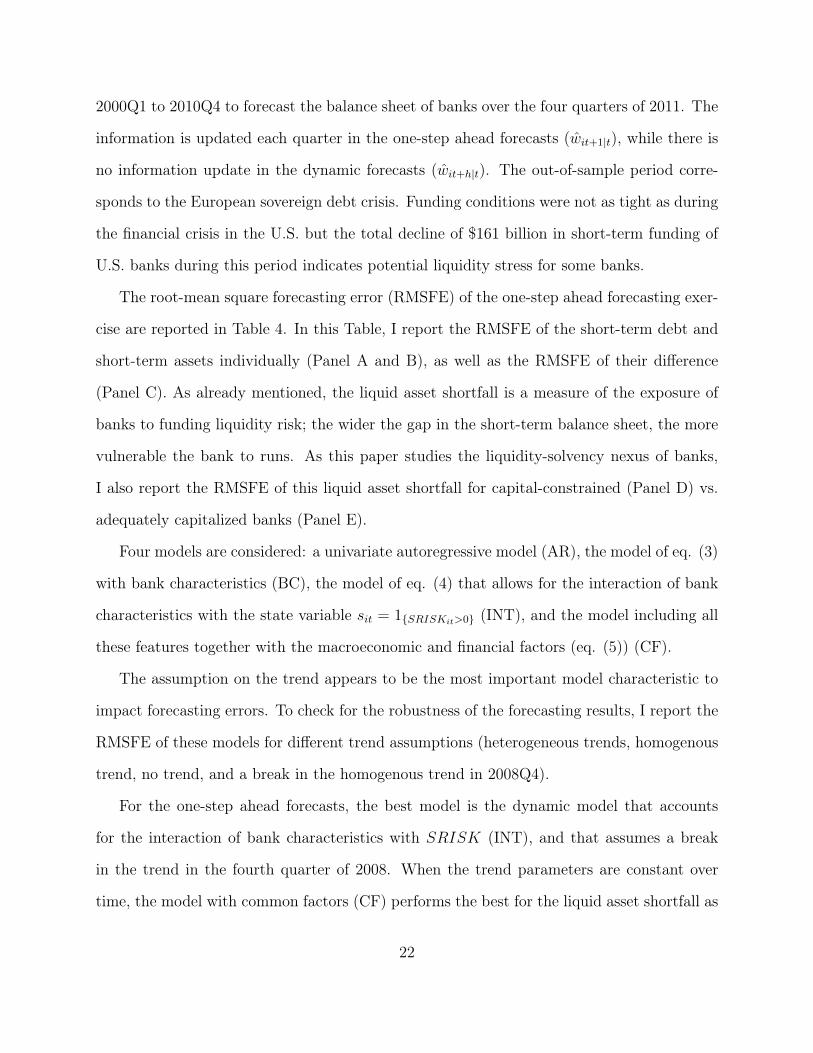
2000Q1 to 2010Q4 to forecast the balance sheet of banks over the four quarters of 2011. The

information is updated each quarter in the one-step ahead forecasts (wit+1|t), while there is

no information update in the dynamic forecasts (wit+h|t). The out-of-sample period corre-

sponds to the European sovereign debt crisis. Funding conditions were not as tight as during

the financial crisis in the U.S. but the total decline of $161 billion in short-term funding of

U.S. banks during this period indicates potential liquidity stress for some banks.

The root-mean square forecasting error (RMSFE) of the one-step ahead forecasting exer-

cise are reported in Table 4. In this Table, I report the RMSFE of the short-term debt and

short-term assets individually (Panel A and B), as well as the RMSFE of their difference

(Panel C). As already mentioned, the liquid asset shortfall is a measure of the exposure of

banks to funding liquidity risk; the wider the gap in the short-term balance sheet, the more

vulnerable the bank to runs. As this paper studies the liquidity-solvency nexus of banks,

I also report the RMSFE of this liquid asset shortfall for capital-constrained (Panel D) vs.

adequately capitalized banks (Panel E).

Four models are considered: a univariate autoregressive model (AR), the model of eq. (3)

with bank characteristics (BC), the model of eq. (4) that allows for the interaction of bank

characteristics with the state variable sit = 1{SRISKit>0} (INT), and the model including all

these features together with the macroeconomic and financial factors (eq. (5)) (CF).

The assumption on the trend appears to be the most important model characteristic to

impact forecasting errors. To check for the robustness of the forecasting results, I report the

RMSFE of these models for different trend assumptions (heterogeneous trends, homogenous

trend, no trend, and a break in the homogenous trend in 2008Q4).

For the one-step ahead forecasts, the best model is the dynamic model that accounts

for the interaction of bank characteristics with SRISK (INT), and that assumes a break

in the trend in the fourth quarter of 2008. When the trend parameters are constant over

time, the model with common factors (CF) performs the best for the liquid asset shortfall as

22

common factors reflect the changing aggregate funding conditions after the financial crisis.

In the last three columns of Table 4, I report the increase in RMSFE when a particular bank

variable is not included in the BC model. This Table shows that omitting SRISK increases

the forecasting errors of the liquid asset shortfall considerably, and particularly for capital

constrained banks during 2011. However, the model with bank characteristics (BC) or the

interaction with solvency risk (INT) does not improve the forecasts of adequately capitalized

banks.

I obtain very similar results for the dynamic forecasts and therefore do not report their

RMSFE. Note that the RMSFE of dynamic forecasts are larger compared to the errors of

one-step ahead forecasts due to the absence of information updates over the forecasting

horizon. The model with interaction with SRISK (INT) and a break in the trend after

the financial crisis is also the preferred model according the RMSFE of dynamic forecasts.

The cross-sectional average dynamic forecasts obtained with this model for the short-term

balance sheet levels and flows over 2011Q1-2013Q1 are illustrated in Figure 5a. It turns out

that the model is outstanding at forecasting short-term financing flows but does a less good

job at forecasting short-term asset flows, which are not sensitive to the factors considered in

the model.

In Figure 5b, I show the average dynamic forecasts of the liquid asset shortfall across

all banks, as well as for the subsamples of capital-constrained vs. adequately capitalized

banks. As mentioned in the introduction, the liquid asset shortfall of capital-constrained

banks spiked in the first quarters of 2007 and suddenly dropped afterwards due to the

sudden freeze of short-term funding markets. In the first quarter of 2011, the average liquid

asset shortfall of capital-constrained banks became negative; capital-constrained firms are

less exposed to funding liquidity risk than adequately capitalized banks for the first time

over the sample period. The model predicts this reversal in the solvency-liquidity nexus and

predicts well the average excess of liquidity of capital-constrained banks during this period.

23

5 Conclusion

This paper reveals the empirical solvency-liquidity nexus of banks. While the interaction

between solvency and liquidity has been well studied in the theoretical economic literature,

this relationship tends to be omitted in the new capital and liquidity regulatory standards

introduced under Basel III. In this paper, I test the solvency-liquidity nexus by examining

the short-term balance sheet and the solvency risk measures of a sample of U.S. bank holding

companies over 2000-2013.

I find that the expected capital shortfall of a bank in a crisis (SRISK) predicts how much

short-term funding the bank has access to. This result appears to be strong under many

robustness checks and supports the theoretical models of the interaction between solvency

and liquidity risks and its amplification (aggregate) effects leading to systemic risk.

Importantly, not all solvency risk measures predict the bank’s access to short-term debt.

The expected capital shortfall SRISK interacts well with the level of short-term funding of

the bank compared to other solvency risk measures because (i) it is a measure of the bank’s

exposure to aggregate risk, and (ii) it combines both book and market values. Suppliers of

liquidity are mostly concerned with the vulnerability of the bank to an aggregate crisis due

to the high liquidation costs the distressed bank will face in the presence of fire sales. When

the crisis happens, ’pure’ solvency risk (measured by the Tier 1 leverage ratio) amplified by

market shocks explains the bank access to short-term funding.

The expected capital shortfall of the bank under stress also interacts with its profitability

in determining its short-term balance sheet. While a profitable bank gets a larger access

to short-term funding and does not hold as much liquid assets, the impact of the bank’s

profitability on its liquidity profile tends to disappear when the bank is expected to be

insolvent in a crisis.

The solvency-liquidity nexus provides useful information for forecasting the short-term

24

financing flows during 2011 (European sovereign debt crisis). I show that the forecasting

errors of the liquid asset shortfall of banks increase considerably when the stressed solvency

risk measure is not included in the regression.

Overall, the results of this paper suggest that the solvency-liquidity nexus should be

accounted for when designing liquidity and capital regulations, where macroprudential regu-

lation of funding liquidity risk would be a combination of both liquid assets requirements and

capital requirements. This paper suggests that maintaining the capitalization of the banking

sector reduces systemic risk not only by addressing solvency risk problems of banks in a cri-

sis; it also attenuates the solvency-liquidity nexus that makes banks particularly vulnerable

to an aggregate crisis. Higher capital requirements for systemically important institutions

serve a dual purpose; they act as a loss-absorbing buffer when banks’ asset values deterio-

rate, and by improving banks’ robustness to an aggregate crisis, they ensure the confidence

of creditors to continue to provide funding to the banks.

25

References

Acharya, V., C. Brownlees, R. Engle, F. Farazmand, and M. Richardson (2010). Measuring

systemic risk. In V. Acharya, T. Cooley, M. Richardson, and I. Walter (Eds.), Regulating

Wall Street: The Dodd-Frank Act and the New Architecture of Global Finance, Chapter 4.

John Wiley & Sons, Ch. 4.

Acharya, V., R. Engle, and M. Richardson (2012). Capital shortfall: a new approach to

rankings and regulating systemic risks. American Economic Review Papers and Proceed-

ings 102:3, 59–64.

Acharya, V., H. Shin, and T. Yorulmazer (2009). Endogenous choice of bank liquidity: the

role of fire sales. Bank of England Working Paper no. 376.

Acharya, V. and S. Viswanathan (2011). Leverage, moral hazard, and liquidity. Journal of

Finance 66, 99–138.

Acharya, V. and T. Yorulmazer (2008). Cash-in-the-market pricing and optimal resolution

of bank failures. Review of Financial Studies 21, 2705–2742.

Adrian, T. and M. Brunnermeier (2010). CoVaR. Federal Reserve Bank of New York Staff

Reports No. 348.

Afonso, G., A. Kovner, and A. Schoar (2011). Stressed, not frozen: The federal funds market

in the financial crisis. Federal Reserve Bank of New York Staff Reports, no. 437.

Aikman, D., P. Alessandri, B. Eklund, P. Gai, S. Kapadia, E. Martin, N. Mora, G. Sterne,

and M. Willison (2009). Funding liquidity risk in a quantitative model of systemic stability.

Bank of England Working Paper No. 372.

Allen, F. and D. Gale (1998). Optimal financial crises. Journal of Finance 53:4, 1246–1284.

26

Allen, F. and D. Gale (2000a). Financial contagion. Journal of Political Economy. 108, 1–33.

Allen, F. and D. Gale (2000b). Optimal currency crises. Carnegie-Rochester Conference

Series on Public Policy 53, 177–230.

Allen, F. and D. Gale (2004). Financial intermediaries and markets. Econometrica 72:4,

1023–1061.

Basel Committee on Banking Supervision (2011, June). Basel III: A global regulatory frame-

work for more resilient banks and banking systems. Bank for International Settlements.

Basel Committee on Banking Supervision (2013a, January). Basel III: The Liquidity Cov-

erage Ratio and Liquidity Risk Monitoring Tools. Bank for International Settlements.

Basel Committee on Banking Supervision (2013b, July). Global systemically important

banks: updated assessment methodology and the higher loss absorbency requirement.

Bank for International Settlements.

Brownlees, C. and R. Engle (2011). Volatility, correlation and tails for systemic risk mea-

surement. NYU Working Paper.

Carney (2013). Crossing the threshold to recovery. Speech August 28, 2013.

Chudik, A. and H. Pesaran (2013). Common correlated effects estimation of heterogeneous

dynamic panel data models with weakly exogenous regressors. Cambridge Working Papers

in Economics no 1317.

Cornett, M., J. McNutt, P. Strahan, and H. Tehranian (2011). Liquidity risk management

and credit supply in the financial crisis. Journal of Financial Economics 101:2, 297–312.

Das, S. and A. Sy (2012). How risky are banks’ risk-weighted assets? Evidence from the

financial crisis. IMF Working Paper WP/12/36.

27

Diamond, D. and P. Dybvig (1983). Bank runs, deposit insurance, and liquidity. Journal of

Political Economy 91:3, 401–419.

Diamond, D. and R. Rajan (2005). Liquidity shortages and banking crises. Journal of

Finance 60:2, 615–647.

Diamond, D. and R. Rajan (2011). Fear of fire sales, illiquidity seeking, and credit freezes.

Quaterly Journal of Economics 126:2, 557–591.

Drehmann, M. and K. Nikolaou (2013). Funding liquidity risk: Definition and measurement.

Journal of Banking & Finance 37, 2173–2182.

Engle, R. (2012). Dynamic conditional beta. NYU Working Paper.

Fontaine, J.-S. and R. Garcia (2012). Bond liquidity premia. The Review of Financial

Studies 25:4, 1207–1254.

Gorton, G. (1988). Banking panics and business cycles. Oxford Economic Papers 40:4,

751–781.

Gorton, G. and A. Metrick (2012). Securitized banking and the run on repo. Journal of

Financial Economics 104:3, 425–451.

Huang, X., H. Zhou, and Z. Haibin (2012). Systemic risk contributions. Journal of Financial

Services Research 42, 55–83.

Judson, R. and A. Owen (1999). Estimating dynamic panel data models: a guide for macroe-

conomists. Economics Letters 65, 9–15.

Morris, S. and H. Shin (2008). Financial regulation in a system context. Brookings Papers

on Economic Activity 2008, 229–261.

28

Perotti, E. and J. Suarez (2011). A Pigovian approach to liquidity regulation. Journal of

International Central Banking 7:4, 3–39.

Pesaran, H. (2006). Estimation and inference in large heterogeneous panels with a multifactor

error structure. Econometrica 74:4, 967–1012.

Pesaran, H. (2007). A simple panel unit root test in the presence of cross-section dependence.

Journal of Applied Econometrics 22, 265–312.

Rochet, J.-C. and X. Vives (2004). Coordination failures and the lender of last resort: was

Bagehot right after all? Journal of the European Economic Association 2:6, 1116–1147.

Shleifer, A. and R. Vishny (1992). Liquidation values and debt capacity: A market equilib-

rium approach. Journal of Finance 47:4, 1343–1366.

Tarullo, D. (2013). Evaluating progress in regulatory reforms to promote financial stability.

Speech May 3, 2013.

29

Panel A Panel B Panel C

Dep. variable: yit zit yit zit yit zit(SRISK/TA)it�1 -1.120** 0.074 -1.063** -0.028 -0.935** -0.120

(0.244) (0.114) (0.245) (0.118) (0.261) (0.101)

(SRISK/TA)it�1 ⇤ sit�1 -0.408 1.757*

(0.751) (0.767)

zit�1 -0.040 -0.038 -0.033

(0.023) (0.023) (0.022)

zit�1 ⇤ sit�1 -0.021*

(0.008)

yit�1 -0.003 -0.004 -0.002

(0.022) (0.021) (0.022)

yit�1 ⇤ sit�1 -0.007*

(0.010)

(NI/TA)it�1 2.354 -4.228 9.704** -7.944*

(2.278) (2.331) (3.290) (3.716)

(NI/TA)it�1 ⇤ sit�1 -9.902* 6.315

(4.396) (5.183)

sit�1 0.347* 0.066

(0.144) (0.159)

R2(%) 20.811 22.157 20.870 22.318 21.278 22.562

Adj. R2(%) 15.430 16.868 15.450 16.997 15.715 17.089

Table 1: Testing the solvency-liquidity nexus. Estimates from pooled OLS re-gression with bank dummies, time trends, and heterogeneous AR parameters. PanelA: model of eq. (3), where xit = SRISKit/TAit. Panel B: model of eq. (3),where xit = (SRISKit/TAit, NIit/TAit)

0. Panel C: model of eq. (4), where xit =(SRISKit/TAit, NIit/TAit)

0 and with state variable sit = 1{SRISKit>0}. Dependent vari-ables: yit = ln(STDebtit), zit = ln(STAssetsit). (NI/TA)it = NetIncomeit/TotalAssetsit,(SRISK/TA)it = SRISKit/TotalAssetsit. SRISK is the expected capital shortfall of thebank in a crisis. Robust standard errors in parentheses. * significant parameter at 5%; **at 1%. Sample: 2107 panel obs. over 2000Q1-2013Q1 (unbalanced), 44 banks.

30

(1)

(2)

(3)

(4)

(5)

(6)

Dep

.va

riab

le:

y it

z it

y it

z it

y it

z it

y it

z it

y it

z it

y it

z it

T1C

Rit�1

0.30

1-0

.070

0.14

4-0

.088

(0.3

37)

(0.1

34)

(0.5

55)

(0.3

60)

T1L

VG

Rit�1

0.50

8-0

.074

-1.1

63-0

.141

(0.4

91)

(0.3

05)

(0.8

80)

(0.8

34)

Rea

lVol

it�1

-0.4

380.

919*

0.69

30.

977

(0.4

12)

(0.4

50)

(0.4

26)

(0.5

47)

DC

Bit�1

-0.0

460.

030

-0.0

15-0

.001

(0.0

27)

(0.0

34)

(0.0

28)

(0.0

39)

4C

oVaR

it�1

-0.4

020.

188

0.07

80.

108

(0.7

61)

(0.7

84)

(0.7

58)

(0.8

00)

(SR

ISK

/TA

) it�

1-1

.587

**-0

.077

(0.0

69)

(0.1

42)

MB

it�1

0.04

2-0

.014

0.04

2-0

.014

0.03

5-0

.001

0.03

6-0

.011

0.04

1-0

.015

-0.0

52**

-0.0

05(0

.026

)(0

.017

)(0

.025

)(0

.017

)(0

.027

)(0

.017

)(0

.025

)(0

.019

)(0

.024

)(0

.017

)(0

.018

)(0

.022

)

R2

(%)

16.6

2122

.196

16.6

0422

.192

16.5

8122

.393

16.6

4522

.235

16.5

4222

.194

21.3

9822

.413

Adj

.R

2(%

)10

.955

16.9

0910

.937

16.9

0510

.913

17.1

1910

.980

16.9

5110

.871

16.9

0715

.844

16.9

30

Tabl

e2:

Testing

alternative

solvency

risk

measures.

Est

imat

esfr

ompo

oled

OLS

regr

essio

nw

ithba

nkdu

mm

ies,

time

tren

dsan

dhe

tero

gene

ous

AR

para

met

ers.

Dep

ende

ntva

riabl

es:y

it=

ln(S

TDebt

it),

z

it=

ln(S

TAssets

it).

T1C

R:

Tie

r1

Com

mon

Cap

italR

atio

,T1L

VG

R:T

ier

1Le

vera

geR

atio

,Rea

lVol

:R

ealiz

edvo

latil

ity,D

CB

:Dyn

amic

Con

ditio

nal

Bet

a,SRISK/TA

=SR

ISK

/Tot

alA

sset

s,M

B:m

arke

t-to

-boo

keq

uity

ratio

.R

obus

tst

anda

rder

rors

inpa

rent

hese

s.*

signi

fican

tpa

ram

eter

at5%

;**

at1%

.Sa

mpl

e:21

07pa

nelo

bs.

over

2000

Q1-

2013

Q1

(unb

alan

ced)

,44

bank

s.

31

(1)

(2)

(3)

(4)

(5)

(6)

Dep

.va

riab

le:

y it

z it

y it

z it

y it

z it

y it

z it

y it

z it

y it

z it

(SR

ISK

/TA

) it�

1-1

.439

**0.

010

(0.1

05)

(0.1

10)

LRM

ES i

t�1

-0.1

620.

205

-0.0

800.

195

(0.0

96)

(0.1

11)

(0.1

10)

(0.1

17)

Lvg i

t�1

-0.0

020.

001

-0.0

020.

000

(0.0

01)

(0.0

01)

(0.0

01)

(0.0

01)

(MV

/TA

) it�

10.

930*

*-0

.002

0.92

5**

0.00

2(0

.051

)(0

.049

)(0

.052

)(0

.046

)

(SM

V/T

A) it�

11.

369*

*-0

.021

(0.0

80)

(0.1

16)

MB

it�1

-0.0

48**

-0.0

140.

032

-0.0

020.

032

-0.0

07-0

.050

**-0

.014

-0.0

51**

-0.0

13-0

.060

-0.0

01(0

.016

)(0

.022

)(0

.025

)(0

.019

)(0

.027

)(0

.019

)(0

.019

)(0

.021

)(0

.016

)(0

.022

)(0

.020

)(0

.024

)

R2

(%)

21.1

1022

.191

16.7

1422

.443

16.7

0122

.254

20.7

2522

.191

21.3

3822

.192

20.9

3122

.446

Adj

.R

2(%

)15

.749

16.9

0411

.055

17.1

7311

.041

16.9

7115

.338

16.9

0315

.993

16.9

0515

.473

17.0

92

Tabl

e3:

Testing

SR

ISK

com

ponents.

Est

imat

esfr

ompo

oled

OLS

regr

essio

nw

ithba

nkdu

mm

ies,

time

tren

dsan

dhe

tero

geno

usA

Rpa

ram

eter

s.D

epen

dent

varia

bles

:y

it=

ln(S

TDebt

it),z

it=

ln(S

TAssets

it).

MV

:mar

ket

capi

taliz

atio

n,TA

:tot

alas

sets

,Rea

lVol

:R

ealiz

edvo

latil

ity,S

RIS

K/T

A=

SRIS

K/T

otal

Ass

ets,

LRM

ES:

Long

-Run

Mar

gina

lExp

ecte

dSh

ortf

all,

Lvg:

quas

i-mar

ket

leve

rage

,MB

:mar

ket-

to-b

ook

equi

tyra

tio,S

MV

/TA

=M

V*(

1-LR

ME

S)/T

A.R

obus

tst

an-

dard

erro

rsin

pare

nthe

ses.

*sig

nific

ant

para

met

erat

5%;

**at

1%.

Sam

ple:

2107

pane

lob

s.ov

er20

00Q

1-20

13Q

1(u

nbal

ance

d),4

4ba

nks.

32

PA

NEL

A:Forecasting

the

short-term

debt

Tren

das

sum

ptio

nA

RB

CIN

TC

F4

RM

SFE

(SR

ISK

)4

RM

SFE

(NI)

4R

MSF

E(S

TA)

hete

roge

neou

str

ends

18567

16338

16267

11939

1871

-236

451

hom

ogen

ous

tren

d10239

10577

7943

10753

813

-519

-198

notr

end

8438

7943

6801

9046

1165

-185

-78

tren

dbr

eak

10038

8295

7581

12986

1252

-43

-148

PA

NEL

B:Forecasting

the

short-term

assets

Tren

das

sum

ptio

nA

RB

CIN

TC

F4

RM

SFE

(SR

ISK

)4

RM

SFE

(NI)

4R

MSF

E(S

TD

)he

tero

gene

ous

tren

ds13079

13817

13596

15011

-113

84

-802

hom

ogen

ous

tren

d13477

13828

13570

14381

45

-127

-228

notr

end

14632

15349

14483

14176

370

-192

-651

tren

dbr

eak

13235

13108

12988

13985

-60

-101

264

PA

NEL

C:Forecasting

the

liquid

asset

shortfall(w

hole

sam

ple)

Tren

das

sum

ptio

nA

RB

CIN

TC

F4

RM

SFE

(SR

ISK

)4

RM

SFE

(NI)

hete

roge

neou

str

ends

19834

17374

15673

13426

1638

-301

hom

ogen

ous

tren

d15737

18475

16891

15244

370

-791

notr

end

15999

17172

15952

14915

1629

-576

tren

dbr

eak

14353

14159

13993

15782

225

-321

PA

NEL

D:Forecasting

the

liquid

asset

shortfallofadequately

capitalized

banks

(SRIS

Kit

0)

Tren

das

sum

ptio

nA

RB

CIN

TC

F4

RM

SFE

(SR

ISK

)4

RM

SFE

(NI)

hete

roge

neou

str

ends

7702

6443

6992

4927

87

-27

hom

ogen

ous

tren

d5294

6003

6672

5338

-185

-84

notr

end

5297

6117

6666

5725

-58

-54

tren

dbr

eak

4431

5374

5654

5081

-236

-49

PA

NEL

E:Forecasting

the

liquid

asset

shortfallofcapital-constrained

banks

(SRIS

Kit>

0)

Tren

das

sum

ptio

nA

RB

CIN

TC

F4

RM

SFE

(SR

ISK

)4

RM

SFE

(NI)

hete

roge

neou

str

ends

25413

22329

19858

17267

2214

-406

hom

ogen

ous

tren

d20337

23916

21615

19658

536

-1057

notr

end

20692

22122

20326

19125

2226

-774

tren

dbr

eak

18624

18170

17877

20439

358

-429

Tabl

e4:

Roo

tM

ean

Squa

reFo

reca

stin

gE

rror

(RM

SFE

):on

e-st

epah

ead

fore

cast

ing

over

2011

.Fi

xed

estim

atio

nsa

mpl

e(2

000-

2010

),in

form

atio

nup

date

dea

chqu

arte

r.A

R:u

niva

riate

auto

regr

essiv

em

odel

.B

C:a

utor

egre

ssiv

em

odel

with

bank

char

acte

ristic

s(e

q.(3

)),w

here

x

it=

(SRISK

it/TA

it,NI

it/TA

it)0.

INT

:aut

oreg

ress

ive

mod

elw

ithba

nkch

arac

teris

tics

and

inte

ract

ion

with

SRIS

K(e

q.(4

)).

CF:

auto

regr

essiv

em

odel

,with

bank

char

acte

ristic

s,in

tera

ctio

nw

ithSR

ISK

and

com

mon

fact

ors

(eq.

(5))

.4

RM

SFE

(x)

isth

edi

ffere

nce

inR

MSF

Ew

hen

varia

ble

xis

not

incl

uded

inth

eB

Cm

odel

.Li

quid

asse

tsh

ortf

all=

STD

ebt

-STA

sset

s.In

bold

:m

inim

umR

MSF

Efo

rea

chlin

e(t

rend

assu

mpt

ion)

.

33

STAssets STDebt STAssetsSTDebt

LTAssets LTDebtLTAssets LTDebt

EquityEquity

Bank is balance-sheet insolvent.Assets are liquidated at a loss, only senior creditors are repaid.

STDebt

LTAssetsLTDebt

Figure 1: Simplified balance sheet. Liquid asset shortfallit = STDebtit�STAssetsit. Capitalshortfallit = k ⇤ (STAssetsit +LTAssetsit)�Equityit. Expected capital shortfall in a crisisSRISKit = E [k ⇤ (STAssetsit+h + LTAssetsit+h)� Equityit+h|crisist+h] = k⇤(LTDebtit+STDebtit) � (1 � k) ⇤ Equityit ⇤ (1 + E(Rit+h|crisist+h)), where k is the prudential capitalratio (8%).

34

2000 2001 2002 2003 2004 2005 2006 2007 2008 2009 2010 2011 2012 2013

0

25000

50000

75000

100000

125000A

vera

ge l

iqui

d as

set

shor

tfal

l ($

m)

Avg(STDebt - STAssets) if SRISK<0 Avg(STDebt - STAssets) if SRISK>0

#firms (SRISK<0) #firms (SRISK>0)

2000 2001 2002 2003 2004 2005 2006 2007 2008 2009 2010 2011 2012 2013

20

40#firms (SRISK<0) #firms (SRISK>0)

Figure 2: Cross-sectional average of the liquid asset shortfall of capital-constrained banks(black line) vs. cross-sectional average of the liquid asset shortfall of adequately capitalizedbanks (dashed line). Liquid asset shortfall = Short-term debt - Short-term assets ($m).“Adequately capitalized” means SRISKit 0.

35

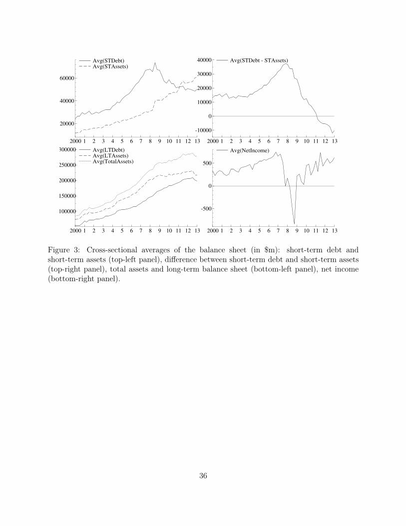
Avg(STDebt) Avg(STAssets)

2000 1 2 3 4 5 6 7 8 9 10 11 12 13

20000

40000

60000

Avg(STDebt) Avg(STAssets)

Avg(STDebt - STAssets)

2000 1 2 3 4 5 6 7 8 9 10 11 12 13

-10000

0

10000

20000

30000

40000 Avg(STDebt - STAssets)

Avg(LTDebt) Avg(LTAssets) Avg(TotalAssets)

2000 1 2 3 4 5 6 7 8 9 10 11 12 13

100000

150000

200000

250000

300000 Avg(LTDebt) Avg(LTAssets) Avg(TotalAssets)

Avg(NetIncome)

2000 1 2 3 4 5 6 7 8 9 10 11 12 13

-500

0

500

Avg(NetIncome)

Figure 3: Cross-sectional averages of the balance sheet (in $m): short-term debt andshort-term assets (top-left panel), difference between short-term debt and short-term assets(top-right panel), total assets and long-term balance sheet (bottom-left panel), net income(bottom-right panel).

36

Avg(T1CR)

2000 2001 2002 2003 2004 2005 2006 2007 2008 2009 2010 2011 2012 2013

0.10

0.12

0.14Avg(T1CR)

Avg(T1LVGR)

2000 2001 2002 2003 2004 2005 2006 2007 2008 2009 2010 2011 2012 2013

0.08

0.09

0.10Avg(T1LVGR)

Avg(SRISK) ($m) Avg(max(0,SRISK)) ($m)

2000 2001 2002 2003 2004 2005 2006 2007 2008 2009 2010 2011 2012 2013

0

10000Avg(SRISK) ($m) Avg(max(0,SRISK)) ($m)

Figure 4: Cross-sectional averages of solvency risk measures. T1CR is the Tier 1 commoncapital ratio (Tier 1 common capital divided by risk-weighted assets); T1LVGR is the Tier 1leverage ratio (Tier 1 capital divided by total assets); SRISK is the expected capital shortfallin a crisis.

37

Actual Forecast

2005 2006 2007 2008 2009 2010 2011 2012 2013

30000

40000

50000

60000

70000

Avg(STDebt) ($m)

Actual Forecast

2005 2006 2007 2008 2009 2010 2011 2012 2013

20000

30000

40000

50000

60000

Avg(STAssets) ($m)

2005 2006 2007 2008 2009 2010 2011 2012 2013

-5000

0

5000

Avg(STDebt flows) ($m)

2005 2006 2007 2008 2009 2010 2011 2012 2013

-5000

0

5000

Avg(STAssets flows) ($m)

(a) Short-term balance sheet levels and flows

Actual Forecast

2005 2006 2007 2008 2009 2010 2011 2012 2013

-10000

0

10000

20000

30000

40000Avg(STDebt - STAssets) ($m)

Actual Forecast

SRISK<0 SRISK>0

2005 2006 2007 2008 2009 2010 2011 2012 2013

0

25000

50000

75000

100000

125000

Avg(STDebt - STAssets) ($m)

SRISK<0 SRISK>0

(b) Liquid Asset Shorfall

Figure 5: Forecasting the short-term balance sheet over 2011Q1-2013Q1: dynamic forecasts(model with SRISK as a state variable (eq. (4)), break in trend).

38

Systemic risk and the solvency-liquidity nexus of banks

Appendix

Diane Pierret1

March 2015

Contents

A Short-term debt and short-term assets composition 1

B Stationarity of the balance sheet 4

C Reverse causality test 5

D Robustness checks 6

D.1 Robustness to common factors . . . . . . . . . . . . . . . . . . . . . . . . . . 6D.2 Short-term debt components . . . . . . . . . . . . . . . . . . . . . . . . . . . 10D.3 Long-term balance sheet . . . . . . . . . . . . . . . . . . . . . . . . . . . . . 11

E Sample of banks 12

1Faculty of Business and Economics (HEC Lausanne), University of Lausanne, CH 1015 Lausanne,Switzerland, email: diane.pierret@unil.ch, phone: +41 21 692 61 28.

A Short-term debt and short-term assets composition

Composition of the short term debt estimate (SNL definitions):

• Fed funds purchased: The gross dollar amount of funds borrowed in the form of imme-diately available funds under agreements or contracts that mature in one business dayor roll over under a continuing contract, regardless of the nature of the transaction orthe collateral involved. Includes securities sold under agreements to repurchase thatinvolve the receipt of immediately available funds and mature in one business day orroll over under a continuing contract.

• Repurchase agreements: The gross dollar amount of security repurchase agreementsthat mature in more than one business day, other than securities sold under repurchaseagreements to maturity, but including sales of participations in pools of securities thatmature in more than one business day.

• Brokered Deposits (< $100K, maturity 1 Year): Brokered deposits issued in de-nominations of less than $100,000 with a remaining maturity of one year or less andare held in domestic offices of commercial banks or other depository institutions thatare subsidiaries of the reporting bank holding company. Remaining maturity is theamount of time remaining from the report date until the final contractual maturity ofa brokered deposit.

• Time Deposits (� $100K, maturity 1Year): Time deposits issued in denominations of$100,000 or more with a remaining maturity of one year or less. Remaining maturity isthe amount of time remaining from the report date until the final contractual maturityof a time deposit.

• Foreign Office Time Deposits (maturity 1Year): All time deposits in foreign officeswith remaining maturities of one year or less. Remaining maturity is the amount oftime remaining from the report date until the final contractual maturity of a timedeposit.

• Commercial Paper: The total amount outstanding of commercial paper issued by thereporting bank holding company or its subsidiaries.

• Other borrowed money: The total amount of money borrowed by the consolidatedbank holding company with a remaining maturity of one year or less. For purposes ofthis item, remaining maturity is the amount of time remaining from the report dateuntil the final contractual maturity of a borrowing without regard to the borrowing’srepayment schedule, if any. Includes the dollar amount outstanding of all interest-bearing demand notes issued to the U.S. Treasury by the depository institutions thatare consolidated subsidiaries of the reporting bank holding company. Also includesmortgage indebtedness and obligations under capitalized leases with a remaining ma-turity of one year or less. Also includes the total amount of money borrowed with a

1

remaining maturity of one year or less: (1) on its promissory notes; (2) on notes andbills rediscounted; (3) on loans sold under repurchase agreements that mature in morethan one business day; (4) by the creation of due bills representing the bank holdingcompany’s receipt of payment and similar instruments, whether collateralized or un-collateralized; (5) from Federal Reserve Banks; (6) by overdrawing ’due from’ balanceswith depository institutions, except overdrafts arising in connection with checks ordrafts drawn by subsidiary depository institutions of the reporting bank holding com-pany and drawn on, or payable at or through, another depository institution either ona zero-balance account or on an account that is not routinely maintained with suffi-cient balances to cover checks or drafts drawn in the normal course of business duringthe period until the amount of the checks or drafts is remitted to the other depositoryinstitution; (7) on purchases of so-called ’term federal funds’; and (8) on any otherobligation for the purpose of borrowing money that has a remaining maturity of oneyear or less and that is not reported elsewhere.

Composition of the short term assets estimate (SNL definitions):

• Cash & Non interest-bearing Deposits: The total of all noninterest-bearing balancesdue from depository institutions, currency and coin, cash items in process of collection,and unposted debits. Includes balances due from banks in the U.S., banks in foreigncountries and foreign central banks, foreign branches of other U.S. banks, Federal HomeLoan Banks, and Federal Reserve Banks.

• Total Interest-bearing Balances: The total of all interest-bearing balances due fromdepository institutions and foreign central banks that are held in offices of the bankholding company or its consolidated subsidiaries.

• Fed Funds Sold: The gross dollar amount of funds lent in the form of immediatelyavailable funds under agreements or contracts that mature in one business day or rollover under a continuing contract. Includes securities purchased under agreements toresell that involve the receipt of immediately available funds and mature in one businessday or roll over under a continuing contract.

• Reverse Repurchases Agreements: The gross dollar amount of security resale agree-ments that mature in more than one business day, other than securities purchasedunder resale agreements to maturity, and of purchases of participations in pools ofsecurities that mature in more than one business day.

• Debt Securities Maturing or Repriced (maturity 1Year): All securities held by theconsolidated bank holding company with a remaining maturity or amount of timeremaining until next repricing date of one year or less. Held-to-maturity securitiesare reported at amortized cost and available-for-sale securities are reported at fairvalue. Remaining maturity is the amount of time remaining from the report date untilthe final contractual maturity of the instrument without regard to the instrument’s

2

repayment schedule. Next repricing date is the date the interest rate on a floating ratedebt security can next change. (Y9 Line Item: BHCK0383)

3

B Stationarity of the balance sheet

To test for the stationarity of yit, zit and other balance sheet quantities, I apply the unitroot test of Pesaran (2007) (CIPS) robust to cross-sectional dependence between individualsin the panel data set. The null hypothesis is H0 : ↵21 = ↵22 = ... = ↵2N = 0, i = 1, 2, ..., N(unit root), and the alternative Ha : ↵21 < 0, ...,↵2N0 < 0, N0 N(a significant fraction ofthe panel is stationary). The regression for the CIPS unit root test is

dyit = ↵0i + ↵1idyit�1 + ↵2iyit�1 + aidyt + biyt�1 + cidyt�1 + ✓it+ "it, (1)

where dyt = N�1PN

i=1 dyit, yt = N�1PN

i=1 yit. The CIPS test statistics are reported in Table1, for both cases with and without trend (i.e. ✓i = 0, 8i). Based on the CIPS statistics andgiven the critical values of the CADF distribution, yit is stationary only when the regressionincludes a trend. The hypothesis of the absence of a trend is rejected based on a Wald test,therefore yit is considered trend stationary in the rest of the paper.

On the other bank sheet aggregates, the UR hypothesis is not rejected for the size (loga-rithm of total assets) and the long-term balance sheet (logarithm of long-term assets Zit andlong-term debt Yit). Finally, the short-term assets, SRISK and the net income divided bytotal assets are stationary with this test.

Intercept only Intercept and trendCIPS CIPSb CIPS CIPSb

yit -2.064 -1.922 -2.725 -2.660zit -2.538 -2.545 -2.798 -2.849

NIit/TAit -3.541 -3.831 -4.101 -4.381Yit -2.071 -2.199 -2.274 -2.468Zit -1.954 -2.098 -2.449 -2.584

log(TAit) -1.709 -1.932 -2.163 -2.336SRISKit/TAit -2.579 -2.434 -2.951 -2.989

Table 1: Panel UR tests: CIPS statistics. CADF 5% critical values: -2.11 (intercept only),-2.60 (intercept and trend). CIPSb is the CIPS statistic based on a balanced panel dataset.yit = ln(STDebtit), zit = ln(STAssetsit), Yit = ln(LTDebtit), Zit = ln(LTAssetsit), NIit:net income, TAit: total assets.

4

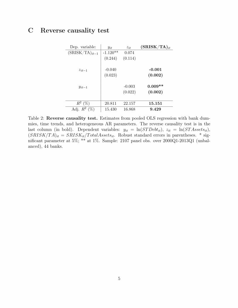
C Reverse causality test

Dep. variable: yit zit (SRISK/TA)it(SRISK/TA)it�1 -1.120** 0.074

(0.244) (0.114)

zit�1 -0.040 -0.001(0.023) (0.002)

yit�1 -0.003 0.009**(0.022) (0.002)

R2 (%) 20.811 22.157 15.151Adj. R2 (%) 15.430 16.868 9.429

Table 2: Reverse causality test. Estimates from pooled OLS regression with bank dum-mies, time trends, and heterogeneous AR parameters. The reverse causality test is in thelast column (in bold). Dependent variables: yit = ln(STDebtit), zit = ln(STAssetsit),(SRISK/TA)it = SRISKit/TotalAssetsit. Robust standard errors in parentheses. * sig-nificant parameter at 5%; ** at 1%. Sample: 2107 panel obs. over 2000Q1-2013Q1 (unbal-anced), 44 banks.

5

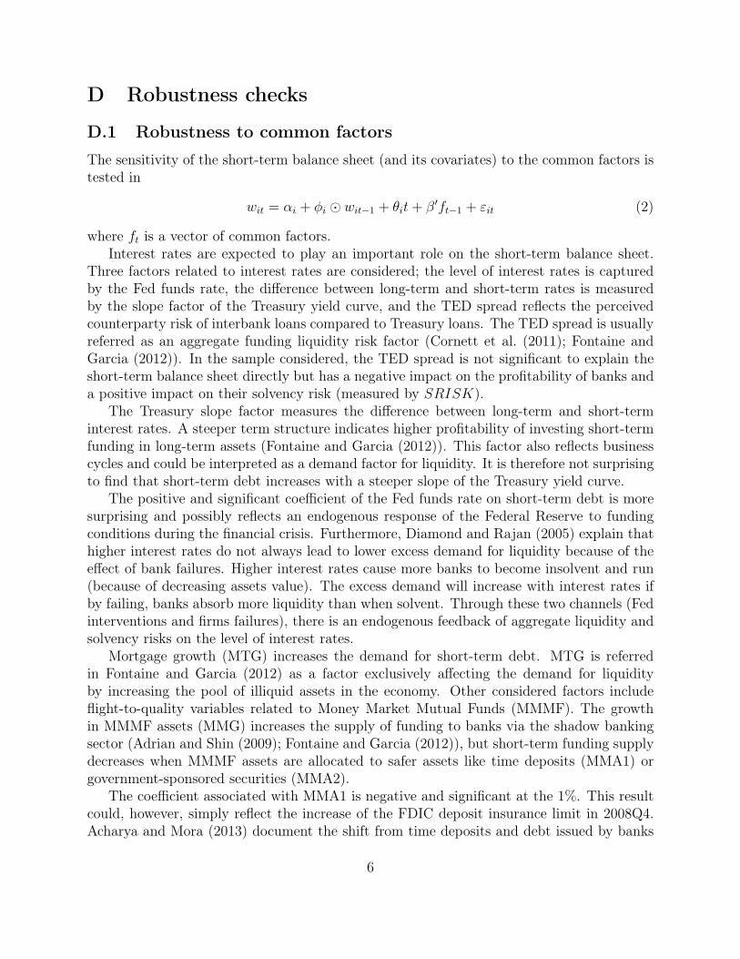
D Robustness checks

D.1 Robustness to common factors

The sensitivity of the short-term balance sheet (and its covariates) to the common factors istested in

wit = ↵i + �i � wit�1 + ✓it+ �0ft�1 + "it (2)

where ft is a vector of common factors.Interest rates are expected to play an important role on the short-term balance sheet.

Three factors related to interest rates are considered; the level of interest rates is capturedby the Fed funds rate, the difference between long-term and short-term rates is measuredby the slope factor of the Treasury yield curve, and the TED spread reflects the perceivedcounterparty risk of interbank loans compared to Treasury loans. The TED spread is usuallyreferred as an aggregate funding liquidity risk factor (Cornett et al. (2011); Fontaine andGarcia (2012)). In the sample considered, the TED spread is not significant to explain theshort-term balance sheet directly but has a negative impact on the profitability of banks anda positive impact on their solvency risk (measured by SRISK).

The Treasury slope factor measures the difference between long-term and short-terminterest rates. A steeper term structure indicates higher profitability of investing short-termfunding in long-term assets (Fontaine and Garcia (2012)). This factor also reflects businesscycles and could be interpreted as a demand factor for liquidity. It is therefore not surprisingto find that short-term debt increases with a steeper slope of the Treasury yield curve.

The positive and significant coefficient of the Fed funds rate on short-term debt is moresurprising and possibly reflects an endogenous response of the Federal Reserve to fundingconditions during the financial crisis. Furthermore, Diamond and Rajan (2005) explain thathigher interest rates do not always lead to lower excess demand for liquidity because of theeffect of bank failures. Higher interest rates cause more banks to become insolvent and run(because of decreasing assets value). The excess demand will increase with interest rates ifby failing, banks absorb more liquidity than when solvent. Through these two channels (Fedinterventions and firms failures), there is an endogenous feedback of aggregate liquidity andsolvency risks on the level of interest rates.

Mortgage growth (MTG) increases the demand for short-term debt. MTG is referredin Fontaine and Garcia (2012) as a factor exclusively affecting the demand for liquidityby increasing the pool of illiquid assets in the economy. Other considered factors includeflight-to-quality variables related to Money Market Mutual Funds (MMMF). The growthin MMMF assets (MMG) increases the supply of funding to banks via the shadow bankingsector (Adrian and Shin (2009); Fontaine and Garcia (2012)), but short-term funding supplydecreases when MMMF assets are allocated to safer assets like time deposits (MMA1) orgovernment-sponsored securities (MMA2).

The coefficient associated with MMA1 is negative and significant at the 1%. This resultcould, however, simply reflect the increase of the FDIC deposit insurance limit in 2008Q4.Acharya and Mora (2013) document the shift from time deposits and debt issued by banks

6

(and MMA1) to government-sponsored securities (and MMA2), and the “liquidity reversal”in 2008Q4 where MMA1 started to increase again. When the FDIC deposit insurance limitincreased from 100K to 250K in the fourth quarter of 2008, uninsured deposits includedin the short-term debt shifted to the long-term part of the balance sheet. Therefore, thenegative impact of MMA1 on banks’ short-term debt is partly explained by the reallocationin 2008Q4 of some previously uninsured time deposits (part of the short-term debt) to thelong-term debt within banks’ balance sheets.

We also note the positive coefficient of the VIX as banks’ exposure to short-term debt wasthe highest when the VIX peaked during the financial crisis. Finally, short-term assets arenot sensitive to any of the considered factors. While the level of short-term assets adjuststo shocks in other parts of the balance sheet, it is not directly affected by financial andmacroeconomic conditions.

7

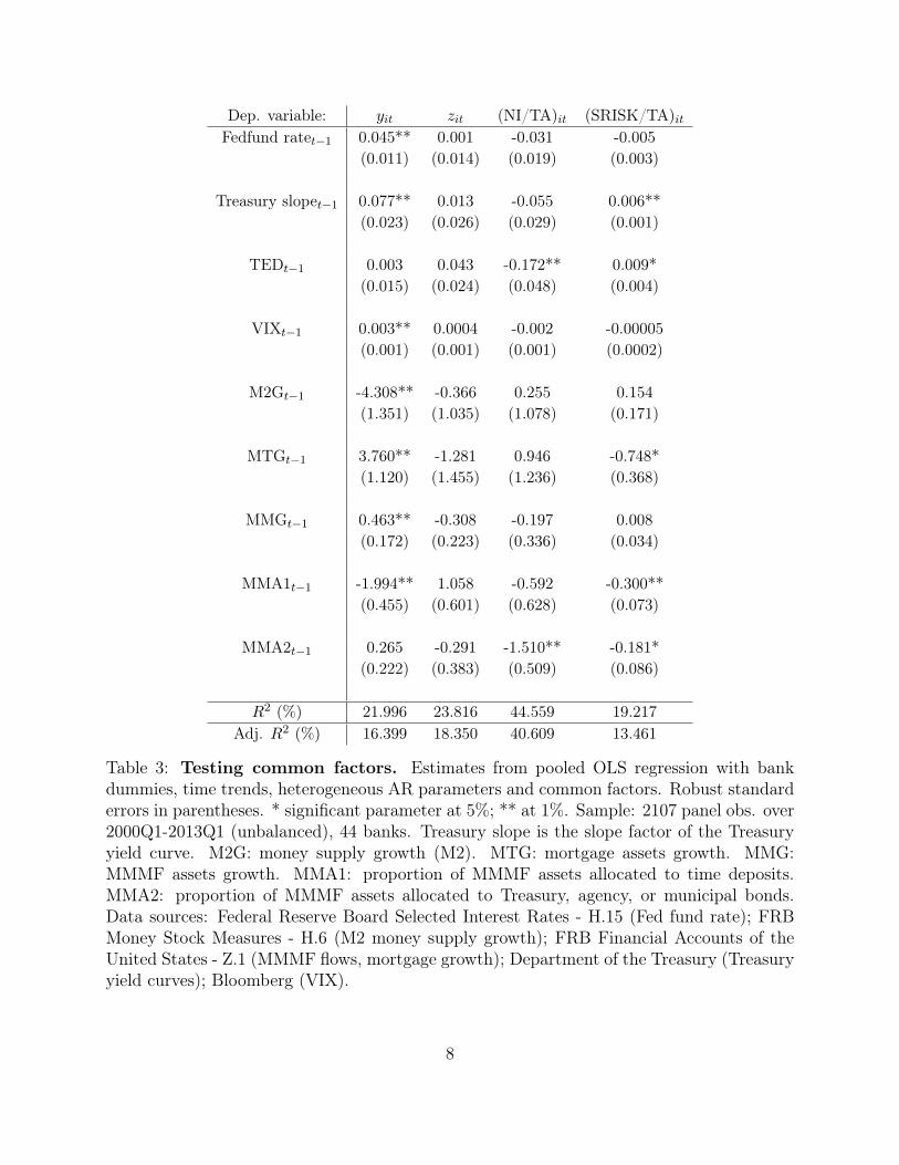
Dep. variable: yit zit (NI/TA)it (SRISK/TA)itFedfund ratet�1 0.045** 0.001 -0.031 -0.005

(0.011) (0.014) (0.019) (0.003)

Treasury slopet�1 0.077** 0.013 -0.055 0.006**(0.023) (0.026) (0.029) (0.001)

TEDt�1 0.003 0.043 -0.172** 0.009*(0.015) (0.024) (0.048) (0.004)

VIXt�1 0.003** 0.0004 -0.002 -0.00005(0.001) (0.001) (0.001) (0.0002)

M2Gt�1 -4.308** -0.366 0.255 0.154(1.351) (1.035) (1.078) (0.171)

MTGt�1 3.760** -1.281 0.946 -0.748*(1.120) (1.455) (1.236) (0.368)

MMGt�1 0.463** -0.308 -0.197 0.008(0.172) (0.223) (0.336) (0.034)

MMA1t�1 -1.994** 1.058 -0.592 -0.300**(0.455) (0.601) (0.628) (0.073)

MMA2t�1 0.265 -0.291 -1.510** -0.181*(0.222) (0.383) (0.509) (0.086)

R2 (%) 21.996 23.816 44.559 19.217Adj. R2 (%) 16.399 18.350 40.609 13.461

Table 3: Testing common factors. Estimates from pooled OLS regression with bankdummies, time trends, heterogeneous AR parameters and common factors. Robust standarderrors in parentheses. * significant parameter at 5%; ** at 1%. Sample: 2107 panel obs. over2000Q1-2013Q1 (unbalanced), 44 banks. Treasury slope is the slope factor of the Treasuryyield curve. M2G: money supply growth (M2). MTG: mortgage assets growth. MMG:MMMF assets growth. MMA1: proportion of MMMF assets allocated to time deposits.MMA2: proportion of MMMF assets allocated to Treasury, agency, or municipal bonds.Data sources: Federal Reserve Board Selected Interest Rates - H.15 (Fed fund rate); FRBMoney Stock Measures - H.6 (M2 money supply growth); FRB Financial Accounts of theUnited States - Z.1 (MMMF flows, mortgage growth); Department of the Treasury (Treasuryyield curves); Bloomberg (VIX).

8

No Common Factor Common Factors Common Correlated EffectsDep. variable: yit zit yit zit yit zit

(SRISK/TA)it�1 -0.935** -0.120 -0.847** -0.178 -0.900** -0.137(0.261) (0.101) (0.318) (0.096) (0.280) (0.106)

(SRISK/TA)it�1 ⇤ sit�1 -0.408 1.757* -0.687 1.291 -1.413 2.384*(0.751) (0.767) (0.853) (0.861) (0.974) (1.009)

(NI/TA)it�1 9.704** -7.944* 8.111* -7.564* 8.512* -7.964*(3.290) (3.716) (3.677) (3.575) (3.542) (3.905)

(NI/TA)it�1 ⇤ sit�1 -9.902* 6.315 -8.087 4.817 -7.181 7.926(4.396) (5.183) (4.788) (4.920) (4.655) (5.512)

zit�1 -0.033 -0.008 0.0004(0.022) (0.024) (0.024)

zit�1 ⇤ sit�1 -0.021* -0.018* -0.013(0.008) (0.008) (0.008)

yit�1 -0.002 0.002 0.004(0.022) (0.002) (0.020)

yit�1 ⇤ sit�1 -0.007* -0.010 -0.013(0.010) (0.009) (0.010)

sit�1 0.347* 0.066 0.327* 0.098 0.253 0.148(0.144) (0.159) (0.140) (0.154) (0.140) (0.158)

R2 (%) 21.278 22.562 25.079 24.247 26.730 27.265Adj. R2 (%) 15.715 17.089 19.416 18.521 21.192 21.767

Table 4: Robustness of the solvency-liquidity nexus to common factors. Esti-mates from pooled OLS regression with bank dummies, time trends, heterogeneous AR pa-rameters and state variable sit = 1{SRISKit>0}. Dependent variables: yit = ln(STDebtit),zit = ln(STAssetsit), (NI/TA)it = NetIncomeit/TotalAssetsit, (SRISK/TA)it =SRISKit/TotalAssetsit. No Common Factor: regression without common factors. Com-mon Factors: regression with all (lagged) common factors of Table 3. Common CorrelatedEffects: regression with common correlated effects. Robust standard errors in parentheses.* significant parameter at 5%; ** at 1%. Sample: 2107 panel obs. over 2000Q1-2013Q1(unbalanced), 44 banks.

9

D.2 Short-term debt components

Dep. variable: yit FFRepo Br Dep Time Dep For Dep ComPaper OtherBor(SRISK/TA)it�1 -1.063** -1.217** 0.147 -0.363* -1.155* -2.330** -0.281

(0.245) (0.403) (0.518) (0.175) (0.531) (0.364) (0.377)

(NI/TA)it�1 2.354 0.152 -11.694 -1.660 10.880 17.540 3.249(2.278) (2.437) (8.376) (4.733) (6.282) (10.392) (9.375)

zit�1 -0.038 0.015 -0.028 -0.046* -0.191* -0.091 -0.233**(0.023) (0.051) (0.096) (0.019) (0.093) (0.083) (0.079)

# obs. 2107 1979 950 2096 1337 966 2035# banks 44 44 40 44 34 27 44R2 (%) 20.870 19.723 23.649 34.947 38.600 25.330 22.656

Adj. R2 (%) 15.450 13.843 12.279 30.459 33.355 18.187 17.152

Table 5: Testing the solvency-liquidity nexus: short-term debt mix. Estimates frompooled OLS regression with bank dummies, time trends and heterogeneous AR parameters.Dependent variables: log of the different components of the short term debt (see definitionsin Appendix A): Fed funds and Repos (FFRepo), Brokered Deposits (Br Dep), uninsuredTime Deposits (Time Dep), Foreign Deposits (For Dep), Commercial Papers (ComPaper)and Other Borrowed Money (OtherBor). Robust standard errors in parentheses. Robuststandard errors in parentheses. * significant parameter at 5%; ** at 1%. Sample: 2107 panelobs. over 2000Q1-2013Q1 (unbalanced), 44 banks.

10

D.3 Long-term balance sheet

Dep. variable: dYit dZit yit zit(SRISK/TA)it�1 -0.013 -0.039 -1.059** -0.038

(0.024) (0.038) (0.235) (0.118)

(NI/TA)it�1 -0.870 0.290 2.313 -4.185(0.592) (0.508) (2.232) (2.348)

zit�1 -0.035** -0.006 -0.034(0.005) (0.006) (0.024)

yit�1 -0.0004 -0.018** -0.002(0.006) (0.006) (0.022)

dZit�1 0.101* 0.004 -0.110(0.046) (0.109) (0.116)

dY it�1 -0.104* -0.137 0.157(0.052) (0.199) (0.096)

R2 (%) 11.319 12.008 21.047 22.411Adj. R2 (%) 5.197 5.934 15.554 17.013

Table 6: Testing the solvency-liquidity nexus: short-term vs. long-term balance

sheet. Estimates from pooled OLS regression with bank dummies, time trends and hetero-geneous AR parameters. Dependent variables: dYit = ln(LTDebtit/LTDebtit�1), dZit =ln(LTAssetsit/LTAssetsit�1), yit = ln(STDebtit), zit = ln(STAssetsit). (NI/TA)it =NetIncomeit/TotalAssetsit, (SRISK/TA)it = SRISKit/TotalAssetsit. Robust standarderrors in parentheses. * significant parameter at 5%; ** at 1%. Sample: 2107 panel obs.over 2000Q1-2013Q1 (unbalanced), 44 banks.

11

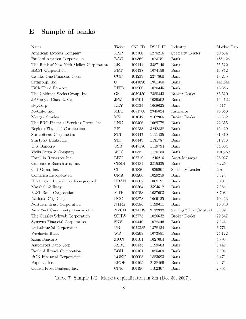
E Sample of banks

Name Ticker SNL ID RSSD ID Industry Market CapAmerican Express Company AXP 102700 1275216 Specialty Lender 60,834Bank of America Corporation BAC 100369 1073757 Bank 183,125The Bank of New York Mellon Corporation BK 100144 3587146 Bank 55,522BB&T Corporation BBT 100438 1074156 Bank 16,852Capital One Financial Corp. COF 103239 2277860 Bank 18,215Citigroup, Inc. C 4041896 1951350 Bank 146,644Fifth Third Bancorp FITB 100260 1070345 Bank 13,386The Goldman Sachs Group, Inc. GS 4039450 2380443 Broker Dealer 85,520JPMorgan Chase & Co. JPM 100201 1039502 Bank 146,622KeyCorp KEY 100334 1068025 Bank 9,117MetLife, Inc. MET 4051708 2945824 Insurance 45,636Morgan Stanley MS 103042 2162966 Broker Dealer 56,362The PNC Financial Services Group, Inc. PNC 100406 1069778 Bank 22,355Regions Financial Corporation RF 100233 3242838 Bank 16,439State Street Corporation STT 100447 1111435 Bank 31,360SunTrust Banks, Inc. STI 100449 1131787 Bank 21,756U.S. Bancorp USB 4047176 1119794 Bank 54,804Wells Fargo & Company WFC 100382 1120754 Bank 101,269Franklin Resources Inc. BEN 102719 1246216 Asset Manager 28,037Commerce Bancshares, Inc. CBSH 100184 2815235 Bank 3,229CIT Group Inc. CIT 102820 1036967 Specialty Lender NAComerica Incorporated CMA 100206 1029259 Bank 6,574Huntington Bancshares Incorporated HBAN 100307 1068191 Bank 5,401Marshall & Ilsley MI 100364 3594612 Bank 7,086M&T Bank Corporation MTB 100253 1037003 Bank 8,708National City Corp. NCC 100378 1069125 Bank 10,433Northern Trust Corporation NTRS 100386 1199611 Bank 16,843New York Community Bancorp Inc. NYCB 1024119 2132932 Savings/Thrift/Mutual 5,689The Charles Schwab Corporation SCHW 102775 1026632 Broker Dealer 29,547Synovus Financial Corporation SNV 100440 1078846 Bank 7,943UnionBanCal Corporation UB 1022285 1378434 Bank 6,776Wachovia Bank WB 100293 1073551 Bank 75,122Zions Bancorp. ZION 100501 1027004 Bank 4,995Associated Banc-Corp ASBC 100135 1199563 Bank 3,442Bank of Hawaii Corporation BOH 100161 1025309 Bank 2,506BOK Financial Corporation BOKF 100003 1883693 Bank 3,471Popular, Inc. BPOP 100165 2138466 Bank 2,971Cullen/Frost Bankers, Inc. CFR 100196 1102367 Bank 2,963

Table 7: Sample 1/2. Market capitalization in $m (Dec 30, 2007).

12

Name Ticker SNL ID RSSD ID Industry Market CapCity National Corporation CYN 100225 1131004 Bank 2,866Discover Financial Services DFS 4096334 3846375 Specialty Lender NAEast West Bancorp, Inc. EWBC 4040606 2734233 Bank 1,527First Citizens BancShares, Inc. FCNCA 100247 1105470 Bank 1,619First Horizon National Corporation FHN 100292 1094640 Bank 2,294Fulton Financial Corporation FULT 100294 1117129 Bank 1,946Hancock Holding Company HBHC 100308 1086533 Bank 1,207Prosperity Bancshares, Inc. PB 1018962 1109599 Bank 1,297SVB Financial Group SIVB 100433 1031449 Bank 1,673TCF Financial Corporation TCB 102002 2389941 Bank 2,272Webster Financial Corporation WBS 102030 1145476 Bank 1,710

Table 8: Sample 2/2. Market capitalization in $m (Dec 30, 2007).

13

References

Acharya, V. and N. Mora (2013). A crisis of banks as liquidity providers. Journal of

Finance forthcoming.

Adrian, T. and H. Shin (2009). Money, liquidity, and monetary policy. NY Fed Staff Reportno. 360.

Cornett, M., J. McNutt, P. Strahan, and H. Tehranian (2011). Liquidity risk managementand credit supply in the financial crisis. Journal of Financial Economics 101:2, 297–312.

Diamond, D. and R. Rajan (2005). Liquidity shortages and banking crises. Journal of

Finance 60:2, 615–647.

Fontaine, J.-S. and R. Garcia (2012). Bond liquidity premia. The Review of Financial

Studies 25:4, 1207–1254.

Pesaran, H. (2007). A simple panel unit root test in the presence of cross-section dependence.Journal of Applied Econometrics 22, 265–312.

14