systematics - wordpress.com · systematics: a course of lectures ward c. wheeler a john wiley &...
TRANSCRIPT


Systematics

Systematics: A Course of Lectures
Ward C. Wheeler
A John Wiley & Sons, Ltd., Publication

This edition first published 2012 c© 2012 by Ward C. Wheeler
Wiley-Blackwell is an imprint of John Wiley & Sons, formed by the merger of Wiley’s global Scientific, Technical and Medicalbusiness with Blackwell Publishing.
Registered office: John Wiley & Sons, Ltd, The Atrium, Southern Gate, Chichester, West Sussex, PO19 8SQ, UK
Editorial offices: 9600 Garsington Road, Oxford, OX4 2DQ, UK
The Atrium, Southern Gate, Chichester, West Sussex, PO19 8SQ, UK111 River Street, Hoboken, NJ 07030-5774, USA
For details of our global editorial offices, for customer services and for information about how to apply for permission to reusethe copyright material in this book please see our website at www.wiley.com/wiley-blackwell.
The right of the author to be identified as the author of this work has been asserted in accordance with the UK Copyright,
Designs and Patents Act 1988.
All rights reserved. No part of this publication may be reproduced, stored in a retrieval system, or transmitted, in any form orby any means, electronic, mechanical, photocopying, recording or otherwise, except as permitted by the UK Copyright, Designsand Patents Act 1988, without the prior permission of the publisher.
Designations used by companies to distinguish their products are often claimed as trademarks. All brand names and productnames used in this book are trade names, service marks, trademarks or registered trademarks of their respective owners. Thepublisher is not associated with any product or vendor mentioned in this book. This publication is designed to provide accurateand authoritative information in regard to the subject matter covered. It is sold on the understanding that the publisher is notengaged in rendering professional services. If professional advice or other expert assistance is required, the services of acompetent professional should be sought.
Library of Congress Cataloging-in-Publication Data has been applied for9780470671702 (hardback)9780470671696 (paperback)
A catalogue record for this book is available from the British Library.
Wiley also publishes its books in a variety of electronic formats. Some content that appears in print may not be available inelectronic books.
Set in Computer Modern 10/12pt by Laserwords Private Limited, Chennai, India
1 2012

For
Kurt Milton Pickett(1972–2011)
Ave atque vale
Contents
Preface xvUsing these notes . . . . . . . . . . . . . . . . . . . . . . . . . . . . . xvAcknowledgments . . . . . . . . . . . . . . . . . . . . . . . . . . . . . xvi
List of algorithms xix
I Fundamentals 1
1 History 21.1 Aristotle . . . . . . . . . . . . . . . . . . . . . . . . . . . . . . . . 21.2 Theophrastus . . . . . . . . . . . . . . . . . . . . . . . . . . . . . 31.3 Pierre Belon . . . . . . . . . . . . . . . . . . . . . . . . . . . . . . 41.4 Carolus Linnaeus . . . . . . . . . . . . . . . . . . . . . . . . . . . 41.5 Georges Louis Leclerc, Comte de Buffon . . . . . . . . . . . . . . 61.6 Jean-Baptiste Lamarck . . . . . . . . . . . . . . . . . . . . . . . . 71.7 Georges Cuvier . . . . . . . . . . . . . . . . . . . . . . . . . . . . 81.8 Etienne Geoffroy Saint-Hilaire . . . . . . . . . . . . . . . . . . . . 81.9 Johann Wolfgang von Goethe . . . . . . . . . . . . . . . . . . . . 81.10 Lorenz Oken . . . . . . . . . . . . . . . . . . . . . . . . . . . . . 91.11 Richard Owen . . . . . . . . . . . . . . . . . . . . . . . . . . . . . 91.12 Charles Darwin . . . . . . . . . . . . . . . . . . . . . . . . . . . . 91.13 Stammbaume . . . . . . . . . . . . . . . . . . . . . . . . . . . . . 121.14 Evolutionary Taxonomy . . . . . . . . . . . . . . . . . . . . . . . 141.15 Phenetics . . . . . . . . . . . . . . . . . . . . . . . . . . . . . . . 151.16 Phylogenetic Systematics . . . . . . . . . . . . . . . . . . . . . . 16
1.16.1 Hennig’s Three Questions . . . . . . . . . . . . . . . . . . 161.17 Molecules and Morphology . . . . . . . . . . . . . . . . . . . . . 181.18 We are all Cladists . . . . . . . . . . . . . . . . . . . . . . . . . . 181.19 Exercises . . . . . . . . . . . . . . . . . . . . . . . . . . . . . . . 19
2 Fundamental Concepts 202.1 Characters . . . . . . . . . . . . . . . . . . . . . . . . . . . . . . . 20
2.1.1 Classes of Characters and Total Evidence . . . . . . . . . 222.1.2 Ontogeny, Tokogeny, and Phylogeny . . . . . . . . . . . . 232.1.3 Characters and Character States . . . . . . . . . . . . . . 23
2.2 Taxa . . . . . . . . . . . . . . . . . . . . . . . . . . . . . . . . . . 26
viii CONTENTS
2.3 Graphs, Trees, and Networks . . . . . . . . . . . . . . . . . . . . 282.3.1 Graphs and Trees . . . . . . . . . . . . . . . . . . . . . . . 302.3.2 Enumeration . . . . . . . . . . . . . . . . . . . . . . . . . 312.3.3 Networks . . . . . . . . . . . . . . . . . . . . . . . . . . . 332.3.4 Mono-, Para-, and Polyphyly . . . . . . . . . . . . . . . . 332.3.5 Splits and Convexity . . . . . . . . . . . . . . . . . . . . . 382.3.6 Apomorphy, Plesiomorphy, and Homoplasy . . . . . . . . 392.3.7 Gene Trees and Species Trees . . . . . . . . . . . . . . . . 41
2.4 Polarity and Rooting . . . . . . . . . . . . . . . . . . . . . . . . . 432.4.1 Stratigraphy . . . . . . . . . . . . . . . . . . . . . . . . . 432.4.2 Ontogeny . . . . . . . . . . . . . . . . . . . . . . . . . . . 432.4.3 Outgroups . . . . . . . . . . . . . . . . . . . . . . . . . . . 45
2.5 Optimality . . . . . . . . . . . . . . . . . . . . . . . . . . . . . . 492.6 Homology . . . . . . . . . . . . . . . . . . . . . . . . . . . . . . . 492.7 Exercises . . . . . . . . . . . . . . . . . . . . . . . . . . . . . . . 50
3 Species Concepts, Definitions, and Issues 533.1 Typological or Taxonomic Species Concept . . . . . . . . . . . . 543.2 Biological Species Concept . . . . . . . . . . . . . . . . . . . . . . 54
3.2.1 Criticisms of the BSC . . . . . . . . . . . . . . . . . . . . 553.3 Phylogenetic Species Concept(s) . . . . . . . . . . . . . . . . . . 56
3.3.1 Autapomorphic/Monophyletic Species Concept . . . . . . 563.3.2 Diagnostic/Phylogenetic Species Concept . . . . . . . . . 58
3.4 Lineage Species Concepts . . . . . . . . . . . . . . . . . . . . . . 593.4.1 Hennigian Species . . . . . . . . . . . . . . . . . . . . . . 593.4.2 Evolutionary Species . . . . . . . . . . . . . . . . . . . . . 603.4.3 Criticisms of Lineage-Based Species . . . . . . . . . . . . 61
3.5 Species as Individuals or Classes . . . . . . . . . . . . . . . . . . 623.6 Monoism and Pluralism . . . . . . . . . . . . . . . . . . . . . . . 633.7 Pattern and Process . . . . . . . . . . . . . . . . . . . . . . . . . 633.8 Species Nominalism . . . . . . . . . . . . . . . . . . . . . . . . . 643.9 Do Species Concepts Matter? . . . . . . . . . . . . . . . . . . . . 653.10 Exercises . . . . . . . . . . . . . . . . . . . . . . . . . . . . . . . 65
4 Hypothesis Testing and the Philosophy of Science 674.1 Forms of Scientific Reasoning . . . . . . . . . . . . . . . . . . . . 67
4.1.1 The Ancients . . . . . . . . . . . . . . . . . . . . . . . . . 674.1.2 Ockham’s Razor . . . . . . . . . . . . . . . . . . . . . . . 684.1.3 Modes of Scientific Inference . . . . . . . . . . . . . . . . 694.1.4 Induction . . . . . . . . . . . . . . . . . . . . . . . . . . . 694.1.5 Deduction . . . . . . . . . . . . . . . . . . . . . . . . . . . 694.1.6 Abduction . . . . . . . . . . . . . . . . . . . . . . . . . . . 704.1.7 Hypothetico-Deduction . . . . . . . . . . . . . . . . . . . 71
4.2 Other Philosophical Issues . . . . . . . . . . . . . . . . . . . . . . 754.2.1 Minimization, Transformation, and Weighting . . . . . . . 75
4.3 Quotidian Importance . . . . . . . . . . . . . . . . . . . . . . . . 764.4 Exercises . . . . . . . . . . . . . . . . . . . . . . . . . . . . . . . 76

CONTENTS ix
5 Computational Concepts 775.1 Problems, Algorithms, and Complexity . . . . . . . . . . . . . . . 77
5.1.1 Computer Science Basics . . . . . . . . . . . . . . . . . . 775.1.2 Algorithms . . . . . . . . . . . . . . . . . . . . . . . . . . 795.1.3 Asymptotic Notation . . . . . . . . . . . . . . . . . . . . . 795.1.4 Complexity . . . . . . . . . . . . . . . . . . . . . . . . . . 805.1.5 Non-Deterministic Complexity . . . . . . . . . . . . . . . 825.1.6 Complexity Classes: P and NP . . . . . . . . . . . . . . . 82
5.2 An Example: The Traveling Salesman Problem . . . . . . . . . . 845.3 Heuristic Solutions . . . . . . . . . . . . . . . . . . . . . . . . . . 855.4 Metricity, and Untrametricity . . . . . . . . . . . . . . . . . . . . 865.5 NP–Complete Problems in Systematics . . . . . . . . . . . . . . . 875.6 Exercises . . . . . . . . . . . . . . . . . . . . . . . . . . . . . . . 88
6 Statistical and Mathematical Basics 896.1 Theory of Statistics . . . . . . . . . . . . . . . . . . . . . . . . . . 89
6.1.1 Probability . . . . . . . . . . . . . . . . . . . . . . . . . . 896.1.2 Conditional Probability . . . . . . . . . . . . . . . . . . . 916.1.3 Distributions . . . . . . . . . . . . . . . . . . . . . . . . . 926.1.4 Statistical Inference . . . . . . . . . . . . . . . . . . . . . 986.1.5 Prior and Posterior Distributions . . . . . . . . . . . . . . 996.1.6 Bayes Estimators . . . . . . . . . . . . . . . . . . . . . . . 1006.1.7 Maximum Likelihood Estimators . . . . . . . . . . . . . . 1016.1.8 Properties of Estimators . . . . . . . . . . . . . . . . . . . 101
6.2 Matrix Algebra, Differential Equations, and Markov Models . . . 1026.2.1 Basics . . . . . . . . . . . . . . . . . . . . . . . . . . . . . 1026.2.2 Gaussian Elimination . . . . . . . . . . . . . . . . . . . . 1026.2.3 Differential Equations . . . . . . . . . . . . . . . . . . . . 1046.2.4 Determining Eigenvalues . . . . . . . . . . . . . . . . . . . 1056.2.5 Markov Matrices . . . . . . . . . . . . . . . . . . . . . . . 106
6.3 Exercises . . . . . . . . . . . . . . . . . . . . . . . . . . . . . . . 107
II Homology 109
7 Homology 1107.1 Pre-Evolutionary Concepts . . . . . . . . . . . . . . . . . . . . . 110
7.1.1 Aristotle . . . . . . . . . . . . . . . . . . . . . . . . . . . . 1107.1.2 Pierre Belon . . . . . . . . . . . . . . . . . . . . . . . . . 1107.1.3 Etienne Geoffroy Saint-Hilaire . . . . . . . . . . . . . . . . 1117.1.4 Richard Owen . . . . . . . . . . . . . . . . . . . . . . . . 112
7.2 Charles Darwin . . . . . . . . . . . . . . . . . . . . . . . . . . . . 1137.3 E. Ray Lankester . . . . . . . . . . . . . . . . . . . . . . . . . . . 1147.4 Adolf Remane . . . . . . . . . . . . . . . . . . . . . . . . . . . . . 1147.5 Four Types of Homology . . . . . . . . . . . . . . . . . . . . . . . 115
7.5.1 Classical View . . . . . . . . . . . . . . . . . . . . . . . . 1157.5.2 Evolutionary Taxonomy . . . . . . . . . . . . . . . . . . . 115
x CONTENTS
7.5.3 Phenetic Homology . . . . . . . . . . . . . . . . . . . . . . 1167.5.4 Cladistic Homology . . . . . . . . . . . . . . . . . . . . . 1167.5.5 Types of Homology . . . . . . . . . . . . . . . . . . . . . . 117
7.6 Dynamic and Static Homology . . . . . . . . . . . . . . . . . . . 1187.7 Exercises . . . . . . . . . . . . . . . . . . . . . . . . . . . . . . . 120
8 Sequence Alignment 1218.1 Background . . . . . . . . . . . . . . . . . . . . . . . . . . . . . . 1218.2 “Informal” Alignment . . . . . . . . . . . . . . . . . . . . . . . . 1218.3 Sequences . . . . . . . . . . . . . . . . . . . . . . . . . . . . . . . 121
8.3.1 Alphabets . . . . . . . . . . . . . . . . . . . . . . . . . . . 1228.3.2 Transformations . . . . . . . . . . . . . . . . . . . . . . . 1238.3.3 Distances . . . . . . . . . . . . . . . . . . . . . . . . . . . 123
8.4 Pairwise String Matching . . . . . . . . . . . . . . . . . . . . . . 1238.4.1 An Example . . . . . . . . . . . . . . . . . . . . . . . . . 1278.4.2 Reducing Complexity . . . . . . . . . . . . . . . . . . . . 1298.4.3 Other Indel Weights . . . . . . . . . . . . . . . . . . . . . 130
8.5 Multiple Sequence Alignment . . . . . . . . . . . . . . . . . . . . 1318.5.1 The Tree Alignment Problem . . . . . . . . . . . . . . . . 1338.5.2 Trees and Alignment . . . . . . . . . . . . . . . . . . . . . 1338.5.3 Exact Solutions . . . . . . . . . . . . . . . . . . . . . . . . 1348.5.4 Polynomial Time Approximate Schemes . . . . . . . . . . 1348.5.5 Heuristic Multiple Sequence Alignment . . . . . . . . . . 1348.5.6 Implementations . . . . . . . . . . . . . . . . . . . . . . . 1358.5.7 Structural Alignment . . . . . . . . . . . . . . . . . . . . 139
8.6 Exercises . . . . . . . . . . . . . . . . . . . . . . . . . . . . . . . 145
III Optimality Criteria 147
9 Optimality Criteria−Distance 1489.1 Why Distance? . . . . . . . . . . . . . . . . . . . . . . . . . . . . 148
9.1.1 Benefits . . . . . . . . . . . . . . . . . . . . . . . . . . . . 1499.1.2 Drawbacks . . . . . . . . . . . . . . . . . . . . . . . . . . 149
9.2 Distance Functions . . . . . . . . . . . . . . . . . . . . . . . . . . 1509.2.1 Metricity . . . . . . . . . . . . . . . . . . . . . . . . . . . 150
9.3 Ultrametric Trees . . . . . . . . . . . . . . . . . . . . . . . . . . . 1509.4 Additive Trees . . . . . . . . . . . . . . . . . . . . . . . . . . . . 152
9.4.1 Farris Transform . . . . . . . . . . . . . . . . . . . . . . . 1539.4.2 Buneman Trees . . . . . . . . . . . . . . . . . . . . . . . . 154
9.5 General Distances . . . . . . . . . . . . . . . . . . . . . . . . . . 1569.5.1 Phenetic Clustering . . . . . . . . . . . . . . . . . . . . . 1579.5.2 Percent Standard Deviation . . . . . . . . . . . . . . . . . 1609.5.3 Minimizing Length . . . . . . . . . . . . . . . . . . . . . . 163
9.6 Comparisons . . . . . . . . . . . . . . . . . . . . . . . . . . . . . 1709.7 Exercises . . . . . . . . . . . . . . . . . . . . . . . . . . . . . . . 171
CONTENTS xi
10 Optimality Criteria−Parsimony 17310.1 Perfect Phylogeny . . . . . . . . . . . . . . . . . . . . . . . . . . 17410.2 Static Homology Characters . . . . . . . . . . . . . . . . . . . . 174
10.2.1 Additive Characters . . . . . . . . . . . . . . . . . . . . . 17510.2.2 Non-Additive Characters . . . . . . . . . . . . . . . . . . 17910.2.3 Matrix Characters . . . . . . . . . . . . . . . . . . . . . . 182
10.3 Missing Data . . . . . . . . . . . . . . . . . . . . . . . . . . . . . 18410.4 Edge Transformation Assignments . . . . . . . . . . . . . . . . . 18710.5 Collapsing Branches . . . . . . . . . . . . . . . . . . . . . . . . . 18810.6 Dynamic Homology . . . . . . . . . . . . . . . . . . . . . . . . . 18810.7 Dynamic and Static Homology . . . . . . . . . . . . . . . . . . . 18910.8 Sequences as Characters . . . . . . . . . . . . . . . . . . . . . . 19010.9 The Tree Alignment Problem on Trees . . . . . . . . . . . . . . 191
10.9.1 Exact Solutions . . . . . . . . . . . . . . . . . . . . . . . 19110.9.2 Heuristic Solutions . . . . . . . . . . . . . . . . . . . . . 19110.9.3 Lifted Alignments, Fixed-States, and Search-Based
Heuristics . . . . . . . . . . . . . . . . . . . . . . . . . . . 19310.9.4 Iterative Improvement . . . . . . . . . . . . . . . . . . . 197
10.10 Performance of Heuristic Solutions . . . . . . . . . . . . . . . . . 19810.11 Parameter Sensitivity . . . . . . . . . . . . . . . . . . . . . . . . 198
10.11.1 Sensitivity Analysis . . . . . . . . . . . . . . . . . . . . . 19910.12 Implied Alignment . . . . . . . . . . . . . . . . . . . . . . . . . . 19910.13 Rearrangement . . . . . . . . . . . . . . . . . . . . . . . . . . . . 204
10.13.1 Sequence Characters with Moves . . . . . . . . . . . . . . 20410.13.2 Gene Order Rearrangement . . . . . . . . . . . . . . . . 20510.13.3 Median Evaluation . . . . . . . . . . . . . . . . . . . . . 20710.13.4 Combination of Methods . . . . . . . . . . . . . . . . . . 207
10.14 Horizontal Gene Transfer, Hybridization, and PhylogeneticNetworks . . . . . . . . . . . . . . . . . . . . . . . . . . . . . . . 209
10.15 Exercises . . . . . . . . . . . . . . . . . . . . . . . . . . . . . . . 210
11 Optimality Criteria−Likelihood 21311.1 Motivation . . . . . . . . . . . . . . . . . . . . . . . . . . . . . . 213
11.1.1 Felsenstein’s Example . . . . . . . . . . . . . . . . . . . . 21311.2 Maximum Likelihood and Trees . . . . . . . . . . . . . . . . . . . 216
11.2.1 Nuisance Parameters . . . . . . . . . . . . . . . . . . . . . 21611.3 Types of Likelihood . . . . . . . . . . . . . . . . . . . . . . . . . 217
11.3.1 Flavors of Maximum Relative Likelihood . . . . . . . . . . 21711.4 Static-Homology Characters . . . . . . . . . . . . . . . . . . . . . 218
11.4.1 Models . . . . . . . . . . . . . . . . . . . . . . . . . . . . 21811.4.2 Rate Variation . . . . . . . . . . . . . . . . . . . . . . . . 21911.4.3 Calculating p(D|T, θ) . . . . . . . . . . . . . . . . . . . . . 22111.4.4 Links Between Likelihood and Parsimony . . . . . . . . . 22211.4.5 A Note on Missing Data . . . . . . . . . . . . . . . . . . . 224
11.5 Dynamic-Homology Characters . . . . . . . . . . . . . . . . . . . 22411.5.1 Sequence Characters . . . . . . . . . . . . . . . . . . . . . 225

xii CONTENTS
11.5.2 Calculating ML Pairwise Alignment . . . . . . . . . . . . 22711.5.3 ML Multiple Alignment . . . . . . . . . . . . . . . . . . . 23011.5.4 Maximum Likelihood Tree Alignment Problem . . . . . . 23011.5.5 Genomic Rearrangement . . . . . . . . . . . . . . . . . . . 23211.5.6 Phylogenetic Networks . . . . . . . . . . . . . . . . . . . . 234
11.6 Hypothesis Testing . . . . . . . . . . . . . . . . . . . . . . . . . . 23411.6.1 Likelihood Ratios . . . . . . . . . . . . . . . . . . . . . . . 23411.6.2 Parameters and Fit . . . . . . . . . . . . . . . . . . . . . . 236
11.7 Exercises . . . . . . . . . . . . . . . . . . . . . . . . . . . . . . . 238
12 Optimality Criteria−Posterior Probability 24012.1 Bayes in Systematics . . . . . . . . . . . . . . . . . . . . . . . . . 24012.2 Priors . . . . . . . . . . . . . . . . . . . . . . . . . . . . . . . . . 241
12.2.1 Trees . . . . . . . . . . . . . . . . . . . . . . . . . . . . . . 24112.2.2 Nuisance Parameters . . . . . . . . . . . . . . . . . . . . . 242
12.3 Techniques . . . . . . . . . . . . . . . . . . . . . . . . . . . . . . 24612.3.1 Markov Chain Monte Carlo . . . . . . . . . . . . . . . . . 24612.3.2 Metropolis–Hastings Algorithm . . . . . . . . . . . . . . . 24612.3.3 Single Component . . . . . . . . . . . . . . . . . . . . . . 24812.3.4 Gibbs Sampler . . . . . . . . . . . . . . . . . . . . . . . . 24912.3.5 Bayesian MC3 . . . . . . . . . . . . . . . . . . . . . . . . 24912.3.6 Summary of Posterior . . . . . . . . . . . . . . . . . . . . 250
12.4 Topologies and Clades . . . . . . . . . . . . . . . . . . . . . . . . 25212.5 Optimality versus Support . . . . . . . . . . . . . . . . . . . . . . 25412.6 Dynamic Homology . . . . . . . . . . . . . . . . . . . . . . . . . . 254
12.6.1 Hidden Markov Models . . . . . . . . . . . . . . . . . . . 25512.6.2 An Example . . . . . . . . . . . . . . . . . . . . . . . . . 25612.6.3 Three Questions—Three Algorithms . . . . . . . . . . . . 25812.6.4 HMM Alignment . . . . . . . . . . . . . . . . . . . . . . . 26212.6.5 Bayesian Tree Alignment . . . . . . . . . . . . . . . . . . 26412.6.6 Implementations . . . . . . . . . . . . . . . . . . . . . . . 264
12.7 Rearrangement . . . . . . . . . . . . . . . . . . . . . . . . . . . . 26612.8 Criticisms of Bayesian Methods . . . . . . . . . . . . . . . . . . . 26712.9 Exercises . . . . . . . . . . . . . . . . . . . . . . . . . . . . . . . 267
13 Comparison of Optimality Criteria 26913.1 Distance and Character Methods . . . . . . . . . . . . . . . . . . 26913.2 Epistemology . . . . . . . . . . . . . . . . . . . . . . . . . . . . . 270
13.2.1 Ockham’s Razor and Popperian Argumentation . . . . . . 27113.2.2 Parsimony and the Evolutionary Process . . . . . . . . . . 27213.2.3 Induction and Statistical Estimation . . . . . . . . . . . . 27213.2.4 Hypothesis Testing and Optimality Criteria . . . . . . . . 272
13.3 Statistical Behavior . . . . . . . . . . . . . . . . . . . . . . . . . . 27313.3.1 Probability . . . . . . . . . . . . . . . . . . . . . . . . . . 27313.3.2 Consistency . . . . . . . . . . . . . . . . . . . . . . . . . . 27413.3.3 Efficiency . . . . . . . . . . . . . . . . . . . . . . . . . . . 28113.3.4 Robustness . . . . . . . . . . . . . . . . . . . . . . . . . . 282
CONTENTS xiii
13.4 Performance . . . . . . . . . . . . . . . . . . . . . . . . . . . . . . 28213.4.1 Long-Branch Attraction . . . . . . . . . . . . . . . . . . . 28313.4.2 Congruence . . . . . . . . . . . . . . . . . . . . . . . . . . 285
13.5 Convergence . . . . . . . . . . . . . . . . . . . . . . . . . . . . . . 28513.6 Can We Argue Optimality Criteria? . . . . . . . . . . . . . . . . 28613.7 Exercises . . . . . . . . . . . . . . . . . . . . . . . . . . . . . . . 287
IV Trees 289
14 Tree Searching 29014.1 Exact Solutions . . . . . . . . . . . . . . . . . . . . . . . . . . . 290
14.1.1 Explicit Enumeration . . . . . . . . . . . . . . . . . . . . 29014.1.2 Implicit Enumeration—Branch-and-Bound . . . . . . . . 292
14.2 Heuristic Solutions . . . . . . . . . . . . . . . . . . . . . . . . . . 29414.2.1 Local versus Global Optima . . . . . . . . . . . . . . . . 294
14.3 Trajectory Search . . . . . . . . . . . . . . . . . . . . . . . . . . 29614.3.1 Wagner Algorithm . . . . . . . . . . . . . . . . . . . . . . 29614.3.2 Branch-Swapping Refinement . . . . . . . . . . . . . . . 29814.3.3 Swapping as Distance . . . . . . . . . . . . . . . . . . . . 30114.3.4 Depth-First versus Breadth-First Searching . . . . . . . . 302
14.4 Randomization . . . . . . . . . . . . . . . . . . . . . . . . . . . . 30414.5 Perturbation . . . . . . . . . . . . . . . . . . . . . . . . . . . . . 30514.6 Sectorial Searches and Disc-Covering Methods . . . . . . . . . . 309
14.6.1 Sectorial Searches . . . . . . . . . . . . . . . . . . . . . . 30914.6.2 Disc-Covering Methods . . . . . . . . . . . . . . . . . . . 310
14.7 Simulated Annealing . . . . . . . . . . . . . . . . . . . . . . . . 31214.8 Genetic Algorithm . . . . . . . . . . . . . . . . . . . . . . . . . . 31614.9 Synthesis and Stopping . . . . . . . . . . . . . . . . . . . . . . . 31814.10 Empirical Examples . . . . . . . . . . . . . . . . . . . . . . . . . 31914.11 Exercises . . . . . . . . . . . . . . . . . . . . . . . . . . . . . . . 323
15 Support 32415.1 Resampling Measures . . . . . . . . . . . . . . . . . . . . . . . . . 324
15.1.1 Bootstrap . . . . . . . . . . . . . . . . . . . . . . . . . . . 32515.1.2 Criticisms of the Bootstrap . . . . . . . . . . . . . . . . . 32615.1.3 Jackknife . . . . . . . . . . . . . . . . . . . . . . . . . . . 32815.1.4 Resampling and Dynamic Homology Characters . . . . . 329
15.2 Optimality-Based Measures . . . . . . . . . . . . . . . . . . . . . 32915.2.1 Parsimony . . . . . . . . . . . . . . . . . . . . . . . . . . . 33015.2.2 Likelihood . . . . . . . . . . . . . . . . . . . . . . . . . . . 33215.2.3 Bayesian Posterior Probability . . . . . . . . . . . . . . . 33415.2.4 Strengths of Optimality-Based Support . . . . . . . . . . 335
15.3 Parameter-Based Measures . . . . . . . . . . . . . . . . . . . . . 33615.4 Comparison of Support Measures—Optimal and Average . . . . 33615.5 Which to Choose? . . . . . . . . . . . . . . . . . . . . . . . . . . 33915.6 Exercises . . . . . . . . . . . . . . . . . . . . . . . . . . . . . . . 339
xiv CONTENTS
16 Consensus, Congruence, and Supertrees 34116.1 Consensus Tree Methods . . . . . . . . . . . . . . . . . . . . . . . 341
16.1.1 Motivations . . . . . . . . . . . . . . . . . . . . . . . . . . 34116.1.2 Adams I and II . . . . . . . . . . . . . . . . . . . . . . . . 34116.1.3 Gareth Nelson . . . . . . . . . . . . . . . . . . . . . . . . 34416.1.4 Majority Rule . . . . . . . . . . . . . . . . . . . . . . . . . 34716.1.5 Strict . . . . . . . . . . . . . . . . . . . . . . . . . . . . . 34716.1.6 Semi-Strict/Combinable Components . . . . . . . . . . . 34816.1.7 Minimally Pruned . . . . . . . . . . . . . . . . . . . . . . 34816.1.8 When to Use What? . . . . . . . . . . . . . . . . . . . . . 350
16.2 Supertrees . . . . . . . . . . . . . . . . . . . . . . . . . . . . . . . 35016.2.1 Overview . . . . . . . . . . . . . . . . . . . . . . . . . . . 35016.2.2 The Impossibility of the Reasonable . . . . . . . . . . . . 35016.2.3 Graph-Based Methods . . . . . . . . . . . . . . . . . . . . 35316.2.4 Strict Consensus Supertree . . . . . . . . . . . . . . . . . 35516.2.5 MR-Based . . . . . . . . . . . . . . . . . . . . . . . . . . . 35516.2.6 Distance-Based Method . . . . . . . . . . . . . . . . . . . 35816.2.7 Supertrees or Supermatrices? . . . . . . . . . . . . . . . . 360
16.3 Exercises . . . . . . . . . . . . . . . . . . . . . . . . . . . . . . . 361
V Applications 363
17 Clocks and Rates 36417.1 The Molecular Clock . . . . . . . . . . . . . . . . . . . . . . . . . 36417.2 Dating . . . . . . . . . . . . . . . . . . . . . . . . . . . . . . . . . 36517.3 Testing Clocks . . . . . . . . . . . . . . . . . . . . . . . . . . . . 365
17.3.1 Langley–Fitch . . . . . . . . . . . . . . . . . . . . . . . . 36517.3.2 Farris . . . . . . . . . . . . . . . . . . . . . . . . . . . . . 36617.3.3 Felsenstein . . . . . . . . . . . . . . . . . . . . . . . . . . 367
17.4 Relaxed Clock Models . . . . . . . . . . . . . . . . . . . . . . . . 36817.4.1 Local Clocks . . . . . . . . . . . . . . . . . . . . . . . . . 36817.4.2 Rate Smoothing . . . . . . . . . . . . . . . . . . . . . . . 36817.4.3 Bayesian Clock . . . . . . . . . . . . . . . . . . . . . . . . 369
17.5 Implementations . . . . . . . . . . . . . . . . . . . . . . . . . . . 36917.5.1 r8s . . . . . . . . . . . . . . . . . . . . . . . . . . . . . . . 36917.5.2 MULTIDIVTIME . . . . . . . . . . . . . . . . . . . . . . 37017.5.3 BEAST . . . . . . . . . . . . . . . . . . . . . . . . . . . . 370
17.6 Criticisms . . . . . . . . . . . . . . . . . . . . . . . . . . . . . . . 37017.7 Molecular Dates? . . . . . . . . . . . . . . . . . . . . . . . . . . . 37317.8 Exercises . . . . . . . . . . . . . . . . . . . . . . . . . . . . . . . 373
A Mathematical Notation 374
Bibliography 376
Index 415
Color plate section between pp. 76 and 77
Preface
These notes are intended for use in an advanced undergraduate or introduc-tory level graduate course in systematics. As such, the goal of the materials isto encourage knowledge of core systematic literature (e.g. works of Aristotle,Linne, Mayr, Hennig, Sokal, Farris, Kluge, Felsenstein) and concepts (e.g. Clas-sification, Optimality, Optimization, Trees, Diagnosis, Medians, ComputationalHardness). A component of this goal is specific understanding of methodolo-gies and theory (e.g. Cluster Analysis, Parsimony, Likelihood, String Match,Tree Search). Exercises are provided to enhance familiarity with concepts andcommon analytical tools. These notes are focused on the study of pattern in bio-diversity; notions of process receive limited attention and are better discussedelsewhere.
Each chapter covers a topic that could easily be the subject of an entire book-length treatment and many have. As a result, the coverage of large literaturesis confined to what I think could be covered in a lecture or two, but may seembrief, idiosyncratic, but hopefully not too superficial. These notes are not meantto be the last word in systematics, but the first.
Students should have basic knowledge of biology and diversity includinganatomy and molecular genetics. Some knowledge of computation, statistics,and linear algebra would be nice but not required. Relevant highlights of thesefields are covered where necessary.
Using these notes
This is not a fugue. In most cases, sections can be rearranged, or separatedentirely without loss of intelligibility. Several sections do build on others (e.g.sections on tree searching and support), while others can be deleted entirely ifstudents have the background (e.g. sections on computational and statisticalbasics). The book was developed for a single semester course and, in general,each chapter is designed to be covered in a single 90 minute class period. Thechapters on Parsimony, Likelihood, Posterior Probability, and Tree Searchingare exceptions, spanning two such classes.
Exercises are of three types: those that can be worked by hand, those that re-quire computational aids, and lastly those that are more suited to larger projectsor group work. Hopefully, they are useful.
xvi PREFACE
Acknowledgments
I would like to thank the support of the National Science Foundation (NSF)as well as the National Aeronautics and Space Administration (NASA) andthe Defense Advanced Research Projects Agency (DARPA) for supporting theresearch that has gone into many sections of these notes.
John Wenzel and Adam Kashuba were supportive and persistent in urgingme to publish these notes.
All errors, polemics, and disturbing asides are of course my own.I thank the following people for offering expert advice in reviewing text,
suggesting improvements, and identifying errors:
• Benjamin de Bivort, Ph.D.Rowland Institute at Harvard
• James M. Carpenter, Ph.D.Division of Invertebrate ZoologyAmerican Museum of Natural History
• Megan Cevasco, Ph.D.Coastal Carolina University
• Ronald M. Clouse, Ph.D.Division of Invertebrate ZoologyAmerican Museum of Natural History
• Louise M. Crowley, Ph.D.Division of Invertebrate ZoologyAmerican Museum of Natural History
• John Denton, M.A.Division of Vertebrate ZoologyAmerican Museum of Natural History
• James S. Farris, Ph.D.Molekylarsystematiska laboratorietNaturhistoriska riksmuseet
• John V. Freudenstein, Ph.D.Director of the Herbarium and Museum of ZoologyHerbarium, 1350 Museum of Biological Diversity
• Darrel Frost, Ph.D.Division of Vertebrate ZoologyAmerican Museum of Natural History
• Taran Grant, Ph.D.Departamento de ZoologiaInstituto de BiocienciasUniversidade de Sao Paulo
PREFACE xvii
• Gonzalo Giribet, Ph.D.Department of Organismic and Evolutionary BiologyMuseum of Comparative ZoologyHarvard University
• Pablo Goloboff, Ph.D.Instituto Superior de EntomologaMiguel Lillo
• Lin Hong, M.S.Division of Invertebrate ZoologyAmerican Museum of Natural History
• Jaakko Hyvonen, Ph.D.Plant Biology (Biocenter 3)University of Helsinki
• Daniel Janies, Ph.D.Biomedical InformaticsThe Ohio State University
• Isabella Kappner, Ph.D.Division of Invertebrate ZoologyAmerican Museum of Natural History
• Lavanya Kannan, Ph.D.Division of Invertebrate ZoologyAmerican Museum of Natural History
• Arnold G. Kluge, Ph.D.Museum of ZoologyThe University of Michigan
• Nicolas Lucaroni, B.S.Division of Invertebrate ZoologyAmerican Museum of Natural History
• Brent D. Mishler, Ph.D.Department of Integrative Biologyand Jepson HerbariaUniversity of California, Berkeley
• Jyrki Muona, Ph.D.Division of EntomologyZoological MuseumUniversity of Helsinki
• Paola Pedraza, Ph.D.Institute of Systematic BotanyNew York Botanical Garden

xviii PREFACE
• Norman Platnick, Ph.D.Division of Invertebrate ZoologyAmerican Museum of Natural History
• Christopher P. Randle, Ph.D.Department of Biological SciencesSam Houston State University
• Randall T. Schuh, Ph.D.Division of Invertebrate ZoologyAmerican Museum of Natural History
• William Leo Smith, Ph.D.Department of ZoologyThe Field Museum of Natural History
• Katherine St. John, Ph.D.Dept. of Mathematics & Computer ScienceLehman College, City University of New York
• Alexandros Stamatakis, Ph.D.Heidelberg Institute for Theoretical Studies (HITS GmbH)
• Andres Varon, Ph.D.Jane Street Capital
• Peter Whiteley, Ph.D.Division of AnthropologyAmerican Museum of Natural History

List of Algorithms
2.1 Farris1974GroupDetermination. . . . . . . . . . . . . . . . . . . . 375.1 SingleLoop . . . . . . . . . . . . . . . . . . . . . . . . . . . . . . . 815.2 NestedLoops . . . . . . . . . . . . . . . . . . . . . . . . . . . . . . 818.1 PairwiseSequenceAlignmentCost . . . . . . . . . . . . . . . . . . . 1258.2 PairwiseSequenceAlignmentTraceback . . . . . . . . . . . . . . . . 1268.3 PairwiseSequenceAlignmentUkkonen. . . . . . . . . . . . . . . . . 1309.1 UPGMA . . . . . . . . . . . . . . . . . . . . . . . . . . . . . . . . 1589.2 DistanceWagner . . . . . . . . . . . . . . . . . . . . . . . . . . . . 1659.3 NeighborJoining . . . . . . . . . . . . . . . . . . . . . . . . . . . . 16810.1 AdditiveDownPass. . . . . . . . . . . . . . . . . . . . . . . . . . . 17610.2 AdditiveUpPass . . . . . . . . . . . . . . . . . . . . . . . . . . . . 17710.3 NonAdditiveDownPass . . . . . . . . . . . . . . . . . . . . . . . . 18010.4 NonAdditiveUpPass . . . . . . . . . . . . . . . . . . . . . . . . . . 18110.5 MatrixDownPass . . . . . . . . . . . . . . . . . . . . . . . . . . . 18310.6 DirectOptimizationFirstPass . . . . . . . . . . . . . . . . . . . . . 19410.7 DirectOptimizationTraceback. . . . . . . . . . . . . . . . . . . . . 19512.1 Viterbi Algorithm . . . . . . . . . . . . . . . . . . . . . . . . . . . 25912.2 Forward–Backward Algorithm . . . . . . . . . . . . . . . . . . . . 26114.1 ExplicitEnumeration. . . . . . . . . . . . . . . . . . . . . . . . . . 29114.2 RecurseAllTrees . . . . . . . . . . . . . . . . . . . . . . . . . . . . 29114.3 Branch-and-Bound Tree Search . . . . . . . . . . . . . . . . . . . 29314.4 BoundRecurse . . . . . . . . . . . . . . . . . . . . . . . . . . . . . 29314.5 WagnerBuild . . . . . . . . . . . . . . . . . . . . . . . . . . . . . . 29614.6 NearestNeighborInterchange . . . . . . . . . . . . . . . . . . . . . 30114.7 SubTreePruningandRegrafting . . . . . . . . . . . . . . . . . . . . 30214.8 TreeBisectionandRegrafting . . . . . . . . . . . . . . . . . . . . . 30414.9 RatchetRefinement . . . . . . . . . . . . . . . . . . . . . . . . . . 30814.10 SectorialSearch. . . . . . . . . . . . . . . . . . . . . . . . . . . . . 31114.11 Rec-I-DCM3 . . . . . . . . . . . . . . . . . . . . . . . . . . . . . . 31314.12 TreeDrift . . . . . . . . . . . . . . . . . . . . . . . . . . . . . . . . 31414.13 GeneticAlgorithmTreeSearch . . . . . . . . . . . . . . . . . . . . . 317
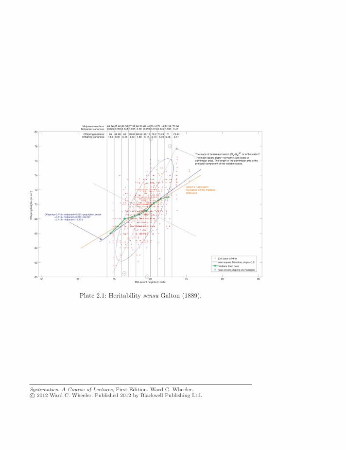
Midparent medians:Midparent variances:
64.860.023
65.600.093
66.560.048
67.520.091
68.560.09
69.400.059
70.160.074
71.180.045
72.390.083
73.660.47
Offspring medians:Offspring variances:
Galton's Regressionline based on the mediansslope=2/3
934 adult children
least-square fitted line, slope=0.71
medians fitted cuve
Offspring=0.713× midparent+0.287× population_mean=0.713× midparent+0.287× 69.247=0.713× midparent+19.874
664.55
80
78
76
74
72
70
68Offs
prin
g he
ight
s (in
inch
)
66
64
62
6055 60 65 70
Mid-parent heights (in inch)75 80 85
66.966.87
686.46
68.043.83
68.584.58
69.125.11
70.25.70
70.745.00
716.26
73.443.17
The slope of semimajor axis is (SY/SX)2, or in this case 2.The least-square slope= corrcoef× sqrt (slope ofsemimajor axis). The length of the semimajor axis is theprincipal component of the variable space.
Plate 2.1: Heritability sensu Galton (1889).
Systematics: A Course of Lectures, First Edition. Ward C. Wheeler.c© 2012 Ward C. Wheeler. Published 2012 by Blackwell Publishing Ltd.
ARHGAP17
AQP8LCMT1
RRM1 STIM1
DCHS1 OR genes
RHBDF1
MPG
C16orf35
MRE
MC DS LA
Jawed vertebrate ancestor
ζ ζ μ α α α θ ζ ζ μ α α α ω π α α
β β β β β
α α α β
β β β α α
α
β
β βα α α α α α α β
ε γ γ η δ β β β
α α α
β
β
α α α
β β β
β
β β
α α
β
α α α
ρ β β εGBY
D A
H A
FOLR1?
?
MC
DS
LA
Human Platypus Chicken
Frog (X. tropicalis)
Fish (Medaka)
16
11
162
2
2114 s357
s1078+
s27
RHBDF1
GBYs733
1
14
8
13
19
MC
DS
LA?
?
MC
RHBDF1
GBY?
LA
?
POLR3K
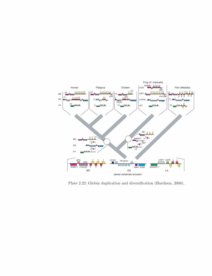
Plate 2.22: Globin duplication and diversification (Hardison, 2008).
5'
C
3'M
3'm
1
2
3
4
5 6
7
8
9
10
11
12
13
14
15
16
17
18
19
2021
22
23
24
25
26
26a
2729
30
31
32
33
34
35
36
3738 39
40
41
42
43
44
45
28
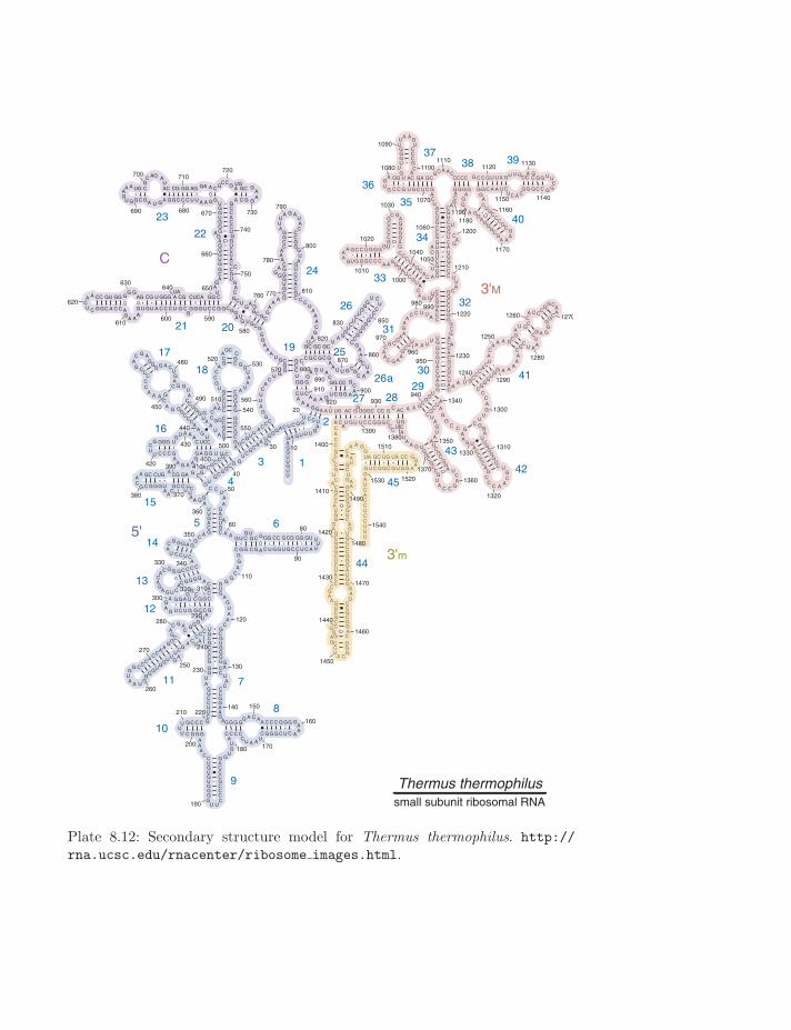
Thermus thermophilussmall subunit ribosomal RNA
Plate 8.12: Secondary structure model for Thermus thermophilus. http://rna.ucsc.edu/rnacenter/ribosome images.html.

Plate 9.21: Neighbor-Joining tree of H5N1 “Avian” flu virus of WHO/OIE/FAO H5N1 Evolution Working Group http://www.cdc.gov/eid/content/14/7/e1-G2.htm.
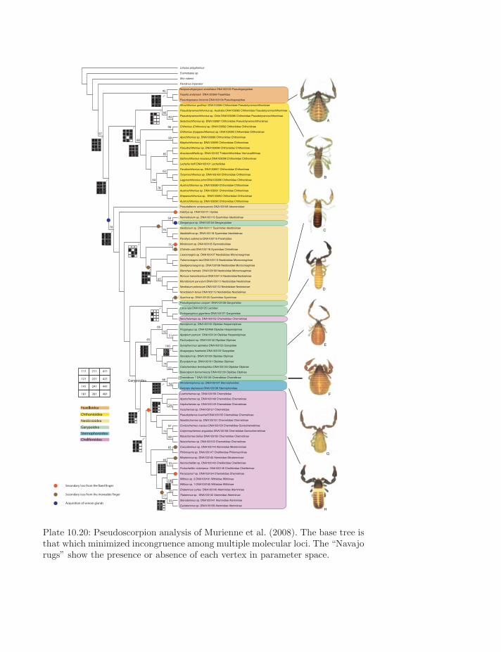
Plate 10.20: Pseudoscorpion analysis of Murienne et al. (2008). The base tree isthat which minimized incongruence among multiple molecular loci. The “Navajorugs” show the presence or absence of each vertex in parameter space.

AA AA AGGG ATT ATTG
A A A A A GG G A T T A GT T- - - - -
A A A A A GG G A T T A GT T
A A- -A A- -A GG GA T T -A GT T
Plate 10.21: Implied alignment (Wheeler, 2003a) of five sequences: AA, AA,AGGG, ATT, and ATTG. The original optimized tree is shown on the upperleft; the implied traces upper right; implied traces with traces extended and gapcharacters filled in lower left; and the final implied alignment in the lower right.
4 Crustaceans (4 orders)
134 Insects (10 orders)
2 Chelicerates (2 orders)
4 Myriapods (2 orders)
Onychophoran
Tardigrade
Pogonophoran, 3 annelids(S–A rather than A–S in Platynereis)
Echiuran
Gastropod, polyplacophoranmolluscs
Arthropoda
COI L(UUR) COII
LrRNA L(CUN) L(UUR) NDI
LrRNA L(CUN) L(UUR) NDI
LrRNA L(CUN) L(UUR) NDI
LrRNA L(CUN) L(UUR) NDI
LrRNA L(CUN) I L(UUR) NDI
LrRNA L(CUN) A S L(UUR) NDI
L(CUN) A S L(UUR) NDI
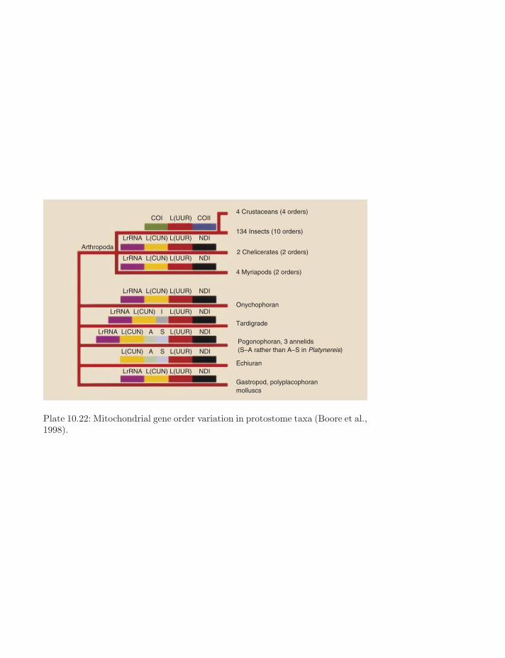
Plate 10.22: Mitochondrial gene order variation in protostome taxa (Boore et al.,1998).
(a)
0 500 1000 1500 2000 2500 3000 3500 40000
500
1000
1500
2000
2500
3000
3500
4000
(b)
0 100 200 300 400 500 600 7000
100
200
300
400
500
600
700
(c)
0 200 400 600 800 1000 1200 14000
200
400
600
800
1000
1200
1400
(d)
0 500 1000 1500 2000 25000
500
1000
1500
2000
2500
(e)
0 200 400 600 800 1000 1200 1400 1600 18000
200
400
600
800
1000
1200
1400
1600
1800
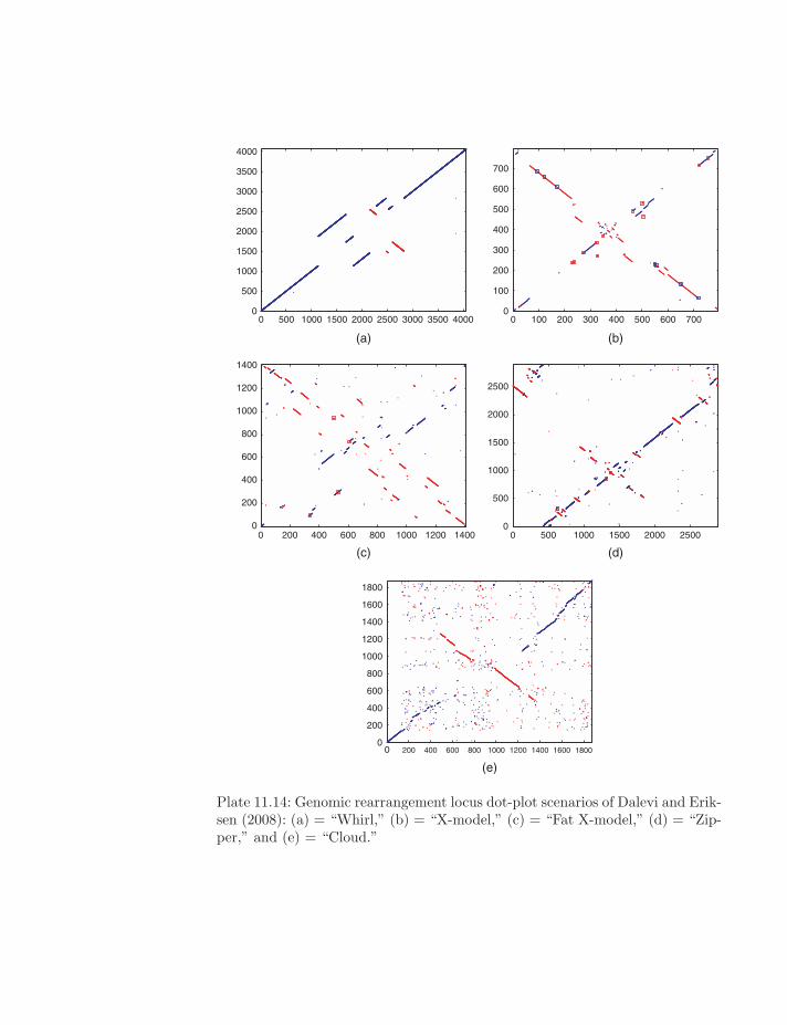
Plate 11.14: Genomic rearrangement locus dot-plot scenarios of Dalevi and Erik-sen (2008): (a) = “Whirl,” (b) = “X-model,” (c) = “Fat X-model,” (d) = “Zip-per,” and (e) = “Cloud.”
HeterogeneousSingle partitionHomogeneous
AverageHomogeneous
Heterogeneous Single partitionHomogeneous
AverageHomogeneous
Fra
ctio
n co
rrec
tF
ract
ion
corr
ect
Fra
ctio
n co
rrec
tF
ract
ion
corr
ect
Fra
ctio
n co
rrec
t
Fra
ctio
n co
rrec
t
Internal branch length Internal branch length
Sequence length
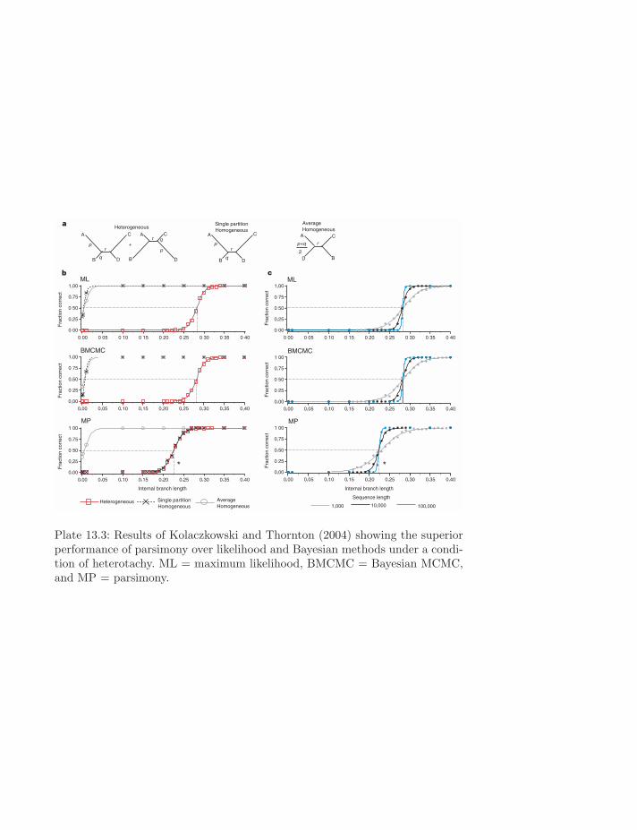
Plate 13.3: Results of Kolaczkowski and Thornton (2004) showing the superiorperformance of parsimony over likelihood and Bayesian methods under a condi-tion of heterotachy. ML = maximum likelihood, BMCMC = Bayesian MCMC,and MP = parsimony.
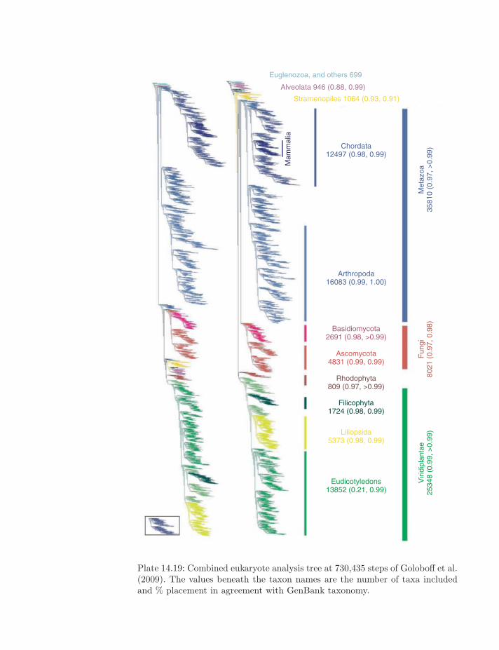
Euglenozoa, and others 699
Alveolata 946 (0.88, 0.99)
Chordata12497 (0.98, 0.99)
Arthropoda16083 (0.99, 1.00)
Basidiomycota2691 (0.98, >0.99)
Ascomycota4831 (0.99, 0.99)
Rhodophyta809 (0.97, >0.99)
Filicophyta1724 (0.98, 0.99)
Eudicotyledons13852 (0.21, 0.99)
Liliopsida5373 (0.98, 0.99)
Met
azoa
3581
0 (0
.97,
>0.
99)
Fun
gi80
21 (
0.97
, 0.9
8)V
iridi
plan
tae
2534
8 (0
.99,
>0.
99)
Mam
mal
ia
Stramenopiles 1064 (0.93, 0.91)
Plate 14.19: Combined eukaryote analysis tree at 730,435 steps of Goloboff et al.(2009). The values beneath the taxon names are the number of taxa includedand % placement in agreement with GenBank taxonomy.
1.0
DasyurusPhascogaleSminthopsisEchymiperaPeramelesNotoryctesDendrolagusPseudocheiridaePhalangerPhascolarctosVombatusDromiciopsCaenolestesRhyncholestesDidelphinaeMonodelphisCaluromysCeratomorphaEquusCynocephalusLeporidaeElephantinaeSireniaBradypus
DasyurusPhascogaleSminthopsisEchymiperaPeramelesNotoryctesDendrolagusPseudocheiridaePhalangerPhascolarctosVombatusDromiciopsCaenolestesRhyncholestesDidelphinaeMonodelphisCaluromysCeratomorphaEquusCynocephalusLeporidaeElephantinaeSireniaBradypus
1.0
1.01.0
1.0
1.0
1.0
1.0
1.0
1.0
1.0
1.0
1.0
1.0
1.0
1.0
1.0
1.0
200 Ma 150 Ma
JURASSIC
(a)
(b)
CRETACEOUS TERTIARY
100 Ma 50 Ma 0 Ma
1.0
0.86
1.0
0.96
0.96
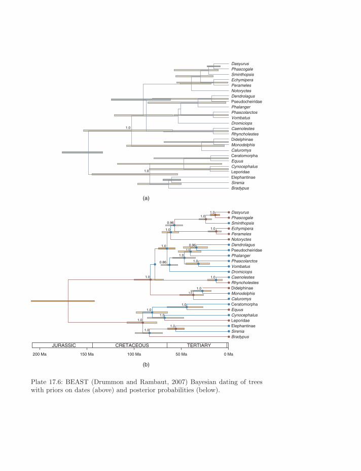
Plate 17.6: BEAST (Drummon and Rambaut, 2007) Bayesian dating of treeswith priors on dates (above) and posterior probabilities (below).

Part I
Fundamentals
Chapter 1
History
Systematics has its origins in two threads of biological science: classification andevolution. The organization of natural variation into sets, groups, and hierarchiestraces its roots to Aristotle and evolution to Darwin. Put simply, systematizationof nature can and has progressed in absence of causative theories relying on ideasof “plan of nature,” divine or otherwise. Evolutionists (Darwin, Wallace, andothers) proposed a rationale for these patterns. This mixture is the foundationof modern systematics.
Originally, systematics was natural history. Today we think of systematicsas being a more inclusive term, encompassing field collection, empirical compar-ative biology, and theory. To begin with, however, taxonomy, now known as theprocess of naming species and higher taxa in a coherent, hypothesis-based, andregular way, and systematics were equivalent.
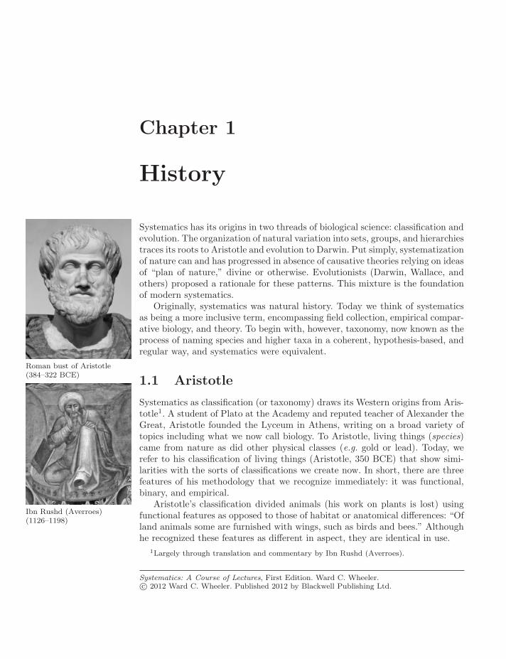
Roman bust of Aristotle(384–322 BCE)
1.1 Aristotle
Systematics as classification (or taxonomy) draws its Western origins from Aris-totle1. A student of Plato at the Academy and reputed teacher of Alexander the
Ibn Rushd (Averroes)(1126–1198)
Great, Aristotle founded the Lyceum in Athens, writing on a broad variety oftopics including what we now call biology. To Aristotle, living things (species)came from nature as did other physical classes (e.g. gold or lead). Today, werefer to his classification of living things (Aristotle, 350 BCE) that show simi-larities with the sorts of classifications we create now. In short, there are threefeatures of his methodology that we recognize immediately: it was functional,binary, and empirical.
Aristotle’s classification divided animals (his work on plants is lost) usingfunctional features as opposed to those of habitat or anatomical differences: “Ofland animals some are furnished with wings, such as birds and bees.” Althoughhe recognized these features as different in aspect, they are identical in use.
1Largely through translation and commentary by Ibn Rushd (Averroes).
Systematics: A Course of Lectures, First Edition. Ward C. Wheeler.c© 2012 Ward C. Wheeler. Published 2012 by Blackwell Publishing Ltd.
1.2 Theophrastus 3
Features were also described in binary terms: “Some are nocturnal, as theowl and the bat; others live in the daylight.” These included egg- or live-bearing,blooded or non-blooded, and wet or dry respiration.
An additional feature of Aristotle’s work was its empirical content. Aspectsof creatures were based on observation rather than ideal forms. In this, he recog-nized that some creatures did not fit into his binary classification scheme: “Theabove-mentioned organs, then, are the most indispensable parts of animals; andwith some of them all animals without exception, and with others animals forthe most part, must needs be provided.” Sober (1980) argued that these depar-tures from Aristotle’s expectations (Natural State Model) were brought about(in Aristotle’s mind) by errors due to some perturbations (hybridization, devel-opmental trauma) resulting in “terata” or monsters. These forms could be noveland helped to explain natural variation within his scheme.
• Blooded Animals
Live-bearing animals
humans
other mammals
Egg-laying animals
birds
fish
• Non-Blooded Animals
Hard-shelled sea animals: Testacea
Soft-shelled sea animals: Crustacea
Non-shelled sea animals: Cephalopods
Insects
Bees
• Dualizing species (potential “terata,” errors in nature)
Whales, seals and porpoises—in water, but bear live young
Bats—have wings and can walk
Sponges—like plants and like animals.
Aristotle clearly had notions of biological progression (scala naturae) from lower(plant) to higher (animals through humans) forms that others later seized uponas being evolutionary and we reject today. Aristotle’s classification of animalswas neither comprehensive nor entirely consistent, but was hierarchical, predic-tive (in some sense), and formed the beginning of modern classification.
1.2 Theophrastus
Theophrastus(c.371–c.287 BCE)
Theophrastus succeeded Aristotle and is best known in biology for his Enquiryinto Plants and On the Causes of Plants. As a study of classification, his work

4 History
KITTÒΣ
" πολυειδη"
" " 'υϕοσ α ιρομενος
''" πλειω γενη"
'"ειδη"
'λευ×ο×αρπος'
λευ×ο−ϕυλλος '
πι×ρο−ξαρπος
'×ορυμβια ποωδης 'λεν×η ' 'ποι×ιλη
ε πιγ ειος
λευ×ος μελας
"διαϕορα""ειοη"
"ελιξ
Th.HP.III. 18 = Hedera
Figure 1.1: Branching diagram after Theophrastus (Vacsy, 1971).
on ivy (κιττoς) discussed extensively by Nelson and Platnick (1981), has beenheld to be a foundational work in taxonomy based (in part at least) on dichoto-mous distinctions (e.g. growing on ground versus upright) of a few essentialfeatures.
Pierre Belon(1517–1564)
Theophrastus distinguished ivies based on growth form and color of leavesand fruit. Although he never presented a branching diagram, later workers (in-cluding Nelson and Platnick) have summarized these observations in a varietyof branching diagrams (Vacsy, 1971) (Fig. 1.1).
1.3 Pierre Belon
Trained as a physician, Pierre Belon, studied botany and traveled widely insouthern Europe and the Middle East. He published a number of works basedon these travels and is best known for his comparative anatomical representationof the skeletons of humans and birds (Belon, 1555) (Fig. 1.2).
1.4 Carolus Linnaeus
Carl von Linne(1707–1778)
Carolus Linnaeus (Carl von Linne) built on Aristotle and created a classificationsystem that has been the basis for biological nomenclature and communicationfor over 250 years. Through its descendants, the current codes of zoological,botanical, and other nomenclature, his influence is still felt today. Linnaeus wasinterested in both classification and identification (animal, plant, and mineralspecies), hence his system included descriptions and diagnoses for the creatureshe included. He formalized the custom of binomial nomenclature, genus andspecies we use today.

1.4 Carolus Linnaeus 5
Figure 1.2: Belon’s funky chicken (Belon, 1555).
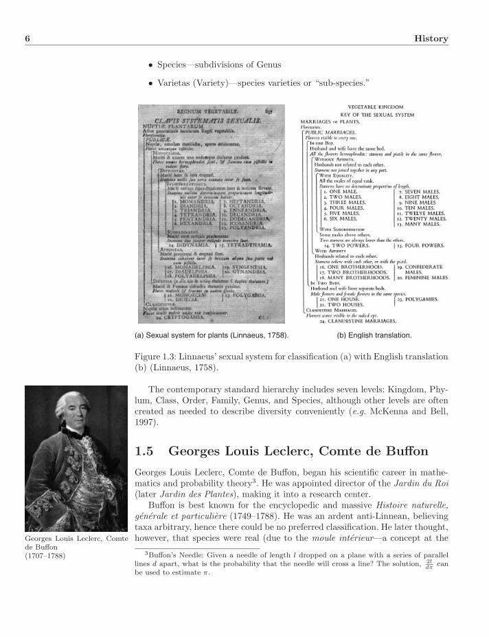
Linnaeus was known, somewhat scandalously in his day, for his sexual systemof classification (Fig. 1.3). This was most extensively applied to plants, butwas also employed in the classification of minerals and fossils. Flowers weredescribed using such terms as visible (public marriage) or clandestine, and singleor multiple husbands or wives (stamens and pistils). Floral parts were evenanalogized to the foreskin and labia.
Nomenclature for many fungal, plant, and other eukaryote groups2 is foundedon the Species Plantarum (Linnaeus, 1753), and that for animals the 10th Edi-tion of Systema Naturae (Linnaeus, 1758). The system is hierarchical withseven levels reflecting order in nature (as opposed to the views of GeorgesLouis Leclerc, 1778 [Buffon], who believed the construct arbitrary and natu-ral variation a result of the combinatorics of components).
• Imperium (Empire)—everything
• Regnum (Kingdom)—animal, vegetable, or mineral
• Classis (Class)—in the animal kingdom there were six (mammals, birds,amphibians, fish, insects, and worms)
• Ordo (Order)—subdivisions of Class
• Genus—subdivisions of Order2For the current code of botanical nomenclature see http://ibot.sav.sk/icbn/main.htm.
6 History
• Species—subdivisions of Genus
• Varietas (Variety)—species varieties or “sub-species.”
(a) Sexual system for plants (Linnaeus, 1758). (b) English translation.
Figure 1.3: Linnaeus’ sexual system for classification (a) with English translation(b) (Linnaeus, 1758).
The contemporary standard hierarchy includes seven levels: Kingdom, Phy-lum, Class, Order, Family, Genus, and Species, although other levels are oftencreated as needed to describe diversity conveniently (e.g. McKenna and Bell,1997).
1.5 Georges Louis Leclerc, Comte de Buffon
Georges Louis Leclerc, Comte de Buffon, began his scientific career in mathe-matics and probability theory3. He was appointed director of the Jardin du Roi(later Jardin des Plantes), making it into a research center.
Georges Louis Leclerc, Comtede Buffon(1707–1788)
Buffon is best known for the encyclopedic and massive Histoire naturelle,generale et particuliere (1749–1788). He was an ardent anti-Linnean, believingtaxa arbitrary, hence there could be no preferred classification. He later thought,however, that species were real (due to the moule interieur—a concept at the
3Buffon’s Needle: Given a needle of length l dropped on a plane with a series of parallellines d apart, what is the probability that the needle will cross a line? The solution, 2l
dπcan
be used to estimate π.
1.6 Jean-Baptiste Lamarck 7
foundation of comparative biology). Furthermore, Buffon believed that speciescould “improve” or “degenerate” into others, (e.g. humans to apes) changing inresponse to their environment. Some (e.g. Mayr, 1982) have argued that Buffonwas among the first evolutionary thinkers with mutable species. His observationthat the mammalian species of tropical old and new world, though living insimilar environments, share not one taxon, went completely against then-currentthought and is seen as the foundation of biogeography as a discipline (Nelsonand Platnick, 1981).
1.6 Jean-Baptiste Lamarck
Jean-Baptiste Lamarck(1744–1829)
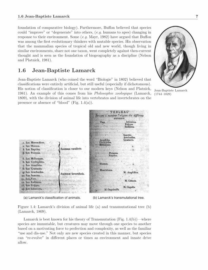
Jean-Baptiste Lamarck (who coined the word “Biologie” in 1802) believed thatclassifications were entirely artificial, but still useful (especially if dichotomous).His notion of classification is closer to our modern keys (Nelson and Platnick,1981). An example of this comes from his Philosophie zoologique (Lamarck,1809), with the division of animal life into vertebrates and invertebrates on thepresence or absence of “blood” (Fig. 1.4(a)).
(a) Lamarck’s classification of animals. (b) Lamarck’s transmutational tree.
Figure 1.4: Lamarck’s division of animal life (a) and transmutational tree (b)(Lamarck, 1809).
Lamarck is best known for his theory of Transmutation (Fig. 1.4(b))—wherespecies are immutable, but creatures may move through one species to anotherbased on a motivating force to perfection and complexity, as well as the familiar“use and dis-use.” Not only are new species created in this manner, but speciescan “re-evolve” in different places or times as environment and innate driveallow.
8 History
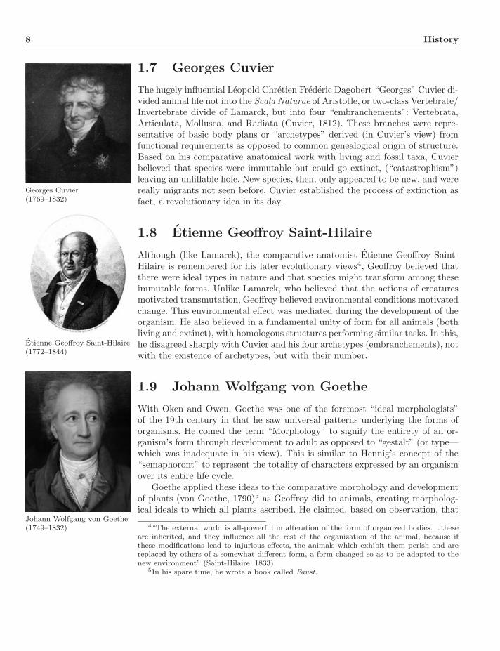
1.7 Georges Cuvier
Georges Cuvier(1769–1832)
The hugely influential Leopold Chretien Frederic Dagobert “Georges” Cuvier di-vided animal life not into the Scala Naturae of Aristotle, or two-class Vertebrate/Invertebrate divide of Lamarck, but into four “embranchements”: Vertebrata,Articulata, Mollusca, and Radiata (Cuvier, 1812). These branches were repre-sentative of basic body plans or “archetypes” derived (in Cuvier’s view) fromfunctional requirements as opposed to common genealogical origin of structure.Based on his comparative anatomical work with living and fossil taxa, Cuvierbelieved that species were immutable but could go extinct, (“catastrophism”)leaving an unfillable hole. New species, then, only appeared to be new, and werereally migrants not seen before. Cuvier established the process of extinction asfact, a revolutionary idea in its day.
1.8 Etienne Geoffroy Saint-Hilaire
Although (like Lamarck), the comparative anatomist Etienne Geoffroy Saint-Hilaire is remembered for his later evolutionary views4, Geoffroy believed that
Etienne Geoffroy Saint-Hilaire(1772–1844)
there were ideal types in nature and that species might transform among theseimmutable forms. Unlike Lamarck, who believed that the actions of creaturesmotivated transmutation, Geoffroy believed environmental conditions motivatedchange. This environmental effect was mediated during the development of theorganism. He also believed in a fundamental unity of form for all animals (bothliving and extinct), with homologous structures performing similar tasks. In this,he disagreed sharply with Cuvier and his four archetypes (embranchements), notwith the existence of archetypes, but with their number.
1.9 Johann Wolfgang von Goethe
With Oken and Owen, Goethe was one of the foremost “ideal morphologists”of the 19th century in that he saw universal patterns underlying the forms oforganisms. He coined the term “Morphology” to signify the entirety of an or-ganism’s form through development to adult as opposed to “gestalt” (or type—which was inadequate in his view). This is similar to Hennig’s concept of the“semaphoront” to represent the totality of characters expressed by an organismover its entire life cycle.
Goethe applied these ideas to the comparative morphology and developmentof plants (von Goethe, 1790)5 as Geoffroy did to animals, creating morpholog-ical ideals to which all plants ascribed. He claimed, based on observation, that
Johann Wolfgang von Goethe(1749–1832) 4“The external world is all-powerful in alteration of the form of organized bodies. . . these
are inherited, and they influence all the rest of the organization of the animal, because ifthese modifications lead to injurious effects, the animals which exhibit them perish and arereplaced by others of a somewhat different form, a form changed so as to be adapted to thenew environment” (Saint-Hilaire, 1833).
5In his spare time, he wrote a book called Faust.
1.10 Lorenz Oken 9
archetypes contained the inherent nature of a taxon, such as “bird-ness” or“mammal-ness.” This ideal was not thought to be ancestral or primitive in anyway, but embodied the morphological relationships of the members of the group.
1.10 Lorenz Oken
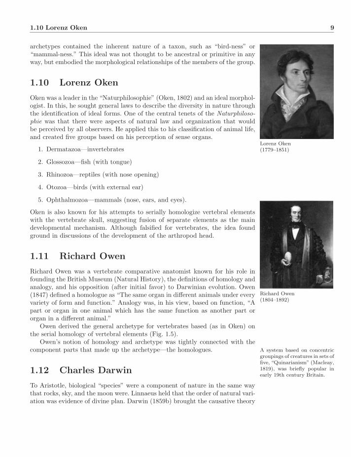
Oken was a leader in the “Naturphilosophie” (Oken, 1802) and an ideal morphol-ogist. In this, he sought general laws to describe the diversity in nature throughthe identification of ideal forms. One of the central tenets of the Naturphiloso-phie was that there were aspects of natural law and organization that wouldbe perceived by all observers. He applied this to his classification of animal life,and created five groups based on his perception of sense organs.
Lorenz Oken(1779–1851)1. Dermatazoa—invertebrates
2. Glossozoa—fish (with tongue)
3. Rhinozoa—reptiles (with nose opening)
4. Otozoa—birds (with external ear)
5. Ophthalmozoa—mammals (nose, ears, and eyes).
Oken is also known for his attempts to serially homologize vertebral elementswith the vertebrate skull, suggesting fusion of separate elements as the maindevelopmental mechanism. Although falsified for vertebrates, the idea foundground in discussions of the development of the arthropod head.
1.11 Richard Owen
Richard Owen was a vertebrate comparative anatomist known for his role infounding the British Museum (Natural History), the definitions of homology andanalogy, and his opposition (after initial favor) to Darwinian evolution. Owen
Richard Owen(1804–1892)
(1847) defined a homologue as “The same organ in different animals under everyvariety of form and function.” Analogy was, in his view, based on function, “Apart or organ in one animal which has the same function as another part ororgan in a different animal.”
Owen derived the general archetype for vertebrates based (as in Oken) onthe serial homology of vertebral elements (Fig. 1.5).
Owen’s notion of homology and archetype was tightly connected with thecomponent parts that made up the archetype—the homologues. A system based on concentric
groupings of creatures in sets offive, “Quinarianism” (Macleay,1819), was briefly popular inearly 19th century Britain.
1.12 Charles Darwin
To Aristotle, biological “species” were a component of nature in the same waythat rocks, sky, and the moon were. Linnaeus held that the order of natural vari-ation was evidence of divine plan. Darwin (1859b) brought the causative theory

10 History
Figure 1.5: Owen’s vertebrate archetype showing his model of a series of un-modified vertebral elements (Russell, 1916; after Owen, 1847).
of evolution to generate and explain the hierarchical distribution of biologicalvariation. This had a huge intellectual impact in justifying classification as a re-flection of genealogy for the first time, and bringing intellectual order (howeverreluctantly) to a variety of conflicting, if reasonable, classificatory schemes.
Charles Darwin(1809–1882)
The genealogical implications of Darwin’s work led him to think in termsof evolutionary “trees,” (Fig. 1.6), the ubiquitous metaphor we use today. Therelationship between classification and evolutionary genealogy, however, wasnot particularly clarified (Hull, 1988). Although the similarities between geneal-ogy and classification were ineluctable, Darwin was concerned (as were manywho followed) with representing both degree of genealogical relationship anddegree of evolutionary modification in a single object. He felt quite clearly that
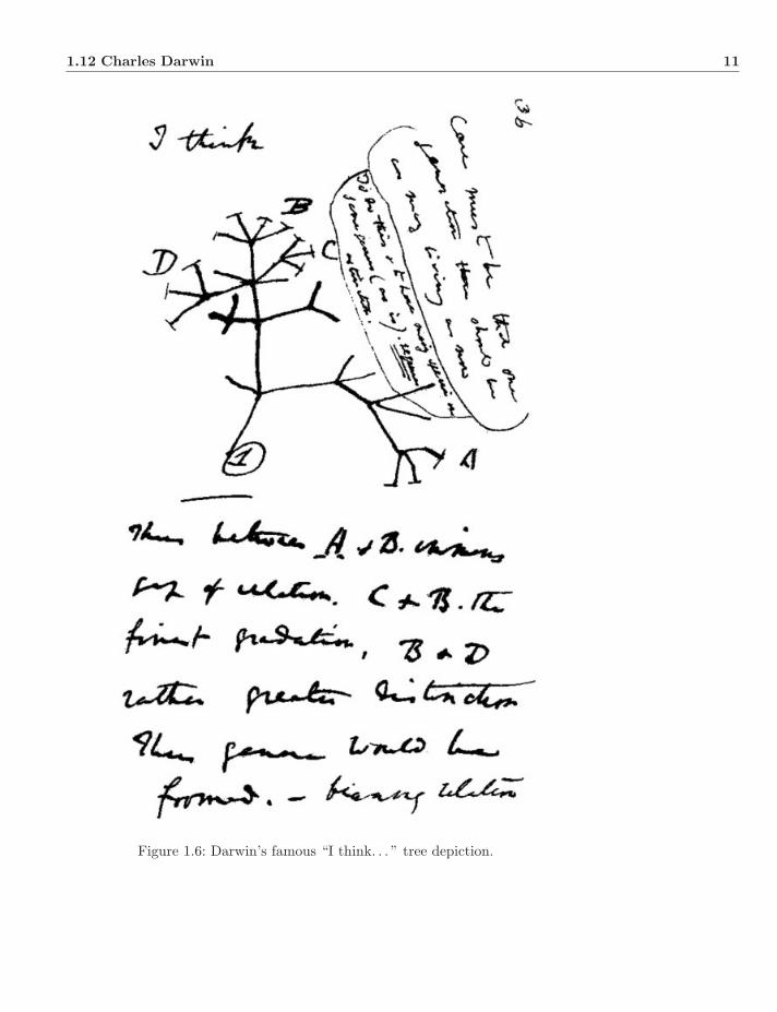
1.12 Charles Darwin 11
Figure 1.6: Darwin’s famous “I think. . . ” tree depiction.
12 History
classifications were more than evolutionary trees, writing that “genealogy byitself does not give classification” (Darwin, 1859a).
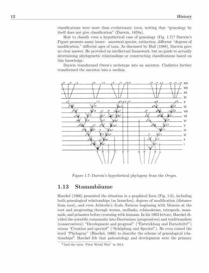
How to classify even a hypothetical case of genealogy (Fig. 1.7)? Darwin’sFigure presents many issues—ancestral species, extinction, different “degrees ofmodification,” different ages of taxa. As discussed by Hull (1988), Darwin gaveno clear answer. He provided an intellectual framework, but no guide to actuallydetermining phylogenetic relationships or constructing classifications based onthis knowledge.
Darwin transformed Owen’s archetype into an ancestor. Cladistics furthertransformed the ancestor into a median.
A B C D E F G H I K L
I
II
III
IV
V
VI
VII
VIII
IX
X
XI
XII
XIII
XIV
Figure 1.7: Darwin’s hypothetical phylogeny from the Origin.
1.13 Stammbaume
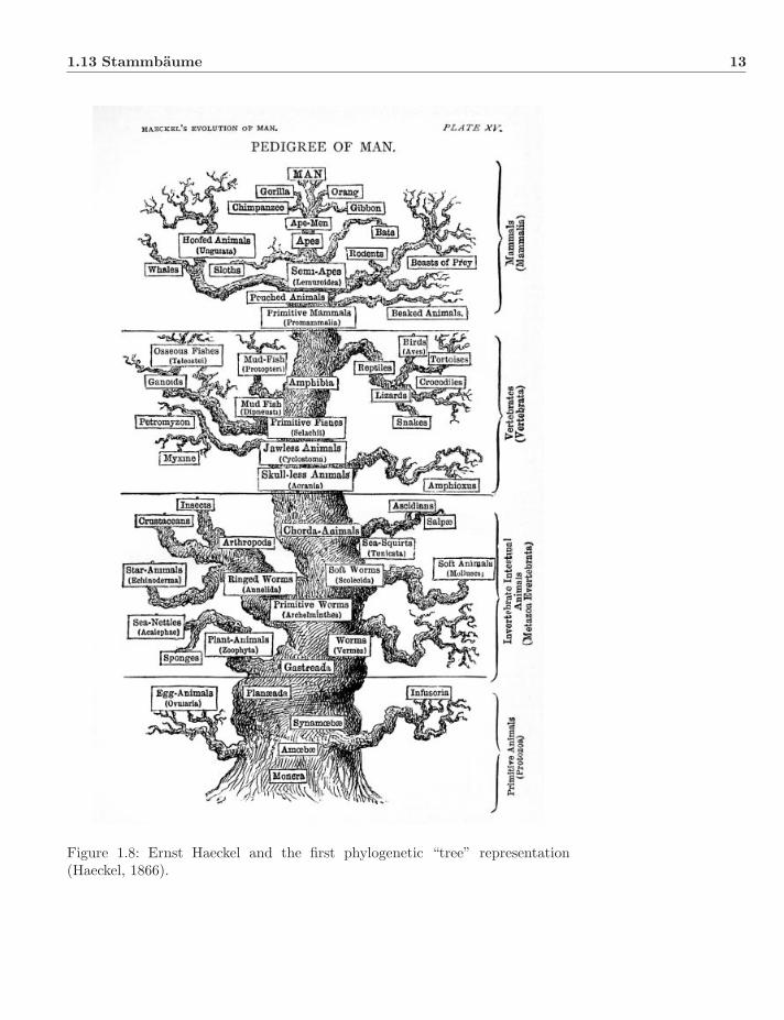
Haeckel (1866) presented the situation in a graphical form (Fig. 1.8), includingboth genealogical relationships (as branches), degrees of modification (distancefrom root), and even Aristotle’s Scala Naturae beginning with Monera at theroot and progressing through worms, mollusks, echinoderms, tetrapods, mam-mals, and primates before crowning with humans. In his 1863 lecture, Haeckel di-vided the scientific community into Darwinians (progressives) and traditionalists(conservatives): “Development and progress!” (“Entwicklung und Fortschritt!”)versus “Creation and species!” (“Schopfung und Species!”). He even coined theword “Phylogeny” (Haeckel, 1866) to describe the scheme of genealogical rela-tionships6. Haeckel felt that paleontology and development were the primary
6And the term “First World War” in 1914.
1.13 Stammbaume 13
Figure 1.8: Ernst Haeckel and the first phylogenetic “tree” representation(Haeckel, 1866).
14 History
ways to discover phylogeny (Haeckel, 1876). Morphology was a third leg, butof lesser importance. Bronn (1858, 1861) also had a tree like representationand was the translator of Darwin into the German version that Haeckel read(Richards, 2005). Bronn found Darwin’s ideas untested, while Haeckel did not.
August Schleicher constructed linguistic trees as Darwin had biological. Afriend of Haeckel, Schleicher “tested” Darwin with language (Schleicher, 1869).Interestingly, he thought there were better linguistic fossils than biological, andhence they could form a strong test of Darwin’s ideas.
1.14 Evolutionary Taxonomy
After publication of the Origin, evolution, genetics, and paleontology went theirown ways. In the middle of the 20th century, these were brought together inwhat became known as the “New Synthesis.” Among many, Dobzhansky (1937),Mayr (1942), Simpson (1944)7, and Wright (1931) were most prominent. TheNew Synthesis brought together these strands of biology creating a satisfyingly
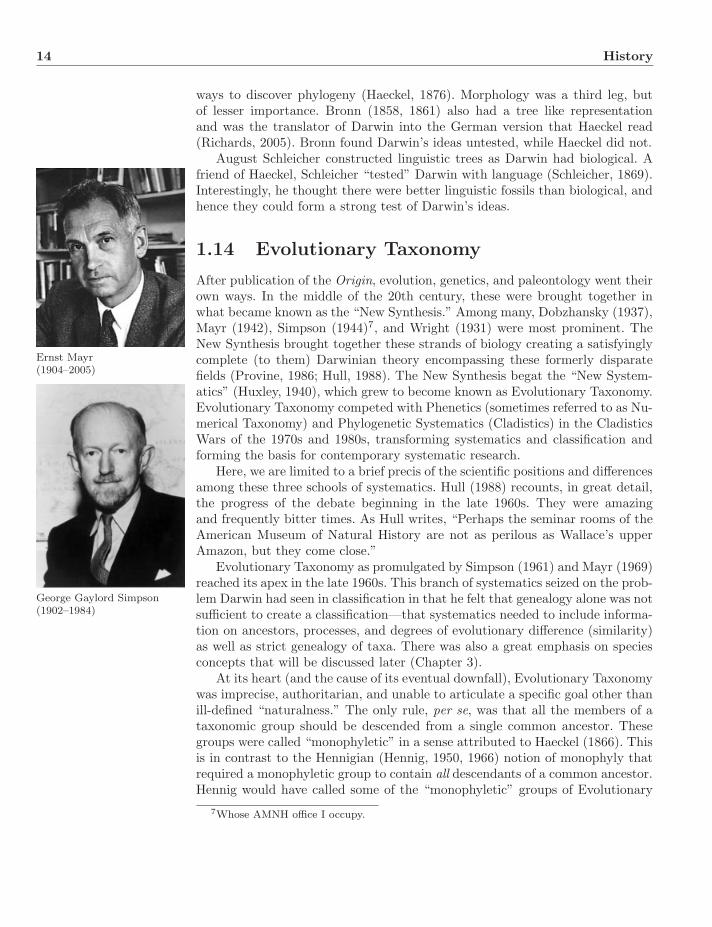
Ernst Mayr(1904–2005)
complete (to them) Darwinian theory encompassing these formerly disparatefields (Provine, 1986; Hull, 1988). The New Synthesis begat the “New System-atics” (Huxley, 1940), which grew to become known as Evolutionary Taxonomy.Evolutionary Taxonomy competed with Phenetics (sometimes referred to as Nu-merical Taxonomy) and Phylogenetic Systematics (Cladistics) in the CladisticsWars of the 1970s and 1980s, transforming systematics and classification andforming the basis for contemporary systematic research.
Here, we are limited to a brief precis of the scientific positions and differencesamong these three schools of systematics. Hull (1988) recounts, in great detail,the progress of the debate beginning in the late 1960s. They were amazingand frequently bitter times. As Hull writes, “Perhaps the seminar rooms of theAmerican Museum of Natural History are not as perilous as Wallace’s upperAmazon, but they come close.”
George Gaylord Simpson(1902–1984)
Evolutionary Taxonomy as promulgated by Simpson (1961) and Mayr (1969)reached its apex in the late 1960s. This branch of systematics seized on the prob-lem Darwin had seen in classification in that he felt that genealogy alone was notsufficient to create a classification—that systematics needed to include informa-tion on ancestors, processes, and degrees of evolutionary difference (similarity)as well as strict genealogy of taxa. There was also a great emphasis on speciesconcepts that will be discussed later (Chapter 3).
At its heart (and the cause of its eventual downfall), Evolutionary Taxonomywas imprecise, authoritarian, and unable to articulate a specific goal other thanill-defined “naturalness.” The only rule, per se, was that all the members of ataxonomic group should be descended from a single common ancestor. Thesegroups were called “monophyletic” in a sense attributed to Haeckel (1866). Thisis in contrast to the Hennigian (Hennig, 1950, 1966) notion of monophyly thatrequired a monophyletic group to contain all descendants of a common ancestor.Hennig would have called some of the “monophyletic” groups of Evolutionary
7Whose AMNH office I occupy.
1.15 Phenetics 15
Taxonomy paraphyletic (e.g. “Reptilia”), while Hennig’s monophyly was re-ferred to as “holophyly” by Mayr (Fig. 1.9). We now follow Hennig’s conceptsand their strict definitions (Farris, 1974). According to Simpson (1961), eventhe “monophyly” rule could be relaxed in order to maintain cherished groupdefinitions (e.g. Simpson’s Mammalia).
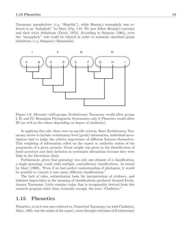
A B C D E F G H I
I II III IV
Figure 1.9: Alternate valid groups. Evolutionary Taxonomy would allow groupsI, II, and IV; Hennigian Phylogenetic Systematics only I; Phenetics would allowIII (as well as the others depending on degree of similarity).
In applying this rule, there were no specific criteria. Since Evolutionary Tax-onomy strove to include evolutionary level (grade) information, individual inves-tigators had to judge the relative importance of different features themselves.This weighting of information relied on the expert or authority status of theproponents of a given scenario. Great weight was given to the identification offossil ancestors and their inclusion in systematic discussions because they werelinks in the Darwinian chain.
Furthermore, given that genealogy was only one element of a classification,a single genealogy could yield multiple, contradictory classifications. As statedby Mayr (1969), “Even if we had perfect understanding of phylogeny, it wouldbe possible to convert it into many different classifications.”
The lack of rules, authoritarian basis for interpretation of evidence, andinherent imprecision in the meaning of classifications produced doomed Evolu-tionary Taxonomy. Little remains today that is recognizably derived from thisresearch program other than, ironically enough, the term “Cladistics.”
1.15 Phenetics
Phenetics, or as it was once referred to, Numerical Taxonomy (as with Cladistics,Mayr, 1965, was the origin of the name), arose through criticisms of Evolutionary
16 History
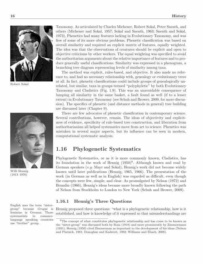
Taxonomy. As articulated by Charles Michener, Robert Sokal, Peter Sneath, andothers (Michener and Sokal, 1957; Sokal and Sneath, 1963; Sneath and Sokal,1973), Phenetics had many features lacking in Evolutionary Taxonomy, and wasfree of some of its more obvious problems. Phenetic classification was based onoverall similarity and required an explicit matrix of features, equally weighted.The idea was that the observations of creatures should be explicit and open toobjective criticisms by other workers. The equal weighting was specified to avoidthe authoritarian arguments about the relative importance of features and to pro-duce generally useful classifications. Similarity was expressed in a phenogram, abranching tree diagram representing levels of similarity among taxa.
Robert Sokal
The method was explicit, rules-based, and objective. It also made no refer-ence to, and had no necessary relationship with, genealogy or evolutionary treesat all. In fact, phenetic classifications could include groups of genealogically un-related, but similar, taxa in groups termed “polyphyletic” by both EvolutionaryTaxonomy and Cladistics (Fig. 1.9). This was an unavoidable consequence oflumping all similarity in the same basket, a fault found as well (if to a lesserextent) in Evolutionary Taxonomy (see Schuh and Brower, 2009, for more discus-sion). The specifics of phenetic (and distance methods in general) tree buildingare discussed later (Chapter 9).
There are few advocates of phenetic classification in contemporary science.Several contributions, however, remain. The ideas of objectivity and explicit-ness of evidence, specificity of rule-based tree construction, and liberation fromauthoritarianism all helped systematics move from art to science. Phenetics wasmistaken in several major aspects, but its influence can be seen in modern,computational systematic analysis.
1.16 Phylogenetic Systematics
Phylogenetic Systematics, or as it is more commonly known, Cladistics, hasits foundation in the work of Hennig (1950)8. Although known and read byGerman speakers (e.g. Mayr and Sokal), Hennig’s work did not become widely
Willi Hennig(1913–1976)
known until later publications (Hennig, 1965, 1966). The presentation of thework (in German as well as in English) was regarded as difficult, even thoughthe concepts were few, simple, and clear. As promulgated by Nelson (1972) andBrundin (1966), Hennig’s ideas became more broadly known following the pathof Nelson from Stockholm to London to New York (Schuh and Brower, 2009).
1.16.1 Hennig’s Three QuestionsEnglish uses the term “sister-group” because Gruppe isfeminine in German. Thosesystematists in romance-language speaking countriesuse “brother” group.
Hennig proposed three questions: “what is a phylogenetic relationship, how is itestablished, and how is knowledge of it expressed so that misunderstandings are
8The concept of what constitutes phylogenetic relationship and has come to be known asthe “sister-group” was discussed both by Rosa (1918) and more prominently by Zimmermann(1931). Hennig (1950) cited Zimmerman as important to the development of his ideas (Nelsonand Platnick, 1981; Donoghue and Kadereit, 1992; Williams and Ebach, 2008).
1.16 Phylogenetic Systematics 17
A. Myriapoda
B. Insecta
B.1 Entognatha
B.1 a Diplura
B.1 b Ellipura
B.1 ba Protura
B.1 bb Collembola
B.2 Ectognatha
Collem
bola
Protu
ra
Diplu
ra
Ectognat
ha
Myriap
oda
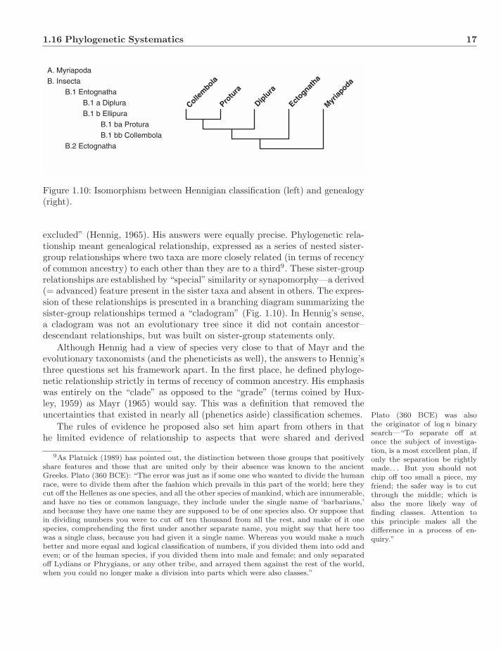
Figure 1.10: Isomorphism between Hennigian classification (left) and genealogy(right).
excluded” (Hennig, 1965). His answers were equally precise. Phylogenetic rela-tionship meant genealogical relationship, expressed as a series of nested sister-group relationships where two taxa are more closely related (in terms of recencyof common ancestry) to each other than they are to a third9. These sister-grouprelationships are established by “special” similarity or synapomorphy—a derived(= advanced) feature present in the sister taxa and absent in others. The expres-sion of these relationships is presented in a branching diagram summarizing thesister-group relationships termed a “cladogram” (Fig. 1.10). In Hennig’s sense,a cladogram was not an evolutionary tree since it did not contain ancestor–descendant relationships, but was built on sister-group statements only.
Although Hennig had a view of species very close to that of Mayr and theevolutionary taxonomists (and the pheneticists as well), the answers to Hennig’sthree questions set his framework apart. In the first place, he defined phyloge-netic relationship strictly in terms of recency of common ancestry. His emphasiswas entirely on the “clade” as opposed to the “grade” (terms coined by Hux-ley, 1959) as Mayr (1965) would say. This was a definition that removed theuncertainties that existed in nearly all (phenetics aside) classification schemes. Plato (360 BCE) was also
the originator of log n binarysearch—“To separate off atonce the subject of investiga-tion, is a most excellent plan, ifonly the separation be rightlymade. . . But you should notchip off too small a piece, myfriend; the safer way is to cutthrough the middle; which isalso the more likely way offinding classes. Attention tothis principle makes all thedifference in a process of en-quiry.”
The rules of evidence he proposed also set him apart from others in thathe limited evidence of relationship to aspects that were shared and derived
9As Platnick (1989) has pointed out, the distinction between those groups that positivelyshare features and those that are united only by their absence was known to the ancientGreeks. Plato (360 BCE): “The error was just as if some one who wanted to divide the humanrace, were to divide them after the fashion which prevails in this part of the world; here theycut off the Hellenes as one species, and all the other species of mankind, which are innumerable,and have no ties or common language, they include under the single name of ‘barbarians,’and because they have one name they are supposed to be of one species also. Or suppose thatin dividing numbers you were to cut off ten thousand from all the rest, and make of it onespecies, comprehending the first under another separate name, you might say that here toowas a single class, because you had given it a single name. Whereas you would make a muchbetter and more equal and logical classification of numbers, if you divided them into odd andeven; or of the human species, if you divided them into male and female; and only separatedoff Lydians or Phrygians, or any other tribe, and arrayed them against the rest of the world,when you could no longer make a division into parts which were also classes.”

18 History
(synapomorphy). Phenetics made no distinction between similarity that wasprimitive or general (symplesiomorphy), and that which was restricted or de-rived (synapomorphy). Furthermore, unique features of a lineage or group playedno role in their placement. An evolutionary taxonomist might place a group asdistinct from its relatives purely on the basis of how different its features werefrom other creatures (autapomorphy) such as Mayr’s rejection of Archosauria(Aves + Crocodilia). The patristic (amount of change) distinctions were irrel-evant to their cladistic relationships. [These terms will be discussed in latersections.] This would all have been fine if all evidence agreed, but that is notthe case. Alternate statements of synapomorphy or homoplasy (convergence orparallelism) confused this issue.
AMNH circa 1910 Hennig annoyed many in that his cladograms made no reference to ances-tors. His methodology required that ancestral species went extinct as splitting(cladogenetic) events occurred. Species only existed between splitting events,hence ancestors were difficult if not impossible to recognize (Chapter 3). Thisseemed anti-evolutionary, even heretical and won no friends among paleontolo-gists. Extinct taxa could be accorded no special status—they were to be treatedas any extant taxon (Chapter 2).
1.17 Molecules and Morphology
The 1980s saw tremendous technological improvement in molecular data gath-ering techniques. By the end of the decade, DNA sequence data were becomingavailable in sufficient quantity to play a role in supporting and challenging phy-logenetic hypotheses, an activity that had previously been the sole province ofanatomical (including developmental) data. Many meeting symposia and paperswere produced agonizing over the issue (e.g. Patterson, 1987). In the interveningyears, the topic has become something of a non-issue. Molecular sequence dataare ubiquitous and easily garnered (for living taxa), forming a component ofnearly all modern analyses. Anatomical information is a direct link to the worldin which creatures live and is the only route to analysis of extinct taxa. Dataare data and all are qualified to participate in systematic hypothesis testing.
A current descendant of this argument is that over the analysis of combinedor partitioned data sets. This plays out in the debates over “Total Evidence”(Chapter 2) and, to some extent, over supertree consensus techniques(Chapter 16).
1.18 We are all Cladists
Today we struggle with different criteria to distinguish between competing anddisagreeing evidence. In contemporary systematics, several methods are usedto make these judgements based on Ockham’s razor (parsimony) or stochas-tic evolutionary models (likelihood and Bayesian techniques). Although theydiffer in their criteria, they all agree that groups must be monophyletic in the

1.19 Exercises 19
Hennigian sense, that classifications must match genealogy exactly, and that ev-idence must rely on special similarity (if differently weighted). All systematiststoday, whether they like it or not, are Hennigian cladists.
1.19 Exercises
1. Were the pre-Darwinians Cladists?
2. What remains of Phenetics?
3. Do we read what we want into the older literature?
4. What about the “original intent” of terms (e.g. monophyly)? Does it mat-ter? Can we know? Is definitional consistency important?
5. What are the relationships among the following terms: archetype, bauplan,semaphoront, ancestor, and hypothetical ancestor?
6. What constitutes “reality” and “natural-ness” in a taxon?
Chapter 2
Fundamental Concepts
This section is a bit of a grab-bag. These are the fundamental concepts uponwhich systematics discussions are based. They include concepts and definitionsof characters, taxa, trees, and optimality. From these, definitions of higher levelconcepts such as homology, polarity, and ancestors are built.
2.1 Characters
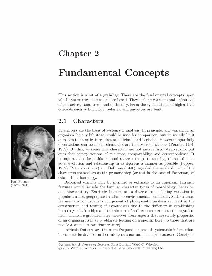
Characters are the basis of systematic analysis. In principle, any variant in anorganism (at any life stage) could be used for comparison, but we usually limitourselves to those features that are intrinsic and heritable. However impartiallyobservations can be made, characters are theory-laden objects (Popper, 1934,1959). By this, we mean that characters are not unorganized observations, butones that convey notions of relevance, comparability, and correspondence. Itis important to keep this in mind as we attempt to test hypotheses of char-acter evolution and relationship in as rigorous a manner as possible (Popper,1959). Patterson (1982) and DePinna (1991) regarded the establishment of thecharacters themselves as the primary step (or test in the case of Patterson) ofestablishing homology.
Karl Popper(1902–1994)
Biological variants may be intrinsic or extrinsic to an organism. Intrinsicfeatures would include the familiar character types of morphology, behavior,and biochemistry. Extrinsic features are a diverse lot, including variation inpopulation size, geographic location, or environmental conditions. Such externalfeatures are not usually a component of phylogenetic analysis (at least in theconstruction and testing of hypotheses) due to the difficulty in establishinghomology relationships and the absence of a direct connection to the organismitself. There is a gradation here, however, from aspects that are clearly propertiesof an organism itself (e.g. obligate feeding on a specific host) to those that arenot (e.g. annual mean temperature).
Intrinsic features are the more frequent sources of systematic information.These may be divided further into genotypic and phenotypic aspects. Genotypic
Systematics: A Course of Lectures, First Edition. Ward C. Wheeler.c© 2012 Ward C. Wheeler. Published 2012 by Blackwell Publishing Ltd.
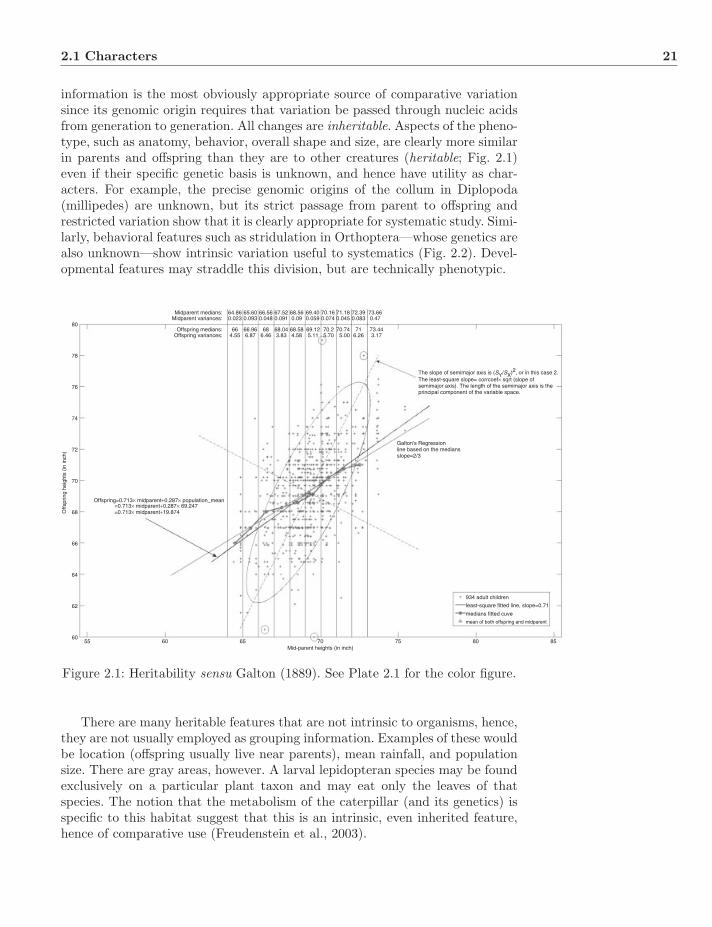
2.1 Characters 21
information is the most obviously appropriate source of comparative variationsince its genomic origin requires that variation be passed through nucleic acidsfrom generation to generation. All changes are inheritable. Aspects of the pheno-type, such as anatomy, behavior, overall shape and size, are clearly more similarin parents and offspring than they are to other creatures (heritable; Fig. 2.1)even if their specific genetic basis is unknown, and hence have utility as char-acters. For example, the precise genomic origins of the collum in Diplopoda(millipedes) are unknown, but its strict passage from parent to offspring andrestricted variation show that it is clearly appropriate for systematic study. Simi-larly, behavioral features such as stridulation in Orthoptera—whose genetics arealso unknown—show intrinsic variation useful to systematics (Fig. 2.2). Devel-opmental features may straddle this division, but are technically phenotypic.
Midparent medians:Midparent variances:
64.860.023
65.600.093
66.560.048
67.520.091
68.560.09
69.400.059
70.160.074
71.180.045
72.390.083
73.660.47
Offspring medians:Offspring variances:
Galton's Regressionline based on the mediansslope=2/3
934 adult children
least-square fitted line, slope=0.71
medians fitted cuve
Offspring=0.713× midparent+0.287× population_mean=0.713× midparent+0.287× 69.247=0.713× midparent+19.874
664.55
80
78
76
74
72
70
68Offs
prin
g he
ight
s (in
inch
)
66
64
62
6055 60 65 70
Mid-parent heights (in inch)75 80 85
66.966.87
686.46
68.043.83
68.584.58
69.125.11
70.25.70
70.745.00
716.26
73.443.17
The slope of semimajor axis is (SY/SX)2, or in this case 2.The least-square slope= corrcoef× sqrt (slope ofsemimajor axis). The length of the semimajor axis is theprincipal component of the variable space.
Figure 2.1: Heritability sensu Galton (1889). See Plate 2.1 for the color figure.
There are many heritable features that are not intrinsic to organisms, hence,they are not usually employed as grouping information. Examples of these wouldbe location (offspring usually live near parents), mean rainfall, and populationsize. There are gray areas, however. A larval lepidopteran species may be foundexclusively on a particular plant taxon and may eat only the leaves of thatspecies. The notion that the metabolism of the caterpillar (and its genetics) isspecific to this habitat suggest that this is an intrinsic, even inherited feature,hence of comparative use (Freudenstein et al., 2003).

22 Fundamental Concepts
G. veletis
G. bimaculatus
G. campestris
G. rubens
G. firmus
G. integer
G. fultoni
G. texensis
G. pennsylvanicus
G. assimilis
G. lineaticeps
G. ovisopis
5 kHz 0.1 s
mute
1, 7
2, 3
2, 5, 6
2
3
3, 6
4
4
4, 7
4
4
5
7
8
8
9
11
13
13
Figure 2.2: Cladogram of orthopteran stridulation (Robillard et al., 2006).
In general, we would like to include as broad and large a collection of charac-ters as possible. This may include molecular sequence, developmental expression,anatomical information, and behavioral observations. With burgeoning molecu-lar genetic and developmental data, situations are rapidly approaching where anobserved variation may be present in multiple data types. Clearly, if we “know”the genetic origins of an anatomical variant, we cannot code a single featurein both data sets [contra Freudenstein et al. (2003)]. The issue, in this case, isindependent information. Can the transformations be traced back to a singlechange or multiple? If single, only one variant can be coded, if multiple (orunknown), the changes are potentially independent and should all be used.
2.1.1 Classes of Characters and Total Evidence
Systematists, being classifiers, typically divide characters into classes: mor-phological, molecular, behavioral, developmental and so forth. Although theseclasses can have descriptive meaning, they do not require that their variation bevalued differentially. The observations “compound eyes” and “adenine at posi-tion 234,” although helpful in understanding where these characters come from
2.1 Characters 23
(anatomy and molecular sequence) and how they were observed, do not conveyany inherent strength or weakness in their ability to participate in hypothesistesting. In short, there may be descriptive character classes, but analyticalclasses do not necessarily follow.
Arnold Kluge
The argument over whether to evaluate all characters simultaneously (“To-tal Evidence” Kluge, 1989; or “Simultaneous Analysis” Nixon and Carpenter,1996b) or separately (partitioned analysis) has focused on two very differentideas of the determination of the “best” phylogenetic hypothesis. The conceptbehind partitioned analysis is one of robustness (i.e. how do different datasources agree or disagree) as opposed to one of optimality and quantity (whichis the best hypothesis given all the data). These will be discussed later in moredetail (Chapter 16).
2.1.2 Ontogeny, Tokogeny, and Phylogeny
Characters and character states can have three types of relationship: “ontoge-netic,” “tokogenetic,” and “phylogenetic” (Hennig, 1950, 1966). When statestransform into one another during development, they have an ontogenetic re-lationship. An example is the imaginal disks of holometabolous insects, whichtransform into adult features such as eyes, genitalia, and wings. Although onto-genetic relationships have been used as indicators of character polarity (prim-itive versus derived) since Haeckel (1868), the transformations in this type ofrelationship are within a single organism.
Tokogeny is the relationship among features that vary within a sexuallyreproducing species1 (Fig. 2.3). As variation within species, such features havebeen considered not to reflect relationships above the species level, hence weretermed “traits” by Nixon and Wheeler (1990). Examples of traits would be colorvariation over the geographic range of a taxon or protein polymorphisms withinpopulations. Nixon and Wheeler argued that true characters must be invariantwithin a species, but variable across species. One of the key issues with thisdistinction is the definition of and distinction between species. Where is the linedrawn to separate traits and characters (Vrana and Wheeler, 1992)?
Features that vary across taxa are referred to as phylogenetic features andare by consensus available for systematic analysis. The fraction of total variationthis constitutes varies.
2.1.3 Characters and Character States
Traditionally, there are characters, which represent comparable features amongorganisms, and character states, which are the set of variations in aspect orexpression of a character. The distinction between the two concepts has alwaysbeen fluid (are crustacean biramous antennae absent/present or a state of ap-pendages?) (Eldredge and Cracraft, 1980), and in dynamic homology (sensuWheeler, 2001b), largely meaningless.
1Also used to describe the parent–offspring relationship, irrespective of reproductive mode.

24 Fundamental Concepts
Species differences
species
species
phylogeneticrelationships
individual
individual
individualpolymorphismsexual dimorphism
met
amor
phos
is
semaphoront
semaphoront
semaphoront
ontogenetic
relationships
cycl
omor
phis
m tokogeneticrelationships
Figure 2.3: Tokogenetic and phylogenetic relationships of Hennig (1966).
As discussed by Platnick (1989), the distinction between character and char-acter state (at least for anatomical features) can be entirely linguistic.
In practice, objections like these sometimes amount only to lin-guistic quibbles. Abdominal spinnerets are not found in organismsother than spiders, and they are a valid synapomorphy of the or-der Araneae regardless of whether they are coded as spinnerets ab-sent versus present, or as ‘distoventral abdominal cuticle smoothlyrounded’ versus ‘distoventral abdominal cuticle distended intospigot-bearing projections.’ The more important point of these ob-jections is that spinneret structure varies among different groups ofspiders. One might treat each identifiable variant in the same way,resulting in a large number of binary characters, with each ‘pres-ence’ representing a different, and additional, modification. If thesequence of modifications is detected correctly, an unobjectionableadditive binary coding of the variable could be achieved. But as the
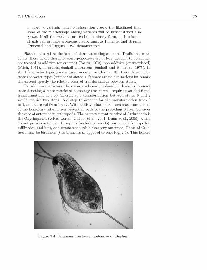
2.1 Characters 25
number of variants under consideration grows, the likelihood thatsome of the relationships among variants will be misconstrued alsogrows. If all the variants are coded in binary form, such miscon-struals can produce erroneous cladograms, as Pimentel and Riggins[Pimentel and Riggins, 1987] demonstrated.
Platnick also raised the issue of alternate coding schemes. Traditional char-acters, those where character correspondences are at least thought to be known,are treated as additive (or ordered) (Farris, 1970), non-additive (or unordered)(Fitch, 1971), or matrix/Sankoff characters (Sankoff and Rousseau, 1975). Inshort (character types are discussed in detail in Chapter 10), these three multi-state character types (number of states > 2; there are no distinctions for binarycharacters) specify the relative costs of transformation between states.
For additive characters, the states are linearly ordered, with each successivestate denoting a more restricted homology statement—requiring an additionaltransformation, or step. Therefore, a transformation between states 0 and 2would require two steps—one step to account for the transformation from 0to 1, and a second from 1 to 2. With additive characters, each state contains allof the homology information present in each of the preceding states. Considerthe case of antennae in arthropods. The nearest extant relative of Arthropoda isthe Onychophora (velvet worms; Giribet et al., 2001; Dunn et al., 2008), whichdo not possess antennae. Hexapods (including insects), myriapods (centipedes,millipedes, and kin), and crustaceans exhibit sensory antennae. Those of Crus-tacea may be biramous (two branches as opposed to one; Fig. 2.4). This feature
Figure 2.4: Biramous crustacean antennae of Daphnia.
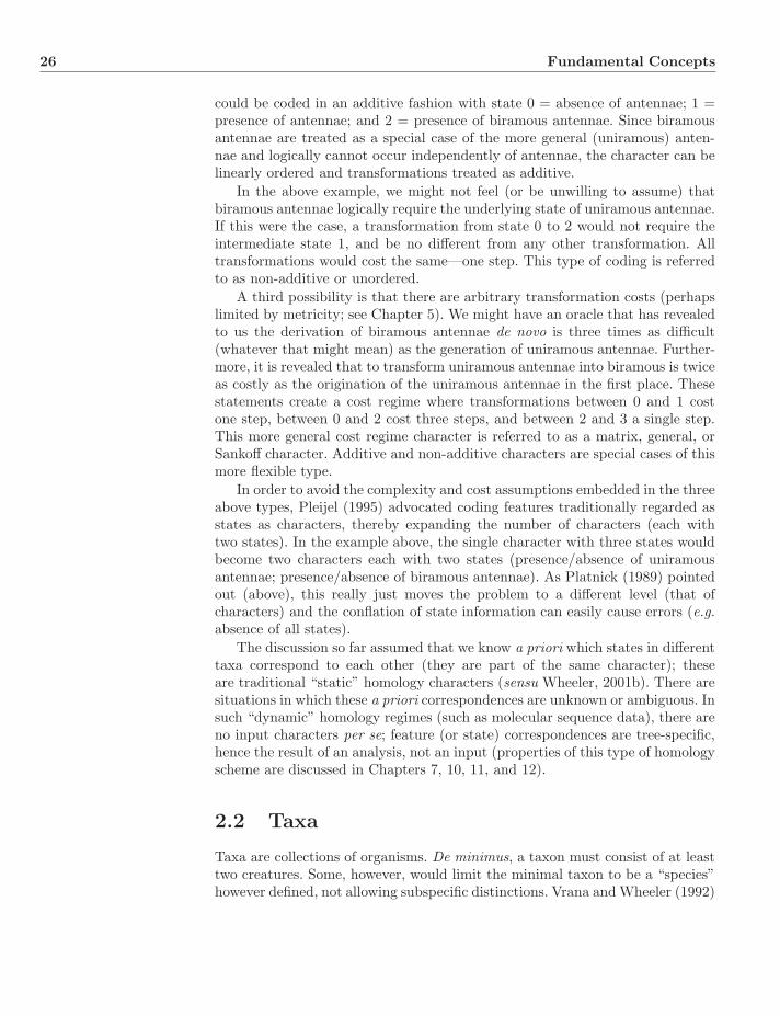
26 Fundamental Concepts
could be coded in an additive fashion with state 0 = absence of antennae; 1 =presence of antennae; and 2 = presence of biramous antennae. Since biramousantennae are treated as a special case of the more general (uniramous) anten-nae and logically cannot occur independently of antennae, the character can belinearly ordered and transformations treated as additive.
In the above example, we might not feel (or be unwilling to assume) thatbiramous antennae logically require the underlying state of uniramous antennae.If this were the case, a transformation from state 0 to 2 would not require theintermediate state 1, and be no different from any other transformation. Alltransformations would cost the same—one step. This type of coding is referredto as non-additive or unordered.
A third possibility is that there are arbitrary transformation costs (perhapslimited by metricity; see Chapter 5). We might have an oracle that has revealedto us the derivation of biramous antennae de novo is three times as difficult(whatever that might mean) as the generation of uniramous antennae. Further-more, it is revealed that to transform uniramous antennae into biramous is twiceas costly as the origination of the uniramous antennae in the first place. Thesestatements create a cost regime where transformations between 0 and 1 costone step, between 0 and 2 cost three steps, and between 2 and 3 a single step.This more general cost regime character is referred to as a matrix, general, orSankoff character. Additive and non-additive characters are special cases of thismore flexible type.
In order to avoid the complexity and cost assumptions embedded in the threeabove types, Pleijel (1995) advocated coding features traditionally regarded asstates as characters, thereby expanding the number of characters (each withtwo states). In the example above, the single character with three states wouldbecome two characters each with two states (presence/absence of uniramousantennae; presence/absence of biramous antennae). As Platnick (1989) pointedout (above), this really just moves the problem to a different level (that ofcharacters) and the conflation of state information can easily cause errors (e.g.absence of all states).
The discussion so far assumed that we know a priori which states in differenttaxa correspond to each other (they are part of the same character); theseare traditional “static” homology characters (sensu Wheeler, 2001b). There aresituations in which these a priori correspondences are unknown or ambiguous. Insuch “dynamic” homology regimes (such as molecular sequence data), there areno input characters per se; feature (or state) correspondences are tree-specific,hence the result of an analysis, not an input (properties of this type of homologyscheme are discussed in Chapters 7, 10, 11, and 12).
2.2 Taxa
Taxa are collections of organisms. De minimus, a taxon must consist of at leasttwo creatures. Some, however, would limit the minimal taxon to be a “species”however defined, not allowing subspecific distinctions. Vrana and Wheeler (1992)
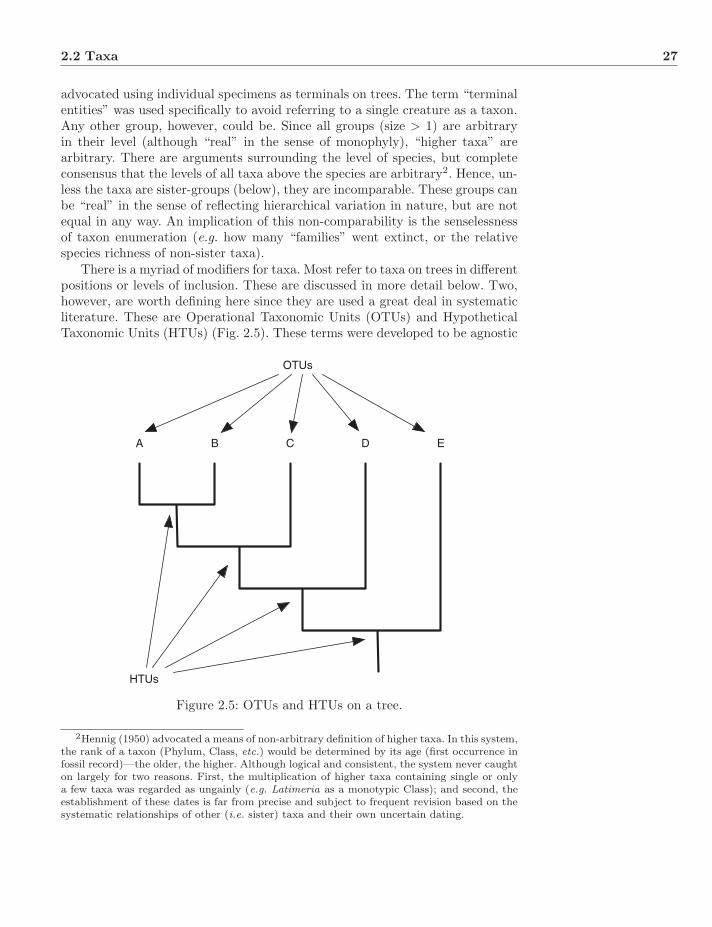
2.2 Taxa 27
advocated using individual specimens as terminals on trees. The term “terminalentities” was used specifically to avoid referring to a single creature as a taxon.Any other group, however, could be. Since all groups (size > 1) are arbitraryin their level (although “real” in the sense of monophyly), “higher taxa” arearbitrary. There are arguments surrounding the level of species, but completeconsensus that the levels of all taxa above the species are arbitrary2. Hence, un-less the taxa are sister-groups (below), they are incomparable. These groups canbe “real” in the sense of reflecting hierarchical variation in nature, but are notequal in any way. An implication of this non-comparability is the senselessnessof taxon enumeration (e.g. how many “families” went extinct, or the relativespecies richness of non-sister taxa).
There is a myriad of modifiers for taxa. Most refer to taxa on trees in differentpositions or levels of inclusion. These are discussed in more detail below. Two,however, are worth defining here since they are used a great deal in systematicliterature. These are Operational Taxonomic Units (OTUs) and HypotheticalTaxonomic Units (HTUs) (Fig. 2.5). These terms were developed to be agnostic
A B C D E
OTUs
HTUs
Figure 2.5: OTUs and HTUs on a tree.
2Hennig (1950) advocated a means of non-arbitrary definition of higher taxa. In this system,the rank of a taxon (Phylum, Class, etc.) would be determined by its age (first occurrence infossil record)—the older, the higher. Although logical and consistent, the system never caughton largely for two reasons. First, the multiplication of higher taxa containing single or onlya few taxa was regarded as ungainly (e.g. Latimeria as a monotypic Class); and second, theestablishment of these dates is far from precise and subject to frequent revision based on thesystematic relationships of other (i.e. sister) taxa and their own uncertain dating.
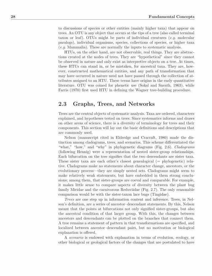
28 Fundamental Concepts
to discussions of species or other entities (mainly higher taxa) that appear ontrees. An OTU is any object that occurs at the tips of a tree (also called terminaltaxon or leaf). OTUs might be parts of individual creatures (e.g. molecularparalogs), individual organisms, species, collections of species, or higher taxa(e.g. Mammalia). These are normally the inputs to systematic analysis.
HTUs, on the other hand, are not observable, real things. They are abstrac-tions created at the nodes of trees. They are “hypothetical” since they cannotbe observed in nature and only exist as interpretive objects on a tree. At times,these HTUs can stand in, or be mistaken, for ancestral taxa. They are, how-ever, constructed mathematical entities, and any path of transformation thatmay have occurred in nature need not have passed through the collection of at-tributes assigned to an HTU. These terms have origins in the early quantitativeliterature. OTU was coined for phenetic use (Sokal and Sneath, 1963), whileFarris (1970) first used HTU in defining the Wagner tree-building procedure.
2.3 Graphs, Trees, and Networks
Trees are the central objects of systematic analysis. Taxa are ordered, charactersexplained, and hypotheses tested on trees. Since systematics informs and drawson other areas of science, there is a diversity of terminology for trees and theircomponents. This section will lay out the basic definitions and descriptions thatare commonly used.
Nelson (manuscript cited in Eldredge and Cracraft, 1980) made the dis-tinction among cladograms, trees, and scenarios. This scheme differentiated the“what,” “how,” and “why” in phylogenetic diagrams (Fig. 2.6). Cladograms(following Hennig) were a representation of nested sister-group relationships.Each bifurcation on the tree signifies that the two descendants are sister taxa.These sister taxa are each other’s closest genealogical (= phylogenetic) rela-tive. Cladograms make no statements about character change, ancestors, or theevolutionary process—they are simply nested sets. Cladograms might seem tomake relatively weak statements, but have embedded in them strong conclu-sions; among them, that sister-groups are coeval and comparable. For example,it makes little sense to compare aspects of diversity between the plant bugfamily Miridae and the carnivorous Reduviidae (Fig. 2.7). The only reasonablecomparison would be with the sister-taxon lace bugs (Tingidae).
Trees are one step up in information content and inference. Trees, in Nel-son’s definition, are a series of ancestor–descendant statements. By this, Nelsonmeant that the points at bifurcations not only signified sister-groups, but alsothe ancestral condition of that larger group. With this, the changes betweenancestors and descendants can be plotted on the branches that connect them.A tree remains a statement of pattern in that transformations are specified, andlocalized between ancestor–descendant pairs, but no motivation or biologicalexplanation is offered.
A scenario is endowed with explanation in terms of evolution, ecology, orother biological or geological factors of the changes that are postulated to have
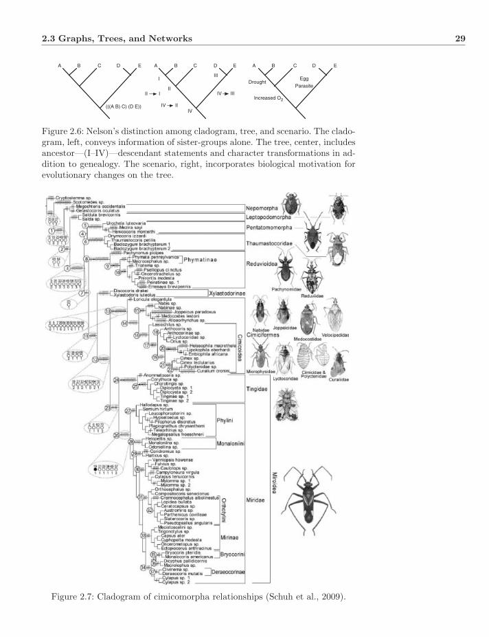
2.3 Graphs, Trees, and Networks 29
A B C D E A B C D E A B C D E
(((A B) C) (D E))
I
II
III
IV
Drought
Increased O
Egg
Parasite
IV II
IV IIIII I
Figure 2.6: Nelson’s distinction among cladogram, tree, and scenario. The clado-gram, left, conveys information of sister-groups alone. The tree, center, includesancestor—(I–IV)—descendant statements and character transformations in ad-dition to genealogy. The scenario, right, incorporates biological motivation forevolutionary changes on the tree.
Figure 2.7: Cladogram of cimicomorpha relationships (Schuh et al., 2009).

30 Fundamental Concepts
occurred on the branches. In general, classifications deal with cladograms, sys-tematics with trees, and evolutionary biology with scenarios.
2.3.1 Graphs and Trees
The mathematics and computer science literature defines trees in a mannernearly identical to that of Nelson, though in different terms. This field definesa tree as a connected, acyclic graph.Sometimes called a free tree.
Graphs
Graphs are general mathematical objects consisting of a pair of sets (V,E) ofvertices (points, V) and edges (lines between vertices, E). The edges can containloops, and two vertices may be connected by multiple edges (Fig. 2.8), or bynone. Simple graphs forbid parallel edges and loops. These are the sorts of graphswe will deal with here. By convention, edges are referred to by their incidentvertices [(u, v)∀eu,v ∈ E]. The degree of a vertex is the number of edges incidentupon it. In Fig. 2.8, vertex v1 has degree 2. Directed graphs can specify in-degreeand out-degree edges, their sum being the degree. Vertex v3 (Fig. 2.8 left) hasin-degree 1 and out-degree 2. It is possible to have a vertex that is unconnectedto any other vertex, hence with degree 0. A graph is said to be connected ifthere are no vertices with degree 0, that is, if all vertices can be be visited by apath over edges. A directed graph can be created from an undirected graph byspecifying an orientation to the edges. In systematics, the root (the only vertexwith degree 2) directs all edges.
v1 v2
v3 v4
v5
v1 v2
v3 v4
v5
v6v6
e1,2
e1,3
e3,4
e'3,4
e1,2
e1,3
e3,4
e2,5
e4,5
e5,5
e2,4 e2,4
e2,5
e4,5
e5,6
Figure 2.8: Graphs on vertex set V = {v1, . . . , v6} and edge set E. On the left,is a directed (digraph) including parallel edges between v3 and v4 (e3,4, e
′3,4), a
self loop edge on v5 (e5,5), and v6 is unconnected. On the right, is an undirected,simple graph.
Trees
A tree T = (V,E) is a connected graph without cycles. A cycle is a path overedges connecting two vertices via one or more additional vertices where each in-termediate edge is visited exactly once. In Fig. 2.8, the set of vertices v1, v2, v3, v4
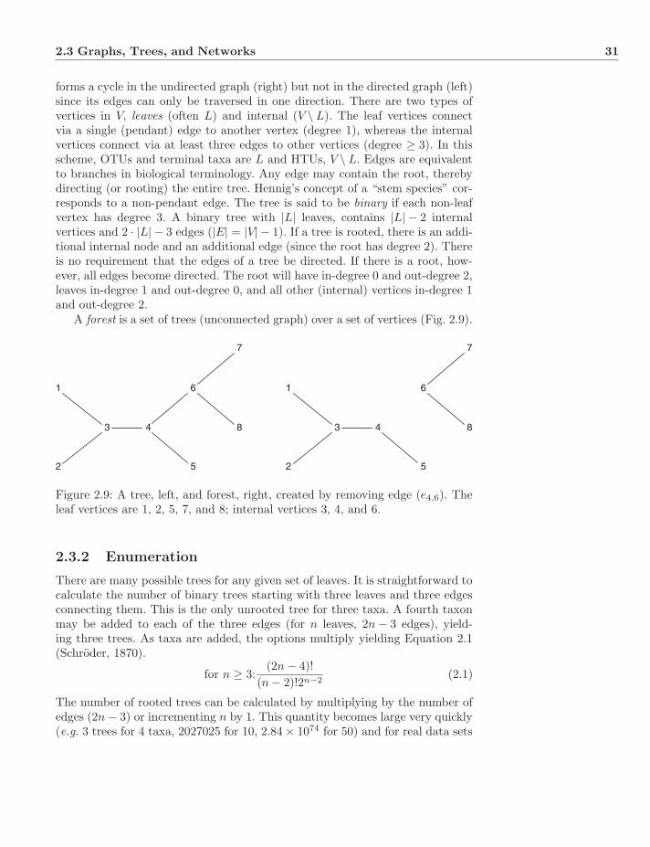
2.3 Graphs, Trees, and Networks 31
forms a cycle in the undirected graph (right) but not in the directed graph (left)since its edges can only be traversed in one direction. There are two types ofvertices in V, leaves (often L) and internal (V \ L). The leaf vertices connectvia a single (pendant) edge to another vertex (degree 1), whereas the internalvertices connect via at least three edges to other vertices (degree ≥ 3). In thisscheme, OTUs and terminal taxa are L and HTUs, V \ L. Edges are equivalentto branches in biological terminology. Any edge may contain the root, therebydirecting (or rooting) the entire tree. Hennig’s concept of a “stem species” cor-responds to a non-pendant edge. The tree is said to be binary if each non-leafvertex has degree 3. A binary tree with |L| leaves, contains |L| − 2 internalvertices and 2 · |L| − 3 edges (|E| = |V| − 1). If a tree is rooted, there is an addi-tional internal node and an additional edge (since the root has degree 2). Thereis no requirement that the edges of a tree be directed. If there is a root, how-ever, all edges become directed. The root will have in-degree 0 and out-degree 2,leaves in-degree 1 and out-degree 0, and all other (internal) vertices in-degree 1and out-degree 2.
A forest is a set of trees (unconnected graph) over a set of vertices (Fig. 2.9).
1
2
3 4
5
6
7
8
1
2
3 4
5
6
7
8
Figure 2.9: A tree, left, and forest, right, created by removing edge (e4,6). Theleaf vertices are 1, 2, 5, 7, and 8; internal vertices 3, 4, and 6.
2.3.2 Enumeration
There are many possible trees for any given set of leaves. It is straightforward tocalculate the number of binary trees starting with three leaves and three edgesconnecting them. This is the only unrooted tree for three taxa. A fourth taxonmay be added to each of the three edges (for n leaves, 2n − 3 edges), yield-ing three trees. As taxa are added, the options multiply yielding Equation 2.1(Schroder, 1870).
for n ≥ 3:(2n − 4)!
(n − 2)!2n−2(2.1)
The number of rooted trees can be calculated by multiplying by the number ofedges (2n − 3) or incrementing n by 1. This quantity becomes large very quickly(e.g. 3 trees for 4 taxa, 2027025 for 10, 2.84 × 1074 for 50) and for real data sets
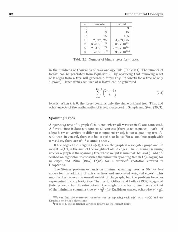
32 Fundamental Concepts
n unrooted rooted3 1 34 3 155 15 105
10 2,027,025 34,459,42520 8.20 × 10²¹ 3.03 × 10²³
50 2.84 × 1074 2.75 × 1076
100 1.70 × 10182 3.35 × 10184
Table 2.1: Number of binary trees for n taxa.
in the hundreds or thousands of taxa analogy fails (Table 2.1). The number offorests can be generated from Equation 2.1 by observing that removing a setof k edges from a tree will generate a forest (e.g. 32 forests for a tree of only4 leaves). Hence from each tree of n leaves can be generated
2n−3∑k=0
(2n − 3
k
)(2.2)
forests. When k is 0, the forest contains only the single original tree. This, andother aspects of the mathematics of trees, is explored in Semple and Steel (2003).
Spanning Trees
A spanning tree of a graph G is a tree where all vertices in G are connected.A forest, since it does not connect all vertices (there is no sequence—path—ofedges between vertices in different component trees), is not a spanning tree. Aswith trees in general, there can be no cycles or loops. For a complete graph withn vertices, there are nn−2 spanning trees.
If the edges have weights (w(e)), then the graph is a weighted graph and itsweight, w(G), is the sum of the weights of all its edges. The minimum spanningtree for a graph is the spanning tree whose weight is minimal. Kruskal (1956) de-scribed an algorithm to construct the minimum spanning tree in O(m log m) form edges and Prim (1957) O(n2) for n vertices3 (notation covered inChapter 5).
The Steiner problem expands on minimal spanning trees. A Steiner treeallows for the addition of extra vertices and associated weighted edges4. Thismay further reduce the overall weight of the graph, but the problem becomesexponential in complexity (see Chapter 5). Gilbert and Pollak (1968) suggested(later proved) that the ratio between the weight of the best Steiner tree and thatof the minimum spanning tree ρ ≥
√3
2 (for Euclidean spaces, otherwise ρ ≥ 12 ).
3We can find the maximum spanning tree by replacing each w(e) with −w(e) and useKruskal’s or Prim’s algorithms.
4For n = 3, the additional vertex is known as the Fermat point.
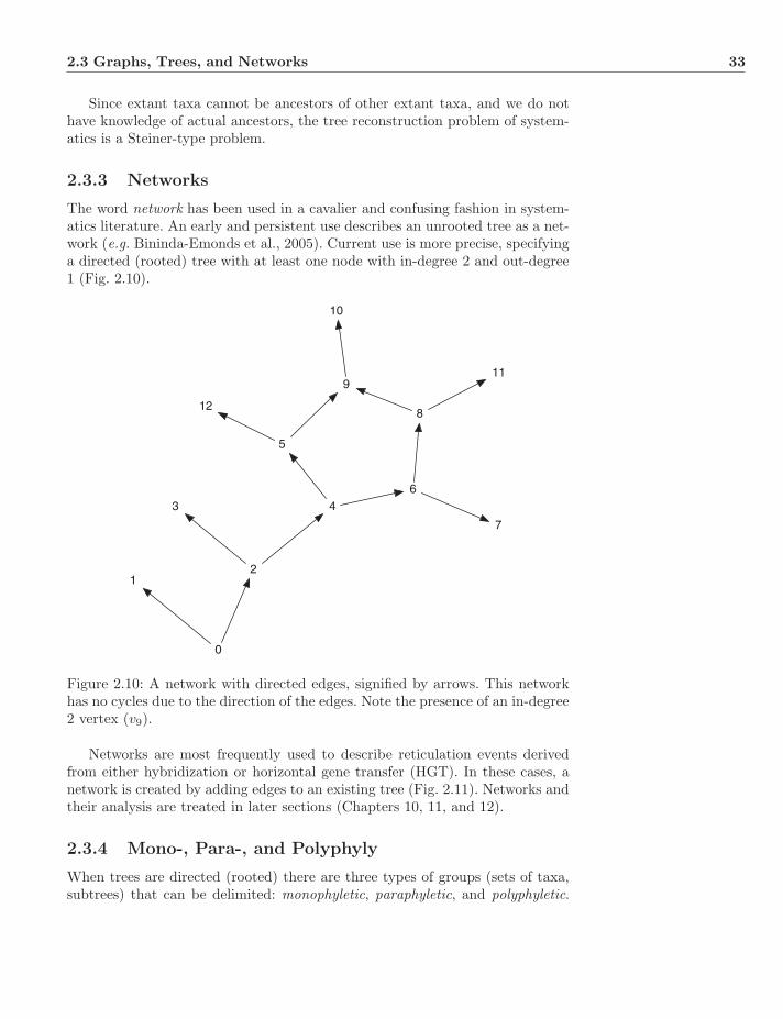
2.3 Graphs, Trees, and Networks 33
Since extant taxa cannot be ancestors of other extant taxa, and we do nothave knowledge of actual ancestors, the tree reconstruction problem of system-atics is a Steiner-type problem.
2.3.3 Networks
The word network has been used in a cavalier and confusing fashion in system-atics literature. An early and persistent use describes an unrooted tree as a net-work (e.g. Bininda-Emonds et al., 2005). Current use is more precise, specifyinga directed (rooted) tree with at least one node with in-degree 2 and out-degree1 (Fig. 2.10).
3
0
2
4
5
6
7
8
1
9
10
11
12
Figure 2.10: A network with directed edges, signified by arrows. This networkhas no cycles due to the direction of the edges. Note the presence of an in-degree2 vertex (v9).
Networks are most frequently used to describe reticulation events derivedfrom either hybridization or horizontal gene transfer (HGT). In these cases, anetwork is created by adding edges to an existing tree (Fig. 2.11). Networks andtheir analysis are treated in later sections (Chapters 10, 11, and 12).
2.3.4 Mono-, Para-, and Polyphyly
When trees are directed (rooted) there are three types of groups (sets of taxa,subtrees) that can be delimited: monophyletic, paraphyletic, and polyphyletic.
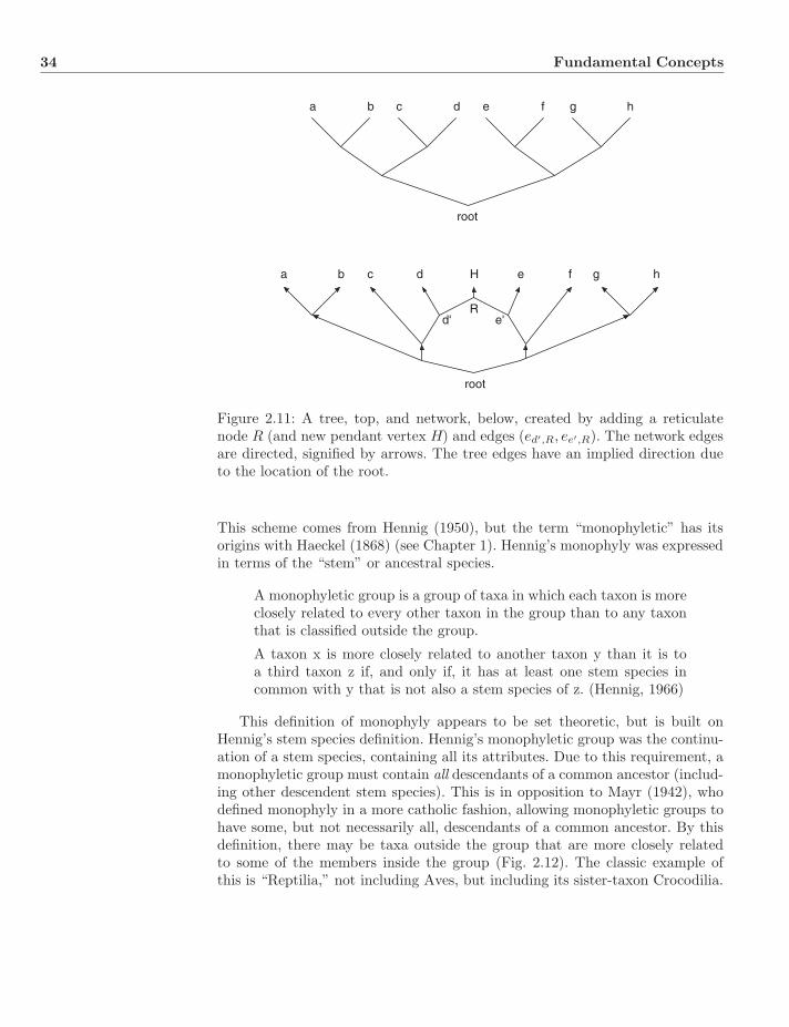
34 Fundamental Concepts
a b c d e f g h
root
a b c d e f g h
R
root
H
d' e'
Figure 2.11: A tree, top, and network, below, created by adding a reticulatenode R (and new pendant vertex H) and edges (ed′,R, ee′,R). The network edgesare directed, signified by arrows. The tree edges have an implied direction dueto the location of the root.
This scheme comes from Hennig (1950), but the term “monophyletic” has itsorigins with Haeckel (1868) (see Chapter 1). Hennig’s monophyly was expressedin terms of the “stem” or ancestral species.
A monophyletic group is a group of taxa in which each taxon is moreclosely related to every other taxon in the group than to any taxonthat is classified outside the group.
A taxon x is more closely related to another taxon y than it is toa third taxon z if, and only if, it has at least one stem species incommon with y that is not also a stem species of z. (Hennig, 1966)
This definition of monophyly appears to be set theoretic, but is built onHennig’s stem species definition. Hennig’s monophyletic group was the continu-ation of a stem species, containing all its attributes. Due to this requirement, amonophyletic group must contain all descendants of a common ancestor (includ-ing other descendent stem species). This is in opposition to Mayr (1942), whodefined monophyly in a more catholic fashion, allowing monophyletic groups tohave some, but not necessarily all, descendants of a common ancestor. By thisdefinition, there may be taxa outside the group that are more closely relatedto some of the members inside the group (Fig. 2.12). The classic example ofthis is “Reptilia,” not including Aves, but including its sister-taxon Crocodilia.
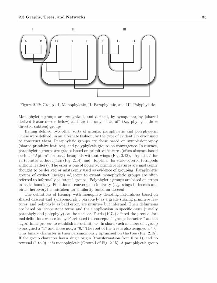
2.3 Graphs, Trees, and Networks 35
A B C D E F G H I
I II III
Figure 2.12: Groups. I. Monophyletic, II. Paraphyletic, and III. Polyphyletic.
Monophyletic groups are recognized, and defined, by synapomorphy (sharedderived features—see below) and are the only “natural” (i.e. phylogenetic =directed subtree) groups.
Hennig defined two other sorts of groups: paraphyletic and polyphyletic.These were defined, in an alternate fashion, by the type of evidentiary error usedto construct them. Paraphyletic groups are those based on symplesiomorphy(shared primitive features), and polyphyletic groups on convergence. In essence,paraphyletic groups are grades based on primitive features (often absence-basedsuch as “Aptera” for basal hexapods without wings (Fig. 2.13), “Agnatha” forvertebrates without jaws (Fig. 2.14), and “Reptilia” for scale-covered tetrapodswithout feathers). The error is one of polarity; primitive features are mistakenlythought to be derived or mistakenly used as evidence of grouping. Paraphyleticgroups of extinct lineages adjacent to extant monophyletic groups are oftenreferred to informally as “stem” groups. Polyphyletic groups are based on errorsin basic homology. Functional, convergent similarity (e.g. wings in insects andbirds, herbivory) is mistaken for similarity based on descent.
The definitions of Hennig, with monophyly denoting naturalness based onshared descent and synapomorphy, paraphyly as a grade sharing primitive fea-tures, and polyphyly as bald error, are intuitive but informal. Their definitionsare based on inconsistent terms and their application in specific cases (usuallyparaphyly and polyphyly) can be unclear. Farris (1974) offered the precise, for-mal definitions we use today. Farris used the concept of “group characters” and analgorithmic process to establish his definitions. In short, each member of a groupis assigned a “1” and those not, a “0.” The root of the tree is also assigned a “0.”This binary character is then parsimoniously optimized on the tree (Fig. 2.15).If the group character has a single origin (transformation from 0 to 1), and noreversal (1 to 0), it is monophyletic (Group I of Fig. 2.15). A paraphlyetic group
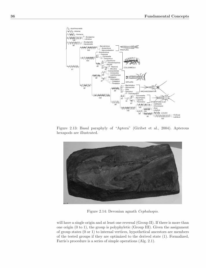
36 Fundamental Concepts
Hutchinsoniella
Artemia
Homarus
ScutigerinaLithobius
ScutigerellaHanseniella
AcerentulusNeocondeellum
Baculentulus
Xenylla
OnychiurusTetrodontophora
NeanuraMorulina
OrchesellaFolsomia
Tomocerus
Sminthurinus
CampodeidaeCampodeaLepidocampa
Catajapyx
MetajapyxHeterojapyx
Parajapyx
DiltaPetrobius
MachiloidesAllomachilis
Tricholepidion
LepismaThermobia
TexoredelliaSquamigera
CallibaetisChoroterpesAnaxLibellula
ForficulaLabidura
Locusta
61
100
100
63
93
60
6082
92
99
89
97
100
99
99
52
63
60
7587
87
100
100
100
100
95
69
100
96
PROTURA
COLLEMBOLA
DIPLURA
ARCHAEOGNATHA
ZYGENTOMA S.S.
Figure 2.13: Basal paraphyly of “Aptera” (Giribet et al., 2004). Apteroushexapods are illustrated.
Figure 2.14: Devonian agnath Cephalaspis.
will have a single origin and at least one reversal (Group II). If there is more thanone origin (0 to 1), the group is polyphyletic (Group III). Given the assignmentof group states (0 or 1) to internal vertices, hypothetical ancestors are membersof the tested groups if they are optimized to the derived state (1). Formalized,Farris’s procedure is a series of simple operations (Alg. 2.1).
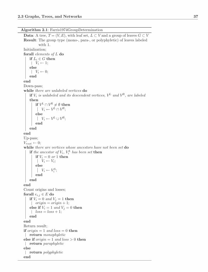
2.3 Graphs, Trees, and Networks 37
Algorithm 2.1: Farris1974GroupDeterminationData: A tree, T = (V,E), with leaf set, L ⊂ V and a group of leaves G ⊂ VResult: The group type (mono-, para-, or polyphyletic) of leaves labeled
with 1.Initialization;forall elements of L do
if Li ∈ G thenVi ← 1;
elseVi ← 0;
endendDown-pass;while there are unlabeled vertices do
if Vi is unlabeled and its descendent vertices, VL and VR, are labeledthen
if VL ∩ VR �= ∅ thenVi ← VL ∩ VR;
elseVi ← VL ∪ VR;
endend
endUp-pass;Vroot ← 0;while there are vertices whose ancestors have not been set do
if the ancestor of Vi, VAi has been set then
if Vi = 0 or 1 thenVi ← Vi;
elseVi ← VA
i ;end
endendCount origins and losses;forall ei,j ∈ E do
if Vi = 0 and Vj = 1 thenorigin = origin + 1;
else if Vi = 1 and Vj = 0 thenloss = loss + 1;
endendReturn result;if origin = 1 and loss = 0 then
return monophyleticelse if origin = 1 and loss > 0 then
return paraphyleticelse
return polyphyleticend
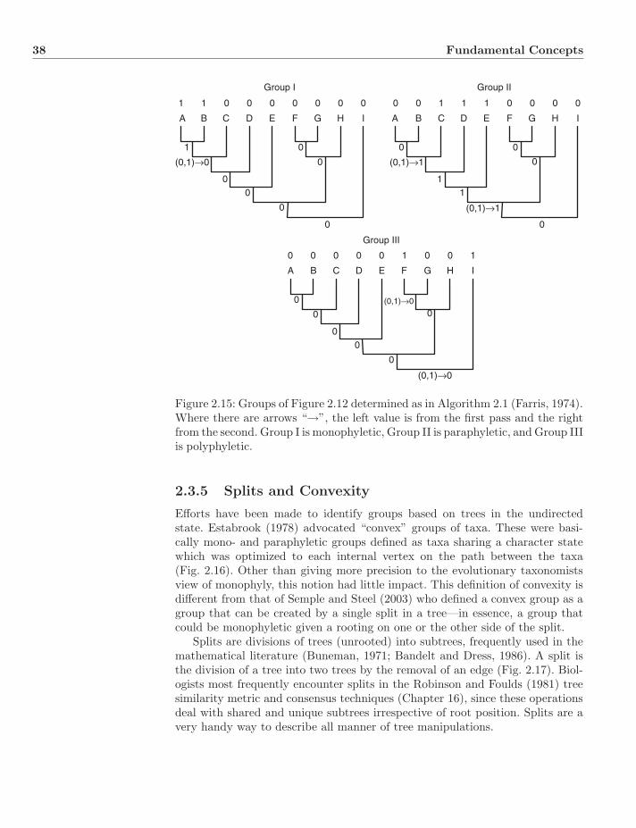
38 Fundamental Concepts
A B C D E F G H I
Group I
1 1 0 0 0 0 0 0 0
1
(0,1)→0
00
0
0
0
0
A B C D E F G H I
Group II
0 0 1 1 1 0 0 0 0
0
11
0
0
0
A B C D E F G H I
Group III
0 0 0 0 0 1 0 0 1
0
0
00
0
0(0,1)→0
(0,1)→1
(0,1)→1
(0,1)→0
Figure 2.15: Groups of Figure 2.12 determined as in Algorithm 2.1 (Farris, 1974).Where there are arrows “→”, the left value is from the first pass and the rightfrom the second. Group I is monophyletic, Group II is paraphyletic, and Group IIIis polyphyletic.
2.3.5 Splits and Convexity
Efforts have been made to identify groups based on trees in the undirectedstate. Estabrook (1978) advocated “convex” groups of taxa. These were basi-cally mono- and paraphyletic groups defined as taxa sharing a character statewhich was optimized to each internal vertex on the path between the taxa(Fig. 2.16). Other than giving more precision to the evolutionary taxonomistsview of monophyly, this notion had little impact. This definition of convexity isdifferent from that of Semple and Steel (2003) who defined a convex group as agroup that can be created by a single split in a tree—in essence, a group thatcould be monophyletic given a rooting on one or the other side of the split.
Splits are divisions of trees (unrooted) into subtrees, frequently used in themathematical literature (Buneman, 1971; Bandelt and Dress, 1986). A split isthe division of a tree into two trees by the removal of an edge (Fig. 2.17). Biol-ogists most frequently encounter splits in the Robinson and Foulds (1981) treesimilarity metric and consensus techniques (Chapter 16), since these operationsdeal with shared and unique subtrees irrespective of root position. Splits are avery handy way to describe all manner of tree manipulations.
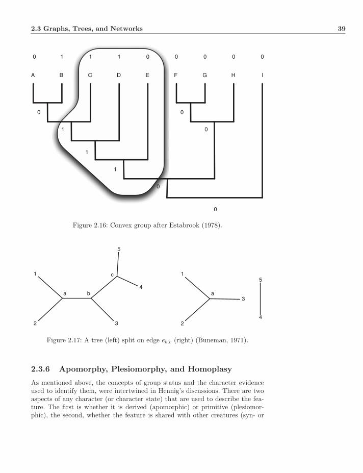
2.3 Graphs, Trees, and Networks 39
A B C D E F G H I
0 1 1 1 0 0 0 0 0
0
1
1
1
0
0
0
0
Figure 2.16: Convex group after Estabrook (1978).
1
2 3
5
4
1
2
3
5
4
a b
c
a
Figure 2.17: A tree (left) split on edge eb,c (right) (Buneman, 1971).
2.3.6 Apomorphy, Plesiomorphy, and Homoplasy
As mentioned above, the concepts of group status and the character evidenceused to identify them, were intertwined in Hennig’s discussions. There are twoaspects of any character (or character state) that are used to describe the fea-ture. The first is whether it is derived (apomorphic) or primitive (plesiomor-phic), the second, whether the feature is shared with other creatures (syn- or
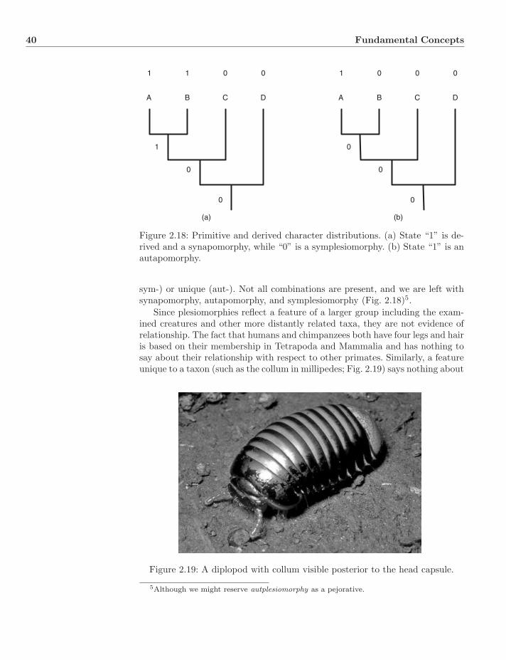
40 Fundamental Concepts
A B C D
1 1 0 0
1
0
0
A B C D
1 0 0 0
0
0
0
(a) (b)
Figure 2.18: Primitive and derived character distributions. (a) State “1” is de-rived and a synapomorphy, while “0” is a symplesiomorphy. (b) State “1” is anautapomorphy.
sym-) or unique (aut-). Not all combinations are present, and we are left withsynapomorphy, autapomorphy, and symplesiomorphy (Fig. 2.18)5.
Since plesiomorphies reflect a feature of a larger group including the exam-ined creatures and other more distantly related taxa, they are not evidence ofrelationship. The fact that humans and chimpanzees both have four legs and hairis based on their membership in Tetrapoda and Mammalia and has nothing tosay about their relationship with respect to other primates. Similarly, a featureunique to a taxon (such as the collum in millipedes; Fig. 2.19) says nothing about
Figure 2.19: A diplopod with collum visible posterior to the head capsule.
5Although we might reserve autplesiomorphy as a pejorative.
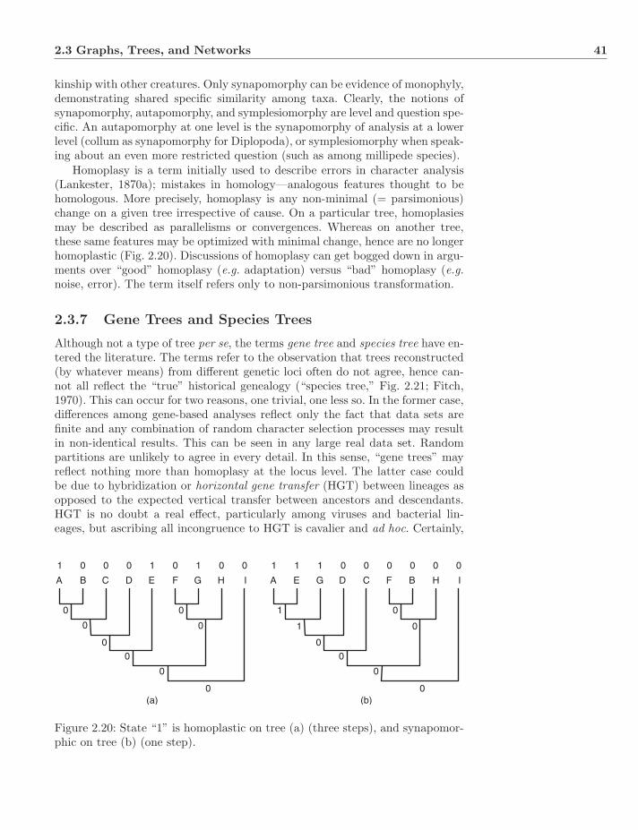
2.3 Graphs, Trees, and Networks 41
kinship with other creatures. Only synapomorphy can be evidence of monophyly,demonstrating shared specific similarity among taxa. Clearly, the notions ofsynapomorphy, autapomorphy, and symplesiomorphy are level and question spe-cific. An autapomorphy at one level is the synapomorphy of analysis at a lowerlevel (collum as synapomorphy for Diplopoda), or symplesiomorphy when speak-ing about an even more restricted question (such as among millipede species).
Homoplasy is a term initially used to describe errors in character analysis(Lankester, 1870a); mistakes in homology—analogous features thought to behomologous. More precisely, homoplasy is any non-minimal (= parsimonious)change on a given tree irrespective of cause. On a particular tree, homoplasiesmay be described as parallelisms or convergences. Whereas on another tree,these same features may be optimized with minimal change, hence are no longerhomoplastic (Fig. 2.20). Discussions of homoplasy can get bogged down in argu-ments over “good” homoplasy (e.g. adaptation) versus “bad” homoplasy (e.g.noise, error). The term itself refers only to non-parsimonious transformation.
2.3.7 Gene Trees and Species Trees
Although not a type of tree per se, the terms gene tree and species tree have en-tered the literature. The terms refer to the observation that trees reconstructed(by whatever means) from different genetic loci often do not agree, hence can-not all reflect the “true” historical genealogy (“species tree,” Fig. 2.21; Fitch,1970). This can occur for two reasons, one trivial, one less so. In the former case,differences among gene-based analyses reflect only the fact that data sets arefinite and any combination of random character selection processes may resultin non-identical results. This can be seen in any large real data set. Randompartitions are unlikely to agree in every detail. In this sense, “gene trees” mayreflect nothing more than homoplasy at the locus level. The latter case couldbe due to hybridization or horizontal gene transfer (HGT) between lineages asopposed to the expected vertical transfer between ancestors and descendants.HGT is no doubt a real effect, particularly among viruses and bacterial lin-eages, but ascribing all incongruence to HGT is cavalier and ad hoc. Certainly,
A B C D E F G H I
1 0 0 0 1 0 1 0 0
0
0
0
0
0
0
0
0
A E G D C F B H I
1 1 1 0 0 0 0 0 0
1
1
0
0
0
0
0
0
(a) (b)
Figure 2.20: State “1” is homoplastic on tree (a) (three steps), and synapomor-phic on tree (b) (one step).
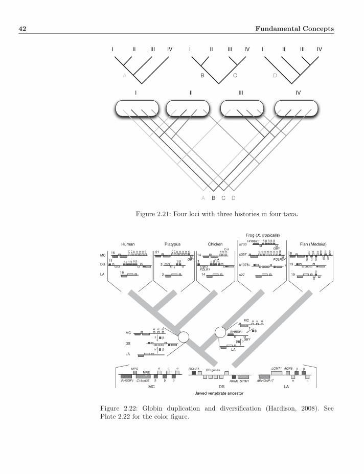
42 Fundamental Concepts
I II III IV
I II III IVI II III IV I II III IV
A B C D
B CA D
Figure 2.21: Four loci with three histories in four taxa.
ARHGAP17
AQP8LCMT1
RRM1 STIM1
DCHS1 OR genes
RHBDF1
MPG
C16orf35
MRE
MC DS LA
Jawed vertebrate ancestor
ζ ζ μ α α α θ ζ ζ μ α α α ω π α α
β β β β β
α α α β
β β β α α
α
β
β βα α α α α α α β
ε γ γ η δ β β β
α α α
β
β
α α α
β β β
β
β β
α α
β
α α α
ρ β β εGBY
D A
H A
FOLR1?
?
MC
DS
LA
Human Platypus Chicken
Frog (X. tropicalis)
Fish (Medaka)
16
11
162
2
2114 s357
s1078+
s27
RHBDF1
GBYs733
1
14
8
13
19
MC
DS
LA?
?
MC
RHBDF1
GBY?
LA
?
POLR3K
Figure 2.22: Globin duplication and diversification (Hardison, 2008). SeePlate 2.22 for the color figure.
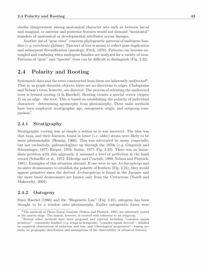
2.4 Polarity and Rooting 43
similar disagreement among anatomical character sets such as between larvaland imaginal, or anterior and posterior features would not demand “horizontal”transfers of anatomical or developmental attributes across lineages.
Another use of “gene trees” concerns phylogenetic patterns of multigene fam-ilies (e.g. vertebrate globins). This sort of tree is meant to reflect gene duplicationand subsequent diversification (paralogy; Fitch, 1970). Patterns can become en-tangled and confusing when multigene families are analyzed for a variety of taxa.Patterns of “gene” and “species” trees can be difficult to distinguish (Fig. 2.22).
2.4 Polarity and Rooting
Systematic data and the trees constructed from them are inherently undirected6.That is, as graph theoretic objects, there are no directions to edges. Cladogramsand Nelson’s trees, however, are directed. The process of orienting the undirectedtrees is termed rooting (a la Haeckel). Rooting creates a special vertex (degree2) on an edge—the root. This is based on establishing the polarity of individualcharacters—determining apomorphy from plesiomorphy. Three main methodshave been employed: stratigraphic age, ontogenetic origin, and outgroup com-parison7.
2.4.1 Stratigraphy
Stratigraphic rooting was as simple a notion as it was incorrect. The idea wasthat taxa, and their features, found in lower (i.e. older) strata were likely to bemore plesiomorphic (Hennig, 1966). This was advocated by many (especially,but not exclusively, paleontologists) up through the 1970s (e.g. Gingerich andSchoeninger, 1977; Harper, 1976; Szalay, 1977; Fig. 2.23). There was an imme-diate problem with this approach: it assumed a level of perfection in the fossilrecord (Schaeffer et al., 1972; Eldredge and Cracraft, 1980; Nelson and Platnick,1981). Examples of this situation abound. If one were to use Archaeopteryx andits sister dromeosaurs to establish the polarity of feathers (Fig. 2.24), they wouldappear primitive since the derived Archaeopteryx is found in the Jurassic andthe more basal dromeosaurs are known only from the Cretaceous (Norell andMakovicky, 2004).
2.4.2 Ontogeny
Since Haeckel (1866) and the “Biogenetic Law” (Fig. 2.25), ontogeny has beenthought to be a window onto plesiomorphy. Earlier ontogenetic forms were
6The methods of Three-Taxon Analysis (Nelson and Platnick, 1991) are inherently rootedat the matrix stage. The matrix, however, is created with reference to an outgroup.
7Several other methods have been proposed and rejected including “common equalsprimitive”—repeatedly falsified (e.g. wings in hexapods), “complex equals derived”—falsifiedby empirical observations of reduction and loss, and “chorological progression”—basing po-larity on geographic distribution and assumptions of the observability of advanced features.
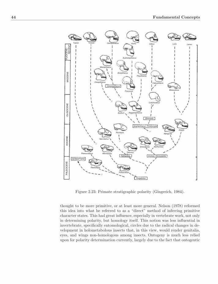
44 Fundamental Concepts
Tupoio
PLI
OC
EN
E-
MIO
CE
NE
OLI
GO
CE
NE
EO
CE
NE
PA
LEO
CE
NE
RE
CE
NT
Mesopithecus
Austrolopithecus
Oreopithecus
Victoriopithecus
Proconsul
Pliopithecus
Cebupithecio
Mioeuoticus
Colichocebus
Apidium Aegyptopithecus
Branisella
Mahgorita
NorthorctusSmilodecies
Tetonius
Teilhardina Contius / DonrusselliaMicrosyops
Necrolemur
Phenocoiemur
DERMOPTERA
Plesiodopis
Poloecnthon
Purgatorius
??
Rooneyia
?
?
?
?
Adopis
Amphipithecus / Pondoungia
?
?
Sivopithecus
Torsius Cercopithecus Homo Cebus Loris Lemur
Figure 2.23: Primate stratigraphic polarity (Gingerich, 1984).
thought to be more primitive, or at least more general. Nelson (1978) reformedthis idea into what he referred to as a “direct” method of inferring primitivecharacter states. This had great influence, especially in vertebrate work, not onlyin determining polarity, but homology itself. This notion was less influential ininvertebrate, specifically entomological, circles due to the radical changes in de-velopment in holometabolous insects that, in this view, would render genitalia,eyes, and wings non-homologous among insects. Ontogeny is much less reliedupon for polarity determination currently, largely due to the fact that ontogentic
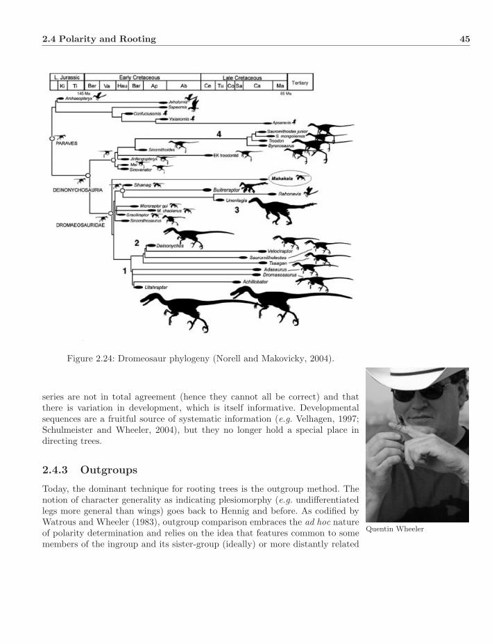
2.4 Polarity and Rooting 45
Figure 2.24: Dromeosaur phylogeny (Norell and Makovicky, 2004).
series are not in total agreement (hence they cannot all be correct) and thatthere is variation in development, which is itself informative. Developmentalsequences are a fruitful source of systematic information (e.g. Velhagen, 1997;Schulmeister and Wheeler, 2004), but they no longer hold a special place indirecting trees.
2.4.3 Outgroups
Quentin Wheeler
Today, the dominant technique for rooting trees is the outgroup method. Thenotion of character generality as indicating plesiomorphy (e.g. undifferentiatedlegs more general than wings) goes back to Hennig and before. As codified byWatrous and Wheeler (1983), outgroup comparison embraces the ad hoc natureof polarity determination and relies on the idea that features common to somemembers of the ingroup and its sister-group (ideally) or more distantly related
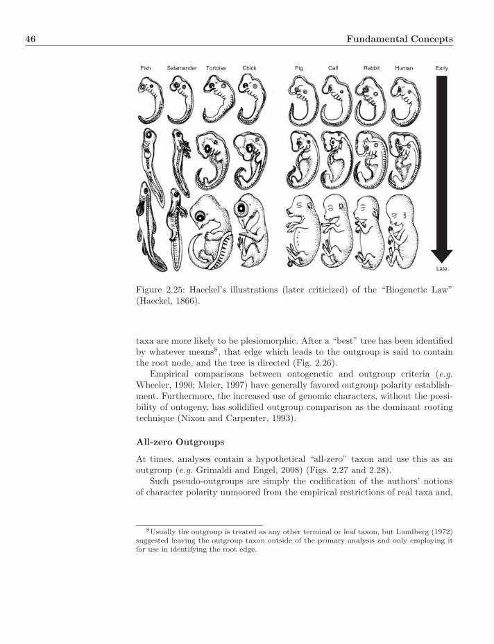
46 Fundamental Concepts
Fish Salamander Tortoise Chick Pig Calf Rabbit Human Early
Late
Figure 2.25: Haeckel’s illustrations (later criticized) of the “Biogenetic Law”(Haeckel, 1866).
taxa are more likely to be plesiomorphic. After a “best” tree has been identifiedby whatever means8, that edge which leads to the outgroup is said to containthe root node, and the tree is directed (Fig. 2.26).
Empirical comparisons between ontogenetic and outgroup criteria (e.g.Wheeler, 1990; Meier, 1997) have generally favored outgroup polarity establish-ment. Furthermore, the increased use of genomic characters, without the possi-bility of ontogeny, has solidified outgroup comparison as the dominant rootingtechnique (Nixon and Carpenter, 1993).
All-zero Outgroups
At times, analyses contain a hypothetical “all-zero” taxon and use this as anoutgroup (e.g. Grimaldi and Engel, 2008) (Figs. 2.27 and 2.28).
Such pseudo-outgroups are simply the codification of the authors’ notionsof character polarity unmoored from the empirical restrictions of real taxa and,
8Usually the outgroup is treated as any other terminal or leaf taxon, but Lundberg (1972)suggested leaving the outgroup taxon outside of the primary analysis and only employing itfor use in identifying the root edge.
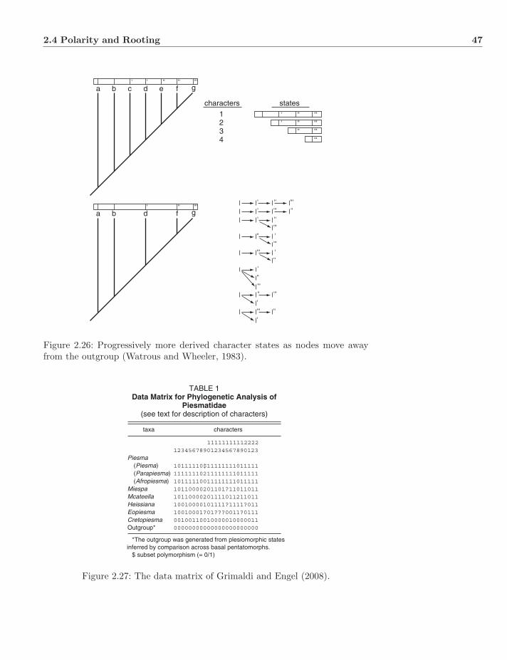
2.4 Polarity and Rooting 47
'
' '
' '' '''' '' '''
'' '' '''a b c d e
characters states1234
f g
a b d f g
'' '''
' '' ''''' '''
'''
' ''' ''
' '''''
'' ''''
''' '''
'
''
''''' '''
'
''' ''
'
Figure 2.26: Progressively more derived character states as nodes move awayfrom the outgroup (Watrous and Wheeler, 1983).
TABLE 1Data Matrix for Phylogenetic Analysis of
Piesmatidae(see text for description of characters)
taxa characters
1111111111222212345678901234567890123
Piesma(Piesma) 10111110$11111111011111(Parapiesma) 11111110211111111011111(Afropiesma) 10111110011111111011111
Miespa 10110000201101?11011011Mcateella 10110000201111011211011Heissiana 10010000101111?1111?011Eopiesma 10010001?01???0011?0111Cretopiesma 00100110010000010000011Outgroup* 00000000000000000000000
*The outgroup was generated from plesiomorphic statesinferred by comparison across basal pentatomorphs. $ subset polymorphism (= 0/1)
Figure 2.27: The data matrix of Grimaldi and Engel (2008).

48 Fundamental Concepts
Outgroup
10
111
1 4 11 12 13 14 17 19 20
1 1 1 1 1 1 1 1 1
13
018
2
3
0
18
1
5 6 7 10 15 21
0 0 0 0 0 0
2
1
8
1
16
0
21
1
76Cretopiesma
Miespa
Mcateella
Heissiana
Eopiesma
Piesma (Piesma)
Piesma (Parapiesma)
Piesma (Afropiesma)
Figure 2.28: Tree of Grimaldi and Engel (2008).
Figure 2.29: The placement of Cretopiesma (Grimaldi and Engel, 2008) based onan all-zero outgroup was revised into an entirely different family (Piesmatidaeto Aradidae) based on character analysis of actual outgroup taxa (Cassis andSchuh, 2009).
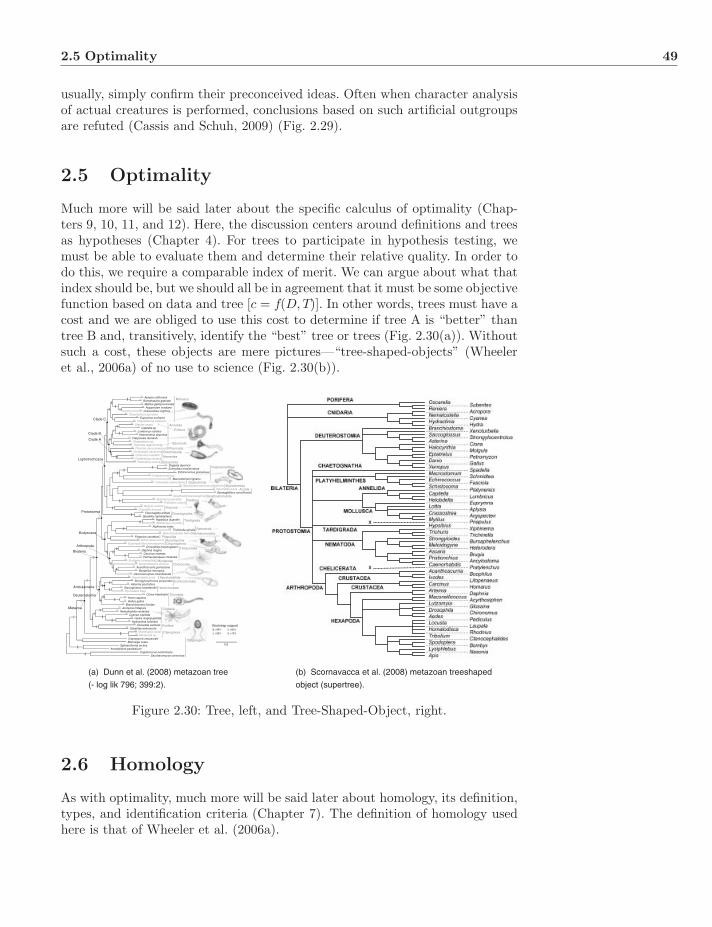
2.5 Optimality 49
usually, simply confirm their preconceived ideas. Often when character analysisof actual creatures is performed, conclusions based on such artificial outgroupsare refuted (Cassis and Schuh, 2009) (Fig. 2.29).
2.5 Optimality
Much more will be said later about the specific calculus of optimality (Chap-ters 9, 10, 11, and 12). Here, the discussion centers around definitions and treesas hypotheses (Chapter 4). For trees to participate in hypothesis testing, wemust be able to evaluate them and determine their relative quality. In order todo this, we require a comparable index of merit. We can argue about what thatindex should be, but we should all be in agreement that it must be some objectivefunction based on data and tree [c = f(D,T)]. In other words, trees must have acost and we are obliged to use this cost to determine if tree A is “better” thantree B and, transitively, identify the “best” tree or trees (Fig. 2.30(a)). Withoutsuch a cost, these objects are mere pictures—“tree-shaped-objects” (Wheeleret al., 2006a) of no use to science (Fig. 2.30(b)).
(a) Dunn et al. (2008) metazoan tree
(- log lik 796; 399:2).
(b) Scornavacca et al. (2008) metazoan treeshaped
object (supertree).
Figure 2.30: Tree, left, and Tree-Shaped-Object, right.
2.6 Homology
As with optimality, much more will be said later about homology, its definition,types, and identification criteria (Chapter 7). The definition of homology usedhere is that of Wheeler et al. (2006a).
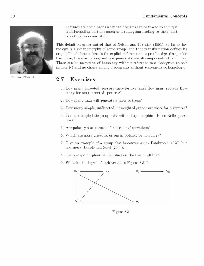
50 Fundamental Concepts
Features are homologous when their origins can be traced to a uniquetransformation on the branch of a cladogram leading to their mostrecent common ancestor.
This definition grows out of that of Nelson and Platnick (1981), so far as ho-mology is a synapomorphy of some group, and that transformation defines its
Norman Platnick
origin. The difference here is the explicit reference to a specific edge of a specifictree. Tree, transformation, and synapomorphy are all components of homology.There can be no notion of homology without reference to a cladogram (albeitimplicitly) and no choice among cladograms without statements of homology.
2.7 Exercises
1. How many unrooted trees are there for five taxa? How many rooted? Howmany forests (unrooted) per tree?
2. How many taxa will generate a mole of trees?
3. How many simple, undirected, unweighted graphs are there for n vertices?
4. Can a monophyletic group exist without apomorphies (Helen Keller para-dox)?
5. Are polarity statements inferences or observations?
6. Which are more grievous: errors in polarity or homology?
7. Give an example of a group that is convex sensu Estabrook (1978) butnot sensu Semple and Steel (2003).
8. Can synapomorphies be identified on the tree of all life?
9. What is the degree of each vertex in Figure 2.31?
V0 V2
V1 V3
V4 V5
Figure 2.31
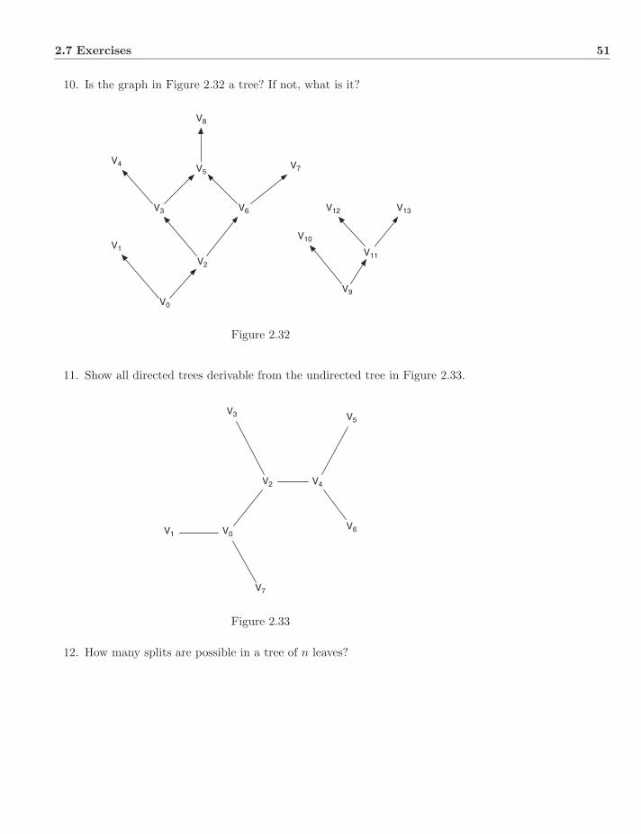
2.7 Exercises 51
10. Is the graph in Figure 2.32 a tree? If not, what is it?
V2
V6V3
V5V4
V8
V7
V1
V0
V13V12
V11
V9
V10
Figure 2.32
11. Show all directed trees derivable from the undirected tree in Figure 2.33.
V2 V4
V3 V5
V6V1 V0
V7
Figure 2.33
12. How many splits are possible in a tree of n leaves?

52 Fundamental Concepts
13. Using Farris’s (1974) procedure, what is the status of groups A, B, and Cin Figure 2.34?
A A A B B C CA
Figure 2.34
14. Contrast the statement “common equals primitive” with “broadly dis-tributed equals primitive.” Is either/both correct?
Chapter 3
Species Concepts,Definitions, and Issues
It is hard to imagine that a field as developed as systematics would have atits core such an unsettled and disputed concept as that of the species. Thereis an enormous literature and literally dozens of published concepts: biologi-cal, ecological, phylogenetic, monophyletic, evolutionary, Hennigian, internodal,taxonomic, and so on (Mayden, 1997; Lherminera and Solignac, 2000; Wilkins’list http://scienceblogs.com/evolvingthoughts/2006/10/a list of 26species concepts.php), many of which overlap in particulars, designed aroundspecific or general categories, patterns, processes, and observational inference1.In addition to definitional differences, the point has even been made that per-haps species are not “real”2 at all. The effects of these differences are not re-stricted to systematics alone. The definition, reality, and philosophical statusof species have an impact on all areas in the study of biological diversity. Howcan “species” distribution, origin and extinction, historical gain and loss of di-versity, even simple enumeration be accomplished without a consensual andconcrete definition?
Without going into every nuance, modern species concepts can be differen-tiated along lines of emphasis of pattern or process and the primacy of mono-phyly. In pre-evolutionary discussions, a typological (static, descriptive) view ofspecies was most often employed. The New Synthesis of the mid-20th centuryemphasized evolutionary coherence through interbreeding, yielding the Biolog-ical Species Concept. More recently, with the rise of cladistic thinking, explicitphylogenetic species concepts have been articulated, differing among themselveson the importance of monophyly and sex, and this has even led to a modern form
1To these we might add the political (designated by national boundaries) and financial (ifthere’s money in it) species concepts.
2Real in the sense of being a component of nature separate from human perception.
Systematics: A Course of Lectures, First Edition. Ward C. Wheeler.c© 2012 Ward C. Wheeler. Published 2012 by Blackwell Publishing Ltd.
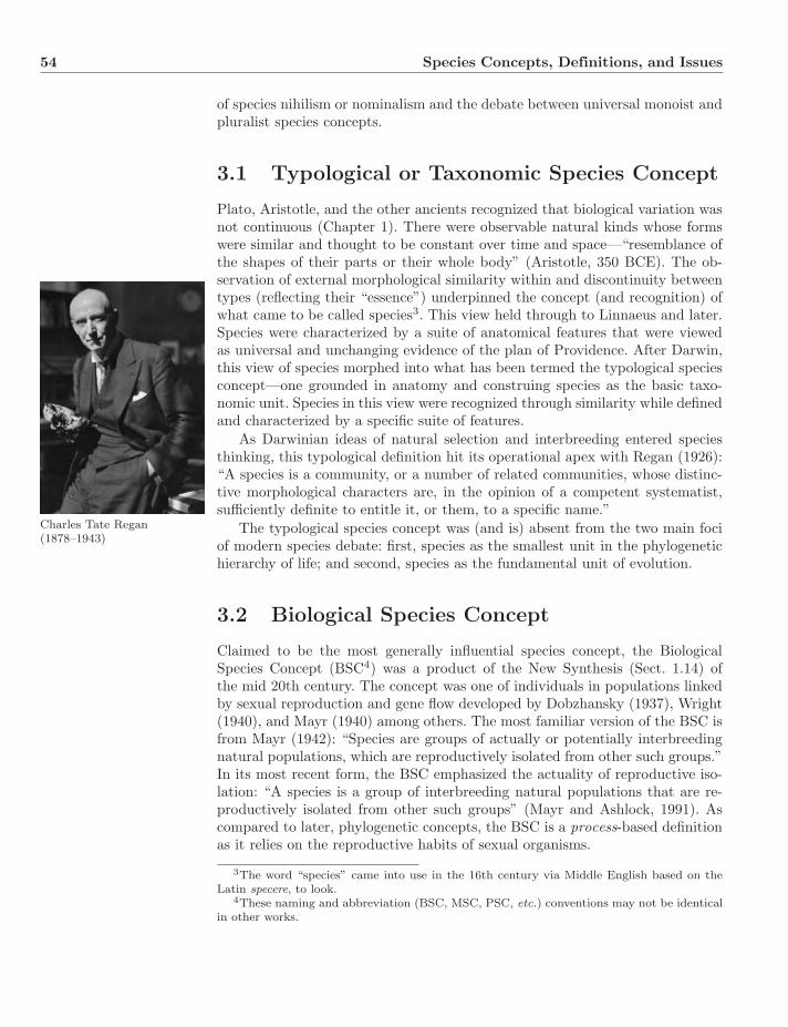
54 Species Concepts, Definitions, and Issues
of species nihilism or nominalism and the debate between universal monoist andpluralist species concepts.
3.1 Typological or Taxonomic Species Concept
Plato, Aristotle, and the other ancients recognized that biological variation wasnot continuous (Chapter 1). There were observable natural kinds whose formswere similar and thought to be constant over time and space—“resemblance ofthe shapes of their parts or their whole body” (Aristotle, 350 BCE). The ob-servation of external morphological similarity within and discontinuity betweentypes (reflecting their “essence”) underpinned the concept (and recognition) ofwhat came to be called species3. This view held through to Linnaeus and later.Species were characterized by a suite of anatomical features that were viewedas universal and unchanging evidence of the plan of Providence. After Darwin,this view of species morphed into what has been termed the typological speciesconcept—one grounded in anatomy and construing species as the basic taxo-nomic unit. Species in this view were recognized through similarity while definedand characterized by a specific suite of features.
As Darwinian ideas of natural selection and interbreeding entered speciesthinking, this typological definition hit its operational apex with Regan (1926):“A species is a community, or a number of related communities, whose distinc-tive morphological characters are, in the opinion of a competent systematist,sufficiently definite to entitle it, or them, to a specific name.”
Charles Tate Regan(1878–1943)
The typological species concept was (and is) absent from the two main fociof modern species debate: first, species as the smallest unit in the phylogenetichierarchy of life; and second, species as the fundamental unit of evolution.
3.2 Biological Species Concept
Claimed to be the most generally influential species concept, the BiologicalSpecies Concept (BSC4) was a product of the New Synthesis (Sect. 1.14) ofthe mid 20th century. The concept was one of individuals in populations linkedby sexual reproduction and gene flow developed by Dobzhansky (1937), Wright(1940), and Mayr (1940) among others. The most familiar version of the BSC isfrom Mayr (1942): “Species are groups of actually or potentially interbreedingnatural populations, which are reproductively isolated from other such groups.”In its most recent form, the BSC emphasized the actuality of reproductive iso-lation: “A species is a group of interbreeding natural populations that are re-productively isolated from other such groups” (Mayr and Ashlock, 1991). Ascompared to later, phylogenetic concepts, the BSC is a process-based definitionas it relies on the reproductive habits of sexual organisms.
3The word “species” came into use in the 16th century via Middle English based on theLatin specere, to look.
4These naming and abbreviation (BSC, MSC, PSC, etc.) conventions may not be identicalin other works.
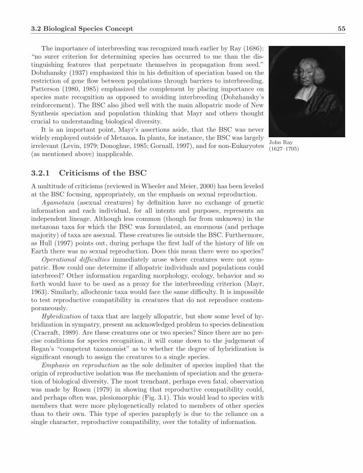
3.2 Biological Species Concept 55
The importance of interbreeding was recognized much earlier by Ray (1686):“no surer criterion for determining species has occurred to me than the dis-tinguishing features that perpetuate themselves in propagation from seed.”Dobzhansky (1937) emphasized this in his definition of speciation based on therestriction of gene flow between populations through barriers to interbreeding.Patterson (1980, 1985) emphasized the complement by placing importance onspecies mate recognition as opposed to avoiding interbreeding (Dobzhansky’sreinforcement). The BSC also jibed well with the main allopatric mode of NewSynthesis speciation and population thinking that Mayr and others thoughtcrucial to understanding biological diversity.
John Ray(1627–1705)
It is an important point, Mayr’s assertions aside, that the BSC was neverwidely employed outside of Metazoa. In plants, for instance, the BSC was largelyirrelevant (Levin, 1979; Donoghue, 1985; Gornall, 1997), and for non-Eukaryotes(as mentioned above) inapplicable.
3.2.1 Criticisms of the BSC
A multitude of criticisms (reviewed in Wheeler and Meier, 2000) has been leveledat the BSC focusing, appropriately, on the emphasis on sexual reproduction.
Agamotaxa (asexual creatures) by definition have no exchange of geneticinformation and each individual, for all intents and purposes, represents anindependent lineage. Although less common (though far from unknown) in themetazoan taxa for which the BSC was formulated, an enormous (and perhapsmajority) of taxa are asexual. These creatures lie outside the BSC. Furthermore,as Hull (1997) points out, during perhaps the first half of the history of life onEarth there was no sexual reproduction. Does this mean there were no species?
Operational difficulties immediately arose where creatures were not sym-patric. How could one determine if allopatric individuals and populations couldinterbreed? Other information regarding morphology, ecology, behavior and soforth would have to be used as a proxy for the interbreeding criterion (Mayr,1963). Similarly, allochronic taxa would face the same difficulty. It is impossibleto test reproductive compatibility in creatures that do not reproduce contem-poraneously.
Hybridization of taxa that are largely allopatric, but show some level of hy-bridization in sympatry, present an acknowledged problem to species delineation(Cracraft, 1989). Are these creatures one or two species? Since there are no pre-cise conditions for species recognition, it will come down to the judgement ofRegan’s “competent taxonomist” as to whether the degree of hybridization issignificant enough to assign the creatures to a single species.
Emphasis on reproduction as the sole delimiter of species implied that theorigin of reproductive isolation was the mechanism of speciation and the genera-tion of biological diversity. The most trenchant, perhaps even fatal, observationwas made by Rosen (1979) in showing that reproductive compatibility could,and perhaps often was, plesiomorphic (Fig. 3.1). This would lead to species withmembers that were more phylogenetically related to members of other speciesthan to their own. This type of species paraphyly is due to the reliance on asingle character, reproductive compatibility, over the totality of information.
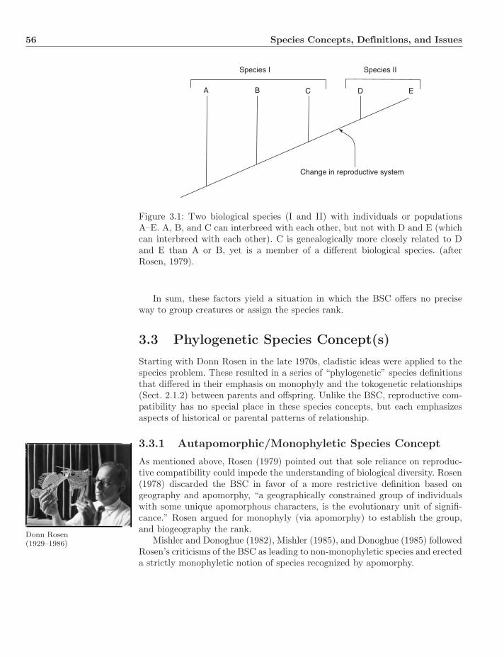
56 Species Concepts, Definitions, and Issues
A B C D E
Change in reproductive system
Species I Species II
Figure 3.1: Two biological species (I and II) with individuals or populationsA–E. A, B, and C can interbreed with each other, but not with D and E (whichcan interbreed with each other). C is genealogically more closely related to Dand E than A or B, yet is a member of a different biological species. (afterRosen, 1979).
In sum, these factors yield a situation in which the BSC offers no preciseway to group creatures or assign the species rank.
3.3 Phylogenetic Species Concept(s)
Starting with Donn Rosen in the late 1970s, cladistic ideas were applied to thespecies problem. These resulted in a series of “phylogenetic” species definitionsthat differed in their emphasis on monophyly and the tokogenetic relationships(Sect. 2.1.2) between parents and offspring. Unlike the BSC, reproductive com-patibility has no special place in these species concepts, but each emphasizesaspects of historical or parental patterns of relationship.
3.3.1 Autapomorphic/Monophyletic Species Concept
As mentioned above, Rosen (1979) pointed out that sole reliance on reproduc-tive compatibility could impede the understanding of biological diversity. Rosen(1978) discarded the BSC in favor of a more restrictive definition based ongeography and apomorphy, “a geographically constrained group of individualswith some unique apomorphous characters, is the evolutionary unit of signifi-cance.” Rosen argued for monophyly (via apomorphy) to establish the group,and biogeography the rank.
Donn Rosen(1929–1986) Mishler and Donoghue (1982), Mishler (1985), and Donoghue (1985) followed
Rosen’s criticisms of the BSC as leading to non-monophyletic species and erecteda strictly monophyletic notion of species recognized by apomorphy.
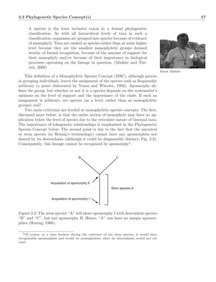
3.3 Phylogenetic Species Concept(s) 57
A species is the least inclusive taxon in a formal phylogeneticclassification. As with all hierarchical levels of taxa in such aclassification, organisms are grouped into species because of evidenceof monophyly. Taxa are ranked as species rather than at some higherlevel because they are the smallest monophyletic groups deemedworthy of formal recognition, because of the amount of support fortheir monophyly and/or because of their importance in biologicalprocesses operating on the lineage in question. (Mishler and The-riot, 2000)
Brent Mishler
This definition of a Monophyletic Species Concept (MSC), although precisein grouping individuals, leaves the assignment of the species rank as Reganesklyarbitrary (a point elaborated by Vrana and Wheeler, 1992). Apomorphy de-fines the group, but whether or not it is a species depends on the systematist’sopinions on the level of support and the importance of the clade. If such anassignment is arbitrary, are species (as a level, rather than as monophyleticgroups) real?
Two main criticisms are leveled at monophyletic species concepts. The first,discussed more below, is that the entire notion of monophyly may have no ap-plication below the level of species due to the reticulate nature of bisexual taxa.The importance of tokogenetic relationships is emphasized in the PhylogeneticSpecies Concept below. The second point is due to the fact that the ancestralor stem species (in Hennig’s terminology) cannot have any apomorphies notshared by its descendants (although it could be diagnosably distinct; Fig. 3.2).Consequently, this lineage cannot be recognized by apomorphy5.
B C
Acquisition of apomorphy II
Acquisition of apomorphy I
Stem species A
Figure 3.2: The stem species “A” will share apomorphy I with descendent species“B” and “C”, but not apomorphy II. Hence, “A” can have no unique apomor-phies (Hennig, 1966).
5Of course, at a time horizon during the existence of the stem species, it would haverecognizable apomorphies and would be monophyletic, since its descendants would not yetexist.

58 Species Concepts, Definitions, and Issues
3.3.2 Diagnostic/Phylogenetic Species Concept
The term Phylogenetic Species Concept (PSC) was coined by Cracraft (1983) todifferentiate his definition as different from those of Rosen and Mayr. One of hiskey points was that monophyly did not apply at the level of species. This ideawas promulgated earlier with Nelson and Platnick (1981) stating that specieswere “the smallest detected samples of self-perpetuating organisms that haveunique sets of characters.” This definition was thought to be compatible withcladistic phylogenetic analysis, but not dependent on it, in that these clustersof organisms need not share apomorphies.
Joel Cracraft
Cracraft (1983) defined species as “the smallest diagnosable cluster of in-dividual organisms within which there is a parental pattern of ancestry anddescent,” the “parental pattern” being the ancestor–descendant relationshipbetween parent and offspring used by Eldredge and Cracraft (1980) in theirdefinition. This concept was general to sexual or asexual taxa, but the parentalcomponent proscribed hybrids (unless they were to create a new group thatcontinued to reproduce on its own).
A central feature of this definition is the absence of apomorphy, which isreplaced by diagnosability. This was further amplified by Nixon and Wheeler(1990), “the smallest aggregation of populations (sexual) or lineages (asexual)diagnosable by a unique combination of character states in comparable indi-viduals (semaphoronts).” This definition also shifted the definition from onereferring to individuals to one based on aggregations of populations or lineages.
These instantiations of the PSC allow, on the face of it, both monophyleticand paraphyletic groups to be recognized as species (but would forbid poly-phyletic species). The authors of these definitions, however, argue strenuouslythat the concept of monophyly does not apply to species, hence species-paraphyly is no sin6. This idea can be traced back to Hennig (1966) in his distinc-tion between phylogenetic relationships (those between species) and tokogenetic(those between individuals within a species) (Fig. 3.3). Nixon and Wheeler referto features that vary within a species and reflect tokogeny as “traits” while thosebetween, reflecting phylogeny, were recognized as “characters,” which are fixedfor all individuals. Species are diagnosed on the basis of unique combinations oftraits (as opposed to the apomorphies of the MSC).
As Nixon and Wheeler (1992) point out, this distinction allows for phyleticspeciation (without cladogenesis) as the diagnosis of a lineage changes throughtime and new features originate and become fixed in populations. A single lin-eage could undergo multiple “speciations” without any cladogenesis. This is di-rectly contrary to speciation modes envisioned by the MSC and other concepts(below) that require splitting events for new species and render the ancestralspecies extinct. Furthermore, in the PSC, species may survive a splitting eventif their diagnosable suite of features is unchanged (as opposed to the new sisterspecies) (Fig. 3.4). The potential for creating species based on plesiomorphy,the possibility of phyletic speciation, and the potential perpetuation of species
6Hennig himself viewed species in a similar manner to the BSC as “reproductive commu-nities” (Hennig, 1966) that were bounded in origin and extinction by splitting (cladogenic)events (see below).
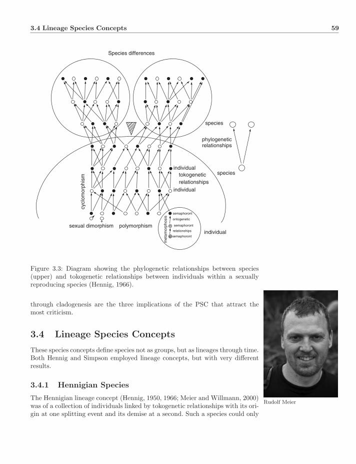
3.4 Lineage Species Concepts 59
Species differences
species
species
phylogeneticrelationships
individual
individual
individualpolymorphismsexual dimorphism
met
amor
phos
is
semaphoront
semaphoront
semaphoront
ontogenetic
relationships
cycl
omor
phis
m tokogeneticrelationships
Figure 3.3: Diagram showing the phylogenetic relationships between species(upper) and tokogenetic relationships between individuals within a sexuallyreproducing species (Hennig, 1966).
through cladogenesis are the three implications of the PSC that attract themost criticism.
3.4 Lineage Species Concepts
These species concepts define species not as groups, but as lineages through time.Both Hennig and Simpson employed lineage concepts, but with very differentresults.
3.4.1 Hennigian Species
Rudolf MeierThe Hennigian lineage concept (Hennig, 1950, 1966; Meier and Willmann, 2000)was of a collection of individuals linked by tokogenetic relationships with its ori-gin at one splitting event and its demise at a second. Such a species could only

60 Species Concepts, Definitions, and Issues
A
Sp.1
Origin ofapomorphictrait
Local or globalextinction ofplesiomorphs
Sp.2 Sp.2 Sp.2 Sp.3Sp.1
Local extinctionof plesiomorphs
Sp.1 Sp.1
TIM
E
B C
Figure 3.4: Three modes of speciation consistent with the PSC: phyletic A,ancestral persistence B, and ancestral extinction C (Nixon and Wheeler, 1992).
persist in the absence of splitting because cladogenesis disrupts the tokogeneticrelationships between the daughter groups, now independent lineages (Fig. 3.3).Unlike the BSC or PSC, there can be neither phyletic speciation nor persistenceof species through splitting. In the former case, tokogeny is maintained through-out the time between splits, and in the latter, tokogeny is necessarily disrupted.These notions were formalized by Kornet (1993) as “internodal” species. TheHennigian species concept emphasizes the reproductive continuity of the lineageand isolation of post-split sister taxa.
3.4.2 Evolutionary Species
Simpson (1961) was dissatisfied with the atemporal aspect of the BSC and pro-posed the Evolutionary Species Concept (ESC) to remedy this shortcoming. Hedefined a species as “a lineage (an ancestor–descendant sequence of populations)evolving separately from others and with its own unitary role and tendencies.”Many of these terms are, to put it mildly, vague. Wiley (1978) and Wiley andMayden (2000) sought to make the concept more precise with:
An evolutionary species is an entity composed of organisms thatmaintains its identity from other such entities through time and
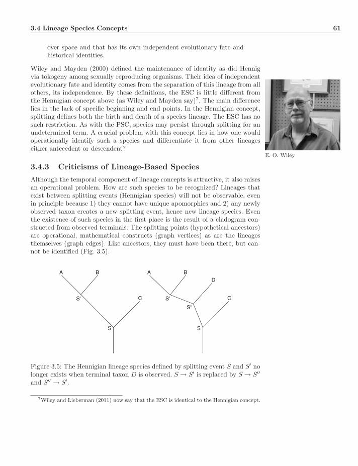
3.4 Lineage Species Concepts 61
over space and that has its own independent evolutionary fate andhistorical identities.
Wiley and Mayden (2000) defined the maintenance of identity as did Hennigvia tokogeny among sexually reproducing organisms. Their idea of independentevolutionary fate and identity comes from the separation of this lineage from allothers, its independence. By these definitions, the ESC is little different fromthe Hennigian concept above (as Wiley and Mayden say)7. The main differencelies in the lack of specific beginning and end points. In the Hennigian concept,splitting defines both the birth and death of a species lineage. The ESC has nosuch restriction. As with the PSC, species may persist through splitting for anundetermined term. A crucial problem with this concept lies in how one wouldoperationally identify such a species and differentiate it from other lineageseither antecedent or descendent?
E. O. Wiley
3.4.3 Criticisms of Lineage-Based Species
Although the temporal component of lineage concepts is attractive, it also raisesan operational problem. How are such species to be recognized? Lineages thatexist between splitting events (Hennigian species) will not be observable, evenin principle because 1) they cannot have unique apomorphies and 2) any newlyobserved taxon creates a new splitting event, hence new lineage species. Eventhe existence of such species in the first place is the result of a cladogram con-structed from observed terminals. The splitting points (hypothetical ancestors)are operational, mathematical constructs (graph vertices) as are the lineagesthemselves (graph edges). Like ancestors, they must have been there, but can-not be identified (Fig. 3.5).
S
S'
A B
C
S
S'
A B
C
D
S''
Figure 3.5: The Hennigian lineage species defined by splitting event S and S′ nolonger exists when terminal taxon D is observed. S → S′ is replaced by S → S′′
and S′′ → S′.
7Wiley and Lieberman (2011) now say that the ESC is identical to the Hennigian concept.

62 Species Concepts, Definitions, and Issues
3.5 Species as Individuals or Classes
One of the prominent issues in the discussion of species as ontological objects iswhether species are individuals or classes. This may seem an arcane topic, butit has far-reaching ramifications in studies of historical diversity, extinction, andconservation.
An ontological class is a universal, eternal collection of similar things. Abiological example might be herbivores, or flying animals that are membersof a set due to the properties they possess. Classes are defined in this wayintentionally, by their specific properties as necessary and sufficient, such aseating plants or having functional wings. Such a class has no beginning or endand no restriction as to how an element of such a set got there. A class suchas the element Gold (in Hull’s example) contains all atoms with 79 protons. Itdoes not matter if those atoms were formed by fusions of smaller atoms or fissionof larger, or by alchemy for that matter. Furthermore, the class of Gold existswithout there being any members of the class. Any new atoms with atomicnumber 79 would be just as surely Gold as any other. One of the importantaspects of classes is that scientific laws operate on them as spatio-temporallyunrestricted generalizations (Hull, 1978). Laws in science require classes.
Michael Ghiselin Individuals on the other hand, have a specific beginning and end, and arenot members of any set (other than the trivial sets of individuals). Species,however defined, are considered to have a specific origin at speciation and aspecific end at subsequent speciation or extinction (or at least will). As such,they are spatio-temporally restricted entities whose properties can change overtime yet remain the same thing (as we all age through time, but remain thesame person). A particular species (like a higher taxon) is not an instance of atype of object; each is a unique instance of its own kind.
Much of the thinking in terms of law-like evolutionary theory at least implic-itly relies on the class nature of species. Only with classes can general statementsbe made about speciation, diversity, and extinction. Ghiselin (1966, 1969, 1974)argued that species were individuals and, as such, their names were propernames referring to specific historical objects, not general classes of things. Assupported by Hull (1976, 1978) and others, this ontology has far-reaching im-plications. This view of species renders many comparative statements devoid ofcontent. While it might be reasonable to ask why a process generated one gramof Gold while another one kilogram, the question “why are there so many speciesof beetles and so few of aardvarks?” has no meaning at all if each species is anindividual. General laws of “speciation” become impossible, and temporally orgeographically based enumerations of species meaningless.
David Hull(1935–2010)
Although the case for species as individuals has wide acceptance currently(but see Stamos, 2003), biologists often operate as if species were classes. As anexample, species descriptions are based on a series of features and those creaturesthat exhibit them are members of that species. This implies that species are anintensionally defined set and would exist irrespective of whether there were anycreatures in it or not.

3.6 Monoism and Pluralism 63
3.6 Monoism and Pluralism
Given the great diversity of species concepts and definitions, some have arguedthat different concepts should be used for different situations, offering a so-lution for the differences between sexual, asexual and hybrid origin taxa. Thisreasoning has been extended to allow for a diversity of concepts to match the di-versity of reproductive systems, life history strategies, and patterns of variation(Cracraft, 2000).
A less extreme version of pluralism, advocated by Mishler and Brandon(1987) and Mishler and Theriot (2000), would have a single rule for grouping—monophyly—but allow a pluralistic view of what level in a tree hierarchy is tobe assigned the rank species, and what the rationale would be. Agreeing withthese authors on monophyly, but unwilling to accept an arbitrarily defined en-tity in systematics, Vrana and Wheeler (1992) urged the separation of patternstatements (monophyly) from process (species), removing the entire issue fromconcern. Wheeler and Platnick (2000) criticized this view, saying that due tothe reticulating nature of the historical patterns of sexual creatures, there isno assurance that different sources of data would yield the same set of relation-ships. This argument loses force, however, with the realization that this can, andusually does, occur in all data sets, at all levels, with sexual or asexual creatures.
The monoist perspective is that there must be a single definition of species,universally applied to all scenarios presented by living things. Even thoughthis does not currently exist (at least consensually), systematists have beenworking to identify one in the thought that it is attainable and desirable, andthe present “a particularly unfortunate time to give up” (Wheeler and Platnick,2000). Furthermore, of what use is a word, like a pluralistically defined species,that means different things to different people in different situations? If speciesare a component of nature, and scientists are to make general statements aboutthem, the word must have a single meaning.
If, however, species are defined as in the MSC and they are ontologicalindividuals, a non-arbitrary designation of a precisely comparable level in thehierarchy of individuals will be difficult to identify. For this reason, Mishler andBrandon (1987) have embraced their convenience-based pluralism.
3.7 Pattern and Process
One of the difficulties in constructing a single species definition relates to thesometimes conflicting goals of incorporating pattern and process inform-ation. The BSC is the most notable—based as it is on gene-flow throughinterbreeding—but not the only (e.g. ecological) concept based on an explicitnotion of biological process. In essence, the concepts state that evolution occursthis way, so species should be defined in this manner.
Other definitions emphasize pattern phenomena, specifically monophyly. Insuch a concept, the patterns that drive diversification are irrelevant to whethera group is monophyletic or not. Such ideas began with Rosen (1978, 1979) and
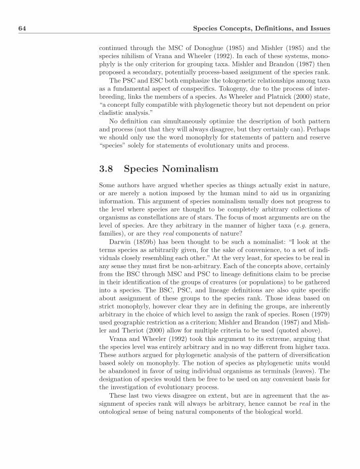
64 Species Concepts, Definitions, and Issues
continued through the MSC of Donoghue (1985) and Mishler (1985) and thespecies nihilism of Vrana and Wheeler (1992). In each of these systems, mono-phyly is the only criterion for grouping taxa. Mishler and Brandon (1987) thenproposed a secondary, potentially process-based assignment of the species rank.
The PSC and ESC both emphasize the tokogenetic relationships among taxaas a fundamental aspect of conspecifics. Tokogeny, due to the process of inter-breeding, links the members of a species. As Wheeler and Platnick (2000) state,“a concept fully compatible with phylogenetic theory but not dependent on priorcladistic analysis.”
No definition can simultaneously optimize the description of both patternand process (not that they will always disagree, but they certainly can). Perhapswe should only use the word monophyly for statements of pattern and reserve“species” solely for statements of evolutionary units and process.
3.8 Species Nominalism
Some authors have argued whether species as things actually exist in nature,or are merely a notion imposed by the human mind to aid us in organizinginformation. This argument of species nominalism usually does not progress tothe level where species are thought to be completely arbitrary collections oforganisms as constellations are of stars. The focus of most arguments are on thelevel of species. Are they arbitrary in the manner of higher taxa (e.g. genera,families), or are they real components of nature?
Darwin (1859b) has been thought to be such a nominalist: “I look at theterms species as arbitrarily given, for the sake of convenience, to a set of indi-viduals closely resembling each other.” At the very least, for species to be real inany sense they must first be non-arbitrary. Each of the concepts above, certainlyfrom the BSC through MSC and PSC to lineage definitions claim to be precisein their identification of the groups of creatures (or populations) to be gatheredinto a species. The BSC, PSC, and lineage definitions are also quite specificabout assignment of these groups to the species rank. Those ideas based onstrict monophyly, however clear they are in defining the groups, are inherentlyarbitrary in the choice of which level to assign the rank of species. Rosen (1979)used geographic restriction as a criterion; Mishler and Brandon (1987) and Mish-ler and Theriot (2000) allow for multiple criteria to be used (quoted above).
Vrana and Wheeler (1992) took this argument to its extreme, arguing thatthe species level was entirely arbitrary and in no way different from higher taxa.These authors argued for phylogenetic analysis of the pattern of diversificationbased solely on monophyly. The notion of species as phylogenetic units wouldbe abandoned in favor of using individual organisms as terminals (leaves). Thedesignation of species would then be free to be used on any convenient basis forthe investigation of evolutionary process.
These last two views disagree on extent, but are in agreement that the as-signment of species rank will always be arbitrary, hence cannot be real in theontological sense of being natural components of the biological world.
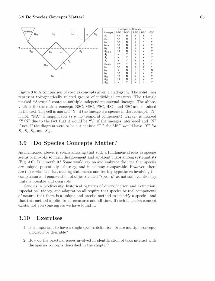
3.9 Do Species Concepts Matter? 65
Asexual
S0
S10S1
S2
S9 S7S11
S12 S8
S3
S4 S5 S6
Lineages as SpeciesLineage BSC MSC PSC HSC ESCS0 NA N Y Y YS1 NA N Y N YS2 NA N Y N YS1+2 NA N Y Y YS3 NA N Y Y YS1+2+3 NA N Y Y YS4 Y Y Y Y YS5 Y Y Y Y YS6 Y Y Y Y YS4+5+6 Y/N Y Y Y YS7 NA N Y Y YS8 Y N N N NS9 NA N Y Y YS10 NA N Y Y YS11 NA N Y Y YS12 N Y Y N Y
T
Figure 3.6: A comparison of species concepts given a cladogram. The solid linesrepresent tokogenetically related groups of individual creatures. The trianglemarked “Asexual” contains multiple independent asexual lineages. The abbre-viations for the various concepts BSC, MSC, PSC, HSC, and ESC are containedin the text. The cell is marked “Y” if the lineage is a species in that concept, “N”if not, “NA” if inapplicable (e.g. no temporal component). S4+5+6 is marked“Y/N” due to the fact that it would be “Y” if the lineages interbreed and “N”if not. If the diagram were to be cut at time “T,” the MSC would have “Y” forS3, S7, S9, and S11.
3.9 Do Species Concepts Matter?
As mentioned above, it seems amazing that such a fundamental idea as speciesseems to provoke so much disagreement and apparent chaos among systematists(Fig. 3.6). Is it worth it? Some would say no and embrace the idea that speciesare unique, potentially arbitrary, and in no way comparable. However, thereare those who feel that making statements and testing hypotheses involving thecomparison and enumeration of objects called “species” as natural evolutionaryunits is possible and desirable.
Studies in biodiversity, historical patterns of diversification and extinction,“speciation” theory, and adaptation all require that species be real componentsof nature, that there is a unique and precise method to identify a species, andthat this method applies to all creatures and all time. If such a species conceptexists, not everyone agrees we have found it.
3.10 Exercises
1. Is it important to have a single species definition, or are multiple conceptsallowable or desirable?
2. How do the practical issues involved in identification of taxa interact withthe species concepts described in the chapter?

66 Species Concepts, Definitions, and Issues
3. Are asexual taxa species? How might horizontal gene exchange affect this?
4. Suppose that each organism in a study group is unique at the wholegenome level (and you have these data). What would be the issues in-volved in applying the various species concepts to identifying species leveltaxa?
5. Give examples of studies where species are treated as a class and as indi-viduals. If all species were individuals how would these studies have beeneffected? If classes?

Chapter 4
Hypothesis Testing and thePhilosophy of Science
This chapter briefly presents several philosophical topics relevant to systematicanalysis. Although there is a large universe of philosophical ideas discussed inthe systematics literature, I have limited the discussion here to a number ofareas that have direct impact on how analyses are done—how decisions aremade as to choices among analytical options and the process of reasoning fromdata acquisition to choice of final tree hypothesis. The discussion is far fromcomplete, but should serve as an entree into the underlying epistemology ofsystematics.
4.1 Forms of Scientific Reasoning
4.1.1 The Ancients
Plato(c.427–c.347 BCE)
Although scientific reasoning has existed as long as science itself, the hypothesis-driven approach is more recent. Plato argued the cause of natural laws in hisideas of universals (Chapter 1). Universals were ideal forms with inherent real-ity. The observed world, however, consisted of shadows, imperfect realizations ofabsolute and unchanging forms. One could learn about ideals from their observedrepresentations and hence study the natural laws that governed Plato’s univer-sals, but this was never embodied in any hypothesis-testing framework.
Aristotle rejected the ideal forms of Plato, placing the real world and obser-vations of it at the center of scientific inquiry. In this, Aristotle was the founder
Aristotle(384–322 BCE)
of Ontology, the metaphysical science of being itself. Aristotle rejected platonicideals and universal forms. He argued that observable objects around us werethe reality of nature, ideals the mental abstractions. Aristotle was not entirelypure in his reasoning, however, and though we associate him with Ontology, hisideas were something of a mix.
Systematics: A Course of Lectures, First Edition. Ward C. Wheeler.c© 2012 Ward C. Wheeler. Published 2012 by Blackwell Publishing Ltd.

68 Hypothesis Testing and the Philosophy of Science
In biology, the classifications of Aristotle can be viewed as hypotheses ofpattern in biological variation with terata as counter, if not falsifying, data.Aristotle did not weigh alternate scenarios based on specific observations, how-ever, he produced narrative classifications to explain what he saw. Aristotle didhave a notion of minimal necessary explanation (parsimony, see below) oftenthought to have originated with Ockham.
4.1.2 Ockham’s Razor
Ockham was an English Franciscan monk who wrote widely in the intellectualareas of medieval thought including logic, metaphysics, physics, and theology.He eventually ran afoul of Pope John XXII (branding Ockham a heretic) overapostolic poverty. For this, Ockham was excommunicated (though rehabilitatedafter his death) and fled to Germany, residing there the remainder of his life. Hispolitical writings urge an early form of separation of church and state, no doubtnot a coincidence. Of most interest to systematics is Ockham’s nominalism andontological parsimony.
William of Ockham(c.1285–c.1347)
Ockham’s nominalism (as with Aristotle) rejected ideal universal forms ashaving reality. He focused, instead, on the individuality of objects. Any gen-eralizations were intensions of the human thought process. These generaliza-tions might have had more weight than mere words, but remained human-generated abstractions, not components of the natural world. Such discussionsin his Summa Logicae (Ockham, 1323) form part of the foundation of modernepistemology.
We look to Ockham most, however, for Ockham’s razor. This is the idea thatin explaining phenomena the simplest explanation is most favored.
For nothing ought to be posited without a reason given, unless it isself-evident (literally, known through itself) or known by experienceor proved by the authority of Sacred Scripture.
Ockham felt that human reasoning was incapable of complete understanding ofnot only nature but theological principles such as the soul, and these could onlybe understood through divine revelation.
Although Ockham did express the idea of simplicity and minimalism in log-ical inference, much more has been ascribed to him than he actually wrote andthe idea of minimal inference goes back as far as Aristotle1. The most commonlyencountered quotes from Ockham:
Pluralitas non est ponenda sine neccesitate [Purality should not beposited without necessity]
and
Frustra fit per plura quod potest fieri per pauciora [It is pointless todo with more what can be done with less]
1The often quoted “Entia non sunt multiplicanda sine necessitate.” is nowhere to be foundin Ockham’s writings.

4.1 Forms of Scientific Reasoning 69
refer to simplicity in elements, parameters, or causations. Anything beyond theminimal is unsupported, hence unnecessary.
The parsimony criterion makes explicit reference to Ockham’s razor in jus-tifying its simplicity argument, but in reality, all optimality-based methodsoperate on this basis (lower cost, higher likelihood or probability). Likelihoodanalyses incorporating model selection explicitly seek to minimize parametersin balance with enhanced tree likelihoods. Parsimony methods, in using a min-imal set of operational assumptions (e.g. lack of a statistical model), are mostexplicit in minimizing operational assumptions as well as explanatory events(see below).
The minimization principle of inference runs through much of formal scien-tific logic as an operational principle. This is not because it will necessarily leadto truth, but because it is precise and efficient2.
4.1.3 Modes of Scientific Inference
Scientific inference is the process of generating explanations of data withhypotheses—here trees. Among the many forms of scientific inference, there arefour of most direct interest to systematics: induction, deduction, abduction, andthe synthetic hypothetico-deduction. Modern systematics employs these formsof logic in multiple guises and often in impure, combined forms.
4.1.4 Induction
Francis Bacon(1561–1626)
Induction is a process whereby multiple observed instances of a phenomenon leadto a generalization (sometimes ascribed in origin to Francis Bacon). In essence,for a series of observations ai each leading to result b: a0 → b, a1 → b, . . . , ak →b ∴ A → b. In a commonly used example, “Every swan I see is white, thereforeall swans are white.”
David Hume(1711–1776)
Hume (1748) cited two problems with this mode of inference. First, sincecertainty would require exhaustive observation of all data (A above), which isimpossible for non-trivial problems, absolute proof is impossible. Second, induc-tion assumes that all future observations will agree with those already gathered.
In systematics, we can see this play out in Bayesian analysis of clades (Chap-ter 12). Clade posterior probabilities are estimated through additional observa-tions generalizing to a high probability (in terms of the data) result. Even thoughvery high probabilities (often 1.0) are recovered, a very small fraction of trees areevaluated and the probabilities depend on specific data sources. Given that cladeposterior probabilities can vary with data source (such as molecular sequenceloci), the identical behavior of past and future data sources cannot be assured.
4.1.5 Deduction
A deductive inference (Socrates) is constructed by building a series of logicalstatements into an argument or syllogism. If the premises are true, the result
2After all, which of the non-minimal solutions should be chosen—and why?
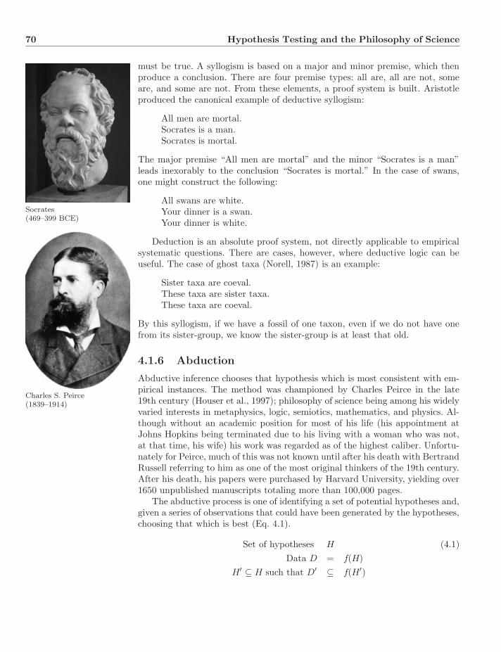
70 Hypothesis Testing and the Philosophy of Science
must be true. A syllogism is based on a major and minor premise, which thenproduce a conclusion. There are four premise types: all are, all are not, someare, and some are not. From these elements, a proof system is built. Aristotleproduced the canonical example of deductive syllogism:
Socrates(469–399 BCE)
All men are mortal.Socrates is a man.Socrates is mortal.
The major premise “All men are mortal” and the minor “Socrates is a man”leads inexorably to the conclusion “Socrates is mortal.” In the case of swans,one might construct the following:
All swans are white.Your dinner is a swan.Your dinner is white.
Deduction is an absolute proof system, not directly applicable to empiricalsystematic questions. There are cases, however, where deductive logic can beuseful. The case of ghost taxa (Norell, 1987) is an example:
Sister taxa are coeval.These taxa are sister taxa.These taxa are coeval.
By this syllogism, if we have a fossil of one taxon, even if we do not have onefrom its sister-group, we know the sister-group is at least that old.
4.1.6 Abduction
Charles S. Peirce(1839–1914)
Abductive inference chooses that hypothesis which is most consistent with em-pirical instances. The method was championed by Charles Peirce in the late19th century (Houser et al., 1997); philosophy of science being among his widelyvaried interests in metaphysics, logic, semiotics, mathematics, and physics. Al-though without an academic position for most of his life (his appointment atJohns Hopkins being terminated due to his living with a woman who was not,at that time, his wife) his work was regarded as of the highest caliber. Unfortu-nately for Peirce, much of this was not known until after his death with BertrandRussell referring to him as one of the most original thinkers of the 19th century.After his death, his papers were purchased by Harvard University, yielding over1650 unpublished manuscripts totaling more than 100,000 pages.
The abductive process is one of identifying a set of potential hypotheses and,given a series of observations that could have been generated by the hypotheses,choosing that which is best (Eq. 4.1).
Set of hypotheses H (4.1)Data D = f(H)
H′ ⊆ H such that D′ ⊆ f(H′)
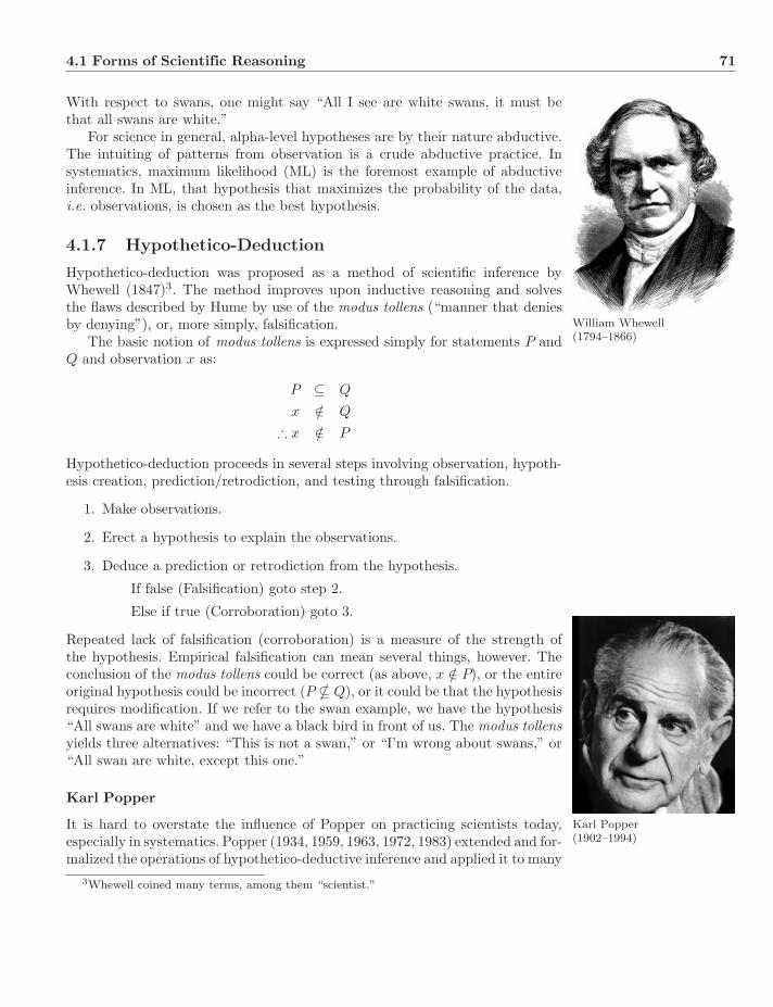
4.1 Forms of Scientific Reasoning 71
With respect to swans, one might say “All I see are white swans, it must bethat all swans are white.”
For science in general, alpha-level hypotheses are by their nature abductive.The intuiting of patterns from observation is a crude abductive practice. Insystematics, maximum likelihood (ML) is the foremost example of abductiveinference. In ML, that hypothesis that maximizes the probability of the data,i.e. observations, is chosen as the best hypothesis.
4.1.7 Hypothetico-Deduction
William Whewell(1794–1866)
Hypothetico-deduction was proposed as a method of scientific inference byWhewell (1847)3. The method improves upon inductive reasoning and solvesthe flaws described by Hume by use of the modus tollens (“manner that deniesby denying”), or, more simply, falsification.
The basic notion of modus tollens is expressed simply for statements P andQ and observation x as:
P ⊆ Q
x /∈ Q
∴ x /∈ P
Hypothetico-deduction proceeds in several steps involving observation, hypoth-esis creation, prediction/retrodiction, and testing through falsification.
1. Make observations.
2. Erect a hypothesis to explain the observations.
3. Deduce a prediction or retrodiction from the hypothesis.
If false (Falsification) goto step 2.
Else if true (Corroboration) goto 3.
Repeated lack of falsification (corroboration) is a measure of the strength ofthe hypothesis. Empirical falsification can mean several things, however. Theconclusion of the modus tollens could be correct (as above, x /∈ P), or the entireoriginal hypothesis could be incorrect (P � Q), or it could be that the hypothesisrequires modification. If we refer to the swan example, we have the hypothesis“All swans are white” and we have a black bird in front of us. The modus tollensyields three alternatives: “This is not a swan,” or “I’m wrong about swans,” or“All swan are white, except this one.”
Karl Popper
Karl Popper(1902–1994)
It is hard to overstate the influence of Popper on practicing scientists today,especially in systematics. Popper (1934, 1959, 1963, 1972, 1983) extended and for-malized the operations of hypothetico-deductive inference and applied it to many
3Whewell coined many terms, among them “scientist.”
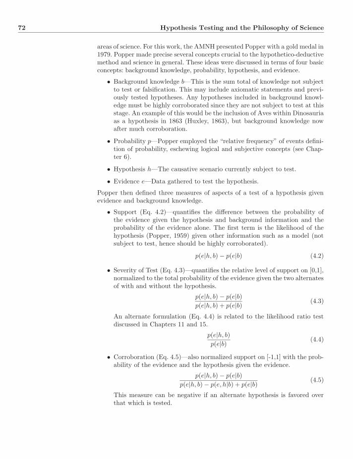
72 Hypothesis Testing and the Philosophy of Science
areas of science. For this work, the AMNH presented Popper with a gold medal in1979. Popper made precise several concepts crucial to the hypothetico-deductivemethod and science in general. These ideas were discussed in terms of four basicconcepts: background knowledge, probability, hypothesis, and evidence.
• Background knowledge b—This is the sum total of knowledge not subjectto test or falsification. This may include axiomatic statements and previ-ously tested hypotheses. Any hypotheses included in background knowl-edge must be highly corroborated since they are not subject to test at thisstage. An example of this would be the inclusion of Aves within Dinosauriaas a hypothesis in 1863 (Huxley, 1863), but background knowledge nowafter much corroboration.
• Probability p—Popper employed the “relative frequency” of events defini-tion of probability, eschewing logical and subjective concepts (see Chap-ter 6).
• Hypothesis h—The causative scenario currently subject to test.
• Evidence e—Data gathered to test the hypothesis.
Popper then defined three measures of aspects of a test of a hypothesis givenevidence and background knowledge.
• Support (Eq. 4.2)—quantifies the difference between the probability ofthe evidence given the hypothesis and background information and theprobability of the evidence alone. The first term is the likelihood of thehypothesis (Popper, 1959) given other information such as a model (notsubject to test, hence should be highly corroborated).
p(e|h, b) − p(e|b) (4.2)
• Severity of Test (Eq. 4.3)—quantifies the relative level of support on [0,1],normalized to the total probability of the evidence given the two alternatesof with and without the hypothesis.
p(e|h, b) − p(e|b)p(e|h, b) + p(e|b) (4.3)
An alternate formulation (Eq. 4.4) is related to the likelihood ratio testdiscussed in Chapters 11 and 15.
p(e|h, b)p(e|b) (4.4)
• Corroboration (Eq. 4.5)—also normalized support on [-1,1] with the prob-ability of the evidence and the hypothesis given the evidence.
p(e|h, b) − p(e|b)p(e|h, b) − p(e, h|b) + p(e|b) (4.5)
This measure can be negative if an alternate hypothesis is favored overthat which is tested.
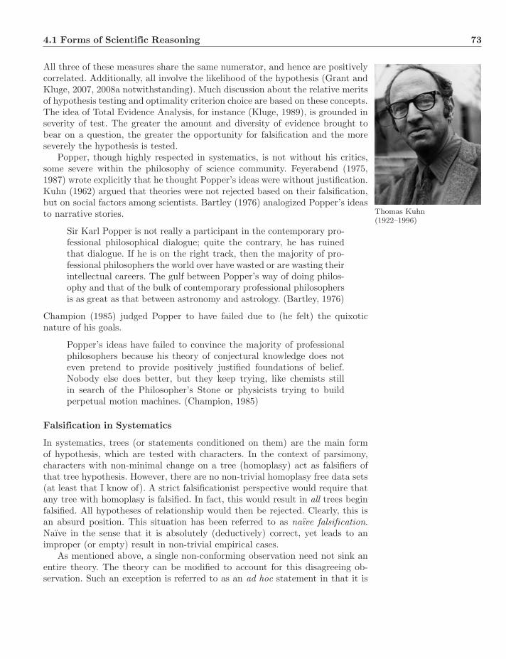
4.1 Forms of Scientific Reasoning 73
All three of these measures share the same numerator, and hence are positivelycorrelated. Additionally, all involve the likelihood of the hypothesis (Grant andKluge, 2007, 2008a notwithstanding). Much discussion about the relative meritsof hypothesis testing and optimality criterion choice are based on these concepts.The idea of Total Evidence Analysis, for instance (Kluge, 1989), is grounded inseverity of test. The greater the amount and diversity of evidence brought tobear on a question, the greater the opportunity for falsification and the moreseverely the hypothesis is tested.
Thomas Kuhn(1922–1996)
Popper, though highly respected in systematics, is not without his critics,some severe within the philosophy of science community. Feyerabend (1975,1987) wrote explicitly that he thought Popper’s ideas were without justification.Kuhn (1962) argued that theories were not rejected based on their falsification,but on social factors among scientists. Bartley (1976) analogized Popper’s ideasto narrative stories.
Sir Karl Popper is not really a participant in the contemporary pro-fessional philosophical dialogue; quite the contrary, he has ruinedthat dialogue. If he is on the right track, then the majority of pro-fessional philosophers the world over have wasted or are wasting theirintellectual careers. The gulf between Popper’s way of doing philos-ophy and that of the bulk of contemporary professional philosophersis as great as that between astronomy and astrology. (Bartley, 1976)
Champion (1985) judged Popper to have failed due to (he felt) the quixoticnature of his goals.
Popper’s ideas have failed to convince the majority of professionalphilosophers because his theory of conjectural knowledge does noteven pretend to provide positively justified foundations of belief.Nobody else does better, but they keep trying, like chemists stillin search of the Philosopher’s Stone or physicists trying to buildperpetual motion machines. (Champion, 1985)
Falsification in Systematics
In systematics, trees (or statements conditioned on them) are the main formof hypothesis, which are tested with characters. In the context of parsimony,characters with non-minimal change on a tree (homoplasy) act as falsifiers ofthat tree hypothesis. However, there are no non-trivial homoplasy free data sets(at least that I know of). A strict falsificationist perspective would require thatany tree with homoplasy is falsified. In fact, this would result in all trees beginfalsified. All hypotheses of relationship would then be rejected. Clearly, this isan absurd position. This situation has been referred to as naıve falsification.Naıve in the sense that it is absolutely (deductively) correct, yet leads to animproper (or empty) result in non-trivial empirical cases.
As mentioned above, a single non-conforming observation need not sink anentire theory. The theory can be modified to account for this disagreeing ob-servation. Such an exception is referred to as an ad hoc statement in that it is
74 Hypothesis Testing and the Philosophy of Science
specific to a particular observation and has no (or at least limited) generality.The discovery of a black swan, for instance, might be accommodated in thetheory that all swans are white, by the ad hoc statement “except for this onehere” (as opposed to eating the swan quickly and invisibly). This process can beextended without limit rendering falsification meaningless (as W. V. Quine ar-gued). This would seem fatal, until it is realized that not all hypotheses requirethe same degree of ad hoc rescue.
Arnold Kluge
The realization and use of the observation that all observations support (andreject) all hypotheses, but not to equal extent, leads to sophisticated or method-ological falsification. This is the form of falsification pursued by Farris (1983)and Kluge (e.g. Kluge, 2009). In this framework, the least falsified (in termsof homoplasy) hypothesis (= tree) is most favored. Farris (1983) emphasizedthe minimization of “extra-steps” as ad hoc hypotheses of character conver-gence or parallelism. This concept is slightly recast as the minimization of totalcost in dynamic homology since the calculation of minimal cost for a charac-ter (sequence character for instance) is tree specific (Wheeler, 2001b, 2011).According to Farris (1983), sophisticated falsification equates to parsimony andPopper and justifies its use. The appeal to Popperian logic underpins much ofthe argumentation in favor of parsimony.
Synthesis of Inference
In light of the above discussion, the model of hypothetico-deduction in sys-tematics can be recast as a combination of methods. Steps 1 and 2 (makingobservations and erecting a hypothesis) are abductive. This is followed (step 3)by the deduction of a predictive statement. This statement is falsified in terms ofan objective function of tree optimality. The prediction is that the current tree(hypothesis) optimizes an objective function more effectively than an alternatetree. The falsification comes in comparing the value of the objective functionbetween the two. If the current tree is “better,” it is corroborated (induction)and the method returns to the previous step (3), identifying another competinghypothesis to be tested against the current best (deductive step). If the currenttree is less optimal than an alternate, it is falsified and the challenger becomesthe current best hypothesis. This process is repeated until all alternate hypothe-ses are tested and as long as the objective function is transitive [if f(A) ≤ f(B)and f(B) ≤ f(C) then f(A) ≤ f(C)] the set of optimal (least falsified) hypotheseswill be identified.
1. Make observations.
2. Erect a hypothesis (tree T) to explain the observations (initially the opti-mal tree T o ← T) and compete with T o.
3. Deduce the prediction that T o will optimize f() better (f(T o) ≤ f(T)).
4. Compare f(T) and f(T o)If f(T o) � f(T)(Falsification) then T o ← T
Else true (Corroboration).
5. If there are trees remaining to be tested, goto step 2, else return T o.
4.2 Other Philosophical Issues 75
The objective function could in principle take many (transitive) forms. Theabove formalism allows model-based methods such as likelihood and topology-based posterior probability (Bayesian Maximum A Posteriori, MAP) as opti-mality criteria (f()). The choice of criterion must then be defended on othergrounds, but the hypothetico-deductive process would remain unchanged.
4.2 Other Philosophical Issues
There are many issues where philosophical considerations affect how we thinkabout problems and what we do to address them. Several are discussed in othersections, including the arguments over whether species are individuals or classesand species nominalism (Chapter 3), the combination (“Total Evidence”) orpartition of data (Sect. 16.2.7), and optimality criteria (Chapter 13).
One topic that is an element of many discussions is the operational meaningof minimization and weighting.
4.2.1 Minimization, Transformation, and Weighting
When we speak of minimizing the cost of a cladogram, especially in a Popperiancontext, what are the components to be minimized? Are we to minimize trans-formations, or overall cost—allowing for weighted transformations? At whatlevel do we apply the parsimony criterion? There is no current consensus onthese issues and they definitely affect systematic results.
Kluge and Grant (e.g. Grant and Kluge, 2005; among many others) haveargued that the entity to be minimized when evaluating competing tree hy-potheses is transformations. This form of minimization requires that all eventsbe weighted equally since only this scheme will minimize both overall cost andabsolute numbers of transformations. Wheeler (1995) and Giribet (2003) ar-gued that alternate transformation weighting schemes should be considered andin some cases favored over homogeneous weighting. They advocated sensitivity
Gonzalo Giribetanalysis (Section 10.11) to evaluate and potentially choose hypotheses basedon alternate weighting schemes. There is no theoretical, in the sense of math-ematical, limitation (other than perhaps metricity) on these weights. Are boththese scenarios—minimizing “steps” and minimizing “cost”—parsimony? Whatof larger-scale genomic events such as locus insertion–deletion and rearrange-ment? If these transformations were to be weighted equal to nucleotide substi-tutions, insertions and deletions, grossly non-metric costs would be implied andtrivial (all large indel) results produced (Fig. 4.1).
The issue is unsettled4.Ockham’s razor appears even within the context of the minimization of trans-
formations. Consider the nucleic acid sequences AAC and TT. If we allow sub-stitution, insertion, and deletion events of one nucleotide, there are a minimumof three events (transformations) required to edit one sequence into the other.If, however, we choose a simpler model, one with only insertions and deletions,a minimum of five events are required (there are multiple five transformation
4This same argument applies to “Implied Weights” (Goloboff, 1993b).
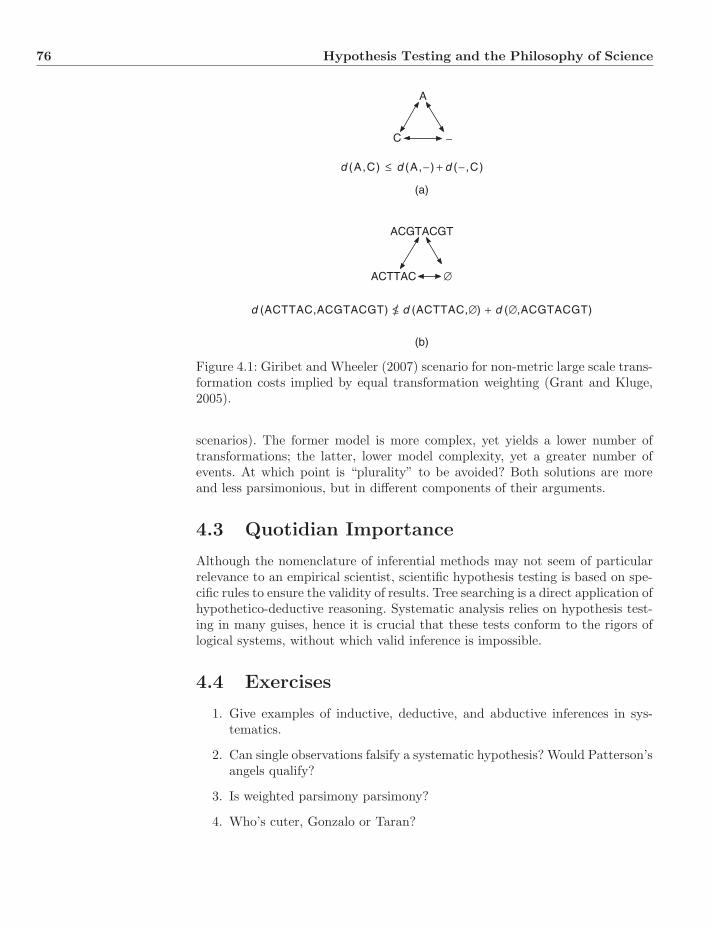
76 Hypothesis Testing and the Philosophy of Science
A
C −
d (A,C) ≤ d (A,− ) + d (− ,C)
ACGTACGT
ACTTAC ∅
(b)
(a)
d (ACTTAC,ACGTACGT) ≤ d (ACTTAC,∅) + d (∅,ACGTACGT)
Figure 4.1: Giribet and Wheeler (2007) scenario for non-metric large scale trans-formation costs implied by equal transformation weighting (Grant and Kluge,2005).
scenarios). The former model is more complex, yet yields a lower number oftransformations; the latter, lower model complexity, yet a greater number ofevents. At which point is “plurality” to be avoided? Both solutions are moreand less parsimonious, but in different components of their arguments.
4.3 Quotidian Importance
Although the nomenclature of inferential methods may not seem of particularrelevance to an empirical scientist, scientific hypothesis testing is based on spe-cific rules to ensure the validity of results. Tree searching is a direct application ofhypothetico-deductive reasoning. Systematic analysis relies on hypothesis test-ing in many guises, hence it is crucial that these tests conform to the rigors oflogical systems, without which valid inference is impossible.
4.4 Exercises
1. Give examples of inductive, deductive, and abductive inferences in sys-tematics.
2. Can single observations falsify a systematic hypothesis? Would Patterson’sangels qualify?
3. Is weighted parsimony parsimony?
4. Who’s cuter, Gonzalo or Taran?

Chapter 5
Computational Concepts
Systematics is a synthetic science, and several fundamental problems fall amongthe most difficult faced by computer science. In order to better understand theissues involved and the techniques developed to deal with them, an introductionto computer science basics is reviewed.
5.1 Problems, Algorithms, and Complexity
5.1.1 Computer Science Basics
David Hilbert(1862–1943)
The theory of computation begins with (Godel, 1931), Kleene (1936), Post(1936), Church (1936a,b), and Turing (1936, 1937). These works answered theEntscheidungsproblem (“Decision Problem”) proposed by Hilbert in 19001 ofwhether a method could always be devised to output correctly whether a state-ment were true or false. In other words, were there unsolvable problems? Godelproved that there were statements that were true, but could not be proven so.
Kurt Godel(1906–1978)
Simply put, for any self-consistent system sufficient to describe the arithmeticof natural numbers, there are true statements that cannot be proven. Church(“undecidable” problems) and Turing2 (“halting” problem) followed this resultand independently proved that there were problems that could not be com-puted (Church’s Theorem), answering the Entscheidungsproblem in the nega-tive. These results, and the mechanisms used to arrive at them, are the heart ofcomputation theory.
Church developed a system, the Lambda Calculus, to study computationthat, with his student Turing’s machine-based approach, form the basis of mod-ern computer science. Both these systems were “universal” in that they could
1This was one of Hilbert’s 23 unsolved problems that drove much of mathematics in the20th century.
2Church’s Ph.D. student.
Systematics: A Course of Lectures, First Edition. Ward C. Wheeler.c© 2012 Ward C. Wheeler. Published 2012 by Blackwell Publishing Ltd.
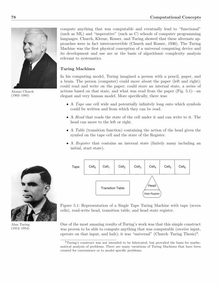
78 Computational Concepts
compute anything that was computable and eventually lead to “functional”(such as ML) and “imperative” (such as C) schools of computer programminglanguages. Church, Kleene, Rosser, and Turing showed that these alternate ap-proaches were in fact interconvertible (Church and Rosser, 1936). The TuringMachine was the first physical conception of a universal computing device andits development and use are at the basis of algorithmic complexity analysisrelevant to systematics.
Alonzo Church(1903–1995)
Turing Machines
In his computing model, Turing imagined a person with a pencil, paper, anda brain. The person (computer) could move about the paper (left and right);could read and write on the paper; could store an internal state, a series ofactions based on that state, and what was read from the paper (Fig. 5.1)—anelegant and very human model. More specifically, there was:
• A Tape one cell wide and potentially infinitely long onto which symbolscould be written and from which they can be read.
• A Head that reads the state of the cell under it and can write to it. Thehead can move to the left or right.
• A Table (transition function) containing the action of the head given thesymbol on the tape cell and the state of the Register.
• A Register that contains an internal state (finitely many including aninitial, start state).
Tape
Transition TableHead
State Register
Cell0 Cell1 Cell2 Cell3 Cell4 Cell5 Cell6
Figure 5.1: Representation of a Single Tape Turing Machine with tape (sevencells), read-write head, transition table, and head state register.
Alan Turing(1912–1954)
One of the most amazing results of Turing’s work was that this simple constructwas proven to be able to compute anything that was computable (receive input,operate on that input, and halt); it was “universal” (Church–Turing Thesis)3.
3Turing’s construct was not intended to be fabricated, but provided the basis for mathe-matical analysis of problems. There are many variations of Turing Machines that have beencreated for convenience or to model specific problems.
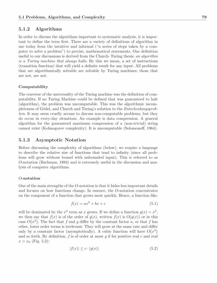
5.1 Problems, Algorithms, and Complexity 79
5.1.2 Algorithms
In order to discuss the algorithms important to systematic analysis, it is impor-tant to define the term first. There are a variety of definitions of algorithm inuse today from the intuitive and informal (“a series of steps taken by a com-puter to solve a problem”) to precise, mathematical statements. One definitionuseful to our discussions is derived from the Church–Turing thesis: an algorithmis a Turing machine that always halts. By this we mean, a set of instructions(transition function) that will yield a definite result for any input. All problemsthat are algorithmically solvable are solvable by Turing machines; those thatare not, are not.
Computability
The converse of the universality of the Turing machine was the definition of com-putability. If no Turing Machine could be defined that was guaranteed to halt(algorithm), the problem was uncomputable. This was the algorithmic incom-pleteness of Godel, and Church and Turing’s solution to the Entscheidungsprob-lem. It may seem cruelly arcane to discuss non-computable problems, but theydo occur in every-day situations. An example is data compression. A generalalgorithm for the guaranteed maximum compression of a (non-trivial) stringcannot exist (Kolmogorov complexity). It is uncomputable (Solomonoff, 1964).
5.1.3 Asymptotic Notation
Before discussing the complexity of algorithms (below), we require a languageto describe the relative size of functions that tend to infinity (since all prob-lems will grow without bound with unbounded input). This is referred to asO-notation (Bachman, 1894) and is extremely useful in the discussion and ana-lysis of computer algorithms.
O-notation
One of the main strengths of the O-notation is that it hides less important detailsand focuses on how functions change. In essence, the O-notation concentrateson the component of a function that grows most quickly. Hence, a function like:
f(x) = ax2 + bx + c (5.1)
will be dominated by the x2 term as x grows. If we define a function g(x) = x2,we then say that f(x) is of the order of g(x), written f(x) is O(g(x)) or in thiscase O
(x2
). The fact that f and g differ by the constant factor a, or that f has
other, lower order terms is irrelevant. They will grow at the same rate and differonly by a constant factor (asymptotically). A cubic function will have O
(x3
)and so forth. By definition, f is of order at most g if for positive real c and realx > x0 (Fig. 5.2):
|f(x)| ≤ c · |g(x)| (5.2)
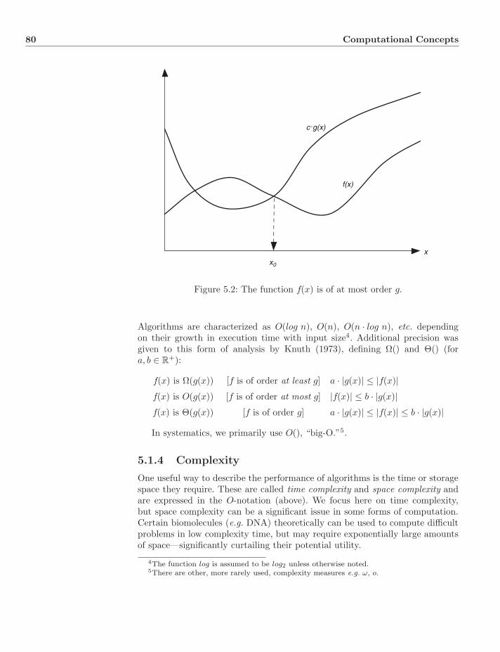
80 Computational Concepts
xx0
f(x)
c.g(x)
Figure 5.2: The function f(x) is of at most order g.
Algorithms are characterized as O(log n), O(n), O(n · log n), etc. dependingon their growth in execution time with input size4. Additional precision wasgiven to this form of analysis by Knuth (1973), defining Ω() and Θ() (fora, b ∈ R+):
f(x) is Ω(g(x)) [f is of order at least g] a · |g(x)| ≤ |f(x)|f(x) is O(g(x)) [f is of order at most g] |f(x)| ≤ b · |g(x)|f(x) is Θ(g(x)) [f is of order g] a · |g(x)| ≤ |f(x)| ≤ b · |g(x)|
In systematics, we primarily use O(), “big-O.”5.
5.1.4 Complexity
One useful way to describe the performance of algorithms is the time or storagespace they require. These are called time complexity and space complexity andare expressed in the O-notation (above). We focus here on time complexity,but space complexity can be a significant issue in some forms of computation.Certain biomolecules (e.g. DNA) theoretically can be used to compute difficultproblems in low complexity time, but may require exponentially large amountsof space—significantly curtailing their potential utility.
4The function log is assumed to be log2 unless otherwise noted.5There are other, more rarely used, complexity measures e.g. ω, o.
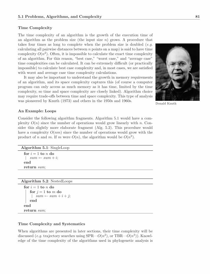
5.1 Problems, Algorithms, and Complexity 81
Time Complexity
The time complexity of an algorithm is the growth of the execution time ofan algorithm as the problem size (the input size n) grows. A procedure thattakes four times as long to complete when the problem size is doubled (e.g.calculating all pairwise distances between n points on a map) is said to have timecomplexity O(n2). Often, it is impossible to calculate the exact time complexityof an algorithm. For this reason, “best case,” “worst case,” and “average case”time complexities can be calculated. It can be extremely difficult (or practicallyimpossible) to calculate best case complexity and, in most cases, we are satisfiedwith worst and average case time complexity calculations.
It may also be important to understand the growth in memory requirementsof an algorithm, and its space complexity captures this (of course a computerprogram can only access as much memory as it has time, limited by the timecomplexity, so time and space complexity are closely linked). Algorithm choicemay require trade-offs between time and space complexity. This type of analysiswas pioneered by Knuth (1973) and others in the 1950s and 1960s.
Donald Knuth
An Example: Loops
Consider the following algorithm fragments. Algorithm 5.1 would have a com-plexity O(n) since the number of operations would grow linearly with n. Con-sider this slightly more elaborate fragment (Alg. 5.2). This procedure wouldhave a complexity O(nm) since the number of operations would grow with theproduct of n and m. If m were O(n), the algorithm would be O(n2).
Algorithm 5.1: SingleLoopfor i = 1 to n do
sum ← sum + i;endreturn sum;
Algorithm 5.2: NestedLoopsfor i = 1 to n do
for j = 1 to m dosum ← sum + i + j;
endendreturn sum;
Time Complexity and Systematics
When algorithms are presented in later sections, their time complexity will bediscussed (e.g. trajectory searches using SPR—O(n2), or TBR—O(n3)). Knowl-edge of the time complexity of the algorithms used in phylogenetic analysis is
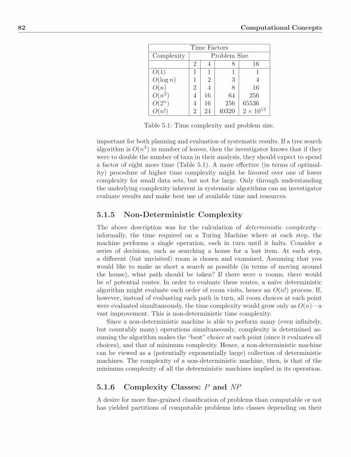
82 Computational Concepts
Time FactorsComplexity Problem Size
2 4 8 16O(1) 1 1 1 1O(log n) 1 2 3 4O(n) 2 4 8 16O(n2) 4 16 64 256O(2n) 4 16 256 65536O(n!) 2 24 40320 2 × 10¹³
Table 5.1: Time complexity and problem size.
important for both planning and evaluation of systematic results. If a tree searchalgorithm is O(n3) in number of leaves, then the investigator knows that if theywere to double the number of taxa in their analysis, they should expect to spenda factor of eight more time (Table 5.1). A more effective (in terms of optimal-ity) procedure of higher time complexity might be favored over one of lowercomplexity for small data sets, but not for large. Only through understandingthe underlying complexity inherent in systematic algorithms can an investigatorevaluate results and make best use of available time and resources.
5.1.5 Non-Deterministic Complexity
The above description was for the calculation of deterministic complexity—informally, the time required on a Turing Machine where at each step, themachine performs a single operation, each in turn until it halts. Consider aseries of decisions, such as searching a house for a lost item. At each step,a different (but unvisited) room is chosen and examined. Assuming that youwould like to make as short a search as possible (in terms of moving aroundthe house), what path should be taken? If there were n rooms, there wouldbe n! potential routes. In order to evaluate these routes, a naıve deterministicalgorithm might evaluate each order of room visits, hence an O(n!) process. If,however, instead of evaluating each path in turn, all room choices at each pointwere evaluated simultaneously, the time complexity would grow only as O(n)—avast improvement. This is non-deterministic time complexity.
Since a non-deterministic machine is able to perform many (even infinitely,but countably many) operations simultaneously, complexity is determined as-suming the algorithm makes the “best” choice at each point (since it evaluates allchoices), and that of minimum complexity. Hence, a non-deterministic machinecan be viewed as a (potentially exponentially large) collection of deterministicmachines. The complexity of a non-deterministic machine, then, is that of theminimum complexity of all the deterministic machines implied in its operation.
5.1.6 Complexity Classes: P and NP
A desire for more fine-grained classification of problems than computable or nothas yielded partitions of computable problems into classes depending on their
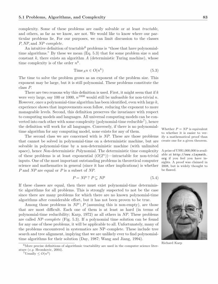
5.1 Problems, Algorithms, and Complexity 83
complexity. Some of these problems are easily solvable or at least tractable,and others, as far as we know, are not. We would like to know where our par-ticular problems lie. For our purposes, we can limit discussion to the classesP,NP, and NP–complete.
An intuitive definition of tractable6 problems is “those that have polynomial-time algorithms.” By these we mean (Eq. 5.3) that for some problem size n andconstant k, there exists an algorithm A (deterministic Turing machine), whosetime complexity is of the order nk.
TimeAn ∈ O(nk) (5.3)
The time to solve the problem grows as an exponent of the problem size. Thisexponent may be large, but it is still polynomial. These problems constitute theclass P.
There are two reasons why this definition is used. First, it might seem that if kwere very large, say 100 or 1000, n1000 would still be unfeasible for non-trivial n.However, once a polynomial-time algorithm has been identified, even with large k,experience shows that improvements soon follow, reducing the exponent to moremanageable levels. Second, this definition preserves the invariance with respectto computing models and languages. All universal computing models can be con-verted into each other with some complexity (polynomial-time reducible7), hencethe definition will work for all languages. Conversely, if there is no polynomial-time algorithm for any computing model, none exists for any of them.
Whether P = NP is equivalentto whether it is easier to ver-ify a mathematical proof thancreate one for a given theorem.
A prize of US$1,000,000 is avail-able at http://www.claymath.
org if you feel you have in-sights. A proof was claimed in2008, but is widely thought tobe flawed.
The second class we are concerned with is NP. These are those problemsthat cannot be solved in polynomial-time on a deterministic machine, but aresolvable in polynomial-time by a non-deterministic machine (with unlimitedspace), hence Non-deterministic Polynomial. The deterministic time complexityof these problems is at least exponential (O(2n))—intractable for non-trivialinputs. One of the most important outstanding problems in theoretical computerscience and mathematics in general (since it has other implications) is whetherP and NP are equal or P is a subset of NP.
P = NP ? P � NP (5.4)
If these classes are equal, then there must exist polynomial-time determinis-tic algorithms for all problems. This is strongly suspected to not be the casesince there are many problems for which there are no known polynomial-timealgorithms after considerable effort, but it has not been proven to be true.
Among those problems in NP \ P (assuming this is non-empty), are thosethat are most difficult. Each one of them is at least as hard (in terms ofpolynomial-time reducibility; Karp, 1972) as all others in NP. These problemsare called NP–complete (Fig. 5.3). If a polynomial time solution can be foundfor any one of these problems, it will be applicable to all. Unfortunately, many ofthe problems encountered in systematics are NP–complete. These include treesearch and tree alignment, implying that we are unlikely ever to find polynomial-time algorithms for their solution (Day, 1987; Wang and Jiang, 1994).
Richard Karp6More precise definitions of algorithmic tractability are used in the computer science liter-
ature (e.g. Hromkovic, 2004).7Usually ≤ O(n3)
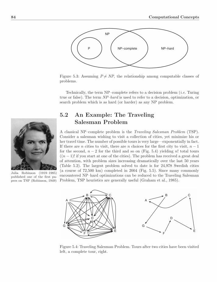
84 Computational Concepts
NP
P NP–complete NP–hard
Figure 5.3: Assuming P �= NP, the relationship among computable classes ofproblems.
Technically, the term NP–complete refers to a decision problem (i.e. Turingtrue or false). The term NP–hard is used to refer to a decision, optimization, orsearch problem which is as hard (or harder) as any NP problem.
5.2 An Example: The TravelingSalesman Problem
Julia Robinson (1919–1985)published one of the first pa-pers on TSP (Robinson, 1949)
A classical NP–complete problem is the Traveling Salesman Problem (TSP).Consider a salesman wishing to visit a collection of cities, yet minimize his orher travel time. The number of possible tours is very large—exponentially in fact.If there are n cities to visit, there are n choices for the first city to visit, n − 1for the second, n − 2 for the third and so on (Fig. 5.4) yielding n! total tours((n − 1)! if you start at one of the cities). The problem has received a great dealof attention, with problem sizes increasing dramatically over the last 50 years(Table 5.2). The largest problem solved to date is for 24,978 Swedish cities(a course of 72,500 km) completed in 2004 (Fig. 5.5). Since many commonlyencountered NP–hard optimizations can be reduced to the Traveling SalesmanProblem, TSP heuristics are generally useful (Graham et al., 1985).
A
B C
D
EF
G
A
B C
D
EF
G
Figure 5.4: Traveling Salesman Problem. Tours after two cities have been visitedleft, a complete tour, right.
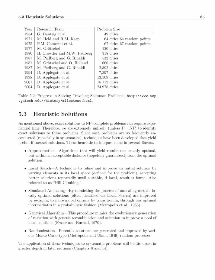
5.3 Heuristic Solutions 85
Year Research Team Problem Size1954 G. Dantzig et al. 49 cities1971 M. Held and R.M. Karp 64 cities 64 random points1975 P.M. Camerini et al. 67 cities 67 random points1977 M. Grotschel 120 cities1980 H. Crowder and M.W. Padberg 318 cities1987 M. Padberg and G. Rinaldi 532 cities1987 M. Grotschel and O. Holland 666 cities1987 M. Padberg and G. Rinaldi 2,392 cities1994 D. Applegate et al. 7,397 cities1998 D. Applegate et al. 13,509 cities2001 D. Applegate et al. 15,112 cities2004 D. Applegate et al. 24,978 cities
Table 5.2: Progress in Solving Traveling Salesman Problems. http://www.tsp.gatech.edu//history/milestone.html.
5.3 Heuristic Solutions
As mentioned above, exact solutions to NP–complete problems can require expo-nential time. Therefore, we are extremely unlikely (unless P = NP) to identifyexact solutions to these problems. Since such problems are so frequently en-countered (especially in systematics), techniques have been developed that yielduseful, if inexact solutions. These heuristic techniques come in several flavors.
• Approximation—Algorithms that will yield results not exactly optimal,but within an acceptable distance (hopefully guaranteed) from the optimalsolution.
• Local Search—A technique to refine and improve an initial solution byvarying elements in its local space (defined for the problem), acceptingbetter solutions repeatedly until a stable, if local, result is found. Alsoreferred to as “Hill Climbing.”
• Simulated Annealing—By mimicking the process of annealing metals, lo-cally optimal solutions (often identified via Local Search) are improvedby escaping to more global optima by transitioning through less optimalintermediates in a probabilistic fashion (Metropolis et al., 1953).
• Genetical Algorithm—This procedure mimics the evolutionary generationof variation with genetic recombination and selection to improve a pool oflocal solutions (Fraser and Burnell, 1970).
• Randomization—Potential solutions are generated and improved by vari-ous Monte Carlo-type (Metropolis and Ulam, 1949) random processes.
The application of these techniques to systematic problems will be discussed ingreater depth in later sections (Chapters 8 and 14).
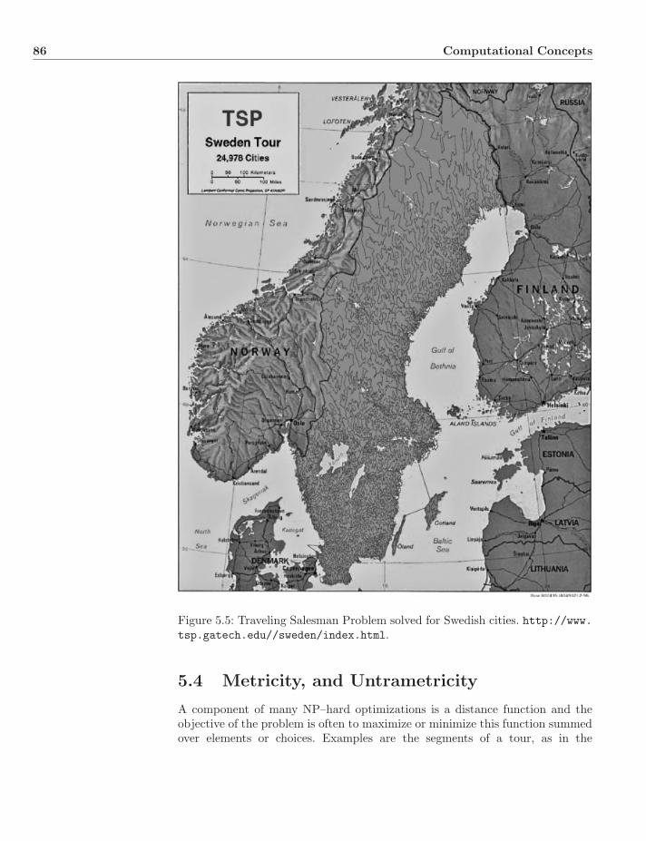
86 Computational Concepts
Figure 5.5: Traveling Salesman Problem solved for Swedish cities. http://www.tsp.gatech.edu//sweden/index.html.
5.4 Metricity, and Untrametricity
A component of many NP–hard optimizations is a distance function and theobjective of the problem is often to maximize or minimize this function summedover elements or choices. Examples are the segments of a tour, as in the
5.5 NP−Complete Problems in Systematics 87
Traveling Salesman Problem, or edges in other graph problems such as phylo-genetic trees.
In order for approximation algorithms and heuristic procedures to havebounded behavior (guaranteed to be within some factor of the optimal solu-tion), these distances or costs used by optimization problems usually must bemetric8. The limitations of metricity on these distances is natural and has far-reaching influence on phylogenetic problems (e.g. Wheeler, 1993). There are fourconditions for metricity (Eq. 5.5).
∀x d(x, x) = 0 (5.5)∀x, y;x �= y d(x, y) > 0
∀x, y d(x, y) = d(y, x)∀x, y, z d(x, y) ≤ d(x, z) + d(z, y)
Put simply, the distance between any element and itself must be zero, all otherdistances must be greater than zero, all distances must be symmetrical, andthe most direct distance between two elements must be lower cost than anyroute through a third element (triangle inequality). Non-metric distances canhave unforeseen and sometimes bizarre effects. An example of this would be toimagine a TSP with a city hovering somewhere—in an alternate universe withzero distance to all other cities (since it resides in another dimension, such thingsare possible). All cities could be reached by traveling first to this bizzaro-cityand then to any other at zero cost. Analogous pathological situations can occurwith sequence data when indels (gaps) are treated as missing data (Sect. 8.3.3;Wheeler, 1993).
There are further constraints that can be placed on distances such as thatof Equation 5.6, resulting in an ultrametric distance.
∀x, y, z d(x, y) ≤ max(d(x, z), d(z, y)) (5.6)
These topics are pursued in the context of distance-based tree reconstructiontechniques (Chapter 9) and molecular clocks (Chapter 17).
5.5 NP−Complete Problems in Systematics
The core problem of phylogeny reconstruction, the Phylogeny Problem, is NP–complete (Foulds and Graham, 1982). In this problem, we seek to find a tree (T =(V,E)), with cost CT (metric cost d summed over edges in E), that minimizes CT
over all trees. Given the exponential number of trees (Eq. 2.1), it is not surprisingthat this problem is beyond polynomial solutions (except under certain unlikelyconditions; Chapter 9). This problem is familiar to most systematists, but thereare many other NP–hard optimizations including the Tree Alignment Problem(Sankoff, 1975) shown to be NP–complete by Wang and Jiang (1994), ML treereconstruction (Roch, 2006), and many problems in genomic analysis (such aschromosomal inversion; Caprara, 1997).
8In fact, most provable results for these problems require metric distances.
88 Computational Concepts
Systematists must understand the theoretical basis and implications of thecomplexity of the problems they desire to solve. Only with a solid ground-ing in these computational concepts, can systematists evaluate the tools andtechniques required to attack the myriad of hard optimizations presented byphylogeny reconstruction.
5.6 Exercises
1. If a rooted tree has n leaves, what is the time complexity of locating aspecific edge?
2. What is the time complexity of writing down all possible DNA sequencesof length n? Up to length n?
3. If the length of a tree could be determined by examining a single edge,what would be the time complexity for evaluating m trees with n taxa?
4. If the evaluation of a genome (size m loci) on a vertex of a tree (n leaves)is O(m3), the evaluation of the entire tree requires visiting each vertex,and a search in tree space requires O(n2 log n), what is the time complexityof the entire operation?
5. If given the optimal phylogenetic tree by an oracle, how could this beverified (decided)?
6. Give examples of metric and non-metric distances for DNA sequence datawith indels.
7. Show that P � NP, or barring that, P = NP 9.
9This will guarantee a passing grade in the class.
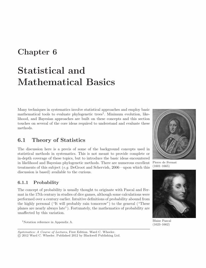
Chapter 6
Statistical andMathematical Basics
Many techniques in systematics involve statistical approaches and employ basicmathematical tools to evaluate phylogenetic trees1. Minimum evolution, like-lihood, and Bayesian approaches are built on these concepts and this sectiontouches on several of the core ideas required to understand and evaluate thesemethods.
6.1 Theory of Statistics
The discussion here is a precis of some of the background concepts used instatistical methods in systematics. This is not meant to provide complete orin-depth coverage of these topics, but to introduce the basic ideas encounteredin likelihood and Bayesian phylogenetic methods. There are numerous excellenttreatments of this subject (e.g. DeGroot and Schervish, 2006—upon which thisdiscussion is based) available to the curious.
Pierre de Fermat(1601–1665)
Blaise Pascal(1623–1662)
6.1.1 Probability
The concept of probability is usually thought to originate with Pascal and Fer-mat in the 17th century in studies of dice games, although some calculations wereperformed over a century earlier. Intuitive definitions of probability abound fromthe highly personal (“It will probably rain tomorrow”) to the general (“Theseplanes are nearly always late”). Fortunately, the mathematics of probability areunaffected by this variation.
1Notation reference in Appendix A.
Systematics: A Course of Lectures, First Edition. Ward C. Wheeler.c© 2012 Ward C. Wheeler. Published 2012 by Blackwell Publishing Ltd.
90 Statistical and Mathematical Basics
There are three general flavors of interpretations of probability in com-mon use:
1. Frequency—The relative frequency of events is commonly used to describethe probability of an event. For example, how many times will heads comeup in a coin toss, given the previous tosses? This interpretation has theproblems of being imprecise (how many events are required to determineprobability) and unclear as to how much variation is allowed around aprobability value. Another obvious shortcoming of this notion is that itimplies a large number of trials or events, hence is difficult to apply insituations where events are few, rare, or in the future (probability of ameteor falling).
2. Classical—This concept comes from the notion of equally likely outcomes,such as those in a coin toss. There are two possible outcomes (head ortails) that seem equally likely, hence have the same probability. Since theseprobabilities must sum to 1, heads and tails are each assigned a probabilityof 1
2 . In general, if there are n possible outcomes, their probabilities will be1n . Problems with this notion include that it is basically circular—thelikelihood of outcomes is their probability—and that it is unclear how toproceed when events are not equally likely.
3. Subjective—This interpretation comes from an individual’s own ideas orintuition as to the probabilities of events (do I think a meteor will fall).Although this notion can be expressed numerically, there is no way toassure accuracy, precision, that any individual will be consistent in as-signing probabilities, or that any two individuals would assign the sameprobability to the same event.
Set Theory and Probability
The basis of probability theory resides in sets. The set of all possible events isthe sample space, S. A specific event s then must reside in S, s ∈ S. If a coinis tossed once, there are two possible events, heads or tails (s0 = H, s1 = T ), inthe sample universe (S = {H,T}). If a coin were tossed n times there would be2n events (sequences of tosses) in the sample space.
Events may overlap, complement, or be disjoint (Fig. 6.1) and the union,intersection, and complement operators describe these relationships. Considerthe sets of hexapods (A) and herbivores (B). Those creatures that are bothhexapods and herbivores would be defined by their intersection (A ∩ B), thosethat are either hexapods or herbivores their union (A ∪ B), and those that areneither their complement ((A ∪ B)c = S \ (A ∪ B)).
Axioms
No matter to which interpretation of probability one cleaves, mathematically,a probability of an event x, Pr(x), must comply with three axioms (S is the

6.1 Theory of Statistics 91
A ∩ B
A B
S
A \ (A ∪ B ) B \ (A ∪ B )
(A ∪ B)c
Figure 6.1: The relationship between events A and B in sample space S.
sample space or set of all events):
For any event A, Pr(A) ≥ 0 (6.1)
Pr(S) = 1 (6.2)
For every infinite sequence of disjoint events A0, A1, . . .
Pr
( ∞⋃i=1
Ai
)=
∞∑i=1
Pr(Ai) (6.3)
Where disjoint events are mutually exclusive (A ∩ B = ∅). From these ax-ioms, a probability distribution or probability on sample space S, is defined as aspecification of Pr(A) that satisfies Equations 6.1, 6.2, and 6.3.
6.1.2 Conditional Probability
The probability of A given that B has occurred is referred to as the conditionalprobability of A given B (Pr(A|B)). This may occur in a situation where theoutcome of a coin toss experiment seems bizarre (assuming a fair coin) but giventhat the coin was biased, not so strange after all. This would be the conditionalprobability of an outcome given that the coin was unfair.
Conditional probability is defined by Equation 6.4 for Pr(B) > 0. The con-ditional probability is undefined when Pr(B) = 0.
Pr(A|B) =Pr(A ∩ B)
Pr(B)(6.4)
Conditional probability is most prominently applied in systematics via Bayes,Theorem (see below) in which the probability of a parameter (such as a tree) isconditioned upon a set of observations.
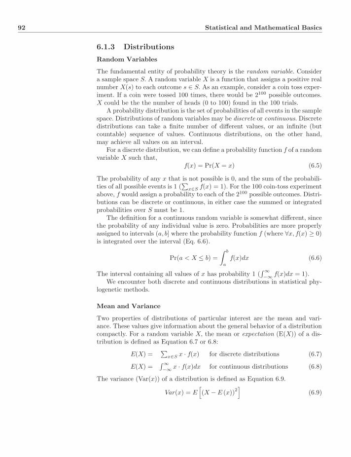
92 Statistical and Mathematical Basics
6.1.3 Distributions
Random Variables
The fundamental entity of probability theory is the random variable. Considera sample space S. A random variable X is a function that assigns a positive realnumber X(s) to each outcome s ∈ S. As an example, consider a coin toss exper-iment. If a coin were tossed 100 times, there would be 2100 possible outcomes.X could be the the number of heads (0 to 100) found in the 100 trials.
A probability distribution is the set of probabilities of all events in the samplespace. Distributions of random variables may be discrete or continuous. Discretedistributions can take a finite number of different values, or an infinite (butcountable) sequence of values. Continuous distributions, on the other hand,may achieve all values on an interval.
For a discrete distribution, we can define a probability function f of a randomvariable X such that,
f(x) = Pr(X = x) (6.5)
The probability of any x that is not possible is 0, and the sum of the probabili-ties of all possible events is 1 (
∑x∈S f(x) = 1). For the 100 coin-toss experiment
above, f would assign a probability to each of the 2100 possible outcomes. Distri-butions can be discrete or continuous, in either case the summed or integratedprobabilities over S must be 1.
The definition for a continuous random variable is somewhat different, sincethe probability of any individual value is zero. Probabilities are more properlyassigned to intervals (a, b] where the probability function f (where ∀x, f(x) ≥ 0)is integrated over the interval (Eq. 6.6).
Pr(a < X ≤ b) =∫ b
a
f(x)dx (6.6)
The interval containing all values of x has probability 1 (∫ ∞−∞ f(x)dx = 1).
We encounter both discrete and continuous distributions in statistical phy-logenetic methods.
Mean and Variance
Two properties of distributions of particular interest are the mean and vari-ance. These values give information about the general behavior of a distributioncompactly. For a random variable X, the mean or expectation (E(X)) of a dis-tribution is defined as Equation 6.7 or 6.8:
E(X) =∑
x∈S x · f(x) for discrete distributions (6.7)
E(X) =∫ ∞−∞ x · f(x)dx for continuous distributions (6.8)
The variance (Var(x)) of a distribution is defined as Equation 6.9.
Var(x) = E[(X − E (x))2
](6.9)
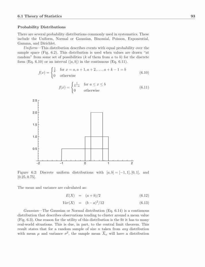
6.1 Theory of Statistics 93
Probability Distributions
There are several probability distributions commonly used in systematics. Theseinclude the Uniform, Normal or Gaussian, Binomial, Poisson, Exponential,Gamma, and Dirichlet.
Uniform—This distribution describes events with equal probability over thesample space (Fig. 6.2). This distribution is used when values are drawn “atrandom” from some set of possibilities (k of them from a to b) for the discreteform (Eq. 6.10) or an interval ([a, b]) in the continuous (Eq. 6.11).
f(x) =
{1k for x = a, a + 1, a + 2, . . . , a + k − 1 = b
0 otherwise(6.10)
f(x) =
{1
b−a for a ≤ x ≤ b
0 otherwise(6.11)
−2 −1 0 1 2
0.5
1.0
1.5
2.0
2.5
Figure 6.2: Discrete uniform distributions with [a, b] = [−1, 1], [0, 1], and[0.25, 0.75].
The mean and variance are calculated as:
E(X) = (a + b)/2 (6.12)
Var(X) = (b − a)2/12 (6.13)
Gaussian—The Gaussian or Normal distribution (Eq. 6.14) is a continuousdistribution that describes observations tending to cluster around a mean value(Fig. 6.3). One reason for the utility of this distribution is the fit it has to manyreal-world situations. This is due, in part, to the central limit theorem. Thisresult states that for a random sample of size n taken from any distributionwith mean μ and variance σ2, the sample mean Xn will have a distribution
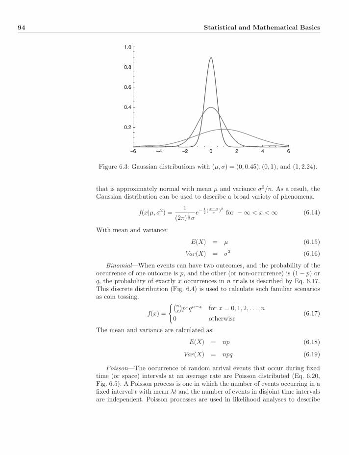
94 Statistical and Mathematical Basics
−6 −4 −2 0 2 4 6
0.2
0.4
0.6
0.8
1.0
Figure 6.3: Gaussian distributions with (μ, σ) = (0, 0.45), (0, 1), and (1, 2.24).
that is approximately normal with mean μ and variance σ2/n. As a result, theGaussian distribution can be used to describe a broad variety of phenomena.
f(x|μ, σ2) =1
(2π)12 σ
e−12 ( x−μ
σ )2 for −∞ < x < ∞ (6.14)
With mean and variance:
E(X) = μ (6.15)
Var(X) = σ2 (6.16)
Binomial—When events can have two outcomes, and the probability of theoccurrence of one outcome is p, and the other (or non-occurrence) is (1 − p) orq, the probability of exactly x occurrences in n trials is described by Eq. 6.17.This discrete distribution (Fig. 6.4) is used to calculate such familiar scenariosas coin tossing.
f(x) =
{(nx
)pxqn−x for x = 0, 1, 2, . . . , n
0 otherwise(6.17)
The mean and variance are calculated as:
E(X) = np (6.18)
Var(X) = npq (6.19)
Poisson—The occurrence of random arrival events that occur during fixedtime (or space) intervals at an average rate are Poisson distributed (Eq. 6.20,Fig. 6.5). A Poisson process is one in which the number of events occurring in afixed interval t with mean λt and the number of events in disjoint time intervalsare independent. Poisson processes are used in likelihood analyses to describe
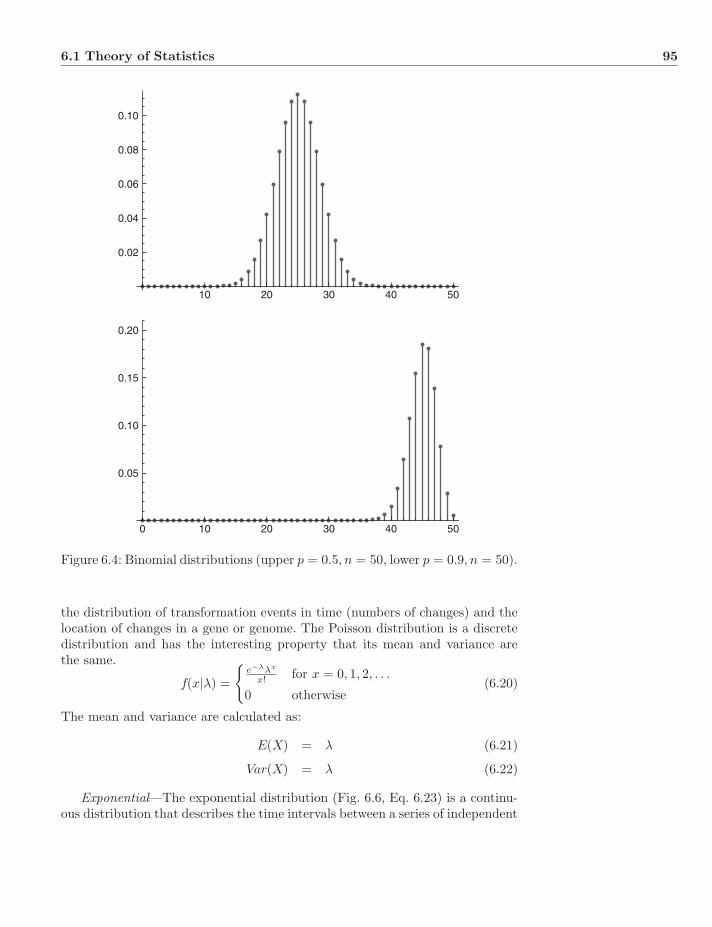
6.1 Theory of Statistics 95
10 20 30 40 50
0.02
0.04
0.06
0.08
0.10
0 10 20 30 40 50
0.05
0.10
0.15
0.20
Figure 6.4: Binomial distributions (upper p = 0.5, n = 50, lower p = 0.9, n = 50).
the distribution of transformation events in time (numbers of changes) and thelocation of changes in a gene or genome. The Poisson distribution is a discretedistribution and has the interesting property that its mean and variance arethe same.
f(x|λ) =
{e−λλx
x! for x = 0, 1, 2, . . .
0 otherwise(6.20)
The mean and variance are calculated as:
E(X) = λ (6.21)
Var(X) = λ (6.22)
Exponential—The exponential distribution (Fig. 6.6, Eq. 6.23) is a continu-ous distribution that describes the time intervals between a series of independent
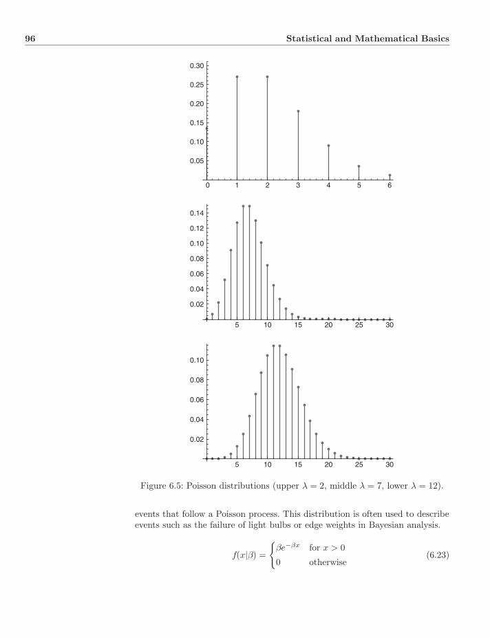
96 Statistical and Mathematical Basics
0 1 2 3 4 5 6
0.05
0.10
0.15
0.20
0.25
0.30
5 10 15 20 25 30
0.02
0.04
0.06
0.08
0.10
0.12
0.14
5 10 15 20 25 30
0.02
0.04
0.06
0.08
0.10
Figure 6.5: Poisson distributions (upper λ = 2, middle λ = 7, lower λ = 12).
events that follow a Poisson process. This distribution is often used to describeevents such as the failure of light bulbs or edge weights in Bayesian analysis.
f(x|β) =
{βe−βx for x > 0
0 otherwise(6.23)
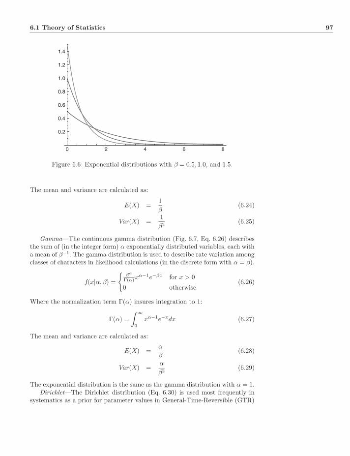
6.1 Theory of Statistics 97
0 2 4 6 8
0.2
0.4
0.6
0.8
1.0
1.2
1.4
Figure 6.6: Exponential distributions with β = 0.5, 1.0, and 1.5.
The mean and variance are calculated as:
E(X) =1β
(6.24)
Var(X) =1β2
(6.25)
Gamma—The continuous gamma distribution (Fig. 6.7, Eq. 6.26) describesthe sum of (in the integer form) α exponentially distributed variables, each witha mean of β−1. The gamma distribution is used to describe rate variation amongclasses of characters in likelihood calculations (in the discrete form with α = β).
f(x|α, β) =
{βα
Γ(α)xα−1e−βx for x > 0
0 otherwise(6.26)
Where the normalization term Γ(α) insures integration to 1:
Γ(α) =∫ ∞
0
xα−1e−xdx (6.27)
The mean and variance are calculated as:
E(X) =α
β(6.28)
Var(X) =α
β2(6.29)
The exponential distribution is the same as the gamma distribution with α = 1.Dirichlet—The Dirichlet distribution (Eq. 6.30) is used most frequently in
systematics as a prior for parameter values in General-Time-Reversible (GTR)
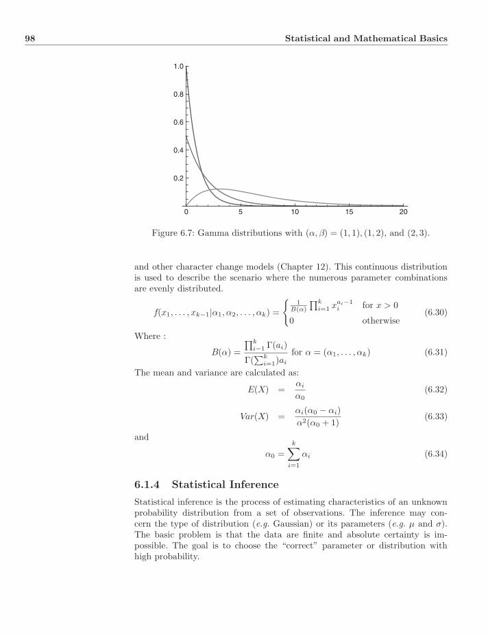
98 Statistical and Mathematical Basics
0 5 10 15 20
0.2
0.4
0.6
0.8
1.0
Figure 6.7: Gamma distributions with (α, β) = (1, 1), (1, 2), and (2, 3).
and other character change models (Chapter 12). This continuous distributionis used to describe the scenario where the numerous parameter combinationsare evenly distributed.
f(x1, . . . , xk−1|α1, α2, . . . , αk) =
{1
B(α)
∏ki=1 xai−1
i for x > 0
0 otherwise(6.30)
Where :
B(α) =
∏ki−1 Γ(ai)
Γ(∑k
i=1)ai
for α = (α1, . . . , αk) (6.31)
The mean and variance are calculated as:
E(X) =αi
α0(6.32)
Var(X) =αi(α0 − αi)α2(α0 + 1)
(6.33)
and
α0 =k∑
i=1
αi (6.34)
6.1.4 Statistical Inference
Statistical inference is the process of estimating characteristics of an unknownprobability distribution from a set of observations. The inference may con-cern the type of distribution (e.g. Gaussian) or its parameters (e.g. μ and σ).The basic problem is that the data are finite and absolute certainty is im-possible. The goal is to choose the “correct” parameter or distribution withhigh probability.
6.1 Theory of Statistics 99
6.1.5 Prior and Posterior Distributions
Priors and Problems
A typical inference problem would be to infer the specific value of a parameterθ in the parameter space Ω. Any observations (x) gathered would have beengenerated from the distribution function f and parameter θ. Observations havebeen drawn from f(x|θ).
Before any observations are gathered from f(x|θ), an investigator may haveknowledge about where in Ω the parameter θ may lie; that θ is more likely to befound in one area than another. As an example, the height of an adult humanfemale is less likely to be less than one meter or greater than three than betweenone and three meters. This knowledge may be based on previous experimentaldata, experiences, or even subjective opinion and can be expressed as a distri-bution of θ on Ω, ξ(θ). That distribution is known as the prior distribution of θ.“Prior” is used because the distribution is specified before any observations aredrawn from f(x|θ).
Disagreements over the validity, and even existence, of prior distributions areextreme within the statistical community. Bayesian statisticians adhere to theproposition that prior distributions can be defined in all circumstances and theseprobabilities are as valid as any other in statistics. This parallels the subjectiveinterpretation of probability itself. If all probabilities are subjective, they are allequally valid no matter their source.
Others disagree, stating that a parameter θ is a fixed, if unknown, valueand is not drawn from a distribution. The only way, then, to establish priorsis through extensive previous observation (such as the historical performanceof a machine). Both factions would agree that in the presence of good priorinformation, it should be used.
Posterior Distribution
The conditional probability of a set of observations given a specific value of θmultiplied by the probability (prior, ξ(θ)) that θ has that value, f(x|θ)ξ(θ), istheir joint distribution. The total probability over all possible values of θ in theparameter space Ω for a given set of observations x is then:
g(x) =∫
θ∈Ω
f(x|θ)ξ(θ)dθ (6.35)
The conditional probability of θ given the observations x is then:
ξ(θ|x) =f(x|θ)ξ(θ)
g(x)(6.36)
which is known as the posterior probability of θ given x. In its discrete form,this is known as Bayes’ (1763) Theorem (Eq. 6.37).
Thomas Bayes(1702–1761)
p(θ = θi|x) =p(x|θi)p(θ = θi)∑
j∈Ω p(x|θj)p(θ = θj)(6.37)
100 Statistical and Mathematical Basics
Since g(x) is always a constant (depending on x not θ):
ξ(θ|x) ∝ f(x|θ)ξ(θ) (6.38)
When the probability of the observations x are treated as a function of θ, f(x|θ)is referred to as the likelihood function.
6.1.6 Bayes Estimators
Let us suppose that there is a universe of possible sets of observations X fromwhich we will draw (observe) a specific set x. An estimator of the parameterθ is a real values function δ(X) that specifies the estimate of θ for each x. Ingeneral, we are interested in estimates that are close to parameter values. Morespecifically, we desire an estimator δ such that δ(X) − θ will be near zero withhigh probability. We can define a “loss” function L(θ, a) that measures the costof an estimate a of θ. Most likely, as the difference between a and θ grows, sodoes L. For a particular estimate a, the expected loss is:
E [L(θ, a)] =∫
Ω
L(θ, a)ξ(θ)dθ (6.39)
Conditioned on a set of observations x:
E [L(θ, a)|x] =∫
Ω
L(θ, a)ξ(θ|x)dθ (6.40)
If an estimator (δ∗) is chosen that minimizes the expected loss in Equation 6.40,it is the Bayes estimator of θ (Eq. 6.41).
E [L(θ, δ∗(x))|x] = mina∈Ω
E [L(θ, a)|x] (6.41)
In systematics, the use of Bayes estimators would be in identifying the spe-cific value of a parameter such as the tree. If the loss function is uniform over all“incorrect” parameter values (all bad choices are equally bad), we can choosethe parameter value that maximizes the posterior probability. Such an estimatoris referred to as the Maximum A Posteriori (MAP) estimate. Since the denom-inator of Bayes’ Theorem (Eq. 6.37) is a constant, the MAP estimator can befound by maximizing the numerator of Equation 6.37 over the parameter space(Eq. 6.42).
θMAP = argmaxθ∈Ω
[p(x|θ) · p(θ)] (6.42)
As an example, consider a coin toss. Let us suppose the coin comes from amint that, in the past, has produced coins with two tails or two heads 1
20 of thetime each, and the remainder are fair coins with heads on one side and tails onthe other. A coin is tossed three times, producing heads each time. What is theMAP estimate of the type of the coin (two headed—θ = 1, two tailed—θ = 0,or fair—θ = 0.5)? Since there are only three possibilities, we can calculate themeasily. Using Equation 6.42, the a posteriori probabilities would be:
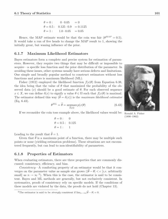
6.1 Theory of Statistics 101
θ = 0 : 0 · 0.05 = 0θ = 0.5 : 0.125 · 0.9 = 0.1125θ = 1 : 1.0 · 0.05 = 0.05
Hence, the MAP estimate would be that the coin was fair (θMAP = 0.5).It would take a run of five heads to change the MAP result to 1, showing theinitially great, but waning influence of the prior.
6.1.7 Maximum Likelihood Estimators
Bayes estimators form a complete and precise system for estimation of param-eters. However, they require two things that may be difficult or impossible toacquire—a specific loss function and the prior distribution of the parameter. Inavoiding these issues, other systems usually have serious defects and limitations.One simple and broadly popular method to construct estimators without lossfunctions and priors is maximum likelihood (ML).
Fisher (1912) employed the likelihood function f(x|θ) from Equation 6.38,the idea being that the value of θ that maximized the probability of the ob-served data (x) should be a good estimate of θ. For each observed sequencex ∈ X, we can define δ(x) to signify a value θ ∈ Ω such that f(x|θ) is maximal.The estimator defined this way (θ = δ(x)) is the maximum likelihood estimator(Eq. 6.43).
θML = θ = argmaxθ∈Ω
p(x|θ) (6.43)
Ronald A. Fisher(1890–1962)
If we reconsider the coin toss example above, the likelihood values would be:
θ = 0 : 0θ = 0.5 : 0.125θ = 1 : 1
Leading to the result that θ = 1.Given that θ is a maximum point of a function, there may be multiple such
points or none (yielding estimation problems). These situations are not encoun-tered frequently, but can lead to non-identifiability of parameters.
6.1.8 Properties of Estimators
When evaluating estimators, there are three properties that are commonly dis-cussed: consistency, efficiency, and bias.
Consistency—A comforting property of an estimator would be that it con-verges on the parameter value as sample size grows (|θ − θ| < ε [i,e. arbitrarilysmall] as n → ∞ 2). When this is the case, the estimator is said to be consis-tent. Bayes and ML methods are generally, but not exclusively consistent. Insystematics, proofs of consistency rely on specific models. If the conditions ofthese models are violated by the data, the proofs do not hold (Chapter 13).
2The estimator is said to be strongly consistent if limn→∞|θ − θ| = 0.
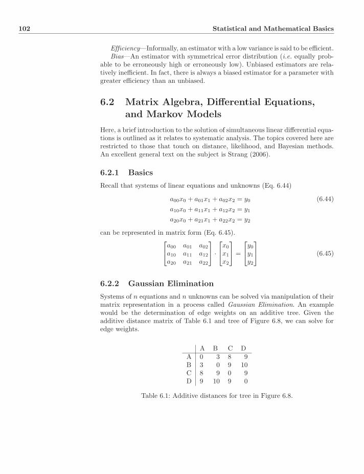
102 Statistical and Mathematical Basics
Efficiency—Informally, an estimator with a low variance is said to be efficient.Bias—An estimator with symmetrical error distribution (i.e. equally prob-
able to be erroneously high or erroneously low). Unbiased estimators are rela-tively inefficient. In fact, there is always a biased estimator for a parameter withgreater efficiency than an unbiased.
6.2 Matrix Algebra, Differential Equations,and Markov Models
Here, a brief introduction to the solution of simultaneous linear differential equa-tions is outlined as it relates to systematic analysis. The topics covered here arerestricted to those that touch on distance, likelihood, and Bayesian methods.An excellent general text on the subject is Strang (2006).
6.2.1 Basics
Recall that systems of linear equations and unknowns (Eq. 6.44)
a00x0 + a01x1 + a02x2 = y0 (6.44)a10x0 + a11x1 + a12x2 = y1
a20x0 + a21x1 + a22x2 = y2
can be represented in matrix form (Eq. 6.45).⎡⎣a00 a01 a02
a10 a11 a12
a20 a21 a22
⎤⎦ ·
⎡⎣x0
x1
x2
⎤⎦ =
⎡⎣y0
y1
y2
⎤⎦ (6.45)
6.2.2 Gaussian Elimination
Systems of n equations and n unknowns can be solved via manipulation of theirmatrix representation in a process called Gaussian Elimination. An examplewould be the determination of edge weights on an additive tree. Given theadditive distance matrix of Table 6.1 and tree of Figure 6.8, we can solve foredge weights.
A B C DA 0 3 8 9B 3 0 9 10C 8 9 0 9D 9 10 9 0
Table 6.1: Additive distances for tree in Figure 6.8.
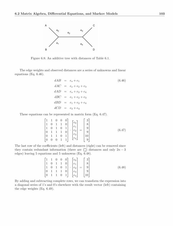
6.2 Matrix Algebra, Differential Equations, and Markov Models 103
A
B
C
D
e0
e1
e2
e3
e4
Figure 6.8: An additive tree with distances of Table 6.1.
The edge weights and observed distances are a series of unknowns and linearequations (Eq. 6.46).
dAB = eo + e1 (6.46)
dAC = eo + e2 + e3
dAD = eo + e2 + e4
dBC = e1 + e2 + e3
dBD = e1 + e2 + e4
dCD = e3 + e4
These equations can be represented in matrix form (Eq. 6.47).⎡⎢⎢⎢⎢⎢⎢⎣
1 1 0 0 01 0 1 1 01 0 1 0 10 1 1 1 00 1 1 0 10 0 0 1 1
⎤⎥⎥⎥⎥⎥⎥⎦·
⎡⎢⎢⎢⎢⎣
e0
e1
e2
e3
e4
⎤⎥⎥⎥⎥⎦ =
⎡⎢⎢⎢⎢⎢⎢⎣
3899
109
⎤⎥⎥⎥⎥⎥⎥⎦
(6.47)
The last row of the coefficients (left) and distances (right) can be removed sincethey contain redundant information (there are
(n2
)distances and only 2n − 3
edges) leaving 5 equations and 5 unknowns (Eq. 6.48).⎡⎢⎢⎢⎢⎣
1 1 0 0 01 0 1 1 01 0 1 0 10 1 1 1 00 1 1 0 1
⎤⎥⎥⎥⎥⎦ ·
⎡⎢⎢⎢⎢⎣
e0
e1
e2
e3
e4
⎤⎥⎥⎥⎥⎦ =
⎡⎢⎢⎢⎢⎣
3899
10
⎤⎥⎥⎥⎥⎦ (6.48)
By adding and subtracting complete rows, we can transform the expression intoa diagonal series of 1’s and 0’s elsewhere with the result vector (left) containingthe edge weights (Eq. 6.49).
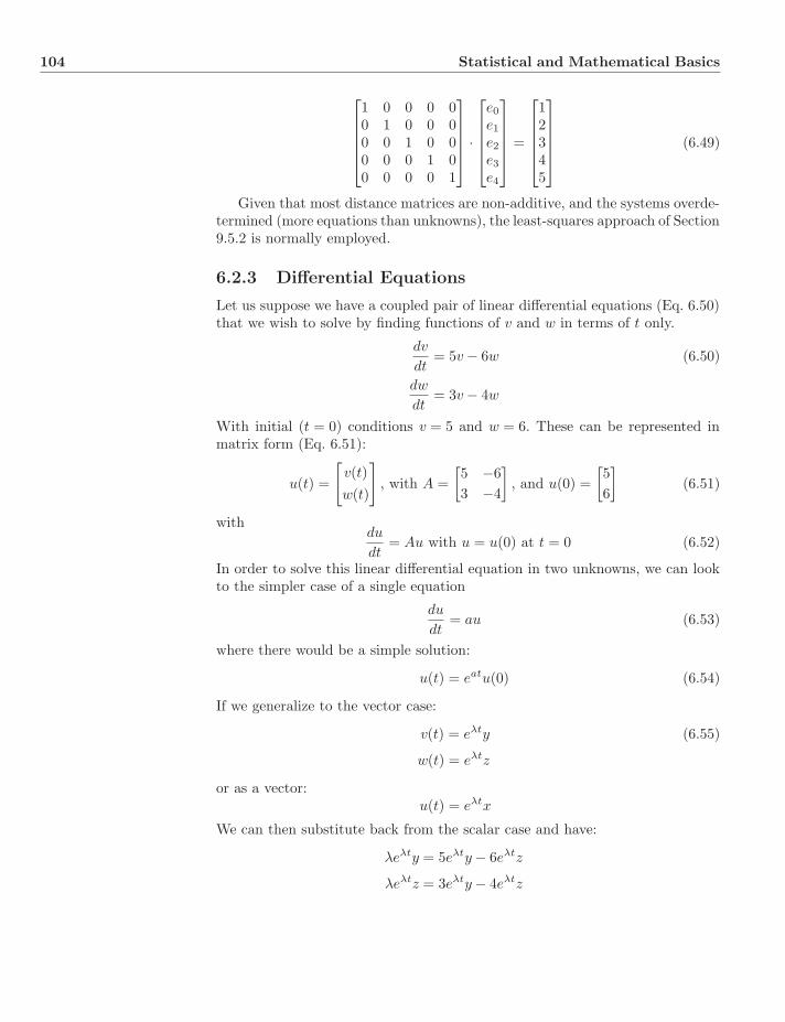
104 Statistical and Mathematical Basics
⎡⎢⎢⎢⎢⎣
1 0 0 0 00 1 0 0 00 0 1 0 00 0 0 1 00 0 0 0 1
⎤⎥⎥⎥⎥⎦ ·
⎡⎢⎢⎢⎢⎣
e0
e1
e2
e3
e4
⎤⎥⎥⎥⎥⎦ =
⎡⎢⎢⎢⎢⎣
12345
⎤⎥⎥⎥⎥⎦ (6.49)
Given that most distance matrices are non-additive, and the systems overde-termined (more equations than unknowns), the least-squares approach of Section9.5.2 is normally employed.
6.2.3 Differential Equations
Let us suppose we have a coupled pair of linear differential equations (Eq. 6.50)that we wish to solve by finding functions of v and w in terms of t only.
dv
dt= 5v − 6w (6.50)
dw
dt= 3v − 4w
With initial (t = 0) conditions v = 5 and w = 6. These can be represented inmatrix form (Eq. 6.51):
u(t) =
[v(t)w(t)
], with A =
[5 −63 −4
], and u(0) =
[56
](6.51)
withdu
dt= Au with u = u(0) at t = 0 (6.52)
In order to solve this linear differential equation in two unknowns, we can lookto the simpler case of a single equation
du
dt= au (6.53)
where there would be a simple solution:
u(t) = eatu(0) (6.54)
If we generalize to the vector case:
v(t) = eλty (6.55)
w(t) = eλtz
or as a vector:u(t) = eλtx
We can then substitute back from the scalar case and have:
λeλty = 5eλty − 6eλtz
λeλtz = 3eλty − 4eλtz

6.2 Matrix Algebra, Differential Equations, and Markov Models 105
This can be represented as the eigenvalue problem:5y − 6z = λy (6.56)
3y − 4z = λz
yielding the eigenvalue equationAx = λx (6.57)
where λ is an eigenvalue and x is its associated eigenvector.
6.2.4 Determining Eigenvalues
λ is an eigenvalue of A if and only if A − λI is a “singular” matrix, meaningthat the determinant must be equal to zero (Eq. 6.58).
det(A − λI) = 0 (6.58)
The determinant is a value associated with a matrix, which can be quite labo-rious (naıvely O(n3), not so naıvely O(n2.376)) to calculate. In this simple caseof a 2 x 2 matrix, the determinant can be calculated easily (Eq. 6.59).
B =[a bc d
](6.59)
det|B| = ad − bc
Hence, we seek the determinant of
B =[a − λ b
c d − λ
](6.60)
yielding:det|B − λI| = (a − λ)(d − λ) − bc = 0
So for Equation 6.51:
det|A − λI| = (5 − λ)(−4 − λ) − (−18) = 0 (6.61)
This rearranges to λ2 − λ − 2, the characteristic polynomial of A with solutionsλ = (−1, 2). By solving back into the original matrix form, we determine theeigenvectors x1 and x2.
λ1 = −1 → (A − λ1I)x1 =[6 −63 −3
] [yz
]=
[00
](6.62)
x1 =[11
](6.63)
λ2 = 2 → (A − λ1I)x2 =[3 −63 −6
] [yz
]=
[00
](6.64)
x2 =[21
](6.65)

106 Statistical and Mathematical Basics
In general, there will be k eigenvalues and eigenvectors for k equations of kvariables.
The complete solution has the form:
u(t) =k∑
i=1
cieλitxi (6.66)
We can then solve back given each eigenvalue and generate our final solution(Eq. 6.67).
u(t) = c1e−t
[11
]+ c2e
2t
[21
](6.67)
For initial conditions (t = 0):
c1x1 + c2x2 = u(0) (6.68)[1 21 1
] [c1
c2
]=
[56
](6.69)
Resulting in:
u(t) = 7e−t
[11
]− e2t
[21
](6.70)
or in the original non-matrix form Eq. 6.71.
v(t) = 7e−t − 2e2t (6.71)
w(t) = 7e−t − e2t
6.2.5 Markov Matrices
A stochastic process where the probability of a successor event is solely depen-dent on its current state (not past) is called a Markov process. Markov processesare employed in character transformation models due to this memoryless prop-erty. As an example from DNA sequences, the probability of an A substituting toa T has nothing to do with whether the A was previously a C, G, or anything else.
A special class of matrix differential equations that models this sort of pro-cess employs a Markov or stationary matrix. In these matrices, the sum of thesolutions is fixed (nothing is gained or lost—only transitioned among states) soeach column sums to 1, and all entries are positive (e.g. Eq. 6.72).
Andrei Markov(1856–1922)
M =
⎡⎢⎢⎣
.7 .1 .1 .1
.1 .7 .1 .1
.1 .1 .7 .1
.1 .1 .1 .7
⎤⎥⎥⎦ (6.72)
In the discrete case, the maximum eigenvalue is always equal to 1 and theothers ≤ 1. As a result, as time steps increase (in essence, multiplication by the

6.3 Exercises 107
Markov transition matrix) the terms derived from the non-dominant (i.e. < 1)eigenvalues diminish and limit to zero, resulting in the steady-state condition.
Continuous time Markov processes are a related form where the net rateof change is zero. In this case, the transition probabilities represented in thecolumns of the matrix sum to zero. As an example, we might have a mutationmatrix with equal forward and reverse rates between states 0 and 1 (μ0↔0 =μ0↔1, μ = μ0↔0 + μ0↔1) (Eq. 6.73).
M =
[−μ
2μ2
μ2 −μ
2
](6.73)
The characteristic polynomial and eigenvalues of M are determined as above(Eq. 6.75).
λ2 + μλ = 0 (6.74)
λ = {0,−μ}
For continuous Markov processes, λmax = 0 in all cases.
This yields eigenvectors {[11
],
[1−1
]}. Solving for the general form with ini-
tial conditions[10
], yields the familiar equation for a two state character.
Pi=j(t) = 0.5 + 0.5e−μt (6.75)
Pi�=j(t) = 0.5 − 0.5e−μt
6.3 Exercises
1. What is the probability of fair coin toss outcome H, H, T, T, T?
2. What are the mean and variance of the estimate of probability of headsin the coin toss experiment of the previous question?
3. What is the probability of tossing a fair coin five times with outcome2H, 3T?
4. Consider the coin toss outcome H, T, H, T, T. There are seven possi-ble values for the probability of heads (θ = 0.01, 0.2, 0.4, 0.5, 0.6, 0.8, 1.0).Consider two prior distributions on θ, uniform and 1
θ . What are the valuesfor θMAP and θML for these observations and the two priors? What arethe posterior probabilities for the MAP solutions? What is the effect ofthe uniform prior on θMAP compared to θML?
5. Consider the tree of Figure 6.8. Using additive distance matrix, Table 6.2,determine the edge weights.
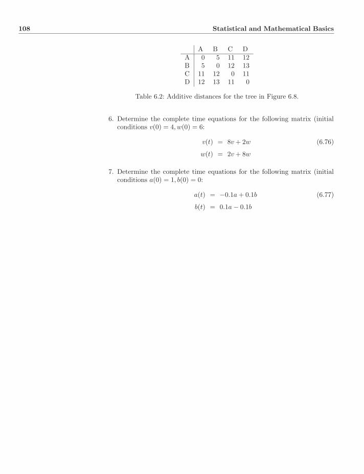
108 Statistical and Mathematical Basics
A B C DA 0 5 11 12B 5 0 12 13C 11 12 0 11D 12 13 11 0
Table 6.2: Additive distances for the tree in Figure 6.8.
6. Determine the complete time equations for the following matrix (initialconditions v(0) = 4, w(0) = 6:
v(t) = 8v + 2w (6.76)
w(t) = 2v + 8w
7. Determine the complete time equations for the following matrix (initialconditions a(0) = 1, b(0) = 0:
a(t) = −0.1a + 0.1b (6.77)
b(t) = 0.1a − 0.1b

Part II
Homology

Chapter 7
Homology
Homology is perhaps the central concept of comparative biology and systemat-ics. First defined by Owen (1843, 1847), the idea has undergone redefinitionand refinement in the succeeding century and a half from pre-evolutionary“same-ness” to the modern cladistic incarnation as an optimized charactertransformation.
7.1 Pre-Evolutionary Concepts
Before evolutionary ideas presented a generative explanation, the observationthat organisms possessed similar parts in similar positions offered biologists abasis for classification. The patterns of similarity and difference were taken asevidence of a natural or super-natural plan and allowed comparative biologists toconstruct classifications and compete them on their ability to explain observedvariation (Hull, 1988).
7.1.1 Aristotle
Pierre Belon(1517–1564)Father of comparative biol-ogy, murdered in the Bois deBoulogne.
The use of anatomical features (Aristotle, 350BCE) to create his classificationimplies comparability between observed features of organisms (e.g. blooded,egg-laying). These similarities among features were organizational and empiri-cal, and perhaps functional, but implied nothing about their origins. For Aris-totle, the similarities and their classifications were statements of organization ofnature. As a result, similar statements could be made about minerals or othernon-living natural phenomena. Aristotle saw a progression of perfection, so tospeak, in moving from “lower” to “higher” forms, but these held no notion ofwhat we would call origins today.
7.1.2 Pierre Belon
Belon’s comparison between the skeleton of a human and bird is striking(Sect. 1.3) not only in its general aspects but in its specific aspects as well.
Systematics: A Course of Lectures, First Edition. Ward C. Wheeler.c© 2012 Ward C. Wheeler. Published 2012 by Blackwell Publishing Ltd.
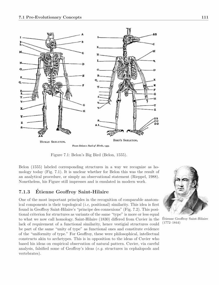
7.1 Pre-Evolutionary Concepts 111
Figure 7.1: Belon’s Big Bird (Belon, 1555).
Belon (1555) labeled corresponding structures in a way we recognize as ho-mology today (Fig. 7.1). It is unclear whether for Belon this was the result ofan analytical procedure, or simply an observational statement (Rieppel, 1988).Nonetheless, his Figure still impresses and is emulated in modern work.
7.1.3 Etienne Geoffroy Saint-Hilaire
Etienne Geoffroy Saint-Hilaire(1772–1844)
One of the most important principles in the recognition of comparable anatom-ical components is their topological (i.e, positional) similarity. This idea is firstfound in Geoffroy Saint-Hilaire’s “principe des connexions” (Fig. 7.2). This posi-tional criterion for structures as variants of the same “type” is more or less equalto what we now call homology. Saint-Hilaire (1830) differed from Cuvier in thelack of requirement of a functional similarity, hence vestigial structures couldbe part of the same “unity of type” as functional ones and constitute evidenceof the “uniformity of type.” For Geoffroy, these were philosophical, intellectualconstructs akin to archetypes. This is in opposition to the ideas of Cuvier whobased his ideas on empirical observation of natural pattern. Cuvier, via carefulanalysis, falsified some of Geoffroy’s ideas (e.g. structures in cephalopods andvertebrates).
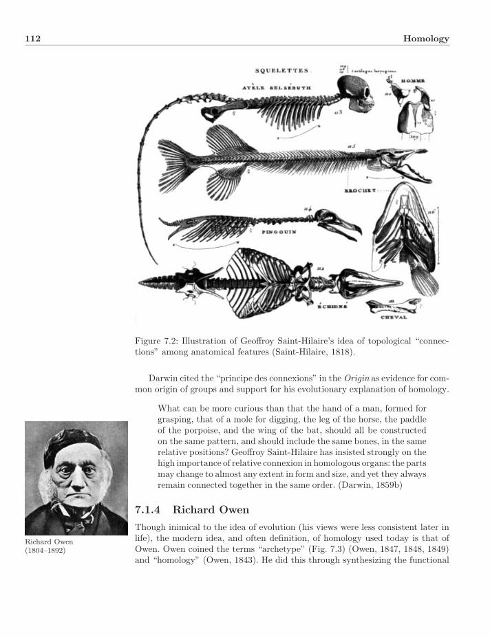
112 Homology
Figure 7.2: Illustration of Geoffroy Saint-Hilaire’s idea of topological “connec-tions” among anatomical features (Saint-Hilaire, 1818).
Darwin cited the “principe des connexions” in the Origin as evidence for com-mon origin of groups and support for his evolutionary explanation of homology.
What can be more curious than that the hand of a man, formed forgrasping, that of a mole for digging, the leg of the horse, the paddleof the porpoise, and the wing of the bat, should all be constructedon the same pattern, and should include the same bones, in the samerelative positions? Geoffroy Saint-Hilaire has insisted strongly on thehigh importance of relative connexion in homologous organs: the partsmay change to almost any extent in form and size, and yet they alwaysremain connected together in the same order. (Darwin, 1859b)
7.1.4 Richard Owen
Richard Owen(1804–1892)
Though inimical to the idea of evolution (his views were less consistent later inlife), the modern idea, and often definition, of homology used today is that ofOwen. Owen coined the terms “archetype” (Fig. 7.3) (Owen, 1847, 1848, 1849)and “homology” (Owen, 1843). He did this through synthesizing the functional
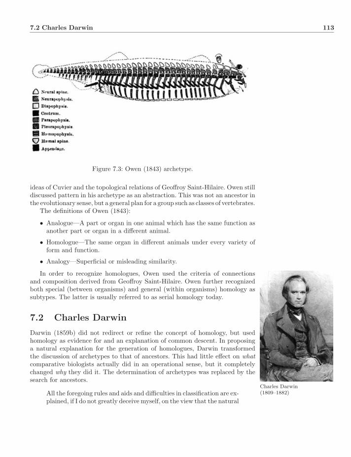
7.2 Charles Darwin 113
Figure 7.3: Owen (1843) archetype.
ideas of Cuvier and the topological relations of Geoffroy Saint-Hilaire. Owen stilldiscussed pattern in his archetype as an abstraction. This was not an ancestor inthe evolutionary sense, but a general plan for a group such as classes of vertebrates.
The definitions of Owen (1843):
• Analogue—A part or organ in one animal which has the same function asanother part or organ in a different animal.
• Homologue—The same organ in different animals under every variety ofform and function.
• Analogy—Superficial or misleading similarity.
In order to recognize homologues, Owen used the criteria of connectionsand composition derived from Geoffroy Saint-Hilaire. Owen further recognizedboth special (between organisms) and general (within organisms) homology assubtypes. The latter is usually referred to as serial homology today.
7.2 Charles Darwin
Darwin (1859b) did not redirect or refine the concept of homology, but usedhomology as evidence for and an explanation of common descent. In proposinga natural explanation for the generation of homologues, Darwin transformedthe discussion of archetypes to that of ancestors. This had little effect on whatcomparative biologists actually did in an operational sense, but it completelychanged why they did it. The determination of archetypes was replaced by thesearch for ancestors.
Charles Darwin(1809–1882)All the foregoing rules and aids and difficulties in classification are ex-
plained, if I do not greatly deceive myself, on the view that the natural
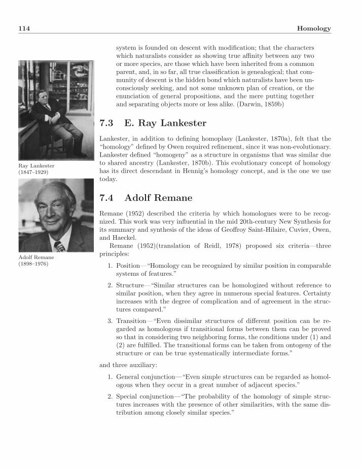
114 Homology
system is founded on descent with modification; that the characterswhich naturalists consider as showing true affinity between any twoor more species, are those which have been inherited from a commonparent, and, in so far, all true classification is genealogical; that com-munity of descent is the hidden bond which naturalists have been un-consciously seeking, and not some unknown plan of creation, or theenunciation of general propositions, and the mere putting togetherand separating objects more or less alike. (Darwin, 1859b)
7.3 E. Ray Lankester
Lankester, in addition to defining homoplasy (Lankester, 1870a), felt that the“homology” defined by Owen required refinement, since it was non-evolutionary.Lankester defined “homogeny” as a structure in organisms that was similar dueto shared ancestry (Lankester, 1870b). This evolutionary concept of homologyhas its direct descendant in Hennig’s homology concept, and is the one we usetoday.
Ray Lankester(1847–1929)
7.4 Adolf Remane
Remane (1952) described the criteria by which homologues were to be recog-nized. This work was very influential in the mid 20th-century New Synthesis forits summary and synthesis of the ideas of Geoffroy Saint-Hilaire, Cuvier, Owen,and Haeckel.
Adolf Remane(1898–1976)
Remane (1952)(translation of Reidl, 1978) proposed six criteria—threeprinciples:
1. Position—“Homology can be recognized by similar position in comparablesystems of features.”
2. Structure—“Similar structures can be homologized without reference tosimilar position, when they agree in numerous special features. Certaintyincreases with the degree of complication and of agreement in the struc-tures compared.”
3. Transition—“Even dissimilar structures of different position can be re-garded as homologous if transitional forms between them can be provedso that in considering two neighboring forms, the conditions under (1) and(2) are fulfilled. The transitional forms can be taken from ontogeny of thestructure or can be true systematically intermediate forms.”
and three auxiliary:
1. General conjunction—“Even simple structures can be regarded as homol-ogous when they occur in a great number of adjacent species.”
2. Special conjunction—“The probability of the homology of simple struc-tures increases with the presence of other similarities, with the same dis-tribution among closely similar species.”
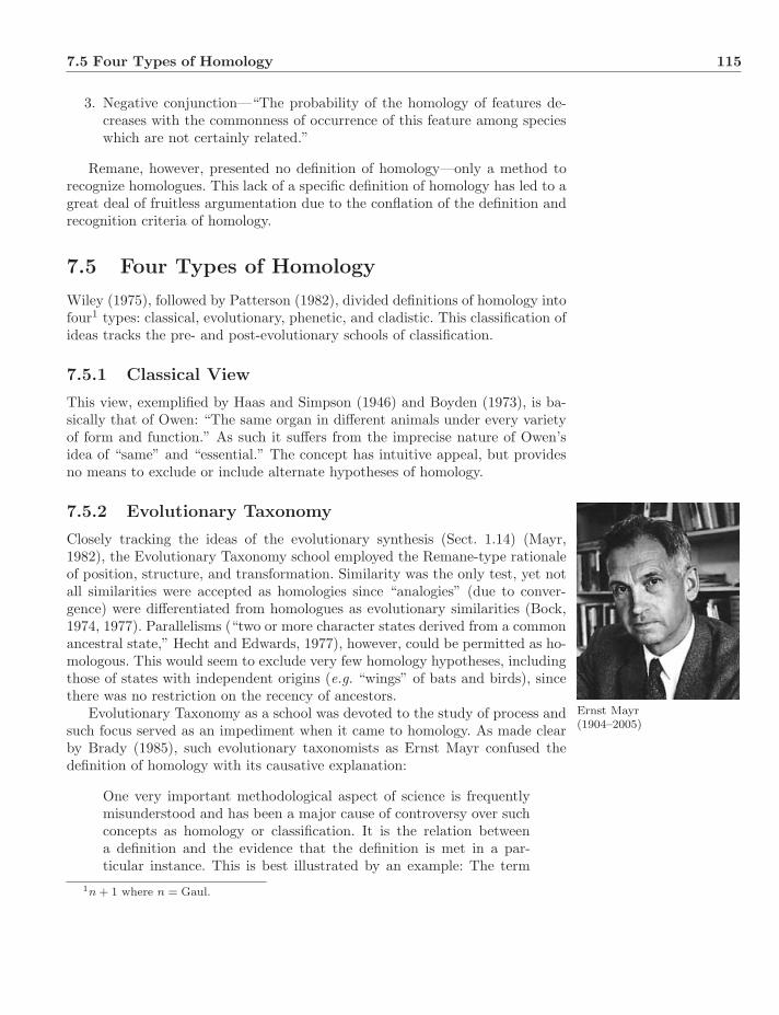
7.5 Four Types of Homology 115
3. Negative conjunction—“The probability of the homology of features de-creases with the commonness of occurrence of this feature among specieswhich are not certainly related.”
Remane, however, presented no definition of homology—only a method torecognize homologues. This lack of a specific definition of homology has led to agreat deal of fruitless argumentation due to the conflation of the definition andrecognition criteria of homology.
7.5 Four Types of Homology
Wiley (1975), followed by Patterson (1982), divided definitions of homology intofour1 types: classical, evolutionary, phenetic, and cladistic. This classification ofideas tracks the pre- and post-evolutionary schools of classification.
7.5.1 Classical View
This view, exemplified by Haas and Simpson (1946) and Boyden (1973), is ba-sically that of Owen: “The same organ in different animals under every varietyof form and function.” As such it suffers from the imprecise nature of Owen’sidea of “same” and “essential.” The concept has intuitive appeal, but providesno means to exclude or include alternate hypotheses of homology.
7.5.2 Evolutionary Taxonomy
Closely tracking the ideas of the evolutionary synthesis (Sect. 1.14) (Mayr,1982), the Evolutionary Taxonomy school employed the Remane-type rationaleof position, structure, and transformation. Similarity was the only test, yet notall similarities were accepted as homologies since “analogies” (due to conver-gence) were differentiated from homologues as evolutionary similarities (Bock,1974, 1977). Parallelisms (“two or more character states derived from a commonancestral state,” Hecht and Edwards, 1977), however, could be permitted as ho-mologous. This would seem to exclude very few homology hypotheses, includingthose of states with independent origins (e.g. “wings” of bats and birds), sincethere was no restriction on the recency of ancestors.
Ernst Mayr(1904–2005)
Evolutionary Taxonomy as a school was devoted to the study of process andsuch focus served as an impediment when it came to homology. As made clearby Brady (1985), such evolutionary taxonomists as Ernst Mayr confused thedefinition of homology with its causative explanation:
One very important methodological aspect of science is frequentlymisunderstood and has been a major cause of controversy over suchconcepts as homology or classification. It is the relation betweena definition and the evidence that the definition is met in a par-ticular instance. This is best illustrated by an example: The term
1n + 1 where n = Gaul.
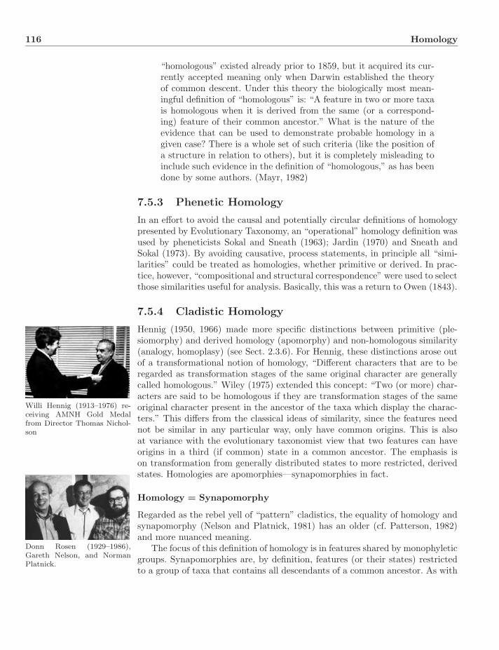
116 Homology
“homologous” existed already prior to 1859, but it acquired its cur-rently accepted meaning only when Darwin established the theoryof common descent. Under this theory the biologically most mean-ingful definition of “homologous” is: “A feature in two or more taxais homologous when it is derived from the same (or a correspond-ing) feature of their common ancestor.” What is the nature of theevidence that can be used to demonstrate probable homology in agiven case? There is a whole set of such criteria (like the position ofa structure in relation to others), but it is completely misleading toinclude such evidence in the definition of “homologous,” as has beendone by some authors. (Mayr, 1982)
7.5.3 Phenetic Homology
In an effort to avoid the causal and potentially circular definitions of homologypresented by Evolutionary Taxonomy, an “operational” homology definition wasused by pheneticists Sokal and Sneath (1963); Jardin (1970) and Sneath andSokal (1973). By avoiding causative, process statements, in principle all “simi-larities” could be treated as homologies, whether primitive or derived. In prac-tice, however, “compositional and structural correspondence” were used to selectthose similarities useful for analysis. Basically, this was a return to Owen (1843).
7.5.4 Cladistic Homology
Willi Hennig (1913–1976) re-ceiving AMNH Gold Medalfrom Director Thomas Nichol-son
Hennig (1950, 1966) made more specific distinctions between primitive (ple-siomorphy) and derived homology (apomorphy) and non-homologous similarity(analogy, homoplasy) (see Sect. 2.3.6). For Hennig, these distinctions arose outof a transformational notion of homology, “Different characters that are to beregarded as transformation stages of the same original character are generallycalled homologous.” Wiley (1975) extended this concept: “Two (or more) char-acters are said to be homologous if they are transformation stages of the sameoriginal character present in the ancestor of the taxa which display the charac-ters.” This differs from the classical ideas of similarity, since the features neednot be similar in any particular way, only have common origins. This is alsoat variance with the evolutionary taxonomist view that two features can haveorigins in a third (if common) state in a common ancestor. The emphasis ison transformation from generally distributed states to more restricted, derivedstates. Homologies are apomorphies—synapomorphies in fact.
Homology = Synapomorphy
Regarded as the rebel yell of “pattern” cladistics, the equality of homology andsynapomorphy (Nelson and Platnick, 1981) has an older (cf. Patterson, 1982)and more nuanced meaning.
Donn Rosen (1929–1986),Gareth Nelson, and NormanPlatnick.
The focus of this definition of homology is in features shared by monophyleticgroups. Synapomorphies are, by definition, features (or their states) restrictedto a group of taxa that contains all descendants of a common ancestor. As with
7.5 Four Types of Homology 117
Wiley’s definition above, an attribute found in the common ancestor and its de-scendants is homologous and a synapomorphy (e.g. wings in pterygote insects).A symplesiomorphy is simply a synapomorphy of a more inclusive group, homol-ogous at that level (e.g. having six legs in Pterygota, plesiomorphic at that level,but a synapomorphy for the more including Hexapoda). Hence, a homology isalways a synapomorphy, (if at a more general level) and a synapomorphy isalways a homology. Furthermore, this definition immediately offers a test. Eachhomology statement, as a synapomorphy, is tested through congruence withother features. If the weight of evidence were to support an alternate scheme,where members of the group possessing a feature were not monophyletic, the hy-pothesis of homology would be falsified. Homologies can be proposed by multipleroutes, but are always tested and potentially falsified by the same congruence-based process2. Brady (1985) traces this idea back to at least Darwin:
The importance, for classification, of trifling characters, mainly de-pends on their being correlated with several other characters of moreor less importance. The value indeed of an aggregate of characters isvery evident in natural history. Hence, as has often been remarked, aspecies may depart from its allies in several characters, both of highphysiological importance and of almost universal prevalence, and yetleave us in no doubt where it should be ranked. Hence, also, it hasbeen found, that a classification founded on any single character,however important that may be, has always failed; for no part of theorganization is universally constant. The importance of an aggregateof characters, even when none are important, alone explains, I think,that saying of Linnaeus, that the characters do not give the genus,but the genus gives the characters; for this saying seems founded onan appreciation of many trifling points of resemblance, too slight tobe defined. (Darwin, 1859b)
7.5.5 Types of Homology
In his review of homology, Patterson (1982) enumerated several types and modesof homology identification and distinguished these from tests. Patterson (1988)further associated terms in use in molecular evolution with their correspondingrelation in morphological comparisons. These relations are organized aroundthree “tests” of homology: congruence (agreement with other characters), simi-larity (likeness in form), and conjunction (discussed above). Only homology (orthe molecular, orthology) meets all three criteria (Table 7.1).
DePinna (1991) refined the ideas of Patterson, defining “primary” and “sec-ondary” homology. A primary homology was a putative homology statementthat had passed the tests of similarity and position, but was as yet untested ona cladogram. DePinna pointed out that the only real test was that of congruence.
2Patterson (1982) also proposed “conjunction,” the presence of two features in a singleorganism (as in wings and forelimbs in “angels”), as a potential falsifier of homology. DePinna(1991) and others have pointed out that such angels can occur as forms of homology (e.g. denovo character origination), leaving congruence as the only absolute test of homology.

118 Homology
Relation Congruence Similarity Conjunction MolecularTest Test Test Term
Homology Pass Pass Pass OrthologyHomonomy Pass Pass Fail ParalogyComplement Pass Fail Pass ComplementTwo homologies Pass Fail Fail Two orthologiesParallelism Fail Pass Pass XenologyHomoeosis Fail Pass Fail ParaxenologyConvergence Fail Fail Pass ConvergenceEndoparasitism Fail Fail Fail -
Table 7.1: Combinatorics of homology and non-homology relations after Patter-son (1982, 1988).
A secondary homology had passed this test with a unique origin on a parsimo-nious cladogram.
7.6 Dynamic and Static Homology
Molecular sequence data presented an interesting challenge to homology deter-mination. These sequences could vary not only in state (elements of the se-quence) but in length as well. At first, when compared among multiple taxa,such variation was placed in the traditional context of putatively homologous(= comparable) columns via a formal or informal alignment process (Chap-ter 8). However, when these sequences were examined directly on trees, it wasimmediately obvious that the putative homology schemes could vary among treetopologies. Some scenarios of putative sequence homology require more trans-formations (however weighted) on a given tree than others. In essence, thatthe congruence principle existed not only between topologies, but within, andapplied to the determination of characters themselves as well at to the disposi-tion of their states. The idea that even putative homology schemes could varyamong trees was termed dynamic homology (Wheeler, 2001b) to distinguish itfrom those schemes that were invariant over topologies (such as many complexanatomical attributes, for example, forelimbs in tetrapods). Such dynamic ho-mologies are not limited to molecular data, but can be found in other sequencessuch as developmental events, call songs in insects, and even “serial” homol-ogy of anatomical features in segmented organisms (Schulmeister and Wheeler,2004; Robillard et al., 2006; Ramırez, 2007).
Salvatore “Lucky” Luciano(1897–1962)
One of the hallmarks of dynamic homology is the lack of transitivity amongsequence elements in taxa (Fig. 7.4). While a forelimb in taxon A, B, and Cis comparable, that of “the third Guanine residue in taxon A” will have mul-tiple potential comparable elements in other taxa. This was formalized in thedefinition of static and dynamic characters (Varon et al., 2010):
Static homology characters. Let A and B be two states of a character.A correspondence between the elements in A and B is a relation

7.6 Dynamic and Static Homology 119
I. AAATTT
II. TTT
III. AAA
I/II
II/III
III/I
AAATTTTTT
TTTAAA
AAATTTAAA
AAATTT
TTT
AAA
Figure 7.4: Non-transitive nature of the relationship among dynamic homologysequence elements (after Wheeler, 2001b).
between them. We define static homology characters as those inwhich for every element in A there is at most one correspondingelement in B, and the correspondence relations are transitive (i.e.let a ∈ A, b ∈ B, and c ∈ C be elements of different states, where acorresponds to b, and b corresponds to c; then a and c must alsocorrespond to each other). Corresponding elements with the samevalue match the notion of primary homology (DePinna, 1991).
Dynamic homology characters. We define as dynamic homology char-acters (Wheeler, 2001b) the complement of their static homologycounterparts: for some pair of states A and B, there exists an ele-ment a ∈ A that has more than one corresponding element in B, orthe correspondences are not transitive. Dynamic homology charac-ters typically have states that may have different cardinalities, andno putative homology statements among the state elements. Thesecharacters formalize the multiple possibilities in the assignment ofcorrespondences (primary homologies) between the elements in apair of states, which can only be inferred from a transformation se-ries linking the states, and the distance function of choice.
With dynamic homology, the principle of connections of Geoffroy Saint-Hilaire drives the optimality function, and the test is still one of congruence(if more generally). Position, composition, and congruence are simultaneouslyand quantitatively optimized and tested (as in Brady, 1985).
This leads to a further modification of the homology definition:
Features are homologous when their origins can be traced to a uniquetransformation on the branch of a cladogram leading to their mostrecent common ancestor (Wheeler et al., 2006a).
120 Homology
In the end, the central issue is whether aspects of organisms have single ormultiple origins. If single, they are homologous; if not, not.
7.7 Exercises
1. Discuss the example of wings in birds, bats, pterosaurs, and moths interms of the homology definitions discussed above. Under what conditionsare these structures homologous?
2. What are the issues involved in the homology of therapod hind limb digits?Discuss these digit homology scenarios in terms of positional, developmen-tal, and dynamic homology frameworks.
3. “Eyes” are broadly distributed, but not uniformly present, in Metazoa.Discuss homology in this context. Are the “eyes” of cephalopods and verte-brates homologous? How would the underlying genetic mechanisms affectthis determination?
Chapter 8
Sequence Alignment
8.1 Background
Traditional analysis of sequence data (Chapters 9, 10, 11, and 12) requires an apriori scheme of correspondences among the observed sequence elements. Giventhat sequence data can vary in length, a process is required to convert thevariable-length sequence data into constant-length aligned data suitable for thisform of character-based optimization. Sequence alignment (or Multiple SequenceAlignment—MSA when there are more that two sequences) is this process.
Sequences can be composed of a variety of objects, from familiar nucleicacid and protein data to observations less frequently treated as sequences suchas developmental, behavioral, and chromosomal data. As pre-aligned characters,MSA can be performed under a variety of criteria. This section will focus oncost minimization (= parsimony), and later sections will take up others (Chap-ters 11 and 12). MSA is not a necessary prerequisite for phylogenetic analysis(Sect. 10.6), but it is a common one.
8.2 “Informal” Alignment
The discussion here is limited to alignment procedures that are precisely definedboth in methodology and objective. There will be no discussion of “by-eye”alignment or subjective hand adjustments made to alignments generated withsoftware tools. Such operations, to the extent that they are ill-defined and notbased in optimizing objective measures of quality, are better discussed elsewhere.
8.3 Sequences
Sequences are linear arrays of elements. As such, they contain two sorts ofinformation—the type of each element and its position relative to other elements.The positional information can come from any one-dimensional ordering suchas body-axis, time and position on a chromosome or within a protein (Fig. 8.1).
Systematics: A Course of Lectures, First Edition. Ward C. Wheeler.c© 2012 Ward C. Wheeler. Published 2012 by Blackwell Publishing Ltd.

122 Sequence Alignment
5'-GCAAAAATAACGAT-3'
Start End
ND1-16SrDNA-12SrDNA-CytB-ND6
Head Tail
Figure 8.1: Example sequences. Top: Segment of heteropteran 18S rRNA(Wheeler et al., 1993); Middle Top: Generalized arthropod body plan; MiddleBottom: Orthopteran stridulation (Robillard et al., 2006); Bottom: Fragment ofmtDNA gene order.
Given that organisms (in general) have defined morphologies (with a body-axis) and undergo growth and development (time-axis), this type of data is quitecommonly encountered. When discussing sequences, there are three aspects thatmust be defined: the sequence alphabet, the transformations it may suffer, andan objective distance function to quantify change.
8.3.1 Alphabets
The set of possible elements that may appear in a sequence defines its alphabet(Σ). Familiar alphabets include those for DNA (Σ = {A,C,G, T, gap}), Morsecode (Σ = {dit, dah, short gap,middle gap, long gap}), and arthropod segmentappendages (Σ = {no appendages, antennae, legs,mouthparts}). Locus syntenymaps (such as mtDNA gene order) are sequences of annotated loci with thegenes themselves as alphabet elements (e.g. 18S rRNA). The set of develop-mental events in the lifetime of an organism presents another alphabet. A spe-cial character representing an empty string of characters (λ)—not an elementitself—is often used to represent “gaps” or indels since there are no actual ele-ments present. The gap symbol (“-”) may be used interchangeably with λ. Anygiven sequence is an instantiation of possible elements and is represented as Σ∗.
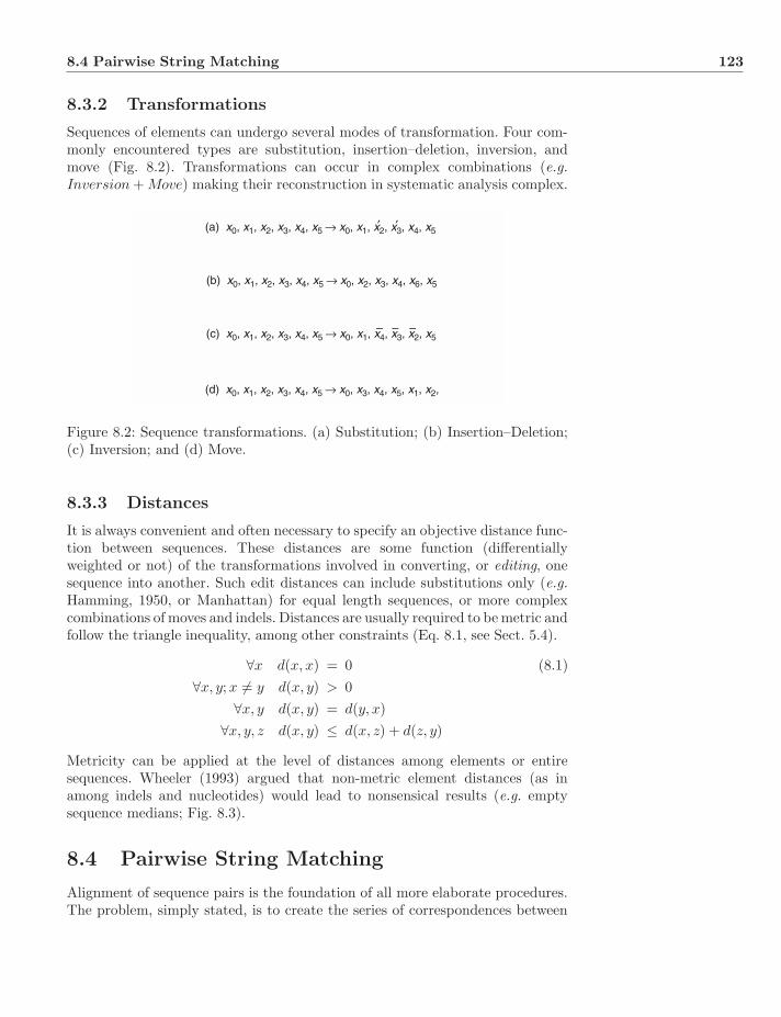
8.4 Pairwise String Matching 123
8.3.2 Transformations
Sequences of elements can undergo several modes of transformation. Four com-monly encountered types are substitution, insertion–deletion, inversion, andmove (Fig. 8.2). Transformations can occur in complex combinations (e.g.Inversion + Move) making their reconstruction in systematic analysis complex.
(b) x0, x1, x2, x3, x4, x5 → x0, x2, x3, x4, x6, x5
(c) x0, x1, x2, x3, x4, x5 → x0, x1, x4, x3, x2, x5
(d) x0, x1, x2, x3, x4, x5 → x0, x3, x4, x5, x1, x2,
– – –
(a) x0, x1, x2, x3, x4, x5 → x0, x1, x2, x3, x4, x5′ ′
Figure 8.2: Sequence transformations. (a) Substitution; (b) Insertion–Deletion;(c) Inversion; and (d) Move.
8.3.3 Distances
It is always convenient and often necessary to specify an objective distance func-tion between sequences. These distances are some function (differentiallyweighted or not) of the transformations involved in converting, or editing, onesequence into another. Such edit distances can include substitutions only (e.g.Hamming, 1950, or Manhattan) for equal length sequences, or more complexcombinations of moves and indels. Distances are usually required to be metric andfollow the triangle inequality, among other constraints (Eq. 8.1, see Sect. 5.4).
∀x d(x, x) = 0 (8.1)∀x, y;x �= y d(x, y) > 0
∀x, y d(x, y) = d(y, x)∀x, y, z d(x, y) ≤ d(x, z) + d(z, y)
Metricity can be applied at the level of distances among elements or entiresequences. Wheeler (1993) argued that non-metric element distances (as inamong indels and nucleotides) would lead to nonsensical results (e.g. emptysequence medians; Fig. 8.3).
8.4 Pairwise String Matching
Alignment of sequence pairs is the foundation of all more elaborate procedures.The problem, simply stated, is to create the series of correspondences between
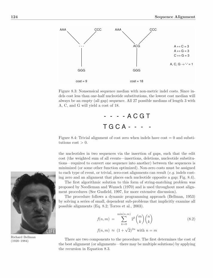
124 Sequence Alignment
A, C, G → '-' = 1
A ↔ C = 3A ↔ G = 3C ↔ G = 3
AAA CCC
GGG
- - -
cost = 9
AAA CCC
GGG
ACG
cost = 18
Figure 8.3: Nonsensical sequence median with non-metric indel costs. Since in-dels cost less than one-half nucleotide substitutions, the lowest cost median willalways be an empty (all gap) sequence. All 27 possible medians of length 3 withA, C, and G will yield a cost of 18.
A C G T
T G C A
----
- - - -
Figure 8.4: Trivial alignment of cost zero when indels have cost = 0 and substi-tutions cost > 0.
the nucleotides in two sequences via the insertion of gaps, such that the editcost (the weighted sum of all events—insertions, deletions, nucleotide substitu-tions—required to convert one sequence into another) between the sequences isminimized (or some other function optimized). Non-zero costs must be assignedto each type of event, or trivial, zero-cost alignments can result (e.g. indels cost-ing zero and an alignment that places each nucleotide opposite a gap; Fig. 8.4).
The first algorithmic solution to this form of string-matching problem wasproposed by Needleman and Wunsch (1970) and is used throughout most align-ment procedures (See Gusfield, 1997, for more extensive discussion).
Richard Bellman(1920–1984)
The procedure follows a dynamic programming approach (Bellman, 1953)by solving a series of small, dependent sub-problems that implicitly examine allpossible alignments (Eq. 8.2; Torres et al., 2003).
f(n,m) =min(n,m)∑
k=0
2k
(m
k
)(n
k
)(8.2)
f(n,m) ≈ (1 +√
2)2n with n = m
There are two components to the procedure. The first determines the cost ofthe best alignment (or alignments—there may be multiple solutions) by applyingthe recursion in Equation 8.3.

8.4 Pairwise String Matching 125
cost[i][j] = min
⎧⎪⎨⎪⎩
cost[i − 1][j − 1] + σi,j match/mismatchcost[i − 1][j] + σindel insertioncost[i][j − 1] + σindel deletion
(8.3)
This is often referred to as the “wavefront” update (Alg. 8.1). The second is the“traceback” (Alg. 8.2), which yields the alignment itself (more complex examples
Algorithm 8.1: PairwiseSequenceAlignmentCostData: Input strings X and Y of lengths |X| and |Y|Data: Element distance matrix σ of pairwise substitution costs between
all elements in Σ and λ (indel)Result: The minimum pairwise alignment cost.Initialize first row and column of matrices;direction [0] [0] ← ‘↘’;cost [0] [0] ← 0;length [0] [0] ← 0;for i = 1 to |X| do
cost [i] [0] ← cost [i − 1] [0] + σXi,λ;direction [i] [0] ← ‘→’;length [i] [0] ← length [i − 1] [0] + 1;
endfor j = 1 to |Y| do
cost [0] [j] ← cost [0] [j − 1] + σYj ,λ;direction [0] [j] ← ‘↓’;length [0] [j] ← length [0] [j − 1] + 1;
endUpdate remainder of matrices cost, direction, and length;for i = 1 to |X| do
for j = 1 to |Y| doins ← cost [i − 1] [j] + σXi,λ;del ← cost [i] [j − 1] + σYj ,λ;sub ← cost [i − 1] [j − 1] + σXi,Yj
;cost [i] [j] ← min (ins, del, sub);if cost [i] [j] = ins then
direction [i] [j] ← ‘→’;length [i] [j] ← length [i − 1] [j] + 1;
else if cost [i] [j] = del thendirection [i] [j] ← ‘↓’;length [i] [j] ← length [i] [j − 1] + 1;
elsedirection [i] [j] ← ‘↘’;length [i] [j] ← length [i − 1] [j − 1] + 1;
endend
endreturn cost [|X|] [|Y|]

126 Sequence Alignment
Algorithm 8.2: PairwiseSequenceAlignmentTracebackData: Strings X and Y of Algorithm 8.1Data: direction matrix of Algorithm 8.1Data: length matrix of Algorithm 8.1Result: X′ and Y′ contain aligned sequences of X and Y via inclusion of
gapsalignCounter ← length [|X|] [|Y|];xCounter ← |X|;yCounter ← |Y|;while xCounter ≥ 0 and yCounter ≥ 0 and alignCounter ≥ 0 do
if direction [i] [j] =‘→’ thenX′ [alignCounter] ← X [xCounter];Y′ [alignCounter] ← GAP;xCounter ← xCounter − 1;alignCounter ← alignCounter − 1;
else if direction [i] [j] =‘↓’ thenX′ [alignCounter] ← GAP;Y′ [alignCounter] ← Y [yCounter];yCounter ← yCounter − 1;alignCounter ← alignCounter − 1;
elseX′ [alignCounter] ← X [xCounter];Y′ [alignCounter] ← Y [yCounter];xCounter ← xCounter − 1;yCounter ← yCounter − 1;alignCounter ← alignCounter − 1;
endend
can be found in Phillips et al. (2000)). Needleman and Wunsch described a maxi-mization of identity algorithm, whereas a minimization of difference is presentedhere. The underlying principles are unchanged.
The first part of the algorithm fills a matrix cost of size (n + 1) × (m + 1)to align a pair of sequences X and Y of lengths n and m respectively. Each cell(i, j) is the cost of aligning the first i characters of a with the first j charactersof b (i.e. aligning x1 · · ·xi and y1 · · · yj). Each value is calculated using thepreviously aligned subsequences—that is the cost of cell (i, j) will be for indeland substitution cost matrix σ.
The additional first row and column (the reason for the +1 in the matrixdimensions) represents the alignment of a sequence with an empty string, thatis, initial gaps. Each decision minimum is recorded, to follow the path that leadsto the cost of aligning X and Y, that is, the cost in cell (n,m).
In order to create the actual alignment between the sequences, a tracebackstep is performed that proceeds back up and to the left of the matrix, keepingtrack of the optimal indels and substitutions performed in the matrix update
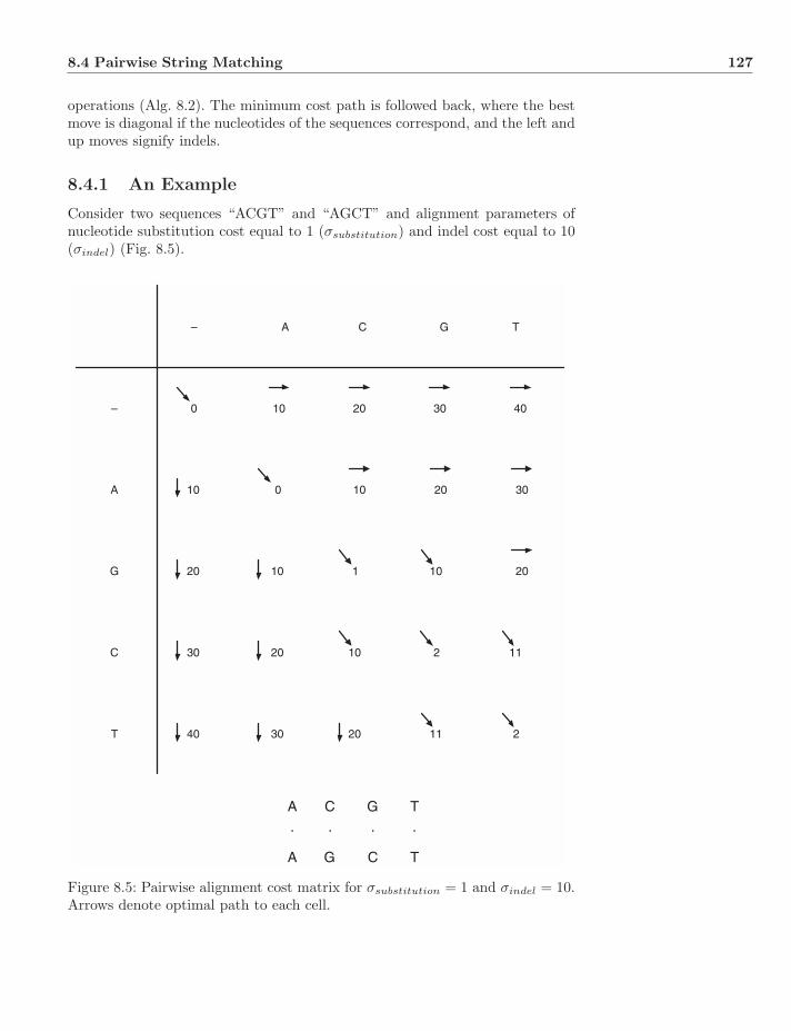
8.4 Pairwise String Matching 127
operations (Alg. 8.2). The minimum cost path is followed back, where the bestmove is diagonal if the nucleotides of the sequences correspond, and the left andup moves signify indels.
8.4.1 An Example
Consider two sequences “ACGT” and “AGCT” and alignment parameters ofnucleotide substitution cost equal to 1 (σsubstitution) and indel cost equal to 10(σindel) (Fig. 8.5).
– A C G T
–
A
G
C
T
0 10 20 30 40
10 20 30
2
10
10 10
11
11 2
20
0
120
20
2030
3040
10
A
A
C
G
G
C
T
T
. . . .
Figure 8.5: Pairwise alignment cost matrix for σsubstitution = 1 and σindel = 10.Arrows denote optimal path to each cell.
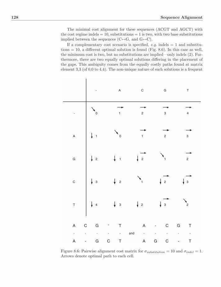
128 Sequence Alignment
The minimal cost alignment for these sequences (ACGT and AGCT) withthe cost regime indels = 10, substitutions = 1 is two, with two base substitutionsimplied between the sequences (C↔G, and G↔C).
If a complementary cost scenario is specified, e.g. indels = 1 and substitu-tions = 10, a different optimal solution is found (Fig. 8.6). In this case as well,the minimum cost is two, but no substitutions are implied—only indels (2). Fur-thermore, there are two equally optimal solutions differing in the placement ofthe gaps. This ambiguity comes from the equally costly paths found at matrixelement 3,3 (of 0,0 to 4,4). The non-unique nature of such solutions is a frequent
- A C G T
-
A
G
C
T
0 1 2 3 4
1 2 3
2
1
1 1
3
3 2
2
0
22
2
23
34
1
A C G T- A - C TG
A G C T-A - G TC
. . . ... . . .. and
Figure 8.6: Pairwise alignment cost matrix for σsubstitution = 10 and σindel = 1.Arrows denote optimal path to each cell.
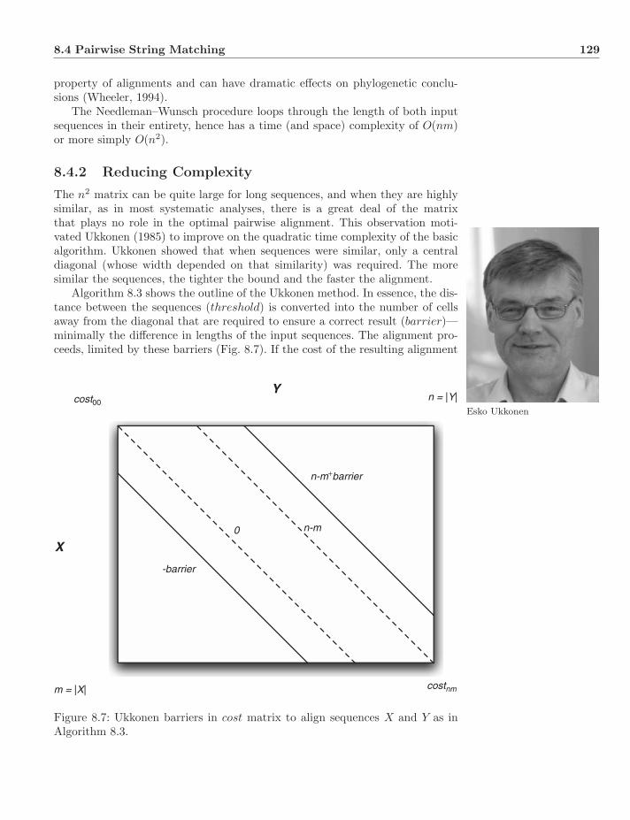
8.4 Pairwise String Matching 129
property of alignments and can have dramatic effects on phylogenetic conclu-sions (Wheeler, 1994).
The Needleman–Wunsch procedure loops through the length of both inputsequences in their entirety, hence has a time (and space) complexity of O(nm)or more simply O(n2).
8.4.2 Reducing Complexity
The n2 matrix can be quite large for long sequences, and when they are highlysimilar, as in most systematic analyses, there is a great deal of the matrixthat plays no role in the optimal pairwise alignment. This observation moti-vated Ukkonen (1985) to improve on the quadratic time complexity of the basicalgorithm. Ukkonen showed that when sequences were similar, only a central
Esko Ukkonen
diagonal (whose width depended on that similarity) was required. The moresimilar the sequences, the tighter the bound and the faster the alignment.
Algorithm 8.3 shows the outline of the Ukkonen method. In essence, the dis-tance between the sequences (threshold) is converted into the number of cellsaway from the diagonal that are required to ensure a correct result (barrier)—minimally the difference in lengths of the input sequences. The alignment pro-ceeds, limited by these barriers (Fig. 8.7). If the cost of the resulting alignment
-barrier
0 n-m
n-m+barrier
n = |Y|
m = |X|
cost00
costnm
X
Y
Figure 8.7: Ukkonen barriers in cost matrix to align sequences X and Y as inAlgorithm 8.3.
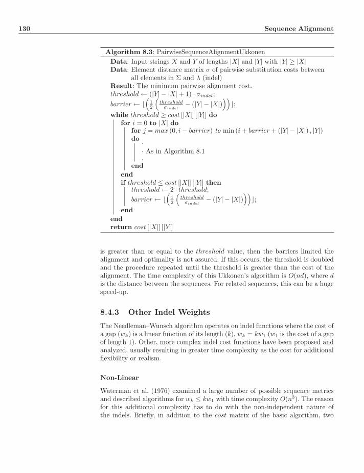
130 Sequence Alignment
Algorithm 8.3: PairwiseSequenceAlignmentUkkonenData: Input strings X and Y of lengths |X| and |Y| with |Y| ≥ |X|Data: Element distance matrix σ of pairwise substitution costs between
all elements in Σ and λ (indel)Result: The minimum pairwise alignment cost.threshold ← (|Y| − |X| + 1) · σindel;barrier ←
(12
(threshold
σindel− (|Y| − |X|)
))�;
while threshold ≥ cost [|X|] [|Y|] dofor i = 0 to |X| do
for j = max (0, i − barrier) to min (i + barrier + (|Y| − |X|) , |Y|)do ·
· As in Algorithm 8.1·
endendif threshold ≤ cost [|X|] [|Y|] then
threshold ← 2 · threshold;barrier ←
(12
(threshold
σindel− (|Y| − |X|)
))�;
endendreturn cost [|X|] [|Y|]
is greater than or equal to the threshold value, then the barriers limited thealignment and optimality is not assured. If this occurs, the threshold is doubledand the procedure repeated until the threshold is greater than the cost of thealignment. The time complexity of this Ukkonen’s algorithm is O(nd), where dis the distance between the sequences. For related sequences, this can be a hugespeed-up.
8.4.3 Other Indel Weights
The Needleman–Wunsch algorithm operates on indel functions where the cost ofa gap (wk) is a linear function of its length (k), wk = kw1 (w1 is the cost of a gapof length 1). Other, more complex indel cost functions have been proposed andanalyzed, usually resulting in greater time complexity as the cost for additionalflexibility or realism.
Non-Linear
Waterman et al. (1976) examined a large number of possible sequence metricsand described algorithms for wk ≤ kw1 with time complexity O(n3). The reasonfor this additional complexity has to do with the non-independent nature ofthe indels. Briefly, in addition to the cost matrix of the basic algorithm, two

8.5 Multiple Sequence Alignment 131
additional matrices are required (P and Q) that track the cost of indels ofvarying length (Eq. 8.4). These matrices are recursed through repeatedly foreach element in cost, greatly adding to execution time.
costi,j = min(costi−1,j−1 + σXi,Yj
, Pi,j , Qi,j
)(8.4)
Pi,j = min1≤k≤i
(costi−k,j + wk)
Qi,j = min1≤k≤j
(costi,j−k + wk)
Affine
A special case of wk ≤ kw1, where gaps have the cost function wk = uk + v(u, v ≥ 0), is often referred to as an “affine” function. Gotoh (1982) was ableto show that for this restricted situation, multiple traversals through P and Qwere not required (Eq. 8.5), yielding a time complexity of O(n2) (but with aconstant factor of 3 over atomic indels).
costi,j = min(costi−1,j−1 + σXi,Yj
, P ′i,j , Q
′i,j
)(8.5)
P ′i,j = min
(costi−k,j + w1, P
′i−1,j + u
)Q′
i,j = min(costi,j−k + w1, Q
′i,j−1 + u
)
8.5 Multiple Sequence Alignment
Other than techniques that operate on pairwise distances (Chapter 9), mostsequence-based tree reconstruction methods begin with a multiple sequencealignment (MSA). This is not necessary (Sections 10.6 and 11.5), but is often thecase. There are potentially huge numbers of MSAs (for m sequences of lengthsn1, . . . , nm; Eq. 8.6; Table 8.1; Slowinski, 1998),
f(n1, . . . , nm) =
∑mk=1 nk∑
N=max(n1,...,nm)
N∑i=0
(−1)i
(N
i
) m∏j=1
(N − i
N − nj − i
)(8.6)
and the problems involved in constructing them are legion and non-obvious.
m 2 3 4 5n = 1 3 13 75 541
2 13 409 23917 22443613 63 16081 10681263 146387567214 321 699121 5552351121 1176299594851215 1683 32193253 3147728203035 1.05 × 10¹⁸
10 8097453 9850349744182729 3.32 × 1026 1.35 × 1038
Table 8.1: Number of multiple sequence alignments for very small data sets(m sequences of length n).
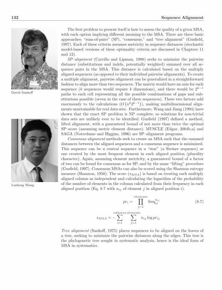
132 Sequence Alignment
The first problem to present itself is how to assess the quality of a given MSA,with each option implying different meaning to the MSA. There are three basicapproaches: “sum-of-pairs” (SP), “consensus,” and “tree alignment” (Gusfield,1997). Each of these criteria assumes metricity in sequence distances (stochasticmodel-based versions of these optimality criteria are discussed in Chapters 11and 12).
David Sankoff
SP–alignment (Carrillo and Lipman, 1988) seeks to minimize the pairwisedistance (substitutions and indels, potentially weighted) summed over all se-quence pairs in the MSA. This distance is calculated based on the multiplyaligned sequences (as opposed to their individual pairwise alignments). To createa multiple alignment, pairwise alignment can be generalized in a straightforwardfashion to align more than two sequences. The matrix would have an axis for eachsequence (k sequences would require k dimensions), and there would be 2k−1
paths to each cell representing all the possible combinations of gaps and sub-stitutions possible (seven in the case of three sequences). These two factors addenormously to the calculations (O
(nk2k−1
)), making multidimensional align-
ments unattainable for real data sets. Furthermore, Wang and Jiang (1994) have
Lusheng Wang
shown that the exact SP–problem is NP–complete, so solutions for non-trivialdata sets are unlikely ever to be identified. Gusfield (1997) defined a method,lifted alignment, with a guaranteed bound of not more than twice the optimalSP–score (assuming metric element distance). MUSCLE (Edgar, 2004b,a) andSAGA (Notredame and Higgins, 1996) are SP–alignment programs.
Consensus alignment methods seek to create an MSA such that the summeddistances between the aligned sequences and a consensus sequence is minimized.This sequence can be a central sequence in a “star” (a Steiner sequence) orone created by the most frequent element in each aligned position (pluralitycharacter). Again, assuming element metricity, a guaranteed bound of a factorof two can be found for consensus as for SP, and by the same “lifting” procedure(Gusfield, 1997). Consensus MSAs can also be scored using the Shannon entropymeasure (Shannon, 1950). The score (sMSA) is based on treating each multiplyaligned column as independent and calculating the logarithm of the probabilityof the number of elements in the column calculated from their frequency in eachaligned position (Eq. 8.7 with nij of element j in aligned position i).
pri =elements∏
j=1
freqnij
ij (8.7)
sMSA = −columns∑
i=1
elements∑j=1
nij log prij
Tree alignment (Sankoff, 1975) places sequences to be aligned on the leaves ofa tree, seeking to minimize the pairwise distances along the edges. This tree isthe phylogenetic tree sought in systematic analysis, hence is the ideal form ofMSA in systematics.
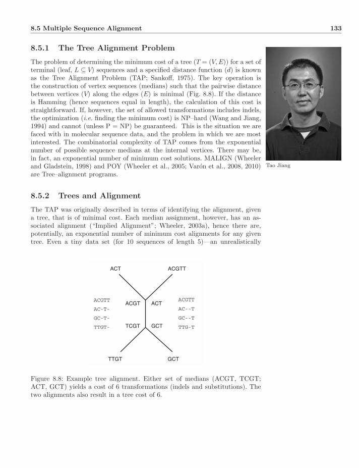
8.5 Multiple Sequence Alignment 133
8.5.1 The Tree Alignment Problem
The problem of determining the minimum cost of a tree (T = (V,E)) for a set ofterminal (leaf, L ⊆ V) sequences and a specified distance function (d) is knownas the Tree Alignment Problem (TAP; Sankoff, 1975). The key operation isthe construction of vertex sequences (medians) such that the pairwise distancebetween vertices (V) along the edges (E) is minimal (Fig. 8.8). If the distanceis Hamming (hence sequences equal in length), the calculation of this cost isstraightforward. If, however, the set of allowed transformations includes indels,the optimization (i.e. finding the minimum cost) is NP–hard (Wang and Jiang,1994) and cannot (unless P = NP) be guaranteed. This is the situation we are
Tao Jiang
faced with in molecular sequence data, and the problem in which we are mostinterested. The combinatorial complexity of TAP comes from the exponentialnumber of possible sequence medians at the internal vertices. There may be,in fact, an exponential number of minimum cost solutions. MALIGN (Wheelerand Gladstein, 1998) and POY (Wheeler et al., 2005; Varon et al., 2008, 2010)are Tree–alignment programs.
8.5.2 Trees and Alignment
The TAP was originally described in terms of identifying the alignment, givena tree, that is of minimal cost. Each median assignment, however, has an as-sociated alignment (“Implied Alignment”; Wheeler, 2003a), hence there are,potentially, an exponential number of minimum cost alignments for any giventree. Even a tiny data set (for 10 sequences of length 5)—an unrealistically
ACT ACGTT
TTGT GCT
ACT
GCT
ACGT
TCGT
ACGTT
AC-T-
GC-T-
TTGT-
ACGTT
AC--T
GC--T
TTG-T
Figure 8.8: Example tree alignment. Either set of medians (ACGT, TCGT;ACT, GCT) yields a cost of 6 transformations (indels and substitutions). Thetwo alignments also result in a tree cost of 6.

134 Sequence Alignment
small and well-behaved case—presents 1.35 × 1038 possible homology schemes(Slowinski, 1998). This problem, for a single cladogram, is as hard as the morefamiliar tree search problem itself.
8.5.3 Exact Solutions
Sankoff and Cedergren (1983) proposed a recursive, exact solution to TAP withO(nk) (k sequences of length n) time complexity based on the recursion in Equa-tion 8.8. Clearly, this was not likely to be useful for non-trivial data sets giventhe k-dimensional sequence alignment. Wheeler (2003c) proposed another exactsolution, also using dynamic programming. In this case, the time complexityis exponential in sequence length (O(k · 42n)) due to the explicit enumerationof possible medians. Both methods could be improved by a branch-and-boundtype procedure, perhaps based on some generalized form of Ukkonen (1985).
di,j,...,k = minδ1+...+δn �=0
(di−δ1,...,k−δN
+ minx1,...,xm
× (cost of 2n vertex state assignments)
)(8.8)
where δi = 0 if gap, 1 otherwise
8.5.4 Polynomial Time Approximate Schemes
Of theoretical use, but almost no practical utility due to the large time complex-ity, Polynomial Time Approximate Schemes (PTAS) are methods with knownbounded behavior for TAP (Wang et al., 1996; Wang and Gusfield, 1997; Wanget al., 2000). These methods use a combination of “lifted” alignment (Sect.10.9.3) and exact O(nk) solutions to create algorithms that achieve provableboundedness, at an increasing cost of time complexity. Currently (Wang et al.,2000), the best procedure is O(kdn5) (for k sequences of length n on a treewith depth d) for a bound of 1.5 over the optimal solution. Clearly, an O(n5)procedure will not be useful for real data sets of thousands of nucleotides, butthis does provide a benchmark to evaluate the bounds and time complexity ofother heuristic procedures.
8.5.5 Heuristic Multiple Sequence Alignment
Current heuristic procedures are similar in that many attempt to render multiplealignment tractable by breaking down simultaneous n–dimensional alignmentsinto a series of manageable pairwise alignments related by a “guide tree” (inthe parlance of Feng and Doolittle, 1987). These differ in the techniques used togenerate the guide tree and conduct the pairwise alignments at the guide treenodes (“profile alignment”). Furthermore, the procedures may or may not beexplicitly linked to optimality criteria. Below several commonly (and some lesscommonly) used methods are discussed. This discussion is by no means exhaus-tive and restricts itself to the algorithmic procedures as opposed to executiontime efficiency. More complete lists can be found at http://pbil.univ-lyon1.fr/alignment.html and additional comparisons in Phillips et al. (2000).
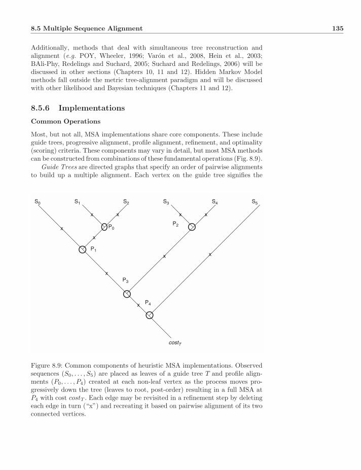
8.5 Multiple Sequence Alignment 135
Additionally, methods that deal with simultaneous tree reconstruction andalignment (e.g. POY, Wheeler, 1996; Varon et al., 2008, Hein et al., 2003;BAli-Phy, Redelings and Suchard, 2005; Suchard and Redelings, 2006) will bediscussed in other sections (Chapters 10, 11 and 12). Hidden Markov Modelmethods fall outside the metric tree-alignment paradigm and will be discussedwith other likelihood and Bayesian techniques (Chapters 11 and 12).
8.5.6 Implementations
Common Operations
Most, but not all, MSA implementations share core components. These includeguide trees, progressive alignment, profile alignment, refinement, and optimality(scoring) criteria. These components may vary in detail, but most MSA methodscan be constructed from combinations of these fundamental operations (Fig. 8.9).
Guide Trees are directed graphs that specify an order of pairwise alignmentsto build up a multiple alignment. Each vertex on the guide tree signifies the
costT
x
x
x
x
x
x x
xx
x
S0 S1 S2 S3 S4 S5
P0
P1
P2
P3
P4
Figure 8.9: Common components of heuristic MSA implementations. Observedsequences (S0, . . . , S5) are placed as leaves of a guide tree T and profile align-ments (P0, . . . , P4) created at each non-leaf vertex as the process moves pro-gressively down the tree (leaves to root, post-order) resulting in a full MSA atP4 with cost costT . Each edge may be revisited in a refinement step by deletingeach edge in turn (“x”) and recreating it based on pairwise alignment of its twoconnected vertices.

136 Sequence Alignment
alignment of the two child vertex sequences (usually O(n2) or so). The treeis traversed post-order (leaves to root) adding up alignments until the root isreached with the complete MSA. Since the guide tree determines alignmentorder, and there are so many possibilities (Eq. 2.1), the choice of guide tree isan important aspect of MSA implementation. Usually, an initial guide tree isconstructed from pairwise distances via Unweighted Pair Group Method usingarithmetic Averages (UPGMA) (Sokal and Michener, 1958), Fitch–Margoliash(Fitch and Margoliash, 1967), Neighbor-Joining (Saitou and Nei, 1987), or another distance-based technique (Chapter 9), since distances can be based onpairwise alignments. The initial guide tree may be revised based on an initialMSA with this second tree constructed via the same distance-based techniques.
Progressive Alignment is the alignment process based on the guide tree (Fengand Doolittle, 1987). As mentioned above, each vertex on the guide tree requiresa pairwise alignment, hence the overall complexity for m sequences is O(mn2)for each MSA. For vertices whose descendants are not exclusively leaves, align-ment techniques are required to align sequences to alignments and alignments toother alignments. In order for the heuristic to be useful, these must be roughlyquadratic, hence sub-alignments are aligned by the same basic pairwise tech-nique, but with the entire aligned column acting as the single element in stan-dard procedures. This may be done on partial alignments, or “profiles,” whichare MSAs reduced to single strings (Fig. 8.10).
AAT AATA
AAT-AATA
CAA
CAA---AAT--AATA
GGGTT AGGGT
-GGGTTAGGGT-
-CAA----AAT---AATA-GGGTTAGGGT-
CCGGTT
-CAA----AAT---AATA-GGGTTAGGGT-CCGGTT
AATA
CA ATA
AGGGTT
MSRRTW¯ ¯ ¯
MSRRTW¯ ¯ ¯
Figure 8.10: Progressive alignment of Feng and Doolittle (1987) where pairwisealignments are performed via post-order tree traversal at non-leaf vertices tocreate partial MSAs following “once a gap, always a gap” (left of vertices) orprofile sequences (right of vertices) of IUPAC symbols for each column with a“bar” if a gap is also present in that aligned column.
.
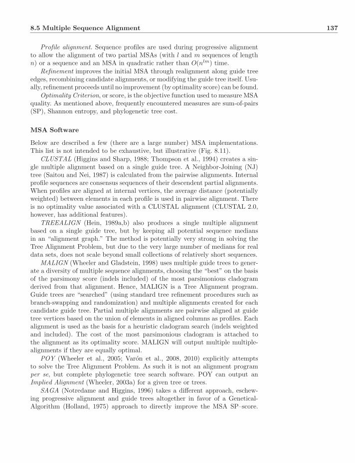
8.5 Multiple Sequence Alignment 137
Profile alignment. Sequence profiles are used during progressive alignmentto allow the alignment of two partial MSAs (with l and m sequences of lengthn) or a sequence and an MSA in quadratic rather than O(nlm) time.
Refinement improves the initial MSA through realignment along guide treeedges, recombining candidate alignments, or modifying the guide tree itself. Usu-ally, refinement proceeds until no improvement (by optimality score) can be found.
Optimality Criterion, or score, is the objective function used to measure MSAquality. As mentioned above, frequently encountered measures are sum-of-pairs(SP), Shannon entropy, and phylogenetic tree cost.
MSA Software
Below are described a few (there are a large number) MSA implementations.This list is not intended to be exhaustive, but illustrative (Fig. 8.11).
CLUSTAL (Higgins and Sharp, 1988; Thompson et al., 1994) creates a sin-gle multiple alignment based on a single guide tree. A Neighbor-Joining (NJ)tree (Saitou and Nei, 1987) is calculated from the pairwise alignments. Internalprofile sequences are consensus sequences of their descendent partial alignments.When profiles are aligned at internal vertices, the average distance (potentiallyweighted) between elements in each profile is used in pairwise alignment. Thereis no optimality value associated with a CLUSTAL alignment (CLUSTAL 2.0,however, has additional features).
TREEALIGN (Hein, 1989a,b) also produces a single multiple alignmentbased on a single guide tree, but by keeping all potential sequence mediansin an “alignment graph.” The method is potentially very strong in solving theTree Alignment Problem, but due to the very large number of medians for realdata sets, does not scale beyond small collections of relatively short sequences.
MALIGN (Wheeler and Gladstein, 1998) uses multiple guide trees to gener-ate a diversity of multiple sequence alignments, choosing the “best” on the basisof the parsimony score (indels included) of the most parsimonious cladogramderived from that alignment. Hence, MALIGN is a Tree Alignment program.Guide trees are “searched” (using standard tree refinement procedures such asbranch-swapping and randomization) and multiple alignments created for eachcandidate guide tree. Partial multiple alignments are pairwise aligned at guidetree vertices based on the union of elements in aligned columns as profiles. Eachalignment is used as the basis for a heuristic cladogram search (indels weightedand included). The cost of the most parsimonious cladogram is attached tothe alignment as its optimality score. MALIGN will output multiple multiple-alignments if they are equally optimal.
POY (Wheeler et al., 2005; Varon et al., 2008, 2010) explicitly attemptsto solve the Tree Alignment Problem. As such it is not an alignment programper se, but complete phylogenetic tree search software. POY can output anImplied Alignment (Wheeler, 2003a) for a given tree or trees.
SAGA (Notredame and Higgins, 1996) takes a different approach, eschew-ing progressive alignment and guide trees altogether in favor of a Genetical-Algorithm (Holland, 1975) approach to directly improve the MSA SP–score.
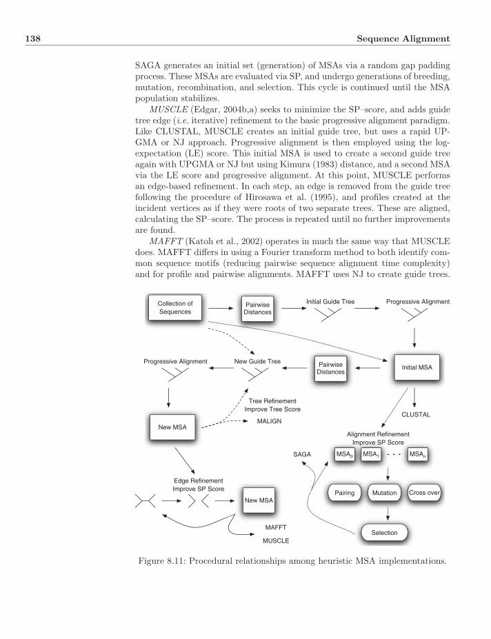
138 Sequence Alignment
SAGA generates an initial set (generation) of MSAs via a random gap paddingprocess. These MSAs are evaluated via SP, and undergo generations of breeding,mutation, recombination, and selection. This cycle is continued until the MSApopulation stabilizes.
MUSCLE (Edgar, 2004b,a) seeks to minimize the SP–score, and adds guidetree edge (i.e. iterative) refinement to the basic progressive alignment paradigm.Like CLUSTAL, MUSCLE creates an initial guide tree, but uses a rapid UP-GMA or NJ approach. Progressive alignment is then employed using the log-expectation (LE) score. This initial MSA is used to create a second guide treeagain with UPGMA or NJ but using Kimura (1983) distance, and a second MSAvia the LE score and progressive alignment. At this point, MUSCLE performsan edge-based refinement. In each step, an edge is removed from the guide treefollowing the procedure of Hirosawa et al. (1995), and profiles created at theincident vertices as if they were roots of two separate trees. These are aligned,calculating the SP–score. The process is repeated until no further improvementsare found.
MAFFT (Katoh et al., 2002) operates in much the same way that MUSCLEdoes. MAFFT differs in using a Fourier transform method to both identify com-mon sequence motifs (reducing pairwise sequence alignment time complexity)and for profile and pairwise alignments. MAFFT uses NJ to create guide trees.
Collection ofSequences
PairwiseDistances
Initial Guide Tree
New Guide TreeInitial MSA
Progressive Alignment
New MSA
PairwiseDistances
CLUSTALMALIGN
Progressive Alignment
Edge RefinementImprove SP Score
Tree RefinementImprove Tree Score
New MSA
MAFFT
MUSCLE
Alignment RefinementImprove SP Score
MSA0 MSA1 MSAn
Pairing Mutation Cross over
Selection
SAGA
Figure 8.11: Procedural relationships among heuristic MSA implementations.
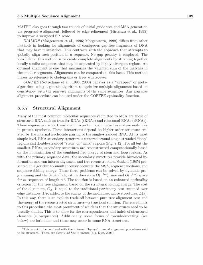
8.5 Multiple Sequence Alignment 139
MAFFT also goes through two rounds of initial guide tree and MSA generationvia progressive alignment, followed by edge refinement (Hirosawa et al., 1995)to improve a weighted SP–score.
DIALIGN (Morgenstern et al., 1996; Morgenstern, 1999) differs from othermethods in looking for alignments of contiguous gap-free fragments of DNAthat may have mismatches. This contrasts with the approach that attempts toglobally align each position in a sequence. No gap penalty is employed. Theidea behind this method is to create complete alignments by stitching togetherlocally similar sequences that may be separated by highly divergent regions. Anoptimal alignment is one that maximizes the weighted sum of the matches inthe smaller segments. Alignments can be compared on this basis. This methodmakes no reference to cladograms or trees whatsoever.
COFFEE (Notredame et al., 1998, 2000) behaves as a “wrapper” or meta-algorithm, using a genetic algorithm to optimize multiple alignments based onconsistency with the pairwise alignments of the same sequences. Any pairwisealignment procedure can be used under the COFFEE optimality function.
8.5.7 Structural Alignment
Many of the most common molecular sequences submitted to MSA are those ofstructural RNA such as transfer RNAs (tRNAs) and ribosomal RNAs (rRNAs).These sequences are not translated into protein and interact as mature moleculesin protein synthesis. These interactions depend on higher order structure cre-ated by the internal nucleotide pairing of the single-stranded RNA. At its mostsimple level, RNA secondary structure is centered around single-stranded “loop”regions and double-stranded “stem” or “helix” regions (Fig. 8.12). For all but thesmallest RNAs, secondary structures are reconstructed computationally-basedon the minimization of the combined free energy of stem and loop regions. Aswith the primary sequence data, the secondary structures provide historical in-formation and can inform alignment and tree reconstruction. Sankoff (1985) pre-sented an algorithm to simultaneously optimize the MSA, sequence medians, andsequence folding energy. These three problems can be solved by dynamic pro-gramming and the Sankoff algorithm does so in O(n3m) time and O(n2m) spacefor m sequences of length n 1. The solution is based on an enhanced optimalitycriterion for the tree alignment based on the structural folding energy. The costof the alignment, CA, is equal to the traditional parsimony cost summed overedge distances, DT , added to the energy of the median sequence structures, E(s).In this way, there is an explicit trade-off between pure tree alignment cost andthe energy of the reconstructed structures—a true joint solution. There are limitsto this procedure, the most prominent of which is that the structures need to bebroadly similar. This is to allow for the correspondences and indels of structuralelements (subsequences). Additionally, some forms of ‘pseudo-knotting’ (seebelow) are forbidden and these may occur in some RNA structures.
1This is not to be confused with the informal “by-eye” manual alignment procedures saidto be structural. These are clearly ad hoc in nature (e.g. Kjer, 2004).

140 Sequence Alignment
5'
C
3'M
3'm
1
2
3
4
5 6
7
8
9
10
11
12
13
14
15
16
17
18
19
2021
22
23
24
25
26
26a
2729
30
31
32
33
34
35
36
3738 39
40
41
42
43
44
45
28
Thermus thermophilussmall subunit ribosomal RNA
Figure 8.12: Secondary structure model for Thermus thermophilus. http://rna.ucsc.edu/rnacenter/ribosome images.html. See Plate 8.12 for the colorfigure.
Sankoff Algorithm
The Sankoff (1985) algorithm is based on three recursions: alignment, folding,and median sequence reconstruction. These are combined to solve the jointproblem simultaneously.

8.5 Multiple Sequence Alignment 141
• Alignment—The core sequence alignment step in this context is slightlygeneralized from that discussed above (Eq. 8.3) in that the cost is definedfor subsequences. For sequences a = {ai, . . . , am} and a = {b1, . . . , bn} and1 ≤ i ≤ j ≤ m and 1 ≤ h ≤ k ≤ n, D(i, j;h, k) is the minimum alignmentcost between partial sequences ai, . . . , aj and bh, . . . , bk. D can be calcu-lated via the recursion relationships:
D(i, j;h, k) = min
⎧⎪⎪⎪⎪⎪⎪⎪⎪⎪⎪⎪⎪⎪⎨⎪⎪⎪⎪⎪⎪⎪⎪⎪⎪⎪⎪⎪⎩
D(i, j;h, k − 1) + y
D(i, j − 1;h, k − 1) + x if aj �= bk
D(i, j − 1;h, k − 1) if aj = bk
D(i, j − 1;h, k) + y
D(i + 1, j;h, k) + y
D(i + 1, j;h + 1, k) + x if ai �= bh
D(i + 1, j;h + 1, k) if ai = bh
D(i, j;h + 1, k) + y
(8.9)
with base indel cost y and substitution cost x, and initial conditions:
D(i, i;h, h) ={
x if ai �= bh
0 if ai = bh(8.10)
This will have a time complexity of O(m2n2) or approximately O(n4)when m ∼ n. In previous sections, we dealt with the special case of wholesequences or D(1,m; 1, n), which then has quadratic time complexity onlyrequiring the upper four terms in Equation 8.9.
• Folding—The central idea behind secondary structure reconstruction is theminimization of the Gibbs Free Energy of the structure. This is determinedby the internal pairing of nucleotides and the geometry of loop and stemregions. The structure S of a sequence a is defined as a set of pairs (i, j) thatcreates bonds between the nucleotides with an experimentally determinedenergy e(s). These pairs must satisfy the “knot constraint” where if i ≤ i′ ≤j ≤ j′, (i, j) and (i′, j′) cannot be distinct elements of S (Fig. 8.13).
i
i' j
j'
Figure 8.13: “Knot” in secondary structure between structure pairs (i, j) and(i′, j′) where i ≤ i′ ≤ j ≤ j′.
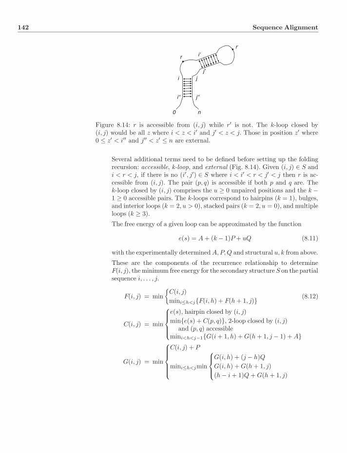
142 Sequence Alignment
i j
i'
j'
r
r'
0 n
i'' j''
Figure 8.14: r is accessible from (i, j) while r′ is not. The k-loop closed by(i, j) would be all z where i < z < i′ and j′ < z < j. Those in position z′ where0 ≤ z′ < i′′ and j′′ < z′ ≤ n are external.
Several additional terms need to be defined before setting up the foldingrecursion: accessible, k-loop, and external (Fig. 8.14). Given (i, j) ∈ S andi < r < j, if there is no (i′, j′) ∈ S where i < i′ < r < j′ < j then r is ac-cessible from (i, j). The pair (p, q) is accessible if both p and q are. Thek-loop closed by (i, j) comprises the u ≥ 0 unpaired positions and the k −1 ≥ 0 accessible pairs. The k-loops correspond to hairpins (k = 1), bulges,and interior loops (k = 2, u > 0), stacked pairs (k = 2, u = 0), and multipleloops (k ≥ 3).
The free energy of a given loop can be approximated by the function
e(s) = A + (k − 1)P + uQ (8.11)
with the experimentally determined A,P,Q and structural u, k from above.
These are the components of the recurrence relationship to determineF(i, j), the minimum free energy for the secondary structure S on the partialsequence i, . . . , j.
F(i, j) = min{
C(i, j)mini≤h<j{F(i, h) + F(h + 1, j)} (8.12)
C(i, j) = min
⎧⎪⎪⎨⎪⎪⎩
e(s), hairpin closed by (i, j)min{e(s) + C(p, q)}, 2-loop closed by (i, j)
and (p, q) accessiblemini<h<j−1{G(i + 1, h) + G(h + 1, j − 1) + A}
G(i, j) = min
⎧⎪⎪⎪⎨⎪⎪⎪⎩
C(i, j) + P
mini≤h<jmin
⎧⎪⎨⎪⎩
G(i, h) + (j − h)QG(i, h) + G(h + 1, j)(h − i + 1)Q + G(h + 1, j)
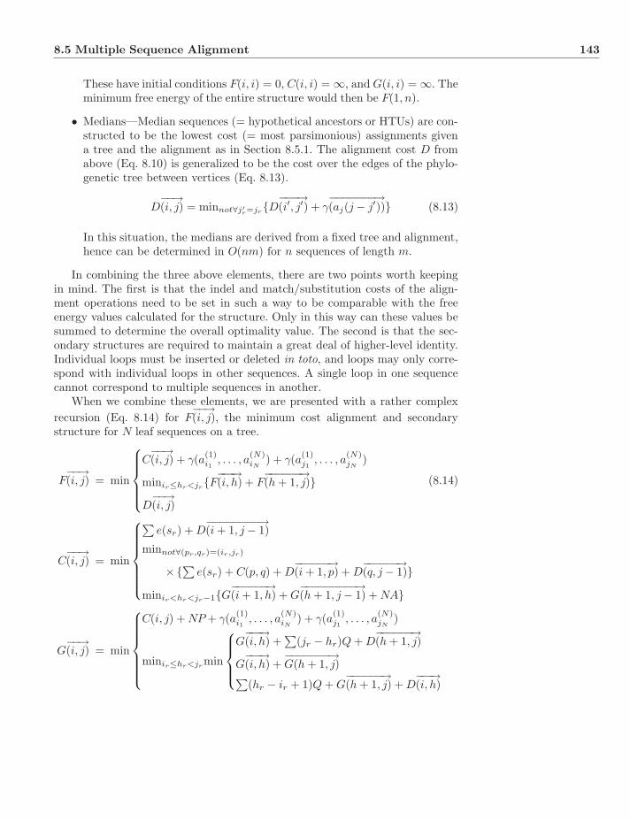
8.5 Multiple Sequence Alignment 143
These have initial conditions F(i, i) = 0, C(i, i) = ∞, and G(i, i) = ∞. Theminimum free energy of the entire structure would then be F(1, n).
• Medians—Median sequences (= hypothetical ancestors or HTUs) are con-structed to be the lowest cost (= most parsimonious) assignments givena tree and the alignment as in Section 8.5.1. The alignment cost D fromabove (Eq. 8.10) is generalized to be the cost over the edges of the phylo-genetic tree between vertices (Eq. 8.13).
D−−→(i, j) = minnot∀j′
r=jr{D−−−→
(i′, j′) + γ−−−−−−−→(aj(j − j′))} (8.13)
In this situation, the medians are derived from a fixed tree and alignment,hence can be determined in O(nm) for n sequences of length m.
In combining the three above elements, there are two points worth keepingin mind. The first is that the indel and match/substitution costs of the align-ment operations need to be set in such a way to be comparable with the freeenergy values calculated for the structure. Only in this way can these values besummed to determine the overall optimality value. The second is that the sec-ondary structures are required to maintain a great deal of higher-level identity.Individual loops must be inserted or deleted in toto, and loops may only corre-spond with individual loops in other sequences. A single loop in one sequencecannot correspond to multiple sequences in another.
When we combine these elements, we are presented with a rather complexrecursion (Eq. 8.14) for F
−−→(i, j), the minimum cost alignment and secondary
structure for N leaf sequences on a tree.
F−−→(i, j) = min
⎧⎪⎪⎪⎨⎪⎪⎪⎩
C−−→(i, j) + γ(a(1)
i1, . . . , a
(N)iN
) + γ(a(1)j1
, . . . , a(N)jN
)
minir≤hr<jr{F−−−→(i, h) + F
−−−−−−→(h + 1, j)}
D−−→(i, j)
(8.14)
C−−→(i, j) = min
⎧⎪⎪⎪⎪⎪⎨⎪⎪⎪⎪⎪⎩
∑e(sr) + D
−−−−−−−−→(i + 1, j − 1)
minnot∀(pr,qr)=(ir,jr)
×{∑ e(sr) + C(p, q) + D−−−−−−→(i + 1, p) + D
−−−−−−→(q, j − 1)}
minir<hr<jr−1{G−−−−−−→(i + 1, h) + G
−−−−−−−−−→(h + 1, j − 1) + NA}
G−−→(i, j) = min
⎧⎪⎪⎪⎪⎪⎨⎪⎪⎪⎪⎪⎩
C(i, j) + NP + γ(a(1)i1
, . . . , a(N)iN
) + γ(a(1)j1
, . . . , a(N)jN
)
minir≤hr<jrmin
⎧⎪⎪⎨⎪⎪⎩
G−−−→(i, h) +
∑(jr − hr)Q + D
−−−−−−→(h + 1, j)
G−−−→(i, h) +
−−−−−−−→G(h + 1, j)∑
(hr − ir + 1)Q + G−−−−−−→(h + 1, j) + D
−−−→(i, h)
144 Sequence Alignment
These have initial conditions F−−→(i, i) = 0, C
−−→(i, i) = ∞, and G
−−→(i, i) = ∞ if any
ir = jr.The overall time complexity of the Sankoff procedure is high—O(n6) for two
sequences of length n, and the MSA case even more daunting, with exponentialdependency on the number of taxa (N), O(n3N ).
Implementations
The basic approach of most implementations of structural alignment is theSankoff algorithm. In order to make the problem tractable, however, simplifyingrestrictions are made. Several of these approaches are compared in Gardner andGiegerich (2004).
FOLDALIGN (Gorodkin et al., 1997) reduces the pairwise alignment com-plexity by not allowing branching structures. In doing so, the time complexityof aligning two sequences is reduced by a quadratic factor to O(n4). The lackof branching in the structures effectively limits the operation to relatively shortsequences. A further reduction in the exponential factor comes from the use ofprogressive alignment (for N sequences, O(N)) after determining the all-pairscosts (O(N2)). The result is a procedure akin to CLUSTAL, but with a struc-tural component.
DYNALIGN (Mathews and Turner, 2002) is limited to pairwise alignment,but is free of the structural restrictions in FOLDALIGN. DYNALIGN limitsthe distance between aligned nucleotide positions to m, thereby reducing thepairwise Sankoff time complexity from O(n6) to O(m3n3), with m3 as a constantfactor.
PMCOMP/PMMULTI (Hofacker et al., 2004) uses a probabilistic pairingmodel to calculate initial pairwise alignments and then uses progressive align-ment to create the full multiple alignment. In the progressive alignment step,the same restriction on distances between subsequence alignments (D(i, j;h, k)above) used in DYNALIGN is applied, reducing time complexity from O(n6) toO(n4). A further factor of N sequences is added for the progressive step, hence,the overall time complexity is O(n4N).
RNAcast (Reeder and Giegerich, 2005) is based on a “consensus shape”approach where the reconstructed structures are limited to those common to abody of sequences. This reduces the space of possible structures and the specificstructures of sequences are optimized within this space. RNAcast does not alignthe input sequences, but creates a set of consensus structural elements.
RNASalsa (Stocsits et al., 2009) is a meta-algorithm implementing a refine-ment procedure based on input alignments and structural models. An aligned setof sequences are input with structural information demarcated for one of theinput sequences. RNASalsa first generalizes the single input structure to theother sequences in the input set based on the input alignment. Second, refinedstructural reconstructions are performed on the input sequences (using the same
8.6 Exercises 145
probability structure codes in PMCOMP above), given the constraints based onthe generalized input structure. The third and final step progressively aligns thesequences based on the refined structural models. Given the reliance on inputalignment and structural information, the main time complexity factors are inthe structural refinements (O(n4) for n nucleotides) and progressive alignment(O(N) for N taxa).
Comparisons−−What is a Good Alignment?
There are myriad comparisons and comparison methodologies that have beenpublished (e.g. Notredame, 2002; Batzoglou, 2005; Wheeler, 2007a) and I haveno desire to create another one here. Comparisons center on two sorts of analy-ses: 1) whether one procedure or another is more similar to a “real” or simulatedalignment (Ogden and Rosenberg, 2007), and 2) whether competing methodsoptimize an objective function (such as SP or tree-length) more effectively or ina more timely fashion (Boujenfa et al., 2008; Wheeler and Giribet, 2009).
It seems most unlikely that we will ever encounter a “real” alignment in na-ture, hence comparison of procedures that are at least nominally optimization-based to simulated, “known” alignment seems fruitless, but see Ogden andRosenberg (2007) for a different view. Even comparison on the basis of objectivefunctions can be difficult, since the various implementations do not attempt tooptimize precisely the same functions.
As far as systematic analysis is concerned, the central goal is to identifyoptimal trees. Those methods that yield better solutions to this problem, nomatter what optimality criterion one chooses, are to be favored. Most likely,the best way a method can do this effectively is to directly attempt to optimizetree costs—the Tree Alignment Problem itself. It is worth remembering thateven for a single tree, there may be an exponential number of equally costlyalignments. This reality is rarely explored, and its impact on the potentiallyequally large number of tree solutions is largely unexamined. Multiple alignmentmethods offer one set of heuristics to this problem; in later sections we willencounter others.
8.6 Exercises
1. Align the two sequences “ACGTTA” and “TCTA” by hand using the costscenarios where all transformations are equally costly.
2. What is the best method to choose a MSA? Should this be optimality-based?
3. Choose a small data set and run it through several MSA programs. Howdo they differ? Change indel and gap extension parameters. How do thealignments change?

146 Sequence Alignment
4. Are MSA columns independent?
5. What are some implications for phylogenetic analysis of affine indelmodels?
6. Is hand (“by-eye”) alignment adequate for phylogenetic analysis?
7. Are there any cases where it would be advisable/defensible to discardsequence data?

Part III
Optimality Criteria

Chapter 9
OptimalityCriteria−Distance
Distance analysis, as opposed to character-based analysis, reconstructs phylo-genetic relationships based on the pairwise overall distances between taxa. Thisapproach has a long history, beginning with the first computational approachesto systematics and the early use of molecular biological data to create phylo-genetic trees. This form of phylogenetic analysis is characterized by fast algo-rithms (generally) and statistically motivated statements about tree topology,edge weights, and correctness. Distances are highly amenable to simulation testsas well. For these reasons, they have been very popular in mathematical treat-ments. Unfortunately, distance analysis is also characterized by a necessary lossof information (i.e. multiple character data sets generating identical dissimilar-ity matrices) and departure from optimizing a set of specific character changes.For these reasons, distances have not been as popular in empirical analyses.
9.1 Why Distance?
Phenetic techniques are inherently distance-based (whether similarity or dis-similarity) given that they are constructed from overall similarity as opposed tospecific primitive or derived character change. The entire foundation of pheneticclassification rests on distance quantified similarity (Chapter 1). Michener andSokal (1957) defined their initial clustering procedures on a data set of soli-tary bees (Megachilidae) comprising 97 taxa and 122 characters. These resultedin 11,834 individual observations, which were converted into 4656 pairwise dis-tances (actually similarities in their example) and analyzed on that basis. Thesedata did not require distance analysis; it was thrust upon them. Other formsof data, especially that from molecular sequences such as DNA or protein, havebeen transformed and treated this way.
Systematics: A Course of Lectures, First Edition. Ward C. Wheeler.c© 2012 Ward C. Wheeler. Published 2012 by Blackwell Publishing Ltd.
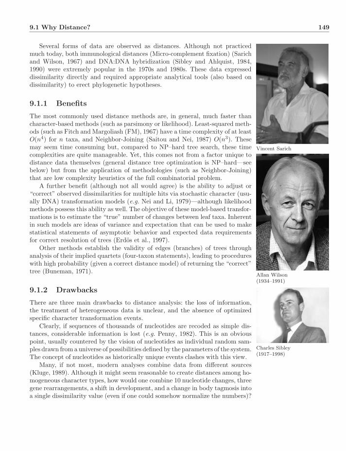
9.1 Why Distance? 149
Vincent Sarich
Allan Wilson(1934–1991)
Charles Sibley(1917–1998)
Several forms of data are observed as distances. Although not practicedmuch today, both immunological distances (Micro-complement fixation) (Sarichand Wilson, 1967) and DNA:DNA hybridization (Sibley and Ahlquist, 1984,1990) were extremely popular in the 1970s and 1980s. These data expresseddissimilarity directly and required appropriate analytical tools (also based ondissimilarity) to erect phylogenetic hypotheses.
9.1.1 Benefits
The most commonly used distance methods are, in general, much faster thancharacter-based methods (such as parsimony or likelihood). Least-squared meth-ods (such as Fitch and Margoliash (FM), 1967) have a time complexity of at leastO(n4) for n taxa, and Neighbor-Joining (Saitou and Nei, 1987) O(n3). Thesemay seem time consuming but, compared to NP–hard tree search, these timecomplexities are quite manageable. Yet, this comes not from a factor unique todistance data themselves (general distance tree optimization is NP–hard—seebelow) but from the application of methodologies (such as Neighbor-Joining)that are low complexity heuristics of the full combinatorial problem.
A further benefit (although not all would agree) is the ability to adjust or“correct” observed dissimilarities for multiple hits via stochastic character (usu-ally DNA) transformation models (e.g. Nei and Li, 1979)—although likelihoodmethods possess this ability as well. The objective of these model-based transfor-mations is to estimate the “true” number of changes between leaf taxa. Inherentin such models are ideas of variance and expectation that can be used to makestatistical statements of asymptotic behavior and expected data requirementsfor correct resolution of trees (Erdos et al., 1997).
Other methods establish the validity of edges (branches) of trees throughanalysis of their implied quartets (four-taxon statements), leading to procedureswith high probability (given a correct distance model) of returning the “correct”tree (Buneman, 1971).
9.1.2 Drawbacks
There are three main drawbacks to distance analysis: the loss of information,the treatment of heterogeneous data is unclear, and the absence of optimizedspecific character transformation events.
Clearly, if sequences of thousands of nucleotides are recoded as simple dis-tances, considerable information is lost (e.g. Penny, 1982). This is an obviouspoint, usually countered by the vision of nucleotides as individual random sam-ples drawn from a universe of possibilities defined by the parameters of the system.The concept of nucleotides as historically unique events clashes with this view.
Many, if not most, modern analyses combine data from different sources(Kluge, 1989). Although it might seem reasonable to create distances among ho-mogeneous character types, how would one combine 10 nucleotide changes, threegene rearrangements, a shift in development, and a change in body tagmosis intoa single dissimilarity value (even if one could somehow normalize the numbers)?
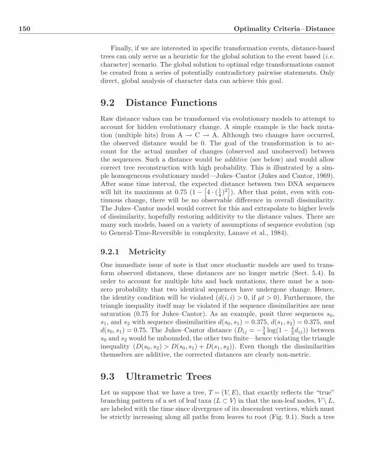
150 Optimality Criteria−Distance
Finally, if we are interested in specific transformation events, distance-basedtrees can only serve as a heuristic for the global solution to the event based (i.e.character) scenario. The global solution to optimal edge transformations cannotbe created from a series of potentially contradictory pairwise statements. Onlydirect, global analysis of character data can achieve this goal.
9.2 Distance Functions
Raw distance values can be transformed via evolutionary models to attempt toaccount for hidden evolutionary change. A simple example is the back muta-tion (multiple hits) from A → C → A. Although two changes have occurred,the observed distance would be 0. The goal of the transformation is to ac-count for the actual number of changes (observed and unobserved) betweenthe sequences. Such a distance would be additive (see below) and would allowcorrect tree reconstruction with high probability. This is illustrated by a sim-ple homogeneous evolutionary model—Jukes–Cantor (Jukes and Cantor, 1969).After some time interval, the expected distance between two DNA sequenceswill hit its maximum at 0.75 (1 − [
4 · ( 14 )2
]). After that point, even with con-
tinuous change, there will be no observable difference in overall dissimilarity.The Jukes–Cantor model would correct for this and extrapolate to higher levelsof dissimilarity, hopefully restoring additivity to the distance values. There aremany such models, based on a variety of assumptions of sequence evolution (upto General-Time-Reversible in complexity, Lanave et al., 1984).
9.2.1 Metricity
One immediate issue of note is that once stochastic models are used to trans-form observed distances, these distances are no longer metric (Sect. 5.4). Inorder to account for multiple hits and back mutations, there must be a non-zero probability that two identical sequences have undergone change. Hence,the identity condition will be violated (d(i, i) > 0, if μt > 0). Furthermore, thetriangle inequality itself may be violated if the sequence dissimilarities are nearsaturation (0.75 for Jukes–Cantor). As an example, posit three sequences s0,s1, and s2 with sequence dissimilarities d(s0, s1) = 0.375, d(s1, s2) = 0.375, andd(s0, s1) = 0.75. The Jukes–Cantor distance (Dij = −3
4 log(1 − 43dij)) between
s0 and s2 would be unbounded, the other two finite—hence violating the triangleinequality (D(s0, s2) > D(s0, s1) + D(s1, s2)). Even though the dissimilaritiesthemselves are additive, the corrected distances are clearly non-metric.
9.3 Ultrametric Trees
Let us suppose that we have a tree, T = (V,E), that exactly reflects the “true”branching pattern of a set of leaf taxa (L ⊂ V) in that the non-leaf nodes, V \ L,are labeled with the time since divergence of its descendent vertices, which mustbe strictly increasing along all paths from leaves to root (Fig. 9.1). Such a tree
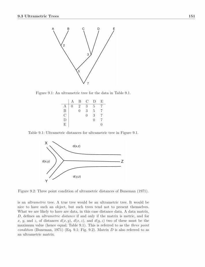
9.3 Ultrametric Trees 151
A B C D E
2
3
5
7
Figure 9.1: An ultrametric tree for the data in Table 9.1.
A B C D EA 0 2 3 5 7B 0 3 5 7C 0 3 7D 0 7E 0
Table 9.1: Ultrametric distances for ultrametric tree in Figure 9.1.
X
Y
Zd(x,y)
d(x,z)
d(y,z)
Figure 9.2: Three point condition of ultrametric distances of Buneman (1971).
is an ultrametric tree. A true tree would be an ultrametric tree. It would benice to have such an object, but such trees tend not to present themselves.What we are likely to have are data, in this case distance data. A data matrix,D, defines an ultrametric distance if and only if the matrix is metric, and forx, y, and z, of distances d(x, y), d(x, z), and d(y, z) two of these must be themaximum value (hence equal; Table 9.1). This is referred to as the three pointcondition (Buneman, 1971) (Eq. 9.1; Fig. 9.2). Matrix D is also referred to asan ultrametric matrix.
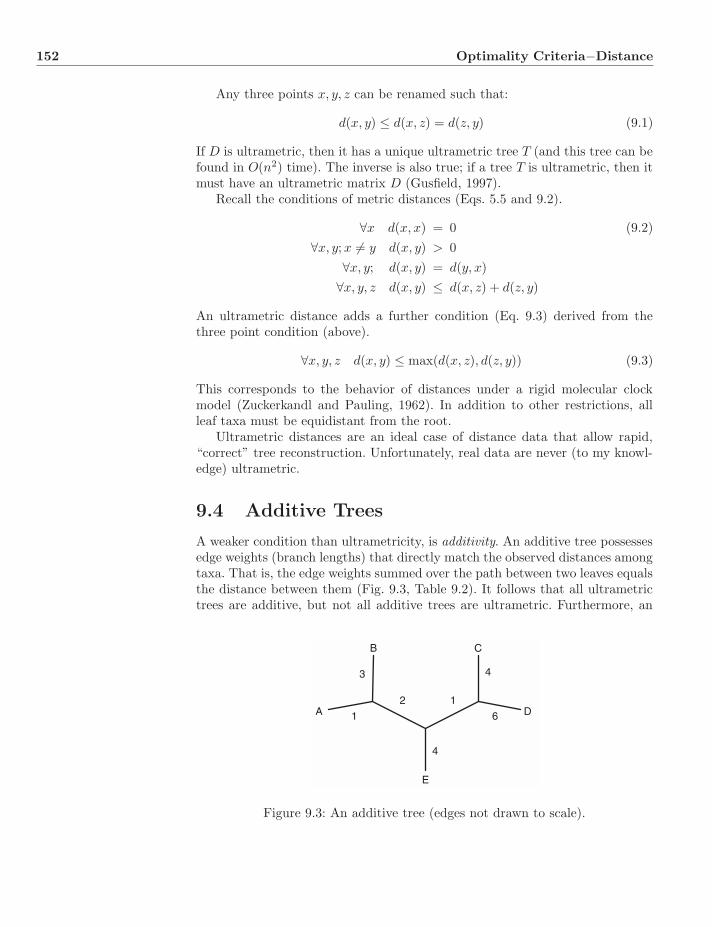
152 Optimality Criteria−Distance
Any three points x, y, z can be renamed such that:
d(x, y) ≤ d(x, z) = d(z, y) (9.1)
If D is ultrametric, then it has a unique ultrametric tree T (and this tree can befound in O(n2) time). The inverse is also true; if a tree T is ultrametric, then itmust have an ultrametric matrix D (Gusfield, 1997).
Recall the conditions of metric distances (Eqs. 5.5 and 9.2).
∀x d(x, x) = 0 (9.2)∀x, y;x �= y d(x, y) > 0
∀x, y; d(x, y) = d(y, x)∀x, y, z d(x, y) ≤ d(x, z) + d(z, y)
An ultrametric distance adds a further condition (Eq. 9.3) derived from thethree point condition (above).
∀x, y, z d(x, y) ≤ max(d(x, z), d(z, y)) (9.3)
This corresponds to the behavior of distances under a rigid molecular clockmodel (Zuckerkandl and Pauling, 1962). In addition to other restrictions, allleaf taxa must be equidistant from the root.
Ultrametric distances are an ideal case of distance data that allow rapid,“correct” tree reconstruction. Unfortunately, real data are never (to my knowl-edge) ultrametric.
9.4 Additive Trees
A weaker condition than ultrametricity, is additivity. An additive tree possessesedge weights (branch lengths) that directly match the observed distances amongtaxa. That is, the edge weights summed over the path between two leaves equalsthe distance between them (Fig. 9.3, Table 9.2). It follows that all ultrametrictrees are additive, but not all additive trees are ultrametric. Furthermore, an
A
B C
D
E
1
3
2 1
4
4
6
Figure 9.3: An additive tree (edges not drawn to scale).

9.4 Additive Trees 153
A B C D EA 0 4 8 10 7B 0 10 12 9C 0 10 9D 0 11E 0
Table 9.2: Additive distances for additive tree in Figure 9.3.
X
Y
U
V
d(x,y)
d(x,u)
d(y,v)
d(u,v)
d(x,v)
d(y,u)
Figure 9.4: Four point condition of additive metric distances of Buneman (1971).
additive tree is characterized by the four point condition (Fig. 9.4; Eq. 9.4;Buneman, 1971).
Any four points x, y, u, v can be renamed such that:
d(x, y) + d(u, v) ≤ d(x, u) + d(y, v) = d(x, v) + d(y, u) (9.4)
There are two important implications of additive distances that bear on treereconstruction: the Farris transform, and Buneman trees.
9.4.1 Farris Transform
Farris et al. (1970) defined a transform of additive data into ultrametric values(in O(n2) time), which can then be reconstructed by O(n2) methods. Com-pletely non-intuitive (at least to me), the Farris transform reveals deep connec-tions between additive and ultrametric distances (Fig. 9.5). Due to its generalimportance (it pops up in many areas of mathematics—Dress et al., 2007), thetransform was given its patronym by Bandelt (1990).
The Farris transform of observed, additive dij to ultrametric d′ij (Eq. 9.5)adds a constant factor δ to distances recalculated from fixed leaf x (originallythe most distant, presumed out-taxon yielding δ ≥ max dxy) to create an ad-vancement index, which is the vertex labeling of ultrametric trees.
if x �= y d′i,j = δ +
12(di,j − dx,i − dxj) (9.5)
if x = y d′i,j = 0
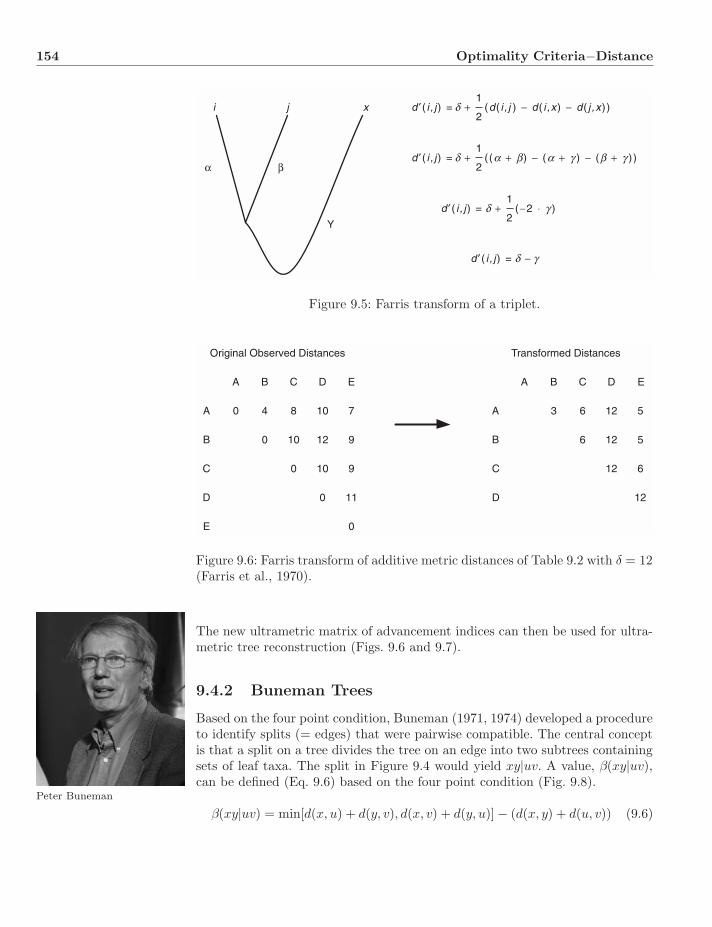
154 Optimality Criteria−Distance
i j x
α β
Y
d ′( i , j) = δ +1
2(d( i , j ) − d ( i ,x) − d ( j ,x ) )
d ′( i , j ) = δ +1
2((α + β) − (α + γ ) − (β + γ ) )
d ′ ( i , j) = δ +1
2(−2 ⋅ γ )
d ′ ( i , j ) = δ − γ
Figure 9.5: Farris transform of a triplet.
Original Observed Distances Transformed Distances
A
B
C
D
A B C D E
4 8 10 7
10 12 9
10 9
11
A
B
C
D
A B C D E
3 6 12 5
6 12 5
12 6
12
0
0
0
0
E 0
Figure 9.6: Farris transform of additive metric distances of Table 9.2 with δ = 12(Farris et al., 1970).
The new ultrametric matrix of advancement indices can then be used for ultra-metric tree reconstruction (Figs. 9.6 and 9.7).
9.4.2 Buneman Trees
Based on the four point condition, Buneman (1971, 1974) developed a procedureto identify splits (= edges) that were pairwise compatible. The central conceptis that a split on a tree divides the tree on an edge into two subtrees containingsets of leaf taxa. The split in Figure 9.4 would yield xy|uv. A value, β(xy|uv),can be defined (Eq. 9.6) based on the four point condition (Fig. 9.8).
Peter Buneman
β(xy|uv) = min[d(x, u) + d(y, v), d(x, v) + d(y, u)] − (d(x, y) + d(u, v)) (9.6)
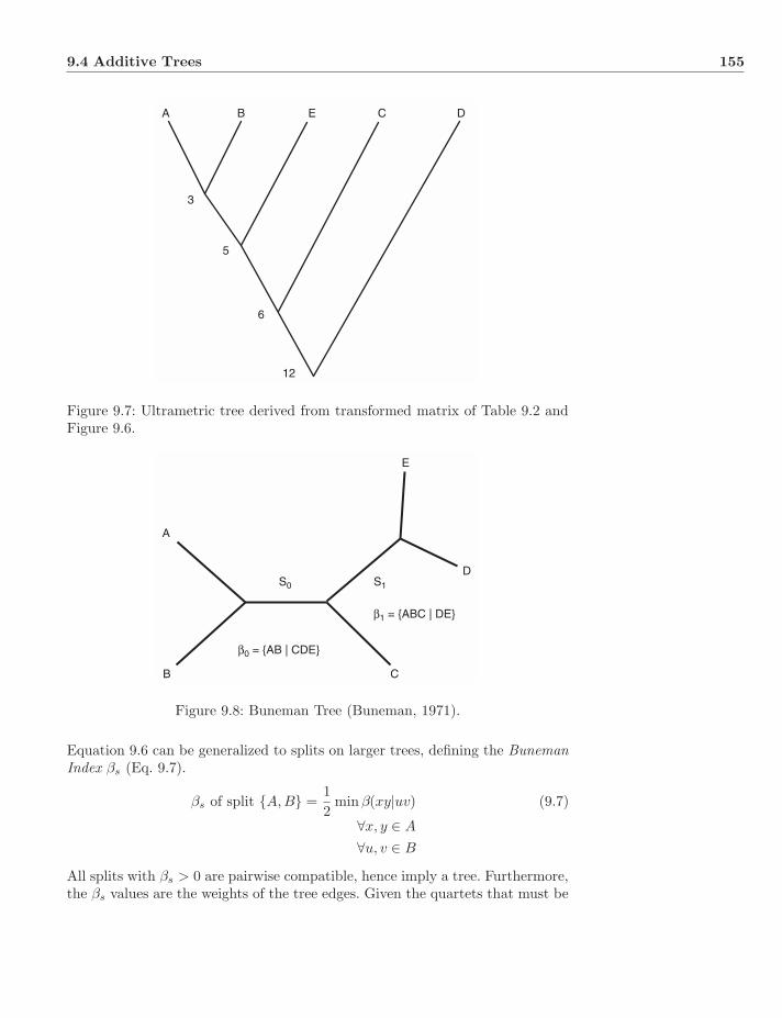
9.4 Additive Trees 155
A B C DE
5
3
6
12
Figure 9.7: Ultrametric tree derived from transformed matrix of Table 9.2 andFigure 9.6.
A
B C
E
DS0 S1
β0 = {AB | CDE}
β1 = {ABC | DE}
Figure 9.8: Buneman Tree (Buneman, 1971).
Equation 9.6 can be generalized to splits on larger trees, defining the BunemanIndex βs (Eq. 9.7).
βs of split {A,B} =12
min β(xy|uv) (9.7)
∀x, y ∈ A
∀u, v ∈ B
All splits with βs > 0 are pairwise compatible, hence imply a tree. Furthermore,the βs values are the weights of the tree edges. Given the quartets that must be
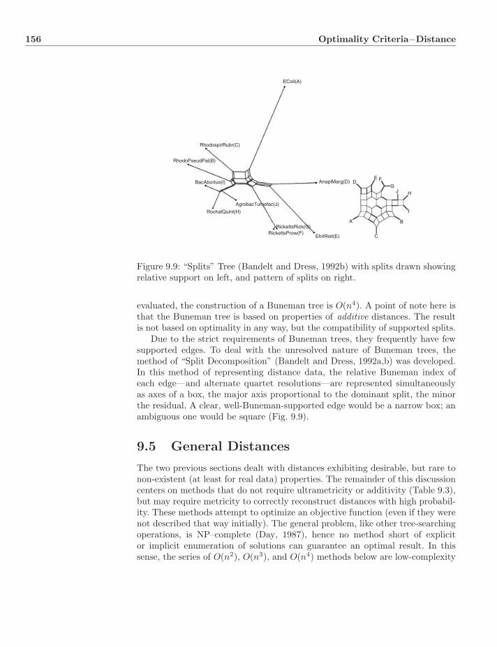
156 Optimality Criteria−Distance
RhodospirRubr(C)
RhodoPseudPal(B)
BacAbortus(I)
RochalQuint(H)
AgrobacTumefac(J)
RickettsRick(G)RickettsProw(F)
EhrlRist(E)
A
C
B
I
HJG
FEDAnaplMarg(D)
EColi(A)
Figure 9.9: “Splits” Tree (Bandelt and Dress, 1992b) with splits drawn showingrelative support on left, and pattern of splits on right.
evaluated, the construction of a Buneman tree is O(n4). A point of note here isthat the Buneman tree is based on properties of additive distances. The resultis not based on optimality in any way, but the compatibility of supported splits.
Due to the strict requirements of Buneman trees, they frequently have fewsupported edges. To deal with the unresolved nature of Buneman trees, themethod of “Split Decomposition” (Bandelt and Dress, 1992a,b) was developed.In this method of representing distance data, the relative Buneman index ofeach edge—and alternate quartet resolutions—are represented simultaneouslyas axes of a box, the major axis proportional to the dominant split, the minorthe residual. A clear, well-Buneman-supported edge would be a narrow box; anambiguous one would be square (Fig. 9.9).
9.5 General Distances
The two previous sections dealt with distances exhibiting desirable, but rare tonon-existent (at least for real data) properties. The remainder of this discussioncenters on methods that do not require ultrametricity or additivity (Table 9.3),but may require metricity to correctly reconstruct distances with high probabil-ity. These methods attempt to optimize an objective function (even if they werenot described that way initially). The general problem, like other tree-searchingoperations, is NP–complete (Day, 1987), hence no method short of explicitor implicit enumeration of solutions can guarantee an optimal result. In thissense, the series of O(n2), O(n3), and O(n4) methods below are low-complexity
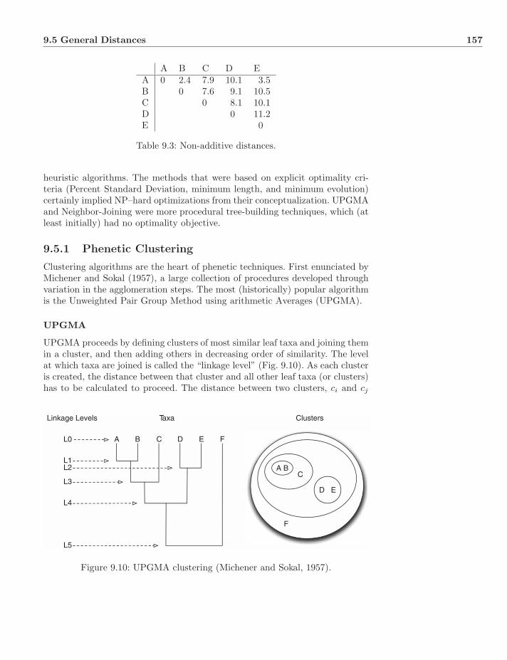
9.5 General Distances 157
A B C D EA 0 2.4 7.9 10.1 3.5B 0 7.6 9.1 10.5C 0 8.1 10.1D 0 11.2E 0
Table 9.3: Non-additive distances.
heuristic algorithms. The methods that were based on explicit optimality cri-teria (Percent Standard Deviation, minimum length, and minimum evolution)certainly implied NP–hard optimizations from their conceptualization. UPGMAand Neighbor-Joining were more procedural tree-building techniques, which (atleast initially) had no optimality objective.
9.5.1 Phenetic Clustering
Clustering algorithms are the heart of phenetic techniques. First enunciated byMichener and Sokal (1957), a large collection of procedures developed throughvariation in the agglomeration steps. The most (historically) popular algorithmis the Unweighted Pair Group Method using arithmetic Averages (UPGMA).
UPGMA
UPGMA proceeds by defining clusters of most similar leaf taxa and joining themin a cluster, and then adding others in decreasing order of similarity. The levelat which taxa are joined is called the “linkage level” (Fig. 9.10). As each clusteris created, the distance between that cluster and all other leaf taxa (or clusters)has to be calculated to proceed. The distance between two clusters, ci and cj
A B C D E F
TaxaLinkage Levels
L0
L1L2
L3
L4
L5
A BC
D E
F
Clusters
Figure 9.10: UPGMA clustering (Michener and Sokal, 1957).
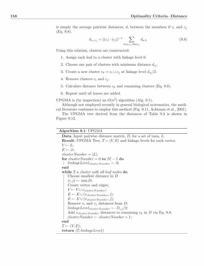
158 Optimality Criteria−Distance
is simply the average pairwise distances, d, between the members if ci and cj
(Eq. 9.8).
dci,cj= (|ci| · |cj |)−1
∑∀a∈ci,∀b∈cj
da,b (9.8)
Using this relation, clusters are constructed:
1. Assign each leaf to a cluster with linkage level 0.
2. Choose one pair of clusters with minimum distance dij .
3. Create a new cluster ck = ci ∪ cj at linkage level dij/2.
4. Remove clusters ci and cj .
5. Calculate distance between ck and remaining clusters (Eq. 9.8).
6. Repeat until all leaves are added.
UPGMA is (by inspection) an O(n2) algorithm (Alg. 9.1).Although not employed recently in general biological systematics, the medi-
cal literature continues to employ this method (Fig. 9.11, Achtman et al., 2001).The UPGMA tree derived from the distances of Table 9.3 is shown in
Figure 9.12.
Algorithm 9.1: UPGMAData: Input pairwise distance matrix, D, for a set of taxa, L.Result: UPGMA Tree, T = (V,E) and linkage levels for each vertex.V ← L;E ← ∅;clusterNumber = |L|;for clusterNumber = 0 to |V| − 1 do
linkageLevelclusterNumber ← 0;endwhile � a cluster with all leaf nodes do
Choose smallest distance in D(i, j) ← min D;Create vertex and edges;V ← V ∪ vclusterNumber;E ← E ∪ (vclusterNumber, i);E ← E ∪ (vclusterNumber, j);Remove vi and vj distances from D;linkageLevelclusterNumber ← Di,j/2;Add vclusterNumber distances to remaining vk in D via Eq. 9.8;clusterNumber ← clusterNumber + 1;
endT ← (V,E);return (T, linkageLevel)

9.5 General Distances 159
Z4713Z4718Z4715Z1376Z4717
ST5
Pgm
3P
gm 1
9
7 0 8 0
% similarity
9 0 100
ST5
ST5ST5
III
IV
VI
X
Z4719Z4720Z6710Z6711Z6699Z6709Z6456Z6458Z6460Z6462Z6464Z6715Z4716Z6714Z4721Z4722Z6848Z6849Z6841Z6845Z6843Z6847Z6842Z6837Z6750Z6838Z6839Z6840Z1375Z6446Z6450Z6751Z4714Z6832Z6829Z6831Z4733Z6824Z4726Z4728Z4730Z4732Z4725Z4731Z4727Z6821Z6822Z6833Z6549Z6741Z6442Z6823Z6444Z6448Z6737Z6816Z6827Z6830Z6828Z6835Z6820Z6712Z6844Z6836Z6570Z6454Z6528Z6539Z6452Z6729Z6734Z6726Z6732Z6725Z6730Z6731Z6735Z6763Z6739Z6740Z6814Z6721Z6724Z6719Z6815Z6736Z6817Z6722Z6723Z6738Z6818Z6834Z6522Z6733Z6728Z6572
ST5
ST7
ST7
ST7
ST5ST7ST7ST7ST4ST2ST2ST2
ST2ST2
ST2
ST2
ST68ST2ST2ST72
ST70ST71
ST2
ST2ST70ST69ST68ST73ST2
ST2ST2
ST76ST76
ST78ST77ST77ST75ST75
ST77
ST76ST76
ST75
ST79
Figure 9.11: UPGMA clustering of meningitis strains (Achtman et al., 2001).
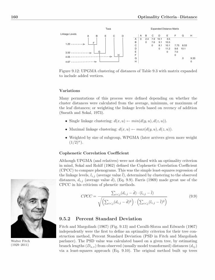
160 Optimality Criteria−Distance
A B E C D
Taxa
Linkage Levels
1.20
3.50
4.05
4.67
F
GH
A B C D E F G HA 0 2.4 7.9 10.1 3.5B 0 7.6 9.1 10.5C 0 8.1 10.1 7.75 8.53D 0 11.2 9.6 10.1E 0 7.0F 0G 0 9.33H 0
Expanded Distance Matrix
Figure 9.12: UPGMA clustering of distances of Table 9.3 with matrix expandedto include added vertices.
Variations
Many permutations of this process were defined depending on whether thecluster distances were calculated from the average, minimum, or maximum ofthe leaf distances; or weighting the linkage levels based on recency of addition(Sneath and Sokal, 1973).
• Single linkage clustering: d(x, u) ← min(d(y, u), d(z, u)).
• Maximal linkage clustering: d(x, u) ← max(d(y, u), d(z, u)).
• Weighted by size of subgroup, WPGMA (later arrivers given more weight(1/2)n).
Cophenetic Correlation Coefficient
Although UPGMA (and relatives) were not defined with an optimality criterionin mind, Sokal and Rohlf (1962) defined the Cophenetic Correlation Coefficient(CPCC) to compare phenograms. This was the simple least-squares regression ofthe linkage levels, li,j (average value l), determined by clustering to the observeddistances, di,j (average value d), (Eq. 9.9). Farris (1969) made great use of theCPCC in his criticism of phenetic methods.
CPCC =
∑i<j(di,j − d) · (li,j − l)√(∑
i<j(di,j − d)2)·(∑
i<j(li,j − l)2) (9.9)
9.5.2 Percent Standard Deviation
Fitch and Margoliash (1967) (Fig. 9.13) and Cavalli-Sforza and Edwards (1967)independently were the first to define an optimality criterion for their tree con-struction method, Percent Standard Deviation (PSD in Fitch and Margoliashparlance). The PSD value was calculated based on a given tree, by estimatingWalter Fitch
(1929–2011) branch lengths (Du,v) from observed (usually model transformed) distances (dij)via a least-squares approach (Eq. 9.10). The original method built up trees
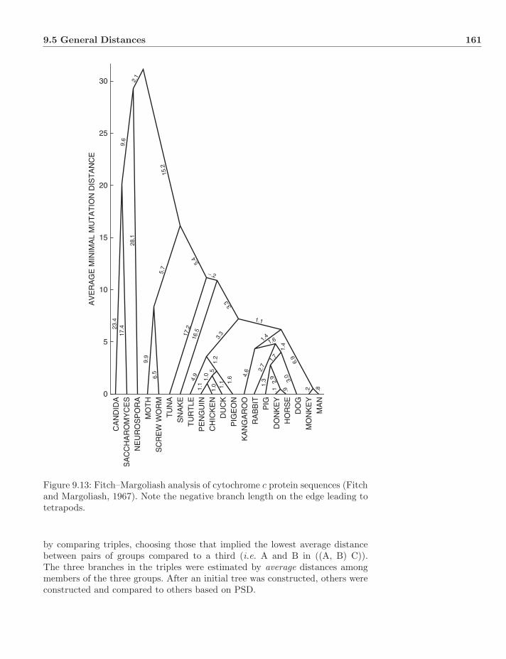
9.5 General Distances 161
CA
ND
IDA
0
23.4
17.4
9.9
17.2
5.4
5.7
28.1
15.2
9.6
2.1
−.2
16.5
4.9
3.3
3.3
1.2
4.6 2.
7
1.1
1.41.6
1.4
6.9
3.0
.2 .8.9
2.9
.1
1.3
1.7
.51.
01.
0 1.1
1.1 1.
66.5
5
10
15
AV
ER
AG
E M
INIM
AL
MU
TA
TIO
N D
IST
AN
CE
20
25
30
SA
CC
HA
RO
MY
CE
SN
EU
RO
SP
OR
AM
OT
HS
CR
EW
WO
RM
TU
NA
SN
AK
ET
UR
TLE
PE
NG
UIN
CH
ICK
EN
DU
CK
PIG
EO
NK
AN
GA
RO
OR
AB
BIT
PIG
DO
NK
EY
HO
RS
ED
OG
MO
NK
EY
MA
N
Figure 9.13: Fitch–Margoliash analysis of cytochrome c protein sequences (Fitchand Margoliash, 1967). Note the negative branch length on the edge leading totetrapods.
by comparing triples, choosing those that implied the lowest average distancebetween pairs of groups compared to a third (i.e. A and B in ((A, B) C)).The three branches in the triples were estimated by average distances amongmembers of the three groups. After an initial tree was constructed, others wereconstructed and compared to others based on PSD.

162 Optimality Criteria−Distance
PSDT=(V,E) =∑e∈E
(duv − Duv)2
d2uv
(9.10)
Later use of the PSD criterion minimized the value over trees as a familiartree search, and with equally familiar NP–hard complexity (Day, 1987). Theprocedure (tree-building heuristic) described by Fitch and Margoliash (1967)has a time complexity of O(n4), but was later improved to O(n3) (Desper andGascuel, 2007).
Estimating Branch Lengths
Several methods, including those that minimize PSD (above) and ME (below),estimate edge weights (branch lengths) by least-squares. This is based on a sta-tistical view of the distribution of distances and the desire to create edge weightsthat conform to their statistical expectation (summarized by Felsenstein, 2004).The process is relatively simple in that each observed distance corresponds toa series of edges on a given tree. With n leaf taxa and 2n − 3 edges, there are(n2 − n)/2 linear equations created by the sum of edge weights linking each pairof leaves. Given that there are more equations than unknowns, the system isoverdetermined and can be solved using elementary linear algebra.
For the tree in Figure 9.14, there are 10 equations and 7 variables (Eq. 9.11).
d(A,B) = e0 + e1 (9.11)d(A,C) = e0 + e2 + e4 + e5
d(A,D) = e0 + e2 + e4 + e6
d(A,E) = e0 + e2 + e3
d(B,C) = e1 + e2 + e4 + e5
d(B,D) = e1 + e2 + e4 + e6
d(B,E) = e1 + e2 + e3
d(C,D) = e5 + e6
d(C,E) = e5 + e4 + e3
d(D,E) = e6 + e4 + e3
A
B C
D
E
e0
e1
e2
e3
e4
e5e6
A
B C
D
E
0.252.15
1.31
4.49
2.11
3.254.85
Figure 9.14: Tree of five leaves and seven edges. Edges labeled on left and esti-mated (distances of Table 9.3) by least-squares on right. The tree has a length(ME) of 18.41 and PSD of 3.24.
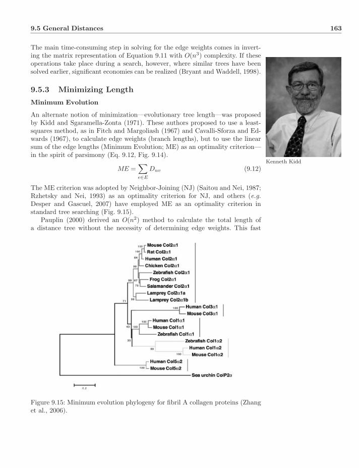
9.5 General Distances 163
The main time-consuming step in solving for the edge weights comes in invert-ing the matrix representation of Equation 9.11 with O(n3) complexity. If theseoperations take place during a search, however, where similar trees have beensolved earlier, significant economies can be realized (Bryant and Waddell, 1998).
9.5.3 Minimizing Length
Minimum Evolution
An alternate notion of minimization—evolutionary tree length—was proposedby Kidd and Sgaramella-Zonta (1971). These authors proposed to use a least-squares method, as in Fitch and Margoliash (1967) and Cavalli-Sforza and Ed-wards (1967), to calculate edge weights (branch lengths), but to use the linearsum of the edge lengths (Minimum Evolution; ME) as an optimality criterion—in the spirit of parsimony (Eq. 9.12, Fig. 9.14).
Kenneth Kidd
ME =∑e∈E
Duv (9.12)
The ME criterion was adopted by Neighbor-Joining (NJ) (Saitou and Nei, 1987;Rzhetsky and Nei, 1993) as an optimality criterion for NJ, and others (e.g.Desper and Gascuel, 2007) have employed ME as an optimality criterion instandard tree searching (Fig. 9.15).
Pauplin (2000) derived an O(n2) method to calculate the total length ofa distance tree without the necessity of determining edge weights. This fast
0.2
Figure 9.15: Minimum evolution phylogeny for fibril A collagen proteins (Zhanget al., 2006).

164 Optimality Criteria−Distance
ME method has been used to improve the execution time of a variety of dis-tance tree-building heuristics (e.g. Balanced Minimum Evolution; Desper andGascuel, 2002).
Distance Wagner
After his (Farris, 1970) character-based method for calculating Wagner trees,Farris (1972) modified his O(n3) (cubed because the closest taxon is chosen ateach point; if the taxon addition order is determined a priori, the process isO(n2)) procedure for distances. The key modification to allow the use of dis-tances comes in the calculation of the distances between median (i.e. internalor HTU) nodes and leaf (or OTU) nodes. Farris used a greatest-lower-boundapproach based on metric distances (specifically the triangle inequality) as op-posed to the least-squares method of Fitch and Margoliash (1967) and Kidd andSgaramella-Zonta (1971). The distance from new node F, is created by addingnode C to edge (G,H) to node Z not yet placed on the tree (Eq. 9.13, Fig. 9.16).Taxa were added to the growing tree by minimizing the patristic (i.e. edge path)distance between the leaf to be added and a specific edge on the tree (Eq. 9.14,Alg. 9.2).
1. Begin by choosing the closest pair of taxa (min dG,H).
2. Add the taxon C closest (via Eq. 9.14) to the pair (G,H) (or to the closestedge of the tree if the tree has > 2 taxa).
3. Create a new vertex F with distances to (C,G,H) calculated via Eq. 9.14,and distances to taxa yet to be added (Z) via Eq. 9.13.
G H
C
d(C,(G,H ) ) =1
2(d (C,G) + d (C,H ) − d(G,H ) )
G H
C
F
Z
d (C,F ) =1
2(d (C,G ) + d (C,H ) − d (G,H ) )
d (G,F ) = (d (G,C ) − d (C,F) )
d (H,F ) = (d (H,C ) − d (C,F ) )
d (Z,F ) = max(d(vi,Z ) − p (vi,F ) )vi∈T
Figure 9.16: Distance Wagner procedure to create edge weights between leavesand non-leaf vertices (upper), and distances between non-leaf vertices and leaves(Farris, 1972). The distances d are observed and p are patristic, previously cal-culated edges.

9.5 General Distances 165
Algorithm 9.2: DistanceWagnerData: Input pairwise distance matrix, D, for a set of taxa, L.Result: Distance Wagner Tree, T = (V,E).V ← L;E ← ∅;Choose two starting taxaE ← (v0, v1);While there are leaf nodes to addwhile ∃vk /∈ T do
Choose smallest distance between next leaf and each edge in tree(i, j) ← mini,j d(vk, ei,j) = 1
2 (d(vk, vi) + d(vk, vj) − d(vi, vj));Remove ei,j
E ← E \ ei,j ;Create vertex and edges;V ← V ∪ vHTU ;E ← E ∪ (vHTU , i);E ← E ∪ (vHTU , j);E ← E ∪ (vHTU , vk);Update treeT ← (V,E);Determine distances from vHTU to vi, vj and vk
d(vk, vHTU ) = 12 (d(vk, vi) + d(vk, vj) − d(vi, vj));
d(vi, vHTU ) = d(vi, vk) − d(vk, vHTU );d(vj , vHTU ) = d(vj , vk) − d(vk, vHTU );Determine distances from vk to remaining nodes∀l /∈ T, d(vl, vHTU ) = maxvp∈i,j,k(d(vp, vl) − p(vp, vHTU ));HTU ← HTU + 1;
endT ← (V,E);return T
4. Repeat until all taxa have been added to the tree.
d(Z,F) = maxvi∈T
(d(vi, Z) − p(vi, F)) (9.13)
d(C, (G,H)) =12(d(C,G) + d(C,H) − d(G,H)) (9.14)
Although not conspicuous in its initial description, the Distance Wagnertechnique strives to minimize total patristic distance over the tree (Fig. 9.17).
Distance Wagner trees can contain negative branch lengths and are oftenlonger (sum of estimated edge weights) than those reconstructed by ME or FM.Both of these effects come from the application of the triangle inequality to thedistances. If metricity is violated, negative branches may occur. The triangleinequality also requires that patristic distances on the tree cannot be less thanthose observed, placing a lower bound on edge weights not found in ME or FM.
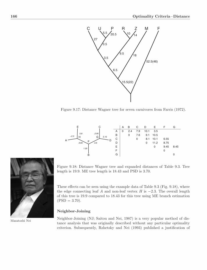
166 Optimality Criteria−Distance
15.5(22)
6.5
3.5
27
0.5
5.5 20.5 10 14
C U P R Z M F
9.518
52.5(46)
Figure 9.17: Distance Wagner tree for seven carnivores from Farris (1972).
A
E C
D
B
−2.35.8
3.65
1.05
3.6
2.95
5.15H
F
G
A B C D E F G
A 0 2.4 7.9 10.1 3.5B 0 7.6 9.1 10.5C 0 8.1 10.1 6.55D 0 11.2 8.75E 0 9.45 8.45F 0G 0
Figure 9.18: Distance Wagner tree and expanded distances of Table 9.3. Treelength is 19.9. ME tree length is 18.43 and PSD is 3.70.
These effects can be seen using the example data of Table 9.3 (Fig. 9.18), wherethe edge connecting leaf A and non-leaf vertex H is −2.3. The overall lengthof this tree is 19.9 compared to 18.43 for this tree using ME branch estimation(PSD = 3.70).
Neighbor-Joining
Masatoshi NeiNeighbor-Joining (NJ; Saitou and Nei, 1987) is a very popular method of dis-tance analysis that was originally described without any particular optimalitycriterion. Subsequently, Rzhetsky and Nei (1993) published a justification of
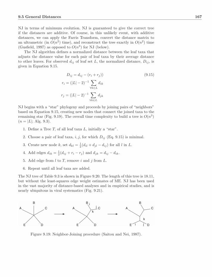
9.5 General Distances 167
NJ in terms of minimum evolution. NJ is guaranteed to give the correct treeif the distances are additive. Of course, in this unlikely event, with additivedistances, we can apply the Farris Transform, convert the distance matrix toan ultrametric (in O(n2) time), and reconstruct the tree exactly in O(n2) time(Gusfield, 1997) as opposed to O(n3) for NJ (below).
The NJ algorithm defines a normalized distance between the leaf taxa thatadjusts the distance value for each pair of leaf taxa by their average distanceto other leaves. For observed dij of leaf set L, the normalized distance, Dij , isgiven in Equation 9.15.
Dij = dij − (ri + rj)) (9.15)
ri = (|L| − 2)−1∑∀k∈L
dik
rj = (|L| − 2)−1∑∀k∈L
djk
NJ begins with a “star” phylogeny and proceeds by joining pairs of “neighbors”based on Equation 9.15, creating new nodes that connect the joined taxa to theremaining star (Fig. 9.19). The overall time complexity to build a tree is O(n3)(n = |L|; Alg. 9.3).
1. Define a Tree T, of all leaf taxa L, initially a “star”.
2. Choose a pair of leaf taxa, i, j, for which Dij (Eq. 9.15) is minimal.
3. Create new node k, set dkl = 12 (dil + djl − dij) for all l in L.
4. Add edges dik = 12 (dij + ri − rj) and djk = dij − dik.
5. Add edge from l to T, remove i and j from L.
6. Repeat until all leaf taxa are added.
The NJ tree of Table 9.3 is shown in Figure 9.20. The length of this tree is 18.11,but without the least-squares edge weight estimates of ME. NJ has been usedin the vast majority of distance-based analyses and in empirical studies, and isnearly ubiquitous in viral systematics (Fig. 9.21).
A
B
C
DE
A
B
C
DE
k
ij A
B
C
DE
k
i j
Figure 9.19: Neighbor-Joining procedure (Saitou and Nei, 1987).
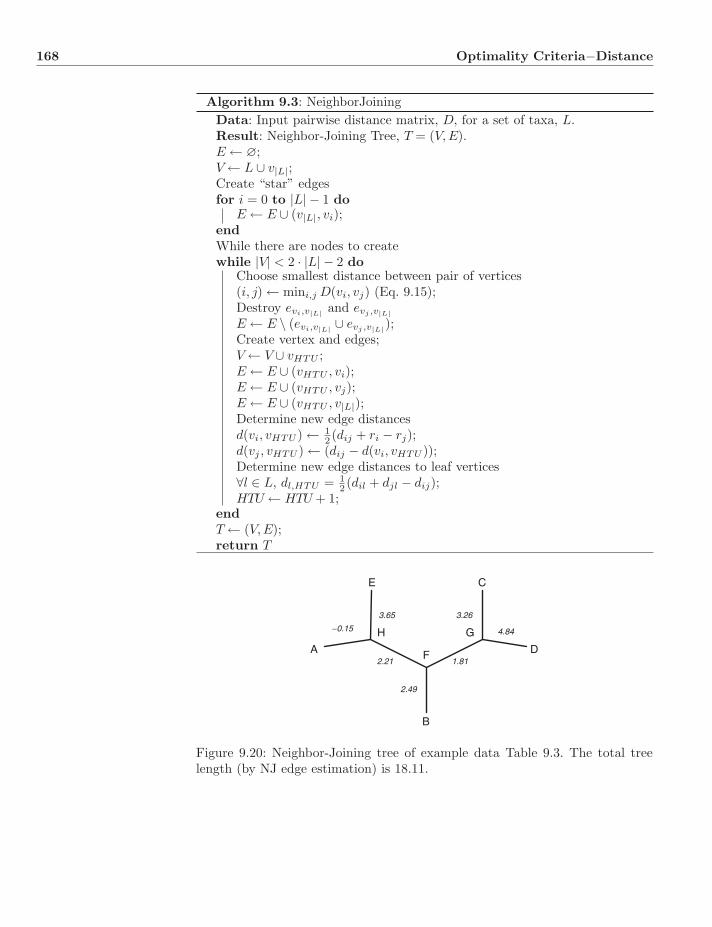
168 Optimality Criteria−Distance
Algorithm 9.3: NeighborJoiningData: Input pairwise distance matrix, D, for a set of taxa, L.Result: Neighbor-Joining Tree, T = (V,E).E ← ∅;V ← L ∪ v|L|;Create “star” edgesfor i = 0 to |L| − 1 do
E ← E ∪ (v|L|, vi);endWhile there are nodes to createwhile |V| < 2 · |L| − 2 do
Choose smallest distance between pair of vertices(i, j) ← mini,j D(vi, vj) (Eq. 9.15);Destroy evi,v|L| and evj ,v|L|E ← E \ (evi,v|L| ∪ evj ,v|L|);Create vertex and edges;V ← V ∪ vHTU ;E ← E ∪ (vHTU , vi);E ← E ∪ (vHTU , vj);E ← E ∪ (vHTU , v|L|);Determine new edge distancesd(vi, vHTU ) ← 1
2 (dij + ri − rj);d(vj , vHTU ) ← (dij − d(vi, vHTU ));Determine new edge distances to leaf vertices∀l ∈ L, dl,HTU = 1
2 (dil + djl − dij);HTU ← HTU + 1;
endT ← (V,E);return T
A
E C
D
B
−0.15
3.65
2.21
2.49
1.81
3.26
4.84H
F
G
Figure 9.20: Neighbor-Joining tree of example data Table 9.3. The total treelength (by NJ edge estimation) is 18.11.
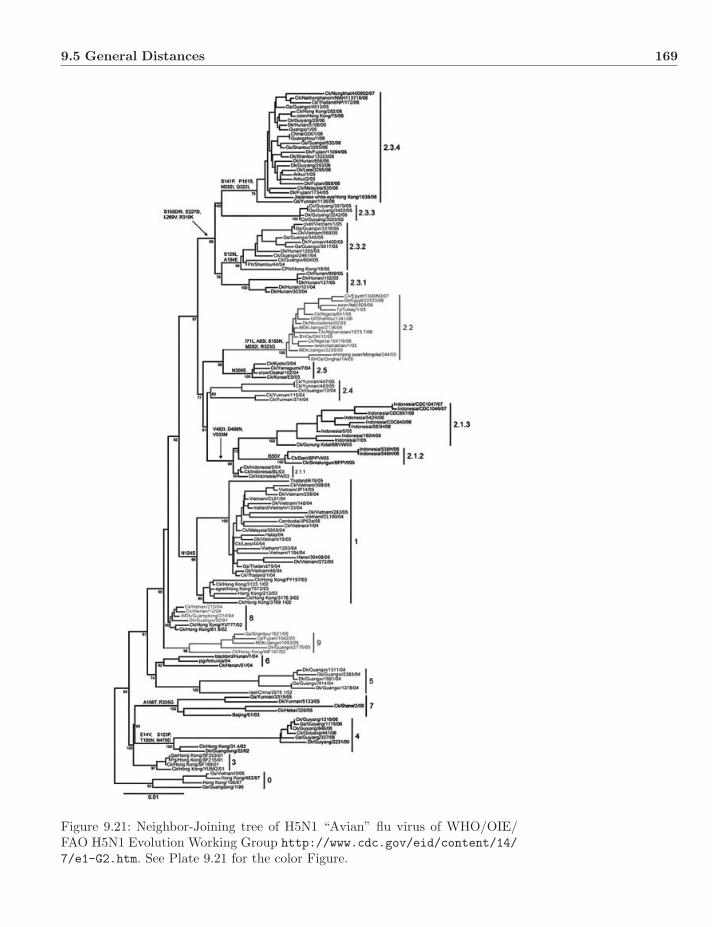
9.5 General Distances 169
Figure 9.21: Neighbor-Joining tree of H5N1 “Avian” flu virus of WHO/OIE/FAO H5N1 Evolution Working Group http://www.cdc.gov/eid/content/14/7/e1-G2.htm. See Plate 9.21 for the color Figure.

170 Optimality Criteria−Distance
Desper and Gascuel (2002) proposed a method analogous to the NJ proce-dure by requiring the weight of sister taxa (the two descendent edges incidenton a vertex) to be equal as opposed to being weighted by the number ofleaves in each subtree. This “Balanced Minimum Evolution” procedure usesthe same optimality value—ME—but with lower time complexity than that forNJ (O(n2 log n)).
ME and Tree Search
The NJ algorithm can be viewed as a heuristic solution to the general MEproblem. If this point of view is taken, standard tree search procedures can beemployed in an effort to optimize ME and identify the optimal tree. As men-tioned before, this will be an NP–hard optimization, as for any other optimalitycriterion.
9.6 Comparisons
There are two means of comparing the various distance approaches: optimalitycriterion and tree-building algorithm. Three optimality criteria (at least by themethods) have been discussed here: Cophenetic Correlation Coefficient, PercentStandard Deviation, and Minimum Evolution. The choice among these is moreone of aesthetic than any empirical means since a tree may be optimal for onecriterion or another. Any argument among them must be made on the relativemerits of the criteria themselves.
One point of comparison is important to make clear in the two forms ofminimum evolution, that of the Distance Wagner (DW) and Minimum Evolutionproper (ME). As mentioned above, the total DW tree lengths will always begreater than or equal to that yielded from ME. This is due to the differentobjectives of the two length criteria. DW seeks to minimize overall tree lengthgiven the constraints of metricity (Sect. 9.2.1 above), specifically the triangleinequality. ME, on the other hand, seeks to create tree lengths based on thestatistical expectation of distances. As a result of this, ME can reconstructbranch lengths that yield patristic distances between taxa that are impossiblylow—less than that observed in the input matrix. In the examples based on Table9.3, the ME paths between AC, AD, BE, and EC are all less than that observed.They are impossibly short. Of the 10 pairwise paths, four are too short, four arelonger than observed, and two are exactly on, coincident with the objective ofcreating edge lengths as expected amount of evolution. The DW does not havethis problem, but does display a negative branch length on AH. This negativevalue indicates that the observed distances are non-metric (similarly, negativebranch lengths in NJ trees are indicative of non-additive distances (Fig. 9.20).Negative branches frequently occur in real and simulated data sets (Gascuel,1997), especially those that have been transformed by evolutionary models.
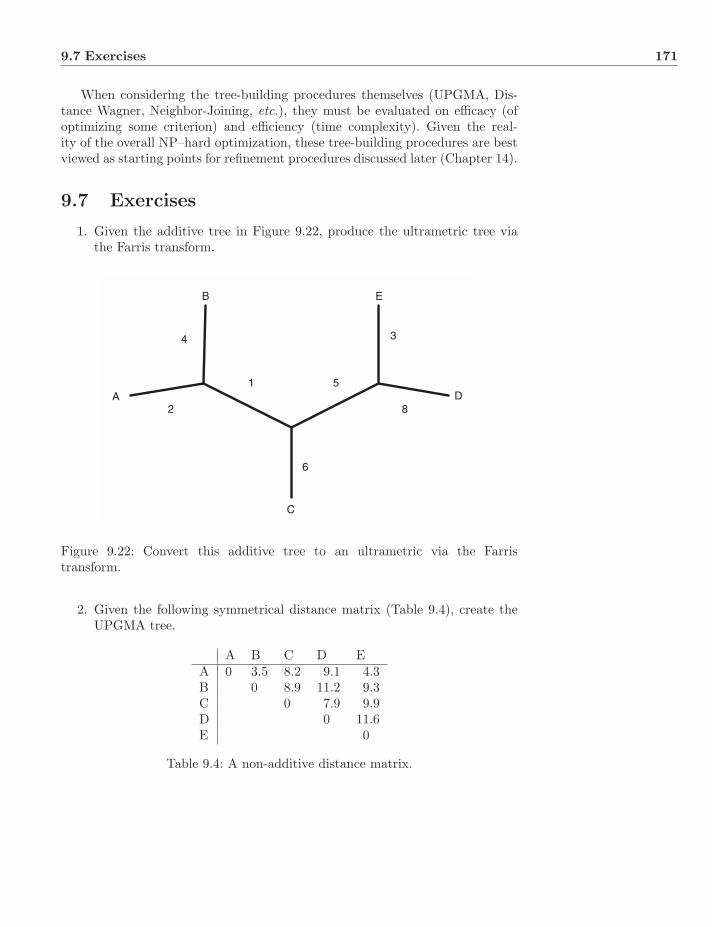
9.7 Exercises 171
When considering the tree-building procedures themselves (UPGMA, Dis-tance Wagner, Neighbor-Joining, etc.), they must be evaluated on efficacy (ofoptimizing some criterion) and efficiency (time complexity). Given the real-ity of the overall NP–hard optimization, these tree-building procedures are bestviewed as starting points for refinement procedures discussed later (Chapter 14).
9.7 Exercises
1. Given the additive tree in Figure 9.22, produce the ultrametric tree viathe Farris transform.
A
B E
D
C
2
4
1 5
3
6
8
Figure 9.22: Convert this additive tree to an ultrametric via the Farristransform.
2. Given the following symmetrical distance matrix (Table 9.4), create theUPGMA tree.
A B C D EA 0 3.5 8.2 9.1 4.3B 0 8.9 11.2 9.3C 0 7.9 9.9D 0 11.6E 0
Table 9.4: A non-additive distance matrix.

172 Optimality Criteria−Distance
3. Given the symmetrical distance matrix (Table 9.4), create the DistanceWagner tree.
4. Given the symmetrical distance matrix (Table 9.4), create the NJ tree.
5. What are the implications for edge weights of the differing methods usedby Distance Wagner and least-squares to estimate them?

Chapter 10
OptimalityCriteria−Parsimony
The operation of assigning states to non-leaf vertices is often referred to asoptimization. This operation implies a set of transformations between adja-cent (ancestor–descendant) vertices, and that assignment is also referred toas optimization. This chapter discusses the operations involved in both theseforms of character optimization under the parsimony criterion. Median (ver-tex) states will be assigned to minimize overall tree cost without reference toa stochastic model of character change or evolution—although there may benon-homogenous transformation cost scenarios.
As per usual, we define a tree, T = (V,E), and a transformation cost matrix σthat specifies the cost of transformations among the elements (character states)of the data set. The purpose of the operation is to determine the minimum costof a tree given a transformation cost matrix and data (T(σ,D)). There are twogeneral types of characters discussed here: static and dynamic sensu Wheeler(2001b). Static characters are those whose correspondences (observations in leaftaxa) are fixed and invariant over alternate trees, while the correspondencesof dynamic characters may vary with tree topology such that overall cost isminimized. The static character types include additive, non-additive, and ma-trix (alternately referred to as general or Sankoff), while unaligned sequenceand chromosomal characters are referred to as dynamic homology characters.A computational distinction between these classes of characters can be drawnbased on the time complexity of their optimization. Static characters can be op-timized on a given tree in polynomial time, whereas the optimization of dynamiccharacters is, in general, NP–hard.
Systematics: A Course of Lectures, First Edition. Ward C. Wheeler.c© 2012 Ward C. Wheeler. Published 2012 by Blackwell Publishing Ltd.

174 Optimality Criteria−Parsimony
10.1 Perfect Phylogeny
The most simple (and potentially satisfying case) is a matrix of n leaf taxaand m binary observations, or features, for each leaf. If the observations arebinary, (0, 1), we can test to see if the character columns are in either of tworelationships. Consider two characters: the set Ai of taxa with a 1 for a characteri (0 can always be set to the out or root state) and a similarly constructed setAj for some character j, where |Ai| ≤ |Aj |. If:
∀i, j ∈ m character set
if Ai ∩ Aj = ∅ or
Ai ⊆ Aj (10.1)
then there is a perfect phylogeny. If:
∀i, j ∈ m character set
∀a, b ∈ n leaf taxa
Aia = 1, Aib = 0 and Aja = 0, Aib = 1 (10.2)
then there is not (this can be tested in O(nm) time; Gusfield, 1997). If the dataare “perfect,” derived distances will be ultrametric, and there will be O(n2) timereconstruction of a unique tree (Fig. 10.1). The problem can be generalizedto r-states characters. If the characters are additive (Sect. 10.2.1), there is apolynomial time algorithm to solve for the tree; if non-additive (Sect. 10.2.2),the problem is NP–hard for r > 2 (Steel, 1992). Of course, these perfect scenariosare nearly non-existent in empirical situations. Homoplasy happens.
10.2 Static Homology Characters
There are three classes of static characters each with exact, polynomial opti-mization procedures: Additive, Non-Additive, and Matrix (or Sankoff). Due to
A B C D E
1
2 3
4
1 2 3
A 0 0 0
B 1 1 0
C 1 1 0
D 1 0 1
E 1 0 1
4
0
0
1
1
0
Figure 10.1: A perfect phylogeny with the characters and states on the left andthe tree in the center. If character 4 were added, the problem is no longer perfect.
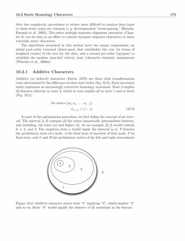
10.2 Static Homology Characters 175
their low complexity, procedures to reduce more difficult to analyze data typesto these static types are common (e.g. developmental “event-pairing,” Bininda-Emonds et al., 2002). The entire multiple sequence alignment enterprise (Chap-ter 8) can be seen as an effort to convert dynamic sequence characters to moretractable static characters.
The algorithms presented in this section have two major components, aninitial post-order traversal (down-pass) that establishes the cost (in terms ofweighted events) of the tree for the data, and a second pre-order (up-pass) toestablish the median (non-leaf vertex) state (character element) assignments(Wheeler et al., 2006a).
10.2.1 Additive Characters
Additive (or ordered) characters (Farris, 1970) are those with transformationcosts determined by the difference in their state index (Eq. 10.3). Each successiveindex represents an increasingly restrictive homology statement. State 3 impliesall features inherent in state 2, which in turn implies all in state 1 and so forth(Fig. 10.2).
for states {s0, s1, . . . , sn−1}σsi,sj
= |i − j| (10.3)
As part of the optimization procedure, we first define the concept of an inter-val. The interval [a, b] contains all the states numerically intermediate between,and including, the lower (a) and higher (b). As an example, [0, 3] would contain0, 1, 2, and 3. The singleton state a would imply the interval [a, a]. P denotesthe preliminary state of a node, A the final state of ancestor of that node, F itsfinal state, and L and R the preliminary states of the left and right descendants
32
1
4
0
Figure 10.2: Additive character states with “4” implying “3”, which implies “2”and so on. State “0” would signify the absence of all variations in the feature.

176 Optimality Criteria−Parsimony
Algorithm 10.1: AdditiveDownPassData: Tree, T = (V,E), with leaf taxa L ⊂ VData: Character set, c ∈ N for V. The down-pass or preliminary states
are cp
Data: Vertex, v, of T, initially the root. If v /∈ L then v has twodescendants vleft and vright
Result: Return the minimum cost of c on TInitialize tree cost to 0cost ← 0;Preliminary state of leaf taxa are their observed statesfor v ∈ L do
cpv ← Lv;
endv is not a leaf taxonif v /∈ L then
if not set cpvleft
thenAdditiveDown(T, c, vleft);
endif not set cp
vrightthen
AdditiveDown(T, c, vright);endcpv ← cp
vleft∩ cp
vright;
No intersection of descendent statesif cp
v = ∅ thenSmallest closed interval between descendent statescpv ← sci{cp
vleft, cp
vright};
Cost of closest elements in cpvleft
and cpvright
l = closest element of cpvleft
in cpvright
;r = closest element of cp
vrightin cp
vleft;
cost ← cost + |l − r|;end
endreturn cost
of the node. For intervals I1 = [a, b] and I2 = [a′, b′], the closest state in I1 toI2 is a′ if a′ > b or b′ if b′ < a. The smallest closed interval between I1 and I2
is defined as [b, a′] if a′ > b and [b′, a] if b′ < a; and the largest closed intervalas [min(a, a′),max(b, b′)]. In order to determine the cost of optimizing characterc on tree T, a post-order traversal of the tree is performed (Alg. 10.1). Thisdown-pass is that of Farris (1970).
1. Begin at leaves (post-order). The preliminary states of the leaves are theirobserved states.
2. Choose a non-leaf node whose descendants have known preliminary states.Test for overlap between descendants by taking the intersection of the
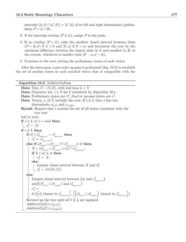
10.2 Static Homology Characters 177
intervals ([a, b] ∩ [a′, b′]) = [a′, b]) of its left and right descendants (prelim-inary P = L ∩ R).
3. If the intervals overlap (P = ∅), assign P to the node.
4. If no overlap (P = ∅), take the smallest closed interval between them(P = [b, a′] if a′ > b and [b′, a] if b′ < a) and increment the cost by theminimum difference between the largest state in L and smallest in R, orthe reverse, whichever is smaller (min (b′ − a, a′ − b)).
5. Continue to the root, setting the preliminary states of each vertex.
After the down-pass, a pre-order up-pass is performed (Alg. 10.2) to establishthe set of median states at each non-leaf vertex that is compatible with the
Algorithm 10.2: AdditiveUpPassData: Tree, T = (V,E), with leaf taxa L ⊂ VData: Character set, c ∈ N for V initialized by Algorithm 10.1.Data: Preliminary states are cp, final or up-pass states are cf .Data: Vertex, v, of T, initially the root. If v /∈ L then v has two
descendants vleft and vright.Result: Require that c contain the set of all states consistent with the
tree costleaf or root;if v ∈ L or v = root then
cfv ← cp
v;if v /∈ L then
if cpv ∩ cf
vparent= cf
vparentthen
cfv ← cf
vparent;
else if (cpvleft
∪ cpvright
) ∩ cfvparent
= ∅ thenX = (cp
vleft∪ cp
vright∪ cp
v) ∩ cfvparent
;if X ∩ cp
v = ∅ thencfv ← X;
elseLargest closed interval between X and cp
v
cfv ← lci{X, cp
v};else
Largest closed interval between {cpv and cf
vparent}
and{(cpvleft
∪ cpvright
) and cfvparent
}cfv ←
lci{[cpv closest to cf
vparent
],[(
cpvleft
∪ cpvright
)closest to cf
vparent
]}
Recurse up the tree until all V /∈ L are updatedAdditiveUp(T, c, vleft);AdditiveUp(T, c, vright);
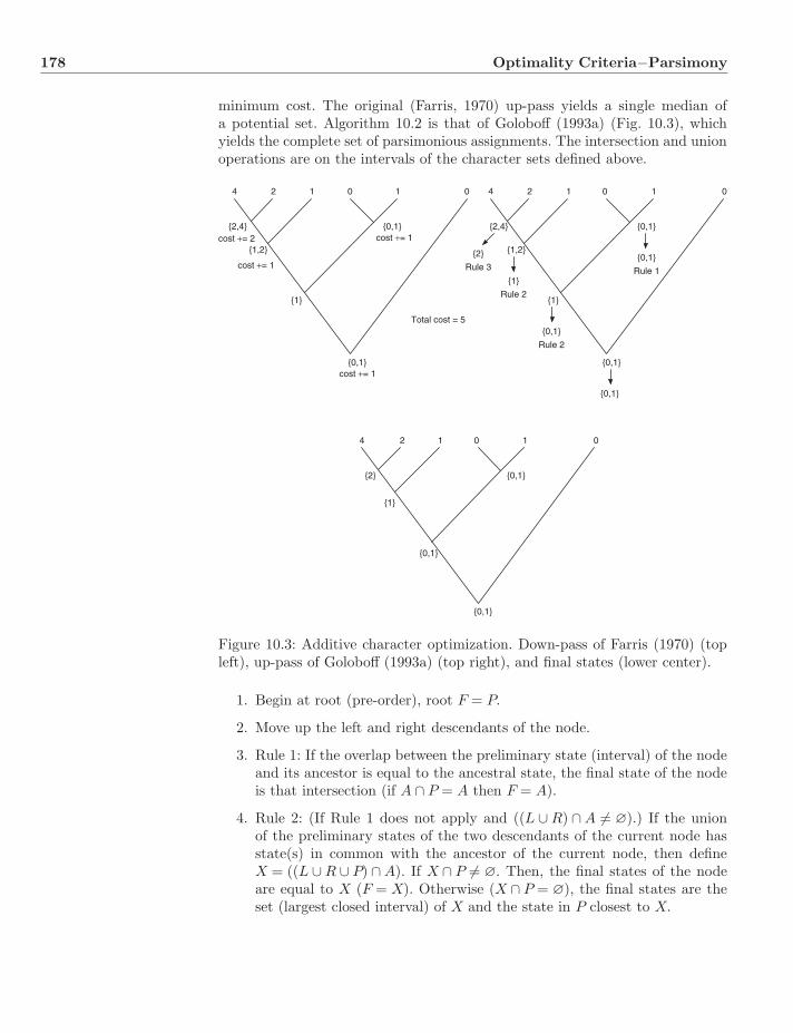
178 Optimality Criteria−Parsimony
minimum cost. The original (Farris, 1970) up-pass yields a single median ofa potential set. Algorithm 10.2 is that of Goloboff (1993a) (Fig. 10.3), whichyields the complete set of parsimonious assignments. The intersection and unionoperations are on the intervals of the character sets defined above.
4 2 1 0 1 0
{2} {0,1}
{0,1}
{0,1}
{1}
4 2 1 0 1 0
{2,4}
{1,2}
{0,1}
{1}
{0,1}
{0,1}
{0,1}
Rule 2
{0,1}
Rule 1{1}
Rule 2
{2}
Rule 3
4 2 1 0 1 0
{2,4}
{1,2}
{0,1}
{1}
{0,1}
cost += 1
cost += 1
cost += 1
Total cost = 5
cost += 2
Figure 10.3: Additive character optimization. Down-pass of Farris (1970) (topleft), up-pass of Goloboff (1993a) (top right), and final states (lower center).
1. Begin at root (pre-order), root F = P.
2. Move up the left and right descendants of the node.
3. Rule 1: If the overlap between the preliminary state (interval) of the nodeand its ancestor is equal to the ancestral state, the final state of the nodeis that intersection (if A ∩ P = A then F = A).
4. Rule 2: (If Rule 1 does not apply and ((L ∪ R) ∩ A = ∅).) If the unionof the preliminary states of the two descendants of the current node hasstate(s) in common with the ancestor of the current node, then defineX = ((L ∪ R ∪ P) ∩ A). If X ∩ P = ∅. Then, the final states of the nodeare equal to X (F = X). Otherwise (X ∩ P = ∅), the final states are theset (largest closed interval) of X and the state in P closest to X.

10.2 Static Homology Characters 179
5. Rule 3: (If Rule 1 and 2 do not apply) Then, the final states (F) of thecurrent node is the largest closed interval between the state in P closestto A and the state in (L ∪ R) closest to A.
6. Continue to leaves (for leaves F = P).
Continuous Characters
Continuous (i.e. real valued) characters, such as measurements of length, or ra-tios can be optimized via this same additive procedure simply by multiplyingthe values by some large constant factor representing the precision of the mea-surement and truncating the result. The “real” values become integerized andcan be optimized as above. The character weight would need to be scaled downto the same degree to maintain parity with other characters and to remove anydependency on units. This approach was taken by Goloboff et al. (2006) and isimplemented in TNT (Goloboff et al., 2003) and POY4 (Varon et al., 2008).
10.2.2 Non-Additive Characters
When character transformation costs are constant1 between all state pairs(Eq. 10.4), those characters are said to be non-additive or unordered (Fitch,1971) (Fig. 10.4).
for states {s0, s1, . . . , sn−1}and constant k
∀i,j σsi,sj= k (10.4)
3
21
4
0
Figure 10.4: Non-additive character states with all possible transformationsequal in cost.
1In practice, all transformation costs are set to unity (1) since the constant term k canbe applied as a character weight after the optimization process. The presentation here is forclarity in comparison with matrix characters (below).
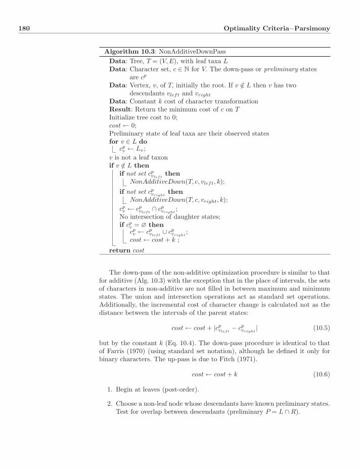
180 Optimality Criteria−Parsimony
Algorithm 10.3: NonAdditiveDownPassData: Tree, T = (V,E), with leaf taxa LData: Character set, c ∈ N for V. The down-pass or preliminary states
are cp
Data: Vertex, v, of T, initially the root. If v /∈ L then v has twodescendants vleft and vright
Data: Constant k cost of character transformationResult: Return the minimum cost of c on TInitialize tree cost to 0;cost ← 0;Preliminary state of leaf taxa are their observed statesfor v ∈ L do
cpv ← Lv;
v is not a leaf taxonif v /∈ L then
if not set cpvleft
thenNonAdditiveDown(T, c, vleft, k);
if not set cpvright
thenNonAdditiveDown(T, c, vright, k);
cpv ← cp
vleft∩ cp
vright;
No intersection of daughter states;if cp
v = ∅ thencpv ← cp
vleft∪ cp
vright;
cost ← cost + k ;
return cost
The down-pass of the non-additive optimization procedure is similar to thatfor additive (Alg. 10.3) with the exception that in the place of intervals, the setsof characters in non-additive are not filled in between maximum and minimumstates. The union and intersection operations act as standard set operations.Additionally, the incremental cost of character change is calculated not as thedistance between the intervals of the parent states:
cost ← cost + |cpvleft
− cpvright
| (10.5)
but by the constant k (Eq. 10.4). The down-pass procedure is identical to thatof Farris (1970) (using standard set notation), although he defined it only forbinary characters. The up-pass is due to Fitch (1971).
cost ← cost + k (10.6)
1. Begin at leaves (post-order).
2. Choose a non-leaf node whose descendants have known preliminary states.Test for overlap between descendants (preliminary P = L ∩ R).
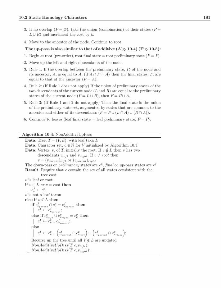
10.2 Static Homology Characters 181
3. If no overlap (P = ∅), take the union (combination) of their states (P =L ∪ R) and increment the cost by k.
4. Move to the ancestor of the node. Continue to root.
The up-pass is also similar to that of additive (Alg. 10.4) (Fig. 10.5):
1. Begin at root (pre-order), root final state = root preliminary state (F = P).
2. Move up the left and right descendants of the node.
3. Rule 1: If the overlap between the preliminary state, P, of the node andits ancestor, A, is equal to A, (if A ∩ P = A) then the final states, F, areequal to that of the ancestor (F = A).
4. Rule 2: (If Rule 1 does not apply) If the union of preliminary states of thetwo descendants of the current node (L and R) are equal to the preliminarystates of the current node (P = L ∪ R), then F = P ∪ A.
5. Rule 3: (If Rule 1 and 2 do not apply) Then the final state is the unionof the preliminary state set, augmented by states that are common to theancestor and either of its descendants (F = P ∪ (L ∩ A) ∪ (R ∩ A)).
6. Continue to leaves (leaf final state = leaf preliminary state, F = P).
Algorithm 10.4: NonAdditiveUpPassData: Tree, T = (V,E), with leaf taxa LData: Character set, c ∈ N for V initialized by Algorithm 10.3.Data: Vertex, v, of T, initially the root. If v /∈ L then v has two
descendants vleft and vright. If v = root thenv = (vparent)left or (vparent)right
The down-pass or preliminary states are cp, final or up-pass states are cf
Result: Require that c contain the set of all states consistent with thetree cost
v is leaf or rootif v ∈ L or v = root then
cfv ← cp
v;v is not a leaf taxonelse if v /∈ L then
if cfvparent
∩ cpv = cf
vparentthen
cfv ← cf
vparent;
else if cpvleft
∪ cpvright
= cpv then
cfv ← cp
v ∪ cfvparent
;else
cfv ← cp
v ∪(cfvparent
∩ cpvleft
)∪
(cfvparent
∩ cpvright
);
Recurse up the tree until all V /∈ L are updatedNonAdditiveUpPass(T, c, vleft);NonAdditiveUpPass(T, c, vright);
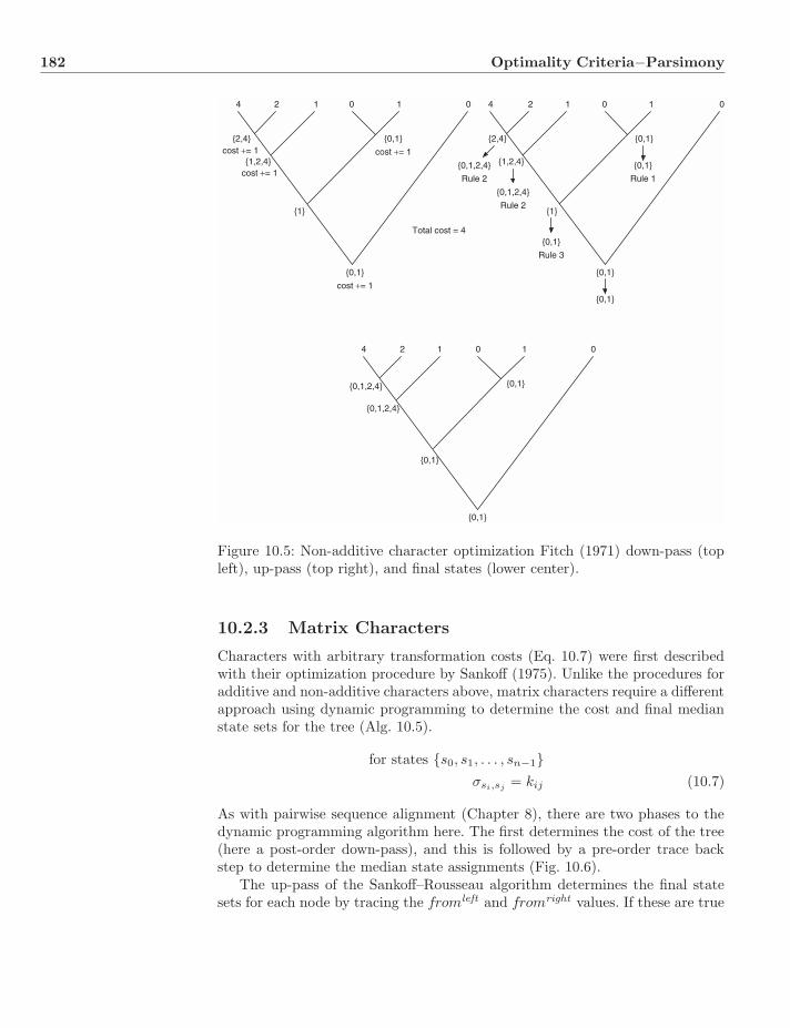
182 Optimality Criteria−Parsimony
4 2 1 0 1 0
{0,1}
{0,1}
{0,1}
4 2 1 0 1 0
{2,4}
{1,2,4}
{0,1}
{1}
{0,1}
{0,1}
{0,1}
Rule 3
{0,1}
Rule 1
{0,1,2,4}
Rule 2
{0,1,2,4}
Rule 2
4 2 1 0 1 0
{2,4}
{1,2,4}
{0,1}
cost += 1
{1}
{0,1}
cost += 1
cost += 1
Total cost = 4
cost += 1
{0,1,2,4}
{0,1,2,4}
Figure 10.5: Non-additive character optimization Fitch (1971) down-pass (topleft), up-pass (top right), and final states (lower center).
10.2.3 Matrix Characters
Characters with arbitrary transformation costs (Eq. 10.7) were first describedwith their optimization procedure by Sankoff (1975). Unlike the procedures foradditive and non-additive characters above, matrix characters require a differentapproach using dynamic programming to determine the cost and final medianstate sets for the tree (Alg. 10.5).
for states {s0, s1, . . . , sn−1}σsi,sj
= kij (10.7)
As with pairwise sequence alignment (Chapter 8), there are two phases to thedynamic programming algorithm here. The first determines the cost of the tree(here a post-order down-pass), and this is followed by a pre-order trace backstep to determine the median state assignments (Fig. 10.6).
The up-pass of the Sankoff–Rousseau algorithm determines the final statesets for each node by tracing the fromleft and fromright values. If these are true
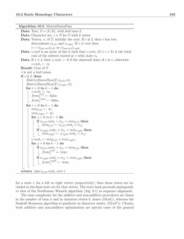
10.2 Static Homology Characters 183
Algorithm 10.5: MatrixDownPassData: Tree, T = (V,E), with leaf taxa LData: Character set, c ∈ N for V with k statesData: Vertex, v, of T, initially the root. If v /∈ L then v has two
descendants vleft and vright. If v = root thenv = (vparent)left or (vparent)right
Data: v.cost is an array of size k such that v.costi (0 ≤ i < k) is the totalcost of the subtree rooted at v with state vk
Data: If v ∈ L then v.costi ← 0 if the observed state of v is i, otherwisev.costi ← ∞
Result: Cost of Tv is not a leaf taxonif v /∈ L then
MatrixDownPass(T, vleft, σ);MatrixDownPass(T, vright, σ);for i = 0 to k − 1 do
v.costi ← ∞;fromleft
i ← false;fromright
i ← false;for i = 0 to k − 1 do
minleft ← ∞;minright ← ∞;for j = 0 to k − 1 do
if vleft.costj + σij < minleft thenminleft ← vleft.costj + σij ;
if vright.costj + σij < minright thenminright ← vright.costj + σij ;
v.costi ← minleft + minright;for j = 0 to k − 1 do
if vleft.costj + σij = minleft thenfromleft
j ← true;
if vright.costj + σij = minright thenfromright
j ← true;
return min vroot.costi over i
for a state i, for a left or right vertex (respectively), then those states are in-cluded in the final state set for that vertex. The trace back proceeds analogouslyto that of the Needleman–Wunsch algorithm (Alg. 8.1) in sequence alignment.
The time complexity for the additive and non-additive procedures are linearin the number of taxa n and in character states k, hence (O(nk)), whereas theSankoff–Rousseau algorithm is quadratic in character states, (O(nk2)). Clearly,both additive and non-additive optimization are special cases of the general

184 Optimality Criteria−Parsimony
5
4 2 0 11 0
0 1 2 3 4State
Cost
LR LR LR LR LRFrom
0 1 2 3 4State
Cost
LR LR LR LR LRFrom
0 1 2 3 4StateCost ∞ ∞ ∞ ∞ 0
0 1 2 3 4StateCost ∞ ∞ 0 ∞ ∞
0 1 2 3 4StateCost ∞ 0 ∞ ∞ ∞
0 1 2 3 4StateCost 0 ∞ ∞ ∞ ∞
0 1 2 3 4StateCost ∞ 0 ∞ ∞ ∞
0 1 2 3 4StateCost 0 ∞ ∞ ∞ ∞
0 1 2 3 4State
Cost
LR LR LR LR LRFrom
0 1 2 3 4State
Cost
LR LR LR LR LRFrom
0 1 2 3 4State
Cost
LR LR LR LR LRFrom
σ States
0 1 2 3 4
0 1 2 3 4
1 0 1 2 3
2 1 0 1 2
3 2 1 0 1
4 3 2 1 0
0
1
2
3
4
42 42 42 42 42
6 4 2 2 2
21 21 21 31 41
5 3 3 3 3
10 11 21 31 31
5 4 5 6 7
10
6 6 9 11
01 01 01 01 01
1 1 3 5 7
Figure 10.6: Matrix character optimized using the Sankoff–Rousseau algorithm(Sankoff, 1975). The states with their costs circled are the final state assignmentsdetermined during the up-pass traceback.
matrix type, with non-diagonal elements either all 1 (non-additive) or the dif-ference in matrix indices (additive).
Although the matrix character optimization algorithm does not requiremetricity, biologically odd results may occur otherwise. As an example, an ad-ditional state could be added to an existing set, with very low transformationcost to all other elements (σk,0 < 1
2 min σi,j). The median state at all internalvertices (V \ L) would then be this new state for all trees, no matter what theleaf conditions were.
10.3 Missing Data
Missing data are always undesirable, not only because of lack of information, butalso because of how they are optimized on trees. The primary requirement of theoptimization of a missing observation is that it should not affect the choice ofoptimal tree, implying that such a non-observation must never contribute costto a tree. In order for this to be the case, optimization routines (such as Addi-tive, Non-Additive, and matrix methods) treat missing values as a maximallypolymorphic state (in order to ensure that the missing datum adds no cost to thetree)—in essence, that all states are present in that non-observation. Recallingthe down-pass of these operations, it is clear that the missing value will conformto the first non-missing observation. This is because of the intersection opera-tions (∩) between the states. This operation is seeking the common information

10.3 Missing Data 185
4 2 1 0 1 0
2 {0,1}
{0,1}
{0,1}
1
X⇒4X⇒2 X⇒1 X⇒0 X⇒0X⇒1
Figure 10.7: Missing character X will assume different states depending on whereit is placed on the tree.
between the two character sets. If one is maximally polymorphic (has all states),then the intersection of that state and any other will be that other set. Anyother scenario would add cost to the optimization, which is impossible. Unfor-tunately, unlike unambiguous observations, the missing data will conform todifferent observations on different trees as it encounters various other taxa first,assuming (in essence) a variety of character states simultaneously (Fig. 10.7).This curious and perhaps undesirable behavior is at the core of the discussions ofPlatnick et al. (1991) and Nixon and Davis (1991). Unfortunately, as bad as thisseems, this treatment of missing data—like democracy—is terrible, except foreverything else.
It is worth noting that autapomorphic data can behave as if they were miss-ing. A unique state of a non-additive character will be lost and conform (as withmissing data) to the first non-unique state it encounters (Fig. 10.8). The samesituation occurs with an additive character but yields different behavior. Dueto the different cost scenario of additive characters, the placement of a uniquestate can affect tree cost (Fig. 10.9). This is due to the fact that a unique statewill either be basal, intermediate, or derived compared to other states. Hence,its homology implications and costs are not uniform.
The behavior of missing data cannot be predicted a priori in any generalway; their pathological effects (if any) are specific to individual analyses.
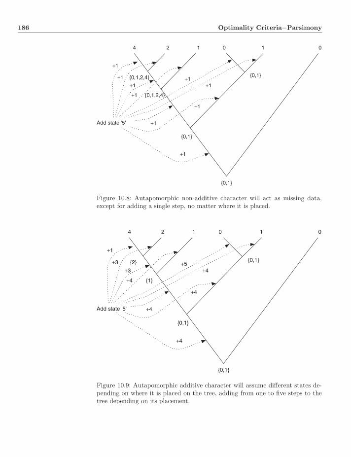
186 Optimality Criteria−Parsimony
4 2 1 0 1 0
{0,1}
{0,1}
{0,1}
{0,1,2,4}
{0,1,2,4}
Add state '5'
+1
+1
+1
+1
+1+1
+1
+1
+1
Figure 10.8: Autapomorphic non-additive character will act as missing data,except for adding a single step, no matter where it is placed.
4 2 1 0 1 0
{0,1}
{0,1}
{0,1}
{2}
{1}
Add state '5'
+1
+3
+3
+4
+5+4
+4
+4
+4
Figure 10.9: Autapomorphic additive character will assume different states de-pending on where it is placed on the tree, adding from one to five steps to thetree depending on its placement.
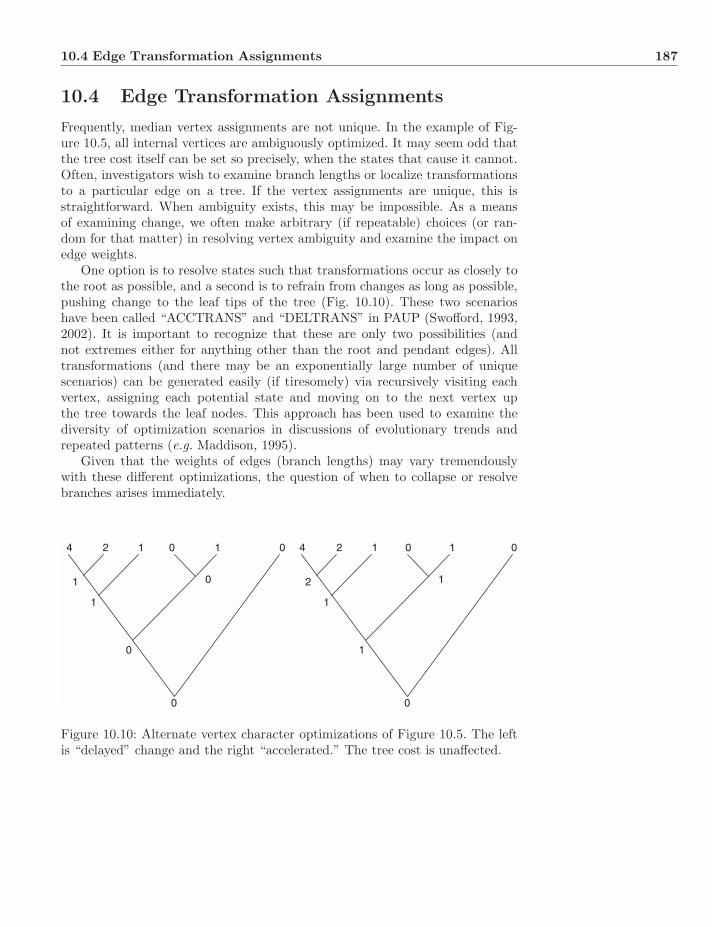
10.4 Edge Transformation Assignments 187
10.4 Edge Transformation Assignments
Frequently, median vertex assignments are not unique. In the example of Fig-ure 10.5, all internal vertices are ambiguously optimized. It may seem odd thatthe tree cost itself can be set so precisely, when the states that cause it cannot.Often, investigators wish to examine branch lengths or localize transformationsto a particular edge on a tree. If the vertex assignments are unique, this isstraightforward. When ambiguity exists, this may be impossible. As a meansof examining change, we often make arbitrary (if repeatable) choices (or ran-dom for that matter) in resolving vertex ambiguity and examine the impact onedge weights.
One option is to resolve states such that transformations occur as closely tothe root as possible, and a second is to refrain from changes as long as possible,pushing change to the leaf tips of the tree (Fig. 10.10). These two scenarioshave been called “ACCTRANS” and “DELTRANS” in PAUP (Swofford, 1993,2002). It is important to recognize that these are only two possibilities (andnot extremes either for anything other than the root and pendant edges). Alltransformations (and there may be an exponentially large number of uniquescenarios) can be generated easily (if tiresomely) via recursively visiting eachvertex, assigning each potential state and moving on to the next vertex upthe tree towards the leaf nodes. This approach has been used to examine thediversity of optimization scenarios in discussions of evolutionary trends andrepeated patterns (e.g. Maddison, 1995).
Given that the weights of edges (branch lengths) may vary tremendouslywith these different optimizations, the question of when to collapse or resolvebranches arises immediately.
4 2 1 0 1 0
0
0
0
1
1
4 2 1 0 1 0
1
0
1
2
1
Figure 10.10: Alternate vertex character optimizations of Figure 10.5. The leftis “delayed” change and the right “accelerated.” The tree cost is unaffected.
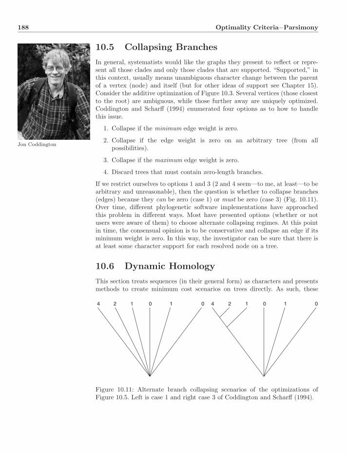
188 Optimality Criteria−Parsimony
10.5 Collapsing Branches
In general, systematists would like the graphs they present to reflect or repre-sent all those clades and only those clades that are supported. “Supported,” inthis context, usually means unambiguous character change between the parentof a vertex (node) and itself (but for other ideas of support see Chapter 15).Consider the additive optimization of Figure 10.3. Several vertices (those closestto the root) are ambiguous, while those further away are uniquely optimized.Coddington and Scharff (1994) enumerated four options as to how to handlethis issue.
Jon Coddington
1. Collapse if the minimum edge weight is zero.
2. Collapse if the edge weight is zero on an arbitrary tree (from allpossibilities).
3. Collapse if the maximum edge weight is zero.
4. Discard trees that must contain zero-length branches.
If we restrict ourselves to options 1 and 3 (2 and 4 seem—to me, at least—to bearbitrary and unreasonable), then the question is whether to collapse branches(edges) because they can be zero (case 1) or must be zero (case 3) (Fig. 10.11).Over time, different phylogenetic software implementations have approachedthis problem in different ways. Most have presented options (whether or notusers were aware of them) to choose alternate collapsing regimes. At this pointin time, the consensual opinion is to be conservative and collapse an edge if itsminimum weight is zero. In this way, the investigator can be sure that there isat least some character support for each resolved node on a tree.
10.6 Dynamic Homology
This section treats sequences (in their general form) as characters and presentsmethods to create minimum cost scenarios on trees directly. As such, these
4 2 1 0 1 0 4 2 1 0 1 0
Figure 10.11: Alternate branch collapsing scenarios of the optimizations ofFigure 10.5. Left is case 1 and right case 3 of Coddington and Scharff (1994).
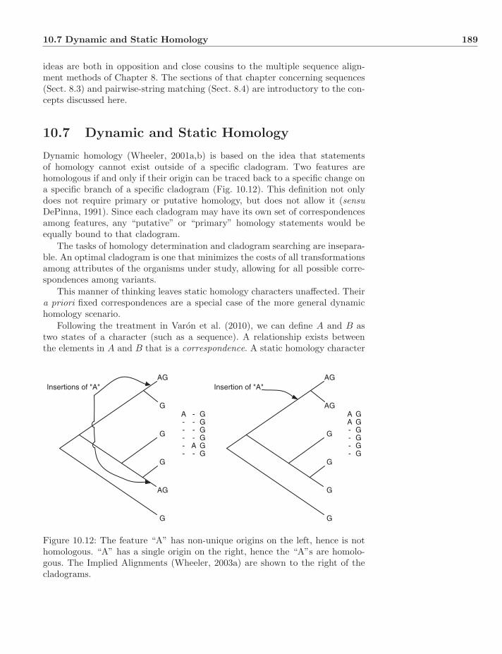
10.7 Dynamic and Static Homology 189
ideas are both in opposition and close cousins to the multiple sequence align-ment methods of Chapter 8. The sections of that chapter concerning sequences(Sect. 8.3) and pairwise-string matching (Sect. 8.4) are introductory to the con-cepts discussed here.
10.7 Dynamic and Static Homology
Dynamic homology (Wheeler, 2001a,b) is based on the idea that statementsof homology cannot exist outside of a specific cladogram. Two features arehomologous if and only if their origin can be traced back to a specific change ona specific branch of a specific cladogram (Fig. 10.12). This definition not onlydoes not require primary or putative homology, but does not allow it (sensuDePinna, 1991). Since each cladogram may have its own set of correspondencesamong features, any “putative” or “primary” homology statements would beequally bound to that cladogram.
The tasks of homology determination and cladogram searching are insepara-ble. An optimal cladogram is one that minimizes the costs of all transformationsamong attributes of the organisms under study, allowing for all possible corre-spondences among variants.
This manner of thinking leaves static homology characters unaffected. Theira priori fixed correspondences are a special case of the more general dynamichomology scenario.
Following the treatment in Varon et al. (2010), we can define A and B astwo states of a character (such as a sequence). A relationship exists betweenthe elements in A and B that is a correspondence. A static homology character
AG
AG
G
G
G
G
Insertion of "A"
AA----
GGGGGG
AG
G
AG
G
G
G
Insertions of "A"
A-----
GGGGGG
----A-
Figure 10.12: The feature “A” has non-unique origins on the left, hence is nothomologous. “A” has a single origin on the right, hence the “A”s are homolo-gous. The Implied Alignments (Wheeler, 2003a) are shown to the right of thecladograms.

190 Optimality Criteria−Parsimony
I. AAATTT
II. TTT
III. AAA
I/II
II/III
III/I
AAATTT
TTT
TTT
AAA
AAATTT
AAA
AAATTT
TTT
AAA
Figure 10.13: Three simple sequences characters showing multiple element cor-respondences and non-transitivity (Wheeler, 2001a).
is one in which, for each element in A, there is at most one element in B, andthese correspondences are transitive (i.e. if a ∈ A corresponds to b ∈ B, and bcorresponds to c ∈ C, then a and c must also correspond). A dynamic homologycharacter would be the complement of this definition. For some pair of states Aand B, there exists an element a ∈ A that corresponds to more than one elementin B, or the correspondences are not transitive (Fig. 10.13).
10.8 Sequences as Characters
Unlike static characters where individual observations constitute states, se-quence character states are extended strings. Individual observations (e.g. nu-cleotides in a DNA sequence) are part of an array of states whose optimizationsare interrelated. The optimization of a given additive (Sect. 10.2.1) or non-additive (Sect. 10.2.2) feature takes place independently of all others (if on thesame cladogram). Those in a sequence character are determined by the lowestcost correspondence among all observations in that sequence. In short, statichomology elements are independent, those of dynamic homology are not. Thisis the root cause of the complexity of their optimization.
A sequence character, then, is the entire contiguous sequence. If the sequenceis a genetic sequence of a particular locus, then that locus is the character.If the sequence is the set of developmental steps involved in the origin of ananatomical feature, then all those steps are components of the character. In the

10.9 The Tree Alignment Problem on Trees 191
case of a nucleotide sequence character, we may or may not specify individuallocus identities (annotations) of sequences (hence, sequences of loci). This is astatic homology statement at the locus level, and the sequence characters of thevarious loci would be optimized independently. This is, however, only a specialcase. The general problem would involve all nucleotides in a genome and allevents that relate them. Annotation, or identification of loci is not a necessaryinput of dynamic homology analysis (but may be a result; Wheeler, 2007b). Iflocus annotations are known, the gene homologies would be static and allow formore rapid optimization.
10.9 The Tree Alignment Problem on Trees
The Tree Alignment Problem (TAP; Sect. 8.5.1) was originally described inthe context of tree optimization (Sankoff, 1975), but later discussed in termsof multiple sequence alignment (Sankoff and Cedergren, 1983). The basic prob-lem is the same—given a tree (T = (V,E)), a set of sequences (L ⊆ V), and ametric distance function (d), determine the median sequence assignments forthe internal vertices (V \ L) such that the overall tree cost (
∑u,v∈E d(u, v)) is
minimal. As mentioned earlier, this optimization problem has been shown tobe NP–hard (Wang and Jiang, 1994). The TAP is the parsimony problem fordynamic homology sequence characters.
10.9.1 Exact Solutions
As mentioned above, exact solutions will be unavailable for non-trivial data sets.Sankoff and Cedergren (1983) proposed a k-dimensional recursive procedure (fork sequences) that used the tree topology to determine the alignment cost foreach cell in cost matrix (Eq. 8.8). The time complexity of this procedure is[O
((2k − 1
) · nk)
for k sequences of length n]. Wheeler (2003c) proposed a sim-ilarly time-complex approach, but based on a different dynamic-programmingmodel. The idea behind this procedure was to use the matrix character opti-mization of Sankoff (1975) with the potential sequences as states. The matrixof character state transformations (σ) is determined by the pairwise edit cost(Sect. 8.4) between sequences. Given the large number of possible sequences(from minimum length n to maximum 2n Nsequences =
∑i=2ni=n i4), the time com-
plexity for an exact solution would be O(n · N2sequences) (after an initial
(Nsequences
2
)set-up operation to determine the pairwise costs). This leads to an unexplored,but potentially useful heuristic procedure where a heuristic sequence set (akinto a heuristic tree search set) could be generated where Nheuristic � Nsequences
with time complexity O(kN2heuristic) (Sect. 10.9.3)(Wheeler, 2003c).
10.9.2 Heuristic Solutions
The central problem in heuristic TAP procedures is the assignment of the in-ternal (V \ L) vertices. Multiple sequence alignment (MSA) can be viewed as aTAP heuristic, constructing median sequences by static optimization (usually
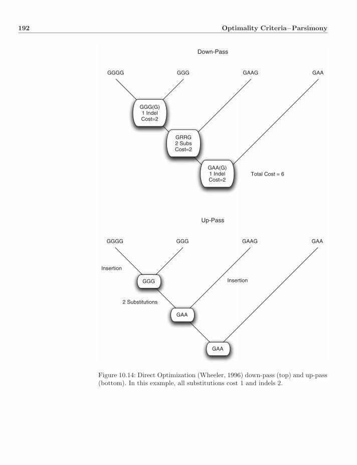
192 Optimality Criteria−Parsimony
Down-Pass
GGGG GGG GAAG GAA
GAA(G)1 IndelCost=2
GRRG2 SubsCost=2
GGG(G)1 IndelCost=2
Total Cost = 6
Up-Pass
GGGG GGG GAAG GAA
GAA
GAA
GGG
Insertion
2 Substitutions
Insertion
Figure 10.14: Direct Optimization (Wheeler, 1996) down-pass (top) and up-pass(bottom). In this example, all substitutions cost 1 and indels 2.
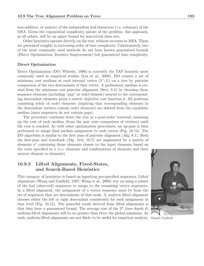
10.9 The Tree Alignment Problem on Trees 193
non-additive, or matrix) of the independent leaf characters (i.e. columns) of theMSA. Given the exponential complexity nature of the problem, this approach,as all others, will be an upper bound for non-trivial data sets.
Other heuristics operate directly on the tree, without recourse to MSA. Theseare presented roughly in increasing order of time complexity. Unfortunately, twoof the most commonly used methods do not have known guaranteed bounds(Direct Optimization, Iterative Improvement) but guaranteed time complexity.
Direct Optimization
Direct Optimization (DO; Wheeler, 1996) is currently the TAP heuristic mostcommonly used in empirical studies (Liu et al., 2009). DO creates a set ofminimum cost medians at each internal vertex (V \ L) on a tree by pairwisecomparison of the two descendants of that vertex. A preliminary median is cre-ated from the minimum cost pairwise alignment (Sect. 8.4) by choosing thosesequence elements (including “gap” or indel element) nearest to the correspond-ing descendent elements given a metric objective cost function d. All positionsconsisting solely of indel elements (implying that corresponding elements inthe descendent vertices contain indel elements) are deleted from the candidatemedian (since sequences do not contain gaps).
The procedure continues down the tree in a post-order traversal, summingup the cost of each median (from the pair wise comparison of vertices) untilthe root is reached. As with other optimization procedures, an up-pass is thenperformed to assign final median assignment to each vertex (Fig. 10.14). TheDO algorithm is similar to the first pass of pairwise alignment (Alg. 8.1). Boththe first-pass and traceback (Alg. 10.6, 10.7) are augmented by a matrix ofelements σ′ containing those elements closest to the input elements based onthe costs specified in σ (i.e. elements and combinations of elements and theirnearest element or elements).
10.9.3 Lifted Alignments, Fixed-States,and Search-Based Heuristics
This category of heuristics is based on inputting pre-specified sequences. Liftedalignments (Wang and Gusfield, 1997; Wang et al., 2000) rely on using a subset
Daniel Gusfield
of the leaf (observed) sequences to assign to the remaining vertex sequences.In a lifted alignment, the assignment of a vertex sequence must be from theset of sequences that are descendants of that node. A uniform lifted alignmentchooses either the left or right descendant consistently for each assignment atthat level (Fig. 10.15). The powerful result derived from lifted alignments isthat they have a guaranteed bound. The average cost of the 2d (tree depth d)uniform-lifted alignments will be no greater than twice the global minimum. Assuch, uniform-lifted alignments are not likely to be useful for empirical analysis,
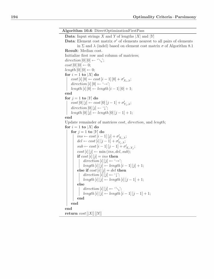
194 Optimality Criteria−Parsimony
Algorithm 10.6: DirectOptimizationFirstPassData: Input strings X and Y of lengths |X| and |Y|Data: Element cost matrix σ′ of elements nearest to all pairs of elements
in Σ and λ (indel) based on element cost matrix σ of Algorithm 8.1Result: Median cost.Initialize first row and column of matrices;direction [0] [0] ← ‘↘’;cost [0] [0] ← 0;length [0] [0] ← 0;for i = 1 to |X| do
cost [i] [0] ← cost [i − 1] [0] + σ′Xi,λ
;direction [i] [0] ← ‘→’;length [i] [0] ← length [i − 1] [0] + 1;
endfor j = 1 to |Y| do
cost [0] [j] ← cost [0] [j − 1] + σ′Yj ,λ;
direction [0] [j] ← ‘↓’;length [0] [j] ← length [0] [j − 1] + 1;
endUpdate remainder of matrices cost, direction, and length;for i = 1 to |X| do
for j = 1 to |Y| doins ← cost [i − 1] [j] + σ′
Xi,λ;
del ← cost [i] [j − 1] + σ′Yj ,λ;
sub ← cost [i − 1] [j − 1] + σ′Xi,Yj
;cost [i] [j] ← min (ins, del, sub);if cost [i] [j] = ins then
direction [i] [j] ← ‘→’;length [i] [j] ← length [i − 1] [j] + 1;
else if cost [i] [j] = del thendirection [i] [j] ← ‘↓’;length [i] [j] ← length [i] [j − 1] + 1;
elsedirection [i] [j] ← ‘↘’;length [i] [j] ← length [i − 1] [j − 1] + 1;
endend
endreturn cost [|X|] [|Y|]
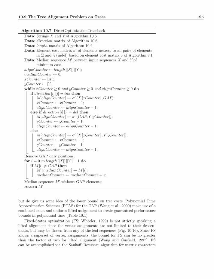
10.9 The Tree Alignment Problem on Trees 195
Algorithm 10.7: DirectOptimizationTracebackData: Strings X and Y of Algorithm 10.6Data: direction matrix of Algorithm 10.6Data: length matrix of Algorithm 10.6Data: Element cost matrix σ′ of elements nearest to all pairs of elements
in Σ and λ (indel) based on element cost matrix σ of Algorithm 8.1Data: Median sequence M′ between input sequences X and Y of
minimum cost.alignCounter ← length [|X|] [|Y|];medianCounter ← 0;xCounter ← |X|;yCounter ← |Y|;while xCounter ≥ 0 and yCounter ≥ 0 and alignCounter ≥ 0 do
if direction [i] [j] = ins thenM[alignCounter] ← σ′ (X [xCounter] , GAP);xCounter ← xCounter − 1;alignCounter ← alignCounter − 1;
else if direction [i] [j] = del thenM[alignCounter] ← σ′ (GAP, Y [yCounter]);yCounter ← yCounter − 1;alignCounter ← alignCounter − 1;
elseM[alignCounter] ← σ′ (X [xCounter] , Y [yCounter]);xCounter ← xCounter − 1;yCounter ← yCounter − 1;alignCounter ← alignCounter − 1;
Remove GAP only positions;for i = 0 to length [|X|] [|Y|] − 1 do
if M [i] = GAP thenM′ [medianCounter] ← M [i];medianCounter ← medianCounter + 1;
Median sequence M′ without GAP elements;return M′
but do give us some idea of the lower bound on tree costs. Polynomial TimeApproximation Schemes (PTAS) for the TAP (Wang et al., 2000) make use of acombined exact and uniform-lifted assignment to create guaranteed performancebounds in polynomial time (Table 10.1).
Fixed-States optimization (FS; Wheeler, 1999) is not strictly speaking alifted alignment since the vertex assignments are not limited to their descen-dants, but may be drawn from any of the leaf sequences (Fig. 10.16). Since FSallows a superset of vertex assignments, the bound for FS can be no greaterthan the factor of two for lifted alignment (Wang and Gusfield, 1997). FScan be accomplished via the Sankoff–Rousseau algorithm for matrix characters

196 Optimality Criteria−Parsimony
s0 s1 s2 s3 s4 s5 s6 s7
s0 s3 s5 s7
s3 s5
s5
s0 s1 s2 s3 s4 s5 s6 s7
s0 s2 s4 s6
s2 s6
s6
Figure 10.15: Lifted assignment (Wang and Gusfield, 1997) (top) and uniform-lifted assignment (Wang et al., 2000) (bottom).
Running time O(kdn3) O(kdn4) O(kdn5) O(kdn6) O(kdn7) O(kdn8) O(kdn9)
TPTAS/Tmin 1.67 1.57 1.50 1.47 1.44 1.42 1.40
Table 10.1: PTAS time complexity for k sequences of length n and tree depth d(Wang et al., 2000).
(Alg. 10.5), with the observed sequences as the states, and their transforma-tion costs determined by their pairwise edit cost (Alg. 8.1). Since the number ofstates is equal to the number of leaves (k), the time complexity of FS is O(k3) foreach tree, which is usually much smaller than that of DO (O(kn2) for sequencelength n) but can grow to be worse for very large data sets (k > n).
Search-based optimization (SBO; Wheeler, 2003c), as mentioned above, ex-pands the possible vertex assignments to non-leaf sequences spanning the di-vide between FS and an exact solution. SBO allows unobserved sequences to
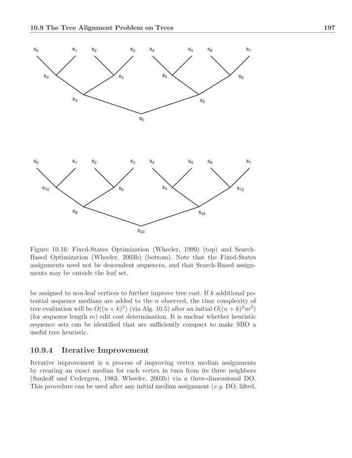
10.9 The Tree Alignment Problem on Trees 197
s0 s1 s2 s3 s4 s5 s6 s7
s3 s3 s5 s6
s3 s5
s5
s0 s1 s2 s3 s4 s5 s6 s7
s10 s9 s4 s12
s8 s45
s23
Figure 10.16: Fixed-States Optimization (Wheeler, 1999) (top) and Search-Based Optimization (Wheeler, 2003b) (bottom). Note that the Fixed-Statesassignments need not be descendent sequences, and that Search-Based assign-ments may be outside the leaf set.
be assigned to non-leaf vertices to further improve tree cost. If k additional po-tential sequence medians are added to the n observed, the time complexity oftree evaluation will be O((n + k)2) (via Alg. 10.5) after an initial O((n + k)2m2)(for sequence length m) edit cost determination. It is unclear whether heuristicsequence sets can be identified that are sufficiently compact to make SBO auseful tree heuristic.
10.9.4 Iterative Improvement
Iterative improvement is a process of improving vertex median assignmentsby creating an exact median for each vertex in turn from its three neighbors(Sankoff and Cedergren, 1983; Wheeler, 2003b) via a three-dimensional DO.This procedure can be used after any initial median assignment (e.g. DO, lifted,

198 Optimality Criteria−Parsimony
s0 s1 s2 s3 s4 s5 s6 s7
v2 v3 v5 v6
v1 v4
Figure 10.17: Iterative improvement (Sankoff and Cedergren, 1983; Wheeler,2003b). Vertices v1, . . . , v6 are each recalculated from their three neighbors.Note that v1 and v4 are neighbors.
or “nearest” leaf). Since the alteration of one vertex may affect its three neigh-bors, the process is repeated, iteratively, over all internal vertices until the vertexset is stable, or the tree cost has reached a stable minimum (Fig. 10.17). Thetime complexity will depend on the number of taxa, k, and the cube of thelength of the sequences, m, for O(km3). Experience shows that tree optimalityis often improved this way, but at high (factor of m) cost (Frost et al., 2006).
10.10 Performance of Heuristic Solutions
There are only a few comparisons of TAP heuristic effectiveness. In general,worst-case effectiveness should follow worst-case time complexity, hence the or-der: lifted assignment, FS, DO, IA, SBO, to exact solutions. Although as yetunstudied, the average case quality of bounds should improve as computationaleffort increases. An area of great interest is in the comparison of MSA as aTAP heuristic to the methods described here (specifically DO as an O(kn2)method similar in complexity to progressive alignment). A handful of limitedstudies (e.g. Wheeler, 2007a; Wheeler and Giribet, 2009) have shown the su-periority (in terms of TAP cost) of DO (via POY; Wheeler et al., 2005; Varonet al., 2008) to MSA (via CLUSTAL; Thompson et al., 1994) in simulated andreal data. More general studies of stronger alignment methods (e.g. MUSCLE,MAFFT) and broader sequence problem sets have yet to reveal themselves.
10.11 Parameter Sensitivity
A topic of great importance to TAP analysis is parameter sensitivity. At its mostbasic, the relative costs of indels and substitutions must be specified (unless anal-yses are limited to areas of exact matching). The objective distance functions

10.12 Implied Alignment 199
that relate sequences to one another via edit costs are based on element editcosts (σ here) among all pairs of sequence elements and the empty (λ) or gapelement. As shown for MSA earlier (Sect. 8.4), the specific values of these pa-rameters are likely to have a large effect on the correspondences among sequenceelements in MSA and TAP. The repercussions of the choice of cost model willcontinue through to the TAP cost and then through tree search playing a rolein the solution to the General Tree Alignment Problem (GTAP; TAP with treesearch to identify the optimal tree). The exploration of this effect has beentermed sensitivity analysis (Wheeler, 1995).
10.11.1 Sensitivity Analysis
Unfortunately, at least in the world of parsimony, there is no method to deter-mine the “true” values of these necessary parameters via observation in nature,and no way to choose one set over another purely on their optimality values(since the numbers are not comparable). As a result, Wheeler (1995) suggestedsensitivity analysis to track the influence of parameter variation on phyloge-netic results (Fig. 10.18). The idea was to repeat analyses using different setsof parameters (indel costs, transition–transversion ratios etc.) and compare theend results on the basis of congruence and stability among data sets. While notan impediment to theoretical studies, empirical studies are driven by the desirefor specific results. Wheeler (1995) suggested two approaches. The first was toidentify those taxonomic groups (= vertices) that were largely or completelyrobust to parameter variation. These groups are relatively insensitive to the un-measurable assumptions of analysis (Fig. 10.19). Unfortunately, as there can behuge variation in parameters, few aspects of tree topology are entirely free ofthis sort of dependence.
The second was to identify those areas in parameter space that minimizedincongruence among characters using an incongruence metric (Wheeler, 1995;Wheeler et al., 2006b) (Fig. 10.20). Studies that report sensitivity results (e.g.Giribet and Edgecombe, 2006; Murienne et al., 2008) usually present both ofthese modes of analysis.
One solution to the problem of sensitivity has been proposed by Grant andKluge (2003, 2005) and that is to treat all transformations as equally costly in allcircumstances. The form of parsimony advocated by Grant and Kluge is one ofminimizing transformations. This interpretive choice was regarded as somewhatarbitrary by Giribet and Wheeler (2007) since this is only one of a very largeset of possible cost regimes. Furthermore, this completely homogeneous costregime could well result in non-metric transformation costs when extended tohigh-order changes involving the insertion and deletion of sequence blocks.
10.12 Implied Alignment
Although DO-based trees (or lifted, FS, and SBO for that matter) are not basedon multiple sequence alignment, and vertex medians may vary in length, it is
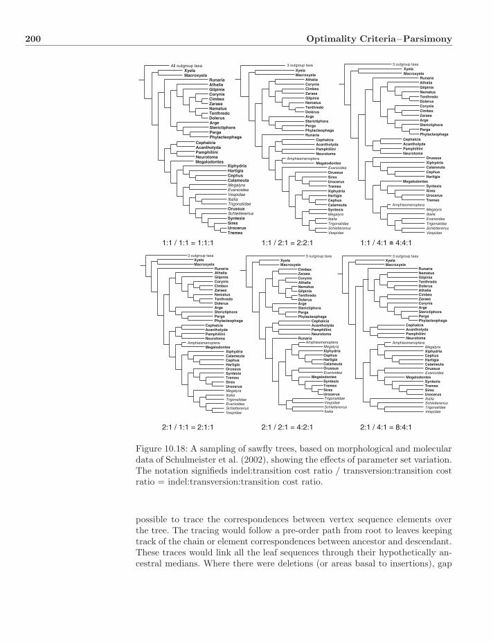
200 Optimality Criteria−Parsimony
3 outgroup taxa
1:1 / 1:1 = 1:1:1 1:1 / 2:1 = 2:2:1 1:1 / 4:1 = 4:4:1
2:1 / 1:1 = 2:1:1 2:1 / 2:1 = 4:2:1 2:1 / 4:1 = 8:4:1
XyelaMacroxyela
Runaria
TenthredoDolerus
Nematus
CimbexZaraea
CorynisGilpiniaAthalia
ArgeSterictiphoraPergaPhylacteophaga
PamphiliiniNeurotoma
CephalciaAcantholyda
AmphiesmenopteraMegalodontes
CephusHartigia
CalameutaXiphydria
SchlettereriusVespidae
Evanioidea
IbaliaTrigonalidae
Megalyra
OrussusSyntexisTremexSirexUrocerus
3 outgroup taxa
AmphiesmenopteraMegalyra
CephusHartigiaCalameuta
Xiphydria
Megalodontes
SirexUrocerus
TremexSyntexis
OrussusEvanioidea
SchlettereriusIbalia
TrigonalidaeVespidae
Runaria
PamphiliiniNeurotoma
CephalciaAcantholyda
TenthredoDolerus
NematusGilpinia
AthaliaCorynis
CimbexZaraea
ArgeSterictiphoraPergaPhylacteophaga
XyelaMacroxyela
3 outgroup taxa
AmphiesmenopteraMegalyra
CephusHartigiaCalameuta
Xiphydria
Megalodontes
SirexUrocerus
TremexSyntexis
OrussusEvanioidea
SchlettereriusTrigonalidaeVespidae
Ibalia
Runaria
TenthredoDolerusAthalia
NematusGilpinia
CimbexZaraeaCorynisArgeSterictiphoraPergaPhylacteophaga
PamphiliiniNeurotoma
CephalciaAcantholyda
XyelaMacroxyela
All outgroup taxaXyelaMacroxyela
Runaria
TenthredoDolerus
Nematus
CimbexZaraea
CorynisGilpiniaAthalia
ArgeSterictiphoraPergaPhylacteophaga
PamphiliiniNeurotoma
CephalciaAcantholyda
Megalodontes
CephusCalameuta
HartigiaXiphydria
MegalyraEvanioidea
IbaliaTrigonalidae
Vespidae
OrussusSchlettereriusSyntexisSirexUrocerusTremex
3 outgroup taxaXyelaMacroxyela
TenthredoDolerus
NematusGilpinia
CimbexZaraea
AthaliaCorynis
ArgeSterictiphoraPergaPhylacteophagaRunaria
PamphiliiniNeurotoma
CephalciaAcantholyda
AmphiesmenopteraMegalodontes
Evanioidea
CephusCalameuta
HartigiaXiphydria
SyntexisMegalyra
SchlettereriusVespidae
IbaliaTrigonalidae
OrussusSirexUrocerusTremex
3 outgroup taxaXyelaMacroxyela
Runaria
TenthredoDolerus
NematusGilpiniaAthalia
CimbexZaraea
Corynis
ArgeSterictiphoraPergaPhylacteophaga
PamphiliiniNeurotoma
CephalciaAcantholyda
CephusHartigia
CalameutaXiphydriaOrussus
AmphiesmenopteraMegalyra
SchlettereriusVespidae
EvanioideaTrigonalidae
Ibalia
MegalodontesSyntexisSirexUrocerusTremex
Figure 10.18: A sampling of sawfly trees, based on morphological and moleculardata of Schulmeister et al. (2002), showing the effects of parameter set variation.The notation signifieds indel:transition cost ratio / transversion:transition costratio = indel:transversion:transition cost ratio.
possible to trace the correspondences between vertex sequence elements overthe tree. The tracing would follow a pre-order path from root to leaves keepingtrack of the chain or element correspondences between ancestor and descendant.These traces would link all the leaf sequences through their hypothetically an-cestral medians. Where there were deletions (or areas basal to insertions), gap
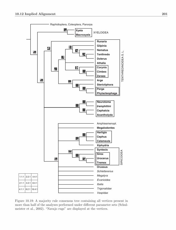
10.12 Implied Alignment 201
Runaria
Gilpinia
Nematus
Tenthredo
Dolerus
Athalia
Corynis
Cimbex
Zaraea
Arge
Sterictiphora
Perga
Phylacteophaga
Neurotoma
Pamphiliini
Cephalcia
Acantholyda
Amphiesmenopt.
Megalodontes
Hartigia
Cephus
Calameuta
Xiphydria
Syntexis
Sirex
Urocerus
Tremex
Orussus
Schlettererius
Megalyra
Evanioidea
Ibalia
Trigonalidae
Vespidae
SIR
ICO
IDE
A
XYELOIDEA
TE
NT
HR
ED
INO
IDE
A S
. L.
Xyela
Macroxyela
Raphidioptera, Coleoptera, Panorpa
1:1:1 2:2:1 4:4:1
2:1:1 4:2:1 8:4:1
4:1:1 8:2:1 16:4:1
Figure 10.19: A majority rule consensus tree containing all vertices present inmore than half of the analyses performed under different parameter sets (Schul-meister et al., 2002). “Navajo rugs” are displayed at the vertices.
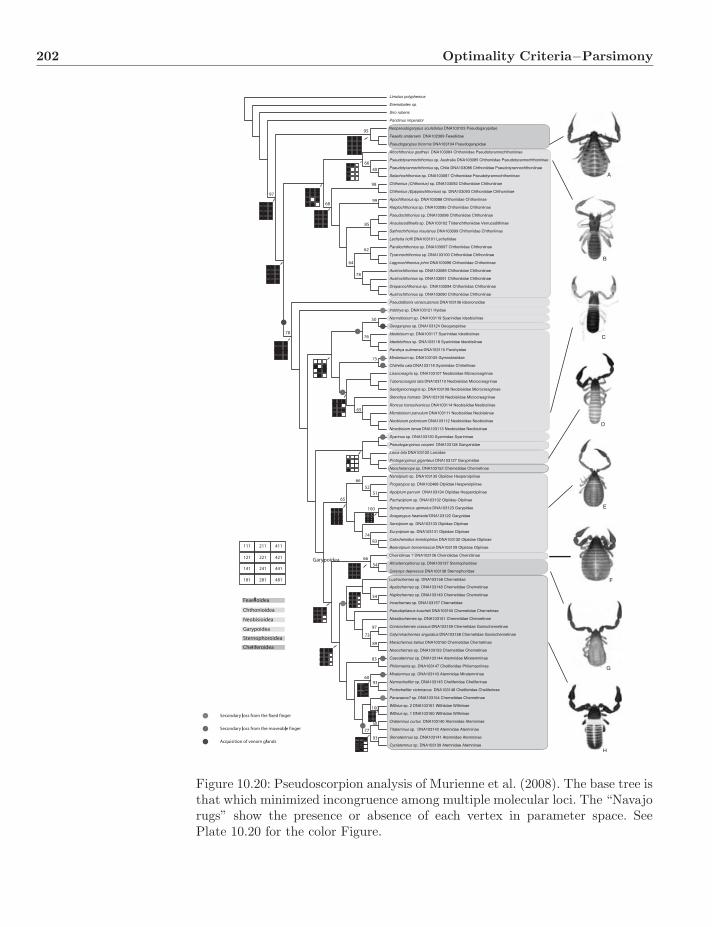
202 Optimality Criteria−Parsimony
Figure 10.20: Pseudoscorpion analysis of Murienne et al. (2008). The base tree isthat which minimized incongruence among multiple molecular loci. The “Navajorugs” show the presence or absence of each vertex in parameter space. SeePlate 10.20 for the color Figure.

10.12 Implied Alignment 203
AA AA AGGG ATT ATTG
A A A A A GG G A T T A GT T- - - - -
A A A A A GG G A T T A GT T
A A- -A A- -A GG GA T T -A GT T
Figure 10.21: Implied alignment (Wheeler, 2003a) of five sequences: AA, AA,AGGG, ATT, and ATTG. The original optimized tree is shown on the upperleft; the implied traces upper right; implied traces with traces extended and gapcharacters filled in lower left; and the final implied alignment in the lower right.See Plate 10.21 for the color Figure.
characters (‘-’) are to be placed. The weighted sum of the transformations alongthese traces would exactly match the tree cost. When displayed in 5’ to 3’ order,these correspondences among leaf elements (with medians removed) would looka great deal like a multiple sequence alignment. It would be the alignmentimplied by the tree and cost parameters. It would be an implied alignment(Fig. 10.21) (Wheeler, 2003a). Implied alignments are different from traditionalmultiple alignments in that the column identity (= putative homology) varieswith, and is linked irrevocably to, the tree topology. Sequence elements (usuallynucleotide, but they could be anything in theory) involving non-homologous(i.e. multiple origin) insertions may appear to be “mis-aligned” when inspectedvisually. This is due, however, to their non-homology (heuristic effects aside).They cannot align since they cannot be homologous. If such elements had asingle origin (such as if they were present in a monophyletic group), they wouldline up (Fig. 10.12).
One nice feature of implied alignments is that they exactly reflect the sequencetransformations that have occurred on the tree. This allows verification of theTAP heuristic cost in that the implied alignment can then be diagnosed as a se-ries of static characters. Given the same tree topology and cost regime (e.g. indelcost), either mode of analysis should return the same cost. This aspect of im-plied alignments leads to a useful TAP search heuristic. Since TAP optimization

204 Optimality Criteria−Parsimony
heuristics such as DO are quadratic in sequence length, and static characters lin-ear, the implied alignment can be used to search for optimal trees much morerapidly than DO can. Of course, the implied alignment potentially would changewith each tree topology, but an alternation between DO and implied alignment(Static Approximation; Wheeler, 2003a) can be a fast and effective tool for initialtree search on unaligned sequence data (Varon et al., 2010).
10.13 Rearrangement
In addition to the insertion–deletion and substitution modes of sequence change,other transformations are possible. These are placed in the general category ofmoves or rearrangement. Chromosomes can be viewed as sequences with generegions (loci) as sequence elements. Variation in gene order, orientation, andcomplement have been used as historical information since the first multi-genemitochondrial sequences became available. Initially, these were informal analyses(e.g. Boore et al., 1995, Fig. 10.22), but more recently, they have been based onexplicit, optimality-based algorithmic procedures (Moret et al., 2002). Most fre-quently, sequence and gene order information have been treated independently.Ideally, however, these data would be optimized simultaneously.
10.13.1 Sequence Characters with Moves
The straightforward, if daunting, simultaneous option is to extend sequence editalgorithms to include moves of blocks of sequences from one position to another(Eq. 10.8). A naıve analysis would suggest complexity for the general case of
4 Crustaceans (4 orders)
134 Insects (10 orders)
2 Chelicerates (2 orders)
4 Myriapods (2 orders)
Onychophoran
Tardigrade
Pogonophoran, 3 annelids(S–A rather than A–S in Platynereis)
Echiuran
Gastropod, polyplacophoranmolluscs
Arthropoda
COI L(UUR) COII
LrRNA L(CUN) L(UUR) NDI
LrRNA L(CUN) L(UUR) NDI
LrRNA L(CUN) L(UUR) NDI
LrRNA L(CUN) L(UUR) NDI
LrRNA L(CUN) I L(UUR) NDI
LrRNA L(CUN) A S L(UUR) NDI
L(CUN) A S L(UUR) NDI
Figure 10.22: Mitochondrial gene order variation in protostome taxa (Booreet al., 1998). See Plate 10.22 for the color Figure.
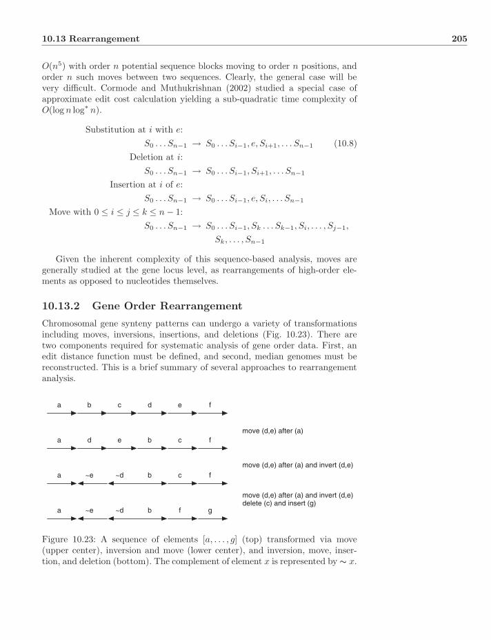
10.13 Rearrangement 205
O(n5) with order n potential sequence blocks moving to order n positions, andorder n such moves between two sequences. Clearly, the general case will bevery difficult. Cormode and Muthukrishnan (2002) studied a special case ofapproximate edit cost calculation yielding a sub-quadratic time complexity ofO(log n log∗ n).
Substitution at i with e:S0 . . . Sn−1 → S0 . . . Si−1, e, Si+1, . . . Sn−1 (10.8)
Deletion at i:S0 . . . Sn−1 → S0 . . . Si−1, Si+1, . . . Sn−1
Insertion at i of e:S0 . . . Sn−1 → S0 . . . Si−1, e, Si, . . . Sn−1
Move with 0 ≤ i ≤ j ≤ k ≤ n − 1:S0 . . . Sn−1 → S0 . . . Si−1, Sk . . . Sk−1, Si, . . . , Sj−1,
Sk, . . . , Sn−1
Given the inherent complexity of this sequence-based analysis, moves aregenerally studied at the gene locus level, as rearrangements of high-order ele-ments as opposed to nucleotides themselves.
10.13.2 Gene Order Rearrangement
Chromosomal gene synteny patterns can undergo a variety of transformationsincluding moves, inversions, insertions, and deletions (Fig. 10.23). There aretwo components required for systematic analysis of gene order data. First, anedit distance function must be defined, and second, median genomes must bereconstructed. This is a brief summary of several approaches to rearrangementanalysis.
a b c d e f
a b cd e f
a b c~d~e f
a b~d~e f g
move (d,e) after (a)
move (d,e) after (a) and invert (d,e)
move (d,e) after (a) and invert (d,e)delete (c) and insert (g)
Figure 10.23: A sequence of elements [a, . . . , g] (top) transformed via move(upper center), inversion and move (lower center), and inversion, move, inser-tion, and deletion (bottom). The complement of element x is represented by ∼ x.
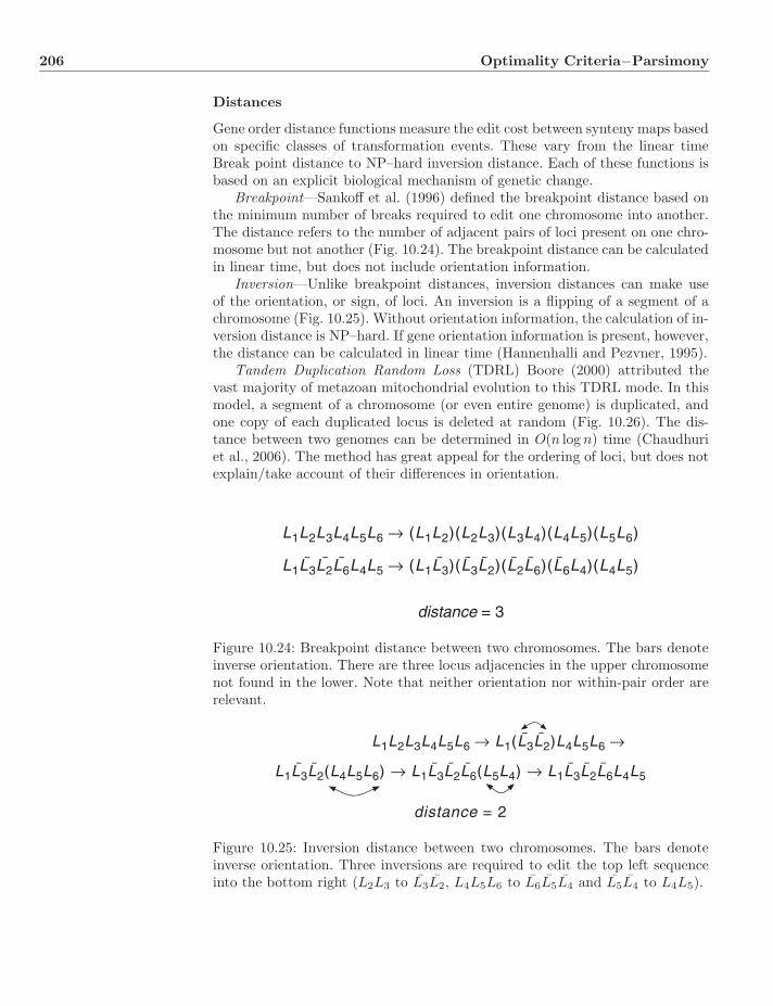
206 Optimality Criteria−Parsimony
Distances
Gene order distance functions measure the edit cost between synteny maps basedon specific classes of transformation events. These vary from the linear timeBreak point distance to NP–hard inversion distance. Each of these functions isbased on an explicit biological mechanism of genetic change.
Breakpoint—Sankoff et al. (1996) defined the breakpoint distance based onthe minimum number of breaks required to edit one chromosome into another.The distance refers to the number of adjacent pairs of loci present on one chro-mosome but not another (Fig. 10.24). The breakpoint distance can be calculatedin linear time, but does not include orientation information.
Inversion—Unlike breakpoint distances, inversion distances can make useof the orientation, or sign, of loci. An inversion is a flipping of a segment of achromosome (Fig. 10.25). Without orientation information, the calculation of in-version distance is NP–hard. If gene orientation information is present, however,the distance can be calculated in linear time (Hannenhalli and Pezvner, 1995).
Tandem Duplication Random Loss (TDRL) Boore (2000) attributed thevast majority of metazoan mitochondrial evolution to this TDRL mode. In thismodel, a segment of a chromosome (or even entire genome) is duplicated, andone copy of each duplicated locus is deleted at random (Fig. 10.26). The dis-tance between two genomes can be determined in O(n log n) time (Chaudhuriet al., 2006). The method has great appeal for the ordering of loci, but does notexplain/take account of their differences in orientation.
distance = 3
L1L2L3L4L5L6 → (L1L2)(L2L3)(L3L4)(L4L5)(L5L6)
L1L3L2L6L4L5 → (L1L3)(L3L2)(L2L6)(L6L4)(L4L5)¯ ¯ ¯ ¯ ¯ ¯ ¯ ¯ ¯
Figure 10.24: Breakpoint distance between two chromosomes. The bars denoteinverse orientation. There are three locus adjacencies in the upper chromosomenot found in the lower. Note that neither orientation nor within-pair order arerelevant.
distance = 2
L1L2L3L4L5L6 → L1(L3L2)L4L5L6 →¯ ¯
L1L3L2(L4L5L6) → L1L3L2L6(L5L4) → L1L3L2L6L4L5¯ ¯ ¯ ¯ ¯ ¯ ¯ ¯
Figure 10.25: Inversion distance between two chromosomes. The bars denoteinverse orientation. Three inversions are required to edit the top left sequenceinto the bottom right (L2L3 to L3L2, L4L5L6 to L6L5L4 and L5L4 to L4L5).
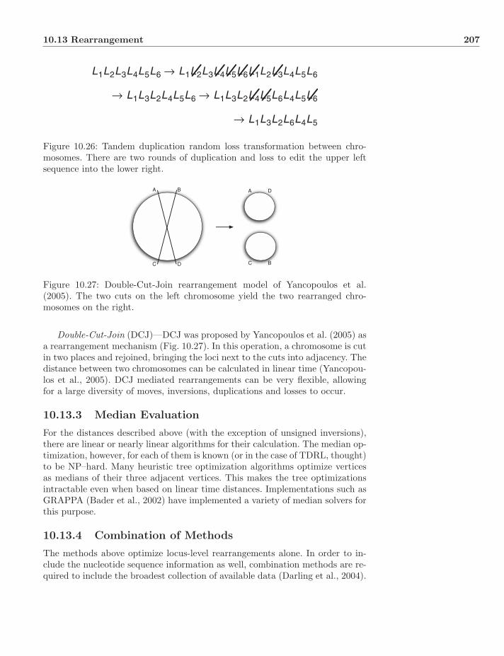
10.13 Rearrangement 207
L1L2L3L4L5L6 → L1L2L3L4L5L6L1L2L3L4L5L6
→ L1L3L2L4L5L6 → L1L3L2L4L5L6L4L5L6
→ L1L3L2L6L4L5
Figure 10.26: Tandem duplication random loss transformation between chro-mosomes. There are two rounds of duplication and loss to edit the upper leftsequence into the lower right.
A B
C D
A D
BC
Figure 10.27: Double-Cut-Join rearrangement model of Yancopoulos et al.(2005). The two cuts on the left chromosome yield the two rearranged chro-mosomes on the right.
Double-Cut-Join (DCJ)—DCJ was proposed by Yancopoulos et al. (2005) asa rearrangement mechanism (Fig. 10.27). In this operation, a chromosome is cutin two places and rejoined, bringing the loci next to the cuts into adjacency. Thedistance between two chromosomes can be calculated in linear time (Yancopou-los et al., 2005). DCJ mediated rearrangements can be very flexible, allowingfor a large diversity of moves, inversions, duplications and losses to occur.
10.13.3 Median Evaluation
For the distances described above (with the exception of unsigned inversions),there are linear or nearly linear algorithms for their calculation. The median op-timization, however, for each of them is known (or in the case of TDRL, thought)to be NP–hard. Many heuristic tree optimization algorithms optimize verticesas medians of their three adjacent vertices. This makes the tree optimizationsintractable even when based on linear time distances. Implementations such asGRAPPA (Bader et al., 2002) have implemented a variety of median solvers forthis purpose.
10.13.4 Combination of Methods
The methods above optimize locus-level rearrangements alone. In order to in-clude the nucleotide sequence information as well, combination methods are re-quired to include the broadest collection of available data (Darling et al., 2004).

208 Optimality Criteria−Parsimony
Wheeler (2007b) coupled genomic rearrangement (via the use of GRAPPA) withsequence optimization (DO and FS—see above) to include the information in an-notated sequences. This annotation was not required for locus homology (= iden-tity), but to mark the potential break points in the rearrangement analysis.LeSy et al. (2006, 2007) removed the annotation requirement, resulting in anentirely dynamic approach to both nucleotide and locus homology (Fig. 10.28).
x1 x2 x3 x4x5
y2 y3 y5y4y1
x2
y5 y4y1 y3 y2
x3 x4x1 x5
(a)
(b)
(c)
(d)
Figure 10.28: The method of LeSy et al. (2007) to identify homologous regionsand loci dynamically: (a) non-rearranged seeds constitute a block, (b) consecu-tive blocks are connected into a large block, (c) blocks are used as anchors todivide genomes into loci, (d) loci are aligned allowing order rearrangements.

10.14 Horizontal Gene Transfer, Hybridization, and Phylogenetic Networks 209
10.14 Horizontal Gene Transfer, Hybridization,and Phylogenetic Networks
There are two sorts of phylogenetic networks that occur in discussions and anal-ysis of reticulate scenarios. The first is motivated by ideas of horizontal genetransfer (HGT, Fig. 10.29) and involves the addition of edges to trees such thatthey accommodate transfer events for specific sets of characters. The second,hybridization networks, produces trees possessing vertices with in-degree 2 andout-degree 1, motivated by the hybridization of lineages (= vertices) (Fig. 10.30).
When dealing with networks as explanations of HGT events, directed edgesare added to binary trees to allow for the individual patterns of sets of characters(N = (V,E)). The resolution of the alternate binary trees implicit in the networkaccount for the diversity of postulated events. In order to arrive at the optimality(cost) of such a network, the sum of cost of the most parsimonious trees (Ti ∈ N)for each set of characters (bi ∈ B) is calculated (Eq. 10.9).
N = (V,E) (10.9)
Ncost =∑bi∈B
(min
T∈T (N)Tcost (bi)
)(10.10)
The construction of hybrid networks involves the calculation of the hybridnumber. This is determined by the SPR (Subtree-Pruning and Regrafting) dis-tance between component trees. This calculation is NP–hard even for a pairof trees (Bordewich and Semple, 2005), hence many operations on this class ofphylogenetic networks have exponential time complexity.
5
Bacteria Archaea
Common ancestral community of primitive cells
Plastids
Mitochondria
Eukarya
3,4
21
Figure 10.29: Depiction of potential horizontal gene transfer events (Smets andBarkay, 2005).
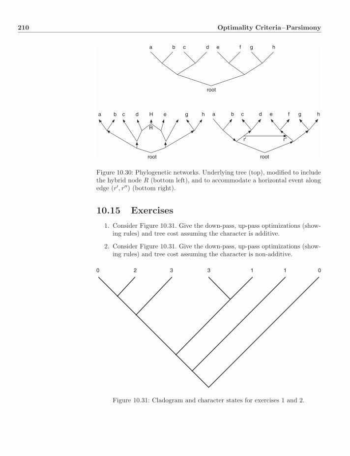
210 Optimality Criteria−Parsimony
a b c d e f g h
root
a b c d e g h
R
root
H a b c d e f g h
root
r' r''
Figure 10.30: Phylogenetic networks. Underlying tree (top), modified to includethe hybrid node R (bottom left), and to accommodate a horizontal event alongedge (r′, r′′) (bottom right).
10.15 Exercises
1. Consider Figure 10.31. Give the down-pass, up-pass optimizations (show-ing rules) and tree cost assuming the character is additive.
2. Consider Figure 10.31. Give the down-pass, up-pass optimizations (show-ing rules) and tree cost assuming the character is non-additive.
0 2 3 3 1 1 0
Figure 10.31: Cladogram and character states for exercises 1 and 2.

10.15 Exercises 211
A C - G T
A C G T -
A 0 1 1 1 1
C 1 0 1 1 1
G 1 1 0 1 1
T 1 1 1 0 1
- 1 1 1 1 0
Figure 10.32: Cladogram, character states, and cost matrix for exercise 3.
3. Consider Figure 10.32. Give the down-pass, up-pass (final states) opti-mizations and tree cost assuming the character is optimized according tothe cost matrix in the figure using dynamic programming.
4. For the above three examples, collapse branches according to rules 1 and3 of Coddington and Scharff (1994). Do you think either (or another) ismore reasonable? For all situations?
5. Consider Figure 10.33. Give the down-pass optimizations and tree costassuming the character is optimized according to the cost matrix in thefigure using direct optimization. Use IUPAC codes to represent nucleotideambiguity.
TA AT TGGTT CCGTT
A C G T -
A 0 1 1 1 1
C 1 0 1 1 1
G 1 1 0 1 1
T 1 1 1 0 1
- 1 1 1 1 0
CAGT AAAATWGG
Figure 10.33: Cladogram, sequence states, and cost matrix for exercise 5.
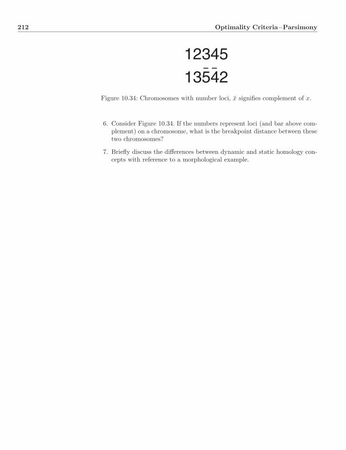
212 Optimality Criteria−Parsimony
12345
13542¯ ¯Figure 10.34: Chromosomes with number loci, x signifies complement of x.
6. Consider Figure 10.34. If the numbers represent loci (and bar above com-plement) on a chromosome, what is the breakpoint distance between thesetwo chromosomes?
7. Briefly discuss the differences between dynamic and static homology con-cepts with reference to a morphological example.
Chapter 11
OptimalityCriteria−Likelihood
The previous two chapters discussed methods to determine the cost of a treebased on overall distance and the minimization of weighted transformations. Wediscuss here the determination of tree cost using stochastic models of characterchange optimizing the probability of the observed data on T given some setof parameters. This probability is proportional to the likelihood function ofSection 6.1.7 and is referred to as the maximum likelihood (ML) criterion.
As with parsimony, ML methods assign median (ancestral) states (either inan optimal or average context) such that the overall likelihood of the tree ismaximized. Unlike minimization-based parsimony, ML methods require explicitmodels of character evolution (as opposed to edit cost regimes) and edge param-eters (branch lengths; parsimony requires none) to determine tree optimality.
The presentation here will also divide characters into static and dynamictypes since they require different analytical techniques.
11.1 Motivation
One might explore alternate optimization criteria for their own sake. ML, how-ever, was proposed in the context of purported problems with parsimony anal-ysis. Although Camin and Sokal (1965) and Farris (1973a) had discussed MLmethods, Felsenstein (1973) was the first to identify concerns with parsimonyand advocate ML as a solution. Much of the discussion centering on the rela-tive merits of parsimony and likelihood in systematics is based on the simplescenario described by Felsenstein (1978).
Joseph Felsenstein
11.1.1 Felsenstein’s Example
Felsenstein posited a four-taxon example (Fig. 11.1) with a simple model ofchange in binary characters to make his point. In this scenario, there are taxa
Systematics: A Course of Lectures, First Edition. Ward C. Wheeler.c© 2012 Ward C. Wheeler. Published 2012 by Blackwell Publishing Ltd.
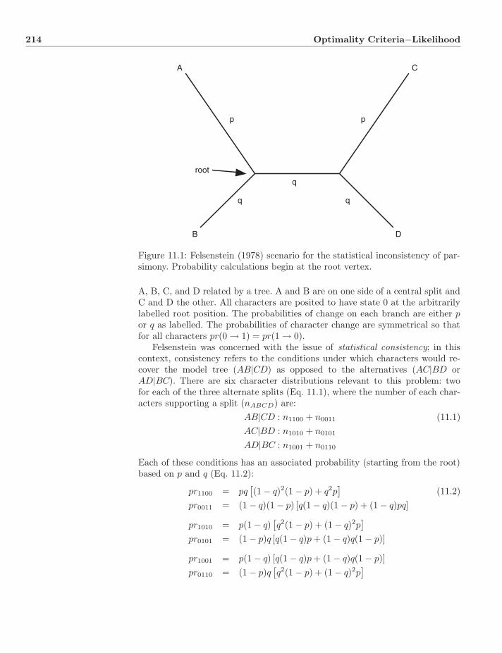
214 Optimality Criteria−Likelihood
A
B
C
D
p p
q
root
Figure 11.1: Felsenstein (1978) scenario for the statistical inconsistency of par-simony. Probability calculations begin at the root vertex.
A, B, C, and D related by a tree. A and B are on one side of a central split andC and D the other. All characters are posited to have state 0 at the arbitrarilylabelled root position. The probabilities of change on each branch are either por q as labelled. The probabilities of character change are symmetrical so thatfor all characters pr(0 → 1) = pr(1 → 0).
Felsenstein was concerned with the issue of statistical consistency; in thiscontext, consistency refers to the conditions under which characters would re-cover the model tree (AB|CD) as opposed to the alternatives (AC|BD orAD|BC). There are six character distributions relevant to this problem: twofor each of the three alternate splits (Eq. 11.1), where the number of each char-acters supporting a split (nABCD) are:
AB|CD : n1100 + n0011 (11.1)AC|BD : n1010 + n0101
AD|BC : n1001 + n0110
Each of these conditions has an associated probability (starting from the root)based on p and q (Eq. 11.2):
pr1100 = pq[(1 − q)2(1 − p) + q2p
](11.2)
pr0011 = (1 − q)(1 − p) [q(1 − q)(1 − p) + (1 − q)pq]
pr1010 = p(1 − q)[q2(1 − p) + (1 − q)2p
]pr0101 = (1 − p)q [q(1 − q)p + (1 − q)q(1 − p)]
pr1001 = p(1 − q) [q(1 − q)p + (1 − q)q(1 − p)]pr0110 = (1 − p)q
[q2(1 − p) + (1 − q)2p
]
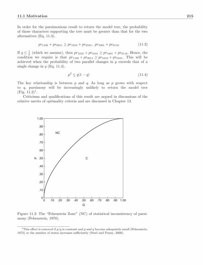
11.1 Motivation 215
In order for the parsimonious result to return the model tree, the probabilityof those characters supporting the tree must be greater than that for the twoalternatives (Eq. 11.3).
pr1100 + pr0011 ≥ pr1010 + pr0101, pr1001 + pr0110 (11.3)
If q ≤ 12 (which we assume), then pr1010 + pr0101 ≥ pr1001 + pr0110. Hence, the
condition we require is that pr1100 + pr0011 ≥ pr1010 + pr0101. This will beachieved when the probability of two parallel changes in p exceeds that of asingle change in q (Eq. 11.4).
p2 ≤ q(1 − q) (11.4)
The key relationship is between p and q. As long as p grows with respectto q, parsimony will be increasingly unlikely to return the model tree(Fig. 11.2)1.
Criticisms and qualifications of this result are argued in discussions of therelative merits of optimality criteria and are discussed in Chapter 13.
00
.10
.20
.30
.40
.50P
.60
.70
.80
.90
1.00
.10 .20 .30 .40 .50
Q
C
NC
.60 .70 .80 .90 1.00
Figure 11.2: The “Felsenstein Zone” (NC) of statistical inconsistency of parsi-mony (Felsenstein, 1978).
1This effect is removed if p/q is constant and p and q become adequately small (Felsenstein,1973) or the number of states increases sufficiently (Steel and Penny, 2000).

216 Optimality Criteria−Likelihood
11.2 Maximum Likelihood and Trees
From the discussion of Section 6.1.7, the likelihood of a hypothesis (in this casea tree T) given data D, is proportional to the probability of the data given thetree (and some model; Eq. 11.5, Edwards, 1972).
l(T |D) ∝ pr(D|T ) (11.5)
A systematic ML method selects T such that pr(D|T ) is maximized. This state-ment includes the requirement of knowledge of a broad variety of quantitiesneeded to determine the likelihood. These include transformation models, edgedistribution (branch lengths), and other parameters bundled together under theterm “nuisance parameters.”
11.2.1 Nuisance Parameters
Nuisance parameters are all those aspects required to calculate pr(D|T ) otherthan the data and tree topology. The three most important and commonly spec-ified nuisance parameters are 1) transformation model (probabilities of changebetween character states), 2) edge parameters (time and rate of change alongbranches), and 3) distribution of rates of change among characters. These pa-rameters can be denoted collectively by θ, and are estimated from observeddata (as with edge parameters), or chosen to maximize the likelihood of a treeor trees. An important assumption for the analysis of character data is thatthey are independent and identically distributed (i.i.d.). This allows the jointlikelihood of several characters to be calculated as the product of their indi-vidual values. Certainly, for many character types, this is not reasonable (e.g.stem and loop sequence characters in rRNA). However, distributional modelscan account for this to a large extent (although dynamic character types wouldbe an exception).
If we have knowledge of the distribution of the nuisance parameters Φ(θ|T ),we can integrate out θ (within parameter space Θ) to determine p(D|T )(Eq. 11.6).
p(D|T ) =∫
θ∈Θ
p(D|T, θ)dΦ(θ|T ) (11.6)
That T which maximizes p(D|T ) in this way is referred to as the maximumintegrated likelihood (MIL) (Steel and Penny, 2000). The MIL is also the MAPBayesian estimate (Chapter 12) if the distribution of tree priors is uniform (flat).
When discussing stochastic model-based systematic methods, it can be usefulto determine the probability that a given method, M, will return the “true”tree given a tree T and set of model parameters θ, ρ(M,T, θ). If we have Φ(θ|T )and a prior distribution of trees, p(T ), the nuisance parameters and tree can beintegrated out, identifying M with the highest expectation of success (Eq. 11.7).
ρ(M) =∑T
p(T )∫
θ∈Θ
ρ(M,T, θ)dΦ(θ|T ) (11.7)
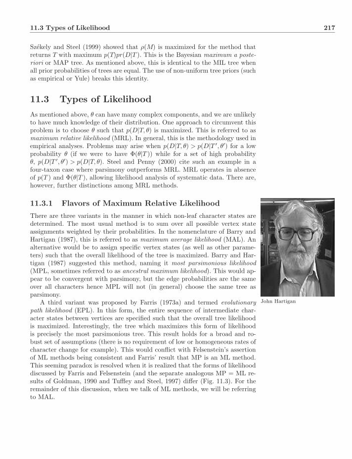
11.3 Types of Likelihood 217
Szekely and Steel (1999) showed that ρ(M) is maximized for the method thatreturns T with maximum p(T)pr(D|T ). This is the Bayesian maximum a poste-riori or MAP tree. As mentioned above, this is identical to the MIL tree whenall prior probabilities of trees are equal. The use of non-uniform tree priors (suchas empirical or Yule) breaks this identity.
11.3 Types of Likelihood
As mentioned above, θ can have many complex components, and we are unlikelyto have much knowledge of their distribution. One approach to circumvent thisproblem is to choose θ such that p(D|T, θ) is maximized. This is referred to asmaximum relative likelihood (MRL). In general, this is the methodology used inempirical analyses. Problems may arise when p(D|T, θ) > p(D|T ′, θ′) for a lowprobability θ (if we were to have Φ(θ|T )) while for a set of high probabilityθ, p(D|T ′, θ′) > p(D|T, θ). Steel and Penny (2000) cite such an example in afour-taxon case where parsimony outperforms MRL. MRL operates in absenceof p(T ) and Φ(θ|T ), allowing likelihood analysis of systematic data. There are,however, further distinctions among MRL methods.
11.3.1 Flavors of Maximum Relative Likelihood
There are three variants in the manner in which non-leaf character states aredetermined. The most usual method is to sum over all possible vertex stateassignments weighted by their probabilities. In the nomenclature of Barry andHartigan (1987), this is referred to as maximum average likelihood (MAL). Analternative would be to assign specific vertex states (as well as other parame-ters) such that the overall likelihood of the tree is maximized. Barry and Har-tigan (1987) suggested this method, naming it most parsimonious likelihood(MPL, sometimes referred to as ancestral maximum likelihood). This would ap-pear to be convergent with parsimony, but the edge probabilities are the sameover all characters hence MPL will not (in general) choose the same tree asparsimony.
John HartiganA third variant was proposed by Farris (1973a) and termed evolutionarypath likelihood (EPL). In this form, the entire sequence of intermediate char-acter states between vertices are specified such that the overall tree likelihoodis maximized. Interestingly, the tree which maximizes this form of likelihoodis precisely the most parsimonious tree. This result holds for a broad and ro-bust set of assumptions (there is no requirement of low or homogeneous rates ofcharacter change for example). This would conflict with Felsenstein’s assertionof ML methods being consistent and Farris’ result that MP is an ML method.This seeming paradox is resolved when it is realized that the forms of likelihooddiscussed by Farris and Felsenstein (and the separate analogous MP = ML re-sults of Goldman, 1990 and Tuffley and Steel, 1997) differ (Fig. 11.3). For theremainder of this discussion, when we talk of ML methods, we will be referringto MAL.
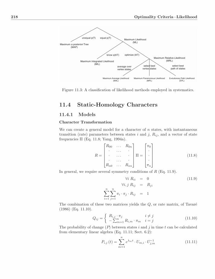
218 Optimality Criteria−Likelihood
Maximum a posteriori Tree(MAP)
unequal p(T) equal p(T)
Maximum Integrated Likelihood(MIL)
know φ(θ|T) optimize (θ|T)Maximum Relative Likelihood
(MRL)
Maximum Likelihood(ML)
Maximum Average Likelihood(MAL)
Maximum Parsimonious Likelihood(MPL)
Evolutionary Path Likelihood(EPL)
average oververtex states
select bestvertex states
select bestpath of states
Figure 11.3: A classification of likelihood methods employed in systematics.
11.4 Static-Homology Characters
11.4.1 Models
Character Transformation
We can create a general model for a character of n states, with instantaneoustransition (rate) parameters between states i and j, Rij , and a vector of statefrequencies Π (Eq. 11.8; Yang, 1994a).
R =
⎡⎢⎢⎢⎢⎣
R00 . . . R0n
· . . . ·· . . . ·· . . . ·
Rn0 . . . Rnn
⎤⎥⎥⎥⎥⎦Π =
⎡⎢⎢⎢⎢⎣
π0
···
πn
⎤⎥⎥⎥⎥⎦ (11.8)
In general, we require several symmetry conditions of R (Eq. 11.9).
∀i Rii = 0 (11.9)∀i, j Rij = Rji
n∑i=1
n∑j=1
πi · πj · Rij = 1
The combination of these two matrices yields the Q, or rate matrix, of Tavare(1986) (Eq. 11.10).
Qij ={
Ri,j · πj i �= j−∑n
m=1 Ri,m · πm i = j(11.10)
The probability of change (P) between states i and j in time t can be calculatedfrom elementary linear algebra (Eq. 11.11; Sect. 6.2):
Pi,j (t) =n∑
m=1
eλmt · Um,i · U−1j,m (11.11)
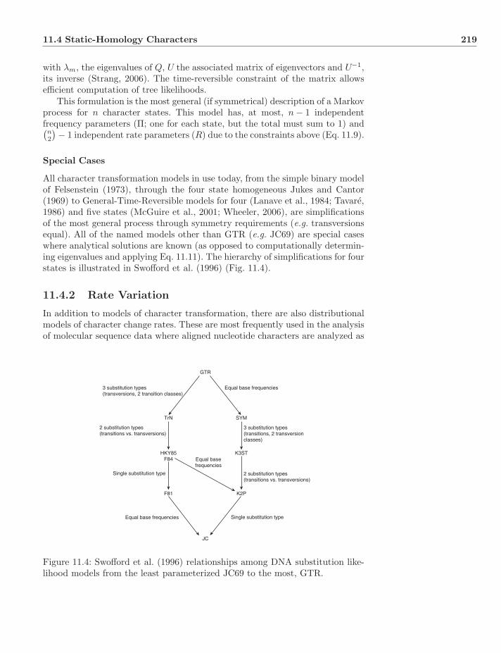
11.4 Static-Homology Characters 219
with λm, the eigenvalues of Q, U the associated matrix of eigenvectors and U−1,its inverse (Strang, 2006). The time-reversible constraint of the matrix allowsefficient computation of tree likelihoods.
This formulation is the most general (if symmetrical) description of a Markovprocess for n character states. This model has, at most, n − 1 independentfrequency parameters (Π; one for each state, but the total must sum to 1) and(n2
) − 1 independent rate parameters (R) due to the constraints above (Eq. 11.9).
Special Cases
All character transformation models in use today, from the simple binary modelof Felsenstein (1973), through the four state homogeneous Jukes and Cantor(1969) to General-Time-Reversible models for four (Lanave et al., 1984; Tavare,1986) and five states (McGuire et al., 2001; Wheeler, 2006), are simplificationsof the most general process through symmetry requirements (e.g. transversionsequal). All of the named models other than GTR (e.g. JC69) are special caseswhere analytical solutions are known (as opposed to computationally determin-ing eigenvalues and applying Eq. 11.11). The hierarchy of simplifications for fourstates is illustrated in Swofford et al. (1996) (Fig. 11.4).
11.4.2 Rate Variation
In addition to models of character transformation, there are also distributionalmodels of character change rates. These are most frequently used in the analysisof molecular sequence data where aligned nucleotide characters are analyzed as
3 substitution types(transversions, 2 transition classes)
3 substitution types(transitions, 2 transversionclasses)
2 substitution types(transitions vs. transversions)
2 substitution types(transitions vs. transversions)
Single substitution type
Single substitution typeEqual base frequencies
Equal base frequencies
Equal basefrequencies
GTR
JC
TrN
HKY85F84
F81
SYM
K3ST
K2P
Figure 11.4: Swofford et al. (1996) relationships among DNA substitution like-lihood models from the least parameterized JC69 to the most, GTR.
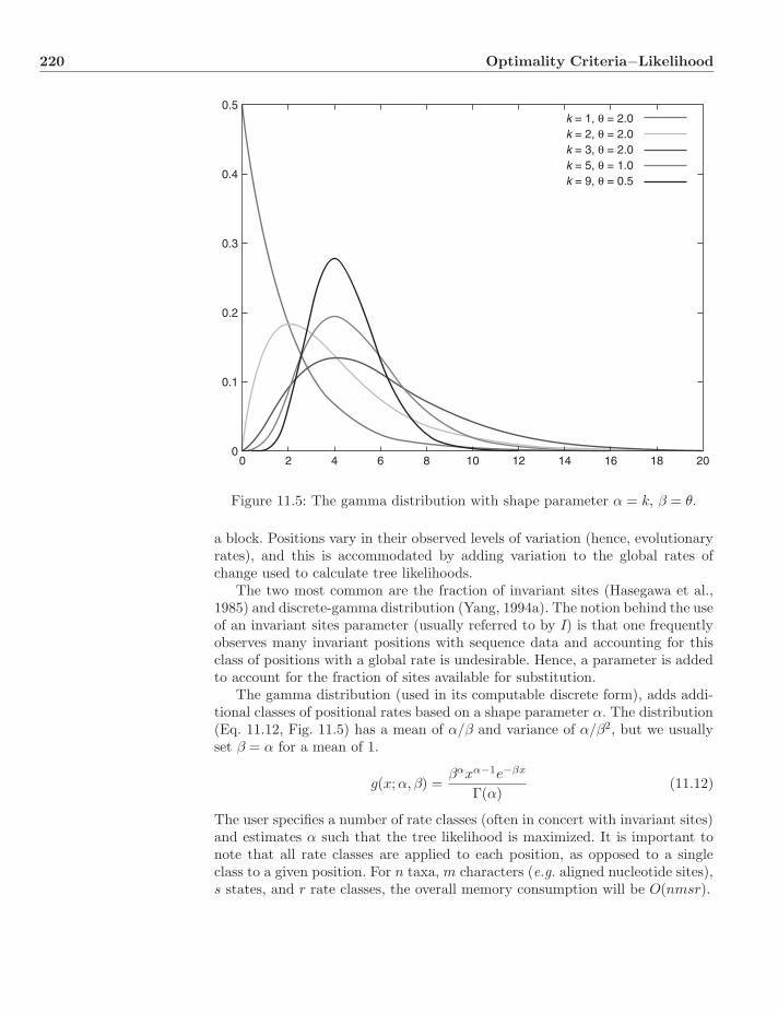
220 Optimality Criteria−Likelihood
00
0.1
0.2
0.3
0.4
0.5
2 4 6 8 10 12
k = 1, θ = 2.0k = 2, θ = 2.0k = 3, θ = 2.0k = 5, θ = 1.0k = 9, θ = 0.5
14 16 18 20
Figure 11.5: The gamma distribution with shape parameter α = k, β = θ.
a block. Positions vary in their observed levels of variation (hence, evolutionaryrates), and this is accommodated by adding variation to the global rates ofchange used to calculate tree likelihoods.
The two most common are the fraction of invariant sites (Hasegawa et al.,1985) and discrete-gamma distribution (Yang, 1994a). The notion behind the useof an invariant sites parameter (usually referred to by I) is that one frequentlyobserves many invariant positions with sequence data and accounting for thisclass of positions with a global rate is undesirable. Hence, a parameter is addedto account for the fraction of sites available for substitution.
The gamma distribution (used in its computable discrete form), adds addi-tional classes of positional rates based on a shape parameter α. The distribution(Eq. 11.12, Fig. 11.5) has a mean of α/β and variance of α/β2, but we usuallyset β = α for a mean of 1.
g(x;α, β) =βαxα−1e−βx
Γ(α)(11.12)
The user specifies a number of rate classes (often in concert with invariant sites)and estimates α such that the tree likelihood is maximized. It is important tonote that all rate classes are applied to each position, as opposed to a singleclass to a given position. For n taxa, m characters (e.g. aligned nucleotide sites),s states, and r rate classes, the overall memory consumption will be O(nmsr).
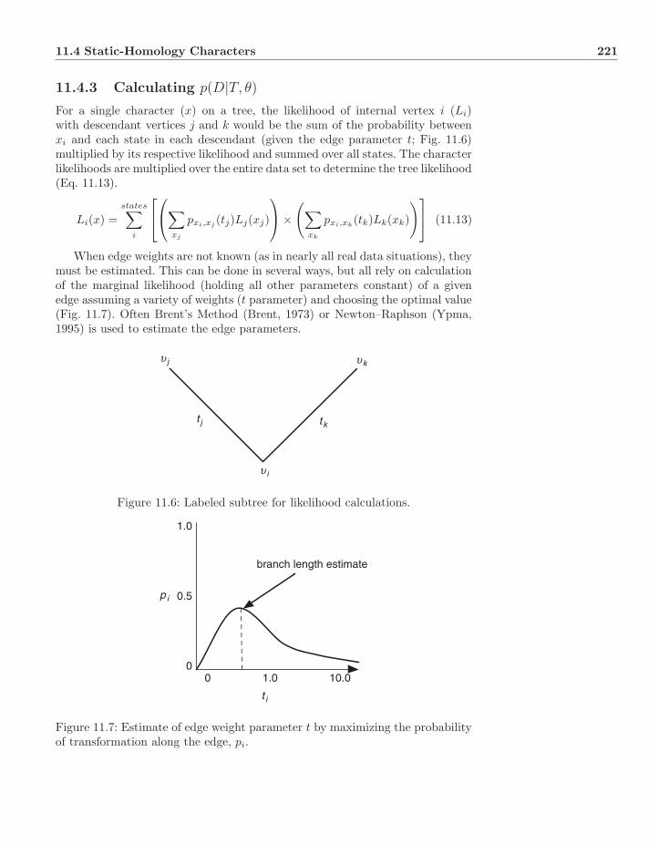
11.4 Static-Homology Characters 221
11.4.3 Calculating p(D|T, θ)
For a single character (x) on a tree, the likelihood of internal vertex i (Li)with descendant vertices j and k would be the sum of the probability betweenxi and each state in each descendant (given the edge parameter t; Fig. 11.6)multiplied by its respective likelihood and summed over all states. The characterlikelihoods are multiplied over the entire data set to determine the tree likelihood(Eq. 11.13).
Li(x) =states∑
i
⎡⎣
⎛⎝∑
xj
pxi,xj(tj)Lj(xj)
⎞⎠ ×
(∑xk
pxi,xk(tk)Lk(xk)
)⎤⎦ (11.13)
When edge weights are not known (as in nearly all real data situations), theymust be estimated. This can be done in several ways, but all rely on calculationof the marginal likelihood (holding all other parameters constant) of a givenedge assuming a variety of weights (t parameter) and choosing the optimal value(Fig. 11.7). Often Brent’s Method (Brent, 1973) or Newton–Raphson (Ypma,1995) is used to estimate the edge parameters.
υ i
υ j υk
tkt j
Figure 11.6: Labeled subtree for likelihood calculations.
pi
0
1.0
t i
0 1.0 10.0
branch length estimate
0.5
Figure 11.7: Estimate of edge weight parameter t by maximizing the probabilityof transformation along the edge, pi.
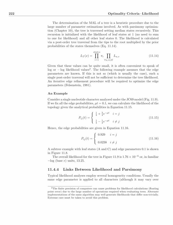
222 Optimality Criteria−Likelihood
The determination of the MAL of a tree is a heuristic procedure due to thelarge number of parameter estimations involved. As with parsimony optimiza-tion (Chapter 10), the tree is traversed setting median states recursively. Thisrecursion is initialized with the likelihood of leaf states at 1 (no need to sumto one for likelihood) and all other leaf states 0. The likelihood is calculatedvia a post-order tree traversal from the tips to the root multiplied by the priorprobabilities of the states themselves (Eq. 11.14).
LT (x) =states∏i=1
πi
∏∀u,v∈E
Lu,v (11.14)
Given that these values can be quite small, it is often convenient to speak oflog or − log likelihood values2. The following example assumes that the edgeparameters are known. If this is not so (which is usually the case), such asingle post-order traversal will not be sufficient to determine the tree likelihood.An iterative edge refinement procedure will be required to optimize the edgeparameters (Felsenstein, 1981).
An Example
Consider a single nucleotide character analyzed under the JC69 model (Fig. 11.9).If we fix all the edge probabilities, μt = 0.1, we can calculate the likelihood of thetopology given the analytical probabilities in Equation 11.15.
Pij(t) =
⎧⎨⎩
14 + 3
4e−μt i = j
14 − 1
4e−μt i �= j(11.15)
Hence, the edge probabilities are given in Equation 11.16.
Pij(t) =
⎧⎨⎩
0.929 i = j
0.0238 i �= j(11.16)
A subtree example with leaf states (A and C) and edge parameters 0.1 is shownin Figure 11.8.
The overall likelihood for the tree in Figure 11.9 is 1.76 × 10⁻⁶ or, in familiar−log (base e) units, 13.25.
11.4.4 Links Between Likelihood and Parsimony
Typical likelihood analyses employ several homogeneity conditions. Usually thesame edge parameter is applied to all characters (although it may vary over
2The finite precision of computers can cause problems for likelihood calculations (floatingpoint error) due to the large number of operations required when evaluating trees. Alternateimplementations of the same algorithm may well generate likelihoods that differ non-trivially.Extreme care must be taken to avoid this problem.
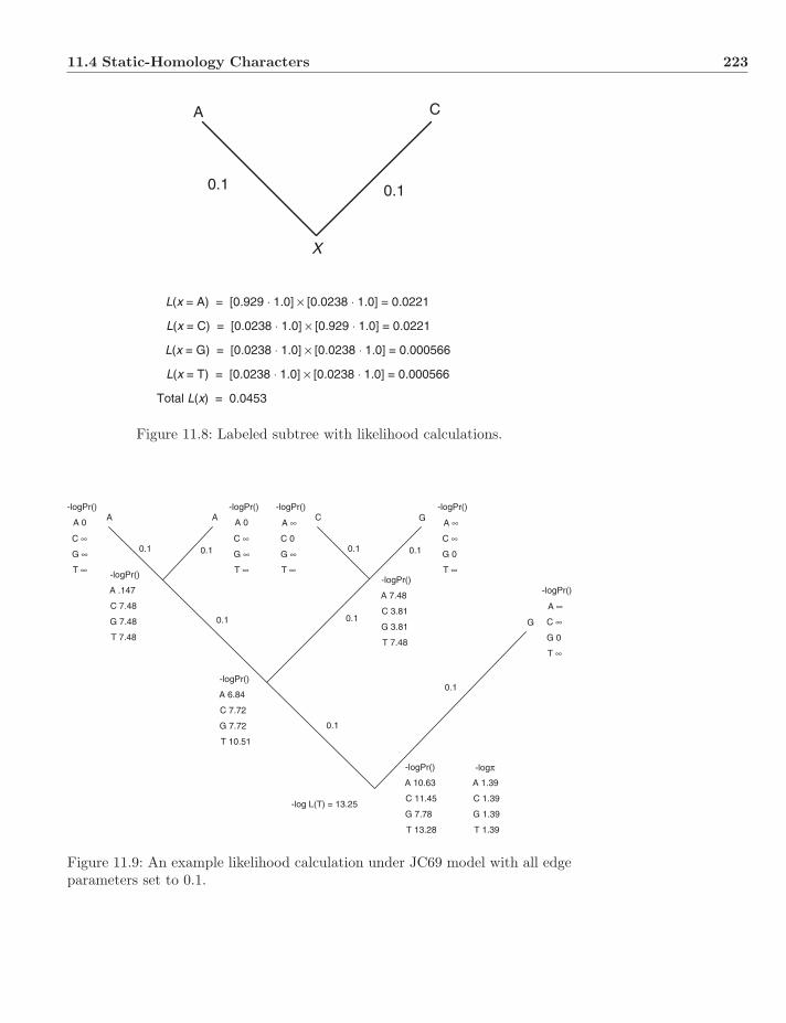
11.4 Static-Homology Characters 223
CA
0.10.1
X
L(x = A) = [0.929 ⋅ 1.0] × [0.0238 ⋅ 1.0] = 0.0221
L(x = C) = [0.0238 ⋅ 1.0] × [0.929 ⋅ 1.0] = 0.0221
L(x = G) = [0.0238 ⋅ 1.0] × [0.0238 ⋅ 1.0] = 0.000566
L(x = T) = [0.0238 ⋅ 1.0] × [0.0238 ⋅ 1.0] = 0.000566
Total L(x) = 0.0453
Figure 11.8: Labeled subtree with likelihood calculations.
A A C G
G
0.1 0.1 0.1 0.1
0.1 0.1
0.1
0.1
-logPr()
A .147
C 7.48
G 7.48
T 7.48
-logPr()
A 6.84
C 7.72
G 7.72
T 10.51
-logPr()
A 7.48
C 3.81
G 3.81
T 7.48
-logPr()
A 10.63
C 11.45
G 7.78
T 13.28
-logπ
A 1.39
C 1.39
G 1.39
T 1.39
-log L(T) = 13.25
-logPr()
A 0
C ∞
G ∞
T ∞
-logPr()
A 0
C ∞
G ∞
T ∞
-logPr()
A ∞
C 0
G ∞
T ∞
-logPr()
A ∞
C ∞
G 0
T ∞
-logPr()
A ∞
C ∞
G 0
T ∞
Figure 11.9: An example likelihood calculation under JC69 model with all edgeparameters set to 0.1.
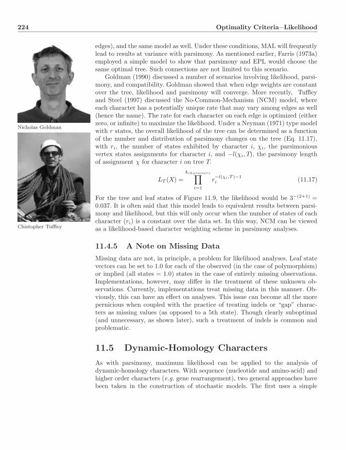
224 Optimality Criteria−Likelihood
edges), and the same model as well. Under these conditions, MAL will frequentlylead to results at variance with parsimony. As mentioned earlier, Farris (1973a)employed a simple model to show that parsimony and EPL would choose thesame optimal tree. Such connections are not limited to this scenario.
Nicholas Goldman
Goldman (1990) discussed a number of scenarios involving likelihood, parsi-mony, and compatibility. Goldman showed that when edge weights are constantover the tree, likelihood and parsimony will converge. More recently, Tuffley
Chistopher Tuffley
and Steel (1997) discussed the No-Common-Mechanism (NCM) model, whereeach character has a potentially unique rate that may vary among edges as well(hence the name). The rate for each character on each edge is optimized (eitherzero, or infinite) to maximize the likelihood. Under a Neyman (1971) type modelwith r states, the overall likelihood of the tree can be determined as a functionof the number and distribution of parsimony changes on the tree (Eq. 11.17),with ri, the number of states exhibited by character i, χi, the parsimoniousvertex states assignments for character i, and −l(χi, T), the parsimony lengthof assignment χ for character i on tree T.
LT (X) =kcharacters∏
i=1
r−l(χi,T )−1i (11.17)
For the tree and leaf states of Figure 11.9, the likelihood would be 3−(2+1) =0.037. It is often said that this model leads to equivalent results between parsi-mony and likelihood, but this will only occur when the number of states of eachcharacter (ri) is a constant over the data set. In this way, NCM can be viewedas a likelihood-based character weighting scheme in parsimony analyses.
11.4.5 A Note on Missing Data
Missing data are not, in principle, a problem for likelihood analyses. Leaf statevectors can be set to 1.0 for each of the observed (in the case of polymorphism)or implied (all states = 1.0) states in the case of entirely missing observations.Implementations, however, may differ in the treatment of these unknown ob-servations. Currently, implementations treat missing data in this manner. Ob-viously, this can have an effect on analyses. This issue can become all the morepernicious when coupled with the practice of treating indels or “gap” charac-ters as missing values (as opposed to a 5th state). Though clearly suboptimal(and unnecessary, as shown later), such a treatment of indels is common andproblematic.
11.5 Dynamic-Homology Characters
As with parsimony, maximum likelihood can be applied to the analysis ofdynamic-homology characters. With sequence (nucleotide and amino-acid) andhigher order characters (e.g. gene rearrangement), two general approaches havebeen taken in the construction of stochastic models. The first uses a simple
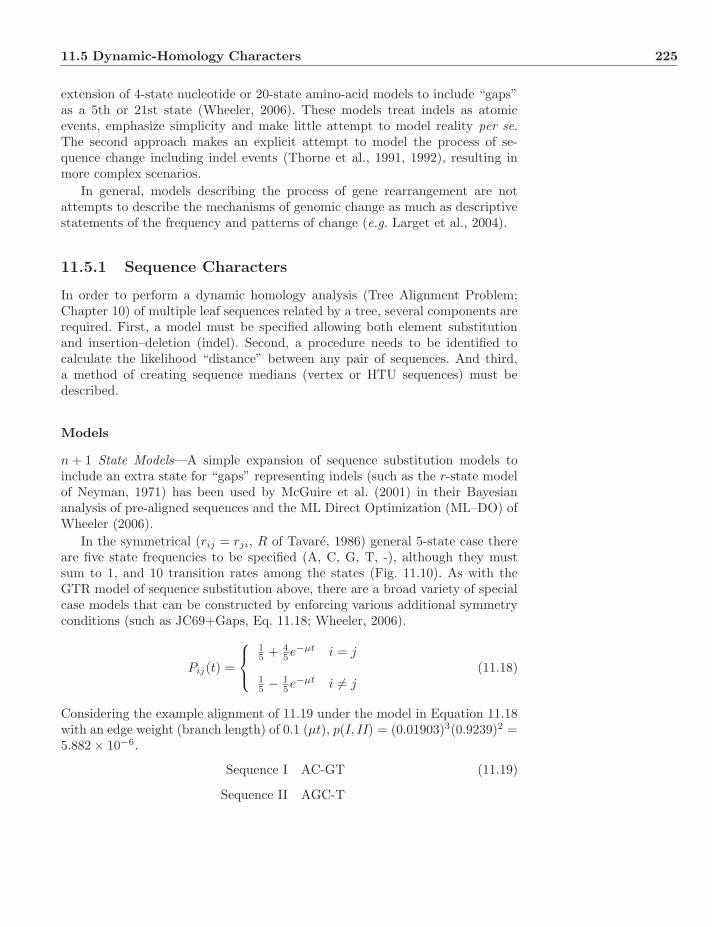
11.5 Dynamic-Homology Characters 225
extension of 4-state nucleotide or 20-state amino-acid models to include “gaps”as a 5th or 21st state (Wheeler, 2006). These models treat indels as atomicevents, emphasize simplicity and make little attempt to model reality per se.The second approach makes an explicit attempt to model the process of se-quence change including indel events (Thorne et al., 1991, 1992), resulting inmore complex scenarios.
In general, models describing the process of gene rearrangement are notattempts to describe the mechanisms of genomic change as much as descriptivestatements of the frequency and patterns of change (e.g. Larget et al., 2004).
11.5.1 Sequence Characters
In order to perform a dynamic homology analysis (Tree Alignment Problem;Chapter 10) of multiple leaf sequences related by a tree, several components arerequired. First, a model must be specified allowing both element substitutionand insertion–deletion (indel). Second, a procedure needs to be identified tocalculate the likelihood “distance” between any pair of sequences. And third,a method of creating sequence medians (vertex or HTU sequences) must bedescribed.
Models
n + 1 State Models—A simple expansion of sequence substitution models toinclude an extra state for “gaps” representing indels (such as the r-state modelof Neyman, 1971) has been used by McGuire et al. (2001) in their Bayesiananalysis of pre-aligned sequences and the ML Direct Optimization (ML–DO) ofWheeler (2006).
In the symmetrical (rij = rji, R of Tavare, 1986) general 5-state case thereare five state frequencies to be specified (A, C, G, T, -), although they mustsum to 1, and 10 transition rates among the states (Fig. 11.10). As with theGTR model of sequence substitution above, there are a broad variety of specialcase models that can be constructed by enforcing various additional symmetryconditions (such as JC69+Gaps, Eq. 11.18; Wheeler, 2006).
Pij(t) =
⎧⎨⎩
15 + 4
5e−μt i = j
15 − 1
5e−μt i �= j(11.18)
Considering the example alignment of 11.19 under the model in Equation 11.18with an edge weight (branch length) of 0.1 (μt), p(I, II) = (0.01903)3(0.9239)2 =5.882 × 10⁻⁶.
Sequence I AC-GT (11.19)
Sequence II AGC-T

226 Optimality Criteria−Likelihood
A
A −(πCα+πGβ+πTγ+π−δ) π−δ
−(πAα+πGε+πTζ+π−η)
−(πAβ+πCε+πTθ+π−κ)
−(πAγ+πCζ+πGθ+π−ν)
−(πAδ+πCη+πGκ+πTν)πTνπGκπCηπAδ
π−νπGθπCζπAγ
π−κπTθπCεπAβ
π−ηπTζπGεπAα
πTγπGβπCα
C
G
T
-
C G T -
Figure 11.10: A general, symmetrical, 5-state model (states A, C, G, T, ‘-’).
These models have the virtue of simplicity and ease of calculation, hencecan be applied to real data sets with multiple loci and empirically interesting(>100) numbers of taxa (Whiting et al., 2006).
Birth–Death Model—The Thorne et al. (1991) and Thorne et al. (1992)models (TKF91 and TKF92), treat the insertion–deletion process in an alter-nate fashion. There are two components to the calculation of the probability oftransforming one sequence into another: the probability of an alignment (α asin 11.19) given a set of insertions, deletions, and matches and model [p(α|α′, θ)];and the probability of a specific pattern of indels and matches given a model[p(α′|θ)]. The method couples a birth–death process (parameters λ—insertionor birth rate; μ—deletion or death rate) with standard four-nucleotide substi-tution models.
Both TKF91 and TKF92 model the indel process in the same way, trans-forming one sequence into another (the model is symmetrical). There are threesorts of events. The first is an insertion (not leading) in the first sequence toyield the second (p). The second transformation type is a deletion (p′), andthe third, a leading insertion, takes place before the left-most residue (p′′). Theprobabilities of these structural events are as in Equation 11.20, with λ birthrate (insertion), μ death rate (deletion), n > 0 indel size, and time t.
pn(t) = e−μt [1 − λβ(t)] [λβ(t)]n−1 (11.20)
p′n(t) =[1 − e−μt − μβ(t)
][1 − λβ(t)] [λβ(t)]n−1
p′′n(t) = [1 − λβ(t)] [λβ(t)]n−1
with
β(t) =1 − e(λ−μ)t
μ − λe(λ−μ)t
The substitution process follows standard models with state frequencies deter-mining the probability of inserting a specific sequence.

11.5 Dynamic-Homology Characters 227
11.5.2 Calculating ML Pairwise Alignment
Both the above models can be optimized for two sequences by versions of thefamiliar dynamic programming procedure used for pairwise sequence alignment(Sect. 8.4). Here, we discuss the algorithm for the n + 1 state model. The recur-sions are more complex for TKF92, but they follow the same basic outline (seeThorne et al., 1992 for specifics).
Dynamic Programming
In order to calculate the probability of transforming one sequence into an-other (or a pairwise alignment; as with parsimony the cost is identical for twosequences), three elements are required: the sequences, the transformationalmodel, and a time parameter to mark the differentiation between the sequences[p(I, II|θ, τ)]. Dynamic programming will optimize the likelihood for a given t,but as with edge weight/branch length optimization, the procedure must berepeated, varying or estimating t until the likelihood is optimized (Eq. 11.21).
p(I, II|θ) = maxt
p(I, II|θ) (11.21)
Since t is chosen to maximize the pairwise probability, the method will yieldan MRL.
It is often convenient to work with the negative logarithm of likelihood andprobability values as opposed to their absolute values and, in this case, it allowsan elegantmodification of theNeedleman andWunsch (1970) algorithm (Alg. 8.1).Based on model and time, the conditional probability of an indel or element matchcan be calculated a priori. In the scenario above (JC69+Gaps with t = 0.1), theprobability of an indel is 1
5 − 15e−0.1 = 0.01903, an element mismatch (substitu-
tion) is the same 15 − 1
5e−0.1 = 0.01903, while an element match 15 + 4
5e−0.1 =0.9239. Using the logarithms of these values, the multiplicative probabilities of ascenario can be optimized as additive sums [log(p(xi) · p(xj)) → log p(xi) +log p(xj)] by treating them as match, mismatch, and indel costs.
Although the log transform probabilities can be used as edit costs (i.e.cost[i][j] = log p(Ii, IIj |θ, t)), the core recursion requires a modification. Theprobability of inter-transforming (or aligning) two sequences is the sum of theprobabilities of all potential transformation (or alignment) scenarios between thetwo. As we know (Eq. 8.6; Slowinski, 1998), there are a large number of theseto calculate. The Needleman–Wunsch algorithm can accomplish this when thecentral alignment recursion is changed to a sum as opposed to the minimumof three paths. This sum is taken among the probabilities (not log probabili-ties) of the three options (element insertion, deletion, and match) at each cell(Eq. 11.22) (cost[i][j] is the − log transformed likelihood).
cost[i][j] = log(e−(cost[i−1][j−1]+σi,j) (11.22)
+ e−(cost[i−1][j]+σindel)
+ e−(cost[i][j−1]+σindel))

228 Optimality Criteria−Likelihood
For sequences of lengths n and m, p(I, II|θ, t) = e−cost[n][m]. The traceback di-agonal marks the maximum likelihood path as before. The complete matrix(in loge units) is shown in Figure 11.11 resulting in a p(I, II|θ = JC69+Gaps,t = 0.1) = 0.0007849. If one were to calculate the probability directly from thefour aligned positions the value would be 0.019032 · 0.85352 = 0.0002638, con-siderably lower than that yielded by the algorithm. This is because the specific
- A C G T
-
A
G
C
T
0.000
4.020 7.962 11.90
6.915
4.020 4.078
7.965
7.965 6.980
8.019
0.07837
4.002
8.019
7.962
11.90
4.078
A
A
C
G
G
C
T
T
. . . .
3.962 7.924 11.89 15.85
3.962
7.924
11.89
15.85
Figure 11.11: Likelihood alignment of two sequences (ACGT and AGCT) underthe JC69+Gaps (5-state Neyman) model with a time parameter (μt) of 0.1 (loge
units).
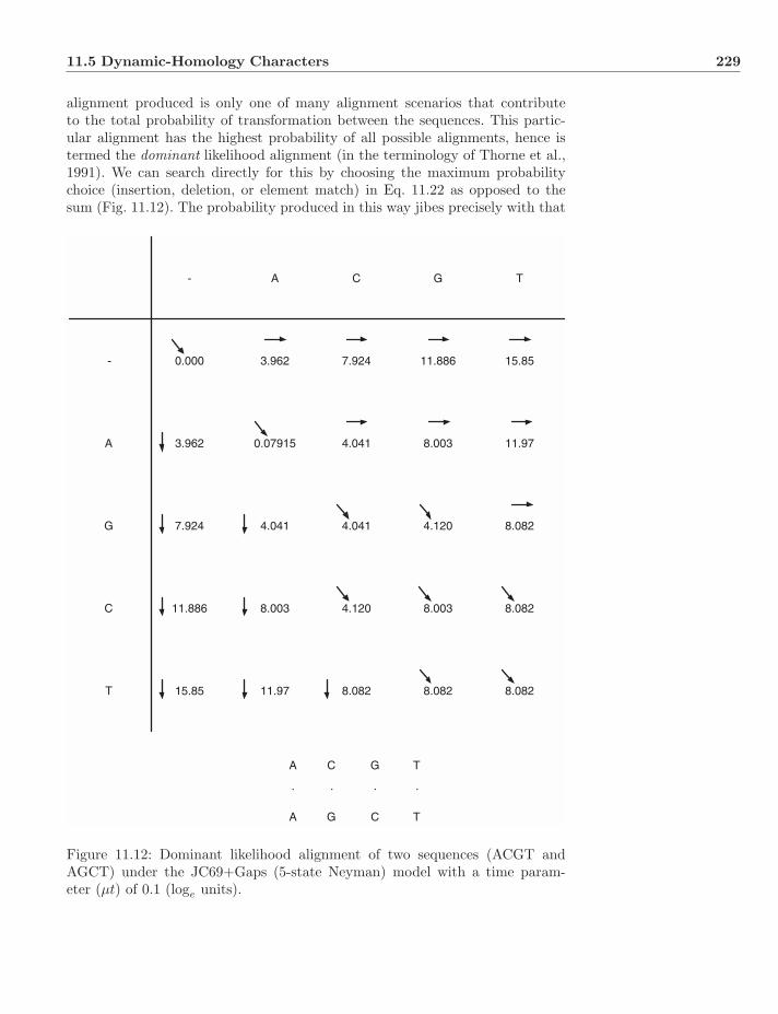
11.5 Dynamic-Homology Characters 229
alignment produced is only one of many alignment scenarios that contributeto the total probability of transformation between the sequences. This partic-ular alignment has the highest probability of all possible alignments, hence istermed the dominant likelihood alignment (in the terminology of Thorne et al.,1991). We can search directly for this by choosing the maximum probabilitychoice (insertion, deletion, or element match) in Eq. 11.22 as opposed to thesum (Fig. 11.12). The probability produced in this way jibes precisely with that
- A C G T
-
A
G
C
T
0.000 3.962 7.924 11.886 15.85
4.041 8.003 11.97
8.003
3.962
4.041 4.120
8.082
8.082 8.082
8.082
0.07915
4.0417.924
8.082
8.00311.886
11.9715.85
4.120
A
A
C
G
G
C
T
T
. . . .
Figure 11.12: Dominant likelihood alignment of two sequences (ACGT andAGCT) under the JC69+Gaps (5-state Neyman) model with a time param-eter (μt) of 0.1 (loge units).

230 Optimality Criteria−Likelihood
expected (e−8.082 = 0.0003091). In this case, both procedures yielded the samealignment, but this need not be the case in general.
The distinction between dominant and total likelihood is an important one.A single alignment may be “best” in a likelihood context, but may contain avery small fraction of the total likelihood (in this case 33%). In the context oflikelihood forms discussed above, the dominant likelihood is akin to an MPLobject, and the total likelihood score MAL. When sequence change is analyzedon a tree, these distinctions have downstream ramifications in the identificationof ML trees, and character change maps on those trees.
11.5.3 ML Multiple Alignment
As with parsimony, there are relatively direct extensions of pairwise alignmentto multiple sequence alignment (MSA). The approach of Wheeler (2006) wasto create an implied alignment (Wheeler, 2003a) using the maximum likelihoodform of Direct Optimization (Wheeler, 1996). In this ML–TAP approach, me-dians (and tree topologies) are chosen to optimize likelihood under a varietyof models from a 5-state Neyman scenario to an enhanced GTR+Gaps model.The relative performance of parsimony and ML implied alignments was testedby Whiting et al. (2006), showing (comfortingly) that ML MSA were superiorfor ML (by 10% log likelihood units) while those based on parsimony were supe-rior for parsimony analysis (by 30%; manual alignments were distant finishers;Table 11.1).
MSA methods based on the TKY92 model (Thorne et al., 1992), such asFleissner et al. (2005) and Redelings and Suchard (2005), make use of BayesianHidden Markov Models and are discussed briefly above and in Chapter 12 inmore detail.
11.5.4 Maximum Likelihood Tree Alignment Problem
Although it is as yet unstudied, given the NP–hard nature of the parsimonyversion of the TAP, the ML variant is likely to be extremely challenging ifnot NP–hard itself. As with parsimony heuristics to the TAP, we can generateseveral heuristic ML–TAP procedures. Unfortunately, almost nothing is knownabout the quality of these solutions (boundedness).
ClustalX Manual DO–MP DO–MLMixed Model Likelihood 61,489.630 55,329.945 51,611.928 50,496.073Single Model Likelihood 61,548.268 55,858.397 51,554.225 51,014.655Parsimony Tree Length 15,154 20,341 11,483 11,702
Table 11.1: Performance of ClustalX (Higgins and Sharp, 1988), Manual, DO–MP, and DO–ML multiple sequence alignment (Whiting et al., 2006). DO im-plied alignment runs were created using Wheeler et al. (2005) and ML scoresby Huelsenbeck and Ronquist (2003).
11.5 Dynamic-Homology Characters 231
Medians and Edges
As with parsimony heuristics to the TAP, the identification of median sequencesis crucial to the quality of the solution. ML–TAP has the added factor of edge orbranch time. As mentioned above for the two sequence case, the probability ofthe alignment is dependent on the time parameter that is identified numericallythrough repeated (or estimated) likelihood optimizations.
Sections 10.9.2, 10.9.3, and 10.9.4 identified sequence medians in ways thatare directly applicable to ML. The algorithm for determining sequence medi-ans using Direct Optimization (Alg. 10.7; DO, Wheeler, 1996) can be appliedlargely without modification. Two issues merit attention. The first is the useof dominant or total likelihood for tree likelihood values and medians. Totallikelihood will reflect more of the probability of alternate medians, but un-less these medians are of optimal (in this case highest probability) cost, theywill not be reflected in the median sequences. Dominant likelihood calculationsmaintain a more consistent approach in that the tree likelihoods are directlytraceable to these specific sequences. When the total likelihood is used, thisconnection can be lost (Wheeler, 2006). The second issue centers around themedian determination and time parameter. The time parameter interacts withthe median identification process, not only to determine the probability of anancestor–descendant transformation, but the ancestral sequences (= medians)themselves. When edge times are estimated to optimize likelihood scores, themedians themselves are likely to change, creating additional time complexityin the process. This is especially prominent when using iterative improvementmethods (Sankoff and Cedergren, 1983; Wheeler, 2003b, 2006). With iterativeimprovement, there are three edges incident on a vertex which require simulta-neous optimization in addition to the 3-dimensional median calculation.
Lifted, Fixed-States, and Search-Based (Sect. 10.9.3) procedures deal witha fixed pool of medians, hence that component of time complexity is reduced.Edge iteration is still an issue in two ways. First, the pairwise probability oftransformation between states is time dependent. This can be either held con-stant over all state pairs, or be optimized (in a fashion akin to Tuffley andSteel, 1997) uniquely for each sequence pair. Secondly, edge times can be ap-plied while a tree is optimized (using a single time) or using optimized timesfrom the pairwise sequence comparisons.
The issue of dominant and total likelihood also enters in this class of heuris-tics through the summing (as in average likelihood) over all potential sequencemedians, or the identification of the most likely medians (MPL) and determiningtree likelihood on that basis.
Wheeler (2006) discussed the above ML–TAP heuristics in the context of a5-state model, although they could be applied to other models. Fleissner et al.(2005) developed a heuristic ML–TAP procedure specifically for the TKF92model. In their approach, simulated annealing (Sect. 14.7) is used in two ways al-ternately. The first is to optimize the analytical parameters (substitution modelparameters, indel birth and death values, fragment length), and the second tooptimize the alignment patterns of indels (h, α′ of Thorne et al., 1991) and tree
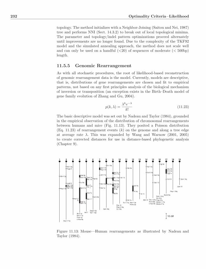
232 Optimality Criteria−Likelihood
topology. The method initializes with a Neighbor-Joining (Saitou and Nei, 1987)tree and performs NNI (Sect. 14.3.2) to break out of local topological minima.The parameter and topology/indel pattern optimizations proceed alternatelyuntil improvements are no longer found. Due to the complexity of the TKF92model and the simulated annealing approach, the method does not scale welland can only be used on a handful (<20) of sequences of moderate (< 500bp)length.
11.5.5 Genomic Rearrangement
As with all stochastic procedures, the root of likelihood-based reconstructionof genomic rearrangement data is the model. Currently, models are descriptive,that is, distributions of gene rearrangements are chosen and fit to empiricalpatterns, not based on any first principles analysis of the biological mechanismof inversion or transposition (an exception exists in the Birth–Death model ofgene family evolution of Zhang and Gu, 2004).
p(k, λ) =λke−λ
k!(11.23)
The basic descriptive model was set out by Nadeau and Taylor (1984), groundedin the empirical observation of the distribution of chromosomal rearrangementsbetween humans and mice (Fig. 11.13). They posited a Poisson distribution(Eq. 11.23) of rearrangement events (k) on the genome and along a tree edgeat average rate λ. This was expanded by Wang and Warnow (2001, 2005)to create corrected distances for use in distance-based phylogenetic analysis(Chapter 9).
Ak-2 1pEno-1 1pFuca 1pc-mos 8q
AsI 7Gapd 12pTpi-1 12p
Aprt 16q
Pyp 10Pep-2 12qCs 12q
Tk-1 17q Acp-1 2pPomc 2p
Adk 10
Sod-2 6q
Pep-1 18q
Lipa 10
Dia-1 22qAs-2 22qc-myc 8q
Sod-1 21qIfrc 21qPrgs 21qMcola-1 17qMcola-2 7q
10 cM
1 2 3 4 5 6 7 8 9 10 11 12 13 14 15 16 17 18 19
Figure 11.13: Mouse—Human rearrangements as illustrated by Nadeau andTaylor (1984).
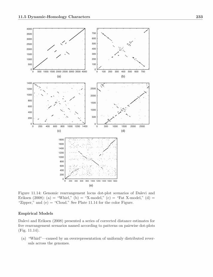
11.5 Dynamic-Homology Characters 233
(a)
0 500 1000 1500 2000 2500 3000 3500 40000
500
1000
1500
2000
2500
3000
3500
4000
(b)
0 100 200 300 400 500 600 7000
100
200
300
400
500
600
700
(c)
0 200 400 600 800 1000 1200 14000
200
400
600
800
1000
1200
1400
(d)
0 500 1000 1500 2000 25000
500
1000
1500
2000
2500
(e)
0 200 400 600 800 1000 1200 1400 1600 18000
200
400
600
800
1000
1200
1400
1600
1800
Figure 11.14: Genomic rearrangement locus dot-plot scenarios of Dalevi andEriksen (2008): (a) = “Whirl,” (b) = “X-model,” (c) = “Fat X-model,” (d) =“Zipper,” and (e) = “Cloud.” See Plate 11.14 for the color Figure.
Empirical Models
Dalevi and Eriksen (2008) presented a series of corrected distance estimates forfive rearrangement scenarios named according to patterns on pairwise dot-plots(Fig. 11.14).
(a) “Whirl”—caused by an overrepresentation of uniformly distributed rever-sals across the genomes.

234 Optimality Criteria−Likelihood
(b) “X-model”—due to a preponderance of reversals symmetrically distributedaround the origins and terminations of replication.
(c) “Fat X-model”—explained by symmetrically distributed reversals with en-hanced variation in their position with respect to the origins and termi-nations of replication.
(d) “Zipper”—thought to result from a large amount of short reversals (up to5% of the genome) distributed uniformly over the genome.
(e) “Cloud”—as rearrangements accrue, the gene order becomes randomizedloosing the previous patterns into a “cloud.”
In general, these descriptions of rearrangement patterns are not used toreconstruct trees directly, but to estimate overall dissimilarity for distance anal-ysis.
11.5.6 Phylogenetic Networks
As with parsimony (Sect. 10.14), horizontal gene transfer and hybridization canbe explained by networks and in an analogous fashion (Strimmer and Moulton,2000). Jin et al. (2006) proposed no biological model of horizontal gene transferor hybridization, but two methods to calculate the likelihood of the network. Inthe same way that the parsimony score of a network is calculated by summingthe minimum tree costs consistent with the network (Eq. 10.9) for each block ofcharacters, likelihoods can be multiplied over the best likelihood tree for eachcharacter block. A second option would be to sum the likelihoods of all treescenarios consistent with the network (Fig. 11.15; Eq. 11.24).
N = (V,E) (11.24)
LallN (S|N, θ) =
∑T∈N
(p(T) · L(S|T, θ))
LbestN (S|N, θ) = max
T∈N(p(T) · L(S|T, θ))
It is unclear which, if either, procedure is appropriate. The first method assumesall blocks are independent. This may or may not be reasonable given that therecognition of blocks is dependent on their relative positions and behavior. Thesecond model has the advantage of including alternate scenarios, weighted bytheir likelihoods, but allows for multiple histories for all blocks.
11.6 Hypothesis Testing
11.6.1 Likelihood Ratios
Often, it is desirable to know whether a difference between two likelihood val-ues is “significant.” As odd as such a concept may seem within the rationale of
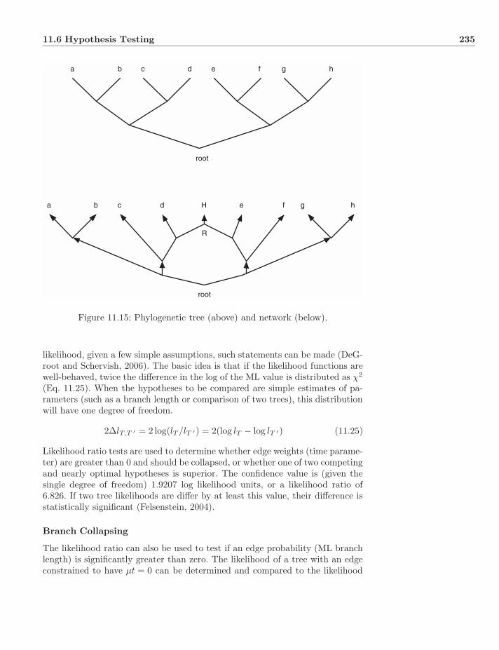
11.6 Hypothesis Testing 235
a b c d e f g h
root
a b c d e f g h
R
root
H
Figure 11.15: Phylogenetic tree (above) and network (below).
likelihood, given a few simple assumptions, such statements can be made (DeG-root and Schervish, 2006). The basic idea is that if the likelihood functions arewell-behaved, twice the difference in the log of the ML value is distributed as χ2
(Eq. 11.25). When the hypotheses to be compared are simple estimates of pa-rameters (such as a branch length or comparison of two trees), this distributionwill have one degree of freedom.
2ΔlT,T ′ = 2 log(lT /lT ′) = 2(log lT − log lT ′) (11.25)
Likelihood ratio tests are used to determine whether edge weights (time parame-ter) are greater than 0 and should be collapsed, or whether one of two competingand nearly optimal hypotheses is superior. The confidence value is (given thesingle degree of freedom) 1.9207 log likelihood units, or a likelihood ratio of6.826. If two tree likelihoods are differ by at least this value, their difference isstatistically significant (Felsenstein, 2004).
Branch Collapsing
The likelihood ratio can also be used to test if an edge probability (ML branchlength) is significantly greater than zero. The likelihood of a tree with an edgeconstrained to have μt = 0 can be determined and compared to the likelihood
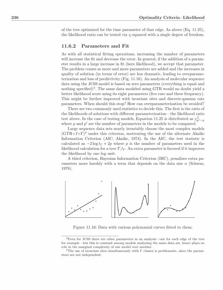
236 Optimality Criteria−Likelihood
of the tree optimized for the time parameter of that edge. As above (Eq. 11.25),the likelihood ratio can be tested via χ-squared with a single degree of freedom.
11.6.2 Parameters and Fit
As with all statistical fitting operations, increasing the number of parameterswill increase the fit and decrease the error. In general, if the addition of a param-eter results in a large increase in fit (here likelihood), we accept that parameter.The problem comes as more and more parameters are added and the increases inquality of solution (in terms of error) are less dramatic, leading to overparame-terization and loss of predictivity (Fig. 11.16). An analysis of molecular sequencedata using the JC69 model is based on zero parameters (everything is equal andnothing specified)3. The same data modeled using GTR would no doubt yield abetter likelihood score using its eight parameters (five rate and three frequency).This might be further improved with invariant sites and discrete-gamma rateparameters. When should this stop? How can overparameterization be avoided?
There are two commonly used statistics to decide this. The first is the ratio ofthe likelihoods of solutions with different parameterization—the likelihood ratiotest above. In the case of testing models, Equation 11.25 is distributed as χ2
p′−p
where p and p′ are the number of parameters in the models to be compared.Large sequence data sets nearly invariably choose the most complex models
(GTR+I+Γ)4 under this criterion, motivating the use of the alternate AkaikeInformation Criterion (AIC; Akaike, 1974). In the AIC, the test statistic iscalculated as −2 log lT + 2p where p is the number of parameters used in thelikelihood calculation for a tree T, lT . An extra parameter is favored if it improvesthe likelihood by one log unit.
A third criterion, Bayesian Information Criterion (BIC), penalizes extra pa-rameters more harshly with a term that depends on the data size n (Schwaz,1978).
Figure 11.16: Data with various polynomial curves fitted to them.
3Even for JC69 there are other parameters in an analysis—one for each edge of the treefor example—but this is constant among models analyzing the same data set, hence plays norole in the marginal complexity of one model over another.
4The use of invariant sites simultaneously with Γ classes is problematic, since the param-eters are not independent.

11.6 Hypothesis Testing 237
TN93+I+Γ 5441.4600 78 11045.5888 0.5221 0.52210.0000
Model l K AICc w Cum(w)Δ AICc
TIM+I+Γ 5441.3765 79 11047.5965 0.1913 0.71342.0077HKY85+I+Γ 5443.6729 77 11047.8422 0.1692 0.88262.2534K81uf+I+Γ 5443.5566 78 11049.7821 0.0641 0.94684.1934GTR+I+Γ 5440.9150 81 11051.0301 0.0344 0.98115.4413TVM+I+Γ 5442.7393 80 11052.4991 0.0165 0.99766.9103TN93+Γ 5448.6792 77 11057.8549 0.0011 0.998812.2661HKY85+Γ 5450.5068 76 11059.3402 0.0005 0.999313.7514TIM+Γ 5448.6577 78 11059.9843 0.0004 0.999714.3955K81uf+Γ 5450.4883 77 11061.4730 0.0002 0.999915.8843GTR+Γ 5448.0298 80 11063.0802 0.0001 1.000017.4914TVM+Γ 5449.6685 79 11064.1804 0.0000 1.000018.5917TN93+I 5470.7568 77 11102.0102 0.0000 1.000056.4214TIM+I 5470.7417 78 11104.1522 0.0000 1.000058.5635GTR+I 5470.3452 80 11107.7110 0.0000 1.000062.1223HKY85+I 5476.8496 76 11112.0257 0.0000 1.000066.4370K81uf+I 5476.8208 77 11114.1381 0.0000 1.000068.5493TVM+I 5476.1650 79 11117.1736 0.0000 1.000071.5849F81+I+Γ 5769.1118 76 11696.5501 0.0000 1.0000650.9614F81+Γ 5782.0566 75 11720.2721 0.0000 1.0000674.6834F81+I 5807.4927 75 11771.1442 0.0000 1.0000725.5554GTR 5805.0576 79 11774.9588 0.0000 1.0000729.3700TVM 5808.4727 78 11779.6141 0.0000 1.0000734.0254TIM 5810.4102 77 11781.3168 0.0000 1.0000735.7280TN93 5813.4780 76 11785.2825 0.0000 1.0000739.6938K81uf 5813.5190 76 11785.3646 0.0000 1.0000739.7758HKY85 5816.5894 75 11789.3375 0.0000 1.0000743.7488SYM+I+Γ 5861.0859 78 11884.8407 0.0000 1.0000839.2520TVMef+I+Γ 5867.6128 77 11895.7221 0.0000 1.0000850.1333SYM+Γ 5876.7803 77 11914.0570 0.0000 1.0000868.4683TVMef+Γ 5884.4272 76 11927.1810 0.0000 1.0000881.5922TIMef+I+Γ 5885.0684 76 11928.4632 0.0000 1.0000882.8745K81+I+Γ 5893.7642 75 11943.6872 0.0000 1.0000898.0984TN93ef+I+Γ 5897.7529 75 11951.6647 0.0000 1.0000906.0759TIMef+Γ 5899.2588 75 11954.6764 0.0000 1.0000909.0877K80+I+Γ 5906.2329 74 11966.4593 0.0000 1.0000920.8706K81+Γ 5908.7876 74 11971.5687 0.0000 1.0000925.9800TN93ef+Γ 5911.5659 74 11977.1254 0.0000 1.0000931.5366SYM+Γ 5908.7021 77 11977.9008 0.0000 1.0000932.3120TVMef+I 5917.6128 76 11993.5521 0.0000 1.0000947.9633K80+Γ 5920.9038 73 11993.6382 0.0000 1.0000948.0494TIMef+I 5928.9629 75 12014.0846 0.0000 1.0000968.4959K81+I 5938.0137 74 12030.0209 0.0000 1.0000984.4321TN93ef+I 5940.7383 74 12035.4701 0.0000 1.0000989.8813K80+I 5949.5186 73 12050.8677 0.0000 1.00001005.2789F81 6088.2227 74 12330.4388 0.0000 1.00001284.8501JC69+I+Γ 6101.2656 73 12354.3618 0.0000 1.00001308.7730JC69+Γ 6114.8408 72 12379.3515 0.0000 1.00001333.7628JC69+I 6142.1719 72 12434.0137 0.0000 1.00001388.4249SYM 6170.8916 76 12500.1097 0.0000 1.00001454.5209TVMef 6190.3394 75 12536.8375 0.0000 1.00001491.2488TIMef 6194.5806 74 12543.1547 0.0000 1.00001497.5659TN93ef 6210.6353 73 12573.1011 0.0000 1.00001527.5123K81 6214.1152 73 12580.0610 0.0000 1.00001534.4723K80 6230.2100 72 12610.0898 0.0000 1.00001564.5011JC69 6411.5161 71 12970.5438 0.0000 1.00001924.9551
Figure 11.17: Model test (Posada and Buckley, 2004) based on mitochondrialdata of Sota and Vogler (2001). l is the log likelihood, K the number of param-eters, AICl the Akaike Information Criterion, DeltaAICl the difference in AICl
with the next “best,” w the Akaike weights, and Cum(w) the cumulative Akaikeweights.
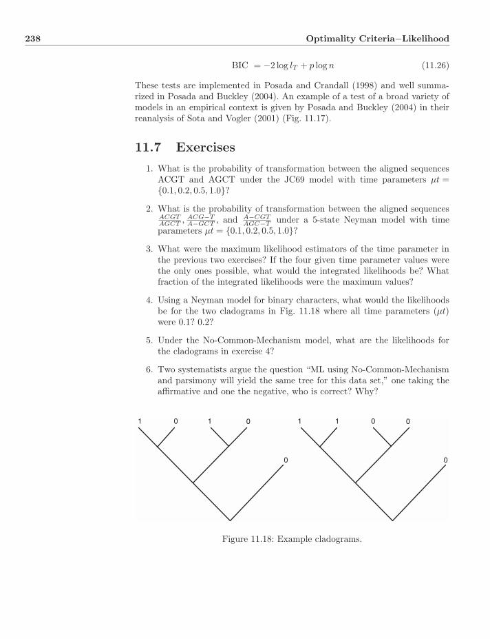
238 Optimality Criteria−Likelihood
BIC = −2 log lT + p log n (11.26)
These tests are implemented in Posada and Crandall (1998) and well summa-rized in Posada and Buckley (2004). An example of a test of a broad variety ofmodels in an empirical context is given by Posada and Buckley (2004) in theirreanalysis of Sota and Vogler (2001) (Fig. 11.17).
11.7 Exercises
1. What is the probability of transformation between the aligned sequencesACGT and AGCT under the JC69 model with time parameters μt ={0.1, 0.2, 0.5, 1.0}?
2. What is the probability of transformation between the aligned sequencesACGTAGCT , ACG−T
A−GCT , and A−CGTAGC−T under a 5-state Neyman model with time
parameters μt = {0.1, 0.2, 0.5, 1.0}?3. What were the maximum likelihood estimators of the time parameter in
the previous two exercises? If the four given time parameter values werethe only ones possible, what would the integrated likelihoods be? Whatfraction of the integrated likelihoods were the maximum values?
4. Using a Neyman model for binary characters, what would the likelihoodsbe for the two cladograms in Fig. 11.18 where all time parameters (μt)were 0.1? 0.2?
5. Under the No-Common-Mechanism model, what are the likelihoods forthe cladograms in exercise 4?
6. Two systematists argue the question “ML using No-Common-Mechanismand parsimony will yield the same tree for this data set,” one taking theaffirmative and one the negative, who is correct? Why?
1 0 1 0
0
1 1 0 0
0
Figure 11.18: Example cladograms.

11.7 Exercises 239
7. Using a Neyman model for sequence characters, and sequences ACGT andAGCT with time parameter μt = 0.2, determine the maximum likelihoodalignment of the two sequences. What are the values of the “total” and“dominant” likelihoods? What fraction of the total likelihood is the dom-inant? Give an example of a non-dominant likelihood alignment (and itslikelihood) included in the total likelihood calculation.

Chapter 12
OptimalityCriteria−PosteriorProbability
Bayesian argumentation and methods have a long history in systematics. Ed-wards (1970) discussed tree priors in order to construct Bayesian estimatorsof phylogeny. Farris (1973a) based his likelihood analysis of parsimony on aninitial Bayesian framework, and his (1977) criticism of Dollo’s law was alsobased in Bayesian formalism. Felsenstein (2004) cites work by Gomberg in 1968on Bayesian analysis in phylogeny. Harper (1979) contrasted his Bayesian ap-proach to phylogenetic systematics with the reasoning of Popper. Smouse andLi (1987) assumed flat priors (for three competing topologies), justifying a like-lihood analysis of primate mtDNA restriction patterns. Wheeler (1991) usedexplicit Bayesian methods with empirical topology priors (and loss function) tojustify data combination (total evidence sensu Kluge, 1989).
Thomas Bayes(1702–1761)
Although these methods sought to maximize posterior probability, theylacked numerical techniques to integrate over nuisance parameters (Sect. 11.2.1)and non-uniform prior distributions of tree topologies (Wheeler, 1991 excepted)allowing a fully Bayesian analysis. The introduction of Monte Carlo MarkovChains (Metropolis and Ulam, 1949; Metropolis et al., 1953; Hastings, 1970) byYang and Rannala (1997) made Bayesian phylogenetics tractable and its recentpopularity is due to this advance.
12.1 Bayes in Systematics
The sine qua non of Bayesian analysis (Sect. 6.1.5) is the prior distribution of theparameter(s) to be estimated. In the case of systematics, the prior of paramount
Systematics: A Course of Lectures, First Edition. Ward C. Wheeler.c© 2012 Ward C. Wheeler. Published 2012 by Blackwell Publishing Ltd.
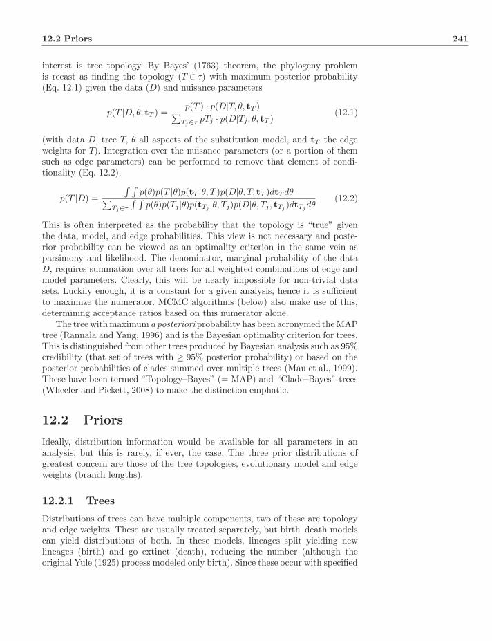
12.2 Priors 241
interest is tree topology. By Bayes’ (1763) theorem, the phylogeny problemis recast as finding the topology (T ∈ τ) with maximum posterior probability(Eq. 12.1) given the data (D) and nuisance parameters
p(T |D, θ, tT ) =p(T ) · p(D|T, θ, tT )∑
Tj∈τ pTj · p(D|Tj , θ, tT )(12.1)
(with data D, tree T, θ all aspects of the substitution model, and tT the edgeweights for T). Integration over the nuisance parameters (or a portion of themsuch as edge parameters) can be performed to remove that element of condi-tionality (Eq. 12.2).
p(T |D) =∫ ∫
p(θ)p(T |θ)p(tT |θ, T )p(D|θ, T, tT )dtT dθ∑Tj∈τ
∫ ∫p(θ)p(Tj |θ)p(tTj
|θ, Tj)p(D|θ, Tj , tTj)dtTj
dθ(12.2)
This is often interpreted as the probability that the topology is “true” giventhe data, model, and edge probabilities. This view is not necessary and poste-rior probability can be viewed as an optimality criterion in the same vein asparsimony and likelihood. The denominator, marginal probability of the dataD, requires summation over all trees for all weighted combinations of edge andmodel parameters. Clearly, this will be nearly impossible for non-trivial datasets. Luckily enough, it is a constant for a given analysis, hence it is sufficientto maximize the numerator. MCMC algorithms (below) also make use of this,determining acceptance ratios based on this numerator alone.
The tree with maximum a posteriori probability has been acronymed the MAPtree (Rannala and Yang, 1996) and is the Bayesian optimality criterion for trees.This is distinguished from other trees produced by Bayesian analysis such as 95%credibility (that set of trees with ≥ 95% posterior probability) or based on theposterior probabilities of clades summed over multiple trees (Mau et al., 1999).These have been termed “Topology–Bayes” (= MAP) and “Clade–Bayes” trees(Wheeler and Pickett, 2008) to make the distinction emphatic.
12.2 Priors
Ideally, distribution information would be available for all parameters in ananalysis, but this is rarely, if ever, the case. The three prior distributions ofgreatest concern are those of the tree topologies, evolutionary model and edgeweights (branch lengths).
12.2.1 Trees
Distributions of trees can have multiple components, two of these are topologyand edge weights. These are usually treated separately, but birth–death modelscan yield distributions of both. In these models, lineages split yielding newlineages (birth) and go extinct (death), reducing the number (although theoriginal Yule (1925) process modeled only birth). Since these occur with specified
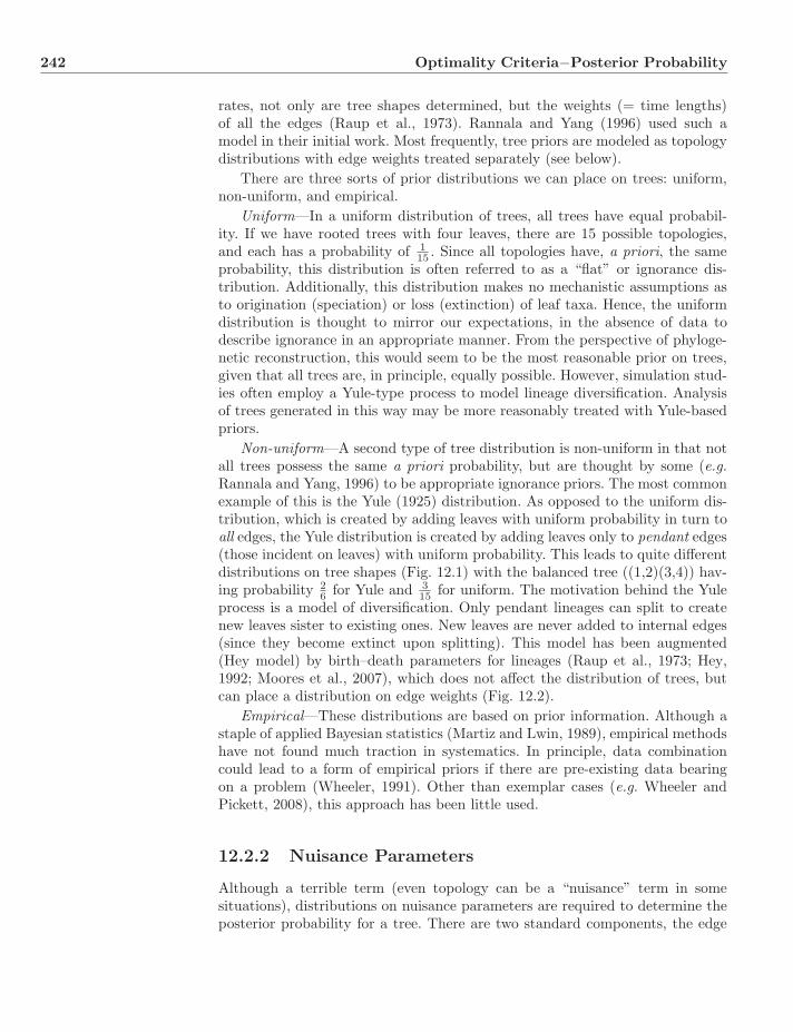
242 Optimality Criteria−Posterior Probability
rates, not only are tree shapes determined, but the weights (= time lengths)of all the edges (Raup et al., 1973). Rannala and Yang (1996) used such amodel in their initial work. Most frequently, tree priors are modeled as topologydistributions with edge weights treated separately (see below).
There are three sorts of prior distributions we can place on trees: uniform,non-uniform, and empirical.
Uniform—In a uniform distribution of trees, all trees have equal probabil-ity. If we have rooted trees with four leaves, there are 15 possible topologies,and each has a probability of 1
15 . Since all topologies have, a priori, the sameprobability, this distribution is often referred to as a “flat” or ignorance dis-tribution. Additionally, this distribution makes no mechanistic assumptions asto origination (speciation) or loss (extinction) of leaf taxa. Hence, the uniformdistribution is thought to mirror our expectations, in the absence of data todescribe ignorance in an appropriate manner. From the perspective of phyloge-netic reconstruction, this would seem to be the most reasonable prior on trees,given that all trees are, in principle, equally possible. However, simulation stud-ies often employ a Yule-type process to model lineage diversification. Analysisof trees generated in this way may be more reasonably treated with Yule-basedpriors.
Non-uniform—A second type of tree distribution is non-uniform in that notall trees possess the same a priori probability, but are thought by some (e.g.Rannala and Yang, 1996) to be appropriate ignorance priors. The most commonexample of this is the Yule (1925) distribution. As opposed to the uniform dis-tribution, which is created by adding leaves with uniform probability in turn toall edges, the Yule distribution is created by adding leaves only to pendant edges(those incident on leaves) with uniform probability. This leads to quite differentdistributions on tree shapes (Fig. 12.1) with the balanced tree ((1,2)(3,4)) hav-ing probability 2
6 for Yule and 315 for uniform. The motivation behind the Yule
process is a model of diversification. Only pendant lineages can split to createnew leaves sister to existing ones. New leaves are never added to internal edges(since they become extinct upon splitting). This model has been augmented(Hey model) by birth–death parameters for lineages (Raup et al., 1973; Hey,1992; Moores et al., 2007), which does not affect the distribution of trees, butcan place a distribution on edge weights (Fig. 12.2).
Empirical—These distributions are based on prior information. Although astaple of applied Bayesian statistics (Martiz and Lwin, 1989), empirical methodshave not found much traction in systematics. In principle, data combinationcould lead to a form of empirical priors if there are pre-existing data bearingon a problem (Wheeler, 1991). Other than exemplar cases (e.g. Wheeler andPickett, 2008), this approach has been little used.
12.2.2 Nuisance Parameters
Although a terrible term (even topology can be a “nuisance” term in somesituations), distributions on nuisance parameters are required to determine theposterior probability for a tree. There are two standard components, the edge
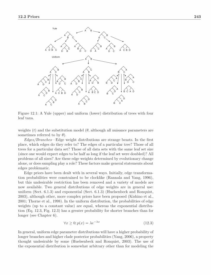
12.2 Priors 243
A B
AB C A
BC
B CA D
A
BC
D
AB
CD A
BC
DA
B
CD A BC D
A B
AB
C A BC A
B C
AB
C
D
A
BC
DA
B
CD
A
B
CD A BC D
A BC
D
AB
C
DA
B
C
D
A
BC
DA B C D
AB C
D
A
BC
D
AB
CD
A
B CD AB C D
Yule
Uniform
Figure 12.1: A Yule (upper) and uniform (lower) distribution of trees with fourleaf taxa.
weights (t) and the substitution model (θ, although all nuisance parameters aresometimes referred to by θ).
Edges/Branches—Edge weight distributions are strange beasts. In the firstplace, which edges do they refer to? The edges of a particular tree? Those of alltrees for a particular data set? Those of all data sets with the same leaf set size(since one would expect edges to be half as long if the leaf set were doubled)? Allproblems of all sizes? Are these edge weights determined by evolutionary changealone, or does sampling play a role? These factors make general statements aboutedges problematic.
Edge priors have been dealt with in several ways. Initially, edge transforma-tion probabilities were constrained to be clocklike (Rannala and Yang, 1996),but this undesirable restriction has been removed and a variety of models arenow available. Two general distributions of edge weights are in general use:uniform (Sect. 6.1.3) and exponential (Sect. 6.1.3) (Huelsenbeck and Ronquist,2003), although other, more complex priors have been proposed (Kishino et al.,2001; Thorne et al., 1998). In the uniform distribution, the probabilities of edgeweights (up to a constant value) are equal, whereas the exponential distribu-tion (Eq. 12.3, Fig. 12.3) has a greater probability for shorter branches than forlonger (see Chapter 6).
∀x ≥ 0; p(x) = λe−λx (12.3)
In general, uniform edge parameter distributions will have a higher probability oflonger branches and higher clade posterior probabilities (Yang, 2006), a propertythought undesirable by some (Huelsenbeck and Ronquist, 2003). The use ofthe exponential distribution is somewhat arbitrary other than for modeling the
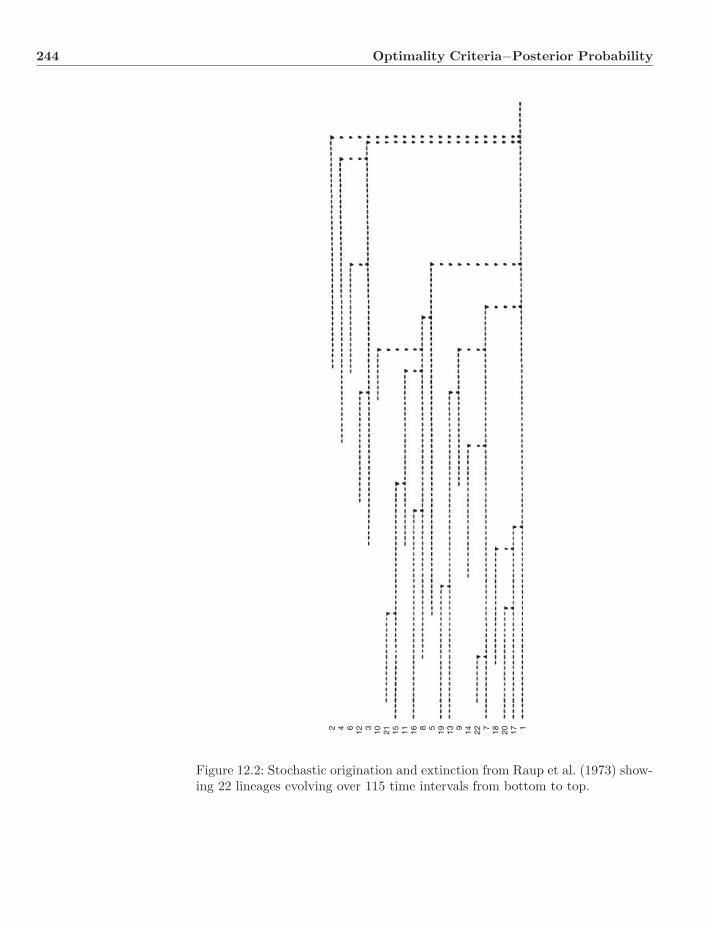
244 Optimality Criteria−Posterior Probability
2 4 6 12 3 10 21 15 11 16 8 5 19 13 9 14 22 7 18 20 17 1
Figure 12.2: Stochastic origination and extinction from Raup et al. (1973) show-ing 22 lineages evolving over 115 time intervals from bottom to top.
12.2 Priors 245
00
0.10.20.30.40.50.60.70.80.9
11.11.21.31.41.5
1 2 3 4 5
λ = 0.5λ = 1.0λ = 1.5
Figure 12.3: The exponential distribution.
wait time between Poisson-distributed lineage splitting events. Of course, thisjustification would assume we know all splitting events, which we cannot knowdue to extinction of unobserved lineages.
In my opinion, this reflects an unreasonable interpretation of the significanceof branch lengths as statements of evolutionary process as opposed to one wheretaxonomic sampling plays a major role. Given that samples of extant taxa arenearly always incomplete, and knowledge of extinct taxa extremely limited ifnot entirely absent, the uniform edge weight distribution seems at least equallyplausible as a statement of prior information. Edge weights are as much state-ments of sampling as of evolutionary process.
A further complication comes in the use of a single parameter for all edges.Some will be larger than others, and almost all (in the course of an analysis)will be “wrong.” For this reason, Yang and Rannala (2005) suggested an empir-ical Bayes’ method where edge parameters are likelihood estimates determineduniquely for each edge on each tree with the data at hand. Given that thesedata are not “prior” in any way, strict Bayesians may howl, but this process(though potentially time-consuming) seems a powerful and reasonable means toestablish appropriate edge parameters.
No matter which distributions of edge weights are used, the objective is thesame, to determine the posterior probability of the tree conditioned solely onthe substitution model.
Substitution Models—Ideally, we would employ a distribution of substitu-tion models in order to integrate out this nuisance parameter and determinep(T |D) directly. This cannot (at present) be done completely (although Hid-den Markov Models—HMM—approach this “model of models”). Typically, theGeneral-Time-Reversible (GTR) model (Lanave et al., 1984; Tavare, 1986) isused whereby the potential parameter values encompass the variety of simplermodels with specific symmetry conditions (e.g. JC69). A distribution on theparameters of this model should contain a variety of other models. Typically, aDirichlet distribution (Sect. 6.1.3) is used to accomplish this. At least for thosemodels reducible from GTR, this is a reasonable procedure.
246 Optimality Criteria−Posterior Probability
12.3 Techniques
Since, in general, we are not concerned with the actual value of p(T |D), and thedenominator of Equation 12.1 is a constant for any particular data set, we canrestrict ourselves to maximizing p(T ) · p(D|T ). This reduces to maximizing theproduct of the tree prior and the tree likelihood with the nuisance parametersintegrated out (MIL). In general, analyses use a flat (= uninformative) priorfor tree topologies, hence the Bayesian analysis boils down to a search for treeswith high MIL (Chapter 11). This could be accomplished via a variety of stan-dard tree-search techniques (Chapter 14) such as exhaustive tree enumeration(Rannala and Yang, 1996) or heuristic branch-swapping (Wheeler and Pickett,2008). These tried and true methods should yield useful MAP trees—if suppliedwith integrated likelihoods for the trees themselves. Without this information,however, these techniques are less directly applicable, and other approaches aremore commonly employed.
Bruce Rannala
Ziheng Yang
12.3.1 Markov Chain Monte Carlo
Typically, the problem of determining the posterior probability of a tree requiresknowledge of the tree prior, the distribution of model parameters and of edgeweights. Even if the priors are not an issue (e.g. flat, as above), there are manyparameters to integrate away. For example, a GTR-model analysis for 100 taxahas at least 205 parameters. Numerical integration in such high dimensionalitywill be extremely time consuming.
Markov Chain Monte Carlo (MCMC) techniques based on the Metropolis–Hastings algorithm of simulated annealing offer an alternate means of deter-mining the relative posterior probabilities (based on the numerator of Eq. 12.2)of competing trees. This technique (Sect. 14.7) has general use in complex op-timization problems and has been adapted for use in tree-searching (Goloboff,1999a, as “Tree-Drifting”).
12.3.2 Metropolis–Hastings Algorithm
As discussed in Chapter 14, the Metropolis–Hastings algorithm (Metropoliset al., 1953; Hastings, 1970) has been used to allow a search to escape local op-tima by accepting suboptimal solutions in the hope of later finding more globalsolutions. In the context of Bayesian estimation in systematics, the objective isa stable population of trees where trees are represented in proportion to theirposterior probability. The Metropolis–Hastings transition probabilities betweenpairs of trees are determined by the ratio of their posteriors (Eq. 12.2). Sincethey share the same denominator, this ratio is based solely on the numeratorof Equation 12.2. This saves us from dependency on the difficult to calculatemarginal data probability.
This is accomplished via a series of proposed changes to the current tree(including the edge parameter vector and substitution model). If we define the
π(T ) = p(θ)p(T |θ)p(tT |θ, T )p(D|θ, T, tT ) (12.4)

12.3 Techniques 247
acceptance ratio based on the relative quality of solutions (Eqs. 12.5 and 12.6)after a change from T to T∗.
α = min(
1,π(T ∗)π(T )
)(12.5)
The probability of accepting a solution (a tree in this case) T∗ is 1 if T∗ is “bet-ter” (higher posterior probability) than T. A worse solution will be acceptedwith probability f(α) > 0 depending on the “temperature” of the system. If thetemperature is relatively high, suboptimal solutions are more likely to be ac-cepted. If the system is too hot, any solution will be accepted, and the procedurebecomes a random walk about the solution space. If the temperature is too low,only better solutions are accepted with the familiar problems of local optima.The sequence of states forms a Markov “chain” that will never (on its own)terminate. The method should converge on the posterior probability as longas two conditions are met: 1) the transition system allows all states to transi-tion into all other states, and 2) the chain is aperiodic. These conditions areeasily met.
As an example, consider a coin. A sequence of tosses (yielding three headsand seven tails) constitutes D. The coin may be fair (state 0; prior probability0.5), biased towards tails (state 1; prior probability 0.25), or biased towardsheads (state 2; prior probability 0.25). These are the three “states” whose pos-terior probabilities we want to estimate (Fig. 12.4). The transition probabilitiesbetween the states will be:
α0→1 =p(biased T) · r(D|biased T)
p(fair) · r(D|fair)=
0.25 · 0.002090.5 · 0.000977
= 1.070 → 1
α1→0 = 0.935
α0→2 =p(biased H) · r(D|biased H)
p(fair) · r(D|fair)=
0.25 · 0.00002570.5 · 0.000977
= 0.0132
α2→0 = 76.0 → 1
α1→2 =p(biased H) · r(D|biased H)p(biased T) · r(D|biased T)
=0.25 · 0.00002570.25 · 0.000209
= 0.123
α2→1 = 8.13 → 1 (12.6)
After some large number of probabilistic transitions, the relative number ofvisited states should settle down on the posterior probabilities of p(fair) = 0.480,p(biased T) = 0.514, and p(biased H) = 0.00631.
The Metropolis–Hastings algorithm for identifying the maximum posteriorprobability tree would follow the general procedure:
1. Choose an initial tree (T), edge weight vector (t), substitution model (θ).
2. Propose a new tree (T∗).
Propose new t
Propose new θ
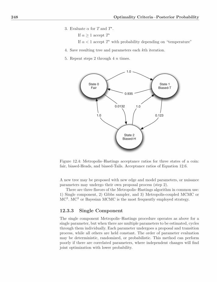
248 Optimality Criteria−Posterior Probability
3. Evaluate α for T and T∗.
If α ≥ 1 accept T∗
If α < 1 accept T∗ with probability depending on “temperature”
4. Save resulting tree and parameters each kth iteration.
5. Repeat steps 2 through 4 n times.
State 0Fair
State 1Biased-T
State 2Biased-H
1.0
0.935
1.0
0.0132 1.0
0.123
Figure 12.4: Metropolis–Hastings acceptance ratios for three states of a coin:fair, biased-Heads, and biased-Tails. Acceptance ratios of Equation 12.6.
A new tree may be proposed with new edge and model parameters, or nuisanceparameters may undergo their own proposal process (step 2).
There are three flavors of the Metropolis–Hastings algorithm in common use:1) Single component, 2) Gibbs sampler, and 3) Metropolis-coupled MCMC orMC3. MC3 or Bayesian MCMC is the most frequently employed strategy.
12.3.3 Single Component
The single component Metropolis–Hastings procedure operates as above for asingle parameter, but when there are multiple parameters to be estimated, cyclesthrough them individually. Each parameter undergoes a proposal and transitionprocess, while all others are held constant. The order of parameter evaluationmay be deterministic, randomized, or probabilistic. This method can performpoorly if there are correlated parameters, where independent changes will findjoint optimization with lower probability.
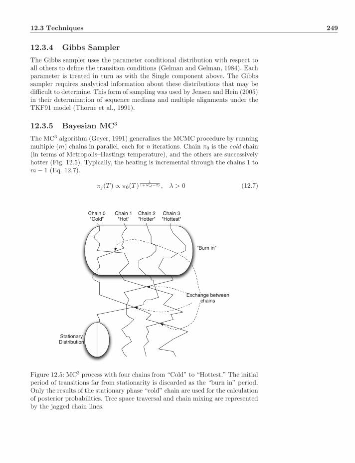
12.3 Techniques 249
12.3.4 Gibbs Sampler
The Gibbs sampler uses the parameter conditional distribution with respect toall others to define the transition conditions (Gelman and Gelman, 1984). Eachparameter is treated in turn as with the Single component above. The Gibbssampler requires analytical information about these distributions that may bedifficult to determine. This form of sampling was used by Jensen and Hein (2005)in their determination of sequence medians and multiple alignments under theTKF91 model (Thorne et al., 1991).
12.3.5 Bayesian MC3
The MC3 algorithm (Geyer, 1991) generalizes the MCMC procedure by runningmultiple (m) chains in parallel, each for n iterations. Chain π0 is the cold chain(in terms of Metropolis–Hastings temperature), and the others are successivelyhotter (Fig. 12.5). Typically, the heating is incremental through the chains 1 tom − 1 (Eq. 12.7).
πj(T ) ∝ π0(T )1
1+λ(j−2) , λ > 0 (12.7)
Chain 0"Cold"
Chain 1"Hot"
Chain 2"Hotter"
Chain 3"Hottest"
"Burn in"
StationaryDistribution
Exchange betweenchains
Figure 12.5: MC3 process with four chains from “Cold” to “Hottest.” The initialperiod of transitions far from stationarity is discarded as the “burn in” period.Only the results of the stationary phase “cold” chain are used for the calculationof posterior probabilities. Tree space traversal and chain mixing are representedby the jagged chain lines.

250 Optimality Criteria−Posterior Probability
Only the cold chain converges to the estimated parameter—the others are formixing between chains to improve solutions (Yang, 2006). These chains (i andj) exchange values periodically according to a second Metropolis–Hastings ac-ceptance ratio (Eq. 12.8).
α = min(
1,πi(Tj)πj(Ti)πi(Ti)πj(Tj)
)(12.8)
The motivation is that the hot chains allow the movements between solutionpeaks, while the cold chains find the local minima in their neighborhood. Peri-odic mixing between chains allows solutions separated by large probability gapsto enter the cold chain. Such gaps may impair the ability of MC3 to find validstationary solutions (Yang, 2006). The end result of the MC3 should be thateach tree is represented in the stationary pool in proportion to its posteriorprobability in the cold chain.
Evaluating MC3
Even with exchanges between m chains and after n iterations it can be difficultto determine whether the chain has converged on the distribution of the desiredparameter reaching stationarity or is still changing (the “burn in” period).
There are several strategies for evaluating whether stationarity has beenreached:
• Run the algorithm without data. The posterior distribution should con-verge on the (known) prior.
• Repeat the process multiple times. The results of independent runs shouldconverge on the same estimates of posteriors.
• Examine the distribution of estimated parameters over the progress of theruns. All parameters should have settled down to their final estimates.
No matter what strategy is employed, great care should be taken to ensure thatstationarity has been reached. The validity of the estimates depends on it.
12.3.6 Summary of Posterior
There are three commonly used methods of summarizing Bayesian analysis oftree topologies. The first is the straightforward (but somewhat uncommon) pre-sentation of the MAP tree as one would present an ML or parsimony result(Rannala and Yang, 1996). The second is to present the minimal set of trees(or their consensus) with total posterior probability of 95% (or some other)level of Bayesian credibility (Rannala and Yang, 1996; Mau et al., 1999). Byfar the most common method is to present the majority consensus of the treesin the stationary pool. Each clade with > 50% posterior probability is pre-sented on a consensus tree labeled by these clade posteriors (Fig. 12.7). Thissummary method was first presented by Mau et al. (1999) and is implementedin the program MrBayes (Huelsenbeck and Ronquist, 2003). It is importantto note that the contributions of a given clade posterior probability will likelycome from multiple, incompatible, tree topologies (Fig. 12.6). Combining such
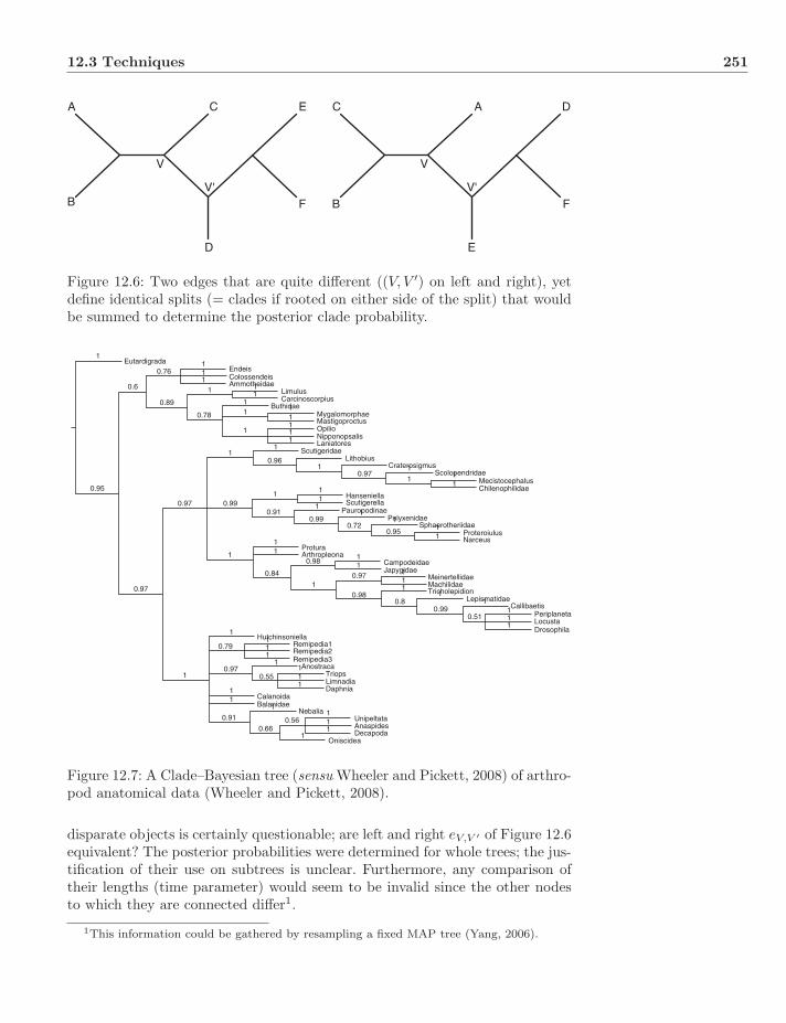
12.3 Techniques 251
A
B
C
D
E
F
V
V'
C
B
A
E
D
F
V
V'
Figure 12.6: Two edges that are quite different ((V, V ′) on left and right), yetdefine identical splits (= clades if rooted on either side of the split) that wouldbe summed to determine the posterior clade probability.
1Eutardigrada
0.76
0.6
0.89
111
1 11
111
1111
1
1
1
1
11
1111
1
1
111
1111
1
1
1
1
1
11
11
111
0.910.99
1
10.97
0.97
0.97
0.91
0.660.56
0.55
0.79
0.720.95
111
0.80.99
0.51
0.98
0.98
0.84
11
11
1
1
1
11
1
0.78
0.96
0.99
0.95
0.97
0.97
EndeisColossendeis
Limulus
MygalomorphaeMastigoproctusOpilioNipponopsalisLaniatores
ScutigeridaeLithobius
CraterosigmusScolopendridae
Hanseniella
Protura
Campodeidae
MeinertellidaeMachilidaeTricholepidion
LepismatidaeCallibaetis
PeriplanetaLocustaDrosophila
Japygidae
Arthropleona
HutchinsoniellaRemipedia1Remipedia2Remipedia3
AnostracaTriopsLimnadiaDaphnia
CalanoidaBalanidae
NebaliaUnipeltataAnaspidesDecapoda
Oniscidea
ScutigerellaPauropodinae
PolyxenidaeSphaerotheriidae
MecistocephalusChilenophilidae
ProteroiulusNarceus
CarcinoscorpiusButhidae
Ammotheidae
Figure 12.7: A Clade–Bayesian tree (sensu Wheeler and Pickett, 2008) of arthro-pod anatomical data (Wheeler and Pickett, 2008).
disparate objects is certainly questionable; are left and right eV,V ′ of Figure 12.6equivalent? The posterior probabilities were determined for whole trees; the jus-tification of their use on subtrees is unclear. Furthermore, any comparison oftheir lengths (time parameter) would seem to be invalid since the other nodesto which they are connected differ1.
1This information could be gathered by resampling a fixed MAP tree (Yang, 2006).
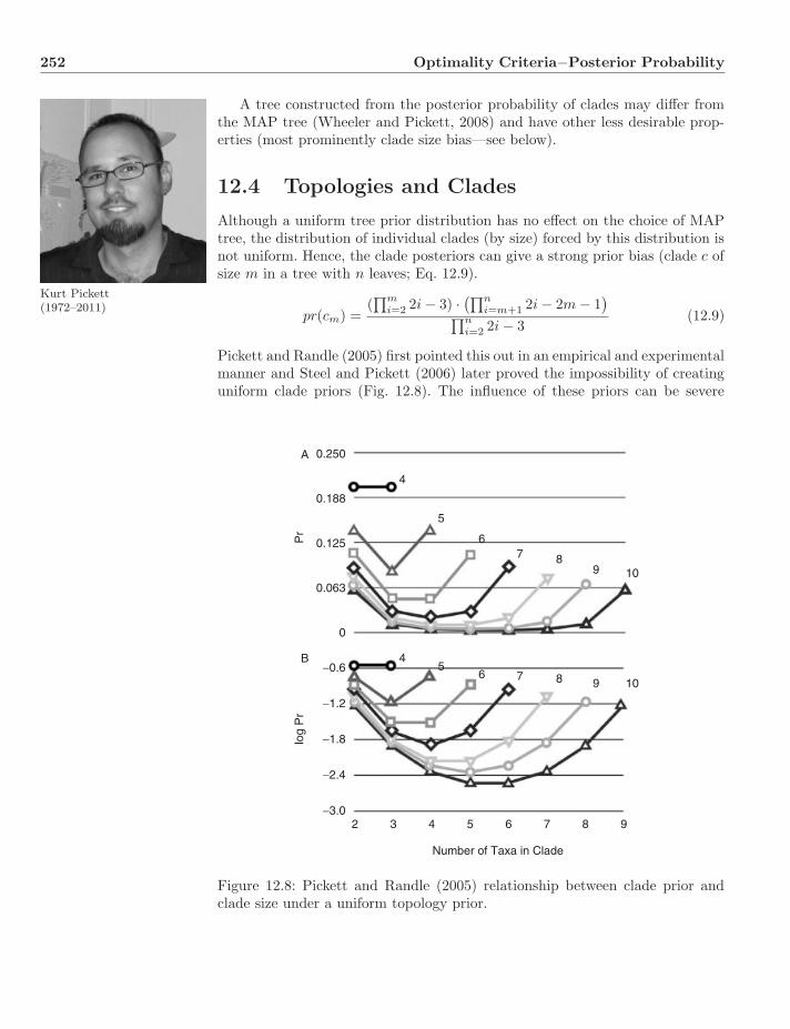
252 Optimality Criteria−Posterior Probability
A tree constructed from the posterior probability of clades may differ fromthe MAP tree (Wheeler and Pickett, 2008) and have other less desirable prop-erties (most prominently clade size bias—see below).
12.4 Topologies and Clades
Kurt Pickett(1972–2011)
Although a uniform tree prior distribution has no effect on the choice of MAPtree, the distribution of individual clades (by size) forced by this distribution isnot uniform. Hence, the clade posteriors can give a strong prior bias (clade c ofsize m in a tree with n leaves; Eq. 12.9).
pr(cm) =(∏m
i=2 2i − 3) · (∏ni=m+1 2i − 2m − 1
)∏n
i=2 2i − 3(12.9)
Pickett and Randle (2005) first pointed this out in an empirical and experimentalmanner and Steel and Pickett (2006) later proved the impossibility of creatinguniform clade priors (Fig. 12.8). The influence of these priors can be severe
0.250
0.188
A
B
4
4
2 3 4 5 6
Number of Taxa in Clade
7 8 9
5
5
6
6
7
7
8
8
9
9
10
10
0.125
0.063
0
−0.6
−1.2
log
Pr
Pr
−1.8
−2.4
−3.0
Figure 12.8: Pickett and Randle (2005) relationship between clade prior andclade size under a uniform topology prior.
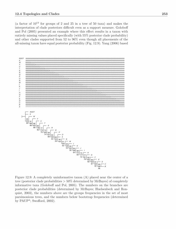
12.4 Topologies and Clades 253
(a factor of 1013 for groups of 2 and 25 in a tree of 50 taxa) and makes theinterpretation of clade posteriors difficult even as a support measure. Goloboffand Pol (2005) presented an example where this effect results in a taxon withentirely missing values placed specifically (with 55% posterior clade probability)and other clades supported from 52 to 96% even though all placements of theall-missing taxon have equal posterior probability (Fig. 12.9). Yang (2006) based
AAAAAAAAAAAAAAAAAAAAAAAAAAAAAAAAAAAAAAAAAAAAAAAAAAAAAAAAAAAAAAAAAAAAAAAAAAAAAAAAAAAAAAAAAAAAAAAAAAAAAAAAAAAAAAAAAAAAAAAAAAAAAAAAAAAAAAAAAAAAAAAAAAAAAAAAAAAAAAAAAAAAAAAAGGGGAAAAAAAAAAAAAAAAAAAAAAAAAAAAAAAAAAAAAAAAAAAAAAAAAAAAAAAAAAAAAAAAAAAAAAAAAAAAAAAAGGGGGGGGAAAAAAAAAAAAAAAAAAAAAAAAAAAAAAAAAAAAAAAAAAAAAAAAAAAAAAAAAAAAAAAAAAAAAAAAAAAAGGGGGGGGGGGGAAAAAAAAAAAAAAAAAAAAAAAAAAAAAAAAAAAAAAAAAAAAAAAAAAAAAAAAAAAAAAAAAAAAAAAAGGGGGGGGGGGGGGGGAAAAAAAAAAAAAAAAAAAAAAAAAAAAAAAAAAAAAAAAAAAAAAAAAAAAAAAAAAAAAAAAAAAAGGGGGGGGGGGGGGGGGGGGAAAAAAAAAAAAAAAAAAAAAAAAAAAAAAAAAAAAAAAAAAAAAAAAAAAAAAAAAAAAAAAAGGGGGGGGGGGGGGGGGGGGGGGGAAAAAAAAAAAAAAAAAAAAAAAAAAAAAAAAAAAAAAAAAAAAAAAAAAAAAAAAAAAAGGGGGGGGGGGGGGGGGGGGGGGGGGGGAAAAAAAAAAAAAAAAAAAAAAAAAAAAAAAAAAAAAAAAAAAAAAAAAAAAAAAAGGGGGGGGGGGGGGGGGGGGGGGGGGGGGGGGAAAAAAAAAAAAAAAAAAAAAAAAAAAAAAAAAAAAAAAAAAAAAAAAAAAAGGGGGGGGGGGGGGGGGGGGGGGGGGGGGGGGGGGGAAAAAAAAAAAAAAAAAAAAAAAAAAAAAAAAAAAAAAAAAAAAAAAAGGGGGGGGGGGGGGGGGGGGGGGGGGGGGGGGGGGGGGGGAAAAAAAAAAAAAAAAAAAAAAAAAAAAAAAAAAAAAAAAAAAAGGGGGGGGGGGGGGGGGGGGGGGGGGGGGGGGGGGGGGGGGGGGAAAAAAAAAAAAAAAAAAAAAAAAAAAAAAAAAAAAAAAAGGGGGGGGGGGGGGGGGGGGGGGGGGGGGGGGGGGGGGGGGGGGGGGGAAAAAAAAAAAAAAAAAAAAAAAAAAAAAAAAAAAAGGGGGGGGGGGGGGGGGGGGGGGGGGGGGGGGGGGGGGGGGGGGGGGGGGGGAAAAAAAAAAAAAAAAAAAAAAAAAAAAAAAAGGGGGGGGGGGGGGGGGGGGGGGGGGGGGGGGGGGGGGGGGGGGGGGGGGGGGGGGAAAAAAAAAAAAAAAAAAAAAAAAAAAAGGGGGGGGGGGGGGGGGGGGGGGGGGGGGGGGGGGGGGGGGGGGGGGGGGGGGGGGGGGGAAAAAAAAAAAAAAAAAAAAAAAAGGGGGGGGGGGGGGGGGGGGGGGGGGGGGGGGGGGGGGGGGGGGGGGGGGGGGGGGGGGGGGGGAAAAAAAAAAAAAAAAAAAAGGGGGGGGGGGGGGGGGGGGGGGGGGGGGGGGGGGGGGGGGGGGGGGGGGGGGGGGGGGGGGGGGGGGAAAAAAAAAAAAAAAAGGGGGGGGGGGGGGGGGGGGGGGGGGGGGGGGGGGGGGGGGGGGGGGGGGGGGGGGGGGGGGGGGGGGGGGGAAAAAAAAAAAAGGGGGGGGGGGGGGGGGGGGGGGGGGGGGGGGGGGGGGGGGGGGGGGGGGGGGGGGGGGGGGGGGGGGGGGGGGGGAAAAAAAAGGGGGGGGGGGGGGGGGGGGGGGGGGGGGGGGGGGGGGGGGGGGGGGGGGGGGGGGGGGGGGGGGGGGGGGGGGGGGGGGAAAAGGGGGGGGGGGGGGGGGGGGGGGGGGGGGGGGGGGGGGGGGGGGGGGGGGGGGGGGGGGGGGGGGGGGGGGGGGGGGGGGGGGGGGGGGGGGGGGGGGGGGGGGGGGGGGGGGGGGGGGGGGGGGGGGGGGGGGGGGGGGGGGGGGGGGGGGGGGGGGGGGGGGGGGG? ? ? ? ? ? ? ? ? ? ? ? ? ? ? ? ? ? ? ? ? ? ? ? ? ? ? ? ? ? ? ? ? ? ? ? ? ? ? ? ? ? ? ? ? ? ? ? ? ? ? ? ? ? ? ? ? ? ? ? ? ? ? ? ? ? ? ? ? ? ? ? ? ? ? ? ? ? ? ? ? ? ? ?
ROOTXWVUTSRQPONMLKJIHGFEDCBA
ROOT
959396
918888
868288
827882
777478
736974
686468
645964
605559
4652 51
5650
555854
606458
646864
687269
737773
778178
828582
869087
919392
959696
WX
VU
TS
RQ
POA
NM
LK
JI
HG
FE
DCB
Figure 12.9: A completely uninformative taxon (A) placed near the center of atree (posterior clade probabilities > 50% determined by MrBayes) of completelyinformative taxa (Goloboff and Pol, 2005). The numbers on the branches areposterior clade probabilities (determined by MrBayes; Huelsenbeck and Ron-quist, 2003), the numbers above are the groups frequencies in the set of mostparsimonious trees, and the numbers below bootstrap frequencies (determinedby PAUP*; Swofford, 2002).
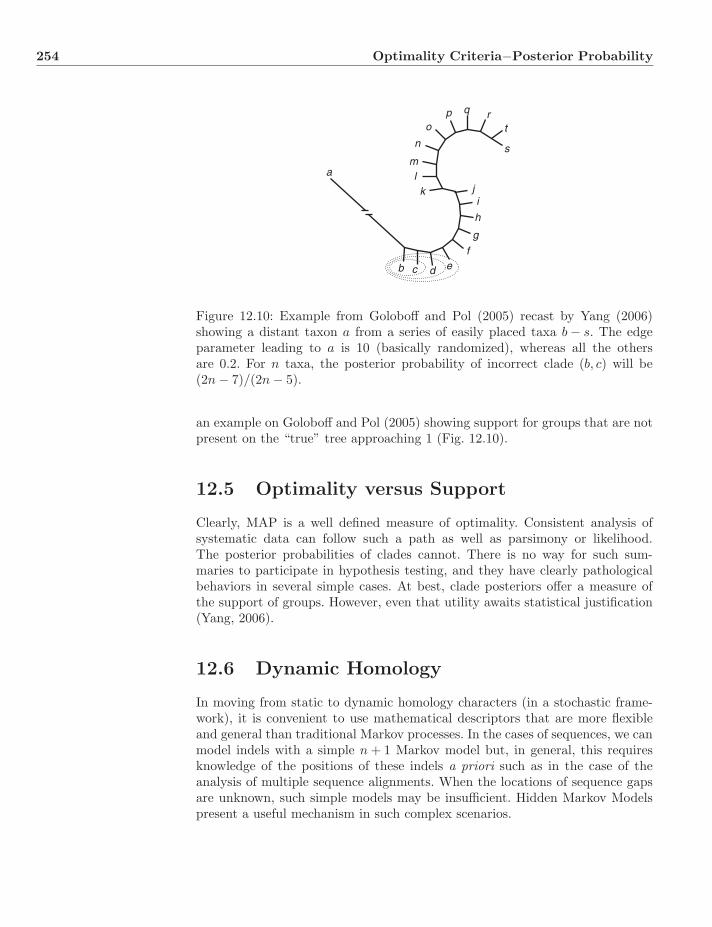
254 Optimality Criteria−Posterior Probability
a
cb d e
g
f
h
ijk
lm
n
op q r
t
s
Figure 12.10: Example from Goloboff and Pol (2005) recast by Yang (2006)showing a distant taxon a from a series of easily placed taxa b − s. The edgeparameter leading to a is 10 (basically randomized), whereas all the othersare 0.2. For n taxa, the posterior probability of incorrect clade (b, c) will be(2n − 7)/(2n − 5).
an example on Goloboff and Pol (2005) showing support for groups that are notpresent on the “true” tree approaching 1 (Fig. 12.10).
12.5 Optimality versus Support
Clearly, MAP is a well defined measure of optimality. Consistent analysis ofsystematic data can follow such a path as well as parsimony or likelihood.The posterior probabilities of clades cannot. There is no way for such sum-maries to participate in hypothesis testing, and they have clearly pathologicalbehaviors in several simple cases. At best, clade posteriors offer a measure ofthe support of groups. However, even that utility awaits statistical justification(Yang, 2006).
12.6 Dynamic Homology
In moving from static to dynamic homology characters (in a stochastic frame-work), it is convenient to use mathematical descriptors that are more flexibleand general than traditional Markov processes. In the cases of sequences, we canmodel indels with a simple n + 1 Markov model but, in general, this requiresknowledge of the positions of these indels a priori such as in the case of theanalysis of multiple sequence alignments. When the locations of sequence gapsare unknown, such simple models may be insufficient. Hidden Markov Modelspresent a useful mechanism in such complex scenarios.
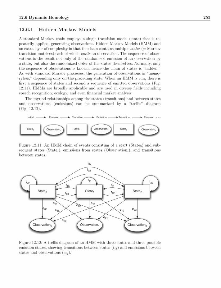
12.6 Dynamic Homology 255
12.6.1 Hidden Markov Models
A standard Markov chain employs a single transition model (state) that is re-peatedly applied, generating observations. Hidden Markov Models (HMM) addan extra layer of complexity in that the chain contains multiple states (= Markovtransition matrices) each of which emits an observation. The sequence of obser-vations is the result not only of the randomized emission of an observation bya state, but also the randomized order of the states themselves. Normally, onlythe sequence of observations is known, hence the chain of states is “hidden.”As with standard Markov processes, the generation of observations is “memo-ryless,” depending only on the preceding state. When an HMM is run, there isfirst a sequence of states and second a sequence of emitted observations (Fig.12.11). HMMs are broadly applicable and are used in diverse fields includingspeech recognition, ecology, and even financial market analysis.
The myriad relationships among the states (transitions) and between statesand observations (emissions) can be summarized by a “trellis” diagram(Fig. 12.12).
State0 State1 State2
Initial Emission Transition
Observation0Observation1 Observation2
Emission Transition Emission
Figure 12.11: An HMM chain of events consisting of a start (State0) and sub-sequent states (Statei), emissions from states (Observationi), and transitionsbetween states.
State0 State2
Observation1 Observation2Observation0
e00
e01 e02
e10
e11
e12
e20e21
e22
t01
t10 t21
t12
t02
t20
t22t00t11
State1
Figure 12.12: A trellis diagram of an HMM with three states and three possibleemission states, showing transitions between states (tij) and emissions betweenstates and observations (eij).
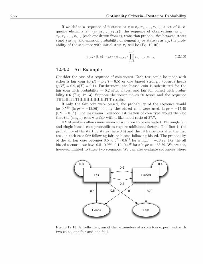
256 Optimality Criteria−Posterior Probability
If we define a sequence of n states as π = π0, π1, . . . , πn−1, a set of k se-quence elements s = {s0, s1, . . . , sk−1}, the sequence of observations as x =x0, x1, . . . , xn−1 (each one drawn from s), transition probabilities between statesi and j as tij , and emission probability of element sj by state πi as eij , the prob-ability of the sequence with initial state π0 will be (Eq. 12.10):
p(x, π|t, e) = p(π0)eπ0,x0 ·n−1∏i=1
tπi−1,πieπi,xi
(12.10)
12.6.2 An Example
Consider the case of a sequence of coin tosses. Each toss could be made witheither a fair coin (p(H) = p(T ) = 0.5) or one biased strongly towards heads(p(H) = 0.9, p(T ) = 0.1). Furthermore, the biased coin is substituted for thefair coin with probability = 0.2 after a toss, and fair for biased with proba-bility 0.6 (Fig. 12.13). Suppose the tosser makes 20 tosses and the sequenceTHTHHTTTHHHHHHHHHHTT results.
If only the fair coin were tossed, the probability of the sequence wouldbe 0.520 (ln pr = −13.86); if only the biased coin were used, ln pr = −17.49(0.913 · 0.17). The maximum likelihood estimation of coin type would then bethat the (single) coin was fair with a likelihood ratio of 37.7.
HMM analysis allows more nuanced scenarios to be evaluated. The single fairand single biased coin probabilities require additional factors. The first is theprobability of the starting states (here 0.5) and the 19 transitions after the firsttoss, in each case fair following fair, or biased following biased. The probabilityof the all fair case becomes 0.5 · 0.520 · 0.819 for a ln pr = −18.79. For the allbiased scenario, we have 0.5 · 0.913 · 0.17 · 0.419 for a ln pr = −35.59. We are not,however, limited to these two scenarios. We can also evaluate sequences where
Fair Biased
TailsHeads
0.5 0.5 0.9 0.1
0.2
0.60.8 0.4
Figure 12.13: A trellis diagram of the parameters of a coin toss experiment withtwo coins, one fair and one foul.
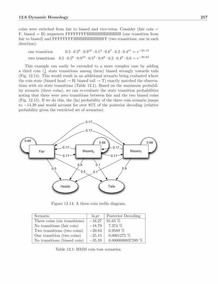
12.6 Dynamic Homology 257
coins were switched from fair to biased and vice-versa. Consider (fair coin =F, biased = B) sequences FFFFFFFFBBBBBBBBBBBB (one transition fromfair to biased) and FFFFFFFFBBBBBBBBBBFF (two transitions, one in eachdirection):
one transition 0.5 · 0.58 · 0.910 · 0.12 · 0.87 · 0.2 · 0.411 = e−25.15
two transitions 0.5 · 0.58 · 0.910 · 0.52 · 0.88 · 0.2 · 0.49 · 0.6 = e−20.83
This example can easily be extended to a more complex case by addinga third coin (1
6 state transitions among them) biased strongly towards tails(Fig. 12.14). This would result in an additional scenario being evaluated wherethe coin state (biased head → H; biased tail → T) exactly matched the observa-tions with six state transitions (Table 12.1). Based on the maximum probabil-ity scenario (three coins), we can re-evaluate the state transition probabilitiesnoting that there were zero transitions between fair and the two biased coins(Fig. 12.15). If we do this, the (ln) probability of the three coin scenario jumpsto −14.39 and would account for over 85% of the posterior decoding (relativeprobability given the restricted set of scenarios).
Fair BiasedH
TailsHeads
0.66 0.66
BiasedT
0.66
0.17
0.17
0.17
0.17
0.17
0.17
0.50.5
0.1
0.9 0.10.9
Figure 12.14: A three coin trellis diagram.
Scenario ln pr Posterior DecodingThree coins (six transitions) −16.27 91.65 %No transitions (fair coin) −18.79 7.374 %Two transitions (two coins) −20.83 0.9589 %One transition (two coins) −25.15 0.0001275 %No transitions (biased coin) −35.59 0.0000000037289 %
Table 12.1: HMM coin toss scenarios.
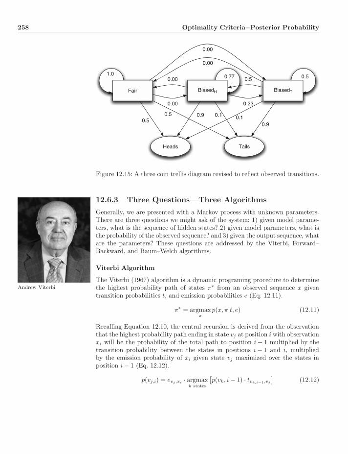
258 Optimality Criteria−Posterior Probability
Fair BiasedH
TailsHeads
0.50.5 0.9 0.1
0.00
0.001.0 0.77
BiasedT
0.1
0.5
0.23
0.5
0.9
0.00
0.00
Figure 12.15: A three coin trellis diagram revised to reflect observed transitions.
12.6.3 Three Questions—Three Algorithms
Generally, we are presented with a Markov process with unknown parameters.There are three questions we might ask of the system: 1) given model parame-ters, what is the sequence of hidden states? 2) given model parameters, what isthe probability of the observed sequence? and 3) given the output sequence, whatare the parameters? These questions are addressed by the Viterbi, Forward–Backward, and Baum–Welch algorithms.
Viterbi Algorithm
Andrew Viterbi
The Viterbi (1967) algorithm is a dynamic programing procedure to determinethe highest probability path of states π∗ from an observed sequence x giventransition probabilities t, and emission probabilities e (Eq. 12.11).
π∗ = argmaxπ
p(x, π|t, e) (12.11)
Recalling Equation 12.10, the central recursion is derived from the observationthat the highest probability path ending in state vj at position i with observationxi will be the probability of the total path to position i − 1 multiplied by thetransition probability between the states in positions i − 1 and i, multipliedby the emission probability of xi given state vj maximized over the states inposition i − 1 (Eq. 12.12).
p(vj,i) = evj ,xi· argmax
k states
[p(vk, i − 1) · tvk,i−1,vj
](12.12)
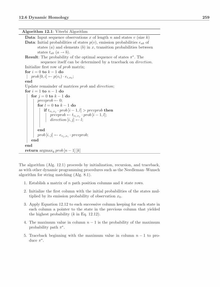
12.6 Dynamic Homology 259
Algorithm 12.1: Viterbi AlgorithmData: Input sequence observations x of length n and states v (size k)Data: Initial probabilities of states p(v), emission probabilities eab of
states (a) and elements (b) in x, transition probabilities betweenstates tab (a → b).
Result: The probability of the optimal sequence of states π∗. Thesequence itself can be determined by a traceback on direction.
Initialize first row of prob matrix;for i = 0 to k − 1 do
prob [0, i] ← p(vi) · ei,x0 ;endUpdate remainder of matrices prob and direction;for i = 1 to n − 1 do
for j = 0 to k − 1 doprevprob ← 0;for l = 0 to k − 1 do
if tvl,vj· prob [i − 1, l] > prevprob then
prevprob ← tvl,vj· prob [i − 1, l];
direction [i, j] ← l;
endprob [i, j] ← evj ,xi
· prevprob;end
endreturn argmaxk prob [n − 1] [k]
The algorithm (Alg. 12.1) proceeds by initialization, recursion, and traceback,as with other dynamic programming procedures such as the Needleman–Wunschalgorithm for string matching (Alg. 8.1).
1. Establish a matrix of n path position columns and k state rows.
2. Initialize the first column with the initial probabilities of the states mul-tiplied by its emission probability of observation x0.
3. Apply Equation 12.12 to each successive column keeping for each state ineach column a pointer to the state in the previous column that yieldedthe highest probability (k in Eq. 12.12).
4. The maximum value in column n − 1 is the probability of the maximumprobability path π∗.
5. Traceback beginning with the maximum value in column n − 1 to pro-duce π∗.
260 Optimality Criteria−Posterior Probability
As with other probabilistic algorithms, it is often convenient to work with log-arithms of probabilities to avoid awkwardly small numbers.
The time complexity of this algorithm for k states and n observations isO(k2n), but since in general k � n, the algorithm is in essence linear with n.
Forward−Backward Algorithm
The Viterbi algorithm found the single sequence of states with maximum prob-ability, but there are an exponential number of paths (in the three coin 20 tossexample there are 320), each with some non-zero probability. As with proba-bilistic sequence alignment, we may want to know what the total probability ofa sequence of observations is given all possible state paths. This is done via asimple modification of the Viterbi algorithm where the maximization over statesin the previous position (Eq. 12.12) is summed (Eq. 12.13)
pF (vj,i) = evj ,xi·∑
k
[pF (vk, i − 1) · tvk,i−1,vj
](12.13)
resulting in the Forward algorithm.In order to determine the posterior probability that a particular observation
xi was emitted from state πi = k, we need to determine the probability of πi = kgiven the sequence from i to the beginning and end of the entire sequence. TheForward algorithm yields the former and, surprisingly enough, the Backwardalgorithm provides the latter.
The Backward algorithm is identical to the Forward except that it begins atthe end of the sequence (i = n) and moves forward (Eq. 12.14).
pB(vj,i) = evj ,xi·∑
k
[pB(vk, i + 1) · tvk,i+1,vj
](12.14)
The posterior probability of a state in position i given observations x is thendetermined from the product of the Forward and Backward probabilities condi-tioned on the total probability from the Forward algorithm (Eq. 12.15, Alg. 12.2).
pPP (πi = vk|x) =pF (vj,i) · pB(vj,i)
P(x)(12.15)
Baum−Welch Algorithm
If the paths are known, or we have a training sequence of observations to fit,transition and emission probabilities can be estimated as simple proportions ofparticular events to the total number. These will be the maximum likelihoodestimators for these parameters given the training sequence.
Lloyd R. Welch If the state paths for the training sequences are unavailable or unknown,such a direct method cannot be used alone, but can be used in concert withan iterative refinement of parameter estimation (Baum et al., 1970). Initialvalues are set, the Forward and Backward algorithms are performed on thetraining sequences, and then the transition and emission frequencies estimates
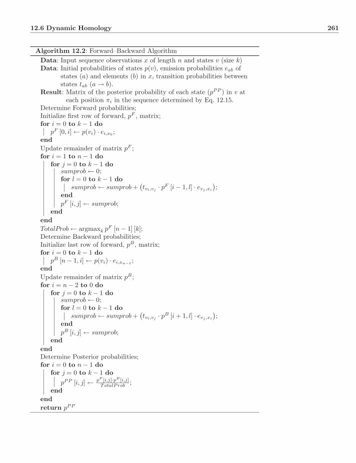
12.6 Dynamic Homology 261
Algorithm 12.2: Forward–Backward AlgorithmData: Input sequence observations x of length n and states v (size k)Data: Initial probabilities of states p(v), emission probabilities eab of
states (a) and elements (b) in x, transition probabilities betweenstates tab (a → b).
Result: Matrix of the posterior probability of each state (pPP ) in v ateach position πi in the sequence determined by Eq. 12.15.
Determine Forward probabilities;Initialize first row of forward, pF , matrix;for i = 0 to k − 1 do
pF [0, i] ← p(vi) · ei,x0 ;endUpdate remainder of matrix pF ;for i = 1 to n − 1 do
for j = 0 to k − 1 dosumprob ← 0;for l = 0 to k − 1 do
sumprob ← sumprob +(tvl,vj
· pF [i − 1, l] · evj ,xi
);
endpF [i, j] ← sumprob;
endendTotalProb ← argmaxk pF [n − 1] [k];Determine Backward probabilities;Initialize last row of forward, pB, matrix;for i = 0 to k − 1 do
pB [n − 1, i] ← p(vi) · ei,xn−1 ;endUpdate remainder of matrix pB ;for i = n − 2 to 0 do
for j = 0 to k − 1 dosumprob ← 0;for l = 0 to k − 1 do
sumprob ← sumprob +(tvl,vj
· pB [i + 1, l] · evj ,xi
);
endpB [i, j] ← sumprob;
endendDetermine Posterior probabilities;for i = 0 to n − 1 do
for j = 0 to k − 1 dopPP [i, j] ← pF [i,j]·pB [i,j]
TotalProb ;end
endreturn pPP
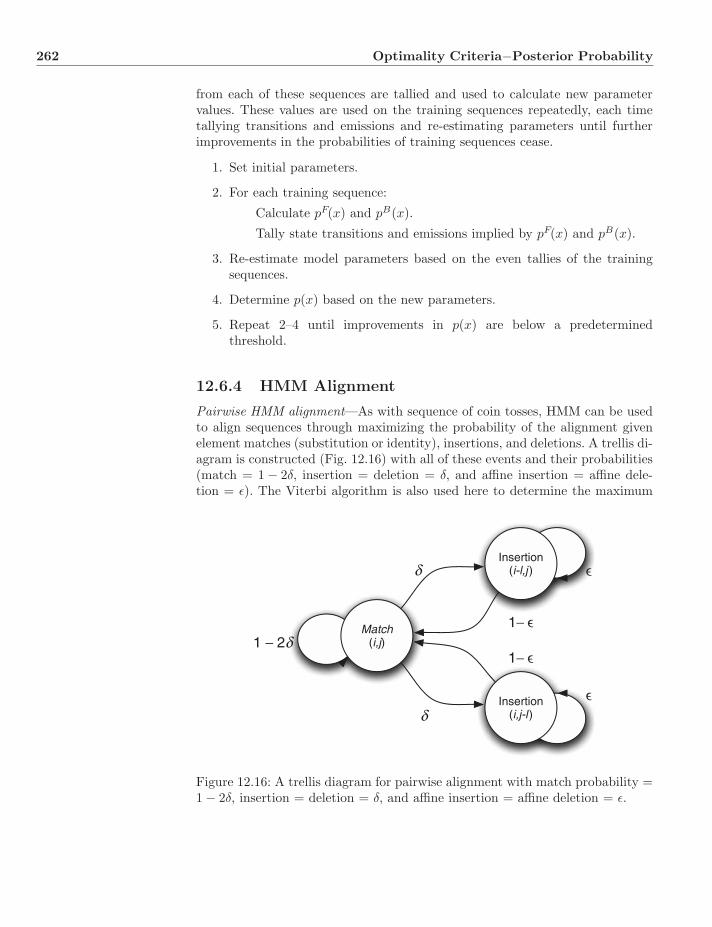
262 Optimality Criteria−Posterior Probability
from each of these sequences are tallied and used to calculate new parametervalues. These values are used on the training sequences repeatedly, each timetallying transitions and emissions and re-estimating parameters until furtherimprovements in the probabilities of training sequences cease.
1. Set initial parameters.
2. For each training sequence:
Calculate pF(x) and pB(x).
Tally state transitions and emissions implied by pF(x) and pB(x).
3. Re-estimate model parameters based on the even tallies of the trainingsequences.
4. Determine p(x) based on the new parameters.
5. Repeat 2–4 until improvements in p(x) are below a predeterminedthreshold.
12.6.4 HMM Alignment
Pairwise HMM alignment—As with sequence of coin tosses, HMM can be usedto align sequences through maximizing the probability of the alignment givenelement matches (substitution or identity), insertions, and deletions. A trellis di-agram is constructed (Fig. 12.16) with all of these events and their probabilities(match = 1 − 2δ, insertion = deletion = δ, and affine insertion = affine dele-tion = ε). The Viterbi algorithm is also used here to determine the maximum
δ
δ
1 − 2δ1− ∋
∋
∋
1− ∋
Match(i,j)
Insertion(i-l,j )
Insertion(i,j-l )
Figure 12.16: A trellis diagram for pairwise alignment with match probability =1 − 2δ, insertion = deletion = δ, and affine insertion = affine deletion = ε.
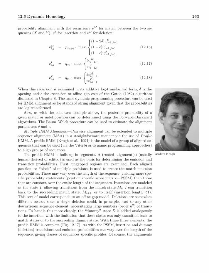
12.6 Dynamic Homology 263
probability alignment with the recurrence vM for match between the two se-quences (X and Y ), vI for insertion and vD for deletion:
vMi,j = pxi,yj
· max
⎧⎪⎨⎪⎩
(1 − 2δ)vMi−1,j−1
(1 − ε)vIi−1,j−1
(1 − ε)vDi−1,j−1
(12.16)
vIi,j = qxi
· max
{δvM
i−1,j
εvIi−1,j
(12.17)
vDi,j = qyi
· max
{δvM
i,j−1
εvDi,j−1
(12.18)
When this recursion is examined in its additive log-transformed form, δ is theopening and ε the extension or affine gap cost of the Gotoh (1982) algorithmdiscussed in Chapter 8. The same dynamic programming procedure can be usedfor HMM alignment as for standard string alignment given that the probabilitiesare log transformed.
Also, as with the coin toss example above, the posterior probability of agiven match or indel position can be determined using the Forward–Backwardalgorithms. The Baum–Welch procedure can be used to estimate the alignmentparameters δ and ε.
Multiple HMM Alignment—Pairwise alignment can be extended to multiplesequence alignment (MSA) in a straightforward manner via the use of ProfileHMM. A profile HMM (Krogh et al., 1994) is the model of a group of aligned se-quences that can be used (via the Viterbi or dynamic programming approaches)to align groups of sequences.
Anders KroghThe profile HMM is built up in segments. A trusted alignment(s) (usuallyhuman-derived or edited) is used as the basis for determining the emission andtransition probabilities. First, ungapped regions are examined. Each alignedposition, or “block” of multiple positions, is used to create the match emissionprobabilities. These may vary over the length of the sequence, yielding more spe-cific probability statements (position specific score matrix—PSSM) than thosethat are constant over the entire length of the sequences. Insertions are modeledas the state I, allowing transitions from the match state Mi. I can transitionback to the succeeding match state, Mi+1, or to itself (insertion length <1).This sort of model corresponds to an affine gap model. Deletions are somewhatdifferent beasts, since a single deletion could, in principle, lead to any otherdownstream sequence element, necessitating large numbers (order n2) of transi-tions. To handle this more cleanly, the “dummy” state D is added analogouslyto the insertion, with the limitation that these states can only transition back tomatch states or to the succeeding dummy state. With these three elements, theprofile HMM is complete (Fig. 12.17). As with the PSSM, insertion and dummy(deletion) transitions and emission probabilities can vary over the length of thesequence, giving classes of sequences specific profiles. Of course, the alignments
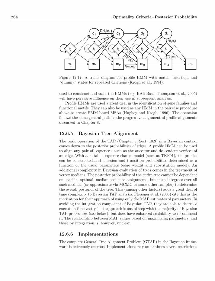
264 Optimality Criteria−Posterior Probability
i0
m0
i1
m1
d1T(d2ld1)
T(d 2li 1
)
T (d 2lm
1)
T(m3 ld
2 )
T (m3 li
2 )
T (m3lm2)
T (i4lm4)
T (i4ld4)
T (i4li4)
d2 d3 d4
i2
m2
i3
m3
i4
m4 m5
Figure 12.17: A trellis diagram for profile HMM with match, insertion, and“dummy” states for repeated deletions (Krogh et al., 1994).
used to construct and train the HMMs (e.g. BAli-Base, Thompson et al., 2005)will have pervasive influence on their use in subsequent analysis.
Profile HMMs are used a great deal in the identification of gene families andfunctional motifs. They can also be used as any HMM in the pairwise procedureabove to create HMM-based MSAs (Hughey and Krogh, 1996). The operationfollows the same general path as the progressive alignment of profile alignmentsdiscussed in Chapter 8.
12.6.5 Bayesian Tree Alignment
The basic operation of the TAP (Chapter 8, Sect. 10.9) in a Bayesian contextcomes down to the posterior probabilities of edges. A profile HMM can be usedto align any pair of sequences, such as the ancestor and descendent vertices ofan edge. With a suitable sequence change model (such as TKF91), the profilescan be constructed and emission and transition probabilities determined as afunction of the usual parameters (edge weight and substitution model). Anadditional complexity in Bayesian evaluation of trees comes in the treatment ofvertex medians. The posterior probability of the entire tree cannot be dependenton specific, optimal, median sequence assignments, but must integrate over allsuch medians (or approximate via MCMC or some other sampler) to determinethe overall posterior of the tree. This (among other factors) adds a great deal oftime complexity to Bayesian TAP analysis. Fleissner et al. (2005) cite this as themotivation for their approach of using only the MAP estimates of parameters. Inavoiding the integration component of Bayesian TAP, they are able to decreaseexecution time vastly. This approach is out of step with the majority of BayesianTAP procedures (see below), but does have enhanced scalability to recommendit. The relationship between MAP values based on maximizing parameters, andthose by integration is, however, unclear.
12.6.6 Implementations
The complete General Tree Alignment Problem (GTAP) in the Bayesian frame-work is extremely onerous. Implementations rely on at times severe restrictions
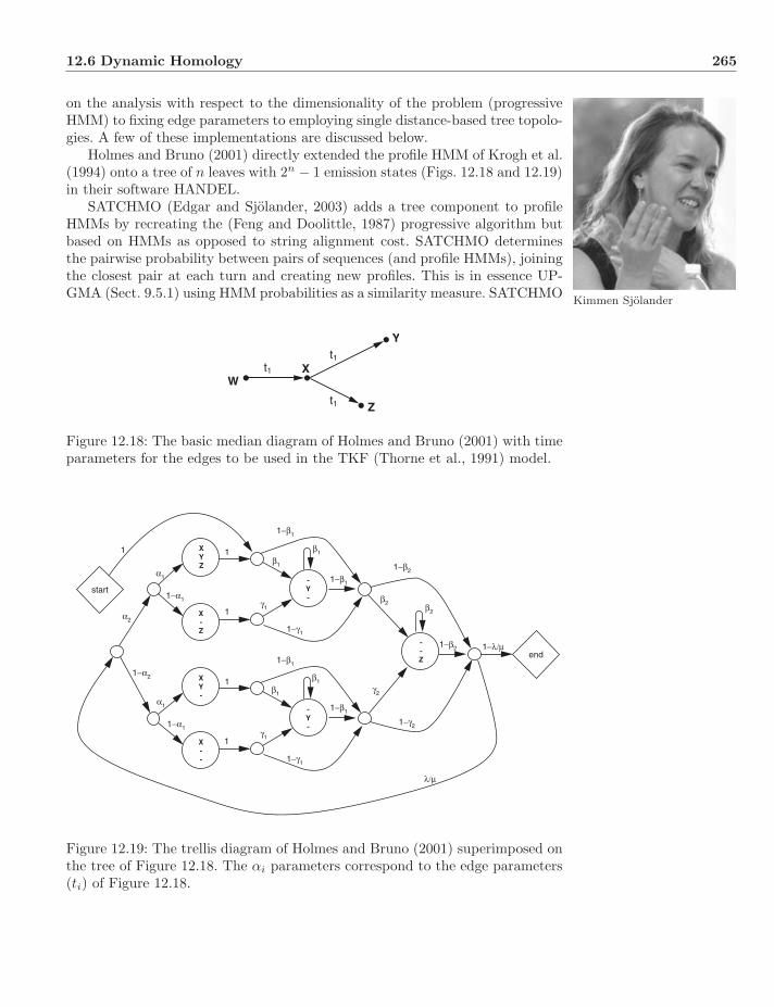
12.6 Dynamic Homology 265
on the analysis with respect to the dimensionality of the problem (progressiveHMM) to fixing edge parameters to employing single distance-based tree topolo-gies. A few of these implementations are discussed below.
Kimmen Sjolander
Holmes and Bruno (2001) directly extended the profile HMM of Krogh et al.(1994) onto a tree of n leaves with 2n − 1 emission states (Figs. 12.18 and 12.19)in their software HANDEL.
SATCHMO (Edgar and Sjolander, 2003) adds a tree component to profileHMMs by recreating the (Feng and Doolittle, 1987) progressive algorithm butbased on HMMs as opposed to string alignment cost. SATCHMO determinesthe pairwise probability between pairs of sequences (and profile HMMs), joiningthe closest pair at each turn and creating new profiles. This is in essence UP-GMA (Sect. 9.5.1) using HMM probabilities as a similarity measure. SATCHMO
WXt1
t1
t1 Z
Y
Figure 12.18: The basic median diagram of Holmes and Bruno (2001) with timeparameters for the edges to be used in the TKF (Thorne et al., 1991) model.
start
end
α2
α1
α1
1−α1
1−β1
1−β1
1−β1
1−β1
1−γ1
1−γ1
1−γ2
1−λ/μ
λ/μ
1−β2
1−β2
β1
γ1
γ2
β2β2
γ1
β1
β1
β1
1−α1
1−α2
XYZ
X-Z
XY-
-Y-
--Z
-Y-
X--
1 1
1
1
1
Figure 12.19: The trellis diagram of Holmes and Bruno (2001) superimposed onthe tree of Figure 12.18. The αi parameters correspond to the edge parameters(ti) of Figure 12.18.
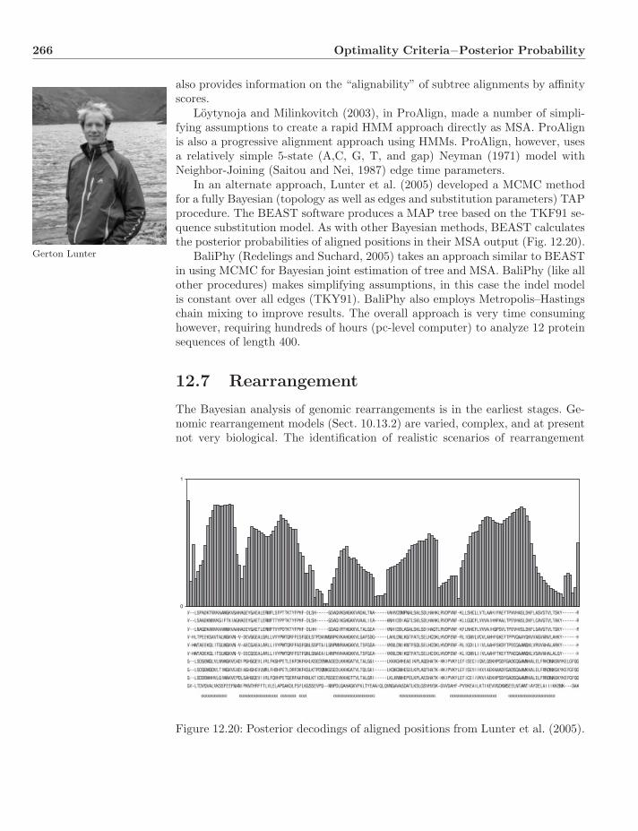
266 Optimality Criteria−Posterior Probability
also provides information on the “alignability” of subtree alignments by affinityscores.
Loytynoja and Milinkovitch (2003), in ProAlign, made a number of simpli-fying assumptions to create a rapid HMM approach directly as MSA. ProAlignis also a progressive alignment approach using HMMs. ProAlign, however, usesa relatively simple 5-state (A,C, G, T, and gap) Neyman (1971) model withNeighbor-Joining (Saitou and Nei, 1987) edge time parameters.
In an alternate approach, Lunter et al. (2005) developed a MCMC methodfor a fully Bayesian (topology as well as edges and substitution parameters) TAPprocedure. The BEAST software produces a MAP tree based on the TKF91 se-quence substitution model. As with other Bayesian methods, BEAST calculatesthe posterior probabilities of aligned positions in their MSA output (Fig. 12.20).
Gerton Lunter BaliPhy (Redelings and Suchard, 2005) takes an approach similar to BEASTin using MCMC for Bayesian joint estimation of tree and MSA. BaliPhy (like allother procedures) makes simplifying assumptions, in this case the indel modelis constant over all edges (TKY91). BaliPhy also employs Metropolis–Hastingschain mixing to improve results. The overall approach is very time consuminghowever, requiring hundreds of hours (pc-level computer) to analyze 12 proteinsequences of length 400.
12.7 Rearrangement
The Bayesian analysis of genomic rearrangements is in the earliest stages. Ge-nomic rearrangement models (Sect. 10.13.2) are varied, complex, and at presentnot very biological. The identification of realistic scenarios of rearrangement
0
1
Figure 12.20: Posterior decodings of aligned positions from Lunter et al. (2005).
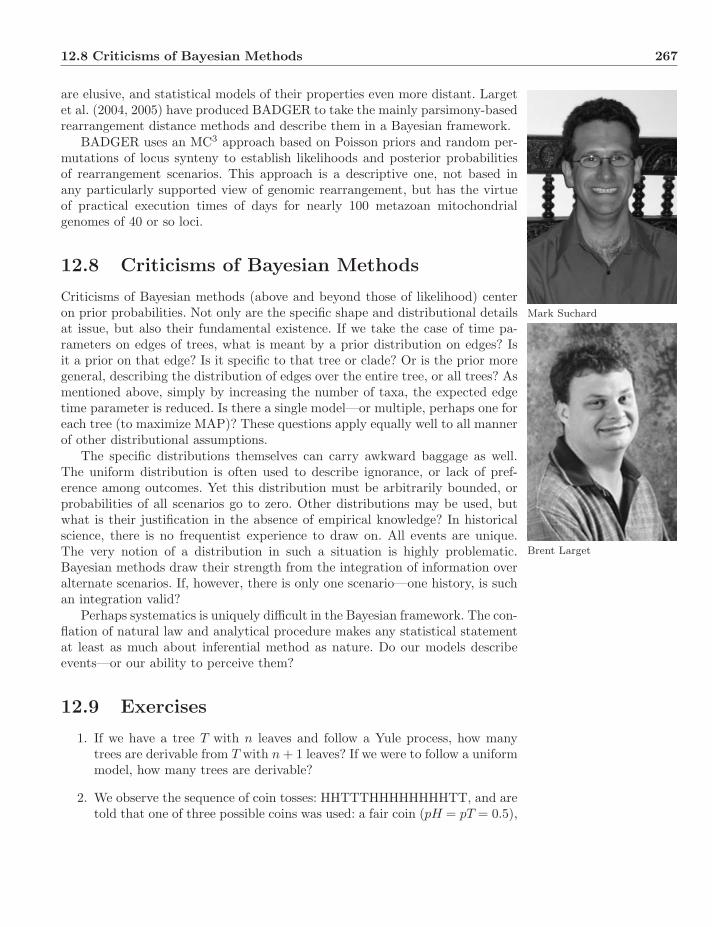
12.8 Criticisms of Bayesian Methods 267
are elusive, and statistical models of their properties even more distant. Largetet al. (2004, 2005) have produced BADGER to take the mainly parsimony-basedrearrangement distance methods and describe them in a Bayesian framework.
Mark Suchard
Brent Larget
BADGER uses an MC3 approach based on Poisson priors and random per-mutations of locus synteny to establish likelihoods and posterior probabilitiesof rearrangement scenarios. This approach is a descriptive one, not based inany particularly supported view of genomic rearrangement, but has the virtueof practical execution times of days for nearly 100 metazoan mitochondrialgenomes of 40 or so loci.
12.8 Criticisms of Bayesian Methods
Criticisms of Bayesian methods (above and beyond those of likelihood) centeron prior probabilities. Not only are the specific shape and distributional detailsat issue, but also their fundamental existence. If we take the case of time pa-rameters on edges of trees, what is meant by a prior distribution on edges? Isit a prior on that edge? Is it specific to that tree or clade? Or is the prior moregeneral, describing the distribution of edges over the entire tree, or all trees? Asmentioned above, simply by increasing the number of taxa, the expected edgetime parameter is reduced. Is there a single model—or multiple, perhaps one foreach tree (to maximize MAP)? These questions apply equally well to all mannerof other distributional assumptions.
The specific distributions themselves can carry awkward baggage as well.The uniform distribution is often used to describe ignorance, or lack of pref-erence among outcomes. Yet this distribution must be arbitrarily bounded, orprobabilities of all scenarios go to zero. Other distributions may be used, butwhat is their justification in the absence of empirical knowledge? In historicalscience, there is no frequentist experience to draw on. All events are unique.The very notion of a distribution in such a situation is highly problematic.Bayesian methods draw their strength from the integration of information overalternate scenarios. If, however, there is only one scenario—one history, is suchan integration valid?
Perhaps systematics is uniquely difficult in the Bayesian framework. The con-flation of natural law and analytical procedure makes any statistical statementat least as much about inferential method as nature. Do our models describeevents—or our ability to perceive them?
12.9 Exercises
1. If we have a tree T with n leaves and follow a Yule process, how manytrees are derivable from T with n + 1 leaves? If we were to follow a uniformmodel, how many trees are derivable?
2. We observe the sequence of coin tosses: HHTTTHHHHHHHHTT, and aretold that one of three possible coins was used: a fair coin (pH = pT = 0.5),

268 Optimality Criteria−Posterior Probability
a coin biased towards heads (pH = 0.8), or one biased towards tails (pT =0.8), and that these three coins had the prior probabilities of 0.5 for thefair coin and 0.25 for each of the biased coins. What are the expectedtransition probabilities (temperature aside) in a Markov Chain amongthese three states? What are the expected frequencies of the three statesafter a long chain?
3. If the prior distribution of tree topologies with 10 leaves is uniform, whatis the prior probability of a clade with 2 leaves? 5 leaves? 8 leaves?
4. For the three coins in exercise 2, if the probability of the same coin beingused in successive tosses is 0.5 and the probability of switching to each ofthe other two is 0.25 (the initial coin choice follows the prior), draw thetrellis diagram for this Hidden Markov Model.
If only a single coin were used, determine the probabilities of the cointoss sequence for the fair and two biased coins.
If the sequence of coins used were FFFFFHHHHHHHHTT (F=fair,H = biased towards heads, and T = biased towards tails), determine theprobability of the coin toss sequence.
5. Given the HMM trellis of 12.14, and the coin toss result HHTTTHHHH-HHHHTT, assuming the three coin states have equal initial probability,determine the maximum probability state path (Viterbi) and the proba-bilities of each state at each position (Forward–Backward).
6. Draw a general (no numbers) profile HMM trellis diagram for a sequencemodel with sites that follow GTR (no indels), sites that follow 5-StateNeyman (A, C, G, T + gaps), and sites that are invariant (no indelseither).
Chapter 13
Comparison of OptimalityCriteria
As discussed in the four previous chapters, there is a diversity of methods toreconstruct phylogenetic trees from comparative data. In general, most formsof such comparative data (e.g. qualitative anatomical features, DNA sequences)are amenable to analysis by any of the currently applied methods. In this chap-ter, the relative merits of the methods are discussed, as are three bases usedto distinguish among the approaches: epistemology, statistical behavior, andperformance.
The approaches discussed here are of four general types: distance analysis,parsimony, or minimization, maximum likelihood, and posterior probability. Theterm “posterior probability” is used in this chapter to refer to the Bayesianapproaches that maximize the posterior probability of trees (MAP or Topology–Bayes), as opposed to their component parts (clade posteriors or Clade–Bayes).As discussed in Chapter 12, clade-based posteriors do not offer an optimalityvalue per se, hence are not directly comparable to the methods discussed inthis chapter.
There is no single answer to “what is the best method?” in same way thereis no single answer to “what is the best tree?” A criterion must be specified inboth cases. Given an optimality criterion, we can rank competing hypothesesand identify the best tree or trees (at least of those we have found). The sameprocedure applies to methods, a criterion must be proposed in order to choosea method; and the criterion justified.
13.1 Distance and Character Methods
Before discussing the main points of comparison among methods, a general dis-tinction needs to be made between methods that rely on overall dissimilarity
Systematics: A Course of Lectures, First Edition. Ward C. Wheeler.c© 2012 Ward C. Wheeler. Published 2012 by Blackwell Publishing Ltd.
270 Comparison of Optimality Criteria
(or similarity) and those that directly operate on individual character obser-vations (e.g. anatomical features, molecular sequence data). Distance methods(Chapter 9) operate on the degree of pairwise difference between taxa. Thedistances may be raw, scaled, or normalized transforms of dissimilarity. Whentrees are constructed from these data, by whatever criterion, no attempt is(or can be) made to identify medians at tree vertices. No hypothetical ances-tral state reconstructions are proposed, no global homology statements erected,and no distinction between primitive and derived similarity made. In contrast,character-based methods are alike in that they make explicit statements aboutmedian ancestral reconstructions. The edges of trees then represent the transfor-mations between ancestral and descendent states (assuming the tree is directedor rooted).
With parsimony, the differences between these node states are summed,yielding the parsimony score. Likelihood multiplies the probabilities of the sameedge transformations given a model and time parameter. Bayesian methods alsodo this, integrating over the distribution of model and time parameters.
Whatever other admirable mathematical qualities distance analysis mayhave, it does not yield the specific events that are reconstructed to have oc-curred on tree edges. The reconstruction of edge events forms much of the basisfor discussion in the comparative biology literature. Biologists are interestedin, and largely motivated by, the desire to discover patterns and understandthe general and specific nature of these events. The entirety of historical evo-lutionary change is contained in these edge transformations. Of course, charac-ter events can be reconstructed ex post facto on a distance tree, but by whatmeans? This brings us back to character-based methods. Furthermore, sincethe distance criterion differs from those of the character methods, any distancetree result is unlikely to be optimal for the character-mapping criterion, againreturning us to character-based analysis ab initio. For this reason, most biol-ogists concerned with tree-based analysis of variation employ character-basedmethods1.
13.2 Epistemology
One of the earliest and most fundamental distinctions among systematic meth-ods was made on the basis of epistemology. That is, how do we “know” things,how are scientific hypotheses proposed and tested, and what is the relation-ship between observation and inference? A fundamental distinction has beenmade between a deductive (or more precisely hypothetico-deductive) processand the inductive approach embodied in statistical estimation procedures asapplied to systematic problems (see Chapter 4 for general discussion of modesof inference).
1There are several biological areas that contain counter examples including the medicalanalysis of human pathogens and evolutionary studies of non-eukaryotic organisms. Thesecases are presumably due more to tradition than any view of the superiority of the method.
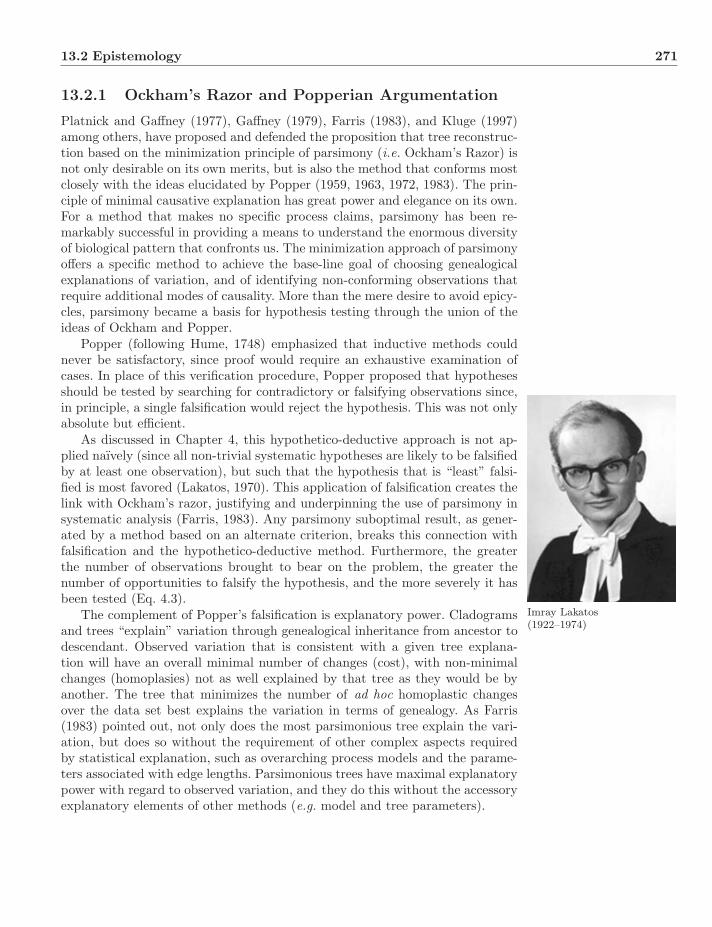
13.2 Epistemology 271
13.2.1 Ockham’s Razor and Popperian Argumentation
Platnick and Gaffney (1977), Gaffney (1979), Farris (1983), and Kluge (1997)among others, have proposed and defended the proposition that tree reconstruc-tion based on the minimization principle of parsimony (i.e. Ockham’s Razor) isnot only desirable on its own merits, but is also the method that conforms mostclosely with the ideas elucidated by Popper (1959, 1963, 1972, 1983). The prin-ciple of minimal causative explanation has great power and elegance on its own.For a method that makes no specific process claims, parsimony has been re-markably successful in providing a means to understand the enormous diversityof biological pattern that confronts us. The minimization approach of parsimonyoffers a specific method to achieve the base-line goal of choosing genealogicalexplanations of variation, and of identifying non-conforming observations thatrequire additional modes of causality. More than the mere desire to avoid epicy-cles, parsimony became a basis for hypothesis testing through the union of theideas of Ockham and Popper.
Popper (following Hume, 1748) emphasized that inductive methods couldnever be satisfactory, since proof would require an exhaustive examination ofcases. In place of this verification procedure, Popper proposed that hypothesesshould be tested by searching for contradictory or falsifying observations since,in principle, a single falsification would reject the hypothesis. This was not onlyabsolute but efficient.
As discussed in Chapter 4, this hypothetico-deductive approach is not ap-plied naıvely (since all non-trivial systematic hypotheses are likely to be falsifiedby at least one observation), but such that the hypothesis that is “least” falsi-fied is most favored (Lakatos, 1970). This application of falsification creates thelink with Ockham’s razor, justifying and underpinning the use of parsimony insystematic analysis (Farris, 1983). Any parsimony suboptimal result, as gener-ated by a method based on an alternate criterion, breaks this connection withfalsification and the hypothetico-deductive method. Furthermore, the greaterthe number of observations brought to bear on the problem, the greater thenumber of opportunities to falsify the hypothesis, and the more severely it hasbeen tested (Eq. 4.3).
Imray Lakatos(1922–1974)
The complement of Popper’s falsification is explanatory power. Cladogramsand trees “explain” variation through genealogical inheritance from ancestor todescendant. Observed variation that is consistent with a given tree explana-tion will have an overall minimal number of changes (cost), with non-minimalchanges (homoplasies) not as well explained by that tree as they would be byanother. The tree that minimizes the number of ad hoc homoplastic changesover the data set best explains the variation in terms of genealogy. As Farris(1983) pointed out, not only does the most parsimonious tree explain the vari-ation, but does so without the requirement of other complex aspects requiredby statistical explanation, such as overarching process models and the parame-ters associated with edge lengths. Parsimonious trees have maximal explanatorypower with regard to observed variation, and they do this without the accessoryexplanatory elements of other methods (e.g. model and tree parameters).
272 Comparison of Optimality Criteria
13.2.2 Parsimony and the Evolutionary Process
When discussing the merits of parsimony as a phylogenetic procedure, it is im-portant to keep clear the distinction between parsimony as an inferential proce-dure and parsimony as a model of evolution. As a philosophical basis for testinghypotheses, parsimony does not assume that evolution occurs parsimoniously. Infact, all non-trivial data sets exhibit non-parsimonious (i.e. homoplastic) events.Neither, in this context, does parsimony assume that homoplasy is rare, or thatrates of evolution are fast or slow (Farris, 1983; Sober, 1988, 2004) (but seebelow). The epistemological basis of parsimony as a process of discovery andhypothesis testing in science is general and useful. As stated by Wiley (1975),systematic analysis “must be done under the rules of parsimony, not becausenature is parsimonious, but because only parsimonious hypotheses can be de-fended by the investigator without resorting to authoritarianism or apriorism.”
Kluge (e.g. Kluge, 2005) has taken a different tack in that he has proposedthat the simple model of evolution as descent with modification (in essence,a minimal evolutionary assumption that offspring resemble their parents morethan non-parents, but not exactly) leads to parsimony as an evaluation prin-ciple. Again, such a statement makes no assertion of rates of change; ratherit is perhaps related to the “evolutionary path” model of Farris (1973a) (Sec-tion 11.3.1).
13.2.3 Induction and Statistical Estimation
One of the strongest criticisms of statistical approaches in systematics is derivedfrom the fact that systematics is a historical science. The events whose expla-nation are sought are unique to time and place. They are historical singulars(Kluge, 1998). As such, notions of “average” behavior inherent in probabilisticmodels is problematic. If each character observation is a unique object, it cannotbe a random sample drawn from a parameterized distribution expressed as amodel of change (e.g. GTR+I+Γ). Interestingly, when characters (and edges)are treated as having uncorrelated evolutionary rates (No-Common-Mechanism;Tuffley and Steel, 1997), parsimony and likelihood become exactly concordant intree choice. This appears to express neatly an important difference not necessar-ily between statistical and minimization-based methods, but between treatingcharacter changes as a class as opposed to historical individuals.
By this rationale, parsimonious trees have explanatory power in minimizingad hoc hypotheses, and increased observation will increase the severity of test,but would not reduce any measure of “sampling error,” since there is no sampledistribution that is measured.
13.2.4 Hypothesis Testing and Optimality Criteria
Much of the argumentation and philosophical constructs surrounding hypothe-sis testing in systematics were developed in the context of parsimony. However,Popper (1959) himself defined support, severity of test, and corroboration in
13.3 Statistical Behavior 273
terms of likelihood functions involving the probabilities of evidence (data) givena hypothesis and background knowledge. He was explicit in saying his probabil-ity was defined as “relative frequency” and the probability of the evidence givena hypothesis, “Fisher’s likelihood function.” Popper’s optimal hypothesis is thatwhich maximizes p(e|h, b), the probability of the data given the hypothesis andbackground knowledge—in short the likelihood.
As discussed in Section 4.1.7, at least in my opinion, hypothetico-deductiveinference can proceed via a falsification step based on any objective (and tran-sitive) optimality function. As long as hypotheses can be competed in a mathe-matically objective manner, hypotheses can be tested, and non-optimal solutionsfalsified. The key question is the appropriateness of the chosen function.
13.3 Statistical Behavior
There is a large literature concerning the statistical properties of systematicmethods, centered on the estimation behavior of various optimality criteria.When contrasting approaches to phylogenetic reconstruction are treated as al-ternate estimators, their behavior is most often discussed in light of three as-pects: consistency, efficiency, and robustness. There are many cases of provableresults, as well as demonstrations on contrived or simulated data. One of themost pressing issues that faces systematists is whether the conditions underwhich these results are generated or proven apply to the empirical cases en-countered in the course of research.
13.3.1 Probability
Before diving into the hurly-burly, it is worth revisiting the ideas embodiedby the concept of probability and their application to historical science. As dis-cussed more fully in Chapter 6, there are alternate interpretations of probability.In the context of the arguments discussed here, probability can have a logicalor degree of belief interpretation or, alternately, it may signify truth statementsabout the natural world akin to the frequency of repeated events. In the firstcase, probabilities reflect relative confidence in an outcome. A statement suchas “this coin has an 80% chance of being fair” would be an example of thefirst interpretation. The coin is either fair or not; the probability attached issimilar to a betting or odds ratio often used in Bayesian analysis (DeGrootand Schervish, 2006). By contrast, in the second case, probabilities imply astatement about what is ontologically “real.” “This coin has an 80% chance ofyielding heads on a given toss,” offers a property of the coin and a statementregarding physical reality.
Historical science does not easily permit a frequentist interpretation. What isto be our course of action if presented with the question, “What is the probabilitythat Octavian and Caesar Augustus were the same person?” Such a situationcannot be re-run or repeated in any way. Either he was or he wasn’t. Anynotion of probability is necessarily limited to our degree of belief, based on the
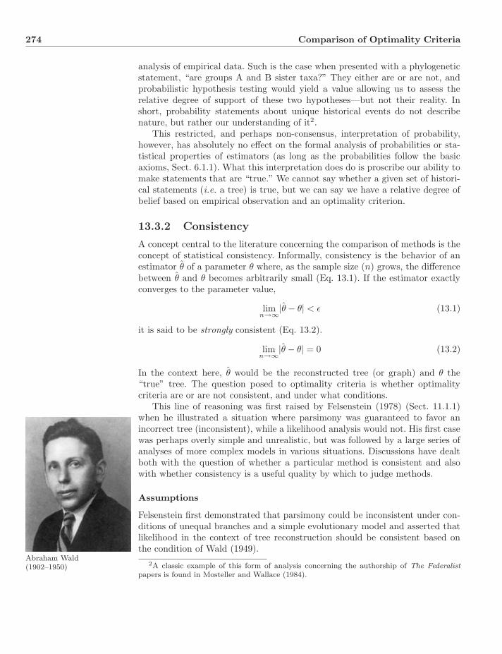
274 Comparison of Optimality Criteria
analysis of empirical data. Such is the case when presented with a phylogeneticstatement, “are groups A and B sister taxa?” They either are or are not, andprobabilistic hypothesis testing would yield a value allowing us to assess therelative degree of support of these two hypotheses—but not their reality. Inshort, probability statements about unique historical events do not describenature, but rather our understanding of it2.
This restricted, and perhaps non-consensus, interpretation of probability,however, has absolutely no effect on the formal analysis of probabilities or sta-tistical properties of estimators (as long as the probabilities follow the basicaxioms, Sect. 6.1.1). What this interpretation does do is proscribe our ability tomake statements that are “true.” We cannot say whether a given set of histori-cal statements (i.e. a tree) is true, but we can say we have a relative degree ofbelief based on empirical observation and an optimality criterion.
13.3.2 Consistency
A concept central to the literature concerning the comparison of methods is theconcept of statistical consistency. Informally, consistency is the behavior of anestimator θ of a parameter θ where, as the sample size (n) grows, the differencebetween θ and θ becomes arbitrarily small (Eq. 13.1). If the estimator exactlyconverges to the parameter value,
limn→∞|θ − θ| < ε (13.1)
it is said to be strongly consistent (Eq. 13.2).
limn→∞|θ − θ| = 0 (13.2)
In the context here, θ would be the reconstructed tree (or graph) and θ the“true” tree. The question posed to optimality criteria is whether optimalitycriteria are or are not consistent, and under what conditions.
This line of reasoning was first raised by Felsenstein (1978) (Sect. 11.1.1)when he illustrated a situation where parsimony was guaranteed to favor anincorrect tree (inconsistent), while a likelihood analysis would not. His first casewas perhaps overly simple and unrealistic, but was followed by a large series ofanalyses of more complex models in various situations. Discussions have dealtboth with the question of whether a particular method is consistent and alsowith whether consistency is a useful quality by which to judge methods.
Assumptions
Felsenstein first demonstrated that parsimony could be inconsistent under con-ditions of unequal branches and a simple evolutionary model and asserted thatlikelihood in the context of tree reconstruction should be consistent based onthe condition of Wald (1949).
Abraham Wald(1902–1950)
2A classic example of this form of analysis concerning the authorship of The Federalistpapers is found in Mosteller and Wallace (1984).

13.3 Statistical Behavior 275
Wald proved that maximum likelihood estimators would be consistent givenseveral conditions3. Many of these same assumptions are found in later consis-tency proofs. The most important of these conditions are: 1) that the observa-tions (data) are independent, 2) that they are identically distributed randomvariables, and 3) that the number of parameters to be estimated is finite, whilethe number of observations increases without bound. Each of these assumptionsis potentially problematic in the situations posed by systematic analysis.
The independence assumption is entirely appropriate for the sorts of stan-dard examples of statistical reasoning such as drawing balls from an urn or toss-ing a coin. In these cases, individual observations have no effect on the chanceof another event or its interpretation. If we take DNA sequence data as an ex-ample set of observations for discussion, empirical studies in no way match thisdescription. Empirical sequence observations are not randomly drawn from thegenome, one at a time. Almost all phylogenetic analyses of sequence data drawtheir observations from a restricted segment of the genome (a locus or loci) de-fined by a common metabolic purpose (e.g. cytochrome oxidases) and adjacencyon a chromosome. Furthermore, sequences are typically identified in a specificregion or locus and all nucleotides between two biochemically defined positions(often primers) determined. These are not random samples of the genome inany way, but are observations from a highly localized, functionally related re-gion. Multi-locus studies certainly improve on this, but even large collections ofloci provided by EST analysis (e.g. Dunn et al., 2008, Hejnol et al., 2009) arelimited to the relatively small fraction of the genome (10−3 or less, if 10−1 ofthe transcriptome) that are expressed as proteins.
A second difficulty with the independence assumption is found in all com-parative data. Even when entire genomes are sampled, these sequences havebeen in the same historical “bottle” so to speak, for their entire history. We areforced by necessity to treat comparative observations of anatomy and sequenceas if they were independent, but their shared history shows this operationalassumption to be false.
A third problem with the independence assumption is derived from thelength-variable nature of many loci used in molecular systematics studies. The“observations” used in systematic analyses are often aligned positions. Theseare constructed from raw observation and are, in fact, highly inferential objects.When sequences of an organism are determined, it is without reference to se-quences in other organisms. The raw sequences undergo an analytical processto determine which nucleotide sequence elements in one organism correspond tothose in another. Alignment and optimization of length-variable sequences infersequence correspondences via the optimization of a function based on param-eters for the transformations between sequences (e.g. transition, transversions,insertion, and deletions) and an optimality criterion (e.g. Sum-of-Pairs distance,Sect. 8.5). The correspondences between any given pair of sequence elements is
3Wald also applied his statistical acumen in the British Air Ministry during the SecondWorld War urging the counter-intuitive path of armoring locations on bombers that did nothave bullet holes. This was because the damage was only found on bombers that came back,not those that suffered fatal damage and left no record—an extreme case of survivor bias.
276 Comparison of Optimality Criteria
highly dependent on those elements adjacent to them and in the remainder ofthe sequences. Hence, comparative sequence data are highly interdependent andobviously do not satisfy the definition of independence.
The identical distribution assumption likewise presents difficulties. Mostanalyses of consistency assume a single evolutionary stochastic model for se-quence change. This may include variable rates among the aligned positions (ifsuch exist) and tree edges, but a unitary model is assumed. Even within a sin-gle locus, there are well-described varying dynamics due to the metabolic rolevarious components of products of the locus play. Obvious examples include the“stem” and “loop” regions of structural RNAs and transmembrane regions ofcytochrome oxidases. More complex models can, of course, be constructed, butthis entails the problems associated with estimating additional parameters withlimited data.
The final assumption concerns limit behavior as the input data increasewithout bound. The data presented by biological problems are finite, and inmany cases, relatively small. If a stochastic model is to be applied to a singlelocus (much less to a subregion), sequence data sizes will be limited to hundredsto low thousands of base-pairs. It is unclear if these sample sizes are sufficientto ensure asymptotic behavior. An entire transcriptome might constitute 104
loci, but it would be difficult to justify a single stochastic model for such aset of metabolically diverse genomic components. Entire genomes vary fromthousands of base-pairs in viruses to billions in vertebrates, setting a hard limiton sample size, and as with transcriptome analysis, a single model is unlikelyto be satisfactory.
The assumption violations discussed above do not impede the use of sta-tistical methods as optimality criteria for the relative ranking of hypotheses,but they do bring into question the application of consistency of estimators inreal-world systematic analysis.
Distances
As mentioned earlier (Chapter 9), one of the more vexing aspects of distanceanalysis is negative branches. These appear in analysis using a variety of branch-length estimation procedures including least-squares (Fitch and Margoliash,1967), greatest-lower-bound (Farris, 1972), and Neighbor-Joining (Saitou andNei, 1987). The analytical meaning of such edges with respect to the methods isclear—the reconstruction assumptions are violated. Biologically, of course, theyare meaningless. They also have clear implications for the behavior of these edgelengths as estimators of amount of evolution. Since there can be no such thingas “negative” evolution, the minimum value for any branch length must be zero.These estimators, then, must be inconsistent.
The tree topology itself, nonetheless, could still be consistently estimatedthrough minimization of the sum of these branch lengths. Gascuel et al. (2001)examined this issue and showed that for the most “reliable” method of branchlength estimation, generalized-least-squares, as well as for the widely usedweighted-least-squares, Minimum Evolution (ME) tree reconstruction was not

13.3 Statistical Behavior 277
1 AABAABB
2 ABABBAA
3 BACCCAA
4 BCAAACC
d (1,2) = 6 d (2,4) = 6
d (3,4) = 6 d (1,4) = 5
d (1,3) = 6 d (2,3) = 5
1
4
2
3
15/2
5/2 5/2
5/2
Figure 13.1: The example of Huson and Steel (2004) showing the underlyingdata (left) perfectly compatible with the tree 12|34, the distance matrix derivedfrom the data (center), and the perfectly additive tree 14|23 (right).
generally consistent (even under a variety of methods employed to avoid negativebranches).
Huson and Steel (2004) examined more general conditions and found thatthere were cases where the underlying character data were homoplasy-free onone tree, but when transformed into (uncorrected) distances were still perfectlytreelike and clocklike, yet on a different tree. The distances are compatible, ad-ditive, and entirely misleading (Fig. 13.1). This is a mathematical instantiationof the problems presented by plesiomorphic and autapomorphic characters thatHennig described.
In addition to this result, Huson and Steel (2004) show a similar result usingstochastic models, where the inconsistent result would be unsuspected becausethe distances appear perfectly tree like. This effect can also occur when distancesare transformed by an incorrect model. In a similar vein, Steel (2009) showedthat distance-based reconstruction can be inconsistent when rate variation ismodeled by the gamma distribution, but the shape parameter unknown.
Parsimony
Felsenstein (1978) showed that parsimony (under a specific 2-state model) wasinconsistent in cases where there was a short central edge connected to two longand two short pendant edges (Fig. 13.2, p1 = p3 and p2 = p4 = p5). Under theseconditions, the random match similarity of the terminals with long branches(p1 and p3) overwhelmed the parsimony signal of the short central branch (p5).Most of the conditions under which parsimony has been shown to be inconsistentcenter on this phenomenon.
Penny et al. (1991) generalized Felsenstein’s four-taxon case to arbitrary edgeprobabilities. With ωi = (1 − 2pi) of Fig. 13.2, parsimony will be consistent ifand only if
ω5 < min(
ω1ω2 + ω3ω4
ω1ω3 + ω2ω4,ω1ω2 + ω3ω4
ω1ω4 + ω2ω3
)(13.3)
These conditions will always be met if change is clocklike and also apply todistance methods.
A more general case, unlimited in number of states or taxa, was analyzedby Steel (2000). Under the Neyman (1971) model, Steel proved that when over-all transformation rates are low and fairly similar among branches, parsimony
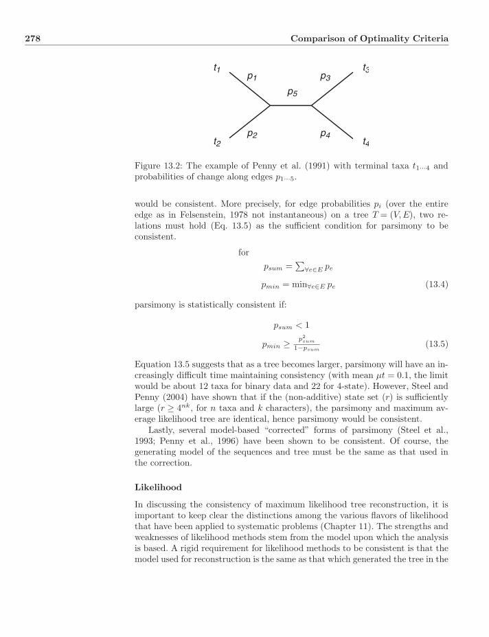
278 Comparison of Optimality Criteria
t1
t2
t3
t4
p1
p2
p5
p3
p4
Figure 13.2: The example of Penny et al. (1991) with terminal taxa t1···4 andprobabilities of change along edges p1···5.
would be consistent. More precisely, for edge probabilities pi (over the entireedge as in Felsenstein, 1978 not instantaneous) on a tree T = (V,E), two re-lations must hold (Eq. 13.5) as the sufficient condition for parsimony to beconsistent.
forpsum =
∑∀e∈E pe
pmin = min∀e∈E pe (13.4)
parsimony is statistically consistent if:
psum < 1
pmin ≥ p2sum
1−psum(13.5)
Equation 13.5 suggests that as a tree becomes larger, parsimony will have an in-creasingly difficult time maintaining consistency (with mean μt = 0.1, the limitwould be about 12 taxa for binary data and 22 for 4-state). However, Steel andPenny (2004) have shown that if the (non-additive) state set (r) is sufficientlylarge (r ≥ 4nk, for n taxa and k characters), the parsimony and maximum av-erage likelihood tree are identical, hence parsimony would be consistent.
Lastly, several model-based “corrected” forms of parsimony (Steel et al.,1993; Penny et al., 1996) have been shown to be consistent. Of course, thegenerating model of the sequences and tree must be the same as that used inthe correction.
Likelihood
In discussing the consistency of maximum likelihood tree reconstruction, it isimportant to keep clear the distinctions among the various flavors of likelihoodthat have been applied to systematic problems (Chapter 11). The strengths andweaknesses of likelihood methods stem from the model upon which the analysisis based. A rigid requirement for likelihood methods to be consistent is that themodel used for reconstruction is the same as that which generated the tree in the
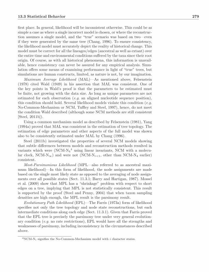
13.3 Statistical Behavior 279
first place. In general, likelihood will be inconsistent otherwise. This could be assimple a case as where a single incorrect model is chosen, or where the reconstruc-tion assumes a single model, and the “true” scenario was based on two—evenif they were generated by the same tree (Chang, 1996). To ensure consistency,the likelihood model must accurately depict the reality of historical change. Thismodel must be correct for all the lineages/edges (ancestral as well as extant) overthe entire time and environmental conditions suffered by the taxa since their rootorigin. Of course, as with all historical phenomena, this information is unavail-able, hence consistency can never be assured for any empirical analysis. Simu-lation offers some means of examining performance in light of “true” trees, butsimulations are human constructs, limited, as nature is not, by our imagination.
Maximum Average Likelihood (MAL)—As mentioned above, Felsenstein(1978) cited Wald (1949) in his assertion that MAL was consistent. One ofthe key points in Wald’s proof is that the parameters to be estimated mustbe finite, not growing with the data size. As long as unique parameters are notestimated for each observation (e.g. an aligned nucleotide sequence position),this condition should hold. Several likelihood models violate this condition (e.g.No-Common-Mechanism or NCM, Tuffley and Steel, 1997), hence, do not meetthe condition Wald described (although some NCM methods are still consistent[Steel, 2011b]).
Using a common mechanism model as described by Felsenstein (1981), Yang(1994a) proved that MAL was consistent in the estimation of tree topology. Theestimation of edge parameters and other aspects of the full model was shownalso to be consistently estimated under MAL by Chang (1996).
Steel (2011b) investigated the properties of several NCM models showingthat subtle differences between models and reconstruction methods resulted invariants which were (NCM-N4
4 using linear invariants, NCM with a molecu-lar clock, NCM-N∞) and were not (NCM-Nr<1, other than NCM-N4 earlier)consistent.
Most-Parsimonious Likelihood (MPL—also referred to as ancestral maxi-mum likelihood)—In this form of likelihood, the node assignments are madebased on the single most likely state as opposed to the averaging of node assign-ments over all possible states (Sect. 11.3.1; Barry and Hartigan, 1987). Mosselet al. (2009) show that MPL has a “shrinkage” problem with respect to shortedges on a tree, implying that MPL is not statistically consistent. This resultis supported by the proof (Steel and Penny, 2004) that when taxon samplingdensities are high enough, the MPL result is the parsimony result.
Evolutionary Path Likelihood (EPL)—The Farris (1973a) form of likelihoodspecifies not only the tree topology and node state reconstructions, but eachintermediate conditions along each edge (Sect. 11.3.1). Given that Farris provedthat the EPL tree is precisely the parsimony tree under very general evolution-ary condition (e.g. no rate restrictions), EPL would have all the strengths andweaknesses of parsimony, including inconsistency in the circumstances describedabove.
4NCM-Ni signifies the No-Common-Mechanism model with i character states.

280 Comparison of Optimality Criteria
Maximum Integrated Likelihood (MIL)—This form of likelihood can be em-ployed when prior distributions on model and edge parameters are known(Sect. 11.2.1). In essence, MIL is a Bayesian analysis where the prior distri-bution on trees is uniform. As a special case of the general Bayesian framework,MIL has been shown to be consistent, given, of course, appropriate priors andmodel (Steel, 2011a).
Bayesian Posterior Probability
Given the derivation of Bayesian methods in likelihood approaches, it was ini-tially thought that the approach of maximizing posterior probability of trees5
would be statistically consistent. This was thrown into doubt in the situationwhere data were evenly supportive of multiple topologies yet a specific tree wasfavored among those that should have been equal (Yang and Rannala, 2005;Lewis et al., 2005; Kolaczkowski and Thornton, 2009). This “Star Paradox”was thought to suffer from long-branch-attraction type problems, rendering themethod inconsistent. The method was later proven to be asymptotically consis-tent by Steel (2011a), and the previous instances likely due to finite data.
Does Consistency Matter?
As mentioned above, Felsenstein (1978) first urged the importance of statisticalconsistency in systematic analysis. Certainly, the idea of a procedure that isguaranteed to converge to the “true” result would seem to be desirable, andone that did not would be undesirable. This sentiment has been expressed bymany statisticians (Fisher, 1950; Neyman, 1952; Kendall and Stuart, 1973) asthe only reasonable course for estimators. Others, however, did not feel this way.Edwards (1972) stated that asymptotic behavior was irrelevant, and that theonly operation that mattered was the relative ranking of hypotheses.
Traditionally, researchers who favor ML have emphasized the centrality ofconsistency, while those more interested in parsimony have downplayed its im-portance. Either way, the relevance of consistency in real world analysis is un-clear for two reasons. The first concerns the requirement of a match betweengenerating (“true”) model and that used during ML reconstruction. The secondreason is finite data size.
Models used currently in systematic ML analysis are clearly simplificationsof the myriad forces molding the evolution of creatures in time and space. Thissimplification makes analysis tractable, and is even desirable to a certain ex-tent, since any tree can be made to match the data perfectly by sufficient ma-nipulation of a large enough collection of parameters (the solution becomesnon-identifiable, violating one of Wald’s assumptions; Steel et al., 1994; Yanget al., 1995). Nonetheless, this invalidates the applicability of proven consistencyresults to any empirical analysis. A stark example of this invalidation is theuse of stochastic models that ignore insertions and deletions in length-variable
5As opposed to that of clades.
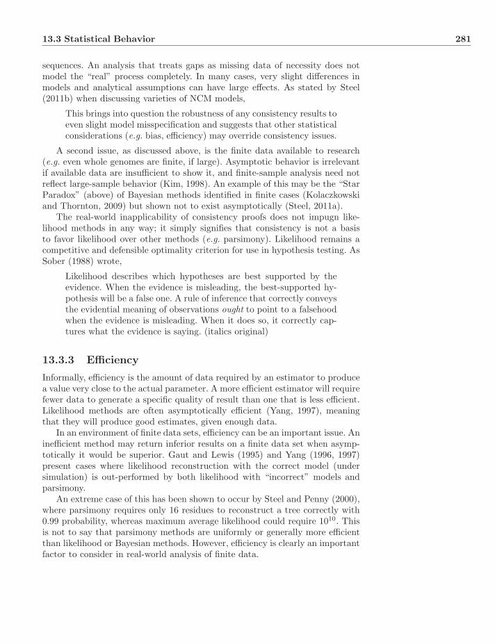
13.3 Statistical Behavior 281
sequences. An analysis that treats gaps as missing data of necessity does notmodel the “real” process completely. In many cases, very slight differences inmodels and analytical assumptions can have large effects. As stated by Steel(2011b) when discussing varieties of NCM models,
This brings into question the robustness of any consistency results toeven slight model misspecification and suggests that other statisticalconsiderations (e.g. bias, efficiency) may override consistency issues.
A second issue, as discussed above, is the finite data available to research(e.g. even whole genomes are finite, if large). Asymptotic behavior is irrelevantif available data are insufficient to show it, and finite-sample analysis need notreflect large-sample behavior (Kim, 1998). An example of this may be the “StarParadox” (above) of Bayesian methods identified in finite cases (Kolaczkowskiand Thornton, 2009) but shown not to exist asymptotically (Steel, 2011a).
The real-world inapplicability of consistency proofs does not impugn like-lihood methods in any way; it simply signifies that consistency is not a basisto favor likelihood over other methods (e.g. parsimony). Likelihood remains acompetitive and defensible optimality criterion for use in hypothesis testing. AsSober (1988) wrote,
Likelihood describes which hypotheses are best supported by theevidence. When the evidence is misleading, the best-supported hy-pothesis will be a false one. A rule of inference that correctly conveysthe evidential meaning of observations ought to point to a falsehoodwhen the evidence is misleading. When it does so, it correctly cap-tures what the evidence is saying. (italics original)
13.3.3 Efficiency
Informally, efficiency is the amount of data required by an estimator to producea value very close to the actual parameter. A more efficient estimator will requirefewer data to generate a specific quality of result than one that is less efficient.Likelihood methods are often asymptotically efficient (Yang, 1997), meaningthat they will produce good estimates, given enough data.
In an environment of finite data sets, efficiency can be an important issue. Aninefficient method may return inferior results on a finite data set when asymp-totically it would be superior. Gaut and Lewis (1995) and Yang (1996, 1997)present cases where likelihood reconstruction with the correct model (undersimulation) is out-performed by both likelihood with “incorrect” models andparsimony.
An extreme case of this has been shown to occur by Steel and Penny (2000),where parsimony requires only 16 residues to reconstruct a tree correctly with0.99 probability, whereas maximum average likelihood could require 1010. Thisis not to say that parsimony methods are uniformly or generally more efficientthan likelihood or Bayesian methods. However, efficiency is clearly an importantfactor to consider in real-world analysis of finite data.
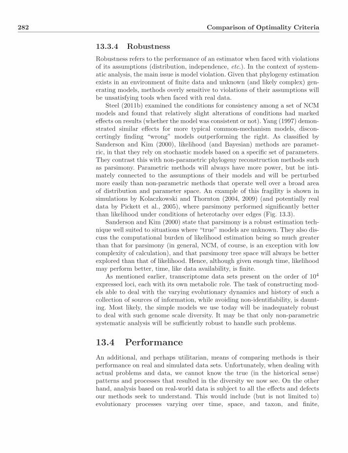
282 Comparison of Optimality Criteria
13.3.4 Robustness
Robustness refers to the performance of an estimator when faced with violationsof its assumptions (distribution, independence, etc.). In the context of system-atic analysis, the main issue is model violation. Given that phylogeny estimationexists in an environment of finite data and unknown (and likely complex) gen-erating models, methods overly sensitive to violations of their assumptions willbe unsatisfying tools when faced with real data.
Steel (2011b) examined the conditions for consistency among a set of NCMmodels and found that relatively slight alterations of conditions had markedeffects on results (whether the model was consistent or not). Yang (1997) demon-strated similar effects for more typical common-mechanism models, discon-certingly finding “wrong” models outperforming the right. As classified bySanderson and Kim (2000), likelihood (and Bayesian) methods are paramet-ric, in that they rely on stochastic models based on a specific set of parameters.They contrast this with non-parametric phylogeny reconstruction methods suchas parsimony. Parametric methods will always have more power, but be inti-mately connected to the assumptions of their models and will be perturbedmore easily than non-parametric methods that operate well over a broad areaof distribution and parameter space. An example of this fragility is shown insimulations by Kolaczkowski and Thornton (2004, 2009) (and potentially realdata by Pickett et al., 2005), where parsimony performed significantly betterthan likelihood under conditions of heterotachy over edges (Fig. 13.3).
Sanderson and Kim (2000) state that parsimony is a robust estimation tech-nique well suited to situations where “true” models are unknown. They also dis-cuss the computational burden of likelihood estimation being so much greaterthan that for parsimony (in general, NCM, of course, is an exception with lowcomplexity of calculation), and that parsimony tree space will always be betterexplored than that of likelihood. Hence, although given enough time, likelihoodmay perform better, time, like data availability, is finite.
As mentioned earlier, transcriptome data sets present on the order of 104
expressed loci, each with its own metabolic role. The task of constructing mod-els able to deal with the varying evolutionary dynamics and history of such acollection of sources of information, while avoiding non-identifiability, is daunt-ing. Most likely, the simple models we use today will be inadequately robustto deal with such genome scale diversity. It may be that only non-parametricsystematic analysis will be sufficiently robust to handle such problems.
13.4 Performance
An additional, and perhaps utilitarian, means of comparing methods is theirperformance on real and simulated data sets. Unfortunately, when dealing withactual problems and data, we cannot know the true (in the historical sense)patterns and processes that resulted in the diversity we now see. On the otherhand, analysis based on real-world data is subject to all the effects and defectsour methods seek to understand. This would include (but is not limited to)evolutionary processes varying over time, space, and taxon, and finite,
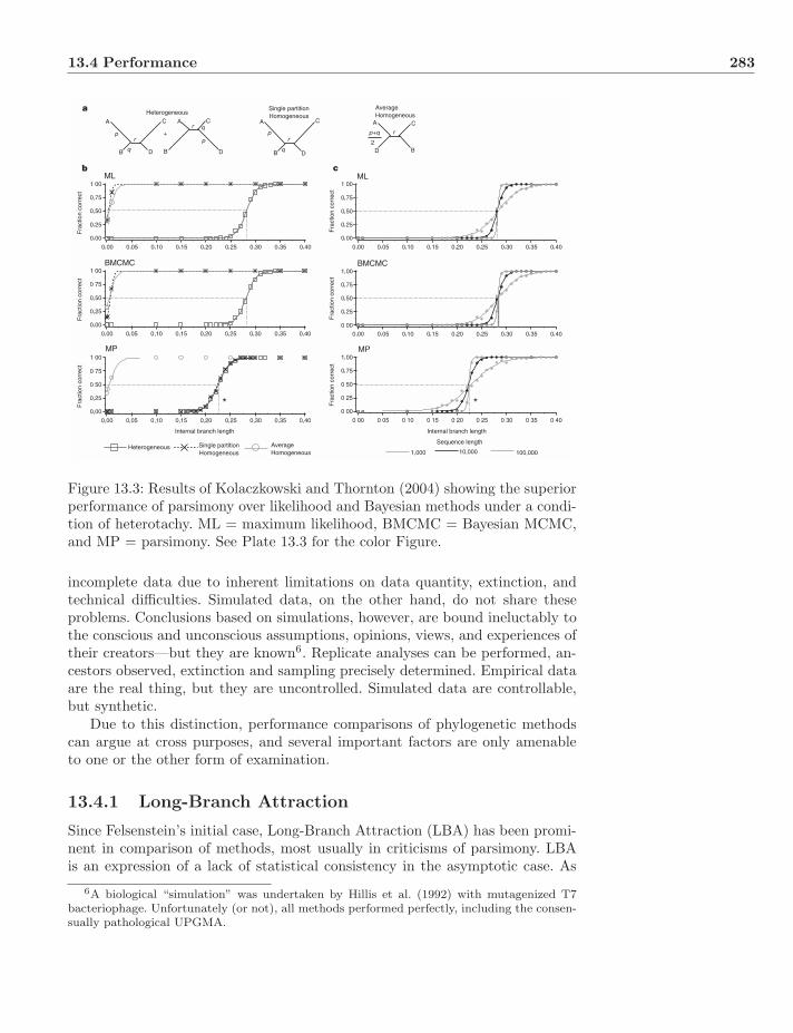
13.4 Performance 283
HeterogeneousSingle partitionHomogeneous
AverageHomogeneous
Heterogeneous Single partitionHomogeneous
AverageHomogeneous
Fra
ctio
n co
rrec
tF
ract
ion
corr
ect
Fra
ctio
n co
rrec
tF
ract
ion
corr
ect
Fra
ctio
n co
rrec
t
Fra
ctio
n co
rrec
t
Internal branch length Internal branch length
Sequence length
Figure 13.3: Results of Kolaczkowski and Thornton (2004) showing the superiorperformance of parsimony over likelihood and Bayesian methods under a condi-tion of heterotachy. ML = maximum likelihood, BMCMC = Bayesian MCMC,and MP = parsimony. See Plate 13.3 for the color Figure.
incomplete data due to inherent limitations on data quantity, extinction, andtechnical difficulties. Simulated data, on the other hand, do not share theseproblems. Conclusions based on simulations, however, are bound ineluctably tothe conscious and unconscious assumptions, opinions, views, and experiences oftheir creators—but they are known6. Replicate analyses can be performed, an-cestors observed, extinction and sampling precisely determined. Empirical dataare the real thing, but they are uncontrolled. Simulated data are controllable,but synthetic.
Due to this distinction, performance comparisons of phylogenetic methodscan argue at cross purposes, and several important factors are only amenableto one or the other form of examination.
13.4.1 Long-Branch Attraction
Since Felsenstein’s initial case, Long-Branch Attraction (LBA) has been promi-nent in comparison of methods, most usually in criticisms of parsimony. LBAis an expression of a lack of statistical consistency in the asymptotic case. As
6A biological “simulation” was undertaken by Hillis et al. (1992) with mutagenized T7bacteriophage. Unfortunately (or not), all methods performed perfectly, including the consen-sually pathological UPGMA.

284 Comparison of Optimality Criteria
has been shown, distance and common-mechanism average likelihood methodscan also be inconsistent in fairly simple cases of either incorrect or insufficientstochastic models (Chang, 1996).
Performance of methods in real-world situations will always be based onfinite data, and many studies have addressed this reality via simulation. Typ-ically, a small set of sequences (4–10 or so, compact enough to be analyzedeasily) are evolved via some model under a variety of branch length scenarios(e.g. Swofford et al., 2001) and then subjected to analysis via a set of methods.The result is compared to the “true” history of the simulation.
Simulations have repeatedly shown LBA for parsimony (e.g. Swofford et al.,2001; Pol and Siddall, 2001), but this phenomenon is not limited to parsimony.Pol and Siddall (2001) showed in a 10-taxon case with 1kb of simulated, alignedsequence data that likelihood was prone to this problem as well (Fig. 13.4).This result holds regardless of whether likelihood analysis is performed usingan incorrect or correct (generating) model. Additionally, likelihood also suffersfrom a Long-Branch Repulsion (a true long branch is not recovered—named the“Farris Zone,” Siddall, 1998, or the Anti or Inverse Felsenstein Zone) not foundin parsimony analyses. Parsimony outperforms likelihood in this context as theprobability of change on the short branches approaches zero and the sequenceson the longer edges approach randomization. With k sites, the probability ofparsimony reconstructing the tree correctly approaches 1 − ( 3
4 )k while that forlikelihood will be no more than 2
3 (Steel and Penny, 2000).
0.1 0.3 0.5 0.7 0.9 1.1 1.3 1.5 1.7 1.9Long branches length
% r
ecov
ery
of tr
ue to
polo
gy
100
90
80
70
60
50
40
30
20
10
0
Parsimony unw
Parsimony ts/tv
Likelihood true
Likelihood JC
Figure 13.4: Figure of Pol and Siddall (2001) showing the failure of both par-simony and likelihood to identify the correct tree as branches show increasingdifferences in length.
13.5 Convergence 285
As mentioned above, a similar case of parsimony outperforming both likeli-hood and Bayesian methods with simulated varying rates of change is shown byKolaczkowski and Thornton (2004). This was observed with even a small frac-tion of characters suffering heterotachy. Kolaczkowski and Thornton (2009) latershowed that LBA could also occur in Bayesian analyses under similar conditions.Simulations have shown that parsimony can also be hindered by heterotachy,but not as severely as statistical methods (Philippe et al., 2005).
So what are we to do about LBA? All methods can, under some conditions,exhibit this behavior. However, the only way to recognize the phenomenon is byknowing the actual history of a group. Yet, we cannot know this history for realdata. What if, as the data would suggest, a “long” branch merely denoted well-supported sister taxa? If, for example, a pair of Panorpa species were includedin an analysis of insect orders (Wheeler et al., 2001), the edge joining thesetaxa would show a great deal of change—a long branch. Should we doubt sucha grouping?
13.4.2 Congruence
In my mind, one of the most powerful tests of any phylogenetic hypothesis iscongruence. Whether that congruence is among characters of a single analysisor between multiple data partitions, we expect that alternate sources of infor-mation should agree about phylogenetic conclusions (assuming a single history,horizontal and reticulate evolution aside). In this way, data and methods arepredictive (or more precisely retrodictive), in that they anticipate new obser-vations. Comparison with “known” phylogenies is really an extreme form ofcongruence where the comparison is between a result and the previous body ofevidence supporting a phylogeny.
As far as I am aware, there are very few explicit comparisons of optimalitycriteria based on the congruence behavior of real data (Wheeler, 2006). This maybe due to the dearth of methods available for the statistical analysis of qualita-tive data in the past, but with the implementations of Neyman (1971) and NCM(Tuffley and Steel, 1997), this problem would seem to have been ameliorated.Given the ability to measure congruence irrespective of the true relationships,this procedure should be a powerful measure of the behavior of methods7.
13.5 Convergence
As discussed above and in previous chapters, several instances have been shownto lead to convergent results between parsimony and other methods, most com-monly likelihood. Farris (1973a) with EPL was the first to show that likelihood(that version at least) and parsimony would rank topologies in exactly the sameway when intermediate ancestors were reconstructed. Goldman (1990) showedthis convergence when change probabilities were invariant over edges. Later, the
7As long as the methods are label invariant, as opposed to something akin to alphabeticalorder, which would be perfectly—if trivially—congruent.
286 Comparison of Optimality Criteria
common edge rate parameter was relaxed and NCM provided a third generalcase of convergence in optimality among methods. To this has been added thecase where the number of character states is large (Steel and Penny, 2004), and,for MPL, when taxon sampling densities are sufficiently great.
One of the implications of method convergence is that potentially we canidentify and evaluate their underlying assumptions. Statements such as “sinceparsimony is statistically consistent in scenario A, parsimony assumes the con-ditions of A,” is clearly misguided (Sober, 2004, 2005). As Sober points out, thebest that can be done is to say that “since parsimony and likelihood convergein situation A, those conditions not assumed by likelihood in that scenario arealso not assumed by parsimony.” This reasoning serves to rule out assumptions,but is unable to rule them in, or to identify necessary and sufficient conditionsfor desirable behavior.
It is difficult to know if continued mathematical analysis of methods willfind increasingly general cases where methods converge. It is possible that morecomplex and realistic models (in the vein of NCM) will identify new areas wheremethods choose the same optimal tree hypothesis, or they may dissolve intonon-identifiability. Whether there is some shore of unification or not, areas ofintersection among methods reveal a great deal about them, their strengths andweaknesses, and thus allow us to evaluate empirical results with greater clarityand precision.
13.6 Can We Argue Optimality Criteria?
How are we to choose an optimality criterion? Neither epistemology nor asymp-totic consistency offer unfailing guidance. All optimality criteria can participatein hypothetico-deductive hypothesis testing, and all methods are subject toinconsistent behavior asymptotically. The empirical reality of finite characterdata and imperfect taxon samples reduces the impact of stochastically idealasymptotic behaviors, leaving us to assay performance in absence of known orrepeatable phenomena.
Another confounding effect is the computational complexity of systematicproblems. Optimality-based tree reconstruction is, in general, an NP–hard prob-lem. As such, we are not likely ever to have a (if there is only one) known, guar-anteed optimal solution to tree reconstruction problems. Given that we cannot,for non-trivial problems, determine optimal solutions, and these would be re-quired to satisfy at least the strong form of statistical consistency, it is unclearif consistency could ever apply to an empirical case.
One choice might be the syncretistic escape of employing multiple methods.Of course, if there is complete agreement, there is no issue. When optimalitycriteria disagree, however, which is the most common situation (at least forlarger data sets), what to do? Alternate optimality criteria have different moti-vations and epistemological underpinnings (Giribet et al., 2002). An average orconsensus of such varied objects is a difficult path, especially since the criteriaare supporting alternate hypotheses (or the problem wouldn’t exist).
13.7 Exercises 287
Optimality criteria are analytical assumptions used to interpret historicallyunique events. As such, they cannot be tested empirically for accuracy in thesense of propinquity to truth. We simply cannot know this. Methods can betested for precision in the guise of congruence, and this may help distinguishamong criteria in a useful and intuitive manner. However, at the core, optimalitycriteria are assumptions that require support and justification when employed.Alternate assumptions lead to alternate results. Only by justifying our assump-tions can we support our conclusions.
13.7 Exercises
1. Under what conditions would distance analysis be appropriate to analyzeunderlying character data?
2. Could Popper’s ideas of support, corroboration, and severity of test bedefined in terms other than Fisher’s likelihood?
3. Would it be reasonable to limit the phylogenetic methods employed tothose cases or those conditions, where methods converge?
4. Consider a data set comprised of anatomical data for a group of taxacomposed of both living and extinct taxa, and complete genomic sequencesfor the extant taxa. How do the strengths and weaknesses of differentmethods apply to this case? Which optimality criterion is best suited toanalyze these data and why?

Part IV
Trees
Chapter 14
Tree Searching
As is well-known (Foulds and Graham, 1982; Day, 1987; Roch, 2006), the searchfor “best” trees is an NP–hard problem. The number of possible trees is exponen-tially large (Eq. 2.1), hence, other than for trivial data sets, systematic analysisrequires the use of heuristic tree search procedures. The discussion here is, forthe most part, general to optimality criteria. Any objective criterion can be ap-plied to a given tree to yield a cost or optimality value. This chapter is limitedto the various exact and heuristic procedures used to explore tree space andidentify “best” solutions.
A corollary of the exponential number of possible trees is that the set of op-timal trees can be exponentially large as well. A search procedure must not onlyseek to find an optimal solution, but the complete (or at least representative)set of optimal solutions.
14.1 Exact Solutions
Although not generally employed, exact solution techniques can be comfort-ing and, at times, useful. Exact solutions can be identified when leaf numbersare small, and the understanding of exact techniques can inform the design ofheuristic procedures and the inference of their effectiveness. Two exact solu-tion procedures are in common use: simple enumeration and the more efficientBranch-and-Bound.
14.1.1 Explicit Enumeration
Explicit enumeration is a brute force method of simply evaluating all possible treetopologies for a given set of taxa. This operation becomes tiresome quickly andis rarely employed for anything other than analytical purposes (Algs. 14.1 and14.2, Fig. 14.1). This is due to the combinatorially large number of trees. Naıvely
Systematics: A Course of Lectures, First Edition. Ward C. Wheeler.c© 2012 Ward C. Wheeler. Published 2012 by Blackwell Publishing Ltd.
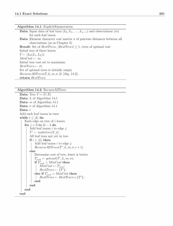
14.1 Exact Solutions 291
Algorithm 14.1: ExplicitEnumerationData: Input data of leaf taxa (L0, L1, . . . , Ln−1) and observations (m)
for each leaf taxonData: Element character cost matrix σ of pairwise distances between all
observations (as in Chapter 8)Result: Set of BestTrees, |BestTrees| ≥ 1, trees of optimal costInitial tree of three leavesT ← (L0(L1, L2));MinCost ← ∞;Initial tree cost set to maximumBestTrees ← ∅;Set of optimal trees is initially emptyRecurseAllTrees(T,L,m, σ, 3) [Alg. 14.2];return BestTrees
Algorithm 14.2: RecurseAllTreesData: Tree T = (V,E)Data: L of Algorithm 14.1Data: m of Algorithm 14.1Data: σ of Algorithm 14.1Data: iAdd each leaf taxon in turnwhile i ≤ |L| do
Each edge on tree of i leavesfor j = 0 to 2i − 4 do
Add leaf taxon i to edge jT ′ ← maketree(T, j);All leaf taxa not yet in treeif i < |L| then
Add leaf taxon i to edge jRecurseAllTrees(T ′, L,m, σ, i + 1)
elseDetermine cost of tree, lower is betterT ′
cost ← getcost(T ′, L,m, σ);if T ′
cost < MinCost thenMinCost ← T ′
cost;BestTrees ← {T ′};
else if T ′cost = MinCost then
BestTrees ← BestTrees ∪ {T ′};end
endend
end

292 Tree Searching
L0 L1
L2
Begin with three leaves
Add a fourth ineach of three edges
L3
L0
L1
L2
L3
L0
L1
L2
L4
L3
L0 L1
L2
L4
L3
L0L1
L2
L4L3
L0
L1
L2
L4
L3
L0
L1
L2
L4
L3
L0
L1
L2
L1
L0
L3
L2
L4
L1
L0 L3
L2
L4
L1
L0L3
L2
L4L1
L0
L3
L2
L4
L1
L0
L3
L2
L4
L2
L0
L1
L3
L2
L0
L1
L3
L4
L2
L0 L1
L3
L4
L2
L0L1
L3
L4L2
L0
L1
L3
L4
L2
L0
L1
L3
L4
Continue until all leaves are added
.
.
.
Evaluate all trees Toptimal = best T0,T1,...,T (2n − 4)!(n − 2)!2n − 2 −1
Figure 14.1: Explicit enumeration and evaluation of all trees.
plodding through space evaluating every possibility will be tractable only for arelatively small number of taxa (usually topping out at 15 or so taxa).
In the algorithmic descriptions of this chapter, the cost function of a tree,getcost(), is left undefined in order to be general with respect to optimalitycriterion.
14.1.2 Implicit Enumeration—Branch-and-Bound
The Branch-and-Bound algorithm (Algs. 14.3 and 14.4; Fig. 14.2) (Land and Doig,1960; Hendy and Penny, 1982) seeks to reduce the number of trees examined bytaking advantage of the fact that partial trees can only become more costly withthe addition of more leaf taxa (assuming distances are metric and all leavesunique). If a partial tree cost is already equal to or greater than a complete tree,that entire line of trees generated by adding more taxa to that subtree, must bemore costly than the current best tree known (the bound) and can be excludedfrom further examination. In general, the method can reduce the number of ex-plicitly enumerated trees greatly (hence the term “implicit enumeration”), butnot with a guaranteed time performance. Individual data sets may have signifi-cant or marginal reductions in numbers of trees examined. This is due to the fact
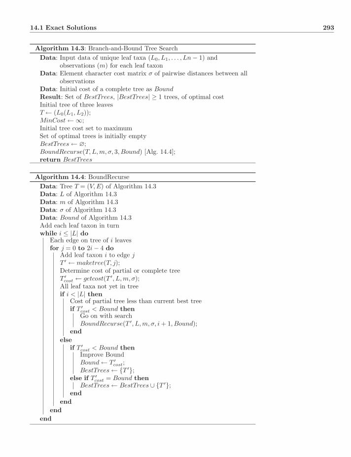
14.1 Exact Solutions 293
Algorithm 14.3: Branch-and-Bound Tree SearchData: Input data of unique leaf taxa (L0, L1, . . . , Ln − 1) and
observations (m) for each leaf taxonData: Element character cost matrix σ of pairwise distances between all
observationsData: Initial cost of a complete tree as BoundResult: Set of BestTrees, |BestTrees| ≥ 1 trees, of optimal costInitial tree of three leavesT ← (L0(L1, L2));MinCost ← ∞;Initial tree cost set to maximumSet of optimal trees is initially emptyBestTrees ← ∅;BoundRecurse(T,L,m, σ, 3, Bound) [Alg. 14.4];return BestTrees
Algorithm 14.4: BoundRecurseData: Tree T = (V,E) of Algorithm 14.3Data: L of Algorithm 14.3Data: m of Algorithm 14.3Data: σ of Algorithm 14.3Data: Bound of Algorithm 14.3Add each leaf taxon in turnwhile i ≤ |L| do
Each edge on tree of i leavesfor j = 0 to 2i − 4 do
Add leaf taxon i to edge jT ′ ← maketree(T, j);Determine cost of partial or complete treeT ′
cost ← getcost(T ′, L,m, σ);All leaf taxa not yet in treeif i < |L| then
Cost of partial tree less than current best treeif T ′
cost < Bound thenGo on with searchBoundRecurse(T ′, L,m, σ, i + 1, Bound);
endelse
if T ′cost < Bound thenImprove BoundBound ← T ′
cost;BestTrees ← {T ′};
else if T ′cost = Bound then
BestTrees ← BestTrees ∪ {T ′};end
endend
end
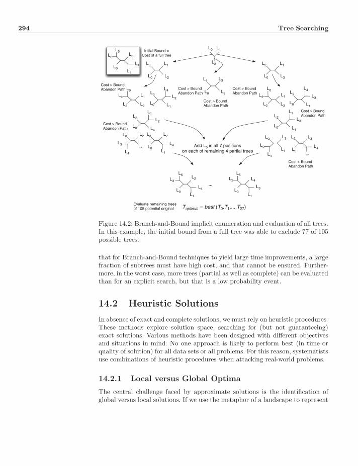
294 Tree Searching
L0 L1
L2L3
L0
L1
L2
L3
L0
L1
L2
L4
L3
L0 L1
L2
L4
L3
L0L1
L2
L4L3
L0
L1
L2
L4
L3
L0
L1
L2
L4
L3
L0
L1
L2
L2
L0
L1
L3
L2
L0
L1
L3
L4
L2
L0 L1
L3
L4
L2
L0L1
L3
L4L2
L0
L1
L3
L4
L2
L0
L1
L3
L4
Evaluate remaining treesof 105 potential original
L2
L0L1
L3
L4
L5 Initial Bound =Cost of a full tree
Cost > BoundAbandon Path
Cost > BoundAbandon Path
Cost > BoundAbandon Path
Cost > BoundAbandon Path
Cost > BoundAbandon Path
Cost > BoundAbandon Path
Cost > BoundAbandon Path
Add L5 in all 7 positionson each of remaining 4 partial trees
L2
L0L1
L3
L4
L5
···
L2
L0L1
L3
L4
L5
Toptimal = best (T0,T1,...,T27)
Figure 14.2: Branch-and-Bound implicit enumeration and evaluation of all trees.In this example, the initial bound from a full tree was able to exclude 77 of 105possible trees.
that for Branch-and-Bound techniques to yield large time improvements, a largefraction of subtrees must have high cost, and that cannot be ensured. Further-more, in the worst case, more trees (partial as well as complete) can be evaluatedthan for an explicit search, but that is a low probability event.
14.2 Heuristic Solutions
In absence of exact and complete solutions, we must rely on heuristic procedures.These methods explore solution space, searching for (but not guaranteeing)exact solutions. Various methods have been designed with different objectivesand situations in mind. No one approach is likely to perform best (in time orquality of solution) for all data sets or all problems. For this reason, systematistsuse combinations of heuristic procedures when attacking real-world problems.
14.2.1 Local versus Global Optima
The central challenge faced by approximate solutions is the identification ofglobal versus local solutions. If we use the metaphor of a landscape to represent
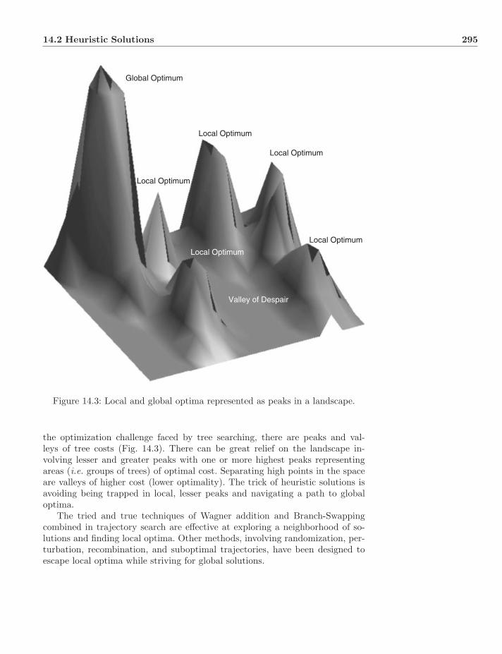
14.2 Heuristic Solutions 295
Local Optimum
Global Optimum
Local Optimum
Local Optimum
Local Optimum
Local Optimum
Valley of Despair
Figure 14.3: Local and global optima represented as peaks in a landscape.
the optimization challenge faced by tree searching, there are peaks and val-leys of tree costs (Fig. 14.3). There can be great relief on the landscape in-volving lesser and greater peaks with one or more highest peaks representingareas (i.e. groups of trees) of optimal cost. Separating high points in the spaceare valleys of higher cost (lower optimality). The trick of heuristic solutions isavoiding being trapped in local, lesser peaks and navigating a path to globaloptima.
The tried and true techniques of Wagner addition and Branch-Swappingcombined in trajectory search are effective at exploring a neighborhood of so-lutions and finding local optima. Other methods, involving randomization, per-turbation, recombination, and suboptimal trajectories, have been designed toescape local optima while striving for global solutions.
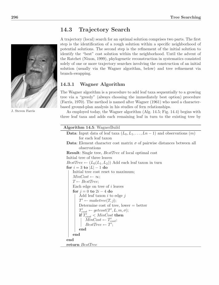
296 Tree Searching
14.3 Trajectory Search
A trajectory (local) search for an optimal solution comprises two parts. The firststep is the identification of a rough solution within a specific neighborhood ofpotential solutions. The second step is the refinement of the initial solution toidentify the “best” cost solution within the neighborhood. Until the advent ofthe Ratchet (Nixon, 1999), phylogenetic reconstruction in systematics consistedsolely of one or more trajectory searches involving the construction of an initialsolution (usually via the Wagner algorithm, below) and tree refinement viabranch-swapping.
14.3.1 Wagner Algorithm
The Wagner algorithm is a procedure to add leaf taxa sequentially to a growingtree via a “greedy” (always choosing the immediately best option) procedure(Farris, 1970). The method is named after Wagner (1961) who used a character-based ground-plan analysis in his studies of fern relationships.
J. Steven Farris As employed today, the Wagner algorithm (Alg. 14.5; Fig. 14.4) begins withthree leaf taxa and adds each remaining leaf in turn to the existing tree by
Algorithm 14.5: WagnerBuildData: Input data of leaf taxa (L0, L1, . . . , Ln − 1) and observations (m)
for each leaf taxonData: Element character cost matrix σ of pairwise distances between all
observationsResult: Single tree, BestTree of local optimal costInitial tree of three leavesBestTree ← (L0(L1, L2)) Add each leaf taxon in turnfor i = 3 to |L| − 1 do
Initial tree cost reset to maximum;MinCost ← ∞;T ← BestTree;Each edge on tree of i leavesfor j = 0 to 2i − 4 do
Add leaf taxon i to edge jT ′ ← maketree(T, j);Determine cost of tree, lower = betterT ′
cost ← getcost(T ′, L,m, σ);if T ′
cost < MinCost thenMinCost ← T ′
cost;BestTree ← T ′;
endend
endreturn BestTree
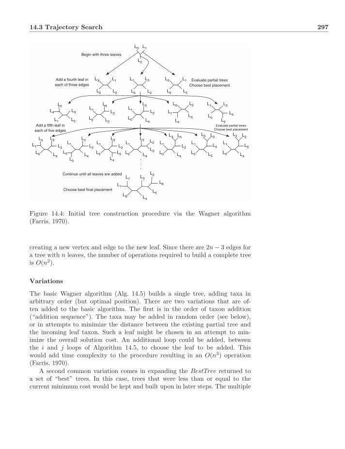
14.3 Trajectory Search 297
L0 L1
L2
Begin with three leaves
Add a fourth leaf ineach of three edges
L3
L0
L1
L2
L3
L0
L1
L2
L1
L0
L3
L2
L4
L1
L0 L3
L2
L4 L1
L0L3
L2
L4L1
L0
L3
L2
L4L1
L0
L3
L2
L4
L2
L0
L1
L3
Continue until all leaves are added
Evaluate partial treesChoose best placement
.
.
.
L1
L0
L3 L2
L4L1
L0 L4
L1
L0
L3
L2
L4
L1
L0
L3
L2
L4
L1
L0
L3
L2
L4
L1
L0
L3 L2
L4
Add a fifth leaf ineach of five edges
Evaluate partial treesChoose best placement
L1
L0
L3
L2
L4
L5L5
L5 L5L5
L5
L5
L3 L2
Choose best final placementL1
L0
L3
L2
L4
L5
L6
L7
Figure 14.4: Initial tree construction procedure via the Wagner algorithm(Farris, 1970).
creating a new vertex and edge to the new leaf. Since there are 2n − 3 edges fora tree with n leaves, the number of operations required to build a complete treeis O(n2).
Variations
The basic Wagner algorithm (Alg. 14.5) builds a single tree, adding taxa inarbitrary order (but optimal position). There are two variations that are of-ten added to the basic algorithm. The first is in the order of taxon addition(“addition sequence”). The taxa may be added in random order (see below),or in attempts to minimize the distance between the existing partial tree andthe incoming leaf taxon. Such a leaf might be chosen in an attempt to min-imize the overall solution cost. An additional loop could be added, betweenthe i and j loops of Algorithm 14.5, to choose the leaf to be added. Thiswould add time complexity to the procedure resulting in an O(n3) operation(Farris, 1970).
A second common variation comes in expanding the BestTree returned toa set of “best” trees. In this case, trees that were less than or equal to thecurrent minimum cost would be kept and built upon in later steps. The multiple
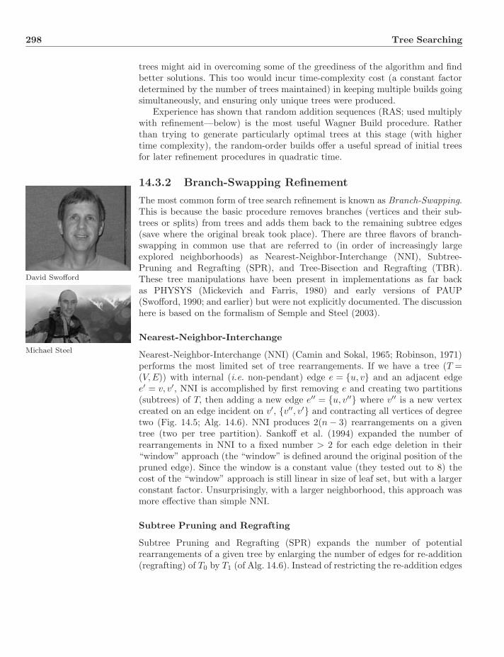
298 Tree Searching
trees might aid in overcoming some of the greediness of the algorithm and findbetter solutions. This too would incur time-complexity cost (a constant factordetermined by the number of trees maintained) in keeping multiple builds goingsimultaneously, and ensuring only unique trees were produced.
Experience has shown that random addition sequences (RAS; used multiplywith refinement—below) is the most useful Wagner Build procedure. Ratherthan trying to generate particularly optimal trees at this stage (with highertime complexity), the random-order builds offer a useful spread of initial treesfor later refinement procedures in quadratic time.
14.3.2 Branch-Swapping Refinement
The most common form of tree search refinement is known as Branch-Swapping.This is because the basic procedure removes branches (vertices and their sub-trees or splits) from trees and adds them back to the remaining subtree edges(save where the original break took place). There are three flavors of branch-swapping in common use that are referred to (in order of increasingly largeexplored neighborhoods) as Nearest-Neighbor-Interchange (NNI), Subtree-Pruning and Regrafting (SPR), and Tree-Bisection and Regrafting (TBR).
David Swofford
Michael Steel
These tree manipulations have been present in implementations as far backas PHYSYS (Mickevich and Farris, 1980) and early versions of PAUP(Swofford, 1990; and earlier) but were not explicitly documented. The discussionhere is based on the formalism of Semple and Steel (2003).
Nearest-Neighbor-Interchange
Nearest-Neighbor-Interchange (NNI) (Camin and Sokal, 1965; Robinson, 1971)performs the most limited set of tree rearrangements. If we have a tree (T =(V,E)) with internal (i.e. non-pendant) edge e = {u, v} and an adjacent edgee′ = v, v′, NNI is accomplished by first removing e and creating two partitions(subtrees) of T, then adding a new edge e′′ = {u, v′′} where v′′ is a new vertexcreated on an edge incident on v′, {v′′, v′} and contracting all vertices of degreetwo (Fig. 14.5; Alg. 14.6). NNI produces 2(n − 3) rearrangements on a giventree (two per tree partition). Sankoff et al. (1994) expanded the number ofrearrangements in NNI to a fixed number > 2 for each edge deletion in their“window” approach (the “window” is defined around the original position of thepruned edge). Since the window is a constant value (they tested out to 8) thecost of the “window” approach is still linear in size of leaf set, but with a largerconstant factor. Unsurprisingly, with a larger neighborhood, this approach wasmore effective than simple NNI.
Subtree Pruning and Regrafting
Subtree Pruning and Regrafting (SPR) expands the number of potentialrearrangements of a given tree by enlarging the number of edges for re-addition(regrafting) of T0 by T1 (of Alg. 14.6). Instead of restricting the re-addition edges

14.3 Trajectory Search 299
eυ ′
e ′
L1
υ ′
e ′
L1
u = L3
u
e″ υ ′
e ′
L1
υ ′
e ′
L1
e″
υ″ υ″
υ
υ
L0
L0
L0 L0
L3
L3
L3
L2
L2
L2 L2
υ″ → L0 υ″ → L1
Figure 14.5: Nearest-Neighbor-Interchange (NNI) rearrangement. Original treeabove, partitioned tree center, and rearranged trees below.
to those incident on v′, all edges in T0 are available (Fig. 14.6, Alg. 14.7).With the added target edges, the neighborhood of SPR rearrangement trees isexpanded over that of NNI by a factor of 2n − 7 for a total of 2(n − 3)(2n − 7)(Allen and Steel, 2001).
Tree-Bisection and Regrafting
Tree-Bisection and Regrafting (TBR; Swofford, 1990) or “Branch-Breaking”Farris, 1988) further enlarges the rearrangement neighborhood by allowing new
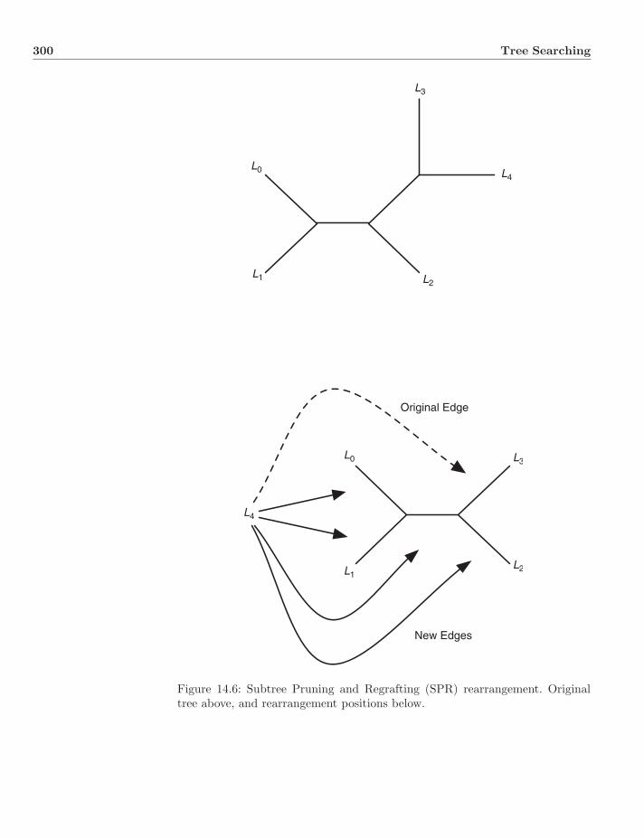
300 Tree Searching
L1
L0
L2
L3
L4
L1
L0
L2
L3
L4
Original Edge
New Edges
Figure 14.6: Subtree Pruning and Regrafting (SPR) rearrangement. Originaltree above, and rearrangement positions below.
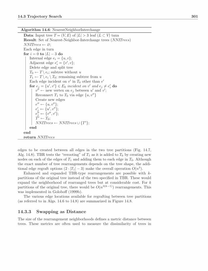
14.3 Trajectory Search 301
Algorithm 14.6: NearestNeighborInterchangeData: Input tree T = (V,E) of |L| > 3 leaf (L ⊂ V) taxaResult: Set of Nearest-Neighbor-Interchange trees (NNITrees)NNITrees ← ∅;Each edge in turnfor i = 0 to |L| − 3 do
Internal edge ei = {u, v};Adjacent edge e′i = {v′, v};Delete edge and split treeT0 ← T \ ei; subtree without uT1 ← T \ ei \ T0; remaining subtree from uEach edge incident on v′ in T0 other than e′
for ej = {u′, v′} ∈ E0 incident on v′ and ej = e′i dov′′ ← new vertex on ej between u′ and v′;Reconnect T1 to T0 via edge {u, v′′}Create new edgese′′ ← {u, v′′};e′j ← {u′, v′′};e′′j ← {v′′, v′};T ′ ← T0;NNITrees ← NNITrees ∪ {T ′};
endendreturn NNITrees
edges to be created between all edges in the two tree partitions (Fig. 14.7,Alg. 14.8). TBR tests the “rerooting” of T1 as it is added to T0 by creating newnodes on each of the edges of T1 and adding them to each edge in T0. Althoughthe exact number of tree rearrangements depends on the tree shape, the addi-tional edge regraft options (2 · |T1| − 3) make the overall operation O(n3).
Enhanced and expanded TBR-type rearrangements are possible with k-partitions of the original tree instead of the two specified in TBR. These wouldexpand the neighborhood of rearranged trees but at considerable cost. For kpartitions of the original tree, there would be O(n3(k−1)) rearrangements. Thiswas implemented in Goloboff (1999b).
The various edge locations available for regrafting between tree partitions(as referred to in Algs. 14.6 to 14.8) are summarized in Figure 14.8.
14.3.3 Swapping as Distance
The size of the rearrangement neighborhoods defines a metric distance betweentrees. These metrics are often used to measure the dissimilarity of trees in
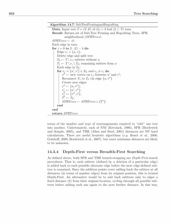
302 Tree Searching
Algorithm 14.7: SubTreePruningandRegraftingData: Input tree T = (V,E) of |L| > 3 leaf (L ⊂ V) taxaResult: Return set of Sub-Tree Pruning and Regrafting Trees, SPR
neighborhood (SPRTrees)SPRTrees ← ∅;Each edge in turnfor i = 0 to 2 · |L| − 4 do
Edge ei = {u, v};Delete edge and split treeT0 ← T \ ei; subtree without uT1 ← T \ ei \ T0; remaining subtree from uEach edge in T0;for ej = {u′, v′} ∈ E0 and ej = ei do
v′′ ← new vertex on ej between u′ and v′;Reconnect T1 to T0 via edge {u, v′′}Create new edgese′′ ← {u, v′′};e′j ← {u′, v′′};e′′j ← {v′′, v′};T ′ ← T0;SPRTrees ← SPRTrees ∪ {T ′};
endendreturn SPRTrees
terms of the number and type of rearrangements required to “edit” one treeinto another. Unfortunately, each of NNI (Krivanek, 1986), SPR (Bordewichand Semple, 2005), and TBR (Allen and Steel, 2001) distances are NP–hardcalculations. There are useful heuristic algorithms (e.g. Bonet et al., 2006;Goloboff, 2008; Bordewich et al., 2007), but exact minimum distances are likelyto be unknown.
14.3.4 Depth-First versus Breadth-First Searching
As defined above, both SPR and TBR branch-swapping are Depth-First searchprocedures. That is, each subtree (defined by a deletion of a particular edge)is added back to each possible alternate edge before the next edge-defined sub-tree is examined. Since the addition points cover adding back the subtree at alldistances (in terms of number edges) from its original position, this is termedDepth-First. An alternative would be to add back subtrees only to edges afixed distance (k) from their original location, cycling through all possible sub-trees before adding each one again to the next further distance. In this way,
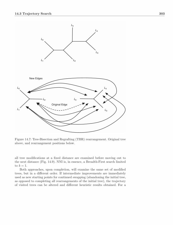
14.3 Trajectory Search 303
L1
L0
L2
L3
L4
L5
Original Edge
New Edges
L1
L0
L2
L3
L4
L5
Figure 14.7: Tree-Bisection and Regrafting (TBR) rearrangement. Original treeabove, and rearrangement positions below.
all tree modifications at a fixed distance are examined before moving out tothe next distance (Fig. 14.9). NNI is, in essence, a Breadth-First search limitedto k = 1.
Both approaches, upon completion, will examine the same set of modifiedtrees, but in a different order. If intermediate improvements are immediatelyused as new starting points for continued swapping (abandoning the initial tree,as opposed to completing all rearrangements of the initial tree), the trajectoryof visited trees can be altered and different heuristic results obtained. For a
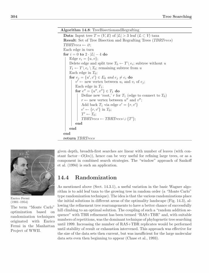
304 Tree Searching
Algorithm 14.8: TreeBisectionandRegraftingData: Input tree T = (V,E) of |L| > 3 leaf (L ⊂ V) taxaResult: Set of Tree Bisection and Regrafting Trees (TBRTrees)TBRTrees ← ∅;Each edge in turnfor i = 0 to 2 · |L| − 4 do
Edge ei = {u, v};Delete edge and split tree T0 ← T \ ei; subtree without uT1 ← T \ ei \ T0; remaining subtree from uEach edge in T0;for ej = {u′, v′} ∈ E0 and ej = ei do
v′ ← new vertex between ui and vi of ej ;Each edge in T1;for e′′ = {u′′, v′′} ∈ T1 do
Define new ‘root,’ r for T1 (edge to connect to T0)r ← new vertex between u′′ and v′′;Add back T1 via edge e′ = {r, v′}e′ ← {r, v′} in T0;T ′ ← T0;TBRTrees ← TBRTrees ∪ {T ′};
endend
endreturn TBRTrees
given depth, breadth-first searches are linear with number of leaves (with con-stant factor—O(kn)), hence can be very useful for refining large trees, or as acomponent in combined search strategies. The “window” approach of Sankoffet al. (1994) is such an application.
14.4 Randomization
Enrico Fermi(1901–1954)
The term “Monte Carlo”optimization based onrandomization techniquesoriginated with EnricoFermi in the ManhattanProject of WWII.
As mentioned above (Sect. 14.3.1), a useful variation in the basic Wagner algo-rithm is to add leaf taxa to the growing tree in random order (a “Monte Carlo”type randomization technique). The idea is that the various randomizations placethe initial solutions in different areas of the optimality landscape (Fig. 14.3), al-lowing the refinement tree rearrangements to have a better chance of successfullyhill climbing to an optimal solution. The coupling of such a “random addition se-quence” with TBR refinement has been termed “RAS+TBR” and, with suitablenumbers of repetitions, was the dominant technique of phylogenetic tree searchinguntil 1999. Increasing the number of RAS+TBR replicates would be performeduntil stability of result or exhaustion intervened. This approach was effective forthe size of the data sets then current, but was insufficient for the large moleculardata sets even then beginning to appear (Chase et al., 1993).

14.5 Perturbation 305
NST
T
T
L1
L0
L2
L3
L4
L5
L6
L7
L8
L9
L1
L0
L2
L3
L4
L5
L6
L7
L8
L9
L7
L8
L9
T1
L1
L0
L2
L3
L4
L5L6
T0
NST
NST
ST ST
STST
STSTST
ST
e
T
Figure 14.8: Edges available for rearrangement after deletion of edge e arelabeled as “N” for NNI, “S” for SPR, and “T” for TBR. T0 and T1 are asin Algs. 14.6 to 14.8. Top left is the original tree, top right, the tree partitions,bottom the rearrangement edges.
14.5 Perturbation
In general, the RAS+TBR technique is effective for data sets with fewer than100 taxa. Assuming sufficient randomizations are performed (typically in thehundreds), investigators achieved stable analytical results (in terms of best costfound), if not guaranteed optimality. In the 1990s, larger data sets, especially inbotany, were produced with hundreds (Chase et al., 1993) and even thousands(Soltis et al., 2000) of taxa. These data sets required months of analysis on thenstandard hardware and yielded clearly unsatisfactory results (Rice et al., 1997).
Kevin Nixon
The basic problem was that searches were stuck in isolated local optima,and the Wagner randomizations were insufficient to identify good enough start-ing points for hill climbing (in the form of branch-swapping) to a stable solu-tion (there were also implementation shortcomings detailed by Nixon, 1999).Nixon (1999) proposed a perturbation-based method, the “Parsimony Ratchet”or more simply the “Ratchet,” that dramatically improved the speed and effec-tiveness of tree searching. In short, the ratchet is a refinement technique thatalternates hill climbing on a perturbed (reweighted) data set with refinement ofthe original data. Multiple cycles of reweighting + branch-swapping and originalweighting + branch-swapping allowed the escape of local optima (“islands” in

306 Tree Searching
L1
L0
L2
L3
L4
L0
L1
L2
L3
L4
L1
L0
L2
L3
L4
L1
L0
L2
L3
L4
L1
L0 L2
L3
L4
L1
L0
L2
L3
L4
L1
L0
L2
L3
L4
Until all partitions examinedat initial reattachment edges
L1
L0
L2
L3
L4
L1
L0
L2
L3
L4
Until all partitions examinedat all reattachment edges
Until all partitions examinedat all reattachment edges
Depth-First Search Breadth-First Search
Figure 14.9: Depth-First (left) and Breadth-First (right) search orders on a tree(top). The Depth-First order evaluates all reattachment points of a subtreebefore moving on to the next tree partition, whereas the Breadth-First searchexamines reattachments of subtrees at fixed distances from their original point,each round examining each tree partition in turn before moving on to the next,more distant reattachment edges.
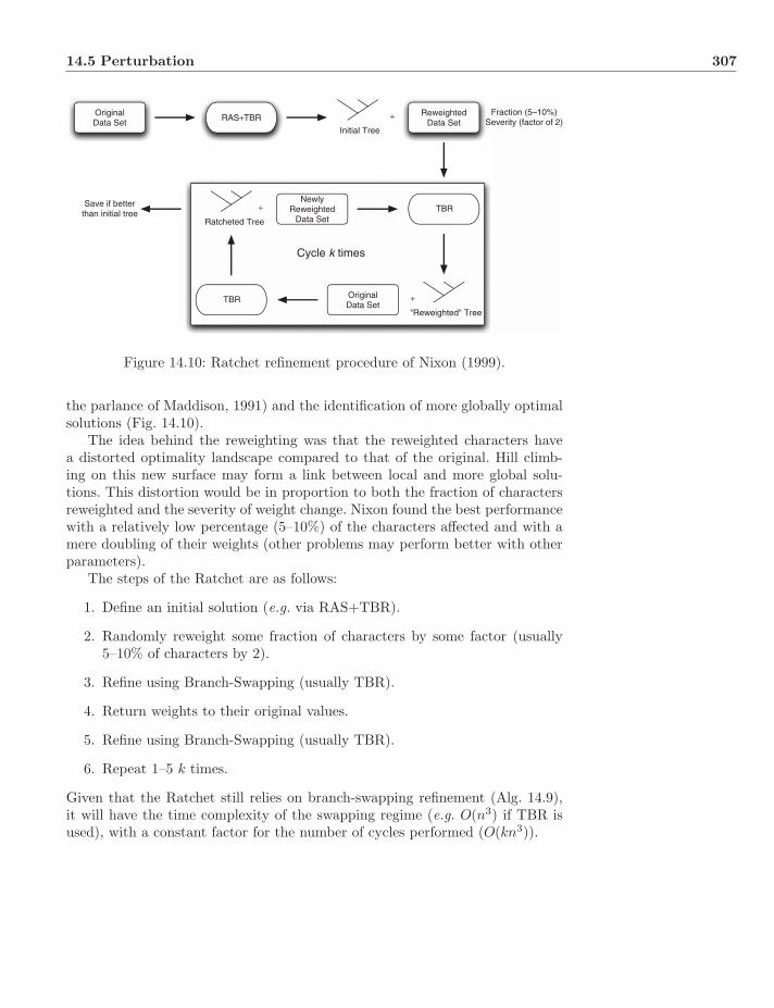
14.5 Perturbation 307
OriginalData Set
RAS+TBRReweighted
Data SetFraction (5–10%)
Severity (factor of 2)
TBR
"Reweighted" Tree
TBR
Ratcheted Tree
Initial Tree
+
Save if betterthan initial tree
NewlyReweighted
Data Set+
OriginalData Set
+
Cycle k times
Figure 14.10: Ratchet refinement procedure of Nixon (1999).
the parlance of Maddison, 1991) and the identification of more globally optimalsolutions (Fig. 14.10).
The idea behind the reweighting was that the reweighted characters havea distorted optimality landscape compared to that of the original. Hill climb-ing on this new surface may form a link between local and more global solu-tions. This distortion would be in proportion to both the fraction of charactersreweighted and the severity of weight change. Nixon found the best performancewith a relatively low percentage (5–10%) of the characters affected and with amere doubling of their weights (other problems may perform better with otherparameters).
The steps of the Ratchet are as follows:
1. Define an initial solution (e.g. via RAS+TBR).
2. Randomly reweight some fraction of characters by some factor (usually5–10% of characters by 2).
3. Refine using Branch-Swapping (usually TBR).
4. Return weights to their original values.
5. Refine using Branch-Swapping (usually TBR).
6. Repeat 1–5 k times.
Given that the Ratchet still relies on branch-swapping refinement (Alg. 14.9),it will have the time complexity of the swapping regime (e.g. O(n3) if TBR isused), with a constant factor for the number of cycles performed (O(kn3)).

308 Tree Searching
Algorithm 14.9: RatchetRefinementCreated via RAS+TBR or other methodData: Input tree T = (V,E)Data: Input data matrix MTypically all weighted to unityData: Input weight regime WData: Input number cycles of ratchet cycles to be performedData: Input fraction fraction of characters to be reweightedData: Input reweight severity factorResult: Single ratchet refined tree (RatchetTree) if lower cost tree than
input is found, ∅ if not.RatchetTree ← ∅;mincost ← Tcost;Each replicate;for i = 0 to cycles − 1 do
Randomly perturb data weight setW′ ← perturb(W, fraction, severity);Perform TBR branch-swapping on input tree with new weight setT ′ ← TBR(T,M,W′);Perform TBR branch-swapping on perturbed tree with original weightsetT ′′ ← TBR(T ′,M,W);Check for better treeif T ′′
cost < mincost thenRatchetTree ← T ′′;mincost ← T ′′
cost;end
endreturn RatchetTree
The Ratchet had an immediate and significant effect on empirical studies.The Chase et al. (1993) data set was analyzable in hours, rather than months,and better (16218 versus 16225 parsimony steps) trees were found. Giribet andWheeler (1999) reanalyzed their metazoan data and also found shorter trees(7032 versus 7028) in greatly reduced time. The method was extended to like-lihood techniques (Voss, 2003; Wheeler, 2006). Ratcheting is now a standardcomponent of phylogenetic tree searching.
Several variations of ratchet procedures have been explored centering aroundthe types of perturbation (Varon et al., 2010, allows perturbing indel and otherparameters as well as character weight) and character selection (complementaryreweighted character sets over pairs of cycles) operations.
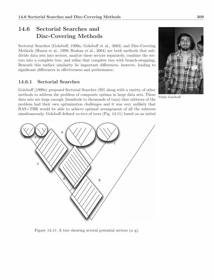
14.6 Sectorial Searches and Disc-Covering Methods 309
14.6 Sectorial Searches andDisc-Covering Methods
Sectorial Searches (Goloboff, 1999a; Goloboff et al., 2003) and Disc-CoveringMethods (Huson et al., 1999; Roshan et al., 2004) are both methods that sub-divide data sets into sectors, analyze these sectors separately, combine the sec-tors into a complete tree, and refine that complete tree with branch-swapping.Beneath this surface similarity lie important differences, however, leading tosignificant differences in effectiveness and performance.
Pablo Goloboff
14.6.1 Sectorial Searches
Goloboff (1999a) proposed Sectorial Searches (SS) along with a variety of othermethods to address the problem of composite optima in large data sets. Thesedata sets are large enough (hundreds to thousands of taxa) that subtrees of theproblem had their own optimization challenges and it was very unlikely thatRAS+TBR would be able to achieve optimal arrangement of all the subtreessimultaneously. Goloboff defined sectors of trees (Fig. 14.11) based on an initial
a b
c
d
e
f
g
Figure 14.11: A tree showing several potential sectors (a–g).
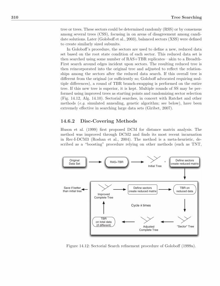
310 Tree Searching
tree or trees. These sectors could be determined randomly (RSS) or by consensusamong several trees (CSS), focusing in on areas of disagreement among candi-date solutions. Later (Goloboff et al., 2003), balanced sectors (XSS) were definedto create similarly sized subunits.
In Goloboff’s procedure, the sectors are used to define a new, reduced dataset based on the root state condition of each sector. This reduced data set isthen searched using some number of RAS+TBR replicates—akin to a Breadth-First search around edges incident upon sectors. The resulting reduced tree isthen reincorporated into the original tree and adjusted to reflect the relation-ships among the sectors after the reduced data search. If this overall tree isdifferent from the original (or sufficiently so; Goloboff advocated requiring mul-tiple differences), a round of TBR branch-swapping is performed on the entiretree. If this new tree is superior, it is kept. Multiple rounds of SS may be per-formed using improved trees as starting points and randomizing sector selection(Fig. 14.12, Alg. 14.10). Sectorial searches, in concert with Ratchet and othermethods (e.g. simulated annealing, genetic algorithm; see below), have beenextremely effective in searching large data sets (Giribet, 2007).
14.6.2 Disc-Covering Methods
Huson et al. (1999) first proposed DCM for distance matrix analysis. Themethod was improved through DCM2 and finds its most recent incarnationin Rec-I-DCM3 (Roshan et al., 2004). The method is a meta-heuristic, de-scribed as a “boosting” procedure relying on other methods (such as TNT,
OriginalData Set RAS+TBR Define sectors
create reduced matrix
TBR onreduced data
"Sector" Tree
TBRon total data(if different)
ImprovedComplete Tree
Initial Tree
+
Save if betterthan initial tree
Cycle k times
AdjustedComplete Tree
Define sectorscreate reduced matrix
Figure 14.12: Sectorial Search refinement procedure of Goloboff (1999a).

14.6 Sectorial Searches and Disc-Covering Methods 311
Algorithm 14.10: SectorialSearchCreated via RAS+TBR or other method;Data: Input tree T = (V,E)Data: Input data matrix MData: Input number SScycles of sectorial searches to be performedResult: Single sectorial search tree (SSTree) if lower cost tree than input
is found, ∅ if notSSTree ← ∅;Each replicate;for i = 0 to SScycles − 1 do
Define set of sectors in T (either randomly—RSS—or byconsensus—CSS—of several input trees) and create a reduced dataset from MS ← defineSector(T,M);Perform RAScycles of RAS+TBR on reduced data set STS ← RASTBR(RAScycles, S);Adjust T to conform to relationships of sectors in TS
T ′ ← makeTree(T, TS);If there were changes in the overall treeif T = T ′ then
Perform TBR branch-swapping on T ′ and full dataT ′′ ← TBR(T ′,M);Check for better treeif T ′′
cost < Tcost then SSTree ← T ′′;end
endreturn SSTree
Goloboff et al., 2003 or POY, Varon et al., 2010) as a “base” method. DCMmethods proceed in four sections:
1. Decompose the data set.
2. Solve subproblems.
3. Merge and reconcile subproblems.
4. Refine the merged tree.
The decomposition component was originally based on distance matrix analysis,but in Rec-I-DCM3 it is based on an initial tree. In this, it is similar to SS, re-cursively dividing the tree into smaller pieces that then can be analyzed easily.Unlike SS, these sectors overlap. The subproblems are analyzed as individualphylogenetic problems. Roshan et al. (2004) advocated sectors of 1
4 to 12 the orig-
inal data set size. The trees resulting from the subproblems are then mergedinto a single tree via strict-consensus + random resolution. In the procedure,
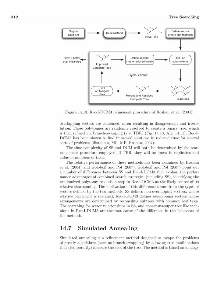
312 Tree Searching
OriginalData Set
Base MethodDefine sectors
create sub-matrices
TBR onsubproblems
SubTrees
TBRon Merged
Tree
ImprovedComplete Tree
Initial Tree
+
Save if betterthan initial tree
Cycle k times
Merged and ResolvedComplete Tree
Define sectorscreate reduced matrix
Figure 14.13: Rec-I-DCM3 refinement procedure of Roshan et al. (2004).
overlapping sectors are combined, often resulting in disagreement and irreso-lution. These polytomies are randomly resolved to create a binary tree, whichis then refined via branch-swapping (e.g. TBR) (Fig. 14.13, Alg. 14.11). Rec-I-DCM3 has been shown to find improved solutions in reduced time for severalsorts of problems (distances, ML, MP; Roshan, 2004).
The time complexity of SS and DCM will both be determined by the rear-rangement procedure employed. If TBR, they will be linear in replicates andcubic in numbers of taxa.
The relative performance of these methods has been examined by Roshanet al. (2004) and Goloboff and Pol (2007). Goloboff and Pol (2007) point outa number of differences between SS and Rec-I-DCM3 that explain the perfor-mance advantages of combined search strategies (including SS), identifying therandomized polytomy resolution step in Rec-I-DCM3 as the likely source of itsrelative shortcoming. The motivation of this difference comes from the types ofsectors defined by the two methods. SS defines non-overlapping sectors, whoserelative placement is searched; Rec-I-DCM3 defines overlapping sectors whosearrangements are determined by reconciling subtrees with common leaf taxa.The searching for sector relationships in SS, and consensus-super tree like tech-nique in Rec-I-DCM3 are the root cause of the difference in the behaviors ofthe methods.
14.7 Simulated Annealing
Simulated annealing is a refinement method designed to escape the problemsof greedy algorithms (such as branch-swapping) by allowing tree modificationsthat (temporarily) increase the cost of the tree. The method is based on analogy
14.7 Simulated Annealing 313
Algorithm 14.11: Rec-I-DCM3Data: Input tree T = (V,E)Data: Input data matrix MResult: Return single Rec-I-DCM3 tree (DCMTree) if lower cost tree
than input is found, ∅ if notDCMTree ← ∅;mincost ← Tcost;foundBetter ← true;while foundBetter = true do
foundBetter ← false;Define set of data sectors in T by recursive centroid edgedecompositionS ← defineSectors(T,M);Analyze subproblems in Sfor si ∈ S do
Analyze subproblem si by favored method—e.g. RAS+TBR orexact if smallTS
i ← methodTree(si);endMerge the TS
i trees created from S via strict consensus merge andrandomly resolve polytomiesTS ← mergeTree({⋃i TS
i });Perform TBR branch-swapping on TS and full data;T ′ ← TBR(TS ,M);Check for better tree;if T ′
cost < mincost thenDCMTree ← T ′;mincost ← T ′
cost;foundBetter ← true;
endendreturn DCMTree
to the annealing of metals, where more stable (i.e. lower energy) crystal config-urations can be achieved by allowing the metal to anneal at moderate tempera-tures and cooling in a step-wise fashion (Chib and Greenberg, 1995). The basicprocedure is a modification of the Metropolis–Hastings algorithm (Metropoliset al., 1953) proposed by Kirkpatrick et al. (1983) and Cerny (1985). The basic
Nicholas Metropolis(1915–1999)
procedure involves establishing analogues to the parameters of metallurgicalannealing. At each iteration, there are two states—s the current state and s′ asecond, candidate state. These states have energies E and E′. The probabilityof transitioning from state s to s′ depends on the energy difference between thestates (higher is worse) and the temperature, T (Eq. 14.1).
P(s, s′) = min(1, e(E−E′)/T ) (14.1)
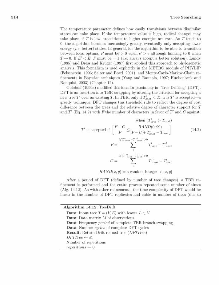
314 Tree Searching
The temperature parameter defines how easily transitions between dissimilarstates can take place. If the temperature value is high, radical changes maytake place, if T is low, transitions to higher energies are rare. As T tends to0, the algorithm becomes increasingly greedy, eventually only accepting lowerenergy (i.e. better) states. In general, for the algorithm to be able to transitionbetween local optima, P must be > 0 when e′ > e although limiting to 0 whenT → 0. If E′ < E, P must be = 1 (i.e. always accept a better solution). Lundy(1985) and Dress and Kruger (1987) first applied this approach to phylogeneticanalysis. This formalism is used explicitly in the METRO module of PHYLIP(Felsenstein, 1993; Salter and Pearl, 2001), and Monte-Carlo-Markov-Chain re-finements in Bayesian techniques (Yang and Rannala, 1997; Huelsenbeck andRonquist, 2003) (Chapter 12).
Goloboff (1999a) modified this idea for parsimony in “Tree-Drifting” (DFT).DFT is an insertion into TBR swapping by altering the criterion for accepting anew tree T ′ over an existing T. In TBR, only if T ′
cost < Tcost is T ′ is accepted—agreedy technique. DFT changes this threshold rule to reflect the degree of costdifference between the trees and the relative degree of character support for Tand T ′ (Eq. 14.2) with F the number of characters in favor of T ′ and C against.
when (T ′cost > Tcost)
T ′ is accepted if[F − C
F≤ RAND(0, 99)
F − C + T ′cost − Tcost
](14.2)
F =if(T i
cost−T ′icost)>0∑
i
Ticost − T ′i
cost
C =if(T ′i
cost−T icost)>0∑
i
T ′icost − Ti
cost
RAND(x, y) = a random integer ∈ [x, y]
After a period of DFT (defined by number of tree changes), a TBR re-finement is performed and the entire process repeated some number of times(Alg. 14.12). As with other refinements, the time complexity of DFT would belinear in the number of DFT replicates and cubic in number of taxa (due to
Algorithm 14.12: TreeDriftData: Input tree T = (V,E) with leaves L ⊂ VData: Data matrix M of observationsData: Frequency period of complete TBR branch-swappingData: Number cycles of complete DFT cyclesResult: Return Drift refined tree (DFTTree)DFTTree ← ∅;Number of repetitionsrepetitions ← 0
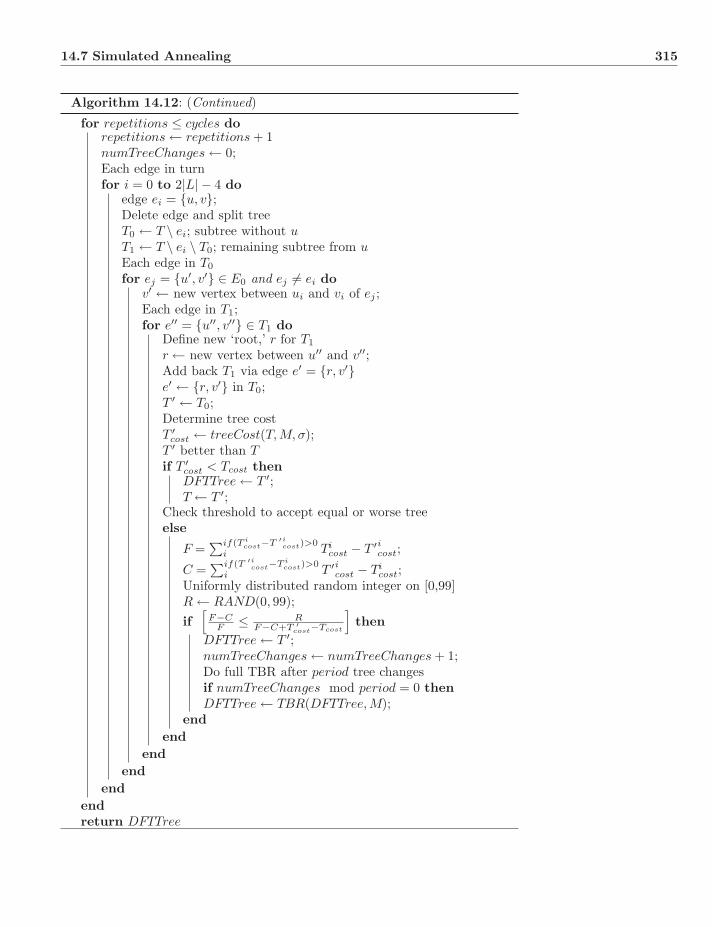
14.7 Simulated Annealing 315
Algorithm 14.12: (Continued)
for repetitions ≤ cycles dorepetitions ← repetitions + 1numTreeChanges ← 0;Each edge in turnfor i = 0 to 2|L| − 4 do
edge ei = {u, v};Delete edge and split treeT0 ← T \ ei; subtree without uT1 ← T \ ei \ T0; remaining subtree from uEach edge in T0
for ej = {u′, v′} ∈ E0 and ej = ei dov′ ← new vertex between ui and vi of ej ;Each edge in T1;for e′′ = {u′′, v′′} ∈ T1 do
Define new ‘root,’ r for T1
r ← new vertex between u′′ and v′′;Add back T1 via edge e′ = {r, v′}e′ ← {r, v′} in T0;T ′ ← T0;Determine tree costT ′
cost ← treeCost(T,M, σ);T ′ better than Tif T ′
cost < Tcost thenDFTTree ← T ′;T ← T ′;
Check threshold to accept equal or worse treeelse
F =∑if(T i
cost−T ′icost)>0
i Ticost − T ′i
cost;
C =∑if(T ′i
cost−T icost)>0
i T ′icost − Ti
cost;Uniformly distributed random integer on [0,99]R ← RAND(0, 99);if
[F−C
F ≤ RF−C+T ′
cost−Tcost
]then
DFTTree ← T ′;numTreeChanges ← numTreeChanges + 1;Do full TBR after period tree changesif numTreeChanges mod period = 0 thenDFTTree ← TBR(DFTTree,M);
endend
endend
endendreturn DFTTree
316 Tree Searching
TBR scaffold). DFT has been shown to be effective at improving locally opti-mal trees in large data sets, especially in combination with Sectorial Searches(Goloboff, 1999a; Giribet, 2007).
14.8 Genetic Algorithm
Genetic (sometimes referred to as “Genetical”) algorithms (GA) simulate theevolutionary process to optimize complex functions (Holland, 1975; Goldberget al., 1989; Sastry et al., 2005). The idea is to model the processes of muta-tion, recombination, and natural selection to identify solutions and escape localoptima through random aspects of population dynamics. One of the key differ-ences between GA and other approaches is that it operates on a collection ofsolutions simultaneously. One weakness is that it has no direct relationship to anexact solution (such as branch-swapping, which would, if sufficiently exhaustive,examine all possible trees).
There are six fundamental components to a GA procedure, which are re-peatedly cycled (after Initialization) until stability or ennui sets in:
1. Initialization—An initial population of solutions (here trees) is generated.
2. Evaluation—Potential solutions are assigned an objective cost (fitness).
3. Selection—Those solutions with higher fitness (here lower cost) are prefer-entially replicated such that the more fit they are, the better representedthey are in the population of solutions.
4. Recombination—Components of two or more candidate solutions are com-bined to create variation and potentially better solutions.
5. Mutation—Modifications are made to individual solutions.
6. Replacement—Those solutions created by selection, recombination, andmutation replace the existing generation in the population of solutions.
One of the tricks of GA is to balance mutation (which modifies existing trees)and selection. If the selection is too strong, the solution space will convergetoo quickly before finding new optimal solutions. If the mutation rate is toohigh, there will be little direction to the process and the search will approachrandomization (as in SA when T is high). If the mutation rate is too low, therewill be insufficient diversity to work with in finding new solutions.
Moilanen (1999, 2001) introduced GA to parsimony-based tree searchingwith PARSIGAL (although Matsuda, 1996, had used GA for likelihood calcula-tions on protein sequences) explicitly to escape the local minima in which tra-jectory searches often found themselves (in multiple sequence alignment, SAGANotredame and Higgins, 1996, is based on GA). Moilanen’s GA did not empha-size mutation, other than through perturbed distance matrix tree reconstruc-tion in the initialization step, and added limited branch-swapping to improvethe post-recombination trees (Fig. 14.14, Alg. 14.13). The time complexity of
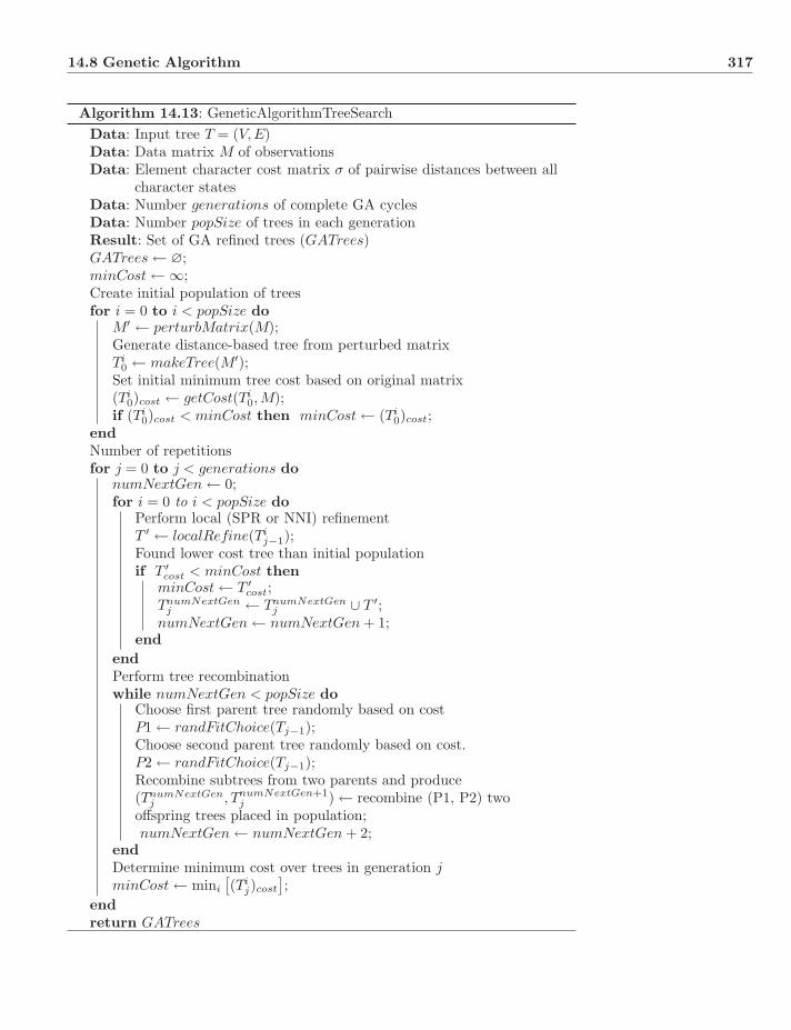
14.8 Genetic Algorithm 317
Algorithm 14.13: GeneticAlgorithmTreeSearchData: Input tree T = (V,E)Data: Data matrix M of observationsData: Element character cost matrix σ of pairwise distances between all
character statesData: Number generations of complete GA cyclesData: Number popSize of trees in each generationResult: Set of GA refined trees (GATrees)GATrees ← ∅;minCost ← ∞;Create initial population of treesfor i = 0 to i < popSize do
M′ ← perturbMatrix(M);Generate distance-based tree from perturbed matrixTi
0 ← makeTree(M′);Set initial minimum tree cost based on original matrix(Ti
0)cost ← getCost(Ti0,M);
if (Ti0)cost < minCost then minCost ← (Ti
0)cost;endNumber of repetitionsfor j = 0 to j < generations do
numNextGen ← 0;for i = 0 to i < popSize do
Perform local (SPR or NNI) refinementT ′ ← localRefine(Ti
j−1);Found lower cost tree than initial populationif T ′
cost < minCost thenminCost ← T ′
cost;TnumNextGen
j ← TnumNextGenj ∪ T ′;
numNextGen ← numNextGen + 1;end
endPerform tree recombinationwhile numNextGen < popSize do
Choose first parent tree randomly based on costP1 ← randFitChoice(Tj−1);Choose second parent tree randomly based on cost.P2 ← randFitChoice(Tj−1);Recombine subtrees from two parents and produce(TnumNextGen
j , TnumNextGen+1j ) ← recombine (P1, P2) two
offspring trees placed in population;numNextGen ← numNextGen + 2;
endDetermine minimum cost over trees in generation jminCost ← mini
[(Ti
j)cost
];
endreturn GATrees

318 Tree Searching
Data Set(Perturbed)
Add ShortestTree to NextGeneration
Save if betterthan initial tree Cycle k generations
GenerationiTree Population
SPR onOriginal Data
RecombineTrees in
Population
Add NewTrees to NextGeneration
SPR onOriginal Data
InitialTree Population
Figure 14.14: Genetic Algorithm tree search procedure of Moilanen (1999).
Moilanen’s complete GA strategy will depend on the number of generations,g, the population size, p, and the complexity of the local swapping operations(SPR) on n taxa, for an overall time complexity of O(gpn2).
Goloboff (1999a) focused on the recombination step of GA (Fig. 14.15)in defining his Tree-Fusing (TF) procedure. Goloboff modified Moilanen’s ap-proach to enhance the capabilities of tree recombination to attack the problemof composite optima in large trees. Goloboff added SPR rearrangement to the re-combination step (as opposed to after the trees are constructed) to optimize theplacement of the exchanged subtrees. TF has been extremely effective at lower-ing tree costs—even when presented with clearly suboptimal inputs, TF is ableto improve the result substantially. This approach has been used in large sensi-tivity analysis (Wheeler, 1995) studies. Combining the results of different param-eter runs with TF and subsequent TBR (SATF) simultaneously enhanced thequality of results across parameter space (Wheeler et al., 2004; Giribet, 2007).
14.9 Synthesis and Stopping
As observed by Nixon (1999) and Goloboff (1999a), implemented in TNT(Goloboff et al., 2003) and POY4 (“search” command; Varon et al., 2010),and reviewed by Giribet (2007), no one search strategy is likely to be effectivefor all data sets, and combinations of procedures have the best opportunity toresult in satisfactory results. Goloboff (1999a) described and tested 11 differentstrategies.
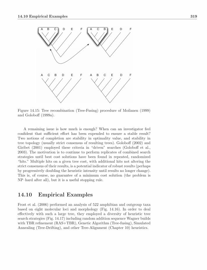
14.10 Empirical Examples 319
A B C D E F A C B E D F
A C B D E F A B C E D F
Figure 14.15: Tree recombination (Tree-Fusing) procedure of Moilanen (1999)and Goloboff (1999a).
A remaining issue is how much is enough? When can an investigator feelconfident that sufficient effort has been expended to ensure a stable result?Two notions of completion are stability in optimality value, and stability intree topology (usually strict consensus of resulting trees). Goloboff (2002) andGiribet (2001) employed these criteria in “driven” searches (Goloboff et al.,2003). The motivation is to continue to perform replicates of combined searchstrategies until best cost solutions have been found in repeated, randomized“hits.” Multiple hits on a given tree cost, with additional hits not altering thestrict consensus of their results, is a potential indicator of robust results (perhapsby progressively doubling the heuristic intensity until results no longer change).This is, of course, no guarantee of a minimum cost solution (the problem isNP–hard after all), but it is a useful stopping rule.
14.10 Empirical Examples
Frost et al. (2006) performed an analysis of 522 amphibian and outgroup taxabased on eight molecular loci and morphology (Fig. 14.16). In order to dealeffectively with such a large tree, they employed a diversity of heuristic treesearch strategies (Fig. 14.17) including random addition sequence Wagner buildswith TBR refinement (RAS+TBR), Genetic Algorithm (Tree-fusing), SimulatedAnnealing (Tree-Drifting), and other Tree-Alignment (Chapter 10) heuristics.
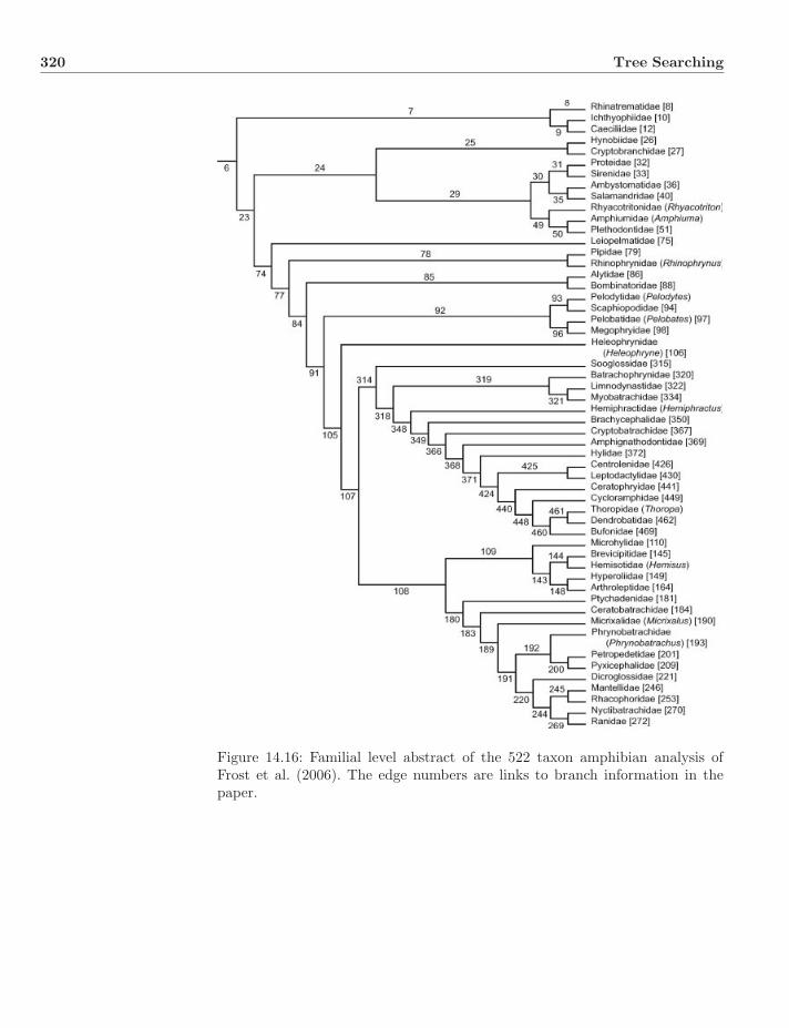
320 Tree Searching
Figure 14.16: Familial level abstract of the 522 taxon amphibian analysis ofFrost et al. (2006). The edge numbers are links to branch information in thepaper.
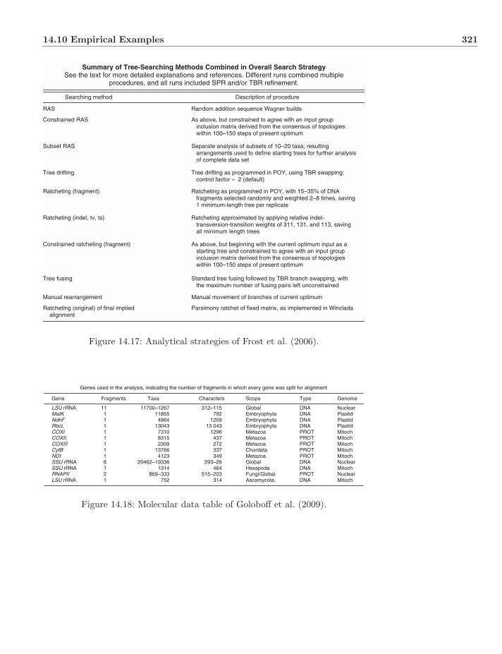
14.10 Empirical Examples 321
Summary of Tree-Searching Methods Combined in Overall Search StrategySee the text for more detailed explanations and references. Different runs combined multiple
procedures, and all runs included SPR and/or TBR refinement.
Searching method Description of procedure
RAS Random addition sequence Wagner builds
Constrained RAS As above, but constrained to agree with an input group inclusion matrix derived from the consensus of topologies within 100–150 steps of present optimum
Subset RAS Separate analysis of subsets of 10–20 taxa; resulting arrangements used to define starting trees for further analysis of complete data set
Tree drifting Tree drifting as programmed in POY, using TBR swapping; control factor = 2 (default)
Ratcheting (fragment) Ratcheting as programmed in POY, with 15–35% of DNA fragments selected randomly and weighted 2–8 times, saving 1 minimum-length tree per replicate
Ratcheting (indel, tv, ts) Ratcheting approximated by applying relative indel- transversion-transition weights of 311, 131, and 113, saving all minimum length trees
Constrained ratcheting (fragment) As above, but beginning with the current optimum input as a starting tree and constrained to agree with an input group inclusion matrix derived from the consensus of topologies within 100–150 steps of present optimum
Tree fusing Standard tree fusing followed by TBR branch swapping, with the maximum number of fusing pairs left unconstrained
Manual rearrangement Manual movement of branches of current optimum
Ratcheting (original) of final implied alignment
Parsimony ratchet of fixed matrix, as implemented in Winclada
Figure 14.17: Analytical strategies of Frost et al. (2006).
Genes used in the analysis, indicating the number of fragments in which every gene was split for alignment
Gene Fragments Taxa Characters Scope Type Genome
LSU rRNA 11 312–115 Global DNA NuclearMatK 1 792 Embryophyta DNA PlastidNdhF 1 1209 Embryophyta DNA PlastidRbcL 1 13 043 Embryophyta DNA PlastidCOXI 1 1296 Metazoa PROT MitochCOXII 1 437 Metazoa PROT MitochCOXIII 1 272 Metazoa PROT MitochCytB 1 337 Chordata PROT MitochNDI 1 349 Metazoa PROT MitochSSU rRNA 6 293–26 Global DNA NuclearSSU rRNA 1 464 Hexapoda DNA MitochRNAPII 2 515–203 Fungi/Global PROT NuclearLSU rRNA 1
11700–126711855
486413043
731083152309
137664123
20462–193361314
869–333752 314 Ascomycota DNA Mitoch
Figure 14.18: Molecular data table of Goloboff et al. (2009).

322 Tree Searching
Euglenozoa, and others 699
Alveolata 946 (0.88, 0.99)
Chordata12497 (0.98, 0.99)
Arthropoda16083 (0.99, 1.00)
Basidiomycota2691 (0.98, >0.99)
Ascomycota4831 (0.99, 0.99)
Rhodophyta809 (0.97, >0.99)
Filicophyta1724 (0.98, 0.99)
Eudicotyledons13852 (0.21, 0.99)
Liliopsida5373 (0.98, 0.99)
Met
azoa
3581
0 (0
.97,
>0.
99)
Fun
gi80
21 (
0.97
, 0.9
8)V
iridi
plan
tae
2534
8 (0
.99,
>0.
99)
Mam
mal
ia
Stramenopiles 1064 (0.93, 0.91)
Figure 14.19: Combined eukaryote analysis tree at 730,435 steps of Goloboffet al. (2009). The values beneath the taxon names are the number of taxaincluded and % placement in agreement with GenBank taxonomy. See Plate14.19 for the color Figure.
14.11 Exercises 323
Goloboff et al. (2009), in the largest empirical analysis to date, created adata set of 73,060 eukaryotic taxa for 17 loci and morphology (Fig. 14.18). Theanalysis relied heavily on Sectorial Searches and Genetical Algorithm (in theguise of Tree-fusing) after many RAS+TBR starting points for trees based onindividual loci. The final result was a tree of length 730,435 parsimony steps(Fig. 14.19).
In both the Frost et al. (2006) and Goloboff et al. (2009) cases, it is very un-likely that any one of these heuristic approaches would have yielded satisfactoryresults on their own. Considerable effort was expended in combining multiplestrategies until stable (if not necessarily optimal) results were obtained.
14.11 Exercises
1. When we search for a tree, how good is good enough?
2. Should we strive for exact solutions at the cost of sampling?
3. Write down the NNI neighborhood for the tree (A (B (C (D (E, F))))).
4. Write down the SPR neighborhood for the tree (A (B (C (D (E, F))))).
5. Write down those trees in the TBR neighborhood for the tree (A (B (C(D (E, F))))) that are not in its SPR neighborhood.
6. If we double the number of taxa in an analysis, how much longer will anNNI search take? SPR? TBR?
7. As we raise the temperature in a simulated annealing search, what happensto the acceptance of suboptimal trees?
8. If Pablo Goloboff were a tree, what sort of tree would he be?
Chapter 15
Support
Support means different things to different people. In general, “support” coversa variety of indices designed to measure confidence in a vertex or clade. Thereis a diversity of flavors of support specific to optimality criteria (parsimony,likelihood, posterior probability) and the aspect that is desired to be quantified.There can be no single “best” support value given that the goals of differentinvestigators and support indices vary.
The discussion here covers the use and measure of support in different con-texts. Although there is a broad variety of support objectives and indices, thereare organizing themes that run through the topic and serve to organize theprinciples of support.
The earliest notions of support were derived from edge weights (branch lengthsas number of synapomorphies “supporting” a clade). These informal ideas werelogical in that the edge weight quantified the amount of change (distance, parsi-mony changes or likelihood), but was thought inadequate since convergent andparallel change (homoplasy) would be conflated with unique historical change(synapomorphy). This led to resampling and optimality-based indices.
15.1 Resampling Measures
Resampling is a technique in general use in statistics to replace an unknowndistribution with a known one based on an observed sample. This is done, ingeneral, in two ways: bootstrapping and jackknifing. In short, bootstrap meth-ods sample a set of observations to create a new sample of equal size withreplacement, while jackknife methods sample without replacement, effectivelydeleting some fraction of the original data.
In systematics, two entities present themselves for resampling—taxa andcharacters. In principle, elements in either set could be used as the basis forjackknife or bootstrap analysis. If we are concerned with the evidentiary basisfor group support, it is logical to focus attention on characters. Given that any
Systematics: A Course of Lectures, First Edition. Ward C. Wheeler.c© 2012 Ward C. Wheeler. Published 2012 by Blackwell Publishing Ltd.
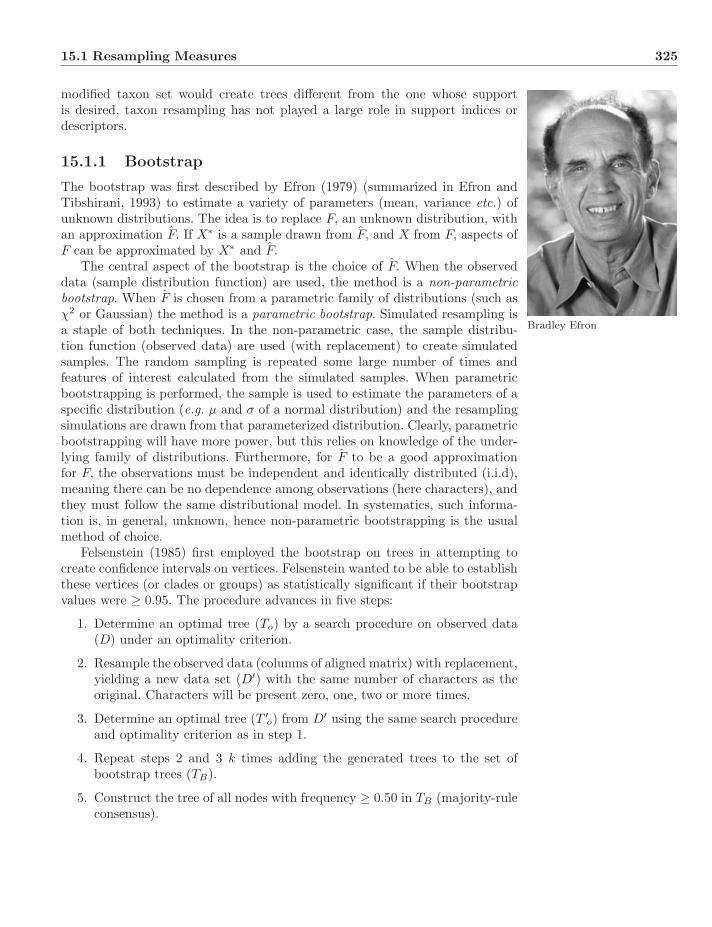
15.1 Resampling Measures 325
modified taxon set would create trees different from the one whose supportis desired, taxon resampling has not played a large role in support indices ordescriptors.
15.1.1 Bootstrap
Bradley Efron
The bootstrap was first described by Efron (1979) (summarized in Efron andTibshirani, 1993) to estimate a variety of parameters (mean, variance etc.) ofunknown distributions. The idea is to replace F, an unknown distribution, withan approximation F. If X∗ is a sample drawn from F, and X from F, aspects ofF can be approximated by X∗ and F.
The central aspect of the bootstrap is the choice of F. When the observeddata (sample distribution function) are used, the method is a non-parametricbootstrap. When F is chosen from a parametric family of distributions (such asχ2 or Gaussian) the method is a parametric bootstrap. Simulated resampling isa staple of both techniques. In the non-parametric case, the sample distribu-tion function (observed data) are used (with replacement) to create simulatedsamples. The random sampling is repeated some large number of times andfeatures of interest calculated from the simulated samples. When parametricbootstrapping is performed, the sample is used to estimate the parameters of aspecific distribution (e.g. μ and σ of a normal distribution) and the resamplingsimulations are drawn from that parameterized distribution. Clearly, parametricbootstrapping will have more power, but this relies on knowledge of the under-lying family of distributions. Furthermore, for F to be a good approximationfor F, the observations must be independent and identically distributed (i.i.d),meaning there can be no dependence among observations (here characters), andthey must follow the same distributional model. In systematics, such informa-tion is, in general, unknown, hence non-parametric bootstrapping is the usualmethod of choice.
Felsenstein (1985) first employed the bootstrap on trees in attempting tocreate confidence intervals on vertices. Felsenstein wanted to be able to establishthese vertices (or clades or groups) as statistically significant if their bootstrapvalues were ≥ 0.95. The procedure advances in five steps:
1. Determine an optimal tree (To) by a search procedure on observed data(D) under an optimality criterion.
2. Resample the observed data (columns of aligned matrix) with replacement,yielding a new data set (D′) with the same number of characters as theoriginal. Characters will be present zero, one, two or more times.
3. Determine an optimal tree (T ′o) from D′ using the same search procedure
and optimality criterion as in step 1.
4. Repeat steps 2 and 3 k times adding the generated trees to the set ofbootstrap trees (TB).
5. Construct the tree of all nodes with frequency ≥ 0.50 in TB (majority-ruleconsensus).
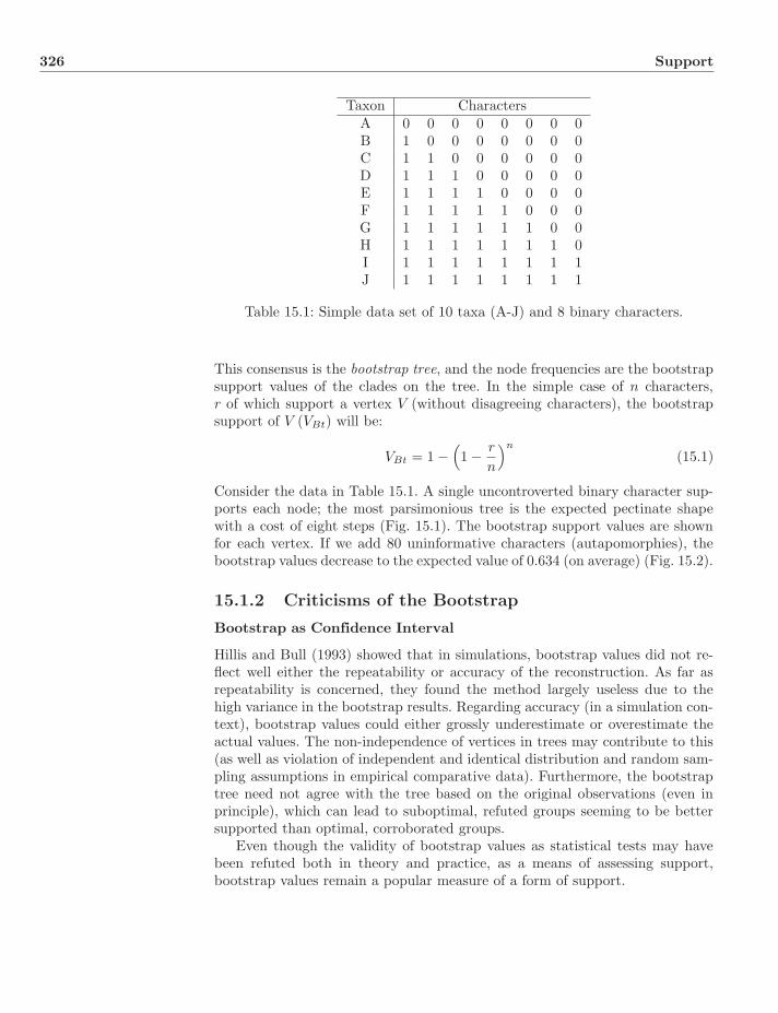
326 Support
Taxon CharactersA 0 0 0 0 0 0 0 0B 1 0 0 0 0 0 0 0C 1 1 0 0 0 0 0 0D 1 1 1 0 0 0 0 0E 1 1 1 1 0 0 0 0F 1 1 1 1 1 0 0 0G 1 1 1 1 1 1 0 0H 1 1 1 1 1 1 1 0I 1 1 1 1 1 1 1 1J 1 1 1 1 1 1 1 1
Table 15.1: Simple data set of 10 taxa (A-J) and 8 binary characters.
This consensus is the bootstrap tree, and the node frequencies are the bootstrapsupport values of the clades on the tree. In the simple case of n characters,r of which support a vertex V (without disagreeing characters), the bootstrapsupport of V (VBt) will be:
VBt = 1 −(1 − r
n
)n
(15.1)
Consider the data in Table 15.1. A single uncontroverted binary character sup-ports each node; the most parsimonious tree is the expected pectinate shapewith a cost of eight steps (Fig. 15.1). The bootstrap support values are shownfor each vertex. If we add 80 uninformative characters (autapomorphies), thebootstrap values decrease to the expected value of 0.634 (on average) (Fig. 15.2).
15.1.2 Criticisms of the Bootstrap
Bootstrap as Confidence Interval
Hillis and Bull (1993) showed that in simulations, bootstrap values did not re-flect well either the repeatability or accuracy of the reconstruction. As far asrepeatability is concerned, they found the method largely useless due to thehigh variance in the bootstrap results. Regarding accuracy (in a simulation con-text), bootstrap values could either grossly underestimate or overestimate theactual values. The non-independence of vertices in trees may contribute to this(as well as violation of independent and identical distribution and random sam-pling assumptions in empirical comparative data). Furthermore, the bootstraptree need not agree with the tree based on the original observations (even inprinciple), which can lead to suboptimal, refuted groups seeming to be bettersupported than optimal, corroborated groups.
Even though the validity of bootstrap values as statistical tests may havebeen refuted both in theory and practice, as a means of assessing support,bootstrap values remain a popular measure of a form of support.
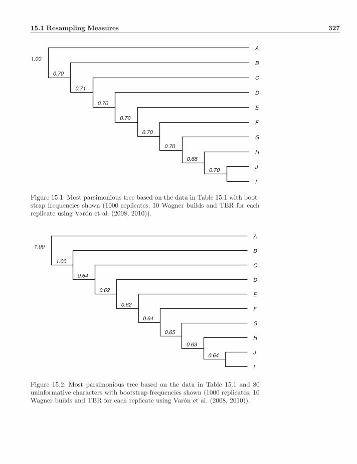
15.1 Resampling Measures 327
1.00
0.70
0.71
0.70
0.70
0.70
0.70
0.68
0.70
I
J
H
G
F
E
D
C
B
A
Figure 15.1: Most parsimonious tree based on the data in Table 15.1 with boot-strap frequencies shown (1000 replicates, 10 Wagner builds and TBR for eachreplicate using Varon et al. (2008, 2010)).
1.00
1.00
0.64
0.62
0.62
0.64
0.65
0.63
0.64
I
J
H
G
F
E
D
C
B
A
Figure 15.2: Most parsimonious tree based on the data in Table 15.1 and 80uninformative characters with bootstrap frequencies shown (1000 replicates, 10Wagner builds and TBR for each replicate using Varon et al. (2008, 2010)).
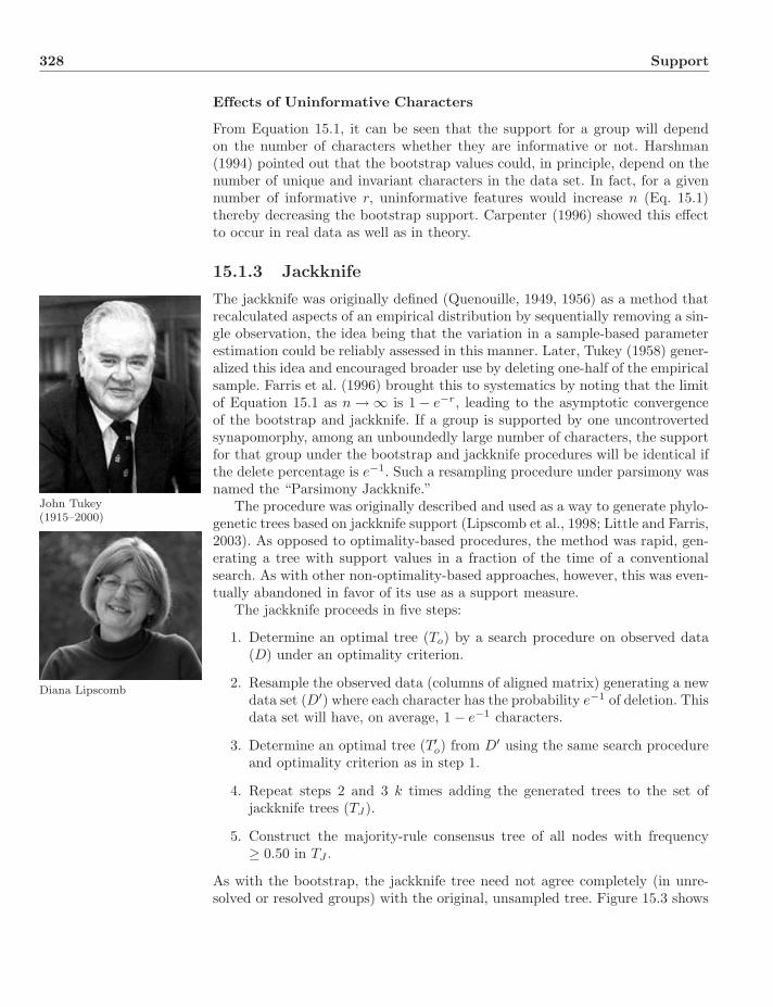
328 Support
Effects of Uninformative Characters
From Equation 15.1, it can be seen that the support for a group will dependon the number of characters whether they are informative or not. Harshman(1994) pointed out that the bootstrap values could, in principle, depend on thenumber of unique and invariant characters in the data set. In fact, for a givennumber of informative r, uninformative features would increase n (Eq. 15.1)thereby decreasing the bootstrap support. Carpenter (1996) showed this effectto occur in real data as well as in theory.
15.1.3 Jackknife
The jackknife was originally defined (Quenouille, 1949, 1956) as a method thatrecalculated aspects of an empirical distribution by sequentially removing a sin-gle observation, the idea being that the variation in a sample-based parameterestimation could be reliably assessed in this manner. Later, Tukey (1958) gener-alized this idea and encouraged broader use by deleting one-half of the empiricalsample. Farris et al. (1996) brought this to systematics by noting that the limitof Equation 15.1 as n → ∞ is 1 − e−r, leading to the asymptotic convergenceof the bootstrap and jackknife. If a group is supported by one uncontrovertedsynapomorphy, among an unboundedly large number of characters, the supportfor that group under the bootstrap and jackknife procedures will be identical ifthe delete percentage is e−1. Such a resampling procedure under parsimony wasnamed the “Parsimony Jackknife.”
John Tukey(1915–2000)
The procedure was originally described and used as a way to generate phylo-genetic trees based on jackknife support (Lipscomb et al., 1998; Little and Farris,2003). As opposed to optimality-based procedures, the method was rapid, gen-erating a tree with support values in a fraction of the time of a conventionalsearch. As with other non-optimality-based approaches, however, this was even-tually abandoned in favor of its use as a support measure.
Diana Lipscomb
The jackknife proceeds in five steps:
1. Determine an optimal tree (To) by a search procedure on observed data(D) under an optimality criterion.
2. Resample the observed data (columns of aligned matrix) generating a newdata set (D′) where each character has the probability e−1 of deletion. Thisdata set will have, on average, 1 − e−1 characters.
3. Determine an optimal tree (T′o) from D′ using the same search procedure
and optimality criterion as in step 1.
4. Repeat steps 2 and 3 k times adding the generated trees to the set ofjackknife trees (TJ ).
5. Construct the majority-rule consensus tree of all nodes with frequency≥ 0.50 in TJ .
As with the bootstrap, the jackknife tree need not agree completely (in unre-solved or resolved groups) with the original, unsampled tree. Figure 15.3 shows

15.2 Optimality-Based Measures 329
1.00
0.61
0.63
0.62
0.62
0.63
0.67
0.62
0.66
I
J
H
G
F
E
D
C
B
A
Figure 15.3: Most parsimonious tree based on the data in Table 15.1 with jack-knife frequencies shown (1000 replicates, 10 Wagner builds and TBR for eachreplicate using Varon et al. (2008, 2010)).
jackknife frequencies of the data in Table 15.1 at their expected values ofapproximately 1 − e−1 or 0.632.
15.1.4 Resampling and Dynamic Homology Characters
Resampling in the context of entirely linked, dependent observations is mean-ingless. The only way to employ such methods (Wheeler et al., 2006a; Varonet al., 2008) would be to convert the dynamic characters to a static set (presum-ably tree-based). The sampling would be entirely conditioned on the underlyingtree, rendering the resulting values inflated for the source tree and unclear forany others. Guide-tree based MSA heuristics (Chapter 8) suffer this same prob-lem, if not to the same degree. If loci or entire genetic regions are treated ascharacters, resampling can take place at the level of loci or transcriptome (e.g.EST analysis such as Dunn et al., 2008). This really just bumps the problemup a level. If entire genome data were considered, all loci would be compo-nents of a larger dynamic homology problem and resampling, once more, losesapplicability.
15.2 Optimality-Based Measures
As opposed to resampling measures, optimality-based measures are calculatedbased on the cost (length, parsimony score, likelihood, posterior probability)

330 Support
of trees. Usually, the comparison is between the best tree found and other,suboptimal trees. The indices commonly used by different optimality criteriaare closely related, even interconvertible in certain circumstances.
15.2.1 Parsimony
Kare Bremer
The most commonly used optimality-based measure of vertex support (S) underthis optimality criterion is the difference between the cost of the minimal costtree (To) without a vertex (v–group or clade) and that with (Eq. 15.2).
SBremerv = To
v/∈V − Tov∈V (15.2)
This value is determined for each vertex on the tree and is usually referred toas Bremer (1988) support.
This form of support is difficult to calculate. In principle, the lowest cost treeoverall would be compared to all other trees in order to identify the minimumcost tree without a particular group. This is obviously an NP–hard problem. Inactual usage, heuristic searches are performed (e.g. based on branch-swapping,constrained searches, or trees visited during the optimal search) and the supportvalues generated are upper bounds. Figure 15.4 shows Bremer values of the
inf
inf
1
1
1
1
1
1
1
J
I
H
G
F
E
D
C
B
A
Figure 15.4: Most parsimonious tree based on the data in Table 15.1 withBremer values shown (10 Wagner builds and TBR for each constrained ver-tex using Varon et al. (2008, 2010)). The infinity values are for edges not brokenin heuristic Bremer search.
15.2 Optimality-Based Measures 331
data in Table 15.1 at their expected values of 1 (a single synapomorphy ateach vertex).
Several modifications have been made to Bremer values to explore more fullyparticular aspects of support desired for different purposes. One of the perceivedshortcomings of this form of support is that it measures only overall support andmakes no allowance for the balance between evidence in favor of and against aparticular clade or vertex. As Goloboff and Farris (2001) point out, two groups,one with 100 character changes in favor and 95 against, and a second with fiveuncontroverted synapomorphies, would have identical Bremer values of five,yet our intuition might suggest that these are very different situations. Somehave responded to this by employing resampling methods (such as the jackknifeabove) to evaluate such situations. Goloboff and Farris (2001) suggested theRelative Fit Difference (RFD) to deal with this issue.
The RFD examines the number of characters that favor a group (F) andcompares that to the number that support some alternative (C). The standardBremer value is their difference, F − C. The RFD normalized this value bydividing by F (Eq. 15.3), yielding an index (on the optimal tree F ≥ C) varyingfrom 0 (ambivalent support) to 1 (uncontroverted).
RFDv =F − C
F(15.3)
One shortcoming of this measure (and with resampling as well) is that its ex-tension to dynamic character types is unclear. If there were several dynamiccharacters (e.g. multiple loci), F could be defined as the sum of the costs ofall loci that had a lower cost when a vertex was present than when it was not,and C defined as its complement. With a completely dynamic system such as atotal genome, such distinctions would be impossible to make since there wouldbe only one character—the genome. Perhaps the difference between costs of acharacter on the optimal and other trees could be used in place of F − C, butthis would be time consuming since the determination of F and C would requireNP–hard optimizations.
Grant and Kluge (2007), out of a desire similar to that of Goloboff and Farris(2001), suggested a normalization of Bremer support based on the difference be-tween the most costly tree (a complete bush—but the “worst” binary tree mightbe a better comparison) and the least (the optimal tree). This they termed theRelative Explanatory Power (REP) value. Unlike the RFD, the normalizationis not vertex specific; each Bremer value is divided by the same factor. In thisway, REP values, like RFD, can be compared between data sets, but unlikeRFD values have no effect on vertex support within a given tree.
Another modified use of Bremer values was proposed by Baker and DeSalle(1997) in cases of multiple sources of information in a “total evidence” (Kluge,1989) analysis. Standard Bremer values would describe the support based on theentire data set. Baker and DeSalle (1997) calculated the individual contributionsof data sets by determining the Bremer supports of the individual data sources(partitions) for each vertex on the favored tree. In this way, those nodes that

332 Support
Nodeno.a
123456789
101112Total
218
15131434
45
1153
30163
445
−41
103261
−116.547.5
42103.542122.2534
28.75
022202.50
−1−1−102.58
20221.5
−21
−21
−0.2522.59.75
81433.51.50333.500
30.5
10
−3428.504
−1−0.75−23
15.75
1012240
−21001
10
1−1340.55.5
−2000.2510.5
12.75
support hb wg ACHE ADH COIII ND1 COII16SBremer Gene partitions
Figure 15.5: Partitioned Bremer support for a series of nodes derived from acollection of molecular loci (Baker and DeSalle, 1997).
had consensual support could be identified and distinguished from those whosesupport was based on a minority of data sources (Fig. 15.5).
A Note on Nomenclature
Morris Goodman(1925–2010)
The notion of support embodied in Bremer support values has been describedseveral times and given different names. Faith (1991) used “length-difference,”and Donoghue et al. (1992) suggested “decay index.” Since Bremer (1988) waspublished earlier, that name has stuck, but recently Grant and Kluge (2008b)have pointed out that Goodman et al. (1982) used the same concept as thatof Bremer in their discussion of primate relationships. This they called the“Strength of Grouping” or SOG value. Based on this seeming priority, Grantand Kluge (2008b) suggest the index be referred to as Goodman–Bremer.
15.2.2 Likelihood
In the same way that optimal tree costs are compared by their difference in parsi-mony, optimal tree likelihoods are compared by their ratio in likelihood methods.The support for a vertex, then (SLR
v ), is the ratio of the likelihoods of the maxi-mum likelihood tree (To) with a vertex divided by that without (Eq. 15.4).
SLRv =
Tov∈V
Tov/∈V
(15.4)
Figure 15.6 shows the likelihood ratio values of the data in Table 15.1 at theirexpected values of 0.693 (under No-Common-Mechanism model; Tuffley andSteel, 1997).
Furthermore, as mentioned earlier (Chapter 11), twice the log-transformedlikelihood ratio is distributed approximately as χ2 with a single degree of freedom(Eq. 15.5).
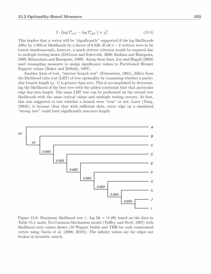
15.2 Optimality-Based Measures 333
2 · (log Tov∈V − log To
v/∈V
) ≈ χ21 (15.5)
This implies that a vertex will be “significantly” supported if the log likelihoodsdiffer by 1.903 or likelihoods by a factor of 6.826. If all n − 2 vertices were to betested simultaneously, however, a much stricter criterion would be required dueto multiple testing issues (DeGroot and Schervish, 2006; Kishino and Hasegawa,1989; Shimodaira and Hasegawa, 1999). Along these lines, Lee and Hugall (2003)used resampling measures to assign significance values to Partitioned BremerSupport values (Baker and DeSalle, 1997).
Another form of test, “interior branch test” (Felsenstein, 1981), differs fromthe likelihood ratio test (LRT) of tree optimality by examining whether a partic-ular branch length (μ · t) is greater than zero. This is accomplished by determin-ing the likelihood of the best tree with the added constraint that that particularedge has zero length. The same LRT test can be performed on the overall treelikelihoods with the same critical values and multiple testing caveats. At first,this was suggested to test whether a branch were “true” or not. Later (Yang,1994b), it became clear that with sufficient data, every edge on a simulated“wrong tree” could have significantly non-zero length.
inf
inf
0.693
0.693
0.693
0.693
0.693
0.693
0.693
I
J
H
G
F
E
D
C
B
A
Figure 15.6: Maximum likelihood tree (− log lik = 11.09) based on the data inTable 15.1 under No-Common-Mechanism model (Tuffley and Steel, 1997) withlikelihood ratio values shown (10 Wagner builds and TBR for each constrainedvertex using Varon et al. (2008, 2010)). The infinity values are for edges notbroken in heuristic search.
334 Support
15.2.3 Bayesian Posterior Probability
Bayesian support measures are, not surprisingly, very similar to those of like-lihood. Three sorts of support are commonly generated in Bayesian analysis:“credibility” intervals, Bayes factors, and vertex or clade posterior probabilities.
Credibility
Credibility intervals are the Bayesian version of confidence intervals. They repre-sent a central fraction (frequently 95%) of the posterior probability distribution.The idea for this measure would be that some aspect of a tree, such as a vertex,would or would not be included in those trees which contain 95% (for exam-ple) of the posterior probability. This is analogous to the confidence intervalinterpretation of bootstrap values (Felsenstein, 1981).
The process of such a test would be first to construct the credibility interval,or in the case of systematics, the minimal set of highest posterior probabilitytrees (MAP) containing the desired fraction of credibility. If trees with a vertexare in that interval, they are supported; if not, not1.
There is a significant difficulty with such an approach. The full posteriorprobability of hypotheses (trees) are required. This includes the denominatorterm of Equation 12.1,
∑Tj∈τ pTj · p(D|Tj , θ). Typically, this is not calculated
due to the difficulty of the integration over all possible trees. A second problemcan occur in standard statistical problems when the optimal set is multi-modal,but this is not a problem with trees since trees do not comprise an ordered set.
Bayes Factors and MAP measures
A more common index for Bayesian support is the Bayes factor (Kass andRaftery, 1995; Lavine and Schervish, 1999). The Bayes factor (B) measuresthe ratio of posterior probability to prior probability for a pair of hypotheses(Eq. 15.6).
B(Tij) =p(Ti|D)/p(Tj)p(Ti|D)/p(Tj)
(15.6)
This can be applied in several contexts. First, whether an entire hypothesis(tree) is superior to another, or second, to examine the effects of the presenceor absence of a group or vertex (Eq. 15.7).
B(Tv) =p(Tv∈V |D)/p(Tv∈V )p(Tv/∈V |D)/p(Tv/∈V )
(15.7)
If the priors are flat (p(Ti) = p(Tj),∀i, j), the Bayes factor is identical to thelikelihood ratio. A comparison can also be made that is analogous to the interior
1Such intervals need not be unique and may not even include the MAP tree if its posteriorprobability is less than 0.05.
15.2 Optimality-Based Measures 335
branch test by comparing posterior probabilities where an edge weight (branchlength) is constrained to zero. One of the issues with this test (as with manyBayesian tests) is that the prior distribution for branch lengths is unclear. Var-ious distributions can be used (e.g. uniform, exponential etc.), but it is notobvious (at least to me) which, if any, are reasonable or model ignorance appro-priately (see Chapter 12).
Bayes factors also contain an element of subjectivity when it comes to inter-pretation. Commonly, some hierarchy of comfort with the strength of evidenceis used such as:
• B(Tv) ≥ 100: Tv is supported.
• 100 < B(Tv) ≤ 101/2: Tv is minimally supported.
• 101/2 < B(Tv) ≤ 101: Tv is substantially supported.
• 101 < B(Tv) ≤ 102: Tv is strongly supported.
• 102 < B(Tv): Tv is decisively supported.
Clade Posteriors
These values were first used by Mau et al. (1999) and Larget and Simon (1999)to summarize the posterior probability of individual vertices. They are createdfrom the stationary pool of trees, whose frequency is determined by their over-all posterior probability (Sect. 12.3.6). These are the support measures that areusually reported as Bayesian support in commonly employed implementations(Huelsenbeck and Ronquist, 2003). Clade posteriors are summaries over mul-tiple trees, and their values exhibited by no single tree. As support measures,clade posteriors are more akin to resampling measures due to their summarynature and are discussed in that context below. As with resampling measures,there is no necessity that a tree constructed of those vertices with ≥ 0.50 pos-terior probability will agree with the MAP tree (Wheeler and Pickett, 2008),and “wrong” clades may achieve near 1.0 support (Goloboff, 2005; Yang, 2006;Chapter 12).
15.2.4 Strengths of Optimality-Based Support
One of the main benefits of optimality-based support is that its meaning is clear.The support value for a given vertex is a function of the best (optimal) tree withthat node, and the best tree without. As such, it is related to the overall objectiveof a tree search—the best tree by whatever criterion—and only those verticesin the best tree are evaluated. Resampling measures (and clade posteriors) mayidentify nodes not found in the best tree as more supported than those that are.This is due in part to the summary aspect of integrating support over a series oftrees which may differ in many fundamental respects, but agree in the presenceof a given vertex. Treating vertices as entities independent of their source treesseems fundamentally at odds with the hierarchical nature of phylogenetic trees.

336 Support
15.3 Parameter-Based Measures
Although often discussed in the context of support, parameter-based support(sensu Wheeler, 1995; as opposed to a distributional parameter) is more of astatement of robustness of phylogenetic results to variations in those param-eters (Wheeler, 1995). As summaries of vertex presence over multiple trees,they are akin to resampling measures and have no direct relationship to any ofthe component “best” trees. Parameter-based trees are also like resampling (orclade-posterior) trees in that they need not agree completely with the “best”tree by any particular measure. These depictions convey the breadth of param-eter choices under which particular groups are supported—usually those on anoptimal tree (Fig. 15.7).
15.4 Comparison of Support Measures—Optimal and Average
As mentioned above, there is an often bewildering variety of things called “sup-port.” One immediate question is how do these descriptors relate to each other?They all measure something, but what? Given the discussions above, we candefine the optimal support of a vertex (Sv) as a function of the costs of the op-timal tree with a vertex (To
v∈V ) and the optimal tree without (Tov/∈V ) (Eq. 15.8)
(Wheeler, 2010).
Sv = f(To
v∈V , Tov/∈V
)(15.8)
For parsimony this function is their difference (Eq. 15.9),
Sv = Tov/∈V − To
v∈V (15.9)
Figure 15.7: Strict (left) and majority-rule (right) consensus trees over param-eter space (Prendini et al., 2005).
15.4 Comparison of Support Measures−−Optimal and Average 337
for likelihood their ratio (Eq. 15.10),
Sv =To
v∈V
Tov/∈V
(15.10)
and for Bayes a prior normalized ratio (with p() denoting prior probability;Eq. 15.11).
Sv =To
v∈V /p(Tov∈V )
Tov/∈V /p(To
v/∈V )(15.11)
Furthermore, if we examine the Bremer support of parsimony and the like-lihood ratio of maximum likelihood under the No-Common-Mechanism (NCM)model (Tuffley and Steel, 1997), we can identify further links.
Taking the log of the likelihood ratio of Equation 15.10 (Eq. 15.12),
log Sv = log Tov∈V − log To
v/∈V (15.12)
and recall that under NCM the likelihood for a given tree with n characterswith r states and li changes in character i is:
Tc =n∏i
r−(li+1)
the log of which would then be:
log Tc =n∑i
−(li + 1) log r
rearranged becomes:
log Tc = n − log r
n∑i
li
noting that∑n
i li = lp, the parsimony length, and substituting back intoEquation 15.12:
log Sv = log Tov∈V − log To
v/∈V = log r · (lpv/∈V − lpv∈V
)Hence, the log likelihood ratio is equal to the Bremer support multiplied bythe log of the number of states in the (non-additive) characters. With uniformtopological priors, the Bayes factor will show the same equivalence under NCM.Bremer support, likelihood ratio, and Bayes factor, then, are closely related asoptimal support measures.
Clade posterior, bootstrap, and jackknife supports are also related, but asaverage or expected support measures. Consider a distribution of trees p(T) =g(T) (e.g. NCM with p(T) = rlp+1). We can define a value vT for each vertex oneach tree (Eq. 15.13).
vT ={
0 v /∈ V1 v ∈ V
(15.13)
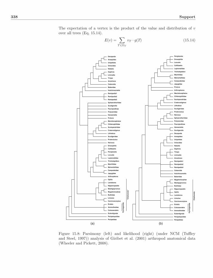
338 Support
The expectation of a vertex is the product of the value and distribution of vover all trees (Eq. 15.14).
E(v) =∑
T∈ΩT
vT · g(T) (15.14)
Peripatidae
Peripatopsidae
Eutardigrada
Colossendeis
Ammotheidae
Endeis
Carcinoscorpius
Limulus
Buthidae
Mygalomorphae
Mastigoproctus
Nipponopsalis
Laniatores
Opilio
Arthropleona
Japygidae
Campodeidae
Meinertellidae
Machilidae
Tricholepidion
Lepismatidae
Locusta
Periplaneta
Callibaetis
Drosophila
Narceus
Proteroiulus
Scutigeridae
Lithobius
Craterostigmus
Scolopendridae
Chilenophilidae
Mecistocephalus
Protura
Hanseniella
Polyxenidae
Pauropodinae
Scutigerella
Sphaerotheriidae
Remipedia3
Remipedia2
Remipedia1
Hutchinsoniella
Balanidae
Calanoida
Anostraca
Triops
Limnadia
Daphnia
Nebalia
Oniscidea
Unipeltata
Anaspides
Decapoda
Peripatidae
Peripatopsidae
Eutardigrada
Ammotheidae
Colossendeis
Endeis
Carcinoscorpius
Limulus
Laniatores
Opilio
Nipponopsalis
Buthidae
Mastigoproctus
Mygalomorphae
Balanidae
Hutchinsoniella
Calanoida
Remipedia3
Remipedia2
Remipedia1
Anostraca
Limnadia
Triops
Daphnia
Nebalia
Oniscidea
Unipeltata
Anaspides
Decapoda
Scutigerella
Hanseniella
Pauropodinae
Polyxenidae
Sphaerotheriidae
Narceus
Proteroiulus
Scutigeridae
Lithobius
Craterostigmus
Scolopendridae
Chilenophilidae
Mecistocephalus
Arthropleona
Protura
Japygidae
Campodeidae
Meinertellidae
Machilidae
Tricholepidion
Lepismatidae
Callibaetis
Locusta
Drosophila
Periplaneta
(a) (b)
“Ch
elic
erat
a”
Pyc
no
go
nid
a
Ch
elic
erat
a
Pyc
no
go
nid
a
Figure 15.8: Parsimony (left) and likelihood (right) (under NCM (Tuffleyand Steel, 1997)) analysis of Giribet et al. (2001) arthropod anatomical data(Wheeler and Pickett, 2008).
15.5 Which to Choose? 339
For Bayesian methods, g(T) is the posterior probability of a tree given data(T|D). Resampling methods yield a distribution of pseudoreplicate data sets,each of which has a single strict consensus tree (Eq. 15.15).
D′ ← RAND(D)T ′ = f(D′)
g(Ti) =1n
replicates∑i
1 if Ti = T ′ (15.15)
Resampling methods and vertex posterior probabilities are measuring an ex-pected or average level of support over all trees. This is still support, but of adifferent type than optimal2. Wheeler and Pickett (2008) demonstrated this intheir analysis of arthropod anatomical data (Fig. 15.8). The branch support-ing chelicerate monophyly had a clade posterior probability of 0.6 (Huelsenbeckand Ronquist, 2003), while the alternate paraphyly in the parsimony analysishad a Bremer support of 2, a jackknife support of 0.57, and a log likelihoodratio/Bayes factor (under uniform tree priors) of 0.25. These are each supportmeasures, but support alternate groupings of the same taxa under the samedata and models.
15.5 Which to Choose?
There is no all-satisfactory measure of support since there is no consensualnotion of support. Alternate measures based on resampling, relative optimality,and statistical distributions are all support measures. The key requirement isto be able to relate the measure to the entity being measured. When we areconcerned with optimal trees, optimality-based measures are most closely linked.
15.6 Exercises
1. Consider the data of Dunn et al. (2008) treating gaps as character states.
Determine a reasonably good tree using parsimony.
Estimate the bootstrap tree using parsimony.
Estimate the bootstrap support values for your “good” tree usingparsimony.
Estimate the delete one-half jackknife tree using parsimony.
Estimate the delete one-half jackknife support values for your “good”tree using parsimony.
Estimate the delete e−1 jackknife tree using parsimony.
2Clade posterior probabilities as support are also burdened with unavoidable clade sizeeffects (Sect. 12.3.6).

340 Support
Estimate the delete e−1 jackknife support values for your “good” treeusing parsimony.
Estimate the Bayesian clade posterior tree using No-Common-Mechanism.
Estimate the Goodman–Bremer support for your best tree.
2. Repeat the above treating gaps as missing data.
3. What general conclusions can you draw from the previous two exercises?
4. If the number of character states were given as 21, when gaps were treatedas states, and 20 when gaps were treated as missing data, what would thelikelihood ratios be for the nodes on the two best trees under No-Common-Mechanism using a Neyman model?
5. If the prior distribution on trees were taken to be uniform, and the universeof topologies and their likelihoods determined by the Goodman–Bremerresults above (i.e. the n − 3 edges with support values represent the entireuniverse of trees), what level of Bayesian credibility is represented by thebest tree(s) under No-Common-Mechanism with gaps treated as statesand missing data? How many trees are required to achieve 95% credibility?How might you summarize this result?
Chapter 16
Consensus, Congruence,and Supertrees
The methods discussed here take as input a set of trees and output a singletree. As commonly used, consensus methods operate on tree sets where eachtree has the same leaf set as opposed to supertree methods, which operate ontrees with different leaf sets. In reality, such consensus methods are a subsetof supertree methods. In all cases, the primary goal is to represent areas ofagreement and disagreement among the input trees and produce a summarystatement in the form of a tree. None of the methods discussed below takeaccount of the underlying character data directly, but operate solely on thetopologies of their derived trees.
In general, consensus and supertree methods operate on sets of leaf taxadefined by splits or rooted clades, looking for “common” information. As aresult, there are many shared operations among the procedures as well as subtleand not so subtle differences.
16.1 Consensus Tree Methods
16.1.1 Motivations
Originally, consensus methods were derived to identify common informationbetween rival classifications (Adams, 1972). The notion was that inputs would berooted trees with identical leaf sets and the consensus should represent generallyshared information. The definition of shared has never been consensual, hencea variety of techniques have arisen to solve this problem.
16.1.2 Adams I and II
Adams (1972) defined two consensus procedures to operate on rooted trees.For convenience we can refer to these as Adams I and Adams II. Adams I
Systematics: A Course of Lectures, First Edition. Ward C. Wheeler.c© 2012 Ward C. Wheeler. Published 2012 by Blackwell Publishing Ltd.
342 Consensus, Congruence, and Supertrees
operates on fully labeled trees (internal vertices as well as leaves). Unlike othermethods, Adams I is ancestor-based, not descendant-based. If a labeled nodeM has an ancestor L shared on all input trees, the edge L → M will exist onthe consensus even if M → (A,B) on one tree and M → (C,D) on another. Themethod proceeds as follows:
1. Define the vertex set of each input tree Ti as VTi
2. Identify one of the input trees as T0
3. Begin at root
4. Choose vertex X on T0 that has no ancestor or a known ancestor (deter-mined by a previous iteration)
Define Y = X ∩i VTi
If Y = ∅, discard X
Else, if X has no ancestors in Y, then X is a root of the consensus(which could be a forest)
Else, define Z to be the set of vertices ancestral to X on all trees.Connect X to the closest element in Z
5. Return to step 4 until all vertices are connected to an ancestor
The algorithm can be followed using Adams’ example (Fig. 16.1). The Adams Iconsensus is rarely, if ever, employed. This is largely due to the fact that equiv-alent labeled ancestors (with potentially different descendants) are unknowable.
The Adams II consensus operates on rooted trees with unlabeled internalnodes. In order to construct the consensus, the method examines each progres-sive split from the root to the leaves, joining the non-empty intersections (leastupper bound or LUB) of the splits in the input trees as sister taxa (Fig. 16.2).
1. Begin at the root vertex of the input trees
2. Define the sets of leaf taxa Ti,j for each tree i and groups j descendentfrom the vertex (two if binary, more otherwise) after removing those leaftaxa that have been placed on the consensus previously
3. Determine the LUB (Fig. 16.2) of each group (j) on each tree (i) witheach on the others
4. For each LUB
If the LUB is empty, ignore
Else, if the LUB had ≤ 2 leaves, place that LUB in the consensus asa descendant of the vertex
Else, the LUB is a vertex for further analysis. Go to step 2
The algorithm can be followed using the example above (Fig. 16.3). Adams IItrees are also not in broad use in systematic analysis since (as in the example)groups not present in any of the input trees can be part of the consensus. This
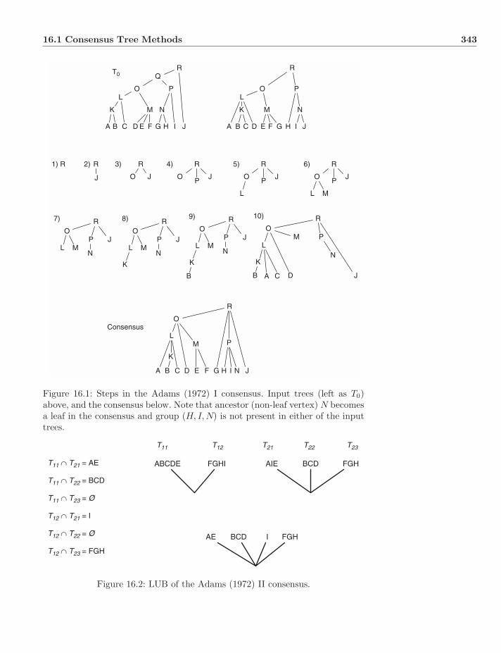
16.1 Consensus Tree Methods 343
A B C D E F G H I J A B C D E F G H I J
K
L
M
O
N
P
QR
K
L
M
O
N
P
RT0
1) R 2) R
J
3) R
JO
4) R
JO P
5) R
JO P
L
6) R
JO P
L M
7) R
JO
PL M
N
8) R
JO
PL M
N
K
9) R
JO
PL M
N
K
B
10) R
J
OP
LM
NK
B A C D
R
J
O
PL
M
N
K
BA C D E F H IG
Consensus
Figure 16.1: Steps in the Adams (1972) I consensus. Input trees (left as T0)above, and the consensus below. Note that ancestor (non-leaf vertex) N becomesa leaf in the consensus and group (H, I,N) is not present in either of the inputtrees.
ABCDE FGHI AIE BCD FGH
AE BCD I FGH
T11 T12 T21 T22 T23
T11 ∩ T21 = AE
T11 ∩ T22 = BCD
T11 ∩ T23 = Ø
T12 ∩ T21 = I
T12 ∩ T22 = Ø
T12 ∩ T23 = FGH
Figure 16.2: LUB of the Adams (1972) II consensus.
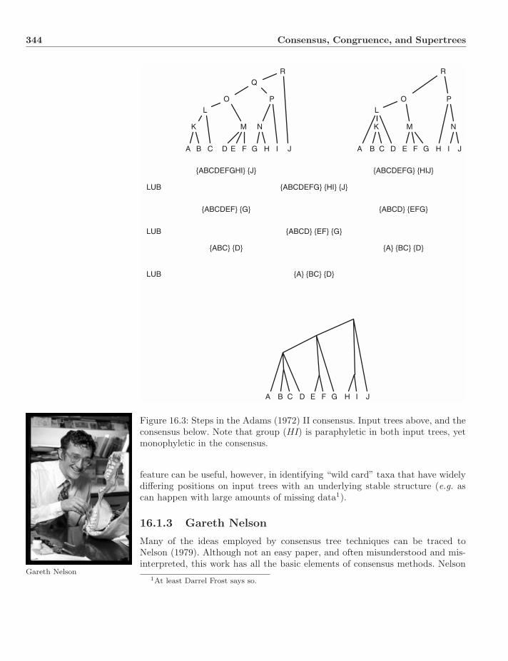
344 Consensus, Congruence, and Supertrees
A B C D E F G H I J A B C D E F G H I J
K
L
M
O
N
P
Q
R
K
L
M
O
N
P
R
A B C D E F G H I J
{ABCDEFGHI} {J} {ABCDEFG} {HIJ}
LUB {ABCDEFG} {HI} {J}
{ABCDEF} {G} {ABCD} {EFG}
LUB {ABCD} {EF} {G}
{ABC} {D} {A} {BC} {D}
LUB {A} {BC} {D}
Figure 16.3: Steps in the Adams (1972) II consensus. Input trees above, and theconsensus below. Note that group (HI) is paraphyletic in both input trees, yetmonophyletic in the consensus.
feature can be useful, however, in identifying “wild card” taxa that have widelydiffering positions on input trees with an underlying stable structure (e.g. ascan happen with large amounts of missing data1).
16.1.3 Gareth Nelson
Gareth Nelson
Many of the ideas employed by consensus tree techniques can be traced toNelson (1979). Although not an easy paper, and often misunderstood and mis-interpreted, this work has all the basic elements of consensus methods. Nelson
1At least Darrel Frost says so.

16.1 Consensus Tree Methods 345
0
0
0
0
2
2
5
5
9
9
9
910
17
16
18
10
11
15
14
10
11
6
6
6
3
3
3
3
4
4
4
1
1
1
7
7
7
8
8
8
0 0
12
13 3
4
A B C D E F G H I J K L M N A D F G H B C E J K M L I N
A B C D E F G H I J K L M N A B F G H C D E I J K L M N
A B F G H K G H I J C D E N A A B C D D E F G H H I J K L M M N' ' ' '
Phylogram Phenogram: Adults
Phenogram : Larvae Phenogram : Males
Phenogram : Pupae Phylogram : Alternative
Figure 16.4: Michener (1977) analysis of allopadine bees based on multiple datasources (Nelson, 1979).
began with a study of bees by Michener (1977) based on multiple sources ofmorphological data (Fig. 16.4).
Nelson defined objects, relations, and operations to formalize consensus.First off, he defined a component as a subtree or clade with ≥ 2 members (ver-tex with ≥ 2 descendent leaves). He then defined three relationships possibleamong components A and B on alternate trees: exclusion, inclusion, and repli-cation (Eq. 16.1).
exclusion: A ∩ B = ∅ (16.1)inclusion: A ∩ B ∈ {A,B}
replication: A = B
Two operations were also defined (Eq. 16.2).
combinability: A ∩ B ∈ {A,B, ∅} (16.2)non-combinability: A ∩ B /∈ {A,B, ∅}
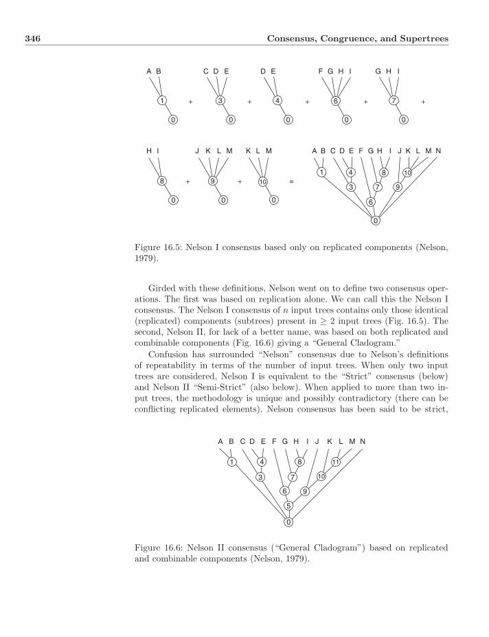
346 Consensus, Congruence, and Supertrees
A
H
=++
+ + + + +
I J K L M K L M A B C D E F G H I J K L M N
B C D E D E F G H I G H I
1010
8 9
0
0
1 3 4 6 7
0 0 0 0
0 0
1 4
3
6
7
8
9
0
Figure 16.5: Nelson I consensus based only on replicated components (Nelson,1979).
Girded with these definitions, Nelson went on to define two consensus oper-ations. The first was based on replication alone. We can call this the Nelson Iconsensus. The Nelson I consensus of n input trees contains only those identical(replicated) components (subtrees) present in ≥ 2 input trees (Fig. 16.5). Thesecond, Nelson II, for lack of a better name, was based on both replicated andcombinable components (Fig. 16.6) giving a “General Cladogram.”
Confusion has surrounded “Nelson” consensus due to Nelson’s definitionsof repeatability in terms of the number of input trees. When only two inputtrees are considered, Nelson I is equivalent to the “Strict” consensus (below)and Nelson II “Semi-Strict” (also below). When applied to more than two in-put trees, the methodology is unique and possibly contradictory (there can beconflicting replicated elements). Nelson consensus has been said to be strict,
10
11
0
1
3
4 8
7
5
6 9
A B C D E F G H I J K L M N
Figure 16.6: Nelson II consensus (“General Cladogram”) based on replicatedand combinable components (Nelson, 1979).
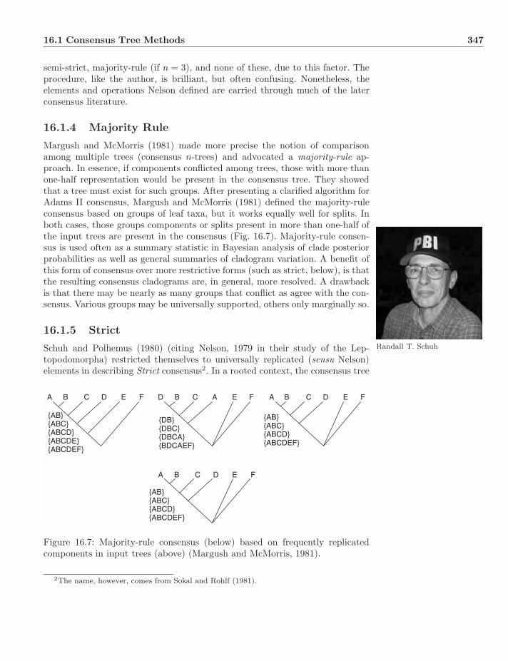
16.1 Consensus Tree Methods 347
semi-strict, majority-rule (if n = 3), and none of these, due to this factor. Theprocedure, like the author, is brilliant, but often confusing. Nonetheless, theelements and operations Nelson defined are carried through much of the laterconsensus literature.
16.1.4 Majority Rule
Margush and McMorris (1981) made more precise the notion of comparisonamong multiple trees (consensus n-trees) and advocated a majority-rule ap-proach. In essence, if components conflicted among trees, those with more thanone-half representation would be present in the consensus tree. They showedthat a tree must exist for such groups. After presenting a clarified algorithm forAdams II consensus, Margush and McMorris (1981) defined the majority-ruleconsensus based on groups of leaf taxa, but it works equally well for splits. Inboth cases, those groups components or splits present in more than one-half ofthe input trees are present in the consensus (Fig. 16.7). Majority-rule consen-sus is used often as a summary statistic in Bayesian analysis of clade posteriorprobabilities as well as general summaries of cladogram variation. A benefit ofthis form of consensus over more restrictive forms (such as strict, below), is thatthe resulting consensus cladograms are, in general, more resolved. A drawbackis that there may be nearly as many groups that conflict as agree with the con-sensus. Various groups may be universally supported, others only marginally so.
16.1.5 Strict
Randall T. SchuhSchuh and Polhemus (1980) (citing Nelson, 1979 in their study of the Lep-topodomorpha) restricted themselves to universally replicated (sensu Nelson)elements in describing Strict consensus2. In a rooted context, the consensus tree
A B C D E F D B C A E F A B C D E F
A B C D E F
{AB}{ABC}{ABCD}{ABCDE}{ABCDEF}
{DB}{DBC}{DBCA}{BDCAEF}
{AB}{ABC}{ABCD}{ABCDEF}
{AB}{ABC}{ABCD}{ABCDEF}
Figure 16.7: Majority-rule consensus (below) based on frequently replicatedcomponents in input trees (above) (Margush and McMorris, 1981).
2The name, however, comes from Sokal and Rohlf (1981).
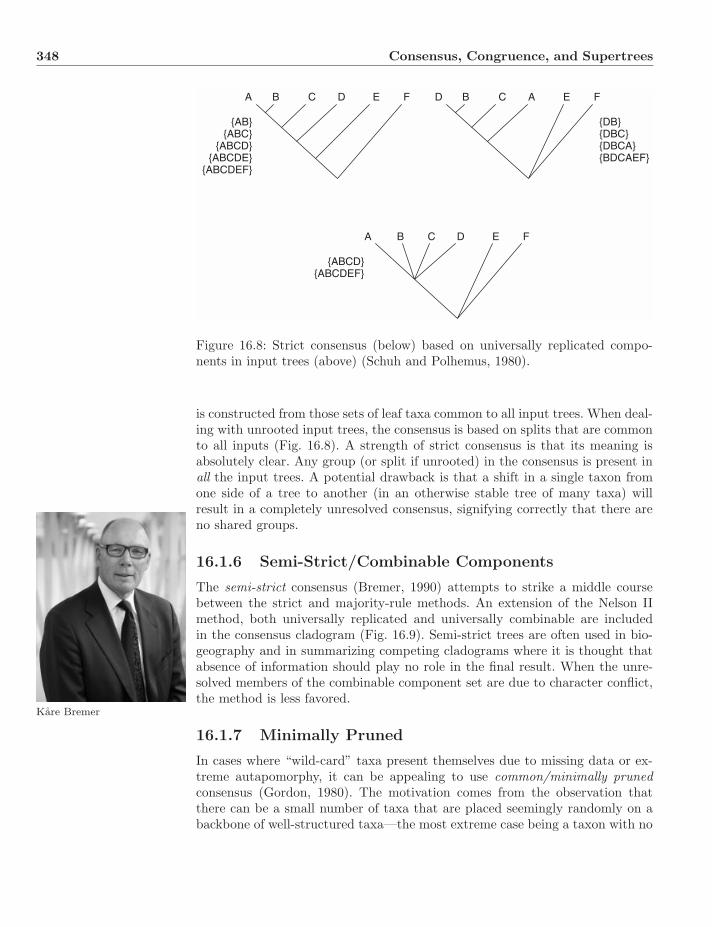
348 Consensus, Congruence, and Supertrees
A B C D E F D B C A E F
{AB}{ABC}
{ABCD}{ABCDE}
{ABCDEF}
{DB}{DBC}{DBCA}{BDCAEF}
A B C D E F
{ABCD}{ABCDEF}
Figure 16.8: Strict consensus (below) based on universally replicated compo-nents in input trees (above) (Schuh and Polhemus, 1980).
is constructed from those sets of leaf taxa common to all input trees. When deal-ing with unrooted input trees, the consensus is based on splits that are commonto all inputs (Fig. 16.8). A strength of strict consensus is that its meaning isabsolutely clear. Any group (or split if unrooted) in the consensus is present inall the input trees. A potential drawback is that a shift in a single taxon fromone side of a tree to another (in an otherwise stable tree of many taxa) willresult in a completely unresolved consensus, signifying correctly that there areno shared groups.
16.1.6 Semi-Strict/Combinable Components
The semi-strict consensus (Bremer, 1990) attempts to strike a middle coursebetween the strict and majority-rule methods. An extension of the Nelson IImethod, both universally replicated and universally combinable are includedin the consensus cladogram (Fig. 16.9). Semi-strict trees are often used in bio-geography and in summarizing competing cladograms where it is thought thatabsence of information should play no role in the final result. When the unre-solved members of the combinable component set are due to character conflict,the method is less favored.
Kare Bremer
16.1.7 Minimally Pruned
In cases where “wild-card” taxa present themselves due to missing data or ex-treme autapomorphy, it can be appealing to use common/minimally prunedconsensus (Gordon, 1980). The motivation comes from the observation thatthere can be a small number of taxa that are placed seemingly randomly on abackbone of well-structured taxa—the most extreme case being a taxon with no
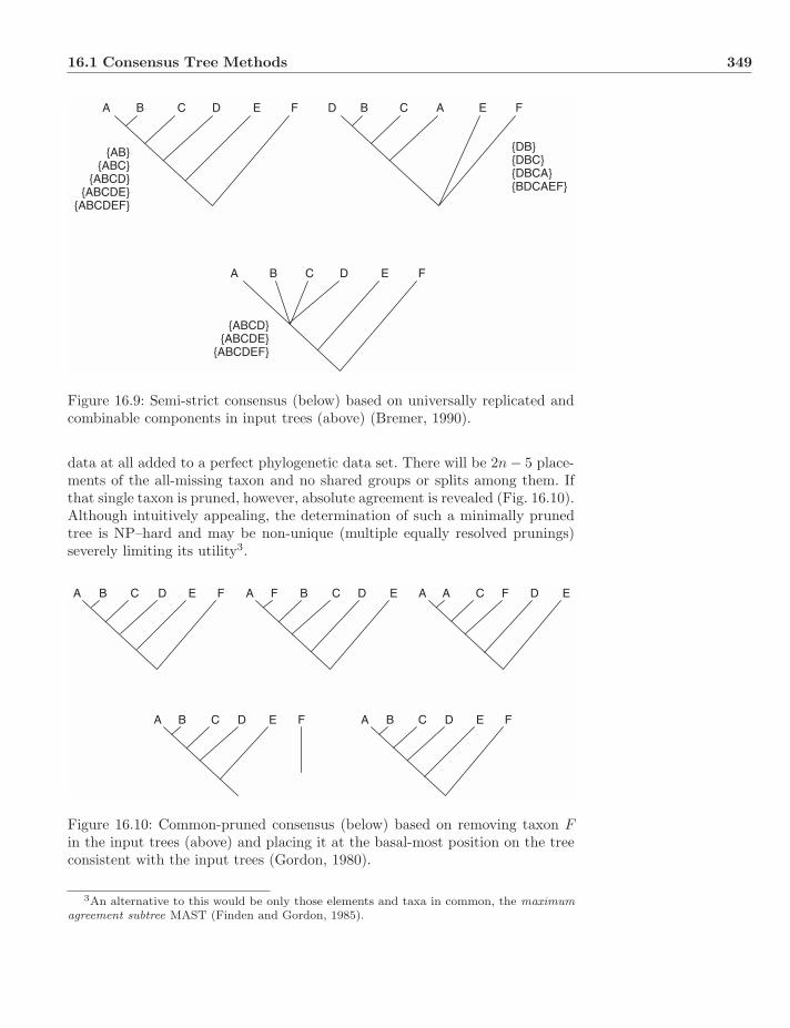
16.1 Consensus Tree Methods 349
A B C D E F D B C A E F
A B C D E F
{AB}{ABC}
{ABCD}{ABCDE}
{ABCDEF}
{DB}{DBC}{DBCA}{BDCAEF}
{ABCD}{ABCDE}
{ABCDEF}
Figure 16.9: Semi-strict consensus (below) based on universally replicated andcombinable components in input trees (above) (Bremer, 1990).
data at all added to a perfect phylogenetic data set. There will be 2n − 5 place-ments of the all-missing taxon and no shared groups or splits among them. Ifthat single taxon is pruned, however, absolute agreement is revealed (Fig. 16.10).Although intuitively appealing, the determination of such a minimally prunedtree is NP–hard and may be non-unique (multiple equally resolved prunings)severely limiting its utility3.
A B C D E F A F B C D E A A C F D E
A B C D E F A B C D E F
Figure 16.10: Common-pruned consensus (below) based on removing taxon Fin the input trees (above) and placing it at the basal-most position on the treeconsistent with the input trees (Gordon, 1980).
3An alternative to this would be only those elements and taxa in common, the maximumagreement subtree MAST (Finden and Gordon, 1985).
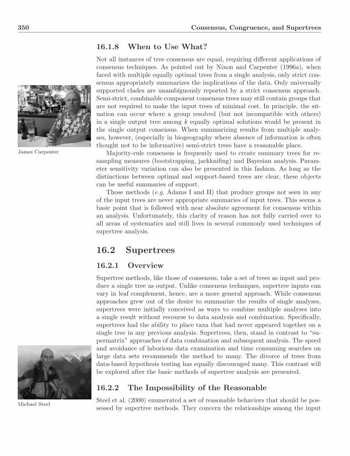
350 Consensus, Congruence, and Supertrees
16.1.8 When to Use What?
Not all instances of tree consensus are equal, requiring different applications ofconsensus techniques. As pointed out by Nixon and Carpenter (1996a), whenfaced with multiple equally optimal trees from a single analysis, only strict con-sensus appropriately summarizes the implications of the data. Only universallysupported clades are unambiguously reported by a strict consensus approach.Semi-strict, combinable component consensus trees may still contain groups thatare not required to make the input trees of minimal cost. In principle, the sit-uation can occur where a group resolved (but not incompatible with others)in a single output tree among k equally optimal solutions would be present inthe single output consensus. When summarizing results from multiple analy-ses, however, (especially in biogeography where absence of information is oftenthought not to be informative) semi-strict trees have a reasonable place.
James Carpenter Majority-rule consensus is frequently used to create summary trees for re-sampling measures (bootstrapping, jackknifing) and Bayesian analysis. Param-eter sensitivity variation can also be presented in this fashion. As long as thedistinctions between optimal and support-based trees are clear, these objectscan be useful summaries of support.
Those methods (e.g. Adams I and II) that produce groups not seen in anyof the input trees are never appropriate summaries of input trees. This seems abasic point that is followed with near absolute agreement for consensus withinan analysis. Unfortunately, this clarity of reason has not fully carried over toall areas of systematics and still lives in several commonly used techniques ofsupertree analysis.
16.2 Supertrees
16.2.1 Overview
Supertree methods, like those of consensus, take a set of trees as input and pro-duce a single tree as output. Unlike consensus techniques, supertree inputs canvary in leaf complement, hence, are a more general approach. While consensusapproaches grew out of the desire to summarize the results of single analyses,supertrees were initially conceived as ways to combine multiple analyses intoa single result without recourse to data analysis and combination. Specifically,supertrees had the ability to place taxa that had never appeared together on asingle tree in any previous analysis. Supertrees, then, stand in contrast to “su-permatrix” approaches of data combination and subsequent analysis. The speedand avoidance of laborious data examination and time consuming searches onlarge data sets recommends the method to many. The divorce of trees fromdata-based hypothesis testing has equally discouraged many. This contrast willbe explored after the basic methods of supertree analysis are presented.
16.2.2 The Impossibility of the Reasonable
Michael SteelSteel et al. (2000) enumerated a set of reasonable behaviors that should be pos-sessed by supertree methods. They concern the relationships among the input
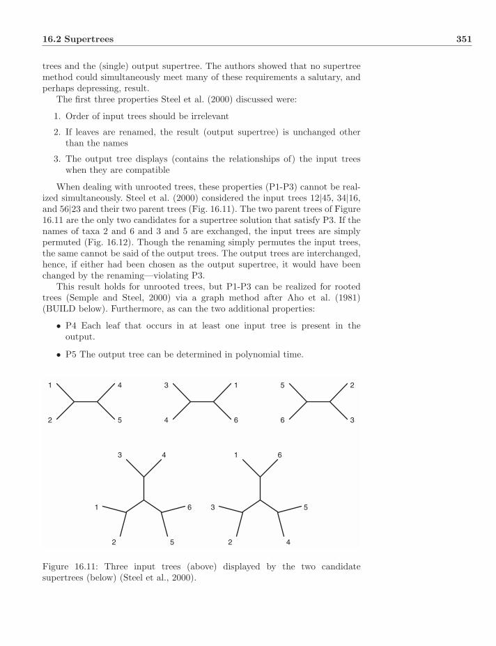
16.2 Supertrees 351
trees and the (single) output supertree. The authors showed that no supertreemethod could simultaneously meet many of these requirements a salutary, andperhaps depressing, result.
The first three properties Steel et al. (2000) discussed were:
1. Order of input trees should be irrelevant
2. If leaves are renamed, the result (output supertree) is unchanged otherthan the names
3. The output tree displays (contains the relationships of) the input treeswhen they are compatible
When dealing with unrooted trees, these properties (P1-P3) cannot be real-ized simultaneously. Steel et al. (2000) considered the input trees 12|45, 34|16,and 56|23 and their two parent trees (Fig. 16.11). The two parent trees of Figure16.11 are the only two candidates for a supertree solution that satisfy P3. If thenames of taxa 2 and 6 and 3 and 5 are exchanged, the input trees are simplypermuted (Fig. 16.12). Though the renaming simply permutes the input trees,the same cannot be said of the output trees. The output trees are interchanged,hence, if either had been chosen as the output supertree, it would have beenchanged by the renaming—violating P3.
This result holds for unrooted trees, but P1-P3 can be realized for rootedtrees (Semple and Steel, 2000) via a graph method after Aho et al. (1981)(BUILD below). Furthermore, as can the two additional properties:
• P4 Each leaf that occurs in at least one input tree is present in theoutput.
• P5 The output tree can be determined in polynomial time.
1
2
4
5
3
4
1
6
5
6
2
3
1
2
3 4
5
6 3
2
1 6
4
5
Figure 16.11: Three input trees (above) displayed by the two candidatesupertrees (below) (Steel et al., 2000).
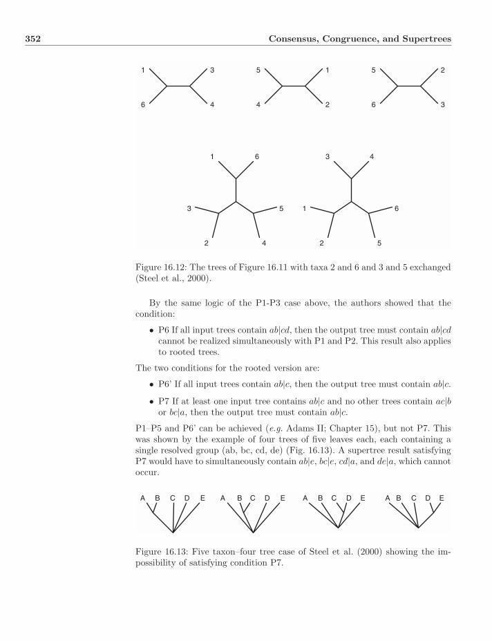
352 Consensus, Congruence, and Supertrees
5
4
1
2
5
6
2
3
1
6
3
4
1
2
3 4
5
63
2
1 6
4
5
Figure 16.12: The trees of Figure 16.11 with taxa 2 and 6 and 3 and 5 exchanged(Steel et al., 2000).
By the same logic of the P1-P3 case above, the authors showed that thecondition:
• P6 If all input trees contain ab|cd, then the output tree must contain ab|cdcannot be realized simultaneously with P1 and P2. This result also appliesto rooted trees.
The two conditions for the rooted version are:
• P6’ If all input trees contain ab|c, then the output tree must contain ab|c.• P7 If at least one input tree contains ab|c and no other trees contain ac|b
or bc|a, then the output tree must contain ab|c.P1–P5 and P6’ can be achieved (e.g. Adams II; Chapter 15), but not P7. Thiswas shown by the example of four trees of five leaves each, each containing asingle resolved group (ab, bc, cd, de) (Fig. 16.13). A supertree result satisfyingP7 would have to simultaneously contain ab|e, bc|e, cd|a, and de|a, which cannotoccur.
A B C D E A B C D E A B C D E A B C D E
Figure 16.13: Five taxon–four tree case of Steel et al. (2000) showing the im-possibility of satisfying condition P7.
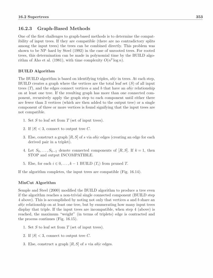
16.2 Supertrees 353
16.2.3 Graph-Based Methods
One of the first challenges to graph-based methods is to determine the compat-ibility of input trees. If they are compatible (there are no contradictory splitsamong the input trees) the trees can be combined directly. This problem wasshown to be NP–hard by Steel (1992) in the case of unrooted trees. For rootedtrees, this determination can be made in polynomial time by the BUILD algo-rithm of Aho et al. (1981), with time complexity O(n2 log n).
BUILD Algorithm
The BUILD algorithm is based on identifying triples, ab|c in trees. At each step,BUILD creates a graph where the vertices are the total leaf set (S) of all inputtrees (T), and the edges connect vertices a and b that have an ab|c relationshipon at least one tree. If the resulting graph has more than one connected com-ponent, recursively apply the graph step to each component until either thereare fewer than 3 vertices (which are then added to the output tree) or a singlecomponent of three or more vertices is found signifying that the input trees arenot compatible.
1. Set S to leaf set from T (set of input trees).
2. If |S| < 3, connect to output tree C.
3. Else, construct a graph [R,S] of s via ab|c edges (creating an edge for eachderived pair in a triplet).
4. Let S0, . . . , Sk−1 denote connected components of [R,S]. If k = 1, thenSTOP and output INCOMPATIBLE.
5. Else, for each i ∈ 0, . . . , k − 1 BUILD (Ti) from pruned T.
If the algorithm completes, the input trees are compatible (Fig. 16.14).
MinCut Algorithm
Semple and Steel (2000) modified the BUILD algorithm to produce a tree evenif the algorithm reaches a non-trivial single connected component (BUILD step4 above). This is accomplished by noting not only that vertices a and b share anab|c relationship on at least one tree, but by enumerating how many input treesdisplay that triple. If the input trees are incompatible, when step 4 (above) isreached, the maximum “weight” (in terms of triplets) edge is contracted andthe process continues (Fig. 16.15).
1. Set S to leaf set from T (set of input trees).
2. If |S| < 3, connect to output tree C.
3. Else, construct a graph [R,S] of s via ab|c edges.

354 Consensus, Congruence, and Supertrees
T1 T2 T3
A B C E C B E D A B F D
A
B
C
D
E
F
A B C C B A B F
A
B
C
F
A B C F D E
Input
Cluster via ab|c
Prune
Cluster via ab|c
Output
Figure 16.14: Example BUILD algorithm of Aho et al. (1981).
4. Let S0, . . . , Sk−1 denote connected components of [R,S]. If k = 1, then cre-ate S \ Emax from ab|c edge weights. Contract Emax and cut all minimumweight edges.
5. For each i ∈ 0, . . . , k − 1, MinCut (Ti) from pruned T.
In terms of the reasonable conditions enumerated above, MinCut realizes P1–P5and P6’. The method is not, however, perfect. Like Adams II consensus trees(above), MinCut can produce groups not present (and not implied) in any ofthe input trees, even when the leaf sets are identical (Fig. 16.16).
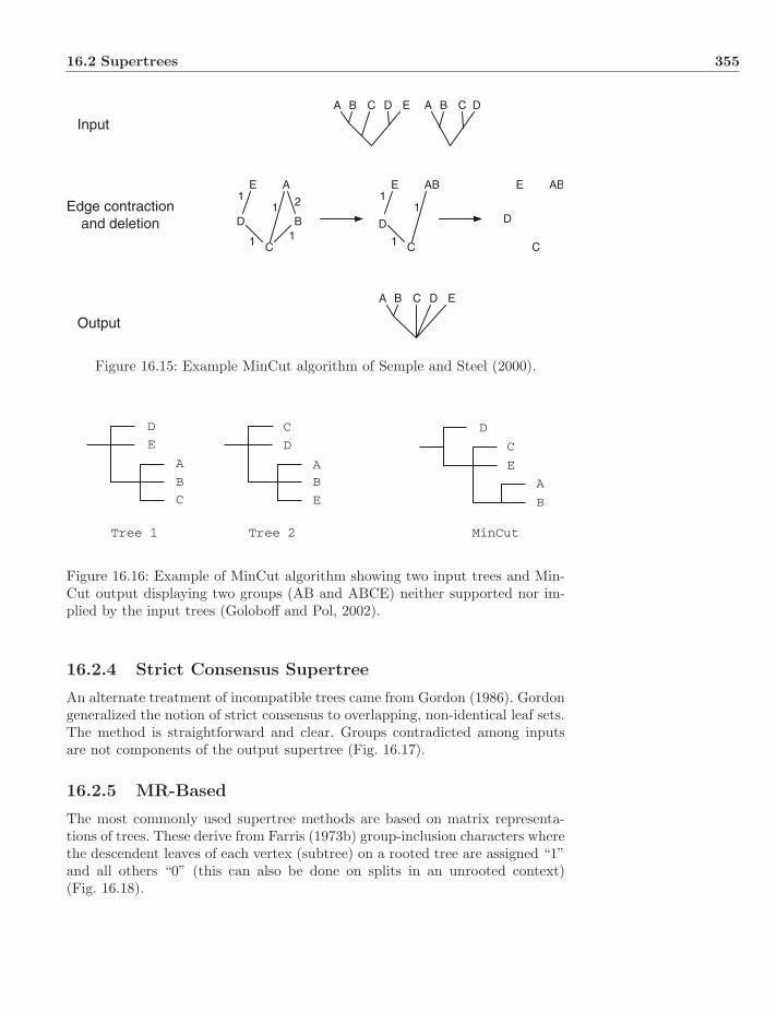
16.2 Supertrees 355
A B C D E A B C D
A B C D E
A
B
C
D
E
21
1 1
1
AB
C
D
E1
1
1
AB
C
D
E
Input
Edge contractionand deletion
Output
Figure 16.15: Example MinCut algorithm of Semple and Steel (2000).
Tree 2 MinCutTree 1
D
D
D
C
C
C
E
E
E
A
AA
B
BB
Figure 16.16: Example of MinCut algorithm showing two input trees and Min-Cut output displaying two groups (AB and ABCE) neither supported nor im-plied by the input trees (Goloboff and Pol, 2002).
16.2.4 Strict Consensus Supertree
An alternate treatment of incompatible trees came from Gordon (1986). Gordongeneralized the notion of strict consensus to overlapping, non-identical leaf sets.The method is straightforward and clear. Groups contradicted among inputsare not components of the output supertree (Fig. 16.17).
16.2.5 MR-Based
The most commonly used supertree methods are based on matrix representa-tions of trees. These derive from Farris (1973b) group-inclusion characters wherethe descendent leaves of each vertex (subtree) on a rooted tree are assigned “1”and all others “0” (this can also be done on splits in an unrooted context)(Fig. 16.18).
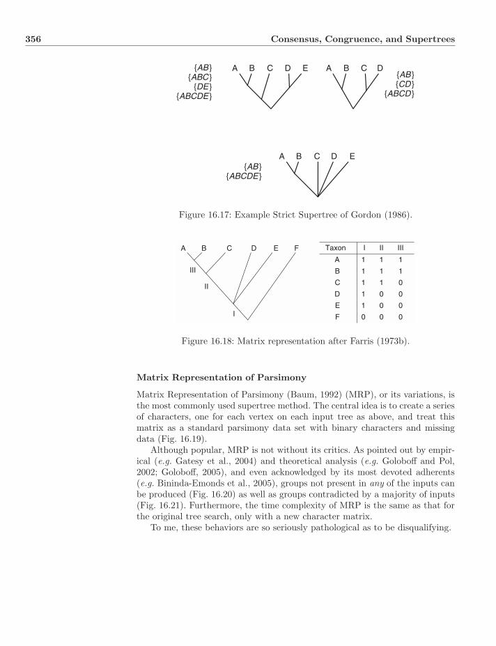
356 Consensus, Congruence, and Supertrees
A B C D E A B C D
A B C D E
{AB}{ABC}
{DE}{ABCDE}
{AB}{CD}
{ABCD}
{AB}{ABCDE}
Figure 16.17: Example Strict Supertree of Gordon (1986).
A B C D E F
I
II
III
Taxon I II III
A 1 1
B 1 1
C 1 0
D 1 0
E 1 0
F 0
1
1
1
0
0
0 0
Figure 16.18: Matrix representation after Farris (1973b).
Matrix Representation of Parsimony
Matrix Representation of Parsimony (Baum, 1992) (MRP), or its variations, isthe most commonly used supertree method. The central idea is to create a seriesof characters, one for each vertex on each input tree as above, and treat thismatrix as a standard parsimony data set with binary characters and missingdata (Fig. 16.19).
Although popular, MRP is not without its critics. As pointed out by empir-ical (e.g. Gatesy et al., 2004) and theoretical analysis (e.g. Goloboff and Pol,2002; Goloboff, 2005), and even acknowledged by its most devoted adherents(e.g. Bininda-Emonds et al., 2005), groups not present in any of the inputs canbe produced (Fig. 16.20) as well as groups contradicted by a majority of inputs(Fig. 16.21). Furthermore, the time complexity of MRP is the same as that forthe original tree search, only with a new character matrix.
To me, these behaviors are so seriously pathological as to be disqualifying.
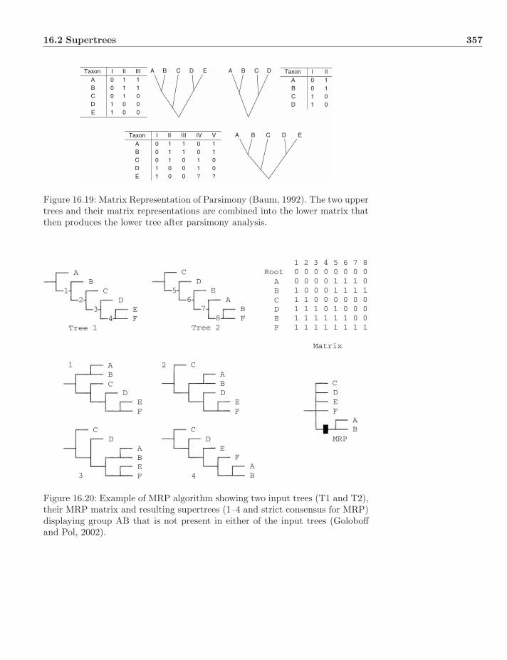
16.2 Supertrees 357
A B C D E A B C D
A B C D E
Taxon I IIA 0B 0C 1D 1
1100
Taxon I II III IV VA 0 1 1B 0 1 1C 0 0 0D 1 0 0E 1
11100 0
0011? ?
Taxon I II IIIA 0 1B 0 1C 0 0D 1 0E 1
11100 0
Figure 16.19: Matrix Representation of Parsimony (Baum, 1992). The two uppertrees and their matrix representations are combined into the lower matrix thatthen produces the lower tree after parsimony analysis.
A
A
C
C C
C C
C
D
D D
D D
D
EF
EF
E
E
F
F
EF
EF
1
1
2
2
3
3
4
4
Tree 1
B
B
AB
AB
AB
AB
CD
EA
BF8
76
5
Tree 2
MRP
Matrix
RootABCDEF
1 2 3 4 5 6 7 80 0 0 0 0 0 0 00 0 0 0 1 1 1 01 0 0 0 1 1 1 11 1 0 0 0 0 0 01 1 1 0 1 0 0 01 1 1 1 1 1 0 01 1 1 1 1 1 1 1
Figure 16.20: Example of MRP algorithm showing two input trees (T1 and T2),their MRP matrix and resulting supertrees (1–4 and strict consensus for MRP)displaying group AB that is not present in either of the input trees (Goloboffand Pol, 2002).
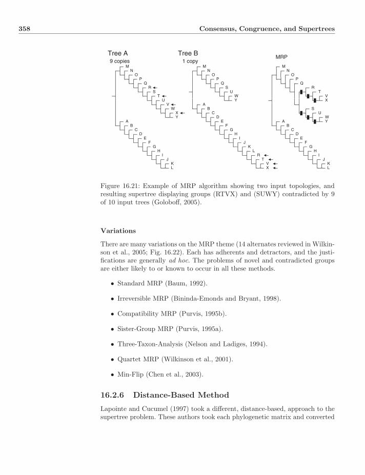
358 Consensus, Congruence, and Supertrees
9 copies 1 copyTree A Tree B
MRP
M M MN N N
O O OP P P
Q Q QR S R
S U TT W V
U Y XV A
W B SX C UY D W
A E A YB F B
C G CD H D
E I EF J F
G K GH L H
I R IJ T J
K V KL X L
Figure 16.21: Example of MRP algorithm showing two input topologies, andresulting supertree displaying groups (RTVX) and (SUWY) contradicted by 9of 10 input trees (Goloboff, 2005).
Variations
There are many variations on the MRP theme (14 alternates reviewed in Wilkin-son et al., 2005; Fig. 16.22). Each has adherents and detractors, and the justi-fications are generally ad hoc. The problems of novel and contradicted groupsare either likely to or known to occur in all these methods.
• Standard MRP (Baum, 1992).
• Irreversible MRP (Bininda-Emonds and Bryant, 1998).
• Compatibility MRP (Purvis, 1995b).
• Sister-Group MRP (Purvis, 1995a).
• Three-Taxon-Analysis (Nelson and Ladiges, 1994).
• Quartet MRP (Wilkinson et al., 2001).
• Min-Flip (Chen et al., 2003).
16.2.6 Distance-Based Method
Lapointe and Cucumel (1997) took a different, distance-based, approach to thesupertree problem. These authors took each phylogenetic matrix and converted

16.2 Supertrees 359
Input
Adams II
MRP Flavors
(a)
A
A
a) StandardMRP
e) Ave.Consensus
f) Ave.Dendrogram
g) Duplication-and-loss GTP
b) Irrev.MRP
c) PurvisMRP
d) MinFlipABCDEGFHIJKLMNOP
ABCDFEGHIJKLMNOP
ALFNBCHMDEGIJKOP
BCADFEGHIJK
ML
NOP
BCHAFLMNEGI
DJ
KOP
ABMCHFNDEGL
JI
KOP
IJABCDEFGHKLMNOP
FLBCHMNDKEGIJOP
BCDEFGHIJKLMNOP
ALFNBMCHDPKOEGIJ
(b)
Figure 16.22: Example behavior of a variety of supertree methods (Wilkinsonet al., 2005).
it into a distance. An overall average distance (d) among |T| datasets was thencreated from these values (Eq. 16.3).
dij =1|T|
|T |−1∑k=0
dkij (16.3)
The supertree itself is contructed via standard distance techniques such as min-imum evolution (Chapter 9; Fig. 16.23).
Macropus
Macropus
Macropus
Wallabia
0.67
4.3
3.5
7.7
0.090.38
0.730.23
0.100.00
1.280.36
0.93
1.75
0.20
0.090.19
1.58
0.69
1.26
2.04
3.39
0.361.55
1.55
11.80.3
8.2
3.3
4.71.4
7.3
2.311.0
16.0
25.0
9.0
10.1
10.1
0.8
2.4
1.0
2.3
2.8
0.83
1.15
1.20
0.90
1.54
3.40
0.29
0.110.04
0.40
0.10
0.24
1.00
Wallabia
Wallabia
Setonix
Setonix
Setonix
Dorcopsulus
Dorcopsulus
Dorcopsulus
Lagorchestes
Lagorchestes
Petrogale
Petrogale
Potorous
Potorous
Bettongia
Bettongia
Thylogale
Aepyprymnus
Aepyprymnus
Lagostrophus
LagostrophusOnychogalea
Onychogalea
Dendrolagus
Dendrolagus
Dendrolagus
Thylogale
Petrogale
Aepyprymnus
Figure 16.23: Distance supertree (Lapointe and Cucumel, 1997) based on mar-supial data.
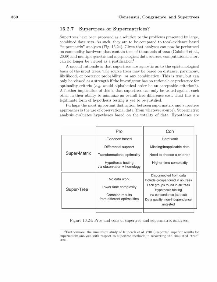
360 Consensus, Congruence, and Supertrees
16.2.7 Supertrees or Supermatrices?
Supertrees have been proposed as a solution to the problems presented by large,combined data sets. As such, they are to be compared to total-evidence based“supermatrix” analyses (Fig. 16.24). Given that analyses can now be performedon commodity hardware that contain tens of thousands of taxa (Goloboff et al.,2009) and multiple genetic and morphological data sources, computational effortcan no longer be viewed as a justification4.
A second rationale is that supertrees are agnostic as to the epistemologicalbasis of the input trees. The source trees may be based on distance, parsimony,likelihood, or posterior probability—or any combination. This is true, but canonly be viewed as a strength if the investigator has no rationale or preference foroptimality criteria (e.g. would alphabetical order be an acceptable criterion?).A further implication of this is that supertrees can only be tested against eachother in their ability to minimize an overall tree difference cost. That this is alegitimate form of hypothesis testing is yet to be justified.
Perhaps the most important distinction between supermatrix and supertreeapproaches is the use of observational data (from whatever source). Supermatrixanalysis evaluates hypotheses based on the totality of data. Hypotheses are
Super-Matrix
Super-Tree
Pro Con
Evidence-based
Differential support
Transformational optimality
Hypothesis testingvia observation = homology
Hard work
Missing/Inapplicable data
Need to choose a criterion
Higher time complexity
Disconnected from data
Include groups found in no trees
Lack groups found in all trees
Hypothesis testing
via concordance (at best)
Data quality, non-independence
untested
No data work
Lower time complexity
Combine resultsfrom different optimalities
Figure 16.24: Pros and cons of supertree and supermatrix analyses.
4Furthermore, the simulation study of Kupczok et al. (2010) reported superior results forsupermatrix analysis with respect to supertree methods in recovering the simulated “true”tree.
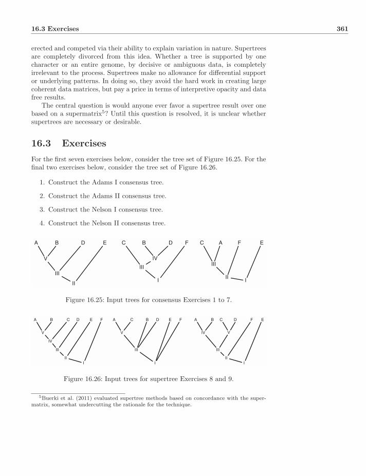
16.3 Exercises 361
erected and competed via their ability to explain variation in nature. Supertreesare completely divorced from this idea. Whether a tree is supported by onecharacter or an entire genome, by decisive or ambiguous data, is completelyirrelevant to the process. Supertrees make no allowance for differential supportor underlying patterns. In doing so, they avoid the hard work in creating largecoherent data matrices, but pay a price in terms of interpretive opacity and datafree results.
The central question is would anyone ever favor a supertree result over onebased on a supermatrix5? Until this question is resolved, it is unclear whethersupertrees are necessary or desirable.
16.3 Exercises
For the first seven exercises below, consider the tree set of Figure 16.25. For thefinal two exercises below, consider the tree set of Figure 16.26.
1. Construct the Adams I consensus tree.
2. Construct the Adams II consensus tree.
3. Construct the Nelson I consensus tree.
4. Construct the Nelson II consensus tree.
A B D E
II
III
V
C B D F
I
III
C A F E
III
IIIIV
Figure 16.25: Input trees for consensus Exercises 1 to 7.
A B C D E F
III
III
IV
V
A C B D E F
I
III
V
A B C D F E
III
III
IV V
Figure 16.26: Input trees for supertree Exercises 8 and 9.
5Buerki et al. (2011) evaluated supertree methods based on concordance with the super-matrix, somewhat undercutting the rationale for the technique.

362 Consensus, Congruence, and Supertrees
5. Construct the Majority Rule consensus tree.
6. Construct the Strict consensus tree.
7. Construct the Semi-Strict consensus tree.
8. Construct the MinCut supertree.
9. Construct the MRP supertree.
10. What is your position in the supermatrix–supertree debate?

Part V
Applications

Chapter 17
Clocks and Rates
Since Zuckerkandl and Pauling (1962, 1965), the dating of phylogenies withmolecular data has been a siren call. At first, the “molecular clock” was em-braced (by some) and used in simple linear dating based on the regression ofmolecular distance and one or more fixed dates based on fossils or vicariantevents. More recently, this has become more sophisticated with the use of mul-tiple rates and sequence change models. The goal is the same, and perhaps justas elusive.
Emil Zuckerkandl
17.1 The Molecular Clock
Zuckerkandl and Pauling (1962) examined vertebrate hemoglobin protein se-quences and noted the approximate constancy of changes in lineages dated withfossils from the presumed root to observed extant taxa. From this, they proposedan extrapolation to all molecules and lineages, stating that such molecular ana-lysis could date events about which we have no fossil information.
Linus Pauling(1901–1994)
It is possible to evaluate very roughly and tentatively the time thathas elapsed since any of the hemoglobin chains present in a givenspecies and controlled by non-allelic genes diverged from a commonchain ancestor. ... From paleontological evidence it may be estimatedthat the common ancestor of man and horse lived in the Cretaceousor possibly the Jurassic period, say between 100 and 160 millionyears ago. ... the presence of 18 differences between human and horseα-chains would indicate that each chain had 9 evolutionary effectivemutations in 100 to 160 millions of years. This yields a figure of11 to 18 million years per amino acid substitution in a chain ofabout 150 amino acids, with a medium figure of 14.5 million years.(Zuckerkandl and Pauling, 1962)1
1More can be found on the development and controversies over attribution in Morgan(1998).
Systematics: A Course of Lectures, First Edition. Ward C. Wheeler.c© 2012 Ward C. Wheeler. Published 2012 by Blackwell Publishing Ltd.
17.2 Dating 365
Zuckerkandl and Pauling did not go into great detail in their analysis, and laterauthors expanded upon this idea to both general molecular calibration and“neutral” molecular evolution (Kimura, 1983).
17.2 Dating
Before immersing ourselves in rate models and tests, it is worth returning tothe nature of the dating process used to calibrate molecular time analyses.
First, as Hennig (1966) described, if a fossil date is known for a taxon, itssister taxon must have been present at that time as well. This is due to the simplelogic of lineage splitting. When a lineage splits, two (sister) taxa are created atthe same time, hence have the same age. Furthermore, if two sister lineageshave been dated, the older date applies to both lineages. All age scenarios arecompatible with all trees. The sister-taxon relationships, and hence minimumtaxon age dates, may change, but dating scenarios do not discriminate amongtrees. This idea has been developed further into the ghost taxon concept (Norell,1987, 1992) for estimating paleo-diversity.
Second, fossil dates yield minimum ages. Fossilization is not a high proba-bility event, and the chance that this occurred immediately following a splittingevent is impossibly small. Furthermore, the fact that the fossil specimen is rec-ognizable as a member of a particular lineage implies that enough time hasintervened to allow for the acquisition of apomorphies. Again, unlikely in theimmediate aftermath of a splitting event.
Third, ages are not absolute, precise values. Many dates are relative (stratum-based), or derived from radiometric dating above and below (not exactly at) thespecimen. Additionally, the dating methods themselves are not without measure-ment error. These factors are discussed in greater detail below.
Fourth, vicariance-based dates have the same sort of imprecision of radio-metric dates, compounded by uncertainty in timing and sequence of land-masssplitting and union. An additional factor is the confounding effect of dispersal.Vicariance is not the only means to account for taxonomic distributions, anddispersal may have occurred well after dramatic events (e.g. primates found inSouth America and Africa are well supported to have a more recent shared his-tory than the land masses). Furthermore, lineage splitting could have occurredwell before that of the land mass. In summary, lineages could have split before,during, or after tectonic change and not necessarily in sync.
17.3 Testing Clocks
17.3.1 Langley–Fitch
The first test of clock like behavior in molecular data was that of Langley andFitch (1974). This method treats amino-acids (or other sequence data) as non-additive (Fitch, 1971) characters. Parsimonious character changes are assignedto each of the edges of the (given or reconstructed) tree. These values are used toestimate the edge parameters under a (now standard) Poisson process likelihood

366 Clocks and Rates
10 20 30 40 50 60 70 80 90 100 110 120 130 190 200 210
10
11.4
20.9
3
5
6
0.6
0.8
1.2
1.2
1.2
0.7
0.7
1.4
1.4
1.4
14
15
1.7
3.216
171.5
0.9
0.7
0.70.8
121.9
1.8
1.3
1.51.3
111.7
9
8
7
2.0
1.0
1.0
0.5
0.8
0.810
1.1
13
4
HUMAN
GORILLA
GIBBON
MONKEY
RODENT
RABBIT
DOG
HORSE
DONKEY
PIG
LLAMA
SHEEP
GOAT
COW
KANGAROO
CHICKEN
FROG
FISH
20 30 40 50 60 70 80 90 100 110 120 130 190 200 210
Figure 17.1: Langley and Fitch (1974) “observed” and corrected α and βhemoglobins, cytochrome c, and fibrinopeptide A edge lengths.
Uncorrected
χ2 (df ) (df ) P<P< χ2
102.7 102.7(62) (62)10−3 10−3
63.0 48.7 0.002(26) (24)10−4
165.7 151.4(88) (86)10−5 10−4
Corrected
Among proteins within legs(relative rates)
Among legs over proteins(total rates)
Total
Figure 17.2: Langley and Fitch (1974) test of clocklike behavior of α and βhemoglobins, cytochrome c, and fibrinopeptide A.
model (Fig. 17.1). The clock test in the model is based on the proportionalityof probabilistic change to “observed” (actually inferred) parsimony changes.The proportionality of change over the edges of the tree is tested against a χ2
distribution with 2n − 3 degrees of freedom for n taxa (Fig. 17.2).With this method, Fitch and Langley rejected clocklike behavior among the
vertebrate lineages and among proteins. They did, however, say that the impliedmolecular dates correlated well with paleontological dating.
17.3.2 Farris
Farris (1981) tested (and attacked) the clock idea in a more direct and simplemanner. If there were a molecular clock, at least in the strict sense, the distancedata would be ultrametric (or at least additive; Sect. 9.3). Furthermore, if this
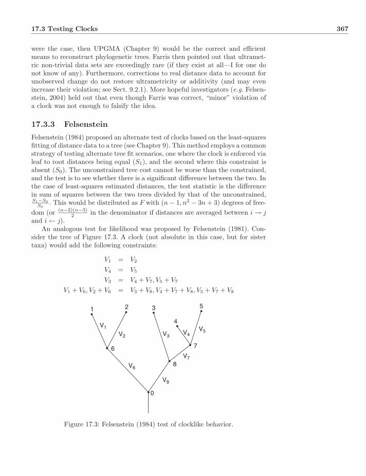
17.3 Testing Clocks 367
were the case, then UPGMA (Chapter 9) would be the correct and efficientmeans to reconstruct phylogenetic trees. Farris then pointed out that ultramet-ric non-trivial data sets are exceedingly rare (if they exist at all—I for one donot know of any). Furthermore, corrections to real distance data to account forunobserved change do not restore ultrametricity or additivity (and may evenincrease their violation; see Sect. 9.2.1). More hopeful investigators (e.g. Felsen-stein, 2004) held out that even though Farris was correct, “minor” violation ofa clock was not enough to falsify the idea.
17.3.3 Felsenstein
Felsenstein (1984) proposed an alternate test of clocks based on the least-squaresfitting of distance data to a tree (see Chapter 9). This method employs a commonstrategy of testing alternate tree fit scenarios, one where the clock is enforced vialeaf to root distances being equal (S1), and the second where this constraint isabsent (S0). The unconstrained tree cost cannot be worse than the constrained,and the test is to see whether there is a significant difference between the two. Inthe case of least-squares estimated distances, the test statistic is the differencein sum of squares between the two trees divided by that of the unconstrained,S1−S0
S0. This would be distributed as F with (n − 1, n2 − 3n + 3) degrees of free-
dom (or (n−2)(n−3)2 in the denominator if distances are averaged between i → j
and i ← j).An analogous test for likelihood was proposed by Felsenstein (1981). Con-
sider the tree of Figure 17.3. A clock (not absolute in this case, but for sistertaxa) would add the following constraints:
V1 = V2
V4 = V5
V3 = V4 + V7, V5 + V7
V1 + V6, V2 + V6 = V3 + V8, V4 + V7 + V8, V5 + V7 + V8
1
V1
V2
V6
V3V4
V5
V7
V8
0
8
6 7
2 3
4
5
Figure 17.3: Felsenstein (1984) test of clocklike behavior.
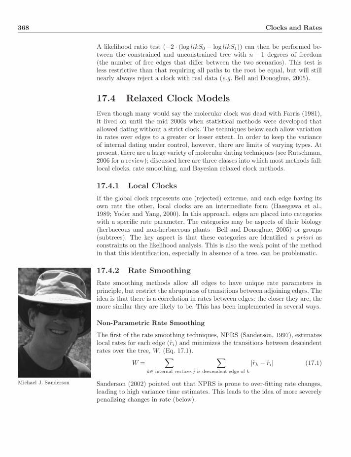
368 Clocks and Rates
A likelihood ratio test (−2 · (log likS0 − log likS1)) can then be performed be-tween the constrained and unconstrained tree with n − 1 degrees of freedom(the number of free edges that differ between the two scenarios). This test isless restrictive than that requiring all paths to the root be equal, but will stillnearly always reject a clock with real data (e.g. Bell and Donoghue, 2005).
17.4 Relaxed Clock Models
Even though many would say the molecular clock was dead with Farris (1981),it lived on until the mid 2000s when statistical methods were developed thatallowed dating without a strict clock. The techniques below each allow variationin rates over edges to a greater or lesser extent. In order to keep the varianceof internal dating under control, however, there are limits of varying types. Atpresent, there are a large variety of molecular dating techniques (see Rutschman,2006 for a review); discussed here are three classes into which most methods fall:local clocks, rate smoothing, and Bayesian relaxed clock methods.
17.4.1 Local Clocks
If the global clock represents one (rejected) extreme, and each edge having itsown rate the other, local clocks are an intermediate form (Hasegawa et al.,1989; Yoder and Yang, 2000). In this approach, edges are placed into categorieswith a specific rate parameter. The categories may be aspects of their biology(herbaceous and non-herbaceous plants—Bell and Donoghue, 2005) or groups(subtrees). The key aspect is that these categories are identified a priori asconstraints on the likelihood analysis. This is also the weak point of the methodin that this identification, especially in absence of a tree, can be problematic.
17.4.2 Rate Smoothing
Rate smoothing methods allow all edges to have unique rate parameters inprinciple, but restrict the abruptness of transitions between adjoining edges. Theidea is that there is a correlation in rates between edges: the closer they are, themore similar they are likely to be. This has been implemented in several ways.
Non-Parametric Rate Smoothing
The first of the rate smoothing techniques, NPRS (Sanderson, 1997), estimateslocal rates for each edge (ri) and minimizes the transitions between descendentrates over the tree, W, (Eq. 17.1).
W =∑
k∈ internal vertices
∑j is descendent edge of k
|rk − ri| (17.1)
Michael J. Sanderson Sanderson (2002) pointed out that NPRS is prone to over-fitting rate changes,leading to high variance time estimates. This leads to the idea of more severelypenalizing changes in rate (below).
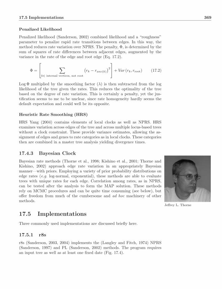
17.5 Implementations 369
Penalized Likelihood
Penalized likelihood (Sanderson, 2002) combined likelihood and a “roughness”parameter to penalize rapid rate transitions between edges. In this way, themethod reduces rate variation over NPRS. The penalty, Φ, is determined by thesum of squares of rate differences between adjacent edges, augmented by thevariance in the rate of the edge and root edge (Eq. 17.2).
Φ =
⎡⎣ ∑
k∈ internal vertices, not root
(rk − ranc(k)
)2
⎤⎦ + Var (rk, rroot) (17.2)
Log Φ multiplied by the smoothing factor (λ) is then subtracted from the loglikelihood of the tree given the rates. This reduces the optimality of the treebased on the degree of rate variation. This is certainly a penalty, yet the jus-tification seems to me to be unclear, since rate homogeneity hardly seems thedefault expectation and could well be its opposite.
Heuristic Rate Smoothing (HRS)
HRS Yang (2004) contains elements of local clocks as well as NPRS. HRSexamines variation across edges of the tree and across multiple locus-based treeswithout a clock constraint. These provide variance estimates, allowing the as-signment of edges and genes to rate categories as in local clocks. These categoriesthen are combined in a master tree analysis yielding divergence times.
17.4.3 Bayesian Clock
Bayesian rate methods (Thorne et al., 1998; Kishino et al., 2001; Thorne andKishino, 2002) approach edge rate variation in an appropriately Bayesianmanner—with priors. Employing a variety of prior probability distributions onedge rates (e.g. log-normal, exponential), these methods are able to evaluatetrees with unique rates for each edge. Correlation among rates, as in NPRS,can be tested after the analysis to form the MAP solution. These methodsrely on MCMC procedures and can be quite time consuming (see below), butoffer freedom from much of the cumbersome and ad hoc machinery of othermethods.
Jeffrey L. Thorne
17.5 Implementations
Three commonly used implementations are discussed briefly here.
17.5.1 r8s
r8s (Sanderson, 2003, 2004) implements the (Langley and Fitch, 1974) NPRS(Sanderson, 1997) and PL (Sanderson, 2002) methods. The program requiresan input tree as well as at least one fixed date (Fig. 17.4).
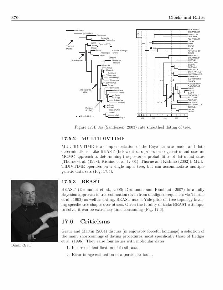
370 Clocks and Rates
Marchantia
LycopodiumEquisetum
MARCHANTIALYCOPODIUM
EQUISETUMOSMUNDAPOLYPODIUMCYCAS
CYC
LP
CON
AG
DUDIC
S
400 300 200 100 0
D C P J K TTR
ZAMIAGINKO
PICEAPOOOCARPUSTAXUSEPHEDRAWELWITSCHIAGNETUMSAURURUSDRIMYSMAGNOLIAEUPOMATIACHLORANTHUSAUSTROBALEYANYMPHAEACALYCANTHUSPERSEA
PACHYSANDRARANUNCULUSPISUM
FAGUSCARYAENKIANTHUSNICOTANANELUMBOPLATANUSSPATHIPHYLLUMSERENOA
LILIUMORYZA
OsmundaPolypodium
Cycas
GinkgoPicea
Podocarpus
Ephedra
WelwitschiaGneturn
SaururusDrimysMagnolia
EupomatiaChloranthus
Austrobaileya
NymphaeaCalycanthus
PerseaPachysandra
RanunculusPisum
FagusCarya
EnkianthusNicotiana
NelumboPlatanus
Spathiphyllum
SerenoaLilium
Oryza
Cycads (CYC)VascularPlants
Seed Plants
Anglosperms(AG)
Eudicots(EUDIC)
10 substitutions
Conifers & Ginkgo(CON)
Taxus
Zamia
Figure 17.4: r8s (Sanderson, 2003) rate smoothed dating of tree.
17.5.2 MULTIDIVTIME
MULTIDIVTIME is an implementation of the Bayesian rate model and datedeterminations. Like BEAST (below) it sets priors on edge rates and uses anMCMC approach to determining the posterior probabilities of dates and rates(Thorne et al. (1998); Kishino et al. (2001); Thorne and Kishino (2002)). MUL-TIDIVTIME operates on a single input tree, but can accommodate multiplegenetic data sets (Fig. 17.5).
17.5.3 BEAST
BEAST (Drummon et al., 2006; Drummon and Rambaut, 2007) is a fullyBayesian approach to tree estimation (even from unaligned sequences via Thorneet al., 1992) as well as dating. BEAST uses a Yule prior on tree topology favor-ing specific tree shapes over others. Given the totality of tasks BEAST attemptsto solve, it can be extremely time consuming (Fig. 17.6).
17.6 Criticisms
Graur and Martin (2004) discuss (in enjoyably forceful language) a selection ofthe many shortcomings of dating procedures, most specifically those of Hedgeset al. (1996). They raise four issues with molecular dates:
Daniel Graur 1. Incorrect identification of fossil taxa.
2. Error in age estimation of a particular fossil.
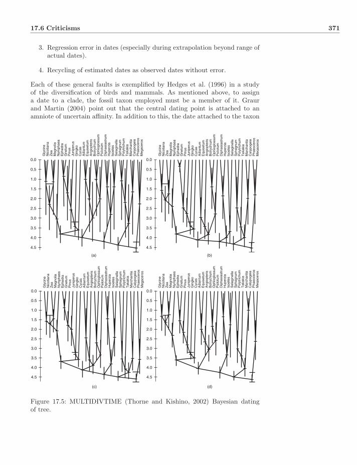
17.6 Criticisms 371
3. Regression error in dates (especially during extrapolation beyond range ofactual dates).
4. Recycling of estimated dates as observed dates without error.
Each of these general faults is exemplified by Hedges et al. (1996) in a studyof the diversification of birds and mammals. As mentioned above, to assigna date to a clade, the fossil taxon employed must be a member of it. Graurand Martin (2004) point out that the central dating point is attached to anamniote of uncertain affinity. In addition to this, the date attached to the taxon
0.0
Gly
cine
Nic
otia
naZ
eaM
agno
liaN
ymph
aea
Eph
edra
Gne
tum
Pin
usJu
nipe
rus
Gin
gko
Cyc
asA
dian
tum
Equ
iset
umA
ngio
pter
isB
otry
chiu
mO
phio
glos
sum
Psi
lotu
mD
ipha
sias
trum
Hup
erzi
aIs
oete
sS
elag
inel
laS
phag
num
Pol
ytric
hum
Tak
akia
Mar
chan
tiaC
alyp
ogei
aP
haeo
cero
sM
egac
eros
Gly
cine
Nic
otia
naZ
eaM
agno
liaN
ymph
aea
Eph
edra
Gne
tum
Pin
usJu
nipe
rus
Gin
gko
Cyc
asA
dian
tum
Equ
iset
umA
ngio
pter
isB
otry
chiu
mO
phio
glos
sum
Psi
lotu
mD
ipha
sias
trum
Hup
erzi
aIs
oete
sS
elag
inel
laS
phag
num
Pol
ytric
hum
Tak
akia
Mar
chan
tiaC
alyp
ogei
aP
haeo
cero
sM
e gac
eros
Gly
cine
Nic
otia
naZ
eaM
agno
liaN
ymph
aea
Eph
edra
Gne
tum
Pin
usJu
nipe
rus
Gin
gko
Cyc
asA
dian
tum
Equ
iset
umA
ngio
pter
isB
otry
chiu
mO
phio
glos
sum
Psi
lotu
mD
ipha
sias
trum
Hup
erzi
aIs
oete
sS
elag
inel
laS
phag
num
Pol
ytric
hum
Tak
akia
Mar
chan
tiaC
alyp
ogei
aP
haeo
cero
sM
egac
eros
0.5
1.0
1.5
2.0
2.5
3.0
3.5
4.0
4.5
(a)
0.0
0.5
1.0
1.5
2.0
2.5
3.0
3.5
4.0
4.5
(b)
0.0
0.5
1.0
1.5
2.0
2.5
3.0
3.5
4.0
4.5
(c)
0.0
0.5
1.0
1.5
2.0
2.5
3.0
3.5
4.0
4.5
(d)
Figure 17.5: MULTIDIVTIME (Thorne and Kishino, 2002) Bayesian datingof tree.
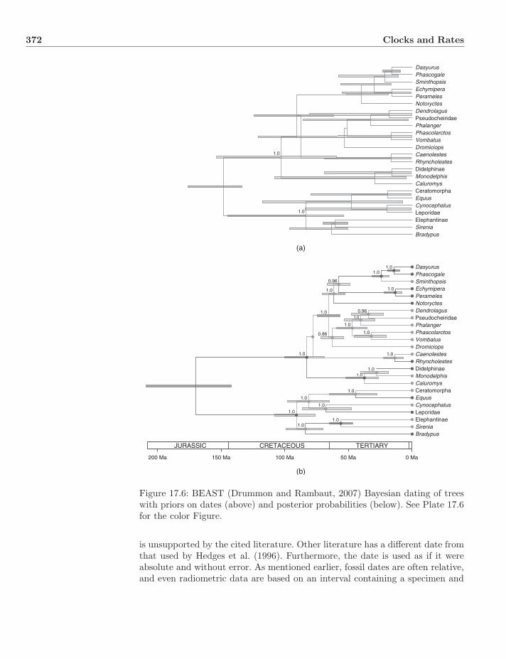
372 Clocks and Rates
1.0
DasyurusPhascogaleSminthopsisEchymiperaPeramelesNotoryctesDendrolagusPseudocheiridaePhalangerPhascolarctosVombatusDromiciopsCaenolestesRhyncholestesDidelphinaeMonodelphisCaluromysCeratomorphaEquusCynocephalusLeporidaeElephantinaeSireniaBradypus
DasyurusPhascogaleSminthopsisEchymiperaPeramelesNotoryctesDendrolagusPseudocheiridaePhalangerPhascolarctosVombatusDromiciopsCaenolestesRhyncholestesDidelphinaeMonodelphisCaluromysCeratomorphaEquusCynocephalusLeporidaeElephantinaeSireniaBradypus
1.0
1.01.0
1.0
1.0
1.0
1.0
1.0
1.0
1.0
1.0
1.0
1.0
1.0
1.0
1.0
1.0
200 Ma 150 Ma
JURASSIC
(a)
(b)
CRETACEOUS TERTIARY
100 Ma 50 Ma 0 Ma
1.0
0.86
1.0
0.96
0.96
Figure 17.6: BEAST (Drummon and Rambaut, 2007) Bayesian dating of treeswith priors on dates (above) and posterior probabilities (below). See Plate 17.6for the color Figure.
is unsupported by the cited literature. Other literature has a different date fromthat used by Hedges et al. (1996). Furthermore, the date is used as if it wereabsolute and without error. As mentioned earlier, fossil dates are often relative,and even radiometric data are based on an interval containing a specimen and
17.7 Molecular Dates? 373
are further subject to observational error as are all aspects of experimentalscience. These errors are exacerbated by incorrect extrapolation variance inthe use of dating regressions and (perhaps worst of all) estimated dates used(without error) as if they were observed.
Another salutary case is that of Near et al. (2005), reanalyzed by Parham andIrmis (2008). Of the 17 literature dates cited in their dating of turtle divergences,15 of the dates are not even mentioned in the literature cited, and two are usedwith a spurious precision of 1 part in 2000 (when authors used words such as“about” and “approximately” to characterize the dates). This was coupled withan analysis-free and idiosyncratic placement of a key taxon making their datingextremely suspect.
There are two sorts of problems with the above examples: those that areinherent to the methods, and those that come about by misuse, poor scholar-ship, or over-interpretation of results. Obviously, it is not the fault of methods ortheir implementations if they are improperly used, but this still leaves the crucialfactor of error analysis. Although improving, the incorporation of the myriadsources of experimental, topological, and statistical (i.e. regression) error mustbe incorporated into the determination of dates. When they are, errors of mag-nitude comparable to or even exceeding the estimated dates can be achieved(Graur and Martin, 2004; Pulquerio and Nichols, 2006).
17.7 Molecular Dates?
Recent Bayesian methods have made great progress in allowing edge-specific rateparameters. This does come at the usual Bayesian price of the necessary priordistributions. What is a reasonable prior for evolutionary rates on tree edges?Given our lack of knowledge, sampling, lineage, environmental, and locus specific(among myriad known and unknown other) effects, the uniform distributionwould seem as appropriate as log-normal or exponential. Such a prior is likelyto lead to large uncertainty in estimated dates, leaving us where we were initially,with rock solid, if limited, minimum ages based on sister taxon relationships.
The central question remains—can hypotheses be falsified with “molecular”dates? Are these estimates sufficiently precise to adjudicate between biogeo-graphic or other scenarios? This does not appear to be the case at present, buttime will tell.
17.8 Exercises
1. Should dates be used in tree construction? What would be the optimalitycriterion?
2. How much variation in a date can be allowed and the date still be useful?
3. What are the pros and cons of different prior distributions for edge rateparameters?

Appendix A
Mathematical Notation
Commonly used mathematical symbols.
A = argmaxx f(x) A is set to the value of x that maximizes f(x).∑ba f(x) summation of f(x) from x = a to x = b.∏ba f(x) product of f(x) from x = a to x = b.
∀x ∈ X for all elements x contained in the set X such as x0, x1
etc.Xi the ith element in a collection (set or array) of objects
X such as x0, x1 etc.|X| the size of an object such as the cardinality (number of
elements) of a set or the length of an array.n! n factorial.
∏i=ni=2 i or n · (n − 1) · (n − 2) · . . . · 2.
X \ Y the set created by subtracting the elements of set Y fromset X.
|x| absolute value of x.R+ the set of positive real numbers.X ⊆ Y X is a subset of or equal to Y.X � Y X is not a subset of or equal to Y.X � Y X is a proper subset of Y.�X� the largest integer ≤ than X.X ∩ Y intersection of sets X and Y.X ∪ Y union of sets X and Y.∅ the empty set.X ← Y assignment of Y to X.(xy
)binomial expansion of x and y = x!
y!(x−y)! .log∗ x iterated logarithm. The number of applications of log
until the result is ≤ 1.
Systematics: A Course of Lectures, First Edition. Ward C. Wheeler.c© 2012 Ward C. Wheeler. Published 2012 by Blackwell Publishing Ltd.

Mathematical Notation 375
Ac complement of set A (S \ A).A ∴ B A therefore B.ab|cd unrooted tree ((a, b)(c, d)).a|bc rooted tree (a(b, c)).x ∈ (a, b) values x in the interval a < x < b.x ∈ [a, b] values x in the interval a ≤ x ≤ b.a ∝ b a is proportional to b.∃ there exists.� there does not exist.
Bibliography
Achtman, M., van der Ende, A., Zhu, P., Koroleva, I. S., Kusecek, B., Morelli,G., Schuurman, I. G., Brieske, N., Zurth, K., Kostyukov, N. N., and Platonov,A. E. 2001. Molecular epidemiology of serogroup A meningitis in Moscow,1969–1997. Emerging Infectious Disease 7:420–427.
Adams, E. N. 1972. Consensus techniques and the comparison of taxonomictrees. Syst. Zool. 21:390–397.
Aho, A. V., Sagiv, Y., Szymanski, T. G., and Ullman, J. D. 1981. Inferring atree from lowest common ancestors with an application to the optimizationof relational expressions. SIAM J. Comput. 10:405–421.
Akaike, H. 1974. A new look at the statistical model identification. IEEE Trans.Autom. Contr. ACM 19:716–723.
Allen, B. and Steel, M. 2001. Subtree transfer operations and their inducedmetrics on evolutionary trees. Annals of Combinatorics 5:1–13.
Aristotle 360BCE. History of animals. http://classics.mit.edu/Aristotle. Trans-lated by D’Arcy Wentworth Thompson.
Bachman, P. 1894. Die analytische Zahlentheorie. Teubner, Leipzig.
Bader, D. A., Moret, B. M. E., Warnow, T., Wyman, S. K., Yan, M.,Tang, J., Siepel, A. C., and Caprara, A. 2002. GRAPPA, version 2.0.http://www.cs.unm.edu/moret/grappa. Technical report, University of NewMexico.
Baker, R. H. and DeSalle, R. 1997. Multiple sources of character informationand the phylogeny of Hawaiian drosophilids. Syst. Biol. 46:654–673.
Bandelt, H. J. 1990. Recognition of tree metrics. SIAM J. Discrete Math. 3:1–6.
Bandelt, H. J. and Dress, A. W. M. 1986. Reconstructing the shape of a treefrom observed dissimilarity data. Adv. Appl. Math. 7:309–343.
Bandelt, H. J. and Dress, A. W. M. 1992a. A canonical decomposition theoryfor metrics on a finite set. Adv. Math. 92:47–105.
Systematics: A Course of Lectures, First Edition. Ward C. Wheeler.c© 2012 Ward C. Wheeler. Published 2012 by Blackwell Publishing Ltd.

BIBLIOGRAPHY 377
Bandelt, H. J. and Dress, A. W. M. 1992b. Split decomposition: A new anduseful approach to phylogenetic analysis of distance data. Mol. Phylo. Evol.1:242–252.
Barry, D. and Hartigan, J. 1987. Statistical analysis of hominid molecular evo-lution. Stat. Sci. 2:191–210.
Bartley, W. W. 1976. The philosophy of Karl Popper. Philosophia 6:3–4.
Batzoglou, S. 2005. The many faces of sequence alignment. Brief. Bioinform.6:6–22.
Baum, B. R. 1992. Combining trees as a way of combining data sets for phyloge-netic inference, and the desirability of combining gene trees. Taxon 41:3–10.
Baum, L. E., Petrie, T., Soules, G., and Weiss, N. 1970. A maximization tech-nique occurring in the statistical analysis of probabilistic functions of Markovchains. Ann. Math. Statist. 41:164–171.
Bayes, T. 1763. An essay towards solving a problem in the doctrine of chances.Philos. T. Roy. Soc. 53:370–418.
Bell, C. D. and Donoghue, M. J. 2005. Dating the Dipsicales: comparing models,genes, and evolutionary implications. Amer. Jour. Botany 92:284–296.
Bellman, R. E. 1953. An introduction to the theory of dynamic programming.Technical Report R-245, The RAND Corporation.
Belon, P. 1555. L’Histoire de la nature des oyseaux. Chez Guillaume Cauellat,Paris.
Bininda-Emonds, O. R., Beck, R. M., and Purvis, A. 2005. Getting to the rootsof matrix representation. Syst. Biol. 54:668–672.
Bininda-Emonds, O. R. P. and Bryant, H. N. 1998. Properties of matrix repre-sentation with parsimony analyses. Syst. Biol. 47:497–508.
Bininda-Emonds, O. R. P., Jeffrey, J. E., Coates, M. I., and Richardson, M. K.2002. From Haeckel to even-pairing: the evolution of developmental sequences.Theor. Biol. 121:297–320.
Bock, W. J. 1974. Philosophical foundations of classical evolutionary classifica-tion. Syst. Zool. 22:375–392.
Bock, W. J. 1977. Foundations and methods in evolutionary classification,pp. 851–895. In M. K. Hecht, P. C. Goody, and B. M. Hecht (eds.), MajorPatterns in Vertebrate evolution. Plenum Press, New York.
Bonet, M. L., St. John, K., Mahindru, R., and Amenta, N. 2006. Approximatingsubtree distances between phylogenies. J. Comput. Biol. 13:1419–1434.
378 BIBLIOGRAPHY
Boore, J. L. 2000. The duplication/random loss model for gene rearrangementexemplified by mitochondrial genomes of deuterostome animals, pp. 133–147.In D. Sankoff and J. Nadeau (eds.), Comparative genomics, computational bi-ology series, volume 1. Kluwer Academic Publishers, Dordrecht, Netherlands.
Boore, J. L., Collins, T. M., Stanton, D., Daehler, L. L., and Brown, W. M.1995. Deducing the pattern of arthropod phylogeny from mitochondrial DNArearrangements. Nature 376:163–165.
Boore, J. L., Lavrov, D. V., and Brown, W. M. 1998. Gene translocation linksinsects and crustaceans. Nature 392:667–668.
Bordewich, M., Linz, S., St. John, K., and Semple, C. 2007. A reduction al-gorithm for computing the hybridization number of two trees. EvolutionaryBioinformatics 3:86–98.
Bordewich, M. and Semple, C. 2005. On the computational complexity of therooted subtree prune and regraft distance. Ann. Combinatorics 8:409–423.
Boujenfa, K., Essoussi, N., and Limam, M. 2008. Comparison of phylogenetictrees of multiple protein sequence alignment methods. World Acad. of Sci.,Eng, and Tech. 44:322–327.
Boyden, A. 1973. Perspectives in Zoology. Pergamon Press, Oxford.
Brady, R. H. 1985. On the independence of systematics. Cladistics 1:113–126.
Bremer, K. 1988. The limits of amino acid sequence data in angiosperm phylo-genetic reconstruction. Evolution 42:795–803.
Bremer, K. 1990. Combinable component consensus. Cladistics 6:369–372.
Brent, R. P. 1973. Algorithms for Minimization without Derivatives, chapter 4.Prentice-Hall, Englewood Cliffs, NJ.
Bronn, H. G. 1858. Untersuchungen uber die Entwickelungs-Gesetze der organ-ischen Welt. E. Schweizerbart’sche Verlagshandlung, Stuttgart.
Bronn, H. G. 1861. Essai d’une response a la question de prix propose en 1850par l’academie des sciences pour le concours de 1853, et pius remise pour celuide 1856, savoir: Etudier les lois de la distribution des corps organises fossilesdans les differents terrains sedimentaires, suivant l’ordre de leur superposi-tion. Comptes Rendu Hebdomadaire des Seances de l’Academie des Sciences,Supplement 2:377–918.
Brundin, L. 1966. Transantarctic relationships and their significance, as evi-denced by chironomid midges with a monograph of the subfamilies Podono-midae and Aphroteniinae and the austral Heptagyiae. Kunliga SvenskaVetenskscapsacadamiens Handlingar 11:1–472.
Bryant, D. and Waddell, P. 1998. Rapid evaluation of least-squares and mini-mum evolution criteria on phylogenetic trees. Mol. Biol. Evol. 15:1346–1359.

BIBLIOGRAPHY 379
Buerki, S., Forest, F., and ans N. Alvarez, N. S. 2011. Comparative perfor-mance of supertree algorithms in large data sets using the soapberry family(Sapindaceae) as a case study. Syst. Biol. 60:32–44.
Buneman, P. 1971. The recovery of trees from measure of dissimilarity, pp.387–395. In F. R. Hodson, D. G. Kendall, and P. Tautau (eds.), Mathematicsand the archeological and historical sciences. Edinburgh University Press,Edinburgh.
Buneman, P. 1974. A note on metric properties on trees. J. Comb. Theory (B)17:48–50.
Camin, J. H. and Sokal, R. R. 1965. A method for deducing branching sequencesin phylogeny. Evolution 19:311–326.
Caprara, A. 1997. Sorting by reversals is difficult. In Proceedings of 1st Confer-ence Computational Molecular Biology, Santa Fe NM, pp. 78–83, New York.ACM Press.
Carpenter, J. M. 1996. Uninformative bootstrapping. Cladistics 12:177–181.
Carrillo, H. and Lipman, D. 1988. The multiple sequence alignment problem inbiology. SIAM J. Appl. Math. 48:1073–1082.
Cassis, G. and Schuh, R. T. 2009. Systematic methods, fossils, and relationshipswithin Heteroptera (Insecta). Cladistics 25:1–19.
Cavalli-Sforza, L. L. and Edwards, A. W. F. 1967. Phylogenetic analysis: modelsand estimation procedures. Evolution 21:550–570.
Cerny, V. 1985. A thermodynamical approach to the traveling salesman prob-lem: an efficient simulation algorithm. J. Optimiz. Theory App. 45:41–51.
Champion, R. 1985. The purpose of Popper. Melbourne Age Monthly Review.
Chang, J. T. 1996. Inconsistency of evolutionary tree topology reconstruc-tion methods when substitution rates vary across characters. Math. Bio.134:189–215.
Chase, M. W., Soltis, D. E., Olmstead, R. G., Morgan, D., Les, D. H., Mishler,B. D., Duvall, M. R., Price, R. A., Hills, H. G., Qiu, Y.-L., Kron, K. A., Rettig,J. H., Conti, E., Palmer, J. D., Manhart, J. R., Sytsma, K. J., Michaels, H. J.,Kress, W. J., Karol, K. G., Clark, W. D., Hedren, M., Gaut, B. S., Jansen,R. K., Kim, K.-J., Wimpee, C. F., Smith, J. F., Furnier, G. R., Strauss, S. H.,Xiang, Q.-Y., Plunkett, G. M., Soltis, P. S., Swensen, S. M., Willimas, S. E.,Gadek, P. A., Quinn, C. J., Eguiarte, L. E., Golenberg, E., Learn, G. H. J.,Graham, S. W., Barret, S. C. H., Dayanandan, S., and Albert, V. A. 1993.Phylogenetics of seed plants: An analysis of nucleotide sequences from theplastid gene RBCL. Ann. Mol. Bot. Gard. 80:528–580.

380 BIBLIOGRAPHY
Chaudhuri, K., Chen, K., Mihaescu, R., and Rao, S. 2006. On the tandemduplication–random loss model of genome rearrangement. In SODA ’06: Pro-ceedings of the seventeenth annual ACM-SIAM symposium on Discrete algo-rithm, pp. 564–570, New York, NY, USA. ACM.
Chen, D., Diao, L., Eulenstein, O., Fenandez-Baca, D., and Sanderson,M. J. 2003. Flipping: A supertree construction method, pp. 135–160. InM. Janowitz, F.-J. Lapointe, F. R. McMorris, B. Mirkin, and F. S. Roberts(eds.), Bioconsensus, DIMACS series in discrete mathematics and theoreticalcomputer science. American Mathematical Society, Providence, Rhode Island.
Chib, S. and Greenberg, E. 1995. Understanding the Metropolis–Hastings algo-rithm. American Statistician 49:327–335.
Church, A. 1936a. A note on the Entscheidungsproblem. J. Symbolic Logic1:40–41.
Church, A. 1936b. An unsolvable problem of elementary number theory. Am.J. Math. 58:345–363.
Church, A. and Rosser, J. B. 1936. Some properties of conversion. T. Am.Math. Soc. 39:472–482.
Coddington, J. and Scharff, N. 1994. Problems with zero-length branches.Cladistics 10:415–423.
Cormode, G. and Muthukrishnan, S. 2002. The string edit distance matchingproblem with moves. In SODA ’02: Proceedings of the thirteenth annualACM-SIAM symposium on Discrete algorithms, pp. 667–676. Society for In-dustrial and Applied Mathematics.
Cracraft, J. 1983. Species concepts and speciation analysis. Current Ornithologypp. 159–187.
Cracraft, J. 1989. Speciation and its ontology: the empirical consequences ofalternative species concepts for understanding patterns and processes of dif-ferentiation, pp. 28–59. In D. Otte and J. A. Endler (eds.), Speciation andits Consequences. Sinauer Associates, Sunderland, England.
Cracraft, J. 2000. Species concepts in theoretical and applied biology: a sys-tematic debate with consequences, pp. 3–14. In Q. D. Wheeler and R. Meier(eds.), Species Concepts and Phylogenetic Theory. Columbia University Press,New York.
Cuvier, G. 1812. Recherches sur les ossemens fossiles de quadrupedes. Deterville,Paris.
Dalevi, D. and Eriksen, N. 2008. Expected gene-order distances and modelselection in bacteria. Bioinformatics 24:1332–1338.
BIBLIOGRAPHY 381
Darling, A. C., Mau, B., Blattner, F. R., and Perna, N. T. 2004. Mauve: Multi-ple alignment of conserved genomic sequence with rearrangements. GenomeResearch 14:1394–1403.
Darwin, C. 1859a. Letter to J. D. Hooker.
Darwin, C. R. 1859b. On the Origin of Species by means of natural selection,or the preservation of favoured races in the struggle for life. John Murray,London, 1st edition.
Day, W. H. E. 1987. Computational complexity of inferring phylogenies fromdissimilarity matrices. B. Math. Biol. 49:461–467.
DeGroot, M. H. and Schervish, M. J. 2006. Probability and Statistics. Addison-Wesley, Boston, 3rd edition.
DePinna, M. G. 1991. Concepts and tests of homology in the cladistic paradigm.Cladistics 7:367–394.
Desper, R. and Gascuel, O. 2002. Fast and accurate phylogeny reconstruc-tion algorithms based on the minimum-evolution principle. J. Comp. Biol.9:687–705.
Desper, R. and Gascuel, O. 2007. The minimum evolution distance-based ap-proach to phylogenetic inference, pp. 1–32. In O. Gascuel (ed.), Mathematicsof Evolution and Phylogeny. Oxford University Press, Oxford.
Dobzhansky, T. 1937. Genetics and the Origin of Species. Columbia UniversityPress, New York.
Donoghue, M. J. 1985. A critique of the biological species concept and rec-comendations for a phylogenetic alternative. Bryologist 88:172–181.
Donoghue, M. J. and Kadereit, J. W. 1992. Walter Zimmerman and the growthof phylogenetic theory. Syst. Biol. 41:74–84.
Donoghue, M. J., Olmstead, R. G., Smith, J. F., and Palmer, J. D. 1992. Phylo-genetic relationships of Dipscales based on RBCL sequences. Ann. Mo. Bot.Gard. 79:333–345.
Dress, A., Huber, K. T., and Moulton, V. 2007. Some uses of the Farris trans-form in mathematics and phylogenetics. Annals of Combinatorics 11:1–37.
Dress, A. and Kruger, M. 1987. Parsimonious phylogenetic trees in metric spacesand simulated annealing. Adv. App. Math. 8:8–37.
Drummon, A. J., Ho, S. Y. W., Phillips, M. J., and Rambaut, A. 2006. Relaxedphylogenetics and dating with confidence. PLoS Biology 4:699–710.
Drummon, A. J. and Rambaut, A. 2007. Beast: Bayesian evolutionary analysisby sampling trees. BMC Evolutionary Biology 7:214.
382 BIBLIOGRAPHY
Dunn, C. W., Hejnol, A., Matus, D. Q., Pang, K., Browne, W. E., Smith, S. A.,Seaver, E., Rouse, G. W., Obst, M., Edgecombe, G. D., Sørensen, M. V.,Haddock, S. H., Schmidt-Rhaesa, A., Okusu, A., Kristensen, R. M., Wheeler,W. C., Martindale, M. Q., and Giribet, G. 2008. Broad phylogenomic sam-pling improves resolution of the animal tree of life. Nature 452:745–749.
Edgar, R. C. 2004a. MUSCLE: a multiple sequence alignment method withreduced time and space complexity. BMC Bioinformatics 5:113–132.
Edgar, R. C. 2004b. MUSCLE: multiple sequence alignment with high accuracyand high throughput. Nucleic Acids Res. 32:1792–1797.
Edgar, R. C. and Sjolander, K. 2003. SATCHMO: sequence alignment and treeconstruction using hidden Markov models. Bioinformatics 19:1404–1411.
Edwards, A. 1972. Likelihood. Cambridge University Press, Cambridge, Eng-land.
Edwards, A. W. F. 1970. Estimation of the branching points of a branchingdiffusion process. J. Royal Stat. Soc. B 32:155–174.
Efron, B. 1979. Bootstrap methods: another look at the jackknife. Ann. Stat.7:1–26.
Efron, B. and Tibshirani, R. 1993. An Introduction to the Bootstrap. Chapmanand Hall, Boca Raton, Florida.
Eldredge, N. and Cracraft, J. 1980. Phylogenetic Patterns and the EvolutionaryProcess. Columbia University Press, New York.
Erdos, P. L., Steel, M. A., Szekely, L., and Warnow, T. J. 1997. Construct-ing big trees from short sequences. In P. Degano, R. Gorrier, and A.Marchetti-Spaccalmela (eds.), Automata, Languages and Programming, 24thInternational Colloquium, ICALP’97, Bologna, Italy, pp. 827–837, Berlin.Springer-Verlag.
Estabrook, G. F. 1978. Some concepts for the estimation of evolutionary rela-tionships in systematic botany. Syst. Bot. 3:146–158.
Faith, D. P. 1991. Cladistic permutation tests for monophyly and nonmonophyly.Syst. Zool. 40:366–375.
Farris, J. S. 1969. On the cophenetic correlation coefficient. Syst. Zool.18:279–285.
Farris, J. S. 1970. A method for computing Wagner trees. Syst. Zool. 19:83–92.
Farris, J. S. 1973a. A probability model for inferring evolutionary trees. Syst.Zool. 22:250–256.
Farris, J. S. 1981. Distance data in phylogenetic analysis, pp. 3–23. In V. A.Funk and D. R. Brooks (eds.), Advances in Cladistics, volume 1. New YorkBotanical Garden, New York.
BIBLIOGRAPHY 383
Farris, J. S. 1983. The logical basis of phylogenetic analysis. In N. I. Platnick andV. A. Funk (eds.), Advances in cladistics, Proceedings of the second meeting ofthe Willi Hennig Society, volume 2, pp. 7–36, New York. Columbia UniversityPress.
Farris, J. S. 1988. Hennig86. Program and documentation distributed by theauthor.
Farris, J. S., Albert, V. A., Kallersjo, M., Lipscomb, D., and Kluge, A. G. 1996.Parsimony jackknifing outperforms neighbor-joining. Cladistics 12:99–124.
Farris, J. S., Kluge, A. G., and Eckardt, M. J. 1970. A numerical approach tophylogenetic systematics. Syst. Zool. 19:172–189.
Farris, S. J. 1972. Estimating phylogenetic trees from distance matrices. Am.Nat. 106:645–668.
Farris, S. J. 1973b. On comparing the shapes of taxonomic trees. Syst. Zool.22:50–54.
Farris, S. J. 1974. Formal definitions of paraphyly and polyphyly. Syst. Zool.23:548–554.
Farris, S. J. 1977. Phylogenetic analysis under Dollo’s law. Syst. Zool. 26:577–88.
Felsenstein, J. 1973. Maximum likelihood and minimum-steps methods for es-timating evolutionary trees from data on discrete characters. Syst. Zool.22:240–249.
Felsenstein, J. 1978. Cases in which parsimony or compatibility methods willbe positively misleading. Syst. Zool. 27:401–410.
Felsenstein, J. 1981. Evolutionary trees from DNA sequences: a maximum like-lihood approach. J. Mol. Evol. 17:368–376.
Felsenstein, J. 1984. Distance methods for inferring phylogenies: A justification.Evolution 38:16–24.
Felsenstein, J. 1985. Confidence limits on phylogenies: An approach using thebootstrap. Evolution 39:783–791.
Felsenstein, J. 1993. PHYLIP: Phylogeny Inference Package.
Felsenstein, J. 2004. Inferring Phylogenies. Sinauer Associates, Sunderland,MA.
Feng, D.-F. and Doolittle, R. F. 1987. Progressive sequence alignment as aprerequisite to correct phylogenetic trees. J. Mol. Evol. 25:351–360.
Feyerabend, P. K. 1975. Against Method. Verso, London.
Feyerabend, P. K. 1987. Farewell to Reason. Verso, London.
384 BIBLIOGRAPHY
Finden, C. and Gordon, A. 1985. Obtaining common pruned trees. J. Classifi-cation 2:255–276.
Fisher, R. A. 1912. On an absolute criterion for fitting frequency curves. Mess.Math. 41:155–160.
Fisher, R. A. 1950. Statistical methods for research workers. Oliver and Boyd,Edinburgh, 11th edition.
Fitch, W. M. 1970. Distinguishing homologous from analogous proteins. Syst.Zool. 19:99–113.
Fitch, W. M. 1971. Toward defining the course of evolution: minimum changefor a specific tree topology. Syst. Zool. 20:406–416.
Fitch, W. M. and Margoliash, E. 1967. Construction of phylogenetic trees.Science 155:279–284.
Fleissner, R., Metzler, D., and von Haeseler, R. 2005. Simultaneous statisticalmultiple alignment and phylogeny reconstruction. Syst. Biol. 54:548–561.
Foulds, L. R. and Graham, R. L. 1982. The Steiner problem in phylogeny isNP-complete. Adv. Appl. Math. 3:43–49.
Fraser, A. and Burnell, D. 1970. Computer Models in Genetics. McGraw-Hill,New York.
Freudenstein, J. V., Pickett, K. M., Simmons, M. P., and Wenzel, J. W. 2003.From basepairs to birdsongs: phylogenetic data in the age of genomics. Cladis-tics 19:333–347.
Frost, D. R., Grant, T., Faivovich, J., Haas, A., Haddad, C. F. B., Bain, R.,de Sa, R. O., Donnellan, S. C., Raxworthy, C. J., Wilkinson, M., Channing,A., Campbell, J. A., Blotto, B. L., Moler, P., Drewes, R. C., Nussbaum, R. A.,Lynch, J. D., Green, D., and Wheeler., W. C. 2006. The amphibian tree oflife. B. Am. Mus. Nat. Hist. 297:1–371.
Gaffney, E. S. 1979. An introduction to the logic of phylogeny reconstruction,pp. 80–111. In J. Cracraft and N. Eldredge (eds.), Phylogenetic analysis andpaleontology. Columbia University Press, New York.
Galton, F. 1889. Natural Inheritance. Macmillan, London.
Gardner, P. P. and Giegerich, R. 2004. A comprehensive comparison of compar-ative RNA structure prediction approaches. BMC Bioinformatics 5:140.
Gascuel, O. 1997. Concerning the NJ algorithm and its unweighted versionUNJ, pp. 149–170. In B. Mirkin, F. S. Roberts, and F. R. McMorris (eds.),Mathematical Hierarchies and Biology. American Mathematical Society, Prov-idence, RI.
Gascuel, O., Bryant, D., and Denis, F. 2001. Strengths and limitations of theminimum evolution principle. Syst. Biol. 50:621–627.
BIBLIOGRAPHY 385
Gatesy, J., Baker, R., and Hayashi, C. 2004. Inconsistencies in arguments forthe supertree approach: Supermatrices versus supertrees of Crocodylia. Syst.Biol. 53:342–355.
Gaut, B. S. and Lewis, P. O. 1995. Success of maximum likelihood phylogenyinference in the four-taxon case. Mol. Biol. Evol. 12:152–162.
Gelman, S. and Gelman, G. D. 1984. Stochastic relaxation, Gibbs distributionsand the Bayes restoration of images. IEEE Trans. Pattern Anal. Mach. Intel6:721–741.
Georges Louis Leclerc, c. d. B. 1749–1778. Histoire naturelle, generale et parti-culiere. Paris.
Geyer, C. J. 1991. Markov chain Monte Carlo maximum likelihood, pp. 156–163.In E. M. Keramidas (ed.), Computing Science and Statistics: Proc 23rd Symp.Interface. Interface Foundation, Fairfax Station, VA.
Ghiselin, M. T. 1966. On psychologism in the logic of taxonomic controversies.Syst. Zool. 15:207–215.
Ghiselin, M. T. 1969. The Triumph of the Darwinian Method. University ofCalifornia Press, Berkeley and London.
Ghiselin, M. T. 1974. A radical solution to the species problem. Syst. Zool.23:536–544.
Gilbert, E. N. and Pollak, H. O. 1968. Steiner minimal trees. SIAM J. AppliedMath. 16:1–29.
Gingerich, P. and Schoeninger, M. 1977. The fossil record and primate phy-logeny. J. Human evol. 6:485–505.
Gingerich, P. D. 1984. Primate evolution: evidence from the fossil record, com-parative morphology, and molecular biology. Yearbook of Physical Anthro-pology 27:57–72.
Giribet, G. 2001. Exploring the behavior of POY, a program for direct opti-mization of molecular data, pp. S60–S70. In One day symposium in numericalCladistics, volume 17. Elsevier.
Giribet, G. 2003. Molecules, development and fossils in the study of metazoanevolution; Articulata versus Ecdysozoa revisited. Zoology 106:303–326.
Giribet, G. 2007. Efficient tree searches with available algorithms. EvolutionaryBioinformatics 3:341–356.
Giribet, G., DeSalle, R., and Wheeler, W. C. 2002. Pluralism and the aims ofphylogenetic research, pp. 141–146. In G. Giribet, R. DeSalle, and W. C.Wheeler (eds.), Molecular Systematics and Evolution: Theory and Practice.Birkhauser Verlag, Basel.

386 BIBLIOGRAPHY
Giribet, G. and Edgecombe, G. D. 2006. Conflict between datasets and phy-logeny of centipedes: an analysis based on seven genes and morphology. Proc.Roy. Soc. B 273:531–538.
Giribet, G., Edgecombe, G. D., Carpenter, J. M., d‘Haese, C., and Wheeler,W. C. 2004. Is Ellipura monophyletic? A combined analysis of basal hexapodrelationships with emphasis on the origin of insects. Organisms, Diversity,and Evolution 4:319–340.
Giribet, G., Edgecombe, G. D., and Wheeler, W. C. 2001. Arthropod phylogenybased on eight molecular loci and morphology. Nature 413:157–161.
Giribet, G. and Wheeler, W. 1999. The position of arthropods in the animalkingdom; Ecdysozoa, islands, trees and the ‘parsimony ratchet’. Mol. Phyl.Evol. 13:619–623.
Giribet, G. and Wheeler, W. C. 2007. The case for sensitivity: a response toGrant and Kluge. Cladistics 23:1–3.
Godel, K. 1931. uber formal unentscheidbare Satze der Principia Mathematicsund verwandter Systeme. Monatshefte fur Mathematik und Physik 38:173–198.
Goldberg, D. E., Deb, K., and Horn, J. 1989. Genetic algorithms. In Search,Optimization, and Machine Learning. Addison-Wesley, Boston, MA.
Goldman, N. 1990. Maximum likelihood inference of phylogenetic trees, withspecial reference to a poisson process model of DNA substitution and to par-simony analysis. Syst. Zool. 39:345–361.
Goloboff, P. 1999a. Analyzing large data sets in reasonable times: solutions forcomposite optima. Cladistics 15:415–428.
Goloboff, P., Farris, S., and Nixon, K. 2003. TNT (Tree analysis using NewTechnology) version 1.0 ver. beta test v. 0.2. Program and documentationavailable at http://www.zmuc.dk/public/phylogeny/tnt. Published by theauthors. Tucuman, Argentina.
Goloboff, P. A. 1993a. Character optimization and calculation of tree lengths.Cladistics 9:433–436.
Goloboff, P. A. 1993b. Estimating character weights during tree search. Cladis-tics 9:83–91.
Goloboff, P. A. 1999b. NONA (No Name) ver. 2. Published by the author.Tucuman, Argentina.
Goloboff, P. A. 2002. Techniques for analysing large data sets, pp. 70–79. InR. DeSalle, G. Giribet, and W. Wheeler (eds.), Techniques in Molecular Sys-tematics and Evolution. Birkhauser Verlag, Basel.
BIBLIOGRAPHY 387
Goloboff, P. A. 2005. Minority rule supertrees? MRP, compatibility, and mini-mum flip may display the least frequent groups. Cladistics 21:282–294.
Goloboff, P. A. 2008. Calculating SPR distances between trees. Cladistics24:591–597.
Goloboff, P. A., Catalano, S. A., Mirande, J. M., Szumik, C. A., Arias, J. S.,Kallersjo, M., and Farris, J. S. 2009. Phylogenetic analysis of 73 060 taxacorroborates major eukaryotic groups. Cladistics 25:211–230.
Goloboff, P. A. and Farris, J. S. 2001. Methods for quick consensus estimation.Cladistics 17:S26–S34.
Goloboff, P. A., Mattoni, C. I., and Quinteros, A. S. 2006. Continuous charactersanalyzed as such. Cladistics 22:589–601.
Goloboff, P. A. and Pol, D. 2002. Semi-strict supertrees. Cladistics 18:514–525.
Goloboff, P. A. and Pol, D. 2005. Parsimony and Bayesian phylogenetics,pp. 148–159. In V. A. Albert (ed.), Parsimony, Phylogeny, and Genomics.Oxford University Press, Oxford.
Goloboff, P. A. and Pol, D. 2007. On divide-and-conquer strategies for par-simony analysis of large data sets: Rec-I-DCM3 versus TNT. Syst. Biol.56:485–495.
Goodman, M., Olson, C. B., Beeber, J. E., and Czelusniak, J. 1982. New per-spectives in the molecular biological analysis of mammalian phylogeny. ActaZoologica Fennica 169:19–35.
Gordon, A. D. 1980. On the assessment and comparison of classifications. InR. Tomassonne (ed.), Analyse de Donniers et Informatique, pp. 149–160, LeChesney. INRIA.
Gordon, A. D. 1986. Consensus supertrees: The synthesis of rooted trees con-taining overlapping sets of labeled leaves. J. Classification 3:335–348.
Gornall, R. J. 1997. Practical aspects of the species concept in plants,pp. 171–190. In H. A. Dawah and M. R. Wilson (eds.), Species: The units ofbiodiversity. Chapman and Hall, London.
Gorodkin, J., Heyer, L. J., and Stormo, G. D. 1997. Finding the most significantcommon sequence and structure motifs in a set of RNA sequences. Nucl. Acid.Res. 25:3724–3732.
Gotoh, O. 1982. An improved algorithm for matching biological sequences. J.Mol. Biol. 162:705–708.
R. Graham, J. K. Lenstra, and R. R. Tarjan (eds.) 1985. The traveling salesmanproblem. Wiley Interscience series in discrete mathematics. John Wiley andSons, New York.

388 BIBLIOGRAPHY
Grant, T. and Kluge, A. G. 2003. Data exploration in phylogenetic inference:Scientific, heuristic, or neither. Cladistics 19:379–418.
Grant, T. and Kluge, A. G. 2005. Stability, sensitivity, science, and heurism.Cladistics 21:597–604.
Grant, T. and Kluge, A. G. 2007. Ratio of explanatory power (REP): A newmeasure of group support. Mol. Phyl. and Evol. 44:483–487.
Grant, T. and Kluge, A. G. 2008a. Clade support measures and their adequacy.Cladistics 24:1051–1064.
Grant, T. and Kluge, A. G. 2008b. Credit where credit is due: The Goodman–Bremer support metric. Mol. Phyl. and Evol. 49:405–406.
Graur, D. and Martin, W. 2004. Reading the entrails of chickens: moleculartimescales of evolution and the illusion of precision. TRENDS in Genetics20:80–86.
Grimaldi, D. A. and Engel, M. S. 2008. An unusual, primitive Piesmatidae(Insecta: Heteroptera) in Cretaceous amber from Myanmar (Burma). Amer.Mus. Novit. 3611.
Gusfield, D. 1997. Algorithms on Strings, Trees, and Sequences: ComputerScience and Computational Biology. Cambridge University Press, Cambridge.
Haas, O. and Simpson, G. G. 1946. Analysis of some phylogenetic terms, withattempts at redefinition. Proc. Amer. Phil. Soc. 90:319–349.
Haeckel, E. 1866. Generelle Morphologie der Organismen: AllgemeineGrundzuger der orgaischen Formen-Wissenschaft, mechanisch begrundetdurch die von C. Darwin reformirte Decendenz-Theorie. G. Reimer, Berlin.
Haeckel, E. 1868. Natuliche Schopsungsgeschichte. Reimer, Berlin.
Haeckel, E. 1876. The history of creation, or, The development of the earthand its inhabitants by the action of natural causes: doctrine of evolution ingeneral, and of that of Darwin. Henry S. King, London, (translation revisedby E. Ray Lankester).
Hamming, R. W. 1950. Error detecting and error correcting codes. Bell SystemTechnical Journal 26:147–160.
Hannenhalli, S. and Pezvner, P. A. 1995. Transforming men into mice (polyno-mial algorithms for genomic distance problem). In Proceedings of the 36thAnnual IEEE Symposium on the Theory of Computing, pp. 581–592, Mil-waukee, Wisconsin.
Hardison, R. C. 2008. Globin genes on the move. J. Biol. 7:35.
Harper, C. W. 1976. Phylogenetic inference in paleontology. J. Paleontol.50:180–193.
BIBLIOGRAPHY 389
Harper, C. W. 1979. A Bayesian probability view of phylogenetic systematics.Syst. Zool. 28:547–553.
Harshman, J. 1994. The effect of irrelevant characters on bootstrap values. Syst.Biol. 43:419–424.
Hasegawa, M., Kashina, H., and Yano, T. 1985. Dating the human-ape splittingby a molecular clock of mitochondrial DNA. J. Mol. Evol. 22:160–174.
Hasegawa, M., Kishino, H., and Yano, T. 1989. Estimation of branching datesamong primates by molecular clocks of nuclear DNA which slowed down inHominoidea. J. Hum. Evol. 18:461–476.
Hastings, W. K. 1970. Monte Carlo sampling methods using Markov chains andtheir applications. Biometrika 57:97–109.
Hecht, M. K. and Edwards, J. L. 1977. The methodology of phylogenetic in-ference above the species level, pp. 3–51. In M. K. Hecht, P. C. Goody, andB. M. Hecht (eds.), Major Patterns in Vertebrate Evolution. Plenum Press,New York.
Hedges, S. B., Parker, P. H., Sibley, C. G., and Kumar, S. 1996. Conti-nental breakup and the ordinal divergence of birds and mammals. Nature381:226–229.
Hein, J. 1989a. A new method that simultaneously aligns and reconstructsancestral sequences for any number of homologous sequences, when the phy-logeny is given. Mol. Biol. Evol. 6:649–668.
Hein, J. 1989b. A tree reconstruction method that is economical in the numberof pairwise comparisons used. Mol. Biol. Evol. 6:669–684.
Hein, J. C., Jensen, J. L., and Pedersen, C. N. S. 2003. Recursions for statisticalmultiple alignment. PNAS 100:14960–14965.
Hejnol, A., Obst, M., Stamatakis, A., Ott, M., Rouse, G. W., Edgecombe, G. D.,Martinez, P., Baguna, J., Bailly, X., Jondelius, U., Wiens, M., Muller, W.E. G., Seaver, E., Wheeler, W. C., Martindale, M. Q., Giribet, G., and Dunn,C. W. 2009. Assessing the root of bilaterian animals with scalable phyloge-nomic methods. Proc. R. Soc. B 22:4261–4270.
Hendy, M. D. and Penny, D. 1982. Branch and bound algorithms to determineminimal evolutionary trees. Mathematical Biosciences 60:133–142.
Hennig, W. 1950. Grundzuge einer Theorie der Phylogenetischen Systematik.Deutcher Zentralverlag, Berlin.
Hennig, W. 1965. Phylogenetic systematics. Ann. Rev. Entomol. 10:97–116.
390 BIBLIOGRAPHY
Hennig, W. 1966. Phylogenetic Systematics. University of Illinois Press, Urbana.
Hey, J. 1992. Using phylogenetic trees to study speciation and extinction. Evo-lution 46:627–640.
Higgins, D. G. and Sharp, P. M. 1988. Clustal: A package for performing multiplesequence alignment on a microcomputer. Gene 73:237–244.
Hillis, D. M., Bull, J. J., White, M. E., Badgett, M. R., and Molineux, I. J.1992. Experimental phylogenetics: Generation of a known phylogeny. Science255:589–592.
Hillis, D. M. and Bull, J. T. 1993. An empirical test of bootstrapping as a methodfor assessing confidence in phylogenetic analysis. Syst. Biol. 42:182–192.
Hirosawa, M., Totoki, Y., Hoshida, M., and Ishikawa, M. 1995. Comprehensivestudy on iterative algorithms of multiple sequence alignment. Comput. Appl.Biosci. 11:13–18.
Hofacker, I. L., Bernhart, S. H. F., and Stadler, P. F. 2004. Alignment of RNAbase pairing probability matrices. Bioinfo. 20:2222–2227.
J. H. Holland (ed.) 1975. Adaptation in Natural and Artificial Systems. Uni-versity of Michigan Press, Ann Arbor, Michigan.
Holmes, I. and Bruno, W. J. 2001. Evolutionary HMMs: a Bayesian approachto multiple alignment. Bioinfo. 17:803–820.
N. Houser, D. D. Roberts, and J. V. Evra (eds.) 1997. Studies in the Logic ofCharles Sanders Peirce. Indiana University Press, Bloomington, IN.
Hromkovic, J. 2004. Theoretical Computer Science, Introduction to Automata,Computability, Complexity, Algorithmics, Randomization, Communication,and Cryptography. Springer-Verlag, Berlin.
Huelsenbeck, J. P. and Ronquist, F. 2003. MrBayes: Bayesian inference ofphylogeny, 3.0 edition. Program and documentation available at http://morphbank.uuse/mrbayes/.
Hughey, R. and Krogh, A. 1996. Hidden Markov models for sequence analysis:extensions and analysis of the basic method. Comput. Appl. Biosci. 12:95–107.
Hull, D. L. 1976. Are species really individuals? Syst. Zool. 25:174–191.
Hull, D. L. 1978. A matter of individuality. Philosophy of Science 45:335–360.
Hull, D. L. 1988. Science as a Process: An Evolutionary Account of the So-cial and Conceptual Development of Science. University of Chicago Press,Chicago.
Hull, D. L. 1997. The ideal species concept–and why we can’t get it, pp. 357–380.In M. F. Claridge, H. A. Dawah, and M. R. Wilson (eds.), Species: The unitsof biodiversity. Chapman and Hall, London.

BIBLIOGRAPHY 391
Hume, D. 1748. An Enquiry concerning Human Understanding, T. Cadell,London.
Huson, D., Nettles, S., and Warnow, T. 1999. Disk-covering, a fast convergingmethod for phylogenetic tree reconstruction. J. Comput. Biol. 6:368–386.
Huson, D. H. and Steel, M. 2004. Distances that perfectly mislead. Syst. Biol.53:327–332.
J. Huxley (ed.) 1940. The new systematics. Oxford University Press, London.583 pp.
Huxley, J. S. 1959. Grades and clades, pp. 21–22. In A. J. Cain (ed.), Functionand taxonomic importance, number 2. Systematics Association, London.
Huxley, T. H. 1863. The structure and classification of the Mammalia. HunterianLectures. Medical Times and Gazette, Volume 1, pp. 607.
Jardin, N. 1970. The observational and theoretical components of homology: astudy based on the morphology of the dermal skull-roofs of rhipidistian fishes.Biol. J. Linn. Soc. 1:327–361.
Jensen, J. L. and Hein, J. 2005. Gibbs sampler for statistical multiple alignment.Statistica Sinica 15:889–907.
Jin, G., Nakhleh, L., Snir, S., and Tuller, T. 2006. Maximum likelihood ofphylogenetic networks. Bioinformatics 22:2604–2611.
Jukes, T. H. and Cantor, C. R. 1969. Evolution of protein molecules, pp. 21–132.In N. H. Munro (ed.), Mammalian Protein Metabolism. Academic Press,New York.
Karp, R. 1972. Reducibility among combinatorial problems, pp. 85–104. InR. Miller (ed.), Complexity of Computer Computation. Plenum Press, NewYork.
Kass, R. E. and Raftery, A. E. 1995. Bayes factors. Journal of the AmericanStatistical Association 90:773–795.
Katoh, K., Misawa, K., Kuma, K., and Miyata, T. 2002. MAFFT: a novelmethod for rapid multiple sequence alignment based on fast fourier transform.Nucl. Acid. Res. 30:3059–3066.
Kendall, M. and Stuart, A. 1973. The advanced theory of statistics, volume2nd. Haffner, New York, 3rd edition.
Kidd, K. K. and Sgaramella-Zonta, L. A. 1971. Phylogenetic analysis: conceptsand methods. Am. J. Hum. Genet. 23:235–252.
Kim, J. 1998. Large-scale phylogenies and measuring the performance of phy-logenetic estimators. Syst. Biol. 47:43–60.
Kimura, M. 1983. The neutral theory of molecular evolution. Cambridge Uni-versity Press, Cambridge.
392 BIBLIOGRAPHY
Kirkpatrick, S., Gelatt, C. D., and Vecchi, M. P. 1983. Optimization by simu-lated annealing. Science 220:671–680.
Kishino, H. and Hasegawa, M. 1989. Evaluation of the maximum likelihoodestimate of the evolutionary tree topologies from DNA sequence data, andthe branching order in Hominoidea. J. Mol. Evol. 29:170–179.
Kishino, H., Thorne, J. L., and Bruno, W. J. 2001. Performance of divergencetime estimation method under a probablistic model of rate evolution. Mol.Biol. Evol. 18:352–361.
Kjer, K. M. 2004. Aligned 18S and insect phylogeny. Syst. Biol. 53:506–514.
Kleene, S. C. 1936. General recursive functions of natural numbers. Mathema-tische Annalen 112:727–742.
Kluge, A. G. 1989. A concern for evidence and a phylogenetic hypothesis ofrelationships among Epicrates (Boidae, Serpentes). Syst. Zool. 38:7–25.
Kluge, A. G. 1997. Testability and the refutation and corroboration of cladistichypotheses. Cladistics 13:81–96.
Kluge, A. G. 1998. Sophisticated falsification and research cycles: Consequencesfor differential character weighting in phylogenetic systematics. ZoologicaScripta 26:349–360.
Kluge, A. G. 2005. What is the rationale for ‘Ockham’s razor’ (a.k.a. parsimony)in phylogenetic analysis, pp. 15–42. In V. Albert (ed.), Parsimony, Phylogeny,and Genomics. Oxford University Press, Great Britain.
Kluge, A. G. 2009. Explanation and falsification in phylogenetic inference:Exercises in Popperian philosophy. Acta Biotheoretica 57:171–186.
Knuth, D. 1973. The Art of Computer Programming. Addison-Wesley, Reading,MA.
Kolaczkowski, B. and Thornton, J. W. 2004. Performance of maximum parsi-mony and likelihood phylogenetics when evolution is heterogeneous. Nature431:980–984.
Kolaczkowski, B. and Thornton, J. W. 2009. Long-branch attraction bias andinconsistency in Bayesian phylogenetics. PLOS One 4:e7891.
Kornet, D. J. 1993. Permanent splits as speciation events: a formal reconstruc-tion of the internodal species concept. J. Theor. Biol. 164:407–435.
Krivanek, M. 1986. Computing the nearest neighbor interchange metric forunlabeled binary trees is NP-Complete. J. Classification 3:55–60.
Krogh, A., Brown, M., Mian, I. S., Sjolander, K., and Haussler, D. 1994. HiddenMarkov models in computational biology: applications to protein modeling.J. Mol. Biol. 235:1501–1531.
BIBLIOGRAPHY 393
Kruskal, J. B. 1956. On the shortest spanning subtree of a graph and thetraveling salesman problem. Proc. Amer. Math. Soc. 7:48–50.
Kuhn, T. S. 1962. The Structure of Scientific Revolutions. University of ChicagoPress, Chicago.
Kupczok, A., Schmidt, H. A., and von Haeseler, A. 2010. Accuracy of phylogenyreconstruction methods combining overlapping gene data sets. Algorithms forMolecular Biology 5:37.
Lakatos, I. 1970. Criticism and the Growth of Knowledge. Cambridge UniversityPress, Cambridge.
Lamarck, J.-B. 1809. Philosophie zoologique ou exposition des considerationsrelatives a l’histoire naturelle des animaux.
Lanave, C., Preparata, G., Saccone, C., and Serio, G. 1984. A new method forcalculating evolutionary substitution rates. J. Mol. Evol. 20:86–93.
Land, A. H. and Doig, A. G. 1960. An automatic method of solving discreteprogramming problems. Econometrica 28:497–520.
Langley, C. H. and Fitch, W. M. 1974. An examination of the constancy of therate of molecular evolution. J. Mol. Evol. 3:161–177.
Lankester, E. R. 1870a. On the use of the term “homology”. Annals andMagazine of Natural History, Zoology, Botany, and Geology 6:342.
Lankester, E. R. 1870b. On the use of the term homology in modern zoology,and the distinction between homogenetic and homoplastic agreements. Annalsand Magazine of Natural History, Zoology, Botany, and Geology 6:34–43.
Lapointe, F.-J. and Cucumel, G. 1997. The average consensus procedure: Com-bination of weighted trees containing identical or overlapping sets of taxa.Syst. Biol. 46:306–312.
Larget, B., Kadane, J. B., and Simon, D. L. 2005. A Bayesian approach to theestimation of ancestral genome arrangements. Mol. Phyl. Evol. 36:214–223.
Larget, B. and Simon, D. L. 1999. Markov chain Monte Carlo algorithms forthe Bayesian analysis of phylogenetic trees. Mol. Biol. Evol. 16:750–759.
Larget, B., Simon, D. L., Kadane, J. B., and Sweet, D. 2004. A Bayesiananalysis of metazoan mitochondrial genome arrangements. Mol. Biol. Evol.22:486–495.
Lavine, M. and Schervish, M. J. 1999. Bayes factors: What they are and whatthey are not. Am. Stat. 53:119–122.
Lee, M. S. Y. and Hugall, A. F. 2003. Partitioned likelihood support and theevaluation of data set conflict. Syst. Biol. 52:15–22.
394 BIBLIOGRAPHY
LeSy, V., Varon, A., Janies, D., and Wheeler, W. C. 2007. Towards phyloge-nomic reconstruction. In Proceedings of the 2007 International Conference onBioinformatics and Computational Biology, pp. 98–104, Las Vegas Nevada,USA.
LeSy, V., Varon, A., and Wheeler, W. C. 2006. Pairwise alignment with rear-rangement. Genome Informatics 17:141–151.
Levin, D. A. 1979. The nature of plant species. Science 204:381–384.
Lewis, P. O., Holder, M. T., and Holsinger, K. E. 2005. Polytomies and Bayesianphylogenetic inference. Sys. Biol. 54:241–253.
Lherminera, P. and Solignac, M. 2000. L’espece: definitions d’auteurs.C. R. Acad. Sci. Paris, Sciences de la vie 323:153–165.
Linnaeus, C. 1753. Species Plantarum. Holmiae, Stockholm.
Linnaeus, C. 1758. Systema Naturae. Holmiae, Stockholm. 10th edition.
Lipscomb, D. L., Farris, J. S., Kallersjo, M., and Theler, A. 1998. Support,ribosomal sequences and the phylogeny of the eukaryotes. Cladistics 14:303–338.
Little, A. T. D. P. and Farris, J. S. 2003. The full-length phylogenetic tree from1551 ribosomal sequences of chitinous fungi, Fungi. Mycological Research107:901–916.
Liu, K., Nelesen, S., Raghavan, S., Linder, C. R., and Warnow, T. 2009. Barkingup the wrong treelength: The impact of gap penalty on alignment and treeaccuracy. IEEE Trans. Comput. Biol. Bioinf. 6:7–20.
Loytynoja, A. and Milinkovitch, M. C. 2003. ProAlign, a probabilistic multiplealignment program. Bioinformatics 19:1505–1513.
Lundberg, J. G. 1972. Wagner networks and ancestors. Syst. Zool. 21:398–413.
Lundy, M. 1985. Applications of the annealing algorithm to combinatorial prob-lems in statistics. Biometrika 72:191–198.
Lunter, G., Drummond, A. J., Miklos, I., and Hein, J. 2005. Statistical align-ment: Recent progress, new applications, and challenges, pp. 375–406. InR. Nielsen (ed.), Statistical Methods in Molecular Evolution. Springer, NewYork.
Macleay, W. S. 1819. Horae Entomologicae. London edition.
Maddison, D. R. 1991. The discovery and importance of multiple islands ofmost parsimonious trees. Syst. Zool. 40:315–328.
Maddison, W. 1995. Calculating the probability distributions of ancestral statesreconstructed by parsimony on phylogenetic trees. Syst. Biol. 44:474–481.
BIBLIOGRAPHY 395
Margush, T. and McMorris, F. R. 1981. Consensus n-trees. Bull. Math. Biol.43:239–244.
Martiz, J. S. and Lwin, T. 1989. Empirical Bayes Methods. Chapman and Hall,London. 2nd Edition.
Mathews, D. H. and Turner, D. H. 2002. Dynalign: An algorithm for find-ing the secondary structure common to two RNA sequences. J. Mol. Biol.317:191–203.
Matsuda, H. 1996. Protein phylogenetic inference using maximum likelihoodwith a genetic algorithm. In L. Hunter and T. E. Klein (eds.), Pacific Sym-posium on Biocomputing ’96, pp. 512–523, London. World Scientific.
Mau, B., Newton, M. A., and Larget, B. 1999. Bayesian phylogenetic inferencevia Markov chain Monte Carlo methods. Biometrics 55:1–12.
Mayden, R. L. 1997. A hierarchy of species concepts: the denouement in thesaga of the species problem, pp. 381–423. In H. A. Dawah and M. R. Wilson(eds.), Species: The units of biodiversity. Chapman and Hall, London.
Mayr, E. 1940. Speciation phenomena in birds. Am. Nat. 74:249–278.
Mayr, E. 1942. Systematics and the origin of species. Cambridge UniversityPress, Cambridge. 334 pp.
Mayr, E. 1963. Animal species and evolution. Harvard University Press, Cam-bridge, MA.
Mayr, E. 1965. Numerical phenetics and taxonomic theory. Syst. Zool. 14:73–97.
Mayr, E. 1969. Principles of systematic biology. McGraw-Hill, New York.
Mayr, E. 1982. The growth of biological thought. Harvard University Press,Cambridge, MA.
Mayr, E. and Ashlock, P. D. 1991. Principles of Systematic Zoology. McGraw-Hill, New York.
McGuire, G., Denham, M. C., and Balding, D. J. 2001. Models of sequenceevolution for DNA sequences containing gaps. Mol. Biol. Evol. 18:481–490.
McKenna, M. and Bell, S. K. 1997. Classification of mammals above the specieslevel. Columbia University Press, New York, NY. 535 pp.
Meier, R. 1997. Test and review of the empirical performance of the ontogeneticcriterion. Syst. Zool. 46:699–721.
Meier, R. and Willmann, R. 2000. The Hennigian species concept, pp. 30–43.In Q. D. Wheeler and R. Meier (eds.), Species Concepts and PhylogeneticTheory. Columbia University Press, New York.

396 BIBLIOGRAPHY
Metropolis, N. and Ulam, S. 1949. The Monte Carlo method. J. Am. Stat.Assoc. 44:335–341.
Metropolis, N. A., Rosenbluth, A., Rosenbluth, M., Teller, A., and Teller, E.1953. Equation of state calculations by fast computing machine. J. Chem.Phys. 21:1087–1092.
Michener, C. D. 1977. Discordant evolution and the classification of allopodinebees. Syst. Zool. 26:32–56.
Michener, C. D. and Sokal, R. R. 1957. A quantitative approach to a problemin classification. Evolution 11:130–162.
Mickevich, M. F. and Farris, J. S. 1980. PHYSYS: Phylogenetic analysis system.
Mishler, B. D. 1985. The morphological, developmental, and phylogenetic basisof species concepts in bryophytes. Bryologist 88:207–214.
Mishler, B. D. and Brandon, R. N. 1987. Individuality, pluralism, and thephylogenetic species concept. Biol. Philos. 2:397–414.
Mishler, B. D. and Donoghue, M. J. 1982. A case for pluralism. Syst. Biol.31:491–503.
Mishler, B. D. and Theriot, E. C. 2000. The phylogenetic species concept (sensuMishler and Theriot): Monophyly, apomorphy, and phylogenetic species con-cepts, pp. 44–54. In Q. D. Wheeler and R. Meier (eds.), Species Conceptsand Phylogenetic Theory. Columbia University Press, New York.
Moilanen, A. 1999. Searching for most parsimonious trees with simulated evo-lutionary optimization. Cladistics 15:39–50.
Moilanen, A. 2001. Simulated evolutionary optimization and local search: In-troduction and application to tree search. Cladistics 17:S12–S25.
Moores, A. O., Harmon, L. J., Blum, M. G. B., Wong, D. H. J., and Heard,S. B. 2007. Some models of phylogenetic tree shape, pp. 149–170. InO. Gascuel and M. Steel (eds.), Reconstructing evolution: New mathemat-ical and computational advances. Oxford University Press, New York.
Moret, B. M. E., Tang, J., Wang, L. S., and Warnow, T. 2002. Steps towardaccurate reconstruction of phylogenies from gene-order data. J. Comput. Syst.Sci.(special issue on computational biology).
Morgan, G. J. 1998. Emile Zuckerkandl, Linus Pauling, and the molecularevolutionary clock. J. Hist. Biol. 31:155–178.
Morgenstern, B. 1999. DIALIGN 2: Improvement of the segment-to-segmentapproach to multiple sequence alignment. Bioinformatics 15:211–218.

BIBLIOGRAPHY 397
Morgenstern, B., Dress, A., and Werner, T. 1996. Multiple DNA and pro-tein sequence alignment based on segment-to-segment comparison. PNAS93:12098–12103.
Mossel, E., Roch, S., and Steel, M. 2009. Shrinkage effect in ancestral maximumlikelihood. IEEE/ACM Transactions in computational biology and bioinfor-matics 6:126–133.
Mosteller, F. and Wallace, D. L. 1984. Applied Bayesian and classical inference:The case of the Federalist papers. Springer-Verlag, New York, 2nd edition.
Murienne, J., Harvey, M. S., and Giribet, G. 2008. First molecular phylogeny ofthe major clades of Pseudoscorpiones (Arthropoda: Chelicerata). Mol. Phyl.Evol. 49:170–184.
Nadeau, J. H. and Taylor, B. A. 1984. Lengths of chromosomal segments con-served since divergence of man and mouse. PNAS 81:814–818.
Near, T. J., Meylan, P. A., and Shaffer, H. B. 2005. Assessing concordance offossil calibration points in molecular clock studies: an example using turtles.Am. Nat. 165:137–146.
Needleman, S. B. and Wunsch, C. D. 1970. A general method applicable to thesearch for similarities in the amino acid sequences of two proteins. J. Mol.Biol. 48:443–453.
Nei, M. and W.-H.Li 1979. Mathematical model for studying genetic variationin terms of restriction endonucleases. PNAS 76:5269–5273.
Nelson, G. 1978. Ontogeny, phylogeny, paleontology, and the biogenetic law.Syst. Zool. 27:324–345.
Nelson, G. 1979. Cladistic analysis and synthesis: Principles and definitions,with a historical note on Adanson’s Familles des plantes (1763–1764). Syst.Zool. 28:1–21.
Nelson, G. and Ladiges, P. Y. 1994. Three-item consensus: Empirical test offractional weighting, pp. 193–209. In R. Scotland, D. J. Siebert, and D. M.Williams (eds.), Models in phylogeny reconstruction, The Systematics Asso-ciation Special Volume No. 52. Oxford University Press, New York.
Nelson, G. J. 1972. Review of Die Rekonstruktion der Phylogenese mit Hennig’sPrinzip by D. Schlee (1971). Syst. Zool. 21:350–352.
Nelson, G. J. and Platnick, N. I. 1981. Systematics and Biogeography: Cladisticsand Vicariance. Columbia University Press, New York.
Nelson, G. J. and Platnick, N. I. 1991. Three-taxon statements: A more preciseuse of parsimony? Cladistics 7:351–366.
Neyman, J. 1952. Lectures and conferences on mathematical statistics and prob-ability. Washington graduate school, USDA, Washington, DC, 2nd edition.
398 BIBLIOGRAPHY
Neyman, J. 1971. Molecular studies in evolution: a source of novel statisticalproblems. In S. S. Gupta and J. Yackel (eds.), Statistical Decision Theoryand Related Topics, pp. 1–27.
Nixon, K. and Wheeler, Q. D. 1990. An amplification of the phylogenetic speciesconcept. Cladistics 6:211–223.
Nixon, K. C. 1999. The parsimony ratchet, a new method for rapid parsimonyanalysis. Cladistics 15:407–414.
Nixon, K. C. and Carpenter, J. M. 1993. On outgroups. Cladistics 9:413–426.
Nixon, K. C. and Carpenter, J. M. 1996a. On consensus, collapsability, andclade concordance. Cladistics 12:305–321.
Nixon, K. C. and Carpenter, J. M. 1996b. On simultaneous analysis. Cladistics12:221–241.
Nixon, K. C. and Davis, J. I. 1991. Polymorphic taxa, missing values andcladistic analysis. Cladistics 7:23–241.
Nixon, K. C. and Wheeler, Q. D. 1992. Extinction and the origin of species,pp. 119–143. In M. J. Novacek and Q. D. Wheeler (eds.), Extinction andphylogeny. Columbia University Press, New York, NY.
Norell, M. A. 1987. The phylogenetic determination of taxonomic diversity:implications for terrestrial vertebrates at the K-T boundary. J. Vertebr. Pa-leontol. 7 (Suppl.).
Norell, M. A. 1992. Taxic origin and temporal diversity: the effect of phylogeny,pp. 88–118. In M. J. Novacek and Q. D. Wheeler (eds.), Extinction andphylogeny. Columbia University Press, New York, NY.
Norell, M. A. and Makovicky, P. J. 2004. Dromaeosauridae, pp. 196–210. In D. B.Weishampel, P. Dodson, and H. Osmolska (eds.), The Dinosauria. Universityof California Press, Berkeley, 2nd edition.
Notredame, C. 2002. Recent progresses in multiple sequence alignment: a survey.Pharmacogenomics 3:131–144.
Notredame, C., Higgins, D., and Heringa, J. 2000. T-Coffee: A novel methodfor multiple sequence alignments. J. Mol. Biol. 302:205–217.
Notredame, C. and Higgins, D. G. 1996. Saga: sequence alignment by geneticalgorithm. Nucleic Acids Res. 24:1515–1524.
Notredame, C., Holm, L., and Higgins, D. G. 1998. Coffee: an objective functionfor multiple sequence alignments. Bioinformatics 14:407–422.
Ockham, W. 1323. Summa Logicae.
BIBLIOGRAPHY 399
Ogden, T. H. and Rosenberg, M. S. 2007. Alignment and topological accuracyof the direct optimization approach via POY and traditional phylogeneticsvia ClustalW + PAUP*. Syst. Biol. 56:182–193.
Oken, L. 1802. Grundriss der Naturphilosophie, der Theorie der Sinne, mit derdarauf gegrundeten Classification der Thiere.
Owen, R. 1843. Lectures on comparative anatomy. Longman, Brown, Green,and Longmans, London.
Owen, R. 1847. Report on the archetype and homologies of the vertebrateskeleton, pp. 169–340. Report on the 16th meeting of the British Associationfor the advancement of science. Murray, London.
Owen, R. 1848. On the archetype and homologies of the vertebrate skeleton.John van Voorst, London.
Owen, R. 1849. On the nature of limbs, a discourse. John van Voorst, London.
Parham, J. F. and Irmis, R. B. 2008. Caveats on the use of fossil calibrationsfor molecular dating: a comment on Near et al. Am. Nat. 171:132–136.
Patterson, C. 1982. Morphological characters and homology, pp. 21–74. In K. A.Joysey and A. E. Friday (eds.), Problems of Phylogenetic Reconstruction.Academic Press, New York.
C. Patterson (ed.) 1987. Molecules and Morphology in Evolution: Conflict orCompromise?, number 3. International Congress of Systematic and Evolu-tionary Biology, Cambridge University Press, Cambridge.
Patterson, C. 1988. Homology in classical and molecular biology. Mol. Biol.Evol. 5:603–625.
Patterson, H. E. H. 1980. A comment on “mate recognition systems”. Evolution34:330–331.
Patterson, H. E. H. 1985. The recognition concept of species, pp. 21–29. InE. S. Vrba (ed.), Species and speciation. Transvaal Museum, Pretoria, SouthAfrica.
Pauplin, Y. 2000. Direct calculation of a tree length using a distance matrix.J. Mol. Evol. 51:41–47.
Penny, D. 1982. Towards a basis for classification: the incompleteness of distancemeasures, incompatibility analysis and phenetic classification. J. TheoreticalBiology 96:129–142.
Penny, D., Hendy, M. D., Lockhart, P. J., and Steel, M. A. 1996. Correctedparsimony, minimum evolution, and Hadamard conjugations. Syst. Biol.45:596–606.

400 BIBLIOGRAPHY
Penny, D., Hendy, M. D., and Steel, M. A. 1991. Testing the theory of descent,pp. 155–183. In M. M. Miyamoto and J. Cracraft (eds.), Phylogenetic Analysisof DNA Sequences. Oxford University Press, London.
Philippe, H., Zhou, Y., Brinkmenn, H., Rodrigue, N., and Delsuc, F. 2005.Heterotachy and long-branch attraction in phylogenetics. BMC EvolutionaryBiology 5:50.
Phillips, A., Janies, D., and Wheeler, W. C. 2000. Multiple sequence alignmentin phylogenetic analysis. Mol. Phyl. Evol. 16:317–330.
Pickett, K. M. and Randle, C. P. 2005. Strange Bayes indeed: uniform topolog-ical priors. Mol. Phyl. Evol. 34:203–211.
Pickett, K. M., Tolman, G. L., Wheeler, W. C., and Wenzel, J. W. 2005. Parsi-mony overcomes statistical inconsistency with the addition of more data fromthe same gene. Cladistics 21:438–445.
Pimentel, R. A. and Riggins, R. 1987. The nature of cladistic data. Cladistics3:301–209.
Platnick, N. I. 1989. Cladistics and phylogenetic analysis today. In B. Fernholm,K. Bremer, and H. Jornvall (eds.), The Hierarchy of Life, pp. 17–24. ElsevierPress, Amsterdam.
Platnick, N. I. and Gaffney, E. S. 1977. Systematics: A Popperian perspec-tive (Reviews of “The Logic of Scientific Discovery,” and “Conjectures andRefutations.” by Karl R. Popper). Syst. Zool. 26:360–365.
Platnick, N. I., Griswold, C. E., and Coddington, J. A. 1991. On missing entriesin cladistic analysis. Cladistics 7:337–343.
Pleijel, F. 1995. On character coding for phylogenetic reconstruction. Cladistics11:309–315.
Pol, D. and Siddall, M. E. 2001. Biases in maximum likelihood and parsimony:A simulation approach to a 10-taxon case. Cladistics 17:266–281.
Popper, K. 1934. Logik der Forschung. Mohr Siebeck, Tubingen.
Popper, K. 1959. The Logic of Scientific Discovery. Routledge, London.
Popper, K. 1963. Conjectures and Refutations. Routledge, London, 2002 edition.
Popper, K. 1972. Objective Knowledge: An Evolutionary Approach. OxfordUniversity Press, Oxford.
Popper, K. 1983. Realism and the Aim of Science. Routledge, London and NewYork.
Posada, D. and Buckley, T. R. 2004. Model selection and model averagingin phylogenetics: Advantages of Akaike information criterion and Bayesianapproaches over likelihood ratio tests. Syst. Biol. 53:793–808.

BIBLIOGRAPHY 401
Posada, D. and Crandall, K. A. 1998. MODELTEST: Testing the model ofDNA substitution. Bioinformatics 14:817–818.
Post, E. 1936. A variant of a recursively unsolvable problem. J. Symbolic Logic1:103–105.
Prendini, L., Weygoldt, P., and Wheeler, W. C. 2005. Systematics of the Damonvariegatus group of African whip spiders (Chelicerata: Amblypygi): Evidencefrom behaviour, morphology and DNA. Organisms, Diversity and Evolution5:203–236.
Prim, R. C. 1957. Shortest connection networks and some generalizations. BellSystems Techn. 36:1389–1401.
Provine, W. B. 1986. Sewall Wright and evolutionary biology. University ofChicago Press, Chicago.
Pulquerio, M. J. and Nichols, R. A. 2006. Dates from the molecular clock: howwrong can we be? Trends Ecol. Evol. 22:180–184.
Purvis, A. 1995a. A composite estimate of primate phylogeny. Phil. Trans. R.Soc. Lond. B 348:405–421.
Purvis, A. 1995b. A modification to Baum and Ragan’s method for combiningphylogenetic trees. Syst. Biol. 44:251–255.
Quenouille, M. H. 1949. Approximate tests of correlation in time-series. J. R.Statist. Soc. B 11:68–84.
Quenouille, M. H. 1956. Notes on bias estimation. Biometrika 43:353–360.
Ramırez, M. J. 2007. Homology as a parsimony problem: a dynamic homologyapproach for morphological data. Cladistics 23:1–25.
Rannala, B. and Yang, Z. 1996. Probability distribution of molecular evolution-ary trees: A new method of phylogenetic inference. J. Mol. Evol. 43:304–311.
Raup, D. M., Gould, S. J., Schopf, T. J., and Simberloff, D. S. 1973. Stochasticmodels of phylogeny and the evolution of diversity. J. Geol. 81:525–542.
Ray, J. 1686. Historia Plantarum.
Redelings, B. D. and Suchard, M. A. 2005. Joint Bayesian estimation of align-ment and phylogeny. Syst. Biol. 54:401–418.
Reeder, J. and Giegerich, R. 2005. Consensus shapes: an alternative to theSankoff algorithm for RNA consensus structure prediction. Bioinformatics21:3516–3523.
Regan, C. T. 1926. Organic evolution. Rept. British Assoc. Advmt. Sci.1925:75–86.
Reidl, R. 1978. Order in living organisms: a systems analysis of evolution. Wiley,Chichester.
402 BIBLIOGRAPHY
Rieppel, O. C. 1988. Fundamentals of comparative biology. Birkhauser Verlag,Basel, Boston, Berlin.
Remane, A. 1952. Die Grundlagen des Naturlichen Systems der VergleichendenAnatomie und der Phylogenetik. Geest and Portig, Leipzig, Germany.
Rice, K. A., Donoghue, M. J., and Olmstead, R. G. 1997. Analyzing large datasets: RBCL 500 revisited. Syst. Biol. 46:554–563.
Richards, R. 2005. The aesthetic and morphological foundations of ErnstHaeckel’s evolutionary project. In M. Kemperink and P. Dassen (eds.), TheMany Faces of Evolution in Europe, 1860–1914. Peeters, Amsterdam.
Robillard, T., Legendre, F., Desutter-Grandcolas, L., and Grandcolas, P. 2006.Phylogenetic analysis and alignment of behavioral sequences by direct opti-mization. Cladistics 22:602–633.
Robinson, D. F. 1971. Comparison of labelled trees with valency three. J. Com-binatorial Theory 11:105–119.
Robinson, D. F. and Foulds, L. R. 1981. Comparison of phylogenetic trees.Mathematical Biosciences 53:131–147.
Robinson, J. B. 1949. On the Hamiltonian game (a traveling-salesman problem).Rand Reports pp. 1–10.
Roch, S. 2006. A short proof that phylogenetic tree reconstruction by maximumlikelihood is hard. Computational Biology and Bioinformatics, IEEE/ACMTransactions on 3:92–94.
Rosa, D. 1918. Ologenesi. R. Bemporad, Florence.
Rosen, D. E. 1978. Vicariant patterns and historical explanation in biogeogra-phy. Syst. Zool. 27:159–188.
Rosen, D. E. 1979. Fishes from the uplands and intermontane basin ofGuatemala: Revisionary studies and comparative geography. Bull. Am. Mus.Nat. Hist. 162:267–376.
Roshan, U. 2004. Algorithmic techniques for improving the speed and accuracyof phylogenetic methods. PhD thesis, The University of Texas at Austin.
Roshan, U., Moret, B., Williams, T., and Warnow, T. 2004. Rec-I-DCM3: Afast algorithmic technique for reconstructing large phylogenetic tree. In Proc.IEEE Computer Society Bioinformatics Conference CSB 2004, Stanford U.
Russell, E. S. 1916. Form and Function a Contribution to the History of AnimalMorphology. John Murray, London.
Rutschman, F. 2006. Molecular dating of phylogenetic trees: A brief review ofcurrent methods that estimate divergence times. Diversity Distrib. 12:35–48.
BIBLIOGRAPHY 403
Rzhetsky, A. and Nei, M. 1993. Theoretical foundation of the minimum-evolution method of phylogenetic inference. Mol. Biol. Evol. 4:406–425.
Saint-Hilaire, E. G. 1818. Philosophie Anatomique. Vol. 1, Des Organes Respi-ratoires sous le Rapport de la Determination et de l‘Identite de leurs PiecesOsseuses. Bailliere, J.-B., Paris.
Saint-Hilaire, E. G. 1830. Principes de Philosophie Zoologique, discutes en Mars1830, au Sein de l’Academie Royale des Sciences. Pichon et Dider, Paris.
Saint-Hilaire, E. G. 1833. Le degre d’influence du monde ambiant pour modifierles formes animales; question interessant l’origine des especes teleosariens etsuccessivement cele des animaux de l’epoque actuelle. Mem. Acad. R. Sci.Inst. France 12:63–92.
Saitou, N. and Nei, M. 1987. The neighbor-joining method: A new method forreconstructing phylogenetic trees. Mol. Biol. Evol. 4:406–425.
Salter, L. A. and Pearl, D. K. 2001. Stochastic search strategy for estimationof maximum likelihood phylogenetic trees. Syst. Biol. 50:7–17.
Sanderson, M. 2004. r8s software package. Available from http://ginger.ucdavis.edu/r8s/.
Sanderson, M. J. 1997. A nonparametric approach to estimating divergencetimes in the absence of rate constancy. Mol. Biol. Evol. 14:1218–1231.
Sanderson, M. J. 2002. Estimating absolute rates of molecular evolution and di-vergence times: A penalized likelihood approach. Mol. Biol. Evol. 19:101–109.
Sanderson, M. J. 2003. r8s: inferring absolute rates of molecular evolutionand divergence times in the absence of a molecular clock. Bioinformatics19:301–302.
Sanderson, M. J. and Kim, J. 2000. Parametric phylogenetics? Syst. Biol.49:817–829.
Sankoff, D. 1985. Simultaneous solution of the RNA folding, alignment andprotosequence problems. SIAM J. Appl. Math. 45:810–825.
Sankoff, D., Abel, Y., and Hein, J. 1994. A tree, a window, a hill; generaliza-tion of nearest-neighbor interchange in phylogenetic optimization. J. Classif.11:209–232.
Sankoff, D., Sundaram, G., and Kececioglu, J. 1996. Steiner points in the spaceof genome rearrangements. Internat. J. Found. Comp. Sci. 7:1–9.
Sankoff, D. M. 1975. Minimal mutation trees of sequences. SIAM J. Appl. Math.28:35–42.

404 BIBLIOGRAPHY
Sankoff, D. M. and Cedergren, R. J. 1983. Simultaneous comparison of threeor more sequences related by a tree, pp. 253–263. In D. M. Sankoff and J. B.Kruskal (eds.), Time warps, string edits, and macromolecules: the theory andpractice of sequence comparison, chapter 9. Addison Wesley, Reading, MA.
Sankoff, D. M. and Rousseau, P. 1975. Locating the vertices of a Steiner tree inarbitrary space. Math. Program. 9:240–246.
Sarich, V. M. and Wilson, A. C. 1967. Immunological time scale for hominidevolution. Science 158:1200–1203.
Sastry, K., Goldberg, D., and Kendall, G. 2005. Genetic Algorithms, chapterSearch Methodologies: Introductory Tutorials in Optimization and DecisionSupport Methodologies. Springer. eds. Burke E. K. and Kendall G.
Schaeffer, B., Hecht, M. K., and Eldredge, N. 1972. Phylogeny and paleontology.Evol. Biol. 6:31–46.
Schleicher, A. 1869. Darwinism Tested by the Science of Language. John Cam-den and Hotten, London.
Schroder 1870. Vier combinatoriche probleme. Zeitschrift fur Matemmatik undPhysik 15:489–503.
Schuh, R. T. and Brower, A. V. Z. 2009. Biological Systematics. Cornell Uni-versity Press, 2nd edition.
Schuh, R. T. and Polhemus, J. T. 1980. Analysis of taxonomic congruenceamong morphological, ecological, and biogeographic data sets for the Lep-topodomorpha (Hemiptera). Syst. Zool. 29:1–26.
Schuh, R. T., Weirauch, C., and Wheeler, W. 2009. Phylogenetic analysis offamily-group relationships in the Cimicomorpha (Hemiptera). Syst. Entomol.34:15–48.
Schulmeister, S. and Wheeler, W. C. 2004. Comparative and phylogenetic anal-ysis of developmental sequences. Evolution and Development 6:50–57.
Schulmeister, S., Wheeler, W. C., and Carpenter, J. M. 2002. Simultaneous anal-ysis of the basal lineages of Hymenoptera (Insecta) using sensitivity analysis.Cladistics 18:455–484.
Schwaz, G. 1978. Estimating the dimension of a model. Ann. Statist. 6:461–464.
Semple, C. and Steel, M. 2000. A supertree method for rooted trees. Disc. Appl.Math 105:147–158.
Semple, C. and Steel, M. 2003. Phylogenetics. Oxford University Press, Oxford.
Shannon, C. E. 1950. Prediction and entropy of printed english. The Bell SystemTechnical Journal 30:50–64.

BIBLIOGRAPHY 405
Shimodaira, H. and Hasegawa, M. 1999. Multiple comparisons of log-likelihoodswith applications to phylogenetic inference. Mol. Biol. Evol. 16:1114–1116.
Sibley, C. and Ahlquist, J. 1984. The phylogeny of the hominoid primates, asindicated by DNA-DNA hybridization. J. Mol. Evol. 20:2–15.
Sibley, C. G. and Ahlquist, J. E. 1990. Phylogeny and classification of birds.Yale University Press, New Haven, CT.
Siddall, M. E. 1998. Success of parsimony in the four-taxon case: Long-branchrepulsion by likelihood in the Farris zone. Cladistics 14:209–220.
Simpson, G. G. 1944. Tempo and mode in evolution. Columbia UniversityPress, New York. 237 pp.
Simpson, G. G. 1961. Principles of animal taxonomy. Columbia UniversityPress, New York.
Slowinski, J. B. 1998. The number of multiple alignments. Mol. Phylogen. Evol10:264–266.
Smets, B. F. and Barkay, T. 2005. Horizontal gene transfer: perspectives at acrossroads of scientific disciplines. Nature Reviews Microbiology 3:675–678.
Smouse, P. E. and Li, W.-H. 1987. Likelihood analysis of mitochondrialrestriction-cleavage patterns for the human-chimpanzee-gorilla trichotomy.Evolution 41:1162–1176.
Sneath, P. H. A. and Sokal, R. R. 1973. Numerical Taxonomy. Freeman, SanFrancisco. Revision of 1963 edition.
Sober, E. 1980. Evolution, population thinking, and essentialism. Philos. Sci.47:350–383.
Sober, E. 1988. Reconstructing the past; parsimony evolution, and inference.The MIT Press, Cambridge, MA.
Sober, E. 2004. The contrast between parsimony and likelihood. Syst. Biol.53:644–653.
Sober, E. 2005. Parsimony and its presuppositions, pp. 43–53. In V. Albert (ed.),Parsimony, Phylogeny, and Genomics. Oxford University Press, Oxford.
Sokal, R. R. and Michener, C. D. 1958. A statistical method for evaluatingsystematic relationships. University of Kansas Scientific Bulletin 28:1409–1438.
Sokal, R. R. and Rohlf, F. J. 1962. The comparison of dendrograms by objectivemeans. Taxon 11:33–40.
Sokal, R. R. and Rohlf, F. J. 1981. Taxonomic congruence in the Leptopodomor-pha re-examined. Syst. Zool. 30:309–325.
406 BIBLIOGRAPHY
Sokal, R. R. and Sneath, P. H. A. 1963. Numerical Taxonomy. Freeman, SanFrancisco.
Solomonoff, R. 1964. A formal theory of inductive inference. Information Con-trol 7:1–22, 224–254. parts 1 and 2.
Soltis, D. E., Soltis, P. S., Chase, M. W., Mort, M. E., Albach, D. C., Zanis, M.,Savolainen, V., Hahn, W. H., Hoot, S. B., Fay, M. F., Axtell, M., Swensen,S. M., Prince, L. M., Kress, W. J., Nixon, K. C., and Farris, J. S. 2000.Angiosperm phylogeny inferred from 18S rDNA, RBCL, and atpB sequences.Bot. J. Linnean Soc. 133:381–461.
Sota, T. and Vogler, A. P. 2001. Incongruence of mitochondrial and nucleargene trees in the carabid beetles Ohomopterus. Syst. Biol. 50:39–59.
Stamos, D. N. 2003. The species problem: biological species, ontology, and themetaphysics of biology. Lexington Books, Lanhan, MD.
Steel, M. 1992. The complexity of reconstructing trees from qualitative charac-ters. J. Classif. 9:91–116.
Steel, M. 2000. Sufficient conditions for two tree reconstruction techniques tosucceed on sufficiently long sequences. SIAM J. Discrete Amth. 14:36–48.
Steel, M. 2009. A basic limit on inferring phylogenies by pairwise sequencecomparisons. J. Theor. Biol. 256:467–472.
Steel, M. 2011a. Consistency of Bayesian inference of resolved phylogenetic trees.Technical report, University of Canterbury, Christchurch, New Zealand.
Steel, M., Dress, A. W. M., and Bocker, S. 2000. Simple but fundamentallimitations on supertree and consensus tree methods. Syst. Biol. 49:363–368.
Steel, M. and Penny, D. 2000. Parsimony, likelihood, and the role of models inmolecular phylogenetics. Mol. Biol. Evol. 17:839–850.
Steel, M. and Penny, D. 2004. Two further links between MP and ML underthe Poisson model. Applied Mathematics Letters 17:785–790.
Steel, M. and Pickett, K. M. 2006. On the impossibility of uniform priors onclades. Mol. Phyl. Evol. 39:585–586.
Steel, M. A. 2011b. Can we avoid “SIN” in the house of “No Common Mecha-nism? Syst. Biol. 60:96–109.
Steel, M. A., Hendy, M. D., and Penny, D. 1993. Parsimony can be consistent.Syst. Biol. 42:581–587.
Steel, M. A., Szekely, L. A., and Hendy, M. D. 1994. Reconstructing trees fromsequences whose sites evolve at variable rates. J. Comput. Biol. 1:153–163.
BIBLIOGRAPHY 407
Stocsits, R. R., Letsch, H., Hertel, J., Misof, B., and Stadler, P. F. 2009. Ac-curate and efficient reconstruction of deep phylogenies from structured rnas.Nucl. Acid. Res. 37:6184–6193.
Strang, G. 2006. Linear Algebra and Its Applications. Wellesley-CambridgePress, Wellesley, MA, 4th edition.
Strimmer, K. and Moulton, V. 2000. Likelihood analysis of phylogenetic net-works using directed graphical models. Mol. Biol. Evol. 17:875–881.
Suchard, M. A. and Redelings, B. D. 2006. BAli-Phy: simultaneous Bayesianinference of alignment and phylogeny. Bioinformatics 22:2047–2048.
Swofford, D. L. 1990. PAUP: Phylogenetic Analysis Using Parsimony.
Swofford, D. L. 1993. PAUP: Phylogenetic Analysis Using Parsimony.
Swofford, D. L. 2002. PAUP*: Phylogenetic analysis using parsimony (*andother methods), version 4.0b 10. Sinauer Associates, Sunderland, Mas-sachusetts.
Swofford, D. L., Olsen, G. L., Waddell, P. J., and Hillis, D. M. 1996. Phylogeneticinference. Molecular Systematics. Sinauer, Sunderland, 2nd edition.
Swofford, D. L., Waddell, P. J., Huelsenbeck, J. P., Foster, P. G., Lewis, P. O.,and Rogers, J. S. 2001. Bias in phylogenetic estimation and its relevance tothe choice between parsimony and likelihood methods. Syst. Biol. 50:525–539.
Szalay, F. S. 1977. Ancestors, descendants, sister-groups and testing of phylo-genetic hypotheses. Syst. Zool. 26:12–18.
Szekely, L. and Steel, M. A. 1999. Inverting random functions. Annals ofCombinatorics 3:103–113.
Tavare, S. 1986. Some probabilistic and statistical problems on the analysis ofDNA sequences. Lec. Math. Life Sci. 17:57–86.
Thompson, J. D., Higgins, D. G., and Gibson, T. J. 1994. CLUSTAL W: im-proving the sensitivity of progressive multiple sequence alignment throughsequence weighting, position specific gap penalties and weight matrix choice.Nucleic Acids Res. 22:4673–4680.
Thompson, J. D., Koehl, P., Ripp, R., and Poch, O. 2005. BAliBASE 3.0:latest developments of the multiple sequence alignment benchmark. Proteins61:127–136.
Thorne, J. L. and Kishino, H. 2002. Divergence time and evolutionary rateestimation with multilocus data. Syst. Biol. 51:689–702.
Thorne, J. L., Kishino, H., and Felsenstein, J. 1991. An evolutionary model formaximum likelihood alignment of DNA sequences. J. Mol. Evol. 33:114–124.
Thorne, J. L., Kishino, H., and Felsenstein, J. 1992. Inching toward reality: animproved likelihood model of sequence evolution. J. Mol. Evol. 34:3–16.
408 BIBLIOGRAPHY
Thorne, J. L., Kishino, H., and Painter, I. S. 1998. Estimating the rate of molecu-lar evolution of the rate of molecular evolution. Mol. Biol. Evol. 15:1647–1657.
Torres, A., Cabada, A., and Nieto, J. J. 2003. An exact formula for the numberof alignments between two DNA sequences. DNA Sequence 19:427–430.
Tuffley, C. and Steel, M. 1997. Links between maximum likelihood and max-imum parsimony under a simple model of site substitution. Bull. Of Math.Biol. 59:581–607.
Tukey, J. W. 1958. Bias and confidence in not-quite large samples (abstract).Ann. Math. Statist. 29:614.
Turing, A. 1936. On computable numbers, with an application to the Entschei-dungsproblem. P. Lond. Math. Soc., 2 42:230–265.
Turing, A. 1937. On computable numbers, with an application to the Entschei-dungsproblem: A correction. P. Lond. Math. Soc., 2 43:544–546.
Ukkonen, E. 1985. Finding approximate patterns in strings. J. Algorithm 6:132–137.
Vacsy, C. 1971. Les origens et les principes du developpement de la nomenclaturebinaire en botanique. Taxon 20:573–590.
Varon, A., Vinh, L. S., Bomash, I., and Wheeler, W. C. 2008. POY 4.0.American Museum of Natural History. http://research.amnh.org/scicomp/projects/poy.php.
Varon, A., Vinh, L. S., and Wheeler, W. C. 2010. POY version 4: Phylogeneticanalysis using dynamic homologies. Cladistics 26:72–85.
Velhagen, W. A. 1997. Analyzing developmental sequences using sequence units.Syst. Biol. 46:204–210.
Viterbi, A. J. 1967. Error bounds for convolutional codes and an asymptoticallyoptimum decoding algorithm. IEEE T. Inform. Theory 13:260–269.
von Goethe, J. W. 1790. Die Metamorphose der Pflanzen. Versuch die Meta-morphose der Pflanzen zu erklaren. C. W. Ettinger, Gotha.
Voss, R. A. 2003. Accelerated likelihood surface exploration: The likelihoodratchet. Syst. Biol. 52:368–373.
Vrana, P. and Wheeler, W. C. 1992. Individual organisms as terminal entities:Laying the species problem to rest. Cladistics 8:67–72.
Wagner, W. H. 1961. Problems in the classification of ferns. In Recent Advancesin Botany, pp. 841–844. University of Toronto Press, Toronto.
Wald, A. 1949. Note on the consistency of the maximum likelihood estimate.Annals of Mathematical Statistics 20:595–601.
BIBLIOGRAPHY 409
Wang, L. and Gusfield, D. 1997. Improved approximation algorithms for treealignment. J. Algorithm 25:255–273.
Wang, L. and Jiang, T. 1994. On the complexity of multiple sequence alignment.J. Comput. Biol. 1:337–348.
Wang, L., Jiang, T., and Gusfield, D. 2000. A more efficient approximationscheme for tree alignment. SIAM J. Comput. 30:283–299.
Wang, L., Jiang, T., and Lawler, E. L. 1996. Approximation algorithms for treealignment with a given phylogeny. Algorithmica 16:302–315.
Wang, L.-S. and Warnow, T. 2001. Estimating true evolutionary distances be-tween genomes. In Proceedings of 33rd Annual ACM Symposium on Theoryof Computing, pp. 637–646. ACM Press, New York.
Wang, L.-S. and Warnow, T. 2005. Distance-based genome rearrangement phy-logeny, pp. 453–383. In O. Gascuel (ed.), Mathematics of Evolution andPhylogeny. Oxford University Press, Oxford.
Waterman, M. S., Smith, T., and Beyer, W. A. 1976. Some biological sequencemetrics. Adv. Math. 20:367–387.
Watrous, L. E. and Wheeler, Q. D. 1983. The out-group comparison method ofcharacter analysis. Syst. Zool. 30:1–11.
Wheeler, Q. D. 1990. Ontogeny and character phylogeny. Cladistics 6:225–268.
Q. D. Wheeler and R. Meier (eds.) 2000. Species Concepts and PhylogeneticTheory. Columbia University Press, New York.
Wheeler, Q. D. and Platnick, N. I. 2000. The phylogenetic species concept (sensuWheeler and Platnick), pp. 55–69. In Q. D. Wheeler and R. Meier (eds.),Species Concepts and Phylogenetic Theory. Columbia University Press, NewYork.
Wheeler, W. C. 1991. Congruence among data sets: a Bayesian approach,pp. 334–346. In M. M. Miyamoto and J. Cracraft (eds.), Phylogenetic Anal-ysis of DNA Sequences. Oxford University Press, London.
Wheeler, W. C. 1993. The triangle inequality and character analysis. Mol. Biol.Evol. 10:707–712.
Wheeler, W. C. 1994. Sources of ambiguity in nucleic acid sequence alignment,pp. 323–352. In G. W. B. Schierwater, B. Streit and R. DeSalle (eds.), Molec-ular Ecology and Evolution: Approaches and Applications. Birkhauser Verlag,Basel, Switzerland.
Wheeler, W. C. 1995. Sequence alignment, parameter sensitivity, and the phy-logenetic analysis of molecular data. Syst. Biol. 44:321–331.
410 BIBLIOGRAPHY
Wheeler, W. C. 1996. Optimization alignment: The end of multiple sequencealignment in phylogenetics? Cladistics 12:1–9.
Wheeler, W. C. 1999. Fixed character states and the optimization of molecularsequence data. Cladistics 15:379–385.
Wheeler, W. C. 2001a. Homology and DNA sequence data, pp. 303–318. InG. Wagner (ed.), The Character Concept in Evolutionary Biology. AcademicPress, New York.
Wheeler, W. C. 2001b. Homology and the optimization of DNA sequence data.Cladistics 17:S3–S11.
Wheeler, W. C. 2003a. Implied alignment. Cladistics 19:261–268.
Wheeler, W. C. 2003b. Iterative pass optimization. Cladistics 19:254–260.
Wheeler, W. C. 2003c. Search-based character optimization. Cladistics19:348–355.
Wheeler, W. C. 2006. Dynamic homology and the likelihood criterion. Cladistics22:157–170.
Wheeler, W. C. 2007a. The analysis of molecular sequences in large data sets:where should we put our effort? pp. 113–128. In T. R. Hodkinson and J. A. N.Parnell (eds.), Reconstructing the Tree of Life: Taxonomy and Systematics ofSpecies Rich Taxa. Systematics Association, Oxford University Press, Oxford.
Wheeler, W. C. 2007b. Chromosomal character optimization. Mol. Phyl. Evol.44:1130–1140.
Wheeler, W. C. 2010. Distinctions between optimal and expected support.Cladistics 26:657–663.
Wheeler, W. C. 2011. Trivial minimization of extra-steps under dynamic ho-mology. Cladistics 27:1–2.
Wheeler, W. C., Aagesen, L., Arango, C. P., Faivovich, J., Grant, T., D’Haese,C., Janies, D., Smith, W. L., Varon, A., and Giribet, G. 2006a. Dynamic Ho-mology and Systematics: A Unified Approach. American Museum of NaturalHistory, New York.
Wheeler, W. C. and Giribet, G. 2009. Phylogenetic hypotheses and the utilityof multiple sequence alignment, pp. 95–104. In M. S. Rosenberg (ed.), Per-spectives on Biological Sequence Alignment. University of California Press,Berkeley, CA.
Wheeler, W. C., Giribet, G., and Edgecombe, G. D. 2004. Arthropod systemat-ics: The comparative study of genomic, anatomical, and paleontological infor-mation, pp. 281–295. In J. Cracraft and M. J. Donoghue (eds.), Assemblingthe Tree of Life. Oxford University Press, Oxford.

BIBLIOGRAPHY 411
Wheeler, W. C. and Gladstein, D. S. 1991–1998. MALIGN. Programand documentation available at http://research.amnh.org/scicomp/projects/malign.php. New York, NY. Documentation by Daniel Janies and W. C.Wheeler.
Wheeler, W. C., Gladstein, D. S., and De Laet, J. 1996–2005. POY ver-sion 3.0. Program and documentation available at http://research.amnh.org/scicomp/projects/poy.php (current version 3.0.11). Documentation by D. Ja-nies and W. C. Wheeler. Commandline documentation by J. De Laet andW. C. Wheeler. American Museum of Natural History, New York.
Wheeler, W. C. and Pickett, K. M. 2008. Topology-Bayes versus clade-Bayes inphylogenetic analysis. Mol. Biol. Evol. 25:447–453.
Wheeler, W. C., Ramırez, M. J., Aagesen, L., and Schulmeister, S. 2006b.Partition-free congruence analysis: implications for sensitivity analysis.Cladistics 22:256–263.
Wheeler, W. C., Schuh, R. T., and Bang, R. 1993. Cladistic relationships amonghigher groups of Heteroptera: congruence between morphological and molec-ular data sets. Ent. Scand. 24:121–138.
Wheeler, W. C., Whiting, M. F., Wheeler, Q. D., and Carpenter, J. C. 2001.The phylogeny of the extant hexapod orders. Cladistics 17:113–169.
Whewell, W. 1847. The philosophy of the inductive sciences. John W. Parker,London.
Whiting, A. S., Sites Jr., J. W., Pellegrino, K. C., and Rodrigues, M. T. 2006.Comparing alignment methods for inferring the history of the new world lizardgenus Mabuya (Squamata: Scincidae). Mol. Phyl. Evol. 38:719–730.
Wiley, E. O. 1975. Karl R. Popper, systematics and classification: A reply toWalter Bock and other evolutionary taxonomists. Syst. Zool. 24:233–243.
Wiley, E. O. 1978. The evolutionary species concept reconsidered. Syst. Zool.27:88–92.
Wiley, E. O. and Lieberman, B. S. 2011. Phylogenetics. Wiley-Blackwell, secondedition.
Wiley, E. O. and Mayden, R. L. 2000. The evolutionary species concept,pp. 70–89. In Q. D. Wheeler and R. Meier (eds.), Species Concepts andPhylogenetic Theory. Columbia University Press, New York.
Wilkinson, M., Cotton, J. A., Creevey, C., Eulenstein, O., Harris, S. R., La-pointe, F.-J., Levasseur, C., McInerney, J. O., Pisani, D., and Thorley, J. L.2005. The shape of supertrees to come: Tree shape related properties of four-teen supertree methods. Syst. Biol. 54:419–431.

412 BIBLIOGRAPHY
Wilkinson, M., Thorley, J., Littlewood, D. T. J., and Bray, R. A. 2001. Towardsa phylogenetic supertree for the Platyhelminthes?, pp. 292–301. In D. T. J.Littlewood and R. A. Bray (eds.), Interrelationships of the Platyhelminthes.Chapman-Hall, London.
Williams, D. M. and Ebach, M. C. 2008. Foundations of Systematics and Bio-geography. Springer, New York.
Wright, S. 1931. Evolution in Mendelian populations. Genetics 16:97–100,155–159.
Wright, S. 1940. The statistical consequences of Mendelian heredity in relationto speciation, pp. 161–184. In J. Huxley (ed.), The new systematics. OxfordUniversity Press, London. 583 pp.
Yancopoulos, S., Attie, O., and Friedberg, R. 2005. Efficient sorting of genomicpermutations by translocation, inversion and block interchange. Bioinformat-ics 21:3340–3346.
Yang, Z. 1994a. Estimating the pattern of nucleotide substitution. J. Mol. Evol.39:105–111.
Yang, Z. 1994b. Statistical properties of the maximum likelhood method ofphylogenetic estimation and comparison with distance matrix methods. Syst.Biol. 43:329–342.
Yang, Z. 1996. Phylogenetic methods using parsimony and likelihood methods.J. Mol. Evol. 42:294–307.
Yang, Z. 1997. How often do wrong models produce better phylogenies? Mol.Biol. Evol. 14:105–108.
Yang, Z. 2004. A heuristic rate smoothing procedure for maximum likelihoodestimation of species divergence times. Acta Zool. Sinica 50:645–656.
Yang, Z. 2006. Computational Molecular Evolution. Oxford University Press,Oxford.
Yang, Z., Goldman, N., and Friday, A. E. 1995. Maximum likelihood treesfrom DNA sequences: a peculiar statistical estimation problem. Syst. Biol.44:384–399.
Yang, Z. and Rannala, B. 1997. Bayesian inference using DNA sequences: aMarkov chain Monte Carlo method. Mol. Biol. Evol. 14:717–724.
Yang, Z. and Rannala, B. 2005. Branch-length prior influences Bayesian poste-rior probability of phylogeny. Syst. Biol. 54:455–470.
Yoder, A. D. and Yang, Z. 2000. Estimation of primate speciation dates usinglocal molecular clocks. Mol. Biol. Evol. 17:1081–1090.
BIBLIOGRAPHY 413
Ypma, T. J. 1995. Historical development of the Newton-Raphson method.SIAM Review 37:531–551.
Yule, G. U. 1925. A mathematical theory of evolution based on the conclusionsof Dr. J. C. Willis, F. R. S. Phil. Trans. Royal Soc. London Biol. 213:21–87.
Zhang, G., Miyamoto, M. M., and Cohn, M. J. 2006. Lamprey type II colla-gen and Sox9 reveal an ancient origin of the vertebrate collagenous skeleton.PNAS 103:3180–3185.
Zhang, H. and Gu, X. 2004. Maximum likelihood for genome phylogeny on genecontent. Statistical Applications in Genetics and Molecular Biology 3:1–16.Article 31.
Zimmermann, W. 1931. Arbeitsweise der botanischen Phylogenetik und andererGruppierungswissenschaften, pp. 941–1053. In E. Abderhalden (ed.), Hand-buch der biologischen Arbeitsmethoden, volume 9. Urban und Swartzenberg,Berlin.
Zuckerkandl, E. and Pauling, L. 1965. Evolutionary divergence and convergencein proteins, pp. 97–116. In V. Bryson and H. J. Vogel (eds.), Evolving Genesand Proteins. Academic Press, New York.
Zuckerkandl, E. and Pauling, L. B. 1962. Molecular disease, evolution, andgenetic heterogeneity, pp. 189–225. In M. Kasha and B. Pullman (eds.),Horizons in Biochemistry. Academic Press, New York.
Index
Achtman et al. (2001), 158, 159, 376Adams (1972), 341, 343, 344, 376Aho et al. (1981), 351, 353, 354, 376Akaike (1974), 236, 376Allen and Steel (2001), 299, 302, 376Aristotle (0BCE), 376Bachman (1894), 79, 376Bader et al. (2002), 207, 376Baker and DeSalle (1997), 331–333,
376Bandelt and Dress (1986), 38, 376Bandelt and Dress (1992a), 156, 376Bandelt and Dress (1992b), 156, 377Bandelt (1990), 153, 376Barry and Hartigan (1987), 217, 279,
377Bartley (1976), 73, 377Batzoglou (2005), 145, 377Baum et al. (1970), 260, 377Baum (1992), 356–358, 377Bayes (1763), 99, 241, 377Bell and Donoghue (2005), 368, 377Bellman (1953), 124, 377Belon (1555), 4, 5, 111, 377Bininda-Emonds and Bryant (1998),
358, 377Bininda-Emonds et al. (2002), 175, 377Bininda-Emonds et al. (2005), 33, 356,
377Bock (1974), 115, 377Bock (1977), 115, 377Bonet et al. (2006), 302, 377Boore et al. (1995), 204, 378Boore et al. (1998), 204, 378, 433
Systematics: A Course of Lectures, First Edition. Ward C. Wheeler.c© 2012 Ward C. Wheeler. Published 2012 by Blackwell Publishing Ltd.
Boore (2000), 206, 378Bordewich and Semple (2005), 209,
302, 378Bordewich et al. (2007), 302, 378Boujenfa et al. (2008), 145, 378Boyden (1973), 115, 378Brady (1985), 115, 117, 119, 378Bremer (1988), 330, 332, 378Bremer (1990), 348, 349, 378Brent (1973), 221, 378Bronn (1858), 14, 378Bronn (1861), 14, 378Brundin (1966), 16, 378Bryant and Waddell (1998), 163, 378Buerki et al. (2011), 361, 379Buneman (1971), 38, 39, 149, 151, 153–
155, 379Buneman (1974), 154, 379Camin and Sokal (1965), 213, 298, 379Caprara (1997), 87, 379Carpenter (1996), 328, 379Carrillo and Lipman (1988), 132, 379Cassis and Schuh (2009), 48, 49, 379Cavalli-Sforza and Edwards (1967),
160, 163, 379Cerny (1985), 313, 379Champion (1985), 73, 379Chang (1996), 279, 284, 379Chase et al. (1993), 304, 305, 308, 379Chaudhuri et al. (2006), 206, 380Chen et al. (2003), 358, 380Chib and Greenberg (1995), 313, 380Church and Rosser (1936), 78, 380Church (1936a), 77, 380
416 INDEX
Church (1936b), 77, 380Coddington and Scharff (1994), 188,
211, 380Cormode and Muthukrishnan (2002),
205, 380Cracraft (1983), 58, 380Cracraft (1989), 55, 380Cracraft (2000), 63, 380Cuvier (1812), 8, 380Dalevi and Eriksen (2008), 233, 380,
434Darling et al. (2004), 207, 381Darwin (1859a), 12, 381Darwin (1859b), 9, 64, 112–114, 117,
381Day (1987), 83, 156, 162, 290, 381DeGroot and Schervish (2006), 89, 235,
273, 333, 381DePinna (1991), 20, 117, 119, 189, 381Desper and Gascuel (2002), 164, 167,
381Desper and Gascuel (2007), 162, 163,
381Dobzhansky (1937), 14, 54, 55, 381Donoghue and Kadereit (1992), 16, 381Donoghue et al. (1992), 332, 381Donoghue (1985), 55, 56, 64, 381Dress and Kruger (1987), 314, 381Dress et al. (2007), 153, 381Drummon and Rambaut (2007), 370,
372, 381, 437Drummon et al. (2006), 370, 381Dunn et al. (2008), 25, 275, 329, 339,
382Edgar and Sjolander (2003), 265, 382Edgar (2004a), 132, 138, 382Edgar (2004b), 132, 138, 382Edwards (1970), 240, 382Edwards (1972), 216, 280, 382Efron and Tibshirani (1993), 325, 382Efron (1979), 325, 382Eldredge and Cracraft (1980), 23, 28,
43, 58, 382Erdos et al. (1997), 149, 382Estabrook (1978), 38, 39, 50, 382Faith (1991), 332, 382
Farris et al. (1970), 153, 154, 383Farris et al. (1996), 328, 383Farris (1969), 160, 382Farris (1970), 25, 28, 164, 175, 176, 178,
180, 296, 297, 382Farris (1972), 164, 166, 276, 383Farris (1973a), 213, 217, 224, 240, 272,
279, 285, 382Farris (1973b), 355, 356, 383Farris (1974), 15, 35, 38, 383Farris (1977), 383Farris (1981), 366, 368, 382Farris (1983), 74, 271, 272, 383Farris (1988), 299, 383Felsenstein (1973), 213, 215, 219, 383Felsenstein (1978), 213–215, 274,
277, 278, 280, 383Felsenstein (1981), 222, 279, 333, 334,
367, 383Felsenstein (1984), 367, 383Felsenstein (1985), 325, 383Felsenstein (1993), 314, 383Felsenstein (2004), 162, 235, 240, 367,
383Feng and Doolittle (1987), 134, 136,
265, 383Feyerabend (1975), 73, 383Feyerabend (1987), 73, 383Finden and Gordon (1985), 349, 384Fisher (1912), 101, 384Fisher (1950), 280, 384Fitch and Margoliash (1967), 136, 160–
164, 276, 384Fitch (1970), 41, 43, 384Fitch (1971), 25, 179, 180, 182, 365,
384Fleissner et al. (2005), 230, 231, 264,
384Foulds and Graham (1982), 87, 290,
384Fraser and Burnell (1970), 85, 384Freudenstein et al. (2003), 21, 22, 384Frost et al. (2006), 198, 319–321, 323,
384Gaffney (1979), 271, 384Galton (1889), 21, 384, 428
INDEX 417
Gardner and Giegerich (2004), 144, 384Gascuel et al. (2001), 276, 384Gascuel (1997), 170, 384Gatesy et al. (2004), 356, 385Gaut and Lewis (1995), 281, 385Gelman and Gelman (1984), 249, 385Georges Louis Leclerc (1778), 5, 385Geyer (1991), 249, 385Ghiselin (1966), 62, 385Ghiselin (1969), 62, 385Ghiselin (1974), 62, 385Gilbert and Pollak (1968), 32, 385Gingerich and Schoeninger (1977), 43,
385Gingerich (1984), 44, 385Giribet and Edgecombe (2006), 199,
386Giribet and Wheeler (1999), 308, 386Giribet and Wheeler (2007), 76, 199,
386Giribet et al. (2001), 25, 338, 386Giribet et al. (2002), 286, 385Giribet et al. (2004), 36, 386Giribet (2001), 319, 385Giribet (2003), 75, 385Giribet (2007), 310, 316, 318, 385Godel (1931), 77, 386Goldberg et al. (1989), 316, 386Goldman (1990), 217, 224, 285, 386Goloboff and Farris (2001), 331, 387Goloboff and Pol (2002), 355–357, 387Goloboff and Pol (2005), 253, 254, 387Goloboff and Pol (2007), 312, 387Goloboff et al. (2003), 179, 309–311,
318, 319, 386Goloboff et al. (2006), 179, 387Goloboff et al. (2009), 319, 321–323,
360, 387, 436Goloboff (1993a), 178, 386Goloboff (1993b), 75, 386Goloboff (1999a), 246, 309, 310, 314,
316, 318, 319, 386Goloboff (1999b), 301, 386Goloboff (2002), 319, 386Goloboff (2005), 335, 356, 358, 387Goloboff (2008), 302, 387
Goodman et al. (1982), 332, 387Gordon (1980), 348, 349, 387Gordon (1986), 355, 356, 387Gornall (1997), 55, 387Gorodkin et al. (1997), 144, 387Gotoh (1982), 131, 263, 387Graham et al. (1985), 84, 387Grant and Kluge (2003), 199, 388Grant and Kluge (2005), 75, 76, 199,
388Grant and Kluge (2007), 73, 331, 388Grant and Kluge (2008a), 73, 388Grant and Kluge (2008b), 332, 388Graur and Martin (2004), 370, 371,
373, 388Grimaldi and Engel (2008), 46–48, 388Gusfield (1997), 124, 132, 152, 167, 174,
388Haas and Simpson (1946), 115, 388Haeckel (1866), 12–14, 43, 46, 389Haeckel (1868), 23, 34, 389Haeckel (1876), 14, 389Hamming (1950), 123, 388Hannenhalli and Pezvner (1995), 206,
388Hardison (2008), 42, 388, 429Harper (1976), 43, 388Harper (1979), 240, 388Harshman (1994), 328, 388Hasegawa et al. (1985), 220, 388Hasegawa et al. (1989), 368, 389Hastings (1970), 240, 246, 389Hecht and Edwards (1977), 115, 389Hedges et al. (1996), 370–372, 389Hein et al. (2003), 135, 389Hein (1989a), 137, 389Hein (1989b), 137, 389Hejnol et al. (2009), 275, 389Hendy and Penny (1982), 292, 389Hennig (1950), 14, 16, 23, 27, 34, 59,
116, 389Hennig (1965), 16, 17, 389Hennig (1966), 14, 16, 23, 24, 34, 43,
57–59, 116, 365, 390Hey (1992), 242, 390

418 INDEX
Higgins and Sharp (1988), 137, 230,390
Hillis and Bull (1993), 326, 390Hillis et al. (1992), 283, 390Hirosawa et al. (1995), 138, 139, 390Hofacker et al. (2004), 144, 390Holland (1975), 137, 316, 390Holmes and Bruno (2001), 265, 390Houser et al. (1997), 70, 390Hromkovic (2004), 83, 390Huelsenbeck and Ronquist (2003),
230, 243, 250, 253, 314, 335,339, 390
Hughey and Krogh (1996), 264, 390Hull (1976), 62, 390Hull (1978), 62, 390Hull (1988), 10, 12, 14, 110, 390Hull (1997), 55, 390Hume (1748), 69, 271, 391Huson and Steel (2004), 277, 391Huson et al. (1999), 309, 310, 391Huxley (1863), 72, 391Huxley (1940), 14, 391Huxley (1959), 17, 391Jardin (1970), 116, 391Jensen and Hein (2005), 249, 391Jin et al. (2006), 234, 391Jukes and Cantor (1969), 150, 219, 391Karp (1972), 83, 391Kass and Raftery (1995), 334, 391Katoh et al. (2002), 138, 391Kendall and Stuart (1973), 280, 391Kidd and Sgaramella-Zonta (1971),
163, 164, 391Kimura (1983), 138, 365, 391Kim (1998), 281, 391Kirkpatrick et al. (1983), 313, 392Kishino and Hasegawa (1989), 333, 392Kishino et al. (2001), 243, 369, 370, 392Kjer (2004), 139, 392Kleene (1936), 77, 392Kluge (1989), 23, 73, 149, 240, 331, 392Kluge (1997), 271, 392Kluge (1998), 272, 392Kluge (2005), 272, 392Kluge (2009), 74, 392
Knuth (1973), 80, 81, 392Kolaczkowski and Thornton (2004),
282, 283, 285, 392, 435Kolaczkowski and Thornton (2009),
280–282, 285, 392Kornet (1993), 60, 392Krivanek (1986), 302, 392Krogh et al. (1994), 263–265, 392Kruskal (1956), 32, 393Kuhn (1962), 73, 393Kupczok et al. (2010), 360, 393Lakatos (1970), 271, 393Lamarck (1809), 7, 393Lanave et al. (1984), 150, 219, 245, 393Land and Doig (1960), 292, 393Langley and Fitch (1974), 365, 366,
369, 393Lankester (1870a), 41, 114, 393Lankester (1870b), 114, 393Lapointe and Cucumel (1997), 358,
359, 393Larget and Simon (1999), 335, 393Larget et al. (2004), 225, 267, 393Larget et al. (2005), 267, 393Lavine and Schervish (1999), 334, 393Lee and Hugall (2003), 333, 393LeSy et al. (2006), 208, 394LeSy et al. (2007), 208, 394Levin (1979), 55, 394Lewis et al. (2005), 280, 394Lherminera and Solignac (2000), 53,
394Linnaeus (1753), 5, 394Linnaeus (1758), 5, 394Lipscomb et al. (1998), 328, 394Little and Farris (2003), 328, 394Liu et al. (2009), 193, 394Loytynoja and Milinkovitch (2003),
266, 394Lundberg (1972), 46, 394Lundy (1985), 314, 394Lunter et al. (2005), 266, 394Macleay (1819), 9, 394Maddison (1991), 307, 394Maddison (1995), 187, 394

INDEX 419
Margush and McMorris (1981), 347,395
Martiz and Lwin (1989), 242, 395Mathews and Turner (2002), 144, 395Matsuda (1996), 316, 395Mau et al. (1999), 241, 250, 335, 395Mayden (1997), 53, 395Mayr and Ashlock (1991), 54, 395Mayr (1940), 54, 395Mayr (1942), 14, 34, 54, 395Mayr (1963), 55, 395Mayr (1965), 15, 17, 395Mayr (1969), 14, 15, 395Mayr (1982), 7, 115, 116, 395McGuire et al. (2001), 219, 225, 395McKenna and Bell (1997), 6, 395Meier and Willmann (2000), 59, 395Meier (1997), 46, 395Metropolis and Ulam (1949), 85, 240,
396Metropolis et al. (1953), 85, 240, 246,
313, 396Michener and Sokal (1957), 16, 148,
157, 396Michener (1977), 345, 396Mickevich and Farris (1980), 298, 396Mishler and Brandon (1987), 63, 64,
396Mishler and Donoghue (1982), 56, 396Mishler and Theriot (2000), 57, 63, 64,
396Mishler (1985), 56, 64, 396Moilanen (1999), 316, 318, 319, 396Moilanen (2001), 316, 396Moores et al. (2007), 242, 396Moret et al. (2002), 204, 396Morgan (1998), 364, 396Morgenstern et al. (1996), 139, 397Morgenstern (1999), 139, 396Mossel et al. (2009), 279, 397Mosteller and Wallace (1984), 274,
397Murienne et al. (2008), 199, 202, 397,
432Nadeau and Taylor (1984), 232, 397Near et al. (2005), 373, 397
Needleman and Wunsch (1970), 124,227, 397
Nei and Li (1979), 149, 397Nelson and Ladiges (1994), 358, 397Nelson and Platnick (1981), 4, 7, 16,
43, 50, 58, 116, 397Nelson and Platnick (1991), 43, 397Nelson (1972), 16, 397Nelson (1978), 44, 397Nelson (1979), 344–347, 397Neyman (1952), 280, 397Neyman (1971), 224, 225, 266, 277,
285, 398Nixon and Carpenter (1993), 46, 398Nixon and Carpenter (1996a), 350, 398Nixon and Carpenter (1996b), 23, 398Nixon and Davis (1991), 185, 398Nixon and Wheeler (1990), 23, 58, 398Nixon and Wheeler (1992), 58, 60, 398Nixon (1999), 296, 305, 307, 318, 398Norell and Makovicky (2004), 43, 45,
398Norell (1987), 70, 365, 398Norell (1992), 365, 398Notredame and Higgins (1996), 132,
137, 316, 398Notredame et al. (1998), 139, 398Notredame et al. (2000), 139, 398Notredame (2002), 145, 398Ockham (1323), 68, 398Ogden and Rosenberg (2007), 145, 399Oken (1802), 9, 399Owen (1843), 110, 112, 113, 116, 399Owen (1847), 9, 10, 110, 112, 399Owen (1848), 112, 399Owen (1849), 112, 399Parham and Irmis (2008), 373, 399Patterson (1980), 55, 399Patterson (1982), 20, 115–118, 399Patterson (1985), 55, 399Patterson (1987), 18, 399Patterson (1988), 117, 118, 399Pauplin (2000), 163, 399Penny et al. (1991), 277, 278, 400Penny et al. (1996), 278, 399Penny (1982), 149, 399
420 INDEX
Philippe et al. (2005), 285, 400Phillips et al. (2000), 126, 134, 400Pickett and Randle (2005), 252, 400Pickett et al. (2005), 282, 400Pimentel and Riggins (1987), 25, 400Platnick and Gaffney (1977), 271, 400Platnick et al. (1991), 185, 400Platnick (1989), 17, 24, 26, 400Pleijel (1995), 26, 400Pol and Siddall (2001), 284, 400Popper (1934), 20, 71, 400Popper (1959), 20, 71, 72, 271, 272,
400Popper (1963), 71, 271, 400Popper (1972), 71, 271, 400Popper (1983), 71, 271, 400Posada and Buckley (2004), 237, 238,
400Posada and Crandall (1998), 238, 401Post (1936), 77, 401Prendini et al. (2005), 336, 401Prim (1957), 32, 401Provine (1986), 14, 401Pulquerio and Nichols (2006), 373, 401Purvis (1995a), 358, 401Purvis (1995b), 358, 401Quenouille (1949), 328, 401Quenouille (1956), 328, 401Ramırez (2007), 118, 401Rannala and Yang (1996), 241–243,
246, 250, 401Raup et al. (1973), 242, 244, 401Ray (1686), 55, 401Redelings and Suchard (2005), 135,
230, 266, 401Reeder and Giegerich (2005), 144, 401Regan (1926), 54, 401Reidl (1978), 114, 401Remane (1952), 114, 402Rice et al. (1997), 305, 402Richards (2005), 14, 402Rieppel (1988), 111, 402Robillard et al. (2006), 22, 118, 122,
402Robinson and Foulds (1981), 38, 402Robinson (1949), 84, 402
Robinson (1971), 298, 402Roch (2006), 87, 290, 402Rosa (1918), 16, 402Rosen (1978), 56, 63, 402Rosen (1979), 55, 56, 63, 64, 402Roshan et al. (2004), 309–312, 402Roshan (2004), 312, 402Russell (1916), 10, 402Rutschman (2006), 368, 402Rzhetsky and Nei (1993), 163, 166, 403Saint-Hilaire (1818), 112, 403Saint-Hilaire (1830), 111, 403Saint-Hilaire (1833), 8, 403Saitou and Nei (1987), 136, 137, 149,
163, 166, 167, 232, 266, 276,403
Salter and Pearl (2001), 314, 403Sanderson and Kim (2000), 282, 403Sanderson (1997), 368, 369, 403Sanderson (2002), 368, 369, 403Sanderson (2003), 369, 370, 403Sanderson (2004), 369, 403Sankoff and Cedergren (1983), 134,
191, 197, 198, 231, 404Sankoff and Rousseau (1975), 25, 404Sankoff et al. (1994), 298, 304, 403Sankoff et al. (1996), 206, 403Sankoff (1975), 87, 132, 133, 182, 184,
191, 403Sankoff (1985), 139, 140, 403Sarich and Wilson (1967), 149, 404Sastry et al. (2005), 316, 404Schaeffer et al. (1972), 43, 404Schleicher (1869), 14, 404Schroder (1870), 31, 404Schuh and Brower (2009), 16, 404Schuh and Polhemus (1980), 347, 348,
404Schuh et al. (2009), 29, 404Schulmeister and Wheeler (2004), 45,
118, 404Schulmeister et al. (2002), 200, 201, 404Schwaz (1978), 236, 404Semple and Steel (2000), 351, 353, 355,
404
INDEX 421
Semple and Steel (2003), 32, 38, 50,298, 404
Shannon (1950), 132, 404Shimodaira and Hasegawa (1999), 333,
405Sibley and Ahlquist (1984), 149, 405Sibley and Ahlquist (1990), 149, 405Siddall (1998), 284, 405Simpson (1944), 14, 405Simpson (1961), 14, 15, 60, 405Slowinski (1998), 131, 134, 227, 405Smets and Barkay (2005), 209, 405Smouse and Li (1987), 240, 405Sneath and Sokal (1973), 16, 116, 160,
405Sober (1980), 3, 405Sober (1988), 272, 281, 405Sober (2004), 272, 286, 405Sober (2005), 286, 405Sokal and Michener (1958), 136, 405Sokal and Rohlf (1962), 160, 405Sokal and Rohlf (1981), 347, 405Sokal and Sneath (1963), 16, 28, 116,
406Solomonoff (1964), 79, 406Soltis et al. (2000), 305, 406Sota and Vogler (2001), 237, 238, 406Stamos (2003), 62, 406Steel and Penny (2000), 215–217, 281,
284, 406Steel and Penny (2004), 278, 279, 286,
406Steel and Pickett (2006), 252, 406Steel et al. (1993), 278, 406Steel et al. (1994), 280, 406Steel et al. (2000), 350–352, 406Steel (1992), 174, 353, 406Steel (2000), 277, 406Steel (2009), 277, 406Steel (2011a), 280, 281, 406Steel (2011b), 279, 281, 282, 406Stocsits et al. (2009), 144, 407Strang (2006), 102, 219, 407Strimmer and Moulton (2000), 234,
407Suchard and Redelings (2006), 135, 407
Swofford et al. (1996), 219, 407Swofford et al. (2001), 284, 407Swofford (1990), 298, 299, 407Swofford (1993), 187, 407Swofford (2002), 187, 253, 407Szalay (1977), 43, 407Szekely and Steel (1999), 217, 407Tavare (1986), 218, 219, 225, 245, 407Thompson et al. (1994), 137, 198, 407Thompson et al. (2005), 264, 407Thorne and Kishino (2002), 369–371,
407Thorne et al. (1991), 225, 226, 229, 231,
249, 265, 407Thorne et al. (1992), 225–227, 230, 370,
407Thorne et al. (1998), 243, 369, 370, 408Torres et al. (2003), 124, 408Tuffley and Steel (1997), 217, 224, 231,
272, 279, 285, 332, 333, 337,338, 408
Tukey (1958), 328, 408Turing (1936), 77, 408Turing (1937), 77, 408Ukkonen (1985), 129, 134, 408Vacsy (1971), 4, 408Varon et al. (2008), 133, 135, 137,
179, 198, 327, 329, 330,333, 408
Varon et al. (2010), 118, 133, 137, 189,204, 308, 311, 318, 327, 329,330, 333, 408
Velhagen (1997), 45, 408Viterbi (1967), 258, 408von Goethe (1790), 8, 408Voss (2003), 308, 408Vrana and Wheeler (1992), 23, 26, 57,
63, 64, 408Wagner (1961), 296, 408Wald (1949), 274, 279, 408Wang and Gusfield (1997), 134, 193,
195, 196, 409Wang and Jiang (1994), 83, 87, 132,
133, 191, 409Wang and Warnow (2001), 232, 409Wang and Warnow (2005), 232, 409
422 INDEX
Wang et al. (1996), 134, 409Wang et al. (2000), 134, 193, 195, 196,
409Waterman et al. (1976), 130, 409Watrous and Wheeler (1983), 45, 47,
409Wheeler and Giribet (2009), 145, 198,
410Wheeler and Gladstein (1998), 133,
137, 411Wheeler and Meier (2000), 55, 409Wheeler and Pickett (2008), 241, 242,
246, 251, 252, 335, 338, 339,411
Wheeler and Platnick (2000), 63, 64,409
Wheeler et al. (1993), 122, 411Wheeler et al. (2001), 285, 411Wheeler et al. (2004), 318, 410Wheeler et al. (2005), 133, 137, 198,
230, 411Wheeler et al. (2006a), 49, 119, 175,
329, 410Wheeler et al. (2006b), 199, 411Wheeler (1990), 46, 409Wheeler (1991), 240, 242, 409Wheeler (1993), 87, 123, 409Wheeler (1994), 129, 409Wheeler (1995), 75, 199, 318, 336, 409Wheeler (1996), 135, 192, 193, 230,
231, 410Wheeler (1999), 195, 197, 410Wheeler (2001a), 189, 190, 410Wheeler (2001b), 23, 26, 74, 118, 119,
173, 189, 410Wheeler (2003a), 133, 137, 189, 203,
204, 230, 410, 433Wheeler (2003b), 197, 198, 231, 410Wheeler (2003c), 134, 191, 196, 410Wheeler (2006), 219, 225, 230, 231,
285, 308, 410Wheeler (2007a), 145, 198, 410Wheeler (2007b), 191, 208, 410Wheeler (2010), 336, 410Wheeler (2011), 74, 410Whewell (1847), 71, 411
Whiting et al. (2006), 226, 230, 411Wiley and Lieberman (2011), 61, 411Wiley and Mayden (2000), 60, 61, 411Wiley (1975), 115, 116, 272, 411Wiley (1978), 60, 411Wilkinson et al. (2001), 358, 412Wilkinson et al. (2005), 358, 359, 411Williams and Ebach (2008), 16, 412Wright (1931), 14, 412Wright (1940), 54, 412Yancopoulos et al. (2005), 207, 412Yang and Rannala (1997), 240, 314,
412Yang and Rannala (2005), 245, 280,
412Yang et al. (1995), 280, 412Yang (1994a), 218, 220, 279, 412Yang (1994b), 333, 412Yang (1996), 281, 412Yang (1997), 281, 282, 412Yang (2004), 369, 412Yang (2006), 243, 250, 251, 253, 254,
335, 412Yoder and Yang (2000), 368, 412Ypma (1995), 221, 413Yule (1925), 241, 242, 413Zhang and Gu (2004), 232, 413Zhang et al. (2006), 163, 413Zimmermann (1931), 16, 413Zuckerkandl and Pauling (1962), 152,
364, 413Zuckerkandl and Pauling (1965), 364,
413
abduction, 70Adams consensus, 341additive character, 25, 175additive tree, 152affine gap cost, 131Akaike information criterion, 236algorithm, 79alphabet, 122American Museum of Natural History,
14apomorphy, 39Aristotle, 2, 67

INDEX 423
Bacon, F., 69Baum–Welch algorithm, 260Bayes estimator, 100Bayes factor, 334Bayes, T., 240Bayesian analysis, 240Bayesian clock model, 369Bayesian credibility, 334Bayesian information criterion, 236BEAST, 370Belon, P., 4, 110binary tree, 31binomial distribution, 94biological species concept, 54bootstrap, 325branch-and-bound, 292branch-swapping, 298breakpoint distance, 206breadth first search, 302Bremer support, 330Bremer, K., 330Brundin, L., 16Buffon, G., 6BUILD algorithm, 353Buneman tree, 154Buneman, P., 154
character, 20character state, 23Church, A., 77clade posterior, 335cladistics, 16cladogram, 28class, 62CLUSTAL, 137clustering, 157COFFEE, 139collapsing branches, 188complexity, 80computability, 79conditional probability, 91congruence, 285consensus alignment, 132consistency, 213, 274continuous character, 179convex, 38
CPCC, 160Cuvier, G., 8
DALIGN, 139Darwin, C., 9, 113dating, 365deduction, 69depth-first search, 302differential equations, 104direct optimization, 193, 231Dirichlet distribution, 97disc-covering methods (DCM), 310distance, 123distance analysis, 148, 276distance supertree, 358distance Wagner, 164distribution, 92Dobzhansky, T., 14, 54double-cut-join, 207down-pass, 175DYNALIGN, 144dynamic homology, 23, 189dynamic homology character, 224dynamic programming, 227
edge, 30efficiency, 281Efron, B., 325eigenvalues, 105epistemology, 270evolutionary path likelihood, 217,
279evolutionary species concept, 60evolutionary taxonomy, 14exact solutions, 191, 290explanatory power, 271explicit enumeration, 290exponential distribution, 95
falsification, 73, 271Farris transform, 153Farris, J. S., 153Felsenstein, J., 213Fitch–Margoliash Tree, 160fixed-states optimization, 193FOLDALIGN, 144forest, 31

424 INDEX
Forward–Backward algorithm, 260four point condition, 153
Godel, K., 77gamma distribution, 97, 220gap, 122Gaussian distribution, 93Gaussian elimination, 102gene tree, 41general tree alignment problem, 264genetic algorithm, 316Geoffroy Saint-Hilaire, E., 8, 111Giribet, G., 75Goethe, J. W. von, 8Goodman, M., 332Grant, T., 75graph, 30GTAP, 264guide tree, 135
Haeckel, E., 12Hennig, W., 16, 116Hennigian species concept, 59heuristic alignment, 134heuristic rate smoothing, 369heuristic solution, 191, 294heuristic techniques, 85Hidden Markov Models, 255HMM alignment, 262holophyly, 15homology, 49homoplasy, 39horizontal gene transfer, 209HTU, 28Hume, D., 69hypothesis testing, 272hypothetico-deduction, 71, 271
implicit enumeration, 292implied alignment, 199indel, 122individual, 62induction, 69, 272inference, 69informal alignment, 121interior branch test, 333invariant sites, 221
inversion, 123inversion distance, 206iterative improvement, 197
jackknife, 328Jiang, T., 133
Karp, R., 83Knuth, D., 81Kuhn, T., 73
Lakatos, I., 271Lamarck, J.-B., 7Lankester, R., 114least-squares branch estimation, 162lifted alignment, 193likelihood, 278likelihood ratio, 234Linnaeus, C., 4Lipsomb, D., 328local clock, 368long-branch attraction, 213, 283
MAFFT, 138majority-rule consensus, 347MALIGN, 137Markov Chain Monte Carlo, 246Markov process, 106matrix algebra, 102matrix character, 25, 182matrix representation parsimony, 355maximum average likelihood, 217,
279maximum integrated likelihood, 216,
280maximum likelihood, 216maximum likelihood estimator, 101maximum relative likelihood, 217Mayr, E., 14, 54metricity, 86, 123, 150Metropolis coupled MCMC, 249MinCut supertree, 353minimum evolution, 163missing data, 184ML alignment, 227models, 218, 225molecular clock, 364
INDEX 425
monoism, 63monophyly, 15, 33most parsimonious likelihood, 217, 279move, 123, 204MRP supertree, 355multiple alignment, 131, 230MUSCLE, 138MultiDivTime, 370
nearest-neighbor-interchange, 298neighbor-joining, 166Nelson consensus, 344Nelson, G., 16, 116, 344network, 33New Synthesis, 14New Systematics, 14NNI, 298no-common-mechanism, 224non-additive character, 25, 179non-parametric rate smoothing, 368normal distribution, 93NP, 82NP–complete, 83NP–hard, 84nuisance parameters, 216, 242numerical taxonomy, 15
O-notation, 79Ockham’s razor, 68, 271Ockham, W., 68Oken, L., 9ontogeny, 23, 43optimality, 49optimality criterion, 137OTU, 28outgroup, 45Owen, R., 9, 112
P, 82pairwise string matching, 123parameterization, 236paraphyly, 15, 33parsimony, 173, 271, 277parsimony ratchet, 305partitioned Bremer support, 331Patterson, C., 16, 117Pauling, L., 364
Peirce, C. S., 70penalized likelihood, 369percent standard deviation, 160perfect phylogeny, 174phenetics, 15phenogram, 16phylogenetic networks, 234phylogenetic species concept, 56phylogenetic systematics, 16phylogeny, 23phylogeny problem, 87Pickett, K., 252Platnick, N. I., 17, 116Plato, 67plesiomorphy, 39pluralism, 63PMCOMP/PMMULTI, 144Poisson distribution, 94polarity, 43polynomial time approximation
scheme, 134polyphyly, 15, 33Popper, K., 71, 270posterior probability, 99prior probability, 99, 241probability, 89, 273profile alignment, 137progressive alignment, 136pruned consensus, 348
r8s, 369random variable, 92randomization, 304Rannala, B., 246rate smoothing, 368rearrangement, 204, 205, 232, 266refinement, 137relative explanatory power, 331relative fit difference, 331relaxed clock models, 368Remane, A., 114resampling, 324reticulate node, 33RNAcast, 144RNASalsa, 144Robinson, J., 84

426 INDEX
robustness, 282Rosen, D., 56, 116
SAGA, 137Sankoff character, 182Sankoff, D., 132scala naturae, 3scenario, 28search-based optimization, 193sectorial search, 309semi-strict consensus, 348sensitivity analysis, 199, 336sequence, 121sequence character, 190, 225set theory, 90similarity, 16Simpson, G. G., 14, 60simulated annealing, 312Sneath, P. H. A., 16Socrates, 69Sokal, R., 16spanning tree, 32species concepts, 54species nominalism, 64species tree, 41splits, 38splits tree, 154SPR, 298static homology, 174, 189static homology character, 218statistical inference, 98Steiner tree, 32stem group, 33stem species, 33stratigraphy, 43strict consensus, 347structural alignment, 139subtree-pruning and regrafting, 298substitution, 123sum-of-pairs alignment, 132supermatrix, 360supertree, 350support, 324
tandem duplication random loss, 206taxon, 26TBR, 299Theophrastus, 3three point condition, 151TKF92 model, 226tokogeny, 23, 56total evidence, 22trajectory search, 296traveling salesman problem, 84tree, 28, 30tree alignment, 133, 264tree alignment problem, 87, 191, 225,
230tree-bisection and regrafting, 299tree-drifting, 314, 318tree search, 87, 290triangle inequality, 87, 123Tukey, J., 328Turing machine, 78Turing, A., 77typological species concept, 54
ultrametric tree, 150ultrametricity, 366uniform distribution, 93up-pass, 175UPGMA, 157
vertex, 30Viterbi algorithm, 258
Wagner algorithm, 296Wald, A., 274Wang, L., 132weighting, 75Whewell, W., 71Wright, S., 14
Yang, Z., 246
Zuckerkandl, E., 364