system z mean time to recovery best practicesinternational technical support organization system z...

ibm.com/redbooks

Front cover

System z Mean Time to Recovery Best Practices

Frank KyneJudi Bank

David SandersMark Todd

David ViguersCheryl Watson

Shulian Yang

Optimize your processes to minimize application downtime

Customize products to minimize shutdown and startup times

Understand the benefit of new product functions

http://www.redbooks.ibm.com/


International Technical Support Organization


February 2010

SG24-7816-00

© Copyright International Business Machines Corporation 2010. All rights reserved.Note to U.S. Government Users Restricted Rights -- Use, duplication or disclosure restricted by GSA ADP ScheduleContract with IBM Corp.

First Edition (February 2010)

This edition applies to Version 1, Release 10 of z/OS (product number 5694-A01).

Note: Before using this information and the product it supports, read the information in “Notices” on page vii.

Contents

Notices . . . . . . . . . . . . . . . . . . . . . . . . . . . . . . . . . . . . . . . . . . . . . . . . . . . . . . . . . . . . . . . . . viiTrademarks . . . . . . . . . . . . . . . . . . . . . . . . . . . . . . . . . . . . . . . . . . . . . . . . . . . . . . . . . . . . . viii

Preface . . . . . . . . . . . . . . . . . . . . . . . . . . . . . . . . . . . . . . . . . . . . . . . . . . . . . . . . . . . . . . . . . ixThe team who wrote this book . . . . . . . . . . . . . . . . . . . . . . . . . . . . . . . . . . . . . . . . . . . . . . . . ixNow you can become a published author, too! . . . . . . . . . . . . . . . . . . . . . . . . . . . . . . . . . . . xiiComments welcome. . . . . . . . . . . . . . . . . . . . . . . . . . . . . . . . . . . . . . . . . . . . . . . . . . . . . . . . xiiStay connected to IBM Redbooks . . . . . . . . . . . . . . . . . . . . . . . . . . . . . . . . . . . . . . . . . . . . . xii

Chapter 1. Introduction. . . . . . . . . . . . . . . . . . . . . . . . . . . . . . . . . . . . . . . . . . . . . . . . . . . . 11.1 Objective of this book . . . . . . . . . . . . . . . . . . . . . . . . . . . . . . . . . . . . . . . . . . . . . . . . . . . 21.2 Thoughts about MTTR . . . . . . . . . . . . . . . . . . . . . . . . . . . . . . . . . . . . . . . . . . . . . . . . . . 2

1.2.1 Data sharing . . . . . . . . . . . . . . . . . . . . . . . . . . . . . . . . . . . . . . . . . . . . . . . . . . . . . . 31.2.2 How much is a worthwhile savings . . . . . . . . . . . . . . . . . . . . . . . . . . . . . . . . . . . . . 41.2.3 The answer is not always in the ones and zeroes . . . . . . . . . . . . . . . . . . . . . . . . . 4

1.3 Our configuration. . . . . . . . . . . . . . . . . . . . . . . . . . . . . . . . . . . . . . . . . . . . . . . . . . . . . . . 41.4 Other systems . . . . . . . . . . . . . . . . . . . . . . . . . . . . . . . . . . . . . . . . . . . . . . . . . . . . . . . . . 61.5 Layout of this book . . . . . . . . . . . . . . . . . . . . . . . . . . . . . . . . . . . . . . . . . . . . . . . . . . . . . 6

Chapter 2. Systems management . . . . . . . . . . . . . . . . . . . . . . . . . . . . . . . . . . . . . . . . . . . 72.1 You cannot know where you are going if you do not know where you have been . . . . . 82.2 Are we all talking about the same IPL time . . . . . . . . . . . . . . . . . . . . . . . . . . . . . . . . . . . 82.3 Defining shutdown time. . . . . . . . . . . . . . . . . . . . . . . . . . . . . . . . . . . . . . . . . . . . . . . . . . 92.4 The shortest outage . . . . . . . . . . . . . . . . . . . . . . . . . . . . . . . . . . . . . . . . . . . . . . . . . . . . 92.5 Automation . . . . . . . . . . . . . . . . . . . . . . . . . . . . . . . . . . . . . . . . . . . . . . . . . . . . . . . . . . 10

2.5.1 Message-based automation . . . . . . . . . . . . . . . . . . . . . . . . . . . . . . . . . . . . . . . . . 102.5.2 Sequence of starting products . . . . . . . . . . . . . . . . . . . . . . . . . . . . . . . . . . . . . . . 102.5.3 No WTORs . . . . . . . . . . . . . . . . . . . . . . . . . . . . . . . . . . . . . . . . . . . . . . . . . . . . . . 112.5.4 AutoIPL and stand-alone dumps. . . . . . . . . . . . . . . . . . . . . . . . . . . . . . . . . . . . . . 12

2.6 Concurrent IPLs . . . . . . . . . . . . . . . . . . . . . . . . . . . . . . . . . . . . . . . . . . . . . . . . . . . . . . 132.7 Expediting the shutdown process . . . . . . . . . . . . . . . . . . . . . . . . . . . . . . . . . . . . . . . . . 142.8 Investigating startup times . . . . . . . . . . . . . . . . . . . . . . . . . . . . . . . . . . . . . . . . . . . . . . 15

2.8.1 Role of sandbox systems . . . . . . . . . . . . . . . . . . . . . . . . . . . . . . . . . . . . . . . . . . . 152.9 Summary. . . . . . . . . . . . . . . . . . . . . . . . . . . . . . . . . . . . . . . . . . . . . . . . . . . . . . . . . . . . 15

Chapter 3. z/OS tools . . . . . . . . . . . . . . . . . . . . . . . . . . . . . . . . . . . . . . . . . . . . . . . . . . . . 173.1 Console commands . . . . . . . . . . . . . . . . . . . . . . . . . . . . . . . . . . . . . . . . . . . . . . . . . . . 183.2 IPLDATA control block . . . . . . . . . . . . . . . . . . . . . . . . . . . . . . . . . . . . . . . . . . . . . . . . . 203.3 Syslog . . . . . . . . . . . . . . . . . . . . . . . . . . . . . . . . . . . . . . . . . . . . . . . . . . . . . . . . . . . . . . 243.4 Resource Measurement Facility (RMF). . . . . . . . . . . . . . . . . . . . . . . . . . . . . . . . . . . . . 263.5 SMF records . . . . . . . . . . . . . . . . . . . . . . . . . . . . . . . . . . . . . . . . . . . . . . . . . . . . . . . . . 303.6 JES2 commands . . . . . . . . . . . . . . . . . . . . . . . . . . . . . . . . . . . . . . . . . . . . . . . . . . . . . . 32

Chapter 4. z/OS IPL processing . . . . . . . . . . . . . . . . . . . . . . . . . . . . . . . . . . . . . . . . . . . . 354.1 Overview of z/OS IPL processing . . . . . . . . . . . . . . . . . . . . . . . . . . . . . . . . . . . . . . . . . 364.2 Hardware IPL . . . . . . . . . . . . . . . . . . . . . . . . . . . . . . . . . . . . . . . . . . . . . . . . . . . . . . . . 384.3 IPL Resource Initialization Modules (RIMs) . . . . . . . . . . . . . . . . . . . . . . . . . . . . . . . . . 384.4 Nucleus Initialization Program (NIP) . . . . . . . . . . . . . . . . . . . . . . . . . . . . . . . . . . . . . . . 43

4.4.1 NIP sequence (Part 1) . . . . . . . . . . . . . . . . . . . . . . . . . . . . . . . . . . . . . . . . . . . . . 44

© Copyright IBM Corp. 2010. All rights reserved. iii

4.4.2 NIP sequence (Part 2) . . . . . . . . . . . . . . . . . . . . . . . . . . . . . . . . . . . . . . . . . . . . . 474.4.3 NIP sequence (Part 3) . . . . . . . . . . . . . . . . . . . . . . . . . . . . . . . . . . . . . . . . . . . . . 554.4.4 NIP sequence (Part 4) . . . . . . . . . . . . . . . . . . . . . . . . . . . . . . . . . . . . . . . . . . . . . 574.4.5 NIP sequence (Part 5) . . . . . . . . . . . . . . . . . . . . . . . . . . . . . . . . . . . . . . . . . . . . . 63

4.5 Master Scheduler Initialization (MSI), phase 1 . . . . . . . . . . . . . . . . . . . . . . . . . . . . . . . 664.6 Master Scheduler Initialization (MSI), phase 2 . . . . . . . . . . . . . . . . . . . . . . . . . . . . . . . 67

Chapter 5. z/OS infrastructure considerations. . . . . . . . . . . . . . . . . . . . . . . . . . . . . . . . 715.1 Starting the z/OS infrastructure. . . . . . . . . . . . . . . . . . . . . . . . . . . . . . . . . . . . . . . . . . . 725.2 Workload Manager . . . . . . . . . . . . . . . . . . . . . . . . . . . . . . . . . . . . . . . . . . . . . . . . . . . . 72

5.2.1 z/OS system address spaces . . . . . . . . . . . . . . . . . . . . . . . . . . . . . . . . . . . . . . . . 735.2.2 SYSSTC . . . . . . . . . . . . . . . . . . . . . . . . . . . . . . . . . . . . . . . . . . . . . . . . . . . . . . . . 745.2.3 Transaction goals . . . . . . . . . . . . . . . . . . . . . . . . . . . . . . . . . . . . . . . . . . . . . . . . . 745.2.4 DB2 considerations. . . . . . . . . . . . . . . . . . . . . . . . . . . . . . . . . . . . . . . . . . . . . . . . 755.2.5 CICS considerations . . . . . . . . . . . . . . . . . . . . . . . . . . . . . . . . . . . . . . . . . . . . . . . 775.2.6 IMS considerations . . . . . . . . . . . . . . . . . . . . . . . . . . . . . . . . . . . . . . . . . . . . . . . . 775.2.7 WebSphere Application Server considerations. . . . . . . . . . . . . . . . . . . . . . . . . . . 785.2.8 Putting them all together . . . . . . . . . . . . . . . . . . . . . . . . . . . . . . . . . . . . . . . . . . . . 79

5.3 SMS . . . . . . . . . . . . . . . . . . . . . . . . . . . . . . . . . . . . . . . . . . . . . . . . . . . . . . . . . . . . . . . 805.4 JES2 . . . . . . . . . . . . . . . . . . . . . . . . . . . . . . . . . . . . . . . . . . . . . . . . . . . . . . . . . . . . . . . 81

5.4.1 Optimizing JES2 start time . . . . . . . . . . . . . . . . . . . . . . . . . . . . . . . . . . . . . . . . . . 815.4.2 JES2 shutdown considerations. . . . . . . . . . . . . . . . . . . . . . . . . . . . . . . . . . . . . . . 84

5.5 OMVS considerations . . . . . . . . . . . . . . . . . . . . . . . . . . . . . . . . . . . . . . . . . . . . . . . . . . 855.5.1 BPXMCDS . . . . . . . . . . . . . . . . . . . . . . . . . . . . . . . . . . . . . . . . . . . . . . . . . . . . . . 855.5.2 Mounting file systems during OMVS initialization . . . . . . . . . . . . . . . . . . . . . . . . . 875.5.3 Commands processed during OMVS initialization . . . . . . . . . . . . . . . . . . . . . . . . 885.5.4 Mounting file systems read/write or read/only. . . . . . . . . . . . . . . . . . . . . . . . . . . . 885.5.5 Shutting down OMVS . . . . . . . . . . . . . . . . . . . . . . . . . . . . . . . . . . . . . . . . . . . . . . 88

5.6 Communications server . . . . . . . . . . . . . . . . . . . . . . . . . . . . . . . . . . . . . . . . . . . . . . . . 895.6.1 VTAM . . . . . . . . . . . . . . . . . . . . . . . . . . . . . . . . . . . . . . . . . . . . . . . . . . . . . . . . . . 895.6.2 TCP/IP . . . . . . . . . . . . . . . . . . . . . . . . . . . . . . . . . . . . . . . . . . . . . . . . . . . . . . . . . 895.6.3 APPC . . . . . . . . . . . . . . . . . . . . . . . . . . . . . . . . . . . . . . . . . . . . . . . . . . . . . . . . . . 90

5.7 Miscellaneous . . . . . . . . . . . . . . . . . . . . . . . . . . . . . . . . . . . . . . . . . . . . . . . . . . . . . . . . 905.7.1 Use of SUB=MSTR . . . . . . . . . . . . . . . . . . . . . . . . . . . . . . . . . . . . . . . . . . . . . . . . 905.7.2 System Management Facilities (SMF) . . . . . . . . . . . . . . . . . . . . . . . . . . . . . . . . . 915.7.3 System Logger enhancements . . . . . . . . . . . . . . . . . . . . . . . . . . . . . . . . . . . . . . . 975.7.4 Health Checker . . . . . . . . . . . . . . . . . . . . . . . . . . . . . . . . . . . . . . . . . . . . . . . . . . . 985.7.5 Optimizing I/O . . . . . . . . . . . . . . . . . . . . . . . . . . . . . . . . . . . . . . . . . . . . . . . . . . . . 98

5.8 Stand-alone dump processing . . . . . . . . . . . . . . . . . . . . . . . . . . . . . . . . . . . . . . . . . . . 995.8.1 Best practices for stand-alone dump processing . . . . . . . . . . . . . . . . . . . . . . . . . 995.8.2 Creating efficient stand-alone dumps . . . . . . . . . . . . . . . . . . . . . . . . . . . . . . . . . 1005.8.3 AutoIPL feature . . . . . . . . . . . . . . . . . . . . . . . . . . . . . . . . . . . . . . . . . . . . . . . . . . 1005.8.4 Test results . . . . . . . . . . . . . . . . . . . . . . . . . . . . . . . . . . . . . . . . . . . . . . . . . . . . . 101

Chapter 6. CICS considerations . . . . . . . . . . . . . . . . . . . . . . . . . . . . . . . . . . . . . . . . . . 1076.1 CICS metrics and tools . . . . . . . . . . . . . . . . . . . . . . . . . . . . . . . . . . . . . . . . . . . . . . . . 1086.2 The CICS and CICSPlex SM configuration used for testing . . . . . . . . . . . . . . . . . . . . 1086.3 CICS START options . . . . . . . . . . . . . . . . . . . . . . . . . . . . . . . . . . . . . . . . . . . . . . . . . 1096.4 General advice for speedier CICS startup . . . . . . . . . . . . . . . . . . . . . . . . . . . . . . . . . 1106.5 The effects of the LLACOPY parameter . . . . . . . . . . . . . . . . . . . . . . . . . . . . . . . . . . . 1126.6 Using DASDONLY or CF log streams?. . . . . . . . . . . . . . . . . . . . . . . . . . . . . . . . . . . . 1176.7 Testing startup scenarios . . . . . . . . . . . . . . . . . . . . . . . . . . . . . . . . . . . . . . . . . . . . . . 1216.8 The effects of placing CICS modules in LPA . . . . . . . . . . . . . . . . . . . . . . . . . . . . . . . 122

iv System z Mean Time to Recovery Best Practices

6.9 Starting CICS at the same time as VTAM and TCP/IP . . . . . . . . . . . . . . . . . . . . . . . . 1246.10 Other miscellaneous suggestions . . . . . . . . . . . . . . . . . . . . . . . . . . . . . . . . . . . . . . . 126

6.10.1 CICSPlex SM recommendations. . . . . . . . . . . . . . . . . . . . . . . . . . . . . . . . . . . . 1266.10.2 The CICS shutdown assist transaction . . . . . . . . . . . . . . . . . . . . . . . . . . . . . . . 126

Chapter 7. DB2 considerations . . . . . . . . . . . . . . . . . . . . . . . . . . . . . . . . . . . . . . . . . . . 1297.1 What you need to know about DB2 restart and shutdown . . . . . . . . . . . . . . . . . . . . . 130

7.1.1 DB2 system checkpoint . . . . . . . . . . . . . . . . . . . . . . . . . . . . . . . . . . . . . . . . . . . 1307.1.2 Two-phase commit processing . . . . . . . . . . . . . . . . . . . . . . . . . . . . . . . . . . . . . . 1317.1.3 Phases of a DB2 normal restart process . . . . . . . . . . . . . . . . . . . . . . . . . . . . . . 1327.1.4 DB2 restart methods . . . . . . . . . . . . . . . . . . . . . . . . . . . . . . . . . . . . . . . . . . . . . . 1377.1.5 DB2 shutdown types . . . . . . . . . . . . . . . . . . . . . . . . . . . . . . . . . . . . . . . . . . . . . . 139

7.2 Configuration and tools for testing . . . . . . . . . . . . . . . . . . . . . . . . . . . . . . . . . . . . . . . 1407.2.1 Measurement system setup . . . . . . . . . . . . . . . . . . . . . . . . . . . . . . . . . . . . . . . . 1407.2.2 Tools and useful commands . . . . . . . . . . . . . . . . . . . . . . . . . . . . . . . . . . . . . . . . 1417.2.3 How we ran our measurements . . . . . . . . . . . . . . . . . . . . . . . . . . . . . . . . . . . . . 142

7.3 Improving DB2 startup performance . . . . . . . . . . . . . . . . . . . . . . . . . . . . . . . . . . . . . . 1427.3.1 Best practices for opening DB2 page sets . . . . . . . . . . . . . . . . . . . . . . . . . . . . . 1427.3.2 Impact of Enhanced Catalog Sharing on data set OPEN processing . . . . . . . . . 1477.3.3 Generic advice about minimizing DB2 restart time . . . . . . . . . . . . . . . . . . . . . . . 148

7.4 Speeding up DB2 shutdown . . . . . . . . . . . . . . . . . . . . . . . . . . . . . . . . . . . . . . . . . . . . 1517.4.1 Impact of DSMAX and SMF Type 30 on DB2 shutdown. . . . . . . . . . . . . . . . . . . 1517.4.2 Shutdown DB2 with CASTOUT (NO) . . . . . . . . . . . . . . . . . . . . . . . . . . . . . . . . . 1537.4.3 PCLOSET consideration. . . . . . . . . . . . . . . . . . . . . . . . . . . . . . . . . . . . . . . . . . . 1547.4.4 Active threads . . . . . . . . . . . . . . . . . . . . . . . . . . . . . . . . . . . . . . . . . . . . . . . . . . . 1547.4.5 Shutdown DB2 with SYSTEMS exclusion RNL . . . . . . . . . . . . . . . . . . . . . . . . . 154

Chapter 8. IMS considerations. . . . . . . . . . . . . . . . . . . . . . . . . . . . . . . . . . . . . . . . . . . . 1558.1 Definition of startup and shutdown times . . . . . . . . . . . . . . . . . . . . . . . . . . . . . . . . . . 1568.2 How we measured . . . . . . . . . . . . . . . . . . . . . . . . . . . . . . . . . . . . . . . . . . . . . . . . . . . 1568.3 Test configuration . . . . . . . . . . . . . . . . . . . . . . . . . . . . . . . . . . . . . . . . . . . . . . . . . . . . 1578.4 Startup and shutdown functions, and when performed. . . . . . . . . . . . . . . . . . . . . . . . 157

8.4.1 Startup functions . . . . . . . . . . . . . . . . . . . . . . . . . . . . . . . . . . . . . . . . . . . . . . . . . 1588.4.2 Shutdown functions. . . . . . . . . . . . . . . . . . . . . . . . . . . . . . . . . . . . . . . . . . . . . . . 159

8.5 IMS parameters. . . . . . . . . . . . . . . . . . . . . . . . . . . . . . . . . . . . . . . . . . . . . . . . . . . . . . 1598.5.1 DFSPBxxx member. . . . . . . . . . . . . . . . . . . . . . . . . . . . . . . . . . . . . . . . . . . . . . . 1598.5.2 DFSDCxxx member . . . . . . . . . . . . . . . . . . . . . . . . . . . . . . . . . . . . . . . . . . . . . . 1618.5.3 DFSCGxxx member . . . . . . . . . . . . . . . . . . . . . . . . . . . . . . . . . . . . . . . . . . . . . . 1618.5.4 CQSSLxxx member . . . . . . . . . . . . . . . . . . . . . . . . . . . . . . . . . . . . . . . . . . . . . . 1628.5.5 DFSMPLxx . . . . . . . . . . . . . . . . . . . . . . . . . . . . . . . . . . . . . . . . . . . . . . . . . . . . . 162

8.6 Starting IMS-related address spaces . . . . . . . . . . . . . . . . . . . . . . . . . . . . . . . . . . . . . 1628.6.1 IMS-related address spaces . . . . . . . . . . . . . . . . . . . . . . . . . . . . . . . . . . . . . . . . 162

8.7 Other IMS options . . . . . . . . . . . . . . . . . . . . . . . . . . . . . . . . . . . . . . . . . . . . . . . . . . . . 1648.7.1 IMS system definition specifications . . . . . . . . . . . . . . . . . . . . . . . . . . . . . . . . . . 1648.7.2 Starting dependent regions. . . . . . . . . . . . . . . . . . . . . . . . . . . . . . . . . . . . . . . . . 1668.7.3 Opening database data sets . . . . . . . . . . . . . . . . . . . . . . . . . . . . . . . . . . . . . . . . 1678.7.4 DBRC Parallel Recon Access. . . . . . . . . . . . . . . . . . . . . . . . . . . . . . . . . . . . . . . 1688.7.5 Message-based processing for CFRM Couple Data Sets . . . . . . . . . . . . . . . . . 1698.7.6 Shutdown . . . . . . . . . . . . . . . . . . . . . . . . . . . . . . . . . . . . . . . . . . . . . . . . . . . . . . 170

8.8 Summary. . . . . . . . . . . . . . . . . . . . . . . . . . . . . . . . . . . . . . . . . . . . . . . . . . . . . . . . . . . 170

Chapter 9. WebSphere considerations . . . . . . . . . . . . . . . . . . . . . . . . . . . . . . . . . . . . . 1719.1 WebSphere Application Server 7 initialization logic . . . . . . . . . . . . . . . . . . . . . . . . . . 1729.2 General recommendations . . . . . . . . . . . . . . . . . . . . . . . . . . . . . . . . . . . . . . . . . . . . . 173

Contents v

9.2.1 Understanding WLM policy . . . . . . . . . . . . . . . . . . . . . . . . . . . . . . . . . . . . . . . . . 1739.2.2 Using zAAPs during WebSphere initialization. . . . . . . . . . . . . . . . . . . . . . . . . . . 1739.2.3 Optimizing WebSphere log stream sizes . . . . . . . . . . . . . . . . . . . . . . . . . . . . . . 1749.2.4 Working with the Domain Name Server . . . . . . . . . . . . . . . . . . . . . . . . . . . . . . . 1759.2.5 Uninstalling default applications . . . . . . . . . . . . . . . . . . . . . . . . . . . . . . . . . . . . . 1759.2.6 Enlarging the WebSphere class cache for 64-bit configurations. . . . . . . . . . . . . 1759.2.7 Optimizing zFS and HFS ownership . . . . . . . . . . . . . . . . . . . . . . . . . . . . . . . . . . 1759.2.8 Defining RACF BPX.SAFFASTPATH FACILITY class . . . . . . . . . . . . . . . . . . . . 1769.2.9 Turning off Java 2 security . . . . . . . . . . . . . . . . . . . . . . . . . . . . . . . . . . . . . . . . . 176

9.3 Startup enhancements in WebSphere Application Server 7 . . . . . . . . . . . . . . . . . . . . 1779.3.1 Ahead-of-time (AOT) compilation . . . . . . . . . . . . . . . . . . . . . . . . . . . . . . . . . . . . 1779.3.2 Provisioning (starting components as needed) . . . . . . . . . . . . . . . . . . . . . . . . . . 1779.3.3 Development Mode. . . . . . . . . . . . . . . . . . . . . . . . . . . . . . . . . . . . . . . . . . . . . . . 1789.3.4 Disabling annotation scanning for Java EE 5 applications . . . . . . . . . . . . . . . . . 1789.3.5 Parallel Start . . . . . . . . . . . . . . . . . . . . . . . . . . . . . . . . . . . . . . . . . . . . . . . . . . . . 1789.3.6 Parallel Servant Startup . . . . . . . . . . . . . . . . . . . . . . . . . . . . . . . . . . . . . . . . . . . 179

9.4 WebSphere Application Server 7 startup test results . . . . . . . . . . . . . . . . . . . . . . . . . 1799.4.1 Test methodology . . . . . . . . . . . . . . . . . . . . . . . . . . . . . . . . . . . . . . . . . . . . . . . . 1799.4.2 WebSphere Application Server measurements results. . . . . . . . . . . . . . . . . . . . 180

Appendix A. Sample IPLSTATS report . . . . . . . . . . . . . . . . . . . . . . . . . . . . . . . . . . . . . 191IPLSTATS report . . . . . . . . . . . . . . . . . . . . . . . . . . . . . . . . . . . . . . . . . . . . . . . . . . . . . . . . 192IPLSTATS comparisons. . . . . . . . . . . . . . . . . . . . . . . . . . . . . . . . . . . . . . . . . . . . . . . . . . . 195

Appendix B. Optimizing use of LLA and VLF . . . . . . . . . . . . . . . . . . . . . . . . . . . . . . . . 197Module Fetch Monitor . . . . . . . . . . . . . . . . . . . . . . . . . . . . . . . . . . . . . . . . . . . . . . . . . . . . 198

Using the Monitor . . . . . . . . . . . . . . . . . . . . . . . . . . . . . . . . . . . . . . . . . . . . . . . . . . . . . 198Sample CSVLLIX2 exit routine. . . . . . . . . . . . . . . . . . . . . . . . . . . . . . . . . . . . . . . . . . . . . . 204

Appendix C. Sample IPL statistics data . . . . . . . . . . . . . . . . . . . . . . . . . . . . . . . . . . . . 207Sample IPLSTATS average elapsed times . . . . . . . . . . . . . . . . . . . . . . . . . . . . . . . . . . . . 208

Related publications . . . . . . . . . . . . . . . . . . . . . . . . . . . . . . . . . . . . . . . . . . . . . . . . . . . . 213IBM Redbooks . . . . . . . . . . . . . . . . . . . . . . . . . . . . . . . . . . . . . . . . . . . . . . . . . . . . . . . . . . 213Other publications . . . . . . . . . . . . . . . . . . . . . . . . . . . . . . . . . . . . . . . . . . . . . . . . . . . . . . . 213Online resources . . . . . . . . . . . . . . . . . . . . . . . . . . . . . . . . . . . . . . . . . . . . . . . . . . . . . . . . 214How to get Redbooks. . . . . . . . . . . . . . . . . . . . . . . . . . . . . . . . . . . . . . . . . . . . . . . . . . . . . 214Help from IBM . . . . . . . . . . . . . . . . . . . . . . . . . . . . . . . . . . . . . . . . . . . . . . . . . . . . . . . . . . 214

Index . . . . . . . . . . . . . . . . . . . . . . . . . . . . . . . . . . . . . . . . . . . . . . . . . . . . . . . . . . . . . . . . . 215

vi System z Mean Time to Recovery Best Practices

Notices

This information was developed for products and services offered in the U.S.A.

IBM may not offer the products, services, or features discussed in this document in other countries. Consult your local IBM representative for information on the products and services currently available in your area. Any reference to an IBM product, program, or service is not intended to state or imply that only that IBM product, program, or service may be used. Any functionally equivalent product, program, or service that does not infringe any IBM intellectual property right may be used instead. However, it is the user's responsibility to evaluate and verify the operation of any non-IBM product, program, or service.

IBM may have patents or pending patent applications covering subject matter described in this document. The furnishing of this document does not give you any license to these patents. You can send license inquiries, in writing, to: IBM Director of Licensing, IBM Corporation, North Castle Drive, Armonk, NY 10504-1785 U.S.A.

The following paragraph does not apply to the United Kingdom or any other country where such provisions are inconsistent with local law: INTERNATIONAL BUSINESS MACHINES CORPORATION PROVIDES THIS PUBLICATION "AS IS" WITHOUT WARRANTY OF ANY KIND, EITHER EXPRESS OR IMPLIED, INCLUDING, BUT NOT LIMITED TO, THE IMPLIED WARRANTIES OF NON-INFRINGEMENT, MERCHANTABILITY OR FITNESS FOR A PARTICULAR PURPOSE. Some states do not allow disclaimer of express or implied warranties in certain transactions, therefore, this statement may not apply to you.

This information could include technical inaccuracies or typographical errors. Changes are periodically made to the information herein; these changes will be incorporated in new editions of the publication. IBM may make improvements and/or changes in the product(s) and/or the program(s) described in this publication at any time without notice.

Any references in this information to non-IBM Web sites are provided for convenience only and do not in any manner serve as an endorsement of those Web sites. The materials at those Web sites are not part of the materials for this IBM product and use of those Web sites is at your own risk.

IBM may use or distribute any of the information you supply in any way it believes appropriate without incurring any obligation to you.

Information concerning non-IBM products was obtained from the suppliers of those products, their published announcements or other publicly available sources. IBM has not tested those products and cannot confirm the accuracy of performance, compatibility or any other claims related to non-IBM products. Questions on the capabilities of non-IBM products should be addressed to the suppliers of those products.

This information contains examples of data and reports used in daily business operations. To illustrate them as completely as possible, the examples include the names of individuals, companies, brands, and products. All of these names are fictitious and any similarity to the names and addresses used by an actual business enterprise is entirely coincidental.

COPYRIGHT LICENSE:

This information contains sample application programs in source language, which illustrate programming techniques on various operating platforms. You may copy, modify, and distribute these sample programs in any form without payment to IBM, for the purposes of developing, using, marketing or distributing application programs conforming to the application programming interface for the operating platform for which the sample programs are written. These examples have not been thoroughly tested under all conditions. IBM, therefore, cannot guarantee or imply reliability, serviceability, or function of these programs.

© Copyright IBM Corp. 2010. All rights reserved. vii

Trademarks

IBM, the IBM logo, and ibm.com are trademarks or registered trademarks of International Business Machines Corporation in the United States, other countries, or both. These and other IBM trademarked terms are marked on their first occurrence in this information with the appropriate symbol (® or ™), indicating US registered or common law trademarks owned by IBM at the time this information was published. Such trademarks may also be registered or common law trademarks in other countries. A current list of IBM trademarks is available on the Web at http://www.ibm.com/legal/copytrade.shtml

The following terms are trademarks of the International Business Machines Corporation in the United States, other countries, or both:

CICSPlex®CICS®DB2®developerWorks®DS8000®FICON®IBM®IMS™

Language Environment®OMEGAMON®OS/390®Parallel Sysplex®RACF®Redbooks®Redpaper™Redbooks (logo) ®

S/390®System z®Tivoli®VTAM®WebSphere®z/OS®

The following terms are trademarks of other companies:

InfiniBand, and the InfiniBand design marks are trademarks and/or service marks of the InfiniBand Trade Association.

ACS, and the Shadowman logo are trademarks or registered trademarks of Red Hat, Inc. in the U.S. and other countries.

Java, and all Java-based trademarks are trademarks of Sun Microsystems, Inc. in the United States, other countries, or both.

UNIX is a registered trademark of The Open Group in the United States and other countries.

Other company, product, or service names may be trademarks or service marks of others.

viii System z Mean Time to Recovery Best Practices

http://www.ibm.com/legal/copytrade.shtml

Preface

This IBM® Redbooks® publication provides advice and guidance for IBM z/OS® Version 1, Release 10 and subsystem system programmers. z/OS is an IBM flagship operating system for enterprise class applications, particularly those with high availability requirements. But, as with every operating system, z/OS requires planned IPLs from time to time.

This book also provides you with easily accessible and usable information about ways to improve your mean time to recovery (MTTR) by helping you achieve the following objectives:

� Minimize the application down time that might be associated with planned system outages.

� Identify the most effective way to reduce MTTR for any time that you have a system IPL.

� Identify factors that are under your control and that can make a worthwhile difference to the startup or shutdown time of your systems.

The team who wrote this book

This book was produced by a team of specialists from around the world working at the International Technical Support Organization (ITSO), Poughkeepsie Center.

Frank Kyne is an Executive IT Specialist at the IBM ITSO, Poughkeepsie Center. He writes extensively and teaches IBM classes worldwide on all areas of Parallel Sysplex® and high availability. Before joining the ITSO 11 years ago, Frank worked for IBM in Ireland as an MVS systems Programmer.

Judi Bank is a Senior Technical Staff Member for IBM U.S. She has 29 years of experience in z/OS Performance. She holds an MS degree in Computer Science from Fairleigh Dickinson University. Her areas of expertise include performance analysis of the z/OS operating system, z/OS middleware, CIM, WebSphere® Application Server, processor sizing, and DB2®. She has written many technical documents and presentations about various topics including z/OS performance, JES2 performance, WebSphere Portal Server, and HTTP Servers and performance problem diagnosis.

David Sanders is a member of the Global System Operations team for IBM U.S. He has 12 years of experience in the mainframe field, the past seven working for IBM. He holds a BA in English from the State University of New York at New Paltz. He has extensive experience as a generalist, working on IBM mainframes including z/OS, IMS™, CICS®, DB2 and other subsystems. He has been involved with developing process improvements and writing procedures for the IBM mainframe.

Mark Todd is a Software Engineer for IBM in Hursley, U.K. He has been with CICS Level 3 for the last 12 years. He also has another 13 years of experience in working as a CICS and MVS Systems Programmer. He holds an HND in Mathematics, Statistics and Computing from Leicester Polytechnic.

© Copyright IBM Corp. 2010. All rights reserved. ix

David Viguers is a Senior Technical Staff Member with the IBM IMS Development team at Silicon Valley Lab, working on performance, test, development, and customer support. He has 38 years of experience with IMS. Dave presents at technical conferences and user group meetings regularly and is also responsible for developing and delivering training about IMS Parallel Sysplex.

Cheryl Watson is an independent author and analyst living in Florida, U.S. She has been working with IBM mainframes since 1965, and currently writes and publishes a z/OS performance newsletter called “Cheryl Watson’s Tuning Letter.” She is co-owner of Watson & Walker, Inc., which also produces z/OS software tools. She has concentrated on performance, capacity planning, system measurements, and chargeback during her career with several software companies. She has expertise with SMF records.

Shulian Yang is an Advisory Software Engineer from IBM China Development Lab. He has been in DB2 for z/OS Level 2 for the last 5 years. He is a critical team member and is being recognized for many contributions in delivering the best possible service to our customers. Before joining IBM in 2004, Shulian worked as a CICS application programmer at a bank located in China. His areas of expertise include DB2 performance, database administration, and backup and recovery.

Thanks to the following people for their contributions to this project:

Richard ConwayRobert HaimowitzInternational Technical Support Organization, Poughkeepsie Center

Michael FergusonIBM Australia

Bart SteegmansIBM Belgium

Juha VainikainanIBM Finland

Pierre CassierAlain ManevilleAlain RichardIBM France

Paul-Robert HeringIBM Germany

Silvio SassoIBM Switzerland

John BurgessCarole FulfordCatherine MoxeyGrant ShaylerIBM U.K.

Riaz AhmadStephen AnaniaDan BelinaMario BezziRick Bibolet

x System z Mean Time to Recovery Best Practices

Jack BradyStephen BranchJean ChangSharon ChelohaScott ComptonKeith CowdenMike CoxJim CunninghamGreg DyckWillie FaveroDave FollisJoe FontanaMarianne HammerDavid A. Harris, Jr.Debra S. HolversonAkiko HoshikawaBeena HotchandaniJohn HutchinsonSteven JonesKevin KelleyJohn KinnRob LebhartColette ManoniNicholas MatsakisGeoff MillerMark NelsonBonnie OrdonezWalt OttoMark PetersDavid PohlDale ReidyPeter RelsonRobert RogersJudy Ruby-BrownBill SchoenNeil ShahAnthony SofiaJohn StaubiDavid SurmanJoe TaylorJames TengJohn VousdenTom WasikDavid WhitneyMark WisniewskiDavid YackelDoug ZobreIBM U.S.A.

Preface xi

Now you can become a published author, too!

Here's an opportunity to spotlight your skills, grow your career, and become a published author - all at the same time! Join an ITSO residency project and help write a book in your area of expertise, while honing your experience using leading-edge technologies. Your efforts will help to increase product acceptance and customer satisfaction, as you expand your network of technical contacts and relationships. Residencies run from two to six weeks in length, and you can participate either in person or as a remote resident working from your home base.

Find out more about the residency program, browse the residency index, and apply online at:

ibm.com/redbooks/residencies.html

Comments welcome

Your comments are important to us!

We want our books to be as helpful as possible. Send us your comments about this book or other IBM Redbooks publications in one of the following ways:

� Use the online Contact us review Redbooks form found at:

ibm.com/redbooks

� Send your comments in an e-mail to:

[email protected]

� Mail your comments to:

IBM Corporation, International Technical Support OrganizationDept. HYTD Mail Station P0992455 South RoadPoughkeepsie, NY 12601-5400

Stay connected to IBM Redbooks

� Find us on Facebook:

http://www.facebook.com/pages/IBM-Redbooks/178023492563?ref=ts

� Follow us on twitter:

http://twitter.com/ibmredbooks

� Look for us on LinkedIn:

http://www.linkedin.com/groups?home=&gid=2130806

� Explore new Redbooks publications, residencies, and workshops with the IBM Redbooks weekly newsletter:

https://www.redbooks.ibm.com/Redbooks.nsf/subscribe?OpenForm

� Stay current on recent Redbooks publications with RSS Feeds:

http://www.redbooks.ibm.com/rss.html

xii System z Mean Time to Recovery Best Practices

http://www.redbooks.ibm.com/residencies.html

http://www.redbooks.ibm.com/residencies.html



http://www.redbooks.ibm.com/contacts.html

http://www.facebook.com/pages/IBM-Redbooks/178023492563?ref=ts

http://twitter.com/ibmredbooks

http://www.linkedin.com/groups?home=&gid=2130806

https://www.redbooks.ibm.com/Redbooks.nsf/subscribe?OpenForm

http://www.redbooks.ibm.com/rss.html

Chapter 1. Introduction

This chapter introduces the objective and contents of this book and provides a description of the configuration we used for the measurements presented in this document.

1

© Copyright IBM Corp. 2010. All rights reserved. 1

1.1 Objective of this book

Some of you might remember when MVS (as z/OS was named at the time) moved from 24-bit to 31-bit mode in 1983. That transition started a multi-year journey to move system control blocks from below the 16-MB line to above the line (you might recall the term virtual storage constraint relief, or VSCR). The reason for the change from 24-bit to 31-bit was to increase the capacity and scalability of MVS. However, the primary reason that the VSCR voyage went on for many years was that the changes had to be implemented in a manner that allowed programs, which had been running on MVS for many years, to continue to run without change.

Move forward to the year 2010. z/OS, the “grandchild” of MVS, now runs in 64-bit mode and supports processors that can scale up to tens of thousands of MIPS, and sysplexes that can contain hundreds of thousands of MIPS. Now, we are embarking on a new journey, one that is designed to help customers minimize the application downtime when a system or subsystem has to be restarted, and is called mean time to recovery (MTTR) reduction. While IBM provides many changes and enhancements in support of this journey over coming releases, there are already things that you can do, and functions that you can exploit to potentially help you reduce your MTTR today.

The objective of this book is to help you identify the most effective way to reduce MTTR for any time you have a system initial program load (IPL). To develop an understanding of the activity during an IPL, and ways that we could shorten that time, we carried out a number of planned scenarios. We did not create failures because the amount of time to recover from a failure depends on precisely what the system was doing at the instant of the failure. However, a change that you make to reduce the time for your applications to be available again after an IPL should deliver benefits for every subsequent IPL, planned or otherwise.

Also, the overwhelming majority of z/OS outages tend to be planned outages, therefore we thought that a more useful approach was to provide information to help you speed up the majority of the cases rather than the exceptions. However, remember that a change that improves restart time, in case of a planned outage, might also improve restart times following an unplanned outage.

1.2 Thoughts about MTTR

You might be wondering precisely what is included in the scope of MTTR. Basically, it covers the time period from the instant you start your shutdown process, through to the time where the online applications are available again. This range is shown diagrammatically in Figure 1-1 on page 3.

Assumptions: As stated previously, the objective of this book is to help you identify things that are under your control and that can make a worthwhile difference to the startup or shutdown time of your systems.

We assume that this information will be applied to a production environment (because those environments typically have more stringent availability requirements). We also assume that the configuration has sufficient capacity to handle the peak workload requirements of your production systems (because the capacity required to IPL is usually less than that required to run your production work).

2 System z Mean Time to Recovery Best Practices

Figure 1-1 Scope of mean time to recovery

We tend to focus more on changes that you can make to improve the startup time. As Figure 1-1 shows, startup after an IPL tends to take longer than the shutdown process, so there may be more room for tuning in that area. However, where we encounter items that can improve your shutdown times, we of course mention them also.

1.2.1 Data sharing

Why do businesses care about how long it takes to bring a system back up after an outage? In reality, the business really cares about the amount of time that critical applications are unavailable. If the application runs only on one system, the elapsed time from when you start to shut down the system, through when the applications are available for use again (the MTTR) can become an issue. This is the situation depicted in Figure 1-1.

However, if you can remove all single points of failure from the application, stopping any single component that is used by the application while maintaining application availability is possible. Therefore, the amount of time that one system is down becomes less of an issue. The only way to remove nearly all single points of failure from a z/OS application is by exploiting Parallel Sysplex data sharing.

Data sharing helps you maintain application availability across unplanned and planned outages. Therefore, if you enable all your critical applications for data sharing and dynamic workload balancing and embrace the concept of doing rolling IPLs, then MTTR becomes less of an issue.

A better solution combines improved MTTRs, data sharing, and rolling IPLs, and you might find that recycling all the members of a large sysplex in a single shift is now possible. By reducing the length of time that each system is unavailable, the combined elapsed time for all the IPLs might reduce to the point that all systems can run an IPL in one night, which is valuable if you need to apply service or a new feature in a short time.

all business processes available

TIME

problem occurs

possibly orderly shutdown

For Unplanned - gather diagnostic information

For Planned - implement planned changes

z/OS

subsystems

middleware

applications

business impact

shutdown restart

Chapter 1. Introduction 3

1.2.2 How much is a worthwhile savings

If you ask any two individuals how much of a savings would be required before they would bother implementing an MTTR-related change, you are likely to get two different answers. However, the reality is that you are unlikely to find a single change that will reduce many minutes from your MTTR. A more likely situation is that any improvements will consist of a minute here and some tens of seconds there. However, a few of these small changes can add up to a valuable improvement.

For this reason, we have attempted to provide as much guidance as possible to reducing MTTR, even if a given improvement might save only a couple of seconds. We decided that a better approach was to provide a menu of potential improvement items and let the reader decide which are of interest and which are not. Also, keep in mind that the scale of the benefit of a change can depend on the environment. So, a change that yields little benefit for one customer can shave valuable minutes off the MTTR in another environment.

In this book, we also provide information about changes that made little or no difference. Why bother providing this information, you wonder? For most customers, IPLs of production systems are few and far between. So, if you are going to test some change during one of those IPLs, we do not want you wasting that opportunity on a change that will not make any difference. We hope that by providing this information, we can help you receive the maximum benefit from any IPL opportunities you get.

1.2.3 The answer is not always in the ones and zeroes

Technicians frequently look to a technical answer to challenging business questions. Fine tuning your configuration and setup can deliver tangible benefits.

However, MTTR is somewhat similar to availability, in that many improvements can be achieved by carefully reviewing and enhancing your processes and practices. In fact, for some customers, more improvements can be obtained from systems management changes than from software or setup changes. For this reason, we include Chapter 2, “Systems management” on page 7.

Another reason exists for placing that chapter near the beginning of the book. We do not want you wasting time tuning a process that is perhaps not even required. By placing the systems management chapter early in the book, we hope to help you make your IPL process as efficient and intelligent as possible. The remainder of the book can then help you tune the remaining processes.

1.3 Our configuration

Although not in one centralized place, the public domain has some information about ways to improve your startup time for z/OS or its subsystems. Some of the way are valid and valuable, but others might be out of date or applicable only to very special situations.

To know which actions deliver real value, and which might not, you must take controlled measurements of the impact of each item. However, the reality is that no one can afford the number of outages to a production environment that are required to carry out such measurements. And, most test configurations are not completely representative of their respective production configurations. Therefore, using a test system for such measurements might be only partly indicative of the benefit you might see in your production environment.


Therefore, we carried out several controlled measurements using our configuration, so that we can give you an indication of which changes delivered the largest benefit for us. An extremely unlikely scenario is that you will see exactly the same results as ours, but the scale of benefits we saw, from one change to another, will bear a relationship to the improvements that you would see if you were to make the same changes that we did.

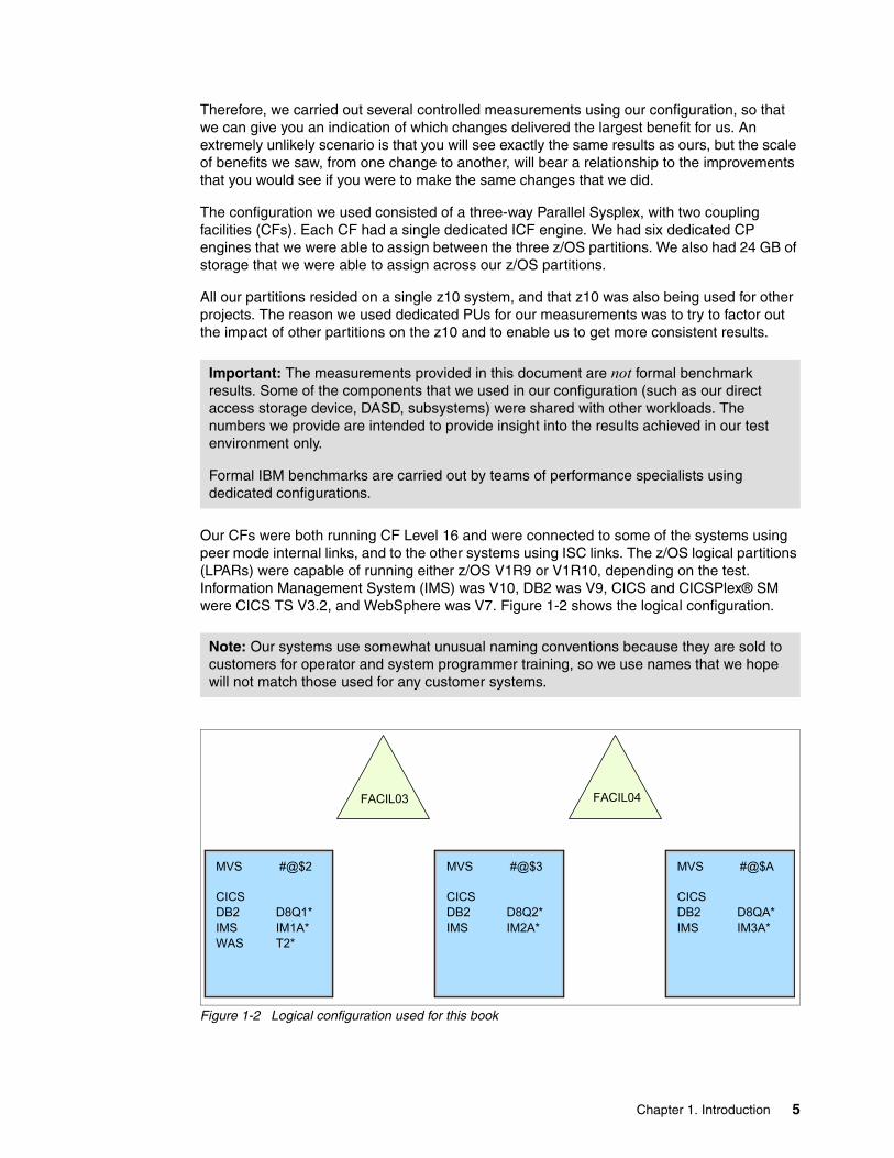
The configuration we used consisted of a three-way Parallel Sysplex, with two coupling facilities (CFs). Each CF had a single dedicated ICF engine. We had six dedicated CP engines that we were able to assign between the three z/OS partitions. We also had 24 GB of storage that we were able to assign across our z/OS partitions.

All our partitions resided on a single z10 system, and that z10 was also being used for other projects. The reason we used dedicated PUs for our measurements was to try to factor out the impact of other partitions on the z10 and to enable us to get more consistent results.

Our CFs were both running CF Level 16 and were connected to some of the systems using peer mode internal links, and to the other systems using ISC links. The z/OS logical partitions (LPARs) were capable of running either z/OS V1R9 or V1R10, depending on the test. Information Management System (IMS) was V10, DB2 was V9, CICS and CICSPlex® SM were CICS TS V3.2, and WebSphere was V7. Figure 1-2 shows the logical configuration.

Figure 1-2 Logical configuration used for this book

Important: The measurements provided in this document are not formal benchmark results. Some of the components that we used in our configuration (such as our direct access storage device, DASD, subsystems) were shared with other workloads. The numbers we provide are intended to provide insight into the results achieved in our test environment only.

Formal IBM benchmarks are carried out by teams of performance specialists using dedicated configurations.

Note: Our systems use somewhat unusual naming conventions because they are sold to customers for operator and system programmer training, so we use names that we hope will not match those used for any customer systems.

FACIL04FACIL03

MVS #@$2

CICSDB2 D8Q1*IMS IM1A*WAS T2*

MVS #@$3

CICSDB2 D8Q2*IMS IM2A*

MVS #@$A

CICSDB2 D8QA*IMS IM3A*

Chapter 1. Introduction 5

The DASD that was accessible to the systems consisted of a mix of IBM 2105-F20, 2105-800, and 2107-922 devices. About 2800 DASD volumes were accessible to the systems. None of the volumes were mirrored. There was also a mix of tape drives, switches, and various communication devices.

1.4 Other systems

In addition to the ITSO systems that were used for IPL testing, we obtained IPL data from about 150 customer and IBM systems. This data gave us a metric to compare our results against. It also gave us valuable insight into the range of elapsed times that a reasonable sample of systems were experiencing.

Based on our analysis of this data, we made the following observations:

� Of the roughly 120 phases of the IPL process, only a relatively small number take more than one second to complete on average.

� Some of the phases exhibited large discrepancies between the average and maximum elapsed times. In nearly all those cases, the discrepancy was related to either prompting the operator, or I/O-related delays.

� The sites that are most likely to find an easy way to significantly reduce their IPL times are those whose elapsed times for one or more of these phases are significantly greater than the average. For example, one process had an average elapsed time (across all the systems) of 1.5 seconds, but on one system the elapsed time was 196 seconds. In this particular case, the customer was prompting the operator for a response, resulting in that out-of-line elapsed time.

The median elapsed times for each component in the IPL process is provided in Appendix C, “Sample IPL statistics data” on page 207. This information helped us identify the parts of the IPL that we should concentrate on in our investigations.

1.5 Layout of this book

One of our objectives in writing this document is to provide you with easy-to-access and easy-to-use information about ways to improve your MTTR. This document does not provide huge amounts of detail about the meaning of one keyword or option versus another; that information is usually available elsewhere and can only clog up this document. Therefore, to keep this document readable, we aim to keep things as concise as possible, with easy-to-interpret figures, showing the effect of using various methods, options, or technologies.

We also want to make the book valuable to, and usable by, specialists in various disciplines. Therefore, we have a chapter about systems management techniques that are related to MTTR, which everyone should read. That is followed by chapters about z/OS, which are primarily of interest to z/OS system programmers. The book then includes individual chapters about CICS, DB2, IMS, and WebSphere, so that you may read only the parts of the book that interest you.

As you read through this book, you might find suggestions that seem obvious, because that is already your practice. Other times, you might find answers to issues that you have wondered about for years. Finally, you might find possibilities that you can explore to improve your MTTR. We hope that you find this document easy to use and informative and that it helps you provide the optimum MTTR for your unique environment.


Chapter 2. Systems management

This chapter provides valuable information and experiences in the area of systems management that can contribute to your achieving significant improvements in your MTTR.

2


2.1 You cannot know where you are going if you do not know where you have been

As with any tuning exercise, the first step in a project to improve your mean time to recovery (MTTR) is to document how long it takes to stop and restart your systems today, and how consistent those stop and start times are. This information is critical to enable you to judge the effect of any changes you make.

Establishing a baseline also provides important tracking information. Even if you are content with your restart times today, changes in your configuration, workload, and software mix might cause elongation to those times, to the extent that they become unacceptable to your business. Putting a measurement and tracking process in place will allow you to be aware of any such changes, and act before they become a business issue.

This book describes a number of programs that can help with this task. One, IPLSTATS, formats information from a set of MVS control blocks that record the elapsed times for each of the phases in z/OS IPL, NIP, and Master Scheduler Initialization processing1. Others analyze system log (syslog) and extract information about how long it takes to start each of your major subsystems. Record and track this information to understand your trends and any unexpected change in these values.

Additionally, IBM System Automation for z/OS now produces a System Management Facility (SMF) record (Type 114) containing the elapsed time to start each subsystem that is under its control. You can find more information about how to create this information in Tivoli System Automation for z/OS: Customizing and Programming, SC33-8260. If you use System Automation for z/OS, consider enabling this record and tracking the information it provides about the startup and shutdown times for your most critical subsystems.

2.2 Are we all talking about the same IPL time

While preparing for this book, we asked a number of customers how long their IPLs took. The answers ranged from “two minutes” to “two hours”. So the obvious next question was “exactly what are you including in that time?”

For the purpose of this book, we define the duration of an IPL to be the elapsed time from the point where you activate or load the LPAR, and concluding at the point where all the production applications are available for use again.

Having said that, the bulk of our investigations were at the z/OS or subsystem level. We wanted to find techniques or options that would have a positive impact on the elapsed time to start the associated system or subsystem for nearly all customers.

We could have started all our subsystems together and then worked to reduce the overall IPL time. However, we thought that the value of such an exercise was limited, for example:

� Some of the delays could have been addressed by moving data sets to different devices or adding more paths to a particular device. This would have reduced our IPL time, but what benefit would that have provided for you?

� Our configuration consisted of a three-way Parallel Sysplex running on a z10 with dedicated CPs.

1 You can also get this information by using IPCS Option 6 and entering “VERBX BLSAIPST MAIN.”


Each z/OS had:

– 200 IMS-dependent regions– 38 CICS and CICSPlex SM regions– 1 DB2 subsystem – 8 WebSphere servants

� Specific tuning actions might be of interest to a customer with a similar configuration, but what about a customer that only has CICS and DB2, or that has WebSphere, IMS, and DB2? Because every customer’s configuration, workloads, and software mix is so different, there is limited value in knowing how long it took to bring up the entire workload on our systems, or in any tuning we might have done to improve that.

If you decide to initiate a project to reduce your MTTR, one of the first things to do is to agree, and clearly and precisely document what is included in the scope of your project: what event or command or message indicates the start of the shutdown, and what message indicates the point where all applications are available again. You might be surprised at how many opinions exist about when the outage starts and ends.

2.3 Defining shutdown time

The shutdown time is a little more nebulous than IPL time. The obvious description is that shutdown time starts when the automation script to shutdown the system is initiated, and ends when the target system places itself in a wait state.

However, from a user perspective, the shutdown of the system may have started a long time before that. For example, a common practice is to start closing down batch initiators, especially those used for long running jobs, an hour or more before the rest of the system is taken down. Another example might be stopping long running queries ahead of the rest of the system. From the data center perspective, the system is still available during these times, but from the user’s perspective, the application is not available.

The particular definition you use for shutdown time has presumably been honed over many years. However what is most important is that everyone in your installation that is involved in an MTTR improvement project is using the same definition. A positive side effect of this discussion might be that starting to shut down these services so far ahead of the IPL is something you no longer find necessary, because technology improvements have reduced the average time of a long-running batch job.

2.4 The shortest outage

The shortest outage is the one you never have. Most planned outages are used to implement a change to the hardware or software configuration. Some are done to clean up the system. Whatever the reason, every planned outage can mean a period of unavailability for the services running on that system.

Based on discussions with customers, most customers have scheduled IPLs between once a month to once a quarter. A small number of customers IPL more frequently than once a month, and some customers run for more than three months between scheduled IPLs. But for most installations, a common trend is pressure from the business to IPL less frequently than is done today.

But you have to ask yourself: Are all those outages really necessary? Obviously you must be able to make changes to your configuration. However, many changes that at one time

Chapter 2. Systems management 9

required a system outage or a subsystem restart can now be done dynamically. z/OS and its major subsystems have delivered significant enhancements over recent releases that enable many options and attributes to be changed dynamically. The book z/OS Planned Outage Avoidance Checklist, SG24-7328, describes many of the things that can be changed dynamically in z/OS (that book, however, was written at the 1.7 level of z/OS). And the subsystem chapters in this document provide pointers to information about what can be changed dynamically in each of those products.

2.5 Automation

Automation is one of the best ways to reduce the elapsed time for an IPL. Although most sites implement some sort of automation, finding ways to improve MTTR by reviewing automation is not unusual. Remember that the automation product provides only the infrastructure to issue commands; what triggers those commands to be issued, and the sequence in which they are issued, is under the control of the installation. Therefore, you must consider many factors when designing your automation.

2.5.1 Message-based automation

Be sure that the startup and shutdown of all address spaces are driven by messages, which indicate that the initialization or shutdown of any prerequisite products has completed. Some installations begin the commands to stop or start address spaces based on waiting a fixed amount of time after an action against a predecessor component; however these methods usually result in startup and shutdown times that are longer than necessary. A much better approach is to trigger actions based on specific messages.

2.5.2 Sequence of starting products

Be sure to consider the criticality of products or functions to your production applications when designing your startup rules. The startup of products that are not critical to production online applications should be delayed until later, after the applications are available. Products in this category might include performance monitors, file transfer products, batch scheduling products: basically anything that is not required to deliver the production online service.

Also consider the relationship between various products. For example, CICS used to require that VTAM® initialization be completed before it was started. As a result, many customers start CICS, DB2, and other subsystems only after VTAM has started. However, this is no

Tip: When asked why they IPL as frequently as they do, system programmers commonly respond “because we have always done it this way.” Do not automatically accept this as a valid reason. What might have been a valid and necessary reason for an IPL five years ago might no longer require an IPL today.

For example, if you IPL very frequently because at some time in the past you suffered from a storage leak, do not simply keep using IPL years later for that reason. Are you still suffering from that problem? If not, it should not be necessary to IPL so often. And if you are, then consider approaching the vendor to have the product fixed.

Additionally, the methodology you use for stopping and starting your systems may also be a product of “we have always done it this way.” We would be surprised if simply re-examining how you are starting and stopping your systems does not yield surprising benefits.


longer the case, meaning that CICS can now be started concurrently with VTAM. Although users will not be able to initiate VTAM sessions with CICS until VTAM has initialized, at least you might save some time by having CICS initialization run in parallel with VTAM initialization.

You might also want to review the messages that you use to trigger dependent address spaces. Using CICS as an example again, starting CICS-related products before CICS issues the “Control is being given to CICS” message might be possible. Not possible, however, is to make a general statement about when dependent address spaces may be started: it depends on which specific capabilities are required by the dependent address space. However, consider investigating improvements that you may be able to make in this area; a relatively easy way to determine this information is to try overlapping the startup on a test system.

2.5.3 No WTORs

There are various places in the startup of z/OS where you have the ability to pause processing and wait for the operator to enter information or make a choice. Although this flexibility is convenient because the operator can alter how the system comes up, the downside is that it takes an amount of time for the operator to enter the requested information. In fact, in the systems that we investigated as part of this project, those that took longer than average to IPL inevitably had one or more WTORs during the IPL.

Another problem with issuing operator prompts early in the IPL process is that all further IPL processing will likely be delayed until the operator responds to the prompt. This fact is especially important during the early part of the IPL: if the operator is prompted for a response during CICS startup (for example), the start of that CICS region will be delayed. However, if the operator is prompted early in the IPL, everything will be delayed by the amount of time that the operator takes to respond.

Based on this observation, one of the best things you can do to improve MTTR is to eliminate all WTORs from the IPL. Although this step might require a change to your processes and operations procedures, the resulting savings can be significant.

Duplicate volsersOperators being presented with duplicate volser messages during the IPL is not uncommon. If at all possible, such messages should be avoided. For one thing, the IPL does not progress until each duplicate volser message is replied to.

From the operator’s perspective, two situations exist:

� The operator has not seen the message for this particular pair of devices before.

In this case, the operator must contact the owner of the volumes to determine which is the correct volume to keep online. This step can be especially painful and time-consuming in cases where there are dozens or even hundreds of such volumes, because each one has to be replied to one at a time. If you assume an average of 10 seconds per reply, this can add up very quickly. Avoid this potentially very time-consuming process.

� The operator has seen the message before and therefore knows which volume to keep online.

Although the operator is able to respond in a more timely manner in this case, a delay in IPL processing still occurs while the system waits for the operator to respond. However, in

Note: For most of the early stages of an IPL, the system runs the tasks in a serial manner, with only a single engine, so if a task is delayed, by waiting for an operator response, all subsequent tasks also have to wait.


a way, this is actually a worse situation than the previous one. A “planned” situation where duplicate volsers are available to a system should not exist. If something is unique about your configuration that requires that two devices with the same volser are accessible, you should update the OS CONFIG in the input/output definition file (IODF) to control which volume will be taken online to each system, thereby ensuring that the operator does not get prompted to decide which device to keep online.

The other reason why duplicate volser prompts should be avoided is that they introduce the risk of a data integrity exposure if the operator were to reply with the wrong device number.

Syntax errors in Parmlib membersA mistake can easily be made when you enter a change to a Parmlib member. Something as simple as a missing or misplaced comma can result in a member that cannot be successfully processed. In the worst case, you must correct the error and re-IPL. In the best case, the operator is prompted with a message, asking for valid input. Both of these events result in an elongated IPL process.

To avoid these situations, we strongly recommend using the Symbolic Parmlib Parser where possible, to ensure that the syntax of any members you change is correct before you do the IPL. This tool is included in SYS1.SAMPLIB and is documented in an appendix in z/OS MVS Initialization and Tuning Reference, SA22-7592.

z/OS 1.10 introduced a new tool, CEEPRMCK, to syntax-check the CEEPRMxx parmlib members. For more information, see the section titled “Syntax checking your PARMLIB members” in z/OS Language Environment Customization, SA22-7564. The USS BPXPRMxx parmlib member can be syntax-checked by using the SETOMVS SYNTAXCHECK command.

2.5.4 AutoIPL and stand-alone dumps

z/OS 1.10 introduced a function called AutoIPL. AutoIPL allows you to specify to z/OS what action should be taken when the system enters one of a specific set of wait states. You can specify that the stand-alone dump program do an automatic IPL, or that z/OS do another automatic IPL, or both. You can also specify that the system should do an automatic IPL as part of the V XCF,xxx,OFFLINE command.

The use of AutoIPL can be a valuable time-saver in the case of a non-restartable wait state where you want a stand-alone dump. Most installations run for long periods of time between stand-alone dumps. In fact, the operator might never have performed one before. If that is the case, the operator must first determine whether a dump is required and, if so, what is the correct volume to IPL from. If you enable AutoIPL, the stand-alone dump program will likely be IPLed and ready for operator input in less time than it would have taken the operator to find the stand-alone dump documentation. And, the faster the stand-alone dump can be completed, the faster the system can be restarted.

In addition to providing the ability to automatically IPL the system following a failure, the AutoIPL support also provides the option to specify on the V XCF,xxx,OFFLINE command (with the REIPL keyword) that the target system should shut itself down and then automatically IPL again without the operator having to use the Hardware Management Console (HMC). Although the resulting IPL does not take any less time than a manually-initiated one, you do save the time that would be associated with logging on to the HMC and initiating the IPL from there. Note that using the AutoIPL feature with the V XCF,xxx,OFFLINE command is effective only if you are using the same IPL volume and load parameters as previously used (unless you update the DIAGxx member to specify the new sysres and load parameters). If you are changing the sysres or load parameters and will not be updating the DIAGxx member, you must use the HMC.


2.6 Concurrent IPLs

Some times you might have to IPL multiple systems at the same time. In general, the recommendation has been that customers do rolling IPLs, which is IPLing one system at a time. This recommendation however, is based on minimizing application impact, rather than because of any specific performance considerations. Obviously, situations do exist, following a disaster, for example, when you must bring all the systems back up at the same time. However, in this section we are primarily concerned with normal sysplex operations and planned IPLs.

If you are in a situation where you have a number of systems down and want them back as quickly as possible, the recommendation has been to IPL one system, log on to make sure that everything is as expected, and then IPL the remaining systems in groups of four. However, as with all guidelines, fine tuning of this recommendation is possible, depending on your configuration.

For example, performance benefits might exist from IPLing a number of systems that share a common sysres all at the same time. The rationale behind this is that the first system to touch a given data set or program will load that into the storage subsystem cache, and all the following systems should then receive the benefits of faster reads from the cache. Measurements taken at IBM confirm that doing an IPL in this manner does result in faster IPLs than if the systems were IPLed from different sysres volumes at the same time.

You might also look at the placement of the partitions across multiple processors. Although the IPL process is generally not CPU-constrained, in certain environments, parts of the IPL process can consume significant amounts of CPU (WebSphere initialization, for example). In situations like this, try to group systems that are resident on different processors, rather than having a group of systems on the same processor all vying for CPU cycles at the same time.

Based on JES2 messages about contention on the JES2 checkpoint, some customers IPL one system at a time, with the IPL of each system starting only when the previous system has completed JES2 initialization. However, the combination of enhancements to JES2 and improved performance for both DASD and CF means that such practices are not necessary. The messages issued by JES2 about contention on the checkpoint only inform you that another JES2 was holding the checkpoint when this JES2 tried to obtain it; if issued when multiple systems are IPLing, these messages do not necessarily indicate a problem. If you have many systems to IPL and traditionally shut them all down together (rather than doing a rolling IPL), changing this methodology can result in significant MTTR improvements for the systems that are further down the list and had to wait for an IPL of all their peers before they can start.


2.7 Expediting the shutdown process

There are many address spaces on a typical z/OS system. Most installations stop all these address spaces as part of their normal shutdown process. And for some address spaces, taking the time to do an orderly shutdown process more than pays for itself by resulting in a faster startup the next time that address space is started (this applies to database managers in particular).

However, for some system address spaces, startup processing is the same regardless of whether or not they were cleanly shut down; LLA system address space is an example. Because many of these types of address spaces run on most z/OS systems, we discuss them in more detail in Chapter 5, “z/OS infrastructure considerations” on page 71.

In this section, we simply want to point out that automation might not necessarily have to wait for every last address space to end cleanly. We recommend that you go through each address spaces that is stopped as part of your automated shutdown process and determine whether a clean shutdown process is really required. In general, any process whose startup is exactly the same, whether or not it was stopped cleanly, is a candidate for removing from your shutdown scripts, or at least escalating the shutdown for the task from a gentle stop to an immediate cancel. Other candidates might be products that are designed to handle frequent restart operations; a good example is a file transfer product, which regularly has to deal with restarts resulting from network glitches.

Note: We have seen cases where two systems can get into a deadly embrace if they are IPLed at the same time. For example, SYSA gets an exclusive ENQ on Resource 1 and tries to get an ENQ on Resource 2. However SYSB already has an exclusive ENQ on Resource 2 and is now hung, waiting to get an ENQ on Resource 1.

Customers get around this situation by spacing out the IPL of the two systems. However, fixing the problem in this way is really only addressing the symptoms; it is not addressing the root cause of the problem. Situations like this must be addressed by ensuring that resources are always ENQed on in the same sequence.

So, in this example, both systems would try to get the ENQ on Resource 1 before they would attempt to get it on Resource 2. If this methodology was followed, the first system to request Resource 1 would get it. It would also be able to get the ENQ on Resource 2, because the other system would not attempt to get Resource 2 until it was able to serialize Resource 1, and that would not happen until Resource 1 is freed up by SYSA.

If you have this type of situation in your installation, you should work with the vendor of the associated product to get this behavior rectified.


2.8 Investigating startup times

One of the challenges in trying to improve startup times is that Resource Measurement Facility (RMF), or other performance monitors, are not running very early in the IPL process, so your visibility of what is happening and where any bottlenecks exist is very limited. Also, the timeframes are very short: many things are happening, but the elapsed time of each one is quite short. So if you have a 20- or 30-minute SMF interval, the activity of each of the address spaces blend together and become smoothed out.

Having said that, facilities are available to provide you with insight into what is happening during the system startup window. For the very earliest stages of the IPL process, you can use the IPLSTATS information. You can also use the RMF LPAR report to get information about the CPU usage of all partitions on the processor. Finally, contention might exist on some ENQs, so you can run an ENQ contention report to obtain insight into what is happening with ENQs during the startup. And, of course, perhaps the most valuable tool is the syslog for the period when the system is starting up.

2.8.1 Role of sandbox systems

In general, installations that are large enough to be concerned about restart times have system programmer test systems. Such systems can be valuable for MTTR reduction projects. For example, you can use a sandbox system to investigate what happens if you start product X before product Y.

The sandbox system is ideal for function testing like this. However, the configuration of most test systems is very different to the production peers: they typically have a lot fewer devices, much less storage, probably fewer CPs, and almost definitely far fewer started tasks. Therefore, be careful not to take any performance results from the test system and infer that you will get identical results from the production environment.

2.9 Summary

The remainder of this book is dedicated to the IBM System z® technology and how it can best be exploited to optimize your MTTR. However, the reason we inserted this chapter about systems management at this location in the book is that we want to encourage you to investigate and address any issues in that area before you get into the technical details. It is in the nature of technical people to look for technical solutions to challenges such as improving MTTR, and we hope that you will find information in this book to help you obtain those improvements. However, we urge you to first take a step back and determine whether there is room for improvement in your current processes.


Chapter 3. z/OS tools

This chapter describes the z/OS tools and utilities that we used during our testing. Subsequent chapters refer back to these tools. The tools described in this section are:

� MVS Operator commands

� Interactive Problem Control System (IPCS) IPLSTATS

� Syslog analysis programs

� Resource Measurement Facility (RMF)

� System Management Facilities (SMF) records

� JES2 commands

3


3.1 Console commands

One prerequisite to understanding the impact of any MTTR-related changes you might have made is to understand what other changes have occurred in the environment. For example, if you change a parameter and then find that the next IPL completes in less time, you want to be sure that the improvement is a result of your change, and not the fact that the LPAR now runs on a z10 whereas it was running on a z990 for the previous IPL.

Several operator commands are available to provide information about your configuration. You might want to have them issued by your automation product just after the IPL so that the information can be recorded in system log (syslog). All MVS commands are described in z/OS MVS System Commands, SA22-7627.

If you want to quickly and easily get the status of all systems in the sysplex at a given time, Example 3-1 contains an example of a simple little started task that will do this for you.

Example 3-1 Sample started task to issue system commands

//STATUS PROC //STEP EXEC PGM=IEFBR14// COMMAND 'RO *ALL,D M=CPU' // COMMAND 'RO *ALL,D M=STOR' // COMMAND 'RO *ALL,D ETR' // COMMAND 'RO *ALL,D XCF,S,ALL' // COMMAND 'RO *ALL,D IPLINFO' // COMMAND 'RO *ALL,D PARMLIB' // COMMAND 'RO *ALL,D SYMBOLS' // COMMAND 'RO *ALL,D CF' // COMMAND 'RO *ALL,D XCF,C'// COMMAND 'D XCF,CF,CFNM=ALL' // COMMAND 'D R,L' // COMMAND 'RO *ALL,D GRS,ALL' // COMMAND 'RO *ALL,D A,L' // COMMAND 'RO *ALL,D SMF,O' // COMMAND 'RO *ALL,D SMF,S'// COMMAND 'RO *ALL,D IOS,CONFIG'// COMMAND 'RO *ALL,D LOGGER'//*

You should tailor the list of commands to report on the configuration information that is of particular interest to you. The example gathers the information listed in Table 3-1 on page 19.


Table 3-1 Commands

Command Description

D M=CPU Provides information about the number of engines available, the number that are currently online, and additional information for each online engine. Note: The one thing that this command does not report on (but that might be important to you) is whether the engines are dedicated or shared. This information can be obtained from RMF.

D M=STOR Shows how much real storage is available to the system.

D ETR Provides information about the sysplex time configuration.

D XCF,S,ALL Shows information about the members of your sysplex and their status.

D IPLINFO Shows the time of the last IPL, the version and release of z/OS, and load and device information for the IPL.

D PARMLIB Displays the data sets in the Parmlib concatenation, together with the volume that each data set resides on.

D SYMBOLS Displays the system symbols defined on this system, and the current value of each symbol. This information can be useful if you subsequently try to determine which Parmlib members were used, and you use system symbols to control which members are selected.

D CF Shows the status of the coupling facilities and the links and subchannels that are used to communicate with them. As of z/OS 1.10, this also shows you whether each CF engine is shared or dedicated.

D XCF,C Provides a wealth of information about the sysplex Couple Data Sets, and the setting of many sysplex options.

D XCF,CF,CFNM=ALL Lists the structures in each CF.

D R,L Lists outstanding WTORs for all systems in the sysplex.

D GRS,ALL Shows the status of the systems in the global resource serialization (GRS) complex, and also GRS configuration options. Adding ,ALL adds information about the GRS RNLs to the output.

D A,L Shows nearly all active address spaces. The sequence of address spaces in the resulting display reflects the sequence in which the address spaces were started after an IPL. Note that this command does not show every system address space running under z/OS; address spaces started using the ASCRE macro are not displayed (the D A,A command can be used to show all address spaces, however the output can be quite lengthy).

D SMF,O Displays the SMF options that are currently in effect.

D SMF,S Displays the names, sizes, and status of the SMF data sets in use by each system.

D IOS,CONFIG Displays information about the system IOS configuration.

D LOGGER Displays the status of the logger subsystem for the system where the command is issued.

Chapter 3. z/OS tools 19

Note that some of these commands are against sysplex resources (for example, D XCF,CF,CFNM=) so you would expect to get the same response on every system. Therefore, issuing those commands on just one system should normally be sufficient. Also, remember that to be able to issue commands as in our example, the Converter/Interpreter must be properly authorized to issue commands, as follows:

� For JES2, this is defined with the JOBCLASS(x) AUTH= and COMMAND= specifications.

� For JES3, it is defined with the CIPARM AUTH= and COMMAND= specifications.

3.2 IPLDATA control block

Information about the elapsed time spent in various modules that make up the IPL process is stored in a system control block called IPLDATA. This information can be formatted by using the IPCS VERBX BLSAIPST MAIN command. Because this information is included in every dump, you can display the same information from an SVC dump or a stand-alone dump.

To get this information for the current running system, follow these steps:

1. Select option 6 in IPCS (Commands).

2. Enter the DROPD MAIN command to clear any previous output.

3. Enter the VERBX BLSAIPST MAIN command to format and display the IPLDATA control block for the current running system.

If you are analyzing a dump and want to display the IPLDATA information, you can simply enter IP VERBX BLSAIPST (or IPLDATA STATUS) using the dump you have selected. An example of the output is shown in three parts: Figure 3-1 on page 21, Figure 3-2 on page 22, and Figure 3-3 on page 23. We provide a description of many of these events in Chapter 4, “z/OS IPL processing” on page 35.

Another possibility is to format the IPLDATA control block by using a program called IPLSTATS that is available from the z/OS Tools and Toys Web site at:

http://www.ibm.com/servers/eserver/zseries/zos/unix/bpxa1ty2.html#IPLSTATS

We added a command to the COMMNDxx member in our systems to start a started task to run this program after every IPL, writing this information to the Syslog and to a data set. The Message Analysis program described in 3.3, “Syslog” on page 24 can then collect and analyze the IPL statistics.


http://www.ibm.com/servers/eserver/zseries/zos/unix/bpxa1ty2.html#IPLSTATS

Figure 3-1 Sample IPLSTATS output (part 1 of 3)

IPLST000I z/OS 01.10.00 #@$A 20970019DE50 2 CPs IPLST001I IPL started at: 2009/05/05 21:27:58.972 **** IPL Statistics **** IEAIPL10 0.000 ISNIRIM - Read SCPINFO IEAIPL20 0.000 Test Block storage to 2G IEAIPL11 0.006 Fast FIND service IEAIPL31 0.001 LOAD service IEAIPL30 0.001 IPLWTO service IEAIPL46 0.096 Read SCHIBs into IPL workspace IEAIPL49 0.000 Process Load and Default parameters IEAIPL50 0.007 IPL parmlib - process LOADxx and NUCLST IEAIPL51 0.000 System architecture IEAIPL43 0.006 Find and Open IODF data set IEAIPL60 0.000 Read NCRs from IODF IEAIPL70 0.042 UIM environment - load CBD and IOS servicesIEAIPL71 0.029 Build DFT for each device IEAIPL08 0.001 Read EDT information from IODF IEAIPL40 0.023 Read MLTs from nucleus IEAIPL42 0.002 Read NMLs from nucleus (IEANynnn modulesIEAIPL41 0.343 Read PDS directory entries and CESD records IEAIPL05 0.000 Build and sort NUCMAP IEAIPL02 1.214 Load nucleus modules IEAIPL04 0.003 Allocate PFT and SQA/ESQA IEAIPL14 0.000 Build LSQA/ELSQA for Master IEAIPL09 0.037 IAXMI - PFT, master RAB, etc. IEAIPL07 0.006 Update AMODE for nucleus resident SVCs IEAIPL03 0.013 Build UCBs, ULUT, etc. IEAIPL18 0.017 Copy and relocate EDT to ESQA IEAIPL99 0.176 Page frame table and cleanup 2.022 TOTAL IPL TIME (seconds) NIP started at: 2009/05/14 22:43:31.730 **** NIP Statistics **** IEAVNIP0 0.008 NIP Base IEAVNIPM 0.050 Invoke NIP RIMs IEAVNPE6 0.049 Service Processor Interface IEAVNPFF 0.029 Loadwait/Restart IEAVNPA6 0.008 RTM - RTCT and recording buffer IEAVNPC6 0.008 WTO IEAVNPC3 0.007 Issue messages from IPL message queue IEAVNP24 0.020 SMS Open/Mount IEAVNP06 0.010 Machine Check IEAVNP27 0.011 Reconfiguration IEAVNPA2 3.948 IOS - Non-DASD UCBs IEAVNPCA 0.008 NIP Console IEAVNPB2 0.682 IOS - DASD UCBs IEAVNP11 0.011 Locate and Open master calalog IEAVNPC7 0.027 Open SYS1.SVCLIB



IEAVNPOP 0.046 Open PARMLIB IEAVNPIL 0.010 Process IEALSTxx IEAVNPC4 0.018 Prompt for System Parameters IEAVNP03 0.004 Merge and analyze system parameters IEAVNPCF 0.134 Process system name and system variables IEAVNP76 0.009 Open LOGREC IEAVNPE8 0.027 RSM - Process REAL= IEAVNP23 0.013 Build GRS blocks in SQA IEAVNP04 0.024 ASM - Open page and swap data sets IEAVNPA8 0.005 VSM - Expand SQA IEAVNP14 0.031 ASM part 2 - Build SQA control blocks IEAVNPGD 0.001 Move console data to ESQA IEAVNP25 0.027 Process SVC= IEAVNP05 4.726 LPA, APF IEAVNP44 0.001 ASA Reuse stuff IEAVNPB1 0.001 Process CSCBLOC= IEAVNPE2 0.002 RACF SAF IEAVNPB8 0.007 Create CSA IEAVNP47 0.002 ENF IEAVNPD6 0.001 RTM - SDUMP, ABDUMP, ESTAE IEAVNP09 0.002 Build ASVT IEAVNPD8 0.769 RSM - Frame queues, VRREGN= and RSU= IEAVNP10 0.007 SRM - OPT=, IPS=, etc. IEAVNPD1 0.009 ABDUMP IEAVNPD2 0.012 SDUMP IEAVNPCX 0.001 Context services, registration IEAVNPX1 0.001 NIP cleanup IEAVNPF5 0.025 PCAUTH IEAVNPF8 0.011 RASP IEAVNP1F 0.028 SRM - I/O measurement blocks IEAVNPC2 0.011 IOS - Move CDT to SQA IEAVNP51 0.016 TRACE IEAVNP20 0.004 Process CLOCK= IEAVNP21 0.024 TOD clock IEAVNP57 0.006 SDUMP IEAVNPF9 72.231 XCF IEAVNP33 2.790 GRS IEAVNPED 0.008 PROD IEAVNP26 1.244 SMS IEAVNPE5 2.008 LNKLST IEAVNPD5 0.274 Load pageable device support modules IEAVNP88 0.077 Allocation move EDT II IEAVNPA1 3.602 CONSOLE IEAVNPDC 0.265 WLM IEAVNP16 0.247 EXCP appendages IEAVNP13 0.018 Prepare NIP/MSI interface IEAVNP17 0.002 GTF Monitor Call interface IEAVNPG8 0.003 VSM defined monitor call enablement IEAVNP18 0.053 PARMLIB Scan Routine interface IEAVNPF2 0.047 Process IOS= IEAVNP15 0.149 Process VATLST IEAVNPRR 0.001 RRS



We recommend that you download the sample IPLSTATS programs and JCL at this point. Note also, that this program might be enhanced periodically, so make sure that you always have the latest version of the program from the Tools and Toys Web site.

IEAVNPOE 0.152 USS IEAVNPSC 0.001 Metal C RTL IEAVNPLE 0.010 System LE RIM IEAVNPUN 0.012 Unicode IEAVNPXL 0.007 zXML Parser IEAVNP1B 0.045 Close catalog IEAVNIPX 0.000 NIP final cleanup 94.137 TOTAL NIP TIME (seconds) **** IEEVIPL Statistics **** IEETRACE 0.001 Master trace ISNMSI 2.019 SPI UCMPECBM 0.268 CONSOLE address space ENFPC005 0.000 CONSOLE ready ENF IEFSCHIN 0.207 IEFSCHAS address space IEFJSINT 0.002 Subsystem interface IEFSJLOD 0.018 JESCT IAZINIT 0.038 JESXCF address space IAZFSII 0.008 FSI trace IEFQBINT 0.015 SWA manager IEFAB4I0 0.118 ALLOCAS address space IEEVIPL 2.694 Uncaptured time: 0.000 MSI started at: 2009/05/14 22:45:08.870 **** IEEMB860 Statistics **** ILRTMRLG 0.277 ASM IECVIOSI 6.748 IOS dynamic pathing ATBINSYS 0.007 APPC IKJEFXSR 0.080 TSO IXGBLF00 0.016 Logger COMMNDXX 0.069 COMMANDxx processing SMFWAIT 0.163 SMF SECPROD 0.843 Security server IEFJSIN2 2.279 SSN= subsystem IEFHB4I2 0.009 ALLOCAS - UCB scan CSRINIT 0.004 Windowing services FINSHMSI 0.034 Wait for attached CMDs MSI ended at: 2009/05/14 22:45:19.500 IEEMB860 10.630 Uncaptured time: 0.100 109.482 TOTAL TIME (seconds)

Note: The sequence of modules shown in the IPLSTATS report generally reflects the sequence in which processing for that module starts. However, minor changes can exist from one release to another as small changes and fine tuning are applied to the operating system.


In Chapter 4, “z/OS IPL processing” on page 35, we go through the report in some detail and provide sample elapsed times from a number of systems. As you read through that chapter, having the corresponding values from your own systems available will be helpful so you can see where your systems fall compared to other systems.

3.3 Syslog

The system log (Syslog) and the operations log (Operlog1) provide most of the information that is used to understand the flow of the IPL. A Syslog is kept by each system. Optionally, console services can also write to Operlog, which stores the messages it receives in a log stream. The Operlog contains all of the messages (not necessarily in complete chronological sequence) from all systems; Syslog contains the messages from just a single system. If one log is unavailable, you can use the other log. The advantage of Operlog is that it provides a sysplex-wide view of console message activity.

Although scanning through all lines of a system log to extract information about the activity during the IPL is possible, an easier way of achieving this is available. IBM provides a non-warranted tool called MSGLG610 that can read any Syslog or major subsystem job log and summarize the information. You can download the tool from the z/OS Tools and Toys Web site at:

http://www.ibm.com/servers/eserver/zseries/zos/unix/bpxa1ty2.html#MSGLG610

Sample JCL to run the program is shown in Example 3-2 on page 25. The example shows the MSGLG610 control statements that we used to obtain IPL information and save it to a data set. The IPLID(FK09) is used to differentiate this IPL from another we will subsequently compare it to.

Important: The information provided in the IPLSTATS report is not a formal IBM published interface, and the IPLSTATS program is provided on an as-is basis. You might find that all the times do not add up. The reason is because not every module that executes during the IPL process is reported on. However, the information provided for each process and module is reliable and provides an invaluable insight into where the time is being spent during IPL that you would not otherwise have.

1 You can find information about how to set up Operlog in S/390 Parallel Sysplex: Resource Sharing, SG24-5666.



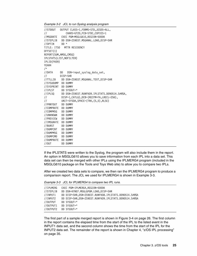
Example 3-2 JCL to run Syslog analysis program

//STDOUT OUTPUT CLASS=I,FORMS=STD,JESDS=ALL, // CHARS=GT20,FCB=STDC,COPIES=1 //MSGRATE EXEC PGM=MSGLG610,REGION=5000K //STEPLIB DD DSN=ZS9037.MSGANAL.LOAD,DISP=SHR //OPTIN DD * TITLE: ITSO MTTR RESIDENCY OFFSET(1)REPORT(SUM,AMSG,CMSG)IPLSTATS(LIST,NOFILTER) IPLID(FK09) YEAR4 /* //DATA DD DSN=input_syslog_data_set, // DISP=SHR //TTLLIB DD DSN=ZS9037.MSGANAL.TEXT,DISP=SHR //SYSUDUMP DD DUMMY //SYSPRINT DD DUMMY //IPLST DD SYSOUT=* //IPLSQ DD DSN=ZS9037.RUNFK09.IPLSTATS.D090514.S#@$A, // DISP=(,CATLG),DCB=(RECFM=FA,LRECL=256), // UNIT=SYSDA,SPACE=(TRK,(5,5),RLSE) //PRNTOUT DD DUMMY //COMPRATE DD DUMMY //COMPMSG DD DUMMY //UNKNOWN DD DUMMY //PREVIEW DD DUMMY //IMSGRATE DD DUMMY //BURST DD DUMMY //DUMPCNT DD DUMMY //DUMPMSG DD DUMMY //DUMPCMD DD DUMMY //DUMPRATE DD DUMMY //OUT DD DUMMY

If the IPLSTATS were written to the Syslog, the program will also include them in the report. An option in MSGLG610 allows you to save information from each IPL into a data set. This data set can then be merged with other IPLs using the IPLMERG4 program (included in the MSGLG610 package on the Tools and Toys Web site) to allow you to compare two IPLs.

After we created two data sets to compare, we then ran the IPLMERG4 program to produce a comparison report. The JCL we used for IPLMERG4 is shown in Example 3-3.

Example 3-3 JCL for IPLMERG4 to compare two IPL runs.

//IPLMERG EXEC PGM=IPLMERG4,REGION=5000K //STEPLIB DD DSN=KYNEF.MSGLGPGM.LOAD,DISP=SHR //INPUT1 DD DISP=SHR,DSN=ZS9037.RUNFK08.IPLSTATS.D090514.S#@$A //INPUT2 DD DISP=SHR,DSN=ZS9037.RUNFK09.IPLSTATS.D090514.S#@$A //OUTPUT DD SYSOUT=* //OUTPUT1 DD SYSOUT=* //OUTPUT2 DD SYSOUT=*

The first part of a sample merged report is shown in Figure 3-4 on page 26. The first column in the report contains the elapsed time from the start of the IPL to the listed event in the INPUT1 data set, and the second column shows the time from the start of the IPL for the INPUT2 data set. The remainder of the report is shown in Chapter 4, “z/OS IPL processing” on page 35.


Figure 3-4 Sample output from IPLMERG4 program, comparing two IPLs

3.4 Resource Measurement Facility (RMF)

Although the RMF is not started until after most of the z/OS IPL has completed, it can be used to identify constraints that might be restricting both the IPL process and the startup of the subsystems. In this section, we describe the reports that we used during our testing. We ran the RMF Monitor I background processing at one-minute intervals to provide the granularity we needed to identify any spikes of activity during our processing. Most installations run with 15-minute or 30-minute intervals.

The reports we used are:

� Type 70 - Summary Report

This report was used to show the general activity of the CPU and storage during the last part of the IPL and starting up and shutting down of subsystems. An example is shown in Figure 3-5, which shows that the startup of a subsystem occurred at 21.28 time. You can see that both the CPU usage and the DASD rate increased during this period. Obtain this report by specifying SUMMARY(INT) as a parameter to the RMF postprocessor.

Figure 3-5 RMF Monitor I: Summary report

*** MERGED RECORDS, SORTED BY INPUT1 EVENT TIME ***

Bold-faced events occurred in INPUT2 after they occurred in INPUT1.

0.00 0.00 0.00 IEA371I SYS0.IPLPARM ON DEVICE D056 SELECTED FOR IPL PARAMETERS 0.00 0.00 0.00 IPLST101I IEAIPL50 IPL PARMLIB - PROCESS LOADXX ANDNUCLSTXX 0.01 0.01 0.00 IPLST101I IEAIPL70 UIM ENVIRONMENT - LOAD CBD AND IOSSERVICES 0.05 0.05 0.00 IPLST101I IEAIPL41 READ PDS DIRECTORY ENTRIES AND CESDRECORDS 0.05 0.05 0.00 IPLST101I IEAIPL42 READ NMLS FROM NUCLEUS (IEANYNNNMODULES) 0.39 0.39 0.00 IPLST101I IEAIPL07 UPDATE AMODE FOR NUCLEUS RESIDENTSVCS 0.40 0.39 -0.01 IPLST201I IEAVNPCF PROCESS SYSTEM NAME AND SYSTEMVARIABLES 0.53 1.43 0.90 IPLST201I IEAVNPCX CONTEXT SERVICES, REGISTRATIONSERVICES 2.02 2.29 0.27 IEA008I SYSTEM PARMS FOLLOW FOR Z/OS 01.10.00 HBB7750 IEASYS00 2.04 2.40 0.36 IEA007I STATIC SYSTEM SYMBOL VALUES &SYSALVL. = "2" 6.90 9.97 3.07 IAR013I 4,096M STORAGE IS RECONFIGURABLE 8.84 12.11 3.27 IXC418I SYSTEM #@$A IS NOW ACTIVE IN SYSPLEX #@$#PLEX24.48 26.25 1.77 IXL014I IXLCONN REQUEST FOR STRUCTURE ISGLOCK WAS SUCCESSFUL. JOBNAME: GRS ASID: 000724.52 26.32 1.80 ISG300I GRS=STAR INITIALIZATION COMPLETE FOR SYSTEM #@$A.25.74 27.23 1.49 IGW061I SMSPDSE INITIALIZATION COMPLETE.

z/OS V1R9 SYSTEM ID #@$2 START 05/15/2009 RPT VERSION V1R9 RMF END 05/15/2009 NUMBER OF INTERVALS 32 TOTAL LENGTH OF INTERVALS 00.31.45 DATE TIME INT CPU DASD DASD JOB JOB TSO TSO STC STC ASCHMM/DD HH.MM.SS MM.SS BUSY RESP RATE MAX AVE MAX AVE MAX AVE MAX05/15 21.27.37 01.00 3.2 0.4 368.4 10 1 1 1 118 117 005/15 21.28.37 01.00 31.9 0.3 1738 10 10 1 1 108 108 005/15 21.29.37 01.00 35.7 0.3 1438 10 10 1 1 108 108 005/15 21.30.37 00.59 38.5 0.3 1222 10 10 1 1 108 108 005/15 21.31.37 01.00 39.7 0.3 1109 10 10 1 1 108 108 005/15 21.32.37 01.00 41.5 0.3 982.1 10 10 1 1 108 108 0


� Type 72 - RMF Workload Activity

If you want to collect detailed information about any address space, you should put it in a unique WLM Report Class. At the end of every RMF interval, you can obtain information about that address space. This information can be used to see whether changes you made had any effect on the CPU usage of the address space.

� Type 74 - Device Activity Report, OMVS Resource, XCF Activity, Coupling Facility Activity, and Cache Subsystem Facility

These reports provide great detail about the online devices, the OMVS kernel, XCF activity, the coupling facilities, and the cache subsystem activity.

� Type 77 - RMF Enqueue Activity

The Enqueue Activity report can be especially useful during the startup of a subsystem. It identifies any enqueues that occurred during the period, and can help you reduce delays by reducing enqueue conflicts. An example is shown in Figure 3-6.

Figure 3-6 RMF Enqueue Contention report

� Type 79 - RMF Monitor II

If you want to see what is happening on a second-by-second basis, running RMF II in background (that is, recording to SMF) can provide a fairly low-cost monitor. For some of our tests, we ran RMF II at one-second intervals. Example 3-4 shows the Parmlib member we used to control RMF Monitor II.

Example 3-4 Parmlib member ERBRMFT1 to monitor SMF

ARDJ(SMF)SINTV(1S)STOP(10M)RECORDNOREPORTDELTA

We then issued the F RMF,S T1,MEMBER(T1) command before starting a measurement run.

An example of the use of RMF Monitor II to monitor SMF activity is shown in Figure 3-7 on page 28. Because both SMF and RMF II were recording at one minute intervals at this time, you can see increases in device connect time at the one-minute intervals. Because CPU time is so small for SMF, you could track the CPU time better by using the ASRMJ command, which provides service unit consumption.

E N Q U E U E A C T I V I T Y PAGE 1 z/OS V1R9 SYSTEM ID #@$2 DATE 06/11/2009 INTERVAL 00.59.999 CONVERTED TO z/OS V1R10 RMF TIME 12.18.00 CYCLE 1.000 SECONDS ENQUEUE DETAIL ACTIVITY GRS MODE: STAR -NAME- ----- CONTENTION TIME ----- -- JOBS AT MAXIMUM CONTENTION-- -%QLEN DISTRIBUTION- AVG Q -REQUEST TYPE - TOTAL MAJOR MIN MAX TOT AVG ----- OWN ----- ----- WAIT ---- 1 2 3 4+ LNGTH -EXCL- -SHARE- EVENT MINOR TOT NAME TOT NAME MIN MAX MIN MAX SYSNAME SYSNAME IGWLHANZ SERIALIZEPDSEANALYSIS 0.000 0.000 0.000 0.000 1 SMSPDSE (E) 1 SMSPDSE1(E) 100 0.0 0.0 0.0 1.00 1 1 0 0 1 #@$2 #@$2


Figure 3-7 RMF Monitor II background monitor of SMF

Another use of RMF Monitor II is to obtain a list of the address spaces in the sequence they were created during IPL. The easiest way to do that is to run an RMF Monitor II with a request for ASD. An example is shown in Figure 3-8 on page 29. This shows that the *MASTER* address space was the first one started, followed by PCAUTH, then RASP, then TRACE, and so on. This report confirms our discussion of the IPL sequence in Chapter 4, “z/OS IPL processing” on page 35.

++++++++++ SMF +++++++ DELTA MODE +++++++++++++++SMF DEV FF FF PRIV LSQA X C SRM TCB CPU EXCP SWAP LPA CSA NVI V&H TIME CONN 16M 2G FF CSF M R ABS TIME TIME RATE RATE RT RT RT RT14:04:59 0.001 8 23 8 1106 X 7.1 0.00 0.00 0.00 0.00 0.0 0.0 0.0 0.014:05:00 0.013 8 23 8 1106 X 29 0.00 0.00 0.00 0.00 0.0 0.0 0.0 0.014:05:01 0.013 8 23 8 1106 X 32 0.00 0.00 0.00 0.00 0.0 0.0 0.0 0.0. . .14:05:25 0.001 8 23 8 1106 X 6.1 0.00 0.00 0.00 0.00 0.0 0.0 0.0 0.014:05:26 0.001 8 23 8 1107 X 0.0 0.00 0.00 2.00 0.00 0.0 0.0 0.0 0.014:05:27 0.001 8 23 8 1107 X 267 0.00 0.00 0.00 0.00 0.0 0.0 0.0 0.014:05:28 0.001 8 23 8 1107 X 0.0 0.00 0.00 0.00 0.00 0.0 0.0 0.0 0.0. . .14:05:41 0.001 8 23 8 1107 X 5.1 0.00 0.00 0.00 0.00 0.0 0.0 0.0 0.014:05:42 0.004 8 23 8 1107 X 0.0 0.00 0.00 15.0 0.00 0.0 0.0 0.0 0.014:05:43 0.001 8 23 8 1107 X 1K 0.00 0.00 0.00 0.00 0.0 0.0 0.0 0.0. . .14:05:59 0.001 8 23 8 1107 X 0.0 0.00 0.00 0.00 0.00 0.0 0.0 0.0 0.014:06:00 0.023 8 23 8 1107 X 76 0.00 0.00 0.00 0.00 0.0 0.0 0.0 0.014:06:01 0.001 8 23 8 1107 X 0.0 0.00 0.00 0.00 0.00 0.0 0.0 0.0 0.0. . .14:06:35 0.001 8 23 8 1107 X 11 0.00 0.00 0.00 0.00 0.0 0.0 0.0 0.014:06:36 0.001 8 23 8 1107 X 0.0 0.00 0.00 0.00 0.00 0.0 0.0 0.0 0.014:06:37 0.002 8 23 8 1107 X 478 0.00 0.00 2.00 0.00 0.0 0.0 0.0 0.014:06:38 0.001 8 23 8 1107 X 0.0 0.00 0.00 0.00 0.00 0.0 0.0 0.0 0.0. . .14:06:59 0.001 8 23 8 1107 X 11 0.00 0.00 0.00 0.00 0.0 0.0 0.0 0.014:07:00 0.019 8 23 8 1107 X 37 0.00 0.00 0.00 0.00 0.0 0.0 0.0 0.014:07:01 0.006 8 23 8 1107 X 37 0.00 0.00 0.00 0.00 0.0 0.0 0.0 0.014:07:02 0.001 8 23 8 1107 X 0.0 0.00 0.00 0.00 0.00 0.0 0.0 0.0 0.0


Figure 3-8 RMF Monitor II ASD report

RPT VERSION V1R9 RMF TIME 14.08.04 ++++++++++ +++++++ DELTA MODE ++++++++++++++++14:08:04 S C R DP CS ESF CS TAR X PIN ES TX SWAP WSM JOBNAME SRVCLASS P L LS PR F TAR WSS M RT RT SC RV RV *MASTER* SYSTEM 1 NS FF 5211 0 ---- 0 0 PCAUTH SYSSTC 1 NS FE 121 0 X ---- 0 0 RASP SYSTEM 1 NS FF 288 0 X ---- 0 0 TRACE SYSSTC 1 NS FE 162 0 X ---- 0 0 DUMPSRV SYSTEM 1 NS FF 346 0 ---- 0 0 XCFAS SYSTEM 1 NS FF 77.4K 0 X ---- 0 0 GRS SYSTEM 1 NS FF 8715 0 X ---- 0 0 SMSPDSE SYSTEM 1 NS FF 899 0 X ---- 0 0 SMSPDSE1 SYSTEM 1 NS FF 2114 0 X ---- 0 0 SMSVSAM SYSTEM 1 NS FF 13.5K 0 X ---- 0 0 CONSOLE SYSTEM 1 NS FF 3509 0 X ---- 0 0 WLM SYSTEM 1 NS FF 4117 0 X ---- 0 0 ANTMAIN SYSTEM 1 NS FF 1213 0 X ---- 1 998 ANTAS000 SYSSTC 1 NS FE 1230 0 X ---- 1 998 DEVMAN SYSTEM 1 NS FF 178 0 X ---- 0 0 OMVS SYSTEM 1 NS FF 26.0K 0 X ---- 0 0 IEFSCHAS SYSTEM 1 NS FF 91 0 X ---- 1 0 JESXCF SYSTEM 1 NS FF 644 0 X ---- 0 998 ALLOCAS SYSTEM 1 NS FF 5941 0 X ---- 1 0 IOSAS SYSTEM 1 NS FF 505 0 X ---- 0 0 IXGLOGR SYSTEM 1 NS FF 19.5K 0 X ---- 0 0 RACFDS SYSTEM 1 NS FF 313 0 X ---- 1 0 AXR OPSDEF 1 NS F4 446 0 X ---- 0 0 CEA SYSTEM 1 NS FF 336 0 X ---- 0 0 SMF SYSTEM 1 NS FF 1721 0 X ---- 0 0 LLA SYSSTC 1 NS FE 2394 0 X ---- 0 0 ZFS SYSSTC 1 NS FE 23.0K 0 X ---- 0 0 RMF SYSSTC 1 NS FE 138K 0 X ---- 0 0 NET SYSSTC 1 NS FE 2803 0 X ---- 0 0 RRS OPSDEF 1 NS F4 2526 0 X ---- 1 0 JES2 SYSSTC 1 NS FE 3739 0 ---- 0 0 VLF SYSSTC 1 NS FE 2355 0 X ---- 0 0 JES2MON SYSTEM 1 NS FF 215 0 ---- 0 0 JES2AUX SYSSTC 1 NS FE 202 0 ---- 1 0 TCPIP SYSSTC 1 NS FE 6040 0 X ---- 0 0 SDSF OPSDEF 1 NS F4 1166 0 X ---- 0 0 SMS SYSSTC 1 NS FE 487 0 X ---- 0 998 RACF SYSSTC 1 NS FE 552 0 X ---- 0 0 CATALOG SYSTEM 1 NS FF 2631 0 X ---- 0 0 TNF SYSSTC 1 NS FE 199 0 X ---- 0 0 VMCF SYSSTC 1 NS FE 259 0 X ---- 0 0 JES2S001 SYSSTC 1 NS FE 313 0 ---- 0 0 RESOLVER SYSSTC 1 NS FE 239 0 X ---- 0 998 RMFGAT SYSSTC 1 NS FE 7880 0 X ---- 0 0 TN3270 SYSSTC 1 NS FE 1880 0 X ---- 0 0


3.5 SMF records

The following SMF record types might provide insight into what is happening during the IPL process. You can find additional information about SMF and the various record types in z/OS MVS System Management Facilitiies, SA22-7630.

The records are described in the following list:

� Type 0 - IPL record

Although this record seems like it might contain the time that the IPL process was started, it does not. It is actually the time that SMF started creating records. But the time is certainly within a minute or two of the actual IPL. The record contains information about the amount of real and virtual storage available to the system, plus a subset of the SMF parameters.

� Type 8 - I/O Configuration

This record contains a 4-byte entry for every device that is online at IPL time. It contains the device class, unit type, and device number.

� Type 10 - Allocation Recovery

Although allocation delays might occur any time during the day, you should avoid any allocation delays during IPL or the startup of any subsystem. If you have any type 10 records during the start up period, you should investigate the reason and eliminate the problem.

� Type 19 - Direct Access Volume

See “SMF Type 19 records” on page 91 for a discussion of how the collection of these records affects IPL time.

� Type 22 - Configuration

This record is written at each IPL and when certain CONFIG operator commands are issued. A record indicator of 1 (one) indicates the IPL record. The record contains the configuration of the system at IPL, including the CPUs, storage, channel paths, and storage controllers. This record can be used to determine whether significant configuration changes occurred between IPLs.

� Type 30 - Job Activity

The interval records (subtypes 2 and 3) and step termination records (subtype 4) provide much information about each address space. Information about system address spaces is written to subtype 6 records each interval. If you want more detailed information about any of the system or subsystem address spaces, the type 30 record can provide usage details about CPU, storage usage, paging, and other resource usage.

� Type 43 - JES Start

These records are written when JES2 or JES3 are started, and contain the type of JES start (for example, cold start or quick start).

� Type 45 - JES Stop

These records are written when the stop command is issued for JES, and indicate the reason for the shutdown (operator command or abnormal).

� Types 70 through 79 - RMF records

See 3.4, “Resource Measurement Facility (RMF)” on page 26.


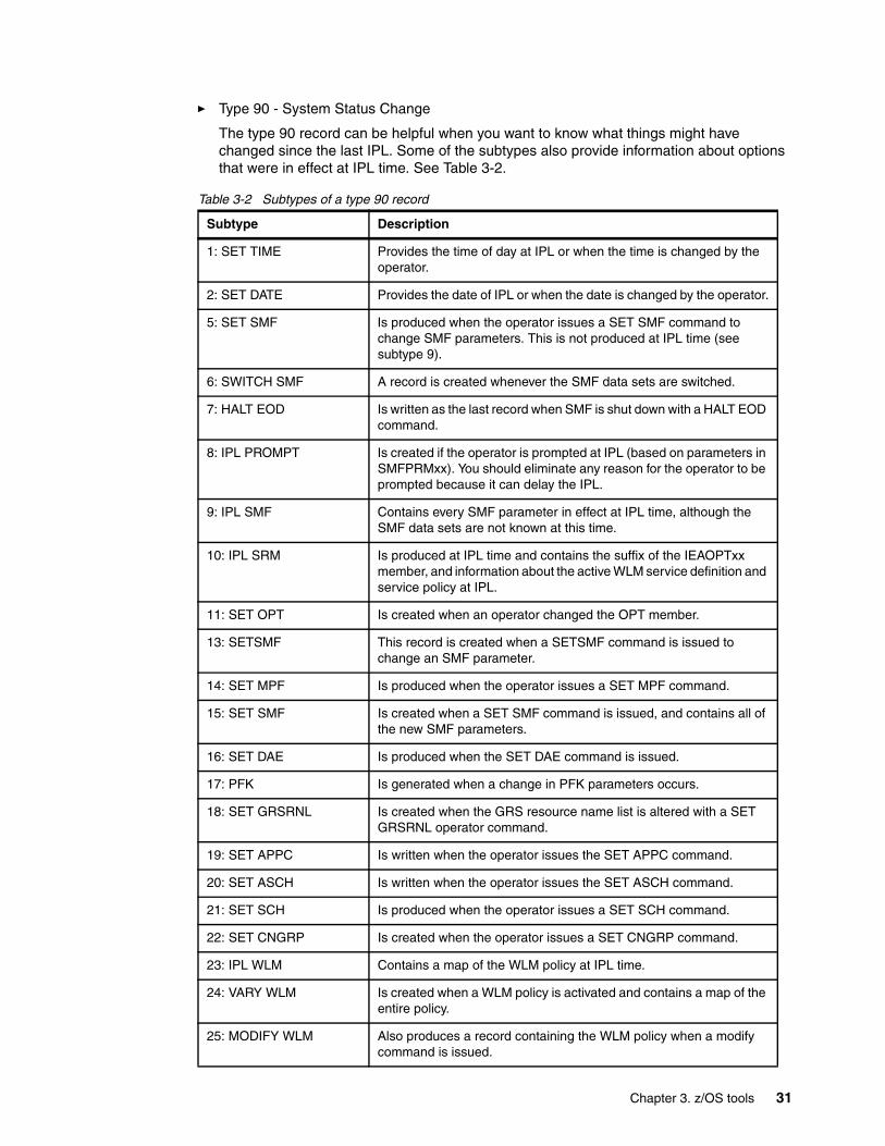
� Type 90 - System Status Change

The type 90 record can be helpful when you want to know what things might have changed since the last IPL. Some of the subtypes also provide information about options that were in effect at IPL time. See Table 3-2.

Table 3-2 Subtypes of a type 90 record

Subtype Description

1: SET TIME Provides the time of day at IPL or when the time is changed by the operator.

2: SET DATE Provides the date of IPL or when the date is changed by the operator.

5: SET SMF Is produced when the operator issues a SET SMF command to change SMF parameters. This is not produced at IPL time (see subtype 9).

6: SWITCH SMF A record is created whenever the SMF data sets are switched.

7: HALT EOD Is written as the last record when SMF is shut down with a HALT EOD command.

8: IPL PROMPT Is created if the operator is prompted at IPL (based on parameters in SMFPRMxx). You should eliminate any reason for the operator to be prompted because it can delay the IPL.

9: IPL SMF Contains every SMF parameter in effect at IPL time, although the SMF data sets are not known at this time.

10: IPL SRM Is produced at IPL time and contains the suffix of the IEAOPTxx member, and information about the active WLM service definition and service policy at IPL.

11: SET OPT Is created when an operator changed the OPT member.

13: SETSMF This record is created when a SETSMF command is issued to change an SMF parameter.

14: SET MPF Is produced when the operator issues a SET MPF command.

15: SET SMF Is created when a SET SMF command is issued, and contains all of the new SMF parameters.

16: SET DAE Is produced when the SET DAE command is issued.

17: PFK Is generated when a change in PFK parameters occurs.

18: SET GRSRNL Is created when the GRS resource name list is altered with a SET GRSRNL operator command.

19: SET APPC Is written when the operator issues the SET APPC command.

20: SET ASCH Is written when the operator issues the SET ASCH command.

21: SET SCH Is produced when the operator issues a SET SCH command.

22: SET CNGRP Is created when the operator issues a SET CNGRP command.

23: IPL WLM Contains a map of the WLM policy at IPL time.

24: VARY WLM Is created when a WLM policy is activated and contains a map of the entire policy.

25: MODIFY WLM Also produces a record containing the WLM policy when a modify command is issued.


3.6 JES2 commands

The following JES2 commands can be helpful. They provide information about the JES2 resources being used when shutting down JES2, during normal operation, and as part of starting up after an IPL. See z/OS JES2 Commands, SA22-7526 for more details about these and other JES2 commands:

� $DJES2

Shows the current activity in the JES2 address space that would hold up the normal shutdown of JES2 if a $PJES2 was issued. It has a much cleaner and more comprehensive display than issuing a $DA or a $DU command. It can be issued anytime to display JES2 activity.

� $JDDETAILS

Displays resource, sampling, and wait statistics for JES2 on the system on which the command is issued. This information helps when you determine whether a resource issue is affecting JES2.

� $JDJES and $JDSTATUS

Displays the current status and possible issues that can affect JES2.

� $DPERFDATA

shows the CPU and elapsed time for each initialization routine module, warm start processing, and MVS initialization (from JES2 start until when HASPNUC is first entered). To measure the JES2 startup time we used this very useful JES2 diagnostic command, $DPERFDATA,INITSTAT. The output from the command for one of our systems is shown in Figure 3-9 on page 33. Note that because this command is specifically intended to help IBM diagnose possible JES2 problems, the command and its output can change at any time; it is not a formal JES2 interface.

26: IPL LOGREC Provides the name of the Logrec data set name or log stream name at IPL.

27: SETXCF START to enable ARM

Is produced when Automatic Restart Management Policy is started.

28: SETXCF STOP to disable ARM

Is produced when an ARM policy is stopped.

29: SET PROG for LNKLST activation

Is not produced for IPL libraries because SMF is not yet running.

30: RESET Is created when the operator resets a job to a different service class.

31: SET PROG for LPALST activation

Is created when the link pack area (LPA) is updated dynamically.

32: WLM policy change Is created whenever the active WLM policy is changed.

Subtype Description


Figure 3-9 JES2 $D PERFDATA(INITSTAT) command

The combined time for the listed JES2 routines on our limited test system was about five seconds.

For reference purposes only, a large customer reported that a four-system sysplex with a large number of jobs in the spool and many explicitly defined lines, printers, functional subsystem (FSSs), and so on had a combined Initialization Routine (IR) time of 16 seconds. Although those are a small sampling of times, knowing this might give you an idea about what might be abnormal.

For a more detailed discussion about the output from the $DPERFDATA command, see “Understanding where the time is being spent” on page 83.

In addition, the ($D PERFDATA) command provides a display of several other JES2 internal performance statistics that are useful for tuning your systems. If issued without any parameters it will display all of the statistics that it collects, or you can limit the output to information about processing during initialization, as we did with the use of the INITSTAT keyword in example Figure 3-9.

For further information regarding the use of the $D PERFDATA command, including additional parameters, see:

� JES2 Performance and Availability Considerations, REDP-3940, available at:

http://www.redbooks.ibm.com/redpapers/pdfs/redp3940.pdf

� IBM Flash Document FLASH100008, available on the Web at:

http://www.ibm.com/support/techdocs/atsmastr.nsf/WebIndex/FLASH10008

$HASP660 $DPERFDATA,INITSTAT $HASP660 STATISTICS FROM INITIALIZATION: $HASP660 ROUTINE=MVSSTART,TIME=3.519227,CPU=0.002103, $HASP660 ROUTINE=LOADINIT,TIME=0.389312,CPU=0.002087, $HASP660 ROUTINE=IRMODCHK,TIME=0.439876,CPU=0.002019, $HASP660 ROUTINE=IRSSI,TIME=1.437123,CPU=0.043638, $HASP660 ROUTINE=IROPTS,TIME=0.036760,CPU=0.000751, $HASP660 ROUTINE=IRSETUP,TIME=0.055736,CPU=0.017000, $HASP660 ROUTINE=IRENF,TIME=0.000127,CPU=0.000126, $HASP660 ROUTINE=IRPL,TIME=0.038796,CPU=0.019641, $HASP660 ROUTINE=IRPOSTPL,TIME=0.185225,CPU=0.004521, $HASP660 ROUTINE=IRDCTDCB,TIME=0.000352,CPU=0.000277, $HASP660 ROUTINE=IRURDEV,TIME=0.000001,CPU=0.000001, $HASP660 ROUTINE=IREMVS,TIME=0.013050,CPU=0.012225, $HASP660 ROUTINE=IRDA,TIME=0.822872,CPU=0.080047, $HASP660 ROUTINE=IRNJE,TIME=0.050709,CPU=0.048423, $HASP660 ROUTINE=IRRJE,TIME=0.002247,CPU=0.002237, $HASP660 ROUTINE=IRCSA,TIME=0.000213,CPU=0.000196, $HASP660 ROUTINE=IRDCTCP,TIME=0.000006,CPU=0.000006, $HASP660 ROUTINE=IRMVS,TIME=0.009742,CPU=0.000470, $HASP660 ROUTINE=IRPCE,TIME=0.000343,CPU=0.000301, $HASP660 ROUTINE=IRINFO,TIME=0.000004,CPU=0.000004, $HASP660 ROUTINE=IRFINAL,TIME=0.000093,CPU=0.000092,$HASP660 ROUTINE=WARMSTRT,TIME=0.063073,CPU=0.011566


http://www.redbooks.ibm.com/redpapers/pdfs/redp3940.pdf


Chapter 4. z/OS IPL processing

This chapter describes the steps of the z/OS initial program load (IPL) process and changes you might be able to make to reduce the overall elapsed time. We used several of the tools described in Chapter 3, “z/OS tools” on page 17 to help you gain a greater understanding of this process and to illustrate how you can use the tools to identify potential areas for improvement in your environment.

4


4.1 Overview of z/OS IPL processing

At the highest level, a z/OS IPL event consists of the following three phases:

� Phase 1: The IPL of the operating system

This phase starts when the load process is invoked for the z/OS partition, and logically ends when everything that is automatically started by the operating system has initialized. Specifically, it does not include address spaces that you start by using automation or from the COMMNDxx member. This phase is shown in the top portion of Figure 4-1 on page 37, from the Hardware IPL through issuing of any commands found in the IEACMD00 and COMMNDxx Parmlib members.

This phase is the subject of this chapter.

� Phase 2: The startup of the system infrastructure

This phase includes starting things such as JES2, VTAM, TCP/IP, and so on. Chapter 5, “z/OS infrastructure considerations” on page 71 provides recommendations for the major z/OS components.

This phase is described in Chapter 5, “z/OS infrastructure considerations” on page 71.

� Phase 3: The startup of the subsystem infrastructure that runs or supports your business applications

This phase includes the startup of CICS, DB2, IMS, and so on. This phase is covered in the subsequent subsystem chapters.

To clarify which phase we are referring to, we call the first phase the z/OS IPL, and the second phase infrastructure startup.

We used two primary sources of information to gain a greater understanding of what is happening during the z/OS IPL:

� Introduction to the New Mainframe: z/OS Basics, SG24-6366

� z/OS MVS System Initialization Logic - Initial Program Load (IPL)

This excellent presentation can be found at:

http://www.ibm.com/support/techdocs/atsmastr.nsf/WebIndex/PRS3699



Figure 4-1 IPL flow diagram

To know which areas to focus on when attempting to reduce the elapsed time for the z/OS IPL phase, you must understand the sequence and elapsed time of events during this phase. The elapsed time for some of the events can be influenced by the installation; others cannot. This information can help you use the tools, described in Chapter 3, “z/OS tools” on page 17, to determine where time is being spent during the IPL. The five steps in the z/OS IPL process (shown in Figure 4-1) are:

1. Hardware IPL

2. IPL Resource Initialization Modules (RIMs)

3. Nucleus Initialization Program (NIP)

4. Master Scheduler Initialization (MSI Phase 1)

5. Master Scheduler Initialization (MSI Phase 2)

For each step, we describe the sequence of the logic, and then follow it with our experiences and recommendations for how to reduce the time of each step.

In 3.2, “IPLDATA control block” on page 20 and 3.3, “Syslog” on page 24, we described tools that analyze the steps and durations of an IPL. We include details from a sample IPLSTATS output in the introduction to each of these phases where we describe them below.

In this section, we refer to several Parmlib members. These are all documented in z/OS MVS Initialization and Tuning Reference, SA22-7592.

Now we look at each step in more detail.

H/W IPL

IPL RIMs

NIP RIMs

MSI

IEACMD00 COMMNDxx

System STCs Auto Ops

JESx

WebSphere

Lock Mgrs Monitors

IMS

CICS

MQDB2

Chapter 4. z/OS IPL processing 37

4.2 Hardware IPL

Prior to an IPL of a system, the ICKDSF utility is used to write IPL records on an IPL volume (starting at cylinder 0, track 0). This volume is called the SYSRES volume. A LOAD command on the HMC causes a hardware system reset to occur, and the IPL records to be read. Only one engine is used for this part of the z/OS IPL, and any others are placed in a stopped state. The fourth record, IEAIPL00, contains the initial program status word (PSW). The hardware IPL, which is all controlled by hardware, is then complete.

Note that the hardware IPL completes before any of the programs included in the IPLSTATS report are initialized, so the processing involved in the hardware IPL is not included in that report. The hardware IPL step completes when you see the message on the HMC telling you that the IPL has completed successfully.

We ran a number of tests to determine whether we could significantly change the hardware IPL time. We tried doing a LOAD NORMAL instead of a LOAD CLEAR (even though LOAD CLEAR is the recommended way to load z/OS). We tried assigning varying amounts of storage to the partition. And, we tried defining varying numbers of engines to the partition. None of these changes resulted in an IPL duration that fell outside the normal fluctuation from one IPL to the next.

Also, in our tests, the hardware IPL takes only a few seconds. As a result, little benefit seems to be gained from trying to reduce this portion of the IPL time. We do not believe that any changes in relation to the options you use for the IPL, or in how you configure the partition, will make any significant difference to the hardware IPL elapsed time.

4.3 IPL Resource Initialization Modules (RIMs)

The IPL RIMs are responsible for reading the LOADxx and NUCLSTxx Parmlib members, locating and loading information from the IODF data set, loading the MVS nucleus from the SYS1.NUCLEUS data set, and initializing the *MASTER* address space. Referring to Figure 3-1 on page 21, this step of the z/OS IPL includes all the IPLSTATS entries that start with “IEAIPL”.

The elapsed time of the IPL RIM part of the z/OS IPL can vary significantly from one system to another. In the systems we studied, this time varied from about 3 - 45 seconds, indicating that there is some scope for tuning or optimizing the processing in this step.

Figure 4-2 on page 39 shows the first part of the IPLSTATS output for one of our systems. It shows the elapsed time for each module, along with the total time for the IPL RIM processing (at the end of this section of the report). We added comments and related Syslog messages (in blue) below several of the steps to further clarify what is happening. The longest-running steps (across our set of customer systems) are shown in bold.

Elapsed time: The elapsed times for many of the processes we study in this chapter are small. Based on that, you might think it is not worth investigating. However, for most of the processing discussed in this chapter, only a single CP is being used by the system, and most of the processing is serial. This means that if one process is taking (for example) three minutes longer than necessary, every subsequent part of the IPL will be delayed by that amount. Therefore, an important approach is that you optimize this part of the overall IPL process as much as possible.


Figure 4-2 IPLSTATS showing the IPL RIM sequence

Figure 4-2 shows that the load of the nucleus modules was the longest step in this part, with the reading of the PDS directories being the next largest component. You might also notice that, in general, the steps with the longest elapsed times are those that were doing I/O.

To ensure that the behavior of our systems was representative, and to understand the variability of elapsed times from one system to another, we reviewed IPLSTATS reports for over 150 other systems. Based on that analysis, we found the following entries tended to have the longest median elapsed times in this phase of the IPL:

� Load nucleus modules� Test block storage to 2 GB� Build and sort NUCMAP� Read PDS directory entries and CESD records� IPL Parmlib: process LOADxx and NUCLSTxx

IPLST000I z/OS 01.10.00 #@$A 20970019DE50 2 CPs IPLST001I IPL started at: 2009/05/05 21:27:58.972 IEAIPL10 0.001 ISNIRIM - Read SCPINFO IEAIPL20 0.000 Test Block storage to 2G

This clears storage up to 2 GBIEAIPL11 0.029 Fast FIND service IEAIPL31 0.005 LOAD service IEAIPL30 0.001 IPLWTO service IEAIPL46 0.124 Read SCHIBs into IPL workspace IEAIPL49 0.000 Process Load and Default parameters IEAIPL50 0.009 IPL parmlib - process LOADxx and NUCLST

Displays the first message on the consoleIEA371I SYS0.IPLPARM ON DEVICE D056 SELECTED FOR IPL PARAMETERSIEA246I LOAD ID FK SELECTEDIEA246I NUCLST ID $$ SELECTED

IEAIPL51 0.000 System architecture IEAIPL43 0.003 Find and Open IODF data set

IEA519I IODF DSN - IODF.IODF02IEA520I CONFIGURATION ID = TRAINER. IODF DEVICE NUMBER = D056

IEAIPL60 0.000 Read NCRs from IODF IEAIPL70 0.164 UIM environment - load CBD and IOS servicesIEAIPL71 0.033 Build DFT for each device IEAIPL08 0.001 Read EDT information from IODF IEAIPL40 0.050 Read MLTs from nucleus IEAIPL42 0.018 Read NMLs from nucleus (IEANynnn modulesIEAIPL41 0.645 Read PDS directory entries and CESD records

Time is dependent on number of parmlibs specified in LOADxxIEAIPL05 0.000 Build and sort NUCMAP IEAIPL02 1.728 Load nucleus modules

Time is dependent on the size of the nucleusIEA091I NUCLEUS 1 SELECTED

IEAIPL04 0.021 Allocate PFT and SQA/ESQA IEAIPL14 0.000 Build LSQA/ELSQA for Master IEAIPL09 0.042 IAXMI - PFT, master RAB, etc. IEAIPL07 0.006 Update AMODE for nucleus resident SVCs IEAIPL03 0.015 Build UCBs, ULUT, etc. IEAIPL18 0.015 Copy and relocate EDT to ESQA IEAIPL99 0.211 Page frame table and cleanup 3.121 TOTAL IPL TIME (seconds)


The minimum, median, and maximum times for each of these activities are shown in Figure 4-3.

Figure 4-3 Largest elapsed time components in IPL RIM phase

Apart from the entry that is related to testing storage, all the other most time-consuming events are DASD I/O-intensive, so anything you can do to speed up that processing and minimize the number of I/Os will deliver the most benefit.

Testing storagePrior to z/OS 1.10, the IEAIPL20 module validated all defined storage up to 2 GB. The elapsed time for this processing could vary from a fraction of a second up to over 10 seconds, depending on the configuration and whether sufficient CPU capacity was available to the system.

In z/OS 1.10, this processing has been changed so that the validation runs asynchronously. As a result, you generally see a time of zero or close to zero seconds being reported for IEAIPL20 on any z/OS 1.10 system.

Loading nucleus modulesThere is little you can do to directly reduce the load time of the nucleus modules, other than to place the sysres on the fastest device available. However, if you are faced with IPLing multiple systems around the same time, initiating the IPLs of the systems that share a sysres should mean that the first system will load the modules into the disk subsystem cache, reducing the elapsed time for the other systems to read those modules.

One of the modules that, in some configurations, might take several seconds to complete is building the NUCMAP - IEAIPL05. In z/OS 1.10, this process has been optimized and streamlined with other processing of nucleus. As a result, the elapsed time for this module on most z/OS 1.10 systems tends to be very small fractions of a second.

IPL RIM Largest Components

0.0

2.0

4.0

6.0

8.0

10.0

12.0

14.0

16.0

18.0

20.0

Test Block storage to2G

Build and sort NUCMAP IPL parmlib - processLOADxx andNUCLSTxx

Read PDS directoryentries and CESD

records

Load nucleus modules

Event

Sec

on

ds Min

Median

Max


The LOADxx memberWhen you initiate the IPL from the HMC, the activation profile for the system that is being loaded must contain a load parameter, as described in Figure 4-4. Part of the load parameter is the suffix that identifies which LOADxx member to use. The LOADxx member (among other things) tells the system which other Parmlib members to use for the IPL.

Figure 4-4 Format of load parameter for IPL

The load parameter also contains the Initial Message Suppression Indicator (IMSI). An IMSI value of blank or M will suppress the Enter System Parameters operator prompts during the IPL process. The possible IMSI values are described in the section “Loading the System Software” in z/OS MVS System Commands, SA22-7627.

Note that you can specify the alternate nucleus ID both in the load parameter and in the LOADxx member. If you specify it in both places, the value on the load parameter overrides what you specified in the LOADxx member.

The LOADxx member defines the Parmlib concatenation that will be used for the IPL, the name of the sysplex, the name of the Master catalog, information about the IODF data set to be used, and other system attributes. The sample member shown in Example 4-1 on page 42 specifies that the IPL use member IEASYMXX from the Parmlib concatenation, that the system use member IEASYS00 from the Parmlib concatenation, that it load IEANUC01 from SYS1.NUCLEUS, and that it use member NUCLST$$ from the same library that contains the LOADxx member.

Recommendation: Use only Initial Message Suppression Indicator values of blank or M. If any other value is used, the operator is prompted for a reply, which will increase the elapsed time for the IPL.

Load Parameters

IODFdddd

LOADxxxx

IMSIi

NUCxn

IODFdddd

LOADxxxx

IMSIi

NUCxn

DDDD: Device number of the volume containing the IODF dataset

DDDXXINN Load Parameter Values

(Default is SYSRES)

XX: ID of the LOADxx member to be used (the default is 00)

I: Initial Message Suppression Indicator (IMSI)

The default (blank or period) suppresses most informational messages and does not prompt for system parameters; will use the LOADxx values

N: Nucleus ID to be used (default is 1: IEANUC01)


Example 4-1 LOADxx member

IODF ** IODF TRAINER 01 Y NUCLEUS 1 NUCLST $$ IEASYM XX SYSPLEX #@$#PLEX Y SYSCAT #@$#M1123CMCAT.V#@$#M1 SYSPARM 00 PARMLIB SYS1.PARMLIB PARMLIB CPAC.PARMLIB PARMLIB SYS1.IBM.PARMLIB

Specifying IODF informationA little background information about the use of double asterisks (**) when specifying the IODF parameter in the LOADxx member might be helpful. Specifying ** on the IODF statement in the LOADxx member informs z/OS to retrieve the current IODF suffix and hardware token from the hardware system area (HSA). This information gets loaded into HSA every time a power-on reset (POR) is done or when a dynamic hardware activation from a new IODF is done. Then, z/OS takes that IODF suffix from HSA and merges it with the IODF data set high-level qualifier (which is also specified on the IODF statement in LOADxx) to create the name of the IODF data set that the system expects will contain information about the current configuration.

As long as you ensure that the system has access to the expected IODF data set before you update the HSA, the use of ** provides great flexibility, and eliminates the need to update the LOADxx member every time you switch to a new IODF. However, let us imagine that the HSA was updated from an IODF data set with a suffix of 97, that your LOADxx member specifies an IODF HLQ of SYSZ, and that for some reason this system does not have access to a data set called SYSZ.IODF97. In this situation, z/OS first searches for a data set called SYSZ.IODF97. When it does not find that data set, it searches for a data set called SYSZ.IODF00. If it finds the the data set, z/OS opens it and searches it for the hardware token that was found in HSA. If that data set does not contain that token, z/OS then searches for a data set called SYSZ.IODF01. If one is found, it will again be searched for the hardware token. This process could potentially go on for all 256 possible IODF data sets until either a data set with the required token is found, or the token is not found in any of the data sets, in which case the system enters a wait state.

Tips: Regarding the search sequence, an important point to remember is that the search order for libraries differs from parameters:

� When looking for a member in library concatenations, such as Parmlib and Linklist, the first member found are used, and members in later libraries are ignored. As an example, if IEASYS00 is in all three of the Parmlib members specified in Example 4-1, only the IEASYS00 from SYS1.PARMLIB is used.

� When determining parameters when multiple members are specified, the parameters in the last member will be used, and will override the corresponding parameters in earlier members. As an example, if IEASYS01 is concatenated after IEASYS00, then any parameter in IEASYS01 will override the same parameter in IEASYS00. See z/OS MVS Initialization and Tuning Reference, SA22-7592 for any exceptions to this rule.


To be able to use ** (but without the risk of encountering the situation described here), we recommend using the following process:

1. Create your new IODF data set and make sure that it is accessible to every z/OS system running on the processor that is going to be updated.

2. On all but one partition on the processor, do activate the software by using the new IODF.

3. Finally, activate the hardware on the last partition. This step updates the hardware token in the HSA.

Even if you are only making a software-only change, perform a hardware-activate operation to update the hardware token in the HSA.

4.4 Nucleus Initialization Program (NIP)

Having loaded the nucleus and started the *MASTER* address space, the next step includes most of the work to get the core of z/OS up and running. This step also includes validating the I/O configuration (based on information about the configuration that was loaded from the IODF data set), starting communication with the NIP console, and finding and opening the Master Catalog and the data sets in the Parmlib concatenation. Optionally, the operator is prompted for system parameters. The various members of Parmlib are processed and system address spaces are started as appropriate (for example, PCAUTH, RASP, TRACE, and so on). Also processed at this time are initialization of the sysplex services and XCF connectivity, GRS, SMS, Console communication, and WLM.

In the IPLSTATS report, NIP processing includes all the lines that start with IEAVNP. Because NIP processing has many steps, we have divided them into several parts to discuss the steps

Recommendations for the LOADxx members:

� Because SYS0.IPLPARM and SYS1.PARMLIB are read in this part of the IPL, you should ensure that no RESERVESa are issued against the volumes containing those data sets.

� When looking for the LOADxx member, the IPL process starts by looking for a data set called SYS0.IPLPARM on the IODF volume. If that data set is not found, it looks for a data set called SYS1.IPLPARM, and so on through SYS9.IPLPARM. Then it looks for SYS1.PARMLIB. If you place your LOADxx member in a data set called SYS0.IPLPARM on the IODF volume, the time for all that data set searching can be minimized.

� Review the description of the LOADxx member in z/OS MVS Initialization and Tuning Reference, SA22-7592, specifically in relation to placement of the IODF data set and the use of the double asterisks (**) in that member to identify the IODF that is to be used for this IPL.

� Try to keep the Parmlib concatenation as short as possible. Specifying a long concatenation of Parmlibs increases the IPL time because more data sets must be searched for every referenced member. Some installations define a minimum set of Parmlibs during IPL, and then add PDSE libraries later with a SETLOAD command.

� A possibility is to define LOAD parameters for multiple images in the same LOADxx member, and use filtering techniques as described in “IEASYMxx member” on page 50. If you do this step, remember to remove unused or obsolete images from the LOADxx member.

a. Monitor the RMF Postprocessor DEVICE reports or use the GRS ENQ/DEQ monitor to identify and address RESERVE activity.


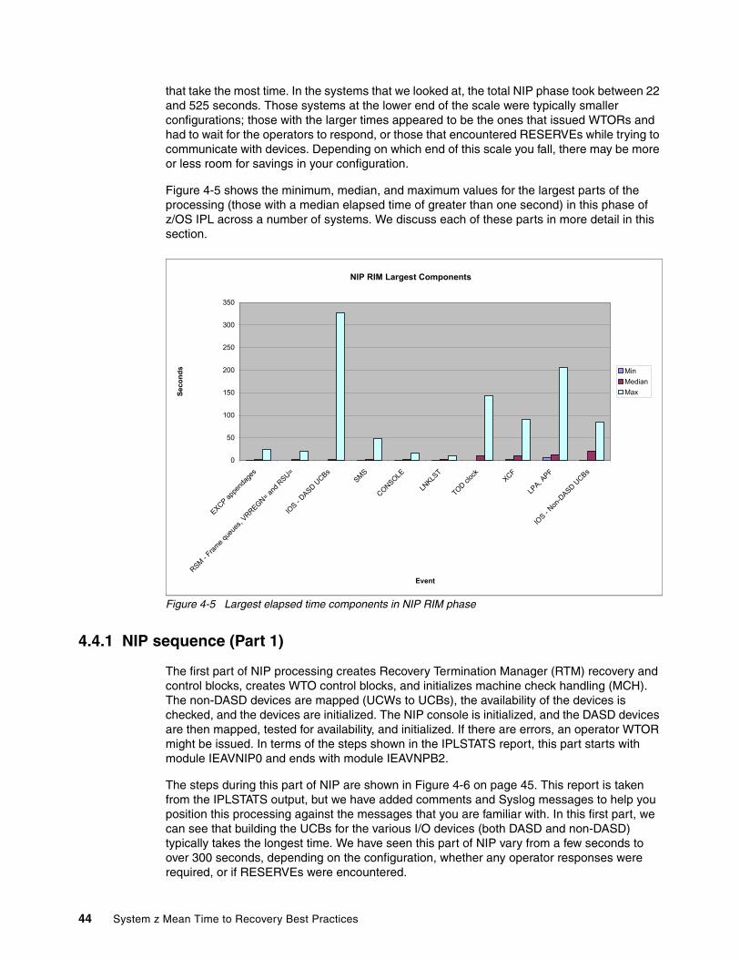
that take the most time. In the systems that we looked at, the total NIP phase took between 22 and 525 seconds. Those systems at the lower end of the scale were typically smaller configurations; those with the larger times appeared to be the ones that issued WTORs and had to wait for the operators to respond, or those that encountered RESERVEs while trying to communicate with devices. Depending on which end of this scale you fall, there may be more or less room for savings in your configuration.

Figure 4-5 shows the minimum, median, and maximum values for the largest parts of the processing (those with a median elapsed time of greater than one second) in this phase of z/OS IPL across a number of systems. We discuss each of these parts in more detail in this section.

Figure 4-5 Largest elapsed time components in NIP RIM phase

4.4.1 NIP sequence (Part 1)

The first part of NIP processing creates Recovery Termination Manager (RTM) recovery and control blocks, creates WTO control blocks, and initializes machine check handling (MCH). The non-DASD devices are mapped (UCWs to UCBs), the availability of the devices is checked, and the devices are initialized. The NIP console is initialized, and the DASD devices are then mapped, tested for availability, and initialized. If there are errors, an operator WTOR might be issued. In terms of the steps shown in the IPLSTATS report, this part starts with module IEAVNIP0 and ends with module IEAVNPB2.

The steps during this part of NIP are shown in Figure 4-6 on page 45. This report is taken from the IPLSTATS output, but we have added comments and Syslog messages to help you position this processing against the messages that you are familiar with. In this first part, we can see that building the UCBs for the various I/O devices (both DASD and non-DASD) typically takes the longest time. We have seen this part of NIP vary from a few seconds to over 300 seconds, depending on the configuration, whether any operator responses were required, or if RESERVEs were encountered.

NIP RIM Largest Components

0

50

100

150

200

250

300

350

EXCP app

enda

ges

RSM -

Fram

e qu

eues

, VRREG

N= an

d RSU=

IOS -

DASD UCBs

SMS

CONSOLE

LNKLS

T

TOD cloc

kXCF

LPA, A

PF

IOS -

Non-D

ASD UCBs

Event

Se

con

ds Min

Median

Max


Figure 4-6 NIP sequence (part 1 of 5)

Several common reasons for elongated IPLs, and where they are reported in the IPLSTATS output, are as follows:

� Duplicate volser

If you have duplicate volsers at IPL time, message IEA213A is issued, and the time that the system spends waiting for the operator to respond is included in module IEAVNPB2.

This time can be extensive if many duplicate volsers exist. These duplicate volser messages appear one pair at a time. After the support team verifies which volser is to remain offline, the operator has to enter R 00,XXXX for which of the two volsers should remain offline, and then wait for the next pair to come up, type in the next entry, and so on. At 5 - 10 seconds per reply cycle, this could take an extra 8 - 16 minutes to respond to only 100 duplicate DASD.

� Message IEA101A

If you specify that the operator should be prompted for System Parameters, message IEA101A is issued. The time spent waiting for the operator to respond to this message is included in module IEAVNPC4 (this is covered in 4.4.2, “NIP sequence (Part 2)” on page 47).

� Operator prompts

Various Parmlib members provide the option of prompting the operator for configuration options. Depending on where the prompt is specified, the resulting wait time will be reported in different modules. Unfortunately no source of information exists that ties PROMPT options to the related modules. However, you should be able to easily test this on a test system by changing the PROMPT value, re-IPLing, and identifying the IPLSTATS field that has significantly changed.

NIP started at: 2009/05/14 22:43:31.730 **** NIP Statistics **** IEAVNIP0 0.011 NIP Base IEAVNIPM 0.099 Invoke NIP RIMs IEAVNPE6 0.108 Service Processor Interface IEAVNPFF 0.028 Loadwait/Restart IEAVNPA6 0.009 RTM - RTCT and recording buffer IEAVNPC6 0.014 WTO IEAVNPC3 0.015 Issue messages from IPL message queue IEAVNP24 0.029 SMS Open/Mount IEAVNP06 0.017 Machine Check IEAVNP27 0.028 Reconfiguration IEAVNPA2 25.697 IOS - Non-DASD UCBs IEAVNPCA 0.301 NIP Console

IEA434I (DF65) ONLINE IS NOT ALLOWED, GREATER THAN 65520 CYLINDERSIEA311I UNLABELED DASD ON D40B. UNIT PUT OFFLINEYou might also see other errors from IODF at this point.

IEAVNPB2 3.260 IOS - DASD UCBs 29.116 Total time for this part of NIP


Minimizing the time to establish the I/O configurationFinding a system where the COMMNDxx member or the automation product varies the unneeded devices offline is not uncommon. However, this is a costly activity for two reasons:

� Having the devices defined as being online at IPL (OFFLINE=NO in HCD) means that the system will do many I/Os to the device during the IPL. This activity is relatively time-consuming, especially if you have a large number of devices. (There is also more device-related activity later in the IPL.)

� Having gone through the cost of processing these online devices, you then give the system yet more work to do to vary them offline.

A far more efficient way to achieve the same end result (from the perspective of speeding up the IPL at least) would be to define any devices that are not required as being offline (OFFLINE=YES) at IPL in the OS CONFIG that is used by that system.

In a large configuration, specific MIH definitions may improve online processing (refer to OA27436 for more information). Changing the IECIOSxx member as described in the APAR should also deliver improvements for the IPL elapsed time.

Sysplex IPL considerationsHopefully you will never have to do a sysplex IPL. However, if you do have to do a planned sysplex IPL for any reason, ensure that the last system in the sysplex to be shut down is the first one that is then IPLed when you are ready to bring up your systems again. The reason for this approach is that very early in the IPL process, XCF checks the sysplex CDS to see if any other systems are active. If the system being IPLed is not the last system to be shut down, the operator is prompted with messages IXC404I and IXC405D and the IPL pauses until a response is received. If the system being IPLed is the last one to be shut down, those messages are not issued and the related delay is avoided.

Recommendations for minimizing the elapsed time NIP processing (Part 1):

� Avoid any operator prompts during the IPL process. For example, the presence of duplicate volsers cannot only cause confusion, they also elongate the IPL, so should be avoided if at all possible.

� Do not define any devices that will not be needed by this system as being online at the IPL. That applies to both DASD and non-DASD devices.

� Heavily used libraries or data sets should be placed on the best-performing DASD devices available to reduce the I/O connect time for much of the startup process. In one test in IBM, moving the system volumes from traditional DS8000® volumes to solid state disk volumes reduced the IPL elapsed time by about 15%.

� Review the Syslog from the most recent IPL and eliminate any error messages that are displayed during IPL. The presence of such errors adds unnecessary time to the IPL.



The IPLSTATS report that relates to the second part of NIP processing is shown in Figure 4-7 on page 48. During these steps (starting with IEAVNP11 and continuing through to IEAVNP05), NIP opens the Master catalog, creates system symbols based on the definitions in IEASYMxx, and opens the SVCLIB, Parmlib, and Logrec data sets. If errors occur, or if the IPL load parameter IMSI indicated that the operator should be prompted, a WTOR is issued. This situation should be avoided in order to minimize the elapsed time of the IPL.

Also during this part, the Parmlib members are read, merged, and analyzed, page data sets are opened by the auxiliary storage manager (ASM), and the SQA parameter is processed. User SVC table entries are specified, and the pageable link pack area (PLPA) is defined using the LPALSTxx Parmlib member and UIM-specified device support from SYS1.NUCLEUS. This can be the most time-consuming step during this part of NIP processing, depending on whether you specified clear link pack area (CLPA) and the number of libraries that you specified in LPALSTxx members.


Figure 4-7 NIP sequence (part 2 of 5)

IEAVNP11 0.044 Locate and Open master catalog IEA370I MASTER CATALOG SELECTED IS MCAT.V#@$#M1

IEAVNPC7 0.012 Open SYS1.SVCLIBIEAVNPOP 0.008 Open PARMLIB

IEE252I MEMBER IEASYMXX FOUND IN SYS1.PARMLIBIEA008I SYSTEM PARMS FOLLOW FOR z/OS 01.09.00 HBB7740 019

IEASYS00IEASYS00IEASYS01

IEE252I MEMBER IEASYS00 FOUND IN SYS1.PARMLIBIEE252I MEMBER IEASYS01 FOUND IN SYS1.PARMLIBIEA007I STATIS SYSTEM SYMBOL VALUES 025

&SYSALVL. = “2”This is followed by all of the symbols from IEASYSxx

IEAVNPIL 0.041 Process IEALSTxx IEAVNPC4 0.096 Prompt for System Parameters IEAVNP03 0.017 Merge and analyze system parameters IEAVNPCF 4.491 Process system name and system variables

The time for this step is dependent on the size of IEASYMxxIEAVNP76 0.032 Open LOGREC

IFB086I LOGREC DATA SET IS SYS1.#@$2.LOGREC 060IEAVNPE8 0.051 RSM - Process REAL= IEAVNP23 0.012 Build GRS blocks in SQA

IEE252O MEMBER GRSCNF00 FOUND IN SYS1.PARMLIBISG313I SYSTEM IS JOINING A GRS STAR COMPLEX. RING CONFIGURATIONKEYWORDS IN GRSCNF00 ARE IGNORED.IEE252I MEMBER GRSRNL00 FOUND IN SYS1.PARMLIB

IEAVNP04 0.121 ASM - Open page and swap data sets IEA940I THE FOLLOWING PAGE DATA SETS ARE IN USE:

PLPA ........... - PAGE.#@$2.PLPACOMMON ......... - PAGE.#@$2.COMMONLOCAL .......... - PAGE.#@$2.LOCAL1

IEAVNPA8 0.009 VSM - Expand SQA IEAVNP14 0.121 ASM part 2 - Build SQA control blocks IEAVNPGD 0.002 Move console data to ESQA IEAVNP25 0.007 Process SVC=

IEE252I MEMBER IEASVC00 FOUND IN SYS1.PARMLIBSVCPARM 213,REPLACE,TYPE(2) /* IMS TYPE 2 SVC */

IEAVNP05 9.828 LPA, APFThe length of this step depends on whether CLPA was specifiedIEE252I MEMBER PROGA0 FOUND IN SYS1.PARMLIBCSV410I APF FORMAT IS NOW DYNAMICIEE252I MEMBER PROGS0 FOUND IN SYS1.PARMLIBIEE252I MEMBER PROGD0 FOUND IN SYS1.PARMLIB....IEE252I MEMBER LPALST00 FOUND IN SYS1.PARMLIBIEA713I LPALST LIBRARY CONCATENATIONSYS1.SYSPROG.LPALIBSYS1.LPALIB... the rest of the LPA libraries are listed hereIEE252I MEMBER IEAPAK00 FOUND IN SYS1.PARMLIB

*ILR005E PLPA PAGE DATA SET FULL, OVERFLOWING TO COMMONIEE252I MEMBER IEALPA00 FOUND IN SYS1.PARMLIB

15.320 Total time for this part


Looking across IPLDATA data we had access to, the elapsed time for this part of NIP processing ranged from 8 seconds to about 225 seconds. The step that took consistently longer than all other steps in this part was processing LPALST and the authorized program facility (APF) list (about 13 seconds on average). Other steps that had low average values, but high maximums, were opening the Master catalog, merging and analyzing the system parameters, and processing the system variables, all with maximums over 10 seconds.

The large difference between average and maximum values for these steps indicate that a possibility might be to reduce these times through actions such as avoiding the use of RESERVE commands, using faster DASD, reducing the number of defined system symbols, reducing the number of data sets in the Parmlib concatenation, or cleaning up the Master catalog.

Processing Parmlib membersMost of the information about how you want to configure your system is contained in SYS1.PARMLIB or concatenated Parmlib data sets. As a result, much of the activity during z/OS IPL revolves around either reading Parmlib members or taking action based on the content of those members.

Explicitly specifying default values or not: Some installations explicitly specify every possible Parmlib keyword, either with their own override value, or with the default. The advantage of doing this is in being able to see exactly what value is being used for every parameter. However, the disadvantage of this philosophy is that if IBM changes a default value, your system might still be running years later with an outdated value. For this reason, we recommend that if you use a default value do not explicitly specify that value.

Tip: z/OS does not retain a record of all the Parmlib members used at IPL. Although possible, a time-consuming task is to identify which members are used by reviewing the several thousand lines of Syslog at IPL time. As an alternative, we recommend that you keep track of these in a spreadsheet.

The one we used for these examples is listed in Table 4-1 on page 50. You start with the LOADxx member, which points to the IEASYMxx member. The IEASYSxx member (or members) are specified in the LOADxx and IEASYMxx members. The IEASYSxx member (or members) in turn provide the suffixes for the other Parmlib members.


Table 4-1 Parmlib members used at IPL time

IEASYMxx memberThe IEASYMxx member is key to the ability to efficiently manage a sysplex environment with the minimum of duplication. Further, the intelligent use of system symbols can deliver significant benefits by simplifying operations and automation, and enforcing good naming conventions. The symbols can be used in any Parmlib member except LOADxx. The IEASYMxx member typically consists of blocks of statements like those shown in Example 4-2.

Example 4-2 Sample IEASYMxx statements

SYSDEF SYSCLONE(&SYSNAME(3:2)) SYMDEF(&LNKLST='C0,C1') /* LNKLST */ SYMDEF(&LPALST='00,L') /* LPALST */ SYMDEF(&VATLST='00') /* VATLST */ SYMDEF(&SMFPARM='00') /* POINT TO SMFPRM00 */ SYMDEF(&SSNPARM='00') /* POINT TO IEFSSN00 */ SYMDEF(&BPXPARM='FS') /* SYSPLEX FILE SHARING */ SYMDEF(&SYSR2='&SYSR1(1:5).2') . . . . .SYSDEF HWNAME(SCZP201) LPARNAME(A05) SYSNAME(#@$2) SYSPARM(00,01) SYMDEF(&SYSNAM='#@$2') SYMDEF(&SYSID1='2') SYMDEF(&TVSID1='2') SYMDEF(&OSREL='ZOSR19') SYMDEF(&TCPM='LOAD') SYMDEF(&VTAMAP='$2') SYMDEF(&CNMTCPN='TCPIP') SYMDEF(&CNMNETID='USIBMSC') SYMDEF(&SADOMAIN='SYS$2') SYMDEF(&CLOCK='00') /* USE CLOCK00 */ SYMDEF(&COMMND='$2') /* USE COMMND00 */

LOADFK IEANUC01NUCLST$$IEASYMXXIEASYS00

IEASYMXX IEASYS00IEASYS01

IEASYS00 ALLOC00BPXPRM00BPXPRMFSCLOCK00COMMND$2IEFSSN00LPALST00PROGA0PROGS0PROGD0PROGC0PROGC1


In this example, the first SYSDEF statement defines symbols that are used by the system if not overridden in later SYSDEF statements. The HWNAME and LPARNAME define the second SYSDEF statement in the example, and your IEASYMxx member, like ours, will likely contain many SYSDEF statements. The parameters in the second SYSDEF apply only to the image that is IPLed with that hardware name (CPC) and LPAR name. In this case, the system name is #@$2, and members IEASYS00 and IEASYS01 are used for the IPL.

Looking across the IPLSTATS reports for a number of systems, we found that the time to process the IEASYMxx member varied from .05 seconds up to nearly 19 seconds. The only significant variables between the processing time for one IEASYMxx compared to another would be the number of statements to be processed and the amount of CPU available to the LPAR at the time it was IPLing.

IEASYSxx memberThis member (or members) contain pointers to most of the other Parmlib members that are used during the startup process. Example 4-3 shows an abbreviated IEASYS00 member.

Notice that the IEASYS01 Parmlib member, shown in Example 4-4 on page 52, contains only the parameters that will override those in IEASYS00. This approach is in line with the IBM recommendations.

Example 4-3 IEASYS00 (partial)

ALLOC=00, CLOCK=&CLOCK., CLPA, CMD=&COMMND., LPA=(&LPALST.), OMVS=(00,&BPXPARM.), PROG=(A0,S0,D0,&LNKLST.,L0,E0), RSU=4G, SMF=&SMFPARM., SSN=&SSNPARM., VAL=&VATLST.

Recommendations for the IEASYMxx member:

� Be aware that, for in the IEASYMxx member, you remove all the statements for the old processors when you migrate to a new CPC. If you have many systems and do not perform this cleanup, the result can be that IEASYMxx member will contain (and process) hundreds of lines of unnecessary definitions.

� Although, IEASYMxx can possibly override the IEASYSxx members that are specified by the LOADxx member, you should avoid long concatenations of many members. Because the system uses the last parameters found in the IEASYSxx concatenation, they must all be read before the parameters can be determined. Most installations use two members: “00” to apply to all images in the sysplex, and “xx” for parameters specific to a given image. This approach allows you to have an IEASYS00 for multiple z/OS images, but include release- or system-specific parameters in the “xx” member.

� In the description of IEASYMxx, concatenate two IEASYMxx members, with the first being for global SYSDEFs, and the second defining each of the LPARs.


Example 4-4 IEASYS01 (complete)

MAXUSER=14000

CLPAAt IPL time, you have the choice of either using the LPA members that are carried over from a previous IPL (and which reside in the PLPA Page Data Set) or loading the PLPA data set with a fresh copy of the modules (a CLPA start). Doing a CLPA is necessary only if you have made any changes to a program in any of the LPALST data sets.

The elapsed time for a CLPA will depend on the performance of your DASD devices, the number of LPALST libraries, and the number of load modules to be loaded. This time tends to be about 13 seconds on average, but one of the systems we analyzed had a maximum of 206 seconds. Changing your IPL definition to not do a CLPA would save most of the time that is associated with loading LPA.

Alternatively, not automatically doing a CLPA on every IPL can complicate your IPL process because you would need to have one procedure for the case where a CLPA is not wanted, and another case where it is wanted. The easiest way to set up your system so that you have the choice of doing a CLPA or not is to remove CLPA from IEASYS00, and define another IEASYSxx with only CLPA. In one LOADxx member, you would specify both members (such as CLPA), and in another LOADxx member, you would specify only IEASYS00 (no CLPA).

To get an indication of the potential savings, we did a number of IPLs with CLPA, followed by an IPL with no CLPA. The results are shown in Figure 4-8 on page 53. You can see that in our configuration, not doing a CLPA would have saved us roughly six seconds.

Tip: z/OS 1.11 adds the ability to update nearly all the values specified in the ALLOC00 member without doing an IPL.

Recommendations for the IEASYSxx member:

� If you use an IEASYSxx member, include only the parameters that are unique to that member or that override the same keyword in the IEASYS00 member.

� To reduce search time, try to keep the number of concatenations to a minimum. In our example, six PROGxx members were specified. Some installations have dozens.

� If you have any APF=xx, LNKLST=xx, or EXITxx parameters in your IEASYSxx members, convert them to be dynamic by using the PROGxx members. Although this step might take slightly longer during an IPL, it will reduce the number of IPLs that you will need to take just to refresh changed modules or exits.


Figure 4-8 Impact of using CLPA

You can determine how long loading LPA takes in your system by looking at the IEAVNP05 line of the IPLSTATS report. With that information, you can decide whether the reduction in IPL time would be sufficient to justify the added complexity. By IPLing without a CLPA, there is a risk that you forget to include the changed modules that should be brought in. That might cause an extra IPL, which would easily remove the savings on each IPL.

Recommendation for CLPS:

Whether or not you default to always doing a CLPA really depends on the procedures in your installation. Some sites want to control when new LPA modules are loaded, and they specifically schedule CLPAs. Other sites want to always pick up any changes to any changed LPA modules, so they use CLPA every time. We do not recommend one method over another, but you should consider which option is the best in your installation. The options and considerations are:

� Always use CLPA to simplify your IPL process and prevent IPLing with old load modules. This will increase your IPL time by some number of seconds.

� Only specify CLPA when you specifically want to bring in new load modules. This option will take less time for each IPL, but might require an additional IPL if the operator specifies the wrong LOADxx member.

Impact of using CLPA

0

1

2

3

4

5

6

7

CLPA CLPA CLPA No CLPA

Seconds


LPALSTxx MemberThis member contains a list of data sets that are to be concatenated to SYS1.LPALIB for building the LPA area. Our LPALST00 member is shown in Example 4-5.

Example 4-5 LPALSTxx member

SYS1.SICELPA, SYS1.SORTLPA, SYS1.SERBLPA, CEE.SCEELPA, ISF.SISFLPA, ISP.SISPLPA, EOY.SEOYLPA, SYS1.SDWWDLPA, TCPIP.SEZALPA, SYS1.MLPA.LOAD, CICST32C.CICS.SDFHLPA(DISTC1)

PROGxx membersThe PROGxx members define dynamically-added modules, libraries, and exits for the APF libraries and Linklist libraries. This is the recommended method to define APF and Linklist libraries. It allows you to add and delete the libraries without requiring an IPL. The four types of parameters in a PROGxx member are:

APF Defines Authorized Program libraries (APF).

LNK Defines linklist libraries. These libraries are searched after any JOBLIB or STEPLIB libraries, and after the LPA directory is searched.

EXT Defines modules that are installation-defined exits.

LPA Defines link pack area libraries that can be added after IPL. These are loaded into extended common service area (ECSA), so you must ensure that ECSA is large enough to hold them.

Recommendation for the LPALSTxx member:

� Remove any old LPA libraries when they are no longer needed. This technique reduces startup time and reduces the size of LPA in storage.

� Consider including only libraries that are required at IPL in this list. In our example, a group of recommended CICS modules are included in the LPA. This technique takes additional time during IPL and means that those modules cannot be replaced without an IPL. A potentially better technique is to add a SET PROG=xx command in COMMNDxx or your automated operations product to dynamically add any additional modules to LPA before CICS is brought up. This approach would speed up the IPL and allow you to subsequently replace those modules without an IPL. Remember, however, that dynamic LPA modules reside in Extended Common System Area (ECSA), so if you are going to use this approach you need to adjust the size of ECSA accordingly.

� Generally speaking (there are always exceptions), the optimal fetch performance for load libraries is achieved by using a block size of 32760. This size is the ServerPac default for load libraries and we recommend that you use this.



The IPLSTATS report for the third part of NIP processing is shown in Figure 4-9 on page 56. During these steps, NIP processes the CSA parameter, builds tables for real storage and processes the VRREGN and RSU parameters of IEASYSxx. It also initializes system resources manager (SRM), and creates the first four address spaces after *MASTER*: PCAUTH, RASP, TRACE, and DUMPSRV. The longest step during this phase is for processing real storage, and is dependent on the amount of real storage you have on this image.

Recommendations for PROGxx members:

� Use PROGxx to dynamically define the APF and LNKLST libraries, and any dynamic installation exits.

� Remove any libraries, which are no longer needed, from the PROGxx members that define LNKLST and APF libraries. Having unnecessary or obsolete entries increases the length of the IPL. And remember that these lists can be modified dynamically, so you do not need spare data sets defined just in case.


Figure 4-9 NIP processing (part 3 of 5)

Looking at the IPLSTATS reports, we see a similar pattern across all the systems. Only two modules in this part of NIP processing had median elapsed times of greater than one second. One of them was IEAVNPD8, which is the module that is responsible for checking real storage. And as we stated, the elapsed time for that module depends on the amount of real storage in the LPAR.

The other module was IEAVNP21. Some of the systems had very low elapsed times for this module: a small fraction of a second. However the remaining systems had long elapsed times: up to tens of seconds. Although the CLOCKxx member offers an OPERATOR PROMPT option, in the majority of cases, the prompt is not actually used. We believe that difference was because of a combination of reasons:

� Whether the LPAR was running in ETRMODE(YES) or STPMODE(YES)

� Waiting for CPU release

If the LPAR is running with ETRMODE(YES), the system has to communicate with both the primary and alternate ETR ports during the process of setting the TOD clock. If the LPAR has ETRMODE(NO), this communication is not necessary. Although STPMODE is also susceptible to longer elapsed times, on average, our experience was that the IEAVNP21 time for STPMODE systems was significantly less than for the ETRMODE systems.

IEAVNP44 0.008 ASA Reuse stuff IEAVNPB1 0.002 Process CSCBLOC= IEAVNPE2 0.003 RACF SAF IEAVNPB8 0.011 Create CSA IEAVNP47 0.002 ENF IEAVNPD6 0.002 RTM - SDUMP, ABDUMP, ESTAE

IEE252I MEMBER DIAG00 FOUND IN SYS1.PARMLIBIEAVNP09 0.002 Build ASVT

IAR013I 4,096M STORAGE IS RECONFIGURABLEIEAVNPD8 5.864 RSM - Frame queues, VRREGN= and RSU=

This time is dependent on the size of storage and not RSUIEAVNP10 0.030 SRM - OPT=, IPS=, etc.

IEE252I MEMBER IEAOPT00 FOUND IN SYS1.PARMLIBIEAVNPD1 0.007 ABDUMP

IEE252I MEMBER IEAABD00 FOUND IN SYS1.IBM.PARMLIBIEE252I MEMBER IEADMP00 FOUND IN SYS1.PARMLIBIEE252I MEMBER IEADMR00 FOUND IN SYS1.IBM.PARMLIB

IEAVNPD2 0.020 SDUMP IEAVNPCX 0.002 Context services, registration IEAVNPX1 0.002 NIP cleanup IEAVNPF5 0.043 PCAUTH

This is ASID=0002, the 2nd address space created after *MASTER*IEAVNPF8 0.033 RASP

This is ASID=0003IEAVNP1F 0.041 SRM - I/O measurement blocks IEAVNPC2 0.011 IOS - Move CDT to SQA IEAVNP51 0.023 TRACE

This is ASID=0004IEAVNP20 0.013 Process CLOCK=

IEE252I MEMBER CLOCK00 FOUND IN SYS.PARMLIBIEAVNP21 0.057 TOD clock IEAVNP57 0.008 SDUMP

This creates the DUMPSRV address space, ASID=0056.184 Total time for this part


Reducing NIP processing in part 3Little can be done to reduce this part of NIP processing, because most of the time is spent building tables, and is based on the amount of real storage in your system. We had considered the possibility that changing the reconfigurable storage (RSU) parameter might make a difference in either the IPL time or in the subsystem startup times, especially for CICS and DB2. We started by using an RSU=4G parameter in a system with 8 GB of real storage. Then, we reduced it to RSU=0, however we could not detect any difference in the elapsed time between the IPLs or the DB2 and CICS startup processing times.

A valid RSU specification does not directly change how much processing RSM does for storage at the time that the RSU statement is read. What it does do is change what might happen later in the life of the system. If too large a value is specified, RSM might have to convert the reconfigurable storage into non-reconfigurable storage and that can be a time consuming process. Also, an RSU value other than 0 (zero) can also have a measurable impact on performance throughout the life of the system, because RSM must move frames from preferred to non-preferred storage when a Page Fix is done and the page resides in a preferred frame.


The IPLSTATS report for the fourth part of NIP processing is shown in Figure 4-10 on page 58. During these steps, NIP starts the cross-system coupling facility (XCF) and cross-system extended services (XES), starts GRS to connect to other systems, and starts System Managed Storage (SMS), which includes bringing up the PDSE address spaces. From this point on, the system can communicate with others members of the sysplex, can handle GRS requests, and can access PDSE libraries.

As you see in Figure 4-10 on page 58, in our test configuration, XCF was the longest-running step in this part of NIP processing. In our case it was over 20 seconds. The next largest step was SMS initialization, at 3.6 seconds. In the IPLSTATS reports, the median time for XCF initialization was about 10 seconds, and a little over 2 seconds for SMS initialization, with maximums of 91 and 45 seconds respectively.

Note: Over-specifying the RSU value can result in an operator prompt, affecting NIP time. The RSU value should not be specified in “storage increment values” because the size of a storage increment can change with each processor or storage upgrade. Instead, RSU value should be specified with xM, xG, or OFFLINE as appropriate.



XCF and XES considerationsXCF initialization in a sysplex can be one of the longer-running steps in the IPL process. Therefore, taking the time to tune your XCF setup as much as possible is important.

The most likely cause of elongated XCF initialization times is if you have over-specified the number of XCF objects in the sysplex Couple Data Set.

The other likely cause of long XCF initialization times is poor XCF signalling response times. Because XCF initialization includes XCF contacting its peers on all the other members of the sysplex, delays in XCF signalling could also result in longer initialization times.

Both of these issues are addressed in this section.

IEAVNPF9 21.169 XCFThe XCFAS address space is created here.IEE252I MEMBER COUPLE12 FOUND IN SYS1.PARMLIBIEE252I MEMBER CRIXCF00 FOUND IN SYS1.PARMLIBIEE252I MEMBER CRIXES00 FOUND IN SYS1.PARMLIBIXL157I PATH A0 IS NOW OPERATIONAL TO CUID: FFE1 117

COUPLING FACILITY 002097.IBM.02.00000001DE50PARTITION: 1E CPCID: 00

. . . all paths are shownIXC306I START PATHOUT REQUEST FOR STRUCTURE IXC_DEFAULT_1 124COMPLETED SUCCESSFULLY: PARMLIB SPECIFICATION. . . all PATHINs and PATHOUTs for all structures are processed hereIXC466I INBOUND SIGNAL CONNECTIVITY ESTABLISHED WITH SYSTEM #@$A 166

VIA STRUCTURE IXC_BIG_2 LIST 8. . . all signals for all systems and structures processed hereIXC286I COUPLE DATA SET 184SYS1.XCF.MAXSYS12.CFRM01,VOLSER #@$X2, HAS BEEN ADDED AS THE PRIMARY FOR CFRM ON SYSTEM #@$2. . .all couple data sets processed here, including SFM if used

IEAVNP33 1.442 GRS IEE252I MEMBER CTIGRS00 FOUND IN SYS1.IBM.PARMLIBIXL014I IXLCONN REQUEST FOR STRUCTURE ISGLOCK 206WAS SUCCESSFUL. JOBNAME: GRS ASID: 007CONNECTOR NAME: ISGLOCK##@$2 CFNAME: FACIL03ISG337I GRS LOCK STRUCTURE (ISGLOCK) CONTAINS 4194304 LOCKS.

IEAVNPED 0.021 PROD IEE252I MEMBER IFAPRD00 FOUND IN SYS1.PARMLIBISG300I GRS=STAR INITIALIZATION COMPLETE FOR #@$2.

IEAVNP26 3.659 SMS IEE252I MEMBER IGDSMS00 FOUND IN SYS1.PARMLIBIEE252I MEMBER CTISMS00 FOUND IN SYS1.IBM.PARMLIBPDSE processing produces several messages at this pointAddress spaces SMSPDSE and SMSPDSE1 are createdOptionally, address space SMSVSAM is created

26.2912 Total for these steps


Sysplex Couple Data Set sizeThe sysplex Couple Data Set contains a multitude of information about the sysplex. When you format the data set (using the IXCL1DSU utility), you must specify:

� The maximum number of systems that will be in the sysplex� The maximum number of XCF groups that will be concurrently active in the sysplex� The maximum number of members that will be active in an XCF group

The normal IBM recommendation is to specify these values to be a little larger than you actually need. The values can be dynamically increased at any time by formatting new Couple Data Sets and dynamically switching to them.

However, some customers specify values that are significantly larger than they will ever need, thinking that over-specifying the values cannot hurt. The down-side of this approach is that when you switch Couple Data Sets, or when z/OS is IPLed, XCF reads through the entire allocated data set to validate it. Table 4-2 illustrates the impact that over-specifying the format values can have on the Couple Data Set (CDS) size.

Table 4-2 Sysplex Couple Data Set sizes

To understand the impact that the very large Couple Data Set would have on our IPL times, we switched from the average-sized CDSs to the very large ones, and then IPLed one of the systems. The results of this change are shown in Figure 4-11. With the average-sized sysplex Couple Data Sets, XCF initialization took about 14 seconds. With the maximum-sized CDS, the XCF initialization time increased to 92 seconds.

Figure 4-11 Impact of sysplex CDS size on IPL times

Unfortunately, although moving to a larger Couple Data Set is easy, moving to a smaller one requires a sysplex IPL, which hopefully is a very rare event. However, if you have small Couple Data Sets today and are planning to increase their sizes, keep in mind the impact of making them far larger than necessary. You can use the D XCF,C command as shown in Figure 4-12 on page 60, to display the size of the current sysplex CDS and its maximum actual usage.

CDS size Systems Groups Members Tracks

Average 12 500 250 2021

Maximum 32 2045 2047 40921

Im pact o f S ysplex C D S siz e

0

10

20

30

40

50

60

70

80

90

100

A verage Run 1 A verage Run 2 A verage Run 3 M ax im um

S econds


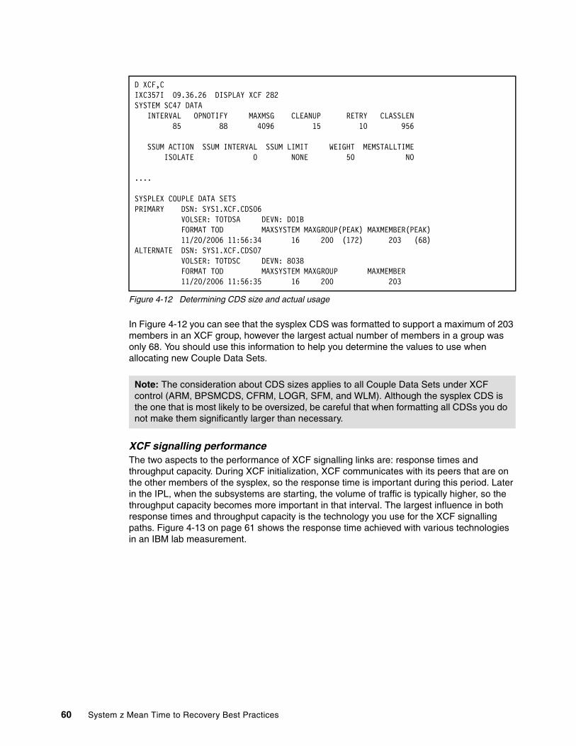
Figure 4-12 Determining CDS size and actual usage

In Figure 4-12 you can see that the sysplex CDS was formatted to support a maximum of 203 members in an XCF group, however the largest actual number of members in a group was only 68. You should use this information to help you determine the values to use when allocating new Couple Data Sets.

XCF signalling performanceThe two aspects to the performance of XCF signalling links are: response times and throughput capacity. During XCF initialization, XCF communicates with its peers that are on the other members of the sysplex, so the response time is important during this period. Later in the IPL, when the subsystems are starting, the volume of traffic is typically higher, so the throughput capacity becomes more important in that interval. The largest influence in both response times and throughput capacity is the technology you use for the XCF signalling paths. Figure 4-13 on page 61 shows the response time achieved with various technologies in an IBM lab measurement.

D XCF,C IXC357I 09.36.26 DISPLAY XCF 282 SYSTEM SC47 DATA INTERVAL OPNOTIFY MAXMSG CLEANUP RETRY CLASSLEN 85 88 4096 15 10 956 SSUM ACTION SSUM INTERVAL SSUM LIMIT WEIGHT MEMSTALLTIME ISOLATE 0 NONE 50 NO ....

SYSPLEX COUPLE DATA SETS PRIMARY DSN: SYS1.XCF.CDS06 VOLSER: TOTDSA DEVN: D01B FORMAT TOD MAXSYSTEM MAXGROUP(PEAK) MAXMEMBER(PEAK) 11/20/2006 11:56:34 16 200 (172) 203 (68) ALTERNATE DSN: SYS1.XCF.CDS07 VOLSER: TOTDSC DEVN: 8038 FORMAT TOD MAXSYSTEM MAXGROUP MAXMEMBER 11/20/2006 11:56:35 16 200 203

Note: The consideration about CDS sizes applies to all Couple Data Sets under XCF control (ARM, BPSMCDS, CFRM, LOGR, SFM, and WLM). Although the sysplex CDS is the one that is most likely to be oversized, be careful that when formatting all CDSs you do not make them significantly larger than necessary.


Figure 4-13 XCF response time by message size and type of link

You can see that the bandwidth of the signalling link makes a bigger difference as the message size increases. But even with small (1 K) messages, ICB4 and InfiniBand 12x links provide superior response times to FICON® channel-to-channels (CTCs).

Figure 4-14 shows the throughput rates of the different signalling link types. Again, you see that ICB and InfiniBand links provide the best performance, but even the ISC links (which did not stand out in the response time measurement) provide more than double the throughput than the highest bandwidth FICON links.

Figure 4-14 XCF signalling throughput

0

0.25

0.5

0.75

1

1K 8K 32K

XC

F I

/O R

esp

on

se T

ime

(mse

c)

XCF Message Size

FICON EX4

FICON EX8

ISC3

ICB4

IB 12X

XCF Signalling Response Times

0102030405060708090

100

Req/Sec (1K)

Th

ou

sa

nd

s

FICON EX4

FICON EX8

ISC3

ICB4

IB 12X

XCF Signalling Rates


Other observationsAn interesting side effect that we noticed during our testing was that the XCF initialization time was over a minute longer when the Couple Data Sets specified in the COUPLExx member did not match those actually in use by the sysplex. Obviously, the incoming system has additional work to do in this case to communicate with its peers to determine the actual Couple Data Set topology. The best practice is that any time you switch any of the Couple Data Sets you should always update the COUPLExx member to accurately reflect the current topology, even if the switch is only temporary.

Other sources of informationSeveral excellent sources of information about XCF performance and setup are:

� Parallel Sysplex Performance: XCF Performance Considerations (V 3.1), an IBM white paper that is a replacement for WSC FLASH 10011 XCF Performance Considerations

� Analyzing XCF Performance with the RMF Spreadsheet Reporter, a presentation available from the RMF home page on the Web at:

ftp://ftp.software.ibm.com/eserver/zseries/zos/rmf/RMF_SpreadsheetReporter_XCF.pdf

� Merging Systems into a Sysplex, SG24-6818

� z/OS MVS Setting Up a Sysplex, SA22-7625

� IBM Software Developer’s forum. RMF in z/OS V1R9 added the jobname to the SMF Type 74 Subtype 2 record so that you can see what address spaces are associated with each XCF group. This is discussed on developerWorks® forum at:

http://www.ibm.com/developerworks/blogs/page/MartinPacker

Recommendations for XCF:

� Use the fastest paths available. Based on current technology, those would be IC links, followed by ICB4, 12x InfiniBand, 1x InfiniBand, and finally ISC.

� If using CTCs for XCF communication, the use of the highest performing FICON links is strongly recommended.

� Tune the XCF transport classes to your configuration: the number of classes, the CLASSLEN values, and the MAXMSG sizes.

� Ensure that enough paths exist between all systems in a sysplex, with at least two failure-isolated paths between every pair of systems.

� Use the D XCF commands, and RMF reports to understand XCF performance and to tune the system.

� Activate and monitor the XCF Health Checks.

� Do not grossly over-specify the values when allocating any of the XCF-managed CDSs. CDS sizes can be increased dynamically at any time, however decreasing the size of a CDS requires a sysplex IPL. Having a very large CDS can affect IPL times.

� Ensure that the COUPLExx member always accurately reflects the names of the CDSs that are currently in use.

� Refer to z/OS MVS Setting Up a Sysplex, SA22-7625 which contains a number of sections with performance recommendations for various aspects of sysplex.


http://www.ibm.com/developerworks/blogs/page/MartinPacker

ftp://ftp.software.ibm.com/eserver/zseries/zos/rmf/RMF_SpreadsheetReporter_XCF.pdf

GRS initializationThe initialization time for GRS is reported in module IEAVNP33. The bulk of the initialization time consists of communicating with XCF, and using XCF to communicate with the GRS instances on the other members of the sysplex. As such, the elapsed time for GRS initialization is based largely on the performance of the underlying XCF infrastructure. The remainder of the time consists of loading GRS modules from sysres and obtaining storage for its control blocks.

SMS considerationsAlthough SMS reports its initialization time in one of the fields in the IPLDATA control block, we discuss SMS in Chapter 5, “z/OS infrastructure considerations” on page 71. The reason is because, strictly speaking, SMS is not started automatically by the system so you must include an entry in the IEFSSN member to get it to start. For that reason, we discuss it in the same chapter where we discuss all other infrastructure address spaces that you are responsible for starting.


The IPLSTATS report for the fifth and final part of NIP processing is shown in Figure 4-15 on page 64. During this part, NIP loads the directories for the LNKLST libraries, creates the CONSOLE address space and initializes console services, initializes WLM, initializes data management, and creates the OMVS address space to provide UNIX® System Services.

The longest step in this part is typically the initializing of LNKLST, and this time is strictly a function of the number of LNKLST libraries, the number of modules in the libraries, and the performance of the DASD devices containing those data sets. The next longest step is typically setting up the consoles. Also, defining the EXCP appendages is usually the only other module that can take a considerable time.



LNKLST considerationsThe z/OS LNKLST enables you to define a set of load libraries that are logically concatenated to SYS1.LINKLIB. The libraries in the concatenation can be defined in the LNKLSTxx member of Parmlib, or using the PROGxx members. All the libraries in LNKLST cannot sum to more than 255 extents.

Although having the flexibility to have a large number of libraries that can be searched without having to specify a STEPLIB or JOBLIB statement is an advantage, the disadvantage is that having a very large LNKLST concatenation can significantly increase the time required to

IEAVNPE5 3.590 LNKLST The linklist libraries are used from this point on

IEAVNPD5 0.821 Load pageable device support modules IEAVNP88 0.112 Allocation move EDT II IEAVNPA1 1.829 CONSOLE

The CONSOLE address is created hereIEE252I MEMBER CONSOL00 FOUND IN SYS1.PARMLIBIEE252I MEMBER CTIOPS00 FOUND IN SYS1.IBM.PARMLIBIEA630I OPERATOR #@$2 NOW ACTIVE, SYSTEM=#@$2 , LU=#@$2IEA549I SYSTEM CONSOLE FUNCTIONS AVAILABLE 240

IEAVNPDC 0.533 WLM The WLM address space is created here, and WLM is initialized

IEAVNP16 2.722 EXCP appendages IEE252I MEMBER IEAAPP00 FOUND IN SYS1.PARMLIB

IEAVNP13 0.033 Prepare NIP/MSI interface IEAVNP17 0.002 GTF Monitor Call interface IEAVNPG8 0.004 VSM defined monitor call enablement IEAVNP18 0.099 PARMLIB Scan Routine interface

IEE252I MEMBER IEACMD00 FOUND IN SYS1.PARMLIBIEE252I MEMBER COMMND$2 FOUND IN SYS1.PARMLIBIEE252I MEMBER MSTJCL00 FOUND IN CPAC.PARMLIBIEE252I MEMBER SCHED00 FOUND IN SYS1.PARMLIBIEE252I MEMBER IECIOS00 FOUND IN SYS1.PARMLIBIEE252I MEMBER CTIIEFAL FOUND IN SYS1.IBM.PARMLIBIEE252I MEMBER VATLST00 FOUND IN SYS1.PARMLIBIEE252I MEMBER ALLOC00 FOUND IN SYS1.PARMLIBIEE252I MEMBER BPXPRMFS FOUND IN SYS1.PARMLIBIEE252I MEMBER BPXPRM00 FOUND IN SYS1.PARMLIB

IEAVNPF2 0.083 Process IOS= IEAVNP15 0.350 Process VATLST IEAVNPRR 0.002 RRS IEAVNPOE 0.415 USS IEAVNPSC 0.010 Metal C RTL IEAVNPLE 0.060 System LE RIM

Language services are initialized hereUNIX system services are initialized hereOMVS address space is created here

IEAVNPUN 0.071 Unicode IEAVNPXL 0.013 zXML Parser IEAVNP1B 0.117 Close catalog

CATALOG address space is created hereIEAVNIPX 0.001 NIP final cleanup

10.867 Total for this part 94.128 TOTAL NIP TIME (seconds)


initialize the LNKLST. In the IPLSTATS reports, the LNKLST initialization time varied from a low of .75 seconds up to nearly 10 seconds.

ConsolesThe elapsed time that is required to initialize all the consoles is related to the number of consoles defined to the system, the performance of the XCF signalling infrastructure, and the release of z/OS that is being used. Obviously, the more consoles that are defined, the longer the time to initialize them, so you should try to minimize the number of consoles, both actual and defined in the CONSOLxx member.

Starting with z/OS 1.10, you can operate z/OS console services in distributed mode within a sysplex. According to the z/OS V1R10 Introduction and Release Guide, GA22-7502, the potential advantages of distributed mode include:

� Reducing the time to IPL a system

� Reducing the time for a system to join a sysplex

� Reducing the scope of console-related hangs

� Reducing the possibility of console-related outages

� Allowing more multiple console support (MCS), SNA MCS (SMCS), and subsystem consoles to be configured

Although we did not run timing tests on this, we expect that installations with a large number of MCS and SMCS consoles will see some reduction in CONSOLE startup time. Distributed mode consoles are only available when all members of a sysplex are running z/OS 1.10 or later. For more information about distributed mode consoles, see z/OS Version 1 Release 10 Implementation, SG24-7605.

An interesting paper, Console Performance Hints and Tips for a Parallel Sysplex Environment, can be found at:

http://www.ibm.com/systems/resources/servers_eserver_zseries_library_techpapers_pdf_gm130166.pdf

The paper refers to identifying the rate of messages by type of message. You can do this with the MSGLG160 program described in 3.3, “Syslog” on page 24.

WLMIn general, WLM initialization time is very short so, from that perspective, WLM is typically not an issue during this part of the IPL. However, WLM does play a vital role as the infrastructure and major subsystems get started. Therefore, WLM, and specifically the setup of the WLM policy, is discussed in detail in 5.2, “Workload Manager” on page 72.

Recommendation for Linklist (LNKLST) libraries:

� Remove any old Linklist libraries when they are no longer needed. This technique reduces startup time and reduces the search of linklist for all applications during the life of the image.

� Generally (there are always exceptions), the optimal fetch performance for load libraries is achieved by using a block size of 32760. This size is the ServerPac default for load libraries and we recommend that you use this.


http://www.ibm.com/systems/resources/servers_eserver_zseries_library_techpapers_pdf_gm130166.pdf

EXCP appendagesI/O appendages, if any, are defined in the IEAAPP00 member of Parmlib. If you find that the IEAVNP16 module is taking a long time (many seconds), consider checking if you have an IEAAPP00 member defined, and if so, whether the appendages defined in that member are actually still required.

Language Environment initializationOn a small number of systems, large values for module IEAVNPLE have been observed. However those cases all appear to be related to systems that are severely CPU-constrained. We tested various options in the CEEPRM00 member, and even not using that member at all, and couldn’t find any measurable difference between the runs.

4.5 Master Scheduler Initialization (MSI), phase 1

The MSI phase follows NIP processing. The statistics in IPLSTATS refer to this phase as IEEVIPL because that is the name for the master scheduler base initialization module. The IPLSTATS report for the first phase of MSI is shown in Figure 4-16.

During this phase, MSI initializes the Master Trace table, enables all MCS consoles, initializes sysplex-wide ENF (Event Notification Facility) services, creates the IEFSCHAS address space (used for cross-system GRS communication), and initializes the MSTR subsystem. It also initializes common Job Entry Subsystem (JES) services, such as creating the JESXCF address space, creates the ALLOCAS address space (for allocation services), and attaches an initiator to start the Master job control language (JCL).

Figure 4-16 Master Scheduler Initialization (phase 1)

As you can see in Figure 4-16, this phase took less than five seconds on our system. In fact, looking at the IPLSTATS reports for those 150 systems, this phase of the IPL varies from a low of just .479 seconds to a high of only 6.251 seconds. Little can be done to tune this phase of the IPL, and with such low elapsed times, there would seem to be little point in doing any tuning even if you could.

**** IEEVIPL Statistics **** IEETRACE 0.003 Master trace ISNMSI 0.758 SPI UCMPECBM 0.996 CONSOLE address space ENFPC005 0.000 CONSOLE ready ENF IEFSCHIN 0.256 IEFSCHAS address space IEFJSINT 0.003 Subsystem interface IEFSJLOD 0.015 JESCT IAZINIT 0.059 JESXCF address space IAZFSII 0.012 FSI trace IEFQBINT 0.021 SWA manager IEFAB4I0 0.194 ALLOCAS address space IEEVIPL 2.334 Uncaptured time: 0.000

4.667 Total for MSI phase 1


4.6 Master Scheduler Initialization (MSI), phase 2

The final phase of z/OS IPL includes validating dynamic paths to I/O devices, bringing all the available CPs out of their stopped state so they are available for use, starting the System Logger and SMF address spaces, starting the subsystems defined in the IEFSSN members, and processing the COMMNDxx and IEACMD00 members. Also during this phase, the Advanced Program-to-Program Communication (APPC) and Time Sharing Option (TSO) services are started.

The IPLSTATS report for the MSI phase 2 part of our IPL is shown in Figure 4-17.

Figure 4-17 MSI Phase 2

MSI started at: 2009/05/14 22:45:08.870 **** IEEMB860 Statistics **** ILRTMRLG 3.079 ASM IECVIOSI 17.735 IOS dynamic pathing

IEE252I MEMBER IEAAPP00 FOUND IN SYS1.PARMLIBIEC336I STORAGE SUBSYSTEM X’89E3’ INITIALIZEDIEC336I STORAGE SUBSYSTEM X’89E5’ INITIALIZED. . . plus one message for each subsystem

ATBINSYS 0.025 APPC IKJEFXSR 0.161 TSO IXGBLF00 0.015 Logger

*IFB081I LOGREC DATA SET IS FULL,16.06.21, 360DSN=SYS1.#@$A.LOGREC

COMMNDXX 31.315 COMMANDxx processing Most of this time is executing the immediate commandsThe rest of the CPUs are varied online at this point

SMFWAIT 116.122 SMF IEE252I MEMBER SMFPRM00 FOUND IN SYS1.PARMLIBInitialize SMF, create SMF address spaceSMF will create all of the SMF IPL records at this time

SECPROD 3.473 Security server IEE712I CONTROL PROCESSING COMPLETEICH508I ACTIVE RACF EXITS: NONE

IEFJSIN2 6.733 SSN= subsystem IEFHB4I2 0.013 ALLOCAS - UCB scan CSRINIT 0.011 Windowing services FINSHMSI 0.077 Wait for attached CMDs MSI ended at: 2009/05/14 22:45:19.500 IEEMB860 10.630 Uncaptured time: 0.100

Remaining CPUs are varied online at this point178.759 Total time for this phase


Figure 4-18 shows the modules that had the highest median times across our sample of 150 systems.

Figure 4-18 Largest elapsed time components in MSI Phase 2

You see that the longest running modules on our system reflect the behavior across that larger set of systems. The one exception we had was that our COMMNDxx processing took an unusually long time.

Dynamic pathing considerationsAt this point in the IPL, all online paths to any device that supports dynamic pathing (DASD, tape, and maybe printers) are validated.

Prior to z/OS 1.10, any CPs in the partition that were in a stopped state would be brought out of the stopped state and made available for use near the end of this phase. However, z/OS 1.10 changed this so that the CPs are made available earlier, providing more CPU capacity available to drive the dynamic path processing.

The elapsed time for this processing is affect by:

� The number of online devices that support dynamic pathing

� The number of defined and online paths to those devices

� The number of PAV base devices

PAV aliases are not initialized during path validation.

In z/OS 1.11, changes were made to reduce contention in the disk subsystems during path validation. As a result, reductions of greater than 50% were seen in some tests in IBM, comparing z/OS 1.10 with z/OS 1.11.

MSI Phase2 Largest Components

0

50

100

150

200

250

SMF SSN= subsystem Security server IOS dynamic pathing

Event

Sec

oo

nd

s

MIN

MEDIAN

MAX


Note that the use of Intelligent Resource Director (IRD) Dynamic Channel Path Management (DCM) can affect dynamic path validation time. When the system is IPLed, any CHPIDs that are defined as being dynamic will be varied offline. The varying of these CHPIDs back online happens in parallel with dynamic path validation and has the following results:

� If the dynamic CHPIDs are still offline when the dynamic paths for a device are being validated, the elapsed time for dynamic path validation can be reduced (compared to a configuration with the same overall number of paths, where all paths are using static CHPIDs).

� If you increase the total number of potential paths to a device as part of implementing DCM, and all the dynamic CHPIDs have been varied online by the time dynamic path validation runs, the elapsed time can increase.

SMF considerationsIn our case, SMF initialization was the largest part of this phase. However, our system was set up to prompt the operator during SMF startup. It was also set up to collect the SMF Type 19 records, which involves going out to each volume to gather space utilization information that is then stored in the Type 19 records. This is discussed in more detail in “SMF Type 19 records” on page 91.

To reduce the SMF start time, do not collect the Type 19 records and also (especially) do not prompt the operator during startup.

Security server considerationsThe median time to complete security server initialization across the set of IPLSTATS reports was less than 2 seconds. However, the maximum time was nearly 34 seconds, indicating that there is some scope for tuning this time to reduce it.

The processing that security server carries out during this time includes:

� Waiting to get access to the RACF® database if other systems that share the same database have the database serialized.

� Loading information from the RACLISTed profiles into storage from the database.

Both situations can be assisted by minimizing access to the RACF database (through the use of the RACF cache structures in the CF, for example), and by placing the RACF database data sets on the best performing DASD available to you. In addition, RACGLIST processing can be used to speed up the loading of profiles into storage.

SSN considerationsSubsystem processing involves reading the IEFSSNxx members of Parmlib, and also the processing associated with defining all the specified subsystems to the operating system and initializing those subsystems. The system reads the first subsystem definition from the IEFSSN member and then does all the processing that is associated with initializing that subsystem. Then, it reads the next subsystem definition and initializes that subsystem, and so on until all the subsystem definitions have been processed and the subsystems initialized.

Because of this method of processing the definitions, you should place the most important subsystems near the top of the member, and the least important subsystems later.

The median elapsed time to process the IEFSSN member was only a little over two seconds, but the maximum was about 35 seconds.


If you find that the SSN startup time (listed under the IEFJSIN2 module) is taking too long, you should be sure that:

� the IEFSSNxx members do not contain large numbers of subsystem definitions for subsystems that are never used, or for old software or subsystems that are no longer used.

� you do not have an inordinately large Parmlib concatenation or a large number of IEFSSNxx members that must be processed.

� The definition for the SMS subsystem is placed as early in the IEFSSNxx member as possible.

The IEFSSNxx member actually supports two formats; keyword and positional. The keyword format has been available for many years now, and is the recommended format. As with the PROGxx members, we would expect that any potential future enhancements related to this member would only apply if the newer format (keyword) is used.

Also, remember that dynamically adding subsystems after the IPL is possible. This process, and several related limitations, is discussed in the “Dynamic Subsystems” section of z/OS Planned Outage Avoidance Checklist, SG24-7328. However, if you order the subsystems in the IEFSSNxx member in a manner that reflects the relative importance of each subsystem, moving the definition of some subsystems out until after the IPL may not buy you much.

COMMNDxx considerationsIn parallel with the last items of the z/OS IPL process, MVS starts processing commands that are typically contained in the COMMNDxx members or issued from an automation product. These commands are typically responsible for starting the infrastructure address spaces (VTAM, TCP, JES2, TSO, and so on).

As stated previously, our system was atypical in the amount of time elapsed for COMMNDxx processing. The reported time for COMMNDxx processing does not actually include the time to process the commands that are contained in these members. During this module, the COMMNDxx members are read, and any commands that are encountered are queued for execution, however the execution time is not included in the IPLSTATS report. Note that there is no guarantee that the commands will actually be processed in the same order that they are specified in the COMMNDxx members.

The best way to reduce the elapsed time to process the COMMNDxx members is to reduce the number of commands issued in those members. Previously we suggested that the COMMNDxx member should not be used to vary devices offline; if the devices are not needed by the system, they should not be marked as being online at IPL in the IODF. Also, in 2.5.2, “Sequence of starting products” on page 10, we suggested that the early part of IPL (when the COMMNDxx members are processed) should be kept for starting the parts of the system that are critical for your online service. Other address spaces should be started by automation later, after the critical components are up and running.

z/OS actually provides two Parmlib members where you can specify system commands: COMMNDxx and IEACMDxx. Both members are read during MSI processing and all commands that are encountered are queued for later processing. Given that both members are treated in the same way, there really is nothing to be achieved by placing a command in one member rather than the other. For that reason, we recommend following the official IBM guidance which is that you should leave the IEACMD00 member as it is delivered by IBM, and apply any customization you want to the COMMNDxx member (or members).


Chapter 5. z/OS infrastructure considerations

Now that we have described the IPL sequence, we move on to the next part of the IPL; the infrastructure startup. This chapter also covers other miscellaneous z/OS topics that are related to both starting and stopping the system, including what happens after you stop it and before you start it again.

5


5.1 Starting the z/OS infrastructure

At the end of Chapter 4, “z/OS IPL processing” on page 35, we had a basic z/OS system up and running. The next step to providing a fully functioning z/OS environment is to start the products that provide infrastructure functions for the middleware and applications that support your business.

The infrastructure functions should be started in a sequence that reflects their importance to that environment, and the dependencies between products.

If you have an automation product that is defined as a subsystem in IEFSSNxx, that product should probably be the first entry in the IEFSSNxx member, because it will start most of the middleware products; we want it up as soon as possible. Also, because many automation products can take some time to start, by placing it first in IEFSSNxx, we can overlap its startup with the initialization of other important subsystems.

For example, because so many data sets are SMS-managed on most systems, the SMS subsystem should be the first started after the automation product is started. And because most started tasks run under the control of a job subsystem, JES should be the next address space to be started.

Before any transactions can be submitted to the system, VTAM and TCP must be started. However TCP requires that OMVS is available before it can start. Therefore, OMVS should be started next (in fact, in recent releases of z/OS, OMVS gets started automatically by the system, using the BPXPRMxx member that you point to in your IEASYSxx member). VTAM and TCP should be started next.

There is one other important subsystem that we discuss: WLM. The WLM policy that you create determines how system resources are distributed across the work running on the system, which in turn can affect how quickly various subsystems and started tasks will start. For that reason, we discuss your WLM setup first, and then continue with the other infrastructure components, in the sequence in which we suggest that you start them.

5.2 Workload Manager

The MVS Workload Manager (WLM) controls the amount of resources that are allocated to every address space in attempting to meet their goals. The early startup of the base z/OS system is unlikely to be affected if the priorities and goals specified for WLM are less than ideal. However these priorities become increasingly important the further we get into the IPL, and especially when we get to the point of starting all the middleware and subsystems.

If you read the documentation for most applications or subsystems, they frequently recommend that their products be placed in the SYSSTC service class, and that everybody else’s address spaces be defined below them. However, as we all know, everyone cannot be top priority. An important point is that you establish effective priorities based on your installation’s requirements.

In this section, we give you guidelines for Workload Manager that can help you optimize your startup, shutdown, and normal processing times. Of course, your installation might have different priorities. For additional information about setting up WLM, see these resources:

� z/OS MVS Planning: Workload Management, SA22-7602

� System Programmer’s Guide to: Workload Manager, SG24-6472


� OS/390 Workload Manager Implementation and Exploitation, SG24-5326

� The WLM home page contains several presentations and documents:

http://www.ibm.com/servers/eserver/zseries/zos/wlm/

� The IBM Techdocs Web site also has several articles about WLM (do a search on WLM):

http://www.ibm.com/support/techdocs/atsmastr.nsf/Web/Techdocs

5.2.1 z/OS system address spaces

A change was made in z/OS 1.10 to automatically assign certain z/OS address spaces to the SYSTEM service class. The reason for this change is that installations sometimes did not classify these address spaces correctly, potentially resulting in performance issues. If you are not running z/OS 1.10 yet, you should change your WLM policy to classify the following started tasks to the SYSTEM service class:

� CATALOG: Catalog address space

� CONSOLE: Console address space

� GRS: Global resource serialization address space

� IEFSCHAS: Cross-system ENF notifications

� IXGLOGR: Logger address space

� SMF: System Management Facilities

� SMSPDSE: PDSE address space

� SMSPDSE1: PDSE optional address space

� XCFAS: cross-system coupling facility

General WLM recommendations:

� Keep your WLM policy as simple as possible. Service classes with only a single period are usually better than two periods, and two periods are almost always better than three periods. Of course there are exceptions to every recommendation, but this provides a good place to start.

� Use response time goals, especially percentile response time goals, when you can. Only use velocity goals when transactions goals are not supported, or for test subsystems. Specifically, you should use percentile response time goals for DB2, CICS, IMS, and WebSphere.

� Remember to review and possibly adjust velocity goals after any hardware upgrade.

� If you have a very large number of classification rules, consider their sequence carefully. The rules are applied serially, starting with the first one, until a match is found.

� Do not have too many service class periods with non-discretionary goals. A good guideline is to have less than 30 non-discretionary service class periods that are active on any one system.

� Any service class with velocity goals should have multiple address spaces assigned to it so that it can collect meaningful statistics. If you need more granularity for reporting reasons, assign the address spaces to report classes.

� If you have not reviewed your WLM policy in several years, take the time to do it now. Several enhancements to WLM have been made that can simplify your policy, or improve response time for transactions.

Chapter 5. z/OS infrastructure considerations 73


http://www.ibm.com/support/techdocs/atsmastr.nsf/Web/Techdocs

After you migrate to z/OS 1.10, you will no longer need these to be explicitly classified and therefore the associated classification rules should be removed. All work in the SYSTEM service class runs at dispatching of priority FF (the highest), and is not storage-managed; that is, pages are not stolen from these address spaces until storage is critical. You can identify all of the SYSTEM services classes by looking at any display of dispatching priorities and at the service class name, or check for address spaces that have a dispatching priority of FF.

5.2.2 SYSSTC

SYSSTC is a service class that is provided by z/OS and runs in the second highest dispatching priority (FE). Like SYSTEM, it is not storage-managed. Unfortunately, this class is over-used in many installations. It should be used only for that work that must run higher than your most important online address spaces. A good example of address spaces that should be assigned to SYSSTC are the lock managers for DB2 and IMS, some monitors or schedulers, and some system tasks. You can find the SYSSTC address spaces on your system by looking at a display for SYSSTC or dispatching priority of FE.

Another candidate for SYSSTC, especially in a WebSphere Application Server environment, is to run the OMVS kernel there. Instead of using the STC subsystem for classification, the OMVS kernal is classified in the OMVS rules, by classifying a UI of OMVSKERN to SYSSTC.

5.2.3 Transaction goals

Most major subsystems support the use of WLM transaction goals. This is very important; we recommend that you use them when possible.

For CICS and IMS, transaction goals are classified in the WLM policy’s CICS and IMS subsystems. Other transaction goals are set for enclaves. Enclaves are created and deleted by each subsystem for each request, and are assigned a goal that carries with the enclave across multiple address spaces. Some enclaves are created for short-running work that has to traverse multiple address spaces, and some are created for long-running work. DB2 and WebSphere Application Server enclaves are addressed in this publication.

CICS and IMS transaction goals can only have a single period, but DB2 and WebSphere Application Server can have multiple periods. When possible, try to use a percentile response time goal and a single period. Velocity goals should be reviewed and possibly adjusted with every processor upgrade, but response goals can generally handle upgrades with no changes. It is important that the response time goals are based on your Service Level Agreements, not on the best possible response time the system can deliver.

Recommendation: If running an earlier release than z/OS 1.10, classify these address spaces to the SYSTEM service class: CATALOG, CONSOLE, GRS, IEFSCHAS, IXGLOGR, SMF, SMSPDSE, SMFPDSE1, and XCFAS.

Recommendation for SYSSTC:

SYSSTC should be used only for important work that does not take over the system. Work in this service class runs higher than any of the other address spaces associated with your online applications. Periodically, you should review the address spaces in SYSSTC and determine the amount of CPU time that each uses. If one address space appears to be taking an exceptionally large amount of CPU time, consider moving it to another service class that is managed to a velocity goal.


A problem with average response time goals is that they can be skewed by a few very long-running transactions, which is why we generally recommend using percentile response time goals. Although some overhead exists when using transaction goals, most installations find that the improved management of the address spaces compensates for the overhead.

When transaction goals are used, the owning address spaces are managed to attempt to meet the goals for the transactions running in that address space; the address space is not managed to the started task service class goal, except at startup and shutdown. Therefore, it is best to assign those started tasks to a high importance, high velocity service class that does not contain any non-managed address spaces; this should ensure that those address spaces receive sufficient resources to start in a timely manner. We suggest a unique service class for all of these servers. In our example, we call it the OPS_SRV service class, which has an assigned velocity of 60 and an importance of 2. We discuss the specific address spaces for each subsystem later.

For IMS and CICS, you can use transaction goals for some regions and use velocity goals for other regions (test regions, for example). We recommend using velocity goals for test regions.

5.2.4 DB2 considerations

Before we describe the DB2 considerations, you should realize that almost all DB2 work, with the exception of distributed data facility (DDF), is managed to the originator’s goal. So if a CICS transaction requests a DB2 service, such as a stored procedure, the DB2 work will run at the dispatch priority of the CICS transaction, and not the dispatch priority of any DB2 address space. As a result, the WLM goals assigned to most DB2 address spaces are only applied during startup and shutdown.

The six types of address spaces used by DB2 are:

� xxxxIRLM

The DB2 lock manager. If this is associated with a production DB2, this address space should be assigned to the SYSSTC service class.

� xxxxMSTR (master control region) and xxxxDBM1 (database management, including buffers)

These are the two primary regions for DB2. After they are started, they are generally managed according to the transactions they are running. Therefore, these two address spaces can be run at a high priority and importance.

� xxxxDIST

This address space controls DDF transactions. Its transactions are run as independent enclaves and should have transaction goals that are classified in the WLM DDF subsystem. If you do not have a default transaction goal defined for DDF, any transactions that are not explicitly classified will be assigned to the SYSOTHER service class, which is the same as discretionary. If you used THREADS=INACTIVE and DBAT is pooled

Recommendations for subsystems with transaction support:

� Use transaction goals when possible, with the exception of development or test regions.

� If you use transaction goals with test regions, avoid using the same service classes as your production subsystems.

� Use only a single period, and use a percentile response time goal for them, such as 80% less than .5 seconds.

� Do not specify the CPU Critical option unless you have no alternative.


(connection inactive), you can use percentile response time service classes. You can also use multiple periods if you need them.

If THREADS=ACTIVE, multiple transactions are treated as one and the user think time is included in the response times. These transactions should be classified to a service class with a single period velocity goal.

If you cannot differentiate between the two types (inactive and active) of transactions, you can use a two-period service class with a percentile response goal on the first period and a velocity goal on the second period. The address space xxxxDIST should be classified to OPS_SRV in the STC subsystem. Be sure that the goal of the xxxxDIST address space is higher (of more importance) than the associated transactions, or DDF logons could be delayed.

� xxxxSPAS

These started tasks are for DB2-managed stored procedures. The transactions are run as dependent enclaves and will be run at the dispatch priority of the originator. The xxxxSPAS address space can be classified in the STC subsystem to OPS_SRV.

� xxxxWLMx

These started tasks are for WLM-managed stored procedures. This is a function that was provided in DB2 V9 with APAR PK75626. These started tasks should be managed the same as the xxxxSPAS address spaces.

The DB2 server can use sysplex query parallelism to distribute parts of a complex query across multiple systems within a sysplex. When these sysplex query transactions arrive on another system, they are classified in WLM using the DB2 subsystem (that is, the WLM service class information does not get sent with the transaction). Because they are expected to be long-running and you no longer have the characteristics of the originator, you can classify these to a separate service class, preferably a one or two-period service class with a velocity goal. APAR PK57429 creates independent enclaves for the DB2 subsystem that are managed by WLM.

A good description of the various WLM recommendations related to DB2 is provided in a SHARE Austin 2009 session 1342, titled Using WLM with DB2 for z/OS, available at:

http://ew.share.org/proceedingmod/abstract.cfm?abstract_id=19582&conference_id=20

Recommendations for DB2:

� Assign the DB2 IRLM address space to the SYSSTC service class.

� Assign xxxxMSTR and xxxxDMB1address spaces to a high importance, high velocity service class.

� Assign the xxxxDIST and xxxxSPAS address spaces to a server service class (slightly lower importance and velocity than MSTR, but they will eventually be managed by the transactions).

� Always classify DDF transactions. You can use two service classes for different types of work, or a single two-period service class with a percentile response goal on period one and a velocity goal on period two.

� Always classify DB2 query transactions. These can be a single-period service class with a velocity goal.


http://ew.share.org/proceedingmod/abstract.cfm?abstract_id=19582&conference_id=20

5.2.5 CICS considerations

CICS is one of the easiest systems to classify, especially when you are using transaction classes. The two types of CICS-provided address spaces are:

� One for running CICSPlex System Manager

� One or more for the regions that run the business workload, the most common of which are:

– Terminal-owning regions (TOR)

– File-owning regions (FOR)

– Application-owning regions (AOR)

Transactions typically arrive into a TOR and are routed to an AOR (which might use an FOR to access data). If you are using transaction classes by classifying work in the CICS subsystem portion of the WLM policy, then the TORs, FORs, and AORs are managed to the transaction goals.

If you use transaction goals for CICS, performance blocks (PBs) are created in every TOR region. The number created is equal to the number specified in MXT (max tasks). If you are using transaction goals, the PBs are sampled every 250 milliseconds, whereas when using region goals, the PBs are sampled every 2.5 seconds. Therefore, you can reduce the cost of using transaction goals in CICS by reducing the MXT to a reasonable number for the region and not setting it to the maximum possible. This is especially true for any smaller CICS systems.

5.2.6 IMS considerations

IMS work can be managed to transaction goals by using the IMS subsystem in WLM. In the WLM policy, you would assign the IMS transaction classes to service classes with response time percentile goals. Except for batch processing, the other IMS address spaces are managed in order to achieve the transaction goals. To improve startup time, however, the primary address spaces should be assigned to a fairly high velocity and importance service class. See 8.6.1, “IMS-related address spaces” on page 162 for a description of the IMS address spaces.

Recommendation for CICS:

� Use transaction goals, but only after tuning the MXT parameter.

� Use a single period service class for the transactions, with a percentile response goal (for example, 80% within .5 seconds).

� Assign the CICS regions to a high importance server service class so they get sufficient resources for an efficient and timely startup. After the startup phase has completed, the regions will be managed based on the transaction goals for the work running in those regions.

� If CICSPlex SM is used, it must be run as a high importance, high-velocity started task (for example, importance 1, velocity 70). Keep in mind that prior to CICS TS Version 4, CICSPlex SM uses the percentile response goal as an average goal.

� For more recommendations about setting up CICS, see Chapter 6, “CICS considerations” on page 107.


For more information about the relationship between IMS and WLM, see the presentation titled Non IMS Performance PARMS, available on the Techdocs Web site at:


5.2.7 WebSphere Application Server considerations

The WebSphere Application Server has two types of configurations:

� Base Application Server, which is used for testing but not ideally suited to large production environments,

� Network Deployment (ND), which can support multiple Application Servers.

A WebSphere Application Server controller region feeds transactions to WLM. WLM then sends the transactions to one or more servant regions that WLM is responsible for creating and deleting, based on a minimum and maximum number of regions specified by the user and WLM’s calculation of how many servant address spaces are required to meet the stated goals.

WebSphere transactions can be classified into a service class using the WLM CB subsystem. If you do not specify a default service class for this subsystem, any transactions that are not explicitly classified will fall into SYSOTHER (discretionary).

Recommendations for IMS:

� IMS IRLM - IMS lock manager: assign this address space to the SYSSTC service class.

� Of the remaining IMS started tasks, the most important one (in terms of having access to the CPU when necessary) is DBRC. DBRC does not use much CPU time, but it must get access to CPU in a timely manner when needed.

The Control Region started task is also very important to IMS. This started task uses a lot more CPU time than DBRC. DLISAS is also a server type of address space for IMS and should be classified along with the control region.

These started tasks should be assigned to the OPS_HI service class to ensure good performance during startup, shutdown, and recovery.

Of the SCI (structured call interface), OM (operations manager), RM (resource manager), and DLISAS (database support), only DLISAS tends to use much CPU time. SCI, OM, and RM are optional, however if enabled, then those functions become critical. These started tasks could be assigned to the OPS_SRV service class.

� Online transaction started tasks: MPPs/MPRs (message processing programs/regions), IFPs (IMS fast path programs), JMPs (Java™ message processing programs). These started tasks could also be assigned to our OPS_SRV service class. The IMS transactions should be assigned to one or more IMS transaction classes, and the transaction classes in turn assigned to one or two single-period service classes with a percentile response goal.

� Batch jobs are: BMPs (batch message processing) and JBPs (Java batch message processing). Assign all batch jobs to one or two service classes, usually one of the standard JES batch service classes. If you want the longest-running jobs to have a lower priority, you can use a multi-period service class that has a lower goal or velocity than the first period. Depending on the characteristic of the work running in the job, use a percentile response goal if possible. Because these transactions are run in batch, these service classes can run at a lower importance, such as 3, 4, or 5.



The first step of the control region startup procedure invokes the BPXBATCH shell script, so is managed by the OMVS subsystem. To reduce the startup time for the control region, it is important to classify the BPXBATCH work to a high importance and velocity OMVS service class.

For more information about WebSphere Application Server and WLM, see Techdocs presentation PRS3317, available at:


The presentation includes an excellent set of references. Technote TD102730 (available on the same Web site) provides a further explanation of the OMVS classification process.

5.2.8 Putting them all together

Although each subsystem would like to run at the highest dispatch priority, each installation must choose which subsystems get priority. This choice is greatly simplified by using transaction goals on the subsystems that support them: CICS, DB2 DDF, DB2 sysplex queries, DB2 stored procedures, IMS, OMVS tasks, and WebSphere server regions. This approach both reduces the need to change the goals when a hardware change occurs, and simplifies the classification of the other address spaces associated with a subsystem. Creating an easy-to-manage workload policy for all of these subsystems by keeping it simple is easy to do. Most of the subsystems can be managed in a very few service classes. To determine the resource usage for each type of work, use several report classes instead of separate service classes.

SuggestionsAlthough these are our suggestions for defining your work to WLM, adjust them as appropriate for your installation:

� SYSSTC service class:

– DB2IRLM and IMS IRLM lock manager started tasks

– Certain monitor started tasks, such as RMF and RMFGAT

– Certain auto operations started tasks

WLM recommendations for WebSphere Application Server:

� Assign controller regions (Daemon, Node Agent, Deployment Manager, and application servers) to a high velocity, high importance server class, but not SYSSTC.

� Use transaction goals to manage servant regions (those managed by WLM), but start at a high velocity, high importance service class (but lower than the controllers) for initial startup. Put them with the OPS_SRV service class.

� Classify transactions that are using the APPLENV name or transaction class in the CB subsystem, using a single period service class with importance 2, and a percentile response goal (for example, 80% within .5 seconds). You can create one or more service classes for these transactions if needed.

� Because the start up of the controller region runs as a UNIX transaction, you will need to classify it in the OMVS classification rules, using the started task name of the controller region.

� Be cautious when defining limits on the number of server regions. A minimum number that is too low can could delay the start up of these regions. A maximum number that is too low could cause some transactions to time out.



– Certain system address spaces: LLA, ZFS, NET, JES2, VLF, JES2AUX, TCPIP, SMS, RACF, TNF, VMCF, JES2S001, RESOLVER, and TN3270

– The OMVS kernel

� Highest velocity started tasks (for example, OPS_HI, importance 1, velocity 70):

– CICSPlex SM CMAS started task

– DB2MSTR and DB2DBM1 started tasks

– IMS controller regions (Control Region, DLISAS, and DBRC) started tasks

– WebSphere Application Server controller region (Daemon, Node Agent, Deployment Manager) started tasks

� High velocity service class for started tasks whose work will use transaction goals (for example, OPS_SRV, importance 2, velocity 60). The velocity service class is only used during startup and shutdown

– CICS AOR, TOR, and FOR started tasks– DB2DIST, and DB2SPAS started tasks– IMS SCI, OM, RM, MPP, IFP, and JFP started tasks for handling transactions– WebSphere Application Server servant region started tasks

� Medium or low velocity started tasks (for example, OPS_DEF, importance 4, velocity 20: test subsystems should be assigned to a service class like OPS_DEF)

Test regions for all subsystems; these are managed by using region goals rather than transaction goals.

� Batch processing (depending on priorities, run these as normal batch jobs):

IMS BMP and JBP jobs (defined in the JES subsystem).

� OMVS high importance transactions (for example, OMVS_HI, importance 1, velocity 60):

– WebSphere Application Server control regions (for first step)– FTPSERVE

� CICS and IMS subsystem transactions (for example, ONL_HI, single period, 80% less than .5 seconds). If different response goals are needed, two classes might be needed: CICS transactions and IMS transactions.

� DB2, DDF, and CB (WebSphere Application Server) enclaves (for example, DDF_DEF, importance 2 or 3, first period 80% within .5 seconds, second period velocity of 40. DB2_DEF and WAS_DEF are similar to the settings for DB2, DDF, and CB enclaves). Although a better solution is using just one period, this is not always possible. Two service classes can be used if the volume of transactions is high enough, and you can identify lower importance work.

5.3 SMS

The first subsystem that is defined in the IEFSSNxx member should be SMS (except perhaps the automation subsystem, and that decision depends on the specific automation product you are using). Because so many data sets are currently capable of being SMS-managed, SMS-managed data sets will very likely be required by other address spaces as they start up after the IPL. In fact, you may have noticed messages in Syslog stating that various address spaces are waiting for SMS to initialize.

As observed previously, SMS initialization was the second-largest contributor to the elapsed time of the part of NIP processing, taking 3.6 seconds in our test, and a maximum of 49 seconds in the systems we had IPLDATA data for.


SMS initialization includes locating and reading the SMS ACDS and COMMDS data sets and loading information about the SMS objects (groups, classes, and ACS routines). Near the end of its initialization, SMS writes information back to the ACDS data set. Although SMS obtains information about the space usage of each volume and places that information in the ACDS, this processing only happens when data sets get allocated on an SMS-managed volume, and not at IPL time.

As with the other system volumes, you should place the SMS CDS data sets on volumes that do not have any RESERVEs issued against them. And ensure that APAR OA23197 is applied to all members of the sysplex. But beyond these actions, there is not much that can be done to impact/improve the SMS initialization time. However, be careful not to jump to conclusions if you see a message about an address space waiting for SMS to initialize; on our system, SMSVSAM issues such a message, but SMS actually finished initializing just two seconds later. So, if you see these messages, be sure to check how long they are actually waiting before you invest a lot of time into trying to speed up SMS startup.

5.4 JES2

JES should be one of the first subsystems started after the core MVS IPL completes. In fact, the z/OS MVS Initialization and Tuning Reference, SA22-7592, recommends that JES2 be defined in IEFSSN immediately after SMS.

5.4.1 Optimizing JES2 start time

In this section, we review some of the more important considerations for getting JES2 up and running as quickly as possible.

You can start JES2 from either the COMMNDxx member or from IEFSSNxx. We tried placing the START JES2 command in the COMMNDxx member and IPLed, then we moved the start to the IEFSSNxx member and IPLed again. The difference in the time to get to the point where JES started was only two seconds, which was well within the normal difference from one IPL to another. Based on this, where JES is started from appears to makes no material difference.

JES2 checkpoint in coupling facility rather than on DASD Many good reasons exist to put your JES2 Primary checkpoint data set in a coupling facility (CF) rather than on DASD; the speed of the shutdown and subsequent re-IPL of your systems are only two of the reasons. More information about the benefits of the use of CF compared to DASD is available in JES2 Performance and Availability Considerations, REDP-3940.

If your checkpoint is still on DASD, we recommend that you convert the JES2 RESERVE to a Global ENQ if you are using GRS Star (which we hope everyone is). The response time for an ENQ request when using GRS Star should be better than can be achieved by using a RESERVE, assuming that the GRS Star structure is in a CF that is configured to deliver good response times. If the CF response time is very poor, the response time benefit of an ENQ over a RESERVE will be reduced, however ENQs are still preferable from the perspective of not locking out all other access to the volume containing the checkpoint data set while the ENQ is held.


JES2 PROC data setsTwo types of data sets can be specified in the JES2 PROC: data sets containing the JES2 parameter members, and data sets containing JCL procedures that JES2 will use. In both cases, we recommend not having huge concatenations with many data sets. The more data sets there are, the longer that allocation processing takes to get through them all. We have seen cases with customers having many hundreds of data sets referenced in the JES2 PROC, resulting in significant delays in starting JES2.

Although it will not change the JES2 start up time, we recommend moving the definitions of the JES2 procedure libraries out of the JES2 PROC and into a JES2 parameter member. The advantage of defining the libraries in this way is that you can subsequently change a proclib concatenation without having to restart JES2.

Impact of JES2 parms on startup timeFor installations that have been in existence for many years, finding that the JES2 parms contain definitions for resources that are no longer needed or used, or perhaps do not even actually exist any more is not unusual. Remember that JES2 has work to do to process every initialization statement, so the more statements there are in the JES2 parms member, the more time it takes JES2 to come up. For this reason, spend a few minutes to review your JES2 parms to see if all the statements there are still actually required.

Also, regarding the JES2 parms, avoid using the asterisk (*) and other generic characters in JES2 initialization statements that contain ranges, such as NODE(1-*) or PRT(1-*). For JES2 devices, referencing a device as part of a range (for example, LINE(1-*)) results in JES2 creating the control blocks it needs to manage that device. Note the following information:

� A subscript with a range references all devices in the range. So subscripts such as (1-10), (50-1000), or (1-*) will create control blocks for all the logical devices in the range.

� A subscript that contains only a generic does not. So specifying a subscript of (*) only effects already-defined devices.

We conducted a test where we used a range containing an asterisk (*) to define printers and nodes to JES2 - the statement we used is shown in Example 5-1. This resulted in 32,767 printers being defined to JES2, all with the same attributes.

Example 5-1 Example of use of * in JES2 initialization parameter

PRINTDEF SEPPAGE=LOCAL=HALF,TRANS=NO,NIFCB=STD3,NIUCS=GT10,LINECT=60PRT(1-*) WS=(W,R,Q,PMD,LIM/F,T,C,P),CLASS=A

The time needed for JES2 to initialize jumped by more than 10 times, from an average of 4.84 seconds to over 50 seconds when using this definition statement. The CPU time used by JES2 experienced an even larger jump as shown in Figure 5-1 on page 83.


Figure 5-1 Impact of use of * on JES2 initialization CPU and elapsed time

Understanding where the time is being spentIf you feel that your JES2 is not initializing as quickly as you would like, the first thing to do is gain an insight into what is taking place between the time you enter the START JES2 command, and when JES2 completes initialization. The best tool for this is the JES2 $DPERFDATA command (this was discussed in 3.6, “JES2 commands” on page 32). In the output from that command, the following fields are particularly of interest:

MVSSTART This field represents the time from the creation of the JES2 address space until when JES2 code gets control. The main processing in this time period is the allocation processing for the JES2 PROCxx statements. If this time is large, focus on the processing of the JES2 PROC. In one case, an installation had hundreds of DD statements in the JES2 PROC. Processing such a large number of DD statements significantly delayed JES2 start processing.

IRPL This field represents the time that JES2 spends reading and processing the JES2 initialization parameters. Improving performance of the volume containing the JES2 initialization parms can help here, and so can removing any parameters that are no longer required.

Also, any time waiting for WTORs as a result of syntax errors in the JES2 initialization parameters will be included here.

IRPOSTPL Similar to IPRL, this field is part of the post-initialization deck processing. This too can be affected by the contents of the initialization stream. Cleaning up any devices that are not necessary or no longer used can help here.

Recommendation: Ideally each node or printer should be defined individually in the JES2 parms. However, if you still want to define multiple devices with one parm statement, use a specific range such as PRT(1-100), rather than using (1-*).

0.25

4.84

41.53

50.67

0

10

20

30

40

50

60

Sec

onds

JES2 Start TimeJES2 CPU TimeJES2 Start TimeJES2 CPU Time

Impact of JES2 Parms

With generic JES2 parms for printers

and nodes

With specific JES2 parms for printers

and nodes


IRDA This field is the processing that reads the JES2 checkpoint, allocates the spool volumes, and validates the job and output queues. This is a significant point in the initialization process. It is in IRDA processing that JES2 gets the checkpoint data set lock; this serializes the checkpoint and locks out other members. The lock is held by this member until JES2 warm or hot start processing completes.

WARMSTRT This field is the warm starting of the job queue. During warm start, jobs that were active when a system comes down must be released for further processing. Certain control blocks are read from the spool and validated for consistency. The timing of this phase is very dependent on the amount of work that was active and the type of start being done. This processing can be greatly improved if reset member processing is done by an active member when a member has to be re-IPLed. See the AUTOEMEM operand on the JES2 MASDEF parm statement for more information.

Starting multiple systems concurrentlyExtensive work was done on JES2 as part of implementing its sysplex support to better (and automatically) handle situations where multiple JES2 subsystems are contending for access to the JES2 checkpoint. As a result, JES2 is much better able to handle the situation where multiple JES2s are being started concurrently.

Some customers do not start more than one JES2 member at a time because of the contention messages that might be produced by JES during its initialization. However these messages are simply informing you that JES2 is waiting for access to the checkpoint; they do not necessarily mean that there is a problem. Even with the JES2s contending for access to the checkpoint during the IPL, it is still far faster to IPL all system concurrently than to hold off the IPL of each system until the previous system has gotten past the JES2 initialization process.

5.4.2 JES2 shutdown considerations

The JES2 address space should be terminated prior to bringing down z/OS. Although this should be done as cleanly as possible, it does not mean that you must use the $PJES2 command and wait for JES2 to completely shut down.

The preferred command to remove JES2 from the system when you plan to IPL is actually to issue a $PJES2,TERM command. Considered “kinder” than using the ABEND parameter, $PJES2,TERM removes JES2 but does not terminate active programs and devices that are running under JES2. In fact, if nothing would have stopped a $PJES2 command from completing, the $PJES2,TERM command behaves in exactly the same manner as $PJES2.

Although the $PJES2, ABEND command ends JES2 abruptly, in a similar manner to how JES2 ends in case of a JES2 abend, the TERM option stops JES2 in a more orderly way, ensuring that track groups are not lost.

However, if you issue a $PJES2,TERM you must IPL; you cannot do a hot start of JES2 after stopping JES with the TERM parameter. If you plan to stop and then hot start a JES2 without an IPL, then the $PJES2,ABEND command should be used. Because of this approach, some sites choose only to use the $PJES2,ABEND for an escalated shutdown, to maintain a consistency point and avoid any confusion that might lead to an unscheduled IPL when only a hot start of JES2 was needed.


If JES2 terminates while work is being done, it will require a warm start which takes longer than a quick start. However, if most of the tasks running under JES2 are already down, the elapsed time for the warm start is likely to be less than the time that would be spent waiting for JES2 to come to an orderly stop. In addition, if you have specified the MASDEF parms of AUTOMEM=ON and RESTART=YES, then another member of the JES2 MAS can do the warm start while the system being stopped is finishing its shutdown and subsequent IPL.

The following ways can help ensure that JES2 is stopped safely and quickly:

� Drain JES2 initiators a reasonable amount of time before the planned shutdown of your system. This approach both reduces the amount of work that JES2 needs to checkpoint at shutdown, and helps you avoid having to either abend the jobs or wait for them to finish before proceeding with the IPL. You might want to stop the initiators in groups: stop the initiators used for long-running jobs first, followed by medium-length jobs, and finally short jobs. Also, you should keep an initiator available to run the IMS archive jobs and similar jobs.

� Cancel any remaining batch jobs running on the system that is being shut down prior to initiating the system shutdown process using your automation. This approach ensures that JES2 and any batch management software will have correct status information about those jobs.

� Most likely your shutdown routine is well established and includes an order in which things are shut down. This process should include bringing down all subsystems and resources that run under JES2 as it needs to have all work completed to exit the system cleanly. To bring down JES2, issue a $PJES2, however if JES2 has any tasks or work being performed it will not stop until either that work finishes, or you escalate the shutdown. How long you wish to wait before your escalation of the JES2 shutdown is something you need to determine based on your unique circumstances. However, as mentioned before, if you have most of the work that JES2 performs completed and you have other members of the MAS up and configured to process the warm start for the departing member, the time you save on the shutdown should easily exceed the warm start time. You can issue a $DJES2 command at anytime to easily see all resources that are still running under JES2. A helpful approach is to issue the command before you start the shutdown process, and then throughout the shutdown process to track your progress and determine where your sticking points are.

5.5 OMVS considerations

Those of you with many years of experience with z/OS (and previously OS/390® and MVS before that) will have noticed the growing role of UNIX System Services in the z/OS environment. OMVS is now an integral part of z/OS, and critical parts of the system cannot initialize without OMVS being available. For this reason, we provide recommendations for how to keep the time for OMVS initialization as short as possible.

5.5.1 BPXMCDS

In “Sysplex Couple Data Set size” on page 59 we describe how XCF reads the entire Couple Data Set (CDS) at IPL time, and how a very large CDS can elongate the time for XCF to initialize. Similarly, the size of the BPXMCDS Couple Data Set can affect how long OMVS takes to initialize.

To understand the impact of oversizing your BPXMCDS data set, we IPLed with two BPXMCDS data sets formatted as shown in Table 5-1 on page 86.


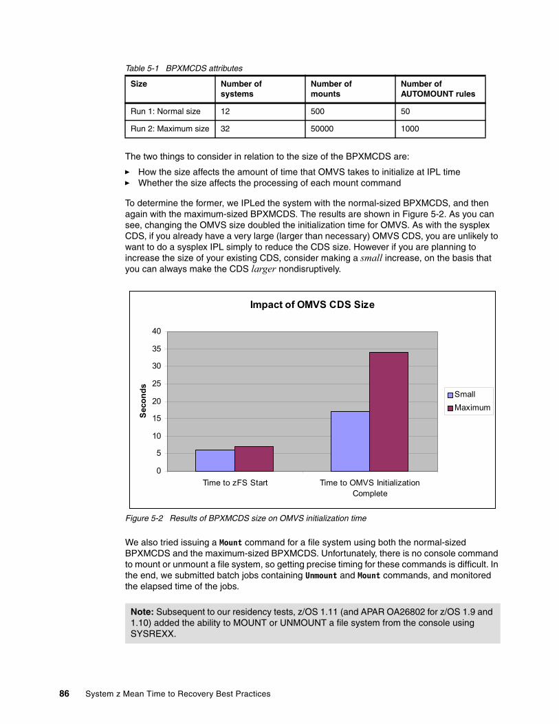
Table 5-1 BPXMCDS attributes

The two things to consider in relation to the size of the BPXMCDS are:

� How the size affects the amount of time that OMVS takes to initialize at IPL time� Whether the size affects the processing of each mount command

To determine the former, we IPLed the system with the normal-sized BPXMCDS, and then again with the maximum-sized BPXMCDS. The results are shown in Figure 5-2. As you can see, changing the OMVS size doubled the initialization time for OMVS. As with the sysplex CDS, if you already have a very large (larger than necessary) OMVS CDS, you are unlikely to want to do a sysplex IPL simply to reduce the CDS size. However if you are planning to increase the size of your existing CDS, consider making a small increase, on the basis that you can always make the CDS larger nondisruptively.

Figure 5-2 Results of BPXMCDS size on OMVS initialization time

We also tried issuing a Mount command for a file system using both the normal-sized BPXMCDS and the maximum-sized BPXMCDS. Unfortunately, there is no console command to mount or unmount a file system, so getting precise timing for these commands is difficult. In the end, we submitted batch jobs containing Unmount and Mount commands, and monitored the elapsed time of the jobs.

Size Number of systems

Number of mounts

Number of AUTOMOUNT rules

Run 1: Normal size 12 500 50

Run 2: Maximum size 32 50000 1000

Note: Subsequent to our residency tests, z/OS 1.11 (and APAR OA26802 for z/OS 1.9 and 1.10) added the ability to MOUNT or UNMOUNT a file system from the console using SYSREXX.

Impact of OMVS CDS Size

0

5

10

15

20

25

30

35

40

Time to zFS Start Time to OMVS InitializationComplete

Sec

on

ds

Small

Maximum


With the maximum-sized CDS, the elapsed time for the job averaged 3.78 seconds. When we switched to the normal-sized CDS (which required a sysplex IPL), the average elapsed time dropped to only .2 seconds.

As with the sysplex couple data sets, we do not expect anyone to do a sysplex IPL simply to move to a smaller BPXMCDS data set. However, if you want to increase the size of your couple data sets, consider making small adjustments (because you can always move to a larger CDS nondisruptively) rather than one large adjustment.

5.5.2 Mounting file systems during OMVS initialization

During OMVS initialization, OMVS attempts to mount any file systems that are referenced on MOUNT statements in the BPXPRMxx Parmlib members that are pointed to on the OMVS parameter in IEASYSxx. Obviously, the more file systems that are listed in this member, the longer OMVS takes to initialize (because it mounts each one serially). Therefore, if you find that important subsystems are being delayed in their startup because they are waiting for OMVS to complete initialization, consider moving non-critical file systems out of the BPXPRMxx member and mounting them later in the IPL process.

One way to achieve this is to define these file systems as AUTOMOUNT-managed, so that if any process attempts to use them before you have a chance to mount them, the file system will be automatically mounted. However, to avoid the delay that is encountered by the first process that causes the file system to be mounted, you can run a small batch job that touches all these file systems, causing them to be mounted before any user actually tries to use them.

Alternatively, after OMVS has initialized, you can:

� Run a little job that would issue MOUNT commands for all those other file systems.

� Use a set omvs=xx command to issue MOUNT commands contained in another BPXPRMxx member.

� Exploit the new SYSREXX APIs for mounting UNIX System Services file systems, for example F AXR,MNTMORE (where MNTMORE is a SYSREXX routine that mounts more file systems.

We highly recommend using the following methodology to determine from where the MOUNT for a given file system is issued:

� In the BPXPRMxx member, mount the SYSPLEX and version file systems, product file systems (including IBM subsystems such as CICS, DB2, and so on), and the /etc, /tmp, and /var file systems.

� In /etc/rc, mount the file systems for critical applications.

� In /etc/local/rc (or some other location) issue the mounts for non-critical applications. You would run a batch job after the system has IPLed to mount these file systems.

One contributor to this book reduced the length of time to make OMVS available by over 20 minutes by organizing the mounts in this matter.

Use of SUB=MSTR for colony address spacesColony address spaces are normally started under JES. However if you are concerned with how long JES takes to start, you have the option of starting the colony address spaces with SUB=MSTR. This capability can allow the startup of the colony address spaces to proceed before JES initialization completes. To use this capability, in your BPXPRMxx member, use SUB=MSTR on FILESYSTYPE statements that use ASNAME. This can apply to zFS, NFS, and TFS.


For more information about this capability, see “Starting colony address spaces outside of JES” in z/OS UNIX System Services Planning, GA22-7800.

5.5.3 Commands processed during OMVS initialization

Just as mounting files can elongate OMVS initialization time, so can the processing of commands. The /etc/rc file contains commands that are issued during OMVS initialization. Review this file to ensure that only commands that must be issued at this time are contained in the file. Any commands that can be issued later in the IPL process should be moved to a different file and issued by automation after the critical subsystems that depend on OMVS being available have completed initialization.

5.5.4 Mounting file systems read/write or read/only

The UNIX System Services sysplex file-sharing method that is implemented by UNIX System Services is basically a function-shipping model, conceptually similar to a CICS FOR. For each file system that will use sysplex file sharing, the file system is mounted on one member of the sysplex, and all read or write requests for that file system from any member of the sysplex is forwarded to that system using XCF. This provides great flexibility, because work that uses that file system can be run anywhere in the sysplex. However, the cost of this flexibility is in reduced performance: asking another system to retrieve some data and pass that data back over XCF obviously takes longer than if the requesting system could just read the data itself.

For file systems that contain mainly programs, such as the version root (that is, the vast majority of accesses are reads), consider moving any files or directories that require write access to another file system. The file system that contains only code can then be mounted as read-only on every member of the sysplex, meaning that each system can do its own I/O, and receive correspondingly better performance.

z/OS 1.11 includes performance enhancements for sysplex file-sharing. However even with these enhancements, performance would still not be equivalent to a file that is mounted as read-only.

5.5.5 Shutting down OMVS

All I/Os to a UNIX file system are processed by OMVS. Just as you would not intentionally IPL a system without first doing an orderly shutdown of your database managers, equally, you should not IPL a system without doing an orderly shutdown of OMVS. The preferred way to shut down OMVS is to follow these steps to bring down OMVS in an orderly manner:

1. Stop any address spaces such as TSO, TCPIP, VTAM, DFSS, FTP, WebSphere Application Server, batch jobs and other address spaces that might use any part of OMVS prior to stopping OMVS.

2. Stop the NFS file system. To do this, issue:

F OMVS,STOPPFS=NFS

3. When you are ready to stop OMVS, issue:

F OMVS,SHUTDOWN

If you need to escalate the shutdown, issue:

F BPXOINIT,SHUTDOWN=FILEOWNER


If you have thousands of OMVS file systems, OMVS shutdown could take quite a long time. To minimize the impact of this time, try to shut down all the OMVS tasks/subsystems, then shut down OMVS, and in parallel, shut down any other non-OMVS tasks

5.6 Communications server

To enable communication between z/OS and the outside world, VTAM, TCP, or both must be started.

5.6.1 VTAM

In general, VTAM startup should take very little time. The most likely reason for an elongated VTAM startup time is if it has to process a huge number of members in VTAMLST. Some sites create one VTAMLST member per resource. Although this approach can help to more easily change and manage the resources, if a very large number of resources (in the thousands) exist, this approach could result in a significantly longer start time for VTAM.

Apart from elongating the start of VTAM itself, TCP cannot initialize until VTAM completes processing all VTAMLST members listed in the ATCSTRxx member (or members), so the longer this takes, the longer TCP startup is delayed.

Also, some subsystems (CICS, for example) cannot complete their initialization until they are able to successfully communicate with VTAM. For all these reasons, you should ensure that VTAM starts as quickly as possible.

Shutdown considerationsThe processing to start VTAM is the same regardless of whether VTAM was stopped in an orderly way, or if you just IPLed over it.

However, VTAM provides one of the ways for work to be routed into z/OS. Stopping VTAM before the IPL will stop the flow of that work, helping you achieve the objective of stopping all work prior to the IPL. For this reason, ensure that you stop VTAM before all planned IPLs.

5.6.2 TCP/IP

There is very little that you can do to influence the startup time of TCP itself. However, TCP requires that both VTAM and OMVS are initialized before it can complete its initialization, so any steps you take to reduce VTAM and OMVS startup time can have a positive effect on TCP.

The only TCP attribute that is known to negatively affect TCP startup time is if you have a very large number of VPN tunnels defined to TCP.

Important: Ensure the zFS address space stops in an orderly manner when possible (the commands in the previous list will stop the zFS address space, along with OMVS). The recovery time for a zFS or NFS file system that was mounted Read/Write and that was not stopped in an orderly way prior to an IPL will far exceed the time that would be required for an orderly shutdown.


Shutdown considerationsThe start of TCP/IP itself is unaffected by whether TCP was shut down cleanly or not before an IPL. So, from that perspective, stopping TCP before you IPL is not necessary.

However, TCP provides a conduit for work to come into z/OS. And because we want all work to be stopped before we IPL, you should include TCP in the list of address spaces that should be stopped in an orderly manner before the system is IPLed.

5.6.3 APPC

APPC startup generally does not depend on how APPC was shut down. No special startup processing is necessary for APPC if it was not shut down cleanly. So whether the operator did an orderly shutdown of APPC, or simply IPLed the system without shutting down APPC, the startup of APPC in the next IPL would be the same.

However, when using protected conversations (the two-phase commit support in APPC), APPC does maintain some persistent information. When protected conversations are in use, additional information is maintained in a log stream. The recovery of data in the log stream is handled transparently; however if APPC was not stopped cleanly, the recovery of that data might take longer.

5.7 Miscellaneous

In addition to the infrastructure address spaces that provide direct services to middleware and other products and programs, other things should also be considered in your quest for optimizing z/OS IPL times.

5.7.1 Use of SUB=MSTR

Started tasks can be started either under JES or as a master subsystem. Starting a started task with SUB=MSTR means that the started task can be started before JES finishes initializing. If the command to start the started task is issued very early (possibly in the COMMNDxx or IEACMDxx member), and if JES initialization takes a long time, starting these tasks quicker than if they were started as normal started tasks is possible.

However, be aware of the restrictions that are associated with running a started task as SUB=MSTR. For one thing, such started tasks do not have a job log, so there is no way to view the messages (either normal messages or error messages) that normally appear in the job log. You still, however, would see messages that went to Syslog, and any dumps generated for the task, because those go to data sets. Also, the started task cannot use any JES services. So, for example, you cannot have a DD SYSOUT=* statement. Also, started tasks that are started with SUB=MSTR cannot use the internal reader to submit jobs.

In an attempt to get RMF started sooner in the IPL process, and to see how much benefit the use of SUB=MSTR would provide, we changed RMF so that it could run as SUB=MSTR. This meant having to change the existing JCL for RMF and RMFGAT, and also adding DD statements for files that were previously allocated dynamically and used SYSOUT. (This procedure, of course, would have to be done for any tasks that you want to run outside of JES2 control.) Having done all that, we found that RMF was only started about eight seconds earlier in the IPL process than was the case when RMF was started under JES.


Based on our experiences, unless the started task has a specific technical need to run with SUB=MSTR as indicated by the software provider, converting your started tasks to run in this way is probably not worth the effort.

5.7.2 System Management Facilities (SMF)

SMF provides a mechanism for applications to record measurement data to a single source: the SMF logs. Parameters for SMF are specified in an SMFPRMxx member, with the suffix being specified in member IEASYSxx. Several parameters in SMFPRMxx can affect the IPL time and subsystem shutdowns. This section addresses those parameters: DDCONS, PROMPT, EMPTYEXCPSEC, INTERVAL, DETAIL, and SMF Type 19 records. The record types are described in z/OS MVS System Management Facilitiies, SA22-7630. The SMFPRMxx parameters are defined in z/OS MVS Initialization and Tuning Reference, SA22-7592.

SMF Type 19 recordsSMF Type 19 records contain information about every DASD volume online to the system at IPL time, when a QUIESCE command is issued, or when the SMF data set is switched. The specifics about the content of the Type 19 records can be found in z/OS MVS System Management Facilitiies, SA22-7630. The important point is that, depending on how many DASD volumes are accessible to the system at the time of the IPL, the level of activity on those volumes from other systems, and the performance characteristics of those volumes, it can take a considerable amount of time to gather this information because a number of I/Os are issued to each volume and a RESERVE is placed on each volume. Fortunately, if you do not use these SMF records (and there are other ways to get this type of information), both the records and the work involved in obtaining the information for the records, can be avoided by turning off the collection of Type 19 records in the SMFPRMxx member.

When you IPL, the time that is spent gathering the information for the Type 19 records is included in the SMFWAIT field in the IPLSTATS report; by monitoring that field, you can get a reasonably accurate indication of the effect of turning on or turning off the Type 19 records.

To determine the effect of collecting this information about our system, we measured with both the Type 19 records turned on and turned off, and with z/OS R9 and R10. The values of the SMFWAIT field for the various runs are shown in Figure 5-3 on page 92.


Figure 5-3 Impact of enabling SMF Type 19 records

The first run was done using z/OS R10, with the Type 19 records turned on and about 3000 online DASD devices. The SMFWAIT time in that case was 33 seconds. We then IPLed the same configuration again, to allow for the fact that the first IPL would have loaded the VTOCs into the disk subsystem’s cache. The result was that the SMFWAIT time was just under 14 seconds. We then IPLed the z/OS R9 system using the same configuration and, again, with the Type 19 records turned on. The SMFWAIT time was very close: just a little over 14 seconds time. We then turned the Type 19 records off in the SMFPRMxx member and IPLed both systems again. The SMFWAIT time for the z/OS R10 system dropped to about .15 seconds, and for the z/OS R9 system it was about .6 seconds.

Obviously, turning the SMF Type 19 records off gave us a valuable performance benefit.

From looking at the actual Type 19 records, we found that SMF was processing roughly 100 devices per second. Obviously, this number can vary depending on your configuration. However if you want to, you can look at the timestamps in the Type 19 records that are created during an IPL of your system and determine how long processing all of your DASD can take.

Given that most or all of the information in the Type 19 records can be obtained by some other means (DCOLLECT, for example), our recommendation would be to turn off the recording of these SMF records unless you have a specific need for them.

Turning off the collection of the Type 19 data has a side benefit of eliminating all the RESERVEs (and the WAITs if there is contention on a volume) that are issued during this processing.

Type 19 Impact

0

5

10

15

20

25

30

35

z/OS R1019s On

z/OS R1019s on

z/OS R919s On

z/OS R1019s Off

z/OS R919s Off

Sec

on

ds

SMFW AIT


SMF Type 30 recordsThe SMF Type 30 record provides interval, step-level, and job-level information about batch jobs, started tasks, and TSO users. These records are used by almost every installation for accounting, reporting, or tuning.

Possible subtypes within a Type 30 record are as follows:

1 Job start or start of other work unit 2 Activity since previous interval ended 3 Activity for the last interval before step termination 4 Step-end total 5 Job termination or termination of other work unit 6 System address space, which did not go through full function start

One section that potentially exists in subtypes 2 through 6 is the EXCP section. It contains the device type, DDname, device connect time for DIV, blocks read and written, and the largest blocksize for every data set allocated during the life of the currently running step or job. There is one 30-byte section for each DD/device pair (for SMS-managed data sets, if the data sets have a VolCnt or DynVolCnt value greater than one). Many installations do not use the EXCP sections because the information is available in an easier-to-use format in other SMF records.

The data for the EXCP sections comes from the TCTIOT control block. The data is placed in the control block by the access method that is managing the associated data set. The data is later retrieved from the TCTIOT by SMF. Note that information is stored in the TCTIOT and retrieved by SMF regardless of whether or not the Type 30 records are enabled: even if the Type 30 records are not enabled now, the possibility exists that they might be enabled before the job ends, in which case the information to populate them must be available.

Certain subsystems, such as DB2, CICS, and IMS might allocate many thousands of data sets, so the EXCP section can be quite large, and therefore take a long time to create. The creation of the EXCP section occurs at the end of an interval (if interval processing is in effect), the end of a step (if Type 30 subtype 4 records are enabled), and at the end of the job (if Type 30 subtype 5 records are enabled). One potential way to reduce the shutdown time for these subsystems, is to reduce the impact of the processing of the EXCP sections.

Four parameters in SMFPRMxx determine how the Type 30 EXCP sections are handled:

� EMPTYEXCPSEC parameter

In z/OS 1.10, a parameter (EMPTYEXCPSEC) was added to enable you to reduce the number of empty EXCP sections. EMPTYEXCPSEC(NOSUPRESS) is the default. In this case, you get an EXCP section for each data set that was allocated, and also get an empty EXCP section for each SMS candidate volume in the storage group that was not allocated to the DD statement. Specifying SUPRESS will suppress the creation of these empty sections.

� DDCONS parameter

The DDCONS(NO) parameter turns off the consolidation of the EXCP sections before they are written to the SMF data sets. This consolidation can take a considerable amount of time when there are thousands of DDs, elongating the shutdown. Using DDCONS(NO) can cause some records to be larger than would otherwise be the case, because there can be multiple sections for the same DD/device pair if the program issued multiple OPEN commands.

“Common wisdom” for years has been to use DDCONS(NO) on the basis that the time to write more SMF data would be offset by the avoidance of the time required to consolidate the records. However, our tests, using a z10 running with both z/OS 1.9 and 1.10, did not show that DDCONS(NO) significantly reduced the shutdown time for either DB2 or IMS.


We suspect that the speed of the z10 is such that the benefit which is achieved from reducing the amount of SMF data to be written is similar to the cost of doing the consolidation.

If DDCONS(YES) is specified, the EXCP data is merged during interval processing into the step-end hold area. This results in more time spent during interval processing, but smaller step-end and job-end records.

� DETAIL and INTERVAL parameters

For started tasks, EXCP sections are generally created at the end of every interval (that is, in the subtype 2 and 3 records) regardless of the setting of the DETAIL keyword.

However, the setting of the DETAIL parameter does affect the subtype 4 and 5 records, as follows:

– If INTERVAL and NODETAIL are specified, the EXCP sections are written to the subtype 2 and 3 records, but not to the subtype 4 and 5 records.

– If INTERVAL and DETAIL are specified, the EXCP sections are written to both the subtype 2 and 3 records and the subtype 4 and 5 records.

– If NOINTERVAL is specified, the EXCP sections are written to the subtype 4 and 5 records, irrespective of the setting of the DETAIL keyword.

Specifying NODETAIL (the default), along with specifying INTERVAL for started tasks, eliminates the EXCP sections for the subtype 4 and 5 records (end of step and job respectively), but will still create them for the interval records (subtypes 2, 3, and 6). This technique does not eliminate all EXCP processing during shutdown because the subtype 3 is created just before the subtype 4. However, it does reduce the processing and creation of EXCP sections at shutdown (in the subtypes 3, 4, and 5) from three times to one.

Specifying NOINTERVAL for started tasks means that no subtype 2 or 3 records are created; instead, the EXCP sections are created for the subtype 4 and 5 records. It also means that you would not get any subtype 6 records from the system address spaces, which are only produced at intervals. Most installations use interval recording so that they will not lose all of the job accounting information for their started tasks if the system fails before the started tasks end.

In an attempt to understand the impact of the various options when used on modern hardware, we ran the following seven tests on z/OS 1.10, and measured the elapsed shutdown times for each case. The tests were made after DB2 had opened 100,000 data sets, so that there were about 100,000 EXCP sections of 30 bytes each (or about 3 MB of

Note: Although DDCONS(NO) and DDCONS(YES) resulted in similar DB2 shutdown times in our measurements, remember that specifying DDCONS(YES) will result in a spike in CPU activity for the consolidation activity at the end of each SMF interval. In a system that is CPU-constrained, this could affect other important workloads, which are running on that system.


EXCP data in each of the Type 30 records). The elapsed times for the DB2 shutdowns are shown in Figure 5-3 on page 92. The SMF interval was set to 15 minutes for these runs.

The tests were ran include:

� Test T1: This test was the baseline measurement, using INTERVAL, NODETAIL, EMPTYEXCPSEC(NOSUPPRESS), and DDCONS(NO). A little over 3 MB of SMF data was created in the subtype 3 records at DB2 shutdown. The subtype 4 and 5 records had only about 5 KB of data each.

� Test T2: This test was similar to T1, except that the subtype 2 and 3 records for SUBSYS(STC) were turned off in SMFPRMxx. Because INTERVAL was specified, the EXCP sections were placed in the subtype 2 and 3 records, rather than in the subtype 4 and 5 records. However because the subtype 2 and 3 records were turned off in SMFPRMxx, those records were never actually written to the SMF data sets. This setup could be used by installations that do not use interval records and do not use the EXCP sections.

The volume of SMF data created in this run was insignificant, about 11 KB in total. Interestingly, turning off the subtype 2 and 3 records did not result in any noticeable reduction in shutdown time. We think this was because the collection of the data is still being done: turning off the subtype records stops only that data being written to the SMF data sets.

� Test T3: This test was also similar to T1, except that NOINTERVAL was specified. This approach resulted in EXCP sections being written for both the step (subtype 4) and job (subtype 5) termination records, however no subtype 3 records needed to be created as part of the shutdown. Although twice as much SMF data was written during DB2 shutdown in this test compared to test T1 (the subtype 4 and 5 records each contained about as much data as the subtype 3s did in T1), this resulted in the shortest shutdown elapsed time of all the tests.

We suspect that the reduction in shutdown time is because the EXCP sections from all of the intervals did not need to be added up to get the totals for the subtype 4 and 5 records. This means that if you do not use the interval records, consider turning them off to reduce the shutdown time, and eliminate SMF CPU time that is used at the synchronization of every interval.

� Test T4: This test was again similar to T1, except that DDCONS(YES) was specified. As you can see in Figure 5-4 on page 96, this combination resulted in the longest shutdown time. The amount of SMF data created during DB2 shutdown was roughly the same as test T1.

All measurements consisted of running a set of jobs to open 100,000 DB2 data sets. The jobs ran for about one hour. After all the jobs completed, DB2 was stopped, and the shutdown time was measured.

Most measurement cycles ran for about five SMF intervals. Presumably, as the number of SMF intervals that has to be consolidated increases, the shutdown time would also increase.

� Test T5: This test was also based on T1, except that DETAIL was specified. This caused EXCP sections to be written for the subtype 3, 4, and 5 at DB2 shutdown. Interestingly, even though this combination of parameters resulted in the largest volume of SMF data being written at DB2 shutdown time (about 30 MB, compared to 3 MB for test T1), the shutdown elapsed time was not as long as test T4.


� Test T6: Again, this test was based on test T1, except that any empty EXCP sections were suppressed (EMPTYEXCPSEC(SUPPRESS)). For this test, the elapsed times of the DB2 shutdown were very similar to test T1, however the number of bytes of SMF data created was a little more than half that created during T1.

� Test T7: This test was also the same as test T1 except that SMF Type 30 records were turned off (NOTYPE(30)). Based on the elapsed time of the shutdown, it appears that the processing relating to gathering the information for the Type 30 records still takes place; turning off the Type 30s simply stops the records from being written to the SMF data sets.

Figure 5-4 SMF parameter effects on shutdown

Based on all our measurements, changing the SMF parameters has only a relatively small impact on the DB2 shutdown times. One clear result was that the volume of SMF data that was written to the SMF data sets at DB2 shutdown is only one of the factors in determining the length of time taken to stop DB2.

NOPROMPTOne very important parameter to specify in SMFPRMxx is NOPROMPT. The default of PROMPT(IPLR/LIST/ALL) requires a response from the operator. This technique could result in a long delay at IPL time, waiting for the operator to reply. If you specify NOPROMPT and the system finds an error in SMFPRMxx, a PROMPT occurs. Your operators should alert the system programmer that an error occurred in the SMFPRMxx members, but simply reply with u to let system initialization continue. Errors in SMFPRMxx can delay an IPL because of the operator prompt.

Note: All these tests were run using a workload that opened 100,000 DB2 data sets. The DB2 DSMAX value was set to 100,000, so no data sets were closed prior to DB2 being shut down.

To see if closing and reopening data sets would make much difference, we did a run with DSMAX set to 10,000. The resulting shutdown time was comparable to the equivalent run when DSMAX was set to 100,000.

Impact of SMF options

505

510

515

520

525

530

535

540

545

550

T1 T2 T3 T4 T5 T6 T7

Test

Sh

utd

ow

n t

ime

Min

Avg

Max


5.7.3 System Logger enhancements

There are many users of System Logger: CICS, IMS, APPC, WebSphere, and Operlog are just some of the more common ones. Normally, when an address space disconnects from a log stream, all the data for that log stream that is still in a CF structure, or a Staging data set on DASD, are moved to an offload data set. However, if a system goes down in a manner that does not allow orderly disconnect operations from the log streams, those log streams must be recovered when the system comes back up. Recovery processing depends on whether the log stream is a CF log stream or a DASDONLY log stream:

� CF log streams have the log data recovered by reading all the data from the appropriate staging data sets, writing it out to the CF structure, and then moving the log data to offload data sets.

� DASDONLY log streams have their log data recovered by reading it all from the staging data set and placing it into the Logger data space. No specific movement to the offload data sets is required for the DASDONLY log streams.

Two important structures in System Logger are the Connect/Disconnect tasks, and the Allocation task. The Connect/Disconnect tasks handles the Logger processing related to connecting to, or disconnecting from, a log stream. And, prior to z/OS 1.11, the Allocation task handled all processing related to the Staging data sets during recovery; specifically, the Allocation task does the SVC 99 (dynamic allocation) and then reads all the data from the Staging data set.

Prior to z/OS 1.10, there were 256 Connect/Disconnect tasks for CF log streams, and just one Connect/Disconnect task for DASDONLY log streams. In z/OS 1.10, Logger was enhanced so that there would also be 256 DASDONLY Connect/Disconnect tasks. This enhancement allowed many more Connect/Disconnect tasks for DASDONLY log streams to run in parallel.

In all releases of z/OS up to and including z/OS 1.11, there is only one Allocation task. And because that task potentially has a lot of work to do for each Connect request for a log stream that has a Staging data set, that task was effectively the biggest bottleneck during System Logger recovery processing.

In z/OS 1.11, Logger was again enhanced. This time, much of the processing that was previously carried out in the Allocation task was moved out to the Connect/Disconnect tasks (and remember that we have up to 512 of these). Therefore, instead of just one Staging data set being read at a time (during recovery processing), potentially 512 staging data sets could be read in parallel. There is still only a single task to do the SVC 99 processing for all Logger offload data sets, however, the scalability of Logger recovery processing has been significantly enhanced.

Recommendation for SMF Parameters:

� Specify NOPROMPT.

� Turn off Type 19 records.

� If you have subsystems with a large number of open data sets, and want to reduce the shutdown time, specify the following information:

– SUBSYS(STC,INTERVAL,NODETAIL,...)– DDCONS(NO), although this recommendation might change in a future release– EMPTYEXCPSEC(SUPPRESS), if at z/OS 1.10 or later.


5.7.4 Health Checker

The IBM Health Checker for z/OS evaluates your active system and potentially provides recommendations to improve the system. The Health Checker provides several checks relating to items that might affect the elapsed time of IPLs and shutdowns, so we recommend that you enable all checks to run on a regular basis and that you take action if any exceptions are detected.

An example of a check that is related to shutdown time is the XCF_CLEANUP_VALUE check. This checks determines whether the XCF cleanup time is greater than 15 seconds, which is the time allowed for members of an XCF group to clean up their processing before the system is placed in a wait state. If this time is set too long, the system waits for longer than necessary before placing itself into a wait state (at which point it can be IPLed again).

Another example is the VSM_CSA_CHANGE check. This check determines whether the amount of CSA has changed from before the last IPL. A change in CSA size can result in the size of below-the-line private storage being decreased by 1 MB. Such a change can result in programs abending, which in turn would require an unplanned IPL to restore the private area to the prior size.

By default, all checks are run when the Health Checker address space (usually called HZSPROC) is started. Because a few of the checks can issue many I/Os, you might decide to delay the starting of the Health Checker until after your online systems start up. However, a good reason to run the VSM_CSA_CHANGE check as soon as possible after the IPL is so that if another IPL is required to address a decrease in below-the-line private size, that IPL can be initiated before all the subsystems are up and running. Each installation site should decide the most appropriate strategy for the site.

For additional information, see IBM Health Checker for z/OS User’s Guide, SA22-7994.

5.7.5 Optimizing I/O

The following items are considered best practices by IBM, but provide a different amount of benefit at each installation depending on the way that the installation is currently configured. These best practices might help you reduce start up time for applications with large amounts of device activity:

� HyperPAV is not expected to play a large role in the z/OS startup processing, but several studies have shown the benefits to major subsystems. Use HyperPAV if it is available; the startup time of DB2, CICS, IMS, and WebSphere should be reduced.

� Especially for systems that run for a long time between planned IPLs, you should ensure that any data sets required during the IPL are not eligible for migration by HSM or a similar product.


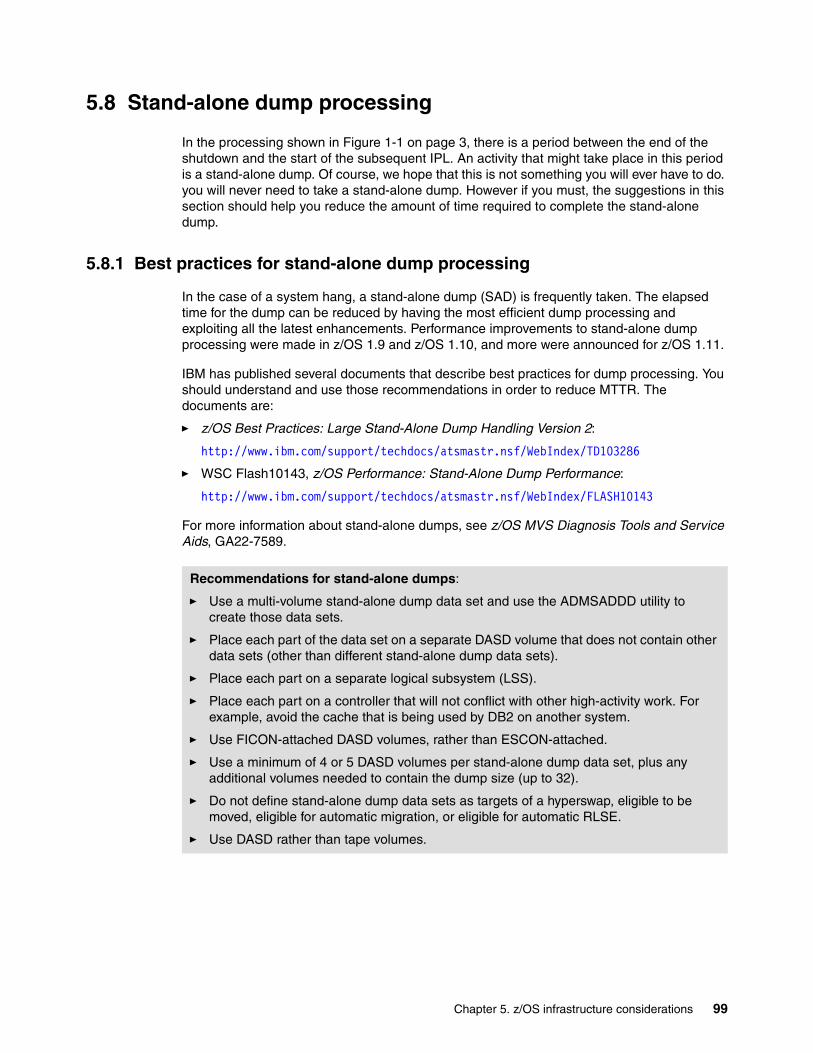
5.8 Stand-alone dump processing

In the processing shown in Figure 1-1 on page 3, there is a period between the end of the shutdown and the start of the subsequent IPL. An activity that might take place in this period is a stand-alone dump. Of course, we hope that this is not something you will ever have to do. you will never need to take a stand-alone dump. However if you must, the suggestions in this section should help you reduce the amount of time required to complete the stand-alone dump.

5.8.1 Best practices for stand-alone dump processing

In the case of a system hang, a stand-alone dump (SAD) is frequently taken. The elapsed time for the dump can be reduced by having the most efficient dump processing and exploiting all the latest enhancements. Performance improvements to stand-alone dump processing were made in z/OS 1.9 and z/OS 1.10, and more were announced for z/OS 1.11.

IBM has published several documents that describe best practices for dump processing. You should understand and use those recommendations in order to reduce MTTR. The documents are:

� z/OS Best Practices: Large Stand-Alone Dump Handling Version 2:

http://www.ibm.com/support/techdocs/atsmastr.nsf/WebIndex/TD103286

� WSC Flash10143, z/OS Performance: Stand-Alone Dump Performance:


For more information about stand-alone dumps, see z/OS MVS Diagnosis Tools and Service Aids, GA22-7589.

Recommendations for stand-alone dumps:

� Use a multi-volume stand-alone dump data set and use the ADMSADDD utility to create those data sets.

� Place each part of the data set on a separate DASD volume that does not contain other data sets (other than different stand-alone dump data sets).

� Place each part on a separate logical subsystem (LSS).

� Place each part on a controller that will not conflict with other high-activity work. For example, avoid the cache that is being used by DB2 on another system.

� Use FICON-attached DASD volumes, rather than ESCON-attached.

� Use a minimum of 4 or 5 DASD volumes per stand-alone dump data set, plus any additional volumes needed to contain the dump size (up to 32).

� Do not define stand-alone dump data sets as targets of a hyperswap, eligible to be moved, eligible for automatic migration, or eligible for automatic RLSE.

� Use DASD rather than tape volumes.


http://www.ibm.com/support/techdocs/atsmastr.nsf/WebIndex/TD103286


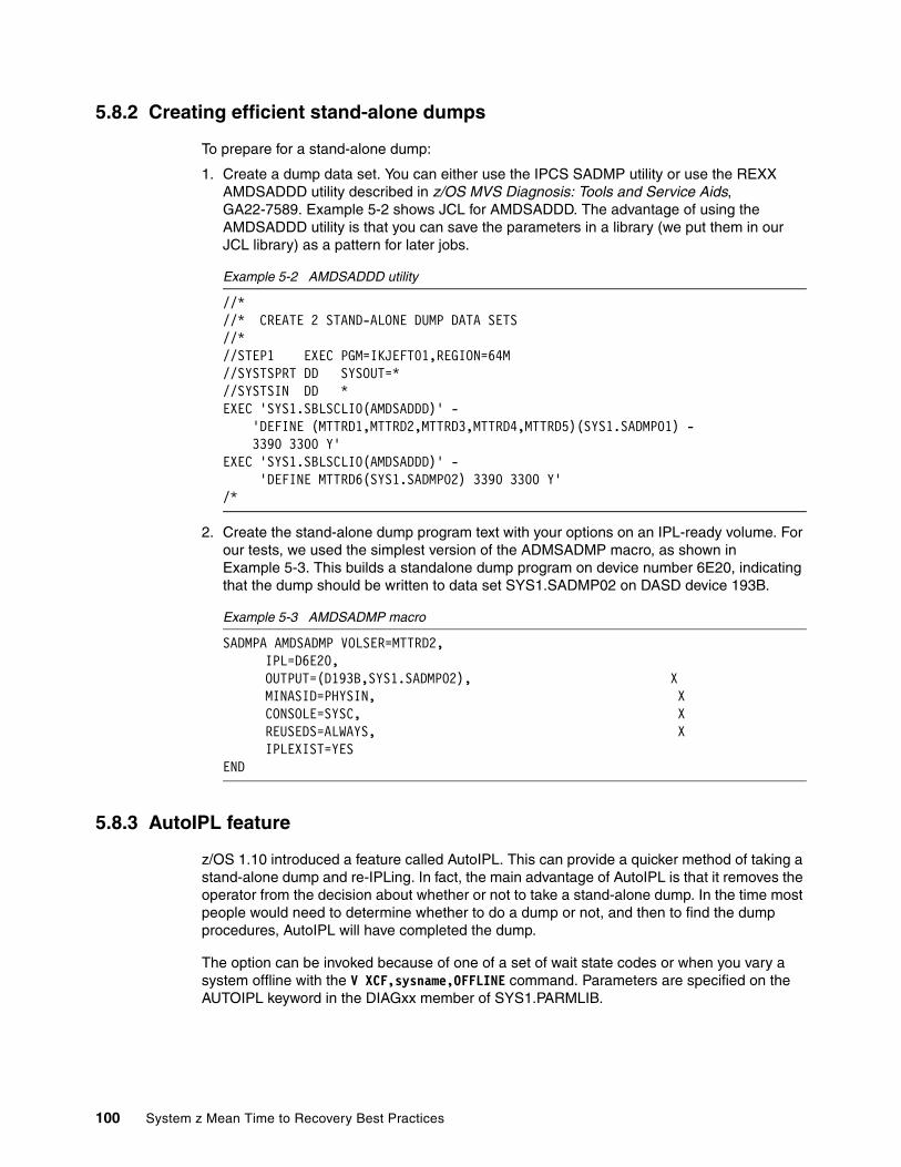
5.8.2 Creating efficient stand-alone dumps

To prepare for a stand-alone dump:

1. Create a dump data set. You can either use the IPCS SADMP utility or use the REXX AMDSADDD utility described in z/OS MVS Diagnosis: Tools and Service Aids, GA22-7589. Example 5-2 shows JCL for AMDSADDD. The advantage of using the AMDSADDD utility is that you can save the parameters in a library (we put them in our JCL library) as a pattern for later jobs.

Example 5-2 AMDSADDD utility

//* //* CREATE 2 STAND-ALONE DUMP DATA SETS //* //STEP1 EXEC PGM=IKJEFT01,REGION=64M //SYSTSPRT DD SYSOUT=* //SYSTSIN DD * EXEC 'SYS1.SBLSCLI0(AMDSADDD)' - 'DEFINE (MTTRD1,MTTRD2,MTTRD3,MTTRD4,MTTRD5)(SYS1.SADMP01) - 3390 3300 Y' EXEC 'SYS1.SBLSCLI0(AMDSADDD)' - 'DEFINE MTTRD6(SYS1.SADMP02) 3390 3300 Y' /*

2. Create the stand-alone dump program text with your options on an IPL-ready volume. For our tests, we used the simplest version of the ADMSADMP macro, as shown in Example 5-3. This builds a standalone dump program on device number 6E20, indicating that the dump should be written to data set SYS1.SADMP02 on DASD device 193B.

Example 5-3 AMDSADMP macro

SADMPA AMDSADMP VOLSER=MTTRD2, IPL=D6E20,OUTPUT=(D193B,SYS1.SADMP02), XMINASID=PHYSIN, XCONSOLE=SYSC, XREUSEDS=ALWAYS, XIPLEXIST=YES

END

5.8.3 AutoIPL feature

z/OS 1.10 introduced a feature called AutoIPL. This can provide a quicker method of taking a stand-alone dump and re-IPLing. In fact, the main advantage of AutoIPL is that it removes the operator from the decision about whether or not to take a stand-alone dump. In the time most people would need to determine whether to do a dump or not, and then to find the dump procedures, AutoIPL will have completed the dump.

The option can be invoked because of one of a set of wait state codes or when you vary a system offline with the V XCF,sysname,OFFLINE command. Parameters are specified on the AUTOIPL keyword in the DIAGxx member of SYS1.PARMLIB.


Example 5-4 shows several parameters.

Example 5-4 DIAGxx parameters for AUTOIPL

AUTOIPL SADMP(device,loadparm) MVS(device,loadparm)This is the format of the AUTOIPL parameter

AUTOIPL SADMP(D111,TEST1) MVS(LAST)This directs that a stand-alone dump be taken when any of the pre-defined wait state codes are encountered. An AutoIPL of MVS will occur after the SADMP using the same load parameters as were used during the previous MVS IPL. The name ‘TEST1’ can be anything, and does not reflect a loadparm.

AUTOIPL SADMP(NONE) MVS(NONE) This statement turns off AUTOIPL.

AUTOIPL SADMP(6E20,TEST2) MVS(C425,C730FKM1)This causes a stand-alone dump to be taken when any of the pre-defined wait state codes are encountered. The dump will be IPLed from device 6E20. An AutoIPL of MVS will be done using the IPL volume of C425 and a loadparm of C730FKM1.

When you remove an image from a sysplex, you can request a SADMP, an immediate re-IPL, or both with the following commands:

� V XCF,sysname,OFF,SADMP

� V XCF,sysname,OFF,REIPL

� V XCF,sysname,OFF,SADMP,REIPL

Further information about AutoIPL can be found in:

� z/OS MVS Initialization and Tuning Reference, SA22-7592, which describes the DIAGxx parameters

� z/OS MVS Planning: Operations, GC28-1760, which describes the wait states that trigger AutoIPL.

� WSC Flash10655, z/OS: AutoIPL for Sysplex Failure Management Users, which describes changes that allow AutoIPL to coexist with sysplex failure management (SFM), and adds support of SADMP with the V XCF command. These were introduced through PTFs in January 2009.

5.8.4 Test results

For our testing, we created two stand-alone dump data sets: a single volume dump data set and a five-volume dump data set. We executed a stand-alone dump using MINASID(ALL) on a z/OS 1.10 system to both dump data sets. We also dumped to a 5-volume data set with MINASD(PHYSIN).

To have a consistent amount of information to dump, we started with a freshly IPLed image, varied the system out of the sysplex, then executed the stand-alone dump. Finally, we did a VARY OFFLINE command with AutoIPL. Figure 5-5 on page 102 shows the results of

Recommendation: In z/OS 1.10 or later, implement AutoIPL, even in installations using an SFM policy. Be sure that the PTFs mentioned in WSC Flash10655 are installed.


following three tests of stand-alone dumps. The results clearly show how multiple volumes can reduce the elapsed time of a stand-alone dump:

� S1: One volume with full data� S2: Five volumes with full data� S3: Five volumes with minimal data

Figure 5-5 Elapsed stand-alone dump times

To save the stand-alone dump statistics to a data set, we issued the commands under TSO and IPCS, as follows:

1. In TSO (select option 6), enter the following commands:

free ddname(ipcstoc) free ddname(ipcsprnt)attrib (list1) dsorg(ps) recfm(v b a) lrecl(125) blksize(1254)alloc ddname(ipcsprnt) dataset('zs9037.sadmttrp') mod keep space(10,5) cyl

using(list1)alloc ddname(ipcstoc) dataset('zs9037.sadmttrt') mod keep space(10,5) tracks

using(list1)

2. In IPCS, browse the stand-alone dump data set (option 2), and enter the name of the stand-alone dump data set.

3. Enter the following IPCS commands:

ip open print (file(ipcsprnt) title(‘Test S1’))ip verbx sadmpmsg ‘stats’ noterm printip close print

To determine the timings for the dump, we used the following command:

IP VERBX SADMPMSG ‘STATS’

Figure 5-6 on page 103 shows an extract from the result of that command. From this output, we can determine the elapsed time to complete the dump. In this case, the dump started at 16:21:06.82 (after the operator replied) and ended at 16:22:27.72, for an elapsed time of 20.90 seconds.

E la p s e d S A D M P tim e

0

5

1 0

1 5

2 0

2 5

3 0

3 5

4 0

S 1 S 2 S 3

T e st ru n

Sec

on

ds


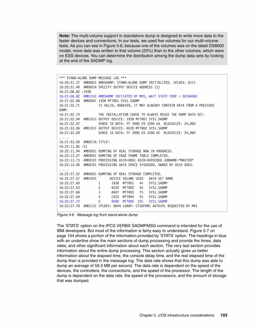
Figure 5-6 Message log from stand-alone dump

The ‘STATS’ option on the IPCS VERBX SADMPMSG command is intended for the use of IBM developers. But most of the information is fairly easy to understand. Figure 5-7 on page 104 shows a portion of the information provided by ‘STATS’ option. The headings in blue with an underline show the main sections of dump processing and provide the times, data rates, and other significant information about each section. The very last section provides information about the entire dump processing. This section actually gives us better information about the elapsed time, the console delay time, and the real elapsed time of the dump than is provided in the message log. The data rate shows that this dump was able to dump an average of 59.3 MB per second. The data rate is dependent on the speed of the devices, the controllers, the connections, and the speed of the processor. The length of the dump is dependent on the data rate, the speed of the processors, and the amount of storage that was dumped.

Note: The multi-volume support in standalone dump is designed to write more data to the faster devices and connections. In our tests, we used five volumes for our multi-volume tests. As you can see in Figure 5-6, because one of the volumes was on the latest DS8000 model, more data was written to that volume (23%) than to the other volumes, which were on ESS devices. You can determine the distribution among the dump data sets by looking at the end of the SADMP log.

*** STAND-ALONE DUMP MESSAGE LOG *** 16:20:51.37 AMD083I AMDSADMP: STAND-ALONE DUMP INITIALIZED. IPLDEV: D11116:20:51.40 AMD001A SPECIFY OUTPUT DEVICE ADDRESS (1) 16:21:06.82 -193B 16:21:06.82 AMD114I AMDSADMP INITIATED BY MVS, WAIT STATE CODE = 001840A216:21:52.68 AMD094I 193B MTTRD1 SYS1.SADMP 16:21:52.71 IS VALID, HOWEVER, IT MAY ALREADY CONTAIN DATA FROM A PREVIOUS DUMP.16:21:52.74 THE INSTALLATION CHOSE TO ALWAYS REUSE THE DUMP DATA SET.16:21:52.94 AMD101I OUTPUT DEVICE: 193B MTTRD1 SYS1.SADMP 16:21:52.97 SENSE ID DATA: FF 3990 E9 3390 0A BLOCKSIZE: 24,96016:21:53.06 AMD101I OUTPUT DEVICE: 6E20 MTTRD2 SYS1.SADMP 16:21:53.09 SENSE ID DATA: FF 3990 E9 3390 0C BLOCKSIZE: 24,960. . .16:21:53.50 AMD011A TITLE= 16:22:11.85 -S1 16:22:11.94 AMD005I DUMPING OF REAL STORAGE NOW IN PROGRESS. 16:22:13.27 AMD005I DUMPING OF PAGE FRAME TABLE COMPLETED. 16:22:13.73 AMD010I PROCESSING ASID=0001 ASCB=00FDC800 JOBNAME=*MASTER*16:22:14.06 AMD076I PROCESSING DATA SPACE SYSDS000, OWNED BY ASID 0003.. . .16:22:27.52 AMD005I DUMPING OF REAL STORAGE COMPLETED. 16:22:27.57 AMD104I DEVICE VOLUME USED DATA SET NAME 16:22:27.60 1 193B MTTRD1 4% SYS1.SADMP 16:22:27.63 2 6E20 MTTRD2 4% SYS1.SADMP 16:22:27.66 3 8407 MTTRD3 7% SYS1.SADMP 16:22:27.69 4 C425 MTTRD4 4% SYS1.SADMP 16:22:27.72 5 D50D MTTRD5 23% SYS1.SADMP 16:22:27.78 AMD113I IPLDEV: DB44 LOADP: C730FKM1 AUTOIPL REQUESTED BY MVS


Figure 5-7 Output from STATS parameter

Restriction: Stand-alone dumps use a single CPU for processing the dump. The practical limit for the speed of any stand-alone dump is the speed of the CPU. In test environments, the SADMP seems to max out at about 80% busy of a single processor. Adding additional data sets at that point does not provide any added benefit.

IARPFT Data Space Dump Statistics Start time 05/29/2009 16:20:51.373440 Stop time 05/29/2009 16:22:13.736530 Elapsed time 00:01:22.36 Elapsed dumping time 00:00:03.58 Console reply wait time 00:01:18.77 . . .Average output data rate 37.31 megabytes per second Page buffers 888 SVC Frequency 0 8,724 3 43 . . .120 224 252 67,642 In Real Virtual Dump Statistics Start time 05/29/2009 16:22:13.736538 Stop time 05/29/2009 16:22:17.644181 Elapsed time 00:00:03.90 . . .In Use Real Dump Statistics Start time 05/29/2009 16:22:17.644192 Stop time 05/29/2009 16:22:17.872555 Elapsed time 00:00:00.22 . . .Paged Out Virtual Dump Statistics Start time 05/29/2009 16:22:17.872567 Stop time 05/29/2009 16:22:18.558727 Elapsed time 00:00:00.68 . . .Available Real Dump Statistics Start time 05/29/2009 16:22:18.558909 Stop time 05/29/2009 16:22:27.550227 Elapsed time 00:00:08.99 . . .Total Dump Statistics Start time 05/29/2009 16:20:51.373440 Stop time 05/29/2009 16:22:27.550227 Elapsed time 00:01:36.17 Elapsed dumping time 00:00:17.40 Console reply wait time 00:01:18.77Logical records dumped 263,381. . .Average output data rate 59.12 megabytes per second


Additional recommendations for stand-alone dumps:

� Keep the control statements for AMDSADDD and AMDSADMP in a JCL library so that you can use them as a pattern for the next dumps.

� Use the MINASID(PHYSIN) option for the shortest dumps, although the dump may not contain all the information you need to debug the problem. In that situation, you might have to wait for a repeat of the problem, in which case you would get a full dump.

� Use IPCS to gather information about stand-alone dumps, such as the usage of the multiple volumes.

� Use multi-volume dumps. Although the Best Practices guidelines say that you can use up to 32 volumes, 16 seems to be the maximum based on the speed of the current processors.


Chapter 6. CICS considerations

This chapter concentrates on the startup and shutdown times of CICS regions. It does not cover the performance for transactions running in a fully-initialized CICS region. For more information about the performance of a CICS region, see CICS Transaction Server for z/OS V3R2 Performance Guide, SC34-6833.

The startup times for your CICS regions only become a major issue when your users do not have access to the applications that run in your CICS regions. If you have a High Availability setup that allows the applications to be spread across a number of regions (which in turn are spread over a number of z/OS systems), providing continued access to your applications, even if one or more CICS regions are down, MTTR should be less of an issue.

This chapter explores options that might help reduce CICS startup times, from a configuration with just a single CICS region, up to a CICSplex with over 100 regions, spread over three z/OS systems. It also shows the results of various measurements to give an indication of where savings can occur.

6


6.1 CICS metrics and tools

The metric we were specifically interested in was the elapsed time for the CICS regions to initialize. We defined the elapsed time as being the time between when the $HASP373 aaaaaa STARTED message is presented for the first CICS region, to when the DFHSI1517 aaaaaa Control is being given to CICS message is presented for the last CICS region to complete initialization.

In our investigation we utilized a number of tools to study the CICS regions. We used the following tools and products to review the CICS Monitoring Facility (CMF) SMF 110 records (which are produced if CICS starts the Monitoring Facility):

� DFH$MOLS

A sample program supplied by CICS that processes and prints SMF records produced by the CICS Monitoring Facility.

� CICS Performance Analyzer

A product that provides comprehensive reporting based on the SMF records produced by the CICS Monitoring Facility, CICS Statistics, and CICS Server Statistics.

� RMF

The RMF Postprocessor program produces workload management reports based on information from the MVS Workload Manager (WLM).

The focus for most of the tests in this chapter was the elapsed time for the CICS regions. We obtained this information from the job logs of the CICS regions.

6.2 The CICS and CICSPlex SM configuration used for testing

The z/OS systems used for our measurements contained both CICS and CICSPlex SM address spaces. Each of the three systems contained five TORs and 30 AORs. Each one also contained a CICSPlex SM CMAS and had a CICSPlex SM WUI region defined. The Maintenance Point CMAS was the one running on LPAR $2. One further address space was started on each LPAR, to be used by CICSPlex SM. This address space was the Environment Services System Services (ESSS) and it provided MVS system services to the CICSPlex SM components. The structures for each region were placed in the same coupling facility, FACIL03.

Figure 6-1 on page 109 shows a simplified diagram of our CICSplex.


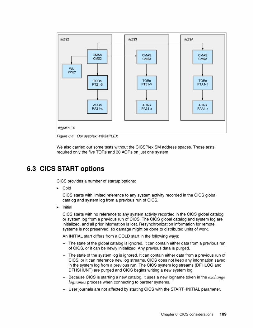
Figure 6-1 Our sysplex: #@$#PLEX

We also carried out some tests without the CICSPlex SM address spaces. Those tests required only the five TORs and 30 AORs on just one system

6.3 CICS START options

CICS provides a number of startup options:

� Cold

CICS starts with limited reference to any system activity recorded in the CICS global catalog and system log from a previous run of CICS.

� Initial

CICS starts with no reference to any system activity recorded in the CICS global catalog or system log from a previous run of CICS. The CICS global catalog and system log are initialized, and all prior information is lost. Resynchronization information for remote systems is not preserved, so damage might be done to distributed units of work.

An INITIAL start differs from a COLD start in the following ways:

– The state of the global catalog is ignored. It can contain either data from a previous run of CICS, or it can be newly initialized. Any previous data is purged.

– The state of the system log is ignored. It can contain either data from a previous run of CICS, or it can reference new log streams. CICS does not keep any information saved in the system log from a previous run. The CICS system log streams (DFHLOG and DFHSHUNT) are purged and CICS begins writing a new system log.

– Because CICS is starting a new catalog, it uses a new logname token in the exchange lognames process when connecting to partner systems.

– User journals are not affected by starting CICS with the START=INITIAL parameter.

#@$#PLEX

CMASCM$2

WUIPW21

TORsPT21-5

AORsPA21-x

#@$2 #@$3

CMASCM$3

TORsPT31-5

AORsPA31-x

#@$A

CMASCM$A

TORsPTA1-5

AORsPAA1-x

Chapter 6. CICS considerations 109

� Warm

CICS starts, after a normal shutdown, restoring CICS to the status it was in at the last normal CICS shutdown, except for some facilities that it initializes as for a cold start. CICS always restores the trace domain according to the system initialization parameters, and will restore other facilities unless the COLD option is specified on their system initialization parameters.

� Emergency

CICS starts, after an abnormal shutdown, restoring recoverable resources to their committed states.

You should specify START=AUTO, which causes a warm start after a normal shutdown, and an emergency restart after failure.

You should also always use the same JCL, even if it specifies START=COLD or START=INITIAL, to ensure that CICS restarts correctly when restarted by the MVS Automatic Restart Manager (ARM) after a failure. With Automatic Restart Manager support, CICS overrides the START parameter when restarted by ARM and enforces START=AUTO if both of the following conditions are met:

� Your startup system initialization parameter specifies START=COLD (or INITIAL).

� Your ARM policy specifies that the Automatic Restart Manager is to use the same JCL for a restart following a CICS failure.

The change in the CICS startup to START=AUTO is reported by message DFHPA1934, and ensures that the resulting emergency restart handles recoverable data correctly.

If the ARM policy specifies different JCL for an automatic restart, and that JCL specifies START=COLD, CICS obeys this parameter but risks losing data integrity. Therefore, if you need to specify different JCL to ARM, specify START=AUTO to ensure data integrity.

6.4 General advice for speedier CICS startup

In this section, we provide a checklist of the areas of CICS that can benefit from a review and that can help with your startup times:

Ensure your GCD, LCD, CSD, temporary storage data sets, and transient data intra-partition data sets are correctly defined for that release of CICS. For details about how to define these data sets, see CICS Transaction Server for z/OS Installation Guide, GC34-6812, at:

http://publibfp.dhe.ibm.com/epubs/pdf/dfha1c02.pdf

When defining terminals, pay attention to the position of the group names within the GRPLIST. If the group containing the TYPETERMs is last, all the storage used for building the terminal definitions is held until the TYPETERMs are known. This could result in a CICS region becoming low on storage. For this reason, place the groups containing the model TERMINAL definitions followed by their TYPETERMs in the GRPLIST before the user transactions and programs. Note that GRPLISTs are only used during cold and initial starts.

Ensure that the DFHVTAM group precedes any TERMINAL or TYPETERM definition in your GRPLIST. The DFHVTAM group is contained in the DFHLIST GRPLIST, so adding DFHLIST first to your GRPLIST ensures this order. If you do not do this, the programs that are used to build the terminal control table (TCT) are loaded for each terminal, thus slowing initial and cold starts.


http://publibfp.dhe.ibm.com/epubs/pdf/dfha1c02.pdf

Try not to have more than 100 entries in any group defined in the CSD. Having more might cause unnecessary overhead during startup processing.

Make sure that changing the START= parameter does not change the default for any facilities that your users do not want to have auto-started. Any facility that you might want to override may be specifically coded in the PARM= parameter in the EXEC statement; or all of them may be overridden by specifying START=(...ALL).

If you do not intend to use of CICS Web support or the Secure Sockets Layer, be sure that TCPIP=NO is specified in the system initialization table (SIT). If TCPIP=YES is specified, the Sockets domain task control block is activated, increasing the CICS startup time.

If a group list contains resource definitions that are needed by another group list, the group list containing those definitions must be installed first.

Specify the buffer, string, and key length parameters in the LSR pool definition. This step reduces the time taken to build the LSR pool, and reduces the open time for the first file to use the pool.

Keep the number of program library data sets that are defined by DFHRPL to a minimum, especially if you are using LLACOPY=YES. One large program library data set requires less time to perform the LLACOPY operation than many smaller libraries. Similar considerations should be applied to any dynamic LIBRARY resources installed at startup.

Placing shared modules in the link pack area (LPA) can help to reduce the time to load the CICS nucleus modules. For more information, refer to:

http://publib.boulder.ibm.com/infocenter/cicsts/v3r2/topic/com.ibm.cics.ts.installation.doc/topics/dfha11d.html#dfha11d

CICS does not load programs at startup time for resident programs. The storage area is reserved, but the program is actually loaded on the first access through program control for that program, which speeds startup. The correct way to find a particular program or table in storage is to use the program-control LOAD facility to find the address of the program or table. The use of the LOAD facility physically loads the program into its predefined storage location if it is the first access.

The use of a PLTPI task to load these programs is one possible technique, but bear in mind that the CICS system is not operational until the PLTPI processing is complete, so you should not load every program. Load only what is necessary, or the startup time will increase.

Try to eliminate any incorrect or obsolete CICS parameters that result in messages being issued unnecessarily.

Avoid writing program list table (PLT) programs that run at startup and issue WTORs.

Ensure that all resources, that are required by startup, are available and avoid WTORs being issued. Such WTORs require an operator response before initialization can continue.

The use of DISP=(...,PASS) on any non-VSAM data set used in steps preceding CICS reduces allocation time, when they are needed next. If you do not use PASS on the DD statement, subsequent allocation of these data sets must go back through the catalog, which is a time-consuming process.

Terminal and program autoinstall checklist items include:

With autoinstall, you do not have to define and install every resource that you intend to use. CICS dynamically creates and installs a definition for you when a resource is requested. CICS bases the new definition on a model definition provided by you. By defining fewer resources during CICS startup, you can reduce the startup elapsed time.


http://publib.boulder.ibm.com/infocenter/cicsts/v3r2/topic/com.ibm.cics.ts.installation.doc/topics/dfha11d.html#dfha11d

Consider the use of autoinstalled terminals as a way of improving cold start, even if you do not expect any storage savings. On startup, fewer terminals are installed, thereby reducing the startup time. CICS provides a transaction called CATD, which delete autoinstalled terminals that are not being used.

Program autoinstall offers the potential for faster restart times. For benefits, see:

http://publib.boulder.ibm.com/infocenter/cicsts/v3r2/index.jsp?topic=/com.ibm.cics.ts.doc/dfha3/topics/dfha30d.html

You might want to increase the number of buffers to improve autoinstall performance. For performance considerations, see:

https://publib.boulder.ibm.com/infocenter/cicsts/v4r1/index.jsp?topic=/com.ibm.cics.ts.performance.doc/topics/dfht3ak.html

The receive-any pool (RAPOOL) system initialization parameter should be set to a value that allows faster autoinstall rates. For more information, see:

http://publib.boulder.ibm.com/infocenter/cicsts/v3r2/index.jsp?topic=/com.ibm.cics.ts.performance.doc/topics/dfht34f.html

6.5 The effects of the LLACOPY parameter

To optimize performance, CICS generally obtains information about the location of CICS modules once and then keeps an in-storage copy of that information. That information is then used on subsequent retrievals of that module. This means that CICS does not need to go out to the PDS or PDSE every time a program is loaded. The information about the location of the module is obtained using either a BLDL call or an LLACOPY call.

BLDL can get its information from one of two places:

� By reading the actual PDS or PDSE, or

� If the module resides in a library in the LLA FREEZE list, the information will be returned from LLA’s in-storage directory, thereby avoiding the I/O to DASD.

LLACOPY gets its information from LLA. In this case, CICS will pass the module and library information to LLA and LLA obtains the information from the PDS and passes it back to CICS.

Whether CICS uses BLDL or LLACOPY to obtain the module information is controlled by the CICS LLACOPY SIT parameter. But before we discuss CICS’ use of LLA, let us look at what LLA does.

LLALibrary lookaside (LLA) minimizes disk I/O in two ways:

� By keeping a version of the library directory in its own address space

� By keeping a copy of frequently used load modules in a virtual lookaside facility (VLF) data space

LLA manages modules (system and application) whose library names you have specified in the appropriate CSVLLAxx member in SYS1.PARMLIB. The two optional parameters in this member that affect the management of specified libraries are:

FREEZE Tells the system always to use the copy of the directory that is maintained in the LLA address space.

NOFREEZE Tells the system always to search the directory that resides on DASD.




https://publib.boulder.ibm.com/infocenter/cicsts/v4r1/index.jsp?topic=/com.ibm.cics.ts.performance.doc/topics/dfht3ak.html

http://publib.boulder.ibm.com/infocenter/cicsts/v3r2/index.jsp?topic=/com.ibm.cics.ts.performance.doc/topics/dfht34f.html

To have a library managed by LLA, you must specify its name in the CSVLLAxx member. The only exception is libraries in LNKLST, which LLA manages by default.

If a library is included in the FREEZE list in the CSVLLAxx member, a BLDL for a member in that library will result in information from the LLA address space being returned. Specifically, the actual PDS or PDSE directory on DASD is not read. This approach provides improved performance, because retrieving the information from the LLA address space is much faster than having to do an I/O.

However, if a load module is updated in the load library, the information in the LLA address space is not automatically updated. This situation can be addressed in one of two ways:

� An LLA UPDATE command can be issued from the console, pointing at a Parmlib member that tells LLA which directory information it needs to get an up-to-date copy of.

� A system service called LLACOPY can be invoked by a program (CICS, in this case), telling LLA which directory information it needs to get an up-to-date copy of.

LLACOPY is a service provided by z/OS to enable address spaces to coordinate their use of LLA-managed libraries with the LLA address space. See z/OS V1R9.0 MVS Authorized Assembler Services Guide, SA22-7608 for more information about the LLACOPY macro.

And that brings us to how CICS uses LLACOPY.

CICS use of LLAThe LLACOPY service can be used by CICS to ensure that LLA has the latest version of the data set directories at CICS startup time, and then to refresh the LLA directory any time that CICS is made aware that a module has been updated.

How CICS uses the LLACOPY service is controlled by the LLACOPY parameter in SIT; the default value is LLACOPY=YES.

When LLACOPY=YES is specified, CICS issues an LLACOPY macro the first time a module is located from the DFHRPL data set concatenation or from a dynamic LIBRARY concatenation. The LLACOPY macro tells LLA to acquire the latest BLDL information from the PDS, update the LLA in-storage copy (if the library is defined in the FREEZE list), and pass the information back to CICS. This ensures that CICS always obtains the latest copy of any LLA-managed modules. However, it is important to point out that if you specify LLACOPY=YES, that CICS does not actually get the benefit of the LLA in-storage directory; every time CICS uses LLACOPY to obtain directory information for a load module, it causes the directory on DASD to be read again. In fact, from a CICS perspective, if LLACOPY=YES is specified, there is really no benefit to be obtained from defining the CICS libraries in the LLA FREEZE list.

The other disadvantage of specifying LLACOPY=YES is that a huge number of LLACOPY calls will result during CICS initialization, when CICS is building its information about all the programs defined to it. This approach drives up the CPU utilization of the LLA address space, which can end up competing with CICS for access to the CPU. Also, because each LLACOPY operation is serialized by an exclusive ENQ on SYSZLLA1, if a large number of CICS regions are started at the same time, they can spend a considerable amount of time queuing for access to this ENQ.

As an alternative to LLACOPY=YES, you can specify LLACOPY=NEWCOPY. In this case, CICS does not issue an LLACOPY at startup time, but it does use the LLACOPY service when loading a module as a result of a NEWCOPY or PHASEIN request. This eliminates the contention and CPU use associated with all the LLACOPY requests, however it introduces


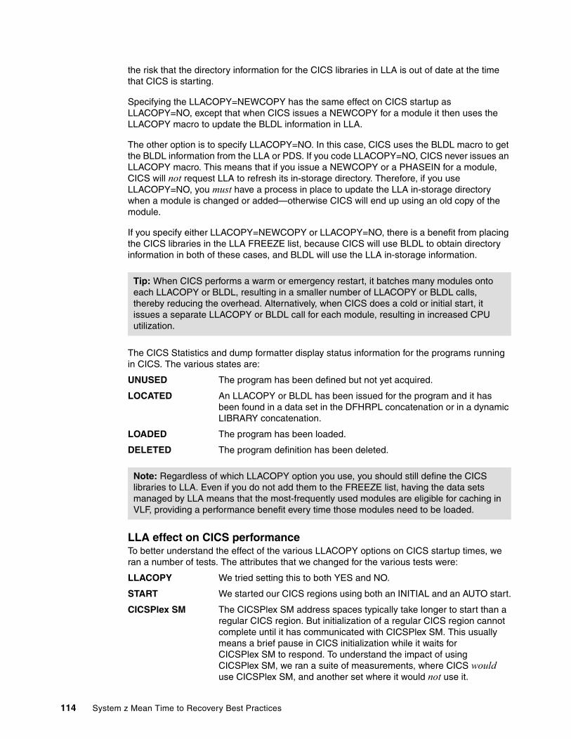
the risk that the directory information for the CICS libraries in LLA is out of date at the time that CICS is starting.

Specifying the LLACOPY=NEWCOPY has the same effect on CICS startup as LLACOPY=NO, except that when CICS issues a NEWCOPY for a module it then uses the LLACOPY macro to update the BLDL information in LLA.

The other option is to specify LLACOPY=NO. In this case, CICS uses the BLDL macro to get the BLDL information from the LLA or PDS. If you code LLACOPY=NO, CICS never issues an LLACOPY macro. This means that if you issue a NEWCOPY or a PHASEIN for a module, CICS will not request LLA to refresh its in-storage directory. Therefore, if you use LLACOPY=NO, you must have a process in place to update the LLA in-storage directory when a module is changed or added—otherwise CICS will end up using an old copy of the module.

If you specify either LLACOPY=NEWCOPY or LLACOPY=NO, there is a benefit from placing the CICS libraries in the LLA FREEZE list, because CICS will use BLDL to obtain directory information in both of these cases, and BLDL will use the LLA in-storage information.

The CICS Statistics and dump formatter display status information for the programs running in CICS. The various states are:

UNUSED The program has been defined but not yet acquired.

LOCATED An LLACOPY or BLDL has been issued for the program and it has been found in a data set in the DFHRPL concatenation or in a dynamic LIBRARY concatenation.

LOADED The program has been loaded.

DELETED The program definition has been deleted.

LLA effect on CICS performanceTo better understand the effect of the various LLACOPY options on CICS startup times, we ran a number of tests. The attributes that we changed for the various tests were:

LLACOPY We tried setting this to both YES and NO.

START We started our CICS regions using both an INITIAL and an AUTO start.

CICSPlex SM The CICSPlex SM address spaces typically take longer to start than a regular CICS region. But initialization of a regular CICS region cannot complete until it has communicated with CICSPlex SM. This usually means a brief pause in CICS initialization while it waits for CICSPlex SM to respond. To understand the impact of using CICSPlex SM, we ran a suite of measurements, where CICS would use CICSPlex SM, and another set where it would not use it.

Tip: When CICS performs a warm or emergency restart, it batches many modules onto each LLACOPY or BLDL, resulting in a smaller number of LLACOPY or BLDL calls, thereby reducing the overhead. Alternatively, when CICS does a cold or initial start, it issues a separate LLACOPY or BLDL call for each module, resulting in increased CPU utilization.

Note: Regardless of which LLACOPY option you use, you should still define the CICS libraries to LLA. Even if you do not add them to the FREEZE list, having the data sets managed by LLA means that the most-frequently used modules are eligible for caching in VLF, providing a performance benefit every time those modules need to be loaded.


The first set of measurements were run with CICS set up to not use CICSPlex SM. We ran a number of starts with a variety of LLACOPY=YES and NO, and START=INITIAL and AUTO. The results of the runs are shown in Figure 6-2. Note that these values represent the time from issuing the command to start all the CICS regions, through to the time the last CICS region issued the Control is being given to CICS message. Also see Table 6-1.

Figure 6-2 LLACOPY timings excluding CICSPlex SM

Table 6-1 Elapsed time to start CICS with different LLACOPY options (without CICSPlex SM)

Given the additional work that is generated by the use of LLACOPY=YES, and the serialization involved in processing the LLACOPY requests, we expected that it would take longer to start CICS with LLACOPY=YES than with LLACOPY=NO, and this proved to be the case. The test involved starting a total of 35 CICS regions, on a system with two dedicated z10 CPs. When LLACOPY=YES was specified, the CPs were 100% utilized for periods during the CICS startup (with the LLA address space using a significant amount of CPU). A subsequent test with six dedicated CPs (to reduce the CPU bottleneck) reduced the CICS startup time by about 6 seconds, however there was still a clear gap in the startup time between LLACOPY=YES and LLACOPY=NO because of the serialized LLACOPY processing. Remember that when LLACOPY=NO is specified, CICS uses BLDL instead of LLACOPY to obtain the directory information. BLDL does not require the exclusive SYSZLLA1 ENQ and is therefore less prone to being delayed by other BLDLs on the same system.

The second set of measurements included CICSPlex SM. Figure 6-3 on page 116 contains the elapsed time (in seconds) to initialize the CICSPlex SM and CICS regions in a single system, with the different LLACOPY and START options specified in each region’s SIT. Also see Table 6-2 on page 116.

Start LLACOPY=YES LLACOPY=NO

START=INITIAL 39 18

START=AUTO 35 15

CICSplex without CICSPlex/SM

0

10

20

30

40

50

Yes No

LLACOPY Value

Sec

on

ds

Start=Initial

Start=Auto


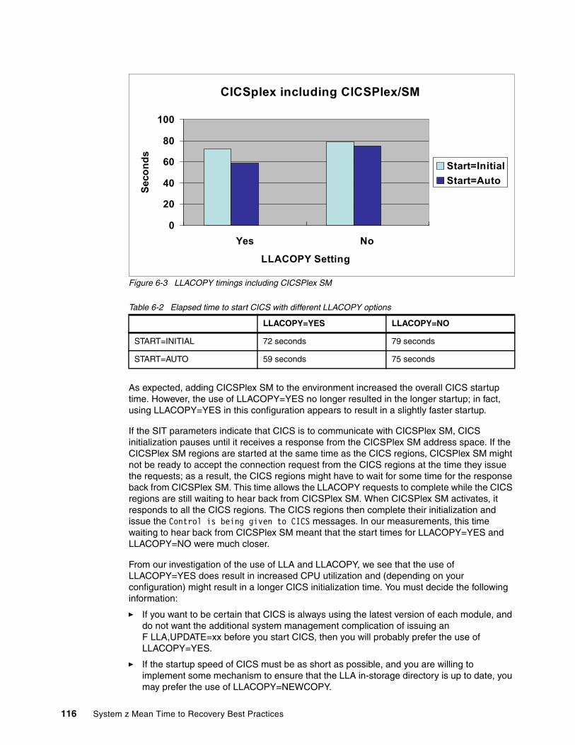
Figure 6-3 LLACOPY timings including CICSPlex SM

Table 6-2 Elapsed time to start CICS with different LLACOPY options

As expected, adding CICSPlex SM to the environment increased the overall CICS startup time. However, the use of LLACOPY=YES no longer resulted in the longer startup; in fact, using LLACOPY=YES in this configuration appears to result in a slightly faster startup.

If the SIT parameters indicate that CICS is to communicate with CICSPlex SM, CICS initialization pauses until it receives a response from the CICSPlex SM address space. If the CICSPlex SM regions are started at the same time as the CICS regions, CICSPlex SM might not be ready to accept the connection request from the CICS regions at the time they issue the requests; as a result, the CICS regions might have to wait for some time for the response back from CICSPlex SM. This time allows the LLACOPY requests to complete while the CICS regions are still waiting to hear back from CICSPlex SM. When CICSPlex SM activates, it responds to all the CICS regions. The CICS regions then complete their initialization and issue the Control is being given to CICS messages. In our measurements, this time waiting to hear back from CICSPlex SM meant that the start times for LLACOPY=YES and LLACOPY=NO were much closer.

From our investigation of the use of LLA and LLACOPY, we see that the use of LLACOPY=YES does result in increased CPU utilization and (depending on your configuration) might result in a longer CICS initialization time. You must decide the following information:

� If you want to be certain that CICS is always using the latest version of each module, and do not want the additional system management complication of issuing an F LLA,UPDATE=xx before you start CICS, then you will probably prefer the use of LLACOPY=YES.

� If the startup speed of CICS must be as short as possible, and you are willing to implement some mechanism to ensure that the LLA in-storage directory is up to date, you may prefer the use of LLACOPY=NEWCOPY.

LLACOPY=YES LLACOPY=NO

START=INITIAL 72 seconds 79 seconds

START=AUTO 59 seconds 75 seconds

CICSplex including CICSPlex/SM

0

20

40

60

80

100

Yes No

LLACOPY Setting

Sec

on

ds

Start=Initial

Start=Auto


In a test or development environment, where startup times are less critical, and changes are likely to be more frequent, you might decide to use LLACOPY=YES for simplicity. For production CICS regions, where the frequency of module updates is probably less, and systems management processes may be more stringent, you might prefer to use LLACOPY=NEWCOPY.

6.6 Using DASDONLY or CF log streams?

Another configuration option that we wanted to investigate was how the use of DASDONLY log streams, as opposed to CF log streams, would affect CICS startup times. We were also interested in whether the number of log streams defined in a single CF structure would make much difference to startup times.

CICS uses the MVS System Logger for all its logging and journaling requirements. CICS uses the services provided by the MVS System Logger for the following CICS logs:

� The CICS system log is used for:

� Dynamic transaction backout

� Warm and emergency restarts

� Cold starts, but only if the log contains information required for resynchronizing in-doubt units-of-work

� Forward recovery logs, auto-journals, and user journals.

The MVS System Logger is a component of z/OS and provides a programming interface to access records on a log stream

The three most common configurations for CICS to operate in are:

� The coupling facility is non-volatile, meaning that the log stream data can be duplexed to a System Logger data space.

� The coupling facility is volatile, meaning that the CICS log streams should be duplexed to a System Logger staging data set.

� The log stream is defined as DASDONLY, meaning that one copy of the log stream data is kept in a staging data set and the duplexed copy is kept in a System Logger data space.

Note: CICS Transaction Server for z/OS Version 4 implemented changes that should result in a faster startup of the CICSPlex SM regions. These changes can affect the dynamics of combining LLACOPY=YES with the use of CICSPlex SM that we observed in our measurements.


Coupling facility and DASDONLY log streamsEach log stream contains a sequence of blocks of user data that the System Logger internally partitions over three types of storage:

� Primary (or interim) storage

This can be in a structure within a coupling facility that holds the most recent records written to the log stream. Log data written to the coupling facility is also copied to either a data space or a staging data set.

For DASDONLY log streams, a CF structure is not used. The primary medium for DASDONLY log streams is the staging data set. Log data written to a DASDONLY log stream is held in a data space and in a staging data set.

� Secondary storage

When the primary storage structure for a log stream reaches the installation-specified HIGHOFFLOAD threshold, older records that have not been logically deleted are automatically moved to secondary storage on DASD (also known as offload data sets by System Logger). This process is known as DASD offloading. For DASDONLY logging, the offloaded log blocks are retrieved from the Logger data space for that log stream. For a CF log stream, log blocks to be offloaded are retrieved from the CF structure. After data is offloaded, it is still available to the MVS System Logger.

� Tertiary storage

This is HSM ML1 or ML2. Your HSM or SMS policy controls the point at which old offload data sets get moved to tertiary storage. However, even when the data sets move to tertiary storage, the data in the data sets remains available to System Logger.

Log data is considered hardened when it is written to the Logger offload data sets.

DASDONLY log streams do not use the coupling facility storage. A DASDONLY log stream has a single-system scope; only one system at a time can connect to a DASDONLY log stream. However multiple applications from the same system can simultaneously connect to a DASDONLY log stream. Alternatively, a CF log stream may be connected to by applications that are running on multiple systems in the sysplex.

We first ran a set of three measurements on a single system, to see how long the CICS startup would take using the following options:

� Each log stream defined as DASDONLY.

� Each log stream defined to use a CF structure and System Logger data spaces, with 15 log streams per structure (we call these tests CF15).

� Each log stream defined to use a CF structure and System Logger data spaces, and only one log stream per structure (we call these tests CF1).

The CICS regions were started with START=INITIAL during all of these tests. We changed the AORs and TORs to use the set up options we listed here. Also, to filter out the effect of waiting for the CICSPlex SM response, we started the CICS regions without CICSPlex SM. We also used LLACOPY=NO to remove the impact of waiting for LLACOPY processing to complete.

In the first test, we started all CICS regions on just one system ($3). The results of the measurements are shown in Figure 6-4 on page 119.


Figure 6-4 Impact of log stream location: single system test

Table 6-3 contains the timings, in seconds, from the tests.

Table 6-3 Timings for $A LPAR testing

Based on these results, when running on a single LPAR, the DASDONLY log streams appear to give the best performance for the TORs, but the worst performance for the AORs. However from analyzing the TOR job logs, it appears that the major cause of the increased startup time for the TORs was contention on the CICS CSD as a result of the shorter AOR initialization times. It important to note as well that there was a considerable amount of variability in the startup time from one region to another, varying by as much as 4 seconds from one region to another during the same measurement run. Also, because the AOR initialization completed in less time when using the CF log streams, there was more CPU contention, with CPU usage hitting 100% a number of times during CICS initialization and this may have contributed to the increase in the TOR startup time.

Note that these tests were conducted on a z/OS 1.10 system; z/OS 1.10 included enhancements to System Logger to enable increased parallelism in connect and disconnect processing for DASDONLY log streams.

We then ran the same series of tests again, but this time we started CICS on all three systems in the sysplex. Other than the fact that we were starting three times as many CICS regions, everything else was the same between these tests and the previous tests.

Because the systems were running different releases of z/OS, we thought it was more meaningful to present the results for each system separately, in each case showing the average startup times for the TORs and AORs when using each of our different log stream options.

TOR or AOR DASDONLY CF1 CF15

Average TOR time 4.2 5.5 7

Average AOR time 19.6 14.9 13.4

CICS Log Stream Type

0

5

10

15

20

25

DASDONLY CF1 CF15

Type

Sec

on

ds

TORs

AORs


Figure 6-5 shows the startup times for the CICS regions running on system $2 (z/OS 1.9). Again, you see that the longest startup times were when we used DASDONLY log streams.

Figure 6-5 Impact of log stream type on CICS startup times on system $2

The corresponding results from the $3 system (z/OS 1.10) are shown in Figure 6-6. Again, you can see the pattern where the startup using the DASDONLY log streams was the slowest.

Figure 6-6 Impact of log stream type on CICS startup times on system $3

System $A showed a similar pattern to these two systems.

$2 Log Stream Comparison

0

10

20

30

40

50

60

DASDONLY CF1 CF15

Log Stream Type

Sec

on

ds

TORs

AORs

$3 Log Stream Comparison

0

10

20

30

40

50

60

DASDONLY CF1 CF15

Log Stream Type

Se

co

nd

s

TORs

AORs


Overall, there is a pattern that using CF log streams appears to result in the fastest CICS startups. However, consider the following observations:

� The numbers shown in the figures are averages. In any run, we saw significant differences from one CICS region to another. In general, the difference was less than 10 seconds, but in one extreme case, the slowest region took nearly twice as long to initialize as the fastest region.

� Comparing the startups on a single system to those where we started the CICS regions on all systems at the same time, we see that starting roughly 100 CICS regions across three LPARs took significantly longer than starting 35 regions on just one system.

� All the CF log stream runs we did were with log streams that were duplexed to System Logger data spaces. If you were using Staging data sets with these log streams, the performance advantage of CF log streams over the DASDONLY runs might disappear.

These observations indicate that contention between the CICS regions plays a significant part in the startup time of a given region. If you do not have many CICS regions to start, the impact of contention is probably not worth worrying about. However, if you have hundreds of regions to start, then starting the regions in waves, instead of all in parallel, can help. Also, if you are using a release of z/OS prior to z/OS R10, the performance difference between CF and DASDONLY log streams might be greater. Although we did not have a chance to measure it, z/OS R11 includes parallelization enhancements to System Logger that should improve the startup times for large numbers of CICS regions that use Staging data sets, especially when restarting after a system failure.

For more information about optimizing the use of CICS and the MVS System Logger, see Systems Programmer’s Guide to: z/OS System Logger, SG24-6898.

6.7 Testing startup scenarios

The objective of the next set of measurements was to identify whether any benefit would be observed from starting the different regions in groups, rather than starting them all at the same time. We thought that perhaps reduced contention between the regions might result in a shorter overall startup time.

For the first test, we started the CICSPlex SM address spaces first. When the EYUXL0010I aaaaaaaa CMAS initialization complete message had been issued on the CMAS, we then started the TORs. As soon as the TORs had issued message DFHSI1517 Control is being given to CICS, we then started all the AORs. See Table 6-4.

Table 6-4 Timings for starting CICS regions in groups

The combined startup time of 80 seconds is slightly better then when we started all the regions at the same time, where we observed an elapsed time of 84 seconds. However, we were starting the regions manually; the use of automation to start each of the groups of CICS regions would almost certainly result in a larger difference.

Regions Base

CMAS 48

TORs 3

AORs 19

Total elapsed time (including manual intervention)

80


The next test was to start the AORs in groups of five rather than all together. Again, we started the CICSPlex SM address spaces first, then the five TORs, and then the AORs in groups of five.

After the CICSPlex SM address spaces were started, we waited 50 seconds and then started the TORs. We waited 50 seconds because the time from the first run told us that the CICSPlex SM CMAS region took about 50 seconds to initialize. We waited this long to try and avoid any sort of contention. We then started the TORs, followed by the first group of AORs. We waited for about four seconds and then started the next group of AORs and so on.

We used a number of combinations of wait times and groupings of AORs. As you would expect, the reduced contention resulted in a shorter startup time for a given CICS region. However, the total elapsed time to start the full set of CICS regions did not vary by more than a few seconds, which is easily within the margin of error from one test to another.

If you have CICS regions that are more critical than others, consider staggering their startup in this manner, starting the more important ones first, especially if you have a large number of CICS regions. However, if all regions support all applications, a simpler approach is probably to start all the regions together. If you do decide to stagger them, starting the AORs first would make sense, followed by the TORs. If you start the TORs first, CICS will appear to the user to be available again, even though, in fact the applications will not be available until the AORs start.

6.8 The effects of placing CICS modules in LPA

The link pack area (LPA) contains common reentrant modules shared by the system, and exists to provide:

� More efficient use of real storage exists by sharing one copy of the module.

� Improved protection: LPA code cannot be overwritten, even by key 0 programs.

� Performance can be improved and the demand for real storage reduced if you use the LPA for program modules.

If more than one copy of the same release of CICS is running in multiple address spaces of the same system, each address space requires access to the CICS nucleus modules. These modules may either be loaded into each CICS address space, or shared in the LPA. Sharing the modules in LPA reduces the working set and, therefore, the demand for real storage.

Additionally, placing the modules in LPA means that they have to be retrieved from DASD only once, instead of every CICS region encountering the delay while the programs are loaded from DASD. This should result in reduced times for CICS to load these modules.

Some CICS modules must be installed in LPA. These modules can be found in data set DFHLPA.

You can optionally install other CICS modules into the LPA. CICS provides a usermod called DFH$UMOD which can be used to move the modules you would like to be in the LPA from the CICS load libraries. It also provides a description and whether the module would be good to include in the LPA; for example, if you are a heavy user of a particular function. And information about whether the module requires USELPACOPY(YES) is provided. User modules may also use the LPA, if they are read-only and have been link-edited with the RENT and REFR options.


The SIT parameter LPA is used to indicate whether you want to use LPA for that CICS region. When the LPA parameter is set to YES, CICS modules installed in the LPA can be used from there instead of being loaded into the CICS region.

Additionally, for each non-nucleus CICS-supplied LPA-eligible module you must specify USELPACOPY(YES) on the associated PROGRAM resource definition. CICS provides a sample DFHCSDUP input called DFH$ULPA, which can be used to change the program definitions in your CSD.

If necessary, you can use the PRVMOD system initialization parameter to exclude a particular module from using the LPA. CICS nucleus modules do not need to specify USELPACOPY(YES), so the way to stop using these modules from the LPA is to use the PRVMOD system initialization parameter.

To determine the benefit of specifying LPA=YES as a SIT parameter, we ran a base measurement with the CICS TORs (5) and AORs (30) on LPAR $3 and using LLACOPY=YES, Start=Auto, LPA=NO, and using the CF1 log stream. We started all the regions in parallel.

For this particular test, we did not use CICSPlex SM because we wanted to see any improvements in startup time using the LPA, and we did not want these values to be lost in the time for the CICS regions to connect to the CICSPlex SM CMAS address space.

We use this run as our base measurement and refer to it as Run 1.

For the next run (which we called Run 2), we ran the CICS-supplied usermod to copy a number of CICS modules into an LPA library and updated the program definitions accordingly. The only other change we made was to change LPA=NO to LPA=YES in the SIT overrides.

For the final measurement, we ran with the same configuration as Run 2, with the exception that we changed LLACOPY=YES to LLACOPY=NO. The results of the three sets of measurements are summarized in Figure 6-7 on page 124.

Note: If you specify USELPACOPY(YES) for a load module that does not exist in an LPA library, you will receive a message similar to the following one:

+DFHLS0109I DSTCPTA1 753DFHLDLD1 is unable to locate module DFHWBMTH in the LPA. DFHRPL or dynamic LIBRARY version of module will be used.


Figure 6-7 Impact of CICS use of LPA for CICS modules

The results show that specifying LPA=YES results in an immediate improvement in the initialization time of the CICS regions (Run 2). For Run 3, when we used LLACOPY=NO, we see the initialization time has decreased again.

We believe that using the LPA=YES SIT parameter is beneficial because it offers you significant improvement in initialization times, and offers you the protection of having your modules in the LPA. It also offers you a saving in the real storage used on your system; a saving that increases as the number of CICS regions you are running increases. The only thing you should be careful about is the impact that placing all those CICS modules in LPA might have on the size of the above-the-line private area. There are also a small number of CICS modules that can optionally be placed in LPA that reside below the line; if you are tight on below-the-line private storage, you should check the size of the CICS modules that would reside in below-the-line LPA to determine if adding them to LPA would adversely affect the size of your below-the-line private area.

6.9 Starting CICS at the same time as VTAM and TCP/IP

Our next area of investigation was to understand how CICS would react if it was started before VTAM initialization had completed. There was a time when CICS would abend if it was started before VTAM, so we wanted to see if this was still the case. If your VTAM takes a long time to initialize, you might be able to save some time if you could start CICS and VTAM in parallel, instead of having to delay the CICS start until after VTAM initialization completes.

The first test was to delay the start of VTAM until we had started all the CICS and CICSPlex SM regions. When the CICS regions reached the point where they tried to communicate with VTAM, they each issued a DFHSI1572 message, as shown in Example 6-1.

Example 6-1 VTAM not available message

DFHSI1572 DSTCCM$A Unable to OPEN VTAM ACB - RC=00000008, ACB Code=5C.

Total CICS Startup time

0

10

20

30

40

50

Run 1 Run 2 Run 3

Test run

Sec

on

ds

Total CICS Startup time


If a CICS region has been defined to use TCP/IP, and the TCP stack has not completed initialization when CICS tries to communicate with it, you see a DFHS00117 message, as shown in Example 6-2.

Example 6-2 TCP/IP not available message

DFHSO0117 DSTCPTA1 131 Unable to determine the TCP/IP host name. OpenEdition return codeX'00000070', reason code X'110A00B6'.

Following these messages, the CICS regions then issue message DFHZC0200, as shown in Example 6-3.

Example 6-3 CICS VTAM retry message

DFHZC0200 DSTCPAA2 547 An attempt by the COVR transaction to OPEN VTAM has failed with return code X'0000005C'; CICS will retry.

CICS then retries to connect to VTAM and TCP every 60 seconds. When it has tried unsuccessfully for 10 minutes, it stops, issues message DFHZC0201, and not try the OPEN again. If VTAM is available, but TCP is not, users can proceed with logons through VTAM; that is, the fact that TCP is not ready yet would not stop VTAM users from being able to use that CICS region.

The only region to have a problem, and in fact shut itself down, was the CICS region controlling the CICS Web User Interface. It issued the messages shown in Example 6-4.

Example 6-4 WUI messages when TCP/IP is not available

EYUVS0001I DSTCPWA1 CICSPlex SM WEB USER INTERFACE INITIALIZATION STARTED. DFHAM4897 W DSTCPWA1 The definition of TCPIPSERVICE EYUWUI specified STATUS=OPEN but the open failed. EYUVS0005S DSTCPWA1 CICSPlex SM Web User Interface initialization failed. (CICS Web Interface initialization.)

A more realistic scenario is that you would issue the start commands for VTAM, TCP/IP, and the CICS regions at the same time. In our experience, VTAM and TCP initialization had completed before CICS got to the point where it tried to communicate with them. Obviously, this depends on how long your VTAM and TCP/IP take to start. But if you are like we are and your VTAM and TCP start in less time that your CICS regions, moving the CICS start to be in parallel with the VTAM and TCP/IP start should improve the time it takes to get your CICS regions on the air by roughly the amount of time it takes for VTAM and TCP/IP to initialize.


6.10 Other miscellaneous suggestions

This section includes other miscellaneous things to consider that might improve either startup or shutdown times.

6.10.1 CICSPlex SM recommendations

For CICS region startup when using CICSPlex SM, the following parameters are recommended when using Business Application Services (BAS), Workload Manager (WLM), or both:

� MASPLTWAIT(YES): This parameter prevents any CICS applications from running and users signing on until CICSPlex SM has initialized and completed installing all the resources for that CICS region from BAS. This parameter should be set when you use BAS because allowing users to log on to CICS is pointless if the transactions have not yet been defined.

� MASINITTIME: The maximum length of time that is allowed for CICSPlex SM initialization is determined by the this parameter. The default is 10 minutes. You should monitor the length of time that it takes for your CICS systems to initialize and install their BAS definitions, and where necessary, increase the MASINITTIME. If MASINIITIME expires before CICSPlex SM initialization completes, that region does not become part of the CICSplex.

If you have a large CICSplex and use CICSPlex SM with many managed application systems (MAS), might find that some of the MASs are very slow to reinitialize if you leave your CMASs active and only restart the MASs. This situation is addressed by CICSPlex SM APAR PK44192.

6.10.2 The CICS shutdown assist transaction

When performing an immediate shutdown, CICS does not allow running tasks to finish, and backout is not performed until emergency restart. This can cause an unacceptable number of units of work to be shunted, with locks being retained. On the other hand, when doing a normal shutdown, CICS waits indefinitely for running transactions to finish, which can delay shutdown to a degree that is unacceptable. The CICS shutdown assist transaction (CESD) improves both these forms of shutdown and, to a large degree, removes the need for an immediate shutdown.

The operation of CESD, for both normal and immediate shutdown, takes place over a number of stages. CESD controls these stages by sampling the number of tasks present in the system, and proceeds to the next stage if the number of in-flight tasks is not reducing quickly enough.

The stages of a normal shutdown with CESD are as follows:

1. In the initial stage of assisted shutdown, CESD attempts to complete a normal shutdown in a reasonable time.

2. After a time is allowed for transactions to finish normally (that is, after the number of tasks has not reduced over a period of eight samples), CESD proceeds to issue a normal purge for each remaining task. The transaction dump data set is closed at this stage.

Note: In CICS TS 4.1, changes have been made to help improve the start up time of the CICSPlex SM CMAS address space.


3. If transactions are still running after a further eight samples (except when persistent sessions support is being used), VTAM is force-closed and interregion communication (IRC) is closed immediately.

4. Finally, if transactions are still running, CICS shuts down abnormally, leaving details of the remaining in-flight transactions on the system log to be dealt with during the subsequent emergency restart.

The operation of CESD is quicker for an immediate shutdown, with the number of tasks in the system being sampled only four times instead of eight.

You should always use the CESD shutdown-assist transaction when shutting down your CICS regions. You can use the DFHCESD program as is, or use the supplied source code as the basis for your own customized version. The CEMT PERFORM SHUTDOWN command automatically uses the CESD transaction to expedite the shutdown unless you specify the NOSDTRAN or SDTRAN(tranname) options on the command or as a SIT parameter.

CICS MAXTASKSIf you have a large number of terminals that are autoinstalled, shutdown can fail because of the MXT system initialization parameter being reached or CICS becoming short on storage. To prevent this possible cause of shutdown failure, you should consider putting the CATD transaction in a class of its own to limit the number of concurrent CATD transactions. Also, AIQMAX can be specified to limit the number of devices that can be queued per autoinstall. If this limit is reached, the AIQMAX system initialization parameter affects the LOGON, LOGOFF, and BIND processing by CICS. CICS requests VTAM to stop passing such request to CICS. VTAM holds the requests until CICS indicates that it can accept further commands.


Chapter 7. DB2 considerations

This chapter delivers basic concepts to help you understand the DB2 restart and shutdown processes and provides advice for reducing the elapsed time for DB2 startup and shutdown.

This chapter covers the following topics:

� What you need to know about DB2 system Restart/Shutdown

� Configuration and tools we used for testing

� How to improve DB2 restart performance

� How to speed up DB2 shutdown process

7


7.1 What you need to know about DB2 restart and shutdown

This section explains what you need to know about DB2 restart and shutdown. These concepts are important background for your work to speed DB2 startup and shutdown times.

7.1.1 DB2 system checkpoint

Startup and shutdown performance has been continuously improved over recent releases of DB2. One of the key factors that affects DB2 restart time is how often the system checkpoint was taken: how many log records DB2 has to process during restart time. Figure 7-1 shows that the longer the time between checkpoints, the more work-status information must be processed when DB2 has to process the checkpoint.

Figure 7-1 DB2 checkpoint

DB2 checkpoints are taken:

� At DB2 startup time

� When the CHKFREQ value is reached

� When the Active Log data sets switch

� At DB2 shutdown time

Other things that trigger a system checkpoint are:

� When you issue one of the following commands to take a system checkpoint:

-SETLOG LOGLOAD(0) -SET CHKTIME(0)

� When you issue a -SET LOG SUSPEND command in a non-data sharing environment

Functions performed at checkpointDB2 records the unit of recovery (UR) information in the system checkpoint so that if DB2 terminates abnormally, DB2 can restart back to the state it was in at the time it failed. DB2 records all data modifications in the DB2 log data sets when data is updated. Both the before image and the after image are recorded in the log for REDO or UNDO processing. At system checkpoint, DB2 performs the following actions:

� Externalizes all changed data (except for workfiles) to a GBP or database on DASD.

� Records the table space (pageset) status information in the log, including database pending writes.

LOG

UR (Unit of Recovery) statusR/W Pageset status

STARTRBA ENDRBA

CHECKPOINTBSDS


� Detects candidate data sets for R/O switching.

� Records pageset exception status.

� Records UR status (for all URs that have not completed).

� Updates the LOGONLY recovery log scan starting point.

� Updates the data sets’ down level detection IDs. The status of all URs is recorded at system checkpoint time.

Checkpoint history in BSDSAt system checkpoint, DB2 also records the checkpoint status information in the bootstrap data set (BSDS). The DSNJU004 (Print Log Map) utility can report the checkpoint status. From the report, you can determine the elapsed time between two consecutive DB2 system checkpoints and calculate the average log record length based on this formula (RBA is the relative byte address):

Avg log record size = DECIMAL (BEGIN CHECKPOINT RBA - PRIOR END CHECKPOINT RBA) --------------------------------------------------------

LOGLOAD

Based on the average log record size and the elapsed time between the two checkpoints, DB2 users can control how frequently DB2 takes system checkpoints by changing the CHKFREQ value. Normally, taking checkpoints too often (not more than once per minute) is not recommended because doing so can cause noticeable system overhead.

7.1.2 Two-phase commit processing

DB2 supports the two-phase commit protocol. Figure 7-2 shows the two-phase commit processing, using IMS or CICS as the transaction coordinator.

Figure 7-2 DB2 two-phase commit

A unit of recovery (UR) is generated only for updating transactions and not for read-only transactions. When a transaction first updates a database as part of an insert, update, or delete operation, a UR is created on behalf of this transaction by writing a “begin UR” log record. The UR persists until a commit is issued by the application.

DB2

IMS/CICS

PHASE 1

BEGIN UR

INCOMMIT

PHASE 2

END UR

APPL PGM SYNCPT

INSTANT OF COMMIT

NEW COMMIT

SQL UPDATE

PREPARE TO COMMIT OK COMMIT OK

INFLIGHT INDOUBT

PHASE 1 PHASE 2

Chapter 7. DB2 considerations 131

When an application program reaches a synchronization point and prepares to commit, the phase-1 commit processing begins. DB2 writes a “begin phase-1” log record and starts to perform phase-1 processing. If DB2 ends before it completes its phase-1 processing and writes the “phase-1 end” log record, the transaction is considered to be in inflight status. At restart time, DB2 rolls back all the database updates done by this inflight transaction to its last commit point.

If DB2 stops after the commit phase-1 end log record is written, but before it receives the notification from the transaction coordinator to proceed with the phase-2 processing, then the UR is considered to be in indoubt status.

The UR will be reclassified as in-commit status as soon as DB2 writes the begin phase-2 log record. And the UR is ended as soon as the commit phase-2 end log record is written after the phase-2 processing is completed.

7.1.3 Phases of a DB2 normal restart process

The five phases that DB2 goes through during restart are:

� Phase 1: Log Initialization is the start-up phase.

� Phase 2: Current Status Rebuild is the analysis phase. DB2 is trying to determine the transaction status when it was last stopped.

� Phase 3: Forward Log Recovery scans the log in a forward direction and performs a redo operation for all database updates that have not been written to GBP or DASD.

� Phase 4: Backward Log Recovery backs out database updates for the inflight and in-abort URs. If long running URs exist, this is the phase where DB2 backs out those URs, meaning that this phase can potentially run for a long time.

� Phase 5: End Restart finishes the processing and makes DB2 ready to start work. DB2 takes a system checkpoint at the end of this phase.

After the End Restart phase is completed, DB2 can accept new work and will perform indoubt resolution with the assistance of the two-phase commit coordinator.

Phase 1: Log InitializationThe first phase of DB2 restart is called the Log Initialization phase. During this phase, DB2 attempts to locate the last log RBA that was written before termination as shown in Figure 7-3 on page 133. Logging continues at the next log relative byte address (RBA) after that.

Note: Indoubt UR is resolved by the coordinating system (CICS, IMS, WebSphere Application Server, and so on) of the two-phase commit, not by DB2 on its own.

Note: DB2 always goes through these phases, but they can be very short if the system was shut down in a clean way (with a shutdown checkpoint).


Figure 7-3 Log Initialization phase

This phase includes processing that starts the DB2 address spaces and loads DB2 load modules into DB2’s MSTR and DBM1 address spaces. It also implicitly starts Internal Resource Lock Manager (IRLM) if IRLM was not explicitly started. The IRLM startup time is typically about one second.

This phase also includes the time spent to open the BSDS and active log data sets. If dual logging is used, both copies of the active log data sets must be opened. After the BSDS and active log data sets are opened, DB2 scans the log to determine the actual endpoint of the log. It uses a pseudo log endpoint stored in the BSDS as the log scan starting point. The pseudo log endpoint value is updated when one of the following situations occur:

� The log output buffer is ready to wrap.

� The active log data sets is filled.

� The system checkpoint is taken.

� DB2 is terminated normally.

Message DSNJ099I identifies the log RBA at which logging will commence for the current DB2 session. This message DSNJ099I signals the end of the log initialization phase of restart.

Phase 2: Current Status RebuildThe second phase of restart is called the Current Status Rebuild (CSR) phase. During this phase, DB2 determines the status of objects and units of recovery (UR) at the time of termination. By the end of the phase, DB2 has determined whether any URs were interrupted by the termination.

This phase also includes the forward log scan pass that is used to determine the transaction status and the attributes and the restart REDO log scan points for all the R/W pending Pagesets or Partitions.

DB2 scans the log, starting from the Begin Checkpoint log record for the last completed DB2 system checkpoint. The maximum number of log records that will be scanned is bounded by the DSNZPARM CHKFREQ value.

This phase also rebuilds the database exception status table (known as the DBET). The DBET information is recorded in every system checkpoint. In a non-data sharing

X XCHKPT

BSDS01 BSDS02Approximate end of LOG

READ

LOG

CHKPT

SYSTEM FAILURE


environment, DB2 reconstructs the status information and build the list of URs from the log. For example, the DBET records the status if a table space is in Recovery Pending State. In a data sharing environment, DB2 does not use the log to rebuild the status; rather, it gets information from the shared communication area (SCA) structure in a coupling facility. However, DBET log records will be used to rebuild the DBET if the SCA is damaged.

At the end of the CSR phase, console message DSNR004I is displayed with all the transaction status information showing how many transactions are inflight, how many are indoubt, and so forth. DB2 can also determine how far it has to go back in the log to start the forward scan, which is the Phase 3 (Forward Log Recovery) of restart.

Phase 3: Forward Log RecoveryBefore the Forward Log Recovery (FLR) phase, DB2 will not perform any database updates. The FLR phase is the first phase where the database actually gets modified. During this third restart phase, DB2 completes the processing for all committed changes and database write operations. Figure 7-4 shows how the FLR phase starts processing at the checkpoint preceding the first log records for the oldest indoubt UR, or the oldest redo logpoint for any pageset, and proceeds forward in time from there.

Figure 7-4 Forward Log Recovery phase

Basically, DB2 performs a REDO operation on the pending writes for all transactions. If no indoubt URs exist, DB2 scans the log, starting from the lowest restart REDO log points from all the R/W pagesets. In general, the log scan starting point is the Begin Checkpoint log of the last completed checkpoint.

If indoubt URs exist that are very long-running URs, DB2 has to go back to the oldest indoubt UR to scan the log to reacquire locks. DB2 uses log information to rebuild lock information. During the Forward Log Recovery phase, DB reads the log records and accesses the data pages to see if the changes actually were hardened to the database. This is why DB2 restart can potentially take a long time.

When processing a log record, DB2 has to read the associated data or index page from GBP or DASD into a buffer pool buffer to determine whether the change has been externalized. DB2 uses the log record sequence number (LRSN) stored in the page header and the LRSN value of the log record to determine whether the database update was successfully externalized to GBP or DASD.

In a non-data-sharing environment, DB2 uses the log data set’s relative byte address (RBA) of the log record as the LRSN value. In a data sharing environment, the LRSN value is derived from the system-generated ascending STCK (Store Clock) value.

Prior to DB2 V6, if a page was not in the DASD subsystem cache, it could take many milliseconds to read the page into the bufferpool using a synchronous read I/O. With the V6 Fast Log Apply List Prefetch technique, reading in a page typically takes just a few milliseconds. However, even with this enhancement, DB2 still has the overhead of waiting for

X X X X X

CHECKPOINT PRECEDING OLDEST PENDING WRITES

Oldest in-doubt UR

CHKPT

LOG

CHKPT


the I/O to bring the page into the memory, even if it then determines that it does not need to reapply the change.

At the end of the FLR phase, DB2 externalizes all the changed pages either to a GBP or to DASD.

During phase 3 of restart in a data sharing environment, DB2 also purges the retained page p-locks. This is because they are no longer needed to protect the unwritten data. DB2 also writes log records to change each in-commit UR to complete UR status.

Phase 3: FLR ExampleAs mentioned previously, DB2 records the LRSN value of the log record in the data page header when a page is updated. For example, when a record is inserted into a table, DB2 writes an insert log record and records the LRSN value of the insert log record in the data page header. During phase 3 of restart, DB2 compares the LRSN value of the log record and the page header LRSN value to determine whether or not the changes were saved to DASD. If not, then redo the changes. Figure 7-5 shows the log records and database records related to three transactions.

Figure 7-5 Example for Forward Log Recovery phase

The committed transaction modified page P4, with 300 as the LRSN value of the log record. During the restart, DB2 reads the Commit log record for the transaction that updated page P4. It then reads page P4 from the database. At this point DB2 discovers that the LRSN for the Commit log record and the LRSN in the page on DASD are different. This means that the update to page P4 was committed, but the write back to DASD had not completed before DB2 went down. As a result, DB2 has to write the updated page to the database on DASD.

For pages P6 and P9, no changes to the database are needed because the page LRSN values are the same as the log LRSN values. Despite this, DB2 still has the cost of reading the pages from DASD before it can decide whether or not any changes must be applied.

Phase 4: Backward Log RecoveryDuring the fourth restart phase, Backward Log Recovery (BLR), DB2 changes previously performed for in-flight or in-abort units of recovery are backed out.

The in-flight and in-abort URs are processed during this phase. An in-abort UR is generated when DB2 fails during a transaction rollback. An in-flight UR occurs if a transaction has not committed or DB2 has not completed its phase-1 commit process when DB2 ends. During the

Note: Fast Log Apply also reads and sorts log records before applying them. It also applies updates in parallel to the pagesets involved.

BEGIN UR P4 commtd END UR P6 inabort CHKPT P9 indoubt

LOG RBA

200 300 400 500 600 700 800

100 P4

500 P6

700 P9 BEFORE PH 3

AFTER PH 3 P4 300

P6 P9 500 700


BLR phase, DB2 scans the logs for all log records belonging to the in-flight and in-abort transactions, as shown in Figure 7-6. It then backs out any changes that had been applied to the database, and writes another log record to compensate the (uncommitted) change made earlier. For example, in the case of an insert log record, DB2 actually writes a delete log record to compensate the insert. It might take a long time to do backout if there are long running URs that do not issue frequent commits.

Figure 7-6 Backward Log Recovery phase

Phase 4: BLR ExampleFigure 7-7 shows the backout process during restart. Basically, DB2 is UNDOing the changes for the inflight and in-abort URs. The in-abort UR that updated page P6 has a log LRSN value of 500. DB2 writes a compensation log record for this in-abort UR at log LRSN value 800 and changes the P6 page LRSN value from 500 to 800. Depending on whether DB2 consistent restart (see “DB2 consistent restart” on page 138) is being used, DB2 restart might end before all UNDOs have been finished.

Figure 7-7 Example of Backward Log Recovery phase

Phase 5: End Restart processingDB2 uses claims and drains instead of locking to serialize between Utilities and SQL. If there are indoubt transactions associated with a particular table space, DB2 has to make sure the table space or Index is not being recovered or reorganized by a database utility before in-doubt URs are resolved. Therefore, write claims are made for every table space or Index touched by the indoubt transactions to prevent a utility from taking over until the indoubt is resolved. As a result, no utility can be run until indoubt URs are resolved.

Thousands of DB2 data sets might open at the time DB2 ends. During the restart process, DB2 opens only the data sets that have restart pending activities. DB2 does not open the objects for read-only table spaces or R/W table spaces without a log record for that object. For a R/W object without a log record, or an object without inflight URs or outstanding

X X X X X

Oldest In-Flight UR

Oldest in-abort UR

X

LOG

CHKPT CHKPT

BEGIN UR P4 commtd END UR P6 inabort CHKPT P9 indoubt

LOG RBA

200 300 400 500 600 700 800

300P4

500 P6

700

P9 BEFORE PH 4

AFTER PH 4 P4 300

P6 P9 800 700

CLR

WRITE CLR


uncommitted updates, DB2 versions prior to DB2 V9 still tries to close the SYSLGRNG entries during the End Restart phase because there was a SYSLGRNG entry created on behalf of that object. In DB2 V9, this processing was moved to take place at the first system checkpoint after the restart; this approach allows the restart to complete quicker so that DB2 can start accepting work sooner.

DB2 externalizes all the data that was modified during the BLR phase to GBP/DASD. It will also purge all the remaining retained locks and trigger a system checkpoint to record the current status of the DB2 subsystem. After the End Restart phase, DB2 is then available for new work.

7.1.4 DB2 restart methods

Beside a normal restart, DB2 can restart in several various methods. Some methods are based on how DB2 is terminated or are based on your DB2 environment. The methods are:

� DB2 group restart

� DB2 conditional restart

� DB2 consistent restart

� DB2 restart light

DB2 group restartIn a data sharing environment, every active member of a data-sharing group must have access to both the SCA and the DB2 lock structure. If a member loses access to either structure, the member fails unless the structure can be rebuilt to another coupling facility that all DB2s in the data-sharing group have access to.

The failure of an individual member is not a reason for a group restart. If at least one member is active that can access both structures successfully, no group restart takes place. Only if none of the other members are active, and the restarting member determines during the DB2 Initialization phase that the SCA or the DB2 lock structure must be recovered, will it automatically perform a group restart.

RecommendationAlthough one member can perform restart on behalf of the group, you should restart all of the non-quiesced members together, perhaps by using an automated procedure. This approach shortens the total restart time. Also, because retained locks are held for non-starting members, it is best to start all members of the group for maximum data availability.

DB2 conditional restartAt restart time, DB2 always attempts to locate the last log RBA written before termination and continues from there. A conditional restart is a special process, activated by a conditional restart control record (CRCR) in the BSDS, which is used when you need to skip some portion of the log processing during DB2 restart (perhaps because of a damaged log data set).

Note: A group restart does not mean that all members of the data-sharing group are automatically restarted. Rather, it means that the SCA or DB2 lock structure are recovered from the logs of the members of the data-sharing group by those members that are restarted.


To perform a conditional restart, use the following procedure:

1. While DB2 is stopped, run the Change Log Inventory Utility (DSNJU003) using the CRESTART control statement to create a new conditional restart control record in the BSDS.

2. Restart DB2. The types of recovery operations that take place are governed by the current CRCR.

A conditional restart can safely be performed only when the objects are recovered to a prior point of consistency because normal recovery operations can be partially or fully bypassed. Choosing this point of consistency carefully is very important. A useful approach is to run the DSN1LOGP utility and review a summary report of the information contained in the log before setting the conditional restart.

DB2 consistent restartThis function allows DB2 to come up more quickly after a subsystem failure by limiting the backout activities for long running applications that issue very infrequent or no commits. The DSNZPARM LBACKOUT and BACKODUR parameters can be modified based on your workload characteristics.

The consistent restart function helps bring DB2 up faster so that it can accept new work faster. For non-data-sharing subsystems, DB2 marks the entire object as “Restart Pending” and unavailable, so those objects touched by the long running URs will not be available until the long running URs are backed out.

DB2 also supports consistent restart in a data sharing environment. Pages that are updated by long-running transactions are protected by the retained lock. DB2 does not purge those retained locks at End Restart; they are held until the backout is finished. The retained locks are on the page or row level and not on the entire pageset level.

If you tend to have long-running jobs that do not issue commit operations as frequently as they should, consider using this DB2 consistent restart capability to get DB2 up and running more quickly. This will mean that objects affected by the long-running job might not be available immediately when DB2 starts accepting new work, but at least all other objects will be available sooner than would otherwise be the case.

DB2 restart lightFor a data-sharing environment, you can use the LIGHT(YES) parameter on the start command to quickly bring up a DB2 member solely to recover retained locks. When DB2 is started with LIGHT(YES), if indoubt URs exist at the end of restart recovery, DB2 will remain up and running so that the indoubts can be resolved, either automatically through resynch processing with the commit coordinators, or manually through the -RECOVER indoubt operator command. After all the indoubt URs have been resolved, the LIGHT(YES) DB2 member self-terminates. APAR PK29791 introduced a new LIGHT(NOINDOUBTS) option on the -START DB2 command. This option specifies that DB2, during a restart light, does not wait for indoubt units of recovery to resolve before it terminates.

Restart Iight mode is not recommended for a restart in place. It is intended only for a cross-system restart of a system that does not have adequate capacity to substain the DB2 and IRLM in the event of a failed z/OS system.

Note: Although conditional restart is faster than normal restart (because it skips some portion of the log processing), data in the associated objects can become inconsistent if a conditional restart skips any database change log record. Any subsequent attempt to process them for normal operations can cause unpredictable results.


7.1.5 DB2 shutdown types

DB2 terminates normally in response to the -STOP DB2 command. If DB2 stops for any other reason, the termination is considered abnormal.

DB2 normal shutdownAt normal system shutdown, DB2 takes a shutdown checkpoint and updates the BSDS. DB2 also quiesces all transactions and flushes out all changed pages from the local bufferpools to a GBP (for shared objects) or to DASD. DB2 also closes all its open data sets.

Now, all URs are completed with the exception of the indoubt URs, if any exist. If indoubt URs do exist, DB2 records the indoubt UR status in the Shutdown Checkpoint log record.

When possible, ensure that DB2 terminates normally because this will result in a significantly faster startup time.

To terminate DB2, issue either of the following commands:

� -STOP DB2 MODE (QUIESCE)

� -STOP DB2 MODE (FORCE)

You should always attempt a -STOP DB2 first (MODE(QUIESCE) is the default). If shutdown is taking too long, you can issue -STOP DB2 MODE (FORCE) command. However be aware that the resulting need to roll back work can take as long as, or even longer than, the completion of QUIESCE. The -STOP DB2 MODE (FORCE) command is the same as MODE (QUIESCE), except that work in process is aborted instead of quiescing to normal termination.

During shutdown, use the DB2 -DISPLAY THREAD TYPE(SYSTEM) command to check the shutdown process.

When stopping in either mode, the following steps occur:

1. Connections end.

2. DB2 stops accepting commands.

3. DB2 disconnects from the IRLM.

4. The shutdown checkpoint is taken and the BSDS is updated. At this point, the DB2 Buffer Manager will also write checkpoint log records, complete all committed database I/O, and close all open page sets.

Stopping DB2 in data sharing environmentConsider specifying CASTOUT(NO) option when you stop an individual member of a data sharing group for maintenance. This option speeds up shutdown because DB2 bypasses castout and associated clearup processing in the group buffer pools.

Note: A data sharing group member started with the LIGHT option is not registered with the Automatic Restart Manager (ARM). Therefore, ARM does not automatically restart a member that has been started with LIGHT(YES).


DB2 abnormal terminationsAn abnormal termination, or abend, is said to happen when DB2 does not, or cannot, terminate in an orderly way. It leaves data in an inconsistent state for any of the following reasons:

� Units of recovery might be interrupted before reaching a point of consistency.

� Committed data might not be written to external media.

� Uncommitted data might be written to external media.

7.2 Configuration and tools for testing

In this section, we introduce the ITSO environment, and the workloads and tools we used for the DB2 measurements.

7.2.1 Measurement system setup

The DB2 measurements were based on a three-way DB2 data-sharing group (DB2 V9) running in a three-way Parallel Sysplex, with 2 CFs. Each system had only one DB2 member. All the systems were on the same z10 and all LPARs had dedicated CPs. The logical configuration is shown in Figure 7-8.

Figure 7-8 DB2 System Environment

We used two workloads for the DB2 measurements. For the measurements that were focused on startup and shutdown times, we created 100,0001 small DB2 segmented table spaces. Relevant information about these table spaces is shown in Table 7-1 on page 141.

1 With APAR PK29281, the DSNZPARM DSMAX has been raised from 65,000 to 100,000.

D8Q1

Locks Buffer Pools

D8Q2

Locks Buffer Pools

D8QA

Locks Buffer Pools

GlobalLocks

GlobalBuffer Pools

z/OS R9 z/OS R10

Coupling Facility

ITSO

z/OS R10

Sysplex Timer

3-Ways Data Sharing Group

D8Q1Log

D8Q2Log

D8QALog

SharedDB2 Data

SharedDB2 Catalog

Shared Disks


Table 7-1 DB2 Objects

We also had another DB2 workload that we used for some of the measurements. That workload is based on the IBM Relational Warehouse Workload.

Information about this workload includes:

� Workload: IBM Relational Warehouse Workload, OLTP type of workload

� Processor: model 2097

� IBM Relational Warehouse Workload DB: 1 GB

� BP and GBP: each are 400 MB

� LOGLOAD: 160,000 log records

� Checkpoint Interval: 3 - 4 minutes

7.2.2 Tools and useful commands

We used OMEGAMON® XE for DB2 Performance Expert V4 to produce DB2 trace and report data for our investigation. We also used the DISPLAY THREAD(*) TYPE(SYSTEM) DB2 command to help us understand what the DB2 System Agent Thread was doing at specific points in time.

If the command is issued during DB2 startup or shutdown, the output tells you what phase of restart or shutdown DB2 is currently in. For example, when the command was issued during DB2 shutdown, the output told us that DB2 was performing a system shutdown checkpoint.

Storage groupsa

a. Each storage group uses a separate user catalog.

Database Table spacesb

b. There was only one table for every table space.

Tablesc

c. Each table had only one column, one record, and no index.

DB2MT1 DBMT1DB 10,000 10,000

DB2MT2 DBMT2DB 10,000 10,000

DB2MT3 DBMT3DB 10,000 10,000

DB2MT4 DBMT4DB 10,000 10,000

DB2MT5 DBMT5DB 10,000 10,000

DB2MT6 DBMT6DB 10,000 10,000

DB2MT7 DBMT7DB 10,000 10,000

DB2MT8 DBMT8DB 10,000 10,000

DB2MT9 DBMT9DB 10,000 10,000

DB2MT10 DBMT10DB 10,000 10,000


7.2.3 How we ran our measurements

Depending on what we wanted to study, we used the following methods to measure the startup and shutdown times:

� Syslog and job logs: These times could be used for those situations where total times or specific functions within startup or shutdown could be tied to various messages.

� SMF records: We turned on DB2 Accounting and Statistics traces with DEST (SMF). The following statistic classes were enabled:

– 01– 03– 04– 05– 06

The following accounting classes were enabled:

– 01– 02– 03– 07– 08

� RMF reports: RMF writes SMF Type 70 - Type 79 records, which can then be reported by the RMF Postprocessor. RMF provides sysplex-wide information about processor utilization, I/O activity, storage, and paging.

7.3 Improving DB2 startup performance

For this section, we performed a number of experiments with opening 100,000 DB2 page sets with various setups.

7.3.1 Best practices for opening DB2 page sets

During restart, DB2 only opens data sets that belong to GBP-dependent objects if it needs to process log records for uncommitted transactions. Additionally, DB2 only opens and accesses data/index page sets when it encounters log records related to those non-shared objects. If no log records were encountered for those non-shared objects in the last one or two checkpoints, then those data sets will not be opened, even if read only (R/O) switching did not occur before DB2 stopped.

During the forward log recovery phase of restart, any page sets for which log records are found must be opened. The number of page sets that must be opened can number in the thousands. The remaining DB2 data sets (which could be a very large number of data sets) that have not been opened during DB2 restart will subsequently be opened physically when a user or application accesses them.

DB2 V9 increased the limit on the number of tasks for the parallel open or close of Virtual Storage Access Method (VSAM) data sets to 40. However, if you have tens of thousands of data sets to open, data set opens can still amount to a significant part of the elapsed time of restart.

Because of this, and the growing trend for customers to have many thousands or many tens of thousands of DB2 data sets open, we performed a number of performance measurements for opening data sets.


DB2 data sets are usually opened as a result of:

� SQL SELECT statements or other SQL thread

� Using the DB2 ACCESS DATABASE command with MODE (OPEN).

In DB2 V9, DB2 introduced a new command, ACCESS DATABASE, which forces a physical open of a table space, index space, or a partition. It can also be used to remove the GBP-dependent status for a table space, index space, or partition. With Mode(OPEN) specified, DB2 forces the physical opening of the page set or partition in read mode on just the local member. This approach moves the cost and delay of the physical open from an SQL thread to the command thread. This approach should improve the response time for the first SQL thread to reference a given page set or partition.

One other thing we wanted to investigate was the impact of improvements in z/OS V1R10 to reduce the elapsed time to open a data set. As a result, you see that many of our tests were run under both z/OS V1R9 and V1R10.

Using the ACCESS DATABASE command to open DB2 data setsWhen the PTF for DB2 APAR PK80925 is applied, the ACCESS DATABASE command can be used in one of two ways: the database and table space names can be fully qualified; you can use an asterisk (*) to specify a name generically.

Examples of both forms of the -ACCESS DATABASE command are shown in Example 7-1.

Example 7-1 ACCESS DATABASE commands using fully specified names

-ACCESS DATABASE (DBMT10DB) SPACENAM (MTA01000) MODE(OPEN)-ACCESS DATABASE (DBMT10DB) SPACENAM (MTA01001) MODE(OPEN)-ACCESS DATABASE (DBMT10DB) SPACENAM (MTA01002) MODE(OPEN)-ACCESS DATABASE (DBMT10DB) SPACENAM (MTA01003) MODE(OPEN)-ACCESS DATABASE (DBMT10DB) SPACENAM (MTA01004) MODE(OPEN)-ACCESS DATABASE (DBMT10DB) SPACENAM (MTA01005) MODE(OPEN)-ACCESS DATABASE (DBMT10DB) SPACENAM (MTA01006) MODE(OPEN)-ACCESS DATABASE (DBMT10DB) SPACENAM (MTA01007) MODE(OPEN)-ACCESS DATABASE (DBMT10DB) SPACENAM (MTA01008) MODE(OPEN)-ACCESS DATABASE (DBMT10DB) SPACENAM (MTA01009) MODE(OPEN)-ACCESS DATABASE (IRWW1DB) SPACENAM (*) MODE(OPEN) -ACCESS DATABASE (IRWW2DB) SPACENAM (*) MODE(OPEN) -ACCESS DATABASE (IRWW3DB) SPACENAM (*) MODE(OPEN) -ACCESS DATABASE (IRWW4DB) SPACENAM (*) MODE(OPEN)

Although the generic form of the command is certainly easier to use, the benefit of the explicit form is that you could place your most heavily used table spaces among the first -ACCESS commands, thereby improving the chances that those tables will already by open by the time the first user transaction is entered. You can, of course, use a combination of the two methods. So you might explicitly identify your most important table spaces and place those statements at the top of the list, and then use generics to get DB2 to open all the remaining table spaces.


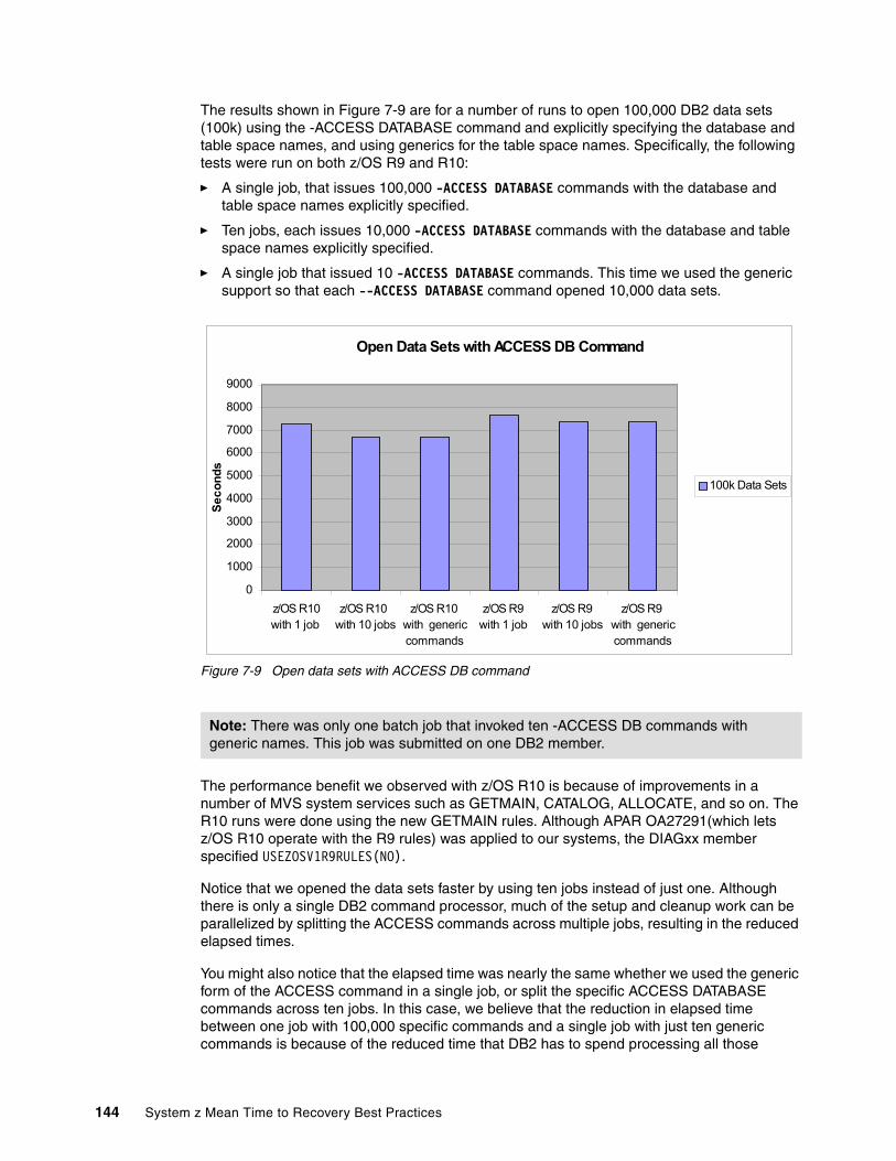
The results shown in Figure 7-9 are for a number of runs to open 100,000 DB2 data sets (100k) using the -ACCESS DATABASE command and explicitly specifying the database and table space names, and using generics for the table space names. Specifically, the following tests were run on both z/OS R9 and R10:

� A single job, that issues 100,000 -ACCESS DATABASE commands with the database and table space names explicitly specified.

� Ten jobs, each issues 10,000 -ACCESS DATABASE commands with the database and table space names explicitly specified.

� A single job that issued 10 -ACCESS DATABASE commands. This time we used the generic support so that each --ACCESS DATABASE command opened 10,000 data sets.

Figure 7-9 Open data sets with ACCESS DB command

The performance benefit we observed with z/OS R10 is because of improvements in a number of MVS system services such as GETMAIN, CATALOG, ALLOCATE, and so on. The R10 runs were done using the new GETMAIN rules. Although APAR OA27291(which lets z/OS R10 operate with the R9 rules) was applied to our systems, the DIAGxx member specified USEZOSV1R9RULES(NO).

Notice that we opened the data sets faster by using ten jobs instead of just one. Although there is only a single DB2 command processor, much of the setup and cleanup work can be parallelized by splitting the ACCESS commands across multiple jobs, resulting in the reduced elapsed times.

You might also notice that the elapsed time was nearly the same whether we used the generic form of the ACCESS command in a single job, or split the specific ACCESS DATABASE commands across ten jobs. In this case, we believe that the reduction in elapsed time between one job with 100,000 specific commands and a single job with just ten generic commands is because of the reduced time that DB2 has to spend processing all those

Note: There was only one batch job that invoked ten -ACCESS DB commands with generic names. This job was submitted on one DB2 member.

Open Data Sets with ACCESS DB Command

0

1000

2000

3000

4000

5000

6000

7000

8000

9000

z/OS R10with 1 job

z/OS R10 with 10 jobs

z/OS R10 with genericcommands

z/OS R9 with 1 job

z/OS R9 with 10 jobs


Se

co

nd

s

100k Data Sets


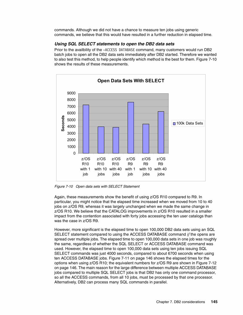
commands. Although we did not have a chance to measure ten jobs using generic commands, we believe that this would have resulted in a further reduction in elapsed time.

Using SQL SELECT statements to open the DB2 data setsPrior to the availbility of the -ACCESS DATABASE command, many customers would run DB2 batch jobs to open all the DB2 data sets immediately after DB2 started. Therefore we wanted to also test this method, to help people identify which method is the best for them. Figure 7-10 shows the results of these measurements.

Figure 7-10 Open data sets with SELECT Statement

Again, these measurements show the benefit of using z/OS R10 compared to R9. In particular, you might notice that the elapsed time increased when we moved from 10 to 40 jobs on z/OS R9, whereas it was largely unchanged when we made the same change in z/OS R10. We believe that the CATALOG improvements in z/OS R10 resulted in a smaller impact from the contention associated with forty jobs accessing the ten user catalogs than was the case in z/OS R9.

However, more significant is the elapsed time to open 100,000 DB2 data sets using an SQL SELECT statement compared to using the ACCESS DATABASE command if the opens are spread over multiple jobs. The elapsed time to open 100,000 data sets in one job was roughly the same, regardless of whether the SQL SELECT or ACCESS DATABASE command was used. However, the elapsed time to open 100,000 data sets using ten jobs issuing SQL SELECT commands was just 4000 seconds, compared to about 6700 seconds when using ten ACCESS DATABASE jobs. Figure 7-11 on page 146 shows the elapsed times for the options when using z/OS R10; the equivalent numbers for z/OS R9 are shown in Figure 7-12 on page 146. The main reason for the large difference between multiple ACCESS DATABASE jobs compared to multiple SQL SELECT jobs is that DB2 has only one command processor, so all the ACCESS commands, from all 10 jobs, must be processed by that one processor. Alternatively, DB2 can process many SQL commands in parallel.

Open Data Sets With SELECT

0

1000

2000

3000

4000

5000

6000

7000

8000

9000

z/OSR10

with 1 job

z/OSR10

with 10 jobs

z/OSR10

with 40 jobs

z/OSR9

with 1 job

z/OSR9

with 10 jobs

z/OSR9

with 40 jobs

Sec

on

ds

100k Data Sets


Figure 7-11 Select versus ACCESS DATABASE on z/OS R10

Figure 7-12 Select versus ACCESS DATABASE on z/OS R9

You might wonder why the performance did not improve further when moving from 10 to 40 SQL SELECT jobs. We believe the reason for this is that DB2 has a maximum of one task per user catalog, and you might recall that our DB2 data sets were spread over 10 user catalogs. Although we did not get an opportunity to test with a larger number of user catalogs, we believe that having the DB2 data sets split over more user catalogs would have resulted in further elapsed time improvements when 40 jobs were used, especially on z/OS R10.

Select vs Access DB on z/OS R10

0

1000

2000

3000

4000

5000

6000

7000

8000

z/OS R10with 1

access job

z/OS R10 with 10

access jobs


z/OS R10 with 1 select

job

z/OS R10 with 10

select jobs

z/OS R10 with 40

select jobs

Se

co

nd

s

100k Data Sets

Select vs Access DB on z/OS R9

0

1000

2000

3000

4000

5000

6000

7000

8000

9000

z/OS R9 with 1

access job

z/OS R9 with 10

accessjobs


z/OS R9 with 1

select job

z/OS R9 with 10

select jobs

z/OS R9 with 40

select jobs

Se

co

nd

s

100k Data Sets


7.3.2 Impact of Enhanced Catalog Sharing on data set OPEN processing

Enhanced Catalog Sharing (ECS) was introduced with DFSMS/MVS 1.5. It exploits the capabilities of the coupling facility (specifically, the cross-invalidation capability of cache structures) to provide the integrity required when you share ICF catalogs across the members of a sysplex, but without the performance impact normally associated with shared catalogs.

More information about Enhanced Catalog Sharing can be found in z/OS DFSMS Managing Catalogs, SC26-7409 and in Enhanced Catalog Sharing and Management, SG24-5594.

To determine if your catalogs are eligible for ECS, issue the F CATALOG,ECSHR(STATUS) command, as shown in Figure 7-13.

Figure 7-13 Output of F CATALOG,ECSHR(STATUS) command

For our test, we took the results of the earlier measurement with 10 jobs running SQL SELECT statements to open a total of 100,000 data sets (that measurement was run with ECS turned on), and then ran the same test again, this time with ECS disabled.

The elapsed time with ECS active, as shown in Figure 7-14 on page 148 was significantly less than that without ECS active: 4028 seconds compared to 5574 seconds.

F CATALOG,ECSHR(STATUS) IEC351I CATALOG ADDRESS SPACE MODIFY COMMAND ACTIVE IEC380I ENHANCED CATALOG SHARING 957 *CAS*************************************************************** * CF Connection: AutoAdd * * ------------------CATALOG------------------- -----STATUS------ * * UCAT.DB2DB9 Active * * UCAT.DB2DB8 Active * * UCAT.DB2DB7 Active * * UCAT.DB2DB6 Active * * UCAT.DB2DB5 Active * * UCAT.DB2DB4 Active * * UCAT.DB2DB3 Active * * UCAT.DB2DB2 Active * * UCAT.DB2DB10 Active * * UCAT.DB2DB1 Active *


Figure 7-14 Open 100,000 data sets with ECS

7.3.3 Generic advice about minimizing DB2 restart time

In addition to the specific measurements described previously, there are other general guidelines you should consider to optimize your DB2 startup times.

DB2 consistent restart Consistent restart will allow DB2 to start up first and then process the backout work, so the whole DB2 system will not suffer from long running URs that do not issue frequent commits. The time saving is in the Backward Log Recovery Phase.

The two ZPARM parameters related to this activity are: LBACKOUT and BACKODUR. Options are:

� LBACKOUT=NO states that no consistent restart should be done, meaning that DB2 must complete all backout work before it can complete its startup.

� LBACKOUT=AUTO (the default) indicates that some backout work might be delayed and will be triggered automatically after DB2 comes up.

� LBACKOUT=YES indicates that users have to issue the RECOVER POSTPONED command to complete the backout activity after DB2 comes up.

The number of checkpoints processed during the Backward Log Recovery phase when doing a consistent restart is defined with the parameter BACKODUR. Specifying a larger value can cause DB2 to go back further in the log. This approach might increase the number of objects that are backed out during this phase, but might also increase the elapsed time of this phase (and therefore, the elapsed time of the DB2 startup).

Open Data Sets With ECS

0

1000

2000

3000

4000

5000

6000

z/OS R10 with ECS

active

z/OS R10with ECSinactive

z/OS R9 with ECS

active

z/OS R9with ECSinactive

Sec

on

ds

100k Data Sets


Fast Log Apply storageThe Fast Log Apply technique sorts the log records for a given pageset into an ascending page number sequence. This can eliminate multiple Getpages for the same page. The Fast Log Apply also improves I/O performance by using list prefetch.

During restart, Fast Log Apply is always enabled. Fast Log Apply involves reading the log and sorting records. Finally the updates are processed by one or more apply tasks, with list prefetches being done to read the appropriate pages. The default value for Fast Log Apply storage starting with DB2 V8 is 100 MB. For more information about the performance considerations of this feature, see DB2 UDB for z/OS Version 8 Performance Topics, SG24-6465.

Minimize the number of data sets to be openedDB2 restart will only open data sets to perform redo/undo activities if they belong to pagesets that were in a R/W state when DB2 crashed. DB2 restart can potentially read logs for up to two system checkpoints. But, in general, it should only read one system checkpoint worth of logs during restart operation.

During restart, DB2 opens data sets that belong to only GBP-dependent objects if it needs to process log records that belong to uncommitted transactions. Therefore, for infrequently updated pagesets or partitions, R/O switching can help to improve restart performance for non-shared or for non-GBP dependent objects in a data sharing environment because logs are skipped for those R/O objects (to avoid data set open and unnecessary read I/Os).

During Restart, DB2 opens and accesses data or index page sets only when it encounters log records belonging to those non-shared objects. If no log records were encountered for those non-shared objects in the last one or two checkpoints, those data sets will not be opened even if R/O switching has not occurred before DB2 was crashed.

If those R/W objects are not opened during forward and backward recovery, DB2 closes SYSLGRNX rows for those table space objects or COPY YES index objects during the End Restart phase in DB V8 and update DBET entries to record the data-set-level ID for Down Level Detection (DLD) checking. In DB2 V9, the process of closing SYSLGRNX and casting out changed pages has been moved to occur after DB2 is up (it is triggered during the first DB2 system checkpoint after DB2 is up).

For GBP-dependent objects in R/W that were not opened during forward and backward recovery, DB2 also must open and cast out changed pages for objects that were only updated by the restarting member (that is, this object was in R/W sharing and only updated by a single member).

To further reduce the number of data sets that must be opened during restart, the DSNZPARMs PCLOSEN and PCLOSET parameters can be used to trigger the read only switching feature. If all updates to a table space or object have been committed and there are no more updates for some time (controlled by PCLOSEN and PCLOSET), DB2 does a read-only-switching, by closing SYSLGRNG entries and indicating that this object is no longer in read/write mode. As a result, DB2 cannot open it at restart time.

Note: Backout against DB2 Catalog or Directory page sets cannot be postponed and are always completed before DB2 completes initialization, regardless of the setting of the LBACKOUT and BACKODUR parameters.


DB2 checkpoint intervalThe DB2 checkpoint interval indicates the number of log records that DB2 writes between successive checkpoints. This value is controlled by the DB2 subsystem CHKFREQ parameter. The default is 500,000, however a smaller value of 50,000 log records results in the fastest DB2 startup time in most cases.

More frequent checkpoints (that is, a smaller CHKFREQ value) can reduce DB2’s startup time after a subsystem failure. However, there is a cost. A checkpoint is a snapshot of all activity in DB2 that would need to be restored at restart. The more activity there is in a DB2 subsystem, the more expensive it is to take a checkpoint. Taking checkpoints too frequently can possibly negatively affect DB2’s performance. To find the correct CHKFREQ value for you, decide which is more important: reduced cost for DB2 in normal operation, or a reduced restart time for DB2.

Control long-running URsDB2 rolls back uncommitted work during startup. On average, the amount of time required for this activity is approximately twice the time that the unit of recovery was running for before DB2 stopped. For example, if a unit of work runs for two hours without a commit before a DB2 abend, it would take at least four hours to restart DB2. In fact, this is a good example of why you should enable DB2 consistent restart: You would not want to delay all DB2 work by four hours just because of this one misbehaving job.

To determine what is an acceptable time for a unit of work to run without a commit, decide how long you can afford to wait during startup, and address any units of work that run for more than half that long.

Long-running URs can be detected using the DB2PM Accounting report. You can control long-running URs by changing the application programs to commit more often. In particular, watch out for single SQLs that are doing mass insert, update, and delete operations.

DB2 can set the threshold to display long-running URs on the console log. The DSNZPARM field is URCHKTH. By default, this function is turned off, however we recommend enabling it by specifying a value of 5 checkpoints.

A related DSNZPARM field, URLGWTH, also exists. It causes DB2 to issue a warning message when an inflight UR writes the specified number of log records without a COMMIT. The current default value is to turn this function off (0 log records), however we recommend setting this value to 10,000.

Avoid archive tape readsTape is not well-suited to backout processing because of its one-direction sequential nature. To optimize DB2 restart time, using archive log data sets on tape is not desirable. Instead, consider keeping the archive log data sets on DASD.

Note: You can use the LOGLOAD or CHKTIME option of the SET LOG command to modify the CHKFREQ value dynamically without recycling DB2. However, DB2 will revert to the value that was specified on the CHKFREQ parameter after the restart.

Recommendation: To detect long-running units of recovery, enable the UR CHECK FREQ option of installation panel DSNTIPL. If long-running units of recovery are unavoidable, consider enabling the LIMIT BACKOUT option on installation panel DSNTIPL. And ensure that all applications do commit operations at reasonable intervals.


Size of active logsEspecially if your archive can be migrated to tape (but even if they do not), you can avoid unnecessary startup delays by making each active log data set large enough to hold the log records for a typical unit of work. This approach lessens the probability that DB2 must wait for tape mounts or many data set allocations during startup. You can also increase the number of active log data sets; with DB2 V9, you can have up to 93 active log data sets for each log copy.

Define large group buffer poolsGBP accesses are in terms of microseconds, compared to DASD access at milliseconds. So having larger GBPs means that the majority of pages touched during restart can be transferred in microseconds which can shorten the restart time by a significant amount.

7.4 Speeding up DB2 shutdown

As you know, the two aspects to the amount of time to restart DB2 are:

� The amount of time to start DB2, which is the aspect we have been focussing on so far. � The amount of time to complete a planned stop of DB2 prior to the restart.

This section examines the second aspect.

7.4.1 Impact of DSMAX and SMF Type 30 on DB2 shutdown

The number of data sets in use by DB2 can affect the DB2 shutdown time in two ways.

� Some amount of time (.1 - .3 seconds per data set, according to DB2 Administration Guide, SC18-7840) is spent to physically close each data set open at shutdown time. The maximum number of concurrently open data sets is determined by the DB2 subsystem parameter DSMAX.

� Assuming that SMF Type 30 records are enabled, z/OS needs time to populate SMF Type 30 records with information about every data set that DB2 opened since DB2 startup.

From the perspective of reducing the cost of constantly opening and closing data sets while DB2 is running, a large DSMAX value is considered a good thing. If DB2 can keep more data sets open concurrently, it is less likely to have to close one data set to be able to open another one. However, a small DSMAX value might be considered a good thing because it would reduce the number of data sets that need to be closed at DB2 shutdown time.

Note: Because “force at commit” is applied to GBP-dependent objects, the restart process can speed up because there is no need to access GBP during restart: updated data belongs to committed transactions.

For log records that are related to non-GBP-dependent objects (for either committed or uncommitted transactions) or log records related to uncommitted transactions, restart will need to read logs (possibly up to two checkpoint’s worth of logs) and examine whether updates were being externalized to GBP or DASD.

Note: DB2 APAR PK29281 increased the maximum number of concurrently open DB2 data sets from 65,000 to 100,000.


To understand the effect of the number of open data sets on DB2 shutdown time, we ran a number of measurements. We started with a DSMAX value of 2k, then increased it to 40k, 60k, 80k, and 100k, measuring how long it would take to stop DB2 in each case. The results are shown in Figure 7-15.

Figure 7-15 Shutdown times for DB2 with differing numbers of open data sets

You can see that the shutdown time scales nonlinearly. There are obvious advantages to shutdown times in having a lower DSMAX value. However, you should balance the shutdown time advantages against the increased overhead if DB2 has to close and reopen many data sets because the DSMAX value is being reached. Although DB2 does not do a physical close operation on its VSAM data sets at shutdown time, it does have to invoke IRLM to free pageset or partition physical (P) locks for each open pageset or partition.

Also, consider the PCLOSET and PCLOSEN values, which also have a role in deciding when a data set should be closed. When the PCLOSET time (or PCLOSEN number of checkpoints) passes without an update to the pageset (or partition), then a pseudo-close is done. This makes that DB2 Read Only DB2 with respect to that pageset/partition.

Additionally, for any object (defined with CLOSE YES) that has ever been GBP-dependent, a physical close operation will eventually be done. After another interval of PCLOSET, the objects that were pseudo-closed in the prior PCLOSET interval will be physically closed. As with DSMAX, determining the correct PCLOSET and PCLOSEN values for your system will depend on your evaluation of the relative priorities of faster DB2 shutdown times versus reduced overhead while DB2 is running.

We also wanted to understand the impact on DB2 shutdown times of various SMF settings. For these measurements, we ran with 100,000 DB2 data sets and then with 20,000 data sets, and measured how long the time was to stop DB2 with the following settings:

� The SMF DDCONS option set to YES� The SMF DDCONS option set to NO

Shutdown DB2 with different open data sets

0

50

100

150

200

250

300

350

400

450

500

20k opendata sets

40k opendata sets

60k opendata sets

80k opendata sets

100k opendata sets

Sec

on

ds

z/OS R10


The SMF DDCONS parameter controls whether SMF consolidates all the EXCP sections for each DD/device pair when the SMF Type 30 job end (subtype 5) records are being created. Specifying NO results in larger volumes of SMF data being created, however this was the recommended value, on the basis that jobs would end faster if they did not have to wait for the EXCP sections to be consolidated. The results of our measurements are shown in Figure 7-16.

Figure 7-16 Shutdown DB2 with DDCONS(YES) or DDCONS(NO)

As you can see, consolidating the EXCP sections in the SMF Type 30 records by specifying DDCONS(YES) resulted in DB2 taking slightly longer (about 9%) to stop than when DDCONS(NO) was specified.

7.4.2 Shutdown DB2 with CASTOUT (NO)

Normally, when DB2 is shut down, it will cast out all pagesets/partitions for which it is the last updating member. If thousands or tens of thousands of data sets are open, this number could be a lot of castouts and could take a considerable amount of time to complete.

If you are shutting down DB2 for a brief period, to apply maintenance, for example, you can use the CASTOUT(NO) option on the DB2 STOP command. This option causes DB2 to skip doing its normal castout processing, and instead an IX mode P-lock for the pageset/partition is retained to track whether the pageset/partition still has changed pages in the GBP.

RecommendationConsider specifying CASTOUT(NO) when you stop an individual member of a data sharing group for a brief period. This option speeds up shutdown because DB2 bypasses castout and associated cleanup processing in the group buffer pools.

Shutdown DB2 with DDCONS

0

100

200

300

400

500

600

100K w ithDDCONS(YES)

100K w ithDDCONS(NO)

20K w ith DDCONS(YES)

20K w ithDDCONS(NO)

Sec

on

ds

z/OS R10


7.4.3 PCLOSET consideration

A very large PCLOSET value can result in one DB2 being the Global Lock Manager for a very large number of lock entries. This in turn can result in an elongated DB2 shutdown time because DB2 must release all the locks of which it is the Global Lock Manager.

7.4.4 Active threads

DB2 cannot shut down until all threads have been terminated. If the DB2 shutdown is taking longer than expected, issue the DB2 DISPLAY THREAD command to determine if any threads are active. If necessary, those threads can be cancelled.

7.4.5 Shutdown DB2 with SYSTEMS exclusion RNL

If you are not doing DB2 data sharing, and you are positive that no other system will attempt to open your DB2 data sets, you can place the DB2 data sets in the SYSTEMS exclusion resource name list (RNL); this approach changes the scope of the ENQs to a single system, and should result in reduced DB2 shutdown times. For details, see z/OS MVS Planning: Global Resource Serialization, SA22-7600.

Note: Do not use CASTOUT(NO) when you shut down multiple members of a data sharing group and you need to maintain consistent data on disk. For example, if you shut down all members to get a consistent copy of the databases on disk that you can copy and send offsite, do not specify CASTOUT(NO), because some of the changed data could still reside in the group buffer pools after all the members have shut down


Chapter 8. IMS considerations

This chapter discusses the Information Management System (IMS) and the options to provide faster startup and shutdown of the subsystem. IMS is an IBM premier transaction and database manager for critical online applications. It is primarily used where high volume transaction processing with data and message integrity is essential, while also providing a low cost per transaction.

IMS has been highly optimized over the 40 plus years it has been in existence. However, IMS and system parameters can affect the time to start IMS (to the point of being able to run applications), and to shut it down in an orderly manner. Those options and parameters are explored in this chapter. Although most information in this chapter is for the normal startup and shutdown situation, various options are discussed that minimize the time to start IMS after an abnormal shutdown.

8


8.1 Definition of startup and shutdown times

For the purposes of this book, the startup time includes everything necessary to begin processing transactions. Everything includes initialization, restart, start dependent regions, and open databases. Key messages that delineate these phases in the startup process are:

� DFS0578I is the first message issued by IMS after it is started.

� DFS810A (or DFS3931I) signals the end of initialization.

� DFS058I is issued when the restart command is in progress.

� DFS994I indicates the end of restart processing.

Shutdown is defined as starting when you enter the IMS checkpoint command to terminate IMS, or from when an abnormal termination starts until the time that the IMS control region is gone from the system. Messages include:

� DFS994I indicates that the checkpoint command is in progress.

� DFS994I informs you when shutdown has completed.

� DFS627I is also issued, indicating that the recovery termination manager (RTM) cleanup is complete.

8.2 How we measured

Depending on the situation, we used the following methods to measure the startup and shutdown times:

� Syslog and JOBLOG

These sources can be used for situations in which total times or specific functions within startup or shutdown can be tied to various messages.

� IMS log record analysis

This method was used in cases to verify what was happening internally between certain messages. However log records cannot be used to analyze initialization or restart because no log records are written during those times.

� CQS log record analysis

The IMS Common Queue Server (CQS) writes log records for certain activities, and statistics records when a CQS checkpoint is taken. These statistics can be used to obtain certain timings.

� SMF

IMS does not specifically write System Management Facility (SMF) records except for the Type 79 Subtype 15 long lock detection record.However, SMF records (such as Type 30 records) may be created for any job, which, of course, includes IMS.

� RMF

Resource Management Facility (RMF) writes SMF Type 7x records, which can then be reported on by the RMF Postprocessor.


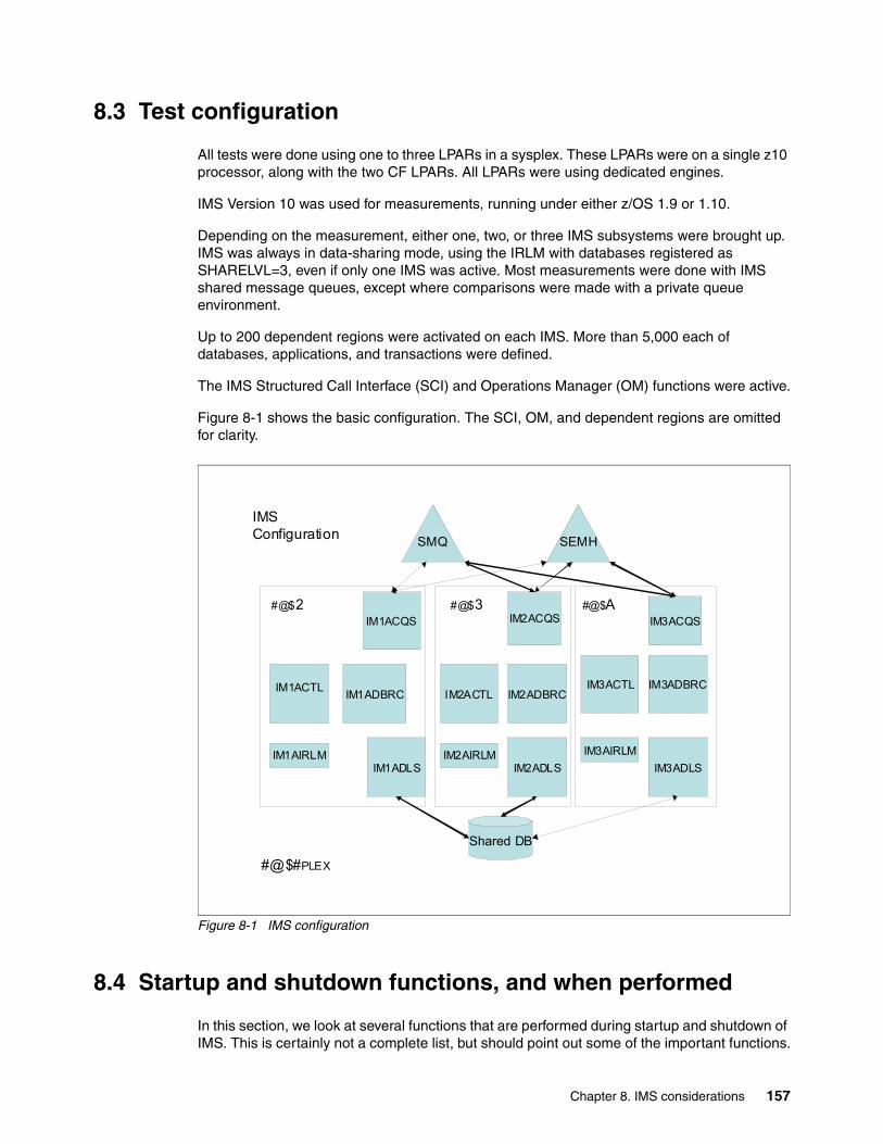
8.3 Test configuration

All tests were done using one to three LPARs in a sysplex. These LPARs were on a single z10 processor, along with the two CF LPARs. All LPARs were using dedicated engines.

IMS Version 10 was used for measurements, running under either z/OS 1.9 or 1.10.

Depending on the measurement, either one, two, or three IMS subsystems were brought up. IMS was always in data-sharing mode, using the IRLM with databases registered as SHARELVL=3, even if only one IMS was active. Most measurements were done with IMS shared message queues, except where comparisons were made with a private queue environment.

Up to 200 dependent regions were activated on each IMS. More than 5,000 each of databases, applications, and transactions were defined.

The IMS Structured Call Interface (SCI) and Operations Manager (OM) functions were active.

Figure 8-1 shows the basic configuration. The SCI, OM, and dependent regions are omitted for clarity.

Figure 8-1 IMS configuration

8.4 Startup and shutdown functions, and when performed

In this section, we look at several functions that are performed during startup and shutdown of IMS. This is certainly not a complete list, but should point out some of the important functions.

IM1ACTLIM2ACTL

IM3ACTL

IM1ADLS

IM1ADBRC

IM1ACQS

IM2ADBRC

IM2ADLS

IM3ADBRC

IM3ADLS

#@$2 #@$3 #@$A

#@$#PLEX

SMQ SEMH

IM2ACQS IM3ACQS

Shared DB

IMS Configuration

IM1AIRLM IM2AIRLM IM3AIRLM

Chapter 8. IMS considerations 157

8.4.1 Startup functions

For the purposes of this book, we divide IMS startup time into three separate phases:

� Initialization

Initialization is the time from issuing the START IMS command, until either the DFS810A IMS READY message, or the DFS3931I IMS INITIALIZED, AUTOMATIC RESTART PROCEEDING, message is presented. The DFS3931I message is presented if automatic restart processing has been enabled. Included in this time are functions such as:

– Loading IMS modules

– Allocating virtual storage for blocks and pools

– Reading and processing IMS PROCLIB members

– Issuing start commands for the other IMS address spaces

– Initializing the various IMS Task Control Blocks (TCBs)

– Initializing the IMS logger and allocating the OLDS and WADS data sets

– Attempting to acquire the IMS master terminal

– DLI connects to the OSAM and VSAM cache structures, if used

– CQS, if used, connects to its CF structures and issue the CQS0020I CQS READY message

� Restart

Restart is the time from when the RESTART command is entered by the user, or from the DFS3931 message, until the DFS994I xxxx START COMPLETED message (where xxxx is the type of restart) is issued. It includes the following activities:

– If this is a warm or emergency start, IMS determines the checkpoint to be used and opens the OLDS and WADS data sets from the previous execution and processes as necessary.

– IMS identifies to IRLM, and then IRLM connects to the lock structure.

– Issue BLDLs for the DBDs and PSBs that are defined to IMS.

– Page-fix the specified areas of storage.

– Open OLDS and WADS.

– Take a simple checkpoint.

– Pre-open specified Fast Path (FP) areas.

– Connect (allocate) any shared VSO structures.

– Preload specified FP areas.

� Post restart

Post restart is the time from the restart complete message (DFS994I), until user logons can begin, dependent regions are started, and applications can begin processing, as follows:

– Start Data Communications (DC) to allow logons.

– Start dependent regions, including any preload processing.

– Open database data sets, either specifically by using the /STA DB command with the OPEN option or implicitly when they are first used by an application.


8.4.2 Shutdown functions

Shutdown of IMS can be normal or abnormal. A normal shutdown is where an IMS checkpoint command is issued. In this case, IMS cleans up all storage, closes database data sets, and finally takes a checkpoint which will subsequently be used by a warm start. The elapsed time for the shutdown process starts from when the /CHE FREEZE, PURGE, or DUMPQ command is entered, and ends when IMS is completely out of the system and can be started again

Abnormal shutdown can be because of a failure in IMS where the z/OS system stays active. This type of failure typically means that dump processing will be invoked, and this can affect shutdown time. IMS ESTAE processing cleans up common storage and closes the log if possible. In the case of a z/OS or hardware failure, IMS of course does not get control so it is up to Fast Database Recovery (FDBR) and emergency restart to handle cleaning up locks and in-flight or in-doubt units of work. The shutdown time in this case is the time from the point of the abend through to when IMS is out of the system, and includes the time for dump processing.

8.5 IMS parameters

As anyone who uses IMS already knows, there are many startup parameters in several different PROCLIB members. However, only those parameters that might affect startup or shutdown time are discussed here. Any parameters or specifications that might affect startup or shutdown, but cannot be changed without affecting system function, are not discussed. Those things might be active transaction and database definitions, pool sizes, and so on. Although certain things could or should be changed for better overall performance, that is not the subject of this book.

8.5.1 DFSPBxxx member

DFSPBxxx contains most of the startup parameters for IMS. It also specifies other members of IMS PROCLIB to be loaded and processed. Those members are discussed separately. The following parameters are processed during IMS startup:

� ARMRST

This parameter tells IMS whether or not to register with the MVS Automatic Restart Manager (ARM). Although the default is yes (Y), for this to take any effect, the necessary ARM policy must have been set up. When using ARM to restart IMS, the AUTO= specification is overridden to YES so that IMS can both initialize and restart with no manual intervention. If you do not want to use ARM because you have other automation in place, then specify ARM=N.

� AUTO

Many installations have automation products to handle the restarting of IMS. However, specifying AUTO=Y enables IMS to internally determine the type of restart that is necessary and proceed to perform the restart without delay. For those instances where a cold start is desired, a manual override of this parameter could be done on those rare occasions. To override at startup, specify S IMS,PARM1=’AUTO=N’ command. The one confusing thing about the AUTO=Y approach is that the normal DFS810A message is replaced by the DFS3139I message stating that automatic restart proceeding is being used and this WTOR remains outstanding until a reply of some type is entered, at which time it will be replaced by the DFS996I IMS READY message. A good practice is to have an automated reply to the DFS3139I WTOR simply to avoid confusion: Although IMS is


not typically in restart processing for very long, this message can remain outstanding for hours or days even though normal processing has continued.

� CPLOG

CPLOG controls when IMS will take automatic checkpoints. Some installations set this very high and perform checkpoints with automation. The frequency of checkpoints is a consideration when an emergency restart must be performed. Most times, IMS goes back to the second most current checkpoint to begin processing the log for restart. Of course, the amount of log data that must be processed affects the time to complete the emergency restart process, not necessarily the time between checkpoints, because the amount of log data produced in a given period will probably vary quite a lot depending on the time of day. The speed of the DASD is also a factor in how long restart takes, therefore you might want to run tests to determine how long, in your environment, processing a given amount of log data takes. That information can then be used as input to determine how to set this value.

� FDRMBR

Specifying the use of Fast DataBase Recovery (FDBR) is mostly considered as an availability option in a data sharing environment; it does provide full data availability to surviving IMS subsystems in the event that one IMS fails. However, by performing the necessary backout or redo processing on behalf of the failed IMS, FDBR eliminates the need to do that processing during the restart and thus reduces the time to get IMS back to the point of processing new transactions. Although FDBR was designed for availability in a data sharing environment it could, in fact, be used in a non-data sharing environment also, to provide faster restart times.

� FMTO

This is an abnormal termination parameter and determines the type of dump that IMS will take. The default setting is D which in most cases is fine. However M or R might be better as long as SYSMDUMP has been set up to provide an alternative dump location if for some reason the offline dump process were to fail. The important point here is to avoid SYSABEND or SYSUDUMP processing because it will take considerably more time and delay IMS getting out of the system.

� FPOPN

Fast Path areas have several options for open and preload. Pre-open and preload are specified in DBRC and these options, as well as opening of areas that are not specified as pre-open, might be affected by this setting. Fast Path pre-opens (or opens) and preloads data sets concurrently with other operations. As a result, whatever option is chosen should not affect the time to initialize and restart IMS. The main effect should be in getting applications to run as soon as possible. Using the DBRC pre-open option for critical databases, and specifying FPOPN=R or A should provide for maximum parallel processing of transactions and the open process.

� PST

This value should specify enough Partition Specification Tables (PSTs) to accommodate all of the dependent regions (or threads for DBCTL) that are expected to be started. IMS allows more regions than this number to be started, up to the specification of MAXPST. However, anything above the PST value causes extra processing when the regions are started. For quickness of restart processing, this is a trade-off of where you want the cost of getting the storage and initializing various control blocks to be incurred. However, it is generally more efficient for IMS to acquire and initialize the blocks during the initialization process to avoid delays during critical online processing.

� SHAREDQ

Specification of this parameter tells IMS to use shared queues instead of private queues. Although more overhead is involved in transaction processing with shared queues, there is


a definite advantage in restart processing. A process that is performed by private queues called QFIX can sometimes be lengthy during emergency restart processing, and depends very much on the amount of queue manager log data to be processed. With shared queues, this process is eliminated, and IMS must only connect to CQS. Considerations for CQS restart, however, must be addressed to optimize that process. These are discussed in 8.5.4, “CQSSLxxx member” on page 162.

8.5.2 DFSDCxxx member

The DFSDCxxx member of PROCLIB contains many parameters with regards to communications options. Two specific parameters can affect restart:

� VACBOPN

This parameter is used to tell IMS when to open the VTAM ACB. Whether this is important depends on how much of your network is SNA. The effect of this parameter is well documented in IMS System Definition Reference, GC18-9966, but is summarized here.

The default value of INIT tells IMS to open the VTAM ACB during initialization. The other value is DELAY, which delays the open until the /STA DC command is executed. With DELAY the logon request is rejected until the ACB is opened with the /STA DC command. If INIT is specified, user logons will be queued by VTAM until the /STA DC command is executed. Depending on the number of requests queued, this can cause a flood of logons when the start command is completed and some or many of those requests might have already timed out. This in turn can cause a considerable amount of unnecessary processing and delays just after restart, when you want to have transaction processing begin.

� PMTO

The value specified for this parameter overrides the node name from the system definition for the master terminal. Regardless of whether this name, or the one from system definition is used, be sure that this node is defined to VTAM, especially if it does not really exist. This approach will prevent VTAM from searching the SNA network for this node, which in some cases can take a very long time.

8.5.3 DFSCGxxx member

The DFSCGxxx member specifies items for the common service layer of IMS including Structured Call Interface (SCI), Operations Manager (OM), and Resource Manager (RM). From a startup perspective, a few key parameters are:

� RMENV

If you intend to use Resource Manager services and specify Y here, the next two items (OMPROC and SCIPROC) are not used. However, although the OMPROC and SCIPROC keywords are ignored, those address spaces must be started in a timely fashion to avoid startup delays. This point is important.

� OMPROC

For this parameter, you can specify the OM procedure name. If RMENV=N is specified, IMS will automatically issue the START command for OM. Certain considerations, about when this START command is issued are covered later in this chapter.

� SCIPROC

Similar to the OMPROC value, this parameter tells IMS to automatically issue the START command for SCI if it has not previously been started. If using SCI or OM or both, a good


idea is to code these values even if you have other procedures in place to start them. This approach provides a fallback in the event that they had not already been started.

Although you might ask why RMENV=Y causes the OMPROC and SCIPROC values to be ignored and why IMS could not start RM as well, the answer at this time is: This is working as designed.

8.5.4 CQSSLxxx member

The CQSSLxxx member specifies information regarding a particular instance of CQS. The only value we discuss is SYSCHKPT.

This SYSCHKPT value is much like the CPLOG value for IMS. It specifies how many CQS logger records there should be between CQS system checkpoints. These checkpoints are for an individual instance of CQS. These checkpoints have very little impact to the system when they occur. Much like IMS, the frequency of these checkpoints has an impact on the time to restart CQS in the unlikely event of a failure. Unfortunately, this setting cannot be changed dynamically while the system is running. However, if you want to take more frequent system checkpoints, you could do this by having automation issue the /CQC command at regular intervals.

8.5.5 DFSMPLxx

This IMS PROCLIB member specifies modules to be preloaded into IMS regions. Although not exclusive to dependent regions, this is the most common use. The number and size of the modules specified in this member can affect region startup times especially when starting many hundreds of dependent regions. Additional information about this subject is covered in 8.7.2, “Starting dependent regions” on page 166.

8.6 Starting IMS-related address spaces

The order in which various IMS address spaces are started can affect (in a good or bad way) the startup process. In this section, we look at which address spaces (such as IRLM, SCI, OM, RM, and so on) may be started before or concurrently with the IMS control region.

8.6.1 IMS-related address spaces

The IMS functions that you exploit in your configuration determines which IMS address spaces are needed. Possibilities include:

� IRLM

The IRLM may be used as the lock manager for IMS in both data-sharing and non-data-sharing environments. It should be started before or perhaps at the same time as IMS. However, you definitely want it to be active before IMS attempts to identify to the IRLM, an action that takes place early in the restart process. If IRLM is not active when IMS tries to identify, IMS issues a DFS039A WTOR, which must then be replied to after the IRLM has been started. When possible, of course, avoid manual intervention.

� FDBR

The Fast DataBase Recovery (FDBR) address space is started separately, and for availability should run on a different LPAR, preferably on a separate physical machine. It can be started at any time before or after IMS. Because we focused primarily on the


normal shutdown and startup situation, we did not have a chance to demonstrate the time that probably would have been saved on emergency restart by not having to do database backout, because FDBR would have done that in advance.

� SCI

The Structured Call Interface (SCI) is used for many functions and is the communications interface for the various IMS address spaces. SCI is optional and can be started automatically by IMS if the procedure name is specified in the DFSCGxxx member of IMS PROCLIB and RMENV=Y has not been specified. The SCI does not terminate if either a normal or abnormal termination of IMS should occur, so this address space need only be started once per IPL of the system. Consider placing the start for SCI in the COMMNDxx member of Parmlib. Depending on the functions being used, IMS might or might not complete initialization before SCI is started. However, IMS automatically detects when SCI has been started without operator intervention.

� OM

Operations Manager (OM) is also an optional address space that might be started automatically by IMS if specified in the DFSCGxxx member. However, as with SCI, IMS does not automatically start either SCI or OM if RMENV=Y is specified in that same member. So, if using the Resource Manager component of IMS you must start RM, SCI, and OM by using COMMNDxx, automation, or manually.

� RM

Resource Manager (RM) is optional too. If using RM, consider the options in the preceding discussion of OM.

� AVM

Availability Manager (AVM) is used with extended recovery facility (XRF) or FDBR. If it is not started, IMS starts it automatically. Although AVM starts in very little time, it also can easily be put in the COMMNDxx member. There is no way to stop AVM other than with an MVS FORCE command. If you stop AVM in this way, you must restart AVM manually because IMS will not start it again until after the next MVS IPL.

� RRS

This parameter is only used if RRS=Y is specified in the DFSPBxxx member. Resource Recovery Services (RRS) is normally started in the COMMNDxx member of parmlib. If IMS tries to use RRS but it is not started, IMS will complete initialization but issue the following message during restart processing and wait for RRS to be started and the reply to the WTOR to be completed:

DFS0548A RRS NOT ACTIVE BUT RRS=Y SPECIFIED - REPLY: RETRY, CONTINUE OR CANCEL

RRS is also used with DBRC parallel recon access but that is separate from the IMS specification.

To understand the impact of starting SCI and OM before IMS, or having IMS start these address spaces, we ran with both options and obtained the results shown in Figure 8-2 on page 164. As it turned out, the delay with SCI being started by IMS was because DBRC, which had already been started, was waiting for SCI and the IMS control region had not yet issued the START command. IMS was actually then waiting for DBRC to complete initialization. This delay can be eliminated by starting SCI prior to, or concurrently with, IMS.


Figure 8-2 SCI & OM started before or during IMS startup

8.7 Other IMS options

This section discusses various other options that can affect the time to start or stop IMS. Options include various system definition items, various functions, and options to improve the mean time to recovery (MTTR).

8.7.1 IMS system definition specifications

The system definition options that can affect startup time are the resident options for databases and applications. These are specified as positional keywords as follows in the IMS stage 1 input:

� DATABASE RESIDENT,DBD=

� APPLCTN RESIDENT,PSB=

RESIDENT option may also be dynamically specified with the SET(RESIDENT(Y)) parameter on the CREATE DB, UPDATE DB, CREATE PGM, or UPDATE PGM commands but will not actually be in effect until IMS is restarted.

The RESIDENT option may be turned off by the RES=N startup option. RES=Y is the default. Startup time can be affected by the number of resident blocks that are loaded. IMS does a BLDL operation at startup for all the defined resources, however those that are defined as resident are actually loaded into storage during the startup process. The DMB and PSB pools can be made large enough such that resident blocks are not necessary, but tuning options are associated with those pools. Tuning for online performance is not covered in this book so only the affect on startup time is shown.

Affect of SCI & OM

0

2

4

6

8

10

12

14

16

18

SCI/OM active SCI/OM not active

Sec

on

ds

sta - rdy


Figure 8-3 shows the effect of the resident option. For this test we had 5,000 databases and 5,000 applications defined as resident in one case and nonresident in the other. The time from start until the IMS ready message remains constant but the time to load the requested control blocks shows up in the resident case in the time between the NRE command and when IMS restart is complete (because this is when the BLDL and resident block load takes place). Of course, this time can vary depending on how many resources are defined to your system.

Figure 8-3 Impact of RESIDENT option on IMS startup times

In addition to the RESIDENT option, there is another consideration, which is the number of databases or applications that are defined, whether resident or not, that are not actually being used. These fall into at least two categories:

� Those that are defined and have ACBs defined. These are very difficult to find and require log analysis over some period of time to identify.

� Those that are defined to IMS but no longer have ACBs. These can be identified by the DFS830I messages that are written during startup, and could be candidates for cleanup.

A few unnecessary applications or databases being defined will have minimal impact on startup, but if there are many hundreds or thousands, then there could be savings in both time and storage. In Figure 8-4 on page 166 we removed 500 DMBs and 500 ACBs from ACBLIB and measured the time from the NRE command until cold start was complete. We then removed those same 1000 resources from the IMS definition to see the impact of cleaning up unused resources. Even though the impact was not a lot, it does show that removing unnecessary resources is a good idea.

Resident vs non resident

0

1

2

3

4

5

6

7

8

9

10

resident non-resident

Sec

on

ds

Start-R eady

NRE-RST Comp


Figure 8-4 BLDL failure impact

8.7.2 Starting dependent regions

Starting the regions is necessary to begin transaction processing. The number of regions used varies considerably by installation. Some sites use only 10 or 20 regions; others use several hundred. We want the dependent regions to be started as quickly as possible. There are a number of options to expedite this process:

� PST value in DFSPBxxx

IMS acquires storage and initializes these control blocks during initialization. Although having more than necessary is probably a good idea, be sure not to get carried away. For example, if you normally need 100 regions, specifying 120 or so would be reasonable. However, specifying the maximum of 999 would waste a lot of storage, and would take more time during initialization.

� Use of JES2 initiators versus WLM-Managed initiators

Always use JES2-managed initiators for IMS-dependent regions. Using WLM-managed initiators slows down the starting of these regions significantly and in some cases might prevent all of the regions from actually starting.

� Use of LLA and VLF for IMS reslib and preloaded modules

Most IMS modules are only loaded once per execution and so the use of LLA and VLF might not provide any significant benefit. However, depending on how many regions are being started and how many of the same modules are being preloaded into each region and their size, using LLA and VLF to reduce the time to load these modules is possible.

� Use of a CSVLLIX2 exit routine to influence the staging process

This exit can be dynamically enabled and disabled after the regions complete startup in the case where you do not want it active all of the time. This exit could also be used to force staging for modules, which might not be preloaded but instead loaded dynamically during application execution. A sample routine is shown in Appendix B, “Optimizing use of LLA and VLF” on page 197.

BLDL Failure Impact

5.4

4 .8

0

1

2

3

4

5

6

BL DL Fa il Rem ove d

Sec

on

ds

NRE - Co ld


As you can see in Figure 8-5, the use of LLA and VLF with the exit routine enabled had some measurable impact on startup time for the 200 dependent regions. In our case the 20 preloaded modules were about 68 KB each. Today’s DASD is very fast and these 20 modules would of course be cached in the DASD controller so this must be considered as to why the impact was not more. LLA with VLF and the CSVLLIX2 exit routine can be a benefit to the online application performance more than startup if numerous subroutines are being called.

You can see that using WLM-managed initiators for the dependent region job class was very detrimental to region startup time. In fact, we only ever got 186 of the 200 regions to start, no matter how long we waited.

Figure 8-5 Time to start 200 regions

8.7.3 Opening database data sets

Databases must be allocated, authorized with DBRC, and opened before they can be used. The options for fast path databases were discussed with the FPOPN option in 8.5.1, “DFSPBxxx member” on page 159.

For full function databases, IMS will, by default, open those data sets when they are first referenced by an application. This option is probably the best one from the standpoint of getting to the point of having applications running in the dependent regions. However, it might be advantageous to start the open process after IMS is restarted, in parallel with the starting of the dependent regions. This can be done by using the IMS START DATABASE command with the OPEN option. Unfortunately, the form of the command with the open option does not support the ALL keyword, and of course you do not want to enter thousands of commands manually. For our test, we created time controlled option (TCO) scripts and used this facility to open our databases. Although opening all of your databases in this way might not be practical, you might consider it for some of the most highly used databases so that they are available immediately when the applications are scheduled, rather than tying up dependent regions waiting for the open process.A sample TCO script that was used to open our databases is shown in Example 8-1.

Start Region Times

8 12 8

398

0

50

100

150

200

250

300

350

400

450

JES2 In it JES2 & 20 preload m odules JES2 & PRLD & LLA WLM init

Sec

on

ds

Start Region


Example 8-1 Sample TCO script

/STA DB DB00001 OPEN/STA DB DB00002 OPEN/STA DB DB00003 OPEN/STA DB DB00004 OPEN/STA DB DB00005 OPEN..../STA DB DB00997 OPEN /STA DB DB00998 OPEN /STA DB DB00999 OPEN /STA DB DB01000 OPEN *TIME DFSTXIT0 S

8.7.4 DBRC Parallel Recon Access

IMS Version 10 introduced an optional function called Parallel Recon Access (PRA), which affects how DBRC accesses its RECON data sets. To maintain integrity and provide backout in the event of an error, DBRC has always provided an internal mechanism for locking and backing out changes if necessary. Basically, the locking mechanism consisted of issuing a RESERVE macro for each of the data sets and tracking updates within the RECON data sets. This could be converted potentially to a global enqueue by the GRSRNLxx member of SYS1.PARMLIB. Either way, the RECON access was serialized across all the IMS images in the sysplex.

With the PRA function of Version 10, DBRC uses the functions of transactional VSAM to provide locking and logging for backout. The implementation of PRA itself is easy, with a few simple DBRC commands. However, implementation of the prerequisite transactional VSAM function (TVS) is much more complex. More details about this implementation can be found in IBM IMS Version 10 Implementation Guide: A Technical Overview, SG24-7526.

Although implementing PRA can require significant planning and tuning to make it perform well, the results could prove valuable. We conducted several measurements, opening 5,000 databases using various methods of locking; the results are shown in Figure 8-6 on page 169.


Figure 8-6 DBRC access times for serial and parallel access

As you can see, there was very little difference in using the RESERVE or Enqueue functions with serial access. However, after tuning transactional VSAM, we were able to significantly improve this time. The first column shows the time when the DBDs were non-resident in order to compare with the other columns, which represented the measurements with RESIDENT. The only reason this first measurement was done was to determine whether loading the DMBs had any significant impact on the overall time.

8.7.5 Message-based processing for CFRM Couple Data Sets

IMS shared queues uses a cross-system extended service (XES) called IXLUSYNC to quiesce and resume activity to the shared queues structures during a structure checkpoint. A good practice is to take a structure checkpoint after starting up IMS and CQS, allowing log stream data to be cleaned up and to provide a current point of recovery. The most critical time for delays because of structure checkpoint is during heavy online activity when any stoppage of the queuing function can affect the entire IMSplex. Although this slight delay at startup might not be critical, it did give us a chance to better understand the factors that can delay or speed up this process.

In addition to the amount of data on the queue that must be read, the other variables are the size of the CFRM Couple Data Set and whether Message-based CFRM processing (delivered with z/OS V1R8) is used. We did not have time, and it was not within the scope of this book, to look at the impact that the amount of data on the queue would have on IMS initialization time. However, we did look at the CFRM Couple Data Set options because they can also affect startup time.

Figure 8-7 on page 170 shows the impact that the size of the CFRM Couple Data Sets had on the time to quiesce activity to the message queue structure. The size of the CFRM CDS is based on variables such as the number of structures and systems in the sysplex. Using CFRM Message-based processing makes the size of the CDS much less important.

DBRC Options

2 61 26 0

249

1 21

0

50

100

150

200

250

300

non-res, grs conv se rial, grs excl se rial, g rs conv pa rallel

Sec

on

ds

Auth-A lloc-Open


So, although milliseconds might not be a factor in startup time, showing these times seemed worthwhile because they can have a much more significant impact during heavy online processing.

Figure 8-7 Couple data set size impact

8.7.6 Shutdown

IMS shutdown time was very repeatable and short in most cases. The one thing that can affect an abnormal shutdown is the FMTO setting, which was discussed in 8.5.1, “DFSPBxxx member” on page 159.

The other rather long wait at shutdown was between the shutdown checkpoint being issued and when the checkpoint is initiated. Investigation showed that this is mostly because of a couple of STIMER waits for APPC and OTMA client cleanup. These waits are for 10 seconds each and they probably will happen even if you do not use one or both of these functions.

8.8 Summary

Although we tried to exercise as many variations as possible for IMS startup and shutdown, only a few made much difference. We probably brought IMS up and down more times in a few weeks than you would in many years; we hope we have given you an idea of what parameters will affect the mean time to recovery.

Structure Checkpoint

38

199

61

430

0

50

100

150

200

250

300

350

400

450

500

Message Based Non Message Based

Mill

isec

on

ds

Small CDS

Large CDS


Chapter 9. WebSphere considerations

This chapter introduces the WebSphere Application Server initialization logic and provides recommendations for reducing the time for WebSphere Application Server to start and restart. The scope of this discussion is primarily limited to WebSphere Application Server Version 7.0 because it features a number of configuration enhancements designed to enable faster initialization.

Some information in this book is also applicable to WebSphere Application Server Version 6.1 and will be identified as such. The following topics are included in this chapter.

� Introduction to WebSphere Application Server 7 Application Server Initialization Logic

� General recommendations

� How we evaluated WebSphere startup time

� WebSphere Application Server 7 startup enhancements

9


9.1 WebSphere Application Server 7 initialization logic

WebSphere Application Server can be configured in a single server standalone environment called a Base configuration. On z/OS, a Base configuration has at least three address spaces, a Control Region, a daemon, and one or more servant regions. Each servant executes in a separate address space. A Base server is managed from its own administration console and is independent of other WebSphere Application Servers.

WebSphere also supports another configuration option called Network Deployment (ND). Using Network Deployment, you can create a more distributed WebSphere environment that is centrally managed by a Deployment Manager and Node Agents. Multiple Application Servers can be grouped in clusters to provide workload distribution and failover. ND is also required for horizontal scaling and rolling upgrades for continuous operations.

We elected to study the ND architecture because many of our larger customers have selected this option. We found that the initialization behavior of the WebSphere Application Server (control region and servants) in an ND configuration is equivalent to that of a basic server in most cases.

Our ND environment consisted of the following components:

� Daemon

� Deployment Manager (control region plus servant)

� Node Agent

� Application Server (control region, adjunct, and n servants)

The Application Server in an ND environment can be started independently of the Deployment Manager and NodeAgent using a command similar to this:

S T1ACRA,JOBNAME=T1SR00A,ENV=T1CELL.T1NODEA.T1SR00A

It can also be terminated independently of the Deployment Manager and other address spaces.

When an Application Server is started, the Control Region initializes first. If the daemon has not been started already, the Control Region will start it. Then, a Java virtual machine (JVM) is created and the WebSphere classes are loaded. The Control Region invokes WLM to start the first (or only) servant address space. The servant also requires a JVM to initialize and classes to be loaded. Each Control Region must execute shell scripts during initialization. You may notice BPXAS address spaces being created or starting. They are required to run the initialization shell scripts. The role of WLM is discussed further in 9.2.1, “Understanding WLM policy” on page 173.

The number of servants started by WLM is determined by the combination of the current workload and two WebSphere parameters specifying the minimum and maximum number of servant regions. During our study, we set the minimum equal to the maximum to ensure that the same number of servants was started every time for consistency. Ordinarily, you would allow WLM to manage the number of servants in a more dynamic manner.

Most of the elapsed and CPU time in WebSphere startup is a result of JVM creation, compiling Java methods with the Java Just-In-Time (JIT) compiler, loading classes, and checking various parts of the file system to ensure that WebSphere files are in a consistent state.

When the server detects that the first servant has reached open for e-business status, it signals WLM to start the remaining servants. Depending upon the initialization options you


have selected, the remaining minimum number of servants, as specified, are started. Note that WebSphere Application Server itself does not start anything, it tells WLM to start them. WebSphere Application Server is only interested when they have all completed starting, but WLM is what controls the start up flow.

If multiple Control Regions are configured at your installation, each Control Region and its servants initialize independently. This means that multiple Control Region/servant pairs can initialize concurrently. This is true of both WebSphere Application Server 6.1 and WebSphere Application Server 7. Therefore, one approach to reducing long initialization time for WebSphere Application Server 6.1 is to divide your servants among multiple Control Regions. However, in doing so, you would lose the ability to balance the workload among all your servant address spaces. You can find more information about WebSphere Application Server workload balancing options in:

http://publib.boulder.ibm.com/infocenter/wasinfo/v5r1//index.jsp?topic=/com.ibm.websphere.zseries.doc/info/zseries/ae/crun_wlmzos.html

As each servant completes initialization, the following messages are written to Syslog:

BBOO0222I: WSVR0001I: Server CONTROL PROCESS t2sr00a open for e-businessBBOO0020I INITIALIZATION COMPLETE FOR WEBSPHERE FOR Z/OS SERVANT PROCESS T2SR00A.

The Control Region does not fully initialize until all servants have signaled open for e-business. However, sometimes the Control Region initialization complete message can be written before all servants have issued their equivalent messages. This occurs when a time lag occurs between the open for e-business and BBOO0248I messages. However, regardless of the sequence in which the messages reach Syslog, the Control Region is ready for work when the following initialization-complete message is issued:

BB000222I: WSVR0001I: SERVER CONTROL PROCESS t2sr00a open for e-business

9.2 General recommendations

The recommendations in this section apply to both WebSphere Application Server 6.1 and WebSphere Application Server 7.

9.2.1 Understanding WLM policy

To optimize initialization time, it is important to classify WebSphere address spaces and UNIX BPXAS address spaces with appropriate WLM performance objectives. WebSphere requires adequate CPU resource and priority when starting up, and BPXAS address spaces are needed for executing shell scripts during initialization. More information about our WLM setup is in 5.4, “JES2” on page 81.

9.2.2 Using zAAPs during WebSphere initialization

Because WebSphere is primarily written in Java, a beneficial approach is to configure one or more IBM System z Application Assist Processors (zAAPs), especially if your installation uses Business Class (BC) System z processor models. zAAPs run at full Enterprise Class (EC) model speed on lower speed models of System z. However, you should be aware of the effects of specifying IFAHONORPRIORITY=NO in the IEAOPTxx member of Parmlib.

If IFAHONORPRIORITY=NO is selected, programs eligible to run on a zAAP, for example Java WebSphere methods, are not permitted to run on a general purpose processor unless

Chapter 9. WebSphere considerations 173


the zAAP (or zAAPs) are not online. Java programs are confined entirely to the zAAP (or zAAPs). Therefore if you have five general purpose CPs and only one zAAP, only the zAAP is eligible to execute Java code during WebSphere initialization. This can cause elongated WebSphere initialization time if zAAP resources are insufficient.

The value of this keyword can be changed dynamically. Depending on your use of zAAPs and the capacity in the LPAR, and if you normally run with IFAHONORPRIORITY set to NO, you may consider setting IFAHONORPRIORITY to YES during the WebSphere Application Server startup period (when WebSphere Application Server typically requires more CPU capacity) and then change it back to NO for normal operation. Specifying IFAHONORPRIORITY=YES means that work will be dispatched on the general purpose CPs if WLM determines the zAAP needs help and there are not higher priority tasks that would like to be dispatched. You could even write a simple automation routine that would switch back and forth between the two IEAOPT members, depending on whether WebSphere Application Server initialization is starting or completing.

With z/OS 1.11 and later, zAAP workloads can run on zIIP engines; this is controlled using the ZAAPZIIP parameter in the IEASYSxx member of Parmlib. The default is YES. See z/OS MVS Initialization and Tuning Reference, SA22-7592 for more information about this capability.

9.2.3 Optimizing WebSphere log stream sizes

Many installations configure the WebSphere Application Server to write error messages to a log stream. Alternatively, you can write the error messages to the spool or to a HFS data set.

To send the messages to a data set, the JCL for all server components be augmented to add the following DD statements:

//HRDCPYDD DD SYSOUT=*,SPIN=UNALLOC,FREE=CLOSE//DEFALTDD DD SYSOUT=*,SPIN=UNALLOC,FREE=CLOSE

Additionally, the following properties must be set on the server:

ras_hardcopy_msg_dd=HRDCPYDDras_default_msg_dd=DEFALTDD

This setting takes take all the WebSphere errors messages away from Syslog and places them instead into the JOBLOG for the task. Be aware, however, that this makes finding potentially useful WebSphere error information in Syslog impossible.

If you specify that the messages should go to a log stream, but then fail to supply a log stream name, or if you specify the name of a nonexistent log stream, WebSphere will write the messages to Syslog. If you specify a non-existent log stream name you will receive an error message similar to the following message:

02:21:25.311 01 SYSTEM=ZZ01 SERVER=WASCRA1BBOO0082E System Logger service IXGCONN for stream WAS1.ERROR.LOG returned with failure

Recovering from the log stream connection failure usually takes 2 - 3 seconds for each of the Control Region and servant address spaces.

However, creating the log stream and specifying the correct name can delay WebSphere even more if you fail to allocate sufficient storage for DASD log streams. You might want to consider using a coupling facility (CF) log stream as that provides the ability to have a sysplex-wide repository of these messages and delivers better performance than DASDONLY log streams.


The log stream size for offload data sets is defined by the LS_SIZE parameter, which is specified in 4 KB blocks. If LS_SIZE is not specified in the log stream definition or in the associated SMS data class, the value is taken from the ALLOCxx member of PARMLIB. The default value in ALLOCxx is only two tracks.

WebSphere writes thousands of messages to the error log at initialization. They certainly require more than two tracks. This lack of space in the offload data set causes Logger to allocate multiple offload data sets. The creation of multiple Logger offload data sets can delay WebSphere initialization. Using the SMF Type 88 record, you can determine the number of offload data sets being created. These are reported as DASD SHIFTS.

Log stream specifications can be customized using the data reported by the IXCMIAPU utility. A methodology for computing optimal log stream sizes is beyond the scope of this book.

9.2.4 Working with the Domain Name Server

The gethostbyname function returns the IP address of a network host when the host name is specified. It is invoked by WebSphere to capture the IP address of the system on which it is executing. If your Domain Name Server (DNS) is not working, or if WebSphere is using a DNS in the network that requires multiple hops, WebSphere Initialization can be delayed.

Another potential problem is if there are dead entries in the list of configured DNSs. In this case, TCP/IP can potentially wait a long time, waiting to hear back from these nonexistent DNSs.

You can circumvent this problem by entering the system host name and IP address in the local /etc/hosts file and have the resolver use that first, rather than calling the DNS.

9.2.5 Uninstalling default applications

If you elected to install the default applications when you initially installed WebSphere Application Server, do one of the following steps before you go to production mode:

� Remove them after you have completed your verification testing.� Not set them to become active at startup time.

Leaving them installed causes an elongated elapsed time and increased CPU utilization each time WebSphere Application Server is started.

9.2.6 Enlarging the WebSphere class cache for 64-bit configurations

Enlarging the WebSphere class cache for 64-bit configurations applies only to WebSphere Application Server 7 or to WebSphere Application Server 6 when running in 64-bit mode. The default size of 50 MB for the WebSphere class cache is normally insufficient when operating in 64-bit mode. We have found that increasing it to 75 MB has a beneficial effect on startup time. The precise number will vary dependent on your configuration, so you should experiment with this if you want to get optimal performance.

9.2.7 Optimizing zFS and HFS ownership

In a sysplex environment, it is important that the file systems used by a WebSphere server are owned by the z/OS system where that server is running. The WebSphere Application Server SMP/E file system (that is, the WebSphere Application Server executables and other files that are maintained by SMP/E) should be mounted Read-Only on every system in the


sysplex. The WebSphere Application Server configuration file systems for the WebSphere Application Server server and the Deployment Manager should be unique to each WebSphere Application Server instance and should be mounted Read-Write on the system where the corresponding WebSphere Application Server server will run. If this is not the case, file access requests will be sent to the owning system through XCF, incurring additional CPU and elapsed time. These delays can be very long.

Even if you initially mount the file system on the “correct” system, if that system is IPLed, ownership of the file system might automatically move to another member of the sysplex. You can display file ownership using the D OMVS,F operator command. You receive a response similar to the following response:

ZFS 37 ACTIVE RDWR 05/24/2009 L=46 NAME=OMVS.WAS70.T2CELL.T2DMNODE.ZFS 16.25.46 Q=0 PATH=/wasv7config/t2cell/t2dmnode AGGREGATE NAME=OMVS.WAS70.T2CELL.T2DMNODE.ZFS OWNER=#@$2 AUTOMOVE=N CLIENT=N

We recommend implementing simple automation to ensure that any file systems written to by a given WebSphere Application Server instance should be mounted on the same system as that instance. You can change the system that owns a shared file system using a command similar to the following command:

SETOMVS FILESYS,FILESYSTEM='POSIX.PAYROLL.HFS',SYSNAME=SYSFRED

This command moves ownership of the shared file system called POSIX.PAYROLL.HFS to the system called SYSFRED. Typically, a command such as this is issued as part of the process of starting WebSphere Application Server, to ensure that any file systems that WebSphere Application Server writes to will be mounted on the correct system. Obviously WebSphere Application Server will work regardless of where the file system is mounted (as long as you specify that it should be shared with UNIX System Services sysplex file sharing). However, the performance is better if the owning system is the same one that does most of the writing to that file system.

9.2.8 Defining RACF BPX.SAFFASTPATH FACILITY class

To improve the performance of security checking done for z/OS UNIX, define the BPX.SAFFASTPATH FACILITY class profile. Defining the profile reduces overhead when doing z/OS UNIX security checks for a wide variety of operations. These checks include file access checking, IPC access checking, and process ownership checking.

When the BPX.SAFFASTPATH FACILITY class profile is defined, the security product is not called if z/OS UNIX can quickly determine that file access will be successful. When the security product is bypassed, better performance is achieved, but the audit trail of successful accesses is eliminated. Also, if you do not define this profile, a large numbers of SMF Type 80 and Type 92 records are created, and you probably do not want these.

For more information about the use of this facility, see z/OS UNIX System Services Planning, GA22-7800.

9.2.9 Turning off Java 2 security

Java 2 security is enabled automatically when you enable WebSphere Global Security. It provides an extra level of security in addition to J2EE role-based security. It can be disabled independently of Global Security. It is appropriate only for applications developed using the Java 2 security programming model.


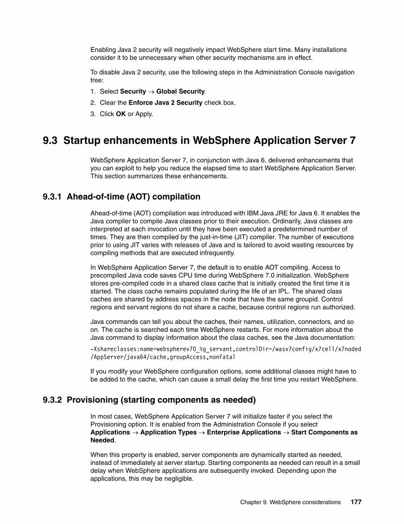
Enabling Java 2 security will negatively impact WebSphere start time. Many installations consider it to be unnecessary when other security mechanisms are in effect.

To disable Java 2 security, use the following steps in the Administration Console navigation tree:

1. Select Security Global Security.

2. Clear the Enforce Java 2 Security check box.

3. Click OK or Apply.

9.3 Startup enhancements in WebSphere Application Server 7

WebSphere Application Server 7, in conjunction with Java 6, delivered enhancements that you can exploit to help you reduce the elapsed time to start WebSphere Application Server. This section summarizes these enhancements.

9.3.1 Ahead-of-time (AOT) compilation

Ahead-of-time (AOT) compilation was introduced with IBM Java JRE for Java 6. It enables the Java compiler to compile Java classes prior to their execution. Ordinarily, Java classes are interpreted at each invocation until they have been executed a predetermined number of times. They are then compiled by the just-in-time (JIT) compiler. The number of executions prior to using JIT varies with releases of Java and is tailored to avoid wasting resources by compiling methods that are executed infrequently.

In WebSphere Application Server 7, the default is to enable AOT compiling. Access to precompiled Java code saves CPU time during WebSphere 7.0 initialization. WebSphere stores pre-compiled code in a shared class cache that is initially created the first time it is started. The class cache remains populated during the life of an IPL. The shared class caches are shared by address spaces in the node that have the same groupid. Control regions and servant regions do not share a cache, because control regions run authorized.

Java commands can tell you about the caches, their names, utilization, connectors, and so on. The cache is searched each time WebSphere restarts. For more information about the Java command to display information about the class caches, see the Java documentation:

-Xshareclasses:name=webspherev70_%g_servant,controlDir=/wasv7config/x7cell/x7noded/AppServer/java64/cache,groupAccess,nonFatal

If you modify your WebSphere configuration options, some additional classes might have to be added to the cache, which can cause a small delay the first time you restart WebSphere.

9.3.2 Provisioning (starting components as needed)

In most cases, WebSphere Application Server 7 will initialize faster if you select the Provisioning option. It is enabled from the Administration Console if you select Applications Application Types Enterprise Applications Start Components as Needed.

When this property is enabled, server components are dynamically started as needed, instead of immediately at server startup. Starting components as needed can result in a small delay when WebSphere applications are subsequently invoked. Depending upon the applications, this may be negligible.


Starting components dynamically is most effective if all the applications deployed on the server use the same components. For example, this option is more beneficial if all of the applications are Web applications that use servlets, and JavaServer Pages (JSP). This option is less effective if the applications use Enterprise JavaBeans (EJB).

9.3.3 Development Mode

The Development Mode option is available with WebSphere Version 6.0 and higher. If you enable Development Mode, it utilizes the Generic JVM properties -Xverify:none and -Xquickstart. These options, which are not recommended for production servers, are:

� The -Xverify:none property eliminates the byte code verification stage during class loading. It is reported to improve startup time by 10 - 15%. However, corrupted or invalid class data is not detected and can potentially cause unexpected behavior on the part of the Application Server.

� Using -Xquickstart can result in faster WebSphere startup time, but might cause a small overall throughput degradation, which can lessen over time. The startup improvement comes from a reduction in JIT operating overhead, achieved through two main tactical decisions. First, in quickstart mode, JIT compiler disables one of its profiling mechanisms used to guide the optimization process. Second, the JIT compiler applies a more conservative set of optimizations to methods compiled for the first time. However, the JIT compiler continuously seeks to recompile the methods it considers important at higher optimization levels, thus replacing the old code with more efficient one and gradually improving the application's throughput.

The default setting for the Development Mode option is FALSE, meaning that the server does not start in this mode. Setting this option to TRUE can decrease server startup time, however the checking that Development Mode disables is highly recommended in a production environment, so we recommend that Development Mode not be used in a production environment.

9.3.4 Disabling annotation scanning for Java EE 5 applications

You can disable annotation scanning of Java EE 5 applications during WebSphere Application Server 7 startup because the applications are scanned for annotations during installation. The default for normal startup is to examine application byte codes, which is a costly operation. This can be disabled only at the time the application is deployed.

To exploit this option, during deployment of an enterprise archive (EAR) file:

1. Do not select the Fast Path option.

2. Select the Detailed option. Proceed as normal until you reach the next-to-last step called “Metadata for Modules.”

3. Select the metadata-complete attribute check box of each EAR file for which you want to eliminate annotation scanning.

9.3.5 Parallel Start

The Parallel Start selection should not be confused with Parallel Servant Startup (described in 9.3.6, “Parallel Servant Startup” on page 179). Parallel Start applies to the initialization behavior of applications installed in the server. It controls the way that server components, services, and applications start.


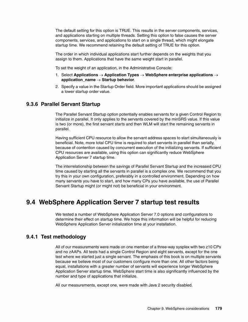
The default setting for this option is TRUE. This results in the server components, services, and applications starting on multiple threads. Setting this option to false causes the server components, services, and applications to start on a single thread, which might elongate startup time. We recommend retaining the default setting of TRUE for this option.

The order in which individual applications start further depends on the weights that you assign to them. Applications that have the same weight start in parallel.

To set the weight of an application, in the Administrative Console:

1. Select Applications Application Types WebSphere enterprise applications application_name Startup behavior.

2. Specify a value in the Startup Order field. More important applications should be assigned a lower startup order value.

9.3.6 Parallel Servant Startup

The Parallel Servant Startup option potentially enables servants for a given Control Region to initialize in parallel. It only applies to the servants covered by the minSRS value. If this value is two (or more), the first servant starts and then WLM will start the remaining servants in parallel.

Having sufficient CPU resource to allow the servant address spaces to start simultaneously is beneficial. Note, more total CPU time is required to start servants in parallel than serially, because of contention caused by concurrent execution of the initializing servants. If sufficient CPU resources are available, using this option can significantly reduce WebSphere Application Server 7 startup time.

The interrelationship between the savings of Parallel Servant Startup and the increased CPU time caused by starting all the servants in parallel is a complex one. We recommend that you try this in your own configuration, preferably in a controlled environment. Depending on how many servants you have to start, and how many CPs you have available, the use of Parallel Servant Startup might (or might not) be beneficial in your environment.

9.4 WebSphere Application Server 7 startup test results

We tested a number of WebSphere Application Server 7.0 options and configurations to determine their effect on startup time. We hope this information will be helpful for reducing WebSphere Application Server initialization time at your installation.

9.4.1 Test methodology

All of our measurements were made on one member of a three-way sysplex with two z10 CPs and no zAAPs. All tests had a single Control Region and eight servants, except for the one test where we started just a single servant. The emphasis of this book is on multiple servants because we believe most of our customers configure more than one. All other factors being equal, installations with a greater number of servants will experience longer WebSphere Application Server startup time. WebSphere start time is also significantly influenced by the number and type of applications that initialize.

All our measurements, except one, were made with Java 2 security disabled.


We used the following events in Syslog to evaluate the startup time of WebSphere Application Server 7:

� We considered initialization to begin at the time we issued the command to start the Application Server and servants.

� The end of WebSphere Application Server initialization occurs when the Control Region writes the open for e-business message. Additional processing occurs subsequent to the appearance of this message, but WebSphere is ready to start accepting transactions at the time it is written. The message that indicates that WebSphere Application Server is ready is:

BBOO0222I: WSVR0001I: Server CONTROL PROCESS t2sr00a open for e-business

We did not include the startup time of the Deployment Manager and Node Agent in our calculations. This allows our data to be more consistent with the startup results reported by the WebSphere Performance Team. The WebSphere performance tests were made with a Basic WebSphere configuration. We found that after the Deployment Manager and Node Agent were started, the elapsed time for starting the Application Server was equivalent to that of a Basic configuration.

The elapsed startup time for the ND Manager and Node Agent is reported in “Run8: Time to start the Deployment Manager and node agent” on page 187. You can simply add them to the Application Server start times to approximate the restart behavior of all WebSphere address spaces at once.

The length of time for WebSphere to initialize at your installation depend on many factors, including your hardware configuration, WebSphere Application Server applications, number of servant regions, and interactions with other subsystems and applications that might be initializing or executing at the same time WebSphere is starting.

The application running under WebSphere and that was used during this project is called DayTrader 1.2. This application is more lightweight than many enterprise applications developed by our customers. Therefore, our WebSphere startup performance may be more optimal than is observed in production environments. You can find information about the DayTrader application at:

http://cwiki.apache.org/GMOxDOC20/daytrader.html

9.4.2 WebSphere Application Server measurements results

Having identified the features and functions that we believed would have the largest effect on WebSphere Application Server startup times, we created a set of measurement runs to determine whether the actual results were in line with our expectations.

We first did a run of an untuned configuration, to set a base line for comparison. In each subsequent run we only made one change, so we could clearly see the effect of that change. Table 9-1 on page 181 shows the options that were enabled or disabled for each run.

Note: The RACF BPX.SAFFASTPATH FACILITY profile was defined before any of the measurements were started.


http://cwiki.apache.org/GMOxDOC20/daytrader.html

Table 9-1 Details of measurement runs

Run1: Turning off Java 2 securityThe first pair of measurements we ran was to determine the impact that turning off Java 2 security would have compared to an untuned startup. An initial measurement with eight servants was made with all configuration defaults and with the default WebSphere applications still installed; this established the base measurement so we could determine the impact of turning off Java 2 security. We then turned off Java 2 and took another measurement. See Figure 9-1.

Figure 9-1 Impact of turning off Java 2 security

As can be seen in Figure 9-1, turning Java 2 security off reduced CPU time and elapsed time. Both decreased by a little over 10%, with the CPU time decreasing by a little more than the elapsed time. This is good news, given that WebSphere Application Server startup tends to be CPU-constrained, so anything that reduces CPU utilization is a very positive move.

Run Provisioning Default apps

AOT Development Mode

Parallel Java 2 Security

Base No Yes Yes No No Yes

Run1 No Yes Yes No No No

Run2 No No Yes No No No

Run3 No No Yes No No No

Run4 Yes No Yes No No No

Run5 Yes No Yes Yes No No

Run6 Yes No No No No No

Run7 Yes No Yes No Yes No

Run 8 Yes No Yes No No No

Run0 Yes No Yes No No No

Impact of turning off Java 2 security

0

100

200

300

400

500

600

700

800

Elapsed Sec CPU Sec

Sec

on

ds

8 Servants No Tuning

8 Servants, No Java 2


Run2: Removing the default applicationsThe next measurement used Run1 (no Java 2 security) as the base. We uninstalled the default WebSphere applications and took another measurement. Removing the default applications meant that WebSphere Application Server had less work to do during its startup, resulting in the times shown in Figure 9-2.

Figure 9-2 Impact of removing the default WebSphere applications

This change resulted in a savings of about 21% in both elapsed and CPU time, compared to the run with the default applications still installed. This improvement is worthwhile, and was obtained without any cost or trade-off.

Run3: Importance of sufficient CPU resourceProviding adequate CPU resource is one of the most important things you can do to accelerate WebSphere Application Server startup time. So, for our next set of measurements, we reduced the number of CPs available during the WebSphere Application Server startup. The base for this set of measurements was the WebSphere Application Server that we used for Run2, that is, after we removed the default applications.

Figure 9-3 on page 183 illustrates the effect on elapsed time when we configured one of our two CPUs offline. WebSphere Application Server initialization time increased from 381 seconds to 509 seconds, an increase of just over 33%. A similar test conducted by the z/OS Performance lab showed that elapsed startup time continually improves as more CPUs are configured.

Impact of removing default apps

0

100

200

300

400

500

600

700

Elapsed Sec CPU Sec

Sec

on

ds

With Default Apps

No Default Apps


Figure 9-3 Benefit of providing more CPU resource

Interestingly, the CPU time increased by even more than the elapsed time. You might imagine that the CPU time would be about the same, given that eight servants were starting up in both cases. However, when significant contention exists for CPU resources, WLM and SRM must work harder to ensure that the CPU time is distributed according to the specifications in the WLM policy. Periodic workload monitoring occurs more often at high CPU loads and more work units are queued waiting for the CPU.

Run4: ProvisioningThe next measurement run was to determine the effect of starting all WebSphere Application Server components as part of the WebSphere Application Server initialization process, compared to starting them later as needed. The results are in Figure 9-4 on page 184.

Benefit of additional CPU

0

100

200

300

400

500

600

700

800

Elapsed Sec CPU Sec

Sec

on

ds

8 Servants 2 CPUs

8 Servants 1 CPU


Figure 9-4 Impact of starting WebSphere Application Server components during startup

An interesting outcome is how much of the WebSphere Application Server startup time can actually be postponed until later: the startup time reduced from 381 to 315 seconds, a saving of over 17%. This is good news for the startup, however you must balance this against the effect on the first application to subsequently require any of these services.

Run5: Enabling -Xquickstart optionWebSphere Application Server 6 delivered the option to start WebSphere in Development Mode. As described in 9.3.3, “Development Mode” on page 178, this mode enables two Java options: -Xquickstart and -Xverifynone. We recommend that -Xverifynone should not be used in any WebSphere Application Server region, however -Xquickstart might be acceptable in a test or development WebSphere Application Server. In return for a reduced startup time (important if you are constantly stopping and starting WebSphere Application Server, as in a test or development system), WebSphere Application Server does not do as much optimization of the runtime environment.

Figure 9-5 on page 185 shows the difference that the use of -Xquickstart can make to the startup time of WebSphere Application Server. The elapsed time for the startup of WebSphere Application Server decreased by over 12% or about 40 seconds. Even more impressive was the reduction in CPU time: a decrease of nearly 22%.

Impact of provisioning

0

100

200

300

400

500

600

Elapsed Sec CPU Sec

Sec

on

ds

Start components at start

Start components as needed


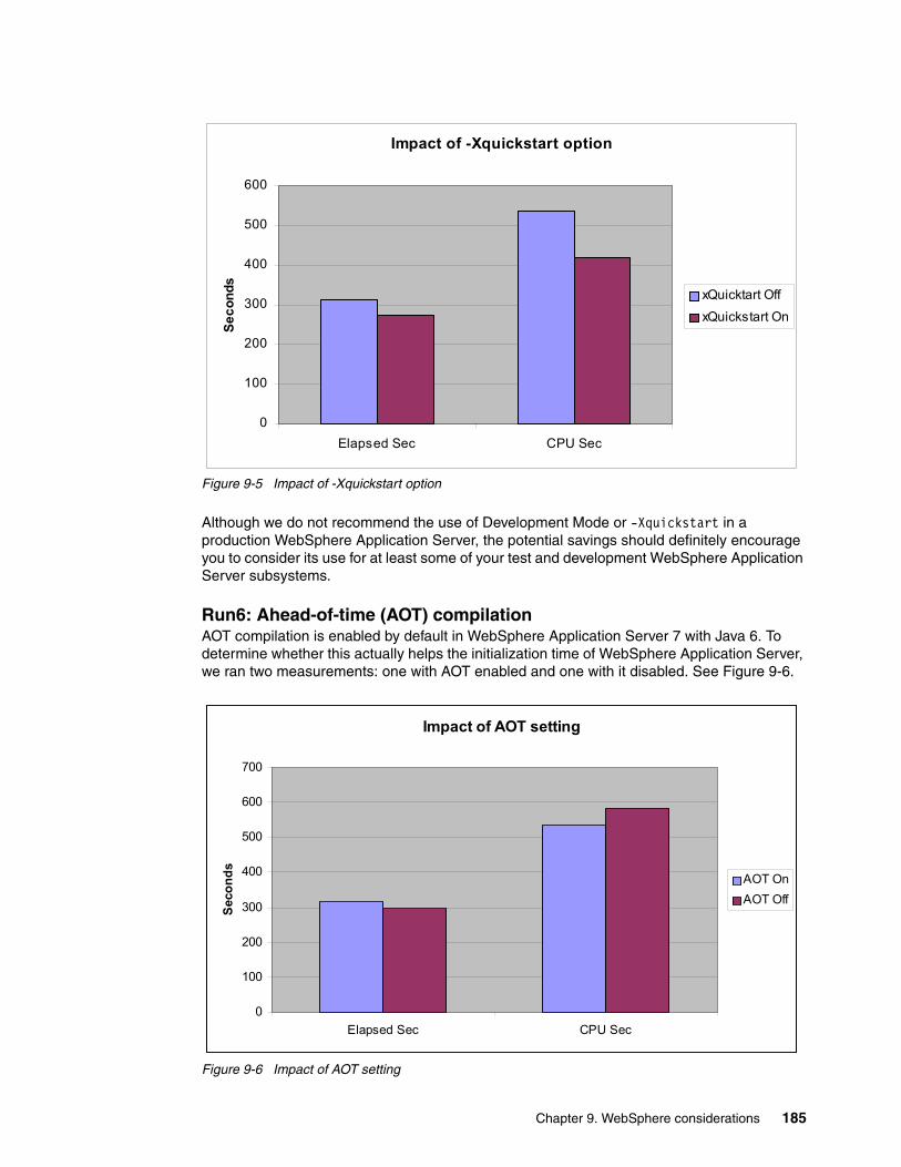
Figure 9-5 Impact of -Xquickstart option

Although we do not recommend the use of Development Mode or -Xquickstart in a production WebSphere Application Server, the potential savings should definitely encourage you to consider its use for at least some of your test and development WebSphere Application Server subsystems.

Run6: Ahead-of-time (AOT) compilationAOT compilation is enabled by default in WebSphere Application Server 7 with Java 6. To determine whether this actually helps the initialization time of WebSphere Application Server, we ran two measurements: one with AOT enabled and one with it disabled. See Figure 9-6.

Figure 9-6 Impact of AOT setting

Impact of -Xquickstart option

0

100

200

300

400

500

600

Elapsed Sec CPU Sec

Se

co

nd

s

xQuicktart Off

xQuickstart On

Impact of AOT setting

0

100

200

300

400

500

600

700

Elapsed Sec CPU Sec

Sec

on

ds

AOT On

AOT Off


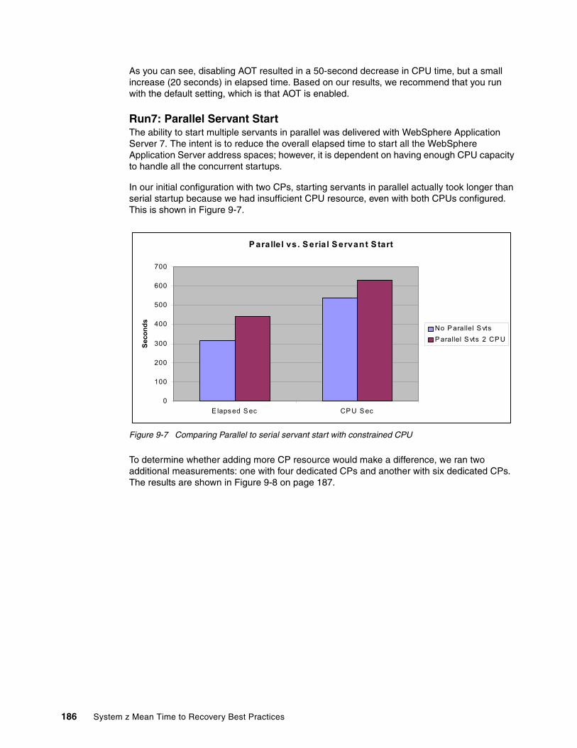
As you can see, disabling AOT resulted in a 50-second decrease in CPU time, but a small increase (20 seconds) in elapsed time. Based on our results, we recommend that you run with the default setting, which is that AOT is enabled.

Run7: Parallel Servant StartThe ability to start multiple servants in parallel was delivered with WebSphere Application Server 7. The intent is to reduce the overall elapsed time to start all the WebSphere Application Server address spaces; however, it is dependent on having enough CPU capacity to handle all the concurrent startups.

In our initial configuration with two CPs, starting servants in parallel actually took longer than serial startup because we had insufficient CPU resource, even with both CPUs configured. This is shown in Figure 9-7.

Figure 9-7 Comparing Parallel to serial servant start with constrained CPU

To determine whether adding more CP resource would make a difference, we ran two additional measurements: one with four dedicated CPs and another with six dedicated CPs. The results are shown in Figure 9-8 on page 187.

P arallel vs. Serial S ervant S tart

0

100

200

300

400

500

600

700

E lapsed S ec CP U S ec

Sec

on

ds

No P arallel S vts

P arallel S vts 2 CPU


Figure 9-8 Impact of using starting servants in parallel

As you can see, enabling Parallel Servant Startup and reducing the number of CPs to just one had a very negative effect on both elapsed and CPU times (startup time increased from 315 seconds to 840 seconds, and CPU time increased by 27%). Using Parallel Servant Startup with the same number of CPs as the base measurement also resulted in increased elapsed and CPU times, although nowhere nearly as drastic as the one CP measurement. However, when using four CPs, we can start to see the benefit of Parallel Servant Startup, with a reduction in elapsed time of over 50%. Moving to six CPs had minimal additional impact on elapsed times.

Run8: Time to start the Deployment Manager and node agentAs we mentioned previously, for our tests, we used WebSphere Application Server in Network Deployment (ND) mode, compared to the Basic mode used by the formal performance group for their tests. To understand how ND mode would affect start times, we did a separate measurement of just the start of the Deployment Manager and the node agent. The results of this measurement are shown in Figure 9-9 on page 188.

Parallel Servant Starts

0

100

200

300

400

500

600

700

800

900

Parallel Svts 1CPU

Parallel Svts 2CPU

Parallel Svts 4CPU

Parallel Svts 6CPU

Sec

on

ds

Elapsed Sec

CPU Sec


Figure 9-9 Startup times for Deployment Manager and node agent

This run was not a comparison; the objective was purely to determine how much additional time you would expect to experience if you start WebSphere Application Server in ND mode rather than Basic mode. The elapsed time we observed was just over 200 seconds, with CPU time of about 240 seconds.

Run9: Different numbers of servantsThe final configuration option that we wanted to investigate was how the number of servants affects the WebSphere Application Server startup time. For this measurement, we reduced the number of servants from eight to one. The results of this measurement are shown in Figure 9-10 on page 189.

Note: Node agent might have to be up before applications will work. If IIOP clients bootstrap into the Node agent, they will fail if it is not started. We recommend to start the node agent with the option to not verify the contents of the file system with the Deployment Manager.

Deployment Manager and node agent startup

0

50

100

150

200

250

300

Elapsed Sec CPU Sec

Se

co

nd

s

DM + node agent


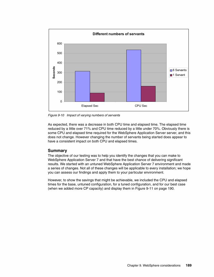
Figure 9-10 Impact of varying numbers of servants

As expected, there was a decrease in both CPU time and elapsed time. The elapsed time reduced by a little over 71% and CPU time reduced by a little under 70%. Obviously there is some CPU and elapsed time required for the WebSphere Application Server server, and this does not change. However changing the number of servants being started does appear to have a consistent impact on both CPU and elapsed times.

SummaryThe objective of our testing was to help you identify the changes that you can make to WebSphere Application Server 7 and that have the best chance of delivering significant results. We started with an untuned WebSphere Application Server 7 environment and made a series of changes. Not all of these changes will be applicable to every installation; we hope you can assess our findings and apply them to your particular environment.

However, to show the savings that might be achievable, we included the CPU and elapsed times for the base, untuned configuration, for a tuned configuration, and for our best case (when we added more CP capacity) and display them in Figure 9-11 on page 190.

Different numbers of servants

0

100

200

300

400

500

600

Elapsed Sec CPU Sec

Sec

on

ds

8 Servants

1 Servant


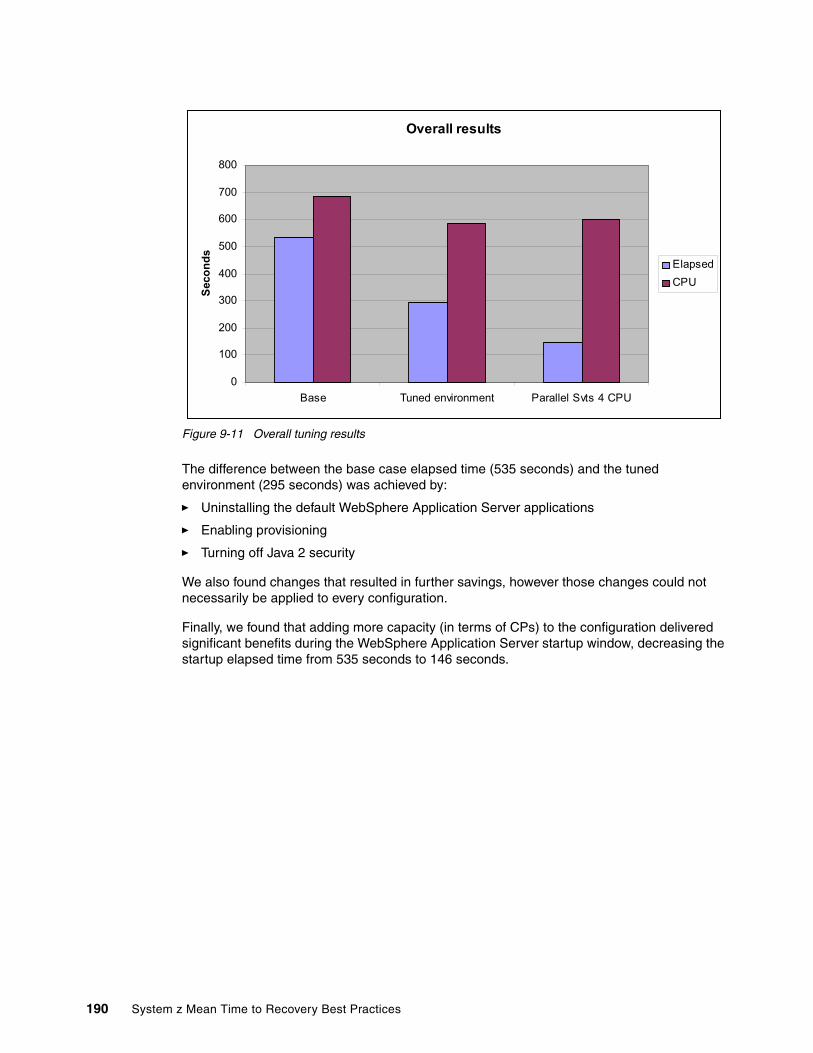
Figure 9-11 Overall tuning results

The difference between the base case elapsed time (535 seconds) and the tuned environment (295 seconds) was achieved by:

� Uninstalling the default WebSphere Application Server applications

� Enabling provisioning

� Turning off Java 2 security

We also found changes that resulted in further savings, however those changes could not necessarily be applied to every configuration.

Finally, we found that adding more capacity (in terms of CPs) to the configuration delivered significant benefits during the WebSphere Application Server startup window, decreasing the startup elapsed time from 535 seconds to 146 seconds.

Overall results

0

100

200

300

400

500

600

700

800

Base Tuned environment Parallel Svts 4 CPU

Sec

on

ds

Elapsed

CPU


Appendix A. Sample IPLSTATS report

This appendix provides a sample of the output from the IPCS command to format the IPLDATA control block.

A


IPLSTATS report

Information about the elapsed time spent in the various modules that make up the IPL process is stored in a control block that can be formatted using the IPCS VERBX BLSAIPST MAIN command. A sample of the output from this command is shown in Figure A-1, Figure A-2 on page 193, and Figure A-3 on page 194.

Figure A-1 IPLSTATS report (part 1 of 3)

**** IPL Statistics **** IEAIPL10 0.000 ISNIRIM - Read SCPINFO IEAIPL20 0.000 Test Block storage to 2G IEAIPL11 0.006 Fast FIND service IEAIPL31 0.001 LOAD service IEAIPL30 0.001 IPLWTO service IEAIPL46 0.096 Read SCHIBs into IPL workspace IEAIPL49 0.000 Process Load and Default parameters IEAIPL50 0.007 IPL parmlib - process LOADxx and NUCLST IEAIPL51 0.000 System architecture IEAIPL43 0.006 Find and Open IODF data set IEAIPL60 0.000 Read NCRs from IODF IEAIPL70 0.042 UIM environment - load CBD and IOS servicesIEAIPL71 0.029 Build DFT for each device IEAIPL08 0.001 Read EDT information from IODF IEAIPL40 0.023 Read MLTs from nucleus IEAIPL42 0.002 Read NMLs from nucleus (IEANynnn modulesIEAIPL41 0.343 Read PDS directory entries and CESD records IEAIPL05 0.000 Build and sort NUCMAP IEAIPL02 1.214 Load nucleus modules IEAIPL04 0.003 Allocate PFT and SQA/ESQA IEAIPL14 0.000 Build LSQA/ELSQA for Master IEAIPL09 0.037 IAXMI - PFT, master RAB, etc. IEAIPL07 0.006 Update AMODE for nucleus resident SVCs IEAIPL03 0.013 Build UCBs, ULUT, etc. IEAIPL18 0.017 Copy and relocate EDT to ESQA IEAIPL99 0.176 Page frame table and cleanup 2.022 TOTAL IPL TIME (seconds) NIP started at: 2009/05/14 22:43:31.730 **** NIP Statistics **** IEAVNIP0 0.008 NIP Base IEAVNIPM 0.050 Invoke NIP RIMs IEAVNPE6 0.049 Service Processor Interface IEAVNPFF 0.029 Loadwait/Restart IEAVNPA6 0.008 RTM - RTCT and recording buffer IEAVNPC6 0.008 WTO IEAVNPC3 0.007 Issue messages from IPL message queue IEAVNP24 0.020 SMS Open/Mount IEAVNP06 0.010 Machine Check IEAVNP27 0.011 Reconfiguration IEAVNPA2 3.948 IOS - Non-DASD UCBs IEAVNPCA 0.008 NIP Console IEAVNPB2 0.682 IOS - DASD UCBs IEAVNP11 0.011 Locate and Open master calalog IEAVNPC7 0.027 Open SYS1.SVCLIB



IEAVNPOP 0.046 Open PARMLIB IEAVNPIL 0.010 Process IEALSTxx IEAVNPC4 0.018 Prompt for System Parameters IEAVNP03 0.004 Merge and analyze system parameters IEAVNPCF 0.134 Process system name and system variables IEAVNP76 0.009 Open LOGREC IEAVNPE8 0.027 RSM - Process REAL= IEAVNP23 0.013 Build GRS blocks in SQA IEAVNP04 0.024 ASM - Open page and swap data sets IEAVNPA8 0.005 VSM - Expand SQA IEAVNP14 0.031 ASM part 2 - Build SQA control blocks IEAVNPGD 0.001 Move console data to ESQA IEAVNP25 0.027 Process SVC= IEAVNP05 4.726 LPA, APF IEAVNP44 0.001 ASA Reuse stuff IEAVNPB1 0.001 Process CSCBLOC= IEAVNPE2 0.002 RACF SAF IEAVNPB8 0.007 Create CSA IEAVNP47 0.002 ENF IEAVNPD6 0.001 RTM - SDUMP, ABDUMP, ESTAE IEAVNP09 0.002 Build ASVT IEAVNPD8 0.769 RSM - Frame queues, VRREGN= and RSU= IEAVNP10 0.007 SRM - OPT=, IPS=, etc. IEAVNPD1 0.009 ABDUMP IEAVNPD2 0.012 SDUMP IEAVNPCX 0.001 Context services, registration IEAVNPX1 0.001 NIP cleanup IEAVNPF5 0.025 PCAUTH IEAVNPF8 0.011 RASP IEAVNP1F 0.028 SRM - I/O measurement blocks IEAVNPC2 0.011 IOS - Move CDT to SQA IEAVNP51 0.016 TRACE IEAVNP20 0.004 Process CLOCK= IEAVNP21 0.024 TOD clock IEAVNP57 0.006 SDUMP IEAVNPF9 72.231 XCF IEAVNP33 2.790 GRS IEAVNPED 0.008 PROD IEAVNP26 1.244 SMS IEAVNPE5 2.008 LNKLST IEAVNPD5 0.274 Load pageable device support modules IEAVNP88 0.077 Allocation move EDT II IEAVNPA1 3.602 CONSOLE IEAVNPDC 0.265 WLM IEAVNP16 0.247 EXCP appendages IEAVNP13 0.018 Prepare NIP/MSI interface IEAVNP17 0.002 GTF Monitor Call interface IEAVNPG8 0.003 VSM defined monitor call enablement IEAVNP18 0.053 PARMLIB Scan Routine interface IEAVNPF2 0.047 Process IOS= IEAVNP15 0.149 Process VATLST IEAVNPRR 0.001 RRS

Appendix A. Sample IPLSTATS report 193


IEAVNPOE 0.152 USS IEAVNPSC 0.001 Metal C RTL IEAVNPLE 0.010 System LE RIM IEAVNPUN 0.012 Unicode IEAVNPXL 0.007 zXML Parser IEAVNP1B 0.045 Close catalog IEAVNIPX 0.000 NIP final cleanup 94.137 TOTAL NIP TIME (seconds) **** IEEVIPL Statistics **** IEETRACE 0.001 Master trace ISNMSI 2.019 SPI UCMPECBM 0.268 CONSOLE address space ENFPC005 0.000 CONSOLE ready ENF IEFSCHIN 0.207 IEFSCHAS address space IEFJSINT 0.002 Subsystem interface IEFSJLOD 0.018 JESCT IAZINIT 0.038 JESXCF address space IAZFSII 0.008 FSI trace IEFQBINT 0.015 SWA manager IEFAB4I0 0.118 ALLOCAS address space IEEVIPL 2.694 Uncaptured time: 0.000 MSI started at: 2009/05/14 22:45:08.870 **** IEEMB860 Statistics **** ILRTMRLG 0.277 ASM IECVIOSI 6.748 IOS dynamic pathing ATBINSYS 0.007 APPC IKJEFXSR 0.080 TSO IXGBLF00 0.016 Logger COMMNDXX 0.069 COMMANDxx processing SMFWAIT 0.163 SMF SECPROD 0.843 Security server IEFJSIN2 2.279 SSN= subsystem IEFHB4I2 0.009 ALLOCAS - UCB scan CSRINIT 0.004 Windowing services FINSHMSI 0.034 Wait for attached CMDs MSI ended at: 2009/05/14 22:45:19.500 IEEMB860 10.630 Uncaptured time: 0.100 109.482 TOTAL TIME (seconds)


IPLSTATS comparisons

As described in 3.3, “Syslog” on page 24, the MSGLG610 program can read the IPLSTATS information in syslog and save the information to an output data set. The IPLMERG4 program can then be used to compare the IPLSTATS information for two IPLs.

The MSGLG610 and IPLMERG4 programs, and information about their use, can be downloaded from:


A sample of part of the output from the IPLMERG4 program is shown in Table 9-2.

Table 9-2 Sample output from IPLMERG4 program

Appendix A. Sample IPLSTATS report 195


Appendix B. Optimizing use of LLA and VLF

This appendix provides information about tools that can help you fine tune, and monitor, your use of library lookaside (LLA) and virtual lookaside facility (VLF) for caching load modules and load library directories.

B


Module Fetch Monitor

IBM provides an unsupported tool called the Module Fetch Monitor that you can use to monitor the activity and the benefits that LLA and VLF can provide in terms of improving the efficiency of fetching load modules. The tool consists of a set of ISPF panels and an LLA exit to collect information about LLA activity. The tool, and supporting documentation, can be obtained from Peter Relson in IBM, by sending e-mail to:

[email protected]

Using the Monitor

Details about installing and using the Monitor are provided with the Monitor, so do not repeat that information here. Instead, we step through a sample invocation of the Monitor, highlighting the fields that might be of interest to you.

Figure B-1 shows the initial menu that you are presented with when you invoke the monitor ISPF application.

Figure B-1 Module Fetch Monitor Main Menu

To understand which load libraries are being heavily used, and the service time that is being experienced by requests to retrieve load modules, we select option 2. DATA_SET List from the menu. The panel shown in Figure B-2 on page 199 opens. Note that data sets must be managed by LLA (that is, they must be defined in the CSVLLAxx member) in order to be tracked by the Monitor.

Module Fetch Monitor - Main Menu Select an option: __ 1. MODULE List Date & Time : 2009.349 14:22 2. DATA_SET List Monitor started at : 2009.348 18:51 3. LLA Allocated Data_Sets Elapsed seconds : 70268 4. Filter List SMF System ID : #@$A ------------------------------------------------------------------------------COUNTERS: Number of LINK . . . .: 411195 Number of LOAD . . . .: 21444 Number of XCTL . . . .: 17 Number of ATTACH . . .: 18821 Number of ESR SVC. . .: 3 Data_set Names. . . . : 10 Module Names. . . . . : 245 Job Names . . . . . . : 15694 Data Space Used .bytes: 672776 32 % Lost Events . . . . . : 0 Active Filter. . . . .: 06


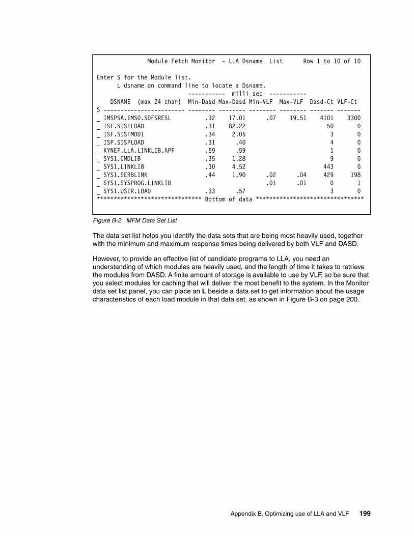
Figure B-2 MFM Data Set List

The data set list helps you identify the data sets that are being most heavily used, together with the minimum and maximum response times being delivered by both VLF and DASD.

However, to provide an effective list of candidate programs to LLA, you need an understanding of which modules are heavily used, and the length of time it takes to retrieve the modules from DASD. A finite amount of storage is available to use by VLF, so be sure that you select modules for caching that will deliver the most benefit to the system. In the Monitor data set list panel, you can place an L beside a data set to get information about the usage characteristics of each load module in that data set, as shown in Figure B-3 on page 200.

Module Fetch Monitor - LLA Dsname List Row 1 to 10 of 10 Enter S for the Module list. L dsname on command line to locate a Dsname. ----------- milli_sec ----------- DSNAME (max 24 char) Min-Dasd Max-Dasd Min-VLF Max-VLF Dasd-Ct VLF-Ct S ------------------------ -------- -------- -------- -------- ------- ------- _ IMSPSA.IMS0.SDFSRESL .32 17.01 .07 19.51 4101 3300 _ ISF.SISFLOAD .31 82.22 50 0 _ ISF.SISFMOD1 .34 2.05 3 0 _ ISP.SISPLOAD .31 .40 4 0 _ KYNEF.LLA.LINKLIB.APF .59 .59 1 0 _ SYS1.CMDLIB .35 1.28 9 0 _ SYS1.LINKLIB .30 4.52 443 0 _ SYS1.SERBLINK .44 1.90 .02 .04 429 198 _ SYS1.SYSPROG.LINKLIB .01 .01 0 1 _ SYS1.USER.LOAD .33 .57 3 0 ******************************* Bottom of data ********************************

Appendix B. Optimizing use of LLA and VLF 199

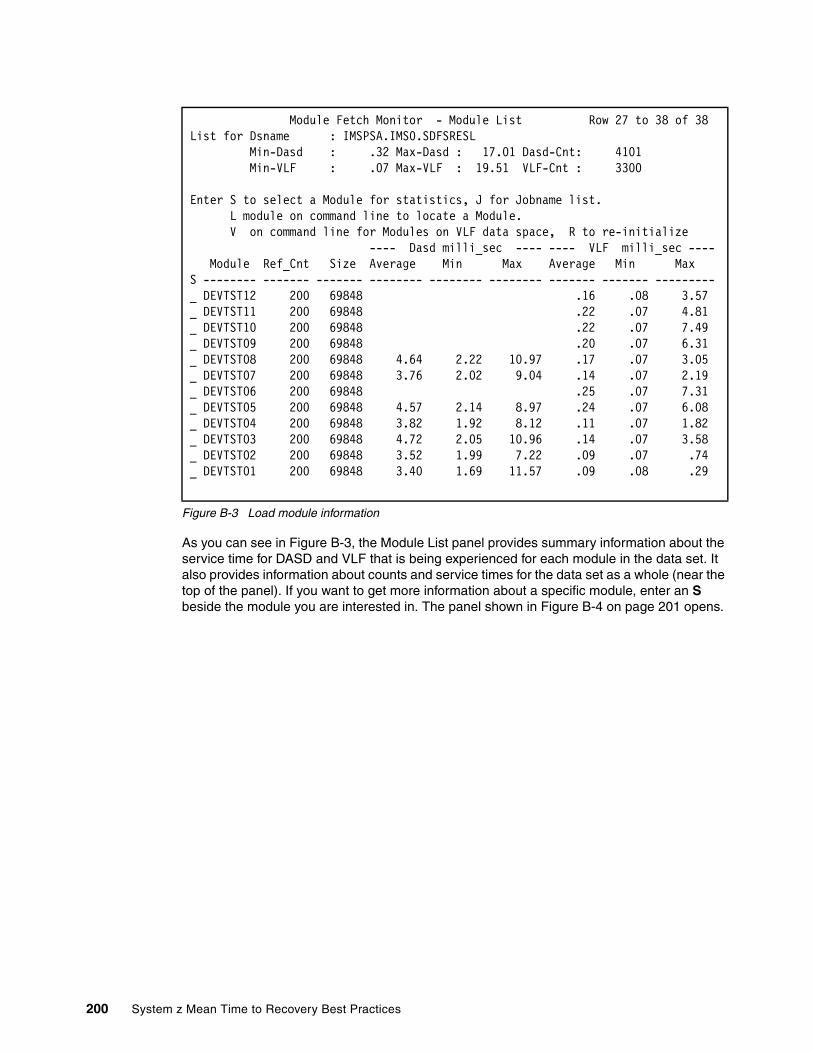
Figure B-3 Load module information

As you can see in Figure B-3, the Module List panel provides summary information about the service time for DASD and VLF that is being experienced for each module in the data set. It also provides information about counts and service times for the data set as a whole (near the top of the panel). If you want to get more information about a specific module, enter an S beside the module you are interested in. The panel shown in Figure B-4 on page 201 opens.

Module Fetch Monitor - Module List Row 27 to 38 of 38 List for Dsname : IMSPSA.IMS0.SDFSRESL Min-Dasd : .32 Max-Dasd : 17.01 Dasd-Cnt: 4101 Min-VLF : .07 Max-VLF : 19.51 VLF-Cnt : 3300 Enter S to select a Module for statistics, J for Jobname list. L module on command line to locate a Module. V on command line for Modules on VLF data space, R to re-initialize ---- Dasd milli_sec ---- ---- VLF milli_sec ---- Module Ref_Cnt Size Average Min Max Average Min Max S -------- ------- ------- -------- -------- -------- ------- ------- ---------_ DEVTST12 200 69848 .16 .08 3.57 _ DEVTST11 200 69848 .22 .07 4.81 _ DEVTST10 200 69848 .22 .07 7.49 _ DEVTST09 200 69848 .20 .07 6.31 _ DEVTST08 200 69848 4.64 2.22 10.97 .17 .07 3.05 _ DEVTST07 200 69848 3.76 2.02 9.04 .14 .07 2.19 _ DEVTST06 200 69848 .25 .07 7.31 _ DEVTST05 200 69848 4.57 2.14 8.97 .24 .07 6.08 _ DEVTST04 200 69848 3.82 1.92 8.12 .11 .07 1.82 _ DEVTST03 200 69848 4.72 2.05 10.96 .14 .07 3.58 _ DEVTST02 200 69848 3.52 1.99 7.22 .09 .07 .74 _ DEVTST01 200 69848 3.40 1.69 11.57 .09 .08 .29


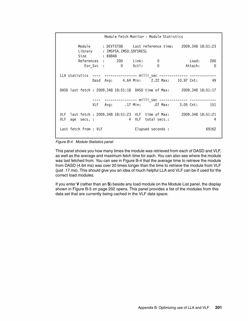
Figure B-4 Module Statistics panel

This panel shows you how many times the module was retrieved from each of DASD and VLF, as well as the average and maximum fetch time for each. You can also see where the module was last fetched from. You can see in Figure B-4 that the average time to retrieve the module from DASD (4.64 ms) was over 20 times longer than the time to retrieve the module from VLF (just .17 ms). This should give you an idea of much helpful LLA and VLF can be if used for the correct load modules.

If you enter V (rather than an S) beside any load module on the Module List panel, the display shown in Figure B-5 on page 202 opens. This panel provides a list of the modules from this data set that are currently being cached in the VLF data space.

Module Fetch Monitor - Module Statistics Module : DEVTST08 Last reference time: 2009.348 18:51:23 Library : IMSPSA.IMS0.SDFSRESL Size : 69848 References : 200 Link: 0 Load: 200 Esr_Svc : 0 Xctl: 0 Attach: 0 LLA statistics ---- ---------------- milli_sec -------------- ------------- Dasd Avg: 4.64 Min: 2.22 Max: 10.97 Cnt: 49 DASD last fetch : 2009.348 18:51:18 DASD time of Max: 2009.348 18:51:17 ---- ---------------- milli_sec -------------- ------------- VLF Avg: .17 Min: .07 Max: 3.05 Cnt: 151 VLF last fetch : 2009.348 18:51:23 VLF time of Max: 2009.348 18:51:21 VLF age secs. : 4 VLF total secs.: 4 Last fetch from : VLF Elapsed seconds : 69162


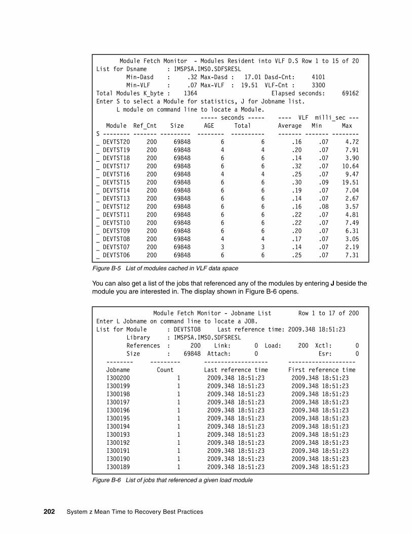
Figure B-5 List of modules cached in VLF data space

You can also get a list of the jobs that referenced any of the modules by entering J beside the module you are interested in. The display shown in Figure B-6 opens.

Figure B-6 List of jobs that referenced a given load module

Module Fetch Monitor - Modules Resident into VLF D.S Row 1 to 15 of 20List for Dsname : IMSPSA.IMS0.SDFSRESL Min-Dasd : .32 Max-Dasd : 17.01 Dasd-Cnt: 4101 Min-VLF : .07 Max-VLF : 19.51 VLF-Cnt : 3300 Total Modules K_byte : 1364 Elapsed seconds: 69162Enter S to select a Module for statistics, J for Jobname list. L module on command line to locate a Module. ----- seconds ----- ---- VLF milli_sec --- Module Ref_Cnt Size AGE Total Average Min Max S -------- ------- --------- -------- ---------- ------- ------- --------_ DEVTST20 200 69848 6 6 .16 .07 4.72_ DEVTST19 200 69848 4 4 .20 .07 7.91_ DEVTST18 200 69848 6 6 .14 .07 3.90_ DEVTST17 200 69848 6 6 .32 .07 10.64_ DEVTST16 200 69848 4 4 .25 .07 9.47_ DEVTST15 200 69848 6 6 .30 .09 19.51_ DEVTST14 200 69848 6 6 .19 .07 7.04_ DEVTST13 200 69848 6 6 .14 .07 2.67_ DEVTST12 200 69848 6 6 .16 .08 3.57_ DEVTST11 200 69848 6 6 .22 .07 4.81_ DEVTST10 200 69848 6 6 .22 .07 7.49_ DEVTST09 200 69848 6 6 .20 .07 6.31_ DEVTST08 200 69848 4 4 .17 .07 3.05_ DEVTST07 200 69848 3 3 .14 .07 2.19_ DEVTST06 200 69848 6 6 .25 .07 7.31

Module Fetch Monitor - Jobname List Row 1 to 17 of 200Enter L Jobname on command line to locate a JOB. List for Module : DEVTST08 Last reference time: 2009.348 18:51:23 Library : IMSPSA.IMS0.SDFSRESL References : 200 Link: 0 Load: 200 Xctl: 0 Size : 69848 Attach: 0 Esr: 0 -------- --------- ------------------- -------------------- Jobname Count Last reference time First reference time I300200 1 2009.348 18:51:23 2009.348 18:51:23 I300199 1 2009.348 18:51:23 2009.348 18:51:23 I300198 1 2009.348 18:51:23 2009.348 18:51:23 I300197 1 2009.348 18:51:23 2009.348 18:51:23 I300196 1 2009.348 18:51:23 2009.348 18:51:23 I300195 1 2009.348 18:51:23 2009.348 18:51:23 I300194 1 2009.348 18:51:23 2009.348 18:51:23 I300193 1 2009.348 18:51:23 2009.348 18:51:23 I300192 1 2009.348 18:51:23 2009.348 18:51:23 I300191 1 2009.348 18:51:23 2009.348 18:51:23 I300190 1 2009.348 18:51:23 2009.348 18:51:23 I300189 1 2009.348 18:51:23 2009.348 18:51:23


In the list shown in Figure B-6 on page 202, the Count of 1 for each job might not seem very impressive. However, 200 jobs referenced this module, so if the module was cached in VLF, every one of those jobs would have benefitted from that.

And, that brings us back to the LLA exit we mentioned previously, where you can provide LLA with a list of modules that you want it to cache in VLF. In Figure B-7 we have activated an exit that specifies that all the DEVTST modules and selected DFS modules should be cached in VLF. After activating the exit and resetting the counters, you can see that all the DEVTST modules in this data set are being retrieved from VLF (note the blank fields in the DASD columns.

Figure B-7 Module activity after activation of LLA exit.

The exit that we used to achieve this is CSVLLIX2, which is described in “Sample CSVLLIX2 exit routine” on page 204.

Module Fetch Monitor - Module List Row 27 to 38 of 38 List for Dsname : IMSPSA.IMS0.SDFSRESL Min-Dasd : .49 Max-Dasd : .49 Dasd-Cnt: 1 Min-VLF : .00 Max-VLF : 32.35 VLF-Cnt : 7400 Enter S to select a Module for statistics, J for Jobname list. L module on command line to locate a Module. V on command line for Modules on VLF data space, R to re-initialize ---- Dasd milli_sec ---- ---- VLF milli_sec ---- Module Ref_Cnt Size Average Min Max Average Min Max S -------- ------- ------- -------- -------- -------- ------- ------- ---------_ DEVTST12 200 69848 .46 .08 19.27 _ DEVTST11 200 69848 .65 .08 21.22 _ DEVTST10 200 69848 .80 .07 16.16 _ DEVTST09 200 69848 .59 .07 22.24 _ DEVTST08 200 69848 .64 .07 21.46 _ DEVTST07 200 69848 .60 .08 16.23 _ DEVTST06 200 69848 .33 .07 13.49 _ DEVTST05 200 69848 .25 .07 17.11 _ DEVTST04 200 69848 .24 .07 19.16 _ DEVTST03 200 69848 .17 .08 4.54 _ DEVTST02 200 69848 .11 .07 .77 _ DEVTST01 200 69848 .11 .08 .67


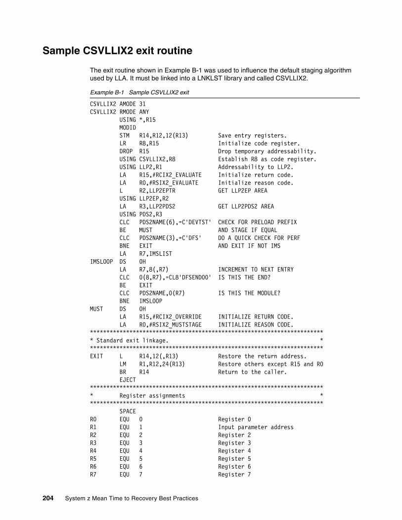
Sample CSVLLIX2 exit routine

The exit routine shown in Example B-1 was used to influence the default staging algorithm used by LLA. It must be linked into a LNKLST library and called CSVLLIX2.

Example B-1 Sample CSVLLIX2 exit

CSVLLIX2 AMODE 31 CSVLLIX2 RMODE ANY USING *,R15 MODID STM R14,R12,12(R13) Save entry registers. LR R8,R15 Initialize code register. DROP R15 Drop temporary addressability. USING CSVLLIX2,R8 Establish R8 as code register. USING LLP2,R1 Addressability to LLP2. LA R15,#RCIX2_EVALUATE Initialize return code. LA R0,#RSIX2_EVALUATE Initialize reason code. L R2,LLP2EPTR GET LLP2EP AREA USING LLP2EP,R2 LA R3,LLP2PDS2 GET LLP2PDS2 AREA USING PDS2,R3 CLC PDS2NAME(6),=C'DEVTST' CHECK FOR PRELOAD PREFIX BE MUST AND STAGE IF EQUAL CLC PDS2NAME(3),=C'DFS' DO A QUICK CHECK FOR PERF BNE EXIT AND EXIT IF NOT IMS LA R7,IMSLIST IMSLOOP DS 0H LA R7,8(,R7) INCREMENT TO NEXT ENTRY CLC 0(8,R7),=CL8'DFSEND00' IS THIS THE END? BE EXIT CLC PDS2NAME,0(R7) IS THIS THE MODULE? BNE IMSLOOP MUST DS 0H LA R15,#RCIX2_OVERRIDE INITIALIZE RETURN CODE. LA R0,#RSIX2_MUSTSTAGE INITIALIZE REASON CODE. ************************************************************************ Standard exit linkage. ************************************************************************EXIT L R14,12(,R13) Restore the return address. LM R1,R12,24(R13) Restore others except R15 and R0 BR R14 Return to the caller. EJECT ************************************************************************ Register assignments ************************************************************************ SPACE R0 EQU 0 Register 0 R1 EQU 1 Input parameter address R2 EQU 2 Register 2 R3 EQU 3 Register 3 R4 EQU 4 Register 4 R5 EQU 5 Register 5 R6 EQU 6 Register 6 R7 EQU 7 Register 7


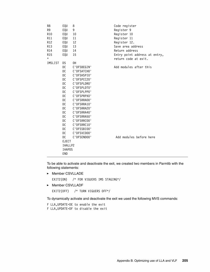
R8 EQU 8 Code register R9 EQU 9 Register 9 R10 EQU 10 Register 10 R11 EQU 11 Register 11 R12 EQU 12 Register 12. R13 EQU 13 Save area address R14 EQU 14 Return address R15 EQU 15 Entry point address at entry,* return code at exit. IMSLIST DS 0H DC C'DFSBEGIN' Add modules after this DC C'DFSATCH0' DC C'DFSHSPI0' DC C'DFSPCC20' DC C'DFSPLDR0' DC C'DFSPLDT0' DC C'DFSPLPP0' DC C'DFSPRPX0' DC C'DFSRRA00' DC C'DFSRRA10' DC C'DFSRRA20' DC C'DFSRRA40' DC C'DFSRRA50' DC C'DFSRRC00' DC C'DFSRRC10' DC C'DFSSBI00' DC C'DFSVC000' DC C'DFSEND00' Add modules before here EJECT IHALLP2 IHAPDS END

To be able to activate and deactivate the exit, we created two members in Parmlib with the following statements:

� Member CSVLLADE

EXIT2(ON) /* FOR VIGUERS IMS STAGING*/

� Member CSVLLADF

EXIT2(OFF) /* TURN VIGUERS OFF*/

To dynamically activate and deactivate the exit we used the following MVS commands:

F LLA,UPDATE=DE to enable the exitF LLA,UPDATE=DF to disable the exit


Appendix C. Sample IPL statistics data

This appendix provides information about the average elapsed times for the IPL modules that are reported by the IPLSTATS program across a sample of customer and IBM systems. This information can be used to identify parts of your IPL process that might be good candidates for tuning. These elapsed times represent a mix of large and small systems, from z800 up to z10, so you should make some allowance based on the size and utilization of your system. A very large system, or one running on older technology, or one running at very high utilizations, or using shared CPs on a CPC that is very busy would reasonably be expected to display elapsed times somewhat larger than these averages.

C


Sample IPLSTATS average elapsed times

The following tables contain the median elapsed times (across 150 representative systems) for the named modules or processes that are reported by the IPLSTATS tool.

IPL RIM Median elapsed times are shown in Table C-1.

Table C-1 IPLSTATS: IPL RIM Median elapsed times

Activity Median elapsed time (in seconds)

Load nucleus modules 2.146

Build UCBs, ULUT, and so on 0.011

Allocate PFT and SQA/ESQA 0.007

Build and sort NUCMAP 0.244

IARMI - RSM blocks, master SGT 0.000

Update AMODE for nucleus resident SVCs 0.020

Read EDT information from IODF 0.001

IAXMI - PFT, master RAB, and so on 0.041

ISNIRIM - Read SCPINFO 0.000

Fast FIND service 0.016

Build LSQA/ELSQA for Master 0.000

Copy and relocate EDT to ESQA 0.064

Test Block storage to 2G 0.180

IPLWTO service 0.001

LOAD service 0.010

Read MLTs from nucleus 0.054

Read PDS directory entries and CESD records 0.722

Read NMLs from nucleus (IEANynnn modules) 0.013

Find and Open IODF data set 0.039

Read SCHIBs into IPL workspace 0.132

Process Load and Default parameters 0.000

IPL parmlib - process LOADxx and NUCLSTxx 0.648

System architecture 0.002

Read NCRs from IODF 0.001

UIM environment - load CBD and IOS services 0.117

Build DFT for each device 0.046

Page frame table and cleanup 0.275


NIP RIM Median elapsed times are shown in Table C-2.

Table C-2 IPLSTATS: NIP RIM Median elapsed times


NIP Base 0.031

Invoke NIP RIMs 0.084

Service Processor Interface 0.051

Loadwait/Restart 0.035

RTM - RTCT and recording buffer 0.011

WTO 0.012

Issue messages from IPL message queue 0.011

SMS Open/Mount 0.029

Machine Check 0.013

Reconfiguration 0.016

IOS - Non-DASD UCBs 23.160

NIP Console 0.014

IOS - DASD UCBs 1.786

Locate and Open master catalog 0.070

Open SYS1.SVCLIB 0.044

Open PARMLIB 0.112

Process IEALSTxx 0.028

Prompt for System Parameters 0.046

Merge and analyze system parameters 0.027

Process system name and system variables 0.473

Open LOGREC 0.053

RSM - Process REAL= 0.029

Build GRS blocks in SQA 0.036

ASM - Open page and swap data sets 0.074

VSM - Expand SQA 0.010

ASM part 2 - Build SQA control blocks 0.168

Move console data to ESQA 0.002

Process SVC= 0.015

LPA, APF 12.909

ASA Reuse stuff 0.002

Process CSCBLOC= 0.002

RACF SAF 0.004

Appendix C. Sample IPL statistics data 209

Create CSA 0.020

ENF 0.003

RTM - SDUMP, ABDUMP, ESTAE 0.002

Build ASVT 0.002

RSM - Frame queues, VRREGN= and RSU= 1.727

SRM - OPT=, IPS=, and so on 0.030

ABDUMP 0.019

SDUMP 0.033

Context services, registration services 0.002

NIP cleanup 0.002

PCAUTH 0.044

RASP 0.036

SRM - I/O measurement blocks 0.037

IOS - Move CDT to SQA 0.014

TRACE 0.032

Process CLOCK= 0.035

TOD clock 9.851

SDUMP 0.011

XCF 9.887

GRS 0.279

License Manager 0.008

PROD 0.034

SMS 2.134

LNKLST 2.491

Load pageable device support modules 0.310

Allocation move EDT II 0.093

CONSOLE 2.183

WLM 0.331

EXCP appendages 1.057

Prepare NIP/MSI interface 0.041

GTF Monitor Call interface 0.003

VSM defined monitor call enablement 0.006

PARMLIB Scan Routine interface 0.068

Process IOS= 0.059



MSI Phase 1 Median elapsed times are shown in Table C-3.

Table C-3 IPLSTATS: MSI Phase 1 Median elapsed times

Process VATLST 0.231

RRS 0.002

UNIX System Services 0.377

Metal C RTL 0.003

System LE RIM 0.067

Unicode 0.060

zXML Parser 0.011

Close catalog 0.127

NIP final cleanup 0.000


CONSOLE ready ENF 0.000

FSI trace 0.004

JESXCF address space 0.032

Master trace 0.002

ALLOCAS address space 0.087

Subsystem interface 0.003

SWA manager 0.009

IEFSCHAS address space 0.057

JESCT 0.027

SPI 0.606

CONSOLE address space 0.277


Appendix C. Sample IPL statistics data 211

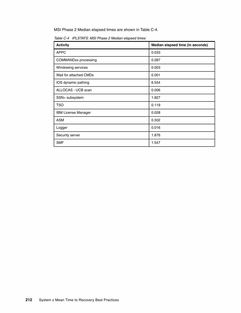
MSI Phase 2 Median elapsed times are shown in Table C-4.

Table C-4 IPLSTATS: MSI Phase 2 Median elapsed times


APPC 0.033

COMMANDxx processing 0.087

Windowing services 0.003

Wait for attached CMDs 0.001

IOS dynamic pathing 6.554

ALLOCAS - UCB scan 0.006

SSN= subsystem 1.827

TSO 0.119

IBM License Manager 0.028

ASM 0.502

Logger 0.016

Security server 1.876

SMF 1.547


Related publications

The publications listed in this section are considered particularly suitable for a more detailed discussion of the topics covered in this book.

IBM Redbooks

For information about ordering these publications, see “How to get Redbooks” on page 214. Note that some of the documents referenced here may be available in softcopy only.

� ABCs of z/OS System Programming Volume 2, SG24-6982

� Enhanced Catalog Sharing and Management, SG24-5594

� IBM IMS Version 10 Implementation Guide: A Technical Overview, SG24-7526

� Introduction to the New Mainframe: z/OS Basics, SG24-6366

� JES2 Performance and Availability Considerations, REDP-3940

� OS/390 Workload Manager Implementation and Exploitation, SG24-5326

� System Programmer’s Guide to: Workload Manager, SG24-6472

� z/OS Planned Outage Avoidance Checklist, SG24-7328

� z/OS Version 1 Release 10 Implementation, SG24-7605

Other publications

These publications are also relevant as further information sources:

� CICS Transaction Server for z/OS V3R2 Performance Guide, SC34-6833

� DB2 Administration Guide, SC18-7840

� z/OS MVS Diagnosis Tools and Service Aids, GA22-7589

� z/OS MVS Initialization and Tuning Reference, SA22-7592

� z/OS MVS System Management Facilitiies, SA22-7630


Online resources

These Web sites are also relevant as further information sources:

� z/OS Tools and Toys

http://www.ibm.com/servers/eserver/zseries/zos/unix/tools/

� IBM Flash Document FLASH100008


� z/OS MVS System Initialization Logic - Initial Program Load (IPL) presentation


� The WLM home page contains several presentations and documents:


� WSC Flash10143


� WebSphere Application Server workload balancing options in:


How to get Redbooks

You can search for, view, or download Redbooks, Redpapers, Technotes, draft publications and Additional materials, as well as order hardcopy Redbooks publications, at this Web site:

ibm.com/redbooks

Help from IBM

IBM Support and downloads

ibm.com/support

IBM Global Services

ibm.com/services




http://www.ibm.com/support/

http://www.ibm.com/support/

http://www.ibm.com/services/

http://www.ibm.com/services/

http://www.ibm.com/servers/eserver/zseries/zos/unix/tools/







Index

Symbols*MASTER* address space 43/etc/rc, role in OMVS initialization duration 88$DPERFDATA command 32

Aahead-of-time (AOT) compilation 177, 185analyzing CICS-related SMF data 108annotation scanning 178application availability 3ARMRST IMS parameter 159AUTO IMS parameter 159autoinstall shutdown failure 127AutoIPL 12Automatic Restart Manager

and IMS 159considerations for DB2 139

automationconsiderations 10design 10IEFSSN definition 80products 72relationship of importance and startup sequence 10sequence in which subsystems are started 10triggering the startup of address spaces 10triggers 11

AUTOMOUNT to accelerate OMVS startup 87avoiding WTORs during IPL 41

Bbaseline measurements 8BPX.SAFFASTPATH RACF profile 176BPXMCDS Couple Data Set 85BPXMCDS size

impact on mount times 86BPXPRMxx parmlib member 87

CCFRM Message-based processing 169CICS

Automatic Restart Manager considerations 110configuration for our tests 108considerations for WLM 77correct data set definitions 110defining terminals 110DFHVTAM group 110High Availability setup 107LLACOPY option 111LSR pool definitions 111Performance Analyzer 108placing modules in LPA 122release used in this document 5

© Copyright IBM Corp. 2010. All rights reserved.

service class definitions in WLM 77shutdown assist transaction 126startup options 109startup time, definition of 108use of autoinstall 112use of LPA 124WLM considerations 74, 77WLM recommendations 77

CICSPlex SMrecommendations 126WLM goals 77

CLPA 52potential savings 52

commands, useful 18COMMNDxx member 36, 70comparing elapsed times for two IPLs 25concatenation rules 42concurrent IPLs 13configuration used for our measurements 4considerations for doing orderly shutdowns 14console commands 18CPLOG IMS parameter 160CSVLLAxx member 112CSVLLIX2

exit 203using to control loading of IMS load modules 166

DDASD offloading 118data sharing

relationship to MTTR 3role in planned outages 3

DB2ACCESS DATABASE command 143address spaces and WLM 75Backward Log Recovery phase 135checkpoint

triggers 130Checkpoint Interval 150Conditional Restart 137Consistent Restart 138, 148Current Status Rebuild phase 133DDF

WLM considerations 75Fast Log Apply function 149Forward Log Recovery phase 134Group Restart 137Log Initialization phase 132log records 131log records in data sharing environment 134Normal Shutdown 139opening data sets at DB2 startup 142options for opening data sets 143PCLOSEN parameter 149

215

PCLOSET parameter 149processing in-abort URs 135processing inflight URs 135release used in this document 5Restart Light 138restart phases 132restart processing 130restart types 137Shutdown types 139System Checkpoint 130two-phase commit processing 132Unit of Recovery 131WLM considerations 75WLM recommendations 76

DB2-managed stored procedures, and WLM 76DBET 133DBRC Parallel Recon Access 168DCOLLECT, using to eliminate collection of SMF Type 19 records 92DDCONS 93deadly embrace during IPL 14definition 9Deployment Manager 180, 187Development Mode in WebSphere Application Server 178DFH$MOLS program 108disk subsystem cache 40duplicate volser messages 11dynamic changes as a way to avoid outages 10dynamic LPA 54dynamically activating LLA exits 205

EEMPTYEXCPSEC parameter for SMF 93Enhanced Catalog Sharing

impact on DB2 147

FFast DataBase Recovery (FDBR) 162FDRMBR IMS parameter 160FMTO IMS parameter 160FPOPN IMS parameter 160

GGETMAIN changes in z/OS R10 144

Hhardened log data 118hardware IPL 37–38hardware used for measurements 5

IIEACMD00 member 36IEAIPL02 39IEAIPL20 40IEAIPL41 39IEASYMxx member 50–51

IEAVNP05 48, 53IEAVNPA2 45IEAVNPB2 45IEAVNPCF 48, 51IEEMB860 67IEEVIPL 66IEFSSNxx member 69, 72, 80–81IFAHONORPRIORITY 173improving load module fetch performance 198IMS

abnormal shutdown 159address spaces

WLM recommendations 78common service layer 161configuration 157considerations for opening databases 167description of test configuration 157dump considerations 160key messages during IMS shutdown 156key messages during IMS startup 156Parallel Recon Access 168RECON data sets 168release used in this document 5Resource Manager 161Shared Message Queue 160, 162Shared Message Queues checkpoint considerations 169shutdown elapsed time 170shutdown phases 159sources of metrics data 156startup parameters 159startup phases 158tips for starting dependent regions 166use of resident DBDs and PSBs 164warm start 159WLM considerations 74, 77

in-commit 132indoubt 132inflight 132Initial Message Suppression Indicator (IMSI) 41investigating startup times 15IODF

data set 38hardware token 42parameter in LOAD member 42

IPCSviewing IPLSTATS 20

IPLduration, definition 8elapsed time reduction project 37frequency 9hardware IPL 38overview 36phases 36process

helpful documentation 36process elapsed times 20Resource Initialization Modules 37–38sources of information 36start sequence for system address spaces 28


steps in the IPL process 35time, definition 8

IPLDATA control block 20IPLing multiple systems concurrently 13IPLMERG4 program 25IPLMERG4 sample report 25IPLSTATS 8, 15, 20

example output 21NIP parts 43RIM parts 38

IPLSTATS data 6IPLSTATS program 20, 37IPLSTATS report 24IRLM

for IMS 162issuing commands from started task 18ITSO configuration 5IXCL1DSU utility 59

JJava 2 security 177, 181Java Just-In-Time (JIT) compiler 172JES2

$DPERFDATA command 32checkpoint and concurrent IPLs 13checkpoint location 81checkpoint performance considerations 81commands 32considerations for IPLing systems concurrently 13displaying interesting statistics 32displaying reasons for shutdown delays 32initialization 81MASDEF parameters 85parms 82parms, impact on startup time 82place in z/OS IPL process 36proclibs 82shutdown considerations 84shutdown tips 85shutting down in a timely manner 84

Llibrary search order 54link pack area (LPA)

use by CICS 122LLA

considerations for IMS 166CSVLLIX2 exit 166exits 205

LLACOPY, use by CICS 112LNKLST initialization 63LOAD CLEAR 38LOAD NORMAL 38Load parm

role in IPL 38LOAD process on the HMC 38LOADxx member 41LPALSTxx Member 54LRSN 134

Mmaking dynamic changes 9Master catalog 49Master Scheduler Initialization 37Module Fetch Monitor tool 198MSGLG610

program 24sample JCL 24

MTTRbest practices 11definition 3enhancements 40scope 2setting the baseline for measurements 8

MVS LLA 112

NNucleus Initialization Program (NIP) 37, 43nucleus modules

loading during IPL 40

Oobjective of this book 2OMPROC 161, 163OMVS

considerations 85initialization

issuing commands during 88initialization duration

importance of an orderly shutdown 88initialization time 85initialization times 87shutdown 88startup 72WLM considerations 74

open for e-business status 172operator prompts 11, 45Operlog 24OPS_DEF service class 80OPS_HI service class 80OPS_SRV service class 80optimal block sizes 54our configuration 4

PParallel Servant Start 186Parallel Servant Startup 179Parallel Start 178Parmlib

concatenation 41, 43search order 42

phases in IMS startup 158planned outage avoidance 9planned outages 3PMTO IMS parameter 161PROGxx members 54PST IMS parameter 160, 166

Index 217

Rrecording system status 18Redbooks Web site 214

Contact us xiiRMF

Enqueue Activity Report 27in relation to understanding IPL processing 26LPAR report 15Monitor II 27using to analyze CICS performance 108

rolling IPLs 13RRS parameter

considerations for IMS 163

SSCIPROC 161, 163servant regions 172SHAREDQ IMS parameter 160shutdown failure 127shutdown time 9SMF 91

initialization 69records that provide insight into IPL process 30suppressing empty EXCP sections 93Type 0 records 30Type 10 records 30Type 114 record 8Type 19 records 30, 91Type 22 records 30Type 30 records 30, 93Type 43 records 30Type 45 records 30Type 79 records, creating from RMF 27Type 8 records 30Type 80 and Type 92 records 176Type 90 records 31Types 70 to 79 records 30

SMFWAIT time from IPLSTATS report 92SMS initialization 80–81SMS subsystem

position in IEFSSN member 72software levels used for our measurements 5sources of additional information 36speeding up the re-IPL process 12standalone dump

using AutoIPL 12stand-alone dump recommendations 99starting IMS related address spaces 162starting JES2 81status

open for e-business 172stopping JES2 84storage types 118SUB=MSTR limitations 90SUB=MSTR use 90subsystems

SMF Type 30 records 93support for WLM transaction goals 75

Symbolic Parmlib Parser 12

SYS0.IPLPARM, use in IPL process 43SYSCHKPT IMS parameter 162syslog 15, 24sysplex

Couple Data Set size 59file sharing

impact on OMVS initialization times 88SYSSTC

address spaces assigned to this service class 79service class 74

system address spaces 43System Automation for z/OS 8System Logger enhancements 97SYSTEM service class 73

Ttarget audience 6TCP startup 72, 89TCP/IP, place in z/OS IPL process 36Techdocs Web site 73Tools and Toys Web site 23

Uunderstanding LLA and VLF usage 198UNIX file system considerations for WebSphere Applica-tion Server 176UNIX System Services

file systems mounted at IPL time 87Mount times 86sysplex file sharing 88version root 88

VVACBOPN IMS parameter 161viewing IPLSTATS with IPCS 20virtual lookaside facility 112virtual storage constraint relief 2VTAM

and CICS 125considerations for IMS 161place in z/OS IPL process 36startup 72startup times 89

VTAMLSTimpact on VTAM and TCP startup times 89

WWebSphere Application Server 172

Ahead of Time compilation 185Ahead of Time Compile 177annotation scanning 178Base Server configuration 172BPXAS address spaces 172class cache 175configuration used for testing 179default applications 175, 182Deployment Manager 180Development Mode 178


DNS considerations 175error messages 174Global Security 176IFAHONORPRIORITY 173impact of lack of CPU 182initialization complete message 173Java 2 security 176, 181log stream 174Network Deployment configuration 172Parallel Servant Start 186Parallel Servant Startup 179Parallel Start 178Provisioning 177, 183servant regions 172SMF Type 80 and Type 92 records 176starting the servant regions 172startup 172startup time 179–180summary of measurements 180use of zAAP processors 173WLM considerations 74, 78, 172WLM recommendations 79workload balancing options 173-Xquickstart 184zFS and HFS considerations 175

WebSphere release used in this document 5WLM

CICS considerations 77DB2 considerations 75enclaves 74general recommendations 73goal types 74IMS considerations 77IMS recommendations 78introduction 72performance blocks 77reference material 72report classes 79response time goal considerations 75role in IPL and subsystem startup times 72role in starting servant regions 172SYSSTC service class 74SYSTEM service class 73transaction goals 74

address space startup 75WebSphere Application Server considerations 78

WLM-managed initiatorsuse for IMS dependent regions 166–167

WLM-managed stored procedures, and WLM 76

XXCF

initialization 58signalling performance 60

-Xquickstart 178, 184-Xverify

none 178

Zz/OS

infrastructurestartup sequence 72

releases in this book 5tools 17

Index 219

(0.2”spine)0.17”<

->0.473”

90<->

249 pages

System z M

ean Time to Recovery Best Practices

System z M

ean Time to Recovery Best

Practices

System z M

ean Time to Recovery

Best Practices

System z M

ean Time to Recovery Best Practices

System z M


Best Practices

System z M


Best Practices

®

SG24-7816-00 ISBN 0738433934

INTERNATIONAL TECHNICALSUPPORTORGANIZATION

BUILDING TECHNICAL INFORMATION BASED ON PRACTICAL EXPERIENCE

IBM Redbooks are developed by the IBM International Technical Support Organization. Experts from IBM, Customers and Partners from around the world create timely technical information based on realistic scenarios. Specific recommendations are provided to help you implement IT solutions more effectively in your environment.

For more information:ibm.com/redbooks

®


Optimize your processes to minimize application downtime

Customize products to minimize shutdown and startup times

Understand the benefit of new product functions

This IBM Redbooks publication provides advice and guidance for IBM z/OS Version 1, Release 10 and subsystem system programmers. z/OS is an IBM flagship operating system for enterprise class applications, particularly those with high availability requirements. But, as with every operating system, z/OS requires planned IPLs from time to time.

This book also provides you with easily accessible and usable information about ways to improve your mean time to recovery (MTTR) by helping you achieve the following objectives:

� Minimize the application down time that might be associated with planned system outages.

� Identify the most effective way to reduce MTTR for any time that you have a system IPL.

� Identify factors that are under your control and that can make a worthwhile difference to the startup or shutdown time of your systems.

Back cover




system z mean time to recovery best practicesinternational technical support organization system z...

Documents