system dynamic model of 1-dimensional unsaturated water
TRANSCRIPT

University of Texas at El Paso University of Texas at El Paso
ScholarWorks@UTEP ScholarWorks@UTEP
Open Access Theses & Dissertations
2019-01-01
System Dynamic Model Of 1-Dimensional Unsaturated Water And System Dynamic Model Of 1-Dimensional Unsaturated Water And
Solute Transport For Predicting Salinity Stress In Crops Solute Transport For Predicting Salinity Stress In Crops
Thomas Poulose University of Texas at El Paso
Follow this and additional works at: https://digitalcommons.utep.edu/open_etd
Part of the Civil Engineering Commons
Recommended Citation Recommended Citation Poulose, Thomas, "System Dynamic Model Of 1-Dimensional Unsaturated Water And Solute Transport For Predicting Salinity Stress In Crops" (2019). Open Access Theses & Dissertations. 2889. https://digitalcommons.utep.edu/open_etd/2889
This is brought to you for free and open access by ScholarWorks@UTEP. It has been accepted for inclusion in Open Access Theses & Dissertations by an authorized administrator of ScholarWorks@UTEP. For more information, please contact [email protected].

SYSTEM DYNAMIC MODEL OF 1-DIMENSIONAL UNSATURATED WATER AND
SOLUTE TRANSPORT FOR PREDICTING SALINITY STRESS IN CROPS
THOMAS POULOSE
Master’s Program in Civil Engineering
APPROVED:
Ivonne Santiago, Ph.D., Chair
Saurav Kumar, Ph.D., Co-Chair
W. Shane Walker, Ph.D.
Girisha Ganjegunte, Ph.D.
Stephen L. Crites, Jr., Ph.D.
Dean of the Graduate School

Copyright ©
by
Thomas Poulose
2019

Dedication
I would like to dedicate this thesis to my beloved wife and all my family members back home.

SYSTEM DYNAMIC MODEL OF 1-DIMENSIONAL UNSATURATED WATER AND
SOLUTE TRANSPORT FOR PREDICTING SALINITY STRESS IN CROPS
by
THOMAS POULOSE, B.E.
THESIS
Presented to the Faculty of the Graduate School of
The University of Texas at El Paso
in Partial Fulfillment
of the Requirements
for the Degree of
MASTER OF SCIENCE
Department of Civil Engineering
THE UNIVERSITY OF TEXAS AT EL PASO
December 2019

v
Acknowledgements
First, I wish to thank God, the Father Almighty, for providing me the strength and wisdom
throughout my graduate studies and for always being there for me, especially in the moments
where I needed Him the most. I would like to express my deepest gratitude to my parents, to my
sisters, and to my wife for their unconditional love and valuable guidance.
Secondly, I would like to thank Dr. Saurav Kumar, Dr. Ivonne Santiago, Dr. Shane Walker
and Dr. Girisha Ganjegunte for their academic support and dedication in the conception and
continuous improvement of my research.

vi
Abstract
There is a complex non-linear system dynamic between the water and salt transport in the
unsaturated vadose zone where the salt transport and accumulation affect the water fluxes and vice
versa. In addition, factors such as precipitation, transpiration, water infiltration and solute transport
in the unsaturated zone of subsurface soil further complicate the processes involved. We have
developed a system dynamics model for simulating the one-dimensional unsaturated water and
solute transport along with root water uptake in the vadose zone. The model uses finite difference
method for solving Richard’s equation with a sink term for water transport and root water uptake;
and advection-diffusion equation for solute transport. The stock–flows for water and solute
transport is discretized into different soil layers from top until it leaches out into an end stock. The
root water uptake, water and solute transport are interconnected using physically based
formulations and empirical assumptions. The model predicts the impact on root water uptake due
to water and salinity stress as a function of matric and osmotic potential. The model’s results were
similar to the results from HYDRUS showing that the model is capable of predicting salinity and
matric stress in crops and could be a useful tool for analyzing various geographical soil and crops.
El Paso county is located in the Chihuahua desert in Texas in an arid region with prolonged
drought conditions. In order to evaluate the salt accumulation in the soil layers, we revisited a
severe drought period in the history of El Paso with record low rainfall from 1947 to 1956. The
system dynamic model was used to simulate water infiltration, solute transport and root water
uptake for cotton and pecan crops with five different combinations of irrigation water. These
waters had a common source as rainfall and two other sources of river and groundwater bringing
an influx of solute into the system. Irrigation water with 100% groundwater predicted the highest
salt concentration in the root zone in the range of 10 mg/cm3 (15.6 dS/m) whereas 100% river

vii
water predicted the lowest in the range of 2 mg/cm3 (3 dS/m). The assessment of root water uptake
for the first and last ten years of simulation period showed a reduction in crop yield for pecan and
cotton by 44% and 88%, respectively.

viii
Table of Contents
Acknowledgements ..........................................................................................................................v
Abstract .......................................................................................................................................... vi
Table of Contents ......................................................................................................................... viii
List of Tables ................................................................................................................................. xi
List of Figures ............................................................................................................................... xii
Section 1 – Development and Simulation of Model and Comparison with Hydrus ........................1
1.0 Introduction ...........................................................................................................1
1.1 System Dynamic Approach .........................................................................3
2.0 Model Overview ...................................................................................................3
3.0 Model Approach ...................................................................................................8
3.1 Soil Water Flow Sector (SWF) ....................................................................8
3.1.1 Finite Difference Approximation ......................................................9
3.1.1.1 Boundary Conditions .............................................................10
3.1.1.2 Water Flow Equations ............................................................10
3.2 Solute Transport Sector (ST) .....................................................................11
3.2.1 Finite Difference Approximation ....................................................12
3.2.1.1 Boundary Conditions .............................................................12
3.2.1.2 Solute Flux Equations ............................................................13
3.3 Root Water Uptake (RWU) .......................................................................14
3.3.1 Root Growth ....................................................................................14
3.3.2 Percentage Root Distribution () ....................................................15
3.3.3 Potential transpiration (Tp) .............................................................16
3.3.4 Matric and Osmotic Stress ..............................................................18
3.3.5 Uptake Equation ..............................................................................19
3.4 Hydraulic Reduction (HR) Function ..........................................................19
4.0 Model Parameters ...............................................................................................21
4.1 Soil Hydraulic Properties ...........................................................................21
4.2 Rainfall and Irrigation Water .....................................................................23
4.3 Initial Salt Concentration (Si) ....................................................................24

ix
5.0 Results and Discussions ......................................................................................25
5.1 Simulation Setup ........................................................................................25
5.2 Simulation Scenarios .................................................................................27
5.3 Simulation Results .....................................................................................28
5.3.1 Soil Water Content ..........................................................................29
5.3.2 Water Stress Response Function (h) .............................................29
5.3.3 Solute Transport ..............................................................................30
5.3.4 Salinity Stress response function (s) .............................................32
5.3.5 Root Water Uptake ..........................................................................34
5.3.6 Water Balance .................................................................................37
5.4 Comparison of results with HYDRUS .......................................................38
5.4.1 Data Analyzes of Results ................................................................42
6.0 Conclusion ..........................................................................................................43
Section 2 – Evaluating Simulation Results for 10 Years ...............................................................45
1.0 Introduction .........................................................................................................45
2.0 Site Specific Data ................................................................................................46
2.1 Site Selection .............................................................................................46
2.2 Soil Dimensioning .....................................................................................47
2.3 Soil Physical and Chemical Properties ......................................................47
3.0 Time varying boundary conditions .....................................................................48
3.1 Rainfall .......................................................................................................49
3.2 Irrigation Water ..........................................................................................49
3.3 Surface Solute Concentration ....................................................................51
3.4 Evapotranspiration .....................................................................................52
4.0 Crop Data ............................................................................................................53
4.1 Root Length ...............................................................................................53
4.2 Percentage Root Distribution () ...............................................................53
5.0 Results and Discussion .......................................................................................55
5.1 Salt Accumulation in Root Zone................................................................55
5.2 Salinity Stress Response function (s) .......................................................57
5.3 Root Water Uptake ....................................................................................59
5.4 Data Analysis .............................................................................................60

x
6.0 Conclusion ..........................................................................................................64
References ......................................................................................................................................65
Appendix A1 – Soil Water Flow (SWF) Sector ............................................................................80
Appendix A2 – Root Water Uptake (RWU) Sector.......................................................................81
Appendix A3 – Solute Transport (ST) Sector................................................................................82
Appendix A4 – Hydraulic Reduction (HR) Sector ........................................................................83
Appendix A5 – Major stock (S), converters (C) and flow (F) variables used in Model ...............84
Vita………………………………………………………………………………………….........87

xi
List of Tables
Table 1. 1 – Cotton Root Length (cm) .......................................................................................... 14 Table 1. 2 – Average ET0 (cm/month) .......................................................................................... 16 Table 1. 3 – Soil Hydraulic Properties .......................................................................................... 23 Table 1. 4 – Irrigation Cycle ......................................................................................................... 23 Table 1. 5 – Initial Salt Concentration (mg/l) ............................................................................... 24 Table 1. 6 – Simulation Scenarios ................................................................................................ 28 Table 1. 7 – RMSE and R ............................................................................................................. 42 Table 2. 1 - Soil Hydraulic Properties (Resize) ............................................................................ 48 Table 2. 2 - Irrigation Cycle for a year ......................................................................................... 50 Table 2. 3 - Combination of Irrigation Water (River water and Groundwater) ............................ 51 Table 2. 4 - Day 1 Salt Concentration in Irrigation Water (mg/l)................................................. 51 Table 2. 5 – Average ET0 (cm/month) .......................................................................................... 52 Table 2. 6 – Cotton Root Length (cm) .......................................................................................... 53 Table 2. 7 - Simulation Scenario................................................................................................... 55 Table 2. 8 – Mean values at every 2 years from 1947 to 1956 ..................................................... 60 Table 2. 9 – Water balance with water depth in cm...................................................................... 62

xii
List of Figures
Figure 1. 1 – Casual loop diagram .................................................................................................. 4 Figure 1. 2 – Icon based model skeletal structure as depicted in STELLA software ..................... 7 Figure 1. 3 – Root Length Density (cm/cm3) for Pecan ............................................................... 15 Figure 1. 4 – Percentage Root Distribution for Cotton ................................................................. 16 Figure 1. 6 – Potential Water Uptake for Cotton (cm/day) ........................................................... 18 Figure 1. 7 – Soil Map at (31°30’32.30” N, 106°13’25.49” W) in El Paso County, Texas ......... 22 Figure 1. 8 – Rainfall for year 2018 .............................................................................................. 26 Figure 1. 9 – Surface Solute Concentration (mg cm-3) ................................................................. 26 Figure 1. 10 – Surface Solute Flux (mg cm-2 day -1) .................................................................... 27 Figure 1. 11 – Water Content of Pecan and Cotton (All Layers) ................................................. 29 Figure 1. 12 – Water Stress response function for pecan and cotton ............................................ 30 Figure 1. 13 – Comparison of Solute accumulation in each layer in Pecan ................................. 31 Figure 1. 14 – Comparison of Solute accumulation in each layer in Cotton ................................ 31 Figure 1. 15 – Comparison of Solute accumulation in pecan and cotton ..................................... 32 Figure 1. 16 – Salinity Stress response function for pecan ........................................................... 33 Figure 1. 17 – Salinity Stress response function for cotton .......................................................... 34 Figure 1. 18 – Comparative cumulative actual root water uptake of pecan under different stresses
....................................................................................................................................................... 35 Figure 1. 19 – Comparative cumulative actual root water uptake of cotton under different stresses
....................................................................................................................................................... 35 Figure 1. 20 – Comparative cum. actual root water uptake for pecan and cotton
for combined stress ....................................................................................................................... 36 Figure 1. 22 – Comparison model results with Hydrus: cum. Actual Root water uptake for pecan
....................................................................................................................................................... 39 Figure 1. 23 – Comparison model results with Hydrus: cum. Actual Root water uptake for cotton
....................................................................................................................................................... 39 Figure 1. 24 – Comparison model results with Hydrus: Actual Root water uptake for pecan ..... 40 Figure 1. 25 – Comparison model results with Hydrus: Actual Root water uptake for cotton .... 40 Figure 1. 26 – Comparison model results with Hydrus: cum. Root zone solute concentration
for pecan........................................................................................................................................ 41 Figure 1. 27 – Comparison model results with Hydrus: cum. Root zone solute concentration
for cotton ....................................................................................................................................... 41 Figure 2. 1 – Soil Map at (31°30’32.30” N, 106°13’25.49” W) in El Paso County, Texas ......... 48 Figure 2. 2 – Daily rainfall for 10 year from 1947 to 1956 .......................................................... 49 Figure 2. 3 – Percentage Root Distribution for Cotton ................................................................. 54 Figure 2. 4 – Percentage Root Distribution for Pecan .................................................................. 54 Figure 2. 5 – Salt accumulation in root zone of Pecan (1947 – 1956) .......................................... 56 Figure 2. 6 – Salt accumulation in root zone of Cotton (1947 – 1956) ........................................ 57 Figure 2. 7 – Salinity stress response function of Pecan (1947 – 1956) ....................................... 58 Figure 2. 8 – Salinity stress response function of Cotton (1947 – 1956)...................................... 58 Figure 2. 9 – Root Water uptake of Pecan for varying salt content (1947 – 1956) ...................... 59 Figure 2. 10 – Root Water uptake of Cotton for varying salt content (1947 – 1956) ................... 60 Figure 2. 11 – Percentage reduction in crop yield in cotton and pecan ........................................ 63

1
Section 1 – Development and Simulation of Model and Comparison with Hydrus
1.0 Introduction
Irrigation in arid and semi-arid region is complicated due to the presence of salinity in soil.
Salinity is caused due to the presence of high concentration of salts in the soil that reduces the
amount of available water for root water uptake by plants. The reduction in the root water uptake
combined with effects of drought and other environment conditions limits the productivity of crop
plants by 20% -50% of their maximum yield (Shrivastava & Kumar, 2015). A wide range of
salinity stress management strategies are required to overcome such impacts of salinity on crop
productivity. Keeping track of salinity in the soil and its associated reduction in root water uptake/
transpiration and crop productivity is the first step in understanding the salinity stress. Modeling
the soil water movement, root water uptake and solute transport plays an important role in
assessing the salinity stress and its related impacts on crops (Šimůnek, Suarez, & Sejna, 1996). In
addition, evaporation and plant transpiration also plays an important role in the solution
composition, water and solute distribution in subsurface conditions (Šimůnek et al., 1996).
The first approach to understand the complex relationship of salinity and crop growth was
quantified by physically measuring the salt tolerance of various crops in a laboratory condition
(Bernstein, 1956). This was followed with separate models on root water extraction using
microscopic (Gardner, 1960; Molz, Fungaroli, Drake, & Remson, 1968) and macroscopic
approaches (Dutt, Shaffer, & Moore, 1972) and salt transport (Bresler, 1973). The first combined
model for soil water flow and root water extraction was proposed by (Nimah & Hanks, 1973). A
comprehensive model combining soil water flow in unsaturated soil, root water extraction and
solute transport was developed by Childs (1975) as an extension to the work by Nimah & Hanks
(1973).

2
Later, various numerical models for the simulation of 1-dimensional water flow and solute
transport were developed. These models were broadly categorized as steady-state and transient
models. The steady state model, WATSUIT (Rhoades & Merrill, 1976) divides the root zone to
four different zones vertically and assumes the root water extraction to be in the ratios of
40/30/20/10. It has a function of precipitation/ dissolution based on the presence or absence of
CaCO3 as an option. Whereas, the transient model simulates the continually changing soil water,
salt effects on evapotranspiration, osmotic and matric effects on root water extraction, multi
component major ion chemistry and transport, precipitation/dissolution, cation exchange, carbon
dioxide - heat production and transportation. Some of the major transient models are ENVIRO-
GRO (Pang & Letey, 1998), SALTMED (Ragab, 2002), SWAP (van Dam, 2000), UNSATCHEM
(Šimůnek et al., 1996; D. L. Suarez & Šimůnek, 1997) and HYDRUS (Šimůnek, J., Huang, & van
Genuchten, 1998; Šimůnek, J., van Genuchten, & Šejna, 2005; Šimůnek, M. Šejna, Saito, Sakai,
& Genuchten, 2013; Vogel, Huang, & Zhang, 1996). The functionality of these models differs in
the root water extraction component where SALTMED and ENVIRO – GRO uses an additive
function whereas SWAP, HYDRUS and UNSATCHEM uses a multiplicative function while
considering the osmotic and matric stress. Additionally, UNSATCHEM calculates the osmotic
coefficient using the Pitzer equations from the major ion chemistry and incorporates a hydraulic
reduction function due to salinity-sodicity interactions that further reduces the soil water flow. A
comprehensive comparison of the simulated results on the yield of forage corn of these models has
been done by Oster, Letey, Vaughan, Wu, & Qadir (2012). These models are developed using
FORTRAN language and require an expertise personnel to integrate and modify various
components as per user requirement. Whereas, system dynamic models provide the option for
3
participatory involvement from various stakeholders due to the simple, graphical and visual
interactive platform of these models allowing easy modification and integration.
1.1 System Dynamic Approach
System dynamics is a graphical approach that can represent the dynamics of soil water
flow, root water extraction and solute transport by numerically solving the finite difference
equations at pre-determined timesteps. The system dynamic approach has been used for various
hydrological and watershed studies (Keshta, Elshorbagy, & Carey, 2009; Ouyang, Xu, Leininger,
& Zhang, 2016). A recent study using the system dynamic approach successfully simulated
infiltration of water in the unsaturated zone using Darcy’s equation showing the effectiveness of
this approach (Huang, Elshorbagy, Barbour, Zettl, & Si, 2011). In this approach, the dynamic
relation of the input, and its downward or upward movement is simulated based on the system’s
framework represented by equations and the feedback mechanism that is either reinforcing
(positive feedback loop) or counteracting (negative feedback loop) (Huang et al., 2011). No studies
were found that used the system dynamic approach to simulate the transient combined soil water
flow, root water extraction and solute transport.
2.0 Model Overview
The objective of this study is to develop a system dynamic model simulating the transient
soil water flow, root water extraction and solute transport in the vadose zone and quantify the
effects of root water uptake under salinity and matric stress, and compare the results with a similar
numerical model, HYDRUS. System dynamic models being graphical are easier to understand and
visualize, particularly for non-expert stakeholders (e.g., growers). They use feedback loops to
represent the systems that are reinforcing (positive feedback loop represented by “+”) or
counteracting (negative feedback loop represented by “-”) as shown in Figure 1.1.

4
Figure 1. 1 – Casual loop diagram
During rainfall or irrigation event, the surface gets ponded with water. In due time, some
water gets infiltrated and stored in the soil and; the rest leaches out. Once this system is in action,
the loops formed by pressure head, hydraulic conductivity and water content becomes the driving
force of the soil infiltration system. Increase in pressure head decreases the infiltration and increase
in hydraulic conductivity increases infiltration, thus representing negative and positive feedback
loops, respectively. When the roots of crop start to grow, it extracts water from the stored water in
the soil. The extraction of water by roots increases the pressure head and in turn, builds up water
stress on the crop reducing the crops ability to extract water from the soil layer, thus representing
another negative feedback loop. Further, if the irrigation water or rain contains dissolved salt, it
gets infiltrated into the soil and accumulates in the root zone. This accumulated salt will buildup
salinity stress and sodacity of the soil. Salinity stress reduces the roots ability to extract water and;
sodacity and pH reduces the hydraulic conductivity that in turn reduces the infiltration rate. This

5
is again represented by negative feedback loops. The system dynamic approach simulates these
nonlinear, dynamic and complex relation between the systems using these feedback loops.
Further, system dynamic models have substantial educational and learning benefits for
stakeholders compared to conventional numerical modeling. These models are easily editable by
stakeholders to integrate any additional formulation or assumptions without prior knowledge of
conventional programming languages. Also, there are methods to develop online web-based
interface for system dynamic models and share them widely. Seeking participatory involvement
from stakeholders was one of the key reasons for developing a system dynamic stock and flow-
based model. Further other models such as HYDRUS does not simulate the effects of soil pH and
clay swelling in soil water infiltration.
Soil is heterogenous in nature and a numerical solution of Richards equation is required for
simulating the one-dimensional flow in unsaturated soil (Parissopoulos & Wheater, 1990). The
system dynamic approach is used for numerically solving Richard’s equation using finite
difference method (Celia, Bouloutas, & Zarba, 1990). The unsaturated soil hydraulic properties
are based on a set of closed-form equations (van Genuchten, 1980) and using the capillary model
of Mualem (1976). Root water uptake is modeled using a sink term in Richard’s equation that was
first proposed by Feddes & Zaradny (1978) and later modified to include osmotic stress by van
Genuchten (1987). Solute transport between multi soil layer is simulated by numerically solving
the advection-diffusion equation for a non-reactive and non-interactive solute (Allan Freeze &
Cherry, n.d.) using a finite difference method (Celia et al., 1990).
The model is developed using ISEE systems STELLA Architect software. A daily time
step was used for all simulations. Due to the binary arithmetic that the computer uses, the time step
between calculations, delta time (DT), in the model is set at 0.125 that falls in the sequence of

6
(1/2)n , i.e., every 1/8th of a day , thus optimizing the computational speed and avoiding round-off
errors (ISEE Exchange).
Figure 1.2 shows the icon based skeletal structure of the model as depicted in the software
interface. The model contains rectangular blocks that are the stock variables representing the
accumulation of water and solute in soil layers, and water in roots. The soil water infiltration and
root water uptake rate, and solute transport flux is simulated using the flow variable symbolized
by valves, between the stocks. Variables and equation leading to the formulation of these flow
variables are formulated using converters, symbolized by circles. The converters are connected to
the flow variables using connectors symbolized by a line and arrow at the end.
The soil layer is divided into three compartments of 30 cm, 30 cm and 40 cm each measured
from the top adding up to 100 cm of soil column under simulation that covers most of the root
zone for irrigated cotton and pecan crops. The rainfall, irrigation water, evapotranspiration, root
growth, consumptive water use of crops and salt concentration for a pre-defined time frame is
loaded to a converter as a csv or excel file. By defining the root growth, consumptive water use,
salt tolerance and root distribution, the model can be used to simulate various annual and perennial
crops and presently, the model is simulated for cotton and pecan.
The model has four sectors namely, “Soil Water Flow” (SWF) simulating the unsaturated
water flow, “Solute Transport” (ST) simulating the transport of solute between layers, “Root
Water Uptake” (RWU) simulating extraction of water by roots under matric and osmotic stress
from each layer and “Hydraulic Reduction” (HR) simulating the salt stress on soil water flow; as
shown in Appendix A1, A2, A3 and A4. All of the four sectors are interconnected based on various
formulations and empirical relations. STELLA gives a user the option for partial simulation by
selecting one or more of the four sectors to be run individually and/or combined.

7
Figure 1. 2 – Icon based model skeletal structure as depicted in STELLA software
Root Water UptakeHydraulic ReductionSalt TransportSoil Water Flow
Soil Water
Layer 2
Soil Water
Layer 3
Soil Water
Layer 1
Leached
Water
Root Water
Uptake1
Root Water
Uptake2
Root Water
Uptake3
Leached
Solute
Solute
Layer 1
Solute
Layer 3
Solute
Layer 2
r1
r3
r31
x 2
Co 2
d 2 c 2
a 2
r11
r12
Solute
Transport 2
Solute
Transport 1
Solute
Infiltration
x
a 1
c 1
v2
ESP
Solute
Leaching
d 1
v3
Co
ESP1
SAR 1
ESP2
SAR 2
dim
Area
mg to g
Area
mg to g
Area
mg to g
Matric Stress
Matric Stress
Matric Stress
Uptake
Rate 1
Uptake
Rate 3
Uptake
Rate 2
Co 1
x 1
r21
EC1
Hs
Osmotic Stress
Osmotic Stress
Hm
Osmotic Stress
Hs 2
Root Growth
Hm 3
Crop
B2
Root Growth
Hs 1
Crop
Hm 1
Root Growth
Infiltration
Leaching
Transmission
Rate 1
Transmission
Rate 2
r 2
Crop
l/mmol
l/mmol
m1
K1
l/mmol
h1
Solute3, g/cm3
Solute2, g/cm3
K3
Solute1, g/cm3
Q2
mg to g
h3
mg to g
Q1
mg to g
h2
TDS, g/cm3
Ponded
mg/l to ds/m
K2
cm to l
ECmax
mg/l to ds/m
Q3
cm to l
ECmax
mg/l to ds/m
cm to l
cm to l
mg to mmol
cm to l
mg to mmol
cm to l
mg to mmol
Ponded
Sodium
ETc1
MagnesiumCalcium
v1
Sodium
MagnesiumCalcium
Sodium
MagnesiumCalcium
Dw
m2
m3
Dw
Dw
Qs3
Qs2
Qs1
z3
z2
z1
Qr3
Qs3
Qs2
Qr2
Qr1
Qs1
Kc
EvapoTranspiration
Kc
EvapoTranspiration
Kc
EvapoTranspiration
Hm50
Hm50
ECmax
Hm50
fm
pH3
pH2
ETc2
ETc3
Kg
z3
Ks3
n3
Alph3
Kg
r22
r23
fmz2
Ks2
n2
Alph2
Kg
pH1
fm
z1
Ks1
n1
Alph1
K1
h1
h2
h3
K3
Q3
h2
h1
K2
Q2
Q1
ESP2
ESP1
ESP
d
Mass Solute3, mg
Mass Solute2, mg
Mass Solute1, mg
c
Cotton3
Pecan3
B3
Cotton2
Pecan2
B1
Cotton1
a
Pecan1
Solute3, g/cm3
Solute2, g/cm3
Solute1, g/cm3
Solute3, mg/l
EC3
Solute2, mg/lEC2
D1
Solute1, mg/l
D2
D3
Mg 2Ca 2
Na 2
Mg 1Ca 1
Na 1
MgCa
Na
Solute1, mmol/l
SAR
Solute3, mmol/l
Solute2, mmol/l

8
The building blocks within a selected sector is run dynamically keeping all other blocks
static. This allows the user to set various combination of simulation based on the presence and
absence of salt and matric stress.
The initial and top, and bottom boundary conditions for the SWF and ST sectors are
assumed to be having a surface ponding due to rainfall and irrigation; and free drainage boundary
conditions, respectively. The initial and top boundary condition is formulated using converters
whereas the bottom boundary conditions is formulated using flow. The free drainage bottom
boundary condition flows out to an end stock representing leached out solute and water from the
soil.
3.0 Model Approach
The model is developed using the stock – flow – converter-based system dynamic approach
to simulate the soil water movement, root water extraction and solute transport. The soil water
flow in the unsaturated zone is considered as one-dimensional flow where the downward flow is
driven by the hydraulic conductivity and pressure gradient of water. Coupled with the effects of
solute buildup in the soil layer and root water extraction due to transpiration, the model simulates
the water and solute movement and buildup in and below the root zone.
3.1 Soil Water Flow Sector (SWF)
The one-dimensional water flow in an unsaturated incompressible porous media is best described
using the modified form of Richard’s equation (Richards, 1952) formulated as:
𝜕𝜃
𝜕𝑡 =
𝜕
𝜕𝑧 [𝐾 (
𝑑ℎ
𝑑𝑧 + 1)] − 𝑆 1
where is the water content (cm3 cm-3), h is the water pressure head/ capillary suction (cm), t is
time (days), z is the depth of soil layer (cm) and S is the sink term (cm3 cm-3day-1) representing the
root water extraction by the plants. The hydraulic conductivity and the capillary suction are

9
calculated using the Mualem (1976) and van Genuchten (1980) equations that was later modified
to include the effects of soil chemical properties such as salt composition and pH (D. L. Suarez &
Šimůnek, 1997):
𝜃(ℎ) = 𝜃𝑟 + 𝜃𝑠 − 𝜃𝑟
(1 + |𝛼ℎ|𝑛)𝑚 2
and
𝑟𝐾(𝜃) = { 𝑟𝐾𝑠𝑆𝑒1 /2
[1 − (1 − 𝑆𝑒1 /𝑚
)𝑚
]2
𝑆𝑒 < 1
𝑟𝐾𝑠 𝑆𝑒 ≥ 1 3
respectively, where
𝑚 = 1 − 1 𝑛⁄ 𝑛 > 1 4
𝑆𝑒 = 𝜃 − 𝜃𝑟
𝜃𝑠 − 𝜃𝑟 5
and where, 𝜃𝑟 and 𝜃𝑠 are the residual and saturated water content (cm3 cm-3), respectively; 𝐾𝑠 is
the saturated hydraulic conductivity (cm/ day); 𝑆𝑒 is the relative hydraulic conductivity; 𝑟 is the
hydraulic reduction function due to the soil chemical properties; and 𝑛 and 𝛼 (cm-1) are the (van
Genuchten, 1980) parameter of the soil water retention curve (SWRC).
3.1.1 Finite Difference Approximation
The conventional numerical solution of the Richard’s equation considers the water balance
of an infinitely small soil volume (Kroes, Van Dam, Groenendijk, Hendriks, & Jacobs, 2008)
whereas in the system dynamic approach, the soil layer are considered as the stock variables and
the rate of water movement is represented by the flow variables. Thus, an implicit backward finite
difference method is used to solve the Richard’s equation transforming it to a discretized form
(Kroes et al., 2008):
𝜕𝜃
𝜕𝑡 =
1
∆𝑧𝑖[𝐾
𝑖−12
( ℎ𝑖−1 + ℎ𝑖
∆𝑧𝑖−1 + ∆𝑧𝑖2
+ 1) − 𝐾𝑖+
12
(ℎ𝑖 + ℎ𝑖+1
∆𝑧𝑖 + ∆𝑧𝑖+12
+ 1) ] − 𝑆𝑖 6

10
where subscript i represents the ith soil layer with values ranging from 1 to 3 and ∆𝑧𝑖 is the soil
compartment thickness. The sink term, 𝑆𝑖 representing root water extraction is calculated as a
separate stock – flow variable from each soil layer. Before defining the equations for flow between
the soil layers, the boundary conditions should be defined for accurate simulation.
3.1.1.1 Boundary Conditions
The initial and top boundary condition is the flux of water entering the soil due to rainfall
and irrigation represented by the converter ‘Ponded depth’ (P) (cm/day) given by:
P = Rainfall (cm/day) + Irrigation Water (cm/day) 7
For the initial condition, the data for daily rainfall and irrigation cycle is loaded as a
datasheet in csv or Excel file. The bottom boundary condition is assumed to be free drainage
condition represented by the converter ‘Leaching’ equal to the hydraulic conductivity of the
bottom and third layer (K3). The drained or percolated water is collected to an end stock variable
‘Leached Water’ for tracking the amount of water drained out of the soil.
3.1.1.2 Water Flow Equations
The stock variable ‘Soil Water Layer’ (SWL) represent the water stored in the soil layers
and therefore, the flow equations are multiplied by the soil compartment thickness, ∆𝑧𝑖.
In a flux controlled top boundary condition, the flow equation from the surface layer to the
stock variable ‘SWL1’ representing the water storage in first layer of subsurface soil has the term
𝐾𝑖−
1
2
( ℎ𝑖−1 + ℎ𝑖
∆𝑧𝑖−1 + ∆𝑧𝑖2
+ 1) replaced by flux of water entering the soil, P. The flow variable
‘Infiltration’ (I) (cm/day) representing this flow is given by:
𝐼 = 𝑃 − [𝐾1 + 𝐾2
2(
ℎ1 − ℎ2
𝑧1 + 𝑧22
+ 1)] 8

11
The downward flow equation from the ‘SWL1’ to ‘SWL2’ is formulated using the flow
variable ‘Transmission Rate 1’ (T1) given by:
𝑇1 = [𝐾1 + 𝐾2
2(
ℎ1 − ℎ2
𝑧1 + 𝑧22
+ 1)] − [𝐾2 + 𝐾3
2(
ℎ2 − ℎ3
𝑧2 + 𝑧32
+ 1)] 9
In a free drainage bottom boundary condition, the downward flow equation from ‘SWL2’
to ‘SWL3’ has the term 𝐾𝑖+
1
2
(ℎ𝑖 + ℎ𝑖+1
∆𝑧𝑖 + ∆𝑧𝑖+12
+ 1) replaced with the hydraulic conductivity of the third
layer (K3) is given by:
𝑇2 = [𝐾2 + 𝐾3
2(
ℎ2 − ℎ3
𝑧2 + 𝑧32
+ 1)] − 𝐾3 10
Major stock (S), converters (C) and flow (F) variables of SWF sector is listed in
Appendix A5.
3.2 Solute Transport Sector (ST)
The solute transport in the subsurface soil under transient water flow condition is given by
(Allan Freeze & Cherry, n.d.; van Dam, 2000):
𝜃𝜕𝑐
𝜕𝑡 = |𝑞|
𝜕𝑐
𝜕𝑧 +
𝜕
𝜕𝑧[𝜃𝐷𝐷𝑖𝑓𝑓
𝑑𝑐
𝑑𝑧] 11
where, c is the total solute concentration per unit volume of soil (g/cm3); q is Darcy’s
volumetric flux (cm/day); and, 𝐷𝑑𝑖𝑓𝑓 is the diffusion constant (cm2/day) given by (Kroes et al.,
2008; Millington & Quirk, 1961):
𝐷𝐷𝑖𝑓𝑓 = 𝐷𝑤
𝜃73
𝜃𝑠2
12
where, 𝐷𝑤 is the solute diffusion coefficient in free water having a value of 2 cm2/day, and
𝑞 is given by Darcy’s law:
12
𝑞 = −𝐾 (𝜕ℎ
𝜕𝑧+ 1) 13
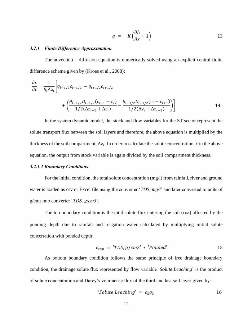
3.2.1 Finite Difference Approximation
The advection – diffusion equation is numerically solved using an explicit central finite
difference scheme given by (Kroes et al., 2008):
𝜕𝑐
𝜕𝑡=
1
𝜃𝑖∆𝑧𝑖[𝑞𝑖−1/2𝑐𝑖−1/2 − 𝑞𝑖+1/2𝑐𝑖+1/2
+ (𝜃𝑖−1/2𝐷𝑖−1/2(𝑐𝑖−1 − 𝑐𝑖)
1/2(∆𝑧𝑖−1 + ∆𝑧𝑖)−
𝜃𝑖+1/2𝐷𝑖+1/2(𝑐𝑖 − 𝑐𝑖+1)
1/2(∆𝑧𝑖 + ∆𝑧𝑖+1))] 14
In the system dynamic model, the stock and flow variables for the ST sector represent the
solute transport flux between the soil layers and therefore, the above equation is multiplied by the
thickness of the soil compartment, ∆𝑧𝑖. In order to calculate the solute concentration, c in the above
equation, the output from stock variable is again divided by the soil compartment thickness.
3.2.1.1 Boundary Conditions
For the initial condition, the total solute concentration (mg/l) from rainfall, river and ground
water is loaded as csv or Excel file using the converter ‘TDS, mg/l’ and later converted to units of
g/cm3 into converter ‘TDS, g/cm3’.
The top boundary condition is the total solute flux entering the soil (ctop) affected by the
ponding depth due to rainfall and irrigation water calculated by multiplying initial solute
concertation with ponded depth:
𝑐𝑡𝑜𝑝 = ′𝑇𝐷𝑆, 𝑔/𝑐𝑚3′ ∗ ′𝑃𝑜𝑛𝑑𝑒𝑑′ 15
As bottom boundary condition follows the same principle of free drainage boundary
condition, the drainage solute flux represented by flow variable ‘Solute Leaching’ is the product
of solute concentration and Darcy’s volumetric flux of the third and last soil layer given by:
′𝑆𝑜𝑙𝑢𝑡𝑒 𝐿𝑒𝑎𝑐ℎ𝑖𝑛𝑔′ = 𝑐3𝑞3 16

13
The leached solute is collected to an end stock variable ‘Leached Solute’ for tracking the
amount of solute leached out of the soil column.
3.2.1.2 Solute Flux Equations
For the initial solute infiltration flux from the topsoil to the stock variable ‘Solute Layer 1’
(SL1) representing the solute flux in first layer of soil surface, the equation is modified to represent
the flux boundary condition. Thus, the solute flux is represented using flow variable ‘Solute
Infiltration’ (Is) (g cm-2 day-1) given by:
𝐼𝑠 = 𝑐𝑡𝑜𝑝 −𝑧1
𝜃1𝑧1[(
𝑞1 + 𝑞2
2) (
𝑐1 + 𝑐2
2) +
(𝜃1 + 𝜃2
2 ) (𝐷1 + 𝐷2
2 ) (𝑐1 − 𝑐2)
(𝑧1 + 𝑧2
2 )] 17
The solute flux from SL1 to SL2 represented by flow variable ‘Solute Transport 1’ (Ts1) (g
cm-2 day-1) is given by:
𝑇𝑠1 =𝑧2
𝜃2𝑧2[(
𝑞1 + 𝑞2
2) (
𝑐1 + 𝑐2
2) − (
𝑞2 + 𝑞3
2) (
𝑐2 + 𝑐3
2) +
(𝜃1 + 𝜃2
2 ) (𝐷1 + 𝐷2
2 ) (𝑐1 − 𝑐2)
(𝑧1 + 𝑧2
2 )
−(
𝜃2 + 𝜃32 ) (
𝐷2 + 𝐷32 ) (𝑐2 − 𝑐3)
(𝑧2 + 𝑧3
2 )] 18
For the solute flux from SL2 to SL3, the free drainage bottom boundary condition is
considered and therefore, the equation for the flow variable ‘Solute Transport 2’ (Ts2) is given by:
𝑇𝑠2 =𝑧3
𝜃3𝑧3[(
𝑞2 + 𝑞3
2) (
𝑐2 + 𝑐3
2) +
(𝜃2 + 𝜃3
2 ) (𝐷2 + 𝐷3
2 ) (𝑐2 − 𝑐3)
(𝑧2 + 𝑧3
2 )] − 𝑐3𝑞3 19
The total solute concentration (g/cm3) of each soil layer is calculated by multiplying the
stocks ‘SL1’, ‘SL2’ and ‘SL3’ with corresponding layer’s soil depths in the converter Solutei.
Major stock (S), converters (C) and flow (F) variables of ST sector is listed in Appendix A5.

14
3.3 Root Water Uptake (RWU)
RWU is the amount of water extracted by the roots from the water stored in the soil layer
given by the sink term, S, in Richard’s equation (Šimůnek et al., 1996). The model simulates the
sink term as water extracted by the flow variable ‘uptake rate i’ (URi) from the stock variable
‘SWLi’ for each soil layer in the SWF sector, where i represent the three layers of soil. S is
depended on the soil water stress, osmotic stress, root characteristics and evapotranspiration
(Skaggs, van Genuchten, Shouse, & Poss, 2006).
3.3.1 Root Growth
Pecan and cotton are two crops commonly grown in El Paso where pecan is a perennial
crop and cotton is an annual crop. The model simulates RWU for these two crops where the root
length, r (cm) is loaded as a csv file. The root length for pecan is assumed to be constant at 80 cm
(Miyamoto, 1982) and cotton is assumed to be linear according to the locally observed root length
for irrigated cotton at El Paso (G. K. Ganjegunte, Clark, Parajulee, Enciso, & Kumar, 2018) for a
growing period of 180 days as shown in Table 1.1.
Table 1. 1 – Cotton Root Length (cm)
Length (cm) Crop Period (days)
0 - 25 0 – 20
25 – 40 21 – 30
40 – 75 31 – 50
75 51 - 180

15
3.3.2 Percentage Root Distribution ()
Root water uptake is depended upon the distribution of roots beneath the soil. These have
been quantified using various root length density (RLD) and root area density function. The
availability of data is important for improving the accuracy of the model’s prediction.
RLD for cotton (Zhi et al., 2017) has been used to calculate the percentage root distribution
in the soil to match the root growth of cotton in El Paso as shown in Figure 1.2.
In order to estimate the normalized root distribution of pecan, its root is considered to be
fully grown at the time of simulation having a span of 300 cm on either side and a total root length
of 80 cm (Woodroof & Woodroof, 1934) as shown in Figure 1.3.
Figure 1. 3 – Root Length Density (cm/cm3) for Pecan
For cotton, the varying root length density with depth is normalized over the root length as
shown in Figure 1.4 (Zhi et al., 2017).
-100
-80
-60
-40
-20
0.00 0.10 0.20 0.30 0.40 0.50 0.60 0.70 0.80 0.90
So
il D
epth
(cm
)
Percentage Root Distribution

16
Figure 1. 4 – Percentage Root Distribution for Cotton
3.3.3 Potential transpiration (Tp)
For simplicity of calculation, the average potential evapotranspiration has been used for
simulating root water uptake. Average potential evapotranspiration (ET0) of El Paso for 52 years
has been used for simulation purpose from Texas ET Network as shown in Table 1.2.
Table 1. 2 – Average ET0 (cm/month)
Month ET0
January 7.0
February 9.0
March 15.4
April 20.8
May 25.0
June 28.2
July 23.3
August 22.7

17
Month ET0
September 19.5
October 15.0
November 9.1
December 6.3
In order to predict the crop’s consumptive or potential transpiration Tp (cm/day) use the
crop’s coefficient Kc for pecan has been adopted from (Miyamoto, 1982) and cotton from
(Phocaides, 2000). represented by converter variable ‘Etc’ is calculated using equation:
𝑇𝑝 = 𝐾𝑐 𝐸𝑇0 20
Tp is the potential transpiration at which the roots can extract water from the soil layer
under most favorable conditions as shown in Figure 1.5 and 1.6.
Figure 1.5 – Potential Water Uptake for Pecan (cm/day)

18
Figure 1. 6 – Potential Water Uptake for Cotton (cm/day)
3.3.4 Matric and Osmotic Stress
Matric stress is the reduction in RWU under water stress expressed as a water stress
response function (0 ≤ 𝛼(ℎ) ≤ 1) i.e., depended on the soil water pressure head, h calculated from
converter variable ‘hi’ in SWF sector and empirical constant ℎ50 representing the pressure head at
50% root water extraction having a value of -150 cm for pecan and -50 cm for cotton (Donald L
Suarez, Vaughan, Brown, & Salinity, 2001; van Genuchten, 1987).
𝛼(ℎ) = 1
1 + (ℎ
ℎ50)
3 21
Osmotic stress is the reduction on RWU under salinity stress due to the presence of salt in
the soil water. It is expressed as an osmotic stress response function (0 ≤ 𝛼(𝑠) ≤ 1) i.e., depended
on the total salt concentration 𝐸𝐶 (dS/m) calculated from converter ‘Solutei’ in ST sector and
threshold value of crop salt tolerance, 𝐸𝐶50 (dS/m) (Oster et al., 2012; van Genuchten, 1980).

19
𝛼(𝑠) = 1
1 + (𝐸𝐶
𝐸𝐶50)
3 22
In order to calculate 𝐸𝐶 of soil water solution, unit of ‘Solutei’ is converted to mg/l and
then, empirically converted to dS/m using (Wallender & Tanji, 2011):
640 ∙ 𝐸𝐶 (𝑑𝑠/𝑚) = 𝑇𝐷𝑆 (𝑚𝑔/𝑙) 23
where, TDS is the total salt concentration in soil water.
3.3.5 Uptake Equation
A macroscopic approach was adopted in calculating the sink term given by (Feddes,
Kowalik, & Zaradny, 1978; van Genuchten, 1987):
𝑆 = 𝛽 𝛼(ℎ) 𝛼(𝑠)𝑇𝑝 24
RWU from each soil layer is formulated using the flow variable ‘Uptake Ratei’ (URi)
connected to the stock variable ‘SWLi’ and an end stock variable ‘Root Water Uptake i’ inferring
that the extracted water from soil layer is stored in the roots at a rate equal to the actual transpiration
rate. Thus, the equation for flow variable URi is given by:
𝑈𝑅𝑖 = 𝛽𝑖 𝛼(ℎ)𝑖 𝛼(𝑠)𝑖𝑇𝑝 25
where, i represent the ith soil layer with i equal to 1,2 and 3. Major stock (S), converters
(C) and flow (F) variables in RWU sector is listed in Appendix A5.
3.4 Hydraulic Reduction (HR) Function
The hydraulic reduction function, (0 ≤ 𝑟 ≤ 1), decreases the hydraulic conductivity due to
the presence of exchangeable sodium and adverse pH in the soil. High level of exchangeable
sodium causes clay dispersion and swelling of the soil (McNeal, 1968; Šimůnek et al., 1996; D. L.
Suarez & Šimůnek, 1997). The pH effects the saturated as well the effective hydraulic conductivity
(D. L. Suarez, Rhoades, Lavado, & Grieve, 1984). HR having a value of one represent that flow

20
is under no stress and less than one and greater than zero represent a flow with reduced hydraulic
conductivity due to salt stress. The hydraulic reduction function is given by:
𝑟 = 𝑟1𝑟2 26
where, 𝑟1 is the effects of exchangeable sodium (McNeal, 1968; Šimůnek et al., 1996; D.
L. Suarez & Šimůnek, 1997) and 𝑟2 is the effects of adverse pH on the hydraulic conductivity (D.
L. Suarez et al., 1984; D. L. Suarez & Šimůnek, 1997), respectively, given by:
𝑟1 = 1 − 𝑐𝑥𝑛
1 + 𝑐𝑥𝑛 27
where 𝑐 and 𝑛 are empirical parameters and 𝑥 is the swelling factor given by:
𝑥 = 3.6 × 10⁻⁴ 𝑓𝑚𝑜𝑛𝑡 𝐸𝑆𝑃 𝑑 28
and
𝑑 = {0 𝑓𝑜𝑟 𝐶0 > 300 𝑚𝑚𝑜𝑙 𝑙−1
356.4 𝐶0−1/2
+ 1.2 𝑓𝑜𝑟 𝐶0 < 300 𝑚𝑚𝑜𝑙 𝑙−1 29
and
𝑛 = {
1 𝑓𝑜𝑟 𝐸𝑆𝑃 < 25
2 𝑓𝑜𝑟 25 ≤ 𝐸𝑆𝑃 ≤ 50 3 𝑓𝑜𝑟 𝐸𝑆𝑃 > 50
30
and
𝑐 = {
35 𝑓𝑜𝑟 𝐸𝑆𝑃 < 25
932 𝑓𝑜𝑟 25 ≤ 𝐸𝑆𝑃 ≤ 5025000 𝑓𝑜𝑟 𝐸𝑆𝑃 > 50
31
respectively,
where, 𝑓𝑚𝑜𝑛𝑡 is the weight fraction of montmorillonite in the soil assumed to be 0.1
(McNeal, 1968; Šimůnek et al., 1996); 𝑑 is the adjusted interlayer spacing; 𝐶0 is total salt
concentration of the solution (mmol l-1) calculated from ‘Solutei’ in the ST sector; and ESP is the
exchangeable sodium percentage calculated from the sodium absorption ratio (SAR) given by
(Wallender & Tanji, 2011) :

21
𝑆𝐴𝑅 = [𝑁𝑎]
[𝐶𝑎 + 𝑀𝑔]1/2 32
Since the model does not simulate ion association or speciation, the total analytical
concentrations (mmol l-1) of Sodium [Na], Calcium [Ca] and Magnesium [Mg] are calculated by
assuming it to be present in the solution as a certain percentage of the total salt concentration. The
percentage value is loaded as a csv file into the converter variable ‘Sodium’, ‘Calcium’ and
‘Magnesium’. For SAR calculation, unit of ‘Solutei’ is empirically converted to mmol/l using
(Tanji et al., n.d.):
𝑆𝑜𝑙𝑢𝑡𝑒 (𝑚𝑔/𝑙) = 𝑆𝑜𝑙𝑢𝑡𝑒 (𝑚𝑚𝑜𝑙/𝑙) ∙ 64 33
and,
[𝐸𝑆𝑃]
[100 + 𝐸𝑆𝑃] = 𝑘𝑔
′ 𝑆𝐴𝑅 34
where, 𝑘𝑔′ is the modified Gapon selectivity coefficient having a value of
0.015 (mmol l)-1/2 (Wallender & Tanji, 2011). However, 𝑘𝑔′ should be estimated based on site
specific data (Doering & Willis, 1980; Jurinak, Amrhein, & Wagenet, 1984; Wallender & Tanji,
2011). The reduction factor, 𝑟2, is calculated using the equation by D. L. Suarez et al., 1984:
𝑟2 = {1 𝑝𝐻 < 6.833.46 − 0.36𝑝𝐻 6.83 ≤ 𝑝𝐻 ≤ 9.3 3 𝑝𝐻 > 9.3
35
Major stock (S), converters (C) and flow (F) variables in HR sector is listed in
Appendix A5.
4.0 Model Parameters
4.1 Soil Hydraulic Properties
In order to obtain a realistic simulation of the dynamic process of soil solutions, the model require
site specific hydraulic properties of soil. The soil properties of a commercially managed field

22
(31°30’32.30” N, 106°13’25.49” W) in El Paso County, Texas having an area of approximately
16 Ha was obtained from Web Soil Survey. The soil consists of Tigua (Tg - 72%), Glendale (Gs -
12%) and Harkey (Hs - 16%) silty clay loam as shown in Figure 1.7. The residual water content
(r) is an assumed value that can be optimized for running the model. The initial value of the stock
variable “Soil Layer” is set as the maximum water holding capacity. A weighted average of the
soil properties has been taken at each depth of soil as shown in Table 1.3. The air entry pressure,
𝛼 (cm-1) and pore size distribution, n of the SWRC was not readily available and therefore a value
of 0.0178 cm-1 for 𝛼 and 1.30 for n has been assumed for all depths (Schaap & Van Genuchten,
2006).
Figure 1. 7 – Soil Map at (31°30’32.30” N, 106°13’25.49” W) in El Paso County, Texas

23
Table 1. 3 – Soil Hydraulic Properties
Soil depth
(from
Topsoil) (z)
cm
Residual
Water
Content (r)
cm3 cm-3
Saturated
Water
Content (s)
cm3cm-3
Saturated
Hydraulic
Conductivity
(Ksat) cm
day-1
Soil pH Maximum
Water Holding
Capacity (cm)
(𝒛 × 𝜽𝒔)
30 0.00 0.34 6.11 8.15 10.2
30 0.01 0.39 15.80 8.15 11.7
40 0.02 0.39 40.44 8.15 15.6
4.2 Rainfall and Irrigation Water
Daily rainfall for El Paso region was downloaded from Climate Data Online (CDO),
National Climatic Data Center (NCDC) for the respective simulation time period. The irrigation
cycle for pecan and cotton was set based on observed practice in El Paso region given in
Table 1.4.
Table 1. 4 – Irrigation Cycle
Month Day Irrigation Water (cm)
Pecan
May 01 12.7
16 12.7
June 01 12.7
16 12.7
July 01 12.7
16 12.7
August 01 12.7
16 12.7
September 01 12.7

24
Month Day Irrigation Water (cm)
16 12.7
October 01 12.7
16 12.7
Total 152.4
Cotton
May 01 12.7
June 30 12.7
July 15 12.7
August 04 12.7
19 12.7
September 01 12.7
Total 76.2
4.3 Initial Salt Concentration (Si)
The ST sector in the model simulates the transport of salt entering the soil surface dissolved
in rain (R), river (RW) and ground water (GW). The irrigated water is categorized as RW and GW
based on their percentage contribution to the total amount of water. Due to the absence of
extensive monitoring salt data in the region, a constant amount of salt is considered to be dissolved
in waters during the entire simulation period given in Table 1.5.
Table 1. 5 – Initial Salt Concentration (mg/l)
Salt Type Total Dissolved Salts Sodium Calcium Magnesium
Rainwater (SR) 32 10.95 19.2 1.77
River Water (SRW) 512 106.94 101.38 16.52
Ground Water (SGW) 4627.2 1941 252 59.52

25
The above concentrations are observed chemistry of different water sources at a given time
period in the El Paso region. The total amount entering the soil surface every day is based on the
type of water used and daily ponding of the soil layer given by:
𝑆𝑖 = 𝑅 ∙ 𝑆𝑅 + 𝑅𝑊 ∙ 𝑆𝑅𝑊 + 𝐺𝑊 ∙ 𝑆𝐺𝑊
𝑅 + 𝑅𝑊 + 𝐺𝑊 36
5.0 Results and Discussions
The model simulates the dynamic process of transient water flow in subsurface soil and
water extraction beneath the root zone under salinity and water stress. The accuracy of simulation
and subsequent prediction of results are depended on the value of parameters closer to a site-
specific data. Due to the non-availability of experimented site data, the soil hydraulic properties
s, r, , n and Ks has been calculated from the Web Soil Survey for a managed field at Texas
A&M Agrilife in El Paso county, Texas. The salt concentration of irrigation water has been
calculated from an initial value obtained from Texas A&M Agrilife and later generated for a
desired time duration for different combination of rain, river water and groundwater. Root growth,
consumptive use and root distribution has been assumed based on available site data and various
literatures.
5.1 Simulation Setup
The simulation duration was set for 365 days representing year 2018. The crop is assumed
to be irrigated using a supply of 30% groundwater and 70% river along with incident rainfall. As
a result, the initial surface solute concentration (mg/cm3) is calculated using the salt concentration
of rainfall, river water and groundwater in their appropriate ratios whereas the surface solute flux
(mg cm-2 day-1) is calculated by multiplying the rainfall for year 2018 with surface solute
concentration as shown in Figure 1.8, 1.9 and 1.10.

26
Figure 1. 8 – Rainfall for year 2018
Figure 1. 9 – Surface Solute Concentration (mg cm-3)

27
Figure 1. 10 – Surface Solute Flux (mg cm-2 day -1)
Pecan is a perennial crop and it is assumed to be fully grown throughout the entire
simulation duration with variation in its canopy cover resulting in a Tp as shown in Figure 1.5.
Cotton is an annual crop and therefore, its growing period is set from May to October with a
specified Kc resulting in a stimulated Tp as shown in Figure 1.6. The threshold value of salt
tolerance, 𝐸𝐶50 of pecan is 3 dS/m (G. Ganjegunte & Clark, 2017) and cotton is 7.7 dS/m (Maas
& Grattan, 1999).
5.2 Simulation Scenarios
In order to assess the model’s capability to predict the effects of salinity stress in cotton
and pecan, it is required to simulate and compare various scenarios. Therefore, the model has been
run as per scenarios shown in Table 1.6 under different condition of stresses.

28
Table 1. 6 – Simulation Scenarios
Scenarios Type of Stress (✓ Active)
Pecan Cotton Osmotic
Stress
Water
Stress
Stress Type
P1 C1 ✓ No Salinity Stress
P2 C2 ✓ ✓ Salinity Stress
Scenario P1, C1 simulates root water uptake with salinity stress response function set at 1,
i.e., no salinity stress and zero solute transport in sector SL. This predicts the actual root water
uptake by crops under water stress and having no salinity stresses.
In scenario P2, C2, the osmotic stress due to salinity is activated. This predicts the root
water uptake by crops under salinity and water stress representing a real-world scenario where
both stresses act in tandem.
The simulation scenarios are designated the way it is run in the model with P and C
representing Pecan and Cotton, respectively. For visualization of the output data, it has been
exported and plotted using Matplotlib in Python.
5.3 Simulation Results
The results of simulation are attributable to a nonlinear complex dynamic circular relation
between water infiltration, solute transport and root water uptake. In order to understand the system
dynamics, the results of each sector need to be interpreted acknowledging the interlink between
them. In order to understand the correlation, the results are discussed in a sequence leading to root
water uptake. For discussion purposes, simulation results for soil water storage, solute transport,
s, and h are considered for simulation scenario P4, C4.

29
5.3.1 Soil Water Content
Infiltrated water is available to the crop from the water stored in each layer. The model
simulates the water infiltration and predicts the water content in each layer as shown in
Figure 1.11.
Figure 1. 11 – Water Content of Pecan and Cotton (All Layers)
5.3.2 Water Stress Response Function (h)
Water stress occurs due to the scarcity of water to the plant during its growing period. It is
expressed as a rating value h between 0 and 1 representing maximum and no stress, respectively.
h is depended on the pressure head created by infiltrated water and soil water storage in the form
of 𝛼(ℎ) = 1
1 + (ℎ
ℎ50)
3. A comparison of h for pecan and cotton as shown in Figure 1.12, shows
that cotton is more prone to water stress than compared to pecan.

30
Figure 1. 12 – Water Stress response function for pecan and cotton
5.3.3 Solute Transport
The model simulates the transport of solute and predicts the solute concentration in the root
zone at each compartment of 30 cm, 30 cm and 40 cm. Root zone solute concentration varies with
layer for each crop as shown in Figure 1.13 and 1.14. These solute concentrations are in turn
responsible for the salinity stress in crops in the form of 𝛼(𝑠) = 1
1 + (𝐸𝐶
𝐸𝐶50)
3 in each respective
layer.

31
Figure 1. 13 – Comparison of Solute accumulation in each layer in Pecan
Figure 1. 14 – Comparison of Solute accumulation in each layer in Cotton

32
To better understand the salt accumulation, the cumulative solute concentration for the
entire root zone is calculated by adding up all layers as shown in Figure 1.15. It is inferred that
pecan has higher solute concentration than cotton given that solute is transported along with
infiltrated water and the roots of crop extracting more water will have higher solute concentrated
in their root zone. Since with its fully grown and longer roots extracts comparatively more water
than cotton.
Figure 1. 15 – Comparison of Solute accumulation in pecan and cotton
5.3.4 Salinity Stress response function (s)
s is calculated dynamically with every t change in root zone solute concentration for
each layer simulated in the solute transport sector and threshold values of their salt tolerance. It is
expressed as a rating with value between 0 and 1 where 0 represents maximum stress and 1
represents no stress. The model prediction of s for cotton and pecan is shown in
Figure 1.16 and 1.17.

33
Pecan being a low salt tolerant crop with a threshold value of 3 dS/m is expected to have
comparatively higher s than the high salt tolerant variant cotton with a threshold value of 7.7
dS/m. The simulation results show a higher s varying between 0.6 to 1 for pecan and lower s
varying between 0.983 to 1 for cotton.
Figure 1. 16 – Salinity Stress response function for pecan

34
Figure 1. 17 – Salinity Stress response function for cotton
5.3.5 Root Water Uptake
The dynamics of root water uptake depends on the stored water in soil layer and solute
transport in the form of rating values, s and h. The entire root water uptake in a soil depth of 100
cm is divided into compartments of 30 cm, 30 cm and 40 cm with each representing the actual root
water uptake in respective layers. The total cumulative root water uptake for cotton and pecan is
calculated by summing up value of all layers as shown in Figure 1.18 and 1.19.
Pecan, with s varying from 0.6 to 1, shows a reduction in root water uptake under salinity
stress as it can been seen that P1 is greater than P2. Since the pecan has a low salt tolerance with
a threshold value of 3 dS/m, it is prone to a salinity stress for a salt accumulation higher than
3 dS/m.

35
Figure 1. 18 – Comparative cumulative actual root water uptake of pecan under different stresses
Figure 1. 19 – Comparative cumulative actual root water uptake of cotton under different stresses

36
Cotton, with s varying from 0.983 to 1, root water uptake under salinity stress (C2) is
almost equal to that at no salinity stress (C1). This is due to the fact that cotton has a high salt
tolerance threshold value of 7.7 dS/m and the salt accumulation is the root zone is lower than this
value for the majority period in the year.
Root water uptake of cotton is expected to be comparatively lesser than pecan due to the
fact that cotton is an annual crop with a lesser growing period. As expected, the model predicts the
root water uptake of cotton lesser than pecan as shown in Figure 1.20. Simulation scenario P2, C2
comprising of salinity and water stress is simulated for comparison of pecan and cotton,
respectively.
Figure 1. 20 – Comparative cum. actual root water uptake for pecan and cotton
for combined stress
A closer look at the simulation results confirms the fact that for cotton, the root water
uptake peaks from May to June when its lateral root density is the maximum. Whereas for pecan,

37
the root water uptake increases gradually since its root distribution is uniform throughout the year.
This shows that the model was successful in predicting the root water uptake in the absence
and presence of stresses for cotton and pecan separately. Also, the prediction of root water uptake
for pecan and cotton shows the variation as observed in perennial and annual crop.
5.3.6 Water Balance
Water balance of a system is the amount of water flowing in and out of the soil column.
Water balance of the soil column of this study is given by:
𝑊𝑎𝑡𝑒𝑟 𝐴𝑝𝑝𝑙𝑖𝑒𝑑 = 𝑅𝑜𝑜𝑡 𝑤𝑎𝑡𝑒𝑟 𝑢𝑝𝑡𝑎𝑘𝑒 + 𝐿𝑒𝑎𝑐ℎ𝑒𝑑 𝑊𝑎𝑡𝑒𝑟 + 𝑆𝑜𝑖𝑙 𝑊𝑎𝑡𝑒𝑟 𝑆𝑡𝑜𝑟𝑎𝑔𝑒 37
The calculated water balance equation for the soil column is shown in Figure 1.21.
Figure 1. 21 – Water Balance for Pecan and cotton for all layers with water depth in cm
From the water balance under salinity stress, it is observed that pecan extracts about 96 cm
of water out of the applied 173 cm adding up to 55%. As for cotton, it extracts 42 cm of water out
of the applied 98 cm adding up to 43%. It can be seen that both pecan and cotton have the similar
amount of water leached out. Pecan with its perennial and fully-grown roots is capable of
extracting more water from the soil than cotton.

38
5.4 Comparison of results with HYDRUS
The model’s prediction can be categorized as the numerical solutions derived from the
finite difference equation using system dynamics. Numerical solutions are approximate estimation
demonstrating a real-world problem. One of the methods for verification of these solutions in an
accurate, comprehensive, exhaustive, efficient and cost-effective manner is to compare with a
similar mathematical model (Abelman & Patidar, 2008; Haverkamp, Vauclin, Touma, Wierenga,
& Vachaud, 1977; Shawagfeh & Kaya, 2004).
HYDRUS solves infiltration, solute transport and root water uptake using finite element
approximation. In order to represent the system dynamic model in in HYDRUS, the soil profile of
100 cm was divided into 30, 30, and 40 cm using 4 nodes. The hydraulic properties for three layers,
node 1 to 2 was selected as material 1, node 2 to 3 as material 2 and node 3 to 4 as material 3
representing the three soil compartments of 30 cm, 30 cm and 40 cm, respectively.
Data for rainfall, surface solute concentration, transpiration, root length and soil hydraulic
properties has been inputted same as the system dynamic model. In the system dynamic model,
hydraulic conductivity is reduced to almost 50% of its value throughout the simulation due to the
effects of hydraulic reduction function and therefore, Ks for HYDRUS was set at 50% of the value
for each layer.
HYDRUS modules for soil water flow, standard solute transport, root water uptake and
root growth were chosen with a simulation duration of 365 days. The simulation results for
cumulative actual root water uptake, actual uptake rate and root zone solute concentration of pecan
and cotton has been compared with the system dynamic model as shown in Figure 1.22, 1.23, 1.24,
1.25, 1.26 and 1.27.

39
Figure 1. 22 – Comparison model results with Hydrus: cum. Actual Root water uptake for pecan
Figure 1. 23 – Comparison model results with Hydrus: cum. Actual Root water uptake for cotton

40
Figure 1. 24 – Comparison model results with Hydrus: Actual Root water uptake for pecan
Figure 1. 25 – Comparison model results with Hydrus: Actual Root water uptake for cotton

41
Figure 1. 26 – Comparison model results with Hydrus: cum. Root zone solute concentration
for pecan
Figure 1. 27 – Comparison model results with Hydrus: cum. Root zone solute concentration
for cotton

42
5.4.1 Data Analyzes of Results
The consistency of the results simulated by the model in comparison with HYDRUS is
further evaluated by computing the Root Mean Square Error (RMSE) and Pearson’s correlation
coefficient, R & R2:
𝑅𝑀𝑆𝐸 = 𝑚𝑒𝑎𝑛 (𝑋 − 𝑌)1/2 38
𝑅 = 𝑐𝑜𝑣𝑎𝑟𝑖𝑎𝑛𝑐𝑒(𝑋, 𝑌) / (𝑠𝑡𝑑𝑣(𝑋) ∗ 𝑠𝑡𝑑𝑣(𝑌)) 39
where, X and Y are the simulated value for the ith observation from HYDRUS and
the Model. The calculated RMSE and R value for the cumulative actual root water uptake and root
zone solute concentration is shown in Table 1.7.
Table 1. 7 – RMSE and R
Parameters RMSE R R2
Pecan Cotton Pecan Cotton Pecan Cotton
Cumulative Actual Root Water
Uptake (cm)
2.810 3.317 0.999 1.000 0.996 0.957
Actual Root Water Uptake (cm/day) 0.104 0.517 0.926 0.879 0.837 0.705
Root Zone Solute Concentration
(mg/cm3)
0.548 1.497 0.981 0.573 0.927 0.317
The model’s prediction for pecan has small RMSE and high R and R2 demonstrating that
the model has predicted results similar to HYDRUS. The prediction for cotton is having a slightly
higher RMSE of 3.317 cm, 0.517 cm/day and 1.497 mg/cm3; and R2 of 0.957, 0.705 and 0.317
demonstrating that the model has slightly overestimated the root water uptake and uptake rate; and
underestimated the root zone solute concentration. This is attributing the fact that pecan had a
constant root length whereas cotton had variable root growth and thus, the normalized root
distribution for cotton might have differed resulting in the variation in results. Overall performance

43
of the model shows that the simulation of soil water infiltration, solute transport and root water
uptake under salinity and matric stress is conforming to the simulation results of HYDRUS.
The model’s prediction for pecan has small RMSE and high R demonstrating that the
simulation has accurately predicted in line with the HYDRUS simulation. The prediction for cotton
is having a RMSE of 0.103 cm and 1.293 mg/cm3 and R2 of 0.854 and 0.533 demonstrating that
the model has slightly overestimated the root water uptake and underestimated the root zone solute
concentration compared to HYDRUS. This is attributing the fact that pecan had a constant root
length whereas cotton had variable root growth and thus, the normalized root distribution for cotton
might have differed resulting in the variation in results. Overall performance of the model shows
that the simulation of soil water infiltration, solute transport and root water uptake under salinity
and matric stress is conforming to the simulation results of HYDRUS.
6.0 Conclusion
A system dynamic model was developed for soil water infiltration, solute transport and
root water uptake by numerically solving one dimensional Richard’s equation and advection –
diffusion equation based on finite difference approach along with other physical based
formulations and empirical assumptions to evaluate the effects of salinity and matric stress on
crops. The model simulated similar results to those from a finite element method based numerical
model, HYDRUS. The operation and structure of the model is easily perceptible and adaptable,
and a user can easily change the variables and parameters according to a project specific
requirement without prior knowledge of any programming language. The accuracy of simulation
result can be increased by adopting a site measured values for r, s, Ks, , n, surface solute
concentration, transpiration and controlled environment values for Kc and (z). The simulated
results show that the salinity and water stress reduce the efficiency of crops to extract water from

44
the soil layer due to accumulated salt in the root zone. Under salinity stress, pecan is able to extract
55% of the applied water whereas cotton extracts 43% of the applied water; and about 20 ~ 30%
of the water is either leached out or stored as soil water. These extraction capacities can be
increased by practicing better irrigation management technique to reduce salt accumulation such
as salt leaching and gypsum.

45
Section 2 – Evaluating Simulation Results for 10 Years
1.0 Introduction
Water in the arid South-West United States is mostly contains a significant concentration of
dissolved salts. The main causes of salinity include the topography, surface water hydrology,
minerals in underground water, low rainfall, high temperature, evaporation, extreme hot and dry
winds and human factors such as irrigation and use of fertilizers (Naeimi & Zehtabian, 2011).
When saline water is used for irrigation, it results in accumulation of salts in the subsurface soil.
El Paso is an arid region in the south west of United States in Chihuahua desert. Most of the
irrigation water for the region is from Rio Grande river and ground water wells. Both sources based
on the location have significant dissolved salts. The well water in El Paso contains 4 times as much
salt as compared to average Rio Grande river and irrigation using well water increases leaching
requirement by 30% (Miyamoto, 1982). Pecan and cotton are the major crops in the region. Many
studies have focused on the irrigation efficiencies for cotton and pecan in the region (G.
Ganjegunte & Clark, 2017; G. K. Ganjegunte et al., 2018; Miyamoto, 1982). These studies are
based on field studies that are time consuming and require extensive monitoring. With the goal of
determining water use efficiency, and salt-buildup numerical models will be both cost effective
and time efficient.
Numerous numerical models are available for analyses of salt accumulation in the soil layers
such as ENVIRO-GRO (Pang & Letey, 1998), SALTMED (Ragab, 2002), SWAP (van Dam,
2000), UNSATCHEM (Šimůnek et al., 1996; D. L. Suarez & Šimůnek, 1997) and HYDRUS
(Šimůnek, J. et al., 1998, 2005; Šimůnek et al., 2013; Vogel et al., 1996). These models predict
the salt accumulation based on numerical solution to physically based formulations and empirical
assumptions. In addition to the simulation of salt accumulation, HYDRUS and UNSATCHEM

46
have an additional option for precipitation and dissolution of calcite, gypsum, nesquehonite,
hydromagnesite and sepiolite that introduces the concept of amendment to the soil for reducing
the accumulated salts (Šimůnek et al., 1996).
With increasing drought like conditions, the accumulation of calcium carbonate and other
soluble salts rapidly increases in the soil. This occurs due to the continuously low rainfall in arid
regions resulting in substantially less effective leaching of salts. The objective of this study is to
simulate a system dynamic model to quantify the salt accumulation in the soil layer with irrigation
water containing different salt concentration for a 10-year period of lowest rainfall recorded in El
Paso region. The model will also predict the variation in root water uptake in cotton and pecan for
different irrigation water.
2.0 Site Specific Data
In order to understand the issue of salt buildup in soil, the system dynamic model require site
specific data for accuracy in prediction.
2.1 Site Selection
Texas A&M Agrilife Center at El Paso commercially manages sites at El Paso and Socorro
for monitoring and assessing the effects of salinity in cotton and pecan production. For this
simulation study, data was obtained for a 16 Ha area located at 31°30’32.30” N, 106°13’25.49” W
of these commercial managed site. This region is classified as arid region with a low average
annual precipitation of 15 cm and potential evapotranspiration of 194 cm; daily maximum and
minimum temperatures of 35.8oC and -3.4oC; solar radiation of 19.78 MJ m-2 d-1 and wind speed
of 1.21 ms-1 (G. K. Ganjegunte et al., 2018).

47
2.2 Soil Dimensioning
Numerical model such as HYDRUS uses finite element method to predict the salt
accumulation by dividing the entire soil depth into nodes of 1 cm each. This allows solute potential
gradients to exist within the layers and increase solute transport rate in the profile. Similarly, the
system dynamic model requires the soil to be divided into layers to create gradients for solute
transport. The simulation in the study site is for a subsurface soil column of 100 cm depth and unit
area of 1 cm2. The entire soil depth is divided into three layers of 30 cm, 30 cm and 40 cm. The
model will simulate the salt transport and predict the salt accumulation in each layer.
Consequently, the corresponding root water uptake will be predicted allowing the comparison of
effects of root water uptake for different irrigation water.
2.3 Soil Physical and Chemical Properties
Field and laboratory estimation of the soil physical and chemical properties various soil
types will be costly. The soil hydraulic properties, r, s, and Ks for the 16 Ha study site was
obtained from Web Soil Survey consisting of Tigua (Tg - 72%), Glendale (Gs - 12%) and Harkey
(Hs - 16%) silty clay loam soils as shown in Figure 2.1. The air entry pressure, 𝛼 (cm-1) and pore
size distribution, n of the Soil Water Retention Curve was not readily available.
Schaap & Van Genuchten, 2006 classified and evaluated soil across United States
determining the soil hydraulic properties. Soil in the study site is classified as silty clay loam and
a value of 0.0178 cm-1 for 𝛼 and 1.30 for n has been adopted from this study (Schaap & Van
Genuchten, 2006). The soil hydraulic properties for the simulation is given in Table 2.1.

48
Figure 2. 1 – Soil Map at (31°30’32.30” N, 106°13’25.49” W) in El Paso County, Texas
Table 2. 1 - Soil Hydraulic Properties (Resize)
Soil depth
(from
Topsoil) (z)
cm
Residual
Water
Content (r)
cm3 cm-3
Saturated
Water
Content (s)
cm3cm-3
Saturated
Hydraulic
Conductivity
(Ksat) cm
day-1
Soil pH Maximum
Water Holding
Capacity (cm)
(𝒛 × 𝜽𝒔)
30 0.00 0.34 6.11 8.15 10.2
30 0.01 0.39 15.80 8.15 11.7
40 0.02 0.39 40.44 8.15 15.6
3.0 Time varying boundary conditions
El Paso experienced historical droughts from year 1950 to 1956 (Manford, Dixon, & Dent,
n.d.). As decreasing rainfall increase salt accumulation, the simulation duration of the system
dynamic model was set for a period of 10 years from 1947 to 1956.

49
3.1 Rainfall
A data analyzes of rainfall records showed that these periods recorded the lowest rainfall
in El Paso. The rainfall data for the period was downloaded from Climate Data Online (CDO),
National Climatic Data Center (NCDC) as shown in Figure 2.2. The simulation duration was set
for 3653 days and the model calculated each variable for every 0.125 of a day.
Figure 2. 2 – Daily rainfall for 10 year from 1947 to 1956
3.2 Irrigation Water
Salinity of water depends upon the type of water used for irrigating the crop. As water from
ground wells will be higher than river or rainwater, the source of irrigation will adversely affect
the salt accumulation in the soil layers. The irrigation cycle of cotton and pecan is as given in

50
Table 2.2. It is assumed that cotton and pecan is irrigated with the same frequency throughout the
period from 1947 to 1956.
Table 2. 2 - Irrigation Cycle for a year
Month Day Irrigation Water (cm)
Pecan
May 01 12.7
16 12.7
June 01 12.7
16 12.7
July 01 12.7
16 12.7
August 01 12.7
16 12.7
September 01 12.7
16 12.7
October 01 12.7
16 12.7
Total 152.4
Cotton
May 01 12.7
June 30 12.7
July 15 12.7
August 04 12.7
19 12.7
September 01 12.7
Total 76.2
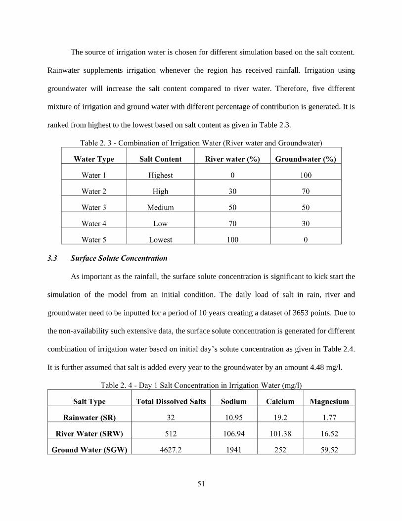
51
The source of irrigation water is chosen for different simulation based on the salt content.
Rainwater supplements irrigation whenever the region has received rainfall. Irrigation using
groundwater will increase the salt content compared to river water. Therefore, five different
mixture of irrigation and ground water with different percentage of contribution is generated. It is
ranked from highest to the lowest based on salt content as given in Table 2.3.
Table 2. 3 - Combination of Irrigation Water (River water and Groundwater)
Water Type Salt Content River water (%) Groundwater (%)
Water 1 Highest 0 100
Water 2 High 30 70
Water 3 Medium 50 50
Water 4 Low 70 30
Water 5 Lowest 100 0
3.3 Surface Solute Concentration
As important as the rainfall, the surface solute concentration is significant to kick start the
simulation of the model from an initial condition. The daily load of salt in rain, river and
groundwater need to be inputted for a period of 10 years creating a dataset of 3653 points. Due to
the non-availability such extensive data, the surface solute concentration is generated for different
combination of irrigation water based on initial day’s solute concentration as given in Table 2.4.
It is further assumed that salt is added every year to the groundwater by an amount 4.48 mg/l.
Table 2. 4 - Day 1 Salt Concentration in Irrigation Water (mg/l)
Salt Type Total Dissolved Salts Sodium Calcium Magnesium
Rainwater (SR) 32 10.95 19.2 1.77
River Water (SRW) 512 106.94 101.38 16.52
Ground Water (SGW) 4627.2 1941 252 59.52

52
The effective solute concentration entering the system dynamic model as initial condition
for each day from 1947 to 1956 is given by:
𝑆𝑖 = 𝑅𝑖 ∙ 𝑆𝑅𝑖 + 𝑅𝑊𝑖 ∙ 𝑆𝑅𝑊𝑖 + 𝐺𝑊𝑖 ∙ 𝑆𝐺𝑊𝑖
𝑅𝑖 + 𝑅𝑊𝑖 + 𝐺𝑊𝑖 1
where, i stands for ith day.
3.4 Evapotranspiration
The daily potential evapotranspiration has been calculated from the average monthly data
of El Paso for last 52 years from Texas ET Network as shown in Table 2.5.
Table 2. 5 – Average ET0 (cm/month)
Month ET0
January 7.0
February 9.0
March 15.4
April 20.8
May 25.0
June 28.2
July 23.3
August 22.7
September 19.5
October 15.0
November 9.1
December 6.3
The consumptive value Kc for pecan has been calculated from (Miyamoto, 1982) and cotton
from (Phocaides, 2000). The crop evapotranspiration (Tp) is calculated by equation given by:
𝑇𝑝 = 𝐾𝑐 𝐸𝑇0 2

53
4.0 Crop Data
Due to the popularity of pecan and cotton in the region, these crops are selected for
assessing the effects on its ability to uptake water from these salt accumulated layers. Cotton is a
highly salt tolerant crop with a threshold electric conductivity (EC) value of 7.7 dS/m implying
that the cotton doesn’t have any effect of salinity stress until it reaches the threshold value (Maas
& Grattan, 1999). Similarly, the threshold EC value of pecan is 3 dS/m implying that it is a low
salt tolerant crop. Both the crops are expected to reach its 50% water extraction potential at a
capillary pressure gradient of -150 cm for pecan and -50 cm for cotton. In addition, the model
requires time varying conditions of the crop such as root length and normalized root distribution
function over the growing period.
4.1 Root Length
The root length for pecan is assumed to be constant at 80 cm and cotton is assumed to be
linear according to the locally observed root length for irrigated cotton at El Paso for a growing
period of 180 days as shown in Table 2.6.
Table 2. 6 – Cotton Root Length (cm)
Length (cm) Crop Period (days)
0 - 25 0 – 20
25 – 40 21 – 30
40 – 75 31 – 50
75 51 - 180
4.2 Percentage Root Distribution ()
Percentage root distribution for cotton has been calculated form the root length density
value from (Zhi et al., 2017) as shown in Figure 2.3.

54
Figure 2. 3 – Percentage Root Distribution for Cotton
The roots of pecan are considered to be fully grown at the time of simulation having a span
of 300 cm on either side and a total root length of 80 cm. As a result, the root length and normalized
root distribution function does not vary with time during the entire simulation period. The
Percentage root distribution is calculated from the root dimensions given in (Woodroof &
Woodroof, 1934) and as shown in Figure 2.4.
Figure 2. 4 – Percentage Root Distribution for Pecan

55
5.0 Results and Discussion
The simulated results infer the effect of different source of irrigation water in root water
uptake of cotton and pecan. The system dynamic model allows the user to have multiple simulation
with option for comparison in the form of graphs. Table 2.7 shows the simulation scenarios chosen
for pecan and cotton as designated in the system dynamic model.
Table 2. 7 - Simulation Scenario
Water Type Salt Content Simulation Runs River water
(%)
Groundwater
(%) Pecan Cotton
Water 1 Highest P1 C1 0 100
Water 2 High P2 C2 30 70
Water 3 Medium P3 C3 50 50
Water 4 Low P4 C4 70 30
Water 5 Lowest P5 C5 100 0
Simulation results are plotted for solute concentration in root zone, salinity stress response
function (s) and root water uptake for different concentration of saline water.
5.1 Salt Accumulation in Root Zone
Salt transport from between layers occurs due to advection – diffusion reaction. Advection
occurs due to the infiltrating water and diffusion due to the potential solute gradient between top
layer, middle layer and bottom layer. Figure 2.5 and 2.6 shows the accumulated total dissolved
solids (TDS) in the root zone for pecan and cotton at different concentration of saline water.
As expected, the model has successfully predicted highest solute concentration in root zone
for both crops irrigated with 100% groundwater. This shows that if the crops are irrigated with
river water with less salt content, it will have less solute accumulated in their root zone less than 2
mg/cm3 or 2000 mg/l that is less than the threshold value of pecan and cotton. This shows that with

56
proper treated water, the solute concentration in the root zone can be considerably reduced to favor
the growth of crop without salinity stress.
Figure 2. 5 – Salt accumulation in root zone of Pecan (1947 – 1956)

57
Figure 2. 6 – Salt accumulation in root zone of Cotton (1947 – 1956)
5.2 Salinity Stress Response function (s)
s is a rated value between 0 and 1 to account for the salinity stress in crops due to the
accumulated solute in the root zone. A value closer to 1 suggests less stress and closer to 0 is high
stress. s is calculated using (Oster et al., 2012; van Genuchten, 1980):
𝛼(𝑠) = 1
1 + (𝐸𝐶
𝐸𝐶50)
3 3
where, EC50 is the threshold value of crop and EC is the solute concentration in the root
zone converted by the model using (Wallender & Tanji, 2011):
640 ∙ 𝐸𝐶 (𝑑𝑠/𝑚) = 𝑇𝐷𝑆 (𝑚𝑔/𝑙) 4
Figure 2.7 and 2.8 shows that s for pecan varies from 0.2 to 1 and cotton from 0.65 to 1
from 1947 to 1956 for different irrigation water, respectively.

58
Figure 2. 7 – Salinity stress response function of Pecan (1947 – 1956)
Figure 2. 8 – Salinity stress response function of Cotton (1947 – 1956)

59
The high variation in pecan is due to the low salt tolerance of the crop whereas cotton being
highly salt tolerant shows less variation. Also, irrigation water with higher salt content (100%
groundwater and 0% irrigation water) has the lowest s value showing that accumulated salts
increases salinity stress on the crops. These salinity stresses directly affect the root water uptake
of cotton and pecan.
5.3 Root Water Uptake
The increased accumulation of salt in the root zone brings s closer to 0 indicating high
stress that reduces the actual root water uptake capacity of the crops. A comparison of the root
water uptake at different concentration of irrigation water in Figure 2.9 and 2.10 shows that crops
have extracted more water when irrigation water with lowest salt content was used. Cotton has less
variation in the total water extracted due to its high salt tolerance.
Figure 2. 9 – Root Water uptake of Pecan for varying salt content (1947 – 1956)

60
Figure 2. 10 – Root Water uptake of Cotton for varying salt content (1947 – 1956)
5.4 Data Analysis
To better understand the trend in cumulative salt accumulation (mg/cm3) (Solute) and root
water (cm) (RWU) for all layers, a comparison of dataset for different water was conducted. The
calculated mean value for every 2 years is quantified in Table 2.8.
Table 2. 8 – Mean values at every 2 years from 1947 to 1956
Simulation P1 P2 P3 P4 P5 C1 C2 C3 C4 C5
1947 - 1949
Solute 2.27 1.65 1.20 0.81 0..28 1.24 0.91 0.69 0.46 0.14
RWU 91.96 92.09 91.77 90.31 90.81 36.31 35.84 35.31 34.97 34.47
1949 – 1951
Solute 5.52 4.81 3.98 2.98 0.90 4.00 3.12 2.42 1.65 0.44
RWU 265.4 274.4 278.4 281.7 283.7 114.9 113.8 112.2 111.2 109.4
1951 - 1953

61
Simulation P1 P2 P3 P4 P5 C1 C2 C3 C4 C5
Solute 6.43 5.97 5.28 4.27 1.34 6.21 4.82 3.75 2.55 0.65
RWU 407.9 437.7 451.8 465.1 478.3 194.7 193.6 191.1 189.6 186.6
1953 – 1955
Solute 7.29 6.75 6.22 5.22 1.66 8.44 6.76 5.39 3.69 0.86
RWU 521.5 581.5 611.2 638.2 669.1 268.8 269.0 266.2 264.7 260.5
1955 - 1957
Solute 8.03 7.37 6.89 5.94 1.84 9.92 8.11 6.60 4.55 1.00
RWU 615.9 710.7 761.9 807.5 862.4 342.2 345.0 343.0 342.0 337.2
The data analyzes shows that the salt accumulation in the root zone for water 1, having the
highest salt content, is the highest ranging from 2.27 to 8.03 mg/cm3 for pecan and 1.24 to 9.92
mg/cm3 for cotton. It can be seen that for water 5 having the least salt content, the salt accumulation
is very low ranging from 0.28 to 1.84 mg/cm3 for pecan and 0.14 to 1.00 mg/cm3 for cotton.
In pecan, during the initial 2 years from 1947 to 1949, the reduction in root water uptake
is not profound since the salt buildup in each layer has not reached its threshold value of 3 dS/m.
Whereas, from year 1951 to 1956, pecan demonstrate considerable reduction in root water uptake
with maximum difference of 246.5 cm in year 1956 between Water 5 and Water 1. This shows
that the salt concentration in each layer has increased considerably enough to surpass its threshold
value increasing the salinity stress.
In the initial 4 years from 1947 to 1951, cotton has hardly any reduction in the root water
uptake even though salt concentration in the root zone has reached a value of 4 mg/cm3. This is
attributable to its high salt tolerance with a threshold value of 7.7 dS/m. From 1951 to 1956, the
accumulated salt has reached a value of 9.7 mg/cm3 and exceeded its threshold value showing a

62
reduction in root water uptake between water 5 and water 1 with maximum reduction of 5 cm
observed in the last year 1956. This shows that cotton is highly salt tolerant and can withstand the
high salt content in the arid region.
Further, Table 2.9 shows the calculated water balance for the soil column for initial and
final 2 years of simulation using:
𝑊𝑎𝑡𝑒𝑟 𝐴𝑝𝑝𝑙𝑖𝑒𝑑 = 𝑅𝑜𝑜𝑡 𝑤𝑎𝑡𝑒𝑟 𝑢𝑝𝑡𝑎𝑘𝑒 + 𝐿𝑒𝑎𝑐ℎ𝑒𝑑 𝑊𝑎𝑡𝑒𝑟 + 𝑆𝑜𝑖𝑙 𝑊𝑎𝑡𝑒𝑟 𝑆𝑡𝑜𝑟𝑎𝑔𝑒 5
Table 2. 9 – Water balance with water depth in cm
Simulation P1 P2 P3 P4 P5 C1 C2 C3 C4 C5
1947 – 1949
RWU 191 194 195 195 194 78.8 77.9 76.8 76 74.8
Percolated 62.9 55.8 52.9 50.6 47.8 62.5 61.8 61.2 60.9 60.2
Soil Water 83.1 87.2 89.1 91.4 95.2 196 197.3 199 200.1 202
Water Applied 337 337 337 337 337 337 337 337 337 337
1955 - 1957
RWU 84 123 147 166 191 70 73 74 75 74
Percolated 175 129 98 73 38 60 54 51 49 47
Soil Water 76.6 83.6 90.6 96.6 106.6 206 208.6 210.6 211.6 214.6
Water Applied 336 336 336 336 336 336 336 336 336 336
In the water balance, an evident trend can be seen for root water uptake that P1 with a
highest salt content has a drastic reduction in root water uptake from 191 cm to 84 cm; and leached
water increased from 63 cm to 175 cm between initial and final 2 years. Similar trends can be seen
for P2, P3, P4 and P5 where the difference between initial and final 2 years’ root water uptake
decreases for each successive simulation. Such a drastic decrease in root water uptake is due to the
increasing salt accumulation in the soil in 10 years. Also, irrigation water with less content of salt
has less reduction in the range of 4 cm between 1947 and 1956. Whereas cotton has a less reduction

63
in root water uptake with a maximum reduction of 9 cm for P1 due to its high salt tolerance
threshold value.
A commonly assumed relationship to calculate the ratio of reduction in crop yield due to
root water uptake for pecan and cotton is given by (Skaggs et al., 2006):
𝑌
𝑌𝑝 =
𝑇𝑎
𝑇𝑝 6
where, Y is the yield under stress; Yp is the yield under most favorable condition; Ta is the
actual root water uptake under stress; and Tp is the actual root water uptake under most favorable
condition. In this study, the most favorable condition is the simulation results from 1947 to 1949
due to the less salt buildup in the initial stage; and under stress is the simulation results from 1955
to 1957 due to the cumulative salt buildup in the final stage. The calculated percentage reduction
in crop yield in the last two years compared to initial two years are shown in Figure 2.11.
Figure 2. 11 – Percentage reduction in crop yield in cotton and pecan

64
It is clearly observed that pecan with highest salt content has a crop yield reduction of 44%
in its crop yield in comparison to the first two years. Whereas, cotton has comparatively less crop
yield reduction of 88% due to its high salt tolerance.
6.0 Conclusion
A system dynamic model was simulated for a period of drought in El Paso County, Texas
from 1947 to 1956 to predict the salt accumulation in the root zone and evaluate the effect of salt
stress on root water uptake of pecan and cotton. The simulation predicted the salt accumulation in
the root zone for waters having five different salt concentration based on the source of water –
river water (low salt) and groundwater (high salt). The prediction showed that higher the
groundwater as a source of irrigation higher the salt buildup in the root zone. When 100% river
water was used for simulation, the model predicted a low salt buildup ranging from 0 to 1.4
mg/cm3. However, irrigation using only river water is not practical in arid region such as El Paso
having very low rainfall. Therefore, proper desalination of groundwater to attain a salinity level of
river water can substantially reduce the salt buildup in root zone from a range of 10 to 2 mg/cm3.
Simulation results for 10 years for irrigation with water having high salt concentration
showed that the root water uptake can reduce drastically resulting in a crop yield reduction of 44%
for pecan and 88% for cotton. A longer regime of same irrigation water or an even higher salt
concentration in irrigation water can result the crops reach its wilting point. Therefore, these
simulations can be used to understand the stress tolerance of crops for different conditions and
plan strategic desalination methods to prevent the crop reaching its wilting point.

65
References
Abelman, S., & Patidar, K. C. (2008). Comparison of some recent numerical methods for initial-
value problems for stiff ordinary differential equations. Computers and Mathematics with
Applications, 55(4), 733–744. https://doi.org/10.1016/j.camwa.2007.05.012
Allan Freeze, R., & Cherry, J. A. (n.d.). GROUNDWATER. Retrieved from https://www.un-
igrac.org/sites/default/files/resources/files/Groundwater book - English.pdf
Bernstein, L. (1956). Salt tolerance of field crops. Riverside, CA.
Bresler, E. (1973). Simultaneous transport of solutes and water under transient unsaturated flow
conditions. Water Resources Research, 9(4), 975–986.
https://doi.org/10.1029/WR009i004p00975
Celia, M. A., Bouloutas, E. T., & Zarba, R. L. (1990). A general mass-conservative numerical
solution for the unsaturated flow equation. Water Resources Research, 26(7), 1483–1496.
Retrieved from https://eurekamag.com/research/002/009/002009806.php%0A
Childs, W. S. (1975). A Model to predict the effect of salinity on crop growth. UTAH State
University.
Doering, E. J., & Willis, W. O. (1980). Effect of soil-solution concentration on cation-exchange
relations. International Symposium on Salt Affected Soils : 18 to 21 February 1980.
Retrieved from http://agris.fao.org/agris-search/search.do?recordID=US201302593273
Dutt, G. R., Shaffer, M. J., & Moore, W. J. (1972). Computer Simulation Model of Dynamic
Bio-Physicochemical Processes in Soils. Retrieved from
https://www.semanticscholar.org/paper/Computer-Simulation-Model-of-Dynamic-
Processes-in-Dutt-Shaffer/d5ca111a6e36ad5a83e112683266ae736ee69538
Feddes, R. A., Kowalik, P. J., & Zaradny, H. (1978). Simulation of field water use and crop

66
yield. Wiley. Retrieved from
https://books.google.com/books/about/Simulation_of_Field_Water_Use_and_Crop_Y.html
?id=zEJzQgAACAAJ
Feddes, R. A., & Zaradny, H. (1978). Model for simulating soil-water content considering
evapotranspiration — Comments. Journal of Hydrology, 37(3–4), 393–397.
https://doi.org/10.1016/0022-1694(78)90030-6
Ganjegunte, G., & Clark, J. (2017). Improved irrigation scheduling for freshwater conservation
in the desert southwest U.S. Irrigation Science, 35(4), 315–326.
https://doi.org/10.1007/s00271-017-0546-8
Ganjegunte, G. K., Clark, J. A., Parajulee, M. N., Enciso, J., & Kumar, S. (2018). Salinity
Management in Pima Cotton Fields Using Sulfur Burner. Age, 1(1), 0.
https://doi.org/10.2134/age2018.04.0006
Gardner, W. R. (1960). Dynamic aspects of water availability to plants. Soil Sci., 89, 63–73.
Retrieved from http://garfield.library.upenn.edu/classics1985/A1985APF9900001.pdf
Haverkamp, R., Vauclin, M., Touma, J., Wierenga, P. J., & Vachaud, G. (1977). COMPARISON
OF NUMERICAL SIMULATION MODELS FOR ONE-DIMENSIONAL
INFILTRATION. Soil Science Society of America Journal, 41(2), 285–294.
https://doi.org/10.2136/sssaj1977.03615995004100020024x
Huang, M., Elshorbagy, A., Barbour, L. S., Zettl, J. D., & Si, B. C. (2011). System dynamics
modeling of infiltration and drainage in layered coarse soil. Canadian Journal of Soil
Science, 91(2), 185–197. https://doi.org/10.4141/cjss10009
isee Exchange. (n.d.). Retrieved September 25, 2019, from
https://exchange.iseesystems.com/directory?query=hydrology&name=on&description=on&

67
keywords=on&sims=on&models=on&diagrams=on&limit=100&fromAuthor=
Jurinak, J. J., Amrhein, C., & Wagenet, R. J. (1984). SODIC HAZARD: THE EFFECT OF SAR
AND SALINITY IN SOILS AND OVERBURDEN MATERIALS. Soil Science, 137(3).
Retrieved from
https://journals.lww.com/soilsci/Fulltext/1984/03000/SODIC_HAZARD__THE_EFFECT_
OF_SAR_AND_SALINITY_IN.4.aspx
Keshta, N., Elshorbagy, A., & Carey, S. (2009). A generic system dynamics model for
simulating and evaluating the hydrological performance of reconstructed watersheds.
Hydrology and Earth System Sciences, 13(6), 865–881. https://doi.org/10.5194/hess-13-
865-2009
Kroes, J. G., Van Dam, J. C., Groenendijk, P., Hendriks, R. F. A., & Jacobs, C. M. J. (2008).
SWAP ver 3.2 Theory description and user manual. Wageningen: Alterra.
Maas, E. V., & Grattan, S. R. (1999). Crop Yields as Affected by Salinity, (38).
https://doi.org/10.2134/agronmonogr38.c3
Manford, D., Dixon, R. M., & Dent, O. F. (n.d.). TEXAS BOARD OF WATER ENGINEERS A
STUDY OF DROUGHTS IN TEXAS.
McNeal, B. L. (1968). Prediction of the Effect of Mixed-Salt Solutions on Soil Hydraulic
Conductivity1. Soil Science Society of America Journal, 32(2), 190.
https://doi.org/10.2136/sssaj1968.03615995003200020013x
Millington, R. J., & Quirk, J. P. (1961). Permeability of porous solids. Transactions of the
Faraday Society, 57, 1200–1207. https://doi.org/10.1039/TF9615701200
Miyamoto, S. (1982). Consumptive water use and irrigation scheduling of pecans in far west
Texas. Proceedings. Annual Conference - Texas Pecan Growers Association (USA).

68
Molz, F. J., Fungaroli, A. A., Drake, R. L., & Remson, I. (1968). Soil water availability for
transpiration. Water Resources Research, 4, 1161–1169.
Mualem, Y. (1976). A new model for predicting the hydraulic conductivity of unsaturated porous
media. Water Resources Research, 12(3), 513–522.
https://doi.org/10.1029/WR012i003p00513
Naeimi, M., & Zehtabian, G. R. (2011). The Review of Saline Water in Desert Management.
International Journal of Environmental Science and Development, (March), 474–478.
https://doi.org/10.7763/ijesd.2011.v2.172
Nimah, M. N., & Hanks, R. J. (1973). Model for Estimating Soil Water, Plant, and Atmospheric
Interrelations: I. Description and Sensitivity1. Soil Science Society of America Journal,
37(4), 522. https://doi.org/10.2136/sssaj1973.03615995003700040018x
Order History | Climate Data Online (CDO) | National Climatic Data Center (NCDC). (n.d.).
Retrieved October 19, 2019, from https://www.ncdc.noaa.gov/cdo-
web/orders?id=1875857&[email protected]
Oster, J. D., Letey, J., Vaughan, P., Wu, L., & Qadir, M. (2012). Comparison of transient state
models that include salinity and matric stress effects on plant yield. Agricultural Water
Management, 103, 167–175. https://doi.org/10.1016/j.agwat.2011.11.011
Ouyang, Y., Xu, D., Leininger, T. D., & Zhang, N. (2016). A system dynamic model to estimate
hydrological processes and water use in a eucalypt plantation. Ecological Engineering, 86,
290–299. https://doi.org/10.1016/j.ecoleng.2015.11.008
Pang, X. P., & Letey, J. (1998). Development and evaluation of ENVIRO-GRO, an integrated
water, salinity, and nitrogen model. Soil Science Society of America Journal, 62, 1418–
1427.

69
Parissopoulos, G. A., & Wheater, H. S. (1990). Numerical study of the effects of layers on
unsaturated-saturated two-dimensional flow. Water Resources Management, 4(2), 97–122.
https://doi.org/10.1007/BF00429800
Phocaides, A. (2000). Technical Handbook on Pressurized Irrigation Techniques.
Ragab, R. (2002). A holistic generic integrated approach for irrigation, crop and field
management: The SALTMED model. Environmental Modelling and Software, 17(4), 345–
361. https://doi.org/10.1016/S1364-8152(01)00079-2
Rhoades, J. D., & Merrill, S. D. (1976). Assessing the suitability of water for irrigation:
Theoretical and empirical approaches. Food and Agriculture Organisation of the United
Nations, Bulletin 3(Rome), 69–109.
Richards, L. A. (1952). Water conducting and retaining properties of soils in relation to
irrigation. In International Symposium on Desert Research. Jerusalem: Research Council of
Israel in Cooperation with United Nations Educational, Scientific and Cultural
Organization. Retrieved from https://collections.lib.utah.edu/details?id=926983
Schaap, M. G., & Van Genuchten, M. T. (2006). A modified Mualem-van Genuchten
formulation for improved description of the hydraulic conductivity near saturation. Vadose
Zone Journal, 5(1), 27–34. https://doi.org/10.2136/vzj2005.0005
Shawagfeh, N., & Kaya, D. (2004). Comparing numerical methods for the solutions of systems
of ordinary differential equations. Applied Mathematics Letters, 17(3), 323–328.
https://doi.org/10.1016/S0893-9659(04)90070-5
Shrivastava, P., & Kumar, R. (2015, March). Soil salinity: A serious environmental issue and
plant growth promoting bacteria as one of the tools for its alleviation. Saudi Journal of
Biological Sciences. Elsevier. https://doi.org/10.1016/j.sjbs.2014.12.001

70
Šimůnek, J., K., Huang, M. Š., & van Genuchten, M. T. . (1998). The Hydrus-1D software
package for simulating the one-dimensional movement of water, heat, and multiple solutes
in variably-saturated media. Version 1.0,. Golden, Colorado.
Šimůnek, J., van Genuchten, M. T., & Šejna, M. (2005). The Hydrus-1D software package for
simulating the one-dimensional movement of water, heat, and multiple solutes in variably-
saturated media. Version 3.0, HYDRUS Software Series 1. Riverside, CA.
Šimůnek, J., M. Šejna, A., Saito, H., Sakai, M., & Genuchten, M. T. Van. (2013). Hydrus
manual, (June), 343.
Šimůnek, J., Suarez, D. L., & Sejna, M. (1996). The UNSATCHEM software Package for
Simulating the One-Dimensional Variably Saturated Water Flow, Heat Transport, Carbon
Dioxide Production and Transport, and Multicomponent Solute Transport with Major Ion
Equilibrium and Kinetic Chemistry Version 2.0. Retrieved from https://www.pc-
progress.com/Documents/programs/UNSATCHM.PDF
Skaggs, T. H., van Genuchten, M. T., Shouse, P. J., & Poss, J. A. (2006). Macroscopic
approaches to root water uptake as a function of water and salinity stress. Agricultural
Water Management, 86(1–2), 140–149. https://doi.org/10.1016/j.agwat.2006.06.005
Suarez, D. L., Rhoades, J. D., Lavado, R., & Grieve, C. M. (1984). Effect of pH on Saturated
Hydraulic Conductivity and Soil Dispersion1. Soil Science Society of America Journal,
48(1), 50. https://doi.org/10.2136/sssaj1984.03615995004800010009x
Suarez, D. L., & Šimůnek, J. (1997). UNSATCHEM: Unsaturated water and solute transport
model with equilibrium and kinetic chemistry. Soil Science Society of America Journal,
61(6), 1633–1646. https://doi.org/10.2136/sssaj1997.03615995006100060014x
Suarez, Donald L, Vaughan, P. J., Brown, G. E., & Salinity, J. (2001). FAO-Salinity Laboratory

71
SWS Model, (147).
Tanji, K., Grattan, S., Grieve, C., Harivandi, A., Rollins, L., Shaw, D., … Wu, L. (n.d.). Salt
Management Guide for Landscape Irrigation with Recycled Water in Coastal Southern
California A Comprehensive Literature Review.
Texas A&M Agrilife Center at El Paso. (n.d.). Retrieved October 31, 2019, from
https://elpaso.tamu.edu/research-project/water-resources-and-salinity-management-
research-program/
TexasET Network. (n.d.). Retrieved October 19, 2019, from
https://texaset.tamu.edu/DataSummary/Daily/38
van Dam, J. C. (2000). Field-scale water flow and solute transport: SWAP model concepts,
parameter estimation and case studies.
van Genuchten, M. T. (1980). CLOSED-FORM EQUATION FOR PREDICTING THE
HYDRAULIC CONDUCTIVITY OF UNSATURATED SOILS. Soil Science Society of
America Journal, 44(5), 892–898.
https://doi.org/10.2136/sssaj1980.03615995004400050002x
van Genuchten, M. T. . (1987). A numerical model for water and solute movement in and below
the root zone. Riverside, CA.
Vogel, T., Huang, K., & Zhang, R. (1996). The HYDRUS Code for Simulating One-
Dimensional Water Flow, Solute Transport, and Heat Movement in Variably-Saturated
Media. Version 5.0 Direct Numerical Simulation of Transport Phenomena in Cathode
Catalyst Layer of PEM Fuel Cell View project Numerical Mo, (August).
https://doi.org/10.13140/RG.2.1.3456.7525
Wallender, W. W., & Tanji, K. K. (Eds.). (2011). Agricultural Salinity Assessment and

72
Management. ASCE Manuals and Reports on Engineer Practice No. 71 (Second). Reston,
VA: American Society of Civil Engineers. https://doi.org/10.1061/9780784411698
Web Soil Survey. (n.d.). Retrieved October 19, 2019, from
https://websoilsurvey.sc.egov.usda.gov/App/WebSoilSurvey.aspx
Woodroof, J. G., & Woodroof, N. C. (1934). Pecan Root Growth and Development, 49(6), 511–
530.
Zhi, X., Han, Y., Li, Y., Wang, G., Feng, L., Yang, B., … Mao, S. (2017). Root growth and
spatial distribution characteristics for seedlings raised in substrate and transplanted cotton.
PLoS ONE, 12(12), 1–17. https://doi.org/10.1371/journal.pone.0190032
Abelman, S., & Patidar, K. C. (2008). Comparison of some recent numerical methods for initial-
value problems for stiff ordinary differential equations. Computers and Mathematics with
Applications, 55(4), 733–744. https://doi.org/10.1016/j.camwa.2007.05.012
Allan Freeze, R., & Cherry, J. A. (n.d.). GROUNDWATER. Retrieved from https://www.un-
igrac.org/sites/default/files/resources/files/Groundwater book - English.pdf
Bernstein, L. (1956). Salt tolerance of field crops. Riverside, CA.
Bresler, E. (1973). Simultaneous transport of solutes and water under transient unsaturated flow
conditions. Water Resources Research, 9(4), 975–986.
https://doi.org/10.1029/WR009i004p00975
Celia, M. A., Bouloutas, E. T., & Zarba, R. L. (1990). A general mass-conservative numerical
solution for the unsaturated flow equation. Water Resources Research, 26(7), 1483–1496.
Retrieved from https://eurekamag.com/research/002/009/002009806.php%0A
Childs, W. S. (1975). A Model to predict the effect of salinity on crop growth. UTAH State
University.

73
Doering, E. J., & Willis, W. O. (1980). Effect of soil-solution concentration on cation-exchange
relations. International Symposium on Salt Affected Soils : 18 to 21 February 1980.
Retrieved from http://agris.fao.org/agris-search/search.do?recordID=US201302593273
Dutt, G. R., Shaffer, M. J., & Moore, W. J. (1972). Computer Simulation Model of Dynamic
Bio-Physicochemical Processes in Soils. Retrieved from
https://www.semanticscholar.org/paper/Computer-Simulation-Model-of-Dynamic-
Processes-in-Dutt-Shaffer/d5ca111a6e36ad5a83e112683266ae736ee69538
Feddes, R. A., Kowalik, P. J., & Zaradny, H. (1978). Simulation of field water use and crop
yield. Wiley. Retrieved from
https://books.google.com/books/about/Simulation_of_Field_Water_Use_and_Crop_Y.html
?id=zEJzQgAACAAJ
Feddes, R. A., & Zaradny, H. (1978). Model for simulating soil-water content considering
evapotranspiration — Comments. Journal of Hydrology, 37(3–4), 393–397.
https://doi.org/10.1016/0022-1694(78)90030-6
Ganjegunte, G., & Clark, J. (2017). Improved irrigation scheduling for freshwater conservation
in the desert southwest U.S. Irrigation Science, 35(4), 315–326.
https://doi.org/10.1007/s00271-017-0546-8
Ganjegunte, G. K., Clark, J. A., Parajulee, M. N., Enciso, J., & Kumar, S. (2018). Salinity
Management in Pima Cotton Fields Using Sulfur Burner. Age, 1(1), 0.
https://doi.org/10.2134/age2018.04.0006
Gardner, W. R. (1960). Dynamic aspects of water availability to plants. Soil Sci., 89, 63–73.
Retrieved from http://garfield.library.upenn.edu/classics1985/A1985APF9900001.pdf
Haverkamp, R., Vauclin, M., Touma, J., Wierenga, P. J., & Vachaud, G. (1977). COMPARISON

74
OF NUMERICAL SIMULATION MODELS FOR ONE-DIMENSIONAL
INFILTRATION. Soil Science Society of America Journal, 41(2), 285–294.
https://doi.org/10.2136/sssaj1977.03615995004100020024x
Huang, M., Elshorbagy, A., Barbour, L. S., Zettl, J. D., & Si, B. C. (2011). System dynamics
modeling of infiltration and drainage in layered coarse soil. Canadian Journal of Soil
Science, 91(2), 185–197. https://doi.org/10.4141/cjss10009
isee Exchange. (n.d.). Retrieved September 25, 2019, from
https://exchange.iseesystems.com/directory?query=hydrology&name=on&description=on&
keywords=on&sims=on&models=on&diagrams=on&limit=100&fromAuthor=
Jurinak, J. J., Amrhein, C., & Wagenet, R. J. (1984). SODIC HAZARD: THE EFFECT OF SAR
AND SALINITY IN SOILS AND OVERBURDEN MATERIALS. Soil Science, 137(3).
Retrieved from
https://journals.lww.com/soilsci/Fulltext/1984/03000/SODIC_HAZARD__THE_EFFECT_
OF_SAR_AND_SALINITY_IN.4.aspx
Keshta, N., Elshorbagy, A., & Carey, S. (2009). A generic system dynamics model for
simulating and evaluating the hydrological performance of reconstructed watersheds.
Hydrology and Earth System Sciences, 13(6), 865–881. https://doi.org/10.5194/hess-13-
865-2009
Kroes, J. G., Van Dam, J. C., Groenendijk, P., Hendriks, R. F. A., & Jacobs, C. M. J. (2008).
SWAP ver 3.2 Theory description and user manual. Wageningen: Alterra.
Maas, E. V., & Grattan, S. R. (1999). Crop Yields as Affected by Salinity, (38).
https://doi.org/10.2134/agronmonogr38.c3
Manford, D., Dixon, R. M., & Dent, O. F. (n.d.). TEXAS BOARD OF WATER ENGINEERS A
75
STUDY OF DROUGHTS IN TEXAS.
McNeal, B. L. (1968). Prediction of the Effect of Mixed-Salt Solutions on Soil Hydraulic
Conductivity1. Soil Science Society of America Journal, 32(2), 190.
https://doi.org/10.2136/sssaj1968.03615995003200020013x
Millington, R. J., & Quirk, J. P. (1961). Permeability of porous solids. Transactions of the
Faraday Society, 57, 1200–1207. https://doi.org/10.1039/TF9615701200
Miyamoto, S. (1982). Consumptive water use and irrigation scheduling of pecans in far west
Texas. Proceedings. Annual Conference - Texas Pecan Growers Association (USA).
Molz, F. J., Fungaroli, A. A., Drake, R. L., & Remson, I. (1968). Soil water availability for
transpiration. Water Resources Research, 4, 1161–1169.
Mualem, Y. (1976). A new model for predicting the hydraulic conductivity of unsaturated porous
media. Water Resources Research, 12(3), 513–522.
https://doi.org/10.1029/WR012i003p00513
Naeimi, M., & Zehtabian, G. R. (2011). The Review of Saline Water in Desert Management.
International Journal of Environmental Science and Development, (March), 474–478.
https://doi.org/10.7763/ijesd.2011.v2.172
Nimah, M. N., & Hanks, R. J. (1973). Model for Estimating Soil Water, Plant, and Atmospheric
Interrelations: I. Description and Sensitivity1. Soil Science Society of America Journal,
37(4), 522. https://doi.org/10.2136/sssaj1973.03615995003700040018x
Order History | Climate Data Online (CDO) | National Climatic Data Center (NCDC). (n.d.).
Retrieved October 19, 2019, from https://www.ncdc.noaa.gov/cdo-
web/orders?id=1875857&[email protected]
Oster, J. D., Letey, J., Vaughan, P., Wu, L., & Qadir, M. (2012). Comparison of transient state

76
models that include salinity and matric stress effects on plant yield. Agricultural Water
Management, 103, 167–175. https://doi.org/10.1016/j.agwat.2011.11.011
Ouyang, Y., Xu, D., Leininger, T. D., & Zhang, N. (2016). A system dynamic model to estimate
hydrological processes and water use in a eucalypt plantation. Ecological Engineering, 86,
290–299. https://doi.org/10.1016/j.ecoleng.2015.11.008
Pang, X. P., & Letey, J. (1998). Development and evaluation of ENVIRO-GRO, an integrated
water, salinity, and nitrogen model. Soil Science Society of America Journal, 62, 1418–
1427.
Parissopoulos, G. A., & Wheater, H. S. (1990). Numerical study of the effects of layers on
unsaturated-saturated two-dimensional flow. Water Resources Management, 4(2), 97–122.
https://doi.org/10.1007/BF00429800
Phocaides, A. (2000). Technical Handbook on Pressurized Irrigation Techniques.
Ragab, R. (2002). A holistic generic integrated approach for irrigation, crop and field
management: The SALTMED model. Environmental Modelling and Software, 17(4), 345–
361. https://doi.org/10.1016/S1364-8152(01)00079-2
Rhoades, J. D., & Merrill, S. D. (1976). Assessing the suitability of water for irrigation:
Theoretical and empirical approaches. Food and Agriculture Organisation of the United
Nations, Bulletin 3(Rome), 69–109.
Richards, L. A. (1952). Water conducting and retaining properties of soils in relation to
irrigation. In International Symposium on Desert Research. Jerusalem: Research Council of
Israel in Cooperation with United Nations Educational, Scientific and Cultural
Organization. Retrieved from https://collections.lib.utah.edu/details?id=926983
Schaap, M. G., & Van Genuchten, M. T. (2006). A modified Mualem-van Genuchten

77
formulation for improved description of the hydraulic conductivity near saturation. Vadose
Zone Journal, 5(1), 27–34. https://doi.org/10.2136/vzj2005.0005
Shawagfeh, N., & Kaya, D. (2004). Comparing numerical methods for the solutions of systems
of ordinary differential equations. Applied Mathematics Letters, 17(3), 323–328.
https://doi.org/10.1016/S0893-9659(04)90070-5
Shrivastava, P., & Kumar, R. (2015, March). Soil salinity: A serious environmental issue and
plant growth promoting bacteria as one of the tools for its alleviation. Saudi Journal of
Biological Sciences. Elsevier. https://doi.org/10.1016/j.sjbs.2014.12.001
Šimůnek, J., K., Huang, M. Š., & van Genuchten, M. T. . (1998). The Hydrus-1D software
package for simulating the one-dimensional movement of water, heat, and multiple solutes
in variably-saturated media. Version 1.0,. Golden, Colorado.
Šimůnek, J., van Genuchten, M. T., & Šejna, M. (2005). The Hydrus-1D software package for
simulating the one-dimensional movement of water, heat, and multiple solutes in variably-
saturated media. Version 3.0, HYDRUS Software Series 1. Riverside, CA.
Šimůnek, J., M. Šejna, A., Saito, H., Sakai, M., & Genuchten, M. T. Van. (2013). Hydrus
manual, (June), 343.
Šimůnek, J., Suarez, D. L., & Sejna, M. (1996). The UNSATCHEM software Package for
Simulating the One-Dimensional Variably Saturated Water Flow, Heat Transport, Carbon
Dioxide Production and Transport, and Multicomponent Solute Transport with Major Ion
Equilibrium and Kinetic Chemistry Version 2.0. Retrieved from https://www.pc-
progress.com/Documents/programs/UNSATCHM.PDF
Skaggs, T. H., van Genuchten, M. T., Shouse, P. J., & Poss, J. A. (2006). Macroscopic
approaches to root water uptake as a function of water and salinity stress. Agricultural

78
Water Management, 86(1–2), 140–149. https://doi.org/10.1016/j.agwat.2006.06.005
Suarez, D. L., Rhoades, J. D., Lavado, R., & Grieve, C. M. (1984). Effect of pH on Saturated
Hydraulic Conductivity and Soil Dispersion1. Soil Science Society of America Journal,
48(1), 50. https://doi.org/10.2136/sssaj1984.03615995004800010009x
Suarez, D. L., & Šimůnek, J. (1997). UNSATCHEM: Unsaturated water and solute transport
model with equilibrium and kinetic chemistry. Soil Science Society of America Journal,
61(6), 1633–1646. https://doi.org/10.2136/sssaj1997.03615995006100060014x
Suarez, Donald L, Vaughan, P. J., Brown, G. E., & Salinity, J. (2001). FAO-Salinity Laboratory
SWS Model, (147).
Tanji, K., Grattan, S., Grieve, C., Harivandi, A., Rollins, L., Shaw, D., … Wu, L. (n.d.). Salt
Management Guide for Landscape Irrigation with Recycled Water in Coastal Southern
California A Comprehensive Literature Review.
Texas A&M Agrilife Center at El Paso. (n.d.). Retrieved October 31, 2019, from
https://elpaso.tamu.edu/research-project/water-resources-and-salinity-management-
research-program/
TexasET Network. (n.d.). Retrieved October 19, 2019, from
https://texaset.tamu.edu/DataSummary/Daily/38
van Dam, J. C. (2000). Field-scale water flow and solute transport: SWAP model concepts,
parameter estimation and case studies.
van Genuchten, M. T. (1980). CLOSED-FORM EQUATION FOR PREDICTING THE
HYDRAULIC CONDUCTIVITY OF UNSATURATED SOILS. Soil Science Society of
America Journal, 44(5), 892–898.
https://doi.org/10.2136/sssaj1980.03615995004400050002x

79
van Genuchten, M. T. . (1987). A numerical model for water and solute movement in and below
the root zone. Riverside, CA.
Vogel, T., Huang, K., & Zhang, R. (1996). The HYDRUS Code for Simulating One-
Dimensional Water Flow, Solute Transport, and Heat Movement in Variably-Saturated
Media. Version 5.0 Direct Numerical Simulation of Transport Phenomena in Cathode
Catalyst Layer of PEM Fuel Cell View project Numerical Mo, (August).
https://doi.org/10.13140/RG.2.1.3456.7525
Wallender, W. W., & Tanji, K. K. (Eds.). (2011). Agricultural Salinity Assessment and
Management. ASCE Manuals and Reports on Engineer Practice No. 71 (Second). Reston,
VA: American Society of Civil Engineers. https://doi.org/10.1061/9780784411698
Web Soil Survey. (n.d.). Retrieved October 19, 2019, from
https://websoilsurvey.sc.egov.usda.gov/App/WebSoilSurvey.aspx
Woodroof, J. G., & Woodroof, N. C. (1934). Pecan Root Growth and Development, 49(6), 511–
530.
Zhi, X., Han, Y., Li, Y., Wang, G., Feng, L., Yang, B., … Mao, S. (2017). Root growth and
spatial distribution characteristics for seedlings raised in substrate and transplanted cotton.
PLoS ONE, 12(12), 1–17. https://doi.org/10.1371/journal.pone.0190032

80
Appendix A1 – Soil Water Flow (SWF) Sector

81
Appendix A2 – Root Water Uptake (RWU) Sector

82
Appendix A3 – Solute Transport (ST) Sector

83
Appendix A4 – Hydraulic Reduction (HR) Sector

84
Appendix A5 – Major stock (S), converters (C) and flow (F) variables used in Model
Variable Type Definition Unit
a_i C Soil swelling parameters Dimensionless
Alph_i C Van Genutchen parameter for fitting soil
water retention curve (SWRC) cm-1
Bi C Normalized root distribution function Dimensionless
c_i C Soil swelling parameters Dimensionless
Ca C Total analytical concentration of calcium mmol/l
Calcium C Percentage of calcium Dimensionless
Co_i C Total salt concentration mmol/L
d_i C Soil interlayer spacing Dimensionless
Di C Diffusion Constant cm2/day
Dw C Diffusion constant of water cm2/day
EC50 C Crop salt tolerance threshold value dS/m
ECi C Salt content at each layer dS/m
ESP_i C Exchangeable Sodium Percentage Dimensionless
ETci C Potential Evapotranspiration cm/day
EvapoTranspiration C Reference Evapotranspiration cm/day
fm C Weight fraction of montmorillonite Dimensionless
h_i C Water pressure head cm
Hm50 C Water stress at 50% water extraction (h50) cm
Hmi C Matric stress response function Dimensionless
Hsi C Osmotic stress response function Dimensionless
Infiltration/
Transmission rate_i F Flow equations cm per day
K_i C Hydraulic conductivity cm/day

85
Variable Type Definition Unit
Kc C Consumptive water use Dimensionless
Kg C Modified Gapon selectivity coefficient (mmol l)-1/2
Ks_i C Saturated Hydraulic Conductivity cm/day
Leached Water S Percolated water cm
Leaching F Leaching rate cm per day
m_i C Van Genutchen parameter for fitting SWRC Dimensionless
Magnesium C Percentage of magnesium Dimensionless
Mass Leached
Solute C Amount of solute leached out mg
Mass Solutei C Mass of Solute mg
Mg C Total analytical concentration of
magnesium mmol/l
n_i C Van Genutchen parameter for fitting SWRC Dimensionless
Na C Total analytical concentration of sodium mmol/l
pH_i C pH of soil Dimensionless
Ponded C Ponded Water head cm
Q_i C Water content cm3 cm-3
Qr_i C Residual Water content cm3 cm-3
Qs_i C Saturated Water content or porosity cm3 cm-3
r_i C Hydraulic reduction function Dimensionless
r_i1 C Hydraulic reduction due to salinity Dimensionless
r_i2 C Hydraulic reduction due to pH Dimensionless
Root Growth C Root Length cm
Root Wateri S Root Water Storage cm
SAR_i C Sodium absorption ratio (mmol l)1/2

86
Variable Type Definition Unit
Sodium C Percentage of sodium Dimensionless
Soil_Water_Layer_i S Soil water storage cm
Solute Infiltration/
Transport_i F Downward solute flux g/cm2
Solute Layer_i S Accumulated solute flux g/cm2
Solute Leaching F Rate of solute leached out g/cm2
Solutei C Solute concentration at ith soil g/cm3
Solutei, mg/l C Total salt concentration mg/l
Solutei, mmol/l C Salt concentration from ST sector mmol/l
TDS, g/cm3 C Initial solute concentration g/cm3
Uptake Ratei F Rate of water extraction cm per day
x_i C Swelling factor of soil Dimensionless
z_i C Soil layer depth cm

87
Vita
Thomas Poulose completed his bachelor’s degree in Civil Engineering from India in 2012.
He joined the civil engineering industry under a Government of India owned company in Delhi,
India and worked under various roles from 2012 to 2018. He was deputed to Rwanda, Africa under
a Government of India line of credit (LoC) project in year 2014 as Project Manager. In Rwanda,
he managed a multimillion US dollar Irrigation Project and was the key person to the Ministry of
Agriculture and Animal Resources, Republic of Rwanda. After completion of his mission in 2018,
he embarked to United States for higher studies in water and environment at University of Texas
at El Paso (UTEP). During his graduate studies, he had successfully secured an internship with
Michael Baker International for hydrological and hydraulic modelling. At UTEP, he has been
involved in the United States Department of Agriculture funded project to develop a system
dynamic model to assess the salinity and water stress of crops in El Paso county, Texas. He has
developed three papers related to research topics covering energy conservation, salinity and water
infiltration. His interests lie in modeling of hydrological and hydraulics process; and infiltration
processes with special emphasis on salinity.
Contact Information : [email protected]