synthesis and filtration dewatering of model colloids in...
TRANSCRIPT
Synthesis and Filtration Dewatering of Model Colloids in the µm Range Master Dissertation at Aalborg University Søren Lorenzen 31/5/2012

Page 2 of 59

Page 3 of 59
Preface This work is based upon studies done at the 9th and 10th semester of the Master of Science in
Chemistry education. The studies were carried out at the Section of Chemistry, Department of
Biotechnology, Chemistry and Environmental Engineering at Aalborg University.
A list of abbreviations and symbols used throughout this work can be found in Appendix A, while
a list of all the chemicals used can be found in Appendix B.
Citations are made as numerical references, which will apply to the entire paragraph if placed
after a full stop, but only to the previous sentence if placed before the full stop. The bibliography
is found in Appendix D, sorted by the numbers given, to the sources, in the text.
I would like to thank Jens Rafaelsen at the department of Physics and Nanotechnology for taking
the SEM-pictures used in this work and my fellow students for taking part in various discussions.
Special thanks go to my wife, Annemette and my three daughters for their patience and good
spirit.
Aalborg, 31-05-2012
Søren Lorenzen

Page 4 of 59

Page 5 of 59
Table of Contents Preface ........................................................................................................................................... 3
Dansk resume (Danish abstract) ..................................................................................................... 7
English abstract .............................................................................................................................. 8
1 Introduction ............................................................................................................................ 9
2 The aim of this work ............................................................................................................. 10
3 Part one – Synthesis of organic polymeric particles ............................................................. 11
3.1 Heterogeneous polymerization in general ................................................................... 11
3.2 Dispersion polymerization ............................................................................................ 13
3.2.1 Particle formation and growth .............................................................................. 13
3.2.2 Mechanism of stabilization ................................................................................... 14
3.2.3 Factors influencing particle size ............................................................................ 15
3.3 Preparation of PVP stabilized PMMA particles ............................................................. 19
3.4 Analysis of the prepared PMMA particles .................................................................... 21
3.4.1 Sizes ...................................................................................................................... 21
3.4.2 Charges ................................................................................................................. 23
3.5 Challenges with the method in use .............................................................................. 24
3.5.1 Keeping the particles monodisperse ..................................................................... 24
3.5.2 Implementing charges on the surface .................................................................. 28
3.6 Preparation of PAA stabilized PS particles .................................................................... 30
3.7 Preparation of PAA and macromonomer stabilized PS ................................................. 31
3.8 Analysis of the prepared PS particles ............................................................................ 32
3.8.1 Size ........................................................................................................................ 32
3.8.2 Charges ................................................................................................................. 34
3.9 Summarization of the results from dispersion polymerization ..................................... 36
4 Part two – Filtration dewatering of the synthesized particles .............................................. 39
4.1 Filtration theory ............................................................................................................ 39
4.1.1 Dead end filtration ................................................................................................ 40
4.2 Filtration setup ............................................................................................................. 42
4.2.1 Method ................................................................................................................. 42
4.3 Presentation and discussion of the obtained results .................................................... 43
4.3.1 Determination of α ............................................................................................... 43
4.3.2 Limitations of the method used ............................................................................ 44
4.3.3 Pressure dependency of α .................................................................................... 47

Page 6 of 59
4.3.4 Blinding effects ...................................................................................................... 49
5 Conclusion............................................................................................................................. 52
Appendix A Nomenclature ....................................................................................................... 54
Appendix B List of chemicals .................................................................................................... 56
Appendix C Equipment information ......................................................................................... 57
Appendix D Bibliography .......................................................................................................... 58

Page 7 of 59
Dansk resume (Danish abstract) Når en membran filtrerings proces skal anvendes, er en forudgående model af interaktionerne,
mellem de suspenderede stoffer og membranen, ofte krævet. De fleste af de matematiske
modeller, der anvendes i dag, stammer fra eksperimenter baseret på uorganiske partikler og er
ofte utilstrækkelige til beskrive komplekse systemer, såsom spildevand af forskellig oprindelse,
som ofte er både kompresibel og negativt ladet. For at forbedre disse modeller, skal der bl.a.
bruges organiske partikler, med kontrollerbar egenskaber.
Denne rapport undersøger dispersions polymerisering af methylmethacrylat med polyvinyl-
pyrrolidone som stabilisator, samt styren med poly(acrylic acid), som en mulig metode til at
fremstille partikler med de nævnte egenskaber.
I den første del af rapporten beskrives den anvendte dispersion polymeriseringen og er en
kombination af litteratur studier og eksperimentelt arbejde. Den anden del er stempel filtrering
af de fremstillede partikler og er sammensat af en beskrivelse af de matematiske modeller der
anvendes i dag til at forudsige den specifikke filtreringsmodstand, α, efterfulgt af resultaterne fra
filtreringseksperimenterne.
Der er fundet ud af, at værdierne for α, når partikler fremstillet fra methylmethacrylat og
polyvinylpyrrolidon filtreres, er tæt på den modelerede værdi, mens α er betydeligt højere for
partikler fremstillet fra styren og poly(acrylic acid). Dette skyldes sandsynligvis de interaktioner,
som finder sted mellem partiklernes ladede overflade og vandet.
Udover dette viste kun én af partiklerne, en lille trykafhængighed af α og kun når der blev
filtreret over længere tid (større volumener). Dette skyldes formodentlig tilføjelsen af en
overfladeaktiv monomer under syntesen, hvilket muligvis kan skabe et højere osmotisk tryk
omkring partiklen.
Når mindre og større partikler blev blandet, blev modstanden hovedsageligt udgjort af de
mindre partikler, sandsynligvis fordi de mindre partikler udfylder hulrummene mellem de større.
Page 8 of 59
English abstract When a membrane filtration process is to be used, a preceding model of the interactions
between the suspended solids and the membrane is often required. Most of the mathematical
models used today, stem from experiments using inorganic particles and are often inadequate in
describing complex systems, such as municipal and industrial waste water. Filter cakes
composed of such organic solids are often both compressible and negatively charged. To
improve these models, organic particles with controllable properties, are in need.
This work investigates the dispersion polymerization, of methyl methacrylate with polyvinyl-
pyrrolidone as stabilizer, as well as styrene with poly(acrylic acid), as a possible method to
produce particles with the wanted properties.
The first part of this work describes the dispersion polymerization employed and is a
combination of literature studies and experimental work. The second part is dead end
dewatering filtration of the produced particles and are composed of a description of the
mathematical models used today, to predict the specific resistance to filtration, α, followed by
the results from the filtration experiments.
It was found that the values of α, when filtering particles made from methyl methacrylate and
polyvinylpyrrolidone, are quite close to the predicted value, whereas α is significantly higher for
the particles produced from styrene and poly(acrylic acid), probably due to the interactions
taking place between the charged surface of the particles and the surrounding water.
In addition to this, only one of the particles showed a slight pressure dependency of α and only
at longer filtration times (larger volumes). This is possibly caused by the addition of surface
active monomer during the synthesis, which might create a higher osmotic pressure around the
particle.
When smaller and larger particles were mixed, the resistance was shown to mainly be governed
by the smaller particles, probably due to blinding effects, where the smaller particles fill the
voids between the larger.
Page 9 of 59
1 Introduction Separation of solids and liquids are a process applied in a large variety of industrial fields and in a
variety of forms, ranging from simple air drying to more advanced membrane filtration. The
latter is used extensively in especially the food and medico industries and increasingly in
municipal waste water plants as MBR’s. The solid materials separated are typical organic
substances, with sizes ranging from a few nm to several µm and with a diversity ranging from a
few components to very complex systems.
When regarding membrane filtration of active sludge from waste water treatment plants, micro
filtration membranes, with a pore diameter ranging from 0.1 to 10 µm, is most commonly
employed.(1) To keep cost down, it is important that the separation module is correctly sized,
according to its intended use, and this will typically require some sort of mathematical model or
a lab-scale test plant. Since these models are greatly dependant on the material you want to
separate, and often only apply well to inorganic particles(2), characterization of the materials
properties will probably be one of the first things to do.
The active sludge can consist of many different components. Here amongst flocs of bacteria,
organic fibers and inorganic particles all held together by extracellular polymeric substances
(EPS). EPS will typically consist of a mixture of proteins, polysaccharides, DNA and different
organic acid, e.g. humic acid. Due to the acid and protein contents of the EPS, the flocs will be
charged, with every charge being associated with a counter ion. These charges and their counter
ions will generate an osmotic pressure, swelling the EPS with up to 98 % water. (2)
Upon filtration, these flocs will, along with other material, not part of the flocs, deposit on the
membrane. This is a part of, what is called fouling and will increase the membrane resistance by,
among other things, generating a gel or cake layer on the membrane surface. The cake layer can
act as a second membrane with different porosity and can be more or less compressible.(3) Cake
layers consisting of activated sludge have been shown to be very compressible (4), probably due
to their soft or loose nature and the high amount of water swollen material. This will affect the
relationship between the membrane pressure drop and the flux of permeate through the
membrane in such a way, that they will no longer be proportional, once the critical flux has been
obtained(3).
Activated sludge is however not suitable for model material as it is way too complex. Systems
resembling activated sludge, with known species of bacteria and a controlled nutrient feed still
prove unusable. The properties of the flocs will simply change over time, as it is still a living
system. It is therefore of high importance that the model material is non-living. Furthermore it
must have the correct size and (simple) shape and remain that way, also under storage of longer
periods. The production of such model particles/colloids still remains a challenge. (2)

Page 10 of 59
2 The aim of this work This work is divided into two parts with the following aims.
1. Is it possible to synthesize organic polymeric particles which can fulfill the following
requirements?
a. Non-living
b. Spherical with a relatively narrow size distribution
c. Sizes above 1 µm
d. Non-flocculating
e. Density close to water
f. Preferably negatively charged
g. Ability to swell in water dependent on pH
h. Relatively easy control of the charge density and the particle size
2. How will the dewatering filtration of these particles, either by themselves or combined
with each other, be affected by, primarily, particle size and charge density?

Page 11 of 59
3 Part one – Synthesis of organic polymeric particles This part will focus on the synthesis and analysis of organic polymeric particles with the
properties outlined in section 2
3.1 Heterogeneous polymerization in general Different methods of heterogeneous polymerization exists, each whit their own possibilities and
limitations. The covered size ranges of the different methods are illustrated in Fig. 3.1 (5)
Fig. 3.1. Particle sizes obtained by 5 different heterogeneous polymerization techniques (5)
Precipitation and suspension polymerization both produces polydisperse particles(6) and has a
poor control of particles size. The particle shape is often irregular, although suspension
polymerization, in some instances, can produce spherical particles. Stabilization consists, in
suspension polymerization mainly of loosely adsorbed steric stabilizers, such as high MW PEG’s,
whereas precipitation polymerization most often is unstabilized. (5)
Emulsion- and emulsifier-free emulsion polymerization of hydrophobic monomers in water, is
probably the most common way of producing polymeric particles. This method results in
monodisperse, spherical particles, between 50 and 1000 nm in diameter. The particles can be
stabilized, either steric or electrostatic, by a multitude of different surfactants and, in the case of
emulsifier-free emulsion polymerization, by a stabilizer produced in situ, by co-polymerization
with a hydrophilic monomer, giving the particle a core/shell morphology, where the core and
shell have different properties.(5),(7)
In the work of Hinge, et al., 2006, monodisperse polystyrene particles in the range of 200 to 500
nm with varying thickness of a polyacrylic acid shell have been synthesized by emulsifier-free
emulsion polymerization and subsequently used for filtration experiments. By changing pH, the
shell can be more or less swollen with water, but the core particle itself, consisting mainly of
long chained polystyrene, can never swell with water.(8), (7)

Page 12 of 59
Dispersion polymerization can also produce monodisperse spherical particles, but the size range
is typically between 0,5 and 10 µm. Since the solvent mostly consists of short chain alcohols or
hydrocarbons, a larger catalogue of monomers, compared to emulsion polymerization, can be
used.(5) Co-polymerization between monomers of different hydrophilicity can also, to some
degree, be obtained with a more random distribution inside the particle, as opposed to the
core/shell morphology obtained in emulsion polymerization (9). This opens up the possibility of
producing particles which are swellable throughout the entire particle. The Stabilizers employed
are most often steric, but electrostatic types have been used in some cases.(10) It has,
furthermore, been shown that dispersion polymerization is effective in incorporating fluorescent
molecules into the particles, making detektion by ultra violet radiation possible, if needed.(11)
Particles produced by dispersion polymerization, thus have the possibility of fulfilling all of the
above mentioned criteria and have been the choice of method for this study.
Page 13 of 59
3.2 Dispersion polymerization Dispersion polymerization was originally developed using a hydrocarbon solvent and an oil
soluble polymeric stabilizers more than 20 years ago. This was achieved in the search of an easy
way of producing particles in between the size ranges of conventional emulsion polymerization
and suspension polymerization. Later the concept was expanded to the use of polar solvents
such as alcohols and much research has gone into the understanding of the particle formation
and growth mechanisms and how to control and even predict/simulate the final particle
size.(12)(10)
The following sections should give a basic understanding of how dispersion polymerization
works.
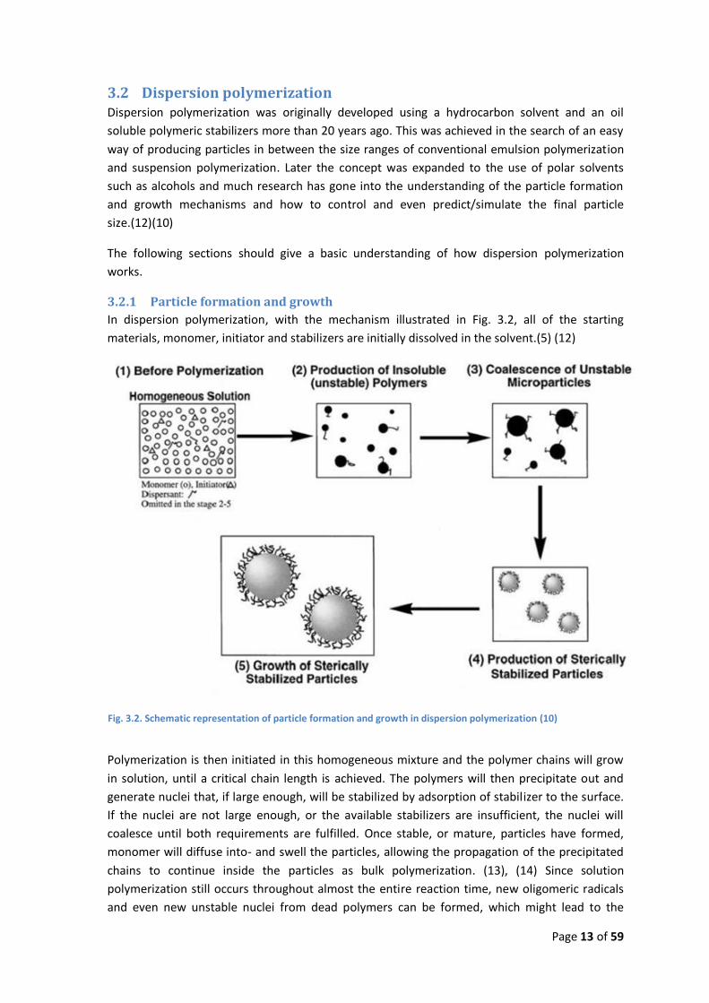
3.2.1 Particle formation and growth
In dispersion polymerization, with the mechanism illustrated in Fig. 3.2, all of the starting
materials, monomer, initiator and stabilizers are initially dissolved in the solvent.(5) (12)
Polymerization is then initiated in this homogeneous mixture and the polymer chains will grow
in solution, until a critical chain length is achieved. The polymers will then precipitate out and
generate nuclei that, if large enough, will be stabilized by adsorption of stabilizer to the surface.
If the nuclei are not large enough, or the available stabilizers are insufficient, the nuclei will
coalesce until both requirements are fulfilled. Once stable, or mature, particles have formed,
monomer will diffuse into- and swell the particles, allowing the propagation of the precipitated
chains to continue inside the particles as bulk polymerization. (13), (14) Since solution
polymerization still occurs throughout almost the entire reaction time, new oligomeric radicals
and even new unstable nuclei from dead polymers can be formed, which might lead to the
Fig. 3.2. Schematic representation of particle formation and growth in dispersion polymerization (10)

Page 14 of 59
production of secondary particles. However, under favorable conditions, these products of
solution polymerization will be scavenged by already existing larger particles.(15) This will
continue until all monomer is used.
Simulations and experimental work carried out by others indicates that the particle count is
fixed early in the reaction before 1 % conversion, and that it can take up to 20 times longer for
the particles to achieve monodispersity. The reason for this is that particles of different sizes
grow at different rates, since the adsorption of monomer and scavenging of oligomeric radicals
and dead polymers from solution is governed by diffusion. This will allow the smaller particles to
catch up in size, given enough time.(10)
3.2.2 Mechanism of stabilization
Stabilization is crucial in understanding the particle formation stage and it is generally accepted
that this can happen in two different ways.
First there is the anchoring of a block or graft co-polymer, where one end of the polymer is
highly soluble in the reaction medium, whereas the other end (the anchor) is not. This leaves
the anchor more or less buried within the particles, while the soluble part protrudes out from
the surface.(14) The block-type co-polymer is mostly of lower MW and the anchoring is
somewhat reversible, making this type a typical co-stabilizer(13). The graft co-polymer is, on the
other hand, typically produced in situ, by chain transfer of active radicals to a soluble polymer of
higher MW, containing active α-hydrogens as possible chain transfer sites.
Chain transfer occurs when an active radical extracts a hydrogen atom, facilitating a homolytic
cleavage of the bond between the α-carbon and the α-hydrogen. This produces an H-terminated
compound (where the radical were before) and a new radical on the α-carbon. This new radical
is, due to electron donating properties of the functional group, stable enough to propagate with
monomer in solution.(16)
Fig. 3.3. PVP (left) and PAA (right) with the α-hydrogen highlighted in red
In polar solvents the, water and short-chain-alcohol soluble, polymer PVP (polyvinylpyrrolidone)
is often used as a steric stabilizer, although many other polymers can be used. Among those, is
PAA (polyacrylic acid) an interesting candidate, since it is a polyelectrolyte and stabilization thus
is achieved by electrostatic forces instead of simply steric means. In Fig. 3.3 the α-hydrogen of

Page 15 of 59
PVP and PAA is highlighted as a red H, while Fig. 3.4 is a schematic representation of the graft
co-polymer in mention (proportions not to scale). The anchor part in the graft co-polymer is
typically of much higher molecular weight than its counterpart from block co-polymers and is
initially incorporated into the particle as an active radical chain end, which will propagate further
inside the monomer swollen particle. This will make the anchor part covalently linked to the
particle, making removal of the stabilizer from the particle highly unlikely.(14) The covalently
linked stabilizers will behave as a “hairy” layer surrounding the particle(15), giving the particle
some of the core/shell properties seen in emulsifier free emulsion co-polymerization of
hydrophobic and hydrophilic monomers, as described earlier. The thickness of this layer
depends on the MW of the stabilizer.
Fig. 3.4. Schematic representation of a particle (grey) with a graft co-polymer, where the anchor part (black) is buried inside the particle and the soluble part (red) is protruding from the surface
The second form of stabilization employed is the loose, and highly reversible, adsorption of
soluble polymers to the particle surface. Some of the stabilizers used to make graft co-polymers
are also believed to have some stabilizing effect by this method, and the two stabilization
mechanisms are not necessarily mutually exclusive. (14) Other polymers, such as PEG’s, will only
act as an adsorbed steric stabilizer as they lack the active α-hydrogen.
3.2.3 Factors influencing particle size
Every single reaction parameter in dispersion polymerization is important when considering the
size of the particles. Seemingly small changes can have great effect, as explained in the
following. For simplicity, charts, examples and explanations will be given from a system of PVP
stabilized PMMA particles in methanol with AIBN as initiator, unless otherwise stated.(17)
3.2.3.1 Reaction temperature
The temperature of the reaction will primarily affect the particle formation stage in the following
ways. The viscosity of the medium will decrease, allowing a higher diffusion rate of
nuclei/particles in the aggregation process. This will produce fewer but larger particles. The
increase in diffusion rates will also make early termination of the PVP-g-PMMA more likely. The
latter effect is enhanced even more by the increase in dissociation rate of the initiator into
radical fragments, leading to the same effect as seen with increased initiator concentration.

Page 16 of 59
Fig. 3.5. Effect of reaction temperature on particle size. Data collected from Shen, et al., 1993
The solvency of the medium will also be affected by temperature in such a way, that the critical
chain length before precipitation will increase, making the nuclei larger from the beginning, just
as the solubility of PVP will increase making adsorption to the particle surface less likely,
prolonging the aggregation time, again producing fewer but larger particles. If the temperature
is too high, the aggregation phase will continue in the lack of sufficient stabilization, resulting in
massive coagulation.(17) The combined effects on size can be seen in Fig. 3.5.
3.2.3.2 Initiator concentration
When the initiator concentration increases, particles size increase as well, as shown in Fig. 3.6.
This can be explained by two processes involved in the particle formation stage. Firstly, the
increased radical concentration will speed up the production of precipitated oligomeric radical
chains, giving more material to aggregate. Secondly, the chance of early termination, of the
stabilizer graft co-polymer, produces shorter anchor chains, increasing the solubility of the entire
graft co-polymer, thus decreasing the adsorption rate.
Fig. 3.6. Effect of AIBN concentrations on particle size at two different PVP-K30 (40 kDa) concentrations, keeping all other reaction parameters constant. Reproduced by data obtained from Shen, et al., 1993
Together this will prolong the aggregation process leading to larger, but fewer particles at the
point where sufficient stabilization is obtained to produce mature particles. Because of the
lower number density and thus a lower total surface area, the scavenging of new nuclei and
dead polymers will be less likely. If the initiator concentration reaches a certain threshold, the
scavenging will be so ineffective that new nuclei will be able to grow to mature particles
2,5
3
3,5
4
4,5
45 50 55 60 65
Size
(μ
m)
Temperature (°C)
2
3
4
5
6
7
8
9
0 0,1 0,2 0,3 0,4 0,5 0,6 0,7
Size
(μ
m)
Initiator concentration (wt. %)
4%
6%

Page 17 of 59
themselves, resulting in an increase in particle size distribution. A similar effect has been
observed for PS particles. (15) (17)
3.2.3.3 Concentration and molecular weight of stabilizer
The size dependency of the concentration and molecular weight of the stabilizer is a
combination of changes in adsorption rates of stabilizer onto the particle surface (primarily
concentration) and the viscosity of the medium. As expected, Fig. 3.7 shows the particle size to
decrease with an increase in both concentration and molecular weight of PVP.(17)
Fig. 3.7. Effect of concentration and molecular weight of PVP on particle size. Reproduced by data obtained from Shen, et al., 1993
This effect is however not considered to be universal amongst all combinations of monomer and
stabilizer. In the work of Paine, et al., 1990, the styrene/PVP system behaves somewhat similar,
but others have seen almost no dependency on concentration. It is however difficult to directly
compare results from different experiments, as several other reaction parameters vary,
especially the type, concentration or absence of a co-stabilizer.
3.2.3.4 Monomer concentration
Changing the initial monomer concentration will primarily affect the solvency of the medium,
increasing the critical chain length with increasing monomer concentration.(15) Some systems
have, however, shown an inverse tendency at the lower monomer concentration range. This is
illustrated in Fig. 3.8 for a PMMA/PVP system.(17)
Fig. 3.8. Effect of initial monomer concentration on particle size. Reproduced by data obtained from Shen, et al., 1993
2
3
4
5
6
0 2 4 6 8 10 12
Size
(μ
m)
PVP concentration (wt. %)
K-30 (40 kDa)
K-90 (360 kDa)
2,5
3
3,5
4
4,5
5
2,5 5 7,5 10 12,5 15 17,5 20 22,5
Size
(μ
m)
Monomer concentration (wt. %)
Page 18 of 59
This phenomenon is thought to be caused by a competition between the change in solvency, as
mentioned above, and a change in propagation rate of the polymer, which also has an impact on
the length of the anchor part of PVP-g-PMMA. At low monomer concentrations the anchor is
short and the stabilization less efficient, leading to larger particles.(17)
3.2.3.5 Solvent system
Dispersion polymerization can be carried out in many different solvent systems and solvency can
affect particle size primarily by changing the critical chain length before precipitation of polymer
and by changing the solubility of the stabilizer and/or grafted stabilizer. A mixture of water and
methanol is commonly used for the preparation of smaller particles.(17)

Page 19 of 59
3.3 Preparation of PVP stabilized PMMA particles With the basics of dispersion polymerization and size control in mind a set of experiments were
conducted. The aim of this was to investigate if the preparation of monodisperse PMMA
particles with sizes above 6 µm is possible, and if the co-polymerization of MMA with MAA and
NaMA would yield particles with charges embedded in the core.
Two sets of standard recipes were made, one with NaMA, called PMMA-A, and one with MAA,
called PMMA-B. The ingredients used can be found in Table 3.1. The MAA was passed through a
short column of activated aluminum oxide to remove the hydroquinone inhibitor. All other
chemicals were used as received.
PMMA-A and PMMA-B
Ingredient Weight (g) MMA 15 MAA/NaMA 0,375 PVP (65 kDa) 4 AIBN 0,2 MeOH 80,5
Table 3.1. List of ingredients in the standard recipes
In the first batch, MMA, NaMA, PVP and most of the MeOH was mixed, at room temperature, in
a 250 mL two-necked round bottomed flask, purged with nitrogen for 15 minutes and heated to
60 °C. Then AIBN was dissolved, at room temperature, in the remaining MeOH (approx. 6 mL),
purged with nitrogen for 15 min and added to the already heated mixture.
This procedure was, due to lack of workspace, however not possible for the batch containing
MAA. Here all ingredients were mixed at once and then subsequently heated to reaction
temperature.
The mixtures were allowed to react under nitrogen for 48 hours, before being cooled on ice,
under normal atmosphere. The particles were cleaned by a repeating sedimentation/
redispersion process in methanol and stored in sealed PP-containers. The cleaning process will
apply to all particles produced throughout this work, although some batches were stored in
sealed glass bottles instead of PP-containers.
Several attempts to produce particles under more extreme conditions, such as less stabilizer,
more initiator, higher temperature and combinations of these, were conducted, with all but one,
called PMMA-C, ending in massive coagulation. Although some coagulation did also form in this,
it was possible to separate the particles and clean them as described above. The ingredients can
be found in Table 3.1, with the setup and temperature being the same as with the standard
recipes.

Page 20 of 59
PMMA-C
Ingredient Weight (g) MMA 20 MAA/NaMA 0,5 PVP (65 kDa) 6 AIBN 0,6 MeOH 73
Table 3.2. List of ingredients in the one successful batch under more extreme conditions
Here the concentration of monomer, co-monomer and AIBN is increased which, according to the
theory described in section 3.2.3, should lead to larger particles. To keep the system stable and
avoid total coagulation, an increased amount PVP were added as well.
On top of the more extreme conditions mentioned above, a batch of seeded polymerization,
called PMMA-seeded, was synthesized as well. The principle being, that the second addition of
reactants will prolong the growth stage, yielding larger and more monodisperse particles. The
ingredients for the first and second stage are listed in Table 3.3
PMMA-seeded
Ingredient Weight, stage 1 (g) Weight, stage 2 (g) MMA 15 5 MAA/NaMA 0 1 PVP (65 kDa) 4 1 AIBN 0,4 0,025 MeOH 83 16
Table 3.3. List of ingredients used in the seeded polymerization of PMMA
The setup and temperature was the same as with the standard recipes, with the exception, that
the second stage was added after 24 hours but the total reaction time remained 48 hours.
Page 21 of 59
Fig. 3.9. Sizes obtained for PMMA-A and PMMA-B. Note that the cumulative percentage is displayed on a secondary axis.
3.4 Analysis of the prepared PMMA particles The analysis methods described below will apply to all particles throughout this work, unless
otherwise stated.
3.4.1 Sizes
The particle sizes were measured on a Microtrac II – particle size analyser II and are reported
here as the volume percentage of particles in different size classes, as well as the cumulative
volume percentage. Further information on the equipment can be found in Appendix C. The
median particle diameter is reported as d50, the diameter at which the cumulative volume
percentage reaches 50 %. The degree of polydispersity is reported as the geometric standard
deviation (GSD), with a value of 1.1 being considered monodisperse, and is calculated from
, as done in the work of Paine, 1990.
Fig. 3.9 shows the measured sizes of the PMMA-A and PMMA-B particles as well as the d50 and
GSD value. Monodispersity is not achieved and there are seemingly two different groups of
particles sizes, one smaller fraction around 3 µm and one larger around 8-10 µm. The smaller
particles of PMMA-B, compared to PMMA-A can be ascribed to the differences in the method
used.
To confirm that the produced particles are spherical, SEM micrographs were taken of PMMA-A
and PMMA-B. The micrograph of PMMA-A is seen in Fig. 3.10 and shows that the particles are
indeed spherical as expected. Furthermore, it supports the measured size data from above with
a group of smaller particles and a group of larger ones. It is assumed that particles from the
other batches are spherical as well.
0
20
40
60
80
100
0
10
20
30
40
50
0,9 1,9 3,9 7,8 16 31
Vo
l %
Vo
l %
Size, μm
MMA-A d50 = 8.11 --- GSD = 1.85
0
20
40
60
80
100
0
10
20
30
40
50
0,9 1,9 3,9 7,8 16 31
Vo
l %
Vo
l %
Size, μm
MMA-B d50 = 6.64 --- GSD = 2.08

Page 22 of 59
Fig. 3.10. SEM micrograph of the PMMA-A particles
The measured sizes from PMMA-C are displayed in Fig. 3.11 and is a broad distribution of
different sizes ranging all the way from 1 µm to above 30 µm
Fig. 3.11. Sizes obtained for PMMA-C. Note that the cumulative percentage is displayed on a secondary axis.
The sample taken from PMMA-seeded just before the addition of the second stage, were
apparently not properly cleaned, as the particles sedimented in a non-reversible manner before
any size measurements could be obtained. The final product was analyzed with the results
shown in Fig. 3.12. The particles produced are significantly larger than the ones from the PMMA-
B batch and the GSD is smaller, but there is still a group of smaller particles present, as seen in
PMMA-A and PMMA-B.
0
20
40
60
80
100
0
10
20
30
40
50
0,9 1,4 1,9 2,8 3,9 5,5 7,8 11 16 22 31 44 62
Vo
l %
Vo
l %
Size, μm
PMMA-C d50 = 5.38 --- GSD = 2.24
Page 23 of 59
Fig. 3.12. Sizes obtained for PMMA-seeded. Note that the cumulative percentage is displayed on a secondary axis.
3.4.2 Charges
The amount of carboxylic acids on and inside the particle was measured by pH titration with 0.1
M NaOH. Further information about the equipment is available in Appendix C. A part of the
original particle dispersion was diluted, with a 0.1 M aqueous NaClO4 solution, to 20 mL with a
dry matter content of approximately 6 g/L. The pH of the sample was then lowered to below 3,
with a 0.1 M HClO4 solution, prior to titration.
The resulting titration plots, an example of which, for PMMA-B, can be seen in Fig. 3.13 show no
sign of any noticeable amount of carboxylic residue. Only the equivalence point of the strong
acid HClO4 is visible. This indicates that the co-polymerization with NaMA and MAA has been
unsuccessful. This is also true for PMMA-A, PMMA-C and PMMA-seeded
Fig. 3.13. pH titration of the PMMA-B particles
0
20
40
60
80
100
0
10
20
30
40
50
0,9 1,4 1,9 2,8 3,9 5,5 7,8 11 16 22 31 44 62
Vo
l %
Vo
l %
Size, μm
PMMA-seeded d50 = 12.56 --- GSD = 1.63
0
2
4
6
8
10
12
14
0 0,5 1 1,5 2 2,5
pH
Titrant volume added (mL
PMMA-B
Page 24 of 59
3.5 Challenges with the method in use The produced particles, described in section 3.3 and 3.4 does not fulfill the aim of this work, as
they are neither monodisperse nor charged, although the literature in general claim this to be
possible(9). The following sections will present the challenges met, as well as give some ideas on
how to solve them.
3.5.1 Keeping the particles monodisperse
As mentioned before, monodispersity is generally achieved by a higher growth rate of the
smaller particles, relative to the larger ones. It can however be difficult to keep the system this
way, since both secondary particle formation and large particle coalescence can occur, if the
reaction parameters are not carefully controlled. To understand what happens, a more detailed
view of, especially, the balance between the aggregation and stabilization processes is required.
Fig. 3.15 show a simulated overview of the dispersion polymerization process, with several
properties of the particles and the system, plotted on a log-log scale, as a function of the degree
of conversion. The numbers above the lines refer to the slope. These simulations and the graphs
are part of the work done by Paine, 1990. In the simulations it is assumed, that stabilization is
done entirely by the graft co-polymer, made from chain transfer to the stabilizer polymer, and
that the produced graft is adsorbed immediately onto the particle surfaces. The production (and
efficiency) of this graft co-polymer is not only directly affected by the factors mentioned in
section 3.2.3, but also, to a large degree, the locus of polymerization, as it can only happen in
solution. If the particles grow mainly by absorption of monomer, and hence solid phase
polymerization within the particles, no grafted stabilizer can be produced. This locus of
polymerization is, however, also more or less affected by these factors, making the control of
the process even more complex. The graft co-polymer responsible for stabilization may, in the
following sections, be referred to only as graft.
3.5.1.1 Simulation with a monodisperse
product
The first graph, Fig. 3.14, is a simulation, where all
the reaction parameters are correctly
chosen/controlled, resulting in monodisperse
particles. The point A is the point where the
available graft exceeds the graft needed, Qmin, to
avoid coalescence of similar sized particles or, in
other words, where the particles become mature.
After this point, the locus of polymerization is likely
to shift from entirely solution polymerization, to a
mix between solution and solid phase
polymerization, with the latter being the dominant
at a higher degree of conversion. This is indicated
by a reduction of the slope of the line
corresponding to the available graft. The particles
will however remain monodisperse, as long as the
available graft is within the band between Qmin and Fig. 3.14. Simulated overview of a dispersion polymerization process, resulting in monodisperse particles (9)

Page 25 of 59
Qmax, with the latter being the maximum amount of grafted stabilizer it is possible to fit on the
particle surface. A further explanation of these terms is given in section 3.5.1.4. (10)
Choosing reaction conditions, not within the boundaries of those giving the situation outlined
above, would result in a polydisperse final product or, in the extreme case, total coagulation.
This complies well with the observation made, when trying to produce particles under more
extreme conditions than normally found in literature, as in section 3.3. In the case of a
polydisperse final product, two things can happen as illustrated in Fig. 3.15.
3.5.1.2 Simulation with secondary particle formation
The left part (Fig. 3.15 A) is a simulation of a dispersion polymerization process where solution
polymerization remains dominant throughout the entire reaction time. The slope of the
available graft will remain 1 and eventually reach Qmax at point B1. The already mature particles
can then no longer adsorb the produced graft, and the graft will instead adsorb to the smaller
nuclei being produced as a product of solution polymerization. Under normal conditions, the
larger particles can only scavenge the nuclei because they are not yet stabilized, so when this
happens, the scavenging stops, and a new population of small mature particles will appear. This
is shown by a jump in particle count along with a corresponding jump in Qmin and Qmax, as the
total surface area will increase as well. This can happen several times (point B2) during the
reaction, giving rise to several populations of particles each with their own class of sizes.(10)
Fig. 3.15. Simulated overview of a dispersion polymerization process, resulting in polydisperse particles due to: A- secondary stabilization (left) and B- large particle coalescence (right) (9)
Page 26 of 59
3.5.1.3 Simulation with large particle coalescence
The right part (Fig. 3.15 B) is the opposite situation where the solid phase polymerization
becomes to dominant too soon (point C), greatly limiting the production of grafted stabilizer, as
indicated with a slope of 0 in the extreme case, with no graft being produced at all. The particles
will continue to grow, by absorption of monomer and subsequent solid phase polymerization,
until the surface area of the particles becomes too large and Qmin exceeds the graft available at
point D. The particles will then become unstable again, as in the beginning of the process, and
coalescence will occur, reducing particle count.(10)
3.5.1.4 Estimating Qmin and Qmax
If the above mentioned simulations should be of any proper practical value, an estimate of Qmin
and Qmax, for the system in use, will be needed. According to Paine, 1990, the value of Qmin is
thought to be linked to the area projected on the particle surface by the hemisphere defined by
the radius of gyration, rg, of the stabilizer polymer in solution. So when the sum of projected
areas equals the surface area of the particle, the particle is assumed to be stable.
The radius of gyration can be calculated as , with a being a proportionality
constant, Mw being the molecular weight of the stabilizer polymer and b being the exponent
relating Mw to rg. a and b are material dependent and can be measured experimentally The
values used here are taken from literature as and , both in MeOH(18).
Significantly lower values of rg have been reported (19), but are not considered here. Since the
chain transfer can happen anywhere on the stabilizer chain, rg of the grafted stabilizer will, on
average, be 75 % of that of the ungrafted stabilizer, leading to . Qmin is then
given by with the units of grafts pr m2. (10) The PVP used in section 3.3 has a molar
weight of 60 kDa giving a rg of 16.3 nm and a Qmin of approximately 1200 grafts/µm2 as opposed
to 14.6 nm and 1500 grafts/µm2 for the 40 kDa PVP used in the referred work of Paine, 1990.
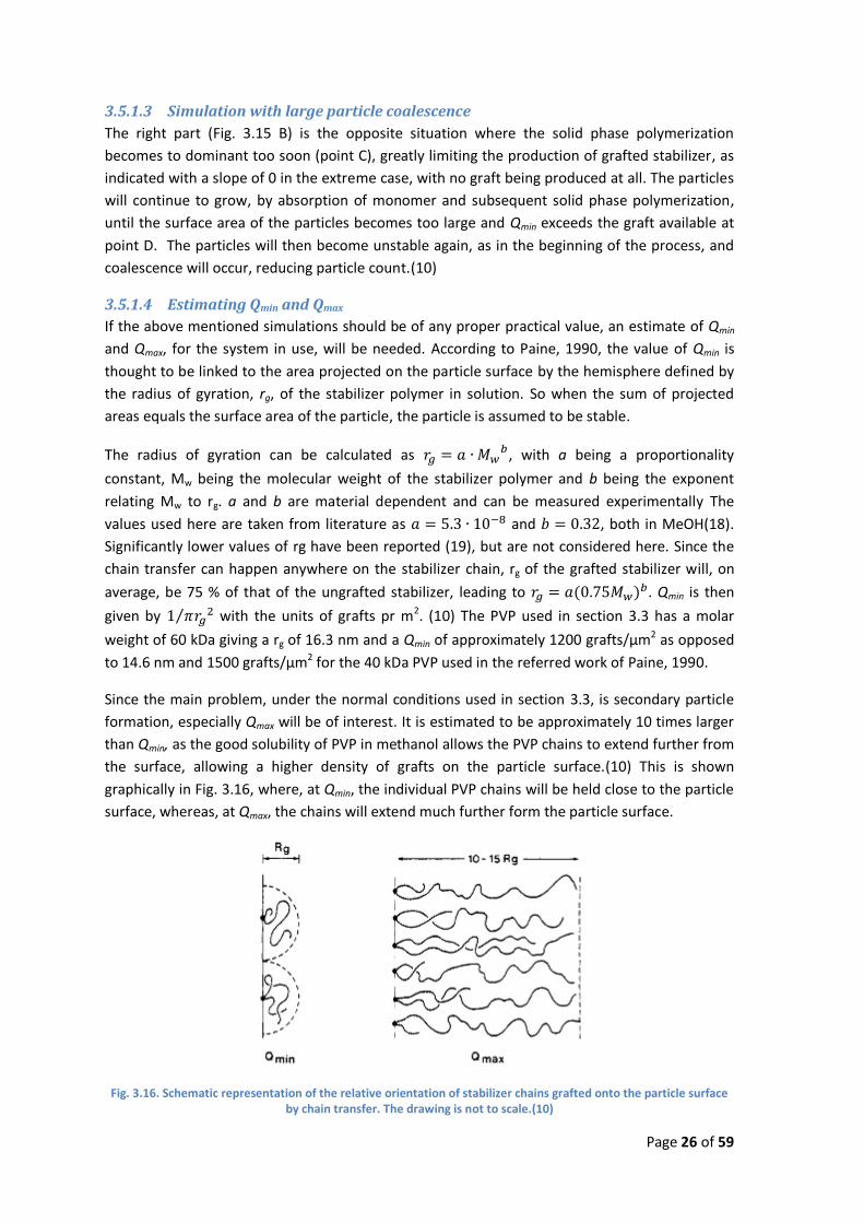
Since the main problem, under the normal conditions used in section 3.3, is secondary particle
formation, especially Qmax will be of interest. It is estimated to be approximately 10 times larger
than Qmin, as the good solubility of PVP in methanol allows the PVP chains to extend further from
the surface, allowing a higher density of grafts on the particle surface.(10) This is shown
graphically in Fig. 3.16, where, at Qmin, the individual PVP chains will be held close to the particle
surface, whereas, at Qmax, the chains will extend much further form the particle surface.
Fig. 3.16. Schematic representation of the relative orientation of stabilizer chains grafted onto the particle surface by chain transfer. The drawing is not to scale.(10)
Page 27 of 59
By using the Qmin of the 60 kDa PVP, it can be calculated, that the minimum amount of grafted
PVP needed per m2, to avoid coalescence of similar sized particles, is 0.12mg/m2. For a batch of
particles produced from 20 mL styrene with a particle diameter of 5 µm, the total surface area
will be close to 21 m2. The minimum amount of grafted PVP for such a batch will then be 2.5 mg.
If the probability of chain transfer is approximately 1 in every 100 PVP chains, as estimated by
(10), the amount of PVP (60 kDa) used in a batch from 20 mL styrene should be between 0.25
and 2.5 g to keep the particles monodisperse.
3.5.1.5 Testing the estimation
Unfortunately it was not possible to find an estimation of the probability of chain transfer when
using MMA, but the maximum amount of grafted PVP is calculated to be 17 mg for a batch made
from the recipes of PMMA-A and PMMA-B in section 3.3, or 23 mg if using 20 mL monomer
instead. If the chain transfer probability is in the same range as with PVP/styrene this would
indicate that too much PVP were used in these recipes. This is consistent with the observation of
secondary particle formation. A series of experiments were conducted to investigate the effect
of a lower amount of PVP, all ending in massive coagulation within the first 30 minutes after the
initial particle formation stage. It seems that the process of dispersion polymerization using
MMA is less well behaved than when using styrene. Firstly, the chain transfer probability can
probably be assumed to be less than 1:100, as all attempts to use less PVP than in the recipes of
PMMA-A and PMMA-B failed very early in the process, indicating that the graft available never
reached Qmin. Secondly, solution polymerization might be more favored in the later part of the
process when using MMA compared to similar recipes using styrene.
Even though the point A, in Fig. 3.14 and Fig. 3.15, is not as sharp in reality as it is defined here,
the window of particle formation is still very short compared to that of particle growth. The
increase in total surface area as a function of conversion, , will therefore be very high in
the beginning of the process, before 1 % conversion is obtained. Since Qmin, and Qmax is
proportional to the total surface area, a lot of graft will have to be produced within this window
of time to keep the system from total coagulation. Even though the simulations only take the
grafted stabilization into account, which might not be at correct assumption, there is still a
tendency to an overproduction of graft at the end, if the PVP concentration is as high as needed
in the beginning. This could be overcome by adding a co-stabilizer which will adsorb more
strongly than ungrafted PVP, thus enabling a lower concentration of PVP. Another solution could
be to use a macromonomer with stabilizing properties, making a comb/brush polymer by the co-
polymerization with the normal monomer, allowing the comb/brush polymer to adsorb very
strongly to the particle, or even anchor to the particle if the branches are far enough from each
other (20). An example of a comb/brush polymer is shown in Fig. 3.17, with every fourth unit in
the backbone being a macromonomer.

Page 28 of 59
n
n n
R R R R R R
O
O
O
O
O
O
Fig. 3.17. Schematic representation of a comb/brush polymer
3.5.2 Implementing charges on the surface
Particle charge is probably one of the most important properties needed for the purpose of this
work. The lack of co-polymerization with MMA/MAA/NaMA was unexpected and unfortunate,
as this could have resulted in particles, where the charge and water swellability, could have been
adjusted by changing the pH value.
3.5.2.1 Using a higher fraction of MAA
Three syntheses, using the same recipes and method as in section 3.3, with a few exceptions
stated below, but with an increased amount of MAA relative to MMA, were conducted to see if
this would yield particles with the properties in question. An overview of the batches can be
found in Table 3.4.
MMA:MAA (mol) Weight of MAA (g) Charges Size / GSD Coagulation
1:0.03 0.387 None 11.3 µm / 2.07 Small 1:0.05 0.645 None 20.3 µm / 1.44 Medium-high 1:0.07 0.903 None - Total
Table 3.4. An overview of three batches made to determine the influence of an increased MAA content
Prior to this, the AIBN had been recrystallized in methanol to remove some insoluble residue.
Furthermore, the MMA were used without removal of the inhibitor, as this will slow the onset of
particle formation, ensuring that the temperature is allowed to rise again after the addition of
the AIBN solution. This will have affected the results in such a way, that the batch with the same
molar ratio of as that in PMMA-B, have produced significantly larger particles than before,
which, however, also could be caused by the fact that the PMMA-B batch were heated after
addition of AIBN, whereas this batch were heated before.
Apart from that, no acidic groups were found by titration, and an increase in the MAA fraction
seems to have the same effect as reducing the PVP content, when regarding size and amount of
coagulation. The GSD decreased when going from 1:0.03 to 1:0.05, which is due to a much
smaller degree of secondary particle formation with the higher fraction of MAA, again showing
the same effect as when reducing the PVP content.
These findings stand in contrast with the work done by Kun, et al., 2000, where too much MAA
increased secondary stabilization and where the acidic groups were both adsorbed and
anchored to the particle surface, as well as buried within the particle core. The only difference is
that Kun, et al., 2000 used a mixture of methanol and water in a 7:3 weight ratio, which,
however, might explain the additional stabilizing effect, as this will make the system resemble

Page 29 of 59
emulsifier free emulsion polymerization a bit more. This will shift the locus of the polymerization
of MMA more towards the solid phase (especially in the later stages), whereas the MAA will
continue to have a higher solubility in the continuous phase, generating chains with a much
higher fraction of MAA subunits.
The batches made in this work does not contain any water, and it is suspected, that the reaction
shown in Fig. 3.18, between PVP and MAA, can occur, with the former being a weak base and
the latter being a weak acid.
NH
+ O
H n
+CH2 CH3
O-
ON
O
H n
+CH2 CH3
OHO
Fig. 3.18. Suspected reaction between PVP and MAA
If the MAA is able to protonate some of the subunits in the PVP polymer, creating a salt where
the MAA is associated to the PVP subunit, then the diffusivity of MAA will be greatly reduced
and with it, the chance of incorporation. The protonated PVP subunit will, furthermore, render
the α-hydrogen inactive, reducing the chance of chain transfer. At the end of the reaction, the
cleaning process will remove most, if not all, of the added MAA.
It is unknown why the NaMA in PMMA-A is not incorporated into the particles, but since it is a
salt, it might not be soluble enough in the polymer, making up the particles, to be efficiently
incorporated, and could therefore be removed during the cleaning process.
3.5.2.2 Polyacrylic acid as stabilizer
In section 3.2.2, PAA is mentioned as a possible stabilizer, with the same general grafting
mechanism as PVP. PAA does also contain an active α-hydrogen and is as such prone to chain
transfer as well. The use of PAA instead of PVP has the advantage that the particles will have a
charged shell, even without the use of MAA as a co-monomer. The particle core will however
not be affected and the particles will have a higher resemblance of those made by Hinge, et al.,
2006
All attempts of using PAA as stabilizer in combination with MMA failed, regardless of the PAA
concentration. It was then found that styrene has a higher chain transfer rate, to some
compounds, than MMA (16), which was also indicated by the results discussed in section 3.5.1.5,
making the PS/PAA couple a possible candidate instead.
The drawback, of this method to introduce charges, is that the charge density can be hard to
control and is probably linked with particle size, making particles with varying size/charge
density ratios hard to obtain in a controlled manner.
Page 30 of 59
3.6 Preparation of PAA stabilized PS particles A new set of synthesis were conducted, with the general aim being the same as in section3.3,
except for the co-polymerization with MAA. This time, styrene was the main monomer and PAA
the stabilizer.
All the ingredients, except AIBN, were mixed in a 250 mL two-necked round-bottomed flask
equipped with a magnetic stirrer and heated to reaction temperature while being purged with
nitrogen. At the same time, the AIBN was dissolved in 10 mL methanol at room temperature,
and purged with nitrogen for the same time as the main mixture. When the reaction
temperature was reached, the AIBN solution was added to the main mixture and kept under
nitrogen atmosphere. After approximately 24 hours, when the mixtures no longer smelled of
styrene, the conversion was assumed complete and any remaining free radicals were quenched
by addition of 5 mL 50 g/L hydroquinone solution in methanol. The cooled dispersions were
cleaned, as in the other synthesis, by a repeating sedimentation/redispersion process in
methanol. All the chemicals were used as received, except AIBN, which were recrystallized in
methanol before use.
At first a PAA with a molecular weight of 25 kDa were used with mixed results. Generally, a lot of
coagulation occurred, but at higher stabilizer concentrations it was possible to salvage some of
the particle dispersion. Two of the batches yielded a recoverable amount. These are called, PS-A
and PS-B and the reaction conditions can be found in Table 3.5 and Table 3.6
PS-A (60 °C)
Ingredient Weight (g) PS 15 PAA (25 kDa) 4 AIBN 0.2 MeOH 80.4
Table 3.5. Reaction conditions for PS-A
PS-B (70 °C)
Ingredient Weight (g) PS 18 PAA (25 kDa) 6 AIBN 0.2 EtOH 79
Table 3.6. Reaction conditions for PS-B
Then a PAA with a molecular weight of 100 kDa, as a 35 w/w % solution in water, were used for
the batches called PS-C and PS-D, with the reaction conditions found in Table 3.7 and Table 3.8.
For these batches, no coagulation at all was observed.
PS-C (60 °C)
Ingredient Weight (g) PS 20 PAA (100 kDa) 3.5 AIBN 0.3 MeOH 100 Water (from PAA) 6.5
Table 3.7. Reaction conditions for PS-C
Page 31 of 59
PS-D (60 °C)
Ingredient Weight (g) PS 25 PAA (25 kDa) 3.5 AIBN 0.3 MeOH 100 Water (from PAA) 6.5
Table 3.8. Reaction conditions for PS-D
3.7 Preparation of PAA and macromonomer stabilized PS In section 3.5.1.5, it was stated that the use of a macromonomer with stabilizing properties,
could help keeping the system stable during the initial phases of the dispersion polymerization
process. In order to test if this statement is true, such a macromonomer would first have to be
synthesized, as the commercially available products are very expensive, in addition to being of
relatively low molecular weight.
It was decided to combine a monomethyl ether PEG (5 kDa) with methacrylic anhydride, creating
a PEGMA macromonomer. This is done by esterification of the hydroxyl group on the PEG, with
Pyridine as base and dimethylaminopyridine (DMAP) as nucleophilic catalyst. The chemicals used
for this can be found in Table 3.9.
PEGMA
Ingredient Amount PEG (5 kDa) 25 g Methacrylic anhydride 4 mL Pyridine 20 mL DMAP 6.1 g Dichloromethane 150 mL Table 3.9. List of chemicals used in the synthesis of PEGMA
All of the ingredients were mixed in a 250 mL two-necked round-bottomed flask, equipped with
a magnetic stirrer, purged with nitrogen for 20 min, and heated to 60 °C. The mixture was then
allowed to stand at this temperature, in nitrogen atmosphere, for 72 hours. The product and any
unreacted PEG’s, was precipitated with diethyl ether at room temperature, redissolved in
chloroform and precipitated again to minimize pollution by pyridine and DMAP.
The synthesized PEGMA were used along with PAA (25 kDa), with the reaction conditions shown
in Table 3.10. No coagulation was observed.
PS-co-P(PEGMA) (60 °C)
Ingredient Weight (g) PS 20 PAA (25 kDa) 4 PEGMA 4 AIBN 0.3 MeOH 100
Table 3.10. reaction conditions for PS-co-P(PEGMA)

Page 32 of 59
3.8 Analysis of the prepared PS particles All of the PS particles were analyzed with regard to size and charge by the same methods as
described in section 3.4.
3.8.1 Size
Fig. 3.19 to Fig. 3.22 show the particle sizes and GSD for the individual batches of PS particles.
Fig. 3.19. Sizes obtained for PS-A. Note that the cumulative percentage is displayed on a secondary axis.
Fig. 3.20. Sizes obtained for PS-B. Note that the cumulative percentage is displayed on a secondary axis.
0
20
40
60
80
100
0
10
20
30
40
50
0,9 1,4 1,9 2,8 3,9 5,5 7,8 11 16 22 31 44 62
Vo
l %
Vo
l %
Size, μm
PS-A d50 = 6.16 --- GSD = 1.73
0
20
40
60
80
100
0
10
20
30
40
50
0,9 1,4 1,9 2,8 3,9 5,5 7,8 11 16 22 31
Vo
l %
Vo
l %
Size, μm
PS-B d50 = 5.81 --- GSD = 1.66
Page 33 of 59
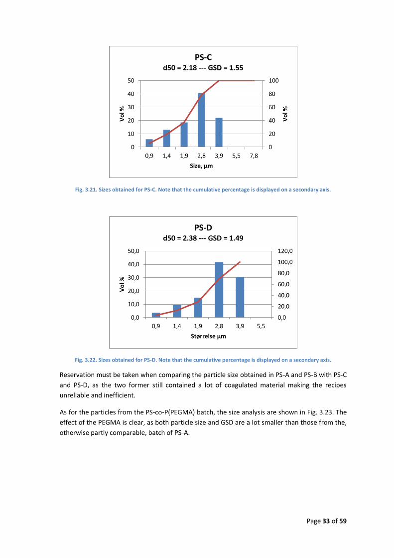
Fig. 3.21. Sizes obtained for PS-C. Note that the cumulative percentage is displayed on a secondary axis.
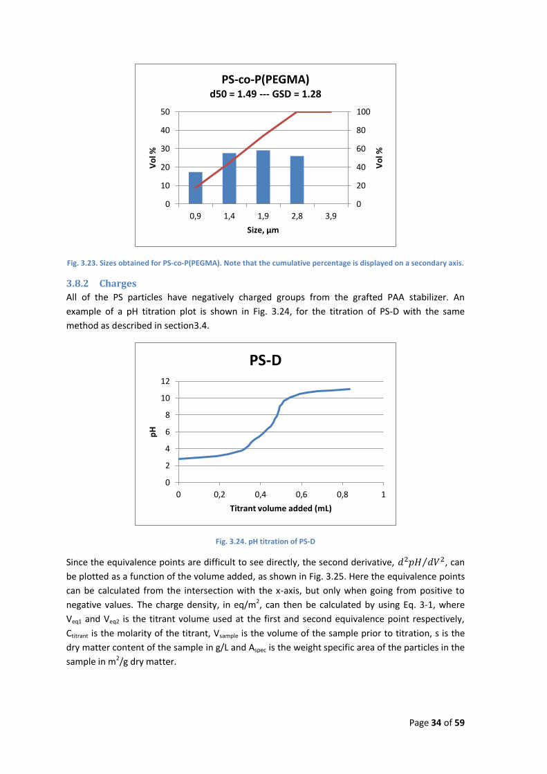
Fig. 3.22. Sizes obtained for PS-D. Note that the cumulative percentage is displayed on a secondary axis.
Reservation must be taken when comparing the particle size obtained in PS-A and PS-B with PS-C
and PS-D, as the two former still contained a lot of coagulated material making the recipes
unreliable and inefficient.
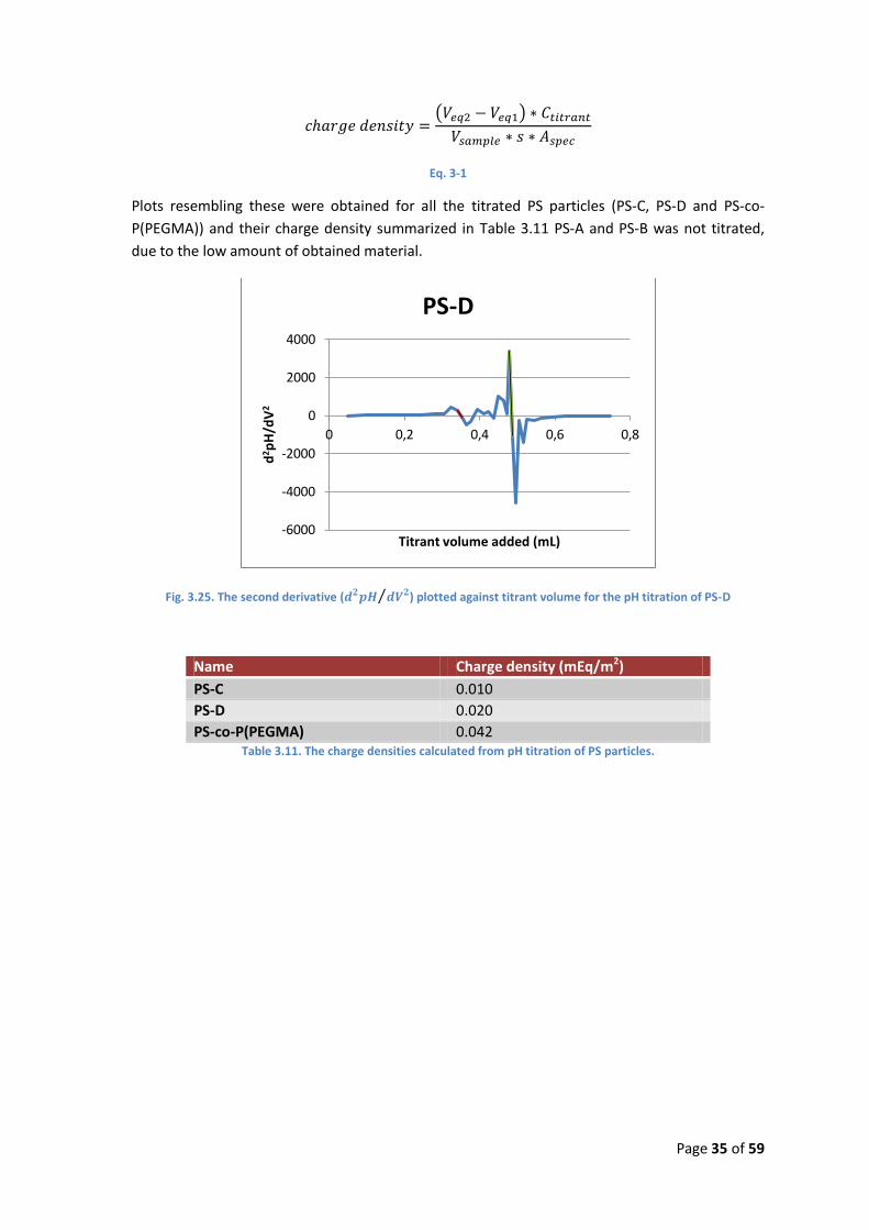
As for the particles from the PS-co-P(PEGMA) batch, the size analysis are shown in Fig. 3.23. The
effect of the PEGMA is clear, as both particle size and GSD are a lot smaller than those from the,
otherwise partly comparable, batch of PS-A.
0
20
40
60
80
100
0
10
20
30
40
50
0,9 1,4 1,9 2,8 3,9 5,5 7,8
Vo
l %
Vo
l %
Size, μm
PS-C d50 = 2.18 --- GSD = 1.55
0,0
20,0
40,0
60,0
80,0
100,0
120,0
0,0
10,0
20,0
30,0
40,0
50,0
0,9 1,4 1,9 2,8 3,9 5,5
Vo
l %
Størrelse μm
PS-D d50 = 2.38 --- GSD = 1.49
Page 34 of 59
Fig. 3.23. Sizes obtained for PS-co-P(PEGMA). Note that the cumulative percentage is displayed on a secondary axis.
3.8.2 Charges
All of the PS particles have negatively charged groups from the grafted PAA stabilizer. An
example of a pH titration plot is shown in Fig. 3.24, for the titration of PS-D with the same
method as described in section3.4.
Fig. 3.24. pH titration of PS-D
Since the equivalence points are difficult to see directly, the second derivative, , can
be plotted as a function of the volume added, as shown in Fig. 3.25. Here the equivalence points
can be calculated from the intersection with the x-axis, but only when going from positive to
negative values. The charge density, in eq/m2, can then be calculated by using Eq. 3-1, where
Veq1 and Veq2 is the titrant volume used at the first and second equivalence point respectively,
Ctitrant is the molarity of the titrant, Vsample is the volume of the sample prior to titration, s is the
dry matter content of the sample in g/L and Aspec is the weight specific area of the particles in the
sample in m2/g dry matter.
0
20
40
60
80
100
0
10
20
30
40
50
0,9 1,4 1,9 2,8 3,9
Vo
l %
Vo
l %
Size, μm
PS-co-P(PEGMA) d50 = 1.49 --- GSD = 1.28
0
2
4
6
8
10
12
0 0,2 0,4 0,6 0,8 1
pH
Titrant volume added (mL)
PS-D
Page 35 of 59
Eq. 3-1
Plots resembling these were obtained for all the titrated PS particles (PS-C, PS-D and PS-co-
P(PEGMA)) and their charge density summarized in Table 3.11 PS-A and PS-B was not titrated,
due to the low amount of obtained material.
Fig. 3.25. The second derivative ( ) plotted against titrant volume for the pH titration of PS-D
Name Charge density (mEq/m2)
PS-C 0.010
PS-D 0.020
PS-co-P(PEGMA) 0.042 Table 3.11. The charge densities calculated from pH titration of PS particles.
-6000
-4000
-2000
0
2000
4000
0 0,2 0,4 0,6 0,8
d2p
H/d
V2
Titrant volume added (mL)
PS-D

Page 36 of 59
3.9 Summarization of the results from dispersion polymerization A lot of interesting and somewhat surprising results were obtained from the dispersion
polymerizations carried out during this project. A summary of the properties and some of the
reaction conditions is found in Table 3.12 and Table 3.13.
Name Solvent Stabilizator Conc, stabilizator * Conc, monomer **
PMMA-A MeOH PVP(60 kDa) 26,7 13,6
PMMA-B MeOH PVP(60 kDa) 26,7 13,6
PMMA-C MeOH PVP(60 kDa) 30 18,8
PMMA-seeded
MeOH PVP(60 kDa) 25,3 (total) 14,4 (total)
PS-A MeOH PAA(25 kDa) 26,67 14,6
PS-B EtOH PAA(25 kDa) 33,33 16,7
PS-C EtOH PAA(100 kDa) 17,5 15,8
PS-D EtOH PAA(100 kDa) 14 19
PS-co-PEGMA
EtOH PAA(25 kDa) + PEGMA 20 + 20 16,7
Table 3.12. Selected properties and reaction conditions of the particles produced. * Wt. % of monomer, ** Vol. % of total liquids, *** d50
Name Conc, co-monomer * Conc, AIBN * Size, µm *** GSD Charge
(mEq/m2)
PMMA-A 2,5 (NaMA) 1,33 8,11 1,85 0
PMMA-B 2,5 (MAA) 1,33 6,64 2,08 0
PMMA-C 2,5 (NaMA) 3 5,38 2,24 0
PMMA-seeded
5 (NaMA) 2 (total) 12,56 1,63 0
PS-A 0 1,33 6,16 1,73 Not measured
PS-B 0 1,1 5,81 1,67 Not measured
PS-C 0 1,5 2,18 1,55 0.010
PS-D 0 1,2 2,38 1,49 0.020
PS-co-P(PEGMA)
0 1,5 1,49 1,29 0.042
Table 3.13. Selected properties and reaction conditions of the particles produced. * Wt. % of monomer, ** Vol. % of total liquids, *** d50
The particles produced from PMMA/PVP were all larger than the PS/PAA particles, although they
were also less monodisperse due to secondary particle formation. Due to lack of time, larger
particles were not obtained by the PS/PAA way, but it should be theoretically possible. It is not
known whether recipes with PS/PAA yielding larger particles, will show the same tendency of
secondary particle formation as with PMMA/PVP.
When using PMMA/PVP there seems to be some maximum obtainable particle sizes, as almost
all attempts with more extreme conditions ended in total coagulation relatively fast. In the only
case where stable particles were obtained, PMMA-C, the size were smaller and the size
distribution wider than for both PS-A and PS-B. The Issue seems to be that, in order to achieve
sufficient stabilization in the beginning of the process, the PVP concentration has to be so high,
that separate groups of particles with different sizes will appear, due to secondary stabilization.

Page 37 of 59
It was speculated that the addition of a co-stabilizer or a macromonomer with stabilizing
properties, could reduce this problem. By comparing PS-A with PS-co-P(PEGMA), this seems
indeed to be the case. PS-A produced larger particles along with an unacceptable amount of
coagulum, while PS-co-P(PEGMA) produces smaller particles with a narrower size distribution
and no coagulum at all. This promises well for the speculation, but more experiments will have
to be conducted to find some consistency in this.
In addition to this, the PS-co-P(PEGMA) particle is believed to have a different morphology in
comparison with the other PS particles. This is because the co-polymerization of styrene and
PEGMA is likely to produce a much denser “hairy” layer of PEG-chains around the particle, while
still keeping the longer chain transfer grafted PAA-chains. If this assumption is true, the particle
might look like the one sketched in Fig. 3.26, with the black lines being PAA and the red ones
being PEG.
Fig. 3.26. Drawing of a possible morphology of the PS-co-P(PEGMA) particles. Note that the proportions are not to scale.
The attempts to co-polymerize MMA with MAA and NaMA, respectively did all fail, as no
titratable acidic groups were found on or in the particles. It is thought that the MAA might react
with PVP, making the PVP less active for chain transfer and creating an association between the
PVP polymer and the MAA, keeping the MMA form being incorporated into the particle. It is,
however, not known why NaMA does not co-polymerizes, as it should not react with PVP in the
same way as MAA, although it is speculated that the solubility of the sodium salt in the main
polymer is too low for it to be incorporated efficiently.
All of the PS particles were charged due to the grafted PAA stabilizer, but the charge density
varies amongst the different batches. Even between PS-C and PS-D there is a factor two
difference, even though the only difference in the recipes is a larger fraction of monomer in PS-
D. According to the mechanism of stabilization, the increased monomer concentration should
actually have the opposite effect, tending to produce larger, but less stabilized particles. If this is
simply a coincidence, or if there is something in the particle growth mechanisms that still are
less understood is not clear, and a more controlled set of experiments will be required to
investigate this further. The difference could also simply be caused by inaccuracy in the pH-
titrations, as the titrations were performed under normal atmosphere, since bubbling with
nitrogen left the sample foaming and spilling over the beaker. In addition, the PAA stabilized

Page 38 of 59
particles tends to become unstable at low pH and some coagulation were observed. The
coagulated masses was however redispersed during the titrations, when pH were increased
above 4, so the coagulation was, at first, not assumed to be of great effect. This assumption
might, however, be false, as the charge density of PS-co-P(PEGMA) is even higher, although the
smaller particles will have a larger specific surface area. If the chain transfer rate is
approximately the same for all batches the larger specific surface area should decrease the
charge density. Since the dense inner layer of PEG-chains on the PS-co-P(PEGMA) particles will
have some stabilizing effect, regardless pH, the sample will be less likely to coagulate at low pH.
The higher charge density of PS-co-P(PEGMA), compared to the other PS particles, can thus
indicate, that the coagulation observed is not totally reversible, trapping some of the acidic
groups inside the coagulated mass.
All in all, dispersion polymerization might still be a promising candidate for producing particles
with the wanted properties, but a higher understanding of the different processes during the
particle formation and growth stages are required, as they appear to be very complex. This can
be obtained by a larger set of experiments with more controlled settings, so that the parameters
of the wanted properties can be investigated one by one.
Page 39 of 59
4 Part two – Filtration dewatering of the synthesized particles This part will focus on how the synthesized model particles, from section 3, behave during a
filtration dewatering process and will involve some general theory and mathematical models of
filtration processes.
4.1 Filtration theory The starting point when regarding a filtration process is the flux equation, Eq. 4-1. Here Ji is the
flux inside the pores, µ is the liquid viscosity, R is the specific resistance and dPl/dl is the liquid
pressure gradient.(4)
Eq. 4-1
In the simplest of situations, the resistance will be composed only of the membrane resistance,
but as soon as material begin to deposit on top of the membrane, the additional resistance of
the filter cake will have to be taken into account. Under most circumstances, the membrane
resistance will be small and constant (except when the pores become partially or totally blocked
by adsorption inside the pore) and can be neglected.(3)
As the liquid flow through the filter cake, the drag generated causes the liquid part of the
pressure to reduce, while the solid pressure, Ps, exerted by the particles, is increased in such a
way that: , with Pe being the external pressure applied. Under ideal conditions,
when the filter cake consists of monodisperse, spherical and non-compressible particles, the
cake will be uniform in every way from top to bottom. This causes the pressure gradient to be
the same everywhere along the length/height of the cake, leading to the following relationship:
, with L being the total length/height of the cake. This relationship is also
illustrated in Fig. 4.1.(4)
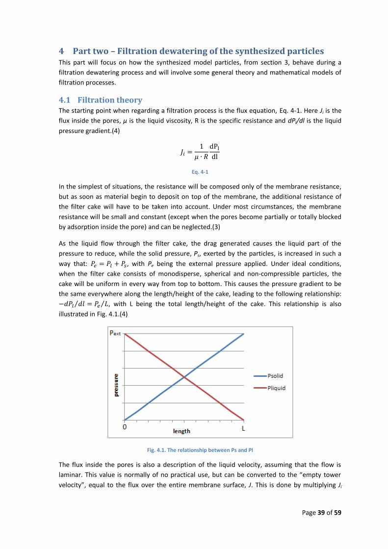
Fig. 4.1. The relationship between Ps and Pl
The flux inside the pores is also a description of the liquid velocity, assuming that the flow is
laminar. This value is normally of no practical use, but can be converted to the “empty tower
velocity”, equal to the flux over the entire membrane surface, J. This is done by multiplying Ji
Page 40 of 59
with the porosity of the filter cake, defined by, . Applying this to Eq. 4-1 and
introducing , will give Eq. 4-2
Eq. 4-2
The resistance term will depend on the cross sectional area of the pores, through which the
liquid will flow down through the cake. These pores can be treated as small, parallel and circular
tubes, where the Hagen–Poiseuilles equation will apply (21). In a cylindrical tube, the cross
sectional area is proportional to the square of the cylinder radius, which can be calculated as the
ratio between the cylinder volume and the surface area of the cylinder wall. For the pores in the
cake, the average pore radius, rp, can thus be assumed to be proportional to the ratio between
the pore volume and the pore surface area. Assuming that the pore surface area is identical to
the total surface area of the particles in the filter cake and utilizing that the volume specific
particle area, , the average pore radius can be calculated by Eq. 4-3 with A being the
area of the membrane.
Eq. 4-3
Inserting the expected dependency of the cross sectional pore area on the resistance will then
give Eq. 4-4, which is the Kozeny-Carman equation (3) and can be used to predict the resistance
as a function of particle size. By combining Eq. 4-2 with Eq. 4-4, to Eq. 4-5, the Kozeny-Carman
equation can then be used to predict the flux. The Kozeny-Carman coefficient, kc, is typically
taken to be 5 for uniform spheres (3).
Eq. 4-4
Eq. 4-5
4.1.1 Dead end filtration
In dead end filtration, the cake height, L, will increase with time, t, but since L is difficult to
obtain experimentally, the material coordinate, , is typically used instead as
, transforming Eq. 4-2 to Eq. 4-6. (4)
Eq. 4-6

Page 41 of 59
A new resistance term, α, is now introduced as giving Eq. 4-7
Eq. 4-7
Inserting the same dependency of rp on R as before, will give Eq. 4-8, a variant of the Kozeny-
Carman equation, using material coordinates. It is important to notice, that the units of R’ and α
are not the same.
Eq. 4-8
The flux also can be describes in terms of volume as in Eq. 4-9, which, in combination with Eq.
4-7, remembering that , will give Eq. 4-10
Eq. 4-9
Eq. 4-10
This will, upon rearrangement and integration, give Eq. 4-11 which can be used to calculate the
specific resistance from experimental data, as a plot of t/Vf vs. Vf should give a straight line with
a slope of . Such a plot is commonly called a Ruth-plot.(4)
Eq. 4-11
The measured specific resistance can then be compared to the one obtained from the Kozeny-
Carman relation.
The effect of the osmotic pressure in the filter cake has deliberately been omitted, as this
normally only play a minor role when filtering particles above 1µm.(22)

Page 42 of 59
4.2 Filtration setup The setup used for the filtration experiments consisted of a dead-end filtration unit, where a
piston moves down through a cylinder at a constant pressure. Further information about the
equipment is found in Appendix C. The filter is placed at the bottom of the cylinder, supported
by a metal grid and the particle dispersion can then be placed in the cylinder, on top of the filter.
Once the piston touches the liquid dispersion, the water is forced out through the filter, due to
the pressure transferred from the piston, and the particles will be retained. The particles will
deposit onto the filter and a filter cake is build.
To avoid leaking of the dispersion, the piston will have to fit tightly into the cylinder. This will
generate some friction between the piston o-ring and the cylinder wall. To avoid errors in the
results, the liquid pressure, at the point of contact between the piston and the liquid, will be
measured and used in the subsequent calculations instead of the external pressure.
Unfortunately, the regulation of the piston movement is still done in regard to external pressure,
giving rise to a series of problems explained further in the presentation of the results.
In addition to the liquid and external pressures, the relative position, or length travelled, of the
piston is measured as well. All the measured data is logged by an external on a PC, at a certain
time interval specified by the user.
4.2.1 Method
Some of the original particle dispersions were diluted to a dry matter content of 10 and 5 g/L for
the PMMA and PS particles respectively. The dry matter content of the original dispersion was
determined gravimetrically, using small aluminum trays. The dilution was done with a 10 mM
aqueous borax solution to maintain a pH value just above 9, as it will ensure, that all of the
carboxylic acid groups on the PAA stabilizer are deprotonated, making the electrostatic repulsion
amongst the individual chain (and particles) as high as possible. The conductivity of the diluted
sample was also checked to ensure that they did not differ too much. As the highest and lowest
conductivity of the samples was within a few percent, it was assumed that no regulation would
be necessary.
Approximately 30 mL of the diluted dispersions were added to the cylinder fitted with a fresh
filter and the piston was driven down, until it reached the liquid surface. The sampling rate was
then set according to the assumed total length of filtration (to avoid too few or too many data
points) and the filtration were started. The filtration was stopped when the piston reached the
filter cake, as the consolidation of the filter cake is not a part of this work.

Page 43 of 59
4.3 Presentation and discussion of the obtained results Filtration experiments have been conducted on some of the synthesized batches. The term Pliq
will be used for the pressure measured at the point of contact between the piston and the
dispersion to be filtered and corresponds to the term Pe in the theory explained in section 4.1
and is as such not to be confused with Pl. The term Pext will, however, be used here as the
pressure measured, where the piston is connected to the rest of the filtration unit. If the
pressure loss due to friction is termed Pfric then the following relation will exist:
. All of the calculations of α will be done by using Eq. 4-11, with ,
and , where is the average of all the measured values of Pliq
within the linear section of the Ruth-plot. The dry matter content is given in , time in
seconds, pressure in Pa and volume in , making the units of α, .
4.3.1 Determination of α
For every successful filtration, a Ruth plot has been made, in order to determine the specific
resistance, α, of the particular conditions used. As an example, a Ruth-plot from the filtration of
PMMA-B is shown in Fig. 4.2. The slope, used to determine α from Eq. 4-11, is found by linear
regression of the linear part of the Ruth-plot, marked in black. The pressure term in this
equation are taken as the average Pliq over the data points included in the linear part of the
Ruth-plot.
Fig. 4.2. Ruth-plot obtained from the filtration of PMMA-B at 0.5 and 0.8 bar
The determined values of α can be found in Table 4.1, as an average over the pressure range
used for the filtration. As the Kozeny-Carman equation can be used to predict α from the size of
the particles, and the porosity of the filter cake, a set of theoretically determined values is also
found in Table 4.1. As the real porosity of the filter cake is unknown, it is assumed that the filter
cake is composed of random close packed spheres, making (23).
Name αexp αK-c
PMMA-B 7,05E+10 4,75E+10 PMMA-seeded 2,91E+10 1,33E+10 PS-co-P(PEGMA) 8,04E+13 1,06E+12 PS-C 2,17E+13 4,95E+11 PS-D 4,60E+12 4,15E+11
0,0E+00
2,0E+06
4,0E+06
6,0E+06
8,0E+06
0 0,00001 0,00002 0,00003 0,00004
t/V
V
PMMA-B
0.5 Bar
0.8 Bar

Page 44 of 59
Table 4.1. Values of α obtained from dead end filtration experiments and the Kozeny-Carman equation, respectively
When comparing the obtained values of α, it is seen that all of the experimentally obtained α’s
are larger than the ones from the Kozeny-Carman equation. Especially PS-C and PS-co-P(PEGMA)
stands out, with a ratio between the two values of 43.8 and 75.9 respectively, while αexp for
PMMA-B and PMMA-seeded is only slightly larger than αK-c. All of the ratios are plotted in Fig.
4.3.
Fig. 4.3. Ratio between αexp and αK-c
The reason for the higher αexp of the PS particles is most probably due to the negatively charged
PAA surrounding the particles, as the Kozeny-Carman equation is only valid when there are no
electrochemical interactions between the particles and the liquid (24). In addition to this, the
dual-layer morphology of the PS-co-P(PEGMA) particles seems to have an effect to. It is however
not clear what causes the difference between PS-C and PS-D as they are approximately the same
size. The only known difference between the two is the charge density, but since the charge
density of PS-D, seemingly, is larger than that of PS-C, this cannot account for the difference in
the measured values of α. The measured charge density is however debatable, as mentioned in
section 3.9, making the comparison between charge density and αexp unsustainable.
4.3.2 Limitations of the method used
As mentioned in section 4.2, the movement of the piston will cause friction between the piston
and the cylinder wall. This friction puts a limit to the usable pressure range, as the external
pressure will have to be high enough to overcome it. Additionally, the amount of friction is not
constant through the length of the cylinder, so the liquid pressure will vary as a function of
piston position, even though the external pressure is constant. The lower pressure limit was
found to be 0.5 bars, but even still, some of the results, from runs at this pressure, would have
to be discarded. This was either due to the filtration stopping too soon, as the friction exceeded
the external pressure, or to very large fluctuations in the liquid pressure. The latter was the
more common of the two and could actually happen at higher pressures as well, although not as
0,0
10,0
20,0
30,0
40,0
50,0
60,0
70,0
80,0
PMMA-B PMMA-seeded PS-co-PEGMA PS-C PS-D
Ratio between αexp and αK-c

Page 45 of 59
often. Fig. 4.4 and Fig. 4.5 are examples of this, showing the external and liquid pressure as
function of piston position, with the fist being the typical result of runs below 0.5 bars.
Fig. 4.4 Pext and Pliq measured as a function of piston position for the filtration of PMMA-B at 0.3 bar
Fig. 4.5. Pext and Pliq measured as a function of piston position for the filtration of PS-co-P(PEGMA) at 1.5 bar
For most of the runs where Pliq fluctuates, the determined value of α appeared to be significantly
larger than for runs where Pliq didn’t fluctuate as much. The Ruth-plot would also be less linear
and in the worst cases have a jagged appearance. An example of this is shown in Fig. 4.6 and is
taken from the same run as Fig. 4.3. The linear trend line is added only to illustrate the non-
linearity of the Ruth-plot.
0
0,1
0,2
0,3
0,4
0,5
0 20 40 60 80
Pre
ssu
re (
bar
)
Piston position (mm)
PMMA-B at 0.3 bar
P(ext)
P(liq)
0
0,5
1
1,5
2
0 20 40 60 80
Pre
ssu
re (
bar
)
Piston position (mm)
PS-co-P(PEGMA) at 1.5 bar
P(ext)
P(liq)

Page 46 of 59
Fig. 4.6. Ruth-plot from the filtration of PMMA-B at 0.3 bar, showing the effect of a fluctuating Pliq
As mentioned, the friction varies down through the cylinder, also for the runs where the above
mentioned phenomenon does not occur, with Fig. 4.7 being an excellent example of this. The
shape of the Pliq curve and the amount of pressure lost to friction, varies greatly between the
different runs and seems to be affected, amongst other things, by the way the piston is inserted
into the piston-holder.
The lower pressure limit is particularly a problem for the PMMA particles, where α is small. The
low resistance to filtration makes it impossible for the filtration unit to move the piston fast
enough to keep the external pressure constant. This leaves a very small usable pressure range,
making it difficult to obtain reliable data from runs at different pressures. The only ways to
overcome this is to; either increase the dry matter content, lowering the number of runs which
are possible from one batch; or change the regulation mechanism on the filtration unit in such a
way, that the regulation is done on basis of the liquid pressure instead of the external pressure.
Fig. 4.7. Pext and Pliq measured as a function of piston position for the filtration of PS-co-P(PEGMA) at 1 bar
On top of the problems arising from friction, it was, as most of the filtration runs were finished,
found that the piston was slightly crocked, due to a bend in the piston holder. This meant that
one side of the cylinder casing would be lifted by the force from the piston to maintain the
4,0E+06
6,0E+06
8,0E+06
1,0E+07
1,2E+07
1,4E+07
0 0,000005 0,00001 0,000015 0,00002 0,000025 0,00003
t/V
V
PMMA-B at 0.3 bar
0
0,2
0,4
0,6
0,8
1
1,2
0 20 40 60 80
Pre
ssu
re (
bar
)
Piston position (mm)
PS-co-P(PEGMA) at 1 bar
P(ext)
P(liq)
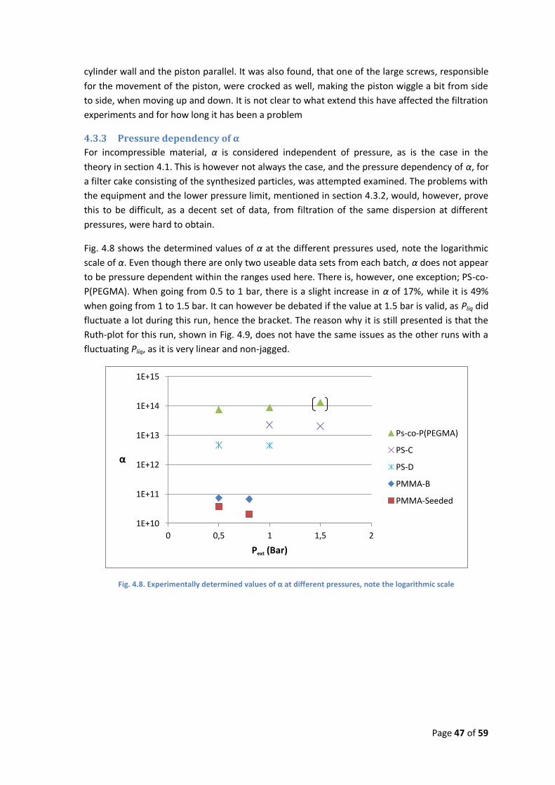
Page 47 of 59
cylinder wall and the piston parallel. It was also found, that one of the large screws, responsible
for the movement of the piston, were crocked as well, making the piston wiggle a bit from side
to side, when moving up and down. It is not clear to what extend this have affected the filtration
experiments and for how long it has been a problem
4.3.3 Pressure dependency of α
For incompressible material, α is considered independent of pressure, as is the case in the
theory in section 4.1. This is however not always the case, and the pressure dependency of α, for
a filter cake consisting of the synthesized particles, was attempted examined. The problems with
the equipment and the lower pressure limit, mentioned in section 4.3.2, would, however, prove
this to be difficult, as a decent set of data, from filtration of the same dispersion at different
pressures, were hard to obtain.
Fig. 4.8 shows the determined values of α at the different pressures used, note the logarithmic
scale of α. Even though there are only two useable data sets from each batch, α does not appear
to be pressure dependent within the ranges used here. There is, however, one exception; PS-co-
P(PEGMA). When going from 0.5 to 1 bar, there is a slight increase in α of 17%, while it is 49%
when going from 1 to 1.5 bar. It can however be debated if the value at 1.5 bar is valid, as Pliq did
fluctuate a lot during this run, hence the bracket. The reason why it is still presented is that the
Ruth-plot for this run, shown in Fig. 4.9, does not have the same issues as the other runs with a
fluctuating Pliq, as it is very linear and non-jagged.
Fig. 4.8. Experimentally determined values of α at different pressures, note the logarithmic scale
1E+10
1E+11
1E+12
1E+13
1E+14
1E+15
0 0,5 1 1,5 2
α
Pext (Bar)
Ps-co-P(PEGMA)
PS-C
PS-D
PMMA-B
PMMA-Seeded
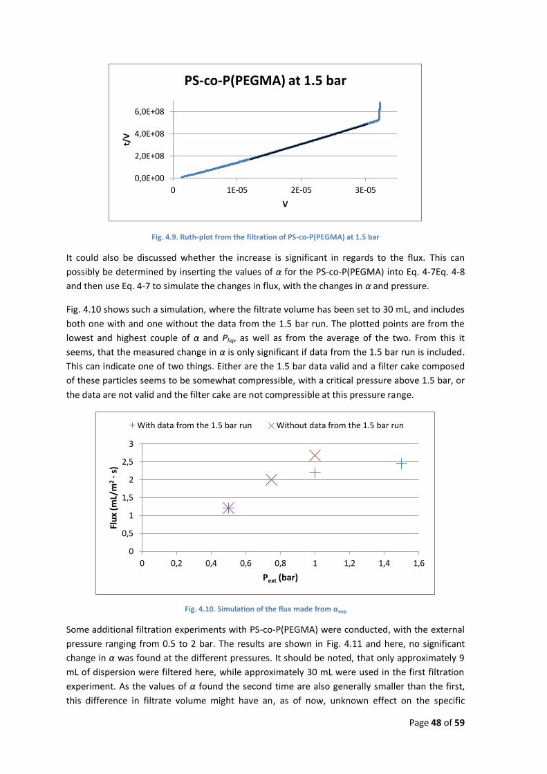
Page 48 of 59
Fig. 4.9. Ruth-plot from the filtration of PS-co-P(PEGMA) at 1.5 bar
It could also be discussed whether the increase is significant in regards to the flux. This can
possibly be determined by inserting the values of α for the PS-co-P(PEGMA) into Eq. 4-7Eq. 4-8
and then use Eq. 4-7 to simulate the changes in flux, with the changes in α and pressure.
Fig. 4.10 shows such a simulation, where the filtrate volume has been set to 30 mL, and includes
both one with and one without the data from the 1.5 bar run. The plotted points are from the
lowest and highest couple of α and Pliq, as well as from the average of the two. From this it
seems, that the measured change in α is only significant if data from the 1.5 bar run is included.
This can indicate one of two things. Either are the 1.5 bar data valid and a filter cake composed
of these particles seems to be somewhat compressible, with a critical pressure above 1.5 bar, or
the data are not valid and the filter cake are not compressible at this pressure range.
Fig. 4.10. Simulation of the flux made from αexp
Some additional filtration experiments with PS-co-P(PEGMA) were conducted, with the external
pressure ranging from 0.5 to 2 bar. The results are shown in Fig. 4.11 and here, no significant
change in α was found at the different pressures. It should be noted, that only approximately 9
mL of dispersion were filtered here, while approximately 30 mL were used in the first filtration
experiment. As the values of α found the second time are also generally smaller than the first,
this difference in filtrate volume might have an, as of now, unknown effect on the specific
0,0E+00
2,0E+08
4,0E+08
6,0E+08
0 1E-05 2E-05 3E-05
t/V
V
PS-co-P(PEGMA) at 1.5 bar
0
0,5
1
1,5
2
2,5
3
0 0,2 0,4 0,6 0,8 1 1,2 1,4 1,6
Flu
x (m
L/m
2 ·
s)
Pext (bar)
With data from the 1.5 bar run Without data from the 1.5 bar run
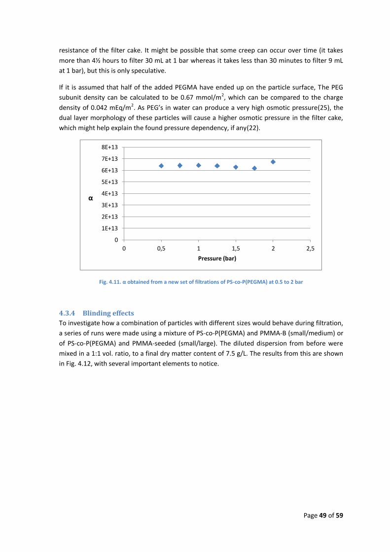
Page 49 of 59
resistance of the filter cake. It might be possible that some creep can occur over time (it takes
more than 4½ hours to filter 30 mL at 1 bar whereas it takes less than 30 minutes to filter 9 mL
at 1 bar), but this is only speculative.
If it is assumed that half of the added PEGMA have ended up on the particle surface, The PEG
subunit density can be calculated to be 0.67 mmol/m2, which can be compared to the charge
density of 0.042 mEq/m2. As PEG’s in water can produce a very high osmotic pressure(25), the
dual layer morphology of these particles will cause a higher osmotic pressure in the filter cake,
which might help explain the found pressure dependency, if any(22).
Fig. 4.11. α obtained from a new set of filtrations of PS-co-P(PEGMA) at 0.5 to 2 bar
4.3.4 Blinding effects
To investigate how a combination of particles with different sizes would behave during filtration,
a series of runs were made using a mixture of PS-co-P(PEGMA) and PMMA-B (small/medium) or
of PS-co-P(PEGMA) and PMMA-seeded (small/large). The diluted dispersion from before were
mixed in a 1:1 vol. ratio, to a final dry matter content of 7.5 g/L. The results from this are shown
in Fig. 4.12, with several important elements to notice.
0
1E+13
2E+13
3E+13
4E+13
5E+13
6E+13
7E+13
8E+13
0 0,5 1 1,5 2 2,5
α
Pressure (bar)
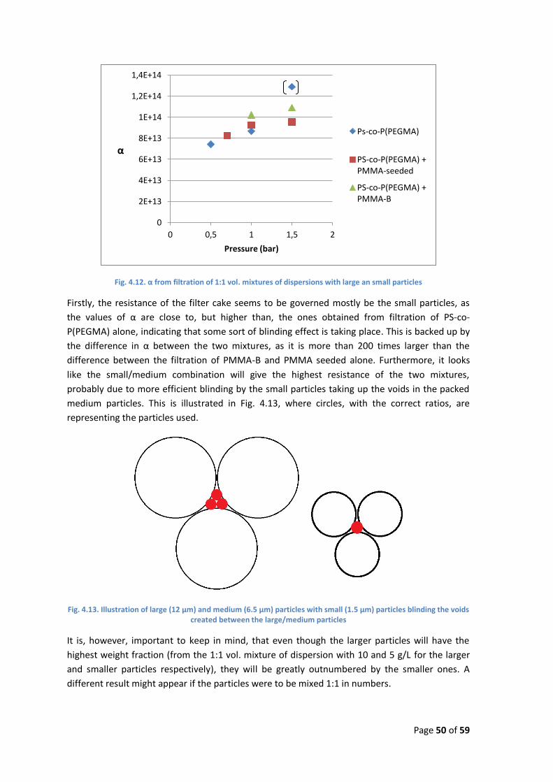
Page 50 of 59
Fig. 4.12. α from filtration of 1:1 vol. mixtures of dispersions with large an small particles
Firstly, the resistance of the filter cake seems to be governed mostly be the small particles, as
the values of α are close to, but higher than, the ones obtained from filtration of PS-co-
P(PEGMA) alone, indicating that some sort of blinding effect is taking place. This is backed up by
the difference in α between the two mixtures, as it is more than 200 times larger than the
difference between the filtration of PMMA-B and PMMA seeded alone. Furthermore, it looks
like the small/medium combination will give the highest resistance of the two mixtures,
probably due to more efficient blinding by the small particles taking up the voids in the packed
medium particles. This is illustrated in Fig. 4.13, where circles, with the correct ratios, are
representing the particles used.
Fig. 4.13. Illustration of large (12 µm) and medium (6.5 µm) particles with small (1.5 µm) particles blinding the voids created between the large/medium particles
It is, however, important to keep in mind, that even though the larger particles will have the
highest weight fraction (from the 1:1 vol. mixture of dispersion with 10 and 5 g/L for the larger
and smaller particles respectively), they will be greatly outnumbered by the smaller ones. A
different result might appear if the particles were to be mixed 1:1 in numbers.
0
2E+13
4E+13
6E+13
8E+13
1E+14
1,2E+14
1,4E+14
0 0,5 1 1,5 2
α
Pressure (bar)
Ps-co-P(PEGMA)
PS-co-P(PEGMA) + PMMA-seeded
PS-co-P(PEGMA) + PMMA-B

Page 51 of 59
Secondly, All of the measured values of α increases with increasing pressure, just as it was found
for the PS-co-P(PEGMA) particles alone. This supports the notion, that a filter cake composed of
this type of particles, either alone or combined with others, might be slightly compressible. The
value from the 1.5 bar filtration run of PS-P(PEGMA) is higher than the one from PS-P(PEGMA) +
PMMA-B at the same pressure, even though the reverse is true for the values at lower
pressures. The notion of this run not being valid is thus strengthened, but the real value might
still be higher than the one at 1 bar.

Page 52 of 59
5 Conclusion Several batches of particles have been synthesized using dispersion polymerization techniques,
covering the following three different types:
Poly(methyl methacrylate) (PMMA) particles with a non-ionic grafted stabilizer made
from Polyvinylpyrrolidone (PVP)
Polystyrene (PS) particles with an anionic grafted stabilizer made from Poly(acrylic acid)
(PAA)
Polystyrene particles (PS) with a dual layer morphology of the shell made from grafted
Poly(acrylic acid) (PAA) and directly co-polymerized Poly(ethylene glycol)-methacrylate
(PEGMA)
All of the synthesized particles fulfill most of the requirements outlined in the aim presented in
section 2, with the following exceptions.
Particles with a water swellable core were not synthesized although methacrylic acid was added
as co-monomer with the expectation that it would be incorporated into the particles. This did,
however, not happen, probably due to interactions between PVP and MAA. Experiments
indicate that the MAA will make some of the PVP unavailable for grafting, reducing the
stabilizing potential while keeping the MAA-PVP couple in solution. As the PS particles were
synthesized with PAA as stabilizer instead of PVP, MAA might co-polymerize with styrene and be
incorporated into the particles, although this have not been attempted.
All of the PS particles are negatively charged, because of the grafted PAA used as stabilizer. This
method of introducing charges will, however, also limit the ability to independently vary size and
charge density, as particle size is strongly linked to the amount of available stabilizer.
Furthermore, the charge density measured by pH-titration is somewhat debatable due to
coagulation of the particles at low pH.
The size range covered is approximately 1.5 to 12.5 µm, while the monodispersity, measured as
the geometric standard deviation (GSD), varies from approximately 1.2 to 2.4 with the PS
particles generally having the lowest GSD. Theory on size control and the ability to produce
monodisperse particles have been found and presented from literature studies, which show that
stabilization and locus of polymerization both play important roles. This knowledge have been
used in the slightly different PS-co-P(PEGMA) particles.
Some of the synthesized particles were used in dead end dewatering filtration experiments, with
the aim of measuring the specific resistance of the filter cake, α. This value was then compared
to predictions of α from the Kozeny-Carman equation, based on the particle size. It was found
that the filter cake resistance of the PMMA particles was very close to the predicted value, while
the resistance of the PS particles all was higher than predicted. Especially the particles made
with both PAA and PEGMA as stabilizer showed this tendency, with the measured α being more
than 75 times higher than the predicted value.
During the filtration experiments, runs were made at different pressures to investigate the
compressibility of the formed filter cakes. Only the PS-co-P(PEGMA) particles showed an

Page 53 of 59
increase in α with increasing pressure, and only if the amount filtered were high enough to allow
the entire run to last several hours.
Finally, blinding effects, when using a mixture of different sized particles, were investigated. This
showed, that the filter cake resistance is mainly governed by the smaller particles, as the values
of α were in the same range as those for PS-co-P(PEGMA) alone. Besides this, the blinding effect
were more pronounced when combining small (1.5 µm) and medium (6.5 µm) particles in
contrast to small (1.5 µm) and large (12 µm). The results from the blinding experiments
supported the ones from the longer filtration runs of PS-co-P(PEGMA), with α increasing with
increasing pressure
All in all, the route taken to synthesize the PS-co-P(PEGMA) particles seems to be the most
viable for now. These particles were the ones closest to what are needed, mimicking some of the
behavior seen when employing membrane filtration to waste water containing organic particles.
If combined with co-polymerization of anionic monomers such as (meth)acrylic acid or if a
method can be found to control particle size and charge density independently, then this type of
particles would be very interesting, when regarding organic model colloids in the µm range.
As an end note, several problems with the filtration equipment were discovered during the
filtration experiments and it is unknown whether this has affected the obtained result in any
way not taken into account in the presentation and discussion of the dewatering filtration
results.
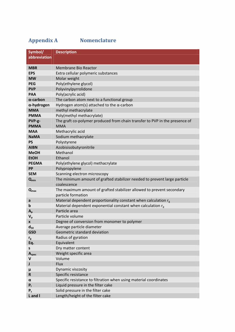
Appendix A Nomenclature
Symbol/ abbreviation
Description
MBR Membrane Bio Reactor EPS Extra cellular polymeric substances MW Molar weight PEG Poly(ethylene glycol) PVP Polyvinylpyrrolidone PAA Poly(acrylic acid) α-carbon The carbon atom next to a functional group α-hydrogen Hydrogen atom(s) attached to the α-carbon MMA methyl methacrylate PMMA Poly(methyl methacrylate) PVP-g-PMMA
The graft co-polymer produced from chain transfer to PVP in the presence of MMA
MAA Methacrylic acid NaMA Sodium methacrylate PS Polystyrene AIBN Azobisisobutyronitrile MeOH Methanol EtOH Ethanol PEGMA Poly(ethylene glycol) methacrylate PP Polypropylene SEM Scanning electron microscopy Qmin The minimum amount of grafted stabilizer needed to prevent large particle
coalescence Qmax The maximum amount of grafted stabilizer allowed to prevent secondary
particle formation a Material dependent proportionality constant when calculation rg
b Material dependent exponential constant when calculation rg Ap Particle area Vp Particle volume x Degree of conversion from monomer to polymer d50 Average particle diameter GSD Geometric standard deviation rg Radius of gyration Eq. Equivalent s Dry matter content Aspec Weight specific area V Volume J Flux µ Dynamic viscosity R Specific resistance α Specific resistance to filtration when using material coordinates Pl Liquid pressure in the filter cake Ps Solid pressure in the filter cake L and l Length/height of the filter cake

Page 55 of 59
Pe External pressure Pliq The pressure measured between the piston and the filtrate (=Pe) Symbol/ abbreviation
Description
Pfric Pressure loss due to friction Papp Applied pressure (Papp=Pliq+Pfric) ε Porosity S0 Volume specific area A Cylinder cross sectional area (membrane area) rp Pore radius Vf Cumulative filtrate volume ρp Particle density ω Amount of material deposited pr m2 t Time αexp α determined experimentally αK-c α determined from the Kozeny-Carman equation
Page 56 of 59
Appendix B List of chemicals
Chemical Cas nr. Purchased from
Purity Additional info
Methyl methacrylate
80-62-6 Sigma-Aldrich 99 % Contains 30 ppm monomethylether hydroquinone
Methacrylic acid 79-41-4 Sigma-Aldrich 99 % Sodium methacrylate
5536-61-8 Sigma-Aldrich n/a
PVP-K30 9003-39-8 Sigma-Aldrich n/a 60 kDa AIBN 78-67-1 Sigma-Aldrich 98 % Recrystallized before use Methanol 67-56-1 Sigma-Aldrich 99.8 % Ethanol 64-17-5 Kemetyl 99.9 % Styrene 100-42-5 Sigma-Aldrich 99 % Contains 10-15 ppm 4-tert-
butylcatechol Poly(acrylic acid) 9003-01-4 Sigma-Aldrich 35 % in H2O 100 kDa Poly(acrylic acid) 9003-01-4 Wako n/a 25 kDa NaOH 1310-73-2 J. T. Baker 50 % in H2O NaClO4 7601-89-0 Merck n/a Monohydrate HClO4 7601-90-3 Merck n/a PEG monomethyl ether
9004-74-4 Sigma-Aldrich n/a 5 kDa
Methacrylic anhydride
760-93-0 Sigma-Aldrich 94 % Contains 2000 ppm Topanol A
Pyridine 110-86-1 Fisher Scientific
n/a Anhydrous
DMAP 1122-58-3 Sigma-Aldrich n/a Dichloromethane 75-09-2 Sigma-Aldrich n/a Diethyl ether 60-29-7 Sigma-Aldrich 99.5 % Borax (sodium tetraborate)
1330-43-4 n/a n/a decahydrate
Hydroquinone 123-31-9 Acros Organics 99 %

Page 57 of 59
Appendix C Equipment information
pH titrations:
The titrations were performed by the use of two ABU901 Autoburettes, combined with a SAM90
Sample station and a Titralab TIM900 Titration manager, all from Radiometer – Copenhagen.
The PC program used to control the titrations and collect the data was TimTalk 9 from LabSoft.
Size measurements:
The particle sizes were measured from multiangle light scattering by the use of a Microtrac II –
particle size analyser and a Recirculator, both from Leeds & Northrup. Before measurements the
equipment was set to automatically give the 16 and 84 percentile values used in the calculations
of GSD as well as the d50 value presented as average particle diameter.
Filtration:
The dead end filtration unit used in this work is shown in Fig. C.1, with the cylinder and piston in
the middle. The filters used were Durapore membrane filters, 0.22 µm GV from Milipore and the
piston o-ring were lubricated with a medium density, high vacuum, silicon grease.
Fig. C.1. The dead end filtration unit used in this work
Page 58 of 59
Appendix D Bibliography
1. Baker, Richard W. Membrane technology and applications. s.l. : John Wiley & Sons Ldt., 2004.
2. Hinge, Mogens. Synthesis of soft shell poly(styrene) colloids for filtration experiments. Section
of Chemistry, Aalborg University. 2006. Ph.D. dissertation.
3. Stephenson, Tom, et al. Membrane Bioreactors for Wastewater Treatment. s.l. : IWA
publishing, 2000.
4. Keiding, Kristian. Phenomenologies in Physical Chemistry. 2009. No other informations
availible .
5. Arshady, R. Suspension, emulsion, and dispersion polymerization: A methodological survey.
Colloid & Polymer Science. 1992, 270, s. 717-732.
6. Suspension polymerisation of methyl methacrylate using sodium polymethacrylate as a
suspending agent. Georgiadou, Styliani og Brooks, Brian W. s.l. : Elsevier, 2005, Chemical
Engineering Science, Årg. 60, s. 7137–7152.
7. Gilbert, G. Robert og Thickett, Stuart C. Emulsion polymerization: State of the art in kinetics
and mechanisms. Polymer. 2007, 48, s. 6965-6991.
8. Hinge, Mogens og Keiding, Kristian. Systematical investigation of the synthesis of core-shell
poly(styrene-co-acrylic acid) colloids with varying shell thickness and core diameter. 2006.
9. Kun, Cao, Bo-Geng, Li og Zu-Ren, Pan. micron-size functiona uniform PMMA particles by
dispersion copolymerization in polar media. Macromolecular Symposium. 2000, 150, s. 195-200.
10. Paine, A. J. Dispersion polymerization of styrene in polar solvents. 7. A simple mechanistic
model to predict particle size. Macromolecules. 23, 1990, s. 3109-3117.
11. de Hoog, Elisabeth Hendrika Andrea. Interfaces and crystallization in Colloid-Polymer
suspensions. s.l. : Proefschrift Universiteit Utrecht, 2001. Dissetation.
12. Kawaguchi, Seigou og Ito, Koichi. Dispersion polymerization. Adv Polym Sci. 2005, 175, s.
299-328.
13. Tseng, C. M., et al. Uniform Polymer Particles by Dispersion Polymerization in Alcohol.
Journal of Polymer Science, Part A: Polymer Chemistry Edition. 1986, 24, s. 2995-3007.
14. Shen, S., Sudol, E. D. og El-Aasser, M. S. Dispersion polymerization of methyl methacrylate:
Mechanism of particle formation. Journal of polymer science, Part A: polymer chemistry. 32, s.
1087-1100.
15. Paine, Anthony James, Luymes, Wayne og McNulty, James. Dispersion Polymerization of
Styrene in Polar Solvents. Influence of Reaction Parameters on Particle Size and Molecular
Page 59 of 59
Weight in Poly(N-vinylpyrrolidone)-Stabilized Reactions. macromolecules. 1990, 23, s. 3104-
3109.
16. Stevens, Malcolm P. Polymer Chemistry - An Introduction. s.l. : Oxford University Press, 1999.
17. Shen, S., Sudol, E. D. og El-Aasser, M. S. Control of particle size in dispersion polymerization
of methyl methacrylate. Journal of polymer science - Part A: polymer chemistry. 31, 1993, s.
1393-1402.
18. Solution properties and unperturbed dimensions of poly(vinylpyrrolidone). Ali, Sabz og
Ahmad, Noor. 3, s.l. : Wiley, British Polymer Journal, Årg. 14, s. 113-116.
19. Protecting Polymers in Suspension of Metal Nanoparticles. Hirai, Hidefumi og Yykura,
Noboru. s.l. : John Wiley & Sons Ltd., Polymers for Advanced Technologies, Årg. 12, s. 724-733.
20. Reactive Surfactants in Emulsion Polymerization. Guyot, A. og Tauer, K. s.l. : Spinger,
Advances in Polymer Science, Årg. 111, s. 44-65.
21. Pressure and concentration profiles in filter cake consisting of core/shell latex particle.
Christensen, Morten Lykkegaard, et al. s.l. : Elsevier, 2006, Colloids and Surfaces A, Årg. 290, s.
295-303.
22. Osmotic effects in sludge dewatering. Keiding, Kristian og Rasmussen, Michael R. s.l. :
Elsevier, 2003, Advances in Environmental Research, Årg. 7, s. 641-645.
23. Song, Chaoming, Wang, Ping og Makse, Hernán A. A phase diagram for jammed matter.
Nature. 2008, Årg. 454, s. 629-632.
24. Carrier, David W. Goodbye, Hazen; Hello, Kozeny-Carman. 2003, s. 1054-1056.
25. Osmotic Pressure of Aqueous Polyethylene Glycols. Money, Nicholas P. 1989, Plant
Physiology, Årg. 91, s. 766-769.