symposium on isotope techniques in
TRANSCRIPT


SYMPOSIUM ON ISOTOPE TECHNIQUES INAN: O4899O-V.OO2UN: 551.49 S989
00000300=111

48900
V


ISOTOPE TECHNIQUESIN GROUNDWATER HYDROLOGY
1974
VOL. II

The following States are Members of the International Atomic Energy Agency:
AFGHANISTANALBANIAALGERIAARGENTINAAUSTRALIAAUSTRIABANGLADESHBELGIUMBOLIVIABRAZILBULGARIABURMABYELORUSSIAN SOVIET
SOCIALIST REPUBLICCAMEROONCANADACHILECOLOMBIACOSTA RICACUBACYPRUSCZECHOSLOVAK SOCIALIST
REPUBLICDENMARKDOMINICAN REPUBLICECUADOREGYPT, ARAB REPUBLIC OFEL SALVADORETHIOPIAFINLANDFRANCEGABON
GERMAN DEMOCRATIC REPUBLICGERMANY, FEDERAL REPUBLIC OFGHANAGREECEGUATEMALA
HAITIHOLY SEEHUNGARYICELANDINDIAINDONESIAIRANIRAQIRELANDISRAELITALYIVORY COASTJAMAICAJAPANJORDANKENYAKHMER REPUBLICKOREA, REPUBLIC OFKUWAITLEBANONLIBERIALIBYAN ARAB REPUBLICLIECHTENSTEINLUXEMBOURGMADAGASCARMALAYSIAMALIMEXICOMONACOMONGOLIAMOROCCONETHERLANDSNEW ZEALANDNIGERNIGERIANORWAY
PAKISTANPANAMAPARAGUAYPERUPHILIPPINESPOLANDPORTUGALROMANIASAUDI ARABIASENEGALSIERRA LEONESINGAPORESOUTH AFRICASPAINSRI LANKASUDANSWEDENSWITZERLANDSYRIAN ARAB REPUBLICTHAILANDTUNISIATURKEYUGANDAUKRAINIAN SOVIET SOCIALIST
REPUBLICUNION OF SOVIET SOCIALIST
REPUBLICSUNITED KINGDOM OF GREAT
BRITAIN AND NORTHERNIRELAND
UNITED STATES OF AMERICAURUGUAYVENEZUELAVIET-NAMYUGOSLAVIAZAIRE, REPUBLIC OFZAMBIA
The Agency's Statute was approved on 23 October 1956 by the Conference on the Statute of the IAEAheld at United Nations Headquarters, New York; it entered into force on 29 July 1957. The Headquarters ofthe Agency are situated in Vienna. Its principal objective is "to accelerate and enlarge the contribution ofatomic energy to peace, health and prosperity throughout the world".
Printed by the IAEA in AustriaSeptember 1974

PROCEEDINGS SERIES
ISOTOPE TECHNIQUESIN GROUNDWATER HYDROLOGY
1974
PROCEEDINGS OF A SYMPOSIUMORGANIZED BY THE
INTERNATIONAL ATOMIC ENERGY AGENCYAND HELD IN VIENNA,
11-15 MARCH 1974
In two volumes
VOL. II
INTERNATIONAL ATOMIC ENERGY AGENCYVIENNA, 1974

ISOTOPE TECHNIQUES IN GROUNDWATER HYDROLOGY 1974IAEA, VIENNA, 1974
STI/PUB/373

FOREWORD
This symposium, held in Vienna on 11-15 March, 1974, was the fourthon the subject of isotope hydrology organized by the International AtomicEnergy Agency. However, this one was limited to groundwater hydrologyin view of the general increase of interest and activity in isotope hydrologysince the previous meeting in 1970.
The proceedings of this symposium are a good indicator of the presentworld status of these techniques. Thus one notes that many of the studiesare in the developing areas of the world. Furthermore, there has been ashift to using these techniques as an additional applied tool in specificproblems of development of water resources. Examples of such applicationsalso give evidence of the closer collaboration between isotope specialists,who originally developed the methods, and hydrogeologists and geochemists.
It is hoped that these proceedings will contribute to a wider apprecia-tion of the potential use of isotope techniques to hydrological problemsassociated with the development of groundwater for agriculture, communitywater supply and industry.

EDITORIAL NOTE
The papers and discussions incorporated in the proceedings publishedby the International Atomic Energy Agency are edited by the Agency's edi-torial staff to the extent considered necessary for the reader's assistance.The views expressed and the general style adopted remain, however, theresponsibility of the named authors or participants.
For the sake of speed of publication the present Proceedings have beenprinted by composition typing and photo-offset lithography. Within the limi-tations imposed by this method, every effort has been made to maintain ahigh editorial standard; in particular, the units and symbols employed areto the fullest practicable extent those standardized or recommended by thecompetent international scientific bodies.
The affiliations of authors are those given at the time of nomination.The use in these Proceedings of particular designations of countries or
territories does not imply any judgement by the Agency as to the legal statusof such countries or territories, of their authorities and institutions or ofthe delimitation of their boundaries.
The mention of specific companies or of their products or brand-namesdoes not imply any endorsement or recommendation on the part of theInternational Atomic Energy Agency.

CONTENTS OF VOL.11
GEOTHERMAL WATERS (Session 5, Part 2)
Oxygen and hydrogen isotope studies of the Larderello (Italy)geothermal system (IAEA-SM-182/27) 3C . P a n i c h i , R . C e l a t i , P. N o t o , P. S q u a r c i ,L. Taff i , E. T o n g i o r g iDis eus sion 28
Hot springs of the igneous terrain of Swaziland: Their noble gases,hydrogen, oxygen and carbon isotopes and dissolved ions(IAEA-SM-182/28) 29E . M a z o r , B.T. Ver hagen , E . N e g r e a n uDiscussion 45
PROBLEMS IN USING ENVIRONMENTAL ISOTOPESPOR GROUNDWATER STUDIES (Session 6)
Local variability of the isotope composition of groundwater(IAEA-SM-182/29) 51J.R. GatDiscussion 58
Sampling of lysimeters for environmental isotopes of water(IAEA-SM-182/51) 61G. Sau z a yDis cus sion 67
Problems in 1 4C dating of water from aquifers of deltaic origin:An example from the New Jersey coastal plain(IAEA-SM-182/31) 69I.J. Winogr ad , G.M. F a r l e k a sDiscussion 91
14C evidence for the origin of arid region groundwater,Northeastern Province, Kenya (IAEA-SM-182/32) 95F.J. P e a r s on , Jr., W.V. Sw ar z e n kiDiscussion 108
Radiocarbon, 1 3 С and tritium in water samples from basalticaquifers and carbonate aquifers on the island of Oahu, Hawaii(IAEA-SM-182/33) I l lТ.Н. Huf en, L.S. L a u , R.W. B u d d e m e i e rDis cus sion 126

ENVIRONMENTAL ISOTOPES, OTHER THAN HYDROGEN,OXYGEN AND CARBON ISOTOPES, IN GROUNDWATERSTUDIES (Session 7, Part 1)
234U and 238U in the Carrizo sandstone aquifer of South Texas(IAEA-SM-182/35) 131J.B. C o w a r t , J.K. OsmondDis eus sion 148
234TJ/238U disequilibrium in waters of the Judea group(Cenomanian-Turonian) aquifer in Galilee, northernIsrael (IAEA-SM-182/34) 151E. W a k s h a l , P. YaronDiscussion 176
39Ar dating of groundwater (IAEA-SM-182/37) 179H . O e s c h g e r , A . G u g e l m a n n , H . L o o s l i ,U. S c h o t t e r e r , U. S iegen th a l e r , W.Wies tDiscussion 189
Distribution of sulphur isotopes of sulphates in groundwatersfrom the principal artesian aquifer of Florida and theEdwards aquifer of Texas, United States of America(IAEA-SM-182/39) 191C.T. R i g h t m i r e , P.J. P e a r s o n , Jr., W.Back,R.O. R y e , B.B.HanshawDis eus sion 206
Utilisation des variations naturelles d'abondance de l'azote-15comme traceur en hydrogéologie — Premiers résultats(IAEA-SM-182/40) 209R . L é t o l l e , A . M a r i o t t iDiscussion 219
AQUIFER CHARACTERISTICS STUDIES (Session 7, Part 2;Session 8)
Utilisation des techniques isotopiques pour la résolution deproblèmes hydrologiques en génie civil — Etude detrois cas précis (IAEA-SM-182/43) 223P.Ch. L é vê qu e , J.C1. G r o s , Catherine M au r in ,J. S é v é r a c , Cl. V i g u i e rDiscus sion 238
Application of single borehole methods in groundwater research(IAEA-SM-182/12) -. 241W . D r o s t , P . N e u m a i e rDis eus sion 253
Modelos matemáticos simplificados para interpretación deresultados por el método de marcación de toda lacolumna piezométrica (IAEA-SM-182/44) 255H.A. MuñeraDiscussion 274
Theoretical possibilities of the two-well pulse method(IAEA-SM-182/45) 277A. Zube rDis eus sion 294

Determination of effective porosities by the two-well pulsemethod (IAEA-SM-182/46) 295A . K r e f t , A. L e n d a , B. T u r e k , A . Z u b e r ,
K . C z a u d e r n aDiscussion 311
Investigations of effective porosity of till by means of a combinedsoil-moisture/density gauge (IAEA-SM-182/47) 313L. N o r d b e r g , S.ModigDis eus sion 339
Hydrodynamic dispersion as aquifer characteristic: modelexperiments with radioactive tracers (IAEA-SM-182/42) 341D. K l o t z , H. Mo s e rDiscussion 355
THEORETICAL AND EXPERIMENTAL STUDIES OF TRACERMOVEMENT IN GROUND WATER (Session 9)
Радиоиндикаторные исследования молекулярной иконвективной диффузии в насыщенных иненасыщенных (песчано-глинистых) породах
(IAEA-SM-18 2/54) 359В.Т. Д у б и н ч у к , 3.Г. К о л е с н и ч е н к о ,О.Ф. Л а п т е в а , B.C. Г о н ч а р о вDiscussion 375
Analyse des informations fournies par les traceurs naturelsou artificiels dans l'étude des systèmes aquifères enhydrogéologie (IAEA-SM-182/48) 377J. G u i z e r i x , R. M a r g r i t a , B. G a i l l a r d ,P . C o r o m p t , M . A l q u i e r
Méthode pour la détermination de caractéristiques de transfertde substances polluantes dans les nappes aquifères(IAEA-SM-182/41) 405P . C o r o m p t , B. G a i l l a r d , J. G u i z e r i x , R. M a r g r i t a ,J . M o l i n a r i , R . C o r d a , N. C r a m p o n , D . O l i v i e rDis eus sion 421
Some conceptual mathematical models and digital simulationapproach in the use of tracers in hydrological systems(IAEA-SM-18 2/49) 425K. P r z e w i f o c k i , Y. Y u r t s e v e rDiscussion 448
Application of digital modelling to the prediction of radioisotopemigration in groundwater (IAEA-SM-182/50) 451J.B. R o b e r t s o nDiscussion 477
Chairmen of Sessions and Secretariat of the Symposium 479List of participants 481Author index 497


GEOTHERMAL WATERS
(Session 5, Part 2)


IAEA-SM-182/27
OXYGEN AND HYDROGEN ISOTOPE STUDIESOF THE LARDERELLO (ITALY)GEOTHERMAL SYSTEM
C. PANICHI, R. CELATI, P. NOTO,P. SQUARCI, L. TAFFI, E. TONGIORGI
Istituto Internazionale per le Ricerche Geotermiche,CNR-Pisa,Pisa, Italy
Abstract
OXYGEN AND HYDROGEN ISOTOPE STUDIES OF THE LARDERELLO (ITALY) GEOTHERMAL SYSTEM.Data collected on water and steam samples enabled a satisfactory picture of the geochemical and
hydrogeological characteristics of the Larderello geothermal field to be obtained. The isotopic andchemical analyses of hot water from non-productive wells and thermal and cold springs enabled two differentcirculation patterns of fluids to be distinguished. The steam samples delivered from the wells show, asexpected, the same deuterium content as local meteoric water, with is О enrichments ranging from 1.7to 8%o. The geographical distribution of the ó18O values of steam provides valid information about thepreferential path of flow in the zone from which the geothermal fluids are derived. These flow lines are inagreement with the reconstruction of the regional hydrogeological scheme. The presence of tritium in thesteam of some périphérie wells has indicated the existence of local influences of recent shallow waters onthe deepest circulation. Repeated 18O measurements in time of the steam samples have shown the usefulnessof the isotopic survey in the control of the evolution of a geothermal field during its exploitation.
1. INTRODUCTION
The hydrogen and oxygen composition of the water has been analysedin samples from the most important geothermal fields in the world [1-3],including the Larderello area [1,4].
In all cases the D/H ratio was shown to be the same in all the hot wateror steam samples from a single area, and the same as the average valueof the meteoric water of the region. The oxygen, on the contrary, wasgenerally found to be enriched by different amounts of 18O isotope comparedwith the meteoric water of the region, as a result of the isotopic exchangesat high temperature between the oxygen of the water and that of the rockswhere deep circulation took place. When deep circulation occurs incarbonate rocks the isotopic exchange is often very evident. It is obviousthat with increasing residence time the 18O/16O ratios in the water willapproach more and more the equilibrium with the same ratio in the rocks.
As a wide range of 18O enrichments was observed in the Larderelloarea, a systematic study of the whole Larderello geothermal area wasconsidered useful to geohydrological research. It can, in fact, providesome suggestions regarding deep circulation patterns, and the interactionbetween the deep circulation waters and those infiltrating in permeablerocks outcropping in the neighbourhood of the field. Furthermore, thelocal waters appear to be a convenient target for the tritium content inrespect to the deep waters. Variable tritium contents are reported byBanwell [5] for the hot water systems of New Zealand, by White and

4 PANIC HI et al .
co-workers [ 6] for the geothermal system of Steamboat Springs, Nevada,and by Koga [7] for the geothermal well waters at Otake, Japan. This wasexplained as a result of a certain mixing of young meteoric water withdeep water systems.
White and co-workers [6] also reported some tritium contents forsteam well samples at The Geysers, which is in agreement with a modelwhich involves shallow condensation of steam, incorporation of some localprecipitation and drainback.
With this aim, cold and thermal spring waters, waters sampled fromnon-productive wells, and steam samples will be examined in this report.
The 618O and 6D values of water and steam samples are referred toSMOW [8], and the errors (la) are 0. l%o and l%0 respectively.
The tritium content is expressed in Tritium Units (TU) and the error(la) is quoted for each individual result.
2. HYDROGEOLOGICAL OUTLINES
The geological features of the Larderello geothermal area are shownschematically in Fig. 1. Details of the geology of the zone have been dis-cussed elsewhere [9-12].
From the hydrogeological point of view, the various outcropping orburied terrains of the region, because of their geometric position andpermeability, can be grouped as follows:
(a) Upper complex. This is on the whole impervious. It consists(from top to bottom) of neogenic deposits (U. Miocene-Pliocene) prevalentlyclay, of flysch faciès formations, mostly consisting of shales and marls(Eocene-Cretaceous), with masses of ophiolites (Jurassic), and of sand-stones alternated with siltstones and shales ("macigno", Oligocène) over-lying a continuous level of impervious varicoloured shales ("scaglia",Eocene-Cretaceous).
In this complex some permeable levels exist which maintain locallyshallow and frequently intense circulation, but usually do not contributeto deep circulation. This complex constitutes the cover of the geothermalfield.
(b) Main pervious complex. This consists in the upper part pre-dominantly of carbonatic formations (Upper Triassic-Jurassic), and, inthe lower part, of a dolomitic-anhydritic formation (Upper Triassic). Thiscomplex constitutes the main reservoir in the region: when it outcrops,it represents absorption areas and, consequently, areas of hydrostaticpressure for the buried reservoir, Within, an active circulation develops,and from this practically all thermal springs of the region emerge.
(c) Basal complex. This consists mostly of phyllites and quartzites(crystalline regional basement, Paleozoic-U. Triassic). It includes aseries of terrains which are generally low-permeable. A circulation offluids is also possible in this complex, but not as actively as in the complexdescribed above. At present steam drawn by new deeper wells in theLarderello geothermal field comes essentially from the more permeablehorizons of this complex.

IAEA-SM-182/2T
Neogenlc deposits:mainly clays
EOCENE I ~\ Flysch-facles formations: U.TRIASSICJURASSIC I fifty mainly shales.ophlolitesi s )
Cavernouslimestones:anhydrites anddolomites
Phyllltesand quartzites
FIG. l . Location map of the samples studied (S = spring waters, W= well waters, С = carbonate from cores),
and schematic representation of the geology of the area.

PA NIC Ш et al.
UPPER COMPLEX (Impermeable as a whole)
QUATERNARY
CRETACEOUS
U. JURASSIC
U. TRIASSIC
U. TRIASSIC
PALEOZOIC
Neogemc deposits (mainly clays), f lysch- faciès formations
( mainly shales ) with ophiolites, sandstones ("Macigno")
and varicoloured shales CScaglia")
MAIN PERVIOUS COMPLEX
Mainly limestones, anhydrites and dolomites
BASAL COMPLEX ( low permeable)
Phyllites and quart zites
2.3-5.7 m.y.
QUATERNARY
U. PLIOCENE
Granites, rhyolites, etc.
Travertines
Isopiestic lines
Steam-dominated areas
O Thermal springs
FIG.2. Hydrogeological sketch map of the Larderello geothermal region.

IAEA-SM-182/27 7
Using this scheme, we have attempted to synthetize in Fig. 2 the hydro-logical situation of a large region surrounding the Larderello geothermalfield. In this figure, the isopiestic lines have been drawn on the basis ofthe elevation of thermal springs directly connected with the main perviouscomplex, or on the piezometric levels measured in the wells whichreached it.
On this map the steam-dominated areas (Larderello and Travale fields)were distinguished from those dominated by water, the piezometric surfaceshowing a marked -depression at the edges of the vapour-dominated areas.This phenomenon is well-defined at Larderello, where exploration andexploitation are at an advanced stage, and a lot of data are available.
3. SPRING WATERS
Thermal springs can be found in all the area studied, as shown inFig. 1. We have assumed as "thermal" all the springs with surfacetemperature above 14°C, which corresponds to the yearly average valueof the temperature in that region. Their chemical and isotopic compositionis reported in Table I, along with analyses of some cold springs forcomparison.
All the springs are HCO3 -type and HCO3 -SO4 -type waters, with theexception of S 1 spring which is Cl-type water. The latter also differsfrom the others in pH value. In fact, all the springs are nearly neutralor slightly acid, through an excess of free CO2 in solution, whereas S 1has a pH value of 10. 0, probably from the presence of basic salts ofmagnesium.
The total salinity does not differ significantly in the cold and thermalsprings, always showing values below 1 g/litre. The flow-rate is alsoalways less than 1 l itre/s.
The deuterium and oxygen composition of these waters indicates acommon meteoric origin. The б 1 8O values range from - 6. 4 to - 8. l%ofor the cold springs and from - 6. 6 to - 7. 7%o for the thermal springs.These variations are clearly connected with the elevation of the samplingpoint, and therefore with that of the absorption area (Fig. 3), confirmingthe hypothesis of a short and shallow circulation of the waters.
The thermality shown by several springs is due to heat conductionby the rocks as the underground path occurs in a zone with a very highgeothermal gradient.
However, it must be noted that these springs could also be heated bysteam, escaping to the surface, because they emerge in vapour-dominatedzones. In this case, the original isotopic composition of cold waters willbe practically unchanged, as the amount of condensed steam (61 8O-0)required to heat the cold water from 14° to 50°C is less than 5% of thedischarged water, and consequently the <518O variations would be less than0. 2%o. However, no volatile components usually accompanying steam,such as H2BO2, H2S and NH3, are present in appreciable amounts in thespring waters; therefore steam condensation at this level seems to beexcluded. This confirms the efficacy of the separation due to the caprocksbetween the geothermal fluid reservoirs and the surface.

TABLE I. CHEMICAL AND ISOTOPIC CHARACTERISTICS OF SELECTED COLD AND THERMAL SPRINGS INTHE LARDERELLO GEOTHERMAL AREAa
No. Name
Cold springs
S 5
S16
S10
Sl l
S12
S13
S 2
S19
Podernuovo
M. Bruciano
Montelegaio
Arzilla
Serra
S. Ottaviano
Miniera rame
S. Edoardo
Thermal springs
S 8
S 9
S 6
S 4
S17
S 7
S 3
S15
S18
S14
S 1
La Perla 1
Fontericci
S. Luigi
Podernuovo
B. Lagoncino
B. Morbo
La mensa
Lumière
T. Bagnolo
Cioccaia
В.S. Michèle
Samplingdate
19. 2.69
30.11.65
29.11.65
30.11.65
30.11.65
30.11.65
29.11.65
30.11.65
29.11.65
29.11.65
30.11.65
29.11.65
28.11.69
29.11.65
29.11.65
30.11.65
3. 3.69
30.11.65
21. 7.67
pH
6.9
7.0
7.1
7.2
7.0
7.1
7.8
7.1
6.2
6.9
6.1
6.7
6.3
7.0
-
6.9
7.4
7.1
10.0
Ca
91
42
103
119
68
157
19
116
142
36
272
109
128
120
281
106
68
75
43
Mg
18
5
8
10
42
20
103
17
22
21
49
6
19
50
59
58
26
111
51
a The geographical distribution of the samples studied is shown in Fig. 1.
Na
15
15
11
18
15
24
15
31
110
18
29
19
14
51
20
24
30
47
55
b
К
2
2
1
2
3
1
2
1
11
3
3
2
3
2
3
4
11
3
13
These
Cl
18
23
18
30
21
26
25
64
15
19
13
15
20
26
15
29
27
40
115
SO4
40
18
11
23
21
249
58
203
18
59
31
40
138
38
549
44
4
189
28
HCO3
b
502
247
348
386
399
300
508
198
1130
210
1509
387
554
687
726
581
675
615
52
T"C
8
12
13
14
13
13
13
14
50
17
22
27
45
42
49
30
38
20
47
6D
(%)
-52
-
-
-
-40
-
-
-38
-
-46
-
-43
-42
-
-
-
-42
-
-
<518OSMOW
-8.1
-7.9
-7.7
-7.3
-6.9
-6.9
-6.7
-6.4
-7.7
-7.7
-7.7
-7.4
-7.2
-7.1
-7.0
-7.0
-6.8
-6.7
'-6.6
figures consist of the CO2 content expressed as HCO 3.
Samplingelevation (m)
530
650
620
425
420
334
400
175
500
560
560
575
475
450
425
370
460
350
325

IAEA-SM-182/27
-6 -
О
100 200 300 4 0 0 500 600 700 800
SAMPLING POINT ELEVATION ( m )
FIG.3. 18O variations with the height of sampling point of the spring waters (thermal: filled circles;cold: open circles).
PLIOCENE
U. MIOCENE
EOCENECRETACEOUS i
OLIGOCENE
EOCENECRETACEOUS
1000 2000
—I Marine deposits:— -1•'•' *J mainly clays
гсДЦ Clay conglomerates" " Ш and evaporites
- =d Flysch- facres f o r m a -^ , 1 tlons mainly shales
•^л\ Maclgno: sandstones
X - l Scaglia: mainly^s~A varicoloured shales
j^cj] Radiolarites and m a r l s
"À-J L imestones
*<p\ Anhydrites and dolomites
2£j Phyllltes and quartzltes
FIG.4. Cross-section and isotherms illustrating the circulation path of the S18 HCO3-type water.

10
1001
PLIOCENE
U. MIOCENE
EOCENECRETACEOUS
-e^__ J Marine deposits:mainly clays
JURASSIC
Clays, conglomerates U T R | A S S | C
and evaporltes
-j] Flysch-fades for-mations
Ophlolltes
Phyl lites andquartzites
FIG. 5. Cross-section and isotherms illustrating the circulation path of the SI Cl-type water.
Also from a geological point of view, it seems logical to consider thesprings in the zone as connected to a shallow circulation in rocks whichhave no hydrogeological connections with the steam-dominated reservoir:
S18: HCO 3~type spring, temperature 38°C, represents the emergencypoint of a perched water which penetrates and circulates in a permeablehorizon (quartzose-feldspatic-micaceous sandstone) interbedded betweentwo mainly shaley formations (Fig. 4). Considering the isotherm distri-bution deriving from thermometric logs carried out in the wells nearby,a relatively shallow circulation (some hundreds of metres) is sufficientto justify the thermality of this water.
SI: Cl-type spring, temperature 47°C, is supplied by local meteoricwaters penetrating and circulating in the permeable formation of theUpper Miocene, NaCl salt-rich, and in the Jurassic fracturated serpentines(Fig. 5). The underground temperatures permit the heating of the waterat quite shallow depths, the 50°C isotherm in this area being 100- 150 mfrom the surface. In this case too, between the permeable surface rocksand the steam-dominated reservoir there is a continuous impermeablehorizon formed by shaley formations in flysch faciès.
4. WATER FROM NON-PRODUCTIVE WELLS
Figure 1 shows the distribution over the geothermal area of the wellssampled for water analyses. From the chemical point of view thedistribution into three main groups is quite significant, each groupincluding wells having the main fracturation in the same geological complex,and practically the same ratios between the major chemical constituentsdissolved in the water. These characteristics are summarized in Fig. 6in which are separately shown wells having:

IAEA-SM-182/27 H
(A) Na-HCO3-type waters which derive their salinity from circulationthrough sandstones;
(B) Ca, Na-SO4-type waters from a dolomitic-anhydritic series;(C) Na-Cl-type waters deriving from the schistose-quartziticbasement.
The waters that have circulated in sandstones (Group A) show 618Ovalues and chemical composition which are very similar to those of thespring waters discussed above, though the total salinity is generallyhigher. This would also suggest that, in this case too, the water foundin these wells had a short circulation in terrain where carbonate mineralsare present in very small amounts. The waters, in fact, may reachseveral hundred metres depth, and can assume very high temperatures,but no significant isotopic exchange occurs with the oxygen of the rocks.
On the contrary, an isotopic exchange between CO2 and water, resultingin a depletion of 18O in water samples, is possible in these wells wherethere is an excess of CO2. This behaviour has been observed in somewaters of thermal springs and mofettes in Tuscany [4], where large amountsof CO2 bubble through the water in small pools. This phenomenon is parti-cularly evident in the W4 well, where we have found water with an 18Ocontent 2%o lower than that of the local meteoric water.
In the water samples of the Groups (B) and (C) we have observedremarkable differences in the 18O contents of different wells, and in somecases in waters sampled in the same well at different depths. This canbe explained if we remember that several factors can contribute to deter-mining the quality of the waters in the well, such as the permeability ofthe reservoir rocks, the isotopic exchange with the rocks, the evaporationin the well and the possibility of the condensation, on the inside or outsideof the well, of steam coming from the surrounding zones.
In specific cases we can have water samples where some factors areprevalent over others.
The isotopic characteristics of the water of the wells located in theimmediate vicinity of the calcareous outcrops suggest that the meteoricwater which is absorbed in these formations reaches the southern limitsof the field undergoing a small isotopic variation. In particular the W5,W12 and W13 wells show values ranging from - 5. 6 to - 6. 0%o, withoutany appreciable change in the deuterium content.
On the other hand, the water of the wells located at a remarkabledistance from the calcareous outcrops appears to be mainly constitutedby steam coming from deeper and hotter zones, and which condenses in theboundaries of the field where the temperature is relatively less. This isthe case, for example, in the waters of the Wl and W2 wells, which arelocated in the north-western zones of the field near the Serrazzano area,in which the 618O values are equal to 0 and +2%o respectively, and theH3BO3 concentration exceeds 1 g/litre. The exceptionally high 18O contentof the W2 well water is not surprising, because this well is located in azone in which there is no intense circulation of either water or steam.Consequently, in this zone the steam condensation on the western edge,which is relatively colder, gives rise to a water phase that undergoes avery slow circulation for which the process of isotopic exchange betweenthe oxygen of the water and that of the rocks crossed is made easier.This determines an 18O enrichment of the circulating water, the same asresults also from the steam samples discussed in Section 5.

12 РАЫЮШ et al.
Na'K **0 Ca CI SO4 HCO3 H3BO3
FIG.6. Chemical characteristics of hot waters from selected geological formations.

IAEA-SM-182/27 13
The wells situated very close to the steam-productive zones have awater which results from a certain mixing of locally infiltrating water, andsome condensed steam. The former has undergone a progressive evapora-tion as it moves towards the vapour-dominated zones. In this case,we observe ô18O values which range from - 5. O%o in the W16 well to- 1. 8%o in the W9 well, reflecting the various amounts of the two componentsof the mixture.
It must be noted that the evaporation process can also play a particularrole inside the wells', especially if they cross low permeability horizons.If the well is situated in a water-dominated zone, evaporation can causenotable increases in salt contents, together with D and 18O enrichments.
5. STEAM AND CARBONATE SAMPLES
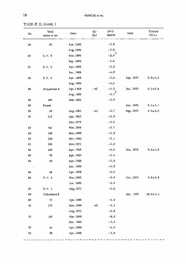
Steam samples from 125 productive wells were collected for 18O, D andT analyses. The wells were widespread in the geothermal area to create asignificant picture of the field. Measurements in single wells were repeatedat different periods as a check on possible changes in the 18O content withtime. All these data are reported in Table II.
In Fig. 7 the isotopic composition of some steam samples is comparedwith that of the local meteoric waters.
The isotopic composition of hydrogen is constant within the measureerrors, whereas the 18O concentrations vary extensively, from - 5. 5 to+ 0. 5%o.
The intersection of the straight line which fits all the steam sampleswith that of local meteoric waters gives values of 5D = -42%0 andб 18O = - 7. 2%o which can be considered a good yearly average value of themeteoric water composition supplying the steam field.
Isotopic exchange between water and oxygenated rocks (limestonesand/or silicates) account for the 18O enrichments. Considering, first,limestones, we have performed several analyses of oxygen and carbonisotopes of samples derived from the limestone intercalations of the cover,and the results are reported in Table III. From these data it appears thatwhereas the 13C contents do not show significant variations with depth,the 18O contents change to a large extent as a function of the distance ofthe sampling point from the reservoir rocks underlying the cover, as shownin Fig. 8. That is, a general tendency exists in which the greater thedistance from the reservoir top the lesser the deviations from the 618Ovalue of - 3. 5%o, which can be assumed to be the representative value ofthis type of limestone, and corresponds well with the observed values forsurface samples collected outside the geothermal area. Conversely, whenthe samples are nearer to the contact surfaces between the cover andreservoir, they show a lighter oxygen isotopic composition, reachingб18 О values of - 16%o, as a consequence of a greater fracturation andhigher temperatures in these zones.
It should also be noted that several samples collected at remarkabledistances from the reservoir top have shown very negative б О values.This fact can be explained by taking into account several emanations thatin the past reached the surface, formed lagoons, fumaroles, etc., andthe existence of faults, which cut through the cover. In fact, during thefirst drillings in the Larderello field, the productive wells never reached

14 PANICMetal.
TABLE II. HYDROGEN AND OXYGEN ISOTOPIC DATA OFGEOTHERMAL STEAM SAMPLES COLLECTED IN THE LARDERELLOAREA FROM 1964 TO 1973
6D <51 8O TritiumN o - D a t e (*) sMow D a t e т и ± о
1 144 Apr. 1968 -0.6
2 Gabbro 9 Apr. 1968 -1.6
-1.7
-1.6
-1.2
-0.3
4 S.Dalmazio4 Aug. 1965 -1.2
5 Gabbro 6 Apr. 1968 -1.3
-1.2
-1.2
6 122 Apr. 1968 -1.4
7 155 Oct. 1971 -3.3
-2.1
-2.6
-2.7
-2.5
10 107 Apr. 1968 -2 .1
11 114 Mar. 1965 -40 -4.2
12 134 Mar. 1965 -1.8
13 118 Aug. 1971 -2.2
14 Miniera 1 Apr. 1968 -2.7
-1.1
15 109 Apr. 1968 -41 -1.2
16 135 Jul. 1971 -2.4
17 102 bis Apr. 1968 -2.5
18 85 Aug.1965 -40 -2.8
19 С Sportivo Mar. 1965 -2.8
- 2 . 45
20 84 Apr. 1968 -2.2
-2.2
21 Pacciana 1 Apr. 1968 -3.0
-3.4
22 Fabiani Apr. 1968 -1.3 Oct. 1972 0.0±0.6
-1.2
Wellname or no.
144
Gabbro 9
Gabbro 7
S. Dalmazio 4
Gabbro 6
122
155
161
162
107
114
134
118
Miniera 1
109
135
102 bis
85
C. Sportivo
84
Pacciana 1
Fabiani
Date
Apr. 1968
Apr. 1968
Jun. 1969
Nov.1971
Aug.1965
Jun. 1969
Aug.1965
Apr. 1968
Jun. 1969
Sep. 1971
Apr. 1968
Oct. 1971
Apr. 1965
Jun. 1969
Apr. 1968
Jun. 1969
Apr. 1968
Mar. 1965
Mar. 1965
Aug. 1971
Apr. 1968
Nov.1971
Apr. 1968
Jul. 1971
Apr. 1968
Aug.1965
Mar. 1965
Jun. 1969
Apr. 1968
Jun. 1969
Apr. 1968
Jun. 1969
Apr. 1968
Jun. 1969

IAEA-SM-182/27 15
TABLE II. (cont. )
No.
23
24
25
26
27
28
29
30
31
32
33
34
35
36
37
38
39
40
41
42
43
44
45
46
47
48
Wellname or no.
Pacciana 3
Ciabattino
54
53
89
129
137
138
101
5
B. Prête
Pacciana 4
120
Sperim. 2
65
А Ною
62
6
71
82
119
97
151
128
58
57
Date
Aug. 1965
Aug. 1965
Apr. 1968
Sep.1971
Nov. 1964
Aug. 1971
Nov.1964
Aug.1965
Aug. 1971
Aug. 1971
Aug. 1971
Aug. 1971
Aug. 1969
Nov. 1964
Apr. 1968
Apr. 1968
Jun. 1969
Apr. 1968
Aug. 1971
Apr. 1968
Jun. 1969
Apr. 1968
Jun. 1969
Nov.1964
Aug. 1965
Nov. 1971
Aug.1969
Apr. 1968
Jun. 1969
Apr. 1968
Mar. 1968
Apr. 1968
Mar.1968
Apr. 1968
Nov.1971
6D
(%o)
-42
-41
-42
-41
-41
-43
61 8OSMOW
-3.4
-2.8
-2.6
-2.6
-3 .1
- 3 . 1
-1.9
-2.3
-2.3
-3.6
-3.8
-3.4
-0.8
-3.1
-3.3
-2.4
-2.6
-2.5
-3.4
-2.8
-2.2
-2.7
-2.8
-4.8
-3.9
-3.6
-3.1
-3.1
-3.0
-2.9
-0.3
-3.4
-3.3
-3.1
-3.3
Date
Oct. 1972
TritiumTU± a
0.7±0.6
1
16 РАШСШ et al.
TABLE II. (cont. )
No.Well
name or no.Date
ÔD
SMOWDate
TritiumTU±a
49
50
51
52
53
54
55
56
57
58
59
60
61
62
63
64
65
66
67
68
69
70
71
72
73
80
S.V. 9
S.V. 6
S.V. 2
Acquabona 2
106
Pineta
59
110
143
102
159
100
108
72
52
44
S.V. 5
S.V. 1
Colombaia 2
73
112
145
45
98
Apr. 1968
Aug.1969
Mar. 1965
Sep.1969
Apr. 1968
Jun. 1969
Apr. 1968
Aug.1969
Apr. 1968
Aug. 1969
Mar. 1965
Aug. 1965
Apr. 1968
Dec.1970
Mar. 1968
Mar. 1968
Nov.1965
Nov. 1971
Apr. 1968
Apr. 1968
Apr. 1968
Jun. 1969
Apr. 1968
Mar.1965
Jun. 1969
Aug.1971
Apr. 1968
Mar. 1968
Aug.1971
Mar. 1968
Jun. 1969
Apr. 1968
Apr. 1968
-43
-40
- 3 . 2
- 3 . 2С
- 2 . о "
-3.6
-3.9
-4.2
-3.4
-3.3
-4.05
-3.7
- 3 . 8
-3.7
-3.9
-3.3
-3.7
-2.9
-2.1
-3.6
-4.0
-3.4
-3.5
-3.8
-4.0
-3.6
-3.3
-5.5
-4.8
-3.4
-3.6
-2.8
-2.1
-4.8
-3.8
Sep. 1973 0.9±0.6
Jan. 1973 0.5±0.6
Jan. 1973 2 . 1 i l . l
Sep. 1973 0.0±0.5
Jan. 1973 8.6 ±1.2
Oct. 1972 0.5±0.6
Jan. 1973 49.0i l .5

IAEA-SM-182/27 17
TABLE II. (cont. )
No.
74
75
76
77
78
79
80
81
82
83
84
85
86
87
88
89
90
91
92
93
94
95
96
Wellname or no.
91
S. Luigi 3
81
38
19
136
141
113
26
Caspeci
Fornace
66
Serr. 8
Pozzaie 2
Vignacce
Cioccaie
Capanna
Soffion. 1
Oliveta
V.C. 10
V.C. 2
V.C. 5
Le Prata 4
Date
Apr. 1968
Nov.1971
Mar. 1965
Jun. 1969
Jul. 1971
Apr. 1968
Jul. 1969
Mar. 1965
Mar. 1968
Jul. 1969
Apr. 1968
Jun. 1969
Mar. 1965
Jun. 1969
Sep. 1969
Mar. 1968
Jul. 1969
Mar. 1968
Apr. 1968
Jul. 1969
Apr. 1968
Jul. 1969
Mar. 1968
Jul. 1969
Mar. 1968
Mar. 1968
Mar. 1968
Mar. 1968
Jun. 1969
Mar. 1968
Mar. 1968
Jun. 1969
ÓD(%)
-42
-43
-41
-43
-44
-43
-43
-44
ô»OSMOW
-4.55
-2 .9
-4 .8
-5 .2
-5 .9
-4.7
-3 .6
-4 .8
-2 .4
-1 .5
-4.2
-3 .9
-4 .2
-4 .2
-5 .5
-3 .0
-2.0
-2 .9
-2 .0
-1 .8
-2 .35
-2.0
-2 .5
-2.7
-1.7
-1.7
-0.7
+ 0.1
0
-1 .5
-2 .4
-2 .0
Date
Sep.1972
Sep. 1973
Sep.1972
Oct. 1972
Oct. 1972
Oct. 1972
Oct. 1973
Oct. 1972
Sep.1972
Dec.1973
Dec. 1973
Dec. 1973
Dec. 1973
Dec.1973
Sep. 1973
TritiumTU±o
4 0 . 7 Ü . 6
30 .0±l .3
27 .Oi l . 1
0 . 9 i 0 . 8
1.0i0.7
6 . 6 i l . 2
4 1 . 3 i l . 6
2 8 . 6 i l . 5
38 .Oi l . 5
0 . 0 i 0 . 5
0 .0 i0 .6
0 .0 i0 .6
0 .0 i0 .6
0 .0 i0 .6
0.8±0.7

18 РАШСШ et al.
TABLE II. (cont. )
No.
97
98
99
100
101
102
103
104
105
106
107
108
109
110
111
112
113
114
115
116
117
118
119
120
Wellname or no.
Le Prata 2
Le Prata 3
S. Amicié 2
Sasso 9
Grotte 2
С ovo
Orto
Querciola
LR-B
Bagnolo
Meli 2
Meli 1
LR1
VC 3
Lago 7
Lago 6
Lago 4
Diga 2
Pescaie
Tassinaie
Capannone
S. Edoardo
S. Federico
V. Madama
Date
Mar. 1968
Jun. 1969
Mar. 1968
Jun. 1969
Mar. 1968
Mar. 1968
Mar. 1968
Jul. 1969
Mar. 1968
Jul. 1969
Mar. 1968
Jul. 1969
Apr. 1968
Mar. 1968
Mar. 1968
Feb. 1968
Mar. 1968
Jun. 1969
Mar. 1968
Jun. 1969
Mar. 1968
Mar. 1968
Jul. 1969
Apr. 1968
Jul. 1969
Mar. 1968
Jul. 1969
. Apr. 1968
Feb. 1968
Feb. 1968
Mar. 1968
Mar. 1968
Jul. 1969
Mar. 1968
Mar. 1968
ÓDS MOW
DateTritiumTU±o
- 42
-39
-41
-43
-40
-3 .3
-3 .2
- 2 . 9
-3 .2
- 3 . 3
-2 .8
-4 .05
- 3 . 5
- 3 . 5
- 2 . 9
-4 .0
- 3 . 4
- 0 . 8
- 2 . 3
-2 .9
-3 .2
-3 .2
-1 .6
- 0 . 5
-0 .7
- 1 . 4
-2 .7
-3 .6
-2 .0
-2 .0
- 1 . 4
-1 .2
-2 .0
-4 .6
- 3 . 4
-2 .7
- 2 . 1
- 1 . 8
-2 .9
- 2 . 4
Sep. 1973
Sep. 1973
Sep.1973
Sep. 1973
Dec. 1973
Dec.1973
Dec. 1973
Dec. 1973
Dec.1973
Dec.1973
Dec. 1973
Dec. 1973
Dec. 1973
Dec.1973
Sep. 1973
0.6±0.7
1.2±0.6
0.5±0.7
0.7±0.7
0 .0±0.5
0.5±0.5
3.3±0.6
2.5±0.7
0 .0±0.5
0.0±0.5
0.7±0.6
6.5±0.8
20.4±1.0
1.4±0.8
3.2±0.9

IAEA-SM-182/27 19
TABLE II. (cont. )
No.
121
122
123
124
125
Wellname or no.
Pianacce 2
M.R. 1
S. Adriana
H.N. 4
M.R. 11
Date
Mar. 1968
Jul. 1969
Mar. 1968
Jul. 1969
Feb. 1968
Feb. 1968
Mar. 1968
Jul. 1969
ÓD 6180SMOW Date
TritiumTU±o
- 3 . 1
-2.9
-3.5
-3.3
-3.3I
- 3 . 3 *
- 3 . 3
- 3 . 0
Sep. 1973
Sep. 1973
5 . 9 ± 0 . 8
3 .5±1 .0
о
£о•о
\J
-10
-20
-30
-40
-50
- 6 0
-7П
1
—
-
л /
-у/
1
1 1 1 1
У; "-À *Л Y
^ i l 1 с
\\ interception:
ÓD - - 4 2Ó'8O=> - 7 . 2
1 1 1
h-JLT40
|
3223 1
i
18
120
MT/Y24/ |
80 96
I
118
27
CP
I
д
О
15
Iiî92
Ispring
steam
109
Óy93
I I
water
—
—
-
Ti 1о
-
1 1-8 - 6 - 3
Ó18O %o (SMOW)FIG.7. Deuterium and oxygen composition of some selected steam samples (circles; the numeration appearson Table II). The spring waters (triangles) represent local meteoric waters (see text).
the underlying Mesozoic formations, but drew the steam from the rocksof the cover.
In the carbonate formations which constitute the geothermal reservoir,one observes systematically more negative values from - 15 to - 23%o(Fig. 8 and Table III) and a more regular distribution within the rockmatrix. This indicates an active circulation over long periods of time,both in the fractures and in the pores of the non-fractured rocks. Thesefacts are confirmed by the analyses of samples of outcropping rocks inTuscany (unpublished data).

20 PANICHI et a l .
TABLE III. OXYGEN AND CAREON ISOTOPE COMPOSITION OF THECARBONATE SAMPLES OBTAINED FROM SOME WELL CORES IN THELARDERELLO FIELD
No.
С 1
С 2
С 3
С 4
С 5
С 6
С 7
Wellname or no.
Stratigrafico 1
111
138
101
89
88
120
Sampling pointdepth(m)
280- 282
425- 426
619- 621
700- 701
750- 751
807- 810
852- 854
909- 911
1047-1048
1151-1160
25- 52
305- 436
81- 106
0- 66
23- 73
212- 228
185- 232
0- 54
208- 370
506- 508
Geologicformation a
Ne
AS
AS
AS
AS
AS
AS
AS
D-An
D-An
AS
AS
AS
AS
AS
AS
AS
AS
AS
AS
618O
(%o)
- 5.3
- 6.3
- 5.2
- 4.7
- 4.5
- 5.8
- 5.8
-13.3
-15.0
-15.1
- 6.9
- 6.6
- 7.6
- 3.8
- 5.3
-13.2
-10.1
- 9.7
- 5.8
-16.1
Ó13CPDB
+ 1.6
+ 0.2
- 0 . 1
+ 0.3
+ 0.6
+ 0.4
+ 0.2
+ 0.9
+ 1.1
+ 2.2
- 0 . 1
+ 0.9
+ 0.1
+ 0.9
+ 0.8
- 2 . 3
- 2 . 4
+ 0.1
+ 1.3
+ 1.2
Distancefrom reservoir top
(m)
774
630
435
355
305
246
202
145
8
0
540
200
300
310
300
170
200
600
350
125
С 8
С 9
119
143
С
с
с
с
10
11
12
13
110
100
112
116
28 AS - 4.2 + 1.5 490
40- 88
316- 354
566- 567
20- 90
0- 81
47- 121
0- 53
89.5
146.4
189- 340
AS
AS
D-An
AS
AS
AS
AS
AS
AS
AS
- 7.5
- 8.2
-19.7
- 8.7
- 6.2
- 6.4
- 5.6
- 6.8
- 6.8
- 7.9
+ 0.5
+ 0.3
-0.6
-1.3
-0.3
+ 0.4
+ 1.4
+ 1.2
+ 1.3
+ 1.0
510
230
0
480
550
580
630
570
510
300

IAEA-SM-182/27 21
TABLE III. (cont. )
No.Well
name or no.
Sampling pointdepth(m)
0- 49
213- 274
433- 549
732- 800
1055-1056
0- 36
221- 240
521- 523
1172-1175
260- 266
474- 476
312- 314
524- 560
645- 730
209- 210
350- 383
412- 454
480- 488
505- 506
570- 603
695- 720
852- 855
941- 943
1017-1025
1160-1162
Geologicformation3
AS
AS
AS
AS
D-An
AS
AS
AS
D-An
L
L
L
L
L
L
L
L
L
L
L
L
L
L
D-An
D-An
<5 1 8 O
- 3.9
- 4.4
- 7.9
- 9.5
-18.3
- 4.7
- 7.7
-10.4
-15.2
-20.8
-19.6
-23.0
-18.5
-16.1
-19.3
-17.8
-16.5
-16.3
-15.4
-16.8
-15.4
-17.9
-18.1
-20.8
-22.3
PDB
+ 1.0
+ 1.0
-0.2
-1.4
-2.6
+ 1.1
+ 0.1
-0.8
-1.4
-0.3
+ 0.8
+ 0.5
+ 2.0
+ 1.8
+ 1.1
+ 3.0
+ 2.3
+ 1.9
+ 2.2
+ 1.8
+ 1.8
+ 1.9
+ 2.0
+ 2.0
+ 4.5
Distancefrom reservoir top
(m)
790
550
300
60
0
620
415
120
0
0
0
0
0
0
0
0
0
0
0
0
0
0
0
0
0
С 14 145
С 15 141
С 16 M. Rotondo 17
С 17 M. Rotondo 15
С 18 M. Rotondo 14
a Ne =Neogenic deposits, mainly clays (U. Miocene - Pliocene); AS = flysch-facies formations:
"argille scagliose" (U. Cretaceous - Eocene); D-A n= dolomites, anhydrites and cavernous limestones
(U. Triassic); L = massive limestones (U. Triassic - U. Jurassic).

22 PANICHI et al.
Г1000 ,_
800
• I г
9 600
400 _
200 _
0 L
O|
o o
о о
ооо о о
о о /
0 о1 i
а> а » Осло осю а р — — "i I i i i i I i i
-25 -20 -15 -10
Ó180%o (PDB)
- 5
FIG.8. Oxygen isotope variations of carbonates from core samples of several drillings, in relation to thedistance of the sampling point from the top of the reservoir.
As regards the role of silicate rocks underlying the calcareous forma-tions, there are, at present, no data related to the 18O content of rocksamples of the Larderello area. However, the steam samples producedby wells that extend across several hundred metres of such formation showan 18O shifting caused by an interaction of water and rocks.
The possibility of isotopic exchange at high temperature in silicateswas illustrated by Clayton and co-workers [13] who have shown a paralleldepletion in 18O contents in the calcareous and siliceous rocks in a wellcore in the Saltón Sea geothermal field.
All these facts confirm that in geothermal areas by far the most simpleexplanation of the oxygen shift is that it is due to isotopic exchange withcarbonates and silicates in the rock matrix through which the waters havemoved. Different 18O enrichments observed in steam samples produced in

IAEA-SM-182/27 23
a certain area reflect, in fact, the effects of complex deep circulationpatterns as well as different thermal conditions that affect, in oppositedirections, equilibrium fractionation and reaction kinetics, and differentresidence times.
In spite of this complicated situation, it can be foreseen that the isotopicexchange process remains dependent upon the distance of the zone of steamproduction from the zone of water infiltration. This factor can contributeto determining the distribution of 18O content in the geothermal field.
However, this mechanism does not seem to be a single one, when thegeological structures of a geothermal field can provide two or more differentcirculations of feeding waters. In other words, when absorption areasexist in the immediate vicinity of the field, and are hydrologically connectedwith the underlying steam-bearing formations, some waters tend to enterthe field and can determine a mixing with deeper fluids.
Now, the shallow component of the mixture certainly represents areservoir water derived directly from the local meteoric water, with littleor no change in isotopic composition, as a consequence of a relativeshort and fast circulation in relation to that required for the isotopicexchange with rocks.
On the contrary, deeper waters can be submitted to a greater exchangebecause of greater temperature conditions and greater contact time withoxygenate rocks. This may result in a large water body of rather uniformisotopic composition that corresponds to a maximum isotopic exchangeprocess which the waters have undergone during their history.
So, if the mixing occurs especially during exploitation conditions,different proportions of the two components in the mixture produce atsurface steam samples with different 18O contents, which progressivelyincrease from the zones nearest to the local absorption areas to zoneswhere the contribution of local water is less important.
6. GEOGRAPHICAL DISTRIBUTION OF 18O VALUES
The data of Table II, referring to the variations in time of the 18Ocontents, will be discussed below. Taking into account that the observedvariations are generally less than 0. 5%o, data relative to samples collectedin different years can be used to draw the map of Fig. 9, showing the618O distribution in the geothermal field, including all the sampling points.
This figure shows the following facts:
(a) The 18O content increases progressively, from the borders of thefield towards the centre, i. e. the 18O enrichment occurs in the samedirection as the flow lines of water into the productive layers.
(b) The 18O enrichment gradient with distance differs from zone tozone: for instance, in Lago and Lagoni Rossi the isotopic gradient is muchhigher than in other fields.
(c) The périphérie wells in the Castelnuovo area have 618O valuesalmost as negative as those observed in liquid water collected in wells inthe non-productive area bordering the geothermal field in the east and inthe south. In addition, in the Castelnuovo area a number of wells exhibithigh tritium, up to a maximum of about 50 TU, indicating an inflow ofrecent water.

24 PANICHI et al.
FIG. 9. Geographical distribution of the б18О values of the steam in the Larderello geothermal area. Thenumeration appears on Table II; the values used are those relative to the first sampling for a single well.The main outcropping formations are also shown (for details see Fig. 1).

IAEA-SM-182/27 25
(d) In the area of Monterotondo and Sasso, where ó18 O values areless negative than those observed in the Castelnuovo area, the tritiumcontent is also lower, indicating that recent water is present in almostnegligible amounts.
(e) The existence of an axis in a SW-NE direction, corresponding tothe inner part of the field, is indicated. It is also deformed by some localsituations which indicate some preferential ways of water infiltration in adirection orthogonal to the axis. In particular, this phenomenon isobserved in the Castelnuovo area, but can also be seen along the Sasso-Monterotondo-Serrazzano directrix. The south-western edge of the field,on which lie the productive zones of Lago and Lagoni Rossi, repeats thesame trend.
All these aspects may be explained by the hypothesis, described inSection 5, by which steam samples coming from the different zones of thegeothermal field are the result of a superimposition by an exchangeprocess and a mixing of steams, the first originated at depth and thesecond originated by a water circulating in a relatively superficial layer.In fact, taking into consideration the geohydrological characters outlinedin Section 2, the following scheme of the Larderello geothermal field maybe outlined.
The groundwater recharged in the limestone outcrops moves into thegeothermal field. These waters follow two different paths in both themore permeable formations (anhydrites, limestones and the upper partof the basement, rather fracturated) and in the deeper and less permeablezone of the basement.
The deeper circulation waters, which experience higher temperaturesand longer residence time, appear to be responsible for the higher 18Ocontent observed in steam which emerges in the inner zones of the field.On the other hand, the negative values of the southern zones of the fieldappear to be affected by a mixing with a relative shallow circulation, forwhich temperature and residence time are much less.
The mixing process is particularly evident in the Castelnuovo zone,where an inflow of recent water (tritium concentration up to 49 TU) canoccur through the outcrop of the semi-permeable sandstone, the so-called"macigno", directly overlying the permeable anhydritic formations. InMonterotondo, the outcrop of sandstone and mainly limestone seems tobe much less efficient for the infiltration of recent water, as indicatedby the lower tritium and the higher 18O compared with Castelnuovo. In fact,it is known that the limestone is made up, in its surficial part, ofradiolarites having low to very low permeability, and which have under-gone an intense silification.
On the other hand, the differences between Castelnuovo andMonterotondo can be due also to the different degree of exploitation of thetwo fields; in the Castelnuovo field the inflow of recent water may havebeen enhanced by the intense exploitation.
The high <518O gradients observed in the southern zones of the field(Lago and Lagoni Rossi), corresponding to the high hydraulic gradientsshown in Fig. 2, may be due to the presence, at the field edges, of zoneswith low permeability which could prevent recent water infiltration in thefield, so limiting at short distance mixing effects.

26 РАШСШ et al.
3 km
FIG. 10. Sketch map of the<5180 variations in time in several wells of the Larderello geothermal area. Theis о contents tend to increase when the arrows indicate a direction from more positive to more negative valuesand vice versa. The circles indicate no detectable variations. The main outcropping formations are alsoshown (for details see Fig. 1).

IAEA-SM-182/27 27
7. VARIATIONS IN TIME OF 18O VALUES OF STEAM SAMPLES
Figure 10 shows, schematically, the 18O variations observed in timein several steam samples. From this figure it appears that in the innerzones the wells have generally shown no variations, indicating that by nowthey are fed one single type of steam which is probably that produced bythe deeper evaporation in the central zone.
On the other hand, in the périphérie area characterized by б 18О valuesranging from - 1 to - 3%o, there is a clear tendency to assume more positivevalues in time. This evidently signifies the widening of that zone in whichthe contribution of the deeper steam is prevalent.
On the contrary, in the most périphérie area, where the isotopic compo-sition ranges from - 3 to - 5%o in some parts of the boundary, there is aclear tendency towards the production of steam with more negative 6 18Ovalues. This indicates that the relative contribution of the water, comingdirectly from the absorption area through the fast circulation, isincreasing.
8. CONCLUSION
The isotopic tool is therefore an attractive one to use in determiningthe origin and mixing of groundwater sources.
Furthermore, in a geothermal field under exploitation, a detailedsurvey of the variation in the 18O (and T) composition in time allows us toreveal the progressive modification that occurs in the field as a conse-quence of its exploitation.
Finally, we suggest that it is possible that this kind of investigationwill also become a valuable tool to check the effects of re-injection ofwaste water in the field.
REFERENCES
[1] CRAIG, H., "The isotopic geochemistry of water and carbon in geothermal areas", Nuclear Geologyon Geothermal Areas (TONGIORGI, E., Ed.), Spoleto (1963).
[2] WHITE, D.E. , "Geochemistry applied to the discovery, evaluation and exploitation of geothermalenergy resources", Sect.V, UN Symp. Development Utilization Geothermal Resources, Pisa (1970).
[3] GONFIANTINI, R., BORSI, S., FERRARA, G., PANICHI, С , Isotopic composition of waters from theDanakil depression (Ethiopia), Earth Planet. Sci. Lett. £8(1973) 13.
[4] FERRARA, G . С , GONFIANTINI, R., PANICHI, С. , La composizione isotópica del vapore di alcunisoffioni di Larderello e dell1 acqua di alcune sorgenti e mofete della Toscana, Atti Soc. Toscana Sci.Nat. Pisa, P.V. Mem., Series A 72 (1965) 570.
[5] BANWELL, C.J. , "Oxygen and hydrogen isotopes in New Zealand thermal areas", Nuclear Geologyon Geothermal Areas (TONGIORGI, E., Ed.), Spoleto (1963).
[6] WHITE, D.E., CRAIG, H., BEGEMANN, F . , "Summary of the geology and isotope geochemistry ofSteamboat Springs, Nevada", Nuclear Geology on Geothermal Areas (TONGIORGI, E., Ed.), Spoleto(1963).
[7] KOGA, A. , Geochemistry of the waters discharged from drillhole at Otake and Hatchobaru areas (Japan),Geothermics 2, Part 1 (1970) Special Issue 2.
[8] CRAIG, H., Standard for reporting concentrations of deuterium and oxygen-18 in natural waters,Science 133 (1961) 1833.
[9] CATALDI, R., STEFANI, G., TONGIORGI, M., Geology of Larderello region (Tuscany); contribution
to the study of the geothermal basins, Nuclear Geology on Geothermal Areas (TONGIORGI, E., Ed.),Spoleto (1963).

2 8 PANICHIetal.
[10] MAZZANTI, R., Geología della zona di Pomarance - Larderello (Prov. diPisa), Mem. Soc.Geológica Italiana í> (1966).
[11] LAZZAROTTO, A. , Geología della zona compresa tta Taita Valle del fiume Comía ed il torrentePavone (Prov. di Pisa e Grosseto), Mem. Soc. Geológica Italiana 6 (1967).
[12] CATALDI, R., ROSSI, A. , SQUARCI, P. , STEFANI, G., TAFFI .1 . , Contribution to the knowledgeof the Larderello geothermal region: remarks on the Travale field, Geothermics 2 ,Part 1 (1970)Special Issue 2.
[13] CLAYTON, R.N., MUFFLER, L.J .P. , WHITE, D.E., Oxygen isotope study of calcite and silicates ofthe River Ranch No. 1 well, Saltón Sea geothermal field, California, Am. J. Sci. 266 (1968) 968.
DISCUSSION
G. H. DAVIS: Have you found that the 18O shift can be used effectivelyas a "geothermometer" in the Larderello area?
C. PANICHI: The reported 18O values for carbonate samples collectedduring well drilling in this area confirm that temperature-dependent isotopicexchange between water and rocks occurs. Consequently, as the isotopiccomposition of the steam in the area is well known, isotopic exchangeeffects can in principle be used in estimating underground temperature.However, the temperatures obtained in this way do not exceed 150°C,whereas temperatures ranging from 200°C to 250°C are measured in thegeothermal steam. I think the discrepancy can be attributed either to thefact that the isotopic exchanges do not reach equilibrium or to the fact thatthe isotopic composition of carbonate reflects previous hydrologicalconditions, when the temperatures of the investigated layers were probablylower than those now observed, that is, before the present vapour-dominatedarea developed as a consequence of exploitation.

IAEA-SM-182/28
HOT SPRINGS OF THE IGNEOUS TERRAINOF SWAZILANDTheir noble gases, hydrogen, oxygenand carbon isotopes and dissolved ions
E. MAZOR*. B.T. VERHAGENNuclear Physics Research Unit,University of Witwatersrand,Johannesburg, Republic of South Africa
E. NEGREANUIsotope Department,The Weizmann Institute of Science,Rehovot, Israel
Abstract
HOT SPRINGS OF THE IGNEOUS TERRAIN OF SWAZILAND: THEIR NOBLE GASES, HYDROGEN, OXYGENAND CARBON ISOTOPES AND DISSOLVED IONS.
The hot springs of Swaziland are of great interest as they occur in an area devoid of recent volcanismand issue in igneous, rather than in sedimentary rocks. An origin from directly infiltrating rain water isconcluded from the Ne, Ar, Kr and Xe concentrations, and the 6D and ô^O values. The noble gases areshown to have been kept in closed system conditions, and their concentrations lead to the deduction ofpaleotemperatures at infiltration of 21°C to 31°C, which are similar to the present local summer temperatures.The MC age of the waters is calculated to be 4500 to 5400 years, and tritium concentrations are very low,indicating that the bulk of groundwater is indigenously deep seated. The chemical composition is unique,the total dissolved salts being 120 ppm, reflecting contact with igneous as opposed to sedimentary rocks.
1. INTRODUCTION
Hot springs are common all over the world, many of them beingsituated in regions of recent volcanic activity, to which their heat is oftenascribed. In addition, many of the world's hot waters issue in sedimentaryrocks and most, if not all, of their salt constituents are often attributedto dissolution from these rocks. Swaziland offers hot springs in a differentgeological setting, unassociated with any recent volcanism, and issuingin igneous rather than sedimentary rocks.
About ten hot springs are known in Swaziland (Fig. 1 and Table I), afew of them with several eyes. Seven of these have been sampled for detailedanalysis of their dissolved noble gases, their stable hydrogen and oxygenisotopes, tritium and the composition of their dissolved ions. 14C datingand stable carbon isotope analysis were carried out on three of the springs.In addition four adjacent rivers have been sampled for comparison.
The geology of Swaziland has been studied by Hunter [1 ] and a generaldescription of the Swaziland hot springs has been given by the same investi-gator [2]. A number of chemical analyses are given by Rindl [3] and by
* On sabbatical leave from the Israel Atomic Energy Commission and the Weizmann Institute ofScience, Rehovot, Israel, during 1972.
29

30 MAZOR et al.
FIG. I . Location map of sampled hot springs ( • ) and adjacent rivers (x). Known hot springs which werenot included in the present study are marked by open circles.
the Geological Survey of Swaziland [4]. A physical description of the thermalMkoba spring, in the Pigg's Peak region, is given by Spar go [5]. Thesprings are all situated in Precambrian granite or gneiss [2]. The springs,apart from Sipofaneni, are regarded by King [6] and Temperley [7] to lieon a line of crustal weakness, on whose South African extension four ofthe Natal hot springs are situated, namely Sulphur Springs (30.1°C),Warmbad (37.2°C), Frischgewaag (29.5°C) and Natal Spa (41.1°C). Thesesprings are described also by Kent [8].
The Swaziland Springs are rather low yielding, with outputs varyingfrom 3 to 19 m3 hourly [2].
2. THE NOBLE GASES
The water samples for noble gas analysis were carefully collected in1 cm3 glass tubes with high vacuum stopcocks at both ends. These weresealed to an extraction system, the gas phase was separated and purifiedover a titanium getter and the noble gases were introduced into a Reynold'stype 60°, 4.5" glass mass spectrometer (Nuclid Co. ) and measured against

IAEA-SM-182/28 31
atmospheric standards. Details of the sampling technique, the mass spectro-metric measurements and the analytical e r rors (± 5% or less for elementalconcentrations in the present work) are given by Mazor [9].
The solubility of He and Ne in water is relatively independent of tempera-ture, but the solubility of Ar, Kr and Xe is highly temperature-dependent(Fig. 2). Dissolved helium is often enriched by radiogenic helium, flushedout of the country rocks, but Ne enters groundwaters via contact with theair alone. As may be seen in Fig. 2, the maximum possible Ne content inair-equilibrated water at temperatures of 10°C to 60°C is 2.3 X 10"7 cm3STP/cm3
water. Air bubbles trapped during sampling may increase this amount signi-ficantly, the contamination caused by free air being highest for Ne and pro-gressively lower for the heavier noble gases. Samples with Ne contentssignificantly higher than the above-mentioned value of 2.3 X 10"7 cm3 STP/cm3
water may thus be rejected as contaminated, whereas samples with Ne ator below this value may be regarded as free from any significant conta-mination. Fifteen of the measured samples are uncontaminated by thiscriterion (Table II) and only one, run No. 23 9, is a borderline case. Theaccompanying Ar, Kr and Xe values are slightly lower than those of thetwin sample, No. 236, however, and hence this case also appears to beuncontaminated (the Ne is probably high because of an analytical errorsomewhat above average). The air contamination problem is furtherdiscussed by Mazor [9].
The noble gas data are given in Table II. The following characteristicsare seen.
2. 1. Noble gas air-supersaturation at the time of sampling
In Fig. 3 the air-saturation percentages for the various samples areplotted for Kr and Xe. These values were obtained by multiplying themeasured values by 100 and dividing by the amount expected in air-saturatedwater at the sampling temperature, the value being read for each case fromthe solubility curve (Fig. 2). It is seen that the samples (except for the Xevalue of run No. 237) were air-supersaturated when sampled. The valuesare 100-150% for Ar, 115-152% for Kr and 96-158% for Xe. Hence, somelosses could occur from the springs before sampling. For this reason eachspring has been sampled two to three times, and in further discussions thesample of highest noble gas contents has been selected from each spring,assuming it to be closest to the indigenous state. The similar values ob-tained in this way for the various springs lead us to believe that the noblegas escape was indeed low for the selected samples.
2.2. Radiogenic helium enrichments4
The He contents are several orders of magnitude higher than thecorresponding air-saturation value, i .e . up to 17 000 X 10"8 cm3 STP/cm3
water. These large excesses are attributed to flush-out of radiogenichelium from the decay of uranium and thorium, present in the ppm rangein all common rocks. Such radiogenic He is often observed in hot watersand seems to be a useful indicator for slow moving, or static, water.

TABLE I. DESCRIPTION OF SPRINGS
Station Spring LocationTemperature
COGeology
Lobamba 3
Mawelawele
Sipofaneni
Ezulwini ("Spa")
Mkoba
Lobamba 1
Lobamba 2
31°13*Е; 26O27*S
31°09'Е; 26°35'S
31°41*Е; 26°39*S
31°10fE; 26°24'S
З П б ' Е ; 26°01fS
31°12'E; 26°26'S
31°12*Е; 26°26'S
44.0
35.0
44.0
45.0
51.5
44.0
45.5
Grey granodiorite
Porphyrite granite
Alluvial valley in granodioriticterrain
Alluvial valley in granitic terrain
Small acidic pink intrusion into greycoarse-grained granite
Alluvial valley in granodioriticterrain
Alluvial valley in granodioriticterrain

IAEA-SM-182/28 33
15X e xlO
о
cu 9
! 8"О у
'•К 6
w 3E 5
1.52.5
2
1.56
5
Kr xlO°
Ar xlO
He x 10'
0 20 40 60 80Temperature (°C)
FIG. 2. Solubility of noble gases in fresh water. Source of data: • - [10]: multiplying his sea-waterdata by his given ratios for solubility in distilled water to solubility in sea-water; + - [11]; O - [12];and Д - [13]: multiplying their data by the atmospheric abundances.

TABLE II. NOBLE GASES (cm3 STP/cm3 WATER)'
StationNo.
4
Run
No.
234
235
238
Spring
Ezulwini("Spa")
Temp.CO
45.0
He X 108
12 266
9 519
9 711
Ne x 108
IS. 5
19.8
21.2
Ar X 104
3.17
3.18
*"Arй А г
312.5
311.5
1 , r m l i r 13 6 Ar
296.8
289.4
(«Ar/xAr)(i0Ar/KAr)
1.053
1.076
224
230
240
227
232
Sipofaneni
Mkoba
44.0
51.5
8 759
7 172
8 560
14 478
17 464
18.2
17.5
20.3
13.5
17.8
3.22
3.05
3.38
3.37
3.76
326.4
326.3
323.7
352.9
354.9
290.0
292.7
296.7
298. 5
1.12
1.11
1.19
1.19
3.
2.
01
95
0.
0.
16
23
58.
64.
0
3
7.
8.
20
20
6
7
1
2
228
237
226
231
236
239
229
233
Lobamba 1
Lobamba 2
Lobamba 3
Mawelawele
44.0
45.5
44.0
35.0
11 720
10 068
8 198
5 083
14 400
17 545
8 427
6 422
17.9
18.8
14.0
12.3
20.9
25.8
22.6
17.1
2.76
3.00
2.93
2.65
3.63
3.65
3.39
3.33
352.4
323.7
312.1
309.5
320.0
325.3
312.2
313.3
286.4
292.5
288.9
292.7
291.2
289.6
298.6
282.1
1.23
1.11
1.080
1.057
1.10
1.12
1.046
1.110
2.24
2.70
2.71
2.51
3.30
3.26
3.23
3.00
0.52
0.30
0.22
0.14
0.33
0.43
0.13
0.33
51.1
52.7
53.8
51.9
64.8
61.6
60.7
61.7
6.65
5.30
7.23
7.25
8.34
8.20
7.32
7.84
2.88
2.75
2.83
3.16
0.34
0.30
0.54
0.60
60.1
56.6
55.7
47.1
61.4
8.70
6.61
6.20
5.54
7.42
Air-saturated 25.0water
4.5 18.5 2.85
Elemental concentration errors are ± 8"7o or less [9], and the 40Ar/ ^Ar ratio is assigned an error range of up to ± 2%

IAEA-SM-182/28 35
FIG. 3. Percentage air saturation of Kr and Xe. The values were obtained by multiplying the measuredvalues (Table II) by 100 and dividing by the amounts expected for air-equilibrated water (Fig. 2) at thesampling temperature (Table I). All samples, apart from the Xe value of sample No. 6, are supersaturated.The corresponding values for Ar are similar to those of the Kr and Xe. This supersaturation at the time ofsampling is taken as an indication that the waters were kept in the ground in closed system conditions withrespect to their noble gases, but some gas could escape into the air before sampling. The highest values foreach spring are therefore taken to be closest to the indigenous values.
2.3. Radiogenic argon
The 4 0Ar/3 6Ar ratio in the samples is significantly higher than in theatmospheric standards measured in the same runs. The 40Ar enrichmentsare in the range of 5 to 23% (Table II). This 40Ar excess is attributed toflush-out of radiogenic argon, formed by decay of 40K, present in the ppmlevel in all common rocks.
A positive correlation is observed for the radiogenic He and Ar enrich-ment, as seen in Fig. 4. The range of radiogenic He/Ar ratio is 2.6 to 5.This is similar to ratios of 2-4 observed in New Zealand hot springs [14]and equal to a value of 4 found in Yellowstone hot waters [15]. This valueis also in the range of the average He/Ar radiogenic production ratio ofabout 10, calculated by Zartman and co-workers [16] for common crustalrocks.

36 MAZOR et al.
i
У 2
8 10 12
Hex10scm3ST(/cm3 water
14 16 18
FIG.4. Correlation of radiogenic 4He and radiogenic ^Ar. The average (He/Ar) radiogenic ratio is 4,similar to the values 2-4 found in New Zealand hot waters [14] and to the value 4 found in Yellowstone [15].
2.4. Atmospheric relative abundances indicating meteoric origin
The relative aboundance of Ne, atmospheric Ar (i.e. after correctionfor radiogenic additions (Table II) by use of the 40Ar/ 36Ar ratio in theaccompanying standard measurement), Kr and Xe closely resemble thosein air-saturated water. In Fig. 5 the selected samples (richest in noblegases for each spring) were plotted along with the abundance values ofair-saturated water at 25°C, and the similarity of the lines is obvious.
This is taken as proof that we are dealing with meteoric water, whichpenetrated the ground after equilibration with air at the then prevailingambient temperature. No other process is likely to exist in nature thatcan load these waters by noble gases in near atmospheric proportion. Thismeteoric nature is independently revealed by the stable isotopes, as dis-cussed below.
2.5. Deduction of p ale ote mpe rature s
Thermal waters were air-supersaturated with respect to their noblegases when sampled. This is taken as an indication that once the meteoricwater entered the ground it was kept in closed system conditions with respectto its atmospheric gas content, even though the water was subsequentlyheated.

- 5
= 4
5_
Е 2
Nex107 Ar x104 КгхЮ8 ХехЮ9
FIG. 5. The noble gas pattern (in the samples of highest noble gas contents in each spring, see text).The values are seen to group closely around the line of air-equilibrated water at 25°C (solid line). Thisis taken as a proof for the meteoric origin of the waters, as no other mechanism could load them with noblegases in atmospheric-like abundances.

TABLE III. PALEOTEMPERATURES
Run No. SpringSampling
temperatureAr
Paleotemperatures ( °C)
Kr Xe Mean
238
237
226
236
233
224
232
Ezulwini ("Spa")
Lobamba 1
Lobamba 2
Lobamba 3
Mawelawele
Sipofaneni
Mkoba
45.0
44.0
45.5
44.0
35.0
44.0
51.5
23
28
28
17
22
24
19
22
32
31
22
23
25
24
24
33 a
29
23
26
22
28
23 ± 1
31 ±2
29 ± 1
21 ± 3
24 ±2
24 ± 1
24 ± 3
The Xe value of run 237 is obviously too low, hence the value of run 228 was applied.The error cited is the mean deviation between the measurements of Ar, Kr and Xe. The estimated analytical error of ± 5°Jo or better of theseelements introduces an uncertainty of about ± 2°C. Thus the deviations observed between the Ar, Kr and Xe paleotemperatures are in the rangeof the analytical accuracy.

IAEA-SM-182/28 39
Hence, the atmospheric Ar and Kr and Xe concentrations maybe usedto calculate the "paleotemperatures" of the waters, i.e. the ambient tempera-tures that prevailed on the ground at the time of infiltration. These tempera-tures can be read from the solubility graph in Fig. 2. The paleotemperaturesmay be calculated for each spring independently from its Ar, Kr and Xecontents. Good agreement is seen (Table III) between the results of calcula-tions for these three gases. The mean deviations of the three values foreach spring vary from ± 1°C to ± 3°C. The mean paleotemperatures them-selves vary from 21°C to 31°C.
The time, or age, to which these paleotemperatures are relevant canbe deduced from С measurements (see below). In any case it is interestingto note that the average "paleotemperatures" are close to the average summertemperatures of Swaziland (and it is the summer temperature that counts,as Swaziland is, and probably has been for some millenia, a summer rainfallarea). In addition this origin from rain water is borne out by the stableisotope composition of the springs.
2.6. Average temperature in the aquifers feeding the hot springs
The noble gas contents enable us to make general deductions on thetemperature of the water reservoirs that feed the springs.
Two basic types of atmospheric noble gas patterns have so far beenfound in hot springs. These are:
(a) Springs with temperatures below boiling point, in which the noble gasesare kept in closed system conditions and hence issue with gas contentsequivalent to those found in air-saturated waters at common surfacetemperatures (10°-30°C). The best examples of such cases so farstudied occur in the Jordan Rift Valley in Israel [9] and a few hot springsin Rhodesia [17].
(b) Springs fed by superheated water from which separating steam canstrip most of the noble gases, before or at the point of issue. Examplesof this type were found in the Yellowstone National Park [15], in SulfurBank of the Pacific Tectonic Belt, United States of Ameria [18] and inthe boiling Binga springs of Rhodesia [17]. In these cases as littleas 10% of the original atmospheric noble gases may remain.
The Swaziland springs clearly belong to the first group, i. e. watersthat retained their atmospheric noble gases. It seems, tentatively, thatthese springs are not fed by superheated water at depth, a conclusionindependently supported by the stable isotopes as is shown below.
3. DEUTERIUM AND 18O
The 6D and 618O values have been measured mass-spectrometricallyin the springs studied as well as in four adjacent rivers (Table IV and Fig. 6).
The four river values plot along a line which is typical for rain andderived surface water. The lightest of the samples is No. 10, collectedfrom the short Mkoba tributary of the Komati River, in the mountainousarea of Piggs Peak which might well have isotopically relatively light rains.

TABLE IV. CHEMICAL AND ISOTOPIC DATA
pH Ka Naa Mga
r 6Cla SO4
a HCO,a
4 SÔD%° б О% (TU)
4 Ezulwini("Spa") 8.6 l 35 11 11 53 123 -14.8 ±1.6 -4.05 i 0.09 0.5 ±0.2
0.026e 1.52 0.16 0.20 0.32 0.31 0.23 1.09 3.85
6
7
1
2
Lobamba 1
Lobamba 2
Lobamba 3
Mawelawele
7.9
7.9
8.0
7.9
1
0.026
1
0.026
1
0.026
1
0.026
48
2.09
45
1.96
45
1.96
45
1.96
1
0.
1
0.
1
0.
2
0.
082
082
082
16
4
0.20
4
0.20
4
0.20
9
0.45
6
0.32
6
0.32
7
0.37
7
0.37
14
0.
14
0.
14
0.
14
0.
40
40
40
40
8
0.17
6
0.13
6
0.13
6
0.13
81
1.44
81
1.44
74
1.33
87
1.54
163
4.70
158
4.55
152
4.48
171
5.03
-15.5
-18.1
-14.4
-18.8
±
±
±
±
1.
1.
1.
1.
6
3
6
6
-4.62 ±0.09
-4.11 ±0.08
-4.48 ±0.09
-4.05 ± 0.09
1.3
0.4
0.6
0.2
±0.
±0.
±0.
±0.
2
2
2
2
3 Sipofaneni 7.9 4 135 1 2 7 121 30 101 401 -14.7 ± 1.6 -4.09 ±0.09 0.4 ±0.2
0.10 5.87 0.082 0.10 0.37 3.41 0.62 1.77 12.3
5 Mkoba 8.3 1 58 1 4 6 21 6 . 93 190 -18.6 ± 1.6 -3.96 ±0.09 1.1 ±0.2
0.026 2.52 0.082 0.20 0.32 0.59 0.13 1.74 5.61
11
8
9
River at LobambaLittle Usutu R.
River at MawelaweleGreat Usutu R.
River at SipofaneniGreat Usutu R.
7.4
7.5
7.6
.
1
0.
1
0.
026
026
7
0.
11
0.
9
0.
30
48
39
4
0.
4
0.
7
0.
33
33
58
2
0.
4
0.
4
0.
10
20
20
1
0.
1
0.
1
0.
053
053
053
7
0.
11
0.
11
0.
20
31
31
5
0.
9
0.
8
0.
10
19
16
27
0.
40
0.
47
0.
,44
,66
,77
53
1.53
81
2.30
88
2.50
-12.1
-10.5
- 4.5
±
i
±
1.
1.
1.
1
••
3
1
-3.
-2.
-2.
27 ± 0.
60 ±0.
16 ± 0 .
08
08
08
46.
53.
46.
9
2
1
± 1.
± 3 .
±2.
8
5
5
River at MkobaMkoba R. (into theKomati)
-13.6 ± 1 . 1 3.40 ±0.08
Geological Survey, Botswana.m g / i i t t e .
m e q / i i t r e .

IAEA-SM-182/28 41
- 2 0 -
- 5
-1
-
1
3«•4
2i
1
X1O
I
x8
9x
-
-
- 418
U\ fool
FIG, 6. Isotopic composition. The river samples (x) lie on a line which is common for rain. The sequenceof the river samples along this trend is understood from their locations and reveals slight progressive evaporation(see text). The hot springs (•) may well originate from non-evaporated infiltrating rain water. The stableisotopes seem to reveal, independently, the meteoric origin of the hot springs studied.
TABLE V. CARBON ISOTOPES AND INFERRED AGES
Source
Ezulwini("Spa")
Lobamba 2
Sipofaneni
1 4 С ( p m c ) a
47.6 ± 2.1
43. 5 ± 1. 8
48. 5 ± 2. 5
-13.6 ± 0
-14.48 ±
-12.4 ±0
i
.07
1.8
.07
Age I (years)
4660
5400
4500
Age II (years) d
1080
2300
200
In per cent modern carbon (pmc).Isotope Department, Weizmann Institute of Science.
c Assuming groundwater initially contains 85 pmc [19] .С value applied as initial content derived by dividing measured value by ô
See text for evaluation of Ages I and II.
The next in the sequence is sample No. 11, collected at a tributary of theLittle Usutu, and this is followed by samples 8 and 9, both from the GreatUsutu, No. 9 being about 220 km downstream from No. 8. The four riversamples thus reveal isotopic values resulting from slight progressive eva-poration. The average rain composition seems to be close to, or veryslightly lighter than, the values of sample No. 10.
The results of the hot springs are grouped around <5D - 17%o andб1 О- 4. 2%o, and are slightly lighter than the river waters, probablyclose to the composition of the local rain at the time of infiltration.
The stable isotope data therefore lead independently to the followingconclusions:
(a) The hot springs are fed by rain water that did not undergo evaporationand, hence, infiltrated directly into the ground.

к Na Са S0AНСО,
FIG. 7. The chemical composition. The hot spring waters (1 - 7) are higher in their salt contents than theadjacent river waters (8,9,11). If the rivers are taken to represent in their composition the original infiltratingmeteoric water, then the hot springs must have picked up from the igneous and metamorphic country rocks,Na, F and HCO3, and have lost Mg, perhaps by exchange reactions. The higher NaCl value of Sipofaneni(sample 3) might be caused by brief contact with Karroo sediments (see text).

IAEA-SM-182/28 43
(b) The hot springs did not suffer from partial losses of a steam phase,which would result in an isotopically heavier residual water phase.These waters are fed by reservoirs at temperatures that are signifi-cantly below boiling, a conclusion already reached on the basis ofdissolved noble gas data.
4. TRITIUM CONCENTRATIONS
The tritium values for three measured rivers are 46-53 TU. Thevalues found in the hot springs are, however, only 0.0-1.3 TU (Table IV).This suggests that the spring waters are virtually not mixed with river,or other very recent water met during their ascent. An upper limit forsuch additions may be reached if it is assumed that the indigenous hotwaters are devoid of tritium. Even in such a case the additions fromintermixing surface water will be limited to 0-2%. Hence, the springwaters may justifiably be regarded as indigenous, deep-seated whendiscussing their noble gas contents, stable isotope composition, 14Cvalues or composition of the dissolved ions.
5. CARBON ISOTOPES AND INFERRED AGES
Water from three springs has been extracted at the field for its carbonextraction. The measured ô 13C and 14C values are given in Table V.
The measured springs issue in igneous terrain and in two of themNaHCO3 is the dominant dissolved salt species. However, the observedб 1 3 С values of 12-14%o are close to values known elsewhere from sedimentaryterrain.
Two types of age calculations were applied in Table V. Age I was basedon the assumption that the groundwaters had an initial 1 4C content of 85 pmc[19, 20]. Age II was calculated by correcting for initial dilution by fossilcarbon by dividing the observed 1 4 C value by <513C/-25 [21]. The set ofAges I seems to reveal a better internal consistency than those of Ages II(Table V). There are, however, no criteria at hand with which to decideon the correct 14C ages. These may perhaps be re-calculated in the future,once the art of 1 4C age deduction reaches a more advanced state.
In conclusion, the 1 4 C content seems to indicate that the hot springwater studied in Swaziland is a few thousand years old, i. e. older than thewater in the active cycle of shallow groundwater but not entirely fossil.
An age of a few thousand years would be in good agreement with theelevated contents of radiogenic He and Ar, which reached the observedlevel by prolonged contact with aquifer rocks.
6. THE CHEMICAL COMPOSITION
The chemical composition of the springs studied and the adjacentrivers is given in Table IV and Fig. 7. Comparison with a number ofchemical analyses previously published [3,4] reveal a general similarity;

44 MAZOR et al.
a detailed comparison is not possible, as these sampling sites could notbe accurately identified. The following features emerge from the chemicaldata:
(a) Remarkably low salt contents. The springs, though thermal, aresurprisingly low in their salt contents, the total ions ranging from one caseof 400 ppm. This is definitely to be attributed to the igneous rock environ-ment composed mainly of granites (Table I), which contain very little solublematerial. This is in remarkable contrast to most hot springs in the world,which are frequently loaded with salts, originating from sedimentary rocks.
In spite of the very low salinity, some of the waters are not palatablebecause of a sulphur taste and an occasional H2S smell.
(b) Reactions with the igneous host rocks. The rivers have a totalion content of 53 to 88 ppm, whereas the hot springs have a content of120 to 400 ppm. It has been shown from the noble gas and stable isotopedata that the springs are of meteoric origin. It seems reasonable thatthe initial salt content of this meteoric water was, at most, as high asin the rivers. Hence, the additional ions result from the igneous rocksor their derived soils. The various springs, except Sipofaneni, havemuch in common in their dissolved salts (Fig. 7), their cations beingNa » Ca > Mg, and their anions being HCO3 > Cl > F > SO4 and thedominant salt species being NaHCO3.
The enrichments above river water are in Na, F, HCO3 and veryslightly in Cl. Magnesium has been depleted, possibly because of ionexchange, a process seen elsewhere, also in other water associations.
Sipofaneni has more than twice the T. D. S. of the other springs,the dominant addition being NaCl (Table IV and Fig. 7). This might wellbe explained by the location of this spring on a post-Karroo joint and adjacentKarroo outcrops. It seems likely that, although Sipofaneni issues in igneousrocks, its water comes into contact with Karroo sediments, which contributeadditional salts [22].
A C K N O W L E D G E M E N T S
We wish to warmly thank G. Sharig, Governmental youth adviser, forhis generous help, and A. Mokatshwa for guidance to the Mkoba spring;also J .R. Abbott, Swaziland Senior Water Officer, for valuable information,and Mr. Ford, Superintendent of the Royal Swazi Spa, for his assistance.
Informative discussions with Professor J. P. F. Sellschop, Director ofthe Nuclear Physics Research Unit, University of the Witwaterstrand, andD.R. Hunter, the Department of Geology, University of the Witwatersrand,are gratefully acknowledged.
The stable hydrogen, oxygen and carbon isotope measurements werekindly done in the laboratories of Professor J. R. Gat, the Isotope Departmentof the Weizmann Institute of Science, Rehovot. The chemical analyses werecarried out in the Chemical Laboratory of the Geological Survey of Botswana,headed by L. Hutton. The help of these colleagues and of the N. P.R. U.Environmental Isotope Group staff is much appreciated.
IAEA-SM-182/2 8 4 5
REFERENCES
[1] HUNTER, D.R., Geological map of Swaziland 1 : 250 000; Geological Survey and Mines Dept.,Mbabane, Swaziland (1966).
[2] HUNTER, D.R., 23rd Int. Geol. Congr. JL9 (1969) 165.[3] RINDL, M., S. Afr. J. Sci. 29, Suppl. 4(1932) 278.[4] Swaziland Geological Survey, Bull. No. 6(1966).[5] SPARGO, P.E., S. Afr. J. Sci. J31 (1965) 179.[6] KING, L.C., Trans. Geol. Soc. S. Afr. 64(1961) 64.[7] TEMPERLEY, B.N., Ann. Rep. Geol. Surv. S. Afr. J3( 1964) 139.[8] KENT, L.E., 23rd Int. Geol. Congr. 19(1969) 143.[9] MAZOR, E., Geochim. Cosmochim. Acta J36 (1972) 1321.
[10] KONIG, von H., Z. Naturforsch. 18a (1963) 363.[11] DOUGLAS, E.J., J. Phys. Chem. j>8 (1964) 169.[12] MORRISON, T.J. , JOHNSTONE, N.B., J. Chem. Soc., Part III (1954) 3441.[13] WEISS, R.F., J. Chem. Eng. Data_16 (1971)235.[14] WASSERBURG, G.J., MAZOR, E., ZARTMAN, R. E., "Isotopic and chemical composition of some
terrestrial natural gases", Earth and Meteorics(GREISS, J., GOLDBERG, E.D., Eds), North-HollandPublishing, Amsterdam (1963).
[15] MAZOR, E., FOURNIER, R., Geochim. Cosmochim. Acta 37 (1973)515.[16] ZARTMAN, R.E., WASSERBURG, G.J., REYNOLDS, J.H., J. Geophys. Res. 66 (1961)277.[17] MAZOR, E., VERHAGEN, B.Th., Geochim. Cosmochim. Acta, in press.[18] MAZOR, E., BARNES, I . , unpublished data.[19] MÜNNICH, K.O., Naturwissenschaften 44 (1957)32.[20] VOGEL, J .C. , EHHALT, D. , "The use of carbon isotopes in groundwater studies", Radioisotopes in
Hydrology (Proc. Symp. Tokyo, 1963), IAEA, Vienna(1963) 383.[21] INGERSON, E., PEARSON, F.J. , Jr., "Estimation of age and rate of motion of ground water by
the MC method", Recent Researches in the Fields of Hydrosphere, Atmosphere and Nuclear Geochemistry,Sugawara volume, Maruzen, Tokyo (1964) 263.
[22] HUNTER, D.R., private communication.
DISCUSSION
J.Ch. FONTES: To what extent was the rain water saturated in noblegases?
E. MAZOR: In the few rain-water analyses which we performed, weobserved slight oversaturation, attributable to lower temperatures in theclouds. In that connection, I would mention that, when the rain waterreached the ground surface, its temperature equilibrated rapidly with theambient temperature.
P. FRITZ: The solubility of a gas depends not only on temperaturebut also on the ionic strength of the solution. Was the concentration ofrare gases in your samples affected by the dissolving of salt underground?
E. MAZOR: No, for our samples contained a total of only 120 ppmT. D. S.
R.R. LETOLLE: With regard to Fig. 4, was the helium excess deter-mined using the 3He/4He ratio?
E. MAZOR: No, we are not able to measure 3He with our methods.We decided that the helium was radiogenic because its concentrations wasfour orders of magnitude higher than in air-equilibrated water.
H. OESCHGER (Chairman): Could you use the radiogenic heliumand argon as a basis for dating?
E. MAZOR: I do not think so, for we do not know the volume ratio ofwater to flushed rock.

46 MAZORetal.
D. В. SMITH: Any loss of dissolved gas from the thermal water beforeobtaining the sample will apparently lead to an overestimate of thetemperature of the recharge water. For two springs (Lobamba 1 and 2)Table III gives significantly higher recharge temperatures. Are there anygeohydrological features associated with these particular springs whichcould cause a higher loss of gas than might occur in the other springs whichwere sampled?
E. MAZOR: Not as far as I am aware. In this connection I wouldstress, however, that our figures represent maximum temperatures andthat additional data would be helpful.
F. J. PEARSON: Hydraulic models of hot spring systems in regionswith no recent volcanism show that a source of heat greater than thatsupplied by a normal geothermal gradient is required for some of thesystems to function. The source may be slightly higher than normalconcentrations of such radioisotopes as 4 0K or uranium in the aquifermaterial. If you have sufficient knowledge of the hydrology of your system,you'may be able to make an order-of-magnitude estimate of aquifer radio-isotope concentrations from your excess 4He and 40Ar concentrations.Such an estimate would be of great interest to those working with geothermalsystems elsewhere.
E. MAZOR: I agree. However, the rise of hot water is oftenattributable to a head of fresh water, and we believe this may be the casein Swaziland.
V. T. DUBINCHUK: The reference data on gas solubility are forequilibrium states. Did you take into account the kinetics of gas dissolutionin atmospheric water or did you assume that the saturation of the atmosphericmoisture was complete and in equilibrium? In other words, was theresufficient time to establish equilibrium between atmospheric moistureand noble gases from the moment of condensation up to the moment ofprecipitation?
E. MAZOR: The saturation values were taken from the literature,where carefully conducted experiments have been reported. As regardsthe second part of your question, we found that the surface waters weregenerally in equilibrium.
M. LEVIN LIPSIN: In Section 6 of your paper you mention a sulphurtaste and an occasional H2S smell. If the waters are not magmatic, whatin your opinion is the origin of the H2S?
E. MAZOR: We assume that the H2S derives from biogenic decompo-sition of the dissolved sulphate.
M. LEVIN LIPSIN: Is there any carbonate or sulphate mineralizationin the fractured zone mentioned by you in your oral presentation?
E. MAZOR: I doubt it, judging by the very low salt contents of thespring waters.
T. FLORKOWSKI: In your oral presentation you mentioned gas bubblesescaping from the water of some of the hot springs. Did you attempt tocollect the gas and determine its composition?
E. MAZOR: Not in this study. We did do so, however, in our studyin the Yellowstone National Park and observed fractionation which can beexplained in terms of a partial loss of dissolved gases.
W. G. MOOK: In your oral presentation you mentioned briefly theproblem of correcting the conventional 1 4 C ages of groundwater. I shouldlike to make a comment in this connection.

IAEA-SM-182/28 47
From a theoretical point of view the situation is quite clear. If youassume that the only source of inorganic carbon in the groundwater issoil limestone dissolved by the action of soil CO2, that there is in theaquifer no isotopic exchange between the dissolved carbon and solidlimestone and no addition of CO2 (of magmatic origin or released fromlimestone by H+ ions), and that there occurs no mixing of water massesof widely different 14C ages, a straightforward calculation gives theoriginal 14C content of the groundwater. I presented this approach at theconference on radiocarbon dating held in New Zealand in 1972 (W. G. Mook,"On the reconstruction of the initial 1 4C content of groundwater from thechemical and isotopic composition").
Two processes are taken into account: the dissolution of CaCO3 byCO2; isotopic exchange between the bicarbonate formed and the soil CO2in the unsaturated zone. It is irrelevant in what order these processesoccur, whether they occur stepwise or even whether they occur continuouslyat the same time. The result is:
_ ^ _ | a A + b A + 1 л л x ( a + b ) 6 s - а 6 а о - b 6 b o
a + b L a o b 0 ( b e b o )¿ b e
where
Abo= 2(A a o+A f i o)and6b o = | ( ô a o +ô l o ) ; ôbe = ôg0 - £g and Afee = Ag0 - 2eg/l0;
eg is the carbon isotope fractionation (inper mille) between gaseous CO2
and dissolved bicarbonate;A is the 14C content as a percentage of the modern standard;6 is the 13C value relative to PDB;a and b refer to the concentrations of dissolved CO2 and bicarbonaterespectively, S refers to the soil limestone and E refers to the totalcarbon content.
Of the nine variables, one is known (eg), and three can be determined(a and b — on the basis of pH, temperature and salinity — and 6 £) . Tocalculate the original 14C content of the sample, A2, four values have tobe assumed: Aao, A í o , 5ao andó£ o . The conventional assumptions (100%,0%, -25%o and 0%o respectively) are not necessarily correct.
Although the model is clear, this does not directly lead to a successfulcorrection procedure. The advantage, however, is that one can play aroundwith the figures and determine, for instance, age limits. Also, it oftenturns out that the assumption of A£ = 85% cannot be true. Conversely,assuming a value for A£, one can calculate Aa0, as was done in a paperpresented earlier in this Symposium.
MAZOR, E., VERHAGEN, B.T. , SELLSCHOP, J.P.F. , ROBINS, N.S. , HUTTON, L.G. ,"Kalahari ground waters: their hydrogen, carbon and oxygen isotopes and dissolved ions", these Proceedings1, IAEA-SM-182/18.


PROBLEMS IN USING ENVIRONMENTALISOTOPES FOR GROUNDWATER STUDIES
(Session 6)


IAEA -SM -182/29
LOCAL VARIABILITY OF THEISOTOPE COMPOSITION OF GROUNDWATER
J.R. GATDepartment of Isotope Research,The Weizmann Institute of Science,Rehovot, Israel
Abstract
LOCAL VARIABILITY OF THE ISOTOPE COMPOSITION OF GROUNDWATER.The local variability of the isotope composition of groundwaters is used to obtain information on the
recharge and flow regimes in the aquifer waters. The method is based on repeated samplings of ground-waters on an evenly spaced time and space grid. The spread of isotope compositions is then compared withthe scatter resulting from the analysis itself and with the variability of composition of the precipitation.The systems investigated were in the phreatic coastal aquifer of Israel and a limestone mountain aquifer,which is largely confined. In the coastal aquifer 130 wells in a 100 km2 test area showed a bimodaldistribution of the 18O isotope composition, which is displaced by a few tenths of a per mille relative to meanprecipitation. Repeat sampling over eight years of wells in that aquifer also gave very reproducible results.By contrast, in the mountain aquifer both the spatial and temporal variability was greatly in excess ofanalytical scatter. Space and time inhomogeneity was also found in leakages into a limestone cavern whichserves as a natural lysimeter for the recharge to such an aquifer.
INTRODUCTION
The stable isotope method attempts to relate t h e 1 8 О and deuteriumcontent of groundwater bodies to the location and season of recharge andto the nature of the recharging waters. The method is based, on the onehand, on the geographic variability of the isotope composition of precipi-tation, primarily as a function of elevation, latitude and distance from thevapour source [l]. On the other hand, one uses characteristic differencesbetween rainwater, snowmelt waters and surface waters which have beenexposed to evaporation. Conservative behaviour of the isotope compositionduring the subsurface flow is one condition for the successful applicationof the method; this condition seems to be satisfied at moderate temperaturesfor limited time periods (up to 104 years). Changes in the isotope compo-sition can occur as a result of mixing with other waters.
There is a large scatter in the isotope composition of individual rainfallevents. These variations are damped in the transition to the aquifers,groundwaters representing an averaged sample of the precipitation. Shiftshave, however, been observed between the amount of weighted compositionof rain and that of groundwaters, due to either selection or fractionationprocesses [2]. Some residual noise remains in the isotope compositionof groundwaters, and it can be asked to what extent aquifer units arecharacterized by a singular isotope composition and how constant in timeand space this composition is. These questions have been posed in thecontext of the sharpness with which the origin of groundwaters can be defined,recognizing that any noise in the isotope data limits the quantitativeapplication of the method [3].
51

52 GAT
The smoothing of the variations during recharge and the degree ofhomogeneity of waters in an aquifer are related to the recharge mechanismand to the flow and mixing patterns in the aquifer. In this report, time andspace variations of the isotope composition in some selected groundwaterbodies are presented. The aim is ultimately to relate this variability tothe recharge and mixing pattern and thus use the scatter of isotope data asa tool for the study of hydrological processes.
ANALYTICAL REPRODUCIBILITY
The present study is based on the evaluation of small variations inthe isotope composition, variations which are of the order of magnitudeof the analytical errors. It then is imperative to define the analyticalreproducibility exactly. The 18O and deuterium content is measured bymass-spectrometer analysis of the isotopic species of CO2 and hydrogengas, respectively, carbon dioxide after isotopic equilibration with the watersample and hydrogen obtained by complete dissociation of water on a hotmetal [4]. The analytical error, as quoted by most laboratories, is basedon the repeated determination of some standard sample. However,analytical reproducibility depends among other factors on the chemicalnature of the samples; volatile organic substances, sulphur compoundsand other not yet identified materials affect the analytical process both inthe determination of the deuterium abundance and in the mass spectro-metry of carbon dioxide. Thus, Fleischer and co-workers [5] reportedthat the reproducibility of 18O measurements of saline formation watersfrom oil-bearing strata was lower by a factor of 2 than that of clean (rain-water) samples. Obviously, the errors determined for some standardmaterial may not be applicable to the set of samples which is beinginvestigated.
The routine procedure of analysis of our Rehovot laboratory overcomesthis problem in part. The measurements are done in batches, using aninterpolation technique between two working standards whose б-values areassigned [6]. Each batch consists of nij aliquots of the j samples, usuallym = 2 for the samples and m = 3 for the standards. If R is the instrumentreading for the ratio of currents of the two isotope beams (or any otherinstrumental reading proportional to the isotope ratio) and assuming anequal statistical distribution of errors in all the samples, then the varianceof the measurements is given [7];
S =
where Rj is the average value of the m aliquots of sample j , S the standarderror, characterizing the reproducibility within one batch. For the deter-mination of 618O the normal range of values lies between s = 0.07%0 ands = 0.13%o. The probable error of the mean a value of each sample isthen a = S/-/mj", which usually is a = S/N/IJ. When comparing samplesprocessed in different batches, this error has to be compounded with theerror of measurement of the substandards. The detailed formulation has

lAEA-SM-182/29 53
been given by Tzur [8]. In actual practice the mean reproducibility ofmeasurements of non-saline groundwater samples has been a (618O) = ±0.13%oThis value, which seems consistent with the error analysis given above,will be taken as representative of the analytical reproducibility in thisstudy. It should be realized, however, that the re-measurement of samplestored for extended periods may introduce additional e r rors due to changesin the samples caused, for example, by evaporation and exchange duringstorage.
THE ISOTOPIC COMPOSITION IN THE PHREATIC COASTAL AQUIFER
A total of 130 wells situated in the coastal plain of Israel, in a testarea of about 10 X 10 km, were sampled in the summer of 1971 (Fig. 1).The aquifer is a free surface aquifer, mainly in sand and sandstoneformations of Pleistocene age. Clay lenses separate it into locally con-fined sub-aquifers. The aquifer is wedge-shaped, narrowing towards the
128 130 132 134 136 138
о >-4.5%о
-4.5--4.8%.
-4.8--5.2e/«
< -5.2%
-158
-156
-154
-152
-150
-148
-146
4 4 4
FIG. 1. Map of the test area, showing location of wells. Co-ordinates show local grid (in km). Symbolsgroup the wells in terms of the ó18O values. Shaded areas are those where groundwaters are predominantlyenriched in heavy isotope species.

54 GAT
east. Possibly some saline waters leak into the aquifer from the mountainaquifers. Groundwater levels generally decrease westwards; however,the extensive pumping has resulted in severe local depressions of thewater table in the Rehovot-Rishon area, whereas beneath the sand duneareas near the sea a ridge has established itself. The whole area is oneof intensive irrigated agriculture. The water table varied in 1971 between-2 to +10 m (MSL), which in this area occurs at depths of 30-100 m.Wells are producing wells, most of which penetrate just a few metres intothe aquifer.
Figure 2 is a frequency diagram which shows the 18O composition dataof these wells. The spread in data (a =0. 24%o) is larger than the analyticalerror. The heavy isotope is somewhat enriched relative to the averagecomposition of precipitation at Beit-Dagan, which is a meteorologicalstation situated at the northern edge of the test area.
For the sake of analysis we can treat the data in terms of two super-imposed Gaussian peaks, the width of which is that defined by the analyticaler rors (shown on the graph by a broken line). The major peak is situatedaround <518O = -5%o with a secondary one at 618O = -4.1%(middle graph ofFig. 2). The data, however, show a tail of enriched samples (up toa = -4.3%o), and there is one sample much more depleted in the 18O composition(<518O = -6.2%o). This latter sample is from a deep well, and its waters areobviously not recharged locally, but the isotope composition agrees verywell with that of waters in the Judean mountain aquifers [9]. The compositionof groundwaters of the whole coastal aquifer, as reported by Gat andDansgaard [9],are shown in the lower graph of Fig. 2. It is interesting tosee that the spread of values throughout the aquifer is very similar to thatfound in the small segment of the test area.
The geographic distribution of the wells belonging to each of the twogroups (the 518O = -5%o and 618O = -4.7%o respectively) is shown in Fig. 1.There is no consistent overall gradient of isotopic composition in the testarea, but the two groups are distinct geographically in a patchy manner.The distribution does not follow the water-level contours. There is alsolittle or no correlation between the isotope composition and the salinity orage of the samples (as measured by tritium).
The information on the temporal variability of the isotopic compositionin this aquifer is more meagre. From 10 wells, randomly situated through-out the coastal aquifer, there are analyses of repeat samples which werecollected at intervals of at least one year. The mean scatter of theserepeat measurements is a(<518O) =0.20%o. At Migdal-1 in the SouthernCoastal Plain there were six repeat samples available, taken during theperiod of 1960-68. Their isotopic compositions (618O) were found to be-4.65%o (1960), -4.39%o (1962), -4.62%. (1963), -4.52%0 (1964), -4.42%o(1966) and -4.46%o (1968); the scatter of 1 8O abundance measurements ofthese samples is ст(518О) =0.10%о, i. e. equal to the expected analyticalreproducibility.
ISOTOPIC VARIABILITY IN A CARBONATE AQUIFER
The carbonate aquifer of the Judean mountains consists of rocks ofCenomanian and Turonian age. Recharge occurs mainly in the outcroparea of the formation close to the groundwater divide, and eastwards and

IAEA-SM-182/29 55
5 r - A
I X X X X X X X X X XYeorly overage
precipitation
о
SiE
0
No.
/O.l
2 0
15
10
5
В—
-
-
-
• i • i i . ...il
• i i i i i i 1 '
Wells irI ft Г1• U l 1
N..... i i 1 i . . i I i i
0
5
i D
Г . 1 1 | 1 i 1.- .ill. 1 . 1 . . 1 .
l l 1 1 1 . . .. 1 • , 1 . . •
Coastal с
1 ' '-6.0 -5.5 -5.0 -4.5 - 4 . 0
8 | 8 0(%о)
FIG. 2. Frequency diagrams of the 1 8 0 content of groundwaters in the coastal aquifer and of the annualprecipitation. A : Mean annual composition of precipitation at Beit-Dagan 1959-73. B: Isotope compositionof 130 wells in the Rehovot-Rishon test area. C: Analysis of these data in terms of Gaussian distribution(13-year mean composition in precipitation is shown by an arrow for comparison). D: Isotope data reportedby Gat and Dansgaard from the coastal plain.
westwards of the mountainous backbone aquifer is confined. The intakearea extends over a considerable range of elevation; this is expected tocontribute to some spread in the isotope composition in wells situatedclose to the replenishment area. Discharge from the aquifer occursnaturally through large springs in the foothill region.
There are far fewer wells in this aquifer, so that sampling is lessmeaningful from a statistical point of view. In the central section of theCenomanian-Turonian aquifer, Gat and Dansgaard [9] have reportedresults from 18 wells and an additional 10 wells were sampled by Magaritz[10].

56 GAT
2°со
- 4
- 5
- 6
- 7
т 1970/71 Seosonoli ? ^ ' A v e r o g ea»awa№ir-'
- ïh* i1971/72 SeosonoK
Average
13 yr averagein precipitation
1972/73 SeasonalAverage
i ш г ж ne si 11 ¿ ^ m 'ж' 'ж' \Í i n г 'ш'
1971 1972 1973
Fig. 3. Isotope composition of -water seepages into the Hartuv (limestone) cave and of the local precipitation.• weighted mean monthly composition of precipitationО seepage No. 1• seepage N o, 2Undulating and dotted lines denote the composition of seasonally averaged and long-term averaged precipitation.Top diagram - monthly rainfall amounts.
However, eight of these are situated in the recharge area (the Ein-Karemwell-field). The 18O composition is spread out between 618O = -4.9%<? to-6.2%o, the range of -5.7%o to -6.2%O representing the Ein-Karem area.Mean temporal reproducibility in eight wells is o(618O) = ±0.41%0. AtKfar-Uriya-4 and Lod-4, five repeat samples from a period of 10 yearswere analysed, the scatter being a(Ó18O) = ±0.165%o and o(ô18O) = ±0.27%orespectively. A well near the recharge area (Ein-Karem-9) showed ascatter of a = 0.225%o over a four-year period, and the well Rosh Ayin-2,which is situated close to the major discharge spring, showed wider scatter.
There are indications in these data of a somewhat greater variabilityof the isotope composition in some of the wells of this aquifer comparedwith those in the coastal aquifer.
In this context, data of Magaritz [10] from a natural lysimeter are ofinterest. Water was collected from two adjacent seepages (2 m distant)in a limestone cavern in the Hartuv area. The three-year period during

IAEA -SM-182/29 57
which the sampling was carried out was exceptional in that the seasonally-averaged isotope composition of precipitation was lower by about l%o thanthe long-term average of the preceding seasons. The data given in Fig. 3show that the percolating waters respond rather rapidly to the change incomposition of the precipitation. From the tritium data given by Magaritz[10], it can be seen that the response of the two seepages is somewhatdifferent; such a difference is less noticeable in the stable isotope data.In evaluating this fact it must be realized that the soil cover above thecave roof is just a few centimetres deep and the bare rock is exposed atsome spots. In the coastal plain, on the other hand, the soil cover usuallyextends to depths of several metres.
DISCUSSION
The isotopic composition of rain spans a wide range of 618O values.In rain samples collected daily at one site in the coastal plain of Israelwe have measured values as low as <518O = -9%0 and up to slightly positivevalues. Even whole-season averaged data retain a scatter ofa(618O) = ±0.45%o. Evidently smoothing of fluctuations occurs in thetransition to the aquifer. The simplest possible model is one of a well-mixed reservoir in which the remnant scatter in the isotope compositionof the groundwater is the expression of the variations in the isotopiccomposition of the precipitation input. The standard error which describesthe scatter of the composition of the same number of samples taken fromsuch a reservoir at periodic intervals is then given by a ~ Oj/n, where nis the size of the reservoir in terms of periodic input volumes and omeasures the input scatter. This relation holds for a reservoir with yearlyinputs that fluctuate randomly round the mean. For the actual data ofprecipitation in the coastal plain one would need a reservoir (mixingvolume) of size n H years, to reduce the variability in the precipitationto the observable limit defined by the analytical errors (cranal>= 0.13%o).
Actually, of course, recharge is not a simple process of addition ofall the local precipitation to a mixed reservoir. Distortion of the isotopecomposition can occur as a result of water loss by surface evaporation,transpiration and run-off. In the coastal plain of Israel the net result ofthese processes is a slight enrichment of the heavy isotopes in the rechargewaters by less than l%0 (618O) on the average. The degree of enrichmentdepends on the local water balance and on parameters such as the intensityand duration of rainfall, the interval between successive showers and themoisture condition of the soil cover. The shift in the isotope compositionhas a time variable component; in most situations the overall effect isone of an increase in the variability of the isotope composition of theinput to the groundwater system.
Another factor to be considered is the change in the composition ofrecharging waters from place to place. Systematic effects are the altitudeeffect on the composition of precipitation [1] and changes in the soil andvegetation cover. Random effects are caused, in addition, by inhomogeneityof rainfall in different areas and variable irrigation practices. Theseeffects are responsible for the spatial variability of the composition ofgroundwater recharge; they may affect other geographic locations throughlateral surface or subsurface transport. Obviously a steady transport

58 GAT
pattern cannot introduce a temporal variability based on the systematiceffects. However, non-steady flow and mixing patterns, caused eitherby variations in the amounts of input water or by over-exploitation ofaquifers by pumping, can transform steady spatial variations into changeswith time of the isotope composition of groundwater. An extreme sampleis found at Beer-Ora-1 in the Negev, where pumping has exhausted thelocal perched aquifer and started exploiting a large regional aquifer; the18O values of the pumped waters were as follows: in 1960, -4.99%o;1962, -5.1%0; 1964, -7.0%o, and 1972, -6.73%o. The first two measurementscorrespond to the locally derived surface waters, whereas the last measure-ments identify contributions from a large paleowater reservoir of the area.
The data presented in this study from the coastal aquifer of Israelshow that there is no measurable change in the isotope composition overthe period of observation, but there is some spatial inhomogeneity. Theaquifer does not constitute a well-mixed system in its lateral extent. Areasonable interpretation of these data is that the soil column acts as anefficient homogenizer of the recharge waters, but that mixing in the aquiferproper is a slow process. Tritium levels in this aquifer are very low [11],corresponding to ages of 30 years or more. This means that not muchlateral movement can be expected during the rather short (in comparison)observation period. It would be of interest to observe drifts in the patternshown in Fig. 1 over longer periods, commensurate with the ages of watersin this system.
In the more fractured mountain aquifer with its karstic developments,water movement is faster and the soil cover less efficient in homogenizingthe input. As a result both temporal and spatial variations are somewhatgreater.
REFERENCES
[1] DANSGAARD, W., Tellus 16(1964) 436.[2] GAT, J. R. , TZUR, Y. , "Modification of the isotopic composition of rainwater by processes which
occur before groundwater recharge", Isotope Hydrology (Proc. Symp. Vienna, 1966), IAEA, Vienna(1967) 49.
[3] GAT, J.R. , Water Resour. Res. 7(1971)980.[4] GONFIANTINI, R., "Techniques of measuring stable isotope variations in natural waters", Hydrogen
and Oxygen Stable Isotopes in Hydrology, IAEA, Vienna (in preparation).[5] FLEISCHER, E., et a l , , Isotopic composition of formation waters from deep drillings in southern Israel
(1974), preprint.[6] DANSGAARD, W., Private communication, IAEA panel meeting, Vienna, 1966.[7] BRANDT, S. , Statistical and Computational Methods in Data Analysis, North-Holland, Amsterdam (1970).[8] TZUR, Y., Isotope Effects in the Evaporation of Water into Air, PhD Thesis, Feinberg Graduate School,
Weizmann Institute of Science, 1971.[9] GAT, J.R. . DANSGAARD, W., J. Hydrology 16 ( 1972) 177.
[ 10] MAGARITZ, M., Carbon and Oxygen Isotopic Composition of Some Carbonate Rocks from Israel,PhD Thesis, Feinberg Graduate School, Weizmann Institute of Science, 1973.
[11] CARMI, I . , GAT, J.R. , Israel J. Earth-Sci. 22(1973)71.
DISCUSSION
G. SAUZAY: In the Lebanon, to explain the isotope concentrations ina Quaternary aquifer we had to postulate the return to it of irrigationwaters from a lower aquifer. In the Rehovot coastal region, where there

lAEA-SM-182/29 59
is intense irrigation, have you considered the influence of the return ofirrigation waters as an explanation of the 18O values?
J. R. GAT: Yes, we have, and I agree that the evaporation of irrigationwaters is probably an important factor in the isotopic enrichment ofrecharge relative to precipitation. We have calculated from the isotopicenrichments that about 30% of the water is recycled, which seems also toagree with independent estimates based on water balances.
C.B. TAYLOR: I think we all agree that interpolation between twoworking standards is necessary for reliable 18O determination; one obtainsfor each measurement batch a ô-value for working standard 2 relative toworking standard 1 which should compare within the limits of the experimentalerror with the cumulative mean value from previous measurements. As amatter of experimental philosophy, if this value is only slightly in error,should one reject the whole batch or make a scale correction to the samplemeasurements?
J. R. GAT: I would at least re-measure some of the samples.C.B. TAYLOR: In New Zealand we have encountered several systems
where the 18O distribution is unimodal in space within satisfactory experi-mental error limits (for example, in lakes and aquifers). In one case,however, we found an unexpected bimodal distribution where the 618O rangewas more than 0.5%o and there was no apparent altitude correlation and noevidence (in terms of the 18O-D correlation) of evaporation. The sampleswere from cold springs in the Rotorua volcanic region. The only differencewe could find was that one set of waters emerged from ignimbrite andrhyolite below surface ash cover, whereas the other set related to volcanicbreccia below ash. The precipitation is well distributed seasonally.
My own opinion is that the isotopic difference between the two setsmust result from different rates of recharge through the surface cover,the time spent in the surface soil cover determining the balance of evapo-ration loss and recharge and hence possibly making for geologically inducedselection of the seasonally varying isotopic composition of precipitation.
A. PLATA BEDMAR: I think that, in the case of wells, dispersion inspace may often — and dispersion in time occasionally — be caused byfaulty sampling. Frequently, due to local conditions, water from formationsor aquifers other than the one of interest find their way into the wells. Forproper sampling it is, in my opinion, essential to know about both thevertical and the horizontal flows so as to be sure of the origin of the waterwhich is being sampled, This can be achieved very simply using artificialtracers. In Brazil, where we took samples from some 200 boreholes fordeuterium, 18O and tritium determinations, almost all discrepancies couldbe explained in terms of mixing of the water of the main aquifer with otherwaters.
B. T. VERHAGEN: I have a comment relating to Fig. 8 of paperIAEA-SM-182/18.1
The clustering of groundwater on the lower end of the rain line is dueto a selection process which is very prevalent in environments like thatof the Kalahari. The evaporation line characterizes groundwaters rechargedfrom the surface drainage system in the north, forming a very distinctgroup.
1 MAZOR, E., VERHAGEN, B. T. , SELLSCHOP, J. P. F. , ROBINS, N .S . , HUTTON, L.G. , "Kalaharigroundwaters: their hydrogen, carbon and oxygen isotopes", these Proceedings JL, IAEA-SM-182/18.

60 GAT
When we plotted 518O values from our Kalahari survey against pmc 14Cand excluded values above -2% as containing recharge from known surfacedrainage, we found that there had been little or no change in average 618Ovalues over the age range covered (about 30 000 years) and that there wasgreater consistency or clustering of the 618O values for the older (and deeper)waters.
The superficial aquifers, which show much greater scatter due tolocal conditions, feed the deeper waters, which tend to reflect a weightedmean from different superficial contributions.

IAEA-SM-182/51
SAMPLING OF LYSIMETERS FORENVIRONMENTAL ISOTOPES OF WATER
G. SAUZ AY*Department of Research and Isotopes,International Atomic Energy Agency,Vienna
Abstract
SAMPLING OF LYSIMETERS FOR ENVIRONMENTAL ISOTOPES OF WATER.A summary is given of the environmental isotopic ( O, deuterium and tritium) concentration of rain
and of water which has percolated through lysimeters, with the object of establishing a relation betweenthese two parameters. Although this has been possible for one lysimeter only, the data for other lysimetersare discussed in terms of the influence of vegetation cover and agricultural practice.
INTRODUCTION
In 1965, the International Atomic Energy Agency initiated a project,the aim of which was to establish the relation between the environmentalisotopic ( 18O, deuterium, tritium) concentration of rain and that of waterinfiltrating through the soil and reaching the water table. It was thoughtthat lysimeters would represent a good tool for such a study.
After seven years, many data have become available and a summaryof their interpretation is presented here. Only in the case of one lysimeterhas it been possible to establish a relation between rain and groundwater.However, the other lysimeters included in the survey permit a discussionof some of the many factors involved in the relation, such as vegetation,time and the influence of man through the practice of irrigation and cutting.
THE THEORY OF THE RELATION BETWEEN RAIN ANDGROUNDWATER ISOTOPE CONCENTRATION
A lysimeter can be considered as a system or a box model with inputsand outputs. During the time interval dt, an amount dR of water is depositedas rain, dE evaporates, dT is transpired and dP percolates. Condensationis neglected, The water balance equation is
dR = dE + dT + dP + dS
where dS is the change in the amount of water storage. Using monthlyintervals and monthly values
R = E + T + P +AS (1)
* Present address: CEN Saclay, Gif-sur-Yvette, France.
61

62 SAUZAY
Any isotopic balance equation is
CRdR = CEdE + CTdT + C pdP+d(SC s)
where CR, CE, CT, CP and Cs are the respective isotopic concentrations.Using monthly intervals,
RCR = E C E + T C r + PC P +C S A S (2)
where the capital letter indicates weighted mean monthly values. Theweighted monthly values CR and Cp have been measured systematicallyin several lysimeters.
The problem is to establish the relation between CR and CP.Another equation can be established. The concentration in the
percolate is obtained by the transformation in the system (the lysimeter)of the concentration function in the input. It may be represented by
J ВДС^т) f(t-r)dT
CP(t) = 1—~ (3)
J I(T) f ( t - r ) d rT
where I and Cj are the input and the concentration in the input. The inputis defined as the resultant of the processes taking place at the top of thesoil: rain and evapotranspiration.
I = R - E - T = P +AS (4)
ICX = RCR - ECE - TC T = PC p + Cs AS (5)
The age distribution function f(t - т) is characteristic of the system.Cs was measured in none of the lysimeters, hence Eqs (2) and (5) couldnot be applied. AS was measured in only one lysimeter which was, there-fore, the only one where the input I could be computed accurately andEq. (3) applied to discuss possible forms for the age distribution functionof the lysimeter percolate. Since both Eqs (2) and (3) can be consideredas representing the relation between the isotopic concentrations of therain and the percolate, it is apparent that this relation was determinedin only one out of seven lysimeters.
DETERMINATION OF THE AGE DISTRIBUTION FUNCTION IN THEGRASS-COVERED LYSIMETER AT PETZENKIRCHEN, AUSTRIA
In this station, two monolith lysimeters are available. One iscovered with grass, and the other one is covered with bare soil. Bothare filled with the same natural colluvial brown loam. The dimensions

IAEA-SM-182/51 63
are 1 X 1 X 1 . 3 m. Tritium, l 8 O and deuterium analyses have beenperformed on weighted monthly samples of rain and percolates from bothlysimeters. Both lysimeters are weighted at monthly intervals betweenMarch and October.
The grass-covered lysimeter has been in steady-state natural condi-tions since the 1950s. Using Eq. (4), monthly input values have beencalculated. Positive values of the input represent a net vertical flow ofwater downward, equivalent to an increase in storage and/or percolate.Negative values of the input represent an upward net movement of waterequivalent to a decrease in storage and/or percolate.
The frequency distribution of the months with positive inputs butweighted for the amount of input is found to be centred on November -December, with 80% of the input taking place between September and
99.9
99
95
75
50
25
5
1
m
TIME DISTRIBUTION OF
AMOUNT
AMOUNT
-
m • o"
m
m - о"
- /
• /
/
l i l i
OF
OF
/
/
INPUT :
PERCOLATE '
X/
/
x /
/
/ // /
r
I I I I
/A /
/ / B
A / Je j /
/ * /
1 x /
/x /
J 1/ /•
1/
1 1 1 1 1 1 1 1
FIG. 1. Probability distribution of the time of water input and percolate in the Petzenkirchen lysimeter.

\ !
RAIN x VIENNA
• PETZENKIRCHEN
PERCOLATE о
1/1961 1/1962 1/1963 1/1964 1/1965 1/1966 1/1967 1/1968 1/1969 1/1970 1/1971
FIG. 2. Time concentration of tritium in rain and percolate in the Petzenkirchen lysimeter.

IAEA-SM-182/51 65
RAIN
PERCOLATE
1/1966 1/1967 1/1968 1/1969 1/1970 1/1971
FIG. 3. Time concentration of о in rain and percolate at Juprelle.
February, two months earlier than the frequency distribution of the amountof percolate (Fig. 1). This represents only the mean of a distribution whichis very variable from one year to the next.
Equation (3) has been applied to the tritium data assuming severaldifferent models for the age distribution function. However, to simplifythe calculations, the monthly inputs and amounts of percolate have beencombined to provide annual rates to which Eq. (3) has been applied. Thetritium data have been used since the concentrations of tritium are notsignificantly influenced by evaporation and transpiration. The tritiumconcentration of positive inputs is taken as that of rain during the samemonth.
The isotopic concentrations in rains are very variable for all threeisotopes. The percolates always show smoothed concentrations (Figs 2 and3).
An attempt has been made to fit the data using symmetric and asym-metric binomial distributions by analogy with the log normal distributionof pore spaces in the soil. The best result has been obtained with an agedistribution function including the contributions (25/50/25%) of three years.
The mean residence time in the lysimeter is found to be one year.Therefore, the rain-percolate relation is governed by the seasonal input(Fig. 1) and the above age distribution function.

66 SAUZAY
DISCUSSION OF SOME OF THE FACTORS INFLUENCING SUCH ARELATION
Influence of the vegetation cover
In the Petzenkirchen lysimeter station, there is a second lysimeterbut without vegetation cover. It has been possible to compute some ofthe inputs since it is a weighable monolith lysimeter. Their distributionshows clearly the contribution of spring and summer rains to the input.It results in a percolate enriched by l%o in 18O and 6%o in deuterium.Thus growing vegetation uses spring and summer rains, leaving autumnand winter rains to percolate through the soil.
Influence of the type of vegetation
In Cedar River (Washington, United States of America), two lysimetricplates have been studied. One is under forest cover, the other is undergrass cover (clear cut). There may be a difference between the isotopicconcentrations in the percolates from the two plots:
Covered plot 618O = -10. 7%o ± 0. 3
Uncovered plot 618O = -11. 3%o ± 0. 5
Although these plates show seasonal variations in the percolate concentra-tions which are probably due to the lack of mixing and short residence timein the small thickness of soil, the forest may be interpreted as inducinga less depleted percolate than the grass. However, the difference is notreally significant and not much weight can be given to the conclusion.
Influence of agricultural practice and vegetation cover
In Coshocton (Ohio, United States of America), two lysimeters havebeen studied. One lysimeter is covered with poverty grass and the farmingoperations are said to be of poor agricultural practice. The yearly meanisotope content of the percolate is
<518O = - 8. 56%o
6D = -54.4%o
After cutting, such a lysimeter would slowly achieve a complete vegetationcover. Thus direct evaporation from the soil surface, infiltration andpercolation of spring and summer rains would be more effective than inthe second lysimeter, said to have a conservation practice of a coverconsisting of blue grass. This lysimeter achieves a faster completevegetation cover and suffers more losses by transpiration. The isotopicconcentrations are
618O = -9. 0%o
ÓD = -57. 8%o

IAEA- SM-182/ 51 6 7
Both spring and summer rains and direct evaporation are known to beenriched or to enrich the water in heavy isotopes but transpiration isbelieved not to change the concentrations. Thus, the difference inisotopic content is in the expected direction.
Influence of irrigation
In a lysimeter in Taastrup (Denmark), after several years of naturalregime, irrigation was applied to the lysimeter during some of the summermonths. Under a natural regime yearly fluctuations of the stable isotopeand tritium contents were observed. After irrigation was applied, thevariations were smoothed out but there has been no significant change inthe mean concentration.
Influence of time
A lysimeter in Juprelle (Belgium) shows a time variation of thepercolate (Fig. 3). In five years it has increased by 0. 65%o. This maybe related to a variation in the autumn-winter rain values from yearto year from 1966 to 1969 indicating a delay in the lysimeter of aboutone year.
D I S C U S S I O N
G. B. ALLISON: You have used a binomial distribution for the flowof water in the soil because of the analogy with pore size distribution.However, it has been shown that diffusion will redistribute tritium andother environmental isotopes quite rapidly, so that perhaps one shouldnot use information only about water movement in predicting the move-ment of isotopes. Would you care to comment on this point?
G. SAUZAY: The observed mixing, which may be quite apparent,can result from the combination in a single sample of waters which haveflowed through pores characterized by different residence times. Calcula-tion of the "input1' values is based on piston flow in pores at differentvelocities. What is measured is only the result, it being impossible todiscuss the process occurring within the soil.
G. B. ALLISON: Have you calculated the isotopic composition ofwater which would percolate through the lysimeter if one had layeredinput with diffusion?
G. SAUZAY: No, we have not, for this diffusion model contradictsthe model which permits determination of the "input" values, and nosolution has been found to the problem of incorporating diffusion into1 ' input1 ' с alculations.
A. PLATA BEDMAR: One often encounters aquifers of differingpermeability within a single region. In such cases, the isotopic compo-sition of the water tends to indicate a higher concentration of deuteriumand 1 8O in the less permeable aquifers owing to fractionation duringinfiltration. In the more permeable aquifers, recharge is faster and theconcentration of the stable isotopes is modified less by evaporation. It

6 8 SAUZAY
would seem, therefore, that the isotopic composition under these circum-stances is related to the recharge rate. In this connection I should like to • :
know whether the isotopic composition of infiltrated water could be relatedto the rate of infiltration in a quantitative manner using the lysimetrictechniques described by you.
G. SAUZAY: The problem was to relate the isotopic contents of rainand groundwater using lysimeters and their percolate. In a lysimeter,the rate of infiltration is given directly by the rate of percolation. Thestable isotope content is quite constant in a lysimeter, whatever the yearlyvariations in the percolation rate.
J. DOWGIAbLO: The data for Juprelle, Belgium, in Fig. 3 indicatea slight tendency for the 18O concentration to increase. What is the reasonfor this tendency?
G. SAUZAY: We do not know. We tried to relate it to weather patterns(polar front, Central Atlantic high, etc. ), but without success.
J. DOWGIALi-iO: Do you intend to continue carrying out measurementswith a view to seeing whether the opposite tendency will set in?
G. SAUZAY: No, we do not. The project ended in 1971, and the datapresented in the paper, covering a period of five years, are the only onesavailable.
W. G. MOOK: In my opinion, it is very difficult to draw conclusionsabout the correlation between the precipitation input and the lysimeteroutput of tritium and 18O from the tritium concentrations and 618O valuesgiven by you. Would it therefore not have been better to give in Figs 2 and 3the amounts of tritium and 1 O?
G. SAUZAY: The paper was too limited in size for the inclusion ofall the data available and required. However, amounts, and not concen-trations, were used in calculating the relationship between precipitationinput and lysimeter output.
J. R. GAT: The change in the slope of the 6D/518O curve is not alwaysa reliable criterion for distinguishing between evaporation losses of rainfalland rainfall selection through vegetation. While the "evaporation line"does usually have slopes AôD/A<518O ~ 4-5, it has been shown that, at highhumidity levels and when the deuterium excess of atmospheric moisture isappreciably greater than that of the evaporating waters, the evaporationslopes can be as high as 7 or 8.
G. SAUZAY: At the Petzenkirchen lysimeter station, there is adifference in apparent enrichment between recharge and percolate in thecase of the grass-covered lysimeter and between the percolates of bothlysimeters. In the case of the grass-covered lysimeter, the enrichmentis associated with a slope of 5, while the difference in vegetation inducesrainfall selection and a shift along the "slope-8" line.
U. SIEGENTHALER: In Fig. 1, the seasonal distributions of inputand, to an even greater degree, percolate are Gaussian. Could youexplain why this is so?
G. SAUZAY: The Gaussian distributions are simply the result ofthe superposition of several processes having different distributions("central limit theorem") and bear no relation to any individual process,such as the recharge for a particular year, which can have a distributionof any shape. The Gaussian distributions represent long-term averageddistributions of the input function.

lAEA-SM-182/31
PROBLEMS IN 14C DATING OF WATERFROM AQUIFERS OF DELTAIC ORIGINAn example from the New Jerseycoastal plain
I.J. WINOGRADUS Geological Survey,Reston, Va.
G. M. FARLEKASUS Geological Survey,Trenton, N. J . ,United States of America
Abstract
PROBLEMS IN 14C DATING OF WATER FROM AQUIFERS OF DELTAIC ORIGIN: AN EXAMPLE FROM THENEW JERSEY COASTAL PLAIN.
Major assumptions common to interpretive studies of 14C in groundwater systems are: (a) no CO2 isintroduced after recharge; (b) 613C of carbonate phases in the aquifer is known and taken to be zero; and(c) inter-formational flow can be neglected. None of these assumptions are fulfilled in deltaic and marginalmarine sediments comprising the Potomac-Raritan-Magothy aquifer system of New Jersey; and it is likelythat the first two cannot be met in most aquifers of deltaic to marginal marine origin because-. (1) variationsof pH, H2CO3, HCOJ, and Ca+Mg in the groundwater show a significant amount of CO2 being generatedwithin the Potomac-Raritan-Magothy aquifer to distances of 45 kilometers down the hydraulic gradient.The hypothesis that coaliflcation of ubiquitous lignitic detritus is the source of CO2 described in other deltaicaquifers is tentatively accepted here; (2) the 613C of common carbonate mineral phases in deltaic andmarginal marine sediments ranges from 0 to -2CP/o<r, (3) the aquifer is recharged both by infiltration on itsoutcrop areas and by leakage from overlying marine strata; the leakage is significantly more mineralizedthan the aquifer water; the 14C content probably also differs. For these reasons, and despite regular variationsof 14C and 613C down the hydraulic gradient, meaningful interpretation of even relative 14C ages and ground-water velocities cannot be made in the New Jersey aquifer. Similar difficulties should be expected in allaquifers of deltaic or marginal marine origin unless 14C and 613C data are supplemented by detailed studiesof subsurface stratigraphy, mineralogy, hydrodynamics, hydrochemistry and dissolved gas content.
INTRODUCTION
The need to adjust the measured 14C content of groundwater for dilutionby non-radiogenic carbonate of mineral origin has been recognized fornearly two decades [1]. Numerous adjustment methods were developed inthe 1960s [2-4] and early 1970s [5, 6], and some have worked very well inthe aquifer for which they were developed [7]. Although it was clearlyrecognized that the 14C content of recharge may be diluted by oxidation of"dead" organic matter in some aquifers [7,8], most of the studies citedabove, and numerous others, have assumed, either explicitly or implicitly,that the diluting dead carbonate is of marine origin, that the principalsource of CO2 is the soil zone, and that cross-flow from strata overlyingor underlying the aquifer can be neglected. Yet, in a major aquifer type,namely unconsolidated sands, silts, and clays of deltaic or marginal
69

70 WINOGRAD and FARLEKAS
marine origin, none of these assumptions appear valid, and interpretationof 14C data for such aquifers is tenuous. These matters are well illustratedby the areal and vertical variations in 613C, 14C, %0¡¡ , H2CO3 and HCO3 inwater from the Potomac-Raritan-Magothy aquifer system of the New JerseyCoastal Plain.
HYDROGEOLOGIC SETTING
The Potomac Group, and the Raritan and Magothy Formations of lateEarly to Late Cretaceous age, comprise the principal artesian aquifer ofNew Jersey. The aquifer contains fresh water beneath an area of at least6500 km2. The average yield of over 100 wells tapping this aquifer inCamden County is about 70 litres/s, with an average specific capacity ofabout 6 l i t res /s per metre [9]. Transmissivities of wells in CamdenCounty vary from about 200 to 2900 m2/day (H. Meisler, written communi-cation, 1973). The aquifer is composed of alternating beds of micaceousquartz sand and silt, and clay deposited in a non-marine to marginal marinedeltaic environment [10]. Lignitic detritus is common in all size fractions,and siderite and pyrite are common accessory minerals. Glauconite andcalcareous fossils, sparse in outcrop, become increasingly importantconstituents southeastward towards the coast [11,12]. The mineralogyand stratigraphy reflect cyclic deposition in river channel, floodplain, andin swamp and other deltaic environments. The aquifer system, about 75 to140 m thick in outcrop (Fig. 1), dips southeastwards (Fig. 2), and thickensto almost 610 m along the central New Jersey coast [11], where its top isabout 550 m below mean sea level.
The Potomac-Raritan-Magothy aquifer system, underlain primarilyby pre-Cretaceous crystalline rocks [13], is capped by an extensive aquitard,the Merchantville Formation and Woodbury Clay of Late Cretaceous age (Fig. 2).The Merchantville Formation consists mainly of micaceous clayey silts andglauconitic sands, whereas the Woodbury Clay is principally a thick massiveclayey silt with lenses of glauconitic sand [14]. The combined thickness ofthese formations is about 30 m in outcrop; downdip, towards the southeast,the thickness doubles (Fig. 2). The sediments comprising the regionalaquitard, in contrast with those comprising the aquifer system, weredeposited in a marine environment.
Late Cretaceous and younger sediments overlying the regional aquitard(Fig. 2) are principally glauconitic quartz sands or quartz sands, principally ofmarine origin. As in the underlying strata, fine- to coarse-grained lignitic matteris abundant, and pyrite and siderite, locally, are important accessoryminerals. Invertebrate fossils are abundant in some of these youngerstrata, specifically in the Mount Laurel Sand, the Navesink Formation andthe Red Bank Sand [14].
Recharge and regional movement of water through the Potomac-Raritan-Magothy aquifer system (hereafter referred to as the principal aquifer)under natural (pre-pumping) conditions was strongly influenced by topography.Recharge occurred both via infiltration on high-level outcrop areas north-east of Trenton, and via leakage (or cross-flow) from overlying stratabeneath topographically high areas located as much as 13 km east-south-east of the outcrop areas (Figs 1 and 2). Regional movement of groundwaterunder natural conditions was towards the northeast, east, southeast and

IAEA-SM-182/31 71
\ New Brunswick
Outcrop of Potomoc-Raritan-Magothy aquifer system
Contour of potentiometric leve2 0 - - (pre-pumping), in feet;
contour interval, variable
Flow direction inferred frompotentiometric contours
FIG. 1. Hydiogeologic map of the Potomac-Raritan-Magothy aquifer system, New Jersey (modified fromH. E. Gill and G. M. Farlekas, written communication, 1969).

Well 3
Well 4 and BrisbaneFarmingdale Child
No. 3 TreatmentCenter Well 5
200
400 —
600-
8 0 0 —
1000 —
1200 —
EXPLANATION
ELECTRIC LOGSelf-potential curve Resistivity curve
(Millivolt and ohm scales omitted)
0Horizontal scale
1 2 3 4 5 6 MILES
0 2 4 6 8 10 KILOMETRES1 i i i i i i i i i i
LINE OF SECTION SHOWN ON FIGURE 3VERTICAL EXAGGERATION 66:1
1400-
•—100
- Sea level
— 200
— 400
-600
—800
—1000
-1200
-1400
FIG. 2. Diagrammatic hydrogeologic section, A-A'-A".

IAEA-SM-182/31 73
south; also, beneath the recharge mounds east of the outcrop area, localflow was towards the northwest, west and southwest. The potentiometriccontours shown on Fig 1 depict conditions in the aquifer before 1900(H.E. Gill and G. M. Farlekas, written communication, 1969). Declinesof the potentiometric surface in excess of 30 m have occurred since 1900due to localized pumping. To obtain water samples representative ofnatural water chemistry, the wells sampled in this study were chosen, inpart, on the basis of their remoteness from major centres of pumpage.The other major selection criterion was that the well sampled a restrictedand accurately known segment of the thick principal aquifer. The mapnumber and sampled interval for the wells is given in Table I, and thelocations shown in Figs 3 and 4.
Water in the Potomac-Raritan-Magothy aquifer, where it has not beenpolluted, is extremely dilute within, and within a few miles of, the outcroprecharge area (Fig. 1). The dissolved-solids content in this region iscommonly less than 2 5 mg/litre in the wells sampled, with SiC , SOfHCO3, and Fe+ as major constituents; pH is normally less than 5.5.In intermediate portions of this regional flow system (namely the bulk ofthe contoured area on Fig. 1), dissolved solids increase gradually from25 to 100 mg/litre, the pH from 5.5 to 7, and the waters acquire a calciummagnesium bicarbonate character. In the distal parts of the flow system,specifically in the vicinity of, and down the hydraulic gradient from wells12, 18, 19 and 20A-C, dissolved solids increase from 100 to 170 mg/litreand pH from 7 to 8.5; these waters retain their calcium magnesiumbicarbonate character but pick up significant amounts of sodium. Waterfrom wells 2 ЗА (a sodium bicarbonate water) and 23B (a sodium chloridebicarbonate water) differ markedly from the other waters reflecting inpart the probable exchange of calcium for sodium in coastal plain aquifers [15],and in part proximity to the fresh-salt water interface in the aquifer.Chemical and isotopic data are presented for these two wells solely todemonstrate the marked vertical variations of key constituents in the distalportions of this thick aquifer system.
The discussion of water and isotopic chemistry that follows is restrictedto the recharge and intermediate portions of the groundwater flow systemin the principal aquifer, that is, to areas up the hydraulic gradient fromwells 12, 18, 19 and 20A-C.
DATA TRENDS
Contours of the 14C and 13C content of the aquifer water (Figs 3 and 4)roughly approximate the potentiometric contours (Fig. 1), and suggestgroundwater flow eastwards, southeastwards and southwards from the highlevel outcrop areas northeast of Trenton, New Jersey. Other contour maps(not reproduced here) of pH, total dissolved carbonate, Ca+Mg, Fe+ 2 andPco2show similar areal patterns. The correspondence between the hydro-chemical and potentiometric contours, though approximate, is gratifyingbecause the number of control points used in constructing Figs 3 and 4was only a fraction of that used in preparation of the potentiometric map.
Variations of 613C, 1 4 C, Pco2> total dissolved carbonate (Н СОз + HCO¿+ CO3 + various carbonate complexes, hereafter referred to as ECO2and expressed as millimoles per litre), pH, Ca+Mg, Fe+2 and temperature

TABLE I. ISOTOPIC, CHEMICAL AND WELL DATA FOR GROUNDWATER SAMPLED FROM THE POTOMAC-RARITAN-MAGOTHY AQUIFER SYSTEM, NEW JERSEY
MapNo.
1
2A
2B
3
4
5
6
7
8
9
10A
10B
IOC
11
12
13
Depthinterval
(ft)
99-120
363-384
641-671
679-760
831-885
1225-1342
1183-1260
205-215
520-560
442-472
846-962
1345-1555
1606-1728
1397-1583
1460-1480
-230
I4C(<#> modem)
85. 0 ± 3. 5
-
-
44. 7 ± 2
30. 0 ± 3
6.1 ± 2
7.3 ± 3
-
—
-
16. 0 ± 2
-
23. 9 ± 3
25.6 ± 3. 5
4.4 ± 2
- -
Ó 1 3 C
("Joo PDB)
-26.0
-22.0
-22. 1
-19.6
-19.1
-16.1
-15.8
-22.9
-
- -
-17.9
-19.3
-21.5
-20.0
•-7.6
-18.5
pH
4.8
5.7
5.0
6.2
6.3
7.1
7.25
5.55
6.03
6.45
7.14
6.5
7.05
6.66
8.17
6.65
£CO2
(mM/litre)a
2.03
0.41
0.47
1.19
1.64
1.42
1.43
0.28
0.40
0.95
1.71
0.84
1.49
0.87
2.54
1.86
H2CO3
(mM/litre)a
1.98
0.35
0.45
0.70
0.89
0.21
0.15
0.25
0.28
0.44
0.24
0.34
0.24
0.28
0.04
0.68
HCO3"(mM/litre)
0.05
0.06
0.02
0.49
0.75
1.20
1.27
0.03
0.11
0.51
1.46
0.49
1.24
0.59
2.45
1.17
Logp aFCO2
-1.37
-2.14
-2.02
-1.80
-1.66
-2.23
-2.36
-2.29
-2.23
-1.99
-2.20
-2.02
-2.17
-2. 10
-3.03
-1.85
Ca+Mg(mM/litre)
0.09
0.04
0.02
0.18
0.30
0.50
0.55
0.05
0.12
0.27
0.59
0.28
0.32
0.32
0.92
0.56
Fe+2
(mM/litre)
0.00
0.05
0.03
0.09
0.15
0.05
0.05
0.05
0.07
0.16
0.05
0.11
0.06
0.11
0.01
0.14

TABLE I. (cont. )
MapNo.
14
15
16
17A
17B
38
19
20A
20B
2 ОС
21
22
23A
23B
Depth
interval
(ft)
293-315
259-274
603-613
490-521
739-815
2102-2117
237-248
400-410
740-750
1125-1145
506-536
645-713
829-839
1485-1495
WC(% modern)
-
10. 3 ± 3
13. 8 ± 2
--
3. 8 ± 3.5
10. 0 ± 2
6. 8 ± 3
3. 1 à 2
12. 3 ± 2
10. 5 ±2
2. 5 ±3
5.4 ± 2
2. 0 ± 2
3.4± 2
(%o PDB)
-18.9
-19.6
-19.0
- -
-18.0
-16.4
-17.0
-16.3
-18.4
-17.7
-16.3
- -
-10.8
-9.5
pH
6.98
7.1
7.03
7.1
7.3
8.9
7.6
7.9
7.6
8.35
7.9
7.9
9.9
7.9
ICO2
(mM/litre)a
1.99
2.07
1.61
1.68
1.41
1.22
2.06
1.79
1.67
1.62
1.70
1.94
3.97
2.89
H2CO3
(mM/litre)
0.42
0.34
0.30
0.24
0.14
0.00
0.10
0.05
0.10
0.02
0.04
0.05
0.00
0.06
HCO3'(mM/litre)
1.56
1.72
1.30
1.43
1.25
1.15
1.92
1.72
1.56
1.57
1.63
1.87
2.74
2.78
LogP a
co2
-2.06
-2. 13
-2. 17
-2.15
-2.44
-4.08
-2.53
-2.93
-2.64
-3.41
-2.90
-2.87
-4.72
-2.79
Ca+Mg(mM/litre)
0.78
0.84
0.61
0.68
0.58
0.42
1.24
0.91
0.61
0.67
0.79
0.58
0.11
0.35
Fe+2(mM/litre)
0.10
0.03
0.06
0.02
0.02
0.02
0.01
0.01
0.03
0.03
0.00
0.00
-
0.01
a LCO2 is the sum of dissolved carbonate species, namely H2CO3 + HCO3" + COf ~ + various carbonate complexes, in millimoles per litre. ICO2, H2CO3 and lojPCO2 calculated by computer program WATEQ [ 16] using field measurements of pH and HCO3. Difference between £CO2 and the sum of H2CO3 + HCOJ equalsCC^' and other minor complexes.

TABLE I. (cont. )
Map
No.Well name
1
2A
2B
3
4
5
6
7
8
9
10A
10B
IOC
11
12
N.J. W.C. - Jamesburg 6
Englishtown W. D. 2
Englishtown W. D. 1
Adelphia W. C. 1
Rokeach and Sons 4
Point Pleasant W. D. 5
Point Pleasant W. D. 7
К entile 1
E. Windsor MUA - Twin Rivers 6
Roosevelt W. D. 3
Glidden-Durkee 1
Glidden-Durkee 4
Glidden-Durkee 3
Lakehurst Naval Air Station 32
Toms River Chem. Co. 84
MapNo.
Well name
13
14
15
16
17A
17B
18
19
20A
2 OB
20C
21
22
23A
23B
N . J . N a t i o n a l Guard 1
T u r n p i k e Junct ion Ind. Park 1
Columbus W. C . 3
Rhodia Corp. Test Well 1
Ionac C h e m , C o . 2
Ionac C h e m . C o . 3
U.S.G.S. Butler Place 1
Rancocas Woods W.C. 1
U.S.G.S. Medford 1
U.S.G.S. Medford 5
U.S.G.S. Medford 4
Medford W.C. 4
Berlin W. D. 10
U.S.G.S. New Brooklyn 2
U.S.G.S. New Brooklyn 1

lAEA-SM-182/31 77
75
EXPLANATION
A A • . t <Line ot geologic orhydrochemicol section.
INNNNNj Outcrop of Potomoc-Rariton-Magothy aquifer system
(% modern); Contour intervalvariable (see note below)
• 1/85.0 First number is well number;
Note: Where two or more depth intervals
40°00'
ISI
3900
sampled at one site, averageMC content used in contouring
Camdená^^
CI \i С/ / ч Í4
V \ £ с \^v ^\ f \i о V * ^ '
/ +1 <«
1 *
N!\ \ 75°
00"
v ^ Г
1?
/J
vV\ New Brunswick
T r e n t o n ^ ^ ^
с
^9/б.в*4- /
S V f ?
WК~гл/ 5
4Л2ЗА/2.0cTB//
>'//\\/
1 /j-S
)/ >
/à
00'
/•^П.17В/3.8•20A/3.12MlV'2.320C/10.5
L
\Íl
&
fV
01
01
^85 ,0И Л
XY\
\ "
18/10*--
101
101
Л^Г уУ
^ A ' B O Y S ; HOME - ^
>?Г2А/ ^S - / 4 2 B / o>
' / vi^^k~~~— 4Л30.0
\ гШ .О-./^]
00'
/Astjury
Park4í
NJnoB/ / Y5/6-1Л»^10С/23.9 2 ^ 6 / 7 . 3
/25.6У \/Т2/4.4кА'У
\ 7 \! //' </
\ \ Cy
7ж ^^ A t l a n t i c
City ^
V
20 MILES
20 30 KILOMETRES1 1
74°
О
00'
40°00'
z4
l u
39°00'
FIG. 3. Variation of 14C in water from the Potomac-Raritan-Magothy aquifer system, New Jersey.

78 WINOGRAD and FARLEKAS
FIG. 4. Variation of 613C of water from the Potomac-Raritan-Magothy aquifer system, New Jersey.

IAEA -SM-182/31 79
along two southeast and one south-southwest trending cross-sections aregiven in Figs 5-7, and variation of the species H2CO3 and HCO3 is shownon Fig. 8. These graphs, like the contour maps, show regular changes ofthe cited parameters down the hydraulic gradient. These hydrochemicalsections (Figs 5-8) also illustrate the magnitude of vertical as well aslateral changes in water and isotopic chemistry in the thick Potomac-Rariton-Magothy aquifer system. The vertical differences shown weredetermined by sampling of adjacent wells tapping different depth intervals,some as much as 240 m apart; multiple depth-zone sampling was possibleat 5 out of 23 sampling locations. In general, the vertical variations ofisotopic and chemical character, though significant, are not of a magnitudeto mask or preclude contouring of the areal variations. However, tofacilitate preparation of the contour maps (Figs 3 and 4), an average valuewas used for sites at which data were available for more than one depthinterval. The isotopic and.chemical data used in preparation of Figs 3-8are given in Table I.
Within the intermediate parts of the flow system, that is, 'up thehydraulic gradient from wells 12, 18, 19 and 20A-20C, the followinggeneral down-gradient trends are evident: (a) the 14C content drops from85 to less than 10% of modern, suggesting maximum groundwater ages inthe range of 1000 to more than 20 000 years; (b) 613C becomes morepositive from -26 to -15%0 (relative to the PDB standard); (c) £CO2increases from 0.4 (average of wells 2A, 2B, 7 and 8) to 1.7 mM/litre1 ;(d) P c o remains relatively constant and may even increase somewhat,varying between values of 0.005 to 0.025 atm (log Pcc,2 -1.6 to -2.3);(e) pH rises from 5 to 7.5; (f) Ca+Mg increases from 0.05 to about0.6 mM/litre; (g) iron (as Fe+2) increases from nearly zero to a maximum of0.15 mM/litre and then decreases to nearly zero; and (h) temperaturerises from about 13° to 25°C. No prominent patterns were observablein the variation of Na+, K+, СГ, or SOf in the intermediate part of theflow system, and accordingly the concentrations of these ions, mostlyless than 10 mg/litre, are neither tabulated nor discussed in this report.
The computer program WATEQ [16] was used to compute the Pc c,and the LCO2, Ca+Mg and F e + 2 molalities used on the hydrochemical mapsand cross-sections. Field measurements of pH, alkalinity and temperature,made at each sampling site, and a complete chemical analysis of the wellwaters comprise the input to this program, which calculates the state ofsaturation of natural water with respect to 90 mineral phases.
Unadjusted 1 4C data for wells 1, 3, 4 and 5 suggest apparent ground-water velocities of about 2 to 5 m yearly along section A1-A" (Fig. 5).These values are similar to velocities computed using available hydraulicdata for the principal aquifer. In making this computation it is assumedthat downward leakage of groundwater from the regional aquitard (namely,the Merchantville Formation and Woodbury Clay) into the principal aquiferis only a fraction of the water in lateral transit through the aquifer fromits high-level outcrop areas.
The anomalous ECO2 and PQQ of well 1 (Table I) is discussed below.

80 WINOGRAD and FARLEKAS
10 20 30 40
DISTANCE, IN KILOMETRES
FIG. 5. Hydrochemical section A* - A" (line of section shown on Fig. 3).

IAEA-SM-182/31 81
10 15 20 25 30 35 40 45 50
DISTANCE, IN KILOMETRES
FIG. 6. Hydrochemical section B-B* (line of section shown on Fig. 3).

82 WINOGRAD and FARLEKAS
10-
1.0-
^ 0 . 5 -
0.0-
3.0-
2.5-
| 2.0-
J. 1.5-
1.0-
0.5-
0.0-
25-
¿ о-
I I I 1TEMPERATURE
I 1
о ^ ^ о
Fe4
Ca + Mg
PCO2
.'O-—O—— O
в А
ECO2-
N
I J I
-30 z-
•20
10
-0.5 I
-0.0
- 1
—2
-3
-4
-10
-15
- 2 0
- 2 5
I I I I I I I I I0 10 20 30 40 50 60 70 80 90 100
DISTANCE, IN KILOMETRES
FIG. 7. Hydrochemical section B-C (line of section shown on Fig. 3).

IAEA-SM-182/31 83
20 30DISTANCE, IN KILOMETRES
40 50
FIG. 8. Variation of total carbonate (ICC^), bicarbonate and carbonic acid, along sections A*-A" and B-B\
INTERPRETATION OF CHEMICAL DATA
A major source of dissolved carbonate other than that derived fromsoil zone CO2 and from the dissolution of carbonate minerals appears tobe present in the principal aquifer. According to the familiar reactions:
(1) CO2 + H2O * HgCOg ** H + + HCOg
(2) ВГ + HCO3 + CaCO3 ** Ca+ 2 + 2HCO¡

84 WINOGRAD and FARLEKAS
and in a closed system, the initial P c o (or Б^СОд content) should decrease,the pH rise, and the Ca+Mg and HCOg contents increase away from therecharge area as carbonate mineral phases (calcite or siderite grainsand cement, or calcareous fossils) are dissolved. However, over distancesof 30-45 km down the hydraulic gradient, that is, within the intermediateparts of the groundwater flow system (as defined above), the P c 0 (or theH2CO3 content) remains constant or increases (Figs 5-8) despite an increasein pH from 5 to 7, an increase in Ca+Mg of 0.05 to 0.55 mM/litre and anincrease in HCO¡ from about 0.05 to 1.5 mM/litre (at well 10A). Thisbehaviour suggests the addition of significant quantities of CO2 to the aquiferwater miles from the principal recharge area. The data for wells 2A, 2B,3 and 4 suggest, for example, a doubling of the H2CO3 content (Table I andFig. 8).
Because of the acknowledged leakage of groundwater into the principalaquifer from overlying strata (see Hydrogeologic Setting section above),it may be argued that the aquifer system is open to the continued additionof CO2 charged waters down the hydraulic gradient and that this process,in fact, accounts for the failure of P c o (or H2CO3 content) to drop in theintermediate portions of the flow system. This argument appears untenable.Firs t , before entering the principal aquifer, such leakage has to traverseup to 300 m of overlying strata including 30-60 m of the regional aquitard.The time needed for this traverse is certainly hundreds and possibly severalthousand years. Moreover, most of the sediments traversed are of marineorigin and some contain abundant fossil assemblages. Thus, it appearsextremely unlikely that the РСОг (or H2CO3 content) of such leakage, as itenters the aquifer, could be as high as that in the recharge areas of theessentially non-fossiliferous (that is non-calcareous) sediments comprisingthe principal aquifer. (The ECO2, particularly the HCOj of the leakagemay, on the other hand, be considerably higher than that in the principalaquifer; see below. ) Second, computations [17] of the effects of mixingof leakage, of various assumed compositions (see below), with aquifer water,indicate a decrease in P c o of the mixed waters.
The initial Pc c, and LCO2 in well 1 in the recharge area appearsanomalously high when compared with other wells in and near the rechargearea (see, for example, wells 7 and 8 in section B-B', Fig. 6, and wells2A and 2B on section A'-A", Fig. 5) and in recharge areas of the sameaquifer on Long Island, New York [18]. The anomalously high value inwell 1 may reflect the shallowness (less than 36 m) and proximity (about60 m) of this well to a lake; the nitrate content of water from this wellis also anomalous, 9 mg/litre versus less than 0.5 mg/litre at other wellsites. In any event, even if the data from well 1 are accepted as accuratelyrepresenting shallow recharge water, they do not detract from the precedingarguments because PQO, ( ° г H2CO3 content) remains relatively constant, orincreases southeastwards from well 2 (see wells 2A, 2B, 3, 4 alongsection A'-A", Fig. 5).
The Pco, values must reflect a balance between that entering, orgenerated in, the aquifer and that utilized to dissolve carbonate mineralphases. Were the strata comprising the principal aquifer rich rather thanpoor in carbonate mineral phases (cement, shell fragments) it is likelythat the РСОг would drop rather than remain relatively constant (within theintermediate part of the flow system) despite the addition of CO2. It isthe paucity of carbonate minerals in the principal aquifer that makes the

IAEA-SM-182/31 85
phenomena of CO2 addition explicit even in simple diagrams such asFigs 5-8. The decrease in Pcc,2 between wells 4 and 5 (Fig. 5) and 10A-Cand 12 (Fig. 6) may reflect the shoreward increase in percentage of marinesediments comprising the aquifer.
In summary, the relatively constant or increasing value of 1 ^ (orH^COg content) over distances of 30-45 km in the intermediate parts ofthis flow system suggest, when coupled with marked increases in HCOg,Ca+Mg and pH, that CO2 is somehow entering, or being generated in,this aquifer system downdip from the recharge area.
The phenomena described above are notnew. Pearson and Friedman[18]documented similar P c o and ECO2 conditions in the Magothy aquifer ofLong Island, New York. Foster [15] has shown that the bicarbonate contentof groundwaters from the distal portions of Atlantic and Gulf Coastal Plainaquifers of deltaic origin is commonly several times greater than can beattributed to the dissolution of calcite minerals by soil-derived CO2.
Before discussing the effect of the non-soil zone CO2 on interpretationof the 14C content of water from the aquifer, some speculation on theorigin of the CO2 is in order.
Coalification processes operating in an anaerobic environment on theubiquitous lignitic detritus in the principal aquifer appear plausible as thesource of the CO2. Foster [15] envisioned the coalification process as adynamochemical one wherein temperature and pressure in an anaerobicenvironment progressively eliminate volatile matter, chiefly COg and H2Ofrom peat and lignite. More recent work by Schumacher and co-workers[19], and by Teichmuller and Teichmuller [20] supports her contention asto the likely gaseous by-products of the coalification of lignite and itsprecursors.
Oxidation of the cellulose content of the lignite is a possible minorsource of the CO2 in the Potomac-Raritan-Magothy aquifer system. Pearsonand Friedman [18] believed that the oxidation of lignite is principallyresponsible for the carbonate content of waters in the Magothy aquifer onLong Island, New York. There, as much as 10 mg/litre dissolved oxygenis available for lignite oxidation in the recharge area, and several mg/litreremain in solution a few kilometres down the hydraulic gradient [21]. Incontrast, little dissolved oxygen occurs in water from the Potomac-Raritan-Magothy aquifer system. Oxygen was detected in only 5 out of 14 wellsand only 3 of these had 1 or more mg/litre oxygen (0.2 mg/litre in well 5;1.0 in well 10A; 2.2 in well 13; 3.0 in well 17A; and 0.8 mg/litre inwell 17B). Surprisingly, only one of these wells (No. 13) is in or near amajor recharge area. In any event, sufficient oxygen is not available inthe principal aquifer to account for the observed H2CO3 content (Fig. 8).Moreover, part of the few mg/litre dissolved oxygen present in the principalaquifer may be utilized in other reactions, e. g. the oxidation of common ironaccessory minerals, such as pyrite.
In summary, the undoubtedly complex processes called coalificationmay somehow be involved in the introduction of amounts of CO2 in theprincipal aquifer comparable with that generated in the soil zone. TheCO2 by virtue of its mobility need not, of course, have originated in theimmediate vicinity of the sampled wells. Some may have migrated manykilometres up-dip from areas where the aquifer is buried at depths of over600 m; some may also have been formed in the lignitic and clayey swampdeposits interbedded with the permeable sands comprising the aquifer.

8 6 WINOGRAD and FARLEKAS
INTERPRETATION OF 1 4C DATA
Two general methods have been developed [3] for handling the pro-gressive dissolution of dead carbonate during movement of water throughan aquifer. The first method involves a mass balance of the 613C contentof water in the recharge area and in the aquifer. This method, introducedby Ingerson and Pearson [3] and modified by Mook [6], rests on the dualassumptions: (a) no input of originally derived CO2 within the aquiferexcept in the recharge area, specifically CO2 generated in the soil zone;and (b) a known and constant б С of-dissolved carbonate mineral phases.In practice this method relies on the large initial difference between the613C of marine carbonate mineral phases (0 ± 3%o PDB) and the ó13 С ofsoil-generated CO2 (average value -25%o).2 The 613C value of the admixturepermits an estimation of the degree of dilution of soil zone-derived 1 4C bydead carbonate dissolved from aquifer cement or shell materials. Neitherassumption is fulfilled in the Potomac - Ra ritan-Ma gothy aquifer system,nor is it likely to be fulfilled in any aquifer of deltaic origin. First , thereappears to be a major source of CO2 within the aquifer itself, and thissource is probably the ubiquitous lignitic detritus (613C value 25 ± 5%o).Second, the aquifer is poor in carbonate mineral phases of marine origin,particularly within the intermediate parts of the groundwater flow system(as defined above). The carbonate mineral phases present are of marginalmarine and deltaic origin, and they probably have ô13C intermediatebetween 0 and -20%o. A summary of the potential sources of dissolvedcarbonate species and their expectable 613C content are listed in Table II.It is evident that a near continuum of б13С values is potentially present inmarginal marine or deltaic sediments, and therefore in view of the cyclicalternation of deltaic, marginal-marine and marine sediments the describedcorrection method is unlikely to be successful. That one or both of thelisted assumptions are unwarranted for the principal aquifer is readilyseen by comparing the graphs of 613C and ECOg (Figs 5-7) or the data inTable I. On the hydrochemical section B-B1 (Fig. 6), for example, ECO2
increases almost six times between wells 7 and 10A, but <513C varies byonly 21%, from -22.9 to -17.9%o.
The second successfully applied adjustment method [3, 7] involves acomparison of the ratio of initial ECO2 (namely that in the recharge area)to a final ECO2 (namely that in water from any well-site of interest). Theratio indicates the magnitude of dilution of the initial carbonate by dis-solution of dead carbonate in the aquifer. To adjust for this dilution, themeasured 14C is divided by the ratio yielding a higher 14C value used tocompute residence times. If the initial ECO2 can be accurately deter-mined, this method should work, in principle, regardless of the generationof CO2, by whatever mechanism, within the aquifer. This method alsofails for data from the principal aquifer yielding a future age or an age ofmodern recharge for water from depths of 200 to as great as 485 m beneaththe surface. For example, using 0.39 mM/litre (average ECO2 of wells 2A,2B, 7 and 8, Table I) as representative of ECO2 in recharge water, thatis, as ECO 2 i n i t i a l , and 1.64 mM/litre (well 4, Table I) as a selectedECO2 f l n a l , the ratio ECO 2 i n i t i a l / ECO 2 f i n a l = 0.238. Dividing the measured14C content of well 4 water (30.0 ± 3% modern; Table I) by this quotient
Calvin (C3) photosynthetic cycle assumed [22].

lAEA-SM-182/31 87
TABLE II. POTENTIAL SOURCES OF DISSOLVED CARBONATESPECIES IN GROUNDWATERS FROM THE POTOMAC -RARIT AN -MAGOTHY AQUIFER SYSTEM AND OTHER UNCONSOLIDATED AQUIFERSOF DELTAIC ORIGIN
Expectable <513CPotential source {% p D B )
1. Soil CO2 -25 [ 22]
2. Cretaceous or Tertiary lignite -25 ± 5 [ 23]
3. Cretaceous or Tertiary marine 0 ± 3 [24, 25]invertebrate shells
4. Cretaceous or Tertiary marginal- -4 ± 4 [26]marine invertebrate shells
5. Cretaceous or Tertiary inorganic -15 ± 5 [27]fresh-water carbonate, includingsiderite (swamp environment)
a Calvin (C3) photosynthetic cycle assumed [22].
yields an adjusted 14C content of 130% modern. The same procedure alsoleads to anomalous adjusted ages for wells 3 and IOC. Both the depth ofthe intervals sampled in these wells (Table I), and frequency of pumpingof these industrial supply wells precludes contamination of this ground-water by H-bomb derived 14C. The LCC^ of water from well 7 (Table I)and that from wells in the recharge area of the Magothy aquifer on LongIsland [18] suggest that £CO2initial may be closer to 0.3 than 0.39 mM/litre.However, use of this lower £CO2initial value leads to still higher adjusted14C contents at the cited wells.
Failure of the second described adjustment method may be due to atleast two factors. Firs t , the value used for £CO2initiaj might be too lowowing perhaps to the presence of dissolved organic species (in rechargewater) not included in the dissolved carbonate inventory as determined bymeans of field pH and alkalinity measurement and use of equilibria forreactions (1) and (2) (F.J . Pearson, J r . , oral communication, Nov. 1973).Alternatively, the value £CO2final
т а У be too large due to cross-flow (orleakage) from the overlying aquifers. The first possibility appearsunlikely in this aquifer system for two reasons: (a) there is little or nooxygen in the groundwater to oxidize the postulated dissolved organiccarbon species; and (b) the non-volatile dissolved organic carbon (DOC)in New Jersey and in other unpolluted groundwaters is extremely low [28].The DOC of groundwater from five wells in New Jersey tapping the principalaquifer ranged from 0.8 to 2.5 mg/litre with median and mean values of1.5 mg/litre. In the United States of America as a whole, the median DOCof groundwater from 100 sites was 0.7 and the mean 1.2 mg/litre [28].These values, it should be emphasized, do not include any dissolved butvolatile organic carbon species.
The second reason cited for failure of the £CO2initial /£CO2f inal 14C
adjustment method, namely that £CO2final is too large due to cross-flow,appears plausible for the Potomac-Raritan-Magothy aquifer system.

88 WINOGRAD and FARLEKAS
As mentioned above, the aquifer is recharged both by infiltrationentering high-level outcrop areas and by leakage from overlying strata,particularly beneath topographically high areas east of the outcrop area.This leakage is reflected by mounds in the potentiometric surface (Fig. 1)which are as much as 13 km east of the outcrop recharge area. Availablehydrogeologic data do not permit estimation of the relative significanceof each source of recharge. In contrast with water moving laterally throughthe aquifer from the outcrop recharge area, the leakage traverses marinesediments rich in carbonate mineral phases relative to the sedimentscomprising the principal aquifer. Calcareous fossils are particularlyabundant in the Mount Laurel Sand, the Nave sink Formation and the RedBank Sand [14] of Late Cretaceous age; lignitic detritus is also commonin the entire sedimentary column overlying the principal aquifer. Thus,granting the likelihood that the initial PCQ2 of recharge water beneath thetopographic highs east of the outcrop area is not significantly different fromthat in the outcrop areas, the ICO2 of water at the base of the regionalaquitard should be considerably higher than water in the principal aquifer,simply because of the availability of abundant calcareous and ligniticdetritus. It is this combination of constituents, namely calcareous andlignitic matter, that is believed to be responsible for the high bicarbonatecontent of the Coastal Plain aquifers studied by Foster [15]. It is notunlikely that the ECO2 of leakage entering the principal aquifer may beabout 1.5 to 2.5 mM/litre; the Pcc, of these waters, conversely, shouldbe considerably less than waters derived from the outcrop area.
If the £CO2 of leakage is indeed significantly greater than that of waterin the aquifer, and some evidence for this is presented below, then it isreadily understandable why the £CO2initial /£CO2final adjustment methodleads to impossible 14C ages. Two systems, not one, are being compared.The £CO2initial is that for the principal aquifer, whereas £CO2final is amixture of water from two sources. Briefly the £CO2final is far too highand not representative of dissolution of carbonate species in the principalaquifer. To complicate the story, the 14C content of the leakage could behigher or lower than that in the aquifer.
Qualitative evidence that the £CO2 of leakage may be significantlygreater than water in the principal aquifer is provided by data from twoshallow (less than 50 m) wells drilled into the marine strata overlying theaquifer. The Edward Marsh and Carousel Farms wells (not shown onFigs 3 or 4) tap the Mer chant ville Formation (Fig. 2), and the MountLaurel Sand and Wenonah Formation respectively. The HCOg, pH andCa+Mg contents of water from these wells are respectively 1.7 and2.5 mM/litre, 8.3 and 8.1, and 0.8 and 1.2 mM/litre (at these pH's, HCO"3is almost equivalent to ECO3). ft is stressed that these wells tap the toprather than the base of the sedimentary column through which leakageinto the aquifer would have to pass, and that the water chemistry couldchange with depth, for example, exchange of alkaline earths for sodium.But removal of HCOg is difficult to visualize. Additional qualitativeevidence is provided by Figs 5-8 and Table I. On these figures, А, Вand С denote respectively the shallowest, intermediate and deepest depthintervals sampled at a given site; actual depths are given in Table I.At wells 10A, 10B and IOC, for example, the <513C, ECO2, HCO¡, log РС О г,pH and Ca+Mg data all qualitatively support the notion that the downwardleakage has moved through strata considerably more calcareous than

IAEA-SM-182/31 89
those comprising the aquifer. Note specifically that the ECO2 and Ca+Mgcontent of the uppermost sampled zone (256-291 m) is twice that of the inter-mediate zone (408-471 m); the uppermost zone is only about 3 m belowthe base of the regional aquitard. Data for the intermediate and deepestintervals (487-524 m), however, are not entirely consistent with leakage(the Na+K content of water from the deepest interval nearly equals thatfor Ca+Mg, suggestive of some ion-exchange phenomena or other cationsources). The ECO2, HCO¡, log РСл, pH and Ca+Mg data for wells 2Aand 2B, 17A and 17B, and 20A-20C also qualitatively support the notionof downward leakage.
In summary, downward leakage of groundwater with a £CC^ considerablyhigher than that in the principal aquifer may account for the failure of the£CO2initiai/CO2finai 14C adjustment method in the Potomac-Raritan-Magothyaquifer system. Available data offer qualitative support for this notion,but it is stressed that groundwater from the base of the regional aquitardhas yet to be sampled and analysed. Gathering of such samples mustprecede mass balance studies of the source and distribution of chemicalor isotopic species in this aquifer system.
SUMMARY AND CONCLUSIONS
1. A major source of CO2, in addition to that generated in the soil zone,significantly affects the dissolved carbonate content of water in the Potomac-Raritan-Magothy aquifer system. Decomposition of the ubiquitous ligniticdetritus in the aquifer may be the source for the additional CO2, as firstproposed by Foster [15].2. The 613C of carbonate mineral phases expectable in deltaic and .marginalmarine sediments ranges from 0 to -20%o.3. Leakage of water from aquitards into aquifers is a common occurrencein regional groundwater flow systems, and significant variations of waterand isotopic chemistry with depth are likely in thick aquifers. Accordingly,in an evaluation of areal changes of water and isotopic chemistry it ismandatory that water should also be sampled from wells tapping differentand restricted depth intervals. Such vertical control is an essential pre-requisite to mass balance studies of the distribution of isotopic and mineralspecies.4. Regular variation of 14C and 613C down the hydraulic gradient neednot guarantee a meaningful interpretation of either absolute or relativegroundwater velocities. Because of the factors listed above neither of twocommonly used methods, for adjustment of 14C data to account for dilutionby non-radiogenic carbonate, work in the Potomac-Raritan-Magothyaquifer system. It is unlikely that either method will work in aquifers ofdeltaic or marginal marine origin unless the 14C and 613C data are augmentedby detailed studies of aquifer stratigraphy, mineralogy, hydrodynamics,hydrochemistry and dissolved gas content.
A C K N O W L E D G E M E N T S
The authors are grateful to R. Hodges and E. Donsky for theirassistance in collecting the water samples and in field determination ofpH, Eh, alkalinity, temperature and dissolved oxygen. The 14C analyses

9 0 WINOGRAD and FARLEKAS
were made in the laboratory of M. Rubin of the US Geological Survey,Washington, D.C., and the 613C analyses by Teledyne Isotopes, Inc., ofWestwood, New Jersey. J. Chemerys analysed the water sampleschemically. The co-operation of the New Jersey Division of WaterResources, Department of Environmental Protection, in expediting thestudy is appreciated. The manuscript benefited from review commentsbyD.W. Fisher, B.F. Jones, F .J . Pearson, J r . , andC.T. Rightmire.The work was funded by the Defense Advanced Research Projects Agency(DARPA) of the United States Department of Defense under Order No. 1813,Amendment no. 1.
R E F E R E N C E S
[ 1] MÜNNICH, K. O., Messungen des 14C Gehaltes von hartem Grundwasser, Naturwissenschaften_44 (1957) 32.[2] VOGEL, J. C. , EHHALT, D., "The use of carbon isotopes in groundwater studies", Radioisotopes in
Hydrology (Proc. Symp. Tokyo, 1963), IAEA, Vienna (1963) 383.[3] INGERSON, E., PEARSON, F.J. , Jr., "Estimation of age and rate of motion of ground water by the C14
method", Recent Researches in the Fields of Hydrosphere, Atmosphere, and Nuclear Geochemistry,Maruzen, Tokyo (1964) 263.
[4] WENDT, I . , STAHL, W., GEYH, M., FAUTH, F., "Model experiments for 14C water-agedeterminations", Isotopes in Hydrology (Proc. Symp. Vienna, 1966), IAEA, Vienna (1967) 321.
[5] GEYH, M. A., "On the determination of the initial 14C content in groundwater", 8th Int. Conf.Radiocarbon Dating, Wellington, New Zealand (1972) D58.
[ 6] MOOK, W. G. , "On the reconstruction of the initial 14C content of groundwater from the chemical andisotopic composition", 8th Int. Conf. Radiocarbon Dating, Wellington, New Zealand (1972) D31.
[7] PEARSON, F.J., Jr., WHITE, D. E., Carbon-14 ages and flow rates of water in Carizzo Sand,A tasc os a County, Texas, Water Resour. Res. 3^(1967) 251.
[8] PEARSON, F.J., Jr., HANSHAW, B. B. , "Sources of dissolved carbonate species in groundwater andtheir effects on carbon-14 dating", Isotope Hydrology 1970 (Proc. Symp. Vienna,1970), IAEA, Vienna(1970)271.
[9] FARLEKAS, G.M., NEMICKAS, В., GILL, H. E., Geology and Ground-water Resources of CamdenCounty, New Jersey, U.S.Geol. Survey open-file report (1973).
[ 10] OWENS, J. P., SOHL, N. F. , "Shelf and deltaic paleoenvironments in the Cretaceous-Tertiary
formations of the New Jersey Coastal Plain", Geology of Selected Areas in New Jersey and EasternPennsylvania (SUBITZKY, S., Ed.), Rutgers University Press, New Brunswick, N.J. (1969) 235.
[11] GILL, H.E., SEABER, P.R., VECCHIOLI, J. , ANDERSON, H.R., Evaluation of Geologic and HydrologieData from the Test-drilling Program at Island Beach State Park, New Jersey; New Jersey Dept. Conserv.and Econ. Development, Water Resources Circular 12 (1963).
[12] BROWN, P.M., MILLER, J. A., SWAIN, F.M., Structural and stratigraphie framework, and spatial
distribution of permeability of the Atlantic Coastal Plain, U. S. Geol. Surv., Prof. Pap. 796 (1972) 37.[13] RICHARDS, H.G. , OLMSTED, F. H. , RUHLE, J. L. , Generalized Structural Contour Maps of the New
Jersey Coastal Plain, New Jersey Geol. Surv., Geol. Rep. Series 4 (1962).[14] OWENS, J. P. , MINARD, J. P. , SOHL, N.F. , MELLO, J. F. , Stratigraphy of the outcropping post-Magothy
Upper Cretaceous formations in southern New Jersey and northern Delmarva Peninsula, Delaware andMaryland, U.S. Geol. Surv., Prof. Pap. 764(1970).
[ 15] FOSTER, M. D., The origin of high sodium bicarbonate waters in the Atlantic and Gulf Coastal Plains,
Geochim. Cosmochim. Acta 1 (1950) 33.[16] TRUESDELL, A.H., JONES, B.F., WATEQ, A Computer Program for Calculating Chemical Equilibria
for Natural Waters, NTIS Publ. No. PB-220464 (1973).[17] DEFFEYES, K.S., Carbonate equilibria: a graphic and algebraic approch, Limnol. Oceanogr. JK)
(1965) 412. ~~[18] PEARSON, F.J., Jr., FRIEDMAN, I . , Sources of dissolved carbonate in an aquifer free of carbonate
minerals, Water Resour. Res. j5(1970) 1775.[19] SCHUHMACHER, J. P. , HUNTJENS, F.J., von KREVELEN, D.W., Fuel 39 (1960) 223.[20] TEICHMULLER, M., TEICHMULLER, R., "Diagenesis of coal (coalification)", Diagenesis in Sediments
(LARSEN, G., CHILINGAR, G.V., Eds), Elsevier, Amsterdam (1967) 391.[21] SMITH, S. O., Occurrence and Treatment of Iron in Groundwater of Long Island, Nassau County,
Nassau County Dept. Health, Div. of Environmental Health, mimeographed rep. (1969).

IAEA-SM-182/31 9 1
[22] RIGHTMIRE, С Т . , HANSHAW, В. В., Relationship between the carbon isotope composition of soilCO2 and dissolved carbonate species in groundwater, Water Resour. Res. £(1973) 958.
[23] DEGENS, E. T . , "Biogeochemistry of stable carbon isotopes", Organic Geochemistry, Methods andResults (EGLINTON, G. , MURPHY, M. I .J . , Eds), Springer, Berlin (1969) 304.
[24] LLOYD, R. M., Variations in the oxygen and carbon isotope ratios of Florida Bay mollusks and theirenvironmental significance, J. Geol. J72_(1964) 84.
[25] KEITH, M. L. , ANDERSON, G. M., EICHLER, R., Carbon and oxygen isotopic composition of molluskshells from marine and fresh-water environments, Geochim. Cosmochim. Acta 28_ (1964) 1757.
[26] KEITH, M. L. , PARKER, R. H., Local variation of 13C and 18O content of mollusk shells and therelatively minor temperature effect in marginal marine environments, Mar. Geol. 3(1965) 115.
[27] WHELAN, T. , Ill, ROBERTS, H. H. , Carbon isotope composition of diagenetic carbonate nodulesfrom freshwater swamp sediments, J. Sediment Petrol. 43 (1973) 54.
[28] LEENHEER, J. A. , MALCOLM, R. L., McKINLEY, P. W., ECCLES, L., Occurrence of dissolved organiccarbon in selected ground water samples in the United States, J. Res. , U. S. Geol. Survey (in press).
DISCUSSION
P. FRITZ: Are <513C values affected by fractionation? To what extent,in your opinion, are the 613C variations a consequence of the groundwaterpH variations?
I. J. WINOGRAD: In view of the widespread variation in the 613C valuesof the carbonate mineral phases I doubt whether such fractionation cal-culations would be worth performing.
H. OESCHGER (Chairman): From your results it looks to me asif we would be better off basing the 14C ages of groundwater s on the 14C/H2Oratio rather than on the 14C/C ratio. If the total carbon increases alongan aquifer by up to a factor of four and if the additional carbon is dead,one may obtain "14C-aging" by two half-lives as an artefact — an error onecan avoid by using the 14C/H2O ratio.
I. J. WINOGRAD: The additional carbon, if derived from lignite, aspostulated, certainly is dead. Your suggestion that one should use the14C/H2O ratio is very interesting.
E. CUSTODIO GIMENA: CanSOf" reduction to sulphides and theaccompanying oxidation of organic matter produce the observed CO2?
I. J. WINOGRAD: The mechanism which you propose certainly appliesin some systems. In the aquifer system which I discussed and in othersbeneath the Atlantic Coastal Plain, SO4" reduction does not appear to beimportant. Firs t , there is too little sulphate (less than 10 mg/litre);second, the sulphate content does not appear to decrease down the hydraulicgradient.
E. CUSTODIO GIMENA: In a deep aquifer in the delta of the riverLlobregat, near Barcelona, it is possible to date the water by chemicalmethods because at present recharge is mainly from the river and fromcanals carrying water which has been contaminated since 1925 by sub-stantial saline effluent and whose composition over time is well known.Zones with water dating from before 1925 have been delimited by suchchemical methods, the results agreeing with those of hydraulic calculations.In 1965, sampling for purposes of tritium determination was carried out,and water dating from later than 1953 was found. In an effort to resolvethis inconsistency, it has been postulated that there may have been verticalinfiltration of water from the surface aquifer through the thick semi-confining mud, for the hydraulic gradient favours such infiltration. This

9 2 WINOGRAD and FARLEKAS
water, being similar to that in the deep aquifer, hardly modifies thechemical composition; however, it can considerably alter the tritiumconcentration in cases of rapid circulation. On the other hand, the dataderived from a hydrodynamic exploitation model contradict the existenceof such rapid circulation. In this connection, samples of the mud havebeen collected for the purpose of determining its chemical composition andtritium content, and confirming beyond doubt that rapid vertical movementis not possible. The only explanation will then be that wells create a short-circuit through the mud. In areas where there are many wells, thismechanism can invalidate the results of dating, or at least one must inter-pret the results with care. Have you observed anything similar?
I. J. WINOGRAD: The question as to whether drawdown in a pumpingwell can cause a significant downward movement of water from shalloweraquifers to the screen, via the annulus between the casing and the wall ofthe bore, is a very important one. The answer is that it can and does,the extent of the drawdown depending on factors such as well constructionand bedrock type.
In the system which I described, I believe that such movement isnegligible. Firs t , the 30-60 m aquitard is composed of clay and silt whichmay seal the annulus above the aquifer; second, the regularity of chemicaland isotopic changes down the hydraulic gradient suggests the absence ofsampling problems; third, as can be seen from Table I, the 14C content ofshallower zones (well groups 10A-C, 20A-C and 23A-B) is less than thatof deeper zones; fourth, the volume of flow along the annulus is probablyjust a small fraction of that coming from the aquifer, so that such flow inany event could only influence the tritium and 14C contents, not the waterchemistry or stable isotope content.
J.Ch. FONTES: In the first of your conclusions you suggest that organicmatter is the source of additional CO2 in the aquifer. This means oxidation.However, if the oxidation is due to dissolved oxygen, the oxygen balanceimposes a maximum for the excess CO2 of organic origin. If dissolvedoxygen is not involved, what oxidation-reduction system would you postulateon the basis of the chemical composition of the water?
I. J. WINOGRAD: Dissolved oxygen is not involved; there is littleor none in the water. Not being an organic chemist, I have no knowledgeof the behaviour of the complex and heavy organic molecules comprisinglignite. My guess is that the oxidation-reduction involved does not affectthe water chemistry, for the change in valence of the carbon in CO2 isbalanced by changes in the remainder of the complex organic moleculesfrom which the CO2 was derived.
F . J. PEARSON: I should like to comment on the point raised byMr. Fontes.
The oxidation of organic matter by dissolved oxygen or accompanyingthe reduction of sulphate to sulphide occurs frequently. As Mr. Winogradhas pointed out, in the system which he described neither mechanismcould have produced most of the additional CO2 found. We know of othersystems in which no reduction reaction balancing the CO2 production withinthe aquifer can be demonstrated.
Lignite can be described crudely as a carbohydrate (C^HgO^) in whichthe carbon has a formal charge of zero. If the carbohydrate reacts —
Cn(H2O) -» — CO2 + ?CnH2n+2

IAEA-SM-182/31 93
— equal amounts of oxidized (+4) carbon and reduced (-4) carbon areproduced, and CO2 will appear in the water without a reducing reactionbeing evident in the water chemistry. Such a process may be occurringin the system described by Mr. Winograd and in other aquifers.
I. J. WINOGRAD: Thank you for what appears to be a plausibleexplanation for the production of CO2 from lignite without a concomitanteffect on the water chemistry.


IAEA-SM-182/32
1 4 С EVIDENCE FOR THE ORIGIN OFARID REGION GROUNDWATER,NORTHEASTERN PROVINCE, KENYA*
F.J. PEARSON, Jr., W.V. SWARZENKI
US Geological Survey,
Reston, Va.,
United States of America
Abstract
1 4 C EVIDENCE FOR THE ORIGIN OF ARID REGION GROUNDWATER, NORTHEASTERN PROVINCE, KENYA.
A major natural resource of the arid Northeastern Province of Kenya is a body of fresh groundwaterunderlying the drainage-ways of the Ewaso Ngiro River and Lagh Dera for about 200 km southeast and eastof Habaswein. Twenty samples of this fresh water and surrounding saline water have been analysed for theirchemical and radio and stable carbon isotopic composition to investigate mechanisms of recharge of thefresh-water body. No samples contain detectable tritium, and measured W C contents range from 2.8 to87.7<7o modern. The higher measured 1 4 C values are associated with the fresher water body, but there is nostrict correlation between 14C and salinity. The samples fall into several groups, the members of each ofwhich show a striking correspondence between measured 1 4 C contents and ( C ^ ) " 1 values. Our hypothesisto account for this correspondence is that each of the 1 4 C - C t o t groups represents a single recharge event.The different 1 4 C contents within each group are due to additions of varying amounts of 1 4C free carbonate(by aquifer carbonate solution or mixing with older water) to water from a single recharge event. Becauseof lack of general knowledge about arid region carbonate chemistry and lack of samples to show chemicaland isotopic variations with depth in the aquifer, we are unwilling to assign absolute ages to these waters.It is probable, though, that the recharge events recurred at intervals of a few millennia.
INTRODUCTION
As part of a range management and livestock development project, theGovernment of Kenya have constructed 70 large and small reservoirs anddrilled 80 exploratory and production boreholes in the Northeastern Provinceof Kenya since 1969 [1]. Concurrently the US Geological Survey, under theauspices of the Agency for International Development, has been studying thegroundwater resources. Twenty water samples for isotope measurementswere collected by the authors in May 1973, as part of this study. The logisticsupport given by the Water Department, Ministry of Agriculture, under thedirection of E. A. Ngunya and G. C. Classen, Deputy Director, is gratefullyacknowledged. Moreover, the authors thank S. Wanyeki and J. O. Achiengfor their assistance in the field and M. Bodden and J. Woodward for theisotopic analyses.
The Northeastern Province of Kenya extends from 2°S, near the IndianOcean, northward to the Ethiopian border, and is bounded on the east by theSomali Republic. The province has a population of about a quarter of amillion, predominantly nomadic Somali tribesmen, whose livelihood is basedalmost exclusively on raising livestock. There are no perennial streamswithin the province, and stock water is obtained from ephemeral natural ponds.
Publication approved by the Director, US Geological Survey.
95

9 6 PEARSON and SWARZENKI
artificial pans and tanks filled during rainy seasons, and dug wells and boreholes. The ephemeral streams flow only for a few hours in seasons ofadequate rainfall. The drainage-ways are generally broad and shallow, and,although many are ill defined, a few are fairly well integrated and extendentirely or nearly across the province. These major drainage channels,commonly from 3 to 15 m deep, interrupt the southeastward and southwardsloping plains, generally less than 300 m above sea level, that constitutemost of the Northeastern Province.
HYDROGEOLOGIC SETTING
The principal aquifer is contained in unconsolidated or semi-consolidatedbeds of late Tertiary age, which extend from south of Wajir to the IndianOcean (Fig. 1). These beds are predominantly fine grained and consist ofclayey and silty sand and pebbly or sandy clay. Groundwater is generallyconfined and found at depths of 100 m or more. Most of the sedimentscontain saline water, but a zone of fresh water from 2 0 to 80 km wide extendsfrom Habaswein southeastward and eastward to the Somali Republic bordernear Liboi. This zone is about 200 km long, and is approximately in linewith the drainage-ways of the Ewaso Ngiro River and Lagh Dera. The zoneconstitutes a major natural resource of the province. The extent to whichit can be developed depends on the extractable volume of the fresh water,and ultimately on long-term recharge.
The Ewaso Ngiro River drains the well-watered central highlands ofKenya, including the northern and western slopes of Mount Kenya. It isperennial in the highlands, but, as it enters the arid Northeastern Province,it loses water, so that only in exceptional years does it flow as far east asHabaswein or the Lorian Swamp. It had been thought that the loss of normalflow from the Ewaso Ngiro River provides recharge to the fresh groundwaterzone extending along its dry drainage-way southeast of Habaswein. However,recent drilling at Sericho, close to the Ewaso Ngiro River northwest ofHabaswein, and also in areas north of the river, indicates that salty ground-water underlies the river bed. Thus, seepage from the river near Sericho,where it normally goes dry, is not a primary contributor to the fresh-waterzone.
A second possible source of recharge is from intermittent major flooding,either of the Ewaso Ngiro River or other drainage-ways that enter the LorianSwamp-Lagh Dera system from the southwest and northwest. This sourceis most in keeping with chemical and isotopic data.
Figure 1 shows the locations of the wells sampled, the chloride contentof the well water and contours on the potentiometric surface in 1973.Unfortunately, data are too scant to suggest if or how fast this surface maybe changing. The potentiometric surface slopes generally to the southeasttowards the Indian Ocean; along the Lorian Swamp-Lagh Dera trend the con-tours are generally convex to the northwest. If the hydraulic conductivityof the system were isotropic, groundwater flow would be parallel to thesteepest gradient of the potentiometric surface, and saline groundwater tothe southwest and northeast would be moving towards the fresh water in theLorian Swamp-Lagh Dera region. Information from test wells [1] shows that,although hydraulic conductivity in the region commonly does not exceed

IAEA-SM-182/32 97
39°E
t 4 Well number4.0 Chloride content (mfjA/litre)
40°E
EXPLANATION
50 ~- Approximate contours on potentiometricsurface of principal aquifer (1973),interval 10 and 25 m;datum is mean sea level.
41°E
Approximate extent of groundwaterwith greater than 10000 mg/litredissolved solids
Approximate extent of groundwaterwith less than 1000 mg/litredissolved solids
FIG. 1. Map of potentiometric surface and chloride contents of samples wells.

9 8 PEARSON and SWARZENKI
3 m daily, higher values are associated with the fresh-water zone, parti-cularly in the Habaswein area and near Liboi, where hydraulic conductivityis as high as 10 m daily. The lower potentiometric surface in the fresh-water zone relative to its level in flanking areas, where salt water is present,may, therefore, reflect these differences in hydraulic conductivity.
Within the fresh-water zone itself, the potentiometric surface suggestsflow from the Habaswein-Sericho area south and southeast toward Liboi.The chloride values on Fig. 1 show that such a simple flow system is notoperating here. Although chloride increases away from the Lorian Swamp -Lagh Dera trend, along the trend chloride seems to be almost randomlydistributed. The lowest chloride in well water, for example, is in wells 1,2 and 3 at the south end of the Lorian Swamp, and chloride content is alsosmall in the Habaswein region. Between these two groups of low-chloridewells, however, are wells 9 and 10, whose waters contain much morechloride. As chloride at these concentrations cannot be removed fromflowing groundwater, a simple flow pattern, as suggested by the potentio-metric surface from Habaswein through the Lorian Swamp towards Liboi,seems unlikely.
Average rainfall in this part of the province is not more than perhaps2 5 cm yearly, whereas potential evapotranspiration may be more than250 cm yearly. There are two maximum precipitations, in April andNovember. Rainfall is characterized by extreme variability, both seasonallyand from year to year. Long-term records indicate wet and dry cycles ofseveral years' duration. The concentration of rainfall and the intensity ofstorms in some seasons may cause considerable internal run-off and a smallamount of groundwater recharge. In spite of the great excess of potentialevapotranspiration over precipitation, there are good stands of grass andmoderate-to-dense bush, which becomes verdant within a week of the rains.
The almost random chloride distribution within the fresh-water zoneshown in Fig. 1 can be understood if the rainfall pattern is kept in mind.In an ordinary storm, rain will penetrate the upper part of the soil, and,in a more intense storm, some local run-off will develop, which itself willenter the soil beyond the immediate area of the storm. The moisture thusintroduced into the soil will rapidly transpire or evaporate in this aridregion. The salts in the rain will be left behind in the soil. The amountof soil salt will vary widely, depending upon the number and intensity of localstorms. If an extraordinary storm leads to general flooding, water may beable to penetrate deeply enough to reach the deep water table, 100 m belowthe land surface, and recharge the groundwater body. Such recharge willhave passed through and dissolved salts previously deposited in the soil,and thus will contribute varying amounts of salts to the groundwater bodyfrom place to place.
DATA COLLECTION AND ANALYSES
Samples for chemical, stable carbon, tritium and radiocarbon analyseswere collected from 2 0 wells. pH and alkalinity were measured in the field,and the major dissolved cations and anions were determined in the laboratoryof the Government Chemist, Nairobi. Samples for stable carbon isotopemeasurements were collected by adding a solution of ammonium hydroxide-strontium chloride to 1 litre of sample in the field. These samples were

IAEA-SM-182/32 99
TABLE I. CHEMICAL AND CARBON ISOTOPE CONTENTS OFGROUNDWATERS, NORTHEASTERN PROVINCE, KENYA
Sample number,this report
Wellnumber
ChloridemM/litre
Total dissolvedcarbonatemM/litre
14 С content(°/o modern
± la)
1
2
3
4
5
6
7
8
9
10
11
12
13
14
15
16
17
18
19
20
C-3788
C-3715
C-3727
C-3667
C-2685
C-3655
C-3831
C-3218
C-3821
C-3792
C-3685
C-3753
C-3751
C-3752
C-3726
С-3893
C-3769
C-3804
C-3822
C-3830
C-3770
1.13
1.80
1.41
3.95
2.82
2.31
1.89
7.22
3.95
3.08
3.67
7.84
5.13
4.23
16.25
23.02
76.17
63.19
76.73
102.97
7.11
7.19
8.20
6.05
9.85
9.49
10.89
7.38
10.23
10.05
12.76
9.88
12.95
18.21
8.46
11.09
30.97
55.15
38.74
22.40
-12.0
-13.1
-11.3
-11.7
-10.2
-11.4
-10.7
-12.0
-9.8
-
-9.5
-11.0
-9.5
-11.8
-9.4
-10.1
-10.4
-8.0
-8.8
-9.2
38.4 ± 0.5
39.4- 0.5
37.9 ± 0.5
48.4 ± 0.5
58.2 ±0.6
12. 8 ± 0.3
57.6 ± 0. 5
42.1 ± 0. 5
64.1 ±1.4
87. 7 ± 0.7
52.4 ± 0.5
18. 6 ± 0.3
21. 0± 0.3
35.0 ± 0.4
2. 8 ± 0.1
13.3 ± 0.4
7.3 ± 0.3
6.7 ± 0.2
28.9 ±0.4
4.4 ± 0.3
filtered in the laboratory and the б13 С measurements made on the strontiumcarbonate precipitate. Samples for 14C were taken by direct precipitationof the total carbonate dissolved in about 100 litres of water. Isotopic ana-lytical results and the chloride contents of the samples are given in Table I.No tritium could be detected at the 0. 2 TU level in any sample.
The results of the chemical analyses were examined, using a theoreticalequilibrium program [2], which, from a chemical analysis, first computesthe distribution of solute species and then the state of saturation of thewater with respect to several mineral species. The total dissolved carbonatecontents given in Table I are from this program. In most samples more

100 PEARSON and SWARZENKI
TABLE II. DISTRIBUTION OF DISSOLVED CARBONATE SPECIES INFRESH (No. 8) AND SALINE (No. 19) WATERS
Sample Number 8 Number 19
Total dissolved carbonate (mM/litre)
Carbonate species (%)
H2CO°3
HCO¡
C O "
MgHco;
MgCO°
NaHCO§
NaCO;
Other
Dissolved CO2
Sum bicarbonate
Sum carbonate a
ô13Cbicarbonate №o)
4.38
17.6
77.3
0.0
i . 6
0.1
3.0
0.1
0.2
0.0
0.1
17.6
82.1
0.3
" 1 3 ' 4
-12.0
38.74
1.3
91.7
1.5
о. о0.0
0.1
0.0
3.5
1.8
0.1
1.3
95.3
3.4
" 8 ' 9
-8.9
6 l 3 cbicarbonate calculated from:
13 _ 13,- £ acbicarbonate " ° ctotal " ^QO £ €cb
where = - 7. and ecb= + 2. at 36°C [3];
£a = Dissolved CO2 and Ec= sum carbonate, above.
than 90% of the total dissolved carbonate was present as bicarbonate (HCO3).,although in a few, less than 80% was bicarbonate. For consistency, theб13 С values measured of the total dissolved carbonate were recalculatedto arrive at the 6 1 3C values for the bicarbonate. The distribution of carbonateamong various possible solution species required to make this calculationwas derived from the computer program.
Table II shows carbonate speciation in two representative samples, onea fresh water of a relatively low pH, the other a more salty water of a higherpH. Complex species, such as NaHCO^ and CaHCOg, contain a significantquantity of the total dissolved carbonate. No carbon isotope fractionationfactors for these species are available, and so it has been assumed thatfractionation factors for equivalent uncomplexed carbonate species are also

IAEA-SM-182/32 101
applicable to their complexes; that i s , fractionation factors for MgHCO",CaHCO" and NaHCOg were taken as equal to fractionation factors for bicar-bonate, and factors for MgCO§, CaCO$, and NaCO¿ to those for carbonate.Fractionation factors used were taken from the work of Emrich and co-workers [3]. The б 1 3CH C O-values are given in Table II.
CARBON ISOTOPE GEOCHEMISTRY
The measured 1 4 C content of a groundwater is a function of the ageof the water, the 1 4 C content at time zero and the diluting effects of anycarbonate added by solution of aquifer material or from mixing with othergroundwater. To interpret the 1 4 C data, therefore, we must look closelyat the implications of the carbonate and other chemical characteristics of thewater in this system. The first consideration must be whether the 1 4 Ccontent of the water has been changed by the addition of 1 4C-free carbonate,either by mixing with older water or by solution of aquifer carbonate mineralswithin the saturated zone. Dilution or mixing effects can be displayed byplotting isotopic concentration, either of 14C or 1 3 C, against the reciprocalof the total dissolved carbonate content. Let " r " and "d" represent theend members of a binary mixture "m", with total carbonate contents of C r ,C d and C m , and isotopic compositions, either 1 4 C or 1 3 C , of I r , I d and I m
respectively. The composition of any mixture will be
I m = ( I r x C r + I d x C d ) / C m
Because C m = Cr + C d ,
I m c m
+ I d ( 1 )
This is a straight line in I m , (C,^)"1 space with intercept I d = I m at (Cj^)"1 =0and slope
x C m = C r
The 1 4 C data plotted against reciprocal-carbonate-content are shown inFig. 2. The points on this figure fall on several straight lines. Two of theselines, designated as II and III, are well defined, whereas the others, I and IV,are not as certain. Lines II, III and IV intercept zero reciprocal-total-carbonate at a 1 4C content of zero, and line I at 1 4 C =8% of modern. Equa-tion (1) means that for each line the product Cr x 1 4 C r is constant. Suchwater might come from a single recharge event and the several lines repre-sent several separate such events. The 1 3 С data and carbonate chemistry ofthe waters support this hypothesis.
A scattered but recognizably linear relationship between 6 1 3C andreciprocal-total-carbonate content is evident in Fig. 3. Such a plot resultsfrom the solution, in a water of low total carbonate content and negativeб 1 3 C value, of additional carbonate material of a more positive <513C value.

102 PEARSON and SWARZENKI
100 50 30CARBONATE (mM/litre)
20 15 12 10 9
100 -
80 -
5 60ZО
иГ 40 -
20
1 1
-
-
-
1 1
/
^ *
) 1
1 1
/
1
1
ж/
1
y10
—
15 x|
8
—
>
-
-
1 10.00 0.02 0.04 0.06 0.08 0.10 0.12
1/CARBONATE (mM/litre)
0.14 0.16
FIG. 2. Graph of measured 1 4 C content versus reciprocal total dissolved carbonate content (symbolscorrespond to linear groups; arabic numerals are well numbers).
TOTAL CARBONATE (mM/litre)
50 30 20 15 12 10 8 7 6 5 4.5 4.0 3.5 3.0
-18 -
g -10
1 1
Щ
- 1 9 • 20
1
1
14
16-
13*
1 1
-ni
1
1 1
X 1 5
1
1 1 1
*4
1 1 1
1 1 1
-
-
1 1
- 6 -
0.00 0.04 0.08 0.12 0.16 0.20 0.24 0.28 0.321/(TOTAL CARBONATE (mM/litre)
FIG. 3. Graph of 6 1 3C (bicarbonate) versus reciprocal total dissolved carbonate content (symbols correspondto linear groups, Fig. 2).

IAEA-SM-182/32 103
The intercept of the line on Fig. 3 at zero reciprocal-carbonate-content is-7.3%o, the composition of bicarbonate in isotopic equilibrium with a mineralcarbonate of a <513C of about -5%o. No soil carbonate samples were takenas part of this study, but measurements of 6 13C of arid zone soil carbonateelsewhere are in the range of 0 to -lO%o, and cluster around -5%o [4-6].
Estimating the initial carbonate content and isotopic composition inthe waters in this system cannot be done as simply as determining theisotopic composition of the diluting carbonate. There is a general lack ofdetailed information about soil and recharge processes in arid regions, andwe have no samples of soil gas or soil carbonate from this region in Kenya.It is therefore necessary to deduce as best we can, from the carbonatechemistry and isotopic composition of the samples taken, what their initialcomposition was likely to have been.
General knowledge of plants and soils puts certain constraints on ourspeculations. First , the CO2 pressure in the gas last in contact with thewater must be within reasonable limits for a soil, say between 10"3 and10"1 atm; second, the carbon isotope composition of the soil CO2 must liebetween approximately -27%O, if all the plants producing CO2 in the soilmetabolize through the Calvin photosynthetic cycle, and about -12%o, if allthe plants in the area have a Hatch-Slack cycle [7]. A third constraint onour speculations is that the initial 14C content (14Cr) in these tritium-freewaters cannot have greatly exceeded 100% of modern.
We first consider a closed-system model. In a closed system, theinitial carbonate present in a water is derived only from solution of soil CO2,the solution being complete before the water is exposed to any solid carbonate.If the soil CO2 pressure were at its maximum, 10"1 atm, which in itselfis unlikely in an arid zone, the carbonate content of a water in equilibriumwith it would be about 2.5 mM/litre. The slope of the line in Fig. 3,Cr x (613Cr + 7.3), is -36. 7. "At Or = 2.5 mM/litre, 613Cr =* - 22%O, not anunreasonable value for soil CO2 in an area of Calvin plants [8]. However,the third constraint, that the initial 14C content of the dissolved carbonatecannot have significantly exceeded 100% of modern, eliminates the closed-system model from further consideration. From Fig. 2, the slopes Cj ( 14Cr+ 14Cd) of line II and I are 650 and 870 respectively. Thus, the minimuminitial total carbonate contents of samples in these groups would have been6.5 and 8.7 mM/litre, much higher than reasonable soil CO2 pressuresin a closed -system model would permit.
We must then consider an open-system model, one in which gas, solidCaCO3 and water are present together. If isotopic equilibrium occurs inthe system, the bicarbonate present will be enriched in 13C relative to thesoil CO2 by 7. 8%o [3], the fractionation factor between bicarbonate andCO2 at 36°C, the temperature of this system. Again, choosing Calvin andHatch-Slack plants as end members means that the ó13С of the initial bicar-bonate present in the water will be between -4 and -19%o. The 1 4 C contentof the dissolved bicarbonate will be that of the soil CO2 plus twice the <513Cfractionation factor, about 102% of modern.
In an open system in equilibrium with calcite, at the highest permissibleCO2 pressure (10"1 atm), only 5 mM/litre of total carbonate can be presentin the solution. To account for the total carbonate present at 100% of modernon Fig. 2, 6.5 m_M/litre for line II and 8.7 mM/litre for line I, we mustconsider the water chemistry more carefully. The theoretical equilibriumcalculations made on all the samples show that they are saturated or nearly

104 PEARSON and SWARZENKI
so with respect to calcite. Inspection of the chemical analyses revealsthat the major cation in most of these samples is sodium,, rather than thecalcium expected if calcite solution were the primary source of cations in thesystem. This suggests that not only is there equilibration between a calciumcarbonate mineral, soil CO2 and water, but also that there is a mechanismby which calcium is replaced in solution by sodium. Removal of calciumpermits more carbonate to go into solution, thus increasing the total carbonatecontent of a water at a given partial pressure of CO2, while maintainingequilibrium saturation conditions with respect to calcite.
The carbonate chemistry of these waters, when recharged and in theirsubsequent history, can be conveniently shown on a graph like that in Fig. 4,in which the total dissolved carbonate is plotted against Na/Ca ratios in thesamples. The lines on the graph show the total dissolved carbonate concen-tration in waters with various Na/Ca ratios in equilibrium with calcite, atCO2 pressures of 0.1 and 0.05 atm. As this figure shows, the most dilutewaters and those which have the highest 1 4 C contents in their respectivegroups in Fig. 2 can be formed with CO2 pressures of less than 0.1 atm.Thus sodium-for-calcium exchange in the soils permits total dissolvedcarbonate contents of the levels found in these waters to be formed at CO2
pressures that are not unreasonably high for soils.Figure 4 also illustrates the changes in the chemistry of the waters
as they dissolve additional carbonate in the saturated part of the system.Once the water has entered the saturated zone, gas is no longer present,and solution of additional carbonate will lower the partial pressure of CO2 inequilibrium with the system. It is likely also that further cation exchangewill take place, increasing the Na/Ca ratio and permitting the total carbonatecontent to increase while maintaining saturation with calcite. On Fig. 4 asample, such as 8 or 9 with an initially high CO2 pressure will, in thesaturated zone, attain higher dissolved carbonate contents and higher Na/Ca
/li
ti
SIE
шI—<
ZОCDОС
<
<
5i—
¿\>
15
10
5
л
i i i i
—
-
•
= • — " "
I I I I
i i i i i i i 11 i1
/ s i /
.—-"^
i , , ! , , , , i
i
/
11• /
1
1 1 1 /
//
/
/ ' '
<?°
2X6
! 1 1 !
T / 1
/ ç4*•
X16X15
1
1 1
1 4 "
—
13
-
—
i i
0.5 1.0 2 5 10 20 50 100 200 500SODIUM/CALCIUM RATIO
FIG. 4. Graph of total dissolved carbonate content versus sodium-to-calcium ratio (symbols correspondto linear groups, Fig. 2).

IAEA-SM-182/32 105
ratios and might follow such a progression as from samples 9 and 5 through7, towards 11 and 14. Likewise, samples with an initially lower Na/Caratio, such as 4 and 8, would follow a progression through 1 and 2, towards3 and 13. These two groups include the same samples in the same order asappear in Fig.2 on line II and line III. Although not as well defined, samples12 and 6, towards sample 16, (line IV, Fig.2),also follow this progression.
INTERPRETATION
A hydrogeologic interpretation of these arguments is that the lineargroups of samples on Fig. 2, which are also discernible on Fig. 4, representseparate recharge events. As water from each event enters the system, itdisplaces the groundwater beneath and to its sides. Recharge should occurprimarily along the drainage-ways of the region, which receive the bulk ofthe run-off from extreme precipitation, when, we believe, recharge occurs.Associated with each event would be a change in the potentiometric surfacein the region, but, because of the time elapsed since the last event, anypotentiometric mound present at the time of recharge may have dissipated,and a surface responsive to regional groundwater flow and permeabilitydifferences been re-established.
The geographic distribution of these groups of wells, shown on Fig. 5,supports this hypothesis. Well waters in the group with the lowest 14Ccontent for a given total carbonate content, well numbers 6, 12, 16, 20 and 15,are in the distal parts of the system, although they are not necessarily themost salty. Samples of the next youngest group, line III on Fig. 2, coverthe lower reaches of Lagh Dera and the region west of the Lorian Swampand south of Sericho. Members of the next youngest group, II, are centredon the Lorian Swamp area itself. The southeastward convexity of the 75 mpotentiometric surface contour on Fig. 1 near well number 3 is , we think,an expression of a local mound on the regional potentiometric surfaceproduced by a recharge event. The high measured 14C content of wellnumber 10 and its inclusion in the youngest group (I) in Fig. 2, is consistentwith its being at an anomalous high on the potentiometric surface. Waterfrom well 19, although it has a very low 14C content, is probably also aboutthe same age as that from well 10. Well 19 is located near the Ewaso NgiroRiver in an area where recharge from flood flow from the river may not beas infrequent as it is farther to the southeast.
It is tempting to try to deduce from the grouping of samples in Fig. 2the length of time between the recharge events that we suggest cause thefour lines. Although we realize that such deduction is tenuous at best, weare unable to resist temptation. Let us assume that the grouping of samples10 and 19 on Fig. 2 is due to their having been recently recharged and,further, that other samples from the same general area were rechargedunder similar conditions of soil chemistry. Such similar samples wouldbe those that on Fig. 2 have a total dissolved carbonate content of about10 mM/litre, that is , sample 10, sample 9, a hypothetical sample between3 and 13, and sample 12. The chloride content of these samples rangesfrom 3.1 mM/litre (number 10) to 7.8 mM/litre (number 12) (Fig. 1), due,presumably, to rainfall variations from well to well between rechargeevents. The differences between the 14C contents of the four sample groupsat 10 rnM/litre total carbonate on Fig. 2 should reflect the time between

106 PEARSON and SWARZENKI
39°E 40°E 41°E
FIG. 5. Map showing areal distribution of linear groups, Fig. 2.
the recharge events they represent. On these assumptions, the time betweenevents II and I is (8270(ln 0.64 -In 0.88)) = 2600 years, between III and II is6300 years and between IV and III is 5200 years. We would certainly beunwilling and unable to defend these age assignments, but they may berepresentative of the frequency of recharge events in this region, a frequencyso low that historical records would be of.little use in estimating it.
It is of interest to see whether the hydrologie data available, scant asthey are, support the 14C estimate that waters recharged from 103 to 104 yearsago remain in the study area. This can be done using the equation

IAEA-SM-182/32 107
dvelocity [ л n 4 ' ^ j = hydraulic conductivity [rrj x 365
x potentiometric gradient I —m/ porosity
Hydraulic conductivity, given above, may be from 3 to 10 m daily, and weassume a porosity of 0.3. The potentiometric gradient in the freshwaterarea (Fig. 1) ranges from 4xlO"4 near well 8 and near Habaswein to lxlO" 3
near well 3. Velocities near Habaswein would then be from 2 to 5 km/103
yearly and near well 3 from 4 to 12 km/103 yearly. These are not maximumflow rates because, except perhaps for the gradient chosen near well 3,they do not reflect the higher local gradients of the potentiometric surfacecaused by recharge-event mounding. However, they are still slow enoughnot to contradict our suggested 1 4 C interpretation.
FURTHER DATA NEEDS
Certain geologic processes and data specific to the area required fora more quantitative interpretation are not available. We think it worthwhileto summarize the data needs as a guide to future studies, and to show whywe have not applied more detailed adjustment techniques, such as thatrecently proposed by Mook [9], to available data. A major lack is know-ledge of soil physical and chemical processes in arid regions. Specificneeds are data on soil gas composition and isotopic composition; soilmineralogy, including the amount, type and isotopic composition of soilcarbonate minerals; and information on the cation exchange capacities andcation specificities of the minerals in the soil. Further, better knowledgeof unsaturated flow phenomena at depths greater than those of interest toagronomists is required. Not only should such data be coHected for present-day conditions, but every effort should be made to estimate what pastconditions might have been, if reasonable assumptions about the isotopiccomposition of waters as they enter the saturated zone are to be made.
A second body of missing data relates to the chemical composition ofrain in an area such as the Northeastern Province of Kenya. The composi-tion of rain is known in, for example, parts of the northeastern United Statesof America and throughout much of Europe, but in these areas industrialfall-out affects the chemistry of rain, presumably not the case in EastAfrica. If, for example, the sodium, calcium and chloride contents of EastAfrican rain were known, it would be possible to estimate the amount ofrain that fell and was evaporated between significant recharge events on thebasis of the chloride content of groundwater. Furthermore, because theinitial carbonate chemistry of the groundwater is apparently strongly affectedby sodium-for-calcium exchange in the soil, it is possible that the sodiumand calcium inputs to the soil from precipitation between recharge eventsmay have an indirect effect on the carbonate chemistry of the rechargewater.
A third type of useful information, we hope, may be forthcoming fromcontinuing hydrologie exploratory work in the Northeastern Province. Allwells described here were drilled only as deep as necessary to producereasonable amounts of water, and so the groundwater body they tap has

1 0 8 PEARSON and SWARZENKI
been defined practically only in two dimensions. Deeper wells sampledat several depths would add a third dimension, knowledge of which wouldbe helpful to test our interpretation that the 14C pattern is a result of severalrecharge events, presumably thousands of years apart and of near cata-strophic proportions.
REFERENCES
[1] SWARZENSKI, W.V., WANYEKI, S., "Groundwater exploration in northeastern Kenya", Proc. Seminaron Ground-Water in East Africa, Nov. 1972, E. A. Agrie, and Forest. Res. Org., in press.
[2] TRUESDELL, A.H. , JONES, B.F., WATEQ - A Computer Program for Calculating Chemical Equilibriain Natural Waters, National Technical Information Service, TB-220464 (1973).
[3] EMRICH, K., EHHALT, D. H., VOGEL, J. C , Carbon isotope fractionation during the precipitationof calcium carbonate, Earth Planet. Sci. Lett. 8_ (1970) 363.
[4] BRINKMANN, R., MÜNNICH, K.O. , VOGEL, J .C . , Anwendung der C14-Methode auf Bodenbildungund Grundwasserkreislauf, Geol. Rundsch. 49 (1960) 244.
[ 5] GALIMOV, E. M., GRINENKO, V. A., Effect of leaching under surface conditions on the isotopiccomposition of carbon in secondary calcite, Geochem. Int. £ (1965) 79.
[6] RIGHTMIRE, C. T . , A Radiocarbon Study of the Age and Origin of Caliche Deposits, Master's thesis,University of Texas at Austin (1967), unpublished.
[7] LERMAN, J . C . , "Carbon-14 dating: Origin and correction of isotope fractionation errors in terrestrialliving matter", Proc. 8th Int. Conf. Radiocarbon Dating, New Zealand, Royal Soc. N .Z . (1972) H16.
[8] RIGHTMIRE, C . T . , HANSHAW, B.B., Relationship between carbon isotope composition of soil CO2
and dissolved carbonate species in ground water, Water Resour. Res. £ (1973) 958.[9] MOOK, W.G., "On the reconstruction of the initial 14C content of groundwater from the chemical and
isotopic composition, Proc. 8th Int. Conf. Radiocarbon Dating, New Zealand, Royal Soc. N.Z. (1972)D31.
DISCUSSION
W. G. MOOK: With regard to Fig. 3, you deduce a <513C value for thesoil carbonate from the interception of the straight line with the ordinateat 1/Cm = 0. What is the significance of the value of the slope?
F. J. PEARSON: The slope of Eq. (1) includes two unknown parameters -the concentration and the isotopic composition of the 14C-bearing carbonatein the recharge. If either parameter can be found independently, the othercan be calculated from this slope.
R. E. ISAACSON: Have you considered the complexities in the 14Cresults which would be introduced if one considered the ingression of catas-trophic floodwaters through layers of caliche such as exist in the westernUnited States of America.
F. J. PEARSON: The soils in the area investigated by us containcaliche-like carbonate, and it is probably such carbonate which gives someof the samples their high dissolved carbonate content, for soil carbonatescommonly have б 1 3С values of around -5%o. Unfortunately, the data onand knowledge of arid-region soil processes are insufficient to permitmore detailed consideration of the effects of soil carbonate on the chemistryof the waters.
R. B. THOMAS: Your paper contains only very sparse hydrogeologicaldata. Will you be making more detailed information available elsewhere?
F. J. PEARSON: Space and time does not permit a full discussion ofthe available hydrogeological information here. Needless to say, ourhydrogeological generalizations and the potentiometric contours in Fig. 1

IAEA-SM-182/32 109
are based on many more wells than were sampled for isotopes. A detailedreport on this region is in preparation and will be published (probably asa Water Supply Paper by the US Geological Survey).
I. SAINZ ORTIZ: Are you sure that the aquifer studied by you is asingle flow system, or are there two or more confined or semi-confinedaquifers of greater depth with different flow patterns ? This could explainthe differences mentioned by you.
F. J. PEARSON: The detailed information to which I referred in replyingto Mr. Thomas indicates that we are dealing with a single flow system.
I. SAINZ ORTIZ: In connection with my question I should like tomention that in the Juárez valley, in the north of Mexico, there is anunconfined shallow aquifer running from northwest to southeast in whichthe waters become saline as they flow. Nevertheless, at a depth of 450 mthere is a confined fresh-water aquifer whose recharge zone lies to thesouth, which runs from south to north and whose waters are older (accordingto 14C data) than those in the shallow aquifer.
I have a second question. Would it not be worth carrying out deeperexplorations in the aquifer and investigating the system piezometricallybefore attributing the fresh water to catastrophic flooding?
F. J. PEARSON: I agree that geological information obtained at greaterdepths would be most valuable.
G. SAUZAY: Your model resembles a mixture of perfect gases,whereas during the mixing of carbonates there may be precipitation. Thisdoes not show up in the mixing model.
F. J. PEARSON: The model is not intended to be chemically rigorous.Other calculations, however, show that precipitation probably does nottake place in this system, so that no error is introduced if one neglects it.
G. SAUZAY: In Fig. 3 you have a correlation between independentmeasurements, so that you can derive a correlation coefficient mathe-matically. However, you have the possibility of two regression curves,depending on the quantity you choose as variable, either <513C or £сагь-The ordinate at the origin depends essentially on this choice, as does theinterpretation which one arrives at.
F. J. PEARSON: Our knowledge of the process involved in this systemdoes not warrant such a rigorous mathematical treatment. Mathematicaloverinterpretation of data on natural systems often leads to neglect of thephysical problems involved, and we have tried to avoid this pitfall.
T. M. DINÇER: The annual precipitation of 2 50 mm mentioned by youis not very low; it does not preclude very heavy showers, which can cause"catastrophic" floods. Large floods occur not infrequently in arid countries.In Saudi Arabia, for example, floods (some of them very extensive) occur inregions with an annual precipitation of only 75 mm. It would therefore bemisleading, in my opinion, to conclude from 14C data (which is imprecisewith regard to ages less than 5000 years) that "catastrophic" floods recurringat intervals of 5000 - 10 000 years constitute the origin of fresh waters.
F. J. PEARSON: Even in years of adequate rainfall, when floods arenot uncommon, the conditions for groundwater recharge are not favourable,because of generally clayey soils and the soil-moisture deficiencies to beovercome. As I pointed out in my oral presentation, however, we are notadamant about our assignments of ages to these events.


IAEA- SM-182/33
RADIOCARBON, 1 3 C AND TRITIUM INWATER SAMPLES FROMBASALTIC AQUIFERS AND CARBONATEAQUIFERS ON THEISLAND OF OAHU, HAWAII
Т . Н . HUFEN, L.S. LAU
Water Resources Research Center,
University of Hawaii, Honolulu
R.W. BUDDEMEIER
Hawaii Institute of Geophysics,
University of Hawaii, Honolulu
Hawaii, United States of America
Abstract
RADIOCARBON, aC AND TRITIUM IN WATER SAMPLES FROM BASALTIC AQUIFERS AND CARBONATEAQUIFERS ON THE ISLAND OF OAHU, HAWAII.
Principal fresh water aquifers on the subtropical island of Oahu consist of basaltic rocks that are devoid offossil carbonate minerals. In southern Oahu fresh water occurs as semi-independent basal lenses which float onsalt water and are bounded by sedimentary formations along the coast and in valley bottoms. The latterformations contain carbonate aquifers. Fresh water also occurs in dike compartments located in the centralparts of the mountains. The radiocarbon content of groundwater recharge on Oahu is between 96 and lOCfcmodern. The 1 3 C concentration associated with fresh groundwater is between -17 and -Vd&% PDB and remainsconstant while such waters reside in, or travel through, basaltic rock aquifers. Radiocarbon and tritium data onbasal waters withdrawn by major pumping stations show these waters to have ages between a few decades andseveral hundred years. Differences in these ages relate systematically to individual pumping rates of the stations,well depths and local lens thickness.
1. INTRODUCTION
The island of Oahu is one of the five major islands of the HawaiianIslands chain. Its climate is subtropical, and perennial vegetation is lush.Temperatures are fairly constant; in the capital, Honolulu, mean monthlytemperatures range between 22. 2° and 25. 8°C. Governmental, industrialand commercial activities are concentrated in the study areas 1 through 5(pop. 320 000) of Honolulu and around Pearl Harbor, both located in southernOahu. Agricultural lands and military bases are scattered over other partsof the island. Demand for fresh water is understandably high, and continuesto increase because of ever-increasing population and per capita consumption.Close to 99% of domestic water used comes from groundwater sources.Accordingly, great concern exists regarding their extent and capacity tosupply sufficient water to meet future demands.
For the past five years the Water Resources Research Center at theUniversity of Hawaii has conducted isotopic studies of Oahu's natural waters,with the principal object of gathering hydrologie information on recharge and
111

HAWAIIAN ISLANDS
CAPROCKMATERIAL
"5b I
KOOLAU RANGE
HONOLULU-
FIG. 1. The island of Oahu, Hawaii, showing mountain ranges, distribution of caprock material and southernisopiestic areas.

IAEA-SM-182/33 113
circulation patterns of high-level groundwaters and basal groundwaters. Thepresent report contains a summary of isotopic data obtained for severaldifferent natural waters on the island, followed by results of a study, still inprogress, on southern Oahu's basal groundwater systems.
2. GEOLOGY AND HYDROLOGY
Oahu consists primarily of two eroded volcanic domes covered by massesof sedimentary material in the coastal areas (Fig. 1). Volcanic material islargely composed of thinly layered lava flows of high permeability. Sediment-ary material, locally called caprock, is of marine and terrestrial origin. Thematerial includes layers of detritus, mud and clay interbedded with corallimestone. Caprock formations occur as valley fills, coastal plains andfringing reefs. The magnitude of these formations is quite variable; in placesthey are over 300 m thick. Overall permeability of this caprock material isquite low compared with that of basalt; hence, it acts as a barrier to the flowof water.
The occurrence and interaction of Oahu's natural waters exemplify aminiature hydrologie cycle. Northeasterly tradewinds normally bringmoisture-laden air masses to the islands, where they give rise to orographic-type precipitation in the central parts of the mountain ranges. Tradewinds
KOOLAU RANGE
TUNNEL
SEALEVEL
BURIED MOUNTAIN SPURS BURIED VALLEYS
X1
FIG.2. Schematic vertical cross-sections of southern Oahu illustrating basaltic rock aquifers. A: Lateral cross-section of the Koolau Range showing the occurrence of dike and basal waters. B: Cross-section normal to cross-section A, at X - X ' , showing compartmentalization of basal water underneath the Honolulu coastal plain.

1 1 4 HUFEN et al.
are occasionally replaced by frontal-cyclonic systems which, especiallybetween November and May, bring torrential rains to many parts of the island.Rainfall is highest over the Koolau Range, with maximum mean annual valuesof 760 to 890 cm near the crest. Overland run-off returns some of the waterdirectly to the ocean, but a considerable fraction filters through the mountainsoils into basaltic aquifers. Under natural conditions recharge must bebalanced by an equivalent amount of discharge (i. e. outflow back into theocean) completing the cycle.
Figure 2 illustrates two major types of basaltic aquifers as they occurin southern Oahu. The two are: dike compartments (located in the KoolauRange), and basal aquifers (Honolulu and Pearl Harbor coastal areas). Dikecompartments consist of masses of permeable flow rock enclosed by verticalor near-vertical intrusive dikes of low permeability. Water trapped in thesecompartments can dam to levels reaching several hundred metres above sealevel. Such water is usually called "high-level dike water" or "dike water".Dike compartments are recharged by rainwater that infiltrates theiroverlying surfaces. Amounts of recharge are potentially large because ofthe high rainfall on these surfaces.
Basal water is fresh water floating on salt water in the lower elevations(see Fig. 2B). Its basic configuration on Oahu is that of a Ghyben-Herzberglens defined by the water table above sea level and the upper surface of atransition zone below sea level. Thick masses of caprock along the coast ofsouthern Oahu somewhat modify this basic lens structure. The caprockconsiderably retards the escape of fresh water into the ocean and thickensthe fresh water lens. In addition, the several valleys on the coastal plainare underlain to considerable depth, with the same sedimentary material asthe caprock, hence creating compartments of basal water. Water communi-cation between these compartments is possible below, but not through, thevalley sediments. As a result, six different areas having this compart-mentalized water exist in southern Oahu, each with a characteristic andquite uniform piezometric head, hence, in Hawaii, designated as isopiesticareas. There are five in the Honolulu area and one in the Pearl Harbor area(Fig. 1). On the basis of geologic and hydrologie data it is known that the highrain in the Koolau montains directly inland from Honolulu provides the majornatural recharge water for isopiestic areas 1 through 5. The northern partof the Koolau mountains is the major intake area for groundwaters in CentralOahu and the down-gradient Pearl Harbor area. Agricultural activities inthese two areas contribute irrigation return water to the top of the PearlHarbor basal waters [ 1 ].
The mode of basal water recharge is complex, but a considerable amountmust take place as direct recharge, i. e. infiltration and percolation of rain-water directly into the free basal water body. It is believed, however, thatrecharge is also derived from leakage of dike compartments.
In addition to dike water and basal water aquifers, a number of relativelysmall perched aquifers occur. These consist of pyroclastic cinderbeds and/orpost-Koolau lava flows. Although of limited value for water supply, thesewaters are of interest because of their exceedingly short residence time.Groundwater occurs also within caprock material; however, it is generallybrackish and high in calcium, magnesium and carbonate concentration.
Dike waters and basal waters generally are low in dissolved chemicalspecies. Bicarbonate concentration is particularly low, due to the absenceof carbonate minerals in basalts or basalt-derived soils. Some contact of

IAEA-SM-182/33 1 1 5
basal water with carbonate minerals cannot be ruled out in systems that areconfined, bordered or interbedded with caprock material, as some of theresults discussed in Subsection 4. 3. 1 will attest.
The sea water or transition-zone water underlying basal water poses acontinuous threat to the fresh water salinity. In this report all samplesdesignated as basal water samples have chloride concentrations of less than300 rag/l. Most of these samples are well below 100 mg/l in chloride. Saltor brackish water contamination of their respective sources is thus minimal.
3. ISOTOPE ANALYSIS
Samples were collected from rain gauges, tunnels (dike waters), springs(perched waters), wells and shafts (basal gauges and other waters). Theanalyses consisted of the following: Radiocarbon (sample size was either 55,80 or 160 gallons): (1) extraction of inorganic carbon, (2) conversion ofgenerated CO2 into benzene, (3) liquid scintillation counting of benzenesamples. 13C: mass spectrometric analyses on aliquots of CO2 gas obtainedin radiocarbon analysis step 1. Tritium (1-| litre water sample): (1) pre-distillation, (2) periodic addition electrolysis of 1000 ml samples down to~ 8 ml, (3) vacuum distillation, (4) liquid scintillation counting of enrichedsamples. Further information on the procedures used can be found elsewhere[2, 3]. Chemical analyses were done using standard methods [4] .
Tritium data are in tritium units: 1 TU = 0.0072 dpm/ml (disintegrations perminute/ml of water). Radiocarbon data are expressed as percentages of theactivity of the Modern Standard (95% NBS oxalic acid). 13C values areexpressed as per mille deviations from the PDB standard. All analyseswere performed in laboratories of the Water Resources Research Center atthe University of Hawaii, except for the 13C analyses which were done byTeledyne Isotypes Inc., Westwood, New Jersey, United States of America.Typical analytical error levels are: radiocarbon, ± 1.0% modern; 13C, ±0.1 6%0PDB; tritium, ±1.0 TU.
4. RESULTS AND DISCUSSION
4. 1. Isotopic composition of various natural waters
Different natural waters on Oahu were investigated as to their isotopiccharacteristics. A specific object was to determine whether or riot "bomb"tritium and "bomb" radiocarbon were present in sufficient quantities to beuseful as tracers. Another specific object was to determine whether ground-waters in the study area might be old enough to qualify for the application ofradiocarbon dating methods. Results are summarized in Table I. Theentries are either typical ranges or averages where ranges are small or fewdata are available. A histogram of radiocarbon and tritium data on ground-waters alone is presented in Fig. 3.
From studies by Von Buttlar and Libby in 1953, it is known that tritiumactivity of pre-bomb Hawaiian precipitation was below 1.0 TU [ 5]. On theother hand post-bomb Hawaiian precipitation, as monitored by the Inter-national Atomic Energy Agency since 1962, has shown activities well inexcess of 15 TU. More specifically, from 1962 through 1965, activities

TABLE I. ISOTOPIC AND CHEMICAL CHARACTERISTICS OF NATURAL WATERS FROM THE ISLAND OF OAHU,HAWAII (1970-73)
Type of waterTritium
(TU)
Radiocarbon(<7o modern) (6 % PDB)
СГ(mg/litre)
HCO3(mg/litre)
Precipitation
Surface waters
Perched waters
Dike waters - Koolau Range
Basal waters - Pearl Harbor area
Basal waters - Honolulu area
Salt waters in basaltic rocks
underneath basal lenses b
Salt waters in confinedcarbonate aquifers
15 - 25
12- 23
18-24
1-14
0 - 3
0 - 1
-
130 - 140
100 - 108
99 - 100
94 - 102
90 - 96
33
13
-
-
16.9 a
18.8
-
18.0
-
3.8
5
12
21
15
40 - 90
45 - 100
~ 18 000
~ 10 000
-
20 - 40
125
45
60 - 90
60 - 80
100
108
TI
Single measurement.
Average of two samples: one taken at 400 m below msl in area 3, and the other taken at 336 m below msl in area 6.

IAEA-SM-182/33 117
mS io
• RADIOCARBON
SAMPLES CONTAINING SUBSTANTIALAMOUNTS OF BOMB TRITIUM (>2.5 TU)
П0 20 40 60 80 100 120
RADIOCARBON (% modern)
FIG.3. Histogram of radiocarbon and tritium data for groundwaters from the island of Oahu, Hawaii (1970-73).
were generally between 40 and 150 TU; from 1965 up to the present they werebetween 15 and 30 TU [ 6]. Clearly any groundwater sample collected todaythat contains tritium in excess of 1.0 TU can be said to contain bomb tritium.Consequently, its source contains waters that were recharged (at least partly)within the past 20 years. Similar conclusions can be reached when observingbomb radiocarbon activities, i. e. activities in excess of the "natural" activitylevel of 100% modern.
Examination of Table I indicates that bomb tritium is definitely presentas expected in precipitation and in surface waters. It also is present inperched waters and in some dike waters. Marginal amounts are present insome basal waters. Bomb radiocarbon is obviously present in surface waters,but its presence in groundwaters is very limited. On the other hand, low tovery low radiocarbon activities are associated with basal waters in theHonolulu area, deep salt waters and waters in confined carbonate aquifers.These data indicate that perched waters have the shortest residence timesfollowed by the other waters in a sequence of increasing residence timesapproximately as given in the order of tabulation.
The magnitude of bomb tritium in perched and dike waters was highenough to make tracer studies possible as reported elsewhere [7] . Currenttritium content of other groundwaters on Oahu is generally too low for suchstudies, although it proved to be useful in the qualitative identification ofrecent recharge [ 8]. The low radiocarbon activities associated with basalwaters in the Honolulu area has prompted the more detailed studies ofradiocarbon dating discussed in Subsection 4. 3.
4.2. Isotopic composition of groundwater recharge
All radiocarbon measurements performed to date on Oahu1 s groundwatersare summarized into the frequency distribution shown in Figure 3. Mostsamples have activities between 80 and 112% modern which corresponds toan interval of apparent radiocarbon ages ranging from 1800 years to less
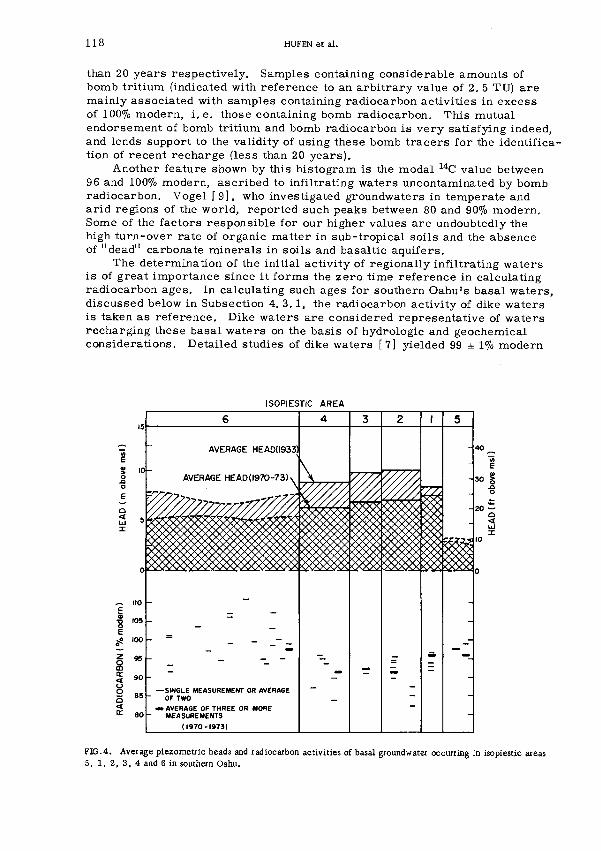
118 HUFEN et al.
than 20 years respectively. Samples containing considerable amounts ofbomb tritium (indicated with reference to an arbitrary value of 2. 5 TU) aremainly associated with samples containing radiocarbon activities in excessof 100% modern, i .e . those containing bomb radiocarbon. This mutualendorsement of bomb tritium and bomb radiocarbon is very satisfying indeed,and lends support to the validity of using these bomb tracers for the identifica-tion of recent recharge (less than 20 years).
Another feature shown by this histogram is the modal 14C value between9 6 and 100% modern, ascribed to infiltrating waters uncontaminated by bombradiocarbon. Vogel [9] , who investigated groundwaters in temperate andarid regions of the world, reported such peaks between 80 and 90% modern.Some of the factors responsible for our higher values are undoubtedly thehigh turn-over rate of organic matter in sub-tropical soils and the absenceof "dead" carbonate minerals in soils and basaltic aquifers.
The determination of the initial activity of regionally infiltrating watersis of great importance since it forms the zero time reference in calculatingradiocarbon ages. In calculating such ages for southern Oahu's basal waters,discussed below in Subsection 4. 3. 1, the radiocarbon activity of dike watersis taken as reference. Dike waters are considered representative of watersrecharging these basal waters on the basis of hydrologie and geochemicalconsiderations. Detailed studies of dike waters [7] yielded 99 ± 1% modern
ISOPIESTIC AREA
AVERAGE HEAD0933)
AVERAGE HEAD(l97O-73)
— SINGLE MEASUREMENT OR AVERAGEOF TWO
» AVERAGE OF THREE OR MOREMEASUREMENTS
(1970-1973)
FIG.4. Average piezometric heads and radiocarbon activities of basal groundwater occurring in isopiestic areas5, 1, 2, 3 , 4 and 6 in southern Oahu.

IAEA-SM-182/33 119
as radiocarbon reference value. The same study indicated that 18 ± 16%o PDBcould be used as a 13C reference to adjust for possible limestone dilutioneffects.
4. 3. Study of southern Oahu's basal waters
Basal water samples have been obtained from numerous wells, shaftsand springs located in southern Oahu. Radiocarbon data for these samplesare shown in Fig. 4, 'with their distribution along the horizontal axis reflectingthe approximate location of the respective sources between the boundariesseparating the isopiestic areas. Pumping station data which are identifiedas such by extra heavy bars are averages of three or more determinationsmade in the period 1970 through 1973. Piezometric heads are averages ofmeasurements made during the same period.
Figure 4 clearly shows that basal waters in area 6 (area around PearlHarbor) display predominantly higher radiocarbon values than do basal watersin areas 1 through 5 (all located in the Honolulu area). • Several values are inthe "bomb" radiocarbon range. The same samples showed small amounts ofbomb tritium as well. None of the samples from areas 1 through 5 hasradiocarbon activity greater than 100%, which would have indicated thepresence of "bomb" radiocarbon. Tritium activities are generally too lowto be significant in terms of our resolution capability of ± 1.0 TU.
A monitor well located in area 2 was sampled at eight different depthsusing specially designed equipment. Radiocarbon and chloride data arelisted below:
Depth(m below msl) :
Chloride(mg/litre) :
Radiocarbon(% modern) :
140 a
52
92.3
210
59
91.
Basal lens
230
59
8 92.2
240
95
94.0
260
83
91.4
320
8050
87
Transitionzone
360
11700
.5 84.8
Saltwater
400
18780
41.6
Just below casing and caprock contact.
No significant variation in radiocarbon activity is apparent in the basal watersamples; on the other hand, the deeper brackish and salt waters are consider-ably lower in radiocarbon activity.
4. 3. 1. Pumping stations
Isotopic and chemical composition of basal waters pumped up by eightmajor pumping stations were studied as a function of time. Samples werecollected and analysed for radiocarbon and tritium and several chemicalspecies, once or twice a year over the period 1970 through 1973. None ofthe isotope records showed any significant trends, although some aresmoother than others. Records for the chemical parameters on the wholeshow little or no variation with time. Average values for the time study data

TABLE II. AVERAGE HYDROLOGIC, CHEMICAL AND ISOTOPIC DATA FOR MAJOR BASAL WATER SOURCES INSOUTHERN OAHU (1970-73)
Area Pumping stationDraft
(106 m3/a)Cl
(mg/litre)HCO¡
(mg/litre)Tritium
(TU)
Radiocarbon(% modern)
i s c a
(ÔfooPDB)"Cage(years)
5
5
1
2
2
3
4
6
ab
Aina Koa WeHs
Waialae Shaft
Kaimuki Wells
Wilder Wells
Beretania Wells
Kalihi Wells
Kalihi Shaft
Halawa Shaft
Single measurement.13C adjusted.
0.57
0.47
7.43
10.79
12.76
10.88
15.89
17.20
134
135
76
43
56
73
79
46
82
102
76
107
73
74
69
67
1.0
0.8
0.6
2.9
0.3
0.3
0.6
1.6
96.1
97.5
96.1
85.0
91.4
92.2
91.2
97.3
-19.2
-17.2
-18.5
-15.5
-18.5
-17.4
-18.3
-19.2
240
120
240
~ O b
640
570
660
140

IAEA-SM-182/33 1 2 1
on radiocarbon, tritium and selected chemical parameters are summarizedin Table II. Entries for draft are averages of measurements over the sametime period. 13C data are single determinations, however.
Previous studies on dike waters and perched waters had shown thatwater samples with greatly varying bicarbonate concentration have similarradiocarbon activities [7] . Comparison of stations (Aina Koa Wells andWaialae Shaft) in area 5 with the one (Halawa Shaft) in area 6 reveals asimilar pattern of relatively high radiocarbon activities for samples thatcontain high as well as low bicarbonate concentrations. It is concludedtherefore that high bicarbonate concentrations may be a consequence ofgeochemical conditions associated with soils in the recharge area, and donot, a priori, indicate dissolution of limestone deposits. The applicationof 13C data [10, 11] appears more useful in this regard.
Basal water 13C data listed in Table II are, with one exception, verysimilar to the dike water 13C data [7] , as is true of data (not presented here)for other wells in areas 1 through 5. This suggests that the carbon isotopecomposition of basal waters has not been altered by dilution or exchangeprocesses involving limestone materials. Any loss of radiocarbon is thusto be ascribed to radioactive decay only, except in the case of Wilder Wells.In comparison, its radiocarbon value (85.0% modern) is quite low, bicarbonate(107 mg/litre) is high, and 13C (-15.5 6%0 PDB) is more positive. There islittle doubt that in this case the low radiocarbon activity is not the resultof radiocarbon decay but rather of limestone dilution effects. Furthersupport for this conclusion is the fact that samples from this stationconsistently show bomb tritium, indicating the presence of recent recharge.Pearson and Hanshaw [11] have shown that 13C data can be successfully usedto separate out non-radiogenic effects, and hence to calculate adjusted ages.Application of their procedure to Wilder Wells data indeed yields approxi-mately "zero age" in agreement with the tritium data.
Ages for basal waters discharged by the pumping stations are listed incolumn 7 of Table II. These ages were calculated using conventional proce-dures with 99% modern (dike waters) as the radiocarbon value for initialrecharge, 13C adjustment was applied only to Wilder Wells data, for reasonsdescribed above. Inspection of Table II reveals that only three pumping stations(Beretania Wells, Kalihi Wells and Kalihi Shaft) show significant radiocarbonages. Ages for the other stations are all "recent". A further distinction inages, other than between these two groups, is not justified considering boththe uncertainties associated with the measurements and the variations of theaveraged data as a function of time. Two sources (Halawa Shaft and Aina KoaWells) show marginal but detectable amounts of bomb tritium (as do WilderWells), testifying to the presence of very recent recharge (< 20 years).
5. HYDROLOGIC INTERPRETATIONS
5. 1. General
Tritium and radiocarbon data presented in Table I and Fig. 3 showthat fresh groundwaters are primarily less than 1800 years old. Perchedwaters and dike waters have residence times of years or decades. Lowradiocarbon values associated with transition-zone water and underlying salt

122 HUFEN et al.
water probably reflect decay of radiocarbon due to long residence times ofthese waters. Further work on these waters involving 13C analyses is neededand planned.
5.2. Basal waters
Representative data in Table I show that basal water in area 5 has achemical and isotopic composition which is distinct from that of basal watersin other areas. As mentioned in Subsection 4.3. 1, this composition isattributed primarily to geochemical conditions in the respective rechargearea. If this is true then it follows that the recharge area of area 5 is distinctfrom the recharge area for areas 1 to 4. One might argue that waters fromother areas flow into area 5 and on their way pick up additional chlorides andbicarbonates. However, such a mechanism would require the dissolution oflimestone material, resulting in low radiocarbon and 13C values, not what isobserved here.
It was suspected from geologic and hydrologie information (not presentedhere) that areas 1 and 5 are separated not only by a valley fill but also by anearby parallel rift zone. Hence the barrier between the two areas isconsidered very effective. Present data support this contention. Area 5 isto be regarded as an independent groundwater system. The distinctivechemistry of the water in this area is ascribed to the relatively low rainfallover its watershed. The latter is also responsible, at least in part, for thelow head in the area.
Several samples collected in the Pearl Harbor area contained bombradiocarbon and bomb tritium. These high values are associated withshallow wells and springs discharging water from relatively shallow depths.Chemical constituents in these waters were high relative to those in waterfrom deeper wells. It is strongly suspected that these isotopic and chemicaldifferences as a function of depth are caused by the presence of returnirrigation water in the upper layers of the lens [12]. Very large amountsof water are used for the irrigation of sugar-cane fields located betweenPearl Harbor and Central Oahu. A substantial part of this irrigation waterafter application percolates into the basal water which is tributary to thebasal water in the Pearl Harbor area. Such irrigation return water, becauseof its exposure to the atmosphere, roots of growing plants and top soil, isbelieved to attain post-bomb radiocarbon activity levels, and as such can beidentified. Current studies are in progress to verify this contention.
5.3. Age relationships
Samples from Wilder Wells have consistently shown bomb tritium,indicating that at least some of its discharge originated over the past 20 years.13C adjusted radiocarbon age is around zero. Further resolution is not justi-fied considering the many variables involved in this calculation. It is clearthough that water of recent origin provides a constant source of rechargesupplying these wells.
Basal lenses that are recharged directly from overland must contain theyoungest water in their upper layers. Shafts are constructed within themountains at sea level elevations (Fig. 2A) so as to "skim" the top of basallenses. Water developed by shafts should therefore be of recent origin also.On the other hand, wells penetrating several hundred metres into lenses and

IAEA-SM-182/33 123
located farther away from the mountain recharge areas should dischargewater containing an undetermined fraction of water that is older than thatfrom the shafts.
Two shafts (Table II) indeed have very young radiocarbon ages; one ofthem (Halawa Shaft) even shows small amounts of bomb tritium. However, athird shaft (Kalihi Shaft) shows a relatively old radiocarbon age, while inter-mediate ages are associated with some of the well stations. It is realizedthat the age of water from a particular source could be a function of locallens thickness, depth of well and pumping rate. To explore such dependence,a new parameter is introduced, Q/d, called draft-distance parameter1, whereQ = pumping rate and d = distance from the bottom of the well down to thefresh water-salt water interface. This parameter expresses the capability ofa source to withdraw water from lesser or greater depth within a particularlens, and as such should relate to the water's radiocarbon age. Figure 5shows this indeed to be the case with the exception of Halawa Shaft. Nosatisfactory reason can be given to explain this exception. It may be relatedto the fact that this shaft is in area 6; an area that on the whole shows higherradiocarbon values (i. e. younger ages) which in turn appears to relate to themagnitude of the groundwater flux which is known to be greater for this areathan it is for those in the Honolulu area. Perhaps it should be pointed outthat in the foregoing discussion distances between sources and rechargearea(s) were considered the same for all stations involved. On the wholethis agrees with reality, although shafts are somewhat farther inland than theother sources.
Based on the relationship shown between age and draft distance in Fig. 5,one could presume that individual lenses might show a vertical age stratifica-tion, but this is not borne out by the samples taken from five different depthsin an observation well adjacent to Beretania Station. However, the data,presented in a previous section, did reveal that samples of brackish and saltwaters taken from greater depths did show lower radiocarbon values. Inter-pretation of these data is in progress together with additional field sampling.
The old ages of water discharged by stations in areas 2, 3 and 4 raisesthe question whether water is being developed from the so-called bottomstorage [ 13]. Interestingly enough these particular areas showed the highesthead in 1933, but have since dropped drastically and are even below that ofarea 1. Additional data are needed before a valid answer can be given to theforegoing question.
1 This parameter is adapted from a relationship expressing "ultimate rise" introduced by Dagan and Bear[14] in their study of upconing of the transition zone between fresh and salt water in coastal aquifers. Ultimaterise is defined as:
1 Q
^ Л У d
У X
where
Q = pumping rate of well
d = distance between the well's bottom and the interface at t = 0
—*- = dimensionless density difference between fresh and salt water
К = horizontal permeability
For this paper in which a parameter is sought for preliminary assessment, the first is assumed constant and hydro-
dynamic dispersion is not yet considered, as was done in Schmorak and Mercado's work [15].

124 HUFEN et al.
S 600 -
< 500 -
оm< 400ооо
оD
-
О
D
i
WELL
SHAFT
//
I
STATION
STATION
О
1 i
/
О
i i i
s
HALAWA
i i
s
О
SHAFT
i i
DRAFT-DISTANCE PARAMETER ,0/d {IÓ*m2/a)
FIG.5. Radiocarbon age of basal water, discharged by major pumping stations in southern Oahu, as a functionof the draft-distance parameter Q/d.
6. CONCLUSIONS
The geologic composition of Oahu together with its subtropical ground-cover gives rise to groundwater systems which are hydrologically and geo-chemically unique. Oahu can be regarded as an ideal testing ground forgroundwater carbon isotope studies because of the occurrence of carbonate-free basaltic aquifers which at lower elevations grade into carbonate -containing aquifers.
Data obtained to date indicate that the pre-bomb radiocarbon activityassociated with waters recharging Oahu1 s aquifers is 99 + 1% modern. Bombradiocarbon and bomb tritium are currently present in groundwater fromsome high-level sources and others.
Dike waters and basal waters both have 13C values ranging between-17 and -19 6%0PDB. Since dike waters are representative of waters r e -charging basal aquifers it follows that groundwater 13C concentrations remainunchanged as long as such waters reside or flow through basaltic aquifers.On the basis of data for groundwater s in carbonate aquifers (Table I) andcertain basal waters (such as Wilder Wells), it is concluded that the effect ofcarbonate dissolution upon groundwater chemistry can be detected by the

IAEA-SM-182/33 125
simultaneous occurrence of high bicarbonate concentrations (> 100 mg/l),large 13C values (> - 16 6%0 PDB), and low radiocarbon activity (< 90% modern).13C data proved to be capable of adjusting "apparent radiocarbon ages" forsuch carbonate dilution effects. However, natural variations in the 13C dataincrease age uncertainties and complicate the resolution of small agedifferences.
In general, Oahu's groundwaters are of recent origin as shown by radio-carbon and tritium data. Old ages are suspected for brackish and salt watersresiding beneath basal-lenses. Basal waters from the six isopiestic areasin southern Oahu show radiocarbon activities which to some extent arecharacteristic for their area. Radiocarbon ages for waters withdrawn fromthese areas by major pumping stations range from a few decades to amaximum of 660 years. Apparently a relationship exists between these ages,pumping rate of the station, well depth and local thickness of the lens. Onearea (5) contains water that is isotopically and chemically distinct from thatin the other areas and thus is considered an independent groundwater system.
This study has shown that the combination of multiple isotope andchemical analyses can yield valuable geochemical and hydrological information.Several of the observations or conclusions presented here serve to endorse orconfirm existing hydrologie knowledge. However, some data such as the agerelationships are unique and provide the tools for subsequent hydrodynamicstudies of the basal lenses.
ACKNOWLEDGEMENTS
This research project was carried out with the active co-operation ofthe Board of Water Supply, City and County of Honolulu. Thanks are due toprivate well owners for their co-operation in sample collection and to allthose who participated in the collection and processing of the samples. Thiswork was financially supported by grants from the Office of Water ResourcesResearch,
This paper constitutes Water Resources Research Center ContributionNo. 55 and Hawaii Institute of Geophysics Contribution No. 589.
REFERENCES
[1] YOUNG, R. H . F . , LAO, C. , Return irrigation water in Hawaii, Water Resour. Bull., Am. Water Resour.Assoc. 9 (1973) 538.
[2] HUFEN, Т . Н . , DUCE, R. A., LAU, L.S., Some Measurements of the Tritium Content in the NaturalWater of Southern Oahu, Hawaii, Technical Rep. No.34, Water Resour. Res. Center, Uniy. of Hawaii,Honolulu (1969).
[3] HUFEN, Т . Н . , BUDDEMEIER, R. W., LAU, L. S., Tritium and Radiocarbon in Hawaiian Natural Waters,Technical Rep. No.53, Water Resour. Res. Center, Univ. of Hawaii, Honolulu (1972).
[4] AMERICAN PUBLIC HEALTH ASSOCIATION, Standard Methods for the Examination of Water and Waste-water, Washington, APHA (1971) 874.
[5] von BUTTLAR, H., LIBBY, W.F., Natural distribution of cosmic-ray produced tritium: II, J. Inorg.Nucl. Chem. 1 (1955) 75.
[6] INTERNATIONAL ATOMIC ENERGY AGENCY, Environmental Isotope Data No. 1: World Survey ofIsotope Concentration in Precipitation (1953-1963), Technical Reports Series No. 96, Vienna (1969);Environmental Isotope Data No. 2: World Survey of Isotope Concentration in Precipitation (1964-1965),Technical Reports Series No. 117, Vienna (1970); Environmental Isotope Data No. 3 : World Survey ofIsotope Concentration in Precipitation (1966-1967), Technical Reports Series No. 129, Vienna (1971);

1 2 6 HUFEN et al.
Environmental Isotope Data No. 4: World Survey of Isotope Concentration in Precipitation (1968-1969),Technical Reports Series No. 147, Vienna (1973).
[7] HUFEN, Т . Н . , BUDDEMEIER, R. W., LAU, L. S., Isotopic and chemical characteristics of high-level
groundwaters on Oahu, Hawaii, Water Resour. Res., in press.[8] LAU, L.S., HUFEN, Т . Н . , Tritium Measurement of Natural Waters on Oahu, Hawaii: A Preliminary
Interpretation, Technical Reports Series No.65, Water Resour. Res. Center, Univ. of Hawaii, Honolulu(1973).
[9] VOGEL, J . C . , "Carbon-14 dating of ground water", Isotope Hydrology 1970 (Proc. Symp. Vienna, 1970),
IAEA, Vienna (1970) 225.[10] RIGHTMIRE, С Т . , HANSHAW, B.B., Relationship between the carbon isotope composition of soil CO2
and dissolved carbonate species in groundwater, Water Resour. Res. 9 (1973) 958.[11] PEARSON, F.J. , Jr., HANSHAW, B.B., "Sources of dissolved carbonate species in groundwater and their
effects on carbon-14 dating", Isotope Hydrology 1970 (Proc. Symp. Vienna, 1970), IAEA, Vienna (1970)271.[12] HUFEN, Т . Н . , Isotopic and chemical characteristics of groundwater on the island of Oahu, Hawaii, Water
Resources Seminar Series No.4, Water Resour. Res. Center, Univ. of Hawaii, Honolulu, in press.[13] WENTWORTH, C.K., Geology and Groundwater Resources of the Honolulu-Pearl Harbor Area, Board of
Water Supply, City and County of Honolulu, Hawaii (1951).[14] DAGAN, G. , BEAR, J. , Solving the problem of local interface upconing in a coastal aquifer by the
method of small perturbations, J. Hydraul. Res. j> 1 (1968).[15] SCHMORAK, S., MERCADO, A., Upconing of fresh water-sea water interface below pumping wells -
field study, Water Resour. Res. 5 6 (1969).
D I S C U S S I O N
J, SILAR: How are the individual isopiestic zones determined?T. H. HUFEN: Piezometric heads are measured at regular intervals at
monitor wells and at a number of pumped wells where the pumps have beenswitched off temporarily.
J, SILAR: Is the surface morphology taken into account?T. H. HUFEN: The surface morphology is not taken into account in this
study of basal waters since, because of the high permeability of the basalticflow rock, we do not think it an important factor with regard to wateroccurrence, flow or ages.
V. T. DUBINCHUK: Could you give more information about your draft-distance parameter?
T. H. HUFEN: The draft-distance parameter incorporates varioushydrological parameters, such as discharge, thickness of lens and depth ofwell. In essence, it expresses the ability of a particular source to withdrawwater from lesser or greater depths. If water in the lower parts of thicklenses is older than water in the upper parts or older than water in thinlenses, then a positive correlation should exist between the draft-distanceand radiocarbon age. The results shown in Fig. 5 indicate that there isindeed such a correlation.
G. P. CONRAD: I should like to confirm what you said in your oralpresentation about the close correlation between high 1 4C activities and aclearly detectable tritium activity.
We have results relating to groundwater in the Saharan arid zone whichagree with those for the Kalahari presented by Mr. Mazor in paperIAEA-SM-182/18.1
1 MAZOR, E., VERHAGEN, B.T., SELLSCHOP, J .P.F., ROBINS, N . S . , HUTTON, L.G., "Kalaharigroundwaters: their hydrogen, carbon and oxygen isotopes", these Proceedings J , IAEA-SM-182/18.

IAEA-SM-182/33 127
14C activities of 100% or more of modern carbon (Conrad, G. P . ,Fontes, J . C . , C.R. Acad. Sci. 245 (1970) 165, and unpublished measurementresults) correspond to 2-12 TU (Conrad, Olive, Mareé, Journal of Hydrology(in press)). These data, which are based on some 20 combined (14C andtritium) measurements, lead me to think that the initial 14C concentration inthe arid zone was not 50% or 85% of modern carbon but close to 100%.


ENVIRONMENTAL ISOTOPES,OTHER THAN HYDROGEN, OXYGEN ANDCARBON ISOTOPES, IN GROUNDWATER
STUDIES
(Session 7, Part 1)


IAEA-SM-182/35
2 3 4 U AND 2 3 8 U IN THECARRIZO SANDSTONE AQUIFEROF SOUTH TEXAS
J.B. COW ART, J.K. OSMONDFlorida State University,Tallahassee, Fla.,United States of America
Abstract
2 3 4 U AND 2 3 8 U IN THE CARRIZO SANDSTONE AQUIFER OF SOUTH TEXAS.The waters of the Carrizo Sand formation of South Texas, United States of America, exhibit a pattern of
uranium isotopic disequilibrium, described in terms of 2 3 4 U / 2 3 8 U activity ratio ("A.R. ") and uranium concentra-tion, which may be a function of geochemical factors and the hydrologie history of the area. In terms ofuranium, two regimes seem to exist. The first, including outcrop and near outcrop sample locations, haswaters with relatively high concentration and low A.R. Somewhat downdip, the uranium concentration decreasessharply at the downdip limit of the oxidation environment, a zone of uranium precipitation. Recoil of daughterproducts from the precipitated uranium causes an increase of A.R. of the water. Water of low uranium con-centration and high A.R. is found throughout the downdip regime. If a constant input of 2 3 4 U through time isassumed, the downdip decrease in A.R. after the initial introduction of 2 3 4 U into the water may be ascribed toradioactive decay of 2 3 4 U . However, this assumption leads to the calculation of a water flow rate one twentieththat determined by other means. Alternatively, this pattern may be an artifact of a change of climate from20 000 years to 10 000 years ago. In this case, the decrease in A.R. downdip is a function of a varying input of2 3 4 U as well as decay.
INTRODUCTION
In a closed system, given sufficient time, themembers of a radioactive decay series will achieve a statewherein the rate of production of each nuclide is equal tothe radioactive decay of that nuclide. This state is calledsecular equilibrium; it follows then that the ratio of theactivity of any two members of a decay series in equilibriumis equal to unity if the decay is in the same mode, forinstance if the two nuclides both decay by emission of alphaparticles.
That the ratio of abundances of 2 3 5
U and 238y is
essentially constant wherever uranium is found has beenknown for about 35 years. The unexpected abundance variationof
2 3 4U relative to 235u and
2 3 8U was first reported in 1955.
This abundance variation may be measured in terms of thevariation of the activity ratio, 234JJ/238U; if the value ofthis ratio is any value except unity, a state of "disequi-librium" exists.
2 34TJ and 238у are, of course, chemically
alike and are separated only by the two short-lived nuclides,234
a n d 2 3 4
P a/
The variation in uranium isotopic abundances innatural waters has applications which have just begun to
131

1 3 2 COWART and OSMOND
be explored. These applications arise from several signi-ficant aspects of uranium geochemistry:
1. The isotopic variation is extreme; the activityratio of 234u to
2 3 8U ("A.R.") varies by more than
a factor of 20.
2. The determination of abundances of uraniumisotopes at very low concentrations is relativelysimple due to their alpha radioactivity.
3. Uranium has two common valence states, +4 and + 6,which makes it sensitive to electrochemicalvariations in its environment.
4. The variable isotope, 2 3
^U, is a daughter of 2 3
°uand both the rate of disequilibrium developmentand its decay are governed by the half life of234 approximately 250 000 years.
There are two principal types of natural watersystems, in terms of their uranium isotope geochemistry,the near surface type and the deep ground water type. Manysurface and shallow ground water systems, under oxidizingconditions, have relatively high uranium concentrationsand moderate disequilibria. The waters of such systems haveyoung ages and the ratio of their isotope abundances, dueto the higher concentrations, is relatively stable andinsensitive to change. Their uranium isotope ratios andabundances can be used as natural tracers to determine flowpatterns and mixing proportions. In the other case, thatof deep ground water systems which are normally reducing,the concentration of uranium is low and the age of the watergreater. Here the isotopic ratio is more susceptible tochange and the variation of isotope abundances can be inter-preted in terms of evolutionary interaction of the uraniumin the water with that of the solid through time.
This report is concerned with an aquifer system inwhich the direction and rate of water movement is welldefined and the difference in age of water between theoxidizing zone of surface recharge and the deep confinedaquifer is appreciable.
BACKGROUND
The fractionation of 2 3
^U from 2 3
^u in nature wasfirst reported in 1955 [1]. Other studies not only sub-stantiated the disequilibrium of the uranium isotopes butbrought out the fact that the disequilibrium is to befound in profoundly different materials and environments.
238The pertinent portion of the decay series of U is
shown in Figure 1. It should be emphasized that, at equili-brium,
2 38u accounts for 99.28%,
2 3 5u for 0.72% and
234u for
0.0054% of the amount indicated by concentration figures.No 235и/
238у disequilibrium has been found in natural uranium
samples investigated [2].

IAE A-SM-182/35 133
238|J11/2= 4.49 xl09yr
a
234 и
t'/2= 2.48xl05yr
4.774.72
Mev
226 Re
t '/2 = 1622 yr
FIG. 1. The first several steps in the decay scheme for 2 3 8 U . At equilibrium every member of a non-branchingchain has the same activity. Inasmuch as alpha particles are easily detected and their energy measured, theratio of 2 3 4 U activity to 2 3 8 U activity is readily determined.
Uranium minerals and ores have been found to vary sothat the ratio of the activity of
2 3 4U to
2 3 8U ("A.R.")
might be somewhat deficient in 234y (A.R. < 1) or might con-tain an excess of 234y (д.д. > i) [3-5]. Many soils andminerals containing uranium as a dispersed element have beenfound to have A.R.s different than unity [6-9].
Most waters are found to have 234u/238u activitydisequilibrium. The ocean, the ultimate destination of mostsurface water, has an excess of 234u of 15% [10-11]. Notsurprisingly, the dissolved uranium in rivers usually hasexcess 234u [12-14]; in small streams A.R.s as high as 6.4have been found [15]. Conversely, the uranium in thesediments carried by rivers is often deficient in 234y, theA.R. seemingly dependent upon the character and geologichistory of the drainage basin and the amount of organicmaterial associated with the sediment [13, 16].
In limestone terranes, dissolved uranium in springsand rivers may have A.R.s either greater or less thanequilibrium. The infiltrating waters probably receive aninput of uranium of given concentration and A.R. in a nearsurface zone. Because the input concentrations and/or A.R.sare different at different locations, natural isotope dilutionsmay occur where several sources contribute to a resultantwater, such as a large spring, a river or a lake. Thequantity of water contributed by each source can be calcu-lated by mixing equations. Such determinations have beenmade and are consistent with independent studies, for groundwater [17], for a ground water-spring system [18-20], andfor a spring-river system [21].
Ground water shows a wide range of values. A.R.sas low as 0.50 have been reported [17] and high ratios havebeen found in deep ground waters, the values ranging from 4to as high as 12 [19, 20, 22].

134 COW ART and OSMOND
Changes in 234^238^^ activity ratio have been notedin seismically active areas [23]. The activity ratios ofwater from boreholes taken after an earthquake were noted tobe smaller by a factor varying from 2 to 5 than the A.R.sfrom the same wells taken before the earthquake. It ispossible that dilatation effects may expedite the transferof uranium at or near crystal boundaries into an aqueousphase.
The mechanism for the fractionation of the isotopeshas frequently been attributed to a natural Szilard-Chalmerseffect whereby the 234y atoms are selectively extracted fromthe lattice because of lattice damage caused by recoil and/or the higher oxidation state of 234u as a result of electronstripping during1recoil [24, 25]. Such extraction might befacilitated by the presence of an aqueous solution, slightlyoxidizing, bathing the crystal grains [26].
That the recoil mechanism itself must be a primarycause of the 234y fractionation was shown by Kigoshi [27],who noted the enrichment of 234rph, the immediate daughter of238u, in the liquid phase surrounding powdered uraniferouszircon. Such a process could cause the buildup of 234yin a liquid not capable of acquiring uranium by leaching.
The geochemistry of uranium is strongly influenced byits mobility in oxidizing environments, usually as a uranylcarbonate complex, and its low solubility in reducingenvironments [2 8, 29]. In sedimentary rocks, accumulationsof uranium as films or encrustations on rock particles isoften observed to have occurred at a well-defined "reducingbarrier"; the updip rocks are oxidized with iron oxidespresent whereas the downdip rocks may still contain pyritewhich shows no effect of oxidation [30]. The zone of uraniumaccumulation is usually quite distinct and compact.
AREA OF INVESTIGATION
The study area is located in central south Texas,USA (see Figure 2). The Carrizo sandstone is a member of theClaiborne group of Eocene age (Lutetian). It is thoughtthat the sands were once part of a remarkably extensive anduniform dune field [31]. The Carrizo is a prolific sourceof irrigation water for this region.
The Carrizo consists almost entirely of quartz sandbut there are small amounts of bentonitic clay, shale, ligniteand isolated crystals of pyrite present. Also, a suite ofheavy minerals, including uranium bearing zircon and xeno-time, is ubiquitous [31]. The thickness of the sand variesfrom about 180m near the outcrop area to approximately 400msome 9 0 km downdip from outcrop (Figure 2). The Carrizodips to the south or southeast at 20m to 25m per km for aboutthe initial 60 km from the outcrop and thereon at a ratesomewhat steeper [32,33].

IAE A-SM-182/35 135
238U
400-
300-
200-
100-
SAMP..E9 Feb. 7317 HRS
425 A
mple
FIG. 2. Three alpha spectra,showing resolution of the threeuranium isotope peaks. In lowconcentration samples (465, 476),development of the naturaluranium peaks (234U and238U) mayrequire considerable time, with aresulting increase in backgroundcounts. In the two upper spectra,the 232U spike peak has beentruncated for the purposes of figurebalance. In high concentrationsamples (425A), good countingstatistics are achieved in a rela-tively short time. (Note verticalscale change. ) The peak to theright of232U in some of thesespectra is 224Ra, a member of the232U decay series.
234 U 232U

136 CO WART and OSMOND
The Carrizo is of specific interest for severalreasons :
1. It is a well confined aquifer with littleleakage in or out of the sand.
2. It is well studied. The Texas Water DevelopmentBoard (TWDB) has numerous observation wells inthe area and some geochemical measurements havebeen made [32].
3. С age determinations and determination ofwater flow rates have been made of water in thearea [34].
4. Almost the entire amount of water in the Carrizois meteoric water which has infiltrated theoutcrop area. The uranium in the ground watermust have its source in the Carrizo itself.
SAMPLING AND PROCESSING
The samples were obtained from wells which wereidentified as obtaining water from the Carrizo on mapscompiled by the TWDB and the United States GeologicalSurvey. The wells were either flowing or were allowed topump for a time sufficient to permit the acquisition of arepresentative sample.
The volumes collected were 14, 28 or 56 liters,depending on the uranium concentration expected at thatlocation. The samples were acidified to pH=l in the fieldand transported to the laboratory for further processing.Each 3.5 liter bottle was prepared by adding 5 ml of aniron carrier solution and 1 ml "FSU Water Spike-2" (157 dph232u/ml). The samples were shaken vigorously daily for 10days in order to effect spike equilibration. Each samplewas brought to a temperature of 95°C for 10 minutes beforethe uranium was separated from interfering elements bycoprecipitation. Organic extraction and anion exchangeresin procedures followed. The separated uranium waselectroplated onto a stainless-steel planchet. The alphaactivities of the isotopes were measured by use ofpartially depleted surface barrier silicon detectorshoused in a vacuum chamber. Each detector was linked toa 100-channel pulse-height analyzer.
Some of the samples from the downdip portion of theCarrizo have very low uranium concentrations, close to thedetection limits of the methods employed. It was necessaryto use counting intervals measured in days; backgroundeffects, which are usually insignificant in alpha counting,had to be carefully monitored. Among the background effectsisolated were:
1. Clean planchet background.
2. "Spike tail," the encroachment of a 232y countsinto the 234u envelope (9 channel window). This

IAEA-SM-182/35 137
is in part due to the presence of a thin filmof iron on some planchets which tends to broadenall peaks; it is aggravated by the growth ofshort-lived 228rph, which has approximately thesame alpha energy as its parent, 232u.
3. Adsorption of radioactive daughter products,including gases, on the planchet, detector andchamber walls.
4. Temperature effects. Since surface barrierdetectors and associated electronic equipmentare sensitive to temperature, stable backgroundrates, usable for such low concentrations, cannotbe maintained above about 22°C.
Each of these background factors was determined foreach counting period and each planchet. In general, a netcount rate above background of as little as 0.2 count perhour per peak envelope could be established as significant.
Each planchet was counted long enough to accumulateat least 10 000 counts per envelope or as long as waspracticable. The errors estimated are at the 95 percentconfidence level. Long counting times were not a seriousproblem since five counting systems were used simultaneously.However, for the achievement of lower detection limits infuture work, the development of a practical field concen-tration procedure would seem to be advisable.
In Figure 3, sample 465 is an example of a downdipsample with high A.R. and low concentration. The amount of232y spike added to all samples was such as to produce apeak height which would be equivalent to a concentrationof 1 pplO9 238U#
Sample 476 is representative of downdip samples withrelatively low A.R. Although the total number of countsaccumulated in either the 238u or 234y envelope is not large,the fact that those samples which were counted numerous timeseach gave A.R.s and concentrations that are quite consistentlends strong support to the validity of the pattern ofactivity ratios.
Sample 425A shows the spectrum of a near outcropsample with a low A.R. (less than unity) and a relativelyhigh concentration. Note that the ordinate scale is tentimes that of the other two samples shown. In this typesample, the background is quite small in comparison withthe natural uranium peaks and presents little difficulty inthe achievement of precise measurement.
RESULTS
The distribution of sample localities is shown on themap of Figure 2 and the uranium data is reported in Table I.
In general, the samples from the outcrop area andshallow aquifer are characterized by relatively high uranium

138 COWART and OSMOND
FIG.3. The study area in South Texas. Shading depicts the outcrop area of the Carrizo Sandstone which dipsgently towards the South-Southeast. A - A' is the line of the cross-section of Fig.4. The projections of samplepoints on to this line are made parallel to the strike of the formation. An underlined sample number, e.g.410,indicates that no uranium data are available for that location.

IAE A- SM-182/35 13 9
concentrations and low activity ratios. Seven samples haveactivity ratios less than the equilibrium value of 1.00, andone sample, 425, has an A.R. of 0.52 which puts it among thegroup of lowest ratios reported [17]. Samples from downdipshow much lower concentrations and higher A.R.s and theboundary between low and high A.R.s appears to be rather welldefined.
Certain samples are transitional, in terms ofgeographic loqation, A.R., and/or uranium concentration,between the samples from the two larger regimes. Examplesof this type along the profile are 423 and 467. Sample423 has a rather low uranium concentration but an A.R.typical of outcrop samples. Sample 467, slightly furtherdowndip, has a still lower concentration but has had enough2 3^U introduced into the water so as to cause the A.R. to
be slightly above unity. Possibly 478 and 472 are tran-sitional, also.
The pattern of variation in concentration and A.R.along a downdip profile is shown in Figure 4. The line ofthis profile (A-A
1) is shown on the map in Figure 2. Along
this profile, the highest A.R.s are somewhat downdip of theboundary between high and low concentrations. The A.R.sshow a general decrease downdip in the direction of agingof the water (Figure 4, lower).
Further east, the pattern is less clear; the boundarybetween high and low concentrations is well defined but theexistence of a maximum peak in A.R. is not as certain.
Samples 410, 412, 415, 416, 418, 419, 420, 477, 479and 480 have uranium concentrations below the detectionlimits of the procedure; in most cases, the difficulty wascompounded by a low yield.
DISCUSSION
The pattern exhibited by the concentration andisotope activity in the Carrizo aquifer is somewhat similarto that observed some 300 km to the northeast in the Trinityaquifer of Cretaceous age [22]. Infiltrating water picksup uranium deficient in 234y but while moving downdip itgains an excess of 234ц
w nu
e at the same time it loses most
of its total uranium content. To explain this sequenceof events the following model is proposed.
The sedimentary rock particles in a zone free fromoxidizing effects may develop a surface zone or "rind"which is deficient in 234y. Because the surrounding wateris strongly reducing in character and uranium is not mobilein such an environment, selective leaching of 234y is notthought to be effective. Recoil of 234тп (a progenitor of234u) from a crystal lattice has been demonstrated by Kigoshi[27]. Such a process should cause the near surface volumeof a grain to become deficient in 234y even though the coreof the grain (if the grain diameter is greater than 2 recoildistances) would remain in equilibrium. In zircon, Kigoshicalculated that the recoil distance is about 500 angstroms.

TABLE I. ACTIVITY RATIO, CONCENTRATION AND 2 3 4 U EXCESS OF SAMPLES
Samplenumber
411
413 A
413 В
414 A
414 В
417
421
422
423 A
423 В
424 A
424 В424 С
425 A
425 В
464
465
466
467
468
469
470
471
Counting
time(hours)
583.0
296.0
258.0
116.3
295.6
691.0
387.0
658.0
243.0
182.9
473.1
384.0294.1
168.2
77.7
712.5
498.8
265.0
226.5
359.6
175.0
187.5
103.7
2 3 8 U
87
251202
8895344
108
130
111
45712016
74126462
21490
6079
247
628
128
602
96
9372
11661
30 865
2 3 4 U
342
353372
842
4806
293
447
571
31541374
536825
3087
11262
3241
1204
5663
' 814
654
526
9784
12 978
23 676
2 3 2 u
21923
10 24712128
638326441
52211
104 903
42 811
2236610 075
1318515 74283 821
14462
4007
66 823
229218
36253
20 859
21895
14 901
41342
12 046
A.
3.93 ±
1.41 ±1.84 ±
0.95 ±0.90 ±
2.71 ±
3.44 ±
5.14 ±
0.69 ±0.68 ±
7.24 ±
6.55 ±6.68 ±
0.52 ±' 0.53 ±
4.87 ±
9.02 ±
6.36 ±
1.09 ±
5.48 ±
1.03 ±
1.11 ±
0.77 ±
R.
1.57
0.270.39
0.090.04
1.00
1.20
1.87
0.03
0.05
2.871.730.85
0.01
0.02
0.95
1.03
1.68
0.16
1.63
0.03
0.03
0.03
Concentration
(PP M9)
0.004 ± 0.002
0.025 ± 0.0040.017 ± 0.003
0.139 ± 0.0100.202 ± 0.006
0.002 ± 0.001
0.0012 ± 0.0004
0.003 ± 0.001
0.204 ± 0.0070.200 ± 0.010
0.006 ± 0.002
0.006 ± 0.00150.006 ± 0.001
1.486 ± 0.032
1.527 ± 0.063
0.004 ± 0.001
0.003 ± 0.001
0.004 ± 0.001
0.029 ± 0.003
0.004 ± 0.001
0.629 ± 0.016
0.282 ± 0.006
2.562 ± 0.055
Excess 2 3 4 U( 2 3 8 U equivalents)
0.012 ± 0.009
0. 010 ± 0. 0060.014 ± 0. 007
-
-
0. 004 ± 0.002
0.003 ± 0.002
0.011 ± 0.006
-
-
0. 035 ± 0. 0200. 034 ± 0. 0140.031 ± 0.005
_
-
0. 014 ± 0. 004
0. 022 ± 0. 004
0.019 ± 0.008
0. 003 ± 0. 005
0. 020 ± 0. 009
-
0.031 ± 0.008
-
о
1О£2Sоzо

TABLE I. (cont. )
472
473
474
475
476
478
575.8
113.4
121.5
124.0
852.0
365.1
360
26325
2458
11601
234
487
639
21405
2140
6732
487
852
42 666
15488
11799
9655
117731
23151
1.77 ±
0.81 ±
0.87 ±
0.58 ±
2.08 ±
1.75 ±
0.29
0.04
0.05
0.02
0.51
0.23
0.088 ± 0.001
1.700 ± 0.034
0.209 ± 0.009
1.202 ± 0.033
0.002 ± 0.0004
0.021 ± 0.002
0.
0.
0.
006 ±
-
-
-
002 ±
016 ±
0.003
0.001
0.005

142 COWART and OSMOND
< 3
2
H
/\\\
•
15km
i
/ '/
~-.
/
5
-
\
r—1\
~ —sS
>
f
[ ^ —<- 4
A
?
FIG.4. (Upper) Cross-section along A- A' of Fig.3, showing the sample well locations relative to the dippingCarrizo aquifer. (Lower) The 2 U / ^ U activity ratios (linear scale on left) and the U concentration values(logarithmic scale on right) as a function of the corresponding well positions.
Although the outermost part of the grain might be as muchas 50% deficient in 234u, a relatively large grain, as awhole, would show only a slight deficiency, the actualvalue depending on the grain size and the ratio of surfacearea to volume.
When such a grain is introduced into an oxidizing,slightly acid environment, it is then possible for leachingto occur. The leaching may be selective in the sense that234u is preferentially extracted because of its greatervulnerability to leaching as has been proposed by variousinvestigators [24-26]. On the other hand, in the near surfacezone of the earth, corrosion of the grain may occur,resulting in an isotopically non-selective input of uraniuminto the ground water. This non-selective input would havea low A.R. (A.R. < 1) because the corrosion would belocalized in the depleted outer zone or rind. This lattercase seems consistent with the observational data withregards to the Carrizo.
Regardless of the source of dissolved uranium in theoutcrop regime, as it is carried downdip a zone of reductionis encountered where almost complete precipitation of

IAEA-SM-182/35 143
U cone ==/2 ррЮ9
(414,474)
U cone =«.005 pp I09
(465,476)
FIG. 5. A diagrammatic model of uranium isotopic geochemistry in an aquifer like the Carrizo. Updip, theuranium concentration is relatively high and the A.R. is low. Downdip, the uranium concentration is low andthe A. R. high. Zone 1 is the site of the reducing barrier where uranium solubility decreases and precipitationoccurs today. Zone 3 is the location of a previous barrier. Low concentration water passing through theuraniferous zone 3 tends to collect an excess of 2 3 *U. Zone 2 is transitional, where uranium concentration hasdecreased but the excess has not yet increased greatly.
uranium occurs, forming an encrustation or film on the sandgrains (see Figure 5). Such a process has been shown toresult in uranium accumulations under similar conditions[26, 35-37]. Further downdip, of course, the water wouldhave only a very small concentration of uranium.
Because the precipitation of uranium is an isoto-pically non-selective process, this process cannot accountfor the excess of 234y found in the water further downdip.However, if the now low uranium concentration water flowsthrough a "fossil" uranium accumulation zone, it willreceive the daughter products recoiling from the radioactivedecay of
238u. Because of the low electrochemical potential
of the water, the uranium coating the sand grains will notbe leached. In effect, the water is only a passive recipientof the recoiling
234iph.
According to the recoil model of Kigoshi [38] andothers [20], a steady state of disequilibrium should beestablished in very old ground water systems in which theaddition of excess 234JJ i
nto the water by recoil processes
would be balanced by decay of the excess with time. Sincethe concentration of uranium in the solid phase is severalorders of magnitude greater than in the liquid phase, such asteady state would result in a net deficiency, thoughrelatively small, in the solid phase, and a correspondingnet excess, often very large relative to the dissolved 238u,in the liquid phase.
As water percolates through a zone of uraniumenrichment, for example at the hypothesized fossil reducingbarrier, this steady state excess would be large, and anincrease in A.R. would be expected, the amount being afunction of the effective uranium concentration in the solid

1 4 4 COW ART and OSMOND
phase relative to that in the liquid phase, and the time overwhich the water is exposed to the enriched zone. By"effective" is meant that uranium within recoil range ofthe liquid phase.
After leaving this zone, the 2 3 4u enriched waterfinds itself in an environment where the amount of uraniumin the solid phase is much less; therefore the initiallarge 2 3 4U excess in the water is unsupported by the solidphase. The "extra excess" now decays toward a new steadystate level which is a function of concentration of thedispersed uranium in the rocks and certain aquifer pro-perties such as surface to volume ratio, porosity andpermeability. In the case of most aquifers, it is likelythat the uranium is widely dispersed in the region below thereducing barrier so that a steady state can be assumed forthe downdip aquifer as a whole.
(1) X = (A.R. - 1.00) (C)
where X is the excess 2 3 4U, ¿п u n
its of 238y equivalents,pplO9,
A.R. is the alpha activity ratio of 2 3 4
U to 2 3 8
U ,
1.00 is the equilibrium alpha activity ratio,
С is the concentration of uranium (essentially 2 3
&U)in pplO^; and
(2) Xp = X
s + (X
o - X
s) exp ( - 0.69 t/T)
where X is the observed excess 2 3 4
U at any point,
X is the steady state excess,S
XQ is the initial excess,
t is the time elapsed between the initial conditionof X
o and the time of measurement of X
p,
T is the half life of 2 3 4
U , approximately 250 000years.
Figure б is a graph of the excess 2 3 4
U relative to theposition of the water samples down the flow direction of theaquifer. The large excess of
234u from sample 467 to sample
421 is due to the presence of the fossil uranium accumula-tion zone in the aquifer. At this accumulation zone, thevalue of X
s is unknown but must be large inasmuch as the
time elapsed during percolation is far short of the timeneeded to achieve the steady state.
The decrease in this excess downdip is such as tosuggest an approach to an equilibrium excess value lessthan about .002 pplO
9 238u equivalent. If this were the
case, a flow rate of less than 8 cm per year for the waterwould be indicated, this being the best fit line ("Apparentdecay") drawn through the data of Figure 6. The two assump-tions of this line are that the steady state excess downdip

IAEA-SM-182/35 145
DISTANCE DOWNDIP (km)
FIG.6. Plot of 234U excess (pp 109 U equivalent) as a function of distance down the flow direction and in thedirection of increasing age of water. The excess decays with a half-life of 250 000 years. If the downdipsamples, e .g. 476, had an original excess like those of 468 through 424, and the flow rate is 150 cm per year,then very little decrease in excess would be expected downdip. That the decrease is considerable is probablydue to a change in position of the reducing barrier rather than to a very slow flow rate.
is small and that the decrease is due to decay only.However, hydrologie estimates (Alexander and White, 19 66)and radiocarbon determinations (Pearson and White, 1967)indicate a flow rate for the Carrizo water which is aminimum of 150 cm/yr. For this flow rate the "Expecteddecay" curve is the upper line of the figure.
The disparity between expected and observed decaylines probably means that the older downdip water was neveras high in 23"4TJ excess as the water presently updip. Whetheror not a high 23 4u/238u ratio is produced depends on theposition of the reducing barrier relative to previouspositions of the reducing barrier, and this relationshipcan change.
A fossil accumulation must be located on the reducingside of the barrier in order to cause striking high activityratios. If the reducing barrier has moved downdip from thefossil accumulation zone, the input of recoil products willbe into water containing a relatively large amount of uranium.

1 4 6 COWART and OSMOND
Although this input might radically change the A.R. of awater containing .005 pplO^, it would be barely noticeablein water containing 1 pplO^. The coincidence of the reducingbarrier with a fossil accumulation would produce a waterwith an activity ratio greater than the A.R. of the oxidizedwater but probably not as great as those observed in theCarrizo (9) or the Trinity (12) [22].
In the uranium deposits found in Eocene sandstonesin Wyoming, which seem to have many similarities to the systemunder discussion, the uranium ore usually has a 234u defi-ciency, the deficiency ranging from a few percent to asmuch as 60 percent [5, 26]. This is consistent with the lowA.R. of oxidizing water being precipitated at the reducingbarrier and a continued loss of 238u daughter products.Furthermore, multiple parallel "roll fronts" or zones ofaccumulation are often found [30] . Interphase isotopicexchange can be a factor in changing uranium activity ratios[39]. In the Powder River Basin, Wyoming, Rosholt et al.,[40] concluded, after investigation, that equilibrationwas not a predominant process at that location. Accordingto the recoil model, such equilibration must be effectedthrough several hundred angstroms of solid crystallinematerial; therefore isotopic equilibration is not believedto be a factor in the downdip decrease in A.R. exhibited bythe Carrizo.
The presence of a fossil accumulation zone at alocation different from the present reducing barrier maybe useful as a paleoclimate indicator. In addition, it hasthe potential of indicating the flow rate of water in certainaquifers.
The updip migration of the reducing barrier may bea function of a slower rate of flow which resulted fromdecreased rainfall on the outcrop area. In the Carrizo, asthe reducing barrier moved updip, it left its accumulateduranium (the incipient fossil zone) which became increasinglyeffective as the source of 234u as the surrounding waterbecame increasingly depleted in uranium. In Figure б, аsegment of the curve shows that the water from sample 421to sample 424 has an increasing excess of 234y
# Radiocarbon
indicates that the water at sample 421 has an age of about20 000 years and sample 424 an age of about 10 000 years.These ages are consistent with the evidence of decreasingvolume of lakes in the Great Basin region of North Americawhich occurred at about this time [41, 42]. The almostconstant excess since that time may indicate that therainfall has not changed significantly although the widespacing of control points makes any such conclusion highlytentative.
Assuming the validity of the ^34у pUi
s e, the location
of such pulses in other confined aquifers could provide flowrate information not otherwise known or could provide anestimate independent of radiocarbon or classical hydrologiemethods.

1AEA-SM-182/35 147
ACKNOWLEDGMENTS
This research was supported by grant no. 14-31-001-3710 of the Water Resources Research Office of the Departmentof Interior. Dr. F. J. Pearson of the U. S. GeologicalSurvey suggested the system to be studied and assisted in thesample collection. M. I. Kaufman made constructive suggestionsregarding the manuscript; and Rosemary Raymond and DennisCassidy assisted in preparation of the figures.
This paper is based on a dissertation [43] submittedin partial fulfillment of the Ph.D. requirements at FloridaState University, Tallahassee.
REFERENCES
[1] CHERDYNTSEV, V. V., CHALOV, P . I . , KHAEDAROV, G . Z . , Transactions of the 3rd Session of theCommittee for Determination of Absolute Ages of Geological Formations, Izv. Akad. Nauk SSSR (1955) 175.
[2] ROSHOLT, J . N . , GARNER, E. L., SHIELDS, W.R., Fractionation of Uranium Isotopes and Daughter Productsin Weathered Granite and Uranium-Bearing Sandstone, Wind River Basin Region, Wyoming, US Geol.Survey, Prof. Paper 501-B(1964) B-84.
[3] BARANOV, V.I . , SIRKOV, Y. A., VILENSKII, V.D., Isotopic shifts in natural uranium compounds,
Geochem. Int. (1958) 591.[4] ISABAEV, E.A., USATOV, E. P., CHERDYNTSEV, V. V., Isotopic composition of uranium in natural
samples, Sov. Radiochem. 2 (1960) 97.[5] ROSHOLT, J . N . , HARSHMAN, E.M., SHIELDS, W.R., GARNER, E.L., Isotopic fractionation of uranium
related to roll features in sandstone, Shirley Basin, Wyoming, Econ. Geol. ^9 (1964) 570.[6] CHERDYNTSEV, V.V., KAZACHEVSKII, I.V., KUZ'MINA, E. A., Isotopic composition of uranium and
thorium in the supergene zone, Geochem. Int. (1963) 271.[7] SYROMYATNIKOV, N. G., TOLMACHEV, I . I . , Study of the isotopic ratio 2 3 4 u / 2 3 8 U in aqueous extracts
from uranium-phosphate-zirconium ores with consideration of their formation, Soviet At. Energy 13(1962) 1333.
[8] DOE, B.R., NEWELL, M . F . , Isotopic composition of uranium in zircon, Am. Mineral. J50 (1965) 613.[9] ROSHOLT, J . N . , DOE, B.R., TATSUMOTO, M., Evolution of the isotopic composition of uranium and
thorium in soil profiles, Geol. Soc. Am., Bull. T7 (1966) 987.[10] THURBER, D.L., Anomalous 2a*V/ziBV in nature, J. Geophys. Res. J37 (1962) 4518.[ 11] КОШЕ, M., GOLDBERG, E.D., " и 4 и / 2 3 8 и ratios in sea water", Progress in Oceanography 3 (SEARS, M.,
Ed.), Pergamon, Oxford (1965).[12] KAZACHEVSKII, I.V. , CHERDYNTSEV, V.V., KUZ'MINA, E. A., SULERZHITSKII, L.D.,
MOCHALOVA, V.F., KYUREGYAN, T . N : , Isotopic composition of uranium and thorium in the supergenezone and in volcanic products (Natural waters and volcanic deposits), Geochem. Int. (1964) 1068.
[13] MOORE, W. S., Amazon and Mississippi River concentrations of uranium, thorium, and radium isotopes,Earth Planet. Sci. Lett. 2 (1967) 231.
[14] BHAT, S.G., KRISHNASWAMY, S., Isotopes of uranium and radium in Indian rivers, Proc. Indian Acad.Sci., Sect. A. LXIX I (1969) 1.
[ 15] THURBER, D.L. , The concentrations of some natural radioéléments in the waters of the Great Basin, Bull.Volcanol. 28 (1965) 195.
[ 16] SCOTT, M. R., Thorium and uranium concentrations and isotope ratios in river sediments, Earth Planet.Sci. Lett. 4 (1968) 245.
[ 17] KAUFMAN, M. I . , RYDELL, H. S., OSMOND, J.K., O 4U/2 S 8U disequilibrium as an aid to hydrologie studyof the Florid an aquifer, J. Hydrol. 9 (1969) 374.
[18] OSMOND, J .K. , RYDELL, H .S . , KAUFMAN, M.I . , Uranium disequilibrium in ground water : an isotopedilution approach in hydrologie investigations, Science JL62 (1968) 997.
[ 19] RYDELL, H. S., Implications of Uranium Isotope Distributions associated with the Floridan Aquifer ofNorth Florida, unpubl. PhD dissertation, 1969, Florida State University, Tallahassee, Florida, UnitedStates of America.
[20] OSMOND, J .K. , KAUFMAN, M.I . , COW ART, J .B. , Mixing volume calculations, sources and aging trendsof the Floridan aquifer water by uranium isotope methods, Geochim. Cosmochim. Acta (1974) in press.

1 4 8 COW ART and OSMOND
[21] BRIEL, L. I . , An Application of the 2 3 4 U / 2 3 8 U Disequilibrium in the Analysis of the Sources and MixingPatterns of the Santa Fe River System of North Central Florida, unpubl. PhD dissertation, 1974, Florida .State University, Tallahassee, Florida, United States of America.
[22] KRONFELD, J., Hydrologie Investigations and the Significance of 2 3 4 и / И 8 и Disequilibrium in the GroundWaters of Central Texas, unpubl. PhD dissertation, 1971, Rice University, Houston, Texas, United Statesof America.
[23] GORBUSHINA, L.V., TYMINSKI, V.G., SPIRIDONOV, A.I. , Significance of radiohydrogeologicalanomalies in a seismically active area for predicting earthquakes, Int. Geol. Rev. JL5 (1973) 380.
[24] CHERDYNTSEV, V.V., Uranium-234, Israel Program for Scientific Translations, Jerusalem (1971), atranslation of Uran-234, Atomizdat, Moskva (1969).
[25] CHALOV, P . I . , MERKULOVA, K.I. , Comparative oxidation rates of U-234 and U-238 atoms in certainminerals, Dokl. Akad. Nauk SSSR W[ (1966) 146.
[26] ROSHOLT, J .N. , BUTLER, A. P., GARNER, E.L., SHIELDS, W.R., Isotopic fractionation of uranium insandstone, Powder River Basin, Wyoming and Slick Rock District, Colorado, Econ. Geol. ^0 (1965) 199.
[27] KIGOSH1, K., Alpha recoil Th-234: dissolution in water and the U-234/U-238 disequilibrium in nature,Science JL73 (1971)47.
[28] LISITSIN, A. K., Form of occurrence of uranium in ground waters and conditions of its precipitation asUO2, Geochem. Int. (1962) 876.
[29] HOSTETLER, P.B. , GARRELS, R.M., Transportation and precipitation of uranium and vanadium at lowtemperatures, with special reference to sand stone-type uranium deposits, Econ. Geol. J57 (1962) 137.
[30] SHAWE, D.R., GRANGER, H.C., Uranium ore rolls - an analysis, Econ. Geol. ^0 (1965) 240.[31] LONSDALE, J . T . , Geology and Ground-Water of Atascosa and Frio Counties, Texas, US Geol. Survey,
Water Supply Paper 676 (1935).[32] ALEXANDER, W.H., WHITE, D.E., Ground-Water Resources of Atascosa and Frio Counties, Texas,
Texas Water Development Board, Rep. 32 (1966).[33] HARRIS, H. B., Ground-Water Resources of LaSalle and McMullen Counties, Texas, Texas Water
Commission, Bulletin 6520 (1965).[34] PEARSON, F. J., WHITE, D. E., Carbon 14 ages and flow rates of water in Carrizo sand, Atascosa County,
Texas, Water Resour. Res. £ (1967) 251.[35] VICKERS, R. С , Alteration of sandstone as a guide to uranium deposits and their origin, northern Black
Hills, South Dakota, Econ. Geol. 52 (1957) 599.[36] EVSEEVA, L.S., IVANOV, K.E., KOCHETKOV, V.I., Some laws of the formation of epigenetic uranium
ores in sandstones, derived from experimental and radiochemical data, Soviet At. Energy J4 (1963) 492.[37] KASHIRTSEVA, M.F., Mineral and geochemical zonation of infiltration uranium ores, Int. Geol. Rev. 9
(1967) 100.[38] KIGOSHI, K., "Uranium 238/234 disequilibrium and age of underground water", Interpretation of Uranium
Isotope Disequilibrium as a Natural Hydrological Tracer, IAEA Panel Meeting, Vienna, 5-9 March 1973(unpublished).
[39] SYROMYATNIKOV, N.G., Interphase isotopic exchange of 2 3 4 U and m U , Geochem. Int. (1960) 320.[40] ROSHOLT, J . N . , TATSUMOTO, M., DOOLEY, J.R., Radioactive disequilibrium studies in sandstone,
Powder River Basin, Wyoming, and Slick Rock District, Colorado, Econ. Geol. 60 (1965) 477.[41] FLINT, R.F., Glacial and Quaternary Geology, Wiley, New York (1971).[42] BROECKER, W. S., "Isotope Geochemistry and the Pleistocene Climatic Record", The Quaternary of the
United States (WRIGHT, H.E., Jr., FREY, D.G., Eds), Princeton University Press, Princeton, N.J- (1965).[43] COW ART, J. B., 2 3 4 U and 2 3 8 U in the Carrizo Sandstone Aquifer of South Texas, unpubl. PhD dissertation,
1974, Florida State University, Tallahassee, Florida, United States of America.
D I S C U S S I O N
K. PRZEWZ.OCKI: The assumption that there must exist within anaquifer a location with a higher uranium concentration is, in my opinion,an oversimplification. For his model of 234U leaching from rocks, Kigoshiassumed that the 2 3 4 U excess was proportional to the concentration of uraniumin the rocks, the contact surface and the contact time. I therefore think it ismore appropriate to assume a low but uniform uranium concentration ratherthan local enrichment. Would you care to comment on this point?

IAEA- SM-182/35 149
J. B. COWART: The model presented in our paper, in which the input of234Th is mostly localized, applies to areas such as those in Texas andWyoming where distinct uranium accumulations in sandstone are known tooccur. In a carbonate aquifer in Florida, locations have been found whichhave overlying water with an activity ratio of less than one and water froma lower zone, perhaps 75 m below the surface, with an activity ratio of aboutfive. In such a system, a well-defined zone of uranium accumulationprobably does not occur.
R. COPPENS: May the transition from238U to ^ U via234Th not automati-cally cause 234u/238 U disequilibrium, because of the low solubility of 234Thand in spite of its short half-life?
J. B. COWART: Disequilibrium occurs only if the 234Th or the 234U isseparated from the parent system. If the 234u/238-[j disequilibrium does occur,as it does, then it occurs despite the low solubility of thorium rather thanbecause of it in cases where the 238U was originally in a solid.
J. A. P. SARROT-REYNAULD: In what form is the uranium present inthe water of the sandstone aquifer and what anions are present?
J. B. COWART: The uranium is most likely present in the form ofuranyl-dicarbonate and -tricarbonate. In the outcrop region, HCO§ and SO2"are present to a few tens of ppm. The chloride concentration is low. In thedowndip region, the concentration of these anions increases to 500 ppm ormore.
J.A. P. SARROT-REYNAULD: Do bacteria participate in reductionreactions and cause isotopic fractionation?
J. B. COWART: Bacteria may play a role in the development of thereducing zone, but no direct role in the fractionation of the 234U and ^(otherwise the 235U would also be fractionated).


IAEA-SM-182/34
2 3 4 U/ 2 3 8 U DISEQUILIBRIUMIN WATERS OF THE JUDEA GROUP(CENOMANIAN-TURONIAN) AQUIFERIN GALILEE, NORTHERN ISRAEL
E. WAKSHALGroundwater Research Center,School of Applied Science and Technology,The Hebrew University of Jerusalem,Jerusalem
F. YARONIsrael Atomic Energy Commission,Nuclear Research Center, Negev,Israel
Abstract
2 3 4 U/ 2 3 8 U DISEQUILIBRIUM IN WATERS OF THE JUDEA GROUP (CENOMANIAN-TURONIAN) AQUIFER INGALILEE, NORTHERN ISRAEL.
Analysis of 2S*u/&8\j activity ratios and uranium concentrations were carried out on samples from 60 watersources of the Judea Group (Cenomanian -Turonian) carbonate aquifer of Galilee, northern Israel. The 2 3 *u/ 2 3 8 Uactivity ratios were found to vary from 1.04 to 2.81, and successive analyses of selected water sources showedthat values from the same sampling sites remained consistent over a three-year period (1970-73). The recordedvalues of the Й 4 и / И 8 и activity ratio may be grouped into three main clusters clearly related to the paleohydro-logical evolution of the area under consideration: (a) Low 2 3 4 u/ 2 3 8 U activity ratios ranging from 1.04 to 1.72(the majority not exceeding 1.55) were reported from the water sources of western Upper Galilee. This areais drained into the Mediterranean, and its meteoric groundwater circulation regime is as old as the Neogene.(b) Intermediate 2^\J/23SU activity ratios (1.65 - 1.93) are common among the water sources of the PleistoceneJordan Rift Valley catchment area, (c) Higher гздц/гзви activity ratios, ranging in general from 1.9 to 2.8,were found in the water sources of the Lower Galilee, where there has been renewed active groundwater circulationboth eastward and westward caused by the latest subsidence of the Jordan Rift Valley and the Mediterranean YoungPleistocene Sea Regression. These results point to the possibility that the mechanism of uranium isotope fraction-ation within this type of aquifer is basically governed by the solid rock-freshwater flow contact history.Further information gained by such studies might be useful in developing a better hydrogeological model for thegroundwater flow regime within carbonate aquifers.
1. INTRODUCTION
Because of their world-wide distribution and good reservoir qualities,carbonate aquifers play an important role in hydrologlcal cycles. Lithologi-cally they consist of limestone, dolomite and chalk, all of which may containvarying percentages of insoluble residue.
The water-bearing properties of carbonate aquifers are determined bydifferent genetic factors: mineralogy and sedimentary textures, solution anddiagenesis, tectonic structure and degree of fissuring. A general classifi-cation of such features is given by Choquette and Pray [1], relating them totime criteria as follows: Primary porosity (pre-depositional and depositionalporosity) and secondary porosity (post-depositional porosity). Using a
151

1 5 2 WAKSHAL and YARON
descriptive approach, carbonate reservoirs may be described in terms ofthree broad categories of porosity systems: intercrystalline-intergranular,fracture and vugular-solution.
In studying the evolution of the hydrological regime within a givencarbonate aquifer, any source of direct information on the system is ofgreat value. Despite the important paleohydrological applications of tech-niques utilizing stable and radioactive isotopes (such as 18O, D, 34S, 14C, 3H)within the water, difficulties arise in the common situation where the ageof the liquid-solid .contact in the aquifer is much greater than the age of thewater itself. In such cases, the most useful information would be in theform of measurable changes in the chemical composition of the waterresulting from known processes occurring during contact with the conduitrock. That is, the sign of the liquid-conduit memory must be transmittedto and by the water in a manner which can be quantitatively analysed. Suchinvestigations in circulating carbonate aquiferous systems could be carriedout by analysing the 234u/238U radioactive disequilibrium [2-4].
The aim of the present research is to study the karst evolution ofcarbonate aquifers using the 2S4u/238U disequilibrium as the memory carrierfor the history of groundwater flow within existing hydrological basins.
As a case history for this approach, the Judea Group Cenomanian-Turonian aquifer of Galilee, northern Israel, was selected. A detailedcomparison was carried out between the radiochemical results obtained andthe regional geological evolution, which has been intensively investigated.These data were recently reviewed by Freund [5, 6] , Horowitz [7],Picard [8], Schulman [9] and Schulman and Weiler [10].
2. HYDROLOGICAL FRAMEWORK OF GALILEE
2.1. Geological background
The Galilee is a mountainous terrain bounded by the Mediterraneancoastal plain on the west, inland structural depressions to the south (Kishon,Esdraelon, Harod and Beit Shean), and the Hula- Jordan Rift Valley on theeast. Northwards Galilee merges with the Lebanon Mountains (Fig. 1).
Physiographically, Galilee is divide'd into two sub-units along a trans-versal fault line facing southwards: Upper Galilee, reaching a maximumelevation of 1208 m above mean sea level (Mt. Meron), and Lower Galilee,ranging in elevation from 600 m above mean sea level down to -260 m southof Lake Kinneret. The area is considered as varying from rainy to semi-arid, with the highest annual precipitation of 1000 mm in central UpperGalilee. In Lower Galilee the precipitation values decrease to an averageof 400 mm yearly (Fig. 1).
The exposed rock sequence [11] ranges in age from Early Cretaceousup to Recent (Fig. 2). Most of the section, excepting its basal and uppermostparts, is dominated by marine carbonate accumulations, as indicated inTable I. The oldest outcrops are Lower Cretaceous sandstone, shale, marland shaley limestone, reaching a total thickness of 450 m. The Cenomanian-Turonian strata overlying it (700 m thick) form the Judea Group, consistingof the following formations [12] :

IAEA-SM-182/34
Mount Scopus Group (Senonian-Paleocene)
153
Sakhnin Dolomite and Bina Formation: 300 m of hard dolomite_ , , and limestone
•< Deir Hana Formation: 200 m of soft chalk and chert with someI dolomite and limestone
Kamon Dolomite: 200 m of well-bedded hard dolomite
Kurnub Group (Lower Cretaceous)
LOW ER 6 A_L I LE'E(—600
H I !Upper-Lower Galilee
FIG.l . Average annual rainfall (mm), 1931-60, in the area studied.

TABLE I. LITHO-HYDROSTRATIGRAPHIC UNITS
Time unit
Neogene-Pleistocene
Eocene
Senonian -Paleocene
Turonian
Cenomanian
LowerCretaceous
Time-rock unit
Group
Avedat
Mount Scopus
Judea
Kurnub
Formation
BinaFormation
SakhninDolomite
Deir HanaFormation
KamonDolomite
Lithology
Sand, conglomerates,marl, clay and limestone ;basalts
Chalk and limestone
Chalk and soft limestone
Bedded limestone anddolomite
Hard dolomite
Soft chalk with somedolomite and limestone
Hard dolomite
Shaley sand and marleylimestone
Average thickness(m)
0 - 800
600
400
100
200
200
200
450
Hydrostratigraphicunits
Basalts and coastalsands — aquifers
Aquitard or aquiclude.In eastern Galilee —aquifer
Aquiclude
Aquifer(JG-UAU)
AquicludeRarely aquitard
Aquifer(JG-LAU)
Aquiclude
Transmissibility rangesa
(mVday)
15 900 - 94 000 (westernLower Galilee)
126 - 3220 (westernUpper Galilee)
a Values are presented according to interference tests only.

IAEA-SM-182/34 155
О 5 10 15 Kl
L E G E N D :
I I Pleistocene ( Undifferentiated)
| | Mainly Neogene - Pleistocene Basalts and some Inland Neogene sediments
j | Senonian - Oligocène (Undiff.) Cross-section (i
| | Cenomanian -Turonian (Undiff. ) Cease-fire line •
¡ Ц Щ Lower Cretaceous Fault
Afier о mop compiled by L.PICARD, 1964
FIG. 2. Geological map of northern Israel.
The Senonian-Eocene-Oligocène sequence above the Judea Group —about 1000 m thick — is mostly a continuous sedimentation of soft chalk andlimestone. Towards the Upper Eocene, and in places even during the MiddleEocene, the present mountainous area had already emerged above sea level,starting a new regional erosion (peneplanation) as well as accumulationcycle.
Because of this emergence, the Neogene strata are almost completelyrestricted in their distribution to the Coastal Plain, and to inland depressionsand basins where intermittent shallow marine connection took place. Thesestrata are composed of elastics, marls and detrital limestone of marine tofresh-water facies. Volcanic flows of alkaline olivine basalt, ranging inage from Miocene to Lower Pleistocene, and reaching a thickness of up toseveral hundreds of metres, cover an appreciable area within easternGalilee and the Golan Plateau.

(a ) A-w-
COASTAL PLAIN CENTRAL UPPERGALILEE
- E -HULA-JORDAN G 0 L A N
RIFT VALLEY PLATEAU
( b )
I*»*-'.I Quotern
-w-
Wtïï\ Neogene
I E-O| Eocene - Oligocène
I E I Eocene
I S I Senonion
| Ç-T | Cenomonion - Turanian
^ • ^ Pleistocene bosalts
TIBERIAS PLATEAUHAIFA COASTAL- SHEFA'MR-NAZARETHDEPRESSION RANSE
BEIT-NATOFA LAKE TIBERIASGRABEN GRABEN
+300
GOLAN PLATEAU
- E -
LEGEND
|"°V | Pleistocene
[ 1 Neogene
| s-E | Senonion - Eocene
c—Trj Cenomanian-Turonion 1* А Л | Pleistocene volcanic rocks
^ Щ Pre - Cenomanian P—H Neogene volcanic rocks
FIG.3. (a) Cross-section through northern Galilee, the Hula depression and the Hauran plateau, showingstratigraphy and structure.
(b) Cross-section through southern Galilee, the Lake Tiberias depression and the Golan plateau,showing stratigraphy and structure.

IAEA-SM-182/34 157
The Quaternary deposits of the Coastal Plain average 90 m in thickness,and consist of gravel and sandstone with interbedded alluvial terra rossa.Along the Jordan Rift Valley the Quaternary is characterized by continuoussubsidence and accumulation of fluviatile-limnic sediments as well as renewedsmall-scale volcanic activity yielding a fill more than 1.7 km thick.
The tectonic pattern of Galilee is presented in the geological cross-sections of Fig. 3. Anticlinal and synclinal axes generally trend in theNE-SW direction. The major folding phase took place during the Post-Middle Eocene — Pre-Neogene period, although earlier slight movementscan also be recognized in the Late Cretaceous and Early Tertiary.
The original folding structure of Galilee is now largely masked by theintensive faulting activity which dominates the present structure of the area.Such faulting phases can be traced during the Neogene (Miocene), Neogene(Pliocene)-Pleistocene transition and the Middle Pleistocene [9].
These faults may be grouped schematically according to the followingorientations:
(a) East-west faults and diagonal faults of NW-SE and NE-SW trends.Many of these faults were active and rejuvenated during the various successivetaphrogenic phases.
(b) The north-south Jordan Rift Valley (= Graben)trend of Pleistocene age.This lithological and structural description of Galilee might be summarized
by the following generalized evolutional sequence (Fig. 4):(a) Continuous marine cover (Tethys) from the Lower Cretaceous
transgression until the Pre-Neogene (Late Eocene — Oligocène) landemergence and sea regression (approximately 30 million years ago).
(b) Continental erosion and peneplanation of the mountainous backbone,with the Mediterranean constituting the sole base level.
(c) Taphrogenic activity yielding the intermittent Inland Neogene Basins.(d) Taphrogenic activity of Middle Pleistocene (about 0.9-0.5 million years
ago) forming two independent erosional base levels as well as the catchmentareas of the Mediterranean and the Jordan-Dead Sea Rift Valley.
2.2. The hydrological regime
The Judea Group aquifer is a well-developed karstic system formingthe major source of water within the replenishment area of Galilee [13-19].The aquifer is bordered at its base and top by impermeable strata of LowerCretaceous and Senonian ages respectively. Because of the poor water-bearing properties of the Deir Hana Formation, the Judea Group is dividedinto two sub-aquifers : The lower aquiferous unit (JG-LAU) of the KamonDolomite, and the upper aquiferous unit (JG-UAU) of the Sakhnin Dolomiteand the Bina Formation.
The flow regime at the replenishment area is phreatic, whereas down-stream either confined flow (with confining pressure up to 50 atm) orphreatic conditions may prevail.
Springs form the natural outlets of the system, and yield a total ofabout 150 X 106 m3 yearly [20]. In addition, the aquifer is exploited bywells, with an annual pumpage of 130 X 106 m3. Several studies indicate thatfurther flow takes place at the subsurface towards the two base levels,reaching the Mediterranean and Lake Kinneret as submarine springs. Thegroundwater divide between these basins follows in general the upward andfolding axis where the impervious Lower Cretaceous strata are at theirhighest structural elevation.

- w -m
1000-800-600-400-200 - Medit. coastal plain
o-
Central GalileeEasf Galilee
- E -Golan(Hauran)
f~~
1 ^1 Cenomanian1 1 у///Щ Eocene-Senonion |i_—_\ Marine Neoqene \°-^~—\ Continental Pliocene
I .'••!• -1 Pleistocene Щ Volcanics (mainly alkaline basalts)
Fossil aquifer base-levels: 1 Miocene?,2 Pliocene, 3 Pleistocene
Middle Pleistocene
Infra-Pleistocene
Pliocene
Miocene
FIG. 4. Diagram illustrating the evolutionary stages from Miocene to Pleistocene in the Levant sector betweenthe Mediterranean, Galilee and the Hauran.

IAEA-SM-182/34 159
A water level map of the various Cenomanian-Turonian water sourcesis presented in Fig. 5. It shows two different hydrodynamic regions inaccordance with the structural-morphological subdivision between Lower andUpper Galilee. Whereas gradients of about 2° prevail within the upliftedUpper Galilee in both the eastern and western drainage directions, LowerGalilee is dominated by flat potentiometric surfaces.
In regard to the chemical quality of the sampled sources (Table III),the chlorinity varies from 18 to 274 mg/litre Cl", with prominent enrich-ment (580 mg/litre Cl") observed in sources Nos 211 and 213.
3. URANIUM DISEQUILIBRIUM IN NATURAL WATERS AND MODE OFFRACTIONATION
The geochemistry of uranium has been intensively investigated and mostof these data have been recently reviewed by Adams, Osmond and Cowart[21],Cherdyntsev [22], Kolodny [23], and Rogers and Adams [24]. Only a fewbasic considerations concerning its occurrence and isotopic distribution willbe discussed briefly here.
The flow of meteoric water in carbonate aquifers is characterized bythe solution and leaching of the rock. The hydrochemical process of thesolution models in carbonate aquifers may be presented schematicallyaccording to the following reactions governed by both environmental andkinetic factors [25, 26]:
CO2(gas in air) + H2O - H¿CO3 ~ H¿O + CO2
(dissolved in water)
CaCO3 + HgCOg -* Ca+2 + 2HCO3"
CaMg(CO3)2 + 2H2CO3 <* Ca+2 + Mg+2 + 4HCO3"
Groundwater flow is accompanied by removal of uranium from thesurface layer of the crystals at the conduits of the carbonate aquifer. Incarbonate rocks, uranium concentrations average 2 ppm [24], with most ofthe uranium substituting for Ca+2 ions within the carbonate mineral crystal-lographic lattice. To a lesser extent (about 20%), the uranium mightfollow thorium in the insoluble residue content. Of the two stable oxidationstates of uranium in nature, U(IV) (uranous) and U(VI) (uranyl), the latteris much more soluble, forming in the presence of CO|" and a pH rangebetween 6 and 9, the uranyl non-polymeric complexes иО2(СОд)2(Н2О)2 andUO2(CO3)3
4. Since the transition from U(IV) to U(VI) has an oxidation poten-tial within the normal range of the common geological environment, oneexpects to find naturally occurring compounds of these valences [27].
Because of the appreciable difference in the life of the parent anddaughter within the 2 3 4U- 2 3 8U pair, secular equilibrium (A234U/A238U = 1,

130
WELL ANO CODE NUMBER
Mediterraneon Catchment Area
о Jordan Rift Volley Catchment Area
Л Lower Galilee
SPRING AND CODE NUMBER
• Mediterranean Catchment Area
о Jordan Rift Valley Catchment Area
M i l Upper-Lower Galilee Transition Zone
О •—•—- Water level contour, metres
>»»«»» Groundwater divide
(NO DIFFERENTIATION WAS MADE
BETWEEN SUBAQUIFERS)
FIG.5. Generalized map of water levels in the Judea Group aquifer, Galilee.

IAEA-SM-182/34 161
where A= alpha activity) should exist between the two isotopes in closeds y s t e m s older than 1 mil l ion y e a r s , according to the radioact ive decayseries:series:
09
a4.51 X 10 9year r 2 34 T h 24.1 day 2 34 P a 1.175 min^
a 0 / 3
2.48 X 10⁵
Cherdyntsev and co-workers [2] were the first to detect an excess ofA U over A238U in some systems of uranium minerals, pointing to selectivemigration of these two isotopes under certain geological environments. Suchdisequilibrium was later confirmed by several others [22] as taking place invarious lithological and mineralogical associations where 2 3 4U is preferentiallyleached by the circulating aquatic phase, yielding, finally, in ocean water,the activity ratio of 234u/238u = 1 Л 5 >
Several models have been proposed for the mode of 2 3 4 u/ 2 3 8 U fraction-ation. Whereas there exists a general agreement among the various hypo-theses that during the 2 3 8 U -»• 2 3 4U transition, in the tetravalent U phase,2 3 4U is more favourably oxidized into the highly soluble uranyl ion than theparent 2 3 8U, the exact mechanism is still controversial.
Cherdyntsev and co-workers [2] relate the fractionation to 234Ure-locationby recoil and radiation damage resulting in crystal defects and micro-fractures. At these sites the daughter 234u is more exposed to the oxidizingagents than the parent 238U. Thus, the higher 234U/238-Q a c t i v i t y ratio shouldbe expected in association with the more oxidizing environment [28].
Rosholt and co-workers [29, 30] and Dooley and co-workers [31] assumethat the recoil energy of alpha decay is sufficient to break the chemicalbonds of uranium and to strip it of two electrons. Following such a trans-formation, the 234U preferentially attains the soluble VI valence comparedwith the tetravalent 2 3 8 U. According to this electron-stripping mechanism,fractionation of 2 3 4U takes place due to the more oxidized state from thetime of transition, and no oxidizing agent is essential.
Kolodny and Kaplan [32] indicate the possibility that the increasingoxidation of U(IV) to U(VI) during the radioactive transformation 238U_.234U
may be the result of an increase in positive charge of the ions caused bybeta decay.
Kigoshi [33] proposed that the main source of 2 3 4U excess in ground-water is alpha recoil 2 3 4Th (Ti = 24.1 d) originating from the solid surfaceof sand or clay. Thus, the excess 234U in groundwater should be directlyrelated to both the surface area of the rock (porosity) and the age of the water.
The general scheme relating 2 3 4U enrichment to the decay and oxidationprocess [4, 28, 32] indicates the enhanced solubility of the 234^ (jy) from
the solid rock in open systems where weathering activity and water circu-lation prevail. Good agreement was found in the few studies estimating thefraction R of radiogenic 234U which is oxidized during radioactive decay.Rydell [4], investigating the Floridan carbonate aquifer, recorded avaluéof 0.35. Analysis of marine phosphorites by Kolodny and Kaplan [32] yieldeda value of 0.3, and the same researchers later similarly interpreted analyti-cal observations on pelagic sediment by Ku [34].

TABLE II. 234-и/238и ACTIVITY RATIO, URANIUM CONCENTRATION AND INSOLUBLE RESIDUE PERCENTAGEIN ROCK SAMPLES OF THE JUDEA GROUP
No. of rock sample
WÍR. 50
W.R. 52
W.R. 57
W.R. 60
W.R. 61
W.R. 62
W.R. 63
W.R. 65
W.R. 66
W.R. 69
W.R. 70
W.R. 71
W.R. 72
W.R. 77
W.R. 81
W.R. 82
W.R. 84
W.R. 86
W.R. 87
234U/238Uactivity
ratio
-
-
-
1.02± 0.04
0.96± 0.03
-
0.91± 0.03
-
0.97± 0.04
-
-
-
-
-
-
-
-
-
-
U concentration (ppm)
Delayed neutronactivation analysisa
3.00 ±0.10
0.70± 0.10
1.39± 0.21
4.77± 0.36
2.51± 0.13
1.28± 0.06
2.14 ± 0.11
1.26 i 0.04
4.44± 0.13
1.51 ± 0.08
1.56 ± 0.16
3.18± 0.10
3.03± 0.12
1.80 ± 0.09
1.79± 0.09
1.71± 0.17
0.74± 0.13
2.50 ± 0.08
0.79± 0.10
Alpha spectrometry
-
-
-
4 .13± 0.30
2.62± 0.15
-
1.77 ± 0.15
-
4 .52± 0.40
-
-
-
-
-
-
-
-
-
-
Insolubleresidue
(%)
0.4
0.8
1.7
1.3
2.7
0.8
9.0
0.5
0.9
0.3
0.2
0.4
12.0
1.5
0.9
0.3
17.9
0.3
3.3
Remarks
Core, 670 m depth
Core, 624 m depth
Core, 243 m depth
Core, 737 m depth
Core, 911 m depth
Core, 484 m depth
Core, 546 m depth
Core, 392 m depth
Core, 782 m depth
Core, 269 m depth
Core, 171 m depth
Core, 734 m depth
Core, 546 m depth
Core, 392 m depth
Outcrop
Outcrop
Outcrop
Outcrop
Outcrop
a Analyses carried out at the Soreq Nuclear Research Center, Yavne, Israel.

IAEA-SM-182/34 163
4. URANIUM ISOTOPE DISTRIBUTION IN THE JUDEA GROUP AQUIFEROF GALILEE
4.1. Rock analyses
Uranium concentration in the rocks of the aquifer were analysed in19 samples collected from outcrops and drill cores located over the entirearea under investigation (Table II). The analytical method used was thedelayed neutron activation technique [35]. The observed range of uraniumconcentration is 0.7 - 4.8 ppm; most of the results are between 1.5 and3.0 ppm. This is in accordance with the values reported for other carbonateterrains [24], but is definitely lower than the values recorded in some of theaquifers of Florida, United States of America [4]. No correlation could beestablished between the concentration of uranium and the percentage ofinsoluble residue (0.1 - 18%) of the specimens, thus indicating that the majordistribution of the uranium in this lithology is in the carbonate minerallattice phase of the rock.
The 2 3 4 U/ 2 3 8 U activity ratio of the rock has been analysed in four samplesonly, although further analyses are currently being prepared. In three of thefour analyses available, the activity ratio approaches 1 (samples W. R. 60,61 and 66), whereas in the fourth sample (W. R. 63) it is 0.91 ± 0.03.
4.2. Water samples
A systematic study and analysis of the various water sources in thearea being researched was begun in the summer of 1970 and is still going on.During this period analyses of 60 springs and wells were performed todetermine the uranium concentration and 234u/238U activity ratios using thealpha-spectrometry method (Appendix).
The results obtained, including the relevant hydrogeological data, arepresented in Table III. A location map of the sampling sites is given in Fig. 6,
In five of the water sources (Code Nos 2, 5, 10, 28 and 130) repeatedanalyses were carried out (Table IV). They indicated a fair consistencyregarding the 234u/238u activity ratio of the successive results, with theexception of a small discrepancy in water source No. 130.
The uranium concentration in some of these determinations showedvariations (such as source Code No. 10), while in the case of Enan 5 well(source Code No. 5) uniform values were obtained.
The constant activity ratios along these sampled intervals indicate thatthe 2 3 4 U/ 2 3 8 U activity ratio constitutes a typical radioisotopic parameter fora hydrologie ally defined water source, in agreement with previous findingsof Chalov and co-workers [36] in Soviet Asia and Rydell [4] in Florida,United States of America. However, as will be discussed below, suchperiodic reproducibility of the 234-цу238-ц activity ratio of a particular watersource is restricted to those cases in which no sudden change occurs in thestructure of the aquifer, e.g. earthquake fractures [37]. As to the changesin the concentration of uranium dissolved in water which could also beobserved in the two studies mentioned above [4, 36], additional research isessential for clarifying the phenomena.

TABLE III. 234и/238и ACTIVITY RATIO AND URANIUM CONCENTRATION IN THE JUDEA GROUP(CENOMANIAN-TURONIAN) WATER SOURCES IN GALILEE, NORTHERN ISRAEL
SourceCode No.
112122
123124126128129130132133140
142143
145
149
152154155
156157160161
Source name
En Tiriyya spring
Rosh Hamabbua
No. 2 well
Kabri: well No. 1Kabri: well No. 2Kabri: well No. 4Kabri: well No. 6
Kabri: well No. 7Kabri: well No. 8Kabri: well No. 15Kabri: well No. 16Nahal Qeren
well No. 3well No. 5
Rosh Haniqrawell
Shelomi
well No. 1Yaara:
well No. 1well No.4well No. 6
Avdon:
well No. 1Gaaton well N o . lGaaton well No. 2Dove well No. 1Dove well No. 2
Date ofsampling
2 3 4 U/ 2 3 8 U
activity
ratio
и(mg/litre)
Ca(mg/litre)
Cl(mg/litre)
UPPER GALILEE, MEDITERRANEAN CATCHMENT AREA
19. 7.1973
14.10.19716.10.19706.10.19706.10.19706.10.19706.10.1970
17. 8.197119. 8.197123. 8.1971
22.10.197121.10.1971
23. 8.1971
7.10.1971
26. 8.19717.10.19717.10.1971
3 1 . 8.197112.10.197023. 8.197112.10.197012.10.1970
1.14 ± 0 . 0 5
1.72± 0.071.04± 0.051.40± 0.051 . 2 7 ± 0 . 0 7 a
1.23 ±0.101.30 ± 0 . 1 0 a
1.30 ± 0 . 0 4
1.56 ± 0.031 . 1 2 ± 0 . 0 3
1.45± 0.051.34 ± 0 . 0 3
1.57 ± 0.03
1.61 ± 0.04
1.44 ± 0.031.48± 0.04
1.43 ± 0 . 0 3
1.37± 0.041.40 ± 0 .09 a
1.67± 0.021.53 ± 0.141.31 ± 0 . 0 7
0.75 ± 0 . 0 4
0.85± 0.05
2 . 1 2 ± 0 . 1 5-
0.58± 0.050.65± 0.06
0.55± 0.05
1.68± 0.05
1.81±0.112.14 ± 0.07
1.37±0.051.71 ± 0.08
1.22± 0.05
1.19± 0.05
1.37 ±0.061.13±0.051.46 ±0.05
1.33±0.060.46 ±0.031.51 ±0.050.85± 0.10
0.82±0.06
_
889793
100100106
.
9392
9087
98
87
919192
92
80-
101
_
24
4931516890
232226
2323
109
49
2324
23
2327-
3641
Hydrogeological remarks
JG-UAU Approximate yield : 10 m3/h
JG-LAU PhreaticJG-UAU PhreaticJG-UAU PhreaticJG-UAU PhreaticJG-UAUJG-UAU Confined
JG-LAU ConfinedJG-LAU ConfinedJG-LAU Confined
JG-LAU ConfinedJG-LAU Confined
JG-LAU Phreatic
JG-LAU Confined
JG-LAU ConfinedJG-LAU ConfinedJG-LAU Confined
JG-LAU ConfinedJG-UAUJG-LAU ConfinedJG-UAU ConfinedJG-UAU Confined

TABLE III. (cont. )
162164166168170172173174175178180183185
235
1016
171821242830
En Misrafot spr.En Zív spr.En Hardalit spr.Gaaton (Anqalit) spr.Gaaton (Tina) spr.En Zuf spr.En Hashayara spr.En Giah spr.En Shefa spr.Amqa No.3 well
KfarYasif No.lwellAkko No. 2 wellAkko No.4 well
Enan No. 2 wellEnan No.3 wellEnan No. 5 wellHula No.3 wellEn Zahav spr.
En Teo spr.Jahula wellTel Hazor well No. lHindaj well No. 2Bir Ubba well No. 1En Poem spr.
UPPER GALILEE, MEDITERRANEAN CATCHMENT AREA
25. 8.197116.10.197122.10.197121.10.197121.10.197126. 8.197125. 8.197119.10.197119.10.197130. 9.197117. 8.19714.10.19704.10.1970
1.52± 0.031.37± 0.041.35± 0.041.36± 0.031.26± 0.031.24 i 0.051.28± 0.101.33± 0.051.34± 0.031.53 ±0.031.35± 0.031.44 ± 0.7a
1.40± 0.08
UPPER GALÍLEE,JORDA1\
12. 7.197314. 8.197014. 8.197019. 8.197019. 8.1970
9. 8.197110. 8.197110. 8.197124. 8.197027. 8.197030. 8.1970
1.76± 0.051.80 ± 0.101.72±0. 111.91± 0.161.93± 0.15
1.73 ±0.041.71 ±0.031.65± 0.041.85± 0.12a
1.77± 0 .11 a
1.20± 0.10a
1.35 ± 0.051.00± 0.050.79 ±0.051.00± 0.051.01± 0.051.00± 0.051.09 ± 0.060.93± 0.050.98± 0.051.66 ± 0.061.05± 0.030.55± 0.030.57± 0.05
91102
728788-889090-
89• 84
80
43232822222425232224335638
RIFT VALLEY CATCHMENT AREA
1.14 ± 0.060.92± 0.061.04± 0.080.82± 0.080.45 ± 0.03
1.18± 0.051.07±0.051.48± 0.051.13 ± 0.091.05± 0.100.75± 0.06
_
6164-69
6971687476
-
_
24231820
272726242823
JG-LAUJG-UAUJG-UAUJG-UAUJG-UAUJG-UAUJG-UAUJG-UAUJG-UAUJG-LAUJG-UAUJG-UAUJG-UAU
JG-UAUJG-UAUJG-UAUJG-UAU
Average annual yield =
ConfinedConfinedConfinedConfined
PhreaticPhreaticPhreaticPhreatic
AAY 926 xAAY 3750 xAAY 3270 x
Л Л X OJ.Í7V л
AAY 1540 xAAY 1540 xAAY 891 xAAY 4550 x
Probably Judea Group aquifer
JG-LAUJG-LAUJG-UAUJG-UAUJG-UAUJG-UAU
PhreaticPhreaticPhreatic
Confined
AAY 4060 xAAY 4490 x
AAY 1430 X
AAYb
103 m 3
103 m 3
103 m 3
If)3 m 3
Xv i l l
103 m 3
103 m 3
103 m 3
103 m 3
103 m 3
103 m 3
103 m 3

TABLE
SourceCode No.
353941
434497
187189200202205211213282
III. (cont . )
Source name
HazonNetofaHittinHittinHittinShefaram
well No. 2well No. lwell No. 1well No. 3well No.4well No. 2
Havat Hazera No. 2BirwaDamunDamunDamunKurdaniAfeq
well No. 3well No. lwell No. 3well No. 6well N o . lwell No. 2
Meged Kramin No. l
Date ofsampling
25. 8.19701. 9.1970
22. 9.197022. 9.197022. 9.197028. 9.197013. 9.19714.10.1970
27. 9.197027. 9.197028. 9.197028. 9.197028. 9.1970
9. 9.1970
234ц/ 238и
activityratio
2.05± 0.092.69± 0.122.65± 0.112.81± 0.092.71± 0.14 a
2.47è 0.081.71 ± 0.041.85± 0.132.10 ± 0.12 a
2.08± 0.08 a
1.86± 0.171.93 ± 0.042.00 ± 0.101.53± 0.07
U(mg/litre)
LOWER GALILEE
1.55 ± 0.101.48± 0.280.19± 0.020.45± 0.030.48± 0.04
-1.12±0.05
-
0.92± 0.071.47±0.081.10 ± 0.14
-1.02± 0.07
-
Ca(mg/litre)
83757676
1059093989999
118131
83
Cl(mg/litre)
3588666955
19549-
20518427458458228
JG-LAUJG-LAUJG-UAUJG-UAUJG-UAUJG-UAUJG-UAUJG-UAUJG-UAUJG-UAUJG-UAUJG-UAUJG-UAUJG-UAU
Hydrogeological remarks
Phreatic
ConfinedConfinedPhreaticConfinedConfinedConfinedConfinedConfinedConfined
ConfinedPhreatic
Indicate an average result of two simultaneous samples.Average annual yield of the springs according to Ref. [20] .

IAEA-SM-182/34 167
An investigation of the 234u/238u activity ratio of the water sources inGalilee compared with the direction of the flow regime (Figs 7 and 8) yieldsthree clusters of values:
(a) Low 234u/238u activity ratios [1.04 - 1.72] are characteristic ofthe western (i. e. Mediterranean) catchment area of Upper Galilee. Activityratio values somewhat higher than 1.55 were found in only three out of thirty-five samples (Code Nos 122, 145 and 157) belonging to this basin. Twowater sources located outside the accepted limits of the hydrographical areaof western Upper Galilee should also be included in this cluster of low234U/238U activity ratios. One is the Ein Po'em spring (source Code No. 30,A234U/A238U = 1.20), which drains eastward towards the Rift, and emerges atthe fringe of a Neogene karstic plain undisturbed by Young Pleistocenetectonics. The other is the Meged Kramim No. 1 well (Code No. 282), whichis situated in Lower Galilee close to the transition zone with western UpperGalilee (A234U/238U= 1.53).
(b) 234U/238-Q activity ratios ranging from 1.65 to 1.91 are common inthe eastern catchment area of Upper Galilee, which drains into the JordanRift Valley. Twelve water sources of this hydrogeologic basin wereanalysed, eleven of which were found to lie in this range of activity ratio,the only exception being the Ein Po'em spring.
(c) A somewhat wider range of A234U/A238U values could be identified infourteen wells along the width of Lower Galilee from the Jordan Rift Valleyto the Mediterranean Sea. These data may be subgrouped as follows:
(i) High 234u/238u a c t iv i ty ratios (2.47 - 2.81) characterize thecentral Lower Galilee (as in Source Code Nos 39, 41, 43, 44 and 97).
(ii) 234u/238-|j activity ratios of about 2.0 ± 0.1 have been found inmost of the water sources within Lower Galilee (Code Nos 35, 189, 200,202, 205, 211 and 213).
(iii) Lower A234U/A238U values, of 1.53 and 1.71, were found in watersources located along the transition zone between Upper and LowerGalilee (Code Nos 187 and 282). Such a tendency to lower activity ratiosin this area could also be inferred from the general trend of slightdecreases in A234U/A238U in a northwesterly direction over the whole ofLower Galilee, as can be seen in Fig. 7.A discussion of the physico-chemical significance of these clusters in
relation to hydrogeological patterns is given in Section 5.
5. THE URANIUM-WATER SYSTEM IN CARBONATE AQUIFERS
The present model for the interpretation of the 234U/238U activity ratiodistribution pattern in the Judea Group aquifer of Galilee is based primarilyon the correlation which could be established between the analytical data andthe paleohydrological evolution of the region.
The Uranium-Water system in carbonate aquifers, where the uraniumoccupies scattered positions in inactive minerals within the rock, reflectsthe freshwater-crystal surface flow providing other physical conditionsremain unchanged.
Preferential leaching and extraction of 234U by water results inA234U/A238U 1 1 within the aquatic phase whereas the surface of the solidminerals becomes impoverished of 234U to a smaller extent due to the lawof mass action [22]. Nevertheless, continued and prolonged leaching of the

0 0
WELL AND CODE NUMBER
Méditerranéen Catchment Area
о Jordan Rift Valley Catchment Area
л Lower Galilee
SPRING AND CODE NUMBER
• Mediterranean Catchment Area
A Jordon Rift Valley Catchment Area
1 1 1 1 Upper-Lower Galilee Transition Zone
FIG.6. Location map of sampling sites.

IAEA-SM-182/34 169
TABLE IV. SUCCESSIVE ANALYSES OF 234U/238U ACTIVITY RATIOAND URANIUM CONCENTRATION IN SELECTED WATER SOURCESOF THE JUDEA GROUP (CENOMANIAN-TURONIAN) AQUIFER
SourceCode No.
2
5
10
28
130
Source name
Enan No. 2 well
Enan No. 5 well
Hula No.3 well
Bir Ubba well
Kabri No. 8 well
Date ofsampling
13. 8.1970
12. 7.1973
20. 5.197014. 8.197021. 5.1973
20. 5.197019. 8.197018. 9.1973
27. 8.1970
18. 9.1973
6.10.1970
17. 8.1971
Yield(m s /h)
1200
1200
130013001300
240240350
70
70
260
260
234U/238Uactivity ratio
1.73 ±0.12
1.76± 0.05
1.75±0.061.72±0.111.68± 0.03
1.90± 0.081.91± 0.161.87±0.06
1.77 ±0.11
1.74±0.06
1.18± 0.06
1.30 ± 0.04
U (mg/Litre)
1.47± 0.13
1.14± 0.06
1.00± 0.091.04± 0.081.06± 0.04
0.90 ± 0.060.82 ± 0.081.17± 0.05
1.05± 0.10
1.27± 0.05
1.68± 0.05
water will cause more depletion of the 234U content, thus lowering with timethe A234U/A238U of the water flowing through. However, analysis for theactivity ratio within a whole rock sample might not reflect these changes,since they are restricted mainly to the boundary layer of the conduits andpores of the aquifer. The quantitative model for time variations ofA234U/A238U in regard both to carbonate and basaltic aquifers will bediscussed elsewhere [38].
The meteoric cycle of groundwater in carbonate aquifers is initiatedwith flow via primary porosity passages, to which may be later added newconduits of a structural origin. Chemical solution of the rock is governedby the amount and rate of CO2* supply, whether from the root zone, as isusual, or by oxidation of organic matter within the carbonate rock. Thisimplies that the corrosive activity of the water is limited mainly to the firststages of the subsurface flow cycle, attacking chiefly and congruently thevadose zone of the aquifer [39]. Thus, during this early hydrochemical stagethe water obtains the A234U/A238U of the rock itself, i. e. 1, since the rate ofsolution is high enough to avoid any fractionation between 238U and 234U in thesolid conduit crust. As the water continues to flow downstream, and activecorrosion ceases, the 234U leaching effect dominates in accordance withfactors discussed above. The possibility cannot be excluded that, becauseof the accumulative 234U leaching from the solid surface, the probability ofadditional 234U nuclide migrating to the water phase may decrease. In thiscase, towards infinite time of subsurface flow in a given conduit, theA234U/A238U of the water may approach that of the solid aquifer in the vadosezone of the replenishment area.

FIG. 7. 23<u/238U activity ratio and groundwater flow direction within the Judea Group aquifer in Galilee,northern Israel.

IAEA-SM-182/34 171
2.8 -
2.6 -
2.4-
2.2 -
< 2.0
>
1.6 -
1.4 -
д41
_
-
-
-
_
-
1
д 4 3
Mediterraneanд 4 4 39 Catchment Area
о Jordan Rift ValleyCatchment Area _
Д Lower Galilee
Д 2 0 0 202^ 3 5
о' 6 о 1 0
г 0 5
4 ) 24
28Оог
122 • 5 Q f '7
И 5 " 187 ,57
,45 2 I
•'« ,32' 6 0 . 162. .
,52.183 # ^ ''
156. * И9»*154185 166 ^ 4 (55 ~
* J ^ f o в142129. I 6 1 »|TJIV5 «130
.*• 'V73
828» #I7230°# " 2 . 1 3 3
. , 2 3
I I 1 I I I
0.1 0.2 0.3 0.5 1.0 2.0 3.0 5.0 10.0
URANIUM CONTENT IN MICR0GRAMS PER LITRE
FIG.8. Distribution of 2 3 4 и / И 8 и activity ratio within natural waters of the Judea Group aquifer, Galilee.
A typical example of the changes which developed in the A234U/A238Uwithin two hydrogeological basins similar in climate, lithology and Eh-pHranges of the water, but differing in the duration of the flow regime, isfound in the two flanks of the Upper Galilee uplift (Figs 3, 7, 8). The46 water sources that were sampled in the area are clearly grouped intotwo clusters representing the structural-paleohydrological evolution ofGalilee. Whereas the continental western drainage system can be tracedback at least twenty million у ears, the eastern drainage, towards the Jordan RiftValley, is muchyounger, in the age magnitude of only about one million years.
A detailed comparison between the A234U/A238U and the hydrologicalregime within Lower Galilee is more difficult, and further research isessential for a completely satisfactory explanation. According to our presentunderstanding of the system, it is proposed to relate the high A234U/A238U tothe inferred structural lowering of Lower Galilee which took place during thePliocene ~ Pleistocene transition. This regional downthrown movement,which followed the filling of the Neogene basins eastwards and southwards,and the Mediterranean Lower Pleistocene ingress ions, considerably reduced

TABLE V. COMPARISON OF 234u/238u ACTIVITY RATIO, TRITIUM AND RADIOCARBON IN WATER SAMPLESFROM THE JUDEA GROUP AQUIFER, GALILEE
Source nameand Code No.
Enan No. 2 well
Hula No. 3 well10
En Zahav spring16
Jahula well18
En Gaaton (Anqalit)spr.168
Kabri No. 8 well122
En Ziv spring164
Amqa No.3 well178
Hazon No. 2 well35
Hit t inNo.3 well43
Date ofsampling
2 3 4 U/ 2 3 8 U
activityratio
UPPER GALILEE JORDAN RIFT
13. 8.1970
19. 8.1970
19. 8.1970
10. 8.1971
1.73
1.91
1.93
1.71
3H content(TU)
1 4 C
(% modern)
Г VALLEY CATCHMENT AREA
< 0 . 5 b
< 2 . 8 b
-
3.6 b
41.4 a
2 2 . 3 a
5 9 . 1 a
3 9 . 5 b
UPPER GALILEE MEDITERRANEAN CATCHMENT AREA
21.10.1971
17. 8.1971
16.10.1971
30. 9.1971
25. 8.1970
22. 9.1970
1.36
1.30
1.37
1.53
20.0 b
< 1 . 4 b
27.5 b
< 3 . 4 b
LOWER GALILEE
2.05
2.81
< 2 . 5 b
oa
81.8 b
53.8 b
81. l b
4 8 . 9 b
77.8 a
50.5 a
Radiocarbon
age c
(years)
5 790
10 770
2 940
6150
310
3 690
390
4460
720
4 200
Remarks
Recent water
Recent water
a Analysed by A. Kaufman, Weizmann Institute of Science, Rehovot, Israel.b Analysed by M. A. Geyh, Niedersâchsisches Landesamt für Bodenforschung, Hanover, Fed.Rep. of Germany.c Assuming 85<7o as initial 14C concentration.

IAEA-SM-182/34 173
the fresh-water circulation. Whereas Upper Galilee northwards was struc-turally sufficiently high to retain the hydraulic gradient towards the baselevels, no similar hydraulic driving head could have prevailed in LowerGalilee. The flat gradient prevented 234U leaching, and thus the A234U/A238Uat the conduit surface could have been re-established towards unity at thattime. Following the Mediterranean sea regression in the west [40], and thedeepening of the Rift Valley in the east, the groundwater flow has againbecome more intensive, resulting in higher 234u/238U activity ratios in thefirst stages of the current drainage system.
The lowering of the 234U/238U activity ratio towards the northwesternpart of the area (in the vicinity of the transition zone between Upper andLower Galilee) is related to a mixing effect with 234U-depleted water flowingsouthwards from western Upper Galilee [41].
A relation such as that mentioned above between the 234U/238U ratio andthe paleohydrological evolution of an area is little influenced by the age ofthe water itself, which in all the cases discussed here is in the upper orderof thousands of years. Table V summarizes the results of some contempora-neous water analyses carried out for A234U/A238U, 3H and 14C. The low234U/238U activity ratios of the western drainage pattern of Upper Galileethus includes water ranging in age from Recent to 4500 years B. P. (sourceCode Nos 164 and 178), whereas the cluster of higher A234U/A238U valuesbelonging to the Jordan Rift Valley catchment area contains sources havingthe age of 3000 years to 11 000 years B. P. (source Code Nos 16 and 10). Thesame disagreement between radiocarbon content and 234u/238U activity ratio isalso observed in the analyses of samples from Lower Galilee (sourceCode Nos 35 and 43).
6. CONCLUSIONS
Variations in the 234U/238U activity ratio were found to represent changesin the paleohydrological evolution of karstic carbonate basins. The magnitudeof the 234U excess in the water could be related to the duration of groundwatercirculation and leaching along a given direction of base level.
Thus, the drainage patterns prevailing in western Upper Galilee sincethe Neogene are responsible for the low activity ratios characterizing thebasin. Intermediate activity ratios in the waters of the Jordan Rift Valleycatchment area represent groundwater flow within both newer conduitsopened by the more recent Rift tectonic activity and older rock planes alreadyleached by the flow since the Neogene. The high values of the Lower Galileecan be attributed to intermittent groundwater flow due to structural evolution;this flow has recently been rejuvenated by the Middle — Young PleistoceneSea Regression and the latest downward movement of the Rift Valley.
No direct correlation could be established between the activity ratiosof the water samples and radiocarbon or tritium ages. This points to thepossibility that the mechanism of uranium isotope fractionation within this •type of aquifer is governed basically by the solid rock-freshwater flow contacthistory. Additional information gained by such studies might be useful indeveloping a better hydrogeological model for the groundwater flow regimewithin carbonate aquifers. It is essential to investigate the distribution of234U/238U activity ratios in differing lithologies and hydrological regimes inorder to obtain sufficient comparative data [42, 43].

1 7 4 WAKSHAL and YARON
A C K N O W L E D G E M E N T S
Grateful acknowledgement is made to A. Kaufman, of the WeizmannInstitute, Rehovot, M. A. Geyh, of the Niedersâchsiches Landesamt fürBodenforschung, Hanover, and Mrs. S. Sheinberg, of the Soreq NuclearResearch Center, for invaluable discussion of theoretical aspects, as wellas various analytical determinations.
The collection of samples was carried out with the help of H. Levi, ofthe Groundwater Research Center, The Hebrew University, Jerusalem, andvarious chemical analyses were performed by Mrs. Z. Schochat. Con-siderable help in the radiochemical analyses was given by R. Levin, of theNuclear Research Center, the Negev, and the staff of the NRCN-IAECAnalytical Laboratories.
Sampling arrangements were worked out in close co-operation with theMekorot Water Company, Israel.
Fruitful discussions concerning the 234-rj/238u activity ratio took placeduring the IAEA Panel in Vienna in March 1973.
The research was supported by Grant No. 37-691 donated to the Ground-water Research Center through the Swiss Friends in Geneva of The HebrewUniversity.
Part of the paper is based on a PhD dissertation submitted to The HebrewUniversity by E. Wakshal.
APPENDIX
ANALYTICAL PROCEDURE
The samples were collected in two 25-litre plastic containers previously washed and rinsed with distilledwater and finally with the sampled water. Since inmost cases several weeks passed between the time of samplingand analysis the samples were brought to pH 1 by addition of nitric acid of analytic purity, in the course ofsampling time. In all cases, the water samples were filtrated using two 37 цт stainless-steel sieves in order toremove any dirt present. Wells were sampled only during routine operation. When necessary, a portable electricpump was used during the sampling of springs.
A measured volume of the sample was spiked with calibrated 2 3 2U and equilibrated by boiling for a fewhours. The volume of the sample was reduced, and after separating the silica, hydroxides were precipitated atpH 8 by the addition of ammonia. The precipitate was centrifuged, the supernate was decanted and thehydroxides were dissolved in HC1, re-precipitated and separated again. This procedure was repeated once moreto get rid of the remaining nitrate. Finally, the solution was brought to 8 N (HC1) and loaded on a Dowex 1 x 8 ,100 - 200 resin, conditioned in 8 NHC1. The column used was 10 mm in diameter and packing height was about20 cm; this ensured a percolation rate of not more than 8 drops per minute. After loading, the resin bed waswashed with 50 ml of 8 NHC1 and then the uranium was eluted with 50 ml water. The eluate was evaporated todryness and the residue was dissolved in 8 NHC1. Iron was extracted with iso-propyl ether, and the uranium-containing eluate was evaporated to dryness. In some cases the residue was then suitable for the direct TTAextraction but mostly more purification was required. In these cases the residue was dissolved in 1 NHNO3
saturated with aluminium nitrate, and from this solution uranium was extracted into ethyl acetate, leavingbehind the impurities. The uranium was back-extracted with water and the solution was evaporated to drynessin a 10 ml beaker.
The residue was dissolved in 0.1 NHC1 and the solution was contacted with an equal volume of a 0.4 molarsolution of TTA (Trifluoro-tienyl-acetone) in benzene. This extraction, like all the others, was done in a test-tube with the help of a "shpitzer"'pipette (a drawn-out eye-dropper). The first extract which may contain -among other things — residual quantities of thorium, was rejected. The solution was then brought to pH 3 andextracted twice with about 20 drops of the TTA solution in benzene. The extracts were combined, and a source

IAEA-SM-182/34 1 7 5
was prepared by dropping the extract on toa stainless-steel planchet kept hot enough to evaporate the benzene.The planchet was then flamed in a Bunsen burner flame to destroy all organic matter and to transform theuranium into a strongly adhering oxide. Alpha-spectrometry was carried out, and the 234ц/238и a n d 238ц/232и r a t i o s
were calculated. Counting of each planchet was performed at least twice, and only results significantly similarwere considered and combined. From the latter ratio and from the quantity of 2 3 2U spike added to the sample,the uranium content was computed. The error given in the summary of the results is based on statistics only (la).
REFERENCES
[1] CHOQUETTE, P.W., PRAY, L.C., Geologic nomenclature and classification of porosity in sedimentarycarbonates, Am.Assoc.Pet.Geol.Bull. 54 (1970) 207.
[2] CHERDYNTSEV, V.V., CHALOV, P.I. , KHAIDAROV, G.Z., Transactions of the Third Session of theCommittee for the Determination of Absolute Ages of Geological Formations, Izv.Akad.Nauk SSR,Ser.Geol. (1955) 175.
[3] KAUFMAN, M.I., RYDELL, H.S., OSMOND, J.K., 2 3 4 U/ 2 3 8 U disequilibrium as an aid to hydrologiestudy of the Floridan aquifer, J.Hydrol. 9_(1969) 374.
[4] RYDELL, H.S., The Implications of Uranium Isotope Distributions associated with the Floridan Aquifer ofNorth Florida, PhD Thesis, Florida State University (1969).
[5] FREUND, R., e t a l . , The shear along the Dead Sea Rift, Philos. Trans. R. S oc. London, Ser. A 267(1970) 107.
[6] FREUND, R., The geometry of faulting in the Galilee, Israel J.Earth-Sci. 19^(1970) 117.[7] HOROWITZ, A., Development of the Hula Basin, Israel, Isr.J.Earth-Sci. 22_(1973) 107.[8] PICARD, L., On Afro-Arabian graben tectonics, Geol.Rundsch. ¿9 (1970) 337.[9] SCHULMAN, N.. The Geology of the Central Jordan Valley, PhD Thesis, The Hebrew University,
Jerusalem (1962), in Hebrew.[10] SCHULMAN, N. . WEILER, Y., The geometry of faulting in the Galilee (Freund, 1970); Reply and
remarks, Isr.J.Earth-Sci. 21_(1972).[11] PICARD, L., Geology and oil exploration of Israel, Bull.Research Council Israel, Section G, Geo-
Sciences 8 (May 1959).[12] GOLANI, U., On the Cenomanian-Turonian lithostratigraphy of Central Galilee, Bull. Research Council
Israel, Section G, 10_(1961) 116.[13] BLAKE, G.S., GOLDSCHMIDT, M.J., Geology and Water Resources of Palestine, Government Printer,
Jerusalem (1947).[14] KAFRI, U., The Cenomanian-Turonian calcareous aquifer of Central and Western Galilee, Israel,
IASHBull. 15_4 (1970) 77.[15] MANDEL, S., ARAD, A., First Report on the Geohydrology of the Western Galilee, Tahal, Tel Aviv
(1958), in Hebrew.[16] SERRUYA, C , La basse Galilée Occidentale: étude hydrogiologique du Bassin de Kurdani, Thèse de
Doctorat de 3°Cycle, Université Paris, Laboratoire de Géologie Dynamique (1958).[17] SHIFT AN, Z . , ROSENTHAL, E., Water Sources Development in the Hula Valley, Geological Survey of
Israel, Jerusalem (1963), in Hebrew.[18] ВЕШ, A., The hydrogeology of the Cenomanian-Turonian aquifer in the Central-Eastern Galilee,
Geological Survey of Israel, Jerusalem (1967), in Hebrew.[19] MERO, F., Hydrological Investigation of the Na'aman Spring Region, Tahal, Tel Aviv (1958).[20] ISRAEL HYDROLOGICAL SERVICE, Hydrological Year-book of Israel, Summary of Records prior to
October 1967, Jerusalem (1971).[21] ADAMS, J.A.S., OSMOND, J. K., COWART, J.B., "Interpretation of uranium isotope disequilibria as a
hydrological tracer", Working Paper, IAEA Panel Meeting, 1973, unpublished.[22] CHERDYNTSEV, V.V., Uranium-234, Israel Program for Scientific Translations, Jerusalem (1971).
English Translation of the Russian edition (1969).[23] KOLODNY, Y., Studies in Geochemistry of Uranium and Phosphorites, PhD Thesis, University of
California, Los Angeles (1969).[24] ROGERS, J.J.W., ADAMS, J.A.S., "Uranium",Ch.92, Handbook of Geochemistry (WEDEPOHL, K.H., Ed.).
Springer, Berlin (1969).[25] GARRELS, R.M., CHRIST, C.L., Solutions, Minerals, and Equilibria, Harper & Row, New York (1965).[26] LANGMUIR, D., The geochemistry of some carbonate ground waters in central Pennsylvania, Geochim.
Cosmochim. Acta 35 (1971) 1023.

176 WAKSHAL and YARON
[27] KRAUSKOPF, K.B., Introduction to Geochemistry, McGraw-Hill, New York (1967).[28] CHALOV, P.I. , MERKULOVA, K.I., Influence of oxidation processes of fractionation of uranium isotopes
during their leaching from minerals, Geokhimiya (1968) 872, in Russian.[29] ROSHOLT, J.N., SHIELDS, W.R., GARNER, E.L., Isotopic fractionation of uranium in sandstone, Science
139 (1963) 224.[30] ROSHOLT, J.N., DOE, B.R., TATSUMOTO, M., Evolution of the isotopic composition of uranium and
thorium in soil profiles, Geol.Soc.Am., Bull. J77(1966) 987.[31] DOOLEY, J.R., Jr., GRANGER, H.C. , ROSHOLT, J.N., Uranium-234 fractionation in the sandstone-type
uranium deposits of the Ambrosia Lake District, New Mexico, Econ.Geol. 61_(1966) 1362.[32] KOLODNY, Y., KAPLAN, I.R., uranium isotopes in sea-floor phosphorites, Geochim.Cosmochim.
Acta 34 (1970) 3.[33] KIGOSHI, K., Recoil Th-234 dissolution into water and the U-234/U-238 disequilibrium in nature,
Science 173 (1971) 47.[34] KU, T.L., An evaluation of the 234U/Z38U method as a tool for dating pelagic sediments, J. Geophys.
Res. 70 (1965) 3457.[35] AMIEL, S., Analytical application of delayed neutron emission in fissionable elements, Anal.Chem. 34
(1962) 1683.[36] CHALOV, P.I. , TUZOVA, T.V., MUSIN, Ye.A., The U-234/U-238 ratio in natural waters and its use
in nuclear geochronology, Geochem.Int. No. 3 (1964) 402.[37] SPIRIDONOV, A.I. , TYMINSKII, V.G., Change of the U-234/U-238 isotope ratio in ground waters in
1966-67 after the 1966 Tashkent earthquake, Izv.Akad.Nauk, SSSR, Fiz. Zemli 3_(1971) 91.[38] WAKSHAL, E., e t a l . , in preparation.[39] THRAILKILL, J., Chemical and hydrologie factors in the excavation of limestone caves, Geol.Soc.Am.,
Bull. 79 (1968) 19.[40] ISSAR, A., KAFRI, U., Neogene and Pleistocene geology of the Western Galilee coastal plain, Isr.Geol.
Survey Bull. No. 53 (1972).[41] MICHAELI, A., SHAHRABANI, M., BLANK, D., Development and Calibration of Groundwater Flow
. Digital Model in Naaman Basin, Tahal, Tel Aviv (1973),in Hebrew.[42] KRONFELD, J., Hydrologie Investigations and the Significance of U-234/U-238 Disequilibrium in the
Ground Waters of Central Texas, PhD Thesis, Rice University, Houston, Texas, 1971, unpublished.[43] KIGOSHI, K., "Uranium 238/234 disequilibrium and age of underground water", IAEA Panel Meeting,
Vienna, 1973, unpublished.
DISCUSSION
K. PRZEWiLOCKI: Did you use delayed-neutron activation analysisbecause it was more accurate in some cases than alpha spectrometry?
E. WAKSHAL: No, we used it in addition to alpha spectrometry mainlybecause it is a rapid analytical technique.
P. Ch. LEVEQUE: We regularly use the concentrations of total uraniumin the same way as those of calcium, magnesium, SQ^' and so on as a meansof obtaining additional information about the origin of waters. In whatforms and concentrations do you expect to find dissolved uranium?
E. WAKSHAL: In normal fresh groundwater, dissolved uranium shouldbe in the form of complexes with CO%~ and SO^". Theoretical considerationssuggest that the total concentration of dissolved uranium will depend on thepH-Eh.
So far we have analytical data only on carbonate aquifers.R. B. THOMAS: From your oral presentation I understood your argument
to be that, during the period of higher Pleistocene Sea levels, outflow andcirculation stopped. In such circumstances, however, recharge would alsohave stopped, and I know of no cases where recharge stopped when the sealevel was higher. It is unlikely, therefore, that the system was static.Would you care to comment on this point?

IAEA-SM-182/34 177
E. WAKSHAL: The rate of 234U leaching from solid rock seems to beinfluenced by the intensity of groundwater circulation. We assume thatthis was reduced in the Lower Galilee area by the higher Pleistocene Sealevels. However, more data are needed before our hypothesis explaining thehigh 234u/238U activity ratios can be proved or disproved.
J. R. GAT: With regard to Mr. Thomas's comment, I imagine that thewhole drainage pattern experienced an upward shift when the sea level rose,leaving the area which is now leached in a stagnant layer. Then, as thesea level fell, the area which had been continuously leached was left in whatis today not part of the Lower Galilee aquifer but a zone located above it.
R. B. THOMAS: Currently available data indicate that the aquifer isactive below the present sea level, so it may have been active when the sealevel was higher.


IAEA-SM-182/37
3 9 Ar DATING OF GROUNDWATER
H. OESCHGER, A. GUGELMANN, H. LOOSLI,U. SCHOTTERER, U. SIEGENTHALER, W. WIESTPhysikalisches Institut,Universitat Bern,Berne, Switzerland
Abstract
39Ar DATING OF GROUNDWATER.The basic information for demonstrating the feasibility of an 39Ar dating method is given. The present
cosmic-ray-produced specific activity of 39Ar in atmospheric argon is 0.112 ± 0. 012 dpm/litre Ar. It can beassumed that this activity has been constant within a few per cents for the last thousand years. For possibleman-made contributions from nuclear explosions and reactors in the period 1940 to 1973, an upper limit of 12%can be given. The 39Ar dating method was successfully checked first by measuring argon extracted from polarice samples of known age. The application of this method, together with 85Kr, hi and 1 4C measurements, ongroundwater has great value in isotope hydrology. A system which allows the extraction of the gases from20 tonnes of water in about one day has been developed, and preliminary details of experiences with it are given.A procedure for the separation of argon and krypton from the extracted gases is described. The 39Ar specificactivity in the argon sample is measured in a low level counting system. Its background for a 1.8 litre argon(STP) gas sample is 0.27 counts/min and the modern net effect is 0.14 counts/min. Up to now only one 39Arage of water of a thermal spring in Zurzach, Switzerland, is available. From the hi result it can be concludedthat the water is older than 50 years. The preliminary age information from 39Ar (younger than 70 years) is incontradiction to the low specific M C activity of 12.4 pmc. Possible reasons for this discrepancy are discussed.
1. INTRODUCTION
Environmental isotope hydrology has mainly been based on the analysisof either D/H- and 1 8O/ 1 6O-ratios on the one hand or on T/H- and 1 4 C/C-ratios on the other. The possibility of applying a new technique to hydrologi-cal problems has been given by the detection of the noble gas isotope 3 9Ar inatmospheric argon. Although the specific activity of cosmic-ray-produced39Ar, ~ 0.1 dpm/litre Ar, is very low compared, for example, with 1 4С(~7 dpm/litre CO2), examination of its possible use in isotope hydrologyseemed justified because of the following reasons:
(a) The 3 9Ar half-life of 269 years allows dating of samples in the range of50 to 1000 years, thus filling in the gap between times accessible with3H (12.3 years) and with 1 4 C (5730 years).
(b) As a noble gas isotope 3 9Ar shows a simple geochemical behaviour.Within its mean life of 390 years there exists only one, well-mixedreservoir, the atmosphere. The behaviour of dissolved Ar (and 39Ar)in water is also simple, since no chemical interaction with the aquifercan take place.
In addition to use in isotope hydrology, 3 9Ar has great potential value inisotope glaciology and in isotope oceanography.
For several years the Physics Institute of the University of Berne hasbeen developing the applications of 3 9Ar in the above-mentioned fields. Areview is given here of the present state of 39Ar dating in glaciology andhydrology, and prospects for its future importance in these fields.
179

1 8 0 OESCHGER et al.
2. THE BASIS OF THE 39Ar-DATING METHOD
39Ar is produced by cosmic radiation in the atmosphere in a similarfashion to 14C and 3H. The most important production reaction is Ar(n, 2n)39Ar. Because its half-life of 269 years is long compared with atmosphericmixing times, the 39Ar activity is uniformly mixed with atmospheric argon.
The present 39Ar activity of atmospheric argon was measured for thefirst time in 1968 [1], and was re-measured again in 1973 [2]. Values of0.10 ± 0.02 and 0.112 ± 0.012 dpm 39Ar/litre Ar were obtained. For thesecond measurement the proportional counter used was calibrated with an39Ar standard provided by Stoenner and Davis, Brookhaven NationalLaboratory. It is important to know whether, similarly to 3H and 14C, 39Aris produced in nuclear bomb tests or in nuclear reactors in amounts com-parable with the naturally occurring atmospheric level. To examine thisproblem, argon extracted from the atmosphere in the years 1940, 1959, 1961,1963, 1965, 1967 and 1973 was analysed. No significant increase in 39Aractivity was observed. An upper limit for a possible bomb contribution forthe whole period is 12%. The small value of the artificial production meansthat in model calculations used for determining ages we can assume aconstant input concentration. This holds for the whole time span that is ofinterest for 39Ar dating.
The amount of argon dissolved in the oceans, in ground- and surfacewater, or trapped in ice is small compared with that in the atmosphericreservoir. The geochemical behaviour therefore is simple, since we dealessentially with one well-mixed atmospheric reservoir only. From 14Cmeasurements in tree rings we know that the 14C/C ratio in atmospheric CO2shows variations which are partly due to changes in the production rate ofthis isotope. In Ref. [3] we assumed the 14C variations during the last1000 years to be due entirely to production rate changes, and calculatedhow much the production rate would need to have varied in order to causethe observed variations. In a second step we have then here assumed these14C production rate variations to be valid for the 39Ar production also, andcalculated the resulting variations of the 39Ar/Ar ratio. The result is givenin Fig. 1. It can be seen that3 9Ar/Ar variations up to about 7% may haveoccurred, corresponding to a maximum error in the age of ~30 years, whichcertainly is unimportant compared with the general uncertainties involved indating of natural water in the range of 50 to 1000 years.
To demonstrate that a dating method based on 39Ar activity measurementsgives useful results, we first applied the technique to ice dating.
During the transition from firn to ice, aii is trapped in bubbles whichthen move with the surrounding ice along the flow lines of the glacier. Ifenough air trapped in a certain ice layer can be extracted to allow themeasurement of the specific 39Ar activity of the argon component, we canthen determine the time elapsed since the occlusion of the air. Air sampleswere collected from ice at Dye 3 (Greenland) in 1971 and at Byrd Station(Antarctica) in 1969-70 and 1971-72. The 39Ar ages obtained correspondwell with those determined by 18O/16O-, 1 4C- and32Si-analyses [2, 4] .
In principle, 39Ar measurements allow age determinations of ground-water in a similar way. Water percolating through the ground down to ground-water reservoirs contains dissolved atmospheric argon with "modern"specific 39Ar activity. In the groundwater an exchange with the atmosphereis negligible, and the 39Ar activity decays according to the law of radioactive

1AEA-SM-182/37 181
39
д Ar-Functionл А г *CU.)
30
20
-10
- 2 0 .
1000 1100 1200 1300 K00 1500 1600 1700 1800 years AD.
FIG.l . Calculated deviations of the atmospheric 39Ar activity. The relative deviation of the 39Ar activity from
the average 39Ar level in atmospheric argon is plotted as function of time. It is assumed that the observed 1 4 C/C
variations are entirely due to production rate changes. By assuming that these production rate changes are also
valid for the 39Ar production, the plotted A 39Ar values were calculated.
decay. If we succeed in extracting the necessary amount of argon from agroundwater well, the 3 9Ar measurement allows an age determination. InTable I we give the equilibrium amounts of argon and krypton dissolved atdifferent temperatures in water. From this it can be estimated that a minimumamount of about 20 tonnes of water is necessary to obtain an argon sample of3 litres, which is the amount required for the radioactivity measurement.
For the application of the 3 9Ar-dating method one has to know if 3 9Ar isproduced in significant amounts underground. A possibility is the3 9K(n, p)39Arreaction, the neutrons coming from the spontaneous fission of 2 3 8U in theaquifer. Although we cannot at present exclude this possibility completelywe consider this interference to be improbable, at least for aquifers withaverage U contents. A possible dilution of the dissolved Ar in the water by4 0Ar originating from 4 0 K decay can be corrected based on 3 6Ar/4 0Ar ratiosmeasured by mass spectrometry.
For 3 9Ar age determinations the following technical procedures arenecessary:
(a) Extraction of the gases contained in about 20 tonnes of water.(b) Separation of the argon from the collected gases, with special attention
given to the separation of krypton because of the relatively high 8 5 K ractivity of recent atmospheric krypton.
(c) Measurement of the 3 9Ar activity of the argon component.
All these steps required the development of new technical procedures.These procedures are described below.

TABLE I. DISSOLVED ARGON AND KRYPTON IN WATER
Temperature (°C)
10°C
20°C
40°C
Ar cm3/tonne
382
302
230
Kr cm3/tonne
0. 078
0.057
0.040
TABLE II. EXTRACTION OF AIR SAMPLES FROM WATER
Location
Zurzach
Marzili
Hilpolt-stein III
Jahrsdorf I
Extractiontime
for one sample
68 h
19 h
25 h
15 h
Amountof gas
extracted
366 It
340 It
350 It
340 It
Amountof water
used
24.5 m3
17.3 m3
28.5 m 3
16.5 m3
Average temperatureof heated water
85 °C
100 °C
90 °C
98 °C
Heaterused
Electric 12 kW(self-made)
Loos. StrahlfixSF 1100
KârchnerHDS 1200
KârchnerHDS 1200
Extractiondate
May 73
Aug. 73
Mar. 74
Mar. 74

IAEA-SM-182/37 183
3. EXPERIMENTAL PROCEDURE
3.1. The extraction of air from water
As mentioned in Section 2, it is necessary to outgas up to 20 tonnes ofwater to obtain an argon sample of a few litres as required for the radio-activity measurement. Outgassing could be done by different methods,e. g. vacuum extraction, extraction at high temperatures or degassing byultrasonic means. For our purpose we heated the water to ~95°C to outgas,and pumped off the escaping gas at about atmospheric pressure. Theadvantages of this method are high extraction yield (~90%), and lowprobability of contamination by modern atmospheric air since the outgassingtakes place at a pressure of about 1.05 atm.
On the other hand, for one sample 2 • 106 kcal of heat are required,which may be a disadvantage in fieldwork done in remote areas. Theextraction line is schematically given in Fig. 2. Up to now four air gasessamples of about 350 litres each have been collected. Two sources inSwitzerland (thermal spring in Zurzach and a groundwater source, "Marzili",near Berne) were selected because their low 3H content indicated that most ofthe water originates from before 1954. We have extended these first extrac-tions of air from water to two groundwater sources in the Federal Republicof Germany (Hilpoltstein III and Jahrsdorf I), near Nuremberg, which havebeen extensively studied by3H-, 14C- and other hydrological methods [5, 6] .The data for the extractions are given in Table II. By using commerciallyavailable heaters of higher power, and by raising the extraction temperature,the extraction yield was increased and the collection time reduced from 68 h(first sample) to 15 h. It is planned to use in future heaters with a powerallowing a complete extraction in about 8 h. Thus it will be possible tocollect an 39Ar sample (and in the same procedure a 85Kr and a 14C sample)in one day, which certainly is not an unreasonable time considering thespecial value of the 39Ar and 85Kr information.
COMPRESSORNEEDLE VALVE
MANOMETER
FIG.2. Field extraction of air from water. The bubbles in the heated water are allowed to reach the watersurface in the outgassing volume. A small over-pressure in the space above the water level is maintained byadjusting the needle valve opening. The dry gas is compressed into containers of known volume to a pressureof up to 100 atm.

TABLE III. CHARACTERISTICS OF THE COUNTING SYSTEMS
Shield andanti-coincidence arrangements
Counter volumeGas pressureGas composition
Background( s 14.4 keV)
Net counting rateof modern Ar (£ 14.4 keV)
Examples of 1, , 2 litres Ar
possible 1results f . ,.(10 000 min) J 5 1 l t r e s A t
System A
15 m rock10 cm of PbAnti-coincidence ring counter2 cm of PbCounter
100 cm3
20 atmAr + 10% CH4
0.26 counts/min
0.14 counts/min(~ 1.8 litres Ar STP)
300 ± 40 years
800 + 1 7 5 y e a l S
- 120 years
System В
20 cm PbAnti-coincidence ring-counter2 cm PbCounter
1 litre3 - 5 atmAr + 5% CH4
1.20 counts/min
0.24 counts/min(~ 3 litres Ar БТР)
300 ± 85 years
+ 130 years- 100 years

IAE A-SM-182/37 185
Accurate extraction yields for the four samples cannot be given sincethe gas contents in the water were not measured. They can, however, beestimated by assuming that the water is saturated with air at a temperatureof 10°C. For the Marzili sample we then obtain a yield of ~ 90%.
3.2. The separation of argon and krypton
The separation of argon and krypton (after adding pre-bomb kryptoncarrier) from the extracted total gas is carried out in essentially three steps.In a first step the gas (approx. 300 litres) is passed through a Cu-furnaceat a temperature of about 600°C. The oxygen is fixed as CuO. In the secondstep most of the nitrogen is removed by fractional distillation. Theremainder of the gas, consisting of the noble gases and the remainingnitrogen, is then further separated by preparative gas chromatography.Argon and krypton are frozen out as they come off one column. After thehydrogen, which serves as carr ier gas, is removed by using CuO, very pureargon and krypton are obtained. The krypton content of the argon fractionis smaller than 0.1 ppm, corresponding to a 85Kr activity of < 0.003 dpm/litreAr. For proportional counting no further purification is necessary. Thecomplete preparation of an argon sample takes about three days. About40 hours are needed for the fractional distillation. A detailed description ofthe procedure is given in Refs [2] and [4] . Probably less laborious than ourprocedure is the removal of the nitrogen and the oxygen with hot CaC2 ascarried out by Currie and co-workers [7] in their procedure for thepreparation of atmospheric argon samples for 37Ar measurements.
3.3. Radioactivity measurement
The radioactivity measurements were carried out in two countingsystems, A and B. Some characteristics are given in Table III and moredetails can be found in Refs [1] , [2] and [4] . System A shows an extremelylow background mainly because the counter is very small, being filled withhigh gas pressure of up to 20 atm. The cosmic-ray-produced equilibriumactivity in the atmosphere is measured to be 0.112 ± 0.012 dpm/litre Ar.The error contains counting statistic (5%). and estimated calibrationuncertainties. With special care it is possible to keep the uncertaintiesfrom one filling to the next below the statistical ones. Table III shows fortwo samples of different age the accuracy (statistical er rors only) whichcan be obtained at present with a counting time of 10 000 min. During thisperiod no changes in the performance of the counters, for example, fromoutgassing of electronegative inpurities from the plastic walls, can beobserved. An increase in sensitivity of the counting system is difficult toobtain, since the background is already extremely low. However, it maybe feasible to work with a smaller counter at even higher pressure and toincrease considerably the counting time. The latter strategy requires theconstruction of a counting system with a series of counters in order to havea reasonable counting capacity.
The measurement of the extremely low specific beta-activities is verydelicate. Sources of error can be:
(a) Small contributions by 222Rn (3.8 d half-life), probably originating froma molecular sieve in some of the cold traps used after the gas chromato-graphic separation.

TABLE IV. GAS COMPOSITION, STABLE AND RADIOACTIVE ISOTOPE CONTENT
Zurzach Marzili Hiltpoltstein III Jahrsdorf I
Composition ofextracted gas
N2
Ac
CO2
96.7%
0.26%
1.76%
1.25%
83.0'
0.6!
1.3!
15%
Not yetmeasured
Not yetmeasured
6 1 8 O/ 1 6 O
3 H
1 4 C age
39Ar age
-10.20%o
s 0.3 TU
> 1000 years(12.4 pmc)
Younger than70 years
-10.27%о
4.9 ± 0.3 TU
Not yetmeasured
Not yetmeasured
-9.61700
35.4 ± 1.4 TU
870 years [6] •
Not yetmeasured
-9.63%o
< 2 TU [ 5]7.3 ± 0.5 TU
1810 ± 310 years [5]
Not yetmeasured

IAEA-SM-182/37 187
(b) Insufficient purity of the samples for porportional counting which leadsto irreproducibility. The purity can be tested by the very sensitivemethod of external calibration of the counter with gamma- and X-raysources.
4. MEASUREMENTS AND FIRST RESULTS
The results available up to now on gas composition and on stable andradioactive isotope content are given in Table IV. With respect to thecomposition of the gases extracted from Zurzach and Marzili the low O2
content is striking. From this low O2 content an upper limit of 1.3% and3.3% respectively for the contamination of the samples with modern atmos-pheric air can be estimated. This means that, in terms of 39Ar dating, thesamples are un conta mina ted, in spite of the long extraction time. The CO2content of the gas samples must be considered as only preliminary. Thisalso does not have much meaning since the CO2 amount extracted dependsvery much on temperature and pressure during the extraction. The Arcontent, which is higher by a factor of 1.4 - 1.9 than in the atmosphere, isin agreement with values obtained from solubility estimates in water.
From the fact that the 3H activity of the water from the thermal springin Zurzach is below the detection limit it can be concluded that this sourcedoes not contain a significant amount of fresh water younger than about20 years. The same was true a few years ago for the Hilpoltstein andJahrsdorf wells [5, 8] . Now, however, in 19 74, a measurable amount of3H has been observed, indicating that these German sources are beginningto contain some young water components. Based on average values in thelast few years, an amount of 3 to 20% of rain-water admixed would benecessary to account for the increased 3H activity. If in recent years theextraction of water from the ground exceeds the flow rate of the groundwaterstreams, then a change of the water components seems possible. Theplanned 85Kr measurements will help to clarify the situation. The 3H valueof about 5 TU in the Marzili water can possibly be explained by contaminationof the water by fresh water since the well is situated in a construction area.For the last two years about 1 - 2 m3/min of water have been released fromthis well, which is in an old moraine near the Aare river. No pressurechange and therefore no significant reduction of the reservoir size has beenobserved during this time.
Up to the present time only one 39Ar result has been obtained, for thethermal spring of Zurzach. It indicates that the age of the water is youngerthan 70 years. This is in disagreement with the 14C result (12. 4 pmc). Thereasons for this could be:
(a) The 39Ar age is incorrect because of contamination in the separationprocedure, or because there is a significant contribution of 39Ar fromthe reaction 39K(n, p)39Ar.
(b) The 14C age is incorrect because of continuous dissolution of aquifermate-rial resulting in a dilution by dead carbon.
5. CONCLUSIONS
To solve water supply problems it has become more and more importantto increase our knowledge of the behaviour of natural water systems. One

1 8 8 OESCHGER et al.
important problem is dating of groundwater. There is a great need for thedevelopment of new techniques in isotope hydrology for the following reasons:
(a) In the currently available dating range by radioisotopes there is a gapbetween 50 years and 1000 years.
(b) There are uncertainties in 14C dating of groundwater regarding the initial14C/C ratio and possible dilution by dead carbon.
(c) Because the 3H concentration in precipitation is levelling off, dating ofgroundwater with ages of a few years is becoming difficult.
(d) Simple mixing models for a groundwater reservoir sometimes do notwork well enough, and more sophisticated models would be preferredif enough parameters could be measured.
The application of noble gas isotope analyses to hydrology in addition toalready known methods would help to overcome these difficulties for thefollowing reasons:
(a) 39Ar is produced in measurable amounts, by cosmic radiation and,because of its half-life of 269- years, it allows water dating in the missingrange of 50 years to 1000 years.
(b) 85Kr is produced mainly in nuclear reactors and released into theatmosphere during fuel reprocessing. During the last decade the 85Krconcentration in atmospheric krypton has shown a nearly linear increasewith time, and it is therefore ideal for dating of groundwater which hasan age of a few years.
The functioning of the 39Ar dating method was demonstrated by themeasurement of air samples of known age, extracted from polar ice. Upto now four gas samples have been extracted from groundwater for 39Arand85Kr determinations. Time and counting capacity allowed only for the39Ar measurement of one of them so far. The hot spring from Zurzachshows an 39Ar age of younger than 70 years. This value is only preliminarysince the sample showed at the beginning a contamination with 222Rn.
On the basis of the present results we are optimistic that the 39Ar methodwill yield as satisfactory results in isotope hydrology as it already has inisotope glaciology. One important application of 39Ar will be the comparisonwith 14C results which will help to provide more information on the initial 14Cconcentration of the hydrocarbon in natural waters.
The amount of work in extracting the gas and separating the componentsfor a 39Ar analysis is several times that of a 14C analysis, but during theextraction CO2 and krypton for 14C- and 85Kr-measurements are simultaneouslycollected. In addition, the determination of the low specific 39Ar activityrequires the best low level counting facilities available at present. But the3H-, 8 5Kr-, 3 9Ar- and 14C-measurements altogether applied on the samewater source will allow its age distributions to be determined in the nowfully covered range of a few years to a few 10 000 years. There are certainlycases where such detailed information is desired in spite of the costs involved.
A C K N O W L E D G E M E N T S
The gas-chromatographic measurements of the gas composition werecarried out by P. Bûcher and W. Berner. Technical support was given byP. Wittwer and K. Hânni.

IAEA- SM-182/37 189
We are thankful to many people who helped during the field work in theextraction of the gas from water at the four wells. We would particularlylike to thank the Electric Co., Zurich, and Kârcher Co., Nuremberg, whosupplied the heaters.
This work has been supported by the Schweizerischer Nationalfonds zurFSrderung der wissenschaftlichen Forschung.
REFERENCES
[1] LOOSLI, H.H. , OESCHGËR, H. , Detection of 39Ar in atmospheric argon, Earth Planet. Sci. Lett. 5(1968) 191.
[2] WIEST, W., Messung von Argon-Isotopen in Luftproben und Vergleich mit Modellrechnungen, Dissertationder Universitât Bern, 1973.
[3] OESCHGER, H. , STAUFFER, В., BUCHER, P. , FROMMER, H., MOELL, M., LANGWAY, C . C . ,
HANSEN, B.L., " 1 4 C and other isotope studies on natural ice", Proc. 8th Int. Conf. Radiocarbon Dating,Lower Hutt, New Zealand, 1972, 1, Roy. Soc. N. Z. (1972) D 70.
[4] LOOSLI, H.H., WIEST, W., OESCHGER, H., STAUFFER, B. , BUCHER, P., An 39Ar dating method forearth sciences, in preparation.
[5] ANDRES, G., GEYH, M. A. , Untersuchungen über den Grundwasserhaushalt im iiberdeckten Sandstein-keuper mit Hilfe von 14C- und ^-Wasseranalysen, Wasserwirtschaft j>0 8 (1970).
[6] ANDRES, G., GEYH, M. A., Palâohydrogeologische Studien mit Hilfe von 14C iiber den pleistozanenGrundwasserhaushalt in Mitteleuropa (südliche Frankenalb), Naturwissenschaften 52 (1972) 418.
[7] CURRIE, L.A., LINDSTROM, R.M., "The NBS measurement system for natural этАг", Proc. Noble GasesSymposium, 22-28 Sep. 1973, Las Vegas, Nevada, in press.
[8] GEYH, M.A., personal communication.
D I S C U S S I O N
T. FLORKOWSKI: In your oral presentation you said that 8 5 Kr measure-ments are much easier to perform than 3 9Ar measurements. Why, then, didyou not start with 8 5Kr?
H. OESCHGER: Because we already had a routine, with calibratedcounters, for 3 9Ar measurements. A counting system for 8 5 Kr is being setup at present.
B. T. VERHAGEN: Why did you choose to take samples from a thermalspring?
H. OESCHGER: We chose the Zurzach thermal spring because of its lowtritium content (á 0.3 TU), hoping to obtain samples with an age in the 39Ardating range. Moreover, for carrying out the first extraction, which lastedseveral days and nights, we could use the local facilities. In other words,practical rather than hydrological considerations prompted our choice.
J. C. LERMAN: Groundwater dating on the basis of radioactive noblegases will, in my opinion, shed light on the problem of the initial 14C activityof groundwater. For this reason I regret the large age discrepancy observedin your first result. Have you a purely hydrological estimate of the age ofyour groundwater? I ask this because we were encouraged to date water onthe basis of radiocarbon when good agreement between isotopic and hydrologi-cal age was obtained by Hanshaw, Back and Rubin1 in the case of the Floridaaquifer.
HANSHAW, B. B., et al., Radiocarbon determination for estimating groundwater flow velocities incentral Florida, Science 148 (1965) 494.

1 9 0 OESCHGER et al.
H. OESCHGER: Perhaps Mr. Schotterer, one of my co-authors, wouldanswer this question.
U. SCHOTTERER: No, we only have dates based on chemical findings,and we have no idea where the water comes from (if it comes from the north,the possibility of a contribution of radiogenic 39Ar cannot be ignored).
E. MAZOR: I feel intuitively that the spring waters are older than a fewtens of years, especially if they come from the mountains some distance away.
As regards the 14C age and the possibility of dilution by magmatic CO2,I would recall the suggestion made by you in the discussion of paperIAEA-SM-182/31 that the 14C/H2O ratio be used.
H. OESCHGER: We could make the necessary correction only if we knewthe initial 14C/H2O ratio, but, as Mr. Schotterer said, we do not know wherethe water comes from.
B. R. PAYNE: Would you like to give your views on the potential use of39Ar as a dating tool in hydrology compared with 32Si?
H. OESCHGER: The dating ranges are similar, but 39Ar is simpler froma geochemical point of view (except in so far as the possible production of39Ar underground is concerned). We plan to obtain samples of 32Si, 85Kr,14C, 39Ar and other isotopes so as to exploit the full spectrum of datingmethods.
J. P. A. MOLINARI: Could you give us some information about the timeinvolved in and the costs of carrying out39Ar and85Kr measurements?
H. OESCHGER: Extraction takes about one day and noble gas separationabout three days with the present technique; sample counting takes 1-3 weeks.In conclusion, I think that the cost of an 39Ar analysis is 3-5 times that of a14C analysis. The separation of 85Kr is simpler and counting much easierbecause of the higher specific activity.
J. P. A. MOLINARI: What improvements do you think are possible?H. OESCHGER: I expect the main improvements to relate to the noble
gas separation process; it will be very difficult to achieve improvementswith regard to the background of the 39Ar counter.
J. P. A. MOLINARI: Do you think other laboratories should start usingthese new dating methods?
H. OESCHGER: I think other laboratories should start 85Kr work, butI have hesitations regarding the 39Ar method because it is very delicate fromthe analytical point of view.

IAEA-SM-182/39
DISTRIBUTION OF SULPHUR ISOTOPES OFSULPHATES IN GROUNDWATERS FROM THEPRINCIPAL ARTESIAN AQUIFER OFFLORIDA AND THE EDWARDS AQUIFER OFTEXAS, UNITED STATES OF AMERICA
C.T . RIGHTMIRE, F.J. PEARSON, Jr. , W. BACKUS Geological Survey,National Center,Reston, Va.
R.O. RYE, B.B. HANSHAWUS Geological Survey,Denver, Colo. ,United States of America
Abstract
DISTRIBUTION OF SULPHUR ISOTOPES OF SULPHATES IN GROUNDWATERS FROM THE PRINCIPAL ARTESIANAQUIFER OF FLORIDA AND THE EDWARDS AQUIFER OF TEXAS, UNITED STATES OF AMERICA.
New information on the sources of sulphate dissolved in groundwater is obtainable from the measurementof the sulphur isotope composition of sulphates. Field studies in the Floridan aquifer, Florida, and the Edwardsaquifer, Texas, show that the use of sulphur isotope data in conjunction with hydrologie and geochemicaltechniques permits refinements of interpretation. In the Floridan the interpretation of the chemical data,particularly the SO4" concentration and the SO|"/Cl" ratio, leads to the conclusion that recharging maritimerainfall, solution of intraformational gypsum, and mixing with ocean-like saline waters are the sources ofsulphate in the groundwater. Sulphur isotope data substantiate this interpretation. The Edwards in the areastudied can be separated into two hydrologie units on the basis of water chemistry and aquifer characteristics.The sulphide-free waters in the part of the aquifer upgradient from a distinct sulphide boundary are low insulphate (less than 100 mg/1) and contain no sulphide. The waters downgradient from that boundary containgreater than 150 mg/1 sulphate and all contain measurable quantities of sulphide. Interpretation of the SO|"concentration and SO|"/C1 ratio on the basis of the Florida study leads to the erroneous conclusion that thesolution of intraformational gypsum is again a major source of sulphate in the sulphide-free part of the aquifer.Isotope analyses, however, show that the gypsum is likely to be Permian in age and introduced into the aquiferby the recharge water. The absence of evidence for enrichment in 34S in the sulphate in the sulphide-bearingportion of the aquifer leads to the possibility of H2S migration upgradient from downdip oil fields.
INTRODUCTION
The sulfur-bearing chemical species most commonly found dissolved inlow temperature natural waters are: SO/ = , HS~ and HoS. Which species dom-inates depends on the oxidation potential and pH of the system. Themajor contributions of these species to a system of interest include solu-tion of evaporite minerals, mixing with encroaching ocean waters, decom-position of organic material, solution and oxidation of sulfide minerals,the inward migration of H2S and recharge of sulfate-bearing precipita-tion. Such sources tend to have differing ranges of stable sulfur iso-tope contents. Most previous sulfur isotope studies have been in thefields of ore genesis, hydrothermal solutions and the atmosphere.
191

192 RIGHTMIRE et al.
The purpose of this paper is to show how sulfur isotope data can becombined with hydrologie and geochemical techniques to determine thesources of sulfate dissolved in ground water. Parts of the Floridanaquifer in central and south Florida and the Edwards aquifer in the vic-inity of San Antonio, Texas, were selected for preliminary studies. Inthe Florida system geochemical and sulfur isotope techniques independ-ently lead to the same conclusions regarding the sources of the sulfate.In the Edwards system consideration of the geochemistry alone leads toan erroneous interpretation of the source of dissolved sulfate, and thesources of dissolved sulfate cannot be determined without sulfur isotopedata.
SULFUR GEOCHEMISTRY
32Sulfur has four stable isotopes, the most common of which are S
and S with relative abundances of 95% and 4.2% respectively. Theother two isotopes, -"S and ^^S, constitute the remaining 0.8%. The sulfatesanalyzed in this study were derived from water samples freed of sulfidein the field by precipitation as zinc sulfide. For samples containinggreater than 100 mg/1 sulfate, sulfate was precipitated as bariumsulfate. For waters containing less th_an 100 mg/1 sulfate, sulfate wasextracted by exchange on chromatographic alumina [1]. The sulfates so col-lected were reduced to silver sulfide (Ag«S) by techniques described byRafter [2] and Thode and others [3]. The Ag~S was oxidized to SO,,, whichwas analyzed for sulfur isotopic composition on a Nuclide RMS--60 double-collecting isotope ratio mass spectrometer. -
Table I shows the distribution of $^4g values in various naturalsulfur-containing substances. The range of $ S values in sulfate frompresent-day sea water is small and has a mean value of +20.3%
o [4]. Al-
though the <5 S of marine evaporite sulfate of various ages range from+8 to +32%
O, Holser and Kaplan [5, Figure 2] have shown that, for samples
of a given geologic age, the range is generally less than 5%0. The
range shown in Table I is the result of combining samples of all geologicages. Because of the narrow range of б S (S0,
=.) values of samples of a
single age, however, the range of í S (S0,=) values of sulfate dissolvedfrom a given formation is likely to be quite narrow.
Sulfate in precipitation is derived mainly from solution of gase-ous SO2 and inclusion of sulfate in sea spray aerosols. The gaseousS02 is derived from oxidation of natural HUS, volcanic emmanations,burning of fossil fuels, and other sources. Sulfate concentrations inprecipitation over continental areas usually range from 1 to 10 mg/1,with an average of 3 mg/1. Over the oceans the values usually range from1 to 2 mg/1 [6]. Low sulfate rainfall most prevalent in nonindustrialrural areas contains sulfate derived mostly from sea spray and the oxida-tion of natural H9S. The <53¿tS (S0,=) is generally within the range of+3.2 to 15.6%O [7J, [8]. Higher sulfate rainfall largely in industrial
1 Sulfur isotope variations are reported in the standard 6 notation:
t R ~1sample ,. „,
1 x 1000, where R = 3 4S/ S.R standard J
The analyses here are reported relative to the Canon Diablo meteorite standard.

IAEA-SM-182/39 193
TABLE I. SULFUR ISOTOPIC COMPOSITION OF THE PRINCIPALSOURCES OF GROUND WATER SULFATEa
Sea water SO4
Marine evaporite sulfate minerals
Precipitation SO4
Biogenic HZS
Sedimentary rock sulfide minerals
Mean 634S (%)
+20.3
__ b
+8.1
-15
-15
Range of 6
+18.9 to
+8 to
-1.5 to
-35 to
-35 to
34S (%)
+20.7
+32
+19.4
+4
+42
a Means and ranges after Refs [ 5] and [ 4] and others.b Since the range of 634S for marine evaporite sulfate minerals differs with geologic age, the
calculation of an overall mean is not meaningful.
areas is depleted in 3^S because of the SCL from fossil fuels. Rafter[9], Rafter and Muzutani [10] and Muzutani and Rafter [11], using sul-fur and oxygen isotopes, determined that both sea spray and industrialS02 were significant contributors to S0,
= in rainfall in New Zealand.Cortecci and Longinelli [12] determined that industrial SO. was the pri-mary contributor in the vicinity of Pisa, Italy.
H2S is mobile, and, where a downgradient source for its migrationinto an oxidizing environment exists, it is a potential source of sulfate.As with the oxidation of sulfide minerals, the presence of a minor amountof r^S-derived sulfur could alter the isotopic composition of dissolvedsulfate significantly, especially where sulfate concentrations are low.The ô 4"S values of reduced sulfur can vary widely, depending on theultimate source of the reduced sulfur. (See Table I.)
FIELD STUDIES
The Floridan aquifer in central and southern Florida and theEdwards aquifer in the vicinity of San Antonio, Texas, were se-lected for field studies because of the great variation in S0,= con-centration in each of them and the availability of good hydrologie andgeochemical control within each system.
Hydrology of the Floridan Aquifer
The area of study in Florida, shown on Figure 1 [13] extends fromabout latitude 25° N to slightly north of 29° N. The area is tropicalto sub-tropical, and the primary climatic controls are its relativelylow latitude, proximity to the Atlantic Ocean and Gulf of Mexico, andnumerous inland lakes. Mean annual rainfall ranges from about 1300 to1500 millimeters.
Descriptions of the Florida peninsula pertinent to geochemicalstudies have been given in previous papers [14], [15], [16]. The prin-cipal artesian (Floridan) aquifer is one of the most extensive limestoneaquifers in the United States. In central Florida the maximum thicknessof the fresh water lens in the aquifer is approximately 650 meters [17].

194 RIGHTMIRE et al.
EXPLANATION
^-10—METERS
Lines of equal headabove sea level
0 10 20 30 40 50 Kilom.lti
FIG. 1. Potentiometric map of the principal artesian aquifer of Florida and location of sampling sites(after Ref.[ 13]).

IAEA-SM-182/39 195
The potentiometric map of the Floridan aquifer south of Ocala isdominated by two ground-water mounds (Figure 1). Areas in which thesepotentiometric highs occur, however, are covered by the rather imper-meable Hawthorne Formation. Water from the central potentiometric highmoves outward in all directions and discharges near the coast to theeast. In the general vicinity of Ocala, overlying sediments that formthe confining bed are thin or lacking. Because the limestone is exposedin this area, a great deal of recharge occurs there, but the potentio-metric gradient is low due to the rapid discharge of the water. Thisdischarge is through the many springs in the area of the ground-watersaddle near Ocala, Because of the lack of an effective confining bed,much rainfall infiltrates to the water table, resulting in small quan-tities of direct runoff to streams.
Although the potentiometric surface has essentially the same grad-ient and shape both to the north and south of the central high, lessrecharge occurs in the southern portion of the elongated dome owing toa thicker confining bed and lower transmissivity of the aquifer. Waterthat flows southward discharges either upward through the confining bedsor to the ocean and the gulf.
Although no chemical analyses of the deep salt water underlyingcentral Florida are available, it probably has (1) sodium, chloride,and sulfate concentrations similar to ocean water; (2) a significantlylower concentration of magnesium because of dolomitization of lime-stone; and (3) a higher concentration of calcium resulting from bothreplacement by magnesium in the dolomitization process and solution oflimestone. These conclusions are based in part by interpretation ofanalyses of brines in southern Florida [15].
In the principal artesian aquifer of central and southern Floridaground water moves at about 7 meters per year [18] in the areas where itis effectively confined. In areas of greatest recharge and discharge themovement is far more rapid and can be as high as a meter per day.
Geochemistry and Sulfur Composition of Sulfate in the Floridan Aquifer
34 -The concentrations and ô S (SO, ) values in 32 samples from cen-
tral and southern Florida are given in Table II. The distribution ofsulfate in the Floridan aquifer is essentially the same as that of otherconstituents in the water. The lowest concentrations are in the rechargearea and in the area of the highest potentiometric surface [14], and thesulfate increases gradually downgradient to values greater than 500 mg/1.The highest concentration (868 mg/1) is in the area of Well 42, south ofTampa Bay. It has been recognized that the high sulfate concentrationsin the waters here and elsewhere in southern Florida result from solutionof sedimentary gypsum that is present in the Floridan aquifer system.Even the waters of highest sulfate content, though, are not saturatedwith respect to gypsum. Sulfide is absent in the recharge area, but ispresent in concentrations of less than 3.5 mg/1 throughout the remainderof the system.
In Figure 2, SO,~/Cl~ratios are plotted against sulfate concentra-tion as an aid to determining the origin of the sulfate dissolved inthe Floridan ground water. Samples 2, 3, 4 and 5 have a SO,=/C1~ ratioof 0.2 to 0.3 and contain less than 5 mg/1 of sulfate in solution. Thesesamples were all taken from the area of high recharge south of Ocala andare characteristic of the recharge to the system as a whole. Althoughno analyses of rainfall in Florida were readily available, studies ofcoastal rainfall in North Carolina [19], and of rainfall on the islandof St. Thomas [20], show that the sulfate concentration_in maritimerainfall is generally less than 2 mg/1 and that the S0,~ concentration of

196 RIGHTMIRE et al.
TABLE IIAQUIFER
Samplenumber
23459
10131416
171821222324
25262829
3031323334
3536373839
404142
. CHEMICAL
Location
Floral CityLeesburgWildwood 2ZephyrhillsSan Antonio
WeekiwacheeBrooksville 2Dade CityZephyrhills 2
Wildwood 1Belleview 1Belleview 2Everglades CityWauchulaVero Beach
Big Pine IslandHull CemeteryBurnt StorePort Charlotte
Fort PierceArcadiaTropical R. GrovesPunta GordaAl va
Peanut IslandRoyal PalmPennecampVernaLa Gorce
Sulfur SpringsMarco IslandSarasota
DATA FOR WATER SAMPLES FROM FLORIDAN
Sulfate concen- £ c34 / с , л ч
tration(mg/1)
2.42.83.23.66.2
6.2121331
3436
112120155158
219257267277
286344358380389
400500500505516
636674868
+12.5+8.1
+14.1+14.3
+9.8
+15.5+23.1+17.7+23.2
+10.5+20.4+20.7+21.4
+24.9+29.6
+24.3+25.3+24.1+24.4
+27.4+24.5+23.8+23.8+23.3
+25.7+26.1+23.1+23.7+22.3
+22.3+22.2+22.8
Sulfide concen-tration as
H2S
(mg/1)
00000
0000
0000.531.23.3
1.32.42.01.3
1.991.51.71.31.5
1.201.81.50.89
0.902.21.5
Chlorideconcen-tration(mg/1)
109
11
98
611
88
1488
38011
705
808117
1160700
3502829
13601340
152030402300
193290
36804040
236
the recharge samples here may be due to evaporative concentration of thewater prior to recharge. Samples 36, 39, 40 and 41 are all near thecoast or salt water embayments and have sulfate concentrations of 500 mg/1or more, and SO,
=/C1~ ratios approaching 0.1. They fall on a line defin-
ing a mixing trend between recharge water and ocean water. Another groupof waters (samples 9, 10, 14, 16, 18 and 21) show increasing SO,
=/C1~
ratios with increasing sulfate concentration. Solution of sedimentarygypsum in waters of the recharge type would produce waters such as arefound in these wells. The remainder of the waters plotted on Figure 2

IAEA-SM-182/39 197
50
20 -
10 —
5 -
2 -
s 1
z
0.50 -
0.20 -
0.10 —
0.07
ОX
-
EXPLANATIONSulfide-free wateSulfide-bearing v
rs/aters
MARITIME~RAINFALL
, , 1 , ,, ,
1 1
/
/17o
¿^X23
X22
э x 2 4
,,.l
32Ж31
X26
X30
X29
x - 33Ç-X 28
36
| 1 1 M
X38 -
X42 ;
-
X37w > 5 ^ _ ^ OCEAN WATER
1 , , , ,1—1
5 10 20 50 100 200 500 1000 2000 5000SO| CONCENTRATION, IN MILLIGRAMS PER LITER
FIG.2. Relationship between SO4/Cl" ratio and SO¡" concentration in water from the Floridan aquifer.
are apparently mixtures in recharge water of sulfate derived both fromthe solution of gypsum and from mixing with water chemically similar toocean water.
These conclusions about the source of sulfate in the water tend tobe substantiated in Figure 3, which is a plot of <5 S (S0^=) versussulfate concentration. The water containing low sulfate concentrationsand identified as being derived predominantly from atmospheric precipi-tation has ô^S (S0^=) values of from +8 to +15%0. Samples with highersulfate concentrations (those exceeding 100 mg/1) have ó* S(SO¿f
==)values more positive than +20.7, with the majority being around +24%0.The curve A-B on Figure 3 represents mixing of sulfate derived frommaritime rainfall, here assumed to have an average O S (S0,=) value
sulfate concentration of 3 mg/1, with sulfate derivedD,~ (ocean water or evaporite minerals) with a ó S
valueof +10, and afrom_marine SO,(SO ") of +22%O. Samples 10, 14, and 18 follow this line reasonablywell. However, samples 9 and 17 contained additional amounts of sulfate,which, from their isotopic composition^ would be expected to be rain-fall-derived. However, the higher S0,~ concentrations of these samples(Figure 2) are not accompanied by higher chloride concentration and thusthey are not simply concentrated rainfall. Samples 13 and 16 seem tocontain excess sulfate derived from the solution of marine evaporitegypsum. 3 4
Although the 6 S (S0,=) values of the Floridan waters containingsulfate concentrations of greater than 100 mg/1 are consistent with asulfate source either in present-day ocean water or from ancient oceanic

198 RIGrîTMIRE et al.
ITER
ас
о.IG
RA
2000
1000
500
200
100
50
20
10
EXPLANATION
o Sulfide-free waters
x Sulfide-bearing waters'42
15.40< у 3 8 Х 3 6
ЗДжжЗЗ х3532 х х31
°I7
MARITIME RAINFALL
+5 +10 +15 +20
ÔS34(SOt) (o/00)
+25 +30
FIG.3. Relationship between ó34S (SO4) and SO4 concentration in water from the Floridan aquifer. CurveA-B represents mixing of sulphate derived from various sources.
evaporite minerals, approximately +22%O , some of the <5S (S0,~) valuesare somewhat more positive than present-day oceanic sulfate. Sulfurisotope fractionation during reduction of sulfate will result in theenrichment of -^S in the sulfate. Production of sulfide by reductionof sulfate dissolved in these waters could, therefore, result in ahigher <5 S (S0,=) value in the residual sulfate in solution and maycause the measured ô S (S0/~) values in these samples to be more posi-tive than +20 to +22%O [21]?
Hydrogeochemistry of the Edwards Aquifer, Central Texas
The Edwards and associated limestones form the aquifer that isthe chief source of water to the city of San Antonio, Texas, and vic-inity (Figure 4). The north and northwestparts of the San Antonioarea are in the Edwards Plateau region, while the south and southeastparts are on the Gulf Coastal Plain. These two physiographic areas areseparated by the Balcones fault zone. The base flow of the streamsthat drain the Edwards Plateau is spring flow from the water table aquiferin the Plateau. This base flow and part of the flood flow are lost byseepage into the outcrop of the Edwards aquifer at the Balcones fault

IAEA-SM-182/39 199
zone. Recharge to the aquifer is partly by this seepage and partly bydirect infiltration of precipitation on the outcrop. Water supply fromthe Edwards is from that section lying just to the south of the Balconesfault zone. The general flow path in the part of the Edwards aquiferused for water supply is to the east and northeast, with natural dis-charge at large springs at New Braunfels and San Marcos. The westernboundary is at a ground-water divide near the western boundary of UvaldeCounty. This sulfide-free water supply is an oxidizing calcium bicar-bonate type with a total dissolved-solids content of 250 to 300 mg/1.The lower limit of sulfide-free water is shown on Figure 4 as the sul-fide boundary. Downdip, the character of the water changes abruptly.It becomes strongly reducing, has a high sulfate content, and containsconsiderable quantities of hydrogen sulfide. The geology and hydrologyof the Edwards have been described by Garza [22] and by Pettit andGeorge [23]; its petrology and depositional environment by Fisherand Rodda [24].
There are differences in the aquifer material as well as thewater on the two sides of the sulfide boundary shown on Figure 4.Studies in progress [25] indicate that calcite is dominant in the sul-fide-free zone and that most of the sulfate minerals have been removed bysolution in zones of fresh water circulation. The dominant mineralogyin the sulfide-bearing part of the Edwards is dolomite, and both celest-ite and gypsum are preserved there, at least in part. In both the sulfide-free and the sulfide-bearing zones, collapse breccias have been formed bysolution of sulfate minerals.
Geochemistry and Sulfur Isotope Composition of Sulfate in the EdwardsAquifer
The concentrations and isotopic composition of sulfate and theconcentration of sulfide dissolved in samples from 29 Edwards wellsand two recharging streams are given in Table III. In the sulfide-free-water part of the aquifer the sulfate concentration ranges from7.8 to 83 mg/1, while in the sulfide-bearing part, the sulfate con-centration is as high as 2 000 mg/1. Mineral equilibrium calculations[26] show that waters of highest sulfate concentration (samples 24, 25,26, 31 and 32) are saturated with gypsum.
Figure 5 shows the variation in the sulfate concentration withSO4~/C1~ ratio in the Edwards water and Figure 6 the variation of <S3 S(S0^=) with sulfate concentration. On Figure 5, the sulfide-freewaters (samples 1 through 17) fall on a liiie apparently representingthe addition of sulfate to a water of low SO^~/C1~ ratio and relativelylow sulfate concentration. By analogy with the Florida system, thesecould be interpreted as waters to which sulfate from the solution ofintraformational gypsum was being added. However, the isotopic data,Figure 6, shows that this is an erroneous interpretation of the chem-ical data.
A sample of playa water collected northwest of the recharge areaimmediately after a rainstorm yielded a sulfate concentration of4.1 mg/1 and a 634S (S0^=) of +3.6%O. The sulfate concentration oftwo recharging streams are 13 and 16 mg/1, and their <53^S (S0.=) valuesare +11.3 and +10.9%o respectively. The sulfate concentration of therainfall could easily be increased to that of the streams by evapora-tion, but this cannot account for S enrichment to 11%o.
If the sulfate in the sulfide-free water were a mixture of atmos-pheric sulfate (<S3 S (S0^=) ~ +4%o) and formation evaporite sulfate(Ô^s (S0,~) ~ +22%O), the sulfate in the samples should have isotopiccompositions between those limits, but approaching +22%O for the higher

EXPLANATION
Northern limit of Edwards aquifer(Approximate position of Balcones Escarpment)
General pattern of groundwater flow
Approximate position of Sulfide boundary
20 MILES
0 10 20 30 KILOMETERS1 i I i I i 1
FIG.4. Index map showing area of Edwards aquifer and sampling sites.

IAEA-SM-182/39 201
TABLE III. CHEMICAL DATA FOR WATER FROM EDWARDS AQUIFER
Sample
12
3456789
1011121314151617
1920212223242526272829303132
Sulfate concen-tration(mg/1)
с о 34 /О/™! \Ô SCD ( S°4 )
CM
Sulfide concen-tration as H2S
(mg/1)
RECHARGING STREAMS
1316*
+11.3+10.9
00
SULFIDE-FREE GROUND WATER
108316141515292923
7.82131222525
+11.5+19.1+13.3+10.5+14.9+10.6+13.3
+8.3+12.8+15.2
+8.6+11.5+14.0+13.4
-
SULFIDE-BEARING GROUND
220490211195619
188020001880
169187466730
14401850
+19.1+20.1+18.3+26.7+22.0+21.5+20.6+21.3+21.8+20.0+21.1+22.5+22.2+22.0
000000000000000
WATER
3.2101.20.046.7
635018
0.53.7
12225546
Chloride concen-tration(mg/1)
1414
П1812141411141312141412101515
86204
97147552870871
15604485
244376
1050934
sulfate waters. In fact, as Figure 6 shows, all the sulfide-free
samples, except number 4, have <534S (S0^
=) values of less than +15%
o.
We interpret the relatively constant 6 S (S0^~) values of the
sulfide-free water in the Edwards as follows: Atmospheric precipi-
tation in the region of Texas from which recharge to the Edwards is
derived often occurs in brief, but rather violent, storms, which are
accompanied by high winds and dust. When the winds in the area of
study are from the west, they have had the opportunity to gather evap-
orite dust as they crossed the exposed reaches of Permian Delaware
Basin evaporite deposits 63^S value of approximately +ll%
0 [27], [5].

202 RIGHTMIRE et al.
50
3at
(Л
/AL
EN
1L
IEQ
Ur
IN M
IL
1_
2 0
10
5
2
1
0.50
0.20 -
0.10
0.07
i
-
о
X
—
-
-
—
-
1
1 1 1 1 1 11 i .
EXPLANATION
Sulfide-free waters
Sulfide-bearing waters
15 0*1
8<b|°13 '
i i I i i 11 1 I
i 1
/
1 i
i i i
— — .
111
1 1
t
X"4""" ' —
X192 8 X X 2 1
— X 2 2 _ _
1 1
' 1 '
X2029 X
1 1
1 1 1
•
Х З О
23* —
1 1 1
1 1 '
X 3 2
X 3 X
OCEAN WATER•
1 1 1 1
1 1 1
-
_
1 1
1
1 1
-
— -
\2j
1 ir10 00010 100 1000
SO| CONCENTRATION, IN MILLIGRAMS PER LITER
FIG.5. Relationship between SO^/Cl" ratio and SO4 concentration in water from the Edwards aquifer.
5000
ITER
atш
CO
<at
LIG
MIL
Z
ION
,
h-
ati-ZU lU
z0u
2000
1000
500
200
100
50
20
10
+5
1 1 1EXPLANATION
0 Sulfide-free waters 25x,x Sulfide-bearing waters 2 i
11 1 11
1 1
1
1
OlO О О ' у,'
0,3 " ° ^ > 6 1 5
O3
: o i 2
i 1
20X „29
2 1 X X 1 9 > ! 1 1Its'
1
&321 X31
1|X23¡X30
/
X27
1
X33
x22
1 1
111
_
+10 +15 +20 +25 +30
FIG, 6. Relationship between б and SO4 concentration in water from the Edwards aquifer.

IAEA-SM-182/39 203
This dust settling or washed to the ground could then be a source ofsulfate in the recharging water. Surface runoff would quickly dissolvesulfate-dust fallout and thereby greatly increase the dissolved sulfateconcentration in the waters of the recharging regional streams.
The chloride in the rainfall is likely to be fairly constant as aresult of oceanic aerosols in the precipitation, but, because of blowingdust, the sulfate concentration may vary greatly from storm to storm, de-pending on the amount of dust associated with the storm. Thus, it ispossible that waters entering the Edwards could have a. widely varyingSO^~/C1 ratio coupled with a relatively constant ó S (S0-=) (Permianevaporites).
This hypothesis would explain the relatively constant chlorideconcentrations of the waters in the sulfide-free water from theEdwards. It would also account for the lack of apparent systematicsof sulfate concentration within the aquifer, such lack resulting fromthe aquifer's many recharge points, each point deriving its water froma region with varying local climatic, dust and precipitation conditions.It is also known from minéralogie studies presently in progress that theaquifer generally contains no gypsum in the sulfide-free part of the aquifer.Well Number 4, which contains sulfide-free water with the highest SO,=/C1~ratio and with a <534S (SOp value of about +19%0, however, is located ina region in the Edwards where water circulation is not as rapid as else-where in the sulfide-free zone and which may still contain some residualsedimentary gypsum. It is, therefore, probably the only one of the sul-fide-free waters that, on the basis of sulfur isotopes, contains signifi-cant sulfate derived from the formation itself.
Water circulation in the sulfide-bearing part of the Edwards is muchmore restricted than in the sulfide-free section, and it is known thatsedimentary gypsum remains in this part of the aquifer. Thus, themore positive <5 S(SO,~) values from samples in the sulfide-bearing por-tion of the formation are not surprising; and, as shown on Figure 6,there is a reasonable agreement between their sulfate contents and sul-fur isotope compositions based on a model of mixing sulfate of +22%O,such as would be typical of the formation, with water typical of the sul-fide-free Edwards with a 634S (S0,=) of 10%o and 12 mg/1 SO^. However,Figure 5 shows that, while there is an enormous increase in the sulfatecontent of the sulfide-bearing water in the Edwards, there is a slightdecrease in the SO,~/C1~ ratio.
A summary of the chemical character of the Edwards aquifer (Figure7) shows a very tight grouping of the samples from the sulfide-freezone in the calcium bicarbonate region of the diagram. This is the typeof water expected in a carbonate aquifer system.
Figures 5 and 7 show the development of approximately paralleltrends away from low sulfate, sulfide-free waters to sulfide-bearingwaters with much higher sulfate concentrations. Generally speaking,waters with the highest sulfate concentrations also yield the highestsulfide concentrations (Table III), indicating the possibility thatboth the sulfide and the sulfate in the sulfide-bearing waters have beenderived, at least in part, from a downdip source. The high sulfatesamples, with the exception of number 22, however, show no evidenceof significant 3^S enrichment in the sulfate that might accompany re-duction of sulfate (Figure 6)[20]. This suggests that the sulfate is aresult less of the solution of sedimentary gypsum than it is of thepresence deeper in the formation of residual brines of marine origin. Suchbrines are known to exist in parts of the Edwards farther downdip from thepart studied here, where they are associated with producing oil fields inthe Edwards, located at Luling and Charlotte (Figure 4).
As total dissolved solids (Figure 7) increase downgradient, awayfrom the sulfide-free water, trends develop, as on Figure 5, pointing

204 RIGHTMIRE et al.
EXPLANATION
Path of increasing totaldissolved solids content
Sulfide-free water inEdwards aquifer
(16 analyses)
CATIONS ANIONS
FIG. 7. Chemical character of water from the Edwards aquifer.
in the direction of a hypothetical residual brine of marine origin ofsome composition intermediate between Brine 1 and Brine 2 (Figures 5 and7), a brine that could be associated with the oil fields at Luling andCharlotte.
SUMMARY
We have shown, using chemical and hydrologie data, that, althougha small part of the sulfate in the water of the Floridan aquifer isderived from maritime rainfall, most results from either solution ofgypsum by recharging rainfall, mixing of maritime rainfall with seawater within the aquifer, or both. The use of the <53 S (S0^=) versusSOA~ concentration (Figure 3) confirms the interpretation. In the re-charge area, both the concentration and the <S3 S of the dissolved sul-fate are in the range of maritime rainfall. Using only Figure 3, <53 S(S0A=) and the sulfate concentration, it would be impossible to dis-tinguish between marine evaporite sulfate and ocean water sulfate. TheSO^=/C1~ ratio versus S0,~ concentration plot (Figure 2) permits the dis-tinction to be made.

IAEA-SM-182/39 205
In the Edwards there are, in effect, two separate hydrologie unitswithin the same aquifer. By studying the hydrology of the sulfide-freewater zone and interpreting the stable isotope data, one can see thatthe dashed line plotted on the SO,~/C1~ versus S0^~ concentration plotfor the Edwards (Figure 5) resembles the solution of gypsum trend shown inthe same plot for the Floridan (Figure 2), although the relative dif-ferences in SO/^/Cl ratio are smaller. Solution of gypsum can be asource of sulfate in low sulfate waters, but the isotopes show that thegypsum is not predominantly sedimentary Cretaceous gypsum that occurs inparts of the aquifer. The major source seems to be sulfate dust de-rived from Permian evaporite deposits and dissolved by precipitationprior to recharge. The decrease in the S(K
=/C1~ ratio accompanying the
large increase in SO," concentration above 100 mg/1 (Figure 5), as wellas the trends developed with increasing total dissolved solids (Figure 7),suggest a mixing of waters of the composition of those in the sulfide-freewater zone with waters with the composition of hypothetical brines 1 and2. The isotope data (Figure 6), which show no indication of S enrich-ment in the sulfates of the samples that contained sulfide, suggest that,unlike the Florida data, the rL S is not derived from the reduction of sul-fate. Instead, this raises the possibility of rL S migration into the system.
It has been shown that, on the basis of chemistry and hydrologyalone, it is not always possible to determine precisely the sources ofdissolved sulfate in ground waters. While the interpretation based onchemical and hydrologie evidence that the source of sulfate in sulfide-free waters is solution of gypsum is accurate, it takes the isotope datato show whether this sulfate is derived from intraformational gypsumwithin the aquifer.
ACKNOWLEDGEMENTS
We would like to thank Messrs. G. H. Davis, D. W. Fisher, and I. J.Winograd for stimulating discussions and reviews of the manuscript. Thisstudy was supported in part by U. S. Army Research Office - Durham, Grant10790-EN.
REFERENCES
L1] BODDEN, M. D. , FISHER, D. W., R1GHTMIRE, С. Т . , Extraction of sulfate ion from low sulfate naturalwaters for isotopic analysis (in preparation).
[2] RAFTER, T.A., Sulphur isotopic variations in nature, 2: A quantitative study of the reduction of bariumsulphate by graphite for recovery of sulphide-sulphur for isotopic measurements, N.Z. J. Sci. Technol.38(1957) 955.
[3] THODE, H . D . , MONSTER, J. , DUNFORD, H.B., Sulphur isotope geochemistry, Geochim. Cosmochim.Acta 25.(1961) 159.
[4] AULT, W.U., KULP, J .L., Isotopic geochemistry of sulphur, Geochim. Cosmochim. Acta 1£ (1959) 201.[5] HOLSER, W.T. , KAPLAN, I.R., Isotope geochemistry of sedimentary sulfates, Chem. Geol. ¿ (1966)92.[6] JUNGE, C.E., "Air chemistry and radioactivity", International Geophysics Series 4, Academic Press,
New York (1963) 365.[ 7] OSTLUND, G., Isotopic composition of sulfur in precipitation and sea water, Tellus 11_ (1959) 478.[8] JENSEN, M.L., NAKAI, N . . Sources and isotopic composition of atmospheric sulfur, Science 134
(1961) 2102.[9] RAFTER, T. A., Recent sulfur isotope measurements on a variety of specimens examined in New Zealand,
Bull. Volcanol. 28_(1965) 3.[10] RAFTER, T .A. , MIZUTANI, Y., Oxygen isotope composition of sulfates, 2: Preliminary results on
oxygen isotopic variation in sulfates and the relationship of their environment and to their ó^S values,N.Z. J. Sci. 10(1967) 816.

2 0 6 R1GHTMIRE et al.
[11] MIZUTANI, Y., RAFTER, T. A., Isotopic composition of sulfate in rain water, Gracefield, New Zealand,N. Z. J. Sci. 1£(1969) 69.
[12] CORTECCI, G., LONGINELLI, A., Isotopic composition of sulfate in rain water. Pisa, Italy, EarthPlanet. Sci. Lett. £(1970) 36.
[13] STRINGFIELD, V. T . , Artesian water in the Florida Peninsula, US Geol. Survey Water Supply Paper773-C(1936) 115.
[ 14] BACK, W., HANSHAW, B. B., Comparison of chemical hydrogeology of the carbonate peninsulas ofFlorida and Yucatan, J. Hydrol. 10 4 (1970) 330.
[ 15] BACK, W., HANSHAW, B. B., "Rates of physical and chemical processes in a carbonate aquifer",Advances in Chemistry Series, No. 106, Nonequilibrium Systems in Natural Water Chemistry (HEM, J. D . ,Ed.) (1971) 77.
[16] HANSHAW, B.B., BACK, W., DEIKE, R. G., A geochemical hypothesis for dolomitization by ground -water, Econ. Geol. 66_(1971) 710.
[ 17] PRIDE, R. W., MEYERS, F. W., CHERRY, R. N. , Hydrology of the Green Swamp Area in Central Florida,Fla. GeolSurv., Rep. of Investigation No.42 (1966).
[18] HANSHAW, B.B., BACK, W., RUBIN, M., Radiocarbon determinations for estimating groundwaterflow velocities in Central Florida, Science 148 3669 (1965) 494.
[19] FISHER, D.W., Annual variations in chemical composition of atmospheric precipitation, Eastern NorthCarolina and Southeastern Virginia, US Geol. Survey Water Supply Paper 1535-M (1968) M1-M21.
[20] JORDAN, D.B., FISHER, D.W., Contribution of bulk precipitation to water quality of St. Thomas,Virgin Islands (in press).
[21] PEARSON, F.J . , RIGHTMIRE, С Т . , RYE, R.O., BACK, W., HANSHAW, B.B., Fractionation ofsulfur isotopes in ground-water systems (in preparation).
[22] GARZA, S., Groundwater Resources of the San Antonio Area, Texas: A Progress Report on Studies,1960-1964, Texas Water Development Board Report 34 (1966).
[23] PETTIT, B.M., Jr., GEORGE, W.O., Groundwater Resources of the San Antonio Area, Texas: TexasBoard Water Engineers Bull. 5608 (1956).
[24] FISHER, W.L., RODDA, P.U., Edwards formation (Lower Cretaceous), Texas: Dolomitization in acarbonate platform system, Bureau of Econ. Geol. Circular 69-1, The Univ. of Texas (1969) 55.
[25] DEIKE, R.G., written communication (1973).[26] TRUESDELL, A. H., JONES, B.F., WATEQ, A computer program for calculating chemical equilibria
for natural waters, NTIS Pub. No. PB-220464 (1973).[27] THODE, H.G., Stable isotopes: a key to our understanding of natural processes, Bull. Con. Petrol.
Geologists 1£ (1964) 242.
DISCUSSION
J. DOWGIAttO: Could you tell us something about the age of theaquifers you were dealing with and the <5 4S values of the gypsum?
C.T. RIGHTMIRE: The Floridan aquifer system is of Eocene age andthe 634S value of the sulphate minerals present is approximately +21%o.The sulphate minerals are largely missing from the recharge zone, owingto dissolution, and their abundance increases downgradient. The Edwardsaquifer is of Cretaceous age and the 534S value of the sulphate minerals isapproximately +22%o. Sulphate minerals are missing almost totally fromthe sulphate-free part of the aquifer and are present in the sulphide-bearingpart as gypsum and celestite.
E. MAZOR: In Fig. 6 we see that the high-SC>4 waters contain sulphidesand the IOW-SO4 waters do not. This is what one would expect if the H2S isa product of biological decomposition; the same pattern has been observedin the Jordan Rift Valley. Perhaps the biological activity is encouraged bya higher SO4 content and one has waters which enter into limited but intensecontact with gypsum strata, only the latter undergoing H2S-forming biologicalprocesses.

IAEA-SM-182/39 207
C.T. RIGHTMIRE: The isotopic composition of the dissolved sulphatein the high-sulphate waters of the Edwards aquifer does not point to 34Senrichment, which would be indicative of sulphate reduction, thereby-suggesting the possibility of H2S migration into the system.
F. J. PEARSON: As a co-author of this paper I should like to makea comment.
I am sure that Mr. Mazor did not mean to imply that the bacterialreduction of sulphate occurs only in high-sulphate waters. We know ofat least one aquifer in-which H2S is forming in water containing less than10 mg of SO4 per l i tre.
J. A. P. SARROT-REYNAULD: Are both the Floridan and the Edwardsaquifers confined systems?
C.T. RIGHTMIRE: Yes, they are.The Edwards aquifer is in effect composed of two hydrological units,
the flow in the up-dip sulphide-free unit being from west to east along thestrike. There is no isotopic evidence of S enrichment in the sulphate ofthe sulphide-bearing unit and hence no indication of sulphate reduction.
P . FRITZ: I should like to mention data we have obtained in a verysimilar study. In the study area (south-west Ontario), the typical <534Svalues of the rain-water are between 0 and +5%o, but the shallow aquifersin the recharge area have typical values between - 2%o and - 10%o. Thus,unlike you, we are not able to start with a mixing line for the mixing ofprecipitation and water with marine sulphate; in our case, mixing beginsafter the water has passed the upper soil horizons. As in your case, thepositive component is water with marine sulphate having 634S values ofup to +25%o.
Both studies clearly show that 34S in groundwater sulphate can besuccessfully employed to obtain information about the origin of the dissolvedsulphur species and the flow paths of groundwaters.


IAEA-SM-182/40
UTILISATION DES VARIATIONSNATURELLES D'ABONDANCE DE L'AZOTE-15COMME TRACEUR EN HYDROGEOLOGIEPremiers résultats
R. LETOLLE, A. MARIOTTIDépartement des Sciences de la Terre,Université de Paris VI,Paris, France
Abstract
UTILIZATION OF NATURAL VARIATIONS IN THE ABUNDANCE OF NITROGEN-15 AS A TRACER INHYDROGEOLOGY - INITIAL RESULTS.
Nitrogen compounds dissolved in natural waters exhibit considerable variations in nitrogen-15 content(more than 10%o). The authors describe briefly the analytical techniques used in measuring 515N, the mainfeatures of the isotopic cycle of nitrogen and the results obtained so far. A simplified model of the nitrogencycle and its isotopic implications is presented; with this model one can deduce from a number of observedvariations the physical or biological mechanism (or mechanisms) involved. Isotopic studies of nitrogen may bea useful additional tool for detecting and interpreting certain forms of pollution.
UTILISATION DES VARIATIONS NATURELLES D'ABONDANCE DE L'AZOTE-15 COMME TRACEUR ENHYDROGEOLOGIE- PREMIERS RESULTATS.
Les composés azotés dissous dans les eaux naturelles montrent des variations notables de leur teneur en15N (plus de 10%o). On expose brièvement les techniques analytiques utilisées pour la mesure de ô15N et lesgrandes lignes du cycle isotopique de l'azote, ainsi que les résultats obtenus jusqu'à présent. Un modèlesimplifié du cycle de l'azote et de ses implications isotopiques est présenté. Il peut permettre de déduired'un certain nombre de variations observées, le ou les mécanismes physiques ou biologiques en jeu. L'étudeisotopique de l'azote peut représenter un bon outil complémentaire pour la détection et l'interprétation decertaines pollutions.
INTRODUCTION
L'hydrologie isotopique tire ses informations, outre de l'eau elle-même,des teneurs en isotopes stables d'un certain nombre de substances dissoutes.Ainsi, les bicarbonates ont déjà fait l'objet de nombreuses publications,tandis que plus récemment on a pu tirer profit de la composition isotopiquedu soufre, des sulfures et sulfates dissous, ainsi que de celle de l'oxygènedes derniers.
Parmi les autres substances dissoutes dont l'étude isotopique peut êtreabordée, on peut citer:
— Les phosphates et la silice, par leur teneur en oxygène-18, mais dontl'approche technologique est très onéreuse et non sans difficultés.
— Les chlorures, par les variations de leur rapport 35C1/37C1. Il semblecependent, au vu de très rares travaux sur cet élément [ 1], que lesvariations détectées soient trop faibles pour être utilisées au traçage naturel.
— Les composés azotés, par leur teneur en azote-15. Dans les eaux, ilssont représentés par un peu d'ion ammonium, en général présent à desteneurs inférieures à 5 mg/1, des nitrites, qui proviennent de l'oxydation duprécédent et sont eux aussi généralement peu abondants, et des nitrates.
209
2 1 0 LETOLLE et MARIOTTI
Les formes organiques dissoutes seront pour l'instant ignorées. Pour lesnitrates, on peut aussi envisager le dosage de l'oxygène-18, possible selonles techniques utilisées classiquement pour les phosphates et les silicates(Longinelli, communication personnelle).
L'intérêt de l'étude isotopique de l'azote est multiple: à côtéd'enseignements purement géochimiques et biochimiques, elle permetd'apporter des informations nouvelles sur le mouvement des substancesazotées, en rapport par exemple avec la protection des eaux. Des normesde protection ont été établies dans divers pays, visant à limiter le rejet desnitrates qui, au-dessus du niveau moyen d'environ 50 mg/l de nitrate, sontsusceptibles de provoquer des troubles du métabolisme sanguin (méthémo-globinurie). D'autre part, l'excès de nitrate dans les eaux libres accélèrela prolifération du plancton avec des conséquences néfastes sur l'équilibrebiologique.
L'augmentation constante de l'emploi d'engrais azotés dans les régionsagricoles a modifié considérablement l'équilibre naturel de l'azote. Alorsque dans les contrées encore peu «colonisées», les teneurs en azote nitriquede l'eau atteignent rarement 1 mg/l, elles peuvent dépasser 10 mg/l dansles zones de culture industrialisées. Là où de surcroît on utilise les eauxusées urbaines comme fertilisant, la teneur en azote (nitrate) peutatteindre 100 mg/l.
Les divers mécanismes naturels qui interviennent dans les transforma-tions pédologiques de l'azote provoquent un fractionnement isotopique dontles grandes lignes sont connues, au moins pour certains d'entre eux. Onpeut ainsi établir des modèles d'évolution isotopique de l'azote dans les solset dans les eaux, grâce auxquels, dès à présent, il est possible d'interpréterles variations naturelles du rapport 15N/14N.
Notre contribution à cette étude générale est encore modeste. Dans lecadre d'un travail sur le cycle de l'azote — y compris les problèmes bio-chimiques — entrepris voici dix-huit mois, nous avons tout d'abord testéles différentes techniques analytiques possibles, avant d'aborder l'étuded'échantillons naturels. Nous avons eu connaissance récemment du résultatdes travaux du Center for the Biology of Natural Systems de Saint-Louis(USA), et il y sera fait fréquemment référence [2-6].
1. LES VARIATIONS ISOTOPIQUES NATURELLES DE L'AZOTE
L'azote-15 a été t r è s largement utilisé comme t raceur artificiel enagronomie et en biologie [7] et de multiples publications ont permisd'apporter de nombreuses précisions sur le devenir de l 'azote dans les sols .Cependant l 'étude des variations naturelles de 15N/14N n'a fait l'objet que dequelques ar t ic les êpars , revus par Létolle [ 8 ] , et ce n'est que récemmentque le cycle isotopique de l 'azote commence à se dessiner .
Les variations isotopiques sont exprimées dans la formulation classiqueen delta par rapport à l 'azote atmosphérique dont la composition est supposéeconstante, par suite de la grande masse de l 'atmosphère et de son brassageconstant par le vent.
(15N/14Nis ,14
(15N/14N)std.1 I X 1000

IAEA-SM-182/40 211
Les variations naturelles actuellement répertoriées dépassent 80%<>; lamajorité des valeurs mesurées ont des deltas positifs par rapport à l'air,quoiqu'un certain nombre d'échantillons d'origine végétale aient des deltasnégatifs, par suite sans doute de fractionnements favorisant l'isotope légerau cours de l'assimilation, comme cela est bien connu par ailleurs pour lecarbone.
C'est dans le domaine pédologique que les variations les plus importantesont été observées, atteignant 3O%o [9-11]; elles sont en grande partieexpliquées par le modèle qui sera décrit ci-dessous et qui rend égalementcompte des variations de teneur en 15N relevées dans l'azote dissous.
2. TECHNIQUES ANALYTIQUES
La préparation des échantillons a largement bénéficié des travauxrelatifs aux traceurs enrichis en azote-15. Cependant, la précision requisepour la détection des faibles variations naturelles est sans commune mesureavec celle qui est demandée pour le dosage de 15N dans les traceurs enrichis,même faiblement: Bremner et al. [ 12] ont fait remarquer à ce sujetl'importance des petites variations naturelles dans l'interprétation despetites différences observées lors du dosage de traceurs enrichis.
La qualité des mesures pour le but recherché ici implique l'utilisationde mesures par double collection, avec système d'introduction visqueuse.Ceci exige des quantités de matériel importantes, de l'ordre de 4 à 5 mgd'azote, et des techniques de préparation non fractionnantes.
Après divers essais, nous avons choisi les méthodes décrites parKeeney et Bremner [ 13] après quelques modifications, en particulier d'aprèsRoss et Martin [14]. Ces techniques seront décrites en détail ailleurs.
Les substances azotées sont tout d'abord concentrées, soit par échangesur résines, soit par simple evaporation. Les nitrates sont réduits parl'alliage de Arndt ou de Devarda, l'ammoniaque étant distillé sur milieusulfurique. Le sulfate d'ammonium est ensuite attaqué par l'hypobromitede lithium, qui libère l'azote moléculaire sans donner d'oxygène libre.L'azote est concentré sur du charbon actif, procédure utilisée par Hoering[15] et qui n'introduit pas de fractionnement notable, avant d'être transférésur le spectromètre de masse. Celui-ci est soit un appareil Varian CH7,soit un VG Micromass 602C, de plus grande sensibilité. Un spectre demasse complémentaire permet de mesurer l'oxygène à la masse 32, etl'argon à la masse 40. Ce dernier permet de vérifier, d'une matièrequelque peu arbitraire, l'existence d'une pollution du gaz analysé par del'air et d'opérer une correction sur le delta mesuré.
La reproductibilité est de l'ordre de 0, 3%o sur les sels d'ammonium etde l%o sur les nitrates. Nous ne disposons pas de méthode permettant deséparer les nitrites, quand ils existent. Ces résultats confirment les donnéesanalytiques de Shearer et al. [4]. Il est vraisemblable que ces reproducti-bilités seront améliorées dans l'avenir, soit en perfectionnant les techniquesde préparation par voie humide utilisées, soit en travaillant à sec dans levide par des méthodes de Dumas; nos essais en ce sens ne sont pourl'instant guère concluants.
Nous donnons (tableau I) nos résultats, obtenus sur un certain nombrede substances (produits synthétiques ou naturels); ces valeurs, à quelquesexceptions près, correspondent bien à celles de Shearer et al. [4] (fig.l).

212 bETOLLE et MARIOTTI
TABLEAU I. RESULTATS OBTENUS PAR NOS SOINS SUR DIVERSECHANTILLONSб en %o par rapport à l'azote de l 'air
KNO3
KNO3
KNO3
KNO3
KNO3
NaNO 3
NaNO 3
NH4NO3
NH4NO3
NH4NO3
NH1NO3
NH4CI
NH,C1
N ^ C l
+ 1,2
+ 4,0
- 6,3
+ 3,2
+ 2,6
+11
+ 4,2
+ 2,5(NO3)
- 1,5 (NU)
+ 1,3 (NO3)
- 4,4(NH4)
- 1 5
- 2,2
- 1,0
Triméthylamine
Diméthy lamine
NHdOH
NHjOH
Engrais
Urée (naturelle)
Urée (naturelle)
Urée (naturelle)
Urée (synthétique)
Salpêtre terreux (CaNO3)2
Compost (N total)
Purin (N total)
Nitrate du Chili
+28
+ 11,6
+ 1,3
+ 0,5
+ 4,3
+ 6,1
+ 2,8
0 ,0
+ 5,3
+13
+23
- 3,3
ш ^ ^
ш I L
£ -5
ïï^nJ=I
NH.
NO.
П CO
FIG. 1. Histogramme des compositions isotopiques déterminées par Shearer et al. [4] , à comparer avec lesrésultats donnés ici.
3. LE CYCLE DE L'AZOTE DANS LE SOL ET DANS LES EAUX
Les grandes étapes en sont rappelées d'une manière synthétique surla figure 2.
Les apports externes dans un milieu naturel sont représentés d'une partpar l'azote atmosphérique (615N = 0%o) fixé par certaines bactéries, quil'incorporent au stock organique avec un fractionnement connu dans le casde Azotobacter vinelandii (-3%o) [ 10], et d'autre part par celui des pluies,

IAEA-SM-182/40
ENGRAIS ATMOSPHERE
213
\
• '. • • . . •
SOL
[|;V
r
л-.-..-..-.-::.-:;.
N organique
aisémentmobilisable
NH4
t 1NOj
t i
H NO3
N organique
non aisémentmobilisable
— * NAPPE
FIG. 2. Schéma simplifié du cycle de l'azote dans les sols.
qui constitue un apport non négligeable. On dispose de quelques résultatsisotopiques obtenus sur la pluie et donnés par Hoering [ 16], montrant unedifférence d'environ 5%o entre ammonium (+5 à 0%o) et nitrate (0 à -5%0).
Indirectement, les plantes qui ont fixé l'azote de diverses sourcesconstituent après leur mort et la dégradation de leur matériel organiqueune source complémentaire (la boucle fermée sur le bloc « azote aisémentmobilisable» de la figure 2). La composition isotopique du matériel végétalfrais est très variable; nous disposons de valeurs sur du matériel varié,allant de -5%o à +28%omais généralement comprises entre +2%o et +5%0.Après fermentation toutefois et départ préférentiel de l'azote léger, l'azoteintégré au réservoir du sol acquiert une composition isotopique supérieureà + 7%o (au moins pour la majorité des sols étudiés jusqu'à présent).
La troisième source est représentée par les engrais artificiels (lesfumures naturelles étant analogues sur le plan isotopique aux sourcesprécédentes), déversés volontairement, mais aussi apportés par le ruissel-lement.
Les engrais artificiels ont des deltas voisins de zéro, tandis que lesamendements naturels atteignent des teneurs en 15N très élevées (tableau I,voir aussi [ 11 ] ).
Les agronomes ont démontré que les diverses sources, quoiqueindépendantes, semblent interrégulées: ainsi il semble que la fixationd'azote atmosphérique soit freinée, sinon arrêtée, par l'arrivée d'azotedirectement assimilable provenant d'une autre source.
L'ion ammonium représente l'étape intermédiaire constante, tant dansle processus d'assimilation biochimique («immobilisation») que dans celuide «dénitrification».

214 LETOLLE et MARIOTTI
La dénitrification présente selon les sols une importance variable etaboutit soit à des oxydes d'azotes, soit à l'azote moléculaire lui-même.Ce processus est fondamental dans l'interprétation des valeurs isotopiquesobtenues sur les eaux.
Les diverses étapes du cycle introduisent un fractionnement isotopiquedont l'importance est connue dans certains cas: la nitrification appauvrit lenitrate d'environ 25%npar rapport à l'ammonium de départ (ceci pourl'équation ammoniun-nitrite [10]); mais le passage nitrite-nitrate, enrégime permanent, n'introduit pas de fractionnement [3]; la dénitrificationpar réduction bactérienne appauvrit les composés formés aux dépens desnitrates, d'environ 17%o [ 10, 17], en régime permanent, mais le processusglobal est t rès complexe [17] .
La fixation d' ammonium dans la matière organique semble aussiappauvrir celui-ci de quelques %0 [10].
Les autres fractionnements n'ont pas encore été étudiés.Shearer et al. [3] ont déjà proposé un modèle pour l'évolution isotopique
de l'azote des sols, basé sur un schéma similaire à celui des figures 2 et 3.Ils dénomment respectivement A, В, С et D les réservoirs d'azotecorrespondant au stock organique général, à l'ammonium libre, dont laconcentration, comme pour A, est supposée constante, au nitrate (l'étapenitrite étant omise car le fractionnement NH4 -» NO3 est le même que pourNH4-> NO2, ainsi qu'ils le démontrent), et enfin à la matière organiquesynthétisée à partir de NH4. R est la vitesse de réaction de la transfor-mation matière organique -»• NH4 (ordre zéro), K^ K3, K2, K4, les constantesde réaction du premier ordre pour la nitrification, la dénitrification et la
D
В
atmos
N organiqueaisémentmobilisable
'K 2
•
NH, !1
Kl, fK4
NO3
phe
к3
r e
N organiquenon aisément
mobilisable A
NAPPE
FIG. 3. Partie du cycle analysé au point de vue isotopique; pour les notations voir le texte.

IAEA-SM-182/40 215
synthèse organique à partir de NH et NO3, respectivement. Leurs observa-tions de terrain les amènent à simplifier leur modèle en prenant K3 etK4 = 0. Les constantes sont évidemment légèrement différentes selon qu'onconsidère 14N ou 15N.
Nous ajouterons une constante supplémentaire, Кб, relative au drainagepar la nappe du nitrate formé dans le sol. Elle peut être considérée commeéquivalente à une constante chimique du premier ordre, et est identiquepour les deux isotopes. On peut écrire pour le nitrate et l'ammonium:
^ Р Г (B) - (K3+K5)- (C) et
Shearer et al. déduisent de ces équations relatives à chaque isotope quelorsque l'état de régime est atteint (15N/14N),Bv ne dépend plus que desdiverses constantes et devient lui-même constant:
K1("N)+K2("N)
414N/(B) R("N) VK1(15N) + K2(15N)-
L1 équation générale donne après intégration:
(С) = {к,- (В) [l-exp -[- (Кд+Kg) tjj + (к3+К5) Со ехр[-(к3+К5) t]}
Après l' établissement du régime permanent, ceci se simplie en:K,
K3+K5
Shearer et a l . désignent par j3 le coefficient de fractionnement isotopiqueKi(16N)/Ki(14N) = i V
1 4 N A C ) V 1 4N
Dans le cadre des hypothèses simplificatrices exposées plus haut,Shearer et al. démontrent que la composition isotopique des divers réservoirsd'azote mobile est fonction inverse du rapport K2I{K1 + K2), donc del'importance relative des processus de nitrification et d'immobilisation sousforme organique de l'ammonium: la diminution relative du processus denitrification s'accompagne d'une diminution du delta de ces réservoirs, doncen particulier des nitrates.
Si, par contre, cas non encore étudié par Shearer et al., la dénitrifi-cation devient notable, avec un fractionnement isotopique de l'ordre de celuitrouvé par Cook et al. [ 17], la quantité de nitrate disponible diminue alorsque son delta augmente; à la limite, comme les deux processus de nitrifi-cation et dénitrification sont antagonistes, on peut prédire au moinsqualitativement le processus prédominant. Comme ils sont fonction demanière complexe de divers paramètres des sols (humidité, oxygène dissous,teneur en matière organique . . . ) eux-mêmes liés entre autres aux variationssaisonnières, la composition isotopique des nitrates doit donc montrer,avant amortissement, une fluctuation périodique annuelle. Shearer et al.l'ont peut être détectée dans leur étude des eaux de la rivière Sangamon.

2 1 6 LETOLLE et MARIOTTI
Ce modèle simple sera évidemment complété et perfectionné. En toutétat de cause, il montre que la variation saisonnière du delta des nitrateset de leur concentration peut être un paramètre auxiliaire très utile enhydrologie, permettant le traçage de masses d'eaux spécifiques qui peuventne pas être distinguées par d'autres indications isotopiques. Une étude plusdétaillée des modèles peut être faite en adaptant la méthodologie présentéepar Przewïocki et Yurtsever [ 18] .
Le nitrate drainé par l'eau des nappes a donc une origine complexe:a) Une partie peut provenir directement des engrais, par simple
percolation, si celle-ci est assez rapide. Il faut cependant noter que, sansmodification chimique, une partie peut en être stockée par adsorption surles argiles et restituée ultérieurement, peut-être avec un fractionnementisotopique, lequel a été démontré en laboratoire [ 10] .
b) Dans le cas d'apports ammoniaques, à delta voisin de zéro, l'azoteapparaît généralement dans la nappe sous forme de nitrate à la suite dedivers phénomènes, d'abord par nitrification directe de cet ammonium quiaboutit à la production de nitrate à delta négatif par rapport à celui observéen régime permanent sans apport ammoniaque (deltas < 0 observés parFeigin et al. [ 2 ] . Mais on observe aussi la mobilisation et mise en solutionpar une sorte d'effet catalytique de l'azote de la matière organique du sol:dans ce cas, l'augmentation de la concentration en nitrate dans le drainagene s'accompagnera pas d'un abaissement du delta par rapport au régimepermanent. Cet effet, dit «priming effect», est bien connu des pédologueset son importance relative par rapport à la nitrification directe del'ammoniaque doit pouvoir être établie par le traçage isotopique.
Dans ces deux cas, l'intervention d'un apport massif d'azote en untemps court équivaut à l'imposition d'un signal «impulsion» à l'entrée dusystème, modifiant simultanément (B) et (15N/14N)(B^. L'évolution dusystème peut être étudiée à partir de l'équation générale.
On peut montrer que, en fonction de la nature physico-chimique du solet de l'importance relative des divers processus utilisant l'azote, le signalsera « étouffé», ou transféré vers la nappe de façon variée et avec undéphasage également différent. La réponse isotopique, comme on 1' a vu,n'est pas nécessairement parallèle à la réponse chimique.
c) Le «bruit de fond» correspond au nitrate produit dans la filièrematière organique /ammonium/nitrate tel qu'on peut le voir dans le modèlede Shearer et al. en équilibre dynamique (steady state) et dont la réalimen-tation naturelle en dernière analyse se fait à partir de N2 atmosphériquepour les sols livrés à eux-mêmes.
Les résultats du groupe de St-Louis (Feigin et al. [2]) et ceux obtenuspar nous-mêmes sur des eaux de régions n'ayant pas subi l'influenced'amendements artificiels (forêts, par exemple), nous amènent à postulerune valeur moyenne pour le delta du nitrate rejeté voisine de + 8%0. Ceci,évidemment, ne tient pas compte de la fluctuation saisonnière que nous avonsévoquée ci-dessus, mais qu'au stade actuel de nos investigations nousn'avons pas encore prouvée.
d) Les sols alimentés depuis longtemps et de manière régulière avecdes engrais synthétiques (ammonium ou urée), à ô15N voisin de zéro,appellent le commentaire suivant: dans un sol naturel, il y a « équilibreisotopique» dynamique entre la matière organique et NH , chacun ayant,comme on l'a vu, un delta assez élevé.

IAEA-SM-182/40 217
ATMOSPHERE,
ENGRAIS
D E N I T R I F I C A T I O N
N I T R I F I C A T I O N
IMMOBILISATION
S O L
I I I I1 г
- 10 0 + 10 6 1 5 N
FIG. 4. Essai de diagnostic des valeurs isotopiques relevées sur les nitrates des eaux.
Donc, si on maintient artificiellement NH4 à un delta inférieur à savaleur naturelle, la matière organique du sol prendra peu à peu elle aussiune valeur isotopique plus basse que celle observée pour les sols n'ayantpas subi d'alimentation artificielle. Comme, toutes choses égales parailleurs, le nitrate passant dans la nappe en régime permanent a une compo-sition isotopique liée à celle de la matière organique, il en ressort qu'enmoyenne, le nitrate sécrété par des sols amendés depuis longtemps avecdes engrais de synthèse à delta peu élevé aura un delta inférieur à celui deceux qui ne l'auront pas été.
La figure 4 est une tentative de diagnostic sur l'origine de l'azote àpartir de sa composition isotopique. Une sorte de grille analytique — trèsprovisoire — est proposée, qui tient compte à la fois du delta et de laconcentration des nitrates:— deltas négatifs et concentrations élevées: apport récent dans le bassin
versant d1 engrais ammoniacaux (cf. [6] et alinéa b) ci-dessus);— deltas voisins de zéro, ou légèrement supérieurs: influence nette et
continue d'une longue pratique d'amendements azotés artificiels(conséquence des conclusions de l'alinéa d) ci-dessus);
— deltas compris entre environ+5 et +15: la surveillance simultanée desdeltas et des concentrations peut permettre, à la faveur des éléments dediscussion donnés plus haut, de préciser la nature du processus bio-chimique en cause;
— deltas élevés (plus grands que 15 environ) et concentrations bassescorrespondent au «régime permanent naturel» et à ses fluctuations;
— deltas élevés et concentrations fortes peuvent (nous soulignons)correspondre à une abondance d'apports azotés extérieurs mais d'origineorganique.

2 1 8 LETOLLE et MARIOTTI
Ces diagnostics ne tiennent pas compte de l'apport possible d1 effluentsd'origine purement industrielle; dans tous les cas, une étude hydrologiquede terrain s'impose pour orienter le diagnostic basé sur l'analyse del'azote.
Les résultats actuellement en notre possession couvrent pour lesnitrates un domaine de deltas allant de 0 à + 15 environ. Obtenus sur deséchantillons variés dans un rayon d'une centaine de kilomètres de Paris,ils n'ont malheureusement pas été choisis en fonction de critères pédo-logiques précis, ni suivis dans le temps. Nous avons entrepris sous cetaspect une surveillance plus rigoureuse sur des parcelles étudiéesrégulièrement sur le plan hydrologique (bassin de l'Orgeval, à 60 km àl'est de Paris).
Les diverses publications citées provenant du groupe de St-Louisillustrent cette méthodologie. Il convient de s'y reporter. Nous donneronsdeux exemples personnels montrant l'intérêt du traçage naturel par l'azote:
a) L' eau des égouts parisiens contient NH+ et pas de nitrate ni denitrite (3 à 5 milliéquivalents de N [19]), dont le delta est de l'ordre de +3;ceci conduit à conclure qu'une part importante de l'azote n'est pas d'originebiologique^ mais correspond à de l'ammonium industriel (détergents) àdelta voisin de zéro. Ces eaux sont épandues sur des sols couverts decultures, à Achères, à l'ouest de Paris. L'eau des drains de ces terrainsd'épandage a un delta compris entre +7 et +13 pour l'ensemble nitrates +nitrites (- 6 milliéquivalents environ; l'ammonium, trop peu abondant, n' apas été dosé isotopiquement). Le bilan azoté global n'est pas équilibrésur le plan isotopique; il y a donc élimination, soit dans la matièreorganique prélevée (cultures vivrières), soit par rejet dans l'atmosphèred'azote isotopiquement plus léger.
b) En amont de Compiègne (France), la rivière Oise, non canalisée,traverse une zone essentiellement agricole et forestière. Nous y avonstrouvé en automne 10 ppm de NO3 pour un delta de +6 à + 7%0. Immédiatementà l'aval de Compiègne, où existent des industries chimiques, nous avonsrelevé le même jour environ 50 ppm de NO3, pour un delta de +2%o.
Le stock de nitrate a complètement changé de nature.
CONCLUSION
Notre ambition a été pour 1' essentiel d'attirer l'attention sur uneméthode nouvelle de traçage isotopique, venant s'ajouter à celles portantsur d'autres ions dissous. De nombreux progrès analytiques doivent êtrefaits afin d'améliorer la finesse des mesures. De nombreuses informationsrelatives aux fractionnements isotopiques sont à acquérir. Le plus groshandicap est la nécessité de disposer d'échantillons de taille suffisante(1 à 50 litres) et de concentrer l'azote. On a ici volontairement négligé deparler de l'ammonium dissous, dont l'étude paraît irréalisable en routine,des nitrites que nous ne savons pas isoler des nitrates, non plus que del'azote organique dissous, qui peut représenter une part très importante del'azote éliminé dans les nappes. Nous estimons que les résultats obtenuspar deux laboratoires indépendants sont suffisamment démonstratifs pourencourager l'extension des recherches dans la même voie.

IAEA-SM-182/40 219
REFERENCES
[1] MORTON, R. D. , CATANZARO, E. J., Stable chlorine isotope abundances in apatites fromO Degardens Verk, Norway, Norsk Geologisk Tidsskrift 44 (1964) 307-13.
[2] FEIGIN, A. , SHEARER, G. , KOHL, D. H., COMMONER, B., The amount and " N / 1 ^ ratio of nitratein soil profiles in two Central Illinois fields in a corn-soybean rotation, Soil Sci. Soc. Am., Proc.(à paraître).
[3] SHEARER, G., DUFFY, J., KOHL, D. H., COMMONER, B., A steady state model of isotopic fractionationaccompanying nitrogen transformations in soil, Soil Sci. Soc. Am., Proc. (à paraître).
[4] SHEARER, G. В., KOHL, D.H., COMMONER, В., 1 5 N / * N ratios in soils, fertilizers and shelf chemicals,Soil Sci. (à paraître).
[5] KOHL, D. H., SHEARER, G.B., COMMONER, В., Fertilizer nitrogen: Contribution to nitrate in surfacewater in a corn belt watershed, Science П 4 (1971) 1331-33.
[6] KOHL, D. H., SHEARER, G.B., COMMONER, B., Variations of 1 5N in corn and soil following applicationof fertilizer nitrogen, Soil Sci. Soc. Am., Proc. (à paraître).
[7] HAUCK, R. A. , BYSTROM, M., 15N, A Selected Bibliography for Agricultural Scientists, Iowa StateUniv. Press (1970).
[8] LETOLLE, R., Etat actuel des connaissances relatives à la géochimie des isotopes de l'azote, Rev. Géogr.Phys. Géol. Dyn. (sous presse).
[9] CHENG, H. H. , BREMNER, J. M., EDWARDS, A. P. , Variations of nitrogen 15 abundances in soils,Science _146 (1964) 1574-75.
[10] DELWICHE, С. С. , STEYN, P. L., Nitrogen isotope fractionation in soils and microbial reactions,Environ. Sci. Technol. 4 (1970) 929-35.
[11] RIGA, A., VAN PRAAG, H.J., BRIGODE, N. , Rapport isotopique naturel de l'azote dans quelques solsforestiers et agricoles de Belgique soumis à des traitements culturaux, Geoderma £ (1971) 213-22.
[12] BREMNER, J .M., CHENG, H. H. , EDWARDS, A. P. , Assumptions and Errors in Nitrogen 15 TracerResearch, Report of the FAO/IAEA Technical Meeting, Brunswick, sept. 1963, Pergamon Press(1963) 429-42.
[13] KEENEY, D. R., BREMNER, J. M., Determination and isotope ratio analysis of different forms of nitrogenin soils, Part. 4, Soil Sci. Soc. Am., Proc. jSO (1966) 583-87.
[14] ROSS, P. J . , MARTIN, A. E., Rapid procedure for preparing gas samples for nitrogen 15 determination,Analyst j)5_ (1970) 817-22.
[15] HOERING, T . , Variations of nitrogen 15 abundance in naturally occuring substances, Science 122(1955) 1233-34.
[16] HOERING, T . , The isotopic composition of the ammonia and the nitrate ion in rain, Geochim.Cosmochim. Acta 12 (1957) 97-102.
[17] COOK, F. D. , WELLMAN, R. P. , KROUSE, H.R., «Nitrogen isotope fractionation in the nitrogen c y c l e » ,Int. Symp. on Hydrochemistry and Biochemistry, Tokyo, août 1970, mémoire BI. 6.
[18] PRZEWtOCKI, K. , YURTSEVER, Y. , «Some conceptual mathematical problems for evaluation of thetracer input-output relations in hydrological systems», ces comptes rendus, IAEA-S M-182/49.
[19] BENOIT, P . , Bilan de l'efficacité des champs d'épandage de la ville de Paris, Thèse, Paris (1973).
DISCUSSION
W.G. MOOK: In Groningen, we too have started isotopic studies ofnitrogen, for 15N/14N variations in molecular nitrogen are also interestingfrom a hydrological point of view.
From your data on nitrates and ammonium one would expect measurabledeviations of the 615N value of soil nitrogen gas from the atmospheric value.Have you looked into this?
R. R. LETOLLE: No, we have not yet investigated the mixing ofatmospheric nitrogen with the nitrogen resulting from soil activity. How-ever, I agree that one would expect measurable deviations of the 615Nvalue of soil nitrogen gas from the atmospheric value.

2 2 0 LETOLLE et MARIOTTI
E. MAZOR: With regard to Mr. Mook's question and the Importanceof elemental nitrogen dissolved in groundwater, I would recall that 36Aris a good monitor for nitrogen entering water by dissolution from air. Onequite frequently encounters significant nitrogen excesses (relative to 3sAr),both in sedimentary and in igneous terrains.
R. R. LETOLLE: Thank you for your comment. In this connection Iwould mention a paper by Richards and Benson (Deep Sea Research ]_ (1961)2 54) where an attempt was made, using the total argon/nitrogen ratio, todetermine the extent of nitrogen production in anaerobic fjord conditions.The authors also demonstrated that there was slight fractionation in thedissolution of nitrogen, and their balance gave very low delta values forbiogenic nitrogen.
G. P. CONRAD: The nitrates found in aquifers can have origins otherthan those indicated in Fig. 3 of your paper.
I might mention as an example the unconfined aquifer in the "Granderg occidental" (Algerian Sahara), where one finds nitrate concentrationsof 20-80 mg/litre in waters sampled at the natural outlets. As there isclearly no substantial biological activity at the surface of the "erg", thenitrates may derive, via precipitation, from direct synthesis in theatmosphere or from the leaching of nitrate-bearing soil.
R. R. LETOLLE: I would think that the nitrates derive from rainwater(up to 10 ppm NOg), in which case their origin is either industrial activityor direct synthesis in the atmosphere. However, they could also have anorigin similar to that of the nitrates of the Atacama caliches, about whichlittle is known (they may derive from leaching of paleosols, the 615N valueof Chilean nitrates being about -2%o).
P. FRITZ: Your discussion of analytical data was essentially limitedto an evaluation of 15N variations in surface waters. Could you commentbriefly on the possible application of such analyses to the evaluation ofsubsurface systems taking into account the extreme complexity of thenitrogen system?
R. R. LETOLLE: I think use could be made of the mean isotopiccomposition of nitrogen in different aquifers; in this connection I wouldmention the work being done by investigators of the Centre for the Biologyof Natural Systems, St. Louis, United States of America.
By way of example I might refer to the results of studies carried outby us in France. Near Compiègne, we took samples from two pondswhich were not connected with any creeks or ditches. For the first pond,which is about 1 km from the river Aisne, we obtained a delta value of+ 7%o, which is close to the delta value obtained for the river; this suggeststhat the pond receives water from an aquifer connected with the river.For the second pond, which is in a forest south-east of Compiègne about15 km from any significant river, we obtained a delta value of +ll%o. Asall samples were collected on the same day, the difference between thedelta values may reflect different nitrogen systems.
G. CREMA: Could ammonium form complex salts with heavy metalspresent in the soil?
R. R. LETOLLE: Yes, but I have no information on whether ammoniumcomplexes fractionate isotopically, for it is generally not possible to obtainsufficient ammonia from soils to perform isotope analyses.

AQUIFER CHARACTERISTICS STUDIES
(Session 7, Part 2; Session 8)


IAEA-SM-182/43
UTILISATION DES TECHNIQUESISOTOPIQUES POUR LA RESOLUTIONDE PROBLEMES HYDROLOGIQUESEN GENIE CIVILEtude de trois cas précis
P.Ch. LEVEQUE, h Cl. GROS, Catherine MAURIN,J. SEVERAC, Cl. VIGUIERLaboratoire de radiogéologieet de mécanique des roches,Université de Bordeaux I,Talence, France
Abstract-Résumé
THE USE OF ISOTOPE TECHNIQUES TO SOLVE HYDROLOGICAL PROBLEMS IN CIVIL ENGINEERING;A STUDY OF THREE SPECIFIC CASES.
Three examples of the use of natural and artificial radioisotopes are presented. The first relates to astudy for a project involving civil engineering work beneath a built-up area. Investigations with tritiumshowed that the age of the water was variable and irregularly distributed within the acquifei; using natural222 Rn and 82Br, it was possible to determine with a high degree of precision the location of permeablezones. The second example relates to investigations with tritium and ffiBr which showed that the confinedaquifer beneath an area where the construction of a large industrial complex is planned also consisted ofunits of different ages and that there was no substantial movement of water in the aquifer. The third examplerelates to an earth dam in which natural tritium and 222Rn, and subsequently 82Br and1311 were used to studycertain anomalies due to differences in the extent to which the earth had been packed. It was found thatthe permeability of the main body of the dam and its structural elements varied. A counter check based onthe potential adsorption of 131Cs + 131Ba demonstrated the presence of granulometric heterogeneities, especiallywith regard to the fine argillaceous particles.
UTILISATION DES TECHNIQUES ISOTOPIQUES POUR LA RESOLUTION DE PROBLEMES HYDROLOGIQUESEN GENIE CIVIL - ETUDE DE TROIS CAS PRECIS.
Le mémoire présente trois exemples d'utilisation d'isotopes radioactifs naturels et artificiels. Lepremier exemple a trait à l'étude d'un projet de souterrain sous une grande agglomération. L'étude del'activité en tritium a montré la présence de nappes sous-multiples d'âges différents. L'utilisation du 222Rnnaturel et du 82Br a permis de préciser la localisation des passages perméables. Le second exemple estcelui de l'étude d'un site industriel, lors de laquelle on a pu montrer, grâce au tritium et au 82Br, que lanappe captive située sous une zone ou l'on projette la construction d'un vaste complexe est égalementformée d'unités d'âges variés et qu'elle n'est pas animée de mouvements notables. Le dernier exempleest constitué par les résultats de travaux de contrôle d'un barrage en terre compactée. Certaines anomaliesdues à des tassements différentiels ont été étudiées grlce au tritium naturel, au 222Rn, puis par 82Br et 131I,qui ont mis en évidence les perméabilités différentielles du corps du barrage et de ses formations. L'utilisationen contre-épreuve de 131Cs+ 131Ba et de leur adsorption potentielle a donné la preuve de certaines hétérogénéitésgranulométriques concernant notamment les particules fines et argileuses.
Depuis plusieurs années, l'utilisation des techniques isotopiques pour la résolu-tion de problèmes hydrodynamiques posés par l'exécution et le contrôle des grandstravaux de Génie civil, a atteint le stade de la routine. Le Laboratoire de Radiogéo-logie et de Mécanique des Roches de l'Université de Bordeaux a été sollicité pour par-ticiper à de nombreuses études préliminaires et aux différents stades de l'évolutiondes projets, soit pendant la réalisation ou la surveillance et le contrôle d'ouvrageshydrauliques et d'installations industrielles, soit lors de travaux de protection del'environnement naturel.
223

224 LEVEQUEetal.
La note qui suit donne trois exemples d'utilisation des radioéléments, le premierlors de l'étude préliminaire d'installations en site urbain, le second pour un projetde constructions industrielles et le troisième dans le cas particulier de contrôle d'unbarrage. Dans ces trois types d'application, l'utilisation de traceurs radioactifs ar-tificiels et celle, conjointe, de marqueurs naturels, ont fourni des solutions directe-ment utilisables aux problèmes posés et ont constitué le moyen de recherche spéci-fique et unique.
1 - ETUDE DE SITE URBAIN
1-1 - Caractéristiques du projet
Le projet prévoit l'installation et la construction d'un réseau de transport engran-de partie souterrain, dans une agglomération de cinq cent mille habitants, ce chiffredevant s'accroître notablement au cours des dix prochaines années.
Les terrains sont constitués,de bas en haut, par une série marno-calcaire, sur-montée de calcaires hétérogènes altérés par dissolution et, de ce fait, particulière-ment perméables dans certaines zones très localisées. Au-dessus des calcaires,desformations plus récentes comprennent des sables et des argiles hétérogènes, puisdes alluvions anciennes d'une terrasse quaternaire 12-15 m, enfin, par endroits,des conglomérats à cimentation irrégulière provenant également de terrasses plusanciennes que la précédente;
La définition des axes principaux du futur réseau a été établie à partir de don-nées économiques et d'une étude prospective de l'aménagement ultérieur de la ville.Les reconnaissances des conditions géologiques générales et, surtout, celles rele-vant de l'hydrogéologie, de la mécanique des sols et de la mécanique des roches,ont suivi obligatoirement les axes précédemment définis.
Le problème principal réside dans la présence de nappes libres et captives, conte-nues dans les calcaires et les marno-calcaires hétérogènes et dans les formationssuperficielles.
1-2 - Travaux réalisés
Les travaux ont consisté en une série de mesures préliminaires et systémati-ques de la transmissivité et des activités en Radon-222, dans les sondages de recon-naissance, par une méthode déjà décrite précédemment (1,2). En ce qui concerne le222Rn, les mesures ont été effectuées sur des échantillons d'eau prélevés tous les25 centimètres, dans les zones les plus perméables ou supposées telles. Par la sui-te, des mesures de diffusivité et de perméabilité relative ont été effectuées avec duBrome-82, suivant les méthodes largement utilisées en routine depuis plusieurs an-nées (3,4,5,6).
Les modalités d'injection du 82Br sont classiques et conformes à celles effec -tuées antérieurement. Rappelons que le procédé consiste à injecter quelques m^d'eau marquée par 1 à 3 mCi de traceur, dans des sondages crépines, de 20 et 30mde longueur moyenne dans le cas présent. La répartition de la radioactivité induiteest mesurée sur la verticale du sondage par une ou plusieurs sondes à scintillation,

IAEA -SM-182/43 225
Profondeur! m)I !
Activité du Brome-82 en cps
Ш 4
Calcaire argileux1Calcaire argileuxfissuré
Alternances calcaire etÇ^J ïe argileux
20,0.
25,0999
Activité en "Rn(10-11Ci)
FIG.l . Exemple n° 1: site urbain (sondage S2).
après injection du traceur puis au cours d'un pompage, en retour, de l'eau injectée.L'ensemble des observations est rassemblé dans les figures 1 et 2 qui montrent lescorrélations entre les résultats obtenus avec la radioactivité naturelle des terrainstraversés et ceux obtenus avec le 82Br.
Les activités relativement fortes mesurées sur le radon sont à rapprocher dela teneur en uranium des eaux de ces nappes, de l'ordre de 6 à 7 Mg. 1-1, teneurexceptionnellement élevée pour la région étudiée. Les pics de radioactivité naturel-le mesurée dans les terrains traversés par les sondages confirment cette teneuren uranium, très localisée dans quelques minces couches.

226 LEVEQUE et al.
щil
0,0m
23,0-
1 Graviers et sables argileux
2 Argile
3 Sable argileux4 Argile á ligniteО Calcaire poreux à Milioles
6 Calcaire altéré à ciment sableux7 Calcaire
Activité du Brome-82 en cps2000 104
25 50 75_"Activiteen222Rn(io-11Cil
FIG. 2. Exemple n° 1: site urbain (sondage S4).
Par ailleurs, des mesures d'activité en tritium, ont donné des valeurs variées,comprises entre 4 et 50 UT, qui ont été comparées à des résultats antérieurs (7,8).
On note une bonne corrélation d'ensemble entre les activités en radon et les zo-nes perméables, bien mises en évidence par les pics de 82Br. La courbe corres-pondant aux activités à la fin du pompage qui a suivi l'injection confirme les don-nées précédentes.

10^0
lAEA-SM-182/43
1 О з Activité en cps
227
101,5
23,5
- —
ЩЩ
Terre végétaArgile
Vase et silt
Graviers^-'et sableé
^-—-.
Marnescompactes
î
" 4 ,
Í
f
„ •
adic
>
——
—
—
ad
—
- •
ivi
V
-
é
. -
-
ia
-
urelle
—
—«4
i
^rAprés\
>
——
*»
—'—~~
pomf
—-—
Ap
-
age
•es ir lect onde tí<Er (
JFIG.3. Exemple n° 2: site industriel (sondage S7).
On devra donc compter sur une distribution hétérogène des sous-ensembles desnappes. L'"âge" relatif de ces sous-ensembles indique soit une répartition très va-riable des vitesses, en supposant une alimentation homogène par les précipitations,soit des alimentations artificielles localisées, provenant d'eaux usées issues des fo-rages profonds de la ville, donc sans tritium.
Les terrassements en tranchées ou en souterrain auront donc à affronter desvenues d'eau importantes et difficilement prévisibles. Ces terrassements devrontêtre précédés par des travaux préliminaires d'étanchement par injections,dont lescaractéristiques et les modalités devront être étroitement adaptées à ce type deterrain. On doit écarter la solution de pompages énergiques et localisés qui épuise-raient rapidement les aquifères hétérogènes, ce qui risquerait d'augmenter dange-reusement la contrainte principale réelle des bâtiments construits, sur leurs fonda-tions .
2 - ETUDE D'UN SITE INDUSTRIEL
2-1 - Problèmes posés et caractéristiques des terrains
Le deuxième exemple présenté s'applique au projet de construction d'un impor-tant complexe de pétrochimie sur la presqu'île du Bec d'Ambès dans le Sud-Ouestde la France. La Garonne et la Dordogne qui longent l'isthme sont soumises à desmarées qui peuvent atteindre 5,50 m d'amplitude.
Les terrains rencontrés sont constitués, de bas en haut, par une série de mar-nes compactes, imperméables, surmontée par des alluvions perméables de puissan-ce très variable, formées de sables et de graviers à la base et de silts vaseux jus-qu'à la surface. La puissance des formations supérieures -alluvions et vases- est

228
ю
LEVEQUE et al.
1 0 з Activité en cps
FIG. 4. Exemple n° 2: site industriel (sondage S19).
comprise entre 20 et 25 mètres. L'utilisation éventuelle de la nappe captive des al-luvions pour des usages industriels a été envisagée, malgré la mauvaise qualité deseaux et notamment sa teneur en chlore. Par ailleurs, les dispositions légales concer-nant la défense contre la pollution ont conduit à poser le problème du potentiel detransport de cette nappe.
2 - 2 - Travaux effectués
Comme précédemment, l'étude de la transmissivité a été abordée par des métho-des traditionnelles. Ces résultats ont été complétés par des mesures d'activité entritium et par des localisations de zones perméables sur les cinq premiers sondagescrépines, destinés à des travaux préliminaires.
Les figures 3 et 4 donnent l'ensemble des résultats obtenus sur deux sondages-types.
Des analyses d'activité en tritium ont été effectuées par ailleurs sur des échan-tillons prélevés aussitôt après la confection du piézomètre et, par la suite, suivantun rythme normalisé, à intervalles réguliers au cours des pompages. Le tableau Idonne les principaux résultats obtenus sur trois des cinq sondages soumis aux tests.
Dans les trois cas, on constate une diminution nette de l'activité en tritium, enfonction de la durée des pompages qui ont été effectués à des débits assez faibles,de 1,6 1. s" 1 au maximum et avec des rabattements compris entre 0,28 et2,80m.La transmissivité était de l'ordre de 1,75.10~4 m2, s"*-, avec une valeur maximalede 1,5.10"3 m2, s"1 au sondage S7(7,8).
La décroissance de l'activité parallèle à l'augmentation du volume pompé, c'est-à-dire l'augmentation corrélative de ltnâge", dans les trois sondages cités, évoqueune mobilisation systématique d'eaux plus anciennes et relativement voisines en plan,

lAEA-SM-182/43 229
TABLEAU I. ACTIVITES EN TRITIUM AU COURS DES MESURES DEPERMEABILITE
S2
S7
S19
Dates
22-05-73avantpompage
22-05-73avantpompage
fin dupompage
05-06-73avantpompage
05-06-73avantpompage
30-05-73avantpompage
30-05-73avantpompage
30-05-73fin dupompage
06-06-73avantpompage
06-06-73avantpompage
fin dupompage
Profondeurde
prélèvement
5 m
18 m
4 m ew.
5 m
18 m
5 m
18 m
3 m env.
5 m
18 m
3 m env.
Activitédu tritiumen U.T.
23
14
8
BdF
BdF
2
6
BdF
20
6
2
Volumetotalpompé
1,7 m3
Transmis-sivité
l,75.10"4
m2. s"1
Rabattementen fin depompage
2,70 m
Prélèvements en
état statique
19,5 m3
3,42 m3
l,5.10~3
m2. S-1
_
0,88 m
0,28 m

230 LEVBQUEetal.
puisque le volume d'eau pompé n'intéresse, en définitive, qu'un volume total de ter-rain assez faible qui interdit d'envisager une alimentation par les deux rivières.D'ailleurs, la teneur en chlore ne permet pas de retenir cette hypothèse.
La répartition des zones perméables déterminées et précisées par le 82Br mon-tre des résultats en général attendus. Les zones les plus absorbantes sont situéesdans les sables et graviers de la base de la série alluviale. On observe toutefois unerépartition bien plus localisée que celle qui est théoriquement admise, des passagesperméables de la formation des alluvions sablo-graveleuses, réputée perméable entotalité.
Bien que l'examen détaillé des mesures de radioactivité naturelle du terrain aitfourni des résultats préliminaires dans le même sens, seule, l'utilisation d'un tra-ceur radioactif pouvait permettre de préciser les limites et les valeurs de la perméa-bilité relative et de localiser, par exemple, les passages perméables sur 3,50m en-viron au sondage S2 -au lieu des 8 m théoriquement admis et correspondant à l'é-paisseur des sables et graviers- sur 3 m au lieu de 5 au sondage S7, sur 1,5 m, soitsur toute la puissance trouvée au sondage S12, sur 5 à 6 m au lieu de 10 au sondageS19, sur 2,5 m au lieu de 5 au sondage T62. Toutefois à ce dernier sondage, deuxpassages perméables de quelques décimètres ont été mis en évidence dans des for-mations dites "vases plus ou moins sableuses".
Les pourcentages de récupération du traceur ont été de 50 à 60%. Les effets dela marée sur les transferts de pression et sur ceux des mouvements des massesd'eau dans les formations perméables, sont responsables de ces valeurs de récupé-ration relativement faibles.
Il est évident que dans l'évaluation de la vitesse réelle de transport des pollu-tions éventuelles par la nappe, les vitesses théoriques calculées à partir de latrans-missivité, elle-même évaluée par une appréciation arbitraire de l'épaisseur des cou-ches perméables, conduisent à des valeurs qui s'écartent notablement de la réalité.Dans le cas présent, cette surévaluation va dans le sens contraire à la sécurité, puis-que les vitesses réelles sont, ici, 2 à 3 fois supérieures aux valeurs théoriques tra-ditionnelles généralements admises.
2-3 - Conclusions recueillies
L'ensemble des données recueillies permet d'énoncer les conclusions suivantes :
-Lanappe est constituée d'unités secondaires, d'"âge" variable. La circulation yest donc très anisotrope, sous l'action conjuguée des alimentations, à frequencealéatoire, dues aux précipitations, ainsi que sous l'action des gradients sinusoïdauxet réguliers, dos aux marées. L'existence d'eaux dont l'"âge" est plus ancien que20ou 25 ans, donc sans tritium mesurable, implique soit la présence de volumes d'eaucaptifs, dans des formations perméables lenticulaires fermées, au sein des vases,soit une alimentation par les calcaires gréseux inférieurs.
-La présence d'une assez forte teneur en chlore dans la plupart des prélèvementssemblerait faire pencher vers l'hypothèse des volumes d'eau captifs. En effet, lesnappes plus profondes ne contiennent que de faibles quantités de chlore et les eauxdes deux rivières n'atteignent pas davantage les concentrations maximales de la nappe.

IAEA-S M-18 2/43 231
sondage 9 couronnement: КАШ sondagel
sondage2
CROSS ARM /V\J
Risberme 1534m
sondage 3
sondage^ 4
+ H- + -h Granite altéré 4- + H-
FIG.5. Exemple n°3: barrage en terre. Coupe partielle perpendiculaire au couronnement.

232 LEVEQUEetal.
-Bien qu'il y ait des mouvements de va-et-vient de la nappe -les pourcentages de ré-cupération du 82вг le suggèrent, ainsi que les variations piézométriqués cycliques-la résultante de ces mouvements au centre de la presqu'île est à peu près nulle,comme l'indique la faible activité en tritium. Le danger de dissémination de la pollu-tion est donc assez faible et, en tous cas, les mouvements d'ensemble de la nappeparaissent assez lents pour qu'il soit possible de procéder à un blocage de la zonepolluée par des moyens classiques, en un temps suffisant.
3 - CONTROLE D'UN BARRAGE
3-1 - Problème posé
Le troisième cas a trait aux contrôles qui ont dû être effectués sur un barrageen terre compactée, composé de matériaux homogènes, à la suite de la découvertede tassements différentiels localisés autour d'un appareillage de mesures et, d'autrepart, de tenter de délimiter en plan l'étendue de la zone intéressée par le phénomène.
Toutefois, après l'étude des documents permettant de localiser et de préciser cet-te zone, il est apparu que la cote des anomalies était située à une profondeur relati-vement basse de l'ouvrage. La figure 5 donne une idée approximative de la zone in-téressée.
3-2 - Caractéristiques de l'ouvrage, des fondations et méthodes utilisées
La partie centrale du barrage correspond sensiblement à l'axe de la vallée ma-jeure de la rivière c'est-à-dire, approximativement à la zone de hauteur maximumde l'ouvrage.
La constatation de tassements différentiels verticaux, avec création probablede zones de tension, conduisait à l'hypothèse de zones à perméabilité préférentiel-le facilement déterminables par le procédé d'injection déjà utilisé à de nombreusesoccasions en France et à l'étranger par notre Laboratoire (5,6,9).
Les sondages ont été effectués soit à partir du couronnement du barrage, soità partir de la zone supérieure du parement amont, soit enfin sur le parement aval. Autotal, 19 sondages ont été traités par des traceurs.
Par ailleurs, une batterie de drains dont les sorties sont particulièrementbien visibles et facilement exploitables à l'aval de l'ouvrage, a également fait l'objetde prélèvements d'échantillons d'eau destinés àdes analyses de tritium, d'uranium etde radon. Quelques éléments chimiques majeurs ont également été dosés, pour complé-ter l'ensemble des informations sur les caractéristiques des eaux.
La chronologie des travaux a été établie de manière à n'envisager les deuxiè-me et troisième phases que dans le cas du plein succès de la première .
La phase initiale a consisté en mesures de radon et en mesures d'activité entritium.
A l'aval de tout barrage en terre construit, comme c'était le cas ici, sur unterrain de fondation plus ou moins fissuré et passablement altéré, il est normal de
lAEA-SM-182/43 233
constater des venues d'eau parasites qui peuvent provenir soit directement de perco-lations à travers la fondation de l'ouvrage, soit indirectement par les rives, après uncircuit assez long. Toutefois, ainsi que nous avons pu le constater sur d'autres ouvra-ges analogues, des fuites à l'aval peuvent provenir simplement de sources dont le tra-jet de résurgences a été perturbé par la construction de l'ouvrage cm qui proviennentdes rives immédiatement à l'aval du barrage. En d'autres termes, ces eaux ne doiventpas avoir d'analogie étroite avec celles de la retenue.
Le barrage étudié est, comme nous l'avons mentionné, fondé sur des granitesde l'axe cristallin pyrénéen, dans l'une de ses zones les plus tectonisées. Le granitedes fondations est particulièrement diaclasé, fracturé et altéré chimiquement, avec ,dans la majorité de la surface des fondations, une dissociation des minéraux. Le ré-sultat de cette altération est un matériau ayant davantage les caractéristiques géotech-niques d'un sable faiblement cimenté que celles d'une roche cristalline.
La perméabilité moyenne de cet ensemble est très variable. En effet, dansles zones peu altérées chimiquement, des diaclases de quelques millimètres à quel-ques centimètres d'épaisseur au maximum, permettent un débit de fuite relativementimportant, du moins si ce réseau de diaclases se prolonge sans interruption de l'amontvers l'aval.
Toutefois, la répartition des masses de granite altéré ne permet guère àcesdiaclases de se prolonger sur de longues distances et elles se referment en généraldans le matériau sableux qui contient également quelques éléments argileux. H. en ré-sulte une perméabilité d'autant plus élevée que le granite est lui-même moins altéré.
Tout d'abord, il a été effectué des mesures d'activité en radon et en tritium surles échantillons d'eau prélevés à l'aval du barrage, à la sortie des tubes de draina-ge du tapis filtrant aval. Les premières, celles de l'activité en radon, ont été effec-tuées sur place, avec le matériel de terrain prévu à cet effet. La seconde série demesures, concernant l'activité en tritium, a été réalisée en Laboratoire, par le pro-cédé classique d'enrichissement ëlectrolytique et comptage en scintillation liquide.
3-3 - Première phase. Utilisation des traceurs naturels
Trois séries d'analyses de ces radioéléments naturels ont été effectuées enMars, en Juillet et en Septembre 1971. Dans l'ensemble, toutes les valeurs de ra-don correspondent bien à un terrain granitique. En effet, certains échantillons ontatteint 580. lO-UCi.l-l. Les variations sont particulièrement importantes, puisquela valeur minimum rencontrée a été de 13.Ю'И Ci.l.-l. On compte 10 valeurs au-dessus de 300.10-11 Ci.l.-l.
En ce qui concerne les activités en tritium, nous n'avons enregistré que troisvaleurs inférieures à 100 UT, sur 70 analyses au total. L'ensemble des autres va-leurs est situé en moyenne autour de 130 à 140 UT, ce qui est un chiffre normal,étant donné l'altitude et la latitude de l'emplacement de l'ouvrage.
Nous verrons par la suite les valeurs des corrélations entre les différents élé-ments. On peut observer tout d'abord que, comme il est de règle, les valeurs de ra-don les plus élevées correspondent précisément aux circuits les plus rapides deseaux de la retenue à travers le corps du barrage.

234 LEVEQUEetal.
Ces vitesses ont pu être mesurées lors de l'injection de brome et d'autres tra-ceurs artificiels dans les différents forages crépines, le traceur étant sorti à l'aval,par les tubes de drainage. Par ailleurs, on trouve également des valeurs relative-ment élevées de tritium, notamment des chiffres de 199 et 170 UT, évoquant despluies antérieures de 1 à 2 ans.
Les différents groupes de valeurs correspondent à des familles de chiffres as-sez bien délimitées.
L'eau de la retenue a été analysée au cours de trois périodes antérieures. Onconstate que l'activité en tritium est comprise entre 116 et 171 UT. La valeur maxi-mum correspond au résultat de la fonte des neiges, c'est-à-dire, aux prélèvementsde Juillet. A part quelques rares valeurs extrêmes, l'ensemble de l'activité en tri-tium mesurée sur les débits de drains et aux résurgences aval correspond bien àlamoyenne des eaux de la retenue.
Par ailleurs, les mesures de résistivité effectuées systématiquement sur l'en-semble des tubes du drain aval varient assez largement. Elles sont comprises entre6950 et 32300 ohms-cm.
Au total, nous avons pu disposer de 72 mesures de tritium sur des prélève-ments effectués pendant les trois périodes, de 22 points de mesures d'activité en ra-don, de 55 mesures de résistivité, ainsi que de nombreuses prises de températuredes eaux de prélèvements.
Cet ensemble de résultats d'analyses a été traité en corrélation linéaire.Les coefficients sont donnés dans ce qui suit, avec les remarques qui suggèrent.
Résistivité/3H : coefficient voisin deO. Ltnâge" des eaux est indépendant de laminéralisation.
2 2 2 Rn/3H : coefficient 0,31, pour 11 couples de valeurs. Sur l'ensemble desdrains de l'ouvrage situés au droit du voile, sur la rive gauche, la dispersion de l'ac-tivité du 2 2 2 Rn ne permet pas de distinguer de corrélation nette entre le tritium etle 222Rn. Toutefois, il y a une certaine probabilité de corrélation.
coefficient 0,85, pour 17 couples sur les résurgences et les drainsde la rive gauche. Dans cette zone où les circulations sont moins faussées par la pré-sence du voile d'étanchêité, la corrélation est bonne.
Résistivité/222Rn : coefficient 0,89, pour 19 couples, sur toute la zone de l'ou-vrage. La corrélation est excellente et les valeurs des deux nuages de points sontbien alignées. Ceci confirme d'une part le drainage efficace qui s'effectue sur la rivegauche, d'autre part l'augmentation de la vitesse de percolation par l'accroissementconsidérable de l'activité en radon dans la zone relativement peu affectée par le voiled'étanchêité.
Débit des drains/222Rn : coefficient voisin de 0,58, pour 11 couples dans la zo-ne du voile. A première vue, on aurait pu espérer une meilleure corrélation. Ce ré-sultat rappelle l'indépendance relative entre vitesse de percolation et débit à l'exté-rieur du drain. Cette notion a été maintes fois confirmée ailleurs et sur le terrain etson existence est une évidence en théorie des écoulements.

lAEA-SM-182/43 235
m so16
17
20
22
23
24
25
—
—
-
Г--
—"
100 5ÔO 1000 9 s
—
. -
>
V
, • *
, — —
Apres injection de
^ 'Cs et après lava
\
' .
• — — _
- —
- J -L
• — • — .
\ZÏ\4
1— • ,
< ^
prés l
:éer
——4,
?
1cp
~—»
>s in
ivagedu^B
—
jectior
1
de "^Br1
(
A
vers!8.IOJ—
FIG. 6. Exemple n° 3: barrage en terre (sondage 6).
Tritium de Juillet /tritium de Septembre : coefficient 0,31, pour l'ensemble des24 couples de valeurs disponibles. Le coefficient montre une certaine probabilité decorrélation sur ces 24 couples. On constate donc des réactions différentes d'écoule-ment sur l'ensemble des drains et des résurgence de l'ouvrage. Or, les valeurs deJuillet/Septembre devraient varier comme les deux résultats d'activité mesurée surl'eau de la retenue, soit respectivement 171/116.
Tritium de Juillet/tritium de Septembre : coefficient 0,68, pour 16 couples devaleurs choisies dans la zone du barrage et du voile. En choisissant des valeurs pluslogiques, on obtient donc un coefficient plus élevé, avec une probabilité de corréla-tion supérieure à 95%. Les 16 couples de valeurs sélectionnées varient comme lesactivités en tritium de la retenue, c'est-à-dire avec un faible retard, donc avec unevitesse de percolation importante.
Certains points de prélèvements montrent toutefois un retard sensible , appa-remment de quelques mois, sur l'écoulement des premiers échantillons cités ci-dessus.
D'une manière générale, après examen des seuls traceurs naturels, on constateque la majorité des fuites àl'aval provient de la retenue ainsi que les percolations re-cueillies par le filtre aval et rejetées par les drains.
3-4 - Deuxième phase de mesures. Utilisation des traceursartificiels anioniques
Cette phase a consisté en l'exécution d'un premier ensemble de sondages cré-pines qui ont été effectués sur le couronnement, dans l'axe central des appareils desurveillance de tassement et perpendiculairement à cet axe. A partir de ces sonda-ges, il a été possible d'obtenir la courbe dite de saturation de l'ouvrage qui amontré

236 LEVEQUEetal.
c*_Aprés injection de^'Cs '— "'*•••* et après lavage-
FIG. 7. Exemple n° 3: barrage en terre (sondage 7).
une pente très raide vers la partie amont du filtre, ce qui dénote des réactions hy-drodynamiques particulièrement saines de l'ouvrage (fig 5).
Les premiers sondages ont fait l'objet d'injections à l'aide d'eau marquée pardu brome-82 et par de l'iode-131. Il est apparu rapidement que le débit d'absorptionde ces piézomêtres était très variable. Dans certains cas, avec un débit de pompesupérieur à 1,5 1/s, le niveau de l'eau dans les piézomètres n'est monté que de quel-ques mètres au-dessus du niveau statique initial.
Dans d'autres cas, le piézomètre a manifesté une perméabilité relativementfaible, puisque le niveau de l'eau est monté jusqu'au sommet du tube du piézomètre,ceci pour des débits de l'ordre de 0,5 1/s ou même légèrement inférieurs.
Les résultats ont été identiques lorsque les deux traceurs ont été utilisésdans le même sondage-piézomètre, pour la localisation des absorptions, c'est-à-dire des couches perméables. La hauteur relative des pics observés est la même.D'autre part, la distribution de ces pics, aussi bien au-dessus qu'au-dessous de lacourbe de saturation, présente une certaine répétitivité.
Dans la zone saturée, lorsque le traceur était laissé sans autre action dans lesondage, on observait, au droit de certaines zones, la disparition rapide de cespics qui étaient remplacés par des zones à valeurs anormalement basses de la ra-dioactivité. Le phénomène s'établissait sur des durées assez courtes, de l'ordrede 10 à 15 minutes, indiquant l'entraînement du traceur par l'eau.

IAEA -SM -182/43 237
Enfin, au droit de la zone où s'étaient manifestés les signes de tassement, despics très importants ont confirmé l'existence de passages à haute perméabilité.
En général, les résultats de cette deuxième phase suggéraient donc soit une ac-tion d'entraînement de particules fines et une augmentation de la perméabilité dans lesplans de compactage du matériau soit, comme dans le cas particulier du tassement,une zone confirmant cet effet par ouverture localisée du terrain.
La contre-épreuve a été réalisée au cours de la phase suivante.
3-5 - Troisième phase. Utilisation de traceurs cationiques
Pour tenter de localiser des passages plus argileux traversés par les sondages,nous avons pensé utiliser un traceur cationique, le 131cs, malgré la faiblesse de sonémission y • En fait, après essais et spectrométrie en laboratoire, une impuretéconstituée de 131ва, contenue dans la livraison, a fortement contribué au succès del'opération, grâce à des émissions y nettement plus énergiques que celles du 131cs.
La contre-épreuve a ététentéesur 9 sondages. Les figures 6 et 7 montrent quel-ques exemples de résultats obtenus.
Aux pics de 82gr correspondent également des pics de 131çs + 131ва puis, a-près lavage à l'eau sans traceur, des déficits très marqués des deux traceurs catio-niques. Par contre, aux zones faiblement marquées par 82Br ou 131.1, correspon-daient des pics très marqués de 131cs + 13lBa.
La mesure de l'activité du 131ва a été effectuée à l'aide d'un ensemble de spec-trométrie de sondage qui fut utilisé avec succès lors d'opérations analogues en Italie(9).
L'hétérogénéité du matériau mise en évidence grâce à 1'adsorption de traceurscationiques par les minéraux, argileux a été observée en détail sur des radiographiesdes carottes obtenues au cours des sondages. П est d'ailleurs fort probable que lamême série d'expériences aboutirait à des constatations analogues sur d'autres bar-rages en matériaux compactés. En effet, les réactions mécaniques des matériauxaux différents types de compactage sont en général rarement isotropes sur la tota-lité de l'épaisseur de la couche traitée.
4 - CONCLUSIONS
Ces trois exemples montrent quelques-unes des nombreuses possibilités d'uti-lisation des radioisotopes dans le domaine du Génie civil.
Les avantages les plus évidents présentés par les radioisotopes résident sur-tout dans leur souplesse d'emploi.
Ainsi, le tritium et le carbone-14fournissent une notion de durée de transfertdes nappes et des masses d'eau en général, qui place les données du problème posédans un cadre chronologique réel. Les traceurs artificiels de leur côté permettent,outre l'obtention classique de notions sur des temps de transfert relativement courts,des informations sur la localisation précise de couches perméables.

238 LEVEQUEetal.
Les études citées dans cette note ne peuvent donner qu'un aperçu des nom-breuses possibilités d'utilisation des traceurs radioactifs dans le domaine du Géniecivil, surtout si l'on tient compte des variations possibles de combinaison de tra-ceurs , en fonction des exigences des problèmes posés.
Si cette utilisation pouvait être assez largement étendue, les ingénieurs res-ponsables de grands travaux de Génie civil, en général sceptiques sur les études decaractère académique, pourtant indispensables, pourraient être sensibilisés parl'apport d'informations nouvelles qui leur permettraient de résoudre leurs problè-mes pratiques et de serrer la réalité de plus près.
REFERENCES
[1] LEVEQUE, P. Ch., MAURIN, С , SEVERAC, J. , Le 222Rn, traceur naturel complémentaire en hydrologiesouterraine, C. R. Acad. Sci. 272 (mai 1971) 2293.
[2] MAURIN, C. , Contribution á l'étude du 222Rn et à son utilisation en géologie de l'environnement, Thèsede spécialité, Bordeaux (sept. 1971).
[3] SZYMANSKI, J . , Détermination des zones perméables dans les puits d'injection à l'aide de traceursradioactifs, Icofiz. Jadrowa, Prace Zjezdzie Geofizkow Jadrow, Krakov, Warzawa Osrodek Infor. Techn.Ekon ( 1962) 942.
[4] DEGOT, В., LEVEQUE, P.Ch. , COURTOIS, G., GASNIER, M., GODAR, S., «Deux utilisations dubrome-82 en hydrodynamique souterraine», Radioisotopes in Hydrology (Compt. Rend. Coll. Tokyo,1963), AIEA, Vienne (1963) 321.
[5] LEVEQUE, P.Ch., Emploi des traceurs radioactifs naturels et artificiels en hydrologie souterraine,
Houille Blanche, Société hydrotechnique de France (12 juin 1969) 833.[6] FRIED, J. J. , Etudes théoriques et méthodologiques de la dispersion en milieu poreux naturel, Thèse
de Doctorat, Bordeaux (1972).[7] LEVEQUE, P., VIGNEAUX, M,, ALVINERIE, J., «Evolution de l'activité en tritium dans le Sud-Ouest
de la France», Isotopes in Hydrology (Compt. Rend. Coll. Vienne, 1966), AIEA, Vienne (1967) 417.[8] PAYNE, B.R., Isotope hydrology, Adv. Hydroscience £ (1972) 95.[9] LEVEQUE, P.Ch., GIANNOTTI, G. P., GRISON, G., MITTEN PERGHER, M., SIDOTI, G., «Critères
hydrodynamiques de garantie de pérennité pour le stockage géologique superficiel des déchets radioactifs»,Réunion de Tokyo, 1972, Association internationale des hydrogéologues (1973) 145.
DISCUSSION
G. S. TAZIOLI: I was particularly interested in the evidence of arelationship between radon concentration and groundwater flow velocity(see in this connection Isotope Hydrology 1970, IAEA, Vienna (1970) 835).
For some years we have been determining groundwater CO2 in additionto radon, and our results have contributed considerably to solving varioushydrogeological problems — especially in relation to aquifers with anirregular natural radioactivity distribution.
I should like to take this opportunity to stress the importance of therelationship between CO2 enrichment and groundwater flow velocity asregards the hydrogeology of carbonate rocks and the behaviour of carbonisotopes.
Have you made CO2 determinations in addition to radon?P. Ch. LEVEQUE: In reply to your question, we have not used your
method of parallel determinations as, in the first two examples given in

lAEA-SM-182/43 239
our paper, the aquifers were too heterogeneous and the risk of contaminationfrom industrial or natural (lignite) sources was too great. However, weintend to make CO2 determinations in the study we are to carry out of alarge homogeneous aquifer in fissured carbonate rocks.
We have been following closely your work on the waters of the karsticsystem of southern Italy, which is of more than just local interest.


IAEA-SM-182/12
APPLICATION OF SINGLE BOREHOLEMETHODS IN GROUNDWATER RESEARCH
W. DROST, F. NEUMAIERGesellschaft fur Strahlen- und Umweltforschung mbH,Institut fur Radiohydrometrie,Munich,Federal Republic of Germany
Abstract
APPLICATION OF SINGLE BOREHOLE METHODS IN GROUNDWATER RESEARCH.Single borehole methods with improved field instrumentation have been extensively and reliably
used in the Federal Republic of Germany for various groundwater investigations. Useful experiences frommeasurements for about hundred projects in more than a thousand boreholes in alluvial and karst aquifersduring the last decade were obtained. While establishing the usefulness of single borehole methods, thisreports offers practical examples of investigations of groundwater exploitation, bank filtration, groundwaterpollution as well as foundation and hydraulic engineering.
1. INTRODUCTION
Many problems of groundwater investigations require an exact insightinto the phenomena of movement of water in the subsurface layers. Forevery groundwater exploration project, the amount of water that can betapped, the spread of the catchment area and the residence time ofgroundwater in the subsoil have to be evaluated. For special problemsof waste water disposal information must be available on the wastevolume the soil can accommodate, the degree of dilution by naturalgroundwater and the direction of movement of the pollutants. In projectsof foundation and hydraulic engineering data are required on the behaviourof groundwater in the vicinity of the structure whether planned or existing.All these investigations essentially require determination of groundwaterflow and direction of its movement.
To measure these hydrological parameters, single borehole methodsemploying the use of radioisotopes have been developed in the Federal Republicof Germany. Reviewing the present status of single borehole measuringtechniques this survey offers practical examples of the investigations ofgroundwater exploitation, bank filtration, waste water disposal as wellas foundation and hydraulic engineering with due regard to the limitationof the methods.
2. MEASURING TECHNIQUES
Single borehole techniques are used for determining filtration velocity,direction of flow and the vertical currents of groundwater in a boring.The requirements for the successful application of these methods have
241

242 DROST and NEUMAIER
been carefully worked out during the last 15 years. The establishmentof experimental and theoretical assumptions was possible followingextensive trial experiments both in the laboratory and in the field [1-8].
The extensive measurements necessitate continuous improvementupon the methods and development of a more versatile instrumentationfor more rational field work. Based on the experiences of the trial runsit was possible to design and use a special borehole probe for measuringfiltration velocity, as shown in Fig.l. Inside the sealed measuring volumeof the probe are the detector, the injector and the mixing coil. Aboveand below this measuring volume are rubber packers in which detectorsare placed to monitor vertical flow. To avoid flow outside in the gravelpack, vertical groundwater currents when present are forced throughthe pressure equalizing tube of the probe. When this is provided theinfluence of vertical currents on the measured filtration rates is negligible.
Cable
Groundwater
Rubber packer
Scintillation detectorNo.1
Motor for themixing coil
Scintillation detectorNo. 2
Mixing coil
Lead shield
Tracer solution
Rubber packer
Injection syringe
Pressure equalizingtube
Filter tube
Filter grave
Scintillation detectorNo. 3
FIG. 1. Borehole probe for determination of filtration velocity of groundwater.

IAEA-SM-182/12 243
The probe can be lowered into the borehole (</> ë 2 in) by means of a cablewhose diameter is only 10 mm. The cable consists of a pressure air linein addition to wires for power supply to the detectors, injecting andmixing devices. Using this probe, measurements of filtration velocitycan be carried out by one person with professional experience of hydro-logical problems, measuring techniques and the basic principles ofradiation protection.
Vertical currents of groundwater in a boring are a function of thefiltration velocity and the pressure distribution in the surrounding aquifer.To ascertain such vertical flows, tracer logging methods have beendeveloped [4, 9]. For performing these logs the probe shown in Fig.2was constructed. This probe consists of an injector for the radioactivetracer solution and two detector units. The injector, which is remotelycontrolled, has a syringe with 10-ml capacity. Each detector unit has twoGM counters (Type LND 732) which are fitted 50 cm apart. The detectorunits can be connected with the injector by bayonet sockets above and below.Because of its small diameter, the probe can be used for logging inborings with a diameter down to ф = 1.5 in. Using a power-driven cabledrum, tracer logging with this probe can likewise be performed by oneperson.
bayonetsocket
injectionoutlet
injection,device
1II
G. M. counter
plug
preamplifier
•G. M. counter
centringaid
FIG. 2. Tracer logging device for determining vertical throughflows in a groundwater boring.

2 4 4 DROST and NEUMAIER
3. FIELD INVESTIGATIONS
Single borehole techniques have proved to be quite reliable in hydro-logical field investigations. For the last decade these techniques havebeen used increasingly for successful investigations of various ground-water problems. We have carried out field measurements for about100 projects in about 1000 boreholes with more than 20 000 m filter casing.It has been possible to obtain the required data from many boreholes ina short time. The field experiments were simplified through the use ofour improved instrumentation.
Single borehole methods have been successfully applied in manyhydrological studies relating to the opening of groundwater fields.Besides evaluating the productivity of fields, data have been obtained onthe protection zone. In many cases the amount of bank filtrate fromrivers into the aquifer was determined. In addition it was possible tolocate better permeable zones in the subsoil so that construction of thewells could be carried out optimally with regard to depth and type offilter casing. Measurements were carried out in areas surroundingcity refuse deposits, nuclear power plants, traffic systems and otherindustrial installations to determine the extent of groundwater pollutionand the degree to which drinking water galleries were adversely influenced.In engineering geology, the single borehole methods were applied to ascertainthe nature and the volume of required pumping in certain practical projectsof subways construction and design of foundations. It was possible to deter-mine to what extent existing structures affect the groundwater movement,and also in which direction groundwater moved after the consolidation ofthe subsoil [4-6, 8, 10].
The investigations were carried out mainly in areas of alluvial graveland sands but many measurements in fractured and karstic rock have alsobeen performed. Water movement in fractured and karstic rock is generallyanisotropic and inhomogeneous, consequently the movement of the ground-water cannot be described by universally valid laws. On the other hand,in gravel and sands, the laws of groundwater have been investigated indetail.
3.1. Investigations in alluvials
Using the single borehole technique in alluvials the filtration velocitycan be determined and, if the gradient is known, the kf-value of a ground-water field. Thus two parameters that play a decisive role in problemsof groundwater investigations can be obtained. In some of the field experi-ments performed by us, the kf-value of the aquifer was determined byconventional hydrological methods. By comparing the results of the singleborehole method with these measurements we could ascertain the extentto which the various methods confirmed and complemented each other.The traditional method of determining the kf-value in situ is pump experi-ments. If we are to compare the results obtained from them with thoseof the single" borehole techniques, the first question that arises is whetherthey are genuinely comparable. In the single borehole methods we measurethe stream line density of the groundwater in the horizontal plane, whereasin pumping experiments both the horizontal and vertical planes are involved.But the horizontal permeability can be up to 20 times as great as the

IAEA-SM-182/12 245
• Groundwatersurface
i |-|
r F
Top of the casing
I »» V, г I »» V,0 1 2 3m/d 0 1 2 3m/d 0 1 2 3m/d 0 1 2 3m/d 0 1 2 3m/d
FIG. 3. Results of single borehole measurements in Nuremberg city in an alluvial-filled valley. Solidline: Filtration velocity measured by the borehole probe shown in Fig. 1. Dashed line: Filtration velocitycalculated from vertical flows.
vertical. In addition, it should be noted that the various methods covera larger or smaller region of the aquifer. For these reasons, in comparingthese independent measuring techniques, there can be said to be agreementas long as the kf-values obtained are of the same order of magnitude [6, 11].
Systematic determination of the kf-value, first by pump tests andthen by single borehole techniques, has been carried out in the BavarianLower Alps by the Munich Waterworks and by our Institute. The MunichWaterworks obtained kf-values by site tests during drilling, using aperforated cylinder introduced into the drill hole, after withdrawing thepipes. The kf-value was ascertained by pumping or infiltration experi-ments. Altogether, 53 comparative measurements in the cylinder werecarried out in the alluvial coarse gravels of the area. The agreementbetween the pair of measured values was up to 85%. In 15% of the casesthe difference was less than ±10%, in 30% it was ±(10-25)%, and in 35%it was ± (25-50)%. In the light of this comparison and in accordance withthe results from other pumping tests in alluvial gravel and sands in thesouthern part of Germany, it can be said that the single borehole methodscan produce substantially the same results as the usually very onerouspumping experiments. In addition to supplementing the pumping technique,the single borehole methods yield the stratification of the kf-values in thevertical profile of a borehole [2, 6, 12, 13].
An important prerequisite for such a comparison test is the exactknowledge of the groundwater slope. Determination of the slope, thoughapparently simple, is often erroneous if the pressure distribution in theaquifer is not uniform. Thus, even an exactly measured filtration velocityis liable to be misinterpreted as is shown in the following example. In

2 4 6 DROST and NEUMAIER
Nuremberg city the course of a planned subway lies through an alluvial-filled valley. Pumping tests revealed that the base of the valley consistsof highly permeable layers. In contrast to this, the single boreholemeasurements carried out at five gauges showed that the lowest filtrationvelocities were at the bottom of the valley (Fig.3). This apparent disagree-ment is due to the fact that the borings near the bottom are situated in ahydrological system where there is hardly any flow because the hydraulicgradient near the base is small. Because of unequal pressure distribu-tion in the aquifer and consequent short circuiting, it was found thatgroundwater was flowing vertically downwards in the borehole. Thevertical currents were in accordance with the permeabilities of thedifferent layers in the aquifer indicating high permeability at the baseof the valley.
In investigating a groundwater field it is often required to estimatethe amount of groundwater flow. The city of Munich has installed a wellgallery in the Loisach valley. Using single borehole methods the ground-water discharge during two measurements series was found to be approxi-mately 5 m 3 / s which corresponded with the value derived from soilmechanical investigations, pump tests and water balances [6, 10, 13].
In many cases, water winning is based on the bank filtration of sur-face water. In the construction of a well gallery in the Hockenheim RhineBend (Badenia), the problem arose of determining the proportion of infil-trating Rhine bank filtrate in addition to the amount of water that couldbe exploited from two groundwater storeys in approximately 50-m-thicksands and gravels. The investigations of Rhine bank filtrate are ofspecial priority because of the increasing trend in the pollution of Rhinewater from organic and inorganic materials. Measurements of filtrationvelocity were performed during a yield pump test. The results obtainedfrom the upper storey at the site of well К 5, closest to the Rhine, arepresented in Fig.4. From a mean velocity Vf ~ 15 m/d within 5 m distancefrom pumped well К 5 on the upper storey, there results a discharge rateof approximately 4000 m 3 /d. After ascertaining the total pumping rateof well К 5 (about 11 000 m s/d) and the results of simultaneous tritiummeasurements 1 (Rhine ~ 350 TU, second storey ~ 10 TU, pumped water~ 130 TU), we could determine the tritium value of the upper storey to beabout 340 TU. Thus it became clear that well К 5 was receiving in theupper storey only the Rhine bank filtrate.
Another well gallery for water supply has been constructed in theWeisser Bogen section of the Rhine near Cologne. Using isotope methodsin this Rhine bend we have begun a series of measurements for investigatinggroundwater movement as a function of the Rhine water level. The resultsof the first series during the lower level of the Rhine indicate that thegallery taps bank filtrate only from the southern part of the catchmentarea ensuring that the residence time of water in the underground is morethan the 50 days required for reasons of hygiene.2
1 The tritium measurements were performed by W. Rauert, Institut fur Radiohydrometrie, N4unich.2 The investigations of bank nitrations within the Weisser Bogen section of the Rhine were performed
in co-operation with U. Chandra, at present at the Institut für Radiohydrometrie, Munich, and H. Kussmaul,Bundesgesundheitsamt, Dusseldorf.

IAEA-SM-182/12 247
FIG. 4. Bank filtration field at Hockenheim Rhine bend. Results of single borehole measurements in theupper storey (thickness about 8 m) of the aquifer at the site of Well К 5. The points are gauges, the numbersbeing the measured filtration velocities (in m/d).
At the site of the refuse dump of the city of Munich numerous tempera-ture and conductivity measurements, chemical analyses and bacterio-logical tests have proved unmistakably that the groundwater is detri-mentally affected with respect to its chemistry and temperature as itpasses through the detritus under the refuse dump. It has been possibleso far to follow the polluted groundwater up to a distance of 3000 m fromthe dump, discovering that it spreads tonguelike in the general directionof flow. Additional tracer measurements to determine filtration velocityand flow direction indicated that beyond this 3000-m zone the groundwaterflows uniformly in the general direction of run-off. Within the polluted zone,on the other hand, most of the flow directions ascertained vary from themain run-off direction and are also inconsistent in relation to each other.This effect is due to the fact that in part the aquifer has been compactedby the pollutants so that the groundwater deviates within local limits fromthe general flow direction [10, 14]. Measurements of this kind are alsoconducted before new waste disposal facilities are established so that anassessment can be made of the filtration velocities and flow directions aswell as the pressure distribution in the aquifer to find out the possible

Depth fromgroundline
Hydrologicol triangle
ВгЗ
Groundwater level tineBr.2
Legend
2 4 6 8 10 0y (l/minlvertical throughflow
. Groundwater surface
! NMagnitude of f \
Filter tube-1 filtration velocity Measured flow! direction
20 40 60 80 100 m 1 2 3 4 5 6 7 8 v t Im/day]
2"Г"б"8~То~12"иТб"*Ьу ll/min]
Solid-wall tube
FIG. 5. Plan of the groundwater borings Br. 1, Br. 2 and Br. 3, at the Isar nuclear power plant; profiles
of the borings with the filtration velocity Vj- are shown, the flow direction and the vertical throughflow
Q v as results of single borehole measurements, as well as the flow direction obtained from the hydrological
triangle.

IAEA-SM-182/12 249
m Groundline
30
¿О-
50-
Pumping tube Ф 200 mm
Solid-wall t u b e L 4 0 0
upwards vertical throughflow
8 "a* [I/sec]
0 "Ï ~2 ~3 "Z ДО» fl/sec)¿h [ m 1Affluent
FIG. 6. Design of a well in the town of Vogt, and the results of a tracer-log for determining verticalthroughflows at a withdrawal rate of 20 litres/s.
extent of groundwater pollutions of varying concentration should water-soluble pollutants enter the groundwater despite all safeguards. At thesite of a nuclear power plant near the Isar River in Bavaria single bore-hole measurements were carried out, before construction began, todetermine the kf-value. Contrary to the findings of the drilling, theresults shown in Fig.5 prove that two groundwater storeys exist in theapproximately 8-m-thick gravels. In the upper storey the filtrationvelocities fall within the range of a few metres daily, and the flow directionagrees with that determined by the hydrological triangle. For the lowerstorey the filtration velocity values are smaller by one magnitude thanthose encountered in the upper storey and the flow direction values deviateby about 100° from those obtained in the upper storey. In the borings

250 DROST and NEUMAIER
there exists a downward vertical exchange of water between the twostoreys, i.e piezometric pressure is higher in the upper storey than inthe lower. From these findings it is possible to make an assessment ofthe spread of a possible pollution of the groundwater by reactor wastes.It could be expected that possible pollutants will be contained only bythe upper storey.
In the exploitation of groundwater the determination of the protectionzones plays a predominant part. In the case of a well in the town of Vogt(Wurttemberg), the drilling indicated water-bearing stratum only nearthe bottom of the boring, but additional measurements of the verticalgroundwater flow in the tertiary sands of the borehole during a pumpingtest revealed that a subsurface storey was contributing about 50% of thewithdrawal (Fig.6). These findings called for a reconsideration of theprotection zone estimated by means of the drilling results.
2 о gauge No.
oM riverbedof Niddo
filtration velocityvector v"
5 0 100 150 200 mО 0.1 0,2 0,3 m/day
FIG. 7. Results of two series of measurements at the site of the Nidda dam. Solid arrows: Filtration velocityvector before cement injection at the base of the dam, storage level ~210 metres above sea level.Dashed arrows: Filtration velocity vector after cementation, storage level ~226 metres above sea level.

IAEA-SM-182/12 251
3.2. Investigations in fractured and karstic aquifers
In the light of the foregoing groundwater investigations, the singleborehole techniques can be considered as reliable methods to determinequantitatively hydrological parameters in alluvial gravel and sands. Onthe other hand, in fractured and karstic rock the results of single bore-hole methods are utilizable normally only quantitatively because of theabsence of a relation between the water movement in the boring and theaquifer. But even relative values prove to be useful for correct inter-pretation. This can be shown by the following examples.
The Nidda barrage at the Vogelsberg site in Hesse, with a capacityof approximately 10 million m3, has been constructed for water manage-ment purposes, flood control and low-water improvement. The foundationof the Nidda dam lies on a basaltic aquifer which is in part highly permeabledue to the presence of fissures and caverns. Surrounding the dam andthe reservoir there are several groundwater gauges with casing in thebasaltic aquifer. Using single borehole techniques a first series ofmeasurements were performed in the network of the gauges at low storage(~ 210 m above sea level). The results shown in Fig.7 (continuous arrows)indicate high seepage rates near the old bed of the Nidda river. But thisfinding can be misleading considering the anisotropy of the basaltic aquifer.A second series of measurements were continued at a higher storage level(~ 226 m above sea level) after the base of the dam was stabilized byinjection of cement. The efficiency of this measure was confirmed by theresults of the second series. At a higher level of the storage lowerseepage rates were observed downstream of the dam. Comparing theresults of the two series at the site of gauge 10, it can be seen that thevelocity vector has turned southwards indicating an inflow to the aquiferat the downstream side after the injection.
Whether the well receives an inflow of subsurface groundwater wasanother problem to be solved during a pump test in a karstic well in thetown of Gammertingen (Wurttemberg), situated under 10-m-tbick gravelsin cavernous and fissured rock of the white Jurassic. The vertical flowmovements in the well were-measured by the tracer logging method. Themeasurement results shown in Fig.8 reveal that no groundwater is beingdrawn from the subsurface gravels. Consequently, the protection zonefor this well will be more confined than had the inflow from the gravelsbeen present. In addition the.measurement results indicate that the wellhas two inflow horizons that exchange water when the well is not pumped.These results are demonstrating the possibilities of measuring verticalgroundwater movement in borings in fractured or karstic aquifers. Underpumping conditions it is possible to determine the discharge rate of aninflow horizon quantitatively. Vertical water movement without pumpinggives only some information about the pressure distribution in the aquiferand the site of water-bearing horizons. Below a depth of 50 m no watermotion towards the well was detected. This result has been confirmedby two gamma logs in the boring: the gamma log recorded after the firsttracer logging (Fig.8d) has a higher radiation level below a depth of 50 min comparison with the gamma log registered before the tracer measure-ments. This was due to the fact that the radioactive tracer solutionadded during tracer logging was incapable of flowing away. It is advisable,as done on many occasions, to perform such measurements before the

252 DROST and NEUMAIER
m GroundlineO-i
10 -
2 0 -
3 0 -
4 0 -
5 0 -
60 -
70 -I
Sotid-wolltube
Pump
Fitter tube
w Groundwotersurfoce
SEffluent
| | Sump tube
S l/smAffluent
l i t »I 20 40 60 l/sThroughflow
\
—T—c»5 l/sm
Affluent
0 20 ¿0 601/sThroughflow
0 100 200 ЗООсрт 0 100 200 ЭООсрт
FIG. 8. Gammertingen karstic well: well design and results of single borehole measurements.(a) Results of a tracer log at a withdrawal rate of 60 litres/s.(b) Results of a tracer log without withdrawal.
(c) Results of a gamma log before the tracer log.
(d) Results of a gamma log after tracer log (a).
IAEA-SM-182/12 253
boring is developed so that the results can be turned to advantage inequipping the boring, and avoiding, as was the case with the Gammertingenwell, an unnecessary filter length for the lowest 20 m of the boring.
A C K N O W L E D G E M E N T S
These investigations were possible only through close co-operationwith many government and communal water-management agencies. Theauthors are grateful to the members of these offices for their assistancein arranging field experiments.
REFERENCES
[1] HALEVY, E. , MOSER, H. , ZELLHOFER, O . , ZUBER, A., "Borehole dilution techniques: a criticalreview", Isotopes in Hydrology (Proc. Symp. Vienna, 1966), IAEA, Vienna (1967) 531.
[2] DROST, W., KLOTZ, D. , KOCH, A., MOSER, H., NEUMAIER, F . , RAUERT, W., The BoreholeDilution Method of Measuring Groundwater Filtration Velocity, GsF-Bericht R16, Munich (1968).
[3] DROST, W., KLOTZ, D. , KOCH, A., MOSER, H., NEUMAIER, F . , RAUERT, W., Point dilutionmethods of investigating groundwater flow by means of radioisotopes, Water Resour. Res. 4 (1968) 125.
[4] DROST, W., "Groundwater measurements at the site of the Sylvenstein dam in the Bavarian Alps",Isotope Hydrology 1970 (Proc. Symp. Vienna, 1970), IAEA, Vienna (1970) 421.
[5] DROST, W., Grundwassermessungen im Bereich eines Mooreinsprengdammes im Degenseemoosbei Penzberg (Oberbayern), Geol. Jb. C2 (1972) 339.
[6] DROST, W., Grundwassermessungen mit radioaktiven Isotopen, Geológica Bay. 64 (1971) 167.[7] KLOTZ, D. , Untersuchungen von Grundwasserstromungen durch Modellversuche im Massstab 1 :1 ,
Geológica Bav. 64 (1971) 75.[8] DROST, W., MOSER, H. , NEUMAIER, F. , RAUERT, W., Isotopenmethoden in der Grundwasserkunde,
Inf. 61_, Biiro Eurisotop, Brussels (1972).[9] DROST, W., Der Tracerlog, ein neues Bohrlochverfahren zu Grundwassermessungen mit radioaktiven
Isotopen, Informationsheft 5£, Büro Eurisotop, Brussels (1972) 379.[10] DROST, W., Application of groundwater measurements by means of radioisotopes on groundwater
exploration, First World Congress on Water Resources, Chicago (1973).[11] WEEKS, E., Determining the ratio of horizontal to vertical permeability by aquifer test analysis.
Water Resour. Res. _5 (1969) 196.[12] LOHR, A., Beitrag zur Ermittlung des k^-Wertes durch hydraulische Feldversuche, Gas-u. WassFach 110
14 (1969) 369.[13] LOHR, A. , Different methods of estimating discharge of subterranean waters, International Water
Supply Congress and Exhibition, Special Subject No. 2, Vienna (1969) E3.[14] EXLER, H.J. , Ausbreitung und Reichweite von Grundwasserverunreinigungen im Unterstrom einer
Mülldeponie, Gas- u. WassFach U3_ 3 (1972) 101.
DISCUSSION
A. PLATA BEDMAR: What are the maximum depths at which youhave used the equipment for measuring horizontal flows ? I ask thisbecause we have found that there is a considerable risk of such equipmentbecoming stuck in the piezometers.
W. DROST: We have used it down to depths of 300 m without anyproblems, and it can be used at even greater depths.
S. GAONA VIZCAYNO: During your oral presentation you showed aslide illustrating groundwater flow directions in the vicinity of a Munich

2 5 4 DROST and NEUMAIER
refuse dump. At some points the flow directions were opposite to thegeneral pattern. Could this be due to blocking of the aquifer pores aroundthe boreholes as a result of the drilling operations?
W. DROST: I do not think so. The deviations from the general flowdirection pattern are confined to the polluted zone and related to thedegree of pollution.
S. GAONA VIZCAYNO: Were the boreholes drilled purely for yourstudy?
W. DROST: No, they were drilled for monitoring pollution by variousconventional methods, including pumping tests. No pumping was carriedout during our measurements.
R.E. ISAACSON: How is your method used to determine anisotropyin hydraulic conductivity in a radial direction?
W. DROST: In the absence of a dense radial network of boreholes atthe investigation site, the single borehole data need to be supplementedby geophysical information.
R.E. ISAACSON: It is not quite clear how variations in permeabilityalong the entire length of a borehole can be determined: is it possible,or must one predetermine which zones are to be tested?
W. DROST: Our measurements were performed in wells, which areprovided with screens in the water-bearing horizons. The verticalpermeability profile was obtained by measurements at different depthsusing the probe mentioned in the paper.
U. CHANDRA: As a member of the Munich field team, I should liketo stress that borehole dilution techniques were useful in detectingstratification of groundwater flow lines even in the absence of a geo-logical stratification at the site, which consisted of Quaternary gravelsand sand. In the lower Bavarian Alps we observed filtration rates nearthe water table two to three times higher than in the bottom layers in aborehole penetrating only 10 m of the aquifer. The flow directions werealso characteristically different in the upper and lower layers. This led usto take samples of water from different depths in the borehole and deter-mine their deuterium contents. The deuterium values for the upper layerscorresponded to the mean value of the surface waters. The deuteriumvalues for the deeper layers were lower and indicated that the water inthe deeper layers was seepage water from the hills. This further con-firmed the stratification of groundwater flow. The borehole logging data,however, did not indicate any geological stratification at the site.

IAEA- SM-182/44
MODELOS MATEMÁTICOS SIMPLIFICADOSPARA INTERPRETACIÓN DE RESULTADOSPOR EL MÉTODO DE MARCACIÓNDE TODA LA COLUMNA PIEZOMETRICA
H.A. MUÑERAInstituto de Asuntos Nucleares,Bogotá, Colombia
Abstract-Resumen
SIMPLIFIED MATHEMATICAL MODELS FOR INTERPRETING THE RESULTS OF TESTS CARRIED OUT BYLABELLING THE WHOLE PIEZOMETRIC COLUMN IN WATER WELLS.
Approximate methods used to interpret the results of tests based on radioactive tracer dilution in a singlewater well by labelling the whole piezometric column are described; these simple mathematical modelshave been used to obtain semi-quantitative data on the apparent velocity (horizontal) in non-homogeneousaquifers with flow rates of metres daily. Measurements have also been made in a homogeneous aquifer withvelocities of centimetres daily. Interpretation is based on determination of the average concentration for thevarious well zones; this involves recognition of a mean velocity for each region. All the tracer dilution effectsthat are not due to horizontal or vertical flow between two zones, i .e . convection, artificial mixing, diffusionand so on, are grouped together as a single term, which is taken arbitrarily to be proportional to the differencein concentration between the regions under consideration; its value is obtained from the experimentaldilution curve.
The model was applied to the solution of the three cases encountered most frequently during our measure-ments in Colombia: (a) when the well penetrates a permeable zone and adjacent impermeable zone;(b) when the well penetrates a permeable zone contained between impermeable regions; and (c) when thewell traverses an aquifer with two adjacent zones of different permeability contained between impermeablezones. The shape of the dilution curve (logarithm of concentration versus time, usually with two or moreslopes) is predicted by the model, the approximate nature of which is consistent with the fact that the methodof labelling the whole piezometric column is semi-quantitative. The results obtained for measurementsmade when there are considerable vertical flows are apparently correct, but there is no other experimentalmeasurement available to confirm them.
MODELOS MATEMÁTICOS SIMPLIFICADOS PARA INTERPRETACIÓN DE RESULTADOS DE ENSAYOS POR ELMÉTODO DE MARCACIÓN DE TODA LA COLUMNA PIEZOMETRICA.
Se describen en esta memoria los métodos aproximados utilizados para interpretar los resultados de losensayos por dilución de trazador rediactivo en pozo único por el método de marcación de toda la columnapiezométrica; estos modelos matemáticos simples han sido usados para obtener información semicuantitativasobre la velocidad horizontal de filtración en acufferos no homogéneos, con flujos del orden de metros por dfa.También se han realizado mediciones en un acuffero homogéneo con velocidades del orden de centímetrospor dfa. La interpretación se basa en la definición de concentraciones promedias para las distintas zonas delpozo, lo que implica aceptar una velocidad promedia para cada región. Todos los efectos de dilución deltrazador no debidos a corrientes horizontales o verticales entre dos zonas, por ejemplo convección, mezcladoartificial, difusión, etc. , se agrupan en un solo término que se toma arbitrariamente como proporcional a ladiferencia de concentración entre las regiones en consideración; su valor se obtiene de la curva experi-mental de dilución.
El modelo se aplicó a la solución de los tres casos más frecuentemente encontrados en nuestras medicionesen Colombia: a) el pozo penetra una zona permeable y una zona impermeable adyacente; b) el pozo penetrauna zona permeable comprendida entre regiones impermeables, y c) el pozo atraviesa un acuffero con doszonas adyacentes de distinta permeabilidad, comprendidas entre zonas impermeables. La forma de las curvasde dilución (logaritmo de concentración en función de tiempo, generalmente con dos o más pendientes) espredicha por el modelo, cuyo carácter aproximado es consistente con la naturaleza semicuantitativa del métodode marcación total de la columna piezométrica. Los resultados obtenidos para mediciones ejecutadas en pre-sencia de flujos verticales apreciables son correctos aparentemente; sin embargo, no existe ninguna otra medidaexperimental para confirmarlos.
255

256 MUÑERA
1. INTRODUCCIÓN
El método de dilución puntual en pozo único para obtener información sobre la velocidad de filtración en el acuífero estáa muy bien establecido; las técnicas disponibles se resumen en1 y 23 . El desarrollo de las técnicas de dilución se inició
en algunos lugares con el método de marcación de toda la colum-na piezométrica [3], que fue más tarde desechado en favor de lamarcación puntual que permite un mayor control experimental, u-na más fácil interpretación y una mejor cuantificación de losresultados.
En los últimos años se ha vuelto a ensayar en la India Г4Г| уen España [5,6] la marcación de toda la columna como un métodoconveniente para obtener rápidamente información semicuantitat¿va a lo largo de todo el perfil de interés. En particular, elsistema empleado por Plata [5,6j es bastante simple, de buenaportabilidad y bajo costo, siendo por lo tanto adecuado paraser utilizado en sitios de difícil acceso y por países o insti-tuciones que no dispongan de abundantes recursos.
Durante la estadía del mencionado autor en Colombia como ex-perto del OIEA (1972), la técnica en cuestión empezó a usarsepara medir el orden de magnitud de la velocidad de filtraciónen el acuífero de la Isla de San Andrés, aprovechando pozos queya habían estado en explotación por varios años; por tratarsede una isla de origen coralino el agua viaja por grietas y fisuras con alta velocidad (m/d). Posteriormente, se han realizadomediciones en un acuífero homogéneo de baja velocidad (cm/d) yen varios pozos localizados en un depósito aluvial (m/d). Eltrazador utilizado ha sido siempre 82j$rf en la forma de bromurode amonio, con abundante portador. Desde la iniciación de lostrabajos se aprecia que es difícil obtener un valor adecuadode la pendiente de la curva de dilución (logaritmo de concentración vs. tiempo) para tiempo cero; igualmente, en algunos casosse nota que dicha curva presenta más de dos pendientes caracte-rísticas, en contraste con los resultados indicados por Plata[5,6J. Entonces, tal como lo habían sugerido Smith y Moser du-rante la discusión de la memoria [5] , se hizo necesario elabo-rar un poco más el proceso de interpretación de los datos experimentales, para así tener en cuenta efectos de convección, deflujo vertical y de incremento en el fondo radiactivo, entreotros.
Si se considera que el método de marcación de toda la columnapiezométrica es esencialmente semicuantitativo, especialmentecuando se trata de flujo por fisuras, no se justifica recurrira un tratamiento riguroso del movimiento del trazador, similar,por ejemplo, al usado en [7,8]]. Se optó, en consecuencia, porun modelo simplificado que definiera implícitamente una veloci-dad aparente promedia sobre la zona de flujos.
A continuación se indican las suposiciones básicas del modeloy se ilustra su aplicación a los distintos casos que se presen-taron en el estudio de la Isla de San Andrés; los resultadosfueron consistentes internamente, en el sentido de que las cur-vas teóricas se ajustan a las experimentalmente halladas.

IAEA-SM-182/44 257
2. SUPOSICIONES BÁSICAS DEL MODELO
Las suposiciones básicas del modelo se refieren principal-mente al comportamiento del trazador, a su forma de inyección ya su distribución posterior en el sistema pozo-acuífero. Lassuposiciones referentes a la interrelación entre el flujo en elacuîfero y el flujo a través del pozo de observación son comu-nes con otros métodos y modelos y se dejan implícitas. Explíci^tamente se supone lo siguiente:
a) El trazador es un material ideal que no se fija en elsistema. Su concentración fuera del pozo de observaciónes cero, tanto antes como después de la inyección.
b) La marcación inicial de toda la columna es instantánea yperfecta, tanto longitudinal como radialmente; esto es,la concentración inicial de trazador es C o en cualquierpunto del pozo.
c) La columna piezométrica del pozo puede dividirse en va-rias zonas de concentración uniforme, sendas representantes de regiones del acuífero con permeabilidad constantey flujo horizontal uniforme.
d) Todos los efectos de transferencia de trazador que nosean debidos a flujo horizontal o vertical de agua se a-grupan en un término de difusión y convección. La co-rriente J (actividad/área*tiempo) de radio-trazador des-de la zona i de concentración C¿ hacia la zona j de con-centración Cj se define como proporcional a la diferen-cia de concentraciones1, por ejemplo
J = - VcíCj - C±) (1)
donde vc es una velocidad de difusión y convección quese espera sea constante.
Las dos últimas condiciones permiten eliminar del modelo t£das las variables de espacio (por ejemplo z, г у в en coordena-das cilindricas) dejando como única variable independiente eltiempo t.
A continuación se ilustra la aplicación del modelo al casoideal de un acuífero homogéneo; el pozo de observación penetrasolamente en este acuífero. Luego se tratan los casos en queel pozo atraviesa varias zonas de diferente permeabilidad.
Nótese que ésta es una versión numérica de la ecuación dedifusión en una sola dimensión z : Jz = - Dz8C/9z. En el casoparticular de que el único efecto importante sea la difusión,la suposición equivale a aceptar a lo largo de z una distribu-ción exponencial de С en cualquier instante.

258 MUÑERA
q -
С,concentración relativo, с.р.m.(Esc. Log)
t 3 >t 2 >t 4 >t 0
a) Flujos existentes y perfiles de concentración.
Iо ^
s ,4--
Tiempo
b) Curva Concentración-Tiempo para la zona de flujos.
FIG. 1. Acuffero homogéneo; pozo completamente contenido en el acuífero.

IAEA-SM-182/44 259
3. CASO No. 1. EL POZO ATRAVIESA SOLAMENTE UN ACUIFEROHOMOGÉNEO
3.1. Aplicación del modelo
Sea un pozo de observación de diámetro d ranurado en todasu extensión h; la velocidad de filtración en el acuîfero Vf es_tá relacionada con el caudal horizontal q que fluye a travésdel pozo por medio de la ecuación
q = hdavf (2)
dónde a es el bien conocido factor que correlaciona los cauda-les que fluyen a través de secciones iguales en el pozo y el acuífero [l] .
Para determinar q experimentalmente, se inyecta uniformemente el pozo con una actividad AQ de trazador en el tiempo t = 0,con lo que se establece una concentración promedia C o [figurala)]. La actividad A remanente dentro del pozo en cualquier ins_tante t_> 0, será proporcional a VC, donde V es el volumen delpozo у С la concentración promedia medida en unidades convenientes (mCi/cm3 o cuentas por minuto -cpm-).
La variación de la actividad según el tiempo solamente tiene doscomponentes:
a) S a l i d a d e l trazador en e l caudal q : qCb) S a l i d a d e l trazador por convecc ión y d i f u s i ó n JS, donde
S e s e l área de t r a n s f e r e n c i a de masa e n t r e e l pozo ye l a c u î f e r o (irdh).
La ecuac ión d i f e r e n c i a l para l a velocidad de dilución es enton-ces
fqQl (3)dt
en la que Q = Svc es el caudal de convección y difusión
Resolviendo la ecuación anterior para C,
С = Co exp(-(q+Q)t/V) (4)
que es una recta en escala semilogarítmica; su pendiente m es
m m _ (q+Q)log(e) (5)
V
De las Ees.(2) y (5) se llega directamente a
irdm w c_ _ _ (6j4alog(e) a

260 MUÑERA
la velocidad de filtración puede entonces calcularse a partirde m, siempre y cuando se disponga de algún estimativo adecuadopara vc.
2
3.2. Tratamiento de la información experimental
Para cada uno de los n perfiles experimentales medidos ent , t-,., t-,.., t i, se obtiene C*(t.) definido por
PC*(t.) = 2 C.(t.) = pC(t.)
D i = 1 i D Э(7)
donde p es el número de puntos con espaciamiento uniforme Ah(por ejemplo, de un metro) que se ha usado para construir elperfil de concentraciones sobre la altura h de la columna piezoraêtrica del pozó [figura la)].
Con estos valores de C*(t•) se construye la curva de dilución [figura Ib) ] de la cual se calcula inmediatamente m como
log(C*(t_)) - log(C*(th))m - : ^—- S- (8)
ta %
donde las unidades de m son T
4. CASO No. 2. EL POZO ATRAVIESA UNA ZONA PERMEABLE
Y UNA IMPERMEABLE
4.1. Aplicación del modelo general
4.1.1. Ecuaciones de С у С-Sea un pozo de observación completamente perforado que atra
viesa un acuífero homogéneo y un estrato adyacente impermeable,tal como se indica en la figura 2a)3. El subscrito 1 se re-fiere a la zona impermeable, los distintos símbolos tienen elsignificado indicado en el caso No. 1, excepto q. que represen-ta flujo vertical hacia la región permeable.
•¿ _ _
Los criterios aproximados indicados por Halevy pj son bas_tante útiles; así, si la difusión es el único efecto importante,expresiones similares a la de Matveev v = 2irD/d pueden ser usadas para estimar el orden de magnitud de este término.
3
Para efectos del modelo las condiciones son iguales si elpozo está ranurado solamente en una porción h de la altura to-tal de la columna piezométrica h + h«, , aunque el estrato externo no sea realmente impermeable.

IAEA-SM-182/44 261
to=O
f T d 2 h,4
11 d 2 b
C, concentración relativo, с.p.m.
(Esc. Log)
t 3 > t 2 > t , > t 0 tô= inyección
a) Flujos existentes y perfiles de concentración.
1 íti te8 Hí3
lo"
idiente m A
Tiempo
b) Pelado de la curva Concentración-Tiempo para la zona de flujos.
FIG.2. Pozo en acuffero homogéneo con zona impermeable.

262 MUÑERA
El balance de trazador en la zona permeable puede escribirse como
= Q1(C1 - С) + q ^ - Q(C - Ce x t
) - (q + q^C (9)¿lv 1d t x *•
2en que Q- = ird v -/4 es el flujo de convección y difusión proveniente de la zona impermeable, y Cex^. = 0. La concentraciónpromedia de trazador en la zona impermeable puede obtenerse deun balance local
- O (10)dt
El sistema de ecuaciones (9) y (10) puede convertirse en u-na ecuación homogénea de segundo grado,
(D2 + bD + c)C = 0 (11)
donde D = d/dt,
q + Q + q., + Q- q1 + Q1b = ± i + _± £ (12)
v Vl
(q + Q + q.) (q. + Q. )с = i i i— (13)
Wl
Resolviendo la ecuación (11) con la condición de contornoС = C
1 = C
Q para t = 0 se obtiene
С = A.expiât) + B.exp(r2t) (14)
) + B1exp(r2t) (15)
donde r- y r~ son las raíces de la ecuación característicax + bx + с = 0,
rl
= |
("
b + / b 2 -
4 c>
ro = -(-b - ^b
2 - 4c) (17)
¿ 2
Los coeficientes no se han utilizado hasta ahora en la in-terpretación de resultados en el modelo; también pueden expre-sarse en términos de r^ y r2:
íl8)

263
(19)
" бо ír2 + Çl/Vi)/^! * r2> Í2°)
- r±) (21)
4.1.2. Pendientes de las curvas de dilución
La ecuación (14) en papel semilogarítmico tiene la forma delas curvas de dilución encontradas experimentalmente, tanto pornosotros como por otros autores [5/6], [figura 2b)]. Lapendiente m para t = 0 está dada por la misma Ec.(5) del casosimple.
Como | r2 | > | r11 es fácil ver que cuando t-*» la pendiente dela curva de dilución tiende а тд,
mA = г
х1од(е) (22)
y que С tiende а СД, donde
CA = A.expí^t) (23)
La pendiente de la curva de la ecuación (15) también se a-proxima asintÓticamente a m. (escala semilogarítmica), cuandot-H». Para t = 0 su pendiente m* esta controlada por el flujovertical,
x ^ i (24)
4.2. Interpretación de los resultados experimentales
Para cada uno de los perfiles experimentalmente obtenidosen el tiempo t. se calcula C*(t.) definido de manera análoga ala Ec.(7), el numero de puntos p que corresponden a la zonapermeable se obtiene por inspección de los perfiles [figura2a)]4.
La curva de dilución tiene forma similar a la figura 2b) ;por extrapolación de la parte final se obtiene С
д у de aquí C B
definida como
C B » С - С д = B.exp(r
2t) (25)
Cuando se usa escala semilogarítmica (con la profundidaden la escala lineal), las concentraciones en la región de transición entre las zonas permeable e impermeable forman una lí-nea recta cuando no hay flujos verticales, lo cual, recordandola nota 1, provee cierta justificación experimental para la suposición d) del modelo. Ver también 4.4.1.

264 MUÑERA
su pendiente es KL
= r2log(e) (26)
La pendiente m puede calcularse de los valores de mobtenidos del "pelado" de la curva de dilución que se adescribir. En efecto, reemplazando las Ees.(16) y (17) eny (26) se tiene
e(22)
m = ±\2
(27)
donde f = V-/V. La solución con signo positivo se seleccionacuando qi/V;, + Q, (l+f)/V- > (q+Q)/V y la de signo negativo encaso contrario; la primera condición es la normalmente existente cuando hay flujo vertical apreciable, mientras que la segúnda es la dominante en su ausencia.
Las pendientes m. у т_ también pueden obtenerse de la curvade dilución para la zona impermeable, o de la curva de diluciónpara toda la columna del pozo, como es obvio por consideraciónde las Ees.(14) y (15). Este hecho es muy interesante pues permite obtener dos estimativos independientes de la pendiente m,con una sola medición experimental.
4.3. Modelo simplificado
Una solución más simple del sistema de Ees.(9) y (10) puedeobtenerse si en un período corto después de la inyección se al-canza el estado C«»C. Bajo estas condiciones C- está dado a-proximadamente por
CQexp (-
donde
(28)
(29)
La concentración en la zona permeable sigue siendo una ex-presión similar a la Ec.(14):
di f 5o dl f 5oС = j — -
2 expí-djt) + Co(l - b7~p) exp(-b't) (30)
en que b1 = b - d^.
La interpretación de los datos experimentales procede de a-cuerdo con los lineamientos de 4.2. para llegar a
m = mg - fтД para (q+Q)/V>d
1(l-f)
m = тД - fm
B para (q+Q)/V<d
1(l-f)
(31)
(31a)

IAEA-SM-182/44 265
Las Ecs.(31) y (31a) son, en efecto, un caso especial de laЕе.(27), a utilizar con un cierto error que depende del menor eque cumpla
m {fnu + q.logíeí/V}• A - 5 , < e (32)
{тд - mg+q^ogfeJ/vH
4.4. Distribución del trazador en la zona impermeable
El valor de C- que se ha utilizado en la Ec.(9) representaen forma aproximaaa el comportamiento total de la zona impermeable, en la que existe una cierta distribución de concentraciónC« (t,z) para cada tiempo t, cuya forma depende del proceso dom:Lnante de transferencia de trazador hacia la región permeabledel pozo. Experimentalmente se ha observado que los perfilesde concentración en la zona impermeable ocurren dentro de dosgrupos, el primero corresponde a transferencia dominada por procesos similares a la difusión, el segundo a transferencia con-trolada por flujos verticales. A continuación se indican brevemente las distribuciones correspondientes a los casos límitesde difusión pura y flujo vertical puro.
4.4.1. Distribución generada por transferencia por difusión
Aplicando la suposición d) de la sección 2 al trazador queabandona en el instante t un diferencial de volumen localizadoa una distancia £ de la interfase entre las zonas permeable eimpermeable se tiene
3cltJ = - D - ^ - = v c(C l t - C(t)) (33)5
donde C-t(z) es la concentración en z en el instante t y D esel coeficiente de difusión de trazador; se elige como origendel sistema de coordenadas Z el primer punto a partir de la interfase -hacia abajo en la figura 2a)- en que Clt sea unmáximo C*(t), la posición de la interfase en este sistema decoordenaaas varía con el tiempo y se define como z*(t) tal quez*(0) = 0 y z* (t-*») = h-; también se cumple que C?(0) = С . Resolviendo la Ec.(33) con las condiciones anteriores para el instante t,
Clt(Ô) - C(t) = {Cj(t) - C(t)}.exp{-vc(z*(t)-Ô)/D}=AC1 (34)
que predice para cualquier momento t una distribución linealde log ДС- vs. Ô, lo que ha sido observado experimentalmentepor nosotros en varios casos.
Nótese que esta ecuación no es un balance de trazador,i.e. una ecuación de continuidad, sino una definición de
V

266 MUÑERA
4.4.2. Distribución generada por un flujo vertical puro
Sea un flujo vertical q- que entra a la zona impermeablepor el extremo opuesto a la interfase con la región permeable,el punto de entrada se elige como origen del sistema de coorde-nadas Z; la interfase estará entonces en z = h.. Despreciandoel efecto de difusión, la ecuación de continuidad puede escri-birse como £9] ,
¡Г 7donde v- = 4q
1/(ird
2) es la velocidad vertical del agua que via-
ja hacia la zona permeable.
Para la condición de contorno t = О, С. = С para todo z,es difícil obtener una expresión explícita de C-(t,z); sin em-bargo, utilizando técnicas numéricas es fácil oétener la vari«ación temporal y espacial de C.,. Para ello se subdivide la zo-na impermeable en p- intervalos de altura Ah^,y se numeran apartir del origen; el balance de trazador para el diferencialde volumen i con concentración C, . lleva a
para 1 = 1,2,..^ (37)
en que C. = 0. Resolviendo con la condición límite indicadaarriba, X'°
- Ci-1 Tj.f0 — (38)
donde el tiempo adimensional т está definido por
( 3 9 )
La Ec.(38) predice que la concentración de trazador disminuye más rápidamente en la zona alejada de la interfase,jmientrasque en ésta tiende a mantenerse en valores cercanos а С ; estecomportamiento ha sido confirmado experimentalmente por nues-tras observaciones.
Los resultados anteriores sugieren que el uso del términoq-CL en la Ec.(9) equivale a una subvaloración de la contribu-ción del flujo vertical, conduciendo, entonces, a estimativosde q por exceso; la substitución de dicho termino por q^C lievaría por el contrario, a obtener un valor de q por defecto.La expresión que se aplicaría para calcular m en este últimocaso sería
m = ¿ {mA + _ 4(l+f)mAmB (40)

IAEA-SM-182/44 2 6 7
en que la solución con signo negativo es válida cuando (q + Q+ <3iJ/V > Q-i (1 + £)/V. (ésta es la condición normalmente exis-tente, sea en presencia de flujo vertical o no); la solucióncon signo positivo rige en caso contrario6. Resumiendo, lasEes.(27) y (40) permiten obtener un rango de valores para v~-Ec.(6)- cuando el flujo vertical es apreciable.
5. CASO No. 3. EL POZO ATRAVIESA UNA ZONA PERMEABLE LIMITADAPOR DOS REGIONES IMPERMEABLES
5.1. Aplicación del modelo general
La ecuación de continuidad del trazador en la zona permea-ble [figura 3a)], puede escribirse en forma similar a la Ec. (9),
2D(CV) = £ (0
±(С
± - С) + q
iC
i) - QC - (q + q
± + q
2)C (41)
donde el subíndice 2 se refiere a esa zona impermeable. El balance local de la región 1 es la misma ecuación (10); el de lazona 2 es idéntico, usando el subscrito apropiado. Resolviendoeste sistema de ecuaciones se llega a una ecuación homogénea detercer grado,
(D3 + pD2 + sD + r)C = 0 (42)
donde
P = (q + Q)/V + dx(l + fx) + d2(l + f2) (43)
+ d1d2(l+f1+f2) + (q1d1 + q2d2)/V (44)
r = d1d2(q+Q+q1+q2)/V (45)
en que d2 está dada por la Ec.(29) usando subíndice 2. Como antes,
f± = V±/V para i = 1,2 (46)
3 2La ecuación característica x + px + sx + r = 0 de la Ec.
(42), tiene cuando más dos raíces negativas, lo que implica unmáximo de dos pendientes en la curva de dilución. De esta in-formación no es posible despejar m.
Como es de esperarse, las Ees.(40) y (27) son idénticasen ausencia de flujo vertical.

268 MUÑERA
Zona
impermeable
Zona
impermeable
Efectos de conoentrockm y,. flujot vertloolet
' C e x f =0
q+q,+q2
С,concentración relativo, c.p.m.(Esc. Log)
t B > t 2 > t , > t 0
a)Flujos existentes y perfiles de concentración.
S
1•I
m,r-m¡n.(b,d| ,d2)log(e)
Tiempo
b) Pelado de la curva concentración-tiempo parala zona de flujos.
FIG. 3. Pozo en acuffero homogéneo con dos zonas impermeables.

IAEA-SM-182/44
Efectos de concentra-
con y flujos verticales.
V =- TTd'h
C, concentración relativa, c.p.m.(Esc. Log)
ts>t2>t, >t0
- Flujos existentes y perfiles de concentración -
FIG.4. Pozo en acuffero con dos zonas de diferente permeabilidad limitadas por zonas impermeables.
5.2. Reducción al caso No. 2
5.2.1. División del pozo en dos sistemas
Cuando existe dentro de la zona permeable un plano a travésdel cual no hay flujos verticales, y si en ese punto el gradiente de concentración es cero7, se tiene entonces una barrera im-permeable que divide el pozo en dos sistemas aislados, simila-res a los mostrados en la figura 4. Cada uno de ellos puedetratarse como un pozo con una zona permeable adyacente a una irapermeable (Caso No. 2), obteniendo así dos valores m 1 y m2 dela pendiente en t = 0. Por tratarse de flujo homogéneo es fá-cil ver que
| + Q¿)/V| = m = (q + Q)/V i = 1,2 (47)
Como se trata de flujo homogéneo esta condición debe cum-plirse en principio. El subscrito i en la Ec. (47) se refierea flujos horizontales en cada uno de los sistemas 1 y 2.

270 MUÑERA
5.2.2. Fusión de las dos zonas impermeables
Si el procedimiento anterior no es factible por no haberseidentificado un plano de flujos verticales inexistentes, se procede a construir la curva de dilución para toda la zona permea-ble. Si se observan tres pendientes se utiliza el modelo aprox:Lmado 5.3.; si únicamente aparecen dos se procede a definir unazona impermeable equivalente pues, como se dijo en 5.1., el mé-todo general no es aplicable.
Sea una zona impermeable con los parámetros
q| = qx + g2
Q£ = Q-L + Q2
Vl = Vl V
(49)
( 5 0 )
que se define adyacente a la región permeable y como equivalente a las dos zonas impermeables 1 y 2, con lo que se genera denuevo el caso No. 2. A las dos pendientes experimentales se aplica, entonces, el tratamiento indicado en 4.2.
El procedimiento acabado de describir es especialmente vá-lido cuando las dos secciones impermeables son aproximadamenteiguales en volumen y flujos. De hecho, en caso de que sean i-dénticas se puede probar que la Ec.(42) se reduce a la (11),con q-, Q. y V 1 reemplazados por qí, Q? y V|.
5.3. Modelo simplificado
Una solución rápida de la Ec.(41) se obtiene admitiendoque la concentración promedia en las dos zonas impermeables decrece en forma exponencial según expresiones análogas a la Ec.(28), en que se usa d- ó d~ de acuerdo con la zona en conside-ración [ figura 3a) ].
Resolviendo para С se tiene,
donde
) exp(-b*t)} (51)
b* = (q + Q)/V

IAEA- SM-182/44 2 7 1
Las tres pendientes m*, nu y nu [figura 3b)] de la curvade dilución (log С vs t) están relacionadas con la Ее.(51) por8
m^ = — min(b*, dl f d
2).log(e) (53)
m2 = - int(b*, d
l f d
2).log(e) (53a)
m3 = - max(b*, d
l f d
2).log(e) (53b)
El valor de m se calcula de las Ees. (5) y (52), aplicandolas condiciones (53) para seleccionar cada uno de los paráme-tros. Por ejemplo, si f1 > 1 y f2 > 1, b* es siempre el mayor,pudiendo usar entonces,
m = m3 - m 2f 1 - m 1f 2 para 41/^r1 > ^2^2 (54)
m = m 3 - m 2f 2 - m ^ para q ^ < q2/V2 ( 5 4 a )
pues Q^ y Q 2 son del mismo orden.
6. CASO No. 4. EL POZO ATRAVIESA UN ACÜIFERO CON DOS REGIONESDE DIFERENTE PERMEABILIDAD COMPRENDIDAS ENTRE ZONASIMPERMEABLES
6.1. Aplicación del modelo general
Este caso se ilustra esquemáticamente en la figura 4; eluso del modelo general lleva a un sistema de cuatro ecuacionesdiferenciales que pueden convertirse en ecuaciones homogéneasde cuarto grado. Las ecuaciones resultantes después de elimi-nar las concentraciones de las zonas impermeables son
(D2 + beD + ce) С = (g 2 1 + Q
2 1) (D + d^C'/V (55)
(D2 + b¿D + ce)C' = Q21(D + d2)C/V' (56)
donde b y bl están dadas por la Ec.(12) reemplazando q y Q porvalores equivalentes:
% = q + q21 y Qe = Q + Q21 p a r a be ( 5 7 )
e q1 У oe =
l + ^2l P
a r a b4
(58>
min = valor menor, int 5 valor intermedio, max = valormáximo. El caso descrito por este modelo hasta ahora sólo hasido observado por nosotros en ausencia de flujos verticales.

272 MUÑERA
igualmente cQ y ce están dados por la Ec. (13). El subscrito 21se refiere a flujos del sistema de menor permeabilidad (el 2)al de mayor (el 1).
La ecuación de cuarto grado resultante de las Ees.(55) y(56) puede tener hasta cuatro raíces reales distintas, pero esdifícil obtener una expresión explícita para calcular m, por loque a continuación se recurre a soluciones aproximadas.
6.2. Solución aproximada
Si el término de la derecha en la Ec. (56) se considera des_preciable9, se obtiene directamente
C1 = A'exp(r^t) + B'exp(rjt)(59)
que es la misma Ec.(14) con valores apropiados de cada uno delos términos -Ees.(16) a (19), usando los caudales equivalentesde la Ec.(58)-. La pendiente m' que se obtiene de la curva dedilución usando el método de 4.2., Ec.(27) es
»¿ = - <<3¿ + QeUog(e)/V' (60)
de las Ees.(2) y (60) se despeja v¿.
Para la zona permeable del sistema 1 se reemplaza C' de laEc.(59) en (55); la solución correspondiente а С es
С = + B.exp(r2t) + A"exp(r|t) + B"exp(r¿t) (61)
donde los primeros dos términos de la derecha corresponden a lasolución de la parte homogénea (Ec.(14) y siguientes) y
A1 (q21 + Q21) (d1 + r')A" = 1±- ^ ± i- (61)
V(r¿2 + ber¿ + ce)B- = B'(q21 + Q21)(d1 + r¿)
V(rj2 + ber' + ce) (62)
Cuando las regiones permeables de los sistemas 1 y 2 tienencaracterísticas aproximadamente iguales, se cumple que q2- ъ 0y Q
2 1 2¡ 0, la curva de dilución solamente tiene dos pendientes
y los dos sistemas se comportan como pozos independientes (estees el mismo caso 5.2.1.); si por el contrario, una de ellas esmucho más permeable se tienen las condiciones apropiadas parautilizar la simplificación aquí indicada. En este caso la cur
Este caso ocurre si: i) Q 2 1 ъ 0, o sea cuando_las dos re-giones tienen permeabilidades casi iguales, o ii) С « С' loque ocurre cuando el sistema 1 es mucho más permeable que el 2.

IAEA-SM-182/44 273
va de dilución tiene cuatro pendientes, dos de ellas idénticasa las del sistema 2; con las restantes se calcula rae usando laEc.(27). El valor de m es, entonces,
m = m e + (q21 + Q21)log(e)/V (63)
el cual se lleva a la Ec.(6) para obtener v-,
7. CONCLUSION
Se ha propuesto en esta memoria un modelo simplificado quepermite obtener información semicuantitativa sobre los flujoshorizontales a través de un pozo, cuando se usa el método dedilución por marcación de toda la columna piezométrica con untrazador radiactivo. El modelo ha sido utilizado para obtenerflujos en el rango de cm/d a m/d, a veces en presencia de flu-jos verticales considerables, aunque en estos últimos casos noexisten mediciones experimentales alternativas directas paraconfirmar los resultados.
Se indicaron los varios casos más frecuentemente encontra-dos en Colombia, y se mostró que casi siempre pueden reducirsea un pozo con una zona permeable adyacente a una impermeable.
AGRADECIMIENTOS
Los métodos aquí propuestos empezaron a desarrollarse du-rante la estadía en el IAN del Dr. Antonio Plata B. como expe£to del OIEA en 1972; se agradecen las provechosas discusionesque se sostuvieron en aquella ocasión.
REFERENCIAS
[l] HALEVY, E., MOSER, H., ZELLHOFER, 0., ZÜBER, A., "Boreholedilution techniques: a critical review", Isotopes in Hydrology (Proceedings of a Symposium, Vienna, 1966), IAEA, Vienna (1967) 531-64.
[2] DROST, W., MOSER, H., NEUMAIER, F., RAUERT, W., "Utilisa-tion des traceurs radioactifs artificiels", Capítulo 3,Méthodes Isotopiques en Hydrogeologie, EUROISOTOP, Bruxe-lles (1973) 17-39.
ГЗЛ MOSER, H., Comunicación privada (1973) y Discusión de lamemoria [5] 710.
[4] KRISHNAMURTHY, K., RAO, S. M., "Tracer logging", SecciónII.D., Nuclear Well Logging in Hydrology, Technical Re-ports Series No. 126, IAEA, Vienna (1971)44.
[5] BAONZA, E., PLATA, A., PILES, E., "Aplicación de la técni-ca del pozo único mediante el marcado de toda la columnapiezométrica11, Isotope Hydrology 1970 (Proceedings of Sym-posium, Vienna, 1970), IAEA, Vienna (1970) 695-711.
[6] PLATA, A., "Hidrología subterránea, zona saturada", Capítulo 7, Isótopos en Hidrología, Editorial Alhambra, S.A., Madrid (1972) 276-80.

274 MUÑERA
[7j LENDA, A., ZUBER, A., "Tracer dispersion in groundwaterexperiments", Isotope Hydrology 1970 (Proceedings of a Symposium, Vienna, 1970), IAEA, Vienna (1970) 619-41.
[8] BAESTLE, L.H., SOUFFRIAU, J., "Fundamentals of the disper-sion of radionuclides in sandy aquifers", Isotopes in Hy-drology (Proceedings of a Symposium, Vienna, 1966), IAEA,Vienna (1967) 617-28.
[9] BIRD, R.B., STEWART, W.E., LIGHTFOOT, E.N., "The equationsof change for multicomponent systems", Capítulo 18, Trans-port Phenomena, John Wiley & Sons, Inc., New York (1960)559.
DISCUSSION
H. MOSER: In the initial stage of our investigations of the boreholedilution method we tried to use the method described by you. However,because various physical processes (such as vertical convection due to den-sity or pressure differences, horizontal displacement of the tracer due tothe groundwater flow, and molecular diffusion) were occurring during thedecrease in tracer concentration (with different concentration decrease func-tions) in the borehole, we were unable to derive appropriate correction for-mulas. As a result, we now think that, for success in using dilutionmethods, it is necessary to stir the dilution volume throughout the measure-ment period so as to maintain a homogeneous distribution of the tracer andto seal off the dilution volume so as to prevent the intrusion of vertical streams.
H.A. MUÑERA: Thank you for your comment.It is precisely because of the difficulties inherent in a rigorous treat-
ment of the processes mentioned by you that we resorted to an approximate,linear correction, using measured values. We do not claim that our correc-tion method takes detailed account of the processes in question, but it is aheuristic method of obtaining semi-quantitative horizontal velocity valueswhich may be of significance in engineering (civil, hydraulic or sanitary).
Our ideas have been confirmed in principle by the internal consistencyof the results and by the fact that the velocities are of the order expectedfor karstic and alluvial soils.
A. PLATA BEDMAR: We recently used the method described in yourpaper to measure flows in aquifers which had already been studied intensi-vely with conventional methods and for which isotransmissibility curveshad been obtained. With a margin of error not exceeding 40-50% ourresults agreed with those obtained with conventional methods.
Using the method described by you in conjunction with several thousandpiezometers, we have found over a period of eight years that:
(a) The exponential attenuation law applies satisfactorily in piezometerswith a diameter greater than about 10 cm when the detector ismoved along the piezometer axis.
(b) With piezometers of smaller diameter we obtain non-exponentialcurves like those in your paper, for we are detecting tracermaterial which is outside the piezometer.
(c) One should therefore use as tracer a gamma-emitter of low energy(131I is better than 82 Br, but a gamma-emitter of even lowerenergy would be still better).
IAEA-SM-182/44 27 5
(d) We have no difficulty in maintaining a homogeneous distribution ofthe tracer in the water column, for the detector creates sufficientturbulence as it is lowered and raised within the piezometer.
(e) The influence of tracer diffusion depends on a number of factors,but mainly on flow velocity and permeable layer thickness. (If theradioactive tracer is used without a carrier, the coefficients ofmolecular and osmotic diffusion are extraordinarily low, and diffu-sion then occurs only in the case of very localized flows or verythin permeable layers; if the permeable layer is more than 2-3 mthick and the flow velocity is greater than about 4 cm daily, diffu-sion occurs only near the surface of the permeable layer — notnear its centre.)
(f) In the presence of vertical flows it is very difficult to obtain quanti-tative or semi-quantitative information about the horizontal flowvelocity, and one has to use the method described by Mr. Drost. 1
H. A. MUÑERA: Thank you for your comments on the work done byyou in Spain, which served as a basis for our work.
I should like to take this opportunity to clarify certain points regardingour measurements. First, the boreholes used by us had a diameter of 15 cmor more, and were generally drilled in heterogeneous aquifers with appa-rent mean velocities of some metres daily or more, so that the influenceof tracer material outside the borehole was reduced (we were unable todetect 82Br outside the borehole and therefore assumed the tracer concen-tration — С — to be zero outside the borehole). Second, the diffusion-likebehaviour of the tracer was due not only to molecular diffusion (which wasrelatively high in our case as we used a considerable amount of carrier)but also to the other processes mentioned by Mr. Moser. Third, the effectof vertical flows has to be eliminated, by point dilution, but in some casesof low vertical flow velocity the proposed model yields semi-quantitativeinformation about the horizontal flows.
DROST, W., NEUMAIER, F. , "Application of single borehole methods in groundwater research",these ProceedingsИ, IAEA-SM-182/12.


IAEA-SM-182/45
THEORETICAL POSSIBILITIES OF THETWO-WELL PULSE METHOD
A. ZUBERInstitute of Nuclear Physics,Cracow,Poland
Abstract
THEORETICAL POSSIBILITIES OF THE TWO-WELL PULSE METHOD.The problems of the determination of aquifer parameters by the two-well pulse method are described.
This method involves an instantaneous injection of tracer in one well and the observation of its transit time toa pumping well. A recent solution of the dispersion equation is used for the theoretical description of theconcentration curve measured in the pumping well. Characteristics of this solution are discussed as opposedto those of the commonly known solution. It is pointed out that only this new solution has its first moment,i .e. the mean arithmetic time, also called the centre of gravity, equal to the mean transit time of water.The conditions under which the first moment for a layered system represents the mean transit time of waterare also discussed. This time can be found from experimental data either by calculating the first moment orby matching a theoretical curve. Other methods often applied such as time of the maximum concentration,and time of the half-width, can be accepted in approximations applicable only for slightly dispersed concentra-tion curves. Interpretational methods for determining the parameters of particular layers in layered systems arereviewed in detail. These methods are based both on individual transit times and on relative recoveries. Underfavourable conditions it is possible to find the mean effective porosity, hydraulic conductivities and thicknessesof all the layers, and the mean thickness or diameter of fissures in fissured rocks. However, under unfavourableconditions it may be difficult to learn anything from a tracer experiment.
1. INTRODUCTION
The two-well pulse method was first used for determination of effectiveporosity in the Soviet Union [1], and later with the aid of radioisotopes byHalevy and Nir [2] . Mercado and Halevy [3] have shown the possibility offinding the permeability coefficients of a layered system. Laguna [ 4] usedthe method for finding partial pumping rates, which in turn served forimproved interpretation by the Jacob method.
The principle of the method consists in an instantaneous injection of atracer in a well situated within the symmetry of the drawdown cone causedby pumping in another well. The tracer concentration is measured in thepumped-out water supplying information on the t ^ns i t time of the tracerbetween the wells. For a homogeneous aquifer the following relation holds:
Qto= 7TX2hn - Vd (1)
where Q is the pumping rate, x is the distance between the wells, t0 is themean transit time of plug flow between the wells, h is the thickness of thewater-bearing formation, n is the effective porosity defined as that fractionof the total volume in which the water movement takes place, and Vd is thevolume of the involved part of the depression cone in a phreatic aquifer, orin a confined aquifer if it reaches the formation. Very often Vd can be
277

27 8 ZUBER
neglected as being much smaller than the second term in Eq. (1). Thedefinition of the effective porosity quoted above means that it gives valueslying between those of the total porosity and the specific yield for phreaticaquifers, the coarser the aquifer material, the closer the values of thesethree parameters.
The following sections deal with the dispersion of tracer, and problemsrelated to the interpretation of experiments in layered systems.
2. DISPERSION OF TRACER
The differential equation of dispersion is the most commonly appliedmathematical model for the description of bulk effects of dissolved matter inflow through porous media. In unidimensional flow of conservative and non-adsorptive matter, called the tracer, this equation reads
at " D э х 2 " v эх ( 2 )
where с is the concentration of the tracer, D is the dispersion coefficient,v is the mean interstitial velocity, and x and t are the space and timevariables respectively. There are a number of solutions of Eq. (2) fordifferent initial and boundary conditions, e. g. Himmelblau [ 5]. Sometimesit may be difficult to decide which initial and boundary conditions are bestfor a given experimental situation. An example is a comparison of severalsolutions of Eq. (2) with another model published by Coats and Smith [ 6].In the quoted paper different values of the effective porosity, related to meantransit time, had to be assumed to obtain a good matching of different theo-retical solutions with the experimental concentration curves measured at theoutput of the experimental column. In extreme cases the differences in theeffective porosities approaching 10% were observed. This means that themean transit time found from a tracer experiment, performed even with anideal tracer, may depend on the chosen theoretical approach. The choice ofa proper model is neither free from ambiguities nor absolutely physicallyclear.
This is especially true in field experiments where many parameters, notnecessarily involved in the model, are neither known nor controlled, and theinitial and boundary conditions difficult to satisfy.
Lenda and Zuber [ 7] derived a new solution of Eq. (2) for the followinginitial and boundary conditions discussed in detail by Hubert and co-workers[8] :
c(0,t) =-— 6(t) (3a)
с(x, 0) = 0 (3b)
с (oo, t) = 0 (3c)
where m is the mass or activity injected, S is the cross-section area of flow,б (t) is the Dirac delta-function, and n appears here if the flow takes place in a

IAEA-SM-182/45 279
porous medium and if с is defined as the concentration in water, i. e. massor activity per unit volume of water. In this report this definition of с willbe used. This new solution given in a normalized form reads
ncSxD / t \
rv^ W/
Si exp 4 D_ t_vx t 0
(4)
where to is the mean transit time of water defined as x/v. It appears thatalmost an identical solution is quoted and used by Niemi [9], and also givenin unnormalized form by Bansal [10], but in the latter case with an erroneousphysical interpretation. If Eq. (4) is denoted by E, and by F the well knownsolution for a continuous tracer injection with the concentration of c 0 atx = 0 [11]
= F = 1/2 erfc + 1/2 exp(jZ-Jerfc (5)
then the following relations hold [ 7]
8F
Э -= E and E d -г- = F (6)
It has also been shown [ 7] that the first moment of Eq. (4) calculated indimensionless time is equal to unity, which implies that the mean real transittime of t racer is equal to the mean transit time of water, i. e.
/tc(t)dt
7c(t)dt= t r (7)
Relations (6) and (7) are not obeyed if the following well-known solutionis applied:
ncSxexp
vx t 0
(8)
The first moment of Eq. (8) is [ 5]
ft 0
(9)

280 ZUBER
Unfortunately Eq, (4) also has its drawbacks as it is neither valid forv = 0, nor normalized in space, i. e. its integral over the space co-ordinatedoes not yield the injected quantity of tracer. However, Eq. (4) gives a betterfitting to experimental data than Eq. (8) when the tracer distribution in timeis measured, and its use is more logical because it satisfies Eq. (6) and Eq. (7).
It is well established that in radial flow the dispersion phenomena mayoften be treated unidimensionally. In the method discussed in this report it isespecially true as all the water lines converge in the pumping well, so thatthe effects of the lateral dispersion disappear in the pumped water. Lendaand Zuber [ 7] have shown that Eq. (4) describes quite satisfactorily theconcentration observed in the pumping well, if the volume given by Eq. (1) isinserted into it instead of Sx. Further discussion related to the problems ofobtaining the concentration curve parameters is given in the following section.
The dispersion coefficient, D, appearing in the dispersion equation maybe thought of as being defined by that equation. The dependence of thiscoefficient on the aquifer parameters is discussed in several excellent papers[12-15]. Lenda and Zuber [7], and in more detail Zuber [16], gave acompilation of theoretical, laboratory and some field data. However, it hasto be kept in mind that the value of the dispersion coefficient obtained from agiven experiment depends, sometimes to a high degree, on the chosensolution or more generally on the mathematical model [6], and/or on thescale of the experiment, as will be discussed below. In spite of theselimitations the importance of D or D/v as one of the aquifer parametersbecomes better understood with the development of both environmental andartificial tracer methods, and a growing danger to groundwater resourcesfrom pollutants and saline water intrusions. For unconsolidated media thefollowing relation is reported [12, 13]
(10)
where Dm is the coefficient of molecular diffusion, d is the mean grainsize diameter, т is the tortuosity factor defined as the tortuous lengthalong which fluid or electric current must flow through the medium dividedby the length of the medium, nis here a constant slightly larger than unity,and б is here a constant which depends on grain shape, packing, and on thatif longitudinal or lateral dispersion is considered [12]. The tortuosityfactor is easily measurable in the laboratory as it is equal to the productof the formation resistivity factor and porosity. Its values range from1.3 to 1.5 for unconsolidated media, and from 1.5 to 2.5 for consolidatedmedia [13]. If v Ф 0, Eq. (10) can roughly be approximated by
- ^ + 6 d (11)V VT
which shows that for large velocities the value of D/v is constant and maybe considered as a parameter of the porous medium. Usually it is calledthe hydrodynamic dispersion coefficient [17] or the dispersion constant [18].Equation (10) and in approximation Eq. (11) are valid for laboratory experi-ments and probably for homogeneous formations of the deep sea. Field

IAEA-SM-182/45 2 8 1
experiments, compiled by Lenda and Zuber [ 7], show that for granularmedia of fluvial or fluvi o-glacial origin the dispersion constant may rangefrom a few centimetres to a few metres, whereas for fissured rocks thequoted values range from 2 to 100 metres or even more [ 7, 16, 18-20]. Itis evident that under field conditions differences in hydraulic conductivityof particular zones are responsible for macroscopic dispersion effects.
In experiments on a small scale, involving a particular zone of a givenpermeability, values of the dispersion constant consistent with Eq. (11) maybe expected under favourable conditions. In intermediate scale experimentslayering may be observed [ 3, 20, 21]. Interpretation of the dispersion maybe then performed for each layer separately, or the joint effect may beestimated, as shown in the following section. Finally, in experiments on alarge scale, for instance, much larger than the extent of particular zones,the dispersion effects may be described again by one term, as postulated bySkibitzke [22]. For example, in recent studies of the movement of pollutantsin a fluvio-glacial formation, a value of 8 m was obtained as the dispersionconstant from measurements performed in piezometers at distances from afew tens of metres to 600 m [23]. The hydraulic conductivity was about12 m/d, the mean grain diameter d = 0.02 cm, the thickness about 10 m, andv about 110 m/year = 3.5 x 10'4 cm/s. It is evident that the dispersionconstant measured in that case exceeds by several orders of magnitude thevalue estimated from Eq. (11) or more exactly from Eq. (10). For instance,putting б = 8.8, n = 1.17, r = 1.5 (line 1 in Fig. 7 in Ref. [ 7]), andDm = 1.2 x 10'5 cm2/s, the following result is obtained:
D D D m _ 1.2 x 10'5 . л„— = :p— x — m = 5 x — -7-4 = 0.17 cmv Dm v 3.5 x 10*
which is 4700 times less than the measured field value of 8 m.The theoretical works of Saffman [ 24] and De Jong [ 25], as well as
Eq. (11), show that the dispersion constant is of the order of the length of anelementary capillary, obviously related to d in unconsolidated media. Itseems that for heterogeneous media, instead of Eq. (10) the following relationmay be postulated:
D _ 1 (va
Dm т \Pm
where /с is a constant, which for a given medium is related to the dimensionsand the permeability distribution of particular zones. In other words, thedispersion constant can be thought of as a measure of the aquifer heterogeneity,if the first two terms on the right hand side of Eq. (12) are negligible.
3. DETERMINATION OF THE MEAN TRANSIT TIME AND THE DISPERSIONCONSTANT
It was shown in the previous section that for a homogeneous medium themean transit time can be found either by fitting the function E to the experi-mental data or by calculation of the first moment. The latter requires thatthe measurement be completed, or that the tail be extrapolated with asufficient degree of accuracy.

282 ZUBER
However, extrapolation is always a dubious procedure and may lead toserious e r rors . The fitting procedure described in several papers [7, 16, 20]consists in matching at a guess and in assuming that the areas under theexperimental and theoretical curves should be equal. The working formulafor the theoretical concentration curve is then [16]
Ec(t) to ' vxy
¡ c(t)dtth
to vx
(13)
where t e i s the end time of the experimental curve. Fitting is done bychoosing to and D/vx for successive approximations. A slide rule and graphsof the E and F functions given in [7] or [16] are sufficient. An improvedprocedure was developed by Kreft and Lenda [26] in which fitting is based onthe chi-square test and executed by a computer. A nice example of themanual interpretation was given in Ref. [ 7] and its computer re-interpretationin [ 20]. One of the worst examples encountered so far is given in Fig. 1.The measurement was not continued until the background count-rate.Matching by Eq. (13) gave a poor agreement in the initial part of the curve,and the mean transit of 45 h. The next step was to extrapolate the curve byan exponential function, which could be done quite well. The mean timecalculated by Eq. (7) was t = 39.6 h. The third method of interpretationconsisted of separating the experimental curve into partial curves, and inthis particular case three curves were obtained.
Ъ
z 3 -
2 -
1 -
Pv
Í iW/ M •If to1 \ °/'// V
1Л
1 1 1
a-
, 1b-
. -
^ \о a ° Q
Experiment
Extrapolated experiment
Theor. curve ; yjf =• 0.5 , to= 45 h
Theor. curve ; ^ =0.05, t o f 15h
Exp. minus curve 1.b.
Theor. curve, ^ =0.1, to2= 40 h
Exp. minus curve 2.b.
$ = 0.05. T3=84.3h
20 40 60TIME(h)
80 1 0 0
FIG. 1. Experimental data interpreted by a single theoretical curve or by three sub-curves.

IAEA-SM-182/45 283
The mean time was then calculated as
t0 = I = Ri t01 + R2 t02 + R3 T3 = 38.3 h (14)
where R¿ is the partial relative recovery defined by
OO OO
/ Ci(t)dt = Ri / c(t)dt (15)
The increased number of parameters implies the presence of three layersor zones, which can be neither rejected nor supported by the geologicalevidence. Applying the general principles for choosing the best model [ 5]it may be safer to adhere to the model of the lowest number of parameters,i .e . the single layer model. This example is also discussed in Ref. [20]where the re-interpretation by a computer is quoted. Analysis of thetheoretical curves, as well as this example, show that in cases of very highdispersion, i .e . low Peclet numbers, P e = vx/D, the interpretation has alimited accuracy as the tail is usually not completely measured, or even isnot measurable at all.
In many papers other intuitive methods of the interpretation were applied,e. g. time of the maximum concentration, time of the half width, and time ofthe half relative recovery. These methods are not physically justified, ascan be seen by inspection of the E function. However, it is also evident thatfor slightly dispersed, nearly symmetrical, curves, i .e . for large P e ,these methods can be applied as an approximation.
It may be of interest to know the total value of the dispersion constantfor an experiment that yields several peaks on the concentration curve.Using the definition of variance as the departure formula
( t - t0)2 dt(16)
/ c(t)dtо
and applying the concepts of the partial relative recovery, Ri, and thepartial mean transit time, toi, one can easily obtain
2 = X R i [ C T ? + ( t 0 - t O i ) 2 ] (17)
Variance of the E function given by Eq. (4) is [16]
a* - |f i (18)
which applied to Eq. (17) gives

284 ZUBER
There is still one crucial question, namely, if the definition (7), or itsequivalent form (14), can be used for irregular curves which result from thepresence of several layers, and under what conditions t 0 = t in such a case.
In a layered system the mean transit time of water is given as
Б Qi *i Б hj k¿ t¡to = = (20)
Eq. (7) is equivalent to
Em i t it = (21)
mIf the injection is performed under some pressure then
(22)h k
where t i n , cm and q are the time, concentration and volumetric flow rateof the injection respectively. Equations (20), (21) and (22) show that for anideal, non-adsorptive tracer, t = to. It still holds if the relative losses oftracer are the same in each layer. Then Eqs (7), (14) and (19) are physicallyjustified.
As was mentioned above, the tailing effect makes the interpretationdifficult. The following sources of this effect can be listed:
(a) High dispersion effects discussed earlier.(b) Heterogeneous medium with more or less continuous stratification
of permeability. An example is given in Ref. [20].(c) Double porosity as shown by Nielsen and Biggar [27].(d) Presence of pores with stagnant water or coat films to which the
tracer diffuses during the rising part of its passage and afterwardsdiffuses back to the mobile water after the passage of the maximumconcentration. Coats and Smith [6] developed this model thoughtheir formulation of the departure equations is not free of mistakes,as will be shown elsewhere. For field experiments in highlypermeable formations this effect can be neglected.
(e) Reversible adsorption of tracer. This can be neglected for radio-isotope compounds and other substances known as good tracers forgroundwater experiments.
(f) Adsorption of a radioisotope tracer near the detection equipment.This is easy to avoid and should be controlled, and if necessaryallowed for, by making use of a control source [ 3].
(g) Trapping effects. A part of the injected volume can be trapped inthe dead zones of the injection well, or perched in its vicinity.These effects probably contribute strongly to the low recoveriesobserved in the pulse-injection experiments.
The first three effects listed above produce necessary informationthough they may be indistinguishable. The next four are unwanted, but only

IAEA-SM-182/45 2 8 5
the last three of these can be controlled to some extent at least. On the otherhand, irreversible losses of tracer are still not well understood. All thetheoretical models suggest that in cases of low recovery the shape of theconcentration curve should be affected. Field experiments [7, 16, 20] seemto show that the shape is not influenced, and the only correction is as if asmaller quantity of tracer were injected. Thus, the concept of the recoverydefined as the ratio of the measured to injected quantity of tracer comes intothe picture in comparing theoretical curves with the experiment [ 7, 16]. Aninteresting laboratory experiment which seems to support this hypothesis isdescribed by Corey and Nielsen [28]. Needless to say when a radioisotopetracer is used, the experimental concentrations have to be corrected for theradioactive decay before comparing them with the theoretical ones.
4. MEAN POROSITY
In a homogeneous layer it is irrelevant how and at what depth theinjection is performed. The effective porosity is then found from Eq. (1).
An identical expression is obtainable for a layered system of p layers:
= Qt = 7ГХ2 -ь-г h = 7rx2h H (23)h
where t = t 0 is determined in one of the ways described in the previoussection. The product hñ is obtained when the thickness is unknown.
5. INDIVIDUAL PUMPING RATES IN A LAYERED SYSTEM
Laguna [4] used the method with the aid of a chemical tracer fordetermining the pumping rates from individual layers in a semi-confinedaquifer. In that case each n¿ has to be assumed as a known quantity
(24)
Pumping rates found in this way served for a considerable improved inter-pretation of pumping tests by the Theis-Jacob method for each layer.
6. SYSTEM OF p LAYERS WITH KNOWN hi, UNKNOWN k t AND n¡ = n
This case was described by Mercado and Halevy [ 3] for a two-layeredsystem and extended in an approximation for a four-layered one. In thepaper quoted the principles of proper weighting given by Eqs (7) and (14) werenot applied, though incidentally this did not lead to serious e r ro rs . Here amore general approach is proposed. However, it has to be stressed thatstarting from here all the interpretational possibilities require that thehydraulic gradient be the same in each layer. In other words, the particularlayers cannot be separated by impermeable or semi-permeable interbeddings.

286 ZUBER
The following set of p + 1 equations is easily obtainable
Q t£ = Trxf n - ^ (25)
ii ki = h к (26)
where к is the mean hydraulic conductivity known from the pumping test.The solution of Eqs (25) and (26) reads [29]
к h xjfkj = 5 -Г (27)
andQ
(28)
In this case the injection can be performed in each layer separately andeven at different distances x i # If each t¿ is interpreted separately, thecondition of the injection proportional to the h^kj product discussed earlierdoes not need to be satisfied. However, if it is satisfied, and the injectionis performed in a single well, then
¡ = к ~ (29)
and n is to be found from Eq. (23).
7. SYSTEM OP p LAYERS WITH UNKNOWN hlt ki AND n¿ = ñ
In this case there are 2p + 1 unknowns, so the same number of independent equations is needed. Equations (23) and (29) serve for finding n and k¡respectively, whereas hi is found from the ratio of recoveries
< 3 0 >
where R = YJ Ri a n d is equal to one if the relative recoveries, defined above,are used. An interpretational example is given in Ref. [20]. Equation (30)can also serve for checking ki values found from Eq. (29) when hi is known.

IAEA-SM-182/45 287
8. SYSTEM OF p LAYERS WITH KNOWN hit BUT UNKNOWN ki AND n¡
Applying Eqs (25) and (30), after simple rearrangements, one obtains
h k R i ( 3 1 )
_ Q tj Rj .
9. COMPARISON WITH OTHER TRACER METHODS
Schwartz [19], and Sternau and co-workers [30] described a methodconsisting in prolonged injection and pumping operations. It seems that,because of economic reasons, their method can be applied only when thereare other justified needs for prolonged pumping operations, e. g. testing ofartificial aquifer recharge. The author has no knowledge whether this methodis currently being applied, and if so to what extent.
Another method, in which the recharging-discharging well-pair is used,was described by Grove and Beetem [18], and in other related papers [31, 32].They applied a continuous injection, which is rather a matter of choice. Themain differences result from the different flow fields. The advantages of thewell-pair method over the two-well method discussed here lie in a muchshorter measuring time and larger volume of the aquifer for the samepumping rate and distance between the wells.
In other words the well-pair method enables larger distances to beapplied, involving larger investigation areas, or the total measurementtime to be shortened for large distances between the wells. However, thisadvantage may sometimes turn into a disadvantage. For instance, in theexperiments No. 1, 2 and 3 performed in the geological situation shown inFig. 1, in Ref. [ 20], it would not be possible to apply a larger distancebecause of the diversion of flow lines into the quaternary sands, which wouldundoubtedly take place in the unconfined area. On the other hand, the use ofthe method in the existing wells would be difficult because of strong recircula-tion effects, which can be accounted for only when their influence is of minorimportance [ 18].
In the well-pair method the tracer travels along different flow lines withdifferent transit times. This causes additional flattening effects which inconsequence may overshadow the differentiation caused by the aquifer layering.Depending on the situation all these characteristics of both methods may betreated either as advantageous or disadvantageous. The well-pair method ismore mathematically complicated, and a computer interpretation is unavoid-able. For some users this may be a deciding factor.
10. PLANNING OF EXPERIMENTS
In planning an experiment the problems considered in the previous sectionhave to be taken into account. For the two-well pulse method the injectionwell has to be situated within the cylindrical symmetry of the depression cone.

288 ZUBER
Roughly speaking this distance should be not larger than half the distance tothe downstream water divide, x0, created during the pumping.
^ i 0.5 Q ,_„.X Xo = T ï (33)
where i is here the areal hydraulic gradient.For existing wells the measuring time has to be estimated from Eq. (1).
If the wells are to be-drilled, their distance has to be chosen depending onthe hydrogeological situation (h, and estimated range of n), and on theavailable technical means in obtaining a given pumping rate (a pump, well-diameter) for a given transmissivity, h к. For deep boreholes it is necessaryto measure their deviation by downhole surveying for a proper calculation ofx at depth [ 18, 20]. Graphs of the E function (for the radial flow Sx in Eq. (4)is changed to 7rx2h) given by Lenda and Zuber [ 7] serve for estimating properquantities of tracer. The dispersion constant can be chosen from the valuesgiven in Section 3 above, whereas the recovery has to be assumed in orderto increase m to a safe margin. Usually, the recovery is not worse than 0.2.Needless to say, the detection efficiency of the measuring equipment has tobe known [7, 16].
11. LIMITATIONS AND APPLICABILITY OF THE METHOD
It is self-evident that the accuracy or reliability of the method dependson how well the condition of the cylindrical symmetry of the depression coneis satisfied. Some experimental evidence on the range of results for a highlyheterogeneous formation is given in Ref. [20]. In general, caution isnecessary in this respect. For a layered formation geological evidenceshould be available to help in attributing particular peaks, or components,of the concentration curve to the particular layers. When differences inhydraulic conductivities are small, the dispersion effects may overshadowthe splitting of the mean transit times. On the other hand, if the hydraulicconductivities differ by a factor of 5 or 10, it may be difficult to measurethe parameters of the less permeable layer. The quantity of the tracerentering this layer may be so low, and the transit time so long, that theywill be hardly measurable.
In addition to these physical limitations there are a number of technicaldifficulties. In the first place, there is the above-mentioned deviation of thewells from the vertical. Secondly, there is difficulty in realizing aninstantaneous injection that ensures the proportionality of the tracer quantitiesto the transmissivities, and at the same time involves negligible disturbancesof the depression cone. The two-pair method does not have this difficulty.Thirdly, a long pumping is necessary in comparison with pumping periodsusually applied in conventional pumping tests. Fourthly, organizationaldifficulties arise in applying radioisotopes, e. g. the need for a licence, highqualifications of the field team and proper planning of the delivery of theradioisotopes.
Experience gained so far in applying the method shows that it is usefulfor determining the effective porosities of fissured rocks. It may also behelpful in determining permeability stratifications. The method should beapplied when some indicative figures for a given aquifer are required or

IAEA- SM-182/45 289
when local information is needed. These remarks become clearer whenone realizes that a general application of the method is not advised when twoclosely situated wells are involved. However, whenever such wells areobtainable the use of the method should be considered as it supplies infor-mation unobtainable in other ways.
The use of the method for determining the effective porosities of granularformations does not seem to be justified. In such media very irregularconcentration curves are observed [20, 33] which bring in an error additionalto the errors mentioned earlier resulting from deviations from the cylindricalsymmetry. A limited accuracy combined with a limited range of the valuesencountered make the method questionable in that case. However, asdiscussed above, Laguna [4] has produced a nice example of the applicabilityin a layered granular formation.
It is hoped that further development of dye tracers and portable fluometersmay lead to cheaper and easier execution of field experiments, and consequentlyto a more frequent application of artificial tracer methods in general, and thismethod in particular.
TABLE I.
Eq.No.
34
35
DIFFERENT
Formula
1k 12 T*
И
MODELS OF
4
2f
Réf.
[24]
[34]
Thiswork
FISSURES
Model
Network ofcapillaries
Tortuouscapillaries
Tortuousslits
Ratio of df to thatgiven by Eq. (34 )
1
0.87 for T = 1.51.45 for T = 2.5
0.55 for T = 1.50.89 for T = 2.5
12. EFFECTIVE THICKNESS OF FISSURES
It will be shown here that any method supplying in situ values of theeffective porosity can be used to estimate the effective fissure thickness if thehydraulic conductivity is known for the same area.
In Table I different formulae for the permeability coefficient, K, arecompared. In Eqs (34) and (35) (Table I), df is the mean or effective dia-meter of capillaries, whereas in Eq. (36) it denotes the mean or effectivethickness of fissures. The effective diameter or thickness has to beunderstood here as that which would give the same hydraulic conductivityif all the fissures had the same dimensions for a given porosity. In otherwords, it is the mean value weighted by flow rates in particular fissures.Equation (36) was derived similarly to Eq. (35), but in that case the departureformula was that for a flow through a slit rather than through a capillary.The approach applied here is somewhat different from that considered byLouis [35]. Equation (34) rearranged to the hydraulic conductivity, k10, at10°C, expressed in m/d reads
k10 = 6800 n (37)

290 ZUBER
20
16
V V
X X
о—о
о о
_ •--•
•--•
THE0RETICA I POINTS /CURVELOAMY SAND
SANDS
SPHERICAL GLASS BE
ELLIPSOIDAL GLASS
COARSE GRAVEL
ROCK RUBE" p
.-•—•
\ND INTER зги ЛТРП .
ADS
ÎEADS
j•7'/
-
20 30 40POROSITY (%)
50
FIG.2. Theoretical ratio of hydraulic conductivity to mean grain diameter versus porosity compared withexperimental values.
where df is in mm's. This formula was checked experimentally for granularmedia, after finding the relationship between the mean pore diameter and themean grain size diameter defined as
d =100
di
(38)
where Wj is the weight percentage of the i-th fraction with diameter di#Figure 2 gives theoretical values of the k i 0 to d2 ratio versus porosity-compared with experimental values obtained for different media having k10from 0.34 to 211 m/d, d from 0.022 to 1.02 mm (dmin < 0.001 mm anddmax = 40 mm) and U (ratio of d60 to d10) from 1.02 to 47.
A significant deviation from the theoretical values is observed in Fig. 2only for materials having a grain shape markedly different from spherical.

IAEA-SM-182/45
TABLE II. EXAMPLES OF df VALUES
291
m/d
9.79.7
41
50
560
Porosity
0.120.04
0.06
0.025
0.01
df(mm)
0.1• 0 . 2
0.3
0.6
3
Ref.
[20][20]
[7,20]
[20]
[36,37]
Remarks
Grzybów region, limestone
Olkusz region, fault zone indiplopora and ore-bearingdolomites
Klucze region, ore-bearingdolomite, diplopora dolomiteassumed as impermeableк = 0.1 m/d
In spite of that, the theoretical values of k1 0 calculated from Fig. 2 are inmuch better agreement with the experimental values than those calculatedfrom the known formulae of Hazen, Slichter, Krüger and others. Detailsof this study will be given elsewhere. Here it has to be noted that Fig. 2may serve both for finding кю from the grain size curve and as an experi-mental check of the theoretical approach. This experimental evidence plusthe closeness of the theoretical values given in Table I show that Eqs (34),(35) and/or (36) may serve for estimating the effective diameter or thicknessof fissures.
Errors of к and n caused by any possible wrong estimation of h cancel inthe formulae for df as long as the same h is used for calculating both к and n.
Table II gives some examples of df values calculated from Eq. (37).Estimation of these data for the Reynolds number shows that an assumptionof a laminar flow holds with an exception for the well vicinity.
The values of the effective porosities for the regions of Olkusz and. Klucze agree with the range of 0.03 to 0.08 found from observations inexisting mines and by the Theis-Jacob method [38, 39]. The evaluation ofthe found df values is more difficult. Usually, the hydraulic conductivitiesdo not exceed 120 m/d, which means that d f does not exceed 1 mm. It isknown from observations in the mines that fissures of about 1 cm, and more,as well as large caverns of about 1 m, are encountered [39-41]. However,there were also about 20 wells in which no depression was obtained during thepumping tests. For the applied pumping rates and the obtainable accuracy ofthe depression measurement it can be estimated that the hydraulicconductivity exceeded 12000 m/d, which in turn gives d f > 6 mm. It seemsthat these highly cavernous and fissured zones are of limited extent, areonly occasionally encountered in drillings, and contribute only slightly tothe average hydraulic conductivity of the region. When encountered bymining works they are, however, highly troublesome [40]. Further in-vestigations in that region and in the Grzybów region are planned.

292 ZUBER
13. CONCLUSIONS
Detailed observations show the applicability of the method for determiningthe mean porosity, hydraulic conductivities and thicknesses of layered systems,the dispersion constant and the effective thickness of fissures. The lattercannot be treated as a hydrological parameter, but it may be useful for sometechnical purposes. The method is limited mainly by possible deviations ofthe depression cone from a cylindrical symmetry, and by difficulties indetermining the mean transit time of water from tracer experiments inheterogeneous media. Experiments performed under unfavourable conditionsmay fail, as they will produce no additional information, or they will beambiguous because of low accuracy. It seems that whenever two wells closetogether are available or planned, the use of the method should be consideredas its cost is usually a small percentage of the drilling. It is hoped thatfurther development of the tracer techniques, particularly dye tracers, maylead to a wider use of the method.
ACKNOWLEDGEMENTS
The author is indebted to J. A. Czubek, Z. Wilk, J. Motyka, A. Kreftand A. Lenda for valuable discussions at different stages of this study.Special thanks are due to J. Tyrala, Hydrological Enterprise, HYDROKOP,Cracow, in whose laboratory the measurements described in Section 12 wereperformed.
REFERENCES
[1] GRINBAUM, 1.1., Geofiziceskie metody izucenija dvizenija podzemnych vod. Gosgeoltehnizdat,
Moscow (1965).[2] HALEVY, E., NIR, A., The determination of aquifer parameters with the aid of radioactive tracers,
J. Geophys. Res. 67 (1966) 2403.[3] MERCADO, A., HALEVY, E., Determining the average porosity and permeability of a stratified aquifer
with the aid of radioactive tracers, Water Resour. Res. 2 (1966) 525.[4] DE LAGUNA, W., Tracer aids interpretation of pumping test, Water Resour. Res. 6 (1970) 172.[5] HIMMELBLAU, D. M., Process Analysis by Statistical Methods, Wiley, New York (1970).[6] COATS, K. H., SMITH, B.D., Dead-end pore volume and dispersion in porous media, SPE Soc. Pet.
Eng. 4 (1964)73; 282.[7] LENDA, A., ZUBER, A., "Tracer dispersion in groundwater experiments", Isotope Hydrology 1970
(Proc. Symp. Vienna, 1970), IAEA, Vienna (1970) 619.[8] HUBERT, J . , LENDA, A., ZUBER, A., A solution of the dispersion-adsorption equation with linear
adsorption isotherm, Nukleonika2§ (1971) 271.[9] NIEMI, A., On the dynamic of a pneumatic flotation cell, Acta Polytech. Scand., Chem. Metall.
Ser., No.49 (1966).
[10] BANSAL, M. K., Dispersion in natural streams, J. Hydr. Div. ASCEjW, No. HY 11 (1971) 1867.[11] BANKS, R. B., OGATA, A., A Solution of the Differential Equation of Longitudinal Dispersion in Porous
Media, US Geol. Surv. Prof. Paper 411-A, Washington (1961).[12] PERKINS, R. K., JOHNSTONE, О. С , A review of diffusion and dispersion in porous media, Trans.
Metall. Soc. AIME. 3 (1963) 70.[13] RICHARDSON, "J. G., "Flow through porous media", Handbook of Fluid Dynamics (STREETER, V.L., Ed.),
McGraw-Hill, New York (1961) 16-1.[ 14] BLACKWELL, R. J . , RAYNE, J. R., TERRY, W. M., Factors influencing the efficiency of miscible
displacement, Trans. Am. Inst. Min. Metall. Petrol. Engrsj217 (1959) 1.[15] FRIED, J . J . , COMBARNOUS, M.A., Dispersion in porous media, Adv. Hydrosciences2 224 (1971) 169.

IAEA- SM-182/45 2 9 3
[ 16] ZUBER, A., Dispersion of tracer in flow through porous media and its aspects in applications to hydrology,Sci. Bull. Acad. Mining and Metall.,No.302 (1971) (in Polish).
[17] NIR, A., On the interpretation of tritium age measurements of groundwater, J. Geophys. Res. 69 (1964)2589.
[18] GROVE, D.B., BEETEM, W. A., Porosity and dispersion constant calculations for a fractured carbonate
aquifer using the two well tracer method, Water Resour. Res. T. (1971) 128.[19] SCHWARZ, J., Underground Water Storage Study, Rep. No.5, Tahal - Water Planning for Israel Ltd.(1963).[20] KREFT, A., LEND A, A., TUREK, В., ZUBER, A., CZAUDERNA, K., "The determination of effective
porosity by the two-well pulse method", these Proceedings I_, IAEA-SM-182/46.[21] MERCADO, A., The Spreading Pattern of Injected Water in a Permeability Stratified Aquifer, Int. Ass.
Sci. Hydr. Symp., Haifa Publ., No. 72 (1967).[22] SKIBITZKE, H.E., Fluid Movement in Earth Materials, US Geol. Survey Paper 411-F, US Govt Printing
Office, WashingtonD.C. (1964).[23] WITCZAK, S., ZUBER, A., HUBERT, J . , ADAMCZYK, A., International Report, Institute of Hydro-
geology, Academy of Mining and Metallurgy, Cracow (1973).[24] SAFFMAN, P.G., Dispersion in flow through a network of capillaries, Chem. Eng. Sci. VI (1959) 125.[25] DE JONG, G. de J . , Longitudinal and transverse diffusion in granular deposits, Trans. Am. Geophys.
Un. 39 (1958) 67.[26] KREFT, A., LENDA, A., A Fortran Program for the Interpretation of Porosity Measurements by the Two-
Well Pulse Technique, Rep. No.46/1, Institute of Nuclear Techniques, Academy of Mining andMetallurgy, Cracow (1974).
[27] NIELSEN, D.R., BIGGAR, J. W., "Radioisotopes and labelled salts in soil-water movement", Soil-Moisture and Irrigation Studies (Proc. Panel, Vienna, 1966), IAEA, Vienna (1967) 61.
[28] COREY, J . C . , NIELSEN, D.R., "Some factors influencing the interpretation of soil-solute-water
interactions", Soil-Moisture and Irrigation Studies II (Proc. Panel, Vienna, 1970), IAEA, Vienna (1973) 87.[29] MAJERCZYK, J . , ZUBER, A., Application of Radioisotopes to Groundwater Investigations, Internal
Report, Institute of Nuclear Techniques, Cracow (1966) (in Polish).[30] STERNAU, R., SCHWARZ, J., MERCADO, A., HARPAZ, Y. , NIR, A., HALEVY, E. , "Radioisotope
tracers in large-scale recharge studies of groundwater", Isotopes in Hydrology (Proc. Symp. Vienna,1966), IAEA, Vienna (1967) 489.
[31] GROVE, D. B., An Analysis of the Flow Field of a Discharging-Recharging Pair of Wells,
Rep. USGS-474-99, USGS, Denver (1971).[32] GROVE, D.B., BEETEM, W. A., SOWER, F.B., Fluid travel time between a recharging and
discharging well pair in an aquifer having a uniform regional flow field, Water Resour. Res. j>(1970) 1404.
[33] WIEBENGA, W. A., ELLIS, W.R., SEATONBERRY, W., ANDREW, J .T. G., Radioisotopes as groundwatertracers, J. Geophys. Res. T2 16 (1967)4081.
[34] PIRSON, S.J., Handbook of Well Log Analysis, Prentice-Hall, Englewood Cliffs, N.J. (1963).[35] LOUIS, C., Strômungsvorgânge in klüftigen Medien und ihre Wirkung auf die Standsicherheit von Bau-
werken und Boschungen im Fels (PhD thesis), Technische Hochschule Karlsruhe, Karlsruhe (1967).[36] HALEVY, E., NIR, A. , Use of Radioisotopes in Studies of Groundwater Flow, Tahal - Water Planning
for Israel Ltd. (1960).[37] NIR, A., HALEVY, E., MANDEL, S., HARPAZ, Y., Research on the Use of Radioactive Isotopes in
Hydrology, Tahal - Water Planning for Israel Ltd. (1959).[38] ZUBER, K., Hydrogeology of the Olkusz Region, Internal Report, Geological Enterprise, Cracow (1964)
(in Polish).[39] WILK, Z . , et a l . , Internal Report, Institute of Hydrogeology, Academy of Mining and Metallurgy,
Cracow (1973) (to be published).[40] WILK, Z. , MOTYKA, J . , NIEWDANA, J. , Characteristics and classification of waters in mine works
of cavernous-fissured formation, Trans. No. 292, Academy of Mining and Metallurgy, Geology No. 14,Cracow (1971) (in Polish).
[41] BOGACZ, K., DZULYÑSKI, S., HARANCZYK, Cz., SOBCZYNSKI, P. , Contact relations of the ore-bearing dolomite in the Triassic of the Cracow-Silesian region, Rocznik Polskiego TowarzystwaGeologicznego 42 (1972) 347.

294 ZUBER
D I S C U S S I O N
D. В. SMITH: Do you pump the abstraction well for a period before theinjection of the tracer, so as to establish equilibrium hydraulic conditions?
A. ZUBER: Yes, we do.D. B. SMITH: Is the method equally applicable to an unconfined aquifer,
where there would be a change in the cross-section of the saturated zonedue to the drawdown near the abstraction well?
A. ZUBER: In thé case of an unconfined aquifer, the volume has to becorrected for the depression cone. The accuracy is then undoubtedly lower.
S. S. H. KASI: What is the accuracy of porosity determination by yourmethod?
A. ZUBER: It is impossible to answer this question on the basis of oneexperiment because deviations from cylindrical symmetry contribute most tothe error . Several measurements in a given region should, however, givesome idea of the range of values and/or of the accuracy of the experiments.
G. SAUZAY: In 19701 we suggested that, when measuring concentrationsover time, one should use the weighted mean of the reciprocals of the res i -dence times rather than the weighted mean of the residence times. You rejectthe usual solution of the diffusion-dispersion equation on the grounds that it isnot in accordance with your Eq. (7), which we do not accept. Have you triedusing the weighted mean of the reciprocals? If so, what do you think of thisapproach? Incidentally, I am surprised that you are satisfied with a lawwhich does not obey completely the fundamental law of mass conservation.
A. ZUBER: I do not agree with you as regards the weighted means ofthe reciprocals of the residence times (the so-called harmonic mean).Whenever the amounts of tracer in particular flow lines are proportional totheir velocities, and hence to the flow rates (even in a single pipe or capillary),the arithmetic mean of the tracer distribution gives the mean transit time ofthe water.
If I recall correctly, in your paper published in Isotope Hydrology 1970you claim that the tracer cloud moves with a velocity different from that ofthe medium (the factor was 1.2). I cannot agree with that either. There aremany solutions of the dispersion equation, depending on the boundary andinitial conditions. It is an open question which conditions best describe agiven experimental situation. Our solution obeys the law of mass conservationover time, for we measure the distribution over time. I would draw yourattention to the fact that the "conventional" solution is not without ambiguitieseither, for it gives the tracer distribution from minus infinity to plus infinity.In other words, part of the tracer moves against the flow lines.
1 ALQUIER, M. , GRUAT, J. , COURTOIS, G., SAUZAY, G., « La notion de «bon mélange» dansl'emploi de traceurs - vitesse débitante et vitesse du centre de gravité d'un nuage de traceurs dans l 'étuded'un écoulement», Isotope Hydrology 1970 (Proc. Symp. Vienna, 1970), IAEA, Vienna (1970) 441.

IAEA-SM-182/46
DETERMINATION OFEFFECTIVE POROSITIES BY THETWO-WELL PULSE METHOD
A. KREFT, A. LENDA, B. TUREK,Institute of Nuclear Physics and Techniques,Academy of Mining and Metallurgy,Cracow
A. ZUBERInstitute of Nuclear Physics,Cracow
K. CZAUDERNAHydrological Enterprise HYDROKOP,Cracow,Poland
Abstract
DETERMINATION OF EFFECTIVE POROSITIES BY THE TWO-WELL PULSE METHOD.Results obtained in the use of the two-well pulse method in fissured and granular media are presented.
The measurements in the former were aimed mainly at obtaining the effective porosity of Zn- Pb and sulphurdeposits in limestone and dolomite formations. Breakthrough curves obtained in these fissured and cavernousformations appeared to be rather regular though highly asymmetrical, due to a high dispersion. Both manualand computer interpretations have been developed on the basis of a new, analytical solution of the dispersionequation. This solution is exact in a unidimensional flow, and approximate in a radial flow. The manualinterpretation is based on an assumption of equal surfaces under both theoretical and experimental curves andfitting at a guess, whereas the computer interpretation is based on minimizing the chi-squared value.Some experiments could be interpreted only under an assumption of a breakthrough curve consisting of twoor more component breakthrough curves. However, the interpretation is not always unambiguous because incases of a high dispersion the tail part of the breakthrough curve is seldom measurable. In granular mediaof fluvial and fluvio-glacial origin usually irregular, though less dispersed, curves were observed. Theirinterpretation was performed either by a rough approximation or by calculating the mean arithmetic timeas the ratio of the first to zero moments.
1. INTRODUCTION
An account is given of the field experience with the two-well pulsemethod, used for determining the effective porosities of aquifers. Theoutline of the method has been given by Halevy and Nir [1], and Mercadoand Halevy [2], who extended the use of the method for the case of a multi-layered aquifer. The recent work of Zuber [3] presents a thorough reviewof the possibilities of the method, following, in addition to the present work,the new interpretational approach to the dispersion phenomena proposedby Lenda and Zuber [4] . This new approach, consisting in applying anapproximate formula for description of the tracer dispersion in a radialflow in porous media, seems to improve considerably the interpretation ofboth the aquifer dispersivity and the mean transit time of tracer.
295

296 KREFTetal.
A number of field tests are presented. The aim of these tests wasto determine effective porosities of fissured dolomites and/or limestones,mineralized either by lead and zinc ores or by sulphur deposits. A seriesof measurements was also performed in granular media. In this case themean transit time of tracer was measured between two rows of boreholes,before and after the installation of a sealing mud screen between them. Themeasurements of the transit times were intended as estimates of the screenefficiency.
All the measurements have been interpreted manually. Recently,however, a number of measurements has been re-interpreted with the aidof a computer program developed by Kreft and Lenda [5]. The results ofthe computer interpretation are presented in Subsection 3. 4.
According to Lenda and Zuber [4], the tracer concentration in thepumping well, resulting from an instantaneous injection in another well, isgiven by the formula
t 2
(1)
vx \ t 0 / vx t 0
where m is the mass (activity) of the injected tracer; t 0 is the mean transittime of water, t 0 = x/v, x being the distance between the two wells and v beingthe mean interstitial velocity of the flow, and D is the dispersion coefficient.In the radial flow v is not constant, but the ratio of D/v remains constant,i. e. Eq. (1) applies for the case of a pure hydrodynamic dispersion [3,4].The volume V appearing in Eq. (1) is the total volume of water-saturated poresin which the water movement takes place. For the case of a cylindricalaquifer of the thickness h and the mean effective porosity n this volume is
V = птгх^ (2)
The above formula applies for the case when the involved volume of thedepression cone is negligible or it does not reach a confined aquifer. Ifthis is not so a more general formula has to be used:
X
V = nnj 2x'h(x<)dx* = 7Tx2hn - Vd (3)
where Vd represents the volume of the involved part of the depression cone.It may also happen that the shape of the water-bearing layer cannot beapproximated by a simple cylinder minus the depression cone. In suchcases the volume V has to be calculated as the volume of a correspondinggeometrical body.
The volume V is, on the other hand, equal to the volume of waterpumped out during the time t0, i. e.
V = Qt0 (4)
where Q is the pumping discharge. Thus combining Eq. (4) with Eq. (2) or(3), one can calculate the effective porosity. The mean transit time is

IAEA- SM-182/46 297
determined from a tracer experiment and usually it can betaken as the parameter to of a theoretical curve of best fit. It may happen, however, thatan experimental curve cannot be fitted by a single curve given by Eq. (1).In such a case the mean transit time can sometimes be calculated directlyfrom its definition formula [3,4] :
/tc(t)dt- del лt = — ^
/c(t)dtо
(5)
This requires however the registration of the complete breakthrough curve,which, especially for highly asymmetric curves, is not easy. For anincomplete curve Eq.(5) can still be used, provided the curve could beextrapolated. Such an extrapolation, however, can be a somewhat trickybusiness, especially for asymmetric curves characterized by a long tail.
Another way of interpreting a breakthrough curve which cannot befitted by a single theoretical curve consists in assuming a multi-layeredsystem. In such a case the experimental concentration curve is fitted bya sum of several theoretical curves and the mean transit time t¡J iscalculated as a weighted mean of the transit times t0 i characterizing eachsub-curve. Such a procedure can unfortunately lead to severe ambiguities,due to the increase in the number of parameters. Unless the introductionof a larger number of parameters is justified from the knowledge ofgeological profiles such an interpretation should be treated with caution(see Section 3).
2. EXPERIMENTAL SET-UP
The general idea of the experimental set-up used in the measurementsdescribed was similar to that of Halevy and Nir [1]. The measuring tank of1 m3 volume contained a horizontal pipe half way up its height, so that theprobes could be introduced and/or replaced into this pipe at the time ofmeasurement. Standard scintillation probes of 2 in. x 2 in. and 1 in. x 1 in.Nal(Tl) crystals, connected with standard electronic equipment, were used.Their sensitivities for 131I were 2500 counts/min» m3//itCi and580 counts/min. m3/)uCi, and the background rates were about 2300 counts/minand 600 counts/min respectively. The minimal detectable concentrations(MDC) of 131I, calculated under the assumption that a single read-out takes5 min [4], were about 0.1 /itCi/m3 and 0.2 /uCi/m3 respectively.
The injection tank with the solution of tracer and carrier was situatedabove a steel pipe connecting both wells. Before the injection, part of thewater pumped out of the pumping well was diverted through this pipe intothe injection well. It was assumed that such an injection performed undersufficient pressure also ensures that quantities of tracer enter particularlayers proportional to their transmissivities [3].
3. THE MEASUREMENTS
3.1. Zn-Pb deposits
The two-well pulse technique was applied in Poland for the first timein 1969 [4] for measuring effective porosities in the region of zinc and lead

298 KREFT et al .
W WELL WELLА В
IMPERMEABLE STRATA (SHALES)
К Й WEAKLY PERMEABLE STRATA
FIG. l . Geological profiles in the effective porosity measurement of a zinc-lead deposit, Subsection 3.1(after S. Kurek).
deposits. A rather complicated geological situation at the measuring siteis shown in Fig. 1. The injection and the pumping were carried out atwells A and В respectively, 22 m apart. The locally confined aquiferconsisted of two layers: diplopora dolomite (upper layer) and ore-bearingdolomite (lower layer). The pumping tests in the upper layer enabledits hydraulic conductivity be determined as equal to 21.6 m/d. The hydraulicconductivity of the second layer, calculated from the pumping tests per-formed in the whole aquifer, was 40.6 m/d. Nevertheless the tracerexperiment did not result in a double-layer concentration curve, so forthe calculations of the effective porosity a single layer of 57-m thicknesshas been assumed.
The measurement was repeated three times with three differentpumping rates (1.7 m3/min; 0.66 m3/min and 1.4 m3/min). The concen-tration curves obtained showed a high asymmetry which could not beexplained on the basis of known solutions of the dispersion equation. Thisexperimental evidence has become a decisive incentive in the search fora new solution, which would have been more adequate for the interpretationof the experimental data. The solution found by Lenda and Zuber [4] hasappeared to agree well with the experimental data, and the asymmetrycould have been explained as due to high values of the dimensionlessparameter D/vx. For the three measurements the value of D/vx rangedfrom 2 to 5, which corresponded to the variation of the dispersion constantD/v from 44 to 110 m. Such values of D/v agree well with other valuesreported for fissured rocks [3].
IAEA-SM-182/46 299
The manual interpretation, assuming a single-layer aquifer, gavethree very close values of the effective porosity (see Table I for detailedresults). One of the breakthrough curves can be seen in Fig. 2(for Q = 1.4 m3/min), another one was quoted earlier [4]. All threemeasurements were recently re-interpreted with the aid of the computerprogram, and the detailed results of the computer and manual interpre-tation can be found in Table I.
Another measurement of effective porosity in similar formations wascarried out in 1972. The pumping rate was about 2 m3/min. The confinedaquifer consisted again of two layers, diplopora and ore-bearing dolomites.The upper layer has been assumed to be practically impermeable as itshydraulic conductivity was about 500 times lower than that of the lower layer.Thus, in the interpretation only the ore-bearing dolomite layer, with athickness of 48 m, was considered. Some difficulties arose in determiningthe pumping-to-injection well distance. The downhole surveying showedthat the wells were declining seriously from the vertical, the distance xbeing 29 m at the surface, 24 m at the top of the investigated layer and18.5 m at the bottom of the layer. In the final calculations a mean valuex = 21.3 m was used. An attempt was also made to carry out the inter-pretation assuming the existence of three hypothetical sub-layers charac-terized by the same values of n, D/v and different values of x, and replacingthe theoretical curve of Eq. (1) (for n, D/v, h and x) by the sum of threetheoretical sub-curves (for n, D/v and hi, x¡j ÇXJ = 3x and Çhj = h,i = 1,2,3). However, it has appeared that both ways were practicallyequivalent.
During the interpretation it became evident that the breakthrough curveobtained (Fig. 3) could not be fitted, in spite of its regular shape, by thesingle theoretical curve given by Eq.(l) . Therefore the interpretation wascarried out assuming a double-layer system, and the mean transit timehas been finally calculated as a weighted mean of the two transit times forassumed sub-layers (the weights were the partial recoveries of the tracer)[3]. The interpreted mean effective porosity was 2.4% (for the otherparameters see Table II). It is to be emphasized that in this particularcase the assumption of a two-layer system was not supported by anygeological evidence, and that the sum of the two theoretical curves matchesrather poorly the tail of the experimental curve. However, the computerinterpretation (Subsection 3.4) resulted also in a double-layer system.
3.2. Sulphur deposits
A series of five measurements was performed in one of the Polish sulphurdeposits in limestone formations. The measurements were carried out ina series of four boreholes situated in a straight line (Fig. 4). The geologicalprofiles showed the existence of three layers in the investigated aquifer:shales, limestones and marls . However, in calculations of both the hydraulicconductivity and the effective porosity only the limestone layer was taken asthe permeable one. Its thickness was determined as varying from 6 to 8 mand the coefficient of the hydraulic conductivity was calculated as equal to9.7 m/d. The pumping tests performed in wells В and С also, as in someother wells situated in the vicinity of the measuring site, showed a highvariability of the hydraulic conductivity with declining values in the directionof wells С and D. In consequence of this fact the second and the fifth

TABLE I. RESULTS OF THE EFFECTIVE POROSITY MEASUREMENTS DESCRIBED IN SUBSECTION 3. 1
Measurement
I
II e
III
Interpretation a
M
С
С
M
с
с
M
с
с
Number of curves
1
2
id
1
4
l d
1
3
l d
Ri(relative)
-
0.32
0.68
-
-
0.140.140.370.35
-
-
0.13
0.50
0.37
-
Rtot
fib)
32.0
27.7
29.5
4.0
3.0
3.1
38.0
32.8
31.2
(7).(m)
110.0
4.811.2
122.0
110.0
1.82
1.29
2.20
1.27
142.0
44.0
92.015.79.35
69.6
<7>(m)
110.0
21.4
122.0
110.0
13.1
142.0
44.0
20.3
69.6
to, i(min)
3150
1661270
3330
8100
164358
10302418
7206
4200
85913243049
5057
to and
t
(min)b
3150
922
817
3330 *
8100
1295
1735
7206
4200
1909
1589
5057
Effective porosity
(°!o)
6.3
1.851.64
6.6
6.2
1.00
1.33
5.5
6.8
3.1
2.6
8.1
a M " manual; С •• computer.b The lower value in this column, where given, represents"calculated by extrapolation from Eq.(5).c The results of this measurement may be doubtful because of the low recovery.
d Imposed by the interpreter.

IAEA- SM-182/46 3 0 1
о EXPERIMENTAL CURVE
— THEORETICAL CURVE
О 5 10 15 20 25 30 35 40 45 50 55 60 65TIME [HOURS]
FIG. 2. Experimental and theoretical concentration curves for an effective porosity measurement in a zinc-leaddeposit (third measurement of Subsection 3.1).
cpm
]
О
Г R
ATE
[
CO
UN
1
12
10
8
6
4
2
О
- Í\
: / Vi Wl ч \
о EXPERIMENTAL POINTS
THEORY - TOTAL CURVE
THEORY - PARTIAL CURVES
-
PARTIAL CURVE .1./q/v « 2.1 m
loi « 8.5 hR1 » 0.726
^PARTIAL CURVE 2.
о / D/v -2.1m
^4fe / / W- 22.5 h
^ W ¿ R2- ° 274
10 20 30 40TIME [HOURS]
FIG.3. Fitting with two theoretical curves a breakthrough curve from a dolomite formation (fourth measure-ment of Subsection 3.1).

TABLE II. RESULTS OF THE MANUAL AND COMPUTER INTERPRETATION OF THE MEASUREMENT OF Fig. 3
Measurement
Fig.3
Fig.3
Interpretation3
M
С
Number of curves
2
2
Ri(relative)
0.73
0.27
0.820.18
RtOt{%
38.2
39.5
Iv/i(m)
2.12.1
2.471.42
<£>(m)
8.1
7.96
to, i(min)
5101350
5661564
tQ_andt
(min)b
L_ 7 3 2
745809
Effective porosity(%)
2.4
2.442.65
M = manual; С = computer.The lower value in this column, where given, represents f calculated by extrapolation from Eq.(5).

IAEA-SM-182/46
В С
303
ZLüZШ
tcCO<ШzUlI\-
оceшmZZ
IV
V
— Js Г —ГА" :~~ш "í"—^ш TL
to=63.4h
Q = 38.2 m3/h
n = 12.3 %
to= 115 h
п= 3.6% to 7.2%
t o = 4 0 h
40.5m3/h
N0 TRACER AFTER92 h PUMPING
NO TRACER AFTER38 h PUMPING
Q=16m/h
K=9.7m/d К = 0.55 m/d
FIG.4. Schematic diagram of the series of measurements described in Subsection 3.2.
measurement (injection at well D, pumping at well С and vice versa) gavenegative results, i. e. no tracer has been observed in spite of a relativelylong pumping. The third measurement (injection at well A, pumping atwell B) was a clear two-layer case, the breakthrough curve having twowell-defined peaks (Fig. 5). The values of the D/v parameter for the twoseparated sub-curves differed seriously, though the corresponding twovalues of the transit time were very close. The mean transit time of tracerwas calculated according to the formula
" R l t oi (6)
where R1 and R2 were the relative recoveries for the two partial curves.As the values of t 0 1 , to2 and T¿ were very close (Table III) it has beenfinally assumed that a single layer was involved and its porosity has beencalculated according to Eq.(2) giving a value of 12.3%.
The first and the fourth measurements were of particular interest asthey represented two measurements in the same layer with the injectionwell replaced by the pumping well and vice versa (wells В and C). Thebreakthrough curve for the first measurement was fitted by a singletheoretical curve, giving t0 = 115 hours. However, the negative resultsof the measurements between the С and D wells show that the effectiveporosity in this measurement cannot be calculated univocally. Two extremevalues can be estimated: the first one (n = 3.6%) corresponding to theassumption that the pumping in well С has been radially symmetric and the

TABLE Ш. RESULTS OF THE EFFECTIVE POROSITY MEASUREMENTS IN A SULPHUR DEPOSIT, MANUALINTERPRETATION (Subsection 3.2 and Fig. 4)
Measurement
I e
III
IVe
Interpretation
M
M
M
Number of curves
1
2
1
3
Ri(relative)
-
0.690.31
-
0.340.510.15
RtOt
СЙ»)
23.7
13.2
20.0d
20.0 d
(m)
20.8
27.0
2.7
20.8
2.14.22.1
ч v /
(m)
20.8
20.4
20.8
11.2
to, i(min)
6900
39003600
2700
90024005060
tp_and
t
(min)b
6900
3800
2700
2300
2380
Effective porosity
№)
3.6 to7.2
12.3
4.2
3.6
3.7
a M = manual.k The lower value in this column, where given, represents t calculated by extrapolation from Eq. (5).c Computer re-interpreted (see Table IV).° Roughly estimated, as the probe sensitivity was not measured for the radioisotope used (^Co-EDTA).

IAEA-SM-182/46 305
THEORY-TOTAL CURVE
THEORY- PARTIAL CURVES
о EXPERIMENTAL POINTS• EXPERIMENT-PARTIAL
CURVE I
10 20 30 40 50 60 70 80TIME [HOURS]
FIG.5. An example of a two-peak breakthrough curve (third measurement of Subsection 3.2).
volume involved in the measurement was that of a cylinder; the second(n = 7.2%) corresponding to the assumption that only the volume of a half-cylinder was "active" in the measurement.
The breakthrough curve for the fourth measurement presented an evenmore complex case. From the detailed analysis of the curve reported inZuber's paper [3] , it has appeared that a single theoretical curve could notbe well fitted to the experimental values. Thus, three theoretical curveswere finally used in fitting, and the mean transit time was calculated as .the weighted mean of the partial to 's. In that case the calculated value oft^ agrees well with the value of t found from Eq. (5). In the latter case theexperimental values were extrapolated by an exponential curve.
Table III gives a detailed account of the results obtained. It is evidentthat the observed heterogeneities of the aquifer undoubtedly affected theradial symmetries of the depression cones in the vicinity of the pumpingwells. Therefore the calculated values of effective porosities can hardlybe treated as univocally representative for different parts of the aquifer.They should be rather considered as constituting a range of the variationsof the effective porosity.
3.3. Granular media
A series of measurements was performed in a shallow sandy formationunderlaid by impermeable clays. The tracer was injected at shallow

306 KREFT et al .
5.10о
mО
LU 8
(Г
1 6
Ои
/л7
//
/ — - .
\ ^ ^\\\
._ \
I
1°
• EXPERIMENTAL CURVE
D/v
te =
R~
n =
4
= 0.18m
276 min
1.00
24Л %
° <
0 60 120 180 240 300 360 420 480 540 600TIME [min]
FIG.6. A typical breakthrough curve from the measurements in sandy aquifers (Subsection 3.3).
piezometers, situated close to the pumping wells (x = 5 to 6 m). Thecalculation of the effective porosities of the investigated layers was hinderedby the varying thickness of the aquifer.
The measured concentration curves did not show a strong asymmetrysimilar to that observed for fissured rocks. In most of the experiments theinterpretation of the transit time was carried out according to the simplifiedprocedure of Lenda and Zuber ([4] , Subsection 2. 2. 3). An example of atypical breakthrough curve is shown in Fig. 6. Another example shown inFig. 7 is of particular interest. In this case the existence of a two-layersystem was known from geological profiles, a fine-sand layer graduallytransgressing into a silty-sand layer. This information has been confirmedin the tracer experiment by a long tail. In this case the concentration curvewas divided into two sub-curves. For the first sub-curve the value of thetransit time was found by the simplified procedure [4] ; for the second, bythe use of Eq. (5) (1^). Together with the values of t 0 1 and t^ the correspondingrecoveries Ri and R2 were calculated. Assuming now that both layers havethe same effective porosity (an assumption which can be accepted forgranular media), one can calculate the corresponding values of the hydraulicconductivities кг and k2 and the thicknesses hi and h 2 of the two sub-layersfrom the system of equations [3] :
k2 toi(7)

IAEA-SM-182/46 307
240
200EXPERIMENTAL CURVE
EXTRAPOLATED SUB - CURVE I
<cc
LUО
ОО
CCШU<ОС
160
120
80
40
100 200 300 400 500TIME [min]
FIG.7. A breakthrough curve for a two-layeied sandy aquifer (Subsection 3.3).
where к is the mean valué of the hydraulic conductivity for the whole layer,as determined from a pumping test. The values in this experiment wereas follows: к = 4. 08 m/d, h = 2.49 m, tO i = 149 min, T2 = 492 min,Ri = 0.58, and R2 = 0.42. From these data (using Eq.(7)) it has been foundthat the aquifer consisted of two sub-layers of 0.33 m and 2.16 m in thick-ness, and characterized by hydraulic conductivities of 12.9 and 2.72 m/drespectively.
3.4. Computer interpretation of the tracer experiments
The manual interpretation of the experimental curves, especially formulti-layered aquifers, is a tiresome and time-consuming procedure.Moreover, its results can be affected by the subjectivism of an interpreter.Therefore a Fortran program has been recently developed [5] , to determinethe mean transit time of tracer from experimental curves.
The program possibilities, its algorithms, flow diagram and fulllisting are presented in Ref. [5]. The input data for the program areexperimental concentrations of the tracer, plus some additional parametersof the measurement (background intensity, pumping discharge, probesensitivity for a given type of tracer, dead time of the electronic equip-ment, etc. ). The program introduces all the corrections allowing for theradioactive decay of the tracer, variation of the pumping discharge, deadtime of the electronic set-up, etc. The fitting of the experimental data bya single theoretical curve of Eq. (1) or by a sum of such curves is thencarried out. The program itself determines the number of sub-curves,which are to be used in fitting, though there is an option of imposing anumber of theoretical curves, together with approximate values of their

TABLE IV. COMPUTER INTERPRETATION OF THE FIRST AND FOURTH MEASUREMENTS OF THE SERIES OFSUBSECTION 3.2
Measurement
I
IV
Interpretation a
С
С
С
С
Number of curves
1
2 C
3
I e
(relative)
-
0.740.26
0.470.270.26
-
Rtot
26.3
24.1
18.4
19.3
(")•
(m)
28.9
13.2
4.40
27.512.812.0
11.0
<">N v '
(m)
28.9
17.0
28.3
11.0
to, i(min)
9439
482812281
99919503329
2049
to andt
(min)b
94397702
67627702
1865
1930
20491930
Effective porosity
4.94.0
3.54.0
2.9
3.0
3.23.0
С = computer.The lower value in this column represents t calculated by extrapolation from Eq. (5).Imposed by the interpreter.

IAEA-SM-182/46 309
parameters t0 and D/vx. In either case the number of sub-curves cannotbe greater than five. The fitting procedure, starting at the values of toand D/xv imposed by an interpreter, or at the values estimated roughlyby one of the program's subroutines, is a trial-and-error technique, usingthe Monte-Carlo random sampling of the values of the parameters. Itmust be pointed out, however, that the criteria used in the computer fittingare different from those used in the case of the manual interpretation.The manual interpretation uses two criteria: first, equal surfaces underboth experimental and theoretical curves; second "good" fitting of thedeclining part of the curve. The program minimizes the chi-squaredvalue giving the best fitting for the time interval in which experimentaldata were collected. The lack of the tail again causes uncertainties in theextrapolated part of the measurement. It is assumed that the curve(s)of the best fitting gives the best extrapolation, but a caution is necessaryas an unfinished measurement is always of a limited accuracy.
The measurements which have been re-interpreted with the help of theprogram are all the measurements reported in Subsection 3. 1 and two ofthe tracer experiments reported in Subsection 3.2.
All the three concentration curves for the first tracer experiment ofSubsection 3. 1 were initially recognized by the program as correspondingto a multi-layered medium (see Table I), the number of layers beingdifferent for every curve (2,4 and 3). Because of this inconsistency theseresults were rejected, and the interpretation was repeated imposing asingle-layer aquifer. The results of this stage of interpretation areconfronted in Table I with those of the manual fitting. The agreementseems to be reasonably good, though the scatter of the computer-interpreted results is somewhat greater than that of the manually calculatedones. One notices the great difference between the values of the transittimes determined via fitting and those calculated by the program accordingto Eq.(5). (Incidentally, the values of T's are similar to those obtained viathe multi-layer fitting. ) This seems to be due to the high asymmetry ofthe breakthrough curves, characterized by strong tailing effects. In sucha case the exponential extrapolation, used by the program in calculationsof t, may lead to serious errors.
Table II contains a comparison of the computer and manual interpretationof the breakthrough curve presented in Fig. 3. It is interesting that thebreakthrough curve has been recognized by the program as a sum of twotheoretical curves, similarly to the manual interpretation. Both ways ofinterpretation led to very similar results, especially for the values of themean transit times of tracer.
Table IV contains the results of the computer interpretation of the firstand fourth measurements of the Subsection 3. 2 series. For the first thebreakthrough curve has been recognized by the program as a single-layercurve, but the value of the transit time differed seriously from thatcalculated manually (Table III). This difference results from a low accuracyof the manual fitting and limited accuracy of both fittings, caused by a highdispersion and the experiment finishing too early. As the quality of the computerfitting with a single curve was still far from perfect the interpretation has beenrepeated for a two-curves fitting. The results of this step of the inter-pretation are given in the second line of Table IV. The quality of the fitwas much better (the chi-squared value has gone down by an order ofmagnitude) but, and this is quite interesting, the essential parameter, the

310 KREFTetal.
mean transit time of tracer has not changed much. The following linesof Table IV contain the results of the computer interpretation of the fourthmeasurement of Subsection 3.2. The program claimed the existence of athree-layered system, but it was re-run, after imposing a single-curvefitting. In this case the differences between the computer and manualinterpretation (Table III) were about 30%. This may be due to the differencementioned in the criteria of the fitting quality employed by the program andthat by an interpreter performing the manual interpretation. Having noother independent information about the hydrological parameters of theinvestigated aquifers, it is practically impossible to state a preference foreither way of interpretation. However, when there is no geological evidencefor accepting a model of several layers, the single-layer model has to beassumed as that of the lowest number of parameters, in accordance withthe general rules for choosing a model. Thus, for the cases given in Table Iin which big differences have been obtained between multi-layer models anda single-layer model, the former were rejected whenever the single-layermodel was acceptable. Obviously this approach is somewhat subjective.To minimize the subjectivism as much as possible judgement must bebased on the available geological evidence. The computer interpretationis undoubtedly faster, more efficient and probably more objective, though,as stated above it is the authors' feeling that the results obtained by acomputer can never be accepted without the critical judgement of theinterpreter.
The first version of the program was worked out for a continuousmeasurement given in a digital form or for any set of readings having thesame measuring time. This version was used for the interpretation of themeasurements given in Table I and IV. However, the actual measure-ments were taken from a sealer in short intervals, and with short measuringtimes at the beginning, and with longer measuring times at the tailing partof the breakthrough curve. A new version of the program allows for thiskind of measurement, and it was used for the interpretation of the measure-ment of Fig. 3 (Table II). It is possible that the first version attributed,for the described measurements, a larger error to the tailing part than theactual one, thus increasing discrepancies between the manual and computerinterpretation (Tables I and IV).
4. CONCLUSIONS
The experimental evidence presented in the previous sections seemsto indicate that the formula given by Lenda and Zuber [4] describes wellthe shape of the breakthrough curves in fissured rocks. Its adequacy is lesspronounced for the case of granular media of fluvial and fluvio-glacialorigin, for which irregular curves are observed. However, even in fissuredrocks, for the cases of a high dispersivity, an ambiguity exists regardingthe determination of the mean transit time. This ambiguity results firstof all from the difficulty or even impossibility in determining the tail partof the breakthrough curve. Different fitting criteria can be used, but whena single theoretical curve is used, the accuracy of the fitting is limited,but resulting effective porosities do not differ more than 20% with anexception for measurement No. IV of Tables III and IV, where the differencewas 30%.

IAEA-SM-182/46 3 1 1
In some cases fitting with a single curve was practically impossibleas a long part of the breakthrough curve remained unaccounted for (Fig. 3,Table II). In such cases fitting with two or more theoretical curves, orcalculations by Eq.(5), are imperative. However, if there is no geologicalevidence for a higher number of parameters such a procedure has to beaccepted with caution.
Measurement No. IV (Tables III and IV and Fig. 1 in Ref. [3] ) gaveclose results when interpreted both by a single-layer and by a three-layermodel. However, in that case the manual and computer interpretationsgave differences of about 20%, which resulted from different fitting criteria.
The most unexpected results are contained in Table I, where the samemeasurement was repeated three times with different pumping rates.In spite of a very high dispersivity, both manual and computer interpretationwith a single-layer model gave a reasonable scatter of the effective porosityvalues, though fitting was far from excellent (except for measurementNo. I in which fitting was quite good). Fitting by a multi-layered model wasmuch better but yielded surprisingly low values of the effective porosity.These values were rejected under the assumption that, in choosing amathematical model, the best one is that of the lowest number of parameters.
It is evident that in unfinished measurements with a high dispersivity,the accuracy of interpretation is limited as it is not possible to interpretobjectively the non-existing part of the measurement. In spite of that theapproximate formula used for the theoretical curves seems to be very use-ful for the interpretation of such measurements. However, when differentmethods of interpretation (single-layer, multi-layer model or definition)yield different results, extreme caution is necessary in accepting orrejecting a given model. It is the authors' feeling that a proper choice ofthe interpretation criteria is still an open question which needs furtherwork.
REFERENCES
[1] HALEVY, E., NIR, A., The determination of aquifer parameters with the aid of radioactive tracers,J. Geophys. Res. j>7 (1962) 2403.
[2] MERCADO, A., HALEVY, E., Determining the average porosity and permeability of a stratifiedaquifer with the aid of radioactive tracers, Water Resour. Res. _2 (1966) 525.
[3] ZUBER, A., "Theoretical possibilities of the two-well pulse method", these Proceedings П,IAEA-SM-182/45.
[4] LEND A, A., ZUBER, A., "Tracer dispersion in groundwater experiments", Isotope Hydrology 1970
(Proc. Symp. Vienna, 1970), IAEA, Vienna (1970) 619.[5] KREFT, A., LENDA, A., A Fortran Program for the Interpretation of Porosity Measurements by the
Two-Well Pulse Technique, Rep. No. 46/1, Institute of Nuclear Physics and Techniques, Academyof Mining and Metallurgy, Cracow (1974).
DISCUSSION
E. CUSTODIO GIMENA: Have you any experience of fractured media?If so, is it easy to interpret the curves obtained and do the permeabilityvalues coincide with those for other media?
A. LENDA: Many of our measurements were performed in fissuredrocks, and the resulting breakthrough curves could be fitted fairly easily

312 KREFT et al.
using the theoretical solution which we had proposed previously.1 Theycould not be fitted, however, using conventional solutions of the dispersionequation. As for the effective porosity values obtained by interpreting thecurves, they were in all cases reasonable and in some cases confirmed bygeological evidence.
A. ZUBER: I would add in this connection that our initial results werelower than had been expected by some hydrologists. There is now a minein the region, however, and the interpretation of Z. Wilk and J. Motykaon the basis of the drainage effects attributable to the mine has confirmedour estimate.
I. SAINZ ORTIZ: Is the water velocity in porous media as calculatedby your method the real velocity of the water in the pores of the soil, or isit the Darcy velocity? If it is the latter, you calculated the flow rate; ifit is the former, you would have to take into account the effective porosity,which is not known with the precision necessary for it to be of practical use.
A. LENDA: We measure the mean transit times, from which particularparameters (such as effective porosity and transmissivity) are calculated.The Darcy velocity does not appear in explicit form in the formulas.
J. P. GAUDET: You attribute regular deformations of the tracerconcentration curve to the superposition of two response curves each dueto a different permeability layer. One could also attribute it, however,to the existence of different water flow velocities within a single layerwith tracer exchange between the different flow lines. If there are differentflow velocities, the apparent propagation velocity of the tracer is not thesame as that of the water. Serious thought should be given to this pheno-menon, which is particularly important when the effective porosity differsfrom the porosity of the porous medium.
I. J. WINOGRAD: Are any of the breakthrough curves for fissured rocksjagged?
A. LENDA: No, they are all smooth.
1 LENDA, A., ZUBER, A., "Tracer dispersion in groundwater experiments", Isotope Hydrology 1970(Proc. Symp. Vienna 1970), IAEA, Vienna (1970) 619.

IAEA-SM-182/47
INVESTIGATIONS OFEFFECTIVE POROSITY OF TILLBY MEANS OF ACOMBINED SOIL-MOISTURE/DENSITY GAUGE
L. NORDBERG, S. MODIG,Geological Survey of Sweden,Stockholm,Sweden
Abstract
INVESTIGATIONS OF EFFECTIVE POROSITY OF TILL BY MEANS OF A COMBINED SOIL MOISTURE/DENSITYGAUGE.
Effective porosity and processes of saturation and dewatering in till have been investigated. The studywas performed in undisturbed till columns, surrounded by ring-shaped excavations filled with sand. Theprocedure allowed for a raising and lowering of an artificial groundwater level in the till under controlledconditions, which in turn made possible controlled processes of saturation and dewatering. A combinedgamma-neutron soil moisture /density gauge was used. The water content was recorded during a period inwhich water was added to a specially prepared, undisturbed in-situ soil column until a state of saturation wasreached. This was followed by a period of induced dewatering by gravity drainage. The drainage wasrecorded until a steady state> approximately equalling field capacity, was approached (5-16 d). Watercontents at saturation are assumed approximately to equal total porosity, having a range of 17. 9 - 32.0°/o in theinvestigated till. The intensity of drainage was highest on the first day of dewatering and then diminishedwith time. A perfectly steady state was never reached. Therefore field capacity is used with indices,indicating the length of time of drainage. Consequently, effective porosity is qualified by the correspondingindices. After 15 -16 days of gravity drainage, effective porosity was calculated to be on the average 7.4%at one test plot and 3.4% at another. The difference has been attributed to a corresponding difference indepth to the natural groundwater level; because of the method used a higher groundwater level and capillaryfringe may have hampered the complete drainage, resulting in a relatively low value of effective porosity.The investigation is most likely to be applicable in water balance studies, groundwater discharge predictionsand various construction and waste-water projects in moraine terrain.
INTRODUCTION
Water balance projects within the framework of the InternationalHydrological Decade (IHD) in Sweden have focused an important part of theirinterest upon the problem of the effective porosity of till. To enableobserved changes of groundwater level in an aquifer to be transformed intochanges of water volumes, knowledge of the effective porosity is necessary.The characteristic, heterogeneous texture and structure of till complicatesthe determination of effective porosity, as it is very difficult to insert tubesinto the ground without disturbing the soil considerably.
ABBREVIATIONS AND SYMBOLS USED IN THIS PAPERn = porosityn1 = effective porosityV w = water content, volume of waterVw max = maximum water content, saturationVwD = 1 5 d = water content after 15 days of drainagegwl = groundwater level
313

314 NORDBERG and MODIG
DEFINITIONS
Total porosity (= porosity), n, stands for the total volume of all voidsin a body of material, including closed pores.
Effective porosity (= specific yield) is "the ratio expressed as apercentage of the volume of water which, after being saturated, can bedrained by gravity to its own volume" [ 1] . Because of the difficulties ofdetermining in the field when a state of no further drainage is at hand, theeffective porosity, in this paper, is referred to with an index, indicatingthe period of drainage, e.g. n 'D = 1 5 d .
Water content, in geotechnical literature, commonly stands for theratio of volume of water to the dry weight of the material. In this paper,however, the hydrological definition is used, i . e . water content equals theratio of water volume to total volume of a body. It is expressed as a volumepercentage (Vw). The methods of this investigation, i . e . the neutronscattering technique, give the water content calculated from calibrationfunctions produced by the instrument manufacturer (see below). '
Saturation is the water content in a body of material when all intersticesare filled with water. In this paper saturation, designated Vw max, isassumed approximately to equal total porosity.
Field capacity is defined as "the amount of water held in the soil afterthe excess gravitational water has drained away and after the rate of down-ward movement of water has materially decreased" [ 1] . Field capacityis expressed as a volume percentage. As for effective porosity, difficultiesarise when determining the length of time necessary for drainage. Thereforefield capacity, in this paper, is designated by indices indicating the timeof drainage, e.g. VwD = 1 5 d .
GEOLOGY OF THE AREA INVESTIGATED
During the latest glaciation the region investigated obtained its maingeological surface features; they have been only very moderately alteredthrough post-glacial activities. At least 75% of the area of Sweden iscovered by till, i . e . a heterogeneous mixture of different grain sizes(boulders, stones, gravel, sand, silt, clay), deposited by the melting ice.The composition of the till reflects mainly the type of underlying bedrockat the point of sampling and at some distance in the direction from wherethe ice was moving. The most common type of bedrock in Sweden isArchaean granites and gneisses; therefore, most of the till is characterizedby fragments of these rocks. The thickness of the till cover is relativelythin, exceeding 10 m in a few places only.
After a small-scale, introductory investigation in the IHD representativebasin of Lapptrásket in northern Sweden, the main investigation wasperformed in the IHD representative basin of Velen in southwestern Sweden(see map, Fig. 1). These two representative basins are established andadministered by the Swedish Meteorological and Hydrological Institute(SMHI).
The representative basin of Velen, an area of 45 km2, is underlain bygranites and gneisses. Minor outcrops of basic rocks are also found. Theglacial overburden is dominated by sandy till, having a very varying boulderfrequency. The composition of the till at the point of investigation is shown

IAEA-SM-182/47 315
1 2 ' 13° 14° 15e
591
Jonkoping
-58
U ' 15 '
FIG. 1. Map showing the position (x) of the investigated area Velen.
in Fig. 15. The range of values refers to samples taken from the wholeprofile of investigation. In many parts of the area the till has a surfacemorphology of its own. Drumlin-shaped ridges in roughly a north-southdirection are found as well as irregularly hilly terrain. Elsewhere the tillforms an even cover conformable with the basement morphology.
The thickness of the till has been investigated within a centrallylocated part of the area [2] . The thickness was determined by seismic andelectric resistivity measurements along five lines, having lengths of 350 m,400 m, 450 m, 250 m and 90 m respectively. The mean thickness was foundto be 4.6 m, 3. 0 m, 3. 4 m, 4.4 m and 4.8 m respectively. As theinvestigation covered different types of moraine terrain, the values obtainedare regarded as representative for a larger area.
Some insignificant glaciofluvial deposits are also found within the basin.Some of them were formed supra-aquatically, and others were formedsub-aquatically. The maximum sea level reached 130 - 140 m above thepresent sea-level, which implies that the exposed parts of the lower portionof the basin were subject to wave-washing after the déglaciation. Theintensity of the wave-washing is assumed to have been very moderate, andto have had little significant influence on the composition of the till.
After the retreat of the sea, the formation of peat began in many low-lying parts of the area. Nowadays 23% of the basin is covered by peat.

316 NORDBERG and MODIG
MAP
m
7 -.
6 -
5 -
t, -
3 -
2 -
1 -
0 -
m
0 -i
1 -
2 -
3 -
A -
SECTION
0 1 2 3 4 5 6 7 mI i i i i i i i
1/1= 111=/II
Д ДД
tillд д
дд д
ring-shapedexcavation
_. . . . (SUIS
У.'-УУ. Д
::::::::: л
s'an'd' £>
д
д
д
гшз///
Д
д
S III S
Д
till
Дд
дД
»
д
д
д
s mД
дд
дд
дj sbñcl
^ p l a s t i c f i l m-ЛЬ р
в ш s/и HД Д
Дtill
д дд
д дdrainage collector
FIG. 2 . S c h e m a t i c m a p and section of a p l o t . Tubes 1 - 2 for g a m m a - n e u t r o n m e a s u r e m e n t , tubes 3 - 7
for observat ion of groundwater l e v e l .
PREPARATORY FIELD ARRANGEMENTS (Fig. 2)
After the preliminary seismic and geo-electrical investigations andpercussion soundings had been completed, two test plots (A and B) wereselected at a distance of 700 m from each other in the representative basinof Velen. The thickness of the soil at plot A was determined by soundingsto be 4.6 m. Three iron tubes about 1 .2m equidistant in a triangle werehammered down to the bedrock. The tubes, with an inner diameter of 50 mm,were designated A 1, A 2 and A 3. Tubes A 1 and A 2 were equipped witha closed lower end; i . e . they were completely waterproof under the groundsurface. They were installed as access tubes for gamma-neutron measure-ments, and were calibrated beforehand for these measurements. Tube A 3was equipped with a perforated lower end allowing for free movement ofwater into and out of the tube. It was supposed to function as a regulargroundwater level observation tube.
At plot В the sounded soil thickness exceeded 6 m. In conformity withthe procedure at plot A, three similar tubes were installed/ В 1, В 2 andВ 3. However, the latter tubes did not penetrate the whole soil thickness,which, from the seismic investigation, was calculated to be 8-8.5 m.
In order to facilitate the work with artificial watering and dewateringof the undisturbed soil sequence at the test plots, a ring-shaped excavation

IAEA-SM-182/47 317
was made around each tube triangle, at a distance of 1.0-1.5 m from thetubes. In this way a free-standing column of undisturbed till was left,surrounded by the excavation. The diameter of the columns containing thetubes was 3 .0-3.5 m, whereas the width of the circular trench excavationswas 1 - 2 m. The depth of the excavation at plot A was a maximum of 2. 8 m.The existing high groundwater level made further deepening impossiblebecause of the risk of the soil column collapsing.
At plot В the excavation reached 3 . 5 m below the ground surface. Nogroundwater was encountered.
Immediately following the process of excavating, a sturdy plastic filmwas placed in position to cover the bottom and the outer walls of theexcavations, in order to obtain a partially closed space defining the testareas. At the bottom of the excavation, encircling the till columns,drainage collectors with a diameter of 90 mm were positioned. From thecollectors two perforated plastic tubes led to above ground. Another twoplastic tubes were installed in each excavation for the control of waterlevels. After the installation of plastic film, drainage collectors and tubes,the ring-shaped excavations were filled with permeable coarse sand, whichgave a support to the column and facilitated the raising and lowering of theartificial groundwater. Finally, the test areas were protected fromprecipitation and wind by shelters of tarpaulin and boards erected over theplots.
PROCESSES OF WATERING AND DEWATERING
In order to saturate the till columns, water was added to the sand-filled excavations after the preparatory field arrangements. In this waythe water penetrated into the till from below and from the sides. Thisprocedure allows for an effective removal of air during the process ofsaturation, as air can escape upwards relatively freely. The volume oftrapped air after saturation is assumed to be negligible with this mode ofaction.
Initially 12 000 l itres of pure water were added within a few hours toeach plot. After that the water supply was continued by pumping from anearby lake (plot A) and from a brook (plot B). A practically continuouswater supply was in action for 6 and 12 days respectively. The supply wasadjusted to maintain uninterruptedly a free water surface above the sand inthe excavations.
When full saturation was assumed to be present in the till columns (theassumptions being verified by minor diggings in the till) the supply of waterwas terminated. The watering process was followed by a process ofdewatering, enforced by continuous pumping from the plastic tubes in theexcavations. The water level was kept close to the bottom of the excavations.The pumped water was run into the lake and brook respectively. Theprocess of dewatering was studied intensively for 15 and 16 days respectively.
METHOD FOR MEASUREMENTS OF WATER CONTENT
A combined soil moisture/density gauge, type BASC, was used. Theinstrument, manufactured by Nordisk Elektrisk Apparatfabrik, Copenhagen,
318 NORDBERG and MODIG
Denmark, utilizes gamma-ray absorption for the determination of wet soildensity and neutron scattering for the determination of soil moisture. TheBASC instrument has been described by Somer [ 3 ] . As this report dealswith the hydrogeological application of the instrument no further discussionof it is made; reference is made to Jensen and Somer [ 4] and Somer [ 3 ] .Calibration functions for the tubes used in the investigation were suppliedby the manufacturer.
MEASURING PROGRAMME
At the two test plots, reference measurements were made before thebeginning of excavation and water supply processes to obtain values ofnatural water content. Readings were taken on every 10th cm from thedepth level of 100 cm to the bottom of the tubes. From the day after thebeginning of the addition of water, readings were made at an interval ofabout 24 hours throughout the periods of watering and dewatering. A totalof 268 7 readings of water content were made during the period of observation,i .e . from 18 September to 19 October 1972.
In order to trace the changing, artificial groundwater level duringwatering and dewatering, the level was gauged in tubes A 3 and В 3 severaltimes daily during the investigation.
RESULTS
The main results of the measurements are presented in Figs 3-10 and12-13. All measuring levels, referred to below, indicate the depth incentimetres below the ground surface.
The dry density of the till was measured with the gamma probe. Attube A 1 (levels 100- 445 cm) the range was found to be from 1.59 to2.10 g/cm3, with a mean value of 1. 79. At tube A 2 (levels 100 - 420 cm),corresponding values were 1. 65 - 2. 08 and 1.85. At tubes В 1 (levels100 - 336 cm) and В 2 (levels 100 - 370 cm), the values were 1. 49 - 1. 84(1.65) and 1.57-1.89 (1.74) respectively.
PLOT A, TUBE A 1 (Figs 3-4)
The initial, natural water content in the investigated soil column(100- 445 cm) ranges from 18. 3 - 30.8%. The range within the depth interval100- 170 cm was 21.7- 26.8%. The corresponding groundwater surface waslocated at 122 cm, which is assumed to be in the middle of the zone ofgroundwater variation.
Water was added to the till column for six consecutive days. In thisway the groundwater level was raised by 74 cm and after the six days ofwatering the column was assumed to be saturated from 6 0 cm downwards.Water content at saturation ranges from 17. 9 - 30.8% through the investigatedprofile, with a mean value of 24. 6%. These values express the total porosityof the till. It is noteworthy that the highest values refer to the deep levelsin the profile, whereas the upper levels consistently have smaller values ofporosity. Contrary conditions were expected as the influence of frost and

vol.%H2030 -,
Measuring levelscm below surface
150110
120.H0
100-
Înoturalwater content
Water addition • Dewatering-
cm19 20 21 22 23 U 25 26 27 28 29 30 9 '10 11 12
SEPTEMBER OCTOBER
below surface 1972
о -iArtificial groundwater level tube A3
FIG. 3. Tube A 1: water content during water addition and dewatering; measuring levels 100 - 170 cmbelow surface.

cmbelow surface100-1
150 -
170- a-f gw I tube A3(D = 15 days)
a Vw m a x ( D = 0 )
b Vw ( D= 1 day )
с Vw ( D= 2 days)
d Vw ( D= 5 days)
e Vw ( D= 10 days )
f Vw ( D= 15 days )
effective porosity
D = 15 days)
b a
19 20 21 22 23—i , 1 1 effective porosity, vol. •/•
0 1 2 3 5 ( D = 15 days)
25 26 27 28 29 vol. % H 2 0
FIG. 4. Tube A 1: water content after different periods of dewatering and effective porosity after 15 days ofdrainage; note the difference in scale.

IAEA-SM-182/47 3 2 1
root wedging on the soil decreases with increasing depth. No indications ofsoil processes were seen below 70 cm when inspecting the trench walls atthe time of excavation. After six days of watering, the process of dewateringbegan. The withdrawal of water, which is wholly attributed to drainage bygravitation, was most intensive during the first day of drainage. Approxima-tely 50% of the totally withdrawn water was drained during the first day.The process of dewatering was studied for 15 days. Daily observations ofthe artificial groundwater level in the till column were made in tube A 3.Almost steady water content conditions were obtained after 5-10 days (Fig. 3).
The values of effective porosity after 15 days of drainage (D- 15 d)range from 1.2-3.9% with a mean value of 2.5%. Because of incompletedewatering below 180 cm, no calculations of effective porosity are presentedfrom a greater depth.
PLOT A, TUBE A 2 (Figs 5-6)
The initial, natural water content in the investigated profile (100-420 cm)ranges from 19.7 - 32.3%. In the depth interval of 100- 170 cm thecorresponding values are 25. 8-30. 4%. Because of the high-lying ground-water level at plot A, these values correspond approximately to full saturation.After six days of watering the investigated till column was assumed to besaturated. The total porosity of the soil profile ranges from 19.3- 31. 9%with a mean value of 24.2%. The highest values are found within the depthinterval 100 - 280 cm, whereas smaller values are obtained at greater depth.
The watering process was terminated after six days, and an initiallyrapid water withdrawal was noted. After 5-10 days of drainage almoststeady water content conditions were obtained. Effective porosity, calculatedafter 15 days of drainage, in the depth interval 100 - 170 cm, ranges from1.1 -8.0% with a mean value of 4.3%. The values of effective porosity forthe levels presented decrease with increasing depth, which corresponds toan analogous distribution of values of total porosity.
PLOT B, TUBE В 1 (Figs 7-8)
The natural groundwater level at plot В is permanently locatedconsiderably deeper than at plot A. Both in April and September 1972 thedepth to the water at plot В was sounded to exceed 4.4 m. Therefore, thenatural water content in the till column at plot В is lower than at plot A.The range of natural water content at tube В 1 was measured as 20. 7 - 27. 7%.After 12 days of watering a state of saturation was present in the column.The values of water content obtained at saturation correspond to totalporosity at various levels in the till column. The range is 20. 7 - 32. 0% witha mean value of 26.4%. The highest values refer to the levels 230- 260 cmand 110- 120 cm.
Because of technical difficulties with the pump equipment the watersupply was temporarily interrupted during the process of watering. Aninsufficient supply of water to the upper levels on 25 - 27 September causeda considerable decrease in water content at the levels 100- 130 cm(Figs 7-8). On the twelfth day of watering, minor diggings in the tillcolumn confirmed saturation from 20 cm downwards.

vol.
н2о
30 -
Meosuring levelscm below surface
120 •
130 .
110
170
tnaturalwater content
-Water addition- Dewatering
19 20 21 22 23 2i 25 26 27 28 29 30S E P T E M BER
1 2 3 4 5 6 7 8 9 1 0 11 12OCTOBER
below surface 1972
not. gwl
Artificial groundwoter level tube A3
FIG. 5. Tube A 2: water content during water addition and dewatering; measuring levels 100- 170 cm
below surface.

cmbelow surface100-1 d a-f
150-
a Vw max ( D= 0)
b Vw (D= 1 day)
с V w ( D = 2 days)
d Vw ( D = 5 days)
e Vw( D=10 days)
f Vw ( D = 15 days)
a-t —"~ effective porosity
(D = 15doys)
a - f gw L tube A 3
( D = 1 5 days )
e d f b c,a
22 23 24 25 26—i effective porosity, vol.*/»
8 (D = 15days)
27 29 30 vol. % H 2 O
FIG. 6. Tube A 2: water content after different periods of dewatering and effective porosity after 15 daysof drainage; note the difference in scale.

H, О Measuring levels
cm below surface
: 320 310290-NS0, 230270^110. 210, f t n - f i 40,170.190,3 0 0 Г l?00.260
Ч 100, 336
330-
naturalwater content
Water addition Dewatering
-\ 1 1 1 1 1 1 h22 23 24
SEPTEMBER25 26 27 28 29 30
1972
4 h ч—i—i—i—i—^9 10
OCTOBER
I . . I . . I11 12 13 К 15 16 17 18 19

IB 19 20 21 22 23 24 25 26 27 28 29 30 1 2 3 4 5 6 7 8 9 10 11 12 13 К 15 16 17 18 19
below surface100 -
Artificial groundwater level tube В 3
FIG. 7. Tube В 1: water content during water addition and dewatering; measuring levels 100-336 cm below surface.
toел

326 NORDBERG and MODIG
- Vw max (D = 0)
- - Vw ( D= 1 doy )
- Vw ( D = 2 days)
Vw ( D= 5 days)
••• Vw ( D = 10 days)
- Vw ( D « 1 6 days)
"* effective porosity( D = 16 doys)
I15 'б 17 18 19 20 21 22 23
4 6i 1 1 effective porosity,vol %8 10 12 ( D = 16dovs)
" 2 5 26 27 28 29 30 vol.'/. H,0

IAEA-SM-182/47 327
After one day of drainage, approximately half the totally withdrawnwater from the depth interval 100 - 250 cm had vanished.
From the levels investigated below 250 cm, however, only about 10%was withdrawn in one day (Fig. 8). After two days, 30 - 50% of the totallywithdrawn water had drained from the depth interval of 260 - 320 cm.Relatively steady conditions were reached after 10-15 days.
The value of effective porosity increases with duration of drainageuntil steady conditions are reached. After 16 days (D = 16 d) the rangethrough the profile is 4 .4- 11.8% with a mean value of 7.2%. There is atrend towards decreasing values of effective porosity with increasing depth.
At the beginning of the dewatering period, the artificial groundwaterlevel fell very rapidly. After one day the level was more than 3 m belowthe ground surface, and after 16 days the groundwater level had fallen tomore than 4 m below the ground surface. Therefore, on the latter occasion,the conditions at the investigated levels are assumed not to be directlyinfluenced by the artificial groundwater.
PLOT B, TUBE В 2 (Figs 9-10)
The initial, natural water content, measured in tube В 2, ranges from17. 9 - 30. 2%. Total porosity, calculated from the values of water contentat saturation, ranges from 21.0- 28.9% with a mean value of 25.4%. Thehighest values refer to the levels 200- 240, 110- 120 and 370 cm.
After one day of drainage approximately half of the totally withdrawnwater from the depth interval of 100 - 260 cm had left that zone. Duringthe second day of drainage a further considerable withdrawal took place,in particular from the levels of 270 - 330 cm. A state of relatively steadyconditions was present after 10-15 days of dewatering.
The effective porosity, calculated after 16 days of drainage, rangesfrom 2.8-11.0% with a mean value of 7.5%.
DISCUSSION OF RESULTS FROM PLOTS A AND В
The initial, natural water content at the two investigated plots rangesfrom 17.9- 32. 3%. Because of the initially high groundwater level atplot A, the values of natural water content correspond fairly well withvalues of saturation. The values at plot B, with a considerably lowergroundwater level, were expected to be correspondingly lower. Thecalculated difference, however, is rather small, which is assumed to becaused by the presence of percolating soil water in the unsaturated zone.Because of earlier rainfalls the water content in the unsaturated zone wasabove field capacity. This circumstance has been verified by soil-moisturemeasurements at adjacent stations within the basin. This is also clearlydemonstrated by groundwater level variations and precipitation from nearbyobservation stations (Fig. 11).
Values of water content at saturation, i .e . total porosity, at plots Aand В range from 17.9- 32. 0%. The mean value for all measurements atplot A is 24. 5% and at plot В 25. 9%.
The process of drainage is very similar in the four investigated soilprofiles. All measured levels at tubes A 1 and A 2 and levels from 100 to

vol.%H20
Measuring levelscm below surface
370 •
110-
2*0-310.320-360-
250,330-
= 270
'• 2»0
300.
3S0
290
260-
naturalwater content
H 1 1 h
Water addition Dewatering
4 Ь -\ 1 r-18 19 20 ' 21 22 ' 23 ' 24 25 26 27 28 29 30
SEPTEMBER
I . I
1972 OCTOBER
I ,, I .. I
'220,230,310
320•~I2O.KO,2AO— 250 ^70 330Î3Q-350
12 13 H 15 16 17 18 19

II—h
Water addition Dewatering
H 1 1 1 h H 1 1 h 1 I , I . I [ , I . I I . . I .. I . . 1 , 1 , , I . . I . . I „ I . . I
1 9 7 2
1 7 1 8 1 9 2 0 2 1 2 2 2 3 2 4 2 5 2 6 2 7 2 8 2 9 3 0 1 2 3 4 5 6 7 8 9 1 0 I I 1 2 ' 1 3 U 1 5 1 6 1 7 1 8 1 9
c m ' S E P T E M B E R 1 O , , O C T O B E R
b e l o w s u r f a c e
100 -/ \ i \ i \ i i
Artificial groundwoter level tube В 3
Гnat. gw I
>A40
FIG. 9. Tube В 2: water content during water addition and dewatering; measuring levels 100 - 370 cm below surface.

330 NORDBERG and MODIG
Vw max (D = 0 )
- Vw ( D = 1 day)
- Vw ( D = 2 days)
Vw ( D = 5 days)
••• Vw ( D =10 days )
- Vw ( D =16 days )
effective porosity
( 0 = 16 days )
f e d,b c,a
| 12 13 U 15 16 17 18 19 20 21 22 23 24 25 26 27 28 29 3 0 v o l . % H 2 0I 1 1 1 1 1 1 effective porosity, vol.*/.0 2 * 6 8 10 12 , O î l 6 d Q y s >
FIG. 10. Tube В 2: water content after different periods of dewatering and effective porosity after 16 daysof drainage; note the difference in scale.

Groundwater levelcm below surface
lOO-i
Groundwater levelcm below surface
180 n Tube 26
FIG. 11. Precipitation and groundwater level at two stations adjacent to the plots.

332 NORDBERG and MODIG
Days ofdrainage
Relativeamount
0-2
2-4
4 - 6
6-8
5 7 %
1 7 %
9 %
7 %
8-1010-1212-1414-16
4 %2 %2 %2 %
2100 %
FIG. 12. Sankey diagram of the relative amount of dewatering from 0 to 16 days. The percentage figuresare the arithmetic mean of the effective porosity from the whole profiles В 1 and В 2. The arithmetic meanafter 16 days of drainage equals 100<7o.
200 cm at tubes В 1 and В 2 were drained by about half the totally withdrawnvolume of water during the first day of dewatering. A correspondingportion of water was drained from the 250 - 330 cm depth interval at tubes В 1and В 2 in two days. The levels investigated beneath 33 0 cm were drainedby 50% of the totally withdrawn water in three days. A similar time lag inthe process of drainage was not discernible at plot A because of the smallthickness of the investigated profile.
The process described is visualized in Fig. 12. The arithmetic meanvalue of the effective porosity from the whole profiles В 1 and В 2 after16 days of drainage (7.4% by volume) equals 100%. The time of drainage isdivided into intervals of two days.
Field capacity is defined in this paper as the "amount of water held inthe soil after the excess gravitational water has drained away and after therate of downward movement of water has materially decreased". Toinvestigate when this state was reached in the soil columns, the process ofdrainage was recorded for as long a period as 15 and 16 days respectively.It was concluded that steady conditions were approached after 5-15 daysof drainage (Fig. 13).
The water content was also recorded at 5, 7 and 12 months after thebeginning of dewatering; during this period, however, the plots were notsheltered from precipitation. The lower levels at plot В showed continu-ously decreasing values of water content, amounting to about 0.5 - 1. 0%further drainage compared with the state after 16 days of drainage. Athigher levels and at plot A the water content increased.

IAEA-SM-182/47 333
Accordingly, the effective porosity was calculated after 15 days (plot A)and 16 days (plot B). The values of effective porosity at plot A (levels100-170 cm) range from 1.1-8.0% with a mean value of 3.4%. Thecorresponding range at plot В (levels 100-370 cm) is 2.8-11.8% with amean value of 7.4%. The frequency distribution of the values obtained isshown in a histogram, Fig. 14, where the material is grouped in classeswith one per cent intervals.
The remarkably large difference in effective porosity between plots Aand В is tentatively explained by the presence, at plot A, of capillarywater due to the high groundwater level. This explanation is supported bythe evident similarity with respect to density, natural and maximum watercontent and drainage characteristics at the two plots. It should be noted,however, that the till in itself, because of its heterogeneous composition,contains a wide range of values of effective porosity even in one limitedlocality.
No significant difference in the composition of the till was noted whenmaking the excavations. Results of analyses of soil samples from the twoplots are shown in Fig. 15. It is clearly demonstrated that the till at thetwo plots is almost identical in composition. This type of sandy till isrepresentative of large areas in Sweden. Therefore, the values obtainedare assumed to have validity also for areas outside the representative basinof Velen.
CONCLUSIONS
The results obtained are assumed to demonstrate that the value ofeffective porosity varies with the soil-water situation at the moment ofgauging and whether the capillary zone influences this situation or not.Effective porosity, calculated from water contents that are influenced by thecapillary zone, may reach a higher value when such an influence ceases.A contrary change may take place if conditions are the opposite.
When calculating the effective porosity in the zone of rise of a risinggroundwater level, attention might be paid to the soil-water situation in theunsaturated zone, as this situation controls the volume available for therising groundwater.
When calculating the effective porosity at falling groundwater levels,due attention should be paid to the period of time that has elapsed sincethe beginning of drainage.
The principle of how the effective porosity is affected by soil-water andgroundwater conditions is schematically shown in Fig. 16. Case 1 isassumed to be indicative of plot A, whereas case 2 probably characterizesplot B. This means that higher values of effective porosity should have beenobtained at plot A if the groundwater level could have been lowered furtherduring the period of measurements.
Generally speaking, conditions represented by plot A are assumed to bethe most common type of situation in the zone of groundwater variation intill. This zone is of the utmost importance for water balance calculations.Nevertheless, conditions represented by plot В are probably presenttemporarily during the year. Thus it is of interest, when making waterbalance calculations in moraine terrain, to evaluate the duration of varioussoil-water and groundwater conditions.

D=1 doy
— gwl В
0 2 4 6 8 10
Î « 1
0 = 5 days
Al A2 B2 Bl
— gwl В
В 10 12
I I ÎA1 A2 B2
D = A1,A2 15 days= B1,B2 16 days
gwl В
2 4 6 8 10 12
tt L
i— gwl В,409
8 10 1 2 v o L . %
î t t¡B2 arithmeticA1 A2 Bl mean
FIG. 13. Effective porosity after different periods of dewatering; note the increase of the arithmetic means from 1 to 15 and 16 days.

IAEA-SM-182/47 3 3 5
number4-,
0 1 2 3 4 5 6 7 8 9 10 11 12 n'
A1 ( D = 1 5 d a y s )
Measuring levels 100-170 cmbelow surface
number
о
5 .
4-
3-
2-
1 .
0
i —
— i
i—i
0 1 2 3 4 5 6 7 8 9 10 11 12 nJ
B1 ( D = 1 6 d a y s )
Measuring levels 1 0 0 - 3 3 6 cmbelow s u r f a c e
number4-,
0 1 2 3 4 5 6 7 8 9 10 11 12 n'
A 2 ( D = 1 5 d a y s )
Measuring levels 100-170 cmbelow surface
numberб-.
0 1 2 3 4 5 6 7 8 9 10 11 12 n'
B 2 ( D = 1 6 d a y s )
Measuring levels 1 0 0 - 3 7 0 cmbelow s u r f a c e
FIG. 14. Histograms of the distribution of the effective porosity: n' = effective porosity (percentage byvolume).
PERMEABILITY
In order to obtain information on the permeability of the till, two soilsamples were analysed in a compressometer at the Swedish GeotechnicalInstitute, Stockholm. The k-values were found to be 2.5 • 10"6 and 2 • 10"6 m/srespectively. The corresponding dry density was determined as 1.86 and1.93 g/cm3 respectively. The k-values indicate that the investigated soilrepresents a rather permeable variant of till.
CONTROL OF OBTAINED RESULTS
In order to study the influence of disturbances introduced along theaccess tubes when they were hammered down, the tubes were carefullyrelieved from the surrounding till by digging after the measurements hadfinished. This procedure also allowed for a close-up examination of stonesand boulders adjacent to the tubes.

100-
90-
80
X 70-
Ш5 60-
Ш 50-
JJ
<40-
Z
o:ш
0- 20-
10-L i У. Дj
•rttXrf
ЦÍ\
Ày i?
¡-Г
Plot B
Plot A
TiSIt X
—
0.5/i
Clay
0.006 0.02 0,06 0Л 0.6
Silt Sand Gravel
-100
-90
-80
-70
•60
50
-30
20
10
020 mm
FIG. 15. Field of cumulative curves showing the composition of the till of plots A and В respectively.

IAEA-SM-182/47 337
effective porosity situation Ieffective porosity situation П
• capillary fringe I
capillary fringe Л
effective porosity situation Иeffective porosity situation I
capillary fringe И
capillary fringe I
g w l l
—> increasing effective porosity I****! <— decreasing effective porosity !=--!
1. Decreasing groundwater level 2. Increasing groundwater level
FIG. 16. Sketch showing the variation of the effective porosity with varying conditions of groundwater leveland capillary fringe.
Two major disturbances were found along the tubes, the largest being avoid space around tube A 2 at the 40 - 100 cm levels. This void, with amaximum width of 5 cm, is assumed to have been caused by swingingvibrations in the tube when it reached underlying bedrock and percussioncontinued for a short time. The disturbance may have been the cause ofthe high values of total and effective porosity at the 100- 120 cm levels.Higher levels were not measured.
A corresponding disturbance, although of less size and extension, at the90- 110 cm levels around tube В 1, may have caused the high values ofporosity at the 100-120 cm levels.
Stones and boulders in close contact with the tubes are generallyreflected by a higher value of density at the levels of contact.
The study of structure and texture around the tubes has shown the needfor this type of examination. The interpretation of data obtained is highlyfacilitated by the availability of information on soil structure and textureimmediately around the access tubes. Disturbances caused by the installationof tubes are likely to be abundant in till. This has been shown by Nordbergand Modig [ 2] from previous investigations. Stones and boulders in thetill, when hit by the point of the access tube, are easily pushed some wayahead of the tube or to the side, thus creating voids and hollows along the tube.
FURTHER INVESTIGATIONS
Measurements performed with the combined soil moisture/density gaugehave produced interesting results. As the effective sphere of measurementis rather large (diameter 20- 80 cm), an average value of different porositiesis obtained. It is desirable that measurements be made in the whole zoneof groundwater variation in several tubes. The effects of disturbancesalong the access tubes should be studied by a careful removal of soil fromaround the tubes. The present investigation will be continued by laboratorytests on undisturbed soil samples taken from the till columns of plots A andB. This work is underway. The final results of the project are planned tobe published in 1974 in publication series С of the Geological Survey ofSweden.

3 3 8 NORDBERG and MODIG
The conventional method of studying effective porosity (= specific yield),i.e. pumping tests, are not very well suited for till, as the inhomogeneitiesof the soil impair the calculations. In localized areas the till has been foundto be very hard, containing thin layers of silt and sand. Water may moverather freely through the layers and along cracks and root channels,whereas the surrounding material has a very low permeability. In suchareas the depression cone from pumping, if any, will be completely irregular,
Another method of investigation is offered by an analysis of recessioncurves of selected rivers or brooks. It can be assumed that a dominatingshare of the winter discharge of rivers in northern Sweden is made up ofgroundwater. No replenishment of groundwater takes place because of thefrozen ground; precipitation is accumulated as snow. Systematic obser-vation of groundwater levels in a well-defined watershed in moraine terrain,therefore, may contribute information on the water-yielding capacity ofthe till.
Finally, the water balance method should be mentioned. Changes ofthe groundwater storage within a basin can be calculated if all other variablesof the water balance equation are known. So far, this method is not satis-factory as other variables, e.g. soil-water storage, are insufficiently wellcalculated.
APPLICATIONS
The results obtained will improve the water balance calculations fromthe representative basin of Velen. The values presented of effectiveporosity agree well with previous, qualified assumptions, arrived at by thetentative use of the water balance method. This investigation, however,proposes the use of different values on effective porosity according to thecurrent soil-moisture state of the unsaturated zone. This proposal refersto monthly water balance calculations; for annual calculations this distinctioncould be omitted.
With the extrapolation of values to northern Sweden, the investigationwill furnish material for a better understanding of the volume of ground-water discharge into lakes, rivers and brooks in moraine terrain. In futurethe knowledge of the effective porosity of till will contribute to the improve-ment of forecasts of winter discharge of rivers used for hydroelectricpower plants.
Knowledge of the quantitative and qualitative behaviour of saturationand dewatering of till facilitates judgements involved in the planning ofvarious types of construction work in moraine terrain.
The investigation has also contributed to the knowledge of how watermoves in till. The effective porosity controls the true permeability ofthe soil. Thus, the investigation has a bearing on the problem of waste-water management in moraine terrain, including judgements on proper andoptimal locations of disposal dumps in such terrain.
ACKNOWLEDGEMENTS
The investigation described here was partly financed with grants fromthe Swedish Natural Science Research Council (the Swedish Committee for

IAEA-SM-182/47 339
the IHD), and pajrtly from the Geological Survey of Sweden. The work wasperformed within the framework of the national groundwater network ofSweden, which is a long-term project of the Geological Survey of Sweden.
A. Hôrnsten, chief geologist with the Geological Survey and projectleader, has followed this work from the first field-reconnoitring to thepresent report. He has followed the investigation with great interest andhas also critically read the manuscript.
The drawings were made by G. Hellstrôm, U. Skarin, I. Palmaer andA.-C. Sjoberg. The manuscript was typed by K. Brodén.
REFERENCES
[1] TODD, D. K. , Ground Water Hydrology, Wiley, New York (1967).[2] NORDBERG, L. , MODIG, S. , Fôrsôk till bestâmning av effektiv porositet i moran (An attempt to
determine the effective porosity of till), Swedish Natural Science Research Council, IHD Rep. No. 30,Stockholm (1973).
[3] SOMER, E. , "The BAS С Combined Soil/Density Equipment produced by NEA, Copenhagen", Int. Symp.on Radiometric Methods and Instruments for the Determination of Density and Moisture of BuildingMaterials and Soils, Brno, 1969.
[4] JENSEN, P. A. , SOMER, E. , "Scintillation techniques in soil-moisture and density measurements",Isotope and Radiation Techniques in Soil Physics and Irrigation Studies (Proc. Symp., Istanbul, 1967),IAEA, Vienna (1967) 31.
DISCUSSION
A.L. BENTZ: I disagree with your assumption that the volume oftrapped air is negligible after "saturation". If one takes your mean drydensity value of 1. 79 g/cm3 for tube A 1 and assumes the specific gravity
to be about 2.65 g/cm3, from the formula n = 1 77: *-rr- one obta ins' specific gravity
a total porosity of some 32%. Even below the groundwater level thehumidity fluctuates around 26%, giving a degree of saturation of about 80%.Would you care to comment?
L.O. NORDBERG: One should not pay too much attention to the exactdry density values. The disturbances along the tubes, which are mentionedin the paper, may explain part of the discrepancy pointed out by you.
A. L. BENTZ: What is the accuracy of your neutron probe for absolutemeasurements?
L.O. NORDBERG: It is supposed to be about ±1%.A. L. BENTZ: Why did the groundwater level of plot A fall to 193 cm
on day 10 and rise to 172 cm on day 15?L.O. NORDBERG: It may have been due to a pump failure at the end
of the investigation period.A. L. BENTZ: What was the shape of the bottoms of the tubes which
you hammered into the ground?L.O. NORDBERG: They were pointed.A. L. BENTZ: It is a pity that you did not carry out permeability
measurements using the auger hole method of Ernst (Wageningen,Netherlands), which is widely used in agriculture for drainage purposes.
L.O. NORDBERG: The groundwater tubes were perforated only at thebottom ends and therefore not very suitable for permeability measurementsin the zones investigated by the probe.

340 NORDBERG and MODIG
J.W. HOLMES: Do you not think that changes in soil porosity and poresize as a result of hammering the access tubes into the ground maysignificantly affect the measurement of effective porosity?
L.O. NORDBERG: Yes, they may; in fact, I am worried about theeffects of disturbances around the tubes. In general, however, the compres-sion around the tubes is restricted to a fairly small fraction of the volume ofthe effective measuring sphere.
Because of the composition of the till, which includes boulders andstones, it is extremely difficult to use augering methods for installing thetubes, so that an error is introduced. In my opinion, however, greatererrors are introduced by the creation of voids around the tubes as theyare hammered down, so that it is important to examine in detail the soilprofiles along the tubes; such examinations may explain deviating values.
J . P . GAUDET: With regard to the discrepancy found between porosityand maximum water content, I should like to point out that after longexperiments on unsaturated zones we have found that the water contentattained during gravity flow is always low in relation to the porosity. Yourresults are therefore representative of what is found in reality.
L.O. NORDBERG:' Thank you for your comment.U. CHANDRA: Figure 8 shows a regular pattern of moisture variation
with depth. With the density profiles obtained using the gamma-loggingprobe one could confirm the stratification of the layers indicated by Fig. 8.Would you care to comment?
L.O. NORDBERG: I did not present density profile values in the paperas they are not very accurate, owing in particular to various disturbancesalong the tubes. There is, however, good agreement between density andporosity at certain levels; high density, usually caused by an abundance ofstones in contact with the tubes, is reflected in low porosity.
IAEA-SM-182/42
HYDRODYNAMIC. DISPERSIONAS AQUIFER CHARACTERISTICModel experiments withradioactive t racers
D. KLOTZ, H. MOSERInstitut fur Radiohydrometrie,Gesellschaft für Strahlen- und
Umweltforschung mbH,Munich,Federal Republic of Germany
Abstract
HYDRODYNAMIC DISPERSION AS AQUIFER CHARACTERISTIC: MODEL EXPERIMENTS WITHRADIOACTIVE TRACERS.
About 2500 dispersion tests using radioactive, salt and dye tracers have been performed on columndevices of varying diameter and different lengths to determine the dependence of the longitudinal dispersioncoefficient on the parameters of the streaming fluid and on the characteristics of the porous medium. Artificialand natural materials were employed differing in grain size, grain shape, grain roughness and angularity,compactness, and having various uniformity coefficients of grain-size distribution. The study generally confirmedthe approximately linear relation between dispersion coefficient and distance velocity found in the literaturefor special conditions. In addition it appeared that in particular the grain size and uniformity coefficientof grain-size distribution substantially affect dispersion, and other parameters also enter into the dispersioncoefficient. It is concluded that the dispersion coefficient is a characteristic quantity independent of permea-bility, which in turn describes the phenomena of tracer spread in aquifers.
1. INTRODUCTION
One of the most important features of hydrological investigations isthe observation of water movements in porous aquifers. For this purposetracer solutions miscible with water are used for following their distributionin the flow. Essentially, this distribution1 is governed by hydrodynamicdispersion which thereby becomes one of the most significant phenomenaof groundwater flow. Knowledge of dispersion has been increasing in practi-cal importance since it plays a decisive part in various problems of ground-water investigations related to protection of the environment. This appliesparticularly to investigation of pollutants entering groundwater from refusetips [1, 2] , safety problems of nuclear power stations [3, 4] and intrusionof salt water into drinking water galleries [5, 6] . Mainly on the basis ofthe statistical model of Scheidegger [7] , the theory of hydrodynamic dis-persion has been developed in detail during the past few years for a varietyof boundary conditions [ 8- 11] .
Laboratory and field experiments involving dispersion have been con-ducted with widely differing aims dictated in many cases by complex practicalproblems. Selected model experiments (see Table I) and field tests have
Other distributing mechanisms are molecular diffusion, density convection and osmotic effects,which however, are not dealt with here.
341

TABLE I. SELECTED MODEL EXPERIMENTS ON COLUMNS TO DETERMINE LONGITUDINAL DISPERSION:d50 = effective grain diameter, U = uniformity coefficient of grain-size distribution3, n = total porosity(according to Ref. [ 13] )
Author
De Jong
Beai
Rumer
Harleman et al.
Baetslè
Andreas
Bertsch
Kaisersberger
[14]
[15]
[16]
[17]
[ 4 ]
[18]
[12]
[13]
Column dimensionsdiameter length
(cm) (cm)
6
10
14
9.8
-
5.820
2040
7.57.5
20.6
20
110
84
Variable
100
205423
100200
210421423
Type
Glass spheres
Quartz sand
Г Glass spheres[Quartz sand
Plastic spheresQuartz sand
Sand
I Quartz sand
У Sand
SandGravel
Natural fluvio-glacial soil
Parameters of porous medium
(mm)
0.2
«0.5
0.391.65
0 .39-20.45 - 1.4
«0.3
0.77
«0.7
Г0. 69I 0.77
I 2 . I{ 9.3
« 6
<1.05
1.30
1.131.26
1.00 - 1.151.08 - 1.15
-
1.8
-
1.61.81.251.55
> 10
n
flo)
38.5
33.4
3939
36 - 4039 -40
-
-
-
Tracer
NaCl
NaCl
NaClNaCl
NaClNaCl
131j
82Br, 3 H,Uranin A,
Sulforhodamin G
SrCl2
-
œBr, 1 3 1 I
Uranin A
5HNtuВО.
S!Осо
a Definition: dn = grain diameter after n weight-per cent passage through à sieve set; U = -^

IAEA -SM-182/42 343
been analysed by Lenda and Zuber [ 10] and Fried [ 11] . Dependence ofdispersion characteristics on distance velocity of the flow, grain diameter,permeabilities of the porous medium as well as on kinematic viscosity ofthe streaming fluid, was observed and partly explained in the past, althoughit was not possible to establish a simple relation between dispersion andcharacteristic parameters of the porous medium and of the flow. Thusapplication of the results of the laboratory measurements to conditions inthe field proved uncertain, and it remained unresolved whether or notdispersion, like permeability or porosity, could be regarded as an inde-pendent characteristic parameter in studies of soil physics. The presentresults, drawing on model experiments, attempt to provide a preliminaryanswer.
2. MEASURING ARRANGEMENT AND PRELIMINARY TESTS
The experiments were performed with the aid of column devices suchas have been used in previous investigations [4, 12- 17, 21]. Figure 1shows a schematic drawing of the measuring set-up. The main column is madeof Plexiglass. All connections as well as the two tracer distributors at the
Syringe
Valves
-Mariotte vessel
i, i
4- Device for instantaneoustracer injection
Tracer reservoir!-
Inlet distributorManometer connection—c
Electrodes forconductivity .-measurements^^
Plexiglass column-
Porous medium —
Valve
Electrodes forconductivitymeasurements^-'"-""'"Manometer connection—Outlet distributor
Constant headcontainer
ColUmated radiationdetector 1 r
Discharge meter —
Radiation detector 2
Fluorimeter
FIG. 1. Schematic representation of the column set-up to measure longitudinal dispersion.

344 KLOTZ and MOSER
top and the bottom of the column are positioned symmetrically with respectto the column centre in order to allow a reversal of the flow direction withoutchanging the configuration of the apparatus. The Mariotte vessel and theconstant-head container ensure a constant rate of flow through the column.De-aerated tap water was used for all experiments with the addition ofsodium hypochlorite from time to time to inhibit bacteria and algae growthin the column. In all experiments labelling of the streaming fluid was doneby pulse injection. The solenoid valve device (Fig. 1) immediately upstreamof the inlet distributor ensured that the tracer solution penetrates the porousmedium as a thin layer distributed over the column cross-section. In thecase of radioactive gamma-emitting tracers , the movement of the tracerwas recorded by two or three collimated scintillation detectors fitted alongthe length of the columns. Besides radioactive tracers such as NH4
82Br,Na131I and 51Cr-EDTA, solutions of NaCl and fluorescent dye Uranin Awere also employed; detection of the electrolyte was done by measuringconductivity in the column, and the fluorescent dye was detected with thehelp of a fluorimeter at the column outlet or after automatic sampling.
In total, 17 columns with different lengths (500 to 4000 mm) anddiameters (10 to 290 mm) were used for tests. Preliminary experimentsascertained the optimum packing of the porous medium in the column, therequired column diameter for a given grain size distribution, and the mini-mum distance of the measuring point from the inlet distributor.
Various methods of packing quartz sand (0.5 - 1.5 mm) in columns(diameter 190 mm, length 1500 mm) were tried which finally led to anoptimum method of packing the porous medium. The materials were packedunder water in steps of small layers of about 50 mm thickness, and werethen evenly compacted with a round rod. Thus the most essential conditionof uniform flow through the column by a homogeneous packing for satisfactorydispersion measurements was satisfied.
Comparative measurements on quartz sand (0.5 to 1.5 mm) in columnsof varying diameter revealed that, in order to be able to neglect boundarydisturbances, the relation between average grain diameter d50 and columndiameter 0 of 0 ë 25 d50 must be maintained.
From measurements with columns with different diameters 0 and varyingdistance 1 between inlet distributor and first measuring point it was foundthat a relation 1 5 2 0 is required to obtain reproducible tracer passagecurves.
/
IГ
л
M
il * " • - —
t1<t,<t,
- 5 - 4 - 3 - 2 - 1 0 1 2 3 4 5 X - V a t
FIG.2. Distribution of a thin layer of tracer after one-dimensional dispersion within a porous medium atdifferent times after injection: с = tracer concentration, x = distance from injection point, v a = distancevelocity, t = time after injection.

IAEA-SM-182/42 345
3. RESULTS
3.1 . Evaluation
As a measure of dispersion, the longitudinal dispersion coefficient Dis used in the evaluation of the measured tracer-concentration-time distri-butions. For one-dimensional flow (in direction x) in an isotropic,homogeneous, porous medium it is defined by the differential equation [ 9, 7, 12].
l £ = D-^-£ - v — (1)
where с is the concentration of the tracer in the streaming fluid, va thedistance velocity of the flow in the column and t the time variable.
For the given test arrangement with pulse injection of the tracer, Eq. (1)must be solved under the boundary condition
c(x, t = 0) = M6(x) (2)
M being the tracer amount added, and б (x) the delta function
(/ б (0) = 1, б (х / 0) = 0). The consequent solution of the Eq. (1) is given
by [10, 19]
C ( X ' t ) =M -(x-v a t) 2
4Dt
where F • n e is the effective flow cross-section (ne =. effective porosity,F = column cross-section). Equation (3) has been plotted in Fig. 2 for
D »[cm2/sec]
10"
10'1
10Г-
10Г
- J f
A
/.
/ i
//5
10"' 10" 101 va[cm/sec]
FIG.3. Longitudinal dispersion coefficient D in relation to distance velocity va; porous medium: sand(0.5 - 1.5 mm), effective grain diameter d5o = 0.75 mm, uniformity coefficient of grain-size distributionU = 1.85, total porosity n » 0.3, permeability coefficient к = 0.125 cm/s, water temperature T = 20°C.

TABLE II, CORRELATION OF THE LONGITUDINAL DISPERSION COEFFICIENT D AND THE DISTANCEVELOCITY va/ ACCORDING TO Eq. (4)
Author Type of porousmedium
Sand, glass spheres
Sand (0.2 - 0.4 mm)
Sand and gravel(0.8 mm <d 5 0 < 9.3 mm)
Fluvioglacial soil(d 5 0 » 6 mm)
Sand(0.45 < d50 < 1.4 mm)
Plastic spheres(0.39 < d50 < 2 mm)
Sand(d 5 0 =0.92 mm)
Range of velocity v a
(cm/s)
8 • 10"3 - 5
3 • 10 ' 4 - 3 • 10' 3
1.10"3 - 2
2.5 • 1 0 ' 3 - 7 • 1О'г
6 ' 10 ' 3 - 2 • 10 - 1
Unknown
Constants in Eq.(4)A
1.08 - 1.10
1
1.03 - 1.06
1.06
1.2
1.205
В
0.027 - 0.2
0.045 - 0.15
0.7 - 1.6
7.7
0.03 - 0.21
0.26
KL
OT
2
вa.
Осл
Rumer [ 16]
Baetslé [4]
Kaisersberger [ 13]
Harleman et al. a [17]
Bruch and Streeta [ 20]
a These authors attempt to correlate the dispersion coefficient D with the Reynolds number Rg and the kinematic viscosity v: D = с • v • R£ (c, f = constants).Re being defined as d50 • va/v the correlations A = f and В = с • dso/f*"1 are used for the quantities A and В in the table.

IÍAEA-SM-182/42 347
different values of t. From the standard deviations, \/4Dt, of the Gaussdistribution curves, it is possible; to calculate the (longitudinal) dispersioncoefficient D. The distance velocity va results from the central point ofthe concentration-time i curve and the column length between the measuringpoints.
An account is given below of the results obtained from about 2500individual experiments. The test parameters were flow velocity, type oftracer solution and porous medium. "Dispersion" in all cases meanslongitudinal dispersion.
3.2. Dispersion and flow velocity
Figure 3 shows the dispersion coefficient D as a function of the distancevelocity va within the range of 10" cm/sec < va < 2 • 10"1 cm/s . The porousmedium used consisted of sand with a grain size of 0.5 to 1.5 mm, its indexproperties being given in the caption to the figure. Unless otherwise indi-cated, NH4
82Br solution was employed as the tracer in these and otherexperiments described below.
In the range of va > 10"3 cm/s, a relationship
log D = A • log va + log В (4)
with constant values for A and В can be obtained. For the experimentsreported here A and В were found to be 1.05 and 0.99 respectively. Thisapproximate linear relation between D and va has been used in the theo-retical presentations of Lenda and Zuber [ 10] to normalize D. Comparativeresults from similar experiments conducted so far by various workers areshown in Table II. The quantity В assumes highly differing values whichat first glance seem to have no relation to the test parameters. Below avelocity of va = 10"3 cm/s, the quantity D attains greater values thanexpected on account of the linear pattern. This increase is probably dueto additional mixing effects which become apparent in the case of limitedhydrodynamic dispersion governed, for instance, by molecular diffusionand density convection. As grain size of the porous medium increases,such deviations from pure hydrodynamic dispersion can also be observed athigher velocities (see Fig. 7). An analysis of this effect has not yet beenmade [ 10].
3.3. Dispersion and physical properties of the streaming fluid
Figure 4 contains a compilation of the results of column experimentsperformed with different tracer solutions under identical experimentalconditions. Within the range of distance velocity maintained the value ofthe dispersion coefficient was found to be independent of the tracer used.Preliminary tests were carried out to determine the proper concentrationsof the t racers which could be used while avoiding the effects due to variation

348 KLOTZ and MOSER
D •cnrW.sec]
in-1-
irr2-
irr3-
_
1X
4
if
10" 10" va [cm/sec]
FIG. 4. Longitudinal dispersion coefficient D in relation to distance velocity v a using different tracer solutions:О ЫН4
ИВг, e Na 1 3 1 I, Д NaCl, Q Uranin A, + 51Cr-EDTA. Porous medium, see Fig.3, but for a differentpacking (total porosity n = 0.38).
[cm2/sec ]I
10"2 ^
/к/
- I
^ ( l 1
10"^ =
10' 10" 10"1 va [cm/sec]
FIG.5. Longitudinal dispersion coefficient D in relation to distance velocity v a for different water tempe-ratures T, and in relation to kinematic viscosity v for v a = 10"1 cm/s: (1) T = 45°C, (2) T = 21°C,(3) T = 5°C. Porous medium: sand (0.9 - 1.12 mm), d50 = 1.0 mm, U = 1.85, n = 0.43.
in density or viscosity of the fluid. In the case of an injection volume ofabout 1 ml, these concentrations amounted to с й 10"1 mol/l H2O for theradioactive tracers and the NaCl solution, and to с i 10"7 g/l H2O for thedye Uranin A.
Figure 5 reveals that dispersion depends on temperature, i.e. onthe viscosity of the streaming fluid. At a lower water temperature, thehigher viscosity causes an increase in the value of dispersion coefficient D.The measurements carried out indicate that D is approximately proportionalto y0 - 3 (y = kinematic viscosity).

IAEA-SM-182/42 349
D t[cm2/sec ]
—
Jr=() 2
£- -
--
/
!. iUA
4
-?'
/ %
À
U
4 ) -3)?)--•-•
I l - -
10'-3 10" 10"' va [cm/sec]
FIG. 6. Longitudinal dispersion coefficient D in relation to distance velocity v a for different degrees ofpacking given by total porosity of the porous medium (sand (0.5 - 1.5 mm), d50 = 0.75, U = 1.85) and inrelation to total porosity n for v a= 10"1 cm/s; water temperature 20°C: (1) n = 0.42, (2) n = 0.40,(3) n = 0.37, (4) n = 0.34.
cm'sec
10'
10',-2
10
10'
// «
y
E".
S' ',
t..
. - ^
' /À
y
//'/ ,Î
/ / ;
5) / •
\2)
/i t j
/ •
1 * /
/ .
10" 10" va[cm/sec]
FIG.7. Longitudinal dispersion coefficient D in relation to distance velocity v a for like-grained materials(U = 1.5 - 1.8) of different grain size with compact packing (n = 0.31 - 0.35): (1) 0.4 - 0.7 mm,d50 = 0.62 mm;- (2) 0.5 - 1.5 mm, d50 = 0.76 mm; (3) 1 - 2 mm, d50 = 1.60 mm; (4) 2 - 3 mm,d50 = 2.70 mm, (5) 5 - 7 mm, d50 = 6 . 3 mm.

350 KLOTZ and MOSER
3.4. Dispersion and index properties of the porous medium
To study the dependence of dispersion on the index properties of theporous medium, systematic measurements were carried out with columnsfilled with artificial porous media (glass spheres, plastic granules) andnatural sands and gravels differing in compactness, grain size, grain shape,grain roughness, grain angularity as well as with varying uniformity coef-ficients of grain-size distribution. All experiments proved that there existsan approximate linear relation noted in Subsection 3.2 between the dis-persion coefficient D and the velocity va . In all these series of measurementsthe quantity A in Eq. (4) was in the range of 1.0 < A < 1.1.
Figure 6 shows that dispersion increases with decreasing porosity,i.e. with greater compactness. The effect is plausible, since growingcompactness leads to a greater branching of the flow paths. The four seriesof measurements taken show that D is more or less proportional to n"3
(n = total porosity).Figure 7 represents dispersion in the case of like-grained materials
of varying grain size with a high degree of compactness whereas all othertest conditions remained unaltered. The dispersion coefficient increaseswith increasing grain size. It is not possible, however, in this instanceto represent a relation between D and the average grain diameter d50 bya function D ~ dg0, since u decreases as grain size becomes larger; althoughan approximately linear relation (u ^ 0.8) is observed up to d50 = 2 mmbetween D and d50 (agreeing more or less with measurements in Ref. [ 17]within the range of 0.4 mm < d50 < 2 mm, where u = 1.2). It can also be seenthat with a higher range of particle size (d50 = 2.7, 6.3 mm), there is onlya slight increase in the value of D. This result conforms well with measure-ments in Ref. [ 13], where an increase in the average grain diameter from0.8 mm to 9.3 mm led to a rise in D by some 13 0% only. It can be said thatsuch comparisons, while dealing with porous media of different grain sizes,
[cm2/sec]
10"
10"
10"
" ~ñ' setYЛ
i
'Аfe
(3)
(
10" 10"' va [cm/sec]
FIG. 8. Longitudinal dispersion coefficient D in relation to distance velocity v a for porous media of grainsizes 2 - 3 mm (U « 1.5) with different grain shapes: (1) spherical shape, n = 0.36; (2) lenticular shape,n = 0.32; (3)'cylindrical shape, n = 0.33.

IAEA-SM-182/42 351
D •
го-1-
m"2-t. *
;
il'}
/
/-t
UJ(3)(?)==: =M 111 ) - - • +
10-3 Ю"2 10 "1 v a [cm/sec]
FIG.9. Longitudinal dispersion coefficient D in relation to distance velocity v a for sands with a grain sizeof 0.9 - 1.12 mm (U = 1.1) with varying roughness and angularity of grains: (1) completely rounded (spheres),n = 0.37; (2) well rounded (filter sand), n = 0.38; (3) averagely rounded, n = 0.39; (4) entirely angular(chip material), n = 0.42.
[cm2/sec]
10"
10"
10"
!
a—
>с
i
~v
/
г
, /
и =20-:
m--••U=10
У U=5
U= 21u=i.r:
10"1 v a [ cm/sec]
FIG. 10. Longitudinal dispersion coefficient D in relation to distance velocity v a for sands of effective graindiameter d50 = 1 . 0 mm with different uniformity coefficients U of grain-size distribution; total porosities:n = 0.39 for U = 1.1; n = 0.33 for U = 2; n = 0.31 for U = 5; n = 0.29 for U = 10; n = 0. 28 for U = 20.
remain problematical, since it is difficult even in the case of like-grainedmaterials to keep all other soil-physics parameters (porosity, for example)constant. Mention was already made in Subsection 3.2 of the deviationsfrom the linear pattern observed at low velocities.
The influence of grain shape on dispersion is illustrated in Fig. 8.It is seen that the dispersion coefficient increases as the grains vary froma spherical shape. This cannot be explained alone by the change in porosity

TABLE III. CORRELATION OF PERMEABILITY COEFFICIENT к AND DISPERSIVITY D/va = D+ WITH FLOWAND AQUIFER PARAMETERS(t increasing, | decreasing, va = distance velocity)
„ . Permeability coefficientParameter }
к ( cm/s)
Kinematic viscosity v of tracer solution i/f - кф
. Temperature T of water Tt ц kt
Porosity n nt : kt
Effective grain size d50 d50t : kt
Deviation sh of grain shape from a sphere sht : kj,
Roughness and angularity С of grains Ct : k |
Uniformity coefficient U Ut : kj.
Longitudinal dispersivityD +
v\ :
Tt :
nt :
d 5 0 t :
sht :
Ct :
Ut •
(cm)
D
D
D
D
D
D
T)
+t
n
и+ t
+t
+t
+ t

IAEA-SM-182/42 3 53
due to greater compactness, which becomes apparent particularly in thetransition from the lenticular to the cylindrical grain shape.
Figure 9 shows that dispersion increases with decreasing roundnessof the grains, i.e. with greater grain roughness and angularity. In theextreme case (from pure spheres to chip material), D increases by about 80%.This is in contrast to measurements in Ref. [ 16], where an increase of Dby a factor of 7 was noted already when changing from glass spheres to like-grained sands. In a similar comparison between glass spheres and like-grained sands [ 17], however, a growth of some 35% only was observed,which corresponds approximately to our measurements.
Figure 10 reveals that of all index properties of the porous mediumthe uniformity coefficient of grain-size distribution has the greatest influenceon dispersion. The rate of increase of the dispersion coefficient D isaccelerated by the increasing uniformity coefficient U. Thus, when passingfrom U = 1.1 to U = 2, D increases by about 20%; but. from U = 10 to U = 20,D increases by a factor of 5. This agrees well with measurements in Ref. [ 13 ]that showed an increase of D by a factor of 5 to 7 in the range of U < 2 toU *%* 20. Comparison with the results of Fig. 6 shows that the increase of Dwith increasing U is caused only partly by the decreasing porosity.
4. CONCLUSIONS
The measurements performed indicate roughly that the longitudinaldispersion coefficient D depends linearly on the distance velocity va ofthe streaming fluid so long as the mixing effect is primarily due to hydro-dynamic dispersion. The quantity D/va ("dispersivity") proposed by Bear [22]with the dimension of length, may therefore be regarded as an index propertyusable in practice of a porous medium (or an aquifer, for instance), whichis well suited to furnish information on spread of a tracer solution in theporous medium. An investigation of the dependence of D/va on soil-physicsparameters of a porous medium led to the finding that essentially grain sizeand the uniformity coefficient of grain-size distribution have an influenceon dispersion, the effect of grain shape, grain roughness, grain angularityand compactness being not so significant. Measurements to date thus indicatethat the dimensionless quotient D/va • d50 is not capable of uniquely describingthe dispersion within a homogeneous isotropic aquifer, which was also notedby Lenda and Zuber [ 10]. The marked increase of dispersion with increasinguniformity explains the discrepancy which is frequently observed betweenfield tests and laboratory experiments.
The in part complicated relationships between D and soil-physics para-meters, and the small number of investigations with respect to the complexityof the problem, do not make it advisable to derive an analytical function forthe calculation of D from the characteristics of an aquifer (from grain-sizedistribution and petrography, for example), as has been attempted repeatedlyin the case of permeability.
Finally the question arises whether there is a unique relationship betweenthe dispersion and permeability of an aquifer. In this connection it was statedin Ref. [ 17], on the basis of dispersion experiments on columns filled withglass spheres and quartz sands, that there exists a simple relation D ~ K0<6
between the specific permeability К and the dispersion D.

3 54 KLOTZ and MOSER
Table III contains a schematic survey of the dependence of the permea-bility2 к and the dispersivity D/va on the characteristics of the streamingfluid and the porous medium, as observed in our measurements. It canbe seen from this comparison that although a unique relationship may beexpected between к and D/va for like-grained materials, it is hardly possibleto establish such a relationship for natural aquifers. This is because,with the exception of the grain size, the dependence of all other soil-physicsparameters on к and D/va is inversely related. The dispersion coefficientmust therefore be an independent parameter in studies of soil physics.
ACKNOWLEDGEMENT
We wish to thank the Deutsche Forschungsgemeinschaft for supportingthese studies financially.
RE FERENCE S
[ 1] EXLER, H.J., Ausbreitung und Reichweite von Grundwasserverunreinigungen im Unterstrom einerMülldeponie, GWF Wasser-Abwasser П3_(1972) 101.
[2] GOLWER, A., MATTHESS, G., SCHNEIDER, E., ..Einflüsse von Abfalldeponien auf das Grundwasser",Der Stadtetag2_(1971) 1.
[3] INOUE, Y., KAUFMANN, W.J., Prediction of movement of radionuclides in solution through porousmedia, Health Phys. 9_(1963) 705.
[ 4] BAETSLE, L. H., Computational methods for the prediction of underground movement of radionuclides,Nucl. Saf. £(1967) 576.
[5] DAY, P.R., Dispersion of a moving salt-water boundary through saturated sand, Trans. Am. Geophys.Un. 3^(1956) 595.
[ 6] BEAR, J. , TODD, D.K., The transition zone between fresh and salt water in coastal aquifers, Universityof California, Hydraulic Lab., Contract 29 (1960) 1.
[7] SCHEIDEGGER, A.E., "Hydrodynamics in porous media", Handbuch der Physik 8/2 (FLÜGGE, S., Ed.),Springer Verlag, Heidelberg (1963) 625.
[8] HARLEMAN, D.R., RUMER, R.R., Longitudinal and lateral dispersion in an isotropic porous medium,J. Fluid Mech. 16(1963) 385.
[9] BACHMAT, BEAR, J. , The general equations of hydrodynamic dispersion in homogeneous, isotropicporous mediums, J. Geophys. Res. 69_(1964) 2561.
[10] LENDA, A., ZUBER, A., "Tracer dispersion in groundwater experiments", Isotope Hydrology 1970(Proc. Symp. Vienna, 1970), IAEA, Vienna (1970) 619.
[11] FRIED, J .J . , Etudes théorétiques et méthodologiques de la dispersion en milieu poreux naturel, Facultéde Sciences de Bordeaux №. 348(1972).
[12] BERTSCH, W., Hydrodynamische Dispersion von SrCl2-Lbsung in Einkornsanden bei gesâ'ttigtem Fliessen,Dtsche Gewâsserkd. Mitt. 14(1970) 131.
[13] KAISERSBERGER, E., Dispersionuntersuchungen in porbsen Medien, Dipl.-Arbeit, Fakultat fur Physik,Univ. München 1972.
[14] De JONG, G. d e j . , Longitudinal and transverse diffusion in granular deposits, Trans. Am. Geophys.Un. 3£(1958) 67.
[15] BEAR, J. , Some experiments in dispersion, J. Geophys. Res. C№(1961) 2455.[16] RUMER, R.R., Longitudinal dispersion in steady and unsteady flow, J. Hydraul. Div. j38(1962) 147.[17] HARLEMAN, D.R., MEHLHORN, P.F. , RUMER, R.R., Dispersion-permeability correlation in porous
media, J. Hydraul. Div. Am. Soc. Civ. Engrs 89_(1963) 67.[18] ANDREAS, G., Dispersion in Tracerlôsungen in porôsen Medien, Dipl.-Arbeit, Naturwiss. Fakultât,
Univ. München 1969.[19] МАСКЕ, W., Thermodynamik und Statistik, Akademische Verlagsgesellschaft, Leipzig (1962).
к is defined by Darcy's Law, Vf = kl (v, = filter velocity, I = head).

IAEA-SM-182/42 3 5 5
[20] BRUCH, J .C . , STREET, R.L., Two-dimensional dispersion, J. Sanit. Engng Div. Am. Soc. Civ.Engrs j>(1967). 17.
[21] KLOTZ, D. , Untersuchungen zur Dispersion in porosen Medien, Z. Dtsch. Geol. Ges., in press.[22] BEAR, J. , On the tensor form of dispersion in porous media, J. Geophys. Res. 6£(1961) 1185.
DISCUSSION
J .B . ROBERTSON: Your experiments are the best laboratory dispersionexperiments I have encountered. However, dispersion is a scale-dependentparameter, so that laboratory results do not necessarily apply to large-scale field problems, and caution must be exercised when extrapolatinglaboratory results to field conditions. The dispersion coefficients for realaquifers are generally a few too many orders of magnitude higher than thoseobserved in the laboratory.
H. MOSER: I agree. Laboratory experiments using like-grainedmaterials give dispersion coefficient values some orders of magnitude toosmall in comparison with those for real aquifers having the same effectivegrain size. We believe the reason for this to be the high non-uniformity ofgrain size distribution in real aquifers. According to measurements, highuniformity coefficients lead to a considerable increase in dispersioncoefficient values (see Fig. 10).
J .B . ROBERTSON: I have a further comment and then a question.It is not surprising that you found D to be dependent on porosity. D, as
derived from your Eq. (1), contains a hidden (1/porosity) term.I should then like to know whether you have extended any of your excellent
studies to the other component of two-dimensional dispersion— transversedispersion.
H. MOSER: We have started investigating dispersion phenomena inthree-dimensional models with a view to determining the relationship betweenlongitudinal and transverse dispersion.
H. A. MUÑERA: With regard to the paper presented by me (IAEA-SM-182/44)1, the final slope of the dilution curves leads to an estimated "apparentdiffusion" (which takes into account molecular effects, convection, density,etc.) of more than 1СГ1 cm 2 /s, the maximum found in your study, whichhas yielded new information. "Apparent diffusion" values can be as highas 20 cm2 /s, which is in line with what Mr. Robertson just said about realaquifers. As these values relate to vertical diffusion in the presence of ahorizontal flow, I should like to know whether you have performed laboratorymeasurements which might yield additional information about this particularform of vertical diffusion.
H. MOSER: We have carried out laboratory experiments involvingmeasurements of low filter velocities by the point dilution method, andhave studied the influence of tracer mixing and concentration within themeasurement volume on the measuring process and also diffusion phenomenaand convection resulting in dilution of the tracer solution. Apparent diffusionexceeding 1 cm2/day occurs only if strong convection streams (caused by,for example, density effects) exist (see D. Klotz, H. Moser, Atomkern-energie 14 (1969) 423).
MUÑERA, H. A., "Modelos matemáticos simplificados para interpretación de resultados de ensayospor el método de marcación de toda la columna piezométrica en pozos de agua", these Proceedings II,IAEA-SM-182/44.


THEORETICAL AND EXPERIMENTAL STUDIESOF TRACER MOVEMENT IN GROUNDWATER
(Session 9)


IAEA-SM-182/54
РАДИОИНДИКАТОРНЫЕ ИССЛЕДОВАНИЯМОЛЕКУЛЯРНОЙ И КОНВЕКТИВНОЙДИФФУЗИИ В НАСЫЩЕННЫХ И НЕНАСЫЩЕННЫХ(ПЕСЧАНО-ГЛИНИСТЫХ) ПОРОДАХ
В.Т.ДУБИНЧУК, З.Г.КОЛЕСНИЧЕНКО,О . Ф . ЛАПТЕВ А, В . С . ГОНЧАРОВВсесоюзный научно-исследовательский институтгидрогеологии и инженерной геологииМинистерства геологии СССР,Москва,Союз Советских Социалистических Республик
Abstract-Аннотация
RADIOISOTOPE STUDIES OF MOLECULAR AND CONVECTIVE DIFFUSION IN SATURATED AND NON-SATURATED (SAND-CLAY) ROCK.
The theoretical, technical and methodological aspects of experimental determinations of the charac-teristics of diffusional transfer of sodium chloride in sand-clay rock are discussed. Knowledge of these charac-teristics is a prerequisite for the solution of problems relating to the formation and chemical composition ofgroundwater and interstitial solutions, to applications of hydrogeology in reclamation work and to the efficientuse of groundwater and its protection from pollution. Laboratory procedures involving the use of gamma tracers,and more particularly sodium-22, have been developed and tested for studying molecular and convectivediffusion in saturated and non-saturated sand-clay rock. Algorithms are discussed for processing the experimentaldata, taking into consideration methods of successive layers and of open and closed diffusion columns as wellas techniques based on non-destructive measurement with collimators. An alternative method is described forfield determination of diffusion parameters, developed during the complex hydrogeological survey of territoryin the Transvolga steppe that it is proposed to irrigate. A number of unsolved problems requiring more detailedtheoretical and methodological study are formulated, more particularly calculation of diffusion characteristicsfor processes which involve several diffusion mechanisms. Radioisotope methods, which can now be consideredas fully developed, make it possible to formulate and, in the very near future, to solve the problem ofdetermining the diffusional transfer characteristics of the main components of groundwater and interstitial watermineralization for the case of typical rock, as a function of such basic conditions as humidity and temperature.As an example of this work, the paper presents the results of some sodium-22 determinations of sodium chloridediffusion.
РАДИОИНДИКАТОРНЫЕ ИССЛЕДОВАНИЯ МОЛЕКУЛЯРНОЙ И КОНВЕКТИВНОЙ ДИФФУ-ЗИИ В НАСЫЩЕННЫХ И НЕНАСЫЩЕННЫХ (ПЕСЧАНО-ГЛИНИСТЫХ) ПОРОДАХ.
Описываются теоретические основы, технические и методические приемы эксперимен-тальных определений характеристик диффузионного переноса хлористого натрия в песчано-глинистых породах. Эти характеристики необходимы для решения проблем формированияхимического состава подземных вод и поровых растворов, для целей мелиоративной гидро-геологии, при решении проблем рациональной эксплуатации подземных вод и защиты их отзагрязнений. Предложены, разработаны и опробованы лабораторные методики изучениямолекулярной и конвективной диффузии в водонасыщенных и ненасыщенных песчано-гли-нистых породах с применением гамма-трассеров, в частности, "Na. Обсуждаются алгорит-мы обработки экспериментальных данных. Рассмотрены методы последовательных слоев,открытых и закрытых диффузионных колонок, методы, основанные на недеструктивных из-мерениях с применением коллиматоров. Описывается вариант полевого определения диф-фузионных параметров, осуществленного в процессе комплексной гидрогеологическойсъемки на территории предполагаемого орошения в степном Заволжье. Формулируется ряднерешенных вопросов, требующих более детальных теоретических и методических исследо-ваний, в частности, расчета диффузионных характеристик для процессов, в которых проявля-ются несколько механизмов диффузии. Радиоиндикаторные методы, которые можно считатьв настоящее время разработанными, позволяют поставить и в ближайшем будущем решить
359

360 ДУБИНЧУК и др.
задачу определения характеристик диффузионного переноса основных компонент минерали-зации подземных и поровых вод для типичных пород и в зависимости от таких основныхусловий как влажность, минерализация и температура. В докладе в качестве примера при-водятся результаты некоторых определений диффузии хлористого натрия с применением*2^.
ВВЕДЕНИЕУспешное решение многих научных и практических задач гидрогео-
логии, гидрологии, гидрогеохимии, агрофизики и мелиорации зависит отразработанности методов исследования процессов диффузии компонен-тов поровых растворов в грунтах и горных породах 11-6].
Исторически сложилось так, что в гидрогеохимии, гидрологии имелиоративной гидрогеологии наиболее распространенным способомизучения миграции компонентов веществ, растворенных в почвенных иподземных водах, являются натурные наблюдения 110]. Другим, срав-нительно более развитым направлением является разработка априорныхтеоретических либо полуэмпирических (на основе натурных данных)аналитических методов расчета диффузионного или конвективно-диф-фузионного переноса макро- и микро-компонентов поровых раство-ров [11,12].
В гораздо меньшей степени развито направление, которое должнобыть связующим (и непременным!) звеном между указанными вышенаправлениями — это экспериментальное изучение механизма и харак-теристик диффузионного переноса. Действительно, как бы ни былахороша сама по себе формальная, математическая модель, но если онане учитывает существенных деталей механизма переноса и отсутству-ют достаточно точные данные о характеристиках переноса, она не смо-жет дать достоверных результатов. С другой стороны, одни натурныеисследования вследствие многофакторности природных условий и ихизменений во времени и пространстве не позволяют добиться однознач-ной интерпретации данных этих исследований, если характер и степеньвлияния среды и внешних условий н,а изучаемый процесс не известны .
Среди наиболее важных факторов, определяющих механизм и харак-теристики диффузии, можно отметить следующие:
1) ионный состав, концентрация и ее градиенты в почвенных раст-ворах и подземных водах;
2) химический и минералогический состав скелета горных породи грунтов;
3) структура (геометрия) порового пространства пород, состоя-ние поверхности пор;
4) сорбционные и обменные эффекты (процессы) между раствороми скелетом породы;
5) температура среды, давление;6) вязкость раствора;7) степень водонасыщенности пород;8) воздействие гидродинамических, электромагнитных и гравита-
ционных полей.Из перечисленного видно, что разработка универсального способа
экспериментального исследования диффузионного переноса в поровыхрастворах представляет весьма сложную задачу. По-видимому, наибо-лее рациональным является путь разработки методов исследованияприменительно к конкретным типичным условиям (задачам).

IAEA-SM-182/54 3 6 1
Существенный прогресс в области диффузионных исследованийбыл достигнут в связи со все расширяющимся использованием методарадиоактивных индикаторов, основные преимущества которого по срав-нению с другими, например, химико-аналитическими методами, сводят-ся к следующему:
1) малая трудоемкость и высокая оперативность, объем препара-тивных и химико-аналитических операций крайне незначителен;
2) при радиоиндикаторных диффузионных экспериментах исследуе-мый объект не разрушается, отпадает необходимость отбора аналити-ческих проб;
3) эксперименты можно проводить без нарушения процесса диффу-зии, с использованием внешних регистраторов и практически со скольугодной временной ( или пространственной ) детальностью;
4) можно одновременно наблюдать диффузию нескольких компонен-тов с использованием нескольких радиоактивных индикаторов;
5) и, наконец, самое важное — можно проводить дистанционныенатурные эксперименты без отбора проб.
На первом этапе перед нами стояла задача разработать и опробо-вать экспериментальные радиоиндикаторные методики исследованиядиффузии хлористого натрия в насыщенных и ненасыщенных водой пес-чано-глинистых породах.
По завершению этого этапа предполагаются систематические иссле-дования механизма и характеристик диффузионного переноса для наи-более типичных объектов и условий, встречающихся в практике гидро-геологии .
В настоящем докладе излагаются некоторые результаты, получен-ные на первом этапе указанных исследований.
ТЕОРЕТИЧЕСКИЕ ОСНОВЫ МЕТОДОВ
Любая практическая методика исследования диффузионного пере-носа базируется на [7,8,9] классическом уравнении вида
— - V(DVc) -V grade -ас, (1)dt
где с — концентрация диффузанта, D— коэффициент диффузии, в об-щем случае зависящий от концентрации, v — скорость конвективногопереноса, а — константа сорбции.
Если v=a=0, a D=const , то имеем
de _ d2 сdt^dx7 <2)
В зависимости от принятых начальных, граничных и некоторыхдругих условий, как само уравнение, так и его решение могут бытьсведены к тому или иному виду [8,9]. При разработке эксперименталь-ного метода обычно стремятся использовать такие условия протеканияпроцесса диффузии, которые обеспечивали бы возможность наипростей-шего способа (алгоритма) обработки результатов наблюдений, а, с дру-гой стороны, возможность оперативного контроля за ходом и качествомэксперимента.

362 ДУБИНЧУК и др.
Трудности экспериментального исследования диффузии в песчано-глинистых породах состоят в том, что:
а) они имеют нефиксированную структуру;б) имеют разнообразный минералогический и гранулометрический
состав;в) в них затруднительно получать образцы с равномернораспреде-
ленной и заданной влажностью;г) в них существенную роль играют обменные и сорбционные эффек-
ты, в связи с чем чисто диффузионные процессы можно наблюдать раз-ве что на чистом кварцевом песке.
Когда речь идет об экспериментах, основанных на применении ра-диоактивных индикаторов, то можно выделить три варианта эксперимен-тов в зависимости от того, в чем и как измеряется активность индика-тора:
1) активность измеряется в растворе, вытекающем из образца илиомывающем образец;
2) активность измеряется в твердой фазе образца, после отделениятем или иным способом жидкой фазы;
3) активность измеряется непосредственно на образце, содержащеми твердую и жидкую фазу.
В каждом из перечисленных вариантов сорбционные эффекты про-являют себя по-разному.
В принципе возможны обратимые и необратимые реакции, приводя-щие к связыванию исследуемого компонента и его индикатора. В слу-чае обратимой реакции можно рассмотреть два крайних случая. Пер-вый, когда реакция связывания идет гораздо быстрее диффузии, а ко-личество связанного вещества N прямопропорционально концентрацииэтого же вещества в поровом растворе, т . е . когда изотерма сорбции
N = cR (3)
В этом случае суммарная активность диффузанта в образце будетописываться уравнением (2), только вместо Dследует поставить
D 3 =D/(1+R). (4)
Параметр R — представляет из себя коэффициент распределения, аDa - эффективный коэффициент диффузии. Если реакция обратимая,а ее скорость сопоставима со скоростью диффузии, то необходимоучитывать кинетику сорбции (десорбции). Если имеет место реакция1-го порядка, то процесс диффузии будет описываться уравнением (1),решения которого приводятся в [7,9].
ТЕОРЕТИЧЕСКИЕ МОДЕЛИ ЭКСПЕРИМЕНТОВ
Метод открытых диффузионных колонок . Полное насыщение.
В основу использованной нами методики была положена известнаясхема одномерной диффузии в ограниченной колонке со связывающимиграницами (рис.1), на которых концентрация всегда равна нулю. Приотсутствии необратимых сорбционных эффектов (а=0) и вынужденногопереноса ( v - О ), при принятых граничных условиях с( 0,t ) = c(l,t ) = 0 иначальном условии с(х,0) = со нетрудно найти решение уравнения (1),

363
Р и с . 1 . Принципиальная схема определения коэффициента диффузии в водонасыщенныхобразцах. 1 - образец насыщенной породы с диффузантом; 2 — цилиндрический корпусдиффузионной ячейки; 3 — сетка, предохраняющая образец от высыпания и обеспечивающаяконтакт между образцом и раствором с нулевой концентрацией диффузанта (условие связы-вания); 4 — навинчивающаяся шайба для удерживания сетки.
см.например [8,9], которое мы не приводим ввиду его общеизвестнос-ти. Если длина образца в диффузионной ячейке 1, а площадь его по-перечного сечения S, то суммарное количество диффузанта, остающе-гося в ячейке в результате диффузии по истечении произвольного вре-мени t ,
где
М=М,Е8
• [(2к+1)тг
,2к+11-—-
2 Dt
Мо = c0V = C.1S
(5)
(6)
- полное начальное количество диффузанта в ячейке.Ряд в формуле (5) быстро сходится и, как показано в работе [8],
при t>4,5 #10*«jL с погрешностью не более одного процента можно при-нять, что
л/г 8 е 12
Мо — е
0 7Г»(7)
Таким образом, экспериментальное определение D состоит из1) равномерного мечения образца по всему его объему и измерения на-чальной активности колонки — Мо ; 2) внесения колонки в раствор с ну-левой концентрацией диффузанта и постоянной температурой; 3) регу-лярного измерения активности образца M(t) в функции времени;4) построения графика In [M(t)] в функции времени t и определения пометоду наименьших квадратов тангенса угла наклона эксперименталь-ного графика, и, наконец, 6) вычисления коэффициента диффузии поформуле
(8)

364 ДУБИНЧУК и др.
Этот метод легко реализуется, если диффундирующее веществометится гамма-излучающим изотопом.
Метод закрытых колонок . Неполное насыщение .
В основу методики была положена известная схема диффузии избесконечно тонкого слоя в полуограниченное тело с отражающей поверхностью. Если начальное количество диффузанта в бесконечно тонкомслое равно Q, то при граничных и начальных условиях: -з— = 0 прих=0, с = 0 при х->°о и с(х,0)=0 уравнение (2) имеет как известно решение:
Совершенно очевидно, что если мы диффундирующее вещество по-метим радиоактивным изотопом суммарной активности Ао , то для ак-тивности единичного слоя образца в диффузионной ячейке имеем за-висимость
A(x,t) 1.
Таким образом, экспериментальная процедура сводится к следующему:1) на торец образца тем или иным способом наносится радиоактивнаяметка в виде тонкого слоя и измеряется ее суммарная активность;2) образец изолируется; 3) в некоторый момент времени t производит-ся послойное измерение активности в образце; 4) строится график ви-да ln.(A/Ao) = f (х2); 5) непосредственно из графика или по методу наи-меньших квадратов определяют тангенс угла наклона графика; и наконец,6) определяют коэффициент диффузии по формуле
D =4t/tg<P/
Возможны два варианта практической реализации метода, а именно:1) разрезание образца на равные последовательные участки и из-
мерение их активности;2) определение активности детектором гамма-излучения, снабжен
ного коллимирующим устройством, обеспечивающим регистрацию радиоактивного излучения с узкого участка диффузионной колонки.
ЭКСПЕРИМЕНТАЛЬНОЕ ОПРЕДЕЛЕНИЕ КОЭФФИЦИЕНТОВДИФФУЗИИ
Полное водонасыщение
Образцы грунта помещались в цилиндрические диффузионные колонки(025мм и 1= 16мм) с непроницаемой боковой поверхностьюи сетчатыми тор-цами сразмеромячеексеткиО,375мм2 (рис.1). Для предохранения грунтаот высыпания между образцом и сеткой вставлялся бумажный фильтр.

IAEA-SM-182/54 365
Затем производилось насыщение образцов в растворе хлористого нат-рия, меченном натрием-22. Объем раствора V= 1л, а его активностьсоставляла в среднем 4мкКи/л. Время насыщения определялось пу-тем проведения предварительных опытов по кинетике насыщения. Дляразных грунтов оно было, естественно разным, и для песков, супесей,суглинков составляло примерно 90,160 и 500 часов, соответственно.Для определения и контроля пористости и влажности производилосьвзвешивание колонок до и после насыщения, а также в ходе диффузи-онного эксперимента. После насыщения колонки помещались в емкостьобъемом 5л, соединенную с термостатом с объмом рабочего раствора 24л.Таким образом создавались условия нулевой концентрации на границеколонок и поддерживалась заданная температура +15°С. Через опреде-ленные интервалы на сцинтилляционной лабораторной установке изме-рялась суммарная активность колонки^ остающаяся к данному времени.По экспериментальным данным строился график вида In lM(t)/M0 ] =f (t),где Мо - значение активности при t = 10 часам. Нормирование на этуактивность вызвано тем, что определение истинной начальной активнос-ти (при t = 0) связано с несколько большими погрешностями, а структу-ра формулы (7) позволяет в принципе производить нормировку на произ-вольное постоянное значение М.
На экспериментальных графиках наблюдается два характерныхучастка. Можно предполагать, что уменьшение активности колонки входе диффузионного эксперимента контролируется двумя механизмами.На участке 3 процесс контролируется скоростью десорбции диффузантаиз материала образца, тогда как на первом участке процесс убыванияконцентрации контролируется диффузией компонента по поровому прос-транству с одновременным некоторым влиянием процесса десорбции.В связи с этим можно расчленить суммарную кривую на две составляю-щие методом последовательного вычитания.
На рис.2 приводится график диффузионной кривой, полученнойуказанным способом. Определив тангенс угла наклона этого графика,по формуле (8) определялось значение коэффициента молекулярнойдиффузии. Используя параметры графика на участке 3 можно оценитькинетический коэффициент скорости реакции а и коэффициент распре-деления R. В табл.1 приводятся для примера результаты некоторыхопределений коэффициента молекулярной диффузии, полученные поописанной выше методике.
Специальные параллельные опыты на одних и тех же образцах по-казали, что погрешность воспроизводимости результатов определениякоэффициента диффузии составляет для песчаносуглинистых грунтов 1-5%.
Неполное насыщение.
Для таких измерений нами применялись разборные секционирован-ные колонки с ф25 мм и 1= 100 мм, в которые помещался образец, пред-варительно насыщенный до определенной влажности. На одну из тор-цевых поверхностей образца помещался бумажный фильтр, равномернопропитанный раствором хлористого натрия, меченного натрием-22.Удельная активность раствора, в котором насыщались "фильтры", сос-тавляла 0,001 мк/л. В зависимости от влажности образца колонки вы-держивались при температуре 15°С примерно от 10 до 40 дней. Этовремя ограничивается, с одной стороны, необходимостью получить дос-таточно протяженный диффузионный фронт, а, с другой, требованием

366 ДУБИНЧУК и др.
О 50 100 150 200 250 300 350 /.00 Д50 500О i i i I i и i I i i i . I i и M и м I i i i i l i i i i I i i i i I i i м I i
t (ч)550 600
I i i , i I
Рис.2. Результаты диффузионного эксперимента при полном водонасыщении образца су-глинистого грунта. Скважина 301 Н-4-4,25м, минерализация 8,94 г/л, D = (l ,08*0,02 )10'6смг/с,а- 2,9< Ю-'1 с1, R= 1,72-10"г. Пунктирная прямая - результат вычитания из эксперименталь-ной кривой (участки 1,2,3) компоненты, характеризующейся участком 3.
о том, чтобы этот фронт не достиг противоположной границы испытуе-мого образца. После разборки колонки на секции измерялась удельнаяактивность каждого слоя, а также контролировалась их толщина по ве-су. Определение коэффициента диффузии производилось согласно при-веденного выше алгоритма (10) и (11).
На рис.3 приводится пример экспериментального графика, а втабл. II — значения D, полученные для суглинистых грунтов с различ-ной влажностью. При рассмотрении зависимости нетрудно заметитьпо данным табл. И, полученным на одном из участков гидрогеологичес-кой съемки, что величина D возрастает с увеличением влажности и впервом приближении в исследованном интервале (6-37%) влажностейэту эмпирическую зависимость можно аппроксимировать прямой. Ука-занная зависимость разумеется не может претендовать на серьезноеобобщение, т . к . требуются дополнительные исследования в областималых и максимально возможных для данного типа грунта влажностей.
МЕТОД НЕРАЗБОРНЫХ КОЛОНОК И РЕГИСТРАЦИИ ПРИ ПОМОЩИКОЛЛИМАТОРОВ
Основными недостатками метода разрезания образца на последова-тельные слои являются: 1) необходимость разрушения образца и прек-ращения опыта; 2) некоторая неопределенность в толщине снимаемых

IAEA-SM-182/54
ТАБЛИЦА I . КОЭФФИЦИЕНТЫ МОЛЕКУЛЯРНОЙ ДИФ-ФУЗИИ ХЛОРИСТОГО НАТРИЯ В СУГЛИНИСТЫХГРУНТАХ ПОЛНОГО ВОДОНАСЫЩЕНИЯ . ОБРАЗЦЫОТОБРАНЫ В РАЙОНЕ ПРЕДПОЛАГАЕМОГО ОРОШЕ-НИЯ СТЕПНОГО ЗАВОЛЖЬЯ
367
Nf№колонок, датаопределения
№
№
к
№
№
m
№
№
4,5
7,8
3,4
17.VII
6.VI
28. VII]
9,10 2.Х.
3,6
7,8
7,8
1,2
3,4
5,6
4,5
3,6
17.VII
18. VII
9.Х.
2.Х.
9.Х .
9.Х .
18.V.
18.V.
.72г.
.72г.
[.72г.
72 г.
.72г.
.72г.
.72г.
72г.
72г.
72г.
72г.
72г.
Диффузионнаясреда
сугл.котлованН-0,75-1м
сугл.шурф 1-71Н-1м
сугл.скв.301Н-1,75-2,0м
сугл.скв.301Н-4-4,25м
сугл.скв.302Н-1,5-1,75м<1)
сугл.скв.302Н-1,5-1,75м(2)
сугл.скв.303Н-4,65-4,9м
сугл.скв.303Н-6,75-7,0м
сугл.скв. 4цН-3,74-4,0м
сугл.скв. 4цН-8,8-9,1м
сугл.шурф 28Н= 1,0м
сугл.шурф 28H = 4,0м
DCM'/C
0,89-Ю"6
0,89-Ю-6
0,78-Ю-6
1,08 -10'6
0,85-10'6
0,81-Ю"6
1,22-10"6
1,08-Ю-6
0,98-10*6
1,18-Ю"6
0,90-Ю-6
1,38-10"6
Минерали-зация поро-вого раст-вора, мг/л
_
-
5774
8939
-
-
5914
1686
-
8578
-
-
слоев особенно для несвязанных, "зернистых" грунтов, а следовательно,неопределенность в нормировании активности каждого слоя, 3) невоз-можность (или крайняя затруднительность) в проведении опытов приполном насыщении.
Этих недостатков лишен способ недеструктивных измерений с ис-пользованием коллиматоров, обеспечивающих регистрацию излученияиндикатора с узких участков диффузионных колонок. Принципиальнаясхема прибора для таких измерений представлена на рис.4. Нами ис-пользовался сферический коллиматор из свинца радиусом 50 мм, с тол-щиной щели 5 мм.

368 ДУБИНЧУК и др.
fnA
Рис.3 . Результаты диффузионного эксперимента при неполном водонасыщении образцасуглинистого грунта. Шурф 28 Н-Зм, W - 37,4%, t - 15°С, D = (1,65*0,02 )10"6см2/с.
ТАБЛИЦА II . КОЭФФИЦИЕНТЫ МОЛЕКУЛЯРНОЙ ДИФФУЗИИХЛОРИСТОГО НАТРИЯ В СУГЛИНИСТЫХ ПОРОДАХ НЕПОЛ-НОГО ВОДОНАСЫЩЕНИЯ. ОБРАЗЦЫ ОТОБРАНЫ В РАЙОНЕПРЕДПОЛАГАЕМОГО ОРОШЕНИЯ СТЕПНОГО ЗАВОЛЖЬЯ
п/п
1.
2 .
3 .
4 .
5 .
6 .
7 .
8 .
9 .
10.
1 1 .
12.
Диффузионнаясреда
Суглинок скв.302Н-4,2-4,4м
Суглинок скв.302Н-1,5-1,75
Суглинок скв.302Н-1,5-1,75
Шурф с/х "Родина"Н-1м
Шурф 28 Н-Зм
Шурф 28 Н-Зм
Шурф 28 Н-5м
Шурф 28 H-5м
Скв.303Н-6,75-7,0м
Скв.303Н-4,65-4,90м
Опытная пл. Nf 188Н-0,75-1м
Скв. 4ц Н-8,8-8,1м
Влажность,вес%
5,7
8,5
18,6
6,8
6,9
37,4
5,2
36,1
18,94
9,3
12,6
26,9
DCM 2 /C
(2,52f0,03) ÎO"7
(4,55*0,05) Ю-1
(1,37*0,02) 10"6
(4,11*0,05) 10'7
(1,92*0,02) 10'7
(1,65*0,02) 10"6
(1,22*0,02) 10'7
(3,56*0,05) 10"6
(1,42*0,02) 10"6
(7,0 *0,l ) 10'7
(6,85*0,09) 10'7
(2,80*0,04) 10"6
Минерализа-ция поровогораствора,м г/л
-
_
_
-
-
-
-
1686
5914
_
8578

IAEA-SM-182/54 369
Рис.4. Коллимирующее устройство. 1 — крышка корпуса сцинтилляционного счетчика,2 — кольцо, 3 — сцинтилляционный кристалл, 4 - сферический свинцовый коллиматор,5 - цилиндрическая вставка, 6 - подставка, 7 - держатель, 8 - направляющая диффузион-ной колонки, 9 — прокладка, 10 — крепящий стержень, 11 - гайка.
Решающее значение при использовании коллиматоров имеет разре-шающая способность установки в целом, которая зависит от геометрииколлиматора, ширины щели в нем, энергии используемого гамма-изо-топа, размеров колонки, плотности упаковки образца и т .д . На рис.5( кривая 1 ) приводится кривая чувствительности коллиматора для ис-пользованной нами экспериментальной установки с размером щели 5мм.Среднеквадратичное распределение функции чувствительности состав-ляет ~20 мм, а сама функция чувствительности имеет практически видГауссова распределения. Это обстоятельство было использовано длярасшифровки экспериментальных кривых, получаемых при изучениидиффузии на колонках с начальным распределением концентрации в виде6-функции. В этом случае начальная дисперсия ст0
2 экспериментальнойкривой зависит только от дисперсии функции чувствительности установ-ки. Все последующие диффузионные кривые, которые согласно форму-ле (9) должны быть гауссианами,имеют дисперсию, являющуюся суммойдисперсии собственно диффузионной кривой и функции разрешения уста-новки. Таким образом, значение коэффициента диффузии может бытьоценено по формуле
2t(12)
где t - время диффузии, сг2
ксп - дисперсия экспериментальной диффузи-онной кривой, а а0
2 - дисперсия функции чувствительности. Практичес-ки величины а0
2 и сгэ
2
ксп оценивались путем построения графиков видаlnA = f (х2), нахождения тангенса угла наклона прямолинейного участкаэтого графика и вычисления по формуле
1(13)
Этот способ обработки был нами использован для оценки коэффи-циента конвективной диффузии. Эксперименты проводились на колон-ках (ф 48 мм и 1 = 200 мм) на суглинистых грунтах при скорости фильт-рации порядка 4-10"3м/сут. В процессе эксперимента через образец

370 ДУБИНЧУК и др.
0 20 40 60 80 100 X
fn A/A,
0,2
0,A
0,6
0.8
1.0
1.2
U1.6
SX Лч
Л ^
i l|\\\• \
'i
д
X
4X
1517 4.185 ч.Оч.
U 16 х.см
Рис.5 . Кривые вынужденной диффузии 2 2Na при свободном напоре воды 3,5см для образ-ца суглинистого грунта скв.301 Н-4-4,25м.
• - начальное распределение,э - через 185ч фильтрации,о - через 1517ч фильтрации.
фильтровался раствор, эквивалентный по своему химическому составупоровому раствору. Результаты одного из таких экспериментов пред-ставлены на рис.5. В табл. III представлены полученные значениякоэффициентов конвективной диффузии Е^ , полученные по описанномувыше дисперсионному алгоритму для разных кривых, а также путемсравнения дисперсии соседних кривых. Табл. IV представляет значенияDK , полученные на различных образцах суглинистых грунтов.
Более строго влияние функции чувствительности коллимирующегоустройства на экспериментальные распределения можно учесть другимболее сложным способом. Действительно, если истинное распределе-ние индикатора вдоль колонки C(x¡), а функция чувствительности F(x¡K),

IAEA-SM-182/54 371
ТАБЛИЦА III . РЕЗУЛЬТАТЫ РАСЧЕТА ЭКСПЕРИМЕНТАЛЬНЫХЗНАЧЕНИЙ КОЭФФИЦИЕНТА КОНВЕКТИВНОЙ ДИФФУЗИИ ДЛЯКОЛОНКИ 2 СКВ.301 ГЛУБИНА ВЗЯТИЯ ПРОБЫ 4-4,25м УЧАСТОК 1
t 4 i u . tg<e ст2 o¡2№ C I I -ст0
2 v - 1 0 3 M / c y T D K . 1 0 6 C M 2 / C
0 1,04-10"1 4,8 0 -
tj = 185 5-Ю-2 10 5,2 4,18-10-3 3,89-10"6
t2 = 1517 8,33-10"3 56 51,2 4,22-Ю'3 4,68-10"6
t 2 - t , = 1 3 3 2 - - 56-10=46 4,31 -lu"3 4,79-10"6
Среднее 4,24 + 0,04 4,45*0,03
ТАБЛИЦА IV. РЕЗУЛЬТАТЫ ИССЛЕДОВАНИЯ КОНВЕКТИВНОЙДИФФУЗИИ ХЛОРИСТОГО НАТРИЯ С ПРИМЕНЕНИЕМ НАТРИЯ-22
Дата t tg<p аг D K CM 2 /C Примечание
17.9.1971 0 0,266 1,90 - 23,5 часа от нача-ла налива
17.9.-25.9.1971 192 0,19 2,63 0,52 -10"6 конец первого
налива
21.6.1972 0,16 3,12 - без налива
2.7.-5.7.1972 72 0,13 3,84 1,40-Ю"6 72 часа после на-
чала второго налива
2.7.-31.7.1972 696 0,11 4,54 0,28-10"6 окончание 2-го
налива
5.7.-31.7.1972 624 - - 0,16 «КГ6
причем ее значения определяют влияние i-го слоя колонки при k-ом по-ложении коллиматора относительно колонки, то экспериментальное рас-пределение регистрируемой скорости счета имеет вид
{ k , , (14)
где п-число слоев с толщиной, равной ширине щели коллиматора. Вматричной записи имеем:
/Y/-/FI/C/ (15)
Очевидно, нахождение истинного распределения сводится к решениюсистемы (14) или к нахожд нию матрицы /F/ f обратной матрице /F/ иумножению ее слева на члены равенства (15). Действительно,
(16)

372 ДУБИНЧУК и др.
В принципе матрица / F / * может быть получена путем обращения мат-рицы / F / , которая в свою очередь получается путем эталонных измере-ний на колонках с известным распределением концентрации [7]. Делоосложняется тем, что из-за наличия экспериментальных погрешностейуравнения системы (14), вообще говоря, несовместны. Поэтому постав-ленная задача может быть решена путем переопределения системы (14)инахождения элементов матрицы /А/ методом наименьших квадратов споследующим ее обращением. Но для этого требуется применение спе-циальных математических приемов и обращение к услугам ЭВЦМ.Кроме того, весьма жесткие требования предъявляются к эталоннымизмерениям. Построение матрицы позволяет, вообще говоря, прово-дить диффузионные эксперименты с произвольным начальным распре-делением. По-видимому, было бы целесообразно также разработатьаналогичный алгоритм обработки данных полевых экспериментов, длякоторых, в связи с ограниченными диаметрами скважин, трудно добить-ся жесткой коллимации гамма-излучения, поступающего из исследуе-мой среды.
2.5 H (M)
Р и с . 6 . Миграция 2 2 Na при естественном режиме влажности пород:• - 2 7 . 9 . 7 1 г . , х - 1 6 . 1 2 . 7 1 г . ,о - 1 9 . 4 . 7 2 г . , А - 1 7 . 6 . 7 2 г . , Д - 1 6 . 8 . 7 2 г .

IAEA-SM-182/54 373
ПОЛЕВЫЕ ИССЛЕДОВАНИЯ КОНВЕКТИВНОЙ ДИФФУЗИИ ХЛОРИС-ТОГО НАТРИЯ
Нами были предприняты предварительные полевые экспериментыс целью оценки практических возможностей радиоиндикаторного спосо-ба определения конвективной диффузии хлористого натрия в нарушенныхи ненарушенных (гидродинамически) условиях с применением натрия-22.
На участке исследования была оборудована скважина, обсаженнаястальной трубой диаметром 89 мм. Вдоль указанной скважины "был из-мерен естественный гамма-фон пород. Затем на расстоянии 0,3 м отнаблюдательной скважины по кругу были пробурены 3 шпура и на днокаждого из них было влито 100 мл раствора, содержащего натрий-22 судельной активностью 1,1мкКи/мл. После этого шпуры засыпались спослойной утрамбовкой породой, отобранной при их проходке. Через8 суток было измерено "начальное" распределение радиоактивной мет-ки. Эти измерения проводились с применением коллимированного гам-ма-детектора дискретно через интервалы 0,05 и 0,1 м. Результаты из-мерений, проведенных за период с IX. 1971г. по VII. 1972 г., приведенына рис.6. Эксперимент проводился на суглинистых грунтах степногоЗаволжья. Для измерения активности индикатора применялся сцинтил-ляционный детектор, кристалл которого был окружен цилиндрическимсвинцовым коллиматором с кольцевой щелью шириной 0,5 см при толщи-не слоя свинца 1,5см. В течение срока наблюдения, как видно, ушире-ния распределения концентрации индикатора не наблюдалось. По-види-
Рис.7 . Схема налива в шурф Ш4. 1 — обсадная труба, 2,3 — двухкольцевой фильтрацион-ный прибор, 4 — сифон, 5 — автоматический регулятор уровня, 6 - источник водоснабжения,7 — песчано-гравийный фильтр, 8 — порода.

374 ДУБИНЧУК и др.
Е<
• 17.9.71. Г.
Д 25.9.71. Г
О 21.6.72.Г
х 5.7.72.Г.
0 31.7.72. Г.
60 х.см
Рис.8. Миграция 22Na при наливе в шурф (концентрации нормированы в максимуме кединице).
мому, на участке исследования создались естественные условия, при-ведшие к замедлению процесса диффузии. Количество атмосферныхосадков в весенне-летний период 1972 г. было значительно ниже сред-немноголетней нормы, что обусловило ничтожные инфильтрационныерасходы; поэтому в течение эксперимента миграция в масштабах, пре-вышающих погрешности эксперимента, не проявилась.
На том же участке были проведены эксперименты в условиях нару-шенного режима влажности. Использованное оборудование для наливаприведено на рис.7. В течение первых четырех суток в шурф налива-лась чистая вода. Затем были проведены измерения фона радиоактив-ности пород (гамма-каротаж) и их влажности (нейтронный каротаж).16 сентября 1971 г. был произведен запуск раствора, содержащегохлористый натрий, меченный натрием-22. Толщина слоя индикаторасоставила примерно 5 см, что позволяет считать запуск практическимгновенным, а начальное распределение концентрации индикатора б-об-разным. После запуска индикатора проводились (начиная с 17 сентяб-ря 1971г.) измерения влажности и радиоактивности. Результаты изме-рения активности представлены на рис.8. По окончании полевых работсезона 1971 г. шурф был засыпан (27 сентября 1971г.) породой, а изме-рения в наблюдательной скважине проводились дважды в зимне-весеннийпериод 1971-1972г.г. В полевой сезон 1972г. шурф был вскрыт и в негобыл продолжен налив со 2 июля. В процессе второго налива также про-водились измерения гамма-активности (рис.8).
Коэффициент конвективной диффузии оценивался аналогично тому,как это делалось в лабораторных экспериментах.
При обработке результатов первого налива в качестве функциичувствительности детектирующей системы использовалось эксперимен-тальное распределение, полученное 17 сентября 1971г. При оценкерезультатов второго налива использовались параметры дисперсии экс-периментального распределения активности от 21 июня 1972 г.

IAEA-SM-182/54 375
ЛИТЕРАТУРА
fl] ПРИКЛОНСКИЙ, В.А., ОКНИНА, H-A ./'Диффузионные процессы в глинистых по-родах и их значение в гидрогеологии и инженерной геологии" . В сб. ПроблемыГидрогеологии., М., Госгеолтехиздат (1960)330-334.
[2] ПОЛЯКОВ, В. А., ДУБИНЧУК, В. Т . , Приближенные математические расчеты, ис-пользуемые для решения вопроса о роли диффузии в процессе формирования хими-ческого состава подземных вод, VIII конференция младших научных сотрудников,аспирантов и инженеров ВСЕГИНГЕО, часть I . М., 1963, 109с.
[3] ЗАТЕНАЦКАЯ, Н.П., Поровые Воды Глинистых Пород и их Роль в ФормированииПодземных Вод, М., изд-во АН СССР, 1963, стр.143.
[4] БОЧЕВЕР, Ф.М., ОРАДОВСКАЯ, А . Е . , Гидрогеологическое Обоснование ЗащитыПодземных Вод и Водозаборов от Загрязнений, "Недра", М.,1972.
[5] СМИРНОВ, С.Н., Происхождение Солености Подземных Вод СедиментационныхБассейнов, " Недра" , M ., 1971.
Í6] ДУБИНЧУК, В.Т. , КОЛЕСНИЧЕНКО, З . Г . , ЛАПТЕВА, О.Ф., В сб. МатериалыМежведомственного Совещания по Мелиоративной Гидрогеологии и ИнженернойГеологии, вып.1,часть 1, стр.174-179.
Í7] IOST, W., Diffusion Methoden der Messung und Auswerting, 1957.fS] БОЛТАКС, Б . И . , Диффузия в Полупроводниках, M., Физматгиз, 1961, 462c.[9] CRANK, I . , The mathematics of diffusion, 1956, Claredon Press , 347 p.
(10] Методическое руководство по гидрогеологическим и инженерно-геологичес-ким исследованиям для мелиоративного строительства, вып. Il l, M., 1972, стр. 132.
|11] ШЕСТАКОВ, В.М., "О кинетике сорбции на грунтах". В сб. ГидрогеологическиеВопросы Подземного Захоронения Промышленных Стоков. Труды ВСЕГИНГЕО,14(1969)23-34.
[12] НИКОЛАЕВСКИЙ, В.Н., Конвективная диффузия в пористых средах, Изв. АН СССР,Отдел техн. наук, Прикладная механика и математика, _23 6(1959).
[13] ФРАНК-КАМЕНЕЦКИЙ, Д. А., Диффузия и Теплопередача в Химической Кинетике,Изд. АН СССР, М. -Л., 1947г.,368стр.
DISCUSSION
S. GAONA VIZCAYNO: What is the relationship between the valuesobtained for diffusion and dispersion?
V. T. DUBINCHUK: When the hydrodynamic velocity is zero, one isdealing with molecular diffusion; otherwise one is dealing with what thephysicists call "dispersion" and the chemists and hydrogeologists call"convective diffusion"; formally, but not phenomenologically, these are thesame process.
S. GAONA VIZCAYNO: What was the soil humidity during the laboratoryexperiment?
V. T. DUBINCHUK: It varied within the range 5-36 wt%.A. L. BENTZ: Did you encounter any technical difficulties, associated
with, for example, adsorption and ion exchange, during your field experimentswhen using NaCl in heavy clay soils? Hydraulic conductivity is generallyreduced by Nah ions in clay soils.
V. T. DUBINCHUK: Yes, we did. The processes mentioned by you werevery pronounced, under both field and laboratory conditions.
H. MOSER (Chairman): Is it possible that the deviation, mentioned inyour oral presentation, of the dispersion coefficient from the expected valuein your experiment is caused by the uniformity coefficient of the soil?
V. T. DUBINCHUK: In principle it is possible. In our laboratoryexperiments, however, we have tried to achieve uniformity. As for the fieldexperiments, the test plot was as uniform as one can expect under naturalconditions.


IAEA-SM-182/48
ANALYSE DES INFORMATIONSFOURNIES PAR LES TRACEURSNATURELS OU ARTIFICIELSDANS L'ETUDE DES SYSTEMESAQUIFERES EN HYDROGEOLOGIE
J. GUIZERIX, R. MARGRITA,B. GAILLARD, P. COROMPTCEA, Centre d'études nucléairesde Grenoble, Grenoble
M. ALQUIERInstitut de mécaniquedes fluides, Toulouse,France
Abstract-Résumé
ANALYSIS OF INFORMATION PROVIDED BY NATURAL OR ARTIFICIAL TRACERS USED TO STUDY AQUIFERSYSTEMS IN HYDROGEOLOGY.
After referring to the use of the transfer function method in the analysis of multivariable linear systems,the authors discuss —on the basis of standard examples - the use of residence time distributions, which area fundamental kind of information provided by tracers. Measurement of flow rates by Allen's classical methodis the first example and illustrates, for confined flows, the method of analysing multivariable systems. Theauthors examine the conditions for employing this method and introduce the property of pulse response identity,the practical significance of which is considerable. This property, which is established by representing theflow by a Markov chain, is extended to underground flows. In another example, the authors analyse theproblem of water transfer between two boreholes. Lastly, they deal with two important sampling problemsinvolving residence time distributions: the dating of water and the study of the kinetics of interactionsbetween pollutants and the medium during their transfer (self-purification).
ANALYSE DES INFORMATIONS FOURNIES PAR LES TRACEURS NATURELS OU ARTIFICIELS DANS L'ETUDEDES SYSTEMES AQUIFERES EN HYDROGEOLOGIE.
Après un rappel sur la méthode des fonctions de transfert pour l'analyse des systèmes linéaires multi-variables on traite, en s'appuyant sur des exemples-types, de l'exploitation des distributions des temps deséjour, qui constituent une information fondamentale fournie par les traceurs. La mesure de débits par laclassique méthode d'Allen constitue le premier exemple et illustre dans le cas des écoulements confinés laméthode d'analyse des systèmes multivariables. On examine les conditions d'application de cette méthodeet introduit la propriété d'identité des réponses impulsionnelles, dont l'incidence sur le plan pratique estd'un grand intérêt. Etablie en représentant l'écoulement par une chaîne de Markov, cette propriété estétendue aux écoulements souterrains. Dans un autre exemple on analyse le problème du transfert de l'eauentre deux forages. On aborde enfin deux problèmes importants d'échantillonnage dans lesquels sont impliquéesles distributions des temps de séjour: la datation des eaux et l'étude de la cinétique d'interaction des substancespolluantes avec le milieu au cours de leur transfert (autoépuration).
1. INTRODUCTION
Nous définissons la méthode des traceurs dans son application à l'étudedes écoulements de la manière suivante: l'objectif étant d'obtenir desinformations sur un écoulement donné, on superpose à ce dernier un écoule-ment de traceur à partir duquel certaines informations sont atteintes. Le
377

378 GUIZERIX et al.
problème est alors de définir les relations qui existent entre ces deux typesd'informations afin de déterminer les premières en fonction des secondes(fig. 1). L'écoulement de traceur est provoqué, dans le cas des traceursartificiels, ou naturellement associé à l'écoulement étudié, dans le casdes traceurs naturels. L'établissement des relations fait intervenir desconditions dont le respect permet une analyse rationnelle du problème posé.Dans le domaine pratique, ces conditions ne sont satisfaites qu'avec certainesapproximations dont il convient de conduire l'analyse au terme le plus avancépossible, la limite étant le plus souvent fixée par le temps et des questionsfinancières.
L'information issue des traceurs la plus fréquemment exploitée dansles études de cinématique des systèmes est la distribution des temps deséjour. Le présent mémoire a pour objet de montrer l'exploitation quien est faite en hydrologie des eaux souterraines, l'accent étant mis surl'analyse des systèmes. L'exposé s'appuie sur des exemples. Le premier,qui concerne la classique méthode d'Allen pour la mesure des débits enconduite, peut étonner par son choix. Nous l'avons fait parce qu'il illustreparfaitement bien un point important de la théorie des traceurs dont l'exposé
Ecoulement de traceur Ecoulement étudié
Conditions
iInformations
fournies parletraceur
Relations
1Informations
désirées surl'écoulement
Approximations
Domainethéorique
Domainepratique
FIG.l. Illustration de la méthode des traceurs pour l'étude des écoulements de matière dans les systèmes.

IAEA-SM -182/48 379
est plus simple dans les écoulements confines; nous verrons que ces résul-tats sont transposables dans les écoulements souterrains. Quelques pointsde vue originaux seront développés sur cette méthode. Les autres pointsoriginaux de ce mémoire ont trait aux propriétés d'identité et d'isomorphismedes réponses impulsionnelles dont les incidences pratiques, comme nousle verrons dans un autre mémoire présenté à ce Colloque [1] , nous parais-sent très intéressantes.
Nous rappellerons d'abord quelques points importants de la méthodedes fonctions de transfert pour l'étude des systèmes linéaires [2] dansle but, en particulier, de préciser les notations que nous utiliserons.
SYSTEMES LINEAIRE INVARIANTS
SYSTEMES SCALAIRES
Slt). réponse impulsionnelle
u(t). réponse à des signaux d'entréequelconques
y ( t ) = u ( t ) * h ( t )
SYSTEMES VECTORIELS
S(t)_L
mit).
um(t)_L
matrice des réponses impulsionnelles
M t ) hi2(t) lnn(t)h2i ( t ) h22(t) hîn{t)
hiw(t) hrra(t) hm'n(t)
réponse à des signaux d'entréequelconques (vecteurs lignes)
um(t)]
yCtb=u (t)*[h(t)]
FIG.2. Réponse des systèmes linéaires invariants.

380 GUIZEMX et al.
2. RAPPELS SUR LES SYSTEMES LINEAIRES MULTIVARIABLES
2 . 1 . Définitions
La méthode des fonctions de tranfert pour l'analyse et la synthèsedes systèmes est aujourd'hui largement utilisée. Ne considérant que lesgrandeurs d'entrée et de sortie des systèmes, elle en constitue une théorieextérieure. Un système ne possédant qu'une seule grandeur d'entrée u(t),et une seule grandeur de sortie y(t), est dit univariable ou scalaire. S'ilpossède plusieurs entrées u^t), et plusieurs sorties y^t), il est dit multi-variable ou vectoriel (fig. 2).
2.2. Principe de superposition et principe de permanence
Si y1 (t), y2(t), • • -Уп^) SOXÏt l e s réponses d'un sytème à des signauxd'entrée UjOt), u2(t), . . . un(t) agissant séparément, la réponse du systèmeà un signal constitué d'une combinaison linéaire des signaux d'entréeZ^aju^t) est la même combinaison des signaux de sortie I ^ a ^ (t). Lorsquece principe est satisfait, le système est dit linéaire.
Le principe de permanence qui permet de définir les systèmes invariants,lorsqu'il est satisfait, s'énonce ainsi: si y(t) est la réponse d'un systèmeà un signal d'entrée u(t) agissant à l'instant t, l'action de ce même signalà t-т entraînera une réponse y(t-T) (une translation sur l'axe des tempsn'affecte pas la réponse).
2 .3 . Réponse des systèmes linéaires scalaires invariants
La réponse impulsionnelle (nous dirons plus loin: «la distribution destemps de séjour») d'un système linéaire scalaire est sa réponse au signalde Dirac ô(t), le système étant initialement au repos.
Soit h(t) cette réponse impulsionnelle. ЕДе permet de déterminer laréponse y(t) à un signal d'entrée quelconque u(t)
y(t) = / U(T) • h(t-r)dT (1)
Cette intégrale de superposition ou intégrale de convolution sera ultérieure-ment notée
y(t) = u(t) * h(t)
Son écriture signifie que tout signal peut être considéré comme la super-position d'une infinité d'impulsions de Dirac u(T)dT:
u(t) = / U(T) • 6(t-T)dr

IAEA-SM -182/48
2.4. Réponse des systèmes linéaires vectoriels invariants
381
Soit ds un élément de la surface d'entrée d'un système que nous repéronspar l'indice i et àa un élément de la surface de sortie repéré par l'indice j .Nous pouvons définir pour chaque couple ij une réponse impulsionnelle hjj(t).
Nous représentons l'ensemble de ces réponses impulsionnelles parune matrice dite matrice des réponses impulsionnelles:
(t)
(t)
112 (t)122 (t)
. . . hlm(t)
hmn(t)
L'ensemble des fonctions d'entrée associées à chaque élément de surfaceds est représenté par une matrice |u(t) | , comportant une ligne et dont nousconsidérons que les éléments sont les composantes d'un vecteur u(t). Demême, pour les fonctions de sortie on définit |y(t)| et y(t). La réponsed'un système linéaire vectoriel invariant est donnée par
(2)y(t) = u(t)
2.5. Réponse des systèmes linéaires vectoriels variants
Les réponses impulsionnelles sont fonction du temps; la réponse dusystème est donnée par
y(t) = u(t) * |h(t,T) (3)
3. TRANSFERTS DANS UN MILIEU CONFINE - EXEMPLE:D'ALLEN POUR LA MESURE DES DEBITS
METHODE
3.1 . Définition de la distribution des temps de séjour, marquage etdetection idéale
Soit un écoulement, par exemple d'eau, constant dans un systèmedont nous déterminons l'entrée par une section L1 et la sortie par unesection £2 (fig.3). Soit Ej l'ensemble des molécules d'eau traversantEl en un temps court dt; cet ensemble représente un échantillon del'écoulement et va permettre de le caractériser. Soit $2(t) I a fréquencede passage des molécules d e E j au travers de £ 2 . La distribution destemps de séjour dans le système est
he(t) =
ф9 (t) dt

382 GUIZERIX et al.
Ensemble T i desmolécules de traceur
Echantillon d'eauensemble E i
Informations fourniespar le traceur
hm(t)
Relation
Informations désiréessur l'écoulement
he(t)
Condition :nombre de molécules de E i _. _ .nombre de molécules de T i - X - C o n s f o n f
FIG.3. Détermination de la distribution des temps de séjour à l'aide d'un traceur.
Il y a identité entre réponse impulsionnelle et distribution des temps deséjour. Cette dernière est une loi de densité de probabilité donnant laprobabilité qu'a une molécule d'eau de rester dans le système un tempscompris entre t et t + dt.
Mélangeons dans Ei un ensemble T1 de molécules d'un traceur quenous choisissons pour sa facilité de mesure; nous avons réalisé uneinjection idéale. Soit (p2 (t) la fréquence de passage des molécules de T^au travers de E2, supposée déterminée par une détection idéale, la distri-bution des temps de séjour du traceur dans le système est
hm(t) =
<p2 (t)dt
Nous avons he(t) = hm(t) à condition que le rapport
nombre de molécules de Ei . , ,^ ; г?—; г——- = X = constante
nombre de molecules de Ti (4)
pour tous les volumes élémentaires intéressant le t raceur dans le système.

1AEA-SM-182/48 383
Injection de traceur
détecteur 3 détecteur
-g„S а>
I*es
s(t)
= Sxt
FIG. 4. Méthode d'Allen pour la mesure des débits en conduite.
Nous retrouvons le schéma d'analyse de notre introduction (fig. 1);la relation he(t) = hm(t) est établie lorsque la condition (4) est remplie.Un bon traceur (première définition) est celui qui satisfait à cette relation.
3.2. Méthode d'Allen pour la mesure des débits
La méthode pour la mesure des débits, en général en conduite, diteméthode d'Allen, est déjà ancienne [3]; c'est une très bonne méthode dontle schéma de la figure 4 illustre le processus. Une injection, souvent brève,de traceur est réalisée en un ou plusieurs points d'une section Eo . Un ouplusieurs capteurs dans une section Ej, en aval, donnent une fonction e(t)(par exemple un seul détecteur nucléaire à l'extérieur de la conduite dansle cas où le traceur est un traceur radioactif). On détermine de même dansune section £2, située en aval de Ej, une fonction s(t).
Si la conduite est rectiligne et présente une section d'aire S constanteentre les sections E, et E9 distantes de x, le débit Q est donné par
Q =Sx
(5)
où t représente la différence des abscisses des centres de gravité de e(t)et s(t). Comme nous le verrons, cette relation est exacte. Cependant,

3 84 GUIZEMX et al.
les interprétations qui en sont faites sont le plus souvent inexactes, incom-plètes ou trop restrictives. On considère souvent que cette méthode estbasée sur une mesure de vitesse en écrivant
Q = ^ -Sv
ce qui est en général inexact sur le plan mathématique. Il faudrait écrire,si l'on veut faire intervenir une vitesse moyenne
Soit h(t) la distribution des temps de séjour de l'eau entre Ех et E2;la vitesse considérée étant la vitesse débitante, c'est-à-dire la projectionsur l'axe principal de l'écoulement du vecteur vitesse, on a
l h ( t ) d t
Cette vitesse moyenne est définie entre Li et E2- И e s ^ dans le casgénéral, incorrect de la multiplier par l'aire de la section de l'écoulementpour obtenir le débit. En effet, dans «débit» il y a une notion de flux etun flux n'intéresse qu'une section et non un volume entre deux sections.Par exemple, il nous importe peu de savoir que, sur une autoroute entreParis et Lyon, la vitesse moyenne des automobiles est de 120 km/h, alorsque la vitesse moyenne est de 2 km/h à la sortie de Paris par suite del'engorgement de cette voie de communication.
En toute rigueur, la relation Q = S (x/t) ne s'applique que si la vitessedes molécules d'eau dans leur transfert entre deux sections peut êtreconsidérée, pour chaque molécule, comme une variable aléatoire centréesur une valeur moyenne constante entre ces deux sections. Il n'est pasnécessaire que cette valeur moyenne soit la même pour toutes les molécules.Bien que de telles situations se rencontrent dans la mesure des débits parla méthode d'Allen, nous pensons qu'il est plus général et plus correct deprésenter cette méthode comme une application de la propriété suivante:
Si l'écoulement d'un fluide incompressible à débit constant Q a lieudans un système de volume V, défini entre deux sections Ex et L2, le débitest donné par
Q = I (6)
où t est le premier moment de la distribution des temps de séjour entre£, et Eo.
t = / th(t)dt

IAEA-SM-182/48 385
L'application de la relation (6) implique que le système soit ferméà la diffusion, à l'entrée et à la sortie, c'est-à-dire que les moléculesd'eau ne traversent qu'une fois Т,г et E2 .
Remarquons que l'application de la relation (5) telle qu'elle est faited'une manière classique est correcte; en effet, un théorème (théorèmed'Aris) nous fait savoir que T, premier moment de h(t), est égal à ladifférence des premiers moments des fonctions de sortie s(t) et d'entrée e(t).
Des démonstrations de la relation (6) ont été faites par Danckwerts [4]et Spalding [5]. Nous en donnons, dans le paragraphe suivant, une démons-tration qui a l'avantage de montrer les relations existant entre les fonc-tions concentration-espace et concentration-temps.
Nous établirons, par la suite, les conditions d'application de la méthoded'Allen.
3.3. Démonstration de la relation Q = V/t
Soit h(t) la distribution des temps de séjour d'un fluide incompressibledéfinie entre L1 et E2, sections d'entrée et de sortie d'un système devolume V, fermé à la diffusion, l'écoulement se faisant à débit constant Q.
FIG. 5. Démonstration de la relation Q = V/t.

3 8 6 GUIZERIX et al.
On définit la réponse indicielle j(t) du système:
tГ
j(t) = J h(u) duо
Considérons l'évolution de l'échantillon de matière E1 défini plus haut(échantillon entré dans le système entre t0 et t0 + dt. La première moléculede EJL sort du système à une date \г, et la dernière à une date t2 (fig. 5).t0 est pris comme origine des temps. La fraction de E1 déjà ressortieà une date t est
tГ/ [Qdth(t)]dt = Qj(t)dt
о
La fraction d'un échantillon entré à une date u et déjà sorti à une date t est
Qj(t-u)du
Ecrivons (volume V du système) = (volume du fluide entré entre t = 0et t2) - (fraction de ce volume ressorti avant t2),
t2V = Qt2 - Q J j(t) dt
о
d'où la relation
Q= г (Vч
t 2 -J j(t)dt0
que l'on peut mettre sous la forme
Q = — (8)
l- j( t)]dtti
On montre que ces relations sont identiques à la relation (6) Q = V/t".
3.4. Détermination pratique des distributions des temps de séjour;condition d'application de la méthode d'Allen
L'application de la méthode d'Allen implique que l'on détermine lepremier moment de la distribution des temps de séjour h(t). Nous avonsdéfini au chapitre 2

IAEA-SM-182/48 387
Ü(t) * |h(t)|
h(t) est la fonction de sortie du système, pour des injections de traceurréalisées à l'entrée selon des impulsions de Dirac. La masse totale detraceur doit être égale à l'unité et, pour que le marquage soit convenable,les masses de traceur injectées au travers des éléments de surface dsjdoivent être proportionnelles aux débits qi relatifs à ces éléments de surface.La réponse impulsionnelle du système, h(t), est donc
h(t) =y1(t) + y2(t) +. . .yn( t )
et les fonctions d'entrée
Uj (t) = a1 ôtu2 (t) = a2 ôt
um(t) =amôt
a1,a2, . . .am sont distribués comme q1, q2, . . . qm et l'on a
Une bonne approximation à ce marquage idéal consiste à faire desinjections multipoints dans la section d'entrée, au travers des surfaces AS,par laquelle on admet que q est constant. On trouvera une illustration decette technique dans la référence [6] pour la détermination des distributionsdes temps de séjour de tronçons de fleuves, dans le cadre d'une étude surla pollution thermique des cours d'eau.
Cette procédure n'est pas toujours possible; aussi, d'une manièregénérale, procède-t-on comme cela a été indiqué par la méthode d'Allen:injection des traceurs dans une section Eo et détermination des fonctionsu(t) et y(t) à l'entrée Ej et à la sortie E2 du système.
Nous supposerons, pour faciliter l'exposé, que l'injection dans Eoest une injection 6(t).
Définissons:- fonction d'entrée u(t) = u^t) + u2(t) +. . . um(t)- fonction de sortie y(t) = уг (t) + y2 (t) + . . .yn (t).
Nous devons nous poser la question importante suivante: Pouvons-nous écrire
y(t) = u(t) * h(t)
en d'autres termes, pourrons-nous obtenir h(t) en dêconvoluant les fonctionsy(t) et u(t)?
Nous recherchons les conditions qui autorisent cette opération.Supposons, et ce sera une première condition, que la distance entre
Eo et L-L soit telle que l'on ait bon mélange en L1: les masses de traceur

3 8 8 GUIZERIX et al.
passant à travers les éléments de surface ds¿ sont distribuées comme lesdébits correspondants q.
1 1 1u2 (t) = a2 f2 (t)
En général, f^t) / f2(t). .. f fm(t), mais
+00 +00 +00
Д (t) dt =fî2 (t) dt = : . . =/fm(t) dt = 10 - 0 0 -00
Nous avons
y(t) = аг fj (t) * [ h n (t) + h 1 2 (t) + . . . + h l n (t)]
+ a2 f2 (t) * [ h 2 1 (t) + h 2 2 (t) + . . . + h 2 n (t)]
+ «mfm(t) * t hml(t) + h m 2 ( t) + . . . + h m n ( t)]
P a r ai l leurs
u(t) * h(t) = { a 1 f 1 ( t ) + a 2 f 2 ( t ) + . . . + a m f m ( t ) }
* {<*! [ h n (t) + h 1 2 (t) + . . . + h l n (t)]
+ a2 [ h 2 1 (t) + h 2 2 (t) + . . . + h 2 n (t)]
Soit, en développant
u(t) * h(t) = [hn(t) + h12(t) +. .. + hln(t)]* {a1a1î1(t)+a1a2f2(t) + . . . +a1ff
+ [h21(t) + h 2 2 ( t ) + . . . + h2n(t)]
* {«2^1^1(1:) + «2^2 f2(t) + • • •
+ [ h m l ( t ) + h m 2 ( t ) + . . . + h m n ( t ) ]
* {aiaot1î1(t)+ama2î2(t)+.. . +ormormfm(t)}
Pour que les seconds membres des égalités (9) et (10) soient identiquesquels que soient les hy (t), il est nécessaire que

IAEA-SM-182/48 389
a1a1í1(t) +а1а2ЩХ) + . . . + «i orm f m(t) = ax f г (t)
a 2 o^f t) + ff2 «2 f2(t) + . . . + a 2 a m f m ( t ) = c*2 f2 (t)
a m e 1 f 1 ( t ) + « m e 2 f a ( t ) + . . . + ^ « m f m ( t ) =a m f m ( t )
c'est-à-dire
a 1 f 1 ( t )+a 2 f 2 ( t ) + . . .+« m f m ( t ) = f1(t)
axíx(t) + a2 f2(t) + . . . + am fm(t) = f2 (t)
c 1 f 1 ( t ) + a 2 f 2 ( t ) + . . . + a m f m ( t ) =
d'où: f j(t) = f2(t) = . . . = fm(t) étant donné que
m
Les fonctions d'entrée fj(t) doivent être identiques. Cette conditionest nécessaire si l'on veut obtenir, d'une manière générale, la distributiondes temps de séjour par déconvolution de la fonction de sortie par la fonctiond'entrée d'un système. Dans l'application de la méthode d'Allen, il n'estpas nécessaire d'expliciter la distribution des temps de séjour et cettecondition d'identité des fonctions d'entrée n'est pas nécessaire. Nous allonsmontrer que la condition à respecter est la condition de bon mélange.
Soit n(P,t) le nombre de particules de traceur en un point P, à l'instant t.Le nombre de particules de traceur dans un volume dV entre t et t + dt est:n(P,t)dVdt. Le bon mélange s'exprime par la relation
/ n(P, t)dt = К = constante (indépendant de P)о
Soient:u(t) le flux de traceur entranty(t) le flux de traceur sortantM(t) le nombre de particules de traceur présentes à l'instant t dans levolume V.
On a Г „ _,u(t) = / n(P,t) V(P) nds
£
où V(P) = vecteur vitesse au point P, n la normale à ds
y(t) = / n(P,t) V(P) nds
M(t) =J n(P,t)dVv

3 9 0 GUIZERIX et al.
La relation de bilan s'écrit —r— = u(t) - y(t).
Multiplions les deux membres de cette égalité par t et intégrons de 0 àl'infini:
J J ' * § ^ * -JV 0 0 0
Une intégration par parties donne
l u d í = [ f n ( P , t ) L - /n(P,t)dtw u С v d0 0
Si la condition de bon mélange est respectée, l'expression au deuxièmemembre de l'égalité est égale à -K. On a ainsi
- KV = / tu(t)dt - / ty(t)dtо о
Soit: t 1 le premier moment du flux de traceur entrant et t2, le premiermoment du flux de traceur sortant:
tu(t)dt /ty(t)dtd
t J t1 2
t =2
J u(t)dt Jy(t)dtо о
Le flux de traceur étant conservatif:
/ u(t)dt = / y(t)dtо о
d'où
n(P,t)V(P) n ds dt = / / n(P,t)V(P) n ds dtd d
2| 0 Z2 0
La relation définissant le bon mélange étant respectée, on peut écrire
/ u(t)dt = / y(t)dt = К / V(P) n ds = KQd d d0 0 0

IAEA-SM-182/48 391
d'où
V _ Л. J .
Cette relation a été établie en ne supposant que le respect de la conditionde bon mélange.
3.5. Existence d'une section pour laquelle le bon mélange est réalisé
On peut trouver en aval de Eo une section L1 pour laquelle
/ C(t)dt = ju± E, où JU est une constante et E peut avoir une valeur aussi
petite qu'on le désire. On dit que le bon mélange est réalisé à 100e/ju %près. Soient, en aval de Eo (sectiond'injection), des sections S1, S2, . . .equidistantes. Nous nous intéressons au mouvement d'une molécule d'eau,en aval de EQ . Cette molécule traverse chaque élément ds. de EQ avec desprobabilités différentes que nous représentons par un vecteur
=7 0
1 'p o }
Nous représentons également par un vecteur l'ensemble des probabilitésde passage de cette molécule dans un élément ds¿ d'une section So
= P° i = 1, 2,
Considérons deux sections consécutives Sk et Sk+1 et repérons par i et jles éléments de surface ds homologues, les deux sections étant supposéesidentiques.
Représentons par une matrice l'ensemble des probabilités de passagede la molécule d'un élément dsj de Sk à un élément dSj de Sk+i
П = ak, k+ii
i, j
i = 1, 2, . . . , mj = 1, 2, . . . . m
Suppons que cette matrice soit indépendante de K; on traduit ainsi lastationnarité de l'écoulement. Nous pouvons alors considérer que le mouve-ment de la molécule correspondante se fait selon un processus de Markovhomogène du premier ordre.
On a
On démontre que si l'on est dans le cas «positivement régulier»,П tend, lorsque a croît, vers une matrice dont toutes les lignes sontidentiques.
• < * • ? •: i "2

3 9 2 GUIZERIX et al.
On montre que cette convergence vers un «régime permanent» est decaractère exponentiel; elle est donc rapide. Par conséquent on doitpouvoir trouver, en aval de £0, une sections , pour laquelle les pro-babilités de passage
Pp = <*i
sont indépendantes des conditions initiales.Si, au lieu d'une molécule, on considère N molécules en évolution dans
le système, les fréquences relatives de passage de ces molécules dans leséléments de surface de Sp convergent (pour N -*• oo) en probabilité, vers lesprobabilités de passage Pj\ Pj\ . . . Soit q. le débit associé à l'élément desurface ds^ on a donc
pP _ qii "Q
La même analyse peut être faite pour décrire l'évolution des moléculesd'un traceur en aval de Eo.
Nous dirons que le traceur est un bon traceur (deuxième définitiond'un bon traceur) si sa matrice de passage est égale à celle de l'eau.
Si la masse de traceur injectée en Eo est A et si Cj(t) est sa concen-tration dans l'élément de surface, dsj de Sp, on a
+ 00
qjc^dt•DP = _ - ü
(11) et (12) permettent d'écrire
j (t)dt = — = constante4
3.6. Existence d'une section pour laquelle la condition d'identité desréponses impulsionnelles est satisfaite
Un traceur ayant été injecté dans une section £0, selon une impulsionde Dirac, nous allons montrer qu'il existe une section de l'écoulement Edpour laquelle les réponses impulsionnelles définies entre le point d'injectionet les différents éléments de surface ds de cette section sont identiques.
Supposons que l'écoulement est représenté par un ensemble de systèmesélémentaires, associés en série et en parallèle comme le représente lafigure 6. Les systèmes, sur chaque ligne, ont même distribution des tempsde séjour hi(t), et nous supposons que le temps de passage d'une ligne à

IAEA-SM -182/48 393
l'autre est négligeable. Supposons enfin que la probabilité pour une moléculede se trouver aux différents nœuds peut être analysée selon un processus deMarkov, homogène dans le temps et «dans le cas régulier». Ces suites deMarkov ont la propriété d'ergodicitê: les moyennes statistiques convergentvers les probabilités a lorsque s tend vers l'infini. Rappelons que lamoyenne statistique d'un événement repéré par l'indice i est le rapport dunombre Z. de ses réalisations et du nombre s de fois où il aurait pu seproduire. On a
Prob
Une molécule arrivant à un noeud quelconque d'une section Ed aura séjournédans les lignes 1, 2, . . . , m avec des fréquences a1, a2 , . . ., am . La réponseimpulsionnelle r(t) relative à chaque noeud de £, sera identique et aurapour valeur
r(t) = >:< hè
L'exposant «a^d indique qu'il faut convoluer c d fois la fonction par elle-même. Nous avons, depuis 1966, fait de nombreuses vérifications de cettepropriété, en hydrologie de surface, sur des fleuves comme la Loire, laSeine et le Rhin. On notera son très grand intérêt sur le plan pratique,étant donné que, dans une section de mesure, on n'est conduit à la déter-mination que d'une seule réponse impulsionnelle, au lieu de déterminer nréponses impulsionnelles et le champ de vitesse, comme cela est nécessairesi l'on ne peut pas choisir une section de mesure assez éloignée .de la sectiond'injection. La figure 7 représente quatre réponses impulsionnellesidentiques, obtenues sur la Loire à 75 km du point d'injection, le débitétant de 108 m 3 /s .
FIG. 6. Modèle utilisé pour la démonstration de l'identité des réponses àmpulsionnelles.

394 GUIZERIX et al.
34 36 40 42 44 46 48
Temps en heures depuis l'injection50
_ distance à la section d'injection : 75 Km
_ débit a la section de mesure : 1 0 8 m^sec!""1
_ largeur de l'écoulement : 2 0 0 m
FIG.7. Réponses impulsionnelles obtenues sur la Loire (pont d'Amboise).
4. TRANSFERT DANS UN MILIEU NON CONFINEISOMORPHISME DES FONCTIONS n ^ , t)
Le second mémoire que nous présentons à ce Colloque [ 1] exposedans les détails un problème de transfert dans un milieu non confiné. Leschapitres 5 et 6 du présent mémoire en sont d'autres illustrations. Dansce chapitre 4, nous établissons une propriété importante sur le plan pratiquedans les problèmes de transfert des eaux ou des substances polluantes,dans le milieu souterrain: Г isomorphisms des réponses impulsionnelles.
Pour la simplicité de l'exposé, le traitement est fait dans le cas d'unécoulement bidimensionnel, dans un milieu homogène en grand. Noussupposons que l'écoulement est constitué de bandes parallèles. Chaquebande, de plus, parallèle à l'axe général de l'écoulement, est identique àcelle du modèle représenté à la figure 6 et présente un axe de symétrie:
hx(t) = hm(t)

IAEA-SM-182/48 395
Position initialede la molécule
h, h2 hj hjL2 hm., hm h2 h,I 1 * 1 ¿S)
bande 1 bande 2 bande 3
FIG.8. Modèle d'écoulement bidimensionnel pour la démonstration de l'isomorphisme des fonctions n(P,t).
La frontière de chaque bande est commune à chaque bande; nous aurons,par exemple, des successions de lignes caractérisées par des réponsesimpulsionnelles.
. . .h . . 1 ( t ) , hm(t), h3(t)
Dans ces conditions, une molécule se trouvant dans une ligne frontièreest dans une situation symétrique et son changement de bande n'a pas d'effetsur sa probabilité ultérieure de se trouver, après un certain nombre d'étapes,dans une ligne d'indice 1, 2, . . . , m. Tout se passe, du point de vue de laprobabilité pour la molécule d'arriver dans une ligne d'indice i, à une sectionL± perpendiculaire à l'écoulement, comme si cette molécule était restéedans sa bande d'origine (fig. 8).
On peut donc en conclure que les réponses impulsionnelles (distributiondes temps de séjour) entre le point de départ et les points d'arrivée dans Xsont identiques. Nous n'avons pas fait d'hypothèses sur les probabilitésd'atteindre un point donné de cette section, il a été seulement montré que,si la molécule atteint un de ces points, la distribution des temps de séjour

396 GUIZEMX et al.
distributionbinomiale
FIG. 9. Isomorphisme des fonctions n(P,t).
correspondante est indépendante de la position de ce point. Comme nousl'indiquons dans [1], la probabilité d'atteindre un point donné de la sectionEj est donnée par une loi binomiale.
Les fonctions n(Pj,t) ont même forme (isomorphisme) et sont desaffines; le coefficient d'affinité est donné par une distribution binomiale.Les réponses impulsionnelles
n(Pi, t)dt
sont identiques (fig. 9).L'extension de cette propriété importante à un écoulement tridimension-
nel pourrait être faite en imaginant un modèle présentant des symétries dansdeux dimensions; il pourrait avoir pour surfaces frontières des cylindress'appuyant sur un réseau d'hexagones réguliers, dans un plan perpendiculaireà l'écoulement. Le modèle bidimensionnel proposé étant déjà difficile àconcevoir, nous pensons que c'est surtout le verdict expérimental qui doitconfirmer les propriétés énoncées, c'est ce qui est montré dans [ 1].
5. TRANSFERTS ENTRE DEUX FORAGES
5.1. Position du problème
Les transferts de masses d'eau entre deux forages intéressant unenappe phréatique concernent, par exemple, des problèmes d'hydrodynamique(calage de modèles mathématiques), des problèmes de pollution d'aquifères

IAEA-SM -182/48 397
(caractéristiques de transfert de substances polluantes) [ 1]. La distributiondes temps de séjour de l'eau entre deux forages permet, encore à titred'exemple, de définir la vitesse moyenne de l'écoulement et de la comparerà la vitesse de Darcy efficace (quotient de la vitesse donnée par la loi deDarcy, par la porosité efficace). Dans ce dernier cas, il résulte desremarques faites au paragraphe 3.2 ci-dessus que l'on ne pourra obtenirune vitesse moyenne que si l'on peut faire l'hypothèse que les vitesses dechaque molécule d'eau entre F^ et F2 peuvent être considérées comme desvariables aléatoires, centrées sur une valeur moyenne constante. Il seraitdonc incorrect d'exploiter la distribution des temps de séjour, pour unenappe fortement cylindrique, dans le but d'obtenir une vitesse moyenne.
Notre objectif est donc de déterminer la' distribution des temps deséjour de l'eau entre deux forages, supposés crépines sur toute la hauteur,tels que Fj et F2 (fig. 10). Chaque forage a une entrée constituée par ledemi-cylindre immergé amont, et une sortie constituée par le demi-cylindre aval. Il constitue lui-même un système. Le transfert qui nousintéresse est défini entre la surface Eo, sortie de Fj , et L1} sortie de F2 .Un traceur est injecté dans Fj et mesuré lors de son passage dans F2 .La technique qui résulte de l'analyse que nous proposons n'est évidemmentpas exclusive.
FIG. 10. Transfert entre deux forages.

3 9 8 GUIZERIX et al.
5.2. Injection du traceur
Si le milieu souterrain est, par exemple, constitué de couches de débitunitaire q^ au niveau du forage d'injection, les quantités de traceur a. àintroduire dans chacune de ces couches doivent alors être proportionnellesà ces débits. Pour réaliser cette opération, la méthode la plus simple,au point de vue technique, consiste à homogénéiser le contenu du forageen lui apportant de l'énergie. On pompe l'eau au fond du forage et on larejette au toit de la nappe, par exemple. Dans ce cas, la concentrationen traceur C(t) de l'eau sortant de ce forage est alors égale à la concen-tration mesurée à l'intérieur du forage (propriété du mélangeur parfait).Le flux sortant du forage est ainsi Q C(t), c'est-à-dire est proportionnelà C(t) (Q étant égal à Eq.). Cette homogénéisation dans le forage d'entréedoit être réalisée pendant un temps égal à la réponse impulsionnelle propredu forage. Si cette réponse impulsionnelle présente un temps non négli-geable devant la durée du transit entre les deux forages (puits fermierspar exemple), l'injection ne pourra plus être considérée comme instantanéeet il sera nécessaire de tenir compte de ce facteur dans l'analyse effectuéeau niveau du forage de détection.
5.3. Conditions de mesure du traceur
Si la surface de sortie Ег du système étudié était la surface d'entréede F2, les concentrations du traceur relevées au niveau de chacune descouches de terrain devraient être composées par le débit de ces couchesqj, pour obtenir le flux entrant dans ce forage de détection qui serait alorségal à Eqj C,(t). Pour éviter une telle procédure, impliquant une mesurede la concentration en traceur par couches et la connaissance du débit d'eaude chaque couche, on mesure le flux sortant de ce forage de détection.Ce flux sortant est obtenu en homogénéisant le contenu du forage (parpompage par exemple) et, comme précédemment, est proportionnel à laconcentration mesurée à l'intérieur du forage (propriété du mélangeurparfait). Cette homogénéisation doit être effectuée pendant toute la duréede passage de la vague de traceur, dans le cas d'enregistrement continude la concentration. Par contre, dans le cas où la mesure de la concen-tration est effectuée par des prélèvements à des dates discrètes, cettecondition d'homogénéisation permanente n'est pas imperative. Il suffitalors d'effectuer cette homogénéisation avant le prélèvement, pendant untemps égal à la réponse impulsionnelle propre du forage. La réponseimpulsionnelle propre du forage étant du type exponentiel caractérisé parun temps в de renouvellement, un pompage d'une durée égale à 3 в, avantla prise d'échantillon, paraît alors suffisante.
Pour chaque forage, les flux d'entrée u(t) et de sortie y(t) sont liéspar une intégrale de convolution:
y(t) = u(t) * h(t)
En effet, le système peut être ici considéré comme scalaire, à con-dition de réaliser par agitation (pompage) un bon mélange du traceur.C'est donc par une opération de dêconvolution que l'on atteindrait u(t),si cela était nécessaire. De telles situations peuvent se présenter auniveau de F2 , par exemple s'il s'agit d'un puits fermier de grand volume.

IAEA-SM-182/48 399
On choisirait alors pour L1 la face d'entrée de l'eau. h(t) serait alorsfacile à déterminer, si le système pouvait être considéré comme unmélangeur parfait.
Si la distribution des temps de séjour dans F1 est trop grande parrapport à celle du transfert entre F- et F2 (et ne peut donc plus êtreconsidérée comme une impulsion de Dirac), il faut en tenir compte endéterminant h-^t) pendant que le système est convenablement mélangé;en utilisant cette fonction comme fonction d'entrée du système F -F2 eten dêconvoluant la fonction de sortie par cette dernière fonction, on obtientla fonction recherchée.
Remarquons enfin que, si les réponses propres des forages Fj et F2
sont égales, h^t) = h2(t), on peut facilement montrer que la distributiondes temps de séjour déterminée entre les surfaces d'entrée des deux foragesest identique à celle qui est déterminée entre leurs surfaces de sortie.
6. IMPORTANCE DE LA DISTRIBUTION DES TEMPS DE SEJOUR DANSLES PROBLEMES D'ECHANTILLONNAGE
Pour illustrer le rôle fondamental de la distribution des temps deséjour dans les problèmes d'échantillonnage, on se propose de commenterles deux exemples suivants:— datation des eaux;— transfert de substances polluantes dans les nappes ou les cours d'eau;
cinétique d'interaction avec le milieu.Ces deux exemples peuvent, a priori, paraître différents mais sont,
en fait, de même nature quant à leur analyse; ils apparaissent tous deuxcomme des problèmes d'échantillonnage en relation avec la distributiondes temps de séjour.
Soient:CA(t) et CB (t) les variations de concentration au cours du temps d'une
substance présente dans l'eau de l'aquifère, respectivement auxpoints A et B;
hAB(t) la réponse impulsionnelle ou distribution des temps de séjour del'eau de l'aquifère entre les points A et B.Supposons que le système entre A et В soit scalaire.Si la substance considérée a même caractéristique de transfert que
l'eau de l'aquifère décrite par la réponse impulsionnelle hAB(t), ces gran-deurs CA(t) et CB(t) sont liées par l'intégrale de convolution habituelle:
CB(t) =CA(t)* hAB(t)
6.1. Datation des eaux
La datation des nappes par le carbone-14 apparaît comme un casrelevant des hypothèses suivantes:— il y a apport continu et constant dans le temps à l'eau de l'aquifère du
carbone-14 (constante radioactive X connue) sous forme de bicarbonatede calcium;
— ce bicarbonate de calcium, marqué au carbone-14, présente les mêmescaractéristiques de transfert que l'eau de l'aquifère et est sans inter-action avec le milieu; sa disparition résulte uniquement de sa décrois-sance radioactive.

4 0 0 GUIZERIX et al.
Dans ces conditions, en utilisant les notations précédentes, on peutécrire
CA(t) = constante = teneur à l'origine du carbone-14dans le bicarbonate des eaux notée No
La réponse impulsionnelle entre les points A et В pour le bicarbonatemarqué au carbone-14 est alors hAB(t) exp (-Xt) où п д в (t) est la réponseimpulsionnelle de l'eau entre A et B.
La teneur NB en carbone-14 au point В est alors obtenue à partir del'intégrale de convolution précédente qui, dans ce cas, s 'écrit
NB = J No hAB (u) exp (-Xu)duо
L'expression communément admise
NB = No exp (-XT)
qui permet de déterminer l'âge de l'eau т à partir de la mesure de NB etde No résulte alors de l'expression ci-dessus, dans le cas et seulementdans le cas où
h. , (t) = ô(t-T) (6 notation de Dirac)A D
Ainsi, l'expression habituelle suppose que le transfert de l'eau entreA et В s'effectue sans dispersion, c 'est-à-dire comme un piston. Or, enfait, dans les écoulements souterrains, hAB (t) est différent de ô(t-T) et unéchantillon d'eau prélevé au point В contient des eaux d'âges différents,dont la proportion est donnée par la distribution des temps de séjour ouréponse impulsionnelle.
La notion d'échantillonnage apparaît ainsi nettement dans cet exemple,et le principe de la datation des eaux par le carbone-14 suppose implicitementque le transfert des eaux dans l'aquifère s'effectue sans dispersion.
Dans le cas du tritium, l'influence de cette distribution des temps deséjour sur «l'âge» des eaux a été étudiée par Nir [7] , dans les cas suivants:écoulement du type piston, mélangeur parfait et dispersif.
La réponse impulsionnelle entre deux points A et В peut être convenable-ment approchée par un modèle du type dispersif unidimensionnel tel que
(L - vt)
où v représente la vitesse moyenne de l'écoulementD le coefficient de dispersionL la distance entre A et B.
Dans le cas de la datation par le carbone-14, on a alors
(L - Vt)e x p 4Dt

IAEA-SM-182/48 401
Cette expression peut se mettre sous une forme adimensionnelle en intro-duisant le nombre de Peclet P = vL/D et la variable réduite в = t/т avecг = L/v.On obtient ainsi
c'est-à-dire après intégration
NB = No expP- JP +4PS
4Ps
avec s = 0,693 т/Т (T période du carbone-14).
N BUM
7
S
S
4
3
г
10"'9a
7
6
5
4
3
г
1 0 *
- -
— —
— ~ ^ -^ .
- • ^
4
—-
s s
•m
m. "•
•-• -
• " •
2T= temps moyen de transitT = période du radioélémen
..
.-
s— —
*>—
\ .
- -
— .
— • -
H. H
..fe.
-4=4T
..£_$T
ai • •
! г г 4 s e 7 « »io г з * TTTTîïo3 Г Г ïeeTTïTo3
Nombre de Peclet(une dispersion nulle correspond à un nombre de Peclet infini )
FIG. l l . Influence du nombre de Peclet dans les problèmes de datation.

2 0004 0006 0007 000
23 00020 00015 00014 000
4 0 2 GUIZERIX et al.
Cette expression montre qu'il est nécessaire de connaître P, nombrede Peclet, pour en déduire le temps moyen т entre deux forages ou unezone d'alimentation des eaux souterraines et un forage, à partir des mesuresde N et No .
Quand P est grand (P > 1000), l'écoulement peut être considéré commepeu dispersif, et l'expression ci-dessus tend vers la relation habituelle:NB = No ехр(-Хт).
La figure 11 montre la valeur du quotient NB/N0 en fonction du nombrede Peclet P, pour différentes valeurs du rapport т/Т OUT = temps moyende transit et T = période du radioélément.
On remarque que, pour des nombres de Peclet supérieurs à 100,il n'y a pratiquement pas de correction à apporter pour la déterminationde l'âge moyen.
Citons enfin les valeurs des limites des distributions des temps deséjour, par exemple pour un âge moyen de 10 000 ans en fonction du nombrede Peclet:
Limites de la distribution __, . , / . Nombredes temps de séjour de Pecletpour T = 10 000 ans
102075
200
II apparaît que nos connaissances sur la dispersion dans le milieuporeux, dans le cas particulier où intervient la diffusion moléculaire,nécessitent de sérieux amendements afin que l'on puisse parfaire le traite-ment de la question importante de l'influence des distributions des tempsde séjour dans la détermination des âges des eaux souterraines. De plus,on saisira facilement que ce problème se complique grandement si l'ona affaire à un système vectoriel.
6.2. Transfert de substances polluantes; cinétique d'interaction avecle milieu
Le transfert de substances polluantes dans un aquifère ou un coursd'eau relève de la même analyse. Si la substance est sans interaction avecle milieu et si son transfert est identique à celui de l'eau, on peut prévoirsa concentration en un point B, par l'intégrale de convolution précédente.
CB(t) = CA(t)* hAB(t)
Si cette éventualité ne se produit pas, c'est-à-dire, s'il y a interactionde la substance avec le milieu, cette expression doit être modifiée pourtenir compte de la cinétique d'interaction. L'intégrale de convolutionmodifiée s'écrit alors
CB(t) = CA(t)* hAB(t)r(t)

IAEA-SM-182/48 403
Rejet de substancepolluante
distance
Сд<0
Bit)1
h(t)
t, \t, t;[hA B(t).nt)| |hA C(t).nt)|
C B ( t ) = C A ( t ) * h A B ( t ) . n t )
FIG. 12. Determination de la cinétique d'interaction avec le milieu.
où r(t) rend compte de cette cinétique d'interaction. Cette analyse supposeimplicitement que cette cinétique d'interaction de la substance avec le milieuest linéaire vis-à-vis de la concentration, c'est-à-dire que F(t) est unique-ment fonction du temps et non pas des concentrations.
La connaissance de hAB(t) et de F(t) permet alors de prévoir la concen-tration enB, à partir de la concentration en A.
Inversement, dans un milieu soumis à pollution, on peut déterminerr(t) à partir des grandeurs mesurées CB(t)etCA(t) et de la réponse impulsion-nelle hAB(t), par une opération de dé convolution. A partir de cette infor-mation r(t)> on peut alors ultérieurement prévoir la réponse du milieu àune pollution entrante. L'exemple ci-après illustre ce cas.
Considérons (fig. 12) un cours d'eau soumis à une pollution et, soientCA(t) et CB (t) les teneurs en fonction du temps de l'oxygène dissous dansles sections A et В (A situé en amont de B). On supposera que l'on a affaireà un écoulement monodimensionnel. La convolution de CA(t) donnerait lateneur en oxygène en B, s'il n'y avait pas de consommation ou d'apportd'oxygène entre A et B. La comparaison de cette courbe théorique C¿ (t)

4 0 4 GUIZERIX et al.
à la concentration en oxygène mesurée en B, CB (t), permet d'établir unbilan correct en oxygène. Ce bilan n'est possible qu'en tenant compte dela réponse impulsionnelle traduisant le transfert entre A et B. Ce casmet en évidence l'importance de cette distribution des temps de séjour etsouligne l'aspect échantillonnage de ce problème.
D'autre part, à partir des teneurs en oxygène mesurées en A et Вet de hAB(t) obtenu par traceur, on peut déterminer la fonction r(t) (pardêconvolution ou optimisation). Cette fonction sera alors définie sur unintervalle de temps (t1,t2) correspondant à la durée de la réponse impul-sionnelle au point B. Une telle analyse peut être effectuée pour une section Сsituée en aval de B, afin d'obtenir F(t), sur un autre intervalle de temps(t3, t4) correspondant à la durée de la réponse impulsionnelle dans lasection C. Cette analyse est toutefois en défaut si les teneurs en oxygènemesurées dans les sections A, B, C. . . sont constantes dans le temps.En effet, une expression du type
CB =CA / hAB(u) T(u)du
ne permet de déterminer F(t) à partir de hAB(t). La seule possibilitéconsiste alors à admettre l'approximation hAB(t) = ô(t-T) où т est le tempsmoyen de transfert entre A et B, défini par le centre de gravité de laréponse impulsionnelle hAB(t) mesurée par traceur. On obtient alorsCB = САГ(т), expression permettant de déterminer la valeur de C(t) pourt = T, à partir des mesures CB et CA. La courbe F(t) peut alors être cons-truite par points, en effectuant des mesures d'oxygène dissous tout aulong du cours d'eau et en admettant cette approximation.
L'analyse a été faite ici pour un écoulement monodimensionnel. Nouspoursuivons actuellement des études traitant de ce problème pour desécoulements tridimensionnels en hydrologie de surface et en hydrologiedes eaux souterraines.
REFERENCES
[1] COROMPT, P., et a l . , «Méthode pour la détermination des caractéristiques de transfert de substancespolluantes dans les nappes aquifères», ces comptes rendus, vol.2, IAEA/SM-182/41.
[2] LIFERMANN, J., Systèmes linéaires, Variables d'état, Masson et Cie, Paris (1972).[3] ALLEN, С М . , TAYLOR, E.A., The salt velocity method of water measurement, Am. Soc. Mech.
Eng. (Dec. 1923).[4] DANCKWERTS, P.V., Continuous flow systems, Chem. Eng. Sci. £1(1953) 1.[ 5] SPALDING, D. B., A note on mean residence times in steady flow of arbitrary complexity, Chem.
Eng. Sci. £(1958) 74.[ 6] GUIZERIX, J., et a l . , «Expériences de traceur réalisées en France dans le cadre d'études sur la
pollution thermique des cours d'eau», Nuclear Techniques in Environmental Pollution (С. R. Coll.Salzburg, 1970), AIEA, Vienne (1971) 63.
[7] NIR, A., On the interpretation of tritium "age" measurements of ground water, J.- Geophys. Res.69_ 12 (1964) 2589.

IAEA-SM-182/41
METHODE POUR LA DETERMINATIONDE CARACTERISTIQUES DE TRANSFERTDE SUBSTANCES POLLUANTESDANS LES NAPPES AQUIFERES
P. COROMPT, B. GAILLARD, J. GUIZERIX,R. MARGRITA, J. MOLINARICEA, Centre d'études nucléairesde Grenoble, Grenoble
R. CORDA, N. CRAMPON, D. OLIVIERMinistère de l'Agricultureet du développement rural,Service de l'Aménagement des eauxde la région lorraine, Metz,France
Abstract-Résumé
METHOD FOR DETERMINING THE CHARACTERISTICS OF POLLUTANT TRANSFER IN AQUIFERS.The problems considered relate mainly to the definition of perimeters for the purpose of protecting
underground water catchment areas. Use is made of a transition analysis method involving the pulseresponses between two (or n) boreholes of a good tracer, the object being to determine minimum pollutanttransfer times. Special attention is paid to the linearity conditions of the system, the representativenessof the ground samples between the boreholes, the signals received in the boreholes and transverse dispersion.It is established that the isochronism and isomorphism of the pulse responses relative to boreholes located ina plane perpendicular to the flow lines are of considerable practical significance. Examples drawn fromcurrent studies are presented.
METHODE POUR LA DETERMINATION DE CARACTERISTIQUES DE TRANSFERT DE SUBSTANCES POLLUANTESDANS LES NAPPES AQUIFERES.
Les problèmes traités concernent principalement la définition des périmètres de protection d'aires decaptage des eaux souterraines. On applique une méthode d'analyse transitoire, dans laquelle sont exploitéesles réponses impulsionnelles d'un bon traceur de l'eau obtenues entre deux ou n forages, afin de définirles temps minimums de transfert de substances polluantes. On analyse en particulier les conditions delinéarité du système, la représentativité de l'échantillon de terrain compris entre deux forages, les signauxrecueillis dans un forage, la dispersion transversale, et l'on expose une propriété aux incidences pratiquesimportantes, qui est l'isochronisme et l'isomorphisme des réponses impulsionnelles relatives à des foragessitués dans un plan perpendiculaire aux lignes de courant. Des exemples pratiques, tirés d'études en cours,sont donnés.
1. INTRODUCTION
1.1. Généralités
Le problème que nous abordons intéresse:— la détermination des périmètres de protection des aires de captage des
eaux souterraines,— les dispositions à prendre dans le cas de rejets accidentels de substances
polluantes pouvant atteindre ces captages (voies de communication, usines),
405

4 0 6 COROMPT et al.
— l'implantation de forages de surveillance,— l'implantation d'ouvrages de protection des captages.
Une solution drastique de ce problème impliquerait que l'on connaisse,pour tous les couples possibles — point de rejet potentiel de substancespolluantes-forages ou puits — les chances, pour toutes les substancespolluantes possibles, d'atteindre le puits, le temps de transfert correspondant,le temps de passage et les variations de concentration traduisant lacontamination.
La méthode d'analyse et la tactique des mesures sur le terrain qui endécoule représentent une solution approchée de ce problème.
Nous supposerons acquis les résultats des analyses exposées dansle mémoire IAEA-SM-182/48 [1], présenté à ce Colloque. L'originalitédu présent mémoire réside dans les hypothèses simplificatrices initiales,dans la séparation des phénomènes de dispersion longitudinale et trans-versale, dans la propriété d'isomorphisme des réponses impulsionnelles,qui, liée aux hypothèses précédentes, autorise cette séparation, dans ladétermination de la représentativité de l'échantillon de terrain intéressantl'expérimentation et, enfin, dans la tactique générale d'acquisition desinformations.
1.2. Définition des périmètres de protection
Un réseau de lignes isopièzes permet de définir une ligne de partagedes eaux souterraines (fig. 1). Supposant que celle-ci subit avec le tempsdes fluctuations, nous retenons la ligne L la plus éloignée de la zone decaptage; elle constitue une partie du périmètre de protection recherché.Une correction, cependant, doit théoriquement être faite pour tenir comptede la dispersion transversale. Cette correction consiste à remplacer L parD, lieu des sommets des pseudo-paraboles définissant la limite du panachede dispersion des substances polluantes, l'une des branches de ces pseudo-paraboles passant par le point R de convergence des lignes de partagedes eaux, à droite et à gauche du puits, sur la figure 1. Cette frontièreD est une ligne limite de partage des eaux; une molécule d'eau lui appar-tenant a une probabilité faible mais non nulle d'atteindre le ou les puitsde captage. En pratique, on adopte, en prenant une certaine distance desécurité, une ligne A à l'extérieur de la surface déterminée par D pourdéfinir, vers l'aval, une partie du périmètre de protection. A l'intérieurde cette courbe Л, le périmètre de protection est défini par des lignesisochrones d'écoulement: llt I2, I3, par exemple, correspondant à différentstemps minimums d'arrivée de substances polluantes dans les puits decaptage. Ayant, à l'aide de traceurs, la possibilité de définir ces lignesavec une bonne précision, l'usage fixera les temps minimums relatifs auxpérimètres de protection immédiats, rapprochés et éloignés. Il ne seraitpas raisonnable, par exemple, d'adopter un périmètre de protectionrapproché au-delà de la ligne correspondant à un temps minimum, t0,inférieur à huit jours.
2. HYPOTHESES FONDAMENTALES
Supposons qu'une substance polluante ait été déversée, par exemple,à la surface du sol en un point I (fig. 2), et qu'après infiltration dans la

IAEA-SM-182/41 407
FIG. 1. Définition du périmètre de protection.
zone non saturée et migration dans la zone saturée d'une nappe phréatique,elle apparaisse, en partie, dans un puits P. Nous désirons définir le modede passage de cette substance de I à P, et, pour résoudre notre problèmegénéral, être capable de définir ce transfert, quelle que soit la positiondu point I.
Au cours de son transfert, la substance polluante sera soumise àdivers phénomènes, connus mais difficiles à préciser, ou inconnus: desphénomènes physiques (dispersion, adsorption, . . . ) , physico-chimiques(échange d'ions, . . . ), chimiques (précipitations,. , . ), biochimiques, etc.Il est pratiquement impossible de prévoir l'effet global de ces phénomènes,dans l'état actuel de nos connaissances.
Isolons par la pensée la substance polluante rejetée pendant unintervalle de temps court, compris entre t¡ et t¿ + dt. Son passage en Pest déterminé par une fonction concentration-temps Cp(t). La réponseimpulsionnelle correspondante h^p (t) est définie par
hñ>(t) =
Elle est représentée à la figure 3.
CP(t)
•/ Cp(t)dt

408 COROMPT et al.
REJET I I TUBE VIRTUEL] | FORAGES CREPINES] ÍPUITS DE CAPTAGE
FIG. 2. Schéma de dispersion d'une substance polluante après rejet â la surface du sol.
Nous ne savons pas si le système intéressant le transfert de cettesubstance est linéaire et si, donc, nous pouvons utiliser fc^p (t) comme uneréponse impulsionnelle, dans une opération de convolution. Cependant,cette fonction est bien définie entre I et P.
Définissons, de même, la réponse impulsionnelle de l'eau, h^t) ,vecteur de la pollution, entre les points A et P, A étant situé au toit dela nappe, sur la verticale passant par I. Soit hjp(t) la réponse impulsionnelled'un bon traceur de l'eau, entre A et P. Si nous adoptons une même originedes temps et si tf/ t2, t3 sont les dates de début des réponses h^p(t), hjp(t)et h^p(t), nous pouvons faire l'hypothèse que nous aurons le classement
t n <
En d'autres termes, le traceur peut ne pas être un traceur idéal et présenterun léger glissement par rapport à l'eau dans son transfert; la substancepolluante sera retardée par rapport au bon traceur de l'eau. Dansl'évaluation des temps, nous avons négligé son transfert entre I et A, dansla zone non saturée. Nous prenons ainsi un facteur de sécurité favorableà la réalisation de t2 < t3.

IAEA -SM -182/41 409
/
L
Гi
fonction d'entrée
\
masseunité
V.1
I
réponse impulsionnelle en eau Ьдр ( t )
\ \iréponse impulsionnelle en traceur
®
С©
substance polluante
réponse impulsionnellela substance polluante
\
hjp(t)
pour
hfp(t)
/ temps
fonction de sortie |
J
FIG. 3. Différents types de réponses obtenues dans le puits P.
b¿, qui représente le temps minimum d'arrivée de la substance polluanteau puits P, est le paramètre essentiel, qui, à notre sens, intéresse lesproblèmes de pollution des ouvrages de captage pour la définition despérimètres de protection immédiats, rapprochés et éloignés (Ij, I2, I3).Son choix, comme nous le verrons, autorise le traitement séparé de l'effetde la diffusion transversale et longitudinale. Par ailleurs, s'il estsouhaitable de disposer de l'ensemble des réponses im pulsionnelle s, defaçon à pouvoir comparer les concentrations maximales admissibles etapprécier le temps de contamination d'un puits, nous pensons qu'il estpratiquement impossible de donner, aujourd'hui, une telle solution, étantdonné l'état de nos connaissances.
Rappelons et complétons nos hypothèses et conditions initiales:— la substance polluante est en solution ou en suspension dans l'eau; nous
n'envisagerons donc pas le cas particulier important de la pollution desnappes par les hydrocarbures;
— le mouvement des substances polluantes les plus rapides est représentépar celui de l'eau;
— la vitesse de transfert est assez grande pour que l'on puisse négligerla diffusion moléculaire.

4 1 0 COROMPT et al.
Notre problème revient alors à définir le transfert de l'eau, vecteurde la pollution, entre un point tel que A et un forage tel que Q (fig. 2), puisentre deux forages tels que Q et R, et à étudier des conditions d'extra-polation à tout l'espace. Nous traiterons enfin ce problème pour un écoule-ment à deux dimensions, le transfert étant défini entre deux forages Q etR; cela revient à prendre, pour le temps minimum de transfert, uncoefficient supplémentaire de sécurité, dans le cas où le point A n'est passitué sur l'horizon le plus perméable.
3. POSSIBILITE DE SEPARER LES PHENOMENES DE DISPERSIONLONGITUDINALE ET TRANSVERSALE
Rappelons une propriété qui est démontrée dans le mémoireIAEA-SM-182/48 [l]. Un traceur étant injecté en un temps court dans unforage Q, l'observation du passage de ce traceur dans des forages Rj,R2, . . . situés dans un plan perpendiculaire à la ligne de courant passantpar Q (fig. 4) fournit après homogénéisation (voir le chapitre 5 de [1]) desfonctions concentration-temps Cjft), (^(t), . . . Les courbes représentativesde ces fonctions sont des affines et se déduisent donc les unes des autres,par multiplication des ordonnées par des constantes. Elles ont mêmeforme. La figure 5 donne un exemple de vérification expérimentale decette propriété. Les réponses impulsionnelles définies par
b'QR(t) • „ C'»>/
sont identiques.Notre objectif étant d'atteindre t0, temps minimum de transfert, il
en résulte qu'un seul forage R sera nécessaire, en aval du forage Qd'injection du traceur, et que sa position dans un plan perpendiculaire àl'écoulement devra satisfaire aux deux seules conditions:— d'intéresser le panache de dispersion;— d'être assez éloignée de Q pour que le système, entre Q et R, puisse
être considéré comme homogène en grand; cette dernière conditionsera examinée au chapitre suivant.
Il est alors possible de traiter séparément, dans l'analyse, lesphénomènes de dispersion transversale et longitudinale dès lors que l'onne désire pas obtenir la valeur absolue des fonctions concentration-tempsdans l'espace. Nous verrons dans lé chapitre 4 qu'une conséquenceimportante de cette méthode d'analyse est de permettre, à l'avenir, lorsqueles études sur l'interaction des substances polluantes avec le milieu aurontprogressé, de pouvoir utiliser des modèles mathématiques complexes quitiendront compte de ces phénomènes d'interaction. Cela ne serait paspossible, à notre sens, avec les modèles mathématiques diffusionnelsclassiques.
Rappelons que ces modèles [2-6] visent à l'obtention des valeurs absoluesdes concentrations dans le temps et dans l'espace, leur écriture traduisantdes bilans de matière.

lAEA-SM-182/41 411
Q
FIG. 4. Identité des réponses impulsionnelles et isomorphisme des fonctions C^t).
4. DISPERSION LONGITUDINALE
4. 1. Cas d'un gradient hydraulique constant
4. 1. 1. Détermination de la réponse impulsionnelle entre deux forages
Ce problème est examiné en détail dans [1]. Le traceur est injectédans un forage tel que Q (fig. 2), l'eau du milieu étant homogénéisée enpermanence par apport d'énergie extérieure. On peut, par exemple, àcette fin, utiliser une pompe qui prélève de l'eau au fond du forage et larejette dans ce dernier au toit de la nappe. On réalise ainsi une injectionpondérée par les débits. Dans un forage R, situé en aval, un dispositifanalogue d'homogénéisation peut être mis en œuvre et l'on détermine la

412 COROMPT et al.
cotes en m/m
qtt)
temps
FIG. 5. Vérification expérimentale de l'isomorphisme des fonctions concentration-temps (cuve).
fonction concentration-temps qui permet de calculer la réponse impulsionnellehQR(t). Si les réponses impulsionnelles propres aux forages Q et R ont unedurée non négligeable devant celle de hQR(t) il faut en tenir compte, et cettedernière fonction est obtenue par une opération de déconvolution entre lesfonctions de sortie et d'entrée du système. L'homogénéisation dans Qn'est nécessaire, avant le prélèvement d'échantillon, qu'un temps au moinségal à la durée de la réponse impulsionnelle propre de ce forage. Si cetteréponse impulsionnelle est exponentielle, on peut adopter un tempsd'homogénéisation égal à trois fois la constante de temps.

413
Ax¡
FIG. 6. Notions d'homogénéité en petit et en grand.
4. 1. 2. Représentativité de l'échantillon de terrain compris entre les deuxforages; linéarité du système
Nous développons, dans ce paragraphe, deux notions importantes qui,dans l'examen de notre problème, sont liées. En premier lieu, la notiond'homogénéité en grand et en petit. L'analyse que nous faisons dans cemémoire suppose que l'on ait affaire à un milieu homogène. Il ne peutêtre supposé homogène qu'à partir d'une certaine dimension (distance QR)que notre objectif est de déterminer. Le milieu peut, par exemple (fig. 6),comporter des lentilles argileuses et l'intuition nous laisse prévoir, surcette figure, que la distance Axi est trop faible pour que l'on puisseconsidérer que le système est homogène alors que la distance AXj paraîtsuffisante.
En second lieu, dans l'extrapolation à tout l'espace intéressant leproblème de l'information représentée par hQR(t) par des opérations deconvolution, comme nous le verrons dans le paragraphe suivant, il estnécessaire que le système constitué par l'ensemble de cet espace soitlinéaire. On peut en effet considérer les sous-systèmes comme desopérateurs au sens mathématique du terme, qui permettent de transformerles fonctions d'entrée en fonctions de sortie. Ces opérations doivent êtrelinéaires pour que l'on puisse réaliser ces transformations par des opérationsde convolution (voir l'exposé détaillé de cette question dans [l]). Nouspouvons traduire cette condition de la manière suivante: la réponse im-pulsionnelle hQR(t) doit être stationnaire dans l'espace, c'est-à-dire, quelque soit le couple QR, ou encore, si la distance Ax est suffisante pour quele milieu soit homogène en grand.
La figure 7 illustre la technique que nous proposons pour vérifier quecette condition est réalisée ou, en d'autres termes, que le «pas» d'espaceadopté, Дх, est suffisant.

414 COROMPT et al.
Q
h(t)
• * тte
h Q R ( t )
/ \
^ T "г и
——•
h Q S ( t )
29t *
= h A ï ( t )# n
FIG. 7. Vérification de la stationnante de h(t) dans l'espace.
Il faut disposer, pour cela, de trois forages tels que Q, R, S,equidistante. Après injection du traceur en Q et mesure de ce dernier enR et S, on détermine les réponses impulsionnelles hgR(t) et hQS(t). Il fautvérifier que
hQs(t) = hgR(t) * hQR(t)
le symbole * représentant une opération de convolution. L'examengéologique du milieu étudié permet de se faire une idée de la grandeur Дх,dans le choix de Q et R, et, éventuellement, du nombre de tests à réalisersi le système est constitué de sous-systèmes qui, seuls, pourront êtreconsidérés comme homogènes. La figure 8 donne un exemple de vérificationexpérimentale obtenue sur un modèle physique.
4. 1. 3. Extrapolation dans l'espace
Notre objectif étant, rappelons-le, de déterminer t0, il est nécessairede connaître les réponses impulsionnelles pour tout l'espace considéré.Dans la zone où le gradient hydraulique est constant, une opération deconvolution donne la solution
ï W t ) = hAx(t)*n
l'exposant *n signifiant qu'il faut convoluer la fonction n fois par elle-même.

lAEA-SM-182/41 415
C(t)
hQR(t * 2 h o s t t )
résultots obtenus sur cuve expérimentale suivant figure 5pour : QR = 5 0 0 m/m
QS =1000 "V"
temps
FIG. 8. Exemple expérimental de la stationnante de h(t) dans l'espace.
Dans le voisinage d'un puits où un pompage est réalisé, le gradientest variable; on peut obtenir une réponse impulsionnelle globale que l'onpourra convoluer pour les réponses impulsionnelles déterminées dans lazone où le gradient est constant, en injectant le traceur dans un foragesitué à la limite de la zone perturbée et en le mesurant dans le puits.
Nous avons, dans le cadre de marchés, réalisé de telles expériences[7-9], pour lesquelles nous utilisons comme traceur Nal, 2H2O dosé parvoie chimique [10] ou par activation (sensibilité 10"9).
4. 2. Cas d'un gradient hydraulique variable
Si la zone étudiée présente un gradient hydraulique variable, laméthode des fonctions de transfert est théoriquement applicable. On a,en effet, affaire à un système qui peut être linéaire et variant dansl'espace [1].
Pour des questions pratiques et économiques, cette méthode ne semblepas la meilleure, nous lui préférons une extrapolation faisant intervenirun modèle diffusionnel simplifié.
L'information particulière que nous désirons, ÎQ, temps minimum detransfert de l'eau, et la propriété d'isomorphisme des réponses impulsion-nelles nous autorisent à traiter le problème dans un écoulement uni-dimensionnel.
Nous adopterons, par exemple, le modèle piston-diffusion (un paramètre)couramment utilisé dans le domaine du génie chimique.
L'expérience montre qu'un modèle aussi simple permet de fort biendécrire les responses impulsionnelles observées. La possibilité de traiterle problème en écoulement monodimensionnel laisse la possibilité d'utiliser

416 COROMPT et al.
des modèles plus complexes et, dans une certaine mesure, plus réalistestel un modèle du type piston-diffusion avec échange avec des zones mortes(trois paramètres) qui, conçu pour les colonnes à garnissage, en géniechimique, doit fort bien s'appliquer aux écoulements souterrains [11].
La tactique générale que nous proposons est la suivante:
a) Détermination par les méthodes classiques du réseau des isopièzesdont on déduit le réseau des lignes de courant.
b) Expérimentation à l'aide de traceur pour déterminer, entre deuxforages Q et R, hQR(t),
c) Ajustement de cette fonction à celle qui est prévue pour un modèlediffusionnel.
Cet ajustement se fait par optimisation mathématique du ou desparamètres du modèle.
Par exemple, dans le cas d'un modèle du type piston-diffusion
V -(Ax-Vt)2
Ш 6 X P 4Dt
où V = vitesse moyenne de l'écoulementD = coefficient de dispersion
Ax = distance entre les forages Q et R.La vitesse moyenne est déterminée à partir des données hydrogéo-
logiques classiques (coefficient de Darcy, gradient hydraulique, porositéefficace).
La fonction hQR(t) obtenue à l'aide de traceur permet un recoupementde cette valeur à condition [l] que les vitesses de chaque molécule d'eaupuissent être considérées entre Q et R comme des variables aléatoirescentrées sur une valeur moyenne constante.
On a alors
V = Ах Г ~hQR(t) dt
En adoptant la variable réduite в = t/т où т = Дх/V, l'expressiondonnant la réponse impulsionnelle devient
-p(l-e)2
e x p - ^ — ¿ -
où p = VAx/D est le classique nombre de Peclet.
d) Extrapolation. Sur une ligne de courant, la fonction V(x) étantconnue il est nécessaire de définir la loi de variation du coefficientde dispersion avec la vitesse. On adopte une loi linéaire: D =KV[12,13]. Notre étude sur modèle réduit tend à confirmer cette loi.
Des études sur différents sites, en grandeur réelle, sont en courspour asseoir cette tactique d'intervention pour la détermination des lignesd1 isotemps minimum de transfert des substances polluantes.

lAEA-SM-182/41 417
FIG. 9. Définition de la densité de probabilité pour une molécule d'eau issue de Q de traverser un planperpendiculaire aux lignes de courant.
5. DISPERSION TRANSVERSALE
II faut tenir compte de la dispersion transversale pour corriger laligne de partage des eaux, comme nous l'avons vu plus haut. Etant donné,d'une part, l'imprécision dans la détermination de la ligne de partage deseaux et donc de la distance de sécurité qu'il est nécessaire d'adopter,et, d'autre part, la faible importance de la dispersion transversalelorsqu'elle n'est pas due à des mouvements convectifs, nous pensons quesa détermination est d'une importance secondaire. Nous traiterons leproblème en termes de probabilité.
5. 1. Détermination de la dispersion pour un pas d'expérience Ax à unedistance Ax de Q
Soit (fig. 9) un forage Q et un plan Ej perpendiculaire aux lignesd'écoulement, en aval de Q. Soient des axes de coordonnées y, z dansEj. Nous recherchons la loi de densité de probabilité f(y), indépendantedu temps, pour une molécule d'eau issue de Q, de traverser Ej dans unebande verticale définie par y et y + dy.

418 COROMPT et al.
Supposons que le milieu est composé de petites sphères de diamètreégal, empilées selon un réseau imbriqué (modèle classique). Supposonsqu'une molécule d'eau arrivant sur une sphère a une chance sur 2 de passerà gauche (probabilité p) et une chance sur 2 d'aller à droite (probabilité q).Après m étapes, la probabilité Pk pour que la molécule soit allée к fois àgauche est donnée par une distribution binomiale
où C¡L = . ,,m\ ., et p = q = 1/2.m k!(m-k)î 'II en résulte, selon nos conventions, que la probabilité pour une moléculede traverser L1 dans une bande dy de L-^ est une distribution binomiale,à condition que dy soit égal au diamètre des sphères considérées. Ladistance Лх est égale à mXdy, X étant une constante.
Cette distribution est une distribution discrète et dy n'est pas, jusqu'ici,un élément différentiel. Nous pourrons, pour n assez grand (n >20), lareprésenter avec une bonne approximation par une loi de Laplace-Gaussde valeur moyenne ц et d'écart-type a
Soit un forage tel que R (fig. 9) dans Llt et CR(t) la fonction concentration-temps d'un traceur, obtenue dans ce forage, après une injection dans Q.
La distribution sur y de / CR(t), quelle que soit la position de R dans-oo
Llt est, à une constante près, égale à f(y).Nous adopterons l'écart-type аЛх pour caractériser la dispersion;
l'indice Дх rappelle que cet écart-type est relatif à une distance.Sur le plan expérimental, on dispose dans Lj trois ou quatre forages
et, à la suite d'une injection de traceur en Q, on détermine les fonctionsCR1 (t), CR2(t), . . . dont les intégrales permettent le calcul de f(y).
5. 2. Extrapolation à une distance mAx
La variance d'une distribution binomiale étant égale à mpq, il enrésulte que l'écart-type varie pour des distances юДх comme i
итДх ~ w l x i u A x
Cette propriété peut encore être vue de la manière suivante: Soient,en aval d'un forage Q, deux plans Ег et L2 perpendiculaires aux lignesd'écoulement, à des distances Дх et т Д х de Q (fig. 10). Soient fj(y) etf2(y) les densités de probabilités de passage, dans des bandes verticalesde largeur dy, pour des molécules d'eau issues de Q.
Si l'on fait l'hypothèse que l'on a affaire à un milieu homogène en avalde Q, c 'est-à-dire, qu'il y a stationnarité dans l'espace de la «réponse

IAEA-SM-182/41 419
FIG. 10. Variation dans l'espace de l'écart-type de la densité de probabilité.
impulsionnelle» fjiy), alors f2(y) peut s'obtenir en convoluant f- y) m foispar elle-même
Nous connaissons, par ailleurs, la propriété d'additivité des variancesdans l'opération de convolution. Si oAx est l 'écart type de f- y) et а т Д х
celui de f2(y)> on a
= та
Soit
II en résulte qu'un panache de dispersion en milieu poreux présente uneallure parabolique, comme le montre la figure 11.
L'étude expérimentale, conduite sur un modèle physique représentantune nappe de 1, 40 X 2,25 m a montré en premier lieu que f(y) était représentéavec une excellente approximation par une distribution binomiale.

420 COROMPT et al.
FIG. 11. Forme du panache de dispersion.
Par ailleurs, pour un sable de granulométrie d50 = 0, 78, a2m = 0,112.Il en résulte que, pour un milieu identique, à 1 km on aurait
a1000m = 0,112 = 2,5 m
En prenant 4a comme «largeur» de panache de dispersion à 1000 m cettelargeur serait seulement de 10 m.
REFERENCES
[1] GUIZERIX, J. , et a l . , «Analyse des informations fournies par les traceurs naturels ou artificiels dansl'étude des systèmes aquiféres en hydrogéologie», ces comptes rendus, vol.2, IAEA-SM-182/48.
[2] BACMAT, Y. , BEAR, J., The general equation of hydrodynamic dispersion in homogeneous isotopicporous media, J. Geophys. Res. 69 12 (1964) 2561-67.

IAEA -SM-182/41 4 2 1
[3] GELHAR, L. W., COLLINS, M.A., General analysis of longitudinal dispersion in nonuniform flow,Water Resour. Res. USA 7 6 (1971) 1511-21.
[4] FRIED, J.J., COMBARNOU, M.A., Dispersion in porous media, Adv. Hydrosci. USA n_ (1971) 169-282.[5] SAUTY, J. P., Modèle mathématique de la propagation d'un front de pollution dans une nappe d'eau
souterraine, Houille Blanche £(1971) 731-35.[6] SCHEIDEGGER, A. E., General theory of dispersion in porous media, J. Geophys. Res. 66 16 (1961)
3273-78.[7] GAILLARD, B. , Mesure de la vitesse limite de transit de substances polluantes dans la nappe alluviale
de la Moselle, Aire de captage de Montigny, DR/AR-G/73-2/BG-MC (janvier 1973) (rapport privé).[8] GAILLARD, B., Mesure de la vitesse limite de transit de substances polluantes dans la nappe alluviale
de la Moselle, Aire de captage de Metz-Sud, DR/AR-G/73-43/BG-MC (octobre 1973) (rapport privé).[9] GAILLARD, B., Détermination à l'aide de traceur de la vitesse maximale de transit de l'eau de la
nappe sur le site du champ de captage des eaux de la ville de Grenoble, DR/AR-G/73-40/BG-EG(septembre 1973) (rapport privé).
[10] GODIN, J. M., ARCHIMBAUD, M., Microdétermination rapide de l'iode dans les eaux, Centre dePierrelatte, Rapport CEA-R-3145 (1967).
[ 11] VILLERMAUX, J., VAN SWAAlJ, W. P. M., Modèle représentatif de la distribution des temps de séjourdans un réacteur semi-infini à dispersion axiale avec zones stagnantes, Application à l'écoulementruisselant dans les colonnes d'anneaux Raschig, Chem. Eng. Sci. 24 7 (1969) 109.
[12] DAY, P.R., Dispersion of a moving salt, Water bondary advancing through satured sand, Trans. Am.Geophys. Union £7 5 (1956) 595-601.
[ 13] BERTSCH, W., Hydrodynamische Dispersion von SrCl2, Lôsung in Einkornsanden bei gesáttigtemFliessen, Dtsch. Gewaesserkd. Mitt. 14 5(1970) 131-38.
DISCUSSION
S. GAONA VIZCAYNO: In your oral presentation you said that, in thecase under consideration, the velocity obtained in the unsaturated zonewhen using a salt solution should be closer to the true velocity of the water.One must bear in mind, however, that there is going to be a change in thevelocities owing to the density difference between the water which wasalready in the porous medium and the water with the salt tracer, especiallyin zones where there are air occlusions in the porous medium. Would youcare to comment on this point?
J. GUIZERLX: The method presented in our paper is only for transferin the saturated zone, and I do not think that, given the small amount oft racers employed, there are density currents. The situation is much morecomplex in the unsaturated zone, and I do not think we shall master thewater velocity approach very soon using a tracer method.
H. A. MUÑERA: How does your model take into account local variationsin the isomorphism of the probability density curves caused by flows inheterogeneous media (with fissures and similar features)?
J. GUIZERIX: If the system between the two boreholes is not "homo-geneous on a large scale", in the sense intended in our paper, the pulseresponse will probably not be isomorphic. This may result from anexcessively small "measurement step" (Дх).
H. A. MUÑERA: For what kind of medium is the piston-dead watersmodel most suitable?
J. GUIZERIX: It is suitable for a medium with grain porosity ratherthan for a fissured medium.
J .B . ROBERTSON: Does your analytical method involve the use oftransverse dispersion coefficients?

422 COROMPT et al.
2 3
RELATIVE VOLUME Ve/Vw
FIG. A. Variation of relative concentration for various water contents.
SOIL
DEAD WATER FLOW
FLOW
AIR
TOTAL SATURATION PARTIAL SATURATION
FIG. B. Effect of trapped air on flow.
J. GUIZERIX: No, it does not. In the experiment with the physicalmodel described in Fig. 5, the ratio of the standard deviations of the con-centration function in space was close to four.
J. P. GAUDET: I should like to present some results, obtained in ourlaboratory, relating to the problems of dispersion in the unsaturated zone.
We established a permanent flow of pure water in a vertical sandcolumn, then, at a moment t = 0, we continued the flow with a non-zeroconstant tracer concentration. The response curves obtained at the columnoutlet are presented in Fig. A. The water contents, which were constantalong the column, were 0.36 cm3/cm3 fortest3 andO. 29 cm3/cm3 for test 4.The concentration front propagation velocities were the same in both cases,and it was reasonable to expect similar response curves. In the casewhere the water content was lower, however, the response was verydifferent, partly because the concentration varies more rapidly with timeat the bottom of the column and partly because the tail of the curve is

IAEA -SM-182/41 423
SOLUTION CONTENT ( c m 3 / c m 3 )
0.1 0.2 0.3
CONCENTRATION (C/Co)
0 0.5 1.0
25
50
75
0.05 h
^ '
0.25 h
0.Л5 h
0 . 6 5 h ^
0.85 h
\ ~
\ 0.95 h
\ /N
)j
7
A/ \1.05 hi
vr
N<
TIAL STATE
0.05 h
0.25h
0.45h
0.65 \\S
[_ 0.85 h /
/ /
/f/f/I
FIG.C. Water and salt transitory flow (cfo = 13.6q cm/h).
longer. We attribute this phenomenon to the fact that, when the waterconcentration is not close to the porosity value, occluded bubbles of airblock some of the hydraulic pathways, thereby creating "dead-end" pores(see Fig. B). These "dead-end" pores give rise to two liquid phases, amobile one and one attached to the solid matrix. In any mathematicalsystem explaining the phenomenon, one must therefore take into accounttracer transfers between the two phases. We have shown experimentallythat in the unsaturated zone one can have very clear separation of themoisture and salinity fronts. The experiment was as follows: we introduced,by infiltration, salt water into a pure water concentration profile obtainedby equilibration after drainage; the propagation of the moisture and relative

4 2 4 COROMPT et al.
concentration profiles is illustrated in Fig. C. Thus, we have shown clearlythat the diffusion approach must take account of the exchange between mobilewater and dead water, and that the tracers in the unsaturated zone do notfollow the water exactly.
A. L. BENTZ: With regard to Fig. С presented by Mr. Gaudet, I shouldlike to know whether he advises against using tracers in studies of unsaturatedmedia.
J . P . GAUDET: No, but I recommend extreme caution when one isinterpreting the results quantitatively.
A. L. BENTZ: If one can use tracers, how does one allow for lagsbetween the moisture and tracer fronts?
J . P . GAUDET: One has to use a diffusion model with three parameters —the dispersion coefficient, the volume of dead water and a transfer coefficient.At present, these parameters have to be determined for each specific case.
J. GUIZEREX: I should like to add a comment.Mr. Gaudet has pointed to the important problem of a possible slower
movement of the tracer than of the water. Little work has been done onthis problem, which deserves to be analysed closely. In this connectionI would emphasize that tritium is not the best tracer for water, as is oftenasserted. From the balance point of view, one can expect to find all thetritium injected into a borehole, but from a kinetic point of view I think itis a bad tracer. We, like other authors, have noticed a considerable lagbetween the pulse responses of tritium and those of, for example, 8 2 Bror 1 3 1 I . It is probably due to isotopic exchange.

IAEA-SM-182/49
SOME CONCEPTUALMATHEMATICAL MODELS ANDDIGITAL SIMULATION APPROACHIN THE USE OF TRACERSIN HYDROLOGICAL SYSTEMS
K. PRZEWLOCKI. Y. YURTSEVERDepartment of Research and Isotopes,International Atomic Energy Agency,Vienna
Abstract
SOME CONCEPTUAL MATHEMATICAL MODELS AND DIGITAL SIMULATION APPROACH IN THE USE OFTRACERS IN HYDROLOGICAL SYSTEMS.
The use of multi-cell models and of recursive equations based on mass-transport for interpretation ofisotopic data in hydrologie systems is discussed with particular emphasis on groundwater aquifers. The effects ofboth geometry and recharge pattern on the behaviour of aquifers in a tracer case are studied. The digitalsimulation with multi-cells in series is applied to actual tritium data from two projects.
1. INTRODUCTION
The use of isotopes as tracers in hydrological investigations generallyaims at the determination of various characteristics of a given hydrologiesystem. The observed tracer output from a hydrologie system reflects theresponse of the system to a known tracer input and, by studying the relationbetween the two, enables conclusions to be drawn regarding the dynamicbehaviour of the system. The general approach in the formulation of suchan evaluation usually requires the adoption of certain response functions forthe system under consideration, so that the computed tracer output iscompared with the actually observed output, to yield interpretation in termsof the hydrodynamic parameters of the system.
Generally, in a real hydrological system, the dispersion and mixingoccurring during the flow makes the whole process rather too complex for afull mathematical formulation, and an a priori adoption of the proper systemresponse function is very difficult, and sometimes perhaps impossible.Although certain simplifying assumptions are inevitable in this respect,models adopted for this purpose should describe the process with a reasonableapproximation to allow realistic interpretations. Frequently used "completely-mixed-reservoir" and "piston-flow" models in applications of environmentalisotopes describe the two limiting cases that may occur in nature, since theformer assumes "complete mixing" of the tracer in the system and the latterassumes "no mixing at all". Whereas some hydrological systems may befairly well approximated by these models, the behaviour of most hydrologiesystems, however, lies probably between these two extreme cases and thedescription of such cases deserves further efforts to be devoted to thedevelopment of methods that will enable the simulation of dispersion andmixing in the system.
425

4 2 6 PRZEWtOCKI and YURTSEVER
2. MATHEMATICAL MODEL BASED ON MASS TRANSPORT THROUGHAN INTERCONNECTED SERIES OF CELLS
Cell models or compartimentai models are generally employed to describerather complex natural processes and, in recent years, more attention isbeing directed towards their use for quantitative evaluations [1-3].
The cell models seem to be quite advantageous in studies concerned withthe use of environmental isotopes as tracers in regional hydrological investi-gations as they enable the study of average properties of the system on atime scale and do not require a detailed description of the parameters andthe processes within the system, which are difficult to define in naturalhydrologie systems, particularly in the case of dispersion and mixing of tracers .
We are here concerned with interconnected cells in series as a modelof a real physical hydrologie system and the application of the principle ofconservation of mass to study the characteristics of the system for thetracer case. The tracer is assumed tobe an ideal one, that is to say, it ismiscible, its physical and chemical properties are identical with those of thetraced water and it behaves exactly in the same manner as the water duringits transport through the system.
While the methodology presented and the equations given can be used forany macro-scale simulation of dispersion and mixing in a given hydrologiesystem, groundwater systems are of special concern in this paper.
2.1. The general concept and recursive equation approach
The term "mathematical model" is used in this paper in the samecontext as defined by R. P. Ibbitt [4]: ". . . to be an algebraic process which,when applied to an input data sequence, results in an output data sequence".Some idealized conceptual models of flow through the aquifer and dispersionand mixing of tracers can be constructed by a basic transport phenomenaapproach. Let us consider some hydrologie system or a part of it as beingrepresented by volume "V" as shown on Fig. 1.
If a finite amount of fluid, carrying some amounts of tracer, enters thesystem, displacing an equal amount of fluid and mixing with the remainingfluid inside the volume, the mass balance of the tracer for such a systemmay be expressed as:
Г Net ] - Г i n P u t to 1 Г output from 1LaccumulationJ Lthe systemj Lthe system J
generation"inside thevolume
consumptioninside thevolume
(1)
The general approach for the solution of the system described above wouldbe to develop the differential equations satisfying the conditions of massbalance and continuity on a finite volume element and integrating the equationsfor known initial and boundary conditions.
Whereas this general mathematical treatment of the problem is possiblefor rather simple flow systems with known initial and boundary conditions,

IAEA-SM-182/49
INFLOW
427
OUTFLOW
FIG. 1. General concept of the mixing cell.
derivation of equations to describe the time evolution of the tracer in morecomplex hydrologie systems becomes rather cumbersome and in some caseseven impossible. However, Eq. (1) describing the mass balance of the tracercan be applied to studying the time evolution of the tracer for a given hydro-logic system with known input conditions, on a discrete time basis. Thegeneral concept, therefore, is to apply the mass balance equation successivelyto each selected finite time increment which will here be referred to as"iteration". Since the state of the system is described at each selectedfinite time increment, the proposed model is a Finite State Model, whereEq. (1) is applied to each iteration and, therefore, will be referred to as"recursive equation". Hence, the flow through the system is also representedby a sequence of finite inputs and the use of the recursive equation offers theadvantage of easy handling with computers.
The use of recursive equations for building mathematical models ofaquifers to study the distribution of tracers was first proposed by E. S. Simpsonof the University of Arizona during his sabbatical leave with the Agency.
Let us replace the traditionally used parameters to describe the motionof fluid such as: co-ordinates, velocities, densities, etc. , by a new concept.Thus, let us assume that the fraction entering volume "V" during eachiteration (so-called "BRF" — boundary recharge fraction) will have a sizeof the fraction of volume. This fraction will carry some concentration ofthe tracer, "BRC" (boundary recharge concentration), having the size of thetracer mass "M" (in grams, counts per second, tritium units, etc. ) over thevolume of the carrying fluid. This concept has the advantage that the productof both units is the mass of the tracer in the cell.
BRF * BRC
ШLet us denote the mass of the tracer in the system by "ST" and call it "stateat iteration T". Then using the principle of the mass balance expressed by

428 PRZEWbOCKI and YURTSEVER
1
BRF,
BRC,
i
!
B R F 2
B R C 2
* !
I
v
B R F n
B R C n
i
n
В DF
В ОС
FIG. 2. Multi-cell mixing model.
Eq. (1) one can derive for the case of a non-expandable mixing cell (first cellon Fig. 2) the following recursive equation describing change of the stateduring unit time :
S = (ST + BRF * BRC - BRF * BDC) r (2)
where BDC = boundary discharge concentration. For the non-expandable
cell BDC = -£
(T + l )= state of the cell at iteration T + l
r = sink term representing the radioactive decay of the tracerinside the system between two iterations
T = number of iterations
Equation (2) governs the transformation of one mixing cell from one state toanother. The unit time is an arbitrary value, which may correspond to anyreal time unit.
Physically, Eq. (2) describes the process of ideal mixing caused by theinstantaneous injection of a portion of the tracer carrying fluid to the system.During the time between two subsequent iterations, a certain amount offluid enters the cell, displaces an equal amount of fluid with the concentrationcharacteristic of the previous iteration, and then mixes with the remainingfluid, creating inside the cell a state characteristic for the next iteration.
Such a concept, in contrast with the "expandable cell" (recharge-expansion-mixing-discharge) is more versatile, as it permits the simulationnot only of mixing, but also of piston flow. This increases the degree offreedom in model making and permits the introduction of the desired amountof mixing.
The application of the recursive equation to a case where the wholeaquifer is represented by one mixing cell does not offer significant advantagesover the traditionally used analytical model of the completely mixed reser-voir. The advantage is clear when one wishes to simulate various degrees ofmixing and a gradient of the tracer concentration inside the system.

IAEA-SM-182/49 429
It is postulated, therefore, that any given aquifer system can be con-sidered as consisting of various sub-component volume elements inter-connected with each other. The above recursive equation can be used tostudy the distribution of the tracer both within the system and at the outflowfor a given tracer input, and for the assigned flow rate through the system.
Computations based on the recursive equations require computerfacilities. For all computations presented here, the authors used a minicomputer Wang 700 c/720, which was sufficient for performing digital simu-lation for all the models described.
2.2-. The case of mixing cells of equal volume in cascade: comparison ofthe analytical solution with that of the recursive equation
A system consisting of n mixing cells connected in series and cellshaving equal volumes is one of the simplest cases, Fig. 3. The concentrationdistribution at the outflow of such a system in steady-state flow conditions andfor various values of "n" has been computed using the above recursiveequation, taking each cell in the cascade to have unit volume, and initiallylabelling the first cell with a non-radioactive tracer of unit concentration.
BRF to the first cell arbitrarily chosen was taken to be always 0.1.The concentration distribution curves obtained are shown in Fig. 4 forn = 2, 4 and 6 as an example. For such a system consisting of well-mixedcells in cascade with cells having equal volume and input to the first cellonly, the analytical solution for the concentration distribution at the outletcan be obtained from the differential equation describing the simple materialbalance of tracer on the "n"th cell [5] :
dt V n - l(3)
where Cn = concentration of the "n"th cellQ = steady flow rate through the systemV = volume of each cell
C ( t )
FIG.3. Mixing cells of equal volume in cascade.

to|o°
0.4
0.3
0.2
0.1I
r
BRF = 0.1 = со ni ta n tBRC-0
V I V»1
© /d)
В R F = 0 1 *c1 BRC = 0
© ®y
y^ © ©
Q VALUES OBTAINED
С
Со
INTERMEDIATE
*• С ( t )
BRF=0.1 =1 BRC-0
V=1 V=1
© ©
FROM THE ANALYTICAL SOLUTION
( n - 1 ) !
ED FROM RECURSIVE EQUATION WITH
100 ITERATIONS FOR EACH TIME UNIT
- ^ C H Z H Z H Z ^ c ( t )
V=1 V = 1 V = 1 V=1
© © © ©
5 10 15 20 25 30 35 40 45 50 55 60 65 70 75 80 85 90TIME UNITS'
FIG.4. Typical concentration outflow curves, from a system of mixing cells of equal volume in cascade.

IAEA -S M-l 82/49 431
TABLE I. COMPARISON OF RECURSIVE EQUATION SOLUTION WITHANALYTICAL SOLUTION FOR THE CASE OF MIXING CELLS OFEQUAL VOLUME IN CASCADE - ORDINATES OF CONCENTRATIONOUTPUT CURVE
Timeunits
0
5
10
15
20
25
30
35
40
45
50
55
60
65
70
75
80
85
90
95
Rec.Eq.
0
0.3031
0.3680
0.3348
0.2708
0.2052
0.1493
0.1056
0.0732
0.0499
0.0336
0.0224
0.0148
0.0097
0.0063
0.0041
0.0026
0.0017
0.0011
0.0007
n= 2
Analyt.Sol.
0
0.3032
0.3678
0.3346
0.2706
0.2052
0.1493
0.1056
0.0732
0.0499
0.0336
0.0224
0.0148
0.0097
0.0063
0.0041
0.0026
0.0017
0.0011
0.0007
Rec.Eq.
0
0.0125
0.0611
0.1254
0.1804
0.2138
0.2241
0.2159
0.1954
0.1687
0.1404
0.1133
0.0892
0.0688
0.0521
0.0388
0.0286
0.0208
0.0149
0.0106
n = 4
Analyt.Sol.
0
0.0126
0.0613
0.1255
0.1804
0.2137
0.2240
0.2157
0.1953
0.1687
0.1403
0.1133
0.0892
0.0688
0.0521
0.0388
0.0286
0.0208
0.0149
0.0106
Rec.Eq.
0
0.0001
0.0030
0.0140
0.0359
0.0667
0.1007
0.1321
0.1563
0.1708
0.1755
0.1714
0.1607
0.1454
0.1277
0.1094
0.0916
0.0752
0.0607
0.0482
n= 6
Analyt.Sol.
0
0.0001
0.0030
0.0141
0.0360
0.0668
0.1008
0.1321
0.1562
0.1708
0.1754
0.1714
0.1606
0.1453
0.1277
0.1093
0.0916
0.0752
0.0607
0.0482
If the first cell is initially labelled with a concentration of С , the solution tothe above differential equation is given by [5]:
C n = C 0V
n - l - ¿ ¿ ,
(n-l).'(4)
which has the form of a Poisson probability distribution. For the samecases shown on Fig. 4, the solution was obtained by Eq. (4) and theresults compared with those obtained by using the recursive equation. Thevalues obtained are given in Table I for both approaches.

432 PRZEWi-OCKI and YURTSEVER
Naturally, both solutions yield almost identical results and the insigni-ficant differences observed on the values shown are due to the computationalaccuracy in the case of the recursive equation which solely depends on thelength of the time increment selected for each iteration. For calculationsshown on Fig. 4 and on Table I, in the case of recursive equations inter-mediate 100 iterations were used for each unit time increment. Althoughthe optimization of the necessary number of iterations for the desiredaccuracy can be worked out, the aim of the above comparison is to show thatthe use of the recursive equation in a finite state model to study the distribu-tion of the tracer at the outflow of a given system yields results identicalwith those of the analytical solution. For rather simple systems analyticalsolutions exist, and therefore there is perhaps no advantage, but the use ofthe recursive equation is most convenient for more complex cases where thederivation of mathematical equations is rather difficult.
2.3. Evaluation of behaviour of various aquifer systems using recursiveequations
The behaviour of a given aquifer system for a tracer case can be studiedwith the aid of the above-derived recursive equation. The basic charac-teristic of an aquifer can be described by a function called the "Transit timedistribution of water in the system". For any given hydrologie system onecan define a function F(t) describing the distribution of transit times in thesystem, which will also describe the "Age-distribution frequency of waterat the outflow". Since this is a continuous function, it can be normalizedusing the condition that the sum of all fractions of water having transit time"t" is unity.
F(t)-dt = 1 (5)
CONSTRAINT
FIG. 5. Dimensionless system response function.

IAEA-SM-182/49 433
The mean of the transit time distribution " t " called the "mean residencetime" can be found from the first moment of function F(t),
t = / t - F ( t ) . d t (6)d0
The age distribution function and the mean residence time for a steady-stateflow system can be experimentally determined from the dimensionlessresponse time curve of the system, which is the concentration distribution atthe outflow of the system when a tracer impulse is introduced to the systemat time t = 0. The dimensionless response time curve С(т), with т = t / t ,and with the reference concentration C° of the tracer being the concentrationof the tracer if uniformly distributed throughout the whole system, is alsothe normalized "age frequency distribution function" [ F ( T ) ] , Fig. 5. Thisfollows from the reasoning that at t= 0, when the impulse of tracer injectionoccurs, all elements of the water begin to live, and the concentration timecurve of the outflow represents the age fraction of water that leaves thesystem at time t = t, which is identical with the F curve, or
C(T) = F(r) = t-F(t) ' (7)
It is this property that enables a study to be made of the behaviour ofvarious aquifers by conducting mathematical simulation experiments toconstruct the normalized response time curve which is also the age distribu-tion frequency curve at the outflow of the system. It can be shown that themean residence time of the system for these conditions will be [1] :
7 t . C ( t ) . d tt - '— (8)
/C(t)-dtо
In the case of recursive equations, the integral in the above equation can bereplaced by a summation and, with the notations already introduced, the meanresidence time can be computed from:
,.!•T * BDC^
VBDCT
It is worthwhile to mention that the system consisting of a cascade of mixedcells with equal volume used in previous sections for comparison of theanalytical solution with that of the recursive equation can be employed as aconceptual mathematical model to simulate a uni-directional dispersion.

** A
1.A
1.3
1.2
1.1
1.0
0.9
0.8
0.7
0.6
0.5
0.4
0.3
0.2
0.1
V V V
Ci) CD Cl) Ü СMIXING CELLS OF EttUAL VOLUME IN CASCADE
n-1 -
X • e
• C( t )
T -~
FIG. 6. Age distribution functions computed from Eq.(lO).

IAEA-SM-182/49 43 5
This can be seen easily from the normalized response-time curve of thesystem for an impulse injection of the tracer, which can be analyticallyderived [6] as:
С rf1 T""1 e'n T
C(r) - ê - (10)C (n-1).1
where т = —t
t - n ' V
Q
C° = initial average concentration of the tracer if uniformly distributedthroughout the system
V = volume of each cellQ = flow rate through the system
The C(T) curves for various values of "n" are shown on Fig. 6. As can beseen from Eq. (10) and Fig. 6 for n= 1, the С(т) curve which, at the sametime is the "age distribution function", is an exponential curve.
t
C ( T ) = e" T = e * (11)
As the number of cells increases, they tend to be more and more peakedclose tor = 1. It can be proved [6] from the moments of the distributioncurves given by Eq. (10), that as n -* oo the distribution will be highly peaked atT = 1 and would correspond to "piston flow". Thus, the so far called"Completely Mixed Reservoir" and "Piston Flow" models can be consideredas special cases of the above, more general, conceptual representation ofdispersion and mixing by a cascade of mixing cells, where n= 1 correspondsto a "Completely Mixed Reservoir" model and n = oo corresponds simultane-ously to a "Piston Flow" model, with the respective uni-directional dis-persion coefficient of DL =oo and DL = 0. Thus, the adoption of a systemresponse function as given by Eq. (10) could be useful for studying caseswhere the dispersion and mixing lie between the two extreme cases ofcomplete mixing and piston flow. The number of cells used are quantitativelyrelated to the uni-directional dispersion coefficient of the system [6].
By using the recursive equation, mathematical simulation experimentswere carried out to study the effects of both the geometry of the aquifer andthe recharge pattern on the age distribution. This necessitates the use ofinterconnected cells of different sizes and various input patterns to describethe aquifers for some of which analytical solutions do not exist at present.The cases studied are:
(A) Geometry of the aquifer
(i) Rectangular surface-unit width — uniform depth;(ii) Rectangular surface-unit width — depth linearly increasing along
flow direction or radial surface — uniform depth — divergent flow;(iii) Rectangular surface-unit width — depth linearly decreasing along
flow direction or radial surface — uniform depth — convergent flow.

©
®
RECTANGULAR SURFACE -DEPTH LINEARLY INCREASINGALONG FLOW DIRECTION
THE SURFACE
MEAN DEPTH i><
V .0 .01 0 12 0.20 0.28 0 36
BRF.0.008 0008 0.006 0 006 0 008
MEAN DEPTH d-3d
• 0 01 0 « 0 40 0.56 0.72
V -012 0 36 0.60 0.8Í 1.01
BRF-O.O08 0 008 0 008 0 008 0 008
a - o 04V , . 1.0
0.-0.04
V, - 3
T . 7 6
RECTANGULAR SURFACE-UNIFORIOEPTH-UNIFORM RECHARGE OVERTHE SURFACE
©
RECTANGULAR SURFACE-DEPTH LINEARLY DECREASINGALONG FLOW ORECTION
RADIAL SURFACE-UNIFORMDEPTH-CONVERGENT FLOWUNIFORM RECHARGE OVERTHE SURFACE
MEAN DEPTH d - d
V . 0.36 0 28 0 20 012 0.04
BRF. 0.008 0 009 0.008 0.008 0.009
MEAN DEPTH J . ! d
MEAN DEPTH d -3d
VOLUMES SAME AS A - i i - B - i ©
VOLUMES SAME AS A - i i - e - l - ©
a .0.04
v ч.о
T-25
3.2 3.4 з.е
т - 4 -
FIG. 7. Dimensionless concentration outflow curves derived for different aquifer systems (uniform recharge).

IAEA-SM-182/49 437
(В) Recharge pattern
(i) Uniform recharge over the surface;(ii) Recharge over the surface linearly decreasing along the flow
direction.
Figures 7 and 8 give the parameters of the cases studied.In each of the cases, the aquifer is taken to consist of five mixing cells
in series, while the volume of the cells and input to the cells are assignedto represent the various geometric configurations and recharge patterns.Whereas the selected geometric configurations and recharge patterns arerather simple hypothetical cases, the simulation experiments aim at pro-viding more insight into the behaviour of aquifers, and a better under-standing of possible effects of these parameters on the age distributionfunction of the system. In each of the cases, the system is initially assumedto be labelled with unit concentration of a non-radioactive tracer, and theC(t) curves and t values are computed with the aid of recursive equationsby washing out the tracer from the system with the assigned flow pattern.The flow through the system is, for each case, in a steady state. Thedimensionless C(r) curves constructed in this way are shown on Figs 7 and 8.It is interesting to note that for cases (A-i—B-i) and (A-iii— B-ii), the agedistribution is an exponential one, equivalent to the one mixing cell or"Completely Mixed Reservoir" model (Figs 7 and 8). Obviously, althoughcomplete mixing throughout the whole volume of the system does not neces-sarily take place (as would be in the case of one mixing cell), the behaviourof some systems may be equivalent to that of the "Completely MixedReservoir" with an age distribution function of the single exponential type,depending on the input conditions.
With regard to the other cases, the С(т) curves have their own charac-teristic shapes and, apparently, the geometry of the aquifer and the rechargepattern have a significant bearing on the behaviour of the system. Therefore,for a most realistic interpretation of the tracer output curves, these factorshave to be taken into account.
It should be noted that in both cases of the aquifers having linearlyincreasing depth and linearly decreasing depth along the flow direction (withuniform recharge over the entire surface), the shape of their respectivedimensionless response curves remains unchanged regardless of the degreeof inclination of the aquifer bed. In Fig. 7, i. e. the cases (A-ii—B-i—1)(A-ii— B-i— 2) and (A-ii — B-i— 3) give practically the same normalizedconcentration outflow curves. This is also true for the cases (A-iii— B-i —1)(A-iii- B-i- 2) and (A-iii- B-i- 3).
Another important finding of the above evaluations is, that for somecases the "mean residence time-t" is not identical with the "hydrologieturnover time" defined as T = V/Q (total volume of the system/discharge).In cases where the age distribution function is of the form С(т) = e'T (cases(A-i— B-i) and (A-iii— B-ii), the "mean residence time-t" of the system isequivalent to the "hydrologie turnover time T= V/Q", a fact which hasalready been discussed in detail by Eriksson [1] and Bolin and Rodhe [2].However, in cases where the age distribution is not a simple exponentialone, the "mean residence time-t" _for: the system is no longer equivalentto the "hydrologie turnover time-Т". The relation between t and T asdeveloped from the results of the above evaluations are shown on Fig. 9.

RECTANGULAR SUROEPlt» LINEARLY INC!ALONO FLOW DI RE I
OR
RAOIAL FLOW-UNIFORMDEPTH-ONERGENT FLOWRECHARGE LINEARLYDECREASING ALONG FLOWDIRECTION
MEAN DEPTH - d0.04 0.12 0.20
BRFiO.OlU 0 011! 0.0*0
RECTANGULAR SURFACE -UNIFORM OEPTH-RECHARGEOVER THE SURFACE LINEARLYDECREASING ALONG THEFLOW (DIRECTION
SRF . 0.0114 0.0112 000» 0.004Í 0 0016
RECHARGE LINEARLYDECREASING ALONG FLOWDIRECTION
MEAN D E P T H S0 36
BRF> 0.0144
0.28 020 0.12 0 04
0 0112 0.080 0.0048 0.0016
FIG. 8. Dimensionless concentration outflow curves derived for different aquifer systems (variable BRF andvolumes).

IAEA-SM-182/49 439
ACUJIFER WITH LINEARLY INCREASING
DEPTH IN THE FLOW (DIRECTION -
UNIFORM RECHARGE OVER
THE SURFACE
AO.UIFER WITH UNIFORM
DEPTH - UNIFORM
RECHARGE OVER
THE SURFACE
AUUIFER WITH LINEARLY DECREASING
DEPTH IN THE FLOW DIRECTION-UNIFORM
RECHARGE OVER THE SURFACE
40 SO 60 70 80 90 100 110 120
MEAN RESIDENCE TIME T '
FIG. 9. Relation between mean residence time t, and hydrological turnover time T, for the cases studied.
For aquifers with linearly increasing depth along their flow direction anduniform recharge, t < T; and for aquifers with linearly decreasing depth inthe flow direction and uniform recharge, t > T. For cases where therecharge is linearly decreasing along the flow direction, t < T for bothaquifers with uniform depth and with depth increasing along the flow direction(Fig. 8, cases A-i— B-ii and A-ii— B-ii respectively). Although the fewcases studied here do no_t_ enable the development of general quantitativerelations between t and T , it is evident that these two mean characteristicscan have significantly different values for a given hydrologie system.Whereas the choice between the use of one or the other of these two meancharacteristics of a given hydrologie system primarily depends on the typeof problem, the realization of a significant difference that may exist regardingtheir quantitative values is of prime importance, especially in studies dealingwith water quality and pollution problems.
All the cases discussed above refer to the behaviour of phreatic aquifersthat are recharged over their entire surface area. An attempt has alsobeen made to evaluate the confined aquifer case using mixing cells in seriesand with an input only to the first cell. Such a representation of the confinedaquifer case yields identical results for systems consisting of the samevolume elements with equivalent total volume and discharge rate, regardlessof the shape of the aquifer. The shape of the dimensionless concentrationoutflow curves for confined aquifer cases is similar to that given on Fig. 6.Apparently, in systems consisting of a series of mixing cells and with aninput to the first cell only, the arrangement (the order) of the cells in theseries is irrelevant.

440 PRZEWbOCKI and YURTSEVER
3. PRACTICAL EXAMPLES OF SIMULATION FOR THE INTERPRETATIONOF ENVIRONMENTAL ISOTOPE DATA
3.1. Project Grafendorf, Austria
For a hydrological project in Austria, which was carried out jointly bythe Society of Hydrological Research in Graz and the International AtomicEnergy Agency in Vienna on an area near Grafendorf, Styria, tritium dataare available for some mountain springs for the period 1969 to 1973. Thereis one spring (Code No. St-29) that in 1969 discharged water with an averagetritium concentration of more than 500 TU. The spring is located at analtitude of 960m above sea level, not far from the water divide, which inthis area is clearly defined by the top of the Massenberger Mountain (1250 mabove sea level). The simplified hydrologie situation is shown on Fig. 10a.The sub-catchment area has a surface of about 0.4 km2.
The results of the monthly measurements of tritium content in precipita-tion for Vienna, beginning in 1960 and correlated with Ottawa tritiummeasurements, were used as a basis to determine the input function. The
SUPPOSED CATCHMENTAREA
SPRING St-29
( a )
TOP OF MASSENBERG
( b )
AQUIFER
SPRING St- 29
FIG. 10. (a) Schematic representation of the catchment area for spring St-29.(b) Schematic representation of the mixing cells arrangement.

IAEA-SM-182/49 441
TABLE II. STAMBACH VALLEY St-29 SPRING (SIMULATION EXPERIMENT)
FSM/1
id
CELL
VOL
*6/MMCab
986000000
No.
.7000
3.000
.200
29.0
64.9
.20085.0
67.3
.200
437.0
16S.4
.200
552.0
263.3
.20080.0
200.2
.200
100.0
163.0
.200
442.0
231.6
.2002070.0
724.4
.200
1581.0
924.0
.200
868.0
863.7
.200
255.0
563.2
.200
236.0
446.0
.200
194.0
35S.2
.200
194.0
247.8
.200200.0
222.6
34.4
.000
.0
61.7
.000
62.8
.000
.0
100.1
.000
.0
179.7
.000
181.7
.000
.0
187.2
.000
.0394.8
.000
.0
691.4
.000
.0
811.5
.000
.0
769.9
.000
.0
651.5
.000
.0
521.4
.000
332.1
.000
.0
273.5
.000
10.7
.000
.040.7
.000
.054.4
.000
67.2
.000
.0
114.5
.000
.0
175.6
.000
.0
185.0
.000
.0
172.6
.000
.0
225.1
.000
.0
449.9
.000
.0
664.0
.000
.0739.7
.000
.0
697.8
.000
386.7
.000
.0
311.8
.000
.0
259.1
.000
19.2
.000
.0
39.9
.000
75.9
.000
.0
124.1
.000
167.6
.000
.0
172.7
.000
.0
276.0
.000
.0
472.2
.000
.0
628.5
.000
.0
677.3
.000
.0
633.7
.000
445.8
.000
.0
360.1
.000
.0
293.0
.000
23.5
.000
47.4
.000
.0
56.7
.000
125.4
.000
.0
151.2
.000
.0
157.2
.000
.0
189.2
.000
.0
310.9
.000
.0475.8
.000
.0
592.2
.000
.0
621.7
.000
.0
.000
.0
498.4
.000
.0
412.2
.000
.0
335.6
.000
11.8
.000
.0
25.4
.000
.037.4
.000
59.8
.000
122.7
.000
.0
141.3
.000
.0
154.1
.000
.0
210.3
.000
.0
332.6
.000
529.6
.000
.0
458.2
.000
.0
381.4
.000
.200
200.0
194.0
211.6
.000
224.2
.000
.0
201.1
.000
245.2
.000
.0
212.8
.000
275.4
.000
.0
231.8
.000
313.0
.000
.0
258.7
.000
.200
200.0
180.9
184.5
.000
185.8
.000
191.1
.000
201.8
.000
219.1
.000
* Value expected.
BRC and С valuei expreued In tritium unit).
Simulation made by means of the Wang 700 adv.

600 -
5 00 -
о 4 0 0 -
200 -
ACTUAL MEASURED
TRITIUM CONTENT
1V, = 2 . 5 V2=0.7 — V3 =0.7 V<=0.7 - V5=0.7 — V6=0.7
BOC
MODEL ADOPTED
BEST FITTING OUTPUT
CURVE COMPUTED WITH
1 YEAR INCREMENT
100 -
1969 1970 1971 1972
Y E A R S
1973 1974
FIG. 11. Best fitting output curve and parameters of the model adopted for Grafendorf.

IAEA-SM-182/49 443
net potential evapotranspiration for this area was calculated according to theThornthwaite formula [7], and subtracted from the amount of monthly pre-cipitation characteristic for this area.
The tritium input function was determined by weighting the monthlyresults of tritium concentration measurements proportionally to the monthlypotential recharge.
It was found that in this case neither the exponential nor the binomialmodel yields acceptable results. More realistic was the reasoning that thebasic catchment area is on the top of the mountain and that the flow isstratified. This means, that under the influence of gravity, separate layersof water become lower each year in the direction of outflow almost withoutmixing (Fig. 10b). This input takes place in the first cell (Cell No. 1) of arelatively high volume. Four instantaneous injections (four iterations peryear) with a constant, characteristic for the particular year's concentration,were assumed to take place each year. From this main cell, the water isthen discharged to the five adjacent cells which are of a smaller volume andconnected in series, in which mixing is much smaller.
Values of the discharge concentration of tritium from the last cell ofthis model were compared with the average yearly values measured for thesame period in the field for spring St-29. The original print of the simulationexperiment showing the best coincidence of the simulated and experimentaldata, is shown in Table II. The state of the system after each iteration wasautomatically corrected for radioactive decay by the proper adjustment ofthe program.
Simulation was started for the water year 1952-53 (beginning September,ending August of the next year). The second column on Table II shows thenumber of iterations performed from the beginning, as four iterations wereused for one year period. The best fit was obtained with the followingassumed parameters for the model: 6 relative volume units (r. v. u. ) for thetotal volume of the system, and a total discharge (= BRF) that equals0. 8. r. v. u. yearly (Fig. 11). Dividing these two figures each through theother yields 7.5 years for the turnover time of the system.
MEASUREMENTPOINT
FIG. 12. Catchment basin of Modr£ Dill.

800
„ 700 •
600 •
5 0 0
400
300 •
BEST FITTING•OUTPUT CURVE
COMPUTED WITH1-YEAR TIME INCREREMENTS
MODEL ADOPTED
0.125U2) 0.125(x2) 0.125C x2) 0.125U2)
0=1.0
RUN No -17
TOTAL VOLUME = 1 0 . 5
О = 1
V = 3 . 0 V=1.5 — V=1.5
ACTUAL MEASURED -*_TRITIUM CONTENTOF BASE FLOW
T=10.5 ( ^ Y E A R ) =• 5-Í- YEARS
2 0 0
100
1965 1966 1967 1968 1 9 6 9Y E A R S
FIG. 13. Best fitting output curve and parameters of the model adopted for the Modr£ Dul Basin.

IAEA-SM-182/49 445
It is also possible to determine the size of an aquifer based on the resultsobtained by simulation. Since
7p _ ^model _ ^real
__ BRF Q (1 2)where T = the turnover t ime
Vmodel = the total volume of the cells in the modelBRF = the year ly boundary recharge fractionVreal = the .volume of water in the r e a l aquiferQ = year ly average spring discharge (measured)
it is possible to es t imate Vreal from Eq. (12). In the case of spring St-29 itwas found that i ts average year ly discharge is 2.75 • 10"3m3 /s [8] . Hencethe r e a l volume of the aquifer is about 6.5 • 105m3 . Es t imates of the localhydrologist agree with this value [9] .
3.2. The Modry DÛ1 representa t ive basin, Czechoslovakia
The Modry Dul watershed in northern Czechoslovakia was selected as arepresenta t ive basin within the IHD programme, where intensive hydrologiestudies were initiated in 1957. Within the scope of the IHD programme, the In te r -national Atomic Energy Agency in Vienna, the University of P i sa and theHydraulic Research Institute in Prague jointly undertook a r e s e a r c h projectduring which extensive bas ic hydrologie data and environmental isotope datawere collected. These data have already been used for a detailed study ofthe snow-melt p rocess in the catchment a rea and the resu l t s have beenpublished [10]. Evaluations made at that t ime concerning the t rans i t t imeof subsurface water in the basin enabled quantitative es t imates to be madeby using the baseflow t r i t ium measurements of the creek draining the catch-ment a rea . However, measurements of the t r i t ium content of the creekcontinued for a further two y e a r s , and observations covering a longer t imespan a r e available which justifies another attempt to be made to study thet rans i t t ime involved in the subsurface flow of the basin.
The Modry Dul basin is located in the eas te rn part of the Krkonosemountain in nor thern Bohemia (Fig. 12), and has a surface a rea of 2.65 km2 .It belongs to the catchment a rea of the Elbe r ive r and is a t r ibutary of theModry Potok creek. The base flow of the creek draining the basin is2 0 - 30 l i t r e s / s e c . A detailed descript ion of the geological and hydrologicalfeatures of the basin has already been given [10]. Tr i t ium measuremen t sperformed on the samples collected during the base-flow period of thecreek cover at present a t ime span of five yea r s (1965- 69).
The evaluations presented here concern the application of recurs iveequations to build a model for studying the t rans i t t ime of subsurface flow inthe catchment. The t r i t ium input function for the a rea was determined frommonthly data of Vienna, since it was found from a corre la t ion of availablemeasu remen t s of monthly rainfall on the catchment a r ea that 1/1 corre la t ionexists with Vienna rainfall t r i t ium data. Tr i t ium values before 1960 wereest imated from the Vienna-Ottawa correla t ion. The evaluations a r e madetaking half a yea r as a unit t ime. The tr i t ium input for half-yearly per iods ,beginning from 1954, was computed by weighting the monthly t r i t ium concen-trat ion with the mean monthly distribution of the amount of precipitat ionthroughout a yea r , as computed from six yea r s of available precipitation datafor the catchment a rea . The t r i t ium input curve obtained is shown on Fig. 13.

TRITIUM INPUT CURVE
ACTUAL MEASURED TRITIUM
CONTENT OF BASEFLOW
62 S3 64 55 56 67 58 59 60 61 62 63 64 65 66 67 68 1969Y E A R S —+•
FIG. 14. Tritium input and computed output curve for Modrjr Dui.

IAEA-SM-182/49 447
The mean monthly distribution of precipitation on the catchment area issuch that about 50% of the annual precipitation falls during each half year.Thus, evaluations are based on steady-state flow conditions taking halfyearly time increments.
The model adopted for the evaluations consists of four mixing cells inseries. The shape of the catchment area suggests the use of a decreasingvolume of the cells in the flow direction. Since it is expected that therecharge of groundwater in the catchment area would be on its entire surface,input occurs to each mixing cell in the adopted model. Various trial runs hadto be conducted to fit the observed tritium values to the adopted model, whilechanging the volume of the cells at each run, until the best fit was obtained.Figure 14 shows the parameters of the model which resulted in the best fitof the output curve to the observed tritium values. The parameters of thebest-fitting model are: Total Volume =10.5 (r. v.u. ) and Q= 1 (per half year).TJius, the turnover time of the subsurface water in the Modry Dul basin isT = 10. 5/1 = 10.5 half years or T = 5.25 years. The value obtained is abouttwice that of earlier findings. Dinçer and co-workers [10], using in theirevaluation a model where the transit time distribution function is assumed tobe of the binomial distribution type, found a value of 2.5 years.
From these two studies, it is clear that the turnover time of the sub-surface water in the Modry Dul catchment area is between 2.5 and 5.2 5 years.However, in view of the fact that evaluations made here are based_on actualtritium measurements covering a longer time span, the value of T = 5.25 yearsis probably a better estimate.
The tritium input function, actually observed tritium values and the bestfitting output curve with the adopted model are shown on Fig. 14. It isinteresting to note that the apparent mean residence time of the water in thebasin is much shorter than 5.25 years. From the relative shift of 1958 and1963 peaks of input and output (Fig. 13), the apparent mean residence timefor the case studied is about one year, compared with an actual turnovertime of 5.25 years. It is an important fact that, when mixing of water ofdifferent ages occurs in the system, the apparent mean residence time isalways smaller than the actual turnover time.
4. DISCUSSION
The use of multi-cell mixing models and the recursive equation approachas discussed above seems to be a quite promising approach for studying thedistribution of tracers within a given hydrologie system and at the outflow ofthe system. They can be employed either as a conceptual mathematicalmodel to simulate dispersion and mixing in a given system or to constructmodels of real hydrologie systems where the knowledge of the system enablesthe subdivision of it into physically valid sub-component volume elements.Whereas in all the cases discussed above the system is assumed to be in asteady state, the use of the recursive equation approach can be employed alsofor non-steady flow systems as the input to the system can be assigned inany desired manner at each subsequent iteration. It should be pointed outthat the multi-cell mixing model can be further extended into two and threedimensions to represent the real physical world, and the required computa-tional work for the use of the recursive equation can easily be handled by acomputer. The use of two or three such dimensional mixing cells would be

448 PRZEWfcOCKI and YURTSEVER
most appropriate, for example, together with groundwater flow models, toobtain a cross-check of the adopted mathematical model with availableisotopic or chemical data. A further advantage of the approach is that allother available chemical and physical data can be incorporated in the evalu-ations to arrive at the most realistic interpretations.
ACKNOWLEDGEMENTS
The authors would like to express their gratitude to ProfessorE. S. Simpson of the University of Arizona for his fruitful ideas and intro-duction to recursive programming. We would also like to thank B. R. Payne,Head of the IAEA Isotope Hydrology Section, for his continuous encourage-ment and constructive discussions, H. Zojer,of the Technical University ofGraz, for help in sampling, and our colleagues in the IAEA Isotope HydrologyLaboratory for carrying out the tritium analyses.
REFERENCES
[1] ERIKSSON, E., Compartment models and reservoir theory, Annu.Rev.Ecol.Systematics 2 (1971) 67.[2] BOLIN, В., RODHE, H., A note on the concepts of age distribution and transit time in natural reservoirs,
Tellus25_(1973) 58.[3] SHEPPARD, C.W., Basic Principles of the Tracer Method, Wiley, New York (1962).[4] IBBITT, R.P., Representative Data Sets for Comparative Testing of Conceptual Catchment Models, IAEA
Internal Report (1972); available in the IAEA Section of Isotope Hydrology.[5] BEAR, J . , ZASLAVSKY, D., IRMAY, S., Physical Principles of Water Percolation and Seepage,
UNESCO (1968).[6] HIMMELBLAU, D.M., BISCHOFF, K.B., Process Analysis and Simulation - Deterministic Systems,
Wiley, New York (1968).
[7] CHOW VEN TE (Ed.), Handbook of Applied Hydrology, McGraw-Hill, New York (1964).[8] ZOETL, J., Technische Hochschule Graz (private communication).[9] ZOJER, H., Society of Hydrological Investigations, Graz (private communication).
[10] DINÇER, T. , PAYNE, B.R., FLORKOWSKI. T . , MARTINEC, J.. TONGIORGI, E., Snowmelt runoff from
measurements of tritium and oxygen-18, Water Resour.Res. 6 (1970) 110.
DISCUSSION
A. ZUBER: Your very interesting approach enables one to take intoaccount more hydrological parameters than other applied models. However,the number of fitting parameters increases. Could you give the exact numberof fitting parameters for the cases described in the paper?
K. PRZEW3L.OCKI: We introduced as small a number of fitting para-meters as possible and used no complicated models representing realhydrological situations. We also tried to incorporate all available hydro-logical constraints so as to obtain a realistic estimate of the fitting para-meters. In fact, we used two bulk parameters: number of cells and rechargeover the volume ratio of the system.
The number of fitting parameters for the cases described in the paperdepends on the number of cells selected. In the case of the Graz project,there are four independent fitting parameters: number of cells, recharge,volume of the first cell and volume of the other five equal cells. In the

IAEA-SM-182/49 449
case of the Modry Dul basin, there are five independent parameters:constant recharge, number of cells, volume of the first cell, volume of thesecond cell and volume of the last two equal cells.
J. MARTINEC: I should like to make a few comments regarding thepart of your paper which deals with the Modry Dul basin.
Because of snow accumulation, the distribution of input into a mountainbasin differs from the distribution of precipitation during the year. In theModry Dul basin, more than 50% of the average annual input from precipi-tation can be concentrated in April or May, when the snows melt.
The transit time obtained from model calculations is greatly affected bythe assumed distribution of recharge. In the earlier study, only winterprecipitation (i. e. snowmelt) was considered effective, whereas in thepresent paper equal importance seems to be ascribed to summer precipitation.
Decreasing compartment volumes were chosen in the light of the shapeof the basin. I suggest that the area-elevation curve also be considered inconnection with such a choice.
The turnover time of 5.25 years and the assumption of recharge all theyear round would imply the existence of a much greater storage capacitythan the subsurface storage volume obtained in the previous study, the earlierestimate already being considered surprisingly high.
K. PRZEWLOCKI: We agree that there is some simplification in theconstruction of our input function for the Modry Dul case. We assumed as areasonable first approximation for practical purposes, that precipitationrecharged the aquifer uniformly over the entire year. As a next step one canalso test your assumption by modelling no recharge for the second half-yearperiod and taking into account only radioactive decay.
Concerning your remark about compartment volumes, we assumed themto be decreasing in the light of the shape of the basin and did not try to modelthem in greater detail because of lack of data.
Concerning the turnover time value for Modry 'Dul (5.25 years), webelieve that this value, which is based on observations over a long period,is a good estimate.
Y. YURTSEVER: As a co-author of this paper I should like to add thatthe tritium input function adopted for the Modry Dul area is the mean tritium,concentration during each half-year weighted by the mean monthly precipi-tation amounts derived from five years of precipitation data available for thestudy area. The difficulty involved in defining the accurate time distributionof actual recharge to a basin is obvious, especially if part of the precipitationis in the form of snow. Since in the early study only winter precipitation(i. e. only snowmelt) was considered, the difference in the estimated turnovertime might be partly explained by this fact.
G. B. ALLISON: Using a similar approach to model an unconfinedaquifer, we have found that a change in the number of compartments willmodify the output generated by the model quite markedly. In your Modry Dulexample you used only four compartments to describe what is quite a largegroundwater system in terms of area. Our work suggests that halving (orquartering) the size of each compartment will have quite a significant effecton the output curve generated. Have you studied the effect of compartmentsize? In practice, I feel that the number of compartments should be increaseduntil the output curve no longer changes with increases in the number ofcompartments.

4 5 0 PRZEWtOCKI and YURTSEVER
K. PRZEWiiOCKI: We have not yet studied the influence of the numberof cells on the shape of the output curve. On the basis of physical reasoningwe intentionally divided the entire aquifer into four- cells in order ofdecreasing volume; in this way, we hoped to simulate the decreasing amountof mixing within the system. This was, however, a rather intuitive criterion,which we used as a first approach. We therefore appreciate your valuableremarks, which will help in our future work.
Y. YURTSEVER: There is no doubt that the number of components is aparameter which will affect the tracer output curve. As regards the sizeof the components in the adopted models, although we have not checked thesensitivity of the models, we had, in the Modry-Dul case for example, morethan 30 trial runs with different volumes to obtain the best fit, and from theresults of this experiment I can say that slight changes in the size of thecomponents would not significantly change the computed tritium output.
V. T. DUBINCHUK: I am favourably impressed by the authors' approach,for it enables one to employ the tools of finite mathematics, logic and com-puter technology.
It is perhaps worth noting that the extreme transition gives a Gaussiandistribution, so that hydrogeological systems with output curves can beconsidered by means of this approach; moreover, any other systems con-sisting of several arbitrary sub-systems can be analysed.
Besides their mathematical treatment, the authors tested their ideas inpractice, and I am pleased at their success.

IAEA- SM-182/50
APPLICATION OF DIGITAL MODELLING TO THEPREDICTION OF RADIOISOTOPE MIGRATIONIN GROUND WATER*
J.B. ROBERTSONUS Geological Survey,National Reactor Testing Station,Idaho Falls, Idaho,United States of America
Abstract
APPLICATION OF DIGITAL MODELLING TO THE PREDICTION OF RADIOISOTOPE MIGRATION INGROUNDWATER.
Recently developed numerical techniques have been adapted to the solution of transient radioactivesolute migration problems in groundwater. The differential equations of groundwater movement are firstsolved by standard finite difference methods, then the differential equations of solute transport are solvedby the method of characteristics. Validity of the simulation techniques is demonstrated for real examplesof tritium, chloride and 90Sr migration in groundwater at the National Reactor Testing Station, Idaho. Thisis probably the first documented field-verification of such a model that includes the effects of convectivetransport, two-dimensional dispersion, radioactive decay and ion exchange. Model results demonstrate therelative sensitivity of groundwater transport systems to various parameters, such as dispersion coefficients andion-exchange distribution coefficients. The models can be very useful in predicting the behaviour of naturalisotopes, artificial tracers or waste in groundwater. The models allow variable hydraulic parameters in spaceand time, as well as variable chemical parameters. Predictive use of such models is demonstrated forseveral different conditions in a heterogeneous basaltic aquifer. Thirty-year predictions of tritium and 90Srmigrations are shown with variable hydraulic and chemical influences. Additional methods and potentialapplications of modelling are suggested, including tracer migration studies and natural isotope distributionsin groundwater.
INTRODUCTION
The concentration distributions of migrating dissolved radioisotopes inground water are difficult to analyze and predict because of many complex,interrelated influences. The significant influences include space and timevariations in ground-water flow, hydraulic dispersion, radioactive decay, ionexchange and other chemical reactions. Many different types of problemsinvolve these processes. Among them are: the movement of radioactive wastesin ground water; design and analysis of tracer tests in ground water systems;analysis of natural isotope distributions in ground water.
Recently developed numerical techniques [1, 2] have made possible theanalysis of many complex solute migration problems in ground water. Thesemethods have been adapted into a model that can predict the migration of radio-isotopes in a heterogeneous aquifer, including the effects of two-dimensionalconvective transport and hydraulic dispersion, radioactive decay, ion exchangeand transient hydraulics. This study demonstrates the applications and useful-ness of this type of modeling in a real example of radioactive waste disposalat the U.S. Atomic Energy Commission's National Reactor Testing Station (NRTS),Idaho (U.S.A.). The model has been verified by correctly simulating theobserved migration of waste tritium, strontium-90 and chloride in the SnakeRiver Plain aquifer beneath the NRTS [3].
* Publication authorized by the Director, US Geological Survey.
451

452 ROBERTSON
THEORY
These types of models consist of two coupled phases--the first simulatesthe hydraulics and the second simulates solute transport. The hydraulic phasesolves the transient, two-dimensional partial differential equation of groundwater flow (equation 1) for a bounded, two-dimensional one-layer aquifer, usingfinite difference techniques (iterative, alternating-direction implicit scheme)as described by Bredehoeft and Pinder [4].
y.f.vh = S Щ + W (x,y,t) (1)
where V= — i + -r— jOX Oy
"f = transmissivity tensor L2^"
1)
h = hydraulic head (L)
S = storage coefficient (L°)
x,y = cartesian coordinates (L)
t = time
W = flux of a source of sink (Lt"1)
From the solution of this equation, ground water velocity vectors can becomputed for every grid point at any finite time step. These velocities arethen transferred to the solute transport phase of the model that solves thetransient partial differential equation of transport, equation 2 [3], usingthe method of characteristics [2, 1].
ЛРС -». ,„ <5(l-e)N6 С ±
- I * - V.Ï.VCn - У.СП3 - sC
na
c Ц - QC
s - X
nsC
n - — ^
where D = dispersion coefficient tensor ( L H "1)
С = concentration of a particular solute, n, (ML"3)
С = concentration of solute n in a source or sink (ML3)
q = Darcy velocity vector of ground water flow (Lt"1)
a = compressibility of medium (M"1Lt
2)
p = fluid pressure (Mt"2L~
1)
Q = production rate of source or sink (t"1)
e = effective porosity (L°)
X - radioactive decay constant for solute n (t"1)
N = concentration of sorbed solute n on solid phase (ML"3)
The terms on the right side of the equation include (left to right):hydraulic dispersion, convective transport, aquifer compression factors, sourcesand sinks, radioactive decay and sorption (or ion exchange). Input for themodel includes the usual aquifer hydraulic parameters (transmissivity, Storagecoefficient and boundaries), hydraulic dispersion coefficients (transverse and

IAEA-SM-182/50 453
longitudinal), initial concentration distributions, ion exchange distributioncoefficient, radioactive decay constant and source-sink inputs. Among themore speculative of these inputs are the dispersion coefficients which are notwell understood.
Hydraulic dispersion
Hydraulic dispersion involves transfer of a dissolved constituent from ahigher concentration zone to a lower concentration zone by means of mixing andmolecular diffusion. Dispersion has been shown in recent studies to be a verysignificant influence on the migration of solutes in large ground watersystems [1,3]. It involves two orthogonal components--transverse (normal toflow direction) and longitudinal (parallel to flow direction). Dispersion cangreatly affect the location and concentration of a tracer interface. It appearsthat the larger and more heterogeneous an aquifer is, the more prominent arethe dispersion effects. These effects are usually quantified by using disper-sion coefficients EL, D
L. In this study the dispersion coefficients are
assumed to be proportional to the ground water velocity, v, and the dispersivity
(aT'
alP
s o ^
а 1 : DT = v a
T anc^ DL = v a
L ^ *Dispersion in porous media is a poorly understood process on a large scale;
consequently it cannot be exactly quantified and described. It is assumed toobey the Fickian type expression in equation 2.
Radioactive Decay
This process can be described simply and precisely if the decay constantfor the isotope is known. It is easily handled in the model.
Ion Exchange
Ion exchange can follow several reaction schemes. When the waterchemistry is relatively constant and the isotope of concern is in low concen-trations, a simple instantaneous equilibrium, linear adsorption isotherm modelmay be used. This scheme is quantified by a distribution coefficient, K,,which is the ratio of the nuclide concentration on the solid phase (pico-curiesper cubic centimeter) to its concentration in liquid phase. In this case,equation 2 can be reduced to equation 3 [3].
-Ж- ' ^фл-} Ir-î>vCn - *-Cn5 - C"^) & - <*=, - V c ¿ COd d
The other factors in equation 2 are either self-explanatory or insignifi-cant.
Method of Characteristics
This scheme of solving equation 3 characterizes the dissolved nuclidesby characteristic imaginary particles. It is a rather cumbersome method touse, but works well, once it is properly set up for a particular problem. Themethod is described more thoroughly by Pinder and Cooper [2].
WASTE DISPOSAL AT THE NATIONAL REACTOR TESTING STATION
The National Reactor Testing Station (NRTS) occupies 894 square miles(2 320 square kilometers) of semiarid land on the eastern Snake River Plain insoutheast Idaho (fig. 1) and is operated by the U.S. Atomic Energy Commission(AEC), for testing of various types of nuclear reactors, principally for

454 ROBERTSON
О 20 50KIL0METERS
EXPLANATION
£$££ji National Reactor Testing Station
Generalized ground-water flowline ( from Mundorff and
others, 1964)
(base from U.S. Geological Survey)
FIG. 1. Relief map of Idaho showing the location of the NRTS, the Snake River Plain, and inferred groundwater flow lines of the Snake River Plain aquifer.

IAEA- SM-182/50 4 5 5
peaceful uses. The first NRTS reactor was finished in 1951 and since then, 50other reactors have been built.
The eastern Snake River Plain is a large structural basin 12 000 squaremiles (31 000 square kilometers) in area (fig. 1) which has been filled in toits present level with perhaps 5 000 feet (1 500 meters) of thin basaltic lavaflows and interbedded sediments. Nearly all of the eastern Snake River Plainis underlain by a vast ground-water reservoir known as the Snake River Plainaquifer, which may contain in excess of 1 billion acre-feet (1 230 cubic kilo-meters) of water. The flow of ground water in the aquifer is principally tothe southwest (fig. 1) at high velocities (generally 5 to 25 feet per day, or1.5 to 8 meters per day).
Since 1952, dilute or low-level aqueous chemical and radioactive wasteshave been discharged to the Snake River Plain aquifer at the NRTS. The wastesmigrate with the moving ground water in accordance with complex chemical andhydrologie influences. Although the migration of several waste products hasbeen monitored, their transport mechanisms proved to be so complex, that, untilnow, rational predictions of the future behavior and migration of wastes havenot been made.
The two facilities with the most significant waste discharges, the TestReactor Area (TRA), and the Idaho Chemical Processing Plant (ICPP) (fig. 2),have discharged wastes continuously since 1952, and are the only ones consid-ered in this study. Discharges from these two facilities comprise 75 percentof the total volume of liquid waste discharged to the ground at NRTS andinclude 80 percent of the total chemical wastes and more than 90 percent of thetotal radioactive waste [5].
Test Reactor Area
An average of about 200 million gallons (7.6xlO8 liters) of water per
year has been discharged to the TRA radioactive waste seepage ponds since1952 [3]. Since 1962, the water has contained an annual average of about 460curies of tritium (
3H), 8 Ci of strontium-90 (
9 0Sr), and 7 Ci of cesium-137
(137Cs) as the most significant long-lived isotopes (Dr. С Wayne Bills,
written communication, 1974).
Waste discharged to the TRA seepage ponds percolates downward to a largeperched ground water zone about 150 feet (46 meters) below the ponds. Thewaste water eventually seeps through that and other perched water zones andenters the Snake River Plain aquifer below the ponds. Tritium (as tritiatedwater) is the only radionuclide that has entered the Snake River Plain aquiferin detectable quantities. Observed tritium concentrations in the aquifer arewell below recommended drinking water standards [5]. All the other nuclidesare cationic and appear to be removed from solution by sorption before reachingthe water table which is about 450 feet (137 meters) below the ponds. Ordinarysodium chloride has been a significant traceable waste discharge to an adjacentTRA seepage pond.
Idaho Chemical Processing Plant
The Idaho Chemical Processing Plant (ICPP) currently discharges all itslow-level or dilute effluents directly into the Snake River Plain aquiferthrough a 600-foot (180-meter) deep disposal "well, CPP-3, (see inset, fig. 2).The disposal well has been in use since 1953. Most of the radioactivity excepttritiated water is currently removed from the effluents by distillation andion exchange before discharge. Small amounts of other significant isotopes,such as strontium-90, have been discharged also. Other wastes carried in theeffluent consist primarily of sodium chloride, acids and bases, plus smallamounts of heat. The effluent has contained an annual average of 513 Ci of3H, 2.3 Ci of
9 0Sr, and 2.7 Ci of
1 3 7Cs (Dr. С Wayne Bills, written communi-
cation, 1974).

456 ROBERTSON
II2°3O'
0 2 4 6 8l i l i
Kilometers
I 1 0 1 2 3 4 5 6 7вMiles
EXPLANATION
NRTS 8oundory
44°
43°30'
Big SoulheiBulte

IAEA- SM-182/50 457
DETAIL A
SITE-19»
Explanation
FIG. 2. Left: Map of the vicinity of the NRTS showing the numbers and locations of NRTS production andobservation wells.
Above: Detail A.

458 ROBERTSON
The disposal well extends about 150 feet (46 meters) below the water table.The average annual discharge to the well has been about 300 million gallons(l.lxlO9 liters) per year. More detailed description of NRTS waste dischargesare described by Robertson, Schoen, and Barraclough [5], and in AEC reports[6, 7, 8 and 9].
Effects of Waste Disposal
During the 20 years of waste discharge at TRA and ICPP, periodic studieshave been made of the migration and distribution of various waste products inthe Snake River Plain aquifer [5], based on samples obtained from about 45observation wells near to and downgradient from points of discharge (fig. 2).
Typical mapped distribution patterns are shown in figures 3, 4, and 5 forchloride, tritium and strontium-90, respectively. The degree of lateraldispersion in the rather rapidly moving chloride and tritium plumes is partic-ularly remarkable. It should be noted that none of the observed concentrationsfor these waste products in the aquifer have exceeded AEC drinking waterstandards for a restricted area [5]. The tritium and chloride plumes occupyan area of about 15 square miles (39 square kilometers). The normal analyt-ical detection limit for tritium in water at NRTS is about 2 pCi/ml.
The 90Sr plume occupies an area of only about 1.5 square miles (4 squarekilometers). This is due mainly to the effects of sorption (principally ionexchange) that attenuate the concentrations and retard the movement of goSr.Mass balances indicate that about 97 percent of the 90Sr discharged down theICPP well has been adsorbed. The detection limit for 90Sr in NRTS watersamples is generally about 0.005 pCi/ml.
Strontium-90 has also been discharged in significant quantities to theTRA ponds, but it is essentially all sorbed out of solution on the sedimentand basalt layers between the pond and the aquifer, preventing detectable 90Srfrom reaching the aquifer.
Cesium-137 is even more affected by sorption than 90Sr and, for thisreason, has never been detected in any aquifer samples near TRA and ICPP.
Studies of waste behavior and aquifer characteristics indicate that thewaste plumes shown in the foregoing maps generally remain as relatively thinlenses in about the upper 250 feet (75 meters) of the aquifer. Although thereis considerable dispersion laterally and longitudinally, there appears to belittle vertically because of low vertical permeability in the layered basaltaquifer.
APPLICATION OF DIGITAL MODEL
Although good documentation has been obtained of changes in waste distri-bution in the aquifer over the 20-year period of disposal, little quantitativeunderstanding of the processes involved had been obtained until recently.Little could be said as to why the wastes behaved as they had or how they couldbe expected to behave in the future. It is of particular interest to be ableto assess water quality impacts and the effects of possible waste managementalternatives. Application of the digital model described herein has enabledboth a better understanding of the processes involved as well as a predictivecapability.
A valid model of this type requires two forms of verification before itcan be used with confidence. First, the hydraulic behavior of the model mustaccurately correspond to historical observations of the aquifer and, second,the historically observed behavior of waste in the aquifer must be adequatelysimulated by the model. The verifications must be accomplished using measuredvalues where possible, for the various physical and chemical characteristicsand parameters of the system such as transmissivities, dispersivities anddistribution coefficients. In the absence of reliable measurements, rationalestimates should be used.

IAEA-SM-182/50 459
MILES1
LI Г
0 1 2 3KILOMETERS
EXPLANATION
EQUAL CHLORIDE CONCENTRATION IN mg/X5 0 FOR NOVEMBER I 9 7 2
NRTS BOUNDARY
FIG.3. Map of the vicinity of the ICPP-TRA showing distribution of waste chloride in the Snake River Plain
aquifer water in 1972.

460 ROBERTSON
MILES0 1
I I I Г0 1 2 3
KILOMETERS
EXPLANATION
„ EQUAL TRITIUM CONCENTRATION IN pCi/тЛFOR NOVEMBER 1972
NRTS BOUNDARY
FIG.4. Map of the vicinity of the ICPP-TRA showing distribution of tritium in the Snake River Plain aquifer
water in 1972.

IAEA-SM-182/50 461
EXPLANATION
4 0.0 5 EQUAL STRONTIUM-90 CONCENTRATION IN pCi/mlFOR MAY 1972
NRTS BOUNDARY
FIG. 5. Map of the vicinity of the ICPP-TRA showing distribution of strontium-90 in the Snake River Plainaquifer water in 1972.

462 ROBERTSON
О 2 4 6 8 10 12KILOMETERS
FIG. 6. Finite difference grid map for one version of hydrology and solute transport model. Solute transportmodel includes only shaded part (smallest nodes). Constant-head boundary nodes are represented by "x"s.

IAEA-SM-182/50 463
il2°3O'
0 2 4 6 8 10 О 2 4 61 • I , I . I i I . I I I I I I I I I I
Kilometers M i | t s
Enplonotion
NRTS Boundary
Contour Showing Altitude of
Water Table ¡n Feet Above Sea
Level. Contour Interval S Feet
Unless Otherwise Labeled.
FIG.7. Map of the NRTS and vicinity showing contours on the regional water table, May through June 1965,upon which the steady state verification of the hydrologie model was made.

4 6 4 ROBERTSON
Hydraulics
The finite grid system for the initial verification model was 36 by 39nodes (fig* 6) and covered an area of 2 600 square miles (6 600 square kilo-meters). It is assumed that, for the purposes intended, the model area islarge enough to justify neglect of aquifer effects outside the area. The onlysignificant surface-water influence on this portion of the aquifer is on theBig Lost River, whose intermittent recharge is simulated by "recharge wells" ateach node along the reach of the river.
Transmissivities for the model were obtained principally by flow net andpumping test analyses and all other physical characteristics were based on thebest field information available on the aquifer. Although the real aquifersystem is probably more than 1 000 feet (300 meters) thick, a thickness of 250feet (27 meters) was used in this study based on apparent layering effects inthe aquifer. This upper layer appears to be somewhat separated from and morepermeable than the lower zones. Details of the hydraulic phase of the modelare described by Robertson [10].
Successful verification of the hydraulic model was obtained for bothsteady state and transient performance of the model. In 1965, a good map ofan apparent near steady-state condition of the potentiometric surface of theaquifer was obtained (fig. 7). The model was then given the corresponding headelevations around the constant head boundary nodes and allowed to bring itselfto a steady head distribution. After some minor adjustments in transmis s ivity,the head pattern was nearly identical with that shown in figure 7. The simulatedpotentiometric surface showed no significant deviations from the well data.
The transient verification was obtained by the accurate simulation ofsubstantial recharge effects from the Big Lost River. With these results, themodel was accepted as valid, hydrologically, and verification procedures wereapplied to the waste transport segment of the model.
Waste Transport
Although the waste transport segment of the model depends directly on thehydraulic segment, the area of concern is much smaller. Solute transport wasinitially modeled only for the area shown by the shaded grids in figure 6.
Porosity of the aquifer is a critical factor in the waste transport modeland was assumed to be 10 percent, based on limited measurements and indirectevidence. The most speculative of the inputs are the dispersivities and distri-bution coefficients. No effective way is presently practical to measure thesecoefficients in the field at this site because of the large-scale aquiferinhomogeneities. These parameters must therefore be estimated.
Chloride. Because of its consistent discharge and conservative nature,waste chloride was first used to verify the transport model. It is neitherradioactive nor subject to significant sorption so those factors were ignored.Therefore the principal unknowns in modeling chloride transport in the aquiferare the dispersivities.
In comparing simulated chloride plumes with those actually mapped from fielddata, for 1958 and 1969, the best fits were obtained using dispersivities ofa L = 300 feet (91 meters) anda = 450 feet (137 meters). Although the valuefor a appears reasonable, a T would appear high compared with BredehoeftandPinder's [1] value of 60 feet (18 meters) in a limestone aquifer. Good matcheswere obtained between model-generated chloride plumes and those mapped fromfield data [3].
Tritium. Using the same dispersivities, good simulations were also madefor tritium. Figure 8 demonstrates a typically good fit. The match is notperfect in all details, but for the purpose of this analysis it is consideredexcellent. Other good tritium matches were also obtained for different years.The radioactive decay part of the model was shown to function properly.

IAEA-SM-182/50 465
EXPLANATION
EQUAL TRITIUM CONCENTRATION IN pCi/ml For 1968
-50 WELL SAMPLES
•50 DIGITAL MODEL
NRTS BOUNDARY
FIG. 8. Comparison of TRA-ICPP waste tritium plumes in the Snake River Plain aquifer for 1968, based onwell sample data and the computer model.

466 ROBERTSON
MILES1
I Г I I0 1 2 3
KILOMETERS
EXPLANATION
EQUAL STRONTIUM 90 CONCENTRATION IN pCi/irJ FOR 1964
0.01 WELL SAMPLES
' - - 0 . 0 1 DIGITAL MODEL
NRTS BOUNDARY
FIG. 9. Comparison of ICPP waste strontium-90 plumes in the Snake River Plain aquifer for 1964, based on
well-sample data and the computer model.

IAEA-SM-182/50 467
Strontium-90. Verification of a sorption routine in the model wasobtained with the simulation of
9 0Sr transport. Because of the small area of
contamination by 9 0Sr, it is more difficult to obtain precisely accurate simu-
lation, due to the coarseness in the model grid. Nevertheless, good matcheswere obtained for 1964 and 1972 (fig. 9). The results were obtained using auniform sorption distribution coefficient (K-.) of 3.0. The value of 3.0 for K-,was the estimate based on extrapolation of measured K,'s and mass balancescalculated for
9 0Sr discharged to the aquifer. In a sense, then, the K, used
is a field measurement over a limited area of the aquifer. One of the simplifi-cations used for this model is that the distribution coefficient is uniformthroughout the model area. This is certainly not true for the real aquifer,however there is no data available on the spatial variations of K-,, thusnecessitating the use of a uniform value. Perhaps better model fits could beforced by varying the K-, spatial distribution in the model, but this was notjustified by any quantitative data.
Model Sensitivity
After proper verification, the model may be used to demonstrate therelative sensitivity of the system to the various controlling processes. Themodel is particularly sensitive to dispersivity values, as shown in thechloride example, figure 10.
If the radioactive decay is relatively fast, such as less than 5 years,the system becomes quite sensitive to that parameter. However, for half-livesof 12 years or longer (such as
3H and
9 0Sr) this process becomes less effective
except in long-term evaluations.The system is, perhaps, most sensitive to the sorption process. This is
demonstrated by comparing the 9 0
Sr plume with those of chloride or tritium (figs.3, 4 and 5).
Examples of Future Projections
With successful verification, the model is a useful tool for estimatingfuture projections of waste distribution in the aquifer. However, the futurebehavior of waste in the aquifer is dependent on future hydrologie and wastedisposal conditions, which cannot be accurately predicted and must therefore beassumed. Several future projections up to the year 2000 have been made fortritium and
9 0Sr under various conditions. Because the grid network for the
verification model (fig. 6) is too limited in area to make long range projec-tions, an expanded version was adapted for the future projections (fig. 11).
There has been a tendency in recent years to reduce or discontinue NETSwaste disposal to the aquifer. If it is assumed that waste discharges werediscontinued in 1973, the simulated 1980 distribution of the previously dis-charged 3H is shown in figure 12. The projection also assumes no future hydro-logic recharge effects from the Big Lost River. Strontium-90 (fig. 13) con-tinues to display a much more limited migration by 1980 than tritium (fig. 12).Although projections to year 2000 have been made for several different condi-tions of hydrology and waste disposal only a few typical examples are shown infigures 14 and 15 for ЗД and 30Sr.
Over a long period, the effects of radioactive decay become more obvious.The tritium plume, for instance, becomes relatively less concentrated than thechloride plume for the year 2000. However the general areal extent of thetritium plume remains similar to that of chloride.
Recharge from the Big Lost River tends to accelerate the southerly move-ment of the plume and diverts it more to the southeast. Caution must be exer-cised in interpreting future projections. The longer the projection, the moresubject to error it is. In this case study, one source of error is verticaldispersion. For short-term projections it is probably insignificant but forlonger ones (perhaps 25 years), vertical dispersion may become very significant.
Text continued on p.475

EXPLANATION
• DISPOSAL WELL
5 O LINE OF EQUAL CHLORIDECONCENTRATfON
a, = 3 f t
a T = 3 f t
a L = 300 ft
а т = 90 ft 0
0
MILES11
1 11 2
KILOMETERS
2|
13
a L =
a T =
300 ft
450 ft
FIG. 10. Model-simulated waste chloride plumes from ICPP for year 1968, showing the effects of varying
dispersivities o^ a n d " т - Chloride concentrations in mg/1.

IAEA- SM-182/50 469
|О 8 16
KILOMETERS
FIG. 11. Finite-difference grid used in second computer model of Snake River Plain aquifer. Shaded areais used for future projections of waste migration.

470 ROBERTSON
EXPLANATION
LINE OF EQUAL• TRITIUM CONCENTRATION
IN pCi/ml FOR 1980
FIG. 12. Model-projected tritium plume for 1980, assuming disposal ceases in 1973 and the Big Lost Riverdoes not recharge the aquifer.

IAEA-SM-182/50 471
EXPLANATION
LINE OF EQUAL STRONTIUM - 90CONCENTRATION, IN pCi/ml, FOR1980
NRTS BOUNDARY
FIG. 13. Model-projected waste strontium-90 plume for 1980, assuming disposal ceases in 1973 and there is nofuture recharge from the Big Lost River.

472 ROBERTSON
20-
Explanation
Line of Equal TritiumConcentration in pCi/ml
Big SouthernButte

IAEA-SM-182/50 473
Big Southern Butte
- , Line of Equal TritiumConcentration in pCi/ml
FIG. 14. Model-projected waste tritium plumes for year 2000, assuming that there is no future rechargefrom Big Lost River and that (a) disposal ceases in 1973; and that (b) disposal continues at current rates.

474 ROBERTSON
EXPLANATION
LINE OF EQUAL STRONTIUM - 90• CONCENTRATION, IN pC¡/ml,FOR
YEAR 2000
NRTS BOUNDARY
FIG. 15. Model-projected strontium-90 plume for year 2000, assuming disposal ceases in 1973 and there is nofuture recharge from the Big Lost River.

IAEA-SM-182/50 47 5
In that case, the actual extent and concentration of the plume would probably beless than those shown by the model projection. Although there are limitations,the model appears to be useful in a general sense for estimates of future wastedistributions, if not too much confidence is placed on exact distribution pat-terns or exact concentration values at specific locations.
The model, or variations thereof, can be used to study many other NKTShydrologie and solute transport problems, both real and hypothetical. Forexample, the effects of an accidental release of waste to the aquifer due to ahypothetical catastrophic event might be studied. Any number of hypothesizedfuture conditions might be analyzed using the model; therefore, no attempt wasmade to include them all in this study. However, any problems of particularinterest could be studied in the future, if desired.
OTHER APPLICATIONS
This report describes real examples of model applications to predictingmigration of waste isotopes in ground water. However, these and related tech-niques have potential application to many other problems, in addition to wastedisposal.
For instance, a solute transport model might be applied to the design andanalysis of aquifer tracer tests. Tracer tests can be important tools inevaluating aquifer characteristics. Preliminary tests on a proper model couldhelp determine potential effects of dispersion and sorption, observation welllocations, test duration, sampling frequencies, proper trace injection concen-tration and other aspects of the tests. The model would also be helpful ininterpreting and evaluating results of tracer tests. With the aid of a modeland a proper tracer test with a sorbable tracer, one could actually measurean adsorption distribution coefficient in place, over a fairly large area ofthe aquifer. The modeling may involve a considerable amount of effort and skilland would therefore require justification based on the magnitude and importanceof the tracer tests.
There are potential applications of this type of modeling also to migration-distribution studies of natural and fallout isotopes in ground water. Forinstance, it may be of interest to study fallout tritium distributions to deter-mine recharge areas of an aquifer. In many complex, heterogeneous systems, itmight be infeasible to interpret such distribution without the aid of a model.This would apply even more to studies of sorbable isotopes. There are alsoseveral additional applications to waste or contamination problems, such as anaccidental spill of high-level liquid radioactive waste into a fresh wateraquifer. A valid model could be invaluable in determining the best recoveryor decontamination plan, such as the proper location and pump capacity ofrecovery wells. Potential effects of hypothetical waste discharges or spillscould also be evaluated with model aids. This could be particularly useful forenvironmental impact evaluations for proposed nuclear power, processing orwaste facilities.
Although the examples cited in this study use the numerical method ofcharacteristics to solve the transport equation, other numerical methods areadaptable to some types of these problems. For instance, the Galerkin techniquehas recently been applied successfully to transport models [11, 12]. Thismethod has some advantages over characteristics for certain types of problems.Limitations of this paper do not permit explanation of the Galerkin technique,but the interested reader can refer to the references [11, 12].
CONCLUSIONS
To summarize, it is apparent that nearly any problem involving two-dimen-sional isotope migration in ground water is amenable to digital modeling. How-ever, the degree of importance of the problem may not justify the application

476 ROBERTSON
of modeling. A model can be an invaluable tool for gaining insight and predic-tive capability for isotope migration problems in ground water, if it is basedon adequate and proper information. Generally, a model of this type requirespersonnel who are intimately familiar with the modeling techniques as well asthe hydrologie system they are modeling.
Although a model may be quite useful it also has many limitations whichthe hydrologist must continually bear in mind. He must avoid the tendency tolet the model do his thinking. Neither should he accept all model results with-out question.
One of the first limitations is simply one of size. These models requirelarge amounts of computer core and time. Thus there are many problems thatmay be too big to fit a particular machine. Because the finite difference gridmust be limited in size, this also limits the extent to which future projectionscan be made. For the problems described in this study, 500 000 to 600 000 unitsof computer core were generally required, with central processing unit executiontimes of 4 to 8 minutes. The computer used was an IBM Model 360/75.
There are many other limitations in the mathematical methods related tofinite difference grid size, variability of aquifer physical and chemicalparameters, duration of time step, and so forth. These are why the modelermust be familiar with the proper theory and application of these techniques.There are many assumptions that go into these models. The modeler must knowthe limits within which his assumptions are valid.
As mentioned previously, one of the limiting assumptions in the NRTS modelis that of no vertical dispersion, which may not be valid for long-term futurepro j ections.
A C K N O W L E D G E M E N T S
Most of the development work for the programs used in these models was doneby John D. Bredehoeft, U.S. Geological Survey, Denver, Colorado. His help inadapting the technique to the NRTS problems is invaluable. Many staff members ofthe U.S. Atomic Energy Commission's Idaho Operations Office, Idaho Falls, Idaho,and Headquarters, Washington, D.C. have been helpful with their active supportand cooperation in these studies.
REFERENCES
[1] BREDEHOEFT, J . D . , PINDER, G.F. , Mass transport in flowing ground water, Water Resour. Res. _9(1973) 144.
[2] PINDER, G.F. , COOPER, H.A., Jr., A numerical technique for calculating the transient position of
the saltwater front, Water Resour. Res. j3 (1970) 875.[3] ROBERTSON, J. В., BARRACLOUGH, J . T . , "Radioactive and chemical waste transport in ground water
at the National Reactor Testing Station, Idaho: 20-year case history and digital model", Proc.International Symposium on Underground Waste Management and Artificial Recharge, New Orleans,26-30 Sep. 1973, American Association of Petroleum Geologists j . (1973) 241.
[4] BREDEHOEFT, J . D . , PINDER, G.F. , Digital analysis of areal flow in multi-aquifer ground-watersystems: A quasi three-dimensional model, Water Resour. Res. Q (1970) 883.
[5] ROBERTSON, J. В., SCHOEN, R., BARRACLOUGH, J . T . , The influence of liquid waste disposal
on the geochemistry of water at the National Reactor Testing Station, Idaho: 1952-70, US Geol.
Survey open-file report (1973).[6] OSLOOND, J . H . , Waste Disposal Data for the National Reactor Testing Station, USAEC Rep.
IDO-12074 (1970).[7] US ATOMIC ENERGY COMMISSION, NRTS radioactive management information for 1971 National
Reactor Testing Station, USAEC Rep. IDO-10052 (1973).[83 US ATOMIC ENERGY COMMISSION, NRTS Radioactive Waste Management Information for 1972,
National Reactor Testing Station, USAEC Rep. IDO-10053 (1973).

IAEA-SM-182/50 4 7 7
[9] US ATOMIC ENERGY COMMISSION, National Reactor Testing Station Radioactive Waste ManagementInformation, 1972summaryandrecord-to-date, USAEC Rep. IDO-10054 (1973).
[10] ROBERTSON, J.B., Digital modeling of radioactive and chemical waste transport in the Snake RiverPlain aquifer at the National Reactor Testing Station, Idaho, U.S. Geol. Survey open-file report (inpress) (1974).
[11] RUBIN, J., JAMES, R.V., Dispersion-affected transport of reacting solutes in saturated porous media:Galerkin method, applied to equilibrium controlled exchange in unidirectional steady water flow,Water Resour. Res. _9 (1973) 1332.
[12] PINDER, G.F., A Galerkin-finite element simulation of ground water contamination on Long Island,New York, Water Resour. Res. _9 (1973) 1657.
DISCUSSION
A. ZUBER: How did you estimate the 90Sr distribution coefficients?J. B. ROBERTSON: We estimated them on the basis of mass balance
calculations for the amount of waste injected in comparison with the amountapparent in the aquifer. The estimates were in good agreement with valuesobtained by extrapolation from laboratory measurements.
A. ZUBER: What values did you use for the different ions?J. B. ROBERTSON: We used a uniform value of 3.0 (dimensionless) for
the entire area modelled.A. ZUBER: Is the distribution coefficient value constant along the
aquifer body?J . B . ROBERTSON: No doubt i tvaries spatially in the real aquifer, but
we have no data on the variation. Distribution coefficients for other aquiferscan be estimated from aquifer samples, or, even better, on the basis ofsmall-scale tracer injection tests.
J. J. FRIED: The method of characteristics is difficult to apply andthe calculation times are long. That being so, why did you use it?
J. B. ROBERTSON: Because it was the best method available at thetime we started modelling. Incidentally, it is not as difficult to apply asmany people think, and it has worked well with our problem.
J. J. FRIED: In your oral presentation you spoke of modifying the method.What modifications did you have in mind?
J. B. ROBERTSON: The method must be adapted to each individualproblem. Such modifications were the only ones which I had in mind.
J. J. FRIED: You spoke of Galerkin and finite elements in your oralpresentation. How will you allow for numerical dispersion?
J. B. ROBERTSON: I am not sufficiently acquainted with Galerkin-finite element methods to discuss the numerical dispersion problemsinvolved. I do know, however, that these methods are being used sucess-fully by such people as George Pinder and Jacob Rubin in the United Statesof America.
U. CHANDRA: What are the groundwater velocities encountered in thearea?
J. B. ROBERTSON: On average some 3-4 m daily, with large localvariations.
U. CHANDRA: Have you any data on 137Cs migration compared withthat of euSr?
J . B . R<extent that no detectable amounts remain in solution. Consequently,migration is very slow and limitedin the aqueous phase of the aquifer.
J . B . ROBERTSON: 137Cs is strongly adsorbed in our aquifer, to ther,147
migration is very slow and limited in area. We have not found any Cs

478 ROBERTSON
R.E. ISAACSON: I should like to make a comment in connection withMr. Chandra's second question. Information on the migration of caesiumin basaltic soils is available in the open literature, in reports issued by thePacific Northwest Laboratories (operated by Battelle Northwest). Caesiummigrates at about one tenth of the rate of strontium or about one hundredthof the rate of water.

CHAIRMEN OF SESSIONS
Session 1
Session 2
Session 3
Session 4
Session 5
Session 6
Session 7
Session 8
Session 9
D.B. SMITH
J. GUIZERIX
J.R. GAT
F . J . PEARSON
I. SAINZ ORTIZ
H.A. OESCHGER
E. SOMER
V.T. DUBINCHUK
H. MOSER
Atomic Energy ResearchE stablishment,
Harwell, Didcot, Berks,United Kingdom
Centre d'études nucléairesde Grenoble,
BP № 35, Centre de tri,38041 Grenoble,France
Isotope Research Department,Weizmann Institute of Science,Rehovot,Israel
US Geological Survey,National Center,Reston, Va. 22092,United States of America
Secretaría de RecursosHidráulicos,
Mexico 1, DF,Mexico
35 Giacomettistrasse,3000 Berne,Switzerland
Danish Isotope Centre,Skelbaekgade 2,1717 Copenhagen V,Denmark
All-Union Research Institutefor Hydrogeology andEngineering Geology,
Moscow,USSR
Gesellschaft für Strahlen- undUmweltforschung mbH,
Luisenstrasse 37,8000 Munich 2,Federal Republic of Germany
479

SECRETARIAT
ScientificSecretary:
AdministrativeSecretary:
Editor:
Records Officer:
R. GONFIANTINI
R. NAJÁR
S. M. FREEMAN
M. DA VIE S
Division of Research andLaboratories,
IAEA
Division of External Relations,IAEA
Division of Publications,IAEA
Division of Languages andPolicy-Making Organs,
IAEA
480

LIST OF PARTICIPANTS
ARGENTINA
Levin Lipsin, M. Comisi&n Nacional de Energía Atómica,Facultad de Ciencias Naturales y Museo,Paseo del Bosque, La Plata
AUSTRALIA
Allison, G. В.
Holmes, J.W.
Pettifer, G.R.
Spragg, W.T.
CSIRO Division of Soils, Private Bag No. 1,P.O. Glen Osmond
Flinders University of South Australia,Bedford Park, SA 5042
Bureau of Mineral Resources,P.O. Box 318, Canberra City, ACT 2601
Isotope Division,Australian Atomic Energy Commission Research Establishment,Private Mail Bag,Sutherland 01, NSW 2232
AUSTRIA
Bauer, F.
Buchtela, K.
Dohlhofer, H.
Frantz, A.M.T.
Frevert, E.
Hacker, P.
Spelâologisches Institut,Hofburg, Bettlerstiege,1010 Vienna
Atominstitut der ôsterreichischen Hochschulen,SchUttelstr. 115,1020 Vienna
Bundesministerium fiir Land- und Forstwirtschaft,Stubenring 1,1010 Vienna
Federal Institute of Hydrobiology,Kaisermühlen, Schiffmühlenstr. 120,1050 Vienna
Ôsterreichische Studiengesellschaft für Atomenergie mbH,Lenaug. 10,1080 Vienna
Bundesversuchs- und Forschungsanstalt,Arsenal, G 1,1030 Vienna
481

482
Heintschel, H.G.
LIST OF PARTICIPANTS
Hygienisch-bakteriologische Untersuchungsanstalt der Stadt Wien,Feldgasse 9,1080 Vienna
Kastanek, F.J.
Klaghofer, E.
Krejsa, P.P.
University of Agriculture, Institute for Hydrology,Gregor Mendelstr. 33,1180 Vienna
Bundesversuchsinstitut für Kulturtechnik und technische Bodenkunde,Ybbserstr. 18,3252 Petzenkirchen
Österreichische Studiengesellschaft fur Atomenergie mbH,Lenaug. 10,1082 Vienna
Mairhofer, J.E. Bundesversuchs- und Forschungsanstalt,Arsenal, Objekt 210,1030 Vienna
Mayer, P.
Niel, A.
Österreichische Studiengesellschaft für Atomenergie mbH,Lenaug. 10,1082 Vienna
Bundesministerium für Land- und Forstwirtschaft,Stubenring 1,1010 Vienna
Nussbaumer, W. Bundesversuchs- und Forschungsanstalt,Arsenal, Objekt 214,1030 Vienna
Rainer, V. Bundes Versuchs- und Forschungsanstalt,Arsenal,1030 Vienna
Rank, D.O.
Rotzer, H.
Bundesversuchs- und Forschungsanstalt,Arsenal,1030 Vienna
Österreichische Studiengesellschaft für Atomenergie mbH,Lenaug. 10,1082 Vienna
Sas-Hubicki, J.E.M. Bundesanstalt für Wasserbiologie und Abwasserforschung,Schiffmühlenstr. 120,1223 Vienna
Schimpf, H. Hydrographisches Zentralbüro,Marx erg. 2,1030 Vienna
Schleifer, H.O. Bundesministerium für Land- und Forstwirtschaft,Abt. 10, Stubenring 1,1010 Vienna
Schmidt, F. Bundesministerium für Land- und Forstwirtschaft,Stubenring 1,1010 Vienna

LIST OF PARTICIPANTS 483
Wiederstein, F.X.
Zellhofer, O.
Zojer, H.
Hydrographisches Zentralbiiro,Marxerg. 2,1030 Vienna
Bundesministerium fur Wissenschaft und Forschung,Wahringerstr. 28,1090 Vienna
Vereinigung fur Hydro geo logis che Forschungen,Rechbauerstr. 12,8010 Graz
BELGIUM
Beken, A.M.L. van der
Constant, R.J.
Depoitier, J.
Gilot, E.E.
Vrije Universiteit Brussel,A. Buyllaan 105,1050 Brussels
Institut national des radioéléments,с/о CEN, Boeretang 200,2400 Mol
Institut national des radioéléments,с/о CEN, Boeretang 200,2400 Mol
Université de Louvain,Laboratoire de chimie nucléaire,chemin du Cyclotron 2,1348 Louvain-la-Neuve
BRAZIL
Salati, E. Centro de Energía Nuclear na Aggricultura,P.O. Box 96, Piracicaba, S.P.
CANADA
Bentz, A. L.
Brown, R.M.
Fritz, P.
Merritt, W.F.
Université Laval, Département des sols,Québec, Que. G1K 7P4
Atomic Energy of Canada Ltd,Chalk River Nuclear Laboratories,Chalk River,Ontario K0J 1J0
Department of Earth Sciences,University of Waterloo,Waterloo, Ont.
Atomic Energy of Canada Ltd,Chalk River Nuclear Laboratories,Chalk River,Ontario K0J 1J0

484
Vonhof, J.A.
LIST OF PARTICIPANTS
Inland Waters Directorate,Environmental Management Services,Environment Canada, 3303-33 St., N. W.,Calgary, Alberta T2L 2A7
CHILE
Silva, С. А. Comisión Chilena de Energía Nuclear,Salvador 943, Santiago
COLOMBIA
Muñera, Н.Л.
Marulanda, T.
Instituto de Asuntos Nucleares,A. A. 8595, Bogota', D.E.
Permanent Mission of Colombia to the IAEA,
Stadiong. 6-8,
1010 Vienna, Austria
CUBA
Arellano Acosta, Daniela M. Grupo Hidráulico Nacional,Humboldt 106 esq.,P. Vedado, Habana
CZECHOSLOVAK SOCIALIST REPUBLIC
Hulla, J.
Silar, J.
Tryzna, P.
Slovak Technical University, Faculty of Construction,Gottwaldovo nám. 52,80000 Bratislava
Department of Hydrogeology and Engineering Geology,Faculty of Natural Sciences,Charles University,Albertov 6, Prague 2
Laboratory of Applied Nuclear Physics,43437 Most
DENMARK
Andersen, L.J.
Sevel, T.
Somer, E.
Geological Survey of Denmark,31 Thoravej, 2400 Copenhagen NV
Danish Isotope Centre,Skelbaekgade 2, 1717 Copenhagen V
Danish Isotope Centre,Skelbaekgade 2, 1717 Copenhagen V

LIST OF PARTICIPANTS 485
FINLAND
Kasi, S.S.H.
Kuoppam'áki, R.J.
Salonen, P. O.
Soveri, J.H.
Helsinki University of Technology,02150 Otaniemi
Reactor Laboratory,Technical Research Centre of Finland,02150 Otaniemi
Reactor Laboratory,Technical Research Centre of Finland,02150 Otaniemi
Hydrological Office,Vuorikatu 24, Helsinki 10
FRANCE
Bakalowicz, M.
Castany, G.
Conrad, G.
Coppens, R.
Evin, J.
Fontes, J.Ch.
Fried, J.J.
Gaillard, B.
Gaudet, J.P.
Guizerix, ] .
Centre national de la recherche scientifique,Laboratoire souterrain, 09410 Moulis
Service géologique national,В.P. 6009, 45018 Orléans Cedex
Laboratoire de géologie, Faculté des sciences,Université de Rouen, 76130 Mont-Saint-Aignan
Institut national polytechnique,Ecole nationale supérieure de géologie appliquée et de prospection minière,Centre de recherches radiogéologiques,B.P. 452, 54501 Nancy Cedex
Laboratoire du radiocarbone,Département de géologie, Université de Lyon I, I .P .N. ,43 bd. du 11 Novembre 1918,69100 Villeurbanne
Laboratoire de géologie dynamique,Université de Paris VI,4 pi. Jussieu,75230 Paris Cedex 05
Institut de mécanique des fluides,Université de Strasbourg,2 rue Boussingault,6700 Strasbourg
CEA, Centre d'études nucléaires de Grenoble,B.P. 85, Centre de tri,38041 Grenoble Cedex
Institut de mécanique,B.P. 53, Centre de tri,38041 Grenoble Cedex
CEA, Centre d'études nucléaires de Grenoble,B.P. 85, Centre de tri,38041 Grenoble Cedex

486
Jouzel, J.
Lerman, J.C.
Létolle, R.
Lévêque, P.Ch.
Mangin, A.
Maurin, Catherine
Molinari, J.
Peyrus, J.C.
Sarrot-Reynauld, J.A.P.
Severac, J.
Têhel, J.F.
Viguier, Cl.
LIST OF PARTICIPANTS
CEA, Centre d'études nucléaires de Saclay,B.P. 2,91190 Gif-sur-Yvette
Centre des faibles radioactivités,Laboratoire mixte CNRS-CEA,B.P. 1, 91190 Gif-sur-Yvette;Laboratoire de géologie dynamique,4 pi. Jussieu, 75230 Paris Cedex 05
Laboratoire de géologie dynamique,Département des sciences de la terre,Université de Paris VI,4 pi. Jussieu, 75230 Paris Cedex 05
Laboratoire de radiogéologie et de mécanique des roches,Université de Bordeaux I,av. des Facultés, 33405 Talence
Centre national de la recherche scientifique,Laboratoire souterrain, 09410 Moulis
Laboratoire de radiogéologie et de mécanique des roches,Université de Bordeaux I,av. des Facultés, 33405 Talence
CEA, Centre d'études nucléaires de Grenoble,B.P. 85, Centre de tri,38041 Grenoble Cedex
CEA, Centre d'études nucléaires de Saclay,B.P. 2, 91190 Gif-sur-Yvette
Laboratoire de géologie, Institut Dolomieu,rue Maurice Gignoux, 38000 Grenoble
Laboratoire de radiogéologie et de mécanique des roches,Université de Bordeaux I,av. des Facultés, 33405 Talence
Institut de mécanique,B.P. 53, Centre de tri,38041 Grenoble
Laboratoire de radiogéologie et de mécanique des roches,Université de Bordeaux I,av. des Facultés, 33405 Talence
GERMANY, FEDERAL REPUBLIC OF
Drost, W.
Faber, E.
Gesellschaft für Strahlen- und Unmweltforschung mbH,Institut für Radiohydrometrie,Luisenstr. 37,8000 Munich 2
Bundesanstalt für Bodenforschung,Stilleweg 2,3000 Hanover

LIST OF PARTICIPANTS 487
Jakubick, A.T. Kernforschungszentrum,Postfach 3640,7500 Karlsruhe
Kussmaul, H. Bundes gesundheitsamt,Aufm Hennekamp 70,4000 Düsseldorf
Lieser, K.H. Technische Hochschule,Hochschulstr.,6100 Darmstadt
Matthess, G. Geologisch -Palaeontologisches Institut,Universität Kiel, Olshausenstr. 40/60,2300 Kiel
Möller, P. Hahn-Meitner Institut für Kernforschung GmbH,Glienicker Str. 100,1000 Berlin 39
Moser, H.
Mundschenk, H.
Gesellschaft für Strahlen- und Umweltforschung mbH,Institut für Radiohydrometrie,Luisenstr. 37,8000 Munich 2
Bundesanstalt für Gewässerkunde,Kaiserin-Augusta-Anlage 15,5400 Koblenz
Neumaier, F.
Rauert, W.
Roether, W.
Stahl, W.
Gesellschaft für Strahlen- und Umweltforschung mbH,Institut für Radiohydrometrie,Luisenstr. 37,8000 Munich 2
Gesellschaft für Strahlen- und Umweltforschung mbH,Institut für Radiohydrometrie,Luisenstr. 37,8000 Munich 2
Zweites Physikalisches Institut der Universität Heidelberg,Philosophenweg 12,6900 Heidelberg
Bundesanstalt für Bodenforschung,Stilleweg 2,3000 Hanover
Stephan, H.
Stichler, W.
Institut für Radiochemie,FH Nürnberg, Kesslerstr. 40,8500 Nuremberg
Gesellschaft für Strahlen- und Umweltforschung mbH,Institut für Radiohydrometrie,Luisenstr. 37,8000 Munich 2
GHANA
Quist, L.G. Water Resources Research Unit,Box M. 32, Accra

488
GREECE
Dimitroulas, C.
Leontiadis, J.
LIST OF PARTICIPANTS
N.R.C. Demokritos, Aghia Paraskevi,Attikis, Athens
N.R.C. Democritos, Aghia Paraskevi,Attikis, Athens
HUNGARY
Csűrös, M.
Dêak, J.
Papp, B.
Institute of Isotopes, Konkoly Th. u . ,Budapest XII
Research Institute for Water Resources Development,Rákóczi fit 41,1088 Budapest
Research Institute for Water Resources Development,Rákóczi út 41,1088 Budapest
INDIA
Chandra, U. Bhabha Atomic Research Centre,Bombay 400085
IRAN
Movahhed, M.A. Centre of Research and Laboratories,Ministry of Water and Power,Varzesh Ave.,Tehran
ISRAEL
Gat, J.R.
Mazor, E.
Wakshal, E.
Isotope Research Department,Weizmann Institute of Science,Rehovot
Isotope Department,Weizmann Institute of Science,Rehovot
Groundwater Research Centre, School of Applied Science and Technology,The Hebrew University of Jerusalem,Jerusalem
ITALY
Bertolami, G.
Crema, G.i
Istituto di Geológia,5, Via Accademia delle Scienze, Turin
ENI Group (Idrotecnico),61047 S. Lorenzo in Campo (Pesaro)
LIST OF PARTICIPANTS 489
Dall'Aglio, M.
Ferrara, G.C.
Magri, G.
Noto, P.
Nuti, S.
Panichi, C.
Tazioli, G.S.
Zuppi, G.M.
Comitato Nazionale Energia Nucleare,C.S.N. Casaccia,00060 S. Maria di Galeria (Roma)
ENEL — Centro Ricerca Geotermica,Piazza B. Sassoferrato 14, Pisa
Comitato Nazionale Energia Nucleare,Traversa 199 Re David 55, 70125 Bari
Istituto Internazionale Ricerche Geotermiche,C.N.R., Lungarno Pacinotti 55, Pisa
Istituto Internazionale Ricerche Geotermiche,C.N.R., Lungarno Pacinotti 55, Pisa
Istituto Internazionale Ricerche Geotermiche,C.N.R., Lungarno Pacinotti 55, Pisa
Istituto di Geologia Applicata e Geotecnica,Università di Bari,Via Re David 200, 70125 Bari
Laboratoire de géologie dynamique,Département des sciences de la terre.,Université de Paris VI,4 pi. Jussieu,75230 Paris Cedex 05, France
LIBYAN ARAB REPUBLIC
Abufila, T. M. General Water Authority,Eshatte Street, Tripoli
MEXICO
Gálvez Cruz, L.
Gaona Vizcayno, S.
Latorre Di ez, C.
Ortiz Aguilar, J.L.
Sainz Ortiz, I.
Instituto Nacional de Energia Nuclear,Insurgentes Sur 1079,3PÌSO, Mexico 18, D.F.
Instituto de Fisica, UNAM,Mexico 20-364
Secretaria de Recursos Hidrâulicos,Grupo de Fisica, Versalles 19,4 Piso, Mexico, D.F.
Secretaria de Recursos Hidrâulicos,Sierra Gorda 23, Mexico 10, D.F.
Secretaria de Recursos Hidrâulicos,Reforma 69, Mexico 1, D.F.

490
MOROCCO
Bentayeb, A.
Guessab, D.
LIST OF PARTICIPANTS
Direction de l'hydraulique,B.P. 535, Rabat-Chellah
Direction de l'hydraulique,B.P. 535, Rabat-Chellah
NETHERLANDS
Groeneveld, D.J.
Mook, W.G.
Romijn, E.
Vermeulen, H.R.
Wart, R. van der
Natuurkundig Laboratorium,Westersingel 34, Groningen
Physics Laboratory, University of Groningen,Westersingel 34, Groningen
Government Institute for Water Supply,Parkweg 13, The Hague
Delft University of Technology, Civil Dept.,1 Stevinweg, Delft
Scientific Council for Nuclear Affairs,Duinweg 24, P.O. Box 5086, The Hague
NORWAY
Ellingsen, K.
Englund, J . -O.
Haagensen, U.H.
Kirkhusmo, L.A.
(Dstmo, S.R.
Steenberg, K.
National Institute of Public Health,Postuttale, Oslo 1
Agricultural University of Norway,1432 Äs-NLH
Institutt for Atomenergi,P.O. Box 40, 2001 Kjeller
Oscars Gt. 63, Oslo 2
Norges geologiske undersokelse,Eilert Sundtsgt. 32, Oslo 2
Isotope Laboratory, Agricultural University,1432 Âs-NLH
PHILIPPINES
Kagahastian, L.D. Bureau of Public Works,Port Area, Manila
POLAND
Czauderna, K. Hydrological Enterprise Hydrokop,ul. tokietka 19, Cracow

LIST OF PARTICIPANTS 491
Dowgia-ito, J.
Florkowski, T.
Lenda, A.M.
Rózkowski, A.
Smietanski, Z.
Zuber, A.
SAUDI ARABIA
Aldalooj, A.E.
Dinçer, T.
Javed, A.R.K.
Noory, M.
SOUTH AFRICA
Botha, B.J.
Henzen, M.R.
Schutte, J.M.
Sellschop, J.P.F.
Verhagen, B. T.
van Wyk, W. L.
Institute of Geological Sciences,Polish Academy of Sciences,Zwirki I Wigury 93, Warsaw
Institute of Nuclear Techniques,Academy of Mining and Metallurgy,Al. Mickiewicza 30, Cracow
Institute of Nuclear Techniques,Academy of Mining and Metallurgy,Al. Mickiewicza 30, Cracow
Institute of Geology,Bialego 5, 41-200 Sosnowiec
Academy of Mining and Metallurgy,Cracow
Institute of Nuclear Physics,Radzikowskiego 132, Cracow
Hydrology Division,Ministry of Agriculture and Water,Riyadh
c/o FAO-UNDP,P.O. Box 558, Riyadh
Geology Division,Water Resources Development Department,Ministry of Agriculture and Water,Riyadh
Geology Division,Water Resources Development Department,Ministry of Agriculture and Water,Riyadh
University of the Orange Free State,Bloemfontein
Water Research Commission,P.O. Box 824, Pretoria
Hydrological Research Institute, Dept. of Water Affairs,Private Bag X 313, 0001 Pretoria
Nuclear Physics Research Unit, University of the Witwatersrand,Johannesburg
Nuclear Physics Research Unit, University of the Witw atersrand,Johannesburg
Department of Water Affairs,Private Bag X 313, 0001 Pretoria

492
SPAIN
Baonza del Prado, E.
Escolano Bueno, A.
Custodio Gimena, E.
Plata Bedmar, A.
LIST OF PARTICIPANTS
Ministry of Public Works, Laboratory of Isotope Hydrology,Paseo Bajo Virgen del Puerto 3, Madrid 5
Ministerio de Obras Pûblicas,Comisaría Aguas, Po. Reding-6, Malaga
Water Agency of the Eastern Pyrenees,calle Beethoven 15, 3 Barcelona 3
Ministry of Public Works,Paseo Bajo Virgen del Puerto 3, Madrid 5
SUDAN
Iskander, W. Rural Water and Development Corporation,P.O. Box 381, Khartoum
SWEDEN
Carlsson, L.F.
Nordberg, L.O.
Persson, G.
Department of Water Supply and Sewerage,Chalmers University of Technology,Fack 40220 Gothenburg 5
Geological Survey of Sweden,Fack 10405 Stockholm
Geological Survey of Sweden,Fack 10405 Stockholm
SWITZERLAND
Emmenegger, C.
Gugelmann, A. A.
Hardy, E.E.
Imboden, D.
Loosli, H.H.
Martinec, J.
Oeschger, H.
Schotterer, U.
Office federal de l'économie hydraulique,Bollwerk 27, 3001 Berne
Physikalisches Institut,Sidlerstr. 5, 3012 Berne
Nordostschweizerische Kraftwerke,Baden
Swiss Federal Institute for Water Resources and Water Pollution Control,Überlandstr. 133, 8600 Dübendorf
Physikalisches Institut,Sidlerstr. 5, 3012 Berne
Federal Institute for Snow and Avalanche Research,7260 Weissfluhjoch/Davos
35 Giacomettistr., 3000 Berne
University of Berne,Sidlerstr. 5, 3012 Berne

LIST OF PARTICIPANTS 4 9 3
Schweizer, H.U. Eidgenössisches Amt för Umweltschutz,Monbijoustr. 8, 3000 Berne
Siegenthaler, U. Physikalisches Institut,Sidlerstr. 5, 3012, Berne
Wiest, W. University of Berne,Sidlerstr. 5, 3012 Berne
USSR
Dimaksyan, A.M. State Hydrological Institute,Leningrad
Dubinchuk, V.T. Ail-Union Research Institute for Hydrogeology and Engineering Geology,Moscow
UNITED KINGDOM
Edmunds, W. M. Institute of Geological Sciences,Exhibition Rd., South Kensington,London, S. W. 7
Smith, D.B. AERE, Harwell, Didcot, Berks.
UNITED STATES OF AMERICA
Bradley, E. US Geological Survey, National Center,Reston, Va. 22092
Cowart, J.B. Department of Geology,Florida State University,Tallahassee, Fla. 32306
Davis, G.H. US Geological Survey, National Center,Reston, Va. 22092
Deines, P. Mineral Sciences Bldg, Room 19,Department of Geosciences,University Park, Pa. 16802
Hufen, T. H. Water Resources Research Center, Holmes Hall,University of Hawaii, Honolulu,Hawaii 96822
Isaacson, R.E. Atlantic Richfield Hanford Co.,P.O. Box 250, Richland, Wash.99332
Pearson, F.J. US Geological Survey, National Center,Reston, Va. 22092
Rightmire, C.T. US Geological Survey, National Center,Reston, Va. 22092
Robertson, J.B. US Geological Survey, P.O. Box 2230,Idaho Falls, Idaho 83401

494
Swarzenski, W. V.
Winograd, I.J.
YUGOSLAVIA
Anovski, T.
Kirkov, P.
PirS, M.
To lev, M.
ZAIRE
Lumu, B.M.
LIST OF PARTICIPANTS
US Geological Survey, W.R.D.,Washington, D.C.
US Geological Survey, National Center,Reston, Va. 22092
Center for Application of Radioisotopes in Science and Industry,91000 Skopje
Center for Application of Radioisotopes in Science and Industry,91000 Skopje
Institute J. Stefan,Jamova 39, Ljubljana
Center for Application of Radioisotopes in Science and Industry,91000 Skopje
Commissariat des sciences nucléaires,Centre régional d'études nucléaires,B.P. 868, Kinshasa 11
ORGANIZATIONS
ASSOCIATION INTERNATIONALE DES HYDROGEOLOGUES (AIH)
Castany, G. BRGM, 74 rue de la Fédération,75739 Paris Cedex 15
FOOD AND AGRICULTURE ORGANIZATION OF THE UNITED NATIONS (FAO)
Barrada, Y. c/o IAEA
Chapond, G. B.P. 3216, Beirut, Lebanon
Hachache, A. B.P. 3216, Beirut, Lebanon
Thomas, R. B. FAO, Viale délie Terme di Caracalla,
00100 Rome
FORUM ATOMIQUE EUROPEEN (FORATOM)
Mayer, P. Österreichische Studiengesellschaft für Atomenergie,Lenaug. 10, 1082 Vienna, Austria (see also under Austria)

LIST OF PARTICIPANTS 495
INTERNATIONAL ATOMIC ENERGY AGENCY (IAEA)
Payne, B.R. Division of Research and Laboratories,IAEA, P.O. Box 590, 1011 Vienna, Austria
Przewtocki, K. Division of Research and Laboratories,IAEA, P.O. Box 590, 1011 Vienna, Austria
Sauzay, G. c/o CEN de Scalay, DCA-SARR, B.P. 2,91190 Gif-sur-Yvette, France
Saxena, R.K. c/o Div. of Hydrology, Dept. of Physical Geography,University of Uppsala,Box 554, 751 22 Uppsala, Sweden
Taylor, C.B. Division of Research and Laboratories,IAEA, P.O. Box 590, 1011 Vienna, Austria
Yurtsever, Y. Division of Research and Laboratories,IAEA, P.O. Box 590, 1011 Vienna, Austria
UNITED NATIONS EDUCATIONAL, SCIENTIFIC AND CULTURALORGANIZATION (UNESCO)
Gilbrich, W.H. Unesco, Office of Hydrology,pi. de Fontenoy, 75 Paris


AUTHOR INDEX
(including participants in discussions)
Roman numbers are volume numbers. Arabic numbers underlined indicate the first page of a paperby an author. Other Arabic numbers denote the page numbers of discussion comments.
Literature references are not indexed.
Airey, P.L.: I 115Allison, G.B.: I 19, £7, 70, 71,
95, 155, 314; II 67, 449Alquier, M.: II 377Andersen, L.J.: I £ 18, 19,20,Anovski, T.: I 465Atakan, Y.: I 21Aust, H.: I 317Babushkin, V.D.: I 399Back, W.: II 191Bentz, A.L.: I 114; II 339, 375,
424Bradley, E.: I 155, 396Bredenkamp, D.B.: I 73Brouwn, A.E.:Brown, L.J.:
II 169
145
Deák, J.: I j_57, 166Derekoy, A.M.: I 293Dinçer, T.M.: I 55, 71, 72, 143,
155, 241, _293, 315, £63, 479;55 II 109
Dounas, A.: I 317Dowgiallo, J.: I 166, 201, 240,
337,338,429,462; 1168,206Drimmie, R.J.: I 379Drost, W.: II 241, 253, 254Dubinchuk, V.T.: I 257, 399, 429,
501;450
Du Toit, G.J.: I 7£Edmunds, W.M.: I 70
Brownell, L.E.: I 97Buddemeier, R.W.: II 111Calf, G.E.: I 115Castany, G.: I 243, 257, 258Celati, R.: II _3Chandra, U.: I 18; H 254, 340,
477Chapond, G.: I 224, 338Conrad, G.: I 227, 240, 241;
II 126, 220Coppens, R.: II 149Corda, R.: II 405Corompt, P.: II £77, 4_05_Cotecchia, V.: I 445Cowart, J.B.: II 131, 149Crampon, N.: II 405Crema, G.: II 220Custodio Gimena, E.: II 91, 311Czauderna, K.: II 95Davis, G.H.: I 240, 241, 338;
II 28
II 46, 126, 359, 375,
IIJB9I 285
I 188, 201; II 46,
Parlekas, G.M.:Perronskij, V.l.Plorkowski, T.:
189Pontes, J.Ch.: I 143, 154, 227,
241, 341, 361, 398, 442;II 45, 92
Pried, J.J.: II 477Fritz, P.: I 70, 154, 155, 224,
257, 315, £79, 396, 397, 398;II 45, 91, 207, 220
Gaillard, B.: II £77, 405Gaona Vizcayno, S.: I 143, 443;
II 253, 254, 375, 421Gat, J.R.: 143,70,283,315,316;
Iljrt, 59, 68, 177Gaudet, J.P.: II 312, 340, 422,
423, 424Goncharov, V.S.: II 359Gonfiantini, R.:
314, 315Groeneveld, D.J.: I 145
I 227, 241, 293,
497

498 AUTHOR INDEX
Gros, J.Cl.: II 223Gugelmann, A.: II 179Guizerix, J.: II 377, 405, 421,
422, 424Hanshaw, B.B.: II 191Hartley, P.E.: I 115Henzen, M.R.: I 95Holmes, J.W.: 119,95,166,167,
282; I I 340Hufen, T.H.: H U I , 126Hughes, M.W.: I _57Hutton, L.G.: I 203Isaacson, R.E.: I £7, 114, 224;
II 108, 254, 478Isaev, N.V.: I 285Javed, A.R.K.: I 363Kacurkov, D.: I 465Karasev, B.V.: I 399Kashkovskij, G.N.: I 399Kasi, S.S.H.: II 294Kirkov, P.: 118,125,166,224,
257, 442, 46j>, 478, 479Klotz, D.: II 341Kolesnichenko, Z.G.: II 35_9Kreft, A.: II 295Kuptsov, V.M.: I ^99Lapteva, O.F.: II 359Lau, L.S.: II 111Lenda, A.: II 295, 311, 312Lerman, J.C.: I 224, 225, 258,
398; II 189Létolle, R.R.: I _34J., 461; II 45,
209, 219, 220Lévêque, P.Ch.: II 176, 223, 238Levin Lipsin, M.: I 462, 463;
II 46II 179: I 126I 445I 243I 243
II 377, 405II 209I 129, 142, 143;
Loosli, H.:Lumu, B.M.Magri, G.:Marce, A.:Margat, J.:Margrita, R.Mariotti, A.:Martinec, J.:
II 449Matthess, G.: I 21_Maurin, Catherine: II 223Mazor, E.: I 71, £03, 224, 339;
II J29, 45, 46, 190, 206, 220Mendes Campos, M.: I 259Menezes Leal, J.: I 259Modig, S.: II 313
Molinari, J.P.A.: I 155, 201, 361;II 190, 405
Mook, W.G.: I 18, 145, 154, 155,201; II 46, 68, 108, 219
Moser, H.: II 274, 341, 355, 375Moussu, H.: I 243Múnera, H.A.: II 255, 274, 275,
355, 421Münnich, K.-O.: I 21Nechaev, V.l.: I 399Negreanu, E.: II £9.Nelson, R.W.: I 97Neumaier, F.: II 241Noory, M.: I 363Nordberg, L.O.: II _31L3, 339, 340Noto, P.: II 3_Nuti, S.: I 363Oeschger, H.: I _129, 397, 398,
429; II 45, 91, 179, 189, 190Olivier, D.: II 4_05Osmond, J.K.: II JJUPanichi, C.: II 3 , 28Payne, B.R.: I 71, 193, 201, 227,
338, 396, 443; II 190Pearson, F.J.: II 46, 92, £5, 108,
109, J191, 207Persson, G.N.: 145, 55, 56Plata Bedmar, A.: I 282; II 59, 67,
253, 274Polyakov, V.A.: I J28_5, 3_99Przewïocki, K.: I 429, 48_1_; II 148,
176, 4^5, 448, 449, 450Quist, L.G.: I 224, 396Rauert, W.: I 4_3_1, 442, 443Render, F.W.: I 379Rightmire, C.T.: II 191, 206, 207Robertson, J.B.: I 397; II 355,
421, 45^, 477Robins, N.S.: I 203Roether, W.: I 21_, 43Roetman, E.L.: I _97Roman. D.: I 115Rózkowski, A.: I 282, 396, 481,
501, 502Rye, R.O.: II 191Sainz Ortiz, I.: I 70, 142, 201, 202;
II 109, 312Salati, E.: I _259, 282Sarrot-Reynauld, J.A.P.: I 361;
II 149, 207Sauzay, G.: I 2^7; II 58,jï l , 67,
68, 109, 294

AUTHOR INDEX 499
Schotterer, U.: II JL79, 190Schutte, J.M.: I 7J3, 95Seletskij, Yu.B.: I £85, £99Sellschop, J .P.F.: I £03Sevel, T.: I 3, 19, 20Sev<§rac, J.: II £23Siegenthaler, U.: I 20, JJ29, 143;
II 68, 179Silar, J.: I 56, 339, 501; II 126Smietanski, Z.: I 429Smith, D.B.: 118,153,442; II 46,
294Spragg, W.T.: I _115, 125, 126Squarci, P.: If _3Stahl, W.: I £17_, 338, 339, 501Stichler, W.: 1431.Swarzenki, W.V.: II 95Taffi, L.: II 3_Taylor, C.B.: I 43, 126, JJ39, 188,
189, 397; II 59Tazioli, G.S.: I 445, 461, 462, 463;
II 238
Thomas, R.B.: 170; 11108,176,177Tolev, M.: I 465Tonglorgi, E.: I £63, II £Turek, B.: II 295Van Ganswijk, A.J.: I 145Verhagen, B.T.: I 56, 114, 154,
££3,315,442,462; II £9, 59,189
Viguier, Cl.: II 223Vuillaume, Y.: I 243Wakshal, E.: II 151, 176, 177Wiest, W.: II 179Winograd, I.J.: I 397; II _69, 91,
92, 93, 312Yakubovskij, A.V.: I 285Yaron, P.: II 151Yurtsever, Y.: 1^93,478; II 425,
449, 450Zuber, A.: I 19, 143, 201, 397;
II £77, 294, £95, 312, 448,477
Zuppi, G.M.: I 341

HOW TO ORDER IAEA PUBLICATIONS
Exclusive sales agents for IAEA publications, to whom all ordersand inquiries should be addressed, have been appointedin the following countries:
UNITED KINGDOM
UNITED STATES OF AMERICA
Her Majesty's Stationery Office, P.O. Box 569, London SE 1 9NH
UNIPUB, Inc., P.O. Box 433, Murray Hill Station, New York, N.Y. 10016
In the following countries IAEA publications may be purchased from thesales agents or booksellers listed or through yourmajor local booksellers. Payment can be made in localcurrency or with UNESCO coupons.
ARGENTINA Comisión Nacional de Energía Atómica, Avenida del Libertador 8250,Buenos Aires
AUSTRALIA Hunter Publications, 58 A GippsStreet, Collingwood, Victoria 3066BELGIUM Office International de Librairie, 30, avenueMarnix, B-1050 BrusselsCANADA Information Canada, 171 Slater Street, Ottawa, Ont. К 1 AOS9
C.S.S.R. S.N.T.L., Spálená 51, CS-11000 PragueAlfa, Publishers, Hurbanovo námestie 6, CS-80000 Bratislava
FRANCE Office International de Documentation et Librairie, 48, rue Gay-Lussac,F-75005 Paris
HUNGARY Kultura, Hungarian Trading Company for Books and Newspapers,P.O. Box 149, H-1011 Budapest 62
INDIA Oxford Book and Stationery Сотр., 17, Park Street, Calcutta 16ISRAEL Heiliger and Co., 3, Nathan Strauss Str., Jerusalem
ITALY Librería Scientifica, Dott. de Biasio Lucio "aeiou",Via Meravigli 16, 1-20123 Milan
JAPAN Maruzen Company, Ltd., P.O.Box 5050, 100-31 Tokyo InternationalNETHERLANDS Marinus Nijhoff N.V., Lange Voorhout 9-11, P.O. Box 269, The Hague
PAKISTAN Mirza Book Agency, 65, The Mall, P.O.Box 729, Lahore-3POLAND Ars Polona, Céntrala Handlu Zagranicznego, Krakowskie Przedmiescie 7,
WarsawROMANIA Cartimex, 3-5 13 Decembrie Street, P.O.Box 134-135, Bucarest
SOUTH AFRICA Van Schaik's Bookstore, P.O.Box 724, PretoriaUniversitas Books (Pty) Ltd., P.O.Box 1557, Pretoria
SPAIN Nautrónica, S.A., Pérez Ayuso 16, Madrid-2SWEDEN CE. Fritzes Kungl. Hovbokhandel, Fredsgatan 2, S-10307 StockholmU.S.S.R. Mezhdunarodnaya Kniga, Smolenskaya-Sennaya 32-34, Moscow G-200
YUGOSLAVIA Jugoslovenska Knjiga, Terazije 27, YU-11000 Belgrade
Orders from countries where sales agents have not yet been appointed andrequests for information should be addressed directly to:
Publishing Section,International Atomic Energy Agency,Kârntner Ring 11, P.O.Box 590, A-1011 Vienna, Austria


INTERNATIONALATOMIC ENERGY AGENCYVIENNA, 1974
PRICE US $24.00Austrian Schillings 440,-(£10.00,- F.Fr. 118,-; DM61,-)
SUBJECT GROUP: IVChemistry, Geology and Raw Materials/Hydrol ogy