Massachusetts Institute of TechnologyDepartment of Physics

Physics 8.962 Spring 2002

Symmetry Transformations, the

Einstein-Hilbert Action, and Gauge

Invariancec©2000, 2002 Edmund Bertschinger. All rights reserved.

1 Introduction

Action principles are widely used to express the laws of physics, including those ofgeneral relativity. For example, freely falling particles move along geodesics, or curvesof extremal path length.

Symmetry transformations are changes in the coordinates or variables that leave theaction invariant. It is well known that continuous symmetries generate conservation laws(Noether’s Theorem). Conservation laws are of fundamental importance in physics andso it is valuable to investigate symmetries of the action.

It is useful to distinguish between two types of symmetries: dynamical symmetriescorresponding to some inherent property of the matter or spacetime evolution (e.g. themetric components being independent of a coordinate, leading to a conserved momentumone-form component) and nondynamical symmetries arising because of the way inwhich we formulate the action. Dynamical symmetries constrain the solutions of theequations of motion while nondynamical symmetries give rise to mathematical identities.These notes will consider both.

An example of a nondynamical symmetry is the parameterization-invariance of thepath length, the action for a free particle:

S[xµ(τ)] =∫ τ2

τ1L1 (x

µ(τ), xµ(τ), τ) dτ =∫ τ2

τ1

[

gµν(x)dxµ

dτ

dxν

dτ

]1/2

dτ . (1)

This action is invariant under arbitrary reparameterization τ → τ ′(τ), implying that anysolution xµ(τ) of the variational problem δS = 0 immediately gives rise to other solutions

1

yµ(τ) = xµ(τ ′(τ)). Moreover, even if the action is not extremal with Lagrangian L1 forsome (non-geodesic) curve xµ(τ), it is still invariant under reparameterization of thatcurve.

There is another nondynamical symmetry of great importance in general relativity,coordinate-invariance. Being based on tensors, equations of motion in general relativityhold regardless of the coordinate system. However, when we write an action involvingtensors, we must write the components of the tensors in some basis. This is becausethe calculus of variations works with functions, e.g. the components of tensors, treatedas spacetime fields. Although the values of the fields are dependent on the coordinatesystem chosen, the action must be a scalar, and therefore invariant under coordinatetransformations. This is true whether or not the action is extremized and therefore it isa nondynamical symmetry.

Nondynamical symmetries give rise to special laws called identities. They are distinctfrom conservation laws because they hold whether or not one has extremized the action.

The material in these notes is generally not presented in this form in the GR text-books, although much of it can be found in Misner et al if you search well. Although thesesymmetry principles and methods are not needed for integrating the geodesic equation,they are invaluable in understanding the origin of the contracted Bianchi identities andstress-energy conservation in the action formulation of general relativity. More broadly,they are the cornerstone of gauge theories of physical fields including gravity.

Starting with the simple system of a single particle, we will advance to the Lagrangianformulation of general relativity as a classical field theory. We will discover that, in thefield theory formulation, the contracted Bianchi identities arise from a non-dynamicalsymmetry while stress-energy conservation arises from a dynamical symmetry. Alongthe way, we will explore Killing vectors, diffeomorphisms and Lie derivatives, the stress-energy tensor, electromagnetism and charge conservation. We will discuss the role ofcontinuous symmetries (gauge invariance and diffeomorphism invariance or general co-variance) for a simple model of a relativistic fluid interacting with electromagnetism andgravity. Although this material goes beyond what is presented in lecture, it is not veryadvanced mathematically and it is recommended reading for students wishing to under-stand gauge symmetry and the parallels between gravity, electromagnetism, and othergauge theories.

2 Parameterization-Invariance of Geodesics

The parameterization-invariance of equation (1) may be considered in the broader con-text of Lagrangian systems. Consider a system with n degrees of freedom — the gen-eralized coordinates qi — with a parameter t giving the evolution of the trajectory inconfiguration space. (In eq. 1, qi is denoted xµ and t is τ .) We will drop the superscripton qi when it is clear from the context.

2

Theorem: If the action S[q(t)] is invariant under the infinitesimal transformationt→ t+ ε(t) with ε = 0 at the endpoints, then the Hamiltonian vanishes identically.

The proof is straightforward. Given a parameterized trajectory qi(t), we define a newparameterized trajectory q(t) = q(t+ ε). The action is

S[q(t)] =∫ t2

t1L(q, q, t) dt . (2)

Linearizing q(t) for small ε,

q(t) = q + qε ,dq

dt= q +

d

dt(qε) .

The change in the action under the transformation t→ t+ ε is, to first order in ε,

S[q(t+ ε)]− S[q(t)] =∫ t2

t1

[

∂L

∂tε+

∂L

∂qiqiε+

∂L

∂qid

dt(qiε)

]

dt

=∫ t2

t1

[

dL

dtε+

(

∂L

∂qiqi)

dε

dt

]

dt

= [Lε]t2t1 +∫ t2

t1

(

∂L

∂qiqi − L

)

dε

dtdt . (3)

The boundary term vanishes because ε = 0 at the endpoints. Parameterization-invariancemeans that the integral term must vanish for arbitrary dε/dt, implying

H ≡ ∂L

∂qiqi − L = 0 . (4)

Nowhere did this derivation assume that the action is extremal or that qi(t) satisfy theEuler-Lagrange equations. Consequently, equation (4) is a nondynamical symmetry.

The reader may easily check that the Hamiltonian H1 constructed from equation(1) vanishes identically. This symmetry does not mean that there is no Hamiltonianformulation for geodesic motion, only that the Lagrangian L1 has non-dynamical degreesof freedom that must be eliminated before a Hamiltonian can be constructed. (A similarcircumstance arises in non-Abelian quantum field theories, where the non-dynamicaldegrees of freedom are called Faddeev-Popov ghosts.) This can be done by replacing theparameter with one of the coordinates, reducing the number of degrees of freedom in theaction by one. It can also be done by changing the Lagrangian to one that is no longerinvariant under reparameterizations, e.g. L2 =

12gµν x

µxν . In this case, ∂L2/∂τ = 0 leadsto a dynamical symmetry, H2 =

12gµνpµpν = constant along trajectories which satisfy the

equations of motion.The identity H1 = 0 is very different from the conservation law H2 = constant arising

from a time-independent Lagrangian. The conservation law holds only for solutions of theequations of motion; by contrast, when the action is parameterization-invariant, H1 = 0holds for any trajectory. The nondynamical symmetry therefore does not constrain themotion.

3

3 Generalized Translational Symmetry

Continuing with the mechanical analogy of Lagrangian systems exemplified by equation(2), in this section we consider translations of the configuration space variables. If theLagrangian is invariant under the translation qi(t) → qi(t) + ai for constant ai, thenpia

i is conserved along trajectories satisfying the Euler-Lagrange equations. This well-known example of translational invariance is the prototypical dynamical symmetry, andit follows directly from the Euler-Lagrange equations. In this section we generalize theconcept of translational invariance by considering spatially-varying shifts and coordinatetransformations that leave the action invariant. Along the way we will introduce severalimportant new mathematical concepts.

In flat spacetime it is common to perform calculations in one reference frame witha fixed set of coordinates. In general relativity there are no preferred frames or coordi-nates, which can lead to confusion unless one is careful. The coordinates of a trajectorymay change either because the trajectory has been shifted or because the underlyingcoordinate system has changed. The consequences of these alternatives are very dif-ferent: under a coordinate transformation the Lagrangian is a scalar whose form andvalue are unchanged, while the Lagrangian can change when a trajectory is shifted. TheLagrangian is always taken to be a scalar in order to ensure local Lorentz invariance (nopreferred frame of reference). In this section we will carefully sort out the effects of bothshifting the trajectory and transforming the coordinates in order to identify the under-lying symmetries. As we will see, conservation laws arise when shifting the trajectory isequivalent to a coordinate transformation.

We consider a general, relativistically covariant Lagrangian for a particle, which de-pends on the velocity, the metric, and possibly on additional fields:

S[x(τ)] =∫ τ2

τ1L(gµν , Aµ, . . . , x

µ) dτ . (5)

Note that the coordinate-dependence occurs in the fields gµν(x) and Aµ(x). An exampleof such a Lagrangian is

L =1

2gµν x

µxν + qAµxµ . (6)

The first piece is the quadratic Lagrangian L2 that gives rise to the geodesic equation.The additional term gives rise to a non-gravitational force. The Euler-Lagrange equationfor this Lagrangian is

D2xµ

dτ 2= qF µ

ν

dxν

dτ, Fµν = ∂µAν − ∂νAµ = ∇µAν −∇νAµ . (7)

We see that the non-gravitational force is the Lorentz force for a charge q, assumingthat the units of the affine parameter τ are chosen so that dxµ/dτ is the 4-momentum(i.e. mdτ is proper time for a particle of mass m). The one-form field Aµ(x) is the

4

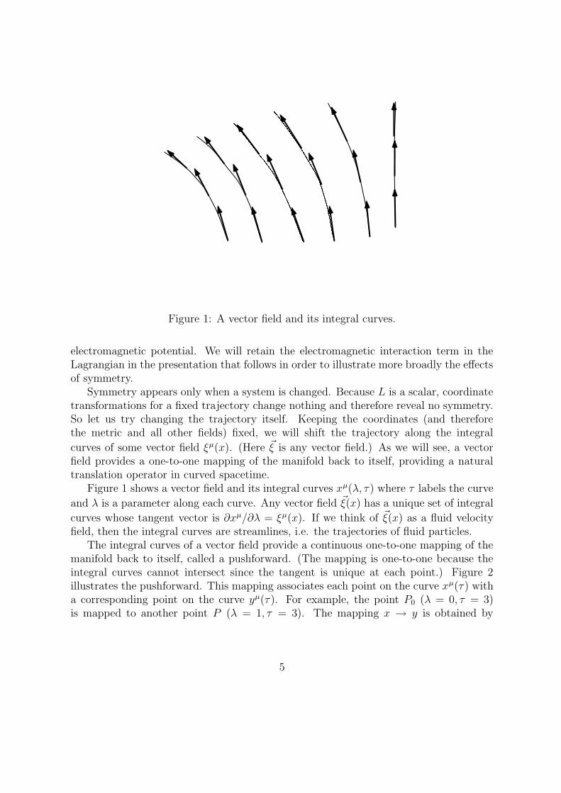
Figure 1: A vector field and its integral curves.

electromagnetic potential. We will retain the electromagnetic interaction term in theLagrangian in the presentation that follows in order to illustrate more broadly the effectsof symmetry.

Symmetry appears only when a system is changed. Because L is a scalar, coordinatetransformations for a fixed trajectory change nothing and therefore reveal no symmetry.So let us try changing the trajectory itself. Keeping the coordinates (and thereforethe metric and all other fields) fixed, we will shift the trajectory along the integral

curves of some vector field ξµ(x). (Here ~ξ is any vector field.) As we will see, a vectorfield provides a one-to-one mapping of the manifold back to itself, providing a naturaltranslation operator in curved spacetime.

Figure 1 shows a vector field and its integral curves xµ(λ, τ) where τ labels the curve

and λ is a parameter along each curve. Any vector field ~ξ(x) has a unique set of integral

curves whose tangent vector is ∂xµ/∂λ = ξµ(x). If we think of ~ξ(x) as a fluid velocityfield, then the integral curves are streamlines, i.e. the trajectories of fluid particles.

The integral curves of a vector field provide a continuous one-to-one mapping of themanifold back to itself, called a pushforward. (The mapping is one-to-one because theintegral curves cannot intersect since the tangent is unique at each point.) Figure 2illustrates the pushforward. This mapping associates each point on the curve xµ(τ) witha corresponding point on the curve yµ(τ). For example, the point P0 (λ = 0, τ = 3)is mapped to another point P (λ = 1, τ = 3). The mapping x → y is obtained by

5

λ=0

λ=1

τ=0 1 2 3 4 5

P0

P

xµ(τ)

yµ(τ)

Figure 2: Using the integral curves of a vector field to shift a curve xµ(τ) to a new curveyµ(τ). The shift, known as a pushforward, defines a continuous one-to-one mapping ofthe space back to itself.

integrating along the vector field ~ξ(x):

∂xµ

∂λ= ξµ(x) , xµ(λ = 0, τ) ≡ xµ(τ) , yµ(τ) ≡ xµ(λ = 1, τ) . (8)

The shift amount λ = 1 is arbitrary; any shift along the integral curves constitutes apushforward. The inverse mapping from y → x is called a pullback.

The pushforward generalizes the simple translations of flat spacetime. A finite trans-lation is built up by a succession of infinitesimal shifts yµ = xµ + ξµdλ. Because thevector field ~ξ(x) is a tangent vector field, the shifted curves are guaranteed to reside inthe manifold.

Applying an infinitesimal pushforward yields the action

S[x(τ) + ξ(x(τ))dλ] =∫ τ2

τ1L(gµν(x+ ξdλ), Aµ(x+ ξdλ), xµ + ξµdλ) dτ . (9)

This is similar to the usual variation xµ → xµ+ δxµ used in deriving the Euler-Lagrangeequations, except that ξ is a field defined everywhere in space (not just on the trajectory)and we do not require ξ = 0 at the endpoints. Our goal here is not to find a trajectorythat makes the action stationary; rather it is to identify symmetries of the action thatresult in conservation laws.

We will ask whether applying a pushforward to one solution of the Euler-Lagrangeequations leaves the action invariant. If so, there is a dynamical symmetry and we

6

will obtain a conservation law. Note that our shifts are more general than the uniformtranslations and rotations considered in nonrelativistic mechanics and special relativity(here the shifts can vary arbitrarily from point to point, so long as the transformationhas an inverse), so we expect to find more general conservation laws.

On the face of it, any pushforward changes the action:

S[x(τ)+ ξ(x(τ))dλ] = S[x(τ)]+dλ∫ τ2

τ1

[

∂L

∂gµν(∂αgµν)ξ

α +∂L

∂Aµ

(∂αAµ)ξα +

∂L

∂xµ

dξµ

dτ

]

dτ .

(10)It is far from obvious that the term in brackets ever would vanish. However, we have onemore tool to use at our disposal: coordinate transformations. Because the Lagrangianis a scalar, we are free to transform coordinates. In some circumstances the effect of thepushforward may be eliminated by an appropriate coordinate transformation, revealinga symmetry.

We consider transformations of the coordinates xµ → xµ(x), where we assume thismapping is smooth and one-to-one so that ∂xµ/∂xα is nonzero and nonsingular every-where. A trajectory xµ(τ) in the old coordinates becomes xµ(x(τ)) ≡ xµ(τ) in the newones, where τ labels a fixed point on the trajectory independently of the coordinates.

The action depends on the metric tensor, one-form potential and velocity components,which under a coordinate transformation change to

gµν = gαβ∂xα

∂xµ

∂xβ

∂xν, Aµ = Aα

∂xα

∂xµ,

dxµ

dτ=∂xµ

∂xα

dxα

dτ. (11)

We have assumed that ∂xµ/∂xα is invertible. Under coordinate transformations theaction does not even change form (only the coordinate labels change), so coordinatetransformations alone cannot generate any nondynamical symmetries. However, we willshow below that coordinate invariance can generate dynamical symmetries which applyonly to solutions of the Euler-Lagrange equations.

Under a pushforward, the trajectory xµ(τ) is shifted to a different trajectory withcoordinates yµ(τ). After the pushforward, we transform the coordinates to xµ(y(τ)).Because the pushforward is a one-to-one mapping of the manifold to itself, we are freeto choose our coordinate transformation so that x = x, i.e. xµ(y(τ)) ≡ xµ(τ) = xµ(τ).In other words, we transform the coordinates so that the new coordinates of the newtrajectory are the same as the old coordinates of the old trajectory. The pushforwardchanges the trajectory; the coordinate transformation covers our tracks.

The combination of pushforward and coordinate transformation is an example of adiffeomorphism. A diffeomorphism is a one-to-one mapping between the manifold anditself. In our case, the pushforward and transformation depend on one parameter λ andwe have a one-parameter family of diffeomorphisms. After a diffeomorphism, the pointP in Figure 2 has the same values of the transformed coordinates as the point P0 has inthe original coordinates: xµ(λ, τ) = xµ(τ).

7

Naively, it would seem that a diffeomorphism automatically leaves the action un-changed because the coordinates of the trajectory are unchanged. However, the La-grangian depends not only on the coordinates of the trajectory; it also depends on tensorcomponents that change according to equation (11). More work will be required beforewe can tell whether the action is invariant under a diffeomorphism. While a coordinatetransformation by itself does not change the action, in general a diffeomorphism, becauseit involves a pushforward, does. A continuous symmetry occurs when a diffeomorphismdoes not change the action. This is the symmetry we will be studying.

The diffeomorphism is an important operation in general relativity. We thereforedigress to consider the diffeomorphism in greater detail before returning to examine itseffect on the action.

3.1 Infinitesimal Diffeomorphisms and Lie derivatives

In a diffeomorphism, we shift the point at which a tensor is evaluated by pushing itforward using a vector field and then we transform (pull back) the coordinates so thatthe shifted point has the same coordinate labels as the old point. Since a diffeomor-phism maps a manifold back to itself, under a diffeomorphism a rank (m,n) tensor ismapped to another rank (m,n) tensor. This subsection asks how tensors change underdiffeomorphisms.

The pushforward mapping may be symbolically denoted φλ (following Wald 1984,Appendix C). Thus, a diffeomorphism maps a tensor T(P0) at point P0 to a tensorT(P ) ≡ φλT(P0) such that the coordinate values are unchanged: xµ(P ) = xµ(P0). (SeeFig. 2 for the roles of the points P0 and P .) The diffeomorphism may be regarded as anactive coordinate transformation: under a diffeomorphism the spatial point is changedbut the coordinates are not.

We illustrate the diffeomorphism by applying it to the components of the one-formA = Aµe

µ in a coordinate basis:

Aµ(P0) ≡ Aα(P )∂xα

∂xµ(P ) , where xµ(P ) = xµ(P0) . (12)

Starting with Aα at point P0 with coordinates xµ(P0), we push the coordinates forwardto point P , we evaluate Aα there, and then we transform the basis back to the coordinatebasis at P with new coordinates xµ(P ).

The diffeomorphism is a continuous, one-parameter family of mappings. Thus, ageneral diffeomorphism may be obtained from the infinitesimal diffeomorphism withpushforward yµ = xµ + ξµdλ. The corresponding coordinate transformation is (to firstorder in dλ)

xµ = xµ − ξµdλ (13)

8

so that xµ(P ) = xµ(P0). This yields (in the xµ coordinate system)

Aµ(x) ≡ Aα(x+ ξdλ)∂xα

∂xµ= Aµ(x) + [ξα∂αAµ(x) + Aα(x)∂µξ

α] dλ+O(dλ)2 . (14)

We have inverted the Jacobian ∂xµ/∂xα = δµα− ∂αξµdλ to first order in dλ, ∂xα/∂xµ =δαµ + ∂µξ

αdλ + O(dλ)2. In a similar manner, the infinitesimal diffeomorphism of themetric gives

gµν(x) ≡ gαβ(x+ ξdλ)∂xα

∂xµ

∂xβ

∂xν

= gµν(x) + [ξα∂αgµν(x) + gαν(x)∂µξα + gµα(x)∂νξ

α] dλ+O(dλ)2 . (15)

In general, the infinitesimal diffeomorphism T ≡ φ∆λT changes the tensor by anamount first-order in ∆λ and linear in ~ξ. This change allows us to define a linearoperator called the Lie derivative:

LξT ≡ lim∆λ→0

φ∆λT(x)− T(x)

∆λwith xµ(P ) = xµ(P0) = xµ(P )− ξµ∆λ+O(∆λ)2 . (16)

The Lie derivatives of Aµ(x) and gµν(x) follow from equations (14)–(16):

LξAµ(x) = ξα∂αAµ + Aα∂µξα , Lξgµν(x) = ξα∂αgµν + gαν∂µξ

α + gµα∂νξα . (17)

The first term of the Lie derivative, ξα∂α, corresponds to the pushforward, shifting atensor to another point in the manifold. The remaining terms arise from the coordinatetransformation back to the original coordinate values. As we will show in the nextsubsection, this combination of terms makes the Lie derivative a tensor in the tangentspace at xµ.

Under a diffeomorphism the transformed tensor components, regarded as functionsof coordinates, are evaluated at exactly the same numerical values of the transformedcoordinate fields (but a different point in spacetime!) as the original tensor components inthe original coordinates. This point is fundamental to the diffeomorphism and thereforeto the Lie derivative, and distinguishes the latter from a directional derivative. Thinkingof the tensor components as a set of functions of coordinates, we are performing an activetransformation: the tensor component functions are changed but they are evaluated atthe original values of the coordinates. The Lie derivative generates an infinitesimaldiffeomorphism. That is, under a diffeomorphism with pushforward xµ → xµ + ξµdλ,any tensor T is transformed to T + LξTdλ.

The fact that the coordinate values do not change, while the tensor fields do, dis-tinguishes the diffeomorphism from a simple coordinate transformation. An importantimplication is that, in integrals over spacetime volume, the volume element d4x does notchange under a diffeomorphism, while it does change under a coordinate transformation.By contrast, the volume element

√−g d4x is invariant under a coordinate transformationbut not under a diffeomorphism.

9

3.2 Properties of the Lie Derivative

The Lie derivative Lξ is similar to the directional derivative operator ∇ξ in its propertiesbut not in its value, except for a scalar where Lξf = ∇ξf = ξµ∂µf . The Lie derivative ofa tensor is a tensor of the same rank. To show that it is a tensor, we rewrite the partialderivatives in equation (17) in terms of covariant derivatives in a coordinate basis usingthe Christoffel connection coefficients to obtain

LξAµ = ξα∇αAµ + Aα∇µξα + T α

µβAαξβ ,

Lξgµν = ξα∇αgµν + gαν∇µξα + gµα∇νξ

α + T αµβgανξ

β + T ανβgµαξ

β , (18)

where T αµβ is the torsion tensor, defined by T α

µβ = Γαµβ − Γα

βµ in a coordinate basis.The torsion vanishes by assumption in general relativity. Equations (18) show that LξAµ

and Lξgµν are tensors.The Lie derivative Lξ differs from the directional derivative ∇ξ in two ways. First,

the Lie derivative requires no connection: equation (17) gave the Lie derivative solelyin terms of partial derivatives of tensor components. [The derivatives of the metricshould not be regarded here as arising from the connection; the Lie derivative of anyrank (0, 2) tensor has the same form as Lξgµν in eq. 17.] Second, the Lie derivative

involves the derivatives of the vector field ~ξ while the covariant derivative does not. TheLie derivative trades partial derivatives of the metric (present in the connection for thecovariant derivative) for partial derivatives of the vector field. The directional derivative

tells how a fixed tensor field changes as one moves through it in direction ~ξ. The Liederivative tells how a tensor field changes as it is pushed forward along the integral curvesof ~ξ.

More understanding of the Lie derivative comes from examining the first-order changein a vector expanded in a coordinate basis under a displacement ~ξdλ:

d ~A = ~A(x+ ξdλ)− ~A(x) = Aµ(x+ ξdλ)~eµ(x+ ξdλ)− Aµ(x)~eµ(x) . (19)

The nature of the derivative depends on how we obtain ~eµ(x + ξdλ) from ~eµ(x). Forthe directional derivative ∇ξ, the basis vectors at different points are related by theconnection:

~eµ(x+ ξλ) =(

δβµ + dλ ξαΓβµα

)

~eβ(x) for ∇ξ . (20)

For the Lie derivative Lξ, the basis vector is mapped back to the starting point with

~eµ(x+ ξdλ) =∂xβ

∂xµ~eβ(x) =

(

δβµ − dλ ∂µξβ)

~eβ(x) for Lξ . (21)

Similarly, the basis one-form is mapped using

eµ(x+ ξdλ) =∂xµ

∂xβeβ(x) =

(

δµβ + dλ ∂βξµ)

eβ(x) for Lξ . (22)

10

These mappings ensure that d ~A/dλ = Lξ~A is a tangent vector on the manifold.

The Lie derivative of any tensor may be obtained using the following rules: (1) TheLie derivative of a scalar field is the directional derivative, Lξf = ξα∂αf = ∇ξf . (2)The Lie derivative obeys the Liebnitz rule, Lξ(TU) = (LξT )U + T (LξU), where T andU may be tensors of any rank, with a tensor product or contraction between them. TheLie derivative commutes with contractions. (3) The Lie derivatives of the basis vectorsare Lξ~eµ = −~eα∂µξα. (4) The Lie derivatives of the basis one-forms are Lξe

µ = eα∂αξµ.

These rules ensure that the Lie derivative of a tensor is a tensor. Using them, theLie derivative of any tensor may be obtained by expanding the tensor in a basis, e.g. fora rank (1, 2) tensor,

LξS = Lξ(Sµνκ~eµ ⊗ eν ⊗ eκ) ≡ (LξS

µνκ)~eµ ⊗ eν ⊗ eκ

= [ξα∂αSµνκ − Sα

νκ∂αξµ + Sµ

ακ∂νξα + Sµ

να∂κξα]~eµ ⊗ eν ⊗ eκ . (23)

The partial derivatives can be changed to covariant derivatives without change (withvanishing torsion, the connection coefficients so introduced will cancel each other), con-firming that the Lie derivative of a tensor really is a tensor.

The Lie derivative of a vector field is an antisymmetric object known also as thecommutator or Lie bracket:

LV~U = (V µ∂µU

ν − Uµ∂µVν)~eν ≡ [~V , ~U ] . (24)

The commutator was introduced in the notes Tensor Calculus, Part 2, Section 2.2. Withvanishing torsion, [~V , ~U ] = ∇V

~U −∇U~V . Using rule (4) of the Lie derivative given after

equation (22), it follows at once that the commutator of any pair of coordinate basisvector fields vanishes: [~eµ, ~eν ] = 0.

3.3 Diffeomorphism-invariance and Killing Vectors

Having defined and investigated the properties of diffeomorphisms and the Lie derivative,we return to the question posed at the beginning of Section 3: How can we tell when theaction is translationally invariant? Equation (10) gives the change in the action under a

generalized translation or pushforward by the vector field ~ξ. However, it is not yet in aform that highlights the key role played by diffeomorphisms.

To uncover the diffeomorphism we must perform the infinitesimal coordinate trans-formation given by equation (13). To first order in dλ this has no effect on the dλ termalready on the right-hand side of equation (10) but it does add a piece to the unperturbedaction. Using equation (11) and the fact that the Lagrangian is a scalar, to O(dλ) weobtain

S[x(τ)] =∫ τ2

τ1L(gµν , Aµ, x

µ) dτ =∫ τ2

τ1L

(

gαβ∂xα

∂xµ

∂xβ

∂xν, Aα

∂xα

∂xµ,dxα

dτ

∂xµ

∂xα

)

dτ

= S[x(τ)] + dλ∫ τ2

τ1

[

∂L

∂gµν(gαν∂µξ

α + gµα∂νξα) +

∂L

∂Aµ

(Aα∂µξα)− ∂L

∂xµ

dξµ

dτ

]

dτ . (25)

11

The integral multiplying dλ always has the value zero for any trajectory xµ(τ) and

vector field ~ξ because of the coordinate-invariance of the action. However, it is a specialkind of zero because, when added to the pushforward term of equation (10), it gives adiffeomorphism:

S[x(τ) + ξ(x(τ))dλ] = S[x(τ)] + dλ∫ τ2

τ1

[

∂L

∂gµνLξgµν +

∂L

∂Aµ

LξAµ

]

dτ . (26)

If the action contains additional fields, under a diffeomorphism we obtain a Lie derivativeterm for each field.

Thus, we have answered the question of translation-invariance: the action is transla-tionally invariant if and only if the Lie derivative of each tensor field appearing in theLagrangian vanishes. The uniform translations of Newtonian mechanics are generalizedto diffeomorphisms, which include translations, rotations, boosts, and any continuous,one-to-one mapping of the manifold back to itself.

In Newtonian mechanics, translation-invariance leads to a conserved momentum.What about diffeomorphism-invariance? Does it also lead to a conservation law?

Let us suppose that the original trajectory xµ(τ) satisfies the equations of motionbefore being pushed forward, i.e. the action, with Lagrangian L(gµν(x), Aµ, x

µ), is sta-tionary under first-order variations xµ → xµ + δxµ(x) with fixed endpoints δxµ(τ1) =δxµ(τ2) = 0. From equation (26) it follows that the action for the shifted trajectory isalso stationary, if and only if Lξgµν = 0 and LξAµ = 0. (When the trajectory is variedxµ → xµ + δxµ, cross-terms ξδx are regarded as being second-order and are ignored.)

If there exists a vector field ~ξ such that Lξgµν = 0 and LξAµ = 0, then we can

shift solutions of the equations of motion along ~ξ(x(τ)) and generate new solutions.This is a new continuous symmetry called diffeomorphism-invariance, and it generalizestranslational-invariance in Newtonian mechanics and special relativity. The result is adynamical symmetry, which may be deduced by rewriting equation (26):

lim∆λ→0

S[x(τ) + ξ(x(τ))∆λ]− S[x(τ)]

∆λ=

∫ τ2

τ1

[

∂L

∂gµνLξgµν +

∂L

∂Aµ

LξAµ

]

dτ

=∫ τ2

τ1

[

∂L

∂xαξα +

∂L

∂xµ

dξµ

dτ

]

dτ

=∫ τ2

τ1

[

d

dτ

(

∂L

∂xµ

)

ξµ +∂L

∂xµ

dξµ

dτ

]

dτ

=∫ τ2

τ1

[

d

dτ(pµξ

µ)

]

dτ

= [pµξµ]τ2τ1 . (27)

All of the steps are straightforward aside from the second line. To obtain this we firstexpanded the Lie derivatives using equation (17). The terms multiplying ξα were then

12

combined to give ∂L/∂xα (regarding the Lagrangian as a function of xµ and xµ). Forthe terms multiplying the gradient ∂µξ

α, we used dξµ(x(τ))/dτ = xα∂αξµ combined

with equation (6) to convert partial derivatives of L with respect to the fields gµν andAµ to partial derivatives with respect to xµ. (This conversion is dependent on theLagrangian, of course, but works for any Lagrangian that is a function of gµν x

µxν andAµx

µ.) To obtain the third line we used the assumption that xµ(τ) is a solution of theEuler-Lagrange equations. To obtain the fourth line we used the definition of canonicalmomentum,

pµ ≡∂L

∂xµ. (28)

For the Lagrangian of equation (6), pµ = gµν xν + qAµ is not the mechanical momentum

(the first term) but also includes a contribution from the electromagnetic field.Nowhere in equation (27) did we assume that ξµ vanishes at the endpoints. The

vector field ~ξ is not just a variation used to obtain equations of motion, nor is it aconstant; it is an arbitrary small shift.

Theorem: If the Lagrangian is invariant under the diffeomorphism generated by avector field ~ξ, then p(~ξ ) = pµξ

µ is conserved along curves that extremize the action, i.e.for trajectories obeying the equations of motion.

This result is a generalization of conservation of momentum. The vector field ~ξ maybe thought of as the coordinate basis vector field for a cyclic coordinate, i.e. one that doesnot appear in the Lagrangian. In particular, if ∂L/∂xα = 0 for a particular coordinatexα (e.g. α = 0), then L is invariant under the diffeomorphism generated by ~eα so thatpα is conserved.

When gravity is the only force acting on a particle, diffeomorphism-invariance hasa purely geometric interpretation in terms of special vector fields known as Killing vec-tors. Using equation (18) for a manifold with a metric-compatible connection (implying∇αgµν = 0) and vanishing torsion (both of these are true in general relativity), we findthat diffeomorphism-invariance implies

Lξgµν = ∇µξν +∇νξµ = 0 . (29)

This equation is known as Killing’s equation and its solutions are called Killing vectorfields, or Killing vectors for short. Thus, our theorem may be restated as follows: If thespacetime has a Killing vector ~ξ(x), then pµξ

µ is conserved along any geodesic. A muchshorter proof of this theorem follows from ∇V (pµξ

µ) = ξµ∇V pµ + pµVν∇νξ

µ. The firstterm vanishes by the geodesic equation, while the second term vanishes from Killing’sequation with pµ ∝ V µ. Despite being longer, however, the proof based on the Liederivative is valuable because it highlights the role played by a continuous symmetry,diffeomorphism-invariance of the metric.

One is not free to choose Killing vectors; general spacetimes (i.e. ones lacking sym-metry) do not have any solutions of Killing’s equation. As shown in Appendix C.3 of

13

Wald (1984), a 4-dimensional spacetime has at most 10 Killing vectors. The Minkowskimetric has the maximal number, corresponding to the Poincare group of transforma-tions: three rotations, three boosts, and four translations. Each Killing vector gives aconserved momentum.

The existence of a Killing vector represents a symmetry: the geometry of spacetime asrepresented by the metric is invariant as one moves in the ~ξ-direction. Such a symmetryis known as an isometry. In the perturbation theory view of diffeomorphisms, isometriescorrespond to perturbations of the coordinates that leave the metric unchanged.

Any vector field can be chosen as one of the coordinate basis fields; the coordinatelines are the integral curves. In Figure 2, the integral curves were parameterized byλ, which becomes the coordinate whose corresponding basis vector is ~eλ ≡ ~ξ(x). For

definiteness, let us call this coordinate λ = x0. If ~ξ = ~e0 is a Killing vector, then x0 isa cyclic coordinate and the spacetime is stationary: ∂0gµν = 0. In such spacetimes, andonly in such spacetimes, p0 is conserved along geodesics (aside from special cases likethe Robertson-Walker spacetimes, where p0 is conserved for massless but not massiveparticles because the spacetime is conformally stationary).

Another special feature of spacetimes with Killing vectors is that they have a con-served 4-vector energy-current Sν = ξµT

µν . Local stress-energy conservation ∇µTµν = 0

then implies ∇νSν = 0, which can be integrated over a volume to give the usual form

of an integral conservation law. Conversely, spacetimes without Killing vectors do nothave an tensor integral energy conservation law, except for spacetimes that are asymp-totically flat at infinity. (However, all spacetimes have a conserved energy-momentumpseudotensor, as discussed in the notes Stress-Energy Pseudotensors and Gravitational

Radiation Power.)

4 Einstein-Hilbert Action for the Metric

We have seen that the action principle is useful not only for concisely expressing theequations of motion; it also enables one to find identities and conservation laws fromsymmetries of the Lagrangian (invariance of the action under transformations). Thesemethods apply not only to the trajectories of individual particles. They are readilygeneralized to spacetime fields such as the electromagnetic four-potential Aµ and, mostsignificantly in GR, the metric gµν itself.

To understand how the action principle works for continuous fields, let us recall how itworks for particles. The action is a functional of configuration-space trajectories. Givena set of functions qi(t), the action assigns a number, the integral of the Lagrangianover the parameter t. For continuous fields the configuration space is a Hilbert space,an infinite-dimensional space of functions. The single parameter t is replaced by thefull set of spacetime coordinates. Variation of a configuration-space trajectory, qi(t) →qi(t)+ δqi(t), is generalized to variation of the field values at all points of spacetime, e.g.

14

gµν(x)→ gµν(x) + δgµν(x). In both cases, the Lagrangian is chosen so that the action isstationary for trajectories (or field configurations) that satisfy the desired equations ofmotion. The action principle concisely specifies those equations of motion and facilitatesexamination of symmetries and conservation laws.

In general relativity, the metric is the fundamental field characterizing the geometricand gravitational properties of spacetime, and so the action must be a functional ofgµν(x). The standard action for the metric is the Hilbert action,

SG[gµν(x)] =∫ 1

16πGgµνRµν

√−g d4x . (30)

Here, g = det gµν and Rµν = Rαµαν is the Ricci tensor. The factor

√−g makes the volumeelement invariant so that the action is a scalar (invariant under general coordinate trans-formations). The Einstein-Hilbert action was first shown by the mathematician DavidHilbert to yield the Einstein field equations through a variational principle. Hilbert’spaper was submitted five days before Einstein’s paper presenting his celebrated fieldequations, although Hilbert did not have the correct field equations until later (for aninteresting discussion of the historical issues see L. Corry et al., Science 278, 1270, 1997).

(The Einstein-Hilbert action is a scalar under general coordinate transformations.As we will show in the notes Stress-Energy Pseudotensors and Gravitational Radiation

Power, it is possible to choose an action that, while not a scalar under general coor-dinate transformations, still yields the Einstein field equations. The action consideredthere differs from the Einstein-Hilbert action by a total derivative term. The only realinvariance of the action that is required on physical grounds is local Lorentz invariance.)

In the particle actions considered previously, the Lagrangian depended on the gen-eralized coordinates and their first derivatives with respect to the parameter τ . In aspacetime field theory, the single parameter τ is expanded to the four coordinates xµ. Ifit is to be a scalar, the Lagrangian for the spacetime metric cannot depend on the firstderivatives ∂αgµν , because ∇αgµν = 0 and the first derivatives can all be transformed tozero at a point. Thus, unless one drops the requirement that the action be a scalar undergeneral coordinate transformations, for gravity one is forced to go to second derivativesof the metric. The Ricci scalar R = gµνRµν is the simplest scalar that can be formedfrom the second derivatives of the metric. Amazingly, when the action for matter andall non-gravitational fields is added to the simplest possible scalar action for the metric,the least action principle yields the Einstein field equations.

To look for symmetries of the Einstein-Hilbert action, we consider its change undervariation of the functions gµν(x) with fixed boundary hypersurfaces (the generalizationof the fixed endpoints for an ordinary Lagrangian). It proves to be simpler to regardthe inverse metric components gµν as the field variables. The action depends explicitlyon gµν and the Christoffel connection coefficients, Γα

µν , the latter appearing in the Riccitensor in a coordinate basis:

Rµν = ∂αΓαµν − ∂µΓ

ααν + Γα

µνΓβαβ − Γα

βµΓβαν . (31)

15

Lengthy algebra shows that first-order variations of gµν produce the following changesin the quantities appearing in the Einstein-Hilbert action:

δ√−g = −1

2

√−g gµνδgµν = +1

2

√−g gµνδgµν ,

δΓαµν = −1

2

[

∇µ(gνλδgαλ) +∇ν(gµλδg

αλ)−∇β(gµκgνλgαβδgκλ)

]

,

δRµν = ∇α(δΓαµν)−∇µ(δΓ

ααν) ,

gµνδRµν = ∇µ∇ν

(

−δgµν + gµνgαβδgαβ)

,

δ(gµνRµν

√−g) = (Gµνδgµν + gµνδRµν)

√−g , (32)

where Gµν = Rµν − 12Rgµν is the Einstein tensor. The covariant derivative ∇µ appearing

in these equations is taken with respect to the zeroth-order metric gµν . Note that,while Γα

µν is not a tensor, δΓαµν is. Note also that the variations we perform are not

necessarily diffeomorphisms (that is, δgµν is not necessarily a Lie derivative), althoughdiffeomorphisms are variations of just the type we are considering (i.e. variations ofthe tensor component fields for fixed values of their arguments). Equations (32) arestraightforward to derive but take several pages of algebra.

Equations (32) give us the change in the gravitational action under variation of themetric:

δSG ≡ SG[gµν + δgµν ]− SG[g

µν ]

=1

16πG

∫

(Gµνδgµν +∇µv

µ)√−g d4x , vµ ≡ ∇ν(−δgµν + gµνgαβδg

αβ) .(33)

Besides the desired Einstein tensor term, there is a divergence term arising from gµνδRµν =∇µv

µ which can be integrated using the covariant Gauss’ law. This term raises the ques-tion of what is fixed in the variation, and what the endpoints of the integration are.

In the action principle for particles (eq. 2), the endpoints of integration are fixedtime values, t1 and t2. When we integrate over a four-dimensional volume, the endpointscorrespond instead to three-dimensional hypersurfaces. The simplest case is when theseare hypersurfaces of constant t, in which case the boundary terms are integrals overspatial volume.

In equation (33), the divergence term can be integrated to give the flux of vµ throughthe bounding hypersurface. This term involves the derivatives of δgµν normal to theboundary (e.g. the time derivative of δgµν , if the endpoints are constant-time hyper-surfaces), and is therefore inconvenient because the usual variational principle sets δgµν

but not its derivatives to zero at the endpoints. One may either revise the variationalprinciple so that gµν and Γα

µν are independently varied (the Palatini action), or one canadd a boundary term to the Einstein-Hilbert action, involving a tensor called the extrin-sic curvature, to cancel the ∇µv

µ term (Wald, Appendix E.1). In the following we willignore this term, understanding that it can be eliminated by a more careful treatment.

16

(The Schrodinger action presented in the later notes Stress-Energy Pseudotensors and

Gravitational Radiation Power eliminates the ∇µvµ term.)

For convenience below, we introduce a new notation for the integrand of a functionalvariation, the functional derivative δS/δψ, defined by

δS[ψ] ≡∫

(

δS

δψ

)

δψ√−g d4x . (34)

Here, ψ is any tensor field, e.g. gµν . The functional derivative is strictly defined onlywhen there are no surface terms arising from the variation. Neglecting the surface termin equation (33), we see that δSG/δg

µν = (16πG)−1Gµν .

4.1 Stress-Energy Tensor and Einstein Equations

To see how the Einstein equations arise from an action principle, we must add to SG

the action for matter, the source of spacetime curvature. Here, “matter” refers to allparticles and fields excluding gravity, and specifically includes all the quarks, leptonsand gauge bosons in the world (excluding gravitons). At the classical level, one couldinclude electromagnetism and perhaps a simplified model of a fluid. The total actionwould become a functional of the metric and matter fields. Independent variation of eachfield yields the equations of motion for that field. Because the metric implicitly appearsin the Lagrangian for matter, matter terms will appear in the equation of motion for themetric. This section shows how this all works out for the simplest model for matter, aclassical sum of massive particles.

Starting from equation (1), we sum the actions for a discrete set of particles, weightingeach by its mass:

SM =∑

a

∫

−ma

(

−g00 − 2g0ixia − gijx

iax

ja

)1/2dt . (35)

The subscript a labels each particle. We avoid the problem of having no global propertime by parameterizing each particle’s trajectory by the coordinate time. Variation ofeach trajectory, xi

a(t)→ xia(t) + δxi

a(t) for particle a with ∆SM = 0, yields the geodesicequations of motion.

Now we wish to obtain the equations of motion for the metric itself, which we do bycombining the gravitational and matter actions and varying the metric. After a littlealgebra, equation (33) gives the variation of SG; we must add to it the variation of SM.Equation (35) gives

δSM =∫

dt∑

a

1

2ma

V µa V

νa

V 0a

δgµν(xia(t), t) =

∫

dt∑

a

−1

2ma

VaµVaν

V 0a

δgµν(xia(t), t) . (36)

Variation of the metric naturally gives the normalized 4-velocity for each particle, V µa =

dxµ/dτa with VaµVµa = −1, with a correction factor 1/V 0

a = dτa/dt. Now, if we are

17

to combine equations (33) and (36), we must modify the latter to get an integral over4-volume. This is easily done by inserting a Dirac delta function. The result is

δSM = −∫

[

1

2

∑

a

ma√−gVaµVaν

V 0a

δ3(xi − xia(t))

]

δgµν(x)√−g d4x . (37)

The term in brackets may be rewritten in covariant form by inserting an integral overaffine parameter with a delta function to cancel it,

∫

dτa δ(t− t(τa))(dt/dτa). Noting thatV 0a = dt/dτa, we get

δSM = −∫ 1

2Tµνδg

µν(x)√−g d4x = +

∫ 1

2T µνδgµν(x)

√−g d4x , (38)

where the functional differentiation has naturally produced the stress-energy tensor fora gas of particles,

T µν = 2δSM

δgµν=∑

a

∫

dτaδ4(x− x(τa))√−g maV

µa V

νa . (39)

Aside from the factor√−g needed to correct the Dirac delta function for non-flat coor-

dinates (because√−g d4x is the invariant volume element), equation (39) agrees exactly

with the stress-energy tensor worked out in the 8.962 notes Number-Flux Vector and

Stress-Energy Tensor.Equation (38) is a general result, and we take it as the definition of the stress-energy

tensor for matter (cf. Appendix E.1 of Wald). Thus, given any action SM for particlesor fields (matter), we can vary the coordinates or fields to get the equations of motionand vary the metric to get the stress-energy tensor,

T µν ≡ 2δSM

δgµν. (40)

Taking the action to be the sum of SG and SM, requiring it to be stationary withrespect to variations δgµν , now gives the Einstein equations:

Gµν = 8πGTµν . (41)

The pre-factor (16πG)−1 on SG was chosen to get the correct coefficient in this equation.The matter action is conventionally normalized so that it yields the stress-energy tensoras in equation (38).

4.2 Diffeomorphism Invariance of the Einstein-Hilbert Action

We return to the variation of the Einstein-Hilbert action, equation (33) without thesurface term, and consider diffeomorphisms δgµν = Lξg

µν :

16πG δSG =∫

Gµν(Lξgµν)√−g d4x = −2

∫

Gµν(∇µξν)√−g d4x . (42)

18

Here, ~ξ is not a Killing vector; it is an arbitrary small coordinate displacement. The Liederivative Lξg

µν has been rewritten in terms of −Lξgµν using gµαgαν = δµν . Note thatdiffeomorphisms are a class of field variations that correspond to mapping the manifoldback to itself. Under a diffeomorphism, the integrand of the Einstein-Hilbert actionis varied, including the

√−g factor. However, as discussed at the end of §3.1, thevolume element d4x is fixed under a diffeomorphism even though it does change undercoordinate transformations. The reason for this is apparent in equation (16): undera diffeomorphism, the coordinate values do not change. The pushforward cancels thetransformation. If we simply performed either a passive coordinate transformation orpushforward alone, d4x would not be invariant. Under a diffeomorphism the variationδgµν = Lξgµν is a tensor on the “unperturbed background” spacetime with metric gµν .

We now show that any scalar integral is invariant under a diffeomorphism that van-ishes at the endpoints of integration. Consider the integrand of any action integral,Ψ√−g, where Ψ is any scalar constructed out of the tensor fields of the problem; e.g.

Ψ = R/(16πG) for the Hilbert action. From the first of equations (32) and the Liederivative of the metric,

Lξ

√−g =1

2

√−g gµνLξgµν = (∇αξα)√−g . (43)

Using the fact that the Lie derivative of a scalar is the directional derivative, we obtain

δS =∫

Lξ(Ψ√−g) d4x =

∫

(ξµ∇µΨ+Ψ∇µξµ)√−g d4x =

∫

Ψξµ d3Σµ . (44)

We have used the covariant form of Gauss’ law, for which d3Σµ is the covariant hyper-surface area element for the oriented boundary of the integrated 4-volume. Physicallyit represents the difference between the spatial volume integrals at the endpoints ofintegration in time.

For variations with ξµ = 0 on the boundaries, δS = 0. The reason for this issimple: diffeomorphism corresponds exactly to reparameterizing the manifold by shiftingand relabeling the coordinates. Just as the action of equation (1) is invariant underarbitrary reparameterization of the path length with fixed endpoints, a spacetime fieldaction is invariant under reparameterization of the coordinates (with no shift on theboundaries). The diffeomorphism differs from a standard coordinate transformation inthat the variation is made so that d4x is invariant rather than

√−g d4x, but the resultis the same: scalar actions are diffeomorphism-invariant.

In considering diffeomorphisms, we do not assume that gµν extremizes the action.Thus, using δSG = 0 under diffeomorphisms, we will get an identity rather than aconservation law.

Integrating equation (42) by parts using Gauss’s law gives

8πG δSG = −∫

Gµνξν d3Σµ +

∫

ξν∇µGµν√−g d4x . (45)

19

Under reparameterization, the boundary integral vanishes and δSG = 0 from above, butξν is arbitrary in the 4-volume integral. Therefore, diffeomorphism-invariance implies

∇µGµν = 0 . (46)

Equation (46) is the famous contracted Bianchi identity. Mathematically, it is anidentity akin to equation (4). It may also be regarded as a geometric property of theRiemann tensor arising from the full Bianchi identities,

∇σRαβµν +∇µR

αβνσ +∇νR

αβσµ = 0 . (47)

Contracting on α and µ, then multiplying by gσβ and contracting again gives equation(46). One can also explicitly verify equation (46) using equation (31), noting that Gµν =Rµν − 1

2Rgµν and Rµν = gµαgνβRαβ. Wald gives a shorter and more sophisticated proof

in his Section 3.2; an even shorter proof can be given using differential forms (Misneret al chapter 15). Our proof, based on diffeomorphism-invariance, is just as rigorousalthough quite different in spirit from these geometric approaches.

The next step is to inquire whether diffeomorphism-invariance can be used to obtaintrue conservation laws and not just offer elegant derivations of identities. Before answer-ing this question, we digress to explore an analogous symmetry in electromagnetism.

4.3 Gauge Invariance in Electromagnetism

Maxwell’s equations can be obtained from an action principle by adding two more termsto the total action. In SI units these are

SEM[Aµ, gµν ] =

∫

− 1

16πF µνFµν

√−g d4x , SI[Aµ] =∫

AµJµ√−g d4x , (48)

where Fµν ≡ ∂µAν − ∂νAµ = ∇µAν −∇νAµ. Note that gµν is present in SEM implicitlythrough raising indices of Fµν , and that the connection coefficients occurring in ∇µAν

are cancelled in Fµν . Electromagnetism adds two pieces to the action, SEM for the freefield Aµ and SI for its interaction with a source, the 4-current density Jµ. Previouslywe considered SI =

∫

qAµxµ dτ for a single particle; now we couple the electromagnetic

field to the current density produced by many particles.The action principle says that the action SEM + SI should be stationary with respect

to variations δAµ that vanish on the boundary. Applying this action principle (left as ahomework exercise for the student) yields the equations of motion

∇νFµν = 4πJµ . (49)

In the language of these notes, the other pair of Maxwell equations,∇[αFµν] = 0, arisesfrom a non-dynamical symmetry, the invariance of SEM[Aµ] under a gauge transformation

20

Aµ → Aµ+∇µΦ. (Expressed using differential forms, dF = 0 because F = dA is a closed2-form. A gauge transformation adds to F the term ddΦ, which vanishes for the samereason. See the 8.962 notes Hamiltonian Dynamics of Particle Motion.) The source-freeMaxwell equations are simple identities in that ∇[αFµν] = 0 for any differentiable Aµ,whether or not it extremizes any action.

If we require the complete action to be gauge-invariant, a new conservation law ap-pears, charge conservation. Under a gauge transformation, the interaction term changesby

δSI ≡ SI[Aµ +∇µΦ]− SI[Aµ] =∫

Jµ(∇µΦ)√−g d4x

=∫

ΦJµ d3Σµ −∫

Φ(∇µJµ)√−g d4x . (50)

For gauge transformations that vanish on the boundary, gauge-invariance is equivalentto conservation of charge, ∇µJ

µ = 0. This is an example of Noether’s theorem: acontinuous symmetry generates a conserved current. Gauge invariance is a dynamicalsymmetry because the action is extremized if and only if Jµ obeys the equations of motionfor whatever charges produce the current. (There will be other action terms, such aseq. 35, to give the charges’ equations of motion.) Adding a gauge transformation toa solution of the Maxwell equations yields another solution. All solutions necessarilyconserve total charge.

Taking a broad view, physicists regard gauge-invariance as a fundamental symmetryof nature, from which charge conservation follows. A similar phenomenon occurs withthe gravitational equivalent of gauge invariance, as we discuss next.

4.4 Energy-Momentum Conservation from Gauge Invariance

The example of electromagnetism sheds light on diffeomorphism-invariance in general rel-ativity. We have already seen that every piece of the action is automatically diffeomorphism-invariant because of parameterization-invariance. However, we wish to single out gravity— specifically, the metric gµν — to impose a symmetry requirement akin to electromag-netic gauge-invariance.

We do this by defining a gauge transformation of the metric as an infinitesimaldiffeomorphism,

gµν → gµν + Lξgµν = gµν +∇µξν +∇νξµ (51)

where ξµ = 0 on the boundary of our volume. (If the manifold is compact, it has anatural boundary; otherwise we integrate over a compact subvolume. See Appendix Aof Wald for mathematical rigor.) Gauge-invariance (diffeomorphism-invariance) of theEinstein-Hilbert action leads to a mathematical identity, the twice-contracted Bianchiidentity, equation (46). The rest of the action, including all particles and fields, mustalso be diffeomorphism-invariant. In particular, this means that the matter action must

21

be invariant under the gauge transformation of equation (51). Using equation (38), thisrequirement leads to a conservation law:

δSM =∫

T µν(∇µξν)√−g d4x = −

∫

ξν(∇µTµν)√−g d4x = 0 ⇒ ∇µT

µν = 0 . (52)

In general relativity, total stress-energy conservation is a consequence of gauge-invarianceas defined by equation (51). Local energy-momentum conservation therefore follows asan application of Noether’s theorem (a continuous symmetry of the action leads to aconserved current) just as electromagnetic gauge invariance implies charge conservation.

There is a further analogy with electromagnetism. Physical observables in generalrelativity must be gauge-invariant. If we wish to try to deduce physics from the metricor other tensors, we will have to work with gauge-invariant quantities or impose gaugeconditions to fix the coordinates and remove the gauge freedom. This issue will ariselater in the study of gravitational radiation.

5 An Example of Gauge Invariance and Diffeomor-

phism Invariance: The Ginzburg-Landau Model

The discussion of gauge invariance in the preceding section is incomplete (although fullycorrect) because under a diffeomorphism all fields change, not only the metric. Similarly,the matter fields for charged particles also change under an electromagnetic gauge trans-formation and under the more complicated symmetry transformations of non-Abeliangauge symmetries such as those present in the theories of the electroweak and stronginteractions. In order to give a more complete picture of the role of gauge symmetriesin both electromagnetism and gravity, we present here the classical field theory for thesimplest charged field, a complex scalar field φ(x) representing spinless particles of chargeq and mass m. Although there are no fundamental particles with spin 0 and nonzeroelectric charge, this example is very important in physics as it describes the effective fieldtheory for superconductivity developed by Ginzburg and Landau.

The Ginzburg-Landau model illustrates the essential features of gauge symmetryarising in the standard model of particle physics and its classical extension to gravity.At the classical level, the Ginzburg-Landau model describes a charged fluid, e.g. a fluidof Cooper pairs (the electron pairs that are responsible for superconductivity). Here wecouple the charged fluid to gravity as well as to the electromagnetic field.

The Ginzburg-Landau action is (with a sign difference in the kinetic term comparedwith quantum field theory textbooks because of our choice of metric signature)

SGL[φ,Aµ, gµν ] =

∫

[

−1

2gµν(Dµφ)

∗(Dνφ) +1

2µ2φ∗φ− λ

4(φ∗φ)2

]√−g d4x , (53)

22

where φ∗ is the complex conjugate of φ and

Dµ ≡ ∇µ − iqAµ(x) (54)

is called the gauge covariant derivative. The electromagnetic one-form potentialappears so that the action is automatically gauge-invariant. Under an electromagneticgauge transformation, both the electromagnetic potential and the scalar field change, asfollows:

Aµ(x)→ Aµ(x) +∇µΦ(x) , φ(x)→ eiqΦ(x)φ(x) , Dµφ→ eiqΦ(x)Dµφ , (55)

where Φ(x) is any real scalar field. We see that (Dµφ)∗(Dνφ) and the Ginzburg-Landauaction are gauge-invariant. Thus, an electromagnetic gauge transformation correspondsto an independent change of phase at each point in spacetime, or a local U(1) symmetry.

The gauge covariant derivative automatically couples our charged scalar field to theelectromagnetic field so that no explicit interaction term is needed, unlike in equation(48). The first term in the Ginzburg-Landau action is a “kinetic” part that is quadratic inthe derivatives of the field. The remaining parts are “potential” terms. The quartic termwith coefficient λ/4 represents the effect of self-interactions that lead to a phenomenoncalled spontaneous symmetry breaking. Although spontaneous symmetry breaking is ofmajor importance in modern physics, and is an essential feature of the Ginzburg-Landaumodel, it has no effect on our discussion of symmetries and conservation laws so weignore it in the following.

The appearance of Aµ in the gauge covariant derivative is reminiscent of the appear-ance of the connection Γµ

αβ in the covariant derivative of general relativity. However,the gravitational connection is absent for derivatives of scalar fields. We will not discussthe field theory of charged vector fields (which represent spin-1 particles in non-Abeliantheories) or spinors (spin-1/2 particles).

A complete model includes the actions for gravity and the electromagnetic field inaddition to SGL: S[φ,Aµ, g

µν ] = SGL[φ,Aµ, gµν ] + SEM[Aµ, g

µν ] + SG[gµν ]. According to

the action principle, the classical equations of motion follow by requiring the total actionto be stationary with respect to small independent variations of (φ,Aµ, g

µν) at each pointin spacetime. Varying the action yields

δS

δφ= gµνDµDνφ+

(

µ2 − λφ∗φ)

φ ,

δS

δAµ

= − 1

4π∇νF

µν + JµGL ,

δS

δgµν=

1

16πGGµν −

1

2TEMµν − 1

2TGLµν , (56)

where the current and stress-energy tensor of the charged fluid are

JGLµ ≡ iq

2[φ(Dµφ)

∗ − φ∗(Dµφ)] ,

23

TGLµν ≡ (Dµφ)

∗(Dνφ) +

[

−1

2gαβ(Dαφ)

∗(Dβφ) +1

2µ2φ∗φ− λ

4(φ∗φ)2

]

gµν . (57)

The expression for the current density is very similar to the probability current densityin nonrelativistic quantum mechanics. The expression for the stress-energy tensor seemsstrange, so let us examine the energy density in locally Minkowski coordinates (wheregµν = ηµν):

ρGL = TGL00 =

1

2|D0φ|2 +

1

2|Diφ|2 −

1

2µ2φ∗φ+

λ

4(φ∗φ)2 . (58)

Aside from the electromagnetic contribution to the gauge covariant derivatives and thepotential terms involving φ∗φ, this looks just like the energy density of a field of rela-tivistic harmonic oscillators. (The potential energy is minimized for |φ| = µ/

√λ. This

is a circle in the complex φ plane, leading to spontaneous symmetry breaking as thefield acquires a phase. Those with a knowledge of field theory will recognize two modesfor small excitations: a massive mode with mass

√2µ and a massless Goldstone mode

corresponding to the field circulating along the circle of minima.)The equations of motion follow immediately from setting the functional derivatives

to zero. The equations of motion for gµν and Aµ are familiar from before; they aresimply the Einstein and Maxwell equations with source including the current and stress-energy of the charged fluid. The equation of motion for φ is a nonlinear relativistic waveequation. If Aµ = 0, µ2 = −m2, λ = 0, and gµν = ηµν then it reduces to the Klein-Gordon equation, (∂2t − ∂2 +m2)φ = 0 where ∂2 ≡ δij∂i∂j is the spatial Laplacian. Ourequation of motion for φ generalizes the Klein-Gordon equation to include the effectsof gravity (through gµν), electromagnetism (through Aµ), and self-interactions (throughλφ∗φ).

Now we can ask about the consequences of gauge invariance. First, the Ginzburg-Landau current and stress-energy tensor are gauge-invariant, as is easily verified usingequations (55) and (57). The action is explicitly gauge-invariant. Using equations (56),we can ask about the effect of an infinitesimal gauge transformation, for which δφ =iqΦ(x)φ, δAµ = ∇µΦ, and δg

µν = 0. The change in the action is

δS =∫

[

δS

δφ(iqΦφ) +

δS

δAµ

(∇µΦ)

]√−g d4x

=∫

[

iqφδS

δφ−∇µ

(

δS

δAµ

)]

Φ(x)√−g d4x , (59)

where we have integrated by parts and dropped a surface term assuming that Φ(x)vanishes on the boundary. Now, requiring δS = 0 under a gauge transformation for thetotal action adds nothing new because we already required δS/δφ = 0 and δS/δAµ = 0.However, we have constructed each piece of the action (SGL, SEM and SG) to be gauge-

24

invariant. This gives:

δSGL = 0 ⇒ iqφδS

δφ−∇µJ

µGL = 0 ,

δSEM = 0 ⇒ − 1

4π∇µ∇νF

µν = 0 . (60)

For SGL, gauge invariance implies charge conservation provided that the field φ obeysthe equation of motion δS/δφ = 0. For SEM, gauge invariance gives a trivial identitybecause F µν is antisymmetric.

Similar results occur for diffeomorphism invariance, the gravitational counterpart ofgauge invariance. Under an infinitesimal diffeomorphism, δφ = Lξφ, δAµ = LξAµ, andδgµν = Lξgµν = ∇µξν +∇νξµ. The change in the action is

δS =∫

[

δS

δφLξφ+

δS

δAµ

LξAµ +δS

δgµνLξgµν

]√−g d4x

=∫

[

δS

δφξµ∇µφ+

(

− 1

4π∇νF

µν + Jµ)

LξAµ +

+(

− 1

8πGGµν + T µν

)

∇µξν

]√−g d4x , (61)

where Jµ = JµGL and T µν = T µν

GL + T µνEM. As above, requiring that the total action be

diffeomorphism-invariant adds nothing new. However, we have constructed each pieceof the action to be diffeomorphism-invariant, i.e. a scalar under general coordinatetransformations. Applying diffeomorphism-invariance to SGL gives a subset of the termsin equation (61),

0 =∫

[

δS

δφξµ∇µφ+ Jµ (ξα∇αAµ + Aα∇µξ

α) + T µνGL∇µξν

]√−g d4x

=∫

[

−δSδφ∇µφ+ Jα∇µAα −∇α (J

αAµ)−∇νTGLµν

]

ξµ(x)√−g d4x

=∫

[

−δSδφ∇µφ− (∇αJ

α)Aµ + JαFµα −∇νTGLµν

]

ξµ(x)√−g d4x , (62)

where we have discarded surface integrals in the second line assuming that ξµ(x) = 0 onthe boundary.

Equation (62) gives a nice result. First, as always, our continuous symmetry (here,diffeomorphism-invariance) only gives physical results for solutions of the equations ofmotion. Thus, δS/δφ = ∇αJ

α = 0 can be dropped without further consideration. Theremaining terms individually need not vanish from the equations of motion. From thiswe conclude

∇νTµνGL = F µνJGL

ν . (63)

25

This has a simple interpretation: the work done by the electromagnetic field transfersenergy-momentum to the charged fluid. Recall that the Lorentz force on a single chargewith 4-velocity V µ is qF µνVν and that 4-force is the rate of change of 4-momentum.The current qV µ for a single charge becomes the current density Jµ of a continuousfluid. Thus, equation (63) gives energy conservation for the charged fluid, including thetransfer of energy to and from the electromagnetic field.

The reader can show that requiring δSEM = 0 under an infinitesimal diffeomorphismproceeds in a very similar fashion to equation (62) and yields the result

∇µTµνEM = −F µνJGL

ν . (64)

This result gives the energy-momentum transfer from the viewpoint of the electromag-netic field: work done by the field on the fluid removes energy from the field. Combiningequations (63) and (64) gives conservation of total stress-energy, ∇µT

µν = 0.Finally, because SG depends only on gµν and not on the other fields, diffeomorphism

invariance yields the results already obtained in equations (45) and (46).

26