.

Symbolic Computation of Conservation Laws

of Nonlinear Partial Differential Equationsin Multi-dimensions

Willy HeremanDepartment of Mathematical and Computer Sciences

Colorado School of MinesGolden, CO 80401-1887, U.S.A.

Dedicated to Ryan Sayers (1982-2003)

Research Supported in Part by the National Science Foundation (NSF) under Grants Nos.DMS-9732069, DMS-9912293, and CCR-9901929.

To appear in: Thematic Issue on “Mathematical Methods and Symbolic Calculation inChemistry and Chemical Biology” of the International Journal of Quantum Chemistry.

Eds.: Michael Barnett and Frank Harris (2006).

Abstract

A direct method for the computation of polynomial conservation laws of polynomial systemsof nonlinear partial differential equations (PDEs) in multi-dimensions is presented. Themethod avoids advanced differential-geometric tools. Instead, it is solely based on calculus,variational calculus, and linear algebra.

Densities are constructed as linear combinations of scaling homogeneous terms with un-determined coefficients. The variational derivative (Euler operator) is used to compute theundetermined coefficients. The homotopy operator is used to compute the fluxes.

The method is illustrated with nonlinear PDEs describing wave phenomena in fluid dy-namics, plasma physics, and quantum physics. For PDEs with parameters, the methoddetermines the conditions on the parameters so that a sequence of conserved densities mightexist. The existence of a large number of conservation laws is a predictor for complete integra-bility. The method is algorithmic, applicable to a variety of PDEs, and can be implementedin computer algebra systems such as Mathematica, Maple, and REDUCE.

1 Introduction

Nonlinear partial differential equations (PDEs) that admit conservation laws arise in manydisciplines of the applied sciences including physical chemistry, fluid mechanics, particleand quantum physics, plasma physics, elasticity, gas dynamics, electromagnetism, magneto-hydro-dynamics, nonlinear optics, and the bio-sciences. Conservation laws are fundamentallaws of physics. They maintain that a certain quantity, e.g. momentum, mass (matter),electric charge, or energy, will not change with time during physical processes. Often thePDE itself is a conservation law, e.g. the continuity equation relating charge to current.

As shown in [8] and the articles in this issue, computer algebra systems (CAS) like Math-ematica, Maple, and REDUCE, are useful to tackle computational problems in chemistry.Finding closed-form conservation laws of nonlinear PDEs is a nice example. Using CASinteractively, we could make a judicious guess (ansatz) and find a few simple densities andfluxes. Yet, that approach is fruitless for complicated systems with nontrivial conservationlaws. Furthermore, completely integrable PDEs [1, 2] admit infinitely many independentconservation laws. Computing them is a challenging task. It involves tedious computationswhich are prone to error if done with pen and paper. The most famous example is theKorteweg-de Vries (KdV) equation from soliton theory [1, 2] which describes water wavesin shallow water, ion-acoustic waves in plasmas, etc. Our earlier work [3, 16] dealt primarilywith the symbolic computation of conservation laws of completely integrable PDEs in (1+1)dimensions (with independent variables x and t). In this paper we present a symbolic methodthat covers PDEs in multi-dimensions (e.g. x, y, z, and t), irrespective of their complete inte-grability. As before, our approach relies on the concept of dilation (scaling) invariance whichlimits it to polynomial conserved densities of polynomial PDEs in evolution form.

There are many reasons to compute conserved densities and fluxes of PDEs explicitly.Invariants often lead to new discoveries as was the case in soliton theory. We may want to

1

verify if conserved quantities of physical importance (e.g. momentum, energy, Hamiltonians,entropy, density, charge) are intact after constitutive relations have been added to close asystem. For PDEs with arbitrary parameters we may wish to compute conditions on theparameters so that the model admits conserved quantities. Conserved densities also facilitatethe study of qualitative properties of PDEs, such as bi- or tri-Hamiltonian structures. Theyoften guide the choice of solution methods or reveal the nature of special solutions. Forexample, an infinite sequence of conserved densities assures complete integrability [1] of thePDE, i.e. solvability by the Inverse Scattering Transform [1] and the existence of solitons [2].

Conserved densities aid in the design of numerical solvers for PDEs [27]. Indeed, semi-discretizations that conserve discrete conserved quantities lead to stable numerical schemes(i.e. free of nonlinear instabilities and blowup). While solving differential-difference equations(DDEs), which arise in nonlinear lattices and as semi-discretizations of PDEs, one shouldcheck that their conserved quantities indeed remain unchanged. Capitalizing on the analogybetween PDEs and DDEs, the techniques presented in this paper have been adapted toDDEs [12, 17, 19, 20, 21] and fully discretized lattices [14, 15].

There are various methods (see [19]) to compute conservation laws of nonlinear PDEs. Acommon approach relies on the link between conservation laws and symmetries as stated inNoether’s theorem [6, 22, 26]. However, the computation of generalized (variational) sym-metries, though algorithmic, is as daunting a task as the direct computation of conservationlaws. Nonetheless, we draw the reader’s attention to DE_APPLS, a package for constructingconservation laws from symmetries available within Vessiot [7], a general purpose suite ofMaple packages for computations on jet spaces. Other methods circumvent the existence ofa variational principle [4, 5, 29, 30] but still rely on the symbolic solution of a determiningsystem of PDEs. Despite their power, only a few of the above methods have been fullyimplemented in CAS (see [16, 19, 29]).

We purposely avoid Noether’s theorem, pre-knowledge of symmetries, and a Lagrangianformulation. Neither do we use differential forms or advanced differential-geometric tools.Instead, we present and implement our tools in the language of calculus, linear algebra,and variational calculus. Our down-to-earth calculus formulas are transparent, easy to useby scientists and engineers, and are readily adaptable to nonlinear DDEs (not covered inVessiot).

To design a reliable algorithm, we must compute both densities and fluxes. For the latter,we need to invert the divergence operator which requires the integration (by parts) of anexpression involving arbitrary functions. That is where the homotopy operator comes intoplay. Indeed, the homotopy operator reduces that problem to a standard one-dimensionalintegration with respect to a single auxiliary parameter. One of the first1 uses of the ho-motopy operator in the context of conservation laws can be found in [5]. The homotopyoperator is a universal, yet little known, tool that can be applied to many problems in whichintegration by parts in multi-variables is needed. A literature search revealed that homotopyoperators are used in integrability testing and inversion problems involving PDEs, DDEs,lattices, and beyond [19]. Assuming the reader is unfamiliar with homotopy operators, we

1We refer the reader to [26, p. 374] for a brief history of the homotopy operator.

2

“demystify” the homotopy formulas and make them ready for use in nonlinear sciences.The particular application in this paper is computation of conservation laws for which

our algorithm proceeds as follows: build a candidate density as a linear combination (withundetermined coefficients) of “building blocks” that are homogeneous under the scaling sym-metry of the PDE. If no such symmetry exists, construct one by introducing parameters withscaling. Subsequently, use the conservation equation and the variational derivative to derivea linear algebraic system for the undetermined coefficients. After the system is solved, usethe homotopy operator to compute the flux. Implementations for (1 + 1)-dimensional PDEs[16, 17] in Mathematica and Maple can be downloaded from [10, 18]. Mathematica code thatautomates the computations for PDEs in multi-dimensions is being designed.

This paper is organized as follows. We establish some connections with vector calcu-lus in Section 2. In Section 3 we list the nonlinear PDEs that will be used throughoutthe paper: the Korteweg-de Vries and Boussinesq equations from soliton theory [1, 2], theLandau-Lifshitz equation for Heisenberg’s ferromagnet [13] and a system of shallow waterwave equations for ocean waves [11]. Sections 4 and 5 cover the dilation invariance and con-servation laws of those four examples. In Section 6, we introduce and apply the tools fromthe calculus of variations. Formulas for the variational derivative in multi-dimensions aregiven in Section 6.1, where we apply the Euler operator for testing the exactness of variousexpressions. Removal of divergence-equivalent terms with the Euler operator is discussedin Section 6.2. The higher Euler operators and homotopy operators in 1D and 2D are inSections 6.3 and 6.4. In the latter section, we apply the homotopy operator to integrateby parts and to invert of the divergence operator. In Section 7 we present our three-stepalgorithm to compute conservation laws and apply it to the KdV equation (Section 7.1),the Boussinesq equation (Section 7.2), the Landau-Lifshitz equation (Section 7.3), and theshallow water wave equations (Section 7.4). Conclusions are drawn in Section 8.

2 Connections with Vector Calculus

We address a few issues in multivariate calculus which complement the material in [9]: (i)To determine whether or not a vector field F is conservative, i.e. F = ∇f for some scalarfield f, one must verify that F is irrotational or curl free, that is ∇× F = 0. The cross (×)denotes the Euclidean cross product. The field f can be computed via standard integrations[24, p. 518, 522].

(ii) To test if F is the curl of some vector field G, one must check that F is incompressibleor divergence free, i.e. ∇ · F = 0. The dot (·) denotes the Euclidean inner product. Thecomponents of G result from solving a coupled system of first-order PDEs [24, p. 526].

(iii) To verify whether or not a scalar field f is the divergence of some vector function F, notheorem from vector calculus comes to the rescue. Furthermore, the computation of F suchthat f = ∇ · F is a nontrivial matter which requires the use of the homotopy operator orHodge decomposition [9]. In single variable calculus, it amounts to computing the primitiveF =

∫f dx.

3

In multivariate calculus, all scalar fields f, including the components Fi of vector fieldsF = (F1, F2, F3), are functions of the independent variables (x, y, z). In differential geometrythe above issues are addressed in much greater generality. The functions f and Fi can nowdepend on arbitrary functions u(x, y, z), v(x, y, z), etc. and their mixed derivatives (up toa fixed order) with respect to (x, y, z). Such functions are called differential functions [26].As one might expect, carrying out the gradient-, curl-, or divergence-test requires advancedalgebraic machinery. For example, to test whether or not f = ∇ · F requires the use ofthe variational derivative (Euler operator) in 2D or 3D as we will show in Section 6.1. Theactual computation of F requires integration by parts. That is where the higher Euler andhomotopy operators enter the picture (see Sections 6.3 and 6.4).

At the moment, no major CAS have reliable routines for integrating expressions involvingarbitrary functions and their derivatives. As far as we know, CAS offer no functions to testif a differential function is a divergence. Routines to symbolically invert the total divergenceare certainly lacking. In Section 6 we will present these tools and apply them in Section 7.

3 Examples of Nonlinear PDEs

Definition: We consider a nonlinear system of evolution equations in (3 + 1) dimensions,

ut = G(u,ux,uy,uz,u2x,u2y,u2z,uxy,uxz,uyz, . . .), (1)

where x=(x, y, z) and t are space and time variables. The vector u(x, y, z, t) has N compo-nents ui. In the examples we denote the components of u by u, v, w, etc.. Throughout thepaper we use the subscript notation for partial derivatives,

ut =∂u

∂t, u2x = uxx =

∂2u

∂x2, u2x3y = uxxyyy =

∂5u

∂x2∂y3, uxy =

∂2u

∂x∂y, etc.. (2)

We assume that G is smooth [9] and does not explicitly depend on x and t. There are norestrictions on the number of components, order, and degree of nonlinearity of G.

We will predominantly work with polynomial systems, although systems involving onetranscendental nonlinearity can also be handled [3, 19]. If parameters are present in (1),they will be denoted by lower-case Greek letters. Throughout this paper we work with thefollowing four prototypical PDEs:

Example 1: The ubiquitous Korteweg-de Vries (KdV) equation [1, 2]

ut + uux + u3x = 0, (3)

for u(x, t) describes unidirectional shallow water waves and ion-acoustic waves in plasmas.

Example 2: The wave equation,

utt − u2x + 3uu2x + 3u2x + αu4x = 0, (4)

4

for u(x, t) with real parameter α, was proposed by Boussinesq to describe surface waves inshallow water [1]. For what follows, we rewrite (4) as a system of evolution equations,

ut + vx = 0, vt + ux − 3uux − αu3x = 0, (5)

where v(x, t) is an auxiliary dependent variable.

Example 3: The classical Landau-Lifshitz (LL) equation,

St = S×∆S + S×DS, (6)

without external magnetic field, models nonlinear spin waves in a continuous Heisenbergferromagnet [13, 28]. The spin vector S(x, t) has real components (u(x, t), v(x, t), w(x, t));∆ = ∇2 is the Laplacian, and D = diag(α, β, γ) is a diagonal matrix with real couplingconstants α, β, and γ along the downward diagonal. Splitting (6) into components we get

ut = vw2x − wv2x + (γ − β)vw,

vt = wu2x − uw2x + (α− γ)uw, (7)

wt = uv2x − vu2x + (β − α)uv.

The second and third equations can be obtained from the first by cyclic permutations

(u → v, v → w, w → u) and (α → β, β → γ, γ → α). (8)

We take advantage of the cyclic nature of (7) in the computations in Section 7.3.

Example 4: The (2+1)-dimensional shallow-water wave (SWW) equations,

ut + (u·∇)u + 2Ω× u = −∇(hθ) + 12h∇θ,

ht + ∇·(hu) = 0, θt + u·(∇θ) = 0, (9)

describe waves in the ocean using layered models [11]. Vectors u = u(x, y, t)i + v(x, y, t)jand Ω = Ωk are the fluid and angular velocities. ∇= ∂

∂xi + ∂

∂yj is the gradient operator and

i, j, and k are unit vectors along the x, y, and z-axes. θ(x, y, t) is the horizontally varyingpotential temperature field and h(x, y, t) is the layer depth. System (9) can be written as

ut + uux + vuy − 2Ωv + 12hθx + θhx =0, vt + uvx + vvy + 2Ωu + 1

2hθy + θhy =0,

ht + hux + uhx + hvy + vhy =0, θt + uθx + vθy =0. (10)

4 Key Concept: Dilation or Scaling Invariance

Definition: System (1) is dilation invariant if it does not change under a scaling symmetry.

Example: The KdV equation (3) is dilation invariant under the scaling symmetry

(x, t, u) → (λ−1x, λ−3t, λ2u), (11)

5

where λ is an arbitrary parameter. Indeed, apply the chain rule to verify that λ5 factors out.

Definition: The weight2, W, of a variable is the exponent in λp which multiplies the variable.

Example: We will always replace x by λ−1x. Thus, W (x) = −1 or W (∂/∂x) = 1. In viewof (11), W (∂/∂t) = 3 and W (u) = 2 for the KdV equation (3).

Definition: The rank of a monomial is defined as the total weight of the monomial. Anexpression is uniform in rank if its monomial terms have equal rank.

Example: All monomials in (3) have rank 5. Thus, (3) is uniform in rank with respect to(11).

Weights of dependent variables and weights of ∂/∂x, ∂/∂y, etc. are assumed to be non-negative and rational. Ranks must be positive integer or rational numbers. The ranks of theequations in (1) may differ from each other.

Conversely, requiring uniformity in rank for each equation in (1) we can compute theweights, and thus the scaling symmetry, with linear algebra.

Example: Indeed, for the KdV equation (3) we have

W (u) + W (∂/∂t) = 2W (u) + 1 = W (u) + 3, (12)

where we used W (∂/∂x) = 1. Solving (12) yields

W (u) = 2, W (∂/∂t) = 3. (13)

This means that x scales with λ−1, t with λ−3, and u with λ2, as claimed in (11).

Dilation symmetries, which are special Lie-point symmetries [26], are common to manynonlinear PDEs. However, non-uniform PDEs can be made uniform by giving appropriateweights to parameters that appear in the PDEs, or, if necessary, by extending the set ofdependent variables with auxiliary parameters with appropriate weights. Upon completionof the computations we can set the auxiliary parameters equal to 1.

Example: The Boussinesq system (5) is not uniform in rank because the terms ux and αu3x

lead to a contradiction in the weight equations. To circumvent the problem we introduce anauxiliary parameter β with (unknown) weight, and replace (5) by

ut + vx = 0,

vt + βux − 3uux − αu3x = 0. (14)

Requiring uniformity in rank, we obtain (after some algebra)

W (u) = 2, W (v) = 3, W (β) = 2, W (∂

∂t) = 2. (15)

Therefore, (14) is invariant under the scaling symmetry

(x, t, u, v, β) → (λ−1x, λ−2t, λ2u, λ3v, λ2β). (16)

2The weights are the remnants of physical units after non-dimensionalization of the PDE.

6

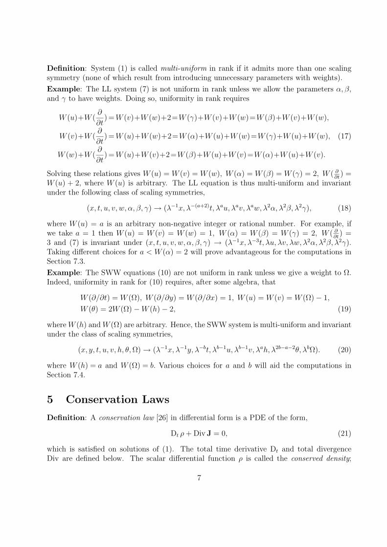
Definition: System (1) is called multi-uniform in rank if it admits more than one scalingsymmetry (none of which result from introducing unnecessary parameters with weights).

Example: The LL system (7) is not uniform in rank unless we allow the parameters α, β,and γ to have weights. Doing so, uniformity in rank requires

W (u)+W (∂

∂t) = W (v)+W (w)+2=W (γ)+W (v)+W (w)=W (β)+W (v)+W (w),

W (v)+W (∂

∂t) = W (u)+W (w)+2=W (α)+W (u)+W (w)=W (γ)+W (u)+W (w), (17)

W (w)+W (∂

∂t) = W (u)+W (v)+2=W (β)+W (u)+W (v)=W (α)+W (u)+W (v).

Solving these relations gives W (u) = W (v) = W (w), W (α) = W (β) = W (γ) = 2, W ( ∂∂t

) =W (u) + 2, where W (u) is arbitrary. The LL equation is thus multi-uniform and invariantunder the following class of scaling symmetries,

(x, t, u, v, w, α, β, γ) → (λ−1x, λ−(a+2)t, λau, λav, λaw, λ2α, λ2β, λ2γ), (18)

where W (u) = a is an arbitrary non-negative integer or rational number. For example, ifwe take a = 1 then W (u) = W (v) = W (w) = 1, W (α) = W (β) = W (γ) = 2, W ( ∂

∂t) =

3 and (7) is invariant under (x, t, u, v, w, α, β, γ) → (λ−1x, λ−3t, λu, λv, λw, λ2α, λ2β, λ2γ).Taking different choices for a < W (α) = 2 will prove advantageous for the computations inSection 7.3.

Example: The SWW equations (10) are not uniform in rank unless we give a weight to Ω.Indeed, uniformity in rank for (10) requires, after some algebra, that

W (∂/∂t) = W (Ω), W (∂/∂y) = W (∂/∂x) = 1, W (u) = W (v) = W (Ω)− 1,

W (θ) = 2W (Ω)−W (h)− 2, (19)

where W (h) and W (Ω) are arbitrary. Hence, the SWW system is multi-uniform and invariantunder the class of scaling symmetries,

(x, y, t, u, v, h, θ, Ω) → (λ−1x, λ−1y, λ−bt, λb−1u, λb−1v, λah, λ2b−a−2θ, λbΩ). (20)

where W (h) = a and W (Ω) = b. Various choices for a and b will aid the computations inSection 7.4.

5 Conservation Laws

Definition: A conservation law [26] in differential form is a PDE of the form,

Dt ρ + Div J = 0, (21)

which is satisfied on solutions of (1). The total time derivative Dt and total divergenceDiv are defined below. The scalar differential function ρ is called the conserved density;

7

the vector differential function J is the associated flux. In electromagnetism, (21) is thecontinuity equation relating charge density ρ to current J.

In general, ρ and J are functions of x, t,u, and the derivatives of u with respect to thecomponents of x. In this paper, we will assume that densities and fluxes (i) are local, whichmeans free of integral terms; (ii) polynomial in u and its derivatives; and (iii) do not explicitlydepend on x and t. So, ρ(u,ux,uy,uz,u2x, . . .) and J(u,ux,uy,uz,u2x, . . .).

Definition: There is a close relationship between conservation laws and constants of motion.Indeed, integration of (21) over all space yields the integral form of a conservation law,

P =∫ ∞

−∞

∫ ∞

−∞

∫ ∞

−∞ρ dx dy dz = constant, (22)

provided that J vanishes at infinity. As in mechanics, the P ’s are called constants of motion.The total divergence Div is computed as Div J = (Dx, Dy, Dz)·(J1, J2, J3) = DxJ1+DyJ2+

DzJ3. In the 1D case, with one spatial variable (x), conservation equation (21) reduces to

Dt ρ + DxJ = 0, (23)

where both density ρ and flux J are scalar differential functions.

The conservation laws (21) and (23) involve total derivatives Dt and Dx. In the 1D case,

Dtρ =∂ρ

∂t+

n∑k=0

∂ρ

∂ukx

Dkx(ut). (24)

where n is the order of u in ρ. Upon replacement of ut, utx, etc. from ut = G, we get

Dtρ =∂ρ

∂t+ ρ(u)′[G], (25)

where ρ(u)′[G] is the Frechet derivative of ρ in the direction of G. Similarly,

DxJ =∂J

∂x+

m∑k=0

∂J

∂ukx

u(k+1)x, (26)

where m is the order of u of J.

Example: Assume that the KdV equation (3) has a density of the form

ρ = c1u3 + c2u

2x, (27)

where c1 and c2 are constants. Since ρ does not explicitly depend on time and is of ordern = 1 in u, application of (24) gives

Dtρ =∂ρ

∂uI(ut) +

∂ρ

∂ux

Dx(ut)

= 3c1u2ut + 2c2uxutx = −3c1u

2(uux + u3x)− 2c2ux(uux + u3x)x

= −3c1u2(uux + u3x)− 2c2ux(u

2x + uu2x + u4x)

= −(3c1u3ux + 3c1u

2u3x + 2c2u3x + 2c2uuxu2x + 2c2uxu4x), (28)

8

where D0x = I is the identity operator and where we used (3) to replace ut and utx. The

generalizations of (24) and (26) to multiple dependent variables is straightforward [26].

Example: Taking u(x, t) = (u(x, t), v(x, t), w(x, t)),

Dtρ =∂ρ

∂t+

n1∑k=0

∂ρ

∂ukx

Dkx(ut) +

n2∑k=0

∂ρ

∂vkx

Dkx(vt) +

n3∑k=0

∂ρ

∂wkx

Dkx(wt), (29)

DxJ =∂J

∂x+

m1∑k=0

∂J

∂ukx

u(k+1)x +m2∑k=0

∂J

∂vkx

v(k+1)x +m3∑k=0

∂J

∂wkx

w(k+1)x (30)

where n1, n2 and n3 are the highest orders of u, v and w in ρ, and m1, m2 and m3 are thehighest orders of u, v, w in J.

Example: Assume that the Boussinesq system (14) has a density of the form

ρ = c1β2u + c2βu2 + c3u

3 + c4v2 + c5uxv + c6u

2x. (31)

where c1 through c6 are constants. Since n1 =1 and n2 =0, application of (29) gives

Dtρ =∂ρ

∂uI(ut) +

∂ρ

∂ux

Dx(ut) +∂ρ

∂vI(vt)

= (c1β2 + 2c2βu + 3c3u

2)ut + (c5v + 2c6ux)utx + (2c4v + c5ux)vt

=−((c1β

2+2c2βu+3c3u2)vx+(c5v+2c6ux)v2x+(2c4v+c5ux)(βux−3uux−αu3x)

),(32)

where we replaced ut, utx, and vt from (14).

Remark: The flux J in (21) is not uniquely defined. In 1D we use (23) and the flux is onlydetermined up to an arbitrary constant. In 2D, the flux is only determined up to a divergence-free vector K = (K1, K2) = (Dyφ,−Dxφ), where φ is an arbitrary scalar differential function.In 3D, the flux can only be determined up to a curl term. Indeed, if (ρ,J) is a valid density-flux pair, so is (ρ,J+∇×K) for any arbitrary vector differential function K = (K1, K2, K3).Recall that ∇×K = (DyK3 −DzK2, DzK1 −DxK3, DxK2 −DyK1).

Example: The Korteweg-de Vries equation (3) is known [1, 2] to have infinitely manypolynomial conservation laws. The first three density-flux pairs are

ρ(1) = u, J (1) =1

2u2 + u2x,

ρ(2) =1

2u2, J (2) =

1

3u3 − 1

2u2

x + uu2x, (33)

ρ(3) =1

3u3 − u2

x, J (3) =1

4u4 − 2uu2

x + u2u2x + u22x − 2uxu3x.

The first two express conservation of momentum and energy, respectively. They are easyto compute by hand. The third one, less obvious and requiring more work, corresponds toBoussinesq’s moment of instability [25]. Observe that the above densities are uniform ofranks 2, 4, and 6. The fluxes are also uniform of ranks 4, 6, and 8.

9

The computations get quickly out of hand for higher ranks. For example, for rank 12

ρ(6) =1

6u6 − 10u3u2

x − 5u4x + 18u2u2x

2 +120

7u2x

3 − 108

7uu3x

2 +36

7u4x

2 (34)

and J (6) is a scaling homogeneous polynomial with 20 terms of rank 14 (not shown).

In general, if in (23) rank(ρ) = R then rank(J) = R + W (∂/∂t) − 1. All the pieces in (21)are also uniform in rank. This comes as no surprise since the conservation law (21) holds onsolutions of (1), hence it ‘inherits’ the dilation symmetry of (1).

Example: The Boussinesq equation (4) also admits infinitely many conservation laws andis completely integrable [1, 2]. The first four density-flux pairs [3] for (14) are

ρ(1) = u, J (1) = v,

ρ(2) = v, J (2) = βu− 3

2u2 − αu2x, (35)

ρ(3) = uv, J (3) =1

2βu2 − u3 +

1

2v2 +

1

2αu2

x − αuu2x,

ρ(4) = βu2 − u3 + v2 + αu2x, J (4) = 2βuv − 3u2v − 2αu2xv + 2αuxvx.

The densities are of ranks 2, 3, 5 and 6, respectively. The corresponding fluxes are of onerank higher. After setting β = 1 we obtain the conserved quantities of (5) even thoughinitially this system was not uniform in rank.

Example: We assume that α, β, and γ in (6) are nonzero. Cases with vanishing parametersmust be investigated separately. The first six density-flux pairs [13, 28] are

ρ(1) = u, J (1) = vxw − vwx, (β = γ 6= α),

ρ(2) = v, J (2) = uwx − uxw, (α = γ 6= β),

ρ(3) = w, J (3) = uxv − uvx, (α = β 6= γ),

ρ(4) = u2 + v2 + w2, J (4) = 0, (36)

ρ(5) = (u2 + v2 + w2)2, J (5) = 0,

ρ(6) = u2x + v2

x + w2x + (γ − α)u2 + (γ − β)v2,

J (6) = 2((vwx − vxw)u2x + (uxw − uwx)v2x + (uvx − uxv)w2x

+ (β − γ)uxvw + (γ − α)uvxw + (α− β)uvwx

).

Note that the second and third density-flux pairs follow from the first pair via the cyclicpermutations in (8). If we select W (u) = W (v) = W (w) = a = 1

4, then the first three

densities have rank 14

and ρ(4), ρ(5), and ρ(6) have ranks 12, 1, 5

2, respectively.

The physics of (6) demand that the magnitude S = ||S|| of the spin field is constant intime. Indeed, using (7) we readily verify that uut + vvt + wwt = 0. Hence, any differentiablefunction of S is also conserved in time. This is apparent in ρ(4) = ||S||2 and ρ(5) = ||S||4,which are conserved (in time) even for the fully anisotropic case where α 6= β 6= γ 6= α.

10

Obviously, linear combinations of conserved densities are also conserved. Hence, ρ(6) =||Sx||2 + (γ − α)u2 + (γ − β)v2 can be replaced by

ρ(6) =1

2(ρ(6) − γρ(4)) =

1

2(u2

x + v2x + w2

x − αu2 − βv2 − γw2). (37)

Now, u2x = Dx(uux)− uu2x, etc., and densities are divergence-equivalent (see Section 6.2) if

they differ by a total derivative with respect to x. So, (37) is equivalent with

ρ(6) = −1

2(uu2x + vv2x + ww2x + αu2 + βv2 + γw2), (38)

which can be compactly written as

ρ(6) = −1

2(S ·∆S + S ·DS), (39)

where ∆ is the Laplacian and D = diag(α, β, γ). So, ρ(6) is the Hamiltonian density [28] in

H = −1

2

∫(S ·∆S + S ·DS) dx

=1

2

∫ (||Sx||2 + (γ − α)u2 + (γ − β)v2

)dx. (40)

The Hamiltonian H expresses that the total energy is constant in time since dH/dt = 0.

Example: The SWW equations (10) admit a Hamiltonian formulation [11] and infinitelymany conservation laws. Yet, that is still insufficient to guarantee complete integrability ofPDEs in (2 + 1)-dimensions. The first few conserved densities and fluxes for (10) are

ρ(1) = h, J(1) =

(uhvh

), ρ(2) = hθ, J(2) =

(uhθvhθ

),

ρ(3) = hθ2, J(3) =

(uhθ2

vhθ2

),

ρ(4) = (u2 + v2)h + h2θ, J(4) =

(u3h + uv2h + 2uh2θv3h + u2vh + 2vh2θ

),

ρ(5) = (2Ω− uy + vx)θ,

J(5) = 16

(12Ωuθ − 4uuyθ + 6uvxθ + 2vvyθ + u2θy + v2θy − hθθy + hyθ

2

12Ωvθ + 4vvxθ − 6vuyθ − 2uuxθ − u2θx −v2θx + hθθx − hxθ2

).

(41)

As shown in [11], system (10) has conserved densities ρ = hf(θ) and ρ = (2Ω−uy + vx)g(θ),where f(θ) and g(θ) are arbitrary functions. Such densities are the integrands of the Casimirsof the Poisson bracket associated with (10). The algorithm presented in Section 7.4 onlycomputes densities of the form ρ = hθk and ρ = (2Ω− uy + vx)θ

l, where k and l are positiveintegers.

11

6 Tools from the Calculus of Variations

In this section we introduce the variational derivative (Euler operator), the higher Euleroperators (also called Lie-Euler operators) from the calculus of variations, and the homotopyoperator from homological algebra and variational bi-complexes [6]. These tools will beapplied in Section 7.

6.1 Variational Derivative (Euler Operator)

Definition: A scalar differential function f is a divergence if and only if there exists avector differential function F such that f = Div F. In 1D, we say that a differential functionf is exact3 if and only if there exists a scalar differential function F such that f = DxF.Obviously, F = D−1

x (f) =∫

f dx is then the primitive (or integral) of f.

Example: Taking f = −Dtρ from (28), that is

f = 3c1u3ux + 2c2u

3x + 2c2uuxu2x + 3c1u

2u3x + 2c2uxu4x, (42)

where4 u(x; t), we will compute c1 and c2 so that f is exact.Upon repeated integration by parts (by hand), we get

F =∫

f dx =3

4c1u

4 +(c2− 3c1)uu2x +3c1u

2u2x− c2u22x +2c2uxu3x +

∫(3c1 + c2)u

3x dx. (43)

Removing the “obstruction” (the last term) requires c2 = −3c1. Substituting a solution,c1 = 1

3, c2 = −1, into (27) gives ρ(3) in (33). Substituting that solution into (42) and (43)

yieldsf = u3ux − 2u3

x − 2uuxu2x + u2u3x − 2uxu4x (44)

which is exact, together with its integral

F =1

4u4 − 2uu2

x + u2u2x + u22x − 2uxu3x, (45)

which is J (3) in (33). Currently, CAS like Mathematica, Maple5, and REDUCE cannotcompute (43) as a sum of terms that can be integrated out and the obstruction.

Example: Consider the following example in 2D

f = uxvy − u2xvy − uyvx + uxyvx, (46)

where u(x, y) and v(x, y). It is easy to verify by hand (via integration by parts) that f isexact. Indeed, f = Div F with

F = (uvy − uxvy,−uvx + uxvx). (47)

3We do not use integrable to avoid confusion with complete integrability from soliton theory [1, 2].4Variable t is parameter in subsequent computations. For brevity, we write u(x) instead of u(x; t).5Future versions of Maple will be able to “partially” integrate such expressions [10, 19].

12

As far as we know, the leading CAS currently lack tools to compute F. Two questions arise:

(i) How can we tell whether f is the divergence of some differential function F?

(ii) How do we compute F automatically and without multivariate integration by parts ofexpressions involving arbitrary functions?

To answer these questions we use the following tools from the calculus of variations: thevariational derivative (Euler operator), its generalizations (higher Euler operators or Lie-Euler operators), and the homotopy operator.

Definition: The variational derivative (zeroth Euler operator), L(0)u(x), is defined [26, p. 246]

by

L(0)u(x) =

∑J

(−D)J∂

∂uJ

, (48)

where the sum is over all the unordered multi-indices J [26, p. 95]. For example, in the2D case the multi-indices corresponding to second-order derivatives can be identified with2x, 2y, 2z, xy, xz, yz. Obviously, (−D)2x = (−Dx)

2= D2x, (−D)xy = (−Dx)(−Dy) = DxDy,

etc.. For notational details see [26, p. 95, p. 108, p. 246].With applications in mind, we give calculus-based formulas for the variational derivatives

in 1D and 2D. The formula for 3D is analogous and can be found in [19].

Example: In 1D, where x = x, for scalar component u(x) we have6

L(0)u(x) =

∞∑k=0

(−Dx)k ∂

∂ukx

=∂

∂u−Dx

∂

∂ux

+ D2x

∂

∂u2x

−D3x

∂

∂u3x

+ · · · , (49)

In 2D where x = (x, y), we have for component u(x, y)

L(0,0)u(x,y) =

∞∑kx=0

∞∑ky=0

(−Dx)kx(−Dy)

ky∂

∂ukxx kyy

=∂

∂u−Dx

∂

∂ux

−Dy∂

∂uy

+ D2x

∂

∂u2x

+DxDy∂

∂uxy

+ D2y

∂

∂u2y

− D3x

∂

∂u3x

− · · · , (50)

Note that ukxx kyy stands for uxx···x yy···y where x is repeated kx times and y is repeated ky

times. Similar formulas hold for components v, w, etc.. The first question is then answeredby the following theorem [26, p. 248].

Theorem: A necessary and sufficient condition for a function f to be a divergence, i.e. thereexists a differential function F so that f = Div F, is that L(0)

u(x)(f) ≡ 0. In words: the Euleroperator annihilates divergences.

If, for example, u(x) = (u(x), v(x)) then both L(0)u(x)(f) and L(0)

v(x)(f) must vanish identically.For the 1D case, the theorem says that a differential function f is exact, i.e. there exists adifferential function F so that f = DxF, if and only if L(0)

u(x)(f) ≡ 0.

6Variable t in u(x; t) is suppressed because it is a parameter in the Euler operators.

13

Example: Avoiding integration by parts, we determine c1 and c2 so that f in (42) will beexact. Since f is of order 4 in the (one) dependent variable u(x), the zeroth Euler operator(49) terminates at k = 4. Using nothing but differentiations, we readily compute

L(0)u(x)(f) =

∂f

∂u−Dx

(∂f

∂ux

)+ D2

x

(∂f

∂u2x

)−D3

x

(∂f

∂u3x

)+ D4

x

(∂f

∂u4x

)= 9c1u

2ux + 2c2uxu2x + 6c1uu3x −Dx(3c1u3 + 6c2u

2x + 2c2uu2x + 2c2u4x)

+D2x(2c2uux)−D3

x(3c1u2) + D4

x(2c2ux)

= 9c1u2ux + 2c2uxu2x + 6c1uu3x − (9c1u

2ux + 14c2uxu2x + 2c2uu3x + 2c2u5x)

+(6c2uxu2x + 2c2uu3x)− (18c1uxu2x + 6c1uu3x)

= −6(3c1 + c2)uxu2x. (51)

Note that the terms in u2ux, uu3x, and u5x dropped out. Hence, L(0)u(x)(f) ≡ 0 leads to

3c1+c2 = 0. Substituting c1 = 13, c2 =−1 into (42) gives (44) as claimed.

Example: As an example in 2D, we readily verify that f = uxvy−u2xvy−uyvx +uxyvx from(46) is a divergence. Applying (50) to f for each component of u(x, y) = (u(x, y), v(x, y))

separately, we straightforwardly verify that L(0,0)u(x,y)(f) ≡ 0 and L(0,0)

v(x,y)(f) ≡ 0.

6.2 Removing Divergences and Divergence-equivalent Terms

It is of paramount importance that densities are free of divergences for they could be movedinto the flux J of the conservation law Dt ρ+Div J = 0. We show how the Euler operator canbe used to remove divergences and divergence-equivalent terms in densities. An algorithmto do so is given in [19]. The following examples illustrate the concept behind the algorithm.

Definition: Two scalar differential functions, f (1) and f (2), are divergence-equivalent if andonly if they differ by the divergence of some vector V, i.e. f (1) ∼ f (2) if and only if f (1)−f (2) =Div V. If a scalar expression is divergence-equivalent to zero then it is a divergence.

Example: Any conserved density of the KdV equation (3) is uniform in rank with respectto W (u)=2 and W (∂/∂x)=1. The list of all terms of, say, rank 6 isR=u3, u2

x, uu2x, u4x.Now, terms f (1) = uu2x and f (2) = −u2

x are divergence-equivalent because f (1) − f (2) =

u2x + uu2x = Dx(uux). Using (49), note that L(0)

u(x)(−u2x) = 2u2x and L(0)

u(x)(uu2x) = 2u2x

are equal (therefore, linearly dependent). So, we discard uu2x. Moreover, u4x = Dx(u3x) is

a divergence and, as expected, L(0)u(x)(u4x) = 0. So, we can discard u4x. Hence, R can be

replaced by S=u3, u2x which is free of divergences and divergence-equivalent terms.

Example: The list of non-constant terms of rank 6 for the Boussinesq equation (14) is

R = β2u, βu2, u3, v2, uxv, u2x, βvx, uvx, βu2x, uu2x, v3x, u4x. (52)

Using (49), for every term ti in R we compute vi = L(0)u(x)(ti) = (L(0)

u(x)(ti),L(0)v(x)(ti)). If

vi = (0, 0) then ti is discarded and so is vi. If vi 6= (0, 0) we verify whether or not vi is

14

linearly independent of the non-zero vectors vj, j = 1, 2, · · · , i− 1. If independent, the termti is kept, otherwise, ti is discarded and so is vi.

Upon application of (49), the first six terms in R lead to linearly independent vectors v1

through v6. Therefore, t1 through t6 are kept (and so are the corresponding vectors). For

t7 = βvx we compute v7 =L(0)u(x)(βvx)= (0, 0). So, t7 is discarded and so is v7. For t8 = uvx

we get v8 =L(0)u(x)(uvx)=(vx,−ux) = −v5. So, t8 is discarded and so is v8.

Proceeding in a similar fashion, t9, t10, t11 and t12 are discarded. Thus, R is replaced by

S=β2u, βu2, u3, v2, uxv, u2x, (53)

which is free of divergences and divergence-equivalent terms.

Example: In the 2D case, f (1) = (ux − u2x)vy and f (2) = (uy − uxy)vx are divergence-equivalent since f (1) − f (2) = uxvy − u2xvy − uyvx + uxyvx = Div (uvy − uxvy,−uvx + uxvx).

Using (50), note that L(0)u(x,y)(f

(1)) = L(0)u(x,y)(f

(2)) = (−vxy − vxxy,−uxy + uxxy).

6.3 Higher Euler Operators

To compute F = Div−1(f) or, in the 1D case, F = D−1x (f) =

∫f dx, we need higher-order

versions of the variational derivative, called higher Euler operators [23, 26] or Lie-Euleroperators [6]. The general formulas in terms of differential forms are given in [26, p. 367].We give calculus-based formulas for the 1D and 2D cases (see [19] for the 3D case).

Definition: The higher Euler operators in 1D (with variable x)7 are

L(i)u(x) =

∞∑k=i

(k

i

)(−Dx)

k−i ∂

∂ukx

, (54)

where(

ki

)is the binomial coefficient. Note that the higher Euler operator for i = 0 matches

the variational derivative in (49).

Example: The first three higher Euler operators in 1D for component u(x) are

L(1)u(x) =

∂

∂ux

− 2Dx∂

∂u2x

+ 3D2x

∂

∂u3x

− 4D3x

∂

∂u4x

+ · · · ,

L(2)u(x) =

∂

∂u2x

− 3Dx∂

∂u3x

+ 6D2x

∂

∂u4x

− 10D3x

∂

∂u5x

+ · · · , (55)

L(3)u(x) =

∂

∂u3x

− 4Dx∂

∂u4x

+ 10D2x

∂

∂u5x

− 20D3x

∂

∂u6x

+ · · · .

Definition: The higher Euler operators in 2D (with variables x, y) are

L(ix,iy)u(x,y) =

∞∑kx=ix

∞∑ky=iy

(kx

ix

)(ky

iy

)(−Dx)

kx−ix(−Dy)ky−iy

∂

∂ukxx kyy

. (56)

7Variable t in u(x; t) is suppressed because it is a parameter in the higher Euler operators.

15

Note that the higher Euler operator for ix = iy =0 matches the variational derivative in (50).

Example: The first higher Euler operators for component u(x, y) are

L(1,0)u(x,y) =

∂

∂ux

− 2Dx∂

∂u2x

−Dy∂

∂uxy

+ 3D2x

∂

∂u3x

+ 2DxDy∂

∂u2xy

− · · · ,

L(0,1)u(x,y) =

∂

∂uy

− 2Dy∂

∂u2y

−Dx∂

∂uyx

+ 3D2y

∂

∂u3y

+ 2DxDy∂

∂ux2y

− · · · , (57)

L(1,1)u(x,y) =

∂

∂uxy

− 2Dx∂

∂u2xy

− 2Dy∂

∂ux2y

+ 3D2x

∂

∂u3xy

+ 4DxDy∂

∂u2x2y

+ · · · ,

L(2,1)u(x,y) =

∂

∂u2xy

− 3Dx∂

∂u3xy

− 2Dy∂

∂u2x2y

+ 6D2x

∂

∂u4xy

+ D2y

∂

∂u2x3y

− · · · .

The higher Euler operators are useful in their own right as the following theorem [23] in 1Dshows.

Theorem: A necessary and sufficient condition for a function f to be an rth order derivative,i.e. there exists a scalar differential function F so that f = Dr

xF, is that L(i)u(x)(f) ≡ 0 for

i=0, 1, . . . , r−1.

6.4 Homotopy Operators

Armed with the higher Euler operators we now turn to the homotopy operator which willallow us to reduce the computation of F = Div−1(f), or in the 1D case F = D−1

x (f) =∫

f dx,to a single integral with respect to an auxiliary variable denoted by λ (not to be confusedwith λ in Section 4). Amazingly, the homotopy operator circumvents integration by parts(in multi-dimensions involving arbitrary functions) and reduces the inversion of the totaldivergence operator, Div, to a problem of single-variable calculus.

As mentioned in Section 6.1, Div−1 is defined up to a divergence-free (curl) term. In3D, Div−1 is an equivalence class Div−1(f) = F + ∇ ×K where K is an arbitrary vectordifferential function. The homotopy operator computes a particular K.

The homotopy operator in terms of differential forms is given in [26, p. 372]. Below wegive calculus-based formulas for the homotopy operators in 1D and 2D which are easy toimplement in CAS. The explicit formulas in 3D are analogous (see [19]).

Definition: The homotopy operator in 1D (with variable x)8 is

Hu(x)(f) =∫ 1

0

N∑j=1

Iuj(f)[λu]

dλ

λ, (58)

where uj is the jth component of u and the integrand Iuj(f) is given by

Iuj(f) =

∞∑i=0

Dix

(uj L(i+1)

uj(x)(f)). (59)

8Variable t in u(x; t) is suppressed because it is a parameter in the homotopy operators.

16

The integrand involves the 1D higher Euler operators in (54). In (58), N is the number ofdependent variables and Iuj

(f)[λu] means that in Iuj(f) we replace u(x) → λu(x), ux(x) →

λux(x), etc.. In practice, we first add the Iuj(f) and then scale the variables. The sum in

Iuj(f) terminates at i = p− 1 where p is the order of uj in f.Given an exact function f, the second question, that is how to compute F = D−1

x (f) =∫f dx, is then answered by the following theorem [26, p. 372].

Theorem: For an exact function f, one has F = Hu(x)(f).

Thus, in the 1D case, applying the homotopy operator (58) allows one to bypass integrationby parts. As an experiment, one can start from some function F , compute f = DxF , thencompute F = Hu(x)(f), and finally verify that F − F is a constant.

Example: Using the homotopy operator (58) with (59), we recompute (45). Since f in (42)is of order p = 4 in u1(x) = u(x), the sum in (59) terminates at i = p− 1 = 3. Hence,

Iu(f) = uL(1)u(x)(f) + Dx

(uL(2)

u(x)(f))

+ D2x

(uL(3)

u(x)(f))

+ D3x

(uL(4)

u(x)(f))

= u∂f

∂ux

− 2uDx

(∂f

∂u2x

)+ 3uD2

x

(∂f

∂u3x

)− 4uD3

x

(∂f

∂u4x

)+ Dx

(u

∂f

∂u2x

− 3uDx

(∂f

∂u3x

)

+6uD2x

(∂f

∂u4x

))+ D2

x

(u

∂f

∂u3x

− 4uDx

(∂f

∂u4x

))+ D3

x

(u

∂f

∂u4x

)= u4 + 8u2u2x + 6uu4x + 4uu2

x − 4Dx

(2u2ux + 3uu3x

)+ D2

x

(u3 + 8uu2x

)− 2D3

x (uux)

= u4 − 6uu2x + 3u2u2x + 2u2

2x − 4uxu3x. (60)

Formula (58), with u = u1 = u, requires an integration with respect to λ :

F =Hu(x)(f) =∫ 1

0Iu(f)[λu]

dλ

λ

=∫ 1

0

(λ3u4 − 6λ2uu2

x + 3λ2u2u2x + 2λu22x − 4λuxu3x

)dλ

=1

4u4 − 2uu2

x + u2u2x + u22x − 2uxu3x. (61)

The crux of the homotopy operator method is that the integration by parts of a differentialexpression like (44), which involves an arbitrary function u(x) and its derivatives, can bereduced to a standard integration of a polynomial in λ.

Example: For a system with N = 2 components, u(x) = (u1(x), u2(x)) = (u(x), v(x)), thehomotopy operator formulas are

Hu(x)(f) =∫ 1

0(Iu(f) + Iv(f)) [λu]

dλ

λ, (62)

with

Iu(f) =∞∑i=0

Dix

(uL(i+1)

u(x) (f))

and Iv(f) =∞∑i=0

Dix

(vL(i+1)

v(x) (f)). (63)

17

Example: Consider f = 3uxv2 sin u− u3

x sin u− 6vvx cos u + 2uxu2x cos u + 8vxv2x, which isno longer polynomial in the two (N = 2) dependent variables u(x) and v(x). Applying Euleroperator (48) for each component of u(x) = (u(x), v(x)) separately, we quickly verify that

L(0)u(x)(f) ≡ 0 and L(0)

v(x)(f) ≡ 0. Hence, f is exact. Integration by parts (by hand) gives

F =∫

f dx = 4v2x + u2

x cos u− 3v2 cos u. (64)

Currently, CAS like Mathematica, Maple9 and Reduce fail this integration due to the presenceof trigonometric functions.

We now recompute (64) with the homotopy operator formulas (62) and (63). First,

Iu(f) = uL(1)u(x)(f) + Dx

(uL(2)

u(x)(f))

= u∂f

∂ux

− 2uDx

(∂f

∂u2x

)+ Dx

(u

∂f

∂u2x

)= 3uv2 sin u− uu2

x sin u + 2u2x cos u. (65)

Second,

Iv(f) = vL(1)v(x)(f) + Dx

(vL(2)

v(x)(f))

= v∂f

∂vx

− 2vDx

(∂f

∂v2x

)+ Dx

(v

∂f

∂v2x

)= −6v2 cos u + 8v2

x. (66)

Finally, using (62),

F =Hu(x)(f) =∫ 1

0(Iu(f) + Iv(f)) [λu]

dλ

λ

=∫ 1

0

(3λ2uv2 sin(λu)−λ2uu2

x sin(λu)+2λu2x cos(λu)−6λv2 cos(λu)+8λv2

x

)dλ

= u2x cos u− 3v2 cos u + 4v2

x. (67)

In contrast to the integration in (64) which involved arbitrary functions u(x) and v(x), in(67) we integrated by parts with respect to the auxiliary variable λ. Any CAS can do that!

We now turn to inverting the Div operator using the homotopy operator.

Definition: We define the homotopy operator in 2D (with variables x, y) through its two

components (H(x)u(x,y)(f),H(y)

u(x,y)(f)). The x-component of the operator is given by

H(x)u(x,y)(f) =

∫ 1

0

N∑j=1

I(x)uj

(f)[λu]dλ

λ, (68)

with

I(x)uj

(f) =∞∑

ix=0

∞∑iy=0

(1 + ix

1 + ix + iy

)Dix

x Diyy

(uj L(1+ix,iy)

uj(x,y) (f)). (69)

9Version 9.5 of Maple can integrate such expressions as a result of our interactions with the developers.

18

Likewise, the y-component is given by

H(y)u(x,y)(f) =

∫ 1

0

N∑j=1

I(y)uj

(f)[λu]dλ

λ, (70)

with

I(y)uj

(f) =∞∑

ix=0

∞∑iy=0

(1 + iy

1 + ix + iy

)Dix

x Diyy

(uj L(ix,1+iy)

uj(x,y) (f)). (71)

Integrands (69) and (71) involve the 2D higher Euler operators in (56). The question howto compute F = (F1, F2) = Div−1(f) is then answered by the following theorem.

Theorem: If f is a divergence, then F = (F1, F2) = Div−1(f) = (H(x)u(x,y)(f),H(y)

u(x,y)(f)).

The superscripts (x) and (y) remind us which components of F we are computing. As amatter of testing, we can start from some vector F and compute f = Div F. Next, wecompute F = (F1, F2) = (H(x)

u(x,y)(f),H(y)u(x,y)(f)) and, finally, verify that K = F − F is

divergence free.

Example: Using (46), we show how application of the 2D homotopy operator leads to (47),up to a divergence free vector. Consider f = uxvy − u2xvy − uyvx + uxyvx, which is thedivergence of F in (47). In order to compute Div−1(f), we use (69) for the u component inu(x, y) = (u(x, y), v(x, y)) :

I(x)u (f) = uL(1,0)

u(x,y)(f) + Dx

(uL(2,0)

u(x,y)(f))

+1

2Dy

(uL(1,1)

u(x,y)(f))

= u

(∂f

∂ux

− 2Dx∂f

∂u2x

−Dy∂f

∂uxy

)+ Dx

(u

∂f

∂u2x

)+

1

2Dy

(u

∂f

∂uxy

)

= uvy +1

2uyvx − uxvy +

1

2uvxy. (72)

Similarly, for the v component of u(x, y) = (u(x, y), v(x, y)) we get

I(x)v (f) = vL(1,0)

v(x,y)(f) = v∂f

∂vx

= −uyv + uxyv. (73)

Hence, using (68),

F1 = H(x)u(x,y)(f) =

∫ 1

0

(I(x)u (f) + I(x)

v (f))

[λu]dλ

λ

=∫ 1

0λ(uvy +

1

2uyvx − uxvy +

1

2uvxy − uyv + uxyv

)dλ

=1

2uvy +

1

4uyvx −

1

2uxvy +

1

4uvxy −

1

2uyv +

1

2uxyv. (74)

Without showing the details, using (70) and (71) we compute analogously

F2 = H(y)u(x,y)(f) =

∫ 1

0

(I(y)u (f) + I(y)

v (f))

[λu]dλ

λ

19

=∫ 1

0λ(−uvx −

1

2uv2x +

1

2uxvx + uxv − u2xv

)dλ

= −1

2uvx −

1

4uv2x +

1

4uxvx +

1

2uxv −

1

2u2xv. (75)

Now we can readily verify that the resulting vector

F =

(F1

F2

)=

(12uvy + 1

4uyvx − 1

2uxvy + 1

4uvxy − 1

2uyv + 1

2uxyv

−12uvx − 1

4uv2x + 1

4uxvx + 1

2uxv − 1

2u2xv

)(76)

differs from F = (uvy − uxvy,−uvx + uxvx) by a divergence-free vector

K= F− F=

(K1

K2

)=

(12uvy − 1

4uyvx − 1

2uxvy − 1

4uvxy = 1

2uyv − 1

2uxyv

−12uvx + 1

4uv2x + 3

4uxvx − 1

2uxv + 1

2u2xv

). (77)

As mentioned in Section 6.1, K can be written as (Dyφ,−Dxφ) with φ = 12uv− 1

4uvx− 1

2uxv.

7 Computation of Conservation Laws

In this section we apply the Euler and homotopy operators to compute density-flux pairsfor the four PDEs in Section 3. Using the KdV equation (3) we illustrate the steps for a1D case (space variable x) and dependent variable u(x, t). Part of the computations for thisexample were done in the previous sections. The Boussinesq equation (14), also in 1D, isused to illustrate the case with two dependent variables u(x, t) and v(x, t) and an auxiliaryparameter with weight.

The LL equation (7), still in 1D, has three dependent variables u(x, t), v(x, t) and w(x, t).The three coupling constants have weights which makes the computations more cumbersome.However, the multi-uniformity of (7) helps to reduce the complexity. The shallow-water waveequations (10) illustrate the computations in 2D (two space variables) and four dependentvariables. Again, we can take advantage of the multi-uniformity of (10) to control “expressionswell” of the computations.

We use a direct approach to compute conservation laws, Dt ρ + Div J = 0, of polynomialsystems of nonlinear PDEs. First, we build the candidate density ρ as a linear combination(with constant coefficients ci) of terms that are uniform in rank with respect to the scalingsymmetry of the PDE. In doing so, we dynamically remove divergences and divergence-equivalent terms to get the shortest possible candidate density.

Second, we evaluate Dtρ on solutions of the PDE, thus removing all time derivativesfrom the problem. The resulting expression, E = −Dtρ, must be a divergence of the as yetunknown flux. Thus, we compute L(0)

u(x)(E) and set the coefficients of like terms to zero.This leads to a linear system for the undetermined coefficients ci. If the given PDE hasarbitrary constant parameters, then the linear system is parametrized. Careful analysis ofthe eliminant is needed to find all solution branches, and, when applicable, the conditionson the parameters. For each branch, the solution of the linear system is substituted into ρand E.

20

Third, we use the homotopy operator Hu(x) to compute J=Div−1(E). The computationsare done with our Mathematica packages [18]. Recall that J is only defined up a curl term.Removing the curl term in J may lead to a shorter flux. Inversion of Div via the homotopyoperator therefore does not guarantee the shortest flux.

7.1 Conservation Laws for the KdV Equation

In (33) we gave the first three density-flux pairs of (3). As an example, we will compute ρ(3)

and J (3). The weights are W (∂/∂x) = 1 and W (u) = 2. Hence, density ρ(3) has rank 6 andflux J (3) has rank 8. The algorithm has three steps:

Step 1: Construct the form of the density

Start from V = u, i.e. the list of dependent variables (and parameters with weight, ifapplicable). Construct the set M of all non-constant monomials of (selected) rank 6 or less(without derivatives). Thus, M=u3, u2, u. Next, for each monomial in M, introduce theneeded x-derivatives so that each term has rank 6. Since W (∂/∂x) = 1, use

∂2u2

∂x2=(2uux)x =2u2

x + 2uu2x,∂4u

∂x4= u4x. (78)

Ignore the highest-order terms (typically the last terms) in each of the right hand sides of(78). AugmentM with the remaining terms (deleting numerical factors) to getR = u3, u2

x.Here S = R since R is free of divergences and divergent-equivalent terms. Linearly

combine the terms in S with constant coefficients to get the candidate density:

ρ = c1u3 + c2u

2x, (79)

which is (27).

Step 2: Compute the undetermined constants ci

Compute Dtρ and use (3) to eliminate ut and utx. As shown in (28), this gives

E = −Dtρ = 3c1u3ux + 3c1u

2u3x + 2c2u3x + 2c2uuxu2x + 2c2uxu4x. (80)

Since E = −Dt ρ = DxJ, the expression E must be exact. As shown in (51), L(0)u(x)(E) =

−6(3c1 + c2)uxu2x ≡ 0 leads to c1 = 13, c2 =−1 and upon substitution into (79) to

ρ =1

3u3 − u2

x (81)

which is ρ(3) in (33).

Step 3: Compute the flux J

Substitute c1 = 13, c2 =−1 into (80) to get

E = u3ux − 2u3x − 2uuxu2x + u2u3x − 2uxu4x. (82)

As shown in (61), application of (58) with (59) to (82) gives

J =1

4u4 − 2uu2

x + u2u2x + u22x − 2uxu3x, (83)

which is J (3) in (33).

21

7.2 Conservation Laws for the Boussinesq Equation

The first few density-flux pairs of (14) were given in (35). Equation (14) has weights W ( ∂∂x

)=1, W (u)=W (β)=2, and W (v)=3. We show the computation of ρ(4) and J (4) of ranks 6 and7, respectively. The presence of the auxiliary parameter β with weight complicates matters.

Step 1: Construct the form of the density

Augment the list of dependent variables with the parameter β (with non-zero weight). Hence,V = u, v, β. Construct M = β2u, βu2, βu, βv, u3, u2, u, v2, v, uv, which contains all non-constant monomials of (chosen) rank 6 or less (without derivatives). Next, for each term inM, introduce the right number of x-derivatives so that each term has rank 6. For example,

∂2βu

∂x2=βu2x,

∂2u2

∂x2=2u2

x + 2uu2x,∂4u

∂x4=u4x,

∂(uv)

∂x= uxv + uvx, etc.. (84)

Ignore the highest-order terms (typically the last terms) in each of the right hand sidesof (84). Augment M with the remaining terms, after deleting numerical factors, to getR = β2u, βu2, u3, v2, uxv, u2

x, βvx, uvx, βu2x, uu2x, v3x, u4x as in (52). As shown in (53),removal of divergences and divergence-free terms in R leads to S=β2u, βu2, u3, v2, uxv, u2

x.Linearly combine the terms in S to get

ρ = c1β2u + c2βu2 + c3u

3 + c4v2 + c5uxv + c6u

2x. (85)

Step 2: Compute the undetermined constants ci

Compute E = −Dtρ and use (14) to eliminate ut, utx, and vt. As shown in (32), this gives

E = (c1β2 + 2c2βu + 3c3u

2)vx + (c5v + 2c6ux)v2x + (2c4v + c5ux)(βux − 3uux − αu3x). (86)

E =−Dt ρ=DxJ must be exact. Thus, apply (48) and require that L(0)u(x)(E) = L(0)

v(x)(E) ≡ 0.Group like terms. Set their coefficients equal to zero to obtain the parametrized system

β(c2 − c4) = 0, c3 + c4 = 0, c5 = 0, αc5 = 0, βc5 = 0, αc4 − c6 = 0. (87)

Investigate the eliminant of the system. Set c1 = 1, to obtain the solution

c1 = 1, c2 = c4, c3 = −c4, c5 = 0, c6 = αc4, (88)

which is valid irrespective of the values of α and β. Substitute (88) into (85) to get

ρ = β2u + c4(βu2 − u3 + v2 + αu2x). (89)

The density must be split into independent pieces. Indeed, since c4 is arbitrary, set c4 = 0or c4 = 1, thus splitting (89) into two independent densities, ρ = β2u and

ρ = βu2 − u3 + v2 + αu2x, (90)

which are ρ(1) and ρ(4) in (35).

22

Step 3: Compute the flux J

Compute the flux corresponding to ρ in (90). Substitute (88) into (86). Take the terms inc4 and set c4 = 1. Thus,

E = 2βuvx + 2βuxv − 3u2vx − 6uuxv + 2αuxv2x − 2αu3xv. (91)

Apply (62) and (63) to (91). For E of order 3 in u(x), compute

Iu(E) = uL(1)u(x)(E) + Dx

(uL(2)

u(x)(E))

+ D2x

(uL(3)

u(x)(E))

= u∂E

∂ux

− 2uDx

(∂E

∂u2x

)+ 3uD2

x

(∂E

∂u3x

)+ Dx

(u

∂E

∂u2x

− 3uDx

(∂E

∂u3x

))+ D2

x

(u

∂E

∂u3x

)= 2βuv − 6u2v − 4αuv2x + 6αDx (uvx)− 2αD2

x (uv)

= 2βuv − 6u2v − 2αu2xv + 2αuxvx. (92)

With E is of order 2 in v(x), subsequently compute

Iv(E) = vL(1)v(x)(E) + Dx

(vL(2)

v(x)(E))

= v∂E

∂vx

− 2vDx

(∂E

∂v2x

)+ Dx

(v

∂E

∂v2x

)= 2βuv − 3u2v − 4αuv2x + 2αDx (uxv) = 2βuv − 3u2v − 2αu2xv + 2αuxvx. (93)

Formula (62) with u(x) = (u(x), v(x)) requires an integration with respect to λ. Hence,

J = Hu(x)(E) =∫ 1

0(Iu(E) + Iv(E))[λu]

dλ

λ

=∫ 1

0

(4βλuv − 9λ2u2v − 4αλu2xv + 4αλuxvx

)dλ

= 2βuv − 3u2v − 2αu2xv + 2αuxvx, (94)

which is J (4) in (35). Set β = 1 at the end of the computations.

7.3 Conservation Laws for the Landau-Lifshitz Equation

Without showing full details, we will compute the six density-flux pairs (36) for (7). Theweights for (7) are W (u) = W (v) = W (w) = a, W (α) = W (β) = W (γ) = 2, W ( ∂

∂t) = a + 2,

where a is an arbitrary non-negative integer or rational number. This example involves threeconstants (α, β, and γ) with weights which makes the computations quite cumbersome unlesswe take advantage of the multi-uniformity and the cyclic nature of (7).

Step 1: Construct the form of the density

Select a small value for a, for example a = 14, and compute a density of, say, rank 1

4. Start

from V = u, v, w, α, β, γ, i.e. the list of dependent variables and the parameters withweight. Construct the set M of all non-constant monomials of the (selected) rank 1

4or less

(without derivatives). Thus, M=u, v, w. Next, for each of the monomials in M, introduce

23

the appropriate number of x-derivatives so that each term has rank 14. No x-derivatives are

needed and the removal of divergences or divergence-equivalent terms is irrelevant. Linearlycombine the terms in R=S=u, v, w to get a candidate density:

ρ = c1u + c2v + c3w. (95)

It suffices to continue with ρ = c1u. The remaining terms follow by cyclic permutation.

Step 2: Compute the undetermined constants ci

Compute E = −Dtρ = −Dt(c1u) = −c1ut. Use (7) to eliminate ut. Hence,

E =−c1

(vw2x − wv2x + (γ − β)vw

), (96)

which is the opposite of the right hand side of the first equation in (7). Since E =−Dt ρ=DxJ,

the expression E must be exact. Obviously L(0)u(x)(E) ≡ 0. Compute

L(0)v(x)(E) =

∂f

∂v(E)−Dx

∂f

∂vx

(E) + D2x

∂f

∂v2x

(E)=−c1(γ − β)w,

L(0)w(x)(E) =

∂f

∂w(E)−Dx

∂f

∂wx

(E) + D2x

∂f

∂w2x

(E)=−c1(γ − β)v. (97)

Set the latter expressions identically equal to zero. Solve c1(β−γ) = 0 for c1 6= 0. Set c1 = 1to get ρ = u, subject to the condition β = γ, which confirms the result in (36).

Step 3: Compute the flux J

Substitute c1 = 1 and β = γ into (96) to get E = wv2x−vw2x. Apply the homotopy operator(58) with (59) to E. In this example u(x) = (u(x), v(x), w(x)). Obviously, Iu(E) = 0, sincethere is no explicit occurrence of u. Compute

Iv(E)=vL(1)v(x)(E)+Dx

(vL(2)

v(x)(E))=v

∂E

∂vx

−2vDx

(∂E

∂v2x

)+Dx

(v

∂E

∂v2x

)=vxw−vwx, (98)

and, analogously, Iw(E)=vxw − vwx. Finally, compute

J = Hu(x)(E) =∫ 1

0(Iu(E) + Iv(E) + Iw(E))[λu]

dλ

λ

=∫ 1

02λ (vxw − vwx) dλ = vxw − vwx, (99)

which is J (1) in (36).

To compute density ρ(4) which is quadratic in u, v, and w, we would start from rank 12

andrepeat the three steps. Step 1 would lead to ρ = c1u

2 + c2uv + c3v2 + c4uw + c5vw + c6w

2.Steps 2 and 3 would result in c1 = c3 = c6 = 1. So, ρ = u2 + v2 +w2 and J = 0, which agreeswith ρ(4) and J (4) = 0 in (36).

Starting with rank 1, Step 1 would generate a polynomial density with the 15 terms that arehomogeneous of degree 4. Steps 2 and 3 would result in ρ(5) and J (5) = 0 in (36).

24

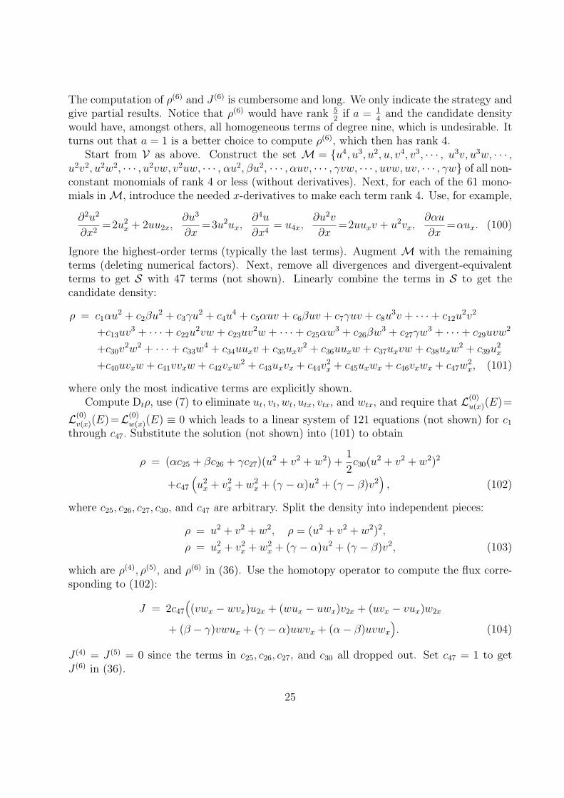
The computation of ρ(6) and J (6) is cumbersome and long. We only indicate the strategy andgive partial results. Notice that ρ(6) would have rank 5

2if a = 1

4and the candidate density

would have, amongst others, all homogeneous terms of degree nine, which is undesirable. Itturns out that a = 1 is a better choice to compute ρ(6), which then has rank 4.

Start from V as above. Construct the set M = u4, u3, u2, u, v4, v3, · · · , u3v, u3w, · · · ,u2v2, u2w2, · · · , u2vw, v2uw, · · · , αu2, βu2, · · · , αuv, · · · , γvw, · · · , uvw, uv, · · · , γw of all non-constant monomials of rank 4 or less (without derivatives). Next, for each of the 61 mono-mials in M, introduce the needed x-derivatives to make each term rank 4. Use, for example,

∂2u2

∂x2=2u2

x + 2uu2x,∂u3

∂x=3u2ux,

∂4u

∂x4= u4x,

∂u2v

∂x=2uuxv + u2vx,

∂αu

∂x=αux. (100)

Ignore the highest-order terms (typically the last terms). Augment M with the remainingterms (deleting numerical factors). Next, remove all divergences and divergent-equivalentterms to get S with 47 terms (not shown). Linearly combine the terms in S to get thecandidate density:

ρ = c1αu2 + c2βu2 + c3γu2 + c4u4 + c5αuv + c6βuv + c7γuv + c8u

3v + · · ·+ c12u2v2

+c13uv3 + · · ·+ c22u2vw + c23uv2w + · · ·+ c25αw3 + c26βw3 + c27γw3 + · · ·+ c29uvw2

+c30v2w2 + · · ·+ c33w

4 + c34uuxv + c35uxv2 + c36uuxw + c37uxvw + c38uxw

2 + c39u2x

+c40uvxw + c41vvxw + c42vxw2 + c43uxvx + c44v

2x + c45uxwx + c46vxwx + c47w

2x, (101)

where only the most indicative terms are explicitly shown.Compute Dtρ, use (7) to eliminate ut, vt, wt, utx, vtx, and wtx, and require that L(0)

u(x)(E)=

L(0)v(x)(E)=L(0)

w(x)(E) ≡ 0 which leads to a linear system of 121 equations (not shown) for c1

through c47. Substitute the solution (not shown) into (101) to obtain

ρ = (αc25 + βc26 + γc27)(u2 + v2 + w2) +

1

2c30(u

2 + v2 + w2)2

+c47

(u2

x + v2x + w2

x + (γ − α)u2 + (γ − β)v2), (102)

where c25, c26, c27, c30, and c47 are arbitrary. Split the density into independent pieces:

ρ = u2 + v2 + w2, ρ = (u2 + v2 + w2)2,

ρ = u2x + v2

x + w2x + (γ − α)u2 + (γ − β)v2, (103)

which are ρ(4), ρ(5), and ρ(6) in (36). Use the homotopy operator to compute the flux corre-sponding to (102):

J = 2c47

((vwx − wvx)u2x + (wux − uwx)v2x + (uvx − vux)w2x

+ (β − γ)vwux + (γ − α)uwvx + (α− β)uvwx

). (104)

J (4) = J (5) = 0 since the terms in c25, c26, c27, and c30 all dropped out. Set c47 = 1 to getJ (6) in (36).

25

7.4 Conservation Laws for the Shallow Water Wave Equations

The SWW equations (10) admit weights (19) in which W (h) and W (Ω) are free. The factthat (10) is multi-uniform is advantageous. Indeed, we can construct a candidate ρ which isuniform in rank for one set of weights and, subsequently, use other choices of weights to splitρ into smaller pieces. This “divide and conquer” strategy drastically reduces the complexityof the computations as was shown in [19].

The first few densities and fluxes were given in (41). We compute ρ(5) and J (5). Notethat ρ(5) has rank 3 if we select W (h) = a = 1 and W (Ω) = b = 2. However, ρ(5) has rank 4if we take W (h)= a=0 and W (Ω)= b=2. If we set W (h)= 0, and W (Ω)=3 then ρ(5) hasrank 7. So, the trick is to construct a candidate density which is scaling homogeneous for aparticular (fixed) choice of a and b in (20) and split the density based on other choices of aand b.

Step 1: Construct the form of the density

Start from V = u, v, θ, h, Ω, i.e. the list of variables and parameters with weights. Use(20) with a = 1, b = 2, to get M=Ωu, Ωv, . . . , u3, v3, . . . , u2v, uv2, . . . , u2, v2, . . . , u, v, θ, hwhich has 38 monomials of (chosen) rank 3 or less (without derivatives).

All terms of rank 3 in M remain untouched. To adjust the rank, differentiate eachmonomial of rank 2 in M with respect to x ignoring the highest-order term. For example,in du2

dx= 2uux, the term can be ignored since it is a total derivative. The terms uxv and

−uvx are divergence-equivalent since d(uv)dx

= uxv + uvx. Keep uxv. Likewise, differentiateeach monomial of rank 2 in M with respect to y and ignore the highest-order term.

Produce the remaining terms for rank 3 by differentiating the monomials of rank 1 inM with respect to x twice, or y twice, or once with respect to x and y. Again ignorethe highest-order terms. Augment the set M with the derivative terms of rank 3 to getR = Ωu, Ωv, · · · , uv2, uxv, uxθ, uxh, · · · , uyv, uyθ, · · · , θyh which has 36 terms.

Use the “divide and conquer” strategy [19] to select from R the terms which are ofranks 4 and 7 using the choices a = 0, b = 2 and a = 0, b = 3, respectively. This gives S =Ωθ, uxθ, uyθ, vxθ, vyθ, which happens to be free of divergences and divergence-equivalentterms. So, no further reduction is needed. Linearly combine the terms in S to get

ρ = c1Ωθ + c2uxθ + c3uyθ + c4vxθ + c5vyθ. (105)

Step 2: Compute the undetermined constants ci

Compute E =−Dtρ and use (10) to remove all time derivatives:

E = −( ∂ρ

∂ux

utx +∂ρ

∂uy

uty +∂ρ

∂vx

vtx +∂ρ

∂vy

vty +∂ρ

∂θθt

)= c2θ(uux + vuy − 2Ωv + 1

2hθx + θhx)x + c3θ(uux + vuy − 2Ωv + 1

2hθx + θhx)y

+ c4θ(uvx + vvy + 2Ωu + 12hθy + θhy)x + c5θ(uvx + vvy + 2Ωu + 1

2hθy + θhy)y

+ (c1Ω + c2ux + c3uy + c4vx + c5vy)(uθx + vθy). (106)

26

Require that L(0,0)u(x,y)(E)=L(0,0)

v(x,y)(E)=L(0,0)θ(x,y)(E)=L(0,0)

h(x,y)(E) ≡ 0, where, for example, L(0,0)u(x,y)

is given in (50). Gather like terms. Equate their coefficients to zero to obtain

c1 + 2c3 = 0, c2 = c5 = 0, c1 − 2c4 = 0, c3 + c4 = 0. (107)

Set c1 = 2. Substitute the solution

c1 = 2, c2 = 0, c3 = −1, c4 = 1, c5 = 0. (108)

into ρ to obtainρ = 2Ωθ − uyθ + vxθ, (109)

which is ρ(5) in (41).

Step 3: Compute the flux J

Compute the flux corresponding to (109). To do so, substitute (108) into (106) to obtain

E = θ(uxvx − uyvy + uv2x − u2yv − uxuy + vxvy − uuxy + vvxy

+2Ωux + 2Ωvy + 12θxhy − 1

2θyhx) + 2Ωuθx + 2Ωvθy − uuyθx

−uyvθy + uvxθx + vvxθy. (110)

Apply the 2D homotopy formulas in (68)-(71) to E = Div J = DxJ1 + DyJ2. So, compute

I(x)u (E) = uL(1,0)

u(x,y)(E) + Dx

(uL(2,0)

u(x,y)(E))

+1

2Dy

(uL(1,1)

u(x,y)(E))

= u

(∂E

∂ux

−2Dx

(∂E

∂u2x

)−Dy

(∂E

∂uxy

))+Dx

(u

∂E

∂u2x

)+

1

2Dy

(u

∂E

∂uxy

)

= uvxθ + 2Ωuθ +1

2u2θy − uuyθ. (111)

Similarly, compute

I(x)v (E) = vvyθ +

1

2v2θy + uvxθ, (112)

I(x)θ (E) =

1

2θ2hy + 2Ωuθ − uuyθ + uvxθ, (113)

I(x)h (E) = −1

2θθyh. (114)

Next, compute

J1(u) = H(x)u(x,y)(E)

=∫ 1

0

(I(x)u (E) + I(x)

v (E) + I(x)θ (E) + I

(x)h (E)

)[λu]

dλ

λ

=∫ 1

0

(4λΩuθ + λ2

(3uvxθ +

1

2u2θy − 2uuyθ + vvyθ +

1

2v2θy

+1

2θ2hy −

1

2θθyh

))dλ

= 2Ωuθ − 2

3uuyθ + uvxθ +

1

3vvyθ +

1

6u2θy +

1

6v2θy −

1

6hθθy +

1

6hyθ

2. (115)

27

Likewise, compute I(y)u (E), I(y)

v (E), I(y)θ (E), and I

(y)h (E). Finally, compute

J2(u) = H(y)u(x,y)(E)

=∫ 1

0

(I(y)u (E) + I(y)

v (E) + I(y)θ (E) + I

(y)h (E)

)[λu]

dλ

λ

= 2Ωvθ +2

3vvxθ − vuyθ −

1

3uuxθ −

1

6u2θx −

1

6v2θx +

1

6hθθx −

1

6hxθ

2. (116)

Hence,

J =

(J1

J2

)=

1

6

(12Ωuθ − 4uuyθ + 6uvxθ + 2vvyθ + u2θy + v2θy − hθθy + hyθ

2

12Ωvθ + 4vvxθ − 6vuyθ − 2uuxθ − u2θx − v2θx + hθθx − hxθ2

), (117)

which matches J(5) in (41).

8 Conclusions

The variational derivative (zeroth Euler operator) provides a straightforward way to testexactness which is key in the computation of densities. The continuous homotopy operatoris a powerful, algorithmic tool to compute fluxes explicitly. Indeed, the homotopy operatorallows one to invert the total divergence operator by computing higher variational derivativesfollowed by a one-dimensional integration with respect to a single auxiliary parameter. Thehomotopy operator is a universal tool that can be applied to problems in which integrationby parts (of arbitrary functions) in multi-variables is crucial.

To reach a wider audience, we intentionally did not use differential forms and the abstractframework of variational bi-complexes and homological algebra. Instead, we extracted theEuler and homotopy operators from their abstract setting and presented them in the languageof standard calculus, thereby making them widely applicable to computational problems inthe sciences. Our calculus-based formulas can be readily implemented in CAS.

Based on the concept of scaling invariance and using tools of the calculus of variations,we presented a three-step algorithm to symbolically compute polynomial conserved densitiesand fluxes of nonlinear polynomial systems of PDEs in multi-spatial dimensions. The stepsare straightforward: build candidate densities as linear combinations (with undeterminedconstant coefficients) of terms that are homogeneous with respect to the scaling symmetryof the PDE. Subsequently, use the variational derivative to compute the coefficients, and,finally, use the homotopy operator to compute the flux.

With our method one can search for conservation laws in chemistry, physics, and engi-neering. Symbolic packages are well suited to assist in the search which covers many fieldsof application including fluid mechanics, plasma physics, electro-dynamics, gas dynamics,elasticity, nonlinear optics and acoustics, electrical networks, chemical reactions, etc..

28

Acknowledgements and Dedication

This material is based upon work supported by the National Science Foundation (NSF) underGrants Nos. DMS-9732069, DMS-9912293, and CCR-9901929. Any opinions, findings, andconclusions or recommendations expressed in this material are those of the author and donot necessarily reflect the views of NSF.

The author is grateful to Bernard Deconinck, Michael Colagrosso, Mark Hickman andJan Sanders for valuable discussions. Undergraduate students Lindsay Auble, Robert “Scott”Danford, Ingo Kabirschke, Forrest Lundstrom, Frances Martin, Kara Namanny, Adam Ringler,and Maxine von Eye are thanked for designing Mathematica code for the project.

The research was supported in part by an Undergraduate Research Fund Award fromthe Center for Engineering Education awarded to Ryan Sayers. On June 16, 2003, whilerock climbing in Wyoming, Ryan was killed by a lightning strike. He was 20 years old. Theauthor expresses his gratitude for the insight Ryan brought to the project. His creativityand passion for mathematics were inspiring. This paper is dedicated to him.

References

[1] Ablowitz, M. J.; Clarkson, P. A. Solitons, Nonlinear Evolution Equations and InverseScattering; Cambridge University Press: Cambridge, 1991.

[2] Ablowitz, M. J.; Segur, H. Solitons and the Inverse Scattering Transform; SIAM:Philadelphia, 1981.

[3] Adams, P. J. Symbolic Computation of Conserved Densities and Fluxes for Systemsof Partial Differential Equations with Transcendental Nonlinearities; MS Thesis, Dept.Math. & Comp. Scs.; Colorado School of Mines: Golden, Colorado, 2003.

[4] Anco, S. C. J Phys A: Math Gen 2003, 36, 8623-8638.

[5] Anco, S. C.; Bluman, G. Euro J Appl Math 2002, 13, 545-566 & 567-585.

[6] Anderson, I. M. The Variational Bicomplex; Dept. Math., Utah State University: Logan,Utah, November 2004, 318 pages;http://www.math.usu.edu/~fg_mp/Publications/VB/vb.pdf.

[7] Anderson, I. M. The Vessiot Package, Dept. Math., Utah State University: Logan, Utah,November 2004, 253 pages;http://www.math.usu.edu/~fg_mp/Pages/SymbolicsPage/VessiotDownloads.html

[8] Barnett, M. P.; Capitani, J. F.; von zur Gathen J.; Gerhard, J. Int J Quan Chem 2004,100, 80-104.

[9] Cantarella, J.; DeTurck, D.; Gluck, H. Am Math Monthly 2002, 109, 409-442.

29

[10] Deconinck, B.; Nivala, M. A Maple Package for the Computation of Conservation Laws;http://www.amath.washington.edu/~bernard/papers.html.

[11] Dellar, P. Phys Fluids 2003, 15, 292-297.

[12] Eklund, H. Symbolic Computation of Conserved Densities and Fluxes for NonlinearSystems of Differential-Difference Equations; MS Thesis, Dept. Math. & Comp. Scs.;Colorado School of Mines: Golden, Colorado, 2003.

[13] Faddeev, L. D.; Takhtajan, L. A. Hamiltonian Methods in the Theory of Solitons;Springer Verlag: Berlin, 1987.

[14] Gao, M.; Kato, Y.; Ito, M. Comp Phys Comm 2002, 148, 242-255.

[15] Gao, M.; Kato, Y.; Ito, M. Comp Phys Comm 2004, 160, 69-89.

[16] Goktas, U.; Hereman, W. J Symb Comp 1997, 24, 591-621.

[17] Goktas, U.; Hereman, W. Phys D 1998, 132, 425-436.

[18] Hereman, W. Mathematica Packages for the Symbolic Computation of ConservationLaws of Partial Differential Equations and Differential-difference Equations;http://www.mines.edu/fs_home/whereman/.

[19] Hereman, W.; Colagrosso, M.; Sayers, R.; Ringler, A.; Deconinck, B.; Nivala, M.;Hickman, M. S. In Differential Equations with Symbolic Computation; Wang, D.; Zheng,Z., Eds.; Birkhauser Verlag: Basel, 2005.

[20] Hereman, W.; Sanders, J. A.; Sayers, J.; Wang, J. P. In Group Theory and NumericalMethods, CRM Proc. Lect. Ser. 39, Winternitz, P.; Gomez-Ullate, D., Eds.; AMS:Providence, Rhode Island, 2005, pp. 267-282.

[21] Hickman, M.; Hereman, W. Proc Roy Soc Lond A 2003, 459, 2705-2729.

[22] Krasil’shchik, I. S.; Vinogradov, A. M. Symmetries and Conservation Laws for Differ-ential Equations of Mathematical Physics. AMS: Providence, Rhode Island, 1998.

[23] Kruskal, M. D.; Miura, R. M.; Gardner, C. S., Zabusky; N. J. J Math Phys 1970, 11,952-960.

[24] Marsden, J. E.; Tomba, A. J. Vector Calculus, 3rd ed.; W. H. Freeman and Company:New York, 1988.

[25] Newell, A. C. J Appl Mech 1983, 50, 1127-1137.

[26] Olver, P. J. Applications of Lie Groups to Differential Equations, 2nd ed.; SpringerVerlag: New York, 1993.

30

[27] Sanz-Serna, J. M. J Comput Phys 1982, 47, 199-210.

[28] Svendsen, M.; Fogedby, H. C. J Phys A: Math Gen 1993, 26, 1717-1730.

[29] Wolf, T. Euro J Appl Math 2002, 13, 129-152.

[30] Wolf, T.; Brand, A.; Mohammadzadeh, M. J Symb Comp 1999, 27, 221-238.

31