applied partial differential equations, 3rd ed. solutions...
TRANSCRIPT
J. David Logan
Department of Mathematics
University of Nebraska Lincoln
Applied Partial Differential
Equations, 3rd ed.
Solutions to Selected
Exercises
February 14, 2015
Springer-Verlag
Berlin Heidelberg NewYork
London Paris Tokyo
HongKong Barcelona
Budapest

Contents
Preface . . . . . . . . . . . . . . . . . . . . . . . . . . . . . . . . . . . . . . . . . . . . . . . . . . . . . . . . . vii
1. The Physical Origins of Partial Differential Equations . . . . . . 1
1.1 Mathematical Models . . . . . . . . . . . . . . . . . . . . . . . . . . . . . . . . . . . . . 1
1.2 Conservation Laws . . . . . . . . . . . . . . . . . . . . . . . . . . . . . . . . . . . . . . . 3
1.3 Diffusion . . . . . . . . . . . . . . . . . . . . . . . . . . . . . . . . . . . . . . . . . . . . . . . . 5
1.4 Diffusion and Randomness . . . . . . . . . . . . . . . . . . . . . . . . . . . . . . . . . 6
1.5 Vibrations and Acoustics . . . . . . . . . . . . . . . . . . . . . . . . . . . . . . . . . . 11
1.6 Quantum Mechanics . . . . . . . . . . . . . . . . . . . . . . . . . . . . . . . . . . . . . . 12
1.7 Heat Flow in Three Dimensions . . . . . . . . . . . . . . . . . . . . . . . . . . . . 13
1.8 Laplace’s Equation . . . . . . . . . . . . . . . . . . . . . . . . . . . . . . . . . . . . . . . 14
1.9 Classification of PDEs . . . . . . . . . . . . . . . . . . . . . . . . . . . . . . . . . . . . 15
2. Partial Differential Equations on Unbounded Domains . . . . . . 17
2.1 Cauchy Problem for the Heat Equation . . . . . . . . . . . . . . . . . . . . . 17
2.2 Cauchy Problem for the Wave Equation . . . . . . . . . . . . . . . . . . . . . 19
2.3 Well-Posed Problems . . . . . . . . . . . . . . . . . . . . . . . . . . . . . . . . . . . . . . 21
2.4 Semi-Infinite Domains . . . . . . . . . . . . . . . . . . . . . . . . . . . . . . . . . . . . . 22
2.5 Sources and Duhamel’s Principle . . . . . . . . . . . . . . . . . . . . . . . . . . . 23
2.6 Laplace Transforms . . . . . . . . . . . . . . . . . . . . . . . . . . . . . . . . . . . . . . . 24
2.7 Fourier Transforms . . . . . . . . . . . . . . . . . . . . . . . . . . . . . . . . . . . . . . . 28
3. Orthogonal Expansions . . . . . . . . . . . . . . . . . . . . . . . . . . . . . . . . . . . . . 35
3.1 The Fourier Method . . . . . . . . . . . . . . . . . . . . . . . . . . . . . . . . . . . . . . 35
3.2 Orthogonal Expansions . . . . . . . . . . . . . . . . . . . . . . . . . . . . . . . . . . . . 36
3.3 Classical Fourier Series . . . . . . . . . . . . . . . . . . . . . . . . . . . . . . . . . . . . 37

vi Applied Partial Differential Equations, 3rd ed. Solutions to Selected Exercises
4. Partial Differential Equations on Bounded Domains . . . . . . . . 41
4.1 Overview of Separation of Variables . . . . . . . . . . . . . . . . . . . . . . . . . 41
4.2 Sturm–Liouville Problems . . . . . . . . . . . . . . . . . . . . . . . . . . . . . . . . . 43
4.3 Generalization and Singular Problems . . . . . . . . . . . . . . . . . . . . . . . 48
4.4 Laplace’s Equation . . . . . . . . . . . . . . . . . . . . . . . . . . . . . . . . . . . . . . . 50
4.5 Cooling of a Sphere . . . . . . . . . . . . . . . . . . . . . . . . . . . . . . . . . . . . . . . 56
4.6 Diffusion in a Disk . . . . . . . . . . . . . . . . . . . . . . . . . . . . . . . . . . . . . . . . 60
4.7 Sources on Bounded Domains . . . . . . . . . . . . . . . . . . . . . . . . . . . . . . 61
4.8 Poisson’s Equation . . . . . . . . . . . . . . . . . . . . . . . . . . . . . . . . . . . . . . . 64
5. Applications in The Life Sciences . . . . . . . . . . . . . . . . . . . . . . . . . . . 67
5.1 Age-Structured Models . . . . . . . . . . . . . . . . . . . . . . . . . . . . . . . . . . . . 67
5.2 Traveling Wave Fronts . . . . . . . . . . . . . . . . . . . . . . . . . . . . . . . . . . . . 70
5.3 Equilibria and Stability . . . . . . . . . . . . . . . . . . . . . . . . . . . . . . . . . . . 71
Preface
This supplement provides hints, partial solutions, and complete solutions to
many of the exercises in Chapters 1 through 5 of Applied Partial Differential
Equations, 3rd edition.
This manuscript is still in a draft stage, and solutions will be added as
the are completed. There may be actual errors and typographical errors in
the solutions. I would greatly appreciate any comments or corrections on the
manuscript. You can send them to me at:
J. David Logan


1The Physical Origins of Partial
Differential Equations
1.1 Mathematical Models
Exercise 1. Verification that u = 1√4πkt
e−x2/4kt satisfies the heat equation
ut = kuxx is straightforward differentiation. For larger k, the profiles flatten
out much faster.
Exercise 2. The problem is straightforward differentiation. Taking the deriva-
tives is easier if we write the function as u = 12 ln(x
2 + y2).
Exercise 5. Integrating uxx = 0 with respect to x gives ux = φ(t) where φ is
an arbitrary function. Integrating again gives u = φ(t)x + ψ(t). But u(0, t) =
ψ(t) = t2 and u(1, t) = φ(t) · 1 + t2, giving φ(t) = 1 − t2. Thus u(x, t) =
(1 − t2)x+ t2.
Exercise 6. Leibniz’s rule gives
ut =1
2(g(x+ ct) + g(x− ct)).
Thusutt =
c
2(g′(x+ ct)− g′(x− ct)).
In a similar manner
uxx =1
2c(g′(x + ct)− g′(x− ct)).

2 1. The Physical Origins of Partial Differential Equations
Thus utt = c2uxx.
Exercise 7. If u = eat sin bx then ut = aeat sin bx and uxx = −b2eat sin bx.Equating gives a = −b2.
Exercise 8. Letting v = ux the equation becomes vt+3v = 1. Multiply by the
integrating factor e3t to get
∂
∂t(ve3t) = e3t.
Integrate with respect to t to get
v =1
3+ φ(x)e−3t,
where φ is an arbitrary function. Thus
u =
∫
vdx =1
3x+ φ(x)e−3t + ψ(t).
Exercise 9. Let w = eu or u = lnw Then ut = wt/w and ux = wx/w,
giving wxx = wxx/w − w2x/w
2. Substituting into the PDE for u gives, upon
cancelation, wt = wxx.
Exercise 10. It is straightforward to verify that u = arctan(y/x) satisfies the
Laplace equation. We want u → 1 as y → 0 (x > 0), and u → −1 as y → 0
(x < 0). So try
u = 1− 2
πarctan
y
x.
We want the branch of arctan z with 0 < arctan z < π/2 for z > 0 and π/2 <
arctan z < π for z < 0.
Exercise 11. Differentiate under the integral sign to obtain
uxx =
∫ ∞
0
−ξ2c(ξ)e−ξy sin(ξx)dξ
and
uyy =
∫ ∞
0
ξ2c(ξ)e−ξy sin(ξx)dξ.
Thusuxx + uyy = 0.
Exercise 12b; 13b. Substitute u = Aei(kx−ωt) into ut + uxxx = 0 to get the
dispersion relation ω = −k3. The solution is thus
u(x, t) = Aei(kx+k3t) = Aeik(x+k3t).
The dispersion relation is real so the PDE is dispersive. Taking the real part
we get u(x, t) = A cos(k(x + k2)t), which is a left traveling wave moving with
speed k2. Waves with larger wave number move faster.

1.2 Conservation Laws 3
1.2 Conservation Laws
Exercise 1. Since A = A(x) depends on x, it cannot cancel from the conser-
vation law and we obtain
A(x)ut = −(A(x)φ)x +A(x)f.
Exercise 2. The solution to the initial value problem is u(x, t) = e−(x−ct)2.
When c = 2 the wave forms are bell-shaped curves moving to the right at speed
2.
Exercise 3. Letting ξ = x− ct and τ = t, the PDE ut + cux = −λu becomes
Uτ = −λU or U = φ(ξ)e−λt. Thus
u(x, t) = φ(x− ct)e−λt.
Exercise 4. In the new dependent variable w the equation becomes wt+cwx =
0.
Exercise 5. In preparation.
Exercise 7. From Exercise 3 we have the general solution u(x, t) = φ(x −ct)e−λt. For x > ct we apply the initial condition u(x, 0) = 0 to get φ ≡ 0.
Therefore u(x, t) = 0 in x > ct. For x < ct we apply the boundary condition
u(0, t) = g(t) to get φ(−ct)e−λt = g(t) or φ(t) = eλt/cg(−t/c). Therefore
u(x, t) = g(t− x/c)e−λx/c in 0 ≤ x < ct.
Exercise 8. Making the transformation of variables ξ = x − t, τ = t, the
PDE becomes Uτ − 3U = τ , where U = U(ξ, τ). Multiplying through by the
integrating factor exp(−3τ) and then integrating with respect to τ gives
U = −(
τ
3+
1
9
)
+ φ(ξ)e3τ ,
or
u = −(
t
3+
1
9
)
+ φ(x − t)e3t.
Setting t = 0 gives φ(x) = x2 + 1/9. Therefore
u = −(
t
3+
1
9
)
+ ((x− t)2 +1
9)e3t.
Exercise 9. Letting n = n(x, t) denote the concentration in mass per unit
volume, we have the flux φ = cn and so we get the conservation law
nt + cnx = −r√n 0 < x < l, t > 0.

4 1. The Physical Origins of Partial Differential Equations
The initial condition is u(x, 0) = 0 and the boundary condition is u(0, t) = n0.
To solve the equation go to characteristic coordinates ξ = x−ct and τ = t. Then
the PDE for N = N(ξ, τ) is Nτ = −r√N . Separate variables and integrate to
get2√N = −rτ +Φ(ξ).
Thus2√n = −rt+Φ(x− ct).
Because the state ahead of the leading signal x = ct is zero (no nutrients have
arrived) we have u(x, t) ≡ 0 for x > ct. For x < ct, behind the leading signal,
we compute Φ from the boundary condition to be Φ(t) = 2√no − rt/c. Thus,
for 0 < x < ct we have
2√n = −rt+ 2
√n0 −
r
c(x − ct).
Along x = l we have n = 0 up until the signal arrives, i.e., for 0 < t < l/c. For
t > l/c we have
n(l, t) = (√n0 −
rl
2c)2.
Exercise 10. The graph of the function u = G(x + ct) is the graph of the
function y = G(x) shifted to the left ct distance units. Thus, as t increases the
profile G(x+ ct) moves to the left at speed c. To solve the equation ut − cux =
F (x, t, u) on would transform the independent variables via x = x+ ct, τ = t.
Exercise 11. The conservation law for traffic flow is
ut + φx = 0.
If φ(u) = αu(β − u) is chosen as the flux law, then the cars are jammed at the
density u = β, giving no movement or flux; if u = 0 there is no flux because
there are no cars. The nonlinear PDE is
ut + (αu(β − u))x = 0,
orut + α(β − 2u)ux = 0.
Exercise 12. Transform to characteristic coordinates ξ = x− vt, τ = t to get
Uτ = − αU
β + U, U = U(ξ, τ).
Separating variables and integrating yields, upon applying the initial condition
and simplifying, the implicit equation
u− αt− f(x) = β ln(u/f(x)).
Graphing the right and left sides of this equation versus u (treating x and t > 0
as parameters) shows that there are two crossings, or two roots u; the solution
is the smaller of the two.

1.3 Diffusion 5
1.3 Diffusion
Exercise 1. We haveuxx(6, T ) ≈ (58−2(64)+72)/22 = 0.5. Since ut = kuxx >
0, the temperatue will increase. We have
ut(T, 6) ≈u(T + 0.5, 6)− u(T, 6)
0.5≈ kuxx(T, 6) ≈ 0.02(0.5).
This gives u(T + 0.5, 6) ≈ 64.005.
Exercise 2. Taking the time derivative
E′(t) =d
dt
∫ l
0
u2dx =
∫ l
0
2uutdx = 2k
∫ l
0
uuxxdx
= 2kuux |l0 −2k
∫
u2x ≤ 0.
Thus E in nonincreasing, so E(t) ≤ E(0) =∫ l
0u0(x)dx. Next, if u0 ≡ 0 then
E(0) = 0. Therefore E(t) ≥ 0, E′(t) ≤ 0, E(0) = 0. It follows that E(t) = 0.
Consequently u(x, t) = 0.
Exercise 3. Take
w(x, t) = u(x, t)− h(t)− g(t)
l(x− l)− g(t).
Then w will satisfy homogeneous boundary conditions. We get the problem
wt = kwxx − F (x, t), 0 < x < l, t > 0
w(0, t) = w(l, t) = 0, t > 0,
w(x, 0) = G(x), 0 < x < l,
where
F (x, t) =l − x
l(h′(t)−g′(t))−g′(t), G(x) = u(x, 0)−h(0)− g(0)
l(x−l)−g(0).
Exercise 4. The steady state equation is u′′− (h/k)u = 0 which has exponen-
tial solution, u(x) = A exp(√
h/kx) + B exp(−√
h/kx). Apply the boundary
conditions u(0) = u(1) = 1.
Exercise 6. The steady state problem for u = u(x) is
ku′′ + 1 = 0, u(0) = 0, u(1) = 1.
Solving this boundary value problem by direct integration gives the steady
state solution
u(x) = − 1
2kx2 = (1 +
1
2k)x,

6 1. The Physical Origins of Partial Differential Equations
which is a concave down parabolic temperature distribution.
Exercise 7. The steady-state heat distribution u = u(x) satisfies
ku′′ − au = 0, u(0) = 1, u(1) = 1.
The general solution is u = c1 cosh√
a/kx + c2 sinh√
a/kx. The constants c1and c2 can be determined by the boundary conditions.
Exercise 8. The boundary value problem is
ut = Duxx + ru(1− u/K), 0 < x < l, t > 0,
ux(0, t) = ux(l, t) = 0, t > 0,
u(x, 0) = ax(l − x), 0 < x < l.
For long times we expect a steady state density u = u(x) to satisfy −Du′′ +ru(1 − u/K) = 0 with insulated boundary conditions u′(0) = u′(l) = 0. There
are two obvious solutions to this problem, u = 0 and u = K. From what we
know about the logistics equation
du
dt= ru(1− u/K),
(where there is no spatial dependence and no diffusion, and u = u(t)), we
might expect the the solution to the problem to approach the stable equilibrium
u = K. In drawing profiles, note that the maximum of the initial condition is
al2/4. So the two cases depend on whether this maximum is below the carrying
capacity or above it. For example, in the case al2/4 < K we expect the profiles
to approach u = K from below.
Exercise 9. These facts are directly verified using the chain rule to change
variables in the equation.
1.4 Diffusion and Randomness
Exercise 1. We have
ut = (D(u)ux)x = D(u)uxx +D(u)xux = D(u)uxx +D′(u)uxux.
Exercise 2. The steady state equation is (Du′)′ = 0, where u = u(x). If D =
constant then u′′ = 0 which has a linear solution u(x) = ax+ b. Applying the
two end conditions (u(0) = 4 and u′(2) = 1) gives b = 4 and a = 1. Thus
u(x) = x + 4. The left boundary condition means the concentration is held
1.4 Diffusion and Randomness 7
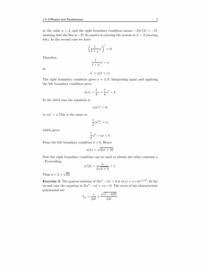
at the value u = 4, and the right boundary condition means −Du′(2) = −D,meaning that the flux is −D. So matter is entering the system at L = 2 (moving
left). In the second case we have
(
1
1 + xu′)′
= 0.
Therefore1
1 + xu′ = a
or
u′ = a(1 + x).
The right boundary condition gives a = 1/3. Integrating again and applying
the left boundary condition gives
u(x) =1
3x+
1
6x2 + 4.
In the third case the equation is
(uu′)′ = 0,
or uu′ = a.This is the same as
1
2(u2)′ = a,
which gives1
2u2 = ax+ b.
From the left boundary condition b = 8. Hence
u(x) =√2ax+ 16.
Now the right boundary condition can be used to obtain the other constant a
. Proceeding,
u′(2) =a
2√a+ 4
= 1.
Thus a = 2 +√20.
Exercise 3. The general solution of Du′′− cu′ = 0 is u(x) = a+ becx/D. In the
second case the equation is Du′′ − cu′ + ru = 0. The roots of the characteristic
polynomial are
λ± =c
2D±
√c2 − 4Dr
2D.

8 1. The Physical Origins of Partial Differential Equations
There are three cases, depending upon upon the discriminant c2 − 4Dr. If
c2 − 4Dr = 0 then the roots are equal ( c2D ) and the general solution has the
form
u(x) = aecx/2D + bxecx/2D.
If c2 − 4Dr > 0 then there are two real roots and the general solution is
u(x) = aeλ+x + beλ−x.
If c2− 4Dr < 0 then the roots are complex and the general solution is given by
u(x) = aecx/2D
(
a cos
√4Dr − c2
2Dx+ b sin
√4Dr − c2
2Dx
)
.
Exercise 4. If u is the concentration, use the notation u = v for 0 < x < L/2,
and u = w for L/2 < x < L.The PDE model is then
vt = vxx − λv, 0 < x < L/2,
wt = wxx − λw, L/2 < x < L.
The boundary conditions are clearly v(0, t) = w(L, t) = 0, and continuity at
the midpoint forces v(L/2) = w(L/2). To get a condition for the flux at the
midpoint we take a small interval [L/2−ǫ, L/2+ǫ]. The flux in at the left minus
the flux out at the right must equal 1, the amount of the source. In symbols,
−vx(L/2− ǫ, t) + wx(L/2 + ǫ) = 1.
Taking the limit as ǫ→ 0 gives
−vx(L/2, t) + wx(L/2) = 1.
So, there is a jump in the derivative of the concentration at the point of the
source. The steady state system is
v′′ − λv = 0, 0 < x < L/2,
w′′ − λw = 0, L/2 < x < L,
with conditions
v(0) = w(L) = 0,
v(L/2) = w(L/2),
−v′(L/2) + w′(L/2) = 1.
Let r =√λ. The general solutions to the DEs are
v = aerx + be−rx, w = cerx + de−rx.

1.4 Diffusion and Randomness 9
The four constants a, b, c, dmay be determined by the four auxiliary conditions.
Exercise 5. The steady state equations are
v′′ = 0, 0 < x < ξ,
w′′ = 0, ξ < x < L,
The conditions are
v(0) = w(L) = 0,
v(ξ) = w(ξ),
−v′(ξ) + w′(ξ) = 1.
Use these four conditions to determine the four constants in the general solution
to the DEs. We finally obtain the solution
v(x) =ξ − L
Lx, w(x) =
x− L
Lξ.
Exercise 6. The equation is
ut = uxx − ux, 0 < x < L.
(With no loss of generality we have taken the constants to be equal to one).
Integrating from x = 0 to x = L gives
∫ L
0
utdx =
∫ L
0
uxxdx−∫ L
0
uxdx.
Using the fundamental theorem of calculus and bringing out the time derivative
gives
∂
∂t
∫ L
0
udx = ux(L, t)−ux(0, t)−u(L, t)+u(0, t) = −flux(L, t)+flux(0, t) = 0.
Exercise 7. The model is
ut = Duxx + agux,
u(∞, t) = 0, −Dux(0, t)− agu(0, t) = 0.
The first boundary condition states the concentration is zero at the bottom (a
great depth), and the second condition states that the flux through the surface
is zero, i.e., no plankton pass through the surface. The steady state equation is
Du′′ + agu′ = 0,
10 1. The Physical Origins of Partial Differential Equations
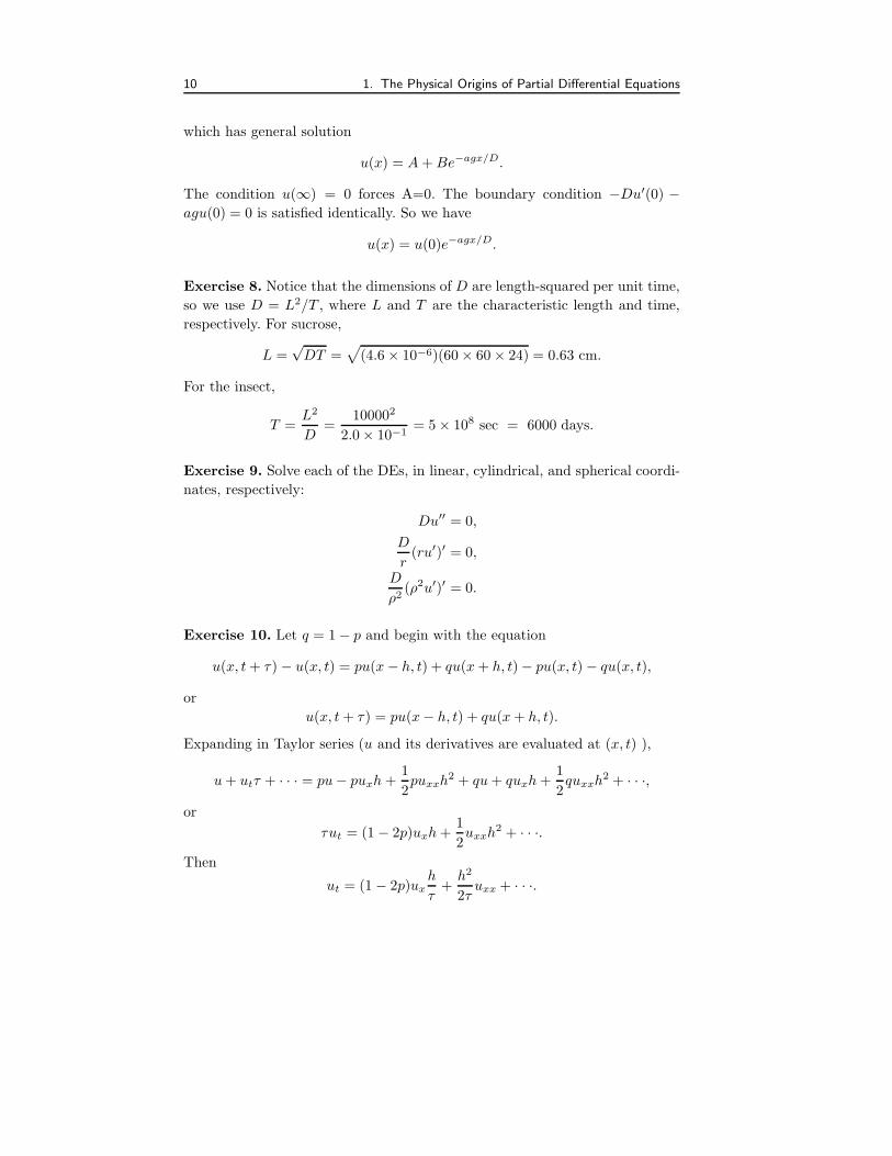
which has general solution
u(x) = A+Be−agx/D.
The condition u(∞) = 0 forces A=0. The boundary condition −Du′(0) −agu(0) = 0 is satisfied identically. So we have
u(x) = u(0)e−agx/D.
Exercise 8. Notice that the dimensions of D are length-squared per unit time,
so we use D = L2/T , where L and T are the characteristic length and time,
respectively. For sucrose,
L =√DT =
√
(4.6× 10⁻⁶)(60× 60× 24) = 0.63 cm.
For the insect,
T =L2
D=
100002
2.0× 10−1= 5× 10⁸ sec = 6000 days.
Exercise 9. Solve each of the DEs, in linear, cylindrical, and spherical coordi-
nates, respectively:
Du′′ = 0,
D
r(ru′)′ = 0,
D
ρ2(ρ2u′)′ = 0.
Exercise 10. Let q = 1− p and begin with the equation
u(x, t+ τ) − u(x, t) = pu(x− h, t) + qu(x+ h, t)− pu(x, t)− qu(x, t),
or
u(x, t+ τ) = pu(x− h, t) + qu(x+ h, t).
Expanding in Taylor series (u and its derivatives are evaluated at (x, t) ),
u+ utτ + · · · = pu− puxh+1
2puxxh
2 + qu+ quxh+1
2quxxh
2 + · · ·,
or
τut = (1 − 2p)uxh+1
2uxxh
2 + · · ·.
Then
ut = (1 − 2p)uxh
τ+h2
2τuxx + · · ·.
1.5 Vibrations and Acoustics 11
Taking the limit as h, τ → 0 gives
ut = cux +Duxx,
with appropriately defined special limits.
Exercise 11. Similar to the example in the text.
Exercise 12. Draw two concentric circles of radius r = a and r = b. The total
amount of material in between is
2π
∫ b
a
u(r, t)rdr.
The flux through the circle r = a is −2πaDur(a, t) and the flux through r=b
is −2πbDur(b, t). The time rate of change of the total amount of material in
between equals the flux in minus the flux out, or
2π∂
∂t
∫ b
a
u(r, t)rdr. = −2πaDur(a, t) + 2πbDur(b, t),
or∫ b
a
ut(r, t)rdr =
∫ b
a
D∂
∂r(rur(r, t))dr.
Since a and b are arbitrary,
ut(r, t)r = D∂
∂r(rur(r, t)).
1.5 Vibrations and Acoustics
Exercise 1. In balancing the vertical forces, add the term −∫ l
0gρ0(x)dx to
the right side to account for gravity acting downward.
Exercise 2. In balancing the vertical forces, add the term −intl0ρ0(x)kutdx to
the right side to account for damping.
Exercise 4. The initial conditions are found by setting t = 0 to obtain
un(x, 0) = sinnπx
l.
The temporal frequency of the oscillation is ω ≡ nπc/l with period 2π/ω. As
the length l increases, the frequency decreases, making the period of oscillation
longer. The tension is τ satisfies ρ0c2 = τ . As τ increases the frequency increases

12 1. The Physical Origins of Partial Differential Equations
so the oscillations are faster. Thus, tighter strings produce higher frequencies;
longer string produce lower frequencies.
Exercise 5. The calculation follows directly by following the hint.
Exercise 6. We have
c2 =dp
dρ= kγργ−1 =
γp
ρ.
Exercise 8. Assume ρ(x, t) = F (x − ct), a right traveling wave, where F is
to be determined. Then this satisfies the wave equation automatically and we
have ρ(0, t) = F (−ct) = 1− 2 cos t, which gives F (t) = 1− 2 cos(−t/c). Then
ρ(x, t) = 1− 2 cos(t− x/c).
Exercise 9. Differentiate the equations with respect to x and with respect to
t. The speed of waves is√
1/LC.
1.6 Quantum Mechanics
Exercise 1. This is a straightforward verification using rules of differentiation.
Exercise 2. Substitute y = e−ax2
into the Schrodinger equation to get
E = ~2a/m, a2 =
1
4mk/~2.
This gives
y(x) = Ce−0.5√mkx2/~.
To find C impose the normality condition∫
Ry(x)2dx = 1 and obtain
C =
(
mk
2π~
)1/4
.
Exercise 4. Let b2 ≡ 2mE/~2. Then the ODE
y′′ + by = 0
has general solution
y(x) = A sin bx+B cos bx.
1.7 Heat Flow in Three Dimensions 13
The condition y(0) = 0 forces B = 0. The condition y(π) = 0 forces sin bπ =
0, and so (assuming B 6= 0) b must be an integer, i.e., n2 ≡ 2mE/~2. The
probability density functions are
y2n(x) = B2 sin2 nx
with the constants B chosen such that∫ π
0 y2dx = 1. One obtains B =√
2/π.
The probabilities are∫ 0
0
.25y2n(x)dx.
1.7 Heat Flow in Three Dimensions
In these exercises we use the notation ∇ for the gradient operation grad.
Exercise 1. We have
div(∇u) = div(ux, uy, uz) = uxx + uyy + uzz.
Exercise 2. For nonhomogeneous media the conservation law (1.53) becomes
cρut − div(K(x, y, z)∇u) = f.
So the conductivity K cannot be brought out of the divergence.
Exercise 3. Integrate both sides of the PDE over Ω to get∫
Ω
fdV =
∫
Ω
−K∆udV =
∫
Ω
−Kdiv(∇u)dV
=
∫
∂Ω
−K ∇u · ndA =
∫
∂Ω
gdA.
The left side is the net heat generated inside Ω from sources; the right side is
the net heat passing through the boundary. For steady-state conditions, these
must balance.
Exercise 4. Follow the suggestion and use the divergence theorem.
Exercise 5. Follow the suggestion in the hint to obtain
−∫
Ω
∇u · ∇u dV = λ
∫
Ω
u2dV.
Both integrals are nonnegative, and so λ must be nonpositive. Note that λ 6= 0;
otherwise u = 0.

14 1. The Physical Origins of Partial Differential Equations
Exercise 6. This calculation is in the proof of Theorem 4.23 of the text.
Exercise 7. Replace φ in equations (1.52) by the given expression and proceed
a indicated in the text.
1.8 Laplace’s Equation
Exercise 1. The temperature at the origin is the average value of the temper-
ature around the boundary, or
u(0, 0) =1
2π
∫ 2π
0
(3 sin 2θ + 1)dθ.
The maximum and minimum must occur on the boundary. The function f(θ) =
3 sin 2θ+1 has an extremum when f ′(θ) = 0 or 6 cos 2θ = 0. The maxima then
occur at θ = π/4, 5π/4 and the minima occur at θ = 3π/4, 7π/4.
Exercise 3. We have u(x) = ax+b. But u(0) = b = T0 and u(l) = al+T0 = T1,
giving a = (T1 − T0)/l. Thus
u(x) =T1 − T0
lx+ T0,
which is a straight line connecting the endpoint temperatures. When the right
end is insulated the boundary condition becomes u′(l) = 0. Now we have a = 0
and b = T0 which gives the constant distribution
u(x) = T0.
Exercise 5. The boundary value problem is
−((1 + x2)u′)′ = 0, u(0) = 1, u(1) = 4.
Integrating gives (1 + x2)u′ = c1, or u′ = c1/(1 + x2). Integrating again gives
u(x) = c1 arctanx+ c2.
But u(0) = c2 = 1, and u(1) = c1 arctan 1 + 1 = 4. Then c1 = 6/π.
Exercise 6. Assume u = u(r) where r =√
x2 + y2. The chain rule gives
ux = u′(r)rx = u′(r)x
√
x2 + y2.
1.9 Classification of PDEs 15
Then, differentiating again using the product rule and the chain rule gives
uxx =x2
r2u′′(r) +
y2
r3.
Similarly
uyy =y2
r2u′′(r) +
x2
r3.
Then
∆u = u′′ +1
ru′ = 0.
This last equation can be written
(ru′)′ = 0
which gives the radial solutions
u = a ln r + b,
which are logarithmic. The one dimensional Laplace equation u′′ = 0 has linear
solutions u = ax+ b, and the three dimensional Laplace equation has algebraic
power solutions u = aρ−1 + b. In the two dimensional problem we have u(r) =
a ln r + b with u(1) = 0 and u(2) = 10. Then b = 0 and a = 10/ ln 2. Thus
u(r) = 10ln r
ln 2.
Exercise 9. We have ∇V = E. Taking the divergence of both sides gives
∆V = div∇V = div E = 0.
1.9 Classification of PDEs
Exercise 1. The equation
uxx + 2kuxt + k2utt = 0
is parabolic because B2 − 4AC = 4k2 − 4k2 = 0. Make the transformation
x = ξ, τ = x− (B/2C)t = x− t/k.
Then the PDE reduces to the canonical form Uξξ = 0. Solve by direct integra-
tion. Then Uξ = f(τ) and U = ξf(τ) + g(τ). Therefore
u = xf(x− t/k) + g(x− t/k),

16 1. The Physical Origins of Partial Differential Equations
where f, g are arbitrary functions.
Exercise 2. The equation 2uxx − 4uxt + ux = 0 is hyperbolic. Make the
transformation ξ = 2x+ t, τ = t and the PDE reduces to the canonical form
Uξτ − 1
4Uξ = 0.
Make the substitution V = Uξ to get Vτ = 0.25V , or V = F (ξ)eτ/4. Then
U = f(ξ)eτ/4 + g(τ), giving
u = f(2x+ t)et/4 + g(t).
Exercise 3. The equation xuxx − 4uxt = 0 is hyperbolic. Under the transfor-
mation ξ = t, τ = t+ 4 lnx the equation reduces to
Uξτ +1
4U = 0.
Proceeding as in Exercise 2 we obtain
u = f(t+ 4 lnx)et/4 + g(t).
Exercise 5. The discriminant for the PDE
uxx − 6uxy + 12uyy = 0
is D = −12 is negative and therefore it is elliptic. Take b = 1/4 +√3i/12 and
define the complex transformation ξ = x+ by, τ = x+ by. Then take
α =1
2(ξ + τ) = x+
1
4y
and
β =1
2i(ξ − τ) =
√3
12y.
Then the PDE reduces to Laplace’s equation uαα + uββ = 0.
Exercise 6. Change variables as indicated.
Exercise 7a. Hyperbolic when y < 1/x, parabolic when y = 1/x, elliptic when
y > 1/x.

2Partial Differential Equations on
Unbounded Domains
2.1 Cauchy Problem for the Heat Equation
Exercise 1a. Making the transformation r = (x− y)/√4kt we have
u(x, t) =
∫ 1
−1
1√4πkt
e−(x−y)2/4ktdy
= −∫ (x−1)/
√4kt
(x+1)/√4kt
1√πe−r2dr
=1
2
(
erf(
(x+ 1)/√4kt)
− erf(
(x− 1)/√4kt))
.
Exercise 1b. We have
u(x, t) =
∫ ∞
0
1√4πkt
e−(x−y)2/4kte−ydy.
Now complete the square in the exponent of e and write it as
− (x− y)2
4kt− y = −x
2 − 2xy + y2 + 4kty
4kt
= −y + 2kt− x)2
4kt+ kt− x.

18 2. Partial Differential Equations on Unbounded Domains
Then make the substitution in the integral
r =y + 2kt− x√
4kt
Then
u(x, t) =1√πekt−x
∫ ∞
(2kt−x)/√4kt
e−r2dr
=1
2ekt−x
(
1− erf(
(2kt− x)/√4kt))
.
Exercise 2. We have
|u(x, t)| ≤∫
R
|G(x− y, t)||φ(y)|dy ≤M
∫
R
G(x − y, t)dy =M.
Exercise 3. Use
erf(z) =2√π
∫ z
0
e−r2dr
=2√π
∫ z
0
(1− r2 + · · · )dr
=2√π(z − z3
3+ · · · ).
This gives
w(x0, t) =1
2+
x0
π√t+ · · · .
Exercise 4. The verification is straightforward. We guess the Green’s function
in two dimensions to be
g(x, y, t) = G(x, t)G(y, t)
=1√4πkt
e−x2/4kt 1√4πkt
e−y2/4kt
=1
4πkte−(x2+y2)/4kt,
where G is the Green’s function in one dimension. Thus g is the temperature
distribution caused by a point source at (x, y) = (0, 0) at t = 0. This guess
gives the correct expression. Then, by superposition, we have the solution
u(x, y, t) =
∫
R2
1
4πkte−((x−ξ)2+(y−η)2)/4ktψ(ξ, η)dξdη.

2.2 Cauchy Problem for the Wave Equation 19
Exercise 6. Using the substitution r = x/√4kt we get
∫
R
G(x, t)dx =1√π
∫
R
e−r2dr = 1.
Exercise 7. Verification is straightforward. The result does not contradict the
theorem because the initial condition is not bounded.
2.2 Cauchy Problem for the Wave Equation
Exercise 1. Applying the initial conditions to the general solution gives the
two equations
F (x) +G(x) = f(x), −cF ′(x) + cG′(x) = g(x).
We must solve these to determine the arbitrary functions F and G. Integrate
the second equation to get
−cF (x) + cG(x) =
∫ x
0
g(s)ds+ C.
Now we have two linear equations for F andG that we can solve simultaneously.
Exercise 2. Using d’Alembert’s formula we obtain
u(x, t) =1
2c
∫ x+ct
x−ct
ds
1 + 0.25s2
=1
2c2 arctan(s/2) |x+ct
x−ct
=1
c(arctan((x+ ct)/2)− arctan((x− ct)/2)).
Exercise 4. Let u = F (x− ct). Then ux(0, t) = F ′(−ct) = s(t). Then
F (t) =
∫ t
0
s(−r/c)dr +K.
Then
u(x, t) = −1
c
∫ t−x/c
0
s(y)dy +K.

20 2. Partial Differential Equations on Unbounded Domains
Exercise 5. Letting u = U/ρ we have
utt = Utt/ρ, uρ = Uρ/ρ− U/ρ2
anduρρ = Uρρ/ρ− 2Uρ/ρ
2 + 2U/ρ3.
Substituting these quantities into the wave equation gives
Utt = c2Uρρ
which is the ordinary wave equation with general solution
U(ρ, t) = F (ρ− ct) +G(ρ+ ct).
Thenu(ρ, t) =
1
r(F (ρ− ct) +G(ρ+ ct)).
As a spherical wave propagates outward in space its energy is spread out over a
larger volume, and therefore it seems reasonable that its amplitude decreases.
Exercise 6. The exact solution is, by d’Alembert’s formula,
u(x, t) =1
2(e−|x−ct| + e−|x+ct|) +
1
2c(sin(x+ ct)− sin(x − ct)).
Exercise 7. Use the fact that u is has the same value along a characteristic.
Exercise 8. Write
v =
∫
R
H(s, t)u(x, s)ds,
whereh(s, t) =
1√
4πt(k/c2)e−s2/(4t(k/c2)),
which is the heat kernel with k replaced by k/c2. Thus H satisfies
Ht −k
c2Hxx = 0.
Then, we have
vt − kvxx =
∫
R
(Ht(s, t)u(x, s)− kH(s, t)uxx(x, s))ds
=
∫
R
(Ht(s, t)u(x, s)− (k/c2)H(s, t)uss(x, s))ds
where, in the last step, we used the fact that u satisfies the wave equation. Now
integrate the second term in the last expression by parts twice. The generated
boundary terms will vanish since H and Hs go to zero as |s| → ∞. Then we
get
vt − kvxx =
∫
R
(Ht(s, t)u(x, s)− (k/c2)Hss(s, t)u(x, s))ds = 0.

2.3 Well-Posed Problems 21
2.3 Well-Posed Problems
Exercise 1. Consider the two problems
ut + uxx = 0, x ∈ R, t > 0,
u(x, 0) = f(x), x ∈ R
If f(x) = 1 the solution is u(x, t) = 1. If f(x) = 1+n−1 sinnx, which is a small
change in initial data, then the solution is
u(x, t) = 1 +1
nen
2t sinnx,
which is a large change in the solution. So the solution does not depend con-
tinuously on the initial data.
Exercise 2. Integrating twice, the general solution to uxy = 0 is
u(x, y) = F (x) +G(y),
where F and G are arbitrary functions. Note that the equation is hyperbolic
and therefore we expect the problem to be an evolution problem where data is
carried forward from one boundary to another; so a boundary value problem
should not be well-posed since the boundary data may be incompatible. To
observe this, note that
u(x, 0) = F (x) +G(0) = f(x). u(x, 1) = F (x) +G(1) = g(x),
where f and g are data imposed along y = 0 and y = 1, respectively. But these
last equations imply that f and g differ by a constant, which may not be true.
Exercise 3. We subtract the two solutions given by d’Alembert’s formula, take
the absolute value, and use the triangle inequality to get
|u1 − u2| ≤ 1
2|f1(x− ct)− f2(x − ct)|+ 1
2|f1(x+ ct)− f2(x+ ct)|
+1
2c
∫ x+ct
x−ct
|g1(s)− g2(s)|ds
≤ 1
2δ1 +
1
2δ1 +
1
2c
∫ x+ct
x−ct
δ2ds
= δ1 +1
2cδ2(2ct)
≤ δ1 + Tδ2.

22 2. Partial Differential Equations on Unbounded Domains
2.4 Semi-Infinite Domains
Exercise 2. We have
u(x, t) =
∫ ∞
0
(G(x− y, t)−G(x+ y, t))dy = erf (x/√4kt).
Exercise 3. For x > ct we use d’Alembert’s formula to get
u(x, t) =1
2((x− ct)e−(x−ct) + (x+ ct)e−(x+ct)).
For 0 < x < ct we have from (2.29) in the text
u(x, t) =1
2((x+ ct)e−(x+ct) − (ct− x)e−(ct−x)).
Exercise 4. Letting w(x, t) = u(x, t)− 1 we get the problem
wt = kwxx, w(0, t) = 0, t > 0, ;w(x, 0) = −1, x > 0.
Now we can apply the result of the text to get
w(x, t) =
∫ ∞
0
(G(x − y, t)−G(x + y, t))(−1)dy = −erf (x/√4kt).
Then
u(x, t) = 1− erf (x/√4kt).
Exercise 5. The problem is
ut = kuxx, x > 0, t > 0,
u(x, 0) = 7000, x > 0,
u(0, t) = 0, t > 0.
From Exercise 2 we know the temperature is
u(x, t) = 7000 erf (x/√4kt) = 7000
2√π
∫ x/√4kt
0
e−r2dr.
The geothermal gradient at the current time tc is
ux(0, tc) =7000√πktc
= 3.7× 10⁻⁴.
2.5 Sources and Duhamel’s Principle 23
Solving for t gives
tc = 1.624× 10¹⁶ sec = 5.15× 10⁸ yrs.
This gives a very low estimate; the age of the earth is thought to be about 15
billion years.
There are many ways to estimate the amount of heat lost. One method is
as follows. At t = 0 the total amount of heat was∫
S
ρcu dV = 7000ρc4
3πR3 = 29321ρcR3,
where S is the sphere of radius R = 4000 miles and density ρ and specific
heat c. The amount of heat leaked out can be calculated by integrating the
geothermal gradient up to the present day tc. Thus, the amount leaked out is
approximately
(4πR2)
∫ tc
0
−Kux(0, t)dt == −4πR2ρck(7000)
∫ tc
0
1√πkt
dt
== −ρcR2(1.06× 10¹²).
So the ratio of the heat lost to the total heat is
ρcR2(1.06× 10¹²)
29321ρcR3=
3.62× 10⁷
R= 5.6.
Exercise 6. Follow the suggested steps. Exercise 7. The left side of the equa-
tion is the flux through the surface. The first term on the right is Newton’s law
of cooling and the second term is the radiation heating.
2.5 Sources and Duhamel’s Principle
Exercise 1. The solution is
u(x, t) =1
2c
∫ t
0
∫ x+c(t−τ)
x−c(t−τ)
sin sds
=1
c2sinx− 1
2c2(sin(x− ct) + sin(x+ ct))

24 2. Partial Differential Equations on Unbounded Domains
Exercise 2. The solution is
u(x, t) =
∫ t
0
∫ ∞
−∞G(x− y, t− τ) sin y dydτ,
where G is the heat kernel.
Exercise 3. The problem
wt(x, t, τ) + cwx(x, t, τ) = 0, w(x, 0, τ) = f(x, τ),
has solution (see Chapter 1)
w(x, t, τ) = f(x− ct, τ).
Therefore, by Duhamel’s principle, the solution to the original problem is
u(x, t) =
∫ t
0
f(x− c(t− τ), τ)dτ.
Applying this formula when f(x, t) = xe−t and c = 2 gives
u(x, t) =
∫ t
0
(x− 2(t− τ))e−τdτ.
This integral can be calculated using integration by parts or a computer algebra
program. We get
u(x, t) = −(x− 2t)(e−t − 1)− 2te−t + 2(1− e−t).
2.6 Laplace Transforms
Exercise 4. Using integration by parts, we have
L
(∫ t
0
f(τ)dτ
)
=
∫ ∞
0
(∫ t
0
f(τ)dτ
)
e−stdt
= −1
s
∫ ∞
0
(∫ t
0
f(τ)dτ
)
d
dse−stdt
= −1
s
∫ t
0
f(τ)dτ · e−st |∞0 +1
s
∫ ∞
0
f(t)e−stdt
=1
sF (s).
2.6 Laplace Transforms 25
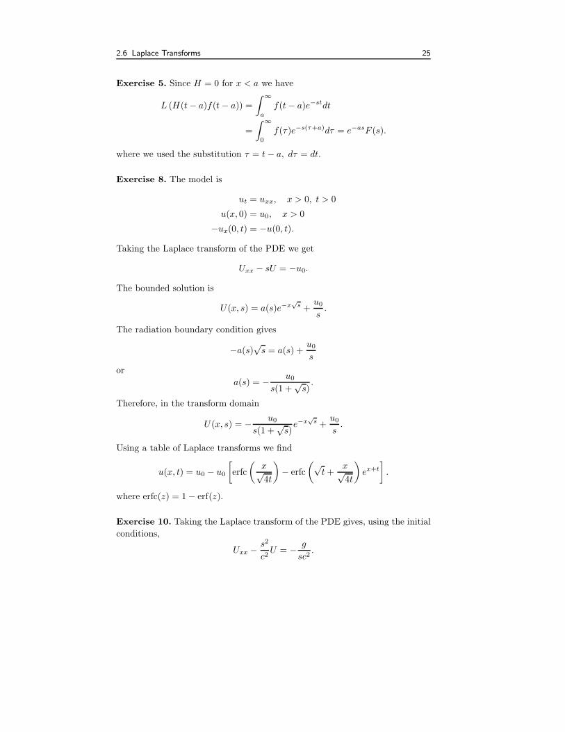
Exercise 5. Since H = 0 for x < a we have
L (H(t− a)f(t− a)) =
∫ ∞
a
f(t− a)e−stdt
=
∫ ∞
0
f(τ)e−s(τ+a)dτ = e−asF (s).
where we used the substitution τ = t− a, dτ = dt.
Exercise 8. The model is
ut = uxx, x > 0, t > 0
u(x, 0) = u0, x > 0
−ux(0, t) = −u(0, t).
Taking the Laplace transform of the PDE we get
Uxx − sU = −u0.
The bounded solution is
U(x, s) = a(s)e−x√s +
u0s.
The radiation boundary condition gives
−a(s)√s = a(s) +
u0s
or
a(s) = − u0s(1 +
√s).
Therefore, in the transform domain
U(x, s) = − u0s(1 +
√s)e−x
√s +
u0s.
Using a table of Laplace transforms we find
u(x, t) = u0 − u0
[
erfc
(
x√4t
)
− erfc
(√t+
x√4t
)
ex+t
]
.
where erfc(z) = 1− erf(z).
Exercise 10. Taking the Laplace transform of the PDE gives, using the initial
conditions,
Uxx −s2
c2U = − g
sc2.
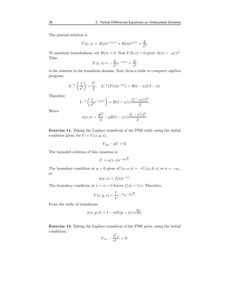
26 2. Partial Differential Equations on Unbounded Domains
The general solution is
U(x, s) = A(s)e−sx/c +B(s)esx/c +g
s3.
To maintain boundedness, set B(s) = 0. Now U(0, s) = 0 gives A(s) = −g/s3.Thus
U(x, s) = − g
s3e−sx/c +
g
s3
is the solution in the transform domain. Now, from a table or computer algebra
program,
L−1
(
1
s3
)
=t2
2, L−1(F (s)e−as) = H(t− a)f(t− a).
Therefore
L−1
(
1
s3e−xs/c
)
= H(t− x/c)(t− x/c)2
2.
Hence
u(x, t) =gt2
2− gH(t− x/c)
(t− x/c)2
2.
Exercise 11. Taking the Laplace transform of the PDE while using the initial
condition gives, for U = U(x, y, s),
Uyy − pU = 0.
The bounded solution of this equation is
U = a(x, s)e−y√s.
The boundary condition at y = 0 gives sU(x, o, s) = −Ux(x, 0, s) or a = −ax,or
a(x, s) = f(s)e−xs.
The boundary condition at x = u = 0 forces f(s) = 1/s. Therefore
U(x, y, s) =1
se−xse−y
√s.
From the table of transforms
u(x, y, t) = 1− erf((y − x)/√4t).
Exercise 13. Taking the Laplace transform of the PDE gives, using the initial
conditions,
Uxx − s2
c2U = 0.

2.6 Laplace Transforms 27
The general solution is
U(x, s) = A(s)e−sx/c +B(s)esx/c.
To maintain boundedness, set B(s) = 0. Now The boundary condition at x = 0
gives U(0, s) = G(s) which forces A(s) = G(s). Thus
U(x, s) = G(s)e−sx/c.
Therefore, using Exercise 4, we get
u(x, t) = H(t− x/c)g(t− x/c).
Exercise 14. The problem is
ut = uxx, x, t > 0
u(x, 0) = 0, x > 0
u(0, t) = f(t), t > 0.
Taking Laplace transforms and solving gives
U(x, s) = F (s)e−x√s
Here we have discarded the unbounded part of the solution. So, by convolution,
u(x, t) =
∫ t
0
f(τ)x
√
4π(t− τ)3e−x2/4(t−τ)dτ.
Hence, evaluating at x = 1,
U(t) =
∫ t
0
f(τ)1
√
4π(t− τ)3e−1/4(t−τ)dτ,
which is an integral equation for f(t). Suppose f(t) = f0 is constant and
U(5) = 10. Then
20√π
f0=
∫ 5
0
e−1/4(5−τ)
√
4π(5− τ)3dτ = 2 erfc (1/
√5),
where erfc = 1− erf. Thus f0 = 59.9 degrees.

28 2. Partial Differential Equations on Unbounded Domains
2.7 Fourier Transforms
Exercise 1. The convolution is calculated from
x ⋆ e−x2
=
∫ ∞
−∞(y − x)e−y2
dy.
Exercise 2. From the definition we have
F−1(e−a|ξ|)) =1
2π
∫ ∞
−∞e−a|ξ|e−ixξdξ
=1
2π
∫ 0
−∞eaξe−ixξdξ +
1
2π
∫ ∞
0
e−aξe−ixξdξ
=1
2π
∫ 0
−∞eaξ−ixξdξ +
1
2π
∫ ∞
0
e−aξ−ixξdξ
=1
2π
1
a− ixe(a−ix)ξ |0−∞ +
1
2π
1
−a− ixe(−a−ix)ξ |∞0
=a
π
1
a2 + x2.
Exercise 3a. Using the definition of the Fourier transform
2πF−1(−ξ) =∫ ∞
−∞u(x)e−i(−ξ)xdx = F(u)(ξ).
Exercise 3b. From the definition,
u(ξ + a) =
∫ ∞
−∞u(x)ei(ξ+a)xdx
=
∫ ∞
−∞u(x)eiaxeiξxdx
= F(eiaxu)(ξ).
Exercise 3c. Use 3(a) or, from the definition,
F(u(x+ a)) =
∫ ∞
−∞u(x+ a)eiξxdx =
∫ ∞
−∞u(y)eiξ(y−a)dy = e−iaξu(ξ).
2.7 Fourier Transforms 29
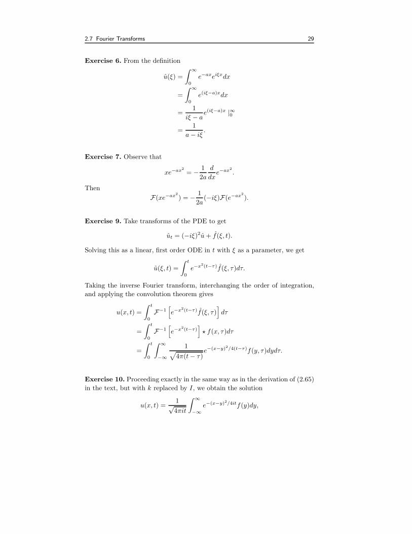
Exercise 6. From the definition
u(ξ) =
∫ ∞
0
e−axeiξxdx
=
∫ ∞
0
e(iξ−a)xdx
=1
iξ − ae(iξ−a)x |∞0
=1
a− iξ.
Exercise 7. Observe that
xe−ax2
= − 1
2a
d
dxe−ax2
.
Then
F(xe−ax2
) = − 1
2a(−iξ)F(e−ax2
).
Exercise 9. Take transforms of the PDE to get
ut = (−iξ)2u+ f(ξ, t).
Solving this as a linear, first order ODE in t with ξ as a parameter, we get
u(ξ, t) =
∫ t
0
e−x2(t−τ)f(ξ, τ)dτ.
Taking the inverse Fourier transform, interchanging the order of integration,
and applying the convolution theorem gives
u(x, t) =
∫ t
0
F−1[
e−x2(t−τ)f(ξ, τ)]
dτ
=
∫ t
0
F−1[
e−x2(t−τ)]
⋆ f(x, τ)dτ
=
∫ t
0
∫ ∞
−∞
1√
4π(t− τ)e−(x−y)2/4(t−τ)f(y, τ)dydτ.
Exercise 10. Proceeding exactly in the same way as in the derivation of (2.65)
in the text, but with k replaced by I, we obtain the solution
u(x, t) =1√4πit
∫ ∞
−∞e−(x−y)2/4itf(y)dy,
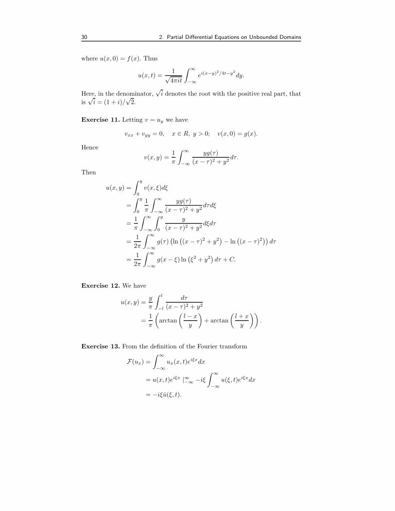
30 2. Partial Differential Equations on Unbounded Domains
where u(x, 0) = f(x). Thus
u(x, t) =1√4πit
∫ ∞
−∞ei(x−y)2/4t−y2
dy.
Here, in the denominator,√i denotes the root with the positive real part, that
is√i = (1 + i)/
√2.
Exercise 11. Letting v = uy we have
vxx + vyy = 0, x ∈ R, y > 0; v(x, 0) = g(x).
Hence
v(x, y) =1
π
∫ ∞
−∞
yg(τ)
(x− τ)2 + y2dτ.
Then
u(x, y) =
∫ y
0
v(x, ξ)dξ
=
∫ y
0
1
π
∫ ∞
−∞
yg(τ)
(x− τ)2 + y2dτdξ
=1
π
∫ ∞
−∞
∫ y
0
y
(x− τ)2 + y2dξdτ
=1
2π
∫ ∞
−∞g(τ)
(
ln(
(x − τ)2 + y2)
− ln(
(x− τ)2))
dτ
=1
2π
∫ ∞
−∞g(x− ξ) ln
(
ξ2 + y2)
dτ + C.
Exercise 12. We have
u(x, y) =y
π
∫ l
−l
dτ
(x− τ)2 + y2
=1
π
(
arctan
(
l− x
y
)
+ arctan
(
l + x
y
))
.
Exercise 13. From the definition of the Fourier transform
F(ux) =
∫ ∞
−∞ux(x, t)e
iξxdx
= u(x, t)eiξx |∞−∞ −iξ∫ ∞
−∞u(ξ, t)eiξxdx
= −iξu(ξ, t).

2.7 Fourier Transforms 31
For the second derivative, integrate by parts twice and assume u and uxtend to zero as x→ ±∞ to get rid of the boundary terms.
Exercise 14. In this case where f is a square wave signal,
F(f(x)) =
∫ ∞
−∞f(x)eiξxdx =
∫ a
−a
eiξxdx =2 sin ξx
ξ.
Exercise 15. Taking the Fourier transform of the PDE
ut = Duxx − cux
gives
ut = −(Dξ2 + iξc)u,
which has general solution
u(ξ, t) = C(ξ)e−Dξ2t−iξct.
The initial condition forces C(ξ) = φ(ξ) which gives
u(ξ, t) = φ(ξ)e−Dξ2t−iξct.
Using
F−1(
e−Dξ2t)
=1√4πDt
e−x2/4Dt
and
F−1(
u(ξ, t)e−iaξ)
= u(x+ a),
we have
F−1(
e−iξcte−Dξ2t)
=1√4πDt
e−(x+vt)2/4Dt.
Then, by convolution,
u(x, t) = φ ⋆1√4πDt
e−(x+vt)2/4Dt.
Exercise 16. (a) Substituting u = exp(i(kx−ωt)) into the PDE ut+uxxx = 0
gives −iω + (ik)3 = 0 or ω = −k3. Thus we have solutions of the form
u(x, t) = ei(kx+k3t) = eik(x+k2t).
The real part of a complex-valued solution is a real solution, so we have solutions
of the form
u(x, t) = cos[k(x+ k2t)].

32 2. Partial Differential Equations on Unbounded Domains
These are left traveling waves moving with speed k2. So the temporal frequency
ω as well as the wave speed c = k2 depends on the spatial frequency, or wave
number, k. Note that the wave length is proportional to 1/k. Thus, higher
frequency waves are propagated faster.
(b) Taking the Fourier transform of the PDE gives
ut = −(−iξ)3u.
This has solution
u(ξ, t) = φ(ξ)e−iξ3t,
where φ is the transform of the initial data. By the convolution theorem,
u(x, t) = φ(x) ⋆ F−1(e−iξ3t).
To invert this transform we go to the definition of the inverse. We have
F−1(e−iξ3t) =1
2π
∫ ∞
−∞e−iξ3te−iξxdξ
=1
2π
∫ ∞
−∞cos(ξ3t+ ξx)dξ
=1
2π
∫ ∞
−∞cos
(
z3
3+
zx
(3t)1/3
)
1
(3t)1/3dz
=1
(3t)1/3Ai
(
x
(3t)1/3
)
.
where we made the substitution ξ = z/(3t)1/3 to put the integrand in the form
of that in the Airy function. Consequently we have
u(x, t) =1
(3t)1/3
∫ ∞
−∞φ(x − y)Ai
(
y
(3t)1/3
)
dy.
Exercise 18. The problem is
utt = c2uxx = 0, x ∈ R, t > 0,
u(x, 0) = f(x), ut(x, 0) = 0, x ∈ R.
Taking Fourier transforms of the PDE yields
utt + c2ξ2u = 0
whose general solution is
u = A(ξ)eiξct +B(ξ)e−iξct.

2.7 Fourier Transforms 33
From the initial conditions, u(ξ, 0) = f(ξ) and ut(ξ, 0) = 0. Thus A(ξ) =
B(ξ) = 0.5f(ξ). Therefore
u(ξ, t) = 0.5f(ξ)(eiξct + e−iξct).
Now we use the fact that
F−1(
f(ξ)eiaξ)
= f(x− a)
to invert each term. Whence
u(x, t) = 0.5(f(x− ct) + f(x+ ct))
Exercise 19. The problem
ut = Duxx − vux, x ∈ R, t > 0; u(x, 0) = e−ax2
, x ∈ R
can be solved by Fourier transforms to get
u(x, t) =
√a√
a+ 4Dte−(x−vt)2/((a+4Dt).
Thus, choosing a = v = 1 we get
U(t) = u(1, t) =1√
1 + 4Dte−(1−t)2/((1+4Dt).
Exercise 20. Notice the left side is a convolution. Take the transform of both
sides, use the convolution theorem, and solve for f . Then invert to get f .


3Orthogonal Expansions
3.1 The Fourier Method
Exercise 1. Form the linear combination
u(x, t) =
∞∑
n=1
an cosnct sinnx.
Then
u(x, 0) = f(x) =∞∑
n=1
an sinnx.
Using the exactly same calculation as in the text, we obtain
an =2
π
∫ π
0
f(x) sinnx dx.
Observe that ut(x, 0) = 0 is automatically satisfied.
When the initial conditions are changed to u(x, 0) = 0, ut(x, 0) = g(x) then
a linear combination of the fundamental solutions un(x, t) = cosnct sinnx does
not suffice. But, observe that un(x, t) = sinnct sinnx now works and form the
linear combination
u(x, t) =∞∑
n=1
bn sinnct sinnx.
Now u(x, 0) = 0 is automatically satisfied and
ut(x, 0) = g(x) =
∞∑
n=1
ncbn sinnx.

36 3. Orthogonal Expansions
Again using the argument in (3.5)–(3.7), one easily shows the bn are given by
bn =2
ncπ
∫ π
0
g(x) sinnx dx.
3.2 Orthogonal Expansions
Exercise 2. The requirement for orthogonality is∫ π
0
cosmx cosnx dx = 0, m 6= n.
For the next part make the substitution y = πx/l to get
∫ l
0
cos(mπx/l) cos(nπx/l); dx =
∫ π
0
cosmy cosny dy = 0, m 6= n.
We have
cn =(f, cos(nπx/l))
|| cos(nπx/l)||2 .
Thus
c0 =1
l
∫ l
0
f(x)dx, cn =2
l
∫ l
0
f(x) cos(nπx/l)dx, n ≥ 1.
Exercise 8. Up to a constant factor, the Legendre polynomials are
P0(x) = 1, P1(x) = x, P2(x) =3
2x2 − 1
2, P3(x) =
5
2x3 − 3
2x.
The coefficients cn in the expansion are given by the generalized Fourier coef-
ficients
cn =1
||Pn||2(f, Pn) =
∫ 1
−1exPn(x)dx
∫ 1
−1 Pn(x)2dx
.
The pointwise error is
E(x) = ex −3∑
n=0
cnPn(x).
The mean square error is
E =
(
∫ 1
−1
[ex −3∑
n=0
cnPn(x)]2dx
)1/2
.
The maximum pointwise error is max−1≤x≤1 |E(x)|.

3.3 Classical Fourier Series 37
Exercise 9. Expanding
q(t) = (f + tg, f + tg)
= ||g||2t2 + 2(f, g)t+ ||f ||2.
which is a quadratic in t. Because q(t) is nonnegative (a scalar product of a
function with itself is necessarily nonnegative because it is the norm-squared),
the graph of the quadratic can never dip below the t axis. Thus it can have at
most one real root. Thus the discriminant b2−4ac must be nonpositive. In this
case the discriminant is
b2 − 4ac = 4(f, g)2 − 4||g||2||f ||2 ≤ 0.
This gives the desired inequality.
Exercise 12. Use the calculus facts that∫ b
0
1
xpdx <∞, p < 1
and∫ ∞
a
1
xpdx <∞, p > 1 (a > 0).
Otherwise the improper integrals diverge. Thus xr ∈ L2[0, 1] if r > −1/2 and
xr ∈ L2[0,∞] if r < −1/2 and r > −1/2, which is impossible.
Exercise 13. We have
cosx =
∞∑
n=1
bn sin 2nx, bn =4
π
∫ π/2
0
cosx sin 2nx dx.
Also,
sinx =
∞∑
n=1
bn sinnx
clearly forces b1 = 1 and bn = 0 for n ≥ 1. Therefore the Fourier series of sinx
on [0, π] is just a single term, sinx.
3.3 Classical Fourier Series
Exercise 1. Since f is an even function, bn = 0 for all n. We have
a0 =1
π
∫ π
−π
f(x)dx =1
π
∫ π/2
−π/2
dx = 1,

38 3. Orthogonal Expansions
and for n = 1, 2, 3, . . . ,
an =1
π
∫ π/2
−π/2
sinnx dx =2
nπsin(nπ/2)
Thus the Fourier series is
1
2+
2
π
∞∑
n=1
1
nsin(nπ/2) cosnx
=1
2+
2
π
(
cosx− 1
3cos 3x+ · · ·
)
.
A plot of a two-term and a four-term approximation is shown in the figure.
Exercise 3. Because the function is even, bn = 0. Then
a0 =1
π
∫ π
−π
x2dx = 2π2/3
and
an =1
π
∫ π
−π
x2 cosnx dx =4(−1)n
n2.
So the Fourier series is
π2
3+
∞∑
n=0
4(−1)n
n2cosnx.
This series expansion of f(x) = x2 must converge to f(0) = 0 at x = 0 since f
is piecewise smooth and continuous there. This gives
0 =π2
3+
∞∑
n=0
4(−1)n
n2,
which implies the result.
The frequency spectrum is
γ0 =2π2
3√2, γn =
4
n2, n ≥ 1.
Exercise 7. This problem suits itself for a computer algebra program to cal-
culate the integrals. We find a0 = 1 and an = 0 for n ≥ 1. Then we find
bn =1
2π
∫ 0
−2π
(x+ 1) sin(nx/2)dx+1
2π
∫ 2π
0
x sin(nx/2)dx
=1
π
−1 + (−1)n + 4π(−1)n+1
n.

3.3 Classical Fourier Series 39
Note that bn = −4/nπ if n is even and bn = (−2 + 4π)/nπ if n is odd. So the
Fourier series is
f(x) =1
2+
1
π
∞∑
n=1
−1 + (−1)n + 4π(−1)n+1
nsin(nx/2).
A five-term approximation is shown in the figure.
Exercise 10. Because cos ax is even we have bn = 0 for all n. Next
a0 =1
π
∫ π
−π
cos ax dx =2 sinaπ
aπ
and, using a table of integrals or a software program, for n ≥ 1,
an =1
π
∫ π
−π
cos ax cosnx dx
=1
π
(
sin(a− n)x
2(a− n)+
sin(a+ n)x
2(a+ n)
)π
−π
=2a(−1)n
π(a2 − n2)sin aπ.
Therefore the Fourier series is
cos ax =sin aπ
aπ+
∞∑
n=1
2a(−1)n
π(a2 − n2)sin aπ cosnx.
Substitute x = 0 to get the series for cscaπ.
Exercise 11. Here f(x) is odd so an = 0 for all n. Then
bn =1
π
∫ 0
−π
−1
2sinnx dx+
1
π
∫ π
0
1
2sinnx dx
=1
nπ(1− (−1)n).
Therefore
b=2
(2k − 1)π, k = 1, 2, 3, . . . .
The Fourier series is
∑
k=1
∞ 2
(2k − 1)πsin(2k − 1)x.
Plots of partial sums show overshoot near the discontinuity (Gibbs phe-
nomenon).


4Partial Differential Equations on Bounded
Domains
4.1 Overview of Separation of Variables
Exercise 2. The solution is
u(x, t) =
∞∑
n=1
ane−n2t sinnx,
where
an =2
π
∫ π
π/2
sinnxdx = − 2
nπ((−1)n − cos(nπ/2)).
Thus
u(x, t) =2
πe−t sinx− 2
πe−4t sin 2x+
2
3πe−9t sin 3x+
2
5πe−25t sin 5x+ · · · .
Exercise 3. The solution is given by formula (4.14) in the text, where the
coefficients are given by (4.15) and (4.16). Since G(x) = 0 we have cn = 0.
Then
dn =2
π
∫ π/2
0
x sinnx dx +2
π
∫ π
π/2
(π − x) sinnx dx.
Using the antiderivative formula∫
x sinnx dx = (1/n2) sinnx − (x/n) cosnx
we integrate to get
dn =4
πn2sin
nπ
2.
42 4. Partial Differential Equations on Bounded Domains
Exercise 4. Substituting u = y(x)g(t) into the PDE and boundary conditions
gives the SLP−y′′ = λy, y(0) = y(1) = 0
and, for g, the equationg′′ + kg′ + c2λg = 0.
The SLP has eigenvalues and eigenfunctions
λn = n2π2, yn(x) = sinnπx, n = 1, 2, . . . .
The g equation is a linear equation with constant coefficients; the characteristic
equations ism2 + km+ c2λ = 0,
which has roots
m =1
2(−k ±
√
k2 − 4c2n2π2).
By assumption k < 2πc, and therefore the roots are complex for all n. Thus the
solution to the equation is (see the Appendix in the text on ordinary differential
equations)gn(t) = e−kt(an cos(mnt) + bn sin(mnt)),
where
mn =1
2
√
4c2n2π2 − k2).
Then we form the linear combination
u(x, t) =
∞∑
n=1
e−kt(an cos(mnt) + bn sin(mnt)) sin(nπx).
Now apply the initial conditions. We have
u(x, 0) = f(x) =
∞∑
n=1
an sin(nπx),
and thus
an =
∫ 1
0
f(x) sinnπx dx.
The initial condition ut = 0 at t = 0 yields
ut(x, 0) = 0 =
∞∑
n=1
(bnmn − kan) sin(nπx).
Thereforebnmn − kan = 0,
or
bn =kanmn
=k
mn
∫ 1
0
f(x) sinnπx dx.

4.2 Sturm–Liouville Problems 43
4.2 Sturm–Liouville Problems
Exercise 1. Substituting u(x, t) = g(t)y(x) into the PDE
ut = (p(x)ux)x − q(x)u
gives
g′(t)y(x) =d
dx(p(x)g(t)y′(x))− q(x)g(t)y(x).
Dividing by g(t)y(x) givesg′
g=
(py′)′ − q
y.
Setting these equal to −λ gives the two differential equations for g and y.
Exercise 2. When λ = 0 the ODE is −y′′ = 0 which gives y(x) = ax + b.
But y′(0) = a = 0 and y(l) = al + b = 0, and so a = b = 0 and so zero is
not an eigenvalue. When λ = −k2 < 0 then the ODE has general solution
y(x) = aekx + be−kx, which are exponentials. If y = 0 at x = 0 and x = l, then
it is not difficult to show a = b = 0, which means that there are no negative
eigenvalues. If λ = k2 > 0 then y(x) = a sinkx+ b coskx. Then y′(0) = 0 forces
a = 0 and then y(l) = b cos kl = 0. But the cosine function vanishes at π/2
plus a multiple of π, i.e.,
kl =√λl = π/2 + nπ
for n = 0, 1, 2, . . .. This gives the desired eigenvalues and eigenfunctions as
stated in the problem.
Exercise 3. The problem is
−y′′ = λy, y(0) + y′(0) = 0, y(1) = 0.
If λ = 0 then y(x) = ax + b and the boundary conditions force b = −a. Thuseigenfunctions are
y(x) = a(1− x).
If λ < 0 then y(x) = a coshkx + b sinh kx where λ = −k2. The boundary
conditions give
a+ bk = 0, a coshk + b sinhk = 0.
Thus sinh k − k coshk = 0 or k = tanhk which has no nonzero roots. Thus
there are no negative eigenvalues.
If λ = k2 > 0 then y(x) = a cos kx + b sinkx. The boundary conditions
imply
a+ bk = 0, a cos k + b sink = 0.
44 4. Partial Differential Equations on Bounded Domains
Thus k = tan k which has infinity many positive roots kn (note that the graphs
of k and tan k cross infinitely many times). So there are infinitely many positive
eigenvalues given by λn = k2n.
Exercise 4. The SLP is
−y′′ = λy, y(0) + 2y′(0) = 0, 3y(2) + 2y′(2) = 0.
If λ = 0 then y(x) = ax + b. The boundary conditions give b + 2a = 0 and
8a + 3b = 0 which imply a = b = 0. So zero is not an eigenvalue. Since this
problem is a regular SLP we know by the fundamental theorem that there are
infinitely many positive eigenvalues.
If λ = −k2 < 0, then y(x) = a coshkx+ b sinhkx. The boundary conditions
force the two equations
a+ 2bk = 0, (3 cosh 2k + 2k sinh 2k)a+ (3 sinh 2k + 2k cosh 2k) = 0.
This is a homogeneous linear system for a and b and it will have a nonzero
solution when the determinant of the coefficient matrix is zero, i.e.,
tan 2k =4k
3− 4k2.
This equation has nonzero solutions at k ≈ ±0.42. Therefore there is one
negative eigenvalue λ ≈ −0.422 = −0.176. (This nonlinear equation for k can
be solved graphically using a calculator, or using a computer algebra package,
or using the solver routine on a calculator).
Exercise 5. When λ = 0 the ODE is y′′ = 0, giving y(x) = Ax + B. Now
apply the boundary conditions to get
B − aA = 0, Al +B + bA = 0.
This homogeneous system has a nonzero solution for A and B if and only if
a + b = −abl. (Note that the determinant of the coefficient matrix must be
zero).
Exercise 7. Multiply the equation by y and integrate from x = 0 to x = l to
get
−∫ l
0
yy′′dx+
∫ l
0
qy2dx = λ
∫ l
0
y2dx.
Integrate the first integral by parts; the boundary term will be zero from the
boundary conditions; then solve for λ to get
λ =
∫ l
0(y′)2dx+
∫ l
0 qy2dx
||y||2 .

4.2 Sturm–Liouville Problems 45
Clearly (note y(x) 6= 0) the second integral in the numerator and the integral in
the denominator are positive ,and thus λ > 0. y(x) cannot be constant because
the boundary conditions would force that constant to be zero.
Exercise 9. When λ = 0 the ODE is −y′′ = 0 which gives y(x) = ax + b.
The boundary conditions force a = 0 but do not determine b. Thus λ = 0 is
an eigenvalue with corresponding constant eigenfunctions. When λ = −k2 < 0
then the ODE has general solution y(x) = aekx+be−kx, which are exponentials.
Easily, exponential functions cannot satisfy periodic boundary conditions, so
there are no negative eigenvalues. If λ = k2 > 0 then y(x) = a sin kx+ b cos kx.
Then y′(x) = ak cos kx− bk sin kx. Applying the boundary conditions
b = a sin kl+ b cos kl, a = a coskl − b sinkl.
We can rewrite this system as a homogeneous system
a sin kl+ b(cos kl − 1) = 0
a(cos kl − 1)− b sin kl = 0.
A homogeneous system will have a nontrivial solution when the determinant
of the coefficient matrix is zero, which is in this case reduces to the equation
cos kl = 0.
Therefore kl must be a multiple of 2π, or
λn = (2nπ/l)2, n = 1, 2, 3, . . . .
The corresponding eigenfunctions are
yn(x) = an sin(2nπx/l) + bn cos(2nπx/l).
Exercise 10. Letting c(x, t) = y(x)g(t) leads to the periodic boundary value
problem
−y′′ = λy, y(0) = y(2l), y′(0) = y′(2l)
and the differential equation
g′ = λDg,
which has solution
g(t) = e−Dλt.
The eigenvalues and eigenfunctions are found exactly as in the solution of
Exercise 4, Section 3.4, with l replaced by 2l. They are
λ0 = 0, λn = n2π2/l2, n = 1, 2, . . .

46 4. Partial Differential Equations on Bounded Domains
and
y0(x) = 1, yn(x) = an cos(nπx/l) + bn sin(nπx/l), n = 1, 2, . . . .
Thus we form
c(x, t) = a0/2 +
∞∑
n=1
e−n2π2Dt/l2(an cos(nπx/l) + bn sin(nπx/l).
Now the initial condition gives
c(x, 0) = f(x) = a0/2 +∞∑
n=1
(an cos(nπx/l) + bn sin(nπx/l),
which is the Fourier series for f . Thus the coefficients are given by
an =1
l
∫ 2
0
lf(x) cos(nπx/l)dx, n = 0, 1, 2, . . .
and
bn =1
l
∫ 2
0
lf(x) sin(nπx/l)dx, n = 1, 2, . . . .
Exercise 11. The operator on the left side of the equation has variable coeffi-
cients and the ODE cannot be solved analytically in terms of simple functions.
Exercise 12. This problem models the transverse vibrations of a string of
length l when the left end is fixed (attached) and the right end experience no
force; however, the right end can move vertically. Initially the string is displaced
by f(x) and it is not given an initial velocity.
Substituting u = y(x)g(t) into the PDE and boundary conditions gives the
SLP
−y′′ = λy, y(0) = y′(l) = 0
and, for g, the equation
g′′ + c2λg = 0.
The SLP has eigenvalues and eigenfunctions
λn = ((2n+ 1)π/l)2, yn(x) = sin((2n+ 1)πx/l), n = 0, 1, 2, . . . ,
and the equation for g has general solution
gn(t) = an sin((2n+ 1)πct/l) + bn cos((2n+ 1)πct/l).
Then we form
u(x, t) =
∞∑
n=0
(an sin((2n+ 1)πct/l) + bn cos((2n+ 1)πct/l)) sin((2n+ 1)πx/l).
4.2 Sturm–Liouville Problems 47
Applying the initial conditions,
u(x, t) = f(x) =
∞∑
n=0
bn sin((2n+ 1)πx/l),
which yields
bn =1
|| sin((2n+ 1)πx/l)||2∫ l
0
f(x) sin((2n+ 1)πx/l).
And
ut(x, 0) = 0 =
∞∑
n=0
ancλn sin((2n+ 1)πx/l),
which gives an = 0. Therefore the solution is
u(x, t) =
∞∑
n=0
bn cos((2n+ 1)πct/l)) sin((2n+ 1)πx/l).
Exercise 13. The flux at x = 0 is φ(0, t) ≡ −ux(0, t) = −a0u(0, t) > 0, so
there is heat flow into the bar and therefore adsorption. At x = 1 we have
φ(1, t) = −ux(1, t) = a1u(1, t) > 0, and therefore heat is flowing out of the bar,
which is radiation. The right side of the inequality a0+ a1 > −a0a1 is positive,
so the positive constant a1, which measures radiation, must greatly exceed the
negative constant a0, which measures adsorption.
In this problem substituting u = y(x)g(t) leads to the Sturm-Liouville prob-
lem
−y′′ = λy, y′(0)− a0y(0) = 0, y′(1) + a1y(1) = 0
and the differential equation
g′ = λg.
There are no nonpositive eigenvalues. If we take λ = k2 > 0 then the solutions
are
y(x) = a cos kx+ b sinkx.
Applying the two boundary conditions leads to the nonlinear equation
tan k =(a0 + a1)k
k2 − a0a1.
To determine the roots k, and thus the eigenvalues λ = k2, we can graph both
sides of this equation to observe that there are infinitely many intersections
occurring at kn, and thus there are infinitely many eigenvalues λn = k2n. The
eigenfunctions are
yn(x) = cos knx+a0kn
sin knx.

48 4. Partial Differential Equations on Bounded Domains
So the solution has the form
u(x, t) =
∞∑
n=1
cne−λ2
nt(cos knx+
a0kn
sin knx).
The cn are then the Fourier coefficients
cn = (f, yn)/||yn||2.
If a0 = −1/4 and a1 = 4 then
tan k =3.75k
k2 + 1.
From a graphing calculator, the first four roots are approximately k1 =
1.08, k2 = 3.85, k3 = 6.81, k4 = 9.82.
4.3 Generalization and Singular Problems
Exercise 1. (a) Yes (divide by x2). (b) No.
Exercise 2. Multiply by y and then integrate. Then integrate the first term
by parts and apply the boundary conditions.
Exercise 3. Rewrite the equation as
x2y′′ + xy′ + λy = 0,
which is a Cauchy-Euler equation. The roots of the characteristic equation are
m = ±√λ, where λ = k2 > 0. So the general solution is y(x) = A cos(k lnx) +
B sin(k lnx). (Note that a simple energy argument shows the eigenvalues are
positive.) Now, y(1) = 0 forces A = 0, and y(b) = B sin(k ln b) = 0. Therefore,
k ln b = nπ, n = 1, 2, 3 . . .. Thus the eigenvalues are λn = nπ/ ln b and the
eigenfunctions are yn(x) = sinnπ, n = 1, 2, 3, . . ..
Exercise 4. Multiplying the differential equation by y and integrating from
x = 1 to x = π gives
−∫ π
1
y(x2y′)′dx = λ
∫ π
1
y2dx
or, upon integrating the left side by parts,
−xyy′ |π1 −∫ π
1
x2(y′)2dx = λ
∫ π
1
y2dx.

4.3 Generalization and Singular Problems 49
The boundary term vanishes because of the boundary conditions. Therefore,
because both integrals are nonnegative we have λ ≥ 0. If λ = 0 then y′ =const=
0 (by the boundary conditions). So λ 6= 0 and the eigenvalues are therefore
positive.
If λ = k2 > 0, then the ODE becomes
x2y′′ + 2xy′ + k2y = 0,
which is a Cauchy-Euler equation (see the Appendix on differential equations
in the text). This can be solved to determine eigenvalues
λn =( nπ
lnπ
)2
+1
4
with corresponding eigenfunctions
yn(x) =1√xsin( nπ
lnπlnx)
.
Exercise 7. Letting u = g(t)y(x) and substituting into the equation and
boundary conditions gives g′′ = λg and the Sturm–Liouville problem
−y′′ = −λ 1
c(x)2y, y(0) = y(l) = 0.
The weight function is 1/c(x)2.
Exercise 8. We have ρ(x)utt = uxx. Putting u = Y (x)g(t) gives, upon sepa-
rating variables,−y′′ = ρ(x)λy, y(0) = y(1) = 0.
We have−y′′f = ρ(x)λf yf , yf(0) = yf (1) = 0.
Integrating from x = 0 to x = s gives
−y′f(s) + y′f (0) = λf
∫ s
0
ρ(x)yf (x)dx.
Now integrate from s = 0 to s = 1 to get
y′f (0) = λf
∫ 1
0
∫ s
0
ρ(x)yf (x)dxds
= λf
∫ 1
0
(1− x)ρ(x)yf (x)dx.
The last step follows by interchanging the order of integration. If ρ(x) =r ho0is a constant, then
ρ0 =y′f(0)
λf∫ 1
0 (1− x)yf (x)dx.
50 4. Partial Differential Equations on Bounded Domains
Exercise 9. From Exercise 2 in Section 4.6 we have the solution
u(x, t) =2
π
∞∑
n=1
1
kn2(1− e−n2kt)
(∫ π
0
f(r) sinnr dr
)
sinnx.
Therefore
U(t) = u(π/2, t) =
∫ π
0
(
2
π
∞∑
n=1
sinnr sin(nπ/2)1
kn2(1− e−n2kt)
)
f(r)dr.
We want to recover f(x) if we know U(t). This problem is not stable, as the
following example shows. Let
u(x, t) = m−3/2(1− e−m2t) sinmx, f(x) =√m sinmx.
This pair satisfies the model. If m is sufficiently large, thenu(x, t) is uniformly
small; yet f(0) is large. So a small error in measuring U(t) will result in a large
change in f(x).
4.4 Laplace’s Equation
Exercise 1. Substituting u(x, y) = φ(x)ψ(y) we obtain the Sturm-Liouville
problem
−φ′′ = λφ, x ∈ (0, l); φ(0) = φ(l) = 0
and the differential equation
ψ′′ − λψ = 0.
The SLP has eigenvalues and eigenfunctions
λn = n2π2/l2, φn(x) = sin(nπx/l),
and the solution to the ψ–equation is
ψn(y) = an cosh(nπy/l) + bn sinh(nπy/l).
Therefore
u(x, y) =
∞∑
n=1
(an cosh(nπy/l) + bn sinh(nπy/l)) sin(nπx/l).
Now we apply the boundary conditions:
u(x, 0) =
∞∑
n=1
an sin(nπx/l) = 0,

4.4 Laplace’s Equation 51
so an = 0. Therefore
u(x, 1) = G(x) =
∞∑
n=1
bn sinh(nπ/l)) sin(nπx/l).
Thus
bn sinh(nπ/l) =2
l
∫ π
0
G(x) sin(nπx/l)dx,
which determines the coefficients bn.
Exercise 2. This problem models the steady state temperatures in a rectangu-
lar plate that is insulated on both sides, whose temperature is zero on the top,
and whose temperature is f(x) along the bottom. Letting u = g(y)φ(x) and
substituting into the PDE and boundary conditions gives the Sturm-Liouville
problem
−φ′′ = λφ, φ′(0) = φ′(a) = 0
and the differential equation
g′′ − λg = 0.
The eigenvalues and eigenfunctions are λ0 = 0, φ(x) = 1 and
λn = n2π2/a2, φn(x) = cos(nπx/a), n = 1, 2, 3, . . . .
The solution to the g equation is, corresponding to the zero eigenvalue, g0(y) =
c0y + d0, and corresponding to the positive eigenvalues,
gn(y) = cn sinh(nπy/a) + dn cosh(nπy/a).
Thus we form the linear combination
u(x, y) = c0y + d0 +
∞∑
n=1
(cn sinh(nπy/a) + dn cosh(nπy/a)) cos(nπx/a).
Now apply the boundary conditions on y to compute the coefficients:
u(x, 0) = f(x) = d0 +
∞∑
n=1
dn cos(nπx/a),
which gives
d0 =1
a
∫ a
0
f(x)dx, dn =2
a
∫ a
0
f(x) cos(nπx/a)dx.
Next
u(x, b) = 0 = c0b+ d0 +
∞∑
n=1
(cn sinh(nπb/a) + dn cosh(nπb/a)) cos(nπx/a).
52 4. Partial Differential Equations on Bounded Domains
Therefore
c0 = −d0/b, cn = −cosh(nπb/a)
sinh(nπb/a)dn.
Exercise 3. The general solution is given in the text. Here
f(θ) = 4 + 3 sin θ.
The right side is its Fourier series, so the Fourier coefficients are given by
a02
= 4, Rb1 = 3,
with all the other Fourier coefficients identically zero. So the solution is
u(r, θ) = 4 +3r
Rsin θ.
Exercise 5. The exterior Poisson formula applies but the integral is difficult.
In this simple case assume a separable solution of the form u(r, θ) = Ar−n cos θ.
Substitute into the radial form of the equation to get n = 1 (to get bounded
solutions). Apply the boundary condition to get A = 1. Therefore
u(r, θ) =1
rcos θ.
Exercise 6. Substituting u(r, θ) = g(θ)y(r) into the PDE and boundary con-
ditions gives the Sturm-Liouville problem
−g′′ = λg, g(0) = g(π/2) = 0
and the differential equation
r2y′′ + ry′ + λy = 0.
This SLP has been solved many times in the text and in the problems. The
eigenvalues and eigenfunctions are
λn = 4n2, gn(θ) = sin(2nθ), n = 1, 2, . . . .
The y equation is a Cauchy-Euler equation and has bounded solution
yn(r) = r2n.
Form
u(r, θ) =
∞∑
n=1
bnr2n sin(2nθ).

4.4 Laplace’s Equation 53
Then the boundary condition at r = R gives
u(R, θ) = f(θ) =
∞∑
n=1
bnR2n sin(2nθ).
Hence the coefficients are
bn =1
πR2n
∫ π/2
0
f(θ) sin(2nθ)dθ.
Exercise 7. Substituting u(r, θ) = g(θ)y(r) into the PDE and boundary con-
ditions gives the Sturm-Liouville problem
−g′′ = λg, g(0) = g′(π/2) = 0
and the differential equation
r2y′′ + ry′ + λy = 0.
The eigenvalues and eigenfunctions are
λn = (2n+ 1)2, gn(θ) = sin((2n+ 1)θ), n = 0, 1, 2, . . . .
The y equation is a Cauchy-Euler equation and has bounded solution
yn(r) = r2n+1
Form
u(r, θ) =
∞∑
n=1
bnr2n+1 sin((2n+ 1)θ).
Then the boundary condition at r = R gives
u(R, θ) = f(θ) =
∞∑
n=1
bnR2n+1 sin((2n+ 1)θ).
Hence the coefficients are
bn =1
πR2n+1
∫ π/2
0
f(θ) sin((2n+ 1)θ)dθ.

54 4. Partial Differential Equations on Bounded Domains
Exercise 10. Let w = u + v where u satisfies the Neumann problem and v
satisfies the boundary condition n · ∇v = 0. Then
E(w) = E(u + v)
=1
2
∫
Ω
(∇u · ∇u+ 2∇u · ∇v +∇v · ∇v)dV −∫
∂Ω
(hu− hv)dA
= E(u) +
∫
Ω
∇u · ∇v dV +1
2
∫
Ω
∇v · ∇vdV −∫
∂Ω
hv dA
= E(u) +
∫
∂Ω
v∇u · n dA−∫
Ω
v∆u dV +1
2
∫
Ω
∇v · ∇vdV −∫
∂Ω
hv dA
= E(u) +
∫
∂Ω
vh dA+1
2
∫
Ω
∇v · ∇vdV −∫
∂Ω
hv dA
= E(u) +1
2
∫
Ω
∇v · ∇vdV
So E(u) ≤ E(w).
Exercise 11. Integrate the partial differential equation over a region Ω and
then use the divergence theorem to get∫
Ω
fdV =
∫
Ω
∆udV =
∫
∂Ω
gradu · ndA =
∫
∂Ω
hdA.
In a steady heat flow context, for example, this states that net rate that heat is
produced by sources in the region must equal the rate that heat leaves through
the boundary.
Exercise 12. Take u = ρ−1w. (NOTE: there is a typographical error in the
exercise.) Then find uρ and uρρ and substitute into the PDE to reduce the
equation to wρρ − k2w = 0. This has general solution w = c1ekρ + c2e
−kρ.
Exercise 13. Multiply both sides of the PDE by u and integrate over Ω. We
obtain∫
Ω
u∆u dV = c
∫
Ω
u2dV.
Now use Green’s first identity to obtain∫
∂Ω
u∇u · ndA−∫
Ω
∇u · ∇u dV = c
∫
Ω
u2dV,
or
−∫
∂Ω
au2dA−∫
Ω
∇u · ∇u dV = c
∫
Ω
u2dV.
The left side is negative and the right side is positive. Then both must be zero,
or∫
Ω
u2dV = 0.

4.4 Laplace’s Equation 55
Hence u = 0 in Ω.
The uniqueness argument is standard. Let u and v be two solutions to the
boundary value problem
∆u− cu = f, x ∈ Ω n · ∇u + au = g, x ∈ ∂Ω.
Then the difference w = u− v satisfies the homogeneous problem
∆w − cw = 0, x ∈ Ω n · ∇w + aw = 0, x ∈ ∂Ω.
By the first part of the problem we know w = 0 and therefore u = v.
Exercise 14. Let w and v be two solutions and take u = w−v. Then ∆u−cu =
0 on Ω and n · gradu + au = 0 on ∂Ω. Now use Exercise 13 to get u = 0, so
that w = v.
Exercise 15. Multiplying the equation ∆u = 0 by u, integrating over Ω, and
then using Green’s identity gives∫
Ω
u∆u dV =
∫
∂Ω
u∇u · ndA−∫
Ω
∇u · ∇udV = 0.
Thus ∫
Ω
∇u · ∇udV = 0,
which implies∇u = 0.
Thus u = constant.
Exercise 16. Let v and w be two solutions and take u = v − w. To show
u = 0 we use an energy argument. Multiply the PDE by u and integrate to get∫
Ωu∆u dV = 0. By Green’s first identity,
∫
∂Ω
u∇u · ndA−∫
Ω
∇u · ∇udV = 0.
Using the boundary condition, we get
−∫
∂Ω
au2dA−∫
Ω
∇u · ∇udV = 0.
Both terms on the left are negative, which is a contradiction. So u = 0 on Ω.
Exercise 18. Typographical error : the boundary condition should be du/dn =
sin2 θ. We have ∫
Ω
fdV = 0 and
∫
∂Ω
sin2 θdA > 0,
which contradicts the result of Exercise 11.
Exercise 19. The radial equation in spherical coordinates is ρ−2(ρ2uρ)ρ = 0
has solution u(ρ) = c1ρ−1 + c2. Apply the boundary conditions to determine
c1 and c2.
56 4. Partial Differential Equations on Bounded Domains
4.5 Cooling of a Sphere
Exercise 1. The problem is
−y′′ − 2
ρy′ = λy, y(0) bounded, y(π) = 0.
Making the transformation Y = ρy we get −Y ′′ = λY . If λ = −k2 < 0 then
Y = a sinh kρ+ b coshkρ,
or
y = ρ−1(a sinh kρ+ b coshkρ).
For boundedness at ρ = 0 we set b = 0. Then y(π) = 0) forces sinh kπ = 0.
Thus k = 0. Consequently, there are no negative eigenvalues.
Exercise 2. From the formula developed in the text the temperature at ρ = 0
is
u(0, t) = 74
∞∑
n=1
(−1)n+1 1
ne−n2kt,
where k = 5.58 inches-squared per hour.
Exercise 3. The boundary value problem is
ut = k(uρρ +2
ρuρ),
uρ(R, t) = −hu(R, t), t > 0,
u(ρ, 0) = f(ρ), 0 ≤ ρ ≤ R.
Assume u = y(ρ)g(t). Then the PDE and boundary conditions separate into
the boundary value problem
y′′ + (2/ρ)y′ + λy = 0, y′(R) = −hy(R), y bounded
and the differential equation
g− = −λkg.
The latter has solution g(t) = exp(−λkt). One can show that the eigenvalues
are positive. So let λ = p2 and make the substitution Y = ρy, as in the text,
to obtain
Y ′′ + p2Y = 0.
This has solution
Y (ρ) = a cos pρ+ b sin pρ.

4.5 Cooling of a Sphere 57
But Y (0) = 0 forces a = 0 (because y is bounded). Then the other boundary
condition forces p to satisfy the nonlinear equation
tanRp =Rp
1−Rh.
If we graph both sides of this equation against p we note that there are infinitely
many intersections, giving infinitely many roots pn, n = 1, 2, . . ., and therefore
infinitely many eigenvalues λn = p2n. The corresponding eigenfunctions are
yn(ρ) = ρ−1 sin(√
λnρ).
Thus we have
u(ρ, t) =
∞∑
n=1
cne−λnktρ−1 sin(
√
λnρ).
The cn are found from the initial condition. We have
u(ρ, 0) = f(ρ) =
∞∑
n=1
cnρ−1 sin(
√
λnρ).
Thus
cn =
∫ R
0 ρf(ρ) sin(√λnρ)dρ
∫ R
0sin2(
√λnρ)ρdρ
.
Exercise 4. Representing the Laplacian in spherical coordinates, the boundary
value problem for u = u(ρ, φ), where ρ ∈ (0, 1) and φ ∈ (0, π), is
∆u = uρρ +2
ρuρ +
1
ρ2 sinφ(sin φuφ) = 0,
u(1, φ) = f(φ), 0 ≤ φ ≤ π.
Observe, by symmetry of the boundary condition, u cannot depend on the
angle θ. Now assume u = R(ρ)Y (φ). The PDE separates into two equations,
ρ2R′′ + 2ρR′ − λR = 0
and1
sinφ(sinφY ′)′ = λY.
We transform the Y equation by changing the independent variable to x =
cosφ. Then we get, using the chain rule,
1
sinφ
d
dφ= − d
dx.

58 4. Partial Differential Equations on Bounded Domains
So the Y –equation becomes
− d
dx
(
(1− x2)dy
dx
)
= λy − 1 < x < 1.
By the given facts, this equation has bounded, orthogonal, solutions yn(x) =
Pn(x) on [−1, 1] when λ = λn = n(n + 1), n = 0, 1, 2, . . .. Here Pn(x) are the
Legendre polynomials.
Now, the R–equation then becomes
ρ2R′′ + 2ρR′ − n(n+ 1)R = 0
This is a Cauchy-Euler equation (see the Appendix in the text) with charac-
teristic equation
m(m− 1) +m− n(n+ 1) = 0.
The roots are m = n,−(n+ 1). Thus
Rn(ρ) = anρn
are the bounded solutions (the other root gives the solution ρ−n−1, which is
unbounded at zero). Therefore we form
u(ρ, φ) =
∞∑
n=0
anρnPn(cosφ)
or, equivalently,
u(ρ, x) =
∞∑
n=0
anρnPn(x).
Applying the boundary condition gives the coefficients. We have
u(1, x) = f(arccosx) =
∞∑
n=0
anPn(x).
By orthogonality we get
an =1
||Pn||2∫ 1
−1
f(arccosx)Pn(x)dx,
or
an =1
||Pn||2∫ π
0
f(φ)Pn(cosφ) sin φ dφ.
By direct differentiation we get
P0(x) = 1, P1(x) = x, P2(x) =1
2(3x2 − 1), P3(x) =
5
2x3 − 3
2x.

4.5 Cooling of a Sphere 59
Also the norms are given by
||P0||2 = 2, ||P1||2 =2
3, ||P2||2 =
2
5.
When f(φ) = sinφ the first few Fourier coefficients are given by
a0 =π
4, a1 = a3 = 0, a2 = −0.49.
Therefore a two-term approximation is given by
u(ρ, φ) ≈ π
4− 0.49
2ρ2(3 cos2 φ− 1).
Exercise 5. To determine the temperature of the earth we must derive the
temperature formula for any radius R (the calculation in the text uses R = π).
The method is exactly the same, but now the eigenvalues are λn = n2π2/R2
and the eigenfunctions are yn = ρ−1 sin(nπρ/R), for n = 1, 2, . . .. Then the
temperature is
u(ρ, t) =2RT0π
∞∑
n=1
(−1)n+1
ne−lamnktρ−1 sin(nπρ/R).
Now we compute the geothermal gradient at the surface, which is uρ(ρ, t) at
ρ = R. We obtain
uρ(R, t) = −2T0R
∞∑
n=1
e−n2π2kt/R2
.
If G is the value of the geothermal gradient at the current time t = tc, then
RG
2T0=
∞∑
n=1
e−n2π2ktc/R2
.
We must solve for tc. Notice that the sum has the form
∞∑
n=1
e−an2
where a = π2ktc/R2. We can make an approximation by noting that the sum
represents a Riemann sum approximation to the integral∫ ∞
0
e−ax2
dx =1
2
√
π/a.
So we use this value to approximate the sum, i.e.,
∞∑
n=1
e−n2π2ktc/R2 ≈ R
2√kπtc
.

60 4. Partial Differential Equations on Bounded Domains
Solving for tc gives
tc =T 20
G2kπ.
Substituting the numbers in from Exercise 5 in Section 2.4 gives tc = 5.15(10)8
years. This is the same approximation we found earlier.
4.6 Diffusion in a Disk
Exercise 1. The differential equation is −(ry′)′ = λry. Multiply both sides by
y and integrate over [0, R] to get
∫ R
0
−(ry′)′ydr = λ
∫ R
0
ry2dr.
Integrating the left hand side by parts gives
−ryy′ |R0∫ R
0
r(y′)2dr = λ
∫ R
0
ry2dr.
But, since y and y′ are assumed to be bounded, the boundary term vanishes.
The remaining integrals are nonnegative and so λ ≥ 0.
Exercise 2. Let y, λ and w, µ be two eigenpairs. Then −(ry′)′ = λry and
−(rw′)′ = µrw. Multiply the first of these equations by w and the second by
y, and then subtract and integrate to get
∫ R
0
[−(ry′)′w + (rw′)′y]dr = (λ− µ)
∫ R
0
ruwdr.
Now integrate both terms in the first integral on the left hand side by parts to
get
(−ry′w + rw′y) |R0 +
∫ R
0
(ry′w′ − rw′y′)dr = (λ− µ)
∫ R
0
ruwdr.
The left side of the equation is zero and so y and w are orthogonal with respect
to the weight function r.
Exercise 3. We have
u(r, t) =∞∑
n=1
cne−0.25λntJ0(znr),
4.7 Sources on Bounded Domains 61
where
cn =
∫ 1
0 5r4(1− r)J0(znr)dr∫ 1
0J0(znr)2rdr
.
We have z1 = 2.405, z2 = 5.520, z3 = 8.654. Use a computer algebra program
to calculate a 3-term approximation.
4.7 Sources on Bounded Domains
Exercise 1. Use Duhamel’s principle to solve the problem
utt − c2uxx = f(x, t), 0 < x < π, t > 0,
u(0, t) = u(π, t) = 0, t > 0,
u(x, 0) = ut(x, 0) = 0, 0 < x < π.
Consider the problem for w = w(x, t, τ), where τ is a parameter:
wtt − c2wxx = 0, 0 < x < π, t > 0,
w(0, t, τ) = w(π, t, τ) = 0, t > 0,
w(x, 0, τ) = 0, wt(x, 0, τ) = 0, 0 < x < π.
This problem was solved in Section 4.1 (see (4.14)–(4.14)). The solution is
w(x, t, τ) =
∞∑
n=1
cn(τ) sinnct sinnx,
where
cn(τ) =2
ncπ
∫ π
0
f(x, τ) sinnx dx.
So the solution to the original problem is
u(x, t) =
∫ t
0
w(x, t− τ, τ)dτ.
Exercise 3. If f = f(x), and does not depend on t, then the solution can be
written
u(x, t) =2
π
∞∑
n=1
(∫ π
0
f(r) sinnr dr
)
(
(∫ t
0
e−n2k(t−τ)dτ
)
sinnx.
But a straightforward integration gives∫ t
0
e−n2k(t−τ)dτ =1
kn2(1− e−n2kt).

62 4. Partial Differential Equations on Bounded Domains
Therefore
u(x, t) =2
π
∞∑
n=1
1
kn2(1− e−n2kt)
(∫ π
0
f(r) sinnr dr
)
sinnx.
Taking the limit as t→ ∞ gives
U(x) ≡ limu(x, t) = u(x, t) =2
π
∞∑
n=1
1
kn2
(∫ π
0
f(r) sinnr dr
)
sinnx.
Now consider the steady state problem
−kv′′ = x(π − x), v(0) = v(π) = 0.
This can be solved directly by integrating twice and using the boundary con-
ditions to determine the constants of integration. One obtains
v(x) = − 1
12k(2πx2 − x4 − π3x).
To observe that the solution v(x) is the same as the limiting solution U(x)
we expand the right side of the v–equation in its Fourier sine series on [0, π].
Then
−kv′′ =∞∑
n=1
cn sinnx,
where
cn =2
π
∫ π
0
r(π − r) sinnrdr.
Integrating the differential equation twice gives
−kv(x) + kv′(0)x =
∞∑
n=1
cnn−2(sinnx− x).
Evaluating at x = π gives
kv′(0) =∞∑
n=1
cnn−2.
Whence
kv(x) =
∞∑
n=1
cnn−2 sinnx,
or
v(x) =2
kπ
∞∑
n=1
1
n2
(∫ π
0
f(r) sinnr dr
)
sinnx.
Hence v(x) = U(x).
4.7 Sources on Bounded Domains 63
Exercise 4. Homogenize the boundary conditions by letting w(x, t) = u(x, t)−Ax. Then the equation for w is wt = wxx with w(0, t) = w(1, t) = 0 and
w(x, 0) = cosx−Ax. The w-problem is a straightforward separation of variables
problem with homogeneous equation and boundary conditions.
Exercise 5. Refer to Remark 4.29. First find the solution of the steady-state
problem which is U ′′(x) = −Q, U(0) = 0, U(1) = 2u0. This is easily solved to
get
U(x) = −1
2x2 + (2u0 +
1
2Q)x.
Now take w(x, t) = u(x, t)−U(x). It is easily seen that w satisfies the problem
wt = wxx with w(0, t) = w(1, t) = 0 and w(x, 0) = u0(1−cosπx)−U(x), which
is a standard separation of variables problem.
Exercise 6. Follow the steps in Remark 4.30.
Exercise 7. Again, use Remark 4.29; the nonhomogeneous equation has a
source term that depends only on x. The steady-state solution satisfies U ′′(x) =− 1
k sin 3πx, with U(0) = U(1) = 0. By integrating twice,
U(x) =1
9π2ksin 3πx.
Take w(x, t) = u(x, t)−U(x). Then w satisfies a homogenous problem wt = wxx
with w(0, t) = w(1, t) = 0, and the initial condition is w(x, 0) = sinπx−U(x).
This is solved by separating variables.
Exercise 8. Typographical error : The boundary condition at R = R1 is u = u1.
Follow Example 4.31.
Exercise 9. Follow Example 4.32.
Exercise 10. The problem is
ut = ∆u+ f(r, t) 0 ≤ r < R, t > 0,
u(R, t) = 0, t > 0,
u(r, 0) = 0, 0 < r < R.
For w = w(r, t, τ) we consider the problem
wt = ∆w 0 ≤ r < R, t > 0,
w(R, t, τ) = 0, t > 0,
w(r, 0, τ) = f(r, τ), 0 < r < R.

64 4. Partial Differential Equations on Bounded Domains
This is the model for heat flow in a disk of radius R; the solution is given by
equation (4.53) in Section 4.5 of the text. It is
w(r, t, τ) =∑
cn(τ)e−λnktJ0(znr/R),
where zn are the zeros of the Bessel function J0, λn = z2n/R2 and
cn(τ) =1
||J0(znr/R)||2∫ R
0
f(r, τ)J0(znr/R)rdr.
Then
u(r, t) =
∫ R
0
w(r, t − τ, τ)dτ.
Exercise 11. The source term depends only on r, so take w(r, t) = u(r, t) −U(r), where U(r) is the steady-state solution to r−1(rU ′)′ = −f(r), U(R) = u0.
We obtain
U(r) =
∫ R
r
1
ρ
∫ ρ
0
σf(σ)dσ dρ+ u0.
Then w satisfies a homogeneous differential equation and boundary condition.
4.8 Poisson’s Equation
Exercise 1. u(r, θ) = (1/√2)r sin θ.
Exercise 2. There is no θ dependence in the problem, so take u = u(r).
Substituting into the equation gives (ru′)′ = −Ar. Integrating twice gives
u(r) = − 14Ar
2 + c1 ln r + c2. For boundedness, take c1 = 0. Applying the
boundary condition at R gives c2 = 1 +AR2/4. Thus
u =1
4(R2 − r2) + 1.
Exercise 4. The solution depends only on r. Try u = U(r), where U is to be
determined.
Exercise 5. The solution depends only on r. Try u = U(r), where U is to be
determined.
Exercise 8. Following the hint in the text we have
u(x, y) =
∞∑
n=1
gn(y) sinnx,

4.8 Poisson’s Equation 65
where we find
g′′n − n2gn = fn(y), gn(0) = gn(1) = 0.
Here, the fn(y) are the Fourier coefficients of f(x, y). From the variation of
parameters formula
gn(y) = aeny + be−ny − 2
n
∫ y
0
sinh(n(ξ − y))fn(ξ)dξ.
Now gn(0) = 0 implies b = −a. So we can write
gn(y) = 2a sinhny − 2
n
∫ y
0
sinh(n(ξ − y))fn(ξ)dξ
which gives, using gn(1) = 0,
a =1
n sinhn
∫ 1
0
sinh(n(ξ − 1))fn(ξ)dξ.
Thus the gn(y) are given by
gn(y) =2 sinhny
n sinhn
∫ 1
0
sinh(n(ξ − 1))fn(ξ)dξ −2
n
∫ y
0
sinh(n(ξ − y))fn(ξ)dξ.


5Applications in The Life Sciences
5.1 Age-Structured Models
Exercise 1.Write
1 =
∫ 8
3
4e−(r+0.03)ada = − 4
r + 0.03
(
e−8(r+0.03) − e−3(r+0.03))
,
and use a software package or calculator to solve for r.
Exercise 2. First note that u(a, t) = 0 for a > t+ δ, since f(a) = 0 for a > δ.
For (a) observe that the renewal equation (5.9) is
B(t) =
∫ t
0
βB(t− a)e−γada+
∫ ∞
0
βf(a− t)e−γtda.
The first integral becomes, upon changing variables to s = t− a,∫ t
0
βB(t− a)e−γada =
∫ t
0
βB(s)e−γ(t−s)ds.
The second integral is∫ ∞
0
βf(a− t)e−γtda =
∫ t+δ
t
βu0e−γtda = βu0δe
−γt.
For (b), differentiate (using Leibniz rule)
B(t) =
∫ t
0
βB(s)e−γ(t−s)ds+ βu0δe−γt

68 5. Applications in The Life Sciences
to get
B′(t) =
∫ t
0
βB(s)e−γ(t−s)ds(−γ) + βB(t)− γβu0δe−γt = (β − γ)B(t).
For (c) note that the last equation is the differential equation for growth-decay
and has solution
B(t) = B(0)e(β−γ)t.
Therefore the solution from (5.7)–(5.8) is given by
u(a, t) =
0, a > t+ δ
u0e−γt, t < a < t+ δ
B(0)e(β−γ)te−βa, 0 < a < t.
Finally, for part (d) we have, using part (c),
N(t) =
∫ t
0
u(a, t)da+
∫ t+δ
t
u(a, t)da
=
∫ t
0
B(0)e(β−γ)te−βada+
∫ t+δ
t
u0e−γtda
=B(0)
βe(β−γ)t(1 − e−βt) + δu0e
−γt.
Exercise 3. Integrate the PDE from a = 0 to a = ∞ to get
N(t) = −∫ ∞
0
uada−m(N)N = B(t)−m(N)N.
To get an equation for B we differentiate the B(t) equation to get
B′(t) =
∫ ∞
0
b0e−γautda =
∫ ∞
0
b0e−γa(−ua −m(N)u)da
= −m(N)B(t)−∫ ∞
0
b0e−γa(ua)da
= −m(N)B(t)−[
b0e−γau|∞0 +
∫ ∞
0
b0γe−γauda
]
= −m(N)B(t)− b0B(t)− γB(t).
To obtain the next-to-last line we used integration by parts. In summary we
have the dynamical system
N ′ = B −m(N)N,
B′ = (b0 − γ −m(N))B.

5.1 Age-Structured Models 69
In the phase plane the paths or integral curves are defined by
dB
dN=
(b0 − γ −m(N))B
B −m(N)N.
Observe that B = (b0 − γ)N is easily shown to be a solution to this equation.
It represents a straight line in the NB plane. The line B=0 is a horizontal
nullcline where the vector field points to the left. Another horizontal nullcline
is the vertical line N = N∗, where N∗ is the root ofm(N) = (b0−γ). The pointP = (N∗, (b0 − γ)N∗) is an equilibrium that lies on the straight line solution
curve B = (b0 − γ)N. The solution cannot oscillate since that it would require
it cross the straight line, violating uniqueness. On the straight line solution,
the direction is toward the point P .
Exercise 5. Let ξ = a− t, τ = t. In these characteristic coordinates the PDE
becomes
Uτ = − c
d− ξ − τU.
Separating variable and integrating gives
U = (d− ξ − τ)cϕ(ξ)
or
u(a, t) = (d− a)cϕ(a− t),
which is the general solution. Now, for the region a > t we use the initial
condition to determine ϕ. We have
u(a, 0) = (d− a)cϕ(a) = f(a),
which gives ϕ(a) = f(a)(d− a)c. Hence
u(a, t) = (d− a)cf(a− t)(d − a− t)−c, a > t.
For the region a < t we use the boundary condition. to determine ϕ. Thus,
u(0, t) = dcϕ(−t) = B(t),
or
ϕ(t) = B(−t)d−c.
Whence
u(a, t) = (d− a)cB(t− a)d−c, 0 < a < t.
Exercise 6. Using Taylor’s expansion to write
u(a+ da, t+ dt) = u(a, t) + ut(a, t)da+ ut(a, t)dt+ higher order terms.

70 5. Applications in The Life Sciences
5.2 Traveling Wave Fronts
Exercise 1. The traveling wave equation can be written
−cU ′ = DU ′′ − 1
2(U2)′.
Integrating, we get
−cU = DU ′ − 1
2U2 +A.
Using the boundary condition at z = +∞ forces A = 0. Using the boundary
condition at z = −∞ gives the wave speed c = 1/2. Therefore
DU ′ =1
2U(U − 1).
This DE has equilibria at U = 0, 1; the solution can be found by separating
variables or noting it is a Bernoulli equation (see the Appendix on Differential
Equations). The graph falls from left to right (decreasing), approaching 0 at
plus infinity and 1 at minus infinity.
Exercise 2. The traveling wave equation may be written
−cU ′ = U ′′ − 1
3(U3)′.
Integrating, we find that the constant of integration is zero from the z = +∞boundary condition. Then
−cU = U ′ − 1
3U3.
Applying the condition at z = −∞ we get
−cUl = −1
3U3l ,
or
−cUl +1
3U3l = −1
3Ul(3c− U2
l ) = 0.
Therefore Ul =√3c.
Exercise 3. To have constant states at infinity we must have F (0, vr) = 0 =
F (ul, 0) = 0. The traveling wave equations are
−cU ′ = DU ′′ − γU ′ − aF (U, V ),
−cV ′ = −bF (U, V ).
5.3 Equilibria and Stability 71
Clearly we may write a single equation
−cU ′ = DU ′′ − γU ′ − ac
bV ′.
Now we may integrate to get
−cU = DU ′ − γU − ac
bV +A.
The right boundary condition forces A = acvr/b. The left boundary condition
then gives
−cul = −γul +ac
bvr
or
(γ − c)ul =ac
bvr > 0.
Therefore c < γ.
Exercise 5. The traveling wave equation is
−c[
(1 + b)U −mU2]′= U ′′ − U ′.
Integrating gives
−c[
(1 + b)U −mU2]
= U ′ − U +A.
¿From the boundary condition U(+∞) = 0 we get A = 0. Since U(−∞) = 1,
we get
c =1
1 + b−m> 0.
The differential equation then simplifies to
U ′ = (1− c− cb)U + cmU2,
which is a Bernoulli equation. It is also separable.
5.3 Equilibria and Stability
Exercise 1. The equilibria are roots of
f(u) = ru(1 − u/K)− hu = u(r − r
Ku− h) = 0.
So the equilibria are
u1 = 0, u2 =r − h
rK.

72 5. Applications in The Life Sciences
To check stability we calculate f ′(u1) = r − 2rK u − h. Then f ′(0) = r > 0, so
u1 = 0 is unstable. Next
f ′(r − h
rK) = r − 2r
K
r − h
rK − h = r − 2r + 2h− h = −r + h.
Therefore u2 is stable if r > h and unstable if r < h.
Exercise 2. Follow the steps indicated in the problem.
Exercise 3. The steady-state solution is ue = 3, ve = 2/9. The Jacobian
matrix is
J =
(
13 9
− 43 −9
)
.
Therefore, equation (5.36) becomes
det
((
σn 0
0 σn
)
+ n2
(
D 0
0 1
)
−(
13 9
− 43 −9
))
= 0.
Simplifying gives
det
(
σn + n2D − 13 −9
− 13 σn + n2 + 9
)
= 0.
Exercise 4. To obtain (a) just substitute ue(x) into the PDE and check the
boundary conditions. To get (b) substitute u = ue(x) + U(x, t) into the PDE
to obtain
Ut = u′′e + Uxx + (ue(x) + U(x, t))(1 − ue(x)− U(x, t)),
or
Ut = u′′e + Uxx + ue(x)(1 − ue(x))− ue(x)U + U(1− ue(x)) − U2(x, t).
But u′′e + ue(x)(1 − ue(x)) = 0, and neglecting the nonlinear term gives
Ut = Uxx + (1− 2ue(x))U,
which is the linearized perturbation equation. The boundary conditions are
U(±π/2) = 0. For part (c) assume that U = eσtg(x) and substitute to get
σg = g′′ + (1− 2ue(x))g,
or
g′′ +cosx− 5
1 + cosxg = σg,
with g = 0 at x = ±π/2. Finally, to prove (d), we proceed as in the hint. If
this BVP has a nontrivial solution, then it must be, say, positive somewhere

5.3 Equilibria and Stability 73
in the interval. (The negative case can be treated similarly). So it must have a
positive maximum in the interval. At this maximum, g > 0, g′′ < 0. Therefore
cosx− 5
1 + cosxg < 0.
So the left side of the DE is negative, so σ < 0.