syllabus stochastic simulation methodsphys.ubbcluj.ro/~zneda/edu/mc/curs_hands.pdf · syllabus...
TRANSCRIPT

1
Stochastic simulation methodsStochastic simulation methods
or: Monteor: Monte--Carlo methodsCarlo methods
course homepage: http://www.phys.ubbcluj.ro/~zneda/mc.html
- lecture notes
- computer codes
- research projects
- papers to discuss
- important announcements
- interesting links on the web
Main objective of the course:
To give a PRACTICAL introduction to Monte Carlo
methods in physics. To study modern problems in the field.
Start research….
ZoltZoltáán Nn Néédada
UBBUBB--ClujCluj, Romania, Romania
znedazneda@@phys.ubbcluj.rophys.ubbcluj.ro
SyllabusSyllabus•About Monte Carlo methods
•Random number generators
• Elements of Statistical Physics, Stochastic Processes and Critical Phenomena
•Brownian dynamics
•Monte Carlo methods
•The Ising model
•Metropolis and Glauber dynamics MC for the Ising model
•The BKL algorithm (grain growth, kinetic Monte Carlo methods)
•Cluster algorithms (Swensen and Wang algorithm)
•The histogram Monte Carlo method
•Microcanonical Monte Carlo
•Quantum Monte Carlo methods
•Frustated systems, spin-glasses
•Application of MC methods in wetting, crack formation, deposition of atoms on surfaces, grain growth ,
random networks…..
•Discussion and presentation of research projects
What are the Monte Carlo methods?What are the Monte Carlo methods?
Computer
simulation
methods:
- Molecular dynamics (deterministic
simulations, based on the integration of the
equation of motion)
- Monte Carlo methods (Stochastic simulation
techniques, where the random number
generation plays a crucial role)
- Cellular automata (approach to a given
phenomena discretized on a lattice, with
deterministic or stochastic update rules)
- In general we speak about Monte Carlo simulation methods whenever the use
of the random numbers are crucial in the algorithm!
- Monte Carlo techniques are widely used in problems from: statistical physics,
soft condensed matter physics, material science, many-body problems, complex
systems, fluid mechanics, biophysics, econo-physics, nonlinear phenomena,
particle physics, heavy-ion physics, surface physics, neuroscience etc….
Example: Molecular dynamics simulations
Drying nanosphere suspension on a substrate
Simulation of crack
propagation (atomistic level)
Simulation of crack
propagation (large-scale)
colliding microasperities
vibrational dynamics of a molecule
Unfolding a protein
colliding elastic balls
Example: Cellular automata simulation
A modulo 2 cellular automata (1D+time evolution)
Cellular
automata
exhibiting self-
organization and
spiral waves
3D cellular
automata (forest
fire model)
3D sandpile
cellular
automata
Some wellSome well--known problems where MC methods are usefulknown problems where MC methods are useful
1 .Random walk on a lattice
Nr ~2 ><

2
Some wellSome well--known problems where MC methods are usefulknown problems where MC methods are useful
2. Percolation problems: 3.The Ising model:
1
,
±=
−−= ∑∑><
i
i
ij
ji
i
S
SBSSJH µ
Some wellSome well--known problems where MC methods are usefulknown problems where MC methods are useful
4. The p-state Potts model
)()(
,
ji
ji
ijJpH σσδ∑
><
−=
Some wellSome well--known problems where MC methods are usefulknown problems where MC methods are useful
Domain growth (coarse-graining) in the Potts model (low temperature)
Feeling what Monte Carlo simulation meansFeeling what Monte Carlo simulation means
- 1. Studying the random walk -
The drunken sailor’s problem
-A basic model in natural sciences
(Brownian motion, fluctuations, diffusion etc…)
-We consider first the simple 1D case
P=1/2P=1/2
Experimental realization:
the Galton board
Analytical study
Quantities of interest:αNr
N~2
?=α ?),( =kNP
N
k
N
W
WkNP =),(
WNk :number of possible paths with N steps that end up at coordinate k
WN: total number of possible paths with N steps
;2N
NW =]!2/)[(]!2/)[(
!2/)(
kNkN
NCW
kN
N
k
N−+
== +
)2ln(]!2/)ln[(]!2/)ln[()!ln()],(ln[ NkNkNNkNP −−−+−=
We study the N>>1 and k<<N limit and use the following approximations:
)2ln(2
1)ln()!ln( nnnnn π+−≈ Stirling’s formula
...2
)1ln(
...2
)1ln(
2
2
2
2
−−−≈−
+−≈+
N
k
N
k
N
k
N
k
N
k
N
k
Taylor expansion
−=
N
k
NkNP
2exp
2),(
2
π
In the continuum limit:
−=
N
x
NxNP
2exp
2
1),(
2
π
Scaling propertiesScaling properties
2
1),(),( 2
22 =→=== ∫∑∞
∞−
αNdxxNPxkNPkkk
N
the 2D and 3D cases: NNN
xxyxrD
N
D
N
D
N
D
N=+=+=+=
22
1
2/
21
2/
22
222
2
NNNN
zyxzyxrD
N
D
N
D
N
D
N
D
N=++=++=++=
333
1
2/
21
2/
21
2/
23
2223
2
The scaling exponent a is independent thus of the dimension!
Interesting problems:
-Random walks with restriction or memory
special case: self-avoiding random walk what is a ?

3
Solving the problem by MCSolving the problem by MC--type simulationstype simulations
-the idea: reproducing the random walk by using “random numbers”, and realizing the
experiment with N random steps many time calculating numerically thus <k2>N
# include <stdio.h>
# include <stdlib.h>
#define N_kezdeti 50
#define m 5000
#define j 50
FILE *fp;
float k_N_medium[j+1];
main()
int k, r, i, ii, ij, N;
for(i=1; i<j+1; i++)
N=i*N_kezdeti;
for(ii=1; ii<m+1 ; ii++)
k=0;
for(ij=1; ij<N+1; ij++)
k=k+((int)((float)(rand())/(RAND_MAX+1.0)*2)*2-1);
k_N_medium[i]=(float)(k_N_medium[i]*(ii-1)+k*k)/(float)(ii);
fp=fopen("result.dat","a");
for(ii=1; ii<j+1; ii++)
fprintf(fp,"%d %f\n", ii*N_kezdeti, k_N_medium[ii]);
fclose(fp);
Result.dat
50 49.055225
100 101.964813
150 151.559158
200 192.649689
250 253.033554
300 298.542023
350 354.043884
400 393.019684
450 453.976074
500 496.323608
550 558.835999
600 616.433716
650 649.309265
700 706.541199
750 718.191101
800 813.707275
850 865.757202
900 876.237854
950 956.739868
1000
995.524902
simulation results
Phase transition in a sociological systemPhase transition in a sociological system
In a room with sizes LxL, there are N rats. Each rat can be in two states: either calm (state 0) or nervous (state 1). The system
of rats obey the following dynamical rules:
1. The rats randomly run through the whole room. From time to time they stop and look around. Each rat can detect only
those rats that are within a distance smaller than r.
2. If a nervous rat see no other rat around him, it becomes calm. Otherwise remains nervous.
3. If a calm rat sees a nervous rat around him, it becomes nervous. Otherwise remains calm.
4. With a very small p 0 probability a calm rat can become nervous accidentally.
Problem: prove, that in the thermodynamic limit (L ∞ and N ∞) the rat system exhibits a phase transition as a function of
the rats density. I.e. there is a critical rat density (ρc) in the system, so that for ρ<ρc the stable dynamic equilibrium is that
the nervous rats concentration n1=0, and for ρ>ρc n1>0.
Analytical solution
notations: density of nervous rats, density of calm rats
probability/event (time) that a nervous rat becomes calm, probability/event (time) that a calm rat becomes nervous
,2
L
N=ρ
N
Nn 1
1 =N
Nn 0
0 =
),( 101 NNP→),(
110NNP →
)1(01
=+ nn
the master equation of the dynamics: 110101101 ),(),( NNNPNNNP
dt
dN→→ −=
1
2
2
110 11),(
N
L
rNNP
−−=→
π;1),(
1
2
2
101
−
→
−=
N
L
rNNP
π
in equilibrium: )1.(0)1()1]()1(1[0 1
1101 1 eqgnng
dt
dN
dt
dN NNnL=−−−−−→== −
notation: 2
2
L
rg
π=
Managing the analytical solution for equilibrium
1/1
0 )1(lim−
→ =− egg
g0)1)(1( )1(
111 =−−− −−− gNgNn
enne
we consider the g0 limit
?1 =n
n1 is the order-parameter in the system
In the vicinity of the critical point n1<<1
?==N
Nc
cρ
111 gNnegNn −≈− 0])1[( )1(
11 =−− −− gNegNnn
01 =n )2.(1)1(
1 eqgN
en
gN
L
−−
−=
cN Always acceptable acceptable only if 0≤n1≤1
01)1(
=−−−
c
gN
gN
e c
ggNc
2
1
2
1
2
1≈+≈
if N<Nc the stable solution is n1=0
if N>Nc the stable solution is n1>0
numerical solution of eq.1 (continuous line)
eq.2 dashed line
Points: MC simulation
MC simulation of the problemMC simulation of the problem
The C program can be found on the course home-page
the “rats” are placed in new random positions at each simulation steps ↔ a fast uncorrelated
random motion
The algorithm:
1. We fix the simulation parameters (r, L, Number of transient steps, p probability of get nervous accidentally , number
of steps on which averaging for n1 is done)
2. We consider simulation with different rats number, outmost cycle….. For each case we initialize the states (calm or
nervous) for each rat
3. Using the dynamical rules 1.-4. we give new random positions for the rats, and update their states. We do this
many times, first as many times as many transient steps are, and than as many steps as needed for the average
4. We study the average value of n1 as a function of N
numerical solution of eq.1 (continuous line)
eq.2 dashed line
Points: MC simulation
Random numbersRandom numbers
- In order to get random numbers we need a real stochastic (random) process like:
throwing a dice or tossing a coin
- In reality there is no stochastic process in our calculator, so in simulations we use
pseudo-random numbers, generated deterministically by our computer. These
numbers will approach a desired random behavior if their statistics satisfy some
properties.
- In principle one can design interfaces which will be able to generate real random
numbers (using for example tunnel diodes, etc..). The speed of these generators are
however very low.
Random numbers
- Uniformly distributed on a given
interval (real numbers or integers)
- Distributed according to a given
distribution
...the key to MC simulations...the key to MC simulations Uniformly distributed pseudoUniformly distributed pseudo--random numbersrandom numbers
The core of most of them are the modulo generators
)mod()( 1 Mcaxx nn += −
Primary task is to arrange integers from 1 to M-1 in “random order”:
this is done by:
(important the proper choice of “a” and “c”, to get a sequence with a periodicity of M-1)
in C this is done by the function: rand()
the simple use of rand() is not indicated!
rand():
- arranges in random order integers between 0
and RAND_MAX. (RAND_MAX is usually the
maximal integer-1)
- it’s period of repetition is RAND_MAX
- it starts from the same x0 seed at each run.
- to start the series from another “random” seed
use the randomize() function
Generating a random “float” in the [0,1)
interval:
Generating a random “float” in the [Rmin, Rmax)
interval:
Generating a random integer in the[Rmin, Rmax-1] interval:
)0.1_/(()))(( += MAXRANDrandfloatx
)(*)0.1_/(()))(( minmaxmin RRMAXRANDrandfloatRx −++=
))(*)0.1_/(()))((int)(( minmaxmin RRMAXRANDrandfloatRk −++=

4
Testing the uniform random number generatorTesting the uniform random number generator1. Determining the repetition period (after how many calls the series will repeat). This must be as
big as possible….
2. Testing the uniformity of the distribution --> the histogram test.
(both for integer and float generators)
idea: construct a histogram for the numbers generated in some fixed constant intervals. Denote by yi
the frequency of generating a number in the “i” -th bin : yi=Ni/N (i=1,2,…..n). The values of yi must
converge to 1/n for a uniform distribution as N--> ∞. or::
3. The return map test --> testing both the uniformity and the absence of correlation in the [0,1)
interval. A visual test by plotting on an x-y coordinate system xn+1 as a function of xn .
If the generator is a proper one, the points must cover uniformly the [0,1) x [0,1) square
4. The absence of short-range correlations --> the correlation test
for the total absence of “k” order correlation
we must have C(k)-->0
0
)/1(1
1
2
→
−= ∑=
χ
χn
i
i nyn
22)(
><−><
>><<−><= ++
ii
kiikii
xx
xxxxkC
PseudoPseudo--random numbers distributed according to a desired distributionrandom numbers distributed according to a desired distribution
Let us suppose that Gen1 gives random numbers distributed
uniformly on the [0,1) interval.
We are looking for a Gen2 random number generator, that gives
random numbers according to the g(x) distribution function, on the
[Rmin, Rmax) interval.
∫ =max
min
1)(
R
R
xg
max
min
211
21
201
RGenGen
yGenxGen
RGenGen
=→=
=→=
=→=
∫ =y
R
xzg
min
)(
∫=
+= −
dxxgxG
RGxGy
)()(
)];([ min
1
)](1[2 min
1RGGenGGen += −
Properties of a good “random number’ generatorProperties of a good “random number’ generator
• the basic generator should have a long period
• no detectable correlation between the terms
• distribution close to the the desired one already for relatively
short series
•should be very fast! (should not contain mathematical functions
like exp(), sin() ….)
•should use small amount of memory
•should be tested before the use
•should be repeatable for optimal debugging purposes
ExercisesExercises
1. Write a simple dice-throwing program
2. Using the rand() function write a simple BINGO-game program (give the numbers from
1-49 in random order)
3. Using the rand() function write a “float” random number generator on the [0,1) interval
and test it!
- make the return-map test
- make the histogram test
- calculate the C(2), C(4) and C(6) correlation values
4. Write a random number generator that generates float random numbers on the [0,4)
interval according to the g(x)=x^2 distribution function.
5. Write a random number generator that generates float random numbers on the [0,100)
interval according to a Gaussian distribution
Elements of statistical physicsElements of statistical physics
-statistical physics deals with systems of large number of particles or stochastic processes
- the (3D) coordinate and (3D) phase-space of one particle
- the (6D) state-space of one particle
- the (6ND) state-space of N particles (the state of the system is characterized by a characteristic point in this
6ND space)
- the allowed region of the state-space (region of the state-space where the characteristic point can move;
points permitted by the externally imposed conditions)
- the externally imposed conditions --> the ensemble in which the systems is
- the ergodic principle: in a very short time (much shorter than the time needed for a physical measurement) the characteristic point of the system visits all the allowed points of the state-space.
(Not all systems respects the ergodic principle!)
- when we measure one physical quantity, we usually measure it’s time-average for the states that are visited
during the measurement time by the characteristic point of the system
- systems that respect ergodicity: time average --> ensemble average (ensamble average is an average over
the allowed points of the state-space)
- for non ergodic systems: time average cannot be replaced by ensemble average!
The The microcanonicalmicrocanonical ensembleensemble
U, V, N fixed
(for magnetic systems: U, B, Nfixed)
relevant thermodynamic potential: S (entropy)
All allowed points of the state-space are equally
probably realized.
Important microscopic quantity:
W : the number of allowed microstates
)ln(WkS = Boltzmann’s equation
VU
NV
NU
N
S
T
U
S
T
V
S
T
P
,
,
,
1
∂
∂−=
∂
∂=
∂
∂=
µ
VU
NV
NU
N
S
T
U
S
T
B
S
T
M
,
,
,
1
∂
∂−=
∂
∂=
∂
∂=
µ
r
r
Generalization of the Boltzmann equation: Renyi
entropy valid for all ensembles:
)ln(
i
i
i ppkS ∑−=
Useful equation for handling analytically or
numerically W-->)2ln(
2
1)ln()!ln( NNNNN π+−≅
Stirling’s formula
5
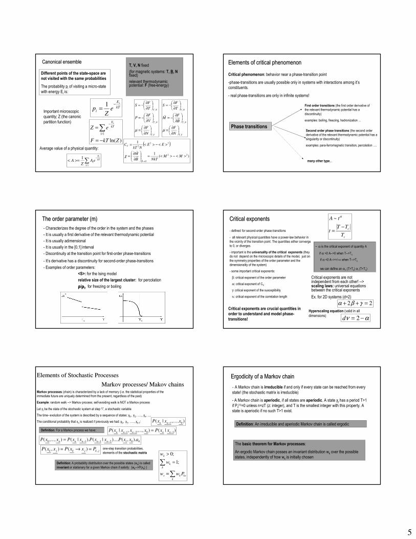
Canonical ensembleCanonical ensembleT, V, N fixed
(for magnetic systems: T, B, Nfixed)
relevant thermodynamic potential: F (free-energy)
Different points of the state-space are
not visited with the same probabilities
The probability pi of visiting a micro-state
with energy Ei is:
kT
E
i
i
eZ
p−
=1
Important microscopic
quantity; Z (the canonic
partition function)
)ln(
ZkTF
eZi
kT
Ei
−=
=∑−
VT
NT
NV
N
F
V
FP
T
FS
,
,
,
∂
∂=
∂
∂−=
∂
∂−=
µVT
NT
NV
N
F
B
FM
T
FS
,
,
,
∂
∂=
∂
∂−=
∂
∂−=
µ
rr
( )
)(1
1
22
0
22
2
><−><=
∂
∂=
><−><=
→
MMNkTB
M
EENkT
C
B
V
r
r
r
χ
Average value of a physical quantity:
kT
E
i
i
i
eAZ
A−
∑>=<
1
Elements of critical phenomenonElements of critical phenomenon
Critical phenomenon: behavior near a phase-transition point
-phase-transitions are usually possible only in systems with interactions among it’s
constituents.
- real phase-transitions are only in infinite systems!
Phase transitions
First order transitions (the first order derivative of
the relevant thermodynamic potential has a
discontinuity)
examples: boiling, freezing, hadronization ...
Second order phase transitions (the second order
derivative of the relevant thermodynamic potential has a
singularity or discontinuity)
examples: para-ferromagnetic transition, percolation ….
many other type...
The order parameter (m)The order parameter (m)
- Characterizes the degree of the order in the system and the phases
- It is usually a first derivative of the relevant thermodynamic potential
- It is usually adimensional
- It is usually in the [0,1] interval
- Discontinuity at the transition point for first-order phase-transitions
- It’s derivative has a discontinuity for second-order phase-transitions
- Examples of order parameters:
<S>: for the Ising model
relative size of the largest cluster: for percolation
ρρρρ/ρρρρ0: for freezing or boiling
Critical exponentsCritical exponents
- defined for second-order phase-transitions
- all relevant physical quantities have a power-law behavior in
the vicinity of the transition point. The quantities either converge
to 0, or diverges.
- important is the universality of the critical exponents (they
do not depend on the microscopic details of the model, just on
the symmetry properties of the order parameter and the
dimensionality of the system)
- some important critical exponents:
β: critical exponent of the order parameter
α: critical exponent of CV
γ: critical exponent of the susceptibility
υ: critical exponent of the correlation length
c
c
T
TTt
tA
−=
α~
- α is the critical exponent of quantity A
if α >0 A-->0 when T-->Tc
if α <0 A-->+/-∞ when T-->Tc
we can define an α+ (T>Tc) α- (T<Tc)
Critical exponents are not independent from each other! -->scaling laws: universal equations between the critical exponents
Ex. for 2D systems (d=2)
22 =++ γβαCritical exponents are crucial quantities in
order to understand and model phase-
transitions!
Hyperscaling equation (valid in all
dimensions) αν −= 2d
Elements of Stochastic ProcessesElements of Stochastic Processes
Markov processes/ Markov processes/ MakovMakov chainschainsMarkov processes (chain) is characterized by a lack of memory (i.e. the statistical properties of the
immediate future are uniquely determined from the present, regardless of the past)
Example: random walk --> Markov process; self-avoiding walk is NOT a Markov process
Let xi be the state of the stochastic system at step “i”, a stochastic variable
The time- evolution of the system is described by a sequence of states: x0, x1, ….., xn, ….
The conditional probability that xn is realized if previously we had: x0, x1, ….., xn-1: ),.....|( 01 xxxP nn −
Definition: For a Markov process we have: )|(),...,,|( 1021 −−− = nnnnn xxPxxxxP
0012110 ).,()....|().|(),...,( axxPxxPxxPxxP nnnnn −−−=
jkjkjk PxxPxxP ,)(),( =→= one-step transition probabilities,
elements of the stochastic matrix
Definition: A probability distribution over the possible states (wk) is called
invariant or stationary for a given Markov chain if satisfy: wk-->P(xk)
ks
k
ks
k
k
k
Pww
w
w
∑
∑
=
=
>
;1
;0
ErgodicityErgodicity of a Markov chainof a Markov chain
- A Markov chain is irreducible if and only if every state can be reached from every
state! (the stochastic matrix is irreducible)
- A Markov chain is aperiodic, if all states are aperiodic. A state xi has a period T>1
if Pii(n)=0 unless n=zT (z: integer), and T is the smallest integer with this property. A
state is aperiodic if no such T>1 exist.
Definition: An irreducible and aperiodic Markov chain is called ergodic
The basic theorem for Markov processes:
An ergodic Markov chain posses an invariant distribution wk over the possible
states, independently of how wk is initially chosen

6
Brownian DynamicsBrownian Dynamics
- It is a hybrid method, involving both deterministic and stochastic dynamics
- in molecular dynamics methods all degrees of freedom were explicitly taken into account --> classical
equation of motion of particles
- in Brownian dynamics some degrees of freedom are represented only through their stochastic influence
- we study Brownian dynamics in canonical ensemble. Basic idea: The effect of the constant temperature
heat-bath --> by a stochastic force-field acting on the particles.
- in Brownian dynamics simulation methods the system is described by stochastic differential equations. For
example the equation of motion of a particle making a Brownian motion:
vtRdt
dvm µ−= )( Langevin equation of motion, stochastic equation of motion. The coupling to the
heat bath is realized through the R(t) stochastic force.
Question: What properties should R(t) have, in order to be equivalent with a heat-
bath at temperature T?
- we are looking for R(t), that will lead for v the classical invariant Maxwell-Boltzmann distribution, expected in
canonical ensemble.
- let us work in 1D!
- by using the theory of stochastic processes and Markov chains, it can be shown, that this is achieved when:
)(2)0()(
0)(
/
)2/exp()2()(
2
222/12
tTkRtR
tR
hTkR
RRRRP
B
B
δµ
µ
π
>=<
>=<
>=<
><−><= − h: is the time-step for numerically integrating the equation of motion.
This choice of R(t) leads to:
Tk
mv
B
BeTk
mvP
2
2
2)(
−
=π
Algorithm for simulating the Brownian dynamics:
1. Assign initial position and velocity for the particle
2. Draw a random number from a Gaussian distribution with mean zero and
variance as described above. This will give us R(t).
3. Integrate the equation of motion with the obtained value of R, and get the
new positions and velocities.
4. Proceed with step 2.
Another way of doing Brownian dynamics:Another way of doing Brownian dynamics:
- by taking into account the coupling of the system to the heat-bath by “statistical” collisions with
virtual particles. In this approach no friction is necessary.
- each stochastic collision is assumed to be an instantaneous event
- the colliding virtual particles have a Maxwell-Boltzmann momentum distribution
- The time intervals at which particle suffers a collision is distributed according to
(λ is the mean collision time)tetP λλ −=)(
Algorithm II. for making Brownian Dynamics:
1. Get initial position and velocity for the particle
2. Choose time intervals according to the above distribution
3. Integrate the equations of motion until the time of a stochastic collision.
4. Choose a momentum at random from the Maxwell-Boltzmann distribution at
temperature T.
5. Proceed with step 3
ExercisesExercises
1. Prove by computer simulations that the given recipe for R(t) leads to a Maxwell-
Boltzmann distribution of the particles velocities (in 1D)
2. Study the motion of a particle in a harmonic potential and subject to a heat-bath
at temperature T. (in 1D)
3. Study the motion of a particle in a W potential valley, in contact with a heat-bath
at temperature T. Both parts of the W potential valley are harmonic.(in 1D)
4. Study problem nr. 3 when the two minimum of the W potential valley is
modulated in anti-phase by a time-like harmonic component. Calculate the
correlation function between the particle’s position and the external modulating
field. (1D case) (the phenomenon of stochastic resonance)
The Monte Carlo methodThe Monte Carlo method
Definition: Monte Carlo methods use random sequence of
numbers to calculate statistical estimates on a sample
population for a desired parameter
known examples: calculating PI, calculating percolation thresholds ..
other examples: calculating average magnetization and energy for the Ising model
in general: applications are enormous and fascinating ….
The outline of MC methods:
1. Description of the system in terms of a Hamiltonian
2. Selecting an appropriate ensemble for the problem
3. Observables are computed using an associated distribution
function. Ultimately the goal is to compute quantities appearing
as results of high-dimensional integrations on the state-space.
The idea is to sample the main contributions to get an estimate
for the observable.
Starting point: one dimensional Monte Carlo integration
One dimensional Monte Carlo integrationOne dimensional Monte Carlo integration
Problem: given a function f(x), compute the integral: ∫=b
a
dxxfI )(
The integral I can be computed by choosing n points (xi) randomly on the [a,b] interval,
and with a uniform distribution:
∑=
−=
n
i
ixfn
abI
1
)(Straightforward sampling
The strong law of large numbers guarantees us that for a sufficiently large sample one can come arbitrary
close to the desired integral!
Let x1,x2,…,xn be random numbers selected according
to a normalized probability density µ(x), then :
(!) the above affirmation is also true if the
random numbers are correlated, or the interval is finite
1)(1
lim
;)()(
1
=
=
=
∑
∫
=∞→
∞
∞−
Ixfn
P
dxxxfI
n
i
in
µ
How rapidly the method converge? --> for µ(x)= const. very badly!!!
Central limit theorem: if:
then:
∫∞
∞−
−= 222 )()( Idxxxf µσ
)1
()2
exp(2|)(1
|2
1 nOdx
x
nIxf
nP
n
i
i +−=
≤− ∫∑
−=
ω
ω
πωσ

7
•For straightforward sampling (µ(x)= const.) the error ~ 1/n1/2 !!
•The error is dependent on the choice of f(x) and µ(x)! --> influencing σ
A better method for calculating ∫=b
a
dxxfI )( dxxpxp
xfI
b
a
)()(
)(∫=
We generate random x1,x2,…,xn points
according to the p(x) distribution
∫ =b
a
dxxp 1)(
∑=
=n
i i
i
xp
xf
nI
1 )(
)(1
The basic idea: If we choose p(x) as close as possible to:
we get σ-->0 and the method converges rapidly for small
values of n!!! ∫=
b
a
dxxf
xfxp
)(
)()(
Problem: The methods needs advance knowledge of I!
One way to overcome the problem is by guessing some p(x) functions, that mimics well
the behavior of f(x)!. The error is also considerably reduced!
importance sampling Sampling in the neighborhood where f(x)
is large!
Monte Carlo for statistical physics problemsMonte Carlo for statistical physics problems
xdxHfZ
xdxHfxAZ
A
)](([
)]([)(1
∫
∫
Ω
Ω
=
>=<We want to compute integrals like:
f(x)--> an appropriate ensemble distribution
x -->elements of the state-space
Ω--> the entire state-space
H(x)--> the Hamiltonian of the system
Very high dimensional integral which is
exactly computable only for a limited
number of problems!!!
Basic idea: to use the importance sampling for calculating these integrals
If in the MC integration we choose the states with
probability P(x)---->
∑
∑
=
−
=
−
>=<n
i
ii
n
i
iii
xHfxP
xHfxPxA
A
1
1
1
1
)]([)(
)]([)()(
By choosingZ
xHfxP
)]([)( = σ-->0 and thus the error-->0
)(1
1
∑=
>=<n
i
ixAn
AProblem: we still don’t know Z!
The Metropolis et al. idea...The Metropolis et al. idea...
An algorithm has to be derived that generates states according to the desired P(x)!
Basic idea: using a Markov chain, such that starting from an initial state x0 further states
states are generated which are ultimately distributed according to P(x)
For this Markov chain need to specify the W(x, x’) transition probabilities from state x to state
x’. In order that the limiting distribution be P(x) we need:
• 1. For all complementary pairs (S,S’) of sets of phase points there exist x∈S and x’∈S’
such that W(x,x’)≠0 (ergodicity)
• 2. For all x, x’: W(x,x’)≥0
• 3. For all x :
• 4. For all x : (existence of the limiting distribution)
1)',('
=∑ xxWx
)()'()',('
xPxPxxWx
=∑
Instead of 4. A stronger but simpler condition can be used, the so called detailed
balance: )'(),'()()',( xPxxWxPxxW =
Result: We can construct Markov chains leading to the desired P(x) distribution,
without the prior knowledge of Z !!!
])(
exp[)]([Tk
xHxHf
B
−∝Example: the canonical ensemble:
Metropolis dynamics:
W(x, x’)=exp[-∆E(x, x’)/kBT] if ∆E(x, x’)>0;
W(x, x’)=1 if ∆E(x, x’)<0 ∆E(x, x’)=H(x’)-H(x)
Glauber dynamics:
W(x, x’)=exp[-∆E(x, x’)/kBT] /1+ exp[-∆E(x, x’)/kBT]
∆E(x, x’)=H(x’)-H(x)
Detailed balance
satisfied
Algorithm for Monte Carlo simulations:
1. Specify an initial point x0 in the phase space
2. Generate a new state x
3. Compute the W(x, x’) transition probability
4. Generate a uniform random number r between [0,1].
5. If r<W --> jump to the new state, and return to 2.
If r>=W --> count the old state as new and return 2.
6. Average the desired A quantity on all states after the initial N>>1 “transient” states
The The IsingIsing modelmodel
1
,
±=
−−= ∑∑><
i
i
ij
ji
i
S
SBSSJH µ
Interaction with nearest neighbors
only!
- In 1D and 2D exactly solvable!
- Due to the local interactions calculating Z is difficult.
- exact solution very difficult in 2D
- No exact solution in 3D
- Approximation methods: mean-field theory,
renormalization, high and low temperature expansion
- spontaneous magnetization is possible (M≠0 for B=0)
- first model for understanding ferro-and anti-ferromagnetism for localized spins
- for J>0 --> ferromagnetic order
- for J<0 --> anti-ferromagnetic order
- no phase transition in 1D
- ferro-paramagnetic phase transition for D>1
- second order phase transition (order-disorder)
Order parameter:N
MSm
|||| =><=
Tc T
m
Important quantities
- m(T) curve
- Tc
- the critical exponent of susceptibility(γ), order parameter(β), specific heat(α) and correlation length(υ)
Exact results:
(1D) Tc=0;
(2D) Tc=2.26918J/kB (square lattice); β=1/8; α=0
(logartihmic divergence!); γ=7/4; υ=1
(3D) no exact results (believed that:
Tc= 4.44 J/kB (square lattice); α=1/8; β=5/16; γ=5/4;
υ=5/8)

8
The transfer matrix solution to the 1D The transfer matrix solution to the 1D IsingIsing chainchain
0=N 1 2 3 4 N N+1=1
( )∑ ∑ ∑= = =
++++−=−+−=
N
i
N
i
N
i
iih
iiJihiiJH1 1 1
)1()(2
)1()()()1()( σσσσσσσ
( ) ( )
)ˆ()1(|ˆ|)1()1(|ˆ|)(...)3(|ˆ|)2(.)2(|ˆ|)1(
)1()(2
)1()(exp)1()(2
)1()(exp...
)1()(
)( 111)1( 1)(
NN
i
i
N
i
N
iN
PTrPNPNPPZ
iih
iiJiih
iiJZ
∑∑
∑ ∏∑∑ ∑
>=<>=+<><><=
++++=
++++=
==±= ±=
σσ
σσ σ
σσσσσσσσ
σσσσβσσσσβ
>=−
>=
1
01|
0
11|
−−
−+=
)](exp[)exp(
)exp()](exp[ˆ
hJJ
JhJP
ββ
ββ NNNPTrZ 21)ˆ( λλ +==
λ1,2 the eigenvalues of P!
)ln()ln()ln( 121 λλλ TNkTkZTkF B
NN
BB −≈+−=−=when N→∞ and
λ1>λ2
JJJ
B eJeJeTNkFβββ ββ 222 )(sinh)cosh(ln −++−=
Exact results in 1D:Exact results in 1D:Jeh
h
h
F
Nim
ββ
βσ
42 )(sinh
)sinh(1)(
−+=
∂
∂−>==<
For h=0: [ ] ξβσσj
jeJjii
−
=>=+< )tanh()()(
ξ the correlation length
( )[ ] 1)tanh(ln
−−= Jβξ
no phase transition at T>0 !!! (Tc=0)
For T→0 we have that ξ→∞
The meanThe mean--field approximation of the field approximation of the IsingIsing modelmodel
<S>
ii SBSqJH )( µ+><−=
The interaction between the
spins is de-coupled!
)(
)cosh(2])(exp[
BSJqx
xeeSBSJqZ xx
S
ii
i
µβ
µβ
+><=
=+=+><= −∑
)tanh()(1
)1(1 xeeZ
PPS xx
i
i =−=−+>=< −−+
)](tanh[ BSJqS µβ +><>=<An implicit equation for
<S>
for B=0Jqt
StS
β=
><>=< )tanh(
a graphical solution:
• for t<=1 the only possible solution: <S>=0 -->paramagnetic behavior
• for t>1two solutions;<S>=0 (unstable solution) and <S> > 0 (stable solution) -->
ferromagnetic behavior
• t=1 the critical point --> B
ck
JqT =
on the square lattice q=4;
on the cubic lattice q=6;
…..
in the neighborhood of Tc (T<Tc):2
1
2
3
13
−
>=<
T
T
T
TS c
c
results of mean-field approach
Tc= 4 J/kB (square lattice) , exact: 2.2692 J/kB
=6 J/kB (cubic lattice), believed 4.44 J/kB
=2 J/kB (Ising chain), exact: 0!
ββββ=1/2; exact 2D: 1/8; believed 3D: 0.31
αααα=0; exact 2D: 0; believed 3D: 0.12
γγγγ=1; exact 2D: 7/4; believed 3D: 1.25
υυυυ=1/2; exact 2D: 1; believed 3D: 0.64
-as the dimensionality of the problem increase, mean-field
approaches become better and better!
- mean-field is totally wrong in 1D !!
Implementing the Metropolis and Implementing the Metropolis and GlauberGlauber Monte Carlo for Monte Carlo for
the 2D the 2D IsingIsing modelmodel
Problem: Study <m(T)>, <E(T)>, <Cv(T)> <χ(T)> and Tc for 2D Ising models by using the Metropolis or Glauber algorithm.
We consider B=0, and fix J=1. The units are considered that kB=1.
1
,
±=
−= ∑><
k
j
ji
i
S
SSH -Let us assume a lattice N x N with free boundary conditions
-We consider a canonical ensemble and fix thus N and T
We would like to calculate:
222)(
N
S
N
S
N
MTm
i
i
i
i ∑∑==>=<
><−>=>=<< ∑><
j
ji
ii SSSHTE,
)()(
[ ]22
2)()(
1)( ><−><>=< TETE
TNkTC
B
v
[ ]22 )()(1
)( ><−><>=< TMTMNkT
Tχ
Tc will be determined from the maxima of
<Cv(T)> and <χ(T)>

9
In order to get the desired quantities we have to calculate the following NxN
dimensional sums (integrals):
∑ ∑∑
−
>=>=<<
)(exp
1)(
iS B
i
i
i
i
iTk
SH
ZSSTM
∑ ∑∑
−
>=>=<<
2
22 )(exp
1)()(
iS B
i
i
i
i
iTk
SH
ZSSTM
∑ ∑∑
−
−>=<−>=<
><>< ,,
)(exp
1)(
iS B
i
ji
ji
ji
jiTk
SH
ZSSSSTE
∑ ∑∑
−
>=>=<<
><><
2
,,
22 )(exp
1)()(
iS B
i
ji
ji
ji
jiTk
SH
ZSSSSTE
We will use the Metropolis MC method to calculate these sums (integrals)!
The algorithm (Metropolis and The algorithm (Metropolis and GlauberGlauber MC for the MC for the IsingIsing model):model):
1. Fix a given temperature
2. Fix an initial spin configuration (x)
3. Calculate the initial value of E and M
4. Consider a new spin configuration by virtually “flipping” one randomly selected spin (x’)
5. Calculate the energy E’ of the new configuration, and the energy change due to this spin-flip
6. Calculate the Metropolis (Glauber) W(x-->x’) probabilities for this move
7. Generate a random number “r” between 0 and 1
8. If r<=W(x-->x’) accept the flip and update the value of the energy to E’ and magnetization to M’
9. Repeat the steps 4 - 8 many times (drive the system to the desired canonical distribution of the states)
10. Repeat the steps 4 -8 by collecting the values of E, E2, M, M2, and calculate their average
11. Compute this average for a large number of steps
12. Calculate the value of <m(T)>, <E(T)>, <Cv(T)> and <χ(T)> by the given formulas
13. Change the temperature and repeat the algorithm for the new temperatures as well.
14. Construct the desired <m(T)>, <E(T)>, <Cv(T)>, <χ(T)> curves
writing the code--> see the computer code
A simple 2D Glauber dynamics code
Variation of <m(T)> as a function of T for different system sizes Variation of <Cv(T)> as a function of T for various system sizes
Variation of <χ(T)> as a function of T for various system sizes Estimates for Tc for various system sizes (step in T is 0.1)

10
Important observations:
• the considered W(x-->x’) transitions leads to an ergodic Markov process
• one MC step is defined as N x N spin flip trials !
• By applying the above algorithm for T<Tc one can also follow how the order arises in
the system. This dynamics might not necessarily be the “real one”. The Metropolis MC
method is intended to yield equilibrium properties and not dynamical simulation of the
system!
•It is believed that the Glauber transition probabilities gives a realistic picture for the
dynamics as well!
•Influence of finite lattice size is strong --> finite size effects (finite lattice size cuts the
correlation length!, no real phase transitions, and no real divergences!) --> important
problem of scaling: get the desired quantities for the N--> ∞ limit.
•One way of making the system quasi-infinite is to impose periodic boundary
conditions. (see the exercise in the computer codes!)
The BKL Monte Carlo (or: kinetic MC, or resident time MC) methodThe BKL Monte Carlo (or: kinetic MC, or resident time MC) method
Used for:
- computing quickly equilibrium properties at low
temperatures in the Metropolis or Glauber algorithm
- simulating jump-like stochastic processes with
exp(-c ∆E) type activation probability.
examples: - diffusion of atoms on crystal substrates
- grain growth process
- dynamics of defects in crystals
- dynamics of spins at low temperature
Reference: Bortz, Kalos,
Lebowitz; J. Computational
Physics, vol. 17, pp. 10
(1975)
Difficulties that are solved by the BKL method:
1. The Metropolis and Glauber dynamics is very ineffective at low temperatures where exp(-
β∆E)<<1 !! (too many rejected steps, where nothing is changed in the system)
(at low temperatures usually ∆E and β are both big!)
2. For jump-like stochastic processes the Glauber and Metropolis dynamics is also ineffective
due to the largely different time-scales that are present in real problems
(more concrete examples in this sense later ….)
The BKL method for low temperature The BKL method for low temperature IsingIsing systemssystems
- When we want to compute the specific heat or the susceptibility at low temperatures we need to follow
the fluctuation of the energy or magnetization for many MC steps
- At low temperature the Metropolis or Glauber algorithm is very ineffective since the system most of the
time waits…and nothing happens.
- A quick solution: make a transition at each flip-attempt and update the “resident time”of each state
(needed in the average) according to the probability of each transition.
- We give now the algorithm and make the theoretical basis later.
1. Set the time t=0.
2. Form a list of the Metropolis or Glauber rates ri (probabilities) for all the possible W(x-->x’) transitions (spin flips) in the system.
3. Calculate the cumulative function for I=1,2……N, where N is the total
number of possible transitions in the system (let R=RN)
4. Get a uniform random number u∈[0,1).
5.Find the event i to carry out by finding the value of i for which
6. Carry out event i.
7. Recalculate all ri values that might have been changed due to the transition
8. Get a new uniform random number u∈[0,1).
9. Update the time (simulation step, or weight in the average) by t=t+∆t where ∆t=-log(u)/R
10. return to step 2.
∑=
=i
j
ji rR1
ii RuRR ≤<−1
Motivation for the basic algorithmMotivation for the basic algorithm
- Let us presume we have a system with 3 possible transitions:
w(1) --> with rate (probability) r1=0.1; w(2) --> with rate (probability) r2=0.5
w(3) ---> with rate (probability) r3=0.5
- In the basic Metropolis (or Glauber) algorithm we make the transitions by attempts with the
given probabilities. The probability to choose a given transition from the possible three transition
is proportional to the values of ri.
- With r1, r2, and r3 we get the cumulative functions R1, R2 and R3:
R1=r1=0.1; R2=r1+r2=0.6; R3=r1+r2+r3=1.1
- We can plot now the values of ri as regions, and Ri as points on a line as follows
r 1 r2 r3
0 R1=0.1 R2=0.6 R3=1.1- If we generate a random number u∈[0,1) and multiply it by R3=1.1, this will correspond to one
point on the line. The probability to get transition w(2) will be proportional with the distance between
R1 and R2, which is r2/R--> this is what we wanted to do!
- At each simulation step we make than a transition, and the rates at which different transitions
occur is the desired one!
Problem: how to update the “time” in order to get the good values of the averages
Motivation for the equation of timeMotivation for the equation of time
-It is easy to determine the fi(t) probability density, that the transition wi with rate ri didn’t occurred up to time t:
dttfrtdf iii )()( −= )exp()( trCtf ii −=
The C=1 constant results from the f(0)=1condition )exp()( trtf ii −=
- the individual transitions form a Poisson process, i.e. the probability to have a transition in a time dt is linearly
proportional with the length of the interval dt.
- a useful feature of Poisson processes is that a large number N of Poisson processes, with rates ri, will behave as
another large Poisson process with properties similar to the single processes. --> denoting by F(t) the probability
that no wi transition occurs up to time t, we get:
)exp()( RttF −= with ∑=i
irR The probability to have the first transition
between time t t∈[0,∞) and t+dt is
dtRtRdtdt
tdFdttgdttP )exp(
)()()( −⋅=−==+In order to have time steps satisfying this probability
distribution,we need to generate thus q random
numbers according to the g(t)=R exp(-Rt) distribution!
This can be done with the known method, after
generating uniformly distributed u random numbers
(see random number generators): R
u
R
uq
)'ln()1ln(−=
−−=
Simulating dynamic processesSimulating dynamic processes
1. Simulating grain-growth by using a T=0 temperature Potts- model
(a trivial application)
Grain-growth in metals: growth of the size of the mono-crystalline domains. Small domains are
“eated up” by larger ones, the grain-boundary moves.Experimentally observed that the <d>
mean-grain size increases as: 2/12 ))0((~)( atdtd +><><The Potts model:
qi
qHji
ji
,....2,1)(
,
)(),(
=
−= ∑><
σ
δ σσ
- we use a square or triangular lattice
- we start with a large q number of initial states
- each lattice site will have a randomly chosen Potts
variable
- Make a Metropolis or Glauber dynamics at T=0
(accept only steps that do NOT increase the energy of
the system)
11
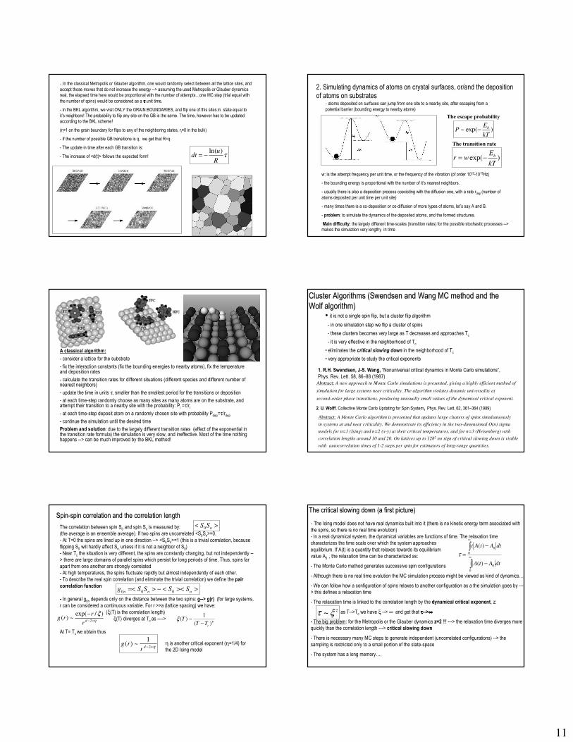
- In the classical Metropolis or Glauber algorithm, one would randomly select between all the lattice sites, and
accept those moves that do not increase the energy --> assuming the used Metropolis or Glauber dynamics
real, the elapsed time here would be proportional with the number of attempts…one MC step (trial equal with
the number of spins) would be considered as a ττττ unit time.
- In the BKL algorithm, we visit ONLY the GRAIN BOUNDARIES, and flip one of this sites in state equal to
it’s neighbors! The probability to flip any site on the GB is the same. The time, however has to be updated
according to the BKL scheme!
(ri=1 on the grain boundary for flips to any of the neighboring states, ri=0 in the bulk)
- If the number of possible GB transitions is q, we get that R=q.
- The update in time after each GB transition is:
- The increase of <d(t)> follows the expected form! τR
udt
)ln(−=
2. Simulating dynamics of atoms on crystal surfaces, or/and the deposition
of atoms on substrates- atoms deposited on surfaces can jump from one site to a nearby site, after escaping from a
potential barrier (bounding energy to nearby atoms)
The escape probability
)exp(~kT
EP b−
The transition rate
)exp(kT
Ewr b−=
w: is the attempt frequency per unit time, or the frequency of the vibration (of order 1012-1013Hz)
- the bounding energy is proportional with the number of it’s nearest neighbors.
- usually there is also a deposition process coexisting with the diffusion one, with a rate rdep (number of
atoms deposited per unit time per unit site)
- many times there is a co-deposition or co-diffusion of more types of atoms, let’s say A and B.
- problem: to simulate the dynamics of the deposited atoms, and the formed structures.
Main difficulty: the largely different time-scales (transition rates) for the possible stochastic processes --> makes the simulation very lengthy in time
A classical algorithm:
- consider a lattice for the substrate
- fix the interaction constants (fix the bounding energies to nearby atoms), fix the temperature and deposition rates
- calculate the transition rates for different situations (different species and different number of nearest neighbors)
- update the time in units τ, smaller than the smallest period for the transitions or deposition
- at each time-step randomly choose as many sites as many atoms are on the substrate, and attempt their transition to a nearby site with the probability: Pi =τ/ri- at each time-step deposit atom on a randomly chosen site with probability Pdep=τ/rdep
- continue the simulation until the desired time
Problem and solution: due to the largely different transition rates (effect of the exponential in the transition rate formula) the simulation is very slow, and ineffective. Most of the time nothing happens --> can be much improved by the BKL method!
Cluster Algorithms (Cluster Algorithms (SwendsenSwendsen and Wang MC method and the and Wang MC method and the
Wolf algorithm)Wolf algorithm)• it is not a single spin flip, but a cluster flip algorithm
- in one simulation step we flip a cluster of spins
- these clusters becomes very large as T decreases and approaches Tc
- it is very effective in the neighborhood of Tc
• eliminates the critical slowing down in the neighborhood of Tc
• very appropriate to study the critical exponents
Abstract: A new approach to Monte Carlo simulations is presented, giving a highly efficient method of
simulation for large systems near criticality. The algorithm violates dynamic universality at
second-order phase transitions, producing unusually small values of the dynamical critical exponent.
1. R.H. Swendsen, J-S. Wang, “Nonuniversal critical dynamics in Monte Carlo simulations”,
Phys. Rev. Lett. 58, 86–88 (1987)
Abstract: A Monte Carlo algorithm is presented that updates large clusters of spins simultaneously
in systems at and near criticality. We demonstrate its efficiency in the two-dimensional O(n) sigma
models for n=1 (Ising) and n=2 (x-y) at their critical temperatures, and for n=3 (Heisenberg) with
correlation lengths around 10 and 20. On lattices up to 1282 no sign of critical slowing down is visible
with autocorrelation times of 1-2 steps per spin for estimators of long-range quantities.
2. U. Wolff, Collective Monte Carlo Updating for Spin System, Phys. Rev. Lett. 62, 361–364 (1989)
SpinSpin--spin correlation and the correlation lengthspin correlation and the correlation length
The correlation between spin S0 and spin Sn is measured by:
(the average is an ensemble average). If two spins are uncorrelated <S0Sn>=0.
- At T=0 the spins are lined up in one direction --> <S0Sn>=1 (this is a trivial correlation, because
flipping S0 will hardly affect Sn, unless if it is not a neighbor of S0)
- Near Tc the situation is very different, the spins are constantly changing, but not independently --
> there are large domains of parallel spins which persist for long periods of time. Thus, spins far
apart from one another are strongly correlated
- At high temperatures, the spins fluctuate rapidly but almost independently of each other.
- To describe the real spin correlation (and eliminate the trivial correlation) we define the pair
correlation function
- In general g0n depends only on the distance between the two spins: g--> g(r) (for large systems,
r can be considered a continuous variable. For r >>a (lattice spacing) we have:
(ξ(T) is the correlation length)
ξ(T) diverges at Tc as ---->
At T= Tc we obtain thus
>< nSS0
>><<−>=< nnn SSSSg 000
η
ξ+−
−2
)/exp(~)(
dr
rrg
υξ
)(
1~)(
cTTT
−
η+−2
1~)(
drrg η is another critical exponent (η=1/4) for
the 2D Ising model
The critical slowing down (a first picture)The critical slowing down (a first picture)
- The Ising model does not have real dynamics built into it (there is no kinetic energy term associated with
the spins, so there is no real time evolution)
- In a real dynamical system, the dynamical variables are functions of time. The relaxation time
characterizes the time scale over which the system approaches
equilibrium. If A(t) is a quantity that relaxes towards its equilibrium
value A0 , the relaxation time can be characterized as:
- The Monte Carlo method generates successive spin configurations
- Although there is no real time evolution the MC simulation process might be viewed as kind of dynamics…
- We can follow how a configuration of spins relaxes to another configuration as a the simulation goes by ---
> this defines a relaxation time
- The relaxation time is linked to the correlation length by the dynamical critical exponent, z:
as T-->Tc we have ξ --> ∞ and get that ττττ-->∞∞∞∞
- The big problem: for the Metropolis or the Glauber dynamics z=2 !!! ---> the relaxation time diverges more
quickly than the correlation length ---> critical slowing down
- There is necessary many MC steps to generate independent (uncorrelated configurations) --> the
sampling is restricted only to a small portion of the state-space
- The system has a long memory….
∫
∫∞
∞
−
−
=
0
0
0
0
)(
)(
dtAtA
dtAtAt
τ
zξτ ~

12
The relaxation time in Metropolis MC simulations The relaxation time in Metropolis MC simulations ----> the autocorrelation time> the autocorrelation time
- The relaxation time in the Metropolis MC characterizes how many MC steps to skip in order to
generate statistically independent configurations.
- If the relaxation time is of the order of a single MC step, every configuration can be used in
measuring averages
- If the relaxation time is longer, than approximately τ MC steps should be discarded between every
point.
- to define a relaxation time we first define the autocorrelation function for a quantity A:
An it’s value at the MC step: n
- if this autocorrelation function decays exponentially
which defines the exponential correlation (relaxation) time (τexp)
- starting from the equalities from below one can suggest another correlation time:
2)( ><−>=< + nknnAAAAAkc
)/exp(~)( expτttcAA −
)0()0()(0
/
0
AA
t
AAAA cecdttc ττ == ∫∫∞
−∞
∑∞
=
+=1
int)0(
)(
2
1
k AA
AA
c
kcτ
ττττint:integrated correlation time;This is what we determine usually
in computer simulations
Critical slowing down (a second look)Critical slowing down (a second look)
- for finite lattices when T---> Tc we get ξ--> L (size of the lattice) ---> no real
divergence
- we get thus:
- for the Metropolis and Glauber dynamics z=2, and we get
(Metropolis, Glauber and BKL are local algorithms….)
and the simulation is very inefficient on large lattices (on small lattices on the other
hand there are important finite-size effects!)
- good news: the value of the dynamical critical exponent is NOT universal, it
depends on the MC algorithm (paper of Swendsen and Wang!)
- the problem: elaborate a MC method for which the value of the dynamical critical
exponent is smaller! --> these must be non-local algorithms!
zL~τ2
~ Lτ
Cluster algorithms:
- we flip together all correlated spins.
- in each flip we generate statistically independent configurations.
- the value of the dynamic exponent becomes as low as z=0.15 !
The The SwendsenSwendsen and Wang cluster algorithm for J>0 and Wang cluster algorithm for J>0 IsingIsing modelmodel
- the basic idea: is to identify the clusters of like and correlated spins and treat the clusters as a
giant spin, flipping it according to a random criterion.
- it is necessary that the algorithm should lead to an ergodic Markov process and the detailed
balance condition is satisfied!
- the algorithm can be generalized for arbitrary (J>0 or J<0) Potts models
Construction of the clusters of correlated spins:- the simple clusters of like nearest neighbor spins are NOT the clusters of correlated spins, these
are too large… (At T=∞ there are still spins with like orientation, although the correlation between
them in this case should vanish)
- the way of constructing the clusters of correlated spins, is to put a link between nearest neighbors
and like spins, with a probability p=1-exp(-2J/kBT).
Flipping the clusters:
- all the clusters are flipped with probability 1/2! (we assign a new common value, +/-1 to all spins in
the cluster)
- the spins in the whole lattice are in this manner updated!
- the algorithm satisfies detailed balance --> appropriate for important sampling
The Swendsen and Wang algorithm for the 2D Ising model:
1. consider a lattice of spins with size N x N
2. fix the parameters (T, J=1, kB=1)
3. consider an initial configuration of the spins
4. put “virtual bonds” with probability 1-exp(-2J/kBT) between nearest neighbor and like spins
5. construct the clusters of correlated spins
6. “flip” the clusters with probability 1/2 (this is one MC step)
7. get the new configuration of the spin system, and count it in the calculation of the desired
averages
8. Identify like nearest neighbor spins and repeat the algorithm starting from 4.
Main difficulty: --> the construction of the clusters of correlated spins
need of clever and fast cluster identification algorithms
An example code --> program nr. ???? (identification of clusters with recursion)
The Wolff single cluster algorithmThe Wolff single cluster algorithm
- even more efficient than the S-W algorithm
- difference: constructing and flipping only one cluster at a time!
- the way of constructing the correlated spins cluster is the same as in the S-W algorithm
The basic of the Wolff algorithm:
- choose a spin randomly in the lattice
- construct the cluster of correlated spins starting from this spin as a “seed”, by connecting
nearest neighbor and like spins with a probability p=1-exp(-2J/kBT). Do this process
recursively until the cluster cannot grow more.
- flip this cluster of correlated spins (this will be one MC step)
- update the time proportionally with the number of flipped spins
- count the new configuration in the average of the desired quantities
- The Wolff algorithm is more effective, because we construct only one cluster an always flip it, +
the probability to choose a cluster is proportional with the size of the cluster --> we will usually flip
bigger clusters --> we generate statistically independent configurations!
- An example program is given as code nr. ?????
- A simple visual program to compare the effectiveness of the Metropolis, BKL and Wolff algorith,:
LMC.exe
The Histogram Monte Carlo techniqueThe Histogram Monte Carlo technique
Idea: During normal Metropolis or SW Monte Carlo procedures a big quantity of information is lost!!! ( we
calculate only the averages <E>, <E2>, <M> and <M2>
- the distribution functions f(E) and g(M) can be however also be obtained, and they carry a lot of important
statistical information
- with the knowledge of f(E) and g(M) at a temperature T we can then calculate averages at other
temperatures WITHOUT making ANY additional simulations at the desired temperature.
),()(
),()(
dMMMPdMMg
dEEEPdEEf
+=
+=
Basics of the methodBasics of the method
Let P(Ei-∆E/2,Ei+∆E/2,T0) be the probability to get in the equilibrium configuration at temperature T0,
energies between Ei-∆E/2 and Ei+∆E/2
(corresponding to the used canonical ensemble)
D(Ei) is the density of states in the neighborhood of Ei (independent of temperature)
During the MC simulation at temperature T0 we cn construct a histogram characterizing P(Ei-
∆E/2,Ei+∆E/2,T0).
ETk
EED
TZETEfT
EE
EEP
B
iiiii ∆−=∆=
∆−
∆+ )exp()(
)(
1),(),
2,
2(
0
00
∑=
∆+
∆+
i
i
iii
TEh
TEhT
EE
EEP
),(
),(),
2,
2(
0
00
Where h(Ei,T0) is the number of spin configurations with
energy in the Ei-∆E/2 and Ei+∆E/2 interval
A.M. Ferrenberg, R.H. Swendsen; Phys. Rev. Lett., vol. 61, 2635 (1988)
13
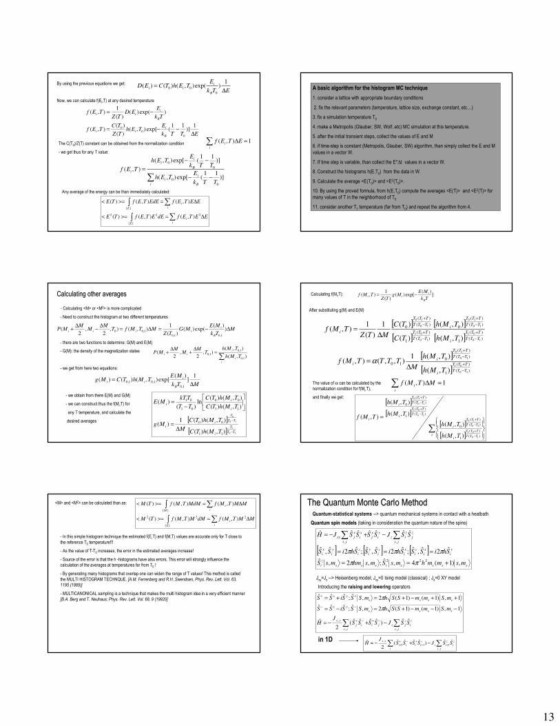
By using the previous equations we get:
Now, we can calculate f(Ei,T) at any desired temperature
ETk
ETEhTCED
B
iii
∆=
1)exp(),()()(
0
00
ETTk
ETEh
TZ
TCTEf
Tk
EED
TZTEf
B
iii
B
iii
∆−−=
−=
1)]
11(exp[),(
)(
)(),(
)exp()()(
1),(
0
00
The C(T0)/Z(T) constant can be obtained from the normalization condition
- we get thus for any T value:
∑ =∆i
i ETEf 1),(
∑ −−
−−
=
i B
ii
B
ii
i
TTk
ETEh
TTk
ETEh
TEf
)]11
(exp[),(
)]11
(exp[),(
),(
0
0
0
0
Any average of the energy can be than immediately calculated:
∫ ∑
∫ ∑
∆=>=<
∆=>=<
222
),(),()(
),(),()(
E i
i
E i
i
EETEfdEETEfTE
EETEfEdETEfTE
A basic algorithm for the histogram MC technique
1. consider a lattice with appropriate boundary conditions
2. fix the relevant parameters (temperature, lattice size, exchange constant, etc…)
3. fix a simulation temperature T0
4. make a Metropolis (Glauber, SW, Wolf..etc) MC simulation at this temperature.
5. after the initial transient steps, collect the values of E and M
6. if time-step is constant (Metropolis, Glauber, SW) algorithm, than simply collect the E and M
values in a vector W.
7. If time step is variable, than collect the E*∆t values in a vector W.
8. Construct the histograms h(E,T0) from the data in W.
9. Calculate the average <E(T0)> and <E2(T0)>.
10. By using the proved formula, from h(E,T0) compute the averages <E(T)> and <E2(T)> for
many values of T in the neighborhood of T0
11. consider another T1 temperature (far from T0) and repeat the algorithm from 4.
Calculating other averagesCalculating other averages
- Calculating <M> or <M2> is more complicated
- Need to construct the histogram at two different temperatures
- there are two functions to determine: G(M) and E(M)
- G(M): the density of the magnetization states
- we get from here two equations:
MTk
MEMG
TZMTMfT
MM
MMP
B
iiiii ∆−=∆=
∆−
∆+ )
)(exp()(
)(
1),(),
2,
2(
1,01,0
1,00
∑=
∆+
∆+
i
i
i
iiTMh
TMhT
MM
MMP
),(
),(),
2,
2(
1,0
1,0
1,0
MTk
METMhTCMg
B
iii
∆=
1]
)(exp[),()()(
1,0
1,01,0
- we obtain from there E(M) and G(M)
- we can construct thus the f(Mi,T) for
any T temperature, and calculate the
desired averages [ ]
[ ] 10
1
10
0
),()(
),()(1)(
),()(
),()(ln
)()(
11
00
11
00
01
01
TT
T
i
TT
T
ii
i
ii
TMhTC
TMhTC
MMg
TMhTC
TMhTC
TT
TkTME
−
−
∆=
−=
Calculating f(Mi,T): ])(
exp[)()(
1),(
Tk
MEMg
TZTMf
B
iii −=
After substituting g(M) and E(M)
[ ]
[ ]
[ ]
[ ] )(
)(
1
)(
)(
0
)(
)(
1
)(
)(
0
10
01
10
10
10
01
10
10
),(
),(
)(
)(1
)(
1),(
TTT
TTT
i
TTT
TTT
i
TTT
TTT
TTT
TTT
i
TMh
TMh
TC
TC
MTZTMf
−
+
−
+
−
+
−
+
∆=
[ ]
[ ] )(
)(
1
)(
)(
010
10
01
10
10
),(
),(1),,(),(
TTT
TTT
i
TTT
TTT
ii
TMh
TMh
MTTTTMf
−
+
−
+
∆= α
The value of α can be calculated by the
normalization condition for f(Mi,T),
and finally we get:
∑ =∆i
i MTMf 1),(
[ ]
[ ][ ]
[ ]∑
=
−
+
−
+
−
+
−
+
i TTT
TTT
i
TTT
TTT
i
TTT
TTT
i
TTT
TTT
i
i
TMh
TMh
TMh
TMh
TMf
)(
)(
1
)(
)(
0
)(
)(
1
)(
)(
0
10
01
10
10
10
01
10
10
),(
),(
),(
),(
),(
<M> and <M2> can be calculated than as:
∫ ∑
∫ ∑
∆=>=<
∆=>=<
222
),(),()(
),(),()(
E i
i
M i
i
MMTMfdMMTMfTM
MMTMfMdMTMfTM
- In this simple histogram technique the estimated f(E,T) and f(M,T) values are accurate only for T close to
the reference T0 temperature!!!
- As the value of T-T0 increases, the error in the estimated averages increase!
- Source of the error is that the h -histograms have also errors. This error will strongly influence the
calculation of the averages at temperatures far from T0 !
- By generating many histograms that overlap one can widen the range of T values! This method is called
the MULTI HISTOGRAM TECHNQUE. [A.M. Ferrenberg and R.H. Swendsen, Phys. Rev. Lett. Vol. 63,
1195 (1989)]
- MULTICANONICAL sampling is a technique that makes the multi histogram idea in a very efficient manner
[B.A. Berg and T. Neuhaus; Phys. Rev. Lett. Vol. 68, 9 (19920]
The Quantum Monte Carlo MethodThe Quantum Monte Carlo MethodQuantum-statistical systems --> quantum mechanical systems in contact with a heatbath
Quantum spin modelsQuantum spin models (taking in consideration the quantum nature of the spins)
[ ] [ ] [ ]ssssisss
z
i
y
i
x
i
z
i
x
i
z
i
y
i
z
i
y
i
x
i
ji
z
j
z
iz
y
i
y
j
ji
x
i
x
jxy
msmmhmsSmshmmsS
ShiSSShiSSShiSS
SSJSSSSJH
,)1(4,ˆ;,2,ˆ
ˆ2ˆ,ˆ;ˆ2ˆ,ˆ;ˆ2ˆ,ˆ
ˆˆˆˆˆˆˆ
222
,,
+==
===
−+−= ∑∑
ππ
πππ
Jxy=Jz --> Heisenberg model; Jxy=0 Ising model (classical) ; Jz=0 XY model
Introducing the raising and lowering operators
∑∑ −+−=
−−−+=−=
++−+=+=
−+−+
−−
++
ji
z
i
z
jzji
ji
ij
yx
ssss
yx
ssss
yx
SSJSSSSJ
H
mSmmSShmSSSiSS
mSmmSShmSSSiSS
,,
, ˆˆ)ˆˆˆˆ(2
ˆ
1,)1()1(2,ˆ;ˆˆˆ
1,)1()1(2,ˆ;ˆˆˆ
π
π
in 1D∑∑ +
−+
+−++ −+−=
ji
z
i
z
izii
i
ii
yxSSJSSSS
JH
,
111
, ˆˆ)ˆˆˆˆ(2
ˆ

14
The Hubbard modelThe Hubbard model
- many body hamiltonian in a second quantized form
- describes interacting electrons in the periodic potential of a lattice
- second quantization in Wannier states (quasi-localized) electron states on a given orbital and with
a given spin orientation at o given ion at position Rαααα
- Hamiltonian written with the creation (a+)
and destruction (a) operators, acting on
states described with occupational number
- interaction is strongly sceened by the
electron gas, thus it is restricted at the same
site
)](exp[1
ˆˆˆˆˆ
'',
,
,
,,
,',
,'',
αααα
σασα
σασασαα
σααα
ε RRkiV
t
nnUaatH
kk
rrr
r
r −=
+−=
∑
∑∑ −+
In 1D, and considering jumps only at nearest neighbor lattice sites, the hamiltonian becomes
σασα
σασασασασα
σα −+
+++ ∑∑ +++−= ,
,
,,,1,1
,
,ˆˆ)ˆˆˆˆ(ˆ nnUaaaatH
nαααα,σσσσ are the particle number operators in state (α,σ)
A lattice model for itinerant electrons in 1DA lattice model for itinerant electrons in 1D
ψψπ
ψ ExVm
hH =+∆−= )(
8ˆ
2
2
for 1 electron:
Discretizing it on a lattice with sites “a”--> L coupled linear equations (L.a=l; l the length of the
considered space);
ψI is the medium of ψ(x) in box “i”
Viis the medium of V(x) in box “i”
introducing “t” and “Wi” we get:
iiiiii EVma
hψψψψψ
π=+−+− −+ )2)(
8( 1122
2
iiiii
ii
EWt
ma
hVW
ma
ht
ψψψψππ
=++−
+==
−+ )(
4;
8
11
22
2
22
2
- the above equations can be written in a secon quantized form
state-vectors --> ni occupation numbers of the cells Li nnnn ,...,...,, 21
LiiLii
LiiLii
LiiLii
nnnnnnnnnn
nnnnnnnnnc
nnnnnnnnnc
,...,,...,,,...,...,ˆ
,...,1,...,,,...,...,ˆ
,...,1,...,,1,...,...,ˆ
2121
2121
2121
=
−=
++=+
[ ] i
i
i
i
iiii
i
L
i
i
nWcccctH
c
ˆˆˆˆˆˆ
0,...0,0ˆ
11
1
∑∑
∑
++−=
=
+++
+
+
=
ψψ
Considering more than one interacting electrons on the same lattice is possible by
considering extra terms. H0 is an on-site repulsion and H1is interaction between particles
in neighboring cells.
∑ −=i
ii nnVH )1ˆ(ˆˆ00 ∑ +=
i
iinnVH 111ˆˆˆ
Taking into account the spin of the particles --> by an additional discrete parameter
characterizing the projection of the spin
Basic idea for the QMC methodBasic idea for the QMC method
Transferring the d dimensional quantum-statistical problem in a d+1 dimensional classical
statistical physics problem
we consider the system in canonical ensemble
L
n
L nnnHnnnHTrZi
,...,,)ˆexp(,...,)]ˆ[exp( 21
21 ββ −=−= ∑
First possibility to tackle the problem: diagonalize H and consider after that the Metropolis
or other MC schemes for the resulted states
problem: if there are only 2 possible particles in each of the L possible cells --> we have to
diagonalize a 2LX2L matrix which is practically impossible for L>>1.
Second possibility: make a classical MC algorithm without diagonalization
- consider an ni0 initial configuration
- consider a possible new nif configuration
- accept the change ni0 --> ni
f with probability:
- continue the algorithm until the thermodynamic equillibrium is reached
- collect periodically the relevant data
problem: calculation of the matrix elements are VERY TIME CONSUMING and it is
not clear from the start which changes will yield reasonable transition probabilities!
00 )ˆexp()ˆexp(
)ˆexp(
ii
f
i
f
i
f
i
f
i
nHnnHn
nHnP
ββ
β
−+−
−=
Third possibility (wise solution): to rewrite Z in a form in which the calculation of the P
probabilities are easy when only a few ni numbers are changed.
- this is possible by the use of the Trotter-Suzuki approximation
The TrotterThe Trotter--Suzuki approximationSuzuki approximation
We consider the general form of the H hamiltonian:
and denote:
∑ ∑∑ ∑ ++++
+ +−+++−=i i
iiiii
i i
iiiii nnVnnVnWcccctH 11011ˆˆ)1ˆ(ˆˆ]ˆˆˆˆ[ˆ
∑ ∑∑ ++−+=i i
iiiii
i
ii nnVnnVnWV 110ˆˆ)1ˆ(ˆˆ
we divide H in two parts:ba HHH ˆˆˆ +=
22ˆˆˆˆˆ:;ˆ...ˆˆˆ
ˆ...ˆˆ)22
ˆˆˆˆ(...
...)22
ˆˆˆˆ()22
ˆˆˆˆ(ˆ
11142
1311
11
433443
211221
++++
+
−−
−++
−
++++
++−−=+++=
+++=++−−+
+++−−+++−−=
iiiiiiiLb
LLL
LLLL
a
VVcctcctHwhereHHHH
HHHVV
cctcct
VVcctcct
VVcctcctH
The terms inside Ha and Hb commute with each other, but: 0]ˆ,ˆ[ ≠ba HH
we can write thus:
)ˆexp(...)ˆexp(
)ˆexp()ˆexp(
13
1
jLiji
jijai
nHnnHn
nHnnHn
−−⋅⋅−⋅
⋅−=−
ββ
ββ
Ideal would be to do this for the whole H=Ha+Hb! This is not possible however, because Ha and
Hb do not commute and have terms acting on the same ni numbers.
- SOLUTION the Trotter-Suzuki (TS) approximation: if A and B are sufficiently SMALL operators:
BABABA
BA eeeeˆˆ]ˆ,ˆ[
2
1ˆˆˆˆ +
++
≈=⋅
Applying the TS approximation: if M>>1 (integer), so that βHa /M and βHb/M is small enough
we can write
)]ˆexp()ˆ[exp()]ˆˆ(exp[
i
M
ba
n
ii
M
ba
n
i nHM
HM
nnHHM
nZii
βββ−⋅−≈+−= ∑∑
To write Z as product of simple terms we insert 2M-1 complete sets of state vectors
between the exponential terms
ααααααα
,,2,1
,,2,1 ,...,,,...,, L
n
L nnnnnn
i
∑

15
Taking into account that Hi acts only on the occupation numbers ni and ni+1 we can write
- i and α label occupation numbers
- from a 1D lattice --> 2D lattice
- all ni,α numbers are independent!
- due to the original trace:ni,2M+1= ni,1
Mwhere
nnennP
PZ
ii
H
iii
n
M L
i
i
i
i
βτ
αατ
ααα
αα
α
=∆
=
=
+++∆−
+
= =
∑∏∏
:
;; 1,!1,
)ˆ(
,1,,
2
1 1
,
,
We transform now the quantum-statistical
problem to a classical one!
αα
αα
β
βα
,,
,
,
ln
)exp(,
ii
n i
i
Pe
eZi
=−
−= ∑ ∑
-ei,α (effective energies) can be calculated from the occupation numbers at sites: (i,α), (i+1,α),
(i,α+1), (i+1,α+1),
- dimension indexed by i --> spatial dimension
- dimension indexed by α --> Trotter or imaginary time dimension
- the method is equivalent with the PATH integral formulation of the Quantum Mechanics
Performing the MC simulation:Performing the MC simulation:
- we have four-site interaction between neighboring sites (i,α), (i+1,α), (i,α+1),
(i+1,α+1) with the values of i and α both even or odd.
- in the i and α space this interaction is represented by a check-board pattern where
the interaction is around the dark plaquets
- the condition for Pi,α≠0 is to satisfy: 1,11,1,, ++++ +=+ αααα iiii nnnn
acceptable changes: (leading to non-infinite final
“energies”)
- the occupation numbers for the left side of a white
plaquet are increased by unity, and the values for
the right side are decreased by unity
- the occupation numbers for the left side of a white
plaquet re decrease by unity and the values from the
right side are increased by unity.
- the occupation numbers cannot become negative!
i0 1 2 3 4 5 6
αααα
7
6
5
4
3
2
1
The QMC algorithm
- we fix M so that the values of βHa/M and βHb/M is much smaller than 1
- we consider an initial acceptable configuration for the ni,α numbers
- we change the values of the occupation numbers around a white plaquet as described earlier
- we calculate the change in the total energy of the system as
the sum being done on the neighboring dark plaquets
- we accept this change with a probability
(Glauber dynamics) (Metropolis or other
dynamics is also OK!)
- we continue the algorithm until thermodynamic equilibrium is reached
- after equilibrium is approached, we collect periodically the relevant data
- 1 MC step is defined as 2M*L trials
∑∆=∆α
α,
,
i
ieE
)exp(1
)exp(
E
EP
∆−+
∆−=
β
β
Calculation of the Calculation of the eeii,,αα factorsfactors
- in general these “energies” are only numerically calculable, after Taylor expansion of the formula
for Pi,α!
- in some simple cases however, it is analytically possible
- example: spinless fermions with only nearest neighbor interactions. (ni,α=0,1)
τ
ββ
ββ
β
τ
∆=
−==
−==
=
∆=
tp
pp
ee
pp
ee
e
Ve
)]ln[sinh(1
)1,0,0,1()0,1,1,0(
)]ln[cosh(1
)0,1,0,1()1,0,1,0(
0)0,0,0,0(
)1,1,1,1( 1
22
2
8 ma
ht
π=
Determination of the relevant physical quantitiesDetermination of the relevant physical quantities
ββ
ββ
ββββ
αα
αα
αα
α
∂
∂−=
∂
∂+=
−∂
∂=
∂
∂−= ∑∑∑
EC
eeE
eeZ
EZ
E
i
i
i
i
i
i
ni
2
,
,
,
,
,
,
)exp(][1
;ln
,
The formula for M and χ in the z
direction is the same as in the
classical case!
2D and 3D cases2D and 3D cases
- the TS approximation is again applicable
- in the QMC method the dimensionality of the problem increased by one
- for the applicability of the TS transformation M has to be big --> the problem becomes
technically difficult… to computer-time demanding
The The MicrocanonicalMicrocanonical Monte Carlo methodMonte Carlo method
M. Creutz, “Microcanonical Monte Carlo Simulation” Phys. Rev. Lett., Vol. 50, 1411-1415 (1983)
• Studies the thermodynamic system not in a canonical but in microcanonical
ensemble E, V, N are fixed!
S(E,V,N)=k ln(W);
W: the number of microstates corresponding to a macro-state with fixed E,V, N
• All microstates have the same probabilities needing no extra random number
generation to compute averages for the given ensemble
where the summation is on all possible microstates
Ai is the value of the physical quantity A in microstate
• The main problem is how to sample states with fixed E values!
• An immediate possibility would be to randomly try to change the state of the
system (using an ergodic Markov chain), and accepting only the changes that
keeps the total energy of the system constant. the big problem is that many
trials are in vain, and are disregarded loosing a lot of computation time!
• The idea for improving this is the “demon algorithm”
∑>=<
/i
i WAA

16
The demon algorithmThe demon algorithm
• We add an extra degree of freedom to the original macroscopic system of interest this is the demon
• The total energy of the demon + thermodynamic system (TS) is conserved!
• There is an energy transfer between the demon and the thermodynamic system, the demon can receive energy from the TS and can give energy to the TS. The only constraint is that the demon energy cannot become negative!
• We realize the following ergodic dynamics to map the micro-canonical ensemble of the TS (specific case of the Ising model):
The Demon algorithm
-choose an initial spin configuration with the desired energy
-choose another spin configuration by flipping one spin
-compute ∆E, the change in the energy of the system due to the considered change
-if ∆E § 0 the system gives the amount | ∆E | to the demon and the trial configuration is accepted.
-If ∆E >0 and the demon has sufficient energy for this change then the demon given the necessary energy for the system and new configuration is again accepted. If the demon \has not enough energy the new trial configuration is rejected.
-the above steps are continued until a representative sample is obtained, and averages on this are calculated
Since the demon is only one degree of freedom in comparison to the many degrees of freedom of the system,
the energy fluctuations of the system will be of order 1/N, which is very small for N>>1, so the calculated
average will approximate well the conditions for the micro-canonical ensemble at the fixed energy
The demon energy distribution, the demon as a thermometerThe demon energy distribution, the demon as a thermometer
• The demon in many respects acts as an ideal thermometer since it is only one degree of freedom in comparison to the many degrees of freedom system (TS) with which it changes energy
• From classical statistical physics we know, that in the considered setup, the probability that the energy of the demon at a given step is Ed :
where is the partition function
for the demon
• One way to characterize thus the “temperature” that the demon (thermometer) experiences is by plotting ln[P(Ed)] as a function of Ed the slope will give indication for 1/kT
• A simpler way to determine the temperature experienced by the demon is by calculating <Ed>. For the case of the Ising model it can be shown, that:
for J/<Ed> <<1 kT=<Ed>
)exp(1
)(kT
E
ZEP d
d −= ∑ −=
)exp(s
s
kT
EZ
)/41ln(
4/
><+=
dEJJkT
Problems to solve by Problems to solve by microcanonicalmicrocanonical Monte CarloMonte Carlo
1. Compute T for N=100 and E=-20, -40, -60 and -80 from the inverse slope of P(Ed) and <Ed>.
Compare Your results to the exact results of the infinite one-dimensional lattice E/N=-
tanh(J/kT). Consider 500 MC steps to heat up the system, and than 1000 Monte Carlo steps
to study the statistics for Ed.
2. Simulate the two-dimensional Ising model on a square lattice by using the demon algorithm.
Compute <Ed> , <M2> and <|M|> as a function of E. From here study the susceptibility as a
function of the temperature of the system. Consider a lattice with sizes 100x100, 500 MCS to
heat up the system and 1000 additional MC steps to study the necessary averages.