Survey of Satisfiability Algorithms

Sachin Ravi

Advisor: Dieter van Melkebeek

University of Wisconsin-Madison

May 15, 2012

Contents

1 Introduction 1

2 Algorithms for k-SAT 22.1 Context . . . . . . . . . . . . . . . . . . . . . . . . . . . . . . . . . . . . . . . . . . . 22.2 Notation . . . . . . . . . . . . . . . . . . . . . . . . . . . . . . . . . . . . . . . . . . . 22.3 PPZ Algorithm . . . . . . . . . . . . . . . . . . . . . . . . . . . . . . . . . . . . . . . 22.4 PPSZ Algorithm . . . . . . . . . . . . . . . . . . . . . . . . . . . . . . . . . . . . . . 62.5 Faster PPSZ . . . . . . . . . . . . . . . . . . . . . . . . . . . . . . . . . . . . . . . . 122.6 Schoning’s Algorithm . . . . . . . . . . . . . . . . . . . . . . . . . . . . . . . . . . . . 162.7 Derandomization of Schoning’s Algorithm . . . . . . . . . . . . . . . . . . . . . . . . 17

3 Algorithms for AC0 223.1 Context . . . . . . . . . . . . . . . . . . . . . . . . . . . . . . . . . . . . . . . . . . . 223.2 Notation . . . . . . . . . . . . . . . . . . . . . . . . . . . . . . . . . . . . . . . . . . . 233.3 AC0 Satisfiability Algorithm . . . . . . . . . . . . . . . . . . . . . . . . . . . . . . . . 23

4 Algorithms for General Formulae 344.1 Context . . . . . . . . . . . . . . . . . . . . . . . . . . . . . . . . . . . . . . . . . . . 344.2 Notation . . . . . . . . . . . . . . . . . . . . . . . . . . . . . . . . . . . . . . . . . . . 344.3 Formula Satisfiability Algorithm . . . . . . . . . . . . . . . . . . . . . . . . . . . . . 34

5 Conclusion 38

1 Introduction

In this paper, we discuss algorithms determining the satisfiability of k-SAT formulae, AC0 circuits,and general Boolean formulae. From an algorithmic perspective, it is interesting to pursue theseproblems so as to find the most efficient solution possible because many of these problems havereal-world applications where such solutions could be applied. From a computational complexityperspective, it is worthwhile to attempt to find solutions to these different formulae because these

1

algorithms may offer a deeper understanding of the structure of the underlying computationalproblem.

We first begin with a discussion of k-SAT. We discuss the original PPZ algorithm and itstwo improved variants PPSZ and modified-PPSZ. We only discuss the results of PPSZ for uniquelysatisfiable formula mainly to motivate modified-PPSZ, as it is faster and its analysis is much simplerto understand. We then move on to talk about another randomized algorithm first conceived byUwe Schoning. This algorithm (widely known as Schoning’s algorithm) is relatively simple to state(when compared to other k-SAT algorithms) but still has a non-trivial run-time. Recently, it hasbeen completely derandomized and we discuss the new derandomized version.

We then move on to talk about AC0 circuits and a new randomized algorithm that decides thesatisfiablity of such circuits. It was partly inspired by the last algorithm we discuss for determiningsatisfiability for general Boolean formulae. Both algorithms involve using a global case analysis inorder to simplify the calculations involved.

2 Algorithms for k-SAT

2.1 Context

SAT is the problem of determining if the variables of a given Boolean formula can be assignedvalues such that the formula evaluates to TRUE. The importance of finding efficient algorithmsto solve SAT is based on the fact that it is a fundamental problem in theory (as it is the majorexample of an NP-complete problem) and because it frequently arises in areas such as ArtificialIntelligence and circuit design.

2.2 Notation

For V a set of Boolean variables, a CNF boolean formula F is a set of clauses over V . A literall over x ∈ V is a either x or its complemented variable x. F is a k-CNF formula if all clausesin F have size at most k. For clause C, let vars(C) be the set of variables appearing in C. Letvars(F ) :=

⋃C∈F vars(C). An assignment α is a mapping α : V → 0, 1. A partial assignment is

defined as a function α : V → 0, 1, ∗, where ∗ indicates that the variable is not assigned a valuein the assignment. For α a partial assignment on V , let F [α] be the restriction of F by α and thisis defined as the formula treating each clause of C of F as follows: if any literal of C is set to 1 byα, then delete C, and otherwise, replace C by C ′, which is C without any of the literals set to 0by α. Let sat(F ) denote the set of satisfying assignments for F .

2.3 PPZ Algorithm

We first present the ppz algorithm and the analysis of its run-time from [10]. The idea behind thealgorithm is the following: we randomly assign a value to a variable if its value is not implied bythe formula (by the existence of a unit clause with a literal involving the variable); otherwise, weassign the value needed to satisfy the unit clause. The analysis needs to show that the randomchoices we make with regard to variables that don’t have corresponding unit clauses have highenough probability of matching the assignment for those variables used in a satisfying assignmentsuch that the number of times we need to repeat the algorithm is low enough to provide an efficientmanner of finding a satisfying assignment for the formula.

2

function ppz(Formula F )

(1) Let SV denote the set of all permutations of the variables of F(2) π ←random SV(3) foreach i ∈ 1, · · · , |vars(F )|(4) x← π(i)(5) if x ∈ F(6) a← 1(7) else if x ∈ F(8) a← 0(9) else a←random 0, 1(10) α← α

⋃x 7→ a(11) F ← F [x 7→a]

(12)(13) return α

We add some structure to the space of possible assignments to a formula F , as this structureallows us to prove results that will prove valuable later.

For a set A, we let the A-cube be the graph with the vertex set 0, 1A(all mappings A→ 0, 1).An edge exists between two vertices γ and β iff α(v) 6= γ(v) for exactly one v ∈ A and this unique vis also used to label this edge. We say the dimension of this A-cube is |A|. For us, A = 1, . . . , n,and we call this graph the n-cube. In this cube, vertices are assignments and an edge existsbetween two assignments if and only if they differ in exactly one position in the bit sequence of theassignments.

For every mapping λ : A→ 0, 1, ∗, we associate a set of vertices

Vλ = α ∈ 0, 1A |α|B = λ|B with B := λ−1(0) ∪ λ−1(1)

These are all the mappings that agree with λ on the elements mapped to 0 and 1 by λ. We callthese mappings the λ-induced face of the A-cube and say the dimension of the λ-induced face is|λ−1(∗)| (the number of elements mapped to * by λ).

Lemma 1. Let S ⊆ 0, 1n where S 6= ∅. For x ∈ S, let deg(x) be the number of sequences in Sthat differ from x in only one position. Then,

∑x∈S 2−deg(x) ≥ 1.

Proof. Consider the elements in S to be vertices in an n-cube. For x ∈ S, we define λx ∈0, 1, ∗1,...,n as:

λx(i) =

x(i) i-labeled edge of x leads to neighbor in S

∗ otherwise(1)

It is clear that λx induces a face of dimension n− deg(x). If we can prove that these faces (onefor each x ∈ S) cover the cube, then we will have that∑

x∈S2n−deg(x) ≥ 2n

3

and so the result will follow.So, consider a vertex u in the n-cube. We need to find a x ∈ S such that the face induced by

λx contains u. We choose x such that x is the closest element to u in S using Hamming distanceas the metric. Then, there does not exist a neighbor of x that is closer in distance to u than x isso all i-labeled edges of x that lead to neighbors closer in distance to u will be mapped to *. Thismeans that all i for which s and u differ will be mapped to * and so u is in the face induced byλx.

We now prove some lemmas from information theory that we also need later. Let S ⊆ 0, 1∗be prefix-free, meaning for no s ∈ S does there exist s′ ∈ S\s and t ∈ 0, 1∗ such that s = s′t.

Lemma 2. For S ⊆ 0, 1n, let g : S → 0, 1∗ be an injective mapping (a prefix-free encoding).Then, the average code length (

∑x∈S |g(x)|)/|S| is at least log2(|S|) .

Proof. The Kraft Inequality tells us that∑

x∈S 2−|g(x)| ≤ 1 so

− log2

1

|S| ≤ − log2

∑x∈S 2−|g(x)|

|S| ≤∑

x∈S − log2 2−|g(x)|

|S| =

∑x∈S |g(x)||S| ,

where the second inequality is a result of Jensen’s Inequality since f(x) = − log2(x) is a convexfunction on R+.

Suppose we have a procedure encode(π, α, F ) that given a random permutation π, randomassignment α, and CNF formula F , returns a string in 0, 1∗ that encodes a solution to F if itexists. Basically, to build the string, the encode procedure goes through vars(F ) according to therandom permutation π, and assigns a random value to each variable according to α if the variableis not forced and skips the variable if its value is forced. The idea is that given the encoded stringand the π and used to encode F , we can decode the assignment α from the string since we candetermine the skipped values from restricting the formula as we go along.

For α ∈ sat(F ), we call x ∈ vars(F ) critical for α if flipping the value for x in α stops theassignment from being a satisfying assignment. If the previous is true, then there has to exist atleast one clause C in F such that changing x’s assignment causes C to be not satisfied. We saysuch a C is critical for x and call such a clause a critical clause. Let j(α) denote the number ofcritical variables for α, and we say that α is m-isolated if j(α) ≥ m and is isolated if j(α) = n.

Lemma 3. If α is a m-isolated satisfying assignment for k-CNF formula F and |vars(F )| = n,then its expected coding length (over all n! permutations chosen u.a.r) is at most n− m

k .

Proof. Because α ism-isolated, there exists at least one critical clause Ci for each xi ∈ x1, · · · , xm.For each such critical clause Ci, there is a 1

|C| ≥ 1k probability that xi appears as the last variable

in Ci according to a random permutation. Then, then the expected number of bits skipped in anencoding of α according to a random permutation is at least m · 1

k , thus displaying the result oflemma.

Lemma 4. A k-CNF formula F with |vars(F )| = n has at most 2n−mk satisfying assignments that

are m-isolated.

4

Proof. For a specific m-isolated satisfying assignment, its average code length over all possiblerandom permutations is at most n − m

k . Therefore, the average code length of a u.a.r chosen m-isolated satisfying assignment over a u.a.r chosen permutation is also at most n − m

k . Then, forat least one specific permutation, the expected code length of a u.a.r chosen m-isolated satisfyingassignment is at most n− m

k . Using Lemma 2, since the average code length is n− mk and we are

considering prefix-free codes, this implies that log2 |S| ≤ n − mk , meaning |S| ≤ 2n−

mk , where S is

the set of all satisfying assignments.

Lemma 5. The probability that the ppz algorithm finds a satisfying assignment for a k-CNFformula with n variables is at least 2−n+n

k .

Proof. Let Sn be the set of permutations possible on 1, . . . , n. Let π be a specific permutation.Then, it is clear that for ppz to generate a specific satisfying assignment α it has |enc(π, α, F )| freechoices, each of which can be correctly picked with probability 1

2 . So the probability that all the

choice are made correctly is 2−|enc(π,α,F )|. So,

Pr(ppz returns α) =∑σ∈P

Pr(ppz returns α|π = σ) · Pr(π = σ) (2)

=∑σ∈P

2−|enc(σ,α,F )| · 1

n!(3)

≥ 21n!·∑σ∈P −|enc(σ,α,F )| (4)

≥ 21n!·(−n!)·(n− j(α)

k) = 2−n+

j(α)k , (5)

where the second-to-last inequality is a result of Jensen’s Inequality (since g(α) = 2a is convex onR). The last inequality results from the fact that the average code length of a m-isolated satisfyingassignment is at most n− m

k .If j(α) = n (only a unique satisfying assignment exists), the result is shown. Otherwise, we

need the following analysis.

Pr(ppz returns some α ∈ satv(F )) =∑

α∈sat(F )

Pr(ppz returns α) (6)

≥∑

α∈sat(F )

2−n+j(α)k (7)

= 2−n+nk

∑α∈satV (F )

2−n−j(α)

k (8)

≥ 2−n+nk

∑α∈sat(F )

2−n−j(α) (9)

≥ 2−n+nk

∑α∈sat(F )

2−deg(α) (10)

≥ 2−n+nk

∑α∈sat(F )

1 (By Lemma 1) (11)

≥ 2−n+nk , (12)

5

where for the second-to-last inequality, we recall that n−j(α) = deg(α) because α has j(α) numberof critical variables so n− j(α) neighbors of α are also in sat(F ).

Theorem 1. For (≤ k)-CNF formula F over n variables with at least one satisfying assignment,the probability that λ · 2n−nk independent repetitions of ppz find no satisfying assignment is at moste−λ. So, for k = 3, ppz solves k-SAT in O(poly(n) · 2(2/3)n).

Proof. The probability of success in finding a satisfying assignment in one run of ppz is p = 2−n+nk .

Thus, the probability of failing to find a satisfying assignment for λp iterations of ppz is

(1− p)λp ≤ e−p·

λp = e−λ

as (1 + x) ≤ ex for x ≥ 0.

2.4 PPSZ Algorithm

After producing the original paper that outlined the ppz algorithm, Paturi, Padlak and Zane joinedwith Saks to introduce an improved version of ppz called ppsz [7]. The improvement lies in buildinga new formula Fs from F that has more clauses but is equivalent to F . The increased number ofclauses increase the probability that a variable will lie last in a critical clause when picked accordingto a random permutation and thus this increases the probability that the variable’s value will beforced by the existence of a unit clause. This higher probability means that we have to repeatthe ppsz algorithm a smaller amount of times than ppz to get success with constant probability,meaning that ppsz algorithm has a faster run-time.

This algorithm has a pre-processing step that consists of bounded resolution. If C1 and C2 aretwo clauses and if C1 and C2 conflict on only one variable, then their resolvent R(C1, C2) is a newclause consisting of all other literals of C1 and C2 except the literals involving the variable theyconflict on. Clearly, the assignments satisfying F = C1, C2 also satisfy the resolvent of C1 andC2. We call a resolvable pair C1 and C2 s-bounded if |R(C1, C2)| ≤ s.

The pre-processing step uses the following procedure:

function resolve(Formula F , Integer s)

(1) Fs ← F(2) while Fs has two clauses C1 and C2 that are s-bounded resolvable with

R(C1, C2) 6∈ Fs(3) Fs ← Fs ∪R(C1, C2)(4) return Fs

And, this procedure is used in the ppsz procedure:

function ppsz(Formula F , Integer s)

(1) Fs ← resolve(F, s)(2) return ppz (Fs, vars(F ))

6

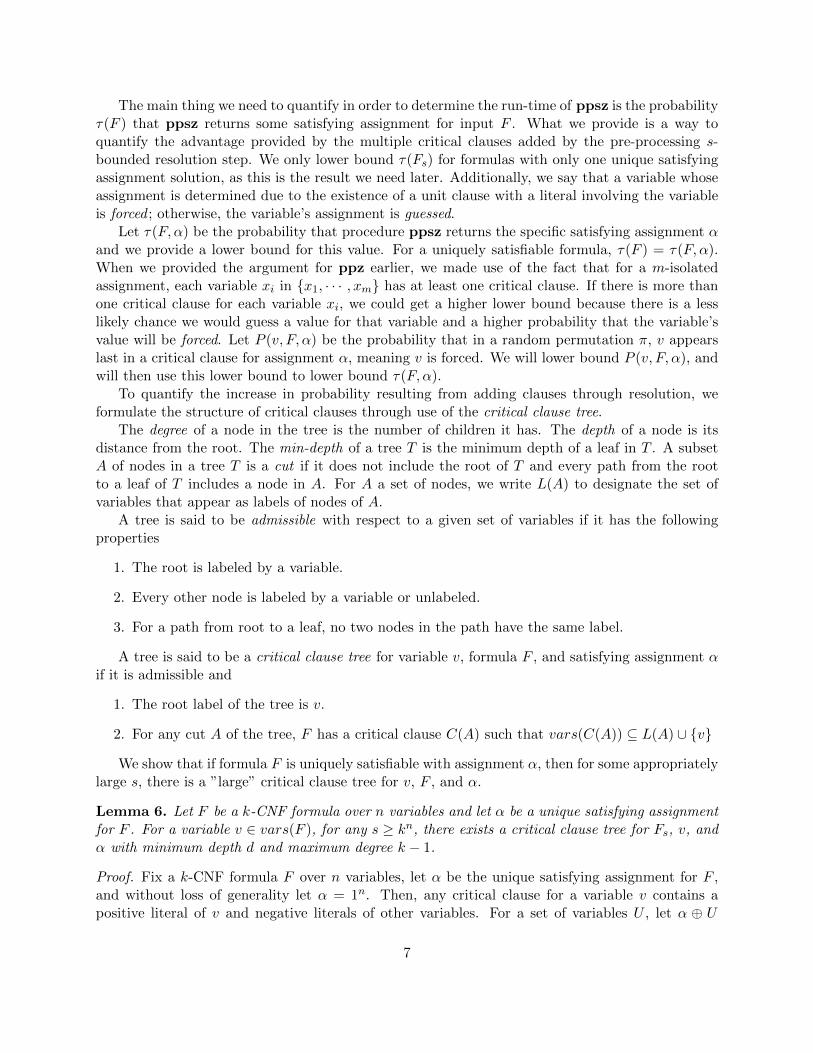
The main thing we need to quantify in order to determine the run-time of ppsz is the probabilityτ(F ) that ppsz returns some satisfying assignment for input F . What we provide is a way toquantify the advantage provided by the multiple critical clauses added by the pre-processing s-bounded resolution step. We only lower bound τ(Fs) for formulas with only one unique satisfyingassignment solution, as this is the result we need later. Additionally, we say that a variable whoseassignment is determined due to the existence of a unit clause with a literal involving the variableis forced ; otherwise, the variable’s assignment is guessed.

Let τ(F, α) be the probability that procedure ppsz returns the specific satisfying assignment αand we provide a lower bound for this value. For a uniquely satisfiable formula, τ(F ) = τ(F, α).When we provided the argument for ppz earlier, we made use of the fact that for a m-isolatedassignment, each variable xi in x1, · · · , xm has at least one critical clause. If there is more thanone critical clause for each variable xi, we could get a higher lower bound because there is a lesslikely chance we would guess a value for that variable and a higher probability that the variable’svalue will be forced. Let P (v, F, α) be the probability that in a random permutation π, v appearslast in a critical clause for assignment α, meaning v is forced. We will lower bound P (v, F, α), andwill then use this lower bound to lower bound τ(F, α).

To quantify the increase in probability resulting from adding clauses through resolution, weformulate the structure of critical clauses through use of the critical clause tree.

The degree of a node in the tree is the number of children it has. The depth of a node is itsdistance from the root. The min-depth of a tree T is the minimum depth of a leaf in T . A subsetA of nodes in a tree T is a cut if it does not include the root of T and every path from the rootto a leaf of T includes a node in A. For A a set of nodes, we write L(A) to designate the set ofvariables that appear as labels of nodes of A.

A tree is said to be admissible with respect to a given set of variables if it has the followingproperties

1. The root is labeled by a variable.

2. Every other node is labeled by a variable or unlabeled.

3. For a path from root to a leaf, no two nodes in the path have the same label.

A tree is said to be a critical clause tree for variable v, formula F , and satisfying assignment αif it is admissible and

1. The root label of the tree is v.

2. For any cut A of the tree, F has a critical clause C(A) such that vars(C(A)) ⊆ L(A) ∪ v

We show that if formula F is uniquely satisfiable with assignment α, then for some appropriatelylarge s, there is a ”large” critical clause tree for v, F , and α.

Lemma 6. Let F be a k-CNF formula over n variables and let α be a unique satisfying assignmentfor F . For a variable v ∈ vars(F ), for any s ≥ kn, there exists a critical clause tree for Fs, v, andα with minimum depth d and maximum degree k − 1.

Proof. Fix a k-CNF formula F over n variables, let α be the unique satisfying assignment for F ,and without loss of generality let α = 1n. Then, any critical clause for a variable v contains apositive literal of v and negative literals of other variables. For a set of variables U , let α ⊕ U

7

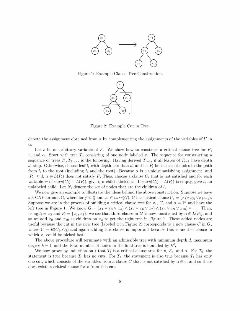
x1

x3 x4

x1

x3 x4

x9 x10

Figure 1: Example Clause Tree Construction.

x1

x3 x4

x9 x10a

Figure 2: Example Cut in Tree.

denote the assignment obtained from α by complementing the assignments of the variables of U inα.

Let v be an arbitrary variable of F . We show how to construct a critical clause tree for F ,v, and α. Start with tree T0 consisting of one node labeled v. The sequence for constructing asequence of trees T1, T2, . . . is the following: Having derived Ti−1, if all leaves of Ti−1 have depthd, stop. Otherwise, choose leaf li with depth less than d, and let Pi be the set of nodes in the pathfrom li to the root (including li and the root). Because α is a unique satisfying assignment, and|Pi| ≤ d, α ⊕ L(Pi) does not satisfy F ; Thus, choose a clause Ci that is not satisfied and for eachvariable w of vars(Ci) − L(Pi), give li a child labeled w. If vars(Ci) − L(Pi) is empty, give li anunlabeled child. Let Ni denote the set of nodes that are the children of li.

We now give an example to illustrate the ideas behind the above construction. Suppose we havea 3-CNF formula G, where for j < n

3 and xj ∈ vars(G), G has critical clause Cj = (xj∨x3j∨x3j+1).Suppose we are in the process of building a critical clause tree for x1, G, and α = 1n and have theleft tree in Figure 1. We know G = (x1 ∨ x3 ∨ x4) ∧ (x2 ∨ x6 ∨ x7) ∧ (x3 ∨ x9 ∨ x10) ∧ . . .. Then,using li = x3 and Pi = x1, x3, we see that third clause in G is now unsatisfied by α⊕L(Pi), andso we add x9 and x10 as children on x3 to get the right tree in Figure 1. These added nodes areuseful because the cut in the new tree (labeled a in Figure 2) corresponds to a new clause C in Gswhere C = R(C1, C3) and again adding this clause is important because this is another clause inwhich x1 could be picked last.

The above procedure will terminate with an admissible tree with minimum depth d, maximumdegree k − 1, and the total number of nodes in the final tree is bounded by kd.

We now prove by induction on i that Ti is a critical clause tree for v, Fs, and α. For T0, thestatement is true because T0 has no cuts. For T1, the statement is also true because T1 has onlyone cut, which consists of the variables from a clause C that is not satisfied by α⊕ v, and so theredoes exists a critical clause for v from this cut.

8

a0

aj

at

...

..

.

.

.

.

. . .. . .

A′

Ni

Figure 3: Case 1: when A′ includes aj .

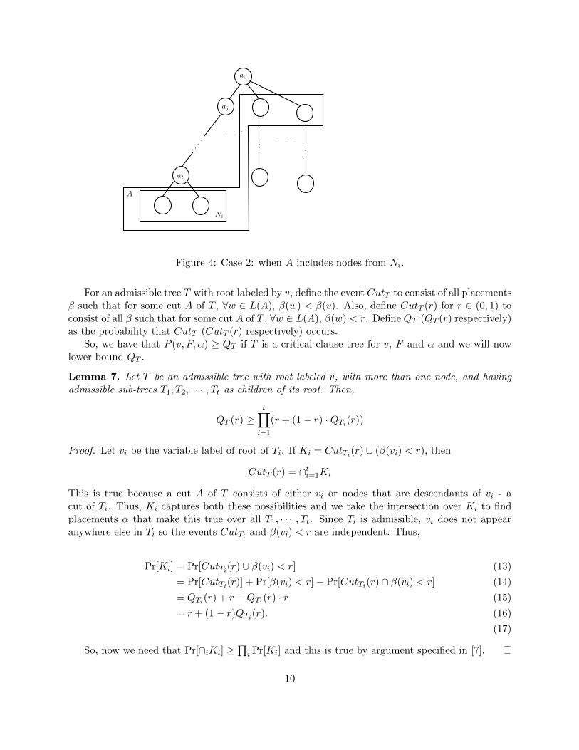
Now, suppose i ≥ 2 and that the statement is true for Ti−1. The tree Ti consists of the nodesfrom Ti−1 and Ni. Suppose A is a cut of Ti and let A′ = A −Ni. Let the nodes of Pi be denotedv = a0, . . . , at = li. Notice that for 1 ≤ j ≤ t, the set Aj = A′ ∪ aj is a cut of Ti and Ti−1.Then, by the induction hypothesis, there exists a critical clause C(Aj) for F , v, and α. If for somej ∈ 1, . . . , t, L(Aj) ⊆ L(A′), then we could choose C(A) to be C(Aj). This is case 1 described inFigure 3.

Let the labeling variable of aj be rj . Suppose L(Aj) 6⊆ L(A′) for every j ∈ [t], meaning rj ,6∈ L(A′) for every j ∈ [t]. This means that A has to include nodes in Ni and this case is describedin Figure 4 Consider the clause Ci of F that is used to construct Ti from Ti−1. We can write Ci inthe form R ∨U where R is the clause consisting of negated variables from L(Ni) and U is a clauseconsisting of positive literals of variables from r0, · · · , rt.

We now prove by reverse induction on j ∈ 0, · · · , t that there is a clause Dj in F of the formDj = R∨Sj ∨Uj , where R is defined as above, Sj is clause consisting of negations of variables fromA′ and Uj is clause consisting of some amount of positive literals of variables from r0, · · · , rj.

To prove existence of Dj , let Dt = Ci, with St being empty clause and Ut = U . For j < t, sincewe have already constructed Dj+1, if rj+1 does not appear in Uj+1, take Dj = Dj+1. Otherwise,let Dj+1 can be resolved with C(Aj+1) and this would give Dj since we will have eliminated rj+1.

Let D0 = R∨ S0 ∨U0, where U0 = v because otherwise D0 would consist of all negative literalsand thus could not be a clause in F . We take C(A) to be D0. This works because we have shownthat D0 must exist by the reverse induction argument from above and because D0 is a critical clausefor v as v is the only positive variable occurring in D0. D0 only contains variables from L(A), otherthan v, because S0 ⊆ L(A′) ⊆ L(A), and R ⊆ L(A) because we assumed L(Aj) 6⊆ L(A′) for everyj ∈ [t].

For the later analysis, it will be useful to see an individual permutation as a random variableon a continuous probability space. Specifically, a placement of the variables in F is a function βthat maps each variable to (0, 1). Given such a placement, we define π = πβ to be a permutationobtained by ranking the variables according to their β values.

9

a0

aj

at

...

..

.

.

.

.

. . .. . .

A

Ni

Figure 4: Case 2: when A includes nodes from Ni.

For an admissible tree T with root labeled by v, define the event CutT to consist of all placementsβ such that for some cut A of T , ∀w ∈ L(A), β(w) < β(v). Also, define CutT (r) for r ∈ (0, 1) toconsist of all β such that for some cut A of T , ∀w ∈ L(A), β(w) < r. Define QT (QT (r) respectively)as the probability that CutT (CutT (r) respectively) occurs.

So, we have that P (v, F, α) ≥ QT if T is a critical clause tree for v, F and α and we will nowlower bound QT .

Lemma 7. Let T be an admissible tree with root labeled v, with more than one node, and havingadmissible sub-trees T1, T2, · · · , Tt as children of its root. Then,

QT (r) ≥t∏i=1

(r + (1− r) ·QTi(r))

Proof. Let vi be the variable label of root of Ti. If Ki = CutTi(r) ∪ (β(vi) < r), then

CutT (r) = ∩ti=1Ki

This is true because a cut A of T consists of either vi or nodes that are descendants of vi - acut of Ti. Thus, Ki captures both these possibilities and we take the intersection over Ki to findplacements α that make this true over all T1, · · · , Tt. Since Ti is admissible, vi does not appearanywhere else in Ti so the events CutTi and β(vi) < r are independent. Thus,

Pr[Ki] = Pr[CutTi(r) ∪ β(vi) < r] (13)

= Pr[CutTi(r)] + Pr[β(vi) < r]− Pr[CutTi(r) ∩ β(vi) < r] (14)

= QTi(r) + r −QTi(r) · r (15)

= r + (1− r)QTi(r). (16)

(17)

So, now we need that Pr[∩iKi] ≥∏i Pr[Ki] and this is true by argument specified in [7].

10

Lemma 8. If T is an admissible tree then for all r ∈ (0, 1),

QT (r) ≥ Q(d)k (r).

Meaning,

QT ≥ Q(d)k

Proof. Let fk(x; r) = (r + (1− r)x)k−1. Define sequence (Q(d)k : d ≥ 0) by recurrence: Q

(0)k (r) = 0

and Q(d)k (r) = fk(Q

(d−1)k (r); r). And, let Q

(d)k =

∫ 10 Q

(d)k (r)dr. Then by induction on d and by result

of Lemma 7, the result is shown.

Lemma 9.

Q(d)k ≥

µkk − 1

− 3

(n− 1)(k − 2) + 2)

where µk =∑∞

j=11

j(j+ 1k−1

).

Proof. See [7].

Thus, we have now shown that P (v, F, α) ≥ µkk−1 − 3

(n−1)(k−2)+2 . We now show how we can use

P (v, F, α) to lower bound τ(F, α).

Lemma 10. For satisfying assignment α of F ,

τ(F, α) ≥ 2−n+∑v∈vars(F ) P (v,F,α)

Proof. Suppose Forced(F, π, α) designates the set of variables that will be forced for α.From (2), we have:

τ(F, α) =∑π

2−|enc(σ,α,F )| · 1

n!(18)

=∑π

2|Forced(F,π,α)|2n

· 1

n!(19)

≥ 2−n+∑π |Forced(F,π,α)|· 1

n! (20)

Since P (v, F, α) is equivalent to the probability that v ∈ Forced(F, π, α) for random permuta-tion π, we get

τ(F, α) ≥ 2−n+∑v∈vars(F ) P (v,F,α) (21)

Thus, we have shown the following theorem

Theorem 2. For k-CNF formula F with a uniquely satisfiable assignment α,

τ(Fs) = τ(F, α) ≥ 2−(1− µkk−1

)n,

where µk =∑∞

j=11

j(j+ 1k−1

). This implies that ppsz can solve uniquely satisfiable k-CNF formulas

in time O(poly(n) · 2(1− µkk−1

)n) time.

11

For k = 3, muk = 4 − 4 ln 2 > 1.226 so the running time of ppsz algorithm on any uniquelysatisfiable 3-CNF is O(poly(n) · 20.387n). Comparitively, ppz determines satisfiability of a 3-CNF

formula in time O(poly(n) · 2 23n) time. For large k, µk =

∑∞j=1

1j2

= π2

6 ≈ 1.644. So, ppsz is afaster algorithm than ppz for uniquely satisfiable 3-CNF formulas.

2.5 Faster PPSZ

This section states an improvement to ppsz formed by Timon Hertli in [1]. The idea is to usean s-implication step when assigning each variable rather than the one s-resolution pre-processingstep used in ppsz.

Let F be a k-CNF formula. We say that a literal l is s-implied in F if there is a subset ofclauses G in F with |G| ≤ s such that all satisfying assignments of G set l to 1. A variable v issaid to be s-implied if one of the literals v or v is s-implied. We use this new idea of s-implicationto produce a faster, modified version of ppsz. Let SV again denote the set of all permutations ofthe variables of F .

function modifiedPPSZ(Function F , Assignment α, Permutation π from SV , Integer s)

(1) foreach i ∈ 1, · · · , |V |(2) x← π(i)(3) while there is an s-implied literal l for value a for variable y in F(4) F ← F [y 7→a]

(5) α← α ∪ y 7→ a(6)(7) if x ∈ vars(F )(8) α← α ∪ x 7→ α(x)(9) F ← F [x 7→a]

(10)(11) return α

function modifiedPPSZ(Function F , Integer s)

(1) α←random assignment on vars(F )(2) π ←random permutation on vars(F )(3) return modifiedPPSZ(F, α, π, s)

Suppose π is a randomly chosen permutation used in modifiedPPSZ and α is a randomlychosen assignment used to assign variables that are not s-implied in modifiedPPSZ. Define thesuccess probability of modifiedPPSZ as the probability that it returns a satisfying assignmentfor F :

psuccess(F, s) := Prπ,α

(modifiedPPSZ(F, α, π, s) ∈ sat(F )).

Now, consider a run of modifiedPPSZ(F, α, π, s). For x ∈ vars(F ), we call x forced if thevalue of x in the assignment returned is determined by s-implication; otherwise, we call it guessed.

For α ∈ sat(F ), we define the probability that x is guessed with respect to random permutation

12

π aspguessed(F, x, α, s) := Pr

π(x is guessed in modifiedPPSZ(F, α, π, s)).

Additionally, we say that x ∈ vars(F ) is frozen if all satisfying assignments of F agree onassignment of x; otherwise, we say x is non-frozen. The probability that a frozen variable isguessed can be bounded:

Theorem 3. If x is a frozen variable, then pguessed(F, x, α, s) ≤ Sk where Sk := 1 − µkk−1 −

3(n−1)(k−2)+2) .

Proof. For the ppsz algorithm, we showed that for a unique assignment there is an upper boundfor the probability that the variable is guessed. In [2], it is shown that this bound also holds foran arbitrary satisfying assignment, as long as the variable is frozen. In ppsz, we used s-resolution,rather than s-implication, and our analysis involved the use of critical clause trees. The resultsproved there are also true here because if we replace the s-bounded resolution step in the ppzalgorithm with the s-implication step stated above, then the ppz algorithm would still function asnecessary.

We denote the non-frozen variables of F by varsN (F ) and the frozen variables of F by varsF (F ).The set of satisfying literals of F (denoted SL(F )) are the literals l such that F [l] is satisfiable.Clearly, SL(F ) consists of all literals over non-frozen variables (since their assignment is not thesame for every satisfying assignment) and only one literal for each frozen variable. So, |SL(F )| =2 · |varsN (F )|+ |varsF (F )|.

By definition of modifiedPPSZ, if F is s-implication free (meaning all the frozen variables ofF have been set):

psuccess(F, s) =1

2n

∑l∈SL(F )

psuccess(F[l], s)

This is true because F is s-implication free and so only non-frozen variables are represented inSL(F ) and there are 2 · n literals corresponding to these variables in SL(F ).

We now prove two lemmas that we need later.

Lemma 11. For l ∈ α, a satisfying assignment for F , we have pguessed(F[l], x, α, s) ≤ pguessed(F, x, α, s).

Proof. Assume x is s-implied in modifiedPPSZ(F, α, π, s). Let y be randomly assigned a valueu.a.r from 0, 1 and call this value l. Let π′ be a permutation on vars(F ), excluding y. Then, xis also s-implied on modifiedPPSZ(F [l], α, π′, s) because of the following: since x was s-impliedin original F , there had to be a set of clauses G that implied x in F ; Setting y 7→ l cannot havesatisfied any of the clauses in G (because then x would not have been implied by G), and so thatclause set still implies x in F [l]. So, we have:

(1− pguessed(F [l], x, α, s)) ≥ (1− pguessed(F, x, α, s))

and so the result of lemma follows.

Lemma 12. For α ∈ sat(F ) with vars(F ) = n and x ∈ vars(F ) such that x is not s-implied, wehave:

pguessed(F, x, α, s)−1

n=

1

n(F )·∑l∈α

pguessed(F[l], x, α, s)

13

Proof. Suppose π is a random permutation on vars(F ) and y is the variable that appears first inπ. We then have,

pguessed(F, x, α, s) = Prπ

(x is guessed in modifiedPPSZ(F, α, π, s))

=∑

y∈vars(F )

Prπ

(y first comes first in π)

· Prπ

(x is guessed in modifiedPPSZ(F, α, π, s)| y first comes first in π) (22)

The above sum can be split into two cases: when x = y and when x 6= y. So, (22) is

= Prπ

(y comes first in π |x = y )

· Prπ

(x is guessed in modifiedPPSZ(F, α, π, s) | y comes first in π ∧ x = y)

+ Prπ

(y first comes first in π |x 6= y )

· Prπ

(x is guessed in modifiedPPSZ(F, α, π, s) | y comes first in π ∧ x 6= y)

=1

n· 1 +

1

n·∑l∈α

pguessed(F[l], x, α, s) (23)

We define the random process AssignSL(F ) to give a probability distribution on the set ofsatisfying assignments for a formula F . AssignSL(F ) produces an assignment on vars(F ) in thefollowing manner: Starting with an empty assignment α, the procedure repeats this step untilvars(F ) is empty: Choose l ∈ SL(F ), add l to α, and let F = F [l]. Output α in the end.

Letting α be assignment on vars(F ), let p(F, α) be the probability that AssignSL(F ) returnsα.

Then, by definition of AssignSL(F ), it always returns a satisfying assignment. It also definesa probability distribution on sat(F ). described as the following:

p(F, α) =1

|SL(F )|∑l∈α

p(F [l], α)

Using this probability distribution, we define a cost function on satisfiable k-CNF formulae. LetS := Sk.

Definition 1. For (≤ k)-CNF formula F we define the cost of a variable x in F as

c(F, x) =

0 x 6∈ vars(F )

S x ∈ varsN (F )∑α∈sat(F ) p(F, α)pguessed(F, x, α, s) x ∈ varsF (F )

(24)

And, we define the cost of F as c(F ) :=∑

x∈vars(F ) c(F, x).

From the definition, and since p(F, α) ≤ 1 and pguessed(F, x, α, s) ≤ S, we have that c(F, x) ≤ S.This means c(F ) ≤ n · S.

We now prove a lemma and a theorem that we will use later.

14

Lemma 13. For literal l in assignment α, p(F [l], α) ≥ p(F, α). If l is over a frozen variable, thenp(F [l], α) = p(F, α) and c(F [l]) ≤ c(F ).

Proof. For a run of AssignSL(F ), we have two possibilities: either l is chosen or l is not chosen.Suppose l is chosen and let α′ be the outputted assignment by AssignSL(F ). Then, α′\l has samedistribution as output of AssignSL(F [l]). Suppose l is not chosen. Then AssignSL(F ) cannot re-turn α. So, the probability AssignSL(F [l]) returns α\l is at least probability AssignSL(F ) returnsα. If the literal l is over a frozen variable, then l will definitely be picked in AssignSL(F ) and soconstricting the formula does not provide any difference in probability when running AssignSL(F ).Since α, p(F [l], α) = p(F, α) for a frozen variable, and pguessed(F

[l], x, α, s) ≤ pguessed(F, x, α, s) (byLemma 10), we can see that c(F [l]) ≤ c(F ).

Theorem 4. Suppose F is s-implication free. For l chosen u.a.r from SL(F ), we have

El[c(F[l])] ≤ c(F )− varsN (F ) · 2S

|SL(F )| − varsF (F ) · 1

|SL(F )|

Proof. See [1].

We can now prove the main theorem involving modifiedPPSZ.

Theorem 5. psuccess(F, s) ≥ 2−c(F ).

Proof. We prove the statement by induction on vars(F ). If vars(F ) = 0, the statement is triviallytrue. We have a CNF formula F . Suppose the statement is true for formulas with less than vars(F )

variables, meaning that for l ∈ SL(F ), psuccess(F[l], s) ≥ 2−c(F

[l]). Suppose F is not s-implicationfree. Then, let l be any s-implied literal that would be picked in modifiedPPSZ. The literal lmust be over a frozen variable (since otherwise the clause set G would be fulfilled by opposite value

of l) and from previous lemma we have c(F ) ≥ c(F [l]), meaning 2−c(F ) ≤ 2−c(F[l]) and so

psuccess(F[l], s) ≥ 2−c(F

[l]) ≥ 2−c(F ).

Now, suppose F is s-implication free. Then by an earlier observation and the induction hy-pothesis, we have

psuccess(F, s) =1

2n

∑l∈SL(F )

psuccess(F[l], s) ≥ 1

2n

∑l∈SL(F )

2−c(F[l]).

Then,

psuccess(F, s) ≥1

2n·|SL(F )|

∑l∈SL(F )

Pr(l)·2−c(F [l]) =|SL(F )|

2nEl[2

−c(F [l])] ≥ |SL(F )|2n

2−El[c(F[l])] = 2log

|SL(F )|2n

−El[c(F[l])].

So, to prove the statement, we need to show that

A := log|SL(F )|

2n− El[c(F

[l])] + c(F ) ≥ 0.

15

We can bound El[c(F[l])] with Theorem 3 and we get

A ≥ log|SL(F )|

2n− c(F ) + varsN (F ) · 2S

|SL(F )| + varsF (F ) · 1

|SL(F )| + c(F ) (25)

= log|SL(F )|

2n+ varsN (F ) · 2S

|SL(F )| + varsF (F ) · 1

|SL(F )| (26)

= log|SL(F )|

n+ log

1

2+ varsN (F ) · 2S

|SL(F )| + varsF (F ) · 1

|SL(F )| (27)

= log(1 +varsN (F )

n) + varsN (F ) · 2S

|SL(F )| − 2 · varsN (F ) · 1

|SL(F )| (28)

Since log(1 + x) ≥ log(e) x1+x , we have

A ≥ log(e)varsN (F )

n|SL(F )n

+ varsN (F ) · 2S

|SL(F )| − 2 · varsN (F ) · 1

|SL(F )| (29)

= log(e)varsN (F )

|SL(F )| − (2− 2S) · varsN (F )

|SL(F )| (30)

Now, S = S3 = 2 ln(2)− 1 ≈ 0.3863, so (2− 2S) = 4− 4 ln(2) < 1.23 < 1.44 < log(e), meaningA ≥ 0 and this completes the proof.

Therefore, we have shown for k-SAT the same bounds that we had for Unique k-SAT. Theresults are summarized in the next theorem.

Theorem 6. Using the randomized modifiedPPSZ procedure, we can solve k-SAT in O(2(1− µkk−1

)n)time where µk =

∑∞j=1

1j(j+ 1

k−1)

.

2.6 Schoning’s Algorithm

We now present Schoning’s algorithm for determining satisfiability of k-SAT formulae. It is arandomized algorithm and so over the years many attempts have been made to derandomize it.Previous attempts did not achieve the running time of Schoning’s algorithm and were very compli-cated. We present a new simple deterministic algorithm that is a derandomization of Schoning’salgorithm.function randomFlip(formula F, integer s, assignment α)

(1) α←random 0, 1vars(F )

(2) if α ∈ sat(F ) then return true(3) while s > 0(4) C ← some unsatisfied clause by F (α)(5) µ←random vars(C)(6) flip assignment for µ in α(7) if F (α) = 1 then return true(8)(9) s← s− 1(10) return false

16

function Schoning(formula F )

(1) n← vars(F )(2) while true(3) if randomFlip(F, 3n, α) returns true then return α

Theorem 7. Using the randomized algorithm Schoning, we can find a satisfying assignment for

a k-CNF formula F in O(poly(n)(

2(k−1)k

)ntime.

Proof. See [4]

2.7 Derandomization of Schoning’s Algorithm

We first state a problem that is useful in our analysis of our derandomization of Schoning’s algo-rithm:

Promise-Ball-k-SAT: Given a (≤ k)-CNF formula F over n variables, an assignment α to thesevariables, r ∈ N, and the promise that the Hamming ball Br(α) contains a satisfying assignment,the goal is to find a satisfying assignment to F .

By definition of being a promise problem, Promise-Ball-k-SAT is solved by an algorithm Aunder the following conditions:

1. If Br(α) does indeed contain a satisfying assignment to F , A will return some satisfyingassignment to F ; however, it is required that this assignment be in Br(α).

2. if F is unsatisfiable or Br(α) does not contain a satisfying assignment to F , then the behaviorof A is unspecified.

Our deterministic algorithm will actually be an algorithm for Promise-Ball-k-SAT. But, usingthe results of the next lemma we can convert our algorithm into an algorithm that solves k-SAT.

Lemma 14. If algorithm A solves Promise-Ball-k-SAT in time O(ar), then there is an algorithmB solving k-SAT in time O(( 2a

a+1)n). Additionally, if A is an deterministic algorithm, then so isB.

We first prove some results regarding Hamming Balls and Covering Codes that we need to proveLemma 14.

For the Hamming Distance metric, the ball of radius r ∈ R with center z ∈ 0, 1n is the set

u ∈ 0, 1n | dH(z, u) ≤ r.

Then, the number of vertices in a ball of radius r from any point in 0, 1n, or the volume, is

vol(n, r) =

r∑i=0

(n

i

),

since to get a point from distance i from our starting point z, we need to flip i bits of z and wehave n bits to choose from.

17

Lemma 15. For n ∈ N, ρ ∈ R+, ρ ≤ 12 ,

vol(n, ρn) ≤ 2n·H(π),

where H(x) is the binary entropy function defined as H(x) := −x · log2(x)− (1− x) · log2(1− x).

Proof.

1 = (ρ+ (1− ρ))n (31)

=

n∑i=0

ρi(1− ρ)n−i (by binomial theorem) (32)

=

n∑i=0

(ρ

1− ρ)i(1− ρ)n (33)

≤ρn∑i=0

(ρ

1− ρ)i(1− ρ)n (since ρ ≤ 1

2) (34)

A code C of length n is defined to be a subset of 0, 1n. The covering radius of a code C isthe smallest radius r such that the union of all balls of radius r centered at all points of C coverall of 0, 1n. This means that every element in 0, 1 is at distance at most r from at least one ofthe points in C. Equivalently,

r := maxu∈0,1minv∈CdH(u, v).

Lemma 16. For n ∈ N, r ∈ N0, there exists a code of length n with covering radius at most r thathas at most ⌈

n · 2nvol(n, r)

⌉= O(2n(1−H(ρ))poly(n))

elements.

Proof. We choose the⌈

n·2nvol(n,r)

⌉elements of the code u.a.r from 0, 1n with replacement and show

that there is a positive probability that this code has covering radius at most r.Let u be some element in 0, 1n. The probability that u is not covered by our randomly

generated code (equivalently, that u has distance exceeding r from all elements in our code) is(1− vol(n, r)

2n

)⌈n·2n

vol(n,r)

⌉≤ e−n,

where(

1− vol(n,r)2n

)is the probability that a point does not belong to the ball of radius r centered

at an element in our code. So, the probability that there is an element in 0, 1n that will not becovered is at most 2n · e−n, implying that the probability that every element is covered is at least1−

(2e

)n> 0.

Lemma 17. For n ∈ N, ρ ∈ R, 0 < ρ < 12 , a code of length n with covering radius ρn and of size

O(2n(1−H(ρ))poly(n)) can be constructed in time O(2n(1−H(ρ))poly(n)).

18

Proof. It is a known fact that a greedy algorithm for constructing a code, where one choose a nextball so that as many as possible yet uncovered vertices are covered, gives a code of size at most(1 + ln 2) = O(n) factor of the size of the optimal cover and takes time O(23npoly(n)). Fixingsome d ∈ (N) such that n is divisible by d, we construct a code C ′ of length n

d with coveringradius

⌊rd

⌋using this greedy procedure. Then, we let our actual code C be the set of all possible

concatenations of any d elements in C ′. We have spent time O((23n/d + |C|)poly(n)) and the sizeof C is

O((2nd

2(1−H(ρ))poly(n/d))d) = O(2n(1−H(ρ))poly(n))

If we pick d such that 3d ≤ (1−H(ρ)), meaning d ≥ 3(1−H(ρ)), then the time to pick the code

is O(2n(1−H(ρ))poly(n)).

With the above algorithm, we show how we can convert an algorithm for Promise-Ball-k-SATinto an algorithm for k-SAT.

Proof of Lemma 14. Let ρ = 1k+1 . Use algorithm from Lemma 17 to build a covering code of length

n and radius ρn. For each element in this covering code, run algorithm A to solve Promise-Ball-k-SAT for r = ρn. If any of these calls is able to find a assignment, we return that assignment;Otherwise, we return false.

The algorithm takes time

O(2n(1−H(ρ))poly(n)) +O(2n(1−H(ρ))poly(n)) · aρn (35)

= O(poly(n) · 2n(1−H(ρ)) · 2log2(k)ρn) (36)

= O(poly(n) · 2n(1−H(ρ))+log2(k)ρn) (37)

= O(poly(n) · 2n(1+ 1k+1

log21k+1

+ kk+1

log2kk+1

+ 1k+1

log2 k) (38)

= O(poly(n) · 2n(1− 1k+1

log2(k+1)+ kk+1

log2 k− kk+1

log2(k+1)+ 1k+1

log2 k) (39)

= O(poly(n) · 2n(1+log2kk+1

) (40)

= O(poly(n) ·(

2k

k + 1

)n(41)

(42)

function searchBall(formula F, integer r, assignment α)

(1) if α satisfies F(2) return true(3) else if r = 0(4) return false(5) else(6) C ← some unsatisfied clause by F (α)(7) for u ∈ C(8) if searchBall(F u:=1), α, r − 1) = true(9) return true

19

(10) return false

Lemma 18. Algorithm searchBall solves Promise-Ball-k-SAT in time O(poly(n)kr).

Proof. In order to see the correctness of searchBall, we see that given F and α, either α satisfiesF or it does not. If it does not, then there has to exist a clause that is not satisfied because allthe literals in that clause are falsified. The algorithm will recursively explore all the assignmentsin Brα and will return true only if some assignment in this ball satisfies F .

Letting s(r) denote the number of calls made by an invocation of searchBall on a formula F ,parameter r and assignment α, we get the following recurrence:

s(r) ≤

1 if r = 0

1 + k · s(r − 1) otherwise

Using induction and the substitution method, we can see that s(r) ≤ kr+1−1k−1 , meaning search-

Ball takes O(poly(n)kr) time.

Lastly, we state some results about k-ary codes, which play an extensive part in our analysisfor our derandomization of Schoning’s algorithm.

Consider the set 1, . . . , kt. It is an extension of the Boolean cube 0, 1t and has the sameHamming distance metric as for u, v ∈ 1, . . . , kt, dH(u, v) is defined to be the number of coordi-nates in which u and v differ. The set also has balls, as we define

B(k)(u) := u′ ∈ 1, . . . , kt | dH(u, u′) ≤ r.To determine the volume of such a ball, we see that there are

(tr

)options for picking the

coordinates in which u and u′ are supposed to differ and for a set u, there are (k−1) different waysin u′ can be set in each of these r coordinates so as to differ from u. Thus,

vol(k)(t, r) := |B(k)(u)| =(t

r

)(k − 1)r.

Similar to the set 0, 1t, a set C ⊆ 1, . . . , kt is called a code with covering radius r if⋃u∈C

B(k)r (u) = 1, . . . , kt.

With a similar argument used in Lemma 16, we get that there exists a code C ⊆ 1, . . . , ktwith covering radius r, where

|C| ≤⌈

t ln(k)kt(tr

)(k − 1)r

⌉.

We further estimate the size of this optimal covering code using an approximation of the binomialcoefficient.

Lemma 19. There exists a code C with covering radius tk such that

|C| ≤ t2(k − 1)t−2tk

20

Proof. From [4], we have for 0 ≤ ρ ≤ 12 and t ∈ N,(

t

ρt

)≥ 1√

8tρ(1− ρ)

(1

ρ

)(1

1− ρ

)(1−ρ)t

.

Setting ρ = 1k , we get(

t

t/k

)≥ 1√

8tkt/k

(k

k − 1

)(k−1)t/k

=kt√

8t(k − 1)k−1t/k

Thus, we have

|C| ≤⌈

t ln(k)kt(tr

)(k − 1)r

⌉≤ t2kt(k − 1)(k−1)t/k

kt(k − 1)t/k≤ t2(k − 1)t−2t/k.

fastSearchBall (Function F , assignment α, integer r, code C ⊆ 1, . . . , kt)

(1) if F (α) = 1(2) return true(3) else if r = 0(4) return false(5) else(6) G ← maximal possible set of pairwise disjoint k-clauses of F that are

unsatisfied by α(7) if |G| < t(8) for each possible assignment β for vars(G)(9) if searchBall(F β, α, r) = true(10) return true(11) else(12) H ← C1, . . . , Ct ⊆ G(13) for u ∈ C(14) if searchBallFast(F, α[H,u], r − (t− 2t

k ), C) = true(15) return true(16) return false

search(Function F , assignment α, integer r)

(1) C ← code for 1, . . . , kt with covering radius tk

(2) return fastSearchBall(F , α, r, C)

The algorithm search first chooses a sufficiently large constant t (depending on ε) and thencomputes code C ⊆ 1, . . . , kt with covering radius t

k .It then calls the recursive helper procedure, which does most of the work. The procedure

searchBallFast first greedily constructs a maximal set G = C1, . . . , Cm consisting of pairwise

21

disjoint, unsatisfied clauses of F , such that each unsatisfied clause in F has at least one literal incommon with clause in G.

Now, we can have two cases. If m < t, the algorithm enumerates all 2km (since each clause hask unique literals in G) assignments for vars(G). For each such assignment β, it calls the earlierdefined recursive procedure searchBall and returns true if at least one of these calls returns true.The correctness argument for this case is as follows: the promised assignment α∗ has to satisfyeach clause in G, and so there is a β with which α∗ will agree on for vars(G), meaning α∗ stillsatisfies F [β]. After finding the right β, F [β] will have no unsatisfied clause of size k (because of themaximality of G). Thus, calling searchBall on F [β] runs in time O(poly(n)(k− 1)r) and thereforethe time complexity in this case is 2km · O(poly(n)(k − 1)r). Because m < t, and t is a constant,this reduces to being O(poly(n)(k − 1)r).

For the second case, where m ≥ t, our code C will be used, the algorithm first choose tclauses from G to set H = Ci, . . . , Ct. We now define notation that will prove useful later. Foru ∈ 1, . . . , kt, for 1 ≤ i ≤ t, let α[u] designate the assignment formed by flipping the value of uthiliteral assigned by α in clause Ci. The α[u] it requires an ordering of clauses in H and ordering ofliterals in each Ci. Notice that α[u] will satisfy exactly one literal in each Ci ∈ H.

Consider the promised satisfying assignment α∗ where we know dH(α∗, α) ≤ r. We can defineu∗ as follows: For each 1 ≤ i ≤ t, set u∗i to the j such that α∗ satisfies the jth literal in Ci. Thiscan be done because α∗ satisfies each of the clauses in H but u∗ may not be unique since α∗ maysatisfy more than literal in each Ci. Here, dH(α[w∗], α∗) = d(α, α∗)− t ≤ r − t.

Rather than iterate and recurse through each u ∈ 1, . . . , kt, we recurse only through eachu ∈ C. By definition, for u∗, there exists some u ∈ C such that dh(u∗, u) ≤ t

k . Consider αcompared to α[u]: they disagree on at most t

k coordinates and for these coordinates, switching theuthi literal in Ci increases the distance between α and α∗; however, they agree on at least t − t

kcoordinates and switching the uthi literal in Ci decreases the distance between α and α∗; Thus,

dh(α[u], α∗) ≤ dH(α, α∗) +t

k− (t− t/k) ≤ r − (t− 2t/k).

Letting 4 := (t − 2t/k), we see that the method will call itself with α[u] and r = r − 4 foreach u ∈ C but at least one of these calls will be successful. We will have a total of |C| recursivecalls and at step of recursion tree will decrease the r parameter by 4. So, the total number of callsmade will be at most

|C|r/4 ≤ (t2(k − 1)4)r/4 =(

(k − 1)t2/4)r.

Since t2/4 = (t1/t)2kk−2 goes to 1 as t grows, the whole above term is bounded by (k−1+ε)r. This

means that search solves the Promise-Ball-k-SAT problem in O(poly(n)(k−1+ε)r) time. Then,

by applying Lemma 14, we see that the algorithm solves the k-SAT problem in O((2(k−1)2k + ε)r)

time.

3 Algorithms for AC0

3.1 Context

AC0 is the set of all languages recognizable by Boolean circuits of constant depth that have un-bounded fan-in and polynomial size. We show a randomized algorithm from [3] to solve the satisfi-ability problem of AC0 circuits. The algorithm works in the following manner: assuming the AC0

22

circuit is over n variables, the algorithm constructs a set of restrictions that partition 0, 1n andensures that under each of these restrictions, the circuit has constant value. To determine satisfia-bility, we can simply go through each of these restrictions and determine if the circuit evaluates totrue under any of them.

3.2 Notation

For circuits on n inputs, we say m = cn is the maximum number of gates in a layer and d is thenumber of layers the circuit has. We number the layers starting with the output gate being layer1 and the inputs being in layer (d + 1). We call such a circuit a (n,m, d)-circuit. Furthermore,(n,m, d, k)-circuits are circuits where the fan-in at level d is bounded by k.

We say that a set of functions f1, . . . , fm : 0, 1n → 0, 1 partition 0, 1n if ∀x ∈ 0, 1n,there exists only one i such that fi(x) = 1. The ith region of the partition is defined by the setx | fi(x) = 1 and can be identified by the function fi. The functions that we use are of the formR = (R ∧ ρ), where R is a k-CNF and ρ is a restriction.

We say a set P = (Ri = (Ri, ρi), Ci)i is a partitioning for C if Rii defines a set of regionswhich partition 0, 1n and for every i, C is equivalent to Ci in region Ri. Call Ci the circuitassociated with the region Ri.

For a CNF f , we use tree(f) to denote a decision tree for f . The leaves of this tree are labeledwith the constant value to which the formula is reduced when evaluated under the choices of valuesfor the variables we made along the path to the specific leaf. The depth of a decision tree is thelength of the longest path in the tree (in terms of the number of variables queried along that path).For F = (f1, . . . , fm) a set of CNFs and/or DNFs, tree(F) indicates a decision tree for the set ofthese functions. To construct tree(F), we first query along f1 and then restrict f2, . . . , fm accordingto the choices made in the path and then query the next remaining formula and repeat.

3.3 AC0 Satisfiability Algorithm

We first show a procedure to convert a set of k-CNFs to a set of k-DNFs. Suppose we have ak-CNF f . Consider the decision tree tree(f) for f . If the depth of tree(f) is at most k, then wecan get an equivalent k-DNF by taking the disjunction (OR) of every path (which consists of theconjunction(AND) of every literal in the path set according to the value picked for the variablealong the path) that leads to a leaf node labeled with 1.

Most likely, however, the depth of tree(f) will be greater than k. In this case, we will split thepaths in tree(f) into two categories: (1) “short” paths of length at most k; (2) “long” paths oflength greater than k.

Let σ′ = σ′1, . . . , σ′l be the set of paths with length greater than k in tree(f). Let σ =σ1, . . . , σl be the set of paths of length k in tree(f) that do not end in a leaf node — these arethe paths in σ′ cut off after querying k variables. Then, letting

τ(f, k) = ¬σ1 ∧ ¬σ2 ∧ . . . ∧ ¬σl,where each σi is a conjunction of literals in that path, we get that τ(f, k) describes a region suchthat the assignments that satisfy τ(f, k) are those that correspond to a path of length at most kin tree(f).

Also, define S(f, k) for tree(f) as

S(f, k) = κ1 ∨ κ2 ∨ . . . ∨ κl,

23

where each κi is a path in the decision tree of length at most k ending in a leaf labeled 1. By thisdefinition, ∀α ∈ τ(f, k), S(f, k)(α) = f(α).

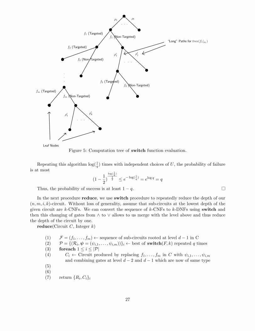
Given these definitions, let us define our switching procedure switch. It accepts a set of k-CNF formulas f1, . . . , fm and outputs a partition P = (Ri = (Ri ∧ ρi),ψi)i where each ψi =(ψi,1, . . . , ψi,m) is a sequence of k-DNFs with at most n

100k variables and for each ψi, for 1 ≤ j ≤ m,ψi,j is equivalent to fj in the region Ri. The computation tree for switch is displayed in Figure 5.The switch procedure utilizes a recursive function recursiveSwitch that performs most of thework. This recursive function, when given a node in the computation tree (represented by a regionand the associated converted k-CNFs), returns all the regions and associated k-CNFS representedby the leaves of the sub-tree rooted at the given node. A branch in the computation tree in whichthe region is modified according to lines (3− 4) means that the formula f here is labeled as being“non-targeted”. A branch in the computation tree in which the region is modified according tolines (10− 11) means that the formula f here is labeled as being “targeted”.

The idea is that the method is given a region and it “fine-tunes” it (makes it more restrictive)based on the formulas that remain to be converted and based on whether the formula to be convertedwill be “targeted” or “non-targeted“. It accepts F (the set of k-DNFs that we wish to convert tok-CNFs) and P (a region and associated already-converted k-CNFs) and returns the set of allregions and associated k-CNFs that can be formed from the given region. In switch, we callrecursiveSwitch with a partition that has an empty(true) k-CNF because our restriction, at thispoint, is only defined by ρ ∈ U .

switch(F = (f1, . . . , fm), Integer k)

(1) p← 1100k

(2) U ← Choose u.a.r a set of pn variables from vars(F) to leave unset(3) U ← ρ | ρ is a restriction that leaves variables in U unset(4) R← empty(true) k-CNF(5) foreach ρ ∈ U(6) P ← P ∪ recursiveSwitch(F , P = ((R, ρ),ψ = ∅))(7) return P

recursiveSwitch(F = (f1, . . . , fm), P = ((R, ρ),ψ = (ψ1, . . . , ψl)), Integer k)

(1) if |F | > 0(2) f ← first function in F(3) R∗ ← R ∧ τ(f |ρ, k)(4) ψ ← S(f |ρ, k)(5) P ′ ← ((R∗, ρ),ψ ∪ ψ)(6) Pnt ← recursiveSwitch(F − f, P ′)(7)(8) Pt ← ∅(9) foreach path ρ′ in tree(f |ρ) of length greater than k(10) ρ∗ ← ρ ∧ ρ′(11) ψ ← b where b is the label of leaf at end of path ρ′

(12) P ′ ← ((R, ρ∗),ψ ∪ ψ)(13) Pt ← Pt ∪ recursiveSwitch(F − f, P ′)

24

(14)(15) return Pnt ∪ Pt(16) else(17) return P

In our analysis below, we will make use of the following lemma.

Lemma 20. Let F = f1, . . . , fm be a sequence of k-CNFs or k-DNFs in same n variables. Forp ≤ 1

13 , for ρ, a random restriction that leaves pn variables unset, the probability that tree(F ) hasa path of length ≥ s, where each fi contributes at least one variable to the path, is at most (13pk)s.

Proof. See [3].

Now, we prove the following lemma involving the procedure switch

Lemma 21. Let F = (f1, . . . , fm) be a sequence of k-CNFs over n variables and let 0 < q ≤ 12

be a parameter. Using the randomized algorithm switch, a partitioning P can be returned for F ,where the formulas in each region of P are k-DNFs in at most n

100k variables. With probabilityat least 1 − q, |P| ≤ s and the algorithm runs in time at most poly(n) · log(1

q ) · |F| · s where

s ≤ 2n100k · 2n−

n100k

+3−km.

Proof. Each leaf of this computation tree can be described (call it its “type”) by the sequence of“targeted” k-CNFs that exist along the path to that leaf. Let us label each leaf by the restrictionthat began the path to the leaf and the leaf’s “type.” We can use this grouping to bound thenumber of leaves in the computation tree.

For any restriction ρ and any type (the sequence of targeted CNFs) T , let Gρ,T denote the setof leaves of type T ending at a path beginning with restriction ρ. Consider the decision tree on allthe “targeted” k-CNFs in T , namely tree(T |ρ). The set of paths in tree(T |ρ)where each CNF inT contributes at least k + 1 variables (call it Pρ,T ) correspond to the leaves in Gρ,T because eachpath in Pρ,T corresponds to the exact long paths ρ′i taken for each of the targeted k-CNFs in T .

By Lemma 20, PrU,ρ[tree(T |ρ) has depth ≥ s] ≤ ( 13100)s, meaning

EU,ρ[|Pρ,T |] ≤pn∑s=0

2s · (13/100)s,

since any decision tree of height s can have at most 2s leaves and the summation comes from thefact that the leaves in the entire tree can vary from 0 to pn, as that is the maximum amount ofvariables we can query because that reflects the amount of unset variables.

We bound the expected number of outputs in the whole partition by summing over all possiblerestrictions, then all possible path lengths (0 to pn) and then sets of possible targeted k-CNFs Tof size at most s

k+1 (since each targeted CNF will contribute at least k+ 1 variables). Additionally,let E(T |ρ,k) denote the event that tree(T |ρ) has depth ≥ s where each targeted formula in Tcontributes at least k + 1 variables. So, we have

25

EU [|P|] =∑ρ

∑T⊆fi,...,fm

EU [|Pρ,T |] (43)

= 2n−pn∑ρ

∑T⊆ 1

2n−pnfi,...,fm

EU [|Pρ,T |]

(44)

= 2n−pn∑

T⊆fi,...,fm

EU,ρ[|Pρ,T |] (45)

= 2n−pnpn∑s=0

∑T⊆fi,...,fm|T |≤ s

k+1

2s · (13/100)s (46)

≤ 2n−pnpn∑s=0

bs/kc∑t=0

(m

t

)2s · (13/100)s (47)

≤ 2n−pnpn∑s=0

bs/kc(

m

bs/kc

)(26/100)s (48)

Replacing bs/kc with s′ we get,

≤ 2n−pn

pnk∑

s′=0

ks′(m

s′

)(26/100)ks

′(49)

Since s′ ≤ pnk and for any value of s′ > m, the binomial coefficient in sum will be 0,

≤ 2n−pn · k · pnk

m∑s′=0

(m

s′

)(26/100)ks

′(50)

= 2n−pn · pnm∑s′=0

(m

s′

)(26/100)ks

′(51)

By the binomial formula and since pn =n

100k, we get (52)

=n

100k2n−pn · (1 + (26/100)k)m (53)

≤ n

100k2n−pn+(log e)(26/100)km (54)

<n

100k2n−

n100k

+3−km. (55)

By Markov’s Inequality, we have

Pr[|P| ≤ 2EU [|P]] ≥n

100k2n−n

100k+3−km

2n100k2n−

n100k

+3−km=

1

2.

26

ρ1 ρl

. . .

f1 (Targeted)f1 (Non-Targeted)

f2 (Targeted)

f2 (Non-Targeted)

f2 (Targeted)f2 (Non-Targeted)

.

.

.

fm (Targeted)

Leaf Nodes

. . .

ρ′1 ρ′j

“Long” Paths for tree(f1|ρ1)

. . .

fm (Non-Targeted)

ρ′1ρ′k

Figure 5: Computation tree of switch function evaluation.

Repeating this algorithm log(1q ) times with independent choices of U , the probability of failure

is at most

(1− 1

2)

log( 1q )

12 ≤ e− log( 1

q)

= elog q = q

Thus, the probability of success is at least 1− q.

In the next procedure reduce, we use switch procedure to repeatedly reduce the depth of our(n,m, i, k)-circuit. Without loss of generality, assume that sub-circuits at the lowest depth of thegiven circuit are k-CNFs. We can convert the sequence of k-CNFs to k-DNFs using switch andthen this changing of gates from ∧ to ∨ allows to us merge with the level above and thus reducethe depth of the circuit by one.

reduce(Circuit C, Integer k)

(1) F = (f1, . . . , fm)← sequence of sub-circuits rooted at level d− 1 in C(2) P = (Ri,ψ = (ψi,1, . . . , ψi,m))i ← best of switch(F, k) repeated q times(3) foreach 1 ≤ i ≤ |P|(4) Ci ← Circuit produced by replacing f1, . . . , fm in C with ψi,1, . . . , ψi,m

and combining gates at level d− 2 and d− 1 which are now of same type(5)(6)(7) return Ri, Cii

27

Lemma 22. Let C be a (n,m, d, k)-circuit and let 0 < q ≤ 12 be a parameter. Using the randomized

reduce algorithm, we can output a partitioning P for C where the circuit associated with each regionof P is an ( n

100k ,m, d−1, k)-circuit. With probability at least 1−q, |P| ≤ s and the entire algorithm

runs in time poly(n) · log(1q ) · |C| · s where s ≤ 2n

100k · 2n−n

100k+3−km.

Proof. From Lemma 21 we know that each ψi produced is a depth 2 circuit (a k-DNF) in at mostn

100k variables. Thus, each Ci will be a ( n100k ,m, d−1, k)-circuit if we combine the gates at level d−1

and d− 2. We know that switch algorithm produces partitioning P with |P| ≤ s with probability

at least 1− q and runs in time poly(n) · log(1q ) · |C| · s where s ≤ 2n

100k · 2n−n

100k+3−km. The algorithm

reduce after the call to switch then goes through and combines levels of depth d − 1 and d − 2and this takes an additional O(|P| · |C|) = O(s · |C|) time.

We now do d − 2 steps of depth reduction to reduce the circuit C to just 2 levels in the nextmethod repeatedReduction. Specifically each partition in P returned by repeatedReductionhas an associated circuit that has depth 2.

repeatedReduction(Circuit C, Integer k)

(1) d← depth of C(2) if d = 2(3) return ((R = 1, ρ = 1), C)(4) if d > 2(5) P = ∅(6) P ′ = Ri, Cii ← best of reduce(C, k) repeated q = q

2 times(7) foreach P ′i ∈ P ′(8) Pi = (Ri,j , Ci,j)j ← best of repeatedReduction(Ci, k) repeated

q = q2n+1 times

(9)(10) foreach j(11) R′i = Ri ∧Ri,j(12) P = P ∪ R′i, Ci,j(13)(14) return P

Lemma 23. Let C be an (n,m, d, k)-circuit and let 0 < q ≤ 12 be a parameter. By running

the repeatedReduction procedure, we can produce a partitioning P for C where the circuit asso-ciated with each region is a ( n

(100k)d−2 ,m, 2, k)-circuit (either a k-CNF or k-DNF). With prob-

ability at least 1 − q, |P| ≤ s and the algorithm runs in time poly(n) · log(1q ) · |C| · s where

s ≤ (2n)d−2

(100k)(d−1)(d−2)/2 2n− n

(100k)d−2 +(d−2)3−km.

Proof. We know |P ′| ≤ 2n100k · 2n−

n100k

+3−km with probability at least 1− q2 based on Lemma 22 and

we say P ′ is “good” if this is the case. For each i, we say Pi is “good” if

|Pi| ≤ (2n)d−3

(100k)(d−2)(d−3)/2 2n−( n

100k)(1− 1

(100k)d−3 +(d−3)3−km). By induction, each Pi is “good” indepen-

dently with probability at least 1− q2n+1 because we assume that running the algorithm on circuits

of depth d− 1 fulfills the properties of the lemma. So,

28

Pr[Pi is not good for all i | P ′ is good] ≤2n∑i=0

Pi is not good (56)

= 2n · q

2n+1=q

2, (57)

where (13) is due to the use of the union bound and because P ′ being “good” implies that at most2n number of Pi’s exist (because in the worst case all 2n restrictions setting all n variables mayoccur in P ′.

Thus,

Pr[Pi is good for all i ∧ P ′ is good] = Pr[P ′ is good] · Pr[Pi is good for all i | P ′ is good] (58)

≥ (1− q

2)(1− q

2) > 1− q. (59)

In this case when all P ′is are ”good” and P ′ is ”good”, the total number of outputs (or the sizeof P) is at most

2n

100k· 2n(1− 1

100k)+3−km · (2n)d−3

(100k)(d−2)(d−3)/22

( n100k

)(1− 1

(100k)d−3 +(d−3)3−km)

=(2n)d−2

(100k)(d−1)(d−2)/22n− n

(100k)d−2 +(d−2)3−km.

After the repeated depth reduction, we end up with a circuit C that is a k-CNF or k-DNFin a region defined by a k-CNF R|ρ. In the method depthTwoReduction, we apply a randomrestriction on some fraction of the remaining variables, construct a decision tree for (C,R), andreturn a partitioning containing regions in which R is satisfied and in which the corresponding Chas constant value. We argue that the total number of leaves in this decision tree is not too large.Each leaf in the decision tree where R ≡ 1 corresponds to the region containing the points for whichR is satisfied and in this region the circuit’s value, as mentioned before, is constant.

depthTwoReduction(Circuit C)

(1) p = 130k

(2) U ← Choose u.a.r a set of pn variables from vars(C) to leave unset(3) PU = ρ | ρ is a restriction that leaves variables in U unset(4) P = ∅(5) foreach ρ ∈ PU(6) T ← decision tree for (C,R)|ρ(7) foreach path ρ′ in T ending at leaf labeled (b, 1)(8) P = P ∪ ρ ∧ ρ′, b(9)(10) return P

29

Lemma 24. Let circuit C be a k-CNF or k-DNF and let R be a k-CNF (that defines a restriction)in the same n variables and let 0 < q ≤ 1

2 be a parameter. In the partitioning P for C in region Rproduced by depthTwoReduction, each region is defined by a restriction and the associated circuitin the region is of constant value. This procedure runs in O(poly(n) · log(1

q ) · (|C| · |R|) · s where

s ≤ 50 · 2n(1− 130k

).

Proof. We need to bound the number of pairs output by depthTwoReduction. ThePrρ[depth(tree(C,R)|ρ) ≥ s] ≤ 3(13/30)s by Lemma 20 and (number of leaves in tree((C,R)|ρ) ≤2s · 3(13/30)s since a decision tree of depth s can have at most 2s leaves. Thus,

EU [|P|] ≤ EU [∑ρ

number of leaves in tree((C,R)|ρ] (60)

= 2n−n·1

30kEU,ρ[ number of leaves in tree((C,R)|ρ] (61)

≤ 2n(1− 130k

)

n30k∑s=0

2s3(13/30)s (62)

≤ 3 · 2n(1− 130k

)∞∑s=0

(26/30)s (63)

< 25 · 2n(1− 130k

) (64)

By Markov’s Inequality,

Pr[|P| ≤ 50 · 2n(1− 130k

)] ≥ 25 · 2n(1− 130k

)

50 · 2n(1− 130k

)=

1

2

We can repeat depthTwoReduction log(1q ) times in parallel with independent choices of

U and output the smallest partition. As in the previous proof for Lemma 21 this increases theprobability of success to 1− q.

The algorithm for determining the satisfiability of an AC0 circuit is a composition of the previousprocedures. We first consider the case where the inputted circuit has bottom fan-in bounded by kand call the method that solves this instance AC0Fan-InSAT.

AC0Fan-InSAT(Circuit C, Integer k)

(1) P = ∅(2) P ′ = ((Ri, ρi), Ci)i = best of repeatedReduction(C, k) repeated q

2 times(3) foreach Ci ∈ P ′(4) Pi = (ρi,j , bi,j)j = best of depthTwoReduction (Ci) repeated q =

q2n+1 times

(5)(6) foreach j(7) P = P ∪ (ρi ∧ ρi,j , bi,j(8)(9) return P

30

Lemma 25. Let C be a (n,m, d, k)-circuit. Using procedure AC0Fan-InSAT, we can outputa partitioning P for C where each region is defined by a restriction and the associated circuit hasconstant value. With probability at least 1−2n, |P| ≤ s and the procedure runs in O(poly(n) · |C| ·s)time where s ≤ 50 · (2n)d−2

(100k)(d−1)(d−2)/2 2n− n

(100k)d−2 +(d−2)3−km.

Proof. From Lemma 23, we know that |P ′| ≤ (2n)d−2

(100k)(d−1)(d−2)/2 2n− n

(100k)d−2 +(d−2)3−kmwith probability

at least 1− q2 and we say P ′ is “good” if this is true. For each i, from Lemma 24, we know that |Pi| ≤

50 · 2n

(100k)d−2)(1− 1

30k)

with probability at least 1− q2n+1 (notice that we run depthTwoReduction

on circuit with n(100k)d−2 variables) and we say Pi is “good” if this is true. So,

Pr[Pi is not good for all i | P ′ is good] ≤2n∑i=0

Pi is not good (65)

= 2n · q

2n+1=q

2, (66)

where (23) is due to the use of the union bound and because P ′ being good implies that atmost 2n number of Pi’s exist (because in the worst case all 2n restrictions setting all n variablesmay occur in P ′.

Thus,

Pr[Pi is good for all i ∧ P ′ is good] = Pr[P ′ is good] · Pr[Pi is good for all i | P ′ is good] (67)

≥ (1− q

2)(1− q

2) > 1− q. (68)

When this occurs, the total number of outputs (or size of P) is at most

(2n)d−2

(100k)(d−1)(d−2)/22n− n

(100k)d−2 +(d−2)3−km · 50 · 2n

(100k)d−2)(1− 1

30k)

≤ 50 · (2n)d−2

(100k)(d−1)(d−2)/22n− n

(100k)d−2 +(d−2)3−km.

So we now have an algorithm for determining satisifiablity of (n,m, d, k) circuits. We can usethis algorithm for (n,m, d) circuits by converting any (n,m, d)-circuit into a (n′,m, d, k)-circuit byconstructing a partition. The procedure fanInReduce accepts a (n,m, d) circuit C and returns apartitioning P where the circuit associated with each region in the partition is a (n,m, d, k) circuit.Assume the bottom level gates of C are ∨ gates.fanInReduce(Circuit C, Integer k)

(1) R← empty(true) k-CNF(2) ρ← restriction in which all vars(C) are unset(3) while there is bottom-level gate ψ with fan-in > k(4) ψ′ ← disjunction of first k inputs of ψ.(5) Branch assuming ψ′ is satisfied:

31

(6) replace ψ with ψ′ in C(7) R = R ∨ ψ′(8) Branch assuming ψ′ is not satisfied:(9) ρ = ρ ∨ ¬ψ′ where ¬ψ′ is viewed as restriction that sets literals in ψ′

to false(10) C = C|¬ψ′(11)(12) return ((R, ρ), C)

Lemma 26. Let C be an (n,m, d)-circuit. Using fanInReduce procedure, we can produce apartitioning P = ∪0≤f≤n/kPf for C where sets Pf are disjoint for each f , Pf contains at most(m+ff

)regions with circuits associated being (n− fk,m, d, k)-circuits. fanInReduce runs in time

poly(n) · |C| · |P|.

Proof. Consider the computation tree of fanInReduce. Along any path in this tree, let f denotethe number of branches where a ψ′ is false. Since each path has at most m branches where ψ′ istrue (because in this case the number of bottom-level gates with fan-in greater than k is reduced),for each value of f there are at most

(m+ff

)paths. At the end of such paths, fk variables are set

by the false branches, resulting in (n− fk,m, d, k)-circuits.

Using the procedures fanInReduce and AC0Fan-InSAT from above, we can now define aprocedure that determines the satisfiablity of a (n,m, d) AC0 circuit.

AC0SAT(Circuit C, Integer k)

(1) P = ∅(2) P ′ = ∪0≤f≤n/kPf = fanInReduce(C, k) where Pf = (Rf,i, Cf,i)i(3) foreach f(4) foreach i(5) Pf,i = (ρf,i,j , bf,i,j)j = best of AC0Fan-InSAT(Cf,i, k) repeated

q = 2−2n times(6)(7) foreach j(8) P = P ∪ (ρf,i,j ∧ ρf,i, bf,i,j)(9)(10) foreach Pi ∈ P(11) if Ci = 1(12) return true(13)(14) return false

Lemma 27. Let C be an (n,m, d)-circuit. Let k ≥ 1 be a parameter. Using method AC0SAT weproduce a partitioning P for C where each region is defined by a restriction and the correspondingcircuit for each region is of constant value. With probability at least 1 − 2−n, |P| ≤ s and thisalgorithm runs in time at most poly(n) · |C| · s where

s ≤ 50 (2n)d−2

(100k)(d−1)(d−2)/2 · 2n− 3n

(100k)d−1 +(d−2)3−km+4·2−kmax(m,n/k).

32

Proof. For each f and i, we say that Pf,i is “good” if

|Pf,i| ≤ 50 · (2n)d−2

(100k)(d−1)(d−2)/2 2(n−fk)(1− 3

(100k)d−1 +(d−2)3−km. By Lemma 25, Pr[Pf,i is good] ≥ 1−2−2n

and by using the union bound in the manner that we have used before, because at most 2n pairsf , i exist, we have

Pr[∀f, ∀i, Pf,i is good] ≥ 1− 2−n.

If this is true, the total number of outputs (the size of P) is at most

=

nk∑

f=0

(m+ f

f

)50

(2n)d−2

(100k)(d−1)(d−2)/22

(n−fk)(1− 3

(100k)d−1 +(d−2)3−km(69)

= 50(2n)d−2

(100k)(d−1)(d−2)/22n(1− 3

(100k)d−1 +(d−2)3−km

nk∑

f=0

(m+ f

f

)2−fk(1− 3

(100k)d−1 +(d−2)3−km(70)

Sincenk∑

f=0

(m+ f

f

)2−fk(1− 3

(100k)d−1 +(d−2)3−km(71)

≤m+n

k∑f=0

(m+ n/k

f

)2−fk (72)

= (1 + 2−k)m+n/k (73)

by the binomial formula

≤ 2(log e)2−k(m+n/k) ≤ 24·2−k·max(m,n/k). (74)

(75)

Thus, (70) is at most

50(2n)d−2

(100k)(d−1)(d−2)/22n(1− 3

(100k)d−1 +(d−2)3−km+4·2−kmax(m,n/k).

We can now bound the running-time (and number of restrictions) of our algorithm.

Theorem 8. There exists an algorithm that decides satisfiability of (n,m, d) circuits by producinga set of restrictions ρii that partition 0, 1n and such that for each restriction ρi, C|ρi hasconstant value. The algorithm’s run-time and total number of restrictions produced are both of

O(poly(n) · |C| · 2n−n

(log c+d log d)d−1 ).

Proof. For C an (n,m, d)-circuit, if m ≥ 2−Ω(n)1d−1

, then we can output all 2n restrictions settingall the variables and checking each restriction. Else, choosing k = Θ(max(log(md ), d log(d)) means

50(2n)d−2

(100k)(d−1)(d−2)/2· 2n−

3n

(100k)d−1 +(d−2)3−km+4·2−kmax(m,n/k) ≤ 22n

(100k)d−1

33

and so we can use the method AC0SAT. In either case, we will output at most

2n− n

O(log(mn )+d log(d))d−1 +O(1)

restrictions.

4 Algorithms for General Formulae

4.1 Context

SAT is the most fundamental of NP-complete problems and has a lot of applications in A.I. andhardware verification and testing. These two facts have motivated a lot of research into findingefficient satisfiability algorithms for SAT. Many of these SAT solvers require the input formula tobe in CNF format. This requirement can be a great disadvantage for two reasons: (1) Convertingto CNF can destroy important structural properties of the original problem; (2) Conversion toCNF can add several new variables, greatly increasing the search space. Thus, it is useful to havesatisfiability algorithms for general Boolean formulae. Here, we study specifically the satisfiabilityproblem for formulae of size linear in the number of variables.

4.2 Notation

There are two representations for Boolean functions that we use: the formula and the decision treerepresentations.

A formula is defined to be binary tree where the internal nodes are binary connectives (ANDor OR) and the leaves are literals (either variables, complemented variables, or constants). Thesize of a formula is the total number of leaves the tree has, and for a formula f , the size is oftenrepresented as |f |. The length of a formula, on the other hand, is the number of bits necessary torepresent the formula in binary.

A decision tree is a binary tree whose internal nodes are labeled with variables and whose leavesare labeled with constants. The leaves of this tree are labeled with the constant value to which theformula is reduced to when evaluated under the choices of values for the variables we made alongthe path to the specific leaf. The size of the decision tree is the number of leaves in the tree.

4.3 Formula Satisfiability Algorithm

We present a deterministic algorithm for formula satisfiability for formulae of linear size that savesa constant factor in the exponent over brute force search.

We first state two procedures, Simplify and Evaluate. The procedure Evaluate is the mainalgorithm that determines the satisfiability of a linear-sized formula, while Simplify is a helpermethod used by Evaluate.

Simplify(Formula f)

(1) Let g denote any formula occurring in f(2) Let y denote a literal(3) Repeat the following until there is no decrease in size of f :(4)(5) if 0 ∨ g or g ∨ 0 occurs as sub-formula in f :

34

(6) replace this sub-formula with g(7) if 0 ∧ g or g ∧ 0 occurs as sub-formula in f :(8) replace this sub-formula with 0(9) if 1 ∧ g or g ∧ 1 occurs as sub-formula in f :(10) replace this sub-formula with g(11) if 1 ∨ g or g ∨ 1 occurs as sub-formula in f :(12) replace this sub-formula with 1(13) if y ∨ g or g ∨ y occurs as sub-formula in f :(14) replace all occurrences of y in g with 0(15) replace all occurrences of y in g with 1(16) if y ∧ g or g ∧ y occurs as sub-formula in f :(17) replace all occurrences of y in g with 1(18) replace all occurrences of y in g with 0

The Simplify tries to decrease the size of formula f if possible while maintaining the set ofsatisfying assignments for f . The first four simplification rules follow directly from simple Booleanlogic and it is clear that these rules preserve the set of satisfying assignments of the formula. Thefirst variable simplification rule results in an equivalent formula because of the following: Let f ′

be the sub-formula y ∨ g, where y is a literal and g is a formula; In an assignment where y = 0,the simplification of g agrees with the assignment. In an assignment where y = 1, y ∨ g = 1 soit does not matter how we simplify g. Thus, in both cases, the simplified formula is equivalent tothe original formula. A similar argument can be made for the second variable simplification ruleto show it too produces a smaller but equivalent formula.

Evaluate(Formula f , Integer n)

(1) if f has no literals:(2) if f evaluates to 1:(3) return “yes”(4) else:(5) return “no”(6) r ← index of variables occurring the maximum number of times in f(7) f0 ← Simplify(f |xr=0)(8) f1 ← Simplify(f |xr=1)(9)(10) Evaluate(f0, n− 1)(11) Evaluate(f1, n− 1)

To prove the savings Evaluate provides over brute-force search, we need a lemma involvingtelescoping products.

Lemma 28. Let aiN−1i=0 be a sequence, where ai = 1 − 1

N−i . Then, for any positive constant ε,

there is a positive constant c < 12 such that if S is a random subset of 1, 2, . . . , (1 − c) · N with

|S| ≥ N4 , then

Pr[Πi∈Sai ≥ ε18 ] ≤ 2−Ω(N)

Theorem 9. Using Evaluate algorithm, we can determine the satisfiability of a formula of size

35

O(n) in time 2n−Ω(n), where n is the number of variables in the formula.

Proof. Consider the computation tree of Evaluate evaluated on a input formula f (see Figure1 for reference). Label each internal node of the tree with < f, z >, where f is the formula thealgorithm is evaluating and z is the variable occurring the maximum number of times in f . Wesay f is the formula label, while z is the variable label. As shown on the figure, a node labeled with< f, z > has a left child with formula label Simplify(f |z=0) and a right child with formula labelSimplify(f |z=1). The leaves of the tree are labeled with constants and are the base case instanceof Evaluate.

For our proof, we need this computation tree to be a complete binary tree of depth n and soif there is a node occurring at depth less than n with a constant label, we extend it to depth nby labeling the added nodes with 〈β, u〉, where β is the constant in the constant label and u is anarbitrary variable.

Given a node v, let fv identify its formula label and zv its variable label. Also, let |v| denotethe depth of the node in the computation tree.

In this tree, for each node, we define a notion of whether a node is “good” and later extendthis definition to paths in the tree. Fix a node v. If the label formula of v is constant, we label theleft child of v “good” and the right child “bad.” In this case, we call v a trivial node and any pathfrom root through v a trivial path. Otherwise, we define r1 and r2 as follows:

• Let r1 be the number of times zv occurs negatively in fv as the child of OR node plus thenumber of times it occurs positively in fv as the child of an AND node.

• Let r2 be the number of times zv occurs positively in fv as the child of OR node plus thenumber of times it occurs negatively in fv as the child of an AND node.

From the definitions above and since zv is the variable that occurs most frequently in fv, wehave

r0 + r1 ≥|fv|

n− |v| , (76)

basically stating that the number of literals involving the most frequently occurring variable is noless than the average number of literals per each remaining variable in fv.

We can quantify the reduction in size of fv0 (the formula corresponding to the left child) andfv1 (the formula corresponding to the right child) relative to the size of fv in the computationtree. Something to notice is that by the time Evaluate is called on a formula it has already been”simplified” by Simplify; So, for no gate is it the case that a variable z or its complement z occursin one child of the gate and that the other child is a formula containing z or z. This observationsimplifies the analysis of the reduction due to the two rules.

So, if zv ← 0, we can see that the size of fv decreases by at least 2r1 + r2, applying the ANDand OR simplification rules in Simplify. Similarly, for zv ← 1, the size of fv decreases by at least2r2 + r1. So, |fv0| ≤ |fv| − 2r1 − r2 and |fv1| ≤ |fv| − 2r2 − r1.

Based on how the formula decreases in size relative to the assignment of zv, if r0 ≥ r1, we callthe left child of v “good” and the right child “bad”; otherwise, we call the left child “bad” and theright child “good.” So, for the good child of v, the decrease in size of the formula correspondingto the good child is at least (r1 + r2) · 3

2 ≥3fv

2(n−|v|) because for a good node the decrease in size

36

is greater than or equal to the average of the two reduction lower bounds stated above. So, for agood child of v, say w,

|fw| ≤ |fv| −3fv

2(n− |v|) = |fv|(1−3

2(n− |v|)) ≤ |fv|(1−1

(n− |v|))32 ,

where the last inequality is due to Bernoulli’s inequality, which states that for every integer r ≥ 0and real number x ≥ −1, (1 + x)r ≥ 1 + rx. We can observe that even for a bad child w′ of v,|fw′ | ≤ |fv| − r1 + r2, implying |fw′ | ≤ |fv|(1− 1

n−|v|).With regard to paths in the computation tree, we call a path in the tree “good” if there at least

n4 good nodes on the path and “bad” otherwise. In the tree, the probability that a path is bad at

most∑n

4i=1

(di

)(1

2)i(12)d−i. Using Hoeffding’s inequality and having ε = d

2 − n4 , we get,

n4∑i=1

(d

i

)(1

2)i(

1

2)d−i ≤ e−2ε2n = e−2( d

2−n

4)2n.

Since d = (1− c′)n for c′ > 12 , we have,

n4∑i=1

(d

i

)(1

2)i(

1

2)d−i = 2−Ω(n).

So, we have shown that the probability that a path is “bad” in the computation tree is expo-nentially small. We now need to show that when a path is “good,” the probability that the formulalabel of the node at depth d in the path has size at most c′n

2 is 1 − 2−Ω(n). We need to applyLemma 28 to show this fact.

If a node is “good,” there is an additional shrinkage factor of at least√

1− 1n−|v| . To apply

Lemma 28, we can interpret S as the set of depths of the “good” nodes in a “good” path and view√1− 1

n−|v| as a12i . Then for any constant ε > 0,

Pr(√

Πi∈Sai ≥ ε116

)≥ 1− 2−Ω(n).

By setting ε = 1(2c)16

and setting c′ = ε4 , we get that the size of the formula at the end of a good

path is at most

ε116 · (cc′n) =

(1

(2c)16

)16

· (cc′n) =c′n

2. (77)

Thus, the cumulative time spent by the algorithm on “good” paths ending in formula label ofsize at most c′n

2 and the sub-trees below those paths is at most

2(1−c′)n · 2 c′n2 = 2n−c

′n+c′n/2 = 2n−Ω(n).

We also have that fraction of paths that are “bad” or are “good” but that do not end in smallformula label is 2−Ω(n) with the time spent along these paths being 2n.

Therefore, the time complexity of this algorithm is:

(1− 2−Ω(n) ·+2n−Ω(n) + 2−Ω(n) · 2n = 2n−Ω(n).

37

5 Conclusion

For k-SAT algorithms, the derandomization of Schoning’s algorithm is no longer the fastest deter-ministic algorithm, as Makino, Tamaki, and Yamamoto in [5] have introduced a derandomization ofan improved version of Schoning’s algorithm that solves 3-SAT in O(1.3303n) time. The fastest ran-domized algorithm for k-SAT is the modified-PPSZ algorithm mentioned above. Recently, PPSZhas been derandomized for uniquely satisfiable formula in [8] and it may be possible to use thetechniques used in the analysis of modified-PPSZ to derandomize PPSZ for k-SAT in general.

In this paper, we concentrate primarily on the algorithmic analysis of the different algorithmsstated above, but do not consider some of the circuit lower bound results that can be derived fromthese algorithms. For example, in [7], results about the coding length of isolated assignments areused to bound the circuit size of unbounded fan-in depth-3 circuits computing Parity. Essentially, inany non-trivial algorithm, we try to take advantage of some underlying special property of whateverwe are analyzing. This property also indicates a limitation in the class and this can be used toprove lower bounds for some Boolean function f that does not have this property. This type ofanalysis is present in both [9] and [3].

References

[1] Timon Hertli. 3-SAT Faster and Simpler - Unique-SAT Bounds for PPSZ Hold in General.CoRR, abs/1103.2165, 2011.

[2] Timon Hertli, Robin A. Moser, and Dominik Scheder. Improving PPSZ for 3-SAT usingCrtitical Variables. CoRR, abs/1009.4830, 2010.

[3] Russell Impagliazzo, William Matthews, and Ramamohan Paturi. A Satisfiability Algorithmfor AC0. CoRR, abs/1107.3127, 2011.

[4] F.J. MacWilliams and N.J.A. Sloane. The Theory of Error-Correcting Codes. Holland Pub-lishing Co, Amsterdam, vol 16 edition, 1977.

[5] Kazuhisa Makino, Suguru Tamaki, and Masaki Yamamoto. Derandomizing HSSW Algorithmfor 3-SAT. CoRR, abs/1102.3766, 2011.

[6] Robin A. Moser and Dominik Scheder. A Full Derandomization of Schoening’s k-SAT Algo-rithm. CoRR, abs/1008.4067, 2010.

[7] Ramamohan Paturi, Pavel Pudlak, Michael E. Saks, and Francis Zane. An ImprovedExponential-Time Algorithm for k-SAT. J. ACM, 52:337–364, May 2005.

[8] Daniel Rolf. Derandomization of PPSZ for unique-k-SAT. In Proceedings of the 8th interna-tional conference on Theory and Applications of Satisfiability Testing, SAT’05, pages 216–225,Berlin, Heidelberg, 2005. Springer-Verlag.

[9] Rahul Santhanam. Fighting Perebor: New and Improved Algorithms for Formula and QBFSatisfiability. pages 183–192, 2010.

[10] Emo Welzl. Boolean Satisfiability - Combinatorics and Algorithms. 2005.

38