Supporting Information for

Rational design of a bi-layered reduced graphene oxide film on

polystyrene foam for solar-driven interfacial water evaporation

Le Shi, Yuchao Wang, Lianbin Zhang and Peng Wang*

Water Desalination and Reuse Center, Division of Biological and Environmental

Sciences and Engineering, King Abdullah University of Science and Technology, Thuwal

23955-6900, Kingdom of Saudi Arabia.

E-mail: peng.wang@kaust.edu.sa

Electronic Supplementary Material (ESI) for Journal of Materials Chemistry A.This journal is © The Royal Society of Chemistry 2017

Figure S1 Photographs of the prepared GSin-PS bi-layered photothermal membranes (n=0,

0.1, 0.2, 0.3, 0.4 and 0.5 g) (a1-f1) with diameter of 4.5cm and the same membranes after

HI reduction (i.e., rGSin-PS) (a2-f2). Porous rGSin-PS bi-layered photothermal membrane

after SBA-15 removal by NaOH (g1). rGO layer is coated on the peripheral edge (g2).

Homemade water evaporation performance measurement system, with white paper as

cover (h1), without cover (h2).

There was a significant color change on the membrane surface after GO reduction to rGO.

As can be seen, with increasing amount of SBA-15, there were more cracks on the

membrane surfaces.

Figure S2 SEM images of the top layer of rGSin-PS (n=0, 0.1, 0.2, 0.3, 0.4 and 0.5g) bi-

layered photothermal membranes before SBA-15 removal in (a1-e1) respectively, and after

SBA-15 removal in (a2-e2) respectively; insets in a-e are magnified views; (f) the cross

sectional images of the porous rGSi0.2 (i.e., after SBA-15 removal); (g) the top view of the

PS substrate.

Figures 2a1-e1 present the rGSin-PS bi-layered photothermal membranes. Clearly seen

were the bar structure of SBA-15 and the film format of the rGO layer. With increasing

amount of SBA-15 powder, there was less rGO that could be seen and more agglomeration

happened. The figures 2a2-e2 are the samples after SBA-15 removal, which show porous

and 3D network structures of the top layers, with a large amount of inter connected pores

(0.5-2.0 um). The walls of these pores consisted of thin layers of stacked graphene sheets.

Figure S3 The absorption (a) and diffuse reflection (b) spectra of (porous) rGSin-PS, n=0,

0.1, 0.2, 0.3, 0.4, and 0.5 g.

Figure S4 IR images of the (porous) rGSin-PS bi-layered photothermal membranes after

100s illumination: PS substrate (a) uncoated, coated (b) with rGSi0, (c) with porous rGSi0.1,

(d) with porous rGSi0.2, (e) with porous rGSi0.3, (f) with porous rGSi0.4, (g) with porous

rGSi0.5 respectively. As a control experiment, the PS substrate coated with 4.0 ml GO/0.2

mg SBA-15 without SBA-15 removal was in (h) (i.e. rGSi0.2).

Figure S5 (a) Light to evaporation conversion efficiency of the (porous) rGSin-PS bi-

layered photothermal membranes prepared with different ratio of GO and SBA-15 (4.0 ml

GO with 0, 0.1, 0.2, 0.3, 0.4 and 0.5g SBA-15 respectively), under the otherwise same

conditions. As a control experiment, the self-supporting porous rGSi0.2 membrane was also

tested. (b) Light to evaporation conversion efficiency of rGSi0.2-PS bi-layered

photothermal membrane in the different systems with aluminum foil, white paper and

without cover. Insect was the time-course of water evaporation performance of each

system.

Figure S6 The cycle stability test of the porous rGSi0.2-PS for light to evaporation

conversion efficiency for 4 cycles. In each cycle, light is on for 3 hours and light is off for

1.5 hours.

Figure S7. Light to evaporation conversion efficiency of the porous rGSi0.2-PS bi-layered

photothermal membranes at different depth under water: (a) experimental efficiency

corresponding to the water evaporation performance in Figure 5b and (b) simulated

efficiency corresponding to the simulated performance in Figure 5c.

Figure S8. Synthetic seawater evaporation rate and light to evaporation conversion

efficiency of the porous rGSi0.2-PS bi-layered photothermal membranes, which was self-

floating on the surface of simulated seawater with 3.5% NaCl solution.

Table S1. The photothermal evaporation performance of a variety of materials reported in

the literature, along with the material reported by this work.

ReferenceLight

intensity (kWm-2)

Photothermal material

Heat barrier material

Evaporation rate

Solar to evaporation efficiency

1 1.0free floating film

of gold nanoparticles

NA 0.4 mg/(s∙W) -

2 10 exfoliated graphite carbon foam - 85%

3 1.0 polypyrrole

coated stainless steel mesh

NA - 58%

4 1 .0 nitrogen doped porous graphene NA - 80%

5 4.5 Au NP Air laden-paper - 77.8%

6 3.0 carbon-black-based gauze NA 6.0g/h -

7 6.0aluminium-based

plasmonic absorber

NA - 91%

8 20.0 thin-film black gold membranes NA - 57%

9 1.0 carbon nanotube macroporoussilica - 82%

10 1.0cermet (BlueTec eta plus) coated

copper sheet

Polystyrene foam disk -

72% at 17oC

28% at 100oC

11 1.0 GO Polystyrene foam - 80%

12 1.0 porous rGO Polystyrene foam 1.31 kg m-2 h-1 83%

(this work)

Model Simulation

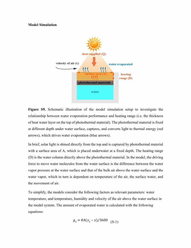
Figure S9. Schematic illustration of the model simulation setup to investigate the

relationship between water evaporation performance and heating range (i.e. the thickness

of heat water layer on the top of photothermal material). The photothermal material is fixed

at different depth under water surface, captures, and converts light to thermal energy (red

arrows), which drives water evaporation (blue arrows).

In brief, solar light is shined directly from the top and is captured by photothermal material

with a surface area of A, which is placed underwater at a fixed depth. The heating range

(D) is the water column directly above the photothermal material. In the model, the driving

force to move water molecules from the water surface is the difference between the water

vapor pressure at the water surface and that of the bulk air above the water surface and the

water vapor, which in turn is dependent on temperature of the air, the surface water, and

the movement of air.

To simplify, the models consider the following factors as relevant parameters: water

temperature, and temperature, humidity and velocity of the air above the water surface in

the model system. The amount of evaporated water is calculated with the following

equations:

(S-1) 𝑔𝑠 = 𝜃𝐴(𝑥𝑠 ‒ 𝑥)/3600

(S-2)𝜃 = (25 + 19𝑣)

(S-3) 𝑥𝑠 = 0.62198𝑝𝑤/(𝑝𝑎 ‒ 𝑝𝑤)

where gs is the amount of evaporated water per second (kg/s), is evaporation coefficient 𝜃

(kg/m2 h), v is the velocity of air above the water surface (m/s), A is the water surface area

exposed to solar light (cm2), xs is humidity ratio of the saturated overlying air (kg/kg) (kg

H2O in kg dry air), and x is humidity ratio of the overlying air (kg/kg) (kg H2O in kg dry

air), pw is partial pressure of the water vapor in the overlying air (Pa), pa is atmospheric

pressure of the overlying air (Pa). It is worth mentioning that the units of in S-1 and S-2 𝜃

do not match with each other as S-2 is a purely empirical formula. 12,13,14

The maximum amount of water vapor in the air is achieved when pw = pws where pws is

saturation pressure of water vapor under the same temperature. pws varies with the air

temperature following S-4:

pws = e(77.3450 + 0.0057 T - 7235 / T) / T8.2 (S-4)

where e is the constant 2.718 and T is the temperature of the overlying air (K). 15

At water vapor saturation, xs is then modified to:

xs = 0.62198 pws / (pa - pws) (S-5)

For the simulation: the air temperature was set at 20oC (293K), the relative humidity 60%,

the humidity ratio in air 0.0085kg/kg, A 15.89 cm2, v above the water surface 0.05 m/s and

D ranging between 0.2 and 7.0 cm.

Some of the major simplifying assumptions in the simulation are: (1) a perfect heat barrier

is assumed and thus no heat and also light is transported to underlying water column; (2) a

uniform temperature profile is assumed for the heating range at all time; (3) a10% energy

loss and thus 90% of the light to evaporation conversion efficiency (i.e., η) of the system

is assumed, which is reasonable based on the experimental results in this study.

It is worth pointing out that that thermal radiation accounts for a significant part of energy

loss in photothermal water evaporation system and is positively related to the temperature

difference between surface water and overlying air, which is then affected by the depth of

the photothermal material underwater. However, for the purpose of simplicity, the same

energy loss (i.e., 10%) is assumed in the model for all cases.

the water mass in the heating range is calculated as:

(S-6)𝑚 = 𝜌𝐴𝐷 = 1.0 𝑔/𝑐𝑚3𝐴𝐷

Table 2: weight of water within the different heating range

D = 0.2 cm is chosen as an exemplifying case here and the simulation results of all the

other heating depths can be found in the excel files.

To start the simulation, the amount of the water evaporated at room temperature (with

T=293.15K, pa = 101.325kPa) (i.e., before light illumination) is calculated as follows:

pws = e(77.3450 + 0.0057 T – (7235 / T)) / T8.2 = 2318 (Pa)

xs = 0.62198 pws / (pa - pws) = 0.62198 pws/(101325-pws)= 0.01456 (kg/kg)

gs = (25 + 19v)A(xs-x)/3600

= (25+19×0.05m/s)(2.25×2.25×10-4 ×3.14 m2)×0.01456kg/kg× (1-60%)/3600

= 6.67×10-8 kg/s

The energy needed to produce the water evaporation is be calculated as:

(S-7)𝑞 = ℎ𝑤𝑒𝑔𝑠

where q is the heat required (kJ/s, kW), hwe=evaporation heat of water (2270kJ/kg).16 Thus

Distance (cm) 0.2 1.0 2.0 4.0 7.0

Weight (g) 3.178 15.89 31.78 63.56 111.23

q = 2270 kJ/kg × 6.67×10-8 kg/s = 0.151J/s = 0.151 W

In the model, the incoming solar light energy is calculated as:

(S-8)𝑄 = 𝐼𝐴

where Q is the incoming solar energy (W), I is the light intensity of solar simulator (AM1.5

100W/cm2). So, Q =100 mW/cm2×15.89cm2=1589 mW=1.589 W

With an assumed energy loss of 10%, the energy utilized by water is:

W𝑃 = (1 ‒ 10%) × 𝑄 = 1.43

In doing the iterative calculation, the temperature of the air above water is set to be equal

to the temperature surface water in the first cycle (i.e., the first second in this case) of the

simulation (the user has freedom to set cycle interval, such as 1 second, 1 minute, etc.).

Thus, the energy available to heat the water within the heating range (qe) is calculated as:

qe = P-q = 1.43-0.151 = 1.279W

At the end of this cycle (1 second), the water temperature in the heating range is

increased by:

𝑑𝑡 =𝑞𝑒

𝐶𝑤𝑚=

1.279𝑊 × 1𝑠

4.2 × 103𝐽/𝑘𝑔 ∙ ℃ × 3.178𝑔= 0.0957℃

where Cw is the specific heat capacity of water ( ).4.2 × 103𝐽/𝑘𝑔 ∙ ℃

The water temperature after 1s illumination is:

20+0.0957 = 20.0957 ℃

For the next cycle, the same calculation procedure takes place, with a starting water

temperature of 20.0957 (293.2457 K).℃

pws = e(77.3450 + 0.0057 T – (7235 / T)) / T8.2 = 2331.901 (Pa) pa = 101.325kPa

xs = 0.62198 pws / (pa - pws) = 0.62198 pws/(101325-pws)= 0.01465

gs = (25 + 19v)A(1-60%)xs/3600

= 6.71×10-8 kg/s

q = 2270 kJ/kg × 6.71×10-8 kg/s

= 0.152 J/s

= 0.152 W

qe = P-q = 1.43-0.152 = 1.278W

The instantaneous water evaporation rate and light to evaporation conversion efficiency

are calculated as:

(S-9)𝑣 = 𝑔𝑠 × 3600 × 10000/𝐴

(S-10)𝜂 = 2270 × 𝑣 × 100/3600

where υ is instantaneous evaporation rate (kg/m2h), and η is light to evaporation conversion

efficiency (%). This computing process continues until qe =Q-q-P=0, which means all the

available energy is utilized fully and there is no extra energy for further water evaporation.

In the model, the water temperature, water evaporation rate, and light to evaporation

efficiency all reach their peak points and would level off beyond this point.

1. Z. Wang, Y. Liu, P. Tao, Q. Shen, N. Yi, F. Zhang, Q. Liu, C. Song, D. Zhang, W. Shang and T. Deng, Small 2014, 10, 3234-3239.

2. H. Ghasemi, G. Ni, A. M. Marconnet, J. Loomis, S. Yerci, N. Miljkovic and G. Chen, Nat Commun 2014, 5.

3. L. Zhang, B. Tang, J. Wu, R. Li and P. Wang, Adv. Mater. 2015, 27, 4889-4894.4. Y. Ito, Y. Tanabe, J. Han, T. Fujita, K. Tanigaki and M. Chen, Adv. Mater. 2015,

27, 4302-4307.5. Y. Liu, S. Yu, R. Feng, A. Bernard, Y. Liu, Y. Zhang, H. Duan, W. Shang, P. Tao,

C. Song and T. Deng, Adv. Mater. 2015, 27, 2768-2774.6. Y. Liu, J. Chen, D. Guo, M. Cao and L. Jiang, ACS Appl. Mater. Interfaces 2015,

7, 13645-13652.7. L. Zhou, Y. Tan, J. Wang, W. Xu, Y. Yuan, W. Cai, S. Zhu and J. Zhu, Nat

Photon 2016, 10, 393-398.8. K. Bae, G. Kang, S. K. Cho, W. Park, K. Kim and W. J. Padilla, Nat Commun

2015, 6.

9. Y. Wang, L. Zhang and P. Wang, ACS Sustainable Chem. Eng 2016, 4, 1223-1230.

10. G. Ni, G. Li, S. V. Boriskina, H. Li, W. Y, T. Z and G. Chen, Nature Energy 2016, 1, 16126

11. X. Li, W. Xu, M. Tang, L. Zhou, B. Zhu, S. Zhu and J. Zhu, Doi: 10.1073/pnas.1613031113

12. V. Mishra, I. Naveen, S. Purkayastha, S. Gupta, International Journal of Advanced Research in Computer Science and Software Engineering 2013, 3, 300-305.

13. O. Vaisala, 2010.14. M. E. Jensen, In Estimating evaporation from water surfaces, Proceedings of the

CSU/ARS Evapotranspiration Workshop, 2010; pp 1-27.15. W. C. Turner, S. Doty, Energy management handbook. The Fairmont Press, Inc.:

2007.16. F. Porges, Handbook of heating, ventilating and air conditioning. Butterworth-

Heinemann: 2013.