supply disruptions with time-dependent parameterslvs2/papers/supply-disrupt-timedep.pdf · supply...

Supply Disruptions with Time-Dependent Parameters

Andrew M. Ross ∗, Ying Rong and Lawrence V. Snyder †

August 23, 2006

Abstract

We consider a firm that faces random demand and receives product from a single supplier whofaces random supply. The supplier’s availability may be affected by events such as storms, strikes,machine breakdowns, and congestion due to orders from its other customers. In our model, weconsider a dynamic environment: the probability of disruption, as well as the demand intensity, canbe time dependent. We model this problem as a two-dimensional non-homogeneous continuous-timeMarkov chain (CTMC), which we solve numerically to obtain the total cost under various orderingpolicies. We propose several such policies, some of which are time dependent and others of which arenot. The key question we address is: How much improvement in cost is gained by using time-varyingordering policies rather than stationary ones?

We compare the proposed policies under various cost, demand, and disruption parameters in anextensive numerical study. In addition, motivated by the fact that disruptions are low-probabilityevents whose non-stationary probabilities may be difficult to estimate, we investigate the robustness ofthe time-dependent policies to errors in the supply parameters. We also briefly investigate sensitivityto the repair-duration distribution. We find that non-stationary policies can provide an effectivebalance of optimality (low cost) and robustness (low sensitivity to errors).

Keywords: inventory, supply disruption, time dependent, CTMC

∗Corresponding author. phone (734) 487-1064, fax (734) 487-2489. Math Dept., Eastern Michigan Univ., Ypsilanti, MI48197 USA. [email protected]

†Industrial and Systems Engineering Dept., Lehigh Univ., Bethlehem, PA 18015 USA. {yir204,lvs2}@lehigh.edu

1

1 Introduction

1.1 Motivation

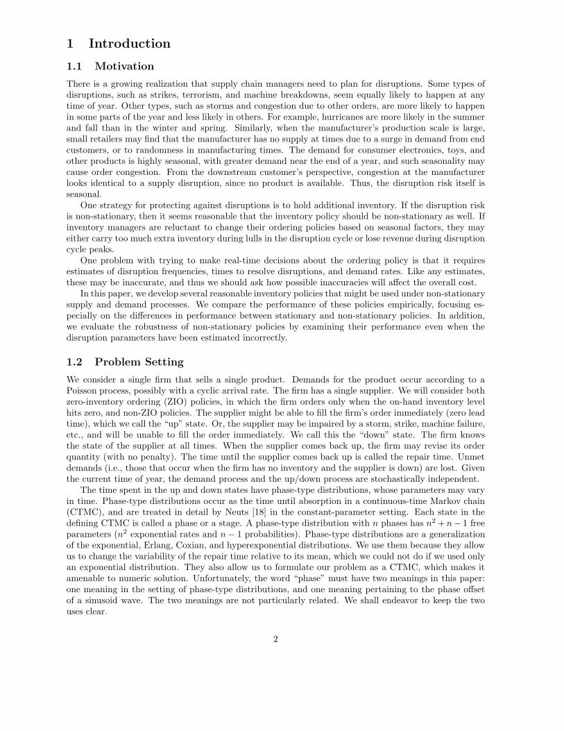
There is a growing realization that supply chain managers need to plan for disruptions. Some types ofdisruptions, such as strikes, terrorism, and machine breakdowns, seem equally likely to happen at anytime of year. Other types, such as storms and congestion due to other orders, are more likely to happenin some parts of the year and less likely in others. For example, hurricanes are more likely in the summerand fall than in the winter and spring. Similarly, when the manufacturer’s production scale is large,small retailers may find that the manufacturer has no supply at times due to a surge in demand from endcustomers, or to randomness in manufacturing times. The demand for consumer electronics, toys, andother products is highly seasonal, with greater demand near the end of a year, and such seasonality maycause order congestion. From the downstream customer’s perspective, congestion at the manufacturerlooks identical to a supply disruption, since no product is available. Thus, the disruption risk itself isseasonal.

One strategy for protecting against disruptions is to hold additional inventory. If the disruption riskis non-stationary, then it seems reasonable that the inventory policy should be non-stationary as well. Ifinventory managers are reluctant to change their ordering policies based on seasonal factors, they mayeither carry too much extra inventory during lulls in the disruption cycle or lose revenue during disruptioncycle peaks.

One problem with trying to make real-time decisions about the ordering policy is that it requiresestimates of disruption frequencies, times to resolve disruptions, and demand rates. Like any estimates,these may be inaccurate, and thus we should ask how possible inaccuracies will affect the overall cost.

In this paper, we develop several reasonable inventory policies that might be used under non-stationarysupply and demand processes. We compare the performance of these policies empirically, focusing es-pecially on the differences in performance between stationary and non-stationary policies. In addition,we evaluate the robustness of non-stationary policies by examining their performance even when thedisruption parameters have been estimated incorrectly.

1.2 Problem Setting

We consider a single firm that sells a single product. Demands for the product occur according to aPoisson process, possibly with a cyclic arrival rate. The firm has a single supplier. We will consider bothzero-inventory ordering (ZIO) policies, in which the firm orders only when the on-hand inventory levelhits zero, and non-ZIO policies. The supplier might be able to fill the firm’s order immediately (zero leadtime), which we call the “up” state. Or, the supplier may be impaired by a storm, strike, machine failure,etc., and will be unable to fill the order immediately. We call this the “down” state. The firm knowsthe state of the supplier at all times. When the supplier comes back up, the firm may revise its orderquantity (with no penalty). The time until the supplier comes back up is called the repair time. Unmetdemands (i.e., those that occur when the firm has no inventory and the supplier is down) are lost. Giventhe current time of year, the demand process and the up/down process are stochastically independent.

The time spent in the up and down states have phase-type distributions, whose parameters may varyin time. Phase-type distributions occur as the time until absorption in a continuous-time Markov chain(CTMC), and are treated in detail by Neuts [18] in the constant-parameter setting. Each state in thedefining CTMC is called a phase or a stage. A phase-type distribution with n phases has n2 + n− 1 freeparameters (n2 exponential rates and n − 1 probabilities). Phase-type distributions are a generalizationof the exponential, Erlang, Coxian, and hyperexponential distributions. We use them because they allowus to change the variability of the repair time relative to its mean, which we could not do if we used onlyan exponential distribution. They also allow us to formulate our problem as a CTMC, which makes itamenable to numeric solution. Unfortunately, the word “phase” must have two meanings in this paper:one meaning in the setting of phase-type distributions, and one meaning pertaining to the phase offsetof a sinusoid wave. The two meanings are not particularly related. We shall endeavor to keep the twouses clear.

2

Although our model and numerical solution procedures can use phase-type distributions, for the mostpart we will use the special case of exponential distributions. This is because our focus is on the cyclicbehavior of the system. The use of exponential distributions makes the failure process a Poisson process,often a non-homogeneous one. In Section 6.4.2 we will examine the impact of non-exponential repairtimes.

The firm faces three types of cost: an inventory holding cost, a fixed cost for orders, and a shortagecost for lost demands. In our solution procedures, each of these costs may vary with time without causingany difficulty. However, in our experiments we keep them constant for the sake of simplicity.

We assume throughout that the supplier provides zero lead time when it is in the up state. Thisassumption allows us to focus more clearly on the effect of disruptions, whereas non-zero lead timeswould dilute this effect. For example, if the normal lead time is 3 months, then a 1-month disruptionwould be much less significant than if the lead time is 0. Since our purpose is to investigate the effectsof time-of-year failure rates, we want to avoid factors that distract from them. We anticipate thatan analysis with non-zero lead times would be significantly more complicated but would yield similarqualitative results.

We propose various ordering policies, varying in complexity, for this problem. Some are simple andhave no parameters for fine-tuning, while others permit some optimization of parameters. We comparethese policies to each other and examine the robustness of a time-dependent ordering policy when thereis a mismatch between the estimated and true parameters of the disruption process.

The remainder of this paper is structured as follows. In Section 2, we review the literature on supplychain disruptions. We also discuss the literature on queueing systems whose arrival rates undergo dailycycles, since the yearly cycles seen in our problem are somewhat similar. We formulate our model inSection 3. In Section 4, we propose several ordering policies, set up a CTMC model, and discuss ourmethod for finding its time-varying probabilities. In Section 5, we discuss the time-dependent behaviorof the system, to build our intuition about how it behaves. In Section 6, we analyze the performanceof various policies under different scenarios and investigate the robustness of some of the policies. Wesummarize our results and make recommendations in Section 7.

2 Literature Review

2.1 Inventory

The classic Economic Order Quantity (EOQ) model does not consider the possibility of supply disruptions.Parlar and Berkin [19] provide several models for the economic order quantity under disruptions (EOQD).They assume that demand is deterministic, that the firm uses a ZIO policy, and that demands that occurwhen the firm has no inventory and the supplier is down are lost. Berk and Arreola-Risa [2] show thatParlar and Berkin’s cost function is incorrect and provide a correct model.

The ZIO assumption is relaxed in several subsequent papers. Parlar and Perry [21] use a (Q, r)model instead of an EOQ model. They consider supply uncertainty in the form of both disruptionsand yield uncertainty (i.e., the amount received by the firm may differ from the order quantity by arandom amount). Gupta [10] provides an analysis of supply disruption together with Poisson demandbased on a (Q, r) model. Mohebbi [15] extends Gupta’s result to the situation of compound Poissondemand and Erlang distributed leadtime. Parlar [20] shows that the cost function of a (Q, r) model isconvex for asymptotic Q (with mild restrictions on the demand distribution) when the duration of theup state is Erlang distributed and down state has a general distribution. Parlar and Perry [22] considerthe EOQD with one, two, or multiple suppliers, allowing the order quantity to depend on the states ofthe suppliers. They show that as the number of suppliers increases, the model reduces to the classicalEOQ; i.e., a ZIO policy becomes optimal. Gurler and Parlar [11] use a (Q, r) model to analyze theproblem with two randomly available supplier when the distributions of up/down durations are Erlangand general. Moinzadeh and Aggarwal [16] consider an unreliable system, analogous to the classicaleconomic production quantity (EPQ) model, with a finite production rate and a fixed cost to startproduction; they propose a continuous-review (s, S) policy for this system. Liu and Cao [14] analyze a

3

similar problem with compound Poisson demand based on an (s, S) policy. Bielecki and Kumar [3] showthat for a somewhat different model, under certain conditions, a policy similar to ZIO may be optimaleven for a supply system subject to disruptions. Heimann and Waage [12] also demonstrate that a ZIOpolicy may be optimal even in the presence of disruptions.

In general, the literature about supply disruptions can be categorized by the distribution of demand,leadtime, duration of up/down state, in addition to backorder/lost sales and with/without fixed cost.

The addition of supply uncertainty to classical inventory models renders most of them analyticallyintractable in the sense that closed-form solutions are rarely available. Nearly all of the models in thepapers discussed thus far must be solved numerically. However, Snyder [23] provides an approximate costfunction for Berk and Arreola-Risa’s [2] EOQD model; his approximation can be solved in closed formand has a number of analytical properties reminiscent of the classical EOQ. The approximate EOQD costfunction plays a role in several of the inventory policies we propose below. Just as Snyder [23] found agood approximation to the optimal order quantity in the ZIO case, Heimann and Waage [12] have foundgood approximations to the optimal reorder point and order-up-to amount in the non-ZIO case. Theseapproximations are also used below.

To our knowledge, only two papers consider non-stationary disruption probabilities. Tomlin andSnyder [25] consider several up-states, called “threat levels,” each of which entails a different disruptionprobability. The state transitions among threat levels, and between up and down states, according to aMarkov process. They show that a state-dependent base-stock policy is optimal and demonstrate thatthe benefit of such a policy over a state-independent policy increases as the difference among the threatlevels increases. Li, Xu, and Hayya [13] allow the disruption probability to vary based on the length oftime since the last disruption; such a model is appropriate for machine breakdowns, for example. Theyprove that an age-dependent base-stock policy is optimal and provide bounds on the optimal base-stocklevels. These two papers model the non-stationarity of the disruption probability as a stochastic process,while we consider cyclic, deterministic changes to the disruption and demand rates.

2.2 Queueing

Cyclic variations in demand rates are common in queueing applications, where arrival rates often varyby time-of-day. Eick, Massey, and Whitt [5, 6] provide fundamental descriptions of the results. Themain intuition is that multiserver queues act like low-pass filters: rapid variations in the arrival rate aredamped out. Also, the peak occupancy in the system occurs after the peak arrival rate (this is referredto as “lag”).

The standard technique for solving a Markovian time-of-day queueing system is to set up a CTMC,then numerically solve its Kolmogorov Ordinary Differential Equations (ODEs). Because this procedureis somewhat laborious, it is common to start by looking at approximations. The two approximations thatare most relevant here are the

SSA : Simple Stationary Approximation, where we consider only the daily average arrival and servicerates, then treat the system as always in steady-state with those average rates, and the

PSA : Pointwise Stationary Approximation, where we estimate the performance measures at each time-point t by taking the arrival and service rates at time t, then using those to find the steady-stateperformance measures.

Green, Kolesar, and Svoronos [9] consider typical time-of-day cases where the average service duration isshort compared to the demand cycle duration. They demonstrate that when the peak arrival rate is aslittle as 10 percent above the daily average arrival rate, the SSA is “likely to produce poor estimates ofperformance.” Green and Kolesar [7] demonstrate that the PSA generally does well when service timesare not too long, and its accuracy increases as the arrival and service rates increase (which was confirmedby Whitt [26]). Green and Kolesar [8] then improved the PSA accuracy by incorporating the lag effect.

Zipkin [27] considers inventory problems with changing rates. He recommends using long-run averagesif the rates change quickly (essentially, an SSA), and current rates if they change slowly (essentially, a

4

0 0.5 1 1.5 2 2.5 30

50

100

150

200

Dem

and

rate

φd =0.3

average=100

RAd = (150−100)/100 = 0.5 = 50%

0 0.5 1 1.5 2 2.5 30

0.5

1

1.5

2

2.5

Fai

lure

rat

e

φf =0.0

average=1

RAf = (1.9−1.0)/1.0 = .9 = 90%

Time (years)

Figure 1: Example demand rate and failure rate functions

PSA). This matches common intuition in the queueing literature. It is the middle ground, where rateschange too slowly for an SSA to be accurate but too quickly for a PSA to be accurate, that we investigatein this paper.

In call centers, a common heuristic for initially setting the number of servers throughout the day is todetermine how many servers are needed at each timepoint to keep the PSA prediction of waiting timeswithin management goals. Thus, we will use this kind of heuristic below as one possible policy whensetting order quantities. We will also allow a lag adjustment.

3 Model Formulation

3.1 Input Parameters

When discussing cycles in disruptions or demand, it is useful to think of the relative amplitude (RA) ofthe cycle. This is defined as the distance from the average level to the peak, divided by the average. Forexample, if the average demand rate is 100 items/year and the peak demand rate is 150 items/year, thenthe relative amplitude is 0.50 or 50 percent.

Since our focus is on exploring the effect of seasonality in demand and disruption risk and on developingeffective but approximate inventory policies, we consider a simple functional form to describe the demandand failure rates. We will use one that is common in the queueing literature in which the cycle length is1 time unit, which we set to be a year. The function that we use to describe the demand rate is given by

λ(t) = λ · (1 − RAd · cos(2π(t + φd)))

See Figure 1 for a diagram. Here, λ is the average demand rate over the whole cycle, RAd is the relativeamplitude of the demand cycle, and φd is the phase shift. Using this form, we are restricted to RAd ≤ 1(otherwise λ(t) may be negative for some t). The failure rate function is defined similarly:

f(t) = f · (1 − RAf · cos(2π(t + φf )))

and we must have RAf ≤ 1. Our basic settings have φf = 0, so this function hits its minimum att = 0, 1, 2, . . . and hits its maximum at the mid-year marks.

We could similarly define a cyclical repair rate, but we will limit our analysis to the constant-repair-rate case for convenience. As mentioned above, the cost parameters could also fluctuate, but we will focuson situations where they are constant as well. Table 1 summarizes our notation for the input parameters

5

Table 1: Input Parameter Notation

Parameters Definition Basic SettingK Fixed cost 31/orderh Holding cost 1/item/yearp Stockout cost 11/itemr Repair rate 12/yearf Average failure rate 1/yearRAf Relative amplitude of failure rate 0.9φf Phase of failure rate 0 yearsλ Average demand rate 100/yearRAd Relative amplitude of demand rate 0φd Phase of demand rate 0 years

and provides sample values that constitute our basic problem settings. The basic settings have an averageof one failure per year, and an average repair time of 1 month. Our numerical procedures do not dependon the sinusoid form of the cyclic functions; any cyclic function may be substituted, though sharplydiscontinuous functions may require more care in computing.

3.2 Cost Equation

Let IL(t) be a random variable representing the inventory level at time t, and let X(t) be a randomvariable representing the state of the supplier at time t. The state of the supplier may be an integer orsymbol denoting which phase of time-to-fail or time-to-repair it is in, but for cost computations we areconcerned mostly with whether it is up or down, which we denote as U or D. We define the time-dependentjoint distribution of these two random variables as

Pr(y, x; t) ≡ Pr(IL(t) = y and X(t) = x). (1)

The marginal distribution of the inventory level is then

Pr(y; t) = Pr(y, U ; t) + Pr(y, D; t) (2)

Also, let L(t) ≡ E[IL(t)] be the expected number of items in inventory at time t.Our main controls on the system are the reorder-point function s(t) and the order-up-to level function

S(t). For ZIO policies, we simply have s(t) = 0 for all t; our policies are then equivalent to an order-quantity policy because of the assumption of lost sales. The value of S(t) is only needed at times t whenan order occurs; since we don’t know a priori what times these will be, we define S(t) for all t. Thisfunction applies to orders placed when the inventory level hits s(t) and the supplier is up and to ordersplaced at the end of a down-state when the supplier comes back up and the inventory level is at or belows(t). The choice of s(t) and S(t) curves determines the probability distributions given in (1) and (2),which then are integrated into the overall cost function as follows.

First, let us consider the instantaneous expected cost due to holding inventory. At time t, it is simplyL(t)h.

Next, let us consider the expected cost due to stockouts. Let α(t) ≡ Pr(0, D; t) be the probabilitythat the system is empty at time t. If the system is empty, then lost demands occur at rate λ(t), andeach incurs the stockout cost p. Thus, our instantaneous expected cost due to lost demands at time t isα(t)λ(t)p.

Now, let us consider the expected cost due to ordering (that is, paying the fixed cost). We will startwith the ZIO case. If we were in state (1, U) at time t (which happens with probability Pr(1, U ; t)) thenwe would order once a demand occurs, which happens with rate λ(t). Or, if we were in state (0, D)(which happens with probability Pr(0, D; t)) we would order once the supplier completes repairs, which

6

happens with rate r. Thus, our instantaneous order rate at time t is β(t) ≡ Pr(1, U ; t)λ(t) + Pr(0, D; t)r.The instantaneous expected cost due to ordering is then β(t)K.

In the non-ZIO case, we need to extend the definition of the instantaneous order rate β(t). It will beuseful below to allow non-integer reorder points, so here we will give examples of how to compute β(t)when s(t) = 1.8,

β(t) =

(

Pr({0, 1, 2}, U ; t) + 0.8 Pr(3, U ; t)

)

λ(t) +

(

Pr({0, 1}, D; t) + 0.8 Pr(2, D; t)

)

r

and when s(t) = 3.9,

β(t) =

(

Pr({0, 1, 2, 3, 4}, U ; t) + 0.9 Pr(5, U ; t)

)

λ(t) +

(

Pr({0, 1, 2, 3}, D; t) + 0.9 Pr(4, D; t)

)

r.

A precise definition of what non-integer reorder points mean will be given in Section 4.3.2.We now have expressions for the expected cost at each time point. The cost over a cycle is simply

the integration of these values. For example, the cost for the year between t = 2 and t = 3 would be

∫ 3

2

[L(t)h + α(t)λ(t)p + β(t)K] dt (3)

4 Methods

4.1 EOQ and EOQD Review

The traditional assumptions for the EOQ model are

• Deterministic and constant demand with rate λ

• Zero lead time

• No stockouts allowed

• Fixed cost of K per order

• Holding cost of h per unit per year

Under these assumptions, it is well known (see, e.g., Nahmias [17]) that the optimal order quantity isgiven by

√

2Kλ/h, with total optimal cost√

2Kλh.The EOQD model is a modified version of the EOQ in which the supplier faces disruptions. The

assumption that stockouts are prohibited can no longer be enforced. Therefore, the EOQD assumes lostsales whenever there is no inventory to satisfy demand. Suppose the disruption rate is given by γ and therepair rate is given by µ. (Therefore, up-states last 1/γ years and disruptions last 1/µ years on average.)Also, let p be the cost per lost demand. Using the approximation given by Snyder [23], the approximateoptimal order quantity is

S∗ =

√

(ρλh)2 + 2hµ(Kλµ + λ2pρ) − ρλh

hµ, (4)

where ρ = γγ+µ

is the long-run probability that the supplier is down. The non-ZIO case treated by

Heimann and Waage [12] has more complicated formulas that may be found in their paper.The EOQ and EOQD both assume deterministic demand. They can be treated as good approx-

imations under stochastic demand when the standard deviation of demand is small compared to itsmean. Under our basic setting, demand is Poisson with rate equal to 100 items/year, so the coefficientof variation is 0.1. Therefore, we may use these two models as approximations for our basic setting.

7

Table 2: Summary of ZIO Policy Types (number of parameters in parentheses)Time-Independent Real time

Non-Tunable EOQ-SSA ZSD-PSAZSD-SSA ZSD-PSA-f

Tunable ZSD-nt (1) ZSD-PSA-ph (1)ZSD-t (3)

4.2 Policies

4.2.1 ZIO policies

In considering various policies, we will start by thinking only of ZIO policies, then expand to non-ZIObelow. In our time-dependent setting, it is unlikely that one could determine the true optimal orderpolicy S(t) for all t. Instead, we focus on a number of heuristics that trade off simplicity and flexibility.We can categorize these policies in two ways. First, does the policy depend on time, or does it insteadprescribe a constant order quantity? Second, does the policy involve parameters that can be tuned toreduce the overall cost? Policies that have no such parameters are substantially easier to implement, butare of course more costly. Table 2 summarizes these categories and gives the names of the policies, whichwe describe in greater detail next. The ZSD stands for (s, S)-with-Disruptions, but when restricted toZIO policies we have s = 0, which we replace with a Z for Zero.

First, we define the policies that prescribe an order quantity that does not change in time. The firsttwo use the SSA approach, while the third is neither an SSA nor a PSA.

EOQ-SSA: Use the optimal Q derived from the ordinary EOQ model under the average value for the

demand rate and ignoring disruptions; that is, S(t) = EOQ(t) =

√

2Kλ/h.

ZSD-SSA: Use the optimal S derived from the approximate EOQD model under the average values fordemand and failure rates; that is, use S∗ from (4), replacing λ with λ in (4) and γ with f in thedefinition of ρ.

ZSD-nt: Numerically find the optimal constant S value, evaluating the overall cost using the time-varyingdemand and failure rates.

The ZSD-nt policy is not a PSA because it evaluates the Kolmogorov ODEs to determine the cost, ratherthan using an approximate cost. Even though it uses a constant order quantity, it is not an SSA becauseit chooses that quantity taking into account the full time-varying behavior rather than just the averages.

Next we define the policies that depend on time but have no tunable parameters. These use thePointwise Stationary Approximation system.

ZSD-PSA: Use the S derived from the EOQD model under the values of the failure and demand ratesat the current time. Let EOQDPSA(t) be the resulting order quantity function:

EOQDPSA(t) ≡√

(ρ(t)λ(t)h)2 + 2hr · (Kλ(t)r + λ(t)2pρ(t)) − ρ(t)λ(t)h

hr, (5)

with ρ(t) ≡ f(t)/(f(t) + r).

In the next policy, we will use the high and low points of the ZSD-PSA policy, so we will define thefollowing notation:

EOQDloPSA = min

0≤t≤1{EOQDPSA(t)}

EOQDhiPSA = max

0≤t≤1{EOQDPSA(t)}

8

Table 3: Summary of non-ZIO Policy Types (number of parameters in parentheses)Time-Independent Real time

Non-Tunable sSD-SSA sSD-PSATunable sSD-nt (2) sSD-PSA-ph1 (1)

sSD-PSA-ph2 (2)sSD-t (6)

ZSD-PSA-f: This essentially fits a sinusoid to the ZSD-PSA function (the -f suffix stands for “fit”):

S(t) =EOQDPSA−f (t)

≡EOQDhiPSA + EOQDlo

PSA

2

(

1 − EOQDhiPSA − EOQDlo

PSA

EOQDhiPSA + EOQDlo

PSA

cos(2πt)

)

We use the ZSD-PSA-f policy to determine the importance of the precise shape of the PSA curve ascompared to a pure sinusoid. This policy fits a pure sinusoid to match the peak and valley of the PSAcurves exactly; other fits are possible.

Lastly, we define two policies that depend on time and that have tunable parameters:

ZSD-t: a sinusoid of the formS(t) = S · (1 − RAS cos(2π(t + φS)))

where we then tune S, RAS , and φS to minimize the total expected cost.

ZSD-PSA-ph: This policy lets us tune a single parameter, the phase shift, to compensate for the lageffect discussed earlier:

S(t) = EOQDPSA(t + φS)

The ZSD-t policy has the most flexibility of any of the policies we consider. The ZSD-PSA-ph policy isattractive because it strikes a balance between the simplicity of a plain PSA policy and the flexibility ofadjusting for the lag. This can make a substantial difference, as we will see.

One might also define a policy, call it ZSD-t-F (the F standing for Fourier), that consists of a sum ofmany sinusoids of progressively higher frequencies. Each sinusoid would have an RA and a phase shiftthat we could tune. Such a policy should outperform the ZSD-t policy since it is more flexible. However,because it involves more dimensions of parameters to optimize, we do not consider this policy in thispaper. We suspect that the benefit of increasing the number of sinusoids diminishes rather quickly.

Since Snyder [23] shows that the EOQD outperforms the EOQ under disruptions, we will not considerEOQ-type policies except the non-time-dependent EOQ itself (which may occur in practice if a firm isignoring the possibility of failures).

4.2.2 Non-ZIO policies

Next we extend the above policies to the non-ZIO case. Each policy here could be defined using eitherthe true optimal steady-state s and S values or the approximations by Heimann and Waage. We use theapproximations rather than the exact values, because of the speed advantage. Table 3 summarizes thenew policies, in a manner parallel to Table 2 in Section 4.2. The sSD stands for (s, S)-with-Disruptions.

The sSD-SSA and sSD-PSA policies are natural extensions of our ZSD-SSA and ZSD-PSA policiesabove. The sSD-nt policy allows us to choose a constant reorder point s and constant order-up-to levelS independently; thus it has two parameters to decide rather than the one parameter that the ZSD-nt policy has. The sSD-PSA-ph1 policy lets us apply a phase shift to the sSD-PSA policy, but bothcurves (s(t) and S(t)) must have the same phase shift. The sSD-PSA-ph2 policy allows them to havedifferent phase shifts. Finally, sSD-t is the natural extension of the ZSD-t policy above; it would allowthree parameters each (average, relative amplitude, and phase shift) for the s(t) and S(t) curves, for atotal of 6 parameters. Finding the optimal set of parameters for sSD-t in any particular situation is toocomputationally intensive, so we will not give the sSD-t policy any further consideration.

9

4.3 CTMC Models

4.3.1 ZIO policies

Now we will develop a CTMC model for the ZIO case. As mentioned in the problem setting, we considerPoisson demand, and phase-type times to failure and repair. This allows us to define a CTMC to modelthe problem. The state space has two dimensions. The first is the inventory level IL(t), which is a non-negative integer due to the lost-sales assumption. The second is the phase of the current time-to-failure ortime-to-repair process, denoted X(t). Figure 2 diagrams the various types of possible transitions. Sincethe lead time is 0 when the supplier is up, the states with IL = 0 cannot be reached when the supplier isup. As we mentioned earlier, we will use only exponential distributions for the time-to-failure, and mostly

1a

2B 2A 2a 2b

1B 1A 1b

0B 0A 0a 0b

supplier up supplier downin

vent

ory

posi

tion

phase trans.

demand

fail/repair

demand, order,

fulfilled.

Legend:

repair, order,fulfilled

Figure 2: CTMC diagram with phase-type up and down times, and ZIO policy

exponential distributions for time-to-repair. We could easily extend our model to have different demandrates depending on the status of the supplier, or on the inventory level, but for the sake of simplicity wewill not do so. Either way, we are supposing that the demand process and the supplier availability arestochastically independent, conditional on the current time of year.

Our order policies are not restricted to integer order quantities. To implement fractional order quan-tities in our CTMC model, we split the transition arc that corresponds to an order. Each of the two newarcs goes to an integer inventory level adjacent to the non-integer order quantity, with linearly interpo-lated weights. For example, an order quantity of 10.2 will result in a shipment of 10 items 80 percent ofthe time, and 11 items 20 percent of the time.

4.3.2 Non-ZIO policies

Having formulated our CTMC model for the ZIO case, we now extend it to the non-ZIO case. Recallthat s(t) denotes the reorder point. Figure 3 shows how we must change the CTMC at a reorder point of1 item. We have simplified the diagram to show only exponential up and down times, but phase-type upand down times are still allowed. The outgoing transitions from states (1, U) and (0, U), which appearto be impossible to enter, are there for two reasons. First, they are important when we want the reorderpoint to fluctuate in time. It is not uncommon to have a low reorder point for a while, let the inventorylevel drop, and then have the reorder point rise above the current inventory level. Then, the firm willplace an order. We imagine that the system is event-based, so that the order will only be placed whena demand occurs. In the meantime, the system could fail, thus giving the arcs from (1, U) to (1, D) andfrom (0, U) to (0, D).

If we wanted the system to place an order when the reorder point crosses the IL from below, we wouldhave to stop the ODE solver each time the reorder point crossed an integer from below. Then, we would

10

2

1

0 0

1

2

3 3

supplier downsupplier up

inve

ntor

y le

vel

Legend:demand

fulfilledrepair, order,

fulfilled.

demand, order,

repair

fail

Reorder point=1

Figure 3: CTMC diagram with reorder point equal to 1

adjust the probability vector to account for the order and fulfillment, and restart the ODE solver. Thisis similar to how a queueing system with a changing staffing level must be solved. However, we will usethe event-based paradigm because it is simpler.

The second reason is that those arcs allow easier treatment for non-integer reorder points (we alsoallow non-integer order quantities, as before). For example, if we want a reorder point of 1.8, we start byconstructing the CTMCs for reorder points of 1 and 2 separately (call their generator matrices R1 andR2 respectively). Then, the generator matrix for our final CTMC is a weighted sum: R = 0.2R1+0.8R2.The resulting CTMC is shown in Figure 4. The outgoing arcs from (1, U) and (0, U) have the same ratesin both R1 and R2, so they appear in the final CTMC unaltered. Notice that R2 will have outbound arcsfrom state (2, U) just as (1, U) and (0, U) did, above. Here is the logic for various transitions, startingfrom states:

(3,U) When a demand occurs, fill it and then flip a coin; with probability 0.8 the reorder point is 2 soplace an order (the upward arc). With probability 0.2 the reorder point is 1 so we transition to(2, U).

(3,D) If a demand occurs, fill it. The firm might want to order (with probability 0.8) but cannot, so wemove to (2, D).

(2,U) If the supplier fails, we move to (2, D) as usual. If a demand occurs, we fill it and then placean order (the upward arc). This is where the outbound arcs from (2, U) in R2 make constructioneasier.

(2,D) If a demand occurs, we fill it but cannot order, so we move to (1, D). If the supplier is repaired,we flip a coin to see if we should order or not, and change state accordingly.

We have a minor discrepancy in when the coin is flipped: if the supplier is up, it is flipped as we leaveIL = 3, but if the supplier is down it is flipped as we leave IL = 2. The reorder point, and thus theprobability on the coin, may have changed in the meantime. However, since the reorder point changesslowly this will make little difference. An inelegant alternative that we have not pursued is to constructa special state to the right of (2, D) that signifies “when repair occurs, immediately place an order,” andsplit the demand arc leaving (3, D).

11

2

1

0 0

1

2

3 3

supplier downsupplier up

inve

ntor

y le

vel

Legend:demand

fulfilledrepair, order,

fulfilled.

demand, order,

repair

fail

Reorder point=1.8

0.8

0.2

0.2

0.8

Figure 4: CTMC diagram with reorder point equal to 1.8; values shown next to arcs multiply the originalrates of the arcs.

4.4 ODE Solution

Because the various rates in our model change in time, our CTMC is non-homogeneous. For either theZIO or non-ZIO case, let R(t) be the infinitesimal generator matrix (rate matrix) at time t. It has as manyrows (and columns) as there are states in our CTMC model; for example, if our order quantity is 1000,uptimes are exponential, and downtimes are Erlang-2, then the number of states is (1001) ·(1+2) = 3003,and our matrix is 3003 by 3003. Its rates are as specified in Figure 2. Its diagonal has negative entriesthat make each row sum to zero. We map the two-dimensional state space (IL = y, X = x) with y ≥ 0and 0 ≤ x < N into one dimension using j = y · N + x, and define the time-dependent state probabilityvector ~p(t) ≡ [pj(t)] with pj(t) ≡ Pr(y, x; t). These probabilities as a function of time are described bythe Kolmogorov ODEs (Stewart [24]),

d

dt~p(t) = ~p(t)R(t)

This ODE system is first-order and linear, and can be large if the order quantity is large, as mentionedabove.

In order to derive the joint distribution of IL(t) and the failure/repair phase, we must solve theKolmogorov ODEs numerically. To do this, we use the workhorse ODE solver in Matlab, the ode45

function. It is a single-step solver, based on the Runge-Kutta formulas [4] of 4th and 5th order.We need an initial distribution on the system status (set of Pr(y, x; t = 0) values) to start the ODE

solver. Ideally, we want something as close to cyclic steady-state as possible, to reduce the amount oftime needed to “warm up” the system (let the initial transient behavior fade away). The easiest methodis to let the system start empty, but that is also perhaps the least accurate method. Instead, we use aPSA at time 0 to find the joint distribution of IL(0) and the failure/repair status, and use this as ourinitial condition.

Another computation-related issue is the choice of a suitable warm up time. To choose an appropriatetime, we plot L(t), α(t) and β(t) from time 0 to 10 for the basic settings under the ZSD-SSA policy (thatis, constant order quantity, determined by EOQD formula) in Figure 5. Ideally, these performancemeasures would stabilize rather quickly, but Figure 5 suggests that there is still some variability in theheight of the peaks even at time 10. However, as shown in equation (3), we actually only need

∫

L(t)dt,∫

α(t)dt and∫

β(t)dt over one steady-state cycle to compute the long-run average cost. From the figure,we can see the average values of IL(t), α(t) and β(t) per cycle are almost the same from year to year,even from time 0. So we use 1 cycle to warm up and compute the average cost based on periods 2 and

12

0 1 2 3 4 5 6 7 8 9 100

0.005

0.01

0.015

Pr(

empt

y)

0 1 2 3 4 5 6 7 8 9 1042

43

44

45

Exp

ecte

d In

vent

ory

Lev

el L

(t)

0 1 2 3 4 5 6 7 8 9 101.05

1.1

1.15

1.2

1.25

Inst

anta

neou

s O

rder

Rat

eTime (years)

Figure 5: Warm-up behavior of performance measures. Yearly averages are shown with “+” symbols atmid-year marks.

3 to get our results. A pilot study showed that this method produced results that were very close to theresults obtained from 9 years of warm-up. Our method is more attractive than using a long warm-upperiod because any real system would almost certainly see a change in its parameters in the many yearsit apparently would take to reach a true steady-state, so a focus on the near future better matches reality.

The run time to solve the ODEs depends on how much fluctuation the order quantity exhibits. Forthe basic settings of the parameters, if we use a time-independent ZIO ordering policy, the run time isapproximately 5.5 seconds for S = 50, 100, 200, 400. If we use a time-dependent order policy with averageorder quantity equal to 100, the run times are approximately 5.5, 15.1, 20.7, 27.1, 35.6, and 45.2 secondsfor RAS = 0, 0.1, 0.2, 0.3, 0.4, 0.5, respectively. The computations were performed on a Dell Dimension4600 P4 with a 2.8GHz processor and 512MB RAM running under Windows XP.

5 System Dynamics

Our system with cyclic rates can exhibit some surprising behavior. In this section we discuss how thesystem dynamics can evolve. Here, we are not concerned with the costs, only with the number of itemsin the system. We focus on ZIO policies for simplicity.

5.1 Stationary Systems

First, we consider stationary systems. It is well known that the inventory level under the ordinary EOQmodel without failures has a uniform distribution. This continues to hold in the discrete demand setting,with the small exception that non-integer order quantities can cause Pr(IL = ⌈S⌉) to be different thanall the others. Furthermore, if the demand rate is changed without changing the order quantity, the sameuniform distribution still holds. This is because there is only one rate in the model, so changing it issimilar to changing the time units.

In the stationary EOQD model, the Uniform distribution does not hold, as shown in Figure 6. We seethat, given that the supplier is up, we are more likely to have a large inventory than a small inventory.Given that the supplier is down, the opposite holds. This is because when an order arrives, we knowthe supplier is up, and it takes a while (as inventory drops) for probability mass to drift over to thesupplier-down states. With two exceptions, the marginal distribution of IL (that is, Pr(y, U)+Pr(y, D))is still Uniform. The exceptions are the Pr(0, d) state and the states just after an order arrives, if the

13

0 10 20 30 40 50 60 70 800

0.002

0.004

0.006

0.008

0.01

0.012

Inventory Level

Pro

babi

lity

Mas

s F

unct

ion

Supplier upSupplier Down

Figure 6: Example joint distribution of inventory level and supplier status

order quantity is non-integer. Also, if we look at the marginal distribution of supplier status, we cancalculate it without considering inventory level, since the supplier status is an alternating renewal processthat is not affected by the inventory level.

In contrast to the behavior of the model without failures, if the demand rate is changed but not theorder quantity, the distribution changes. This is because the demand rate is not the only rate in themodel (the others are the failure and repair rates). Changing the demand rate without changing theserates changes the probability that the supplier will be down when an order is requested.

5.2 Cyclic Systems, Inventory Level Distribution

Now we move from stationary to cyclic systems. The easiest case to analyze is an EOQ (no failures)model with a constant order quantity and a cyclic demand rate. The cyclic-steady-state distribution ofinventory level remains uniform, as we might expect from knowing that it does not change in steady-stateif the demand rate changes. If we add failures to the model, then cyclic demand rates cause non-uniformdistributions, again as we might expect from the steady-state case with different demand rates.

Building in complexity, we next look at an EOQ system (no failures) with an order quantity thatchanges in time. In practice, we would only do this if the demand rate varied in time, because it is knownthat stationary order quantities are optimal for the stationary EOQ problem. However, to keep ourexamination of system dynamics uncluttered, we will set the demand rate to be a constant and examinethe impact of cyclic order quantity policies.

A first question is: is this a linear system? In particular, if the input is sinusoidal, is the outputsinusoidal? This is the case for the queueing system analyzed by Eick, Massey, and Whitt [5, 6]. However,it is not the case for our inventory system. Sinusoidal order quantity policies can give markedly non-sinusoidal curves for L(t), among other performance measures. Thus, our system is not as easily describedas we might hope. For example, the amount of lag can vary not only with cycle frequency but also withcycle amplitude.

A second question is: does the inventory level still have a uniform distribution? Let us take an exampleusing our basic settings. Our order quantity function will be sinusoidal with S = 86.614, RAS = 0.1,φS = 0. Here, the average order quantity comes from the ZSD-SSA policy, but we have chosen a differentRAS and φS . Figure 7 shows the distribution at a few time points in a cyclic-steady-state order quantitycycle. The relative amplitude of the order quantity is only 10 percent. The distributions are markedlynon-uniform at all time points. We have added vertical lines to indicate the L(t) value for each curve(between 30 and 60 items) and to indicate the current order quantity at the right-hand edge of eachcurve. At values above this quantity, the curves drop off rapidly. The dropoff is more rapid for the curves

14

0 10 20 30 40 50 60 70 80 900

0.005

0.01

0.015

0.02

0.025

0.03

Inventory Level

Pro

babi

lity

Mas

s F

unct

ion

t=0.00t=0.25t=0.50t=0.75

Figure 7: Distribution of inventory level at various time-points

for time points when the order quantity is rising. This figure is essentially a series of stills from a movie,available as an Internet supplement to this article.

5.3 Cyclic Systems, Equilibrium Behavior

Now we turn from the distribution of the inventory level to its mean L(t) and its interactions with theinstantaneous order rate β(t). This will give us an idea of when orders tend to get placed. We will plotexamples between years 7 and 10 to show 3 full cycles, but we will refer to times in the cycles using onlythe fractional part of the cycle. Our demand rate is 100 units/year.

If the order quantity is small, there are many orders per year, and the fluctuations in L(t) and β(t) arenot large. This is demonstrated in Figure 8, where there are an average of 12 orders per year. We can see

7 7.5 8 8.5 9 9.5 100

5

10

15

Ord

er Q

uant

ity

7 7.5 8 8.5 9 9.5 100

2

4

6

Avg

Inve

ntor

y L

evel

L(t

)

7 7.5 8 8.5 9 9.5 100

5

10

15

20

Inst

anta

neou

s O

rder

Rat

e

Time (years)

Figure 8: Order quantity S(t), Expected inventory L(t), and instantaneous order rate β(t) using anaverage of 12 orders per year, and RAS = 0.3

a small lag in the peak L(t) values relative to the peaks of the order quantity curve, and the instantaneousorder rate curve is roughly a half-cycle out of phase. This essentially says that when the order quantityis small, orders are frequent, and when they are large, orders are infrequent, which matches our intuition.

15

However, when the average number of orders per year is small, interesting effects occur. If we makethe order size match the yearly demand, so we average one order per year, we can get different resultsdepending on the amplitude of the order quantity curve. For a low RA of 10 percent, Figure 9 showsa phase-lock phenomenon. Our L(t) curve has more of a sawtooth shape, similar to what we are used

7 7.5 8 8.5 9 9.5 100

50

100

Ord

er Q

uant

ity7 7.5 8 8.5 9 9.5 10

0

20

40

60

80

Avg

Inve

ntor

y L

evel

L(t

)

7 7.5 8 8.5 9 9.5 100

1

2

3

4

Inst

anta

neou

s O

rder

Rat

e

Time (years)

Figure 9: Order quantity S(t), Expected inventory L(t), and instantaneous order rate β(t) using anaverage of 1 order per year, and RAS = 0.1

to seeing in the traditional EOQ model. Orders are much more likely to happen around the t = .75point in the cycle (September and October) than at other times. This is because the order quantitycycle crosses its average then. If we ordered exactly at t = 0.75, we would order 100 units (the yearlyaverage demand), which would last us roughly until the same time next year. That is, ordering at thistime is an equilibrium. We might ask why a similar equilibrium does not seem to occur at t = 0.25 (lateMarch/early April), when the order quantity curve is also at 100 units. In fact, an equilibrium does occurthere, but it is unstable. For t = 0.75, if the order is a little early, it will be a little larger and will lastlonger, bringing the next order point closer to t = 0.75 in the cycle. Similarly, if the order is a littlelate, it will be a little smaller and not last as long, making t = 0.75 a stable equilibrium. However, theopposite behavior happens around t = 0.25, making it unstable.

If we increase the RA of the order quantity to 50 percent, we are met with another surprise. Figure 10shows that the relative variation in L(t) actually goes down, and orders are more spread through theyear. Consider an order near mid-year, when the order quantity curve is highest at 150 items. This willlast roughly 18 months, causing another order when the order quantity curve is lowest at 50 items, andthis order will last 6 months. Thus, we still average 1 order per year, but we alternate between long andshort inter-order intervals. There is also a stable equilibrium around t = 0.75 as before.

Now that we have seen how the system can behave under fluctuating order quantities without regardto cost, we turn to how the various policies affect overall cost.

6 Results

We look at three questions in our numerical experiments. First, how do the policies behave in a widevariety of parameter settings? Second, how do the policies behave as the parameters are varied in theneighborhood of our central example from Table 1? And third, how robust are the policies to thepossibility of poor estimates of various parameters? We start, though, by looking at the optimal solutionto our central example, using ZIO policies for simplicity.

16

7 7.5 8 8.5 9 9.5 100

50

100

150

Ord

er Q

uant

ity

7 7.5 8 8.5 9 9.5 100

20

40

60

Avg

Inve

ntor

y L

evel

L(t

)7 7.5 8 8.5 9 9.5 10

0

0.5

1

1.5

2

Inst

anta

neou

s O

rder

Rat

eTime (years)

Figure 10: Order quantity S(t), Expected inventory L(t), and instantaneous order rate β(t) using anaverage of 1 order per year, and RAS = 0.5

60 70 80 90 100 110 12082

83

84

85

86

87

88

89

90The impact of average order quantity on the total cost

Avg Order Size

Tot

al c

ost

ZSD−ntZSD−t with opt. RA and PHOpt. Avg. ZSD−tOpt. ZSD−ntEOQ−SSAZSD−SSA

Figure 11: Cost versus order quantity

6.1 Central Example

Before we explore the general behavior of our policies under a variety of parameter settings in Section 6.3,we start by focusing on a single set of parameters. We compare the EOQ-SSA, ZSD-SSA, ZSD-nt andZSD-t policies for our basic settings described in Table 1. As expected, the optimal ZSD-t policy returnsthe lowest cost. This is intuitive since this policy is both time dependent and tunable. In Figure 11, weplot the cost functions as we vary the average order quantity, under the ZSD-nt and ZSD-t policies. Here,we have fixed RAS = .2 and φS = .7, which are the optimal values for the ZSD-t policy. We can seethat the optimal average order quantity for the ZSD-t policy is greater than the order quantity for theoptimal ZSD-nt policy. In this case, the optimal order quantity for the ZSD-nt policy is essentially equalto what the ZSD-SSA uses, so their costs are the same. If we used the optimal ZSD-nt policy rather thanZSD-t, our cost would increase by 5 percent. Later examples will show larger differences.

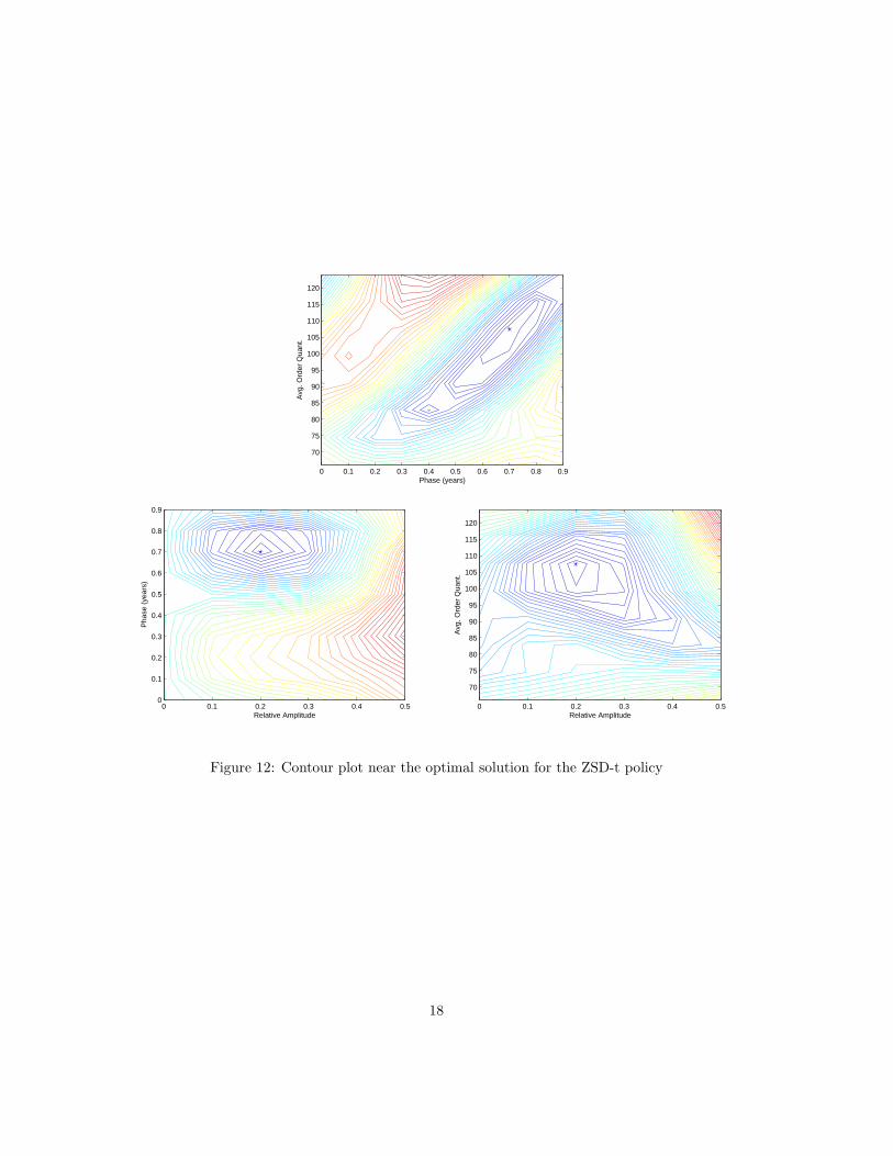
Our ZSD-t policy has three decision variables: average order quantity, relative amplitude, and phaseshift. It would be difficult to visualize the objective function in these three dimensions, so we will lookat cross-sections. In Figure 12, we plot contours of the objective function for the ZSD-t policy, with eachsubplot fixing one of the variables at its optimal value. In each subplot, the optimal solution is marked

17

Phase (years)

Avg

. Ord

er Q

uant

.

0 0.1 0.2 0.3 0.4 0.5 0.6 0.7 0.8 0.9

70

75

80

85

90

95

100

105

110

115

120

Relative Amplitude

Pha

se (

year

s)

0 0.1 0.2 0.3 0.4 0.50

0.1

0.2

0.3

0.4

0.5

0.6

0.7

0.8

0.9

Relative Amplitude

Avg

. Ord

er Q

uant

.

0 0.1 0.2 0.3 0.4 0.5

70

75

80

85

90

95

100

105

110

115

120

Figure 12: Contour plot near the optimal solution for the ZSD-t policy

18

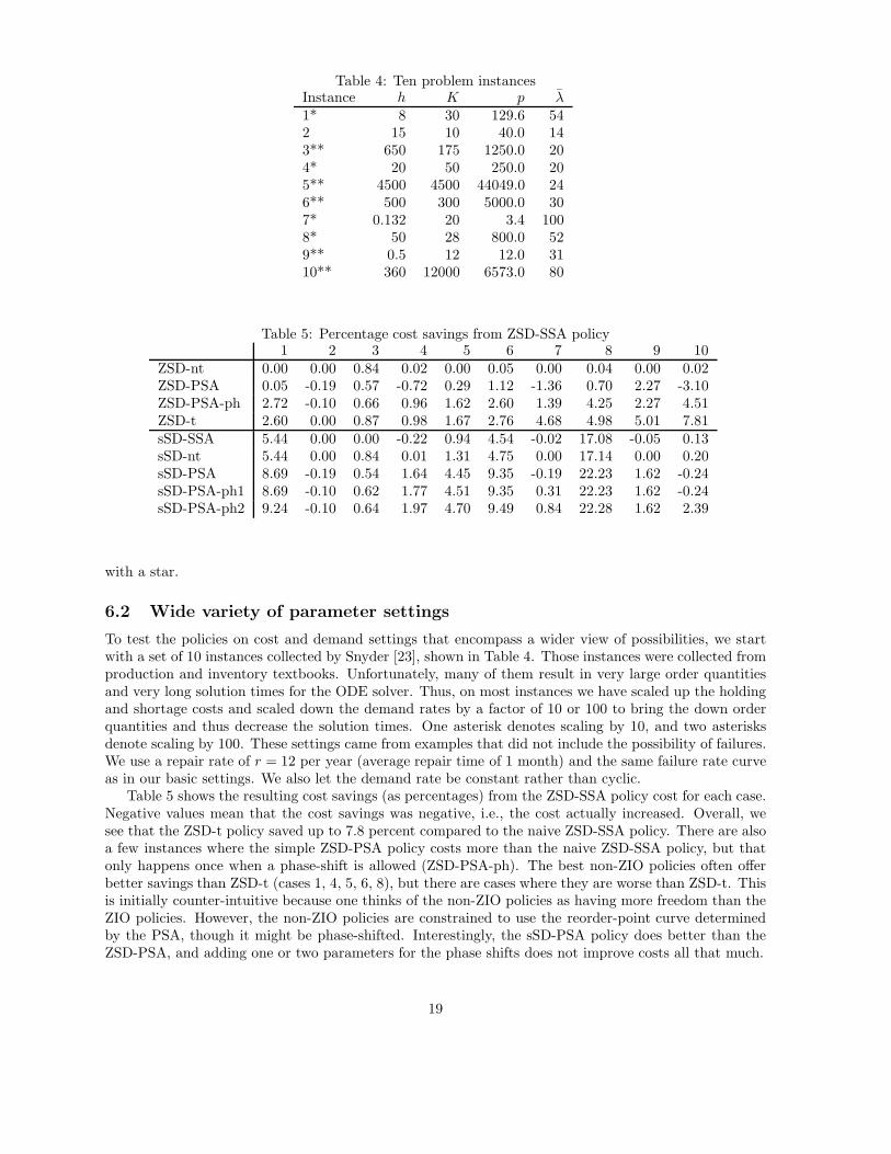
Table 4: Ten problem instancesInstance h K p λ1* 8 30 129.6 542 15 10 40.0 143** 650 175 1250.0 204* 20 50 250.0 205** 4500 4500 44049.0 246** 500 300 5000.0 307* 0.132 20 3.4 1008* 50 28 800.0 529** 0.5 12 12.0 3110** 360 12000 6573.0 80

Table 5: Percentage cost savings from ZSD-SSA policy1 2 3 4 5 6 7 8 9 10

ZSD-nt 0.00 0.00 0.84 0.02 0.00 0.05 0.00 0.04 0.00 0.02ZSD-PSA 0.05 -0.19 0.57 -0.72 0.29 1.12 -1.36 0.70 2.27 -3.10ZSD-PSA-ph 2.72 -0.10 0.66 0.96 1.62 2.60 1.39 4.25 2.27 4.51ZSD-t 2.60 0.00 0.87 0.98 1.67 2.76 4.68 4.98 5.01 7.81sSD-SSA 5.44 0.00 0.00 -0.22 0.94 4.54 -0.02 17.08 -0.05 0.13sSD-nt 5.44 0.00 0.84 0.01 1.31 4.75 0.00 17.14 0.00 0.20sSD-PSA 8.69 -0.19 0.54 1.64 4.45 9.35 -0.19 22.23 1.62 -0.24sSD-PSA-ph1 8.69 -0.10 0.62 1.77 4.51 9.35 0.31 22.23 1.62 -0.24sSD-PSA-ph2 9.24 -0.10 0.64 1.97 4.70 9.49 0.84 22.28 1.62 2.39

with a star.

6.2 Wide variety of parameter settings

To test the policies on cost and demand settings that encompass a wider view of possibilities, we startwith a set of 10 instances collected by Snyder [23], shown in Table 4. Those instances were collected fromproduction and inventory textbooks. Unfortunately, many of them result in very large order quantitiesand very long solution times for the ODE solver. Thus, on most instances we have scaled up the holdingand shortage costs and scaled down the demand rates by a factor of 10 or 100 to bring the down orderquantities and thus decrease the solution times. One asterisk denotes scaling by 10, and two asterisksdenote scaling by 100. These settings came from examples that did not include the possibility of failures.We use a repair rate of r = 12 per year (average repair time of 1 month) and the same failure rate curveas in our basic settings. We also let the demand rate be constant rather than cyclic.

Table 5 shows the resulting cost savings (as percentages) from the ZSD-SSA policy cost for each case.Negative values mean that the cost savings was negative, i.e., the cost actually increased. Overall, wesee that the ZSD-t policy saved up to 7.8 percent compared to the naive ZSD-SSA policy. There are alsoa few instances where the simple ZSD-PSA policy costs more than the naive ZSD-SSA policy, but thatonly happens once when a phase-shift is allowed (ZSD-PSA-ph). The best non-ZIO policies often offerbetter savings than ZSD-t (cases 1, 4, 5, 6, 8), but there are cases where they are worse than ZSD-t. Thisis initially counter-intuitive because one thinks of the non-ZIO policies as having more freedom than theZIO policies. However, the non-ZIO policies are constrained to use the reorder-point curve determinedby the PSA, though it might be phase-shifted. Interestingly, the sSD-PSA policy does better than theZSD-PSA, and adding one or two parameters for the phase shifts does not improve costs all that much.

19

0 20 40 60 80 100 12020

40

60

80

100

120

140

160The optimality of different policies

Fixed Cost

Tot

al C

ost

ZSD−PSA−fZSD−PSAEOQ−SSAZSD−SSAZSD−ntZSD−PSA−phZSD−t

0 20 40 60 80 100 1200

5

10

15

20

25

30

35

40

45Cost increase percentage of different policies compared to the ZSD−t policy

Fixed Cost

Cos

t inc

reas

e pe

rcen

tage

ZSD−PSA−fZSD−PSAEOQ−SSAZSD−SSAZSD−ntZSD−PSA−ph

Figure 13: Total cost under different policies when the fixed cost changes

0 10 20 30 40 50 6075

80

85

90

95

100

105

110

115


Stockout Cost

Tot

al C

ost


0 10 20 30 40 50 600

5

10

15

20

25


Stockout Cost

Cos

t inc

reas

e pe

rcen

tage


Figure 14: Total cost under different policies when the stockout cost changes

Having looked at these examples, we will turn to an exploration of the parameter space near ourcentral case.

6.3 Sensitivity around the central example

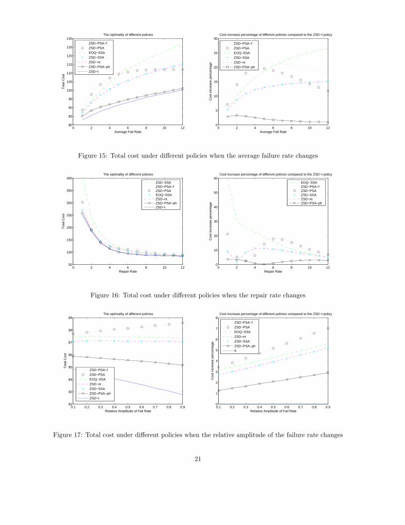
In order to investigate the benefit of the ZSD-t policy, we vary, one by one, the fixed cost K (Figure 13),stockout cost p (Figure 14), average failure rate f (Figure 15), repair rate r (Figure 16), RA of thefailure rate RAf (Figure 17), RA of the demand rate RAd (Figure 18), and phase of the demand rate φd

(Figure 19). Each figure varies one parameter with the other parameters staying at the values given inTable 1. Each figure shows the actual cost curves on the left, and the percent increase above the ZSD-tcost on the right. Compared to those constant-order-quantity policies, the benefit of the ZSD-t policyincreases with stockout cost, average failure rate and its relative amplitude, and the relative amplitudeof demand rate.

From these plots, it is clear that the ZSD-t policy generally outperforms the other proposed policies.The second best policy is ZSD-PSA-ph, which is clearly better than ZSD-PSA; that is, the ability to adjustthe phase in response to the system lag is important, as we mentioned when we first introduced ZSD-PSA-ph. Generally, ZSD-PSA-ph stays within 5 to 10 percent of the ZSD-t policy. However, Figure 18 shows

20

0 2 4 6 8 10 1280

85

90

95

100

105

110

115

120

125


Average Fail Rate

Tot

al C

ost


0 2 4 6 8 10 120

5

10

15

20

25


Average Fail Rate

Cos

t inc

reas

e pe

rcen

tage


Figure 15: Total cost under different policies when the average failure rate changes

0 2 4 6 8 10 1250

100

150

200

250

300

350


Repair Rate

Tot

al C

ost

ZSD−SSAZSD−PSA−fZSD−PSAEOQ−SSAZSD−ntZSD−PSA−phZSD−t

0 2 4 6 8 10 120

10

20

30

40

50


Repair Rate

Cos

t inc

reas

e pe

rcen

tage

EOQ−SSAZSD−PSA−fZSD−PSAZSD−SSAZSD−ntZSD−PSA−ph

Figure 16: Total cost under different policies when the repair rate changes

0.1 0.2 0.3 0.4 0.5 0.6 0.7 0.8 0.982

83

84

85

86

87

88


Relative Amplitude of Fail Rate

Tot

al C

ost

ZSD−PSA−fZSD−PSAEOQ−SSAZSD−ntZSD−SSAZSD−PSA−phZSD−t

0.1 0.2 0.3 0.4 0.5 0.6 0.7 0.8 0.90

1

2

3

4

5

6

7



Cos

t inc

reas

e pe

rcen

tage

ZSD−PSA−fZSD−PSAEOQ−SSAZSD−ntZSD−SSAZSD−PSA−ph0

Figure 17: Total cost under different policies when the relative amplitude of the failure rate changes

21

0.1 0.2 0.3 0.4 0.5 0.6 0.7 0.8 0.980

85

90

95

100


Relative Amplitude of Demand Rate

Tot

al C

ost


0.1 0.2 0.3 0.4 0.5 0.6 0.7 0.8 0.90

5

10

15

20

25



Cos

t inc

reas

e pe

rcen

tage


Figure 18: Total cost under different policies when the relative amplitude of the demand rate changes;here, φd = 0, so the demand peak coincides with the failure rate peak.

0 0.1 0.2 0.3 0.4 0.5 0.6 0.7 0.8 0.970

75

80

85

90

95

100


Demand Phase

Tot

al C

ost


0 0.1 0.2 0.3 0.4 0.5 0.6 0.7 0.8 0.90

5

10

15

20

25

30

35


Demand Phase

Cos

t inc

reas

e pe

rcen

tage


Figure 19: Total cost under different policies when the phase of the demand rate changes; here, we haveRAd = 0.9 instead of our basic setting of RAd = 0.

22

Table 6: Extreme cases near the basic settings, percentage cost savings from ZSD-SSA policyBasic K = 1 p = 51 f = 12 r = 1 RAd = 0.9

ZSD-nt 0.0 0.1 0.0 0.2 0.0 0.4ZSD-PSA -1.7 2.4 -2.1 2.9 -11.1 -9.0ZSD-PSA-f 2.2 4.9 14.6 12.4 6.5 2.6ZSD-PSA-ph 2.2 4.7 14.7 12.3 5.0 2.5ZSD-t 4.9 4.9 14.7 13.2 8.3 14.5sSD-SSA 0.0 12.2 10.0 13.6 18.8 0.4sSD-nt 0.0 12.3 10.0 13.6 19.5 0.7sSD-PSA -0.1 17.9 12.4 15.0 17.0 -5.4sSD-PSA-ph1 0.5 17.9 12.4 15.0 19.4 2.1sSD-PSA-ph2 1.3 18.0 12.5 15.2 20.6 13.6

that the difference can climb toward 15 percent when the demand rate has a large relative amplitude.The ZSD-PSA and ZSD-PSA-f curves are close in many cases; this shows that the exact shape of

the curve (the near-sinusoid PSA versus a pure sinusoid) is not so important. The exception is whenthe demand phase is not synchronous with the failure rate phase. Then, the ZSD-PSA is not nearly asinusoid, and so there are larger differences in cost between it and the ZSD-PSA-f policy. One surprise isthat these time-dependent ZSD-PSA and ZSD-PSA-f policies are actually substantially worse than theconstant-order-quantity policies ZSD-nt and ZSD-SSA (and even EOQ-SSA) in many cases. This reflectsthe importance of accounting for the system lag.

The constant-order-quantity policies ZSD-SSA and ZSD-nt are very close in almost all cases. Thus,there is little benefit to be obtained by optimizing a constant order quantity instead of simply using theZSD-SSA policy. The EOQ-SSA is even close to (but always worse than) the ZSD-SSA in some cases. Aphenomenon of minor interest is shown in Figure 17: policies with constant order quantities are almostentirely insensitive to changes in RAf , as long as the demand level does not fluctuate at all.

When the failure rate amplitude increases (Figure 17), we are met with another surprise: the costsfor ZSD-t and ZSD-PSA-ph go down rather than up. Inspection of the optimal policies reveals that theytend to concentrate their orders during the time of low failure rate, and avoid the peak failure rate. Thisillustrates the benefits of a real-time ordering policy, as opposed to a constant order quantity.

When the demand amplitude increases rather than the failure rate amplitude (Figure 18), the ZSD-tpolicy still saves more money. This is also surprising, because in many fields and models (call centers,electric power generation, etc.) it costs more to meet non-constant demand than steady demand. Theoptimal ZSD-t policies in these cases tend to place their orders as the demand curve is increasing, soholding costs are reduced.

Next, we look at the effects of the non-ZIO policies in some of the extreme cases of the above figures.These cases are chosen to make failures even more of a factor than they are in the central case. Forexample, we have (individually) increased the stockout cost, increased the failure rate, and decreasedthe repair rate. Since in these cases it is more important to avoid stockouts, we should see more of abenefit from the non-ZIO policies. The resulting Table 6 is similar to Table 5: it shows percent costincreases compared to the ZSD-SSA policy for some parameter settings. Just as in Table 5, we see thatthe non-ZIO policies are not uniformly better than ZSD-t. In the basic case, the increased stockout costcase, and the RAd = 0.9 case the ZSD-t policy is better than all of the non-ZIO policies. Also, whenRAd = 0.9 the phase shift allowed by sSD-PSA-ph1 substantially improves the cost compared to theplain PSA, but in the other cases it is not so important.

6.4 Robustness

In most cases, the overall probability of disruption is low, which makes it difficult to estimate the ratesneeded for the CTMC. Also, using an exponential distribution to approximate the repair process may

23

not be accurate, as an exponential distribution has an unchangeable variability relative to its mean. Onemight expect variability to be larger if disruptions vary widely in severity, or smaller if the supplier isequipped to handle a small number of foreseeable disruptions. In this section we concentrate on the ZIOpolicies for simplicity.

Suppose we obtain the optimal ZSD-t policy using the assumptions introduced earlier. We would liketo evaluate its performance under “real” settings as compared to the optimal ZSD-nt policy for thosesettings. Therefore, we study the tradeoff between the savings by employing a time-dependent controlsystem and the robustness obtained by using a time-independent control rule.

6.4.1 Supplier Parameters

We start by investigating the effect of errors in the relative amplitude and phase of the failure rate.Starting with our basic settings from Table 1 as the “true” parameters, we consider the optimal ZSD-tpolicy and its cost, as was done in Section 6.1. Then, we suppose that the firm has mis-estimated RAf

and φf , and compute the ZSD-t and ZSD-nt policies they would have found. We then take these policiesand evaluate them using the true parameters, to determine the resulting cost increase.

We are using both ZSD-t and ZSD-nt because one might think that it could be better to use aconstant-order-quantity policy in the presence of uncertainty about the behavior of the failure rate. Ifthe failure rate is the only fluctuating rate (as it is in our basic settings), then the ZSD-nt policy isentirely insensitive to φf because it amounts only to a change of time origin.

In our experiment, we let the firm’s estimates of RAf and φf vary as follows: RAf = 0, 0.1, . . . , 1and φf = 0, 0.1, . . . , 1. This would result in 11 · 11 = 121 data points, with the exception that somedata points with RAf = 1.0 result in numeric difficulties because the failure rate hits zero, and thus areexcluded (this is also common in queueing models). Each of these has a cost for the misguided ZSD-tused in the true-parameter model, and for the misguided ZSD-nt used in the true-parameter model.From these roughly 121 cost increases for the two policy types, we examine the maximum, minimum,and average (with all combinations given equal weight). Note that, as we saw in Figure 17, the ZSD-ntpolicy experiences almost exactly the same cost regardless of the value of RAf when RAd = 0; thus, itsaverage, minimum, and maximum are essentially the same.

Intuition would predict that the worst-case cost increase occurs when the failure rate’s relative am-plitude, RAf , is large and the phase, φf , is mis-estimated by half a yearly cycle. This is indeed thecase. However, when the relative amplitude is large, more data will be available concerning when thepeak occurs, because failures will be more concentrated there. Thus, the worst case of mis-estimation isunlikely to occur. In that sense, giving equal weight to all possibilities of mis-estimation in taking theaverage is being conservative.

Figure 20 shows the resulting total costs as various system parameters change. In these plots, thedemand rate is constant. We only plot the average cost for the ZSD-nt policy, because its minimum andmaximum are negligibly different, as previously noted. The figure shows that there are some cases whereusing the ZSD-nt policy guards against the worst case of mis-estimation when using ZSD-t. However,even in those cases, it is still better on average to use the ZSD-t policy. In other cases, the ZSD-t policycalculated based on the most-wrong estimates is still better than the corresponding ZSD-nt policy.

Next, we turn to the case where the demand rate varies in time, shown in Figure 21. We are supposingthat the demand rate function is certain; it is the failure rate function that is uncertain, as before. Thisis reasonable, because the firm should have plenty of data on demand rates, since demand is nowherenear as rare as failures. In the fluctuating-demand scenario, the ZSD-nt policy costs are not essentiallyconstant as they were in the previous figure. We see that the ZSD-nt policy is, on average, worse thanthe worst-case scenario for the ZSD-t policy. Thus, it is better to use the ZSD-t policy rather than theZSD-nt policy.

6.4.2 Repair Distribution

Because failures and their subsequent repairs are not particularly common, it is difficult to estimate thedistribution of the time it takes to repair the system. Estimates of anything beyond the mean (variance,

24

0 20 40 60 80 100 12020

40

60

80

100

120

140

160

Fixed Cost

Tot

al C

ost

Average cost under opt. ZSD−ntHighest cost under opt. ZSD−tAverage cost under opt. ZSD−tLowest cost under opt. ZSD−t

0 10 20 30 40 50 6075

80

85

90

95

100

105

110

115

120

Stockout Cost

Tot

al C

ost

Highest cost under opt. ZSD−tAverage cost under opt. ZSD−ntAverage cost under opt. ZSD−tLowest cost under opt. ZSD−t

0 2 4 6 8 10 1280

85

90

95

100

105

110

115

120

Average Fail Rate

Tot

al C

ost


0 2 4 6 8 10 1250

100

150

200

250

300

Repair Rate

Tot

al C

ost


0 0.1 0.2 0.3 0.4 0.5 0.6 0.7 0.8 0.982.5

83

83.5

84

84.5

85

85.5

86

86.5

87

87.5


Tot

al C

ost


Figure 20: Robustness plot when the demand rate is constant over time

0.1 0.2 0.3 0.4 0.5 0.6 0.7 0.8 0.970

75

80

85

90

95

100


Tot

al C

ost

Highest cost under opt. ZSD−ntAverage cost under opt. ZSD−ntHighest cost under opt. ZSD−tLowest cost under opt. ZSD−ntAverage cost under opt. ZSD−tLowest cost under opt. ZSD−t

Figure 21: Robustness plot when the relative amplitude of demand increases

25

skewness, etc.) would be rough at best. Thus, we should investigate the effects of assuming a simple (i.e.exponential) distribution when the true distribution is different.

As mentioned in Section 1.2, we will use phase-type distributions. For a distribution that is lessvariable than exponential, we will use an Erlang distribution with 2 phases, abbreviated E2. Its coefficientof variation (standard deviation divided by mean) is 1/

√2 ≈ 0.707. For a distribution that is more variable

than exponential, we will use a hyperexponential with two phases (abbreviated H2). We have chosen itscoefficient of variation to be 2. We have used a balanced-means hyperexponential, which is a commonchoice (see Allen [1]).

From our basic settings, we change the exponentially distributed repair time to an E2 distribution tomake repair times less variable. We find numerically that the optimal ZSD-t policy changes only by aninsignificant amount. Thus, there is practically no harm in using an exponential distribution for repairtimes if the true distribution is E2. We conjecture that higher-order Erlang distributions (Erlang-3, etc.),which become less and less variable, may induce somewhat larger differences. The number of states inour CTMC, and thus the run-time of our solution procedures, goes up approximately linearly with thenumber of stages in the repair distribution. Thus, there is a disincentive to use Erlang distributions witha large number of stages.

If we change the exponentially distributed repair time to the H2 distribution that we have chosen,and find the new optimal ZSD-t policy (knowing that the H2 distribution holds), its true cost is 90.82. Ifwe apply the old ZSD-t policy determined under the exponential repair time assumption, but evaluate itusing H2 repair times, its cost is 90.88, a very small increase. The policies are mildly different: the new(H2-optimal) policy has an average order quantity 5.7 percent higher than the old (exponential-optimal)policy, and the phase shift increases by 0.05 to 0.75.

7 Conclusions

We said in Section 2.2 that we would explore the middle ground between PSA and SSA applicability.We have seen that the plain PSA-type policies (ZSD-PSA and ZSD-PSA-f) are worse than the SSA-typepolicies (ZSD-SSA, ZSD-nt) in most of the cases we evaluated. So, it would seem that our parameterchoices have tended toward the SSA side of the middle ground. However, we have also seen that the ZSD-tpolicy (which is decidedly not an SSA) is much better than the SSA policies. Also, the ZSD-PSA-phpolicy is second best, and it is also neither a true PSA nor an SSA. Thus, we conclude that our parameterchoices have indeed established an interesting middle ground.

The effect of lag in the system is important, and in many cases it is better to use a plain stationarypolicy (such as ZSD-SSA or ZSD-nt) than to use a nonstationary policy that ignores lag effects (such asZSD-PSA).

Overall, we see that the ZSD-PSA-ph policy balances cost savings with ease of computation, sinceonly one parameter must be optimized, as opposed to 3 parameters for the ZSD-t policy. However, if thedemand fluctuations are medium-large, only the ZSD-t policy can take better advantage of them and isprobably worth the extra effort.

The non-ZIO policies, in allowing a positive reorder point, sometimes offer extra cost savings but notalways.

When we looked at the effects of mis-estimating the failure rate phase and relative amplitude, wefound that the benefits of using a time-dependent policy outweigh the virtual insensitivity of a non-real-time policy in almost every case. Thus, we conclude that our time-dependent policy is robust in theface of uncertainty about these parameters. While it may suffer some cost increase, that cost increase ispreferable to what the firm would suffer if a too-simple policy was used. We also found that the systemwas robust against the changes in the repair-time distribution that we tested. This is important becauselittle data are available on the distribution of repair times.

It would be straightforward to include a variety of other features in the model and still be able toformulate it as a CTMC. Such features include phase-type demand arrivals (to model smooth or burstydemand), phase-type random lead times even when the supplier is up, backordered demand, batch demand

26

arrivals of random sizes, and random yield.

References

[1] Arnold O. Allen. Probability, statistics, and queueing theory : with computer science applications,

2nd Ed. Harcourt Brace Jovanovich, 1990.

[2] Emre Berk and Antonio Arreola-Risa. Note on “Future supply uncertainty in EOQ models”. Naval

Research Logistics, 41:129–132, 1994.

[3] T. Bielecki and P. R. Kumar. Optimality of zero-inventory policies for unreliable manufacturingsystems. Operations Research, 36(4):532–541, 1988.

[4] J.R. Dormand and P.J. Prince. A family of embedded Runge-Kutta formulae. J. Comp. Appl. Math.,6:19–26, 1980.

[5] Stephen G. Eick, William A. Massey, and Ward Whitt. Mt/G/∞ queues with sinusoidal arrivalrates. Management Science, 39(2):241–252, February 1993.

[6] Stephen G. Eick, William A. Massey, and Ward Whitt. The physics of the Mt/G/∞ queue. Opera-

tions Research, 41(4):731–742, July-August 1993.

[7] Linda V. Green and Peter J. Kolesar. The pointwise stationary approximation for queues withnonstationary arrivals. Management Science, 37(1):84–97, January 1991.

[8] Linda V. Green and Peter J. Kolesar. The lagged PSA for estimating peak congestion in Markovianqueues with periodic arrival rates. Management Science, 43(1):80–87, Jan 1997.

[9] Linda V. Green, Peter J. Kolesar, and Anthony Svoronos. Some effects of nonstationarity on multi-server Markovian queueing systems. Operations Research, 39(3):502–511, May–June 1991.

[10] Diwakar Gupta. The (q,r) inventory system with an unreliable supplier. INFOR, 34:59–76, 1996.

[11] Ulku Gurler and Mahmut Parlar. An inventory problem with two randomly available suppliers.Operations Research, 45(6):904–918, 1997.

[12] David Heimann and Frenck Waage. A closed-form approximation solution for an inventory modelwith supply disruptions and non-ZIO reorder policy, Oct. 2005. submitted to MSOM.

[13] Zhaolin Li, Susan H. Xu, and Jack Hayya. A periodic-review inventory system with supply inter-ruptions. Probability in the Engineering and Informational Sciences, 18:33–53, 2004.

[14] Bin Liu and Jinhua Cao. Analysis of a production-inventory system with machine breakdowns andshutdowns. Computer & Operations Research, 26(1):73–91, 1999.

[15] Esmail Mohebbi. Supply interruptions in a lost-sales inventory system with random lead time.Computer & Operations Research, 30(3):411–426, 2003.

[16] Kamran Moinzadeh and Prabhu Aggarwal. Analysis of a production/inventory system subject torandom disruptions. Management Science, 43(11):1577–1588, 1997.

[17] Stephen Nahmias. Production and Operations Analysis. McGraw-Hill/Irwin, 5th edition, 2005.

[18] Marcel F. Neuts. Matrix-Geometric Solutions in Stochastic Models: An Algorithmic Approach.Dover, 1981.

[19] M. Parlar and D. Berkin. Future supply uncertainty in EOQ models. Naval Research Logistics,38:107–121, 1991.

27

[20] Mahmut Parlar. Continuous-review inventory problem with random supply interruptions. European

Journal of Operational Research, 99:366–385, 1997.

[21] Mahmut Parlar and David Perry. Analysis of a (Q, r, T ) inventory policy with deterministic andrandom yeilds when future supply is uncertain. European Journal of Operational Research, 84:431–443, 1995.

[22] Mahmut Parlar and David Perry. Inventory models of future supply uncertainty with single andmultiple suppliers. Naval Research Logistics, 43:191–210, 1996.

[23] Lawrence V. Snyder. A tight approximation for a continuous-review inventory model with supplierdisruptions. working paper, Lehigh University, 2005.

[24] William J. Stewart. Introduction to the Numerical Solution of Markov Chains. Princeton, 1994.

[25] Brian T. Tomlin and Lawrence V. Snyder. Inventory management with advanced warning of disrup-tions. working paper, Lehigh University, 2006.

[26] Ward Whitt. The pointwise stationary approximation for Mt/Mt/s queues is asymptotically correctas the rates increase. Management Science, 37(3):307–314, Mar 1991.

[27] Paul H. Zipkin. Foundations of Inventory Management. McGraw Hill, 2000.

28

supply disruptions with time-dependent parameterslvs2/papers/supply-disrupt-timedep.pdf · supply...

Documents