strategic risk from supply chain disruptions - michigan rosswebuser.bus.umich.edu/whopp/working...
TRANSCRIPT

Strategic Risk from Supply Chain Disruptions
Wallace J. HoppStephen M. Ross School of Business, University of Michigan, Ann Arbor, MI
Seyed M. R. Iravani and Zigeng LiuDepartment of Industrial Engineering and Management Science,
Northwestern University, Evanston, IL
Abstract
Supply chain disruptions can lead to both tactical (loss of short term sales) and strategic (loss of longterm market share) consequences. In this paper, we model the impact of regional supply disruptionson competing supply chains. We describe generic strategies that consist of two stages: (i) preparation,which involves investment prior to a disruption in dedicated backup capacity and/or measures thatfacilitate quick detection of a problem, and (ii) response, which involves post-disruption purchase ofshared (non-dedicated) backup capacity for a component whose availability has been compromised.Using expected loss of profit due to lack of preparedness as a measure of risk, we characterize theconditions that pose the greatest risk and suggest ways to reduce the risk exposure. This analysisreveals that a dominant firm in the market should focus primarily on protecting its market share,while a weaker firm should focus on being ready to take advantage of a supply disruption to gainmarket share. We distinguish between preparedness activities related to monitoring and detectionas systemic preparation, which affects many components simultaneously, and preparedness activitiesrelated to securing extra dedicated backup capacity as targeted preparation, which affects only a specificcomponent. We characterize conditions that affect the optimal ratio of investment in these two typesof preparation and conclude that larger firms should use targeted preparation defensively, while smallerfirms should use it offensively. Finally, we discuss how firms can use both long term information (e.g.,estimates of the likelihood of disruptions) and real-time information (e.g., severity of disruption afterit occurs) as part of their preparedness strategy.
Keywords: supply chain disruption, risk, preparedness
———————————————————————————————————————————————
1 Introduction
High profile incidents of global terrorism have elevated concerns about risks in all aspects of private
and public life, including management of business operations. However, while terrorist activities are
particularly newsworthy, other sources of risk, such as natural disasters and political/economic shocks,
present a more widespread challenge to managers. Regardless of the source, it is clear that preparation
for and management of major disruptions is an important part of modern operations management.
In this paper, we focus on the risk of supply disruption, which is inherent in global supply chains.
We divide this risk into two categories: (1) tactical risk, which characterizes events that result in only a
short term loss of sales revenue, and (2) strategic risk, which is associated with events that result in a
long term loss of market share, in addition to a loss of sales.
An example of a strategic risk event occurred on March 17, 2000, when a ten-minute fire at a Royal
Philips Electronics semiconductor plant in Albuquerque, New Mexico, “touched off a corporate crisis
that shifted the balance of power between two of Europe’s biggest electronics companies...” (Wall Street
1

2Hopp et al. Strategic Risk from Supply Chain Disruptions
Article Submitted to Management Science
19981997 1999 2000 2001 2002 2003 2004
Market Share
10%
30%
20% MOTOROLA
SAMSUNG
NOKIA
End of OutageFire at Philips’ Plant
Year ERICSSON
Figure 1: Global Mobile Market Share from 1997 to 2004 (Gartner (2006)).
Journal, January 29, 2001). This occurred because, besides directly destroying several thousand chips for
mobile phones, the fire contaminated the clean room environment in the semiconductor plant, effectively
shutting it down for weeks. At the time, both Nokia and Ericsson were sourcing microchips from the
Philips plant. However, while Nokia was able to quickly shift production to other Philips plants and
some Japanese and American suppliers, Ericsson was trapped by its sole source dependence on the
Philips plant. Consequently, Ericsson had no way to make a rapid response to the disruption, and wound
up losing around $400 million in sales by the end of the first disruption-impacted quarter (Elgin (2003)).
Worse, six months after the fire, Ericsson’s market share of the global handset market had fallen by
3%, its stock price had decreased by 12%, and Ericsson’s mobile phone division reported a $2.34 billion
loss for 2000 (Sheffi (2005)). This setback almost certainly accelerated Ericsson’s decline in the handset
market (see Figure 1). In combination with a variety of other problems, this led Ericsson to merge its
mobile phone unit with Sony in 2001 (Kharif (2001), Sheffi (2005)).
Such dramatic consequences from a seemingly minor disruption seem to be the rule rather than
the exception. Hendricks and Singhal (2005) considered a sample of 827 disruptions (ranging from a
shipment delay to a key part shortage) announced between 1989 and 2000 and examined stock prices
over a three-year period beginning one-year prior to the announcement of a disruption and ending two
years after it. They found that firms who reported supply chain disruptions had stock returns over the
three-year period that were nearly 40 percent lower than comparable firms that did not report disruptions.
Evidently, supply chain disruptions are major business events that have lasting effects.
However, not all consequences of supply chain disruptions are negative. At the end of 2001, Nokia
and Samsung reported large increases in market share, while Motorola stopped a steady decline in market

Hopp et al. Strategic Risk from Supply Chain DisruptionsArticle Submitted to Management Science 3
share (see Figure 1). Apparently, Ericsson’s loss was these other firms’ gain, since some customers who
were unsupplied by Ericsson shifted their purchases to other brands. Evidently, supply chain disruptions
can pose opportunities for strategic gain, as well as loss.
To understand why the Philips disruption had such an unbalanced impact on Nokia and Ericsson, we
must go back to the year 1995. At that time, due to poor delivery performance and a relatively weak
product line, Nokia was experiencing mismatches between supply and demand. To remedy the situation,
Nokia installed a monitoring process, which enabled it to spot the disruption quickly (even before Philips
officially notified it of the problem) and to initiate a dialogue with Philips about alternate supplies. Once
Nokia’s component-purchasing manager knew about the fire, he quickly reported it to his upper-level
managers, in keeping with Nokia’s culture of encouraging dissemination of bad news. Nokia decided to
scrutinize the situation and call Philips daily to monitor the event. When Nokia realized the shortage due
to the fire would last for more than month, it assembled a task force to investigate all possible alternative
sources of supply (Sheffi (2005)). This included capacity of other Philips facilities, as well as that of other
suppliers. The ability to use non-Philips chips was facilitated by an earlier decision by Nokia to redesign
its phones to accommodate a wider range of chips that could be supplied by various suppliers in Japan
and the United States. In contrast, Ericsson did not realize the severity of the disruption until Nokia
had locked up all available supplies of the original chips and Ericsson did not have product flexibility to
allow use of other more widely available chips.
A major reason that a small-scale disruption resulted in a huge loss for Ericsson is that it resulted
in the loss of unsatisfied customers (Stauffer (2003)). In hindsight, it is clear that Ericsson grossly
underestimated the impact of what it thought would be a one-week delay of its chip supply. When
Philips called two weeks after the fire to explain that the delay would be much longer, Ericsson realized
too late that it would have thousands of disappointed customers, some of whom would not return. In
recognition of this type of customer dynamics, Zsidisin et al. (2000) concluded that firms implementing
high efficiency supply management techniques (e.g., single sourcing, just-in-time deliveries for production)
must be aware that such practices may increase their exposure to risk. Stauffer (2003) noted that it is
no longer feasible to try to cover losses from supply chain disruptions through insurance, since the 9/11
terrorist attack and other major events have altered the policies of insurance companies to limit coverage.
Although there has been a great deal of research devoted to the design, coordination and improvement
of supply chains (see, e.g., Fisher et al. (1997), Fine (2000), Lee (2003), Graves and Willems (2003), Gan
et al. (2005)), relatively little of this has focused on supply chain risks. Much of what has been done is
descriptive in nature. For example, Johnson (2001) divided supply chain risks into two categories: (a)

4Hopp et al. Strategic Risk from Supply Chain Disruptions
Article Submitted to Management Science
demand risks, including seasonal imbalances, fab volatility, and new product adoption, and (b) supply
risks, such as manufacturing and logistics capacity limitations, currency fluctuations, and supply disrup-
tions from political issues. Chopra and Sodhi (2004) further refined these into a taxonomy of risks faced
in supply chains and qualitatively discussed the different strategies for mitigating them. Kleindorfer and
Saad (2005) discussed the implications of designing supply chain systems to deal with disruption risks,
based on a conceptual framework, which they termed the “SAM-SAC” Framework, and generated several
empirical results from a data set of the U.S. Chemical Industry. Christopher and Peck (2004) also dis-
cussed how to design resilient supply chains in qualitative terms, with an emphasis on fully recognizing
the nature of supply chain risks. In this same vein, Christopher and Lee (2004) suggested that improved
end-to-end visibility is a key element for mitigating supply chain risk.
Some researchers have considered supply chain disruptions in multi-echelon settings. Snyder and
Shen (2006) investigated both supply uncertainty and demand uncertainty in simple multi-echelon supply
chains using simulation. They pointed out that these two types of uncertainties require opposite responses
and therefore firms should consider both types simultaneously to identify an optimal strategy. Hopp and
Liu (2006) developed an analytical model for striking a balance between the costs of inventory and/or
capacity protection and the costs of lost sales in an arborescent assembly network subject to disruption.
They showed that, under certain conditions, it is optimal locate inventory or capacity protection at no
more than one node along each path to the customer. In a related vein, Tomlin (2006) considered a
firm that has two suppliers: one inexpensive and unreliable and the other expensive and reliable with
volume flexibility. They described management strategies for using the two types of supplier to mitigate
disruptions under various environmental assumptions. Tomlin and Snyder (2006) further considered
disruption mitigation strategies for the situation in which disruptions are stochastic and the firm gets
some advance warning of the disruptions. Tomlin and Tang (2008) studied five stylized models (which
correspond to five types of flexible strategies) and suggested that flexibility can be used as a powerful
defensive protection mechanism to mitigate supply chain risks.
While the above research is beginning to reveal principles of supply chain risk mitigation, to our
knowledge, there is not yet a comprehensive modeling framework with which to evaluate both tactical
and strategic risks to a firm from supply disruptions. In this paper, we develop such a framework and use
it to analyze both how firms in competitive environments should prepare for potential disruptions and
how they should respond to disruptions once they occur. In some cases, this analysis gives quantitative
confirmation of intuitive behavior. In others, it reveals insights that are not otherwise apparent.
The remainder of this paper is structured as follows: In Section 2, we introduce a duopoly model

Hopp et al. Strategic Risk from Supply Chain DisruptionsArticle Submitted to Management Science 5
with a third party, in which two firms compete for a common backup supply after a disruption of the
primary supply of a key component, but the third party, which produces a competitive product, is not
affected by the disruption. Note that this matches the Philips-Nokia-Ericsson scenario, in which Nokia
and Ericsson are the duopoly and firms like Samsung and Motorola collectively constitute the outside
firm. Section 2.1 analyzes the Backup Capacity Competition (BC Competition) within this model in order
to characterize the optimal plan of action to be followed by firms after a disruption. In Section 2.2 we
study the Advanced Preparedness Competition (AP Competition), in which firms compete by investing
in strategies for mitigating supply chain risks in advance of a disruption. In Section 2.3 we perform a
sensitivity analysis of factors that influence the AP Competition. In Section 3 we investigate the factors
that influence the degree of strategic risk faced by firms and develop insights into preparation strategies.
Section 4 summarizes our conclusions and points to future research directions.
2 Model Formulation
To create a framework within which to evaluate the strategic impact of a supply disruption, we begin
by considering a market consisting of two firms, A and B, that sell competing products. Both products
require a key component that is purchased from a common supplier or region that is subject to disruption.
Because the key components is essential, a disruption in supply will prevent production. In addition to
the two firms affected by the disruption, there is a third firm C, which offers a substitute for the products
offered by firms A and B. However, because the third firm C’s product is sufficiently different from those
of firms A and B to allow it to rely on different components, it is not affected by the supply disruptions
under consideration. Because of this, a disruption presents an opportunity for Firm C to steal customers
from Firms A and B, but not for Firms A and B to steal customers from Firm C.1
We model the disruption as a random event that completely stops the supply of the disrupted com-
ponent and consists of two periods: (i) a fixed lead time T between the time of the disruption and the
time when the backup capacity is able to begin supplying the key component, and (ii) a random duration
of time after the lead time that extends to the end of the outage, which we assume follows a cumulative
probability distribution F (·) with an average of µ units of time (see Figure 2).
To create a model, we suppose Firm i (i ∈ A,B) has capacity to produce Ki products per unit
time and sells its products at a profit margin of ri per product. Each product requires one unit of the
key component. Before a disruption, demand for Firm i’s product is d0i
per unit time. To allow us to
1Note that if firms have independent suppliers, a disruption will affect only one of the competing firms. In our framework,this can be represented by a model with Firms A and C, but no Firm B. As such, it represents a simpler case than the onewe consider in this paper.

6Hopp et al. Strategic Risk from Supply Chain Disruptions
Article Submitted to Management Science
TimeOutage
EndsBackup CapacityComes On Line
Outage Occurs
(with mean )µ Remaining Outage Time
(T) Fixed Lead Time
Pre-Disruption Period Outage (Post-Disruption Period)
Figure 2: Time sequence of events after a disruption.
consider cases where the firm purchases more backup capacity for the key component than it actually
needs, we define the “holding cost” for one unit unused backup capacity for Firm i be hi per unit time.
We assume that, during the outage, customers of Firm i who are unable to purchase from Firm i will
buy the product from the other firm, Firm j, as long as Firm j can provide substitute products. If there
is no alternate supply with which to replace the disrupted parts, then neither firm will be able to meet
demand. We further assume that, the third party, Firm C, offers a less-than-perfect substitute for the
products offered by Firms A and B, which customers may turn to if neither Firm A nor Firm B have
supply available.
We focus primarily on the situation where a backup supplier exists that could provide an alternate
supply of the disrupted parts. However, if the backup capacity is limited, as we would expect it to be,
the question of how it is allocated is critical. Several factors could influence which firm (A or B) has an
advantage in securing the backup capacity. One firm might have a prior relationship with the backup
supplier that gives them an edge. Or a firm’s size or reputation might make them a more desirable
customer. Or, as seems to have been the case in the competition between Nokia and Ericsson, it might
simply be a matter of who monitors the situation more carefully and therefore asks first. Our framework
will accommodate any of these, but we will focus on the first-come-first-serve rule as the most interesting
scenario.
We assume a contractual business-to-business (OEM) relationship between the firms and their cus-
tomers. That is, the firms have contracts with their existing customers and are therefore obligated to fill
orders from these customers before filling orders from new customers. In contrast, in a retail business-to-
consumer environment, firms often cannot control which customers—existing or new—have their orders
filled first. (For example, Kellogg cannot ensure that their corn flakes go to loyal Kellogg customers, as
opposed to Post customers who are unable to buy their usual brand.) Under the business-to-business
conditions, a firm will supply its own customers first. But if the firm is able to secure a backup capacity of
the disrupted parts beyond those needed for its own customers (and it has ample supplies of other parts
and the necessary production capacity), then it could meet demand from the competitor’s customers. We

Hopp et al. Strategic Risk from Supply Chain DisruptionsArticle Submitted to Management Science 7
assume that the firm will take advantage of the situation to do this if the competitor firm is unable to
satisfy its own customers during the outage. If one firm makes sales to the other firm’s customers, then
the second firm will lose revenue in the short term. Furthermore, if some of these customers shift their
future sales to the new firm, then the second firm will also lose long term market share.
Our assumption that, during the outage, customers of a firm unable to meet demand are willing to
switch to another firm, is motivated by the fact that these customers are themselves firms. If the customer
firms make use of lean practices, they will have limited supplies of components on hand. To avoid shutting
down production, they must seek alternate supplies almost immediately in the face of a disruption. This is
what happened when cellular services companies unable to obtain Ericsson handsets were quick to satisfy
their customers with alternate brands. However, whether a customer will switch permanently depends
on his/her brand loyalty. We model brand loyalty of Firm i’s (i ∈ A,B) customer by the length of time
that customers of Firm i wait during the disruption before they permanently switch to the other firm’s
product. Specifically, we assume that a customer of Firm i who uses Firm j’s (j 6= i, j ∈ A,B, C)product during an outage, waits for an exponentially distributed amount of time with an average of γij
before permanently switching to Firm j’s product, and hence we refer to γij as Firm i’s customer loyalty
relative to Firm j. We define mij as the (finite) net present value of the long term market share that
Firm j gains from one customer who permanently switches from Firm i to Firm j, where j 6= i; define
mii as the (finite) net present value of the market share of Firm i to Firm i.
In situations where the first firm (either A or B) to detect the disruption and contact the backup
supplier will have the option to buy as much of the backup capacity as it chooses, there is incentive
to invest in early detection capabilities. Indeed, this is precisely what Nokia did when it installed its
new monitoring system. Hence, we include a preparedness period, in which firms invest in monitoring
technology, research potential backup suppliers and take other measures to enable them to be first to
secure the backup capacity in the event of a disruption. Specifically, we consider the following two periods:
• Pre-Disruption Period: Before a disruption occurs, both Firm A and Firm B serve their own
customers. Each firm estimates the likelihood of a disruption of the key component, which may differ
from the true likelihood of the disruption (p0). After a disruption occurs, firms will seek available
backup capacity for the key component. There are two types of backup capacity: (a) dedicated
capacity that is committed to a specific firm (e.g., due to a contractual or informal relationship),
and (b) shared capacity, for which the two firms compete, if the dedicated backup capacity is
not enough to cover the shortage. To model this competition, we denote the amount of Firm i’s
sales (i ∈ A,B) that cannot be covered by the dedicated capacity as d0i, and the shared backup

8Hopp et al. Strategic Risk from Supply Chain Disruptions
Article Submitted to Management Science
capacity by S. Both firms know that if the disruption occurs, the firm that detects the disruption
and moves first has the advantage of securing some or all of the total available backup capacity
for the key component. Therefore, each firm must decide how to invest in preparedness in order to
be able to detect the disruption first. This results in an Advanced Preparedness Competition (AP
Competition), in which the two firms invest in preparedness and thereby determine their respective
probabilities of being first to detect the problem in the event of a disruption.
• Post-Disruption Period: After the disruption occurs, the firm (either A or B) that detects the
disruption must decide how much of the total available backup capacity of S to buy in order to
maximize its short- and long term profits. This results in a Backup Capacity Competition (BC
Competition), in which one of the firms (i.e., the winner of the AP competition) is designated as the
“Leader” and gets first chance at purchasing the backup capacity. After the first firm has made its
purchase, the other firm, the “Follower”, then decides how much of the leftover backup capacity to
purchase. Once both firms have made their purchase amount decisions, there is a lead time period
required to bring the backup capacity on-line. During this period, both Firm A and Firm B lose
all of their short term sales, as well as some long term market share, to Firm C. The amount of the
market share of Firm i (i ∈ A,B) that is lost to Firm C during the lead time is d0i− di , where
di is the demand for Firm i’s product at the end of the lead time. Since the profit loss during
the lead time is unavoidable for both firms, we can treat the moment immediately after the lead
time as the beginning of the post-disruption period. Furthermore, we assume that, after the lead
time, if the available backup capacity is not enough to cover the total market, then all unsatisfied
customers will buy substitute products from Firm C during the outage. The number of customers
that permanently switch to Firm C, depends on the customer brand loyalty.
It is clear that if ample backup capacity of the key component existed (i.e., S is infinite), then there
would be no AP Competition or BC Competition between Firm A and Firm B, because there would be
no shortage to allow an opportunity to “poach” customers from the other firm. Hence, Firm i will only
purchase di units of the capacity per unit time to satisfy its own customers (i, j ∈ A,B). However,
when the backup capacity is limited, then both the AP Competition and the BC Competition have
an important impact on firms’ short- and long-term profits and market shares. We analyze these two
competitions (games) in reverse order, using profit maximization for the objective in the BC Competition
and a Nash equilibrium to define the outcome in the AP Competition.

Hopp et al. Strategic Risk from Supply Chain DisruptionsArticle Submitted to Management Science 9
2.1 Backup Capacity Competition (BC Competition)
In this section we consider the beginning of the post-disruption period when the winner of the AP
competition, which we call the Leader, has detected the disruption before the other firm, which we call
the Follower. The question that the Leader faces is how much of the shared backup capacity it should
buy, while the Follower can only purchase from whatever backup capacity is left after the Leader has
made its purchase. Both firms will seek to maximize profit from both short term sales and long term
sales. Note that it may be optimal for the Leader to purchase more capacity than it needs for its own
customers and to poach those of the Followers.
One factor that each firm must consider when making its purchase of backup capacity is its production
capacity, which corresponds to the maximum number of products it can produce given ample supplies of
raw materials. If, for instance, Firm A has only enough production capacity to meet demand from its
existing customers, then it cannot make sales to the customers of Firm B, regardless of how much backup
capacity it purchases.
We define Yi,k as the amount of backup capacity that Firm i (i ∈ A,B) buys, when Firm i is in
position k (k ∈ L,F, where L = Leader, F = Follower). Let ci (i ∈ A,B) be the premium cost of
one unit of the backup capacity for Firm i, and consider Πi,k (for i ∈ A,B and k ∈ L,F) as the sum
of the total expected profit of Firm i, given it is in position k during the outage. The total expected
profit includes both the short term sales profit during the outage and also the long term sales profit due
to market share gained from the competitor. Without loss of generality, suppose Firm A is the Leader
and Firm B is the Follower. Then we have:
ΠA,L(YA,L , YB,F ) = rA(Average number sold to A’s customers during the outage)
+rA(Average number sold to B’s customers during the outage)
+mBA(Average number of customers (i.e., market share) gained from B)
−mAB(Average number of customers (i.e., market share) lost to B)
−mAC (Average number of customers (i.e., market share) lost to C)
−cA(Average backup capacity bought during the outage)
−hA(Average “inventory” of unused backup capacity during the outage).
Since it is clear that the Follower will not purchase backup capacity in excess of its own production

10Hopp et al. Strategic Risk from Supply Chain Disruptions
Article Submitted to Management Science
capacity (because it cannot use it), we can express the expected profit of the Leader as:
ΠA,L(YA,L , YB,F ) = rA
(∫ ∞
0min
YA,L , dA
tdF0(t)
)
+rA
(∫ ∞
0min
[dB − YB,F ]+,min
[YA,L − dA ]+,KA − dA
tdF0(t)
)
+mBA
( ∫ ∞
0min
[dB − YB,F ]+, min
[YA,L − dA ]+,KA − dA
× (1− e− t
γBA )dF0(t)
)
−mAB
( ∫ ∞
0min
[YB,F − dB ]+, [dA − YA,L ]+
(1− e
− tγAB )dF0(t)
)
−mAC
(∫ ∞
0
[[dA − YA,L ]+ − [YB,F − dB ]+
]+(1− e
− tγAC )dF0(t)
)
−cA
(∫ ∞
0YA,LtdF0(t)
)
−hA
(∫ ∞
0
[YA,L −minYA,L , dA −min
[dB − YB,F ]+,
min[YA,L − dA ]+,KA − dA]+
tdF0(t)).
After some algebra, we can reduce this to:
ΠA,L(YA,L , YB,F ) = rA min
YA,L , dA
µ
+ψA min
[dB − YB,F ]+, min[YA,L − dA ]+, KA − dA
−mABξAB min
[YB,F − dB ]+, [dA − YA,L ]+
−mAC ξAC
[[dA − YA,L ]+ − [YB,F − dB ]+
]+
−cAYA,Lµ
−hA
[YA,L −minYA,L , dA −
min
[dB − YB,F ]+, min[YA,L − dA ]+,KA − dA
]+µ, (1)
where ψi = riµ + mjiξji, and
ξij =∫ ∞
0(1− e
− tγij )dFo(t) : j 6= i, i ∈ A,B, j ∈ A,B, C
is defined as the probability that a customer of Firm i permanently switches to Firm j after the outage.
Since Firm B (the Follower) knows its demand, and cannot obstruct Firm A, it has no incentive to
hold inventory. Therefore, we can write its profit function as:
ΠB,F (YA,L , YB,F ) = rB min
YB,F , dB
µ + ψB min
[dA − YA,L ]+, [YB,F − dB ]+
−mBAξBA min
min[YA,L − dA ]+,KA − dA
, [dB − YB,F ]+
−mBC ξBC
[[dB − YB,F ]+ −min
[YA,L − dA ]+, KA − dA
]+− cBYB,F µ. (2)

Hopp et al. Strategic Risk from Supply Chain DisruptionsArticle Submitted to Management Science 11
Hence, for a given YB,F , where 0 ≤ YB,F ≤ minS, KB, the problem of finding the optimal backup
capacity purchase for Firm A (the Leader) reduces to the following optimization problem:
Problem PA: max∀ Y
A,L
ΠA,L(YA,L , YB,F )
Subject to:
0 ≤ YA,L ≤ S
The optimal backup capacity purchase for the Follower (Firm B) can also be obtained for a given YA,L ,
where 0 ≤ YA,L ≤ minS, KA, from the optimization problem as follows:
Problem PB: max∀ Y
B,F
ΠB,F (YA,L , YB,F )
Subject to:
0 ≤ YB,F ≤ maxS − YA,L , 0
Proposition 1 shows that the optimal backup capacity purchases for both firms are restricted to a
small number of possible values, and shows how these values depend on the Leader’s production capacity
(KA) and the amount of available backup capacity (S). The proof of Proposition 1 and all other analytical
results can be found in the Online Appendix.
PROPOSITION 1:
(Large Capacity Leader:) If the Leader’s production capacity is greater than the combined market
share of both firms (i.e., KA ≥ dA + dB), and
(1) if the backup capacity is less then the combined market share of both firms (i.e., S ≤ dA + dB), then
the only possible choices for the optimal backup capacity purchases for the two firms are:
(Y ∗A,L
, Y ∗B,F
) ∈
(0, 0), (0, dB ),(0,minKB , S), (S − dB , 0), (S − dB , dB),
(dA , 0), (dA , S − dA), (S, 0)
;
(2) if the backup capacity is larger than the combined market share of both firms (i.e., S > dA + dB),
then the only possible choices for the optimal backup capacity purchases for the two firms are:
(Y ∗A,L
, Y ∗B,F
) ∈
(0, 0), (0, dB ),(0, minKB , dA + dB
), (dA , 0), (dA , dB ),
(dA + dB , 0), (S, 0)
.
(Small Capacity Leader:) If the Leader’s production capacity cannot cover the combined market share
of both firms (i.e., KA < dA + dB), and

12Hopp et al. Strategic Risk from Supply Chain Disruptions
Article Submitted to Management Science
(1) if the backup capacity is less than the Leader’s market share (i.e., S ≤ KA), then the only possible
choices for the optimal backup capacity purchases for the two firms are:
(Y ∗A,L
, Y ∗B,F
) ∈
(0, 0), (0, dB ), (0, minKB , S), (S − dB , 0), (S − dB , dB ),
(dA , 0), (dA , S − dA), (S, 0)
;
(2) if the backup capacity is larger than the Leader’s market share, but it is smaller than the combined
market share of both firms (i.e., KA < S ≤ dA + dB), then the only possible choices for the optimal
backup capacity purchases for the two firms are:
(Y ∗A,L
, Y ∗B,F
) ∈
(0, 0), (0, dB ), (0, minKB , S), (S − dB , 0), (S − dB , dB ),
(dA , 0), (dA , S − dA), (KA , 0), (KA , S −KA)
;
(3) if the backup capacity can cover the combined market share of both firms (i.e., S > dA + dB), then
the only possible choices for the optimal backup capacity purchases for the two firms are:
(Y ∗A,L
, Y ∗B,F
) ∈
(0, 0), (0, dB ), (0, minKB , dA + dB), (dA , 0), (dA , dB), (KA , 0),(S − (dA + dB ) + KA , 0
),
(S − (dA + dB) + KA , (dA + dB )−KA
).
Proposition 1 presents a set of solutions that dominates all feasible solutions of the BC Competition,
and therefore includes all candidates for the optimal solution. Using the results of this proposition, we
characterize the structure of the optimal solution of the BC Competition in Proposition 2.
PROPOSITION 2: The optimal policy of the Backup Capacity Competition has a five-region structure.
The thresholds that describe the five regions of the optimal policies for both the Leader and the
Follower are presented in Table 8 and Table 9 in Online Appendix B. Based on the system parameters,
the optimal policy for the BC Competition results in one of the following five scenarios: (i) Firms A and
B Forfeit, (ii) Firm A is aggressive, (iii) Firm A protects, (iv) Firm A forfeits to Firm B, and (v) Firm
B forfeits to Firm A.
To further describe the optimal policy, we present an example in Figure 3, in which maxdA , dB ≤S ≤ KA < dA + dB . As Figure 3 shows, the optimal solution results in five different scenarios:
(i) Firms A and B Forfeit: When rA ≤ cIA
and rB ≤ c1B, the optimal strategies for the Leader and
Follower are (Y ∗A,L
, Y ∗B,F
) = (0, 0).2 This scenario presents situations in which neither Firm A nor Firm B is
willing to buy any backup capacity due to its high premium cost. Consequently, all unsatisfied customers
2Note that the thresholds, cIA
and c1B
, do not depend on the result of the BC Competition, but only on the firms’ systemparameters. Furthermore, cI
Aand c1
Bare increasing functions of cA and cB , respectively, (see Table 9 in Online Appendix
B).

Hopp et al. Strategic Risk from Supply Chain DisruptionsArticle Submitted to Management Science 13
rAA
( 0 , minS, K )B
A Forefeits
A is Aggressive
( S , 0 )
( S , 0 )
B Forefeits
( S - d , 0 )B
A Protects
B B
( d , 0 )
( S - d , d ) ( d , S - d )AA
A
A & B Forefeit
( 0 , 0 )
B
B
c
c
cA
cIAc
rB
II
IV II
1
Figure 3: Five-region structure for optimal BC Competition strategy when (maxdA, d
B ≤)S ≤ K
A< d
A+d
B.
will buy from Firm C, and depending on their customer loyalty, some of them may permanently switch
to Firm C after the outage.
(ii) Firm A is Aggressive: When rA > cIIA
and rB > cIIB
, the optimal strategies for the Leader and
Follower are (Y ∗A,L
, Y ∗B,F
) =(minS, KA, [S −KA ]+
), where the Leader (Firm A) buys the minimum
of the entire backup capacity and its full production capacity. The reason is one of the following: (1)
it is profitable for Firm A to satisfy its own customers and Firm B’s customers using backup capacity,
or (2) although it is not profitable to satisfy Firm A’s customers due to the high premium cost, it is
still profitable for Firm A to satisfy Firm B’s customers. (Recall that, we are considering a business-to-
business environment, in which Firm A must satisfy all its own customers before it satisfies any of Firm
B’s customers.) Thus, under either of these two cases, Firm A buys either the entire backup capacity
or an amount equivalent to its full production capacity. Notice that, although there may be still some
remaining backup capacity for Firm B to purchase, it is guaranteed that the unsatisfied customers of
Firm B will be enough for Firm A to use up all of its production capacity.
(iii) Firm A Protects: When the premium cost of the backup capacity is high, it is not profitable
in the short term for Firm A to serve its customers using the backup capacity; however, the firm may
need to protect itself in the long term from losing customers to Firms B and C. There are two types of
protection strategies for Firm A (the Leader):
• (Y ∗A,L
= S − dB ), which occurs when Firm A mainly focuses on protecting itself from losing market
share to Firms B. To prevent Firm B from poaching Firm A’s customers, Firm A purchases an
amount that leaves only dB units of backup capacity for Firm B to satisfy its own customers. Note

14Hopp et al. Strategic Risk from Supply Chain Disruptions
Article Submitted to Management Science
that this case occurs when Firm A’s customer loyalty relative to Firm C is high, so that even if Firm
A cannot satisfy its customers during the outage, it will lose relatively few unsatisfied customers to
Firm C.
• (Y ∗A,L
= dA), which occurs when Firm A protects itself from losing market share to both Firms B
and Firm C. In contrast to the above case, this case occurs when Firm A’s customer loyalty relative
to Firm C is low. Thus, compared to the high premium cost of the backup capacity, it is economical
for Firm A to buy the backup capacity and prevent Firm C from poaching its customers.
(iv) Firm A Forfeits: In this case Y ∗A,F
= 0 (but Y ∗B,F
6= 0), which corresponds to the situation where the
premium cost of the backup capacity is too expensive for Firm A to purchase for any purpose; therefore,
Firm A does not buy any capacity.
(v) Firm B Forfeits: This corresponds to (Y ∗A,F
, Y ∗B,F
) =(minS, dA + dB , KA, 0
). In this case, the
premium cost of the backup capacity is too expensive for Firm B to use it to satisfy its own customers.
Therefore, Firm B does not buy any capacity.
2.2 Advanced Preparedness Competition (AP Competition)
In the previous section, we assumed the allocation of backup capacity is entirely determined by which firm
approaches the backup supplier first. But we recognize that supplier behavior may be influenced by other
factors, such as: (1) firm size: the largest firm may receive the highest priority; (2) business history: the
firm perceived by the supplier as a better customer may receive higher priority. (3) contractual agreements:
a firm may contract with a supplier to provide backup capacity if needed (effectively converting shared
backup capacity to dedicated backup capacity). In practice, the outcome may well be determined by a
combination of these factors, as well as the firms’ preparedness, which affects the speed with which they
recognize the situation and approach the shared backup supplier.
While a firm can take advantage of the first two factors; it cannot easily influence them. A firm
can invest in dedicated backup capacity to influence the third factor, so we will examine when this is
attractive later in the paper. Here we focus on the firms’ preparedness, which seems to have been the
dominant factor in the competition between Nokia and Ericsson. We consider a case in which the firm
can affect the outcome by making more effort to carefully monitor the situation and detect the disruption
first. This results in the Advanced Preparedness Competition (AP Competition).
Suppose xi (i ∈ A,B) is the effort that Firm i spends in preparedness activities such as monitoring
and detection. We assume that, πi, the probability that Firm i detects the disruption first (and therefore

Hopp et al. Strategic Risk from Supply Chain DisruptionsArticle Submitted to Management Science 15
becomes the Leader in the BC Competition) is proportional to the preparedness effort of Firm i as a
fraction of total preparedness effort. Specifically, we assume:
πi =xi
xi + xj: j 6= i, and i, j ∈ A,B,
and πj = 1− πi, i 6= j.
Recall that we defined p0 as the true likelihood of a disruption. However, it is often the case that
firms do not know p0 and so can only estimate it. Hence, we define:
• pi0 is Firm i’s estimate of the likelihood of a disruption;
• pj0,i is Firm i’s belief of Firm j’s estimate of the likelihood of a disruption.
In the following, we define the AP Competition for Firm i (i ∈ A,B) as the game in which Firm i
plays the AP Competition based on its estimate of the likelihood of a disruption (i.e., pi0), its belief of
Firm j’s estimate of the likelihood of a disruption (i.e., pj0,i), and its belief that Firm j knows Firm i’s
estimate of the disruption probability is pi0 .
We let Ce denote the cost per unit of effort spent on preparedness activity, and ΠAPi is defined as
Firm i’s total expected profit in the AP Competition for Firm i, which is given by:
ΠAPi = pi0
(πiΠi,L(Y ∗
i,L, Y ∗j,F )+πjΠi,F (Y ∗
i,F , Y ∗j,L)−miC(d0
i −di))
+(1−pi0)(rid
0i (µ+T )
)−Cexi +miid
0i ,
where rid0i (µ+T ) is the total regular sales profit of Firm i during the (µ+T )-day interval if no disruption
occurs and miid0i is Firm i’s discounted future sales profit.
At the same time, Firm i believes that Firm j uses pj0,i as its estimate for the likelihood of a disruption,
and hence, believes that Firm j is maximizing the following:
ΠAPj,i = pj0,i
(πjΠj,L(Y ∗
j,L, Y ∗i,F )+πiΠj,F (Y ∗
j,F , Y ∗i,L)−mjC(d0
j−dj))+(1−pj0,i)
(rjd
0j (µ+T )
)−Cexj+mjjd
0j .
Symmetrically, Firm j solves its own AP competition problem, in which it maximizes ΠAPj and believes
that Firm i maximizes ΠAPi,j , in which the probability of a disruption is thought to be pi0,j .
To simplify notation we use Π∗i,L and Π∗i,F instead of Πi,L(Y ∗i,L, Y ∗
j,F ) and Πi,F (Y ∗i,F , Y ∗
j,L), respectively.
Hence, the AP Competition for Firm i is to find xi that maximizes ΠAPi , the firm’s total expected profit:
maxxi
ΠAPi = pi0
(πiΠ∗i,L + πjΠ∗i,F −miC(d0
i − di))
+ (1− pi0)(rid
0i (µ + T )
)− Cexi + miid
0i j 6= i,
where πi = xi/(xi + xj) and πj = 1− πi.
Note that both firms would like to increase their chance (πi) to become the Leader in the BC Com-
petition. This can be achieved by increasing preparedness effort (i.e., xi). However, increasing xi does

16Hopp et al. Strategic Risk from Supply Chain Disruptions
Article Submitted to Management Science
not necessarily guarantee an increase in the probability of being first, since this probability also depends
on the amount of effort by the other firm. This results in a competition in preparedness efforts between
the two firms (Firm A and Firm B).
PROPOSITION 3: A unique Nash Equilibrium exists for each firm’s Advanced Preparedness Compe-
tition.
By Proposition 3, there is a unique Nash Equilibrium for the AP Competition for Firm i, i.e., (x∗i , x∗j ),
and there is also a unique Nash Equilibrium for the AP Competition of Firm j, i.e., (w∗j , w∗i ). That is, x∗i is
the actual preparedness effort Firm i spends given it believes Firm j’s preparedness effort x∗j , while, w∗j is
the actual preparedness effort Firm j spends given it believes Firm i’s preparedness effort w∗i . Therefore,
the preparedness investment by Firms A and B in the AP Competition is given by (x∗i , w∗j ), which is the
result of the Nash equilibrium of two games (AP Competition for Firm i and AP Competition for Firm
j). Consequently, Firm i’s probability of becoming the Leader in the BC Competition is,
π∗i =x∗i
x∗i + w∗j, π∗j = 1− π∗i .
Note that both Firms A and B find their optimal effort levels based on their estimates of the probability
of a disruption, which might be different from the actual probability of disruption. Considering the actual
probability of a disruption, p0 , the actual expected profit of Firm i, Πi under the effort levels (x∗i , w∗j ) is
Πi = p0
( x∗ix∗i + w∗j
Π∗i,L +w∗j
x∗i + w∗jΠ∗i,F −miC(d0
i − di))
+ (1− p0)(rid
0i (µ + T )
)− Cex
∗i + miid
0i .
2.3 Sensitivity Analysis
To better understand the AP Competition, we consider the case we call the symmetric information
case, in which both firms know the other firm’s estimate of the likelihood of a disruption (i.e., pi0,j =
pi0 , i 6= j, i, j ∈ A,B), but their estimate of the likelihood of a disruption may be accurate (i.e.,
pi0,j = pi0 = p0 , i 6= j, i, j ∈ A,B) or may be inaccurate (i.e., pi0,j = pi0 6= p0 , i 6= j, i, j ∈ A,B),where p0 is the actual likelihood of a disruption.
Under these conditions, Proposition 4 shows that we can clearly characterize the sensitivity of the
optimal effort level of the firms to cost structure and customer loyalty.
PROPOSITION 4: Under the symmetric information conditions, for a given level of Firm j’s pre-
paredness effect, the optimal preparedness effort of Firm i (i.e., x∗i ) is nondecreasing in mij, miC , mji,
and ri, and is nonincreasing in γij, γiC , γji, ci, and hi, for j 6= i, and i, j ∈ A,B.
Consider cases in which the system parameters of the problem (e.g., profit margin, production capacity,
etc.) are such that the optimal backup capacity purchasing policy corresponds to the “A is Aggressive”

Hopp et al. Strategic Risk from Supply Chain DisruptionsArticle Submitted to Management Science 17
area (see Figure 3). That is, if it is the Leader, Firm A will buy all available backup capacity in an
attempt to steal sales from Firm B. We define Firm A to be an “aggressive” firm if this occurs.
PROPOSITION 5: Under the symmetric information conditions, if both firms are “aggressive” and
are identical except for their size (i.e., dA 6= dB), then both firms spend the same amount of effort on
preparedness, and therefore will have the same chance (50%) to become the Leader in the BC Competition.
Intuitively, the larger firm faces a small market share gain (from the competitor) as the Leader, but
faces a large market share loss (to the competitor) as the Follower in the BC Competition. In contrast, the
smaller firm faces a large market share gain as the Leader, but a small market share loss as the Follower.
Since the two firms are identical except for their size, the opportunity cost (i.e., the gap between the
expected profit from being the Leader and that of being the Follower) is exactly the same for both firms.
Hence, both firms will invest the same amount in preparedness in the AP Competition.
3 Numerical Study
Characterizing the optimal policies in the BC Competition and the AP Competition gives us a basic
understanding of the behavior of competing firms in the face of supply chain disruptions. But from a
management perspective, the most valuable outcome of our framework is the insight it can provide into
the conditions that present the greatest risk from supply chain disruptions.
To qualitatively and quantitatively investigate the factors that influence the consequences of a dis-
ruption, we use our framework to examine the sensitivity of a specific risk measure to a variety of factors.
The measure of risk we use is Firm i’s loss due to lack of preparedness, which is defined as:
Ωi = Πi −(p0
(Π∗i,F −miC(d0
i − di))
+ (1− p0)(rid
0i (µ + T )
)+ miid
0i
). (3)
This measure represents the difference between the expected profit to Firm i if it made strategic prepa-
ration in the AP Competition and if it did not. We assume that in both cases, the rival firm prepares
optimally. Therefore, when Firm i does not prepare, it usually winds up being the Follower in the BC
Competition. Hence, Ωi characterizes risk as the opportunity cost of not preparing for a disruption. Note
that, it is possible for Ωi to be negative in extreme cases where Firm i would “over-prepare” because
its estimate on the likelihood of a disruption is much larger than the true likelihood. In such cases, not
preparing at all is economically preferred to such over-preparation. Without loss of generality, we focus
on the loss due to lack of preparation for Firm A, ΩA .
Although we have an analytic relation between Ωi and the various parameters of the model, it is so
complex that, at most, we can perform single parameter sensitivity analysis using it. The expression itself
cannot show us how the model factors interact and compare with each other. Therefore, we make use of

18Hopp et al. Strategic Risk from Supply Chain Disruptions
Article Submitted to Management Science
regression analysis to generate a statistical relation between loss due to lack of preparedness (ΩA) and
the various factors in the model. The results of this regression show us which factors are most important
in identifying high risk situations.
3.1 Design of Numerical Experiments
Our numerical study is based on a test suite that includes 322 × 2× 4 cases, created using values for the
32 model parameters that cover the range of scenarios we could observe in practice. For example, we
chose values of $60, $90, and $120, for the profit margin ri for Firm i. These numbers were chosen to
reflect the cell phone market with a 50% gross margin (Marsal (2007)). Another example is the set of
values for p0, which is 0.01, 0.05, 0.2, 0.4. Since p0 is the true likelihood that a disruption occurs this
year, p0 = 0.05 means that such a failure will happen on average once every 20 years. To motivate our
choices of p0, we note that the annual frequency of earthquakes in the U.S. with magnitude larger than
seven is 0.03 events per year (Mathewson (1999)), while the rate in Taiwan is five to ten times higher
than this. For details on the definitions and values for all model parameters see Online Appendix A.
From a managerial perspective, we are interested in identifying the most important factors that affect
the firm’s risk exposure from a given component, so that management can target their preparedness efforts
where they will have the greatest impact. Since it is not reasonable to expect a firm with thousands of
components to estimate all of the model parameters for every part in their portfolio, our hope is that a
simpler model consisting of only a few important factors can reliably identify the high risk components.
In our numerical study we look at the top five factors that affect risk. To find the top five factors that
have the most impact on the strategic risk for each firm, we performed a stepwise regression analysis in
which, Ωi, the strategic risk for firm i (i.e., loss due to lack of preparedness) was the dependent variable.
We considered a set of 547 independent variables corresponding to the 8 system parameters, 5 profit
factors, and 19 normalized factors. Specifically, we considered 32 linear terms, 19 squared terms, and 496
interaction terms (combinations of the 32 predictor variables). The value of α for entering or removing
a variable in our step-wise regression was 0.05. We performed the step-wise regression to find the best
regression model with 1, 2, . . . , and 5 independent variables that best explain the variation in Ωi (i.e.,
have the highest R-square).
To get a sense of how different competitive conditions affect the factors that characterize supply chain
risk, we consider both the ABC and AB environments in our numerical studies.

Hopp et al. Strategic Risk from Supply Chain DisruptionsArticle Submitted to Management Science 19
Number of Independent Variables in the Regression ModelVariables in the Model R2 p0LLC p0LLB
dA
S |pB0−p0p0
| KB−d
B
dA
1 42.1 +2 46.8 + +3 47.6 + + +4 48.7 + + + −5 49.2 + + + − +
Table 1: Regression models with the five most important factor(s) under the ABC Model when Firm A is largerthan Firm B. Sign + or − corresponds to the sign of coefficients in the regression model.
3.2 ABC Model
In this section, our regression studies are based on the ABC Model, which considers two competitors
(Firms A and B) subject to disruption and a third firm (Firm C) not vulnerable to disruption.
In Table 1 we display the best fitting regression models with one to five parameters under the condition
that Firm A is larger than Firm B. The results of Table 1 show that:
Top 1 Factor: If only one factor were included in the regression model, it would be p0LLC, Firm A’s
expected worst-case long term loss to the third party C, which is clearly essential in quantifying risk and
can be written as:
p0LLC =p0 ×mAC
γAC
× (T × d0
A+ µ× dA).
As expected, this term has a positive coefficient. While we have seen expected short term loss used as
a gauge of supply chain risk in industry, we are not aware of any firms that evaluate long term risk. So
this observation is of practical significance. It says that, under the range of conditions described by our
numerical examples, the expected long term loss to the third party C (not to the competitor, Firm B) is
the most important factor in determining the risk of a supply disruption.
Top 2 Factors: The best two-factor model adds p0LLB, Firm A’s expected worst-case long term loss
to Firm B, which can be written as:
p0LLB = p0 ×mAB ×µ
γAB
× dA ,
to Firm A’s expected worst-case long term loss to the third party C. Again this factor appears in the
model with a positive coefficient, as expected. Along with expected long term loss to Firm C, this factor
characterizes total expected long term loss.
Top 5 Factors: The regression model with five factors has an R2 of about 50%, and, in addition to the
two long term loss factors, includes

20Hopp et al. Strategic Risk from Supply Chain Disruptions
Article Submitted to Management Science
Number of Independent Variables in the Regression ModelVariables in the Model R2 p0LLC p0LG p0LLB
KA−d
A
dB
p0SG
1 27.2 +2 35.1 + +3 39.6 + + +4 41.1 + + + +5 42.1 + + + + +
Table 2: Regression models with the five most important factor(s) under the ABC Model when Firm A is smallerthan Firm B. Sign + or − corresponds to the sign of coefficients in the regression model.
1. Firm A’s sales relative to the total available backup capacity (dAS ), which implies that Firm A faces
greater risk when backup capacity is limited,
2. the absolute percent error in Firm B’s estimate of the likelihood of a disruption (|pB0−p0
p0|), which
has a negative coefficient and hence implies that more error (i.e., positive or negative) by Firm B
in estimating the likelihood of a disruption results in less risk to Firm A, and
3. the fraction of Firm A’s demand that Firm B has capacity to meet after satisfying its own customers
(KB−d
Bd
A), which we term Firm B’s “poaching potential”. This factor has a positive coefficient,
implying that risk to Firm A increases in Firm B’s poaching potential.
In Table 2 we display the best regression models with one to five factors under the condition that
Firm A is smaller than Firm B. From the results of Table 2, we can conclude the following:
Top 1 Factor: The best one factor model again uses p0LLC, Firm A’s expected worst-case long term
loss to the third party C.
Top 2 Factors: The best two-factor model adds p0LG, Firm A’s expected best-case long term gain,
which can be written as:
p0LG = p0 ×mBA ×µ
γBA
× dB
This is an interesting and potentially significant result, since it suggests that the smaller firm in a market
should consider the possibility of gaining market share during a supply chain disruption. Failure to do
this can substantially decrease expected profit.
Top 5 Factors: The regression model with five factors has an R2 of about 42%, and, in addition to
the two factors already mentioned, includes (1) Firm A’s expected worst-case long term loss to Firm B
(p0LLB), (2) Firm A’s “poaching potential” (KA−d
Ad
B), and (3) Firm A’s expected best-case short term

Hopp et al. Strategic Risk from Supply Chain DisruptionsArticle Submitted to Management Science 21
gain (p0SG), which can be written as:
p0SG = p0 × µ× rA × dB .
Thus, the most important factors for predicting risk when Firm A is smaller than Firm B are similar to
those for the case where Firm A is larger than Firm B, except that they also include some factors related
to potential market share gains during a disruption.
To gain more insight into these results, we classify factors related to a firm’s sales profit and/or market
share losses as loss factors and factors related to a firm’s capability to capture sales and/or market share
from the competitor firm as gain factors. Any factors that are in neither of these categories are classified
as neutral factors.3 For instance, in Table 1, p0LLC (Firm A’s expected worst-case long term loss to the
third party C) is a loss factor from Firm A’s perspective. Note that none of the factors listed in Table 1
are gain factors for Firm A. The factor p0LG (Firm A’s expected best-case long term gain) in Table 2 is
a gain factor from Firm A’s perspective. Based on the above results, we conclude that,
Observation 1:
• When Firm A is larger than Firm B, loss factors (e.g., expected long term loss, “poaching potential”of competition, ...) are the primary determinants of the level of strategic risk faced by Firm A.
• When Firm A is smaller than Firm B, gain factors (e.g., expected long term gain, Firm A’s “poach-ing potential”, ...) become important determinants of the level of strategic risk that faced by FirmA.
The structural reason behind the first conclusion of Observation 1 follows from the fact that for the
larger firm fewer outcomes lead to gains than to losses. For instance, when dAS is large (greater than one,
i.e., Firm A’s sales exceed the total available backup capacity), then even if Firm A is the Leader in the
BC Competition, it will still lose some customers to the third party C. On the other hand, when dAS is
quite small (i.e., total backup capacity is substantially larger than the total sales of Firms A and B),
then, although it is profitable for Firm A to purchase supply sufficient to cover its own customers, it is
too expensive for Firm A to corner the backup capacity market in order to steal customers from Firm
B. This is because, to do that, Firm A must buy all backup capacity S, even though some of them (i.e.,
S − dA − dB ) will not be used. Only when backup capacity is in a relatively narrow vicinity of dA + dB
does Firm A have a good opportunity to gain sales and market share from Firm B. The fact that “gain
scenarios” tend to require specialized conditions implies that Firm A will be more likely to find products
where the value of preparation is in the prevention of loss than in the generation of gain. This observation3We classify all 32 model parameters into these three categories (i.e., loss factors, gain factors, and neutral factors) in
Table 6 of Online Appendix A.

22Hopp et al. Strategic Risk from Supply Chain Disruptions
Article Submitted to Management Science
is consistent with the widely used financial investment strategy known as dollar-cost averaging (DCA),
which is based on the Sharpe ratio and is also known as the reward-to-variability ratio. This strategy
attempts to reduce the risk of investing too much at the “wrong” time and too little at the “right” time
by balancing the upside potential and the downside risk. The DCA strategy weights downside risk more
heavily than upside potential, even though this may result in investors losing opportunities to profit from
the upside potential. Despite some recent research questioning the use of the Sharpe ratio as the preferred
measure (e.g., Leggio and Lien (2003)), researchers still find that the DCA ranking based on different
performance measures (e.g., the Sortino ratio) tends to outperform alternative investment strategies, such
as lump-sum investing.
The intuition behind the second conclusion of Observation 1 is that when Firm A is the smaller player
in the market (i.e., dA < dB ), it has incentive to pay more attention to gain factors when evaluating
protection policies, because in this case there is more market share (up to the total demand of the
competitor, dB ) to poach than the case in which Firm A is the larger player. Hence, Firm A, the smaller
player, considers more “gain factors” in selecting components to focus on. Therefore, when a firm has
market sales smaller than those of the competitor, the firm should consider the important factors listed
in Table 2 in selecting components to prioritize in its preparation strategy.
Our numerical study confirms that a firm faces the greatest risk when (1) the likelihood of a disruption
is large, (2) its market share is valuable, (3) its customers loyalty (especially relative to the third party
unaffected by a disruption) is low, (4) its market sales exceed the available total backup capacity, and
(5) total backup capacity exceeds sales of the competition and the competitor firm has a high “poaching
potential”.
Although these risk factors are all qualitatively intuitive, they: (a) validate our model, (b) confirm
our intuition, and more importantly (c) provide quantitative comparison of the relative importance of
the individual factors, as they are ranked in Tables 1 and 2.
Since Firm B is in direct competition with Firm A, and since its product is a assumed to be a closer
substitute to the product of Firm A than is the product of Firm C, one would expect that Firm A
should be more concerned about its customers’ loyalty relative to Firm B than to Firm C. Observation
2, however, shows that this is not the case.
Observation 2: Under our assumptions that the third party: (1) is not affected by the disruption, (2)provides a less-than-perfect substitute for the products offered by Firms A and B, which customers onlyturn to if neither Firm A nor Firm B has product available, and (3) has enough production capacity, afirm’s customer loyalty relative to the third party is a more important factor than its customer loyaltyrelative to the competitor.
Hopp et al. Strategic Risk from Supply Chain DisruptionsArticle Submitted to Management Science 23
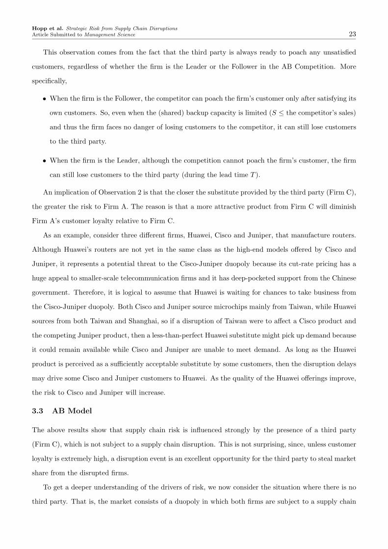
This observation comes from the fact that the third party is always ready to poach any unsatisfied
customers, regardless of whether the firm is the Leader or the Follower in the AB Competition. More
specifically,
• When the firm is the Follower, the competitor can poach the firm’s customer only after satisfying its
own customers. So, even when the (shared) backup capacity is limited (S ≤ the competitor’s sales)
and thus the firm faces no danger of losing customers to the competitor, it can still lose customers
to the third party.
• When the firm is the Leader, although the competition cannot poach the firm’s customer, the firm
can still lose customers to the third party (during the lead time T ).
An implication of Observation 2 is that the closer the substitute provided by the third party (Firm C),
the greater the risk to Firm A. The reason is that a more attractive product from Firm C will diminish
Firm A’s customer loyalty relative to Firm C.
As an example, consider three different firms, Huawei, Cisco and Juniper, that manufacture routers.
Although Huawei’s routers are not yet in the same class as the high-end models offered by Cisco and
Juniper, it represents a potential threat to the Cisco-Juniper duopoly because its cut-rate pricing has a
huge appeal to smaller-scale telecommunication firms and it has deep-pocketed support from the Chinese
government. Therefore, it is logical to assume that Huawei is waiting for chances to take business from
the Cisco-Juniper duopoly. Both Cisco and Juniper source microchips mainly from Taiwan, while Huawei
sources from both Taiwan and Shanghai, so if a disruption of Taiwan were to affect a Cisco product and
the competing Juniper product, then a less-than-perfect Huawei substitute might pick up demand because
it could remain available while Cisco and Juniper are unable to meet demand. As long as the Huawei
product is perceived as a sufficiently acceptable substitute by some customers, then the disruption delays
may drive some Cisco and Juniper customers to Huawei. As the quality of the Huawei offerings improve,
the risk to Cisco and Juniper will increase.
3.3 AB Model
The above results show that supply chain risk is influenced strongly by the presence of a third party
(Firm C), which is not subject to a supply chain disruption. This is not surprising, since, unless customer
loyalty is extremely high, a disruption event is an excellent opportunity for the third party to steal market
share from the disrupted firms.
To get a deeper understanding of the drivers of risk, we now consider the situation where there is no
third party. That is, the market consists of a duopoly in which both firms are subject to a supply chain

24Hopp et al. Strategic Risk from Supply Chain Disruptions
Article Submitted to Management Science
Number of Independent Variables in the Regression ModelVariables in the Model R2 p0LLB p0LG
dA
S |pB0−p0p0
| KA−d
A
dB
1 33.1 +2 40.8 + +3 43.1 + + −4 45.4 + + − −5 46.0 + + − − +
Table 3: Regression models (without the third party) with the top 1–5 most important factor(s) under the ABModel when Firm A is larger than Firm B.
Number of Independent Variables in the Regression ModelVariables in the Model R2 p0LG
dB
S p0SGK
A−d
A
dB
|pB0−p0p0
|1 31.7 +2 34.3 + −3 37.1 + − +4 38.8 + − + +5 39.9 + − + + −
Table 4: Regression models (without the third party) with the top 1–5 most important factor(s) under the ABModel when Firm A is smaller than Firm B.
disruption. More specifically, we assume that products by competitors who do not rely on the vulnerable
supplier are not close substitutes for the products produced by the duopoly firms.
We repeated our regression analysis under these conditions, which resulted in Tables 3 and 4, from
which we can draw the following conclusions:
Observation 3: Gain factors have more impact on Firm A’s strategic risk in the AB Model than in theABC Model.
As Table 3 shows, when Firm A is larger than Firm B, there is only one loss factor among the five,
namely Firm A’s expected worst-case long term loss (p0LLB). On the other hand, when Firm A is smaller
than Firm B, there is no loss factor among the five factors listed in Table 4. As stated in Observation 1,
loss factors are the primary determinants of the strategic risks.
Intuitively, the isolated market in the AB Model (involving only Firms A and B) makes it more
attractive to firms to pay attention to gain factors when evaluating protection policies, since they are
not at risk of losing customers to a third party. In a sense, this duopolistic market presents a zero sum
situation, in which Firms A and B compete for each others’ customers.
3.4 Predictive Power of the First Important Factor
As we noted previously, some firms in industry (including a firm with whom we have worked, which is
widely considered to be among the most sophisticated about managing supply chain risks) use expected

Hopp et al. Strategic Risk from Supply Chain DisruptionsArticle Submitted to Management Science 25
short term loss as a measure of supply chain risk. We call this the expected short-term loss heuristic. Of
course, the five factor models summarized in Tables 1-4 provide a more accurate characterization of risk.
But they also require considerably more data. Therefore, to get a sense of how well a single factor risk
metric can work, we suppose that Firm A considers its specific environment (e.g., ABC or AB ; larger or
smaller than Firm B), and uses the single most important factor from the regression model to identify the
products in their portfolio for which they should invest in specific preparedness activities (e.g., setting up
tighter supply monitoring mechanisms, cultivating a closer relationship with the supplier, pre-qualifying
backup suppliers, modifying designs to make products more flexible with regard to input components,
etc.). Clearly, a single factor is not a perfect predictor of risk due to lack of preparedness (i.e., the
R2 of our single-factor regression model is not very high), but it does not need to be. The problem is
not to predict actual losses (or gains) with numerical precision, but rather to accurately identify those
components for which risk is greatest.
To test the utility of our model, we evaluate the ability of the most important factor in Tables 1, 2, 3,
and 4, which we call the Top 1 Factor heuristic, or T1F heuristic, against the expected short term loss
heuristic to choose top five riskiest components among 150 randomly picked items from our test suite.
We did this by computing the expected short term loss heuristic:
p0 × (T + µ)× rA × d0
A
for each component, and then performing the following simulation experiment:
Step 1: Randomly pick 150 components from the set of scenarios. The record for each component
contains (1) the values for all of the model factors from which we can calculate the exact value of
ΩA , and (2) the value of the most important factor (which depends on the specific environment)
and the value of the expected short term loss heuristic.
Step 2: Sequence (from large to small) the components according to the value of the most important
factor from 1 to 150, and calculate the total risk from the top five components as UFactor =∑5
i=1 Ω(i)A
.
Step 3: Sequence (from large to small) the components according to the value of the expected short term
loss heuristic, and calculate the total risk from the top five components as UHeuri =∑5
i=1 Ω(i)A
. (Note
that this value will differ from that in Step 2 if the indices are different.)
Step 4: Record the value Udiff
= (UFactor −UHeuri)/UHeuri, which represents the percent gain of profit
that Firm A experiences if the firm invests in preparedness for the five items determined by the

26Hopp et al. Strategic Risk from Supply Chain Disruptions
Article Submitted to Management Science
Difference in ABC Model AB ModelPerformance A is Larger A is Smaller A is Larger A is Smaller
Umax
diff207.5% 127.9% 229.4% 248.4%
Udiff
126.14% 71.98% 120.96% 104.77%
Table 5: Numerical study of the percent gain of Firm A’s expected profit due to using the most important factorin place of the expected short term loss heuristic.
value of the most important factor, rather than investing in the five components determined by the
expected short-term loss heuristic.
Step 5: Go to Step 1 until 50 replicates have been run (so that the obtained sample mean is close to the
true mean). Find the maximum and mean of Udiff
and denote them by Umax
diffand U
diff, respectively.
The results of this experiment are shown in Table 5.
Observation 4: On average, using the most important factor (i.e., T1F heuristic) to select the riskiestcomponents is much better than using the expected short term loss heuristic to rank components. Whencustomer loyalty differs across products, the T1F heuristic significantly outperforms the expected shortterm loss heuristic in most cases because it explicitly considers expected long term loss.
Observation 5: When customer loyalty is similar across products or when customer loyalty is lower foritems with higher short term loss of sales (i.e., so that short term loss is highly correlated with long termloss), then the expected short term loss heuristic is also a good predictor of total risk.
Note that in practice, the condition in Observation 5 that, “customer loyalty is lower for items with
higher short term sales loss”, does not always hold. In general, we would expect high demand products
to have high customer loyalty because of customers’ preference and due to network externality effects.
For example, comparing Apple’s notebook with Toshiba’s notebook, Apple’s notebook has high sales and
high customer loyalty because of network externalities. On the other hand, Toshiba’s notebook is not as
big a seller as Apple’s notebook in the U.S. market and does not have the same level of network driven
loyalty (Martellaro (2008) and Hruska (2008)). Hence, we would expect a disruption to cause a larger
short term loss of sales to Apple’s notebook but a larger long term loss of market share to Toshiba’s
notebook. Consequently, short term loss may not be a good predictor of long term loss, which implies
that firms using short term loss to allocate preparedness efforts may not be investing optimally. Indeed,
as we note in the following observation, the loss can be substantial.
Observation 6:
• In both ABC and AB models, the percent gain in profit a firm experiences from using the T1Fheuristic in place of the expected short term loss heuristic in evaluating Firm A’s risk due to lackof preparation is substantial.

Hopp et al. Strategic Risk from Supply Chain DisruptionsArticle Submitted to Management Science 27
• For the smaller firm, the percent gain is higher in the AB model than the ABC Model.
As Table 5 shows, the average percent gain in profit in most cases is more than 100%. This implies
that firms can gain a significant increase in their profit, if they prepare for a supply possible supply chain
disruption based on the most important factor presented in this paper rather than the expected short
term loss factor.
Furthermore, as shown in Table 5, when Firm A is the smaller firm, the average and maximum of the
percent gain (104.77% and 248%) are higher in the AB model than in the ABC Model (71.98% and 127%).
The reason is as follows. Comparing Table 2 and Table 4, we see that the smaller firm’s most important
risk factor is a “loss factor” in the ABC model, but a “gain factor” in the AB model. In contrast, the
expected short-term loss heuristic uses a loss factor to evaluate the smaller firm’s risk. Knowing that the
smaller firm in the AB model should focus on the gain factor (which is what the T1F heuristic does),
we expect the performance of the T1F heuristic to be better than that of the expected short-term loss
heuristic in the AB model, but not so much better in the ABC model.
3.5 Impact of the Post-disruption Information
In our basic modeling assumptions, we assumed that (1) firms do not know the true likelihood of a
disruption and so can only estimate it, and (2) a random duration of outage time after the lead time
follows a cumulative probability distribution with an average of µ units of time, which represents cases
in practice where a firm has some knowledge about the ability of its key components suppliers to recover
from a disruptive event. For example, in the 1990’s, Lattice Semiconductor Corp. mainly sourced
semiconductor products from wafer fabs in Japan (Seiko Epson) instead of the more popular Taiwan
area. This decision was based on historical data for Seiko Epson that showed its average recovery period
from a disruptive event was less than two weeks. So, while Seiko Epson was vulnerable to earthquake as
were the Taiwanese suppliers, it was expected to be disrupted for less time by such an event. Long term
recovery data can help manufacturers reduce risk of supply chain disruptions.
In addition to long term data, firms can also make use of real time data about the severity of the
outage (i.e., the length of the mean outage time) immediately after disruption occurs. For instance,
knowing that the disruption is due to a fire, an earthquake, or other incident can help the firm refine its
estimate of the outage time. Gathering information about the incident, as Nokia did from Philips, can
help firms refine their estimate even further.
In this section, we examine (1) whether or not our previous insights (Observations 1 to 3) still hold
under the case in which the post-disruption information exists, and (2) which firm, the firm with a larger

28Hopp et al. Strategic Risk from Supply Chain Disruptions
Article Submitted to Management Science
market share or the firm with a smaller market share, benefits more from the post-disruption information.
To do these, we consider the following information scenarios:
• Pre-Disruption Information: Prior to a disruption, Firm i knows that, if a disruption occurs, it
could be one the following two types:
(a) with probability pS
i0the disruption will be a long disruption with Severe consequences, which
lasts an average of µS units of time with distribution FS (·), or
(b) with probability of pM
i0the disruption will be a short disruption with Minor consequences,
which lasts an average of µM units of time with distribution of FM (·).
Firms use this information to play the Advanced Preparedness Competition and decide how much
to invest in preparation. We refer to the disruption with severe consequences as a type S disruption,
and the one with minor consequences as a type M disruption.
• Post-Disruption Information: After the disruption, we use the conditional probability Pi(h|h),
i ∈ A,B, and h ∈ S, M, to denote the probability that Firm i is correct about the type of
disruption. This conditional probability represents the accuracy of the firm in its assessment of
the disruption type. If the post-disruption information is perfect, then Pi(S|S) = 1, Pi(S|M) = 0,
Pi(M |S) = 0, and Pi(M |M) = 1. Note that, we assume Pi(h|h) 6= Pj (h|h), because we want to
investigate the impact of one firm having more accurate post-disruption information than the other.
We incorporate these new information scenarios as follows:
Advanced Preparedness (AP) Competition: Firm i plays the AP Competition based on its esti-
mates of the likelihoods of each type of disruption, pS
i0and p
M
i0, and its belief of Firm j’s estimates
of these likelihoods, pS
j0,iand p
M
j0,i(i 6= j and i, j ∈ A,B).
Backup Capacity (BC) Competition: After a disruption occurs, firms play the BC Competition
based on the conditional probability Pi(h|h), i ∈ A,B, and h, h =∈ S,M. We define Πh|hi,L(·, ·)
to represent Firm i’s expected profit when it is the Leader in the BC Competition, and it believes
the disruption is of type h when the disruption is actually of type type h. Note that, since Firm
i believes the disruption is type h, it will use the distribution of Fh(·) with an average of µ
hto
optimize its expected profit.
We also introduce the following new factors to study the impact of the Post-disruption Information:
µS/µM : the ratio of the mean outage times of the two types of disruption.

Hopp et al. Strategic Risk from Supply Chain DisruptionsArticle Submitted to Management Science 29
pS
0/p
M
0: the ratio of the probabilities of the two types of disruption.
We repeated the regression analysis of Sections 3.2 and 3.3 under these conditions. We observed the
same top five factors that have the most impact on ΩA, Firm A’s loss due to lack of preparedness, and
hence Observations 1 to 3 hold under the case in which post-disruption information exists.
To answer the question of which firm benefits more from post-disruption information, we evaluated
the Value of Information, which measures the difference between the expected profit of Firm i in the
following two cases:
• Complete post-disruption information case in which Firm i knows for sure whether the disruption
is severe or minor, immediately after it occurs.
• Incomplete post-disruption information case in which Firm i knows only the estimated (i.e., condi-
tional) probabilities of the two types of disruption.
Note that, in both cases, the profit of Firm i depends on whether Firm j has the complete information or
not. To make a conservative (lower bound) assessment of the value of information for Firm i, we assume
that in the complete information case, Firm j also has complete information, and in the incomplete
information case, Firm j also uses its estimates of the probabilities of the two types of disruption.
Regression analysis on “Value of Information” reveals most of the same top factors we observed earlier
for the regressions on “Loss Due to Lack of Preparedness”. However, µS/µM , the ratio of mean outage
times of the two types of disruption, enters the top five factors correlated with the “Value of Information”
for the larger firm under both the ABC and AB Models and for the smaller firm under the ABC Model
(see Tables 11 to 14 in Online Appendix C for details). This variable also becomes the sixth factor for the
smaller firm under the AB Model. The ratio of the probabilities of the two types of disruption, pS
0/p
M
0, is
the seventh factor correlated with the “Value of Information” for the larger firm and the eleventh factor
for the smaller firm under both the ABC and AB Models. These results indicate that the longer and
more likely type S disruptions become, the greater the value of post-disruption information. However, as
we note below, the size of the firm affects the value of information.
Observation 7: The firm with the larger market share benefits from post-disruption information morethan the one with the smaller market share.
The intuition behind this observation is that the larger firm should pay more attention to loss factors
when evaluating protection policies than the smaller firm, and is therefore more inclined to pay for the
additional protection provided by better post-disruption information.
30Hopp et al. Strategic Risk from Supply Chain Disruptions
Article Submitted to Management Science
3.6 Dedicated Backup Capacity as a Protection Option
Up to this point, we have assumed that there are two types of backup capacity: (a) dedicated capacity
that is committed to a specific firm (e.g., due to a contractual or informal relationship), and (b) shared
capacity, for which the two firms compete. We have treated the dedicated backup capacity as fixed. But
in practice firms may be able to take steps (e.g., negotiate contracts) to acquire additional dedicated
backup capacity to use in case of a disruption. To examine the conditions under which investment in
such capacity is an attractive alternative to investment in monitoring and detection (i.e., xi, i ∈ A,B),we define θi, i ∈ A,B as the effort by Firm i devoted to acquiring extra dedicated backup capacity. We
define Cθ
e,i(i ∈ A,B) as the cost per unit of such effort. The effort level θi can also be considered as
the cost of purchasing capacity options from other suppliers, which will be exercised only if there is a
disruption of the regular supplier.
Once Firms A and B have made their investments in dedicated backup capacity (i.e., chosen θA
and θB), which will come on line when the outage occurs, the model becomes the same as that studied
above, so all results in Sections 3.2 – 3.4 hold. But we now face the new question of which factors affect
the investment ratio θ∗i /(θ∗i + x∗i ), the fraction of preparation investment that is devoted to acquiring
dedicated backup capacity if needed, as opposed to reacting quickly.
In Section 2.2, we defined ΠAPi as Firm i’s total expected profit in the AP Competition for Firm i with
two (decision) variables: xi (i ∈ A,B). In this Section ΠAPi becomes a function with four (decision)
variables: xi and θi (i ∈ A,B), which are simultaneously decided. Adding θi into the AP Competition
changes the game. See Online Appendix D for details of the game and corresponding analytical results.
To find the top factors that have the most impact on the preparation investment ratio, we performed
regression analysis of a numerical study like those presented earlier with θ∗i /(θ∗i + x∗i ) as the dependent
variable. Because the 4th
and 5th
factors have a very small effect on R2, and hence do not offer much
predictive value, we report only the top three factors. These are:
• If Firm A has the larger market share, then
1. the most important factor affecting the investment ratio for Firm A is p0LLC (Firm A’s
expected worst-case long term loss to Firm C) with a positive sign. So, the larger firm that
pays more attention to loss factors when evaluating protection policies, will invest more in
extra dedicated backup capacity as its expected worst-case long term loss to Firm C increases,
which implies the risk level Firm A faces gets higher.
2. the second most important factor isd0
AS (Firm A’s uncovered demand after using the original

Hopp et al. Strategic Risk from Supply Chain DisruptionsArticle Submitted to Management Science 31
dedicated backup capacity relative to the total available shared backup capacity), with a
positive sign. Intuitively, when the shared backup capacity is very limited, as the larger firm,
which pays more attention to loss factors when evaluating protection policies, it has more
incentive to protect against a loss by securing extra dedicated backup capacity.
3. the third most important factor is p0LLB (Firm A’s expected worst-case long term loss to
Firm B) with a positive sign. Intuitively, the larger Firm A’s expected worst-case long term
loss to Firm B, the higher level of risk it faces, and hence, as the firm paying more attention
to loss factors when evaluating protection policies, it will increase the preparation investment
in securing extra dedicated backup capacity.
• If Firm A has the smaller market share, then
1. the most important factor is p0LG (Firm A’s expected best-case long term gain from Firm
B) with a negative sign. Intuitively, when the opportunity for gain increases, the smaller
firm, which pays more attention to gain factors when evaluating protection policies, has more
incentive to try to win the AP Competition vis investment in monitoring and detection, rather
than avoiding it through investment in extra dedicated backup capacity. When the shared
backup capacity, S, is enough to satisfy Firm A’s customers plus some or all of the competitor’s
unsatisfied customers, Firm A prefers to invest more in monitoring and detection with an eye
toward acquiring the extra shared backup capacity and poaching the competitor’s unsatisfied
customers. However, when the shared backup capacity is limited (S < mindA , dB), then the
firm cannot acquire enough shared backup capacity to poach the competitor’s customers. So,
it may be worthwhile to invest more in extra dedicated backup capacity to be positioned to
take market share from the competitor.
2. the second and third most important factors affecting the investment balance in preparedness
activities of Firm A are p0LLC and p0LLB with positive signs, which implies that when Firm
A’s expected worst-case long term loss to Firm C/B increases, Firm A will invest more in
securing extra dedicated backup capacity.
Based on the above results, we conclude that,
Observation 8: Increased opportunity for gain motivates Firm i with the smaller market share toincrease the fraction of its preparedness effort in monitoring and detection rather than in securing extradedicated backup capacity than the firm with the larger market share (i.e., θ∗i /(θ∗i + x∗i ) is smaller forsmaller firm). This ratio for Firm i increases as the available shared backup capacity S decreases and thededicated backup capacity of Firm j decreases.

32Hopp et al. Strategic Risk from Supply Chain Disruptions
Article Submitted to Management Science
Observation 8 discusses situations in which firm should increase its investment in acquiring dedicated
backup capacity (i.e., conditions that cause θ∗i /(θ∗i + x∗i ) to increase). In the following, we examine the
conditions that cause firms to prefer to devote more effort to monitoring and detection than to securing
extra dedicated backup capacity (i.e., cause θ∗i /(θ∗i + x∗i ) < 0.5). To do this, we group the regression
results from the above numerical study into two groups: one with preparation investment ratios less than
0.5; the other with preparation investment ratios greater than or equal to 0.5. We compared the values
of independent variables in these two groups and observed:
Observation 9: The firm with the larger market share prefers investing in monitoring and detection when(1) its customer loyalty relative to the competitor and the third party are both high, (2) its uncovereddemand (before using the extra dedicated backup capacity) relative to the total available shared backup
capacity (d0
iS ) is low, and (3) its expected worst-case long term loss to the third party (p0LLC) is low.
Observation 10: The firm with the smaller market share prefers investing in monitoring and detectionwhen (1) its competitor’s customer loyalty relative to the firm (γji) is low, (2) its uncovered demand(before using the extra dedicated backup capacity) relative to the total available shared backup capacity
(d0
iS ) is low, and (3) its expected best-case long term gain from the competitor (p0LG) is high.
From Observations 9 and 10, we can see that the larger firm prefers to invest in monitoring and
detection when its customer loyalty is high, which makes the firm feel safe to take a relatively aggressive
action. In contrast, the smaller firm prefers to invest in monitoring and detection when its competitor’s
customer loyalty relative to the firm is low, which gives it a great opportunity for gain by poaching the
competitor’s unsatisfied customers.
From a managerial perspective, preparedness activities related to monitoring and detection can be
viewed as a systemic preparation, since they can protect majority or all components. The Nokia-Ericsson
story is an example of systematic preparedness. To appreciate Nokia’s response to the Philips fire in
March 2000, it is informative to look back to the year 1995. At that time, Nokia was experiencing poor
delivery performance and frequent imbalances between supply and demand. To fix these problems, Nokia
launched a collaborative planning process involving its key suppliers and installed a monitoring process.
This system was critical to the detection and evaluation of the situation in the wake of the Philip fire.
The seeds for Nokia’s fast response in 2000 had been sown years earlier. Moreover, the monitoring system
that proved so useful in the Philips fire would be equally useful for other types of disruptions of other
components.
In contrast, preparedness activities related to securing extra dedicated backup capacity can be viewed
as targeted preparation, since they are specific to a small number of components. A firm with thousands of
components probably cannot economically provide extra dedicated backup capacity for all its components.
Hopp et al. Strategic Risk from Supply Chain DisruptionsArticle Submitted to Management Science 33
Hence, such protection makes sense only for very critical or very risky components. An example of such
protection was Intel’s response to the 1999 Taiwan earthquake. At the time, Taiwan was the world’s third
largest supplier of semiconductor materials, including microprocessor chips. These chips were central to
the battle between the AMD Athlon and the Intel Pentium III, which was in full swing in 1999. Prior to
the earthquake, AMD believed it was poised to exploit surging demand with its powerful new Athalon
K7. Unfortunately, all Athlon facilities were located in Taiwan, while Intel had a Pentium III facility in
Korea (i.e., dedicated backup capacity), which sourced semiconductors from Korean suppliers (XbitLabs
(1999)). Because Intel was able to exploit this capacity during the Taiwan outage, it weathered the event
better than AMD and thus staved off a potential loss of market share.
3.7 Impact of Firms’ Risk Attitude
Note that, up to this point, we have assumed that all firms are risk neutral. In this section, we perform
a detailed numerical study to extend our results in Sections 3.2 and 3.3 to cases where firms are Risk
Averse (RA) or Risk Seeking (RS). Specifically, we consider: (1) a risk-averse (RA) exponential utility
function of the form u(x) = −e−ax
, and (2) a risk-seeking (RS) exponential utility function of the form
u(x) = eax
, where a is a positive constant. We test cases where a = 0.1, 1, 10, and 100 and compared the
results to the risk neutral case. Since there are three types of risk attitude (Risk Averse, Risk Seeking
and Risk Neutral) for each of the two firms, Firms A and B, we have nine main cases as shown in Table
15 in Online Appendix E. Comparing these revealed the following:
Observation 11: A risk averse firm tends to pay more attention to loss factors when evaluating protectionpolicies (i.e., with more loss factors in its top five risk factors), while a risk seeking firm tends pay moreattention to gain factors when evaluating protection policies (i.e., with more gain factors in its top fiverisk factors). Furthermore, the fact that the competitor is more risk averse motivates a firm to pay moreattention to gain factors when evaluating protection policies. In contrast, a more risk seeking competitormotivates a firm to pay more attention to loss factors when evaluating protection policies.
This observation complements our previous observations about firm size. Larger and/or risk averse
firms should pay attention to loss factors when evaluating protection policies, while smaller and/or risk
seeking firms should pay attention to gain factors when evaluating protection policies. Factors that make
the opponent pay more attention to loss (gain) factors when evaluating protection policies tend to make
a firm pay more attention to gain (loss) factors when evaluating protection policies. These results are
intuitive, but they confirm that our earlier insights about the conditions that magnify the risks from
supply chain disruptions are still valid when firms are not risk neutral.

34Hopp et al. Strategic Risk from Supply Chain Disruptions
Article Submitted to Management Science
4 Conclusions and Future Work
In this paper we have developed a modeling framework that captures both the tactical consequences
(short term sales loss) and the strategic consequences (long term market share shifts) of supply chain
disruptions in competitive environments. The resulting models help strike a balance between the costs
of preparedness and the risks of disruptions in such environments.
To gain structural insights into policies for protecting supply chains against disruptions, we separated
the overall process into two periods: (1) a “pre-disruption period” in which the Advanced Preparedness
(AP) Competition occurs (i.e., firms invest in dedicated backup capacity and/or monitoring and detection
to enhance their probabilities of being first to detect a disruption), and (2) a “post-disruption period”,
during which the Backup Capacity (BC) Competition occurs (i.e., firms purchase shared backup capacity
and use it to satisfy their own customers and possibly steal market share from the opponent).
For the BC Competition, we showed that the optimal backup capacity purchasing policy is a five-region
policy, which can be computed by comparing a small number of possible values. For the AP Competition,
we showed a unique Nash Equilibrium exists for each firm, which describes the preparedness investment
for the market.
From a managerial perspective, our numerical results suggest that a firm will face large tactical and
strategic risks when (1) the likelihood of a disruption is large, (2) the firm’s market share is highly
valuable, (3) its customers exhibit low loyalty (especially relative to a third party), (4) its market sales
exceed the available backup capacity, and (5) the backup capacity exceeds sales of the competitor firm
and the competitor has the potential to use this capacity to steal market share. To reduce the firm’s risk
due to lack of preparedness, it should (a) improve its speed of detecting and reacting to a disruption, (b)
cultivate greater customer loyalty, and (c) increase the amount of backup capacity (this includes both
developing additional dedicated backup capacity and making it more likely that the firm will get whatever
backup capacity is shared). On-Line Appendix F provides a list of policies firms can pursue to mitigate
the tactical and strategic consequences of supply chain disruptions.
Since collecting data is time-consuming and expensive, it is not practical for firms to carefully estimate
all of the parameters used in this paper. Fortunately, our results suggest that the single most important
factor (i.e., Top 1 Factor) can make reasonable predications of which components in the firm’s catalog
pose the highest risks. The data collection overhead of this single factor is similar to that for a single
factor method currently being used in industry, although it can predict risks much more accurately. From
a qualitative standpoint, our regression studies illustrate that large and/or risk averse firms should focus

Hopp et al. Strategic Risk from Supply Chain DisruptionsArticle Submitted to Management Science 35
on investing in preparedness to protect sales and market share from disruptions, while small and/or risk
seeking firms should invest in preparedness in hopes of taking advantage of a disruption to gain market
share.
We can distinguish between preparedness activities related to monitoring and detection as systemic
preparation, which affect many components simultaneously, and preparedness activities related to securing
extra dedicated backup capacity as targeted preparation, which affect only a few specific component.
Because of their limited range, targeted protection is only economical for vital or highly risky components.
Systemic protection can be achieved in a variety of ways, most of which revolve around acquiring, sharing,
and using information. This includes both long term information (e.g., estimates of the likelihood and
duration of disruptions) and real-time information (e.g., severity of disruption after it has begun). Our
results suggest that larger firms have more incentive to invest in both types of information because they
have more market share to lose than do smaller firms.
While our framework offers significant managerial insights into the science of supply chain risk man-
agement, there is still considerable need for further research. We describe two of these below.
First, in this paper we have studied the scenario in which a disruption affects a single component of
a single product of one firm and its competitor is affected in a symmetric fashion. However, a firm may
have many final products that rely on the disrupted key component. Alternatively, a disruption (e.g., an
earthquake) may affect an entire region and hence several components at once. To help guide real-world
decision making, the framework needs to be extended to cover these scenarios.
Second, we have considered only business-to-business (OEM) relationships between firms and their
customers. The business-to-consumer (retail) environment remains open. In a retail situation, firms have
no control over which customers – existing or new – will have their orders filled first. Hence, even if a firm
secures an amount of backup capacity of the disrupted component that is smaller than its sales, it may
still make some sales to unsatisfied customers of the competitor. This may mean that environments with
small amount of available backup capacity present greater risk than they do under the OEM assumption.
To characterize risk in this setting, we first need to better understand the customer brand loyalty, so we
can model the dynamics of how customers choose products and switch between brands.
Acknowledgement: This research was supported in part by the National Science Foundation under
grants DMI-0243377 and DMI-0423048.
References
Chopra, S. and M.S. Sodhi, 2004. Managing Risk to Avoid Supply-chain Breakdown. MIT Sloan ManagementReview 46, 53-61.
36Hopp et al. Strategic Risk from Supply Chain Disruptions
Article Submitted to Management Science
Christopher, M. and H. Peck, 2004. Building the Resilient Supply Chain. International Journal of LogisticsManagement 15 (2), 1-13.
Christopher, M. and H. Lee, 2004. Mitigating Supply Chain Risk Through Improved Confidence. InternationalJournal of Physical Distribution and Logistics Management 34 (5), 388-396.
Eglin, R., 2003. Can Suppliers Bring Down Your Firm? Sunday Times (London), November 23rd, page 6.
Fine, C.H., 2000. Clockspeed-based Strategies for Supply Chain Design. Production and Operations Management9 (3), 213-221.
Fisher, M., Hammond, J., Obermeyer, W. and A. Raman, 1997. Configuring a Supply Chain to Reduce the Costof Demand Uncertainty. Production and Operations Management 6 (3), 211-225.
Gan, X., Sethi, S.P., and H. Yan, 2005. Channel Coordination with a Risk-neutral Supplier and a DownsideRisk-adverse Retailer. Production and Operations Management 14 (1), 80-89.
Gartner, 1999-2006. Gartner Press Releases, www.gartner.com.
Graves, S.C. and S.P. Willems, 2003. Supply Chain Design: Safety Stock Placement and Supply Chain Configu-ration. Handbooks in OR&MS 11, Elsevier, Amsterdam.
Hendricks, K.B. and V.R. Singhal, 2005. An Empirical Analysis of the Effect of Supply Chain Disruption onLong-Run Stock Price Performance and Equity Risk of the Firm. Production and Operations Management14 (1), 35-52.
Hager, W.W., and S.Park, 2004. The Gradient Projection Method with Exact Line Search. Journal of GlobalOptimization 30 (1), 103-118.
Hopp, W.J., and Z.-G. Liu, 2006. Protecting supply chain networks against catastrophic failures. Working paper,Department of Industrial Engineering and Management Sciences. Northwestern University.
Hruska, J., 2008. Apple, Dell big winners as PC market shows healthy growth. July, 16, 2008. Available onhttp://arstechnica.com/news.ars/post/20080716-apple-dell-big-winners-as-pc-market-shows-healthy-growth.html.
Johnson, M.E., 2001. Learning From Toys: Lessons in Managing Supply Chain Risk from the Toy Industry.California Management Review 43 (3), 106-124.
Kharif, Olga, 2001. Will Ericsson Hang Up on Cell-Phones Altogether? February 12, 2001. Available onhttp://www.businessweek.com/bwdaily/dnflash/feb2001/nf20010212 208.htm
Kleindorfer, P.R., and G. Saad, 2005. Managing Disruption Risks in Supply Chains. Productions and OperationsManagement 14 (1), 53-68.
Lee, H., 2003. Aligning Supply Chain Strategies with Products Uncertainties. California Management Review 44(3), 105-119.
Leggio, K.B., and D. Lien, 2003. Comparing Alternative Investment Strategies Using Risk-Adjusted PerformanceMeasures. Journal of Financial Planning 16, (1), 82-86,
Marsal, Katie, 2007. Apple may see 50 percent margin on each iPhone sale. January 18, 2007. Available onhttp://www.appleinsider.com/articles/07/01/18/apple may see 50 percent margin on each iphone sale.html
Martellaro, John, 2008. Apple Notebook Market Share Rises, Steals from Acer, Toshiba. September 17th, 2008.Available onhttp://www.macobserver.com/tmo/article/Apple Notebook Market Share Rises Steals from Acer Toshiba /
Mathewson, S.B., 1999. U.S. Earthquake Frequency Estimation – Ratemaking for Unusual Events. CAS ForumRatemaking Discussion Papers, Winter 1999, 133-152.INFORMS Annual Meeting 2003, Atlanta, GA. 85.
Sheffi, Y., 2005. The Resilient Enterprise: Overcoming Vulnerability for Competitive Advantage. MIT Press.Cambridge, Massachusetts.
Snyder, L.V., and Z.-J. Shen, 2006. Supply and demand uncertainty in multi-echelon supply chains. Workingpaper, Department of Industrial Engineering and Operations Research. University of California, Berkeley.
Stauffer, D., 2003. Supply Chain Risk: Deal With It. HBS Working Knowledge, Available onhttp://hbswk.hbs.edu/item/3442.html.

Hopp et al. Strategic Risk from Supply Chain DisruptionsArticle Submitted to Management Science 37
Tomlin, B.T., 2006. On the value of mitigation and contingency strategies for managing supply chain disruptionrisks. Management Science 52 (5), 639-657.
Tomlin, B.T., and L.V. Snyder, 2006. On the value of a threat advisory system for managing supply chaindisruptions. Working paper, Department of Industrial and Systems Engineering, Lehigh University.
Tomlin, B.T., and C. Tang, 2008. The power of flexibility for mitigating supply chain risks. Working paper.Anderson Graduate School of Management. University of California, Los Angeles.
XbitLabs. 1999. Earthquake in taiwan. Available on: www.xbitlabs.com.
Zsidisin, G.A., Panelli, A., and R. Upton, 2000. Purchasing Organization Involvement in Risk Assessments, Con-tingency Plans, and Risk Management: An Exploratory Study. Supply Chain Management: An InternationalJournal 5 (4), 187-197.

38Hopp et al. Strategic Risk from Supply Chain Disruptions
Article Submitted to Management Science
ONLINE APPENDIX A
Design of Numerical Experiments
We created a large set of scenarios (322 × 2× 4 cases in total) using values for the 32 model parameters
chosen to cover the majority of realistic scenarios we could observe in practice. We randomly picked onemillion scenarios from this large set and fit a regression model to this reduced sample.
Below we summarize the 8 parameters of the model, along with 5 profit factors, and 19 normalized factorsused in our numerical studies. We classify the factors as gain, loss, or neutral factors in Table 6.
A.1 Single Parameters:
We consider eight parameters in our model including p0, µ, CV (= σ/µ), T , γAB , γAC , γBA , and γBC .The values of these parameters are summarized in Table 7. Note that, given the distribution of the outagetime, the customer loyalty coefficients of 18, 42, 130, 260 correspond to cases in which (approximately)80%, 50%, 20%, 10% of customers who use the competitor’s (or the third party’s) products during theoutage will permanently switch to those firms. We assume that the remaining outage times (after leadtime T ) are normally distributed.
A.2 Profit Factors:
We include the following five variables corresponding to the profit loss or gain for each firm, i.e., SLTotal
,LLB, LLC, LG, and SG.
• Firm A’s worst-case short term loss:
SLTotal
= SLT + SLµ = T × rA × d0
A+ µ× rA × dA
which is the loss of profit during the lead time and outage that occurs, if Firm A cannot satisfy anyof its customers.
• Firm A’s worst-case long term loss to Firm B (i.e., LLB) and to Firm C (i.e., LLC):
LLB = mAB ×µ
γAB
× dA
LLC = LLCT + LLCµ = mAC ×T
γAC
× d0
A+ mAC ×
µ
γAC
× dA
These long terms losses correspond to the worst case in which Firm A cannot satisfy any of itsown customers. Note that, Firm A’s worst-case long term loss to Firm B is actually expressed asmAB × ξAB × dA , where
ξAB =∫ ∞
0(1− e
− tγAB )dFo(t),
and Fo is a distribution with mean µ and standard deviation σ. However when σ → 0, we have,
ξAB = 1− e− µ
γAB ' µ
γAB
.
Therefore, to simplify, we define,
LLB = mAB ×µ
γAB
× dA .
We use the same approximation to define LLC and LG.

Hopp et al. Strategic Risk from Supply Chain DisruptionsArticle Submitted to Management Science 39
Firm A’s Gain Factors Firm A’s Loss Factors Firm A’s Neutral FactorsSG SL
Totalp0
LG LLB, LLC µ,CV ,TγBA γAB ,γAC γBC
mAA365rA
, mBB365rB
, mBC365rA
mBA365rB
mAB365rA
, mAC365rA
crA
|pB0−p0
p0|
KA−dAdB
KB−dBdA
|pA0,B−p
A0
pA0
|rA
rB
|pA0−p0
p0| 365hA
rA,365hB
rBdAS ,dB
S
|pB0,A−p
B0
pB0
| Sd
A+d
B
Table 6: Firm A’s classified model factors.
• Firm A’s best-case short term gain (i.e., SG) and long term gain (i.e., LG):
SG = µ× rA × dB LG = mBA ×µ
γBA
× dB
which correspond to the case where Firm B cannot satisfy any of its own customers.
A.3 Normalized Factors:
We consider the following 19 normalized factors (whose ranges are determined by the values of associatedparameters and summarized in Table 7):
• rA
rB
, which is the relative profitability of the two firms;
• mij
365ri, which is the present-worth factor of one unit market share of Firm i for Firm j based on a 15%
interest factor for continuous compounding interest (Thuesen et al. 1977), i ∈ A,B, j ∈ A,B, C.So, for example, if mAB
365rA= 0.1 and rA = $120, then mAB = $4380;
• 365hiri
, which is the relative annual cost for Firm i to hold one unit of unused backup capacity,i ∈ A,B;
• crA
, which is the relative premium Firm A pays per unit of backup capacity;
• diS , which is Firm i’s sales relative to the total available backup capacity, i ∈ A, B;
• Ki−didj
, which is defined as the “poaching potential” of Firm i (notice that, the numerator is Firmi’s remaining production capacity after satisfying its own customers), i 6= j, i, j ∈ A,B;
• Sd
A+d
B, which is the fraction of total market sales represented by the backup capacity;
• |pi0−p0p0
|, which is the absolute percent error in Firm i’s estimate of the likelihood of a disruption,i ∈ A,B;
• |pj0,i−pj0
pj0|, which is the absolute percent error in Firm i’s belief of Firm j’s estimate of the likelihood
of a disruption, i 6= j, i, j ∈ A,B.
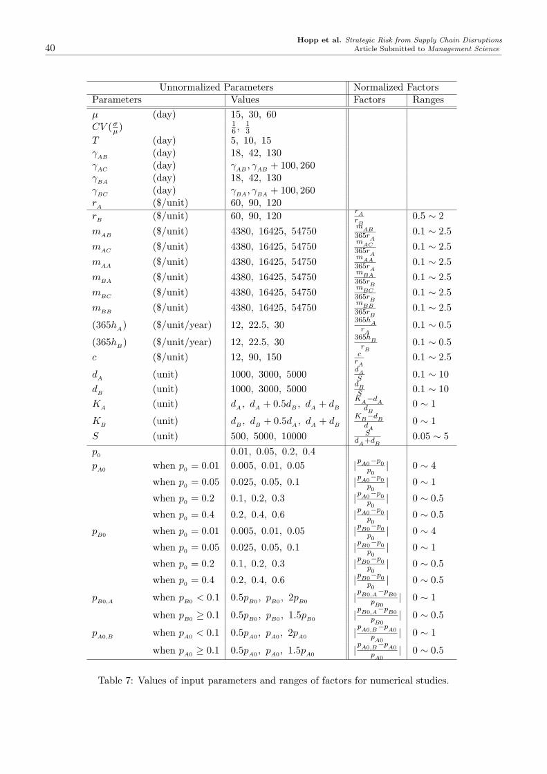
40Hopp et al. Strategic Risk from Supply Chain Disruptions
Article Submitted to Management Science
Unnormalized Parameters Normalized FactorsParameters Values Factors Rangesµ (day) 15, 30, 60CV (σ
µ) 16 , 1
3
T (day) 5, 10, 15γAB (day) 18, 42, 130γAC (day) γAB , γAB + 100, 260γBA (day) 18, 42, 130γBC (day) γBA , γBA + 100, 260rA ($/unit) 60, 90, 120rB ($/unit) 60, 90, 120 r
ArB
0.5 ∼ 2mAB ($/unit) 4380, 16425, 54750 m
AB365r
A0.1 ∼ 2.5
mAC ($/unit) 4380, 16425, 54750 mAC
365rA
0.1 ∼ 2.5mAA ($/unit) 4380, 16425, 54750 m
AA365r
A0.1 ∼ 2.5
mBA ($/unit) 4380, 16425, 54750 mBA
365rB
0.1 ∼ 2.5mBC ($/unit) 4380, 16425, 54750 m
BC365r
B0.1 ∼ 2.5
mBB ($/unit) 4380, 16425, 54750 mBB
365rB
0.1 ∼ 2.5
(365hA) ($/unit/year) 12, 22.5, 30 365hA
rA
0.1 ∼ 0.5
(365hB ) ($/unit/year) 12, 22.5, 30 365hB
rB
0.1 ∼ 0.5c ($/unit) 12, 90, 150 c
rA
0.1 ∼ 2.5
dA (unit) 1000, 3000, 5000 dAS 0.1 ∼ 10
dB (unit) 1000, 3000, 5000 dBS 0.1 ∼ 10
KA (unit) dA , dA + 0.5dB , dA + dB
KA−d
Ad
B0 ∼ 1
KB (unit) dB , dB + 0.5dA , dA + dB
KB−d
Bd
A0 ∼ 1
S (unit) 500, 5000, 10000 Sd
A+d
B0.05 ∼ 5
p0 0.01, 0.05, 0.2, 0.4pA0 when p0 = 0.01 0.005, 0.01, 0.05 |pA0
−p0p0
| 0 ∼ 4
when p0 = 0.05 0.025, 0.05, 0.1 |pA0−p0
p0| 0 ∼ 1
when p0 = 0.2 0.1, 0.2, 0.3 |pA0−p0
p0| 0 ∼ 0.5
when p0 = 0.4 0.2, 0.4, 0.6 |pA0−p0
p0| 0 ∼ 0.5
pB0 when p0 = 0.01 0.005, 0.01, 0.05 |pB0−p0
p0| 0 ∼ 4
when p0 = 0.05 0.025, 0.05, 0.1 |pB0−p0
p0| 0 ∼ 1
when p0 = 0.2 0.1, 0.2, 0.3 |pB0−p0
p0| 0 ∼ 0.5
when p0 = 0.4 0.2, 0.4, 0.6 |pB0−p0
p0| 0 ∼ 0.5
pB0,A when pB0 < 0.1 0.5pB0 , pB0 , 2pB0 |pB0,A−p
B0
pB0
| 0 ∼ 1
when pB0 ≥ 0.1 0.5pB0 , pB0 , 1.5pB0 |pB0,A−p
B0
pB0
| 0 ∼ 0.5
pA0,B when pA0 < 0.1 0.5pA0 , pA0 , 2pA0 |pA0,B−p
A0
pA0
| 0 ∼ 1
when pA0 ≥ 0.1 0.5pA0 , pA0 , 1.5pA0 |pA0,B−p
A0
pA0
| 0 ∼ 0.5
Table 7: Values of input parameters and ranges of factors for numerical studies.

Hopp et al. Strategic Risk from Supply Chain DisruptionsArticle Submitted to Management Science 41
References
Thuesen, H.G., Fabrycky, W.J., and G.J.Thuesen, 1977. Engineering Economy (5rd Ed.). Prentice-Hall, Inc.,New Jersey.

42Hopp et al. Strategic Risk from Supply Chain Disruptions
Article Submitted to Management Science
ONLINE APPENDIX B
Proofs of Analytical Results
PROPOSITION 1:
(Large Capacity Leader:) If the Leader’s production capacity is greater than the combined market share of bothfirms (i.e., K
A≥ d
A+ d
B), and
(1) if the backup capacity is less then the combined market share of both firms (i.e., S ≤ dA
+ dB), then the only
possible choices for the optimal backup capacity purchases for the two firms are:
(Y ∗A,L
, Y ∗B,F
) ∈
(0, 0), (0, dB ),(0, minKB , S), (S − dB , 0), (S − dB , dB ),
(dA, 0), (d
A, S − d
A), (S, 0)
;
(2) if the backup capacity is larger than the combined market share of both firms (i.e., S > dA
+ dB), then the
only possible choices for the optimal backup capacity purchases for the two firms are:
(Y ∗A,L
, Y ∗B,F
) ∈
(0, 0), (0, dB ),(0,minK
B, d
A+ d
B), (d
A, 0), (d
A, d
B),
(dA + dB , 0), (S, 0)
.
(Small Capacity Leader:) If the Leader’s production capacity cannot cover the combined market share of bothfirms (i.e., KA < dA + dB ), and
(1) if the backup capacity is less than the Leader’s market share (i.e., S ≤ KA), then the only possible choicesfor the optimal backup capacity purchases for the two firms are:
(Y ∗A,L
, Y ∗B,F
) ∈
(0, 0), (0, dB), (0, minK
B, S), (S − d
B, 0), (S − d
B, d
B),
(dA , 0), (dA , S − dA), (S, 0)
;
(2) if the backup capacity is larger than the Leader’s market share, but it is smaller than the combined marketshare of both firms (i.e., K
A< S ≤ d
A+ d
B), then the only possible choices for the optimal backup capacity
purchases for the two firms are:
(Y ∗A,L
, Y ∗B,F
) ∈
(0, 0), (0, dB), (0, minK
B, S), (S − d
B, 0), (S − d
B, d
B),
(dA , 0), (dA , S − dA), (KA , 0), (KA , S −KA)
;
(3) if the backup capacity can cover the combined market share of both firms (i.e., S > dA
+ dB), then the only
possible choices for the optimal backup capacity purchases for the two firms are:
(Y ∗A,L
, Y ∗B,F
) ∈
(0, 0), (0, dB), (0, minK
B, d
A+ d
B), (d
A, 0), (d
A, d
B), (K
A, 0),
(S − (d
A+ d
B) + K
A, 0
),
(S − (d
A+ d
B) + K
A, (d
A+ d
B)−K
A
).
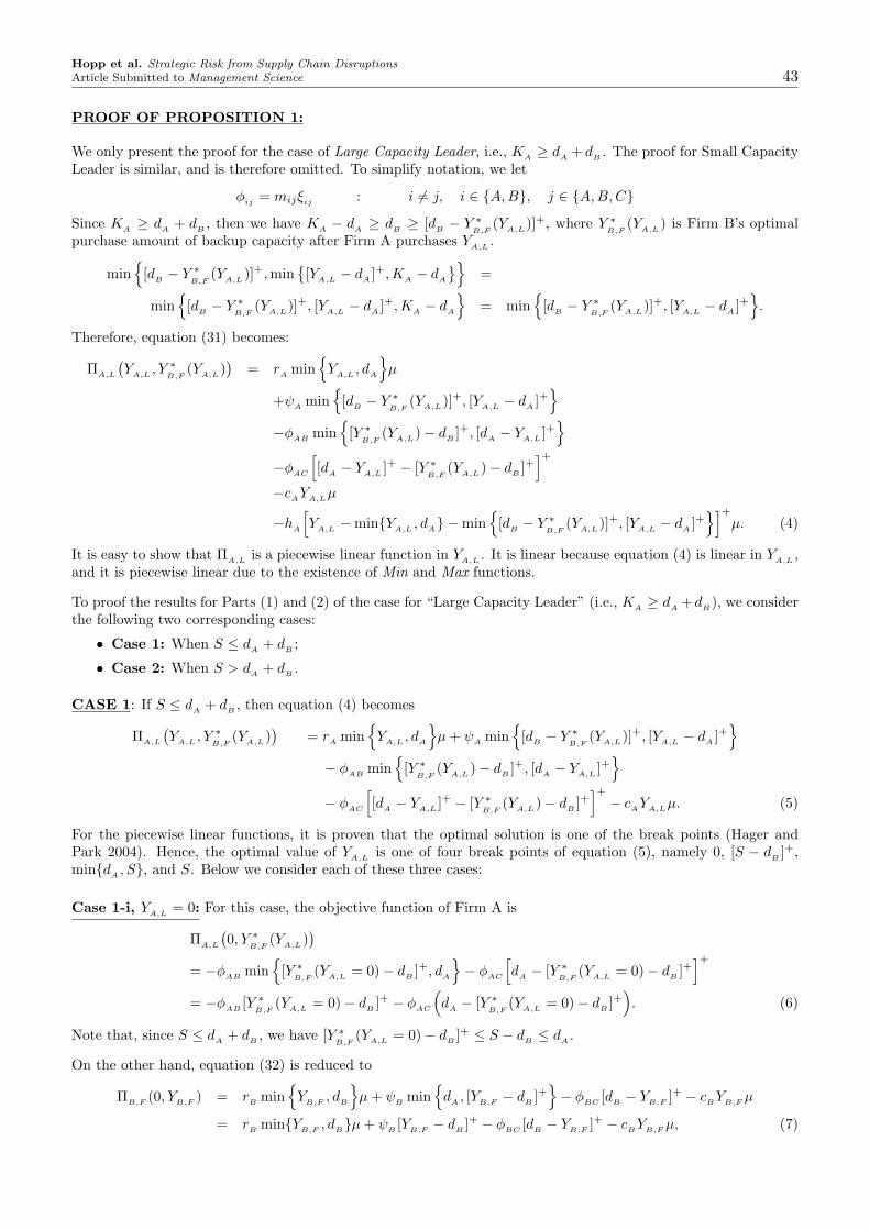
Hopp et al. Strategic Risk from Supply Chain DisruptionsArticle Submitted to Management Science 43
PROOF OF PROPOSITION 1:
We only present the proof for the case of Large Capacity Leader, i.e., KA≥ d
A+ d
B. The proof for Small Capacity
Leader is similar, and is therefore omitted. To simplify notation, we let
φij
= mijξij: i 6= j, i ∈ A,B, j ∈ A, B,C
Since KA ≥ dA + dB , then we have KA − dA ≥ dB ≥ [dB − Y ∗B,F
(YA,L)]+, where Y ∗B,F
(YA,L) is Firm B’s optimalpurchase amount of backup capacity after Firm A purchases Y
A,L.
min
[dB− Y ∗
B,F(Y
A,L)]+, min
[Y
A,L− d
A]+,K
A− d
A
=
min
[dB− Y ∗
B,F(Y
A,L)]+, [Y
A,L− d
A]+,K
A− d
A
= min
[d
B− Y ∗
B,F(Y
A,L)]+, [Y
A,L− d
A]+
.
Therefore, equation (31) becomes:
ΠA,L
(Y
A,L, Y ∗
B,F(Y
A,L))
= rA
min
YA,L
, dA
µ
+ψA
min
[dB− Y ∗
B,F(Y
A,L)]+, [Y
A,L− d
A]+
−φAB
min
[Y ∗B,F
(YA,L
)− dB]+, [d
A− Y
A,L]+
−φAC
[[d
A− Y
A,L]+ − [Y ∗
B,F(Y
A,L)− d
B]+
]+
−cAYA,Lµ
−hA
[Y
A,L−minY
A,L, d
A −min
[d
B− Y ∗
B,F(Y
A,L)]+, [Y
A,L− d
A]+
]+
µ. (4)
It is easy to show that ΠA,L
is a piecewise linear function in YA,L
. It is linear because equation (4) is linear in YA,L
,and it is piecewise linear due to the existence of Min and Max functions.
To proof the results for Parts (1) and (2) of the case for “Large Capacity Leader” (i.e., KA ≥ dA +dB ), we considerthe following two corresponding cases:
• Case 1: When S ≤ dA + dB ;
• Case 2: When S > dA + dB .
CASE 1: If S ≤ dA + dB , then equation (4) becomes
ΠA,L
(Y
A,L, Y ∗
B,F(Y
A,L))
= rA
min
YA,L
, dA
µ + ψ
Amin
[d
B− Y ∗
B,F(Y
A,L)]+, [Y
A,L− d
A]+
− φAB
min
[Y ∗B,F
(YA,L
)− dB]+, [d
A− Y
A,L]+
− φAC
[[dA − YA,L ]+ − [Y ∗
B,F(YA,L)− dB ]+
]+
− cAYA,Lµ. (5)
For the piecewise linear functions, it is proven that the optimal solution is one of the break points (Hager andPark 2004). Hence, the optimal value of Y
A,Lis one of four break points of equation (5), namely 0, [S − d
B]+,
mindA, S, and S. Below we consider each of these three cases:
Case 1-i, YA,L
= 0: For this case, the objective function of Firm A is
ΠA,L
(0, Y ∗
B,F(YA,L)
)
= −φAB
min
[Y ∗B,F
(YA,L
= 0)− dB]+, d
A
− φ
AC
[d
A− [Y ∗
B,F(Y
A,L= 0)− d
B]+
]+
= −φAB
[Y ∗B,F
(YA,L
= 0)− dB]+ − φ
AC
(d
A− [Y ∗
B,F(Y
A,L= 0)− d
B]+
). (6)
Note that, since S ≤ dA
+ dB, we have [Y ∗
B,F(Y
A,L= 0)− d
B]+ ≤ S − d
B≤ d
A.
On the other hand, equation (32) is reduced to
ΠB,F (0, YB,F ) = rB min
YB,F , dB
µ + ψB min
dA , [YB,F − dB ]+
− φBC [dB − YB,F ]+ − cBYB,F µ
= rB
minYB,F
, dBµ + ψ
B[Y
B,F− d
B]+ − φ
BC[d
B− Y
B,F]+ − c
BY
B,Fµ, (7)

44Hopp et al. Strategic Risk from Supply Chain Disruptions
Article Submitted to Management Science
which is piecewise linear and has three break points: 0, mindB, S, and minK
B, S. So, the optimal value of
Y ∗B,F
∈
0, dB, minK
B, S
. Consequently, the possible combination of the optimal capacity purchase for firms
A and B in this case are
(Y ∗A,L
, Y ∗B,F
) ∈
(0, 0), (0, dB), (0,minK
B, S)
.
Case 1-ii, YA,L
= [S − dB]+: Notice that, if [S − d
B]+ = 0, i.e., S ≤ d
B, then it becomes similar to Case 1-i, so
here we are only interested in the case of [S − dB]+ = S − d
B.
Since S ≤ dA + dB , YA,L = S − dB ≤ dA and Y ∗B,F
(YA,L) ≤ dB must hold. Then the objective function of Firm Abecomes
ΠA,L
(S − dB , Y ∗
B,F(YA,L)
)= (rA − cA)(S − dB )µ− φAC
(dA − (S − dB )
). (8)
It is easy to see that the reason why YA,L
= S − dB
is that Firm A aims at protecting itself from loosing marketshare to Firm B (although sales profit is negative), i.e., if Y
A,L= 0, then Y ∗
B,F= S due to the linearity property of
the profit function. Based on Firm A’s protection strategy, the objective function of Firm B becomes
ΠB,F
(S − dB, Y
B,F) = (r
B− c
B)Y
B,Fµ− φ
BC(d
B− Y
B,F), (9)
which is a linear function with two end points: 0 and dB. Thus, the optimal capacity purchase Y ∗
B,F∈ 0, d
B.
Consequently, in this case the only possible combination of the optimal capacity purchase for firms A and B are
(Y ∗A,L
, Y ∗B,F
) ∈
(S − dB , 0), (S − dB , dB )
.
Case 1-iii, YA,L = mindA , S: For this case, the objective function of Firm A is
ΠA,L
(mind
A, S, Y ∗
B,F(Y
A,L))
= (rA− c
A)mind
A, Sµ− φ
AC
(d
A−mind
A, S)
= (rA − cA)mindA , Sµ− φAC [dA − S]+. (10)
On the other hand, since Firm A purchases capacity to only satisfy its own customers, i.e.,YA,L = mindA , S, theobjective function of Firm B, becomes
ΠB,F
(mindA, S, Y
B,F) = (r
B− c
B)Y
B,Fµ− φ
BC(d
B− Y
B,F), (11)
which is a linear function with two end points: 0 and [S − mindA, S]+ = [S − d
A]+. Thus, Y ∗
B,F∈ 0, [S −
mindA, S]+ = [S − d
A]+. Consequently, in this case the only possible combination of the optimal capacity
purchase for firms A and B are
(Y ∗A,L
, Y ∗B,F
) ∈
(mindA, S, 0), (mind
A, S, [S − d
A]+)
.
Case 1-iv, YA,L
= S: For this case, Y ∗B,F
(YA,L
) = 0 is the only possibility. Since S ≤ dA
+dB, then [S−d
A]+ ≤ d
B
must hold. Hence, the objective function of Firm A is
ΠA,L
(S, 0) = rA
minS, dAµ + ψ
A[S − d
A]+ − φ
AC[d
A− S]+ − c
ASµ, (12)
and the objective function of Firm B, becomes
ΠB,F
(S, 0) = −φBA
min[S − d
A]+, d
B
− φBC
(d
B− [S − d
A]+
).
The only possible combination of the optimal capacity purchase for this case is (Y ∗A,L
, Y ∗B,F
) ∈ (S, 0).
If we combine the results for Case 1-i to Case 1-iv, we get the following possible combinations of the optimalcapacity purchase for firms A and B, when S ≤ d
A+ d
B
(Y ∗A,L
, Y ∗B,F
) ∈
(0, 0), (0, dB ),(0,minKB , S), (S − dB , 0), (S − dB , dB ),
(mindA , S, 0)
,(mindA , S, [S − dA ]+
), (S, 0)
.
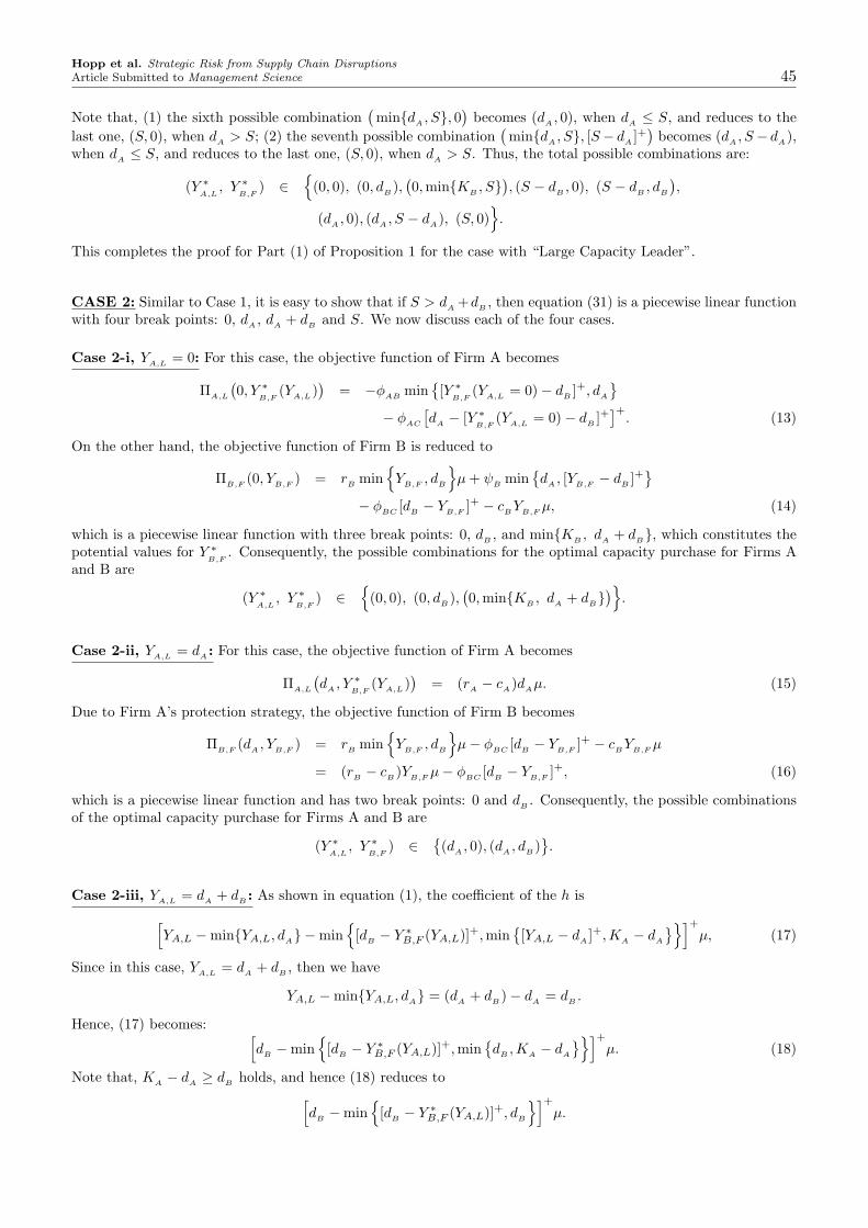
Hopp et al. Strategic Risk from Supply Chain DisruptionsArticle Submitted to Management Science 45
Note that, (1) the sixth possible combination(mind
A, S, 0)
becomes (dA, 0), when d
A≤ S, and reduces to the
last one, (S, 0), when dA
> S; (2) the seventh possible combination(mind
A, S, [S− d
A]+
)becomes (d
A, S− d
A),
when dA≤ S, and reduces to the last one, (S, 0), when d
A> S. Thus, the total possible combinations are:
(Y ∗A,L
, Y ∗B,F
) ∈
(0, 0), (0, dB),
(0, minK
B, S), (S − d
B, 0), (S − d
B, d
B
),
(dA, 0), (d
A, S − d
A), (S, 0)
.
This completes the proof for Part (1) of Proposition 1 for the case with “Large Capacity Leader”.
CASE 2: Similar to Case 1, it is easy to show that if S > dA
+dB, then equation (31) is a piecewise linear function
with four break points: 0, dA, d
A+ d
Band S. We now discuss each of the four cases.
Case 2-i, YA,L
= 0: For this case, the objective function of Firm A becomes
ΠA,L
(0, Y ∗
B,F(Y
A,L))
= −φAB
min[Y ∗
B,F(Y
A,L= 0)− d
B]+, d
A
− φAC
[d
A− [Y ∗
B,F(Y
A,L= 0)− d
B]+
]+. (13)
On the other hand, the objective function of Firm B is reduced to
ΠB,F (0, YB,F ) = rB min
YB,F , dB
µ + ψB min
dA , [YB,F − dB ]+
− φBC
[dB− Y
B,F]+ − c
BY
B,Fµ, (14)
which is a piecewise linear function with three break points: 0, dB , and minKB , dA + dB, which constitutes thepotential values for Y ∗
B,F. Consequently, the possible combinations for the optimal capacity purchase for Firms A
and B are
(Y ∗A,L
, Y ∗B,F
) ∈
(0, 0), (0, dB ),(0, minKB , dA + dB
).
Case 2-ii, YA,L = dA : For this case, the objective function of Firm A becomes
ΠA,L
(dA , Y ∗
B,F(YA,L)
)= (rA − cA)dAµ. (15)
Due to Firm A’s protection strategy, the objective function of Firm B becomes
ΠB,F
(dA, Y
B,F) = r
Bmin
Y
B,F, d
B
µ− φ
BC[d
B− Y
B,F]+ − c
BY
B,Fµ
= (rB− c
B)Y
B,Fµ− φ
BC[d
B− Y
B,F]+, (16)
which is a piecewise linear function and has two break points: 0 and dB. Consequently, the possible combinations
of the optimal capacity purchase for Firms A and B are
(Y ∗A,L
, Y ∗B,F
) ∈ (d
A, 0), (d
A, d
B).
Case 2-iii, YA,L = dA + dB : As shown in equation (1), the coefficient of the h is
[YA,L −minYA,L, dA −min
[dB − Y ∗
B,F (YA,L)]+,min[YA,L − dA ]+,KA − dA
]+
µ, (17)
Since in this case, YA,L = dA + dB , then we have
YA,L −minYA,L, dA = (d
A+ d
B)− d
A= d
B.
Hence, (17) becomes: [d
B−min
[d
B− Y ∗
B,F (YA,L)]+,mind
B,K
A− d
A
]+
µ. (18)
Note that, KA − dA ≥ dB holds, and hence (18) reduces to[dB −min
[dB − Y ∗
B,F (YA,L)]+, dB
]+
µ.

46Hopp et al. Strategic Risk from Supply Chain Disruptions
Article Submitted to Management Science
• If dB≥ Y ∗
B,F (YA,L), then the coefficient of the h is Y ∗B,F (YA,L)µ.
• If dB
< Y ∗B,F (YA,L), then the coefficient of the h is d
Bµ.
Therefore,
ΠA,L
(d
A+ d
B, Y ∗
B,F(Y
A,L))
= rAd
Aµ + ψ
A[d
B− Y ∗
B,F(Y
A,L)]+
− cA(d
A+ d
B)µ− h
Amin
d
B, Y ∗
B,F(Y
A,L= d
A+ d
B)µ. (19)
On the other hand, the objective function of Firm B is reduced to
ΠB,F
(dA
+ dB, Y
B,F) = (r
B− c
B)Y
B,Fµ− φ
BA[d
B− Y
B,F]+, (20)
which is a piecewise linear function and has two break points: 0 and minS − dA − dB , dB. Thus, Y ∗B,F
=0, minS − d
A− d
B, d
B.
However, the combination of(Y ∗
A,L= d
A+ d
B, Y ∗
B,F= minS − d
A− d
B, d
B) implies that only part of Y ∗
A,L,
which is the difference between dB
and Y ∗B,F
, will be used by Firm A to gain both sales profit and market sharefrom Firm B. But, due to the linearity property, it cannot be an optimal solution, because, in this case, if oneunit of firm B’s customer is profitable, then Firm A will definitely want to gain all possible units. So, if FirmA knows that B will buy all or some of the remaining backup capacity, i.e., minS − d
A− d
B, d
B, to protect
itself, the decision of dA
+ dB
will never be optimal for Firm A. Therefore, Y ∗A,L
= dA
+ dB
can be optimal onlyif Y ∗
B,F= 0, i.e., the only possible combinations of the optimal capacity purchase for firms A and B in this case is
(Y ∗A,L
, Y ∗B,F
) ∈ (dA
+ dB, 0).
Case 2-iv, YA,L
= S: In this case, Y ∗B,F
(YA,L
= S) = 0 is the only possibility. Thus, (Y ∗A,L
, Y ∗B,F
) ∈ (S, 0). Theobjective function of Firm A is
ΠA,L(S, 0) = rAdAµ + ψAdB − cASµ− hA(S − dA − dB )µ. (21)
If we combine the results for Case 2-i to Case 2-iv, we get the following possible combinations of the optimalcapacity purchase for firms A and B, when S > d
A+ d
B,
(Y ∗A,L
, Y ∗B,F
) ∈
(0, 0), (0, dB ),(0, minKB , dA + dB
), (dA , 0), (dA , dB ), (dA + dB , 0), (S, 0)
.
This completes the proof for Part (2) of Proposition 1 for the case of “Large Capacity Leader”. ¤
PROPOSITION 2: The optimal policy of the Backup Capacity Competition has a five-region structure.
PROOF OF PROPOSITION 2:
We present the proof for the case of Large Capacity Leader, i.e., KA ≥ dA + dB . The proof for Small CapacityLeader is similar, and is therefore omitted.
PROOF for the Follower, Firm B:
We first determine the regions for the optimal capacity purchase for the Follower. We consider the following twocorresponding cases (same as the configuration of the proof for Proposition 1):
• Case 1: When S ≤ dA + dB . For this case, we introduce three thresholds on Firm B’s unit profit margin to
(i) separate the region in which Firm B forfeits and the region in which Firm B is aggressive,
(ii) separate the region in which Firm B forfeits and the region in which Firm B protects, and
(iii) separate the region in which Firm B protects and the region in which Firm B is aggressive.
• Case 2: When S > dA + dB . For this case, we introduce four thresholds on Firm B’s unit profit margin to
(i) separate the region in which Firm B forfeits and the region in which Firm B is aggressive,
(ii) separate the region in which Firm B forfeits and the region in which Firm B protects,

Hopp et al. Strategic Risk from Supply Chain DisruptionsArticle Submitted to Management Science 47
(iii) separate the region in which Firm B protects and the region in which Firm B is aggressive, and
(iv) separate the following two responses: Given Firm A purchases the amount of dA + dB , Firm B caneither buy the remaining to protect itself from losing customers to Firm A (this response implies thatd
A+ d
Bcannot be optimal for Firm A), or buy nothing (this response implies that d
A+ d
Bis optimal
for Firm A).
The summary of the thresholds introduced in this proof can be found in Table 8.
We present the proof based on the same cases that we presented in Proposition 1.
Case 1-i, YA,L = 0: Define
cIB
= cB− φ
AB
[minK
B, S − d
B
]+ + φBC
mind
B, minK
B, S
µ minKB, S .
We now show that when rB ≥ cIB, then ΠB,F
(0, minK
B, S) ≥ Π
B,F(0, 0). By equation(7) we have
ΠB,F
(0,minK
B, S)−Π
B,F(0, 0)
= rB
min
minKB, S, d
B
µ + ψ
B
[minK
B, S − d
B
]+
− φBC
[d
B−minK
B, S]+ − c
BminK
B, Sµ
−(rB min0, dBµ + ψB [0− dB ]+ − φBC [dB − 0]+ − cB (0)µ
),
= rB
min
minKB, S, d
B
µ + (r
Bµ + φ
AB)[minK
B, S − d
B
]+
− φBC
[d
B−minK
B, S]+ − c
BminK
B, Sµ
− (−φBC
dB),
= rB
minKB, Sµ + φ
AB
[minK
B, S − d
B
]+
+ φBC mindB ,minKB , S− cB minKB , Sµ,
= rB
minKB, Sµ−
(c
BminK
B, Sµ
− φAB
[minK
B, S − d
B
]+ − φBC
mind
B,minK
B, S
).
It is clear that if rB≥ cI
B, then the right-hand side is positive, which implies
ΠB,F
(0, minK
B, S) ≥ Π
B,F(0, 0).
Therefore, if rB≥ cI
B, then Y ∗
B,F(Y
A,L= 0) = minK
B, S; otherwise, Y ∗
B,F(Y
A,L= 0) = 0.
DefinecII
B= c
B− φ
BC
µ.
We now show that when rB≥ cII
B, then Π
B,F(0, d
B) ≥ Π
B,F(0, 0). By equation (7) we have
ΠB,F
(0, dB)−Π
B,F(0, 0) = r
Bd
Bµ− c
Bd
Bµ
−(r
Bmin0, d
Bµ + ψ
B[0− d
B]+ − φ
BC[d
B− 0]+ − c
B(0)µ
),
= (rB− c
B)d
Bµ− (−φ
BCd
B),
= rBd
Bµ− (c
Bd
Bµ− φ
BCd
B).
It is clear that if rB≥ cII
B, then the right-hand side is positive, which implies
ΠB,F
(0, dB) ≥ Π
B,F(0, 0).
Therefore, if rB≥ cII
B, then Y ∗
B,F(Y
A,L= 0) = d
B; otherwise, Y ∗
B,F(Y
A,L= 0) = 0.
DefinecIII
B= c
B− φ
AB
µ.

48Hopp et al. Strategic Risk from Supply Chain Disruptions
Article Submitted to Management Science
We now show that when rB≥ cIII
B, then Π
B,F
(0, minK
B, S) ≥ Π
B,F(0, d
B). By equation (7) we have
ΠB,F
(0,minK
B, S)−Π
B,F(0, d
B)
= rB min
minKB , S, dB
µ + (rBµ + φAB )
[minKB , S − dB
]+
− φBC
[dB −minKB , S]+ − cB minKB , Sµ
−((rB − cB )dBµ
),
= (rB− c
B)minK
B, Sµ + φ
AB
(minK
B, S − d
B
)
− (rB− c
B)d
Bµ,
= rB
(minKB , S − dB
)µ−
(cB
(minKB , S − dB
)µ
− φAB
(minKB , S − dB
)).
It is clear that if rB ≥ cIIIB
, then the right-hand side is positive, which implies
ΠB,F
(0,minK
B, S) ≥ Π
B,F(0, d
B).
Therefore, if rB≥ cIII
B, then Y ∗
B,F(Y
A,L= 0) = minK
B, S; otherwise, Y ∗
B,F(Y
A,L= 0) = d
B.
Case 1-ii, YA,L
= S − dB: We now show that when r
B≥ cII
B, then Π
B,F(S − d
B, d
B) ≥ Π
B,F(S − d
B, 0). By
equation (9) we have
ΠB,F
(S − dB, d
B)−Π
B,F(S − d
B, 0) = (r
B− c
B)d
Bµ− φ
BC(d
B− d
B)
−((r
B− c
B)(0)µ− φ
BC(d
B− 0)
),
= (rB− c
B)d
Bµ + φ
BCd
B,
= rBd
Bµ− (c
Bd
Bµ− φ
BCd
B).
It is clear that if rB≥ cII
B, then the right-hand side is positive, which implies
ΠB,F
(S − dB , dB
) ≥ ΠB,F (S − dB , 0).
Therefore, if rB ≥ cIIB
, then Y ∗B,F
(YA,L = S − dB ) = dB ; otherwise, Y ∗B,F
(YA,L = S − dB ) = 0.
Case 1-iii, YA,L
= dA: By equation (11), it is easy to see that, if r
B≥ cII
B, then Y ∗
B,F(Y
A,L= d
A) = S − d
A;
otherwise, Y ∗B,F
(YA,L
= dA) = 0.
Case 2-i, YA,L
= 0: Define
ciB
= cB −φAB
(minKB , dA + dB − dB
)+ φBC dB
µ minKB, d
A+ d
B .
By equation (14), we have
ΠB,F
(0, minKB , dA + dB
)−ΠB,F (0, 0)
= rB
min
minKB, d
A+ d
B, d
B
µ + ψ
B
[minK
B, d
A+ d
B − d
B]+
− φBC
[dB −minKB , dA + dB
]+ − cB minKB , dA + dBµ−
(r
Bmin
0, d
B
µ + ψ
Bmin
d
A, [0− d
B]+
− φBC
[dB− 0]+ − c
B(0)µ
),
= rB
min
minKB, d
A+ d
B, d
B
µ
+ (rBµ + φ
AB)[minK
B, d
A+ d
B − d
B
]+− c
BminK
B, d
A+ d
Bµ
− (−φBC
dB),
= rB minKB , dA + dBµ−(cB minKB , dA + dBµ
− φAB
(minKB , dA + dB − dB
)− φBC dB
).

Hopp et al. Strategic Risk from Supply Chain DisruptionsArticle Submitted to Management Science 49
It is clear that, if rB≥ ci
B, then the right-hand-side is positive, which implies that
ΠB,F
(0, minK
B, d
A+ d
B) ≥ Π
B,F(0, 0).
Therefore, if rB ≥ ciB
holds, then Y ∗B,F
(YA,L = 0) = minKB , dA + dB; otherwise, Y ∗B,F
(YA,L = 0) = 0.
Definecii
B= cB −
φBC
µ= cII
B.
By equation (14), we have
ΠB,F
(0, dB)−Π
B,F(0, 0) = (r
B− c
B)d
Bµ− (−φ
BCd
B),
= rBd
Bµ− (c
Bd
Bµ− φ
BCd
B).
It is clear that, if rB≥ cII
B, then the right-hand-side is positive, which implies that
ΠB,F
(0, dB) ≥ Π
B,F(0, 0).
Therefore, if rB ≥ cIIB
holds, then Y ∗B,F
(YA,L = 0) = dB ; otherwise, Y ∗B,F
(YA,L = 0) = 0.
Defineciii
B= c
B− φ
AB
µ= cIII
B.
By equation (14), we have
ΠB,F
(0,minKB , dA + dB
)−ΠB,F (0, dB )
= rB
min
minKB, d
A+ d
B, d
B
µ + ψ
B
[minK
B, d
A+ d
B − d
B]+
− φBC
[dB −minKB , dA + dB
]+ − cB minKB , dA + dBµ−
((r
B− c
B)d
Bµ),
= rB
min
minKB, d
A+ d
B, d
B
µ
+ (rBµ + φ
AB)[minK
B, d
A+ d
B − d
B
]+− c
BminK
B, d
A+ d
Bµ
− (rB− c
B)d
Bµ,
= rB
(minK
B, d
A+ d
B − d
B
)µ−
(c
B
(minK
B, d
A+ d
B − d
B
)µ
− φAB
(minKB , dA + dB − dB
)).
It is clear that, if rB ≥ cIIIB
, then the right-hand-side is positive, which implies that
ΠB,F
(0, minK
B, d
A+ d
B) ≥ Π
B,F(0, d
B).
Therefore, if rB ≥ cIIIB
holds, then Y ∗B,F
(YA,L = 0) = minKB , dA + dB; otherwise, Y ∗B,F
(YA,L = 0) = dB .
Case 2-ii, YA,L = dA : By equation (16), we have
ΠB,F
(dA, d
B)−Π
B,F(d
A, 0) = r
Bd
Bµ− c
Bd
Bµ− (−φ
BCd
B)
= rBd
Bµ− (c
Bd
Bµ− φ
BCd
B).
It is clear that, if rB ≥ cIIB
, then the right-hand-side is positive, which implies that
ΠB,F
(dA, d
B) ≥ Π
B,F(d
A, 0).
Therefore, if rB ≥ cIIB
holds, then Y ∗B,F
(YA,L = dA) = dB ; otherwise, Y ∗B,F
(YA,L = dA) = 0.
Case 2-iii, YA,L = dA + dB : Define
civB
= cB− φ
BA
µ,

50Hopp et al. Strategic Risk from Supply Chain Disruptions
Article Submitted to Management Science
and notice that, cIIB≥ civ
B, since we have assumed that ξ
BA≥ ξ
BC. By equation (20)
ΠB,F (dA + dB ,minS − dA − dB , dB)−ΠB,F (dA + dB , 0)
= rB
min
minS − dA− d
B, d
B, d
B
µ
− φBA
[dB −minS − dA − dB , dB
]+− c
BminS − d
A− d
B, d
Bµ
− (−φBA
dB)
=(r
B− (c
B− φ
BA
µ))minS − d
A− d
B, d
Bµ.
Therefore, if rB≥ civ
Bholds, then Y ∗
B,F(Y
A,L= d
A+d
B) = minS−d
A−d
B, d
B; otherwise, Y ∗
B,F(Y
A,L= d
A+d
B) =
0.
In summary, we found thresholds on Firm B’s unit profit margin in two cases (same as the configuration of theproof for Proposition 1): (The summary of the thresholds can be found in Table 8.)
• Case 1: When S ≤ dA
+ dB. For this case, we introduce three thresholds on Firm B’s unit profit margin,
namely,
(i) cIB, separating the region in which Firm B forfeits and the region in which Firm B is aggressive,
(ii) cIIB
, separating the region in which Firm B forfeits and the region in which Firm B protects, and
(iii) cIIIB
, separating the region in which Firm B protects and the region in which Firm B is aggressive.
• Case 2: When S > dA + dB . For this case, we introduce four thresholds on Firm B’s unit profit margin,namely,
(i) ciB, separating the region in which Firm B forfeits and the region in which Firm B is aggressive,
(ii) ciiB(= cII
B), separating the region in which Firm B forfeits and the region in which Firm B protects,
(iii) ciiiB
(= cIIIB
), separating the region in which Firm B protects and the region in which Firm B is aggressive,and
(iv) civB
, which separates the following two responses: Given Firm A purchases the amount of dA
+dB, Firm
B can either buy the remaining to protect itself from losing customers to Firm A (this response impliesthat dA + dB cannot be optimal for Firm A), or buy nothing (this response implies that dA + dB isoptimal for Firm A).
PROOF for the Leader, Firm A:
We now present our proofs for the regions of the optimal capacity purchasing policy for the Leader. We considerthe following two corresponding cases:
• Case 1: When S ≤ dA + dB ;
• Case 2: When S > dA
+ dB.
CASE 1, S ≤ dA + dB : For this case, in the following we will construct the threshold structure for optimal backupcapacity competition strategy under condition KA ≥ dA +dB ≥ S. We consider the following four sub-cases, whichcan occur depending on the profit margin of Firm B:
1. As Firm A’s profit margin increases (i.e., we move from left to right along the x-axis of the five-regionstructure), the following three scenarios occur:
• Both Firm A and Firm B forfeit, i.e., (Y ∗A,L
, Y ∗B,F
) = (0, 0), which guarantees that Y ∗B,F
(∀ YA,L
) = 0.
• Firm A protects and Firm B forfeits, i.e., (Y ∗A,L
, Y ∗B,F
) = (S − dB , 0) and (Y ∗A,L
, Y ∗B,F
) = (dA , 0).
• Firm A buys all and Firm B forfeits, i.e., (Y ∗A,L
, Y ∗B,F
) = (S, 0).

Hopp et al. Strategic Risk from Supply Chain DisruptionsArticle Submitted to Management Science 51
In this sub-case, we want to construct the relationship among ΠA,L
(0, 0), ΠA,L
(S − dB, 0), Π
A,L(d
A, 0), and
ΠA,L
(S, 0). In other words, we want to find the thresholds among the “A and B Forfeit” region, the “AProtects” region, and the “B Forfeits” region.
2. As Firm A’s profit margin increases (i.e., we move from left to right along the x-axis of the five-regionstructure), the following three scenarios occur:
• Firm A forfeits and Firm B protects, i.e., (Y ∗A,L
, Y ∗B,F
) = (0, dB). This guarantees that when the Leader,
Firm A, decides to protect itself against losing customers to Firm B (and Firm C), the Follower, FirmB, will purchase to satisfy as many of its own customers as possible to protect against losing customersto Firm C.
• Both Firm A and Firm B protect, i.e., (Y ∗A,L
, Y ∗B,F
) = (S − dB, d
B) and (Y ∗
A,L, Y ∗
B,F) = (d
A, S − d
A).
• Firm A is aggressive, which results in (Y ∗A,L
, Y ∗B,F
) = (S, 0).
In this sub-case, we want to construct the relationship among ΠA,L
(0, dB), Π
A,L(S−d
B, d
B), Π
A,L(d
A, S−d
A),
and ΠA,L
(S, 0). In other words, we want to find the thresholds among the “A Forfeits” region, the “AProtects” region, and the “A is Aggressive” region.
3. As Firm A’s profit margin increases (i.e., we move from left to right along the x-axis of the five-regionstructure), the following three scenarios occur:
• Firm A forfeits and Firm B is aggressive, i.e., (Y ∗A,L
, Y ∗B,F
) = (0,minKB , S).• Firm A protects and Firm B forfeit, i.e., (Y ∗
A,L, Y ∗
B,F) = (S − d
B, 0) and (Y ∗
A,L, Y ∗
B,F) = (d
A, 0).
• Firm A is aggressive, which results in (Y ∗A,L
, Y ∗B,F
) = (S, 0).
In this sub-case, we want to construct the relationship among ΠA,L(0, minKB , S), ΠA,L(S − dB , 0),ΠA,L(dA , 0), and ΠA,L(S, 0). In other words, we want to find the thresholds among the the “A Forfeits”region, the “A Protects” region, and the “A is Aggressive” region.
4. As Firm A’s profit margin increases (i.e., we move from left to right along the x-axis of the five-regionstructure), the following three scenarios occur:
• Firm A forfeits and Firm B is aggressive, i.e., (Y ∗A,L
, Y ∗B,F
) = (0,minKB , S).• Both Firm A and Firm B protect, i.e., (Y ∗
A,L, Y ∗
B,F) = (S − d
B, d
B) and (Y ∗
A,L, Y ∗
B,F) = (d
A, S − d
A).
• Firm A is aggressive, which results in (Y ∗A,L
, Y ∗B,F
) = (S, 0).
In this sub-case, we want to construct the relationship among ΠA,L(0, minKB , S), ΠA,L(S − dB , dB ),ΠA,L(dA , S − dA), and ΠA,L(S, 0). In other words, we want to find the thresholds among the “A Forfeits”region, the “A Protects” region, and the “A is Aggressive” region.
CASE 1 – Subcase 1: In this sub-case, by investigating the relationship among ΠA,L
(0, 0), ΠA,L
(S − dB, 0),
ΠA,L
(dA, 0), and Π
A,L(S, 0), we find the thresholds among the “A and B Forfeit” region, the “A Protects” region,
and the “B Forfeits” region.If rA ≥ cI
A, which is defined as
cIA
= cA− φ
AC
µ,
then by equation (6) and equation (8), we have
ΠA,L(S − dB , 0)−ΠA,L(0, 0) = (rA − cA)(S − dB )µ− φAC
(dA − (S − dB )
)− (−φAC dA)
=(r
A− (c
A− φ
AC
µ))(S − d
B)µ ≥ 0;
also, by equation (8) and equation (10), we have
ΠA,L
(dA, 0)−Π
A,L(S − d
B, 0) = (r
A− c
A)d
Aµ−
((r
A− c
A)(S − d
B)µ− φ
AC
(d
A− (S − d
B)))
=(rA − (cA −
φAC
µ))(
dA − (S − dB ))µ ≥ 0.
That is, cIA
is the threshold between the “A and B Forfeit” region and the “A Protects” region. Also, cIA
is thethreshold between the following two scenarios: the “A Protects against only B” scenario and the “A Protectsagainst both B and C” scenario.

52Hopp et al. Strategic Risk from Supply Chain Disruptions
Article Submitted to Management Science
• If rA≥ cI
A, then we have
ΠA,L
(dA, 0) ≥ Π
A,L(S − d
B, 0) ≥ Π
A,L(0, 0).
Now, to check the relationship between ΠA,L(S, 0) and ΠA,L(dA , 0), we define
cIIA
= cA− φBA
µ.
If rA≥ cII
A, then by equation (10) and equation (12), we have
ΠA,L
(S, 0)−ΠA,L
(dA, 0) = r
Ad
Aµ + ψ
A(S − d
A)− c
ASµ− (
rAd
Aµ− c
Ad
Aµ)
=((r
Aµ + φ
BA)− c
Aµ)(S − d
A)
=(r
A− (c
A− φ
BA
µ))(S − d
A)µ ≥ 0.
That is, cIIA
is the threshold between the “A Protects” region and the “B Forfeits” region.
• If rA
< cIA, then we have
ΠA,L
(0, 0) ≥ ΠA,L
(S − dB, 0) ≥ Π
A,L(d
A, 0).
Now, to check the relationship between ΠA,L
(S, 0) and ΠA,L
(0, 0), we define
cIIIA
= cA− φ
BA[S − d
A]+ + φ
ACmind
A, S
µS.
If rA ≥ cIIIA
, then by equation (6) and equation (12), we have
ΠA,L
(S, 0)−ΠA,L
(0, 0) = rA
minS, dAµ + ψ
A[S − d
A]+ − φ
AC[d
A− S]+ − c
ASµ− (−φ
ACd
A)
= rASµ− (
cASµ− φ
BA[S − d
A]+ − φ
ACmind
A, S) ≥ 0.
That is, cIIIA
is the threshold between the “A and B Forfeit” region and the “B Forfeits” region.
CASE 1 – Subcase 2: In this sub-case, by investigating the relationship among ΠA,L
(0, dB), Π
A,L(S − d
B, d
B),
ΠA,L
(dA, S − d
A), and Π
A,L(S, 0), we find the thresholds among the “A Forfeits” region, the “A Protects” region,
and the “A is Aggressive” region.
By equation (6), equation (8), and equation (10), we know
• if rA ≥ cIA, then
ΠA,L(dA , S − dA) ≥ ΠA,L(S − dB , dB ) ≥ ΠA,L(0, dB ).
That is, cIA
is the threshold between the “A Forfeits” region and the “A Protects” region.By equation (10) and equation (12), we know, if r
A≥ cII
A, then
ΠA,L
(S, 0) ≥ ΠA,L
(dA, S − d
A).
That is, cIIA
is the threshold between the “A Protects” region and the “A is Aggressive” region.
• if rA
< cIA, then
ΠA,L(0, dB ) ≥ ΠA,L(S − dB , dB ) ≥ ΠA,L(dA , S − dA).
By equation (6) and equation (12), we know, if rA ≥ cIIIA
, then
ΠA,L(S, 0) ≥ ΠA,L(0, dB ).
That is, cIIIA
is the threshold between the “A Forfeits” region and the “A is Aggressive” region.
CASE 1 – Subcase 3: In this sub-case, by investigating the relationship among ΠA,L(0, minKB , S), ΠA,L(S−d
B, 0), Π
A,L(d
A, 0), and Π
A,L(S, 0), we find the thresholds among the “A Forfeits” region, the “A Protects” region,
and the “A is Aggressive” region.

Hopp et al. Strategic Risk from Supply Chain DisruptionsArticle Submitted to Management Science 53
If rA≥ cIV
A, which is defined as
cIVA
= cA−
φAB
(minK
B, S − d
B
)+ φ
AC
((S − d
B)− (
minKB, S − d
B
))
µ(S − dB)
= cA− φ
AC
µ− (φ
AB− φ
AC)(minK
B, S − d
B
)
µ(S − dB)
,
then by equation (6) and equation (8), we have
ΠA,L
(S − dB, 0)−Π
A,L
(0,minK
B, S)
= (rA− c
A)(S − d
B)µ− φ
AC
(d
A− (S − d
B))
−(− φ
AB[minK
B, S − d
B]+ − φ
AC
(d
A− [
minKB , S − dB
]+))
= rA(S − d
B)µ−
(c
A(S − d
B)µ
− φAB
(minK
B, S − d
B
)− φAC
((S − d
B)− (
minKB, S − d
B
))) ≥ 0.
That is, cIVA
is the threshold between the “A Forfeits” region and the “A Protects against only B” region.If r
A≥ cV
A, which is defined as
cVA
= cA −φ
AB
[minK
B, S − d
B
]+ + φAC
(d
A− [
minKB, S − d
B
]+)
µdA
= cA− φ
AC
µ− (φ
AB− φ
AC)[minK
B, S − d
B
]+µd
A
,
(Notice that dA ≥ [S − dB ]+, so cV
A≥ cIV
A.)
then by equation (6) and equation (10), we have
ΠA,L(dA , 0)−ΠA,L
(0,minKB , S)
= (rA − cA)dAµ
−(− φ
AB
[minK
B, S − d
B
]+ − φAC
(d
A− [
minKB, S − d
B
]+))
= rAd
Aµ−
(c
Ad
Aµ
− φAB
[minK
B, S − d
B
]+ − φAC
(d
A− [
minKB, S − d
B
]+))≥ 0.
That is, cVA
is the threshold between the “A Forfeits” region and the “A Protects against both B and C” region.
Recall, by equation (8) and equation (10), we have shown, if rA ≥ cIA, then
ΠA,L(dA , 0)−ΠA,L(S − dB , 0) = (rA − cIA)(dA − (S − dB )
)µ ≥ 0.
Therefore, (Note that cIA≥ cV
A≥ cIV
Aautomatically holds),
• if rA ≥ cIA, then
ΠA,L
(dA, 0) ≥ Π
A,L(S − d
B, 0) ≥ Π
A,L(0, minK
B, S).
That is, cIA
is the threshold between the “A Forfeits” region and the “A Protects” region.Now, we want to check the relationship between ΠA,L(S, 0) and ΠA,L(dA , 0). Note that, we have shown thatif rA ≥ cII
A, then
ΠA,L(S, 0) ≥ ΠA,L(dA , 0).
That is, cIIA
is the threshold between the “A Protects against both B and C” region and the “A is Aggressive”region.
• if rA ≤ cIA
but rA ≥ cVA
(so rA ≥ cIVA
must hold), then
ΠA,L
(S − dB, 0) ≥ Π
A,L(d
A, 0) ≥ Π
A,L(0, minK
B, S);

54Hopp et al. Strategic Risk from Supply Chain Disruptions
Article Submitted to Management Science
also if rA≤ cV
Abut r
A≥ cIV
A, then
ΠA,L
(S − dB, 0) ≥ Π
A,L(0, minK
B, S) ≥ Π
A,L(d
A, 0);
Now, to check the relationship between ΠA,L
(S, 0) and ΠA,L
(S − dB, 0), we define
cV IA
= cA −φ
BA[S − d
A]+ + φ
AC
(mind
A, S − (S − d
B))
µdB
.
If rA≥ cV I
A, then by equation (8) and equation (12), we have
ΠA,L
(S, 0)−ΠA,L
(S − dB, 0) = r
AminS, d
Aµ + ψ
A[S − d
A]+ − φ
AC[d
A− S]+ − c
ASµ
−((r
A− c
A)(S − d
B)µ− φ
AC
(d
A− (S − d
B)))
= rAd
Bµ−
(c
Ad
Bµ
−φBA
[S − dA]+ − φ
AC
(mind
A, S − (S − d
B))) ≥ 0.
That is, cV IA
is the threshold between the “A Protects against only B” region and the “A is Aggressive”region.
• if rA≤ cIV
A, then
ΠA,L
(0, minKB, S) ≥ Π
A,L(S − d
B, 0) ≥ Π
A,L(d
A, 0).
Now, to check the relationship between ΠA,L
(S, 0) and ΠA,L
(0,minKB, S), we define
cV IIA
= cA− φ
AB[minK
B, S − d
B]+ + φ
BA[S − d
A]+
µS
−φAC
(mindA , S − [
minKB , S − dB
]+)
µS.
If rA≥ cV II
A, then by equation (6) and equation (12), we have
ΠA,L
(S, 0)−ΠA,L
(0, minK
B, S)
= rA
minS, dAµ + ψ
A[S − d
A]+ − φ
AC[d
A− S]+ − c
ASµ
−(− φ
AB
[minK
B, S − d
B
]+ − φAC
(d
A− [
minKB, S − d
B
]+))
= rASµ−(cASµ− φAB
[minKB , S − dB
]+ − φBA [S − dA ]+
− φAC
(mindA , S − [
minKB , S − dB
]+))≥ 0.
That is, cV IIA
is the threshold between the “A Forfeits” region and the “A is Aggressive” region.
CASE 1 – Subcase 4: In this sub-case, by investigating the relationship among ΠA,L
(0, minKB, S), Π
A,L(S−
dB , dB ), ΠA,L(dA , S − dA), and ΠA,L(S, 0), we find the thresholds among the “A Forfeits” region, the “A Protects”region, and the “A is Aggressive” region.
By equation (6) and equation (8), we know, if rA≥ cIV
A, then
ΠA,L
(S − dB, d
B) ≥ Π
A,L
(0,minK
B, S).
By equation (6) and equation (10), we know, if rA ≥ cVA
, then
ΠA,L(dA , S − dA) ≥ ΠA,L
(0, minKB , S).
By equation (8) and equation (10), we know, if rA ≥ cIA, then
ΠA,L
(dA, S − d
A) ≥ Π
A,L(S − d
B, d
B).
Therefore, (Not that cIA≥ cV
A≥ cIV
Aautomatically holds),

Hopp et al. Strategic Risk from Supply Chain DisruptionsArticle Submitted to Management Science 55
• if rA≥ cI
A, then
ΠA,L
(dA, S − d
A) ≥ Π
A,L(S − d
B, d
B) ≥ Π
A,L(0,minK
B, S).
That is, cIA
is the threshold between the “A Forfeits” region and the “A Protects” region.
By equation (10) and equation (12), we know, if rA≥ cII
A, then
ΠA,L
(S, 0) ≥ ΠA,L
(dA, S − d
A).
That is, cIIA
is the threshold between the “A Protects against both B and C” region and the “A is Aggressive”region.
• if rA≤ cI
Abut r
A≥ cV
A(so r
A≥ cIV
Amust hold), then
ΠA,L
(S − dB, d
B) ≥ Π
A,L(d
A, S − d
A) ≥ Π
A,L(0,minK
B, S),
and if rA≤ cV
Abut r
A≥ cIV
A, then
ΠA,L
(S − dB, d
B) ≥ Π
A,L(0, minK
B, S) ≥ Π
A,L(d
A, S − d
A).
By equation (8) and equation (12), we know, if rA≥ cV I
A, then
ΠA,L
(S, 0) ≥ ΠA,L
(S − dB, d
B).
That is, cV IA
is the threshold between the “A Protects against only B” region and the “A is Aggressive”region.
• if rA≤ cIV
A, then
ΠA,L
(0,minKB, S) ≥ Π
A,L(S − d
B, d
B) ≥ Π
A,L(d
A, S − d
A).
By equation (6) and equation (12), we know, if rA≥ cV II
A, then
ΠA,L(S, 0) ≥ ΠA,L
(0, minKB , S).
That is, cV IIA
is the threshold between the “A Forfeits” region and the “A is Aggressive” region.
CASE 2, S > dA + dB : For this case, in the following we will construct the threshold structure for the optimalbackup capacity competition strategy under condition KA ≥ dA + dB and S > dA + dB . We consider the followingfive sub-cases:
1. As Firm A’s profit margin increases (i.e., we move from left to right along the x-axis of the five-regionstructure), the following three scenarios occur:
• Both Firm A and Firm B forfeit, i.e., (Y ∗A,L
, Y ∗B,F
) = (0, 0), which guarantees that Y ∗B,F
(∀ YA,L
) = 0.
• Firm A protects and Firm B forfeits, i.e., (Y ∗A,L
, Y ∗B,F
) = (dA, 0).
• Firm A buys enough to satisfy the total market and Firm B forfeits, i.e., (Y ∗A,L
, Y ∗B,F
) = (dA
+ dB, 0).
In this sub-case, we want to construct the relationship among ΠA,L(0, 0), ΠA,L(dA , 0), and ΠA,L(dA + dB , 0).In other words, we want to find the thresholds among the “A and B Forfeit” region, the “A Protects” region,and the “B Forfeits” region.
2. As Firm A’s profit margin increases (i.e., we move from left to right along the x-axis of the five-regionstructure), the following three scenarios occur:
• Firm A forfeits and Firm B protects, i.e., (Y ∗A,L
, Y ∗B,F
) = (0, dB). This guarantees that when the Leader,
Firm A, decides to protect itself against losing customers, the Follower, Firm B, will purchase to satisfyas many of its own customers as possible to protect against losing customers to Firm C.
• Both Firm A and Firm B protect, i.e., (Y ∗A,L
, Y ∗B,F
) = (dA, d
B).
• Firm A is aggressive, which results in (Y ∗A,L
, Y ∗B,F
) = (S, 0).
In this sub-case, we want to construct the relationship among ΠA,L(0, dB ), ΠA,L(dA , dB ), and ΠA,L(S, 0). Inother words, we want to find the thresholds among the “A Forfeits” region, the “A Protects” region, and the“A is Aggressive” region.

56Hopp et al. Strategic Risk from Supply Chain Disruptions
Article Submitted to Management Science
3. As Firm A’s profit margin increases (i.e., we move from left to right along the x-axis of the five-regionstructure), the following three scenarios occur:
• Firm A forfeits and Firm B is aggressive, i.e., (Y ∗A,L
, Y ∗B,F
) = (0,minKB, d
A+ d
B).
• Firm A protects and Firm B forfeits, i.e., (Y ∗A,L
, Y ∗B,F
) = (dA , 0).
• Firm A is aggressive and Firm B forfeits. More specifically, The Follower, Firm B, decides to buynothing when the Leader, Firm A, purchases the amount of d
A+ d
Bto cover the total market, i.e.,
(Y ∗A,L
, Y ∗B,F
) = (dA + dB , 0).
In this sub-case, we want to construct the relationship among ΠA,L
(0,minKB, d
A+ d
B), Π
A,L(d
A, 0), and
ΠA,L
(dA
+ dB, 0). In other words, we want to find the thresholds among the “A Forfeits” region, the “A
Protects” region, and the “A is Aggressive” region.
4. As Firm A’s profit margin increases (i.e., we move from left to right along the x-axis of the five-regionstructure), the following three scenarios occur:
• Firm A forfeits and Firm B is aggressive, i.e., (Y ∗A,L
, Y ∗B,F
) = (0,minKB , dA + dB).• Firm A protects and Firm B forfeit, i.e., (Y ∗
A,L, Y ∗
B,F) = (d
A, 0).
• Firm A is aggressive, which results in (Y ∗A,L
, Y ∗B,F
) = (S, 0). Note that, comparing with the thirdscenario in the above sub-case, here, instead of purchasing the amount of d
A+ d
B, Firm A has to buy
all available backup capacity to corner the whole market, because if Firm A purchases the amount ofdA + dB , Firm B will buy the remaining backup capacity to protect itself against losing customers toFirm A, and hence d
A+ d
Bis not optimal for Firm A.
In this sub-case, we want to construct the relationship among ΠA,L(0,minKB , dA + dB), ΠA,L(dA , 0), andΠ
A,L(S, 0). In other words, we want to find the thresholds among the “A Forfeits” region, the “A Protects”
region, and the “A is Aggressive” region.
5. As Firm A’s profit margin increases (i.e., we move from left to right along the x-axis of the five-regionstructure), the following three scenarios occur:
• Firm A forfeits and Firm B is aggressive, i.e., (Y ∗A,L
, Y ∗B,F
) = (0,minKB, d
A+ d
B).
• Both Firm A and Firm B protect, i.e., (Y ∗A,L
, Y ∗B,F
) = (dA , dB ).
• Firm A is aggressive, which results in (Y ∗A,L
, Y ∗B,F
) = (S, 0).
In this sub-case, we want to construct the relationship among ΠA,L(0, minKB , dA +dB), ΠA,L(dA , dB ), andΠA,L(S, 0). In other words, we want to find the thresholds among the “A Forfeits” region, the “A Protects”region, and the “A is Aggressive” region.
CASE 2 – Subcase 1: In this sub-case, by investigating the relationship among ΠA,L
(0, 0), ΠA,L
(dA, 0), and
ΠA,L(dA + dB , 0), we find the thresholds among the “A and B Forfeit” region, the “A Protects” region, and the “BForfeits” region.
First of all, it is easy to see that ΠA,L
(YA,L
= dA
+ dB, Y
B,F= 0) ≥ Π
A,L(Y
A,L= S, Y
B,F= 0) is always satisfied
due to the saving of holding cost.
• If rA≥ ci
A, which is defined as
ciA
= cA −φ
AC
µ= cI
A,
then by equation (13) and equation (15), we have
ΠA,L
(dA, 0)−Π
A,L(0, 0) = (r
A− c
A)d
Aµ− (−φ
ACd
A)
=(r
A− (c
A− φ
AC
µ))d
Aµ ≥ 0.
That is, cIA
is the threshold between the “A and B Forfeit” region and the “A Protects” region.

Hopp et al. Strategic Risk from Supply Chain DisruptionsArticle Submitted to Management Science 57
• If rA≥ cii
A, which is defined as
ciiA
= cA− φ
BA
µ= cII
A,
then by equation (15) and equation (19), we have
ΠA,L
(dA
+ dB, 0)−Π
A,L(d
A, 0) = r
Ad
Aµ + ψ
Ad
B− c
A(d
A+ d
B)µ− (r
A− c
A)d
Aµ
=(r
A− (c
A− φ
BA
µ))d
Bµ ≥ 0.
That is, cIIA
is the threshold between the “A Protects” region and the “B Forfeits” region.
• If rA≥ ciii
A, which is defined as
ciiiA
= cA− φ
BAd
B+ φ
ACd
A
µ(dA
+ dB)
,
then by equation (13) and equation (19), we have
ΠA,L
(dA
+ dB, 0)−Π
A,L(0, 0) = r
Ad
Aµ + ψ
Ad
B− c
A(d
A+ d
B)µ− (−φ
ACd
A)
=(r
A(d
A+ d
B)µ− (
cA(d
A+ d
B)µ− φ
BAd
B− φ
ACd
A
)) ≥ 0.
That is, ciiiA
is the threshold between the “A and B Forfeit” region and the “B Forfeits” region.
CASE 2 – Subcase 2: In this sub-case, by investigating relationship among ΠA,L(0, dB ), ΠA,L(dA , dB ), andΠ
A,L(S, 0), we find the thresholds among the “A Forfeits” region, the “A Protects” region, and the “A is Aggressive”
region.
• By equation (13) and equation (15), we know, if rA≥ ci
A(i.e., cI
A), then
ΠA,L
(dA, d
B) ≥ Π
A,L(0, d
B).
That is, cIA
is the threshold between the “A Forfeits” region and the “A Protects” region.
• If rA ≥ civA
, which is defined as
civA
= cA
S − dA
dB
+hA(S − d
A− d
B)
dB
− φBA
µ,
then by equation (15) and equation (21), we have
ΠA,L(S, 0)−ΠA,L(dA , dB ) = rAdAµ + ψAdB − cASµ− hA(S − dA − dB)µ− ((rA − cA)dAµ
)
= rAd
Bµ−
(c
A(S − d
A)µ + hA(S − d
A− d
B)µ− φ
BAd
B
)≥ 0.
That is, civA
is the threshold between the “A Protects” region and the “A is Aggressive” region.
• If rA≥ cv
A, which is defined as
cvA
= cA
S
dA + dB
+hA(S − dA − dB )
dA + dB
− φBAdB
µ(dA + dB )− φAC dA
µ(dA + dB ),
then by equation (13) and equation (21), we have
ΠA,L
(S, 0)−ΠA,L
(0, dB) = rAdAµ + ψAdB − cASµ− hA(S − dA − dB)µ− (−φ
ACd
A)
= rA(d
A+ d
B)µ−
(c
ASµ + hA(S − d
A− d
B)µ− φ
BAd
B− φ
ACd
A
)≥ 0.
That is, cvA
is the threshold between the “A Forfeits” region and the “A is Aggressive” region.
CASE 2 – Subcase 3: In this sub-case, by investigating the relationship among ΠA,L(0,minKB , dA + dB),Π
A,L(d
A, 0), and Π
A,L(d
A+ d
B, 0), we find the thresholds among the “A Forfeits” region, the “A Protects” region,
and the “A is Aggressive” region.

58Hopp et al. Strategic Risk from Supply Chain Disruptions
Article Submitted to Management Science
• If rA≥ cvi
A, which is defined as
cviA
= cA− φ
AB
(minK
B, d
A+ d
B − d
B
)
µdA
−φ
AC
(d
A− (
minKB, d
A+ d
B − d
B
))
µdA
,
= cA− φ
AC
µ− (φ
AB− φ
AC)(minK
B, d
A+ d
B − d
B
)
µdA
,
then by equation (13) and equation (15), we have
ΠA,L(dA , 0)−ΠA,L
(0,minKB , dA + dB
)
= (rA− c
A)d
Aµ
−(− φ
ABmin
minK
B, d
A+ d
B − d
B, d
A
− φ
AC
[d
A− (
minKB, d
A+ d
B − d
B
)]+)
= rAd
Aµ−
(c
Ad
Aµ
− φAB
(minK
B, d
A+ d
B − d
B
)− φAC
(d
A− (minK
B, d
A+ d
B − d
B))) ≥ 0.
That is, cviA
is the threshold between the “A Forfeits” region and the “A Protects” region.
• We have shown that if rA≥ cII
A, then
ΠA,L
(dA
+ dB, 0) ≥ Π
A,L(d
A, 0).
That is, cIIA
is the threshold between the “A Protects” region and the “A is Aggressive” region.
• If rA≥ cvii
A, which is defined as
cviiA
= cA −φAB
(minKB , dA + dB − dB
)
µ(dA + dB )− φBAdB
µ(dA + dB )
−φ
AC
(d
A− (
minKB, d
A+ d
B − d
B
))
µ(dA
+ dB)
,
then by equation (13) and equation (19), we have
ΠA,L
(dA
+ dA, 0)−Π
A,L
(0, minK
B, d
A+ d
B)
= rAd
Aµ + ψ
Ad
B− c
A(d
A+ d
B)µ
−(− φ
ABmin
minK
B, d
A+ d
B − d
B, d
A
− φAC
[d
A− (
minKB, d
A+ d
B − d
B
)]+)
= rA(d
A+ d
B)µ−
(c
A(d
A+ d
B)µ
− φAB
(minKB , dA + dB − dB
)− φBAdB
− φAC
(d
A− (
minKB, d
A+ d
B − d
B
)))≥ 0.
That is, cviiA
is the threshold between the “A Forfeits” region and the “A is Aggressive” region.
CASE 2 – Subcase 4: In this sub-case, by investigating the relationship among ΠA,L
(0,minKB, d
A+ d
B),
ΠA,L(dA , 0), and ΠA,L(S, 0), we find the thresholds among the “A Forfeits” region, the “A Protects” region, andthe “A is Aggressive” region.
• We have shown that if rA≥ cvi
A, then
ΠA,L
(dA, 0) ≥ Π
A,L
(0, minK
B, d
A+ d
B).
That is, cviA
is the threshold between the “A Forfeits” region and the “A Protects” region.

Hopp et al. Strategic Risk from Supply Chain DisruptionsArticle Submitted to Management Science 59
• If rA≥ civ
A, then by equation (15) and equation (21), we have
ΠA,L
(S, 0)−ΠA,L
(dA, 0)
= rAdAµ + ψAdB − cASµ− hA(S − dA − dB)µ− (
(rA− c
A)d
Aµ)
= rAdBµ−(cA(S − dA)µ + hA(S − dA − dB )µ− φBAdB
)≥ 0.
That is, civA
is the threshold between the “A Protects” region and the “A is Aggressive” region.
• If rA≥ cviii
A, which is defined as
cviiiA
= cA
S
dA
+ dB
+hA(S − d
A− d
B)
dA
+ dB
− φAB
(minK
B, d
A+ d
B − d
B
)
µ(dA
+ dB)
− φBA
dB
µ(dA
+ dB)
−φ
AC
(d
A− (
minKB, d
A+ d
B − d
B
))
µ(dA
+ dB)
,
then by equation (13) and equation (21), we have
ΠA,L
(S, 0)−ΠA,L
(0, minKB, d
A+ d
B)
= rAdAµ + ψAdB − cASµ− hA(S − dA − dB)µ
−(− φAB min
minKB , dA + dB − dB , dA
− φAC
[dA −
(minKB , dA + dB − dB
)]+)
= rA(d
A+ d
B)µ−
(c
ASµ + hA(S − d
A− d
B)µ
− φAB
(minK
B, d
A+ d
B − d
B
)− φBA
dB
− φAC
(dA − (minKB , dA + dB − dB )
)) ≥ 0.
That is, cviiiA
is the threshold between the “A Forfeits” region and the “A is Aggressive” region.
CASE 2 – Subcase 5: In this sub-case, by investigating the relationship among ΠA,L
(0,minKB, d
A+ d
B),
ΠA,L(dA , dB ), and ΠA,L(S, 0), we find the thresholds among the “A Forfeits” region, the “A Protects” region, andthe “A is Aggressive” region.
• By equation (13) and equation (15), we know, if rA ≥ cviA
, then
ΠA,L
(dA, d
B) ≥ Π
A,L
(0, minK
B, d
A+ d
B).
That is, cviA
is the threshold between the “A Forfeits” region and the “A Protects” region.
• By equation (15) and equation (21), we know, if rA≥ civ
A, then
ΠA,L(S, 0) ≥ ΠA,L(dA , dB ).
That is, civA
is the threshold between the “A Protects” region and the “A is Aggressive” region.
• By equation (13) and equation (21), we know, if rA≥ cviii
A, then
ΠA,L(S, 0) ≥ ΠA,L(0,minKB , dA + dB).That is, cviii
Ais the threshold between the “A Forfeits” region and the “A is Aggressive” region.
This completes the proof of Proposition 2 for the “Large Capacity Leader”. ¤
PROPOSITION 3: A unique Nash Equilibrium exists for each firm’s Advanced Preparedness Competition.
PROOF OF PROPOSITION 3:
To prove that a unique Nash Equilibrium exists for the AP Competition of Firm A, first we must show the following(Rudin 1976):

60Hopp et al. Strategic Risk from Supply Chain Disruptions
Article Submitted to Management Science
Thresholds Expression
When S ≤ dA + dB
cIA
cA −φ
ACµ
cIIA
cA −φ
BAµ
cIIIA
cA −φ
BA[S−d
A]+
µS − φAC
mindA
,SµS
cIVA
cA −φ
ACµ − (φ
AB−φ
AC)(
minKB
, S−dB
)µ(S−d
B)
cVA
cA −φ
ACµ −
(φAB
−φAC
)
[minK
B, S−d
B
]+
µdA
cV IA
cA −φ
BA[S−d
A]+
µdB
−φ
AC
(mind
A,S−(S−d
B)
)
µdB
cV IIA
cA −φ
AB
[minK
B, S−d
B
]+
µS − φBA
[S−dA
]+
µS −φ
AC
(mind
A, S−
[minK
B, S−d
B
]+)
µS
cIB
cB −φ
AB
[minK
B, S−d
B
]+
µ minKB
, S −φ
BCmin
d
B,minK
B, S
µ minKB
, S
cIIB
cB −φ
BCµ
cIIIB
cB −φ
ABµ
When S > dA + dB
cIA
cA −φ
ACµ
cIIA
cA −φ
BAµ
ciiiA
cA −φ
BAd
Bµ(d
A+d
B) −
φAC
dA
µ(dA
+dB
)
cviA
cA
S−dA
dB
+ hA(S−dA−d
B)
dB
− φBAµ
cvA
cAS
dA
+dB
+ hA(S−dA−d
B)
dA
+dB
− φBA
dB
µ(dA
+dB
) −φ
ACd
Aµ(d
A+d
B)
cviA
cA −φ
ACµ − (φ
AB−φ
AC)(
minKB
, dA
+dB−d
B
)µd
A
cviiA
cA −φ
AB
(minK
B, d
A+d
B−d
B
)µ(d
A+d
B) − φ
BAd
Bµ(d
A+d
B) −
φAC
(d
A−(
minKB
, dA
+dB−d
B
))
µ(dA
+dB
)
cviiiA
cAS
dA
+dB
+ hA(S−dA−d
B)
dA
+dB
− φAB
(minK
B, d
A+d
B−d
B
)µ(d
A+d
B)
− φBA
dB
µ(dA
+dB
) −φ
AC
(d
A−(
minKB
, dA
+dB−d
B
))
µ(dA
+dB
)
ciB
cB −φ
AB
(minK
B, d
A+d
B−d
B
)
µ minKB
, dA
+dB − φ
BCd
Bµ minK
B, d
A+d
B
cIIB
cB −φ
BCµ
cIIIB
cB −φ
ABµ
civB
cB −φ
BAµ
Table 8: Thresholds for the “Large Capacity Leader” case.

Hopp et al. Strategic Risk from Supply Chain DisruptionsArticle Submitted to Management Science 61
Thresholds Expression
cIA
cA −φ
ACµ
cIIA
cA −φ
BAµ
cIIIA
cA −φ
BA[S−d
A]+
µS − φAC
mindA
,SµS
cIVA
cA −φ
ACµ −
(φAB
−φAC
)
(minK
B, S−d
B
)
µ(S−dB
)
cVA
cA −φ
ACµ −
(φAB
−φAC
)
[minK
B, S−d
B
]+
µdA
cV IA
cA −φ
BA[S−d
A]+
µdB
−φ
AC
(mind
A,S−(S−d
B)
)
µdB
cV IIA
cA −φ
AB
[minK
B, S−d
B
]+
µS − φBA
[S−dA
]+
µS −φ
AC
(mind
A, S−
[minK
B, S−d
B
]+)
µS
c8A
cA −φ
BA(K
A−d
A)
µKA
− φAC
dA
µKA
c9A
cA −φ
BA(K
A−d
A)
µ
(K
A−(S−d
B)
) −φ
AC
(d
A−(S−d
B)
)
µ
(K
A−(S−d
B)
)
c10A
cA −φ
AB
[minK
B, S−d
B
]+
µKA
− φBA
(KA−d
A)
µKA
−φ
AC
(d
A−[
minKB
, S−dB
]+)
µKA
c11A
cA
S−(2dA
+dB
)+KA
µ(KA−d
A) + hA
S−(dA
+dB
)
µ(KA−d
A) −
φBAµ
c12A
cA
S−(dA
+dB
)+KA
KA
+ hAS−(d
A+d
B)
KA
− φBA
(KA−d
A)
µKA
− φAC
dA
µKA
c13A
cA −φ
AB
(minK
B, d
A+d
B−d
B
)µ(d
A+d
B) −
φAC
(d
A−(
minKB
, dA
+dB−d
B
))
µ(dA
+dB
)
c14A
cA −φ
AB
(minK
B, d
A+d
B−d
B
)µK
A− φ
BA(K
A−d
A)
µKA
−φ
AC
(d
A−(
minKB
, dA
+dB−d
B
))
µKA
c15A
cA
S−(dA
+dB
)+KA
µKA
+ hAS−(d
A+d
B)
µKA
− φAB
(minK
B, d
A+d
B−d
B
)µK
A
− φBA
(KA−d
A)
µKA
−φ
AC
(d
A−(
minKB
, dA
+dB−d
B
))
µKA
c1B
cB −φ
AB
[min
mind
A+d
B,S, K
B
−d
B
]+
µ min
mind
A+d
B,S, K
B
−φ
BCmin
d
B,min
mind
A+d
B,S, K
B
µ min
mind
A+d
B,S, K
B
cIIB
cB −φ
BCµ
cIIIB
cB −φ
ABµ
c4B
cB −φ
BCµ − (φ
BA−φ
BC)(S−d
A−d
B)
µ(S−KA
)
c5B
cB −φ
BCµ − (φ
BA−φ
BC)(K
A−d
A)
µdB
Table 9: Thresholds for the “Small Capacity Leader” case.

62Hopp et al. Strategic Risk from Supply Chain Disruptions
Article Submitted to Management Science
• Function ΠAPi does have a unique maximum, i ∈ A,B.
• Function ΠAPj,i does have a unique maximum, i 6= j and i, j ∈ A,B.
• Function xi(x
j) is continuous in x
jand strictly concave in x
j, i 6= j and i, j ∈ A,B.
Let Π∗i,L and Π∗i,F be the optimal expected profits for Firm i when it is the Leader and the Follower, respectively,in the BC Competition. It is easy to see that for Firm i, the profit of being the Leader in the BC Competitionis, at least, as much as being the Follower, and furthermore, if Π∗i,L = Π∗i,F , then Firm i will definitely have nointerest in the AP Competition, which is obviously not an interesting case. So here we assume that Π∗i,L > Π∗i,F ,i ∈ A,B. Also xi > 0, since xi represents Firm i’s preparedness effort, and that zero implies that Firm i has nointerest in the AP Competition.
To show that, for any given Firm B’s preparedness effort xoB, function ΠAP
i has a unique maximum, xA, consider
f(xA|xo
B) ≡ ΠAP
A = pA0
(π
AΠ∗
A,L+ π
BΠ∗
A,F−m
AC(d0
A− d
A))
+ (1− pA0)rA
d0A(µ + T )
−CexA+ m
AAd0
A,
= CAL
( xA
xA + xoB
)+ CA
F
( xoB
xA + xoB
)− CexA
+ constant, (22)
where CAL = p
A0Π∗A,L
, CAF = p
A0Π∗A,F
. Note that CAL , CA
F and Ce are independent of xi, and xi is positive. So,
f′(x
A|xo
B) =
d
d xA
f(xA|xo
B) =
(CAL − CA
F )xoB
(xA
+ xoB)2
− Ce.
By setting f′(x
A|xo
B) = 0, and solving for x
A, we get
xA
=
√(CA
L − CAF )
Cexo
B− xo
B,
=
√pA0(Π∗A,L
−Π∗A,F
)Ce
xoB− xo
B. (23)
Notice that, CAL − CA
F ≥ 0 always holds, since p0 is non-negative and we have already argued that Π∗A,L
> Π∗A,F
.It is clear that for any fixed xo
B, there exists a unique x
A, which is a non-negative real number, i.e., the optimal
solution of f(xA|x
B) does exist and it is unique.
Furthermore,
f′′(x
A|xo
B) =
−2(CAL − CA
F )xoB
(xA + xoB)3
< 0,
which implies that the optimal solution of f(xA |xB ) is a maximum.
Similarly, we can show that, for any given Firm A’s preparedness effort xoA, function ΠAP
B,Ahas a unique maximum,
xB. Consider,
f(xB |xoA) ≡ ΠAP
B,A= pB0,A
(πBΠ∗
B,L+ πAΠ∗
B,F−mBC (d0
B− dB )
)+ (1− pB0,A)rBd0
B(µ + T )
−CexB+ m
BBd0
B
= pB0,A
Π∗B,L
( xB
xoA
+ xB
)+ p
B0,AΠ∗
B,F
( xoA
xoA
+ xB
)− CexB
+ constant, (24)
and,
xB
=
√p
B0,A(Π∗
B,L−Π∗
B,F)
Cexo
A− xo
A. (25)
We now show that function xA(x
B) is continuous in x
Band strictly concave in x
B. Letting H =
√CA
L−CAF
Ce, which
is a non-negative constant, from equation (23) we obtain
xA(x
B) = H ×√x
B− x
B+ constant.

Hopp et al. Strategic Risk from Supply Chain DisruptionsArticle Submitted to Management Science 63
First of all, it is easy to see that the above expression of xA(x
B) is continuous by the form of its function. Secondly,
it is strictly concave becaused2
dx2B
xA(x
B) = −1
4H × (x
B)−3/2 < 0
is satisfied. Similarly, xB(x
A) is continuous and strictly concave.
Having the above results, we now show that Nash Equilibrium exists and is unique. Since we have already shownthat x
A(x
B) is strictly concave, to prove that the Nash Equilibrium exists, we need to show that at the very
beginning of the range of xB∈ (0,∞), we must have d
dxB
xA(x
B) > 1 (Rudin 1976). Intuitively, this condition
guarantees xA(xB ) will intersect with the line, xA = xB , and the similar condition of xB (xA) will guarantee itsintersection with x
A= x
B. Therefore, a unique Nash Equilibrium does exist.
We now check whether there exists a xB, which is within the very beginning of the range (0,∞), such that
H2 (xB )−1/2 − 1 > 1.
d
dxB
xA(x
B) =
H
2(x
B)−1/2 − 1 > 1
⇔ x1/2B
< H4
⇔ xB <CA
L−CAF
16Ce,
which obviously can be easily satisfied by some xB
within the very beginning of the range (0,∞), since the right-hand-side is just a positive constant. Similar arguments hold for xB (xA). This completes the proof of Proposition3. ¤
PROPOSITION 4: Under the symmetric information conditions, for a given level of Firm j’s preparedness effect,the optimal preparedness effort of Firm i (i.e., x∗i ) is nondecreasing in mij, miC , mji, and ri, and is nonincreasingin γij, γiC , γji, ci, and hi, for j 6= i, and i, j ∈ A, B.
PROOF OF PROPOSITION 4:
We assumed that both firms know the other firm’s estimate of the likelihood of a disruption, i.e., pi0,j = pi0 , i 6=j, i, j ∈ A, B, and based on the firm’s knowledge on the actual likelihood of a disruption, we consider two mutuallyexclusive and collectively exhaustive sub-cases:
• Case 1: both firms know the actual likelihood of a disruption.
• Case 2: their estimate of the likelihood of a disruption may not be accurate.
Since the proof procedure is similar, we will just give one detailed example. In the following, we show that theproposition hold under Case 1.
In the proof of Proposition 3, we have already shown that, for any given Firm B’s preparedness effort xoB, Firm
A’s optimal preparedness effort is
xA
=
√CA
L − CAF
Cexo
B− xo
B.
Thus, to show that xA is nondecreasing (or nonincreasing) in say parameter α, we only need to show that CAL −CA
F
is nondecreasing (or nonincreasing) in α. According to equations (31) and (32), under complete information, wehave
CAL = po
(rA min
Y ∗
A,L, dA
µ + ψA min
[dB − Y ∗
B,F]+, min
[Y ∗
A,L− dA ]+,KA − dA
−mABξAB min
min[Y ∗
B,F− dB ]+,KB − dB
, [dA − Y ∗
A,L]+
−mAC ξAC
[[dA − YA,L ]+ −min
[Y ∗
B,F− dB ]+,KB − dB
]+
− cAY ∗A,L
µ− hA(some non-negative terms)),

64Hopp et al. Strategic Risk from Supply Chain Disruptions
Article Submitted to Management Science
and
CAF = po
(rA min
Y ∗
A,F, dA
µ + ψA min
[dB − Y ∗
B,L]+,min
[Y ∗
A,F− dA ]+,KA − dA
−mAB
ξAB
min
min[Y ∗
B,L− d
B]+,K
B− d
B
, [d
A− Y ∗
A,F]+
−mAC
ξAC
[[d
A− Y ∗
A,F]+ −min
[Y ∗
B,L− d
B]+, K
B− d
B
]+
− cAY ∗
A,Fµ).
Therefore,
CAL − CA
F = po
(r
A
(minY ∗
A,L, d
A −minY ∗
A,F, d
A)µ
− cA(Y ∗
A,L− Y ∗
A,F)µ− h
A(some non-negative terms)
+ ψA min
[dB − Y ∗B,F
]+, min[Y ∗
A,L− dA ]+,KA − dA
− ψA
min
[dB− Y ∗
B,L]+, min
[Y ∗
A,F− d
A]+,K
A− d
A
−mAB
ξAB
min
min[Y ∗
B,F− d
B]+,K
B− d
B
, [d
A− Y ∗
A,L]+
+ mABξAB min
min[Y ∗
B,L− dB ]+,KB − dB
, [dA − Y ∗
A,F]+
−mAC
ξAC
[[d
A− Y ∗
A,L]+ −min
[Y ∗
B,F− d
B]+,K
B− d
B
]+
+ mAC ξAC
[[dA − Y ∗
A,F]+ −min
[Y ∗
B,L− dB ]+,KB − dB
]+). (26)
It is easy to see that for Firm i, the purchasing amount when the firm is the Leader is at least as many as that whenthe firm is the Follower. The reason is the when the firm is the Leader it has access to a larger backup capacitythan that when it is the Follower. Thus, Y ∗
A,L≥ Y ∗
A,Fand Y ∗
B,L≥ Y ∗
B,F. We have
• With respect to the coefficient of ψA , i.e., the third and the fourth lines on the right-hand-side of equation(26), we have [dB − Y ∗
B,F]+ ≥ [dB − Y ∗
B,L]+ and [Y ∗
A,L− dA ]+ ≥ [Y ∗
A,F− dA ]+, so
min
[dB− Y ∗
B,F]+, min
[Y ∗
A,L− d
A]+,K
A− d
A
−min
[d
B− Y ∗
B,L]+, min
[Y ∗
A,F− d
A]+, K
A− d
A
≥ 0,
i.e., the coefficient of ψA
in equation (26) is non-negative. Furthermore, we know
ψA
= rAµ + m
BAξ
BA
= rAµ + mBA
∫ ∞
0
(1− e− t
γBA )dFo(t).
So, equation (26) (and therefore xA) is nondecreasing in mBA and nonincreasing in γBA . Furthermore, thesummation of the third and the fourth lines on the right-hand-side of equation (26) is also nondecreasing inr
A.
• With respect to the coefficient of rA
in the first line on the right-hand-side of equation (26), we have
minY ∗A,L
, dA −minY ∗
A,F, d
A ≥ 0
since Y ∗A,L
≥ Y ∗A,F
. Therefore, we can conclude that the coefficient of rA in the first line on the right-hand-sideof equation (26) is non-negative, and therefore equation (26) (and therefore xA) is nondecreasing in rA .
• With respect to the coefficient of mABξAB , i.e., the fifth and the sixth lines on the right-hand-side of equation(26), we know [Y ∗
B,L− d
B]+ ≥ [Y ∗
B,F− d
B]+ and [d
A−Y ∗
A,F]+ ≥ [d
A−Y ∗
A,L]+, so the coefficient of mABξAB in
equation (26) is non-negative. So, equation (26) (and therefore xA) is nonincreasing in γ
AB. Furthermore, the
coefficient of mAB
(i.e., the fifth and the sixth lines in on the right-hand-side of equation (26)) is non-negative.Therefore, that part of equation (26) is non-decreasing in mAB .
• With respect to the other coefficient of mAC ξAC , i.e., the last two lines on the right-hand-side of in equation(26), we will show that
[[d
A− Y ∗
A,L]+ −min
[Y ∗
B,F− d
B]+,K
B− d
B
]+
−[[dA − Y ∗
A,F]+ −min
[Y ∗
B,L− dB ]+,KB − dB
]+
≤ 0. (27)

Hopp et al. Strategic Risk from Supply Chain DisruptionsArticle Submitted to Management Science 65
It is easy to see that,
– if [dA−Y ∗
A,L]+ = 0, then equation (27) is smaller than or equal to zero. This is because δ ≡ min
[Y ∗
B,F−
dB]+,K
B−d
B
≥ 0 since both [Y ∗B,F
−dB]+ ≥ 0 and K
B−d
B≥ 0. Therefore, the first term of equation
(27) becomes [0− δ]+ = 0. Furthermore, the second term of equation (27) is non-negative.
– if dA − Y ∗A,L
> 0, then by Proposition 1, we know, Y ∗A,L
∈ 0, S − dB. Hence,
∗ if Y ∗A,L
= 0, then Y ∗A,F
= 0 and Y ∗B,L
= Y ∗B,F
must hold. This is because Y ∗A,F
≤ Y ∗A,L
always holds,so Y ∗
A,L= 0 implies that Y ∗
A,F= 0. Thus, Firm A always purchases nothing, i.e., Firm A’s position
in the BC Competition has no effect on Firm B’s purchase decision, and hence Y ∗B,L
= Y ∗B,F
. As aresult, equation (27) is equal to zero.
∗ if Y ∗A,L
= S − dB , then it is easy to see that, Y ∗B,L
= minKB , S and Y ∗B,F
∈ 0, dB must hold.Because Y ∗
A,L= S − d
Bmeans that to be the Leader Firm A protects, which by Proposition 2
implies that Firm B must be aggressive to steal Firm A’s customers. So Y ∗B,L
= minKB, S, and
Y ∗B,F
∈ 0, dB can be obtained directly from Proposition 1. As a result, equation (27) becomes
(dA − (S − dB )
)−(dA −minS − dB ,KB − dB
)
= minS − dB,K
B− d
B − (S − d
B) ≤ 0.
Therefore, equation (27) is non-positive, i.e., the coefficient of mAC
ξAC
in equation (26) is non-negative.Consequently, equation (26) (and therefore x
A) is nonincreasing in γ
AC. Furthermore, we can conclude that
equation (26) (and therefore xA) is nondecreasing in mAC .
Finally, it is clear that equation (26) (and therefore xA) is nonincreasing in cA and hA . This completes the prooffor Case 1. The proof of Case 2 is similar, and therefore omitted. ¤
PROPOSITION 5: Under the symmetric information conditions, if both firms are “aggressive” and are identicalexcept for their size (i.e., d
A6= d
B), then both firms spend the same amount of effort on preparedness, and therefore
will have the same chance (50%) to become the Leader in the BC Competition.
PROOF OF PROPOSITION 5:
We know that the probability for Firm i to be the Leader in the BC Competition is,
π∗i =x∗i
x∗i + w∗j, π∗j = 1− π∗i ,
where x∗i is the preparedness effort Firm i spends in the AP Competition and w∗j is the preparedness effort Firm jspends in the AP Competition.
Based on the proof of Proposition 3, we have the expression of x∗A from equations (23) and (25). Recall that x∗i isFirm A’s actual preparedness effort Firm i given it believes Firm j’s preparedness effort is x∗j . Plugging the uniqueNash Equilibrium for the AP Competition for Firm i, i.e., (x∗A, x∗B), into equations (23) and (25), under interfirminformation, we have
x∗A =
√p
A0(Π∗A,L−Π∗
A,F)
Cex∗B − x∗B ,
and
x∗B =
√p
A0(Π∗B,L−Π∗
B,F)
Cex∗A − x∗A.
Note that interfirm information indicates pi0,j = pi0 , i, j ∈ A,B, and identical firms implies pA0 = p
B0 .
We can write out the preparedness investment by Firm A in the AP Competition, x∗A, as follows:
x∗A
=pA0
Ce
(∆Π∗A)2∆Π∗B(∆Π∗A + ∆Π∗B)2
, (28)
where ∆Π∗i = Π∗i,L −Π∗i,F , i ∈ A,B.

66Hopp et al. Strategic Risk from Supply Chain Disruptions
Article Submitted to Management Science
Similarly, we obtain w∗B
based on equations (23) and (25) as follows:
w∗B
=p
A0
Ce
(∆Π∗B)2∆Π∗A(∆Π∗B + ∆Π∗A)2
. (29)
Now, by the Equations (28) and (29), the probability for Firm i to be the Leader in the BC Competition becomes,
π∗i
=x∗i
x∗i + w∗j=
∆Π∗i∆Π∗i + ∆Π∗j
.
Therefore, to show π∗i
= 50%, we only need to show that ∆Π∗i = ∆Π∗j .
In the following, since two firms are identical except the firm size, we omit the subscript of all parameters exceptthe firm size that indicates Firm i or Firm j (e.g., K ≡ KA = KB ). Also, without loss of generality, we assumed
A> d
B.
When dA
> dB, based on the relationship among d
A, d
B, K, and d
A+d
Bwe have the following two different cases:
dB≤ d
A≤ K ≤ d
A+ d
Band d
B≤ d
A≤ d
A+ d
B≤ K. Furthermore, under each case, we also need to discuss the
relationship among the backup capacity S, firms’ sales, the total market sales, and their production capacities, sofor each case, we consider five mutually exclusive and collectively exhaustive sub-cases:
• Case 1: dB≤ d
A≤ K ≤ d
A+ d
B:
– S ≤ dB;
– dB ≤ S ≤ dA ;
– dA≤ S ≤ K;
– K ≤ S ≤ dA + dB ;
– dA
+ dB≤ S.
• Case 2: dB≤ d
A≤ d
A+ d
B≤ K:
– S ≤ dB;
– dB ≤ S ≤ dA ;
– dA≤ S ≤ d
A+ d
B;
– dA + dB ≤ S ≤ K;
– K ≤ S.
Since the proof procedure is similar, we will just give one detailed example. In the following, we show that theproposition hold under the situation where d
B≤ d
A≤ K ≤ S ≤ d
A+ d
B.
When K ≤ S ≤ dA + dB , based on Proposition 1, since both firms are “aggressive”, i.e., given the chance, a firmwill buy all available backup capacity in an attempt to steal sales from the competitor, it is easy to see that theonly two possible optimal purchases combinations are:
(Y ∗i,L, Y ∗
j,F ; Y ∗j,L, Y ∗
i,F ) ∈
(K, S −K;K,S −K), (K, 0; K, 0)
.
• If (Y ∗i,L, Y ∗
j,F ;Y ∗j,L, Y ∗
i,F ) = (K,S −K; K,S −K), then we have,
∆Π∗i = rµ(di − (S −K)
)+ (rµ + mξ)(K − di) + mξ(K − dj) + mξ
C
((di + dj)− S
)
−cµ(K − (S −K)
),
= (r − c)µ(2K − S) + mξ(2K − (di + dj)
)+ mξC
((di + dj)− S
),
which clearly depends on the total duopoly market size, di + dj .
• If (Y ∗i,L, Y ∗
j,F ;Y ∗j,L, Y ∗
i,F ) = (K, 0;K, 0), then we have,
∆Π∗i = (r − c)µK + mξ(2K − (di + dj)
)+ mξ
C
((di + dj)−K
),
which clearly depends on the total duopoly market size, di + dj .

Hopp et al. Strategic Risk from Supply Chain DisruptionsArticle Submitted to Management Science 67
So, when dB≤ d
A≤ K ≤ S ≤ d
A+ d
B, ∆Π∗i = ∆Π∗j holds, and hence each firm has a probability of 50% to win
the BC Competition. This completes the proof for this case. The proofs of other cases are similar, and thereforeomitted. ¤
References
Rudin, W., 1976. Principles of Mathematical Analysis (3rd Ed.). McGraw-Hill, New York.

68Hopp et al. Strategic Risk from Supply Chain Disruptions
Article Submitted to Management Science
ONLINE APPENDIX C
Numerical Study on Impact of the Post-disruption Information
In this appendix, we examine the impact of post-disruption information on the firm’s preparedness investment, aswell as on their capacity decisions after the disruption. To do this, we consider the following information scenarios:
• Pre-Disruption Information: Prior to a disruption, Firm i knows that, if a disruption occurs, it could be onethe following two types:
(a) with probability pS
i0the disruption will be a long disruption with Severe consequences, which lasts an
average of µS
units of time with distribution FS(·), or
(b) with probability of pM
i0the disruption will be a short disruption with Minor consequences, which lasts
an average of µM
units of time with distribution of FM
(·).Firms use this information to play the Advanced Preparedness Competition and decide how much to investin preparation. We refer to the disruption with severe consequences as a type S disruption, and the one withminor consequences as a type M disruption.
• Post-Disruption Information: After the disruption, we use the conditional probability Pi(h|h), i ∈ A,B,
and h ∈ S,M, to denote the probability that Firm i is correct about the type of disruption. This conditionalprobability represents the accuracy of the firm in its assessment of the disruption type after the disruptionoccurs. If the post-disruption information is perfect, then Pi(S|S) = 1, Pi(S|M) = 0, Pi(M |S) = 0, andPi(M |M) = 1. Note that, we assume Pi(h|h) 6= Pj (h|h), because we want to investigate the impact of onefirm having more accurate post-disruption information than the other.
We incorporate these new information scenarios as follows:
Advanced Preparedness (AP) Competition: Firm i plays the AP Competition based on its estimates of thelikelihoods of each type of disruption, p
S
i0and p
M
i0, and its belief of Firm j’s estimates of these likelihoods,
pS
j0,iand p
M
j0,i(i 6= j and i, j ∈ A,B).
So we have, ΠAPi , which defined as Firm i’s total expected profit in the AP Competition for Firm i as:
ΠAPi = p
S
i0
( xi
xi + xjΠ
S
i,L(Y ∗i,L, Y ∗
j,F ) +xj
xi + xjΠ
S
i,F (Y ∗i,F , Y ∗
j,L)−miC (d0i − di)
)
+pM
i0
( xi
xi + xjΠ
M
i,L(Y ∗i,L, Y ∗
j,F ) +xj
xi + xjΠ
M
i,F (Y ∗i,F , Y ∗
j,L)−miC (d0i − di)
)
+(1− pS
i0− p
M
i0)(rid
0i (µ + T )
)− Cexi + miid
0i ,
where Πh
i,k(Y ∗i,k, Y ∗
j,k) (i, j ∈ A,B and i 6= j, k, k ∈ L,F, and h ∈ S,M) is defined as the sum of the
total expected profit of Firm i, given it is in position k during a type h disruption.
At the same time, Firm i believes that Firm j uses pS
j0,iand p
M
j0,ias its estimates for the likelihood of a
disruption, and hence, believes that Firm j is maximizing the following:
ΠAPj,i = p
S
j0,i
( xj
xi + xjΠ
S
j,L(Y ∗j,L, Y ∗
i,F ) +xi
xi + xjΠ
S
j,F (Y ∗j,F , Y ∗
i,L)−mjC (d0j − dj)
)
+pM
j0,i
( xj
xi + xjΠ
M
j,L(Y ∗j,L, Y ∗
i,F ) +xi
xi + xjΠ
M
j,F (Y ∗j,F , Y ∗
i,L)−mjC (d0j − dj)
)
+(1− pS
j0,i− p
M
j0,i)(rjd
0j (µ + T )
)− Cexj + mjj d
0j .
Backup Capacity (BC) Competition: After a disruption occurs, firms play the BC Competition based on theconditional probability Pi(h|h), i ∈ A,B, and h, h =∈ S, M. We define Π
h|hi,k (Y ∗
i,k, Y ∗j,k
) (i, j ∈ A,Band i 6= j, k, k ∈ L,F, and h, h ∈ S, M) to represent Firm i’s expected profit when it is in position kin the BC Competition, and it believes the disruption is of type h when the disruption is actually of type h.Note that, since Firm i believes the disruption is type h, it will use the distribution of F
h(·) with an average
of µh
to optimize its expected profit in the BC Competition.

Hopp et al. Strategic Risk from Supply Chain DisruptionsArticle Submitted to Management Science 69
To answer the question of which firm benefits more from post-disruption information, we evaluated the Value ofInformation, which measures the difference between the expected profit of Firm i in the following two cases:
• Complete post-disruption information case in which, immediately after the disruption occurs, Firm i knowsfor sure whether the disruption is severe or minor.
• Incomplete post-disruption information case in which Firm i knows only the estimated (i.e., conditional)probabilities of the two types of disruption.
Note that the expected profit of Firm i in both cases depend on whether Firm j has the complete informationor not. To get a conservative (i.e., lower bound) on the value of information for Firm i, we assume that in thecomplete information case, Firm j also has complete information, and in the incomplete information case, Firm jdoes not have he complete information and uses its estimates of the probabilities of the two types of disruption.
For the case of incomplete post-disruption information, Firm i’s actual expected profit under effort levels (x∗i , w∗j )
is:
Πincmpl
i = pS
0Pi(S|S)
( x∗ix∗i + w∗j
ΠS|Si,L (Y ∗
i,L, Y ∗j,F ) +
w∗jx∗i + w∗j
ΠS|Si,F (Y ∗
i,F , Y ∗j,L)−m
iC(d0
i − di))
+pS
0P
i(M |S)
( x∗ix∗i + w∗j
ΠM|Si,L (Y ∗
i,L, Y ∗j,F ) +
w∗jx∗i + w∗j
ΠM|Si,F (Y ∗
i,F , Y ∗j,L)−m
iC(d0
i − di))
+pM
0Pi(M |M)
( x∗ix∗i + w∗j
ΠM|Mi,L (Y ∗
i,L, Y ∗j,F ) +
w∗jx∗i + w∗j
ΠM|Mi,F (Y ∗
i,F , Y ∗j,L)−miC (d0
i − di))
+pM
0Pi(S|M)
( x∗ix∗i + w∗j
ΠS|Mi,L (Y ∗
i,L, Y ∗j,F ) +
w∗jx∗i + w∗j
ΠS|Mi,F (Y ∗
i,F , Y ∗j,L)−miC (d0
i − di))
+(1− pS
0− p
M
0)(rid
0i (µ + T )
)− Cex
∗i + miid
0i ,
On the other hand, Firm i’s actual expected profit under the effort levels (x∗i , w∗j ) when both firms have complete
post-disruption information can be written as,
Πcmpl
i = pS
0
( x∗ix∗i + w∗j
ΠS|Si,L (Y ∗
i,L, Y ∗j,F ) +
w∗jx∗i + w∗j
ΠS|Si,F (Y ∗
i,F , Y ∗j,L)−m
iC(d0
i − di))
+pM
0
( x∗ix∗i + w∗j
ΠM|Mi,L (Y ∗
i,L, Y ∗j,F ) +
w∗jx∗i + w∗j
ΠM|Mi,F (Y ∗
i,F , Y ∗j,L)−m
iC(d0
i − di))
+(1− pS
0− p
M
0)(rid
0i (µ + T )
)− Cex
∗i + miid
0i ,
We define the difference between Πcmpl
i and Πincmpl
i as a conservative proxy (i.e., an underestimation) for the “Valueof Information for Firm A”.
We introduce the following new factors to study the impact of the Post-disruption Information:
µS/µ
M: the ratio of the mean outage times of the two types of disruption.
pS
0/p
M
0: the ratio of the probabilities of the two types of disruption.
The ranges of the new parameters and factors are summarized in Table 10 for (i, j ∈ A,B and i 6= j; q ∈ M,S.In Tables 11 to 14, we display the best regression models with one to five factors (corresponding to the“Value of Information for Firm A” as the dependent variable) under the conditions that Firm A is eitherlarger than Firm B or smaller than Firm B and under either the ABC model or AB model. Note that,
p0 = pM
0+ p
S
0, µ = p
M
0× µM + p
S
0× µS .

70Hopp et al. Strategic Risk from Supply Chain Disruptions
Article Submitted to Management Science
Un-normalized Parameters Normalized FactorsParameters Values Factors Rangesµ
M(day) 10, 20, 30
µS
(day) = µM× µ
S
µM
µS
µM
1.5, 3, 5
pM
00.01, 0.05, 0.1, 0.25
pS
00.01, 0.05, 0.1, 0.25
pS
0
pM
0
0.04 ∼ 25
pq
i0when p
q
0= 0.01 0.005, 0.01, 0.05 |p
q
i0−p
q
0p
q
0| 0 ∼ 4
when pq
0= 0.05 0.025, 0.05, 0.1 |p
q
i0−p
q
0p
q
0| 0 ∼ 1
when pq
0= 0.1 0.05, 0.1, 0.15 |p
q
i0−p
q
0p
q
0| 0 ∼ 0.5
when pq
0= 0.25 0.125, 0.25, 0.375 |p
q
i0−p
q
0p
q
0| 0 ∼ 0.5
pq
j0,iwhen p
q
j0< 0.05 0.5p
q
j0, p
q
j0, 2p
q
j0|p
q
j0,i−p
q
j0
pq
j0| 0 ∼ 1
when pq
j0≥ 0.05 0.5p
q
j0, p
q
j0, 2p
q
j0|p
q
j0,i−p
q
j0
pq
j0| 0 ∼ 1
Pi(S|S) 0, 0.25, 0.75, 1
Pi(M |S) = 1− P
i(S|S)
Pi(M |M) 0, 0.25, 0.75, 1Pi(S|M) = 1− Pi(M |M)
Table 10: Values of new input parameters and ranges of new factors for numerical studies.
Number of Independent Variables in the Regression ModelVariables in the Model R2 p0LLC p0LLB
µS
µM
dA
S |pB0−p0p0
|1 29.1 +2 36.8 + +3 40.1 + + +4 42.5 + + + +5 43.3 + + + + −
Table 11: Regression models with the top 5 most important factor(s) corresponding to the “Value of Informationfor Firm A” under the ABC Model when Firm A is larger than Firm B.
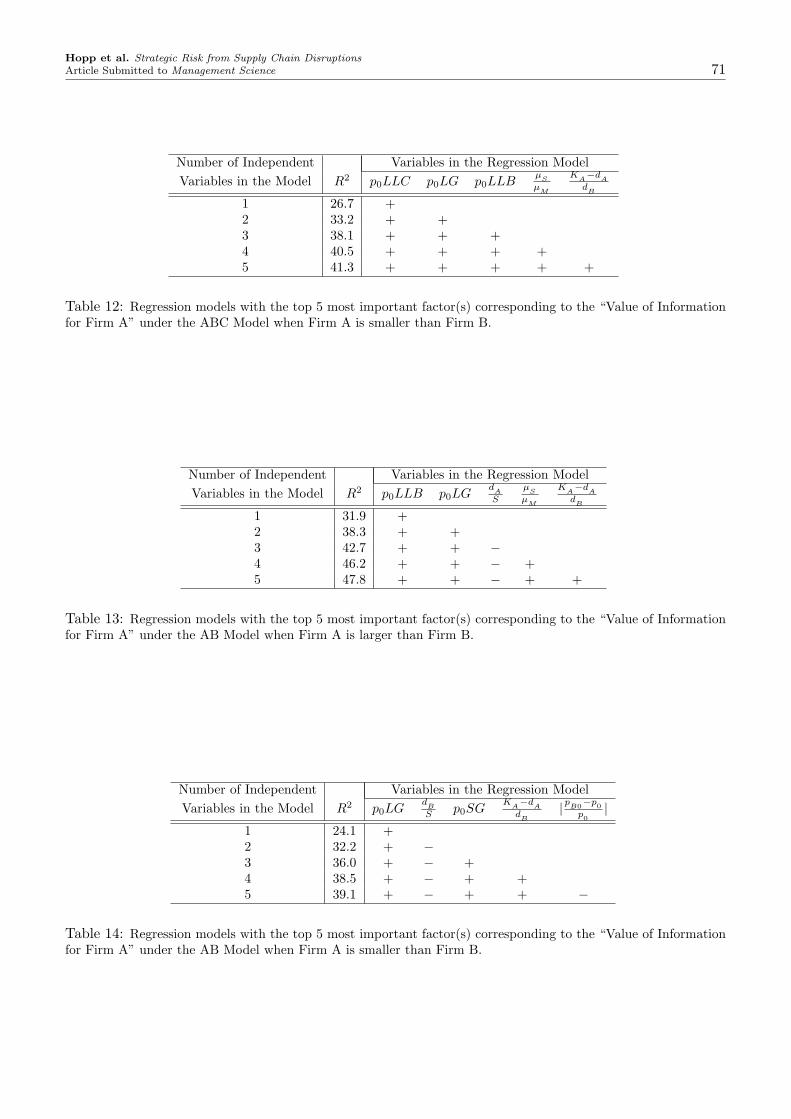
Hopp et al. Strategic Risk from Supply Chain DisruptionsArticle Submitted to Management Science 71
Number of Independent Variables in the Regression ModelVariables in the Model R2 p0LLC p0LG p0LLB
µS
µM
KA−d
A
dB
1 26.7 +2 33.2 + +3 38.1 + + +4 40.5 + + + +5 41.3 + + + + +
Table 12: Regression models with the top 5 most important factor(s) corresponding to the “Value of Informationfor Firm A” under the ABC Model when Firm A is smaller than Firm B.
Number of Independent Variables in the Regression ModelVariables in the Model R2 p0LLB p0LG
dA
S
µS
µM
KA−d
A
dB
1 31.9 +2 38.3 + +3 42.7 + + −4 46.2 + + − +5 47.8 + + − + +
Table 13: Regression models with the top 5 most important factor(s) corresponding to the “Value of Informationfor Firm A” under the AB Model when Firm A is larger than Firm B.
Number of Independent Variables in the Regression ModelVariables in the Model R2 p0LG
dB
S p0SGK
A−d
A
dB
|pB0−p0p0
|1 24.1 +2 32.2 + −3 36.0 + − +4 38.5 + − + +5 39.1 + − + + −
Table 14: Regression models with the top 5 most important factor(s) corresponding to the “Value of Informationfor Firm A” under the AB Model when Firm A is smaller than Firm B.

72Hopp et al. Strategic Risk from Supply Chain Disruptions
Article Submitted to Management Science
ONLINE APPENDIX D
Analytical Results for the Model with Systematic andTargeted Preparedness Investments
In this appendix, in addition to the effort that Firm i spends in preparedness activities related to moni-toring and detection (i.e., xi, i ∈ A, B), we also consider the effort that Firm i spends in preparednessactivities related to acquiring extra dedicated backup capacity (i.e., θi, i ∈ A,B). We considered C
θ
e,i
(i ∈ A,B) as the cost per unit of effort θi. The effort level θi can also be considered as the cost ofpurchasing capacity options from other suppliers, where the options will be exercised only if there is adisruption at the regular supplier. We define Θi (i ∈ A, B) as the upper limit on the available extradedicated backup capacity for Firm i.
We define ΠAPi (xi | xj) (i ∈ A,B) as Firm i’s total expected profit in the AP Competition for Firm
i (given Firm j’s preparedness effort level is xj) with one decision variables: xi. ΠAPi (xi, θi | xj , θj),
i ∈ A,B, Firm i’s total expected profit in the AP Competition for Firm i (given Firm j’s preparednesseffort levels are xj and θj), is a function with two decision variables: xi and θi, which are simultaneouslydecided by Firm i. Note that, we still consider two periods: Pre-Disruption Period and Post-DisruptionPeriod, but after adding θi into the AP Competition, we have:
• Pre-Disruption Period: Before a disruption occurs, both Firm A and Firm B serve their own cus-tomers. After a disruption occurs, firms will seek available backup capacity for the key component.There are three types of backup capacity: (a) dedicated capacity that is specific to each firm, (b)additional dedicated backup capacity that has already been contracted to be used in case of a dis-ruption, and (c) shared capacity, for which the two firms compete, if the dedicated backup capacityis not enough to cover the shortage. To model this competition with three possible backup capacitysources, we denote the amount of Firm i’s sales (i ∈ A,B) that cannot be covered by the dedi-cated capacity as d0
i, and the amount of Firm i’s sales (i ∈ A,B) that cannot be covered after
using both the dedicated capacity and the additional dedicated backup capacity is d0i− θi, where θi
is defined as the investment by Firm i (measured in unit capacity) devoted to acquiring additionaldedicated backup capacity. We denote the shared backup capacity by S. Under this setting, eachfirm must decide (1) how to invest in acquiring extra dedicated backup capacity, and (2) how toinvest in monitoring and detection in order to be able to detect the disruption first. This resultsin an Advanced Preparedness Competition for Firm i with two decision variables: xi and θi, whichare simultaneously decided.
• Post-Disruption Period: After the disruption occurs, the firm (either A or B) that detects thedisruption must decide how much of the total available backup capacity of S to buy in order tomaximize its total short- and long-term profits. This results in a Backup Capacity Competition(BC Competition). Once both firms have made their purchase decisions, there is a lead time periodrequired to bring the backup capacity (i.e., dedicated and shared) on line. During this period, bothFirm A and Firm B lose all of their short term sales, as well as some long term market share, toFirm C. The amount of the demand of Firm i (i ∈ A,B) that is lost to Firm C during the leadtime is (d0
i− θi)− di , where di is the demand for Firm i’s product at the end of the lead time.
All detailed analytical results are given in the following. Note that,
• adding θi (i ∈ A,B) into the AP Competition only changes the structure of the AP Competition:previously firm only makes one decision on how to invest in monitoring and detection, but nowfirm needs to make two simultaneous decisions of how to invest in acquiring extra dedicated backupcapacity and how to invest in monitoring and detection. Therefore, Proposition 3 needs to be provenin this new setting. On the other hand, since the relationship between the optimal preparednesseffort in monitoring and detection of Firm i (i.e., x∗i ) and the system parameters (e.g., mij , miC ,mji, ri, γij , γiC , γji, ci, and hi) will not be affected by adding θi into the AP Competition, it is easy
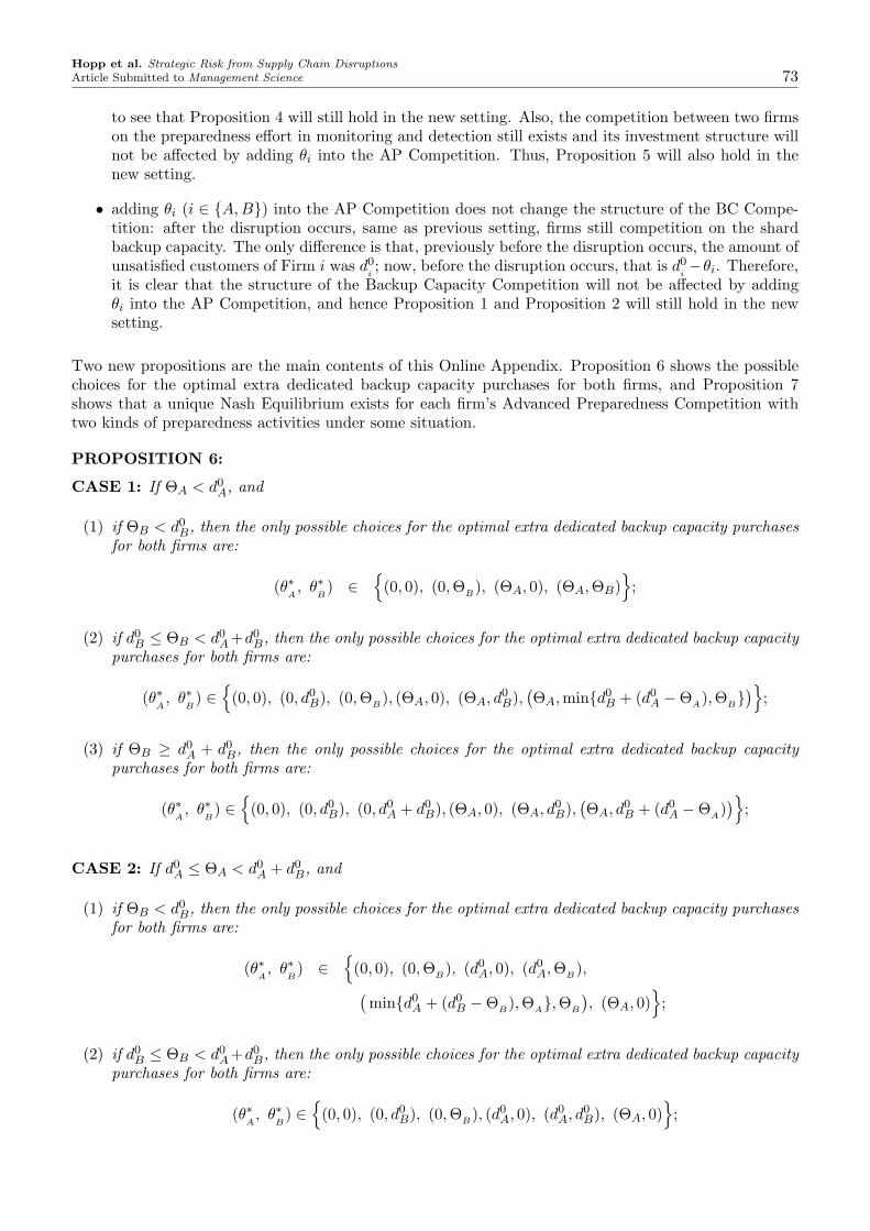
Hopp et al. Strategic Risk from Supply Chain DisruptionsArticle Submitted to Management Science 73
to see that Proposition 4 will still hold in the new setting. Also, the competition between two firmson the preparedness effort in monitoring and detection still exists and its investment structure willnot be affected by adding θi into the AP Competition. Thus, Proposition 5 will also hold in thenew setting.
• adding θi (i ∈ A,B) into the AP Competition does not change the structure of the BC Compe-tition: after the disruption occurs, same as previous setting, firms still competition on the shardbackup capacity. The only difference is that, previously before the disruption occurs, the amount ofunsatisfied customers of Firm i was d0
i; now, before the disruption occurs, that is d0
i−θi. Therefore,
it is clear that the structure of the Backup Capacity Competition will not be affected by addingθi into the AP Competition, and hence Proposition 1 and Proposition 2 will still hold in the newsetting.
Two new propositions are the main contents of this Online Appendix. Proposition 6 shows the possiblechoices for the optimal extra dedicated backup capacity purchases for both firms, and Proposition 7shows that a unique Nash Equilibrium exists for each firm’s Advanced Preparedness Competition withtwo kinds of preparedness activities under some situation.
PROPOSITION 6:
CASE 1: If ΘA < d0A, and
(1) if ΘB < d0B, then the only possible choices for the optimal extra dedicated backup capacity purchases
for both firms are:
(θ∗A, θ∗
B) ∈
(0, 0), (0, ΘB ), (ΘA, 0), (ΘA, ΘB)
;
(2) if d0B ≤ ΘB < d0
A +d0B, then the only possible choices for the optimal extra dedicated backup capacity
purchases for both firms are:
(θ∗A, θ∗
B) ∈
(0, 0), (0, d0
B), (0, ΘB ), (ΘA, 0), (ΘA, d0B),
(ΘA, mind0
B + (d0A −ΘA),ΘB
);
(3) if ΘB ≥ d0A + d0
B, then the only possible choices for the optimal extra dedicated backup capacitypurchases for both firms are:
(θ∗A, θ∗
B) ∈
(0, 0), (0, d0
B), (0, d0A + d0
B), (ΘA, 0), (ΘA, d0B),
(ΘA, d0
B + (d0A −ΘA)
);
CASE 2: If d0A ≤ ΘA < d0
A + d0B, and
(1) if ΘB < d0B, then the only possible choices for the optimal extra dedicated backup capacity purchases
for both firms are:
(θ∗A, θ∗
B) ∈
(0, 0), (0, ΘB ), (d0
A, 0), (d0A, ΘB ),
(mind0
A + (d0B −ΘB ), ΘA, ΘB
), (ΘA, 0)
;
(2) if d0B ≤ ΘB < d0
A +d0B, then the only possible choices for the optimal extra dedicated backup capacity
purchases for both firms are:
(θ∗A, θ∗
B) ∈
(0, 0), (0, d0
B), (0, ΘB ), (d0A, 0), (d0
A, d0B), (ΘA, 0)
;

74Hopp et al. Strategic Risk from Supply Chain Disruptions
Article Submitted to Management Science
(3) if ΘB ≥ d0A + d0
B, then the only possible choices for the optimal extra dedicated backup capacitypurchases for both firms are:
(θ∗A, θ∗
B) ∈
(0, 0), (0, d0
B), (0, d0A + d0
B), (d0A, 0), (d0
A, d0B), (ΘA, 0)
;
CASE 3: If ΘA ≥ d0A + d0
B, and
(1) if ΘB < d0B, then the only possible choices for the optimal extra dedicated backup capacity purchases
for both firms are:
(θ∗A, θ∗
B) ∈
(0, 0), (0,ΘB ), (d0
A, 0), (d0A,ΘB),
(d0
A + (d0B −ΘB ), ΘB
), (d0
A + d0B, 0)
;
(2) if d0B ≤ ΘB < d0
A +d0B, then the only possible choices for the optimal extra dedicated backup capacity
purchases for both firms are:
(θ∗A, θ∗
B) ∈
(0, 0), (0, d0
B), (0,ΘB), (d0A, 0), (d0
A, d0B), (d0
A + d0B, 0)
;
(3) if ΘB ≥ d0A + d0
B, then the only possible choices for the optimal extra dedicated backup capacitypurchases for both firms are:
(θ∗A, θ∗
B) ∈
(0, 0), (0, d0
B), (0, d0A + d0
B), (d0A, 0), (d0
A, d0B), (d0
A + d0B, 0)
;
PROOF OF PROPOSITION 6:
Before we show that the optimal extra backup capacity purchases for both firms are restricted to a smallnumber of possible values, we need to show:
• Part I: ΠAPA (xA, θA | xB, θB), Firm i’s total expected profit in the AP Competition for Firm i
given Firm j’s preparedness effort levels are xj and θj , is linear in θA, and ΠAPA (xA, θA | xB, θB)
can be written as,
ΠAPA (xA, θA | xB, θB) = pA0
( xA
xA + xBΠA,L(Y ∗
A,L, Y ∗
B,F| θA, θB) +
xB
xA + xBΠA,F (Y ∗
B,L, Y ∗
A,F| θA, θB)
−mAC (d0A − θA)(1− e
− TγAC )
)+ (1− pA0)
(rA(d0
A − θA)(µ + T ))
−Cx
exA − C
θ
eθA + mAA(d0
A − θA), (30)
where Πi,k(Y ∗i,k
, Y ∗j,k| θi, θj) (i, j ∈ A,B and i 6= j, and k, k ∈ L,F) is the total expected profit
of Firm i when it is in position k in the BC Competition, given firms’ preparedness effort levels onacquiring extra dedicated backup capacity are θi and θj . For simplification, in the following, wewill write Πi,k(Y ∗
i,k, Y ∗
j,k| θi, θj) as Πi,k(θi, θj).
• Part II: ΠAPA (xA, θA | xB, θB) is piecewise linear in θA for given xj and θj .
Part I: In this part, we will show that ΠAPA (xA, θA | xB, θB) is linear in θA for given xj and θj .
First of all, it is easy to see that all terms in equation (30) except the first term,
pA0
xA
xA + xBΠA,L(θA, θB),

Hopp et al. Strategic Risk from Supply Chain DisruptionsArticle Submitted to Management Science 75
and the second term,
pA0
xB
xA + xBΠA,F (θA, θB),
are linear in θA, so we only need to show that both ΠA,L(θA, θB) and ΠA,F (θA, θB) are also linear in θA.
In the following, we will show that for any given θB, both Π∗A,L
(θA, θB) and Π∗B,F
(θA, θB) are linear inθA. Let’s look at the Backup Capacity Competition.
Part I – Case 1. d0i < θi ≤ Θi, i ∈ A,B:
It is easy to see that this case cannot be optimal. (All customers of Firm i can be satisfied by Firm i,so it cannot be optimal for the competitor of Firm i to buy more than what it needs to satisfy its owncustomers, i.e., the amount of d0
i .)
Part I – Case 2. θi = d0i , i ∈ A,B:
It is clear that in this case, no firm will play the Backup Capacity Competition.
Part I – Case 3. d0i < θi ≤ Θi, but θj ≤ mind0
j , Θj: For simplification, we call this as CONDITION3 .
Under CONDITION 3 , there are two possible cases:
• Subcase 1: If d0j ≤ Θj , then θj ≤ mind0
j , Θj becomes θj ≤ d0j . But, note that, it is easy to
show that the combination of d0i < θi and θj = d0
j cannot be optimal, so CONDITION 3 becomesd0
i < θi(≤ Θi), but θj < d0j (≤ Θj).
• Subcase 2: If d0j > Θj , then θj ≤ mind0
j , Θj becomes θj ≤ Θj . CONDITION 3 becomesd0
i < θi(≤ Θi), but θj ≤ Θj(< d0j ).
In both cases, Firm i not only can cover all its own customers, but also has an amount of θi − d0i extra
capacity, which can be used to steal the competitor’s unsatisfied customers. Therefore, the optimalamount of the shared backup capacity that Firm i will buy is the difference between the remaining extracapacity, θi − d0
i , and the number of competitor’s unsatisfied customers, dj (θj) − Yj,F , where dj (θj)(=
(d0j − θj)e
− TγjC ) is the uncovered demand of Firm j’s product at the end of the lead time, which is a
function of θj . Without loss of generality, let i = A and j = B, the optimal shared backup capacitypurchase amount of Firm A given it is the Leader in the BC competition is
Y ∗A,L
=[[dB (θB)− YB,F ]+ − (θA − d0
A)]+
,
where dB (θB) = (d0B − θB)e−
TγBC .
It is easy to see that, for any given θB, both ΠA,L(θA, θB) and ΠB,F (θA, θB) are linear in θA.
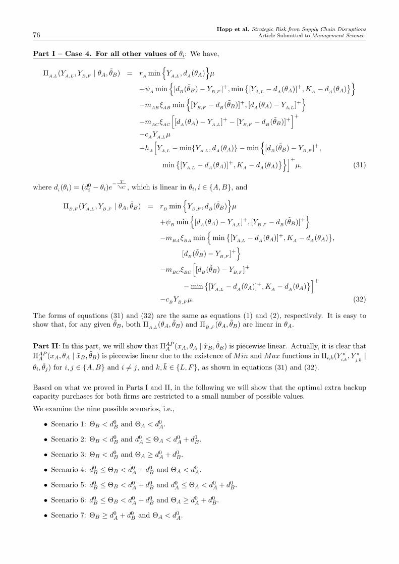
76Hopp et al. Strategic Risk from Supply Chain Disruptions
Article Submitted to Management Science
Part I – Case 4. For all other values of θi: We have,
ΠA,L(YA,L , YB,F | θA, θB) = rA min
YA,L , dA(θA)
µ
+ψA min
[dB (θB)− YB,F ]+,min[YA,L − dA(θA)]+,KA − dA(θA)
−mABξAB min
[YB,F − dB (θB)]+, [dA(θA)− YA,L ]+
−mAC ξAC
[[dA(θA)− YA,L ]+ − [YB,F − dB (θB)]+
]+
−cAYA,Lµ
−hA
[YA,L −minYA,L , dA(θA) −min
[dB (θB)− YB,F ]+,
min[YA,L − dA(θA)]+,KA − dA(θA)
]+µ, (31)
where di(θi) = (d0i − θi)e
− TγiC , which is linear in θi, i ∈ A,B, and
ΠB,F (YA,L , YB,F | θA, θB) = rB min
YB,F , dB (θB)
µ
+ψB min
[dA(θA)− YA,L ]+, [YB,F − dB (θB)]+
−mBAξBA min
min[YA,L − dA(θA)]+,KA − dA(θA)
,
[dB(θB)− YB,F ]+
−mBCξBC
[[dB (θB)− YB,F ]+
−min[YA,L − dA(θA)]+,KA − dA(θA)
]+
−cBYB,F µ. (32)
The forms of equations (31) and (32) are the same as equations (1) and (2), respectively. It is easy toshow that, for any given θB, both ΠA,L(θA, θB) and ΠB,F (θA, θB) are linear in θA.
Part II: In this part, we will show that ΠAPA (xA, θA | xB, θB) is piecewise linear. Actually, it is clear that
ΠAPA (xA, θA | xB, θB) is piecewise linear due to the existence of Min and Max functions in Πi,k(Y ∗
i,k, Y ∗
j,k|
θi, θj) for i, j ∈ A,B and i 6= j, and k, k ∈ L,F, as shown in equations (31) and (32).
Based on what we proved in Parts I and II, in the following we will show that the optimal extra backupcapacity purchases for both firms are restricted to a small number of possible values.
We examine the nine possible scenarios, i.e.,
• Scenario 1: ΘB < d0B and ΘA < d0
A.
• Scenario 2: ΘB < d0B and d0
A ≤ ΘA < d0A + d0
B.
• Scenario 3: ΘB < d0B and ΘA ≥ d0
A + d0B.
• Scenario 4: d0B ≤ ΘB < d0
A + d0B and ΘA < d0
A.
• Scenario 5: d0B ≤ ΘB < d0
A + d0B and d0
A ≤ ΘA < d0A + d0
B.
• Scenario 6: d0B ≤ ΘB < d0
A + d0B and ΘA ≥ d0
A + d0B.
• Scenario 7: ΘB ≥ d0A + d0
B and ΘA < d0A.
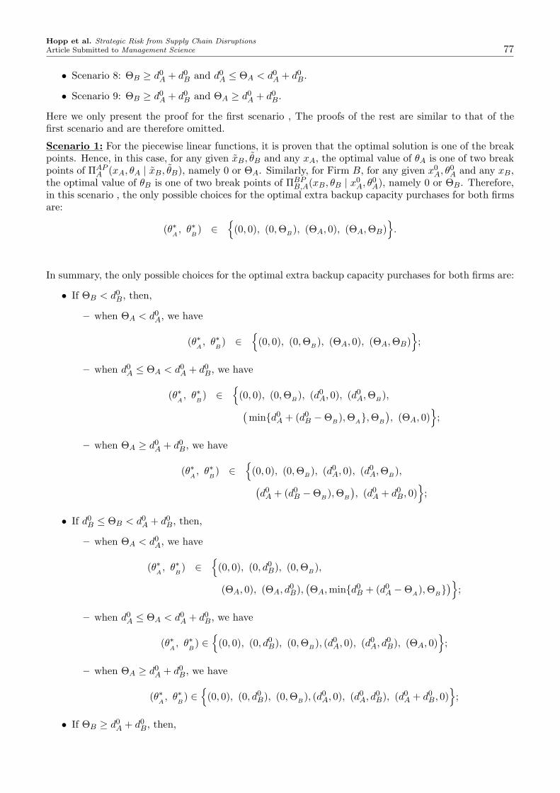
Hopp et al. Strategic Risk from Supply Chain DisruptionsArticle Submitted to Management Science 77
• Scenario 8: ΘB ≥ d0A + d0
B and d0A ≤ ΘA < d0
A + d0B.
• Scenario 9: ΘB ≥ d0A + d0
B and ΘA ≥ d0A + d0
B.
Here we only present the proof for the first scenario , The proofs of the rest are similar to that of thefirst scenario and are therefore omitted.
Scenario 1: For the piecewise linear functions, it is proven that the optimal solution is one of the breakpoints. Hence, in this case, for any given xB, θB and any xA, the optimal value of θA is one of two breakpoints of ΠAP
A (xA, θA | xB, θB), namely 0 or ΘA. Similarly, for Firm B, for any given x0A, θ0
A and any xB,the optimal value of θB is one of two break points of ΠBP
B,A(xB, θB | x0A, θ0
A), namely 0 or ΘB. Therefore,in this scenario , the only possible choices for the optimal extra backup capacity purchases for both firmsare:
(θ∗A, θ∗
B) ∈
(0, 0), (0, ΘB ), (ΘA, 0), (ΘA, ΘB)
.
In summary, the only possible choices for the optimal extra backup capacity purchases for both firms are:
• If ΘB < d0B, then,
– when ΘA < d0A, we have
(θ∗A, θ∗
B) ∈
(0, 0), (0, ΘB ), (ΘA, 0), (ΘA, ΘB)
;
– when d0A ≤ ΘA < d0
A + d0B, we have
(θ∗A, θ∗
B) ∈
(0, 0), (0,ΘB), (d0
A, 0), (d0A,ΘB),
(mind0
A + (d0B −ΘB ),ΘA,ΘB
), (ΘA, 0)
;
– when ΘA ≥ d0A + d0
B, we have
(θ∗A, θ∗
B) ∈
(0, 0), (0, ΘB ), (d0
A, 0), (d0A, ΘB ),
(d0
A + (d0B −ΘB ),ΘB
), (d0
A + d0B, 0)
;
• If d0B ≤ ΘB < d0
A + d0B, then,
– when ΘA < d0A, we have
(θ∗A, θ∗
B) ∈
(0, 0), (0, d0
B), (0,ΘB ),
(ΘA, 0), (ΘA, d0B),
(ΘA, mind0
B + (d0A −ΘA), ΘB
);
– when d0A ≤ ΘA < d0
A + d0B, we have
(θ∗A, θ∗
B) ∈
(0, 0), (0, d0
B), (0, ΘB ), (d0A, 0), (d0
A, d0B), (ΘA, 0)
;
– when ΘA ≥ d0A + d0
B, we have
(θ∗A, θ∗
B) ∈
(0, 0), (0, d0
B), (0, ΘB ), (d0A, 0), (d0
A, d0B), (d0
A + d0B, 0)
;
• If ΘB ≥ d0A + d0
B, then,
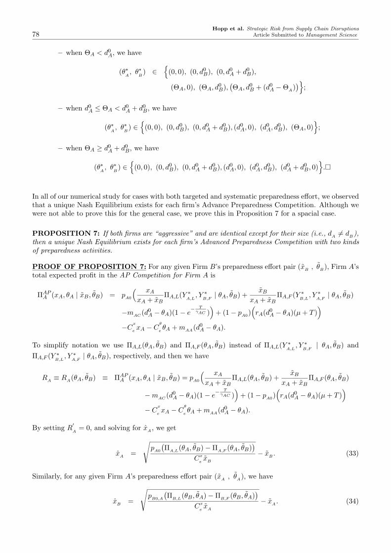
78Hopp et al. Strategic Risk from Supply Chain Disruptions
Article Submitted to Management Science
– when ΘA < d0A, we have
(θ∗A, θ∗
B) ∈
(0, 0), (0, d0
B), (0, d0A + d0
B),
(ΘA, 0), (ΘA, d0B),
(ΘA, d0
B + (d0A −ΘA)
);
– when d0A ≤ ΘA < d0
A + d0B, we have
(θ∗A, θ∗
B) ∈
(0, 0), (0, d0
B), (0, d0A + d0
B), (d0A, 0), (d0
A, d0B), (ΘA, 0)
;
– when ΘA ≥ d0A + d0
B, we have
(θ∗A, θ∗
B) ∈
(0, 0), (0, d0
B), (0, d0A + d0
B), (d0A, 0), (d0
A, d0B), (d0
A + d0B, 0)
.¤
In all of our numerical study for cases with both targeted and systematic preparedness effort, we observedthat a unique Nash Equilibrium exists for each firm’s Advance Preparedness Competition. Although wewere not able to prove this for the general case, we prove this in Proposition 7 for a spacial case.
PROPOSITION 7: If both firms are “aggressive” and are identical except for their size (i.e., dA 6= dB),then a unique Nash Equilibrium exists for each firm’s Advanced Preparedness Competition with two kindsof preparedness activities.
PROOF OF PROPOSITION 7: For any given Firm B’s preparedness effort pair (xB , θB ), Firm A’stotal expected profit in the AP Competition for Firm A is
ΠAPA (xA, θA | xB, θB) = pA0
( xA
xA + xBΠA,L(Y ∗
A,L, Y ∗
B,F| θA, θB) +
xB
xA + xBΠA,F (Y ∗
B,L, Y ∗
A,F| θA, θB)
−mAC (d0A − θA)(1− e
− TγAC )
)+ (1− pA0)
(rA(d0
A − θA)(µ + T ))
−Cx
exA − C
θ
eθA + mAA(d0
A − θA).
To simplify notation we use ΠA,L(θA, θB) and ΠA,F (θA, θB) instead of ΠA,L(Y ∗A,L
, Y ∗B,F
| θA, θB) andΠA,F (Y ∗
B,L, Y ∗
A,F| θA, θB), respectively, and then we have
RA ≡ RA(θA, θB) ≡ ΠAPA (xA, θA | xB, θB) = pA0
( xA
xA + xBΠA,L(θA, θB) +
xB
xA + xBΠA,F (θA, θB)
−mAC (d0A − θA)(1− e
− TγAC )
)+ (1− pA0)
(rA(d0
A − θA)(µ + T ))
− Cx
exA − C
θ
eθA + mAA(d0
A − θA).
By setting R′A
= 0, and solving for xA , we get
xA =
√pA0
(ΠA,L(θA, θB)−ΠA,F (θA, θB)
)
Cx
exB
− xB . (33)
Similarly, for any given Firm A’s preparedness effort pair (xA , θA), we have
xB =
√pB0,A
(ΠB,L(θB, θA)−ΠB,F (θB, θA)
)
Cx
exA
− xA . (34)

Hopp et al. Strategic Risk from Supply Chain DisruptionsArticle Submitted to Management Science 79
By equations (33) and (34), we can write out x∗A
as follows
x∗A
=1
Cx
e
(pA0∆Π∗A)2(pB0,A∆Π∗B)(pA0∆Π∗A + pB0,A∆Π∗B)2
, (35)
where ∆Π∗i = Π∗i,L(θ∗i , θ∗j )−Π∗i,F (θ∗i , θ
∗j ), i = A,B, i 6= j. Similarly, we have
x∗B
=1
Cx
e
(pB0,A∆Π∗B)2(pA0∆Π∗A)(pA0∆Π∗A + pB0,A∆Π∗B)2
, (36)
After ignoring all constant terms, by equations (35) and (36), we have
RA(θ∗A, θ∗B) =p2
A0∆Π∗A
pA0∆Π∗A + pB0,A∆Π∗BΠ∗
A,L(θ∗A, θ∗B) +
pA0pB0,A∆Π∗BpA0∆Π∗A + pB0,A∆Π∗B
Π∗A,F
(θ∗A, θ∗B)
− (pA0∆Π∗A)2(pB0,A∆Π∗B)(pA0∆Π∗A + pB0,A∆Π∗B)2
−mAC (1− e− T
γAC )θ∗A − rA(1− pA0)(µ + T )θ∗A − Cθ
eθ∗A −mAAθ∗A.
In the proof of Proposition 5, we have shown that if both firms are “aggressive” and are identical exceptfor their size (i.e., dA 6= dB ), then we have ∆Π∗A = ∆Π∗B. Hence, we get
RA(θ∗A, θ∗B) =p2
A0
pA0 + pB0,A
Π∗A,L
(θ∗A, θ∗B) +pA0pB0,A
pA0 + pB0,A
Π∗A,F
(θ∗A, θ∗B)
− (pA0)2pB0,A
(pA0 + pB0,A)2(Π∗
A,L(θ∗A, θ∗B)−Π∗
A,F(θ∗A, θ∗B)
)
−mAC (1− e− T
γAC )θ∗A − rA(1− pA0)(µ + T )θ∗A − Cθ
eθ∗A −mAAθ∗A.
= ηA
1Π∗
A,L(θ∗A, θ∗B) + η
A
2Π∗
A,F(θ∗A, θ∗B)− η
A
3θ∗A + constant,
where
ηA
1=
p3A0
(pA0 + pB0,A)2, η
A
2=
2p2A0
pB0,A + pA0p2B0,A
(pA0 + pB0,A)2, and
ηA
3= mAC (1− e
− TγAC ) + rA(1− pA0)(µ + T ) + C
θ
e+ mAA .
Without loss of generality, let dA > dB . As we showed in the proof of Proposition 5, based on therelationship among dA , dB , K, and dA + dB we have the following two main cases, each including fivemutually exclusive and collectively exhaustive sub-cases:
• Case 1: dB ≤ dA ≤ K ≤ dA + dB :
– S ≤ dB ;
– dB ≤ S ≤ dA ;
– dA ≤ S ≤ K;
– K ≤ S ≤ dA + dB ;
– dA + dB ≤ S.
• Case 2: dB ≤ dA ≤ dA + dB ≤ K:
– S ≤ dB ;
– dB ≤ S ≤ dA ;
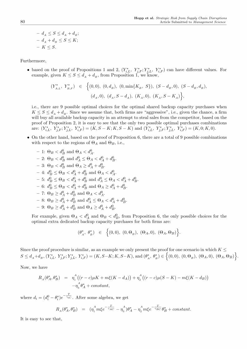
80Hopp et al. Strategic Risk from Supply Chain Disruptions
Article Submitted to Management Science
– dA ≤ S ≤ dA + dB ;
– dA + dB ≤ S ≤ K;
– K ≤ S.
Furthermore,
• based on the proof of Propositions 1 and 2, (Y ∗i,L, Y ∗
j,F ; Y ∗j,L, Y ∗
i,F ) can have different values. Forexample, given K ≤ S ≤ dA + dB , from Proposition 1, we know,
(Y ∗A,L
, Y ∗B,F
) ∈
(0, 0), (0, dB ), (0, minKB , S), (S − dB , 0), (S − dB , dB ),
(dA , 0), (dA , S − dA), (KA , 0), (KA , S −KA)
,
i.e., there are 9 possible optimal choices for the optimal shared backup capacity purchases whenK ≤ S ≤ dA + dB . Since we assume that, both firms are “aggressive”, i.e., given the chance, a firmwill buy all available backup capacity in an attempt to steal sales from the competitor, based on theproof of Proposition 2, it is easy to see that the only two possible optimal purchases combinationsare: (Y ∗
i,L, Y ∗j,F ; Y ∗
j,L, Y ∗i,F ) = (K,S −K;K,S −K) and (Y ∗
i,L, Y ∗j,F ; Y ∗
j,L, Y ∗i,F ) = (K, 0;K, 0).
• On the other hand, based on the proof of Proposition 6, there are a total of 9 possible combinationswith respect to the regions of ΘA and ΘB, i.e.,
– 1: ΘB < d0B and ΘA < d0
A.
– 2: ΘB < d0B and d0
A ≤ ΘA < d0A + d0
B.
– 3: ΘB < d0B and ΘA ≥ d0
A + d0B.
– 4: d0B ≤ ΘB < d0
A + d0B and ΘA < d0
A.
– 5: d0B ≤ ΘB < d0
A + d0B and d0
A ≤ ΘA < d0A + d0
B.
– 6: d0B ≤ ΘB < d0
A + d0B and ΘA ≥ d0
A + d0B.
– 7: ΘB ≥ d0A + d0
B and ΘA < d0A.
– 8: ΘB ≥ d0A + d0
B and d0A ≤ ΘA < d0
A + d0B.
– 9: ΘB ≥ d0A + d0
B and ΘA ≥ d0A + d0
B.
For example, given ΘA < d0A and ΘB < d0
B, from Proposition 6, the only possible choices for theoptimal extra dedicated backup capacity purchases for both firms are:
(θ∗A, θ∗
B) ∈
(0, 0), (0, ΘB ), (ΘA, 0), (ΘA, ΘB)
.
Since the proof procedure is similar, as an example we only present the proof for one scenario in which K ≤S ≤ dA+dB , (Y ∗
i,L, Y ∗j,F ; Y ∗
j,L, Y ∗i,F ) = (K,S−K;K, S−K), and (θ∗
A, θ∗
B) ∈
(0, 0), (0, ΘB ), (ΘA, 0), (ΘA, ΘB)
.
Now, we have
RA(θ∗A, θ∗B) = ηA
1
((r − c)µK + mξ(K − dA)
)+ η
A
2
((r − c)µ(S −K)−mξ(K − dB)
)
−ηA
3θ∗A + constant,
where di = (d0i − θ∗i )e
− TγiC . After some algebra, we get
RA(θ∗A, θ∗B) = (ηA
1mξe
− TγAC − η
A
3)θ∗A − η
A
2mξe
− TγBC θ∗B + constant.
It is easy to see that,

Hopp et al. Strategic Risk from Supply Chain DisruptionsArticle Submitted to Management Science 81
• if ηA
1mξe
− TγAC − η
A
3> 0, then Firm A prefers θ∗A = ΘA regardless of whether θ∗B = 0 or ΘB , i.e.,
ΘA is strictly dominated;
• if ηA
1mξe
− TγAC − η
A
3≤ 0, then Firm A prefers θ∗A = 0 regardless of wether θ∗B = 0 or ΘB , i.e., 0 is
(weakly) dominated.
That is, there is always a dominated strategy for Firm A.
For Firm B, we have the similar result,
• if ηB
1mξe
− TγBC − η
B
3> 0, then Firm B prefers θ∗B = ΘB regardless of whether θ∗A = 0 or ΘA , i.e.,
ΘB is strictly dominated;
• if ηB
1mξe
− TγBC − η
B
3≤ 0, then Firm B prefers θ∗B = 0 regardless of whether θ∗A = 0 or ΘA , i.e., 0 is
(weakly) dominated.
That is, there is always a dominated strategy for Firm B too.
We summarize the possible optimal extra dedicated backup capacity purchases combinations are:
• when ηA
1mξe
− TγAC − η
A
3> 0 and η
B
1mξe
− TγBC − η
B
3> 0, then (θ∗A, θ∗B) = (ΘA,ΘB);
• when ηA
1mξe
− TγAC − η
A
3> 0 and η
B
1mξthene
− TγBC − η
B
3≤ 0, (θ∗A, θ∗B) = (ΘA, 0);
• when ηA
1mξe
− TγAC − η
A
3≤ 0 and η
B
1mξe
− TγBC − η
B
3> 0, then (θ∗A, θ∗B) = (0,ΘB);
• when ηA
1mξe
− TγAC − η
A
3≤ 0 and η
B
1mξe
− TγBC − η
B
3≤ 0, then (θ∗A, θ∗B) = (0, 0).
So, we can claim that if both firms are “aggressive” and are identical except for their size (i.e., dA 6= dB ),then a unique Nash Equilibrium exists for each firm’s Advanced Preparedness Competition with twokinds of preparedness activities. ¤

82Hopp et al. Strategic Risk from Supply Chain Disruptions
Article Submitted to Management Science
ONLINE APPENDIX E
Numerical Study on Impact of Firms Risk Attitudes
In this appendix, we perform a numerical study which extends our results in Sections 3.2 and 3.3 forrisk-neutral firms to cases where firms are Risk Averse (RA) and/or Risk Seeking (RS). Specifically, weconsider: (1) a risk-averse (RA) exponential utility function of the form u(x) = −e
−ax, and (2) a risk-
seeking (RS) exponential utility function of the form u(x) = eax
, where a is a positive constant. We testcases where a = 0.1, 1, 10, and 100 and compare the results to the risk neutral cases.
Based on equation (3), as a RA firm, Firm i’s loss due to lack of preparedness is:
ΩRA
i = Πi −(p0
(− e−(Π∗i,F−miC(d0
i−di)+miid0i
))+ (1− p0)
(− e−(rid
0i (µ+T )+miid
0i
))), (37)
where Πi is the actual expected profit of Firm i, when the firm follows the optimal preparedness strategy:
Πi = p0
(− e
−(
x∗ix∗
i+w∗
j
(−e
−(Π∗i,L−miC (d0i−di)+miid0
i−Cex∗i ))+
w∗jx∗
i+w∗
j
(−e
−(Π∗i,F−miC (d0i−di)+miid0
i−Cex∗i ))))
+(1− p0)(− e−
(rid
0i (µ+T )+miid
0i−Cex∗i
)). (38)
The equation for the measure of risk for a RS firm can be obtained similarly.
Firm A (Larger) Firm B (Smaller)Case 1 Risk-averse Risk-averseCase 2 Risk-averse Risk-neutralCase 3 Risk-averse Risk-seekingCase 4 Risk-neutral Risk-averseCase 5 Risk-neutral Risk-neutralCase 6 Risk-neutral Risk-seekingCase 7 Risk-seeking Risk-averseCase 8 Risk-seeking Risk-neutralCase 9 Risk-seeking Risk-seeking
Table 15: Possible combinations of firms’ risk attitudes.
As shown in Table 15, since there are three types of risk attitude (Risk Averse, Risk Seeking and RiskNeutral) for each of the two firms, we will have 9 cases, each of which corresponds to a possible combinationof firms’ risk attitudes.
Tables 16 to 19 display the best regression models with five parameters under the ABC Model and ABModel with different combination of firms’ risk attitudes. Note that, the case in which both firms arerisk-neutral has already been studied in Sections 3.2 and 3.3, and is therefore omitted here.
As these tables show, when evaluating protection policies against disruption, a risk averse firm tends topay more attention to loss factors while a risk seeking firm tends to pay more attention to gain factors.Furthermore, we find that for cases where the competition is more risk averse, a firm should focus moreon gain factors. On the other hand, the competition being more risk seeking makes a firm paying moreattention to loss factors when evaluating protection policies.
This observation complements our previous observations about firm size. Larger and/or risk averse firmsshould pay attention to loss factors when evaluating protection policies, while smaller and/or risk seeking

Hopp et al. Strategic Risk from Supply Chain DisruptionsArticle Submitted to Management Science 83
firms should pay attention to gain factors when evaluating protection policies. Factors that make theopponent pay more attention to loss (gain) factors when evaluating protection policies tend to make a firmpay more attention to gain (loss) factors when evaluating protection policies. These results are intuitive,but they confirm that our earlier insights about the conditions that magnify the risks from supply chaindisruptions are still valid when firms are not risk neutral.
Firm A Firm B R2 Top 5 Factors
RA RA 57.1 p0LLC p0LLBK
B−d
B
dA
dA
S |pB0−p0p0
|RA RN 59.4 p0LLC p0LLB
KB−d
B
dA
dA
S p0SLtotal
RA RS 60.4 p0LLC p0LLBK
B−d
B
dA
p0SLtotal
dA
S
RN RA 45.2 p0LLC p0LLBd
A
S |pB0−p0p0
| KB−d
B
dA
RN RS 58.6 p0LLC p0LLBK
B−d
B
dA
dA
S |pB0−p0p0
|RS RA 50.3 p0LG p0LLC p0LLB
KA−d
A
dB
dA
S
RS RN 47.7 p0LGK
A−d
A
dB
p0LLCd
A
S p0LLB
RS RS 41.3 p0LG p0LLCK
A−d
A
dB
p0LLBd
A
S
Table 16: Regression models for the top five factors for Firm A in the ABC Model with different combination offirms’ risk attitudes, when Firm A is the larger firm.
Firm A Firm B R2 Top 5 Factors
RA RA 50.3 p0LLC p0LLBd
B
S p0LG |pB0−p0p0
|RA RN 52.8 p0LLC p0LLB
dB
S p0LG |pB0−p0p0
|RA RS 54.9 p0LLC p0LLB
dB
S
KB−d
B
dA
p0LG
RN RA 40.1 p0LLC p0LG p0LLBd
B
S
KA−d
A
dB
RN RS 52.7 p0LLC p0LLBd
B
S p0LGK
A−d
A
dB
RS RA 43.8 p0LGK
A−d
A
dB
p0LLC p0SG p0LLB
RS RN 41.5 p0LGK
A−d
A
dB
p0LLC p0SG p0LLB
RS RS 39.2 p0LGK
A−d
A
dB
p0SGd
B
S p0LLC
Table 17: Regression models for the top five factors for Firm A in the ABC Model with different combination offirms’ risk attitudes, when Firm A is the smaller firm.
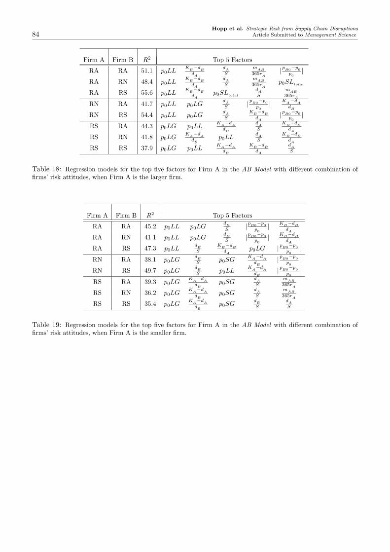
84Hopp et al. Strategic Risk from Supply Chain Disruptions
Article Submitted to Management Science
Firm A Firm B R2 Top 5 Factors
RA RA 51.1 p0LLK
B−d
B
dA
dA
S
mAB
365rA
|pB0−p0p0
|RA RN 48.4 p0LL
KB−d
B
dA
dA
S
mAB
365rA
p0SLtotal
RA RS 55.6 p0LLK
B−d
B
dA
p0SLtotal
dA
S
mAB
365rA
RN RA 41.7 p0LL p0LGd
A
S |pB0−p0p0
| KA−d
A
dB
RN RS 54.4 p0LL p0LGd
A
S
KB−d
B
dA
|pB0−p0p0
|RS RA 44.3 p0LG p0LL
KA−d
A
dB
dA
S
KB−d
B
dA
RS RN 41.8 p0LGK
A−d
A
dB
p0LLd
A
S
KB−d
B
dA
RS RS 37.9 p0LG p0LLK
A−d
A
dB
KB−d
B
dA
dA
S
Table 18: Regression models for the top five factors for Firm A in the AB Model with different combination offirms’ risk attitudes, when Firm A is the larger firm.
Firm A Firm B R2 Top 5 Factors
RA RA 45.2 p0LL p0LGd
B
S |pB0−p0p0
| KB−d
B
dA
RA RN 41.1 p0LL p0LGd
B
S |pB0−p0p0
| KB−d
B
dA
RA RS 47.3 p0LLd
B
S
KB−d
B
dA
p0LG |pB0−p0p0
|RN RA 38.1 p0LG
dB
S p0SGK
A−d
A
dB
|pB0−p0p0
|RN RS 49.7 p0LG
dB
S p0LLK
A−d
A
dB
|pB0−p0p0
|RS RA 39.3 p0LG
KA−d
A
dB
p0SGd
A
S
mAB
365rA
RS RN 36.2 p0LGK
A−d
A
dB
p0SGd
A
S
mAB
365rA
RS RS 35.4 p0LGK
A−d
A
dB
p0SGd
B
S
dA
S
Table 19: Regression models for the top five factors for Firm A in the AB Model with different combination offirms’ risk attitudes, when Firm A is the smaller firm.

Hopp et al. Strategic Risk from Supply Chain DisruptionsArticle Submitted to Management Science 85
ONLINE APPENDIX F
Implications for Risk Management
We can boil down our insights from the our analytical and numerical analysis to produce the following list of policiesfirms can pursue to mitigate the tactical and strategic consequences of supply chain disruptions.
F.1. Speed Polices
In scenarios where a supply disruption affects multiple firms (i.e., the ABC and AB models), earlier detectionand quicker reaction make it more likely the firm will be able to secure the limited backup capacity before thecompetition. Therefore, we suggest firms (1) install monitoring processes on key components in order to spotdisruptions quickly and to better distinguish a true disruption from day-to-day variations, and (2) build a company-wide culture of awareness and communication so that relevant parties will be made aware of suspicious situationsquickly and will be able to work collaboratively to craft a response.
In addition to promoting detection and response speed from the within firms, firms can improve reaction speed toan external disruptive event by strengthening relationships with suppliers. Enhancing the firm’s reputation withsuppliers can make it more likely that these suppliers will share information with the firm and work with it toresolve a problem. For instance, the 1997 fire at Aisin (which made 99% of Toyota’s P-valves) provided an exampleof a successful business relationship between a manufacturer and a supplier, which led to a rapid collaborativeresponse to a disruptive situation (see Reitman (1997), Nishiguchi and Beaudet (1998) for discussions).
F.2. Customer Loyalty Polices
Under the ABC and AB models, our regression analysis indicates that Firm A faces lower risk when it has highercustomer loyalty (relative to either Firm B or Firm C). Indeed, high customer loyalty pays dividends not onlyduring disruptive events, but also during normal operations. It has been estimated that the cost of acquiring a newcustomer is six to ten times higher than the cost of maintaining a repeat customer (LeBoeuf (2000)). So a firm’smarketing dollars will go further if some of them are devoted to building, nurturing, and developing its currentcustomer relationships. Our results suggest that such efforts will also make the firm more resilient to supply chaindisruptions.
There are many ways a firm can cultivate greater customer loyalty, including:
• Discounts. During normal production, discounts for repeat customers can be an effective way to retaincustomers. In a similar fashion, firms can avoid permanently losing customers who cannot be satisfiedduring a supply outage by offering discounts or rebates to customers who are willing to return after theoutage. Similarly, if the firm has similar product(s) available as substitute(s) to the disrupted one(s), it candiscount these during the outage to encourage customers of the disrupted product(s) to buy them insteadof competitive products. Customer recover can substantially impact profitability. Studies indicate thatcustomer recovery investments yield returns of 30%-150% (Wreden (2009)).
• Exceed customer expectations. Delivering more than customers expect is one of the most powerful ways togain customer loyalty. For instance, Lexus had a recall early in its history in the United States. They calledcustomers, arranged to pick up their cars, and left identical cars as loaners for the day in their places. Whenthey returned the car that evening, it was fixed, cleaned, and had a full tank of gas and a coupon for a freeoil change. Lexus wisely used this disruption as an opportunity to impress its customers and hence increasecustomer loyalty (Sheffi (2005)).
• Pay great attention to unhappy customers. It is impossible for a firm to keep 100% of its customers happy, sostrategies are needed to identify unhappy customers who may be inclined to post negative comments (or evenvideos) on the web. A firm should consider giving unhappy customers an outlet for their comments, so thatit can monitor and respond to them. For example, in 1999, Intel was notified by a mathematics professorabout a floating-point-operation defect of its Pentium 486DX. When Intel failed to respond, the professorposted this problem on a mathematics web site, where it rapidly generated public attention. Intel initiallyresponded by offering to replace the 486DX chip for users who could prove a need for using floating-pointoperations. This served to further aggravate customer unhappiness and led to a demand for a complete recall.Intel finally gave in and recalled the 486DX, which cost more than four-hundred million dollars, and evenmore importantly, damaged its reputation and customer loyalty (Mueller and Soper (2001), Sheffi (2005)).An example of a successful response to a difficult situation occurred in 2001, after the 9/11 attack shut down

86Hopp et al. Strategic Risk from Supply Chain Disruptions
Article Submitted to Management Science
all U.S. air freight traffic, when Continental Teves (a supplier of automotive, industrial, and agriculturalproducts) saw an opportunity to impress customers affected by the disruption. On the afternoon of 9/11,Continental Teves picked out those shipments deemed most important to its customers, promised to reroutethem via ground transportation, and tried its best to deliver them on time. Although this action was costly,Continental Teves successfully impressed its customers and made them more loyal in the long term (Marthaand Vratimos (2002)).
F.3. Backup Capacity Polices
Our results show clearly that a firm faces the greatest risk when the shared backup supply for a component subjectto disruption is limited relative to sales. So, one way to reduce risk is to take steps to increase this potential supply.There are several ways this could be done, including:
• Increase the number of firms with capability to supply the needed component. This might be accomplishedby multi-sourcing a component or by otherwise allocating business to suppliers to help them develop specificcapabilities.
• Contractually obligate suppliers to be able to deliver more than the contracted amount within a specifiedamount of time. This would ensure that a secondary supplier could be turned into a primary supplier ifneeded. For research on capacity contracts, see Barnes-Schuster, Bassok, and Anupindi (2002), Kleindorferand Wu (2003), and Anupindi and Jiang (2008).
• Design products to be more flexible with regard to their constituent components. As we noted, Nokia didthis prior to the Philips fire and was able to purchase chips from suppliers who were not previously suitable.
• Cultivate process and organizational flexibility. For example, the previously cited case in which a host ofsuppliers were tapped by Toyota to produce p-valves to replace the supply disrupted by the fire at an Aisinplant is an illustration of the power of having an organizationally flexible supply chain. Working together intask force mode, the many firms in Toyota’s keiretsu quickly expanded p-valve capacity that did not existprior to the incident. For research on flexibility contracts, see Pasternack (1985), Tsay (1999), and Tsay andLovejoy (1999).
References
Anupindi, R. and L. Jiang, 2008. Capacity Investment Under Postponement Strategies, Market Competition, andDemand Uncertainty. Management Science, November 1, 54(11), 1876 - 1890.
Barnes-Schuster, D., Y. Bassok, and R. Anupindi, 2002. Coordination and Flexibility in Supply Contracts withOptions. Manufacturing and Service Operations Management, Vol. 4, No. 3, 171-207.
Kleindorfer, P. R. and D. J. Wu, 2003. Integrating Long- and Short-Term Contracting via Business-to-BusinessExchanges for Capital-Intensive Industries. Management Science, November 1, 49(11), 1597-1615.
LeBoeuf, M., 2000. How to Win Customers and Keep Them for Life. Berkley Trade.
Martha, J. and E. Vratimos, 2002. Creating a Just-in-Case Supply Chain for the Inevitable Disaster. MercerManagement Journal, No. 14.
Mueller, S. and M. E. Soper, 2001. Microprocessor Types and Specifications. June, 8, 2001. Available onhttp://www.informit.com/articles/article.aspx?p=130978&seqNum=28
Nishiguchi, T. and A. Beaudet, 1998. The Toyota group and the Aisin fire. MIT Sloan Management Review 40,No. 1, 49-59.
Pasternack, B., 1985. Optimal pricing and returns policies for perishable commodities. Marketing Science 4,166-176.
Reitman, V., 1997. To the Rescue: Toyota’s Fast Rebound After Fire at Supplier Shows Why It Is Tough. TheWall Street Journal, May 8th, page A1.
Sheffi, Y., 2005. The Resilient Enterprise: Overcoming Vulnerability for Competitive Advantage. MIT Press.Cambridge, Massachusetts.
Tsay, A. A., 1999. The Quantity Flexibility Contract and Supplier-Customer Incentives. Management Science,Vol. 45, No. 10, 1339-1358.

Hopp et al. Strategic Risk from Supply Chain DisruptionsArticle Submitted to Management Science 87
Tsay, A. A. and W. S. Lovejoy, 1999. Quantity Flexibility Contracts and Supply Chain Performance. Manufac-turing and Service Operations Management, Vol. 1, No. 2, 89-111.
Wreden, N., 2009. How to Recover Lost Customers. Available on: http://www.smartbiz.com/article/articleview/112/1/7/