supply and demand -...

Thomson Learning™

Sett ing the Scene

chapter3SUPPLY AND DEMANDTHEORY

James Beider is a law student at Columbia Law School. He lives on the Upper West Side of Manhattan, about 30 blocks from the school. The following events occurred on a day not too long ago.

9:03 A.M.James is sitting in front of a com-puter in the law library at ColumbiaUniversity. He’s not checking onbooks but on the current prices ofthree stocks he owns (Wal-Mart,Microsoft, and Dell). He also checkson the exchange rate between thedollar and the euro. He plans totake a trip to Europe in the summerand is hoping that the dollar willbe stronger (against the euro) thanit has been in the last few weeks.Last week, a person paid $1.10 for1 euro; today, a person has to pay$1.28 for a euro. James muttersunder his breath that if the dollargets any weaker, he might have tocancel his trip.

1:30 P.M.James is sitting in Tommy’s Restau-rant (three blocks from Columbia

University), eating lunch with a fewfriends. His last class of the day is at2:00 P.M. He picks up his cell phoneand calls his apartment supervisor.No answer. James frowns as he putshis phone away. “What’s wrong?”one friend asks. “I’ve been trying toget this guy to fix my shower for twoweeks now,” James answers. “I’m justfrustrated.” “Ah, the joys of living ina rent-controlled apartment,” hisfriend says.

4:55 P.M.James and his girlfriend Kelly are ina taxi on their way to the EdSullivan Theater at 1697 Broadwayto see the Late Show with DavidLetterman. James has wanted to seethe show for two years and finallymanaged to get tickets. The ticketsare free—but the wait time to obtain

two tickets is approximately ninemonths.

11:02 P.M.James is watching the 11 o’clocknews as he eats a slice of cold pizza.

The TV reporter says, “Themayor said today that he is con-cerned that the city’s burglary ratehas been rising.”

Cut to mayor at today’s newsconference.

“This city and this mayor are notgoing to be soft on crime. We’regoing to do everything in our powerto make sure that everyone knowsthat crime doesn’t pay.”

James says, “You tell ’em,mayor.” Then he reaches for anotherslice of pizza.

60 Part 1 Economics: The Science of Scarcity

How would an economist look at these events? Later in the chapter, discussions based on thefollowing questions will help you analyze the scene the way an economist would.

• At the time James checks stock prices, Wal-Mart is sellingfor $52.42, Microsoft for $27.75, and Dell for $35.75. Whydoesn’t Dell sell for more than Wal-Mart? Why doesn’tMicrosoft sell for more than Dell?

• Why is the euro selling for $1.28 and not higher or lower?

• What does getting his shower fixed have to do with Jamesliving in a rent-controlled apartment?

• Why does it take so long (nine months) to get tickets to seethe Late Show with David Letterman?

• Does the burglary rate have anything to do with how “hard”or “soft” a city is on crime?

Thomson Learning™

A NOTE ABOUT THEORYChapter 1 discusses theory-building in economics, explaining that economists build the-ories in order to answer questions that do not have obvious answers. This chapter discussesone of the most famous and widely used theories in economics: the theory of supply anddemand.

What questions does the supply-and-demand theory seek to answer? One importantquestion is: What determines price? Specifically, why is the price of, say, a share of Wal-Mart stock $53 and not $43 or $67? How did the stock price come to be $53?

As you read through this chapter, think back to the discussion of theory in Chapter 1.Many of the topics discussed there will be applied here. For example, Chapter 1 states thatwhen building theories, economists identify certain variables that they think will explainor predict what they seek to explain or predict. This chapter explains the variables thateconomists think are important to explaining and predicting prices.

DEMANDThe word demand has a precise meaning in economics. It refers to (1) the willingness andability of buyers to purchase different quantities of a good (2) at different prices (3) dur-ing a specific time period (per day, week, and so on).1 For example, we can express part ofJohn’s demand for magazines by saying that he is willing and able to buy 10 magazines amonth at $4 per magazine and that he is willing and able to buy 15 magazines a monthat $3 per magazine.

Remember this important point about demand: Unless both willingness and ability tobuy are present, a person is not a buyer and there is no demand. For example, Josie maybe willing to buy a computer but be unable to pay the price; Tanya may be able to buy acomputer but be unwilling to do so. Neither Josie nor Tanya demands a computer.

The Law of DemandWill people buy more units of a good at lower prices than at higher prices? For example,will people buy more personal computers at $1,000 per computer than at $4,000 percomputer? If your answer is yes, you instinctively understand the law of demand. The lawof demand states that as the price of a good rises, the quantity demanded of the good falls,and as the price of a good falls, the quantity demanded of the good rises, ceteris paribus.Simply put, the law of demand states that the price of a good and the quantity demandedof the good are inversely related, ceteris paribus:

P↑ Qd↓P↓ Qd↑ ceteris paribus

where P � price and Qd � quantity demanded.Quantity demanded is the number of units of a good

that individuals are willing and able to buy at a particu-lar price during some time period. For example, supposeindividuals are willing and able to buy 100 TV dinnersper week at the price of $4 per dinner. Therefore, 100units is the quantity demanded of TV dinners at $4.

DemandThe willingness and ability of buyersto purchase different quantities of agood at different prices during aspecific time period.

Law of DemandAs the price of a good rises, thequantity demanded of the good falls,and as the price of a good falls, thequantity demanded of the good rises,ceteris paribus.

Supply and Demand: Theory Chapter 3 61

1. Demand takes into account services as well as goods. Goods are tangible and include such things as shirts, books,and television sets. Services are intangible and include such things as dental care, medical care, and an economics lec-ture. To simplify the discussion, we refer only to goods.

When Bill says, “The more income a personhas, the more expensive cars (Porsches,Corvettes) he will buy,” he is not thinking like

an economist. An economist knows that the ability to buy something doesnot necessarily imply the willingness to buy it. After all, Bill Gates, thebillionaire cofounder of Microsoft, Inc., has the ability to buy manythings that he chooses not to buy.

T H I N K I N G L I K E A N

E C O N O M I S T

Thomson Learning™

Demand ScheduleThe numerical tabulation of thequantity demanded of a good atdifferent prices. A demand schedule isthe numerical representation of thelaw of demand.

(Downward-sloping) DemandCurveThe graphical representation of thelaw of demand.


Question from Setting the Scene: Does the burglary rate have anything to do with how “hard” or “soft” acity is on crime?The law of demand holds for apples—raise the price of apples and fewer apples will be sold. But does the law of demand holdfor burglary too? The mayor of New York City hinted that it does in a report on the 11 o’clock news. The mayor said, “This cityand this mayor are not going to be soft on crime. We’re going to do everything in our power to make sure that everyone knowsthat crime doesn’t pay.” He said these words in response to the rise in the city’s burglary rate. Obviously, the mayor thinks thatif the city raises the “price” a person has to pay for committing burglary (in terms of fines or jail time), there will be fewer bur-glaries. Do you agree? Why or why not?

Four Ways to Represent the Law of DemandEconomists use four ways to represent the law of demand.

• In Words. We can represent the law of demand in words; we have done soalready. The law of demand states that as price rises, quantity demanded falls,and as price falls, quantity demanded rises, ceteris paribus.

• In Symbols. We can also represent the law of demand in symbols, which wehave also done earlier. In symbols, the law of demand is:

P↑ Qd↓P↓ Qd↑ ceteris paribus

• In a Demand Schedule. A demand schedule is the numerical representation ofthe law of demand. A demand schedule for good X is illustrated in Exhibit 1a.

• As a Demand Curve. In Exhibit 1b, the four price-quantity combinations inpart (a) are plotted and the points connected, giving us a (downward-sloping)demand curve. A (downward-sloping) demand curve is the graphical represen-tation of the inverse relationship between price and quantity demanded speci-fied by the law of demand. In short, a demand curve is a picture of the law ofdemand.

exhibit 1Demand Schedule and Demand CurvePart (a) shows a demand schedule forgood X. Part (b) shows a demand curve,obtained by plotting the different price-quantity combinations in part (a) andconnecting the points. On a demandcurve, the price (in dollars) representsprice per unit of the good. The quantitydemanded, on the horizontal axis, isalways relevant for a specific time period(a week, a month, and so on).

4

3

2

1

0 10 20 30 40

B

C

A

D

Pric

e (d

olla

rs)

Demand Curve

Quantity Demanded of Good X

(b)

Demand Schedule for Good X

Price Quantity Point in(dollars) Demanded Part (b)

4 10 A

3 20 B

2 30 C

1 40 D

(a)

Thomson Learning™

Absolute and Relative PriceIn economics, there are absolute (or money) prices and relative prices. The absolute priceof a good is the price of the good in money terms. For example, the absolute price of a carmight be $30,000. The relative price of a good is the price of the good in terms of anothergood. For example, suppose the absolute price of a car is $30,000 and the absolute priceof a computer is $2,000. The relative price of the car—that is, the price of the car in termsof computers—is 15 computers. A person gives up the opportunity to buy 15 computerswhen he or she buys a car.

Relative price of a car (in terms of computers) �

� �$$320,0,00000

�

� 15

Thus, the relative price of a car in this example is 15 computers.Now let’s compute the relative price of a computer, that is, the price of a computer in

terms of a car:

Relative price of a computer (in terms of cars) =

= �$$320,0,00000

�

= �115�

Thus, the relative price of a computer in this example is 1/15 of a car. A person gives upthe opportunity to buy 1/15 of a car when he or she buys a computer.

Now consider this question: What happens to the relative price of a good if itsabsolute price rises and nothing else changes? For example, if the absolute price of a carrises from $30,000 to $40,000 what happens to the relative price of a car? Obviously, itrises from 15 computers to 20 computers. In short, if the absolute price of a good risesand nothing else changes, then the relative price of the good rises too.

Knowing the difference between absolute price and relative price can help you under-stand some important economic concepts. In the next section, relative price is used in theexplanation of why price and quantity demanded are inversely related.

Why Quantity Demanded Goes Down as Price Goes UpThe law of demand states that price and quantity demanded are inversely related, but itdoes not say why they are inversely related. We identify two reasons. The first reason isthat people substitute lower-priced goods for higher-priced goods.

Often many goods serve the same purpose. Many different goods will satisfy hunger,and many different drinks will satisfy thirst. For example, both orange juice and grape-fruit juice will satisfy thirst. Suppose that on Monday, the price of orange juice equals theprice of grapefruit juice. Then on Tuesday, the price of orange juice rises. As a result, somepeople will choose to buy less of the relatively higher-priced orange juice and more of therelatively lower-priced grapefruit juice. In other words, a rise in the price of orange juicewill lead to a decrease in the quantity demanded of orange juice.

The second reason for the inverse relationship between price and quantity demandedhas to do with the law of diminishing marginal utility, which states that for a given timeperiod, the marginal (additional) utility or satisfaction gained by consuming equal suc-cessive units of a good will decline as the amount consumed increases. For example, you

Absolute price of a computer��

Absolute price of a car

Absolute price of a car��Absolute price of a computer

Absolute (Money) PriceThe price of a good in money terms.

Relative PriceThe price of a good in terms ofanother good.

Law of Diminishing MarginalUtilityFor a given time period, the marginal(additional) utility or satisfactiongained by consuming equal successiveunits of a good will decline as theamount consumed increases.


Thomson Learning™

FPO

THE WORLDTHE WORLD

ORLD

The World

Economics In

U4E (((H))) ^5 Yours Forever, Big Hug, High Five

In December, 2002, the average number of text messages sent byan American mobile subscriber was 5. In the same month and yearin Singapore, the average number of text messages sent was 247;in the Philippines, it was 198; in Ireland, 70; in Norway, 62; in Spain,45; and in Great Britain, 32.2 These data point out what we haveknown for awhile: Americans do not send text messages as oftenas do residents of many other countries. But why? According toAlan Reiter, a telecommunications analyst in Chevy Chase,Maryland, “it’s partly a cultural issue.” 3

When someone explains something by saying “it’s a culturalissue,” the economist believes the person simply doesn’t knowwhat the real explanation is. Saying “it’s a cultural issue” is sort oflike saying that the difference between Americans and others (whenit comes to any particular activity) is explained by saying,“Americans are Americans and non-Americans are non-Americans.” Sorry, but that’s not much of an explanation.

Economists believe one of the things that explains the differ-ence in the amount of text messaging is price. Consider a text mes-sage and a local phone call. In much of the world, people arecharged for each local call they make. However, most Americanspay a set dollar amount for their local phone service. They pay thesame amount each month whether they make10 local phone callsor 100 local phone calls. (Most Americans will say, “Local calls arefree,” which prompts some to argue that “talk is cheap” in America.)

For an American, it is cheaper to make a voice call than to textmessage because, unlike local phone calls, a price is charged foreach text message.

Also, because local calls are “free” in the United States, peopleare much more likely to send instant messages (via their comput-ers) than to text message. Although, instant messaging isn’t a per-fect substitute for text messaging because a computer is needed tosend an instant message, it appears to be a “good enough” sub-stitute that many Americans choose it over text messaging.

In addition, the actual dollar and cents price of sending a textmessage is higher in the United States than it is in many countries.For example, the price of a text message is roughly 5 to 10 centsin the United States, whereas it is generally 2 cents in much of Asia.

So, do Americans use text messaging less than most otherpeople in the world because Americans are somehow culturally dif-ferent? It’s doubtful. The explanation is much more likely to be aneconomic one: where the price of text messaging is relatively low,people will buy more text messages than where the price is rela-tively high.

may receive more utility or satisfaction from eating your first hamburger at lunch thanfrom eating your second and, if you continue on, more utility from your second ham-burger than from your third.

What does this have to do with the law of demand? Economists state that the moreutility you receive from a unit of a good, the higher price you are willing to pay for it; theless utility you receive from a unit of a good, the lower price you are willing to pay for it.According to the law of diminishing marginal utility, individuals obtain less utility fromadditional units of a good. It follows that they will only buy larger quantities of a good atlower prices. And this is the law of demand.

Individual Demand Curve and Market Demand CurveAn individual demand curve represents the price-quantity combinations of a particulargood for a single buyer. For example, a demand curve could show Jones’s demand for CDs.


2. “No text please, we’re American,” The Economist, April 3, 2003.3. “U.S. Cellphone Users Don’t Seem To Get Message About Messaging,” TheNew York Times, September 2, 2002.

Thomson Learning™

POPULAR CU

POPULAR CULTUREPOPULAR CULTURE

Popular Culture

Economics In

Ticket Prices at Disneyland

The Walt Disney Company operates two major theme parks in theUnited States, Disneyland in California and Disney World in Florida.Every year millions of people visit each site. The ticket price for vis-iting Disneyland or Disney World differs depending on how manydays a person visits the theme park. For example, Disneyland sellsone-, two-, and three-day passports (tickets). On the day wechecked, the price of a one-day passport was $49.75, the price ofa two-day passport was $99, and the price of a three-day passportwas $129.

How are the prices for one-, two-, and three-day passportsrelated? If we take the price of a one-day passport ($49.75) anddouble it, we get $99.50. But Disneyland doesn’t charge visitors$99.50 for visiting two days; it charges $99. Why does Disneylandcharge 50 cents less than double the price of a one-day passportfor a two-day passport? Similarly, triple the price of a one-day pass-port is $149.25. But Disneyland doesn’t charge $149.25 for athree-day passport; it charges $129. Why does Disneyland charge$20.25 less than triple the price of a one-day passport for a three-day passport?

Disneyland is effectively telling a visitor that if she wants to visitthe theme park for one day, she has to pay $49.75. But if she wantsto visit the theme park for two days, the second day will cost her

$49.25 more, not $49.75 more. And if she wants to visit the themepark for three days, the third day will cost her only $30 more, not$49.75 more. In short, for a three-day passport, Disneylandcharges $49.75 for the first day, $49.25 for the second day, and$30 for the third day, for a grand total of $129.

Why does Disneyland charge less for the second day than thefirst day? Why does it charge less for the third day than the secondday?

An economic concept, the law of diminishing marginal utility, isthe reason behind Disneyland’s pricing scheme. The law of dimin-ishing marginal utility states that as a person consumes additionalunits of a good, eventually the utility from each additional unit of thegood decreases. Assuming the law of diminishing marginal utilityholds for Disneyland, individuals will get more utility from the firstday at Disneyland than from the second day and more utility fromthe second day than from the third day. The less utility or satisfac-tion a person gets from something, the lower the dollar amount heis willing to pay for it. Thus, a person would not be willing to pay asmuch for the second day at Disneyland as the first, and he wouldnot be willing to pay as much for the third day as the second.Disneyland knows this and therefore prices its one-, two-, andthree-day passports accordingly.

A market demand curve represents the price-quantity combinations of a particular goodfor all buyers. In this case, the demand curve would show all buyers’ demand for CDs.

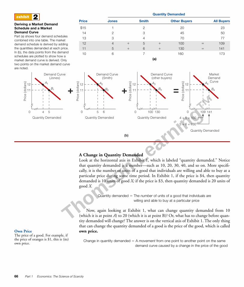
Exhibit 2 shows how a market demand curve can be derived by “adding” individualdemand curves. The demand schedules for Jones, Smith, and other buyers are shown inpart (a). The market demand schedule is obtained by adding the quantities demanded ateach price. For example, at $12, the quantities demanded are 4 units for Jones, 5 units forSmith, and 100 units for other buyers. Thus, a total of 109 units are demanded at $12.In part (b), the data points for the demand schedules are plotted and “added” to producea market demand curve. The market demand curve could also be drawn directly from themarket demand schedule.

A Change in Quantity Demanded Versus a Change in DemandEconomists often talk about (1) a change in quantity demanded and (2) a change indemand. Although “quantity demanded” may sound like “demand,” they are not thesame. In short, a “change in quantity demanded” is not the same as a “change in demand.”(Read the last sentence at least two more times.) We use Exhibit 1 to illustrate the differ-ence between “a change in quantity demanded” and “a change in demand.”


Thomson Learning™

Own PriceThe price of a good. For example, ifthe price of oranges is $1, this is (its)own price.


exhibit 2Deriving a Market DemandSchedule and a Market Demand CurvePart (a) shows four demand schedulescombined into one table. The marketdemand schedule is derived by addingthe quantities demanded at each price.In (b), the data points from the demandschedules are plotted to show how amarket demand curve is derived. Onlytwo points on the market demand curveare noted.

5

11

12

4

+ + =12

11

5 6

12

11

100 130

Pric

e (d

olla

rs)

Quantity Demanded

Pric

e (d

olla

rs)

Quantity Demanded

Demand Curve(other buyers)

Demand Curve(Smith)

Demand Curve(Jones)

12

11

109 141

4 + 5 + 100

5 + 6 + 130

0000

MarketDemand

CurveA1

B1

A2

B2

A3

B3

A4

B4

Pric

e (d

olla

rs)

Quantity Demanded

Pric

e (d

olla

rs)

Quantity Demanded

(b)

Quantity Demanded

Price Jones Smith Other Buyers All Buyers

$15 1 2 20 23

14 2 3 45 50

13 3 4 70 77

12 4 � 5 � 100 � 109

11 5 � 6 � 130 � 141

10 6 7 160 173

(a)

A Change in Quantity DemandedLook at the horizontal axis in Exhibit 1, which is labeled “quantity demanded.” Noticethat quantity demanded is a number—such as 10, 20, 30, 40, and so on. More specifi-cally, it is the number of units of a good that individuals are willing and able to buy at aparticular price during some time period. In Exhibit 1, if the price is $4, then quantitydemanded is 10 units of good X; if the price is $3, then quantity demanded is 20 units ofgood X.

Quantity demanded � The number of units of a good that individuals are willing and able to buy at a particular price

Now, again looking at Exhibit 1, what can change quantity demanded from 10(which it is at point A) to 20 (which it is at point B)? Or, what has to change before quan-tity demanded will change? The answer is on the vertical axis of Exhibit 1. The only thingthat can change the quantity demanded of a good is the price of the good, which is calledown price.

Change in quantity demanded � A movement from one point to another point on the samedemand curve caused by a change in the price of the good

Thomson Learning™

A Change in DemandLet’s look again at Exhibit 1, this time focusing on the demand curve. Demand is repre-sented by the entire curve. When an economist talks about a “change in demand,” he orshe is actually talking about a change—or shift—in the entire demand curve.

Change in demand = Shift in demand curve

Demand can change in two ways: demand can increase and demand can decrease.Let’s look first at an increase in demand. Suppose we have the following demand schedule.

Demand Schedule A

Price Quantity Demanded

$20 500

$15 600

$10 700

$ 5 800

The demand curve for this demand schedule will look like the demand curve in Exhibit 1.What does an increase in demand mean? It means that individuals are willing and

able to buy more units of the good at each and every price. In other words, demand sched-ule A will change as follows:

Demand Schedule B (increase in demand)


$20 500 600

$15 600 700

$10 700 800

$ 5 800 900

Whereas individuals were willing and able to buy 500 units of the good at $20, now theyare willing and able to buy 600 units of the good at $20; whereas individuals were will-ing and able to buy 600 units of the good at $15, now they are willing and able to buy700 units of the good at $15; and so on.

As shown in Exhibit 3a, the demand curve that represents demand schedule B lies tothe right of the demand curve that represents demand schedule A. We conclude that anincrease in demand is represented by a rightward shift in the demand curve and means thatindividuals are willing and able to buy more of a good at each and every price.

Increase in demand = Rightward shift in the demand curve

Now let’s look at a decrease in demand. What does a decrease in demand mean? Itmeans that individuals are willing and able to buy less of a good at each and every price.In this case, demand schedule A will change as follows:

Demand Schedule C (decrease in demand)


$20 500 400

$15 600 500

$10 700 600

$ 5 800 700


Thomson Learning™

Normal GoodA good the demand for which rises(falls) as income rises (falls).

Inferior GoodA good the demand for which falls(rises) as income rises (falls).


exhibit 3Shifts in the Demand CurveIn part (a), the demand curve shiftsrightward from DA to DB. This shiftrepresents an increase in demand. Ateach price, the quantity demanded isgreater than it was before. For example,the quantity demanded at $20 increasesfrom 500 units to 600 units. In part (b),the demand curve shifts leftward fromDA to DC. This shift represents adecrease in demand. At each price, thequantity demanded is less. For example,the quantity demand at $20 decreasesfrom 500 units to 400 units.

Pric

e (d

olla

rs)

Quantity Demanded

(a)

20

15

10

5

0800 900

DA to DB: Increase indemand (rightward shift in demand curve).

DA: Based on demand schedule A

DB: Based on demandschedule B

700600500

Pric

e (d

olla

rs)

Quantity Demanded

(b)

20

15

10

5

0700 800

DA to DC: Decrease indemand (leftward shift in demand curve).

DC: Based on demand schedule C

DA: Based on demandschedule A

600500400

As shown in Exhibit 3b, the demand curve that represents demand schedule C obvi-ously lies to the left of the demand curve that represents demand schedule A. We concludethat a decrease in demand is represented by a leftward shift in the demand curve and meansthat individuals are willing and able to buy less of a good at each and every price.

Decrease in demand = Leftward shift in the demand curve

What Factors Cause the Demand Curve to Shift?We know what an increase and decrease in demand mean: An increase in demand meansconsumers are willing and able to buy more of a good at every price. A decrease in demandmeans consumers are willing and able to buy less of a good every price. We also know thatan increase in demand is graphically portrayed as a rightward shift in a demand curve anda decrease in demand is graphically portrayed as a leftward shift in a demand curve.

But, what factors or variables can increase or decrease demand? What factors or vari-ables can shift demand curves? We identify and discuss these factors or variables in thissection.

IncomeAs a person’s income changes (increases or decreases), his or her demand for a particulargood may rise, fall, or remain constant.

For example, suppose Jack’s income rises. As a consequence, his demand for CDsrises. For Jack, CDs are a normal good. For a normal good, as income rises, demand forthe good rises, and as income falls, demand for the good falls.

X is a normal good: If income ↑ then DX↑If income ↓ then DX↓

Now suppose Marie’s income rises. As a consequence, her demand for canned bakedbeans falls. For Marie, canned baked beans are an inferior good. For an inferior good, asincome rises, demand for the good falls, and as income falls, demand for the good rises.

Y is an inferior good: If income ↑ then DY↓If income ↓ then DY↑

Thomson Learning™

Finally, suppose when George’s income rises, his demand for toothpaste neither risesnor falls. For George, toothpaste is neither a normal good nor an inferior good. Instead,it is a neutral good. For a neutral good, as income rises or falls, the demand for the gooddoes not change.

PreferencesPeople’s preferences affect the amount of a good they are willing to buy at a particularprice. A change in preferences in favor of a good shifts the demand curve rightward. Achange in preferences away from the good shifts the demand curve leftward. For example,if people begin to favor Tom Clancy novels to a greater degree than previously, thedemand for Clancy novels increases and the demand curve shifts rightward.

Prices of Related GoodsThere are two types of related goods: substitutes and complements. Two goods aresubstitutes if they satisfy similar needs or desires. For many people, Coca-Cola and Pepsi-Cola are substitutes. If two goods are substitutes, as the price of one rises (falls), thedemand for the other rises (falls). For instance, higher Coca-Cola prices will increase thedemand for Pepsi-Cola as people substitute Pepsi for the higher-priced Coke (Exhibit 4a).

Neutral GoodA good the demand for which doesnot change as income rises or falls.

SubstitutesTwo goods that satisfy similar needs ordesires. If two goods are substitutes,the demand for one rises as the priceof the other rises (or the demand forone falls as the price of the other falls).


exhibit 4Substitutes and Complements(a) Coca-Cola and Pepsi-Cola aresubstitutes: The price of one and thedemand for the other are directly related.As the price of Coca-Cola rises, thedemand for Pepsi-Cola increases.(b) Tennis rackets and tennis balls arecomplements: The price of one and thedemand for the other are inverselyrelated. As the price of tennis racketsrises, the demand for tennis ballsdecreases.

Quantity Demanded of Coca-Cola

(a)

Pric

e of

Ten

nis

Rac

kets

Pric

e of

Ten

nis

Bal

ls

Quantity Demanded of Tennis Rackets Quantity Demanded of Tennis Balls

00

If tennis rackets andtennis balls are complements, a higherprice for tennis rackets leads to . . .

. . . a leftwardshift in the demandcurve for tennis balls.

COMPLEMENTS

(b)

DTB2

DTB1

Quantity Demanded of Pepsi-Cola

DPC2

DTR

Qd1Qd2

P1

P2

A

B

Pric

e of

Coc

a-C

ola

0

If Coca-Cola andPepsi-Cola aresubstitutes, ahigher price forCoca-Cola leads to . . .

SUBSTITUTES

Pric

e of

Pep

si-C

ola

0

. . . a rightward shift in the demandcurve for Pepsi-Cola.

DPC1

Qd1Qd2

P1

P2

DCC

A

B

Thomson Learning™

ComplementsTwo goods that are used jointly inconsumption. If two goods arecomplements, the demand for onerises as the price of the other falls (orthe demand for one falls as the priceof the other rises).


EVERYDAY LIFEEVERYDAY LIFE

EVERYDAY LIFE

Economics In

Does the Law of Demand Explain Obesity?

An accepted definition of obesity is that a person is consideredobese if his weight in pounds exceeds 4.25 percent of the squareof his height in inches. For example, suppose a person weighs 200pounds and is 5 feet tall. The person’s height in inches is 60; thesquare of 60 is 3,600. Because 200 (weight in pounds) is 5.5 per-cent of 3,600 (square of height in inches), the person is obese.

Steven Landsburg, an economist and a contributing columnistto the magazine Slate, reports that 21.1 percent of the people inGeorgia are obese according to this definition. Ten years earlier,only 9.5 percent of Georgians were obese (using the same defini-tion of obesity). Landsburg asks the question: Why are we gettingso fat?4 The rise of obesity in Georgia is mirrored across the coun-try, says Landsburg. He reports that obesity has been rising in everyage group, in every race, in both males and females, and in everystate. In 1991, a little over 12 percent of the people in the countrywere obese; in 1999, almost 20 percent were.5

How does Landsburg explain the rise in obesity? He partlyexplains it using the law of demand. The law of demand states that

as the price of something falls, the quantity demanded of it rises,ceteris paribus. So, if the quantity demanded of obesity has risen inrecent years, has the price of obesity fallen to bring this about?Landsburg argues that in the 1990s, drugs were developed thatreduce cholesterol and increase life expectancy. In other words,these drugs decrease two of the many undesirable consequencesof obesity—high cholesterol and shorter life expectancy. Thus,these drugs have reduced the price of obesity. As a result, thequantity demanded of obesity has risen.

Other examples of substitutes are coffee and tea, corn chips and potato chips, two brandsof margarine, and foreign and domestic cars.

X and Y are substitutes: If PX ↑ then DY ↑If PX ↓ then DY ↓

Two goods are complements if they are consumed jointly. For example, tennis rack-ets and tennis balls are used together to play tennis. If two goods are complements, as theprice of one rises (falls), the demand for the other falls (rises). For example, higher tennisracket prices will decrease the demand for tennis balls, as Exhibit 4b shows. Other exam-ples of complements are cars and tires, light bulbs and lamps, and golf clubs and golf balls.

A and B are complements: If PA ↑ then DB ↓If PA ↓ then DB ↑

Number of BuyersThe demand for a good in a particular market area is related to the number of buyers inthe area: More buyers, higher demand; fewer buyers, lower demand. The number of buy-ers may increase owing to a higher birthrate, increased immigration, the migration of peo-ple from one region of the country to another, and so on. The number of buyers may

4. Steven Landsburg, “Why Are We Getting So Fat?” Slate, 1 May 20015. In 1991, 4 out of 45 states surveyed had obesity rates of 15–19 percent. Nostate had an obesity rate over 20 percent. In 2002, 20 of the 50 states surveyedhad obesity rates of 15–19 percent, 29 states had obesity rates of 20–24 percentand 1 state (Mississippi) had an obesity rate over 25 percent. Also, according tothe 1999–2000 National Health and Nutrition Examination Survey, 64 percent ofU.S. adults are overweight or obese. This is 8 percent higher than for the period1988–1994. (By the way, there is a difference between being overweight andbeing obese.)

Thomson Learning™

decrease owing to a higher death rate, war, the migrationof people from one region of the country to another, andso on.

Expectations of Future PriceBuyers who expect the price of a good to be higher nextmonth may buy the good now—thus increasing the cur-rent demand for the good. Buyers who expect the priceof a good to be lower next month may wait until nextmonth to buy the good—thus decreasing the currentdemand for the good.

For example, suppose you are planning to buy ahouse. One day, you hear that house prices are expectedto go down in a few months. Consequently, you decideto hold off your purchase of a house for a few months.Alternatively, if you hear that prices are expected to risein a few months, you might go ahead and purchase ahouse now.

S E L F - T E S T (Answers to Self-Test questions are in

the Self-Test Appendix.)

1. As Sandi’s income rises, her demand for popcorn rises. As Mark’s income falls, his demandfor prepaid telephone cards rises. What kinds of goods are popcorn and telephone cardsfor the people who demand each?

2. Why are demand curves downward-sloping?3. Give an example that illustrates how to derive a market demand curve.4. What factors can change demand? What factors can change quantity demanded?

Economists analyze numerous curves as theylook for answers to their questions. In theiranalyses, economists identify two types of fac-

tors related to curves: (1) factors that can move us along curves and(2) factors that can shift curves.

The factors that move us along curves are sometimes called move-ment factors. In many economic diagrams—such as the diagram of thedemand curve in Exhibit 1—the movement factor is on the vertical axis.

The factors that actually shift the curves are sometimes called shiftfactors. The shift factors for the demand curve are income, preferences,the price of related goods, and so on. Often the shift factors do not appearin the economic diagrams. For example, in Exhibit 1, the movementfactor—price—is on the vertical axis, but the shift factors do not appearanywhere in the diagram. We just know what they are and that they canshift the demand curve.

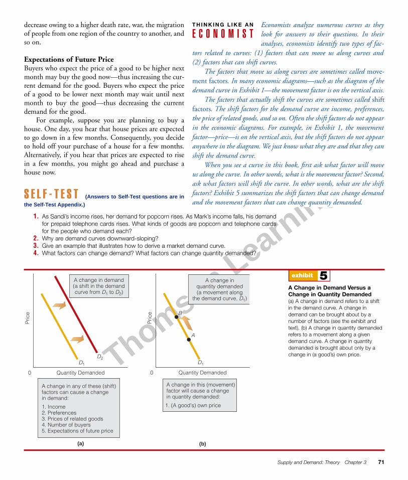
When you see a curve in this book, first ask what factor will moveus along the curve. In other words, what is the movement factor? Second,ask what factors will shift the curve. In other words, what are the shiftfactors? Exhibit 5 summarizes the shift factors that can change demandand the movement factors that can change quantity demanded.


E C O N O M I S T


exhibit 5A Change in Demand Versus aChange in Quantity Demanded(a) A change in demand refers to a shiftin the demand curve. A change indemand can be brought about by anumber of factors (see the exhibit andtext). (b) A change in quantity demandedrefers to a movement along a givendemand curve. A change in quantitydemanded is brought about only by achange in (a good’s) own price.

Pric

e

0 Quantity Demanded

A change in demand(a shift in the demandcurve from D1 to D2)

Pric

e

0 Quantity Demanded

B

A

A change in any of these (shift) factors can cause a change in demand:

1. Income2. Preferences3. Prices of related goods4. Number of buyers5. Expectations of future price

A change in this (movement) factor will cause a change in quantity demanded:

1. (A good’s) own price

D1

D2D1

(b)(a)

A change inquantity demanded(a movement along

the demand curve, D1)

Thomson Learning™

SupplyThe willingness and ability of sellers toproduce and offer to sell differentquantities of a good at different pricesduring a specific time period.

Law of SupplyAs the price of a good rises, thequantity supplied of the good rises,and as the price of a good falls, thequantity supplied of the good falls,ceteris paribus.

(Upward-sloping) Supply CurveThe graphical representation of thelaw of supply.

Supply ScheduleThe numerical tabulation of thequantity supplied of a good atdifferent prices. A supply schedule isthe numerical representation of thelaw of supply.


SUPPLYJust as the word demand has a specific meaning in economics, so does the word supply.Supply refers to (1) the willingness and ability of sellers to produce and offer to sell dif-ferent quantities of a good (2) at different prices (3) during a specific time period (per day,week, and so on).

The Law of SupplyThe law of supply states that as the price of a good rises, the quantity supplied of thegood rises, and as the price of a good falls, the quantity supplied of the good falls, ceterisparibus. Simply put, the price of a good and the quantity supplied of the good are directlyrelated, ceteris paribus. (Quantity supplied is the number of units of a good sellers are will-ing and able to produce and offer to sell at a particular price.) The (upward-sloping)supply curve is the graphical representation of the law of supply (see Exhibit 6).The law of supply can be summarized as follows:

P ↑ QS↑P ↓ QS ↓ ceteris paribus

where P � price and QS � quantity supplied.The law of supply holds for the production of most goods. It does not hold when

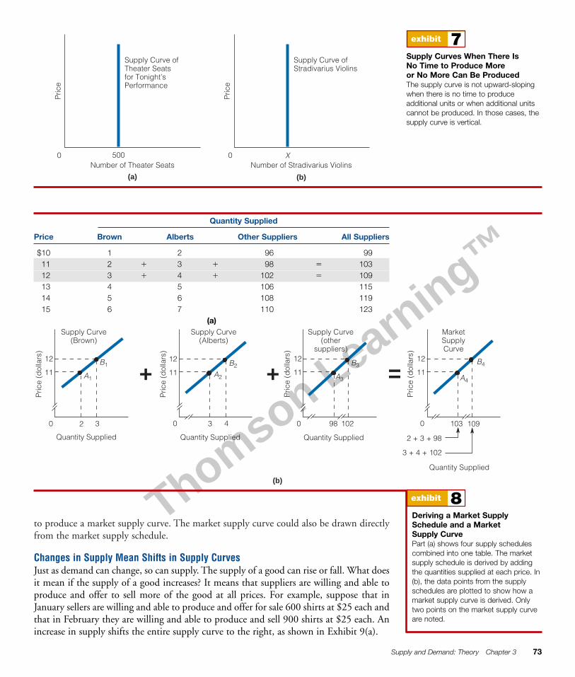
there is no time to produce more units of a good. For example, suppose a theater inAtlanta is sold out for tonight’s play. Even if ticket prices increased from $30 to $40, therewould be no additional seats in the theater. There is no time to produce more seats. Thesupply curve for theater seats is illustrated in Exhibit 7a. It is fixed at the number of seatsin the theater, 500.6

The law of supply also does not hold for goods that cannot be produced over anyperiod of time. For example, the violinmaker Antonio Stradivari died in 1737. A rise inthe price of Stradivarius violins does not affect the number of Stradivarius violins sup-plied, as Exhibit 7b illustrates.

Why Most Supply Curves Are Upward-SlopingThink back to the discussion of the law of increasing opportunity costs in Chapter 2. Thatdiscussion shows that if the production possibilities frontier (PPF) is bowed outward,increasing costs exist. In other words, increased production of a good comes at increasedopportunity costs. An upward-sloping supply curve simply reflects the fact that costs risewhen more units of a good are produced.

The Market Supply CurveAn individual supply curve represents the price-quantity combinations for a single seller.The market supply curve represents the price-quantity combinations for all sellers of aparticular good. Exhibit 8 shows how a market supply curve can be derived by “adding”individual supply curves. In part (a), a supply schedule, the numerical tabulation of thequantity supplied of a good at different prices, is given for Brown, Alberts, and other sup-pliers. The market supply schedule is obtained by adding the quantities supplied at eachprice, ceteris paribus. For example, at $11, the quantities supplied are 2 units for Brown,3 units for Alberts, and 98 units for other suppliers. Thus, a total of 103 units are sup-plied at $11. In part (b), the data points for the supply schedules are plotted and “added”

6. The vertical supply curve is said to be perfectly inelastic.

exhibit 6A Supply CurveThe upward-sloping supply curve is thegraphical representation of the law ofsupply, which states that price andquantity supplied are directly related,ceteris paribus. On a supply curve, theprice (in dollars) represents price per unitof the good. The quantity supplied, onthe horizontal axis, is always relevant fora specific time period (a week, a month,and so on).

Pric

e (d

olla

rs)

0

4

1

10 20 30 40

2

3

A

B

D

C

Supply Curve

Quantity Supplied of Good X

Thomson Learning™

to produce a market supply curve. The market supply curve could also be drawn directlyfrom the market supply schedule.

Changes in Supply Mean Shifts in Supply CurvesJust as demand can change, so can supply. The supply of a good can rise or fall. What doesit mean if the supply of a good increases? It means that suppliers are willing and able toproduce and offer to sell more of the good at all prices. For example, suppose that inJanuary sellers are willing and able to produce and offer for sale 600 shirts at $25 each andthat in February they are willing and able to produce and sell 900 shirts at $25 each. Anincrease in supply shifts the entire supply curve to the right, as shown in Exhibit 9(a).


exhibit 7Supply Curves When There IsNo Time to Produce More or No More Can Be ProducedThe supply curve is not upward-slopingwhen there is no time to produceadditional units or when additional unitscannot be produced. In those cases, thesupply curve is vertical.

Pric

e

500

Supply Curve ofTheater Seats for Tonight’s Performance

Number of Theater Seats

(a) (b)

Pric

e

X

Supply Curve ofStradivarius Violins

Number of Stradivarius Violins0 0

exhibit 8Deriving a Market SupplySchedule and a MarketSupply CurvePart (a) shows four supply schedulescombined into one table. The marketsupply schedule is derived by addingthe quantities supplied at each price. In(b), the data points from the supplyschedules are plotted to show how amarket supply curve is derived. Onlytwo points on the market supply curveare noted.

3

11

12

2

Supply Curve(Brown)

Supply Curve(Alberts)

Supply Curve(other

suppliers)

+ + =12

11

3 4

12

11

98 102

Pric

e (d

olla

rs)

Pric

e (d

olla

rs)

Pric

e (d

olla

rs)

Pric

e (d

olla

rs)

12

11

Quantity SuppliedQuantity SuppliedQuantity Supplied

Quantity Supplied

(b)

103 109

2 + 3 + 98

3 + 4 + 102

0000

A1

B1

A2

B2

A3

B3

A4

B4

MarketSupplyCurve

Quantity Supplied

Price Brown Alberts Other Suppliers All Suppliers

$10 1 2 96 9911 2 � 3 � 98 � 10312 3 � 4 � 102 � 10913 4 5 106 11514 5 6 108 11915 6 7 110 123

(a)

Thomson Learning™


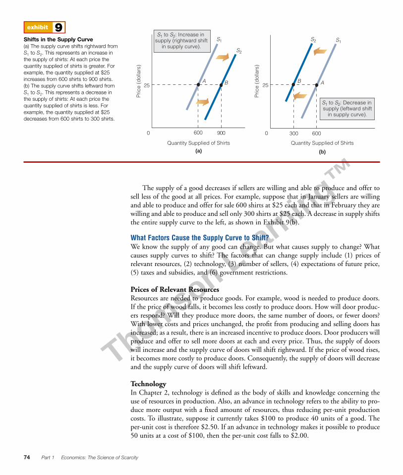
exhibit 9Shifts in the Supply Curve(a) The supply curve shifts rightward fromS1 to S2. This represents an increase inthe supply of shirts: At each price thequantity supplied of shirts is greater. Forexample, the quantity supplied at $25increases from 600 shirts to 900 shirts.(b) The supply curve shifts leftward fromS1 to S2. This represents a decrease inthe supply of shirts: At each price thequantity supplied of shirts is less. Forexample, the quantity supplied at $25decreases from 600 shirts to 300 shirts.

Pric

e (d

olla

rs)

0

S1 to S2: Increase in supply (rightward shift

in supply curve).

(b)(a)

0

S2

S1

Quantity Supplied of Shirts Quantity Supplied of Shirts

600 900

Pric

e (d

olla

rs)

600300

S1S2

25 25A B B A

S1 to S2: Decrease in supply (leftward shift

in supply curve).

The supply of a good decreases if sellers are willing and able to produce and offer tosell less of the good at all prices. For example, suppose that in January sellers are willingand able to produce and offer for sale 600 shirts at $25 each and that in February they arewilling and able to produce and sell only 300 shirts at $25 each. A decrease in supply shiftsthe entire supply curve to the left, as shown in Exhibit 9(b).

What Factors Cause the Supply Curve to Shift?We know the supply of any good can change. But what causes supply to change? Whatcauses supply curves to shift? The factors that can change supply include (1) prices ofrelevant resources, (2) technology, (3) number of sellers, (4) expectations of future price,(5) taxes and subsidies, and (6) government restrictions.

Prices of Relevant ResourcesResources are needed to produce goods. For example, wood is needed to produce doors.If the price of wood falls, it becomes less costly to produce doors. How will door produc-ers respond? Will they produce more doors, the same number of doors, or fewer doors?With lower costs and prices unchanged, the profit from producing and selling doors hasincreased; as a result, there is an increased incentive to produce doors. Door producers willproduce and offer to sell more doors at each and every price. Thus, the supply of doorswill increase and the supply curve of doors will shift rightward. If the price of wood rises,it becomes more costly to produce doors. Consequently, the supply of doors will decreaseand the supply curve of doors will shift leftward.

TechnologyIn Chapter 2, technology is defined as the body of skills and knowledge concerning theuse of resources in production. Also, an advance in technology refers to the ability to pro-duce more output with a fixed amount of resources, thus reducing per-unit productioncosts. To illustrate, suppose it currently takes $100 to produce 40 units of a good. Theper-unit cost is therefore $2.50. If an advance in technology makes it possible to produce50 units at a cost of $100, then the per-unit cost falls to $2.00.

Thomson Learning™

If per-unit production costs of a good decline, we expect the quantity supplied of thegood at each price to increase. Why? The reason is that lower per-unit costs increase prof-itability and therefore provide producers with an incentive to produce more. For example,if corn growers develop a way to grow more corn using the same amount of water andother resources, it follows that per-unit production costs will fall, profitability willincrease, and growers will want to grow and sell more corn at each price. The supply curveof corn will shift rightward.

Number of SellersIf more sellers begin producing a particular good, perhaps because of high profits, the sup-ply curve will shift rightward. If some sellers stop producing a particular good, perhapsbecause of losses, the supply curve will shift leftward.

Expectations of Future PriceIf the price of a good is expected to be higher in the future, producers may hold back someof the product today (if possible; for example, perishables cannot be held back). Then,they will have more to sell at the higher future price. Therefore, the current supply curvewill shift leftward. For example, if oil producers expect the price of oil to be higher nextyear, some may hold oil off the market this year to be able to sell it next year. Similarly, ifthey expect the price of oil to be lower next year, they might pump more oil this year thanpreviously planned.

Taxes and SubsidiesSome taxes increase per-unit costs. Suppose a shoe manufacturer must pay a $2 tax perpair of shoes produced. This tax leads to a leftward shift in the supply curve, indicatingthat the manufacturer wants to produce and offer to sell fewer pairs of shoes at each price.If the tax is eliminated, the supply curve shifts rightward.

Subsidies have the opposite effect. Suppose the government subsidizes the produc-tion of corn by paying corn farmers $2 for every bushel of corn they produce. Because ofthe subsidy, the quantity supplied of corn is greater at each price and the supply curve ofcorn shifts rightward. Removal of the subsidy shifts the supply curve of corn leftward. Arough rule of thumb is that we get more of what we subsidize and less of what we tax.

Government RestrictionsSometimes government acts to reduce supply. Consider a U.S. import quota on Japanesetelevision sets. An import quota, or quantitative restriction on foreign goods, reduces thesupply of Japanese television sets in the United States. It shifts the supply curve leftward.The elimination of the import quota allows the supply of Japanese television sets in theUnited States to shift rightward.

Licensure has a similar effect. With licensure, individuals must meet certain require-ments before they can legally carry out a task. For example, owner-operators of day-carecenters must meet certain requirements before they are allowed to sell their services. Nodoubt this reduces the number of day-care centers and shifts the supply curve of day-carecenters leftward.

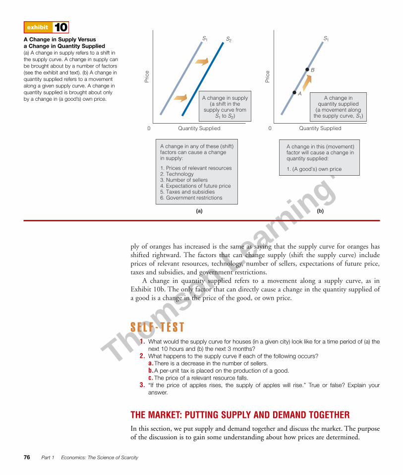
A Change in Supply Versus a Change in Quantity SuppliedJust as a change in demand is not the same as a change in quantity demanded, a changein supply is not the same as a change in quantity supplied. A change in supply refers to ashift in the supply curve, as illustrated in Exhibit 10a. For example, saying that the sup-

(Production) SubsidyA monetary payment by governmentto a producer of a good or service.


Thomson Learning™

ply of oranges has increased is the same as saying that the supply curve for oranges hasshifted rightward. The factors that can change supply (shift the supply curve) includeprices of relevant resources, technology, number of sellers, expectations of future price,taxes and subsidies, and government restrictions.

A change in quantity supplied refers to a movement along a supply curve, as inExhibit 10b. The only factor that can directly cause a change in the quantity supplied ofa good is a change in the price of the good, or own price.

S E L F - T E S T1. What would the supply curve for houses (in a given city) look like for a time period of (a) the

next 10 hours and (b) the next 3 months?2. What happens to the supply curve if each of the following occurs?

a.There is a decrease in the number of sellers.b.A per-unit tax is placed on the production of a good.c.The price of a relevant resource falls.

3. “If the price of apples rises, the supply of apples will rise.” True or false? Explain youranswer.

THE MARKET: PUTTING SUPPLY AND DEMAND TOGETHERIn this section, we put supply and demand together and discuss the market. The purposeof the discussion is to gain some understanding about how prices are determined.


exhibit 10A Change in Supply Versusa Change in Quantity Supplied(a) A change in supply refers to a shift inthe supply curve. A change in supply canbe brought about by a number of factors(see the exhibit and text). (b) A change inquantity supplied refers to a movementalong a given supply curve. A change inquantity supplied is brought about onlyby a change in (a good’s) own price.

Pric

e

0 Quantity Supplied

A change in supply(a shift in the

supply curve fromS1 to S2)

Pric

e

(b)(a)

0 Quantity Supplied

A

B

S2S1

A change in any of these (shift) factors can cause a change in supply:

1. Prices of relevant resources2. Technology3. Number of sellers4. Expectations of future price5. Taxes and subsidies6. Government restrictions

A change in this (movement) factor will cause a change inquantity supplied:

1. (A good’s) own price

S1

A change inquantity supplied

(a movement alongthe supply curve, S1)

Thomson Learning™

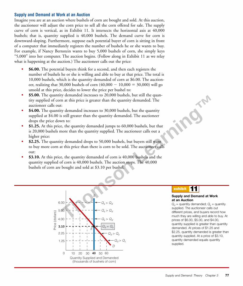
Supply and Demand at Work at an AuctionImagine you are at an auction where bushels of corn are bought and sold. At this auction,the auctioneer will adjust the corn price to sell all the corn offered for sale. The supplycurve of corn is vertical, as in Exhibit 11. It intersects the horizontal axis at 40,000bushels; that is, quantity supplied is 40,000 bushels. The demand curve for corn isdownward-sloping. Furthermore, suppose each potential buyer of corn is sitting in frontof a computer that immediately registers the number of bushels he or she wants to buy.For example, if Nancy Bernstein wants to buy 5,000 bushels of corn, she simply keys“5,000” into her computer. The auction begins. (Follow along in Exhibit 11 as we relaywhat is happening at the auction.) The auctioneer calls out the price:

• $6.00. The potential buyers think for a second, and then each registers thenumber of bushels he or she is willing and able to buy at that price. The total is10,000 bushels, which is the quantity demanded of corn at $6.00. The auction-eer, realizing that 30,000 bushels of corn (40,000 � 10,000 � 30,000) will gounsold at this price, decides to lower the price per bushel to:

• $5.00. The quantity demanded increases to 20,000 bushels, but still the quan-tity supplied of corn at this price is greater than the quantity demanded. Theauctioneer calls out:

• $4.00. The quantity demanded increases to 30,000 bushels, but the quantitysupplied at $4.00 is still greater than the quantity demanded. The auctioneerdrops the price down to:

• $1.25. At this price, the quantity demanded jumps to 60,000 bushels, but thatis 20,000 bushels more than the quantity supplied. The auctioneer calls out ahigher price:

• $2.25. The quantity demanded drops to 50,000 bushels, but buyers still wantto buy more corn at this price than there is corn to be sold. The auctioneer callsout:

• $3.10. At this price, the quantity demanded of corn is 40,000 bushels and thequantity supplied of corn is 40,000 bushels. The auction stops. The 40,000bushels of corn are bought and sold at $3.10 per bushel.


exhibit 11Supply and Demand at Work at an AuctionQd = quantity demanded; Qs = quantitysupplied. The auctioneer calls outdifferent prices, and buyers record howmuch they are willing and able to buy. Atprices of $6.00, $5.00, and $4.00,quantity supplied is greater than quantitydemanded. At prices of $1.25 and$2.25, quantity demanded is greater thanquantity supplied. At a price of $3.10,quantity demanded equals quantitysupplied.

3010 20 40 50 600

6.00

5.00

4.00

3.10

2.25

1.25

Pric

e (d

olla

rs)

Quantity Supplied and Demanded(thousands of bushels of corn)

D

S

Qs > Qd

Qs > Qd

Qd = QsE

Qs > Qd

Qd > Qs

Qd > Qs

Thomson Learning™

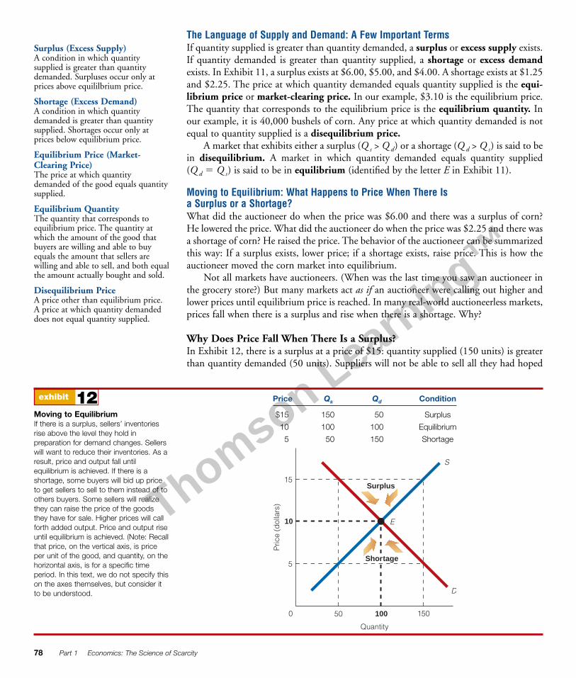
The Language of Supply and Demand: A Few Important TermsIf quantity supplied is greater than quantity demanded, a surplus or excess supply exists.If quantity demanded is greater than quantity supplied, a shortage or excess demandexists. In Exhibit 11, a surplus exists at $6.00, $5.00, and $4.00. A shortage exists at $1.25and $2.25. The price at which quantity demanded equals quantity supplied is the equi-librium price or market-clearing price. In our example, $3.10 is the equilibrium price.The quantity that corresponds to the equilibrium price is the equilibrium quantity. Inour example, it is 40,000 bushels of corn. Any price at which quantity demanded is notequal to quantity supplied is a disequilibrium price.

A market that exhibits either a surplus (Q s > Q d) or a shortage (Q d > Q s) is said to bein disequilibrium. A market in which quantity demanded equals quantity supplied(Q d � Q s) is said to be in equilibrium (identified by the letter E in Exhibit 11).

Moving to Equilibrium: What Happens to Price When There Is a Surplus or a Shortage?What did the auctioneer do when the price was $6.00 and there was a surplus of corn?He lowered the price. What did the auctioneer do when the price was $2.25 and there wasa shortage of corn? He raised the price. The behavior of the auctioneer can be summarizedthis way: If a surplus exists, lower price; if a shortage exists, raise price. This is how theauctioneer moved the corn market into equilibrium.

Not all markets have auctioneers. (When was the last time you saw an auctioneer inthe grocery store?) But many markets act as if an auctioneer were calling out higher andlower prices until equilibrium price is reached. In many real-world auctioneerless markets,prices fall when there is a surplus and rise when there is a shortage. Why?

Why Does Price Fall When There Is a Surplus?In Exhibit 12, there is a surplus at a price of $15: quantity supplied (150 units) is greaterthan quantity demanded (50 units). Suppliers will not be able to sell all they had hoped


exhibit 12Moving to EquilibriumIf there is a surplus, sellers’ inventoriesrise above the level they hold inpreparation for demand changes. Sellerswill want to reduce their inventories. As aresult, price and output fall untilequilibrium is achieved. If there is ashortage, some buyers will bid up priceto get sellers to sell to them instead of toothers buyers. Some sellers will realizethey can raise the price of the goodsthey have for sale. Higher prices will callforth added output. Price and output riseuntil equilibrium is achieved. (Note: Recallthat price, on the vertical axis, is priceper unit of the good, and quantity, on thehorizontal axis, is for a specific timeperiod. In this text, we do not specify thison the axes themselves, but consider itto be understood.

Pric

e (d

olla

rs)

Quantity

S

D

50 1501000

5

15

10 E

Surplus

Shortage

Surplus (Excess Supply)A condition in which quantitysupplied is greater than quantitydemanded. Surpluses occur only atprices above equililbrium price.

Shortage (Excess Demand)A condition in which quantitydemanded is greater than quantitysupplied. Shortages occur only atprices below equilibrium price.

Equilibrium Price (Market-Clearing Price)The price at which quantitydemanded of the good equals quantitysupplied.

Equilibrium QuantityThe quantity that corresponds toequilibrium price. The quantity atwhich the amount of the good thatbuyers are willing and able to buyequals the amount that sellers arewilling and able to sell, and both equalthe amount actually bought and sold.

Disequilibrium PriceA price other than equilibrium price.A price at which quantity demandeddoes not equal quantity supplied.

Price Qs Qd Condition

$15 150 50 Surplus

10 100 100 Equilibrium

5 50 150 Shortage

Thomson Learning™

to sell at $15. As a result, their inventories will grow beyond the level they hold in prepa-ration for demand changes. Sellers will want to reduce their inventories. Some will lowerprices to do so, some will cut back on production, others will do a little of both. As shownin the exhibit, there is a tendency for price and output to fall until equilibrium is achieved.

Why Does Price Rise When There Is a Shortage?In Exhibit 12, there is a shortage at a price of $5: quantity demanded (150 units) is greaterthan quantity supplied (50 units). Buyers will not be able to buy all they had hoped tobuy at $5. Some buyers will bid up the price to get sellers to sell to them instead of toother buyers. Some sellers, seeing buyers clamor for the goods, will realize that they canraise the price of the goods they have for sale. Higher prices will also call forth added out-put. Thus, there is a tendency for price and output to rise until equilibrium is achieved.

Also, see Exhibit 13 which brings together much of what we have discussed aboutsupply and demand.

Speed of Moving to EquilibriumOn January 9, 2004, at 1:28 P.M., the price of a share of IBM stock was $91.88. A fewseconds later, the price had risen to $92.11. Obviously, the stock market is a market thatequilibrates quickly. If demand rises, then initially there is a shortage of the stock at thecurrent equilibrium price. The price is bid up and there is no longer a shortage. All thishappens in seconds.

Now consider a house offered for sale in any city in the country. It is not uncommonfor the sale price of a house to remain the same even though the house does not sell formonths. For example, a person offers to sell her house for $400,000. One month passes,no sale; two months pass, no sale; three months pass, no sale; and so on. Ten months later,the house has still not sold and the price is still $400,000.

Is $400,000 the equilibrium price of the house? Obviously not. At the equilibriumprice, there would be a buyer for the house and a seller of the house (quantity demandedwould equal quantity supplied). At a price of $400,000, there is a seller of the house but

DisequilibriumA state of either surplus or shortage ina market.

EqulibriumEquilibrium means “at rest.”Equilibrium in a market is the price-quantity combination from whichthere is no tendency for buyers orsellers to move away. Graphically,equilibrium is the intersection point ofthe supply and demand curves.


exhibit 13A Summary Exhibit of a Market(Supply and Demand)This exhibit ties together the topicsdiscussed so far in this chapter. A marketis composed of both supply anddemand, as shown. Also shown are thefactors that affect supply and demandand therefore indirectly affect theequilibrium price and quantity of a good.

PRICE,QUANTITY

Income

Preferences Numberof Buyers

Prices ofRelated Goods

(Substitutesand

Complements)

Expectationsof Future Price Government

Restrictions

Taxesand

Subsidies

Numberof

Sellers

Expectationsof

Future Price

Technology

Prices ofRelevant

Resources

DEMAND SUPPLY

MARKET

Thomson Learning™

no buyer. The price of $400,000 is above equilibrium price. At $400,000, there is a sur-plus in the housing market; equilibrium has not been achieved.

Some people may be tempted to argue that supply and demand are at work in thestock market but not in the housing market. A better explanation, though, is that not allmarkets equilibrate at the same speed. While it may take only seconds for the stock marketto go from surplus or shortage to equilibrium, it may take months for the housing mar-ket to do so.

Moving to Equilibrium: Maximum and Minimum PricesThe discussion of surpluses illustrates how a market moves to equilibrium, but there isanother way to show this. Exhibit 14 shows the market for good X. Look at the first unitof good X. What is the maximum price buyers would be willing to pay for it? The answer is$70. This can be seen by following the dotted line up from the first unit of the good tothe demand curve. What is the minimum price sellers need to receive before they would bewilling to sell this unit of good X? It is $10. This can be seen by following the dotted lineup from the first unit to the supply curve. Because the maximum buying price is greaterthan the minimum selling price, the first unit of good X will be exchanged.

What about the second unit? For the second unit, buyers are willing to pay a maxi-mum price of $60 and sellers need to receive a minimum price of $20. The second unitof good X will be exchanged. In fact, exchange will occur as long as the maximum buyingprice is greater than the minimum selling price. The exhibit shows that a total of fourunits of good X will be exchanged. The fifth unit will not be exchanged because the max-imum buying price ($30) is less than the minimum selling price ($50).

In the process just described, buyers and sellers trade money for goods as long as bothbenefit from the trade. The market converges on a quantity of 4 units of good X and aprice of $40 per unit. This is equilibrium. In other words, mutually beneficial trade drivesthe market to equilibrium.

Equilibrium in Terms of Consumers’ and Producers’ SurplusEquilibrium can be viewed in terms of two important economic concepts, consumers’ sur-plus and producers’ (or sellers’) surplus. Consumers’ surplus is the difference between themaximum buying price and the price paid by the buyer.

Consumers’ surplus = Maximum buying price � Price paid

For example, if the highest price you would pay to see a movie is $10 and you pay $7to see the movie, then you have received $3 consumers’ surplus. Obviously, the more con-sumers’ surplus consumers receive, the better off they are. Wouldn’t you have preferred topay, say, $4 to see the movie instead of $7? If you had paid only $4, your consumers’ sur-plus would have been $6 instead of $3.

Producers’ surplus is the difference between the price received by the producer orseller and the minimum selling price.

Producers’ (sellers’) surplus = Price received � Minimum selling price

Suppose the minimum price the owner of the movie theater would have accepted foradmission is $5. But she doesn’t sell admission for $5, but $7. Her producers’ or sellers’surplus is $2. A seller prefers a large producers’ surplus to a small one. The theater ownerwould have preferred to sell admission to the movie for $8 instead of $7 because then shewould have received $3 producers’ surplus.


Producers’ (Sellers’) Surplus (PS)The difference between the pricesellers receive for a good and theminimum or lowest price for whichthey would have sold the good. PS �Price received � Minimum sellingprice

Consumers’ Surplus (CS)The difference between the maximumprice a buyer is willing and able to payfor a good or service and the priceactually paid. CS � Maximum buyingprice � Price paid

Thomson Learning™


exhibit 14Moving to Equilibrium in Terms ofMaximum and Minimum PricesAs long as the maximum buying price isgreater than the minimum selling price,an exchange will occur. This condition ismet for units 1–4. The market convergeson equilibrium through a process ofmutually beneficial exchanges.

Pric

e (d

olla

rs)

Quantity of Good X

NOEXCHANGEEXCHANGE

S

D

0 1 2 3 4 5 6 7

10

20

30

40

50

60

70

Total surplus is the sum of the consumer’s surplus and producer’s surplus.

Total surplus = Consumers’ surplus + Producers’ surplus

In Exhibit 15a, consumers’ surplus is represented by the shaded triangle. This trian-gle includes the area under the demand curve and above the equilibrium price. Accordingto the definition, consumers’ surplus is the highest price buyers are willing to pay (maxi-mum buying price) minus the price they pay. For example, the window in (a) shows thatbuyers are willing to pay as high as $7 for the 50th unit, but only pay $5. Thus, the con-sumers’ surplus on the 50th unit of the good is $2. If we add the consumers’ surplus oneach unit of the good between and including the first and the 100th (100 units being theequilibrium quantity), we obtain the shaded consumers’ surplus triangle.

In Exhibit 15b, producers’ surplus is represented by the shaded triangle. This triangleincludes the area above the supply curve and under the equilibrium price. Keep in mindthe definition of producers’ surplus—the price received by the seller minus the lowestprice the seller would accept for the good. For example, the window in (b) shows that sell-ers would have sold the 50th unit for as low as $3 but actually sold it for $5. Thus, theproducers’ surplus on the 50th unit of the good is $2. If we add the producers’ surplus oneach unit of the good between and including the first and the 100th, we obtain the shadedproducers’ surplus triangle.

Now consider consumers’ surplus and producers’ surplus at the equilibrium quantity.Exhibit 16 shows that consumers’ surplus at equilibrium is equal to areas A � B � C �D, and producers’ surplus at equilibrium is equal to areas E � F � G � H. At any other

Total Surplus (TS)The sum of consumers’ surplus andproducers’ surplus. TS � CS � PS

Units of Maximum MinimumGood X Buying Price Selling Price Result

1st $70 $10 Exchange

2d 60 20 Exchange

3d 50 30 Exchange

4th 40 40 Exchange

5th 30 50 No Exchange

Thomson Learning™


Pric

e

0Quantity

$5

D

S

100

Consumers’Surplus

$5

$7

100500

D

SCS

Q

P

Window

(a)

Consumers’ Surplus (CS)

(b)

Producers’ Surplus (PS)

Pric

e

0Quantity

$5

D

S

100

Producers’Surplus

$5

$3

100500

D

S

PSQ

P

Window

exhibit 15Consumers’ and Producers’Surplus(a) Consumers’ surplus. As the shadedarea indicates, the difference betweenthe maximum or highest amountbuyers would be willing to pay and theprice they actually pay is consumers’surplus. (b) Producers’ surplus. As theshaded area indicates, the differencebetween the price sellers receive forthe good and the minimum or lowestprice they would be willing to sell thegood for is producers’ surplus.

exchangeable quantity, such as at 25, 50, or 75 units, both consumers’ surplus and pro-ducers’ surplus are less. For example, at 25 units, consumers’ surplus is equal to area A andproducers’ surplus is equal to area E. At 50 units, consumers’ surplus is equal to areasA � B and producers’ surplus is equal to areas E � F.

Is there a special property to equilibrium? At equilibrium, both consumers’ surplusand producers’ surplus are maximized. In short, total surplus is maximized.

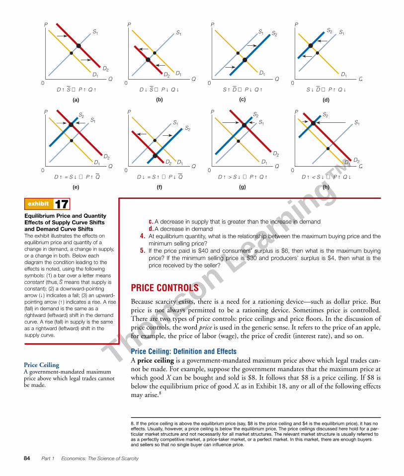
What Can Change Equilibrium Price and Quantity?Equilibrium price and quantity are determined by supply and demand. Wheneverdemand changes or supply changes or both change, equilibrium price and quantitychange. Exhibit 17 illustrates eight different cases where this occurs. Cases (a)–(d) illus-trate the four basic changes in supply and demand, where either supply or demandchanges. Cases (e)–(h) illustrate changes in both supply and demand.

• (a) Demand rises (the demand curve shifts rightward), and supply is constant(the supply curve does not move). Equilibrium price rises, equilibrium quantityrises.

• (b) Demand falls, supply is constant. Equilibrium price falls, equilibrium quan-tity falls.

• (c) Supply rises, demand is constant. Equilibrium price falls, equilibrium quan-tity rises.

• (d) Supply falls, demand is constant. Equilibrium price rises, equilibrium quan-tity falls.

• (e) Demand rises and supply falls by an equal amount. Equilibrium price rises,equilibrium quantity is constant.

• (f ) Demand falls and supply rises by an equal amount. Equilibrium price falls,equilibrium quantity is constant.

• (g) Demand rises by a greater amount than supply falls. Equilibrium price rises,equilibrium quantity rises.

• (h) Demand rises by a lesser amount than supply falls. Equilibrium price rises,equilibrium quantity falls.

Thomson Learning™


exhibit 16Equilibrium, Consumers’ Surplus,and Producers’ SurplusConsumers’ surplus is greater atequilibrium quantity (100 units) than atany other exchangeable quantity.Producers’ surplus is greater atequilibrium quantity than at any otherexchangeable quantity. For example,consumers’ surplus is areas A + B + C at75 units, but areas A + B + C + D at 100units. Producers’ surplus is areas E + F +G at 75 units, but areas E + F + G + H at100 units.

Pric

e

Quantity

25 50 75 1000

$5D

D

S

CBAHGFE

Noexchange

in thisregion

(b)

Quantity Consumers’ Producers’(units) Surplus Surplus

25 A E

50 A � B E � F

75 A � B � C E � F � G

100 (Equilibrium) A � B � C � D E � F � G � H

(a)

S E L F - T E S T1. When a person goes to the grocery store to buy food, there is no auctioneer calling out

prices for bread, milk, and other items. Therefore, supply and demand cannot be operative.Do you agree or disagree? Explain your answer.

2. The price of a given-quality personal computer is lower today than it was five years ago. Isthis necessarily the result of a lower demand for computers? Explain your answer.

3. What is the effect on equilibrium price and quantity of the following?a.A decrease in demand that is greater than the increase in supplyb.An increase in supply

Questions from Setting the Scene: At the time James checks stock prices, Wal-Mart is selling for $52.42,Microsoft for $27.75, and Dell for $35.75. Why doesn’t Dell sell for more than Wal-Mart? Why doesn’tMicrosoft sell for more than Dell? Why is the euro selling for $1.28 and not higher or lower?The price of each stock is determined by supply and demand. The price of Wal-Mart stock is higher than the price of Dell stockbecause the demand for Wal-Mart stock is higher than the demand for Dell stock and/or the supply of Wal-Mart stock is lowerthan the supply of Dell stock. Similar reasoning explains why Microsoft stock sells for less than Dell stock does.

The exchange rate between the euro and the dollar is also determined by supply and demand. Just as there is a demandfor and supply of apples, oranges, houses, and computers, there is a demand for and supply of various currencies (such as thedollar and the euro). The dollar price James has to pay for a euro has to do with the demand for and supply of euros. Thus,supply and demand may determine whether or not James takes a trip to Europe this summer.7

7. The supply and demand of currencies are analyzed in a later chapter.

Thomson Learning™


c.A decrease in supply that is greater than the increase in demandd.A decrease in demand

4. At equilibrium quantity, what is the relationship between the maximum buying price and theminimum selling price?

5. If the price paid is $40 and consumers’ surplus is $6, then what is the maximum buyingprice? If the minimum selling price is $30 and producers’ surplus is $4, then what is theprice received by the seller?

PRICE CONTROLSBecause scarcity exists, there is a need for a rationing device—such as dollar price. Butprice is not always permitted to be a rationing device. Sometimes price is controlled.There are two types of price controls: price ceilings and price floors. In the discussion ofprice controls, the word price is used in the generic sense. It refers to the price of an apple,for example, the price of labor (wage), the price of credit (interest rate), and so on.

Price Ceiling: Definition and EffectsA price ceiling is a government-mandated maximum price above which legal trades can-not be made. For example, suppose the government mandates that the maximum price atwhich good X can be bought and sold is $8. It follows that $8 is a price ceiling. If $8 isbelow the equilibrium price of good X, as in Exhibit 18, any or all of the following effectsmay arise.8

8. If the price ceiling is above the equilibrium price (say, $8 is the price ceiling and $4 is the equilibrium price), it has noeffects. Usually, however, a price ceiling is below the equilibrium price. The price ceilings discussed here hold for a par-ticular market structure and not necessarily for all market structures. The relevant market structure is usually referred toas a perfectly competitive market, a price-taker market, or a perfect market. In this market, there are enough buyersand sellers so that no single buyer can influence price.

Price CeilingA government-mandated maximumprice above which legal trades cannotbe made.

exhibit 17Equilibrium Price and QuantityEffects of Supply Curve Shiftsand Demand Curve ShiftsThe exhibit illustrates the effects onequilibrium price and quantity of achange in demand, a change in supply,or a change in both. Below eachdiagram the condition leading to theeffects is noted, using the followingsymbols: (1) a bar over a letter meansconstant (thus, S̄ means that supply isconstant); (2) a downward-pointingarrow (↓ ) indicates a fall; (3) an upward-pointing arrow (↑ ) indicates a rise. A rise(fall) in demand is the same as arightward (leftward) shift in the demandcurve. A rise (fall) in supply is the sameas a rightward (leftward) shift in thesupply curve.

0

P

Q0

P

Q0

P

Q0

P

Q

0

P

Q0

P

Q0

P

Q0

P

Q

S1

D1

D2

(h)(g)(f)(e)

(a) (b) (c) (d)

S1

D1D2

S1 S2

D1

S1S2

D1

D1

D2

S1

S2

S1S2

D1D2

S1

S2

D1

D2

S1

S2

D1D2

D ↑ S ⇒ P ↑ Q ↑ D ↓ S ⇒ P ↓ Q ↓

D ↑ = S ↓ ⇒ P ↑ Q D ↓ = S ↑ ⇒ P ↓ Q

S ↑ D ⇒ P ↓ Q ↑

D ↑ > S ↓ ⇒ P ↑ Q ↑

S ↓ D ⇒ P ↑ Q ↓

D ↑ < S ↓ ⇒ P ↑ Q ↓

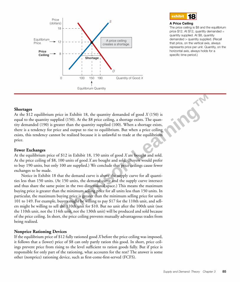
Thomson Learning™


exhibit 18A Price CeilingThe price ceiling is $8 and the equilibriumprice $12. At $12, quantity demanded =quantity supplied. At $8, quantitydemanded > quantity supplied. (Recallthat price, on the vertical axis, alwaysrepresents price per unit. Quantity, on thehorizontal axis, always holds for aspecific time period.)

0 100 150 190

8

12

18

A price ceilingcreates a shortage.

D

SPrice

(dollars)

EquilibriumPrice

PriceCeiling

Equilibrium Quantity

Quantity of Good X

Shortage

ShortagesAt the $12 equilibrium price in Exhibit 18, the quantity demanded of good X (150) isequal to the quantity supplied (150). At the $8 price ceiling, a shortage exists. The quan-tity demanded (190) is greater than the quantity supplied (100). When a shortage exists,there is a tendency for price and output to rise to equilibrium. But when a price ceilingexists, this tendency cannot be realized because it is unlawful to trade at the equilibriumprice.

Fewer ExchangesAt the equilibrium price of $12 in Exhibit 18, 150 units of good X are bought and sold.At the price ceiling of $8, 100 units of good X are bought and sold. (Buyers would preferto buy 190 units, but only 100 are supplied.) We conclude that price ceilings cause fewerexchanges to be made.

Notice in Exhibit 18 that the demand curve is above the supply curve for all quanti-ties less than 150 units. (At 150 units, the demand curve and the supply curve intersectand thus share the same point in the two dimensional space.) This means the maximumbuying price is greater than the minimum selling price for all units less than 150 units. Inparticular, the maximum buying price is greater than the minimum selling price for units101 to 149. For example, buyers might be willing to pay $17 for the 110th unit, and sell-ers might be willing to sell the 110th unit for $10. But no unit after the 100th unit (notthe 110th unit, not the 114th unit, not the 130th unit) will be produced and sold becauseof the price ceiling. In short, the price ceiling prevents mutually advantageous trades frombeing realized.

Nonprice Rationing DevicesIf the equilibrium price of $12 fully rationed good X before the price ceiling was imposed,it follows that a (lower) price of $8 can only partly ration this good. In short, price ceil-ings prevent price from rising to the level sufficient to ration goods fully. But if price isresponsible for only part of the rationing, what accounts for the rest? The answer is someother (nonprice) rationing device, such as first-come-first-served (FCFS).

Thomson Learning™

In Exhibit 18, 100 units of good X will be sold at $8 although buyers are willing tobuy 190 units at this price. What happens? Possibly, good X will be sold on an FCFS basisfor $8 per unit. In other words, to buy good X, a person must not only pay $8 per unitbut also be one of the first people in line.

Buying and Selling at a Prohibited PriceBuyers and sellers may regularly circumvent a price ceiling by making their exchanges“under the table.” For example, some buyers may offer some sellers more than $8 per unitfor good X. No doubt some sellers will accept the offers. But why would some buyers offermore than $8 per unit when they can buy good X for $8? The answer is because not allbuyers can buy the amount of good X they want at $8. As Exhibit 18 shows, there is ashortage. Buyers are willing to buy 190 units at $8, but sellers are willing to sell only 100units. In short, 90 fewer units will be sold than buyers would like to buy. Some buyers

will go unsatisfied. How, then, does any one buyer makeit more likely that sellers will sell to him or her instead ofto someone else? The answer is by offering to pay ahigher price. Because it is illegal to pay a higher price, thetransaction must be made “under the table.”

Tie-in SalesIn Exhibit 18, the maximum price buyers would be will-ing and able to pay per unit for 100 units of good X is$18. (This is the price on the demand curve at a quan-

tity of 100 units.) The maximum legal price, however, is $8. This difference between twoprices often prompts a tie-in sale, a sale whereby one good can be purchased only ifanother good is also purchased. For example, if Ralph’s Gas Station sells gasoline to cus-tomers only if they buy a car wash, the two goods are linked together in a tie-in sale.

Suppose that the sellers of good X in Exhibit 18 also sell good Y. They might offer tosell buyers good X at $8 only if the buyers agree to buy good Y at, say, $10. We choose$10 as the price for good Y because $10 is the difference between the maximum per-unit

Tie-in SaleA sale whereby one good can bepurchased only if another good is alsopurchased.


Economists think in terms of unintendedeffects. For example, a price ceiling policyintended to lower prices for the poor may cause

shortages, the use of nonprice rationing devices, illegal market transac-tions, and tie-in sales. When we consider both the price ceiling and itseffects, it is not clear that the poor have been helped. The economistknows that wanting to do good (for others) is not sufficient. It is impor-tant to know how to do good too.


E C O N O M I S T

Questions from Setting the Scene: What does getting his shower fixed have to do with James living in arent-controlled apartment? Why does it take so long (nine months) to get tickets to see the Late Show withDavid Letterman?Both these questions relate to disequilibrium prices. James has been trying for two weeks to get his apartment supervisor tofix his shower. James’s friend thinks it has taken so long because James lives in a rent-controlled apartment. (A rent-controlledapartment has a rent ceiling; James’s rent is lower than the equilibrium, or market-clearing rent.) Is James’s friend right? Witha rent ceiling, the quantity demanded of apartments is greater than the quantity supplied, that is, a shortage of apartmentsexists. The apartment supervisor knows there is a shortage of apartments, and realizes he could rent the apartment easily ifJames moved. The supervisor is likely to be less responsive to James’s request to fix the shower than he would be if the rentalmarket were in equilibrium or surplus.

For the second question, let’s recall the facts and do some economic analyzing. We know that the price of a ticket is zero(which is not the equilibrium or market-clearing price). At a price of zero, the quantity demanded of tickets is much greaterthan quantity supplied. How are the tickets rationed? They’re rationed on a first-come-first-served basis. James had to “standin line” or “wait” for nine months to get tickets to see the show. That’s one long line.

Thomson Learning™

EVERYDAY LIFEEVERYDAY LIFE

EVERYDAY LIFE

Economics In

Ticket Scalping

I got two for Pavarotti—Ticket scalper

At a big rock concert, a major sports game, or a popular Broadwayplay, ticket scalpers are likely to be nearby trying to sell tickets.Many people do not like scalpers; they believe scalpers are takingadvantage of them by charging many times more than the originalsupplier of the ticket charged. Some states have outlawed ticketscalping or permit it only if the scalper charges a limited amount,say, 5 to 10 percent more than the original ticket price. Scalperswho continue to practice their trade in defiance of the law are fined.

The question the economist asks is: Why does ticket scalpingexist in the first place? The noneconomist may answer, “Becausethere is greed and selfishness in the world.” But surely greed andselfishness do not surface just for major sports events or Broadwayplays. Ticket scalpers are not at all events, only some. Put thequestion this way: What condition is necessary before ticket scalp-ing will exist?

If you think in terms of supply and demand, you will have theanswer. Certainly, there will be no ticket scalping if the equilibriumprice is initially charged for a ticket. At the equilibrium price, thequantity demanded of tickets will equal the quantity supplied.

Suppose the ticket price is above equilibrium. Will ticket scalp-ing exist then? No, because at a price higher than equilibrium price,

people will buy fewer tickets than there are tickets available. No onehas ever seen a ticket scalper trying to sell a ticket that can be pur-chased from the ticket office.

Ticket scalping will exist only when the ticket price initiallycharged is lower than the equilibrium price. For example, supposethe equilibrium price to see a particular rock band is $80 a ticket,but only $50 a ticket is charged. Someone will likely buy the ticketfor $50 and then turn around and sell it for $70. In other words,before ticket scalping exists, a profitable opportunity must presentitself.

But why would a seller choose to sell tickets for less than equi-librium price? One answer is that the seller many not know whatequilibrium price is in a particular setting. In other words, a sellermay simply make a mistake and charge more or less than equilib-rium price. Another answer is that the seller may be concernedabout sacrificing the goodwill of her customers (many of whom shehopes will be repeat customers) if she charges the equilibriumprice. For example, some Broadway theaters charge below equilib-rium prices for tickets to plays. They even know they are chargingbelow-equilibrium prices because they know the prices thescalpers are getting paid. But as the president of one Broadwaytheater said, “Even though we could sell tickets for $100, we’d becutting our throats because it would be a PR disaster forBroadway.”

price buyers are willing and able to pay for 100 units of good X ($18) and the maximumlegal price ($8).

In New York City and other communities with rent-control laws, tie-in sales some-times result from rent ceilings on apartments. Occasionally, in order to rent an apartment,an individual must agree to buy the furniture in the apartment.

Do Buyers Prefer Lower Prices to Higher Prices?“Of course,” someone might say, “buyers prefer lower prices to higher prices. What buyerwould want to pay a higher price for anything?” But wait a minute. Price ceilings are oftenlower than equilibrium prices. Does it follow that buyers prefer price ceilings to equilib-rium prices? Not necessarily. Price ceilings have effects that equilibrium prices do not:shortages, use of first-come-first-served as a rationing device, tie-in sales, and so on. Abuyer could prefer to pay a higher price (an equilibrium price) than to pay a lower priceand have to deal with the effects of a price ceiling. All we can say for certain is that buy-


Thomson Learning™


exhibit 19A Price FloorThe price floor is $20 and the equilibriumprice is $15. At $15, quantity demanded= quantity supplied. At $20, quantitysupplied > quantity demanded.

0 90 130 180

15

20

A price floorcreates a surplus.

D

SPrice

(dollars)

EquilibriumPrice

PriceFloor

Equilibrium Quantity

Quantity of Good X

Surplus

ers prefer lower prices to higher prices, ceteris paribus. As in many cases, the ceteris paribuscondition makes all the difference.

Price Floor: Definition and EffectsA price floor is a government-mandated minimum price below which legal trades cannotbe made. For example, suppose the government mandates that the minimum price atwhich good X can be sold is $20. It follows that $20 is a price floor (see Exhibit 19). Ifthe price floor is above the equilibrium price, the following two effects arise.9

SurplusesAt the $15 equilibrium price in Exhibit 19, the quantity demanded of good X (130) isequal to the quantity supplied (130). At the $20 price floor, a surplus exists. The quantitysupplied (180) is greater than the quantity demanded (90). A surplus is usually a tempo-rary state of affairs. When a surplus exists, there is a tendency for price and output to fallto equilibrium. But when a price floor exists, this tendency cannot be realized because itis unlawful to trade at the equilibrium price.

Fewer ExchangesAt the equilibrium price in Exhibit 19, 130 units of good X are bought and sold. At theprice floor, 90 units are bought and sold. (Sellers want to sell 180 units, but buyers buyonly 90.) We conclude that price floors cause fewer exchanges to be made.

S E L F - T E S T1. Do buyers prefer lower prices to higher prices?2. “When there are long-lasting shortages, there are long lines of people waiting to buy goods.

It follows that the shortages cause the long lines.” Do you agree or disagree? Explain youranswer.

3. Who might argue for a price ceiling? a price floor?

9. If the price floor is below the equilibrium price (say, $20 is the price floor and $25 is the equilibrium price), it has noeffects. Usually, however, a price floor is above the equilibrium price. As with price ceilings, the price floor effects dis-cussed here hold for a perfectly competitive market. See footnote 8.

Price FloorA government-mandated minimumprice below which legal trades cannotbe made.

Thomson Learning™


A knowledge of supply and demand can be used both to explainand to predict. Let’s look at prediction first. Suppose you learn thatthe federal government is going to impose a quota on imported tel-evision sets. What will happen when the quota is imposed? Withyour knowledge of supply and demand, you can predict that theprice of television sets will rise. In other words, you can use yourknowledge of supply and demand to predict what will happen.Stated differently, you can use your knowledge of supply anddemand to see into the future. Isn’t the ability to see into the futureuseful?

Supply and demand also allows you to develop richer andfuller explanations of events. To illustrate, suppose there is a short-age of apples in country X. The cause of the shortage, someone says,is that apple growers in the country are simply growing too fewapples. Well, of course, it’s true that apple growers are growing “too

few” apples as compared to the number of apples consumers wantto buy. But does this explanation completely account for the short-age of apples? Your knowledge of supply and demand will promptyou to ask why apple growers are growing too few apples. Whenyou understand that quantity supplied is related to price, youunderstand that apple growers will grow more apples if the price ofapples is higher. What is keeping the price of apples down? Couldit be a price ceiling? Without a price ceiling, the price of appleswould rise, and apple growers would grow (and offer to sell) moreapples. The shortage of apples will vanish.

In other words, without a knowledge of supply and demandyou may have been content to explain the shortage of apples by say-ing that apple growers are growing too few apples. With yourknowledge of supply and demand, you delve deeper into why applegrowers are growing too few apples.

READER ASKS How Does Knowing About Supply and Demand Help Me?

Some things are interesting but not useful. Other things are useful but not interesting. For exam-ple, supply and demand are interesting, but not useful. Learning how to fix a car is useful, but notparticularly interesting. Am I wrong? Have I missed something? Is knowledge of supply anddemand useful? If it is, what can you do with it?

Demand> The law of demand states that as the price of a good rises, the

quantity demanded of the good falls, and as the price of a goodfalls, the quantity demanded of the good rises, ceteris paribus.The law of demand holds that price and quantity demanded areinversely related.

> Quantity demanded is the total number of units of a good thatbuyers are willing and able to buy at a particular price.

> A (downward-sloping) demand curve is the graphical represen-tation of the law of demand.

> Factors that can change demand and cause the demand curveto shift include income, preferences, prices of related goods(substitutes and complements), number of buyers, and expec-tations of future price.

> The only factor that can directly cause a change in the quantitydemanded of a good is a change in the good’s own price.

Absolute Price and Relative Price> The absolute price of a good is the price of the good in money

terms.> The relative price of a good is the price of the good in terms of

another good.

Supply> The law of supply states that as the price of a good rises, the

quantity supplied of the good rises, and as the price of a good

falls, the quantity supplied of the good falls, ceteris paribus. Thelaw of supply asserts that price and quantity supplied aredirectly related.

> The law of supply does not hold when there is no time to pro-duce more units of a good or when goods cannot be producedat all (over any period of time).

> The upward-sloping supply curve is the graphical representa-tion of the law of supply. More generally, a supply curve (nomatter how it slopes) represents the relationship between priceand quantity supplied.

> Factors that can change supply and cause the supply curve toshift include prices of relevant resources, technology, number ofsellers, expectations of future price, taxes and subsidies, andgovernment restrictions.

> The only factor that can directly cause a change in the quantitysupplied of a good is a change in the good’s own price.

The Market> Demand and supply together establish equilibrium price and

equilibrium quantity.> A surplus exists in a market if, at some price, quantity supplied

is greater than quantity demanded. A shortage exists if, at someprice, quantity demanded is greater than quantity supplied.

> Mutually beneficial trade between buyers and sellers drives themarket to equilibrium.

Chapter Summary

Thomson Learning™


1. True or false? As the price of oranges rises, the demand fororanges falls, ceteris paribus. Explain your answer.

2. “The price of a bushel of wheat, which was $3.00 last month,is $3.70 today. The demand curve for wheat must have shiftedrightward between last month and today.” Discuss.

3. “Some goods are bought largely because they have ‘snobappeal.’ For example, the residents of Beverly Hills gain pres-tige by buying expensive items. In fact, they won’t buy someitems unless they are expensive. The law of demand, whichholds that people buy more at lower prices than higher prices,obviously doesn’t hold for the residents of Beverly Hills. Thefollowing rules apply in Beverly Hills: high prices, buy; lowprices, don’t buy.” Discuss.

4. “The price of T-shirts keeps rising and rising, and people keepbuying more and more. T-shirts must have an upward-slopingdemand curve.” Identify the error.

5. Predict what would happen to the equilibrium price of mari-juana if it were legalized.

6. Compare the ratings for television shows with prices for goods.How are ratings like prices? How are ratings different fromprices? (Hint: How does rising demand for a particular televi-sion show manifest itself?)

7. Must consumers’ surplus equal producers’ surplus at equilib-rium price? Explain your answer.

8. Many movie theaters charge a lower admission price for thefirst show on weekday afternoons than they do for a weeknightor weekend show. Explain why.

9. A Dell computer is a substitute for a Compaq computer. Whathappens to the demand for Compaqs and the quantitydemanded of Dells as the price of a Dell falls?

10. Describe how each of the following will affect the demand forpersonal computers: (a) a rise in incomes (assuming comput-

Questions and Problems

DemandLaw of DemandAbsolute (Money) PriceRelative PriceLaw of Diminishing Marginal UtilityDemand ScheduleDemand CurveNormal GoodInferior GoodNeutral GoodSubstitutes

ComplementsOwn PriceSupplyLaw of SupplySupply CurveSupply ScheduleSubsidySurplus (Excess Supply)Shortage (Excess Demand)Equilibrium Price (Market-Clearing

Price)

Equilibrium QuantityDisequilibrium PriceDisequilibriumEquilibriumConsumers’ SurplusProducers’ (Sellers’) SurplusTotal SurplusPrice CeilingTie-in SalePrice Floor

Key Terms and Concepts

Consumers’ Surplus, Producers’ Surplus, andTotal Surplus> Consumers’ surplus is the difference between the maximum

buying price and price paid by the buyer.

Consumers’ surplus = Maximum buying price � Price paid

> Producers’ (or sellers’) surplus is the difference between theprice the seller receives and minimum selling price.

Producers’ surplus = Price received � Minimum selling price

> The more consumers’ surplus that buyers receive, the better offthey are. The more producers’ surplus that sellers receive, thebetter off they are.

> Total surplus is the sum of consumers’ surplus and producers’surplus.

> Total surplus (the sum of consumers’ surplus and producers’surplus) is maximized at equilibrium.

Price Ceilings> A price ceiling is a government-mandated maximum price. If a

price ceiling is below the equilibrium price, some or all of thefollowing effects arise: shortages, fewer exchanges, nonpricerationing devices, buying and selling at prohibited prices, andtie-in sales.

> Consumers do not necessarily prefer (lower) price ceilings to(higher) equilibrium prices. They may prefer higher prices andnone of the effects of price ceilings to lower prices and some ofthe effects of price ceilings. All we can say for sure is that con-sumers prefer lower prices to higher prices, ceteris paribus.

Price Floors> A price floor is a government-mandated minimum price. If a

price floor is above the equilibrium price, the following effectsarise: surpluses and fewer exchanges.

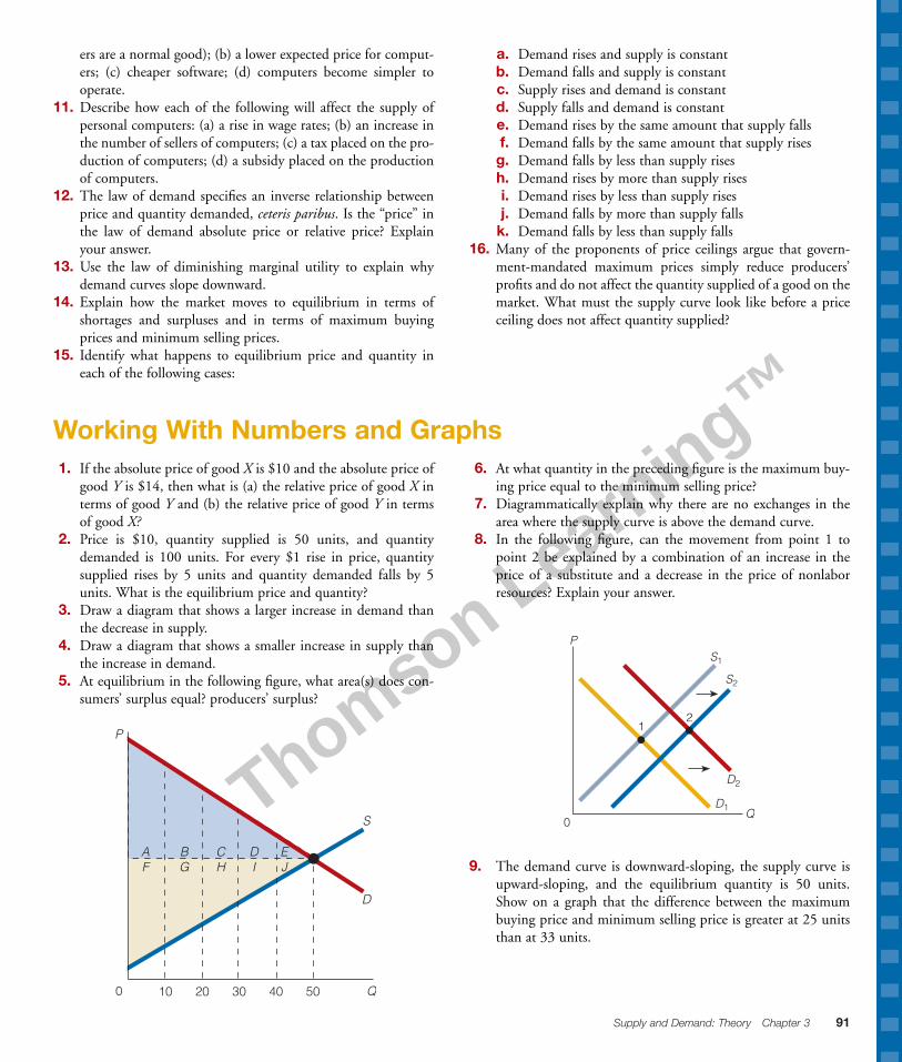
Thomson Learning™


ers are a normal good); (b) a lower expected price for comput-ers; (c) cheaper software; (d) computers become simpler tooperate.

11. Describe how each of the following will affect the supply ofpersonal computers: (a) a rise in wage rates; (b) an increase inthe number of sellers of computers; (c) a tax placed on the pro-duction of computers; (d) a subsidy placed on the productionof computers.

12. The law of demand specifies an inverse relationship betweenprice and quantity demanded, ceteris paribus. Is the “price” inthe law of demand absolute price or relative price? Explainyour answer.

13. Use the law of diminishing marginal utility to explain whydemand curves slope downward.

14. Explain how the market moves to equilibrium in terms ofshortages and surpluses and in terms of maximum buyingprices and minimum selling prices.

15. Identify what happens to equilibrium price and quantity ineach of the following cases:

a. Demand rises and supply is constantb. Demand falls and supply is constantc. Supply rises and demand is constantd. Supply falls and demand is constante. Demand rises by the same amount that supply fallsf. Demand falls by the same amount that supply rises

g. Demand falls by less than supply risesh. Demand rises by more than supply risesi. Demand rises by less than supply risesj. Demand falls by more than supply falls

k. Demand falls by less than supply falls16. Many of the proponents of price ceilings argue that govern-

ment-mandated maximum prices simply reduce producers’profits and do not affect the quantity supplied of a good on themarket. What must the supply curve look like before a priceceiling does not affect quantity supplied?

1. If the absolute price of good X is $10 and the absolute price ofgood Y is $14, then what is (a) the relative price of good X interms of good Y and (b) the relative price of good Y in termsof good X?

2. Price is $10, quantity supplied is 50 units, and quantitydemanded is 100 units. For every $1 rise in price, quantitysupplied rises by 5 units and quantity demanded falls by 5units. What is the equilibrium price and quantity?

3. Draw a diagram that shows a larger increase in demand thanthe decrease in supply.

4. Draw a diagram that shows a smaller increase in supply thanthe increase in demand.

5. At equilibrium in the following figure, what area(s) does con-sumers’ surplus equal? producers’ surplus?

Working With Numbers and Graphs

10 20 30 40 500 Q

D

D

S

CBAI

EJHGF

P

6. At what quantity in the preceding figure is the maximum buy-ing price equal to the minimum selling price?

7. Diagrammatically explain why there are no exchanges in thearea where the supply curve is above the demand curve.

8. In the following figure, can the movement from point 1 topoint 2 be explained by a combination of an increase in theprice of a substitute and a decrease in the price of nonlaborresources? Explain your answer.

9. The demand curve is downward-sloping, the supply curve isupward-sloping, and the equilibrium quantity is 50 units.Show on a graph that the difference between the maximumbuying price and minimum selling price is greater at 25 unitsthan at 33 units.

0

12

P

Q

S1

S2

D2

D1

Thomson Learning™


10. Diagrammatically show and explain why a price ceiling that isabove the equilibrium price will not prompt a tie-in sale.

11. Xavier is willing and able to pay up to $40 for a good that hebuys for $22. Keri is willing and able to sell the good to Xavier

for no less than $21. What does consumers’ surplus equal?What does producers’ (sellers’) surplus equal?

1. Go to the California Association of Realtors site at http://www.car.org/. Select “Economics,” and then choose “CaliforniaHousing Market @ A Glance.” Various housing market indi-cators are shown, including “Existing Homes Sales” (quantitytraded) and “Median Home Price” (housing price) inCalifornia.a. Compare the current period, the last period, and the year

ago information regarding median home price and existinghome sales. What is the relationship between housingprices and sales?

b. What could shift the demand curve in the housing market?c. What could shift the supply curve in the housing market?d. Use a demand and supply diagram to explain the changes

observed in the above housing market.e. Do you think the level of interest rates is a factor in the

housing market? Explain.

2. Go to Economic Report of the President at http://www.gpoaccess.gov/eop/index.html. Select “Download entire reports and sta-tistical tables” and then “2004.” Next, select “Table B-60.”This table shows price indices for selected spending categories.Keep in mind that the higher the number, the higher the price.For example, medical care was 21.5 in 1959 and 22.3 in 1960,which means that medical care prices were higher in 1960 thanin 1959.a. Which increased faster between 1999 and 2003, the price

of medical care or the price of housing?b. Which increased faster between 1995 and 2003, the price

of food or the price of apparel?c. Which increased faster between 1990 and 2003, the price

of transportation or the price of entertainment?

Internet Activities

supply and demand -...

Documents