supplementary material for - science€¦ · other supplementary material for this manuscript...
TRANSCRIPT

www.sciencemag.org/content/346/6208/1257998/suppl/DC1
Supplementary Material for
Lattice light-sheet microscopy: Imaging molecules to embryos at high spatiotemporal resolution
Bi-Chang Chen, Wesley R. Legant, Kai Wang, Lin Shao, Daniel E. Milkie, Michael W. Davidson, Chris Janetopoulos, Xufeng S. Wu, John A. Hammer III, Zhe Liu, Brian P.
English, Yuko Mimori-Kiyosue, Daniel P. Romero, Alex T. Ritter, Jennifer Lippincott-Schwartz, Lillian Fritz-Laylin, R. Dyche Mullins, Diana M. Mitchell, Joshua N.
Bembenek, Anne-Cecile Reymann, Ralph Böhme, Stephan W. Grill, Jennifer T. Wang, Geraldine Seydoux, U. Serdar Tulu, Daniel P. Kiehart, Eric Betzig*
*Corresponding author. E-mail: [email protected]
Published 24 October 2014, Science 346, 1257998 (2014)
DOI: 10.1126/science.1257998
This PDF file includes:
Supplementary Text
Figs. S1 to S26
Table S1
Full Reference List Other Supplementary Material for this manuscript includes the following: (available at www.sciencemag.org/content/346/6208/1257998/suppl/DC1)
Movies S1 to S18

2
Contents: Lattice Light Sheet Microscopy Supplementary Material
Section Page
Supplementary Notes
1. Theoretical Relationships between Bessel Beams and 2D Optical Lattices…………...3
2. Calculating the SLM Pattern That Generates the Desired Lattice Light Sheet……......9
3. Detailed Optical Path……………………………………………………………….....12
4. SLM Operation……………………………………………………………………......13
5. Sample Preparation…………………………………………………………………....14
Supplementary Figures…………………………………………………………………….....19
Supplementary Table…………………………………………………………………….…...42
Captions for Supplementary Movies………………………………………………………....46
Full Reference List…………………………………………………………………………...64

3
SUPPLEMENTARY NOTES
1. Theoretical Relationships between Bessel Beams and 2D Optical Lattices
a. Non-diffracting beams
The electric field ( , )te x of any continuous-wave, coherent light beam of free-space wavelength oλ propagating in a homogeneous medium of real refractive index n can be decomposed into a sum or integral over the electric fields ne of a set of planes waves propagating in various directions defined by their wavevectors nk :
( )1
( , ) expN
n nn
t i tω=
= ⋅ − ∑e x e k x (1)
where 2 /cω π λ= , /o nλ λ= is the wavelength in the medium, and c is the speed of light.
In the special case where all the wavevectors nk lie on the surface of a single cone (fig. S1A), ˆ cosn y k θ⋅ =k e n∀ where 2 /k π λ= and the y axis is defined as the axis of the cone, which has a half-angle of θ . Hence, Eq. 1 becomes:
[ ] ( ) [ ]1
( , ) exp ( cos ) exp ( , )exp ( cos )( ) ( )N
nn
x n z nt i ky t i x z i ky tk x k zθ ω θ ω=
= − = − +∑e x e e (2)
In other words, the electric field of the light beam propagates in the y direction without any change in its spatial distribution or amplitude in the xz plane. Such a beam is termed non-diffracting. The constraint that all the wavevectors lie on a cone is equivalent to the constraint that the light entering the objective lens used to create the cone is confined to points on an infinitesimally thin ring in the rear pupil of the lens.
b. Bessel beams
Now additionally assume that the rear pupil is illuminated with a uniform, infinitesimally thin ring of light of constant phase and uniform polarization e. The cone is then filled with a continuum of wavevectors, so in the scalar approximation Eq. 2 becomes:
[ ] ( )2
0( , ) exp ( cos ) exp sin sin cost A i ky t ik x z d
πθ ω θ φ φ φ= − + ∫e x e (3)
where we have used ˆ ˆ ˆsin sin cos sin cosx y zk k kθ φ θ θ φ= + +k e e e in spherical coordinates. If we
also express ˆ ˆ ˆsin cosx y zyρ φ ρ φ′ ′= + +x e e e , 2 2x zρ = + in cylindrical coordinates, we get:

4
[ ] ( )2
0( , ) exp ( cos ) exp sin sin sin ' cos cost A i ky t ik d
πθ ω ρ θ φ φ φ φ φ′= − + ∫e x e (4)
or, with the aid of the trigonometric identity sin sin ' cos cos cos( )φ φ φ φ φ φ′ ′+ = − :
[ ] ( )2
0( , ) exp ( cos ) exp sin cost A i ky t ik d
πθ ω ρ θ φ φ φ′= − − ∫e x e (5)
We recognize the expression at right as the integral representation of the Bessel function of the first kind of order zero:
( )2
0
1( ) exp cos2
oJ i dπ
α α φ φπ
= ∫ (6)
And thus we conclude:
( ) [ ]( , ) ( , , ) sin exp ( cos )2
oAt y t J k i ky tρ ρ θ θ ωπ
= = −e x e e (7)
In other words, a uniform ring of illumination in the rear pupil of an objective lens produces a non-diffracting light beam propagating along the axis of the lens and having an electric field whose amplitude in any plane transverse to this axis is described by the circularly symmetric Bessel function ( sin )oJ kρ θ . This is termed a Bessel beam (59). The size of the pattern scales linearly with the wavelength λ and inversely with the numerical aperture sinNA n θ= .
The more rigorous vector field of a Bessel beam can be approximated by subtracting the vector fields of two focused beams produced by uniform illumination (60) at the rear pupil at two slightly different numerical apertures. The electric field consists of a narrow central peak surrounded by an infinite series of concentric side lobes of opposite phase and decreasing amplitude (fig. S24). The narrow peak and infinite extent of an ideal Bessel beam make it an attractive candidate for light sheet microscopy, wherein the beam is scanned across the focal plane defined by an orthogonal detection objective.
c. Two-dimensional optical lattices
Now instead consider a non-diffracting beam of the form of Eq. 2 where ( , )x ze is periodic in two-dimensions:
1 1 2 2( , ) ( , )t m m t= + +e x e x a a (8)
where 1 2,m m can be any integer and 1 2,a a are two-dimensional primitive vectors that define the periodic pattern. There are only five such patterns of unique symmetry in 2D, termed Bravais lattices. A non-diffracting light beam having the cross-sectional symmetry of a 2D Bravias lattice is termed a 2D optical lattice. A 2D optical lattice is comprised of a minimum of three wavevectors nk , all of which must lie on the surface of a single cone (12), (fig. S1A). Note from

5
Eq. 1 that the spatial dependence of the lattice electric field is separable from the polarizations ne of its constituent plane waves, and thus the symmetry and periodicity of the lattice depends
only on the nk , whereas the electric field pattern that repeats in every unit cell of the lattice depends on both the nk and the ne (12).
Multiple pairs of primitive vectors can be used to define a 2D lattice of given parameters (i.e., Bravais symmetry and, where appropriate, aspect ratio and angle). For each such pair, a wavevector set { }1 2 3, ,k k k can be found that yields an optical lattice having these parameters (11). However, while the lattice parameters produced by these wavevector sets are the same, the periods of the resulting optical lattices, scaled to the excitation wavelength λ , take on any one of a series discrete values defined by the parameters (11). The smallest period, three wavevector lattice for a given parameter set is termed the fundamental one (fig. S1B), while larger period three wavevector lattices are termed sparse (fig. S1C).
Since the symmetry of a lattice is defined by the set of operations that transform the lattice onto itself, application of any valid symmetry operation to the wavevector set of a given optical lattice produces a new wavevector set and a new optical lattice of the same parameters and periodicity, but with an electric field in each unit cell also transformed by the chosen symmetry operation (fig. S1D). Adding multiple wavevector sets generated in this manner produces a composite 2D optical lattice of the same parameters, but comprised of more than three wavevectors (fig. S1E). Because these wavevectors converge from a broader range of azimuthal angles, they produce an electric field of higher 2D spatial frequency content m n−k k . Adding together all wavevector sets obtained by applying all valid symmetry operations to a given lattice produces a maximally symmetric composite lattice that has the maximum possible spatial frequency content for that particular Bravais symmetry (11), (fig. S1F).
When all input plane waves have the same phase and have their polarizations ne maximally projected onto the same desired state e , constructive interference between all these waves produces an intense, highly confined intensity maximum at one point in each unit cell, while partial destructive interference yields a background of low intensity elsewhere in each cell. The more wavevectors that comprise the lattice, the higher the contrast of this maximum to the background, and the closer the maximum approximates an ideal, circularly symmetric, diffraction-limited spot. Having the greatest 2D symmetry, hexagonal and square lattices produce maximally symmetric composite lattices with the greatest number of wavevectors from the broadest range of directions, and hence tend to be the ones best suited to serve as multifocal excitation arrays (11).
d. Bessel-Gauss beams and bound 2D optical lattices
Neither an ideal Bessel beam nor an ideal 2D optical lattice is directly useful for light sheet microscopy. The ideal Bessel beam contains equal energy in the central peak and each side lobe (59). Hence, sweeping this beam in x across the xy detection focal plane produces excessive fluorescence excitation outside this plane. In a similar vein, the ideal 2D optical lattice extends across all 3D space, and must be somehow confined in z to limit the excitation to the xy detection

6
focal plane. Furthermore, like any ideal non-diffracting beam, both these constructs require illumination confined to an infinitesimally thin ring at the rear pupil of an excitation objective, which is not physically possible.
The solution in either case is to illuminate the rear pupil over an annulus of finite width. The resulting beam will no longer be strictly non-diffracting, but will still have a cross-sectional profile in the xz plane that remains nearly constant over a field of view in y defined by the annulus width. For Bessel beam plane illumination microscopy (7, 8, 57), the annulus is illuminated uniformly, resulting in a Bessel-Gauss beam having a mix of the characteristics of each: a suppression of higher order Bessel side lobes due to a Gaussian envelope provided by the continuum of wavevectors in ρk across the annulus, and a much longer beam waist than a traditional Gaussian beam due to the elimination of wavevectors corresponding to pk values inside the inner diameter of the annulus.
For lattice light sheet microscopy, we wish to preserve the broad field of view of an ideal 2D optical lattice in the x direction as well as its high spatial frequency content in this direction to obtain the best possible resolution for the SIM mode. However, at the same time, we wish to confine the lattice in z in order to make the light sheet as thin as possible. The resulting bound lattice (15) is obtained by spreading the energy in the z direction at each of the discrete points in the rear pupil that create the lattice, creating a series of narrow parallel stripes (movie S1). The energy in these stripes remains constrained by the dimensions of the annulus, in order to ensure that the resulting light sheet covers the desired y field of view. However, within this constraint, increasing the length of these stripes creates an increasingly broad continuum of wavevectors in
zk that confine the lattice in z within an increasing narrow envelope (movie S1). In particular, when the width of this envelope is comparable to or narrower than the period of the lattice in z, only one row of lattice maxima in a single plane is dominantly excited, creating a narrow lattice light sheet (Fig 1C).
Note that the illumination stripes associated with lattice wavevectors closest to the x axis can be extended in z by the greatest amount before they are clipped by the edges of the annulus. Hence it is often advantageous to choose the orientation of the lattice around its propagation axis y such that one or more pairs of its wavevectors symmetrically straddle the z axis while falling close to the x axis within the rear pupil. This not only permits the tightest possible z confinement for that particular lattice, it also results in the highest possible spatial frequencies in x yielding the highest possible spatial resolution in that direction in the SIM mode.
On the other hand, besides shortening the y field of view, another disadvantage of a thick annulus and long illumination stripes is that at very high confinement, the lattice maxima become broadened in z, creating a thicker light sheet yielding poorer z resolution in the dithered mode (Fig. 1C). It is therefore doubly important to choose an annulus no wider than is absolutely necessary to confine the lattice in z by the desired amount. Fortunately, for many lattices in both the dithered and SIM modes, it is not necessary to completely confine the excitation to a single lattice plane – in the dithered mode, the contribution of flanking lattice planes to the overall PSF is suppressed by the z envelope of the detection PSF (Fig. 1D, fig. S2), whereas in the SIM mode, the additional lattice planes increase the strength of the highest

7
zk spatial frequencies in the excitation (fig. S3), yielding SIM reconstructions of higher SNR at lower power.
e. Linear arrays of coherent Bessel beams
Another way to create a thin light sheet that spreads the excitation across the entire field of view in the same manner as a bound 2D optical lattice is to use a linear array of closely spaced Bessel-Gauss beams. Indeed, it was the effectiveness of using an array of seven such beams in reducing phototoxicity in Bessel beam structured plane illumination microscopy (8) that sparked our interest in finding a way of further spreading the illumination across the plane. With seven beams, the beam separation was large enough that the coherent interaction between the side lobes of adjacent beams was negligible. However, for a dense array of Bessel-Gauss beams, it is essential to model these coherence effects.
We consider two different cases: where all beams have the same phase at the central peak, and where adjacent beams have opposite phase. In either case, as the period of the linear array decreases, the side lobes of adjacent beams interfere, creating an alternating series of increasingly strong resonant and anti-resonant patterns of constructive and destructive interference (movie S18, right). Recall from above that the side lobes of a Bessel beam alternate in phase (fig. S24B). Thus, at specific periods:
min( 0.5)j j+−Τ = − λ / ΝΑ (beams of alternating opposite phase) (9)
minj j++Τ = λ / ΝΑ (beams of identical phase) (10)
1j ≥ , minΝΑ being the numerical aperture associated with the inner diameter of the annulus, side lobes of the same phase from adjacent beams overlap in the xy plane, producing strong modulation in this plane. At the same time, the side lobes that overlap just outside this plane have different phases, and interfere destructively. The result is a tightly confined structured excitation plane (fig. S25) similar to those achieved with bound 2D optical lattices.
An alternative explanation for this confinement emerges when we consider the illumination patterns at the rear pupil plane of the excitation objective that give rise to these coherent arrays (movie S18, left). As the period of the array decreases, the initially continuous annulus of illumination that produces a single Bessel beam breaks into an expanding periodic array of stripes aligned along the z-axis, yet still bound by the dimensions of the annulus. At the specific periods j
+−Τ and j++Τ from above, the outermost stripe of this periodic array that still fits within
the annulus is tangent to the annulus inner diameter. As was the case with 2D lattices, at this location the stripe contains the broadest possible range of zk wavevectors within the constraint of annular illumination, creating the narrowest possible envelope confining the excitation, and thus resulting in a narrow structured light sheet suitable for light sheet microscopy in either the dithered or SIM modes.
8
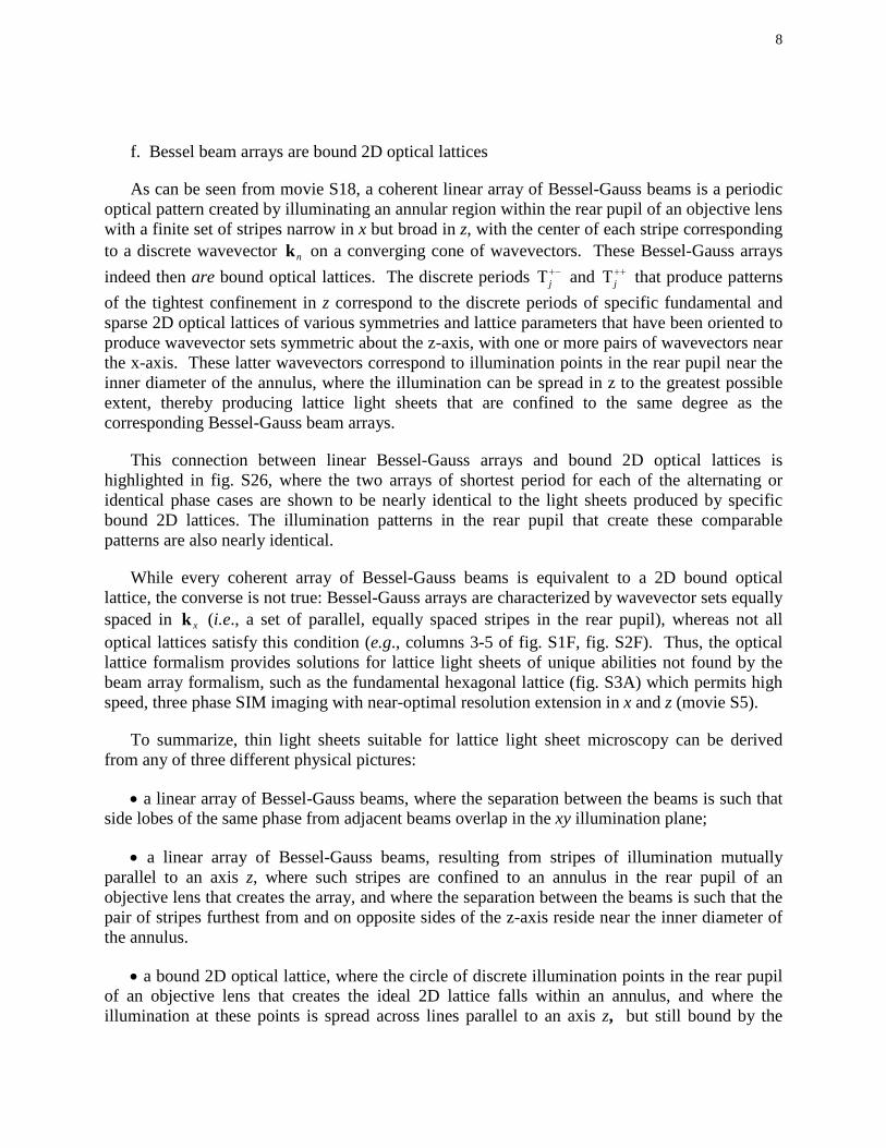
f. Bessel beam arrays are bound 2D optical lattices
As can be seen from movie S18, a coherent linear array of Bessel-Gauss beams is a periodic optical pattern created by illuminating an annular region within the rear pupil of an objective lens with a finite set of stripes narrow in x but broad in z, with the center of each stripe corresponding to a discrete wavevector nk on a converging cone of wavevectors. These Bessel-Gauss arrays indeed then are bound optical lattices. The discrete periods j
+−Τ and j++Τ that produce patterns
of the tightest confinement in z correspond to the discrete periods of specific fundamental and sparse 2D optical lattices of various symmetries and lattice parameters that have been oriented to produce wavevector sets symmetric about the z-axis, with one or more pairs of wavevectors near the x-axis. These latter wavevectors correspond to illumination points in the rear pupil near the inner diameter of the annulus, where the illumination can be spread in z to the greatest possible extent, thereby producing lattice light sheets that are confined to the same degree as the corresponding Bessel-Gauss beam arrays.
This connection between linear Bessel-Gauss arrays and bound 2D optical lattices is highlighted in fig. S26, where the two arrays of shortest period for each of the alternating or identical phase cases are shown to be nearly identical to the light sheets produced by specific bound 2D lattices. The illumination patterns in the rear pupil that create these comparable patterns are also nearly identical.
While every coherent array of Bessel-Gauss beams is equivalent to a 2D bound optical lattice, the converse is not true: Bessel-Gauss arrays are characterized by wavevector sets equally spaced in xk (i.e., a set of parallel, equally spaced stripes in the rear pupil), whereas not all optical lattices satisfy this condition (e.g., columns 3-5 of fig. S1F, fig. S2F). Thus, the optical lattice formalism provides solutions for lattice light sheets of unique abilities not found by the beam array formalism, such as the fundamental hexagonal lattice (fig. S3A) which permits high speed, three phase SIM imaging with near-optimal resolution extension in x and z (movie S5).
To summarize, thin light sheets suitable for lattice light sheet microscopy can be derived from any of three different physical pictures:
• a linear array of Bessel-Gauss beams, where the separation between the beams is such that side lobes of the same phase from adjacent beams overlap in the xy illumination plane;
• a linear array of Bessel-Gauss beams, resulting from stripes of illumination mutually parallel to an axis z, where such stripes are confined to an annulus in the rear pupil of an objective lens that creates the array, and where the separation between the beams is such that the pair of stripes furthest from and on opposite sides of the z-axis reside near the inner diameter of the annulus.
• a bound 2D optical lattice, where the circle of discrete illumination points in the rear pupil of an objective lens that creates the ideal 2D lattice falls within an annulus, and where the illumination at these points is spread across lines parallel to an axis z, but still bound by the

9
inner and outer diameters of the annulus. It is often advantageous to rotate the lattice about its propagation direction y such that two of its illumination points are positioned on or near the x axis and symmetrically about the z-axis, where they can be spread in z by the great possible amount within the confines of the annulus.
Lattice light sheets consisting of parallel stripes of illumination that provide confinement of excitation to a single xy plane might be designed by other paradigms, but are not considered in depth here. These include using linear arrays of other non-diffracting beams, such as the first order Bessel beam 1( sin )J kρ θ (where the phase varies linearly with azimuthal angle ϕ around the annulus), or 3D optical lattices having additional wavevectors not confined to a single ring in the rear pupil. These would produce modulation along the propagation axis y as well as the usual modulation axis x, but a temporally uniform average intensity in y could be attained by dithering the pattern in y, either with an objective-mounted piezo, or with a relay lens of electrically adjustable focal length.
2. Calculating the SLM Pattern That Generates the Desired Lattice Light Sheet
We create a lattice light sheet by using a binary SLM that is conjugate to the front focal plane of the excitation objective (fig. S4A). The light diffracted by the SLM is filtered by an annular mask that is conjugate to the rear pupil plane. The mask filters out unwanted diffraction orders and ensures that the resulting light sheet covers the desired y field of view. We need to find binary SLM patterns for lattice light sheets of specific desired properties (e.g., field of view in y, excitation confinement in z, breadth of spatial frequencies in ,x zk k (SIM mode), and overall resolution in z (dithered mode)), and confirm theoretically that light beams diffracted by these patterns and filtered by the annulus do indeed produce the desired light sheets within the specimen.
We start with an ideal 2D optical lattice of electric field ( , )ideal x zE , initially using our intuition to select a lattice of symmetry, periodicity, and orientation about y as discussed above that we expect will produce a light sheet that can be optimized for our ends. We then calculate the real amplitude ( , )realE x z of the component of ( , )ideal x zE that projects on the desired polarization state ˆ de (fig. S5A):
{ }ˆ( , ) Re ( , )real ideal dE x z x z= ⋅E e (11)
Since the SLM pattern is imaged at the sample to create the confined light sheet, ( , )realE x z must be bound in z (fig. S5B):
( , ) ( ) ( , )bound realE x z z E x zψ= ⋅ (12)
where the binding function ( ) 0zψ → as z → ∞ . Gaussian bounding, 2 2( ) exp( 2 / )z z aψ = − , is a common choice. Choosing a more steeply bound function increases the confinement of the light sheet to a single plane (movie S1), thereby minimizing out-of-focus background, bleaching,

10
and phototoxicity. However, it also decreases the y field of view and reduces the effective z resolution by underweighting the highest zk spatial frequencies in the pattern. Thus, part of the art of lattice light sheet microscopy involves judicious choice of the bounding function to balance these tradeoffs.
We use a binary phase ferroelectric SLM for its large number of pixels (necessary to cover a large field of view when projected at a Nyquist sampling interval consistent with diffraction-limited resolution) and fast switching time (necessary for rapid, sequential, plane-by-plane multicolor imaging). Thus, we need to convert ( , )boundE x z to a binary phase pattern (fig. S5C):
( , ) ( , )SLM boundx z H E x zϕ π ε= ⋅ − (13)
where ( )H ξ is the Heaviside step function ( ( ) 0H ξ = for 0ξ < , ( ) 1H ξ = for 0ξ > ) and
( )max ( , )boundE x zε < is a threshold level that determines which pixels are set high (ϕ π= ) or low ( 0ϕ = ). Increasing ε increases the confinement of the light sheet, with the tradeoffs discussed above. In practice, we typically set ( )0.1 max ( , )boundE x zε = ⋅ .
While Eq. 12 gives us a candidate for the pattern we should apply to the SLM, we still need to verify that this pattern theoretically produces a lattice light sheet of the desired properties. We do this by calculating the resulting light pattern at successive stages from the SLM to the specimen. First, passage through a lens (fig. S4A) of the light that is phase modulated by the SLM produces a diffraction pattern (fig. S5D) at the plane of the annular mask given by:
[ ] 2( , ) exp( ( , ))SLMdiff x zI k k FT i x zϕ= (14)
where [ ]( , ) (1 / 2 ) ( , )exp( )x zFT F x z F x z ik x ik z dxdzπ∞ ∞
−∞ −∞= ⋅ +∫ ∫ is the 2D Fourier transform.
After passage through the transmissive annulus of center radius a and thickness τ (fig. S5E):
( )2 2( . ) / 2x z x zA k k H k k aτ= − + − (15)
the intensity pattern that is then projected to the rear pupil of the excitation objective is given by (fig. S5F):
( , ) ( , ) ( , )pupil x z x z diff x zI k k A k k I k k= ⋅ (16)
while the electric field at the rear pupil is:
[ ]( , ) ( , ) exp( ( , ))SLMpupil x z x zE k k A k k FT i x zϕ= ⋅ (17)
Finally, this field produces a lattice light sheet of cross-sectional intensity profile (fig. S5G):
[ ]{ } 2( , ) ( , ) exp( ( , ))SLMexc x zPSF x z FT A k k FT i x zϕ= ⋅ (18)

11
after passage through the excitation objective. In most cases, the theoretical ( , )excPSF x z closely resembles the experimentally measured one (Fig. S6).
We next need to evaluate the performance of the microscope when using this light sheet in either the SIM or dithered mode. The expanded optical transfer function (OTF) that defines the xz resolution after SIM reconstruction is given by:
[ ]( , ) ( , ) ( , )SIM x z exc detectOTF k k FT PSF x z PSF x z= ⋅ (19)
where ( , )detectPSF x z is the point spread function of the detection objective as determined by a vector model of diffraction at the focus of a high NA lens (60). Alternatively, the cross-section of the dithered lattice light sheet is found by integrating ( , )excPSF x z over one period xΤ of the lattice in the dither direction (fig. S5H):
0( ) ( , )
x
dither excPSF z PSF x z dxΤ
= ∫ (20)
and the overall PSF that defines the xz resolution in the dithered mode is given by:
det( , ) ( ) ( , )overall dither ectPSF x z PSF z PSF x z= ⋅ (21)
The usable y field of view for the light sheet can be estimated by calculating the intensity ( )BesselI y along the y axis of a Bessel beam created with an annulus of the same maximum and
minimum NA as the lattice light sheet:
max min2
( ) (0, ,0) (0, ,0)NA NABessel focus focusI y y y= −E E (22)
where ( )NAfocusE x is the 3D vector electric field near the focus under uniform illumination of the
rear pupil (60).
In practice, we first choose according to Eq. 22 an annulus of maximum and minimum NA that produces a light sheet that spans the thickness of the specimen in the y direction. Choosing a light sheet that is longer than necessary risks creating an unnecessarily thick light sheet, and/or one with excessive sideband excitation beyond the central lattice plane. We then choose a particular lattice and bounding function ( )zψ , and use Eqs. 11-22 to calculate the cross-sectional profile ( , )excPSF x z , SIM transfer function ( , )SIM x zOTF k k , and dithered mode overall point spread function ( , )overallPSF x z of the resulting lattice light sheet. Common choices for the lattice in the dithered mode are the maximally symmetric fundamental lattices of rectangular, square, and hexagonal symmetry of figs. S2A-C, respectively. Common choices in the SIM mode are the three beam fundamental hexagonal lattice (fig. S3A) and the maximally symmetric fundamental hexagonal and first sparse square lattices of figs. S3C & S3D. Next, we iterate through the calculation, keeping the initial seed lattice and annulus dimensions constant, while varying ( )zψ and observing the tradeoff between excitation confinement and z resolution in the SIM and dithered modes. If an acceptable compromise cannot be found, the process is repeated with a different annulus – for example, one of reduced maximum and minimum NA that

12
produces a somewhat thicker light sheet of the same y extent but with more strongly suppressed sidebands.
3. Detailed Optical Path
The schematic of the optical system is shown in Figure S4A. The beam from a laser combiner equipped with 405 nm (250mW, RPMC, Oxxius LBX-405-300-CIR-PP), 445 nm (100mW, RPMC, Oxxius LBX-445-100-CIR-PP), 488 nm (300 mW, MPB Communications, 2RU-VFL-P-300-488-B1R), 532 nm (500 mW, MPB Communications, 2RU-VFL-P-500-532-B1R), 560 nm (500 mW, MPB Communications, 2RU-VFL-P-500-560-B1R), 589 nm (500 mW, MPB Communications, 2RU-VFL-P-500-589-B1R) and 642 nm (500 mW, MPB Communications, 2RU-VFL-P-500-642-B1R) lasers is expanded to a 1/e2 diameter of 2.5 mm by two lenses (8 mm FL/12.24 mm dia, Thorlabs C240TME-A, 20 mm FL/12.5 mm dia Edmund 47-661) before passing through a half wave plate (Bolder Vision Optik, BVO AHWP3) and an acousto-optic tunable filter (AA Quanta Tech, Optoelectronic AOTF AOTFnC-400.650-TN). The AOTF is used to select the wavelengths, control intensities and synchronize to the spatial light modulator (SLM) which generates the lattice patterns. Following the AOTF, two pairs of cylindrical lens (25 mm FL/12.5 mm dia, Edmund NT68-160 and 200 mm FL/25.4 mm dia, Thorlabs, ACY254-200-A to expand the beam in x, and 250 mm FL/25.4 mm dia, ThorLabs, ACY254-250-A and 50 mm FL/25.4 mm dia, Thorlabs, ACY254-050-A to contract the beam in z) are positioned to expand the beam elliptically with 1/e2 minor and major semi-axis of 0.5 and 20 mm, respectively. This expanded beam uniformly illuminates a thin strip of the SLM on which the lattice light sheet pattern is displayed. If wider SLM patterns are used, or if a more uniform illumination intensity is desired, the second set of cylindrical lenses contracting the beam in z may be omitted. The SLM itself is composed of 1280 x1024 ferroelectric-liquid-crystal pixels (Forth Dimension, SXGA-3DM), which together with a polarizing beam splitter cube (Newport, 10FC16PB.3) and a half-wave-plate (Bolder Vision Optik, BVO AHWP3) provide a 0 or π phase shift in the diffracted beam depending on the pixel state (61). The diffracted light from the SLM is then focused though a 500 mm focal length lens (500 mm FL/40 mm dia, Edmund 49-283) onto an annular mask (Photo Sciences Inc). The annular mask physically filters out the zeroth and higher order, unwanted, diffracted light caused by the finite-sized pixels of the SLM. After passing through the mask, the desired diffraction orders are demagnified .75X through relay lenses (80 mm FL/12.5 mm dia, Edmund NT47-670, 60 mm FL/12.5 mm dia, Edmund NT47-668) and conjugated to a scanning system composed of 2 3 mm galvos (Cambridge Technology, 6215H) and one pair of matched focal length achromatic relay lenses (25 mm FL/12.5 mm dia, Edmund NT47-662) in a 4f arrangement. As each galvo is aligned conjugate to the back pupil of the excitation objective, this system provides scanning along the x and z axis at the sample. After passing through the scanning system, the image of the annular mask is re-magnified 3.2X through relay lenses (125 mm FL/25 mm dia, Edmund NT49-361, 400 mm FL/25 mm dia, Edmund 47-650) and conjugated to the back focal plane of a custom manufactured excitation objective (Special Optics, 0.65 NA, 3.74 mm WD). Thus, the SLM and excitation focus, and the annular mask, scanning galvos, and the back pupil form two sets of conjugate planes in the illumination path. After the lattice light sheet is projected onto the focal plane of the excitation objective, the excited fluorescence of the sample is collected by an orthogonally mounted detection objective (Nikon, CFI Apo LWD 25XW, 1.1 NA, 2 mm WD)

13
whose focal plane is coincident with lattice light sheet illumination. The fluorescence signal is then imaged through an emission filter onto an sCMOS camera (Hamamatsu, Orca Flash 4.0 v2 sCMOS) by a 500 mm tube lens (500 mm FL/25 mm dia, Edmund 47-651) to provide an overall magnification of 62.5X. Two inspection cameras (AVT Guppy F-146 CCD camera, FireWire.A, Edmund 59-731), located in planes conjugate to either the back pupil of the excitation objective or to the sample, aid in alignment and verification of the lattice light sheet pattern.
4. SLM Operation
a. SLM basics
The SLM displays binary images on the device in a user programmable “Running Order”. The timing of each image displayed in a Running Order is governed by its Sequence. The Sequences used in our software consist of a Reload time (401 µs), Positive image, Invert time (60 µs) and Negative image. Both the Positive and Negative images on the SLM display result in the same illumination intensity at the sample, but cause a 0 or π phase inversion of the electric field. The duration of the Positive image and Negative image times are user programmable, but the physics of the ferroelectric SLM device require each pixel to spend an approximately equal duration in each state. During Reload and Invert times, the SLM is changing state and should not be used for imaging. A single digital output hardware line (LED Enable) is set high when the SLM is in the Positive or Negative image state (Figure S15). An SLM sequence cannot be interrupted once it has begun. This makes external clocking of each SLM image a poor choice for high speed applications. Therefore, the SLM is run with internal timing and is chosen as the master time source for the lattice light sheet microscope.
b. SLM synchronization
Within a single image acquisition, the SLM pattern, the AOTF frequency, power and blanking, the camera exposure, and the x- and z-galvo, sample piezo and objective piezo waveforms must all be synchronized. To accomplish this, the control software reads the LED Enable line from the SLM. However, since the SLM does not provide a way to query which part of the Running Order (i.e. which image is currently being displayed), the current SLM state must be obtained by counting the number of LED Enable pulses from a known starting point. To set the SLM to the beginning of a Running Order, the following is performed prior to the start of a scan: 1) the SLM is placed into a deactivated state, 2) the Running Order is loaded, 3) the first step of the Running Order is programmed to await a hardware Start trigger signal, 4) the hardware trigger Start signal is sent from the FPGA to the SLM to initiate the Running Order. By recording the number of LED Enable line transitions, the state of the SLM is known and deterministic (Figure S16).
14
c. Camera synchronization
The camera operates in external trigger mode in the rolling shutter readout mode. When the camera receives an external trigger, it begins a readout of the sensor. The readout time is determined by the number of sensor rows in the region of interest and the readout rate (~4.8 µs/row). During the camera readout, the Timing output 1 (Camera Fire) digital line goes low. Otherwise the Camera Fire line is set high. For volumetric scanning, we require all emission photons within a specific time window to be recorded by a single camera readout (i.e. when the sample/objective-piezo are at specific planes, or when a specific pattern is displayed on the SLM), thus the readout time of the camera is generally not usable and we perform all illumination only when Camera Fire is high. In order to maximize imaging efficiency, it is advantageous to overlap the readout time of the camera with the reload time of the SLM (Figure S17).
d. SLM synchronized acquisition
The FPGA is preloaded with the timing information for the Running Order, and the readout time of the camera. The FPGA triggers the camera, so that the camera readout ends when the SLM LED Enable is triggered. This maximizes imaging efficiency. A rising Camera Fire line begins the playback of the output scan waveforms. These waveforms control the x-galvo, z-galvo, objective-piezo, sample-piezo, AOTF frequency, and AOTF power. The AOTF blanking channel is independently synchronized with the LED Enable signal of the SLM. This ensures that the laser is off during the Invert time of the SLM, which is typically small compared to a camera exposure (Figure S18).
5. Sample Preparation
a. Mammalian cell culture and imaging
All mammalian cells were cultured on pre-cleaned 5 mm diameter cover slips coated with 10 micrograms/ml of fibronectin (Millipore, FC010) to aid adhesion. For comparison of the various imaging modes (Bessel vs. lattice light sheet, dithered mode vs. SIM, Fig. 2, movies 1, S3-S5, ) HeLa cells were transiently transfected with mEmerald-Lifeact using an Amaxa 96 well shuttle system (Lonza) with 1 ug DNA per 400,000 cells with nucleofection solution and program optimized for the individual cell line per the manufactures instructions. Imaging was performed at 37°C in L15 medium without phenol red (Life Technologies) with 10% fetal bovine serum (Life Technologies).
For PALM imaging (Fig. 3F-H, movie S10), U2OS cells were transiently transfected with Dendra2-lamin A/C using an Amaxa 96 well shuttle system (Lonza) with 1ug DNA per 400,000 cells, cultured for 12 hours prior to fixing in a solution of 4% paraformaldehyde (Electron Microscopy Sciences), and 0.1% gluteraldehyde (Electron Microscopy Sciences) in PHEM buffer containing 60mM PIPES, 25mM HEPES, 10mM EGTA and 2mM MgCl2 (all from
15
Sigma) for 1 hr. Samples were then rinsed 3 times in phosphate buffered saline prior to imaging in phosphate buffered saline at room temperature for the duration of the experiment.
For three color imaging of organelles during mitosis (Fig. 4B, movie 6), LLCPK1 cells stably expressing mEmerald-Calnexin and mApple-H2B were labeled with MitoTracker Deep Red dye (Life Technologies) as per the manufacturer’s instructions and imaged at 37 °C in L15 medium (Life Technologies) without phenol red with 10% fetal bovine serum.
For tracking microtubule dynamics (Fig. 4A, figs. S8, S9, movies 5, S11-S12), HeLa cell clones (A1) stably expressing GFP-EB1 and Tag-RFP-H2B (evrogen) were plated on coverslips for approximately 12 hours prior to imaging at 37°C in L15 medium without phenol red with 10% fetal bovine serum. The HeLa cell clones were established as described in (62).
b. Mouse embryonic stem cell culture and imaging
Mouse D3 (ATCC) ES cells stably expressing halo-Sox2 were cultured on 0.1% gelatin coated plates in the absence of feeder cells. See (22) for details of stable cell line construction. The ES cell medium was prepared by supplementing knockout DMEM (Life Technologies) with 15% FBS, 1mM glutamax, 0.1mM nonessential amino acids, 1mM sodium pyruvate, 0.1mM 2-mercaptoethanol and 1000 units of LIF (Millipore). One day before imaging, cells were plated onto a clean cover glass pre-coated with Matrigel (BD). Imaging experiments were performed in the ES cell imaging medium, which was prepared by supplementing FluoroBrite medium (Invitrogen) with 10% FBS, 1mM glutamax, 0.1mM nonessential amino acids, 1mM sodium pyruvate, 10mM Hepes (pH 7.2~7.5), 0.1mM 2-mercaptoethanol and 1000 units of LIF (Millipore) at 37 °C. Before imaging, we treated samples with 1nM haloTag-TMR ligand (Promega: G8251) for 10mins. Under this sparse labeling condition, Sox2 single-molecules were immediately visible under the microscope without extensive pre-bleaching (Fig. 3A-E, movies S8, S9).

16
c. Generation of Mouse Cytotoxic T Cells and Cell Culture.
OT-I splenocytes were stimulated with 10 nM OVA257-264 peptide for 3 days in RPMI medium 1640 supplemented with 10% FCS, 50 mM β-mercaptoethanol, 10 U/mL human recombinant IL-2, L-glutamine, sodium pyruvate, and 50 U/mL penicillin and streptomycin (Gibco). After 3 days, cells were washed and seeded into fresh media with IL2 daily. EL4 target cells stably expressing a plasma membrane marker fused to tagRFP were maintained in Dulbecco’s Modified Eagle’s Medium (DMEM) supplemented with 10% FCS, L-glutamine, and 50U/mL penicillin and streptomycin (Gibco).
OT-I T cells were transfected with plasmid DNA coding for mEmerald-Lifeact 5-7 days after primary stimulation using the AMAXA mouse T cell nucleofector kit (Lonza) according to the manufacturer’s protocol. Cells were used for experiments 18-24 hours after nucleofection.
Prior to imaging, EL4 target cells were pulsed with 1 µM OVA peptide for 1 hour at 37 °C, washed twice in DMEM (GIBCO)and plated onto 5mm coverslips coated with 1µg/ml murine ICAM-1/FC (R&D Systems) overnight at 4°C. Target cells were allowed to settle for 5 minutes before the media was replaced with an imaging buffer of RPMI lacking phenol red (Gibco) supplemented with 10% FCS, and 50 U/mL penicillin/streptomycin at 37 °C. Approximately 2 million OT-I were centrifuged at 1600RPM for 3 minutes and resuspended in 50 µl of imaging medium. T cells were added drop-wise over target cells and were allowed to settle and adhere for 3 minutes. Imaging was performed within 10 minutes of T cell introduction. T cells migrating toward target cells were identified, and the cell pair was imaged during the formation of the immunological synapse (Fig. 5A-C, movie 8).
d. Neutrophil migration studies
mCherry-utrophin HL-60 cells were derived by lentiviral transduction of ATCC cell line #CCL-240, and were grown in medium RPMI 1640 supplemented with 15% FBS, 25mM Hepes, and 2.0g/L NaHCO3, and at 37C with 5% CO2. Lentivirus was produced in HEK293T grown in 6-well plates and transfected with equal amounts of the lentiviral backbone vector (a protein expression vector derived from pHRSIN-CSGW (63), by cloning the actin-binding domain of utrophin (64) followed by a flexible linker (amino acid sequence: GDLELSRILTR) to the N-terminus of mCherry), pCMV∆8.91 (encoding essential packaging genes) and pMD2.G (encoding VSV-G gene to pseudotype virus). After 48hr, the supernatant from each well was removed, centrifuged at 14,000g for 5 minutes to remove debris and then incubated with ~1 x 10⁶ HL-60 cells suspended in 1mL complete RPMI for 5-12 hours. Fresh medium was then added and the cells were recovered for 3 days to allow for target protein expression, and expressing cells were selected florescence-activated cell sorting (FACS). Prior to imaging, HL-60 cells were differentiated by treatment with 1.3% DMSO for 5 days. For 2D migration, differentiated HL-60 cells were allowed to adhere to fibronectin-coated coverslips for 30 minutes before coverslip was moved to the imaging chamber (movie 10). For 3D migration, cells were over-layed onto coverslips containing pre-formed 1.7% collagen matrix polymerized as

17
described (65) using 50% FITC-collagen (Sigma) and allowed to migrate into the network for one hour before removing the coverslip to the imaging chamber (Fig. 5D-F, movie 9). Cells were imaged in 1X HBSS supplemented with 3% FBS, 1X pen/strep, and 40 nM of the tripeptide formyl-MLP (to stimulate migration).
e. Dictyostelium discoideum and Tetrahymena thermophila cell culture and imaging
Vegetative D. discoideum cells expressing GFP-tubulin (66) (movie 2) were grown in HL5 media (MP Biomedicals) and imaged in DB buffer at 22 °C. D. discoideum cells expressing GFP-dajumin (67) (movie S7) were imaged in 20 mM PBS (pH 6.6) buffer at 22°C. D. discoideum cells expressing GFP-LimE (67) (movie 3) were imaged in DB buffer at 22 °C.
D. discoideum cells expressing RFP-LimE were grown in HL5 media. Cells were starved for 5 hrs in DB buffer and plated onto a 5 mm dia cover slip prior to imaging. Their migration and aggregation in response to natural oscillations of cAMP were then imaged (fig. S11, movie S14) in DB buffer at 22 °C.
To prepare the T. thermophila specimen, the scramblase coding sequence (TTHERM_00264820) was amplified by PCR from genomic DNA and cloned into the ‘donor’ plasmid pENTR D-TOPO, which was subsequently cloned by the Gateway (Clonase) method into the ‘destination’ vector pIGF-gtw (55). This vector includes the T.t. rDNA with a point change in the 17S rRNA for paromomycin resistance (positive selection of T.t. transformants), the MTT1 promoter (inducible by Cd++), and the GFP cds upstream of the Clonase-mediated recombination site. Conjugating T.t. cells (CU427 X CU428) were transformed with the vector (pIGF :: T.t.Scr1) by electroporation 9 hours after the initiation of conjugation, and transformed exconjugants selected with 100 µg/ml paromomycin. Expression of the GFP-Scr1 fusion protein in transformants was induced by the addition of 1.5 µg/ml CdCl2. Expressing cells were embedded in 0.5% low melting point agarose (Fisher). A single specimen trapped in a small pocket (Fig. 4C, fig. S10, movies 7, S13) was imaged in Dryl’s buffer at 22 °C.
f. Caenorhabditis elegans culture and imaging
C. elegans embryos imaged in the three-fold stage (movies S6, S15) were strain OD95 (Strain information: OD95 unc-119(ed3)III;ItIs37[pAA64;pie-1/mCherry::his-58;unc-119(+)]IV;ItIs38[pAA1;pie-1/GFP::PH(PLC1delta1); unc-119(+)], (68) expressing GFP-PH (a plasma membrane marker) and mCherry-H2B. Samples were imaged in M9 buffer at 24°C.

18
C. elegans embryos expressing GFP-AIR2, mCherry-H2B, and mCherry-PH, a (Fig. 6A, fig. S12, movie 11) were imaged in M9 buffer at 20°C.
C. elegans embryos expressing eGFP-Lifeact (Fig. 6B, fig. S13, movie 12) were rapidly affixed to coverslips with BD Cell-Tak adhesive (BD Biosciences) after dissection and imaged in M9 buffer at 22°C.
g. Drosophila melanogaster culture and imaging
D. melanogaster embryos were dechorionated using 50 % bleach and desiccated ~3 minutes for alignment and imaging. They were immersed in Schneider’s S2 medium (Sigma) supplemented with a 100 fold dilution of 100x antibiotic/antimycotic (Life Technologies) at room temperature for the duration of imaging. The fly lines used in these experiments include the following. A ubiquitously expressed DE-cadherin-eGFP (69) and Gal4-UAS driven RFP-Moe-ABD (actin binding domain of Moesin) expressed in the epidermis using the e22c-Gal4 driver (Bloomington #1973) (70), (Fig. 6C, movie S16). Although both cadherin and moesin were acquired in a 2 color dataset, only cadherin is shown. An endogenously GFP-labeled zipper, nonmuscle myosin-II recovered from an exon trap screen (Flytrap #CC01626) (71), (Fig. 6D, movie 13). GFP-Moe-ABD expressed under the control of the sqh promoter enhancer cassette (a.k.a. sGMCA) to visualize actin (72) and mCherry-nonmuscle myosin light chain also expressed under the control of the sqh promoter enhancer cassette (73) (Fig. 6E, F, movie S17). Although both sGMCA and myosin light chain were acquired in a 2 color dataset, only sGMCA is shown.

19
SUPPLEMENTARY FIGURES
Fig. S1. Principles and definitions for two-dimensional optical lattices. (A) All wavevectors nk of any 2D optical lattice lie on the surface of a single cone. (B) Fundamental 2D optical lattices for each of the five possible Bravais lattice symmetries. Insets show the locations (white) of the light beams in the rear pupil (red) that are needed produce the wavevectors that generate the corresponding lattice. (C) The five shortest period 2D sparse optical lattices of square symmetry. Scaling assumes 0.6 NA excitation. (D) Generation of new sparse 2D optical lattices by applying one of the symmetry transformations valid for that lattice type to an existing sparse lattice. (E) Composite lattices formed by stepwise addition of the wavevector sets from the different sparse lattices of the same

20
symmetry and period from (D). The rightmost example shows the maximally symmetric composite lattice created by applying all symmetry operations of a square Bravais lattice to the sparse lattice at left. (F) The five shortest period 2D maximally symmetric composite lattices of square symmetry, derived from the sparse lattices in (C).

21
Fig. S2. Lattices optimized for the dithered mode. Calculated examples of lattices where the axial bounding has been optimized to produce high resolution in the z direction when used in the dithered lattice mode. Columns from left to right: the ideal 2D lattice in the xz plane upon which light sheet is based; the intensity pattern at the rear pupil of the excitation objective that produces the light sheet; the xz cross-sectional intensity profile of the stationary lattice light sheet at the sample; the xz cross-sectional intensity after the light sheet is dithered; and the overall point spread function (PSF) defined by the product of the dithered intensity profile and the PSF of the detection. (A)

22
Maximally symmetric fundamental rectangular lattice, with z period = 1.5 × x period, where x period = 2.641 /exc excNA n× × λ , and excNA and excλ are the numerical aperture and free space wavelength, respectively, of the light used to create the ideal lattice, and n is the refractive index of the imaging medium. The ideal lattice is comprised of four wavevectors. (B) Maximally symmetric fundamental square lattice, rotated to place two of the four wavevectors of the ideal lattice along the x axis. These two wavevectors become two vertical bands in the bound lattice, which are then clipped by the annulus to create four smaller vertical bands in the rear pupil. x period = 4.828 /exc excNA n× × λ . (C) Maximally symmetric fundamental hexagonal lattice, rotated to place two of the six wavevectors of the ideal lattice along the z axis. The ideal lattice is comprised of six wavevectors. x period = 4.896 /excexcNA n× × λ . (D) Maximally symmetric first order sparse square lattice. x period = 6.952 /exc excNA n× × λ . (E) Maximally symmetric first order sparse square lattice, rotated 45° with respect to (D). The ideal lattice is comprised of eight wavevectors. x period = 9.485 /exc excNA n× × λ . (F) Maximally symmetric first order sparse hexagonal lattice, x period = 20.92 /exc excNA n× × λ . The ideal lattice is comprised of twelve wavevectors.
23
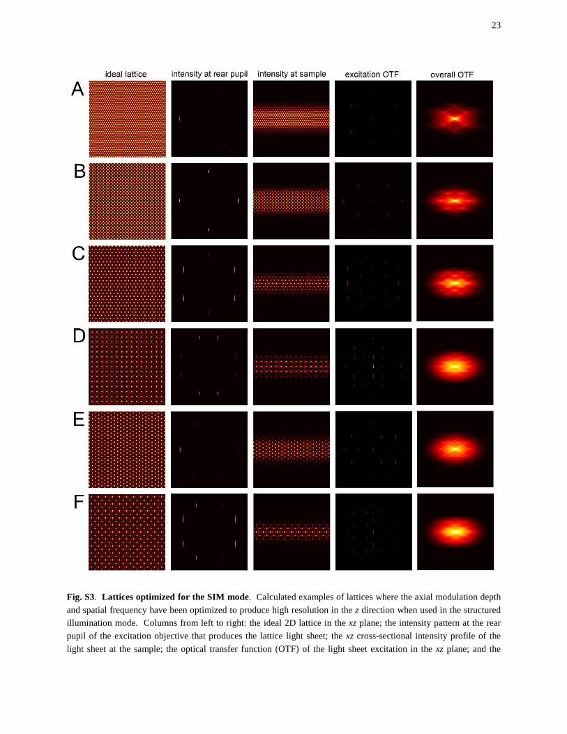
Fig. S3. Lattices optimized for the SIM mode. Calculated examples of lattices where the axial modulation depth and spatial frequency have been optimized to produce high resolution in the z direction when used in the structured illumination mode. Columns from left to right: the ideal 2D lattice in the xz plane; the intensity pattern at the rear pupil of the excitation objective that produces the lattice light sheet; the xz cross-sectional intensity profile of the light sheet at the sample; the optical transfer function (OTF) of the light sheet excitation in the xz plane; and the

24
overall xz OTF defined by the convolution of the excitation and detection OTFs. (A) Fundamental hexagonal lattice, comprised of three wavevectors, rotated to place one of the wavevectors on the x axis. The pattern requires three phase-stepped images for SIM reconstruction. (B) Maximally symmetric fundamental square lattice of the same type as in fig. S2B, but with less axial confinement for optimization in the SIM mode. Five phase-stepped images are required for SIM reconstruction. (C) Maximally symmetric fundamental hexagonal lattice of the same type as in fig. S2C, but also with reduced axial confinement. Five phase-stepped images are required for SIM reconstruction. (D) Maximally symmetric first order sparse square lattice of the same type as in fig. S2D, except with reduced axial confinement. Seven phase-stepped images are required for SIM reconstruction. (E) Maximally symmetric fundamental hexagonal lattice, rotated 90° with respect to the lattice in (C). Nine phase-stepped images are required for SIM reconstruction. (F) Maximally symmetric first order sparse square lattice, of the same type and orientation as in fig. S2E. Nine phase-stepped images are required for SIM reconstruction.

25
Fig. S4. Schematic, mechanical design, and implementation of the lattice light sheet microscope. (A) Schematic of the optical path through the microscope. A linearly polarized circular input beam is stretched by a pair of cylindrical lenses in the x direction and compressed by another pair in the z direction, illuminating a thin stripe across the center of a binary, ferroelectric spatial light modulator (SLM), upon which the desired lattice pattern is projected. The light reflected from the SLM then passes through a transform lens, creating a Fourier diffraction pattern at an opaque mask containing a transparent annulus. The mask filters out unwanted diffraction orders and enforces maximum and minimum NA of illumination that dictate the y extent of the eventual lattice light sheet. The mask is serially conjugate to x and z galvanometers as well as the rear pupil of the excitation objective, so that the light sheet can be translated in x and z and rapid oscillated in x for the dithered mode of operation. The SLM itself is then conjugate to the sample plane, so that the lattice pattern projected on the SLM is imaged within the sample. The lattice light sheet generates fluorescence in a plane within the sample, which is imaged via a 1.1
NA detection objective and tube lens onto an sCMOS camera. Although the light sheet and objective can be translated in z to acquire a 3D volume, we more commonly use a piezoelectric flexure stage to translate the sample through the light sheet. (B) 3D solid model of the microscope. All components (except lasers) are mounted on an 18 x 24 inch breadboard which is in turn vertically mounted on an optical table. The sample itself is then horizontal in the shallow, media filled bath. (C) Photograph of the assembled microscope. (D, E) Magnified views of the sample chamber region, showing: the two objectives surrounded by temperature control blocks; the media bath; the sample holder; and the sample translation subassembly underneath.

26
Fig. S5. Generation of the SLM pattern for a specific lattice light sheet. (A) Real part of the electric field E of an ideal 2D lattice serving as the seed for a particular desired lattice light sheet. (B) E field of the bound lattice obtained after multiplication by a bounding function ( )zψ . (C) SLM pattern created via 0 / π binarization of the bound lattice E field. (D) Predicted diffraction pattern impinging upon the annular mask. (E) Annular filter mask that is conjugate to the rear pupil of the excitation objective. (F) Predicted illumination pattern at the rear pupil. (G) Predicted xz excitation cross-section of the lattice light sheet. (H) Predicted cross-section of the dithered lattice light sheet. (I) Predicted overall PSF for the lattice light sheet in the dithered mode.
27
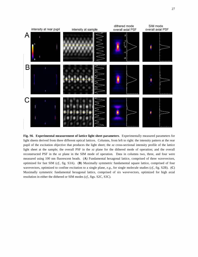
Fig. S6. Experimental measurement of lattice light sheet parameters. Experimentally measured parameters for light sheets derived from three different optical lattices. Columns, from left to right: the intensity pattern at the rear pupil of the excitation objective that produces the light sheet; the xz cross-sectional intensity profile of the lattice light sheet at the sample; the overall PSF in the xz plane for the dithered mode of operation; and the overall reconstructed PSF in the xz plane in the SIM mode of operation. Data in columns two, three, and four were measured using 100 nm fluorescent beads. (A) Fundamental hexagonal lattice, comprised of three wavevectors, optimized for fast SIM (cf., fig. S3A). (B) Maximally symmetric fundamental square lattice, comprised of four wavevectors, optimized to confine excitation to a single plane, e.g., for single molecule studies (cf., fig. S2B). (C) Maximally symmetric fundamental hexagonal lattice, comprised of six wavevectors, optimized for high axial resolution in either the dithered or SIM modes (cf., figs. S2C, S3C).

28
Fig. S7. Axial confinement and point spread functions of two dithered lattice light sheets. (A) Maximally symmetric first sparse square lattice optimized to confine the axial excitation (green) to a single plane. (B) Maximally symmetric fundamental hexagonal lattice optimized to minimize the axial width of the overall axial point spread function (red). Both cases assume restriction of the rear pupil illumination to an NA range of 0.57 to 0.65. NA 1.1 is assumed for the axial detection PSF (blue).

29
Fig. S8. 3D quantification of microtubule growth during mitosis. (A) Trajectories of the endpoints of growing microtubules in HeLa cells expressing GFP-EB1 at four different time points during division of a HeLa cell, color coded by velocity, from a 4D data set covering 500 time points. (B) Distributions of the mean velocity of each growth track, collated over nine to eleven different cells at seven different stages before and during mitosis. Velocities increase from interphase to metaphase, and then decrease back to the interphase level during cytokinesis. (C) Distributions of the velocities of the endpoints as measured between successive time points. Trends are the same as in (B).
30
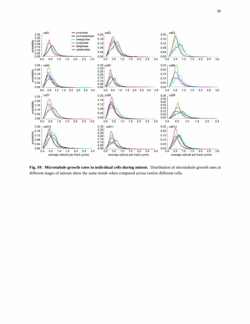
Fig. S9. Microtubule growth rates in individual cells during mitosis. Distribution of microtubule growth rates at different stages of mitosis show the same trends when compared across twelve different cells.

31
Fig. S10. Cilia motion in Tetrahymena. 2D imaging at a fixed plane through the protozoan T. thermophila. When the specimen is nearly at rest, imaging at 3ms intervals is fast enough to follow the shape and motion of beating cilia.

32
Fig. S11. Initial aggregation of starved D. discoideum. Volume renderings at three time points from a 4D data set of 300 time points showing the chemotaxis of starved amoeboid cells expressing RFP-LimE as they aggregate in the initial stages of forming a multicellular fruiting body.

33
Fig. S12. Distribution of AIR-2 during early embryogenesis of C elegans. (A) Volume renderings of GFP-AIR-2 localized at condensed chromosomes during prophase and metaphase at one time point from a 4D data stack covering 50 time points. Left to right: GFP-AIR-2, green channel; mCherry-H2B and PH (chromosomes and plasma membrane), red channel; overlay. (B) Volume renderings of GFP-AIR-2 present on microtubules in the spindle midzone of the AB cell and on the midbody, chromosomes, and the pericentriolar material at a slightly later time point. (C) Volume rendering of GFP-AIR-2 highlighting astral microtubules. A-C, also show AIR2, H2B, and PH localization at the polar bodies (bright spots at the top of the embryos). (D) 2D orthoslice showing the GFP-AIR-2 midbody remnant (magenta) in the extracellular space between the plasma membranes of AB and P1 cells after the first division.

34
Fig. S13. Distribution of actin during early embryogenesis of C elegans. Maximum intensity projections in an xy view of the top half of a developing embryo expressing GFP-Lifeact, at eight time points from a 4D data set covering 300 time points. (A) Single cell during pseudocleavage ingression, showing an intracellular actin comet. (B, C) Relaxation of the pseudocleavage furrow. (D) Bright cortical actin bundles present in maintenance phase during pronuclear meeting. (E) Smooth embryo, presumably near the time of nuclear centration or initial spindle displacement. (F) During and (G) after the first division. (H) After division of the AB cell.

35
Fig. S14. Control schematic for the microscope. The SLM LED Enable output is used as the master clock source, but the FPGA provides the analog /digital outputs to control most of the other electronics critical to image acquisition. Additional boards in the computer receive the data from the sCMOS and inspection cameras, and control the sample positioning stages.
36
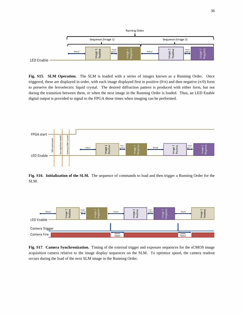
Fig. S15. SLM Operation. The SLM is loaded with a series of images known as a Running Order. Once triggered, these are displayed in order, with each image displayed first in positive (0/π) and then negative (π/0) form to preserve the ferroelectric liquid crystal. The desired diffraction pattern is produced with either form, but not during the transition between them, or when the next image in the Running Order is loaded. Thus, an LED Enable digital output is provided to signal to the FPGA those times when imaging can be performed.
Fig. S16. Initialization of the SLM. The sequence of commands to load and then trigger a Running Order for the SLM.
Fig. S17. Camera Synchronization. Timing of the external trigger and exposure sequences for the sCMOS image acquisition camera relative to the image display sequences on the SLM. To optimize speed, the camera readout occurs during the load of the next SLM image in the Running Order.
37
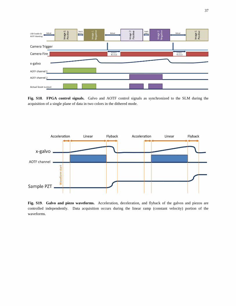
Fig. S18. FPGA control signals. Galvo and AOTF control signals as synchronized to the SLM during the acquisition of a single plane of data in two colors in the dithered mode.
Fig. S19. Galvo and piezo waveforms. Acceleration, deceleration, and flyback of the galvos and piezos are controlled independently. Data acquisition occurs during the linear ramp (constant velocity) portion of the waveforms.

38
Fig. S20. Timing diagram for three color objective scan imaging with a dithered lattice light sheet.
Fig. S21. Timing diagram for two color objective scan imaging in the three phase SIM mode.

39
Fig. S22. Timing diagram for three color sample scan imaging with a dithered lattice light sheet.
Fig. S23. Timing diagram for two color sample scan imaging in the three phase SIM mode.

40
Fig. S24. Properties of an ideal Bessel beam. (A) Magnitude of the electric field E of an ideal Bessel beam. (B) Phase of the beam. Since E is real, the pattern consists of concentric rings of alternating opposite phase (0/π). (C) Intensity of the beam.
Fig. S25. Tightly confined light sheets derived from linear arrays of coherent Bessel-Gauss beams. The six shortest period linear arrays of Bessel-Gauss beams of either identical or alternate opposite phase that produce optimally confined light sheets (cf., movie S18). At these specific periods, the side lobes of adjacent beams are in phase in the xy plane. All cases assume a maximum NA of 0.60, and a minimum NA of 0.54.

41
Fig. S26. Optimally confined Bessel-Gauss beam arrays are bound 2D optical lattices. The four shortest period linear Bessel-Gauss beam arrays of optimal confinement and the corresponding bound 2D optical lattices that produce nearly identical light sheets from nearly identical rear pupil illumination patterns. (A) 0.45 µm period array of beams of alternating opposite phase, compared to a lattice light sheet derived from the maximally symmetric primitive rectangular lattice of aspect ratio 3:1. (B) 0.89 µm period array of beams of identical phase, compared to a lattice light sheet derived from the maximally symmetric fundamental square lattice. (C) 1.35 µm period array of beams of alternating opposite phase, compared to a lattice light sheet derived from the maximally symmetric first sparse square lattice. (D) 1.79 µm period array of beams of identical phase, compared to a lattice light sheet derived from the maximally symmetric fundamental hexagonal lattice.

42
SUPPLEMENTARY TABLE
Table S1. Imaging conditions for all experiments.
Mod
e Sa
mpl
e (im
agin
g T,
o C)
Fluo
resc
ent l
abel
Ex
t λ (n
m)
Voxe
l vol
ume
(dx,
dy,
dz/
ds n
m3 )
Imag
e pi
xels
(x, y
, z)
Expo
sure
tim
e (c
h1,c
h2…
) (#
tim
e pt
s)
(imag
e +
rest
)
Pow
er
(uW
)
Exci
tatio
n N
.A.
(out
er,in
ner)
be
am le
ngth
(u
m)
Phot
o-bl
each
ing
corr
ectio
n
Fig
2A
hex
latt
ice
5 ph
ase
SIM
sa
mpl
e sc
an
HeLa
(37)
m
Emer
ald-
Life
Act
488
72x1
04x1
90/3
50
512x
256x
150
RAW
51
2x86
9x15
0 DS
KW
5ms
340p
ts
(3.7
5s+3
.75s
) 93
0.
55 ,
0.48
15
Imag
e J –
hi
stog
ram
m
atch
ing
Fig 2B
singl
e Be
ssel
5
phas
e SI
M
sam
ple
scan
He
La (3
7)
mEm
eral
d-Li
feAc
t 48
8 72
x104
x190
/350
51
2x25
6x15
0 RA
W
512x
869x
150
DSKW
20m
s 32
pts
(15s
+15s
) 93
0.
55 ,
0.48
15
Imag
e J –
hi
stog
ram
m
atch
ing
Fig 2C
hex
latt
ice
dith
ered
sa
mpl
e sc
an
HeLa
(37)
m
Emer
ald-
Life
Act
488
104x
104x
240/
443
512x
256x
150
RAW
51
2x81
5x15
0 DS
KW
5ms
300p
ts
(0.7
5s+0
.75s
) 93
0.
55 ,
0.48
15
Imag
e J –
hi
stog
ram
m
atch
ing
Fig
2D
singl
e Be
ssel
di
ther
ed
sam
ple
scan
He
La (3
7)
mEm
eral
d-Li
feAc
t 48
8 10
4x10
4x24
0/44
3 51
2x25
6x15
0 RA
W
512x
815x
150
DSKW
5ms
300p
ts
(0.7
5s+0
.75s
) 93
0.
55 ,
0.48
15
Imag
e J –
hi
stog
ram
m
atch
ing
Fig
3ABC
squa
re
latt
ice
dith
ered
sin
gle
plan
e
Mou
se E
SC
sphe
roid
(37)
Ha
lo-T
ag T
MR-
SOX2
56
0 10
0x10
0 51
2x51
2 10
ms
1000
pts
900
0.55
, 0.4
4 10
no
Fig
3FGH
squa
re
latt
ice
dith
ered
sa
mpl
e sc
an
U2O
S (2
5)
Dend
ra2-
Lam
inA
560
100x
100x
271/
500
10x1
0x20
PAL
M
512x
256x
61 R
AW
512x
512x
61 D
SKW
30
01x2
001x
301
PALM
95m
s 31
658p
ts
5000
0.
5, 0
.42
15
no
Fig
4A
squa
re
latt
ice
dith
ered
ob
ject
ive
scan
HeLa
(37)
GF
P-EB
1 ta
gRFP
-H2B
48
8 56
8 10
4x10
4x20
0 32
0x32
0x10
1 5m
s,5m
s 40
0pts
(1
s+0.
25s)
13
, 10
0.50
, 0.
42
15
no
Fig 4B
squa
re
latt
ice
dith
ered
sa
mpl
e sc
an
LLCP
K1 (3
7)
mEm
eral
d-Ca
lnex
in
mCh
erry
-H2B
m
itotr
acke
r dee
p re
d-m
ito
488
568
640
104x
104x
190/
350
576x
256x
201
RAW
57
6x84
7x20
1 DS
KW
5ms
300p
ts
(3s+
0.5s
) 6,
3,1
2 0.
50 ,
0.42
15
99.9
th
perc
entil
e
Fig 4C
squa
re
latt
ice
dith
ered
ob
ject
ive
scan
Tetr
ahym
ena
(25)
GF
P-sc
ram
blas
e 48
8 10
4x10
4x10
00
512x
512x
151
3ms
1250
pts
(0.1
5s+0
.11s
) 6
0.4
, 0.3
25
20
99.9
th
perc
entil
e
Fig
5ABC
squa
re
latt
ice
dith
ered
ob
ject
ive
scan
T ce
ll/Ta
rget
ce
ll (3
7)
mEm
eral
d -Li
feAc
t(T
cell)
ta
gRFP
-PM
(targ
et)
488
568
104x
104x
200
512x
300x
131
5ms,
5ms
150p
ts
(1.0
s+1s
) 20
, 10
0.55
, 0.
48
15
no

43
Fig
5DEF
squa
re
latt
ice
dith
ered
ob
ject
ive
scan
HL60
/col
lage
n (3
7)
FITC
-col
lage
n m
cher
ry-U
trop
hin
488
568
104x
104x
250
672x
352x
141
5ms,
5ms
250p
ts
(1.3
s+0.
1s)
20,
10
0.4
, 0.3
25
20
Imag
e J –
hi
stog
ram
m
atch
ing
Fig
6A
squa
re
latt
ice
dith
ered
ob
ject
ive
scan
C el
egan
s (25
) GF
P-AI
R2
mCh
erry
-PM
+ H
2B
488
568
104x
104x
300
512x
416x
111
50m
s,50m
s 62
pts
(11s
+52s
)
53,
33
0.
50 ,
0.44
2 20
Imag
e J –
hi
stog
ram
m
atch
ing
Fig 6B
squa
re
latt
ice
dith
ered
ob
ject
ive
scan
C el
egan
s (25
) GF
P Li
feac
t 48
8 10
4x10
4x30
0 57
6x35
2x51
95m
s 36
9pts
NM
0.
4, 0
.325
20
99.9
th
perc
entil
e
Fig 6C
squa
re
latt
ice
dith
ered
sa
mpl
e sc
an
Dros
ophi
la
(25)
eG
FP-C
adhe
rin
RFP-
moe
sin
488
100x
100x
206/
328
896x
652x
158
RAW
89
6x10
87x1
58 D
SKW
20m
s,20m
s 84
1pts
(5
.054
s+3s
) N
M
0.4,
0.3
25
20
no
Fig
6D
squa
re
latt
ice
dith
ered
sa
mpl
e sc
an
Dros
ophi
la
(25)
eG
FP-m
yosin
48
8 10
0x10
0x20
6/32
8 89
6x51
2x26
3 RA
W
896x
1237
x263
DSK
W
15m
s 10
00pt
s (4
.561
+0.5
s)
NM
0.
4, 0
.325
20
99.9
th
perc
entil
e
Fig
6EF
squa
re
latt
ice
dith
ered
sa
mpl
e sc
an
Dros
ophi
la
(25)
eG
FP-s
GMCA
m
Cher
ry-s
qs
488
560
100x
100x
206/
328
1024
x512
x263
RAW
10
24x1
237x
263
DSKW
20m
s,20m
s 63
9pts
(7
.984
s+4s
) N
M
0.4,
0.3
25
20
no
Fig
S8, S
9
squa
re
latt
ice
dith
ered
ob
ject
ive
scan
HeLa
(25)
GF
P-EB
1 RF
P-H2
B 48
8 56
8 10
4x10
4x20
0 32
0x32
0x10
1 5m
s,5m
s 40
0pts
(1
s+0.
25s)
1
3,10
0.
50 ,
0.42
15
no
Fig
S10
squa
re
latt
ice
dith
ered
sin
gle
plan
e
Tetr
ahym
ena
(25)
GF
P-sc
ram
blas
e 48
8 10
4x10
4 51
2x51
2 3m
s 18
000p
ts
6
0.4
, 0.3
25
20
no
Fig
S11
squa
re
latt
ice
dith
ered
sa
mpl
e sc
an
Star
ving
dic
ty
(25)
GF
P-Lim
E 48
8 10
4x10
4x24
0/44
3 67
2x35
2x20
1 RA
W
672x
1100
x201
DSK
W
10m
s 40
0pts
(2
s+8s
) 1
3 0.
4 , 0
.325
20
Imag
e J –
hi
stog
ram
m
atch
ing
Fig
S12
squa
re
latt
ice
dith
ered
ob
ject
ive
scan
C el
egan
s (25
) GF
P-AI
R2
mCh
erry
-PM
+ H
2B
488
568
104x
104x
300
512x
416x
111
50m
s,50m
s 62
pts
(11s
+52s
)
53,
33
0.
50 ,
0.44
2 20
Imag
e J –
hi
stog
ram
m
atch
ing

44
Fig
S13
Corr
espo
ndin
g to
Fig
6B
Mov
1
squa
re
latt
ice
dith
ered
sa
mpl
e sc
an
HeLa
(37)
m
Emer
ald-
Life
Act
488
104x
104x
190/
350
512x
256x
150
RAW
51
2x69
7x15
0 DS
KW
5ms
100p
ts
(3.7
5s+3
.75s
) 9
3 0.
55 ,
0.48
15
Imag
e J –
hi
stog
ram
m
atch
ing
hex
latt
ice
5 ph
ase
SIM
sa
mpl
e sc
an
HeLa
(37)
m
Emer
ald-
Life
Act
488
72x1
04x1
90/3
50
512x
256x
150
RAW
86
9x51
2x15
0 DS
KW
5ms
750p
ts
(0.7
5s+0
.25s
) 3
0.
55 ,
0.48
15
Imag
e J –
hi
stog
ram
m
atch
ing
Mov
2
squa
re
latt
ice
dith
ered
ob
ject
ive
scan
Dict
y (2
5)
GFP-
mic
rotu
bule
s 48
8 10
4x10
4x20
0 51
2x32
0x15
1 10
ms
1460
pts
(1.5
s+0.
5s)
10
0.4
, 0.3
25
20
Imag
e J –
hi
stog
ram
m
atch
ing
Mov
3
squa
re
latt
ice
dith
ered
ob
ject
ive
scan
Dict
y (2
5)
GFP-
PI3K
RF
P-Lim
E 48
8 56
8 10
4x10
4x20
0 25
6x25
6x15
1 5m
s,5m
s 15
0pts
(1
.5s+
1s)
20,
13
0.50
, 0.
42
15
Imag
e J –
hi
stog
ram
m
atch
ing
Mov
4
Corr
espo
ndin
g to
Fig
4A
Mov
5
Corr
espo
ndin
g to
Fig
4A
Mov
6
Corr
espo
ndin
g to
Fig
4B
Mov
7
Corr
espo
ndin
g to
Fig
4C
Mov
8
Corr
espo
ndin
g to
Fig
5ABC
Mov
9
Corr
espo
ndin
g to
Fig
5DEF
Mov
10
squa
re
latt
ice
dith
ered
sa
mpl
e sc
an
HL60
(37)
GF
P-Li
feAc
t 48
8 10
4x10
4x21
0/38
8 67
2x25
2x20
1 RA
W
672x
908x
201
DSKW
5ms
143p
ts
(1s+
0.2s
) 10
0.
55 ,
0.48
15
no
Mov
11
Co
rres
pond
ing
to F
igS1
2
Mov
12
Co
rres
pond
ing
t o F
ig6B
Mov
13
Co
rres
pond
ing
to F
ig6D
Mov
S3
Co
rres
pond
ing
to F
ig2A
and
Fig
2B
Mov
S4
Co
rres
pond
ing
to F
ig2A
and
Fig
2B

45
Mov
S5
hex
latt
ice
3 ph
ase
SIM
sa
mpl
e sc
an
HeLa
(37)
m
Emer
ald-
Life
Act
488
72x1
04x1
90/3
50
512x
256x
150
RAW
51
2x86
9x15
0 DS
KW
5ms
245p
ts
(2.2
s+1.
8s)
93
0.55
, 0.
48
15
Imag
e J –
hi
stog
ram
m
atch
ing
Mov
S6
squa
re
latt
ice
dith
ered
sin
gle
plan
e
C el
egan
s (25
) GF
P-PH
m
Cher
ry-H
2B
488
560
100x
100
640x
760
10m
s,10m
s 10
000p
ts
NM
0.
50 ,
0.42
15
Imag
e J –
ex
pone
ntia
l fit
Mov
S7
squa
re
latt
ice
dith
ered
ob
ject
ive
scan
Dict
y (2
5)
GFP-
cont
ract
ile
vacu
ole
488
104x
104x
150
256x
192x
101
5ms
417p
ts
(0.5
s+0.
15s)
1
0 0.
55 ,
0.44
10
no
Mov
S8
squa
re
latt
ice,
sin
gle
Bess
el,
epi
dith
ered
sin
gle
plan
e
Mou
se E
SC
sphe
roid
(37)
Ha
lo-T
ag T
MR-
SOX2
56
0 10
0x10
0 51
2x51
2 50
ms
200p
ts
452m
b 49
3sb
0.55
, 0.4
4 10
no
Mov
S9
squa
re
latt
ice
dith
ered
sin
gle
plan
e
Mou
se E
SC
sphe
roid
(37)
Ha
lo-T
ag T
MR-
SOX2
56
0 10
0x10
0 51
2x51
2 50
,20,
10m
s 10
00pt
s 90
0 0.
55, 0
.44
10
no
Mov
S1
0 Co
rres
pond
ing
to F
ig3F
,G,H
Mov
S1
1 Co
rres
pond
ing
to F
ig4A
Mov
S1
2 Co
rres
pond
ing
to F
ig4A
Mov
S1
3 Co
rres
pond
ing
to F
igS1
0
Mov
S1
4 Co
rres
pond
ing
to F
igS1
1
Mov
S1
5
squa
re
latt
ice
dith
ered
sa
mpl
e sc
an
C el
egan
s (25
) GF
P-PH
m
Cher
ry-H
2B
488
560
100x
100x
271/
500
640x
882x
128
RAW
64
0x14
20x1
28 D
SKW
10
ms,1
0ms
100p
ts
NM
0.
50 ,
0.42
15
Imag
e J –
ex
pone
ntia
l fit
Mov
S1
6 Co
rres
pond
ing
to F
ig6C
Mov
S1
7 Co
rres
pond
ing
to F
ig6E
,F

46
CAPTIONS FOR SUPPLEMENTARY MOVIES
Movie S1. Transition from an infinite 2D optical lattice to an axially bound lattice light sheet, as seen in views of the illumination pattern in the rear pupil of the excitation objective (left) and the cross-sectional intensity profile of the resulting light sheet at the specimen (right).

47
Movie S2. Animation of the image acquisition process, showing a lattice light sheet (blue/green) intersecting a cell (gray) to produce fluorescence (orange). As the cell is swept through the light sheet, a series of 2D images of the fluorescence are recorded to build up a 3D image of the cell. The lattice is dithered in its patterned direction to mimic a continuous light sheet.
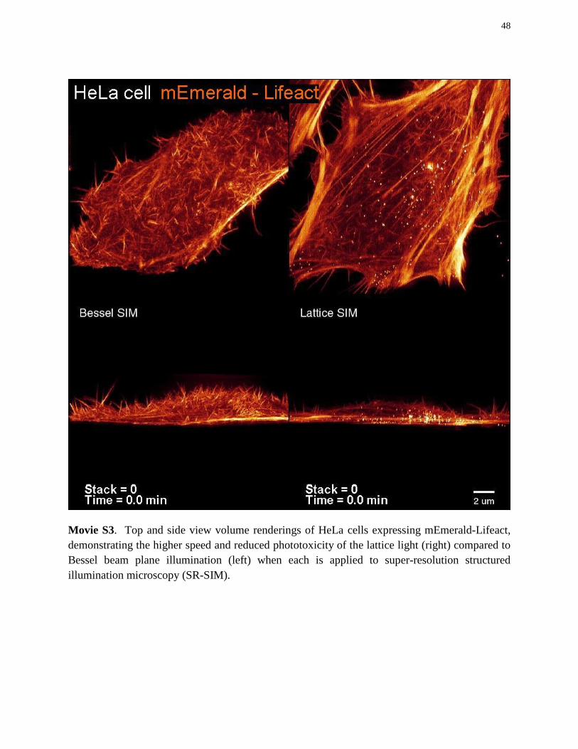
48
Movie S3. Top and side view volume renderings of HeLa cells expressing mEmerald-Lifeact, demonstrating the higher speed and reduced phototoxicity of the lattice light (right) compared to Bessel beam plane illumination (left) when each is applied to super-resolution structured illumination microscopy (SR-SIM).

49
Movie S4. Raw 2D image frames during acquisition of a 3D data volume in the SR-SIM mode for two HeLa cells expressing mEmerald-Lifeact, demonstrating the higher modulation amplitude and lower background obtained with a lattice light sheet (right) as opposed to a stepped Bessel beam (left).

50
Movie S5. Side view volume rendering of filopodia dynamics at 4.0 sec intervals on the dorsal surface of a HeLa cell expressing mEmerald-Lifeact, acquired in the SR-SIM mode using a three phase hexagonal lattice light sheet.
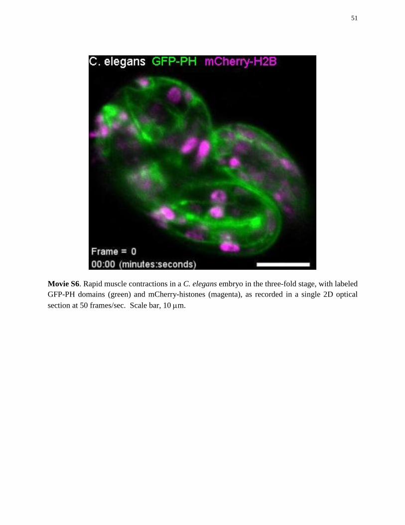
51
Movie S6. Rapid muscle contractions in a C. elegans embryo in the three-fold stage, with labeled GFP-PH domains (green) and mCherry-histones (magenta), as recorded in a single 2D optical section at 50 frames/sec. Scale bar, 10 µm.

52
Movie S7. Volume rendering of GFP-dajumin in a D. discoideum cell, highlighting the rapid dynamics of the osmoregulatory contractile vacuole network over 400 time points at 0.6 sec intervals. A slight rocking is present in the viewer perspective during the time lapse to illustrate 3D depth.

53
Movie S8. Single molecule tracking of TMR-labeled Sox2 transcription factors in an ∼35 µm diameter spheroid of mouse embryonic stem cells, as seen by a dithered lattice light sheet at a fixed plane (top), a single Bessel beam scanned across the same plane (middle), and widefield, epi-illumination across the entire specimen (bottom).

54
Movie S9. SNR as a function of exposure time when tracking single TMR-labeled Sox2 transcription factors in one plane across a stem cell spheroid illuminated by a dithered lattice light sheet.
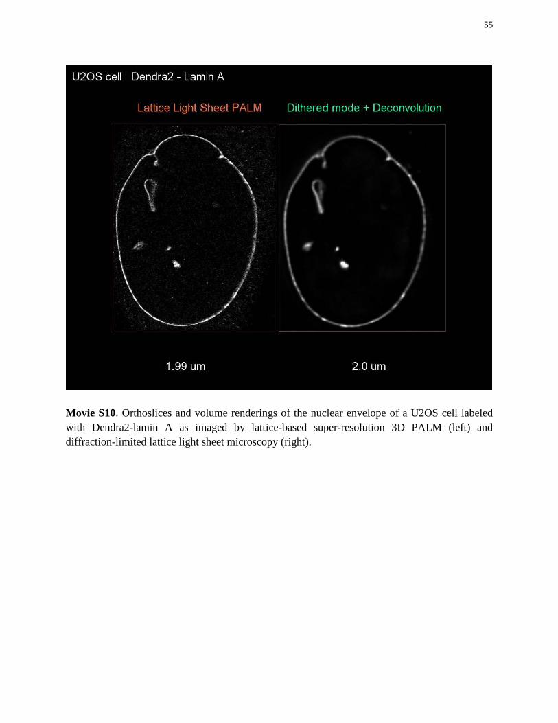
55
Movie S10. Orthoslices and volume renderings of the nuclear envelope of a U2OS cell labeled with Dendra2-lamin A as imaged by lattice-based super-resolution 3D PALM (left) and diffraction-limited lattice light sheet microscopy (right).

56
Movie S11. Maximum intensity projections and measured GFP-EB1 trajectories for a single HeLa cell in interphase. Growing microtubule endpoints and tracks are color coded by z-position above the substrate. Bounding box, 47 x 50 x 11 µm.

57
Movie S12. Maximum intensity projections and measured GFP-EB1 trajectories for a single HeLa cell in metaphase. Growing microtubule endpoints and tracks are color coded by growth phase lifetime. Bounding box, 29 x 36 x 26 µm.

58
Movie S13. Imaging T. thermophila expressing GFP-scramblase in a single 2D plane at 3 ms intervals reveals the motions of individual cilia (cf., fig. S10). Magnified view is shown at right.

59
Movie S14. Top and oblique view volume rendering of the mutual chemotaxis of starved D. discoideum cells expressing RFP-LimE, marking their transition from unicellular to multicellular morphology (cf., fig. S11).

60
Movie S15. Volume rendering of GFP-PH domains (green) and mCherry-H2B (orange) in a C. elegans embryo at the three-fold stage, after the onset of muscle contractions. Bounding box, 41 x 39 x 60 µm.

61
Movie S16. Volume rendering of the amnioserosa and the encroaching epithelium during dorsal closure in a D. melanogaster embryo expressing GFP/DE-cadherin to highlight cell-cell junctions, over 840 time points at 8 sec intervals (cf., Fig. 6C). Bounding box, 86 x 80 x 31 µm.

62
Movie S17. Various views of dorsal closure in a D. melanogaster embryo expressing sGMCA, a marker of filamentous actin at the plasma membrane, over 639 time points at 12.0 sec intervals. Top left: orthoslice through the center of the amnioserosa. Top right: maximum intensity projection through a thin rectangular slab encompassing the apical surface of the amnioserosa. Bottom right: MIP through a similar slab encompassing the basal surface of the amnioserosa. Bottom left, volume rendering, with the apical surface in blue/green and the basal surface in orange/red (cf., Fig. 6E, F). Bounding box, 73 x 73 x 26 µm.

63
Movie S18. Rear pupil excitation pattern (left) and cross-sectional intensity at the sample (right) for a linear array of mutually interfering Bessel-Gauss beams, as a function of the period of the array. Top: all beams have the same phase; Bottom: adjacent beams have opposite phase.

References and Notes 1. D. B. Murphy, M. W. Davidson, Fundamentals of Light Microscopy and Electronic Imaging
(Wiley-Blackwell, Hoboken, NJ, ed. 2, 2013).
2. D. J. Stephens, V. J. Allan, Light microscopy techniques for live cell imaging. Science 300, 82–86 (2003). Medline doi:10.1126/science.1082160
3. J. Huisken, D. Y. Stainier, Selective plane illumination microscopy techniques in developmental biology. Development 136, 1963–1975 (2009). Medline doi:10.1242/dev.022426
4. J. Huisken, J. Swoger, F. Del Bene, J. Wittbrodt, E. H. Stelzer, Optical sectioning deep inside live embryos by selective plane illumination microscopy. Science 305, 1007–1009 (2004). Medline doi:10.1126/science.1100035
5. U. Krzic, S. Gunther, T. E. Saunders, S. J. Streichan, L. Hufnagel, Multiview light-sheet microscope for rapid in toto imaging. Nat. Methods 9, 730–733 (2012). Medline doi:10.1038/nmeth.2064
6. R. Tomer, K. Khairy, F. Amat, P. J. Keller, Quantitative high-speed imaging of entire developing embryos with simultaneous multiview light-sheet microscopy. Nat. Methods 9, 755–763 (2012). Medline doi:10.1038/nmeth.2062
7. T. A. Planchon, L. Gao, D. E. Milkie, M. W. Davidson, J. A. Galbraith, C. G. Galbraith, E. Betzig, Rapid three-dimensional isotropic imaging of living cells using Bessel beam plane illumination. Nat. Methods 8, 417–423 (2011). Medline doi:10.1038/nmeth.1586
8. L. Gao, L. Shao, C. D. Higgins, J. S. Poulton, M. Peifer, M. W. Davidson, X. Wu, B. Goldstein, E. Betzig, Noninvasive imaging beyond the diffraction limit of 3D dynamics in thickly fluorescent specimens. Cell 151, 1370–1385 (2012). Medline doi:10.1016/j.cell.2012.10.008
9. M. G. Gustafsson, L. Shao, P. M. Carlton, C. J. Wang, I. N. Golubovskaya, W. Z. Cande, D. A. Agard, J. W. Sedat, Three-dimensional resolution doubling in wide-field fluorescence microscopy by structured illumination. Biophys. J. 94, 4957–4970 (2008). Medline doi:10.1529/biophysj.107.120345
10. R. Gräf, J. Rietdorf, T. Zimmermann, Live cell spinning disk microscopy. Adv. Biochem. Eng. Biotechnol. 95, 57–75 (2005). Medline doi:10.1007/b102210
11. E. Betzig, Sparse and composite coherent lattices. Phys. Rev. A 71, 063406 (2005). doi:10.1103/PhysRevA.71.063406
12. K. I. Petsas, A. B. Coates, G. Grynberg, Crystallography of optical lattices. Phys. Rev. A 50, 5173–5189 (1994). Medline doi:10.1103/PhysRevA.50.5173
13. I. Bloch, Ultracold quantum gases in optical lattices. Nat. Phys. 1, 23–30 (2005). doi:10.1038/nphys138
14. M. Campbell, D. N. Sharp, M. T. Harrison, R. G. Denning, A. J. Turberfield, Fabrication of photonic crystals for the visible spectrum by holographic lithography. Nature 404, 53–56 (2000). Medline doi:10.1038/35003523

2
15. E. Betzig, Excitation strategies for optical lattice microscopy. Opt. Express 13, 3021–3036 (2005). Medline doi:10.1364/OPEX.13.003021
16. I. Tikhonenko, D. K. Nag, D. N. Robinson, M. P. Koonce, Microtubule-nucleus interactions in Dictyostelium discoideum mediated by central motor kinesins. Eukaryot. Cell 8, 723–731 (2009). Medline doi:10.1128/EC.00018-09
17. G. Jung, M. A. Titus, J. A. Hammer 3rd, The Dictyostelium type V myosin MyoJ is responsible for the cortical association and motility of contractile vacuole membranes. J. Cell Biol. 186, 555–570 (2009). Medline doi:10.1083/jcb.200810147
18. S. Diez, G. Gerisch, K. Anderson, A. Müller-Taubenberger, T. Bretschneider, Subsecond reorganization of the actin network in cell motility and chemotaxis. Proc. Natl. Acad. Sci. U.S.A. 102, 7601–7606 (2005). Medline doi:10.1073/pnas.0408546102
19. M. Coelho, N. Maghelli, I. M. Tolić-Nørrelykke, Single-molecule imaging in vivo: The dancing building blocks of the cell. Integr. Biol. 5, 748–758 (2013). Medline doi:10.1039/c3ib40018b
20. J. G. Ritter, R. Veith, J. P. Siebrasse, U. Kubitscheck, High-contrast single-particle tracking by selective focal plane illumination microscopy. Opt. Express 16, 7142–7152 (2008). Medline doi:10.1364/OE.16.007142
21. M. Tokunaga, N. Imamoto, K. Sakata-Sogawa, Highly inclined thin illumination enables clear single-molecule imaging in cells. Nat. Methods 5, 159–161 (2008). Medline doi:10.1038/nmeth1171
22. J. Chen, Z. Zhang, L. Li, B. C. Chen, A. Revyakin, B. Hajj, W. Legant, M. Dahan, T. Lionnet, E. Betzig, R. Tjian, Z. Liu, Single-molecule dynamics of enhanceosome assembly in embryonic stem cells. Cell 156, 1274–1285 (2014). Medline doi:10.1016/j.cell.2014.01.062
23. J. C. Gebhardt, D. M. Suter, R. Roy, Z. W. Zhao, A. R. Chapman, S. Basu, T. Maniatis, X. S. Xie, Single-molecule imaging of transcription factor binding to DNA in live mammalian cells. Nat. Methods 10, 421–426 (2013). Medline doi:10.1038/nmeth.2411
24. E. Betzig, Proposed method for molecular optical imaging. Opt. Lett. 20, 237–239 (1995). Medline doi:10.1364/OL.20.000237
25. F. Cella Zanacchi, Z. Lavagnino, M. Perrone Donnorso, A. Del Bue, L. Furia, M. Faretta, A. Diaspro, Live-cell 3D super-resolution imaging in thick biological samples. Nat. Methods 8, 1047–1049 (2011). Medline doi:10.1038/nmeth.1744
26. M. Speidel, A. Jonás, E. L. Florin, Three-dimensional tracking of fluorescent nanoparticles with subnanometer precision by use of off-focus imaging. Opt. Lett. 28, 69–71 (2003). Medline doi:10.1364/OL.28.000069
27. H. P. Kao, A. S. Verkman, Tracking of single fluorescent particles in three dimensions: Use of cylindrical optics to encode particle position. Biophys. J. 67, 1291–1300 (1994). Medline doi:10.1016/S0006-3495(94)80601-0
28. E. Betzig, G. H. Patterson, R. Sougrat, O. W. Lindwasser, S. Olenych, J. S. Bonifacino, M. W. Davidson, J. Lippincott-Schwartz, H. F. Hess, Imaging intracellular fluorescent

3
proteins at nanometer resolution. Science 313, 1642–1645 (2006). Medline doi:10.1126/science.1127344
29. J. Ellenberg, E. D. Siggia, J. E. Moreira, C. L. Smith, J. F. Presley, H. J. Worman, J. Lippincott-Schwartz, Nuclear membrane dynamics and reassembly in living cells: Targeting of an inner nuclear membrane protein in interphase and mitosis. J. Cell Biol. 138, 1193–1206 (1997). Medline doi:10.1083/jcb.138.6.1193
30. Y. Mimori-Kiyosue, N. Shiina, S. Tsukita, The dynamic behavior of the APC-binding protein EB1 on the distal ends of microtubules. Curr. Biol. 10, 865–868 (2000). Medline doi:10.1016/S0960-9822(00)00600-X
31. K. T. Applegate, S. Besson, A. Matov, M. H. Bagonis, K. Jaqaman, G. Danuser, plusTipTracker: Quantitative image analysis software for the measurement of microtubule dynamics. J. Struct. Biol. 176, 168–184 (2011). Medline doi:10.1016/j.jsb.2011.07.009
32. A. Khodjakov, C. L. Rieder, Imaging the division process in living tissue culture cells. Methods 38, 2–16 (2006). Medline doi:10.1016/j.ymeth.2005.07.007
33. N. Taguchi, N. Ishihara, A. Jofuku, T. Oka, K. Mihara, Mitotic phosphorylation of dynamin-related GTPase Drp1 participates in mitochondrial fission. J. Biol. Chem. 282, 11521–11529 (2007). Medline doi:10.1074/jbc.M607279200
34. L. Lu, M. S. Ladinsky, T. Kirchhausen, Cisternal organization of the endoplasmic reticulum during mitosis. Mol. Biol. Cell 20, 3471–3480 (2009). Medline doi:10.1091/mbc.E09-04-0327
35. D. Wloga, J. Frankel, From molecules to morphology: Cellular organization of Tetrahymena thermophila. Methods Cell Biol. 109, 83–140 (2012). Medline doi:10.1016/B978-0-12-385967-9.00005-0
36. A. T. Ritter, K. L. Angus, G. M. Griffiths, The role of the cytoskeleton at the immunological synapse. Immunol. Rev. 256, 107–117 (2013).
37. D. Dormann, C. J. Weijer, Imaging of cell migration. EMBO J. 25, 3480–3493 (2006). Medline doi:10.1038/sj.emboj.7601227
38. P. H. Wu, A. Giri, S. X. Sun, D. Wirtz, Three-dimensional cell migration does not follow a random walk. Proc. Natl. Acad. Sci. U.S.A. 111, 3949–3954 (2014). Medline doi:10.1073/pnas.1318967111
39. P. Friedl, S. Borgmann, E. B. Bröcker, Amoeboid leukocyte crawling through extracellular matrix: Lessons from the Dictyostelium paradigm of cell movement. J. Leukoc. Biol. 70, 491–509 (2001). Medline
40. A. B. Hauert, S. Martinelli, C. Marone, V. Niggli, Differentiated HL-60 cells are a valid model system for the analysis of human neutrophil migration and chemotaxis. Int. J. Biochem. Cell Biol. 34, 838–854 (2002). Medline doi:10.1016/S1357-2725(02)00010-9
41. W. R. Legant, J. S. Miller, B. L. Blakely, D. M. Cohen, G. M. Genin, C. S. Chen, Measurement of mechanical tractions exerted by cells in three-dimensional matrices. Nat. Methods 7, 969–971 (2010). Medline doi:10.1038/nmeth.1531

4
42. J. N. Bembenek, K. J. Verbrugghe, J. Khanikar, G. Csankovszki, R. C. Chan, Condensin and the spindle midzone prevent cytokinesis failure induced by chromatin bridges in C. elegans embryos. Curr. Biol. 23, 937–946 (2013). Medline doi:10.1016/j.cub.2013.04.028
43. J. M. Schumacher, A. Golden, P. J. Donovan, AIR-2: An Aurora/Ipl1-related protein kinase associated with chromosomes and midbody microtubules is required for polar body extrusion and cytokinesis in Caenorhabditis elegans embryos. J. Cell Biol. 143, 1635–1646 (1998). Medline doi:10.1083/jcb.143.6.1635
44. M. Carmena, W. C. Earnshaw, The cellular geography of aurora kinases. Nat. Rev. Mol. Cell Biol. 4, 842–854 (2003). Medline doi:10.1038/nrm1245
45. N. Velarde, K. C. Gunsalus, F. Piano, Diverse roles of actin in C. elegans early embryogenesis. BMC Dev. Biol. 7, 142 (2007). Medline doi:10.1186/1471-213X-7-142
46. S. W. Grill, Growing up is stressful: Biophysical laws of morphogenesis. Curr. Opin. Genet. Dev. 21, 647–652 (2011). Medline doi:10.1016/j.gde.2011.09.005
47. A. Sokolow, Y. Toyama, D. P. Kiehart, G. S. Edwards, Cell ingression and apical shape oscillations during dorsal closure in Drosophila. Biophys. J. 102, 969–979 (2012). Medline doi:10.1016/j.bpj.2012.01.027
48. K. Wang, D. E. Milkie, A. Saxena, P. Engerer, T. Misgeld, M. E. Bronner, J. Mumm, E. Betzig, Rapid adaptive optical recovery of optimal resolution over large volumes. Nat. Methods 11, 625–628 (2014). Medline doi:10.1038/nmeth.2925
49. G. Donnert, C. Eggeling, S. W. Hell, Major signal increase in fluorescence microscopy through dark-state relaxation. Nat. Methods 4, 81–86 (2007). Medline doi:10.1038/nmeth986
50. N. Ji, J. C. Magee, E. Betzig, High-speed, low-photodamage nonlinear imaging using passive pulse splitters. Nat. Methods 5, 197–202 (2008). Medline doi:10.1038/nmeth.1175
51. T. Shimozawa, K. Yamagata, T. Kondo, S. Hayashi, A. Shitamukai, D. Konno, F. Matsuzaki, J. Takayama, S. Onami, H. Nakayama, Y. Kosugi, T. M. Watanabe, K. Fujita, Y. Mimori-Kiyosue, Improving spinning disk confocal microscopy by preventing pinhole cross-talk for intravital imaging. Proc. Natl. Acad. Sci. U.S.A. 110, 3399–3404 (2013). Medline doi:10.1073/pnas.1216696110
52. J. D. Sander, J. K. Joung, CRISPR-Cas systems for editing, regulating and targeting genomes. Nat. Biotechnol. 32, 347–355 (2014). Medline doi:10.1038/nbt.2842
53. T. Zimmermann, J. Rietdorf, R. Pepperkok, Spectral imaging and its applications in live cell microscopy. FEBS Lett. 546, 87–92 (2003). Medline doi:10.1016/S0014-5793(03)00521-0
54. J. Livet, T. A. Weissman, H. Kang, R. W. Draft, J. Lu, R. A. Bennis, J. R. Sanes, J. W. Lichtman, Transgenic strategies for combinatorial expression of fluorescent proteins in the nervous system. Nature 450, 56–62 (2007). Medline doi:10.1038/nature06293
55. E. Lubeck, L. Cai, Single-cell systems biology by super-resolution imaging and combinatorial labeling. Nat. Methods 9, 743–748 (2012). Medline doi:10.1038/nmeth.2069

5
56. A. M. Valm, J. L. Mark Welch, C. W. Rieken, Y. Hasegawa, M. L. Sogin, R. Oldenbourg, F. E. Dewhirst, G. G. Borisy, Systems-level analysis of microbial community organization through combinatorial labeling and spectral imaging. Proc. Natl. Acad. Sci. U.S.A. 108, 4152–4157 (2011). Medline doi:10.1073/pnas.1101134108
57. L. Gao, L. Shao, B. C. Chen, E. Betzig, 3D live fluorescence imaging of cellular dynamics using Bessel beam plane illumination microscopy. Nat. Protoc. 9, 1083–1101 (2014). Medline doi:10.1038/nprot.2014.087
58. B. P. English, V. Hauryliuk, A. Sanamrad, S. Tankov, N. H. Dekker, J. Elf, Single-molecule investigations of the stringent response machinery in living bacterial cells. Proc. Natl. Acad. Sci. U.S.A. 108, E365–E373 (2011). Medline doi:10.1073/pnas.1102255108
59. J. Durnin, J. J. Miceli Jr., J. H. Eberly, Comparison of Bessel and Gaussian beams. Opt. Lett. 13, 79 (1988). Medline doi:10.1364/OL.13.000079
60. B. Richards, E. Wolf, Electromagnetic diffraction in optical systems. 2. Structure of the image field in an aplanatic system. Proc. R. Soc. London Ser. A 253, 358–379 (1959). doi:10.1098/rspa.1959.0200
61. P. Kner, B. B. Chhun, E. R. Griffis, L. Winoto, M. G. Gustafsson, Super-resolution video microscopy of live cells by structured illumination. Nat. Methods 6, 339–342 (2009). Medline doi:10.1038/nmeth.1324
62. S. Nakamura, I. Grigoriev, T. Nogi, T. Hamaji, L. Cassimeris, Y. Mimori-Kiyosue, Dissecting the nanoscale distributions and functions of microtubule-end-binding proteins EB1 and ch-TOG in interphase HeLa cells. PLOS ONE 7, e51442 (2012). Medline doi:10.1371/journal.pone.0051442
63. C. Demaison, K. Parsley, G. Brouns, M. Scherr, K. Battmer, C. Kinnon, M. Grez, A. J. Thrasher, High-level transduction and gene expression in hematopoietic repopulating cells using a human immunodeficiency virus type 1-based lentiviral vector containing an internal spleen focus forming virus promoter. Hum. Gene Ther. 13, 803–813 (2002). Medline doi:10.1089/10430340252898984
64. B. M. Burkel, G. von Dassow, W. M. Bement, Versatile fluorescent probes for actin filaments based on the actin-binding domain of utrophin. Cell Motil. Cytoskeleton 64, 822–832 (2007). Medline doi:10.1002/cm.20226
65. M. Sixt, T. Lämmermann, In vitro analysis of chemotactic leukocyte migration in 3D environments. Methods Mol. Biol. 769, 149–165 (2011). Medline doi:10.1007/978-1-61779-207-6_11
66. E. Octtaviani, J. C. Effler, D. N. Robinson, Enlazin, a natural fusion of two classes of canonical cytoskeletal proteins, contributes to cytokinesis dynamics. Mol. Biol. Cell 17, 5275–5286 (2006). Medline doi:10.1091/mbc.E06-08-0767
67. M. Clarke, A. Müller-Taubenberger, K. I. Anderson, U. Engel, G. Gerisch, Mechanically induced actin-mediated rocketing of phagosomes. Mol. Biol. Cell 17, 4866–4875 (2006). Medline doi:10.1091/mbc.E06-04-0365
68. A. Essex, A. Dammermann, L. Lewellyn, K. Oegema, A. Desai, Systematic analysis in Caenorhabditis elegans reveals that the spindle checkpoint is composed of two largely

6
independent branches. Mol. Biol. Cell 20, 1252–1267 (2009). Medline doi:10.1091/mbc.E08-10-1047
69. H. Oda, S. Tsukita, Real-time imaging of cell-cell adherens junctions reveals that Drosophila mesoderm invagination begins with two phases of apical constriction of cells. J. Cell Sci. 114, 493–501 (2001). Medline
70. P. A. Lawrence, R. Bodmer, J. P. Vincent, Segmental patterning of heart precursors in Drosophila. Development 121, 4303–4308 (1995). Medline
71. M. Buszczak, S. Paterno, D. Lighthouse, J. Bachman, J. Planck, S. Owen, A. D. Skora, T. G. Nystul, B. Ohlstein, A. Allen, J. E. Wilhelm, T. D. Murphy, R. W. Levis, E. Matunis, N. Srivali, R. A. Hoskins, A. C. Spradling, The carnegie protein trap library: A versatile tool for Drosophila developmental studies. Genetics 175, 1505–1531 (2007). Medline doi:10.1534/genetics.106.065961
72. K. A. Edwards, M. Demsky, R. A. Montague, N. Weymouth, D. P. Kiehart, GFP-moesin illuminates actin cytoskeleton dynamics in living tissue and demonstrates cell shape changes during morphogenesis in Drosophila. Dev. Biol. 191, 103–117 (1997). Medline doi:10.1006/dbio.1997.8707
73. A. C. Martin, M. Kaschube, E. F. Wieschaus, Pulsed contractions of an actin-myosin network drive apical constriction. Nature 457, 495–499 (2009). Medline doi:10.1038/nature07522