Super Awesome Study Guide for Algorithms

Chapter 1 What is an algorithm?

Problem ↓Algorithm ↓

Input → Computer → Output

Basic number of operations determine a function that defines the number of basic operations in terms of the input size(n)

The growth rate of a function is used to categorize various algorithms (especially those that solve the same problem

↓Analysis Framework

asymptotic orders of growthbest-case worst-case and average case

Chapter 2: Theoretical Framework

Asymptotic NotationO(n) notation - t(n) < cg(n) for all n>=n;

A function t(n) is said to be in O(g(n)) if t(n) is bounded above by some constant multiple of g(n) for all large n.

Ω(n) notation - t(n) > cg(n) for all n>=n;A function t(n) is said to be in Ω(g(n)) if t(n) is bounded below by some positive constant multiple of g(n) for all large n .

O(n) notation - c2g(n) < t(n) < c1g(n)A function t(n) is said to be O(g(n)) if t(n) is bounded both above and below by some positive constant multiples of g(n) for all large n.

Non-Recursive problems 5 step plan for analyzing time efficiency

1. Decide on a parameter (or parameters) indicating input's size.2. Identify the algorithm's basic operation.(as a rule, it is located in the

innermost loop.)3. Check whether the number of times the basic operation is executed

depends only on the size of an input. If It also depends on some additional property, the worst-case, average-case, and, if necessary, best-case efficiencies have to be investigated separately

4. Set up a sum expressing the number of times the algorithm's basic operation is executed

5. Using standard formulas and rules of sum manipulation, either find a closed form formula for the count or, at the very least, establish its order of growth.

Common Summation formulasi=LΣu 1 = u – L +1 where L< u are some lower and upper integer limitsi=1Σn i = n(n+1) / 2 = O(n2)

Recursive problems 5 step plan for analyzing time efficiency

1. Decide on parameter (or parameters) indicating an input's size.2. Identify the algorithm's basic operations3. Check whether the number of times the basic operation is executed can

vary on different inputs of the same size; if it can the worst-case, average-case, and best-case efficiencies must be investigated separately

4. Set up a recurrence relation, with an appropriate initial condition, for the number of times the basic operation is executed

5. Solve the recurrence or at least ascertain the order of growth of its solution

The Method of Backwards Substitution – inspect the first few outcomes of a pattern. Formulate an equation to predict the next outcome.

Master Theorem -

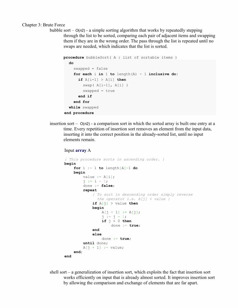
Chapter 3: Brute Forcebubble sort – О(n2) - a simple sorting algorithm that works by repeatedly stepping

through the list to be sorted, comparing each pair of adjacent items and swapping them if they are in the wrong order. The pass through the list is repeated until no swaps are needed, which indicates that the list is sorted.

procedure bubbleSort( A : list of sortable items ) do swapped = false for each i in 1 to length(A) - 1 inclusive do: if A[i-1] > A[i] then swap( A[i-1], A[i] ) swapped = true end if end for while swappedend procedure

insertion sort – O(n2) - a comparison sort in which the sorted array is built one entry at a time. Every repetition of insertion sort removes an element from the input data, inserting it into the correct position in the already-sorted list, until no input elements remain.

Input array A { This procedure sorts in ascending order. }begin for i := 1 to length[A]-1 do begin value := A[i]; j := i - 1; done := false; repeat { To sort in descending order simply reverse the operator i.e. A[j] < value } if A[j] > value then begin A[j + 1] := A[j]; j := j - 1; if j < 0 then done := true; end else done := true; until done; A[j + 1] := value; end;end

shell sort – a generalization of insertion sort, which exploits the fact that insertion sort works efficiently on input that is already almost sorted. It improves insertion sort by allowing the comparison and exchange of elements that are far apart.

input: an array a of length n with array elements numbered 0 to n − 1inc ← round(n/2)while inc > 0 do: for i = inc .. n − 1 do: temp ← a[i] j ← i while j ≥ inc and a[j − inc] > temp do: a[j] ← a[j − inc] j ← j − inc a[j] ← temp inc ← round(inc / 2.2)

string matching

Horspool's algorithm1. for a given pattern of length m and the alphabet used in both the

pattern and the text, construct a shift table.2. Align the pattern against the beginning of the text.3. Repeat the following until either a matching substring is found or

the pattern reaches beyond the last character of the text. Starting with the last character in the pattern, compare the corresponding characters in the pattern and text until either all m characters are matched or a mismatching pair is encountered. In the latter case, retrieve the entry t(c) from the C’s column of the shift table where c is the text's character currently aligned against the last character of the pattern, and shift the pattern by t(c) characters to the right along the text.

Boyer Moore – preprocesses the target string (key) that is being searched for, but not the string being searched in. If the first comparison of the rightmost character in the pattern with the corresponding character c in the text fails, the algorithm does exactly the same thing as Horspool's algorithm. Namely, it shifts the pattern to the right by the number of characters retrieved from the table.

Closest PairConvex Hull – The convex-hull problem of constructing the convex hull for a

given set S of n points. To solve, find the points that will serve as the vertices of the polygon in question.

Exhaustive SearchTSPknap-sackassignment

Chapter 4: Divide and Conquer

Mergesort - is anO(nlogn)comparison-based sorting algorithm. 1. if the list is of length 0 or 1, then it is already sorted Otherwise:2. Divide the unsorted list into two sub-lists of about half the size3. Sort each sub list back into the sorted list Merge sort incorporates two main ideas to improve its runtime:

1. A small list will take fewer steps to sort than a large list2. Fewer steps are required to construct a sorted list from two sorted lists

than two unsorted lists

Quicksort- A sorting algorithm that makes O(nlogn) comparisons to sort n items. 1. Pick an element, called a pivot, from the list.2. Reorder the list so that all elements with values less than the pivot come before the pivot, while all elements with values greater than the pivot come after it (equal values can go either way). After this partitioning, the pivot is in its final position. This is called the partition operation.3. Recursively sort the sub-list of lesser elements and the sub-list of greater elements.

The base case of the recursion are lists of size zero or one, which never need to be sorted.

Binary Search - a search that locates the position of an item in a sorted array. Binary search works by comparing an input value to the middle element of the array. The comparison determines whether the element equals the input, less than the input, or greater than the input. When the element being compared to equals the input the search stops and typically returns the position of the element/ if the element is not equal to the input then a comparison is made to determine whether the input is less than or greater than the element. Depending on which is the algorithm then starts over but only searching the top or bottom subset of the array's elements/ if the input is not lovated within the arraythe algorithm will usually output a unique value indicating this. Binary search algorithms typically halve the number of items to check with each successive iteration, thus locating the given item in logarithmic time. A binary search is a dichotomic divide and conquer search algorithm

Binary Tree TraversalDepth-first search (DFS) is an algorithm for traversing or searching a tree, tree structure, or

graph. One starts at the root (selecting some node as the root in the graph case) and explores as far as possible along each branch before backtracking.

Breadth-first search (BFS) is a graph search algorithm that begins at the root node and explores all the neighboring nodes. Then for each of those nearest nodes, it explores their unexplored neighbor nodes, and so on, until it finds the goal.

Multiplication of Large Integers Geometric Problems

Chapter 5: Decrease and ConquerDecrease by a ConstantDecrease by a Variable FactorDecrease by a Constant Factor

Chapter 6: Transform and ConquerInstance SimplificationRepresentation Change Problem reduction

DAG (directed acyclic graph) is a graph formed by a collection of vertices and directed edges. Each edge connects the vertexes together without creating a cycle by looping back to an original vertex

Chapter 7 Hashing

Open Hashing (chaining) – defined as each slot in the hash table to be head of a linked list. All records that hash to a particular slot are placed on that slot's linked list.

Records within a slot's list can be ordered in several ways: by insertion order. By key value order. Or by frequency-of-access order. Ordering the list by key value provides an advantage in the case of unsuccessful search, because we know to stop searching the list once we encounter a key that is greater than the one being searched for. If records on the list are unordered or ordered by frequency, then an unsuccessful search will need to visit every record in the list. The position in the list is determined by the number to be placed in the list modded with the number of places in the list. So 2007 % 10 = 7;

Closed Hashing(linear probing) – All keys are stored in the hash table itself without the use of linked lists. Different strategies can be employed for collision resolution. The simplest is linear probing.

Linear probing – checks the cell following the one where the collision occurs. If that cell is empty, the new key is installed there; if the next cell is already occupied, the availability of that cell's immediate successor is checked, and so on. If the end of the hash table is reached, the search is wrapped to the beginning of the table and treats list as a circular array.

Chapter 8Dynamic programming

find a recursive solutionidentify the recursive def and base cases

start form the base case and build solutions to smaller problems store in table use values to generate more complex larger and larger sub-problems

Computing binomial coefficient -denoted C(n,k) or (n choose k), is the number of

combinations( subsets) of k elements from an n-element set(0<k<n). to compute C(n,k), we fill a table row by row, starting with row 0 and ending with row n. each row I is filled left to right, starting with 1. rows 0 through k also end with 1 on the tables main diagonal. We compute the other entries by the formula {(a+b)n = C(n,0)an+...+c(n,k)an-k bk}, adding the contents of the cells in the preciding row and the previous column and in the preceding row and the same column.

Warshal's algorithm – Recall that the adjacency matrix A = {aij} of a directed graph is the boolean matrix that has 1 in its ith row and the jth column iff there is a directed edge form the ith vertex to the jth vertex. We may also be interested in a matrix containing the information about the existence of directed paths of arbitrary lengths between verticels of a given graph.

Transitive Closure- of a directed graph with n vertices can be defined as the n-by-n boolean matrix T = {tij}, in which the element in the ith row and the jth column is 1 there exists a nontrivial directed path form the ith vertex to the jth vertex; otherwise, tij is 0.

Floyd's algorithm – Given a weighted connected graph, the all pairs shortest paths asks to find the distances from each vertex to all other vertices. It is convenient to record the lengths of the shortest paths in an n-by-n matrix D called the distance matrix

Distance Matrix: the element dij in the ith row and the jth column of this matrix with an algorithm that is very similar to Warshall's algorithm.

Binary Search Tree – a node based binary tree data structure which has the following propertiesThe left sub-tree of a node contains only nodes with keys less than the node's key.the right sub-tree of a node contains only nodes with keys greater than the node's key.both left and right sub-trees must also be binary search trees.

Optimal Binary Search Tree – If probabilities of searching for elements of a set are known. It is natural to pose a question about an optimal binary search tree for which the average number of comparisons in a search is the smallest possible.

Knapsack problem – to design a dynamic programming algorithm, we need to derive a recurrence relation that expresses a solution to an instance of the knapsack problem in terms of solutions to its smaller sub-instances.

Dynamic programming solution – Let I be the highest-numbered item in an optimal

solution S for W pounds. Then s' = S -{i} is an optimal solution for W – wi pounds and the value to the solution S is Vi plus the value of the sub-problem.

We can express this fact in the following formula: define c[i,w] to be the solution for items 1,2,....,i and max weight w. then

0 If i = 0 or w = 0c[i,w] = c[i-1,w] ifwi≥ 0

max [vi + c[i-1,w-wi], c[i-1,w]} If i>0 and w ≥ wiThis says that the value of the solution to I items either include ith item, in which the case it is vi plus a subproblem solution for (i=1) items and the weight excluding vi , or does not include ith item, in which case it is a subproblem's solution for (i-1) items and the same weight. That is, if the thief picks item I, the theif takes vi value, and the theif can choose form items w-wi, and get c[i-1,w-wi] additional value. On the other hand, if thief decides not to take item i, thief can choose from item 1,2, . . . , i- 1 up to the weight limit w, and getc[i- 1,w] value. The better of these two choices should be made.Although the 0-1 knapsack problem, the above formula for c is similar to LCS formula: boundary values are 0, and other values are computed from the input and "earlier" values of c. So the 0-1 knapsack algorithm is like the LCS-length algorithm given in CLR for finding a longest common subsequence of two sequences.

The algorithm takes as input the maximum weight W, the number of items n, and the two sequences v = <v1, v2, . . . , vn> and w = <w1, w2, . . . , wn>. It stores the c[i,j] values in the table, that is, a two dimensional array, c[0 . .n, 0 . .w] whose entries are computed in a row-major order. That is, the first row of c is filled in from left to right, then the second row, and so on. At the end of the computation, c[n,w] contains the maximum value that can be picked into the knapsack.

Dynamic-0-1-knapsack (v, w, n, W)FOR w = 0 TO W

Do c[0,w] = 0FOR i=1 to n

DO c[i, 0] = 0FOR w=1 TOW DO Iff wi ≤ w

THEN IF vi + c[i-1, w-wi] THENc[i,w] = vi + c[i-1, w-wi]

ELSE c[i,w] = c[i-1, w] ELSE

c[i,w] = c[i-1, w]

The set of items to take can be deduced from the table, starting at c[n. w] and tracing backwards where the optimal values came from. If c[i, w] = c[i-1, w] item i is not part of the solution, and we are continue tracing with c[i-1, w]. Otherwise item i is part of the solution, and we continue tracing with c[i-1, w-W].

This dynamic-0-1-kanpsack algorithm takes θ(nw) times, broken up as follows: θ(nw) times to fill the c-table, which has (n +1).(w +1) entries, each requiring θ(1) time to compute. O(n) time to trace the solution, because the tracing process starts in row n of the table and moves up 1 row at each step.

chapter 9greedy technique – any algorithm that follows the problem solving heuristic(finding a good enough solution to the problem) of making the locally optimal choice at each stage with the hope of finding the global optimum.

Change Making Problem – give change for a specific amount n with the least number of coins of the denominations d1 > d2 > . . . > dm used in that locale.

prim – greedy algorithm for finding the minimum spanning tree for a connected weighted undirected graph. This means it finds a subset of the edges that forms a tree that includes every vertex. Where the total weight of the edges in the tree is minimized

Minimum Spanning Tree-given a connected, undirected graph, a spanning tree of that graph is a subgraph that is a tree and connects all the vertices together. A single graph can have many different spanning trees. We can also assign a weight to each edge, which is a number representing how unfavorable it is, and use this to assign a weight to a spanning tree by computing the sum of the weights of the edges in that spanning tree. A minimum spanning tree (MST) or minimum weight spanning tree is then a spanning tree with weight less than or equal to the weight of every other spanning tree. More generally, any undirected graph (not necessarily connected) has a minimum spanning forest, which is a union of minimum spanning trees for its connected components.

Kruskal's - • create a forest F (a set of trees), where each vertex in the graph is a separate tree• create a set S containing all the edges in the graph• while S is nonempty and F is not yet spanning• remove an edge with minimum weight from S• if that edge connects two different trees, then add it to the forest, combining two trees into

a single tree• otherwise discard that edge.

At the termination of the algorithm, the forest has only one component and forms a minimum spanning tree of the graph.

Dijkstra's algorithm – a graph search algorithm that solves the single-source shortest path problem for a graph with non-negative edge path costs, producing a shortest path tree.

Let the node at which we are starting be called the initial node. Let the distance of node Y be the distance from the initial node to Y. Dijkstra's algorithm will assign some initial distance values and will try to improve them step by step.

1. Assign to every node a distance value: set it to zero for our initial node and to infinity for all other nodes.

2. Mark all nodes as unvisited. Set initial node as current.3. For current node, consider all its unvisited neighbors and calculate their tentative distance. For

example, if current node (A) has distance of 6, and an edge connecting it with another node

(B) is 2, the distance to B through A will be 6+2=8. If this distance is less than the previously recorded distance, overwrite the distance.

4. When we are done considering all neighbors of the current node, mark it as visited. A visited node will not be checked ever again; its distance recorded now is final and minimal.

5. If all nodes have been visited, finish. Otherwise, set the unvisited node with the smallest distance (from the initial node, considering all nodes in graph) as the next "current node" and continue from step 3.

Single Source Shortest Path - the problem of finding a path between two vertices (or nodes) such that the sum of the weights of its constituent edges is minimized.

Prim – a greedy algorithm that finds a minimum spanning tree for a connected weighted undirected graph. This means it finds a subset of the edges that forms a tree that includes every vertex, where the total weight of all the edges in the tree is minimized.

Huffman codes – an entropy encoding algorithm used for lossless data compression. The term refers to the use of a variable-length code table for encoding a source symbol (such as a character in a file) where the variable-length code table has been derived in a particular way based on the estimated probability of occurrence for each possible value of the source symbol.

Given a set of symbols and their weights, Find a prefix-free binary code with minimum expected codeword length.

Compression - O(log n) -Create a leaf node for each symbol and add it to the priority queue.

1. While there is more than one node in the queue:1. Remove the two nodes of highest priority (lowest probability) from the queue2. Create a new internal node with these two nodes as children and with probability

equal to the sum of the two nodes' probabilities.3. Add the new node to the queue.

2. The remaining node is the root node and the tree is complete.

Char Freq Codespace 7 111

a 4 010e 4 000f 3 1101h 2 1010i 2 1000m 2 0111n 2 0010s 2 1011t 2 0110l 1 11001o 1 00110p 1 10011r 1 11000u 1 00111x 1 10010

Chapter 11 – limitations of algorithm powerlower bound

trivial lower bounds Decision trees - a decision support tool that uses a tree-like graph or model of decisions and their

possible consequences, including chance event outcomes, resource costs, and utility.

Adversary Argument Linear Reduction - A problem X, reduces to another problem, Y, if we can efficiently transform instances of the problem X into instances of the problem B in such a way that solving the transformed instances yields the solution to the original instance.Formal DefinitionsThe problem A is linearly reducible to perform B, Denoted A ≤ lB, if the existence an algorithm for B that runs in a time O(t(n)) for any function t(n) implies that there exists an algorithm for A that also runs in a time O(t(n)).

If A ≤ lB and B ≤ lA then A and B are linearly equivalent and denoted A == lB.

Also, the linear reduction are transitive: if A ≤ lB and B ≤ lC, then A ≤ lC.

Linear equivalence are transitive reflexive and symmetric. (Hence, equivalent.)

Problem reduction - a transformation of one problem into another problem. Depending on the transformation used this can be used to define complexity classes on a set of problems.

P, NP, and NPC.P – solvable in polynomial timeNP – Non-deterministic polynomialNPC – Non deterministic polynomial complete- known to be reducable to an instance of another problem in polynomial time. ie... A key for a security system

Diagram of complexity classes provided that P≠ NP. The existence of problems outside both P and NP-complete in this case was established by Ladner.