Page 1

Paper: Analysis & Design of Algorithms

Chapter 1: Introduction to Algorithm

Concept of algorithm An algorithm is a set of rules for carrying out calculation that transform the input to the output.

A common man’s belief is that a computer can do anything and everything that he imagines. It is

very difficult to make people realize that it is not really the computer but the man behind

computer who does everything.

In the modern internet world man feels that just by entering what he wants to search into the

computers he can get information as desired by him. He believes that, this is done by computer.

A common man seldom understands that a man made procedure called search has done the entire

job and the only support provided by the computer is the executional speed and organized

storage of information.

In the above instance, a designer of the information system should know what one frequently

searches for. He should make a structured organization of all those details to store in memory of

the computer. Based on the requirement, the right information is brought out. This is

accomplished through a set of instructions created by the designer of the information system to

search the right information matching the requirement of the user. This set of instructions is

termed as program. It should be evident by now that it is not the computer, which generates

automatically the program but it is the designer of the information system who has created this.

Thus, the program is the one, which through the medium of the computer executes to perform all

the activities as desired by a user. This implies that programming a computer is more important

than the computer itself while solving a problem using a computer and this part of programming

has got to be done by the man behind the computer. Even at this stage, one should not quickly

jump to a conclusion that coding is programming. Coding is perhaps the last stage in the process

of programming. Programming involves various activities form the stage of conceiving the

problem upto the stage of creating a model to solve the problem. The formal representation of

this model as a sequence of instructions is called an algorithm and coded algorithm in a specific

computer language is called a program.

One can now experience that the focus is shifted from computer to computer programming and

then to creating an algorithm. This is algorithm design, heart of problem solving.

Characteristics of an algorithm

Every algorithm should have the following five characteristic feature

1. Input

Page 2

2. Output

3. Definiteness

4. Effectiveness

5. Finiteness

Therefore, an algorithm can be defined as a sequence of definite and effective instructions, which

terminates with the production of correct output from the given input.

In other words, viewed little more formally, an algorithm is a step by step formalization of a

mapping function to map input set onto an output set.

The problem of writing down the correct algorithm for the above problem of brushing the teeth

is left to the reader.

For the purpose of clarity in understanding, let us consider the following examples.

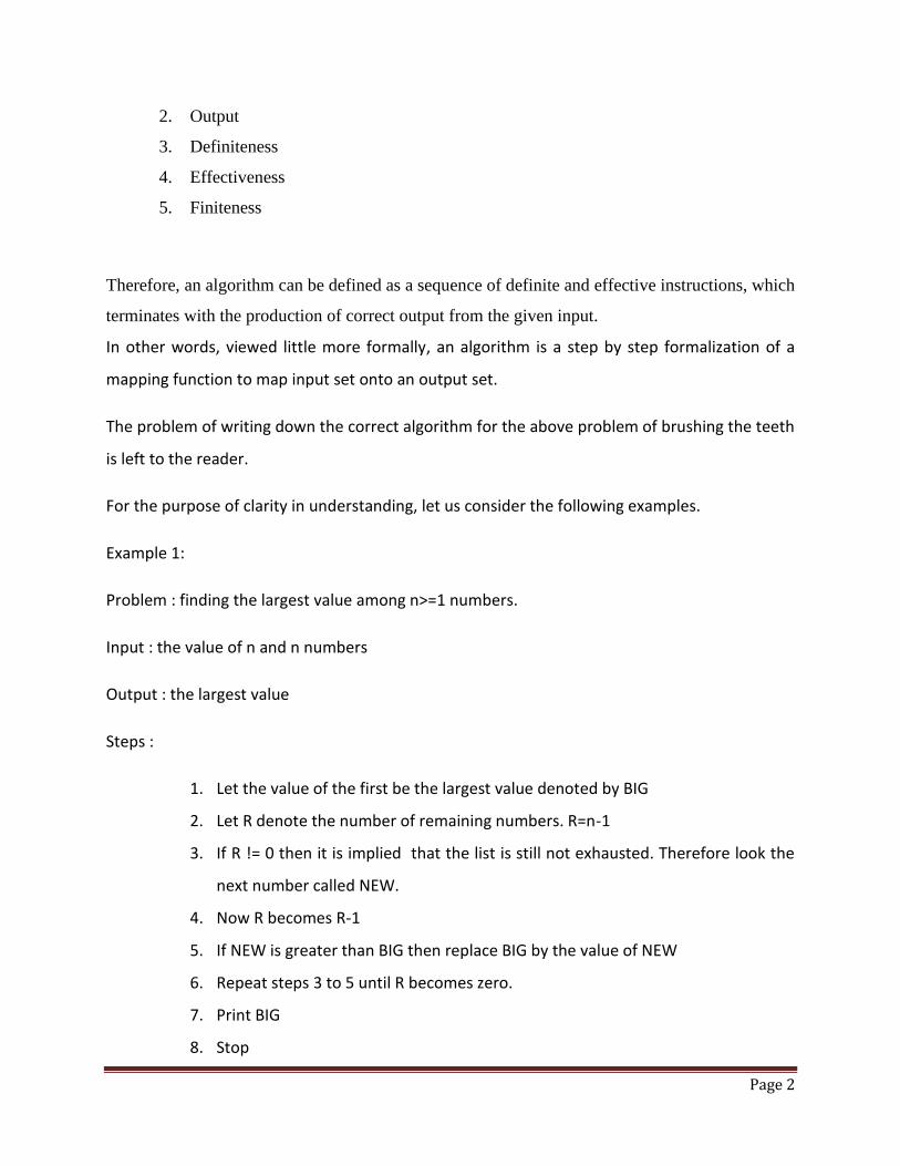
Example 1:

Problem : finding the largest value among n>=1 numbers.

Input : the value of n and n numbers

Output : the largest value

Steps :

1. Let the value of the first be the largest value denoted by BIG

2. Let R denote the number of remaining numbers. R=n-1

3. If R != 0 then it is implied that the list is still not exhausted. Therefore look the

next number called NEW.

4. Now R becomes R-1

5. If NEW is greater than BIG then replace BIG by the value of NEW

6. Repeat steps 3 to 5 until R becomes zero.

7. Print BIG

8. Stop

Page 3

End of algorithm

• Analyze the algorithm

– Time Complexity : time needed to execute the algorithm

• Worse case, best case, average case.

• For some algorithms, worst case occurs often, average case is often

roughly as bad as the worst case. So generally, worse case running time.

– Space Complexity: space needed to execute the algorithm

• Worst case

Provides an upper bound on running time

An absolute guarantee

• Average case

Provides the expected running time

• Best case

Provides an lower bound on running time

Asymptotic notation

Definition

Page 4

Page 5

Page 6

Page 7

Page 8

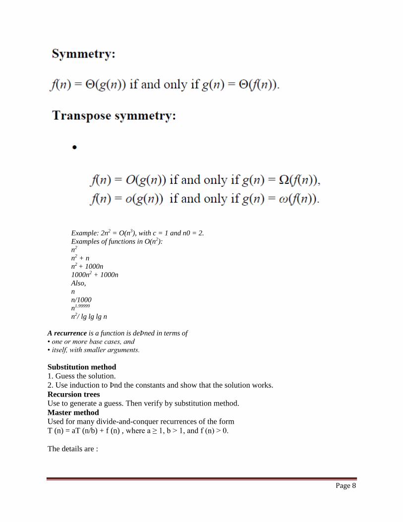
Example: 2n2 = O(n3), with c = 1 and n0 = 2.

Examples of functions in O(n2):

n2

n2 + n

n2 + 1000n

1000n2 + 1000n

Also,

n

n/1000

n1.99999

n2/ lg lg lg n

A recurrence is a function is deÞned in terms of

• one or more base cases, and

• itself, with smaller arguments.

Substitution method

1. Guess the solution.

2. Use induction to Þnd the constants and show that the solution works.

Recursion trees

Use to generate a guess. Then verify by substitution method.

Master method

Used for many divide-and-conquer recurrences of the form

T (n) = aT (n/b) + f (n) , where a ≥ 1, b > 1, and f (n) > 0.

The details are :

Page 9

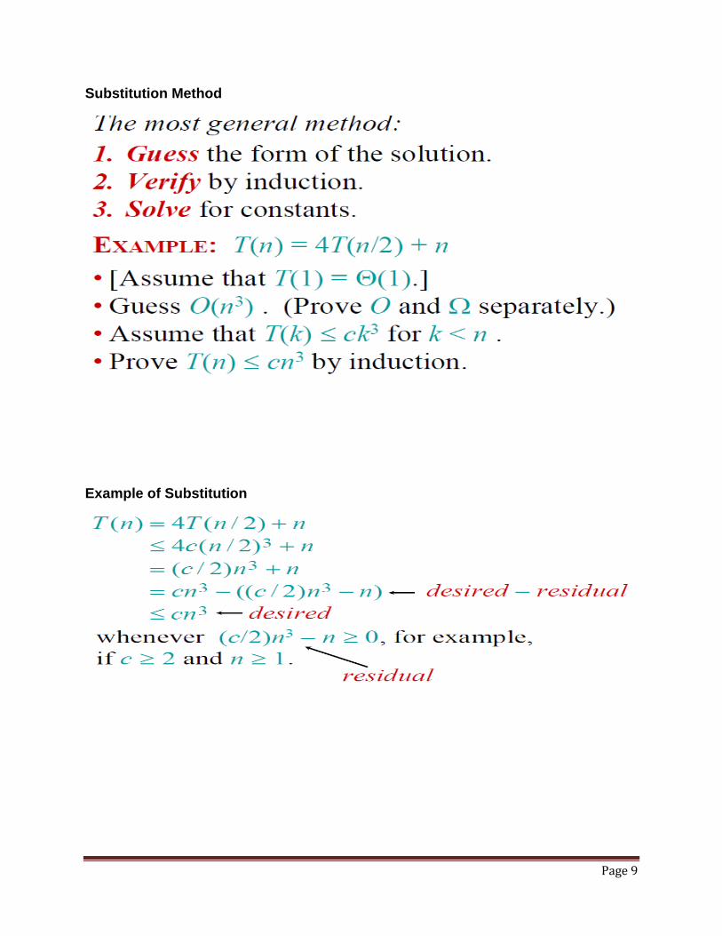
Substitution Method

Example of Substitution

Page 10

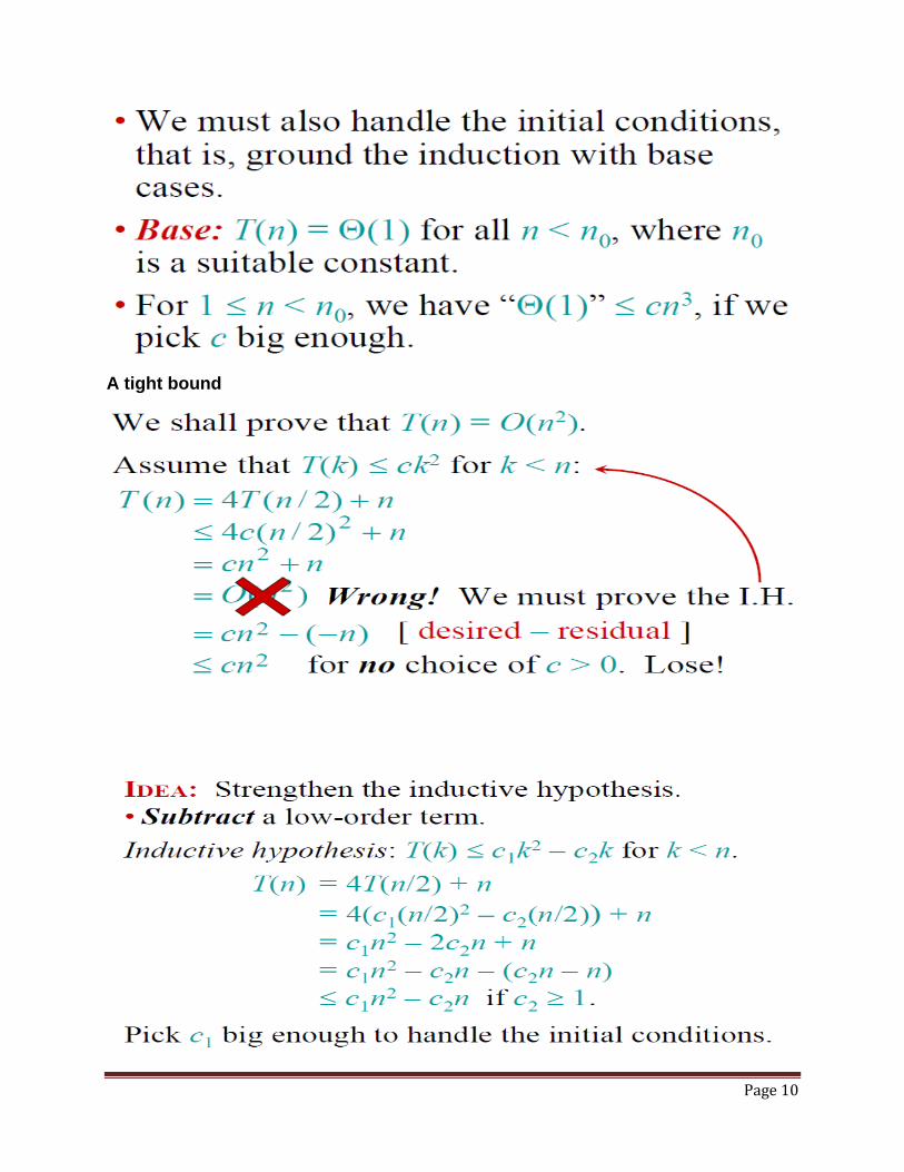
A tight bound

Page 11

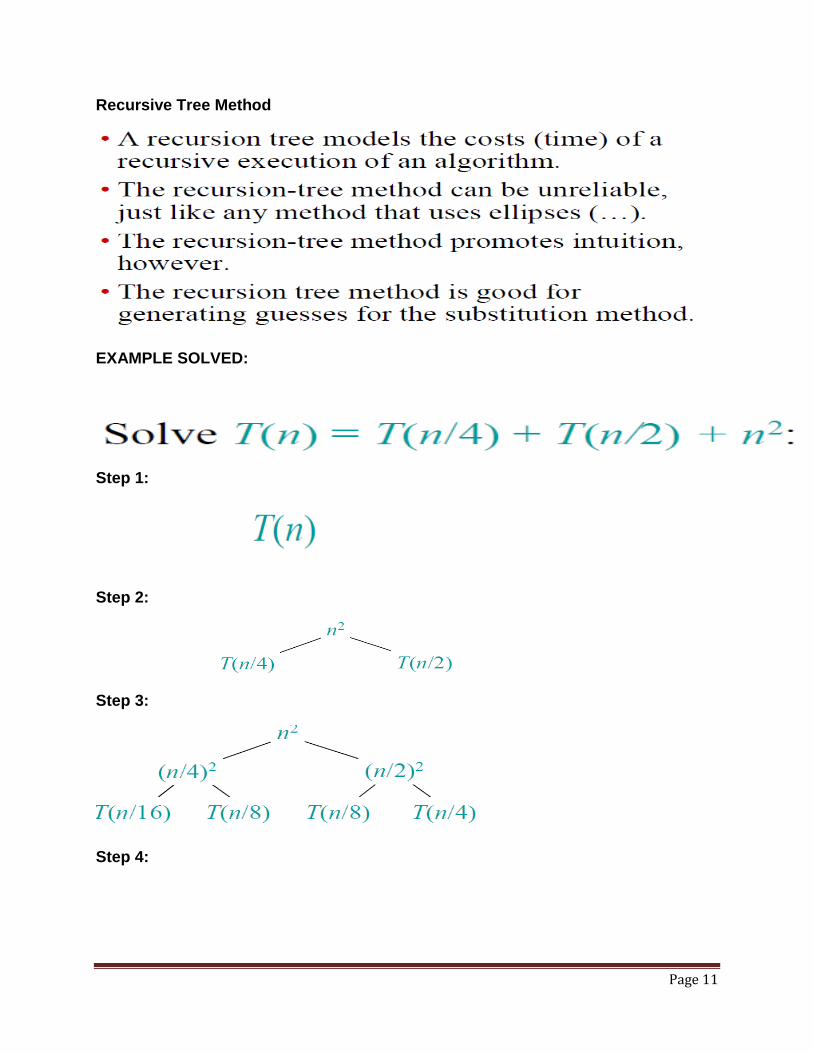
Recursive Tree Method

EXAMPLE SOLVED:

Step 1:

Step 2:

Step 3:

Step 4:

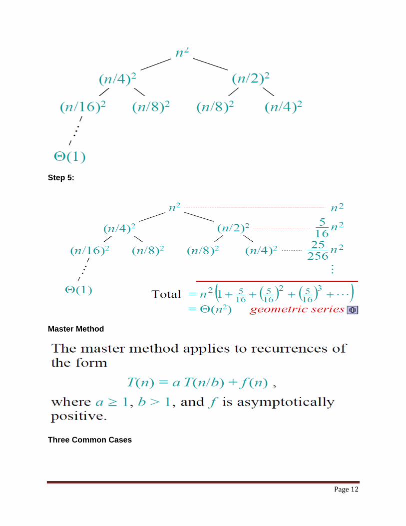
Page 12

Step 5:

Master Method

Three Common Cases

Page 13

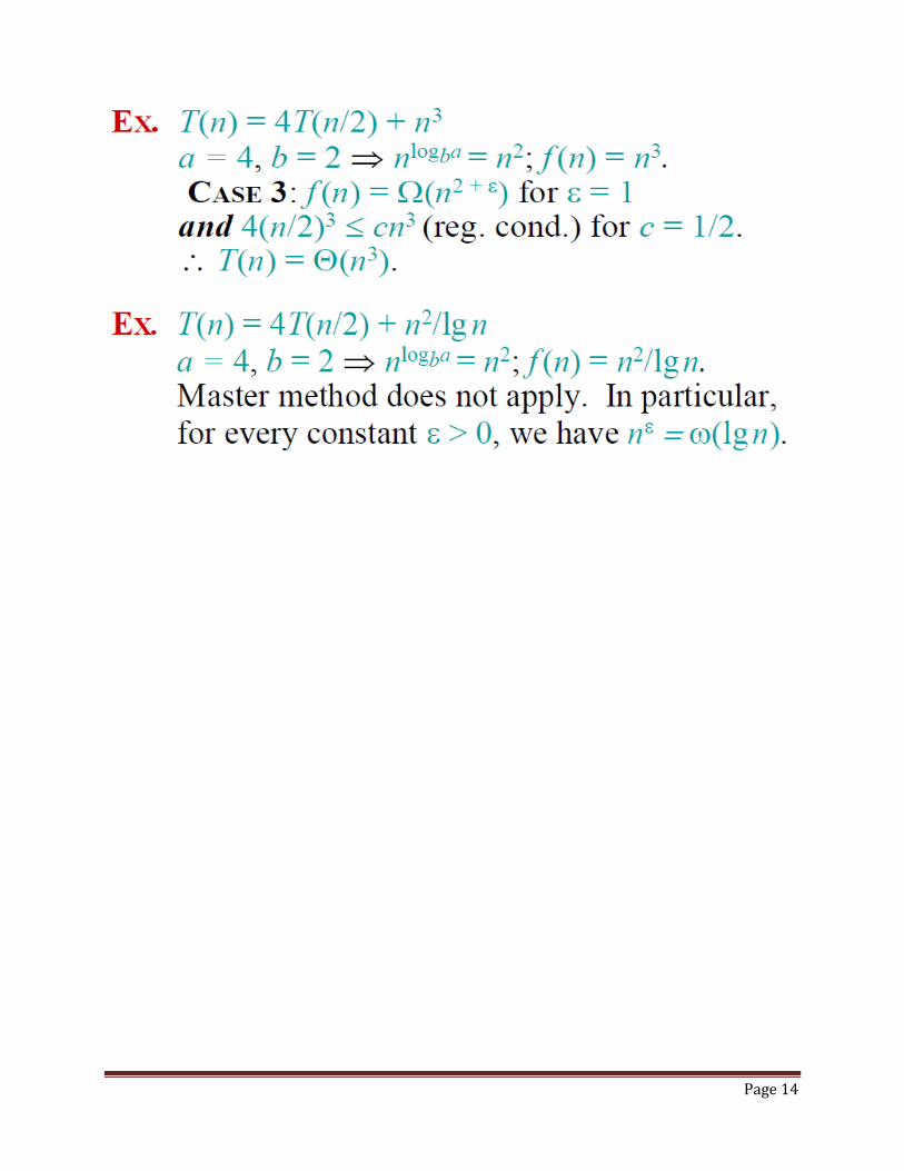
Page 14

Page 15

Chapter 2: Divide-and-conquer

Divide-and-conquer is a top-down technique for designing algorithms that consists of dividing

the problem into smaller sub problems hoping that the solutions of the sub problems are easier to

find and then composing the partial solutions into the solution of the original problem.

Little more formally, divide-and-conquer paradigm consists of following major phases:

Divide : divide the problem into several sub-problems that are similar to the original

problem but smaller in size,

Solve the sub-problem recursively (successively and independently), If sub problem is

small enough, solve it in a straightforward manner (base case).

Combine: Combine these solutions to sub problems to create a solution to the original

problem.

Divide and Conquer Examples

Binary Search

Heap Construction

Tower of Hanoi

Quick Sort

Merge Sort

Multiplying large Integers

Exponentiation

Matrix Multiplication (Strassen’s way)

Binary Search (simplest application of divide-and-conquer)

Binary Search is an extremely well-known instance of divide-and-conquer paradigm. Given an

ordered array of n elements, the basic idea of binary search is that for a given element we

"probe" the middle element of the array. We continue in either the lower or upper segment of the

array, depending on the outcome of the probe until we reached the required (given) element.

Problem Let A[1 . . . n] be an array of non-decreasing sorted order; that is A [i] ≤ A [j]

whenever 1 ≤ i ≤ j ≤ n. Let 'q' be the query point. The problem consist of finding 'q' in the

array A. If q is not in A, then find the position where 'q' might be inserted.

Formally, find the index i such that 1 ≤ i ≤ n+1 and A[i-1] < x ≤ A[i].

Binary Search

Look for 'q' either in the first half or in the second half of the array A. Compare 'q' to an element

in the middle, n/2 , of the array. Let k = n/2 . If q ≤ A[k], then search in the A[1 . . . k];

otherwise search T[k+1 . . n] for 'q'. Binary search for q in subarray A[i . . j] with the promise

that

A[i-1] < x ≤ A[j]

If i = j then

return i (index)

k= (i + j)/2

if q ≤ A [k]

Page 16

then return Binary Search [A [i-k], q]

else return Binary Search [A[k+1 . . j], q]

Analysis

Binary Search can be accomplished in logarithmic time in the worst case , i.e., T(n) = θ(log n).

This version of the binary search takes logarithmic time in the best case.

Quick Sort

The basic version of quick sort algorithm was invented by C. A. R. Hoare in 1960 and

formally introduced quick sort in 1962. It is used on the principle of divide-and-

conquer. Quick sort is an algorithm of choice in many situations because it is not difficult to

implement, it is a good "general purpose" sort and it consumes relatively fewer resources during

execution.

Good points

It is in-place since it uses only a small auxiliary stack.

It requires only n log(n) time to sort n items.

It has an extremely short inner loop

This algorithm has been subjected to a thorough mathematical analysis, a very precise

statement can be made about performance issues.

Bad Points

It is recursive. Especially if recursion is not available, the implementation is extremely

complicated.

It requires quadratic (i.e., n2) time in the worst-case.

It is fragile i.e., a simple mistake in the implementation can go unnoticed and cause it to

perform badly.

Quick sort works by partitioning a given array A[p . . r] into two non-empty sub array A[p . . q]

and A[q+1 . . r] such that every key in A[p . . q] is less than or equal to every key in A[q+1 . . r].

Then the two subarrays are sorted by recursive calls to Quick sort. The exact position of the

partition depends on the given array and index q is computed as a part of the partitioning

procedure.

QuickSort

1. If p < r then

2. q Partition (A, p, r)

3. Recursive call to Quick Sort (A, p, q)

4. Recursive call to Quick Sort (A, q + r, r)

Note that to sort entire array, the initial call Quick Sort (A, 1, length[A])

As a first step, Quick Sort chooses as pivot one of the items in the array to be sorted. Then array

is then partitioned on either side of the pivot. Elements that are less than or equal to pivot will

move toward the left and elements that are greater than or equal to pivot will move toward the

right.

Partitioning the Array

Partitioning procedure rearranges the subarrays in-place.

Page 17

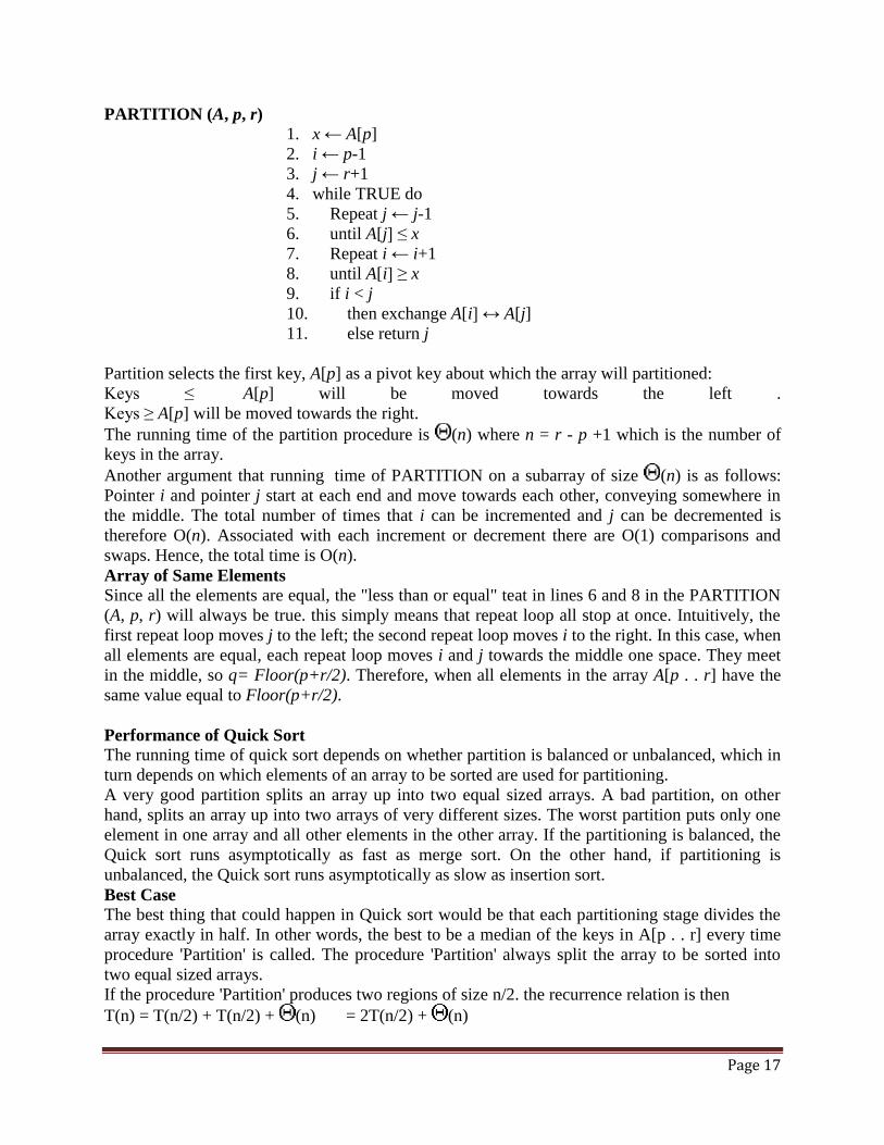
PARTITION (A, p, r) 1. x ← A[p]

2. i ← p-1

3. j ← r+1

4. while TRUE do

5. Repeat j ← j-1

6. until A[j] ≤ x

7. Repeat i ← i+1

8. until A[i] ≥ x

9. if i < j

10. then exchange A[i] ↔ A[j]

11. else return j

Partition selects the first key, A[p] as a pivot key about which the array will partitioned:

Keys ≤ A[p] will be moved towards the left .

Keys ≥ A[p] will be moved towards the right.

The running time of the partition procedure is (n) where n = r - p +1 which is the number of

keys in the array.

Another argument that running time of PARTITION on a subarray of size (n) is as follows:

Pointer i and pointer j start at each end and move towards each other, conveying somewhere in

the middle. The total number of times that i can be incremented and j can be decremented is

therefore O(n). Associated with each increment or decrement there are O(1) comparisons and

swaps. Hence, the total time is O(n).

Array of Same Elements

Since all the elements are equal, the "less than or equal" teat in lines 6 and 8 in the PARTITION

(A, p, r) will always be true. this simply means that repeat loop all stop at once. Intuitively, the

first repeat loop moves j to the left; the second repeat loop moves i to the right. In this case, when

all elements are equal, each repeat loop moves i and j towards the middle one space. They meet

in the middle, so q= Floor(p+r/2). Therefore, when all elements in the array A[p . . r] have the

same value equal to Floor(p+r/2).

Performance of Quick Sort

The running time of quick sort depends on whether partition is balanced or unbalanced, which in

turn depends on which elements of an array to be sorted are used for partitioning.

A very good partition splits an array up into two equal sized arrays. A bad partition, on other

hand, splits an array up into two arrays of very different sizes. The worst partition puts only one

element in one array and all other elements in the other array. If the partitioning is balanced, the

Quick sort runs asymptotically as fast as merge sort. On the other hand, if partitioning is

unbalanced, the Quick sort runs asymptotically as slow as insertion sort.

Best Case

The best thing that could happen in Quick sort would be that each partitioning stage divides the

array exactly in half. In other words, the best to be a median of the keys in A[p . . r] every time

procedure 'Partition' is called. The procedure 'Partition' always split the array to be sorted into

two equal sized arrays.

If the procedure 'Partition' produces two regions of size n/2. the recurrence relation is then

T(n) = T(n/2) + T(n/2) + (n) = 2T(n/2) + (n)

Page 18

And from case 2 of Master theorem

T(n) = (n lg n)

Worst case The worst-case occurs if given array A[1 . . n] is already sorted. The PARTITION (A, p, r) call

always return p so successive calls to partition will split arrays of length n, n-1, n-2, . . . , 2 and

running time proportional to n + (n-1) + (n-2) + . . . + 2 = [(n+2)(n-1)]/2 = (n2). The worst-case

also occurs if A[1 . . n] starts out in reverse order.

Merge Sort

Merge-sort is based on the divide-and-conquer paradigm. The Merge-sort algorithm can be

described in general terms as consisting of the following three steps:

1. Divide Step

If given array A has zero or one element, return S; it is already sorted. Otherwise, divide

A into two arrays, A1 and A2, each containing about half of the elements of A.

2. Recursion Step

Recursively sort array A1 and A2.

3. Conquer Step

Combine the elements back in A by merging the sorted arrays A1 and A2 into a sorted

sequence.

We can visualize Merge-sort by means of binary tree where each node of the tree represents a

recursive call and each external nodes represent individual elements of given array A. Such a tree

is called Merge-sort tree. The heart of the Merge-sort algorithm is conquer step, which merge

two sorted sequences into a single sorted sequence.

Page 19

To begin, suppose that we have two sorted arrays A1[1], A1[2], . . , A1[M] and A2[1], A2[2], . . . ,

A2[N]. The following is a direct algorithm of the obvious strategy of successively choosing the

smallest remaining elements from A1 to A2 and putting it in A.

MERGE (A1, A2, A)

i.← j 1

A1[m+1], A2[n+1] ← INT_MAX

For k ←1 to m + n do

if A1[i] < A2[j]

then A[k] ← A1[i]

i ← i +1

else

A[k] ← A2[j]

j ← j + 1

Merge Sort Algorithm

MERGE_SORT (A)

Page 20

A1[1 . . n/2 ] ← A[1 . . n/2 ]

A2[1 . . n/2 ] ← A[1 + n/2 . . n]

Merge Sort (A1)

Merge Sort (A1)

Merge Sort (A1, A2, A)

Analysis

Let T(n) be the time taken by this algorithm to sort an array of n elements dividing A into

subarrays A1 and A2 takes linear time. It is easy to see that the Merge (A1, A2, A) also takes the

linear time. Consequently,

T(n) = T( n/2 ) + T( n/2 ) + θ(n)

for simplicity

T(n) = 2T (n/2) + θ(n)

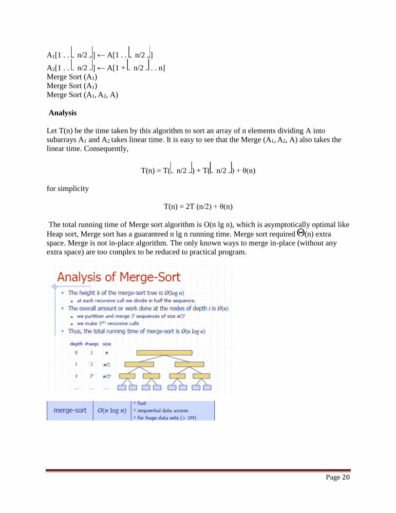
The total running time of Merge sort algorithm is O(n lg n), which is asymptotically optimal like

Heap sort, Merge sort has a guaranteed n lg n running time. Merge sort required (n) extra

space. Merge is not in-place algorithm. The only known ways to merge in-place (without any

extra space) are too complex to be reduced to practical program.

Page 21

Chapter 3: Greedy Algorithm Greedy algorithm make a locally optimal choice in hope of getting a globally optimal solution.

Greedy-choice property A globally optimal solution can be arrived at by making a locally optimal (greedy) choice. Difference between greedy and dynamic programming: Dynamic programming: • Make a choice at each step. • Choice depends on knowing optimal solutions to subproblems. Solve subproblems first. • Solve bottom-up. Greedy: • Make a choice at each step. • Make the choice before solving the subproblems. • Solve top-down. Typically show the greedy-choice property by what we did for activity selection: • Look at a globally optimal solution. • If it includes the greedy choice, done. • Else, modify it to include the greedy choice, yielding another solution that’s just as good. Can get efficiency gains from greedy-choice property. • Preprocess input to put it into greedy order. • Or, if dynamic data, use a priority queue. The knapsack problem is a good example of the difference. 0-1 knapsack problem: • n items. • Item i is worth $vi , weighs wi pounds.

• Find a most valuable subset of items with total weight ≤ W.

• Have to either take an item or not take it.can.t take part of it. Fractional knapsack problem: Like the 0-1 knapsack problem, but can take fraction of an item. Both have optimal substructure. But the fractional knapsack problem has the greedy-choice property, and the 0-1 knapsack problem does not. To solve the fractional problem, rank items by value/weight: vi/wi .

Knapsack Problem

There are n items in a store. For i =1,2, . . . , n, item i has weight wi > 0 and worth vi > 0. Thief can carry a maximum weight of W pounds in a knapsack. In this version of a problem the items can be broken into smaller piece, so the thief may decide to carry only a fraction xi of object i, where 0 ≤ xi ≤ 1. Item i contributes xiwi to the total weight in the knapsack, and xivi to the value of the load.

In Symbol, the fraction knapsack problem can be stated as follows. maximize nSi=1 xivi subject to constraint nSi=1 xiwi ≤ W

Page 22

It is clear that an optimal solution must fill the knapsack exactly, for otherwise we could add a fraction of one of the remaining objects and increase the value of the load. Thus in an optimal solution nSi=1 xiwi = W.

knapsack (w, v, W)

FOR i =1 to n do x[i] =0 weight = 0 while weight < W do i = best remaining item IF weight + w[i] ≤ W then x[i] = 1 weight = weight + w[i] else x[i] = (w - weight) / w[i] weight = W return x

Analysis

If the items are already sorted into decreasing order of vi / wi, then the while-loop takes a time in O(n) Therefore, the total time including the sort is in O(n log n).

Minimum Spanning Tree Kruskal’s Algorithm: 1. Kruskal’s Algorithm is a greedy algorithm because at each step it adds to the forest

an edge of least possible weight.

2. It uses disjoint set data structures to maintain several disjoint elements. Each set

Contains the vertices in a tree of the current forest.

3. Using FINDSET we determine whether two vertices u and v belong to the same tree

The combining of two trees is done by UNION.

4. With each node ‘x’ we maintain the integer rank[x] which is an upper bound on the

Height x[the number of edges in the longest path between a descendent leaf and x].

5. Algorithm:

Page 23

MST-KRUSKAL(G, w)

1 A ← Ø

2 for each vertex v _ V[G]

3 do MAKE-SET(v)

4 sort the edges of E into nondecreasing order by weight w

5 for each edge (u, v) _ E, taken in nondecreasing order by weight

6 do if FIND-SET(u) ≠ FIND-SET(v)

7 then A ← A _ {(u, v)}

8 UNION(u, v)

9 return A

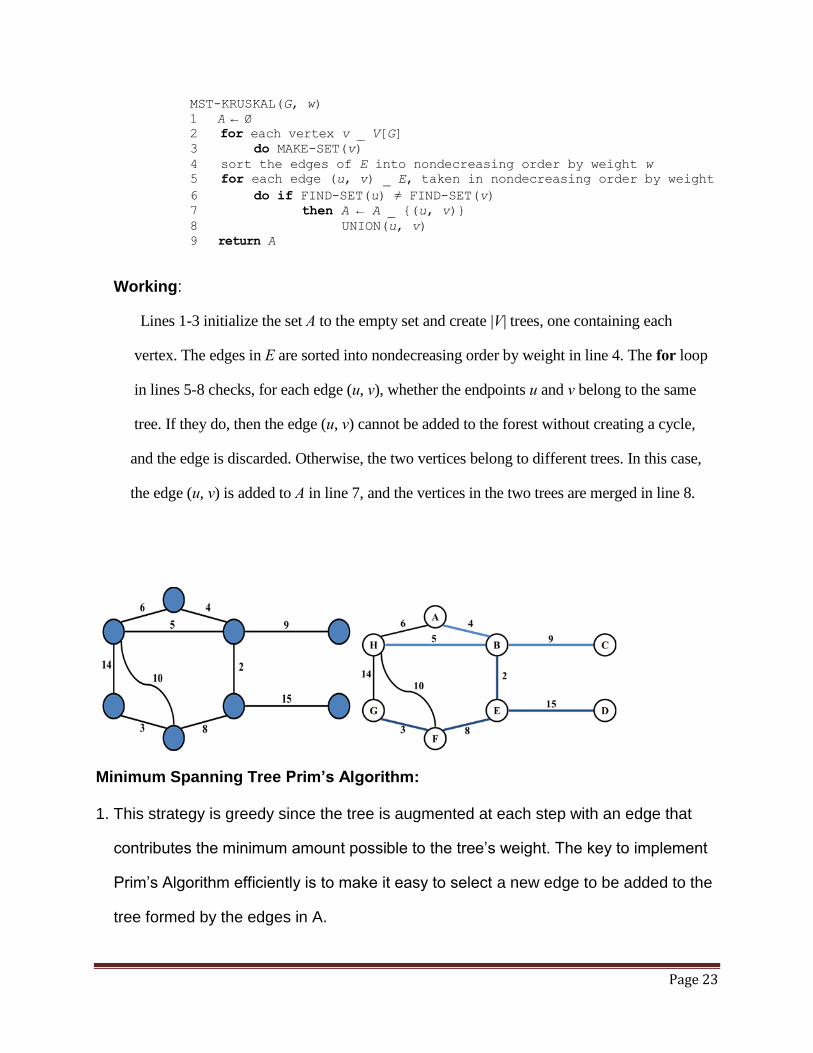
Working:

Lines 1-3 initialize the set A to the empty set and create |V| trees, one containing each

vertex. The edges in E are sorted into nondecreasing order by weight in line 4. The for loop

in lines 5-8 checks, for each edge (u, v), whether the endpoints u and v belong to the same

tree. If they do, then the edge (u, v) cannot be added to the forest without creating a cycle,

and the edge is discarded. Otherwise, the two vertices belong to different trees. In this case,

the edge (u, v) is added to A in line 7, and the vertices in the two trees are merged in line 8.

Minimum Spanning Tree Prim’s Algorithm: 1. This strategy is greedy since the tree is augmented at each step with an edge that

contributes the minimum amount possible to the tree’s weight. The key to implement

Prim’s Algorithm efficiently is to make it easy to select a new edge to be added to the

tree formed by the edges in A.

Page 24

2. The tree starts from an arbitrary root vertex r and grows until the tree spans all the

vertices in V. At each step, a light edge is added to the tree A that connects A to

an isolated vertex of GA = (V, A).

3. Algorithm:

MST-PRIM(G, w, r) 1 for each u _ V [G]

2 do key[u] ← ∞

3 π[u] ← NIL

4 key[r] ← 0

5 Q ← V [G]

6 while Q ≠ Ø

7 do u ← EXTRACT-MIN(Q)

8 for each v _ Adj[u]

9 do if v _ Q and w(u, v) < key[v]

10 then π[v] ← u

11 key[v] ← w(u, v)

Working:

Lines 1-5 set the key of each vertex to ∞ (except for the root r, whose key is set to 0 so that it will be the first vertex processed), set the parent of each vertex to NIL, and initialize the min-priority queue Q to contain all the vertices. The algorithm maintains the following three-part loop invariant:

Prior to each iteration of the while loop of lines 6-11,

1. A = {(v, π[v]) : v _ V - {r} - Q}. 2. The vertices already placed into the minimum spanning tree are those in V - Q. 3. For all vertices v _ Q, if π[v] ≠ NIL, then key[v] < ∞ and key[v] is the weight of a light edge (v, π[v]) connecting v to some vertex already placed into the minimum spanning tree. Line 7 identifies a vertex u _ Q incident on a light edge crossing the cut (V -Q, Q) (with the exception of the first iteration, in which u = r due to line 4). Removing u from the set Q adds it to the set V - Q of vertices in the tree, thus adding (u, π[u]) to A. The for loop of lines 8-11 update the key and π fields of every vertex v adjacent to u but not in the tree. The updating maintains the third part of the loop invariant.

Dijkstra's algorithm: Dijkstra's algorithm solves the single-source shortest-path problem when

all edges have non-negative weights. It is a greedy algorithm and similar to Prim's algorithm.

Algorithm starts at the source vertex, s, it grows a tree, T, that ultimately spans all vertices

reachable from S. Vertices are added to T in order of distance i.e., first S, then the vertex closest

Page 25

to S, then the next closest, and so on. Following implementation assumes that graph G is

represented by adjacency lists.

DIJKSTRA (G, w, s)

1. INITIALIZE SINGLE-SOURCE (G, s)

2. S ← { } // S will ultimately contains vertices of final shortest-

path weights from s

3. Initialize priority queue Q i.e., Q ← V[G]

4. while priority queue Q is not empty do

5. u ← EXTRACT_MIN(Q) // Pull out new vertex

6. S ← S È {u}

// Perform relaxation for each vertex v adjacent to u

7. for each vertex v in Adj[u] do

8. Relax (u, v, w)

Analysis

Like Prim's algorithm, Dijkstra's algorithm runs in O(|E|lg|V|) time.

All pair shortest path problem by Floyd’s algorithm

Page 26

Chapter 4 : Dynamic Programming

1. Dynamic programming, like the divide-and-conquer method, solves problems by combining the

solutions to subproblems.

2. divide-and-conquer algorithms partition the problem into independent subproblems, solve the

subproblems recursively, and then combine their solutions to solve the original problem. In

contrast, dynamic programming is applicable when the subproblems are not independent, that is,

when subproblems share subsubproblems.

3. A dynamic-programming algorithm solves every subsubproblem just once and

then saves its answer in a table, thereby avoiding the work of recomputing the

answer every time the subsubproblem is encountered.

4. Dynamic programming is typically applied to optimization problems. In such

Problems there can be many possible solutions. Each solution has a value, and we

wish to find a solution with the optimal (minimum or maximum) value. We call

such a solution an optimal solution to the problem, as opposed to the optimal

solution, since there may be several solutions that achieve the optimal value.

5. The development of a dynamic-programming algorithm can be broken into a

Sequence of four steps.

1. Characterize the structure of an optimal solution.

2. Recursively define the value of an optimal solution.

3. Compute the value of an optimal solution in a bottom-up fashion.

4. Construct an optimal solution from computed information.

6. Steps 1-3 form the basis of a dynamic-programming solution to a problem. Step

4 can be omitted if only the value of an optimal solution is required. When we

do perform step 4, we sometimes maintain additional information during the

computation in step 3 to ease the construction of an optimal solution.

7. Elements of Dynamic Programming

* Optimal Substructure

*Overlapping Subproblems

8. A problem exhibits optimal substructure if an optimal solution to the problem

contains within it optimal solutions to subproblems. Whenever a problem

exhibits optimal substructure, it is a good clue that dynamic programming might

apply.

9. Optimal substructure varies across problem domains in two ways:

Page 27

1. How many subproblems are used in an optimal solution to the original problem, and

2. How many choices we have in determining which subproblem(s) to use in an

optimal solution.

10. Overlapping subproblems :

The second ingredient that an optimization problem must have for dynamic programming to be

applicable is that the space of subproblems must be "small" in the sense that a recursive algorithm

for the problem solves the same subproblems over and over, rather than always generating new

subproblems. Typically, the total number of distinct subproblems is a polynomial in the input size.

When a recursive algorithm revisits the same problem over and over again, we say that the

optimization problem has overlapping subproblems.

Optimal Matrix Chain Multiplication We are given a sequence of matrices to multiply:

A1 A2 A3 ... An Matrix multiplication is associative, so

A1 ( A2 A3 ) = ( A1 A2 ) A3 that is, we can can generate the product in two ways.

The cost of multiplying an nxm by an mxp one is O(nmp) (or O(n3) for two nxn ones). A poor choice of parenthesisation can be expensive: eg if we have

Matrix Rows Columns

A1 10 100

A2 100 5

A3 5 50

the cost for ( A1 A2 ) A3 is

A1A2 10x100x5 = 5000 => A1 A2 (10x5)

(A1A2) A3 10x5x50 = 2500 => A1A2A3 (10x50)

Total 7500

but for A1 ( A2 A3 )

A2A3 100x5x50 = 25000 => A2A3 (100x50)

A1(A2A3) 10x100x50 = 50000 => A1A2A3 (10x50)

Total 75000

Clearly demonstrating the benefit of calculating the optimum order before commencing the product calculation!

Optimal Sub-structure

As with the optimal binary search tree, we can observe that if we divide a chain of matrices to be multiplied into two optimal sub-chains:

(A1 A2 A3 ... Aj) (Aj+1 ... An )

Page 28

then the optimal parenthesisations of the sub-chains must be composed of optimal chains. If they were not, then we could replace them with cheaper parenthesisations.

This property, known as optimal sub-structure is a hallmark of dynamic algorithms: it enables us to solve the small problems (the sub-structure) and use those solutions to generate solutions to larger problems.

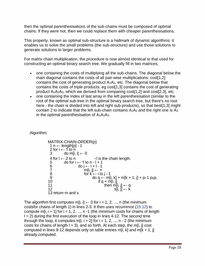
For matrix chain multiplication, the procedure is now almost identical to that used for constructing an optimal binary search tree. We gradually fill in two matrices,

one containing the costs of multiplying all the sub-chains. The diagonal below the main diagonal contains the costs of all pair-wise multiplications: cost[1,2] contains the cost of generating product A1A2, etc. The diagonal below that contains the costs of triple products: eg cost[1,3] contains the cost of generating product A1A2A3, which we derived from comparing cost[1,2] and cost[2,3], etc.

one containing the index of last array in the left parenthesisation (similar to the root of the optimal sub-tree in the optimal binary search tree, but there's no root here - the chain is divided into left and right sub-products), so that best[1,3] might contain 2 to indicate that the left sub-chain contains A1A2 and the right one is A3 in the optimal parenthesisation of A1A2A3.

Algorithm: MATRIX-CHAIN-ORDER(p) 1 n ← length[p] - 1 2 for i ← 1 to n 3 do m[i, i] ← 0

4 for l ← 2 to n ▹l is the chain length. 5 do for i ← 1 to n - l + 1 6 do j ← i + l - 1 7 m[i, j] ← ∞ 8 for k ← i to j - 1 9 do q ← m[i, k] + m[k + 1, j] + pi-1 pkpj

10 if q < m[i, j] 11 then m[i, j] ← q 12 s[i, j] ← k 13 return m and s

The algorithm first computes m[i, i] ← 0 for i = 1, 2, ..., n (the minimum costsfor chains of length 1) in lines 2-3. It then uses recurrence (15.12) to compute m[i, i + 1] for i = 1, 2, ..., n -1 (the minimum costs for chains of length l = 2) during the first execution of the loop in lines 4-12. The second time through the loop, it computes m[i, i + 2] for i = 1, 2, ..., n - 2 (the minimum costs for chains of length l = 3), and so forth. At each step, the m[i, j] cost computed in lines 9-12 depends only on table entries m[i, k] and m[k + 1, j] already computed.

Page 29

PRINT-OPTIMAL-PARENS(s, i, j) 1 if i = j 2 then print "A"i

3 else print "(" 4 PRINT-OPTIMAL-PARENS(s, i, s[i, j]) 5 PRINT-OPTIMAL-PARENS(s, s[i, j] + 1, j) 6 print ")"

The above algorithms are used to find optimal solution for the matrix.

Optimal binary search trees we are given a sequence K = k1, k2, ..., kn_ of n distinct keys in sorted order (so that k1 < k2 < ··· <

kn), and we wish to build a binary search tree from these keys. For each key ki, we have a

probability pi that a search will be for ki. Some searches may be for values not in K, and so we

also have n + 1 "dummy keys" d0, d1, d2, ..., dn representing values not in K. In particular, d0

represents all values less than k1, dn represents all values greater than kn, and for i = 1, 2, ..., n -1,

the dummy key di represents all values between ki and ki+1. For each dummy key di, we have a

probability qi that a search will correspond to di.

Problem

» Given sequence K = k1 < k

2 <··· < k

n of n sorted keys,with a search probability p

i for each key k

i.

» Want to build a binary search tree (BST) with minimum expected search cost.

» Actual cost of items examined.

» For key ki, cost = depth

T(k

i)+1, where depth

T(k

i) = depth of k

i in BST T .

Page 30

Expected Cost

n

i

iiT

n

i

n

i

iiiT

n

i

iiT

pk

ppk

pk

TE

1

1 1

1

)(depth1

)(depth

)1)(depth(

]in cost search [

Sum of probabilities is 1.

Example

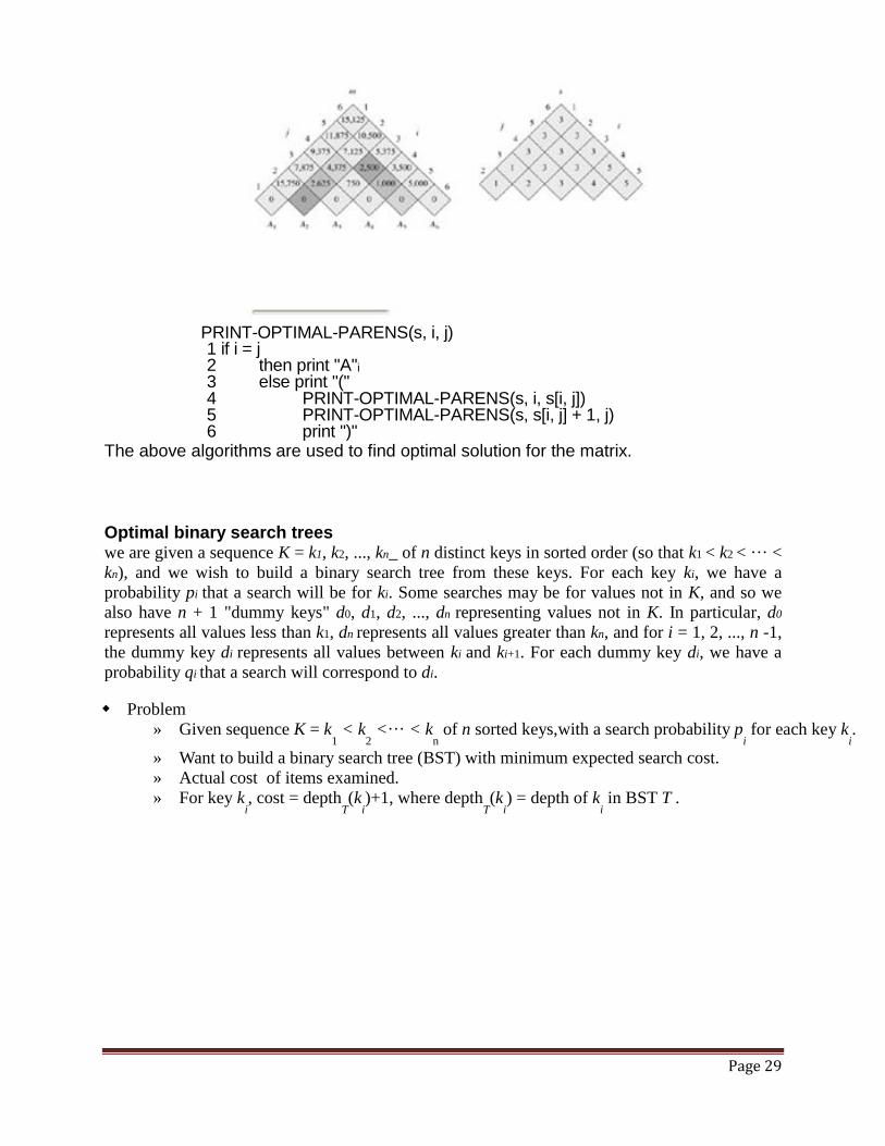
Consider 5 keys with these search probabilities: p1 = 0.25, p

2 = 0.2, p

3 = 0.05, p

4 = 0.2, p

5 = 0.3.

k2

k1 k

4

k3 k

5

i depthT(k

i) depth

T(k

i)·p

i

1 1 0.25

2 0 0

3 2 0.1

4 1 0.2

5 2 0.6

1.15

Therefore, E [search cost] = 2.15.

Page 31

Observations: » Optimal BST may not have smallest height.

» Optimal BST may not have highest-probability key at root.

Build by exhaustive checking?

» Construct each n-node BST.

» For each, assign keys and compute expected search cost.

» But there are (4n/n3/2) different BSTs with n nodes.

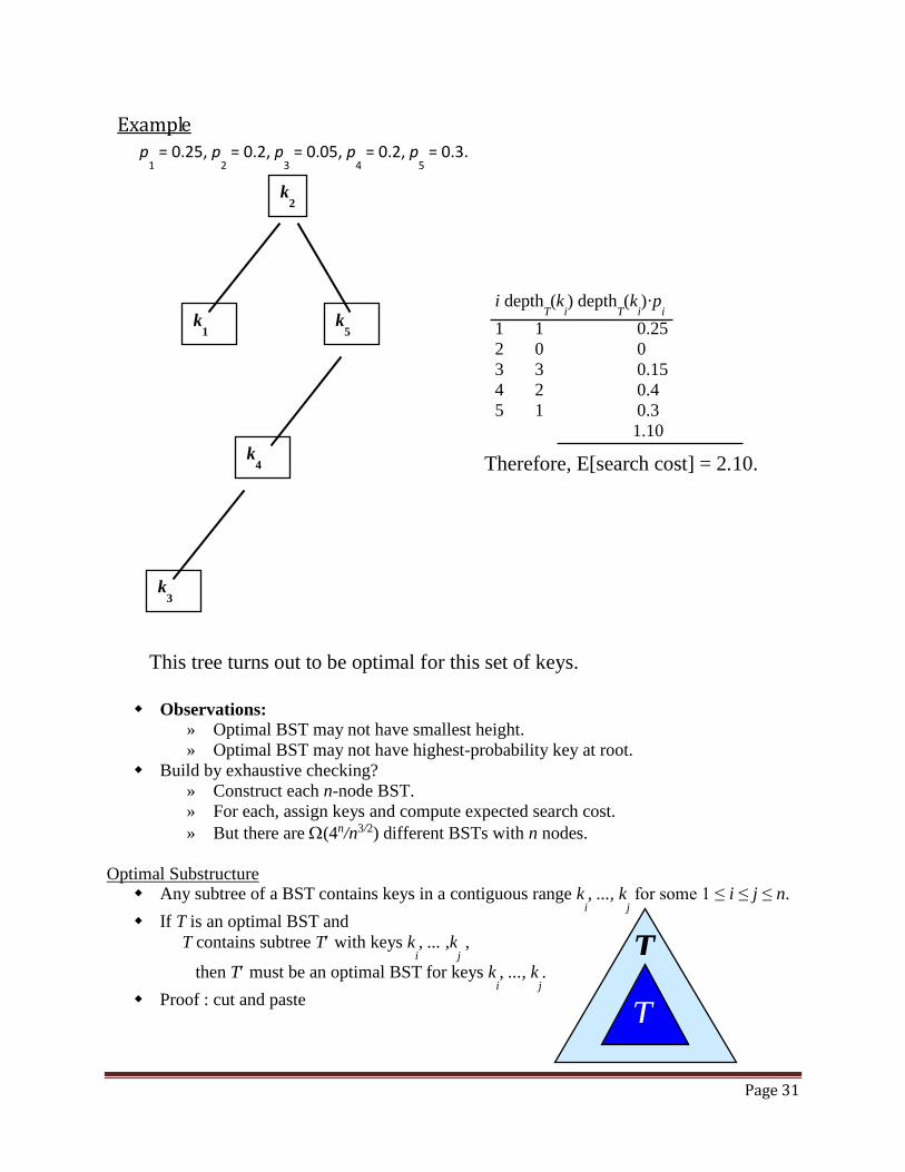
Optimal Substructure Any subtree of a BST contains keys in a contiguous range k

i, ..., k

j for some 1 ≤ i ≤ j ≤ n.

If T is an optimal BST and

T contains subtree T with keys ki, ... ,k

j ,

then T must be an optimal BST for keys ki, ..., k

j.

Proof : cut and paste

Example

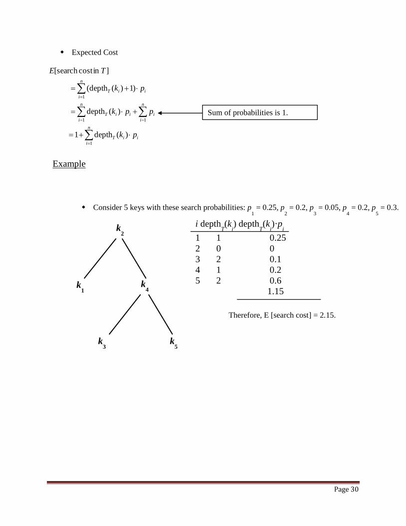
p1 = 0.25, p

2 = 0.2, p

3 = 0.05, p

4 = 0.2, p

5 = 0.3.

i depthT(k

i) depth

T(k

i)·p

i

1 1 0.25

2 0 0

3 3 0.15

4 2 0.4

5 1 0.3

1.10

Therefore, E[search cost] = 2.10.

k2

k1 k

5

k4

k3

This tree turns out to be optimal for this set of keys.

T

T

Page 32

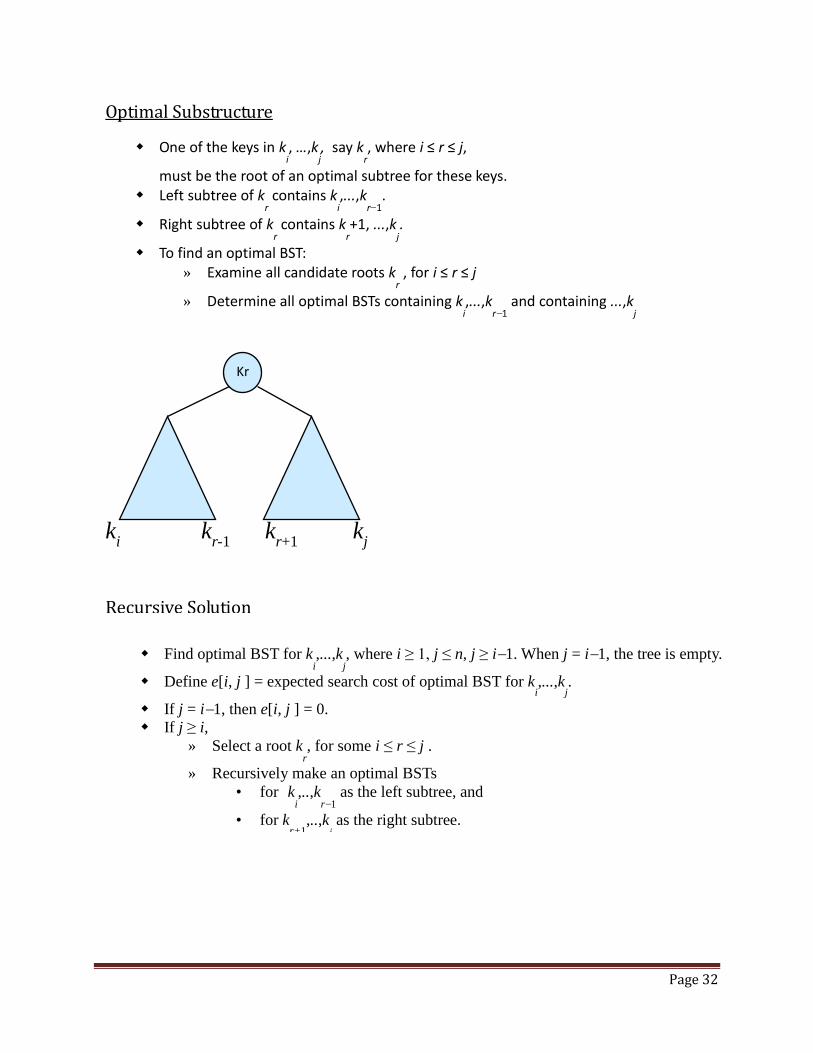
Optimal Substructure

One of the keys in ki, …,k

j, say k

r, where i ≤ r ≤ j,

must be the root of an optimal subtree for these keys. Left subtree of k

r contains k

i,...,k

r1.

Right subtree of kr contains k

r+1, ...,k

j.

To find an optimal BST: » Examine all candidate roots k

r , for i ≤ r ≤ j

» Determine all optimal BSTs containing ki,...,k

r1 and containing ...,k

j

kr

kr-1

kr+1

kj

Kr

ki k

r-1 k

r+1 k

j

Recursive Solution

Find optimal BST for ki,...,k

j, where i ≥ 1, j ≤ n, j ≥ i1. When j = i1, the tree is empty.

Define e[i, j ] = expected search cost of optimal BST for ki,...,k

j.

If j = i1, then e[i, j ] = 0.

If j ≥ i,

» Select a root kr, for some i ≤ r ≤ j .

» Recursively make an optimal BSTs

• for ki,..,k

r1 as the left subtree, and

• for kr+1

,..,kj as the right subtree.

Page 33

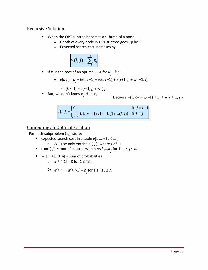
Recursive Solution

When the OPT subtree becomes a subtree of a node: » Depth of every node in OPT subtree goes up by 1. » Expected search cost increases by

If kr is the root of an optimal BST for k

i,..,k

j :

» e[i, j ] = pr + (e[i, r1] + w(i, r1))+(e[r+1, j] + w(r+1, j))

= e[i, r1] + e[r+1, j] + w(i, j). But, we don’t know k

r. Hence,

j

il

lpjiw ),(

(Because w(i, j)=w(i,r1) + pr + w(r + 1, j))

jijiwjrerie

ijjie

jri if)},(],1[]1,[{min

1 if0],[

Computing an Optimal Solution

For each subproblem (i,j), store: expected search cost in a table e[1 ..n+1 , 0 ..n]

» Will use only entries e[i, j ], where j ≥ i1. root[i, j ] = root of subtree with keys k

i,..,k

j, for 1 ≤ i ≤ j ≤ n.

w[1..n+1, 0..n] = sum of probabilities

» w[i, i1] = 0 for 1 ≤ i ≤ n.

» w[i, j ] = w[i, j-1] + pj for 1 ≤ i ≤ j ≤ n.

Page 34

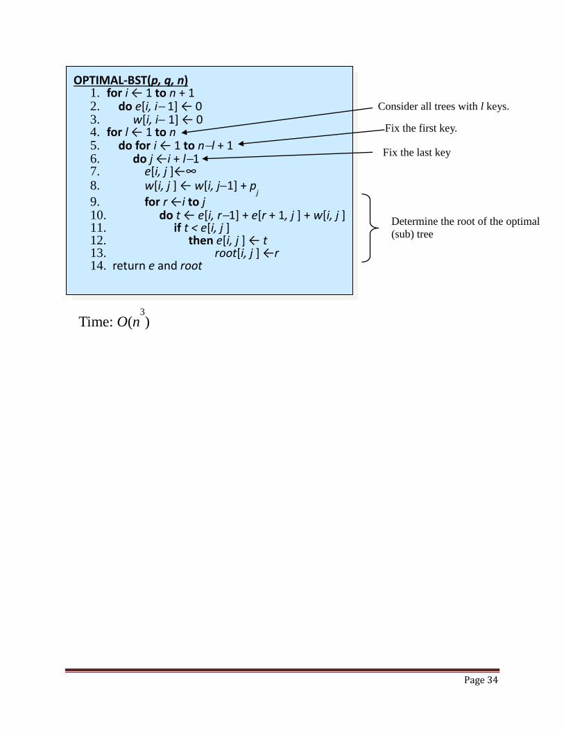
OPTIMAL-BST(p, q, n) 1. for i ← 1 to n + 1 2. do e[i, i 1] ← 0 3. w[i, i 1] ← 0 4. for l ← 1 to n 5. do for i ← 1 to nl + 1 6. do j ←i + l1 7. e[i, j ]←∞ 8. w[i, j ] ← w[i, j1] + p

j

9. for r ←i to j 10. do t ← e[i, r1] + e[r + 1, j ] + w[i, j ] 11. if t < e[i, j ] 12. then e[i, j ] ← t 13. root[i, j ] ←r 14. return e and root

Time: O(n3

)

Consider all trees with l keys.

Fix the first key.

Fix the last key

Determine the root of the optimal

(sub) tree

Page 35

Chapter 5 Backtracking Algorithm

Backtracking is one of the design techniques used for solving such problems which deal with

searching for a set of solutions or which ask for an optimal solution satisfying some constraints

can be solved using the backtracking formulation. In backtracking method, the desired solution is

expressible as an n-tuple (x1,x2,….xn) where the xi are chosen from some finite set si often the

problem to be solved calls for finding one vector that maximizes(or minimizes or satisfies) a

criterion function P(x1,x2,…..xn). Sometimes it seeks all vectors that satisfy P. Many of the

problems we solve using backtracking require that all the solution using backtracking require

that all the solution satisfy a complex set of constraints. These constraints are divided into two

categories, for any problem. The constraints may be explicit or implicit.

Explicit constraints are rules, which restrict each vector element to be chosen from the given set.

Implicit constraints are rules, which determine which of the tuples in the solution space, actually

satisfy the criterion function.

Explicit constraint are rules that restrict each xi to take on values only from a given set. Some

examples that are common for explicit constraints are:

xi >= 0 or Si = {all non negative real numbers}

xi = 0 or 1 or Si = {0,1}

li <= xi <= ui or Si = { ai li <= a <= ui}

The explicit constraints depend on the particular instance depend on the particular instance l if a

particular instance l of a particular being solved. All tuples that satisfy the explicit constraints

define a possible solution space for 1.The implicit constraints are rules that determine which of

the tuples in the solution space of I satisfy the criterion function. Thus implicit constraints

describe the way in which the xi must relate to each other.

The major advantage of this algorithm is that if it is realized that the partial vector generated

does not lead to an optimal solution then that vector may be ignored.

Backtracking algorithm determine the solution by systematically searching the solution space for

the given problem. This search is accomplished by using a free organization. Backtracking is a

depth first search with some bounding function.

Applications of Back Tracking:

The most widespread application of backtracking is the execution of back tracking is the

execution of regular expression. For Example, the simple pattern “a*a” will fail to match the

sequence “aa” without backtracking (because on the first pass, both a’s are eaten by “*” leaving

nothing behind for the remaining “a” to match. Another common use of backtracking is in path

finding algorithms where the function traces over a graph of nodes and backtracks until it finds

the least cost path. Backtracking is used in the implementation of programming languages and

Page 36

other areas such as text parsing. Backtracking is also utilized in the difference engine for the

mediawiki software.

8 queen problem

The 8 queen problem can be stated as follows. Consider a chessboard of order 8X8. The

problem is to place 8 queens on this board such that no two queens are can attack each other.

1. If the remainder from dividing N by 6 is not 2 or 3 then the list is simply all even numbers

followed by all odd numbers ≤ N

2. Otherwise, write separate lists of even and odd numbers (i.e. 2,4,6,8 - 1,3,5,7)

3. If the remainder is 2, swap 1 and 3 in odd list and move 5 to the end (i.e. 3,1,7,5)

4. If the remainder is 3, move 2 to the end of even list and 1,3 to the end of odd list (i.e.

4,6,8,2 - 5,7,1,3)

5. Append odd list to the even list and place queens in the rows given by these numbers, from

left to right (i.e. a2, b4, c6, d8, e3, f1, g7, h5)

For N = 8 this results in the solution shown above.

GRAPH COLORING A coloring of a graph is an assignment of a color to each vertex of the graph so that no two vertices

connected by an edge have the same color. It is not hard to see that our problem is one of coloring the

graph of incompatible turns using as few colors as possible.

The problem of coloring graphs has been studied for many decades, and the theory of algorithms tells

us a lot about this problem. Unfortunately, coloring an arbitrary graph with as few colors as possible

is one of a large class of problems called "NP-complete problems," for which all known solutions are

essentially of the type "try all possibilities."

A k-coloring of an undirected graph G = (V, E) is a function c : V → {1, 2,..., k} such that c(u) ≠ c(v) for every edge (u, v) E. In other words, the numbers 1, 2,..., k represent the k colors, and adjacent vertices must have different colors. The graph-coloring problem is to determine the minimum number of colors needed to color a given graph. Hamiltonian cycle

A Hamiltonian cycle is a cycle in a graph passing through all the vertices once

Page 37

Chapter 6 Branch and Bound

The term branch and bound refer to all state space search methods in which all possible branches

are derived before any other node can become the E-node. In other words the exploration of a

new node cannot begin until the current node is completely explored.

Branch and bound (BB or B&B) is an algorithm design paradigm

for discrete and combinatorial optimization problems. A branch-and-bound algorithm consists of

a systematic enumeration of candidate solutions by means of state space search: the set of

candidate solutions is thought of as forming a rooted tree with the full set at the root. The

algorithm explores branches of this tree, which represent subsets of the solution set. Before

enumerating the candidate solutions of a branch, the branch is checked against upper and lower

estimated bounds on the optimal solution, and is discarded if it cannot produce a better solution

than the best one found so far by the algorithm.

The method was first proposed by A. H. Land and A. G. Doig in 1960 for discrete programming,

and has become the most commonly used tool for solving NP-hard optimization problems.[2] The

name "branch and bound" first occurred in the work of Little et al. on the traveling salesman

problem

In order to facilitate a concrete description, we assume that the goal is to find the minimum value

of a function , where ranges over some set of admissible or candidate

solutions (the search space or feasible region). Note that one can find the maximum value

of by finding the minimum of . (For example, could be the set of all

possible trip schedules for a bus fleet, and could be the expected revenue for schedule .)

A branch-and-bound procedure requires two tools. The first one is a splitting procedure that,

given a set of candidates, returns two or more smaller sets whose union covers .

Note that the minimum of over is , where each is the minimum

of within . This step is called branching, since its recursive application defines a search

tree whose nodes are the subsets of .

The second tool is a procedure that computes upper and lower bounds for the minimum value

of within a given subset of . This step is called bounding.

The key idea of the BB algorithm is: if the lower bound for some tree node (set of candidates)

is greater than the upper bound for some other node , then may be safely discarded from

the search. This step is called pruning, and is usually implemented by maintaining a global

variable (shared among all nodes of the tree) that records the minimum upper bound seen

Page 38

among all subregions examined so far. Any node whose lower bound is greater than can be

discarded.

The recursion stops when the current candidate set is reduced to a single element, or when the

upper bound for set matches the lower bound. Either way, any element of will be a minimum

of the function within .

When is a vector of , branch and bound algorithms can be combined with interval

analysis and contractor techniques in order to provide guaranteed enclosures of the global

minimum.

Generic pseudocode

The following pseudocode is a skeleton branch and bound algorithm for minimizing an objective

function f. A bounding function g is used to compute lower bounds of f on nodes of the search

tree.

Using a heuristic, find a solution xh to the optimization problem. Store its value, B = f(xh).

(If no heuristic is available, set B to infinity.) B will denote the best solution found so far,

and will be used as an upper bound on candidate solutions.

Initialize a queue to hold a partial solution with none of the variables of the problem

assigned.

Loop until the queue is empty:

Take a node N off the queue.

If N represents a single candidate solution x and f(x) < B, then x is the best solution so

far. Record it and set B ← f(x).

Else, branch on N to produce new nodes Ni. For each of these:

If g(Ni) > B, do nothing; since the lower bound on this node is greater than the upper

bound of the problem, it will never lead to the optimal solution, and can be discarded.

Else, store Ni on the queue.

Several different queue data structures can be used. A stack (LIFO queue) will yield a depth-

first algorithm. A best-first branch and bound algorithm can be obtained by using apriority

queue that sorts nodes on their g-value

Applications

This approach is used for a number of NP-hard problems

Integer programming

Nonlinear programming

Page 39

Travelling salesman problem (TSP)[3][8]

Quadratic assignment problem (QAP)

Maximum satisfiability problem (MAX-SAT)

Nearest neighbor search (NNS)

Cutting stock problem

False noise analysis (FNA)

Computational phylogenetics

Set inversion

Parameter estimation

0/1 knapsack problem

Structured prediction in computer vision[9]:267–276

Branch-and-bound may also be a base of various heuristics. For example, one may wish to stop

branching when the gap between the upper and lower bounds becomes smaller than a certain

threshold. This is used when the solution is "good enough for practical purposes" and can greatly

reduce the computations required. This type of solution is particularly applicable when the cost

function used is noisy or is the result of statistical estimates and so is not known precisely but

rather only known to lie within a range of values with a specific probability. An example of its

application here is in biology when performing cladistic analysis to evaluate evolutionary

relationships between organisms, where the data sets are often impractically large without

heuristics

Travelling salesman problem (TSP) asks the following question: Given a list of cities and the

distances between each pair of cities, what is the shortest possible route that visits each city

exactly once and returns to the origin city? It is an NP-hard problem in combinatorial

optimization, important in operations research and theoretical computer science.

TSP is a special case of the travelling purchaser problem.

In the theory of computational complexity, the decision version of the TSP (where, given a

length L, the task is to decide whether the graph has any tour shorter than L) belongs to the class

of NP-complete problems. Thus, it is possible that the worst-case running time for any algorithm

for the TSP increases superpolynomially (or perhaps exponentially) with the number of cities.

The problem was first formulated in 1930 and is one of the most intensively studied problems in

optimization. It is used as a benchmark for many optimization methods. Even though the

problem is computationally difficult, a large number of heuristics and exact methods are known,

so that some instances with tens of thousands of cities can be solved completely and even

problems with millions of cities can be approximated within a small fraction of 1%.[1]

Page 40

The TSP has several applications even in its purest formulation, such as planning, logistics, and

the manufacture of microchips. Slightly modified, it appears as a sub-problem in many areas,

such as DNA sequencing. In these applications, the concept city represents, for example,

customers, soldering points, or DNA fragments, and the concept distance represents travelling

times or cost, or a similarity measure between DNA fragments. In many applications, additional

constraints such as limited resources or time windows may be imposed.

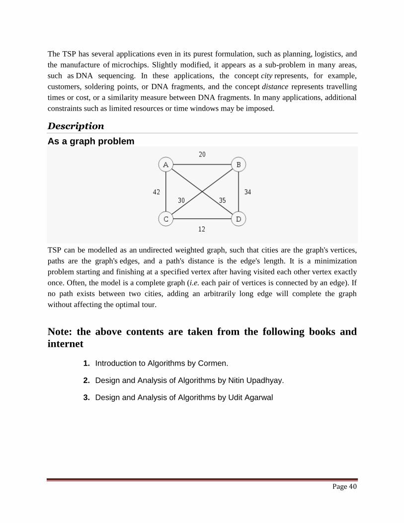
Description

As a graph problem

TSP can be modelled as an undirected weighted graph, such that cities are the graph's vertices,

paths are the graph's edges, and a path's distance is the edge's length. It is a minimization

problem starting and finishing at a specified vertex after having visited each other vertex exactly

once. Often, the model is a complete graph (i.e. each pair of vertices is connected by an edge). If

no path exists between two cities, adding an arbitrarily long edge will complete the graph

without affecting the optimal tour.

Note: the above contents are taken from the following books and

internet

1. Introduction to Algorithms by Cormen.

2. Design and Analysis of Algorithms by Nitin Upadhyay.

3. Design and Analysis of Algorithms by Udit Agarwal