summary of salt marsh trends analysis within the town of ... summary report on salt... · t006429...

Summary of Salt Marsh Trends AnalysisWithin the Town of Hempstead

Results as of June 30, 2014

T006429 Salt Marsh Erosion Trend Analysis

Summary of Salt Marsh Trends AnalysisWithin the Town of Hempstead

Summary

This report summarized the preliminary data from the study of salt marshes in the Town of Hempstead. Overall, about half of the marshlands that existed in 1926 were gone by 2004. While the main source of this loss, the direct destruction of marshland, was stopped in the 1960s, there are continued losses. Two forms of loss were documented here. The retreat of the outer edges was measured for islands not affected by direct destruction from 1926 to 2012, and the loss has proceeded at a very linear rate. Whatever the phenomenon, or combination of phenomena, was that caused the overall loss, it has apparently been occurring at about the same pace throughout the past century. The overall pattern of change seems to indicate that sediment movement allowed marsh coverage increases at some locations,but the overall amount of sediment deposition is not keeping up with sea-level rise. Several factors were studied that may control the rate of local change, including patterns of wave generation over fetchor by storms, tidal water flow with meanders, capture of sediment by deep pits, and direct human damage to marsh edges. With the exception of deep quiet pits that may be sediment traps, these phenomena would effect the rate of sediment movement thereby driving shifts in the location of marshes rather than their size if sea level rise and sediment inflow were not factors. The dominant overall influence on salt marsh size may be the balance between sediment input and the additional marsh volume needed to compensate for sea-level rise is.

A more troubling result is the expansion of unvegetated areas, commonly called ponds or pannes, on the surface of the marshes during recent years. The active draining of marsh ponds by mosquito controlemployes was discontinued after the mid 1970s, and the collapse of internal sections of salt marsh has accelerated. The pattern of marsh collapse may be significant, as it is accelerating more rapidly in the parts of the bay where nutrient input is declining. While this runs counter to reports that nutrient input is a cause of salt marsh collapse, it is supported by other experiments that relate elevated nutrients to increased above-ground Spartina growth and more efficient sediment capture. Further research into thesediment budget and more comparisons between salt marshes over a wider study area will be needed toresolve these seemingly conflicting results.

Introduction

The disappearance of salt marshes is a crisis along all of the eastern seaboard. The salt marshes are required habitat for many marine and wildlife species, provide a moderating influence on water quality,and protect sea side communities by attenuating waves. As the manager of a significant portion of NewYork State's salt marshes, The Town of Hempstead's Department of Conservation and Waterways realized that an assessment of trends in these marshes was critical for their management. In particular, it was important to distinguish between the impacts from several possible causes of erosion or accretion. This project required the collection of as many complete aerial photography sets of the town

1


marshlands as possible and, for older photographic sets, the referencing to a common spatial projection for GIS analysis. This project also required the amassing of other data sources to be used for correlations with the changes in the marshlands. These additional data sets included the Town's water quality data, USGS wind data from Point Lookout NY, the modeling of wave generation under storm wind conditions, bathymetry data, hydrological conditions such as tidal flows, and others.

We believe that these results form a more complete analysis than has been done elsewhere and make animportant contribution to the understanding and management of salt marshes in general and particularlywithin New York State.

Tasks and preliminary results from using the products

Tasks 1-6: The project was entirely completed in house with no subcontract and with the agreement of NYS DOS.

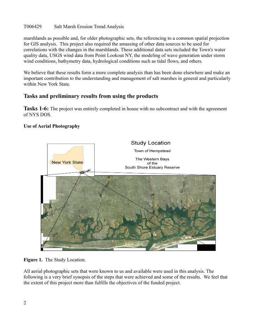
Use of Aerial Photography

Figure 1. The Study Location.

All aerial photographic sets that were known to us and available were used in this analysis. The following is a very brief synopsis of the steps that were achieved and some of the results. We feel that the extent of this project more than fulfills the objectives of the funded project.

2


Task 7: The creation of a reference marsh edge outline.

7.1 The creation of base outline using the 1994 set was completed. This 1994 orthophotography was the most recent set available at the start of this project.

7.2 Trends in the change of area were included. As they became available, the outlines of 5 additional years were also derived from these sets as ESRI shapefiles to provide at least 5 sets 1926 – 2004, the minimum for defining a trend. After hurricane Sandy, 2012 was also outlined to help asses the extent of changes. The comparisons between these edge outlines provided the opportunity for a trends analysis of in overall area About 50% of the salt marsh that still remained in 1926 was lost by 2004 (Figure 2). Most of the losses were caused by direct destruction, the filling and building on salt marsh and some dredging away of marshland. The Town of Hempstead possessed 5,460 hectares (13,500 acres) in 1926, 2,580 ha (6,375 ac) were lost between 1926 and 1983, and an additional 173 ha (430 ac)1983 to 2004. this averages to be about 45.25 ha (112 ac) per year 1926-1983 and reduced to about 8.25 ha (20.4 ac) per year 1983-2004 (Figure 3). A very linear loss over the time interval 1926-2012 is seen in a subset of marshes not affected by filling and building. This constant rate of loss implies that about 640 ha (11,580 ac), or about 8.6% of the original area, were lost to an imbalance of erosion over accretion, most likely reflecting a continuing increase in sea level rise without sufficient additional sedimentation to compensate.

The consistency of the loss raises the question of what had happened prior to 1926 that switched the salt marshes from an accretional mode to an erosional one. We are currently working with researchers from several universities to collect and analyze cores from our salt marshes that should help reconstructthe history of the local marshlands.

Although these losses are extensive, they are about half of what was previously estimated by the NYS DEC when the same subsets of islands were compared.

Figure 2. The salt marsh losses between 1926 and 2004 are reflected in red, while earlier loss cannot be estimated.

3


Trends in islands not directly affected by fill &build or dredging were picked as focal islands (Figure 4). A very linear lost through time wasseen looking at a subset of islands not affectedby fill & build or other forms of directdestruction. In those locations, the losses werevery linear over the entire 1926-2012 timeinterval that averaged 0.2 % per year. Theselected islands started in 1926 with 1,470 ha (3,632.5 ac) and ended in 2012 with 1,205 ha (3,980 ac).

Figure 3. Total marsh area compared to trendsin islands not affected by direct destruction.

Figure 4. Islands chosen for the estimation of the background loss rates on islands not affected by the fill and build or direct cutting of edges that were the main cause of overall losses, 1926-2012.

Task 8: Georeferencing complete photo sets in NY State Pland, LI Zone, NAD83

8.1 Eight complete sets of aerial photographs from the Town of Hempstead archives were referenced. Two sets were extracted from composite images and six were created from original contact prints. The list of years completed includes 1926, 1950, 1956, 1966, 1973, 1978, 1983, 1989. The 1989 set is illustrated in Figure 5.

4


Figure 5. An example of the referenced photo sets, the 1989 photographs as an overlay.

8.2 Five of the more recent years were covered using publicly available photo sets used for at least some parts of the analysis, including 4 from New York State and the post-Sandy NOAA flyover 2012. Specifically 1994, 2000, 2004, 2007, and 2012

Task 9: Derive Shoreline Recession Rates.

9.1 To measure recession rates for edges, 500 random points were generated as an ArcMap shapefile using a PYTHON script written for the purpose of randomly placing them along the 1994 reference edges. Lines representing the direction of edge regression, each centered on a particular point, were simultaneously generated as ArcMap shapefiles (Figure 6). This approach was used because the influence on a particular point of a given edge, may vary greatly even for different edges of the same island.

Figure 6. A close view of some random points showing the trend lines that were used and the different pattern of loss at different edges of the same marsh islands due to the different local influences illustrated using the 5 island area data sets 1926-2004.

5


9.2 collection of point changes for time interval 1926 – 2007.

A Visual Basic tool was written for use in ArcMap 9.3 that would convert a mouse click on the point where the trend line crosses the edge in a photograph into a calculation of distance between that crossing point and the associated point along the 1994 edge and then store it into the attribute table of the GIS layer. When collected at the same point for all of the years that aerial photography was available, these distances then provided a history of the edge change at that point (Figure 6). The accuracy of the 1926 photography was approximately 1.5 meters, and this improve as the photographs become newer and more clear, approaching 0.3 meters in recent years. Once the data were collected at each point, the trend of marsh change could then be statistically compared with environmental conditions at that point.

Figure 7. The changes from 1926 to 2007 at all points, with gains represented as green, losses by red, and scaled in size to the amount of change.

9.2 comparison of trends with environmental drivers local to the pointsThe list of potential drivers includes: cut edges, fetch, major storm waves, boat use, tidal water flow rates, nutrient concentrations (NH3, NO2, NO3, P, Ch a, salinity), borrow pits, differences between recent development in the 1960s and prior to that period including boat engine size.

6


Due to covarience between parameters, the parameters were tested using cluster and PCA analysis (Figure 8 and Figure 9 respectively) resulting in list of variables with reduced effects from covarience prior to testing against marsh losses. The nutrients showed strong covariance, so only nitrates(NO3)were used for most analysis. Results were checked for the possibility of spatial autocorrelation, and this was were taken into consideration in developing results.

Figure 8. A cluster analysis Figure 9. A PCA analysis

9.3 Trends related to major tested factors

Cut edges

The dredging of channels through marshes and upto the edges of marshes produces deep verticaledges that can slump and exposes sediment beneaththe protective layer of Spartina roots.

These locations were identified by comparisonbetween the photographic sets and between thephotographs and the 1879 Coast and Geodeticsurvey.

These locations showed the greatest amount of Figure 10. Edge differences relative to 1994,

erosion of any edges(Figures 10 and 11). X=no boats, DT=CutEdge, A-E=boat use.

7


Figure 11. A comparison between cut edges (DT=Dredged Through) and navigational channels of similar width and level of boat use (EC).

Fetch

The width of a water body is one of the factors that determines the height of waves, and the power of waves increases with the square of the wave height. Because the channels often have long maximum distances over water looking down even a narrow channel, the narrowest distance across the water was used to estimate the effect of fetch on waves. Figure 12 shows the effect from fetch between 1926 and 1966, and Figure 13 shows the effect between 1966 and 2007.

8


Figure 12. A correlation between edge change 1926-1966 and the square root of the shortest distance tothe next land mass.

Figure 13. A correlation between edge change 1966-2007 and the square root of the shortest distance tothe next land mass.

9


StormsBathymetry from NOAA and NOAA nautical charts were used in combination with the wind data from the Point Lookout USGS station (Station 01310740 is partially funded by the Town of Hempstead) to populate the input to a SWAN wave generation model that produced a spatial pattern of expected significant wave height as output. The calculated significant wave heights for the 500 chosen points was then analyzed against edge change for those same locations to estimate the effect from storms. The predicted significant wave heights are plotted against 1926 to 1966 non-channel edge change in Figure 14.

Figure 14. A representation of the effect of storm waves modeled as significant wave height in meters and the edge change between 1926 and 1966.

10


Boat use

Navigational channels were categorized by the traffic patterns observed over many years. The categories started with A, the heavily used channels trafficked by larger fast boats, down to E that represents channels occasionally used by small boots. Channels that were dredged through marshes or otherwise characterized by cut edges were categorized separately.

Effects from boat use were not very strong or easily measured. By simply using the median change between boat channels of different degrees of use, only the least used channels (E) were significantly different from the other channels (Figure 15). However, the heavily used channels (A) erode more rapidly when close to an edge when lightly used channels (C, D and E) do not (Figure 16). One possible confounding effect is that natural eroding edges on the outside of meander bends will also be deepest at the edge, and some navigational channels take advantage of the natural deep water. A better estimate of the influence of boat traffic may be to compare erosion rates at each point for time intervals before and after the general use of large fast engines (page 14).

Figure 15. A box plot showing the edges changes along navigational channels with negative representing loss with notches that represent significant differences if they do not overlap.

11


Figure 16. Plots of edge change and the distance of a channel from the measured edge points.

Water Flow RatesThe tidal water flow rates, as modeled by the Great South Bay Model (Flagg and Wilson, SoMAS Stony Brook University) show sediment movement, including both erosion and some accretion, when against modeled peak tidal water flow rates (Figures 17 and 18).

Figure 17. Channel edge 1926-1966. Figure 18. Channel edge 1966-2007.

NutrientsUsing mean 1990-2004 Nitrates as the proxy for all nutrients in most analyses. Dissolved Inorganic Nitrogen (DIN) is the sum of nitrates, nitrites, and ammonia, and was used as a proxy for some other analyses. No effect from nutrient concentration although Nitrates vary by a factor of 3 and DIN varied by a factor of over 4, even after using several tests, only one plot is shown here (Figure 19).

Figure 19. Nutrients represented by the log transform of nitrates (NO3) are plotted against edge change.

12


Borrow pitsThe influence of borrow pits on salt marsh erosion is unclear. Borrow pits are basically underwater sand mines that were the source of material for much of the filling done on salt marshes. Borrow pits are much deeper than needed for navigation, typically reaching 10 or 20 meters in depth. It is expected that borrow pits should act as sediment traps, capturing sediment that would otherwise contribute to theexpansion of salt marshes or to the surface elevation in the face of sea level rise. There is little previousdocumentation of this effect. In this study, no influence was confirmed on edges that were not along navigational channels. However, the edges along navigational channels where the effects from stirred up sediment and sediment traps are combined, an increase in the erosion rate is indicated along edges that are approximately 500 meters or less from the pits (Figure 20). This effect is statistically marginal,and more data points would be needed to clarify the relationship.

Figure 20. A marginal relationship is seen between the distance to borrow pits and the erosion rates of navigational channels.

Comparisons of early and late time intervals The overall time interval of 1926 to 2007 was split into two intervals of 1926 to 1966 and 1966 to 2007for analysis to understand changing conditions between these time periods. In addition to splitting the time interval roughly in half, this split roughly divided the period into functional categories, before andafter intensive urbanization and into an early period of few large motor boats and a later intreval of intensive use by large fast motorboats.

13


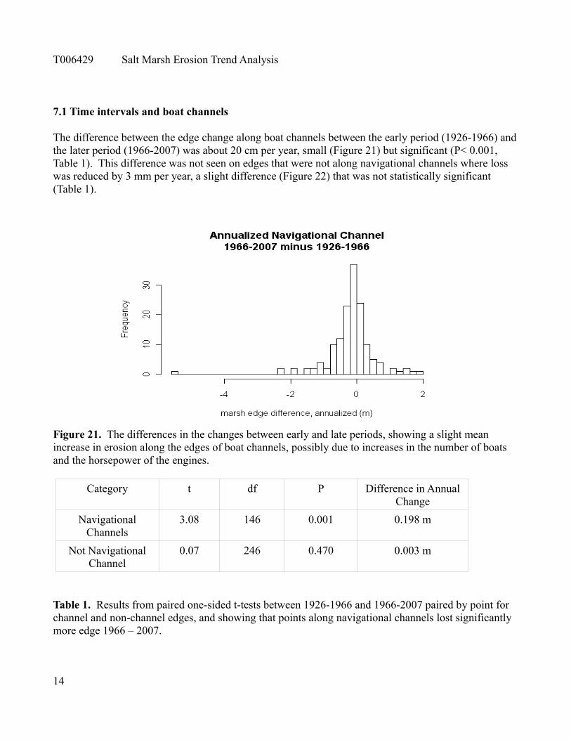
7.1 Time intervals and boat channels

The difference between the edge change along boat channels between the early period (1926-1966) andthe later period (1966-2007) was about 20 cm per year, small (Figure 21) but significant (P< 0.001, Table 1). This difference was not seen on edges that were not along navigational channels where loss was reduced by 3 mm per year, a slight difference (Figure 22) that was not statistically significant (Table 1).

Figure 21. The differences in the changes between early and late periods, showing a slight mean increase in erosion along the edges of boat channels, possibly due to increases in the number of boats and the horsepower of the engines.

Category t df P Difference in AnnualChange

NavigationalChannels

3.08 146 0.001 0.198 m

Not NavigationalChannel

0.07 246 0.470 0.003 m

Table 1. Results from paired one-sided t-tests between 1926-1966 and 1966-2007 paired by point for channel and non-channel edges, and showing that points along navigational channels lost significantly more edge 1966 – 2007.

14


Figure 22. The difference between the changes along edges that were not along channels showed no difference between the two periods.

7.2 Urbanization

In general there was no general difference between edge change when comparing the two periods (Figure 23), and the general change in land use could not be shown to have an effect.

Figure 23. The general difference between edge changes for the time intervals 1926 to 1966 and 1966 to 2007.

15


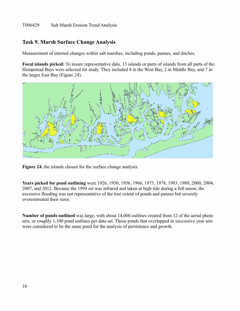
Task 9. Marsh Surface Change Analysis

Measurement of internal changes within salt marshes, including ponds, pannes, and ditches.

Focal islands picked: To insure representative data, 13 islands or parts of islands from all parts of the Hempstead Bays were selected for study. They included 4 in the West Bay, 2 in Middle Bay, and 7 in the larger East Bay (Figure 24).

Figure 24. the islands chosen for the surface change analysis.

Years picked for pond outlining were 1926, 1950, 1956, 1966, 1973, 1978, 1983, 1989, 2000, 2004, 2007, and 2012. Because the 1994 set was infrared and taken at high tide during a full moon, the excessive flooding was not representative of the true extent of ponds and pannes but severely overestimated their sizes.

Number of ponds outlined was large, with about 14,000 outlines created from 12 of the aerial photo sets, or roughly 1,100 pond outlines per data set. Those ponds that overlapped in successive year sets were considered to be the same pond for the analysis of persistence and growth.

16


Overall trends

One analysis that was done with the ponds/pannes was to look at the portion of unvegetated areas that overlapped a pond or panne in the succeeding data set. In most cases, there was consistency and roughly 90% of these unvegetated areas were still in the next set. Because the size of the chosen marshes varied, all analyses were based on the percent of total area that were unvegetated. A noticeabledrop to about 75 % occurred between the 1978 and the 1983 data sets, a period of intensive ditching and pond draining. Because not all unvegetated areas were actual ponds, this never aproached zero.

Figure 25. The probability of pond/panne survival dropped sharply between 1973 and 1983 when ponds were intensively drained and Spartina could regrow. Trends in pond/panne growth with the bays categorized by nutrient concentrations

A graph (Figure 26) that shows the percentage of unvegetated area on islands categorized by Dissolved Inorganic Nitrogen (DIN) level, showing the loss of ponds during intensive pond draining for mosquitocontrol, followed by the most rapid pond/panne growth at low nutrient levels. The ponds/pannes in higher nutrient locations did little more than recover to the 1926 percent of marsh surface. Figure 27 shows a slide from a conference presentation illustrating the same section of East Bay in 1956 and 2012. In another form of analysis, a Stratified Cox survival model was used to compare the persistenceand recurrence of ponds that differed by size (Figure 28). Larger ponds/pannes were more likely to persist and grow while smaller ponds wee more likely to disappear.

17


Figure 26. The changes in pond area as a percentage of the islands they were found on, West Bay as red stars, Middle Bay as green squares, and East Bay as hollow purple triangles.

Figure 27. A slide from the Geological Society of America, North East Chapter, Spring 2013 conference presentation showing pond expansion in East Bay.

18


Survival analysis, how random are the ponds and how likely are they to fill in or expand.

Figure 28. A survival analysis plot comparing the fate of different initial pond sizes and the recurrence of ponds after draining.

Ditches and their changes

The ditching, usually referred to as mosquito ditches, were tracked for their through time and relative tonutrient in the adjoining water. A recent paper by Deegan et al. (2012) about marshes exposed to dissolved nitrates over an interval of 8 years raised the question of edge deterioration at high nutrients, although other research by Morris et al. (2002) and Anisfeld and Hill (2012) indicate increased sedimentation rates. While our data on the expansion of ponds (Figure 29) seem to indicate increased sedimentation at higher nutrient levels, the response of ditching required separate attention.

Figure 29. The changes in ditch area for the same focal islands as used with the pond analysis.

19

West Middle East-2

0

2

4

6

8

Percent Creek & Ditch change

Dif


In general, the ditches in the high nutrient West Bay, traced for 8 decades, did show the softened edges predicted by Degan et al. (2012), but instead of increasing erosion, the Spartina colonized the ditches and seems to be collecting sediment and filling in most of the ditches (Figure 30). The mouths of the ditches do show increased erosion at the outer corners (Figure 31). The remaining ditches seem to be carrying the tidal water flow and expanded. In the Middle and East Bays, the ditches retain their form, but enlarged due to erosion (Figure 27). In sum, the West Bay ditches may look like they are in worse shape than those in the East Bay, but that may be an illusion.

Figure 27. A ditch located on South Black Banks showing Spartina growing in the ditch and collectingsediment.

Figure 28. The expanded mouth of a ditch on East Meadow Island in the Wast Bay, showing the expanded mouth but with Spartina growing in the ditch further inland.

20


References

Anisfeld, S.C. and T.D. Hill. 2012. Fertilization effects on elevation change and belowground carbon balance in a Long Island Sound tidal marsh.Estuaries and coasts 35(1):201-211. DOI: 10.1007/s12237-011-9440-4.

Morris, J.T., P.V. Sundareshwar, C.T. Nietch, B. Kjerfve, and D.R. Cahoon, 2002. Responses of coastal wetlands to rising sea level. Ecology, 93:2869-2877.

Deegan, L.A., D.S. Johnson, R.S. Warren, B.J. Peterson, J.W. Fleager, S. Fagherazzi, and W.M. Woliheim, 2012. Coastal eutrophication as a driver of salt marsh loss. Nature, 490: 388-392.

21

summary of salt marsh trends analysis within the town of ... summary report on salt... · t006429...

Documents