summary - math.toronto.edu
TRANSCRIPT

Entropy along the Mandelbrot set
Giulio TiozzoUniversity of Toronto
André Aisenstadt Lecture – Montréal, 15th October, 2021
October 15, 2021

Summary
1. What is... (topological) entropy?
2. Entropy in dynamical systems3. A crash course in complex dynamics4. Definition of core entropy5. The quadratic case6. The higher degree case

Summary
1. What is... (topological) entropy?2. Entropy in dynamical systems
3. A crash course in complex dynamics4. Definition of core entropy5. The quadratic case6. The higher degree case

Summary
1. What is... (topological) entropy?2. Entropy in dynamical systems3. A crash course in complex dynamics
4. Definition of core entropy5. The quadratic case6. The higher degree case

Summary
1. What is... (topological) entropy?2. Entropy in dynamical systems3. A crash course in complex dynamics4. Definition of core entropy
5. The quadratic case6. The higher degree case

Summary
1. What is... (topological) entropy?2. Entropy in dynamical systems3. A crash course in complex dynamics4. Definition of core entropy5. The quadratic case
6. The higher degree case

Summary
1. What is... (topological) entropy?2. Entropy in dynamical systems3. A crash course in complex dynamics4. Definition of core entropy5. The quadratic case6. The higher degree case

English or Gibberish?
You are a spy, and you intercept two messages: one of them isin English, and another is just a random sequence of letters.
Which one is the English one? Unfortunately, both messagesare encrypted by substituting letters with numbers....
Text A1, 14, 4, 27, 20, 8, 5, 14, 3, 5, 27, 23, 5, 27, 9, 19, 19, 21, 5, 4, 27, 6,15, 18, 20, 8, 27, 20, 15, 27, 19, 5, 5, 27, 1, 7, 1, 9, 14, 27, 20, 8, 5,27, 19, 20, 1, 18, 19
Text B25, 18, 9, 10, 5, 4, 11, 20, 17, 20, 9, 15, 27, 3, 18, 6, 26, 17, 11, 6, 6,18, 26, 14, 16, 21, 7, 17, 21, 9, 13, 17, 18, 27, 20, 6, 4, 25, 8, 22, 2,3, 26, 11, 19, 6, 12, 5, 23

English or Gibberish?
You are a spy, and you intercept two messages: one of them isin English, and another is just a random sequence of letters.Which one is the English one?
Unfortunately, both messagesare encrypted by substituting letters with numbers....
Text A1, 14, 4, 27, 20, 8, 5, 14, 3, 5, 27, 23, 5, 27, 9, 19, 19, 21, 5, 4, 27, 6,15, 18, 20, 8, 27, 20, 15, 27, 19, 5, 5, 27, 1, 7, 1, 9, 14, 27, 20, 8, 5,27, 19, 20, 1, 18, 19
Text B25, 18, 9, 10, 5, 4, 11, 20, 17, 20, 9, 15, 27, 3, 18, 6, 26, 17, 11, 6, 6,18, 26, 14, 16, 21, 7, 17, 21, 9, 13, 17, 18, 27, 20, 6, 4, 25, 8, 22, 2,3, 26, 11, 19, 6, 12, 5, 23

English or Gibberish?
You are a spy, and you intercept two messages: one of them isin English, and another is just a random sequence of letters.Which one is the English one? Unfortunately, both messagesare encrypted by substituting letters with numbers....
Text A1, 14, 4, 27, 20, 8, 5, 14, 3, 5, 27, 23, 5, 27, 9, 19, 19, 21, 5, 4, 27, 6,15, 18, 20, 8, 27, 20, 15, 27, 19, 5, 5, 27, 1, 7, 1, 9, 14, 27, 20, 8, 5,27, 19, 20, 1, 18, 19
Text B25, 18, 9, 10, 5, 4, 11, 20, 17, 20, 9, 15, 27, 3, 18, 6, 26, 17, 11, 6, 6,18, 26, 14, 16, 21, 7, 17, 21, 9, 13, 17, 18, 27, 20, 6, 4, 25, 8, 22, 2,3, 26, 11, 19, 6, 12, 5, 23

English or Gibberish?
Idea: natural languages have redundancies
Th_ art_st is __e creato_ of be__t_ful th_ng_.To revea_ a_t and con_ea_ the _rtist _s art’_ a_m.The cr_t_c is he wh_ _an tra_slat_ into ano_he_ manneror a n_w mate_ial hi_ impre_sio_ of b_a_tiful _h_ngs.
(Osc__ Wil__, The Picture __ ______ ____)"

English or Gibberish?
in 1948, Shannon came up with an idea:
h := limn→∞
log #{subsequences of length n}n
Text A1, 14, 4, 27, 20, 8, 5, 14, 3, 5, 27, 23, 5, 27, 9, 19, 19, 21, 5, 4, 27, 6,15, 18, 20, 8, 27, 20, 15, 27, 19, 5, 5, 27, 1, 7, 1, 9, 14, 27, 20, 8, 5,27, 19, 20, 1, 18, 19h = 2.52095
Text B25, 18, 9, 10, 5, 4, 11, 20, 17, 20, 9, 15, 27, 3, 18, 6, 26, 17, 11, 6, 6,18, 26, 14, 16, 21, 7, 17, 21, 9, 13, 17, 18, 27, 20, 6, 4, 25, 8, 22, 2,3, 26, 11, 19, 6, 12, 5, 23h = 3.06246 (Random selection: log 27 = 3.29...)

English or Gibberish?
in 1948, Shannon came up with an idea:
h := limn→∞
log #{subsequences of length n}n
Text A1, 14, 4, 27, 20, 8, 5, 14, 3, 5, 27, 23, 5, 27, 9, 19, 19, 21, 5, 4, 27, 6,15, 18, 20, 8, 27, 20, 15, 27, 19, 5, 5, 27, 1, 7, 1, 9, 14, 27, 20, 8, 5,27, 19, 20, 1, 18, 19
h = 2.52095
Text B25, 18, 9, 10, 5, 4, 11, 20, 17, 20, 9, 15, 27, 3, 18, 6, 26, 17, 11, 6, 6,18, 26, 14, 16, 21, 7, 17, 21, 9, 13, 17, 18, 27, 20, 6, 4, 25, 8, 22, 2,3, 26, 11, 19, 6, 12, 5, 23h = 3.06246 (Random selection: log 27 = 3.29...)

English or Gibberish?
in 1948, Shannon came up with an idea:
h := limn→∞
log #{subsequences of length n}n
Text A1, 14, 4, 27, 20, 8, 5, 14, 3, 5, 27, 23, 5, 27, 9, 19, 19, 21, 5, 4, 27, 6,15, 18, 20, 8, 27, 20, 15, 27, 19, 5, 5, 27, 1, 7, 1, 9, 14, 27, 20, 8, 5,27, 19, 20, 1, 18, 19h = 2.52095
Text B25, 18, 9, 10, 5, 4, 11, 20, 17, 20, 9, 15, 27, 3, 18, 6, 26, 17, 11, 6, 6,18, 26, 14, 16, 21, 7, 17, 21, 9, 13, 17, 18, 27, 20, 6, 4, 25, 8, 22, 2,3, 26, 11, 19, 6, 12, 5, 23h = 3.06246 (Random selection: log 27 = 3.29...)

English or Gibberish?
in 1948, Shannon came up with an idea:
h := limn→∞
log #{subsequences of length n}n
Text A1, 14, 4, 27, 20, 8, 5, 14, 3, 5, 27, 23, 5, 27, 9, 19, 19, 21, 5, 4, 27, 6,15, 18, 20, 8, 27, 20, 15, 27, 19, 5, 5, 27, 1, 7, 1, 9, 14, 27, 20, 8, 5,27, 19, 20, 1, 18, 19h = 2.52095
Text B25, 18, 9, 10, 5, 4, 11, 20, 17, 20, 9, 15, 27, 3, 18, 6, 26, 17, 11, 6, 6,18, 26, 14, 16, 21, 7, 17, 21, 9, 13, 17, 18, 27, 20, 6, 4, 25, 8, 22, 2,3, 26, 11, 19, 6, 12, 5, 23h = 3.06246
(Random selection: log 27 = 3.29...)

English or Gibberish?
in 1948, Shannon came up with an idea:
h := limn→∞
log #{subsequences of length n}n
Text A1, 14, 4, 27, 20, 8, 5, 14, 3, 5, 27, 23, 5, 27, 9, 19, 19, 21, 5, 4, 27, 6,15, 18, 20, 8, 27, 20, 15, 27, 19, 5, 5, 27, 1, 7, 1, 9, 14, 27, 20, 8, 5,27, 19, 20, 1, 18, 19h = 2.52095
Text B25, 18, 9, 10, 5, 4, 11, 20, 17, 20, 9, 15, 27, 3, 18, 6, 26, 17, 11, 6, 6,18, 26, 14, 16, 21, 7, 17, 21, 9, 13, 17, 18, 27, 20, 6, 4, 25, 8, 22, 2,3, 26, 11, 19, 6, 12, 5, 23h = 3.06246 (Random selection: log 27 = 3.29...)

English or Gibberish?
h := limn→∞
log #{subsequences of length n}n
Text A“and thence we issued forth to see again the stars"h = 2.52095
Text B“yrijedktqtio crfzqkffrznpugquimqr tfdyhvbczksflew"h = 3.06246 (Random selection: log 27 = 3.29...)

English or Gibberish?
h := limn→∞
log #{subsequences of length n}n
Text A“and thence we issued forth to see again the stars"h = 2.52095
Text B“yrijedktqtio crfzqkffrznpugquimqr tfdyhvbczksflew"h = 3.06246 (Random selection: log 27 = 3.29...)

English or Gibberish?
h := limn→∞
log #{subsequences of length n}n
Text A“and thence we issued forth to see again the stars"h = 2.52095
Text B“yrijedktqtio crfzqkffrznpugquimqr tfdyhvbczksflew"h = 3.06246
(Random selection: log 27 = 3.29...)

English or Gibberish?
h := limn→∞
log #{subsequences of length n}n
Text A“and thence we issued forth to see again the stars"h = 2.52095
Text B“yrijedktqtio crfzqkffrznpugquimqr tfdyhvbczksflew"h = 3.06246 (Random selection: log 27 = 3.29...)
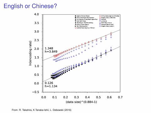
English or Chinese?
From: R. Takahira, K.Tanaka-Ishii, L. Debowski (2016)

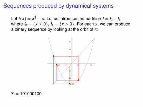
Sequences produced by dynamical systems
Let f (x) = x2 + c.
Let us introduce the partition I = I0 ∪ I1where I0 = {x ≤ 0}, I1 = {x > 0}. For each x , we can producea binary sequence by looking at the orbit of x :
-1.5 -1.0 -0.5 0.5 1.0 1.5
-1.0
-0.5
0.5
1.0
1.5
Σ = 1

Sequences produced by dynamical systems
Let f (x) = x2 + c. Let us introduce the partition I = I0 ∪ I1where I0 = {x ≤ 0}, I1 = {x > 0}.
For each x , we can producea binary sequence by looking at the orbit of x :
-1.5 -1.0 -0.5 0.5 1.0 1.5
-1.0
-0.5
0.5
1.0
1.5
Σ = 1

Sequences produced by dynamical systems
Let f (x) = x2 + c. Let us introduce the partition I = I0 ∪ I1where I0 = {x ≤ 0}, I1 = {x > 0}. For each x , we can producea binary sequence by looking at the orbit of x :
-1.5 -1.0 -0.5 0.5 1.0 1.5
-1.0
-0.5
0.5
1.0
1.5
Σ = 1

Sequences produced by dynamical systems
Let f (x) = x2 + c. Let us introduce the partition I = I0 ∪ I1where I0 = {x ≤ 0}, I1 = {x > 0}. For each x , we can producea binary sequence by looking at the orbit of x :
-1.5 -1.0 -0.5 0.5 1.0 1.5
-1.0
-0.5
0.5
1.0
1.5
Σ = 1

Sequences produced by dynamical systems
Let f (x) = x2 + c. Let us introduce the partition I = I0 ∪ I1where I0 = {x ≤ 0}, I1 = {x > 0}. For each x , we can producea binary sequence by looking at the orbit of x :
-1.5 -1.0 -0.5 0.5 1.0 1.5
-1.0
-0.5
0.5
1.0
1.5
Σ = 1

Sequences produced by dynamical systems
Let f (x) = x2 + c. Let us introduce the partition I = I0 ∪ I1where I0 = {x ≤ 0}, I1 = {x > 0}. For each x , we can producea binary sequence by looking at the orbit of x :
-1.5 -1.0 -0.5 0.5 1.0 1.5
-1.0
-0.5
0.5
1.0
1.5
Σ = 10

Sequences produced by dynamical systems
Let f (x) = x2 + c. Let us introduce the partition I = I0 ∪ I1where I0 = {x ≤ 0}, I1 = {x > 0}. For each x , we can producea binary sequence by looking at the orbit of x :
-1.5 -1.0 -0.5 0.5 1.0 1.5
-1.0
-0.5
0.5
1.0
1.5
Σ = 101

Sequences produced by dynamical systems
Let f (x) = x2 + c. Let us introduce the partition I = I0 ∪ I1where I0 = {x ≤ 0}, I1 = {x > 0}. For each x , we can producea binary sequence by looking at the orbit of x :
-1.5 -1.0 -0.5 0.5 1.0 1.5
-1.0
-0.5
0.5
1.0
1.5
Σ = 1010

Sequences produced by dynamical systems
Let f (x) = x2 + c. Let us introduce the partition I = I0 ∪ I1where I0 = {x ≤ 0}, I1 = {x > 0}. For each x , we can producea binary sequence by looking at the orbit of x :
-1.5 -1.0 -0.5 0.5 1.0 1.5
-1.0
-0.5
0.5
1.0
1.5
Σ = 10100
Sequences produced by dynamical systems
Let f (x) = x2 + c. Let us introduce the partition I = I0 ∪ I1where I0 = {x ≤ 0}, I1 = {x > 0}. For each x , we can producea binary sequence by looking at the orbit of x :
-1.5 -1.0 -0.5 0.5 1.0 1.5
-1.0
-0.5
0.5
1.0
1.5
Σ = 101000100

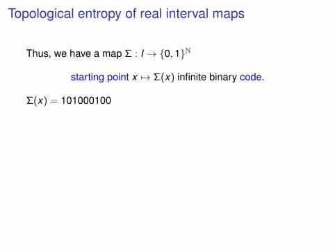
Topological entropy of real interval maps
Thus, we have a map Σ : I → {0,1}N
starting point x 7→ Σ(x) infinite binary code.
Σ(x) = 101000100How many different sequences can I obtain?The topological entropy of f is the quantity
htop(f ) := limn→∞
log #{admissible codes of length n}n
Note: For quadratic maps htop(f ) ≤ log 2.
Topological entropy of real interval maps
Thus, we have a map Σ : I → {0,1}N
starting point x 7→ Σ(x) infinite binary code.
Σ(x) = 101000100
How many different sequences can I obtain?The topological entropy of f is the quantity
htop(f ) := limn→∞
log #{admissible codes of length n}n
Note: For quadratic maps htop(f ) ≤ log 2.

Topological entropy of real interval maps
Thus, we have a map Σ : I → {0,1}N
starting point x 7→ Σ(x) infinite binary code.
Σ(x) = 101000100How many different sequences can I obtain?
The topological entropy of f is the quantity
htop(f ) := limn→∞
log #{admissible codes of length n}n
Note: For quadratic maps htop(f ) ≤ log 2.

Topological entropy of real interval maps
Thus, we have a map Σ : I → {0,1}N
starting point x 7→ Σ(x) infinite binary code.
Σ(x) = 101000100How many different sequences can I obtain?The topological entropy of f is the quantity
htop(f ) := limn→∞
log #{admissible codes of length n}n
Note: For quadratic maps htop(f ) ≤ log 2.
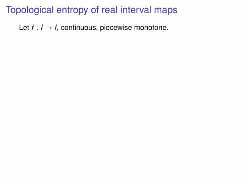
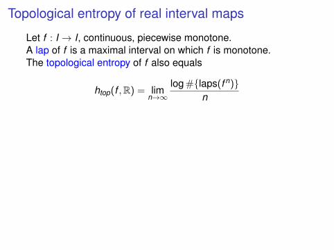
Topological entropy of real interval maps
Let f : I → I, continuous, piecewise monotone.
A lap of f is a maximal interval on which f is monotone.The topological entropy of f also equals
htop(f ,R) = limn→∞
log #{laps(f n)}n

Topological entropy of real interval maps
Let f : I → I, continuous, piecewise monotone.A lap of f is a maximal interval on which f is monotone.
The topological entropy of f also equals
htop(f ,R) = limn→∞
log #{laps(f n)}n

Topological entropy of real interval maps
Let f : I → I, continuous, piecewise monotone.A lap of f is a maximal interval on which f is monotone.The topological entropy of f also equals
htop(f ,R) = limn→∞
log #{laps(f n)}n
Topological entropy of real interval maps
Let f : I → I, continuous, piecewise monotone.A lap of f is a maximal interval on which f is monotone.The topological entropy of f also equals
htop(f ,R) = limn→∞
log #{laps(f n)}n

Topological entropy of real interval maps
Let f : I → I, continuous, piecewise monotone.A lap of f is a maximal interval on which f is monotone.The topological entropy of f also equals
htop(f ,R) = limn→∞
log #{laps(f n)}n

Topological entropy of real maps
Let f : I → I, continuous, piecewise monotone.
htop(f ,R) = limn→∞
log #{laps(f n)}n

Topological entropy of real maps
Let f : I → I, continuous, piecewise monotone.
htop(f ,R) = limn→∞
log #{laps(f n)}n

Topological entropy of real maps
Let f : I → I, continuous, piecewise monotone.
htop(f ,R) = limn→∞
log #{laps(f n)}n

Topological entropy of real maps
Let f : I → I, continuous, piecewise monotone.
htop(f ,R) = limn→∞
log #{laps(f n)}n

Topological entropy of real maps
Let f : I → I, continuous, piecewise monotone.
htop(f ,R) = limn→∞
log #{laps(f n)}n

Topological entropy of real maps
Let f : I → I, continuous, piecewise monotone.
htop(f ,R) = limn→∞
log #{laps(f n)}n

Topological entropy of real maps
Let f : I → I, continuous, piecewise monotone.
htop(f ,R) = limn→∞
log #{laps(f n)}n

Topological entropy of real maps
Let f : I → I, continuous, piecewise monotone.
htop(f ,R) = limn→∞
log #{laps(f n)}n
Agrees with general definition for maps on compact spacesusing open covers (Misiurewicz-Szlenk)

Topological entropy of real maps
Let f : I → I, continuous, piecewise monotone.
htop(f ,R) = limn→∞
log #{laps(f n)}n
Agrees with general definition for maps on compact spacesusing open covers (Misiurewicz-Szlenk)

Example: the airplane mapf : I → I is postcritically finite if the forward orbits of the criticalpoints of f are finite.
Then the entropy is the logarithm of analgebraic number.
A 7→ A ∪ BB 7→ A
⇒(
1 11 0
)⇒ λ =
√5+12 = ehtop(fc ,R)

Example: the airplane mapf : I → I is postcritically finite if the forward orbits of the criticalpoints of f are finite. Then the entropy is the logarithm of analgebraic number.
A 7→ A ∪ BB 7→ A
⇒(
1 11 0
)⇒ λ =
√5+12 = ehtop(fc ,R)

Example: the airplane mapf : I → I is postcritically finite if the forward orbits of the criticalpoints of f are finite. Then the entropy is the logarithm of analgebraic number.
A 7→ A ∪ BB 7→ A
⇒(
1 11 0
)⇒ λ =
√5+12 = ehtop(fc ,R)

Example: the airplane mapf : I → I is postcritically finite if the forward orbits of the criticalpoints of f are finite. Then the entropy is the logarithm of analgebraic number.
A 7→ A ∪ BB 7→ A
⇒(
1 11 0
)
⇒ λ =√
5+12 = ehtop(fc ,R)

Example: the airplane mapf : I → I is postcritically finite if the forward orbits of the criticalpoints of f are finite. Then the entropy is the logarithm of analgebraic number.
A 7→ A ∪ BB 7→ A
⇒(
1 11 0
)⇒ λ =
√5+12
= ehtop(fc ,R)

Example: the airplane mapf : I → I is postcritically finite if the forward orbits of the criticalpoints of f are finite. Then the entropy is the logarithm of analgebraic number.
A 7→ A ∪ BB 7→ A
⇒(
1 11 0
)⇒ λ =
√5+12 = ehtop(fc ,R)

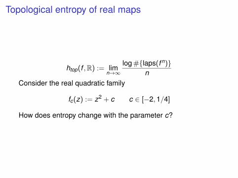
Topological entropy of real maps
htop(f ,R) := limn→∞
log #{laps(f n)}n
Consider the real quadratic family
fc(z) := z2 + c c ∈ [−2,1/4]
How does entropy change with the parameter c?
Topological entropy of real maps
htop(f ,R) := limn→∞
log #{laps(f n)}n
Consider the real quadratic family
fc(z) := z2 + c c ∈ [−2,1/4]
How does entropy change with the parameter c?

The function c → htop(fc ,R):
I is continuous and monotone (Milnor-Thurston, 1977).I 0 ≤ htop(fc ,R) ≤ log 2.

The function c → htop(fc ,R):
I is continuous
and monotone (Milnor-Thurston, 1977).I 0 ≤ htop(fc ,R) ≤ log 2.

The function c → htop(fc ,R):
I is continuous and monotone (Milnor-Thurston, 1977).
I 0 ≤ htop(fc ,R) ≤ log 2.

The function c → htop(fc ,R):
I is continuous and monotone (Milnor-Thurston, 1977).I 0 ≤ htop(fc ,R) ≤ log 2.

The function c → htop(fc ,R):
I is continuous and monotone (Milnor-Thurston, 1977).I 0 ≤ htop(fc ,R) ≤ log 2.

The function c → htop(fc ,R):
I is continuous and monotone (Milnor-Thurston, 1977).I 0 ≤ htop(fc ,R) ≤ log 2.

The function c → htop(fc ,R):
I is continuous and monotone (Milnor-Thurston, 1977).I 0 ≤ htop(fc ,R) ≤ log 2.
Question : Can we extend this theory to complex polynomials?

The function c → htop(fc ,R):
I is continuous and monotone (Milnor-Thurston, 1977).I 0 ≤ htop(fc ,R) ≤ log 2.
Remark. If we consider fc : C→ C entropy is constanthtop(fc , C) = log 2. (Lyubich 1980)

Mandelbrot set
The Mandelbrot setM is the connectedness locus of thequadratic family fc(z) := z2 + c.
M = {c ∈ C : f nc (0) 9∞}

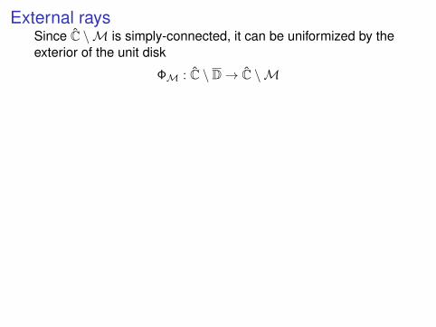
External rays
Since C \M is simply-connected, it can be uniformized by theexterior of the unit disk
ΦM : C \ D→ C \M

External rays
Since C \M is simply-connected, it can be uniformized by theexterior of the unit disk
ΦM : C \ D→ C \M
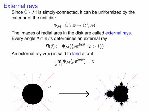
External raysSince C \M is simply-connected, it can be uniformized by theexterior of the unit disk
ΦM : C \ D→ C \M
The images of radial arcs in the disk are called external rays.Every angle θ ∈ R/Z determines an external ray
R(θ) := ΦM({ρe2πiθ : ρ > 1})An external ray R(θ) is said to land at x if
limρ→1
ΦM(ρe2πiθ) = x

External raysSince C \M is simply-connected, it can be uniformized by theexterior of the unit disk
ΦM : C \ D→ C \MThe images of radial arcs in the disk are called external rays.Every angle θ ∈ R/Z determines an external ray
R(θ) := ΦM({ρe2πiθ : ρ > 1})
An external ray R(θ) is said to land at x if
limρ→1
ΦM(ρe2πiθ) = x

External raysSince C \M is simply-connected, it can be uniformized by theexterior of the unit disk
ΦM : C \ D→ C \MThe images of radial arcs in the disk are called external rays.Every angle θ ∈ R/Z determines an external ray
R(θ) := ΦM({ρe2πiθ : ρ > 1})An external ray R(θ) is said to land at x if
limρ→1
ΦM(ρe2πiθ) = x

Rational rays land
Theorem (Douady-Hubbard, ’84)If θ ∈ Q/Z, then the external ray R(θ) lands and determines apostcritically finite quadratic polynomial fθ.
Conjecture (Douady-Hubbard, MLC)All rays land, and the boundary map R/Z→ ∂M is continuous.As a consequence, the Mandelbrot set is homeomorphic to aquotient of the closed disk (hence locally connected).

Rational rays land
Theorem (Douady-Hubbard, ’84)If θ ∈ Q/Z, then the external ray R(θ) lands and determines apostcritically finite quadratic polynomial fθ.
Conjecture (Douady-Hubbard, MLC)All rays land, and the boundary map R/Z→ ∂M is continuous.
As a consequence, the Mandelbrot set is homeomorphic to aquotient of the closed disk (hence locally connected).

Rational rays land
Theorem (Douady-Hubbard, ’84)If θ ∈ Q/Z, then the external ray R(θ) lands and determines apostcritically finite quadratic polynomial fθ.
Conjecture (Douady-Hubbard, MLC)All rays land, and the boundary map R/Z→ ∂M is continuous.As a consequence, the Mandelbrot set is homeomorphic to aquotient of the closed disk
(hence locally connected).

Rational rays land
Theorem (Douady-Hubbard, ’84)If θ ∈ Q/Z, then the external ray R(θ) lands and determines apostcritically finite quadratic polynomial fθ.
Conjecture (Douady-Hubbard, MLC)All rays land, and the boundary map R/Z→ ∂M is continuous.As a consequence, the Mandelbrot set is homeomorphic to aquotient of the closed disk (hence locally connected).

Thurston’s quadratic minor lamination (QML)
Define θ1 ∼M θ2 on Q/Z if RM(θ1) and RM(θ2) land together.
The closure of this equivalence relation defines a laminationon the disk

Thurston’s quadratic minor lamination (QML)
Define θ1 ∼M θ2 on Q/Z if RM(θ1) and RM(θ2) land together.The closure of this equivalence relation defines a laminationon the disk

Thurston’s quadratic minor lamination (QML)
Define θ1 ∼M θ2 on Q/Z if RM(θ1) and RM(θ2) land together.The closure of this equivalence relation defines a laminationon the disk

Thurston’s quadratic minor lamination (QML)Define θ1 ∼M θ2 on Q/Z if RM(θ1) and RM(θ2) land together.The closure of this equivalence relation defines a laminationon the disk
The quotientMabs of the disk by the lamination is a (locallyconnected) model for the Mandelbrot set, and homeomorphicto it if MLC holds.

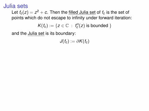
Julia setsLet fc(z) = z2 + c. Then the filled Julia set of fc is the set ofpoints which do not escape to infinity under forward iteration:
K (fc) := {z ∈ C : f nc (z) is bounded }
and the Julia set is its boundary:
J(fc) := ∂K (fc)
Julia setsLet fc(z) = z2 + c. Then the filled Julia set of fc is the set ofpoints which do not escape to infinity under forward iteration:
K (fc) := {z ∈ C : f nc (z) is bounded }
and the Julia set is its boundary:
J(fc) := ∂K (fc)

Julia setsLet fc(z) = z2 + c. Then the filled Julia set of fc is the set ofpoints which do not escape to infinity under forward iteration:
K (fc) := {z ∈ C : f nc (z) is bounded }
and the Julia set is its boundary:
J(fc) := ∂K (fc)

The complex case: Hubbard treesThe Hubbard tree Tc of a quadratic polynomial is a forwardinvariant, connected subset of the filled Julia set which containsthe critical orbit.

The complex case: Hubbard treesThe Hubbard tree Tc of a quadratic polynomial is a forwardinvariant, connected subset of the filled Julia set which containsthe critical orbit.

Complex Hubbard treesThe Hubbard tree Tc of a quadratic polynomial is a forwardinvariant, connected subset of the filled Julia set which containsthe critical orbit.

Complex Hubbard treesThe Hubbard tree Tc of a quadratic polynomial is a forwardinvariant, connected subset of the filled Julia set which containsthe critical orbit. The map fc acts on it.
The core entropy
Definition (W. Thurston)Let f be a polynomial whose Julia set is connected and locallyconnected
(e.g. a postcritically finite f ). Then the core entropyof f is the entropy of the restriction
h(f ) := h(f |Tf )
where Tf is the Hubbard tree of f .

The core entropy
Definition (W. Thurston)Let f be a polynomial whose Julia set is connected and locallyconnected (e.g. a postcritically finite f ).
Then the core entropyof f is the entropy of the restriction
h(f ) := h(f |Tf )
where Tf is the Hubbard tree of f .

The core entropy
Definition (W. Thurston)Let f be a polynomial whose Julia set is connected and locallyconnected (e.g. a postcritically finite f ). Then the core entropyof f
is the entropy of the restriction
h(f ) := h(f |Tf )
where Tf is the Hubbard tree of f .

The core entropy
Definition (W. Thurston)Let f be a polynomial whose Julia set is connected and locallyconnected (e.g. a postcritically finite f ). Then the core entropyof f is the entropy of the restriction
h(f ) := h(f |Tf )
where Tf is the Hubbard tree of f .

The core entropy
Definition (W. Thurston)Let f be a polynomial whose Julia set is connected and locallyconnected (e.g. a postcritically finite f ). Then the core entropyof f is the entropy of the restriction
h(f ) := h(f |Tf )
where Tf is the Hubbard tree of f .

The core entropy
Definition (W. Thurston)Let f be a polynomial whose Julia set is connected and locallyconnected (e.g. a postcritically finite f ). Then the core entropyof f is the entropy of the restriction
h(f ) := h(f |Tf )
where Tf is the Hubbard tree of f .

The core entropy - example
h(f ) := h(f |Tf )
A→ BB → CC → A ∪ DD → A ∪ B
M =
0 0 1 11 0 0 10 1 0 00 0 1 0
det(M − xI) == −1− 2x + x4
λ ≈ 1.39534h ≈ log 1.39534

The core entropy - example
h(f ) := h(f |Tf )
A→ BB → CC → A ∪ DD → A ∪ B
M =
0 0 1 11 0 0 10 1 0 00 0 1 0
det(M − xI) == −1− 2x + x4
λ ≈ 1.39534h ≈ log 1.39534

The core entropy - example
h(f ) := h(f |Tf )
A→ B
B → CC → A ∪ DD → A ∪ B
M =
0 0 1 11 0 0 10 1 0 00 0 1 0
det(M − xI) == −1− 2x + x4
λ ≈ 1.39534h ≈ log 1.39534

The core entropy - example
h(f ) := h(f |Tf )
A→ BB → C
C → A ∪ DD → A ∪ B
M =
0 0 1 11 0 0 10 1 0 00 0 1 0
det(M − xI) == −1− 2x + x4
λ ≈ 1.39534h ≈ log 1.39534

The core entropy - example
h(f ) := h(f |Tf )
A→ BB → CC → A ∪ D
D → A ∪ B
M =
0 0 1 11 0 0 10 1 0 00 0 1 0
det(M − xI) == −1− 2x + x4
λ ≈ 1.39534h ≈ log 1.39534

The core entropy - example
h(f ) := h(f |Tf )
A→ BB → CC → A ∪ DD → A ∪ B
M =
0 0 1 11 0 0 10 1 0 00 0 1 0
det(M − xI) == −1− 2x + x4
λ ≈ 1.39534h ≈ log 1.39534

The core entropy - example
h(f ) := h(f |Tf )
A→ BB → CC → A ∪ DD → A ∪ B
M =
0 0 1 11 0 0 10 1 0 00 0 1 0
det(M − xI) == −1− 2x + x4
λ ≈ 1.39534h ≈ log 1.39534

The core entropy - example
h(f ) := h(f |Tf )
A→ BB → CC → A ∪ DD → A ∪ B
M =
0 0 1 11 0 0 10 1 0 00 0 1 0
det(M − xI) == −1− 2x + x4
λ ≈ 1.39534h ≈ log 1.39534

The core entropy - example
h(f ) := h(f |Tf )
A→ BB → CC → A ∪ DD → A ∪ B
M =
0 0 1 11 0 0 10 1 0 00 0 1 0
det(M − xI) == −1− 2x + x4
λ ≈ 1.39534
h ≈ log 1.39534

The core entropy - example
h(f ) := h(f |Tf )
A→ BB → CC → A ∪ DD → A ∪ B
M =
0 0 1 11 0 0 10 1 0 00 0 1 0
det(M − xI) == −1− 2x + x4
λ ≈ 1.39534h ≈ log 1.39534

The core entropy
Let θ ∈ Q/Z. Then the external ray at angle θ lands, anddetermines a postcritically finite quadratic polynomial fθ, withHubbard tree Tθ.
Definition (W. Thurston)The core entropy of fθ is
h(θ) := h(fθ |Tθ)
Question: How does h(θ) vary with the parameter θ?
The core entropy
Let θ ∈ Q/Z. Then the external ray at angle θ lands, anddetermines a postcritically finite quadratic polynomial fθ, withHubbard tree Tθ.
Definition (W. Thurston)The core entropy of fθ is
h(θ) := h(fθ |Tθ)
Question: How does h(θ) vary with the parameter θ?

The core entropy
Let θ ∈ Q/Z. Then the external ray at angle θ lands, anddetermines a postcritically finite quadratic polynomial fθ, withHubbard tree Tθ.
Definition (W. Thurston)The core entropy of fθ is
h(θ) := h(fθ |Tθ)
Question: How does h(θ) vary with the parameter θ?

Core entropy as a function of external angle (W.Thurston)
0.2 0.4 0.6 0.8 1.0
0.1
0.2
0.3
0.4
0.5
0.6
0.7

Core entropy as a function of external angle (W.Thurston)
0.1 0.2 0.3 0.4 0.5
0.1
0.2
0.3
0.4
0.5
0.6
0.7
Question Can you see the Mandelbrot set in this picture?

Core entropy as a function of external angle (W.Thurston)
0.1 0.2 0.3 0.4 0.5
0.1
0.2
0.3
0.4
0.5
0.6
0.7
Question Can you see the Mandelbrot set in this picture?

Monotonicity of entropy
Observation.
If RM(θ1) and RM(θ2) land together, then h(θ1) = h(θ2).
Monotonicity still holds along veins.
Let us take two rays θ1 landing at c1 and θ2 landing at c2.Then we define θ1 <M θ2 if c1 lies on the arc [0, c2].
Theorem (Li Tao; Penrose; Tan Lei; Zeng Jinsong)If θ1 <M θ2, then
h(θ1) ≤ h(θ2)
In fact, entropy determines the lamination.
PropositionIf h(θ1) = h(θ2) and h(θ) > h(θ1) for all θ ∈ (θ1, θ2), thenθ1 ∼M θ2.

Monotonicity of entropy
Observation.If RM(θ1) and RM(θ2) land together, then h(θ1) = h(θ2).
Monotonicity still holds along veins.
Let us take two rays θ1 landing at c1 and θ2 landing at c2.
Then we define θ1 <M θ2 if c1 lies on the arc [0, c2].
Theorem (Li Tao; Penrose; Tan Lei; Zeng Jinsong)If θ1 <M θ2, then
h(θ1) ≤ h(θ2)
In fact, entropy determines the lamination.
PropositionIf h(θ1) = h(θ2) and h(θ) > h(θ1) for all θ ∈ (θ1, θ2), thenθ1 ∼M θ2.

Monotonicity of entropy
Observation.If RM(θ1) and RM(θ2) land together, then h(θ1) = h(θ2).
Monotonicity still holds along veins.
Let us take two rays θ1 landing at c1 and θ2 landing at c2.Then we define θ1 <M θ2 if c1 lies on the arc [0, c2].
Theorem (Li Tao; Penrose; Tan Lei; Zeng Jinsong)If θ1 <M θ2, then
h(θ1) ≤ h(θ2)
In fact, entropy determines the lamination.
PropositionIf h(θ1) = h(θ2) and h(θ) > h(θ1) for all θ ∈ (θ1, θ2), thenθ1 ∼M θ2.

Monotonicity of entropy
Observation.If RM(θ1) and RM(θ2) land together, then h(θ1) = h(θ2).
Monotonicity still holds along veins.
Let us take two rays θ1 landing at c1 and θ2 landing at c2.Then we define θ1 <M θ2 if c1 lies on the arc [0, c2].
Theorem (Li Tao; Penrose; Tan Lei; Zeng Jinsong)If θ1 <M θ2, then
h(θ1) ≤ h(θ2)
In fact, entropy determines the lamination.
PropositionIf h(θ1) = h(θ2)
and h(θ) > h(θ1) for all θ ∈ (θ1, θ2), thenθ1 ∼M θ2.
Monotonicity of entropy
Observation.If RM(θ1) and RM(θ2) land together, then h(θ1) = h(θ2).
Monotonicity still holds along veins.
Let us take two rays θ1 landing at c1 and θ2 landing at c2.Then we define θ1 <M θ2 if c1 lies on the arc [0, c2].
Theorem (Li Tao; Penrose; Tan Lei; Zeng Jinsong)If θ1 <M θ2, then
h(θ1) ≤ h(θ2)
In fact, entropy determines the lamination.
PropositionIf h(θ1) = h(θ2) and h(θ) > h(θ1) for all θ ∈ (θ1, θ2),
thenθ1 ∼M θ2.

Monotonicity of entropy
Observation.If RM(θ1) and RM(θ2) land together, then h(θ1) = h(θ2).
Monotonicity still holds along veins.
Let us take two rays θ1 landing at c1 and θ2 landing at c2.Then we define θ1 <M θ2 if c1 lies on the arc [0, c2].
Theorem (Li Tao; Penrose; Tan Lei; Zeng Jinsong)If θ1 <M θ2, then
h(θ1) ≤ h(θ2)
In fact, entropy determines the lamination.
PropositionIf h(θ1) = h(θ2) and h(θ) > h(θ1) for all θ ∈ (θ1, θ2), thenθ1 ∼M θ2.

Rays landing on the real slice of the Mandelbrot set

Harmonic measureGiven a subset A of ∂M, the harmonic measure νM is theprobability that a random ray lands on A:
νM(A) := Leb({θ ∈ S1 : R(θ) lands on A})
For instance, take A =M∩R the real section of the Mandelbrotset. How common is it for a ray to land on the real axis?
Harmonic measureGiven a subset A of ∂M, the harmonic measure νM is theprobability that a random ray lands on A:
νM(A) := Leb({θ ∈ S1 : R(θ) lands on A})
For instance, take A =M∩R the real section of the Mandelbrotset.
How common is it for a ray to land on the real axis?

Harmonic measureGiven a subset A of ∂M, the harmonic measure νM is theprobability that a random ray lands on A:
νM(A) := Leb({θ ∈ S1 : R(θ) lands on A})
For instance, take A =M∩R the real section of the Mandelbrotset. How common is it for a ray to land on the real axis?

Real section of the Mandelbrot setTheorem (Zakeri, ’00)The harmonic measure of the real axis is 0.
However,the Hausdorff dimension of the set of rays landing on the realaxis is 1.

Real section of the Mandelbrot setTheorem (Zakeri, ’00)The harmonic measure of the real axis is 0. However,
the Hausdorff dimension of the set of rays landing on the realaxis is 1.

Real section of the Mandelbrot setTheorem (Zakeri, ’00)The harmonic measure of the real axis is 0. However,the Hausdorff dimension of the set of rays landing on the realaxis is 1.

Real section of the Mandelbrot setTheorem (Zakeri, ’00)The harmonic measure of the real axis is 0. However,the Hausdorff dimension of the set of rays landing on the realaxis is 1.
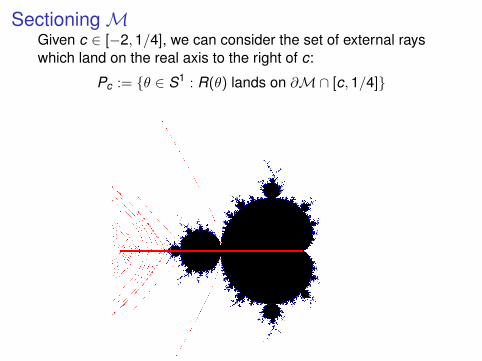
SectioningMGiven c ∈ [−2,1/4], we can consider the set of external rayswhich land on the real axis to the right of c:
Pc := {θ ∈ S1 : R(θ) lands on ∂M∩ [c,1/4]}

SectioningMGiven c ∈ [−2,1/4], we can consider the set of external rayswhich land on the real axis to the right of c:
Pc := {θ ∈ S1 : R(θ) lands on ∂M∩ [c,1/4]}

SectioningMGiven c ∈ [−2,1/4], we can consider the set of external rayswhich land on the real axis to the right of c:
Pc := {θ ∈ S1 : R(θ) lands on ∂M∩ [c,1/4]}

SectioningMGiven c ∈ [−2,1/4], we can consider the set of external rayswhich land on the real axis to the right of c:
Pc := {θ ∈ S1 : R(θ) lands on ∂M∩ [c,1/4]}
SectioningMGiven c ∈ [−2,1/4], we can consider the set of external rayswhich land on the real axis to the right of c:
Pc := {θ ∈ S1 : R(θ) lands on ∂M∩ [c,1/4]}

Pc := {θ ∈ S1 : R(θ) lands on ∂M∩ [c,1/4]}The function
c 7→ H.dim Pc
decreases with c, taking values between 0 and 1.

Pc := {θ ∈ S1 : R(θ) lands on ∂M∩ [c,1/4]}The function
c 7→ H.dim Pc
decreases with c, taking values between 0 and 1.

Pc := {θ ∈ S1 : R(θ) lands on ∂M∩ [c,1/4]}The function
c 7→ H.dim Pc
decreases with c, taking values between 0 and 1.

Pc := {θ ∈ S1 : R(θ) lands on ∂M∩ [c,1/4]}The function
c 7→ H.dim Pc
decreases with c, taking values between 0 and 1.

Entropy formula, real caseTheorem (T.)Let c ∈ [−2,1/4]. Then
htop(fc ,R)
log 2= H.dim Pc

Entropy formula, real caseTheorem (T.)Let c ∈ [−2,1/4]. Then
htop(fc ,R)
log 2= H.dim Pc

Entropy formula, real caseTheorem (T.)Let c ∈ [−2,1/4]. Then
htop(fc ,R)
log 2= H.dim Pc
I It relates dynamical properties of a particular map to thegeometry of parameter space near the chosen parameter.
I Entropy formula: relates dimension, entropy and Lyapunovexponent (Manning, Bowen, Ledrappier, Young, ...).
I It does not depend on MLC.I If Bc := {θ ∈ R/Z : θ biaccessible for fc} = Lc ∩ ∂D
(see e.g. Zakeri, Smirnov, Zdunik, Bruin-Schleicher ...) then also
htop(fc ,R)
log 2= H. dim Bc
I It can be generalized to non-real veins.

Entropy formula, real caseTheorem (T.)Let c ∈ [−2,1/4]. Then
htop(fc ,R)
log 2= H.dim Pc
I It relates dynamical properties of a particular map to thegeometry of parameter space near the chosen parameter.
I Entropy formula: relates dimension, entropy and Lyapunovexponent (Manning, Bowen, Ledrappier, Young, ...).
I It does not depend on MLC.
I If Bc := {θ ∈ R/Z : θ biaccessible for fc} = Lc ∩ ∂D(see e.g. Zakeri, Smirnov, Zdunik, Bruin-Schleicher ...) then also
htop(fc ,R)
log 2= H. dim Bc
I It can be generalized to non-real veins.
Entropy formula, real caseTheorem (T.)Let c ∈ [−2,1/4]. Then
htop(fc ,R)
log 2= H.dim Pc
I It relates dynamical properties of a particular map to thegeometry of parameter space near the chosen parameter.
I Entropy formula: relates dimension, entropy and Lyapunovexponent (Manning, Bowen, Ledrappier, Young, ...).
I It does not depend on MLC.I If Bc := {θ ∈ R/Z : θ biaccessible for fc}
= Lc ∩ ∂D(see e.g. Zakeri, Smirnov, Zdunik, Bruin-Schleicher ...) then also
htop(fc ,R)
log 2= H. dim Bc
I It can be generalized to non-real veins.

Entropy formula, real caseTheorem (T.)Let c ∈ [−2,1/4]. Then
htop(fc ,R)
log 2= H.dim Pc
I It relates dynamical properties of a particular map to thegeometry of parameter space near the chosen parameter.
I Entropy formula: relates dimension, entropy and Lyapunovexponent (Manning, Bowen, Ledrappier, Young, ...).
I It does not depend on MLC.I If Bc := {θ ∈ R/Z : θ biaccessible for fc} = Lc ∩ ∂D
(see e.g. Zakeri, Smirnov, Zdunik, Bruin-Schleicher ...) then also
htop(fc ,R)
log 2= H. dim Bc
I It can be generalized to non-real veins.

Entropy formula, real caseTheorem (T.)Let c ∈ [−2,1/4]. Then
htop(fc ,R)
log 2= H.dim Pc
I It relates dynamical properties of a particular map to thegeometry of parameter space near the chosen parameter.
I Entropy formula: relates dimension, entropy and Lyapunovexponent (Manning, Bowen, Ledrappier, Young, ...).
I It does not depend on MLC.I If Bc := {θ ∈ R/Z : θ biaccessible for fc} = Lc ∩ ∂D
(see e.g. Zakeri, Smirnov, Zdunik, Bruin-Schleicher ...) then also
htop(fc ,R)
log 2= H. dim Bc
I It can be generalized to non-real veins.

Entropy formula along complex veinsA vein is an embedded arc in the Mandelbrot set.

Entropy formula, complex case
A vein is an embedded arc in the Mandelbrot set.
Given a parameter c along a vein, we can look at the set Pc ofparameter rays which land on the vein between 0 and c.
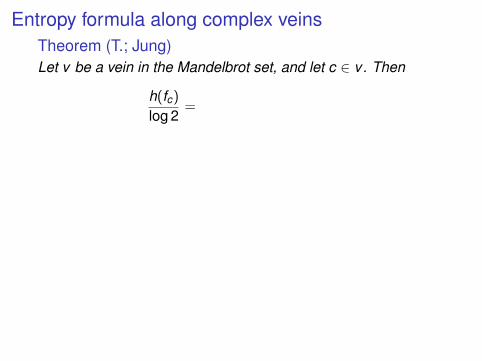
Entropy formula along complex veinsTheorem (T.; Jung)Let v be a vein in the Mandelbrot set, and let c ∈ v.
Then
h(fc)
log 2= H.dim Bc = H.dim Pc
Entropy formula along complex veinsTheorem (T.; Jung)Let v be a vein in the Mandelbrot set, and let c ∈ v. Then
h(fc)
log 2=
H.dim Bc = H.dim Pc

Entropy formula along complex veinsTheorem (T.; Jung)Let v be a vein in the Mandelbrot set, and let c ∈ v. Then
h(fc)
log 2= H.dim Bc
= H.dim Pc

Entropy formula along complex veinsTheorem (T.; Jung)Let v be a vein in the Mandelbrot set, and let c ∈ v. Then
h(fc)
log 2= H.dim Bc = H.dim Pc

Entropy formula along complex veinsTheorem (T.; Jung)Let v be a vein in the Mandelbrot set, and let c ∈ v. Then
h(fc)
log 2= H.dim Bc = H.dim Pc
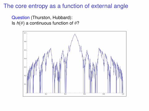
The core entropy as a function of external angle
Question (Thurston, Hubbard):Is h(θ) a continuous function of θ?
0.2 0.4 0.6 0.8 1.0
0.1
0.2
0.3
0.4
0.5
0.6
0.7

The Main Theorem: Continuity
Theorem (T.)The core entropy function h(θ) extends to a continuous functionfrom R/Z to R.
0.2 0.4 0.6 0.8 1.0
0.1
0.2
0.3
0.4
0.5
0.6
0.7

Regularity properties of the core entropyIn fact:
Theorem (T.)The core entropy is locally Hölder continuous at θ if h(θ) > 0,and not locally Hölder at θ where h(θ) = 0.
0.2 0.4 0.6 0.8 1.0
0.1
0.2
0.3
0.4
0.5
0.6
0.7

Regularity properties of the core entropyIn fact:
Theorem (T.)The core entropy is locally Hölder continuous at θ if h(θ) > 0,and not locally Hölder at θ where h(θ) = 0.
0.2 0.4 0.6 0.8 1.0
0.1
0.2
0.3
0.4
0.5
0.6
0.7

Regularity properties of the core entropy
In fact:
Theorem (T.)The core entropy is locally Hölder continuous at θ if h(θ) > 0,and not locally Hölder at θ where h(θ) = 0.
Theorem (T.)Let h(θ) be the entropy of the real quadratic polynomial withexternal ray θ. Then the local Hölder exponent α(h, θ) of h at θsatisfies
α(h, θ) :=h(θ)
log 2
(Conjectured by Isola-Politi, 1990)

Regularity properties of the core entropy
In fact:
Theorem (T.)The core entropy is locally Hölder continuous at θ if h(θ) > 0,and not locally Hölder at θ where h(θ) = 0.
Theorem (T.)Let h(θ) be the entropy of the real quadratic polynomial withexternal ray θ.
Then the local Hölder exponent α(h, θ) of h at θsatisfies
α(h, θ) :=h(θ)
log 2
(Conjectured by Isola-Politi, 1990)

Regularity properties of the core entropy
In fact:
Theorem (T.)The core entropy is locally Hölder continuous at θ if h(θ) > 0,and not locally Hölder at θ where h(θ) = 0.
Theorem (T.)Let h(θ) be the entropy of the real quadratic polynomial withexternal ray θ. Then the local Hölder exponent α(h, θ) of h at θsatisfies
α(h, θ) :=h(θ)
log 2
(Conjectured by Isola-Politi, 1990)

Regularity properties of the core entropy
In fact:
Theorem (T.)The core entropy is locally Hölder continuous at θ if h(θ) > 0,and not locally Hölder at θ where h(θ) = 0.
Theorem (T.)Let h(θ) be the entropy of the real quadratic polynomial withexternal ray θ. Then the local Hölder exponent α(h, θ) of h at θsatisfies
α(h, θ) :=h(θ)
log 2
(Conjectured by Isola-Politi, 1990)

Maxima of core entropyGiven θ1 < θ2 with θ1 ∼M θ2 (= landing together),
define theirpseudocenter θ? as the dyadic rational in [θ1, θ2] of lowest complexity
θ? := {x = p/2q : x ∈ [θ1, θ2],q minimal}
E.g.: θ1 = 1/7, θ2 = 2/7, θ? = 1/4(Carminati-T. for continued fractions)
Conjecture (T.)The maximum of the entropy on [θ1, θ2] is achieved at θ = θ?.

Maxima of core entropyGiven θ1 < θ2 with θ1 ∼M θ2 (= landing together), define theirpseudocenter θ? as the dyadic rational in [θ1, θ2] of lowest complexity
θ? := {x = p/2q : x ∈ [θ1, θ2],q minimal}
E.g.: θ1 = 1/7, θ2 = 2/7,
θ? = 1/4(Carminati-T. for continued fractions)
Conjecture (T.)The maximum of the entropy on [θ1, θ2] is achieved at θ = θ?.

Maxima of core entropyGiven θ1 < θ2 with θ1 ∼M θ2 (= landing together), define theirpseudocenter θ? as the dyadic rational in [θ1, θ2] of lowest complexity
θ? := {x = p/2q : x ∈ [θ1, θ2],q minimal}
E.g.: θ1 = 1/7, θ2 = 2/7, θ? = 1/4
(Carminati-T. for continued fractions)
Conjecture (T.)The maximum of the entropy on [θ1, θ2] is achieved at θ = θ?.

Maxima of core entropyGiven θ1 < θ2 with θ1 ∼M θ2 (= landing together), define theirpseudocenter θ? as the dyadic rational in [θ1, θ2] of lowest complexity
θ? := {x = p/2q : x ∈ [θ1, θ2],q minimal}
E.g.: θ1 = 1/7, θ2 = 2/7, θ? = 1/4(Carminati-T. for continued fractions)
Conjecture (T.)The maximum of the entropy on [θ1, θ2] is achieved at θ = θ?.

Maxima of core entropyGiven θ1 < θ2 with θ1 ∼M θ2 (= landing together), define theirpseudocenter θ? as the dyadic rational in [θ1, θ2] of lowest complexity
θ? := {x = p/2q : x ∈ [θ1, θ2],q minimal}
E.g.: θ1 = 1/7, θ2 = 2/7, θ? = 1/4
Theorem (Dudko-Schleicher)The maximum of the entropy on [θ1, θ2] is achieved at θ = θ?.

The core entropy for cubic polynomials

The core entropy for cubic polynomials

The core entropy for cubic polynomials

The unicritical slice
0.05 0.10 0.15 0.20 0.25 0.30
0.1
0.2
0.3
0.4
0.5
0.6
0.7
f (z) = z3 + c

The symmetric slice
0.1 0.2 0.3 0.4 0.5
0.2
0.4
0.6
0.8
1.0
f (z) = z3 + cz

Continuity in higher degree, combinatorial versionFor polynomials of degree d , the analog of the circle at infinityfor the Mandelbrot set is the set PM(d) of primitive majors.
Theorem (W. Thurston)
PM(d) ∼= K (Bd ,1)
where Bd is the braid group on d strands.(see Baik, Gao, Hubbard, Lindsey, Tan, D. Thurston)Example. π1(PM(3)) = 〈x , y : x2 = y3〉

Continuity in higher degree, combinatorial versionFor polynomials of degree d , the analog of the circle at infinityfor the Mandelbrot set is the set PM(d) of primitive majors.
Theorem (W. Thurston)
PM(d) ∼= K (Bd ,1)
where Bd is the braid group on d strands.
(see Baik, Gao, Hubbard, Lindsey, Tan, D. Thurston)Example. π1(PM(3)) = 〈x , y : x2 = y3〉

Continuity in higher degree, combinatorial versionFor polynomials of degree d , the analog of the circle at infinityfor the Mandelbrot set is the set PM(d) of primitive majors.
Theorem (W. Thurston)
PM(d) ∼= K (Bd ,1)
where Bd is the braid group on d strands.(see Baik, Gao, Hubbard, Lindsey, Tan, D. Thurston)
Example. π1(PM(3)) = 〈x , y : x2 = y3〉

Continuity in higher degree, combinatorial versionFor polynomials of degree d , the analog of the circle at infinityfor the Mandelbrot set is the set PM(d) of primitive majors.
Theorem (W. Thurston)
PM(d) ∼= K (Bd ,1)
where Bd is the braid group on d strands.(see Baik, Gao, Hubbard, Lindsey, Tan, D. Thurston)Example. π1(PM(3)) = 〈x , y : x2 = y3〉

Continuity in higher degree, combinatorial versionTheorem (T. - Yan Gao)Fix d ≥ 2. Then the core entropy extends to a continuousfunction on the space PM(d) of primitive majors.

Continuity in higher degree, combinatorial versionTheorem (T. - Yan Gao)Fix d ≥ 2. Then the core entropy extends to a continuousfunction on the space PM(d) of primitive majors.

Continuity in higher degree, analytic version
Define Pd as the space of monic, centered polynomials ofdegree d .
One says fn → f if the coefficients of fn converge tothe coefficients of f .
Theorem (T. - Yan Gao)Let d ≥ 2. Then the core entropy is a continuous function onthe space of monic, centered, postcritically finite polynomials ofdegree d.

Continuity in higher degree, analytic version
Define Pd as the space of monic, centered polynomials ofdegree d . One says fn → f if the coefficients of fn converge tothe coefficients of f .
Theorem (T. - Yan Gao)Let d ≥ 2. Then the core entropy is a continuous function onthe space of monic, centered, postcritically finite polynomials ofdegree d.

Further questions
1. What are the local maxima of the core entropy in d > 3?
Howmany are there?
2. Can you use core entropy in higher degree case to define ahierarchical structure of parameter space?(Compare veins for d = 2)
3. Jung’s conjecture: self-similarity of entropy graph nearMisiurewicz points(where the Mandelbrot set is self-similar! (Tan Lei))
4. Can we us core entropy to define transverse measures on thelamination?Thurston: surface laminations (Teichmüller theory) carry atransverse measureSullivan dictionary: Teichmüller theory⇔ complex dynamics(Answer: Yes! [T. ’21])
5. What about the other eigenvalues of the transition matrix?(Bray-Davis-Lindsey-Wu, ...)

Further questions
1. What are the local maxima of the core entropy in d > 3? Howmany are there?
2. Can you use core entropy in higher degree case to define ahierarchical structure of parameter space?
(Compare veins for d = 2)
3. Jung’s conjecture: self-similarity of entropy graph nearMisiurewicz points(where the Mandelbrot set is self-similar! (Tan Lei))
4. Can we us core entropy to define transverse measures on thelamination?Thurston: surface laminations (Teichmüller theory) carry atransverse measureSullivan dictionary: Teichmüller theory⇔ complex dynamics(Answer: Yes! [T. ’21])
5. What about the other eigenvalues of the transition matrix?(Bray-Davis-Lindsey-Wu, ...)

Further questions
1. What are the local maxima of the core entropy in d > 3? Howmany are there?
2. Can you use core entropy in higher degree case to define ahierarchical structure of parameter space?(Compare veins for d = 2)
3. Jung’s conjecture: self-similarity of entropy graph nearMisiurewicz points(where the Mandelbrot set is self-similar! (Tan Lei))
4. Can we us core entropy to define transverse measures on thelamination?Thurston: surface laminations (Teichmüller theory) carry atransverse measureSullivan dictionary: Teichmüller theory⇔ complex dynamics(Answer: Yes! [T. ’21])
5. What about the other eigenvalues of the transition matrix?(Bray-Davis-Lindsey-Wu, ...)

Further questions
1. What are the local maxima of the core entropy in d > 3? Howmany are there?
2. Can you use core entropy in higher degree case to define ahierarchical structure of parameter space?(Compare veins for d = 2)
3. Jung’s conjecture: self-similarity of entropy graph nearMisiurewicz points
(where the Mandelbrot set is self-similar! (Tan Lei))
4. Can we us core entropy to define transverse measures on thelamination?Thurston: surface laminations (Teichmüller theory) carry atransverse measureSullivan dictionary: Teichmüller theory⇔ complex dynamics(Answer: Yes! [T. ’21])
5. What about the other eigenvalues of the transition matrix?(Bray-Davis-Lindsey-Wu, ...)

Further questions
1. What are the local maxima of the core entropy in d > 3? Howmany are there?
2. Can you use core entropy in higher degree case to define ahierarchical structure of parameter space?(Compare veins for d = 2)
3. Jung’s conjecture: self-similarity of entropy graph nearMisiurewicz points(where the Mandelbrot set is self-similar! (Tan Lei))
4. Can we us core entropy to define transverse measures on thelamination?Thurston: surface laminations (Teichmüller theory) carry atransverse measureSullivan dictionary: Teichmüller theory⇔ complex dynamics(Answer: Yes! [T. ’21])
5. What about the other eigenvalues of the transition matrix?(Bray-Davis-Lindsey-Wu, ...)

Further questions
1. What are the local maxima of the core entropy in d > 3? Howmany are there?
2. Can you use core entropy in higher degree case to define ahierarchical structure of parameter space?(Compare veins for d = 2)
3. Jung’s conjecture: self-similarity of entropy graph nearMisiurewicz points(where the Mandelbrot set is self-similar! (Tan Lei))
4. Can we us core entropy to define transverse measures on thelamination?
Thurston: surface laminations (Teichmüller theory) carry atransverse measureSullivan dictionary: Teichmüller theory⇔ complex dynamics(Answer: Yes! [T. ’21])
5. What about the other eigenvalues of the transition matrix?(Bray-Davis-Lindsey-Wu, ...)

Further questions
1. What are the local maxima of the core entropy in d > 3? Howmany are there?
2. Can you use core entropy in higher degree case to define ahierarchical structure of parameter space?(Compare veins for d = 2)
3. Jung’s conjecture: self-similarity of entropy graph nearMisiurewicz points(where the Mandelbrot set is self-similar! (Tan Lei))
4. Can we us core entropy to define transverse measures on thelamination?Thurston: surface laminations (Teichmüller theory) carry atransverse measure
Sullivan dictionary: Teichmüller theory⇔ complex dynamics(Answer: Yes! [T. ’21])
5. What about the other eigenvalues of the transition matrix?(Bray-Davis-Lindsey-Wu, ...)

Further questions
1. What are the local maxima of the core entropy in d > 3? Howmany are there?
2. Can you use core entropy in higher degree case to define ahierarchical structure of parameter space?(Compare veins for d = 2)
3. Jung’s conjecture: self-similarity of entropy graph nearMisiurewicz points(where the Mandelbrot set is self-similar! (Tan Lei))
4. Can we us core entropy to define transverse measures on thelamination?Thurston: surface laminations (Teichmüller theory) carry atransverse measureSullivan dictionary: Teichmüller theory⇔ complex dynamics
(Answer: Yes! [T. ’21])
5. What about the other eigenvalues of the transition matrix?(Bray-Davis-Lindsey-Wu, ...)

Further questions
1. What are the local maxima of the core entropy in d > 3? Howmany are there?
2. Can you use core entropy in higher degree case to define ahierarchical structure of parameter space?(Compare veins for d = 2)
3. Jung’s conjecture: self-similarity of entropy graph nearMisiurewicz points(where the Mandelbrot set is self-similar! (Tan Lei))
4. Can we us core entropy to define transverse measures on thelamination?Thurston: surface laminations (Teichmüller theory) carry atransverse measureSullivan dictionary: Teichmüller theory⇔ complex dynamics(Answer: Yes! [T. ’21])
5. What about the other eigenvalues of the transition matrix?(Bray-Davis-Lindsey-Wu, ...)

Further questions
1. What are the local maxima of the core entropy in d > 3? Howmany are there?
2. Can you use core entropy in higher degree case to define ahierarchical structure of parameter space?(Compare veins for d = 2)
3. Jung’s conjecture: self-similarity of entropy graph nearMisiurewicz points(where the Mandelbrot set is self-similar! (Tan Lei))
4. Can we us core entropy to define transverse measures on thelamination?Thurston: surface laminations (Teichmüller theory) carry atransverse measureSullivan dictionary: Teichmüller theory⇔ complex dynamics(Answer: Yes! [T. ’21])
5. What about the other eigenvalues of the transition matrix?
(Bray-Davis-Lindsey-Wu, ...)

Further questions
1. What are the local maxima of the core entropy in d > 3? Howmany are there?
2. Can you use core entropy in higher degree case to define ahierarchical structure of parameter space?(Compare veins for d = 2)
3. Jung’s conjecture: self-similarity of entropy graph nearMisiurewicz points(where the Mandelbrot set is self-similar! (Tan Lei))
4. Can we us core entropy to define transverse measures on thelamination?Thurston: surface laminations (Teichmüller theory) carry atransverse measureSullivan dictionary: Teichmüller theory⇔ complex dynamics(Answer: Yes! [T. ’21])
5. What about the other eigenvalues of the transition matrix?(Bray-Davis-Lindsey-Wu, ...)


Coda: LaminationsTheorem (W. Thurston)Let θ ∈ R/Z.
Then there exists a lamination Lθ on the disk suchthat θ1 ∼ θ2 if R(θ1) and R(θ2) “land" at the same point.

Coda: LaminationsTheorem (W. Thurston)Let θ ∈ R/Z. Then there exists a lamination Lθ on the disk suchthat
θ1 ∼ θ2 if R(θ1) and R(θ2) “land" at the same point.

Coda: LaminationsTheorem (W. Thurston)Let θ ∈ R/Z. Then there exists a lamination Lθ on the disk suchthat θ1 ∼ θ2 if R(θ1) and R(θ2) “land" at the same point.

Coda: LaminationsTheorem (W. Thurston)Let θ ∈ R/Z. Then there exists a lamination Lθ on the disk suchthat θ1 ∼ θ2 if R(θ1) and R(θ2) “land" at the same point.

LaminationsTheorem (W. Thurston)Let θ ∈ R/Z. Then there exists a lamination Lθ on the disk suchthat θ1 ∼ θ2 if R(θ1) and R(θ2) “land" at the same point.
Also Thurston: surface laminations (Teichmüller theory) carry atransverse measureSullivan dictionary: Teichmüller theory⇔ complex dynamicsQuestion. Can we define a transverse measure on Lθ?

LaminationsTheorem (W. Thurston)Let θ ∈ R/Z. Then there exists a lamination Lθ on the disk suchthat θ1 ∼ θ2 if R(θ1) and R(θ2) “land" at the same point.
Also Thurston: surface laminations (Teichmüller theory) carry atransverse measure
Sullivan dictionary: Teichmüller theory⇔ complex dynamicsQuestion. Can we define a transverse measure on Lθ?

LaminationsTheorem (W. Thurston)Let θ ∈ R/Z. Then there exists a lamination Lθ on the disk suchthat θ1 ∼ θ2 if R(θ1) and R(θ2) “land" at the same point.
Also Thurston: surface laminations (Teichmüller theory) carry atransverse measureSullivan dictionary: Teichmüller theory⇔ complex dynamics
Question. Can we define a transverse measure on Lθ?

LaminationsTheorem (W. Thurston)Let θ ∈ R/Z. Then there exists a lamination Lθ on the disk suchthat θ1 ∼ θ2 if R(θ1) and R(θ2) “land" at the same point.
Also Thurston: surface laminations (Teichmüller theory) carry atransverse measureSullivan dictionary: Teichmüller theory⇔ complex dynamicsQuestion. Can we define a transverse measure on Lθ?

Laminations
Question. Can we define a transverse measure on Lθ?
Theorem (T. ’21)There exists a transverse measure mθ on Lθ such that
f ?θ (mθ) = λθmθ
and h(θ) = logλθ.
Such a measure induces a semiconjugacy betweenfθ : Tθ → Tθ and a piecewise linear model with slope λθ.(Compare: Milnor-Thurston, Baillif-deCarvalho, Sousa-Ramos, . . . )

Laminations
Question. Can we define a transverse measure on Lθ?
Theorem (T. ’21)There exists a transverse measure mθ on Lθ such that
f ?θ (mθ) = λθmθ
and h(θ) = logλθ.
Such a measure induces a semiconjugacy betweenfθ : Tθ → Tθ and a piecewise linear model with slope λθ.
(Compare: Milnor-Thurston, Baillif-deCarvalho, Sousa-Ramos, . . . )

Laminations
Question. Can we define a transverse measure on Lθ?
Theorem (T. ’21)There exists a transverse measure mθ on Lθ such that
f ?θ (mθ) = λθmθ
and h(θ) = logλθ.
Such a measure induces a semiconjugacy betweenfθ : Tθ → Tθ and a piecewise linear model with slope λθ.(Compare: Milnor-Thurston, Baillif-deCarvalho, Sousa-Ramos, . . . )

A transverse measure on QML
Let `1 < `2 two leaves, and τ a transverse arc connecting them.
Then we defineµ(τ) := h(fc2)− h(fc1)
It givesMabs (rather, a quotient) the structure of a metric tree.
“Combinatorial bifurcation measure”?

A transverse measure on QML
Let `1 < `2 two leaves, and τ a transverse arc connecting them.Then we define
µ(τ) := h(fc2)− h(fc1)
It givesMabs (rather, a quotient) the structure of a metric tree.
“Combinatorial bifurcation measure”?

A transverse measure on QML
Let `1 < `2 two leaves, and τ a transverse arc connecting them.Then we define
µ(τ) := h(fc2)− h(fc1)
It givesMabs (rather, a quotient) the structure of a metric tree.
“Combinatorial bifurcation measure”?

A transverse measure on QML
Let `1 < `2 two leaves, and τ a transverse arc connecting them.Then we define
µ(τ) := h(fc2)− h(fc1)
It givesMabs (rather, a quotient) the structure of a metric tree.
“Combinatorial bifurcation measure”?