sucharit sarkar and jiajun wang- an algorithm for computing some heegard floer homologies

8/3/2019 Sucharit Sarkar and Jiajun Wang- An Algorithm for Computing Some Heegard Floer Homologies

http://slidepdf.com/reader/full/sucharit-sarkar-and-jiajun-wang-an-algorithm-for-computing-some-heegard-floer 1/20

a r X i v : m a t h / 0

6 0 7 7 7 7 v 4

[ m a t h . G

T ] 1 0 S e p 2 0 0 8

AN ALGORITHM FOR COMPUTING SOME HEEGAARD FLOER

HOMOLOGIES

SUCHARIT SARKAR AND JIAJUN WANG

Abstract. In this paper, we give an algorithm to compute the hat version of Heegaard Floerhomology of a closed oriented three-manifold. This method also allows us to compute the filtrationcoming from a null-homologous link in a three-manifold.

1. Introduction

Heegaard Floer homology is a collection of invariants for closed oriented three-manifolds, intro-

duced by Peter Ozsvath and Zoltan Szabo [8, 9]. There are four versions, denoted byH F , H F ∞, HF +

and HF −, which are graded abelian groups. The hat version HF (Y ) is defined as the homologyof a chain complex CF (Y ) coming from a Heegaard diagram of the three-manifold Y . The differ-entials count the number of points in certain moduli spaces of holomorphic disks, which are hardto compute in general.

There is also a relative version of the theory corresponding to pairs (Y, K ), where K is a knotin Y . If K is null-homologous, then a Seifert surface S of K induces a filtration of the chain

complex CF (Y ), and the chain homotopy type of the filtered chain complex is a knot invariant.

The homology groups HF K (Y, K ) of successive quotients of filtration levels are called knot Floerhomology groups ([12, 19, 15]).

A cobordism between two three-manifolds induces homomorphisms on the Heegaard Floer ho-mology groups of the two three-manifolds. In fact, the homomorphisms on HF − and HF + can

be used to construct an invariant of smooth four-manifolds with b+

2 > 1 ([11]), called the Ozsvath-Szabo invariant. Conjecturally, the Ozsvath-Szabo four-manifold invariant is equivalent to thegauge-theoretic Seiberg-Witten invariant.

Heegaard Floer homology turns out to be a fruitful and powerful theory in the study of three-dimensional and four-dimensional topology. It gives an alternate proof of the Donaldson diagonal-ization theorem and the Thom conjecture for CP2 ([10]). Heegaard Floer homology also detectsthe Thurston norm of a three-manifold ([16, 7]). Moreover, knot Floer homology detects the genus([13]) and fiberedness ([1, 6, 2]) of knots and links in the three-sphere. There is an invariant τ coming from the knot filtration, whose absolute value gives a lower-bound of the slice genus forknots in the three-sphere ([14]).

Despite its success, there was no general method to compute the invariants. There were combina-torial descriptions in certain special cases, but the computation for an arbitrary three-manifold was

an open problem ([18]). In this paper, we give an algorithm to compute HF (Y ) for a three-manifoldY , and also HF K (Y, K ) for a knot K in any three-manifold. All our computations will be donewith coefficients in F2 = Z/2Z. We show that one can always find Heegaard diagrams satisfyingcertain properties (Definition 3.1). Using such Heegaard diagrams, which we call nice, it will be

easy to compute HF and HF K . Our main results are summarized in the following theorems.

Date: May 1st, 2008.1991 Mathematics Subject Classification. Primary 57R58.Key words and phrases. Heegaard Floer homology; knot Floer homology; algorithm.

1

http://arxiv.org/abs/math/0607777v4









































2 SUCHARIT SARKAR AND JIAJUN WANG

Theorem 1.1. Given a nice Heegaard diagram of a closed oriented three-manifold Y , HF (Y )

can be computed combinatorially. Similarly, for a knot K ⊂ Y , HF K (Y, K ) can be computed

combinatorially in a nice Heegaard diagram.

Theorem 1.2. Every closed oriented three-manifold Y admits a nice Heegaard diagram. For a

null-homologous knot K in a closed oriented three-manifold Y , the pair (Y, K ) admits a compatible

nice Heegaard diagram. In fact, there is an algorithm to convert any pointed Heegaard diagram toa nice Heegaard diagram via isotopies and handleslides.

It will be interesting to compare our result with the recent work of Ciprian Manolescu, PeterOzsvath and the first author in [5], where they gave a combinatorial description of knot Floerhomology of knots in S 3, in all versions.

We hope this method can be generalized to compute some of the other versions, notably HF −(Y )and HF +(Y ). It would also be nice to have a proof of the invariance of the combinatorial descriptionwithout using holomorphic disks.

The paper is organized as follows. In Section 2, we give an overview of certain concepts in Hee-gaard Floer theory. In Section 3, we give a combinatorial characterization of index one holomorphicdisks in nice Heegaard diagrams. In Section 4, we give an algorithm to get such Heegaard diagrams.

In Section 5, we give examples to demonstrate our algorithm for three-manifolds and knots in thethree-sphere.

Acknowledgement

The first author wishes to thank Zoltan Szabo for introducing him to the subject of HeegaardFloer homology and having many helpful discussions at various points.

This work was done when the second author was an exchange graduate student in ColumbiaUniversity. He is grateful to the Columbia math department for its hospitality. He also would liketo thank Rob Kirby and Peter Ozsvath for their continuous guidance, support and encouragement.

We thank Matthew Hedden, Robert Lipshitz, Ciprian Manolescu, Peter Ozsv ath, Jacob Ras-mussen and Dylan Thurston for making comments and having helpful discussions during the de-velopment of this work.

We also thank the referees for their comments and suggestions.

2. Preliminaries

In this section, we review the definition of Heegaard Floer homology. See [8, 9, 15, 3] for details.

2.1. Definition of HF . The Heegaard Floer homology of a closed oriented three-manifold Y isdefined from a pointed Heegaard diagram representing Y .

A Heegaard splitting of Y is a decomposition of Y into two handlebodies glued along theirboundaries. We fix a self-indexing Morse function f on Y with k index zero critical points and kindex three critical points. (We usually choose k = 1.) Then f gives a Heegaard splitting of Y ,where the two handlebodies are given by f −1(−∞, 3

2 ] and f −1[ 32 , ∞). If the number of index one

critical points or the number of index two critical points of f is (g + k − 1), then Σ = f −1(3/2) is

a genus g surface. We fix a gradient like flow on Y corresponding to f . We require f to have theproperty that Y contains a disjoint union of k flow lines, each flowing from an index zero criticalpoint to an index three critical point. We get a collection α = (α1, · · · , αg+k−1) of α circles on Σwhich flow down to the index one critical points, and another collection β = (β 1, · · · , β g+k−1) of β circles on Σ which flow up to the index two critical points. Note that both Σ \α and Σ \β have kcomponents.

We fix k points w1, . . . , wk (called basepoints) in the complement of the α circles and the β circles in Σ, such that each component of Σ \ α contains exactly one wi and each component of Σ \ β contains exactly one w j . This is equivalent to the condition that the trajectories of wi’s



AN ALGORITHM FOR COMPUTING SOME HEEGAARD FLOER HOMOLOGIES 3

under the gradient like flow, hit all the index zero and all the index three critical points. We writew = (w1, · · · , wk). The tuple (Σ,α,β,w) is called a pointed Heegaard diagram for Y .

There are some moves on a Heegaard diagram that do not change the underlying three-manifold.An isotopy moves the α curves and β curves in two one-parameter families αt and βt in Σ \ w,moving by isotopy, such that the α curves remain disjoint and the β curves remain disjoint for eacht. In a handleslide of α, we replace a pair of α curves αi and α j with a pair αi and α′

j, such that

the three curves αi, α j and α′ j bound a pair of pants in Σ \w disjoint from all the other α curves.

A handleslide of β is defined similarly. There is also a move called stabilization , but we will not beusing it in the present paper. These moves are called Heegaard moves.

Heegaard Floer homology is a certain version of Lagrangian Floer homology. The ambientsymplectic manifold is the symmetric product Symg+k−1(Σ). The two half-dimensional totally realsubspaces are the tori T α = α1 × · · · × αg+k−1 and T β = β 1 × · · · × β g+k−1. The generators for the

chain complex CF (Σ,α,β,w) are the intersection points between these two tori, and the boundarymaps are given by counting certain holomorphic disks. For more details see [8], and see [15] for theissue of boundary degenerations when k > 1.

Theorem 2.1 (Ozsvath-Szabo, [8, 15]). When k = 1, the homology of the chain complex

CF (Σ,α,β,w)

is an invariant for the three-manifold Y , written as HF (Y ). For a general k, and Y a rational

homology three-sphere, we have

H ∗(CF (Σ,α,β,w)) ∼= HF (Y ) ⊗ H ∗(T k−1),

where H ∗(T k−1) is the singular homology of the (k − 1)-dimensional torus with coefficients in F2.

When we have a link L in Y , we ensure that L is a union of flow lines from index zero criticalpoints to index three critical points. We also ensure that L contains all index zero and index threecritical points and contains no index one or two critical points. We orient L and Σ and definewi’s as the positive intersection points between L and Σ. We write the other k intersections asz = (z1, · · · , zk). Such a Heegaard diagram, denoted by (Σ,α,β,w, z), is called a pointed Heegaard

diagram for the pair (Y, L). (For a link with l components, we usually choose k = l.) The knot

(link) Floer homology HF K (Y, L) is defined similarly, where the boundary maps count a more

restricted class of holomorphic disks. See [12, 19, 15] for details.

2.2. Cylindrical reformulation of HF . In the present paper, we will use the cylindrical refor-mulation of the Heegaard Floer homology by Lipshitz. See [3] for details.

Given a pointed Heegaard diagram (Σ,α,β,w), the generators of the chain complexCF are givenby formal sums of (g + k − 1) distinct points in Σ, x = x1 + · · · + xg+k−1, such that each α circlecontains some xi and each β circle contains some x j. A connected component of Σ \(α∪β) is calleda region . A formal sum of regions with integer coefficients is called a 2-chain . Given two generatorsx and y, we define π2(x,y) to be the collection of all 2-chains φ such that ∂ (∂ (φ)|α) = y − x.Such 2-chains are called domains. Given a point p ∈ Σ \ (α∪β), let n p(φ) be the coefficient of theregion containing p in φ. A domain φ is positive if n p(φ) ≥ 0 for all points p ∈ Σ \ (α ∪ β). Wedefine π0

2(x,y) = {φ ∈ π2(x,y) | nwi(φ) = 0 ∀i}. A Heegaard diagram is admissible, if, for every

generator x, any positive domain φ ∈ π02(x,x) is trivial. If the three-manifold Y has b1(Y ) > 0,we require the Heegaard diagram to be admissible.

Fix two generators x, y and a domain φ ∈ π02(x,y). Let S be a surface with boundary, with

2(g + k − 1) marked points (X 1, · · · , X g+k−1, Y 1, · · · , Y g+k−1) on ∂S , such that the X points andthe Y points alternate. The 2(g + k − 1) arcs on ∂S in the complement of the marked points aredivided into two groups A and B, each containing (g + k − 1) arcs, such that the A arcs and the Barcs alternate. Let p1 and p2 be the projection maps from Σ × D2 onto its first and second factors.Look at maps u : S → Σ × D2 such that the image of p1 ◦ u is φ (as 2-chains) and the image of p2 ◦ u is (g + k − 1)D2 (in second homology). We also want the X points on ∂S to map injectively




by p1 ◦ u to the xi’s and to map to −i in the unit disk by p2 ◦ u. Similarly we want the Y points tomap injectively to the yi’s by p1 ◦ u and to i in the unit disk by p2 ◦ u. Furthermore we also requirethe A arcs in ∂S to map to α arcs by p1 ◦ u and under p2 ◦ u to map to the arc e1 in ∂ (D2) joining−i to i in half-plane Re(s) > 0. Similarly we require the B arcs to map to β arcs by p1 ◦ u and tomap to the arc e2 in ∂ (D2) in the half-plane Re(s) < 0 by p2 ◦ u.

Now fix complex structures on Σ and D2 and take the product complex structure on Σ × D2.

A generic perturbation gives an almost complex structure which achieves transversality for thehomology class φ. In our case, we can achieve this by a generic perturbation of the α curves andthe β curves ([3, Lemma 3.10]).

The holomorphic embeddings u which satisfy the above conditions and whose homology class isφ form a moduli space, which we denote by M(φ). The Maslov index µ(φ) of φ gives the expecteddimension of M(φ). It can be computed combinatorially in terms of the Euler measure and thepoint measures, which are defined as follows. For a generator x =

xi and a domain φ, µxi

(φ) isdefined to be the average of the coefficients of the four regions around xi in φ. The point measure

µx(φ) is defined as

µxi(φ). If we fix a metric on Σ which makes all the α and β circles geodesic,

intersecting each other with right angles, then the Euler measure e(φ) is defined to be 12π of the

integral of the curvature on φ. The Euler measure is clearly additive, and if D is a 2n-gon region,then e(D) = 1 − n

2.

Proposition 2.2 (Lipshitz, [3]). For a domain φ ∈ π2(x,y), the Maslov index is given by

µ(φ) = e(φ) + µx(φ) + µy(φ)

If φ is non-trivial, the moduli space M(φ) admits a free R-action coming from the one-parameterfamily of holomorphic automorphisms of D2 which preserve ±i and the b oundary arcs e1 and e2. Inparticular, if µ(φ) = 1, the unparametrized moduli space M(φ)/R is a zero-dimensional manifold,and then the count function c(φ) is defined to be the number of points in M(φ)/R, counted modulo

2. The boundary map in the chain complex CF is given by

∂ x =y

{φ∈π0

2(x,y) | µ(φ)=1}

c(φ)y.

Theorem 2.3 (Lipshitz, [3]). For a three-manifold Y , the homology of the chain complex (C F , ∂ )

is isomorphic to H ∗(CF (Σ,α,β,w)).

Note that the only non-combinatorial part of the theory is the count function c(φ).

2.3. Positivity of domains with holomorphic representatives. We will need the followingproposition, which asserts that only positive domains can have holomorphic representatives.

Proposition 2.4. Let φ be a domain in π02(x,y). If φ has a holomorphic representative, then φ is

a positive domain. In particular, if c(φ) = 0, then φ is a positive domain.

Proof. If φ has a holomorphic representative, then there exists some holomorphic embedding u of the type described above. Then for any point p ∈ Σ \ (α ∪ β), n p(φ) is simply the intersectionnumber of u(S ) and { p} × D2. Since both of them are holomorphic objects in the product complexstructure, they have positive intersection number and hence n p(φ) ≥ 0. Here we require the complexstructure on Σ × D2 to be standard near the basepoints. See [3] for a general discussion.

If a domain φ has a holomorphic representative, the number of branch points of p2 ◦ u is given byµx + µy − e(φ) ([3, 19]). Furthermore, in such a situation the Maslov index can also be calculatedas µ(φ) = 2e(φ) + g + k − 1 − χ(S ) = e(φ) + b + 1

2 (g + k − 1 − t), where b denotes the number of branch points of p1 ◦ u, and t denotes the number of trivial disks, i.e. the components of S whichare mapped to a point by p1 ◦ u (which correspond to coordinates xi of x with µxi

= 0).




3. Holomorphic disks in nice Heegaard diagrams

In this section, we study index one holomorphic disks in nice Heegaard diagrams.

Definition 3.1. Let H = (Σ,α,β,w) be a pointed Heegaard diagram for a three-manifold Y . H is

called nice if any region that does not contain any basepoint wi in w is either a bigon or square.

Let Y be a closed oriented three-manifold. Suppose Y has a nice admissible Heegaard diagramH = (Σ,α,β,w). We choose a product complex structure on Σ × D2.

Definition 3.2. A domain φ ∈ π02(x,y) with coefficients 0 and 1 is called an empty embedded

2n-gon, if it is topologically an embedded disk with 2n vertices on its boundary, such that at each

vertex v, µv(φ) = 14 , and it does not contain any xi or yi in its interior.

The following two theorems show that, for a domain φ ∈ π02(x,y), the count function c(φ) = 0 if

and only if φ is an empty embedded bigon or an empty embedded square, and in that case c(φ) = 1.Thus c(φ) can be computed combinatorially in a nice Heegaard diagram.

Theorem 3.3. Let φ ∈ π02(x,y) be a domain such that µ(φ) = 1. If φ has a holomorphic repre-

sentative, then φ is an empty embedded bigon or an empty embedded square.

Proof. We know that only positive domains can have holomorphic representatives. We also knowthat bigons and squares have non-negative Euler measure. We will use these facts to limit thenumber of possible cases.

Suppose φ =

aiDi, where Di’s are regions containing no basepoints. Since φ has a holomorphicrepresentative, we have ai ≥ 0, ∀i. Since each Di is a bigon or a square, we have e(Di) ≥ 0 andhence e(φ) ≥ 0. So, by Lipshitz’ formula µ(φ) = e(φ) + µx(φ) + µy(φ), we get 0 ≤ µx + µy ≤ 1 .

Now let x = x1 + · · · + xg and y = y1 + · · · + yg, with xi, yi ∈ αi. We say φ hits some α circle if ∂φ is non-zero on some part of that α circle. Since φ = nΣ, it has to hit at least one α circle, sayα1, and hence µx1 , µy1 ≥ 1

4 as ∂ (∂φ|α) = y − x. Also if φ does not hit αi, then xi = yi and they

must lie outside the domain φ, since otherwise we have µxi= µyi ≥ 1

2 and hence µx + µy becomestoo large.

We now note that e(φ) can only take half-integral values, and thus only the following cases mightoccur.

• Case 1. φ hits α1 and another α circle, say α2, φ consists of squares, µx1 = µx2 = µy1 =µy2 = 1

4 , and there are (g + k − 3) trivial disks.

• Case 2. φ hits α1, D(φ) consists of squares and exactly one bigon, µx1 = µy1 = 14 , and

there are (g + k − 2) trivial disks.• Case 3. φ hits α1, D(φ) consists of squares, µx1 + µy1 = 1, and there are (g + k − 2) trivial

disks.

Using the reformulation by Lipshitz, in each of these cases, we will try to figure out the surfaceS which maps to Σ × D2. Recall that a trivial disk is a component of S which maps to a point inΣ after post-composing with the projection Σ × D2 → Σ.

The first case corresponds to a map from S to Σ with χ(S ) = (g + k − 2), and S has (g + k − 3)trivial disk components. If the rest of S is F , then F is a double branched cover over D2 withχ(F ) = 1 and 1 branch point (for holomorphic maps, the number of branch points is given byµx + µy − e(φ)), i.e. F is a disk with 4 marked points on its boundary. Call the marked pointscorners, and call F a square.

In the other two cases, S has (g + k − 2) trivial disk components, so if F denotes the rest of S ,then F is just a single cover over D2. Thus the number of branch points has to be 0. But in thethird case the number of branch points is 1, so the third case cannot occur. In the second case, F is a disk with 2 marked points on its boundary. Call the marked points corners, and call F a bigon.




Thus in both the first and the second cases, φ is the image of F and all the trivial disks map tothe x-coordinates (which are also the y-coordinates) which do not lie in φ. Note that in both cases,the map from F to φ has no branch point, so it is a local diffeomorphism, even at the boundaryof F . Furthermore using the condition that µxi

(or µyi) = 14 whenever it is non-zero, we conclude

that there is exactly one preimage for the image of each corner of F .All we need to show is that the map from F to Σ is an embedding, or in other words, the local

diffeomorphism from F to φ is actually a diffeomorphism. We will prove this case by case.

Case 1. In this case we have an immersion f : F → Σ, where F is a square (with boundary). Lookat the preimage of all the α and β circles in F . Using the fact f is a local diffeomorphism, we seethat each of the preimages of α and β arcs are also 1-manifolds, and by an abuse of notation, wewill also call them α or β arcs. Using the embedding condition near the 4 corners, we see that ateach corner only one α arc and only one β arc can come in. The different α arcs cannot intersectand the different β arcs cannot intersect, and all intersections between α and β arcs are transverse.

Note that since the preimage of each square region is a square, F (with all the α and β arcs) isalso tiled by squares. Thus the α arcs in F cannot form a closed loop, for in that case F \{insideof loop} has negative Euler measure and hence cannot be tiled by squares. Similarly the β arcscannot form a loop. Also no α arc can enter and leave F through the same β arc on the boundary,

for again the outside will have negative Euler measure. Thus the α arcs slice up F into verticalrectangles, and in each rectangle, no β arc can enter and leave through the same α arc. This showsthat the α arcs and β arcs make the standard co-ordinate chart on F , as in Figure 1.

Figure 1. Preimage of α and β arcs for a square. We make the conventionfor all figures in the paper that the thick solid arcs denote α arcs and the thin solidarcs denote β arcs.

We call the intersection points between α and β arcs in F vertices (and we are still calling the fouroriginal vertices on the boundary of the square F corners). Note that to show f is an embedding,it is enough to show that no two different vertices map to the same point. Assume p, q ∈ F aredistinct vertices with f ( p) = f (q). There could be two subcases.

• Both p and q are in F .• At least one of p and q is in ∂F .

We will reduce the first subcase to the second. Assume both p and q are in the interior of F .Choose a direction on the α arc passing through f ( p) = f (q) in Σ, and keep looking at successivepoints of intersection with β arcs, and locate their inverse images in F . For each point, we will getat least a pair of inverse images, one on the α arc through p, and one on the α arc through q, untilone of the points falls on ∂F , and thus we have reduced it to the second subcase.

In the second subcase, without loss of generality, we assume that p lies on a β arc on ∂F . Thenchoose a direction on the β arc in Σ through f ( p) = f (q) and proceed as above, until one of thepreimages hits an α arc on ∂F . If that preimage is on the β arc through q, then reverse the directionand proceed again, and this time we can ensure that the preimage which hits α arc on ∂F first is




the one that was on the β arc through p. Thus we get 2 distinct vertices in F mapping to the samepoint in Σ, one of them being a corner. This is a contradiction to the embedding assumption nearthe corners.

Case 2. In this case we have an immersion f : F → Σ with F being a bigon. Again look at thepreimage of α and β circles. All intersections will be transverse (call them vertices), and at each

of the 2 corners there can be only one α arc and only one β arc. Again there cannot be any closedloops. We get an induced tiling on F with squares and 1 bigon.

This time the α arcs can (in fact they have to) enter and leave F through the same β arc, butthey have to do it in a completely nested fashion, i.e., there is only one bigon piece in F \ α, the“innermost bigon”. Thus F decomposes into two pieces, the innermost bigon and the rest. In casethere are no α arcs in F , the rest might be empty, but otherwise it is a square. From the argumentsin the earlier case, the β arcs must cut up the square piece in a standard way, and from the previousargument the β arcs must enter and leave the bigon in a nested fashion, as in Figure 2.

Figure 2. Preimage of α and β arcs for a bigon.

Again to show f is an embedding, it is enough to show that it is an embedding restricted tovertices. Take 2 distinct vertices p, q mapping to the same point, and follow them along α arcs

in some direction, until one of them hits a β arc on ∂F . Then follow them along β arcs, andthere exists some direction such that one of them will actually hit a corner, giving the requiredcontradiction.

So in either case, f is an embedding.

Theorem 3.4. If φ ∈ π02(x,y) is an empty embedded bigon or an empty embedded square, then the

product complex structure on Σ × D2 achieves transversality for φ under a generic perturbation of

the α and the β circles, and µ(φ) = c(φ) = 1.

Proof. Let φ be an empty embedded 2n-gon. Each of the corners of φ must be an x-coordinate ora y-coordinate, and at every other x (resp. y) coordinate the point measure µxi

(resp. µyi) is zero.Therefore µx(φ) + µy(φ) = 2n · 1

4 = n2 . Also φ is topologically a disk, so it has Euler characteristic

1. Since it has 2n corners each with an angle of π4 , the Euler measure e(φ) = 1 − 2n4 = 1 − n

2 . Thus

the Maslov index µ(φ) = 1.By [3, Lemma 3.10], we see that φ satisfies the boundary injective condition, and hence under a

generic perturbation of the α and the β circles, the product complex structure achieves transver-sality for φ.

When φ is an empty embedded square, we can choose F to be a disk with 4 marked pointson its boundary, which is mapped to φ diffeomorphically. Given a complex structure on Σ, theholomorphic structure on F is determined by the cross-ratio of the four points on its boundary, andthere is an one-parameter family of positions of the branch point in D2 which gives that cross-ratio.Thus there is a holomorphic branched cover F → D2 satisfying the boundary conditions, unique up




to reparametrization. Hence φ has a holomorphic representative, and from the proof of Theorem3.3 we see that this determines the topological type of F , and hence it is the unique holomorphicrepresentative.

When φ is an empty embedded bigon, we can choose F to be a disk with 2 marked pointson its boundary, which is mapped to φ diffeomorphically. A complex structure on Σ induces acomplex structure on F , and there is a unique holomorphic map from F to the standard D2 after

reparametrization. Thus again φ has a holomorphic representative, and similarly it must be theunique one.

Proof of Theorem 1.1. Theorems 3.3 and 3.4 make the count function c(φ) combinatorial in anice Heegaard diagram. For a domain φ ∈ π0

2(x,y) with µ(φ) = 1, we have c(φ) = 1 if φ is anempty embedded bigon or an empty embedded square, and c(φ) = 0 otherwise.




4. Algorithm to get nice Heegaard diagrams

In this section, we prove Theorem 1.2. We will demonstrate an algorithm which, starting withan admissible pointed Heegaard diagram, gives an admissible nice Heegaard diagram by doingisotopies and handleslides on the β curves.

For a Heegaard diagram, we call bigon and square regions good and all other regions bad . We

will first do some isotopies to ensure all the regions are disks. We will then define a complexityfor the Heegaard diagram which attains its minimum only if all the regions not containing thebasepoints are good. We will do an isotopy or a handleslide which will decrease the complexity if the complexity is not the minimal one.

4.1. The algorithm. Let H = (Σ,α,β, w) be a pointed Heegaard diagram with a single basepointw. We consider Heegaard diagrams with more basepoints in the last subsection.

Step 1. Killing non-disk regions.

We do finger moves on β circles to create new intersections with α circles. After doing thissufficiently many times, every region in H becomes a disk. We first ensure that every α circleintersects some β circle and every β circle intersects some α circle.

If αi does not intersect any β circle, we can find an arc c connecting αi to some β j avoiding the

intersections of α and β circles, as indicated in Figure 3(a). We can select c such that c intersectsβ just at the endpoint. Doing a finger move of β j along c as in Figure 3(b) will make αi intersectsome β circle.

(a) (b)

αiαi

c

β j β j

Figure 3. Making each α circle intersect some β circle.

Similarly, if β i does not intersect any α circle, we find an arc c connecting β i to some α j so thatc ∩ α contains a single point as in Figure 4(a). We then do the operation as depicted in Figure4(b).

(a) (b)

α jα j

c

β i β i

Figure 4. Making each β circle intersect some α circle.

Repeating the above process, we can make sure that every α circle intersects some β circle andevery β circle intersects some α circle.

Note that the complement of the α curves is a punctured sphere. Thus every region is a planarsurface. A non-disk region D has more than one boundary component. Every boundary component




must contain both α and β arcs since every α (resp. β ) circle intersects some β (resp. α) circle.Then we make a finger move on the β curve to reduce the number of boundary components of Dwithout generating other non-disk regions. See Figure 5 for this finger move operation. Repeatingthis process as many times as necessary, we will kill all the non-disk regions.

D

Figure 5. Killing non-disk regions. The dotted arcs indicate our finger moves.After our finger move, the region D becomes a disk region.

Step 2. Making all but one region bigons or squares.

We consider Heegaard diagrams with only disk regions. Note that our algorithm will not generatenon-disk regions.

Let D0 be the disk region containing the basepoint w. For any region D, pick an interior pointw′ ∈ D and define the distance of D, denoted by d(D), to be the smallest number of intersectionpoints between the β curves and an arc connecting w and w′ in the complement of the α circles.For a 2n-gon disk region D, define the badness of D as b(D) = max{n − 2, 0}.

For a pointed Heegaard diagram H with only disk regions, define the distance d(H) of H to bethe largest distance of bad regions. Define the distance d complexity of H to be tuple

cd(H) =

mi=1

b(Di), −b(D1), −b(D2), · · · , −b(Dm)

,

where D1, · · · , Dm are all the distance d bad regions, ordered so that b(D1) ≥ b(D2) ≥ · · · ≥ b(Dm).We call the first term the total badness of distance d of H, and denote it by bd(H). If thereare no distance d bad regions, then cd(H) = (0). We order the set of distance d complexities

lexicographically.

Lemma 4.1. For a distance d pointed Heegaard diagram H with only disk regions, if cd(H) = (0),

we can modify H by isotopies and handleslides to get a new Heegaard diagram H′ with only disk

regions, satisfying d(H′) ≤ d(H) and cd(H′) < cd(H).

Proof. We order the bad regions of distance d as in the definition of the distance d complexity.Now we look at Dm. It is a (2n)-gon with n ≥ 3. Pick an adjacent region D∗ with distance d − 1having a common β edge with Dm. Let b∗ be (one of) their common β edge(s). We order the αedges of Dm counterclockwise, and denote them by a1, a2, · · · , an starting at b∗.




We try to make a finger move on b∗ into the Dm and out of Dm through a2, as indicated inFigure 6 when Dm is an octagon. Our finger will separate Dm into two parts, Dm,1 and Dm,2.

Dm,1

Dm,2

D∗

a1

a2

a3

a4

Dm

b∗

Figure 6. Starting our finger move.

If we reach a square region of distance ≥ d, we push up our finger outside the region via theopposite edge, as in Figure 7. Note that doing a finger move through regions of distance ≥ d doesnot change the distance of any of the bad regions, since they all have distance ≤ d.

(a) (b)

Figure 7. Moving across a square region.

We continue to push up our finger as far as possible, until we reach one of the following:

(1) a bigon region.(2) a region with distance ≤ d − 1.(3) a bad region with distance d other than Dm, i.e., Di with i < m.(4) Dm.

We will prove our lemma case by case.

Case 1. A bigon is reached.

Before we reach the bigon region, all regions in between are square regions with distance ≥ d.After our finger moves inside a bigon region, our finger separates the bigon into a square and a newbigon, as in Figure 8.




Figure 8. Case 1. A bigon is reached.

Denote the new Heegaard diagram by H′. We have b(Dm,1) = b(Dm) − 1. Since Dm,2 is a squareand is good, we get bd(H′) = bd(H) − 1. Note that we will not increase the distance of any badregion since we do not pass through any region of distance ≤ d − 1 and all bad regions has distance≤ d. Hence d(H′) ≤ d(H) and cd(H′) < cd(H).

Case 2. A smaller distance region is reached.

Let D′ be the region with distance < d we reached by our finger. Suppose d(D′) = d′. Let H′ bethe new Heegaard diagram. See Figure 9. Note that D′ might be a bigon, which could be coveredin both Case 1 and Case 2.

D′

1

D′

2

D′

Figure 9. Case 2. A smaller distance region is reached.

We have b(Dm,1) = b(Dm) − 1 and Dm,2 is good. Our finger separates D′ into a bigon regionD′

1 and the other part D′2. When D′ is a square or a bad region, D′

2 will be a bad region of

distance d′

< d. We might have increased the distance d′

complexity, but we have d(H′

) ≤ d(H)and cd(H′) < cd(H).

Case 3. Another distance d bad region is reached.

In this case, we reach some distance d bad region Di with i < m. See Figure 10 for an indication.Denote by Di,1 and Di,2 the two parts of Di separated by our finger. Then Di,1 is good while Di,2

is a bad region of distance d. We have b(Di,2) = b(Di) + 1 and b(Dm,1) = b(Dm) − 1. Thus thetotal badness of distance d remains the same. But we are decreasing the distance d complexitysince we are moving the badness from a later bad region to an earlier bad region. Hence for thenew Heegaard diagram H′, we have d(H′) = d(H) and cd(H′) < cd(H).




Di,1

Di,2

Di

Figure 10. Case 3. Another distance d bad region is reached.

Case 4. Coming back to Dm. This is the worst case and we need to pay more attention. Wedivide this case into two subcases, according to which edge the finger is coming back through.

Subcase 4.1. Coming back via an adjacent edge.

This subcase is indicated in Figure 11. Without loss of generality, we assume the finger comes

Dm,1

Dm,2

D∗

a1

a2

a3

a4

Dm

b∗

β i

Figure 11. Case 4.1 Coming back via an adjacent edge - finger move.

The finger is denoted by the dotted arc.

back via a1. In this case, we see the full copy of some β curve, say β i, one the right side along ourlong finger. Suppose b∗ ⊂ β j. Note that i = j since otherwise b∗ ⊂ β i and we will reach either Dm

or D∗ at an earlier time. Now instead of doing the finger move, we handleslide β j over β i. This isindicated in Figure 12.

Note that after the handle slides, we are not increasing the distance of any bad region. Wehave increased the badness of D∗, but it is a distance d − 1 region. Dm,2 is a bigon region andb(Dm,1) = b(Dm) − 1. Thus for the new Heegaard diagram H′ after the handleslide, the totalbadness of distance d is decreased by 1. We have d(H′) ≤ d(H) and cd(H′) < cd(H).




Dm,1

Dm,2

D∗

a1

a2

a3

a4

Dm

b∗

β i

Figure 12. Case 4.1 & 4.2 Coming back via an adjacent edge - han-

dleslide. The dotted arc denotes the β curve after the handleslide.

Subcase 4.2. Coming back via a non-adjacent edge.

If we return through ak with 3 < k ≤ n, then, instead of the finger move through a2, we do afinger move through a3 (starting from b∗). If we reach one of the first three cases, we are decreasingthe distance d complexity by similar arguments as before.

Suppose instead that we come back to Dm, say via ai. We claim that 3 < i < k. Certainly wecan not come back via a3. The finger can not come back via ak since the chain of squares from akis connected to a2. If i > k or i < 3, we could close the cores the two fingers to get two simpleclosed curves c1 and c2, as indicated in Figure 13. Then c1 and c2 intersect transversely at exactly

a1

a2

a3

ak

ai

c1c2

b∗

Dm

D∗

Figure 13. Case 4.2 There are no crossing fingers. The fingers are notshowed here. Instead, the two dotted arcs denote the cores of the two fingers.




one point and they are in the complement of the β curves. The complement of the β curves is apunctured sphere. Attach disks to get a sphere. Then as homology classes, we get [c1] · [c2] = 1.But H 1(S 2) ∼= 0. This is a contradiction. Thus we must have 3 < i < k. (The argument of thisclaim was suggested by Dylan Thurston.)

Now, instead of the finger move through a3, we do another finger move through a4. Continuingthe same arguments, we see that we either end up with a finger which does not come back, or we

get some finger that starts at a j and comes back via a j+1. If the finger does not come back, wereduce it to the previous cases and the lemma follows.

If there is a finger which starts at a j and comes back at a j+1, we see a full β circle. Wedo a handleslide similar to the one in Subcase 4.1. We have b(Dm,1) = max{n − j − 1, 0} andb(Dm,2) = max{ j − 2, 0}. We also have b(Dm,1) + b(Dm,2) ≤ n − 3. Thus for the new Heegaarddiagram H′ after the handleslide, the total badness of distance d decreases. We have d(H′) ≤ d(H)and cd(H′) < cd(H).

Thus we end the proof of our lemma.

Repeat this process to make cd = (0). Repeating the whole process sufficiently many times willeventually kill all the bad regions other than D0.

4.2. Admissibility. In this subsection, we show that our algorithm will not change the admissi-bility, that is, if we start with an admissible Heegaard diagram, then our algorithm ends with anadmissible Heegaard diagram. There are two operations involved in our algorithm: isotopies andhandleslides, and we will consider them one by one.

The isotopy is the operation in Figure 14. Let H and H′ be the Heegaard diagrams before and

D2

D1

D3

D′1

D′2 D′4 D′3

D′5

Figure 14. Isotopy of the β curve.

after the isotopy. Suppose H is admissible. For a periodic domain in H′

φ′ = c1D′1 + c2D′

2 + c3D′3 + c4D′

4 + c5D′5 + · · ·

we have c2 −c1 = c4 −c3 = c2 −c5 and c1 −c3 = c2 −c4 = c5 −c3. Hence c1 = c5 and c4 = c2 +c3 −c1.Note that the regions are all the same except those in Figure 14. Therefore,

φ = c1D1 + c2D2 + c3D3 + · · ·

is a periodic domain for H. Since H is admissible, φ has both positive and negative coefficients,and so does φ′. Hence H′ is admissible.

Our handleslide operation is indicated in Figure 15. Suppose H is admissible. For a periodicdomain in H′

φ′ = c∗D′∗ + c1D′

m,1 + c2D′m,2 + c1,1S ′1,1 + c1,2S ′1,2 + · · · + ck,1S ′k,1 + ck,2S ′k,2 + · · ·




Dm

D∗

S 1

S 2

S k

H − before the handleslide

D′∗

D′m,2

S ′k,2S ′k,1

S ′2,2S ′2,1

S ′1,2

S ′1,1

D′m,1

H′ − after the handleslide

Figure 15. Handleslide of the β curve.

we get c1 − c∗ = c1,1 − c1,2 = · · · = ck,1 − ck,2 = c2 − c∗. Suppose c1 − c∗ = c0, then ci,1 = ci,2 + c0

and c1 = c2. Now

φ = c∗D∗ + c1Dm + c1,1S 1 + · · · + ck,1S k + · · ·

is a periodic domain for H. Since H is admissible, φ has both positive and negative coefficients.Hence φ′ has both positive and negative coefficients, so H′ is admissible.

Remark. In fact, it can be shown that nice Heegaard diagrams are always (weakly) admissible([4, Corollary 3.2]).

We have similar conclusions for Heegaard diagrams with multiple basepoints. Our algorithmcould be modified to get nice Heegaard diagrams in that case. Note that every region is connectedto exactly one region containing some w point in the complement of the α curves, so we can definethe distance and hence the complexity in the same way, and thus our algorithm works as before.




Proof of Theorem 1.2. Starting with an admissible one-pointed Heegaard diagram, our algo-rithm described in Section 4.1 gives an admissible Heegaard diagram with only one bad region,the one containing the basepoint w. The algorithm can be modified for multiple basepoints asdescribed above.

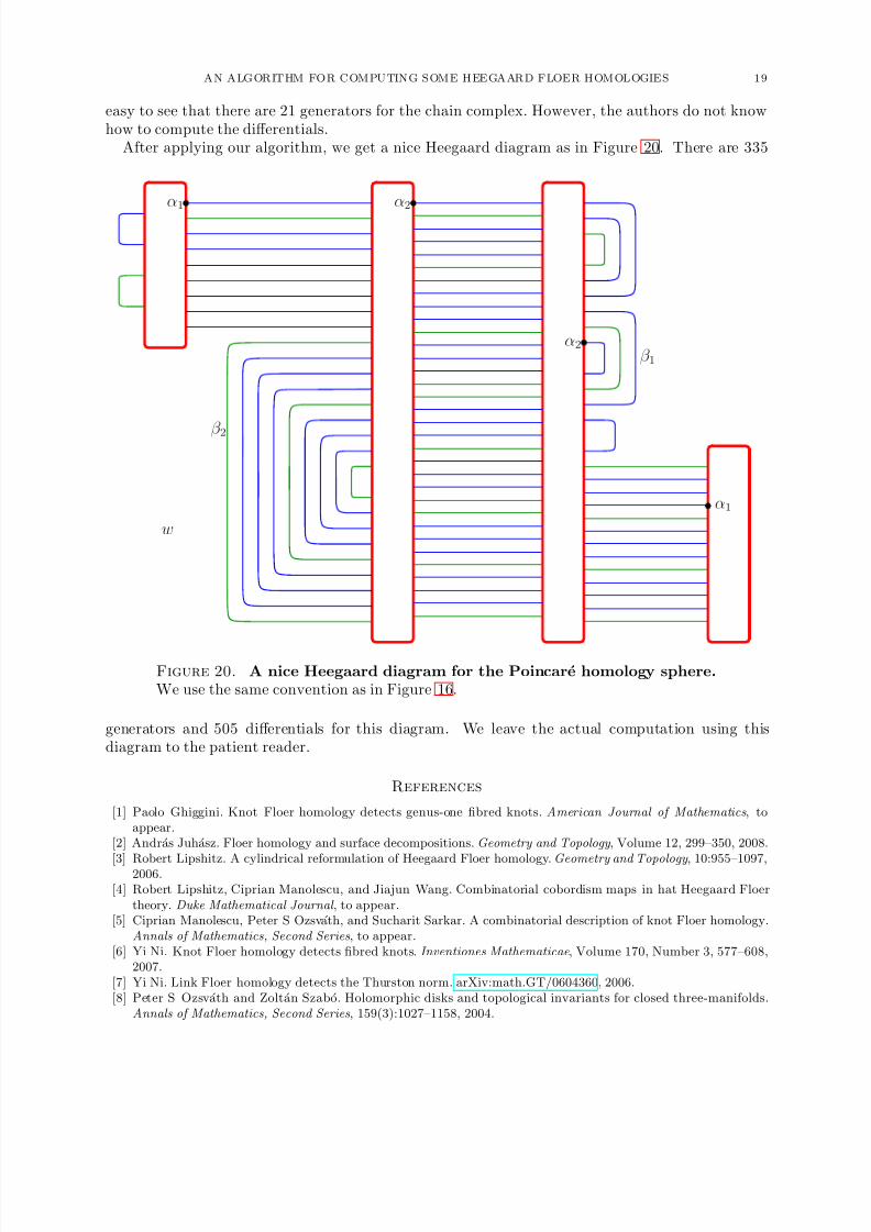
5. Examples

In this section, we give two examples to demonstrate our algorithm. One is on knot Floerhomology and the other is on the Heegaard Floer homology of three-manifolds.

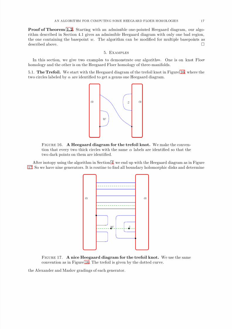
5.1. The Trefoil. We start with the Heegaard diagram of the trefoil knot in Figure 16, where thetwo circles labeled by α are identified to get a genus one Heegaard diagram.

w

zα α

Figure 16. A Heegaard diagram for the trefoil knot. We make the conven-tion that every two thick circles with the same α labels are identified so that thetwo dark points on them are identified.

After isotopy using the algorithm in Section 4, we end up with the Heegaard diagram as in Figure17. So we have nine generators. It is routine to find all boundary holomorphic disks and determine

w z

α α

Figure 17. A nice Heegaard diagram for the trefoil knot. We use the sameconvention as in Figure 16. The trefoil is given by the dotted curve.

the Alexander and Maslov gradings of each generator.




[9] Peter S Ozsvath and Zoltan Szabo. Holomorphic disks and three-manifold invariants: properties and applications.Annals of Mathematics, Second Series, 159(3):1159–1245, 2004.

[10] Peter S Ozsvath and Zoltan Szabo. Absolutely graded Floer homologies and intersection forms for four-manifoldswith boundary. Advances in Mathematics, 173(2):179–261, 2003.

[11] Peter S Ozsvath and Zoltan Szabo. Holomorphic triangles and invariants for smooth four-manifolds. Advances

in Mathematics, 202(2):326–400, 2006.[12] Peter S Ozsvath and Zoltan Szabo. Holomorphic disks and knot invariants. Advances in Mathematics, 186(1):58–

116, 2004.[13] Peter S Ozsvath and Zoltan Szabo. Holomorphic disks and genus bounds. Geometry and Topology , 8:311–334,

2004.[14] Peter S Ozsvath and Zoltan Szabo. Knot Floer homology and the four-ball genus. Geometry and Topology ,

7:615–639, 2003.[15] Peter S Ozsvath and Zoltan Szabo. Holomorphic disks, link invariants and the multi-variable Alexander polyno-

mial. arXiv:math.GT/0512286, 2005.[16] Peter S Ozsvath and Zoltan Szabo. Link Floer homology and the Thurston norm. Journal of the American

Mathematical Society , Volume 21, Number 3, 671-709, 2008.[17] Peter S Ozsvath and Zoltan Szabo. Heegaard diagrams and Floer homology. International Congress of Mathe-

maticians, Volume II , 1083–1099, European Mathematical Society, Zurich, 2006.[18] Peter S Ozsvath and Zoltan Szabo. Heegaard diagrams and holomorphic disks. Different Faces of Geometry ,

301–348, International Mathematical Series (New York), 3, Kluwer/Plenum, New York, 2004.[19] Jacob Rasmussen. Floer homology and knot complements. Ph.D Thesis, Harvard University, 2003.

Department of Mathematics, Princeton University, Princeton, NJ 08544

E-mail address: [email protected]

Department of Mathematics, California Institute of Technology, Pasadena, CA 91125

E-mail address: [email protected]

http://arxiv.org/abs/math/0512286

http://arxiv.org/abs/math/0512286

sucharit sarkar and jiajun wang- an algorithm for computing some heegard floer homologies

Documents