PROCEEDINGS, 44th Workshop on Geothermal Reservoir Engineering

Stanford University, Stanford, California, February 11-13, 2019

SGP-TR-214

___________________________________________________

3J. Ajo-Franklin, S.J. Bauer, T. Baumgartner, K. Beckers, D. Blankenship, A. Bonneville, L. Boyd, S.T. Brown, J.A. Burghardt, C.

Chai, T. Chen, Y. Chen, K. Condon, P.J. Cook, P.F. Dobson, T. Doe, C.A. Doughty, D. Elsworth, J. Feldman, A. Foris, L.P. Frash, Z.

Frone, P. Fu, K. Gao, A. Ghassemi, H. Gudmundsdottir, Y. Guglielmi, G. Guthrie, B. Haimson, A. Hawkins, J. Heise, C.G. Herrick, M.

Horn, R.N. Horne, J. Horner, M. Hu, H. Huang, L. Huang, K. Im, M. Ingraham, T.C. Johnson, B. Johnston, S. Karra, K. Kim, D.K.

King, T. Kneafsey, H. Knox, J. Knox, D. Kumar, K. Kutun, M. Lee, K. Li, R. Lopez, M. Maceira, N. Makedonska, C. Marone, E.

Mattson, M.W. McClure, J. McLennan, T. McLing, R.J. Mellors, E. Metcalfe, J. Miskimins, J.P. Morris, S. Nakagawa, G. Neupane, G.

Newman, A. Nieto, C.M. Oldenburg, W. Pan, R. Pawar, P. Petrov, B. Pietzyk, R. Podgorney, Y. Polsky, S. Porse, S. Richard, B.Q.

Roberts, M. Robertson, W. Roggenthen, J. Rutqvist, D. Rynders, H. Santos-Villalobos, M. Schoenball, P. Schwering, V. Sesetty, A.

Singh, M.M. Smith, H. Sone, C.E. Strickland, J. Su, C. Ulrich, N. Uzunlar, A. Vachaparampil, C.A. Valladao, W. Vandermeer, G.

Vandine, D. Vardiman, V.R. Vermeul, J.L. Wagoner, H.F. Wang, J. Weers, J. White, M.D. White, P. Winterfeld, T. Wood, H. Wu, Y.S.

Wu, Y. Wu, Y. Zhang, Y.Q. Zhang, J. Zhou, Q. Zhou, M.D. Zoback

This manuscript has been authored in part by UT-Battelle, LLC, under contract DE-AC05-00OR22725 with the US Department of

Energy (DOE). The US government retains and the publisher, by accepting the article for publication, acknowledges that the US

government retains a nonexclusive, paid-up, irrevocable, worldwide license to publish or reproduce the published form of this

manuscript, or allow others to do so, for US government purposes. DOE will provide public access to these results of federally

sponsored research in accordance with the DOE Public Access Plan (http://energy.gov/downloads/doe-public-access-plan).

1

Subsurface Seismic Structure Around the Sanford Underground Research Facility

Chengping Chai1, Monica Maceira1,2, Hector J. Santos-Villalobos1, EGS Collab team3

1Oak Ridge National Laboratory, Oak Ridge, TN 37830

2Deparment of Physics and Astronomy, University of Tennessee, Knoxville, TN 37996

Email: chaic@ornl.gov, maceiram@ornl.gov, hsantos@ornl.gov

Keywords: 3D seismic structure, joint inversion, Black Hills, SURF, EGS Collab

ABSTRACT

To address the fundamental challenges of understanding processes associated with enhanced or engineered geothermal systems (EGS),

teams from the EGS Collab SIGMA-V project are conducting stimulations at the Sanford Underground Research Facility. Various

modalities of geophysical observations are collected and analyzed, and different types of parameters are modeled to help investigate these

critical processes. Among these parameters, the three-dimensional stress field is one of the primary objectives. Seismic velocity models

have been used to estimate the 3D stress field for other regions. A detailed seismic velocities and density model can help us infer spatial

variations of the stress field in the study area. We inverted the 3D seismic structure around the site by using body-wave travel times,

surface-wave dispersions and gravity observations simultaneously. The resulting model will be a starting point for more detailed

investigations and could also be used to study subsurface geological and stress field variations of the broad area.

1. INTRODUCTION

Reliable and high-resolution seismic models of the subsurface do not only expand our geophysical and geodynamical knowledge of a

specific area but also help us address the ever-growing energy challenges. Enhanced or engineered geothermal systems (EGS) have great

potential to expand our renewable energy supply. Though they have been intensively studied, critical processes of EGS development such

as fracture creation and fluid flow are not fully understood. To address the fundamental challenges of understanding these processes, the

EGS Collab SIGMA-V project (e.g. Kneafsey et al., 2019) is conducting experiments at the Sanford Underground Research Facility

(SURF) in the Black Hills region. Various modalities of observations are collected and analyzed, and different types of parameters are

modeled to help investigate these critical processes. One of the goals of the project is to understand the basic relationships between stress,

seismicity, and permeability enhancement (e.g. White et al., 2017). A detailed stress model is needed to study these relationships. The

stress field around the SURF region is inevitably influenced by tectonic forces and matter surrounding and beneath the area. A geophysical

model can be used as a proxy to study the spatial variations in the stress field (Levandowski et al., 2016). A seismic model for the broader

area around SURF (Figure 1) can also provide a starting point for more detailed investigations and improve our understanding of the

surrounding region. It is necessary to study the seismic structure around the broad SURF area.

Three-dimensional (3D) seismic imaging (tomography) has been widely used to investigate the subsurface structure for more than 40

years now. Since the first application by Aki et al., 1977, numerous studies have been conducted to improve imaging algorithms and/or

geophysical models of the subsurface. In particular, the Spectral Element Method (SEM, e.g. Komatitsch and Tromp, 1999) provides a

comprehensive approach to image subsurface at different scales (e.g. Tape et al., 2009; Bozdağ et al., 2016). However, the substantial

computational requirements of the technique limit its applications; especially for high-frequency observations. On the other hand,

improvements in the data collection techniques and processing algorithms provide various types of geophysical observations that can be

Chai et al.

2

analyzed with much less computational investment. For example, surface wave dispersions are being extracted from both earthquake

observations (e.g. Ritzwoller and Levshin, 1998) and ambient noise data (e.g. Shapiro et al., 2005). Receiver functions (e.g. Langston,

1979; Ammon, 1991; Ligorría and Ammon, 1999) are being processed using seismic records from three-component stations. Arrival times

of various seismic phases are routinely being measured and archived (e.g. Preliminary Determination of Epicenters Bulletin, United States

Geological Survey). Integrating multiple types of these geophysical observations has shown better results than using an individual type

(e.g. Julià et al., 2000; Monica and Ammon, 2009; Bodin et al., 2012; Chai et al., 2015; Shen and Ritzwoller, 2016; Chong et al., 2016;

Syracuse et al., 2017). We jointly invert multiple geophysical observations including surface-wave dispersions, Bouguer gravity and body-

wave travel-time observations to solve for seismic velocity changes in the region surrounding the SURF.

2. DATA

We used three different types of geophysical observations including P-and S-wave travel-times, group and phase velocities measured from

both Rayleigh and Love waves, and satellite-derived Bouguer gravity observations. Various quality control procedures were applied to

remove outliers. We also used Hypertext Markup Language (HTML) based interactive tools (Chai et al., 2018) to examine the datasets

visually. The following paragraphs document details on each dataset as well as the related quality control procedures. Since the 3D imaging

problem is nonlinear, we start with an a priori model and solve the equations iteratively. The starting model is linearly interpolated from

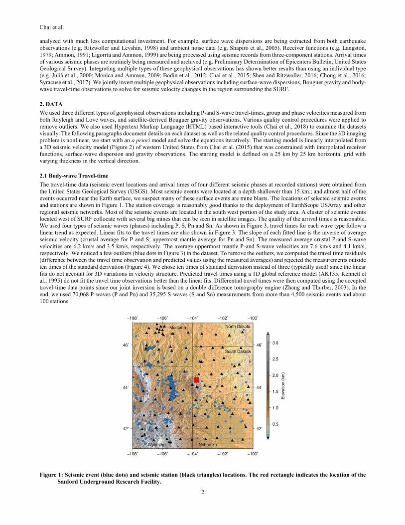
a 3D seismic velocity model (Figure 2) of western United States from Chai et al. (2015) that was constrained with interpolated receiver

functions, surface-wave dispersion and gravity observations. The starting model is defined on a 25 km by 25 km horizontal grid with

varying thickness in the vertical direction.

2.1 Body-wave Travel-time

The travel-time data (seismic event locations and arrival times of four different seismic phases at recorded stations) were obtained from

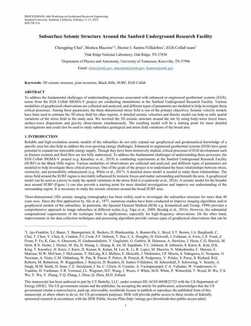
the United States Geological Survey (USGS). Most seismic events were located at a depth shallower than 15 km.; and almost half of the

events occurred near the Earth surface, we suspect many of these surface events are mine blasts. The locations of selected seismic events

and stations are shown in Figure 1. The station coverage is reasonably good thanks to the deployment of EarthScope USArray and other

regional seismic networks. Most of the seismic events are located in the south west portion of the study area. A cluster of seismic events

located west of SURF collocate with several big mines that can be seen in satellite images. The quality of the arrival times is reasonable.

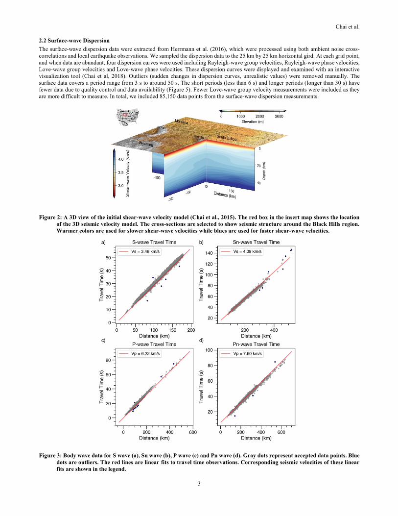
We used four types of seismic waves (phases) including P, S, Pn and Sn. As shown in Figure 3, travel times for each wave type follow a

linear trend as expected. Linear fits to the travel times are also shown in Figure 3. The slope of each fitted line is the inverse of average

seismic velocity (crustal average for P and S; uppermost mantle average for Pn and Sn). The measured average crustal P-and S-wave

velocities are 6.2 km/s and 3.5 km/s, respectively. The average uppermost mantle P-and S-wave velocities are 7.6 km/s and 4.1 km/s,

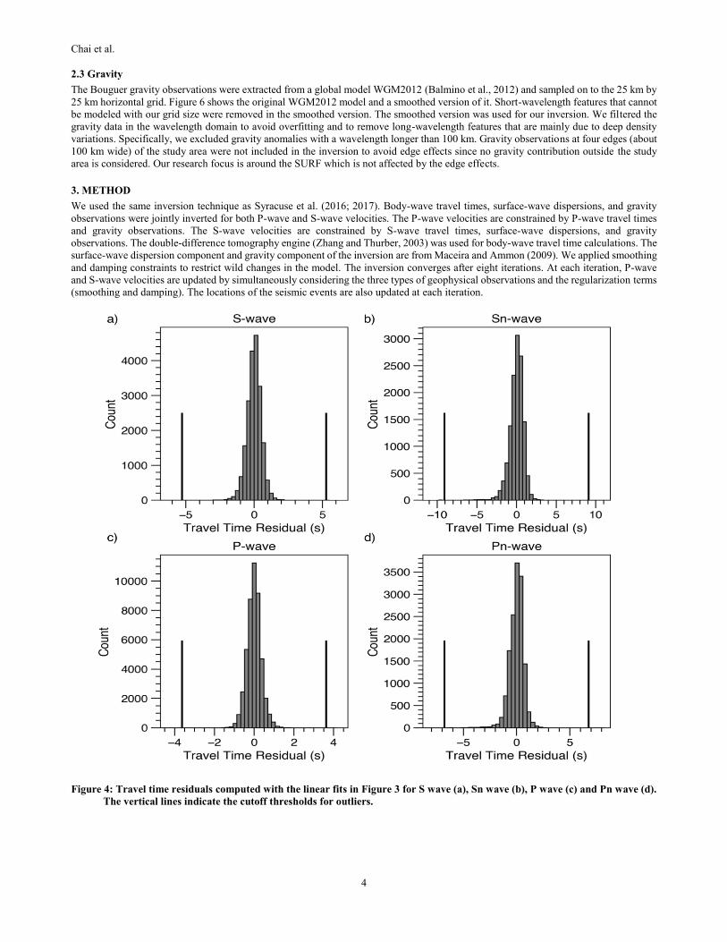
respectively. We noticed a few outliers (blue dots in Figure 3) in the dataset. To remove the outliers, we computed the travel time residuals

(difference between the travel time observation and predicted values using the measured averages) and rejected the measurements outside

ten times of the standard derivation (Figure 4). We chose ten times of standard derivation instead of three (typically used) since the linear

fits do not account for 3D variations in velocity structure. Predicted travel times using a 1D global reference model (AK135, Kennett et

al., 1995) do not fit the travel time observations better than the linear fits. Differential travel times were then computed using the accepted

travel-time data points since our joint inversion is based on a double-difference tomography engine (Zhang and Thurber, 2003). In the

end, we used 70,068 P-waves (P and Pn) and 35,295 S-waves (S and Sn) measurements from more than 4,500 seismic events and about

100 stations.

Figure 1: Seismic event (blue dots) and seismic station (black triangles) locations. The red rectangle indicates the location of the

Sanford Underground Research Facility.

Chai et al.

3

2.2 Surface-wave Dispersion

The surface-wave dispersion data were extracted from Herrmann et al. (2016), which were processed using both ambient noise cross-

correlations and local earthquake observations. We sampled the dispersion data to the 25 km by 25 km horizontal gird. At each grid point,

and when data are abundant, four dispersion curves were used including Rayleigh-wave group velocities, Rayleigh-wave phase velocities,

Love-wave group velocities and Love-wave phase velocities. These dispersion curves were displayed and examined with an interactive

visualization tool (Chai et al, 2018). Outliers (sudden changes in dispersion curves, unrealistic values) were removed manually. The

surface data covers a period range from 3 s to around 50 s. The short periods (less than 6 s) and longer periods (longer than 30 s) have

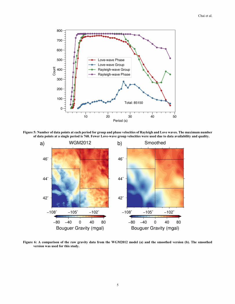
fewer data due to quality control and data availability (Figure 5). Fewer Love-wave group velocity measurements were included as they

are more difficult to measure. In total, we included 85,150 data points from the surface-wave dispersion measurements.

Figure 2: A 3D view of the initial shear-wave velocity model (Chai et al., 2015). The red box in the insert map shows the location

of the 3D seismic velocity model. The cross-sections are selected to show seismic structure around the Black Hills region.

Warmer colors are used for slower shear-wave velocities while blues are used for faster shear-wave velocities.

Figure 3: Body wave data for S wave (a), Sn wave (b), P wave (c) and Pn wave (d). Gray dots represent accepted data points. Blue

dots are outliers. The red lines are linear fits to travel time observations. Corresponding seismic velocities of these linear

fits are shown in the legend.

Chai et al.

4

2.3 Gravity

The Bouguer gravity observations were extracted from a global model WGM2012 (Balmino et al., 2012) and sampled on to the 25 km by

25 km horizontal grid. Figure 6 shows the original WGM2012 model and a smoothed version of it. Short-wavelength features that cannot

be modeled with our grid size were removed in the smoothed version. The smoothed version was used for our inversion. We filtered the

gravity data in the wavelength domain to avoid overfitting and to remove long-wavelength features that are mainly due to deep density

variations. Specifically, we excluded gravity anomalies with a wavelength longer than 100 km. Gravity observations at four edges (about

100 km wide) of the study area were not included in the inversion to avoid edge effects since no gravity contribution outside the study

area is considered. Our research focus is around the SURF which is not affected by the edge effects.

3. METHOD

We used the same inversion technique as Syracuse et al. (2016; 2017). Body-wave travel times, surface-wave dispersions, and gravity

observations were jointly inverted for both P-wave and S-wave velocities. The P-wave velocities are constrained by P-wave travel times

and gravity observations. The S-wave velocities are constrained by S-wave travel times, surface-wave dispersions, and gravity

observations. The double-difference tomography engine (Zhang and Thurber, 2003) was used for body-wave travel time calculations. The

surface-wave dispersion component and gravity component of the inversion are from Maceira and Ammon (2009). We applied smoothing

and damping constraints to restrict wild changes in the model. The inversion converges after eight iterations. At each iteration, P-wave

and S-wave velocities are updated by simultaneously considering the three types of geophysical observations and the regularization terms

(smoothing and damping). The locations of the seismic events are also updated at each iteration.

Figure 4: Travel time residuals computed with the linear fits in Figure 3 for S wave (a), Sn wave (b), P wave (c) and Pn wave (d).

The vertical lines indicate the cutoff thresholds for outliers.

Chai et al.

5

Figure 5: Number of data points at each period for group and phase velocities of Rayleigh and Love waves. The maximum number

of data points at a single period is 768. Fewer Love-wave group velocities were used due to data availability and quality.

Figure 6: A comparison of the raw gravity data from the WGM2012 model (a) and the smoothed version (b). The smoothed

version was used for this study.

Chai et al.

6

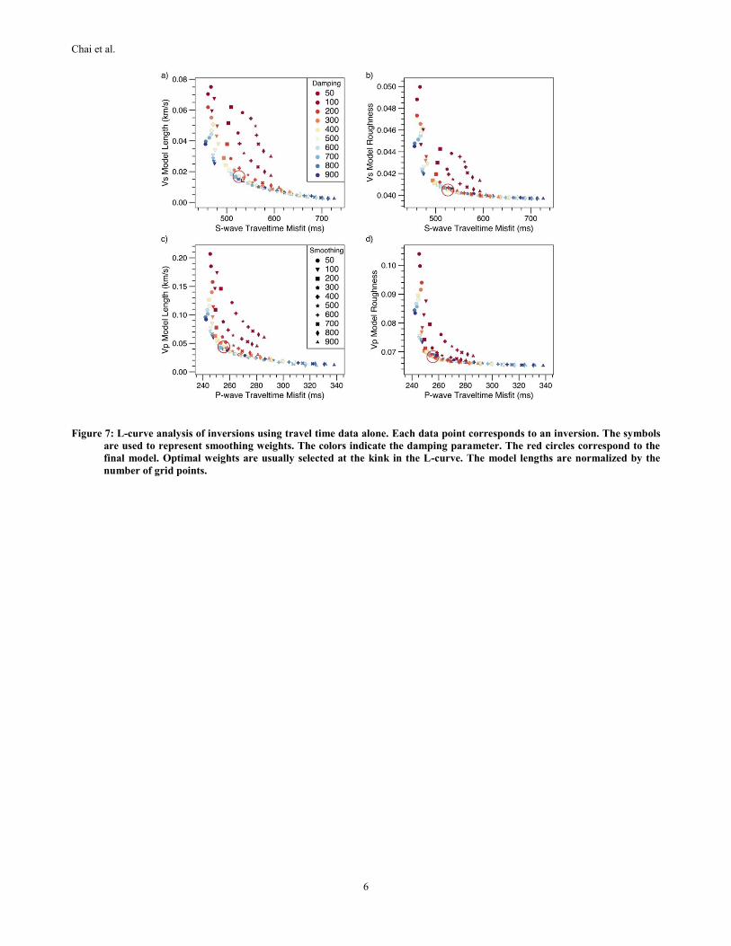
Figure 7: L-curve analysis of inversions using travel time data alone. Each data point corresponds to an inversion. The symbols

are used to represent smoothing weights. The colors indicate the damping parameter. The red circles correspond to the

final model. Optimal weights are usually selected at the kink in the L-curve. The model lengths are normalized by the

number of grid points.

Chai et al.

7

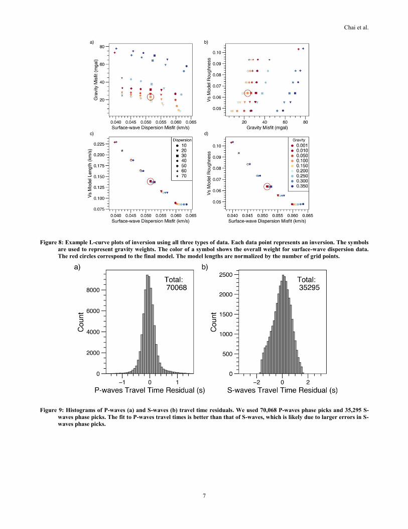
Figure 8: Example L-curve plots of inversion using all three types of data. Each data point represents an inversion. The symbols

are used to represent gravity weights. The color of a symbol shows the overall weight for surface-wave dispersion data.

The red circles correspond to the final model. The model lengths are normalized by the number of grid points.

Figure 9: Histograms of P-waves (a) and S-waves (b) travel time residuals. We used 70,068 P-waves phase picks and 35,295 S-

waves phase picks. The fit to P-waves travel times is better than that of S-waves, which is likely due to larger errors in S-

waves phase picks.

Chai et al.

8

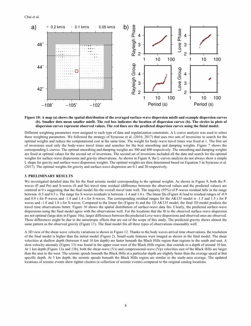
Figure 10: A map (a) shows the spatial distribution of the averaged surface-wave dispersion misfit and example dispersion curves

(b). Smaller dots mean smaller misfit. The red box indicates the location of dispersion curves (b). The circles in plots of

dispersion curves represent observed values. The red lines are the predicted dispersion curves using the finial model.

Different weighting parameters were assigned to each type of data and regularization constraints. A L-curve analysis was used to select

these weighting parameters. We followed the strategy of Syracuse et al. (2016; 2017) that uses two sets of inversions to search for the

optimal weights and reduce the computational cost at the same time. The weight for body-wave travel times was fixed at 1. The first set

of inversions used only the body-wave travel times and searches for the best smoothing and damping weights. Figure 7 shows the

corresponding L-curves. The optimal smoothing and damping weights are 300 and 400 respectively. The smoothing and damping weights

are fixed at optimal values for the second set of inversions. The second set of inversions included all the data and search for the optimal

weights for surface-wave dispersions and gravity observations. As shown in Figure 8, the L-curves analysis do not always show a simple

L shape for gravity and surface-wave dispersion weights. The optimal weights are then determined based on Equation 5 in Syracuse et al.

(2017). The optimal weights for gravity and surface-wave dispersion are 0.1 and 30 respectively.

3. PRELIMINARY RESULTS

We investigated detailed data fits for the final seismic model corresponding to the optimal weights. As shown in Figure 9, both the P-

waves (P and Pn) and S-waves (S and Sn) travel time residual (difference between the observed values and the predicted values) are

centered at 0 s suggesting that the final model fits the overall travel time well. The majority (95%) of P-waves residual falls in the range

between -0.5 and 0.5 s. The range for S-waves residuals is between -1.4 and 1.4 s. The linear fits (Figure 4) lead to residual ranges of -0.9

and 0.9 s for P-waves and -1.4 and 1.4 s for S-waves. The corresponding residual ranges for the AK135 model is -1.5 and 1.5 s for P

waves and -1.8 and 1.8 s for S-waves. Compared to the linear fits (Figure 4) and the 1D AK135 model, the final 3D model predicts the

travel time observations better. Figure 10 shows the spatial distribution of surface-wave data fits. Clearly, the predicted surface-wave

dispersions using the final model agree with the observations well. For the locations that the fit to the observed surface-wave dispersion

are not optimal (large dots in Figure 10a), larger differences between the predicted Love-wave dispersions and observed ones are observed.

These differences might be due to the anisotropic effects that are out of the scope of this study. The predicted gravity shows almost the

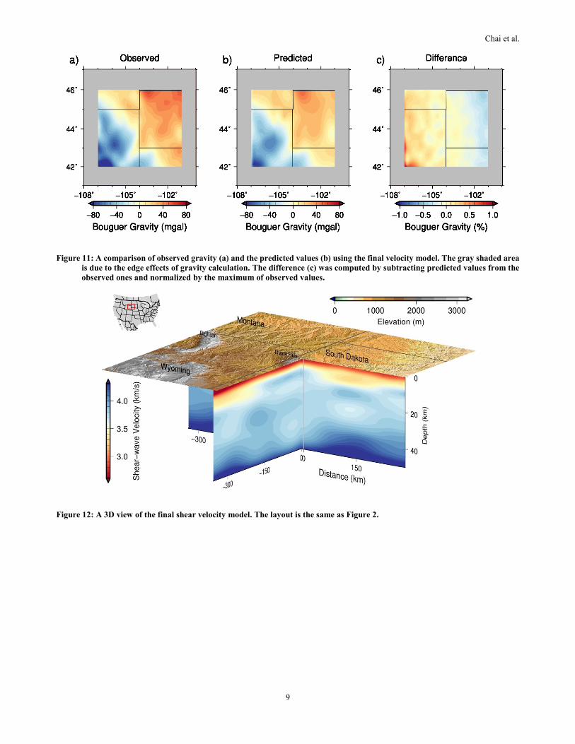
same pattern as the observed gravity (Figure 11). The final model fits all three types of observations reasonably well.

A 3D view of the shear-wave velocity variations is shown in Figure 12. Thanks to the body waves arrival time observations, the resolution

of the final model is higher than the initial model (Figure 2). Small-scale features were imaged as shown in the final model. The shear

velocities at shallow depth (between 4 and 10 km depth) are faster beneath the Black Hills region than regions to the south and east. A

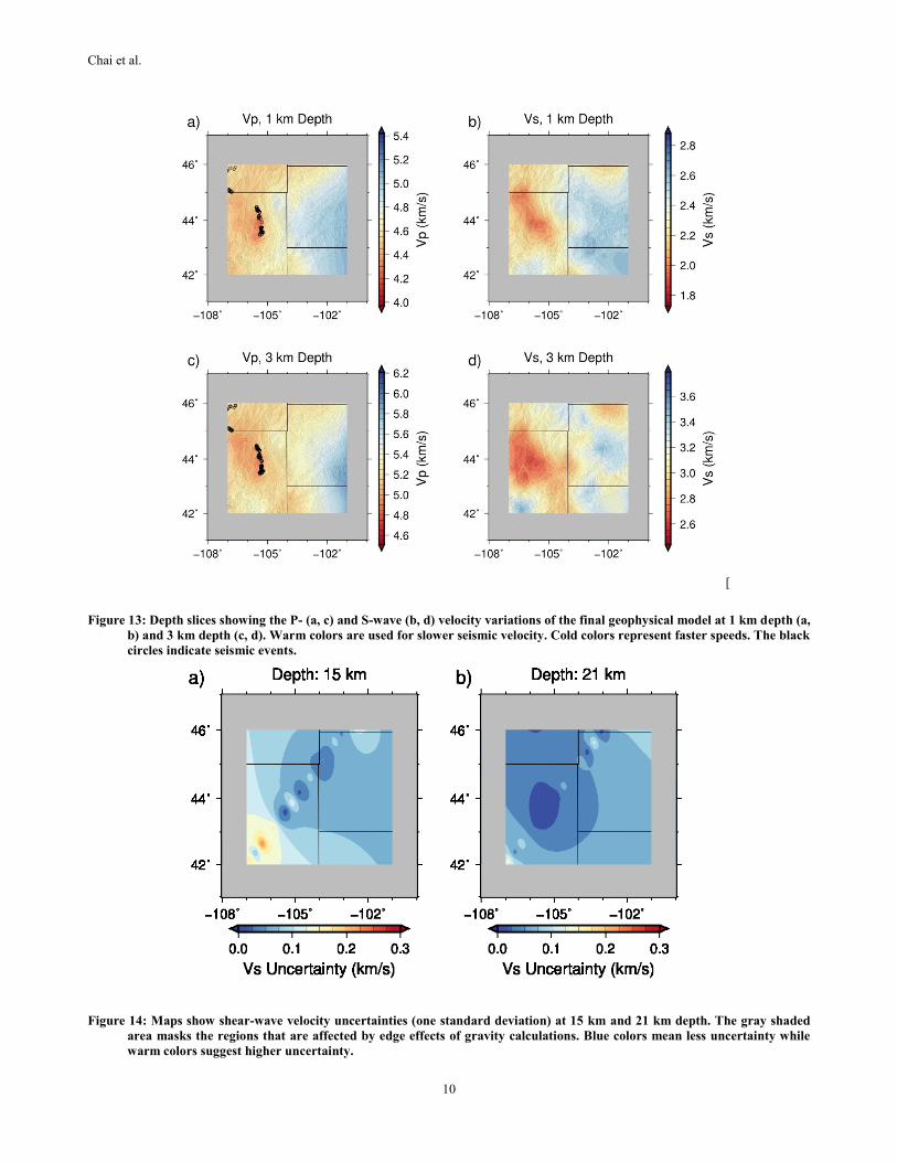
slow-velocity anomaly (Figure 13) was found in the upper crust west of the Black Hills region, that extends to a depth of around 10 km.

At 1 km depth (Figure 13a and 13b), both the shear-wave (Vs) and compressional-wave (Vp) velocities east of the Black Hills are larger

than the area to the west. The seismic speeds beneath the Black Hills at a particular depth are slightly faster than the average speed at that

specific depth. At 3 km depth, the seismic speeds beneath the Black Hills region are similar to the study-area average. The updated

locations of seismic events show tighter clusters (a collection of seismic events) compared to the original catalog locations.

Chai et al.

9

Figure 11: A comparison of observed gravity (a) and the predicted values (b) using the final velocity model. The gray shaded area

is due to the edge effects of gravity calculation. The difference (c) was computed by subtracting predicted values from the

observed ones and normalized by the maximum of observed values.

Figure 12: A 3D view of the final shear velocity model. The layout is the same as Figure 2.

Chai et al.

10

[

Figure 13: Depth slices showing the P- (a, c) and S-wave (b, d) velocity variations of the final geophysical model at 1 km depth (a,

b) and 3 km depth (c, d). Warm colors are used for slower seismic velocity. Cold colors represent faster speeds. The black

circles indicate seismic events.

Figure 14: Maps show shear-wave velocity uncertainties (one standard deviation) at 15 km and 21 km depth. The gray shaded

area masks the regions that are affected by edge effects of gravity calculations. Blue colors mean less uncertainty while

warm colors suggest higher uncertainty.

Chai et al.

11

4. DISCUSSION AND CONCLUSIONS

The Black Hills region has experienced several cycles of uplift and deposition (e.g. DeWitt et al., 1986). The high-velocity anomaly

beneath Black Hills could be due to uplifts that eroded sedimentary layers. Geological observations suggest different geological history

across Black Hills. To the west of Black Hills is the Wyoming carton while the area east of Black Hills was deformed by the Trans-

Hudson orogen (e.g. Foster et al., 2006). The differences in seismic velocity at 1 km depth from west to east across Black Hills agrees

with geological observations. We used the inverted models to check the uncertainties due to the choice of weights for different data and

regularization terms. The weight-related uncertainties can be as large as 0.5 km/s. As shown in Figure 14, the high uncertainty area is

focused at small regions sometimes. The large uncertainties suggest that it is necessary to perform a thorough search of weights. Otherwise,

the resulting seismic models may contain small-scale artifacts.

ACKNOWLEDGEMENTS

This material is based upon work supported by the U.S. Department of Energy, Office of Energy Efficiency and Renewable Energy

(EERE), Office of Technology Development, Geothermal Technologies Office, under Award Number DE-AC05-00OR22725 with

ORNL. The views and conclusions contained in this document are those of the authors and should not be interpreted as necessarily

representing the official policies, either expressed or implied, of the U.S. Government. The United States Government retains, and the

publisher, by accepting the article for publication, acknowledges that the United States Government retains a non-exclusive, paid-up,

irrevocable, world-wide license to publish or reproduce the published form of this manuscript, or allow others to do so, for United States

Government purposes.

We thank developers of the Generic Mapping Tools (GMT, Wessel et al., 2013), Obspy (Beyreuther et al., 2010), Numpy

(http://numpy.org, last accessed January 2019), Matplotlib (Hunter, 2007), and Bokeh (http://bokeh.pydata.org, last accessed January

2019) for making their packages available. The surface-wave dispersion data are available online at

http://eqinfo.eas.slu.edu/eqc/eqc_research/NATOMO/ (last accessed January 2019). The Bouguer gravity data were obtained online at

http://bgi.omp.obs-mip.fr/data-products/Grids-and-models/wgm2012 (last accessed January 2019).

REFERENCES

Aki, K., Christoffersson, A., and Husebye, E. S. Determination of the Three-dimensional Seismic Structure of the Lithosphere. Journal

of Geophysical Research, 82(2), (1977). 277-296.

Ammon, C. J.: The Isolation of Receiver Effects from Teleseismic P -waveforms. Bulletin of the Seismological Society of America, 81(6),

(1991), 2504-2510.

Balmino, G., Vales, N., Bonvalot, S., and Briais, A.: Spherical Harmonic Modelling to Ultra-high Degree of Bouguer and Isostatic

Anomalies. Journal of Geodesy, 86(7), (2012), 499-520.

Beyreuther, M., Barsch, R., Krischer, L., Megies, T., Behr, Y., and Wassermann, J.: ObsPy: A Python Toolbox for Seismology.

Seismological Research Letters, 81(3), (2010), 530-533.

Bodin, T., Sambridge, M., Tkalčić, H., Arroucau, P., Gallagher, K., and Rawlinson, N.: Transdimensional Inversion of Receiver Functions

and Surface Wave Dispersion. Journal of Geophysical Research: Solid Earth, 117(B2), (2012), 207-213.

Bozdağ, E., Peter, D., Lefebvre, M., Komatitsch, D., Tromp, J., Hill, J., et al.: Global Adjoint Tomography: First-generation model.

Geophysical Journal International, 207(3), (2016), 1739-1766.

Chai, C., Ammon, C. J., Maceira, M., and Herrmann, R. B.: Interactive Visualization of Complex Seismic Data and Models Using Bokeh.

Seismological Research Letters, 89(2A), (2018), 668-676.

Chai, C., Ammon, C. J., Maceira, M., and Herrmann, R. B.: Inverting Interpolated Receiver Functions with Surface Wave Dispersion and

Gravity: Application to the western U.S. and adjacent Canada and Mexico. Geophysical Research Letters, 42(11), (2015), 4359-

4366.

Chong, J., Ni, S., Chu, R., and Somerville, P.: Joint Inversion of Body‐Wave Receiver Function and Rayleigh‐Wave Ellipticity. Bulletin

of the Seismological Society of America, 106(2), (2016), 537-551.

DeWitt, E., Redden, J. A., Wilson, A. B., Buscher D., and Dersch, J. S.: Mineral Resource Potential and Geology of the Black Hills

National Forest, South Dakota and Wyoming with a Section on Salable Commodities. U.S. Geological Survey Bulletin, 1580, (1986),

1-135.

Foster, D. A., Mueller, P. A., Mogk, D. W., Wooden, J. L., and Vogl, J. J. Proterozoic Evolution of the Western Margin of the Wyoming

Craton: Implications for the tectonic and magmatic evolution of the northern Rocky Mountains. Canadian Journal of Earth Sciences,

43(10), (2006), 1601-1619.

Herrmann, R. B., Benz, H. M., and Ammon, C. J.: Mapping Love/Rayleigh Phase/Group Velocity Dispersion between 2 and 100 seconds

in North America Using Ambient Noise Cross-correlations and Earthquake Observations (abs). Seismological Research Letters,

87(2B), (2016), 546.

Hunter, J. D.: Matplotlib: A 2D Graphics Environment. Computing in Science & Engineering, 9(3), (2007), 90-95.

Chai et al.

12

Julià, J., Ammon, C. J., Herrmann, R. B., and Correig, A. M.: Joint Inversion of Receiver Function and Surface Wave Dispersion

Observations. Geophysical Journal International, 143(1), (2000), 99-112.

Kennett, B. L. N., Engdahl, E. R., and Buland, R.: Constraints on Seismic Velocities in the Earth from Traveltimes. Geophysical Journal

International, 122(1), (1995), 108-124.

Kneafsey, T. J., Blankenship, D., Knox, H. A., Johnson, T. C., Ajo-Franklin, J. B., Schwering, P. C., et al.: EGS Collab Project: Status

and Progress. in PROCEEDINGS, 44th Workshop on Geothermal Reservoir Engineering, edited, Stanford University, Stanford,

California, (2019).

Komatitsch, D., and Tromp, J.: Introduction to the Spectral Element Method for Three-dimensional Seismic Wave Propagation.

Geophysical Journal International, 139(3), (1999), 806-822.

Langston, C. A.: Structure under Mount Rainier, Washington, Inferred from Teleseismic Body Waves. Journal of Geophysical Research,

84(B9), (1979), 4749.

Levandowski, W., Boyd, O. S., and Ramirez-Guzmán, L.: Dense Lower Crust Elevates Long-term Earthquake Rates in the New Madrid

Seismic Zone. Geophysical Research Letters, 43(16), (2016), 8499-8510.

Ligorría, J. P., and Ammon, C. J.: Iterative Deconvolution and Receiver-function Estimation. Bulletin of the Seismological Society of

America, 89(5), (1999), 1395-1400.

Maceira, M., and Ammon, C. J.: Joint Inversion of Surface Wave Velocity and Gravity Observations and Its Application to Central Asian

Basins Shear Velocity Structure. Journal of Geophysical Research, 114(B2), (2009), B02314.

Ritzwoller, M. H., and Levshin, A. L.: Eurasian Surface Wave Tomography: Group velocities. Journal of Geophysical Research: Solid

Earth, 103(B3), (1998), 4839-4878.

Shapiro, N. M., Campillo, M., Stehly, L., and Ritzwoller, M. H.: High-resolution Surface-wave Tomography from Ambient Seismic

Noise. Science, 307(5715), (2005), 1615-1618.

Shen, W., and Ritzwoller, M. H.: Crustal and Uppermost Mantle Structure beneath the United States. Journal of Geophysical Research:

Solid Earth, 121(6), (2016), 4306-4342.

Syracuse, E. M., Zhang, H., and Maceira, M.: Joint Inversion of Seismic and Gravity Data for Imaging Seismic Velocity Structure of the

Crust and Upper Mantle beneath Utah, United States. Tectonophysics, 718, (2017), 105-117.

Syracuse, E. M., Maceira, M., Prieto, G. A., Zhang, H., and Ammon, C. J.: Multiple Plates Subducting beneath Colombia, as Illuminated

by Seismicity and Velocity from the Joint Inversion of Seismic and Gravity data. Earth and Planetary Science Letters, 444, (2016),

139-149.

Tape, C., Liu, Q., Maggi, A., and Tromp, J.: Adjoint Tomography of the Southern California Crust. Science, 325(5943), (2009), 988-992.

Wessel, P., Smith, W. H. F., Scharroo, R., Luis, J., and Wobbe, F.: Generic Mapping Tools: Improved Version Released. Eos, Transactions

American Geophysical Union, 94(45), (2013), 409-410.

White, M., Fu, P., Huang, H., Ghassemi, A., Kneafsey, T., Blankenship, D., et al.: The Role of Numerical Simulation in the Design of

Stimulation and Circulation Experiments for the EGS Collab project. In Transactions - Geothermal Resources Council, (2017).

Zhang, H., and Thurber, C.: Double-Difference Tomography: The Method and Its Application to the Hayward Fault, California. Bulletin

of the Seismological Society of America, 93(5), (2003), 1875-1889.