a new method for more eﬃcient seismic image …sep new method for more eﬃcient seismic image...

A new method for more efficient seismic image

segmentation

Adam Halpert

ABSTRACT

Seismic images of the subsurface are often very large and tedious to interpretmanually; as such, automatic segmentation algorithms can be highly useful fortasks such as locating large, irregularly-shaped salt bodies within the images.However, seismic images present unique challenges for image segmentation algo-rithms. Here, a new segmentation algorithm using a “pairwise region comparison”strategy is implemented and tested on seismic images. Numerous modificationsto the original algorithm are necessary to make it appropriate for use with seismicdata, including: (1) changes to the nature of the input data, (2) the way in whichthe graph is constructed, and (3) the formula for calculating edge weights. Initialresults, including a preliminary 3D implementation, indicate that the new methodcompares very favorably with an existing implementation of the eigenvector-basednormalized cuts approach, both in terms of accuracy and efficiency.

INTRODUCTION

A proper salt interpretation is one necessary component of any imaging project wheresalt bodies play a prominent role in the subsurface geology. Because of the sharp ve-locity contrast between salt and nearly any other material, inaccurate placement ofsalt boundaries has a disproportionate effect on the accuracy of the resulting veloc-ity model. Such errors can have damaging imaging and engineering consequences.Unfortunately, interpreting salt boundaries is not only crucial, but also extremelytedious and time-consuming when undertaken manually. Thus, while some degree ofautomation would be ideal for salt picking, any such method must be highly accurateas well as efficient.

One approach to implementing automatic salt-picking is to use graph-based imagesegmentation. In this method, each pixel in a seismic image is treated as a node orvertex in a graph; then edges are constructed between specific pixels and weightedaccording to some property. Image segments are created by partitioning the graph –here, a partition is a salt boundary.

In this paper, I will review a previous effort to apply a graph-based image segmen-tation algorithm to seismic data, and then introduce a new, more efficient methodusing an algorithm from Felzenszwalb and Huttenlocher (2004). Since seismic images

SEP-140

Halpert 2 Faster image segmentation

are very different from more “conventional” images (such as photographs) for whichthis newer algorithm was designed, I will detail several modifications necessary forthe algorithm to be useful for seismic images. Finally, I demonstrate the results ofapplying the new method to the examples seen in Figures 1(a) and 1(b), and (forthe field data example) compare these results with those obtained using the previousalgorithm.

BACKGROUND

As mentioned previously, graph-based segmentation methods are popular for au-tomating salt interpretation. More specifically, the eigenvector-based NormalizedCuts Image Segmentation (NCIS) algorithm (Shi and Malik, 2000) has attracted agreat deal of interest because of its capability to capture global aspects of the image,rather than just track local features. Local feature trackers are ubiquitous in seismicinterpretation software (for example, tracking reflections between manually-picked“seed” points), but often struggle when they encounter situations such as a dis-continuous boundary, or one which varies in intensity. Such situations are extremelycommon in seismic data, especially along the boundary between salt bodies and othertypes of rock. Recent research has involved implementing the NCIS algorithm for thepurpose of tracking these salt boundaries [e.g., Lomask et al. (2007); Lomask (2007);Halpert et al. (2009)]. Results of this line of research are encouraging; however, thereare significant limitations, most notably computational. The NCIS algorithm calls foran edge weight matrix of size n2, where n is the number of pixels in the image; thismatrix quickly grows very large, especially for 3D surveys. Computationally, calcula-tion of eigenvectors for such a large matrix is an extremely demanding task. As such,this method is limited to relatively small images; alternatively, we can restrict thecomputational domain to a specific region around a previously interpreted boundary.However, this means the method is of limited utility if there is no “best guess” modelavailable, or if the accuracy of that model is in question.

Thus, a more efficient global segmentation scheme that can include the entireimage in the computational domain would be a very useful tool for interpretation ofseismic images. One candidate for such a scheme is the algorithm from Felzenszwalband Huttenlocher (2004), who write:

“Our algorithm is unique, in that it is both highly efficient and yet cap-tures non-local properties of images.”

These two features are crucial for the task of seismic image segmentation. The algo-rithm is designed to run in O(n log n) time, where n is the number of pixels in thegraph; in contrast, other methods such as NCIS require closer to O(n2) time to run.This represents a significant cost savings, especially for very large 3D seismic datasetsthat are becoming increasingly common.

SEP-140


(a)

(b)

Figure 1: A perfect-velocity migration of the Sigsbee synthetic model (a), and a fieldseismic image (b) that will be used as examples throughout this paper. [ER]

SEP-140


Figure 2: Modified from Zahn(1971). A graph with weightededges (a); a spanning tree of thatgraph (b); and the minimum span-ning tree of the graph (c). [NR]

IEEE TRANSACTIONS ON COMPUTERS, JANUARY 1971

A

8 gE4~~~~~~~

C

F

(b)

(c) (d)Fig. 4. Graphs and minimal spanning trees. (a) Weighted linear graph.

(b) Spanning tree. (c) Minimal spanning tree. (d) Illustration ofTheorem 3 showing clusters C1 and C2 and the "inconsistent" cluster-joining edge (A, B).

tree of graph G is a spanning tree whose weight is minimumamong all spanning trees of G. Fig. 4(c) is the MST for Fig.4(a). The computational problem of constructing an MSThas been treated by several authors [11]-[13] and is brieflydiscussed in the Appendix. It is a surprisingly simple com-

putation.A partition of the nodes of graph G is a division into two

disjoint nonempty subsets (P, Q). For the graph of Fig. 4(a),P= (A, B, C) and Q= (D, E, F) constitute a partition. Thedistance p(P, Q) across a partition is the smallest weightamong all edges which have one end node in P the other inQ. The distance p((A, B, C), (D, E, F)) = 8 for the example

above since the other two edges which span across P and Qare CD and CF with greater weight than edge AD. The setofedges C(P, Q) which span a partition will be referred to as

the cut-set of (P, Q) and a link is any edge in C(P, Q) whoseweight is equal to the distance p(P, Q). The set of all links inC(P, Q) is called the link-set A(P, Q). For the sample parti-tion above C(P, Q)= (AD, CD, CF) and A(P, Q)= (AD).Looking at the graph of Fig. 4(a) it seems plausible to

expect that the minimal spanning tree would choose edgeAD as the bridge spanning from set (A, B, C) to (D, E, F)since that edge does the-job at minimal expense. This is infact true as is shown in the following.

Theorem 1: Any MST contains at least one edge fromeach A(P, Q).

Furthermore, it is true that the following theorem holds.Theorem 2: All MST edges are links of some partition

of G.The following theorem is important because it reveals

the inherent relationship betweenP the MST and clusterstructure.

Theorem 3: If S denotes the nodes of G and C is a non-

empty subset ofS with the property that p(P, Q)<p(C, S - C)for all partitions (P, Q) of C, then the restriction of any

MST to the nodes of C forms a connected subtree of theMST.The significance of Theorem 3 for cluster detection is

illustrated in Fig. 4(d) which depicts the MST for a pointset consisting of two clusters C1 and C2. No partition(P2, Q2) of C2 is such that p(P2, Q2) >22 and therefore thehypothesis of Theorem 3 holds since p(C2, C1) = 78>22.This assures us that the subgraph of the MST which spansonly the nodes of C2 will be a connected subtree as we see inFig. 4(d). The same is also true for C1.

It is quite helpful that the MST does not break up the realclusters in S, but on the other hand neither does it forcebreaks where real gaps exist in the geometry of the point set.A spanning tree is forced by its very nature to span all thepoints but at least the MST jumps across the smaller gapsfirst. Theorem 2 says that any MST edge is the smallestjumpfrom some set to the rest of the nodes. We still have theproblem of deleting edges from an MST so that the result-ing connected subtrees correspond to the observableclusters. In the example of Fig. 4(d) we need an algorithmwhich can detect the appropriateness of deleting the edgeAB and no others.The following criterion is suggested for this type of two-

dimensional clustering observable by humans. A tree edgeXY, whose weight W(XY) is significantly larger than theaverage of nearby edge weights on both sides of the edgeXY, should be deleted. We call such an edge inconsistent.There are two natural ways to measure the significance re-ferred to. One is to see how many sample standard devia-tions separate W(XY) from the average edge weights oneach side. The other is to calculate the factor or ratio be-tween W(XY) and the respective averages. See SectionXVII for details.Edge AB in Fig. 4(d) has a length (weight) of 78. There

are four edges which are within two steps of A and theiraverage length is (21 +22+19+ 15)/4= 19.25. The samplestandard deviation for these four edge lengths is approxi-mately 2.7 so that the length of edge AB is more than 20standard deviations in excess of the average lengths at A.If we assumed a normal distribution for edge lengths, thenone exceeding three or four standard deviations would oc-cur less than one percent of the time and hence may be re-garded as significant. A similar situation exists for theneighborhood of node B. The definition of edge inconsis-tency depends on several factors-the size of neighbor-hood explored for each end node, the number of standarddeviations and the factor considered as significant, andwhether or not inconsistency is required at both ends. Alater section discusses our computational experience withthese factors including some difficulties encountered nearthe fringes ofthe MST where small sample sizes can give dis-torted results. Finally, we should mention that AB is theonly edge in Fig. 4(d) which meets our criterion at a signifi-cance level oftwo standard deviations.

Occasionally we shall refer to a factor of inconsistencywhich is the ratio between edge weight and the average ofother nearby edge weights. A factor of 2 usually means theseparation is quite apparent. The example above suggests

A

8

B D 3E2 9

(10F

(a)

72

Authorized licensed use limited to: Stanford University. Downloaded on January 27, 2010 at 16:52 from IEEE Xplore. Restrictions apply.


A

8 gE4~~~~~~~

C

F

(b)





















A

8

B D 3E2 9

(10F

(a)

72



A

8 gE4~~~~~~~

C

F

(b)





















A

8

B D 3E2 9

(10F

(a)

72


The algorithm proposed by Felzenszwalb and Huttenlocher (2004) relies heavilyon the concept of the “Minimum Spanning Tree” [see Zahn (1971)]. A graph’s edgesmay be weighted using a measure of dissimilarity between vertex pairs; a connectedgraph is defined as one in which all such edges are assigned a weight value. If aspanning tree is a connected graph which connects all vertices of the graph withoutforming a circuit, the minimum spanning tree (MST) of a graph is the spanning treewith the minimum sum of edge weights (see Figure 2). In Zahn (1971), partitioning ofa graph was achieved simply by cutting through edges with large weights. However,this approach is inadequate for images with coherent regions that are nonethelesshighly heterogeneous (for example, consider the heterogeneous nature of the intensityvalues within the salt bodies in the examples above). However, the MST conceptallows Felzenszwalb and Huttenlocher (2004) to develop what they term a “pairwiseregion comparison” predicate. They define the internal difference of a region (C) inthe graph to be the largest edge weight of the MST of that region:

Int(C) = maxe∈MST

w(e), (1)

where e is a graph edge and w(e) is the edge’s weight, defined according to somesimple algorithm. When comparing two regions (such as C1 and C2), they define theminimum internal difference for the two regions to be

MInt(C1, C2) = min(Int(C1) + τ(C1), Int(C2) + τ(C2)), (2)

where τ is a thresholding function that in a sense determines the scale at which thesegmentation problem is approached, and thus indirectly the size of the regions in thefinal segmentation. Finally, they define the difference between the two regions to bethe smallest edge weight that connects them:

Dif(C1, C2) = minvi∈C1,vj∈C2

w((vi, vj)), (3)

SEP-140


where vi and vj are vertices (or pixels) in the two different regions. When determin-ing whether these two regions should be considered separate segments of the graph,or merged into a single region, they simply compare the values of Dif(C1, C2) andMInt(C1, C2). If Dif(C1, C2) is greater, the “pairwise comparison predicate” is deter-mined to be true, and the two regions are separated. While this is a relatively simpleprocedure, it is designed to allow highly heterogeneous regions to be segmented as asingle component of an image. Additionally, Felzenszwalb and Huttenlocher (2004)note that their algorithm produces segmentations that are “neither too coarse nortoo fine,” referring to the global capabilities of the segmentation process.

In the next section, I will provide more detail about the algorithm itself, andexplain the modifications necessary to make it suitable for use with seismic images.

APPROACH

The goal of this paper is to apply the algorithm of Felzenszwalb and Huttenlocher(2004), introduced above, to seismic data. Publicly-available code from Felzenszwalb(2010) allows for relatively easy implementation for standard images; however, seismicimages are very different from photographs or other types of images. The followingsections describe the rationale and procedure for modifying and adding additionalfeatures to the algorithm in order to apply it to seismic data.

Data input and manipulation

After modifying the original algorithm to work with seismic data rather than integerRGB values, seismic images may be segmented according to the same rules used byFelzenszwalb and Huttenlocher (2004) to segment RGB images. The results can beseen in Figure 3(a) for the synthetic seismic image, and Figure 3(b) for the fielddata image. In these figures, each segment or region is assigned a random color,and the segments are overlain on the seismic image itself for reference. The resultsfrom the (relatively) unaltered algorithm are promising, but require improvement.In Figure 3(a), the salt body is fairly well-resolved. However, it appears that thesmaller canyon along the left of the salt body has been improperly included, alongwith another portion adjacent to the salt body at the far right of the image. Thesegmentation of the field data example in Figure 3(b) is especially poor; however, itis interesting to note that portions of the salt boundary itself have been recognizedas segments. This may be related to the nature of the input data, an issue treated inthe next section.

Transformation of input data

Seismic data may be thought of as signals with amplitude and phase varying asa function of time (or depth). This could present problems for any segmentation

SEP-140


algorithm, and we may see an indication of this in Figure 3(b). At the boundarybetween the salt body and the surrounding rocks, the seismic waves change phaserapidly; this is common behavior when the waves encounter an interface and reflectback to the surface. As originally written, the algorithm may interpret the area aroundthe boundary as several regions, instead of an interface between just two regions. Inthis case, the boundary itself becomes its own “region” in several locations. Toavoid this situation, we would like the seismic image to be represented as amplitudeinformation only, since this would indicate a single boundary between two regions. AsTaner et al. (1979) point out, seismic data may be represented as a complex valuedfunction:

A(z)eiφ(z), (4)

where z can be time or depth. The exponential term in this expression represents thephase information for the seismic data, while the leading term represents the ampli-tude information. By transforming the data such that the amplitude information isthe only information present, the problem described above may be avoided. Figures4(a) and 4(b) show the result of this process, also known as taking the “amplitudeof the envelope” of the data, for the synthetic and field seismic images, respectively.We see that in both instances the phase information is no longer present, and theboundaries delineating the salt bodies are more clearly visible. By using these trans-formed images as inputs to the segmentation algorithm, it is likely that much of theunwanted behavior seen in the original examples can be avoided.

Creating the graph

The original implementation of the pairwise region comparison algorithm from Felzen-szwalb (2010) creates a graph with eight edges per node (pixel). This graph is con-structed by looping over every pixel, and performing four calculations at each vertex.The left side of Figure 5 illustrates this process – if the “active” pixel is the one inred, edges are drawn or built to each of the blue pixels. Since every pixel in the imageundergoes this process, a form of reciprocity allows for each pixel to be connected toits eight immediate neighbors via edges. While this process allows for the extremeefficiency of the algorithm, the unique and often irregular nature of seismic data doesnot lend itself well to segmentations using so few edges per vertex or pixel. Instead, amuch larger “stencil,” shown on the right of Figure 5, has been implemented. Ratherthan building edges that extend only one pixel in each direction, this stencil createsfive edges extending in each horizontal, vertical and diagonal direction from the centerpixel. This scheme allows for many more comparisons (40) per pixel, and a far greateramount of information goes into the segmentation algorithm. Near the boundaries ofthe image, the stencil shrinks to the largest size allowable by the image dimensions.While this approach obviously decreases the efficiency of the algorithm, the increasedaccuracy seen in the final results appears to make it a worthwhile trade-off. Evenwith the sharply increased number of edges per node, this algorithm is still far lesscomputationally intensive than the NCIS algorithm from Shi and Malik (2000).

SEP-140


(a)

(b)

Figure 3: Segmentation of the example seismic images from Figure 1, using theoriginal algorithm from Felzenszwalb and Huttenlocher (2004). [NR]

Calculating edge weights

The previous section details the construction of a graph used for segmentation ofseismic images containing 40 edges per pixel. However, perhaps the most importantpart of any graph-based segmentation scheme is the calculation of weights for each ofthese edges. It is in this aspect that the algorithm described here differs most fromthe original implementation provided by Felzenszwalb (2010).

When using the original stencil seen on the left in Figure 5, determining edgeweights is relatively straightforward. Since each pair of vertices are at most onepixel apart in the image, we can simply compare the adjacent pixel values and usesome expression to determine the likelihood that the two pixels reside in differentregions or segments. This process is further simplified by the fact that the original

SEP-140


(a) (b)

Figure 4: Result of calculating the amplitude envelope of the example images seen inFigure 1. These become the input to the new segmentation algorithm. [ER]

Figure 5: Stencils used for com-paring pixel values and assign-ing edge weights for the graph.At left, the five-point stencil (8edges per pixel) used in the orig-inal implementation from Felzen-szwalb and Huttenlocher (2004);at right, a modified 21-point sten-cil (40 edges per pixel) used for theseismic images. [NR]

implementation was designed to segment regions with coherent interiors; that is, evenif the interior of a region is relatively chaotic, it is still distinct from the interiors ofother regions of the image. However, this is not necessarily the case for seismic images– the interior of a salt body might not be distinct from other areas in the image thatlack reflections. In this case a region is defined by its boundary rather than thecharacter of its interior. Therefore, we must create a process for calculating edgeweights that treats a boundary between two vertices as more convincing evidence forthe existence of two regions than simply the difference in intensity at the two pixelsthemselves.

As described in the previous section, the stencil used for determining graph edgesforms what are essentially four line “segments” at each vertex – one horizontal, onevertical, and two diagonal. Recall that once the entire graph is constructed, eachvertex will actually be connected with eight such segments due to reciprocity of thecalculations. Since two vertices that are the endpoints of a graph edge are no longernecessarily adjacent in the image, determining the existence of a boundary betweenthem is no longer straightforward. However, the construction of distinct line segments

SEP-140


extending from each pixel suggests one method of searching for a boundary: existenceof a large amplitude value at any point along the line segment between the two pixelscomprising the edge is evidence of a boundary. In other words, the intensity valuesof the two vertex pixels themselves will not be used to determine the edge weight;rather, the largest intensity value of any pixel along the line segment connecting thetwo endpoint vertices will be used. This strategy follows the approach of Lomask(2007) in his NCIS implementation. Figure 6 illustrates the logic behind this process.If all pixels in a segment are ranked according to intensity, the highest ranked pixelbetween the two edge vertices will be used for the weight calculation.

Figure 6: Diagram illustrating thelogic behind deciding which pixelintensity value to use when cal-culating edge weights. Pixel in-tensities are shown and ranked onthe left; the numbers in the rightcolumn indicate which intensityvalue will be used when calculat-ing the edge weight between thepixel in red and the adjacent bluepixel. [NR]

PIXEL INDEX

1 2 3 4 5

INTENSITY RANK

4 3 5 1 2

USE INTENSITY VALUE FROM INDEX:

1 2 2 4 4

This process obviously involves some degree of algorithmic complexity, as it re-quires sorting and searching the pixel intensity values along each segment. Algorithm1 illustrates the steps for carrying out the process shown graphically in Figure 6. Aftercreating the edges linking each pixel in a line segment to the “active” pixel, sort theline segment’s pixels in decreasing order of pixel intensity. Once this is done, comparethe index value of the edge vertex pixel with the intensity-ranked list of pixel indices.To find the highest-intensity pixel value between the two vertices, simply take thevalue of the first pixel index on the sorted list that is less than the index of the vertexpixel.

Once we have selected the intensity value to use for determining the edge weight,we must still calculate the weight value itself. The original implementation fromFelzenszwalb (2010) used a simple Euclidean “distance” between adjacent pixel val-ues. For RGB images, this expression is the equivalent of taking the square root ofthe sum of the squared differences for each of the three color components at eachpixel. However, for the purposes of seismic image segmentation I have found it moreappropriate to use an exponential function:

wij = exp((max I(pij))2), (5)

where pij is the vector of all pixels between i and j. Additionally, since the edges inthe graph can now be much longer than with the adjacent-pixels-only approach takenin the original implementation, it makes sense to include a distance-weighting term

SEP-140


Algorithm 1 Calculating graph edge weights

for each pixel ipix in image docreate four line segments with five pixels per segment;record relative position (path.ind) and intensity (path.val) of each pixel;for each line segment do

sort the segment in decreasing order of pixel intensity;for each pixel ix in the segment (nearest to furthest from pixel ipix) do

for ij = 1...5 doif path[ij].ind <= ix then

calculate edge weight using path[ij].val;end if

end forend for

end forend for

to the edge weight calculation:

wij = exp((max I(pij))2) exp(dij), (6)

where dij is simply the Euclidean distance (in samples) between the two pixels.

Once each of the edges is assigned a weight, the segmentation of the image canproceed as described in Felzenszwalb and Huttenlocher (2004). In summary, theprocess begins with each pixel as its own image segment; then individual pixels, andeventually, groups of pixels, are merged according to the criteria set forth in section 2.Segments can also be merged in post-processing if they are smaller than a “minimumsegment size” parameter specified by the user.

RESULTS

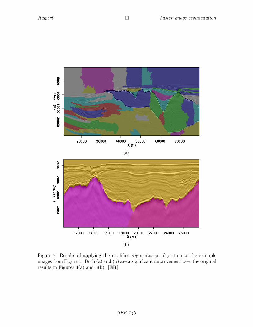
The results of the procedure detailed in the sections above can be seen in Figures 7(a)and 7(b). In Figure 7(a), although the salt body has been segmented into severalregions, all of these regions are contained within the salt body and fully conformto its boundaries. This represents an improvement over the original segmentationin Figure 3(a). The improvement is even more dramatic for the field data example(original image in Figure 1(b)). In Figure 7(b), we see that the salt body has beensegmented virtually perfectly; no longer do the salt body segments spill over theboundary, nor are parts of the boundary itself treated as individual segments as wesaw in the original example.

A major motivation behind this research was to improve on segmentation resultsusing the NCIS method from Shi and Malik (2000), and adapted for use with seismicimages by Lomask et al. (2007). The first indication that the newer method does

SEP-140


(a)

(b)

Figure 7: Results of applying the modified segmentation algorithm to the exampleimages from Figure 1. Both (a) and (b) are a significant improvement over the originalresults in Figures 3(a) and 3(b). [ER]

SEP-140


indeed represent a substantial improvement is the fact that the synthetic image fromFigure 1(a) is simply too large to be segmented on a single processor using the ex-isting NCIS implementation. The necessity of holding a giant, sparse weight matrixin memory and calculating an eigenvector precludes problems of this size from beingfeasible. The smaller field data example, however, is well-suited for the NCIS algo-rithm, and will allow us to make a relatively fair comparison. Figure 8(a) shows theeigenvector produced by the NCIS method to segment the image. In this case, thegraph partition will occur between the negative (red) and positive (blue) values ofthe eigenvector. The boundary resulting from this partition is drawn on the image inFigure 8(b). Recall that in order to make the problem more computationally feasible,the computational domain is already limited around a “prior guess” of the boundary.The pairwise region comparison method developed here requires no such limitation,which is another indication of its superiority.

Efficiency comparison

One of the primary means of comparison for the relative effectiveness of these twoapproaches to image segmentation is the computational efficiency of the method.The following table summarizes the computational expense required to create theexamples seen in the paper.

Table 1: Comparison of CPU times for two segmentation methods

CPU time (s)Image type Pixels NCIS PRC

Synthetic data 2761000 n/a 31Field data 55000 156 1

Again, due to memory constraints the existing NCIS implementation is unableto segment an image the size of Figure 1(a). The implementation described here,however, produces an accurate segmentation in 31 seconds; during this time, approx-imately 55 million edges are created, weighted, and used to segment the graph. Theefficiency advantage for the new implementation is quantified using the field dataexample; in this case, the image is segmented over 150 times faster using the newimplementation. These differences are extremely significant and represent a hugesavings of time and computational expense, especially for larger problems.

Accuracy comparison

Of course, computational efficiency means little if the resulting segmentation is notaccurate. For the synthetic image result in Figure 7(a), we can get a qualitativesense for the accuracy of the new segmentation implementation; while the salt body is

SEP-140


(a)

(b)

Figure 8: Eigenvector (a) used to segment the image in Figure 1(b) according to theNCIS algorithm of Shi and Malik (2000) and adapted for seismic data by Lomasket al. (2007), and the resulting salt boundary (b). [CR]

SEP-140


divided into multiple segments, these segments do indeed fit almost exactly inside theboundaries of the salt body. A more direct comparison of the relative accuracy of theNCIS and PRC methods can be obtained via analysis of the field data results. Figure9 shows both calculated salt boundaries overlain on the image: the NCIS boundaryin green, and the PRC boundary in pink. Visually, we can see very little differencebetween these two results; in many locations, they are almost exactly on top of oneanother. The most noticeable difference between the two results is near X = 20000m,where the PRC boundary dips deeper than the NCIS boundary. Examination of theinput image in Figure 1(b) suggests that in this location, an error in the migrationvelocity model has led to a discontinuity in the boundary image. The new methodappears to do a better job of “correcting” the error. This result serves to increaseconfidence in the viability of this new segmentation scheme as an alternative to theexisting NCIS implementation.

Figure 9: Comparison of the boundaries obtained using the NCIS eigenvector method(green) and the pairwise region comparison method (pink). [CR]

3D implementation

The pairwise region comparison strategy described here is easily extendable to threedimensions. While the theory and general approach remain the same as with the two-dimensional case, in three dimensions the stencil used to construct the graph mustchange. Along with the four co-planar segments extending from each pixel used forthe second stencil in Figure 5, a 3D stencil must incorporate four additional segmentsthat extend the graph edges into the extra dimension. Fortunately, the additionalinformation this brings to the segmentation algorithm allows for the stencil’s segmentsto shrink in length; initial tests indicate that the most accurate results are obtained

SEP-140


with segments that are three pixels in length. Thus, the computational impact ofextending any algorithm from two to three dimensions is somewhat mitigated in thiscase.

Figures 10(a) and 10(b) show a segmentation example resulting from a prelim-inary 3D implementation of the new algorithm. While further improvements seemnecessary, note that both the salt body (in multiple segments) and the water columnhave been accurately identified.

CONCLUSIONS

This paper presented an implementation of the pairwise region comparison (PRC)scheme of Felzenszwalb and Huttenlocher (2004) for segmenting seismic images. Nu-merous modifications were made to the original algorithm, including structural changesto allow for seismic images as inputs, a change in the way edges are constructed forthe graph, and a change in the weighting calculation for each edge. Each of thesemodifications increased the accuracy of the method when applied to seismic data.

Initial results from applying the modified algorithm to both synthetic and fieldseismic images are extremely encouraging. Segmentation of a synthetic image ac-curately located the boundaries of a complex salt body, although several differentsegments were required. Segmentation of both 2D and 3D field seismic data waseven more successful. Compared to an existing implementation of the NormalizedCuts algorithm from Shi and Malik (2000), the new method performs extremely well– it required only half a minute to segment the synthetic data image (which is toolarge for the NCIS implementation to handle on a single processor), and only onesecond to segment the smaller field data example, over 150 times faster than NCIS.An additional advantage is that the newer algorithm is able to operate on the entireimage, rather than only within a certain windowed radius of a previously interpretedboundary. This approach has many advantages, not least of which is the opportunityto identify segments other than only salt bodies. Instead of a binary salt/no-saltdetermination, the ability to identify coherent sedimentary “segments” as well wouldbe tremendously useful for constructing seismic velocity models.

While these results are promising, there are many potential improvements thatremain to be explored. First, the fact that the salt body is in some cases dividedinto multiple segments is a situation that should be examined. One possibility is tomodify the edge weight calculation to include the relative importance of the ampli-tude/intensity and distance factors; right now, both terms are weighted equally (seeequation 6). Another option is to change either the shape or size of the stencil (Figure5) used to build the graph. Yet another potential improvement is the incorporation ofmultiple seismic attributes – for example, dip and frequency attributes. This enhance-ment can be accomplished relatively simply by taking multiple volumes as inputs, andcalculating edge weights using some weighted combination of the different attributesat each pixel.

SEP-140


(a)

(b)

Figure 10: Slices through a 3D image (a) and the resulting 3D segmentation (b) usingthe new PRC algorithm. [ER]

SEP-140


Interpreting subsurface salt bodies in large, 3D seismic images is an incrediblycomplex and tedious task. With further improvement, however, an accurate, efficientautomatic segmentation scheme such as this one has the potential to be an extremelyuseful and powerful tool for processing and interpreting seismic images.

ACKNOWLEDGMENTS

I thank SMAART JV and Unocal (now Chevron) for providing the data used forexamples in this paper, and Robert Clapp for many helpful suggestions.

SEP-140


REFERENCES

Felzenszwalb, P. F., 2010, Image segmentation.(http://people.cs.uchicago.edu/ pff/segment/).

Felzenszwalb, P. F. and D. P. Huttenlocher, 2004, Efficient graph-based image seg-mentation: International Journal of Computer Vision, 59, 167–181.

Halpert, A., R. G. Clapp, and B. L. Biondi, 2009, Seismic image segmentation withmultiple attributes: SEG Technical Program Expanded Abstracts, 28, 3700–3704.

Lomask, J., 2007, Seismic volumetric flattening and segmentation: PhD thesis, Stan-ford University.

Lomask, J., R. G. Clapp, and B. Biondi, 2007, Application of image segmentation totracking 3d salt boundaries: Geophysics, 72, P47–P56.

Shi, J. and J. Malik, 2000, Normalized cuts and image segmentation: Institute ofElectrical and Electronics Engineers Transactions on Pattern Analysis and MachineIntelligence, 22, 838–905.

Taner, M. T., F. Koehler, and R. E. Sheriff, 1979, Complex seismic trace analysis:Geophysics, 44, 1041–1063.

Zahn, C. T., 1971, Graph-theoretical methods for detecting and describing gestaltclusters: IEEE Transactions on Computers, C-20, 68–86.

SEP-140

a new method for more eﬃcient seismic image …sep new method for more eﬃcient seismic image...

Documents