efficient algorithms for geometric optimization∗†michas/optsurvnew.pdf · efficient algorithms...
TRANSCRIPT

Efficient Algorithms for Geometric Optimization∗†
Pankaj K. Agarwal ‡ Micha Sharir §
October 15, 2013
Abstract
We review the recent progress in the design of efficient algorithms for various prob-lems in geometric optimization. We present several techniques used to attack theseproblems, such as parametric searching, geometric alternatives to parametric searching,prune-and-search techniques for linear programming and related problems, and LP-type problems and their efficient solution. We then describe a variety of applications ofthese and other techniques to numerous problems in geometric optimization, includingfacility location, proximity problems, statistical estimators and metrology, placementand intersection of polygons and polyhedra, and ray shooting and other query-typeproblems.
∗Both authors are supported by a grant from the U.S.-Israeli Binational Science Foundation. PankajAgarwal has also been supported by National Science Foundation Grant CCR-93–01259, by an Army Re-search Office MURI grant DAAH04-96-1-0013, by a Sloan fellowship, and by an NYI award and matchingfunds from Xerox Corp. Micha Sharir has also been supported by NSF Grants CCR-94-24398 and CCR-93-11127, by a Max-Planck Research Award, and by a grant from the G.I.F., the German-Israeli Foundationfor Scientific Research and Development.
†A preliminary version of this paper appeared as: P. K. Agarwal and M. Sharir, Algorithmic techniquesfor geometric optimization, in Computer Science Today: Recent Trends and Developments, Lecture Notes in
Computer Science, vol. 1000 (J. van Leeuwen, ed.), 1995, pp. 234–253.‡Department of Computer Science, Box 90129, Duke University, Durham, NC 27708-0129, USA.§School of Mathematical Sciences, Tel Aviv University, Tel Aviv 69978, ISRAEL; and Courant Institute
of Mathematical Sciences, New York University, New York, NY 10012, USA.
0

Introduction 1
1 Introduction
Combinatorial optimization deals with problems of maximizing or minimizing a function of
one or more variables subject to a large number of inequality (and equality) constraints.
Many problems can be formulated as combinatorial optimization problems, which has made
this a very active area of research during the past half century. In many applications,
the underlying optimization problem involves a constant number of variables and a large
number of constraints that are are induced by a given collection of geometric objects; we
refer to such problems as geometric optimization problems. In such cases one expects that
faster and simpler algorithms can be developed by exploiting the geometric nature of the
problem. Much work has been done on geometric optimization problems during the last
twenty years. Many new elegant and sophisticated techniques have been developed and
successfully applied to a variety of geometric optimization problems, and the aim of this
paper is to survey the main techniques and applications of this kind.
This survey consist of two parts. The first part describes several general techniques that
have led to efficient algorithms for a variety of geometric optimization problems, the most
notable of which is linear programming. The second part lists many geometric applications
of these techniques, and discusses some of them in more detail.
The first technique that we present is called parametric searching. Although restricted
versions of parametric searching already existed earlier (see e.g. [97]), the full-scale technique
was presented by Megiddo in the late 1970’s and early 1980’s [179, 180]. The technique
was originally motivated by so-called parametric optimization problems in combinatorial
optimization, and did not receive much attention by the computational geometry community
until the late 1980’s. In the last seven years, though, it has become one of the major
techniques for solving geometric optimization problems efficiently. We outline the technique
in detail in Section 2, first exemplifying it on the slope-selection problem [67], and then
presenting various extensions of the technique.
Despite its power and versatility, parametric searching has certain drawbacks, which we
discuss next. Consequently, there have been several recent attempts to replace parametric
searching by alternative techniques, including randomization [14, 64, 170], expander graphs
[27, 151, 153, 154], geometric cuttings [17, 43], andmatrix searching [105, 107, 108, 106, 111].
We present these alternative techniques in Section 3.
Almost concurrently with the development of the parametric searching technique, Megiddo
devised another ingenious technique for solving linear programming and several related op-
timization problems [181, 183]. This technique, now known as decimation or prune-and-
search, was later refined and extended by Dyer [85], Clarkson [59], and others. The tech-
nique can be viewed as an optimized version of parametric searching, in which certain special
properties of the problem allows one to improve further the efficiency of the algorithm. For
example, this technique yields linear-time deterministic algorithms for linear programming
Geometric Optimization October 15, 2013

Introduction 2
and for several related problems, including the smallest-enclosing-ball problem, when the
dimension is fixed. (However, the dependence of the running time of these algorithms on
the dimension is at least exponential.) We illustrate the technique in Section 4 by applying
it to linear programming.
In the past decade, randomized algorithms have been developed for a variety of problems
in computational geometry and in other fields; see, e.g., the books by Mulmuley [194] and by
Motwani and Raghavan [193]. Clarkson [62] and Seidel [211] gave randomized algorithms for
linear programming, whose expected time is linear in any fixed dimension, which are much
simpler than their earlier deterministic counterparts. The dependence on the dimension
of the running time of these algorithms is better (though still exponential). Actually,
Clarkson’s technique is rather general, and is also applicable to a variety of other geometric
optimization problems. We describe this technique in Section 5.
Another significant progress on linear programming was made about four years ago,
when new randomized algorithms for linear programming were obtained independently by
Kalai [149], and by Matousek et al. [178, 218] (these two algorithms are essentially dual
versions of the same technique). The expected number of arithmetic operations performed
by these algorithms is ‘subexponential’ in the input size, and is still linear in any fixed
dimension, so they constitute an important step toward the still open goal of obtaining
strongly polynomial algorithms for linear programming. (Recall that the polynomial-time
algorithms by Khachiyan [155] and by Karmarkar [150] are not strongly polynomial, as the
number of arithmetic operations performed by these algorithms depends on the size of the
coefficients of the input constraints.) This new technique is presented in Section 6. The
algorithm in [178, 218] is actually formulated in a general abstract framework, which fits
not only linear programming but many other problems. Such “LP-type” problems are also
reviewed in Section 6, including the connection, recently noted by Amenta [32, 33], between
abstract linear programming and “Helly-type” theorems.
In the second part of this paper, we survey many geometric applications of the tech-
niques described in the first part. These applications include problems involving facility
location (e.g., finding p congruent disks of smallest possible radius whose union covers a
given planar point set), geometric proximity (e.g., computing the diameter of a point set in
three dimensions), statistical estimators and metrology (e.g., computing the smallest-width
annulus that contains a given planar point set), placement and intersection of polygons and
polyhedra (e.g., finding the largest similar copy of a convex polygon that fits inside a given
polygonal environment), and query-type problems (e.g., the ray-shooting problem, in which
we want to preprocess a given collection of objects, so that the first object hit by a query
ray can then be determined efficiently).
Numerous non-geometric optimization problems have also benefited from the techniques
presented here (see [21, 65, 105, 120, 196] for a sample of such applications), but we will
concentrate only on geometric applications.
Geometric Optimization October 15, 2013

Parametric Searching 3
Although the common theme of most of the applications reviewed here is that they can
be solved efficiently using parametric-searching, prune-and-search, LP-type, or related tech-
niques, each of them requires a problem-specific, and often fairly sophisticated, approach.
For example, the heart of a typical application of parametric searching is the design of
efficient sequential and parallel algorithms for solving the appropriate problem-specific ‘de-
cision procedure’ (see below for details). We will provide details of these solutions for some
of the problems, but will have to suppress them for most of the applications.
PART I: TECHNIQUES
The first part of the survey describes several techniques commonly used in geometric opti-
mization problems. We describe each technique and illustrate it by giving an example.
2 Parametric Searching
We begin by outlining the parametric-searching technique, and then illustrate the technique
by giving an example where this technique is applied. Finally, we discuss various extensions
of parametric searching.
2.1 Outline of the Technique
The parametric searching technique of Megiddo [179, 180] can be described in the following
general terms (which are not as general as possible, but suffice for our purposes). Suppose
we have a decision problem P(λ) that depends on a real parameter λ, and is monotone in
λ, meaning that if P(λ0) is true for some λ0, then P(λ) is true for all λ < λ0. Our goal
is to find λ∗, the maximum λ for which P(λ) is true, assuming such a maximum exists.
Suppose further that P(λ) can be solved by a (sequential) algorithm As that takes λ and a
set of data objects (independent of λ) as the input, and that, as a by-product, As can also
determine whether the given λ is equal to, smaller than, or larger than the desired value
λ⋆. Assume moreover that the control flow of As is governed by comparisons, each of which
amounts to testing the sign of some low-degree polynomial in λ.
Megiddo’s technique then runs As ‘generically’ at the unknown optimum λ∗ and main-
tains an open interval I that is known to contain λ∗. Initially, I is the whole line. Whenever
As reaches a branching point that depends on some comparison with an associated poly-
nomial p(λ), it computes all the roots λ1, λ2, . . . of p and computes P(λi) by running (the
standard, non-generic version of) As with the value of λ = λi. If one of the λi is equal
to λ⋆, we stop since we have found the value of λ⋆. Otherwise, we have determined the
Geometric Optimization October 15, 2013

Parametric Searching 4
open interval (λi, λi+1) that contains λ∗. Since the sign of p(λ) remains the same for all
λ ∈ (λi, λi+1), we can compute the sign of p(λ∗) by evaluating, say, p((λi + λi+1)/2). The
sign of p(λ∗) also determines the outcome of the comparison at λ⋆. We now set I to be
I ∩ (λi, λi+1), and the execution of the generic As is resumed. As we proceed through
this execution, each comparison that we resolve constrains the range where λ⋆ can lie even
further; and we thus obtain a sequence of progressively smaller intervals, each known to
contain λ⋆, until we either reach the end of As with a final interval I, or hit λ⋆ at one of the
comparisons of As. In practically all applications, the generic algorithm will always make a
comparison whose associated polynomial vanishes at λ⋆, which will then cause the overall
algorithm to terminate with the desired value of λ⋆.
If As runs in time Ts and makes Cs comparisons, then, in general, the cost of the proce-
dure just described is O(CsTs), and is thus generally quadratic in the original complexity.
To speed up the execution, Megiddo proposes to implement the generic algorithm by a
parallel algorithm Ap (under Valiant’s comparison model of computation [228]; see below).
If Ap uses P processors and runs in Tp parallel steps, then each parallel step involves at
most P independent comparisons; that is, we do not need to know the outcome of such a
comparison to be able to execute other comparisons in the same ‘batch’. We can then com-
pute the O(P ) roots of all the polynomials associated with these comparisons, and perform
a binary search to locate λ∗ among them, using (the non-generic) As at each binary step.
The cost of simulating a parallel step of Ap is thus O(P +Ts logP ) (there is no need to sort
the O(P ) roots; instead, one can use repeated median finding, whose overall cost is only
O(P )), for a total running time of O(PTp + TpTs logP ). In most cases, the second term
dominates the running time.
This technique can be generalized in many ways. For example, given a concave function
f(λ), we can compute the value λ∗ of λ that maximizes f(λ), provided we have sequential
and parallel algorithms for the ‘decision’ problem (of comparing λ∗ with a specific λ);
these algorithms compute f(λ) and its derivative, from which the relative location of the
maximum of f is easy to determine. We can compute λ∗ even if the decision algorithm As
cannot distinguish between, say, λ < λ∗ and λ = λ∗; in this case we maintain a half-closed
interval I containing λ∗, and the right endpoint of the final I gives the desired value λ∗.See [13, 68, 225, 226] for these and some other generalizations.
It is instructive to observe that parallelism is used here in a very weak sense, since
the overall algorithm remains sequential and just simulates the parallel algorithm. The
only feature that we require is that the parallel algorithm performs only a small number of
batches of comparisons, and that the comparisons in each batch are independent of each
other. We can therefore assume that the parallel algorithm runs in the parallel comparison
model of Valiant [228], which measures parallelism only in terms of the comparisons being
made, and ignores all other operations, such as bookkeeping, communication between the
processors, and data allocation. Moreover, any portion of the algorithm that is independent
of λ can be performed sequentially in any manner we like. These observations simplify the
Geometric Optimization October 15, 2013

Parametric Searching 5
technique considerably in many cases.
2.2 An example: The slope-selection problem
As an illustration, consider the slope selection problem, which we formulate in a dual setting,
as follows: We are given a set L of n nonvertical lines in the plane and an integer 1 ≤ k ≤ (n2
)
,
and we wish to find an intersection point between two lines of L that has the k-th smallest
x-coordinate. (We assume, for simplicity, general position of the lines, so that no three lines
are concurrent, and no two intersection points have the same x-coordinate.) We are thus
seeking the k-th leftmost vertex of the arrangement A(L) of the lines in L; see [93, 216] for
more details concerning arrangements. (The name of the problem comes from its primal
setting, where we are given a set of n points and a parameter k as above, and wish to
determine a segment connecting two input points that has the k-th smallest slope among
all such segments.)
We define P(λ) to be true if the x-coordinates of at most k vertices of A(L) are smaller
than or equal to λ. Obviously, P(λ) is monotone, and λ∗, the maximum value of λ for which
P(λ) is true, is the x-coordinate of the desired vertex. After having computed λ∗, the actualvertex is rather easy to compute, and in fact the algorithm described below can compute the
vertex without any additional work. In order to apply the parametric-searching technique,
we need an algorithm that, given a vertical line ℓ : x = λ, can compare λ with λ∗. If we
denote by kλ the number of vertices of A(L) that lie to the left of (or on) the line x = λ,
then, clearly, we have λ∗ < λ (resp. λ∗ > λ, λ∗ = λ) if and only if kλ > k (resp. kλ < k,
kλ = k).
Let (ℓ1, ℓ2, . . . , ℓn) denote the sequence of lines in L sorted in the decreasing order of
their slopes, and let (ℓπ(1), ℓπ(2), . . . , ℓπ(n)) denote the sequence of these lines sorted by their
intercepts with x = λ. An easy observation is that two lines ℓi, ℓj , with i < j, intersect to
the left of x = λ if and only if π(i) > π(j). In other words, the number of intersection points
to the left of x = λ can be counted, in O(n logn) time, by counting the number of inversions
in the permutation π, using a straightforward tree-insertion procedure [156]. Moreover, we
can implement this inversion-counting procedure by a parallel sorting algorithm that takes
O(logn) parallel steps and uses O(n) processors (e.g., the one in [26]). Hence, we can count
the number of inversions in O(n logn) time sequentially or in O(logn) parallel time using
O(n) processors. Plugging these algorithms into the parametric-searching paradigm, we
obtain an O(n log3 n)-time algorithm for the slope-selection problem.
2.3 Improvements and extensions
Cole [66] observed that in certain applications of parametric searching, including the slope
selection problem, the running time can be improved to O((P +Ts)Tp), as follows. Consider
a parallel step of the above generic algorithm. Suppose that, instead of invoking the decision
Geometric Optimization October 15, 2013

Parametric Searching 6
procedure O(logn) times in this step, we call it only O(1) times, say, three times. This will
determine the outcome of 7/8 of the comparisons, and will leave 1/8 of them unresolved
(we assume here, for simplicity, that each comparison has only one critical value of λ where
its outcome changes; this is the case in the slope-selection problem). Suppose further that
each of the unresolved comparisons can influence only a constant (and small) number (say,
two) of comparisons executed at the next parallel step. Then 3/4 of these comparisons
can still be simulated generically with the currently available information. This leads to
a modified scheme that mixes the parallel steps of the algorithm, since we now have to
perform together new comparisons and yet unresolved old comparisons. Nevertheless, Cole
shows that if carefully implemented (by assigning an appropriate time-dependent weight
to each unresolved comparison, and by choosing the weighted median at each step of the
binary search), the number of parallel steps of the algorithm increases only by an additive
logarithmic term, which leads to the improvement stated above. An ideal setup for Cole’s
improvement is when the parallel algorithm is described as a circuit (or network), each of
whose gates has a constant fan-out. Since sorting can be implemented efficiently by such a
network [26], Cole’s technique is applicable to problems whose decision procedure is based
on sorting.
Cole’s idea therefore improves the running time of the slope-selection algorithm to
O(n log2 n). (Note that the only step of the algorithm that depends on λ is the sorting
that produces π. The subsequent inversion-counting step is independent of λ, and can be
executed sequentially. In fact, this step can be totally suppressed, since it does not pro-
vide us with any additional information about λ.) Using additional machinery, Cole et al.
[67] gave an optimal O(n logn)-time solution. They observe that one can compare λ∗ with
a value λ that is ‘far away’ from λ∗ in a faster manner, by counting inversions only ap-
proximately. This approximation is progressively refined as λ approaches λ∗ in subsequent
comparisons. Cole et al. show that the overall cost of O(log n) calls to the approximating
decision procedure is only O(n logn), so this also bounds the running time of the whole
algorithm. This technique was subsequently simplified in [43]. Chazelle et al. [52] have
shown that the algorithm of [67] can be extended to compute, in O(n logn) time, the k-th
leftmost vertex in an arrangement of n line segments.
The slope-selection problem is only one of many problems in geometric optimization
that have been efficiently solved using parametric searching. See [5, 9, 13, 17, 51, 200]
for a sample of other problems, many of which are described in Part II, that benefit from
parametric searching.
The parametric searching technique can be extended to higher dimensions in a natural
manner. Suppose we have a d-variate (strictly) concave function F (λ), where λ varies over
Rd. We wish to compute λ∗ ∈ R
d at which F (λ) attains its maximum value. Let As, Ap
be, as above, sequential and parallel algorithms that can compute F (λ0) for any given
λ0. As above, we run Ap generically at λ∗. Each comparison involving λ now amounts to
evaluating the sign of a d-variate polynomial p(λ1, . . . , λd), and each parallel step requires
Geometric Optimization October 15, 2013

Alternative Approaches to Parametric Searching 7
resolving P such independent comparisons at λ∗. Resolving a comparison is more difficult
because p(λ1, . . . , λd) = 0 is now a (d − 1)-dimensional variety. Cohen and Megiddo [65]
described a recursive procedure to execute a parallel step for the case in which the poly-
nomial corresponding to each of the comparisons is a linear function. The total running
time in simulating Ap, using their procedure, is 2O(d2)Ts(Tp logP )d; see also [21, 183, 196].
The running time was subsequently improved by Agarwal et al. [17] to dO(d)Ts(Tp logP )d.
Later Toledo [227] extended these techniques to comparisons involving nonlinear polyno-
mials, using Collins’s cylindrical algebraic decomposition [69]. The total running time of
his procedure is O(Ts(Tp log n)2d−1). For the sake of completeness, we present these higher-
dimensional extensions in an Appendix.
3 Alternative Approaches to Parametric Searching
Despite its power and versatility, the parametric searching technique has some shortcomings:
(i) Parametric searching requires the design of an efficient parallel algorithm for the
generic version of the decision procedure. This is not always easy, even though it only
needs to be done in the weak comparison model, and it often tends to make the overall
solution quite complicated and impractical.
(ii) The generic algorithm requires exact computation of the roots of the polynomials p(λ)
whose signs determine the outcome of the comparisons made by the algorithm. In
general, the roots of a polynomial cannot be computed exactly, therefore one has to
rely either on numerical techniques to compute the roots of p(λ) approximately, or
on computational-algebra techniques to isolate the roots of p(λ) and to determine the
sign of p(λ∗) without computing the roots explicitly. Both of these alternatives are
rather expensive.
(iii) Finally, from an aesthetic point of view, the execution of an algorithm based on
parametric searching may appear to be somewhat chaotic. Such an algorithm neither
gives any insight to the problem, nor does its execution resemble any ‘intuitive’ flow
of execution for solving the problem.
These shortcomings have led several researchers to look for alternative approaches to
parametric searching for geometric optimization problems. Roughly speaking, parametric
searching effectively conducts an implicit binary search over a set Λ = λ1, . . . , λt of
‘critical values’ of the parameter λ, to locate the optimum λ∗ among them. (For example,
in the slope-selection problem, the critical values are the Θ(n2) x-coordinates of the vertices
of the arrangement A(L).) The power of the technique stems from its ability to perform
the binary search by generating only a small number of critical values during the search,
without computing the entire Λ explicitly. In this section we describe some alternative ways
of performing such a binary search, which also generates only a small set of critical values.
Geometric Optimization October 15, 2013

Alternative Approaches to Parametric Searching 8
3.1 Randomization
Randomization is a natural approach to perform an implicit binary search over the critical
values [170, 229, 235]. Suppose we know that λ∗ lies in some interval I = [α, β]. Suppose
further that we can randomly choose an element λ0 ∈ I ∩ Λ, where each item is chosen
with probability 1/|I ∩ Λ|. Then it follows that, by comparing λ∗ with a few randomly
chosen elements of I ∩Λ (i.e., by executing the ‘decision’ algorithm at these values), we can
shrink I to an interval I ′ that is guaranteed to contain λ∗ and that is expected to contain
significantly fewer critical values.
The difficult part is, of course, choosing a random element from I ∩Λ. In many cases, a
procedure for computing |I ∩Λ| can be converted into a procedure for generating a random
element of I ∩Λ. For example, in the slope-selection problem, given a set L of n lines in the
plane and a vertical strip W = (l, r) × R, an inversion-counting algorithm for computing
the number of vertices of A(L) within W can be used to generate a multiset of q random
vertices of A(L) ∩ W in time O(n logn + q) [170]. Based on this observation, Matousek
[170] obtained the following simple slope-selection algorithm: Each step of the algorithm
maintains a vertical strip W (a, b) = (x, y) | a ≤ x ≤ b that is guaranteed to contain
the k-th leftmost vertex; initially a = −∞ and b = +∞. Let m be the number of vertices
of A(L) lying inside W . We repeat the following step until the algorithm terminates. If
m ≤ n, the k-th leftmost vertex of A(L) can be computed in O(n logn) by a sweep-line
algorithm (through W ). Otherwise, set k∗ to be the number of vertices lying to the left of
the line x = a. Let j = ⌊(k − k∗) · n/m⌋, ja = j − ⌊3√n⌋, and jb = j + ⌊3√n⌋. We choose
n random vertices of A(L) lying inside W (a, b). If the k-th leftmost vertex lies in W (ja, jb)
and the vertical strip W (ja, jb) contains at most cm/√n vertices, for some appropriate
constant c > 0, we set a = ja, b = jb, and repeat this step. Otherwise, we discard the
random sample of vertices, and draw a new sample. It can be shown, using Chernoff’s
bound [193], that the expected running time of the above algorithm is O(n logn). Shafer
and Steiger [214] gave a slightly different O(n logn) expected-time algorithm for the slope-
selection algorithm. They choose a random subset of u = O(n logn) vertices of A(L). Let
a1, a2, . . . , au be the x-coordinates of these vertices. Using the algorithm by Cole et al. [67]
for counting the number of inversions approximately, they determine in O(n logn) time the
vertical strip W (ai, ai+1) that contains the k-th leftmost vertex of A(L). They prove that,
with high probability, W (ai, ai+1) contains only O(n) vertices of A(L), and therefore the
desired vertex can be computed in an additional O(n logn) time by a sweep-line algorithm.
See [77] for yet another randomized slope-selection algorithm. We will mention below a few
more applications of this randomized approach.
Geometric Optimization October 15, 2013
Alternative Approaches to Parametric Searching 9
3.2 Expanders and cuttings
In many cases, the above randomized approach can be derandomized, without affecting the
asymptotic running time, using techniques based on expanders or on geometric cuttings.
Expander graphs are special graphs that can be constructed deterministically (in a rather
simple manner), have a linear number of edges, and share many properties with random
graphs; see [29] for more details. For example, in the slope-selection problem, we can
construct expander graphs whose vertices are the given lines and whose edges correspond
to appropriate vertices of the arrangement (each edge corresponds to the intersection of the
two lines that it connects). If we search among these vertices for the optimal λ∗, we obtain
a slab containing λ∗ and free of any of the expander-induced vertices. One can then show,
using properties of expander graphs, that the number of vertices of A(L) within the slab
is rather small, so that the search for λ∗ within the slab can proceed in a more efficient
manner. This is similar to the randomized solution in [170]. (The precise construction of
the expander graph is somewhat involved, and is described in [154].)
Although expanders have been extensively used in many areas, including parallel com-
putation, complexity theory, communication networks, their applications in computational
geometry have been rather sparse so far. Ajtai and Megiddo [27] gave an efficient parallel
linear-programming algorithm based on expanders, and later Katz [151] and Katz and Sharir
[153, 154] applied expanders to solve several geometric optimization problems, including the
application to the slope-selection problem, as just mentioned.
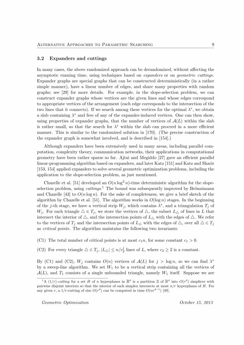
Chazelle et al. [51] developed an O(n log2 n)-time deterministic algorithm for the slope-
selection problem, using cuttings.1 The bound was subsequently improved by Bronnimann
and Chazelle [43] to O(n logn). For the sake of completeness, we give a brief sketch of the
algorithm by Chazelle et al. [51]. The algorithm works in O(logn) stages. In the beginning
of the j-th stage, we have a vertical strip Wj , which contains λ∗, and a triangulation Tj of
Wj . For each triangle ∈ Tj , we store the vertices of , the subset L of lines in L that
intersect the interior of , and the intersection points of L with the edges of . We refer
to the vertices of Tj and the intersection points of L with the edges of , over all ∈ Tj
as critical points. The algorithm maintains the following two invariants:
(C1) The total number of critical points is at most c1n, for some constant c1 > 0.
(C2) For every triangle ∈ Tj , |L| ≤ n/cj2 lines of L, where c2 ≥ 2 is a constant.
By (C1) and (C2), Wj contains O(n) vertices of A(L) for j > log n, so we can find λ∗
by a sweep-line algorithm. We set W1 to be a vertical strip containing all the vertices of
A(L), and T1 consists of a single unbounded triangle, namely W1 itself. Suppose we are
1A (1/r)-cutting for a set H of n hyperplanes in Rd is a partition Ξ of Rd into O(rd) simplices with
pairwise disjoint interiors so that the interior of each simplex intersects at most n/r hyperplanes of H. Forany given r, a 1/r-cutting of size O(rd) can be computed in time O(nrd−1) [49].
Geometric Optimization October 15, 2013

Alternative Approaches to Parametric Searching 10
in the beginning of the j-th stage. For every triangle with |L| > n/cj2, we compute a
(1/4c)-cutting Ξ of L, clip each triangle τ ∈ Ξ within , re-triangulate τ ∩ , and
compute the critical points for the new triangulation of Wj . If the total number of critical
points after this refinement is at most c1n, we move to the next stage. Otherwise, we
shrink the strip Wj as follows. We choose a critical point with the median x-coordinate,
say x = λm, and, using the decision algorithm described in Section 2.2, determine whether
λ∗ is greater than, smaller than, or equal to λm. If λ∗ = λm, then we stop, otherwise we
shrink Wj to either (l, λm)×R or (λm, r)×R, depending on whether λ∗ is smaller or larger
than λm. In any case, the new strip contains only half of the critical points. After repeating
this procedure for a constant number of times, we can ensure that the number of critical
points in the current strip is at most c1n/4. We set Wj+1 to this strip, clip T ′j within Wj+1,
re-triangulate every clipped triangle, and merge two triangles if the their union is a triangle
intersecting at most n/cj2 lines of L. The total number of critical points after these steps
can be proved to be at most c1n. As shown in [51], each stage takes O(n logn) time, so
the overall running time is O(n log2 n). Using the same idea as in [67] (of counting the
number of inversions approximately), Bronnimann and Chazelle [43] managed to improve
the running time to O(n logn).
3.3 Matrix searching
An entirely different alternative to parametric searching was proposed by Frederickson and
Johnson [105, 107, 108], which is based on searching in sorted matrices. It is applicable
in cases where the set Λ of candidate critical values for the optimum parameter λ∗ can be
stored in an n × n matrix A, each of whose rows and columns is sorted. The size of the
matrix is too large for an explicit binary search through its elements, so an implicit search
is called for. Here we assume that each entry of the matrix A can be computed in O(1)
time. We give a brief sketch of this matrix-searching technique.
Let us assume that n = 2k for some k ≥ 0. The algorithm works in two phases. The
first phase, which consists of k steps, maintains a collection of disjoint submatrices of A so
that λ∗ is guaranteed to be an element of one of these submatrices. In the beginning of the
i-th step, the algorithm has at most Bi = 2i+2 − 1 matrices, each of size 2k−i+1 × 2k−i+1.
The i-th step splits every such matrix into four square submatrices, each of size 2k−i×2k−i,
and discards some of these submatrices, so as to be left with only Bi+1 matrices. After the
k-th step, we are left with O(n) singleton matrices, so we can perform a binary search on
these O(n) critical values to obtain λ∗.
The only nontrivial step in the above algorithm is determining which of the submatrices
should be discarded in each step of the first phase, so that at most Bi+1 matrices are left
after the i-th step. After splitting each submatrix, we construct two sets U and V : U is
the set of the smallest (i.e., upper-leftmost) element of each submatrix, and V is the set of
largest (i.e., bottom-rightmost) element of each submatrix. We choose the median elements
Geometric Optimization October 15, 2013

Prune-and-Search Technique and Linear Programming 11
λU and λV of U and V , respectively. We run the decision algorithm at λU and λV , to
compare them with λ∗. If any of them is equal to λ∗, we are done. Otherwise, there are
four cases to consider:
(i) If λU < λ∗, we discard all those matrices whose largest elements are smaller than λU .
(ii) If λU > λ∗, we discard all those matrices whose smallest elements are larger than λU ;
at least half of the matrices are discarded in this case.
(iii) If λV < λ∗, we discard all those matrices whose largest elements are smaller than λV ;
at least half of the matrices are discarded in this case.
(iv) If λV > λ∗, we discard all those matrices whose smallest elements are larger than λV .
It can be shown that this prune step retains at most Bi+1 submatrices [105, 107, 108],
as desired. In conclusion, one can find the optimum λ∗ by executing only O(log n) calls to
the decision procedure, so the running time of this matrix-searching technique is O(logn)
times the cost of the decision procedure. The technique, when applicable, is both efficient
and simple compared to the standard parametric searching.
Aggarwal et al. [22, 23, 24, 25] studied a different matrix-searching technique for op-
timization problems. They gave a linear-time algorithm for computing the minimum (or
maximum) element of every row of a totally monotone matrix; a matrix A = ai,j is called
totally monotone if ai1,j1 < ai1,j2 implies that ai2,j1 < ai2,j2 , for any 1 ≤ i1 < i2 ≤ m, 1 ≤j1 < j2 ≤ n. Totally monotone matrices arise in many geometric, as well as nongeometric,
optimization problems. For example, the farthest neighbors of all vertices of a convex poly-
gon and the geodesic diameter of a simple polygon can be computed in linear time, using
such matrices [23, 129].
4 Prune-and-Search Technique and Linear Programming
Like parametric searching, the prune-and-search (or decimation) technique also performs an
implicit binary search over the finite set of candidate values for λ∗, but, while doing so, it
also tries to eliminate input objects that are guaranteed not to affect the value of λ∗. Eachphase of the technique eliminates a constant fraction of the remaining objects. Therefore,
after a logarithmic number of steps, the problem size becomes a constant, and the problem
can be solved in a final, brute-force step. Because of the ‘decimation’ of input objects, the
overall cost of the resulting algorithm remains proportional to the cost of the first pruning
phase. The prune-and-search technique was originally introduced by Megiddo [181, 183],
in developing a linear-time algorithm for linear programming with n constraints in 2- and
3-dimensions. Later he extended the approach to obtain an O(22d
n)-time algorithm for
linear programming in Rd. Since then the prune-and-search technique has been applied to
Geometric Optimization October 15, 2013

Prune-and-Search Technique and Linear Programming 12
many other geometric optimization problems. We illustrate the technique by describing
Megiddo’s two-dimensional linear-programming algorithm.
We are given a set H = h1, . . . , hn of n halfplanes and a vector c, and we wish to
minimize cx over the feasible region K =⋂n
i=1 hi. Without loss of generality, assume that
c = (0, 1) (i.e., we seek the lowest point of K). Let L denote the set of lines bounding the
halfplanes of H, and let L+ (resp. L−) denote the subset of lines ℓi ∈ L whose associated
halfplane hi lies below (resp. above) ℓi. The algorithm pairs up the lines of L into disjoint
pairs (ℓ1, ℓ2), (ℓ3, ℓ4), . . ., so that either both the lines in a pair belong to L+, or both belong
to L−. The algorithm computes the intersection points of the lines in each pair, and chooses
the median, xm, of their x-coordinates. Let x∗ denote the x-coordinate of the optimal (i.e.,
lowest) point in K (if such a point exists). The algorithm then uses a linear-time decision
procedure (whose details are omitted here, though some of them are discussed below), that
determines whether xm = x∗, xm < x∗, or xm > x∗. If xm = x∗ we stop, since we have
found the optimum. Suppose that xm < x∗. If (ℓ, ℓ′) is a pair of lines both of which belong
to L− and whose intersection point lies to the left of xm, then we can discard the line with
the smaller slope from any further consideration, because that line is known to pass below
the optimal point of K. All other cases can be treated in a fully symmetric manner, so
we have managed to discard about n/4 lines. We have thus computed, in O(n) time, a
subset H ′ ⊆ H of about 3n/4 constraints such that the optimal point of K ′ =⋂
h∈H′ h is
the same as that of K. We now apply the whole procedure once again to H ′, and keep
repeating this (for O(logn) stages) until either the number of remaining lines falls below
some small constant, in which case we solve the problem by brute force (in constant time),
or the algorithm has hit x∗ ‘accidentally’, in which case it stops right away. (We omit here
the description of the linear-time decision procedure, and of handling cases in which K is
empty or unbounded; see [93, 181, 183] for details.) It is now easy to see that the overall
running time of the algorithm is O(n).
Remark. It is instructive to compare this method to the parametric searching technique,
in the context of two-dimensional linear programming. In both approaches, the decision
procedure aims to compare some given x0 with the optimal value x∗. The way this is
done is by computing the maximum and minimum values of the intercepts of the lines in
L− and in L+, respectively, with the line x = x0. A trivial method for computing those
maximum and minimum in parallel is in a binary-tree manner, computing the maximum
or minimum of pairs of lines, then of pairs of pairs, and so on. Both techniques begin by
implementing generically the first parallel step of this decision procedure. The improved
performance of the prune-and-search algorithm stems from the realization that (a) there
is no need to perform the full binary search over the critical values of the comparisons
in that stage—a single binary search step suffices (this is similar to Cole’s enhancement of
parametric searching, mentioned above), and (b) this single comparison allows us to discard
a quarter of the given lines, so there is no point in continuing the generic simulation, and
it is better to start the whole algorithm from scratch, with the surviving lines. From this
Geometric Optimization October 15, 2013

Randomized Algorithms for Linear Programming 13
point of view, the prune-and-search technique can be regarded as an optimized variant of
parametric searching.
This technique can be extended to higher dimensions, although it becomes more com-
plicated, and requires recursive invocations of the algorithm on subproblems in lower di-
mensions. It yields a deterministic algorithm for linear programming that runs in O(Cdn)
time, where Cd is a constant depending on d. One of the difficult steps in higher dimen-
sions is to develop a procedure that can discard a fraction of the input constraints from
further consideration by invoking the (d− 1)-dimensional linear-programming algorithm a
constant number of times; the value of Cd depends on this constant. The original approach
by Megiddo [183] gives Cd = 22d
, which was improved by Clarkson [59] and Dyer [86] to
3d2
. Their procedure can be simplified and improved using geometric cuttings as follows
(see [17, 90]). Let H be the set of hyperplanes bounding the input constraints. Choose
r to be a constant, and compute a 1/r-cutting Ξ. By invoking the (d − 1)-dimensional
linear-programming algorithm recursively O(rd) times (at most three times for each hyper-
plane h supporting a facet of a simplex in Ξ: on h itself, and on two parallel hyperplanes
parallel to h, one on each side and lying very close to h), one can determine the simplex
∆ of Ξ that contains x∗. The constraints whose bounding hyperplanes do not intersect ∆
can be discarded because they do not determine the optimum value. We solve the problem
recursively with the remaining n/r constraints. Dyer and Frieze [90] (see also Agarwal et
al. [17]) have shown that the number of calls to the recursive algorithm can be reduced to
O(dr). This yields an dO(d)n-time algorithm for linear programming in Rd. An entirely
different algorithm with a similar running time was given by Chazelle and Matousek [65].
It is an open problem whether faster deterministic algorithms can be developed. Although
no progress has been made on this front, there have been significant developments on ran-
domized algorithms for linear programming, which we will discuss in the next two sections.
Recently there has been a considerable interest in parallelizing Megiddo’s prune-and-
search algorithm. Deng [76] gave an O(log n)-time and O(n)-work algorithm for two-
dimensional linear programming, under the CRCW model of computation. His algorithm,
however, does not extend to higher dimensions. Alon and Megiddo [28] gave a randomized
algorithm under the CRCW model of computation that runs, with high probability, in O(1)
time using O(n) processors. Ajtai and Megiddo [27] gave an O((log log n)d)-time deter-
ministic algorithm using O(n) processors under Valiant’s model of computation. Goodrich
[117] and Sen [213] gave an O((log logn)d+2)-time, O(n)-work algorithm under the CRCW
model; see also [88].
5 Randomized Algorithms for Linear Programming
Random sampling has become one of the most powerful and versatile techniques in compu-
tational geometry, so it is no surprise that this technique has also been successful in solving
Geometric Optimization October 15, 2013

Randomized Algorithms for Linear Programming 14
many geometric optimization problems. See the book by Mulmuley [194] and the survey
papers by Clarkson [60] and Seidel [212] for applications of the random-sampling technique
in computational geometry. In this section, we describe a randomized algorithm for linear
programming by Clarkson [62], based on random sampling, which is actually quite general
and can be applied to any geometric set-cover and related problems [6, 45]. Other random-
ized algorithms for linear-programming, which run in expected linear time for any fixed
dimension, are proposed by Dyer and Frieze [90], Seidel [211], Kalai [149], and Matousek et
al. [178].
Let H be the set of constraints. We assign a weight µ(h) ∈ Z to each constraint; initially
µ(h) = 1 for all h ∈ H. For a subset A ⊆ H, let µ(A) =∑
h∈A µ(h). The algorithm works
in rounds, each of which consists of the following steps. Set r = 6d2. If |H| ≤ 6d2, we
compute the optimal solution using the simplex algorithm. Otherwise, choose a random
sample R ⊂ H such that µ(R) = r. (We can regard H as a multiset in which each constraint
appears µ(h) times, and we choose a multiset R ∈ (Hr
)
of r constraints.) We compute the
optimal solution xR for R and the subset V ⊂ H \ R of constraints that xR violates (that
is, the subset of constraints that do not contain xR). If V = ∅, the algorithm returns xR.
If µ(V ) ≤ 3µ(H)/d, we double the weight of each constraint in V ; in any case, we repeat
the sampling procedure. See Figure 1 for a pseudocode of the algorithm.
function procedure RANDOM lp (H) /* H: n constraints in Rd
if n ≤ 6d2 then /* µh = 1 for all h ∈ H
return Simplex(H) /* returns v(H)
else
r = 6d2
repeat
choose random R ∈(
Hr
)
xR := Simplex(R)
V := h ∈ H |xR violates hif µ(V ) ≤ µ(H)/3d then
for all h ∈ V do µh := 2µh
until V = ∅return xR
Figure 1: Clarkson’s randomized LP algorithm
Let B be the set of d constraints whose boundaries are incident to the optimal solution.
A round is called successful if µ(V ) ≤ 3µ(H)/d. Using the fact that R is a random subset,
one can argue that each round is successful with probability at least 1/2. Every successful
round increases µ(H) by a factor of at most (1 + 1/3d), so the total weight µ(H) after kd
successful rounds is at most n(1 + 1/3d)kd < nek/3. On the other hand, each successful
iteration doubles the weight of at least one constraint in B (it is easily verified that V must
Geometric Optimization October 15, 2013

Abstract Linear Programming 15
contain such a constraint), which implies that after kd iterations µ(H) ≥ µ(B) ≥ 2k. Hence,
after kd successful rounds, 2k ≤ µ(H) ≤ nek/3. This implies that the above algorithm
terminates in at most 3d lnn successful rounds. Since each round takes O(dd) time to
compute xR and O(dn) time to compute V , the expected running time of the algorithm is
O((d2n+dd+1) log n). By combining this algorithm with a randomized recursive algorithm,
Clarkson improved the expected running time to O(d2n) + (d)d/2+O(1) logn.
6 Abstract Linear Programming
In this section we present an abstract framework that captures linear programming, as well
as many other geometric optimization problems, including computing smallest enclosing
balls (or ellipsoids) of finite point sets in Rd, computing largest balls (ellipsoids) circum-
scribed in convex polytopes in Rd, computing the distance between polytopes in d-space,
general convex programming, and many other problems. Sharir and Welzl [218] and Ma-
tousek et al. [178] (see also Kalai [149]) presented a randomized algorithm for optimization
problems in this framework, whose expected running time is linear in terms of the number
of constraints whenever the combinatorial dimension d (whose precise definition, in this
abstract framework, will be given below) is fixed. More importantly, the running time is
‘subexponential’ in d for many of the LP-type problems, including linear programming.
This is the first subexponential ‘combinatorial’ bound for linear programming (a bound
that counts the number of arithmetic operations and is independent of the bit complexity
of the input), and is a first step toward the major open problem of obtaining a strongly
polynomial algorithm for linear programming. The papers by Gartner and Welzl [110] and
by Goldwasser [112] also survey the known results on LP-type problems.
6.1 An abstract framework
Let us consider optimization problems specified by a pair (H,w), where H is a finite set,
and w : 2H → W is a function into a linearly ordered set (W,≤); we assume that W has
a minimum value −∞. The elements of H are called constraints, and for G ⊆ H, w(G) is
called the value of G. Intuitively, w(G) denotes the smallest value attainable by a certain
objective function while satisfying all the constraints of G. The goal is to compute a minimal
subset BH of H with w(BH) = w(H) (from which, in general, the value of H is easy to
determine), assuming the availability of three basic operations, which we specify below.
Such a minimization problem is called LP-type if the following two axioms are satisfied:
Axiom 1. (Monotonicity) For any F,G with F ⊆ G ⊆ H, we have
w(F ) ≤ w(G).
Geometric Optimization October 15, 2013
Abstract Linear Programming 16
Axiom 2. (Locality) For any F ⊆ G ⊆ H with −∞ < w(F ) = w(G) and any
h ∈ H,
w(G) < w(G ∪ h) ⇒ w(F ) < w(F ∪ h).
Linear programming is easily shown to be an LP-type problem, if we set w(G) to be the
vertex of the feasible region that minimizes the objective function and that is coordinate-
wise lexicographically smallest (this definition is important to satisfy Axiom 2), and if we
extend the definition of w(G) in an appropriate manner to handle empty or unbounded
feasible regions.
A basis B ⊆ H is a set of constraints satisfying −∞ < w(B), and w(B′) < w(B) for all
proper subsets B′ of B. For G ⊆ H, with −∞ < w(G), a basis of G is a minimal subset
B of G with w(B) = w(G). (For linear programming, a basis of G is a minimal set of
halfspace constraints in G such that the minimal vertex of their intersection is the minimal
vertex of G.) A constraint h is violated by G if w(G) < w(G ∪ h), and it is extreme in G
if w(G − h) < w(G). The combinatorial dimension of (H,w), denoted as dim(H,w), is
the maximum cardinality of any basis. We call an LP-type problem basis regular if for any
basis with |B| = dim(H,w) and for any constraint h, every basis of B ∪ h has exactly
dim(H,w) elements. (Clearly, linear programming is basis-regular, where the dimension of
every basis is d.)
We assume that the following primitive operations are available.
(Violation test) h is violated by B: for a constraint h and a basis B, tests
whether h is violated by B.
(Basis computation) basis(B, h): for a constraint h and a basis B, computes a
basis of B ∪ h.(Initial basis) initial(H): An initial basis B0 with exactly dim(H,w) elements
is available.
For linear programming, the first operation can be performed in O(d) time, by substituting
the coordinates of the vertex w(B) into the equation of the hyperplane defining h. The
second operation can be regarded as a dual version of the pivot step in the simplex algorithm,
and can be implemented in O(d2) time. The third operation is also easy to implement.
We are now in position to describe the algorithm. Using the initial-basis primitive, we
compute a basis B0 and call SUBEX lp(H,B0), where SUBEX lp is the recursive algorithm,
given in Figure 2, for computing a basis BH of H.
A simple inductive argument shows the expected number of primitive operations per-
formed by the algorithm is O(2δn), where n = |H| and δ = dim(H,w) is the combinatorial
dimension. However, using a more involved analysis, which can be found in [178], one
can show that basis-regular LP-type problems can be solved with an expected number of
Geometric Optimization October 15, 2013

Abstract Linear Programming 17
function procedure SUBEX lp(H,C); /* H: set of n constraints in Rd;
if H = C then /* C ⊆ H: a basis;
return C /* returns a basis of H.
else
choose a random h ∈ H \ C;
B := SUBEX lp(H \ h, C);
if h is violated by B then
return SUBEX lp(H, basis(B, h))
else
return B;
Figure 2: A randomized algorithm for LP-type problems.
at most e2√
δ ln((n−δ)/√δ )+O(
√δ+lnn) violation tests and basis computations. This is the
‘subexponential’ bound that we alluded to.
Matousek [173] has given examples of abstract LP-type problems of combinatorial di-
mension d with 2d constraints, for which the above algorithm requires Ω(e√2d/ 4
√d) primi-
tive operations. Here is an example of such a problem. Let A be a lower-triangular d × d
0, 1-matrix, with all diagonal entries being 0, i.e., ai,j ∈ 0, 1 for 1 ≤ j < i ≤ d and
aij = 0 for 1 ≤ i ≤ j ≤ d. Let x1, . . . , xd denote variables over Z2, and suppose that all
additions and multiplications are performed modulo 2. We define a set of 2d constraints
H(A) = hci | 1 ≤ i ≤ d, c ∈ 0, 1, where
hci : xi ≥i−1∑
j=1
aijxj + c .
That is, xi = 1 if the right-hand side of the constraint is 1 modulo 2 and xi ∈ 0, 1if the right-hand side is 0 modulo 2. For a subset G ⊆ H, we define w(G) to be the
lexicographically smallest point of⋂
h∈G h. It can be shown that the above example is an
instance of a basis-regular LP-type problem, with combinatorial dimension d. Matousek
showed that if A is chosen randomly (i.e., each entry aij , for 1 ≤ j < i ≤ d, is chosen
independently, with Pr[aij = 0] = Pr[aij = 1] = 1/2) and the initial basis is also chosen
randomly, then the expected number of primitive operations performed by SUBEX lp is
Ω(e√2d/ 4
√d).
6.2 Linear programming
We are given a set H of n halfspaces in Rd. We assume that the objective vector is c =
(1, 0, 0, . . . , 0), and the goal is to minimize cx over all points in the common intersection
Geometric Optimization October 15, 2013

Abstract Linear Programming 18
⋂
h∈H h. For a subset G ⊆ H, define w(G) to be the lexicographically smallest point (vertex)
of the intersection of halfspaces in G. (As noted, some care is needed to handle unbounded
or empty feasible regions; we omit here details concerning this issue.)
As noted above, linear programming is a basis-regular LP-type problem, with combi-
natorial dimension d, and each violation test or basis computation can be implemented in
time O(d) or O(d2), respectively. In summary, we obtain a randomized algorithm for lin-
ear programming, which performs e2√
d ln(n/√d )+O(
√d+lnn) expected number of arithmetic
operations. Using SUBEX lp instead of the simplex algorithm for solving the small-size prob-
lems in the RANDOM lp algorithm (given in Figure 1), the expected number of arithmetic
operations can be reduced to O(d2n) + eO(√
d log d).
In view of Matousek’s lower bound, one should aim to exploit additional properties of
linear programming to obtain a better bound on the performance of the algorithm for linear
programming; this is still a major open problem.
6.3 Extensions
Recently, Chazelle and Matousek [54] gave a deterministic algorithm for solving LP-type
problems in time O(δO(δ)n), provided an additional axiom holds (together with an additional
computational assumption). Still, these extra requirements are satisfied in many natural
LP-type problems. Matousek [175] has investigated the problem of finding the best solution,
for an abstract LP-type problem, that satisfies all but k of the given constraints. He proved
that the number of bases that violate at most k constraints in a non-degenerate instance of
an LP-type problem is O((k+1)δ), where δ is the combinatorial dimension of the problem,
and that they can be computed in time O(n(k + 1)δ). In some cases the running time can
be improved using appropriate data structures; see [175] for details.
Amenta [32] considers the following extension of the abstract framework: Suppose we
are given a family of LP-type problems (H,wλ), monotonically parameterized by a real
parameter λ; the underlying ordered value set W has a maximum element +∞ representing
infeasibility. The goal is to find the smallest λ for which (H,wλ) is feasible, i.e. wλ(H) <
+∞. See [32, 33] for more details and related work.
6.4 Abstract linear programming and Helly-type theorems
In this subsection we describe an interesting connection between Helly-type theorems and
LP-type problems, as originally noted by Amenta [32].
Let K be an infinite collection of sets in Rd, and let t be an integer. We say that K
satisfies a Helly-type theorem, with Helly number t, if the following holds: If K is a finite
subcollection of K with the property that every subcollection of t elements of K has a
Geometric Optimization October 15, 2013

Facility-Location Problems 19
nonempty intersection, then⋂K 6= ∅. (The best known example of a Helly-type theorem is
Helly’s theorem itself [123], which applies for the collection K of all convex sets in Rd, with
the Helly number d+1; see [70] for an excellent survey on this topic.) Suppose further that
we are given a collection K(λ), consisting of n sets K1(λ), . . . ,Kn(λ) that are parametrized
by some real parameter λ, with the property that Ki(λ) ⊆ Ki(λ′), for i = 1, . . . , n and
for λ ≤ λ′, and that, for any fixed λ, the family K1(λ), . . . ,Kn(λ) admits a Helly-type
theorem, with a fixed Helly number t. Our goal is to compute the smallest λ for which⋂n
i=1Ki(λ) 6= ∅, assuming that such a minimum exists. Amenta proved that this problem
can be transformed to an LP-type problem, whose combinatorial dimension is at most t.
As an illustration, consider the smallest-enclosing-ball problem. Let P = p1, . . . , pnbe the given set of n points in R
d, and let Ki(λ) be the ball of radius λ centered at pi, for
i = 1, . . . , n. Since the Ki’s are convex, the collection in question has Helly number d+ 1.
It is easily seen that the minimal λ for which the Ki(λ)’s have nonempty intersection is
the radius of the smallest enclosing ball of P . This shows that the smallest-enclosing-ball
problem s LP-type, and can thus be solved in O(n) randomized expected time in any fixed
dimension. See below for more details.
There are several other examples where Helly-type theorems can be turned into LP-type
problems. They include (i) computing a line transversal to a family of translates of a convex
object in the plane, (ii) computing a smallest homothet of a given convex set that intersects
(or contains, or is contained in) every member in a given collection of n convex sets in Rd,
and (iii) computing a line transversal to certain families of convex objects in 3-space. We
refer the reader to [32, 33] for more details and for additional examples.
PART II: APPLICATIONS
In the first part of the paper we focused on general techniques for solving geometric
optimization problems. In this second part, we list numerous problems in geometric opti-
mization that can be attacked using some of the techniques reviewed above. For the sake of
completeness, we will also review variants of these problems for which the above techniques
are not applicable.
7 Facility-Location Problems
A typical facility-location problem is defined as follows: Given a set D = d1, . . . , dn of
n demand points in Rd, a parameter p, and a distance function δ, we wish to find a set S
of p supply objects (points, lines, segments, etc.) so that the maximum distance between a
Geometric Optimization October 15, 2013

Facility-Location Problems 20
demand point and its nearest supply object is minimized. That is, we minimize, over all
possible appropriate sets S, the following objective function
c(D,S) = max1≤i≤n
mins∈S
δ(di, s).
Instead of minimizing the above quantity, one can choose other objective functions, such as
c′(D,S) =n∑
i=1
mins∈S
δ(di, s).
In some applications, a weight wi is assigned to each point di ∈ D, and the distance from dito a point x ∈ R
2 is defined as wiδ(di, x). The book by Drezner [83] describes many other
variants of the facility-location problem.
The set S = s1, . . . , sp of supply objects partitions D into p clusters, D1, . . . , Dp,
so that si is the nearest supply object to all points in Di. Therefore a facility-location
problem can also be regarded as a clustering problem. These facility-location (or cluster-
ing) problems arise in many areas, including operations research, pattern matching, data
compression, and data mining. A useful extension of the facility-location problem, which
has been widely studied, is the capacitated facility-location problem, in which we have an
additional constraint that the size of each cluster should be at most c for some parame-
ter c ≥ n/p. If p is considered as part of the input, most facility-location problems are
NP-hard, even in the plane or even when only an approximate solution is being sought
[101, 113, 159, 186, 187, 167]. Although many of these problems can be solved in poly-
nomial time for a fixed value of p, some of them still remain intractable. In this section
we review efficient algorithms for a few specific facility-location problems, to which the
techniques introduced in Part I can be applied; in these applications, p is usually a small
constant.
7.1 Euclidean p-center
Given a set D of n demand points in Rd, we wish to find a set S of p supply points so that
the maximum Euclidean distance between a demand point and its nearest neighbor in S is
minimized. This problem can be solved efficiently, when p is small, using the parametric
searching technique. The decision problem in this case is to determine, for a given radius
r, whether D can be covered by the union of p balls of radius r. In some applications, S
is required to be a subset of D, in which case the problem is referred to as the discrete
p-center problem.
General results. A naive procedure for the p-center problem runs in time O(ndp+2),
observing that the critical radius r∗ is determined by at most d + 1 points, which also
determine one of the balls; similarly, there are O(nd(p−1)) choices for the other p− 1 balls,
Geometric Optimization October 15, 2013

Facility-Location Problems 21
and it takes O(n) time to verify whether a specific choice of balls covers D. For the planar
case, Drezner [79] gave an improved O(n2p+1)-time algorithm, which was subsequently
improved by Hwang et al. [142] to nO(√p). Hwang et al. [141] have given another nO(
√p)-
time algorithm for computing a discrete p-center. Therefore, for a fixed value of p, the
Euclidean p-center (and also the Euclidean discrete p-center) problem can be solved in
polynomial time in any fixed dimension. However, either of these problems is NP-complete
for d ≥ 2, if p is part of the input [104, 187]. This has led researchers to develop efficient
algorithms for approximate solutions and for small values of p and d.
Approximation algorithms. Let r∗ be the minimum value of r for which p disks of
radius r cover D. The greedy algorithm described in Figure 3, originally proposed by
Gonzalez [113] and by Hochbaum and Shmoys [132, 133], computes in O(np) time a set S
of p points so that c(D,S) ≤ 2r∗.
function procedure GREEDY COVER (D, p); /* D: set of n points in Rd;
for i = 1 to n do
Max Dist(i) = ∞;
for i = 1 to p do
si = dj s.t. Max Dist(j) = max1≤l≤n Max Dist(l);
for j = 1 to n do
Max Dist(j) = minMax Dist(j), δ(si, dj);return s1, . . . , sp;
Figure 3: Greedy algorithm for approximate p-center.
This algorithm works equally well for any metric and for the weighted case [89]. Note
that it also provides an approximate solution to the discrete p-center problem. The running
time was improved toO(n log p) by Feder and Green [101]. They also showed that computing
a set S of p supply points such that c(D,S) ≤ 1.822r∗ under the Euclidean distance function,
or c(D,S) < 2r∗ under the L∞-metric, is NP-Hard. See [114, 159] for other approximation
algorithms.
Another way of seeking an approximation is to find a small number of balls of a fixed
radius, say r, that cover all demand points. Computing k∗, the minimum number of balls of
radius r that cover D, is also NP-complete [104]. A greedy algorithm can construct k∗ lognballs of radius r that cover D. Hochbaum and Maass gave a polynomial-time algorithm
to compute a cover of size (1 + ε)k∗, for any ε > 0 [130]; see also [45, 101, 114]. No
constant-factor approximation algorithm is known for the capacitated covering problem,
with unit-radius disks, that is, the problem of partitioning a given point set S in the plane
into the minimum number of clusters, each of which consists of at most c points and can be
covered by a disk of radius r. Nevertheless, the greedy algorithm can be modified to obtain
Geometric Optimization October 15, 2013

Facility-Location Problems 22
an O(logn)-factor approximation for this problem [36].
The general results reviewed so far do not make use of parametric searching: since there
are only O(nd+1) candidate values for the optimum radius r∗, one can simply enumerate
all these values and run a standard binary search among them. The improvement that one
can gain from parametric searching is significant only when p is relatively small, which is
what we are going to discuss next.
Euclidean 1-center. The 1-center problem is to compute the smallest ball enclosing D.
The decision procedure for the 1-center problem is thus to determine whether D can be
covered by a ball of radius r. For d = 2, the decision problem can be solved in O(logn)
parallel steps using O(n) processors, e.g., be testing whether the intersection of the disks of
radius r centered at the points of D is nonempty. This yields an O(n log3 n)-time algorithm
for the planar Euclidean 1-center problem. Using the prune-and-search paradigm, one can,
however, solve the 1-center problem in linear time [86], and this approach extends to higher
dimensions, where, for any fixed d, the running time is dO(d)n [17, 54, 90]. Megiddo [185, 189]
extends this approach to obtain a linear-time algorithm for the weighted 1-center problem.
Dynamic data structures for maintaining the smallest enclosing ball of a set of points, as
points are being inserted and deleted, are given in [11, 37]. See [78, 82, 84, 102, 182] for
other variants of the 1-center problem. A natural extension of the 1-center problem is to
find a disk of the smallest radius that contains k of the n input points. The best known
deterministic algorithm runs in time O(n logn+nk log k) using O(n+k2 log k) space [100, 72]
(see also [96]), and the best known randomized algorithm runs in O(n logn+ nk) expected
time using O(nk) space, or in O(n logn + nk log k) expected time using O(n) space [174].
Matousek [175] also showed that the smallest disk covering all but k points can be computed
in time2 O(n logn+ k3nε).
The smallest-enclosing-ball problem is an LP-type problem, with combinatorial dimen-
sion d+1 [218, 232]. Indeed, the constraints are the given points, and the function w maps
each subset G to the radius of the smallest ball containing G. Monotonicity of w is trivial,
and locality follows easily from the uniqueness of the smallest enclosing ball of a given set
of points in general position. The combinatorial dimension is d + 1 because at most d + 1
points are needed to determine the smallest enclosing ball. This problem is, however, not
basis-regular (the smallest enclosing ball may be determined by any number, between 2 and
d+1, of points), and a naive implementation of the basis-changing operation may be quite
costly (in d). Nevertheless, Gartner [109] showed that this operation can be performed in
this case using expected eO(√d) arithmetic operations. Hence, the expected running time of
the algorithm is O(d2n) + eO(√
d log d).
2In this paper, the meaning of complexity bounds that depend on an arbitrary parameter ε > 0, like theone stated here, is that given any ε > 0, we can fine-tune the algorithm so that its complexity satisfies thestated bound. In these bounds the constant of proportionality usually depends on ε, and tends to infinitywhen ε tends to zero.
Geometric Optimization October 15, 2013

Facility-Location Problems 23
There are several extensions of the smallest-enclosing-ball problem. They include: (i)
computing the smallest enclosing ellipsoid of a point set [54, 87, 201, 232], (ii) computing
the largest ellipsoid (or ball) inscribed inside a convex polytope in Rd [109], (iii) computing
a smallest ball that intersects (or contains) a given set of convex objects in Rd (see [185],
and (iv) computing a smallest area annulus containing a given planar point set. All these
problems are known to be LP-type, and thus can be solved using the algorithm described
in Section 6. However, not all of them run in subexponential expected time because they
are not basis regular. Linear-time algorithms, based on prune-and-search technique, have
also been developed for many of these problems in two dimensions [40, 41, 42, 145].
Euclidean 2-center. In this problem we want to cover a set D of n points in Rd by two
balls of smallest possible common radius. There is a trivial O(nd+1)-time algorithm for the
2-center problem in Rd, because the ‘clusters’ D1 and D2 in an optimal solution can be
separated by a hyperplane [80]. Faster algorithms have been developed for the planar case
using parametric searching. Agarwal and Sharir [13] gave an O(n2 logn)-time algorithm for
determining whether D can be covered by two disks of radius r. Their algorithm proceeds as
follows: There are O(n2) distinct subsets of D that can be covered by a disk of radius r, and
these subsets can be computed in O(n2 logn) time, by processing the arrangement of the n
disks of radius r, centered at the points of D. For each such subset D1, the algorithm checks
whether D\D1 can be covered by another disk of radius r. Using a dynamic data structure,
the total time spent is shown to be O(n2 log n). Plugging this algorithm into the parametric
searching machinery, one obtains an O(n2 log3 n)-time algorithm for the Euclidean 2-center
problem. Matousek [170] gave a simpler randomized O(n2 log2 n) expected-time algorithm
by replacing parametric searching with randomization. The running time of the decision
algorithm was improved by Hershberger [126] to O(n2), which has been utilized in the best
near-quadratic solution, by Jaromczyk and Kowaluk [146], which runs in O(n2 log n) time;
see also [147].
A major progress on this problem was recently made by Sharir [215], who gave an
O(n log9 n)-time algorithm, by combining the parametric searching technique with several
additional techniques, including a variant of the matrix searching algorithm of Frederickson
and Johnson [108]. Eppstein [99] has simplified Sharir’s algorithm, using randomization
and better data structures, and obtained an improved solution, whose expected running
time is O(n log2 n).
Recently Agarwal et al. [19] have developed an O(n4/3 log5 n)-time algorithm for the
discrete 2-center problem.
Rectilinear p-center. In this problem the metric is the L∞-distance, so the decision
problem is now to cover the given set D by a set of p axis-parallel cubes, each of length 2r.
The problem is NP-Hard if p is part of the input and d ≥ 2, or if d is part of the input and
Geometric Optimization October 15, 2013

Facility-Location Problems 24
p ≥ 3 [104, 186]. Ko et al. [159] showed that computing an S with c(D,S) < 2r∗ is also
NP-Hard.
The rectilinear 1-center problem is trivially solved in linear time, and a polynomial-time
algorithm for the rectilinear 2-center problem, even if d is unbounded, is given in [186]. A
linear-time algorithm for the planar rectilinear 2-center problem is given by Drezner [81]
(see also [157]); Ko and Lee [158] gave an O(n logn)-time algorithm for the weighted case.
Recently, Sharir and Welzl [219] have developed a linear-time algorithm for the rectilinear
3-center problem, by showing that it is an LP-type problem (as is the rectilinear 2-center
problem). They have also obtained an O(n logn)-time algorithm for computing a rectilinear
4-center (and have shown that this algorithm is worst-case optimal), and an O(n log5 n)-
time algorithm for computing a rectilinear 5-center. The algorithms for the 4-center and
5-center employ the Frederickson-Johnson matrix searching technique. See [152, 219] for
additional related results.
7.2 Euclidean p-line-center
Let D be a set of n points in Rd and δ be the Euclidean distance function. We wish to
compute the smallest real value w∗ so that D can be covered by the union of p strips of
width w∗. Megiddo and Tamir showed that the problem of determining whether w∗ = 0
(i.e, D can be covered by p lines) is NP-Hard [188], which not only proves that the p-line-
center is NP-Complete, but also proves that approximating w∗ within a constant factor is
NP-Complete. Approximation algorithms for this problem are given in [121].
The 1-line center is the classical width problem. For d = 2, an O(n logn)-time algorithm
was given by Houle and Toussaint [138]. A matching lower bound was proved by Lee and
Wu [163]. They also gave an O(n2 log n)-time algorithm for the weighted case, which was
improved to O(n logn) in [137].
For the 2-line-center problem in the plane, Agarwal and Sharir [13] (see also [12]) gave
an O(n2 log5 n)-time algorithm, using parametric searching. This algorithm is very similar
to their 2-center algorithm, i.e., the decision algorithm finds all subsets of S that can be
covered by a strip of width w and for each such subset S1, it determines whether S \S1 can
be covered by another strip of width w. The heart of this decision procedure is an efficient
algorithm for the following off-line width problem: given a sequence Σ = (σ1, . . . , σn) of
insertions and deletions of points in a setD and a real number w, is there an i such that after
performing the first i updates, the width of the current point set is at most w? A solution to
this off-line width problem, that runs in O(n2 log3 n) time, is given in [12]. The running time
for the optimization problem was improved to O(n2 log4 n) by Katz and Sharir [154] and by
Glozman et al. [111], using expander graphs and the Frederickson-Johnson matrix searching
technique, respectively. The best known algorithm, by Jaromczyk and Kowaluk [148], runs
in O(n2 log2 n) time. It is an open problem whether a near-linear (or just subquadratic)
Geometric Optimization October 15, 2013

Facility-Location Problems 25
time algorithm exists for computing a 2-line center.
7.3 Euclidean p-median
Let D be a set of n points in Rd. We wish to compute a set S of p supply points so
that the sum of distances from each demand point to its nearest supply point is minimized
(i.e., we want to minimize the objective function c′(D,S)). This problem can be solved in
polynomial time for d = 1 (for d = 1 and p = 1 the solution is the median of the given
points, whence the problem derives its name), and it is NP-Hard for d ≥ 2 [187]. The
special case of d = 2, p = 1 is the classical Fermant-Weber problem, and it goes back to the
17th century. It is known that the solution for the Fermant-Weber problem is unique and
algebraic. Several numerical approaches have been proposed to compute an approximate
solution. See [48, 233] for the history of the problem and for the known algorithms, and
[197] for some heuristics for the p-median problem that work well for a set of random points.
7.4 Segment-center
Given a segment e, we wish to find a translated and rotated copy of e so that the maximum
distance from each point of the given set D of demand points to this copy is minimized. This
problem was originally considered by Imai et al. [143], who had given an O(n4 log n)-time
algorithm. An improved solution, based on parametric searching, with O(n2α(n) log3 n)
running time, was later obtained in [8] (here α(n) denotes the extremely slowly growing
inverse of Ackermann’s function). The decision problem in this case is to determine whether
there exists a translated and rotated copy of the ‘hippodrome’ H = e⊕Br, the Minkowski
sum of the segment e with a disk of radius r, which fully contains D. Since H is convex, this
is equivalent to H containing P = conv(D). Hence the decision procedure is actually: Given
a convex polygon P and the hippodrome H, does H contain a translated and rotated copy
of P? see Figure 4. Note that placements of P can be specified in terms of three parameters,
two for the translation and one for the rotation. Let FP ⊆ R3 denote the set of placements
of P at which P lies inside H. Using Davenport–Schinzel sequences [216], Agarwal and
Sharir showed that the complexity of FP is O(n22α(n)), and that it can be computed in
time O(n22α(n) log n). By exploiting various geometric and combinatorial properties of FP
and using some elegant results from combinatorial geometry, Efrat and Sharir [95] showed
that the complexity of FP is only O(n logn), and that one can determine in time O(n1+ε)
whether FP 6= ∅. Plugging this into the parametric searching technique, one obtains an
O(n1+ε)-time solution to the segment-center problem.
Geometric Optimization October 15, 2013

Proximity Problems 26
e
r
H
P
Figure 4: The segment-center problem
7.5 Other facility-location problems
Besides the problems discussed above, several other variants of the facility-location prob-
lem have been studied. For example, Hershberger [125] described an O(n2/ log log n)-time
algorithm for partitioning a given set S of n points into two subsets so that the sum of
their diameters is minimized. If we want to minimize the maximum of the two diameters,
the running time can be improved to O(n logn) [127]. Glozman et al. [111] have studied
problems of covering S by several different kinds of shapes. Maass [167] showed that the
problem of covering S with the minimum number of unit-width annuli is NP-Hard even
for d = 1 (a unit-width annulus in 1-dimension is a union of two unit-length intervals),
and Hochbaum and Maass [131] gave an approximation algorithm for covering points with
annuli.
8 Proximity Problems
8.1 Diameter in 3-space
Given a set S of n points in R3, we wish to compute the diameter of S, that is, the maximum
distance between any two points of S. The decision procedure here is to determine, for a
given radius r, whether the intersection of the balls of radius r centered at the points of
S contains S. The intersection of congruent balls in R3 has linear complexity [118, 124],
therefore it is natural to ask whether the intersection of n congruent balls can be computed
in O(n logn) time. (Checking whether all points of S lie in the intersection can then be
performed in additional O(n logn) time, using straightforward point-location techniques.)
Clarkson and Shor [64] gave a very simple O(n logn) expected-time randomized algorithm
(which is worst-case optimal) for computing the intersection, and then used a randomized
prune-and-search algorithm, summarized in Figure 5, to compute the diameter of S.
Geometric Optimization October 15, 2013

Proximity Problems 27
function procedure DIAMETER (S);
choose a random point p ∈ S;
q = a farthest neighbor of p;
compute I =⋂
p′∈S B(p′, δ(p, q))
S1 = S \ Iif S1 = ∅
then return d(p, q)
else return DIAMETER (S1)
Figure 5: A randomized algorithm for computing the diameter in 3D.
The correctness of the above algorithm is easy to check. The only nontrivial step in the
above algorithm is computing I and S1. If δ is the Euclidean metric, I can be computed in
O(|S| log |S|) expected time, using the ball-intersection algorithm. S1 can then be computed
in additionalO(|S| log |S|) time, using any optimal planar point-location algorithm (see, e.g.,
[208]). Hence, each recursive step of the algorithm takes O(|S| log |S|) expected time. Since
p is chosen randomly, |S1| ≤ 2|S|/3 with high probability, which implies that the expected
running time of the overall algorithm is O(n logn).
It was a challenging open problem whether an O(n logn)-time deterministic algorithm
can be developed for computing the intersection of n congruent balls in 3-space. This
has been answered in the affirmative by Amato et al. [31], following a series of near-linear
time but weaker deterministic algorithms [51, 177, 202]. Amato et al. derandomized the
Clarkson-Shor algorithm, using several sophisticated techniques.3 Their algorithm yields an
O(n log3 n)-time algorithm for computing the diameter. Obtaining an optimal O(n logn)-
time deterministic algorithm for computing the diameter in 3-space still remains elusive.
8.2 Closest line pair
Given a set L of n lines in R3, we wish to compute a closest pair of lines in L. Let d(L,L′)
denote the Euclidean distance between the closest pair of lines in L×L′, for two disjoint sets
L,L′ of lines. Two algorithms for this problem, both based on parametric searching, were
given independently by Chazelle et al. [51] and by Pellegrini [199]; both algorithms run in
O(n8/5+ε) time. Using Plucker coordinates [53, 220] and range-searching data structures,
the algorithms construct, in O(n8/5+ε) time, a family of pairs (L1, L′1), . . . , (Lk, L
′k),
so that every line in Li lies below (in the z-direction) all the lines of L′i and d(L,L′) =
min1≤i≤k d(Li, L′i). Hence, it suffices to compute a closest pair in Li × L′
i, for each i ≤ k,
which can be done using parametric searching. The decision procedure is: For a given real
number r, determine whether d(Li, L′i) ≤ r, for each i ≤ k. Since lines in 3-space have
3An earlier attempt by Bronnimann et al. [44] to derandomize Clarkson-Shor algorithm had an error.
Geometric Optimization October 15, 2013

Proximity Problems 28
four degrees of freedom, each of these subproblems can be transformed to the following
point-location problem in R4: Given a set S of n points in R
4 (representing the lines in
Li) and a set Γ of m surfaces, each being the graph of an algebraic trivariate function of
constant degree (each surface is the locus of lines in R3 that pass above a line of L′
i at
distance r from it), determine whether every point in S lies below all the surfaces of Γ. It is
shown in [51] that this point-location problem can be solved in time O(n4/5+εm4/5+ε), which
implies an O(n8/5+ε)-time algorithm for computing d(L,L′). Agarwal and Sharir [14] have
shown that d(Li, L′i) can be computed in O(n3/4+εm3/4+ε) expected time, by replacing
parametric searching with randomization and by exploiting certain geometric properties
that the surfaces in Γ possess. Roughly speaking, this is accomplished by generalizing the
Clarkson-Shor algorithm for computing the diameter, described in Figure 5. However, this
algorithm does not improve the running time for computing d(L,L′), because we still need
O(n8/5+ε) time for constructing the pairs (Li, L′i).
If we are interested in computing a pair of lines with the minimum vertical distance, the
running time can be improved to O(n4/3+ε) [199].
8.3 Distance between polytopes
We wish to compute the Euclidean distance d(P1,P2) between two given convex polytopes
P1 and P2 in Rd. If the polytopes intersect, then this distance is 0. If they do not intersect,
then this distance equals the maximum distance between two parallel hyperplanes separating
the polytopes; such a pair of hyperplanes is unique, and they are orthogonal to the segment
connecting two points a ∈ P1 and b ∈ P2 with d(a, b) = d(P1,P2). It is shown by Gartner
[109] that this problem is LP-type, with combinatorial dimension at most d + 2 (or d + 1,
if the polytopes do not intersect). It is also shown there that the primitive operations
can be performed with expected eO(√d) arithmetic operations. Hence, the problem can be
solved by the general LP-type algorithm, whose expected number of arithmetic operations
is O(d2n) + eO(√
d log d), where n is the total number of facets in P1 and P2. For d = 2,
the maximum and the minimum distance between two convex polygons can be computed
in O(logn) time, assuming that the vertices of each Pi are stored in an array, sorted in a
clockwise order [92].
8.4 Selecting distances
Let S be a set of n points in the plane, and let 1 ≤ k ≤ (n2
)
be an integer. We wish
to compute the k-th smallest distance between a pair of points of S. This can be done
using parametric searching. The decision problem is to compute, for a given real r, the
sum∑
p∈S |Dr(p) ∩ (S − p)|, where Dr(p) is the closed disk of radius r centered at p.
(This sum is twice the number of pairs of points of S at distance ≤ r.) Agarwal et al.
[5] gave an O(n4/3 log4/3 n) expected-time randomized algorithm for the decision problem,
Geometric Optimization October 15, 2013
Proximity Problems 29
using the random-sampling technique of [64], which yields an O(n4/3 log8/3 n) expected-time
algorithm for the distance-selection problem. Goodrich [115] derandomized this algorithm,
at a cost of an additional polylogarithmic factor in the running time. Katz and Sharir
[153] obtained an expander-based O(n4/3 log3+ε n)-time (deterministic) algorithm for this
problem. See also [207].
8.5 Shape matching
Let P and Q be two polygons with m and n edges, respectively. The problem is to measure
the ‘resemblance’ between P and Q, that is, to determine how well can a copy of P fit Q,
if we allow P to translate or to both translate and rotate. The Hausdorff distance is one of
the common ways of measuring resemblance between two (fixed) sets P and Q [139]; it is
defined as
H(P,Q) = max maxa∈P
minb∈Q
d(a, b), maxa∈Q
minb∈P
d(a, b) ,
where d(·, ·) is the Euclidean distance.
If we allow P to translate only, then we want to compute minv H(P+v,Q). The problem
has been solved by Agarwal et al. [18], using parametric searching, in O((mn)2 log3(mn))
time, which is significantly faster than the previously best known algorithm by Alt et al. [30].
If P and Q are finite sets of points, a more efficient solution, not based on parametric
searching, is proposed by Huttenlocher et al. [140]. Their solution, however, does not apply
to the case of polygons. If we measure distance by the L∞-metric, faster algorithms, based
on parametric searching, are developed in [55, 57].
If we allow P to translate and rotate, then computing the minimum Hausdorff distance
becomes significantly harder. Chew et al. [56] have given an O(m2n2 log3mn)-time algo-
rithm when both P and Q are finite point sets, and an O(m3n2 log3mn)-time algorithm
when P and Q are polygons.
Another way of measuring the resemblance between two polygons P and Q is by com-
puting the area of their intersection (or, rather, of their symmetric difference). Suppose we
wish to minimize the area of the symmetric difference between P and Q, under translation
of P . For this case, de Berg et al. [73] gave an O(n logn)-time algorithm, using the prune-
and-search paradigm. Their algorithm extends to higher dimensions at a polylogarithmic
cost, using parametric searching.
8.6 Surface simplification
A generic surface-simplification problem is defined as follows: Given a polyhedral object P
in R3 and an error parameter ε > 0, compute a polyhedral approximation Π of P with the
minimum number of vertices, so that the maximum distance between P and Π is at most
Geometric Optimization October 15, 2013

Proximity Problems 30
ε. There are several ways of defining the maximum distance between P and Π, depending
on the application. We will refer to an object that lies within ε distance from P as an
ε-approximation of P . Surface simplification is a central problem in graphics, geographic
information systems, scientific computing, and visualization.
One way of solving the problem is to run a binary search on the number of vertices
of the approximating surface. We then need to solve the decision problem of determining
whether there exists an ε-approximation with at most k vertices, for some given k. Unfor-
tunately, this problem is NP-Hard [20], so one seeks efficient techniques for computing an
ε-approximation of size (number of vertices) close to kOPT, where kOPT is the minimum
size of an ε-approximation. Although several ad-hoc algorithms have been developed for
computing an ε-approximation [74, 75, 135, 136, 168], none of them guarantees any rea-
sonable bound on the size of the output, and many of them do not even ensure that the
maximum distance between the input and the output surface is indeed at most ε. There
has been some recent progress on developing polynomial-time approximation algorithm for
computing ε-approximations in some special cases.
The simplest, but nevertheless an interesting, special case is when P is a convex polytope
(containing the origin). In this case we wish to compute another convex polytope Q with the
minimum number of vertices so that (1−ε)P ⊆ Q ⊆ (1+ε)P (or so that P ⊆ Q ⊆ (1+ε)P ).
We can thus pose a more general problem: Given two convex polytopes P1 ⊆ P2 in R3,
compute a convex polytope Q with the minimum number of vertices such that P1 ⊆ Q ⊆ P2.
Das and Joesph [71] have attempted to prove that this problem is NP-Hard, but their proof
contains an error, and it still remains an open problem. Mitchell and Suri [192] have shown
that there exists a nested polytope Q with at most 3kOPT vertices, whose vertices are a
subset of the vertices of P2. The problem can now be formulated as a hitting-set problem,
and, using a greedy approach, they presented an O(n3)-time algorithm for computing a
nested polytope with O(kOPT logn) vertices. Clarkson [61] showed that the randomized
technique described in Section 5 can compute a nested polytope with O(kOPT log kOPT)
vertices in O(n logc n) expected-time, for some constant c > 0. Bronnimann and Goodrich
[45] extended Clarkson’s algorithm to obtain a polynomial-time, deterministic algorithm
that constructs a nested polytope with O(kOPT) vertices.
A widely-studied special case of surface simplification, motivated by applications in ge-
ographic information systems and scientific computing, is when P is a polyhedral terrain
(i.e., the graph of a continuous piecewise-linear bivariate function). In most of the appli-
cations, P is represented as a finite set of n points, sampled from the input surface, and
the goal is to compute a polyhedral terrain Q with the minimum number of vertices, such
that the vertical distance between any point of P and Q is at most ε. Agarwal and Suri
[20] showed that this problem is NP-Hard. They also gave a polynomial-time algorithm
for computing an ε-approximation of size O(kOPT log kOPT), by reducing the problem to
a geometric set-cover problem, but the running time of their algorithm is O(n8), which is
rather high. Agarwal and Desiken [6] have shown that Clarkson’s randomized algorithm can
Geometric Optimization October 15, 2013

Statistical Estimators and Related Problems 31
be extended to compute a polyhedral terrain of size O(k2OPT log2 kOPT) in expected time
O(n2+δ + k3OPT log3 kOPT). The survey paper by Heckbert and Garland [122] summarizes
most of the known results on terrain simplification.
A dual version of the problem of computing an ε-approximation is: Given a polyhedral
surface P and an integer k, compute an approximating surface Q that has at most k vertices,
whose distance from P is the smallest possible. Very little is known about this problem,
except in the plane. Goodrich [116] showed that, given a set S of n points in the plane,
an x-monotone polygonal chain Q with at most k vertices that minimizes the maximum
vertical distance between Q and the points of S can be computed in time O(n logn). His
algorithm is based on the parametric-searching technique, and uses Cole’s improvement of
parametric searching. (See [116] for other related work on this problem.) If the vertices of
Q are required to be a subset of S, the best known algorithm is by Varadarajan [229]; it is
based on parametric searching, and its running time is O(n4/3+ε).
9 Statistical Estimators and Related Problems
9.1 Plane fitting
Given a set S of n points in R3, we wish to fit a plane h through S so that the maximum
distance between h and the points of S is minimized. This is the same problem as computing
the width of S (the smallest distance between a pair of parallel supporting planes of S),
which is considerably harder than the two-dimensional variant mentioned in Section 7.2.
Houle and Toussaint [138] gave an O(n2)-time algorithm for computing the width in R3.
This can be improved using parametric searching. The decision procedure is to determine,
for a given distance w, whether the convex hull of S has two ‘antipodal’ edges, such that
the two parallel planes containing these edges are supporting planes of S and lie at distance
≤ w. (One also needs to consider pairs of parallel planes, one containing a facet of conv(S)
and the other passing through a vertex. However, it is easy to test all these pairs in
O(n logn) time.) The major technical issue here is to avoid having to test quadratically
many pairs of antipodal edges, which may exist in the worst case. Chazelle et al. [51] gave
an algorithm that is based on parametric searching and runs in time O(n8/5+ε) (see [2]
for an improved bound). They reduced the width problem to the problem of computing a
closest pair between two sets L,L′ of lines in R3 (each line containing an edge of the convex
hull of S), such that each line in L lies below all the lines of L′. The fact that this latter
problem now has an improved O(n3/2+ε) expected-time solution [14] implies that the width
can be computed in expected time O(n3/2+ε). See [160, 176, 221, 222, 230] for other results
on hyperplane fitting.
Geometric Optimization October 15, 2013

Statistical Estimators and Related Problems 32
9.2 Circle fitting
Given a set S of n points in the plane, we wish to fit a circle C through S so that the
maximum distance between the points of S and C is minimized. This is equivalent to
finding an annulus of minimum width that contains S. Ebara et al. [91] observed that the
center of a minimum-width annulus is either a vertex of the closest-point Voronoi diagram
of S, or a vertex of the farthest-point Voronoi diagram, or an intersection point of a pair
of edges of the two diagrams. Based on this observation, they obtained a quadratic-time
algorithm. Using parametric searching, Agarwal et al. [18] have shown that the center
of the minimum-width annulus can be found without checking all of the O(n2) candidate
intersection points explicitly; their algorithm runs in O(n8/5+ε) time; see also [2] for an
improved solution. Using randomization and an improved analysis, the expected running
time has been improved to O(n3/2+ε) by Agarwal and Sharir [14]. Finding an annulus
of minimum area that contains S is a simpler problem, since it can be formulated as an
instance of linear programming in R4, and can thus be solved in O(n) time [183]. In certain
metrology applications [134, 206, 231], one wants to fit a circle C through S so that the
sum of distances between C and the points of S is minimized. No algorithm is known for
computing an exact solution, though several numerical techniques have been proposed; see
[38, 161, 224]. See [162, 223] for other variants of the circle-fitting problem and for some
special cases.
9.3 Cylinder fitting
Given a set S of n points in R3, we wish to find a cylinder of smallest radius that contains S.
Using parametric searching, the decision problem in this case can be rephrased as: Given a
set B of n balls of a fixed radius r in R3, determine whether there exists a line that intersects
all the balls of B (the balls are centered at the points of S and the line is the symmetry axis
of a cylinder of radius r that contains S). Agarwal and Matousek [10] showed that finding
such a line can be reduced to computing the convex hull of a set of n points in R9, which,
combined with parametric searching, leads to an O(n4 logO(1) n)-time algorithm for finding
a smallest cylinder enclosing S; see e.g. [209]. The bound has recently been improved by
Agarwal et al. [4] to O(n3+ε), by showing that the combinatorial complexity of the space of
all lines that intersect all the balls of B is O(n3+ε), and by designing a different algorithm,
also based on parametric searching, whose decision procedure calculates this space of lines
and determines whether it is nonempty. Faster algorithms have been developed for some
special cases [103, 209]. Agarwal et al. [4] also gave an O(n/δ2)-time algorithm to compute
a cylinder of radius ≤ (1 + δ)r∗ containing all the points of S, where r∗ is the radius of the
smallest cylinder enclosing S.
Note that this problem is different from those considered in the two previous subsections.
The problem analogous to those studied above would be to find a cylindrical shell (a region
Geometric Optimization October 15, 2013

Statistical Estimators and Related Problems 33
enclosed between two concentric cylinders) of smallest width (difference between the radii
of the cylinders), which contains a given point set S. This problem is considerably harder,
and no solution for it that improves upon the naive brute-force technique is known.
9.4 Center points
Given a set S of n points in the plane, we wish to compute a center point σ ∈ R2, such
that any halfplane containing σ also contains at least ⌊n/3⌋ points of S. It is a known
consequence of Helly’s Theorem that σ always exists [93]. In a dual setting, let L be the
set of lines dual to the points in S, and let K1,K2 be the convex hulls of the ⌊n/3⌋ and
⌊2n/3⌋ levels of the arrangement A(L), respectively.4 The dual of a center point of S is a
line separating K1 and K2. This implies that the set of center points is a convex polygon
with at most 2n edges.
Cole et al. [68] gave an O(n log3 n)-time algorithm for computing a center point, using
multi-dimensional parametric searching. Using the prune-and-search paradigm, Matousek
[169] obtained an O(n log3 n)-time algorithm for computing K1 and K2, which in turn yields
the set of all center points. Recently, Jadhav and Mukhopadhyay [144] gave a linear-time
algorithm for computing a center point, using a direct and elegant technique.
Near-quadratic algorithms for computing a center point in three dimensions were de-
veloped in [68, 195]. Clarkson et al. [63] gave an efficient algorithm for computing an
approximate center point in Rd.
9.5 Ham-sandwich cuts
Let S1, . . . , Sd be d (finite) point sets in Rd. A ham-sandwich cut is a hyperplane h such
that each of the two open halfspaces bounded by h contains at most ⌊|Si|/2⌋ points of Si,
for each 1 ≤ i ≤ d. The ham-sandwich theorem (see, e.g., [93]) guarantees the existence of
such a cut. For d = 2, there is always a ham-sandwich cut whose dual is an intersection
point of the median levels of A(L1) and A(L2), where Li is the set of lines dual to the
points in Si, for i = 1, 2. It can be shown that the number of intersection points between
the median levels of A(L1) and of A(L2) is always odd.
Several prune-and-search algorithms have been proposed for computing a ham-sandwich
cut in the plane. Megiddo [184] gave a linear-time algorithm for the special case where S1
and S2 are linearly separable. Modifying this algorithm, Edelsbrunner and Waupotitsch [94]
gave an O(n logn)-time algorithm when S1 and S2 are not necessarily linearly separable.
A linear-time, recursive algorithm for this general case is given by Lo and Steiger [166].
4The level of a point p with respect to A(L) is the number of lines lying strictly below p. The k-level ofA(L) is the closure of the set of edges of A(L) whose level is k (the level is fixed over an edge of A(L)); eachk-level is an x-monotone connected polygonal chain.
Geometric Optimization October 15, 2013

Placement and Intersection 34
It works as follows. At each level of recursion, the algorithm maintains two sets of lines,
R and B, and two integers p, q, such that any intersection point between KpR, the p-level
of A(R), and KqB, the q-level of A(B), is dual to a ham-sandwich cut of the original sets;
moreover, the number of such intersections is guaranteed to be odd. The goal is to compute
an intersection point of KpR and Kq
B. Initially R and B are the sets of lines dual to S1
and S2, and p = ⌊|S1|/2⌋, q = ⌊|S2|/2⌋. Let r be a sufficiently large constant. One then
computes a (1/r)-cutting Ξ of R ∪ B. At least one of the triangles of Ξ contains an odd
number of intersection points of the levels. By computing the intersection points of the
edges of Ξ with R ∪ B, such a triangle ∆ can be found in linear time. Let R∆ ⊆ R and
B∆ ⊆ B be the subsets of lines in R and B, respectively, that intersect ∆, and let p′ (resp.q′) be the number of lines in R (resp. B) that lie below ∆. We then solve the problem
recursively for R∆ and B∆ with the respective levels p∗ = p− p′ and q∗ = q − q′. It easily
follows that the p∗-level of A(R∆) and the q∗-level of A(B∆) intersect at an odd number of
points. Since |R∆|+ |B∆| = O(n/r), the total running time of the algorithm is O(n). Lo et
al. [165] extend this approach to R3, and obtain an O(n3/2)-time algorithm for computing
ham-sandwich cuts in three dimensions.
10 Placement and Intersection
10.1 Intersection of polyhedra
Given a set P = P1, . . . , Pm of m convex polyhedra in Rd, with a total of n facets,
is their common intersection I =⋂m
i=1 Pi nonempty? Of course, this is an instance of
linear programming in Rd with n constraints, but the goal is to obtain faster algorithms
that depend on m more significantly than they depend on n. Reichling [203] presented an
O(m log2 n)-time prune-and-search algorithm for d = 2. His algorithm maintains a vertical
strip W bounded by two vertical lines bl, br, such that I ⊆ W . Let k be the total number
of vertices of all the Pi’s lying inside W . If k ≤ m log n, the algorithm explicitly computes
I ∩W in O(m log2 n) time. Otherwise, it finds a vertical line ℓ inside W such that both W+
and W− contain at least k/4 vertices, where W+ (resp. W−) is the portion of W lying to
the right (resp. to the left) of ℓ. By running a binary search on each Pi, one can determine
whether ℓ intersects Pi and, if so, obtain the top and bottom edges of Pi intersecting ℓ.
This allows us to compute the intersection I ∩ ℓ as the intersection of m intervals, in O(m)
time. If this intersection is nonempty, we stop, since we have found a point in I. Otherwise,
if one of the polygons of P lies fully to the right (resp. to the left) of ℓ, then I cannot lie
in W− (resp. in W+); if one polygon lies fully in W− and another lies fully in W+, then
clearly I = ∅. Finally, if ℓ intersects all the Pi’s, but their intersection along ℓ is empty,
then, following the same technique as in Megiddo’s two-dimensional linear-programming
algorithm [181], one can determine, in additional O(m) time, which of W+,W− can be
asserted not to contain I. Hence, if the algorithm has not stopped, it needs to recurse
Geometric Optimization October 15, 2013

Placement and Intersection 35
in only one of the slabs W+, W−. Since the algorithm prunes a fraction of the vertices
in each stage, it terminates after O(log n) stages, from which the asserted running time
follows easily. Reichling [204] and Eppstein [98] extended this approach to d = 3, but their
approaches do not extend to higher dimensions. However, if we have a comparison-based
data structure that can determine in O(log n) time whether a query point lies in a specified
Pi, then, using multi-dimensional parametric searching, we can determine in O(m logO(1) n)
time whether I 6= ∅.
10.2 Polygon placement
Let P be a convex m-gon, and let Q be a closed planar polygonal environment with n
edges. We wish to compute the largest similar copy of P (under translation, rotation, and
scaling) that can be placed inside Q. Using generalized Delauney triangulation induced
by P within Q, Chew and Kedem [58] obtained an O(m4n22α(n) log n)-time algorithm.
Faster algorithms have been developed using parametric searching [3, 217]. The decision
problem in this case is: Given a convex polygon B with m edges (a scaled copy of P )
and a planar polygonal environment Q with n edges, can B be placed inside Q (allowing
translation and rotation)? Each placement of B can be represented as a point in R3, using
two coordinates for translation and one for rotation. Let FP denote the resulting three-
dimensional space of all free placements of B inside Q. Leven and Sharir [164] have shown
that the complexity of FP is O(mnλ6(mn)), where λs(n) is the maximum length of a
Davenport–Schinzel sequence of order s composed of n symbols [216] (it is almost linear in
n for any fixed s). Sharir and Toledo [217] gave an O(m2nλ6(mn) logmn)-time algorithm
to determine whether FP 6= ∅ — they first compute a superset of the vertices of FP ,
in O(mnλ6(mn) logmn) time, and then spend O(m log n) time for each of these vertices
to determine whether the corresponding placement of B is free, using a standard triangle
range-searching data structure. Recently, Agarwal et al. [3] gave an O(mnλ6(mn) logmn)
expected-time randomized algorithm to compute FP . Plugging these algorithms into the
parametric searching machinery, one can obtain an O(m2nλ6(mn) log3mn log logmn)-time
deterministic algorithm, or an O(mnλ6(mn) log4mn) expected-time randomized algorithm,
for computing a largest similar placement of P inside Q.
Faster algorithms are known for computing a largest placement of P inside Q in some
special cases. If both P and Q are convex, then a largest similar copy of P inside Q can be
computed in time O(mn2 log n) [1]; if P is not allowed to rotate, then the running time is
O(m+ n log2 n) [225].
The biggest-stick problem is another interesting special case of the largest-placement
problem; here Q is a simple polygon and P is a line segment. In this case, we are interested
in finding the longest segment that can be placed inside Q. This problem can be solved
using a divide-and-conquer algorithm, developed in [18], and later refined in [2, 14]. It
proceeds as follows: Partition Q into two simple polygons Q1, Q2 by a diagonal ℓ so that
Geometric Optimization October 15, 2013

Placement and Intersection 36
each of Q1 and Q2 has at most 2n/3 vertices. Recursively compute the longest segment that
can be placed in each Qi, and then determine the longest segment that can be placed in Q
and that intersects the diagonal ℓ. The decision step for this subproblem is to determine
whether there exists a placement of a line segment of length w that lies inside Q and crosses
ℓ. Agarwal et al. [18] have shown that this problem can be reduced to that in which we are
given a set S of points and a set Γ of algebraic surfaces in R4, where each surface is the
graph of a trivariate function, and we wish to determine whether every point of S lies below
all the surfaces of Γ. Agarwal and Sharir [14] gave a randomized algorithm with O(n3/2+ε)
expected running time for this point-location problem. Using randomization, instead of
parametric searching, they obtained an O(n3/2+ε) expected-time procedure for the overall
merge step (finding the biggest stick that crosses ℓ). The total running time of the algorithm
is therefore also O(n3/2+ε). Finding a longest segment inside Q whose endpoints are vertices
of Q is a simpler problem, and can be solved by a linear-time algorithm due to Hershberger
and Suri [129].
10.3 Collision detection
Let P and Q be two (possibly nonconvex) polyhedra in R3. P is assumed to be fixed and
Q to move along a given trajectory π. The goal is to determine the first position on π,
if any, at which Q intersects P . This problem can be solved using parametric searching.
Suppose, for example, that Q is only allowed to translate along a line. Then the decision
problem is to determine whether Q intersects P as it translates along a segment e in R3. Let
Qe = Q⊕ e be the Minkowski sum of Q and e. Then Q intersects P as it translates along e
if and only if Qe intersects P . This intersection problem can be solved in O(n8/5+ε) time,
using simplex range-searching data structures [198, 210]. Plugging this into the parametric
searching machinery, we can compute, in O(n8/5+ε) time, the first intersection of Q with P
as Q moves along a line.
If Q rotates around a fixed axis ℓ, then the decision problem is to determine whether Q
intersects P as it rotates by a given angle θ from its initial position. In this case, each edge
of Q sweeps a section of a hyperboloid. Schomer and Thiel [210] have shown that, using
a standard linearization technique (as described in [10, 234]), the intersection-detection
problem can be formulated as an instance of simplex range searching in R5, and can be
solved in time O(n8/5+ε). Plugging this algorithm into the parametric searching technique,
we can also compute the first intersection in time O(n8/5+ε).
Gupta et al. [119] have studied various collision-detection problems for a set of moving
points in the plane. For example, they give an O(n5/3 log6/5 n)-time algorithm for deter-
mining whether a collision occurs in a set of points, each moving in the plane along a line
with constant velocity.
Geometric Optimization October 15, 2013

Query-Type Problems 37
11 Query-Type Problems
Parametric searching has also been successfully applied in designing efficient data structures
for a number of query-type problems. In this section we discuss a few of these problems,
including ray shooting and linear optimization queries.
11.1 Ray shooting
The general ray-shooting problem can be defined as follows. Preprocess a given set S of
objects in Rd (usually d = 2 or 3), so that the first object hit by a query ray can be
computed efficiently. The ray-shooting problem arises in computer graphics, visualization,
and in many other geometric problems [9, 10, 11, 200]. The connection between ray shooting
and parametric searching was observed by Agarwal and Matousek [9]. Here the decision
problem is to determine, for a specified point σ on the query ray ρ, whether the initial
segment sσ of ρ intersects any object in S (where s is the origin of ρ). Hence, we need to
execute generically, in the parametric-searching style, an appropriate intersection-detection
query procedure on the segment sσ, where σ is the (unknown) first intersection point of ρ
and the objects in S. Based on this technique, several efficient ray-shooting data structures
have been developed [2, 9, 15, 16]. We illustrate this technique by giving a simple example.
Let S be a set of n lines in the plane, and let S∗ be the set of points dual to the lines of
S. A segment e intersects a line of S if and only if the double-wedge e∗ dual to e contains
a point of S∗. Hence, a segment intersection-detection query for S can be answered by
preprocessing S∗ into a triangle (or a wedge) range-searching structure; see, e.g., [171, 172].
Roughly speaking, we construct a partition tree T on S∗ as follows. We fix a sufficiently large
constant r. If |S∗| ≤ 2r, T consists of a single node storing S∗. Otherwise, using a result of
Matousek [171], we construct, in O(n) time, a family of pairs Π = (S∗1 ,∆1), . . . , (S
∗u,∆u)
such that (i) S∗1 , . . . , S
∗u form a partition of S∗, (ii) n/r ≤ |S∗
i | ≤ 2n/r for each i, (iii) each
∆i is a triangle containing S∗i , and (iv) every line intersects at most c
√r triangles ∆i of Π,
for some absolute constant c (independent of r). We recursively construct a partition tree
Ti on each S∗i , and attach it as the i-th subtree of T . The root of Ti stores the simplex ∆i.
The total size of T is linear, and the time spent in constructing T is O(n logn).
Let e be a query segment, and let e∗ be its dual double wedge. To determine whether
e intersects any line of S (that is, whether e∗ contains any point of S∗), we traverse T in a
top-down fashion, starting from the root. Let v be a node visited by the algorithm. If v is a
leaf, we explicitly check whether any point of S∗v lies in the double wedge e∗. Suppose then
that v is an internal node. If ∆v ⊆ e∗, then clearly e∗ ∩S 6= ∅, and we stop. If ∆v ∩ e∗ = ∅,then we stop processing v and do not visit any of its children. If ∂e∗ intersects ∆v, we
recursively visit all the children of v. Let Q(nv) denote the number of nodes in the subtree
rooted at v visited by the query procedure (nv is the size of S∗v). By construction, a line
intersects at most c√r triangles of Πv (the partition constructed at v), so ∂e∗ intersects at
Geometric Optimization October 15, 2013

Query-Type Problems 38
most 2c√r triangles of Πv. Hence, we obtain the following recurrence:
Q(nv) ≤ 2c√rQ(2nv/r) +O(r).
The solution of the above recurrence is O(n1/2+ε), for any ε > 0, provided r is chosen
sufficiently large (as a function of ε). Since the height of T is O(logn), we can answer a
query in O(logn) parallel time, using O(n1/2+ε) processors, by visiting the nodes of the
same level in parallel.
s
ρ
σ
p∗
ξp
p
s∗ σ∗
∆
ξ∗p
Figure 6: A ray-shooting query
Returning to the task of answering a ray-shooting query, let ρ be a query ray with origin
s, and let σ be the (unknown) first intersection point of ρ with a line of S. We compute σ
by running the parallel version of the segment intersection-detection procedure generically,
in the parametric searching style, on the segment γ = sσ. At each node v that the query
procedure visits, it tests whether ∆v ⊆ γ∗ or ∆v∩∂γ∗ 6= ∅. Since σ is the only indeterminant
in these tests, the tests reduce to determining, for each vertex p of ∆v, whether p lies above,
below, or on the line σ∗ dual to σ; see Figure 6. Let ξp be the intersection point of the dual
line p∗ and the line containing ρ; and set γp = sξp. By determining whether the segment γpintersects a line of S, we can determine whether p lies above or below σ∗. Hence, using this
parametric searching approach, a ray-shooting query can be answered in O(n1/2+ε) time.
Several other ray-shooting data structures based on this technique have been developed
in [9, 10, 11, 200].
11.2 Linear-optimization queries
We wish to preprocess a setH of halfspaces in Rd into a linear-size data structure so that, for
a linear objective function c, we can efficiently compute the vertex of⋂
H that minimizes c.
Using multi-dimensional parametric searching and data structures for answering halfspace-
emptiness queries, Matousek [172] presented an efficient algorithm for answering linear-
Geometric Optimization October 15, 2013
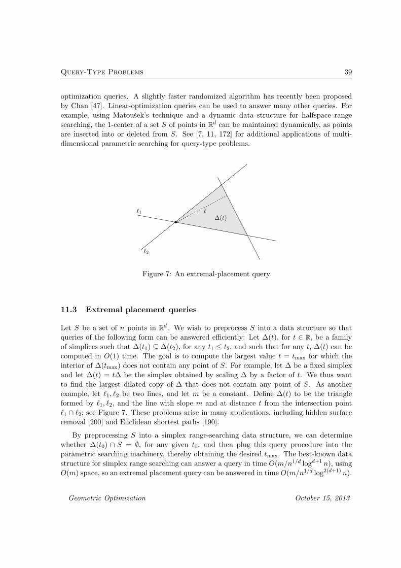
Query-Type Problems 39
optimization queries. A slightly faster randomized algorithm has recently been proposed
by Chan [47]. Linear-optimization queries can be used to answer many other queries. For
example, using Matousek’s technique and a dynamic data structure for halfspace range
searching, the 1-center of a set S of points in Rd can be maintained dynamically, as points
are inserted into or deleted from S. See [7, 11, 172] for additional applications of multi-
dimensional parametric searching for query-type problems.
ℓ1
ℓ2
t∆(t)
Figure 7: An extremal-placement query
11.3 Extremal placement queries
Let S be a set of n points in Rd. We wish to preprocess S into a data structure so that
queries of the following form can be answered efficiently: Let ∆(t), for t ∈ R, be a family
of simplices such that ∆(t1) ⊆ ∆(t2), for any t1 ≤ t2, and such that for any t, ∆(t) can be
computed in O(1) time. The goal is to compute the largest value t = tmax for which the
interior of ∆(tmax) does not contain any point of S. For example, let ∆ be a fixed simplex
and let ∆(t) = t∆ be the simplex obtained by scaling ∆ by a factor of t. We thus want
to find the largest dilated copy of ∆ that does not contain any point of S. As another
example, let ℓ1, ℓ2 be two lines, and let m be a constant. Define ∆(t) to be the triangle
formed by ℓ1, ℓ2, and the line with slope m and at distance t from the intersection point
ℓ1 ∩ ℓ2; see Figure 7. These problems arise in many applications, including hidden surface
removal [200] and Euclidean shortest paths [190].
By preprocessing S into a simplex range-searching data structure, we can determine
whether ∆(t0) ∩ S = ∅, for any given t0, and then plug this query procedure into the
parametric searching machinery, thereby obtaining the desired tmax. The best-known data
structure for simplex range searching can answer a query in time O(m/n1/d logd+1 n), using
O(m) space, so an extremal placement query can be answered in time O(m/n1/d log2(d+1) n).
Geometric Optimization October 15, 2013

Discussion 40
12 Discussion
In this survey we have reviewed several techniques for geometric optimization, and discussed
many geometric problems that benefit from these techniques. There are of course quite a few
non-geometric parametric optimization problems that can also be solved efficiently using
these techniques. For example, parametric searching has been applied to develop efficient
algorithm for the following problems: (i) let G be a directed graph, in which the weight of
each edge e is a d-variate linear function we(x), and let s and t be two vertices in G, find
the point x ∈ Rd, so that the maximum flow from s to t is maximized over all points x ∈ R
d
[65]; (ii) compute the minimum edit distance between two given sequences, where the cost
of performing an insertion, deletion, and substitution is a univariate linear function [120].
There are several other geometric optimization problems that are not discussed here,
and we conclude by mentioning two classes of them. The first class is the optimal motion-
planning problem, where we are given a moving robot B, an environment with obstacles,
and two placements of the robot, and we want to compute an “optimal” collision-free
path for B between the given placements. The cost of a path depends on B and on the
application. In the simplest case, B is point robot, O is a set of polygonal obstacles in
the plane or polyhedral obstacles in 3-space, and the cost of a path is its Euclidean length.
We then face the Euclidean shortest-path problem, which has been studied intensively in
the past decade; see [46, 128, 205]. The problem becomes much harder if B is not a point,
because even the notion of optimality is not well defined. See [191] for an excellent survey
on this topic.
The second class of problems that we want to mention can be called geometric graph
problems. Given a set S of points in Rd, we can define a weighted complete graph in-
duced by S, where the weight of an edge (p, q) is the distance between p and q under some
suitable metric (two of the most commonly used metrics are the Euclidean and the rec-
tilinear metrics). We can now pose many optimization problems on this graph, including
the Euclidean travelling salesperson, Euclidean matching, Euclidean (rectilinear) Steiner
trees, and minimum weight triangulation. Although all these problems can be solved using
techniques known for general graphs, the hope is that better and/or simpler algorithms
can be developed by exploiting the geometry of the problem. There have been several sig-
nificant developments on geometric graph problems over the last few years, of which the
most exciting is an nO(1/ε)-time (1 + ε)-approximation algorithm for the Euclidean travel-
ling salesperson problem [35]. We refer the reader to [39] for a survey on approximation
algorithms for such geometric optimization problems.
References
Geometric Optimization October 15, 2013

References 41
[1] P. K. Agarwal, N. Amenta, and M. Sharir, Placement of one convex polygon inside another,Tech. Report CS-1995-29, Duke University, 1995.
[2] P. K. Agarwal, B. Aronov, and M. Sharir, Computing envelopes in four dimensions withapplications, Proc. 10th Annu. ACM Sympos. Comput. Geom., 1994, pp. 348–358.
[3] P. K. Agarwal, B. Aronov, and M. Sharir, Motion planning for a convex polygon in a polygonalenvironment, manuscript, 1996.
[4] P. K. Agarwal, B. Aronov, and M. Sharir, Line transversals of balls and smallest enclosingcylinders in three dimensions, Proc. 8th ACM-SIAM Sympos. Discrete Algorithms, 1997.
[5] P. K. Agarwal, B. Aronov, M. Sharir, and S. Suri, Selecting distances in the plane, Algorith-mica, 9 (1993), 495–514.
[6] P. K. Agarwal and P. K. Desikan, An approximation algorithm for terrain simplification, Proc.8th ACM-SIAM Sympos. Discrete Algorithms, 1997.
[7] P. K. Agarwal, A. Efrat, and M. Sharir, Vertical decomposition of shallow levels in 3-dimensional arrangements and its applications, Proc. 11th Annu. ACM Sympos. Comput.
Geom., 1995, pp. 39–50.
[8] P. K. Agarwal, A. Efrat, M. Sharir, and S. Toledo, Computing a segment center for a planarpoint set, J. Algorithms, 15 (1993), 314–323.
[9] P. K. Agarwal and J. Matousek, Ray shooting and parametric search, SIAM J. Comput.,22 (1993), 794–806.
[10] P. K. Agarwal and J. Matousek, On range searching with semialgebraic sets, Discrete Comput.
Geom., 11 (1994), 393–418.
[11] P. K. Agarwal and J. Matousek, Dynamic half-space range reporting and its applications,Algorithmica, 13 (1995), 325–345.
[12] P. K. Agarwal and M. Sharir, Off-line dynamic maintenance of the width of a planar pointset, Comput. Geom. Theory Appl., 1 (1991), 65–78.
[13] P. K. Agarwal and M. Sharir, Planar geometric location problems, Algorithmica, 11 (1994),185–195.
[14] P. K. Agarwal and M. Sharir, Efficient randomized algorithms for some geometric optimizationproblems, Proc. 11th Annu. ACM Sympos. Comput. Geom., 1995, pp. 326–335.
[15] P. K. Agarwal and M. Sharir, Ray shooting amidst convex polygons in 2D, J. Algorithms,21 (1996), 508–519.
[16] P. K. Agarwal and M. Sharir, Ray shooting amidst convex polyhedra and polyhedral terrainsin three dimensions, SIAM J. Comput., 25 (1996), 100–116.
[17] P. K. Agarwal, M. Sharir, and S. Toledo, An efficient multi-dimensional searching techniqueand its applications, Tech. Report CS-1993-20, Dept. Comp. Sci., Duke University, 1993.
Geometric Optimization October 15, 2013

References 42
[18] P. K. Agarwal, M. Sharir, and S. Toledo, Applications of parametric searching in geometricoptimization, J. Algorithms, 17 (1994), 292–318.
[19] P. K. Agarwal, M. Sharir, and E. Welzl, The discrete 2-center problem, manuscript, 1996.
[20] P. K. Agarwal and S. Suri, Surface approximation and geometric partitions, Proc. 5th ACM-
SIAM Sympos. Discrete Algorithms, 1994, pp. 24–33.
[21] R. Agarwala and D. Fernandez-Baca, Weighted multidimensional search and its applicationsto convex optimization, SIAM J. Comput., 25 (1996), 83–99.
[22] A. Aggarwal and M. M. Klawe, Applications of generalized matrix searching to geometricalgorithms, Discrete Appl. Math., 27 (1987), 3–23.
[23] A. Aggarwal, M. M. Klawe, S. Moran, P. Shor, and R. Wilber, Geometric applications of amatrix-searching algorithm, Algorithmica, 2 (1987), 195–208.
[24] A. Aggarwal, D. Kravets, J. K. Park, and S. Sen, Parallel searching in generalized Monge ar-rays with applications, Proc. 2nd ACM Sympos. Parallel Algorithms Architect., 1990, pp. 259–268.
[25] A. Aggarwal and J. Park, Notes on searching in multidimensional monotone arrays, Proc.29th Annu. IEEE Sympos. Found. Comput. Sci., 1988, pp. 497–512.
[26] M. Ajtai, J. Komlos, and E. Szemeredi, Sorting in c log n parallel steps, Combinatorica,3 (1983), 1–19.
[27] M. Ajtai and N. Megiddo, A deterministic poly(log log n)-time n-processor algorithm for linearprogramming in fixed dimensions, SIAM J. Comput., 25 (1996), 1171–1195.
[28] N. Alon and N. Megiddo, Parallel linear programming in fixed dimension almost surely inconstant time, Proc. 31st Annu. IEEE Sympos. Found. Comput. Sci., 1990, pp. 574–582.
[29] N. Alon and J. Spencer, The Probabilistic Method, J. Wiley and Sons, New York, NY, 1993.
[30] H. Alt, B. Behrends, and J. Blomer, Approximate matching of polygonal shapes, Ann. Math.
Artif. Intell., 13 (1995), 251–266.
[31] N. M. Amato, M. T. Goodrich, and E. A. Ramos, Parallel algorithms for higher-dimensionalconvex hulls, Proc. 35th Annu. IEEE Sympos. Found. Comput. Sci., 1994, pp. 683–694.
[32] N. Amenta, Bounded boxes, Hausdorff distance, and a new proof of an interesting Hellytheorem, Proc. 10th Annu. ACM Sympos. Comput. Geom., 1994, pp. 340–347.
[33] N. Amenta, Helly-type theorems and generalized linear programming, Discrete Comput.
Geom., 12 (1994), 241–261.
[34] D. S. Arnon, G. E. Collins, and S. McCallum, Cylindrical algebraic decomposition I: Thebasic algorithm, SIAM J. Comput., 13 (1984), 865–877.
[35] S. Arora, Polynomial time approximation schemes for Euclidean TSP and other geometricproblems, Proc. 37th Annu. IEEE Sympos. Found. Comput. Sci, 1996, pp. 2–11.
Geometric Optimization October 15, 2013

References 43
[36] J. Bar-Ilan, G. Kortsarz, and D. Peleg, How to allocate network centers, J. Algorithms,15 (1993), 385–415.
[37] R. Bar-Yehuda, A. Efrat, and A. Itai, A simple algorithm for maintaining the center of aplanar point-set, Proc. 5th Canad. Conf. Comput. Geom., 1993, pp. 252–257.
[38] M. Berman, Large sample bias in least squares estimators of a circular arc center and itsradius, Comput. Vision, Graphics, and Image Process, 45 (1989), 126–128.
[39] M. Bern and D. Eppstein, Approximation algorithms for geometric problems, in: Approxi-
mation Problems for NP-Hard Problems (D. S. Hochbaum, ed.), PWS Publishing Company,Boston, MA, 1996, pp. 296–345.
[40] B. Bhattacharya, J. Czyzowicz, P. Egyed, G. Toussaint, I. Stojmenovic, and J. Urrutia, Com-puting shortest transversals of sets, Proc. 7th Annu. ACM Sympos. Comput. Geom., 1991,pp. 71–80.
[41] B. Bhattacharya and G. Toussaint, Computing shortest transversals, Computing, 46 (1991),93–119.
[42] B. K. Bhattacharya, S. Jadhav, A. Mukhopadhyay, and J.-M. Robert, Optimal algorithms forsome smallest intersection radius problems, Proc. 7th Annu. ACM Sympos. Comput. Geom.,1991, pp. 81–88.
[43] H. Bronnimann and B. Chazelle, Optimal slope selection via cuttings, Proc. 6th Canad. Conf.
Comput. Geom., 1994, pp. 99–103.
[44] H. Bronnimann, B. Chazelle, and J. Matousek, Product range spaces, sensitive sampling, andderandomization, Proc. 34th Annu. IEEE Sympos. Found. Comput. Sci., 1993, pp. 400–409.
[45] H. Bronnimann and M. T. Goodrich, Almost optimal set covers in finite VC-dimension, Dis-
crete Comput. Geom., 14 (1995), 263–279.
[46] J. Canny and J. H. Reif, New lower bound techniques for robot motion planning problems,Proc. 28th Annu. IEEE Sympos. Found. Comput. Sci., 1987, pp. 49–60.
[47] T. M. Chan, Fixed-dimensional linear programming queries made easy, Proc. 12th Annu.
ACM Sympos. Comput. Geom., 1996, pp. 284–290.
[48] R. Chandrasekaran and A. Tamir, Algebraic optimization: the Fermat-Weber location prob-lem, Math. Program., 46 (1990), 219–224.
[49] B. Chazelle, Cutting hyperplanes for divide-and-conquer, Discrete Comput. Geom., 9 (1993),145–158.
[50] B. Chazelle, H. Edelsbrunner, L. Guibas, and M. Sharir, A singly-exponential stratificationscheme for real semi-algebraic varieties and its applications, Theoret. Comput. Sci., 84 (1991),77–105.
[51] B. Chazelle, H. Edelsbrunner, L. Guibas, and M. Sharir, Diameter, width, closest line pairand parametric searching, Discrete Comput. Geom., 10 (1993), 183–196.
Geometric Optimization October 15, 2013

References 44
[52] B. Chazelle, H. Edelsbrunner, L. Guibas, and M. Sharir, Algorithms for bichromatic linesegment problems and polyhedral terrains, Algorithmica, 11 (1994), 116–132.
[53] B. Chazelle, H. Edelsbrunner, L. J. Guibas, M. Sharir, and J. Stolfi, Lines in space: Combi-natorics and algorithms, Algorithmica, 15 (1996), 428–447.
[54] B. Chazelle and J. Matousek, On linear-time deterministic algorithms for optimization problems in fixed dimension, J. Algorithms, 21 (1996), 579–597.
[55] L. P. Chew, D. Dor, A. Efrat, and K. Kedem, Geometric pattern matching in d-dimensionalspace, Proc. 2nd Annu. European Sympos. Algorithms, Lecture Notes in Computer Science,Vol. 979, Springer-Verlag, 1995, pp. 264–279.
[56] L. P. Chew, M. T. Goodrich, D. P. Huttenlocher, K. Kedem, J. M. Kleinberg, and D. Kravets,Geometric pattern matching under Euclidean motion, Proc. 5th Canad. Conf. Comput. Geom.,1993, pp. 151–156.
[57] L. P. Chew and K. Kedem, Improvements on geometric pattern matching problems, Proc. 3rdScand. Workshop Algorithm Theory, Lecture Notes in Computer Science, Vol. 621, Springer-Verlag, 1992, pp. 318–325.
[58] L. P. Chew and K. Kedem, A convex polygon among polygonal obstacles: Placement andhigh-clearance motion, Comput. Geom. Theory Appl., 3 (1993), 59–89.
[59] K. L. Clarkson, Linear programming in O(n3d2
) time, Inform. Process. Lett., 22 (1986), 21–24.
[60] K. L. Clarkson, Randomized geometric algorithms, in: Computing in Euclidean Geometry
(D.-Z. Du and F. K. Hwang, eds.), World Scientific, Singapore, 1992, pp. 117–162.
[61] K. L. Clarkson, Algorithms for polytope covering and approximation, Proc. 3rd Workshop
Algorithms Data Struct., Lecture Notes in Computer Science, Vol. 709, Springer-Verlag, 1993,pp. 246–252.
[62] K. L. Clarkson, Las Vegas algorithms for linear and integer programming, J. ACM, 42 (1995),488–499.
[63] K. L. Clarkson, D. Eppstein, G. L. Miller, C. Sturtivant, and S.-H. Teng, Approximatingcenter points with iterated Radon points, Proc. 9th Annu. ACM Sympos. Comput. Geom.,1993, pp. 91–98.
[64] K. L. Clarkson and P. W. Shor, Applications of random sampling in computational geometry,II, Discrete Comput. Geom., 4 (1989), 387–421.
[65] E. Cohen and N. Megiddo, Maximizing concave functions in fixed dimension, in: Complexity
in Numeric Computation (P. Pardalos, ed.), World Scientific, Singapore, 1993.
[66] R. Cole, Slowing down sorting networks to obtain faster sorting algorithms, J. ACM, 34 (1987),200–208.
[67] R. Cole, J. Salowe, W. Steiger, and E. Szemeredi, An optimal-time algorithm for slope selec-tion, SIAM J. Comput., 18 (1989), 792–810.
Geometric Optimization October 15, 2013

References 45
[68] R. Cole, M. Sharir, and C. K. Yap, On k-hulls and related problems, SIAM J. Comput.,16 (1987), 61–77.
[69] G. E. Collins, Quantifier elimination for real closed fields by cylindrical algebraic decomposi-tion, Proc. 2nd GI Conference on Automata Theory and Formal Languages, Lecture Notes in
Computer Science, Vol. 33, Springer-Verlag, 1975, pp. 134–183.
[70] L. Danzer, B. Grunbaum, and V. Klee, Helly’s theorem and its relatives, in: Convexity, Proc.Symp. Pure Math., Vol. 7, Amer. Math. Soc., Providence, 1963, pp. 101–180.
[71] G. Das and D. Joseph, The complexity of minimum convex nested polyhedra, Proc. 2nd
Canad. Conf. Comput. Geom., 1990, pp. 296–301.
[72] A. Datta, H.-P. Lenhof, C. Schwarz, and M. Smid, Static and dynamic algorithms for k-pointclustering problems, J. Algorithms, 19 (1995), 474–503.
[73] M. de Berg, O. Devillers, M. van Kreveld, O. Schwarzkopf, and M. Teillaud, Computingthe maximum overlap of two convex polygons under translation, Proc. 7th Annu. Internat.
Sympos. Algorithms Comput., 1996.
[74] L. De Floriani, A graph based approach to object feature recognition, Proc. 3rd Annu. ACM
Sympos. Comput. Geom., 1987, pp. 100–109.
[75] M. DeHaemer and M. Zyda, Simplification of objects rendered by polygonal approximations,Computers and Graphics, 15 (1992), 175–184.
[76] X. Deng, An optimal parallel algorithm for linear programming in the plane, Inform. Process.
Lett., 35 (1990), 213–217.
[77] M. B. Dillencourt, D. M. Mount, and N. S. Netanyahu, A randomized algorithm for slopeselection, Internat. J. Comput. Geom. Appl., 2 (1992), 1–27.
[78] Z. Drezner, On a modified 1-center problem, Manage. Sci., 27 (1981), 838–851.
[79] Z. Drezner, The p-centre problems — Heuristic and optimal algorithms, J. Oper. Res. Soc.,35 (1984), 741–748.
[80] Z. Drezner, The planar two-center and two-median problem, Transp. Sci., 18 (1984), 351–361.
[81] Z. Drezner, On the rectangular p-center problem, Naval Res. Logist. Q., 34 (1987), 229–234.
[82] Z. Drezner, Conditional p-centre problems, Transp. Sci., 23 (1989), 51–53.
[83] Z. Drezner, ed., Facility Location, Springer-Verlag, New York, 1995.
[84] Z. Drezner, A. Mehrez, and G. O. Wesolowsky, The facility location problems with limiteddistances, Transp. Sci., 25 (1992), 183–187.
[85] M. E. Dyer, Linear time algorithms for two- and three-variable linear programs, SIAM J.
Comput., 13 (1984), 31–45.
[86] M. E. Dyer, On a multidimensional search technique and its application to the Euclideanone-centre problem, SIAM J. Comput., 15 (1986), 725–738.
Geometric Optimization October 15, 2013

References 46
[87] M. E. Dyer, A class of convex programs with applications to computational geometry, Proc.8th Annu. ACM Sympos. Comput. Geom., 1992, pp. 9–15.
[88] M. E. Dyer, A parallel algorithm for linear programming in fixed dimension, Proc. 11th Annu.
ACM Sympos. Comput. Geom., 1995, pp. 345–349.
[89] M. E. Dyer and A. M. Frieze, A simple heuristic for the p-centre problem, Oper. Res. Lett.,3 (1985), 285–288.
[90] M. E. Dyer and A. M. Frieze, A randomized algorithm for fixed-dimension linear programming,Math. Program., 44 (1989), 203–212.
[91] H. Ebara, N. Fukuyama, H. Nakano, and Y. Nakanishi, Roundness algorithms using theVoronoi diagrams, Abstracts 1st Canad. Conf. Comput. Geom., 1989, p. 41.
[92] H. Edelsbrunner, Computing the extreme distances between two convex polygons, J. Algo-rithms, 6 (1985), 213–224.
[93] H. Edelsbrunner, Algorithms in Combinatorial Geometry, Springer-Verlag, Heidelberg, 1987.
[94] H. Edelsbrunner and R. Waupotitsch, Computing a ham-sandwich cut in two dimensions, J.Symbolic Comput., 2 (1986), 171–178.
[95] A. Efrat and M. Sharir, A near-linear algorithm for the planar segment center problem,Discrete Comput. Geom., 16 (1996), in press.
[96] A. Efrat, M. Sharir, and A. Ziv, Computing the smallest k-enclosing circle and related prob-lems, Comput. Geom. Theory Appl., 4 (1994), 119–136.
[97] M. Eisner and D. Severance, Mathematical techniques for efficient record segmentation inlarge shared databases, J. ACM, 23 (1976), 619–635.
[98] D. Eppstein, Dynamic three-dimensional linear programming, ORSA J. Comput., 4 (1992),360–368.
[99] D. Eppstein, Faster construction of planar two-centers, Proc. 8th ACM-SIAM Sympos. Dis-
crete Algorithms, 1997.
[100] D. Eppstein and J. Erickson, Iterated nearest neighbors and finding minimal polytopes, Dis-
crete Comput. Geom., 11 (1994), 321–350.
[101] T. Feder and D. H. Greene, Optimal algorithms for approximate clustering, Proc. 20th Annu.
ACM Sympos. Theory Comput., 1988, pp. 434–444.
[102] F. Follert, E. Schomer, and J. Sellen, Subquadratic algorithms for the weighted maximinfacility location problem, Proc. 7th Canad. Conf. Comput. Geom., 1995, pp. 1–6.
[103] F. Follert, E. Schomer, J. Sellen, M. Smid, and C. Thiel, Computing a largest empty anchoredcylinder, and related problems, Proc. 15th Conf. Foundations of Software Technology and
Theoretical Comput. Sci., Lecture Notes in Computer Science, Vol. 1026, Springer-Verlag,1995, pp. 428–442.
Geometric Optimization October 15, 2013

References 47
[104] R. J. Fowler, M. S. Paterson, and S. L. Tanimoto, Optimal packing and covering in the planeare NP-complete, Inform. Process. Lett., 12 (1981), 133–137.
[105] G. N. Frederickson, Optimal algorithms for tree partitioning, Proc. 2nd ACM-SIAM Symp.
Discr. Algo., 1991, pp. 168–177.
[106] G. N. Frederickson and D. B. Johnson, The complexity of selection and ranking in X+Y andmatrices with sorted rows and columns, J. Comput. Syst. Sci., 24 (1982), 197–208.
[107] G. N. Frederickson and D. B. Johnson, Finding kth paths and p-centers by generating andsearching good data structures, J. Algorithms, 4 (1983), 61–80.
[108] G. N. Frederickson and D. B. Johnson, Generalized selection and ranking: sorted matrices,SIAM J. Comput., 13 (1984), 14–30.
[109] B. Gartner, A subexponential algorithm for abstract optimization problems, SIAM J. Com-
put., 24 (1995), 1018–1035.
[110] B. Gartner and E. Welzl, Linear programming — Randomized and abstract frameworks, Proc.13th Sympos. Theoret. Aspects Comput. Sci., Lecture Notes in Computer Science, Vol. 1046,Springer-Verlag, 1996, pp. 669–687.
[111] A. Glozman, K. Kedem, and G. Shpitalnik, On some geometric selection and optimizationproblems via sorted matrices, Proc. 4th Workshop Algorithms Data Struct., Lecture Notes in
Computer Science, Vol. 955, Springer-Verlag, 1995, pp. 26–37.
[112] M. Goldwasser, A survey of linear programming in randomized subexponential time, ACM-
SIGACT News, 26 (1995), 96–104.
[113] T. Gonzalez, Clustering to minimize the maximum intercluster distance, Theoret. Comput.
Sci., 38 (1985), 293–306.
[114] T. Gonzalez, Covering a set of points in multidimensional space, Inform. Process. Lett.,40 (1991), 181–188.
[115] M. T. Goodrich, Geometric partitioning made easier, even in parallel, Proc. 9th Annu. ACM
Sympos. Comput. Geom., 1993, pp. 73–82.
[116] M. T. Goodrich, Efficient piecewise-linear function approximation using the uniform metric,Discrete Comput. Geom., 14 (1995), 445–462.
[117] M. T. Goodrich, Fixed-dimensional parallel linear programming via relative epsilon-approximations, Proc. 7th ACM-SIAM Sympos. Discrete Algorithms, 1996, pp. 132–141.
[118] B. Grunbaum, A proof of Vazsonyi’s conjecture, Bull. Research Council Israel, Section A,6 (1956), 77–78.
[119] P. Gupta, R. Janardan, and M. Smid, Fast algorithms for collision and proximity prob-lems involving moving geometric objects, Report MPI-I-94-113, Max-Planck-Institut Inform.,Saarbrucken, Germany, 1994.
[120] D. Gusfield, K. Balasubramanian, and D. Naor, Parametric optimization of sequence align-ment, Algorithmica, 12 (1994), 312–326.
Geometric Optimization October 15, 2013

References 48
[121] R. Hassin and N. Megiddo, Approximation algorithms for hitting objects by straight lines,Discrete Appl. Math., 30 (1991), 29–42.
[122] P. S. Heckbert and M. Garland, Fast polygonal approximation of terrains and height fields,Report CMU-CS-95-181, Carnegie Mellon University, 1995.
[123] E. Helly, Uber Systeme von abgeschlossenen Mengen mit gemeinschaftlichen Punkten,Monaths. Math. und Physik, 37 (1930), 281–302.
[124] A. Heppes, Beweis einer Vermutung von A. Vazsonyi, Acta Math. Acad. Sci. Hungar., 7 (1956),463–466.
[125] J. Hershberger, Minimizing the sum of diameters efficiently, Comput. Geom. Theory Appl.,2 (1992), 111–118.
[126] J. Hershberger, A faster algorithm for the two-center decision problem, Inform. Process. Lett.,47 (1993), 23–29.
[127] J. Hershberger and S. Suri, Finding tailored partitions, J. Algorithms, 12 (1991), 431–463.
[128] J. Hershberger and S. Suri, Efficient computation of Euclidean shortest paths in the plane,Proc. 34th Annu. IEEE Sympos. Found. Comput. Sci., 1993, pp. 508–517.
[129] J. Hershberger and S. Suri, Matrix searching with the shortest path metric, Proc. 25th Annu.
ACM Sympos. Theory Comput., 1993, pp. 485–494.
[130] D. S. Hochbaum and W. Maass, Approximation schemes for covering and packing problemsin image processing and VLSI, J. ACM, 31 (1984), 130–136.
[131] D. S. Hochbaum and W. Maass, Fast approximation algorithms for a nonconvex coveringproblem, J. Algorithms, 8 (1987), 305–323.
[132] D. S. Hochbaum and D. Shmoys, A best possible heuristic for the k-center problem, Math.
Oper. Res., 10 (1985), 180–184.
[133] D. S. Hochbaum and D. Shmoys, A unified approach to approximation algorithms for bottle-neck problems, J. ACM, 33 (1986), 533–550.
[134] R. Hocken, J. Raja, and U. Babu, Sampling issues in coordinate metrology, Manufacturing
Review, 6 (1993), 282–294.
[135] H. Hoppe, T. DeRose, T. Duchamp, M. Halstead, H. Jin, J. McDonald, J. Schweitzer, andW. Stuetzle, Piecewise smooth surface reconstruction, Proc. SIGGRAPH 94, 1994, pp. 295–302.
[136] H. Hoppe, T. DeRose, T. Duchamp, J. McDonald, and W. Stuetzle, Mesh optimization, Proc.SIGGRAPH 93, 1993, pp. 19–26.
[137] M. E. Houle, H. Imai, K. Imai, and J.-M. Robert, Weighted orthogonal linear L∞-approximation and applications, Proc. 1st Workshop Algorithms Data Struct., Lecture Notes
in Computer Science, Vol. 382, Springer-Verlag, 1989, pp. 183–191.
Geometric Optimization October 15, 2013
References 49
[138] M. E. Houle and G. T. Toussaint, Computing the width of a set, IEEE Trans. Pattern Anal.
Mach. Intell., PAMI-10 (1988), 761–765.
[139] D. P. Huttenlocher and K. Kedem, Computing the minimum Hausdorff distance for point setsunder translation, Proc. 6th Annu. ACM Sympos. Comput. Geom., 1990, pp. 340–349.
[140] D. P. Huttenlocher, K. Kedem, and M. Sharir, The upper envelope of Voronoi surfaces andits applications, Discrete Comput. Geom., 9 (1993), 267–291.
[141] R. Z. Hwang, R. C. Chang, and R. C. T. Lee, The generalized searching over separatorsstrategy to solve some NP-Hard problems in subexponential time, Algorithmica, 9 (1993),398–423.
[142] R. Z. Hwang, R. C. T. Lee, and R. C. Chang, The slab dividing approach to solve the Euclideanp-center problem, Algorithmica, 9 (1993), 1–22.
[143] H. Imai, D. Lee, and C. Yang, 1-segment center covering problems, ORSA J. Comput.,4 (1992), 426–434.
[144] S. Jadhav and A. Mukhopadhyay, Computing a centerpoint of a finite planar set of points inlinear time, Discrete Comput. Geom., 12 (1994), 291–312.
[145] S. Jadhav, A. Mukhopadhyay, and B. Bhattacharya, An optimal algorithm for the intersectionradius of a set of convex polygons, J. Algorithms, 20 (1996), 244–267.
[146] J. W. Jaromczyk and M. Kowaluk, An efficient algorithm for the Euclidean two-center prob-lem, Proc. 10th Annu. ACM Sympos. Comput. Geom., 1994, pp. 303–311.
[147] J. W. Jaromczyk and M. Kowaluk, A geometric proof of the combinatorial bounds for thenumber of optimal solutions to the 2-center Euclidean problem, Proc. 7th Canad. Conf. Com-
put. Geom., 1995, pp. 19–24.
[148] J. W. Jaromczyk and M. Kowaluk, The two-line center problem from a polar view: A newalgorithm and data structure, Proc. 4th Workshop Algorithms Data Struct., Lecture Notes in
Computer Science, Vol. 955, Springer-Verlag, 1995, pp. 13–25.
[149] G. Kalai, A subexponential randomized simplex algorithm, Proc. 24th Annu. ACM Sympos.
Theory Comput., 1992, pp. 475–482.
[150] N. Karmarkar, A new polynomial-time algorithm for linear programming, Combinatorica,4 (1984), 373–395.
[151] M. J. Katz, Improved algorithms in geometric optimization via expanders, Proc. 3rd Israel
Symposium on Theory of Computing and Systems, 1995, pp. 78–87.
[152] M. J. Katz and F. Nielsen, On piercing sets of objects, Proc. 12th Annu. ACM Sympos.
Comput. Geom., 1996, pp. 113–121.
[153] M. J. Katz and M. Sharir, An expander-based approach to geometric optimization, Proc. 9thAnnu. ACM Sympos. Comput. Geom., 1993, pp. 198–207.
[154] M. J. Katz and M. Sharir, Optimal slope selection via expanders, Inform. Process. Lett.,47 (1993), 115–122.
Geometric Optimization October 15, 2013

References 50
[155] L. G. Khachiyan, Polynomial algorithm in linear programming, U.S.S.R. Comput. Math. and
Math. Phys., 20 (1980), 53–72.
[156] D. E. Knuth, Sorting and Searching, Addison-Wesley, Reading, MA, 1973.
[157] M. T. Ko and Y. T. Ching, Linear time algorithms for the weighted tailored 2-partitionproblem and the weighted rectilinear 2-center problem under L∞-distance, Discrete Appl.
Math., 40 (1992), 397–410.
[158] M. T. Ko and R. C. T. Lee, On weighted rectilinear 2-center and 3-center problems, Inform.
Sci., 54 (1991), 169–190.
[159] M. T. Ko, R. C. T. Lee, and J. S. Chang, An optimal approximation algorithm for therectilinear m-center problem, Algorithmica, 5 (1990), 341–352.
[160] N. M. Korneenko and H. Martini, Hyperplane approximation and related topics, in: New
Trends in Discrete and Computational Geometry (J. Pach, ed.), Algorithms and Combina-
torics, Vol. 10, Springer-Verlag, Heidelberg, 1993, pp. 135–161.
[161] U. M. Landau, Estimation of circular arc and its radius, Comput. Vision, Graphics, and Image
Process, 38 (1987), 317–326.
[162] V. B. Le and D. T. Lee, Out-of-roundness problem revisited, IEEE Trans. Pattern Anal.
Mach. Intell., PAMI-13 (1991), 217–223.
[163] D. T. Lee and Y. F. Wu, Geometric complexity of some location problems, Algorithmica,1 (1986), 193–211.
[164] D. Leven and M. Sharir, On the number of critical free contacts of a convex polygonal objectmoving in two-dimensional polygonal space, Discrete Comput. Geom., 2 (1987), 255–270.
[165] C.-Y. Lo, J. Matousek, and W. L. Steiger, Algorithms for ham-sandwich cuts, Discrete Com-
put. Geom., 11 (1994), 433–452.
[166] C.-Y. Lo and W. Steiger, An optimal-time algorithm for ham-sandwich cuts in the plane,Proc. 2nd Canad. Conf. Comput. Geom., 1990, pp. 5–9.
[167] W. Maass, On the complexity of nonconvex covering, SIAM J. Comput., 15 (1986), 453–467.
[168] P. Magillo and L. De Floriani, Maintaining multiple levels of detail in the overlay of hierarchicalsubdivisions, Proc. 8th Canad. Conf. Comput. Geom., 1996, pp. 190–195.
[169] J. Matousek, Computing the center of planar point sets, in: Computational Geometry: papers
from the DIMACS special year (J. E. Goodman, R. Pollack, and W. Steiger, eds.), Amer.Math. Soc., Providence, 1991, pp. 221–230.
[170] J. Matousek, Randomized optimal algorithm for slope selection, Inform. Process. Lett.,39 (1991), 183–187.
[171] J. Matousek, Efficient partition trees, Discrete Comput. Geom., 8 (1992), 315–334.
[172] J. Matousek, Linear optimization queries, J. Algorithms, 14 (1993), 432–448.
Geometric Optimization October 15, 2013

References 51
[173] J. Matousek, Lower bound for a subexponential optimization algorithm, Random Structures
& Algorithms, 5 (1994), 591–607.
[174] J. Matousek, On enclosing k points by a circle, Inform. Process. Lett., 53 (1995), 217–221.
[175] J. Matousek, On geometric optimization with few violated constraints, Discrete Comput.
Geom., 14 (1995), 365–384.
[176] J. Matousek, D. M. Mount, and N. S. Netanyahu, Efficient randomized algorithms for therepeated median line estimator, Proc. 4th ACM-SIAM Sympos. Discrete Algorithms, 1993,pp. 74–82.
[177] J. Matousek and O. Schwarzkopf, A deterministic algorithm for the three-dimensional diam-eter problem, Comput. Geom. Theory Appl., 6 (1996), 253–262.
[178] J. Matousek, M. Sharir, and E. Welzl, A subexponential bound for linear programming,Algorithmica, 16 (1996), 498–516.
[179] N. Megiddo, Combinatorial optimization with rational objective functions, Math. Oper. Res.,4 (1979), 414–424.
[180] N. Megiddo, Applying parallel computation algorithms in the design of serial algorithms, J.ACM, 30 (1983), 852–865.
[181] N. Megiddo, Linear-time algorithms for linear programming in R3 and related problems, SIAMJ. Comput., 12 (1983), 759–776.
[182] N. Megiddo, The weighted Euclidean 1-center problem, Math. Oper. Res., 8 (1983), 498–504.
[183] N. Megiddo, Linear programming in linear time when the dimension is fixed, J. ACM,31 (1984), 114–127.
[184] N. Megiddo, Partitioning with two lines in the plane, J. Algorithms, 6 (1985), 430–433.
[185] N. Megiddo, On the ball spanned by balls, Discrete Comput. Geom., 4 (1989), 605–610.
[186] N. Megiddo, On the complexity of some geometric problems in unbounded dimension, J.
Symbolic Comput., 10 (1990), 327–334.
[187] N. Megiddo and K. J. Supowit, On the complexity of some common geometric location prob-lems, SIAM J. Comput., 13 (1984), 182–196.
[188] N. Megiddo and A. Tamir, On the complexity of locating linear facilities in the plane, Oper.
Res. Lett., 1 (1982), 194–197.
[189] N. Megiddo and E. Zemel, A randomized O(n log n) algorithm for the weighted Euclidean1-center problem, J. Algorithms, 7 (1986), 358–368.
[190] J. S. B. Mitchell, Shortest paths among obstacles in the plane, Proc. 9th Annu. ACM Sympos.
Comput. Geom., 1993, pp. 308–317.
[191] J. S. B. Mitchell, Shortest paths and networks, Technical Report, State University of NewYork at Stony Brook, 1996.
Geometric Optimization October 15, 2013

References 52
[192] J. S. B. Mitchell and S. Suri, Separation and approximation of polyhedral objects, Comput.
Geom. Theory Appl., 5 (1995), 95–114.
[193] R. Motwani and P. Raghavan, Randomized Algorithms, Cambridge University Press, NewYork, NY, 1995.
[194] K. Mulmuley, Computational Geometry: An Introduction Through Randomized Algorithms,Prentice Hall, Englewood Cliffs, NJ, 1994.
[195] N. Naor and M. Sharir, Computing a point in the center of a point set in three dimensions,Proc. 2nd Canad. Conf. Comput. Geom., 1990, pp. 10–13.
[196] C. H. Norton, S. A. Plotkin, and E. Tardos, Using separation algorithms in fixed dimensions,J. Algorithms, 13 (1992), 79–98.
[197] C. H. Papadimitriou, Worst-case and probabilistic analysis of a geometric location problem,SIAM J. Comput., 10 (1981), 542–557.
[198] M. Pellegrini, Ray shooting on triangles in 3-space, Algorithmica, 9 (1993), 471–494.
[199] M. Pellegrini, On collision-free placements of simplices and the closest pair of lines in 3-space,SIAM J. on Computing, 23 (1994), 133–153.
[200] M. Pellegrini, Repetitive hidden surface removal for polyhedra, J. Algorithms, 21 (1996),80–101.
[201] M. J. Post, Minimum spanning ellipsoids, Proc. 16th Annu. ACM Sympos. Theory Comput.,1984, pp. 108–116.
[202] E. Ramos, Intersection of unit-balls and diameter of a point set in R3, Computat. Geom.
Theory Appl., 6 (1996), in press.
[203] M. Reichling, On the detection of a common intersection of k convex objects in the plane,Inform. Process. Lett., 29 (1988), 25–29.
[204] M. Reichling, On the detection of a common intersection of k convex polyhedra, in: Computa-
tional Geometry and its Applications, Lecture Notes in Computer Science, Vol. 333, Springer-Verlag, 1988, pp. 180–186.
[205] J. H. Reif and J. A. Storer, A single-exponential upper bound for finding shortest paths inthree dimensions, J. ACM, 41 (1994), 1013–1019.
[206] U. Roy and X. Zhang, Establishment of a pair of concentric circles with the minimum radialseparation for assessing roundness error, Computer Aided Design, 24 (1992), 161–168.
[207] J. Salowe, L∞ interdistance selection by parametric search, Inform. Process. Lett., 30 (1989),9–14.
[208] N. Sarnak and R. E. Tarjan, Planar point location using persistent search trees, Commun.
ACM, 29 (1986), 669–679.
[209] E. Schomer, J. Sellen, M. Teichmann, and C. Yap, Efficient algorithms for the smallest en-closing cylinder problem, Proc. 8th Canad. Conf. Comput. Geom., 1996, pp. 264–269.
Geometric Optimization October 15, 2013

References 53
[210] E. Schomer and C. Thiel, Efficient collision detection for moving polyhedra, Proc. 11th Annu.
ACM Sympos. Comput. Geom., 1995, pp. 51–60.
[211] R. Seidel, Small-dimensional linear programming and convex hulls made easy, Discrete Com-
put. Geom., 6 (1991), 423–434.
[212] R. Seidel, Backwards analysis of randomized geometric algorithms, in: New Trends in Discrete
and Computational Geometry (J. Pach, ed.), Springer-Verlag, Heidelberg, Germany, 1993,pp. 37–68.
[213] S. Sen, Parallel multidimensional search using approximation algorithms: with applicationsto linear-programming and related problems, Proc. 8th ACM Sympos. Paral. Algorithms and
Architectures, 1996, pp. 251–260.
[214] L. Shafer and W. Steiger, Randomizing optimal geometric algorithms, Proc. 5th Canad. Conf.
Comput. Geom., 1993, pp. 133–138.
[215] M. Sharir, A near-linear algorithm for the planar 2-center problem, Proc. 12th Annu. ACM
Sympos. Comput. Geom., 1996, pp. 106–112.
[216] M. Sharir and P. K. Agarwal, Davenport-Schinzel Sequences and Their Geometric Applica-
tions, Cambridge University Press, New York, 1995.
[217] M. Sharir and S. Toledo, Extremal polygon containment problems, Comput. Geom. Theory
Appl., 4 (1994), 99–118.
[218] M. Sharir and E. Welzl, A combinatorial bound for linear programming and related problems,Proc. 9th Sympos. Theoret. Aspects Comput. Sci., Lecture Notes in Computer Science, Vol.577, Springer-Verlag, 1992, pp. 569–579.
[219] M. Sharir and E. Welzl, Rectilinear and polygonal p-piercing and p-center problems, Proc.12th Annu. ACM Sympos. Comput. Geom., 1996, pp. 122–132.
[220] D. M. H. Sommerville, Analytical Geometry in Three Dimensions, Cambridge UniversityPress, Cambridge, 1951.
[221] A. Stein and M. Werman, Finding the repeated median regression line, Proc. 3rd ACM-SIAM
Sympos. Discrete Algorithms, 1992, pp. 409–413.
[222] A. Stein and M. Werman, Robust statistics in shape fitting, Proc. IEEE Internat. Conf.
Comput. Vision Pattern. Recogn., 1992, pp. 540–546.
[223] K. Swanson, D. T. Lee, and V. L. Wu, An optimal algorithm for roundness determination onconvex polygons, Comput. Geom. Theory Appl., 5 (1995), 225–235.
[224] S. M. Thomas and Y. T. Chen, A simple approach for the estimation of circular arc and itsradius, Comput. Vision, Graphics, and Image Process, 45 (1989), 362–370.
[225] S. Toledo, Extremal Polygon Containment Problems and Other Issues in Parametric Search-
ing, M.S. Thesis, Dept. Comput. Sci., Tel Aviv Univ., Tel Aviv, 1991.
[226] S. Toledo, Approximate parametric search, Inform. Process. Lett., 47 (1993), 1–4.
Geometric Optimization October 15, 2013
Appendix: Multidimensional Parametric Searching 54
[227] S. Toledo, Maximizing non-linear concave functions in fixed dimension, in: Complexity in
Numerical Computations (P. M. Pardalos, ed.), World Scientific, Singapore, 1993, pp. 429–447.
[228] L. Valiant, Parallelism in comparison problems, SIAM J. Comput., 4 (1975), 348–355.
[229] K. R. Varadarajan, Approximating monotone polygonal curves using the uniform metric,Proc. 12th Annu. ACM Sympos. Comput. Geom., 1996, pp. 311–318.
[230] K. R. Varadarajan and P. K. Agarwal, Linear approximation of simple objects, Proc. 7th
Canad. Conf. Comput. Geom., 1995, pp. 13–18.
[231] H. Voelcker, Current perspective on tolerancing and metrology, Manufacturing Review,6 (1993), 258–268.
[232] E. Welzl, Smallest enclosing disks (balls and ellipsoids), in: New Results and New Trends in
Computer Science (H. Maurer, ed.), Lecture Notes in Computer Science, Vol. 555, Springer-Verlag, 1991, pp. 359–370.
[233] G. Wesolowsky, The Weber problem: History and perspective, Location Science, 1 (1993),5–23.
[234] A. C. Yao and F. F. Yao, A general approach to D-dimensional geometric queries, Proc. 17thAnnu. ACM Sympos. Theory Comput., 1985, pp. 163–168.
[235] E. Zemel, A linear time randomizing algorithm for searching ranked functions, Algorithmica,2 (1987), 81–90.
Appendix: Multidimensional Parametric Searching
In this appendix we describe how to extend the parametric searching technique to higher
dimensions. Suppose we have a d-variate (strictly) concave function F (λ), where λ varies
over Rd. We wish to compute the point λ∗ ∈ R
d at which F (λ) attains its maximum value.
Let As be, as above, an algorithm that can compute F (λ0) for any given λ0. As in the
parametric searching, we assume that the control flow of As is governed by comparisons,
each of which amounts to computing the sign of a d-variate polynomial p(λ) of a constant
maximum degree. We also need a few additional assumptions on As. We call a variable in
As dynamic if its value depends on λ. The only operations allowed on dynamic variables are:
(i) evaluating a polynomial p(λ) of degree at most δ, where δ is a constant, and assigning
the value to a dynamic variable, (ii) adding two dynamic variables, and (iii) multiplying a
dynamic variable with a constant. These assumptions imply that if λ is indeterminant, then
each dynamic variable is a polynomial in λ of degree at most δ; and that F is a piecewise
polynomial, each piece being a polynomial of degree at most δ.
We run As generically at λ∗. Each comparison involving λ now amounts to evaluating
the sign of a d-variate polynomial p(λ1, . . . , λd) at λ∗.
Geometric Optimization October 15, 2013

Appendix: Multidimensional Parametric Searching 55
First consider the case where p is a linear function of the form a0 +∑
1≤i≤d aiλi, such
that ad 6= 0. Consider the hyperplane h : λd = −(a0+∑d−1
i=1 aiλi)/ad. It suffices to describe
an algorithm for computing the point λ∗h ∈ h such that F (λ∗
h) = maxλ∈h F (λ). By invoking
this algorithm on h and two other hyperplanes hε+ and hε− , where
hε+ : λd = −(a0 + ε+d−1∑
i=1
aiλi)/ad and λd = −(a0 − ε+d−1∑
i=1
aiλi)/ad
for some arbitrarily small constant ε, we can determine whether λ∗ ∈ h, λ∗ ∈ h+, or
λ∗ ∈ h−, where h+ and h− are the two open halfspaces bounded by h. (Technically, one
can, and should, treat ε as an infinitesimal quantity; see [183] for details. Also, a similar
perturbation scheme works when ad = 0.) We solve the following more general problem:
Let g be a k-flat in Rd contained in a (k + 1)-flat η, and let g+ ⊂ η (resp. g− ⊂ η) be
the halfspace of η lying above (resp. below) g, relative to a direction in η orthogonal to
g. We wish to compute the point λ∗g ∈ g such that F (λ∗
g) = maxλ∈g F (λ). Denote by
A(k)s an algorithm for solving this problem. As above, by running A
(k)s on g and on two
infinitesimally shifted copies of g within η, we can determine whether the point λ∗η where
F attains its maximum on η lies in g, in g+, or in g−. Notice that A0s = As, and that
A(d−1)s is the algorithm for computing λ∗
h. Inductively, assume that we have an algorithm
A(k−1)s that can solve this problem for any (k − 1)-dimensional flat. We run As generically
at λ∗g, where λ varies over g. Each comparison involves the determination of the side of a
(k − 1)-flat g′ ⊂ g that contains λ∗g. Running A
(k−1)s on g′ and on two other infinitesimally
shifted copies, g′ε+ and g′ε− , of g′ within g, we can perform the desired location of λ∗
g with
respect to g′, and thereby resolve the comparison. When the simulation of As terminates,
λ∗g will be found.
The total running time of the algorithmA(k)s isO(T k+1
s ). The details of this approach can
be found in [17, 65, 172, 196]. If we also have a parallel algorithm Ap that evaluates F (λ0)
in time Tp using P processors, then the running time of A(k)s can be improved, as in the one-
dimensional case, by executing Ap generically at λ∗g in each recursive step. A parallel step,
however, requires resolving P independent comparisons. The goal is therefore to resolve, by
invoking A(k−1)s a constant number of times, a fixed fraction of these P comparisons, where
each comparison requires the location of λ∗g with respect to a (k − 1)-flat g′ ⊂ g. Cohen
and Megiddo [65] developed such a procedure that yields a 2O(d2)Ts(Tp logP )d-time algo-
rithm for computing λ∗; see also [183]. Agarwala and Fernandez-Baca [21] extended Cole’s
improvement of Megiddo’s parametric searching to multidimensional parametric searching,
which improves the running time of the Cohen-Megiddo algorithm in some cases by a poly-
logarithmic factor. Agarwal et al. [17] showed that these procedures can be simplified and
improved, using (1/r)-cuttings, to dO(d)Ts(Tp logP )d.
Toledo [227] extended the above approach to resolving the signs of nonlinear polynomi-
als, using Collins’s cylindrical algebraic decomposition [69]. We describe his algorithm for
Geometric Optimization October 15, 2013

Appendix: Multidimensional Parametric Searching 56
d = 2. That is, we want to compute the sign of a bivariate, constant-degree polynomial
p at λ∗. Let ∨p denote the set of roots of p. We compute Collins’ cylindrical algebraic
decomposition Π of R2 so that the sign of p is invariant within each cell of Π [34, 69]. Our
aim is to determine the cell τ ∈ Π that contains λ∗, thereby determining the sign of p at
λ∗.
The cells of Π are delimited by O(1) y-vertical lines — each passing through a self-
intersection point of ∨p or through a point of vertical tangency of ∨p; see Figure 8. For
each vertical line ℓ, we run the standard 1-dimensional parametric-searching procedure to
determine which side of ℓ contains λ∗. If any of these substeps returns λ∗, we are done.
Otherwise, we obtain a vertical strip σ that contains λ∗. We still have to search through the
cells of Π within σ, which are stacked one above the other in the y-direction, to determine
which of them contains λ∗. We note that the number of roots of p along any vertical line
ℓ : x = x0 within σ is the same, that each root varies continuously with x0, and that their
relative y-order is the same for each vertical line. In other words, the roots of ∨p in σ
constitute a collection of disjoint, x-monotone arcs γ1, . . . , γt whose endpoints lie on the
boundary lines of σ. We can regard each γi as the graph of a univariate function γi(x).
Next, for each γi, we determine whether λ∗ lies below, above, or on γi. Let x∗ be the
x-coordinate of λ∗, and let ℓ be the vertical line x = x∗. If we knew x∗, we could have run
As at each γi ∩ ℓ, and could have located λ∗ with respect to γi, as desired. Since we do
not know x∗, we execute the 1-dimensional parametric-searching algorithm generically, on
the line ℓ, with the intention of simulating it at the unknown point λi = γi ∩ ℓ. This time,
performing a comparison involves computing the sign of some bivariate, constant-degree
polynomial g at λi (we prefer to treat g as a bivariate polynomial, although we could have
eliminated one variable, by restricting λ to lie on γi). We compute the roots r1, . . . , ru of
g that lie on γi, and set r0 and ru+1 to be the left and right endpoints of γi, respectively.
As above, we compute the index j so that λ∗ lies in the vertical strip σ′ bounded between
rj and rj+1. Notice that the sign of g is the same for all points on γi within the strip σ′, sowe can now compute the sign of g at λi.
When the generic algorithm being simulated on λi terminates, it returns a constant-
degree polynomial Fi(x, y), corresponding to the value of F at λi (i.e., Fi(λi) = F (λi)), and
a vertical strip σi ⊆ σ that contains λ∗. Let ρi(x) = Fi(x, γi(x)). Let γ+i (resp. γ−i ) be the
copy of γi translated by an infinitesimally small amount in the (+y)-direction (resp. (−y)-
direction), i.e., γ+i (x) = γi(x) + ε (resp. γ−i (x) = γi(x)− ε), where ε > 0 is an infinitesimal.
We next simulate the algorithm at λ+i = γ+i ∩ ℓ and λ−
i = γ−i ∩ ℓ. We thus obtain two
functions ρ+i (x), ρ−i (x) and two vertical strips σ+
i , σ−i . Let σi = σi ∩ σ+
i ∩ σ−i . We need to
evaluate the signs of ρi(x∗)−ρ+i (x
∗) and ρi(x∗)−ρ−i (x
∗) to determine the location of λ∗ withrespect to γi (this is justified by the concavity of F ). We compute the x-coordinates of the
intersection points of (the graphs of) ρi, ρ+i , ρ
−i that lie inside σi. Let x1 ≤ x2 ≤ · · · ≤ xs be
these x-coordinates, and let x0, xs+1 be the x-coordinates of the left and right boundaries
of σi, respectively. By running As on the vertical lines x = xj , for 1 ≤ j ≤ s, we determine
Geometric Optimization October 15, 2013

Appendix: Multidimensional Parametric Searching 57
(i) (ii)
γ1
γ2
λ∗ r2r1
g = 0
(iii)
σ′
λ∗
σ σ
Figure 8: (i) roots of p; (ii) the cylindrical algebraic decomposition of p; (iii) the curvesg = 0 and γ1
the vertical strip Wi = [xj , xj+1]×R that contains λ∗. Notice that the signs of polynomials
ρi(x)− ρ+i (x), ρi(x)− ρ−i (x) are fixed for all x ∈ [xj , xj+1]. By evaluating ρi, ρ+i , ρ
−i for any
x0 ∈ [xj , xj+1], we can compute the signs of ρi(x∗)− ρ+i (x
∗) and of ρi(x∗)− ρ+(x∗).
Repeating this procedure for all γi’s we can determine the cell of Π that contains λ∗,and thus resolve the comparison involving p. We then resume the execution of the generic
algorithm.
The execution of the 1-dimensional procedure takes O(T 2s ) steps, which implies that
the generic simulation of the 1-dimensional procedure requires O(T 3s ) time. The total time
spent in resolving the sign of p at λ∗ is therefore O(T 3s ). Hence, the total running time of
the 2-dimensional algorithm is O(T 4s ). As above, using a parallel version of the algorithm
for the generic simulation reduces the running time considerably. In d dimensions, the
running time of Toledo’s original algorithm is O(Ts(Tp log n)2d−1), which can be improved
to Ts(Tp logn)O(d2)), using the result by Chazelle et al. [50] on vertical decomposition of
arrangements of algebraic surfaces.
Geometric Optimization October 15, 2013