SUBMARINE CABLES IN OLYMPIC COAST NATIONAL MARINE

SANCTUARY: HISTORY, IMPACT, AND MANAGEMENT LESSONS

AUGUST 2018| sanctuaries.noaa.gov | MARINE SANCTUARIES CONSERVATION SERIES ONMS-18-01

U.S. Department of Commerce Wilbur Ross, Secretary National Oceanic and Atmospheric Administration RDML Timothy Gallaudet, Acting Administrator National Ocean Service Russell Callender, Ph.D., Assistant Administrator Office of National Marine Sanctuaries John Armor, Director Report Authors: Liam Antrim1, Len Balthis2, and Cynthia Cooksey3

1Olympic Coast National Marine Sanctuary 2National Centers for Coastal Ocean Science 3National Marine Fisheries Service

Suggested Citation: Antrim, L., Balthis, L., Cooksey, C. 2018. Submarine cables in Olympic Coast National Marine Sanctuary: History, Impact, and Management Lessons. Marine Sanctuaries Conservation Series ONMS-18-01. U.S. Department of Commerce, National Oceanic and Atmospheric Administration, Office of National Marine Sanctuaries, Silver Spring, MD. 60 pp. Cover Photo: OCNMS.

i

About the Marine Sanctuaries Conservation Series

The Office of National Marine Sanctuaries, part of the National Oceanic and Atmospheric Administration, serves as the trustee for a system of marine protected areas encompassing more than 620,000 square miles of ocean and Great Lakes waters. The 13 national marine sanctuaries and two marine national monuments within the National Marine Sanctuary System represent areas of America’s ocean and Great Lakes environment that are of special national significance. Within their waters, giant humpback whales breed and calve their young, coral colonies flourish, and shipwrecks tell stories of our maritime history. Habitats include beautiful coral reefs, lush kelp forests, whale migration corridors, spectacular deep-sea canyons, and underwater archaeological sites. These special places also provide homes to thousands of unique or endangered species and are important to America’s cultural heritage. Sites range in size from one square mile to almost 583,000 square miles and serve as natural classrooms, cherished recreational spots, and are home to valuable commercial industries. Because of considerable differences in settings, resources, and threats, each marine sanctuary has a tailored management plan. Conservation, education, research, monitoring and enforcement programs vary accordingly. The integration of these programs is fundamental to marine protected area management. The Marine Sanctuaries Conservation Series reflects and supports this integration by providing a forum for publication and discussion of the complex issues currently facing the sanctuary system. Topics of published reports vary substantially and may include descriptions of educational programs, discussions on resource management issues, and results of scientific research and monitoring projects. The series facilitates integration of natural sciences, socioeconomic and cultural sciences, education, and policy development to accomplish the diverse needs of NOAA’s resource protection mandate. All publications are available on the Office of National Marine Sanctuaries website (http://www.sanctuaries.noaa.gov).

ii

Disclaimer

Report content does not necessarily reflect the views and policies of the Office of National Marine Sanctuaries or the National Oceanic and Atmospheric Administration, nor does the mention of trade names or commercial products constitute endorsement or recommendation for use.

Report Availability

Electronic copies of this report may be downloaded from the Office of National Marine Sanctuaries website at http://sanctuaries.noaa.gov.

Contact Carol Bernthal, Superintendent Olympic Coast National Marine Sanctuary 115 E. Railroad Ave., Suite 301 Port Angeles, WA 98362 Carol.Bernthal@noaa.gov

iii

Table of Contents Table of Contents ............................................................................................................... iii Abstract .............................................................................................................................. iv Key Words .......................................................................................................................... v Introduction ......................................................................................................................... 1 Cable History ...................................................................................................................... 5 Monitoring ........................................................................................................................ 10 Results ............................................................................................................................... 16 Discussion ......................................................................................................................... 42 Literature Cited ................................................................................................................. 48 Acknowledgements ........................................................................................................... 52 Glossary of acronyms ....................................................................................................... 53 Appendices ........................................................................................................................ 54

iv

Abstract

Two submarine cables were installed by plow burial in the seafloor through Olympic Coast National Marine Sanctuary for the Pacific Crossing fiber optic telecommunications system in 1999 and 2000. At the time, there were no published studies on impacts of submarine cable installation to seafloor habitats or biological communities. This made it challenging for resource management and permitting agencies to determine appropriate measures associated with these installations. A reasonable assumption was that the trenching required to bury the cables could disrupt benthic communities. As a result, the authorization to install the cable in Olympic Coast National Marine Sanctuary required post-installation field studies to monitor the impact of cable installation on benthic habitats and biological communities and the extent of recovery over time. A cable inspection survey contracted by PCL in 2001 revealed that significant portions of each PC-1 cable in the sanctuary were not buried to 0.6 meter depth, and considerable lengths of cable were unburied or suspended above the seafloor. Protracted negotiations between PCL, Tyco, OCNMS, U.S. Army Corps of Engineers, and the Makah Tribe resulted in an agreement requiring cable re-installation throughout the sanctuary. Re-installation of the PC-1 cables was accomplished in 2006. Data analyzed in this report are from surveys completed between 2000 and 2004. The monitoring program used a crewed submersible and remotely operated vehicle to collect video and still imagery of the seafloor. Benthic sediment grabs were collected across the affected area to characterize the seafloor and to verify habitat interpretation at locations where acoustic mapping data were available. Post-installation field studies conducted by sanctuary staff found recovery of seafloor habitats and biological communities to be relatively rapid, within months to a few years, particularly in areas of granular substrates. The longest lasting impacts may be changes to the physical structure of the seafloor along the trench. Investment in higher resolution data during the route planning phase can improve both cable burial and alignment of expectations between project proponents and marine area managers. Sanctuary managers are responsible for balancing the needs of society, the ecological condition of natural resources, and consideration for existing uses of the area. The information presented in this report provides useful scientific information about the sanctuary’s benthic habitats as well as management implications and monitoring recommendations for cable installations. Effective cable route planning can help identify areas susceptible to significant or persistent impacts that could be avoided during project construction. In areas where user conflicts are clearly identified, such as where bottom contact fisheries are conducted, post-installation surveys of submarine cables are recommended to identify where exposed cables put fishers at risk of snagging gear or damaging submarine cables.

v

Key Words

submarine cables, seafloor habitat, marine protected area, national marine sanctuary

1

Introduction

Submarine cables are laid on the seafloor between land-based stations, typically for communications and electricity transmission. The first submarine communication cables were laid in the 1850s to carry telegraph messages. Modern telecommunications cables use optical fiber technology to connect continents across vast stretches of oceans. In nearshore and shallow waters where these cables are vulnerable to damage from fishing trawlers, anchors, earthquakes, and other external aggressions, burial of submarine cables for protection has been common practice since the early 1980s. Today, cable burial typically is recommended in waters shallower than 1,500 to 2,000 meters and is often accomplished using large seaplows towed across the seabed. The wedge-shaped plowshare (sometimes also a disc cutter) penetrates into the seabed to create a trench within which the cable is laid. With target burial depths of one meter or more, these seaplows are massive, skid across the seafloor and cut deep into surface sediments. Jetted water can also be used to penetrate sediments and facilitate cable burial. Such cable burial methods physically disturb a swath of seafloor along the cable route. The Pacific Crossing-1 system (PC-1) consists of approximately 11,201 nautical miles (20,800 km) of submarine fiber optic cable for telecommunications between North America and Japan. This PC-1 system includes two cables originating in Washington state: PC-1 North that links to Japan and PC-1 East that links to Grover Beach, California. Off Washington state, the cables land at Mukilteo, Washington, and lie in U.S. waters through the Strait of Juan de Fuca. At the western end of the strait and across the northern portion of Olympic Coast National Marine Sanctuary (OCNMS, or sanctuary), both PC-1 cable routes run for approximately 29 nautical miles (52 km), roughly parallel to one another and separated by several hundred meters at water depths of 100-330 m (Figure 1). In November/December 1999 (PC-1 North) and February/March 2000 (PC-1 East), Tyco Submarine Systems, Ltd. (Tyco), on contract to Pacific Crossing, Ltd. (PCL), installed these cables off Washington using a Sea Plow VII, weighing 15.4 tons or over 30,000 pounds (SEA 1999; Figure 2). The minimum anticipated service life for these cables was 25 years (David Evans and Associates 1999).

2

Figure 1: Map showing location of PC-1 cable routes across the northern portion of OCNMS.

.

Figure 2: Sea Plow VII, similar to one used for initial PC-1 cable installation across OCNMS. The unit is 8.3

m long, 4 m wide, 4.2 m tall and weighs 14.5 tons.

3

OCNMS is a federally designated marine protected area of special national significance, recognized for its rich natural resources and cultural values. OCNMS was designated in 1994 and is one of 13 sites currently designated in U.S. waters under the authority of the National Marine Sanctuaries Act (NMSA; 16 U.S.C. § 1431 et seq.). OCNMS protects about 8,259 km² of the Pacific Ocean between Cape Flattery and the mouth of the Copalis River, which cover the continental shelf as well as parts of three major submarine canyons. It has a coastline of about 217 km. This area contains an array of benthic habitats from rocky hard bottom to diverse soft-bottom sands and muds. Unconsolidated, soft-bottom sediments comprise the majority of habitat in the sanctuary (Figure 3). The soft-bottom habitats of OCNMS support a rich, diverse community of benthic fauna (Nelson et al. 2008). Benthic fauna play critical roles in the ecosystem, including sediment bioturbation and stabilization, organic matter decomposition and nutrient regeneration, and secondary production and energy flow to higher trophic levels (Danovaro et al. 2008, Thistle 2003, Gage 2003, Gray 1981, Tenore 1977). Soft-bottom seafloor habitats are important reservoirs of marine biodiversity (e.g., Hessler and Sanders 1967, Jumars 1976, Hecker and Paul 1979, Rex 1981, Grassle and Morse-Porteous 1987, Grassle and Maciolek 1992, Nelson et al. 2008). From a cultural perspective, the Olympic Coast has sustained human communities for at least 6,000 years. The sanctuary lies within the traditional fishing areas for four coastal Indian tribes: the Makah, Quileute, and Hoh tribes, and the Quinault Indian Nation. Over 180 documented shipwrecks have historical association with the Olympic Coast.

4

OCNMS regulations prohibit specific activities within or beyond sanctuary boundaries that could injure sanctuary resources or qualities (15 CFR § 922.152). Because PC-1 submarine cable installation involves significant seafloor disturbance and placement of a structure on the seabed, it would not be allowed under 15 CFR § 922.152(a)(4), which prohibits “drilling into, dredging or otherwise altering the seabed of the sanctuary; or constructing, placing or abandoning any structure, material or other matter on the seabed of the sanctuary”. But the NMSA also directs NOAA to “support, promote, and coordinate scientific research on, and long-term monitoring of, the resources of these marine areas; [and] to facilitate to the extent compatible with the primary objective of resource protection, all public and private uses of the resources of these marine areas not prohibited pursuant to other authorities” (16 U.S.C. 1431 (b)(5) and (6)). Thus, OCNMS regulations can allow exceptions to these otherwise prohibited activities through established permitting processes.

Figure 3: Predominant benthic sediments along PC-1 routes in OCNMS include unconsolidated soft mud and sand composition with bedrock outcrops and boulders. (Coastal & Marine Ecological Classification Standard).

5

Cable History

Permitting Pacific Crossing applied for and received permits from Army Corps of Engineers and OCNMS to install PC-1 cables through the sanctuary. Cable burial is the primary method used to protect cables from external aggressions in continental shelf areas with active fisheries, and was an industry standard identified by PCL throughout PC-1 project planning. The Supplemental Environmental Assessment prepared by the cable installer indicated the seafloor, described as primarily gravel, cobble, sand, and clay along the preferred route through the sanctuary (C&C Technologies 1999), was suitable for burial (SEA 1999). The OCNMS permit for this project, issued in November 1999 (Authorization/ Special Use Permit Number OCNMS-01-99), contained special conditions, including condition 2.A.v, which reads:

“Within the Sanctuary, the cables shall be buried wherever possible. Where plow-burial is not possible, ROV burial shall be used. The authorization/special use Permit holder shall seek to bury the cables in sediments to a depth of between 0.6 – 1 m. Plow-burial shall be undertaken in such a way and at such speeds so as to minimize turbidity. If burial is not possible due to the substrate encountered, the Permit holder shall notify the sanctuary Superintendent and positions shall be provided to fishing groups, OCNMS, NMFS, Coast Survey, and the U.S. Coast Guard at the completion of construction. No blasting shall be allowed in the Sanctuary.”

This language acknowledged that in limited locations the target burial depth might not be achieved due to the substrate or other conditions encountered. Nevertheless, the permit provisions sought to minimize conflicts with bottom contact commercial fisheries, acute and chronic disturbance to the seafloor and natural resources, and the risk of cable failure and disturbance during repairs. Cable Installation and Burial The requirement for cable burial as the primary method of cable protection in water depths less than 1000 meters is an industry standard. It was prioritized from the start of PC-1 project planning in the Desk Study Report, the first document to review the cable routes and recommend requirements for submarine cables proposed for the entire PC-1 cable network (C&C Technologies 1998). Addressing cable protection it states, “Cable burial, where feasible, should be considered essential to cable protection… Simultaneous cable burial by plough to a minimum of 1.0 m should be considered as the primary method” (C&C Technologies 1998). The Final Route Survey Report noted that “the single greatest threat to the integrity of submarine cables is bottom trawling” (p. 34, C&C Technologies 1999). Bottom trawls used in the study area can penetrate more than 0.1 m into most

6

seafloor sediments and as much as 0.3 m in soft substrates (SEA 1999). The SEA stated the objective “to provide the maximum separation between cables and fishing gear that may penetrate the seabed” (SEA 1999). From the cable owner’s perspective, these repeated statements of intent and need to bury the PC-1 fiber optic cables emphasize the importance of cable burial for maintenance of cable integrity. Lack of success in achieving cable burial to >0.6 meter depth over significant portions of the PC-1 routes in OCNMS would put the cables at significantly higher risk of damage and fault from external aggressions. For the PC-1 system in OCNMS, this is a particular concern because light wire armored (LWA) cable was used where bottom fishing activity was well documented. LWA cable is designed to be protected by burial (C&C Technologies 1998, David Evans and Associates 1998, SEA 1999). It was not designed to withstand persistent suspension, exposure, and external aggression, and typically is not used where seabed exposure is anticipated (Wilson and June 2002). Effective cable burial reduces the possibility that additional disturbance to benthic communities would be necessitated by cable repair. The SEA, completed before permit issuance specifically to address the OCNMS portion of the system, stated “There is only a 1.5 percent chance that there would be a repair due to submerged plant failure within the sanctuary over the entire 25 year design life of the system.” This risk estimate includes malfunction in a repeater, or in-line amplifiers periodically incorporated into the cable, as well as cable fault from physical damage to the cables. In 2000, it was not a common industry practice to conduct a thorough post-installation inspection of achieved cable burial, which could have been accomplished by visual inspection of the cable route(s) to note where unburied cable was visible or using equipment designed to measure cable depth relative to the sediment surface. Consequently, an assessment of achieved cable burial success was not completed immediately after the PC-1 cable installations through OCNMS. Post-installation reports based on data collected during installation operations indicated the cables were “successfully buried” throughout the sanctuary, with relatively shallow burial by jetting at cable crossings (Tyco 2000a, Tyco 2000b). These data, however, document plow and cable tension parameters and do not consistently and accurately reflect the achieved cable burial, or position of the cable relative to the seafloor in its installed state. The first visual inspection of PC-1 cables in the sanctuary was conducted in 2000 by OCNMS during the habitat and biological community recovery study. Video taken along the PC-1 East cable route revealed that considerable portions of cable were unburied and suspended above the seafloor. This prompted an inspection status survey of PC-1 cables by the permittee in June 2001, which was limited to the cable route segments within OCNMS. This survey revealed that 6.2 percent of PC-1 East in OCNMS was unburied (3.4 kilometers cumulative length, including 1.7 kilometer cumulative length of cable suspended above the seafloor) and 1.6 percent of PC-1 North was unburied (0.8 kilometer cumulative length, including 0.2 kilometer cumulative length of cable suspended above the seafloor) (ERM 2002). Unburied and suspended sections were widely distributed over the

7

PC-1 routes through the sanctuary and at some locations appeared to be at risk as exposed cable occurred in areas with active commercial fishing. In addition, at numerous places the cables were found to be suspended over boulders, points at which physical abrasion can damage cables resulting in an operational failure or fault. Adding to this concern, surveys conducted in 2001 by OCNMS, about 18 months after cable installation, revealed damage to the outer protective layers of the cable and exposed metal armoring in several places. By September 2003, fraying of the outer protective layers of cable and exposure of metal armoring appeared to have increased over time where cable was suspended over rock near the western edge of the sanctuary. OCNMS was concerned primarily about three issues: risk to commercial bottom trawl fishers of gear snags on exposed cable, limitations on access to usual and accustomed fishing grounds of the Makah Tribe, and exposed cable susceptible to faults requiring repeated repairs and seabed disturbance in the future. After the unsuccessful burial was discovered, a cable burial status survey was completed in June 2001, and the results were summarized in two reports (ERM 2001, ERM 2002). These reports concluded that sediment type encountered, seabed conditions, and post-lay burial operations were the principal causes for not attaining 100 percent cable burial. For an independent evaluation, NOAA contracted with marine geology experts who reviewed geophysical data and post-installation seafloor video. Their analyses concluded that 1) sediments along the existing PC-1 routes in OCNMS are suitable for sea plow burial with exception of limited areas (Greene and Watt 2002; Bornhold 2003); 2) it is unlikely that new sediment deposits would eventually cover and protect the cable where it was unburied (Greene and Watt 2002, Bornhold 2003); 3) strumming or vibration of unburied cable would prevent natural burial of the cable and could result in further excavation of the cable (Greene and Watt 2002); and 4) inadequate pre-installation geophysical characterization of the cable routes in OCNMS, inattention to potential problem areas, and deviation from the proposed cable routes likely contributed to cable burial of <0.6 meter depth (Bornhold 2003). NOAA also contracted cable installation experts who reviewed geophysical data, cable installation records, and post-installation seafloor video to conclude that two operational factors contributed significantly to shallow buried, unburied, and suspended PC-1 cables in OCNMS: high residual tension, or tension remaining on the cables after installation, and plowing speed (Wilson and Darbyshire 2003). During installation even where the plow penetrated effectively into sediments, patterns of fluctuating and generally high residual tension levels in some locations prevented the cable from remaining buried deep under sediments. Compounding this issue, these experts concluded that the average installation speeds were high for the sea conditions and substrates encountered particularly during installation of PC-1 East. High residual tension also likely contributed to sub-standard burial at the two cable crossings along the PC-1 routes in OCNMS. At crossings points submarine cables are surface laid, not plow-buried, and post-lay water jetting operations are employed to bury cable. Burial on both PC-1 cables was generally poor at cable crossings where substrates appeared conducive to cable burial, indicating that tension in

8

the cables limited effectiveness of jetting operations. Tension on the cables prevents them from relaxing into fluidized sediments during jetting operations. In general, it is probable that cable burial depth could have been improved during initial installations by reducing the plow speed and giving greater attention to residual tension (Wilson and June 2002). It must be acknowledged that seaplow installation of submarine cables is not an exact science. Cable burial is susceptible to a multitude of unpredictable and immeasurable pressures, forces and circumstances that should be considered during planning, permitting, and evaluation phases of submarine cable projects (Wilson and Darbyshire 2003, ERM 2002). Monitoring Requirement In 1999, buried installation of fiber optic submarine cables was a relatively recent technology, and environmental impacts of this technology were not well documented. Furthermore, the Sea Plow VII used to install the PC-1 cables weighed nearly 15 tons. The massive tool uses a disc cutter to lift a soil wedge at a 35° angle and the 0.3 meter wide plowshare can penetrate over a meter into sediment as the cable is laid. In addition, the sea plow’s skids move across the sediment surface applying pressure, which can crush epibenthic organisms over an installation swath 5.8 meters (19 feet) wide (SEA 1999). Therefore, a requirement of PCL’s sanctuary permit was to fund what permit language called “a comprehensive monitoring program,” which OCNMS implemented to determine impacts to the seafloor habitat and biological communities from cable installation and to assess the recovery of these communities over time. This monitoring program supported an evaluation of dual goals of OCNMS: conservation of natural and maritime heritage resources and multiple use, as articulated in the National Marine Sanctuaries Act (16 U.S.C. §§ 1431 et seq.). Specifically, post-installation monitoring was to address the question: “Can this type of human-caused disturbance be accommodated while conserving biological diversity within a national marine sanctuary?” OCNMS began habitat and community recovery monitoring of the PC-1 East cable in September 2000, less than one year following installation. PC-1 North had been installed several months earlier, and was not as suitable as the more recent installation for evaluation of initial impact. Video and grab samples were taken to characterize the seafloor biological communities and habitats along the PC-1 cable routes and in adjacent areas that were not disturbed by cabling for comparison. Additional surveys were completed in 2001, 2003, and 2004 and included portions of both PC-1 cables in the sanctuary. While the goal of this monitoring program was to assess physical disturbance and biological community recovery from the cable installation, one objective had been to compare this disturbance, a one-time event, to that from chronic commercial bottom trawling. Unfortunately, the lack of precise location data from trawling, its widespread

9

impact (i.e., across habitat types), and the high spatial resolution required for the cable assessment precluded this. The monitoring program also provided an opportunity to establish baseline information on benthic communities within the northernmost portion of the sanctuary, where future cable laying was most likely to occur. Information on benthic communities and benthic habitats within the sanctuary, combined with estimates of recovery from submarine cable installation, would provide natural resource managers with information critical for future cable permitting and the ability to improve the design of future impact assessments.

10

Monitoring To reach the seafloor at depths of 100 meters or more and to conduct surveys along a narrow swath where the cables were placed, the monitoring program required use of a submersible and remotely operated vehicle (ROV). Although no survey was conducted immediately after installation of the cable in late 1999, OCNMS completed surveys in all years between 2000 and 2004, except 2002 when efforts were thwarted by equipment failures. The crewed submersible Delta, owned by Delta Oceanographics, was used in September 2000 and September 2001 (Figure 4), and an ROV, the Canadian Scientific Submersible Facility’s ROPOS, was used in September 2003 and August 2004 (Figure 5). Though installation occurred in the fall and the surveys occurred in the spring/summer months, because of the depth of the benthic habitat, NOAA assumed there was not a strong seasonal signal in the microbenthic community being monitored. Both platforms had cameras to collect video and still imagery, manipulator arms and tools for benthic collections, and a cable sensor to locate the cable where a visible trench was not apparent. During these surveys of the PC-1 cable routes, benthic sediment grabs were collected across the northern sanctuary area using a Smith-McIntyre grab sampler (0.1 m2 sample area). These sediment samples were used to characterize the sanctuary’s seafloor, to verify habitat interpretation at locations where acoustic mapping data were available.

Figure 4: The Delta submersible owned and operated by Delta Oceanographics

11

Figure 5: The ROPOS ROV owned and operated by the Canadian Scientific Submersible Facility

Physical Disturbance from Plow-Burial Monitoring for physical disturbance focused on a 2-3 m swath captured by the ROV’s cameras along the cable route and trench that typically remained where the plowshare cut into sediment. Physical disturbance to seafloor substrate and habitat was documented as presence/absence of a visible trench, essentially a linear scar or depression across the seafloor along the cable route, and qualitative characterization included differences in shape, size, and persistence in relation to sediment types. Physical Disturbance from Fish Trawls Given the recognition of impacts in the area caused by bottom trawling, and the potential conflict between cables and fishing gear, a reasonable monitoring objective would be to compare the physical and biological impacts of both. Unfortunately, data on fishing intensity in the area are lumped into 10 by 10 nautical mile blocks, and the fishing itself can be conducted across multiple habitat types during any given deployment. For a study on cable impacts, comparisons were required within habitats, and in proximity to a comparatively narrow cable trench, which required much finer scale sampling. Comparing cable vs. bottom trawl impacts would require a different study design than used here. Survey Design A stratified-random sampling design was used to survey the benthos along the cable route and in locations away from the cable route within the sanctuary. Strata and corresponding survey transects (Figure 6) were based on bottom type (sand, mud, gravel). Areas along the PC-1 cable routes with exposed and suspended cable were not included in these surveys, first because of the risk of gear entanglement or damage to the cable by

12

submersible or ROV operations. Secondly, the continued disturbance caused by movement of an exposed or suspended cable precludes the evaluation of recovery.

Figure 6: Locations of video survey transects along cable route, primarily along PC-1 East which was installed approximately six months prior to the initial monitoring surveys.

Seafloor Habitat To plan initial surveys, seafloor habitat types along the PC-1 routes were characterized using available side scan sonar imagery and video taken during the cable laying process. Following completion of each OCNMS survey, habitat characterization was refined by review of video and classification of the primary and secondary sediment types using categories of substrate texture of mud, sand, and gravel following Greene et al. (1999). Benthic Grab Sampling To characterize the benthic community in the northern sanctuary and general vicinity of the PC-1 cable routes, sediment grab samples were collected using a Smith McIntyre grab sampler (0.1 m2) deployed from the research vessel. Samples were collected opportunistically along the cable routes when ROV operations were halted, and along transects and opportunistically over a larger area (Figure 7). Grab samples were not collected within 0.2 km of the cable routes due to risk of exposed cables. Benthic infauna samples were processed on the vessel by wet sieving sediment through a 1 mm screen, then

13

collecting and preserving biota retained on the screen. Specimens were sent to expert taxonomists for enumeration and identification to the lowest feasible taxonomic level. Samples for grain size analysis were subsampled from grab samples and sent to a qualified laboratory for analysis.

Figure 7: Smith McIntyre benthic grab stations, 2000 – 2004. Population and community-level indices were used to characterize the benthic infaunal assemblages inhabiting the soft-bottom sediments. These included species richness, H′ diversity (Shannon and Weaver 1949) derived with base-2 logarithms, density (m-2) of total fauna (all species combined), and density of numerically dominant fauna. Similarities in the community of benthic infauna among stations were examined by hierarchical cluster analysis using double-square-root-transformed abundance. Group-average sorting (unweighted pair-group method; Sneath and Sokal 1973) was used as the clustering method and Bray-Curtis dissimilarity (Bray and Curtis 1957) was used as the resemblance measure for abundance data aggregated to taxonomic order, and represented as a dendrogram in which samples were ordered into groups of increasing similarity based on resemblances of component-species abundances. Ordination methods on unaggregated species data (non-metric multidimensional scaling; NMDS) were used to assess similarity of benthic assemblages within and among three sediments types (sand, gravel, mud). Principal

14

Components Analysis (PCA) of abiotic data (sediment type and water depth) was performed on normalized data. Similarity Percentage (SIMPER) one-way analysis among the three dominant sediment types was completed on data aggregated to the order level to quantify the percentage contribution of each order to the overall similarity/dissimilarity within and between habitat types. All multivariate analyses were performed in PRIMER 6 (Clarke and Gorley 2006). Cable Route Transects and Sediment Samples Directly along the cable route and adjacent control areas, sediment and organisms were recorded from video and still photography, and suction samples were collected using tools attached to the submarine and ROV. Video provided information on the epibenthic community, or organisms living on or visible at the sediment surface. Suction samples provided information on organisms living both on (epibenthos) and within (infauna) sediments. Video transects were established directly along the cable route (on cable; Figure 6) where the cable was buried, and control transects were along a parallel route offset about 50 m to the south from the cables. It was assumed that a route close and parallel to the cable route would provide the closest equivalent to the habitat and species composition present before disturbance from the cable laying. The submersible (2000, 2001) or ROV (2003, 2004) was equipped with a video camera and two or four lasers emitting parallel beams to allow quantitative analysis from video footage. The width of the field of view was calculated as

𝑓𝑓𝑓𝑓𝑓𝑓𝑓𝑓𝑓𝑓 𝑤𝑤𝑓𝑓𝑓𝑓𝑤𝑤ℎ (𝑚𝑚) = [(𝑓𝑓𝑤𝑤 ⋅ 𝑠𝑠𝑤𝑤)/𝑚𝑚𝑤𝑤] ⋅ 0.01,

where lw = distance between lasers (10 cm), sw = viewable screen width (39 cm), and mw = on-screen measured distance (in cm) between lasers. The total area of each transect segment was calculated as field width x length (50 m), and used to estimate invertebrate density (# m-2) as count/area. Videos were acquired at ~1 knot survey speed. Within each habitat type, video transects were selected following a stratified random sampling approach. Three 20-minute video transects were selected in each habitat type along both the cable corridor and the parallel or control route 50 m to the south. The start point for these transects was randomly selected within the habitat type using Geographic Information System software. The ability to complete three, 20-minute transects of a particular habitat type depended on the homogeneity of the bottom habitat. For instance, if gravel habitat was encountered, it may not have extended far enough to allow for >60 minutes of video. The number of transects completed was dictated by the number of successful dives during field operations in a given year. Video review was conducted by OCNMS staff in two stages. First, substrate type (sand, mud, or gravel), cable burial status (buried or exposed), and trench depth were characterized. Next, epibenthic invertebrate taxa were counted and identified to the lowest

15

taxonomic level possible. Paired transects (On cable vs. Control) were post-processed in a Geographic Information System (GIS) and partitioned into 50-m segments. From each paired transect, every other 50-m segment was selected for analysis in order to minimize spatial autocorrelation. The paired 50-m segments were matched geographically between years, so that matching, paired 50-m segments were used for within and between years comparisons (even though not all transect segments were surveyed in each year of sampling). Collection of three replicate suction samples (0.1 m2 x 6 cm deep) was attempted within each habitat type along the cable corridor and the parallel or control route. To collect these samples, a metal ring 0.1 m2 in area was placed on the seafloor, and a suction hose manipulated by the ROV was used to pull the upper 6 cm of deposits with water through a filter (1 ml mesh), on which organisms were captured. Specimens were sent to expert taxonomists for enumeration and identification to the lowest feasible taxonomic level.

16

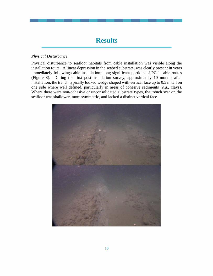
Results Physical Disturbance Physical disturbance to seafloor habitats from cable installation was visible along the installation route. A linear depression in the seabed substrate, was clearly present in years immediately following cable installation along significant portions of PC-1 cable routes (Figure 8). During the first post-installation survey, approximately 10 months after installation, the trench typically looked wedge shaped with vertical face up to 0.5 m tall on one side where well defined, particularly in areas of cohesive sediments (e.g., clays). Where there were non-cohesive or unconsolidated substrate types, the trench scar on the seafloor was shallower, more symmetric, and lacked a distinct vertical face.

17

Figure 8. Examples of seafloor disturbance and visible trench along PC-1 cables in OCNMS. Vertical face on side of trench is more distinct in middle photo. Bottom photo shows exposed cable in visible trench through gravel/cobble substrate. Because trench data were not recorded in a systematic manner during video review, interpretation of this information was qualitative and limited to presence/absence of a visible trench. In general terms, a trench was visible more often than not in 2000-2003 in video transects. No survey was completed in 2002. More observations of trench presence were recorded in 2000 and 2001 than in 2003, suggesting surficial substrate recovery to pre-installation conditions. By the 2004 survey, completed more than 4.5 years after cable installations, no observations of visible trench were recorded; trench absence was routinely recorded. The persistence of a visible trench was dependent on substrate type. Trench presence or absence was noted along video transects, with 57 percent of observations in areas dominated by sand, 29 percent by mud, 10 percent by clay, and 4 percent by gravel. Trenches were observed almost exclusively in sand (60 percent) and mud (40 percent) habitats, all years combined. Few observations of visible trench (<2 percent) were recorded where the substrate was predominantly clay. A visible trench was never noted where substrate was predominantly gravel in 2000 or later years. The proportion of visible trench observations at different substrate types changed over time, with a lower proportion of observations of visible trench in mud and higher proportion in sand substrate between 2000 and 2003. In 2000, 56 percent of visible trench observations were in sand substrate and 44 percent in mud substrate. By 2003, 83 percent of visible trench observations were in sand substrate and 15 percent in mud substrate. Benthic community characterization of northern sanctuary waters A total of 133 grab stations were sampled from 2000 to 2004 for benthic infauna (see Figure 9 and Appendix A). Stations were broadly distributed across the northern sanctuary, between 48.1º N and 48.5º N, as far west as 125.4º W, within and adjacent to the Juan de Fuca Canyon complex at water depths between 40 and 1035 meters depth. Of those 133

18

stations 114 stations, all collected during 2000 and 2001, had corresponding grain-size information and could be used for the analysis of spatial patterns associated with substrate type (Table 1 and Appendix B). Table 1. Water depth and key benthic community metrics averaged by year, dominant sediment type, and year x dominant sediment type for 2000 and 2001.

Mean Water Depth (m)*

Mean Richness

(#taxa/grab)

Mean Diversity (H´/grab)

Mean Density (#/m2)

Year 2000 567.2 28 3.9 869.0 2001 165.3 41 4.4 1450.5

Sediment Type Gravel 358.2 44 4.8 1226.1 Sand 334.2 35 3.9 1409.6 Mud 346.6 15 3.3 349.0

Year x Sed. Type 2000 Gravel 493.6 33 4.5 690.9 Sand 633.0 27 3.5 1231.0 Mud 644.4 9 2.8 203.3

2001 Gravel 166.9 60 5.2 1981.6 Sand 149.6 40 4.2 1520.0 Mud 211.2 17 3.5 415.2

*The mean water depth was very different between those two years, making the comparison problematic.

A total of 29,322 organisms representing 860 invertebrate taxa from 18 broad taxonomic groups were collected in benthic grab samples. Of the 860 invertebrate taxa, 538 were identified to the species level. Annelida was the dominant taxonomic group by abundance (65.7 percent) followed by Mollusca (11.3 percent), Echinodermata (7.5 percent) and Cnidaria (2.2 percent). Figure 9 depicts percent abundance of these groups and an “other” category comprised of 13 taxonomic groups combined that accounted for 13.2 percent of the total abundance.

19

Figure 9. Dominant taxa by percent abundance for benthic grab data. Data were combined for 2000, 2001, 2003 and 2004.

The top 50 dominant taxa from all years are listed in Table 2. The dominant species across the sampling area, by both abundance and frequency of occurrence, was an annelid, the polychaete Galathowenia oculata, a member of Family Oweniidae, which occurred at 67 percent of the stations. The brittlestar Ophiura sarsii, an echinoderm, was the third dominant taxon by abundance and occurred at 40 percent of the stations sampled across the survey area. The bivalve mollusk Axinopsida serricata, was the ninth dominant taxon by abundance and occurred at 26 percent of the stations.

20

Table 2. Dominant taxa in 0.1m2 Smith McIntrye grab samples, 2000-2004. Taxon

Mean Density (#/m2)

Percent

Frequency

Phylum

Class

Order

Family

Galathowenia oculata 124.1 67.2 Annelida Polychaeta Oweniida Oweniidae Spiophanes berkeleyorum 52.4 39.2 Annelida Polychaeta Spionida Spionidae Ophiura sarsii 39.8 39.9 Echinodermata Ophiuroidea Ophiurida Ophiuridae Pholoides asperus 33.5 45.7 Annelida Polychaeta Phyllodocida Pholoididae Spiophanes bombyx 28.7 4.4 Annelida Polychaeta Spionida Spionidae Sternaspis nr. fossor 18.7 24.2 Annelida Polychaeta Sternaspida Sternaspidae Polycirrus sp. complex 13.1 30.4 Annelida Polychaeta Terebellida Terebellidae Notoproctus pacificus 11.6 25.2 Annelida Polychaeta Capitellida Maldanidae Axinopsida serricata 11.0 25.9 Mollusca Bivalvia Veneroida Thyasiridae Amphipholis pugetana 9.6 17.7 Echinodermata Ophiuroidea Ophiurida Amphiuridae Ampharete finmarchica 9.3 30.7 Annelida Polychaeta Terebellida Ampharetidae Myriochele olgae 9.3 13.3 Annelida Polychaeta Oweniida Oweniidae Idanthyrsus saxicavus 9.2 30.4 Annelida Polychaeta Terebellida Sabellariidae Typosyllis heterochaeta 8.7 26.6 Annelida Polychaeta Phyllodocida Syllidae Magelona longicornis 7.8 19.4 Annelida Polychaeta Spionida Magelonidae Pista wui 7.8 27.6 Annelida Polychaeta Terebellida Terebellidae Anthopleura artemisia 7.7 1.4 Cnidaria Anthozoa Actiniaria Actiniidae Melinna elisabethae 7.7 27.6 Annelida Polychaeta Terebellida Ampharetidae Glycera nana 7.4 47.8 Annelida Polychaeta Phyllodocida Glyceridae Nicomache personata 7.4 13.6 Annelida Polychaeta Capitellida Maldanidae Ischnochiton trifidus 6.8 31.4 Mollusca Polyplacophora Neoloricata Ischnochitonidae Pectinaria californiensis 6.5 21.5 Annelida Polychaeta Terebellida Pectinariidae Lepidozona mertensii 6.4 16.4 Mollusca Polyplacophora Neoloricata Ischnochitonidae Sipuncula sp. Indet. 6.3 21.8 Sipuncula Nynantheae sp. 6.2 3.7 Cnidaria Anthozoa Actiniaria

21

Taxon

Mean Density (#/m2)

Percent

Frequency

Phylum

Class

Order

Family

Maldanidae sp. Indet. 5.8 23.5 Annelida Polychaeta Capitellida Maldanidae Euclymeninae sp. Indet. 5.8 18.1 Annelida Polychaeta Capitellida Maldanidae Petaloproctus sp. 5.8 6.8 Annelida Polychaeta Capitellida Maldanidae Cirratulidae sp. Indet. 5.7 18.4 Annelida Polychaeta Spionida Cirratulidae Dipolydora socialis 5.7 21.8 Annelida Polychaeta Spionida Spionidae Rhodine bitorquata 5.6 28.3 Annelida Polychaeta Capitellida Maldanidae Onuphis iridescens 5.5 28.3 Annelida Polychaeta Eunicida Onuphidae Prionospio jubata 5.5 27.3 Annelida Polychaeta Spionida Spionidae Thyasira flexuosa 5.5 26.6 Mollusca Bivalvia Veneroida Thyasiridae Petaloproctus borealis 5.4 10.2 Annelida Polychaeta Capitellida Maldanidae Asclerocheilus beringianus 5.1 15.7 Annelida Polychaeta Opheliida Scalibregmatid Euclymeninae sp. 4.8 13.6 Annelida Polychaeta Capitellida Maldanidae Maldane sarsi 4.8 14.3 Annelida Polychaeta Capitellida Maldanidae Pista estevanica 4.7 24.6 Annelida Polychaeta Terebellida Terebellidae Anobothrus gracilis 4.7 17.7 Annelida Polychaeta Terebellida Ampharetidae Echiurus alaskanus 4.7 3.1 Echiura Echiurida Echiuroinea Echiuridae Macoma carlottensis 4.6 12.6 Mollusca Bivalvia Veneroida Tellinidae Nicomache sp. 4.6 9.9 Annelida Polychaeta Capitellida Maldanidae Nemertinea sp. Indet. 4.6 23.5 Nemertea Nemertinea Corella willmeriana 4.5 10.6 Urochordat Ascidiacea Phlebobranchiata Corellidae Amphissa columbiana 4.5 20.5 Mollusca Gastropoda Neogastropoda Columbellidae Ninoe gemmea 4.5 27.3 Annelida Polychaeta Eunicida Lumbrineridae Decamastus nr. gracilis 4.4 8.9 Annelida Polychaeta Capitellida Capitellidae Mediomastus sp. Indet. 4.3 20.1 Annelida Polychaeta Capitellida Capitellidae

22

Using benthic infaunal data from 2000, 2001, 2003, and 2004, spatial patterns in density (Figure 10) and H′ diversity (Figure 11) were visualized using inverse distance weighting, a GIS spatial interpolation method, within the survey area. Inverse distance weighting does not take into account the spatial structure of the sample points and results are influenced by the spacing and density of the sampling points. Given the geographic spread of the grab samples combined with the likely heterogeneity of the seabed, the reader is advised to assess interpolated values with caution. There is a general trend of decreasing density moving across the survey area from east to west, which corresponds to increasing distance from shore and increasing depth. Spatial patterns in H′ diversity appear to be more varied across the survey area and are likely associated with small-scale heterogeneity in bottom sediments, which can range from coarse gravel-sand to a much finer mud in this region. A lack of paired grain-size data for all stations precluded further assessment of these patterns, so detailed analysis of relationships between benthic infauna and abiotic variables was limited to stations sampled in 2000 and 2001. Results from PCA on normalized abiotic data highlighted a distinct separation in stations by bottom type and indicated a slight increase in fine sediments with increasing water depth (Figure 12; Table 3).

Figure 10: Spatial interpolation of density within the survey area for benthic grabs. Darker colors indicate increasing density. Classification scale based on equal intervals. Derived from 2000, 2001, 2003, and 2004 benthic grab data.

23

Figure 11: Spatial interpolation of H´ diversity within the survey area for benthic grabs. Darker colors indicate increasing H´ diversity. Derived from 2000, 2001, 2003, and 2004 benthic grab data.

Figure 12: Principal Components Analysis (PCA) on normalized abiotic data for 2000 and 2001 benthic grab stations.

24

Table 3. Summary of results of principal component analysis (PCA) on normalized abiotic data for 2000 and 2001. Eigenvalues and percent of variation explained by the first 3 ordination axes are given. Linear coefficients (eigenvectors) of each PC are given for each abiotic variable. PC1 PC2 PC3 Eigenvalues 2.54 1.4 0.9 percent of variation

l i d 50.9 28.0 17.5

Eigenvectors Gravel -0.198 0.802 0.001 Sand -0.444 -0.572 0.203 Silt 0.581 -0.142 -0.242 Clay 0.588 -0.061 -0.064 Water Depth 0.284 0.081 0.947

Results of non-metric multidimensional scaling of benthic invertebrate abundance derived from 2000 and 2001 benthic grabs are displayed in Figure 13. From this ordination plot it is clear that there is a separation in stations driven predominantly by grain size. Coarse, gravel bottoms have the highest benthic invertebrate diversity and richness, while mud habitats have the lowest (Table 1). It is likely that water depth is also an important factor in species distribution; however, covariance in water depth by year (Table 1) made it impossible to evaluate depth or inter-annual variation in a meaningful way.

Figure 13: Ordination plot derived from non-metric multidimensional scaling (NMDS) of Bray-Curtis similarities calculated from square root transformed invertebrate abundance on un-aggregated 2000 and 2000 benthic grab data. Given the high levels of diversity found within the survey area and the large number of rare species, taxa were aggregated to taxonomic order to facilitate analysis of community spatial patterns. The non-metric multidimensional scaling based on species similarities generally separated stations into three groups, which were associated with dominant bottom type: gravel, sand, and mud. The percent contribution of the most important orders

25

(i.e., those with percent cumulative contribution > 90 percent) responsible for these patterns are provided in Table 4 by dominant sediment type. While polychaete worms (i.e., orders Terebellida, Phyllodocida, Capitellida, Spionida, Oweniida, Eunicida) are dominant in all three sediment types, gravel bottom habitats are generally more diverse, with brittle stars a dominant order (Ophiurida) compared to mud habitats, where amphipods dominate. Polychaetes comprised over 50 percent of invertebrates in sand habitats. Table 4. Results of the similarity percentage (SIMPER) one-way analysis among the three dominant sediment types for 2000 and 2001 benthic grab samples. Taxa aggregated to the order level. Dominant Sediment Type

Order

Percent

Contribution

Cumulative Percent

Contribution Gravel - average similarity 61 percent Terebellida 8.8 8.8 Phyllodocida 8.7 17.5 Capitellida 8.6 26.1 Ophiurida 7.5 33.6 Spionida 6.9 40.4 Amphipoda 6.0 46.5 Eunicida 5.1 51.6 Neoloricata 4.5 56.1 Sabellida 4.2 60.3 Oweniida 3.7 64.0 Decapoda 3.7 67.6 Cnidaria 2.9 70.5 Bryozoa 2.8 73.3 Nemertinea 2.8 76.1 Phlebobranchiata 2.5 78.7 Veneroida 2.4 81.1 Opheliida 2.2 83.3 Terebratulida 2.1 85.5 Porifera 1.8 87.3 Sipuncula 1.8 89.0 Neogastropoda 1.5 90.5 Sand - average similarity 55 percent Spionida 10.8 10.8 Oweniida 10.7 21.5 Phyllodocida 8.79 30.2 Capitellida 8.6 38.8 Amphipoda 8.2 47.0 Terebellida 7.8 54.8 Veneroida 7.1 61.9

26

Dominant Sediment Type

Order

Percent

Contribution

Cumulative Percent

Contribution Eunicida 6.6 68.6 Ophiurida 5.8 74.4 Gadilida 2.7 77.1 Neogastropoda 2.4 79.5 Nemertinea 2.0 81.5 Sabellida 2.0 83.5 Decapoda 1.8 85.3 Sternaspida 1.8 87.1 Orbinida 1.6 88.7 Opheliida 1.5 90.2

Mud - average similarity 48 percent Amphipoda 11.2 11.2 Eunicida 10.5 21.7 Veneroida 9.9 31.6 Phyllodocida 8.7 40.3 Spionida 8.4 48.7 Gadilida 7.5 56.2 Terebellida 7.3 63.5 Spatangoida 6.1 69.6 Sternaspida 4.5 74.1 Oweniida 4.4 78.5 Opheliida 4.3 82.8 Ophiurida 3.3 86.1 Cumacea 3.1 89.2 Capitellida 2.4 91.6

27

Benthic Community on Cable Route - Video Transects From video footage, epibenthic community data from paired (On Cable vs. adjacent Control) 50-m segments were analyzed for 14 transects surveyed in 2000, 2001, 2003, and 2004 (Figure 6). All but one of the 14 transects were on the PC-1 East cable (the cable most recently installed prior to the first sampling, and thus more suitable for monitoring impact and recovery). For each transect and treatment (On Cable vs. Control), from six to 22 segments were available for analysis in any given year, resulting in a total of 837 segments (Table 5).

28

Table 5. Number of 50-m segments sampled showing associated sediment type (m=mud, s=sand, g=gravel) by transect as seen in Figure 6 treatment (Control/On), and year. Subtotals appear in the margins.

2000 2001 2003 2004 Subtotals Sediment type

Transect Control On Control On Control On Control On

17-19 7m 7m 7m 7m

28 All mud

27-29 12m 4m, 8s

12m 13m 11m 4m, 8s

20m 18m 110 94 mud, 16 sand

31-33

10m 10g 5s, 12g

11s, 6g

54 10 mud, 16 sand, 28 gravel

34-36 11m 10m

9m 9m 16m 16m 71 All mud

40-42 2s, 4g 7s 3s, 14g

18s 17s, 5g

15s 5m, 17g

17s, 5g

129 5 mud, 79 sand, 45 gravel

43-45

10g 1m, 9g

8g 8g 10g 10g 56 1 mud, 55 gravel

46-48

20s 19s

17s 16s, 1g

73 72 sand, 1 gravel

49-51

3s, 9g 2s, 10g

2s, 9g 4s, 7g

12s 12s 70 35 sand, 35 gravel

52-54

10s 10s 8s 8s 36 All sand

55-57

8m 8m 7s 7s 30 16 mud, 14 sand

58-60

2s, 5g 4s, 3g

7s 7s 28 20 sand, 8 gravel

79-81

1s, 7g 6s, 2g 3s, 7g 2s, 8g

3s, 8g 11s, 6g

58 26 sand, 32 gravel

29

85-87

11m, 1g

3s, 9m

12s 12s 48 20 mud, 27 sand, 1 gravel

88-90

12g 12g

11g 11g 46 All gravel

SUBTOTALS 36 36 110 111 106 100 170 168 837

30

A total of 204,689 epibenthic organisms, representing 82 invertebrate taxa from 17 broad taxonomic groups, were identified from the processed video recordings. Roughly half of total abundance was unidentified shrimp (Order Decapoda, 80,591 individuals) and brittle stars (Genus Ophiura, 26,628 individuals). Unidentified shrimp were present in 74 percent of sampling units, with a mean density of 2.8 m-2 per segment (averaged over 837 segments). In contrast, Ophiura brittle stars exhibited a high degree of patchiness, occurring in only 3.3 percent of segments (mean density per segment = 1 m-2). The 10 dominant epibenthic taxa, in order of decreasing mean density and percent frequency of occurrence, are listed in Table 6.

Table 6. Abundance, mean density, and frequency of occurrence (percent of segments) of ten dominant taxa in order of decreasing mean density (a) and percent frequency of occurrence (b).

a

Taxon Group Total Abundance Mean Density

(# m-2)

Frequency (percent of segments)

Other Shrimp Shrimp 80591 2.77 73.8 Brittle Star - Ophiura Brittle Stars 26628 0.91 3.3 Munida Squat Lobster Squat Lobsters 17030 0.58 38.9 Strongylocentrotus Urchin (white) Urchins 12272 0.40 56.4 Encrusting White Sponge Sponges 7180 0.31 35.0 Brown Ball Sponge, Solitary Sphere Sponges 5931 0.25 52.6 Yellow Cloud Sponge >3cm Sponges 6184 0.23 48.7 White Cloud Sponge >3cm Sponges 5731 0.23 52.6 Allocentrotus Pink Urchin Urchins 5317 0.19 52.6 Branch Sponge Sponges 2635 0.11 7.8

b

Taxon Group Total Abundance Mean Density

(# m-2)

Frequency (percent of segments)

Other Shrimp Shrimp 80591 2.77 73.8 Strongylocentrotus Urchin (white) Urchins 12272 0.40 56.4 Brown Ball Sponge, Solitary Sphere Sponges 5931 0.25 52.6 White Cloud Sponge >3cm Sponges 5731 0.23 52.6 Allocentrotus Pink Urchin Urchins 5317 0.19 52.6 Yellow Cloud Sponge >3cm Sponges 6184 0.23 48.7 White Cidarina-like snail Snails 1968 0.08 41.9 Munida Squat Lobster Squat Lobsters 17030 0.58 38.9 Encrusting White Sponge Sponges 7180 0.31 35.0

When aggregated to broad taxonomic group, unidentified shrimp were still the dominant group in terms of abundance, but sponges displaced brittle stars as the second most abundant group (Table 7). The brittle star group, which also includes Genus Ophiopholis and other, non-commensal brittle stars, was the third dominant group in terms of abundance, but only occurred in 47 (~ 6 percent) of the 837 segments analyzed. Of these 47 segments, 21 percent were in mud habitat, 47 percent were sand, and 32 percent were gravel. However, only 0.1 percent of brittle star abundance was in mud substrate; 61.8

31

percent of abundance was in sand, and 38.1 percent of abundance occurred in gravel habitat.

Table 7. Abundance, mean density, and frequency of occurrence (percent of segments) of ten dominant taxonomic groups in order of decreasing mean density (a) and percent frequency of occurrence (b).

a Group Total Abundance Mean Density (# m-2)

Frequency (percent of segments)

Shrimp 80887 2.78 75.3 Sponges 39253 1.59 74.3 Brittle Stars 26711 0.91 5.6 Squat Lobsters 18210 0.63 51.6 Urchins 17981 0.60 80.9 Corals 6608 0.25 28.9 Snails 6170 0.22 72.2 Bryozoans 3023 0.09 24.3 Hermit Crabs 1952 0.08 48.5 Anemones 1724 0.06 53.3

b Group Total Abundance Mean Density

(# m-2) Frequency

(percent of segments) Urchins 17981 0.60 80.9 Shrimp 80887 2.78 75.3 Sponges 39253 1.59 74.3 Snails 6170 0.22 72.2 Sea Stars 1570 0.06 60.1 Anemones 1724 0.06 53.3 Squat Lobsters 18210 0.63 51.6 Hermit Crabs 1952 0.08 48.5 Corals 6608 0.25 28.9

Results of non-metric multidimensional scaling of mean invertebrate density from transect video, averaged over segments for each transect-treatment-year combination, are displayed in Figure 14. Most of the separation was between transects (and possibly years), while treatments (On Cable vs. Control) for the same transect and year tended to be similar. Vectors of habitat variables are superimposed on the plot and represent directions in the ordination space towards which the environmental vectors change most rapidly and to which they have maximal correlations with the ordination configuration (Oksanen et al. 2017). Lengths of arrows are proportional to correlation with the ordination; hence, P_MUD (the proportion of segments having mud habitat type for a given transect-treatment-year combination) was most highly correlated with the observed distribution of benthic fauna, followed by P_SAND, P_GRAVEL, DEPTH, and DISTANCE. For example, transects composed of all mud segments (i.e., 17-19, 34-36; Table 5) occur in the extreme upper left portion of the plot. Segments for transect 55-57 were either all mud (in 2003) or all sand (2004); transect 85-87 was composed of all sand segments in 2004 and mostly mud in 2001; transect 40-42 comprised a mix of mostly sand or gravel segments, but it was one of the shallower transects as well as the most distant (Figure 6). The apparent separation by year (the numbers within each symbol), with 2004 transects off to the upper

32

right of the plot, can also be explained by habitat type. For example, for transect 55-57, 2004 segments were all sand, while in 2003 they were all mud; for transect 85-87, the 2004 transects were all sand, and the 2001 transects were mostly mud (Control 92 percent mud, On 75 percent mud). Similarly, transect 58-60 segments were all sand in 2004; those in 2001 were a mix of sand and gravel (Control 71 percent gravel, On 43 percent gravel). These results suggest that habitat type (mud vs. sand or gravel) best explains the observed patterns, with lesser influences of depth and distance from shore. All of the environmental variables listed above except for distance from shore were significant (p<0.05) based on a permutation test (999 permutations) that fits environmental vectors having maximal correlation with the ordination (Oksanen et al. 2017).

Figure 14. Ordination plot derived from non-metric multidimensional scaling (NMDS) of Bray-Curtis dissimilarities calculated from square-root transformed mean invertebrate abundance based on analysis of video. Numbers inside symbols indicate year of sampling (0=2000, 1=2001, 3=2003, 4=2004). Vectors of environmental variables are superimposed on the plot (see text for detailed description).

33

Results of permutational analysis of variance using distance matrices, with Bray-Curtis dissimilarity as the distance measure, found no significant differences in invertebrate assemblages between Treatments (On Cable vs. Control). Furthermore, analysis of multivariate homogeneity of group dispersions, analogous to Levene’s test for homogeneity of variances in a multivariate setting, suggested that the variation within each group was similar (Figure 15). Taken together, the foregoing results do not suggest that invertebrate assemblages differ significantly along the cable route (On) compared to reference (Control). In fact, it appears that differences were mainly due to environmental effects, principally habitat type.

Figure 15: Plot illustrating results of analysis of multivariate homogeneity of group dispersions (variances). Distances to centroid and 90percent confidence ellipses are shown for each of the two treatments (Control = triangle, On=circle). A similar pattern emerged upon performing the ordination on individual transect segments, rather than pooled transects as in Figure 14. In this case, mud, sand, and gravel (Figure 16) represent averages of ordination scores for each level of the habitat factor (measured on individual segments), while DEPTH and DISTANCE vectors are as described for Figure 14. As noted above, segments for transects in all-mud habitat (17-19, 34-36) occur in the

34

left portion of the ordination plot (extreme negative values for NMDS1, mostly positive values for NMDS2). Other differences due to habitat type, depth, or distance from shore that were noted previously still hold, although the large number of symbols (837 individual segments) in the plot make it a bit more challenging to read and interpret.

Figure 16. Results of non-metric multidimensional scaling ordination of individual transect segments. Symbol color corresponds to transect; symbol shape differentiates on-cable versus control. Environmental variables, either as habitat factor levels (mud, gravel, or sand) or vectors (depth, distance from shore), are superimposed on the plot. Comparisons of number of taxa, Shannon H′ diversity, and log-transformed density among habitat types (Figure 17) also suggest differences among habitat types; all three metrics were significantly lower for mud habitat than for either sand or gravel. The greatest difference was between mud and gravel (and, to a lesser extent, mud and sand), although the difference between sand and gravel was also significant (Figure 17; all pair-wise comparisons significant, p < 0.01).

35

Figure 17. Box-and-whisker plots of number of taxa, Shannon H′ diversity, and log-transformed density by habitat type (m=mud; s=sand; g=gravel). Lower panel presents 95percent confidence intervals (Tukey) for pair-wise comparisons among the three habitat types (overall ANOVA p<0.001 for all three benthic metrics).

Because of the mix of different habitat types among segments within individual transect-year combinations as noted above, comparisons among transects, treatments, and years were also made separately for each habitat type (mud, sand, gravel). In each case, however, no significant difference between treatments (On Cable vs. Control) was found, and the results of analysis by habitat type were similar to the overall results described above. Benthic Community on Cable Route - Suction Samples Suction samples were analyzed for benthic invertebrates, both epibenthos and infauna, collected from paired treatments (On Cable vs. Control) at 14 transects in 2000, 2001, and 2004. For each Transect-Treatment-Year combination, from one to seven replicates were collected and enumerated with respect to species composition. A total of 12,975 organisms, representing 569 taxa, were identified in 139 replicate samples. Dominant taxa included arrow worms (Sagitta sp.), the polychaete Galathowenia oculata, the notched brittlestar Ophiura sarsii, the eualid shrimp Eualus pusiolus, and

36

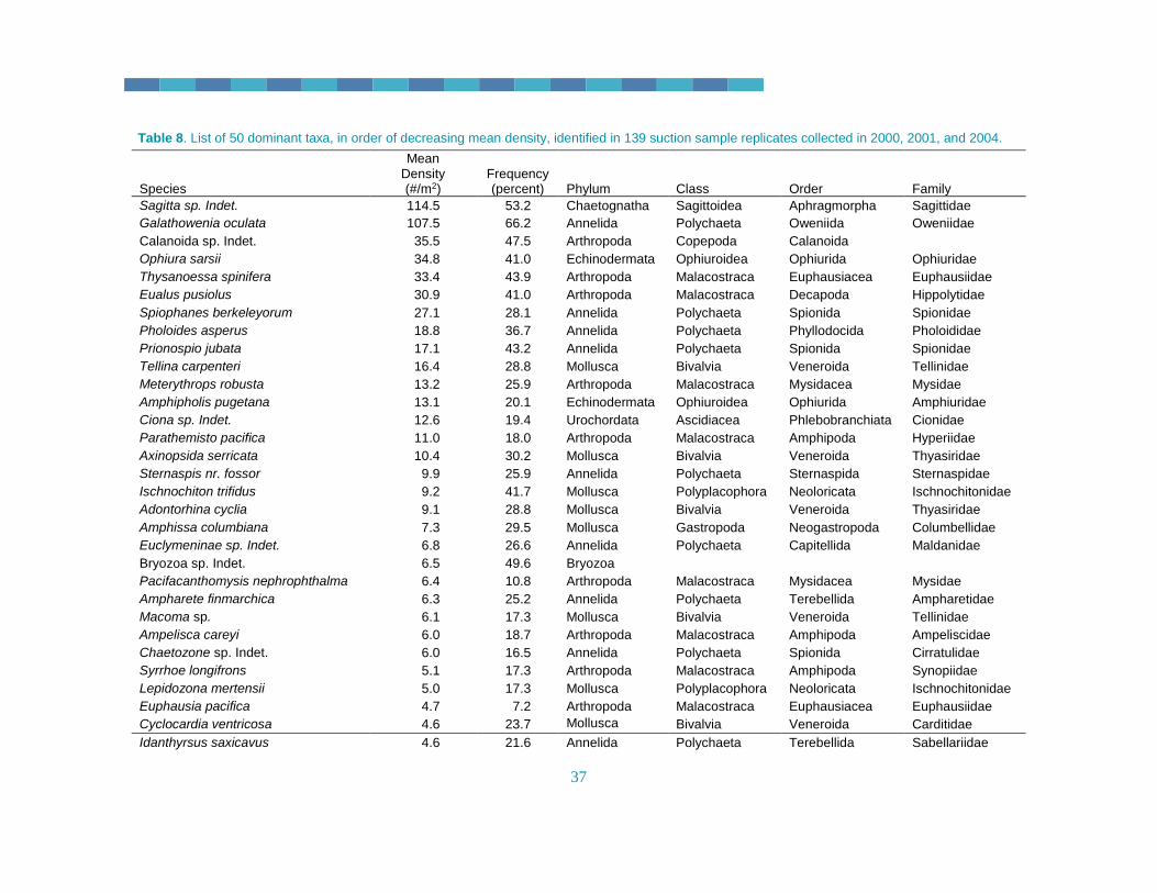
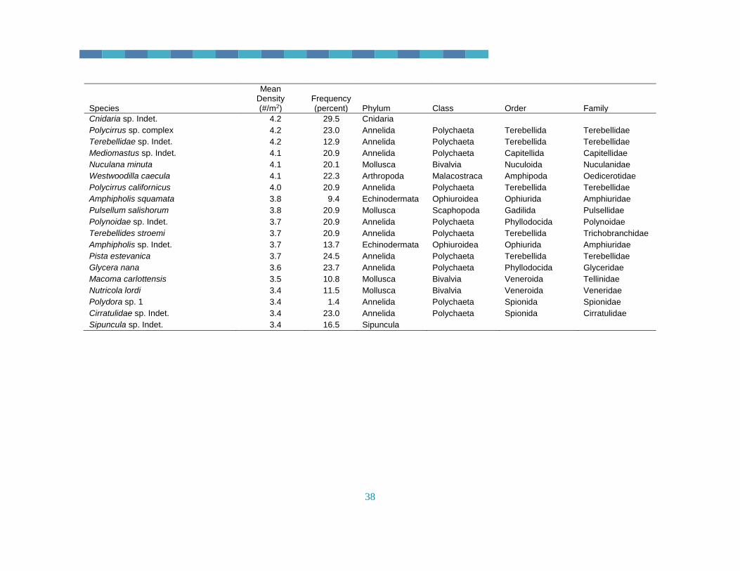
calanoid copepods (Calanoida sp. Indet.). Table 8 lists the 50 dominant taxa, which made up 72 percent of the total abundance. Measures of mean richness (# of taxa), diversity (Shannon H′), and density by transect, treatment, and year are listed in Table 9.

37

Table 8. List of 50 dominant taxa, in order of decreasing mean density, identified in 139 suction sample replicates collected in 2000, 2001, and 2004.

Species

Mean Density (#/m2)

Frequency (percent) Phylum Class Order Family

Sagitta sp. Indet. 114.5 53.2 Chaetognatha Sagittoidea Aphragmorpha Sagittidae Galathowenia oculata 107.5 66.2 Annelida Polychaeta Oweniida Oweniidae Calanoida sp. Indet. 35.5 47.5 Arthropoda Copepoda Calanoida Ophiura sarsii 34.8 41.0 Echinodermata Ophiuroidea Ophiurida Ophiuridae Thysanoessa spinifera 33.4 43.9 Arthropoda Malacostraca Euphausiacea Euphausiidae Eualus pusiolus 30.9 41.0 Arthropoda Malacostraca Decapoda Hippolytidae Spiophanes berkeleyorum 27.1 28.1 Annelida Polychaeta Spionida Spionidae Pholoides asperus 18.8 36.7 Annelida Polychaeta Phyllodocida Pholoididae Prionospio jubata 17.1 43.2 Annelida Polychaeta Spionida Spionidae Tellina carpenteri 16.4 28.8 Mollusca Bivalvia Veneroida Tellinidae Meterythrops robusta 13.2 25.9 Arthropoda Malacostraca Mysidacea Mysidae Amphipholis pugetana 13.1 20.1 Echinodermata Ophiuroidea Ophiurida Amphiuridae Ciona sp. Indet. 12.6 19.4 Urochordata Ascidiacea Phlebobranchiata Cionidae Parathemisto pacifica 11.0 18.0 Arthropoda Malacostraca Amphipoda Hyperiidae Axinopsida serricata 10.4 30.2 Mollusca Bivalvia Veneroida Thyasiridae Sternaspis nr. fossor 9.9 25.9 Annelida Polychaeta Sternaspida Sternaspidae Ischnochiton trifidus 9.2 41.7 Mollusca Polyplacophora Neoloricata Ischnochitonidae Adontorhina cyclia 9.1 28.8 Mollusca Bivalvia Veneroida Thyasiridae Amphissa columbiana 7.3 29.5 Mollusca Gastropoda Neogastropoda Columbellidae Euclymeninae sp. Indet. 6.8 26.6 Annelida Polychaeta Capitellida Maldanidae Bryozoa sp. Indet. 6.5 49.6 Bryozoa Pacifacanthomysis nephrophthalma 6.4 10.8 Arthropoda Malacostraca Mysidacea Mysidae Ampharete finmarchica 6.3 25.2 Annelida Polychaeta Terebellida Ampharetidae Macoma sp. 6.1 17.3 Mollusca Bivalvia Veneroida Tellinidae Ampelisca careyi 6.0 18.7 Arthropoda Malacostraca Amphipoda Ampeliscidae Chaetozone sp. Indet. 6.0 16.5 Annelida Polychaeta Spionida Cirratulidae Syrrhoe longifrons 5.1 17.3 Arthropoda Malacostraca Amphipoda Synopiidae Lepidozona mertensii 5.0 17.3 Mollusca Polyplacophora Neoloricata Ischnochitonidae Euphausia pacifica 4.7 7.2 Arthropoda Malacostraca Euphausiacea Euphausiidae Cyclocardia ventricosa 4.6 23.7 Mollusca

Bivalvia Veneroida Carditidae Idanthyrsus saxicavus 4.6 21.6 Annelida Polychaeta Terebellida Sabellariidae

38

Species

Mean Density (#/m2)

Frequency (percent) Phylum Class Order Family

Cnidaria sp. Indet. 4.2 29.5 Cnidaria

Polycirrus sp. complex 4.2 23.0 Annelida Polychaeta Terebellida Terebellidae Terebellidae sp. Indet. 4.2 12.9 Annelida Polychaeta Terebellida Terebellidae Mediomastus sp. Indet. 4.1 20.9 Annelida Polychaeta Capitellida Capitellidae Nuculana minuta 4.1 20.1 Mollusca Bivalvia Nuculoida Nuculanidae Westwoodilla caecula 4.1 22.3 Arthropoda Malacostraca Amphipoda Oedicerotidae Polycirrus californicus 4.0 20.9 Annelida Polychaeta Terebellida Terebellidae Amphipholis squamata 3.8 9.4 Echinodermata Ophiuroidea Ophiurida Amphiuridae Pulsellum salishorum 3.8 20.9 Mollusca Scaphopoda Gadilida Pulsellidae Polynoidae sp. Indet. 3.7 20.9 Annelida Polychaeta Phyllodocida Polynoidae Terebellides stroemi 3.7 20.9 Annelida Polychaeta Terebellida Trichobranchidae Amphipholis sp. Indet. 3.7 13.7 Echinodermata Ophiuroidea Ophiurida Amphiuridae Pista estevanica 3.7 24.5 Annelida Polychaeta Terebellida Terebellidae Glycera nana 3.6 23.7 Annelida Polychaeta Phyllodocida Glyceridae Macoma carlottensis 3.5 10.8 Mollusca Bivalvia Veneroida Tellinidae Nutricola lordi 3.4 11.5 Mollusca Bivalvia Veneroida Veneridae Polydora sp. 1 3.4 1.4 Annelida Polychaeta Spionida Spionidae Cirratulidae sp. Indet. 3.4 23.0 Annelida Polychaeta Spionida Cirratulidae Sipuncula sp. Indet. 3.4 16.5 Sipuncula

39

Table 9. Mean richness (taxa/sample), diversity (Shannon H′), and density (#/m2) of suction samples by transect, treatment, and year.

Transect Treatment Year Replicates Mean Richness (taxa/sample)

Mean Diversity

(H′)

Mean Density (#/m2)

14-16 Control 2000 2 9.5 2.1 355 14-16 On 2000 4 11.3 2.1 485 17-19 Control 2000 4 15.3 2.8 888 17-19 On 2000 4 19.3 2.8 1688 27-29 Control 2000 2 19.5 3.7 385 27-29 On 2000 4 15.8 3.4 368 27-29 Control 2001 4 28.8 4.0 893 27-29 On 2001 4 25.3 3.9 838 27-29 Control 2004 2 23.5 4.2 605 27-29 On 2004 3 12.0 2.2 540 31-33 Control 2000 4 31.0 4.4 683 31-33 On 2000 4 15.8 3.8 228 34-36 Control 2000 4 19.0 3.5 518 34-36 On 2000 3 12.3 2.3 750 34-36 Control 2004 5 15.2 3.4 332 34-36 On 2004 5 16.0 2.9 498 40-42 Control 2000 4 25.5 2.3 1503 40-42 On 2000 6 15.3 3.1 428 40-42 Control 2001 4 40.3 4.7 985 40-42 On 2001 4 30.0 3.8 950 43-45 Control 2001 4 74.5 5.6 2140 43-45 On 2001 2 64.5 5.2 2050 46-48 Control 2001 4 55.3 5.3 1190 46-48 On 2001 2 29.5 4.2 520 49-51 Control 2001 4 17.5 3.5 423 49-51 On 2001 4 25.0 3.3 1608 52-54 Control 2001 4 45.3 3.8 2105 52-54 On 2001 2 63.0 4.5 2620 55-57 Control 2001 4 32.0 3.4 1388 55-57 On 2001 2 43.0 3.4 2430 55-57 Control 2004 2 37.5 3.8 1140 55-57 On 2004 5 27.2 4.3 508 58-60 Control 2001 2 38.0 4.2 1305 58-60 On 2001 2 35.0 4.8 585 79-81 Control 2001 4 51.8 5.1 1140 79-81 On 2001 4 28.3 3.7 1008 79-81 Control 2004 3 24.0 4.4 417 79-81 On 2004 3 20.3 3.6 390 85-87 Control 2001 2 40.0 4.8 1065 85-87 On 2001 4 27.8 3.9 998

40

Results of non-metric multidimensional scaling of invertebrate abundance by transect, treatment, and year (pooled replicate samples) derived from the suction sample data appear in Figure 17. Vectors of environmental variables (depth, distance from shore) fit to the ordination are superimposed as arrows on the plot. Depth was correlated significantly with the ordination configuration (p<0.05); distance from shore was not. Although sediment data were not available for these specific suction samples, the plot shares some features in common with ordinations performed previously with the video transect data (as in Figure 13). For example, transects previously observed in the video data to have consisted of all or mostly mud segments (17-19, 34-36, 27-29) appear as before on the left side of the ordination plot (negative NMDS1). Sediment samples from transect 14-16, which was also the deepest site (326 m), were mostly mud (70 percent silt+clay). As before with the video data, permutational analysis of variance did not find any significant differences in assemblages between Treatments (On Cable vs. Control).

Figure 12. Ordination plot derived from non-metric multidimensional scaling (NMDS) of Bray-Curtis dissimilarities calculated from square-root transformed invertebrate abundance in suction samples. Numbers

41

inside symbols indicate year of sampling (0=2000, 1=2001, 4=2004). Vectors of environmental variables (depth and distance) are superimposed on the plot.

42

Discussion Cable Impacts The data from the physical and biological observations in this study suggest that, in general, the impacts from cable installation were limited in both scope and scale in all affected habitats, and that habitat recovery following the installation was fairly rapid, and that it varied by habitat type. The rate of recovery of benthic community composition could not be determined because it differed more by habitat type, transect location and year of sampling than by treatment (On or Off cable). Less impact was likely in the areas where complete burial was accomplished than in locations with exposed cable, where movement could cause persistent bottom disturbance. Physical disturbance The persistence of visual evidence of the trench varied with location and depended on several natural factors, including type of seafloor substrate, in-fill rate of new material, and water movement (i.e., near-bottom currents or wave action). Where gravel dominated the substrate, habitat recovery from the physical disturbance of the sea plow was rapid, with no trench evident less than one year after installation. These tend to be areas with higher energy caused by waves and currents, which winnows finer sediments (Bornhold 2003) but facilitates in-filling of the trench by larger sediments. Where sand, mud, or clay dominated, a visible trench was discernible in places for more than three years after cable installation. Clay is more cohesive than sand or mud, and a sea plow reportedly can bury cable in clay substrate without leaving a deep trench (SEA 1999). Although a trench was noted in some areas of clay substrate in this study, a visible trench was more commonly evident in mud and sand than in clay. Because the supply of new sediment to the study area is scarce (Greene and Watt 2002), material filling a trench most likely comes from redistribution of local materials. Mud consists of finer grained particles than sand, and mud deposits typically indicate a lower energy seafloor environment than sand. Thus, one might expect mobile particles in a sand habitat to redistribute and fill a depression more quickly than in a mud dominated habitat. Curiously, the trench along PC-1 cable routes in OCNMS persisted longer in sand substrate than in mud or clay, suggesting fairly active redistribution of mud in the area. Along the PC-1 cable routes, areas do exist where mobile sands occur at water depths greater than 100 meters, as evidenced by large sand waves (Bornhold 2003). Here, the cable trench could quickly be obscured, but surveys were not conducted in these high energy, sandy areas. By 2004 or more than 4.5 years after cable installations, a visible trench was not evident in surveyed areas regardless of substrate type. In general terms, the physical habitat within OCNMS had returned to pre-installation conditions within five years of cable installation. Some of the few published studies on submarine cable installation on seafloor habitat and

43

biota focus on the Hibernia Atlantic fiber optic cable installed in 2000 in the western Gulf of Maine. The sea plow used for the Hibernia Atlantic installation had a larger disturbance footprint with its water-jetted plowshare and target burial depth of 1.5 m, resulting in a trench initially estimated at 3 m wide (Auster et al. 2013). The cable trench was noticeably less prominent two years after installation (Grannis 2005), but it remained visible in places 10 years after installation (although substrate type and other seafloor conditions were not specified where this was evident; Auster et al. 2013). Elsewhere, persistent alteration of seafloor substrate has been demonstrated where surface laid submarine cables traverse hard rock substrates (Kogan et al. 2003). Benthic Community Benthic communities reported here are similar to an earlier study conducted in the 1960’s (Lie and Kisker, 1969) and in 2003 (Nelson et al. 2008). The northern portion of OCNMS supports a diverse assemblage of benthic communities, with sediment type being the primary abiotic factor controlling community composition. Annelid worms (primarily polychaetes) were the most abundant infauna and were broadly distributed across the study area and its various sediment types. Coarse, gravel sediments support a distinct infaunal community with the highest diversity and density. In comparison, there was a distinctly lower species diversity in mud habitats. On the sediment surface, roughly half of total abundance was accounted for by amphipods and brittle stars. Amphipods were abundant and widely distributed across sediment types. Brittle stars were more patchy in their distribution, predominantly associated with sand and gravel substrate and far less commonly found on mud. When both epibenthic and infaunal organisms are considered, annelid worms (mostly polychaetes) and bivalves (mostly clams) account for over 75 percent of total invertebrate abundance. In the context of impacts from undersea cables, benthic communities along the cable route in Olympic Coast National Marine Sanctuary were indistinguishable from those in control areas during the post-installation surveys. More precise sampling of fauna in sediments in the trench itself might have enabled a more highly resolved assessment, but logistical and safety issues precluded that. Even if it had been possible, it is likely that such sampling would have only confirmed the conclusion of a limited spatial impact of the cable installation. Challenges of the Study Design and Conduct Several aspects of data interpretation highlight the challenges of study design and research in deep, offshore areas. Two types of human-made disturbance occur in the study area. Plow burial of telecommunications cables is a single, but acute disturbance event. Bottom trawl fishing for groundfish typically occurs repeatedly over multiple years. Precise data were available for the cable installations, but data documenting historic and ongoing disturbance from bottom trawl fisheries were limited and spatially imprecise. As noted by Jennings et al. (2001) for New England waters, in the early 2000’s there were very few sources of data to quantify levels of trawling disturbance in U.S. waters on appropriate

44

temporal and spatial scales, and few studies examined trawling effects across quantifiable gradients of disturbance, such as differing levels of bottom trawl frequency. This was the case for OCNMS. For example, the largest data set available was National Marine Fisheries Service (NMFS) fish blocks, 10 X 10 nautical mile squares in which non-tribal, commercial bottom trawl frequency numbers were lumped. Individual trawls typically were recorded as an event occurring within a designated fish block with no information on a specific location, trawl pathway or continuation into an adjacent fish block. In comparison, the cable installation disturbance occurred on a known date over narrow strips about 6 m wide along a defined route, and monitoring could focus along a cable corridor about 1 – 2 m wide. In essence, the study design for low and high fishing intensity would have to be based on a generalized sense of trawling intensity. Lacking were specific data on the number of times a trawl may have traversed a location along the cable route, and the timing of recent disturbance from trawl passes at that location. Recent trends in electronic monitoring of bottom trawl activity will significantly improve the precision in these data and enhance our ability to evaluate the impacts of trawl fisheries in the context of other seafloor disturbance activities. While trawling impacts could not be evaluated, trawling may have affected the data collected here. Even if we assume that the impact was similar at controls and treatment sites, the lack of a true control cannot be ignored. Therefore, it was not possible to evaluate the impact of disturbance from plow burial without the confounding factor of trawling disturbance. Here again, more precise data now collected for bottom trawling activity will improve the ability to identify control, or unimpacted sites, and to distinguish impacts from different disturbance activities. Statistical analysis was confounded by both the consistency and completeness of the available data set. The precision and resolution of seafloor substrate and habitat data for the study area were poor when this monitoring program began, making sample site selection difficult, sometimes erroneous, and leading to unbalanced sampling. Weather conditions and equipment problems sometimes prevented surveys of all planned transects, resulting in an incomplete data set for some years. This all affected the strength of statistical analyses and the ability to resolve differences among variables. Differences between transects and years also overwhelmed separation between treatments, which suggests that the distribution of invertebrate taxa was similar along the cable route (On) compared to reference (Off cable or Control). Differences in invertebrate community metrics between On-cable and Control were not statistically significant. In cases where the difference was significant, measures of abundance, richness, and diversity were as likely to be higher On-cable as for Control segments. Thus, there does not appear to be a consistent pattern in any of the calculated metrics with respect to On-cable vs. Control treatment comparisons. Management Implications

45

Experienced project proponents and marine area managers alike recognize that operations on and under the water are challenging for many reasons, particularly construction or installation projects such as cable laying and scientific surveys at water depths in excess of 100 meters. Numerous factors are at play, such as surface sea state, near-bottom currents, unexpected substrates and slopes encountered, and equipment malfunctions, any of which can result in variances between planned and achieved results. In planning and environmental impacts assessment phases of construction projects, project proponents will likely have more technical knowledge of marine technology than scientists and marine area managers. To avoid differences in expectations, project proponents need to be realistic and transparent about what can be accomplished, and effectively communicate uncertainty with marine area managers. Marine area managers need to clearly articulate their concerns, recommendations to mitigate potential negative impacts, and terms or conditions of approvals or permits granted. All involved need to acknowledge potential for deviations from the ideal. Realistic expectations are best understood when supported by adequate information and evaluated by appropriate expertise. One challenge identified by this project is that marine area managers, typically with scientific, policy, and resource management experience, may not have technical expertise in subjects like marine construction or cable installation. Government agencies that manage marine areas may lack financial resources to contract for the appropriate expertise to assess potential project impacts, particularly in understudied environments such as deep-sea environments. This discrepancy in technical knowledge can lead to unrealistic expectations or lack of alignment in expectations of project proponents and marine area managers. One solution is to have fees associated with permits that are adequate to support agency staff and contractor time associated with evaluation and processing of complex projects. In addition, fair market value charges for access to or use of public lands can support administrative, monitoring and other aspects of permit and project management. With the Pacific Crossing submarine cable project, one conclusion reached by NOAA is that more investment during the route planning phase could have improved both achieved cable burial and alignment of expectations between project proponents and marine area managers. Improved detail or higher resolution data collected for route planning surveys could have been more effective in identifying problem areas along PC-1 routes where achievement of target burial depth would be a challenge, such as slopes, highly mobile sediments, subsurface boulders, and dense or consolidated substrates that compromised PC-1 cable burial operations. Investment in data acquisition and analysis during route planning benefits all involved. In support of this, the permittee’s cable burial status report concluded that areas where the PC-1 cables were exposed and at risk from external aggression resulted largely from differences between pre-installation analysis and as-found substrate, the primary cause of ineffective cable burial (ERM 2002). From a marine area manager’s perspective, improved route planning also could serve to avoid areas of high ecological value and habitats most susceptible to physical disturbance. These include areas with high density of emergent biota or biogenic habitats (e.g., corals and sponges) that form essential fish habitat and hard substrates where more persistent impacts are anticipated.

46

Unfortunately, availability of such ecological data along the PC-1 cable routes was also poor when project planning and installation occurred, and there was limited to no capacity to incorporate avoidance of ecologically valuable or vulnerable areas into route cable planning. Installation of PC-1 cables occurred when OCNMS was initiating its efforts to conduct seafloor mapping and habitat characterization within the sanctuary with modern acoustic and camera technologies. Now, nearly 2 decades later, OCNMS has acquired accurate bathymetry data and completed substrate and habitat characterization on a broad scale covering the sanctuary area. Although these bathymetry data can be considered high resolution (<1m accuracy), data for seafloor surface substrate composition and presence of biogenic habitats is more generalized and less precise. In particular, accurate identification of biogenic habitats requires visual confirmation, a process that is very time and resource consuming over a broad area. Whereas seafloor data available today would support more informed route planning than was possible in the late 1990’s, even currently available data would need to be supplemented with more detailed surveys along a construction route, for example to collect subsurface data to locate near-surface bedrock and bolder fields. As the information and experience base for a given topic grows, the ability to predict and assess impacts to natural resources is improved. In this case, there were no previous studies on the scale and persistence of seafloor impacts associated with sea plow installation of submarine cables. In addition, the project was located in deep marine waters where existing data were relatively sparse and environmental studies are challenging and costly to implement. With limited available information, managers needed to assess the scale and duration of natural resource impacts from this large construction project, which was accomplished through post-installation studies funded by the permittee along the PC-1 cable routes. Without funding from Pacific Crossing that was required through the permitting process, it is unlikely these studies would have been completed. Of potential interest to both industry and marine area managers, this monitoring revealed that recovery of seafloor habitats and biological communities can be relatively quick, within months to a few years where soft or depositional substrates exist. Areas of hard substrate or emergent, slow-growing biogenic habitats are where impacts could be more severe and persistent. Thus, one finding from these studies is that areas susceptible to persistent post-installation impacts should be identified during the route planning phase and avoided during construction to the extent possible. In the early 2000s, it was not common practice to conduct post-installation surveys to document achieved cable burial status. Of value to the cable owner, post-installation surveys can identify where cables are at risk from external aggression and where remedial actions could be considered. Presumably the cable owner would balance risk to cables with expense involved with a post-installation survey and remedial actions. However, in areas where user conflicts are clearly identified, such as where bottom contact fisheries are conducted, post-installation surveys funded by a project proponent may be necessary to identify where exposed cables put existing users, such as commercial fishers at risk of snagging gear or damaging submarine cables. Marine area managers have the

47

responsibility to balance allowing installations and consideration of existing uses of the area. Throughout the permitting process and the negotiation of the reinstallation of the cable, OCNMS supported the Makah Tribe’s involvement as a way of fulfilling our treaty trust responsibility. The 1855 Treaty of Neah Bay with the Makah Indian Tribe, and subsequent legal interpretations of treaty language, governs the relationships between the federal government and the Makah Tribe. NOAA’s treaty trust responsibility includes the protection of treaty trust resources, tribal access to treaty resources and the sustainable implementation of treaty rights. In the case of permitting the installation of fiber optic cables, NOAA needed to ensure that the Makah’s access to their usual and accustomed fishing areas was not restricted. With the PC-1 cables in OCNMS, post-installation monitoring of the seafloor addressed the question - can this type of human-caused disturbance be accommodated while conserving biological diversity within a national marine sanctuary? The documented recovery of seafloor habitat and biological community demonstrated in this study indicated that single, temporary event disturbance of submarine cable installation can be tolerated where substrates are unconsolidated and, given the narrow footprint of a cable route, such disturbance could be consistent with long term protection of biological communities within marine protected areas.

48

Literature Cited Andrews, B., 2003. Techniques for spatial analysis and visualization of benthic mapping data: final report. Charleston, SC, NOAA/National Ocean Service/Coastal Services Center, SAIC Report, 623 (http://aquaticcommons.org/2214/) Andrulewicz, E., D Napierska, and Z. Otremba. 2003. The environmental effects of the installation and functioning of the submarine SwePol Link HVDC transmission line: a case study of the Polish Marine Area of the Baltic Sea. J. Sea Research 49: 337-345. Auster, P., J. Lindholm, A. Cramer, M. Nenandovic, C. Prindle, and A. Tamsett. 2013. The Seafloor Habitat Recovery Monitoring Project (SHRMP) at Stellwagen Bank National Marine Sanctuary. Final Report dated 31 December 2013. 35 pages plus appendices. Bornhold, B. D. 2003. Marine Geological Aspects Along Portions of Cable Routes PC-1 North and PC-1 East. Submitted to Olympic Coast National Marine Sanctuary, Port Angeles, Washington. March 17, 2003. Bray, J.R. and J.T. Curtis. 1957. An ordination of the upland forest communities of southern Wisconsin. Ecological Monographs 27:320–349. Brooks, R.A. and Sulak, K.J., 2005. Quantitative assessment of benthic food resources for juvenile Gulf sturgeon, Acipenser oxyrinchus desotoi in the Suwannee River estuary, Florida, USA. Estuaries, 28(5), pp.767-775. C&C Technologies, Inc. 1998. Pacific Crossing 1 Submarine Cable System. Desk Study Report. June 1998. Submitted to Tyco Submarine Systems, Ltd. Prepared by C&C Technologies, Survey Services., Lafayette, Louisiana. C&C Technologies, Inc. 1999. Pacific Crossing 1 Submarine Cable System. Final Route Survey Report. November 1999. Submitted to Tyco Submarine Systems, Ltd. Submitted by C&C Technologies, Inc., Lafayette, Louisiana. Clarke, K.R and R.N Gorley 2006. PRIMER v6: User Manual/Tutorial. PRIMER-E Ltd, Plymouth England. David Evans and Associates, Inc. 1998. Environmental Assessment for the Pacific Crossing 2 (PC-1) submarine fiber optic cable Mukilteo Landing, Mukilteo, Washington. Prepared for U.S. Army Corps of Engineers, Seattle District. David Evans and Associates, Inc., Bellevue, Washington.

49

Danovaro, R.,C. Gambi, A.D. Anno, C. Corinaldesi, S. Fraschetti, A. Vanreusel, M. Vincx, and A.J. Gooday. 2008. Exponential decline of deep-sea ecosystem functioning linked to benthic biodiversity loss. Current Biology, 18: 1-8. Dunham, A., J.R. Pegg, W. Carolsfeld, S. Davies, I. Murfitt, and J. Boutillier. 2015. Effects of submarine power transmission cables on a glass sponge reef and associated megafaunal community. Mar. Env. Res. 107: 50-60. ERM (Environmental Resources Management). 2002. Revised Cable Burial Assessment Report, Volumes 1 and 2. August 2002. Gage, J.D. 2003. Food inputs, utilization, carbon flow, and energetics. Chapter 11, pp. 313-380, in P.A. Tyler (ed), Ecosystems of the Deep, Elsevier Science B.V., Amsterdam, The Netherlands, 569 p. Grannis, B. M. 2005. Impacts of Mobile Fishing Gear and a Buried Fiber-optic Cable on Soft-sediment Benthic Community Structure. The University of Maine. M.S. Thesis. May 2005. Grassle, J.F. and N.J. Maciolek. 1992. Deep-sea species richness: Regional and local diversity estimates from quantitative bottom samples. Am. Nat., 139: 313-341. Grassle, J.F. and L. Morse-Porteous. 1987. Macrofaunal colonization of disturbed deep-sea environments and the structure of deep-sea benthic communities. Deep-Sea Res., 34: 1911-1950. Gray, J.S. 1981. The ecology of marine sediments. Cambridge Univ. Press, Cambridge, UK, 185 p. Greene, H.G., M.M. Yoklavich, R.M. Starr, V.M. O'Connell, W.W. Wakefield, D.E. Sullivan, J.E. McRea Jr., and G.M. Cailliet. 1999. A classification scheme for deep seafloor habitats. Oceanologica Acta. Vol 22: 6. pp. 663-678. Greene, H.G. and S. Watt. 2002. Literature and Physical Oceanography Data. Review of Global Crossing Telecommunication Cable Installation in the Olympic Coast National Marine Sanctuary. CapRock Marine Geology, Inc., Salinas, CA. Prepared for Natural Resources Consultants, Inc. Seattle, WA. 21 pages plus appendices. Hecker, B. and A.Z. Paul. 1979. Abyssal community structure of the benthic infauna of the eastern equatorial Pacific: DOMES sites A, B, and C. Pages 287-308 in J.F. Bischoff and D.Z. Piper, eds, Marine geology and oceanography of the Pacific Manganese Nodule Province. Mar. Sci. 9, Plenum, New York.

50

Hessler, R.R. and H.L. Sanders. 1967. Faunal diversity in the deep sea. Deep-Sea Res., 14: 65-78. Jennings, S., J. K. Pinnegar, N. V. C. Polunin, and K. J. Warr. 2001. Impacts of trawling disturbance on the trophic structure of benthic invertebrate communities. Marine Ecology Progress Series 213:127-142. Jumars, P.A. 1976. Deep-sea species diversity: does it have a characteristic scale? J. Mar. Res., 34: 217-246. Kogan, I. C.K. Paull, L. Kuhnz, E.J. Burton, S. Von Thun, H.G. Greene, and J.P. Barry. 2003. Environmental Impact of the ATOC/Pioneer Seamount Submarine Cable. November 2003. 80 pp. Lie, U. and D.S. Kisker. 1970. Species composition and structure of benthic infauna communities off the coast of Washington. J. Fish. Res. Bd. Canada 27: 2273-2285. Martin, G., Kotta, J., Möller, T. and Herkül, K., 2013. Spatial distribution of marine benthic habitats in the Estonian coastal sea, northeastern Baltic Sea. Estonian Journal of Ecology, 62(3). Nelson, W.G., J.L. Hyland, H. Lee II, C.L. Cooksey, J.O. Lamberson, F.A. Cole, and P.J. Clinton. 2008. Ecological Condition of Coastal Ocean Waters along the U.S. Western Continental Shelf: 2003. EPA 620/R-08/001, U.S. EPA, Office of Research and Development, National Health and Environmental Effects Research Laboratory, Western Ecology Division, Newport OR, 97365; and NOAA Technical Memorandum NOS NCCOS 79, NOAA National Ocean Service, Charleston, SC 29412-9110. 137 p. Nenadovic, M. 2009. The effects of bottom-tending mobile fishing gear and fiber-optic cable burial on soft-sediment benthic community structure. The University of Maine, Orono, Maine. Oksanen, J., F.G. Blanchet, M. Friendly, R. Kindt, P. Legendre, D. McGlinn, P.R. Minchin, R.B. O'Hara, G.L. Simpson, P. Solymos, M.H.H. Stevens, E. Szoecs, and H. Wagner (2017). vegan: Community Ecology Package. R package version 2.4-3. https://CRAN.R-project.org/package=vegan OSPAR Commission. 2009. Assessment of the environmental impacts of cables. Prepared by T. Merck and R. Wasserthal for the OSPAR Commission, London, UK. Biodiversity Series, Publication Number 437/2009. Preston, B.L., 2002. Spatial patterns in benthic biodiversity of Chesapeake Bay, USA (1984–1999): association with water quality and sediment toxicity. Environmental toxicology and chemistry, 21(1), pp.151-162.

51

Rex, M. A. 1981. Community structure in the deep-sea benthos. An. Rev. Ecol. & System., 12:331–353. SEA (Supplemental Environmental Assessment). 1999. Supplemental Environmental Assessment for the Pacific Crossing 1 (PC-1) Submarine Fiber Optic Cable Mukilteo Landing. Prepared for National Oceanic and Atmospheric Administration, Olympic Coast National Marine Sanctuary. November 1999. 47 pp. plus appendices. Shannon, C.E. and Weaver, W. 1949. The Mathematical Theory of Communication. University of Illinois Press, Urbana, IL, USA. Sneath P.H.A., andR.R. Sokal. 1973. Numerical Taxonomy. Freeman, San Francisco, CA. Tenore, K.R. 1977. Food chain pathways in detrital feeding benthic communities: A review, with new observations on sediment resuspension and detrital recycling. Pages 37-54, in B.C. Coull (ed), Ecology of the Marine Benthos, Univ. of South Carolina Press, Columbia, South Carolina, 467 p. Tyco 2000a. Pacific Crossing 1, Segment N, Olympic Coast National Marine Sanctuary Operations Report. March 17, 2000. Tyco 2000b. Pacific Crossing 1, Segment Ea, Olympic Coast National Marine Sanctuary Operations Report. June 27, 2000. Warton, D.I., Wright, T.W., Wang, Y. 2012. Distance-based multivariate analyses confound location and dispersion effects. Methods in Ecology and Evolution, 3, 89–101. Wilson, M. and J. Darbyshire. 2003. PC-1 (N) and (E) installation through the OCNMS area. Analysis and burial feasibility. Cable engineering aspects. Prepared for Olympic Coast National Marine Sanctuary. Pacific International Cable Consulting, Inc., Cobble Hill, British Columbia, Canada. 84 pp. + appendices. Wilson, M. and J. June. 2002. OCNMS/Global Crossing PC-1(N) and PC-1(E) Cable Remediation Alternatives. Prepared for Olympic Coast National Marine Sanctuary. Pacific International Cable Consulting, Inc., Cobble Hill, British Columbia, Canada. 42 pp.

52

Acknowledgements Authors would like to acknowledge former Olympic Coast National Marine Sanctuary staff who contributed significantly to this work. Mary Sue Brancato and Ed Bowlby were the principal investigators who put substantial effort into planning, conduct, and preliminary data analysis for the surveys covered in this report. Katie Brenkman supported these surveys in numerous ways, particularly as lead for data management. Jennifer Bright completed numerous hours of post-survey video review for characterization of habitats and invertebrate observations. These studies were funded by the permittee, Pacific Crossing, Ltd. This report was improved significantly by suggestions provided by anonymous peer reviewers of the draft manuscript.

53

Glossary of acronyms GIS Geographic Information System NMDS Non-metric multidimensional scaling NMFS National Marine Fisheries Service NMSA National Marine Sanctuaries Act NOAA National Oceanic and Atmospheric Administration OCNMS Olympic Coast National Marine Sanctuary PCA Principal Components Analysis PCL Pacific Crossing, Ltd. PC-1 Pacific Crossing-1 ROV Remotely Operated Vehicle SEA Supplemental Environmental Assessment SIMPER Similarity Percentage Tyco Tyco Submarine Systems, Ltd.

54

Appendices

Appendix A. Olympic Coast National Marine Sanctuary station information and summary of key benthic community characteristics for 0.1m2 Smith McIntyre grab samples, 2000-2004.

Station Latitude (DD)

Longitude (DD) Year

Water Depth

(m)

Num. of

Reps

Mean Richness

(#taxa/grab)

Mean Diversity (H´/grab)

Mean Density (#/m2)

BCS5 48.2502 -124.8801 2000 205 5 33.8 3.0 2790.0 HFI1 48.3969 -125.1614 2000 558 3 35.3 4.6 646.7 HFI2 48.3840 -125.1743 2000 594 3 30.0 4.3 896.7 HFI3 48.3770 -125.1965 2000 579 3 9.7 2.9 140.0 HFI4 48.3650 -125.1692 2000 588 3 19.7 4.1 310.0 HFI5 48.3612 -125.2136 2000 594 3 10.3 3.2 136.7 HM01 48.4233 -124.6433 2000 438 4 25.5 4.3 537.5 HM02 48.4323 -124.6929 2000 378 4 26.8 2.8 1207.5 HM03 48.4496 -124.7772 2000 871 3 39.0 4.7 1046.7 HM04 48.4487 -124.7772 2000 867 3 11.0 1.7 1416.7 HM05 48.4470 -124.7956 2000 1000 3 33.7 4.0 1273.3 HM06 48.4324 -124.8688 2000 938 3 11.3 1.9 980.0 HM12 48.4083 -124.9583 2000 885 4 29.3 4.5 742.5 HM13 48.3981 -124.9652 2000 730 4 25.0 4.4 407.5 HM14 48.3903 -124.9920 2000 941 3 22.3 2.4 2143.3 HM15 48.3942 -125.0510 2000 359 3 29.3 4.5 483.3 HM16 48.3986 -125.0852 2000 376 3 44.7 5.2 863.3 HM17 48.3851 -125.1170 2000 366 3 24.0 3.8 730.0 HM18 48.3822 -125.1588 2000 404 3 34.0 4.7 560.0 HM19 48.3755 -125.1635 2000 450 3 28.7 4.4 496.7 HM20 48.3768 -125.1832 2000 560 3 22.0 4.1 376.7 HM21 48.3790 -125.2577 2000 423 3 35.0 4.9 526.7 HM22 48.3581 -125.2882 2000 459 3 31.7 4.5 626.7 HM23 48.3616 -125.2949 2000 380 3 29.7 4.5 586.7 HM24 48.3446 -125.3412 2000 377 3 24.3 4.1 476.7 HM25 48.2502 -124.9430 2000 602 3 29.7 3.8 1140.0 HM26 48.2703 -124.9400 2000 632 3 29.0 3.4 1646.7 HM27 48.2693 -124.9456 2000 641 3 35.3 3.5 1826.7 HM28 48.2712 -124.9699 2000 632 3 33.3 4.6 633.3 HM29 48.3250 -124.8848 2000 555 3 23.0 3.5 843.3 HM30 48.3252 -124.8714 2000 497 3 34.7 4.0 1676.7 HM41 48.2505 -124.9411 2000 600 1 24.0 3.7 990.0 HM43 48.2524 -125.0432 2000 858 1 13.0 2.8 510.0

55

Station Latitude (DD)

Longitude (DD) Year

Water Depth

(m)

Num. of

Reps

Mean Richness

(#taxa/grab)

Mean Diversity (H´/grab)

Mean Density (#/m2)

HM44 48.2496 -125.0920 2000 376 1 26.0 4.7 360.0 HM45 48.2502 -125.1412 2000 382 1 40.0 5.0 700.0 HM46 48.2502 -125.1879 2000 450 1 40.0 5.0 700.0 HM47 48.2502 -125.2377 2000 550 1 32.0 4.4 660.0 HM60 48.3886 -125.1212 2000 373 1 29.0 4.0 880.0 HM61 48.3588 -125.2887 2000 452 1 46.0 5.2 870.0 HM62 48.3603 -125.2665 2000 597 1 5.0 2.2 90.0 HM63 48.3630 -125.2335 2000 594 1 9.0 3.1 140.0 LFI1 48.4358 -124.7210 2000 588 3 30.3 4.4 623.3 LFI2 48.3942 -125.0751 2000 367 3 41.7 4.9 956.7 LFI3 48.3776 -125.1214 2000 379 3 34.3 4.3 883.3 LFI4 48.3476 -125.3359 2000 376 3 36.7 4.6 763.3 LFI5 48.4111 -124.9382 2000 802 3 29.7 4.0 923.3 MFI1 48.3975 -125.0065 2000 950 1 30.0 3.0 2200.0 MFI2 48.3687 -124.9621 2000 370 3 46.7 5.0 1090.0 MFI3 48.3680 -124.9540 2000 383 3 16.7 2.8 800.0 MFI5 48.4435 -124.8111 2000 1035 3 24.0 3.3 1140.0 HFI101 48.3762 -125.2333 2001 185 3 11.7 3.3 176.7 HFI102 48.4020 -125.0480 2001 111 3 19.0 4.1 290.0 HFI103 48.3875 -125.2452 2001 172 3 42.3 4.5 1023.3 HFI104 48.3555 -125.2497 2001 180 3 9.3 3.0 116.7 HFI105 48.3740 -125.2025 2001 178 3 13.3 3.6 186.7 HFI106 48.4040 -125.0177 2001 226 3 28.7 4.2 713.3 HFI107 48.3607 -125.2030 2001 178 3 17.7 4.0 260.0 HFI108 48.3680 -125.2105 2001 179 3 11.7 3.3 163.3 HM105 48.4468 -124.7507 2001 243 1 94.0 6.1 6060.0 HM107 48.4428 -124.7993 2001 306 1 31.0 1.9 4880.0 HM108 48.4443 -124.8147 2001 319 1 69.0 5.4 2370.0 HM109 48.4310 -124.8410 2001 334 3 39.0 4.4 1220.0 HM111 48.4277 -124.9280 2001 256 1 40.0 3.6 1790.0 HM112 48.4000 -124.9335 2001 224 3 25.0 3.4 786.7 HM113 48.4250 -124.9413 2001 257 1 25.0 3.5 700.0 HM114 48.4223 -124.9552 2001 260 1 14.0 2.9 400.0 HM115 48.4088 -124.9607 2001 276 1 10.0 2.7 380.0 HM116 48.4038 -124.9623 2001 246 1 42.0 5.0 1830.0 HM117 48.3913 -124.9748 2001 190 3 62.7 5.6 1796.7 HM118 48.3878 -124.9910 2001 279 3 16.7 3.4 560.0 HM119 48.4002 -125.0792 2001 113 3 45.0 5.1 940.0

56

Station Latitude (DD)

Longitude (DD) Year

Water Depth

(m)

Num. of

Reps

Mean Richness

(#taxa/grab)

Mean Diversity (H´/grab)

Mean Density (#/m2)

HM120 48.3835 -125.0830 2001 115 1 67.0 5.8 1810.0 HM121 48.3762 -125.1013 2001 118 3 45.0 5.0 933.3 HM122 48.3762 -125.1255 2001 118 3 39.3 3.2 1870.0 HM123 48.3812 -125.1638 2001 147 1 53.0 5.5 810.0 HM124 48.3298 -124.7497 2001 43 1 37.0 4.4 1610.0 HM125 48.3483 -124.7608 2001 64 1 41.0 3.1 3920.0 HM126 48.3703 -124.7698 2001 81 1 68.0 5.1 2820.0 HM127 48.2903 -124.8905 2001 117 3 30.7 3.8 1366.7 HM128 48.2992 -124.9428 2001 227 3 43.7 4.1 1440.0 HM129 48.3802 -125.1520 2001 116 1 54.0 5.5 1100.0 HM130 48.3995 -125.2103 2001 178 1 9.0 3.1 100.0 HM131 48.3405 -125.2090 2001 182 1 16.0 4.0 200.0 HM132 48.3577 -125.3097 2001 118 1 61.0 5.5 1230.0 HM133 48.4021 -124.8688 2001 340 1 31.0 3.6 1520.0 HM134 48.3702 -124.8895 2001 337 3 30.3 3.5 1273.3 HM135 48.5009 -124.9131 2001 81 1 67.0 5.6 1720.0 HM136 48.4805 -124.9796 2001 95 1 60.0 3.6 2730.0 HM137 48.4502 -125.0606 2001 176 3 29.0 3.4 1696.7 HM138 48.4198 -125.0988 2001 107 1 26.0 3.8 540.0 HM139 48.3201 -125.1207 2001 113 3 58.7 5.2 1510.0 HM140 48.3172 -125.2301 2001 184 1 15.0 3.8 190.0 HM141 48.3140 -125.3263 2001 105 1 36.0 5.0 620.0 HM142 48.3195 -125.0416 2001 202 1 21.0 3.7 380.0 HM145 48.4360 -124.7137 2001 165 1 67.0 5.6 1760.0 HM146 48.4328 -124.6997 2001 132 1 88.0 5.7 3560.0 HM148 48.4277 -124.6743 2001 132 1 92.0 5.8 4540.0 HM149 48.4250 -124.6617 2001 132 1 57.0 5.3 2070.0 HM150 48.4232 -124.6513 2001 124 1 81.0 5.8 2460.0 HM151 48.3332 -125.3283 2001 113 1 21.0 3.8 490.0 HM152 48.3510 -125.3287 2001 117 1 25.0 4.4 400.0 HM155 48.3285 -124.7863 2001 40 1 36.0 4.6 1260.0 HM156 48.3503 -124.7837 2001 50 1 28.0 3.4 1470.0 HM157 48.3513 -124.8247 2001 69 1 49.0 5.3 1940.0 HM158 48.3817 -124.9718 2001 109 1 68.0 5.1 2440.0 HM159 48.4700 -124.9139 2001 155 1 42.0 4.7 1030.0 HM160 48.4659 -125.0327 2001 113 1 57.0 5.1 1380.0 HM161 48.4454 -125.0642 2001 184 1 28.0 3.3 1610.0 HM162 48.3988 -125.1068 2001 108 1 62.0 5.0 1850.0

57

Station Latitude (DD)

Longitude (DD) Year

Water Depth

(m)

Num. of

Reps

Mean Richness

(#taxa/grab)

Mean Diversity (H´/grab)

Mean Density (#/m2)

HM163 48.3506 -125.1237 2001 163 1 41.0 4.2 1110.0 HM164 48.3448 -125.1624 2001 152 1 43.0 5.0 890.0 HM165 48.3589 -125.0014 2001 115 1 74.0 5.8 1640.0 CH8 48.3480 -125.2954 2003 122 4 41.8 5.0 882.5 CL5 48.3817 -125.1271 2003 116 3 48.0 5.3 826.7 FH6 48.3550 -125.2815 2003 165 4 44.0 5.0 907.5 FH7 48.3744 -125.2225 2003 182 4 8.0 2.6 120.0 FH8 48.3832 -125.2149 2003 182 4 13.0 3.5 205.0 FH9 48.3725 -125.2184 2003 182 4 12.8 3.4 185.0 SF1 48.4196 -124.6820 2003 87 2 64.0 5.8 1260.0 OC04001 48.2452 -125.0100 2004 215 3 69.3 5.2 2130.0 OC04003 48.1470 -124.9955 2004 270 3 38.7 4.8 686.7 OC04004 48.1274 -125.0618 2004 144 3 74.7 5.6 2156.7 OC04005 48.1116 -125.1416 2004 208 3 16.0 3.7 300.0 OC04011 47.2983 -124.7850 2004 271 3 24.7 4.3 396.7 OC04013 48.1090 -125.0630 2004 167 3 55.7 5.3 1253.3 CH1 48.3814 -125.2659 2004 123 1 48.0 5.4 840.0 CH10 48.3915 -125.0379 2004 121 3 30.7 4.2 873.3 CH3 48.3897 -125.0222 2004 206 1 47.0 5.4 850.0 CL7 48.3683 -125.1412 2004 115 2 40.0 5.2 695.0 FH2 48.3698 -125.2475 2004 184 2 14.0 3.5 295.0 FH3 48.3819 -125.1847 2004 172 2 19.0 3.9 380.0

FL1 48.3929 -125.1297 2004 116 3 26.7 4.7 413.3

58

Appendix B. Olympic Coast National Marine Sanctuary grain-size characteristics for 0.1m2 Smith McIntrye grab samples, 2000-2001.

Station Gravel (percent)

Sand (percent) Silt (percent) Clay (percent) Mud (Silt+Clay) (percent)

BCS5 0.3 93.9 6.1 0.3 6.4 HFI1 44.2 32.2 17.1 6.6 23.7 HFI2 0.4 23.0 49.3 27.9 77.2 HFI3 0.5 5.5 58.5 35.5 94.0 HFI4 35.4 43.4 9.9 11.1 21.0 HFI5 0.5 4.0 74.8 20.7 95.5 HM01 63.6 30.7 4.3 1.3 5.6 HM02 70.9 19.0 9.4 1.2 10.6 HM03 17.3 18.5 31.5 32.4 63.9 HM04 4.9 43.5 35.8 15.1 50.9 HM05 0.3 53.2 39.2 8.0 47.2 HM06 0.3 85.1 7.6 7.7 15.3 HM12 16.8 36.9 32.4 13.8 46.2 HM13 77.0 9.6 10.5 2.5 13.0 HM14 0.5 82.7 11.5 5.9 17.4 HM15 53.2 31.5 10.3 4.7 15.0 HM16 44.1 40.2 10.4 5.2 15.6 HM17 0.3 94.2 3.0 2.8 5.8 HM18 44.0 32.6 13.8 8.8 22.6 HM19 17.0 50.6 19.4 13.0 32.4 HM20 0.4 19.7 60.0 20.0 80.0 HM21 61.2 23.7 5.4 9.3 14.7 HM22 37.1 19.1 26.6 17.3 43.9 HM23 45.4 34.3 9.1 11.1 20.2 HM24 1.6 94.5 1.0 2.8 3.8 HM25 0.4 23.6 63.1 13.8 76.9 HM26 0.4 36.8 51.1 12.1 63.2 HM27 0.4 46.8 41.3 11.2 52.5 HM28 63.4 18.7 14.1 4.2 18.3 HM29 80.7 13.3 6.2 0.4 6.6 HM30 0.5 42.5 47.8 9.8 57.6 HM41 0.4 21.4 66.2 13.6 79.8 HM43 0.3 6.8 76 16.6 92.6 HM44 52.4 30.3 9.4 8.2 17.6 HM45 60.9 21.3 9.5 8.3 17.8 HM46 43.6 27.8 18.3 10.6 28.9 HM47 0.3 69.7 18.4 11.6 30.0

59

Station Gravel (percent)

Sand (percent) Silt (percent) Clay (percent) Mud (Silt+Clay) (percent)

HM60 0.3 95.1 3.9 1.3 5.2 HM61 37.6 34.6 18.3 9.6 27.9 HM62 3.2 9.7 64.6 22.7 87.3 HM63 0.5 9.1 59.5 30.9 90.4 LFI1 59.8 31.1 7.1 2.1 9.2 LFI2 49.3 39.7 5.9 5.4 11.3 LFI3 0.6 95.6 2.0 2.0 4.0 LFI4 80.8 14.8 3.8 1.1 4.9 LFI5 0.4 53.7 34.9 10.5 45.4 MFI1 1.6 75.4 17.2 6.0 23.2 MFI2 27.7 40.1 25.2 6.8 32.0 MFI3 1.8 63.7 24.4 10.4 34.8 MFI5 11.1 35.4 28.2 25.5 53.7 HFI101 0.3 6.2 74.0 20.1 94.1 HFI102 63.1 17.9 12.2 7.0 19.2 HFI103 14.8 73.0 7.0 5.2 12.2 HFI104 2.6 7.1 66.5 24.8 91.3 HFI105 0.3 6.8 74.0 18.4 92.4 HFI106 0.4 54.8 34.9 9.9 44.8 HFI107 0.3 19.2 60.6 20.7 81.3 HFI108 0.5 6.8 73.0 20.7 93.7 HM105 55.4 28.8 12.0 3.9 15.9 HM107 2.9 87.9 6.6 2.3 8.9 HM108 41.7 49.0 8.0 1.9 9.9 HM109 4.1 43.8 37.7 14.8 52.5 HM111 0.3 82.9 12.1 4.4 16.5 HM112 0.4 58.5 31.2 10.8 42.0 HM113 48.4 28.8 18.2 5.0 23.2 HM114 0.3 51.4 31.3 16.8 48.1 HM115 6.7 36.8 42.5 14.1 56.6 HM116 61.7 20.7 14.8 2.9 17.7 HM117 44.9 28.1 18.2 8.8 27.0 HM118 0.3 82.7 12.0 5.8 17.8 HM119 0.5 86.9 8.4 4.9 13.3 HM120 29.8 60.4 6.7 3.9 10.6 HM121 18.0 60.3 14.9 7.1 22.0 HM122 0.3 94.2 4.2 2.1 6.3 HM123 33.6 48.2 11.5 6.3 17.8 HM124 0.3 93.3 5.8 1.6 7.4

60

Station Gravel (percent)

Sand (percent) Silt (percent) Clay (percent) Mud (Silt+Clay) (percent)

HM125 0.5 49.3 44.0 6.9 50.9 HM126 17.0 66 13.5 3.0 16.5 HM127 0.3 69.5 24.2 6.3 30.5 HM128 45.1 37.4 14.0 1.1 15.1 HM129 23.4 60.7 9.0 7.5 16.5 HM130 0.3 4.9 70.0 25.1 95.1 HM131 0.7 6.5 72.0 21.2 93.2 HM132 51.4 30.0 11.1 8.0 19.1 HM133 0.8 23.2 57.7 19.3 77.0 HM134 3.0 20.6 62.6 15.0 77.6 HM135 52.7 29 14.2 4.5 18.7 HM136 19.3 62.6 13.8 4.1 17.9 HM137 3.2 85.3 8.7 3.3 12.0 HM138 0.3 91.1 6.5 2.0 8.5 HM139 57.6 19.9 12.5 9.4 21.9 HM140 0.3 6.2 71.0 23.9 94.9 HM141 28.8 38.2 20.0 13.6 33.6 HM142 0.3 18.1 61.0 20.6 81.6 HM145 62.9 28.9 7.3 1.4 8.7 HM146 36.0 42.1 18.2 3.6 21.8 HM148 40.8 36.5 19.6 3.2 22.8 HM149 44.8 40.2 12.3 3.1 15.4 HM150 38.4 49.6 8.1 3.4 11.5 HM151 0.6 97.0 2.4 0.3 2.7 HM152 0.6 93.6 5.3 0.8 6.1 HM155 0.3 92.3 7.4 0.9 8.3 HM156 0.3 93.3 5.6 1.5 7.1 HM157 0.7 79.5 17.7 2.4 20.1 HM158 11.1 53.0 28.0 8.5 36.5 HM159 8.2 83.0 7.5 1.2 8.7 HM160 41.1 37.5 17.2 4.4 21.6 HM161 0.3 82.0 17.6 0.4 18.0 HM162 0.3 96.6 2.7 0.4 3.1 HM163 6.8 87.7 5.6 0.4 6.0 HM164 53.6 31.3 11.6 3.8 15.4 HM165 40.0 35.0 17.5 7.5 25.0