Subjective Home Valuationsand the Cross-Section of Housing Returns

[JOB MARKET PAPER]

Cecil Wang∗

January 10, 2014

AbstractThis paper studies the cross-sectional effects of valuation bias in one of the largestmarkets dominated by unsophisticated investors and limits to arbitrage – residentialreal estate. Using a combination of weather and health in a novel identification strat-egy along with nationally representative survey responses from 1968 to 2011, I testwhether household optimism affects residential housing returns. I find that housingmarkets with a higher proportion of homeowners who overestimate home prices ex-perience greater booms during market expansions, but also bust more severely dur-ing subsequent contractions. These overvaluations lead to more conservative leverage(loan-to-value) ratios but weaker affordability (loan-to-income) ratios, stretching bor-rowers and increasing market fragility.

∗The author is a PhD Candidate in Financial Economics at Yale University School of Management.Address: 135 Prospect Street, New Haven, CT, 06511. Email: cecil.wang@yale.edu. Phone: 646-321-0255.This paper uses survey data from the Panel Study of Income Dynamics public use dataset, produced anddistributed by the Survey Research Center, Institute for Social Research, University of Michigan, Ann Arbor,MI 2013. The collection of data used in this study was partly supported by the National Institutes of Healthunder grant number R01 HD069609 and the National Science Foundation under award number 1157698.I thank my adviser William N. Goetzmann and dissertation committee members Zhiwu Chen, MatthewSpiegel, and Heather E. Tookes for their support. I am also grateful to my fellow doctoral students in theYale School of Management Finance program for helpful comments and discussions. Please do not distributeor cite without permission from the author. All errors are my own.

1 Introduction

Residential housing often represents a substantial proportion of household net worth. How-

ever, these assets are notoriously difficult to value. The infrequent turnover of properties, the

discontinuous observability of market prices, and the uniqueness of locations all complicate

attempts to arrive at timely estimates of current housing values.1 As a result, homeowners

can develop subjective valuations of their largest financial asset that differ significantly from

underlying fundamentals.

A number of studies have attributed housing bubbles to the psychological biases of in-

dividual households.2 Case and Shiller (2003) and Case, Shiller, and Thompson (2012) find

that homeowners often consider their homes as investments and have unrealistic return ex-

pectations, particularly over the long term. Soo (2013) finds that sentiment predicts the

boom and bust of the recent U.S. housing bubble. Brunnermeier and Julliard (2008) provide

evidence that an investor bias, money illusion, can lead to naive rent or buy decisions which

artificially inflate home prices.

Experimental evidence has also supported the role of mood in asset bubbles. Lahav

and Meer (2010) show that prices deviate more from fundamentals in a trading game when

positive moods are induced in experiment participants. Andrade, Odean, and Lin (2012) find

that when subjects are primed with “excitement” prior to trading, they exhibit a stronger

tendency to extrapolate past returns and generate asset bubbles.3 Therefore, the aggregate

mood of irrational households may help to explain why housing bubbles exist.

In this paper, I study systematic biases in subjective housing valuations and their impli-

cations for residential real estate returns in the United States. I hypothesize that estimation1The complexities of this problem has received substantial attention by industry practitioners and re-

searchers alike, and the approaches developed thus far to aid in the valuation of real estate vary widely.Pagourtzi, Assimakopoulos, Hatzichristos, and French (2003) provides an extensive survey of commonmethodologies used in practice and research.

2Although this paper focuses on households, the irrationality of other economic players can also fuelspeculative behavior. For example in Asian markets, developer overconfidence has also been linked withoverbuilding and volatility in real estate cycles (Wang, Zhou, Chan, and Chau, 2000)

3The authors define “excitement” as a mood which is both pleasant and arousing.

2

errors in subjective valuations reveal how positively individual homeowners feel about the

value of their home and, hence, their overall wealth. Aggregating over large samples of

households, I test for the effects of this home valuation bias on asset prices and leverage

decisions in residential housing markets. My empirical approach uses a novel set of plausibly

exogenous instruments to address endogeneity issues and omitted variables bias.4 Moreover,

the richness of my dataset allows me to distinguish between rational and behavioral theories

of asset prices.

I find that in states where owners overestimate the current value of their home, subsequent

returns to housing are higher in the following year. Symmetrically, when individuals within

a state underestimate current housing values, subsequent returns to housing are lower next

year. A hypothetical long-short strategy which purchases homes in states with overvaluations

and sells homes in states with undervaluations achieves a total cumulative return of 60%

from 1982 to 2005. These effects are even larger (257%) in those states with above median

contemporaneous housing returns.5

Because home prices and investor biases may be jointly determined by fundamentals

(an endogeneity problem) and investor biases could be correlated with neighborhood un-

observables (an omitted variables bias problem), I use a combination of abnormal weather

patterns and self-health perceptions to instrument for home valuation bias. I take the excess

number of rainy days relative to historical averages in a state as my proxy for abnormally

bad weather. This variable is negatively correlated with positive biases in home valuations

across states, consistent with evidence that shows bad weather negatively affects mood and

asset prices. Saunders (1993) and Hirshleifer and Shumway (2003) show that abnormally

inclement weather in cities with major exchanges negatively correlate with the performance

of their stock indices. Using survey data, Goetzmann, Kim, Kumar, and Wang (2013) find a4The endogeneity problem in this context refers to the concern that home prices and investor biases may

be jointly determined by fundamentals. For example, the renovation of state parks could simultaneouslyincrease individual perceptions of home values and housing returns. Furthermore, there could also exist anomitted variables bias problem if investor biases are correlated with unobservables. Local air quality andtraffic conditions, for example, could be omitted variables which would affect housing returns.

5Beracha and Skiba (2011) find momentum returns in residential housing as large as 8.9% annually.

3

positive link between cloudy days and perceptions of overpricing in stocks, which increases

the propensity of institutional investors to sell. Moreover, because Goetzmann et. al.’s (2013)

study focuses on survey responses about market perceptions instead of prices, their evidence

directly supports my conjecture that excessive rain captures investor pessimism.

My second instrument is constructed from survey questions on health and is motivated

by medical research on the accuracy of self-reported health assessments. Layes, Asada,

and Kephart (2012) decompose self-rated health into two components: latent health and

reporting behavior.6 This subjective, second component is what I isolate to instrument

for home valuation bias. In the PSID, respondents are asked to rate their overall health

on a five point scale. In addition, they are also asked specific questions about taking sick

days, going to the hospital, their ability to do physical work, their height, and their weight.

Comparing the initial overall assessment of health to these more objective reports of specific

health attributes, I construct a measure of health perception bias for each survey respondent

and aggregate by state. This variable is positively correlated with upward biases in home

valuations across states.

Both of these instruments are unlikely to be directly correlated with housing fundamentals

and transaction prices. Average levels of rainfall may affect property values, but because real

estate is a long lived asset, temporary year-on-year deviations from this average should not

have a large impact on prices.7 Similarly, the actual health status of a state’s citizens may

be reflected in home prices in that state, but perceptions of health which deviate from

this actual level should not be priced, other than via home valuation bias. Using this

instrumental variables approach, a one standard deviation increase in the overestimate of

residential home prices leads to a 2.4% rise in residential housing returns in the following6These authors find evidence of both over-reporting and under-reporting across different sample groups

and link these patterns to socioeconomic status. For example, they find that people with lower income andeducation tend to be more optimistic about their health. Common variation with socioeconomic status maypose a concern for my identification strategy if housing returns are also affected by status. To control for this,I include an array of economic covariates, including income level and income growth rates, in my regressions.

7More average rainfall, for example, could even mean higher property values for states with an abundanceof farmland.

4

year. This corresponds to an increase of 52% relative to the average annual return (4.6%)

on residential real estate from 1975 to 2011.

If homeowners were unbiased, the overestimation of property values could simply reflect

superior information about local housing markets. In subsequent years, this private informa-

tion should be realized on average through higher returns. However, if valuations are high

today only because homeowners expect valuations to be higher tomorrow, then fundamentals

may not justify prices. In this case, a bubble, in the Stigliz (1990) sense, could exist.

To test this, I look at both booms and recessions. If homeowners were simply good

forecasters, they should be successful on the upside as well as the downside. Instead, I

find that the effects are only present outside of recessions. In economic expansions, a one

standard deviation rise in the overestimation of housing values leads to a 6.9% increase

in returns next year. During recessions, however, states that similarly overestimate housing

values experience a 0.6% net decline in returns the following year. Reversals during recessions

contradict the prediction of rational models. Rather, the existence of lower returns following

overestimates of housing values suggests that households adjust their expectations too slowly

and are not forming unbiased forecasts of future prices.8

There are many reasons to expect that behavioral models can offer superior frameworks

for understanding these effects in residential housing. Frictions such as the absence of short

selling, the amount of capital required to diversify housing assets, and the magnitude of

search and transaction costs prevent arbitrageurs from correcting the mistakes of irrational

market participants. Therefore the marginal buyers and sellers pricing single-family homes

are likely to be unsophisticated and prone to make behavioral biases in judgment.

Daniel, Hirshleifer, and Subrahmanyam (1998) offer one possible explanation for my

findings. Their framework incorporates a combination of overconfidence in one’s noisy private

signal and self-attribution bias upon seeing public signals consistent with that private signal.8Case et. al. (2012) provide survey evidence that home buyers resisted negative signals around the turning

point in residential housing in 2007-2008. Gylnn, Lunney, and Huge (2009) use Gallup survey evidence toshow that public perceptions to market prices are delayed during downturns.

5

In their model, overconfident investors weight private signals more heavily than they should.

They also attribute positively correlated public signals to the precision of their own private

information.

In the residential housing setting, this mechanism can affect returns through the inter-

action of subjective home valuations with market prices and other macroeconomic signals.

To illustrate this, assume that subjective home valuations approximate the average private

signal of potential sellers - their reservation prices. Furthermore, assume that potential buy-

ers observe an average private signal on home values which is slightly below that of sellers.

Private signals follow some distribution, and buyers and sellers are overconfident about their

private valuations.

If both types of market participants rely on macroeconomic trends as a public signal,

then during economic booms, buyers will see a signal which contradicts their beliefs while

sellers will see one which confirms their beliefs. On average, this positive trend will push

prices higher in subsequent periods as buyers slowly revise their valuations upward and

sellers self-attribute the macroeconomic shift to the accuracy of their reservation prices.9 A

“seller’s market” for homes emerges. Moreover, the magnitude of the change will depend on

the degree to which sellers have subjectively valued their homes.

Analogously during downturns, buyers self-attribute the macroeconomic shift to their

prior beliefs while sellers adjust their expectations too slowly.10 In these environments,

buyers withdraw from the market most when sellers have high reservation prices relative to

market prices. Subsequent returns are on average lower because of these delayed sales, and

a “buyer’s market” ensues.9Under this scenario, it is difficult to distinguish between self-attribution bias and other psychological

biases such as cognitive dissonance since both predict that individuals place little weight on signals whichcontradict their priors. However, this effect is unlikely due to the endowment effect since homeowners bothsystematically overestimate and underestimate their housing values at the state level.

10Antoniou, Doukas, and Subrahmanyam (2013) show that retail investors are reluctant to sell whenthey are optimistic. These authors hypothesize that cognitive dissonance prevents them from processinginformation which contradicts their sentiment. Consequently, they find that momentum profits arise onlyduring optimistic periods and are followed by long-run reversals. Cognitive dissonance has also been proposedto affect housing decisions by Michelson (1980).

6

I find two separate facts that are consistent with this model of investor behavior. First, I

show that the upward effects of overestimation bias are over three times stronger in periods

when a contemporaneous public signal (i.e. higher returns) confirms the overestimation.

Second, I also show that while overestimation of housing values generally predicts higher

returns one year ahead, in recessions, overestimation leads to lower returns next period.

Alternative behavioral explanations have more difficulty reconciling the empirical results

of this paper. Models of positive feedback trading and representativeness bias, such as

Hong and Stein (1999) and Barberis, Shleifer, and Vishny (1998) respectively, are unable

to explain why my results persist even after controlling for past returns. Positive feedback

traders are myopic investors who form their asset demands only using past information.

Similarly, investors with a representativeness bias condition only on recent trends, even

when the true underlying distribution is a random walk. Therefore, both models predict

that after adjusting for past returns, the predictive power of home valuation bias should

attenuate. Since my findings are robust to the inclusion of past returns, these explanations

are insufficient to explain this incremental impact. Scheinkman and Xiong (2003) show

that when short sales constraints are binding and investors disagree in a dynamic context

about a risky asset, the group of optimistic investors will hold this asset in equilibrium. As

assets change hands in this dynamic model, these frictions push up both market prices and

transaction volumes. In my sample, however, there appears to be no correlation between

overestimates of home prices and loan application volumes, which is inconsistent with their

second prediction. Lastly, theories of general investor sentiment, as in Baker and Wurgler

(2006), also cannot fully explain the results in this paper.11 This is because their model

requires sentiment to be a forward predictor of prices. In this setting, it would imply that

overvaluations are always positive predictors of higher future returns. Instead, I show that

in recessions, overvaluations negatively predict returns one year ahead.

This paper highlights an important psychological component affecting differences be-11Empirical studies have particularly focused on the role of media in shaping investor sentiment in the

real estate. See Jin (2009) and Soo (2013) for examples.

7

tween self-reported housing values and actual home prices. Because estimation errors in the

subjective valuation of homes can contain valuable information about investors in housing

markets, these errors carry important implications for asset prices. Combining this insight

with Daniel et. al.’s (1998) theory of overconfidence and the stock market, this paper offers

evidence that similar price patterns arise in residential housing.

The remainder of this paper proceeds as follows. Section 2 describes the data.12 Section

3 develops the measure of overestimated housing prices as well as the two instrumental

variables which are plausibly exogenous to changes in home prices. Section 4 presents the

results of the paper. Section 5 gives a brief summary of related literature.13 Section 6

concludes.

2 Data description

2.1 The Panel Study of Income Dynamics (PSID)

The PSID is the longest running longitudinal household survey in existence. Started in 1968,

the PSID provides a comprehensive and nationally representative database of U.S. individuals

and families for the study of a wide range of sociological, economic, and demographic issues.14

I collect annual surveys from the PSID Family Main Interview from 1968 to 2011. House-

holds were interviewed annually from 1968 to 1997, and biannually from 1999 to 2011. Every

survey is designed to measure each family’s demographics including employment, income,

wealth, housing, and health. While not all fields are available in each year of the PSID,15 the

primary survey question of interest for this paper appears each year since the inception of12A more detailed description of control variables is provided in Appendix I.13A theoretical overview of rational and behavioral explanations for the results in this paper is provided

in Appendix II.14A more comprehensive treatment of the PSID can be found in Meyer and Mok (2013).15For example: Wealth questions were only asked every 5 years until 1999. Subjective health evaluations

(out of a five point scale) were only introduced in 1984. Questions on height and weight were asked in 1986and not repeated again until 1999. And starting in 1999, the PSID converted into a bi-annual survey tobring costs in line with a funding plan for the long term.

8

the PSID survey in 1968.16 This question asks survey respondents what they feel the present

value of their home would be if it was sold immediately at the time of the interview. It is

reproduced in Figure 1 from 1968 - the year of the first interview, 1975 - the earliest year

with available FHFA home price indices, and 2011 - the latest surveyed year.

Most PSID survey questions focus on objective characteristics of the household such as

family income. The question on housing, however, solicits subjective information from the

interviewee. The respondent is never asked to justify or rationalize the dollar amount she

provides, but the phrasing of the question is carefully constructed to prevent systematically

biased responses.17

Because the PSID surveys families based on population representation rather than ge-

ography, certain states may have an insufficient number of respondents to estimate average

single-family home prices in that state. For example, 705 PSID survey families reside in

California whereas only 3 reside in Vermont. Therefore, I require that a state must have

a minimum of 30 surveyed families in a year for that state-year observation to be included

in my sample.18 This criteria eliminates 10 states from my sample in all.19 However, it

also allows me to approximate subjective home valuations with a higher degree of accuracy.

Table 1 provides a summary of families interviewed by state and the average level of home

valuation bias in each state.

Given the subjective nature of these estimates, PSID responses on home values track

repeat-sale prices surprisingly well at the national level. Figure 2 plots these relationships

over time. From 1976 to 2011, the aggregate time-series correlation between PSID implied16Average home prices which can be inferred from the PSID at the national level predate publicly available

home price indices by seven years.17The interviewee is specifically asked to provide the present value of their home, and instructed to imagine

the sale occurring immediately today. But subjective estimates may nevertheless contain some random noiseif respondents misunderstand the question. Such noise may bias my coefficients toward zero, underestimatingthe true effect of subjective valuation bias.

18The choice of N ≥ 30 is somewhat arbitrary. This criteria, however, allows for a sufficient number ofretained U.S. states in the cross-section to avoid small-sample biases in the clustering of standard errors(Petersen, 2009).

19These states include Montana, Rhode Island, Wyoming, North Dakota, New Hampshire, Idaho, Alaska,Vermont, Delaware, and Hawaii. Nevada, South Dakota, Maine, New Mexico, Oklahoma, Kansas, and WestVirginia are only included during part of the full sample period.

9

returns, calculated from responses to the survey, and FHFA index returns is 0.93.

Another important feature of the PSID is that it also contains non-financial informa-

tion about individuals within each household. For the purposes of identification, I exploit

another subjective question asked of respondents in the health section of the PSID. Each

year since 1984, surveyed respondents have been asked to subjectively assess their overall

health. Subsequently, they are asked a series of more specific questions about their underly-

ing physical condition and health histories. I use these latter responses to form an objective

measure of their health, and compare the two assessments.20 Assuming that individuals

who overestimate their health are also more likely to overestimate their property values,

this subjective assessment of health provides a useful instrument for home valuation bias in

the cross-section. I provide additional details on this instrument constructed from health

comparisons in Section 3.2.2.

2.2 The National Oceanic and Atmospheric Administration (NOAA)

To construct the weather instrument used in this paper, I obtain historical data from NOAA’s

National Climatic Data Center (NCDC), the world’s largest climate data archive. The

NCDC maintains the Climate Data Online database, which provides detailed historical mea-

surements of an array of climate variables at a granular weather station level over various

intervals (e.g. daily, monthly, yearly).21

I approximate weather unpleasantness using the number of days in a year with greater

than or equal to 0.1 inches of precipitation. I collect annual information across all U.S.

weather stations from 1975 to 2012 using the NCDC’s Climate Data Online database and

aggregate by state using an equally-weighted average across weather stations in that state.

As noted in Hirshleifer and Shumway (2003), weather patterns can contain fixed effects

across states. For example, California is known for clearer skies than Washington on average.20For example, the weight and height of an individual can be combined to create a BMI index for each

individual. Those individuals who evaluate themselves as in “Excellent” health, but with a BMI near theoverweight or obese threshold may be considered optimistic about their health.

21Available at http://www.ncdc.noaa.gov/cdo-web/

10

Thus I follow their approach and use the excess deviation from the mean to represent the

“surprise” factor in weather that correlates with home valuation bias. The excess deviation of

this precipitation variable from historical norms correlates negatively with reported estimates

of housing values. States which experience greater than normal rainfall within a year are

more likely to contain survey respondents who underestimate the value of their homes relative

to other states and other years. I further discuss the construction of this weather instrument

using NCDC data in Section 3.2.1.

2.3 Federal Housing Finance Agency (FHFA)

Average housing prices are used to scale subjective estimates of housing value. They are

matched to PSID responses in each U.S. state based on the year and quarter when the

interview took place. Housing prices between 2000 and 2010 are taken from a special release

of estimated mean and median prices provided by the FHFA.22 Since this is not a regularly

scheduled release, I extrapolate the price data using FHFA repeat-sales indices to cover the

entire sample period from 1975 to 2012. To do so, I convert average prices from the special

release into returns and compare correlations across the various indices available from FHFA

to select the best return index with which to extrapolate outside of the 2000 to 2010 range.

The FHFA Expanded-Data Housing Price Index is available from 1991 to present, and

has the highest correlation (0.95) with returns calculated from average prices in the special

release. Therefore, I use these returns along with average prices from 2000 and 2010 to

extrapolate average prices outside of this range (i.e. from 1991 to 2000 and from 2010 to

2012). Since the Expanded-Data Housing Price Index only begins in 1991, I use the FHFA

All Transactions Index to extrapolate from 1975 to 1991. The All Transactions Index is a

blend of repeat-sales transactions and expert appraisals and has a correlation of 0.51 with

returns calculated from the special release.

Annual returns for single family residential homes are similarly taken from these two22Available at http://www.fhfa.gov/webfiles/17435/median_prices_rp_9_30_2010.pdf

11

FHFA indices. Over the period 1991 to 2012, I use the Expanded-Data Housing Price Index.

These returns are estimated exclusively using repeat-sales transactions from Fannie Mae,

Freddie Mac, DataQuick, and Federal Housing Administration.23 Prior to 1991, I rely on

the All Transactions Index due to data limitations. I model residential real estate returns

using an autoregressive framework with two period lags (AR2), selected from standard time-

series approaches, along with other economic controls described in the following section.24

As shown in Table 2, the average one year FHFA housing return is 4.6% per year with a

standard deviation of 7.8% over the 1975 to 2012 sample period.

2.4 Controlling for observable fundamentals

The object of this paper is to study the impact of estimation bias on residential house prices.

However, if economic fundamentals are correlated with my bias measure, the results will suf-

fer from omitted variable bias. Absent a true model of housing prices or returns, I include a

wide array of economic, real estate, and lending variables to mitigate this concern.25 Specif-

ically, I control for population, income, unemployment, mortgage interest rates, rental rates,

and home ownership. Appendix I elaborates on each of these control variables and motivates

its use. All variables are collected at the annual level and merged by state identifiers each

year.23A detailed description of the FHFA Expanded-Data House Price Index can be found at

http://www.fhfa.gov/webfiles/22603/Focus2q11.pdf24Both the Akaike information criterion and Bayesian information criterion suggest that an AR2 model

best describes the aggregate time-series properties of housing returns. Augmented Dickey-Fuller rejectsthe null hypothesis of a unit root and indicates this series is stationary. Breusch-Godfrey tests for serialdependence is not rejected, suggesting that additional autoregressive corrections are unnecessary. Thesetime-series results are consistent with the observations of Goetzmann, Peng, and Yen (2012).

25For the interested reader who is nevertheless concerned that either (1) the following economic controls arenot an exhaustive list to address the omitted variables bias or (2) unobservables in the market for residentialhomes at the state level create systematic biases in estimation, I use two instrumental variables in Section 4to address these concerns.

12

3 Measures of Subjective Valuation Bias

In this section, I develop the measure of home valuation bias (HVB) and its associated

instruments. First, I discuss the main measure of HVB derived from the question on housing

from the PSID. These are questions which were designed to solicit present value estimates of

home prices if homes were sold immediately on the open market at the time of the interview.

Second, I discuss two instruments which are plausibly exogenous to the housing market and

which have strong correlations with HVB.

3.1 Subjective Housing Values versus Repeat Sales Values

The simple insight into the HVB measure is that when a typical family is asked in an

interview to approximate the value of their home, they are not quoting the true market

price. Frictions in the housing market prevent individual homeowners from tracking their

real estate values with a high degree of accuracy. Rather, most homeowners make a guess

with error.

To measure these errors, I compare a respondent’s answer to the PSID survey question

on home values with the objective house price implied by FHFA repeat-sales indices during

the year and quarter that the interview took place. In this comparison, I assume that repeat-

sale transaction prices fully reflect objective, justified market valuations. This assumption

is reasonable because a transaction price represents a negotiated and agreed upon value

between buyer and seller. Furthermore, most real estate transactions conclude only after

sufficient information production occurs by both parties about the relevant property.26 The

following equation provides the calculation of home valuation bias as a percent of market

values.26Therefore, the benchmark for fundamental value in this paper does not involve a separate model of

“true” home prices. Instead, the market price is taken to be the true price. See Stevenson (2008) for adiscussion of issues in estimating fundamental values in housing markets.

13

HV Bs,t =∑

f

PSIDweightf,s,t ∗(SubjectiveHouseV aluef,s,t

EstimatedPriceFHFAs,t

− 1)

Subscript f denotes each of the surveyed families within the PSID, s denotes the state of

residency for each family at the time of the interview, and t denotes the interview year.27 The

weighting function PSIDweight comes directly from each PSID survey release. It represents

the adjustment factor applied to each family observation and is designed to improve the

representativeness of the PSID sample. SubjectiveHouseV alue is the survey respondent’s

valuation of their home. EstimatedPriceFHFA is the implied actual home price from

FHFA repeat-sales indices.

The average subjective house value provided by PSID respondents is $95,985 from 1968

to 2011, while the average estimated price from FHFA indices is $108,988 from 1975 to

2011. Figure 3 plots national HVB over time. Throughout the 1970’s and 1980’s HVB at

the national level was slightly negative. People on average subjectively valued their homes

at prices slightly less than those implied by FHFA indices. Beginning in the early 1990’s,

however, average national subjective valuations began to rise dramatically compared with

actual home price appreciation in repeat-sales transactions.

Averaged across all surveyed individuals and all years, the HVB measure has a mean of

approximately negative 3% - indicating correct valuations on average. However, the HVB

measure has substantial variation at the state level, with a standard deviation of 23%.

Figure 3 also provides HVB estimates for select states of Arizona, Florida, California, and

New York to illustrate differences in cross-sectional comparisons. New York residents appear

to consistently value their properties at a 15% premium above market values. In contrast,

Florida and California experienced dramatic increases in HVB during 2005 and 2007 only

to peak in 2009 at 41% and 29% respectively, and subsequently decline in 2011. Arizona27Although overconfidence is calculated at an annual level, for the purposes of matching, each survey

response on housing values in matched to the year and quarter of objective FHFA estimated housing pricesbefore averaging across individuals.

14

experienced an even larger shift in HVB from 1996 to 2009. In 1996, Arizona families

underestimated home values by 37% but by 2009, they were overestimating by 71%.

HVB also exhibits persistence from year to year. Table 3 summarizes this persistence in

a transition matrix. Approximately 83% of states who undervalue or overvalue their homes

by more than 10% of market value in year t continue to undervalue or overvalue their homes

by more than 10% in year t+1. For those states which do switch, most of these changes are

toward average market values. Few states transition from undervaluation to overvaluation

(0.9%) or from overvaluation to undervaluation (1.5%) over consecutive survey years.

3.2 Instruments for home valuation bias

Because the difference between a person’s subjective assessment of housing value and actual

market values may arise endogenously from her perceptions about real estate fundamentals,

any relationship between HVB and future returns could simply reflect her valuation of those

fundamentals. Alternatively, if unobserved housing characteristics are simultaneously corre-

lated with both HVB and future returns, an omitted variable bias could lead an empiricist

to falsely identify HVB as the causal effect driving subsequent returns. In order to resolve

these two concerns, I rely on a novel set of instrumental variables.

3.2.1 Abnormal weather

The first instrument is motivated by the psychology and finance literature linking weather to

mood and stock prices. Saunders (1993) provides an extensive list of psychological evidence

on differences in mood during rainy versus sunny days, and shows that major stock indices

are affected by New York City weather conditions. The absence of sunshine and the presence

of rain has since been linked to depression, seasonal affective disorder, and even stock market

cycles (Kamstra, Kramer, and Levi, 2003).

A number of recent papers in finance provides additional evidence on the connection

between weather, mood, and investor behavior. These studies include Saunders (1993) and

15

Hirshleifer and Shumway (2003) who show that weather patterns in cities with stock ex-

changes significantly affect stock market indices in that country. Kamstra, Kramer, and

Levi (2003) find a cyclical component of stock returns is related to seasonal affective disor-

der and the lack of sunlight. Goetzmann and Zhu (2005) and Goetzmann, Kim, Kumar, and

Wang (2013) suggest that weather effects on the stock market are driven by institutional

rather than retail investors. This argument is particularly compelling since institutional

investors are likely to be the marginal investor pricing equity assets (Adrian, Etula, and

Muir, 2013). In the housing market, however, this is unlikely the case. Individual consumers

should be the marginal investors for residential real estate assets.

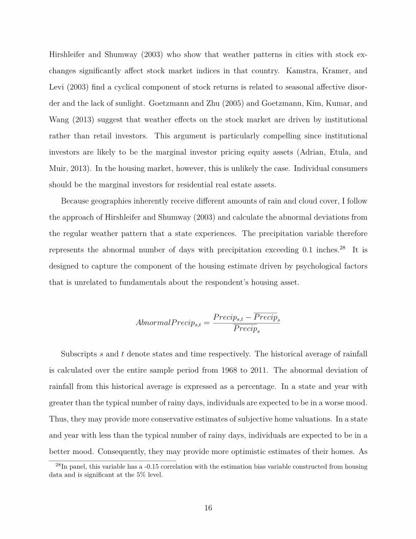
Because geographies inherently receive different amounts of rain and cloud cover, I follow

the approach of Hirshleifer and Shumway (2003) and calculate the abnormal deviations from

the regular weather pattern that a state experiences. The precipitation variable therefore

represents the abnormal number of days with precipitation exceeding 0.1 inches.28 It is

designed to capture the component of the housing estimate driven by psychological factors

that is unrelated to fundamentals about the respondent’s housing asset.

AbnormalPrecips,t = Precips,t − Precips

Precips

Subscripts s and t denote states and time respectively. The historical average of rainfall

is calculated over the entire sample period from 1968 to 2011. The abnormal deviation of

rainfall from this historical average is expressed as a percentage. In a state and year with

greater than the typical number of rainy days, individuals are expected to be in a worse mood.

Thus, they may provide more conservative estimates of subjective home valuations. In a state

and year with less than the typical number of rainy days, individuals are expected to be in a

better mood. Consequently, they may provide more optimistic estimates of their homes. As28In panel, this variable has a -0.15 correlation with the estimation bias variable constructed from housing

data and is significant at the 5% level.

16

predicted by the psychology literature, this measure of rainfall negatively correlates (-0.08)

with the degree which U.S. states overestimate their property values.29 Because this weather

variable is scaled by the mean, the average excess amount of rainy days across states is zero

with a standard deviation of 0.12 annually.30

3.2.2 Subjective health assessments

A person who overestimates one aspect of life (i.e. home value) may also be more likely

to overestimate others, such as personal health conditions. If this assumption is true, self-

reported health can serve as a useful instrument in the identification of the HVB effect. In

order to be a valid instrument, however, self-rated health should be correlated with HVB

but uncorrelated with housing fundamentals. Vartanian and Houser (2010) provide evidence

consistent with this exclusionary restriction. They show that while a person’s self-assessment

of health is influenced by her childhood neighborhood, there appears to be no relationship

between the person’s adult neighborhood and their health perceptions. Similarly, Böckerman

and Ilmakunnas (2009) show that while actual health varies with employment status, self-

assessed health is not incrementally affected by unemployment.

To construct a measure of health analogous to HVB, I isolate the part of the self-rated

health assessment which corresponds to the perceived health of the respondent, rather than

this actual health. Layes, Asada, and Kephart (2012), for example, decompose self-rated

health into two components: latent health and reporting behavior. Furthermore, these

authors find evidence of both optimistic and pessimistic views of health across different

populations. I approximate this reporting behavior component of self-rated health using

differences between the subjective reported health scale and objective measures of health29One potential concern with using weather as an instrument is that weather may sometimes directly

affect property values. Using rain as an example, states with a high fraction of farmland may indeed benefitfrom more rain. However, because real estate is such a long lived asset, temporary deviations are unlikelyto be priced. Therefore while the average amount of rainfall can certainly affect cross-sectional differencesin property prices, small year-to-year departures from average levels should not be associated with changesin fundamental property values.

30For robustness, I have also used other variables which approximate for weather unpleasantness such asheating degree days, which also negatively correlate with HVB.

17

from the PSID.31

Since 1984, the PSID has asked survey respondents to subjectively rate their own health

on a scale from 1 to 5 (5 = “Excellent”, 4 = “Very Good”, 3 = “Good”, 2 = “Fair”, 1 =

“Poor”).32 It then asks more specific questions on health including (1) whether the person has

any physical limitations which prevents them from working, (2) whether the person took sick

days in the last year due to personal illness (3) whether the person has been hospitalized in

the last year, and (4) the person’s height and weight.33 The first three measures all provide

clear and direct objective assessments of healthiness, while the fourth provides the data

necessary to calculate an indirect objective measure of health.

Using these last two responses, height and weight, I am able to calculate a body-mass-

index (BMI) for each individual.34 I then compare this metric with the World Health Or-

ganization’s (WHO) threshold for overweight individuals to determine if respondents over-

estimate their health.35 According to the WHO (2000), a healthy BMI ranges from 18 to

25. Anything above is considered overweight and anything below is considered underweight.

Since only a small fraction of Americans fall into the underweight category, and obesity is a

much more pressing issue than malnourishment in the United States, I simplify this criteria

and use an above/below 25 threshold as my fourth objective measure of healthiness.36

The calculation for health perception bias is as follows. For simplicity of presentation, I

drop all subscripts. This calculation is done at the individual level in all PSID surveys from31While this paper focuses on negative indicators of actual health, positive factors, such as feelings of

energy or social support, have also been shown to affect health perceptions (Benyamini, Idler, H. Leventhal,and E. Leventhal, 2000).

32The raw health scores available directly from PSID are in reverse order (i.e. Excellent=1 and Poor=5)to the ones used in this paper. I have inverted this scale to make the interpretation more natural.

33In 1986 the PSID experimented with questions asking for the height and weight of it’s survey respondents,but these questions did not reappear until 1999.

34The BMI is a standard, objective measure of health and has been associated with incidences of mortality,cardiovascular disease, and certain cancers (De Gonzalez et. al., 2010). It is calculated as weight/height2 ∗703, where weight is expressed in pounds, height is expressed in inches, and 703 is the conversion factor fromthe U.S. to a metric scale.

35This calculation is always done for the same respondent who provides the estimate of home value. Forexample, if the male spouse answers the housing question, I look at his self-reported health assessment. Ifthe female spouse answers the housing question, I look at her self-reported health assessment.

36Note that I do not require that BMI be a perfect measurement of health or obesity. In fact, Keys et al.(1972) suggest that it is better to use BMI as a measure over populations rather than individuals.

18

1984 to 2011, then aggregated to the state level each year.

HealthPerceptionBias = HealthReport− 3

If either...

1) HealthReport ∈ {Excellent(5), Very Good(4)} and HealthIssues = 1

2) HealthReport ∈ {Fair(2), Poor(1)} and HealthIssues = 0

Because HealthReport ranges from 1 to 5, HealthAssessBias will take on a value in the

set {−2,−1} depending on the magnitude by which an individual underestimates her health

or {1, 2} depending on the magnitude by which she overestimates it.37 HealthIssues is an

indicator variable which takes on a value of 1 if the respondent reports either (1) limited

ability to do physical work,38 (2) taking sick days from work in the last year due to illness,

(3) being hospitalized overnight in the last year, or (4) a height and weight consistent with

being overweight.39 For example, an individual with a BMI of 27 is considered unhealthy

under my criteria. Therefore, I require this individual to subjectively estimate her health

as either “Good”, “Fair”, or “Poor” in order to be classified as unbiased. Alternatively, if

this individual subjectively responds with “Excellent” or “Very Good,” I classify her health

optimism as either a 2 or a 1, depending on the degree of the upward bias. This measure of

health overestimation is positively correlated (0.09) with subjective home valuations.40

37Those providing “reasonable” health assessments are omitted from this calculation. Individuals mustprovide a self-health diagnosis of “Good” or worse if they have any health issues to be considered “reasonable,”and individuals must provide a self-health diagnosis of “Good” or better if they have no health issues to beconsidered “reasonable.”

38While the limited work variable also captures people with disabilities, Meyer and Mok (2013) reportthat in the period from 1968 to 2009, only 17% of male head-of-household respondents qualified as having achronic and severe disability - other respondents are either disabled temporarily (24% report being disabledfor just one year only) or not severely disabled.

39Overweight is defined as having a Body Mass Index (BMI) > 25 as defined by the World Health Orga-nization. The obesity threshold is BMI > 30. Approximately half of all PSID respondents over the sampleperiod are overweight. Approximately 25% are classified as obese.

40One potential concern with this instrument is that positive wealth shocks may simultaneously lead people

19

Table 2 provides summary statistics on these health measures from the PSID. The average

subjective health report at a statewide level is 3.56, indicating that the typical respondent

feel that her health is between “Good” and “Very Good” on the five point scale. In terms

of objective health assessments, on average 20% of the population within a state has trouble

doing physical work, 36% to 37% of the population took sick days from work in the past year

due to personal illness, and 11% to 14% of the population was hospitalized in the past year.41

In addition, the average BMI across respondents at the statewide level is 25.7 to 27.2, which

is above the overweight threshold defined by the WHO. The average health perception bias

across is 1.06 with a standard deviation of 0.32, suggesting that individuals are typically

optimistic about their health.

4 Results

My results show that cross-sectional differences in HVB have significant impacts on housing

returns and leverage. States in which individuals overestimate the value of their homes rel-

ative to market prices (high HVB) experience higher housing returns next year relative to

other states. However, this effect is conditional on the performance of the economy and of

the housing sector. In a recession, this relationship reverses, and forward housing returns be-

come lower in states with high HVB. Similarly, across areas where contemporaneous housing

returns are low, homes in high HVB states underperform homes in low HVB states over the

following year. These effects are very persistent, and can culminate for up to a decade before

reversing. Moreover, they carry important implications for leverage patterns in residential

housing.

to become both optimistic about their health and optimistic about their homes. Indeed, Layes, Asada, andKephart (2012) show that self-reported health varies with socioeconomic status. These wealth shocks pose aproblem for identification because they also may be correlated to future home price appreciation. To addressthis issue, I include both the level of income and income growth rates as control variables in a variety ofempirical specifications. My results are unaffected by these controls.

41I do not observe the specific reason for taking sick days or hospitalization. For example, if a womanwas hospitalized due to giving birth, this will add noise to my health variable and will bias correlations withHVB toward zero.

20

4.1 Hypothetical long-short portfolios of residential homes

I use cross-sectional variation in HVB to test for the effect of subjective valuations on housing

returns. A series of hypothetical portfolio sorts highlights the main results.42 In this section,

I consider arbitrage strategies which consists of (1) a long portfolio of equally weighted

positions in single-family homes of states in the highest HVB quantile and (2) a short portfolio

of equally weighted positions in single-family homes of states in the lowest HVB quantile.

The portfolio is rebalanced each survey year and held for one year thereafter.43 Figure 4

illustrates cumulative profits to this hypothetical portfolio over time using quintiles.

Higher levels of HVB in one year correspond with higher housing returns in the next.

If such a strategy were possible, investors would realize a total cumulative return of 60%

from 1982 to 2005. Furthermore if investors first separate contemporaneous housing returns

by median and implement this strategy only in the above median sample, this double sort

strategy would generate even larger cumulative profits of 257% over the 1982 to 2005 window

or 5.7% compounded annually. These magnitudes are slightly smaller than the results of

Beracha and Skiba (2011), who find momentum returns in residential housing as large as

8.9% annually.

If homeowners are unbiased, the overestimation of property values could simply reflect

superior information about local housing markets. In subsequent years, this private infor-

mation should be realized on average through higher returns. To test this, I examine the

relationship separately over economic expansions and contractions. If homeowners are good

forecasters, they should be successful when markets improve as well as when they decline.

Additional sorts, provided in Table 4, reveal that homeowners are correct only during

economic booms. Partitioning the data by NBER recession years, I find that across three

different quantile sorts, this strategy generates returns of 1.2% to 1.8% annually when mar-42I emphasize the hypothetical nature of this exercise because it is practically impossible for an investor

to form diversified residential real estate portfolios at the state level and short sell one of these portfolios.Furthermore, the timing of this strategy also makes it non-tradeable because the PSID is typically releasedwith a significant delay.

43I assume no transactions costs or other market frictions.

21

kets have done well from 1975 to 2011. However, this strategy appears to lose money when

markets do poorly. Returns are consistently negative ranging from -1.3% to -3.1% on an

annual basis during recessionary periods over this window. Therefore, homeowners are not

making unbiased forecasts of future prices.

4.2 Home valuation bias and housing returns

My primary tests estimate how HVB affects forward housing returns in a panel regression.

The FHFA index return one year forward is regressed upon current values of HVB and a

series of controls.44 Due to the time-series properties of FHFA index returns, I control for

two lagged returns in each specification to remove any mechanical autoregressive structure.45

Because forward housing returns could reflect economic fundamentals, I also include a set of

controls for state level economic influences. Furthermore, differences in housing market fun-

damentals could also contribute to forward return differences, so I add covariates to control

for local housing conditions. Lastly, I incorporate year fixed effects to remove the common

time trend and regional fixed effects to capture unobservable return premia arising from

broad geographic preferences. For example, there may be a premium for homes on the West

Coast because people working in the finance industry enjoy the 3-hour time difference with

their headquarter offices in New York City. The results from the OLS regression equation

below are summarized in Models 1-3 of Table 5.44Because I use return information from repeat-sales indices, one potential concern is that this result may

be driven by econometric biases which have been documented in the construction of these indices. Goetzmannand Peng (2006) use a model of reservation prices versus market values to show that when individuals havea higher reservation price relative to market values, trading volume declines and results in an upward bias inobserved transaction values used in the construction of repeat sales indices. While the price patterns of therepeat-sales bias are indeed consistent the evidence in this section, I find no correlation between householdoptimism and volume effects. In addition, these biases cannot explain the observed patterns in recessions,the magnified effect when current returns are high, or the effects on leverage discussed in subsequent sections.

45Using monthly data, Goetzmann Peng and Yen (2009) similarly find that the best ARIMA model fittingthe time-series of home prices is a model based on the first difference of prices (i.e. returns) with 24 monthlags (i.e. 2 years), and a 3 month moving average. The analysis in this paper uses annual information, so itomits the moving average component.

22

Returns,t+1 = α + β ∗HV Bs,t

+ EconControlss,t +HouseMktControlss,t + LagReturnss,t

+ Y earFEt +RegionFEs + εs,t

Subscripts s and t index states and years respectively. EconControls represents control

variables for unemployment, population level, income level, population growth, and income

growth. HouseMktControls represents control variables for capitalization rate, ownership

rate, mortgage interest rate, and loan-to-value ratios.46 RegionFE are a set of broadly

defined regional fixed effects from the U.S. Census.47 LagReturns include both the contem-

poraneous FHFA index return and the FHFA index return one year prior.

Another motivation for including lagged returns is to differentiate predictions of positive

feedback trading (De Long, Shleifer, Summers, and Waldmann, 1990; Hong and Stein, 1999)

from from other behavioral theories. Positive feedback traders are investors who condition

their investment actions myopically on past and present returns. Hence, if households are

simply positive feedback traders, HVB should be based on return histories alone. Controlling

for lagged returns should weaken or cancel the effect of HVB. Instead, after controlling

for lagged returns, the effect of HVB is economically and statistically significant in every

specification, suggesting that households are more than myopic chasers of market prices.

As shown in Table 5, HVB (along with basic time-series and return controls) accounts

for 57% of the variation in subsequent house price appreciation. Under each model spec-

ification, the coefficient on HVB is economically large and statistically significant. A one46Capitalization rate (cap rate) is calculated as total annual rent divided by the average market price of

single-family homes. It approximates the rate of return on residential real estate. An alternative way tothink about the cap rate is to view it as the dividend yield on homes. This is because the cap rate statesthe annual utility from housing consumption as a percentage of the total cost of home ownership.

47The U.S. Census separates the United States into four broad regions: Northeast, Midwest, South, andWest .

23

standard deviation in HVB in Models 1-3 correspond to an increase in FHFA returns one

year thereafter of 0.3% to 0.6%. This corresponds to a 6.4% to 11.9% change relative to the

mean annual FHFA return (4.6%) from 1975 to 2011.

4.3 Weather and health as instruments for home valuation bias

There exist two potential challenges to identification in Section 4.2. An endogeneity problem

arises if home prices and investor biases may be jointly determined by fundamentals, and

an omitted variables bias problem occurs if investor biases are correlated with neighborhood

unobservables. For example, the renovation of state parks could simultaneously increase

individual perceptions of home values and housing returns. Furthermore, local air quality

and traffic conditions, could be omitted variables which would affect housing returns.48

As described in Section 3, I use a combination of abnormal weather patterns and self-

health perceptions to instrument for home valuation bias. Models 4-6 in Table 5 provide

these coefficient estimates using two-stage least squares. The first stage of my IV estimation

predicts the estimation bias of home prices using either abnormal weather, health perception

bias, or a combination of the two.

HV Bs,t = α + γ ∗ AbnormalPrecips,t + ω ∗HealthPerceptionBiass,t,

+ Controlss,t + LagReturnss,t + Y earFEt +RegionFEs + υs,t

Again, subscripts s and t index states and years respectively. AbnormalPrecip is the48Another source of endogeneity could arise if investors misinterpret the PSID housing question as asking

how much would their home sell for in the future as opposed to how much it would sell for today. Theremay be a variety of reasons why individual survey respondents interpret the question this way in spite of theinterviewer’s efforts to inquire the true current value of their home. For example, investors may be implicitlyconsidering unavoidable market frictions in selling a home because the logistics involves in selling often takea substantial amount of time.

24

abnormal number of rainy or snowy days in a year. It is described at length in Section

3.2.1. HealthAssessBias measures the optimism of individuals about their health at the

state level . It is described at length in Section 3.2.2. For brevity,Controls represents both

EconControls and HouseMktControls from the previous section. All other variables are as

defined in the previous section too. In the first stage where both instruments are included,

a one standard deviation increase in AbnormalPrecip corresponds to an -0.085 change in

standardized HVB. Similarly, a one standard deviation increase in HealthAssessBias cor-

responds to a 0.162 change in standardized HVB. The Cragg-Donald F -statistic from this

regression is 8.18, indicating that the instruments are fairly strong. Furthermore, the Hansen

J -statistic is insignificant at the 10% level, indicating that overidentification is not an issue.

In the second stage, forward returns are regressed on the predicted HVB from the first

stage and the same series of control variables as the OLS specification. The combination of

these two instruments delivers the best estimate of home valuation bias in the cross-section

of residential housing returns.

Returns,t+1 = α + β ∗ HV Bs,t

+ Controlss,t + LagReturnss,t + Y earFEt +RegionFEs + εs,t

HV Bs,t is the estimated home valuation bias from the first stage regression. All other

variables and subscripts are as previously defined. In the second stage which includes both

instruments, I find that a one standard deviation increase in the overestimate of residential

home prices leads to a 2.4% rise in residential housing returns in the following year. This

corresponds to an increase of 52% relative to the average annual return on residential real

estate from 1975 to 2011 of 4.6%. Second stage results using each instrument variable

individually are weaker, but consistent in sign. Using either the weather instrument or

25

health instrument individually, a one standard deviation increase in HVB is associated with

a 1.8% increase subsequent returns.

4.4 Home valuation bias and recessions

Recall the hypothesis from Section 4.1 that the patterns documented in Sections 4.2 and

4.3 may arise if homeowners were simply good forecasters. Under this view, respondents

estimate home values based on superior information about their local real estate markets.

To test this hypothesis in a regression setting, this section modifies the empirical specification

from these previous sections to consider the effects of HVB in booms and busts.

There are only two differences between the specification below than those in the aforemen-

tioned sections. First, an indicator for NBER recessions replaces year fixed effects. Second,

an interaction term between NBER recessions and the HVB variable is included to show

the incremental effect of HVB during a downturn. For the purposes of IV estimation, an

additional variable of abnormal rainfall interacted with NBER recessions is used to assist in

identification. Thus, the first stage is estimated using three instruments: abnormal rainfall,

health perception bias, and the interaction of abnormal rainfall with the NBER recession in-

dicator. I provide the basic OLS specification below. The analogous IV specification follows

naturally from Section 4.3.

Returns,t+1 = α + β1 ∗HV Bs,t + β2 ∗Recessiont + β3 ∗ (HV Bs,t ∗Recessiont)

+ EconControlss,t +HouseMktControlss,t + LagReturnss,t

+RegionFEs + εs,t

Recession takes on a value of one for any year in which a recession quarter was recorded

and zero elsewhere. All other variables and subscripts are as previously defined. Models 1-3

26

in Table 6 provide OLS estimates of these effects while Model 4 provides the IV regression

using the three instruments mentioned above. Across all three OLS estimates, the coefficient

on HVB is 67% larger than those from Section 4.2 on average. A one standard deviation

increase in HVB outside of an economic recession leads to a 0.7% increase in FHFA returns

one year forward. Conversely, a similar increase within a recessionary period leads to a 0.4%

net decline in FHFA returns the following year.

As before, the problems of endogeneity and omitted variables bias lead to lower OLS

estimates of these HVB effects. In IV estimation, the effect of a one standard deviation

increase during boom periods is 6.9% the following year. In recessions, this effect translates

instead to a 0.6% net decline in forward one year returns. If homeowners are unbiased

forecasters, the effects of HVB in booms and busts should be identical. The reversal of

the HVB effect during economic recessions shows that superior private information cannot

explain this pattern in housing returns.

4.5 Market fragility and risk taking

Another important channel through which household optimism may affect asset prices is

leverage. This section examines the effect of HVB on household debt. Recent papers have

argued that behavioral biases can alter an individual’s borrowing decisions. Agarwal (2007)

shows that overestimation of housing wealth can increase a homeowners probability to cash-

out refinance their mortgage. Similarly, M. Seiler, V. Seiler, Harrison, and Lane (2013)

suggest that when homeowners believe their property is less prone to devaluation, adverse

effects can occur in selling, financing, and refinancing decisions. The common theme in

these arguments is that as individuals grow more optimistic about their wealth portfolio,

they engage in riskier investment decisions.49

49Recent experimental evidence has also supported the conjecture that weather has a sizable effect on riskattitudes. Bassi, Colacito, and Fulghieri (2013) offer experimental evidence that good weather promotesindividual risk-taking behavior via its effect on mood. Kramer and Weber (2012) find that subjects sufferingfrom seasonal affective disorder exhibit higher risk aversion than those who do not and that this is transmittedthrough the channel of depression.

27

I test for additional household risk taking by studying the effect of HVB on two forms of

leverage: loan-to-value (LTV) and loan-to-income (LTI). Both forms of leverage are related

to the overall risk of lending. A low LTV ratio for a lender implies that should the borrower

default, the property can be sold relatively easily without incurring a loss on the mortgage.

A low LTI ratio for a lender implies that there is a low probability that the borrower will be

unable to service the mortgage and default on the loan.50 I regress each form of leverage on

HVB and a similar array of controls to Section 4.2.

Leverages,t = α + β ∗HV Bs,t

+ Controlss,t + LagReturnss,t + Y earFEt +RegionFEs + εs,t

Leverage either represents LTV or LTI. All other variables are as described in previous

specifications. Table 7 summarizes these results. The effects of HVB on leverage are clearly

asymmetric. Higher HVB correlates with lower LTV ratios but higher LTI ratios. Therefore,

as optimistic homeowners inflate the value of their collateral and push up home prices, they

also reduce their ability to service these mortgages.

In the data, individual homeowners appear to take on higher loan-to-income ratios as

their perceived housing wealth increases. Model 6 of Table 7 shows that a one standard

deviation increase in HVB is associated with a 3.2% increase in LTI relative to the average

LTI of 2.25x. This result is consistent with Mian and Sufi (2011). These authors find

that existing homeowners borrowed more in the recent housing bubble as their home prices

appreciated between 2002 and 2006. My result shows that subjective valuation biases may be

driving the relationship between home price appreciation and more aggressive home equity

based borrowings in their work.50However, as explained Mian and Sufi (2011), LTI is a more relevant measure of household leverage

because it represents the extent to which household are stretching themselves financially.

28

Although higher HVB makes leverage appear more conservative by raising the price of the

underlying collateral, it also has the perverse effect of encouraging borrowers to stretch their

financial means relative to their income. If higher prices were sustainable in equilibrium, this

would not be a problem. Debt issued upon collateral which has fundamentally appreciated

becomes safer, because it is more likely to be repaid. Even if a borrower can no longer service

the mortgage, she can sell the home, collect profits from home equity appreciation, pay off

the debt in full, and shift into a more affordable option.

However, this guaranteed ability to repay the debt occurs only if the appreciation on

home equity is justified. If home price appreciation is temporary or due to mispricing, then

the eventual collapse in housing prices will result in high LTV ratios and high LTI ratios.51

These higher leverage ratios simultaneously increase the incentives of the lender to foreclose

before prices decline any further and encourage borrowers to default before making more

mortgage payments into a home with negative equity.52 As these leverage effects feed back

into prices, a vicious cycle in falling home prices could ensue.

I find evidence that household optimism increases the fragility of residential housing

markets. The relationship between HVB and LTI highlights how subjective valuations can

affect household leverage decision. These findings offer an alternative explanation for the

return effects of HVB during economic downturns. Overly optimistic homeowners push

prices higher in good times. As a result, borrowers take on too much debt relative to their

income stream to purchase these homes. Lenders may be willing to lend because of the

perceived safety in LTV ratios. Because the run-up in prices is not driven by fundamentals,

when asset prices collapse, thinly stretched borrowers are forced to default, creating excess

housing supply and perpetuating the decline in home prices.51Recall that LTI was already high due to the mispricing.52The default option varies by state depending on the laws concerning recourse versus non-recourse debt.

See Curtis (2013) for a discussion.

29

5 Related literature

The importance of the housing market to the aggregate economy has been well documented.

Peng and Thibodeau (2013) study idiosyncratic risk in home prices and review the literature

connecting house prices to consumption, savings and economic production. Furthermore, in

a recent set of papers, Miller, Peng, and Sklarz (2011) and Miller, Peng, and Sklarz (2011a),

show that predictable home price changes, or even anticipated changes as approximated by

home sales, can impact future housing returns local economic activity.

Numerous studies have also emerged which highlight the impact of household irrationality

on real estate markets. Case and Shiller (2003) find evidence of unrealistic return expecta-

tions and investment motives in the home purchase decision. Case, Shiller, and Thompson

(2012) show that return expectations are particularly optimistic over long forecast horizons.

Genesove and Mayer (2001) show that loss aversion is a significant determinant of seller be-

havior in housing markets. Soo (2013) finds that local, news-implied sentiment was a leading

predictor of the boom and bust cycle in the recent U.S. housing bubble. Brunnermeier and

Julliard (2008) provide evidence that money illusion can distort home prices when inflation

declines. This is because investors mistake changes in inflation with changes in the real

rate of interest. Such naive comparisons between mortgage payments and rents makes home

ownership artificially more attractive when inflation declines. In line with the money illu-

sion mechanism, Shiller (2008) finds that real estate bubbles often begin with an innocuous

shock to economic fundamentals, such as employment or inflation, which is subsequently

exacerbated by irrational household behavior.

Some experimental evidence has, more generally, supported the role of mood in asset

bubbles. Lahav and Meer (2010) show that prices deviate more from fundamentals in a

trading game when positive moods are induced via film clips in experiment participants.

Using a similar game, Andrade, Odean, and Lin (2012) prime subjects with various moods

prior to playing. They find that when subjects are primed with “excitement,” defined as a

mood which is both pleasant and arousing, they exhibit a stronger tendency to extrapolate

30

past returns and generate asset bubbles.

Many researchers have used survey methods to understanding asset prices in residential

housing. Case and Shiller (1988) began surveying households in 1988 on their expectations

of future home price appreciation. Apart from popular national surveys such as the Michigan

Survey of Consumers and the National Association of Home Builders, which both publish

housing confidence indices at an aggregate level, concern over the accuracy of solicited hous-

ing values has also been extensively researched. Several papers have specifically addressed

the issue of reported housing values versus transaction values. Kiel and Zabel (1999) use the

American Housing Survey to ask whether it is appropriate to use reported housing values as

an approximation of transaction values across three cities from 1978 to 1991 and find that

new owners overestimate the current selling prices of homes by roughly 8%. They further

claim that this overestimation is uncorrelated to the characteristics of the owner, house,

or neighborhood. Piazzesi and Schneider (2009) examine survey responses from the Michi-

gan Survey of Consumers to study the time-series effect of momentum traders in housing

markets. Similar to this paper, Henriques (2013) uses the Survey of Consumer Finances (a

triennial survey) to show that owner-reported home values increased by more than home

price indices during housing booms and decreased by less during housing busts. She finds

that these changes correlate with aggregate changes in the housing stock but concludes that

sample composition differences can explain variation in valuation biases from 2001 to 2010.

Benítez-silva, Eren, Heiland, and Jiménez-Martín (2010) use the Health and Retirement

Study to study differences in self-reported housing values and the eventual realized sale

prices of those properties and find that individuals overestimate housing prices by roughly

10%. However, the Health and Retirement Study has several shortcomings. Firstly, there is

a strong bias toward the behavior of older and retired Americans. Beginning in 1992, the

survey only covered senior individuals aged 51 to 61. Therefore, it cannot be interpreted as

a representative US sample since it omits a large fraction of the population currently active

in the workforce and in housing market transactions. By contrast in the PSID sample,

31

the average age of male homeowners is 46 years old, with 90% of all male homeowners

between the ages of 26 and 77. The Health and Retirement Study also misses the real estate

boom in the 1980s, as well as three separate recessions therein. It only captures the run-

up in overestimation since 1994, which is consistent with the PSID time-series used in this

paper. Furthermore, Benítez-silva et. al. (2010) examine housing values at an individual

level - which leads to other complications on the endogeneity of self-reported prices due to

unobserved heterogeneity in local markets and unobserved housing characteristics.53 My

paper avoids this problem by using aggregated reports across sufficiently large samples (i.e.

at the state level) to approximate the average selling prices of single-family residential homes

within that state, eliminating local and house specific noise.

The instruments used in this paper are also related to other literatures. One instru-

ment is motivated by the behavioral literature studying the effects of weather on mood and

asset prices. Saunders (1993) and Hirshleifer and Shumway (2003) show that abnormally

inclement weather in cities with major exchanges negatively correlate with the performance

of their stock indices. Goetzmann, Kim, Kumar, and Wang (2013) find a positive link

between cloudy days and perceptions of overpricing in stocks using survey data of institu-

tional investors. Chhaochharia, Korniotis, and Kumar (2012) show that weather can also

broadly affect regional levels of economic activity and resiliency. The other instrument in

this paper relates to a field of medical research that examines how best to interpret people’s

self-assessments of health. Layes, Asada, and Kephart (2012) decompose self-rated health

into two components, latent health and reporting behavior, and find evidence of both over-

reporting and under-reporting across different sample groups. For example, they find that

people with lower income and education tend to be more optimistic about their health than

warranted.

Lastly, this paper is connected to many behavioral theories of asset prices. These include

theories of positive feedback trading (De Long et. al., 1990; Hong and Stein, 1999), theories of53These complications are outlined in a separate paper by Benítez-silva, Eren, Heiland, and Jiménez-Martín

(2010a).

32

investor bias (Daniel, Hirshleifer, and Subrahmanyam, 1998; Barberis, Shleifer, and Vishny,

1998), theories of disagreement and market frictions (Miller, 1977; Harrison and Kreps,

1978; Scheinkman and Xiong, 2003), and theories of general investor sentiment (Baker and

Wurgler, 2006). A comprehensive treatment of these theories as applied to the results in this

paper is available in Appendix II.

6 Conclusion

I show that the aggregate mood of households is an important determinant of home prices and

leverage decisions and that these effects help explain asset bubbles in residential real estate.

For asset prices, I find that systematic biases in homeowner valuations can have significant

impacts on housing returns. When individuals within a state overestimate the current value

of their homes, housing returns are indeed higher in the following year. However, I reject

the hypothesis that these differences in subjective valuations are simply due to superior

information about local property trends or characteristics. I find evidence that homeowners

fail to consistently forecast future price appreciation. During recessions, housing markets in

states with higher overvaluations significantly underperform housing markets in other states.

The existence of lower returns following overestimates of housing values contradicts the view

of homeowners as unbiased forecasters.

Instead, I propose that subjective valuation biases occur due to general levels of optimism

or pessimism at the household level. I find that differences between subjective valuations

and market prices at the state level strongly correlate with self-assessments of health as well

as abnormally unpleasant weather. Both of these covariates serve as useful instruments in

identifying the impact of subjective valuations on housing returns. Across different theories

of asset prices, I find that the mechanism of overconfidence and self-attribution bias in

Daniel, Hirshleifer, and Subrahmanyam (1998), offers the most consistent interpretation of

my results on housing returns.

33

In addition, I also find important implications of subjective valuations on leverage pat-

terns in residential housing. Higher overvaluations negatively correlate with loan-to-value

but positively correlate with loan-to-income. This asymmetric effect on leverage suggests

that as optimistic homeowners inflate the value of their collateral (i.e. home prices), they

also stretch their ability to service the mortgage. Residential housing markets become more

vulnerable to unanticipated shocks as a result, especially if lenders forgo affordability con-

siderations in favor of higher collateral values when homeowners voice their excitement.

34

References

[1] Tobias Adrian, Erkko Etula, and Tyler Muir. Financial Intermediaries and the Cross-

Section of Asset Returns. 2013.

[2] Sumit Agarwal. The Impact of Homeowners’ Housing Wealth Misestimation on Con-

sumption and Savings Decisions. Real Estate Economics, 35(2):135–154, 2007.

[3] Eduardo B Andrade, Terrance Odean, and Shengle Lin. Bubbling with Excitement: An

Experiment. 2012.

[4] Constantinos Antoniou, John A. Doukas, and Avanidhar Subrahmanyam. Cognitive

Dissonance, Sentiment, and Momentum. Journal of Financial and Quantitative Analy-

sis, 48(1):245–275, November 2013.

[5] Malcolm Baker and Jeffrey Wurgler. Investor Sentiment and the Cross-Section of Stock

Returns. Journal of Finance, 61(4):1645–1680, 2006.

[6] Nicholas Barberis, Andrei Shleifer, and Robert Vishny. A model of investor sentiment.

Journal of Financial Economics, 49:307–343, 1998.

[7] Anna Bassi, Riccardo Colacito, and Paolo Fulghieri. ’O Sole Mio: An Experimental

Analysis of Weather and Risk Attitudes in Financial Decisions. Review of Financial

Studies, 26(7):1824–1852, February 2013.

[8] Hugo Benítez-silva, Selçuk Eren, Frank Heiland, and Sergi Jiménez-Martín. Using the

Health and Retirement Study To Analyze Housing Decisions , Housing Values , and

Housing Prices. Cityscape: A Journal of Policy Development and Research, 12(2):149–

159, 2010.

[9] Hugo Benítez-silva, Selcuk Eren, Frank Heiland, and Sergi Jiménez-Martín. How Well

do Individuals Predict the Selling Prices of their Homes ? (5), 2010.

35

[10] Yael Benyamini, Ellen L. Idler, Howard Leventhal, and Elaine A. Leventhal. Positive

Affect and Function as Influences on Self-Assessments of Health: Expanding Our View

Beyond Illness and Disability. The journals of gerontology. Series B, Psychological

sciences and social sciences, 55(2):P107–16, March 2000.

[11] Eli Beracha and Hilla Skiba. Momentum in Residential Real Estate. The Journal of

Real Estate Finance and Economics, 43(3):299–320, October 2011.

[12] Petri Böckerman and Pekka Ilmakunnas. Unemployment and Self-Assessed Health:

Evidence from Panel Data. Health Economics, 18(2009):161–179, 2009.

[13] Markus K. Brunnermeier and Christian Julliard. Money Illusion and Housing Frenzies.

Review of Financial Studies, 21(1):135–180, November 2008.

[14] Karl E. Case and Robert J. Shiller. The Behavior of Home Buyers in Boom and Post-

Boom Markets. New England Economic Review, pages 29–46, 1988.

[15] Karl E. Case and Robert J. Shiller. Is There a Bubble in the Housing Market? Brookings

Papers on Economic Activity, 2003(2):299–362, 2003.

[16] Karl E Case, Robert J Shiller, and Anne Thompson. What Have They Been Thinking?

Home Buyer Behavior in Hot and Cold Markets. Working paper, National Bureau of

Economic Research, September 2012.

[17] Joseph Chen, Harrison Hong, and Jeremy C Stein. Breadth of ownership and stock

returns. Journal of Financial Economics, 66:171–205, November 2002.

[18] Vidhi Chhaochharia, George M Korniotis, and Alok Kumar. Prozac for Depressed

States? Effect of Mood on Local Economic Recessions. 2011.

[19] Quinn Curtis. State Foreclosure Laws and Mortgage Origination in the Subprime.

Journal of Real Estate Finance and Economics, August 2013.

36

[20] Kent Daniel, David Hirshleifer, and Avanidhar Subrahmanyam. Investor Psychology and

Security Market Under- and Overreactions. The Journal of Finance, 53(6):1839–1885,

1998.

[21] Amy Berrington De Gonzalez, Patricia Hartge, James R Cerhan, Alan J Flint, Lindsay

Hannan, Robert J MacInnis, Steven C Moore, Geoffrey S Tobias, Hoda Anton-Culver,

Laura Beane Freeman, W Lawrence Beeson, Sandra L Clipp, Dallas R English, Aaron R

Folsom, D Michal Freedman, Graham Giles, Niclas Hakansson, Katherine D Henderson,

Judith Hoffman-Bolton, Jane A Hoppin, Karen L Koenig, I-Min Lee, Martha S Linet,

Yikyung Park, Gaia Pocobelli, Arthur Schatzkin, Howard D Sesso, Elisabete Weider-

pass, Bradley J Willcox, Alicja Wolk, Anne Zeleniuch-Jacquotte, Walter C Willett, and

Michael J Thun. Body-Mass Index and Mortality among 1.46 Million White Adults.

The New England journal of medicine, 363(23):2211–9, December 2010.

[22] J Bradford De Long, Andrei Shleifer, Lawrence H Summers, and Robert J Waldmann.

Positive Feedback Investment Strategies and Destabilizing Rational Speculation. Jour-

nal of Finance, 45(2):379–395, 1990.

[23] Henry S Farber. Unemployment in the Great Recession: Did the Housing Market Crisis

Prevent the Unemployed from Moving to Take Jobs ? American Economic Review,

102(3):1–6, 2012.

[24] David Genesove and Christopher Mayer. Loss Aversion and Seller Behavior: Evidence

from the Housing Market. Quarterly Journal of Economics, 116(4):1233–1260, 2001.

[25] Carroll J. Glynn, Carole A. Lunney, and Michael E. Huge. The Polls–Trends: Pub-

lic Perceptions of the U.S. Residential Housing Market Before, During, and After the

Housing Bubble (1990-2009). Public Opinion Quarterly, 73(4):807–832, November 2009.

37

[26] William Goetzmann and Liang Peng. Estimating House Price Indexes in the Presence

of Seller Reservation Prices. Review of Economics and Statistics, 88(February):100–112,

2006.

[27] William N Goetzmann, Dasol Kim, Alok Kumar, and Qin Wang. Weather-Induced

Mood , Institutional Investors , and Stock Returns. 2013.

[28] William N Goetzmann, Liang Peng, and Jacqueline Yen. The Subprime Crisis and

House Price Appreciation. Journal of Real Estate Finance and Economics, 44(1):36–66,

2012.

[29] William N. Goetzmann and Ning Zhu. Rain or Shine: Where is the Weather Effect?

European Financial Management, 11(5):559–578, November 2005.

[30] J Michael Harrison and David M Kreps. Speculative Investor Behavior in a Stock

Market with Heterogeneous Expectations. Quarterly Journal of Economics, 92(2):323–

336, 1978.

[31] Alice M Henriques. Are Homeowners in Denial about their House Values ? Comparing

Owner Perceptions with Transaction-Based Indexes. 2013.

[32] David Hirshleifer and Tyler Shumway. Good Day Sunshine: Stock Returns and the

Weather. Journal of Finance, 58(3):1009–1032, 2003.

[33] Harrison Hong and Jeremy C Stein. A Unified Theory of Underreaction , Momentum

Trading , and Overreaction in Asset Markets. Journal of Finance, 54(6):2143–2184,

1999.

[34] Changha Jin. The Impact of Local Media Pessimism on Residential Real Estate Markets.

2009.

[35] Mark J Kamstra, Lisa A Kramer, and Maurice D Levi. Winter Blues : A SAD Stock

Market Cycle. American Economic Review, 93(1):324–343, 2003.

38

[36] Ancel Keys, Flaminio Fidanza, Martti J Karvonen, Noboru Kimura, and Henry L Tay-

lor. Indices of relative weight and obesity. Journal of chronic diseases, 25(6):329–343,

July 1972.

[37] Katherine a. Kiel and Jeffrey E. Zabel. The Accuracy of Owner-Provided House Values:

The 1978-1991 American Housing Survey. Real Estate Economics, 27(2):263–298, June

1999.

[38] Lisa A. Kramer and J. Mark Weber. This is Your Portfolio on Winter: Seasonal Affective

Disorder and Risk Aversion in Financial Decision Making. Social Psychological and

Personality Science, 3(2):193–199, July 2012.

[39] Yaron Lahav and Shireen Meer. The Effect of Induced Mood on Prices in Experimental

Asset Markets. 2010.

[40] Owen Lamont and Jeremy C. Stein. Leverage and house-price dynamics in U.S. cities.

RAND Journal of Economics, 30(3):498–514, January 1999.

[41] Audrey Layes, Yukiko Asada, and George Kepart. Whiners and deniers - What does

self-rated health measure? Social Science & Medicine, 75(1):1–9, July 2012.

[42] N Gregory Mankiw and David N Weil. The Baby Boom, the Baby Bust, and the

Housing Market. Regional Science and Urban Economics, 19:235–258, 1989.

[43] Bruce D. Meyer and Wallace K.C. Mok. Disability, Earnings, Income, and Consumption.

2013.

[44] Atif Mian and Amir Sufi. House Prices, Home Equity-Based Borrowing, and the US

Household Leverage Crisis. American Economic Review, 101(August):2132–2156, 2011.

[45] William Michelson. Long and Short Range Criteria for Housing Choice and Environ-

mental Behavior. Journal of Social Issues, 36(3):135–149, July 1980.

39

[46] Edward M Miller. Risk, Uncertainty, and Divergence of Opinion. Journal of Finance,

32(4):1151–1168, 1977.

[47] Norman Miller, Liang Peng, and Michael Sklarz. House Prices and Economic Growth.

Journal of Real Estate Finance and Economics, 42(4):522–541, July 2011.

[48] Norman G. Miller, Liang Peng, and Michael A. Sklarz. The Economic Impact of An-

ticipated House Price Changes-Evidence from Home Sales. Real Estate Economics,

39(2):345–378, June 2011.

[49] Elli Pagourtzi, Vassilis Assimakopoulos, Thomas Hatzichristos, and Nick French. Real

estate appraisal: a review of valuation methods. Journal of Property Investment &

Finance, 21(4):383–401, 2003.

[50] Liang Peng and Thomas G Thibodeau. Idiosyncratic Risk of House Prices : Evidence

from 26 Million Home Sales. 2013.

[51] Mitchell A Petersen. Estimating Standard Errors in Finance Panel Data Sets: Com-

paring Approaches. Review of Financial Studies, 22(1):435–480, April 2009.

[52] Monika Piazzesi and Martin Schneider. Momentum Traders in the Housing Market:

Survey Evidence and a Search Model. American Economic Review, 99(2):406–411,

April 2009.

[53] Edward M Saunders. Stock Prices and Wall Street Weather. American Economic

Review, 83(5):1337–1345, 1993.

[54] José A. Scheinkman and Wei Xiong. Overconfidence and Speculative Bubbles Jose.

Journal of Political Economy, 111(6):1183–1219, 2003.

[55] Anna Scherbina and Bernd Schlusche. Asset Bubbles: an Application to Residential

Real Estate. European Financial Management, 18(3):464–491, June 2012.

40

[56] Michael J Seiler, Vicky L Seiler, David M Harrison, and Mark Lane. Familiarity Bias and

Perceived Future Home Price Movements. Journal of Behavioral Finance, 14(1):9–24,

2013.

[57] Robert J Shiller. Historic Turning Points in Real Estate. Eastern Economic Journal,

34(1):1–13, 2008.

[58] Cindy K Soo. Quantifying Animal Spirits: News Media and Sentiment in the Housing

Market. 2013.

[59] Jeremy C. Stein. Prices and Trading Volume in the Housing Market : A Model with

Down-Payment Effects. Quarterly Journal of Economics, 110(2):379–406, 1995.

[60] Simon Stevenson. Modeling Housing Market Fundamentals : Empirical Evidence of

Extreme Market Conditions. Real Estate Economics, 36(1):1–29, 2008.

[61] Joseph E Stiglitz. Symposium on Bubbles. Journal of Economic Perspectives, 4(2):13–

18, 1990.

[62] Thomas P Vartanian and Linda Houser. The effects of childhood neighborhood condi-

tions on self-reports of adult health. Journal of Health and Social Behavior, 51(3):291–

306, September 2010.

[63] Ko Wang, Yuqing Zhou, Su Han Chan, and K. W. Chau. Over-Confidence and Cycles in

Real Estate Markets : Cases in Hong Kong and Asia. International Real Estate Review,

3(1):93–108, 2000.

[64] World Health Organization. Obesity: Preventing and Managing the Global Epidemic.

Technical report, 2000.

41

Appendix I: Observable fundamentals

The object of this paper is to study the impact of overconfidence and estimation bias on

residential house prices. However if economic fundamentals are correlated with my measure

of this bias, the results will suffer from omitted variable bias. Absent a true model of housing

prices or returns, I include a wide array of economic, real estate, and lending variables to

mitigate this concern. All of the below variables are collected at the annual level and merged

by state identifiers each year.54

Population and income. Mankiw and Weil (1989) has argued that population dynam-

ics can have large and lasting impacts on the evolutions of real estate prices. They focus

on the demand bubble created by baby boomers entering and leaving the housing market,

and have predicted eventual declines in housing markets upon the mass retirement of this

generation. I thus include common measures of population and income dynamics as controls

to absorb potential variation at this macroeconomic level. I collect levels and growth rates

for population and income from the Bureau of Economic Analysis (BEA) over the period

1968 to 2012.

Labor. Labor markets can also correlate strongly with the performance of real financial

assets (Faber (2012)). Therefore, I control for workforce demographics using the unemploy-

ment rate. Unemployment rates are gathered from the Bureau of Labor Statistics (BLS)

and span the years 1976 to 2012.

Lending and interest rates. Leverage effects can significantly impact residential hous-

ing. Lamont and Stein (1999) find that cities which are more highly levered are also more

sensitive to city-specific shocks. Stein (1995) models how leverage arising from down-payment

requirements can induce volatility in housing prices as well as a correlation between prices

and volume. I consider two forms of leverage in this paper: loan-to-value (LTV) and loan-to-54For the interested reader who is nevertheless concerned that either (1) the following economic controls are

not an exhaustive list to address the omitted variables bias or (2) unobservables in the market for residentialhomes at the state level create systematic biases in estimation, I use two instrumental variables in Section 4to address these concerns.

42

income (LTI). LTV ratios are taken from the FHFA Finance Board’s Monthly Interest Rate

(MIR) survey historical summary tables. Each month the FHFA has surveyed a sample of

lenders to determine market rates,55 terms, and LTV ratios on conventional single-family

non-farm mortgage loans by state since 1978.56 LTI is obtained from the Home Mortgage

Disclosure Act (HMDA) from 2000 to 2012 and includes loan information from over 7000

lending institutions reporting a combined volume of 14 to 42 million loan records per year

since 2000.

Rental rates and ownership. Other fundamentals which could potentially affect re-

turns include state level rents and ownership rates. Rents represent the opportunity cost of

not purchasing a home, and if rents are high in an area, potentially home prices will sub-

sequently rise as well as more people substitute ownership for rental properties. Ownership

rates could also affect returns since it reveals the total fraction of the population who are

potential homeowners next period. High current ownership rates may mitigate rises in home

prices in future periods. I obtain rent and ownership information from the PSID survey.

Rents are scaled by price information collected from the FHFA to calculate an implied cap-

italization rate (Cap Rate) which approximates the perpetual yield on a real estate asset.

Ownership is calculated as the fraction of respondents who report living in a single-family

residence at the time of the PSID interview.55These market rates are effective interest rates, inclusive of fees, set during the initial purchase of a home.56One disadvantage to this dataset is that the survey only reports only conventional mortgages and ex-

cludes loans backed by the Federal Housing Administration or the Veterans Administration - which arenormally lower priced. Unless the cross-sectional differences between states issuing these insured or guaran-teed mortgages is substantial, estimates using controls from the MIR will still be consistent.

43

Appendix II: Alternative theoretical perspectives

A primary contribution of this paper is to offer evidence which can distinguish not only be-

tween rational and behavioral theories, but also distinguish which specific behavioral mech-

anisms may be most likely to generate observed patterns in residential home prices. In this

section, I provide a brief outline of the general predictions under each model and discuss

their applicability to the stylized facts documented in this paper. The consistency of these

different perspectives with the patterns documented in this paper are summarized in Table

8.

The rational perspective

Rational, unbiased behavior can generate some of the patterns documented in this paper.

For example, higher returns following higher overvaluations may reflect superior private

information from residents of each state about the unobserved quality of their neighborhoods,

strength of their school system, or plans for future renovation. This would imply that

the calculated returns from the FHFA repeat-sales indices lag current market information

available to homeowners. Since this is private information at the household level, it will

be predictive of future returns in excess of past returns as we observe. Higher loan-to-

income ratios could also be justified by homeowners if they expect home prices to rise, since

appreciation in the equity value of the home decreases the probability of default.

To test this hypothesis, I examine the ability of these housing estimates to forecast

booms and busts. If these overvaluations only reflected unobserved private information, this

pattern should be symmetric. Prices should rise consistently when subjective valuations

are higher than market valuations. But this is not the case. While overvaluations predict

subsequent higher returns overall and during market expansions, overvaluations also predicts

lower returns during market contractions. Over the years (or partial years) in which NBER

records a recession, a one standard deviation in overvaluation predicts a 1.3% decline in

44

the forward 1-year housing price. This cannot occur if homeowners are making unbiased

forecasts.

Similarly rational explanations have trouble accounting for the 20-year period of declining

prices, following the 10-year period of price appreciation for overvalued states. Over the entire

sample, this boom and bust cycle brings prices back close to their initial values. Lastly these

rational forecasts should not be influenced by the presence of information already contained

within home prices. That is, the resulting appreciation in home prices for overvalued areas

should be independent of the current returns to housing if overvaluations only reflected

private information outside of repeal-sales models. However, in the data, the relationship

between overvaluation and subsequent higher returns is much more pronounced when current

returns are high compared with when current returns are low.

Behavioral perspectives

Many mechanisms in the behavioral literature on asset pricing can generate previously doc-

umented patterns in residential real estate.57 Broadly, these mechanisms can be placed into

five categories based on the type of irrationality they impose on market participants. These

include models of (1) overconfidence with self-attribution bias, (2) conservatism and rep-

resentativeness biases, (3) positive feedback trading with slow diffusion of information, (4)

disagreement with short-sale constraints, and (5) general investor sentiment. While these

theories perform much better in answering questions about asset prices, each falls short of

being able to explain observed patterns in leverage in Section 4.5 of the paper.

Overconfidence with self-attribution bias

Daniel et. al.’s (1998) model of overconfidence endows the representative investor with

two biases: overconfidence and self-attribution bias, a well documented psychological bias

whereby people overweight signals which confirm their prior beliefs and dismiss those which57Scherbina and Schlusche (2012) survey the literature on real estate asset bubbles and behavioral finance.

45

contradict them. Investors observe a noisy private signal about the risky asset. Because

they are overconfident, they place significant weight on this signal. In the following period,

a public signal arrives, which could also be noisy and thus can be rationally ignored. Since

these investors suffer from self-attribution bias, however, they will put more weight on their

private signal whenever the public signal confirms their private information. They will pay

less attention to the public signal when it contradicts their private information. Therefore

these models predict that a sequence of events confirming investor’s prior beliefs will lead to

higher prices than a sequence of events which contradicts these beliefs. Reversals occur in

this framework when enough conflicting signals eventually forces the representative investor

to revise his prior beliefs.

The overconfidence model of Daniel et. al. (1998) offers the most consistent explanation

for the empirical results of this paper. Applied to the residential real estate setting, house-

holds are overconfident about their private valuations of house value.58 When a public signal

arrives which matches their private signal (i.e. a positive return), they treat is as confirming

their prior beliefs and push prices higher. When they observe a signal which contradicts this

signal (i.e. a negative return), they largely ignore it.

Considering the interaction of housing returns and HVB, I estimate the effects of when

high HVB coincides with a positive public signal - the current period real estate return. I find

that the upward effects of this estimation bias in residential housing returns are over three

times stronger in periods of such a confirming public signal relative to the base case. When

high HVB occurs concurrently with low real estate returns, the effect disappears or reverses.

Moreover, only in the presence of a large and significantly contradictory observation, like a

recession, do these investors then adjust their valuations of home prices downward, leading

to subsequently lower housing returns. Lastly, because overconfidence in the private signal

is based entirely on forward expectations, we expect that the effect remains once we control

for past return histories.58Private valuations are considered to exist for exogenous reasons. In fact, the two instruments I use to

identify these effects are both plausibly exogenous to housing market dynamics.

46

Conservatism and representativeness biases

Similarly, the model of Barberis et. al. (1998) blends two psychological phenomena, conser-

vatism and representativeness, to explain the evolution of asset prices. Conservatism leads

investors to change their beliefs too slowly in the presence of new evidence. Representative-

ness, in contrast, leads them to see patterns in a series of consistent trending signals when

in reality there is none. For example, individuals who have a representativeness bias would

perceive a series of positive earnings surprises as indicative of a positive trend, even though

this could occur by chance if the underlying asset behaves randomly. Together these effects

generate both underreaction and overreaction to earnings information. Due to the underly-

ing randomness of the true price process, mispricing can arise randomly and only reverse,

again similar to Daniel et. al. (1998), once a sufficient amount of contradictory information

forces investors to revise their beliefs.

The conservatism bias could help to understand why areas with a high and positive HVB

perform poorly during recessions. A high HVB implies that potential sellers are too slow to

adjust to the observed evidence of a recession. These potential sellers may temporarily delay

their sale, effectively limiting the supply of homes that would enter the market in equilibrium

because they refuse to accept a lower price. In future periods, once a recession is evident to

everyone, they adjust their expectations and sell the home, resulting in a net decline relative

to markets with a low HVB.

However, the pattern of high HVB leading to higher forward housing returns during

non-recession periods cannot be generated by the representative bias. This bias predicts

that homeowners who observe signals that markets are improving will believe they are in a

trending environment, and will form higher than market estimates of home prices. However,

because these investors condition their beliefs solely on past trends, the predictability of

their estimate of home values should disappear after controlling for lagged housing returns.

In the data, controlling for lagged returns does not affect this main result.

47

Positive feedback trading with slow diffusion of information

Hong and Stein (1999) generate irrational price movements by grouping investors into one of

two classes. The first group is a collection of myopic traders who form their asset demands

solely on the basis of past price movements.59 The second group, in contrast, is comprised of

individuals who only condition on news when it reaches them and do not infer information

from prices. In these models it is common for a run-up in asset prices to begin quite

innocuously with a small positive change in prices which is not observed by everyone. That

is, the news-watchers trade it first. Once this change is noticed by this group of positive

feedback traders, they pile into the asset assuming that it is an indication of higher future

returns to come, and in the process push prices even higher, creating a self-fulfilling prophecy

which in turn attracts more positive feedback traders, and so on. Together, these traders

therefore magnify the impact of a small fundamental change in fair value, which is only

deflated once capital flows into the asset diminish. At this time, a negative signal could

cause similar reversals in prices.

Positive feedback trading can explain many of the observed patterns contained within this

paper. For instance, the presence of positive feedback traders can explain why the patter

of high HVB and higher forward returns reverses during times of recession. Since these

myopic investors do not trade based off of any information other than historical trends,

they cannot forecast market turning points. Therefore when HVB is high at the peak of an

economic cycle, these are the areas which will experience the largest market corrections in the

subsequent year. However this irrational property of positive feedback traders also presents

a problem. Because they solely focus on the past history of asset prices, the explanatory

power of HVB should disappear after controlling for lagged housing returns. The persistence

of the effect after including these controls suggest that homeowners must be more than just

positive feedback traders.59De Long, Shleifer, Summers, Waldmann (1990) similarly features positive feedback traders. However,

their model suggests that when the positive feedback traders are present, it may be optimal for rationalspeculators to trade in the direction of the mispricing instead of against it.

48

Disagreement with short-sale constraints

Models of disagreement with short-sale constraints are sometimes considered a class of

bounded rationality models.60 These designs feature a class of dogmatic, optimistic investors

who do not form fully rational forecasts about the beliefs of other investors in the market.61

Specifically these investors do not internalize that these other investors could have lower

valuations of the common risky asset than themselves. In a static context then, these groups

of optimistic and pessimistic investors will disagree. When short-selling constraints are in-

troduced, the optimistic group would hold all the assets in equilibrium and prices would be

higher than their fair values would be if all investors were able to freely express their beliefs

in the risky asset. In a dynamic context, where beliefs and therefore optimism may change

over time, these models generate higher prices alongside higher volumes. Prices converge to

fair values once disagreement disappears (perhaps due to the resolution of uncertainty about

the risky asset) or once short-selling constraints are relaxed.

The patterns documented by this paper do not fit easily into a disagreement framework.

Under this interpretation, deviations between survey and repeat-sales estimates of home

prices would represent the amount to which homeowners disagree with current market val-

uations. Differences in either direction would thus predict subsequent increases in home

prices. Furthermore, such a model would imply that concurrent with an appreciation in

housing prices, we should also observe higher transaction volumes in the residential housing

market.

These two facts are absent in the data. Positive differences between subjective and

objective valuations lead to subsequently higher returns, but negative differences lead to

lower returns next period. Also, in unreported results using loan level information from

the HMDA from 2000 to 2011, I find no evidence of a rise in loan applications associated60Examples include Miller (1977), Harrison and Kreps (1978), Chen, Hong, and Stein (2002), and

Scheinkman and Xiong (2003).61Scheinkman and Xiong (2003), for example, motivate this conviction based on overconfidence in the

precision of privately observed signals.

49

with high subjective valuations of home prices. Lastly, the disagreement framework also has

difficulty explaining the stronger effect of HVB on future returns when current returns are

higher.

Investor sentiment

Perhaps the most broad based behavioral explanation of asset prices currently available is

that of investor sentiment (Baker and Wurgler, 2006). Under this explanation, optimistic

and pessimistic views about asset prices arise based on the general mood of the investor.

Mispricing therefore occurs as animal spirits are rising and collapse once they fall. Soo

(2013) specifically proposes a general level of sentiment as an explanation for housing price

dynamics. Looking at local news on housing prices, she is able to infer time-series variation

in sentiment across the United States and shows that aggregate sentiment is a significant

predictor of subsequent returns to housing.

Because the framework is so flexible, investor sentiment is one of the most difficult behav-

ioral explanations to reject.62 However this paper presents an empirical finding that sharply

contradicts the predictions of investor sentiment. If asset prices are driven by sentiment,

then sentiment must change prior to an observed change in asset prices. Sentiment must

be a forward predictor of prices, and in this context it would imply that the HVB always

positively predicts forward housing returns. I show that during the course of recessions,

this effect is negative. Areas with higher than justified subjective estimates of home values

experience lower returns in subsequent periods. Sentiment cannot be the only explanation

for the observed patterns in the cross-section of residential real estate.62It is also difficult to disentangle from the effects of business cycles, as addressed in Baker and Wurgler

(2006).

50

Figure 1: Excerpts of Housing Questions from the PSID

From 1968:

-38-

I STUDY OF FAMILY ECONOMICS BB # 116-R0135

(INTERVIEW NUMBER) 1 Project 768 Approv. Exp. 2-69

I I I

I

SURVEY RESEARCH CENTER

INSTITUTE FOR SOCIAL RESEARCH

THE UNIVERSITY OF MICHIGAN (Do not write in above spaces.)

2. P. S.U. v. 92

1. Interviewer’s Label 3. Your Interview No. v. 98

4. Date v. 99

5. Length of Interview v 100

Al. Are you the head of this household?

cl YES N0 - (ASK FOR HEAD)

A2. When did you move into this (house/apartment)? v. 101 (DATE, OR YEARS AGO)

A3. How many rooms do you have here for your family (not counting bathrooms)? V 102)

A4. Do you own this (home/apartment), pay rent, or what? v, 103

OWNS OR PAYS RENT - - NEITHER OWNS NOR RENTS - IS BUYING (TURN TO All) (TURN to A14)

IF OWNS OR IS BUYING)

A5. How much did all your utilities like heat and electricity cost you last year -- was it less than $100, $100-200, $200-300, $300-400, or more than $400?

LESS THAN $100 $100-200 $200-300

$300-400 q MORE THAN $400

A6. Could you tell me what the present value of this house (farm) is -- I mean about what would it bring if you sold it today?

$

A7. Do you have a mortgage on this property? IL IOY- YES N0 - (TURN TO PAGE 3, A19)

1st Mortgage 2nd Mortgage

A8. How much are your monthly payments? $ L A9. About how much is the remaining

principal on this mortgage? $

(IF A9a. About how many more DON'T payments do you have

KNOW) left to make? $ A10. Do you also have a second mortgage?

YES - (ASK A8-A9, FOR N0 - TURN TO PAGE 3, A19) SECOND MORTGAGE) (TURN TO A19)

Copyright c 1968 THE UNIVERSITY OF MICHIGAN All Rights Reserved

From 1975:

-10-

(V3937) C7. How many rooms do you have for your family (not counting bathrooms)?

(V3938) C8. D o you live in a one-family house,

1. ONE-FAMILY 2. TWO-FAMILY

a two-family house, an apartment, or what?

3. APARTMENT OTHER (SPECIFY)

(V3939) C9. D o you own the (home/apartment), pay rent, or what?

1. OWNS OR IS BUYING 5. PAYS RENT 8. NEITHER OWNS NOR RENTS

t (GO TO C11) (GO TO C12)

(IF OWNS OR IS BUYING)

C10. Could you tell me what the present value of your house (farm) is -- I mean about what would it bring if you sold it today?

$ I (GO TO C14)

(IF PAYS RENT)

C11. About how much rent do you pay a month? $

(GO TO C14)

(IF NEITHER OWNS NOR RENTS)

C12. How is that?

(V3940)

C13. How much would it rent for if it were rented? $ per (MONTH, YEAR)

(GO TO C14)

(ASK EVERYONE)

(V3941) C14. Have you (HEAD) moved since the spring of 1974?

(TURN TO PAGE 5, C17)

(V3942) C15. What month was that?

(V3943) C16. Why did you move?

(MOST RECENT MOVE)

From 2011:

2

A19. Do [R=FU MEMBER: you [CYEAR FU COUNT>1: or anyone else in your family living there] / R=PROXY: they [CYEAR FU

COUNT>1: or anyone else in the family living there]] own the [A4=APT: apartment / A4=MOBILE: mobile home /

ALL OTHERS: home], pay rent, or what?

5. FU pays rent 8. FU neither owns nor rents DK/RF NOT ALLOWED 1. Any FU member owns or is

buying (fully or jointly)

↓

GO TO A31 GO TO A34

A20. Could you tell me what the present value of [R=FU MEMBER: your / R=PROXY: their] [A4=APT: apartment /

A4=MOBILE: mobile home / ALL OTHERS: house] is [A4=MOBILE: including the value of the lot if [R=FU

MEMBER: you / R=PROXY: they] own the lot] – I mean about how much would it bring if [R=FU

MEMBER: you / R=PROXY: they] sold it today?

$ 0 – 9,999,997 → GO TO A20F RULE DK/RF

↓

A20A. Would it amount to $100,000 or more?

1. Yes 5. No DK/RF

↓ ↓

→ GO TO A20F RULE

A20B. (Would it amount to) A20D. (Would it amount to)

$200,000 or more? $75,000 or more?

1. Yes 5. No DK/RF 1. Yes 5. No DK/RF

↓ GO TO A20F RULE GO TO A20F RULE ↓ GO TO A20F RULE

A20C. (Would it amount to) A20E. (Would it amount to)

$400,000 or more? $25,000 or more?

1. Yes 5. No DK/RF 1. Yes 5. No DK/RF

↓ ↓

A20F RULE. WHETHER FU LIVES IN MOBILE HOME (A4=4)

FU LIVES IN MOBILE HOME ALL OTHERS → GO TO A21

↓

A20F. Do [R=FU MEMBER: you / R=PROXY: they] rent the lot (where [R=FU MEMBER: your / R=PROXY: their]

mobile home is located)?

1. Yes 5. No → GO TO A21

↓

A20G. How much do [R=FU MEMBER: you / R=PROXY: they] pay to rent the lot?

• ENTER amount here, then ENTER unit of time on next screen (Week, Two weeks, Month, Year)

$ 0 – 99,997 DK/RF → GO TO A20H

↓

A20GPER. The amount entered is: [A20G] per ____

• SELECT the unit of time below

3. Week 4. Two weeks 5. Month 6. Year

7. Other-specify → A20GPERSPEC. Specify. (String 100)

51

Figure 2: PSID Survey Valuation vs. FHFA Repeat Sales Valuation

Prices

0

50

100

150

200

250

300

1968

1969

1970

1971

1972

1973

1974

1975

1976

1977

1978

1979

1980

1981

1982

1983

1984

1985

1986

1987

1988

1989

1990

1991

1992

1993

1994

1995

1996

1997

1999

2001

2003

2005

2007

2009

2011

Ave

rage

Pri

ce o

f Si

ngle

-Fam

ily H

omes

($0

00's

)

Subjective PSID Housing

Objective FHFA Index

One Year Returns

-25

-20

-15

-10

-5

0

5

10

15

20

25

30

1969

1970

1971

1972

1973

1974

1975

1976

1977

1978

1979

1980

1981

1982

1983

1984

1985

1986

1987

1988

1989

1990

1991

1992

1993

1994

1995

1996

1997

1999

2001

2003

2005

2007

2009

2011

Ave

rage

Ret

urns

of Si

ngle

-Fam

ily H

omes

(%

)

Subjective PSID HousingObjective FHFA Index

Note: Figure 2 plots home prices and returns implied by PSID survey responses versus market prices andreturns obtained from FHFA indices. Subjective home valuations are aggregated to the national level usingsampling weights from PSID. Subjective returns are calculated using these aggregate estimates. Marketprices and returns are extracted from the FHFA Extended-Data Index (1991 to 2000 and 2010 to 2011), theFHFA All-Transactions Index (1975 to 1991), and a special “ad hoc” release of average home prices providedby the FHFA (2000 to 2010). Price levels have a correlation of 0.99 and returns have a correlation of 0.93over the 1975 to 2011 sample period.

52

Figure 3: Home Valuation Bias over Time

National

-15

-10

-5

0

5

10

15

20

25

30

1975

1976

1977

1978

1979

1980

1981

1982

1983

1984

1985

1986

1987

1988

1989

1990

1991

1992

1993

1994

1995

1996

1997

1999

2001

2003

2005

2007

2009

2011

Hom

e V

alua

tion

Bia

s (%

)

Select States

-0.6

-0.4

-0.2

0

0.2

0.4

0.6

0.8

1975

1976

1977

1978

1979

1980

1981

1982

1983

1984

1985

1986

1987

1988

1989

1990

1991

1992

1993

1994

1995

1996

1997

1999

2001

2003

2005

2007

2009

2011

Hom

e V

alua

tion

Bia

s (%

)

Arizona

Florida

California

New York

Note: Figure 3 plots home valuation bias (HVB) at a national level at at the individual state level for fourstates: Arizona, Florida, California, and New York. HVB is percentage difference between subjective homevaluations from the PSID and actual market values as implied by FHFA indices. The average HVB acrossall states and years is -3% with a standard deviation of 23%.

53

Figure 4: A Hypothetical Estimation Bias “Long-Short” Portfolio Strategy

-10

0

10

20

30

40

50

60

70

1975

1976

1977

1978

1979

1980

1981

1982

1983

1984

1985

1986

1987

1988

1989

1990

1991

1992

1993

1994

1995

1996

1997

1999

2001

2003

2005

2007

2009

2011

Cum

ulat

ive

"Lon

g-Sh

ort"

Str

ateg

y R

etur

ns (

%)

-100

-50

0

50

100

150

200

250

300

350

1975

1976

1977

1978

1979

1980

1981

1982

1983

1984

1985

1986

1987

1988

1989

1990

1991

1992

1993

1994

1995

1996

1997

1999

2001

2003

2005

2007

2009

2011

Cum

ulat

ive

"Lon

g-Sh

ort"

Str

ateg

y R

etur

n (%

)

With High Current Returns

With Low Current Returns

Note: The top chart in Figure 4 plots the cumulative raw 1-year forward return of a hypothetical arbitrageportfolio. This portfolio consists of an equally weighted long position in single-family homes of states withthe most positive (top quintile) valuation biases and an equally weighted short position in homes of stateswith the most negative (bottom quintile) valuation biases. The portfolio is rebalanced annually. Grey barsindicate any year in which an NBER recession quarter was recorded. The bottom chart in Figure 4 is adouble sort. Contemporaneous housing returns are sorted by median, then quintiles are formed within eachreturn bucket (for a total of 10 similar hypothetical portfolios) based on the degree of valuation bias insubjective home prices.

54

Figure 5: Short-run versus Long-run Effects

-1.0

-0.5

0.0

0.5

1.0

1.5

2.0

2.5

3.0

3.5

1 2 3 4 5 6 7 8 9 10 11 12 13 14 15 16 17 18 19 20 21 22 23 24 25 26 27 28 29 30

Cumulative Forward Returns from Fama-MacBeth

Estimate of a One S.D. Change in HVB (%)

Number of Years from Deviation

Note: Figure 5 plots the cumulative impact of a one standard deviation increase in HVB over time. Fama-MacBeth regressions are used to estimate the coefficient on HVB for each interval year from the year ofdeviation. A one standard deviation increase in HVB is shown to generate a bubble over an eleven yearperiod thereafter which deflates over the subsequent two decades.

55

Figure 6: Time Series Pattern of the Cross-Sectional Variation

**

**

**

**

***

**

-15

-10

-5

0

5

10

15

20

1975

1976

1977

1978

1979

1980

1981

1982

1983

1984

1985

1986

1987

1988

1989

1990

1991

1992

1993

1994

1995

1996

1997

1999

2001

2003

2005

2007

Forw

ard

5-Yea

r Cum

ulat

ive

Ret

urn

Diff

eren

ce

for One

S.D

. Cha

nge

in H

VB (%

)

Note: Figure 6 plots the impact of a one standard deviation change in HVB on the forward 5-year cumulativereturn over time. Each year, a cross-sectional univariate regression is estimated and the resulting coefficienton HVB is plotted above. The mid-1980’s and late 1990’s were periods when the effect of HVB was strongest.The recent housing crisis exhibits the negative relationship between overvaluations and lower subsequentreturns during economic downturns. Significance levels of 10% (*), 5% (**), and 1% (***) are indicatedrespectively.

56

Table 1: Home Valuation Bias by State

State Name Mean Min MaxYears with 30+ Survey Families HVB

Subjective House Value

FHFA Est. Price HVB

Subjective House Value

FHFA Est. Price

Montana 4 1 11 None 0.633 205,316 93,301Rhode Island 4 2 7 None 0.601 221,154 132,486Wyoming 7 1 16 None 0.452 119,488 92,695Nevada 36 9 79 1990 to 2011 0.373 192,884 134,803 0.488 271,008 181,913South Dakota 30 22 36 See Note* 0.352 81,095 72,761 0.235 81,364 75,264Washington 115 80 165 All Years 0.346 172,419 123,720 0.346 172,419 123,720New Jersey 179 123 272 All Years 0.209 192,925 160,737 0.209 192,925 160,737Utah 55 33 88 All Years 0.182 115,125 100,346 0.182 115,125 100,346Minnesota 110 77 157 All Years 0.181 121,226 99,710 0.181 121,226 99,710Alabama 95 63 128 All Years 0.178 99,493 82,706 0.178 99,493 82,706North Dakota 4 1 8 None 0.172 71,886 63,764Massachusetts 146 122 173 All Years 0.163 193,144 164,579 0.163 193,144 164,579New York 324 258 492 All Years 0.150 158,674 138,131 0.150 158,674 138,131Maine 29 23 33 See Note* 0.124 92,422 96,556 -0.031 123,947 129,911Illinois 238 197 309 All Years 0.096 122,032 106,779 0.096 122,032 106,779Michigan 358 292 425 All Years 0.089 91,944 81,996 0.089 91,944 81,996New Hampshire 10 5 22 None 0.074 147,125 124,166Idaho 7 2 16 None 0.067 85,834 84,189Oregon 120 78 162 All Years 0.066 108,194 102,352 0.066 108,194 102,352Connecticut 54 37 78 All Years 0.033 179,689 178,772 0.033 179,689 178,772Ohio 324 281 381 All Years 0.028 87,880 83,341 0.028 87,880 83,341Georgia 213 147 302 All Years 0.026 112,468 99,887 0.026 112,468 99,887Florida 326 182 801 All Years 0.007 117,919 111,253 0.007 117,919 111,253New Mexico 20 4 101 1990 to 1993 -0.032 114,425 97,827 -0.158 73,952 88,130California 705 435 1144 All Years -0.034 213,075 213,850 -0.034 213,075 213,850Wisconsin 77 45 110 All Years -0.039 88,511 90,488 -0.039 88,511 90,488Arkansas 157 127 202 All Years -0.068 69,218 73,179 -0.068 69,218 73,179Alaska 10 2 23 None -0.076 119,176 126,420South Carolina 365 258 484 All Years -0.084 94,053 94,991 -0.084 94,053 94,991Oklahoma 42 21 63 1981 to 2011 -0.084 70,009 75,135 -0.057 78,558 82,948Maryland 269 186 341 All Years -0.089 157,454 155,280 -0.089 157,454 155,280Missouri 218 188 255 All Years -0.091 75,359 80,706 -0.091 75,359 80,706Pennsylvania 354 283 426 All Years -0.098 85,827 92,512 -0.098 85,827 92,512Virginia 229 168 292 All Years -0.106 116,166 125,501 -0.106 116,166 125,501Vermont 3 1 9 None -0.111 120,968 122,071Indiana 195 145 276 All Years -0.133 70,507 77,842 -0.133 70,507 77,842North Carolina 353 242 492 All Years -0.136 89,501 98,249 -0.136 89,501 98,249Texas 476 314 863 All Years -0.140 83,325 92,589 -0.140 83,325 92,589Kentucky 125 104 149 All Years -0.159 71,214 80,871 -0.159 71,214 80,871Iowa 134 103 181 All Years -0.174 60,791 72,432 -0.174 60,791 72,432Colorado 97 57 158 All Years -0.190 105,589 124,327 -0.190 105,589 124,327Kansas 31 12 55 1990 to 2011 -0.191 67,452 76,476 -0.075 95,938 97,228District of Columbia 85 32 115 All Years -0.196 154,204 181,717 -0.196 154,204 181,717Tennessee 128 91 170 All Years -0.202 68,518 79,666 -0.202 68,518 79,666Arizona 110 78 155 All Years -0.215 125,228 145,691 -0.215 125,228 145,691Mississippi 281 182 373 All Years -0.216 60,862 74,993 -0.216 60,862 74,993Nebraska 52 41 72 All Years -0.287 55,400 74,128 -0.287 55,400 74,128West Virginia 20 10 36 1993 to 1996 -0.296 46,814 69,157 -0.397 41,544 68,982Louisiana 157 99 197 All Years -0.313 66,402 86,937 -0.313 66,402 86,937Delaware 5 3 9 None -0.437 64,040 120,967Hawaii 7 1 10 None -0.766 207,550 229,920

Number of Families Per State Average Average in 30+ Family Years

Note: For each state-year observation, I require a minimum of 30 surveyed PSID families to represent thestatewide average evaluation of housing value. I exclude these state-year observations to reduce measurementerror in the solicited question on housing values, since there should be some sufficient number of familyresponses before a housing value assessment can be assumed to be representative of that state. While thespecific cutoff (N ≥ 30) has been chosen arbitrarily here, primary results hold for various other cutoff criteriaas well.Note*: The 30 surveyed families criteria includes years 1980 to 1987, 1991 to 1992, 1994 to 1996, 2001, and2009 to 2011 for South Dakota and includes years 1980, 1984, 1988 to 1989, 1991, 1993 to 1995, and 2005 to2011 for Maine.

57

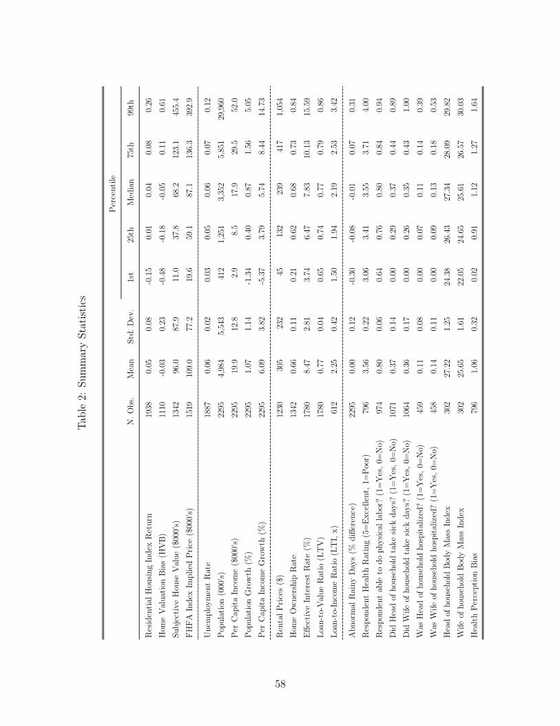
Table2:

SummaryStatist

ics

Perc

entil

e

N. O

bs.

Mea

nSt

d. D

ev.

1st

25th

Med

ian

75th

99th

Res

iden

tial H

ousin

g In

dex

Ret

urn

1938

0.05

0.08

-0.1

50.

010.

040.

080.

26H

ome

Val

uatio

n Bi

as (

HV

B)11

10-0

.03

0.23

-0.4

8-0

.18

-0.0

50.

110.

61Su

bjec

tive

Hou

se V

alue

($0

00's)

1342

96.0

87.9

11.0

37.8

68.2

123.

145

5.4

FHFA

Inde

x Im

plie

d Pr

ice

($00

0's)

1519

109.

077

.219

.659

.187

.113

6.3

392.

9

Une

mpl

oym

ent

Rat

e18

870.

060.

020.

030.

050.

060.

070.

12Po

pula

tion

(000

's)22

954,

984

5,54

341

21,

251

3,35

25,

851

29,9

60Pe

r C

apita

Inco

me

($00

0's)

2295

19.9

12.8

2.9

8.5

17.9

29.5

52.0

Popu

latio

n G

row

th (

%)

2295

1.07

1.14

-1.3

40.

400.

871.

565.

05Pe

r C

apita

Inco

me

Gro

wth

(%

)22

956.

093.

82-5

.37

3.79

5.74

8.44

14.7

3

Ren

tal P

rices

($)

1230

305

232

4513

223

941

71,

054

Hom

e O

wne

rshi

p R

ate

1342

0.66

0.11

0.21

0.62

0.68

0.73

0.84

Effe

ctiv

e In

tere

st R

ate

(%)

1780

8.47

2.81

3.74

6.47

7.83

10.1

315

.59

Loan

-to-

Val

ue R

atio

(LT

V)

1780

0.77

0.04

0.65

0.74

0.77

0.79

0.86

Loan

-to-

Inco

me

Rat

io (

LTI,

x)61

22.

250.

421.

501.

942.

192.

533.

42

Abn

orm

al R

ainy

Day

s (%

diff

eren

ce)

2295

0.00

0.12

-0.3

0-0

.08

-0.0

10.

070.

31R

espo

nden

t H

ealth

Rat

ing

(5=

Exce

llent

, 1=

Poor

)79

63.

560.

223.

063.

413.

553.

714.

00R

espo

nden

t ab

le t

o do

phy

sical

labo

r? (

1=Y

es, 0

=N

o)97

40.

800.

060.

640.

760.

800.

840.

94D

id H

ead

of h

ouse

hold

tak

e sic

k da

ys?

(1=

Yes

, 0=

No)

1071

0.37

0.14

0.00

0.29

0.37

0.44

0.89

Did

Wife

of h

ouse

hold

tak

e sic

k da

ys?

(1=

Yes

, 0=

No)

1064

0.36

0.17

0.00

0.26

0.35

0.43

1.00

Was

Hea

d of

hou

seho

ld h

ospi

taliz

ed?

(1=

Yes

, 0=

No)

459

0.11

0.08

0.00

0.07

0.11

0.14

0.39

Was

Wife

of h

ouse

hold

hos

pita

lized

? (1

=Y

es, 0

=N

o)45

80.

140.

110.

000.

090.

130.

180.

53H

ead

of h

ouse

hold

Bod

y M

ass

Inde

x30

227

.22

1.25

24.3

826

.43

27.3

428

.09

29.8

2W

ife o

f hou

seho

ld B

ody

Mas

s In

dex

302

25.6

51.

6122

.05

24.6

525

.61

26.5

730

.03

Hea

lth P

erce

ptio

n Bi

as79

61.

060.

320.

020.

911.

121.

271.

64

����������������������������������������������������������������������������������������������������������������������������������������������������������������������������������������������������������������������������������������������������������������������������������������������������������������������������������������������������������������������������������������������������������������������������������������������������������������������������������������������������������������������������������������������������������������������������������������������������������������������������������������������������������������������������������������������������������������������������������������������������������������������������������������������������������������������������������������������������������������������������������������������������������������������������������������������������������������������������������������������������������������������������������������������������������������������������������������������������������������������������������������������������������������������������������������������������������������������������������������������������������������������������������������������������������������������������������������������������������������������������������������������������������������������������������������������������������������������������������������������������������������������������������������������������������������������������������������������������������������������������������������������������������������������������������������������������������������������������������������������������������������������������������������������������������������������������������������������������������������������������������������������������������������������������������������������������������������������������������������������������������������������������������������������������������������������������������������������������������������������������������������������������������������������������

����������������������������������������������������������������������������������������������������������������������������������������������������������������������������������������������������������������������������������������������������������������������������������������������������������������������������������������������������������������������������������������������������������������������������������������������������������������������������������������������������������������������������������������������������������������������������������������������������������������������������������������������������������������������������������������������������������������������������������������������������������������������������������������������������������������������������������������������������������������������������������������������������������������������������������������������������������������������������������������������������������������������������������������������������������������������������������������������������������������������������������������������������������������������������������������������������������������������������������������������������������������������������������������������������������������������������������������������������������������������������������������������������������������������������������������������������������������������������������������������������������������������������������������������������������������������������������������������������������������������������������������������������������������������������������������������������������������������������������������������������������������������������������������������������������������������������������������������������������������������������������������������������������������������������������������������������������������������������������������������������������������������������������������������������������������������������������������������������������������������������������������������������������������������������

����������������������������������������������������������������������������������������������������������������������������������������������������������������������������������������������������������������������������������������������������������������������������������������������������������������������������������������������������������������������������������������������������������������������������������������������������������������������������������������������������������������������������������������������������������������������������������������������������������������������������������������������������������������������������������������������������������������������������������������������������������������������������������������������������������������������������������������������������������������������������������������������������������������������������������������������������������������������������������������������������������������������������������������������������������������������������������������������������������������������������������������������������������������������������������������������������������������������������������������������������������������������������������������������������������������������������������������������������������������������������������������������������������������������������������������������������������������������������������������������������������������������������������������������������������������������������������������������������������������������������������������������������������������������������������������������������������������������������������������������������������������������������������������������������������������������������������������������������������������������������������������������������������������������������������������������������������������������������������������������������������������������������������������������������������������������������������������������������������������������������������������������������������������������������

58

Table 3: Ex-Post Transition Probabilities of Estimation Bias

N. Obs. Low Average High Total

Low 368 67 4 439

Average 45 254 60 359

High 4 42 225 271

Fraction Low Average High Total

Low 0.838 0.153 0.009 1.00

Average 0.125 0.708 0.167 1.00

High 0.015 0.155 0.830 1.00

Low > 10% UndervaluationAverage Within 10% of Market ValueHigh > 10% Overvaulation

Subsequent Survey (t+1)Current Survey (t)

Current Survey (t)

���������������������������������������������������������������������������������������������������������������������������������������������������������������������������������������������������������������������������������������������������������������������������������������������������������������������������������������������������������������������������������������������������������������������������������������������������������������������������������������������������������������

����������������������������������������������������������������������������������������������������������������������������������������������������������������������������������������������������������������������������������������������������������������������������������������������������������������������������������������������������������������������������������������������������������������������������������������������������������������������������������������������������������

Note: Home valuation bias is grouped into three categories: greater than 10% overvaluation, greater than10% undervaluation, and within 10% of market prices implied by FHFA indices. The upper matrix providesthe number of U.S. states which transition between the three categories of home valuation bias. Transitionprobabilities in the lower matrix are expressed as a fraction of 1. All transitions are shown from one surveyyear to the next. From 1968 to 1997 this was on an annual basis. From 1999 to present, it is on a biannualbasis.

59

Table 4: Quantile Portfolio Means

Panel A: Market Expansions (Non-recessions)1-Year Forward Return (%)

Terciles Quintiles DecilesQuantiles Mean SE Mean SE Mean SE

1 5.282 (0.309) 5.448 (0.420) 5.241 (0.689)2 5.976 (0.330) 5.408 (0.361) 5.618 (0.519)3 6.532 (0.415) 5.684 (0.452) 5.304 (0.532)4 6.452 (0.449) 5.526 (0.482)5 6.655 (0.577) 5.917 (0.676)6 5.451 (0.605)7 6.399 (0.584)8 6.504 (0.684)9 6.287 (0.763)10 7.103 (0.883)

High minus Low 1.250 (0.517) 1.207 (0.714) 1.862 (1.120)p-value [0.016] [0.092] [0.099]

Panel B: Market Contractions (NBER Recessions)1-Year Forward Return (%)

Terciles Quintiles DecilesQuantiles Mean SE Mean SE Mean SE

1 2.181 (0.558) 2.172 (0.766) 2.940 (1.296)2 1.800 (0.625) 1.894 (0.631) 1.558 (0.915)3 0.865 (0.887) 2.036 (0.825) 2.492 (0.885)4 1.675 (0.988) 1.221 (0.897)5 0.242 (1.247) 2.297 (0.885)6 1.767 (1.417)7 1.803 (1.366)8 1.555 (1.442)9 0.564 (1.441)10 -0.157 (2.176)

High minus Low -1.316 (1.047) -1.930 (1.464) -3.097 (2.532)p-value [0.211] [0.190] [0.228]

Note: States are ranked by the degree of home valuation bias and sorted into terciles, quintiles, and deciles bymacroeconomic environment. Market expansions are all years without an NBER recession quarter. Marketcontractions are any years in which an NBER recession quarter was recorded. Returns are calculated fromFHFA indices over the subsequent year. High minus Low is the portfolio which hypothetically purchaseshomes in states with a high home valuation bias and sells homes in states with a low home valuation bias.

60

Table 5: Overestimates Increase Future Real Estate Returns

1-Year Forward FHFA Index Returns (%)

IV

OLS Weather Health All

(1) (2) (3) (4) (5) (6)

Home Valuation Bias (HVB) 0.296 0.315 0.550 1.813 1.829 2.429[0.002] [0.002] [0.035] [0.104] [0.213] [0.021]0 0 0 0 0 0

Current FHFA Return 2.926 2.532 2.666 2.758 6.341 6.317[0.000] [0.003] [0.000] [0.000] [0.000] [0.000]0 0 0 0 0 0

1-Yr Lagged FHFA Return 1.298 1.054 0.534 0.662 -1.306 -1.192[0.018] [0.043] [0.260] [0.133] [0.030] [0.054]

Economic Controls No Yes Yes Yes Yes YesHousing Market Controls No No Yes Yes Yes YesYear Fixed Effects Yes Yes Yes Yes Yes YesRegion Fixed Effects No No Yes Yes Yes Yes

Observations 1076 1076 893 893 682 682R-Squared 0.574 0.593 0.606 0.581 0.710 0.677First Stage F -statistic 11.251 10.170 8.177J statistic p -value 0.425

p -values in brackets. Standard errors clustered at the state level.

Note: The dependent variables in each regressions of Table 5 is the forward 1-year annual return calculatedusing FHFA indices. Home valuation bias (HVB) is the subjective estimate of single-family home valueprovided by PSID respondents scaled by the market values of single-family home prices obtained fromFHFA indices. Economic control variables include unemployment rate, population level (log), income level(log), population growth, and income growth. Housing market control variables include capitalization rate,ownership rate, mortgage interest rate, and loan-to-value ratio. Control variables are discussed in greaterdetail in Appendix I. Weather is the abnormal number of days with precipitation greater than or equal to0.1 inches relative to the statewide average over the entire NOAA sample period starting from 1968. Healthis a variable which measures a person’s self-reported health relative to his report of various health issues.These health issues include hospitalization history, the use of sick days, the physical ability to do work, andthe risk of health complications arising from obesity (approximated by the respondent’s body-mass-index).All covariates are standardized. Standard errors are clustered by state. p-values are reported in brackets.

61

Table 6: Overestimated Markets more Fragile in Recession

1-Year Forward Returns (%)

OLS IV (Both)

(1) (2) (3) (4)

Home Valuation Bias (HVB) 0.417 0.715 0.738 6.816[0.001] [0.000] [0.001] [0.002]0 0 0 0

NBER Recession -2.741 -2.697 -2.731 -0.793[0.000] [0.000] [0.000] [0.412]0 0 0 0

HVB * NBER Recession -1.299 -1.301 -1.137 -7.363[0.000] [0.000] [0.067] [0.004]0 0 0 0

Current FHFA Return 4.012 3.677 3.593 6.468[0.000] [0.000] [0.000] [0.000]0 0 0 0

1-Yr Lagged FHFA Return 0.332 0.066 -0.347 -1.761[0.587] [0.903] [0.459] [0.010]

Economic Controls No Yes Yes YesHousing Market Controls No No Yes YesRegion Fixed Effects No No Yes Yes

Observations 1076 1076 895 684R-Squared 0.385 0.417 0.437 0.226First Stage F -statistic 4.795J statistic p -value 0.762

p -values in brackets. Standard errors clustered at the state level.

Note: The dependent variables in each regressions of Table 6 is the forward 1-year annual return calculatedusing FHFA indices. Home valuation bias (HVB) is the subjective estimate of single-family home valueprovided by PSID respondents scaled by the market values of single-family home prices obtained from FHFArepeat-sales indices. Economic control variables include unemployment rate, population level (log), incomelevel (log), population growth, and income growth. Housing market control variables include capitalizationrate, ownership rate, mortgage interest rate, and loan-to-value ratio. Control variables are discussed ingreater detail in Appendix I. The NBER recession indicator is a time-series variable, taking a value of onefor any year in which a recession quarter was recorded and zero elsewhere. Only the instrumental variablesapproach using both weather and health is reported. All covariates are standardized. Standard errors areclustered by state. p-values are reported in brackets.

62

Table 7: Asymmetric effects on leverage risk

Loan-to-Value Ratio (%) Loan-to-Income Ratio (x)

(1) (2) (3) (4) (5) (6)

Home Valuation Bias (HVB) -0.984 -0.685 -0.371 0.153 0.064 0.074[0.002] [0.012] [0.138] [0.001] [0.080] [0.017]0 0 0 0 0 0

Current FHFA Return -0.950 -0.984 -1.153 -0.049 -0.065 -0.028[0.000] [0.000] [0.000] [0.115] [0.035] [0.340]0 0 0 0 0 0

1-Yr Lagged FHFA Return -0.678 -0.537 -0.278 0.178 0.088 0.053[0.001] [0.027] [0.289] [0.000] [0.047] [0.155]

Economic Controls No Yes Yes No Yes YesHousing Market Controls No No Yes No No YesYear Fixed Effects Yes Yes Yes Yes Yes YesRegion Fixed Effects No No Yes No No Yes

Observations 1007 1007 894 190 190 190R-Squared 0.326 0.436 0.498 0.343 0.613 0.797

p -values in brackets. Standard errors clustered at the state level.

Note: Loan-to-value (LTV) is the dependent variable in columns 1-3 while loan-to-income (LTI) is the depen-dent variable in columns 4-6. LTV is taken from a sample of survey responses on single-family homes fromthe Monthly Interest Rate survey of the FHFA from 1978 to 2012. LTI is calculated from loan applicationsrecorded by the HMDA from 2000 to 2011. Home valuation bias (HVB) is the subjective estimate of single-family home value provided by PSID respondents scaled by the market values of single-family home pricesobtained from FHFA repeat-sales indices. Control variables include unemployment rate, population, income,capitalization rate, ownership rate, and mortgage interest rate by state and are discussed in Appendix I. Allcovariates are standardized. Standard errors are clustered by state. p-values are reported in brackets.

63

Table8:

Con

sistencywith

Vario

usTheoriesof

Asset

Prices

Overestimation of hom

e prices is related to…

Rational

BWSX

HS

BSV

DHS

(1)

Higher returns 1-yr forw

ard

��

��

��

(2)

Lower returns 1-yr forw

ard durin

g recessions

��

��

(3)

Stronger effects when current returns are high

��

��

(4)

Higher returns controlling for past returns

��

��

(5)

Positive cumulative returns up to 11 years out

��

��

��

(6)

Negative cumulative returns over next 19 years

��

��

�

(7)

Lower loan-to-value ratio

s�

??

??

?(8)

Higher loan-to-income ratio

s�

??

??

?

BW - Ba

ker and Wurgler (2006)

SX - Scheinkm

an and Xiong (2003)

HS - H

ong and Stein (1999)

BSV - Ba

rberis, Shleifer, Vish

ny (1998)

DHS - D

aniel, Hirshleifer, and Subrahmanyam (1998)

Behavioral

Note:

Fore

achem

piric

alfact

documentedin

thispa

per,acheckmark“!

”ap

pearsu

nder

theap

prop

riate

theory

containing

mecha

nism

swhich

could

generate

such

apredictio

n.Questionmarks

“?”ap

pear

underbe

havioral

theorie

sbe

causethesemod

elsdo

notad

dressleverage

patterns.

64