Japan Advanced Institute of Science and Technology

JAIST Repositoryhttps://dspace.jaist.ac.jp/

TitleStudy of predictive thermal comfort control for

cyber-physical smart home system

Author(s)OOI, Sian En; MAKINO, Yoshiki; FANG, Yuan; LIM,

Yuto; TAN, Yasuo

Citation IEICE Technical Report, 117(426): 29-34

Issue Date 2018-01-23

Type Journal Article

Text version publisher

URL http://hdl.handle.net/10119/15491

Rights

Copyright (C) 2018 The Institute of Electronics,

Information and Communication Engineers (IEICE).

Sian En OOI, Yoshiki MAKINO, Yuan FANG, Yuto LIM,

and Yasuo TAN, IEICE Technical Report, 117(426),

2018, 29-34.

Description

一般社団法人 電子情報通信学会 信学技報 THE INSTITUTE OF ELECTRONICS, IEICE Technical Report INFORMATION AND COMMUNICATION ENGINEERS

This article is a technical report without peer review, and its polished and/or extended version may be published elsewhere.

Copyright ©20●● by IEICE

Study of Predictive Thermal Comfort Control for Cyber-Physical Smart Home System

Sian En OOI† Yoshiki MAKINO† Yuan FANG†† Yuto LIM† Yasuo TAN†

†Japan Advanced Institute of Science and Technology, 1-1 Asahidai, Nomi City, Ishikawa Prefecture, 923-1292 Japan

††Dalian Polytechnic University, Qinggongyuan 1#, Dalian, Liaoning, China E-mail: †{sianen.ooi, m-yoshi, ylim, ytan}@jaist.ac.jp, ††fangy@dlpu.edu.cn

Abstract Classical control methods such proportional integral derivative (PID) are common in thermal comfort control

applications as they are lightweight in terms of the computing power and well-received in the industry sector. Such thermal comfort classical controllers often suffer from non-optimal control input as they do not anticipate any future process. In this paper, we present a model predictive control (MPC) based thermal comfort system, which also incorporates the cyber-physical systems (CPS) approach into the system. The proposed system is evaluated and verified in a cyber-physical smart home system simulation using raw environmental data from the experimental smart house, iHouse.

Keywords Model Predictive Control, iHouse, Cyber-Physical Systems, Smart Homes, Thermal Comfort 1. INTRODUCTION

Recent increase in home automation efforts validates the growing importance of improving quality of life (QOL) and energy efficiency, especially in residential and office buildings [1,2]. Besides, many vital elements in a smart home coincide with the cores of CPS, which rationalizes the need of CPS in smart homes.

Our previous effort in application of CPS in smart homes involves the Energy Efficient Thermal Comfort Control (EETCC) algorithm [3] and its implementation in an actual experimental smart home [4]. EETCC aims to promote energy efficient by prioritizing the utilization of natural resource to maintain thermal comfort than using HVAC (heating, ventilation and air-conditioner) system. Although EETCC achieved its goals, it is still a reactive controller by design that suffers from non-optimal control strategy as it senses and estimates deviations in thermal comfort level without foreseeing any future events. Thus, to address this shortcoming, this paper aims to implement predictive thermal comfort controller into the smart home environment using CPS approach. By integrating predictive capability, controller should be able to compute optimal control strategies to further enhance energy efficiency and thermal comfort in CPS home systems.

The rest of the paper is organized as follows. Section 2 introduces the background on relevant topics to this paper. The EETCC system, plant modeling and MPC controller details are described in Section 3. Proposed controllers are simulated under various seasons while its results and discussions are presented in Section 4. Finally, some

relevant conclusions and future works are summarized in Section 5.

2. BACKGROUND 2.1. Cyber-Physical Systems

CPS encompass many real-life systems today, where their physical and computational resources are strictly interlinked together [5]. CPS often requires deep integration between sensing, computation, communication and control, which shares a lot of similarities to the more popular term: Internet-of-Things (IoT). However, IoT slightly differs from CPS as it focused on the openness of the system while CPS focused on the closed-loop system.

2.2. iHouse iHouse is an advanced experimental smart house,

located at Nomi City, Ishikawa prefecture, Japan as shown in Fig. 1. It is a conventional two-floor Japanese-styled house featuring more than 300 sensors, home appliances, and electronic house devices that are connected using ECHONET Lite version 1.1 and ECHONET version 3.6.

Fig. 1: iHouse – experiment house of smart homes.

一般社団法人 電子情報通信学会 信学技報 THE INSTITUTE OF ELECTRONICS, IEICE Technical Report INFORMATION AND COMMUNICATION ENGINEERS ASN2017-88 (2018-01)

Copyright ©2018 by IEICE This article is a technical report without peer review, and its polished and/or extended version may be published elsewhere.

- 29 -

2.3. Thermal Comfort Thermal comfort is defined as the state of the mind that

expresses satisfaction with its thermal surrounding [6]. Temperature only control systems are commonly used to regulate thermal level in indoor spaces. However, thermal comfort takes into account many factors such as wind speed, humidity, metabolic rate, clothing insulation and radiant temperature [6]. Thus, thermal comfort regulation not only provides greater comfort but also the possibility of energy saving when compared to regulation of air temperature. Predicted Mean Vote (PMV) thermal comfort is described by a seven-point thermal sensation scale, where hot sensations are depicted by positive numbers and cold sensations are depicted by negative numbers.

3. THERMAL COMFORT CONTROL SYSTEM 3.1. EETCC System Architecture

The EETCC system architecture is shown in Fig. 2, which is comprised of three main components: (i) controller; (ii) communication protocol; and (iii) plant. The plant simulated in this paper is the iHouse Bedroom A. Modeling of the plant and controllers are discussed while networking components are excluded in this paper.

Fig. 2: System architecture.

3.2. Mathematical Representation The plant room temperature can be modeled with heat

equations. Thus, the dynamic room temperature equation of the plant model is given by

𝑑𝑑𝑇𝑇#$$%𝑑𝑑𝑑𝑑

=1𝛽𝛽

𝑄𝑄+,, (1)

where 𝑇𝑇#$$% is the temperature of the room in ℃, 𝛽𝛽 is the product of air density in 𝑘𝑘𝑘𝑘/𝑚𝑚2, volume of the room in 𝑚𝑚2 and specific heat capacity of air in 𝑘𝑘𝑘𝑘/𝑘𝑘𝑘𝑘℃. 𝑄𝑄+,, is the total heat gain of the room, which comprised of heat gain from HVAC, conduction and solar radiation through window and occupants in the room.

The heat gain from the HVAC is can be given by

𝑄𝑄+4#5$67 = 1.08×𝐶𝐶𝐶𝐶𝐶𝐶× 𝑇𝑇?@A − 𝑇𝑇#$$% (2)

where 𝐶𝐶𝐶𝐶𝐶𝐶 is the room volumetric airflow in 𝑓𝑓𝑑𝑑2/𝑚𝑚𝑚𝑚𝑚𝑚 and 𝑇𝑇?@A is the setting temperature of HVAC in ℃.

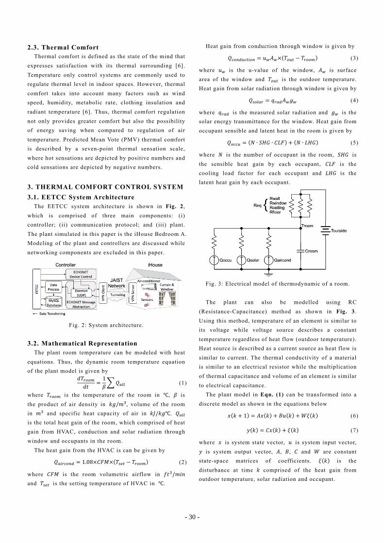
Heat gain from conduction through window is given by

𝑄𝑄5$67F5A4$6 = 𝑢𝑢H𝐴𝐴H× 𝑇𝑇$FA − 𝑇𝑇#$$% (3)

where 𝑢𝑢H is the u-value of the window, 𝐴𝐴H is surface area of the window and 𝑇𝑇$FA is the outdoor temperature. Heat gain from solar radiation through window is given by

𝑄𝑄?$,+# = 𝑞𝑞#+7𝐴𝐴H𝑘𝑘H (4)

where 𝑞𝑞#+7 is the measured solar radiation and 𝑘𝑘H is the solar energy transmittance for the window. Heat gain from occupant sensible and latent heat in the room is given by

𝑄𝑄$55F = 𝑁𝑁 ∙ 𝑆𝑆𝑆𝑆𝑆𝑆 ∙ 𝐶𝐶𝐶𝐶𝐶𝐶 + 𝑁𝑁 ∙ 𝐶𝐶𝑆𝑆𝑆𝑆 (5)

where 𝑁𝑁 is the number of occupant in the room, 𝑆𝑆𝑆𝑆𝑆𝑆 is the sensible heat gain by each occupant, 𝐶𝐶𝐶𝐶𝐶𝐶 is the cooling load factor for each occupant and 𝐶𝐶𝑆𝑆𝑆𝑆 is the latent heat gain by each occupant.

Fig. 3: Electrical model of thermodynamic of a room.

The plant can also be modelled using RC

(Resistance-Capacitance) method as shown in Fig. 3. Using this method, temperature of an element is similar to its voltage while voltage source describes a constant temperature regardless of heat flow (outdoor temperature). Heat source is described as a current source as heat flow is similar to current. The thermal conductivity of a material is similar to an electrical resistor while the multiplication of thermal capacitance and volume of an element is similar to electrical capacitance.

The plant model in Eqn. (1) can be transformed into a discrete model as shown in the equations below

𝑥𝑥 𝑘𝑘 + 1 = 𝐴𝐴𝑥𝑥 𝑘𝑘 + 𝐵𝐵𝑢𝑢 𝑘𝑘 +𝑊𝑊𝑊𝑊 𝑘𝑘 (6)

𝑦𝑦 𝑘𝑘 = 𝐶𝐶𝑥𝑥 𝑘𝑘 + 𝑊𝑊 𝑘𝑘 (7)

where 𝑥𝑥 is system state vector, 𝑢𝑢 is system input vector, 𝑦𝑦 is system output vector, 𝐴𝐴, 𝐵𝐵, 𝐶𝐶 and 𝑊𝑊 are constant state-space matrices of coefficients. 𝑊𝑊 𝑘𝑘 is the disturbance at time 𝑘𝑘 comprised of the heat gain from outdoor temperature, solar radiation and occupant.

- 30 -

3.3. MPC Controller The section will discuss about MPC formulation,

especially on the optimization problem for various control strategies. A general MPC controller is shown in Fig. 4, where process block is the plant, prediction block is MPC internal estimated plant and optimization block performs control signal optimization with respect to the imposed cost and constraints. The plant is the iHouse Bedroom A, where its input is HVAC cooling or heating power and its output is the temperature of the room.

Fig. 4: MPC controller system.

A general optimization problem can be formulated

where its cost function, 𝐽𝐽W penalizes both the output deviation from the reference set point and the plant input control error can be given by

𝐽𝐽W = 𝑤𝑤4Y 𝑟𝑟 𝑘𝑘 + 𝑖𝑖|𝑘𝑘 − 𝑦𝑦 𝑘𝑘 + 𝑖𝑖|𝑘𝑘

\6]

4^_

+ 𝑤𝑤4∆F ∆𝑢𝑢 𝑘𝑘 + 𝑖𝑖|𝑘𝑘\

6ab_

4^c

(8)

where 𝑛𝑛Y is the prediction horizon, 𝑛𝑛F is the input

horizon, 𝑤𝑤4Y is the plant output tuning weight at 𝑖𝑖 th

prediction horizon step, 𝑤𝑤4∆F is the change in plant input tuning weight at 𝑖𝑖 th prediction horizon step, 𝑟𝑟 is the reference, 𝑦𝑦 is the predicted output and ∆𝑢𝑢 𝑘𝑘 + 𝑖𝑖|𝑘𝑘 is the change in the optimal plant input signal at time 𝑘𝑘 + 𝑖𝑖 computed at interval 𝑘𝑘.

Every sensors and actuators have their performance limits. Since HVAC is used to cool and heat the room, it has its saturation point which can be defined as hard constraints in MPC formulation. Hence, hard constraint based on both HVAC saturation points, 𝑢𝑢%46 and 𝑢𝑢%+d can be presented as

𝑢𝑢%46 ≤ 𝑢𝑢 𝑘𝑘 + 𝑖𝑖|𝑘𝑘 ≤ 𝑢𝑢%+d (9)

A) Temperature Boundary, PMV Boundary and Temperature Reference Optimization

This control strategy performs similarly to classical PID controller as tracking reference signal is their main objective. Multiple constraints can also be imposed on

MPC, where in scenarios such as the given reference signal is out-of-bound, the MPC controller will attempt to satisfy the reference signal without violating any of its constraints. Similar implementation with PID controller would be complex.

The cost function for this control strategy is shown in Eqn. (8), where the sum of both tracking error and input control error are minimized while bounded by the following constraints

𝑢𝑢%46 ≤ 𝑢𝑢 𝑘𝑘 + 𝑖𝑖|𝑘𝑘 ≤ 𝑢𝑢%+d𝑦𝑦A,%46 ≤ 𝑦𝑦A 𝑘𝑘 + 𝑖𝑖|𝑘𝑘 ≤ 𝑦𝑦A,%+d

𝑦𝑦ghi,%46 ≤ 𝑦𝑦ghi 𝑘𝑘 + 𝑖𝑖|𝑘𝑘 ≤ 𝑦𝑦ghi,%+d (10)

where 𝑦𝑦A is the plant output temperature, 𝑦𝑦ghi is the computed plant PMV, 𝑦𝑦A,%46 and 𝑦𝑦A,%+d are the plant output temperature boundary, 𝑦𝑦ghi,%46 and 𝑦𝑦ghi,%+d are

the plant PMV boundary. B) PMV Boundary and Minimizing Energy Cost

This control strategy objective is to minimize the energy consumption of HVAC while maintaining thermal comfort according to ASHRAE standards. The cost function can be given by

𝐽𝐽W = 𝑤𝑤4F 𝑢𝑢 𝑘𝑘 + 𝑖𝑖|𝑘𝑘 − 𝑢𝑢A+#j@A 𝑘𝑘 + 𝑖𝑖|𝑘𝑘\

6a

4^_

(11)

where 𝑤𝑤4F is the plant input tuning weight at 𝑖𝑖 th prediction horizon step and 𝑢𝑢A+#j@A is the target reference

for the plant input. The plant input target reference can be represented by the availability of green energy, variable rate energy tariff or just a nominal value for the energy consumption optimization.

While minimizing energy consumption, the optimizer is also bounded by the following constraints

𝑢𝑢%46 ≤ 𝑢𝑢 𝑘𝑘 + 𝑖𝑖|𝑘𝑘 ≤ 𝑢𝑢%+d𝑦𝑦ghi,%46 ≤ 𝑦𝑦ghi 𝑘𝑘 + 𝑖𝑖|𝑘𝑘 ≤ 𝑦𝑦ghi,%+d

(12)

4. NUMERICAL SIMULATION This section investigates the performance of MPC under

various constraints, where PID is used as baseline controller. The simulation utilizes outdoor environment data from the iHouse that are sampled every 10 second. Hence, the time-step size for the simulation is 10 second. The MPC sample time is also equal to the simulation time-step while its prediction and control horizon is configured to 5 minutes. The prediction horizon used in this simulation is very short when compared with most MPC implementations. This is due to the sampling time of most MPC implementation are generally about 1 hour, justifying their long prediction time horizon between 5 to 48 hours [7].

- 31 -

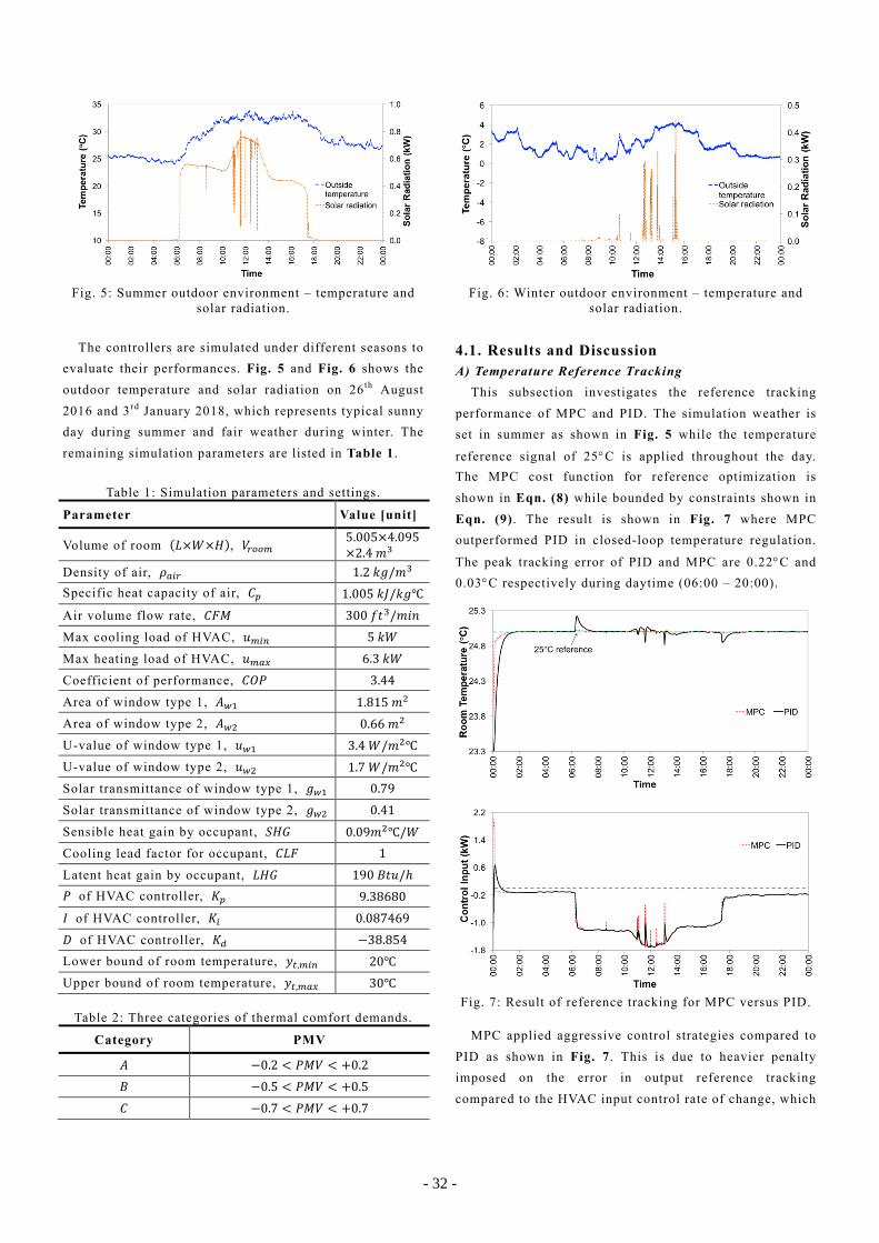
Fig. 5: Summer outdoor environment – temperature and

solar radiation.

The controllers are simulated under different seasons to evaluate their performances. Fig. 5 and Fig. 6 shows the outdoor temperature and solar radiation on 26th August 2016 and 3rd January 2018, which represents typical sunny day during summer and fair weather during winter. The remaining simulation parameters are listed in Table 1.

Table 1: Simulation parameters and settings.

Parameter Value [unit]

Volume of room 𝐿𝐿×𝑊𝑊×𝐻𝐻 , 𝑉𝑉#$$% 5.005×4.095×2.4𝑚𝑚2

Density of air, 𝜌𝜌+4# 1.2𝑘𝑘𝑘𝑘/𝑚𝑚2 Specific heat capacity of air, 𝐶𝐶r 1.005𝑘𝑘𝑘𝑘/𝑘𝑘𝑘𝑘℃

Air volume flow rate, 𝐶𝐶𝐶𝐶𝐶𝐶 300𝑓𝑓𝑓𝑓2/𝑚𝑚𝑚𝑚𝑚𝑚

Max cooling load of HVAC, 𝑢𝑢%46 5𝑘𝑘𝑊𝑊

Max heating load of HVAC, 𝑢𝑢%+d 6.3𝑘𝑘𝑊𝑊

Coefficient of performance, 𝐶𝐶𝐶𝐶𝐶𝐶 3.44

Area of window type 1, 𝐴𝐴H_ 1.815𝑚𝑚\ Area of window type 2, 𝐴𝐴H\ 0.66𝑚𝑚\ U-value of window type 1, 𝑢𝑢H_ 3.4𝑊𝑊/𝑚𝑚\℃ U-value of window type 2, 𝑢𝑢H\ 1.7𝑊𝑊/𝑚𝑚\℃ Solar transmittance of window type 1, 𝑘𝑘H_ 0.79

Solar transmittance of window type 2, 𝑘𝑘H\ 0.41

Sensible heat gain by occupant, 𝑆𝑆𝐻𝐻𝑆𝑆 0.09𝑚𝑚\℃/𝑊𝑊 Cooling lead factor for occupant, 𝐶𝐶𝐿𝐿𝐶𝐶 1

Latent heat gain by occupant, 𝐿𝐿𝐻𝐻𝑆𝑆 190𝐵𝐵𝑓𝑓𝑢𝑢/ℎ 𝐶𝐶 of HVAC controller, 𝐾𝐾r 9.38680

𝐼𝐼 of HVAC controller, 𝐾𝐾4 0.087469

𝐷𝐷 of HVAC controller, 𝐾𝐾7 −38.854 Lower bound of room temperature, 𝑦𝑦A,%46 20℃ Upper bound of room temperature, 𝑦𝑦A,%+d 30℃

Table 2: Three categories of thermal comfort demands.

Category PMV

𝐴𝐴 −0.2 < 𝐶𝐶𝐶𝐶𝑉𝑉 < +0.2

𝐵𝐵 −0.5 < 𝐶𝐶𝐶𝐶𝑉𝑉 < +0.5

𝐶𝐶 −0.7 < 𝐶𝐶𝐶𝐶𝑉𝑉 < +0.7

Fig. 6: Winter outdoor environment – temperature and

solar radiation.

4.1. Results and Discussion A) Temperature Reference Tracking

This subsection investigates the reference tracking performance of MPC and PID. The simulation weather is set in summer as shown in Fig. 5 while the temperature

reference signal of 25°C is applied throughout the day. The MPC cost function for reference optimization is shown in Eqn. (8) while bounded by constraints shown in Eqn. (9). The result is shown in Fig. 7 where MPC outperformed PID in closed-loop temperature regulation.

The peak tracking error of PID and MPC are 0.22°C and 0.03°C respectively during daytime (06:00 – 20:00).

Fig. 7: Result of reference tracking for MPC versus PID.

MPC applied aggressive control strategies compared to

PID as shown in Fig. 7. This is due to heavier penalty imposed on the error in output reference tracking compared to the HVAC input control rate of change, which

- 32 -

MPC will compute the required cooling or heating power to minimize the error in the shortest time without violating its pre-defined constraints. Thus, MPC temperature regulation is better than PID even under large disturbance. This is consistent with the transient analysis results shown in Fig. 8 and Table 3. Rise time is the time taken for the controller response to increase from 10% of its steady-state value to 90% of output reference while settling time is the time taken for the controller response reach and stay within 5% of the output reference signal.

Fig. 8: Comparison between MPC and PID step response.

Table 3: Three categories of thermal comfort demands.

Controller Rise Time (s) Settling Time (s)

𝑃𝑃𝑃𝑃𝑃𝑃 208.89 293.13

𝑀𝑀𝑃𝑃𝑀𝑀 114.80 135.65

B) PMV Boundary and Energy Minimization Based MPC Optimization

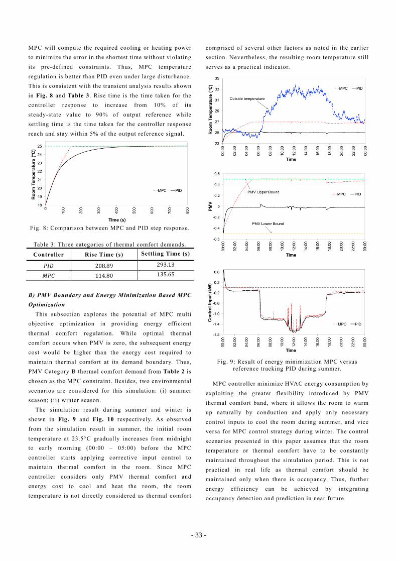
This subsection explores the potential of MPC multi objective optimization in providing energy efficient thermal comfort regulation. While optimal thermal comfort occurs when PMV is zero, the subsequent energy cost would be higher than the energy cost required to maintain thermal comfort at its demand boundary. Thus, PMV Category B thermal comfort demand from Table 2 is chosen as the MPC constraint. Besides, two environmental scenarios are considered for this simulation: (i) summer season; (ii) winter season.

The simulation result during summer and winter is shown in Fig. 9 and Fig. 10 respectively. As observed from the simulation result in summer, the initial room

temperature at 23.5°C gradually increases from midnight to early morning (00:00 – 05:00) before the MPC controller starts applying corrective input control to maintain thermal comfort in the room. Since MPC controller considers only PMV thermal comfort and energy cost to cool and heat the room, the room temperature is not directly considered as thermal comfort

comprised of several other factors as noted in the earlier section. Nevertheless, the resulting room temperature still serves as a practical indicator.

Fig. 9: Result of energy minimization MPC versus

reference tracking PID during summer.

MPC controller minimize HVAC energy consumption by exploiting the greater flexibility introduced by PMV thermal comfort band, where it allows the room to warm up naturally by conduction and apply only necessary control inputs to cool the room during summer, and vice versa for MPC control strategy during winter. The control scenarios presented in this paper assumes that the room temperature or thermal comfort have to be constantly maintained throughout the simulation period. This is not practical in real life as thermal comfort should be maintained only when there is occupancy. Thus, further energy efficiency can be achieved by integrating occupancy detection and prediction in near future.

- 33 -

Fig. 10: Result of energy minimization MPC versus

reference tracking PID during winter. C) Energy Consumption

This subsection focuses on the energy consumption of control strategies by MPC and PID that are simulated in this paper. The energy consumption of HVAC is given by

𝐸𝐸+4#5$67 =1𝐶𝐶𝐶𝐶𝐶𝐶

𝑄𝑄+4#5$67 𝑡𝑡 𝑑𝑑𝑡𝑡A~�€

AÅ‚ƒ„‚ (13)

where 𝐶𝐶𝐶𝐶𝐶𝐶 is the coefficient of performance, 𝑡𝑡?A+#A and 𝑡𝑡@67 is the start and end time of the simulation. Fig. 11 shows that PID utilize more energy compared to various MPC controllers except for reference optimization MPC in summer. Aggressive control strategy by reference optimization MPC during summer contributes to lower tracking error at the expense of higher energy consumption.

Comparing reference optimization MPC to PMV bound energy minimization MPC, improvements of 10.4% and

12.1% is observed during summer and winter respectively. This improvement is also consistent with other research finding [8].

Fig. 11: Comparison between multiple controller energy

consumptions for summer and winter.

5. CONCLUDING REMARKS This paper summarizes the implementation details of

MPC in smart home environment using CPS approach. Various MPC implementations are carried out under two seasons to evaluate the performance and advantages of predictive capabilities in the domain of thermal comfort control. Simulations showed improvements in both temperature reference tracking and PMV boundary energy minimization based MPC. Further work can be expanded to economic based controller that takes into account the availability of green energy and electricity tariff.

References [1] C. Wilson, T. Hargreaves, R. Hauxwell-Baldwin,

“Benefits and risks of smart home technologies”, Energy Policy, pp.72-83, 2017.

[2] G. Lobaccaro, S. Carlucci, E. Löfström, “A Review of Systems and Technologies for Smart Homes and Smart Grids”, Energies, pp.348-380, 2016.

[3] Z. Cheng, W.W. Shein, Y. Tan, A.O. Lim, “Energy efficient thermal comfort control for cyber-physical home system”, IEEE Int. Conf. on Smart Grid Comm., pp.797-802, 2013.

[4] Y. Lim, S.E. Ooi, M. Yoshiki, T.K. Teo, R. Alfred, Y. Tan, “Implementation of Energy Efficient Thermal Comfort Control for Cyber-Physical Home Systems”, Advanced Science Letters, pp.400-407, 2016.

[5] S. Zanero, “Cyber-Physical Systems”, Computer, pp.14-16, 2017.

[6] ASHRAE Standard 55-2010, “Thermal Environment Conditions for Human Occupancy”, 2010.

[7] A. Afram, F. Janabi-Sharifi, “Theory and applications of HVAC control systems – a review of model predictive control (MPC)”, Building and Environment, pp.343-355, 2014.

[8] J. Cigler, S. Prívara, Z. Vána, E. Žáčeková, L. Ferkl, “Optimization of Predicted Mean Vote index within Model Predictive Control framework: Computationally tractable solution”, Energy and Building, pp.39-49, 2012.

- 34 -