study of fractional order integro-differential equations...

© 2017 Sarkhosh S. Chaharborj, Shahriar S. Chaharborj and Yaghoub Mahmoudi. This open access article is distributed

under a Creative Commons Attribution (CC-BY) 3.0 license.

Journal of Mathematics and Statistics

Original Research Paper

Study of Fractional Order Integro-Differential Equations by

using Chebyshev Neural Network

1Sarkhosh S. Chaharborj,

2Shahriar S. Chaharborj and

3Yaghoub Mahmoudi

1School of Mathematics and Statistics, Carleton University, Ottawa, Canada 2Department of Mathematics, Islamic Azad University, Bushehr Branch, Bushehr, Iran 3Department of Mathematics, Tabriz Branch, Islamic Azad University, Tabriz, Iran

Article history

Received: 11-04-2016

Revised: 01-02-2017

Accepted: 06-02-2017

Corresponding Author:

Sarkhosh S. Chaharborj

School of Mathematics and

Statistics, Carleton University,

Ottawa, Canada Email: [email protected]

Abstract: Recently fractional integro-differential equations have been

proposed for the modeling of many complex systems. Simulation of these

equations requires the development of suitable numerical methods. This

paper is devoted to finding the numerical solution of some classes of

fractional integro-differential equations by employing the Chebyshev

Neural Network (ChNN). The accuracy of proposed method is shown by

comparing the numerical results computed by using Chebyshev neural

network method with the analytical solution.

Keywords: Integro-Differential Equations, Fractional Order, Chebyshev

Neural Network, Error Back Propagation Algorithm, Feed Forward Neural

Network

Introduction

Numerical methods are very power tools for solving

the complicated problems in many fields (Bianca et al.,

2009; Bhrawy and Alghamdi, 2012; Yang et al., 2014;

Bhrawy and Aloi, 2013; Doha et al., 2011;

Irandoust-Pakchin et al., 2013; Irandoust-Pakchin and

Abdi-Mazraeh, 2013; Saha Ray, 2009; Mittal and

Nigam, 2008; Saeedi and Samimi, 2012; Saeed and

Sdeq, 2010; Ahmed and Salh, 2011). Newly, few

numerical methods for solving the Fractional

Differential Equations (FDEs) and Fractional Integro-

Differential Equations (FIDEs) have been presented.

Bhrawy and Alghamdi (2012; Yang et al., 2004) used

collocation method to solve the nonlinear fractional

Langevin equation involving two fractional orders in

different intervals and the fractional Fredholm

Integro-differential equations. Doha et al. (2011;

Bhrawy and Aloi, 2003; Irandoust-pakchin et al.,

2013), proposed the Chebyshev polynomials method

to solve the nonlinear Volterra and the Fredholm

Integro-differential equations of fractional order and

the multiterm fractional orders differential equations.

Irandoust-Pakchin and Abdi-Mazraeh (2013) applied

the variational iteration method to solve the fractional

Integro-differential equations with the nonlocal

boundary conditions. Few other methods presented for

solving the fractional diffusion; the fractional Integro-

differential and the fractional nonlinear Fredholm

Integro-differential equations in (Saha Ray, 2009;

Mittal and Nigam, 2008; Saeedi and Samimi, 2012;

Saeed and Sdeq, 2010).

In this study, Chebyshev neural network method

with a unit layer has been proposed to solve the

integro-differential equations from fractional order.

To minimize the computed error function, a neural

network with feed forward and with fundamental error

back propagation will be used. This paper deals with

numerical analysis of fractional order integro-

differential equation as follows:

( ) ( ) ( ) ( )

( ) ( )

1

2

,

, , ,

x

a

b

a

D y x g x f x y d

f x y d a x b

α τ τ τ

τ τ τ τ

= +

+ ≤ ≤

∫

∫ (1)

with the following initial conditions:

( ) ( )0 , 1 ,i

iy n n n Nβ α= − < ≤ ∈

The problem of the nonlinear multi-order fractional

differential equations studies by using the Chebyshev

neural network to obtain the numerical results. The

hidden layer was excluded by extending the input style

by the Chebyshev polynomials and has been used a

single layer neural network. The idea of the method is to

find the semi-analytical solution of this kind equations

with high accuracy.

Sarkhosh S. Chaharborj et al. / Journal of Mathematics and Statistics 2017, 13 (1): 1.13

DOI: 10.3844/jmssp.2017.1.13

2

In section 2, basic definitions of the fractional

derivatives will be presented. In section 3, main results

of proposed method including learning algorithm of

the Chebyshev neural network, Chebyshev neural

network formulation for the fractional integro-

differential equations, computation of gradient for the

Chebyshev neural network and algorithm of the

proposed method will be presented. Applications of

the proposed method will be shown in Section 4 with

solving few examples. Finally we end the paper with

some conclusion in section 5.

Basic Definitions of the Fractional

Derivatives

Few definitions of the fractional derivative of

order α > 0 can find (Miller and Ross, 1993). The

Riemann-Liouville and Caputo fractional derivative

are most commonly definitions that we will use in this

study. Also, the Riemann-Liouville fractional

integration of order α which using in this research is

defined as follows (Grigorenko and Grigorenko, 2003;

Podlobny, 2002):

( )( )

( ) ( )1

0

1, 0, 0

x

J h x x h d xαα τ τ τ α

α−

= − > >Γ ∫ (2)

In Equation 2 Γ is gamma function and we have:

( ) 1

0

x tx t e dt∞ − −Γ = ∫ (3)

Caputo and Riemann-Liouville fractional

derivatives of order α (Fadi et al., 2011), respectively

can be define:

( ) ( )( )

( )( ) ( ) ( )1

0

1; 1 ,

nn

n

x n

dD h x J h x

dx

x n h d n n n Nn

α α

ατ τ τ αα

−

− −

=

= − − < ≤ ∈Γ − ∫

(4)

( ) ( )n

n

n

dD h x J h x

dx

α α−∗

=

(5)

where, Dα∗ is the Caputo fractional derivative. The

properties of the operator Jα

are defined:

( ) ( )( ) ( )

( )( )

,

, ; , 0 1

1

1

m m

J J h x J h x

J J h x J J h x and m

mJ x x

m

α β α β

α β β α

α α

α β

α

+

+

=

= ≥ ≥ −

Γ +=

Γ + +

(6)

Fundamental property of the Caputo’s fractional

derivative are shown as follows (Fadi et al., 2011):

( ) ( ) ( ) ( ) ( )1

0

0 ; 1 ,!

knk

k

xJ D h x h x h n n n N

k

α β α−

+

=

= − − < ≤ ∈∑ (7)

( ) ( ) ( ) ( ) ( )0

k k

k

D h x g x g x D h xk

α αα∞−

=

=

∑ (8)

Main Results

Learning Algorithm of the Chebyshev Neural

Network

Figure 1 shows the structure of proposed

Chebyshev neural network which consists of the unit

input block, one output block and a functional

extension block based on the Chebyshev polynomials. In

this network input data is extended to several terms

using Chebyshev polynomials. The learning algorithm

can be used to update the network parameters and

minimizing the error function. Functions F(z) = z;

sinh(z); tanh(z) are considered as activation functions.

The network output with input data x and weights w may

be computed as (Mall and Chakraverty, 2014; 2015):

( ) ( );N x w F z= (9)

where, z is a weighted sum of expanded input data:

( )1

1

m

j j

j

z w T x−=

=∑ (10)

where, x is the input data, Tj-1(x) and wj with j = 1,

2,...,m denote the expanded input data and weight

vector, respectively. Two first Chebyshev

polynomials are, T0(x) = 1, T1(x) = x. The higher order

Chebyshev polynomials can be computed by, Tn+1(x) =

2xTn(x)-Tn-1(x), where Tn(x) denotes nth order

Chebyshev polynomial. Here n dimensional input

pattern is expanded to m dimensional enhanced

Chebyshev polynomials.

Now, weights of proposed network may be modified

by using the fundamental back propagation (Mall and

Chakraverty, 2014; 2015):

( )1;

k

k k k k

j j j j

j

E x ww w w w

wη+

∂ = + ∆ = + − ∂

(11)

where, η and k are the learning parameter and iteration

step, respectively; which is used to update the weights

and E(x;w) is the error function.


DOI: 10.3844/jmssp.2017.1.13

3

Fig. 1. Proposed Chebyshev Neural Network Structure

Chebyshev Neural Network Formulation for the

Fractional Integro-Differential Equations

A general form of the fractional integro-differential

equations can be shown as follows:

( ) ( ) ( ) ( )2, , , ,..., 0,n nx y x y x y x y x x D R Ψ ∇ ∇ ∇ = ∈ ⊆ (12)

where, Ψ defines the structure of fractional integro-

differential equations, y(x) and r mean the solution and

differential operator, respectively. If yt(x,w) indicate the

trial solution with variable parameters w, then from

Equation 12 we will have:

( ) ( )( ) ( )2

, , , , ,0

, ,..., ,

t t

n

t t

x y x w y x w

y x w y x y

∇Ψ =

∇ ∇ (13)

From Equation 13, the following minimization

equation can conclude (Mall and Chakraverty, 2014;

2015; Hoda and Nagla, 2011):

( ) ( )( ) ( )

2

2

, , , , ,1min

2 , ,..., ,

t t

nwx D t t

x y x w y x w

y x w y x w∈

∇ Ψ ∇ ∇

∑ (14)

Now, we note the general form of fractional order

integro-differential equations as shown:

( )

( ) ( )( )( )0, , , , , 0 1, 0 1

x

D y x

F x y x K x y d x

α

τ τ τ α= < < < ≤∫ (15)

with the boundary condition, y(0) = γ0. The trial

solution yt(x,w) of feed forward neural network with

input x and variable parameters w for above equation

is written as:

( ) ( )0, ;ty x w xN x wγ= + (16)

where, N(x;w) = z; sinh(z); tanh(z). The error function for

the Equation 15 in general form can be shown as (Mall and

Chakraverty, 2014; 2015):

( )( )

( ) ( )( )( )

2

10

,1

;2 , , , , , ,

n t i

x

it t

D y x w

E x wF x y x w K x y w d

α

τ τ τ=

= −

∑∫

(17)

To minimize the error function E(x;w) respect to w

and corresponding to input x, we differentiate E(x;w)

with respect to the parameters w.

Gradient Computation for the Proposed Algorithm

The fractional gradient of proposed network output

with respect to network inputs when N(x;w) = z; sinh(z);

tanh(z) is computed as below. Fractional derivatives of

N(x;w) can be define as:

( )

( )( ) ( ) ( )1

0

;

1; , 0, 1

x n n

D N x w

x N w d x n nn

α

ατ τ τ αα

− −= − > − < ≤

Γ − ∫ (18)

where, α > 0 is order of fractional derivative and n ∈ N

is smallest integer greater than α.


DOI: 10.3844/jmssp.2017.1.13

4

If N(x;w) = z

Fractional derivatives of N(x;w) = z with respect to

input x is as follows:

( )

( )( ) ( )1

01

;

1, 0, 0 1

1

Mx

j j

j

D N x w

x w T d x

α

ατ τ τ αα

−

−=

′= − > < ≤Γ − ∑∫

(19)

If N(x;w) = sinh(z)

Fractional derivatives of N(x;w) = sinh(z) with

respect to input x is as follows:

( )

( )( )

( )

( )

1

1

0

1

1

;

cosh

, 0, 0 11

M

j jx j

M

j j

j

D N x w

w Tx

d x

w T

α

α ττ

τ αα

τ

− −=

−=

′

− = > < ≤ Γ − ′

∑∫

∑

(20)

If N(x;w) = tanh(z)

Fractional derivatives of N(x;w) = tanh(z) with

respect to input x is as follows:

( )

( )( )

( )( )( )( )

2

11

0

11

;

1 tanh, 0, 0 1

1

M

j jx j

M

j jj

D N x w

wTxd x

wT

α

α τττ α

ατ

−−=

−=

′− − = > < ≤

Γ − ′

∑∫

∑

(21)

where, wj denote parameters of network and 1jT −′ denote

first derivative of the Chebyshev polynomials. From

Equation 16 we have:

( ) ( )

( )

( ) ( )

( )

0

0

; ; ,

; ;1

1

t

x

D y x w D xN w

dN w N w

d dx

α α

α

γ τ

τ τ ττ τ

α τ

+

+ =

Γ − −

∫

Also, from Equation 17 we have:

( )

( )( ) ( )( )( )

2

10

;

,1

2 , , , , , ,

n t i

x

i

E x w

wj

D y x w

wj F x y x w K x y w d

α

τ τ τ=

∂

∂

∂ = ∂ −

∑∫

(22)

In end, approximate solutions can be computed by

using the converged proposed Chebyshev neural network

results in Equation 16.

Applications

In this section, we consider the fractional order

integro-differential equations to show the powerfulness

of the proposed method. Active functions updated as,

F(z) = z; sinh(z); tanh(z) are considered to find the

numerical results with high accuracy. The first five

Chebyshev polynomials have been used. Algorithm 1 Chebyshev Neural Network Algorithm

• Calculating the Chebyshev polynomials T0, T1, ..., Tm

• Replacing the Chebyshev polynomials in the

Equation 10

• Obtained z in the step 2 Can be replaced in the

equations N(x;w) = z; sinh(z); tanh(z)

• Obtained N(x;w) in step 3 Can be replaced in the

training answer yt(x;w)

• In continue, training answer yt(x;w) will be replaced

instead y(x) in the fractional differential equation.

• Now, interval [a, b] can be partitioned to n equal

parts with arbitrary distance h. All values for the

fractional differential equation in corresponding

points can be defined as, E0, E1,..., En, respectively

• Error function E can be defined as, E(x;w) =

2

1

1

2

n

i

i

E=∑ . This error function must to minimize

respect to unknown weights w1, w2,..., wn

• To minimize the error function E respect to

unknown weights, Gradient of E respect to w1, w2,...,

wn will be used as, ( );E x w

wj

∂

∂= 0. This give us a

system with n equations and n unknowns

• Solving the obtained system by using matrix method

or numerical methods as Genetic Algorithm, Bee

Colony Optimization Algorithm, Ant Colony

Optimization Algorithm, when N(x;w) is linear or

nonlinear, respectively

• The weights may be modified by using the back

propagation principle Equation 11

• After replacing modified weights in the training

answer yt(x;w), can get approximate solutions for the

mentioned equations in this study

Example 1

First we consider the following fractional integro-

differential equation (Fadi et al., 2011):

( ) ( )( )

( ) [ ] ( )

0.5 1.5 2 3

0

8 1

3 0.5 3

, 0,1 , 0 0t

D y t y t t t t

y d t yτ τ

= + − −Γ

+ ∈ =∫ (23)

The exact solution of the above equation is given as:


DOI: 10.3844/jmssp.2017.1.13

5

( ) 2y t t= (24)

The proposed network was trained for ten points in

interval [0, 1] with the first five Chebyshev polynomials

(m = 5). Comparison of absolute and maximum absolute

errors between exact and ChNN solutions with F(z) = z;

sinh(z); tanh(z) are cited in Table 1 and 2, respectively.

Figure 2 shows comparison between analytical and

ChNN solutions when the active function is as, F(z) = z.

Plot of the absolute error between analytical and ChNN

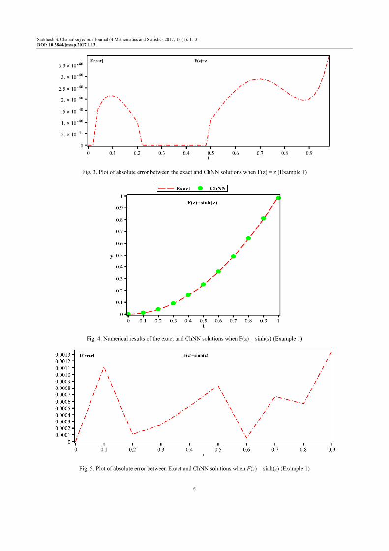
results with F(z) = z is shown in Fig. 3. Comparison

between analytical and ChNN solutions and absolute

error between them with F(z) = sinh(z) are showed in

Fig. 4 and 5, respectively. Numerical results between

analytical and ChNN solutions and absolute error

between them with F(z) = tanh(z) are cited in Fig. 6 and

7, respectively. According Table 2 the maximum

absolute error for active functions F(z) = z; sinh(z);

tanh(z) are as 3.40000×10−40

, 0.13542×10−2

and

0.40843×10−1

, respectively. Therefore, the analytical and

ChNN solutions have good agreement with the active

function F(z) = z.

Example 2

We consider the following fractional integro-

differential equation (Fadi et al., 2011):

( )( )

( ) ( ) ( )

( ) ( ) [ ] ( )

0.250.75

0

cos sin1.25

sin , 0,1 , 0 0t

tD y t t t t y t

t y d t yτ τ τ

= + − Γ

+ ∈ =∫ (25)

Table 1. Comparison of absolute errors between the exact and ChNN solutions when F(z) = z; sinh(z); tanh(z) (Example 1)

t

------------------------------------------------------------------------------------------------------------------------------------------

F(z) 0.1 0.2 0.3 0.4 0.5 0.6 0.7 0.8 0.9

z [1.9783 1.2490 0.5480 0.8000 1.7600 2.6800 2.9300 2.6300 3.4000] ×10−40

sinh(z) [1.1111 0.1096 0.2494 0.5286 0.8353 0.05314 0.6717 0.5634 1.3542] ×10−3

tanh(z) [0.02331 0.01347 0.00713 0.06345 0.2544 0.2544 0.77492 1.9234 4.0843] ×10−2

Table 2. Comparison of maximum absolute errors between the exact and ChNN solutions when F(z) = z; sinh(z); tanh(z)

(Example 1)

F(z) Z sinh(z) tanh(z)

Max Error 3.40000×10−40 0.13542×10−2 0.40843×10−1

Fig. 2. Numerical results of the exact and ChNN solutions when F(z) = z (Example 1)


DOI: 10.3844/jmssp.2017.1.13

6

Fig. 3. Plot of absolute error between the exact and ChNN solutions when F(z) = z (Example 1)

Fig. 4. Numerical results of the exact and ChNN solutions when F(z) = sinh(z) (Example 1)

Fig. 5. Plot of absolute error between Exact and ChNN solutions when F(z) = sinh(z) (Example 1)


DOI: 10.3844/jmssp.2017.1.13

7

Fig. 6. Numerical results of the exact and ChNN solutions when F(z) = tanh(z) (Example 1)

Fig. 7. Plot of absolute error between the exact and ChNN solutions when F(z) = tanh(z) (Example 1)

The exact solution of the above equation is given as:

( )y t t= (26)

Comparison between analytical and ChNN solutions

with the active function as, F(z) = z is cited in Fig. 8.

Plot of absolute error between analytical and ChNN

solutions with F(z) = z is shown in Fig. 9.

Example 3

Consider the following fractional integro-differential

equation (Hasan et al., 2013):

( )

( ) [ ] ( )

3/2 1/ 20.5

3 2

0

8 / 3 2

12

, 0,1 , 0 0t

t t tD y t

t d t y

π

τ τ τ

−= +

+ − ∈ =∫ (27)

with the exact solution as:

( ) 2y t t t= − (28)


ChNN solutions with the active function as, F(z) = z.

Figure 11 presents plot of absolute error between

analytical and ChNN solutions with F(z) = z.

Example 4


equation (Hasan et al., 2013):

( ) ( )( )( )

( ) ( ) [ ] ( )

1/6 2

5/6

13

0

5 / 6 91 2163

91

5 2 , 0,1 , 0 0

t tD y t

e t te d t yτ

π

τ τ τ

Γ − +=

+ − + − ∈ =∫ (29)


DOI: 10.3844/jmssp.2017.1.13

8


( ) 3y t t t= − (30)

Comparison between analytical and ChNN

solutions and plot of absolute error with the active

function as, F(z) = z are presented in Fig. 12 and 13,

respectively.

Example 5


equation (Changqing and Jianhua, 2013):

( ) ( )( )

( ) ( ) [ ] ( )9/4 2

3/4

0

6, 0,1 , 0 0

13/ 4 5

tt

tt t eD y t y t e y d t yτ τ τ= − + ∈ =

Γ ∫ (31)


( ) 3y t t= (32)

Comparison between analytical and ChNN solutions

with active function as, F(z) = z is showed in Fig. 14.

Plot of absolute error between analytical and ChNN

solutions with F(z) = z is showed in Fig. 15.




DOI: 10.3844/jmssp.2017.1.13

9





DOI: 10.3844/jmssp.2017.1.13

10



Fig. 15. Plot of the absolute error between the exact and ChNN solutions when F(z) = z (Example 5)


DOI: 10.3844/jmssp.2017.1.13

11

Fig. 16. Numerical results of Exact and ChNN solutions when F(z) = z (Example 6)


Example 6


equation (Mittal and Nigam, 2008):

( ) ( )( )

( )2 2.25

0.75 1.5

0

6

5 3.25

tt

tt e tD y t y t t e y dτ τ τ

= − + Γ

∫ (33)

with the initial conditions y(0) = 0 and exact solution as:

( ) 3y t t= (34)


ChNN solutions with active function as, F(z) = z. Figure

17 presents plot of absolute error between analytical and

ChNN solutions with F(z) = z.

Conclusion

Chebyshev neural network is applied for solving

the linear and the nonlinear fractional integro-

differential equations. A Chebyshev neural network

with single layer is presented to prevail the difficulty

and hardness of this type of equations. Numerical

results from the proposed method are compared with


DOI: 10.3844/jmssp.2017.1.13

12

the analytical solutions. The maximum absolute error

between exact and Chebyshev neural network

solutions with F(z) = z, is showing a good agreement

between Chebyshev neural network and analytical

solutions. Comparisons of the obtained results from

Chebyshev neural network with exact solutions show

that this method is a capable tool for solving this kind

of the linear and the nonlinear problems. This method

can be applied to solve any kind of the complex

ordinary and the partial differential equations from the

fractional order.

Acknowledgment

The author would like to thank the referees for their

valuable comments that help to improve the manuscript.

Author’s Contributions

Sarkhosh S. Chaharborj: Analyzing, programing,

producing the results and writing the paper.

Shahriar S. Chaharborj: Offering ideas,

encouragement, proof read text and equations.

Yaghoub Mahmoudi: Supervising the contents and

flow of the paper.

Ethics

The authors confirm that they have read and

approved the manuscript and no ethical issues involved.

References

Ahmed, S. and S.A.H. Salh, 2011. Generalized Taylor

matrix method for solving linear integro-fractional

differential equations of Volterra type. Applied

Math. Sci., 5: 1765-1780.

Bhrawy, A.H. and A.S. Aloi, 2013. The operational

matrix of fractional integration for shifted

Chebyshev polynomials. Applied Math. Lett., 26:

25-31. DOI: 10.1016/j.aml.2012.01.027

Bhrawy, A.H. and M.A. Alghamdi, 2012. A shifted

Jacobi-Gauss-Lobatto collocation method for

solving nonlinear fractional Langevin equation

involving two fractional orders in different intervals.

Boundary Value Prob., 2012: 62-62.

DOI: 10.1186/1687-2770-2012-62

Bianca, C., F. Pappalardo and S. Motta, 2009. The MWF

method for kinetic equations system. Comput. Math.

Applic., 57: 831-840.

DOI: 10.1016/j.camwa.2008.09.018

Changqing, Y. and H. Jianhua, 2013. Numerical solution

of integro-differential equations of fractional order

by Laplace decomposition method. Wseas Trans.

Math., 12: 1173-1183.

Doha, E.H., A.H. Bhrawy and S.S. Ezz-Eldien, 2011.

Efficient Chebyshev spectral methods for solving

multi-term fractional orders differential

equations. Applied Math. Modell., 35: 5662-5672.

DOI: 10.1016/j.apm.2011.05.011

Fadi, A., E.A. Rawashdeh and H.M. Jaradat, 2011.

Analytic solution of fractional integro-differential

equations. Annals Univ. Craiova Math. Comput.

Sci., 38: 1-10.

Grigorenko, I. and E. Grigorenko, 2003. Chaotic

dynamics of the fractional Lorenz system. Phys.

Rev. Lett., 91: 034101-4.

DOI: 10.1103/PhysRevLett.91.034101

Hasan, B., B. HaciMehmet and F.B. BinMuhammad,

2013. The analytical solution of some fractional

ordinary differential equations by the Sumudu

transform method. Abstract Applied Anal., 2013:

203875-203875. DOI: 10.1155/2013/203875

Hoda, S.A. and H.A. Nagla, 2011. Neural network

methods for mixed boundary value problems. Int. J.

Nonlinear Sci., 11: 312-316.

Irandoust-Pakchin, S. and S. Abdi-Mazraeh, 2013. Exact

solutions for some of the fractional integro-

differential equations with the nonlocal boundary

conditions by using the modification of He’s

variational iteration method. Int. J. Adv. Math. Sci.,

1: 139-144.

Irandoust-pakchin, S., H. Kheiri and S. Abdi-Mazraeh,

2013. Chebyshev cardinal functions: An effective

tool for solving nonlinear Volterra and Fredholm

integro-differential equations of fractional order.

Iran. J. Sci. Technol. Trans. A, 37: 53-62.

Mall, S. and S. Chakraverty, 2014. Chebyshev Neural

Network based model for solving Lane-Emden type

equations. Applied Math. Comput., 247: 100-114.

DOI: 10.1016/j.amc.2014.08.085

Mall, S. and S. Chakraverty, 2015. Numerical solution of

nonlinear singular initial value problems of Emden-

Fowler type using Chebyshev Neural Network

method. Neurocomputing, 149: 975-982.

DOI: 10.1016/j.neucom.2014.07.036

Miller, K.S. and B. Ross, 1993. An Introduction to the

Fractional Calculus and Fractional Differential

Equations. 1st Edn., John Wiley and Sons Inc., New

York, ISBN-10: 0471588849, pp: 384.

Mittal, R.C. and R. Nigam, 2008. Solution of fractional

integro-differential equations by Adomian

decomposition method. Int. J. Applied Math.

Mechan., 4: 87-94.

Podlobny, I., 2002. Geometric and physical

interpretation of fractional integration and fractional

differentiation. Fract. Calculus Applied Anal., 5:

367-38.


DOI: 10.3844/jmssp.2017.1.13

13

Saeed, R.K. and H.M. Sdeq, 2010. Solving a system

of linear fredholm fractional integro-differential

equations using homotopy perturbation method.

Austral. J. Basic Applied Sci., 4: 633-638.

Saeedi, H. and F. Samimi, 2012. He's homotopy

perturbation method for nonlinear ferdholm

integro-differential equations of fractional order.

Int. J. Eng. Res. Applic., 2: 52-56.

Saha Ray, S., 2009. Analytical solution for the space fractional diffusion equation by two-step Adomian decomposition method. Commun. Nonlinear Sci. Numerical Simulat., 14: 1295-1306.

DOI: 10.1016/j.cnsns.2008.01.010 Yang, Y., Y. Chen and Y. Huang, 2014. Spectral-

collocation method for fractional Fredholm integro-differential equations. J. Korean Math. Society, 51: 203-224. DOI: 10.4134/JKMS.2014.51.1.203

study of fractional order integro-differential equations...

Documents