Journal of Mathematics and Statistics 8 (3): 348-360, 2012 ISSN 1549-3644 © 2012 Science Publications

Corresponding Author: Gurudeo AnandTularam, Senior Lecturer in Mathematics and Statistics in School of Environment, Environment Future Centre, Griffith University, Australia

348

Modeling Tourist Arrivals Using Time Series Analysis: Evidence From Australia

1Gurudeo AnandTularam, 2Victor Siew Howe Wong and 3Seyed AbdelhamidShobeiriNejad

1Mathematics and Statistics, Science Environment Engineering and Technology (ENV), 2Finance, School of Business, Finance and Economics

3Science Environment Engineering and Technology (ENV), Environment Future Centre, Griffith University, Australia

Abstract: Australian tourism has a logistic trend as Butler’s model shows. The stagnation has not been reached so opportunities exist to increase tourism. The logistic model predicts 7.2 million tourists in 2015 but time series models of ARIMA and VAR improve the prediction and explain the data. The ARIMA (2, 2, 2) fits well while the VAR lead to Granger causalities between the three data sets. A regression model (R2 = 0.99) using Australian tourist arrival as a function of Europe and World arrivals allowed to further understand the Granger causality. The ARIMA model predicts tourist numbers to be approximately 6 million in 2015. The VAR technique allowed impulse response analysis as well. A two-way causality between the tourist in Australia, Europe and World exists, while impulse response indicated different effect patterns, where tourist arrivals increase in the first period and declines in the second period but experience seasonal fluctuations in the third period. The strongest causalities in were period 1 between World and Europe; period 2-a one-way causality from Australia to World and period 3-a two-way causalities between Australia, Europe and World. The impulse responses results were aligned with the Butler theory. Keywords: ARIMA, auto-regression, mathematical modeling, butler model, tourism modeling,

granger causality, impulse response, variance decomposition model, logistic regression, time series

INTRODUCTION

The number of tourists has significant impacts on global economy. These impacts can be counted as both of negative and positive effects. The most important effect of tourism on economy can be known as number of changes on supply and demand chain in the destination which is the host of tourists. Tourists’ demand or simply tourist consumption contributes to GDP, increasing the employment rate, making new source of revenue for local people, private and public sectors and destination’s government and so on. For instance, the consumption international and domestic tourism was approximately AUD$ 95.653 billion from July 2010 to year-ended June 2011. It shows that the tourism share of GDP and total employment rate were 2.5 and 4.5%, respectively. Moreover, the share of tourism industry in export was 8% 0f total Australian export in 2010-11 (ABS, 2011). This significant impact is enough to

encourage researches to investigate on number of tourist arrivals and attempt to make a more accurate prediction for future planning. The number of short-term international arrivals to Australia has significantly grown over the last 6 decades from about 60,000 to approximately 6 million arrivals per year presently. From 1956 to 2009 the Australian tourism industry has been growing steadily following the trend of worldwide tourism and increasing over time. However, in recent times the number of tourist arrivals has starting slowing down and this may be just evident in Fig. 1. However when compared with actual numbers Australian tourism is significantly less than either Europe or the World as shown in Fig. 2. This Fig. 1 shows the trend of changes in tourist arrivals to both Australia and the world. The above model gives this chance to look at the trend of growth of both Australia and the world international arrivals at the same time.

J. Math. & Stat., 8 (3): 348-360, 2012

349

Fig. 1: Short-Term International visitors Arrivals 1956-2010 compared to the World (Based on ABS, 2011)

Fig. 2: Low levels of tourism in Australia compared to Europe and the World

J. Math. & Stat., 8 (3): 348-360, 2012

350

This Fig. 2 shows the trend of changes in international arrivals to both Europe and the world. For easier comparison in the next graph the trend of international arrival is shown. Australian investments on projects facilitating tourism are costly and require a long-term approach and planning in order to develop relevant infrastructures (Song and Turner, 2006). The contribution and impact of tourism to Australian economy is also well accepted and to cater for the arrivals much planning and development is indeed necessary for future needs in terms of infrastructure and like. In order to prepare for the future, Australian governments, companies and organizations often rely on mathematical models (Song and Turner, 2006). It is then important for our models to accurately predict arrival numbers at it is critical for both public and private organizations budgeting and monetary positions (Li et al., 2005). According to Song and Li (2008), tourist arrivals or tourist population at a particular time is the most common variable to measure tourism demand and usually given by the total number of tourist arrivals from an origin to a destination. The Tourist Area Cycle Theory (TACT) is a conceptual framework proposed by Butler (1980) for modeling. This framework is used to model tourist arrivals. In the first part of this study a mathematical a logistic model is developed based on the Tourist Area Cycle Theory (Nejad and Tularam, 2010). However in this study an integrated time series ARIMA model is considered together with a linear multivariate Vector Auto-Regression (VAR) model is also for a more detailed study of drivers of Australian tourism in terms of Europe and the World. Similar analyses have been done in other areas (Tularam, 2010; Tularam and Illahee, 2010). A Variance decomposition model (VAR) can be used to study Granger Causality and impulse response for furthering understanding of tourism numbers worldwide. The VAR model allows an examination of the nature of integration of the tourism market when compared with Europe and the World tourism numbers. In fact, by aggregation of the concept of TACT and the study in this study, the number of tourist arrivals can be linked in both Area Cycle as well as the world’s tourism cycle. Literature review: Butler (1980) theoretically studied the conceptual cycle of tourist evolution and identified five stages; namely; exploration, involvement, development, consolidation and stagnation (Fig. 3). The first stage of exploration tourism is not recognized as an economic activity in that only a few people travel to the destination. The involvement stage is a time period in which tourist numbers increase mainly due to an increased awareness of the destination as a tourist base.

By the start of the development stage, the destination’s tourism facilities in both public and private areas become well developed while in the fourth consolidation stage, the tourists number continue to increase but the destination now becomes well known and visited by many; thus not listed now as a priority for potential tourists in that the rate of growth of the tourist numbers gradually declines until finally, a stagnation stage is reached when potentially all tourists know the destination well including the facilities on offer. In addition, Butler (1980) argued two possibilities after stagnation stage is reached, namely; rejuvenation or decline. The evolution of tourist area’s stages including: Exploration, Involvement, Development, Consolidation and Stagnation over time. Mathematical model:The initial tourist model may be written as xt = x0 e

m (t-t0) where x is positive and when t = 0 given t0 = 0, the initial value tourist number is greater than zero (x0 >0). When t0 = 0 the model may be written as xt = x0

mt, representing an exponential growth. A more comprehensive model is developed by combining Malthus’ law and the Verhulst assumption (Nejad and Tularam, 2010); where the negative effects and leveling or stagnation period are both captured by the model. The model is given as:

tt

x

X= β

Where:

t m(t a)

1

1 e− −β =+

A represents time at half the carrying capacity and X being the maximum tourist capacity. This model demonstrates that the tourist numbers growth at time t+1 is proportional to constant growth rate m (as before); tourist number at last time t (as before); and discrepancy of tourist numbers at previous time t as a ratio of maximum tourist numbers X.

The growth is proportional to tX x

X

− Eq. 1:

tt t

X xx m x

X

− =

ɺ (1)

The solution to the differential equation developed above can be given by Eq. 2:

t m(t a )

Xx

1 e− −=+

(2)

J. Math. & Stat., 8 (3): 348-360, 2012

351

Fig. 3: The evolution of a tourist area (Adapted from Nejad and Tularam, 2010)

Fig. 4: Fitted growth rate and observed data (Nejad and Tularam, 2010)

The constant parameter ‘a’ and the maximum capacity X are both assumed to be fixed for a particularly destination. As shown, given

t m(t a)

1

1 e− −β =+

the model may be written as t t

x

X= β ;

where βt is proportion (percentage) of tourist at time t to the capacity (Nejad and Tularam, 2010). Based on the 2010 paper, the authors have updated the data and recalculated the predictions based on the model in Equation 2 (Fig. 3). It was noted that the Nejad and Tularam (2010) prediction was 5,594,500 arrivals using

the logistic model and the actual result for 2010 at updated in this study is 5,692,400 (within the 95% range of 5,594,500). The new model in this study includes the “actual arrivals” in 2010 and the new prediction is 5,878,709 (5,824,886-5,932,065) suggesting the theoretical model predictions are somewhat overestimates; however, reasonably good in general given that cyclones, floods and financial crises have all impacted Queensland in this time period.

This Table 1 shows the prediction of tourist arrivals within 95% ran based on logistic model.

J. Math. & Stat., 8 (3): 348-360, 2012

352

Table 1: Predictions of tourist arrivals to Australia by Nejad and Tularam (2010)

Year Lower bound Point estimate Upper bound 2010 5,757,412 5,817,344 5,871,799 2011 5,827,883 5,884,440 5,935,400 2012 5,890,755 5,943,801 5,991,199 2013 5,946,695 5,996,177 6,040,023 2014 5,996,348 6,042,281 6,082,646 Table 2: New logistic model predictions of tourist arrivals to Australia Year Lower bound Point estimate Upper bound 2010 5,824,886 5,878,709 5,932,065 2011 5,890,580 5,949,745 6,007,930 2012 5,948,205 6,012,656 6,075,683 2013 5,998,612 6,068,214 6,136,022 2014 6,042,598 6,117,157 6,189,622 2015 6,080,900 6,160,179 6,237,130

This Fig. 4 shows the model results of logistic regression international arrivals to Australia. A 95% confidence interval shows a good fit.

The logistic model (Fig. 4) fits the data well with an R-squared value of 0.991. The calculated carrying capacity for this model is 6,453,205 (6,325,129-6,581,159) with the international arrivals growth rate of 0.144 (0.137-0.152). Using the turning point as the half of the carrying capacity occurring around in the middle of 1993 (1993.85), the mathematical model can now be written as:

( )t 0.144054 t 1993.85

6453205x

1 e− −=+

(3)

Nejad and Tularam (2010) analyzed their results in

terms of the Butler model and identified the year for each stage. The updated data confirms the stages as follows: • Exploration (1973 to 1974) • Involvement (1973-74 to 1983-84) • Development (1983-84 to 2003-04) • Consolidation (2003-04 to 2008) • Stagnation (2008-dependent to the world’s rate)

The theoretical model’s 95% range predictions using Eq. 3 for international Australian tourist arrivals are shown in Table 2.

This Table 2 shows the prediction of tourist arrivals within 95% rang for-squared 0.991.

A more in depth analysis of the tourism data is conducted in this study in terms of time series using ARIMA and VAR methods, similar to those used in other studies (Roca and Tularam, 2012; Tularam et al., 2010; Tularam and Illahee, 2010). Model of tourism evolution: ARIMA-autoregressive integrated moving average model: The common time series analysis may be conducted using autoregressive moving average models known as ARIMA (p, d, q) (Box et al., 1994) including

autoregressive and moving average parameters. ARIMA models explicitly include differencing (Tularam, 2010). The three types of parameters are: the autoregressive parameters (p), the number of differencing (d) and moving average parameters (q). For example ARIMA (2, 2, 2) contains 2 autoregressive (p) parameters and 2 moving average (q) parameters computed for the series differenced twice. In general form, ARIMA (p, d, q) model can be written using intercept form or with lag notation (L) as follows Eq. 4:

p q

t i t i t j t ji 1 j 1

d 2 pt 1 2 p

2 q1 2 p t

Y Y u u

Y (1 L L ... L )

(1 L L ... L )u

− −= =

= ϕ + + θ

∆ − ϕ − ϕ − − ϕ

= − θ − θ − − θ

∑ ∑

(4)

Where: Y = The time series data u = The usual error term - ui~i.id(0,σ2) Variance decomposition-granger causality and impulse response analyses: The VAR modeling process allows more specific examinations of the relationships between the three data series. The structure of the VAR model is such that it provides information about a variable’s forecasting ability for other variables (Roca et al., 2010). Granger (1969) argued that if a variable, or group of variables, y1 is found to be helpful for predicting another variable, or group of variables, y2 then y1 is said to Granger-cause y2; otherwise it is said to fail to Granger-cause y2. The notion of Granger Causality does not imply true Causality in that it only implies forecasting ability (Roca and Tularam, 2012). In particular, the structure allows Granger Causality tests to be conducted that may indicate whether there is one or two-way Granger Causality between tourist arrivals in Australia, Europe and World. To study impacts over different periods time series data was divided into sub-periods, where a structural break due could be identified (financial crises); for example, Period 1 (1950-1987) consisted of the stock market crash in October 1987, Period 2 (1988-2001) consisted of the September 11, 2001 attacks in the US and Period 3 (2002-2009) was the Global Financial Crisis (GFC) in 2008. As an example, a general form of a two-variable VAR (1, 1) with k = 2 are shown in Eq. 5:

t 10 12 t 11 t 1 12 t 1 yt

t 20 21 t 21 t 1 22 t 1 zt

y b b z c y c z

z b b y c y c z− −

− −

= − + + + ε

= − + + + ε (5)

with 2

it i~ i.i.d(0, )εε σ and cov (εy,εz) = 0 in matrix form

the above can be written as Eq. 6:

t 10 t 1 yt12 11 12

t 20 t 1 zt21 21 22

y b y1 b c c

z b zb 1 c c−

−

ε = + + ε

(6)

J. Math. & Stat., 8 (3): 348-360, 2012

353

The test of the joint hypothesis that none of the z’s is a useful predictor, above and beyond lagged values of y, is called a Granger Causality test. It is noted that Granger Causality simply refers to (marginal) predictive content. The significance of the tourist modeling and prediction analysis can be strengthened further using impulse response analysis to observe duration and impact of tourism in one country to another. The impulse response functions traces the effect of a shock to one country on to the other countries. Every structural shock affects every other variable. Thus, we can construct an impulse graph for each variable as the response to a certain shock. For our VAR (1, 1) example, interest may be in: • The impulse response of y in response to a shock in

the z-equation, εz • The impulse response of z in response to a shock in

the z-equation, εz • The impulse response of y in response to a shock in

the y-equation, εy • The impulse response of z in response to a shock in

the y-equation, εy The impulse response functions will all have the same general shape and if the system is stable, the impulse responses will all approach zero. There will be a difference in the timing of the effects. Finally, it is customary to set the size of the shock equal to its standard deviation. The impulse response then shows the reaction to a shock of unit size. Impulse response analysis provides useful information for example, how, Australian tourist arrivals at a particular time is likely to respond to changes in Europe and World tourist numbers.

Consider now the moving average representation of the multiple-equation, VAR (m) model where the constant terms may be ignored: Yt = ψ (L) xt If

( )t tE x x x′ =∑ such that shocks are contemporaneously

correlated, then the generalized impulse response function of Yi to a unit (one standard deviation) shock in Xj is given by Eq. 7:

( ) ( )1/2

ij,h ii j ie x e ,− ′Ψ = σ ∑ (7)

Where: σii = The ith diagonal element of ∑x ei = A selection vector with the ith element equal to

one and all other elements equal to zero h = The horizon The impulse responses computed using the generalized method is invariant to re-ordering of the variables in the VAR. Since orthogonality is not imposed, meaningful interpretations of the initial

impact response of each variable to shocks to any other variable may be determined.

RESULTS ARIMA: A code in R was used to obtain a timer series ARIMA (2, 2, 2) model that fitted the Australian tourist arrival data with a high degree of it and low AIC, BIC (AIC = -57.27 and BIC = -46.9) suggesting an excellent fitted model: with p = 2, q = 2 and d = 2 Eq. 8:

2 2 2t 1 2 1 2 tY (1 L L ) (1 L L )u∆ − ϕ − ϕ = − θ − θ (8)

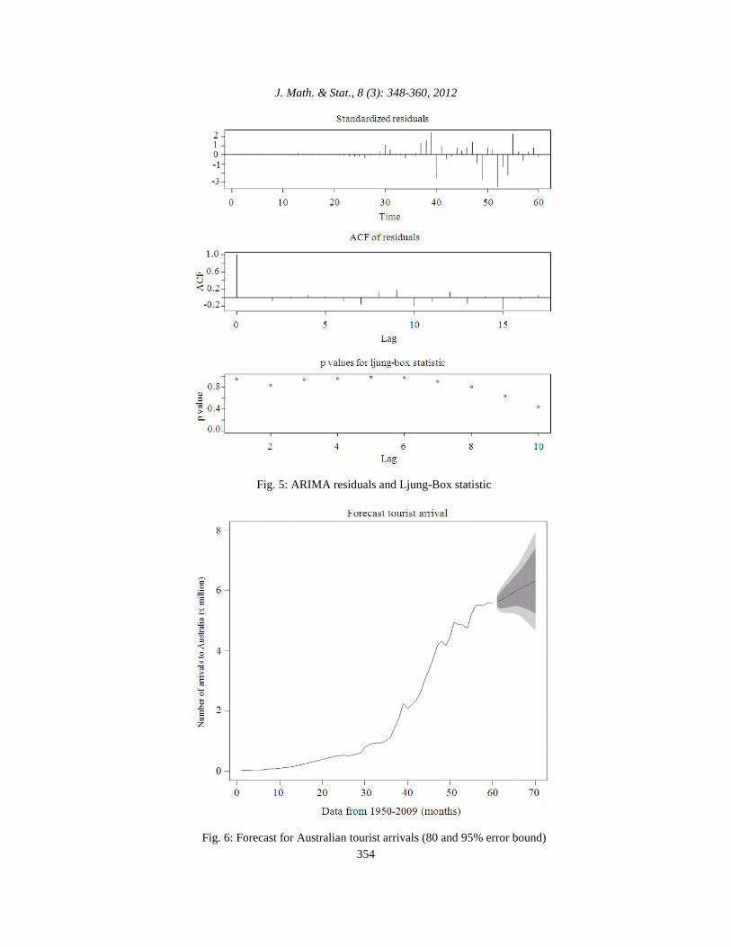
The results of the Residuals, ACF and Lung-Box

tests for the ARIMA analysis is shown in Fig. 5. This Fig. 5 shows that the model satisfies all

required tests for a suitable model for tourist data. The estimated coefficients for the ARIMA mode are present in Table 3 suggesting a close fit with data.

This Table 3 shows the ARIMA (2,2,2) model parameters with significances ME = 0.0036, RMSE = 0.130 and MAE = 0.076

The forecast using the ARIMA (2,2,2) is given for 80 and 95% accuracy limits for the next ten years in Table 4 and the 2010 actual value fits rather well in the set. The 80 and 95% bounds are shown Figure for the predictions made up to year 2015.

This Table 4 shows the prediction of tourist arrivals to Australia within 80 and 95% accuracy range.

This Fig. 6 shows the forecast of Australian tourist arrivals based on the ARIMA model. Error bounds are highlighted in darker grey shows 80% and lighter grey shows 95% error bound.

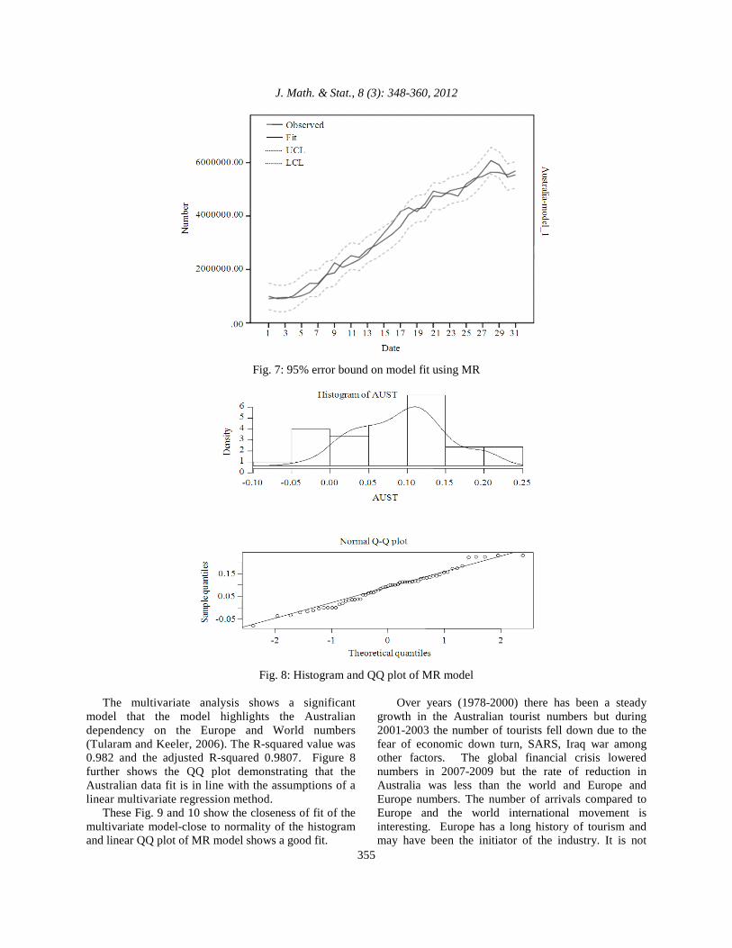
Figure 6 shows the ARIMA predicted number of Australian arrivals up to 2015; it is noted that the 2010 prediction is a much a better: 5,613,810 (5,353,809-5,873,811) compares well to the actual of 5,692,400 even when both a flood and a second wave of the financial crises placed rather sudden shocks to tourism numbers. MR-multivariate analysis: To further cross check the nature of the predictions and examine the kind of relationship between Australian, Europe and the World, another analysis was undertaken using the multiple regression method. The results of a Multivariate linear Regression (MR) model based on Australian dependency on Europe and the World highlighted in Table 5 and Fig. 7.

This Table 5 shows parameters for multiple regression analysis. *** indicates 1% level of significance. The equation is expressed as: Australia = -2,445,285.59 + 0.028(Europe) + -0.006(World) + εt.

This Fig. 7 shows the 95% error bound.as fitted using the multivariate analysis.

J. Math. & Stat., 8 (3): 348-360, 2012

354

Fig. 5: ARIMA residuals and Ljung-Box statistic

Fig. 6: Forecast for Australian tourist arrivals (80 and 95% error bound)

J. Math. & Stat., 8 (3): 348-360, 2012

355

Fig. 7: 95% error bound on model fit using MR

Fig. 8: Histogram and QQ plot of MR model

The multivariate analysis shows a significant model that the model highlights the Australian dependency on the Europe and World numbers (Tularam and Keeler, 2006). The R-squared value was 0.982 and the adjusted R-squared 0.9807. Figure 8 further shows the QQ plot demonstrating that the Australian data fit is in line with the assumptions of a linear multivariate regression method.

These Fig. 9 and 10 show the closeness of fit of the multivariate model-close to normality of the histogram and linear QQ plot of MR model shows a good fit.

Over years (1978-2000) there has been a steady growth in the Australian tourist numbers but during 2001-2003 the number of tourists fell down due to the fear of economic down turn, SARS, Iraq war among other factors. The global financial crisis lowered numbers in 2007-2009 but the rate of reduction in Australia was less than the world and Europe and Europe numbers. The number of arrivals compared to Europe and the world international movement is interesting. Europe has a long history of tourism and may have been the initiator of the industry. It is not

J. Math. & Stat., 8 (3): 348-360, 2012

356

surprising then that Europe is the world’s leading tourist destination having about 50% of the world’s international arrivals.

This Table 5 shows the proportion of arrivals to Europe to the World.

This Table 6 shows the proportion of arrivals to Australia to the World.

This table shows average growth rate for World, Europe and Australia during 1956-2009.

Table 6 shows the world’s international arrivals average is around 6.3% while Europe has a rate around 5.9%. In the same period, Australia experienced an average growth rate of around 9%. This is around 1.5 times the world’s growth rate.

This Fig. 11 shows the number of international arrivals in Australia and World during 1950-2010.

The pattern of Australian tourist numbers over time is similar to the world growth as shown in Fig. 11. Further analysis of Fig. 11 shows that Australian arrivals was growing from 1956 to 1985 at an average rate of 0.04 million persons per year (Mp/yr), while the world was growing in the same period at an average rate of 8 Mp/yr; similarly, in the period 1985 to 2000, Australia was growing at 0.26 Mp/yr and the world was 25.33 Mp/yr; and from 2000 to 2007, Australia was growing at 0.065 Mp/yr while the world was growing at an average rate of 28.5 Mp/yr. Clearly, a significant growth has occurred in Australia in terms of actual numbers. Australian rate increased 6.5 times from the first to the second period, when the world increased by 3 times respectively. Australia decreased by a quarter in the next period, while the World was increasing at 1.1 times that of the earlier period rate. Australian increasing rate reached a maximum around 1990 and continued to grow but at a lower rate until the 2007 financial crisis. While there is a dip after 2007, the market started recovering. The effects of both the cyclone Yasi and Queensland floods do not appear in 2010 numbers because of a lag effect. Granger causality: The VAR modeling process showed interesting relationships between the three data series. In particular, the Granger Causality tests indicate if there is two-way Granger Causality between the tourist in Australia, Europe and World. As noted earlier, Period 1 (1950-1987) consists of the stock market crash in October 1987, Period 2 (1988-2001) consists of the September 11, 2001 attacks in the US; and Period 3 (2002-2009) refers to the Global Financial Crisis (GFC, 2007-2008).

The flow and strength of Causality or interaction between the countries is summarized in Fig. 12. In the whole study period, all countries are Granger causing the tourist arrivals between one country and the other at 1% (high) level of significance; however, only Australia is causing the World at 5% (medium) level of

significance. In the first period (1950-1987), the Causality was both ways for Europe and the World and a 10% (low) level of significance from Europe to Australia. In this period, the economy is growing stronger for the European continents and tourists are travelling to the European countries during 1950 to 1987 because there were 8 Olympics events in the European countries (1952, 1956, 1960, 1964, 1968, 1972, 1976 and 1984).

In the second period, the Australian economy is performing better and there is one-way Causality from Australia to the World. This is possibly due to the Olympics in 2000 located in Sydney, when Australia attracted millions of tourists. The Causality is at 10% (weak) level of significance from Australia to the World. In the final period, economies are globalised with more information coming from media and news; tourist can easily search for places to visit from the internet with increased attention using marketing campaigns. The results of this is a two-way Causality for all the countries at 1% (high) level of significance, except for Australia at 10% (weak) level of significance to Europe and the World. Impulse response analysis: The impulse response analysis analyzed the duration and impact of tourism in one country to another by tracing the effect of a shock to one country on to the other countries. Such dynamic relationships are captured in the impulse response functions found. Figure 13 shows the impulse responses for the full period, period 1, 2 and 3. In the full period, the responses are plotted over 100 periods/years. The responses are generally the same pattern among the countries where the number of tourists fall up to 40-50 years, increase for 70-90 years and declines afterwards. In the first period (1950-1987) may be characterized by Exploration and Involvement stages, where the responses show a sharp peak in tourist number after 25 years for Australia, followed by the World and Europe. The second period (1988-2001) shows a decline in tourism for Europe and the World; however, Australia responses show an increase of tourists coming from Europe and the World. The responses generally decrease/increase for the first 5 years and gradually declining afterwards. This period is characterized by the Development stage. In the last period (2002-2009), the responses show mixed signals. The responses generally show signs of fluctuations every 5 years and it indicated a season cycle and the responses completes after 20-25 years. This is the period characterized by Consolidation and Stagnation stages of the Butler theory.

This Fig. 12 shows the results of Granger causality estimated based on the VAR model in a visual diagram.

J. Math. & Stat., 8 (3): 348-360, 2012

357

Fig. 9: Percentage of share of Europe to the World (1950-2010)

Fig. 10: Percentage of share of Australia to the World (1956-2010)

Fig. 11: World and Australia international arrivals 1950-2010

J. Math. & Stat., 8 (3): 348-360, 2012

358

Fig. 12: Significant linkages between tourist in Australia, Europe and World Table 3: Estimated parameters of the ARIMA Coefficients Coefficients AR1 0.9945** AR2 -0.4615** MA1 -1.7195** MA2 0.8739** Table 4: Forecast for the next 6 years based on ARIMA(2,2,2) Year Point Low80% - high80% Low95% - high95% 2010 5,613,810 5,443,804-5,78,3815 5,353,809-5,873,811 2011 5,679,011 5,403,521-5,954,501 5,257,686-6,100,336 2012 5,764,731 5,417,662-6,111,800 5,233,934-6,295,527 2013 5,854,525 5,448,805-6,260,244 5,234,030-6,475,019 2014 5,938,902 5,468,510-6,409,294 5,219,499-6,658,304 2015 6,016,012 5,462,093-6,569,930 5,168,86606,863,157 Table 5: MR model coefficients for the tourist arrivals to Australia Model Coefficients T Sig. Constant -2,445,285.590 -10.184 0*** Europe 0.028 6.556 0*** World -0.006 -2.790 0.009*** Table 6: Average growth rate for World, Europe and Australia (1956

2009) Growth rate (%) World 6.3 Europe 5.9 Australia 9.0

The Table 7 shows the Granger causality results estimated based on the VAR model. The null hypothesis is that the row variable does not Granger cause the column variable. All test statistics are Chi-square with the p-values listed in brackets. ***, ** and * indicate significance at the 1, 5 and 10 percent levels respectively.

The following regression estimates was estimated with the following equations. For the interest of saving

space, we only show the full period equations as follows (ε-N (0,1)):

For example, the Granger Causality Equations for the Full Period: Australia = Australia(-1) + 9.3670Europe(-1) + ε Australia = Australia(-1) + 6.3101World(-1) + ε Europe = Europe(-1) + 10.5009Australia(-1) + ε Europe = Europe(-1) + 17.2942World(-1) + ε World = World(-1) + 7.9444Australia(-1) + ε World = World(-1) + 13.7392Europe(-1) + ε

This Fig. 13 shows the impulse responses analysis based on the VAR model. Concluding comments: In this study a number of models of tourist arrivals were developed and analyzed using time series analyses. The Granger and impulse response analyses related to VAR modeling process was cross checked and justified with the use of a multivariate linear model and ARIMA model was shown to be in line with and better than the theoretical model based on Butler. The models were calibrated using Australian tourist arrival data (1956-2010) and the modified Butler model predicts growth predicts around 7.2 million arrivals in 2015 but a more realistic 6,160,179 and 95% range of arrivals may be given as 6,080,900-6,237,130 using the updated theoretical logistic model presented in this study. The ARIMA (2, 2, 2) model predicts using data up to and including 2009 more accurately predicts for the year 2010 with a value of 6,016,012 in 2015. The actual value is well within the 95% range of 5,168,866-6,863,157. That is, a 95% range of arrival numbers predicted lie within the range 5,618,866 to 6,863,157 for 2015.

J. Math. & Stat., 8 (3): 348-360, 2012

359

Fig. 13: Impulse response for Australia, Europe and World - full period, period 1, 2 and 3 The results of the analysis show: There is a close relationship between the tourist numbers recorded for Europe, Australia and the World even though Australia’s tourist arrives are very low in actual terms when compared to the other numbers of tourists. Australia tourist arrivals have been growing since 1974 and have strong influences from tourist arrival to

Europe and indeed the World. The logistic model derived from theory was compared with the time series data based ARIMA model and the ARIMA performed the better in terms of the prediction for 2010. The theoretical model was not as accurate but performed well and can be used a benchmark for checking performance of other models.

J. Math. & Stat., 8 (3): 348-360, 2012

360

Table 7: Granger causality results --------------Australia-------------- ----------------Europe---------------- -----------------World----------------- Full Period Australia - 9.3670 (0.0022)*** 6.3101 (0.0120)** Europe 10.5009 (0.0012)*** - 17.2942 (0.0000)*** World 7.9444 (0.0048)*** 13.7392 (0.0002)*** - Period 1 Australia - 0.5974 (0.4396) 1.2488 (0.2638) Europe 3.8158 (0.0508)* - 3.2888 (0.0698)* World 1.5817 (0.2085) 4.5237 (0.0334)** - Period 2 Australia - 1.9824 (0.1591) 3.0652 (0.0800)* Europe 1.0557 (0.3042) - 0.4159 (0.5190) World 0.6489 (0.4205) 0.1372 (0.7111) - Period 3 Australia - 3.3814 (0.0659)* 3.1351 (0.0766)* Europe 7.7974 (0.0052)*** - 7.1000 (0.0077)*** World 24.7292 (0.0000)*** 38.2832 (0.0000)*** -

The interactions studied with the VAR model

allowed more in depth analyses based as the Granger Causality and impulse response calculations were possible based in this structure. The validity of the models can be further clarified by the examination of a multiple regression and further analyses of the VAR in term Granger Causality to provide the justification and predictive ability of models. The nature of influence factors is better exemplified by the impulse response analyses. Detailed analyses not only showed the nature of significant interactions but the impulse response further showed that the Butler’s stages can be verified when the data is studied using important structural breaks such as financial crises, SARS.

Finally, the differential equation, ARIMA and VAR models all helped in the development of a better understanding the overall picture of the tourism story suggesting that in different periods, tourist numbers from different regions tend to drive new short term arrivals around to Australia. Such information is particularly useful for new investors and developers as well as longer term planners and government departments.

REFERENCES ABS, 2011. Australian national accounts: Tourism

satellite account, 2010-11. Australian Bureau of Statistics.

Box, G., G.M. Jenkins and G. Reinsel, 1994. Time Series Analysis: Forecasting and Control. 3rd Edn., Prentice Hall, ISBN-10: 0130607746, pp: 592.

Butler, R.W., 1980. The concept of a tourist area cycle of evolution: Implications for management of resources. Canadian Geographer, 24: 5-12.

Granger, C.W.J., 1969. Investigating causal relations by econometric models and cross-spectral methods. Econometrica, 37: 424-438. DOI: 10.2307/1912791

Li, G., H. Song and S.F. Witt, 2005. Recent developments in econometric modeling and forecasting. J. Travel Res., 44: 82-99. DOI: 10.1177/0047287505276594

Nejad, S.A.H.S. and G.A. Tularam, 2010. Modeling tourist arrivals in destination countries: An application to Australian. J. Math. Stat., 6: 431-441. DOI: 10.3844/jmssp.2010.431.441

Roca, E. and G.A. Tularam, 2012. Which way does water flow? An econometric analysis of the global price integration of water stocks. Applied Econom., 44: 2935-2944. DOI: 10.1080/00036846.2011.568403

Roca, E., V.S.H. Wong and G.A. Tularam, 2010. Are socially responsible investment markets worldwide integrated. Account. Res. J., 23: 281-301. DOI: 10.1108/10309611011092600

Song, H. and G. Li, 2008. Tourism demand modeling and forecasting. Tourism Manage., 29: 203-220.

Song, H. and L. Turner, 2006. Tourism Demand Forecasting. In: International Handbook on the Economics of Tourism, Dwyer, L. and P. Forsyth, (Ed.,) Edward Elgar, Cheltenham.

Tularam, G.A. and H.P. Keeler, 2006. The study of coastal groundwater depth and salinity variation using time-series analysis. Environ. Impact Assessment Rev., 26: 633-642.

Tularam, G.A. and M. Illahee, 2010. Time series analysis of rainfall and temperature interactions in coastal catchments. J. Mathematics Statistics. 6: 372-380.

Tularam, G.A., 2010. Relationship between El Nino southern oscillation index and rainfall (Queensland, Australia). Int. J. Sustain. Dev. Plann., 5: 378-391.

Tularam, G.A., V.S.H. Wong and E.D. Roca, 2010. An analysis on Australian superannuation funds volatility using EGARCH approach. Stud. Regional Urban Plann.