study of electromagnetic wave scattering from rough...

Study of Electromagnetic Wave Scatteringfrom Rough Icy Surfaces

Dissertation submitted in partial fulfillment of the requirements for the degree of

Master of Technology

in

Opto-Electronics and Optical Communication

Submitted by

Akashdeep Bansal

2014JOP2485

Under the supervision of

Dr. Uday K Khankhoje

Department of Electrical Engineering

Indian Institute of Technology Delhi

July, 2016

Certificate

This is to certify that the following dissertation titled “Study of electromagneticwave scattering from rough icy surfaces”, submitted by Mr. Akashdeep Bansal, EntryNo. 2014JOP2485 in partial fulfillment of the academic requirements of the courseJOD802, M.Tech Project represents bonafide work done under my supervision. It hasnot been submitted elsewhere to the best of my knowledge.

Dr. Uday K KhankhojeDept. of Electrical Engineering

Indian Institute of Technology, DelhiNew Delhi - 110016

i

Acknowledgements

I thank my Supervisor Dr. Uday K Khankhoje for his guidance and for giving methe opportunity to work on this project. Your valuable suggestions and the fruitfuldiscussions were the source for the project to progress continuously. Apart from theproject, you have been an excellent mentor also. I am thankful for all the advice youhave given regarding my career.

I am very thankful to my lab colleagues Nitin K. Lohar, Yaswanth Kalapu andSayak Bhattacharya for providing such friendly environment in the lab. Specially forNitin K Lohar, I really appreciate the encouragement you have given me whenever Iwas feeling down. I would like to thank my classmates Kandlagunta Sridhar Reddyfor making this journey memorable. I would also like to thank my family for theirsupport and inspiration.

Akashdeep BansalIIT DelhiJune, 2016

ii

Abstract

We present a semi-analytical, second-order perturbative solution to the problem ofelectromagnetic plane wave scattering from a dielectric medium with a randomly roughsurface using the small perturbation approach. Using the results, we have analyseddifferent type of icy surfaces on the basis of Radar cross section (RCS) and CircularPolarisation Ratio (CPR). And we found that random rough surface with boulderslike configuration may explain the high radar albedo and CPR from Enceladus.

iii

Contents

1 Introduction 1

2 Analysis of Random Rough Surfaces using SPM 32.1 Small Perturbation Method . . . . . . . . . . . . . . . . . . . . . . . . 3

2.1.1 Extinction Theorem . . . . . . . . . . . . . . . . . . . . . . . . 32.1.2 Green’s Function . . . . . . . . . . . . . . . . . . . . . . . . . . 52.1.3 Assumptions in analysis . . . . . . . . . . . . . . . . . . . . . . 6

2.2 Boundary Conditions . . . . . . . . . . . . . . . . . . . . . . . . . . . . 62.3 Analysis using SPM . . . . . . . . . . . . . . . . . . . . . . . . . . . . . 7

2.3.1 Zeroth Order . . . . . . . . . . . . . . . . . . . . . . . . . . . . 82.3.2 First order . . . . . . . . . . . . . . . . . . . . . . . . . . . . . . 92.3.3 Second order . . . . . . . . . . . . . . . . . . . . . . . . . . . . 10

3 Scattered Field from Random Rough Surfaces 133.1 Scattered Field . . . . . . . . . . . . . . . . . . . . . . . . . . . . . . . 13

3.1.1 Zeroth Order . . . . . . . . . . . . . . . . . . . . . . . . . . . . 133.1.2 First Order . . . . . . . . . . . . . . . . . . . . . . . . . . . . . 143.1.3 Second Order . . . . . . . . . . . . . . . . . . . . . . . . . . . . 15

3.2 Scattered Field as a Function of Incident and Scattered Angles . . . . . 173.2.1 Zeroth Order . . . . . . . . . . . . . . . . . . . . . . . . . . . . 183.2.2 First Order . . . . . . . . . . . . . . . . . . . . . . . . . . . . . 19

4 Ice Configurations: Analysis using RCS and CPR 244.1 Radar Cross Section (RCS) . . . . . . . . . . . . . . . . . . . . . . . . 244.2 Circular Polarisation Ratio (CPR) . . . . . . . . . . . . . . . . . . . . . 254.3 Analysis using Radar Cross Section . . . . . . . . . . . . . . . . . . . . 25

4.3.1 Random Rough Surface . . . . . . . . . . . . . . . . . . . . . . 254.3.2 Random Rough Surface with Boulders . . . . . . . . . . . . . . 27

4.4 Analysis using CPR . . . . . . . . . . . . . . . . . . . . . . . . . . . . . 294.4.1 Random Rough Surface . . . . . . . . . . . . . . . . . . . . . . 304.4.2 Random Rough Surface with Uniformly Distributed Smooth

Square Boulders . . . . . . . . . . . . . . . . . . . . . . . . . . . 32

5 Conclusion 35

A Green’s Function and Its Gradient 37

iv

B Auto Correlation Function of a Random Rough Surface 39

v

List of Figures

2.1 An inhomogeneous medium composed of two homogeneous mediums. . 42.2 An electromagnetic wave falling on a random rough horizontal surface. 5

3.1 Decomposition of propagation vectors along x- and z-axes . . . . . . . 173.2 Zeroth order Reflected power in specular direction for TE polarisation

as a function of the incident angle, θi . . . . . . . . . . . . . . . . . . . 193.3 Zeroth order reflected power in specular direction for TM polarisation

as a function of the incident angle, θi . . . . . . . . . . . . . . . . . . . 203.4 First order scattered power for TE polarisation as a function of the

scattering angle, θs at incident angle, θi = 40◦ ensemble averaged over1000 surfaces. . . . . . . . . . . . . . . . . . . . . . . . . . . . . . . . . 21

3.5 First order scattered power for TE polarisation as a function of thescattering angle, θs at incident angle, θi = 40◦. . . . . . . . . . . . . . . 21

3.6 First order scattered power for TM polarisation as a function of thescattering angle, θs at incident angle, θi = 40◦ ensemble averaged over1000 surfaces. . . . . . . . . . . . . . . . . . . . . . . . . . . . . . . . . 22

3.7 First order scattered power for TM polarisation as a function of thescattering angle, θs at incident angle, θi = 40◦. . . . . . . . . . . . . . . 23

4.1 Backscattering phenomenon from random rough surface . . . . . . . . . 264.2 Backscatter Power variation as a function of Monostatic Radar viewing

angle for TE polarisation. . . . . . . . . . . . . . . . . . . . . . . . . . 264.3 Backscatter Power variation as a function of Monostatic Radar viewing

angle for TM polarisation. . . . . . . . . . . . . . . . . . . . . . . . . . 274.4 Backscattering phenomena from random rough Surface with smooth

boulder . . . . . . . . . . . . . . . . . . . . . . . . . . . . . . . . . . . 274.5 Backscatter Power variation as a function of Boulder factor (α) for TE

polarisation at an incident angle of 40◦. . . . . . . . . . . . . . . . . . . 294.6 An RHCP electric field is incident on a random rough surface. . . . . . 314.7 The variation of the backscatter CPR from random rough surface with

incident angle w.r.t. normal to the surface. . . . . . . . . . . . . . . . . 314.8 The variation in CPR w.r.t. the incident angle assuming both surface

and boulder as smooth. . . . . . . . . . . . . . . . . . . . . . . . . . . . 334.9 Variation in backscatter CPR from a random rough surface as a func-

tion of the rms height of the rough surface,h, keeping correlation length,l,constant. . . . . . . . . . . . . . . . . . . . . . . . . . . . . . . . . . . . 34

vi

4.10 Variation in Backscatter CPR from a random rough surface as a func-tion of the auto correlation length,l, of the rough surface keeping rmsheight,h, constant . . . . . . . . . . . . . . . . . . . . . . . . . . . . . . 34

vii

Chapter 1

Introduction

Humans are continuously trying to search for life on planets other than the Earth ofthe Solar system. This has led to the emergence of the field for searching water/ice oncelestial bodies. Not only this, they are also highly curious about knowing the factsbehind the formation of the Solar system.

The curiosity of human towards the celestial bodies has led to the growth of thefield known as “Remote Sensing”. Remote sensing is defined as obtaining informationabout any object without any physical contact with it [1]. The object can be on Earthor may be on other celestial bodies of the universe. Radar (RAdio Detection AndRanging) is one of the important instruments used in remote sensing. During radarscan, it is observed that some of the celestial bodies having ice on their surface givevery high radar albedo as compared to the North and South pole of the Earth. Oneamongst them is the Enceladus (moon of the Saturn) [2] [3]. This leads to a mystery,why are we getting high radar albedo from the Enceladus?

To understand this, we first have to understand the interaction of the electromag-netic waves with the random rough surfaces. The analysis of electromagnetic wavescattering from random rough surfaces has its roots in classical works of the previoustwo centuries. This field is highly important for remote sensing, communications,oceanography, optics and material science.

Early approaches for analysing the electromagnetic wave scattering from the ran-dom rough surfaces are based on asymptotic approximations like small-perturbationmethod (SPM) by Rice [4], Kirchoff or tangent plane approximation (KA), phaseperturbation method (PPM), small-slope approximation (SSA), momentum trans-fer expansion (MTE), unified perturbation method (UPM) and the integral equationmodel (IEM) [5].

Due to a large number of applications, this was the field of interest continuouslyand lot of work was done in finding the domain of validity region for various ana-lytical techniques, like for Kirchoff approximation by Thoros [6]. These methods areanalytical, hence highly useful in understanding the physical insight of the interaction.

1

Due to tedious manual calculations, lack of accuracy and limited domain of valid-ity of analytical techniques, some numerical techniques were developed like method ofmoments (MOM), finite difference time domain (FDTD) and finite element method(FEM).

In [7], Johnson observed polarisation dependence of electromagnetic wave scat-tering from random rough surfaces and depolarisation of electromagnetic waves wasobserved by Valenzuela [8]. In [9], it was observed that Lunar crater deposits exhibitmaximum CPR (Circular Polarisation Ratio, µc) values of 2 to 3 at 12.6 and 70-cmwavelengths, Maxwell Montes on Venus range up to about 1.5 at 12.6-cm wavelength,Echoes from SP Flow in Arizona exhibit values up to 2 at 24-cm wavelength, rockedges and cracks (dipole-like) produce µc of unity for single scattering and up to about2 for multiple reflections, Natural corner reflectors (dihedrals) formed by pairs of rockfacets can yield an average value of 3 to 4. The CPR is defined as “the ratio betweenpower reflected in the same sense of circular polarisation (SC) as that of transmittedand the echo in the opposite sense (OC) of circular polarisation” [9].

In [2], the authors through 2D FEM (finite element method) analysis show thathighly porous substrates, possibly combined with nearly circular pebbles of ice atopcan explain the high radar albedo from the Enceladus.

The above researches in the past have given the idea that different configurationsof ice will generate different scattered electromagnetic field and will provide differentvalues of radar cross section (RCS) and circular polarisation ratio (CPR). The RCSis defined as the ratio of the reflected radiation from the surface to incident radiationupon it.

Objective

To categorise different configurations of icy surfaces on the basis of two parameters:radar cross section (RCS) and circular polarisation ratio (CPR). Finally, to solve themystery of getting high radar albedo from icy celestial bodies like Enceladus than theNorth/South pole of the Earth.

Organisation of the thesis

In Chapter 2, we analyse electromagnetic wave scattering from random rough sur-faces by using small perturbation method (SPM) with a continuation in Chapter 3,derivation of scattered field for different orders of perturbation of the height of randomrough surfaces. In Chapter 4, we analyse two configurations of icy surfaces: randomrough surface and random rough surface with smooth square boulders, on the basisof RCS and CPR. In Chapter 5, we end our discussion with a conclusion.

2

Chapter 2

Analysis of Random RoughSurfaces using SPM

In this chapter, we develop the basic understanding of small perturbation method(SPM) [4] [10]. We solve the second-order partial differential equation (Helmholtzwave equation), derived from Maxwell’s differential equations, using SPM, extinctiontheorem [11] and Green’s function.

2.1 Small Perturbation Method

Small perturbation method (SPM) is a traditional approach for analysing the elec-tromagnetic wave scattering from random rough surfaces. This is semi analytical,asymptotic approximation based technique for solving complex Maxwell’s differentialequation using boundary conditions. This technique was given by Rice in 1951 [4].This approach is valid only for slightly rough surfaces, i.e., low frequency of random-ness of the surface [12] [5].

In SPM, we expand the unknown fields at the interface into terms of different ordersof the height of random rough surface, f(x), similar to the Taylor series expansion:

g(p+ r) = g(p) + r g′(p) +r2

2!g”(p) + · · ·

where, and then we compare the different order terms to get an approximate value ofthe unknown field parameters at the interface.

2.1.1 Extinction Theorem

In practical situations, we do not find homogeneous media. To determine the fieldexpressions in a medium, we need to solve wave equation in that medium. To solvethe wave equation in an inhomogeneous medium requires some technique to avoidcomplexity and tediousness of mathematical calculations. If the inhomogeneties arepiecewise constant for each region, then we can use the surface integral equation tech-nique [11]. In this technique, the homogeneous-medium Green’s functions are foundfor each region. Then, the field in each region is written in terms of the field due to any

3

k1

ψ1

k

ψ

SourceQ

Region 1

Region 2

Sinf

S

Figure 2.1: An inhomogeneous medium composed of two homogeneous mediums [1].

sources in the region plus the field due to surface sources at the interfaces betweenthe regions, following Huygens’ principle. Next, the boundary conditions at theseinterfaces are used to set up integral equations known as surface integral equations.Then these equations can be solved to get the unknown surface sources at the interface.

Let us assume an inhomogeneous medium composed of two homogeneous mediumswith ψ and ψ1 be the total fields in medium 1 and 2, respectively, as shown in Fig. 2.1.In region 1, the field will be due to source Q and the surface sources at the interfacesdue to the field in region 2. Similarly, in region 2, the field will be due to the surfacesources at the interface due to field in region 1. And these fields will be zero inopposite regions. Now, on solving the Helmholtz wave equation using homogeneousgreen’s function g(r, r′) and g1(r, r

′) for region 1 and 2, respectively, we get

(2.1)Q(−→r ′)−∫s

ds n ·[g(−→r ,−→r ′)∇ψ(r)− ψ(r)∇g(−→r ,−→r ′)

]= 0, for region 2

(2.2)

∫s

ds n ·[g1(−→r ,−→r ′)∇ψ1(r)− ψ1(r)∇g1(−→r ,−→r

′)]

= 0, for region 1

where,

ψ, ψ1 = Total field in medium 1 and 2, respectively

Q = Source field in medium 1

n = Unit normal vector at the medium interface

Now, on applying to our problem statement, where a field ψinc is falling on arandom rough surface separating two semi-infinite upper and lower dielectric mediumswith dielectric constants ε and ε1, respectively, as shown in Fig. 2.2, we get

ψinc(−→r ′)+

∫s

dx

[a(x)

√1 + (

df

dx)2n · ∇g(−→r ,−→r ′)− g(−→r ,−→r ′) η b(x)

]= 0, for z′ < f(x′)

(2.3)

4

z = f(x)

x

zki

θi

Figure 2.2: An electromagnetic wave falling on a random rough horizontal surface[10].

∫s

dx

[a(x)

√1 + (

df

dx)2n · ∇g1(−→r ,−→r

′)− g1(−→r ,−→r

′) b(x)

]= 0, for z′ > f(x′), (2.4)

where,

n =1√

1 + ( dfdx

)2

(− dfdxx+ z

)

η =

{1, TE Polarisationεε1, TM Polarisation

a(x) = ψ1(x, f(x))

and

b(x) =

√1 +

(df

dx

)2

[n · ∇ψ1(−→r )]z=f(x)

a(x) and b(x) are known as surface field unknowns. The second term in the Eq.(2.3) is giving us the scattered field due to random rough surface. g(−→r ,−→r ′) andg1(−→r ,−→r ′) are the Green’s function in upper and lower dielectric medium.

2.1.2 Green’s Function

Green’s function is defined as the field in a medium due to point source i.e., it isthe solution of the second order partial differential equation (Helmholtz equation),derived from the Maxwell’s equation, where the driving force is a unit source (Diracdelta or impulse function). i.e.,

∇2g(r, r′) + ω2µεg(r, r′) = −δ(r − r′)

where ∇2 is Laplace operator, ω is angular frequency of the wave, µ amd ε be themagnetic permeability and electrical permittivity of the medium, respectively. In 2D,the solution of the Helmholtz equation with a Dirac delta function is given by Hankel

5

function, whose plane wave representations for the g(−→r ,−→r ′) and g1(−→r ,−→r ′) are given

by [13]

g(−→r ,−→r ′) =i

4π

∫ ∞−∞

dkx1

kzexp[ikx(x

′ − x) + ikz|z′ − z|] (2.5)

g1(−→r ,−→r ′) =

i

4π

∫ ∞−∞

dk1x1

k1zexp[ik1x(x

′ − x) + ik1z|z′ − z|] (2.6)

where, kz =√k2 − k2x, k1z =

√k21 − k21x, k and k1 be the propagation vector of the

wave in upper and lower dielectric medium, respectively, with kx, k1x and kz, k1z arethe respective components along x- and z-axes.

2.1.3 Assumptions in analysis

In the analysis, we have taken some assumptions to make calculations simpler and tosatisfy the validity domain of the SPM, which are-

• 2D Geometry, i.e., randomness of surface is along one direction only with anotherdimension infinite.

• Zero mean, low rms height, h, and correlation length, l, satisfying SPM criterionkh ≤ 0.3 and h

l< 17π

180√2

[1].

• Homogeneous substrate to avoid effect of internal scattering.

• Randomness of the surface is assumed to have Gaussian auto correlation func-tion, C(x) = exp(−x2/l2) and spectral density function, W (kx) = h2l

2√π

exp(−k2xl2/4)

These are the reasonable assumptions for various geometries and hold valid for SPManalysis.

2.2 Boundary Conditions

In a 2D problem, consider an electromagnetic plane wave incident at an angle θiwith the z axis, and the incident wavevector, ki, being in the xz plane, falling on arandom rough surface profile z = f(x) separating two upper and lower non-magnetic,homogeneous, linear dielectric media with dielectric constants ε and ε1, respectively,as shown in Fig. 2.2. The incident field, ψinc, may be expressed as

ψinc(−→r ) = exp[i(kixx− kizz − ωt)]y

where kix = k sin θi and kiz = k cos θi, and ω is the angular frequency of the wave inupper dielectric.

6

Let ψ and ψ1 be the field components directed along y-axis in upper and lowerdielectric, respectively. So, the boundary conditions become

ψ(−→r ) = ψ1(−→r )

andn · ∇ψ(−→r ) = η n · ∇ψ1(

−→r )

where,

η =

{1, TE Polarisationεε1, TM Polarisation

and

n =1√

1 + ( dfdx

)2

(− dfdxx+ z

)

2.3 Analysis using SPM

To analyse the electromagnetic wave scattering from random rough surfaces, we haveto determine the field expressions in both the media. To obtain field expressions inboth the media, we solve the Eqs. (2.3) and (2.4) to find the surface field unknowns,a(x) and b(x). We use the small perturbation method [14], for which we expanda(x) and b(x) into different order terms of the random rough surface profile, f(x), asdefined below

a(x) = a0(x) + a1(x) + a2(x) + · · ·and

b(x) = b0(x) + b1(x) + b2(x) + · · ·where, ai/bi(x) is ith order component of f(x). On substituting a(x) and b(x) in

Eqs. (2.3) and (2.4), we get

exp(i(kixx′ − kizz′))−

1

2

∫ ∞−∞

dkx

[exp(ikxx

′ − ikzz′)1

2π

∫ ∞−∞

dx exp(−ikxx+ ikzf(x))[(df(x)

dx

kxkz

+ 1

)(a0(x) + a1(x) + a2(x) + · · ·) +

iη

kz(b0(x)+b1(x) + b2(x) + · · ·)

]]= 0 (2.7)

and

1

2

∫ ∞−∞

dk1x exp[ik1xx′ + ik1zz

′]1

2π

∫ ∞−∞

dx exp(−ik1xx− ik1zf(x))[(−df(x)

dx

k1xk1z

+ 1

)(a0(x) + a1(x) + a2(x) + · · ·)− i

k1z(b0(x) + b1(x) + b2(x) + · · ·)

]= 0 (2.8)

Now we will solve Eqs. (2.7) and (2.8) for different orders of a(x) and b(x) indi-vidually. Solution for the first three orders are as follows-

7

2.3.1 Zeroth Order

a0(x) and b0(x) are the zeroth order components of a(x) and b(x). Zeroth order impliesthat there in no perturbation on the surface, i.e., surface is perfectly smooth. So, wecan put f(x) = 0. On comparing the zeroth order terms of Eq. (2.7), we get

exp[i(kixx′ − kizz′)]−

1

2

∫ ∞−∞

dkx exp[ikxx′ − ikzz′]

1

2π

∫ ∞−∞

dx exp(−ikxx)[a0(x)

+iη

kzb0(x)

]= 0 (2.9)

exp[i(kixx′ − kizz′)]−

1

2

∫ ∞−∞

dkx exp[ikxx′ − ikzz′]

[A0(kx) +

iη

kzB0(kx)

]= 0

(2.10)

Here, A0(kx) and B0(kx) are the Fourier transform1 of a0(x) and b0(x), respectively.To make above equation independent of x′ and z′, on taking Fourier transform w.r.t.x′ and z′, we get

δ(kx − kix)−[

1

2A0(kx) +

iη

2kzB0(kx)

]= 0 (2.11)

Similarly, by Eq. (2.8) we get

A0(k1x) =i

k1zB0(k1x) (2.12)

On solving Eqs. (2.11) and (2.12) simultaneously, we get

A0(kx) = A0δ(kx − kix) (2.13)

B0(kx) = B0δ(kx − kix) (2.14)

where,

A0 =2kiz

kiz + ηk1izand

B0 =−2ikizk1izkiz + ηk1iz

where, k1iz is the z-component of the propagation constant in lower dielectricmedium corresponding to the incident wave. On taking inverse Fourier transform,2

we get

a0(x) = A0 exp(ikixx) (2.15)

b0(x) = B0 exp(ikixx)1Fourier transform: F (kx) = 1

2π

∫∞−∞ dx exp(−ikxx)f(x)

2Inverse Fourier transform: f(x) =∫∞∞ dkx exp(ikxx)F (kx)

8

For TE Polarisation, η = 1

A0 =2kiz

kiz + k1izand B0 =

−2ikizk1izkiz + k1iz

For TM Polarisation, η = εε1

A0 =2ε1kiz

ε1kiz + εk1izand B0 =

−2iε1kizk1izε1kiz + εk1iz

2.3.2 First order

Assuming small perturbation, we can consider f(x) and df(x)/dx, both are of firstorder. On comparing the first order terms in Eq. (2.7), we get

−1

2

∫ ∞−∞

dkx exp(ikxx′ − ikzz′)

1

2π

∫ ∞−∞

dx exp(−ikxx) (1 + ikzf(x))[(df(x)

dx

kxkz

+ 1

)(a0(x) + a1(x)) +

iη

kz(b0(x) + b1(x))

]= 0 (2.16)

−1

2

∫ ∞−∞


1

2π

∫ ∞−∞

dx exp(−ikxx)[df(x)

dx

kxkza0(x) + a1(x)

+ ikzf(x)a0(x) +iη

kz(ikzf(x)b0(x) + b1(x))

]= 0 (2.17)

−1

2

∫ ∞−∞


[kxkz

(ikxF (kx) ∗ A0(kx)) + A1(kx) + ikz(F (kx) ∗ A0(kx))

+iη

kz(B1(kx) + ikz(B0(kx) ∗ F (kx)))

]= 0 (2.18)

On taking Fourier transform w.r.t. x, we get

kxkz

(ikxF (kx) ∗ A0(kx)) + A1(kx) + ikz(F (kx) ∗ A0(kx)) +iη

kz(B1(kx)

+ikz(B0(kx) ∗ F (kx))) = 0 (2.19)

On substituting A0(kx) and B0(kx) from Eqs. (2.11) and (2.12), respectively, weget3

ikxkz

(kx − kix)F (kx − kix)A0 + A1(kx) + ikzF (kx − kix)A0 +iη

kzB1(kx)

− ηB0F (kx − kix) = 0 (2.20)

3F (kx) ∗ δ(kx − kix) = F (kx − kix)

9

−ikzA1(kx) + ηB1(kx) = −kx(kx − kix)A0 − k2zA0 − ikzηB0 (2.21)

Similarly, using Eq. (2.8), we get

ik1zA1(kx) + B1(kx) = −k21zA0 − kx(kx − kix)A0 + ik1zB0 (2.22)

On solving simultaneously, we get

A1(kx) = A1(kx)F (kx − kix)

B1(kx) = B1(kx)F (kx − kix)where,

A1(kx) =− (k2z − ηk21z) A0 − kx(kx − kix) (1− η) A0 − iη(kz + k1z)B0

−ikz − iηk1z

and

B1(kx) =ikzk1z (kz + k1z) A0 + ikx(kx − kix) (kz + k1z) A0 + kzk1z (1− η) B0

−ikz − iηk1z


A1(kx) = i (k1z − kz) A0 + B0 and B1(kx) = −kzk1zA0 − kx(kx − kix)A0


A1(kx) =−(k2z − ε

ε1k21z

)A0 − kx(kx − kix)

(1− ε

ε1

)A0 − i εε1 (kz + k1z)B0

−ikz − i εε1k1z

and

B1(kx) =ikzk1z (kz + k1z) A0 + ikx(kx − kix) (kz + k1z) A0 + kzk1z

(1− ε

ε1

)B0

−ikz − i εε1k1z

2.3.3 Second order

On comparing the coefficient of second order terms we get,

−1

2

∫ ∞−∞


1

2π

∫ ∞−∞

dx exp(−ikxx)

[a2(x) +

kxkz

df(x)

dxa1(x)

+ ikzf(x)a1(x) + ikxdf(x)

dxf(x)a0(x)− k2z

2f 2(x)a0(x) +

iη

kz

(b2(x)

+ ikzf(x)b1(x)− k2z2f 2(x)b0(x)

)]= 0 (2.23)

10

A2(kx) +kxkz

(ikxF (kx) ∗ A1(kx)) + ikz(F (kx) ∗ A1(kx)) + ikx(ikxF (kx) ∗ F (kx) ∗ A0(kx))

− k2z2

(F (kx) ∗ F (kx) ∗ A0(kx)) +iη

kzB2(kx)− η(F (kx) ∗B1(kx))

− iηkz2

(F (kx) ∗ F (kx) ∗B0(kx)) = 0 (2.24)

On taking ensemble average, we get

〈A2(kx)〉+kxkz〈ikxF (kx) ∗ A1(kx)〉+ ikz〈F (kx) ∗ A1(kx)〉+ ikx〈ikxF (kx) ∗ F (kx) ∗ A0(kx)〉

− k2z2〈F (kx) ∗ F (kx) ∗ A0(kx)〉+

iη

kz〈B2(kx)〉 − η〈F (kx) ∗B1(kx)〉

− iηkz2〈F (kx) ∗ F (kx) ∗B0(kx)〉 = 0 (2.25)

− ikizA2 + ηB2 = −ik3iz

2A0

∫ ∞−∞

dkxW (kx − kix)− ikixkizA0

∫ ∞−∞

dkxW (kx − kix)(kix − kx)

− k2iz∫ ∞−∞

dkxW (kx − kix)A1(kx)− kix∫ ∞−∞

dkxW (kx − kix)(kix − kx)A1(kx)

+ηk2iz

2B0

∫ ∞∞

dkxW (kx − kix)− ikizη∫ ∞−∞

dkxW (kx − kix)B1(kx) (2.26)

Similarly, by equation (2.8) we get

ik1izA2 + B2 = ik31iz2A0

∫ ∞−∞

dkxW (kx − kix) + ikixk1izA0

∫ ∞−∞


− k21iz∫ ∞−∞



+k21iz2B0

∫ ∞−∞

dkxW (kx − kix) + ik1iz

∫ ∞−∞



− ikizA2 + B2 = −ik3iz

2A0

∫ ∞−∞


∫ ∞−∞


− k2iz∫ ∞−∞



+k2iz2B0

∫ ∞∞

dkxW (kx − kix)− ikiz∫ ∞−∞


11

and


∫ ∞−∞


∫ ∞−∞


− k21iz∫ ∞−∞



+k21iz2B0

∫ ∞−∞


∫ ∞−∞


By Eqs.(2.28) and (2.29), we get

(2.30)A2 =

h2

2A0(k

2iz + k21iz − kizk1iz) + i(k1iz − kiz)

∫ ∞−∞

dkxA1(kx)W (kx − kix)

+ ikiz − k1iz

2h2B0 +

∫ ∞−∞

dkxB1(kx)W (kx − kix)

and

(2.31)B2 = ikiz(k

21iz − kizk1iz)

h2

2A0 − kizk1iz

∫ ∞−∞

dkxA1(kx)W (kx − kix)

+ kizk1izh2

2B0 − kix

∫ ∞−∞



− ikizA2 +ε

ε1B2 = −ik

3iz

2A0

∫ ∞−∞


∫ ∞−∞


− k2iz∫ ∞−∞



+εk2iz2ε1

B0

∫ ∞∞

dkxW (kx − kix)− ikizε

ε1

∫ ∞−∞


and


∫ ∞−∞


∫ ∞−∞


− k21iz∫ ∞−∞



+k21iz2B0

∫ ∞−∞


∫ ∞−∞


In this chapter, we have determined the expressions for surface field unknowns,a(x) and b(x) up to second order terms for both TE and TM polarisations. In the nextchapter, we will continue the analysis for determining the scattered field expressionsfor both TE and TM polarisations.

12

Chapter 3

Scattered Field from RandomRough Surfaces

In the last chapter, we derived the expressions for different orders of surface fieldunknowns. In this chapter, we derived the expressions for the scattered field forzeroth, first and second orders of perturbation in random rough surface profile, f(x).

3.1 Scattered Field

According to extinction theorem, the total field in a medium is defined as the super-position of the field due to the source in that medium and the field due to the surfacesources at the interface. In our problem statement, their is no field source in lowerdielectric medium. So, the field in medium 1 due to the surface source at the interfacewill be the scattered field. Hence, the scattered field, ψs, is given by

ψs =

∫s

dx

a(x)

√1 +

(df

dx

)2

n · ∇g(−→r ,−→r ′)− g(−→r ,−→r ′) η b(x)

, for z′ > f(x)

(3.1)

On substituting expressions for a(x), b(x) and Green’s function, we get

ψs = −1

2

∫ ∞−∞

dkx

[exp(ikxx

′ + ikzz′)

1

2π

∫ ∞−∞

dx exp(−ikxx− ikzf(x))[(df(x)

dx

kxkz

− 1

)(a0(x) + a1(x) + a2(x) + · · ·) +

iη

kz(b0(x) + b1(x) + b2(x) + · · ·)

]](3.2)

Now we evaluate the different order terms individually.

3.1.1 Zeroth Order

The terms in which the degree of f(x), of derivative of f(x) or of their combination iszero are known as zeroth order terms. Here, we are assuming that the random rough

13

surface profile, f(x), is a slowly varying function, which provides us the freedom toassume order of f(x) and its derivative as same. On comparing the zeroth order termsof Eq. (3.2), the zeroth order scattered field ψs0 will be given by

ψs0 = −1

2

∫ ∞−∞

dkx

[exp(ikxx

′ + ikzz′)

1

2π

∫ ∞−∞

dx exp(−ikxx)

[−a0(x) +

iη

kzb0(x)

]](3.3)

= −1

2

∫ ∞−∞

dkx

[exp(ikxx

′ + ikzz′)

[−A0(kx) +

iη

kzB0(kx)

]](3.4)

On substituting expressions for A0(kx) and B0(kx) and simplifying, we get

ψs0(kx) = ψs0δ(kx − kix) (3.5)

or

ψs0(x′, z′) = ψs0 exp(ikixx

′ + ikizz′) (3.6)

where,

ψs0 =kiz − η k1izkiz + η k1iz

(3.7)


ψs0 =kiz − k1izkiz + k1iz

(3.8)

For TM polarisation, η = εε1

ψs0 =ε1kiz − εk1izε1kiz + εk1iz

(3.9)

3.1.2 First Order

The terms in which the degree of f(x), of derivative of f(x) or of their combination isone are known as first order terms. On comparing the first order terms of Eq. (3.2),the first order scattered field, ψs1 is given by

ψs1 =− 1

2

∫ ∞−∞

dkx

[exp(ikxx

′ + ikzz′)

1

2π

∫ ∞−∞

dx exp(−ikxx)[df(x)

dx

kxkza0(x)

− a1(x) + ikzf(x)a0(x) +iη

kz(−ikzf(x)b0(x) + b1(x))

]](3.10)

14

=− 1

2

∫ ∞−∞

dkx exp(ikxx′ + ikzz

′)[ikxkzA0(kx − kix)F (kx − kix)− A1(kx)F (kx − kix)

+ ikzA0F (kx − kix) + ηB0F (kx − kix) +iη

kzB1(kx)F (kx − kix)

](3.11)

On taking Fourier transform, we get

ψs1(kx) = ψs1(kx)F (kx − kix) (3.12)

where,

ψs1 =i

2kz

[−k2zA0 − kx(kx − kix)A0 − ikzA1(kx) + ikzηB0 − ηB1(kx)

](3.13)

On substituting expressions of A0, B0, A1(kx) and B1(kx) in above equation andsimplification, we get

(3.14)ψs1 =2ikiz [(η − 1)(ηk1izk1z − kx(kix − kx)) + ηk21z − k2z ]

(kiz + ηk1iz)(kz + ηk1z)


ψs1 =2ikiz(k1z − kz)kiz + k1iz

(3.15)


ψs1 =−2ikizε1

[k2z − ε

ε1k21z +

(1− ε

ε1

)(k2x − kxkix)

]− iε(1− ε

ε1)kizk1zk1iz

kz(ε1kiz + εk1iz) + εk1z

(kiz + ε

ε1k1iz

) (3.16)

3.1.3 Second Order

The terms in which the degree of f(x), of derivative of f(x) or of their combinationis two are known as second order terms. On comparing the second order terms of Eq.(3.2), the second order scattered field, ψs2 is given by

ψs2(x′) = −1

2

∫ ∞−∞


′)1

2π

∫ ∞−∞

dx exp(−ikxx) [−a2(x)

+kxkz

df(x)

dxa1(x) + ikzf(x)a1(x)− ikxf(x)

df(x)

dxa0(x) +

k2z2f 2(x)a0(x)

+iη

kzb2(x) + ηf(x)b1(x)− iηkz

2f 2(x)b0(x)]

(3.17)

On solving the inner integral, we get

15

(3.18)

ψs2(x′) = −1

2

∫ ∞−∞


′)(− A2(kx) +

kxkz

(ikxF (kx) ∗ A1(kx))

+ ikz(F (kx) ∗ A1(kx))− ikx(ikxF (kx) ∗ F (kx) ∗ A0(kx))

+k2z2

(F (kx) ∗ F (kx) ∗ A0(kx)) + η(F (kx) ∗B1(kx))

− iηkz2

(F (kx) ∗ F (kx) ∗B0(kx)) +iη

kzB2(kx)

)On taking Fourier transform w.r.t. x′, we get

(3.19)

ψs2(kx) = −1

2

(− A2(kx) +

kxkz

(ikxF (kx) ∗ A1(kx)) + ikz(F (kx) ∗ A1(kx))

− ikx(ikxF (kx) ∗ F (kx) ∗ A0(kx)) +k2z2

(F (kx) ∗ F (kx) ∗ A0(kx))

+ η(F (kx) ∗B1(kx))− iηkz2

(F (kx) ∗ F (kx) ∗B0(kx)) +iη

kzB2(kx)

)On taking ensemble average of the above equation, we get

〈ψs2(kx)〉 =[A2

2− i kix

2kiz

∫ ∞−∞

dkx (kix − kx)A1(kx)W (kx − kix)

− ikiz2

∫ ∞−∞

dkx A1(kx)W (kx− kix)−kix2A0

∫ ∞−∞

dkx (kix− kx)W (kx− kix)

− k2iz4A0

∫ ∞−∞

dkx W (kx − kix)− iη

2kizB2 −

η

2

∫ ∞−∞

dkx B1(kx)W (kx − kix)

+ iηkiz

4B0

∫ ∞−∞

dkx W (kx − kix)]δ(kx − kix)

(3.20)

On substituting expressions for A1(kx), B1(kx), A0(kx) and B0(kx) and simplifica-tion, we get

〈ψs2(kx)〉 = ψs2δ(kx − kix) (3.21)

where,

ψs2 =− k2izh2

2ψs0 +

A2

2− i η

2kizB2 − i

kix2kiz

∫ ∞−∞


− ikiz2

∫ ∞−∞

dkx A1(kx)W (kx − kix)−η

2

∫ ∞−∞

dkx B1(kx)W (kx − kix) (3.22)

16


ψs2 =− k2izh2

2ψs0 +

A2

2− i kix

2kiz

∫ ∞−∞


− ikiz2

∫ ∞−∞

dkx A1(kx)W (kx − kix)− i1

2kizB2

− 1

2

∫ ∞−∞


(3.24)ψs2 = −2kizk1izh2ψs0 + 2kizψs0

∫ ∞−∞

dkx(k1z − kz)W (kx − kix)


ψs2 =− k2izh2

2ψs0 +

A2

2− i ε

2ε1kizB2 − i

kix2kiz

∫ ∞−∞


− ikiz2

∫ ∞−∞

dkx A1(kx)W (kx − kix)−ε

2ε1

∫ ∞−∞


3.2 Scattered Field as a Function of Incident and

Scattered Angles

In the last section, we derived the expressions for the zeroth, first and second orderscattered fields. In this section, we transform them as a function of incident angle, θi,and scattered angle, θs, which is more convenient form for analysis and visualisation.From the Fig. 3.1, we get

x

ε

ε1

zki

k

k1i

θi θs

θr

Figure 3.1: Decomposition of propagation vectors along x- and z-axes

17

kix = k1ix

= k sin θi

kiz = −k cos θi (3.26)

k1iz = −k√εr − sin2 θi

kx = k sin θs

kz = −k cos θs

k1iz = −k√εr − sin2 θs

where k is the propagation constant in upper dielectric medium, θi and θs bethe incident and scattering angle w.r.t. normal to the surface, respectively, as shownin Fig. 3.1, and εr be the the relative electrical permittivity of the lower dielectricmedium w.r.t. upper dielectric medium.

3.2.1 Zeroth Order

On substituting Eq (3.26) in Eq (3.7) and simplification, we get

(3.27)ψs0(θi, θs) =cos θi − η

√εr − sin2 θi

cos θi + η√εr − sin2 θi

δ(k[sin θs − sin θi])

and the corresponding scattered power is given by the mod square of the scatteredfield. On taking mod square of the above equation, we get

|ψs0(θi, θs)|2=(1 + η2) cos2 θi + η2(εr − 1)− 2η cos θi

√εr − sin2 θi

(1 + η2) cos2 θi + η2(εr − 1) + 2η cos θi√εr − sin2 θi

δ(k[sin θs − sin θi]) (3.28)


(3.29)ψs0(θi, θs) =cos θi −

√εr − sin2 θi

cos θi +√εr − sin2 θi


and

(3.30)|ψs0(θi, θs)|2 =cos 2θi + εr − 2 cos θi

√εr − sin2 θi

cos 2θi + εr + 2 cos θi√εr − sin2 θi


The variation of the zeroth order reflected power in specular direction for an TEpolarised incident field as a function of the incident angle is shown in Fig. 3.2. TypicalParameter: relative electrical permittivity, εr = 3.

18

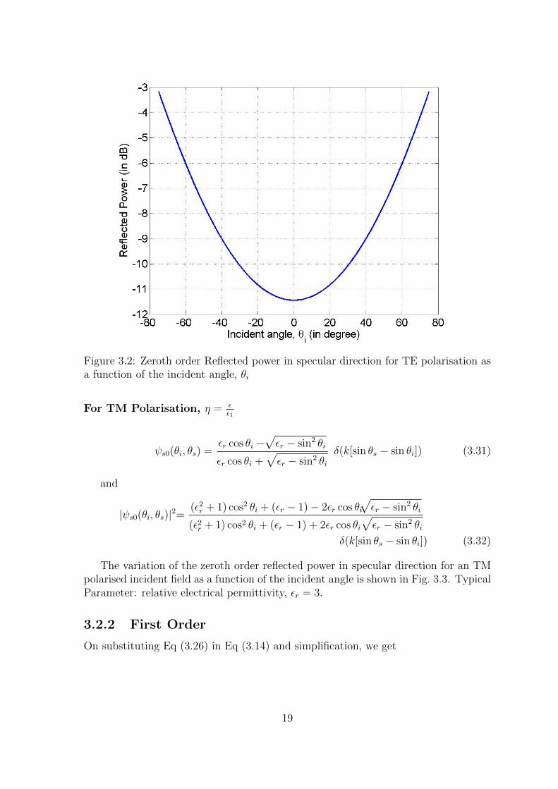
Figure 3.2: Zeroth order Reflected power in specular direction for TE polarisation asa function of the incident angle, θi


(3.31)ψs0(θi, θs) =εr cos θi −

√εr − sin2 θi

εr cos θi +√εr − sin2 θi


and

|ψs0(θi, θs)|2=(ε2r + 1) cos2 θi + (εr − 1)− 2εr cos θi

√εr − sin2 θi

(ε2r + 1) cos2 θi + (εr − 1) + 2εr cos θi√εr − sin2 θi

δ(k[sin θs − sin θi]) (3.32)

The variation of the zeroth order reflected power in specular direction for an TMpolarised incident field as a function of the incident angle is shown in Fig. 3.3. TypicalParameter: relative electrical permittivity, εr = 3.

3.2.2 First Order

On substituting Eq (3.26) in Eq (3.14) and simplification, we get

19

Figure 3.3: Zeroth order reflected power in specular direction for TM polarisation asa function of the incident angle, θi

ψs1(θi, θs) =−2ik cos θi

[(η − 1)(η

√εr − sin2 θi

√εr − sin2 θi − sin θs(sin θi − sin θs))

](cos θs + η

√εr − sin2 θs)(cos θi + η

√εr − sin2 θi)

F (k[sin θs − sin θi])(3.33)


ψs1(θi, θs) =−2ik cos θi (εr − 1)

(cos θs +√εr − sin2 θs)(cos θi +


F (k[sin θs − sin θi]) (3.34)

and the corresponding ensemble averaged scattered power will be given by

〈|ψs1(θi, θs)|2〉 =

∣∣∣∣∣ −2k cos θi (εr − 1)

(cos θs +√εr − sin2 θs)(cos θi +


∣∣∣∣∣2

W (k[sin θs − sin θi])

(3.35)

The variation in scattered power as a function of the scattering angle for TEpolarised field incident at 40◦ w.r.t. the normal to the surface is shown in Fig. 3.4 and3.5.

20

Figure 3.4: First order scattered power for TE polarisation as a function of the scat-tering angle, θs at incident angle, θi = 40◦ ensemble averaged over 1000 surfaces.

Figure 3.5: First order scattered power for TE polarisation as a function of the scat-tering angle, θs at incident angle, θi = 40◦.

21

Fig. 3.4 is plotted by using Eq (3.34) and random rough surface generated usingthe method given by Thorsos [6] and ensemble averaged over 1000 surfaces. Whereas,Fig. 3.35 is plotted using the Eq (3.35). Typical Parameters used are: wavelength, λ =23cm, incident angle, θi = 40◦, relative electrical permittivity, εr = 3 and Gaussianauto correlation function with rms height, h = 1cm and surface correlation length,l = 10cm, surface length, L = 9.2m.


ψs1(θi, θs) =−2ik(εr − 1) cos θi

[εr sin θi sin θs −

√εr − sin2 θi

√εr − sin2 θs

](εr cos θi +

√εr − sin2 θi

)(εr cos θs +

√εr − sin2 θs

)F (k[sin θs − sin θi]) (3.36)

and the corresponding ensemble averaged scattered power will be given by

〈|ψs1|2〉 =

∣∣∣∣∣∣−2k(εr − 1) cos θi

[εr sin θi sin θs −

√εr − sin2 θi

√εr − sin2 θs

](εr cos θi +

√εr − sin2 θi

)(εr cos θs +

√εr − sin2 θs

)∣∣∣∣∣∣2

W (k[sin θs − sin θi]) (3.37)

Figure 3.6: First order scattered power for TM polarisation as a function of thescattering angle, θs at incident angle, θi = 40◦ ensemble averaged over 1000 surfaces.

22

Figure 3.7: First order scattered power for TM polarisation as a function of thescattering angle, θs at incident angle, θi = 40◦.

The variation in scattered power as a function of the scattering angle for TM po-larised field incident at 40◦ w.r.t. normal to the surface is shown in Fig. 3.6 and 3.7.

Fig. 3.6 is plotted by using Eq (3.36) and random rough surface generated usingthe method given by Thorsos [6] and ensemble averaged over 1000 surfaces. Whereas,Fig. 3.37 is plotted using the Eq (3.35). Typical Parameters used are: wavelength,λ = 23cm, incident angle, θi = 40◦, relative electrical permittivity, εr = 3 and Gaus-sian auto correlation function with rms height, h = 1cm and surface correlation length,l = 10cm, surface length, L = 9.2m.

In summary, we have derived the scattered field expressions for the zeroth, first andsecond orders of random rough surface profile, f(x) in this chapter. In the next Chap-ter, we will use these expressions and compare the two types of icy surfaces: randomrough surface and random rough surface with uniformly distributed smooth squareboulders, on the basis of RCS (Radar Cross Section) and CPR (Circular PolarisationRatio).

23

Chapter 4

Ice Configurations: Analysis usingRCS and CPR

In the previous chapters, we analysed the electromagnetic wave scattering from ran-dom rough surfaces for both TE (Transverse Electric) and TM (Transverse Magnetic)polarisations. In the analysis, we observed that scattering behaviour were different forTE and TM polarisations. Which means, surface will behave differently for h- and v-pol (Horizontal and Vertical Polarisation, respectively). It means that if we transmit acircularly polarised signal, then the reflected field may be an elliptically polarised sig-nal, due to the different reflection co-efficients for horizontal and vertical components.By the principle of orthogonality, we can decompose it into RHCP (Right HandedCircularly Polarised) and LHCP (Left Handed Circularly Polarised) signals. In thischapter, we analyse the two types of icy surface configurations: random rough surfaceand random rough surface with uniformly distributed smooth square boulders, on thebasis of RCS (Radar Cross Section) and CPR (Circular Polarisation Ratio).

4.1 Radar Cross Section (RCS)

Radar cross section (RCS) is defined as the ratio of the backscattered power per unitsteradian to the total incident power on the target. RCS is basically same as com-monly used term reflection co-efficient and is a good measure to calculate how mucha target reflect power in the direction of the receiver.

Considering up to second order terms, the total scattered field is given by

(4.1)ψs = ψs0 + ψs1 + ψs2

and the corresponding scattered power is given by the mod square of the scatteredfield, which is equal to the product of field and its complex conjugate.

|ψs|2 = ψsψ∗s (4.2)

= (ψs0 + ψs1 + ψs2) (ψs0 + ψs1 + ψs2)∗ (4.3)

24

On solving and taking ensemble average, we get

(4.4)〈|ψs|2〉 = |ψs0|2 + ψs0〈ψ∗s1〉+ ψs0〈ψ∗s2〉+ 〈ψs1〉ψ∗s0 + 〈|ψs1|2〉+ 〈ψs1ψ∗s2〉+ ψ∗s0〈ψs2〉+ 〈ψ∗s1ψs2〉+ 〈|ψs2|2〉

Here, the terms containing 〈ψs1〉 or 〈ψ∗s1〉 become zero due to the assumption ofzero mean random rough surface, i.e., f(x) = 0. Hence, we get

(4.5)〈|ψs|2〉 = |ψs|2 + ψs0〈ψ∗s2〉+ 〈|ψs1|2〉+ ψ∗s0〈ψs2〉+ 〈ψs1ψ∗s2〉+ 〈ψ∗s1ψs2〉+ 〈|ψs2|2〉

The reflection coefficient, r, is defined as the ratio of the reflected power dividedby the incident power. On assuming amplitude of the incident field as unity, thereflection coefficient is given by

r = 〈|ψs|2〉

4.2 Circular Polarisation Ratio (CPR)

“The circular-polarization ratio, µ is defined as the ratio of the echo power in thesame circular polarisation state (SC) to that in the opposite circular polarisationstate (OC)” [9].

(4.6)µ =Same Circularly Polarise (SC)

Opposite Circularly Polarise (OC)

4.3 Analysis using Radar Cross Section

Scattering pattern from a surface is highly dependent on its configuration. Theremay be multiple bounces before the signal reach back to the radar. So, each surfacehas different reflection co-efficient, i.e., radar cross section. In this section, we willanalyse two icy surface configurations on the basis of RCS. In general, the radar usedin remote sensing are monostatic. In a monostatic radar system, transmitter andreceiver are collocated. So, the radar will receive the signal scattered in the directionexactly opposite to the incident field direction, i.e., scattering angle will be equal tothe negative of the incident angle, i.e., θs = −θi.

4.3.1 Random Rough Surface

Let us assume a TE polarised wave of unit magnitude is incident on a icy randomrough surface with Gaussian auto correlation function and small surface height asshown in Fig. 4.1. As we are assuming monostatic radar system, the signal receivedby the radar will be the signal scattered at scattering angle equals to −θi. Zeroth andSecond orders give scattering field in specular direction only. So, only first order willcontribute to the direct backscatter to radar from the random rough surface, whichcan be calculated by substituting θs = −θi in Eq (3.35). On substituing, we get

(4.7)PBS = 2k2h2l√π

cos2 θi |χ|2 exp(−k2l2 sin2 θi)

25

Figure 4.1: Backscattering phenomenon from random rough surface

where,

χ =cos θi −

√εr − sin2 θi

cos θi +√εr − sin2 θi

The variation of backscatter power from random rough surface as a function of theincident angle, i.e., monostatic radar viewing angle for a TE polarised incident waveis shown in Fig. 4.2.

Figure 4.2: Backscatter Power variation as a function of Monostatic Radar viewingangle for TE polarisation.

Similarly, for TM polarisation, on substituting θs = −θi in Eq (3.37). we get

(4.8)〈PBS〉 = 2k2h2l√π

∣∣∣∣∣(εr − 1) cos θi(sin2 θi(1− εr)− εr)

(εr cos θi +√εr − sin2 θi)2

∣∣∣∣∣2

exp(−k2l2sin2θi)

The variation of backscatter power from random rough surface as a function ofthe incident angle, i.e., monostatic radar viewing angle for an TM polarised incident

26

wave is shown in Fig. 4.3.

Figure 4.3: Backscatter Power variation as a function of Monostatic Radar viewingangle for TM polarisation.

4.3.2 Random Rough Surface with Boulders

Now, let us assume an icy random rough surface with smooth faced boulder as shownin Fig. 4.4. In this configuration, two types of scattering phenomena will occur. Onewill be the direct backscatter from random rough surface and another will be thedouble bounce through boulder as shown in Fig. 4.4 as case 1 and 2, respectively.

1 2

Boulders

Figure 4.4: Backscattering phenomena from random rough Surface with smooth boul-der

In previous section, we have already derived the expression for direct backscatterpower from the random rough surface (case 1). In this section, we will derive the

27

expression for the backscatter power due to double bounce through boulder (case 2).

Firstly, we calculate the total power scattered in specular direction (θs = θi). Andthen we multiply it with the Fresnel reflection coefficient, as we have assumed smoothfaced boulder, to get the backscatter field after double bounce through boulder.

The reflected power in specular direction will be given by

Pspecular = (ψs0 + ψs1 + ψs2)(ψs0 + ψs1 + ψs2)∗|θs=θi

On simplifying and taking ensemble average, we get

(4.9)〈Pspecular〉 = |ψs0|2 + ψs0〈ψ∗s2〉+ 〈|ψs1|2〉+ 〈ψs2〉ψ∗s0 + 〈|ψs2|2〉

Here, we neglect 〈|ψs2|2〉, due to complexity of its computation. So, on substitutingθs = θi in Eqs. (3.30), (3.35) and using these equations and Eq (3.21) in aboveequation, we get

(4.10)〈Pspecular〉 = |χ|2 + χψ∗s2 + 2k2h2l√π

cos2 θi |χ|2 + χ∗ψs2

Now, we multiply 〈Pspecular〉 by Fresnel reflection co-efficient with incident angle90− θi. So, the backscatter power after the double bounce, PDB, is given by

(4.11)〈PDB〉 = 〈Pspecular〉 × |χ1|2

where,

χ1 =sin θi −

√εr − cos2 θi

sin θi +√εr − cos2 θi

Now, let us assume a plane wave is incident on a random rough surface of lengthL with uniformly distributed smooth square boulders of size S, the scattered powerfor a 2-D scattering geometry (1-D surface) is given by

〈P 〉 =

〈PBS〉(L−nS(1+tan θi))+2 nS tan θi〈PDB〉

L, 0 ≤ nS

L≤ 1

1+2 tan θi(〈PBS〉+2〈PDB〉)(L−nS(1+tan θi))

L, 1

1+2 tan θi≤ nS

L≤ 1

1+tan θi

0, 11+tan θi

≤ nSL≤ 1

where,

〈PBS〉 = Ensemble averaged direct backscatter power from random rough surface,

〈PDB〉 = Ensemble averaged backscatter power after double bounce through random

rough surface and the boulder,

n = Number of boulders,

and

Boulder factor(α) =Length covered by boulders

Total Length

=nS

L

28

Here, the factor of tan θi is coming due to consideration of shadows of the boulderon the surface and a factor of 2 is due to the consideration of symmetry. i.e., there willbe two cases of double bounce: field falls on vertical face of the boulder after reflectionfrom the random rough surface and the field falls on the random rough surface afterreflection from the vertical face of the boulder.

The boulder factor (α) is basically defining how much fraction of the surface iscovered with the boulders. On substituting, nS/L = α, we get

〈P 〉 =

〈PBS〉(1− α(1 + tan θi)) + 2α tan θi〈PDB〉, 0 ≤ α ≤ 1

1+2 tan θi

(〈PBS〉+ 2〈PDB〉)(1− α(1 + tan θi)),1

1+2 tan θi≤ α ≤ 1

1+tan θi

0, 11+tan θi

≤ α ≤ 1

The variation in backscatter power as a function of the boulder factor, α, for TEpolarised wave incident at an incident angle of 40◦ w.r.t. normal of the surface isshown in Fig. 4.5.

Figure 4.5: Backscatter Power variation as a function of Boulder factor (α) for TEpolarisation at an incident angle of 40◦.

4.4 Analysis using CPR

In section 3.2, we saw that the reflection coefficient for TE and TM polarised waveswere different. Which implies that the reflection coefficient for the horizontal and

29

vertical components, h and v component, respectively, will be different. A circularlypolarised field can be written as the superposition of horizontal and vertical linearlypolarised field components. As the reflection coefficients are different for horizontaland vertical field components, the amplitude of the horizontal and vertical compo-nents in scattered field will be different and scattered field will not remain as circularlypolarised. Due to different amplitudes of the horizontal and vertical field components,the resulting scattered field will be elliptically polarised. By the principle of orthogo-nality, we know that an elliptically polarised field can be written as the superpositionof RHCP (Right Handed Circularly Polarised) and LHCP (Left Handed CircularlyPolarised) field components. This will provide us the ratio of same sense of circularlypolarised (SC) and opposite sense of circularly polarised field components, which isknown as circular polarisation ratio.

Relation between reflection coefficients of Electric and Magnetic field com-ponents of a transverse wave -

By the principle of Fresnel reflection [15], we know that

EiHi

= −ErHr

So,ErEi

= −Hr

Hi

where,

Ei, Hi = electric and magnetic field component of the incident field, respectively

Er, Hr = electric and magnetic field component of the reflected field, respectively

rTM = Reflection coefficient of Magnetic field component of a TM wave

So, the reflection coefficient for the electric field component of a TM polarisedwave with rTM being the reflection coefficient for the magnetic field component willbe given by −rTM .

Now, let us assume the incident field is circularly polarised electric field. So, thereflection coefficient for the horizontal and vertical component will be given by rTEand −rTM , respectively.

Now, we will analyse two types of icy surfaces: random rough surface and randomrough surface with uniformly distributed square smooth boulders, on the basis of theCPR.

4.4.1 Random Rough Surface

Let a RHCP (Right Handed circularly Polarised) electric field with propagation vectork = h× v be incident on a random rough surface as shown in Fig. 4.6. The incidentfield can be written as:

ψinc = a(h+ jv)

30

Figure 4.6: An RHCP electric field is incident on a random rough surface.

Figure 4.7: The variation of the backscatter CPR from random rough surface withincident angle w.r.t. normal to the surface.

On scattering from the surface, the horizontal component, h gets multiplied byrTE and the vertical component, v gets multiplied by −rTM as described in section4.4. Hence, the scattered field, ψs is given by

(4.12)ψs = a(rTE(θi, θs)h− j rTM(θi, θs)v)

with propagation vector k = v × h. On rewriting the above equation, we get

ψs = a(rTE(θi, θs)− rTM(θi, θs))

2(h+ jv) + a

(rTE(θi, θs) + rTM(θi, θs))

2(h− jv)

Here, first and second terms are giving the LHCP (Left Handed Circularly Polarised)and RHCP (Right Handed Circularly Polarised) components of the scattered field,respectively. As we have assumed that the incident field is RHCP polarised, RHCPcomponent of the scattered field is the same sense circularly polarised field (SC) and

31

LHCP is the opposite sense circularly polarised field (OC). So, the CPR is given by

(4.13)CPR =rTE(θi, θs) + rTM(θi, θs)

rTE(θi, θs)− rTM(θi, θs)

For backscatter, θs = −θi. So, the backscatter CPR, CPRBS is given by

CPRBS = CPR|θs=−θi

The variation of the CPRBS as a function of the incident angle w.r.t. normal isshown in Fig. 4.7.

4.4.2 Random Rough Surface with Uniformly DistributedSmooth Square Boulders

Now, let us assume that there is a smooth square boulder over the random roughsurface as shown in Fig. 4.4. As discussed in previous section, there will be doublebounce in this case, one from the random rough surface and another will be from theboulder face.

Using Eq.(4.12), scattered field from the surface is given by

(4.14)ψs = a(rTEs(θi, θs)h− j rTMs(θi, θs)v)

where,

rTEs = Reflection coefficient for TE polarise component from surface

rTMs = Reflection coefficient for TM polarise component from surface

Due to smooth faced boulders, only specular field will go back to the radar. So,the scattering angle will be equal to the incident angle, i.e., θs = θi. Now scatteredfield will be the function of incident angle, θi only.

(4.15)ψs(θi) = a(rTEs(θi)h− j rTMs(θi)v)

with propagation vector, k = v × h. Now, let this field fall on the perpendicularface of the boulder. As we are assuming, smooth square perpendicular boulder, thescattered field from the surface will make 90 − θi incident angle with the normal tothe perpendicular face of the boulder. As boulder faces are smooth, the reflectionco-efficient will be given by zeroth order term or the Fresnel reflection coefficient. So,the backscatter field after double bounce with propagation vector k = h × v will begiven by

(4.16)ψs(θi) = a(rTEs(θi) rTEb(90− θi)h+ j rTMs(θi) rTMb(90− θi)v)

where,

rTEb = Reflection coefficient for TE polarise component from boulder

rTMb = Reflection coefficient for TM polarise component from boulder

32

On rewriting the above equation, we get

(4.17)ψs(θi) = a

rTEs(θi) rTEb(90− θi) + rTMs(θi) rTMb(90− θi)2

(h+ jv)

+ j arTEs(θi) rTEb(90− θi)− rTMs(θi) rTMb(90− θi)

2(h− jv)

Here, first and second terms are the RHCP and LHCP components of the backscat-ter field after double bounce through boulder, respectively. As we have assumedincident wave as RHCP, the CPR after double bounce, CPRDB will be given by

(4.18)CPRDB =rTEs(θi) rTEb(90− θi) + rTMs(θi) rTMb(90− θi)rTEs(θi) rTEb(90− θi)− rTMs(θi) rTMb(90− θi)

Figure 4.8: The variation in CPR w.r.t. the incident angle assuming both surface andboulder as smooth.

The above all expressions of CPR are valid only if various reflection coefficientsare real and positive. If not, the above will change accordingly.

In Fig. 4.8, we have assumed both the surface and the boulder are smooth. Now thequestion arises, how the CPR will change, if the surface is randomly rough? To obtainits answer, we have plotted the variation in CPR after double bounce as a functionof the randomness of the surface. In Fig. 4.9, we vary the rms height of the surfacekeeping correlation length constant. And in Fig. 4.10, we varied the correlation lengthkeeping rms height of the surface constant.

33

Figure 4.9: Variation in backscatter CPR from a random rough surface as a functionof the rms height of the rough surface,h, keeping correlation length,l, constant.

Figure 4.10: Variation in Backscatter CPR from a random rough surface as a functionof the auto correlation length,l, of the rough surface keeping rms height,h, constant

34

Chapter 5

Conclusion

To understand the high radar albedo from the Enceladus (moon of the Saturn), westart with the analysis of the electromagnetic wave scattering from random rough sur-faces. We used SPM (Small Perturbation Method) for the analysis and determinedthe scttered field expressions up to second order of perturbation. Further, we haveanalysed the various configurations of icy surfaces on the basis of RCS and CPR. Inthe analysis we have used incident angle equal to 40◦, which is same as the incidenceangle used by SMAP (Soil Moisture Active Passive) mission ot the JPL laboratory,NASA.

In chapter 2, we have analysed electromagnetic wave scattering from random roughsurfaces. We continued the analysis in chapter 3, and derived the expressions forzeroth, first and second order scattered fields for both TE and TM polarised wave.

In zeroth order, for TE polarised wave, reflected power curve is like an upwardparabola. Whereas, for TM polarisation, it has a null at the Brewster angle, θp =tan−1(n2/n1). We have done the analysis for icy surfaces with εr = 3. So, the Brew-ster angle, θp = tan−1(

√(3)) = 60◦. At θi = 0, the reflected power for both the

polarisations are same.

In first order, for TE polarised wave, the scattered power is more in the speculardirection. Whereas, in TM polarisation, more power goes in the backscatter direc-tion. The amplitude of oscillations are the function of the ratio of the correlationlength, l and the surface length, L, i.e., l/L.

In chapter 4, we have analysed two types of surfaces: random rough surface andrandom rough surfaces with uniformly distributed smooth square boulders on the ba-sis of RCS (Radar Cross Section) and CPR (Circular Polarisation Ratio). Backscatterpower for a TE polarised wave at 40◦ incident angle is about -38 dB as shown in Fig.4.2. And from Fig. 4.5, we have observed that there is about 25 dB variation in thebackscatter power. Maximum backscatter power is about -11 dB at boulder factor,α = 0.5.

Further, we have analysed the same surfaces using CPR and found very big varia-

35

tion in the values of CPR from the surface with boulder compared to the CPR fromthe rough surface. As shown in Fig. 4.7, the CPR from the random rough surface isaround 0.18. Whereas, the CPR from the smooth surface with smooth square boulderis around 1.38 as shown in Fig. 4.8. Further, we observed a variation of about 0.12on varying the roughness of the surface in case of double bounce at an incident angleof 40◦ keeping correlation length constant and a variation of about 0.24 in CPR onvarying correlation length of the surface keeping rms height constant.

The analysis of icy surfaces on the basis of RCS and CPR shows that radar albedoand CPR goes to higher values due to presence of boulder like structures over thesurface. This has very high priority on the surface of the Enceladus due to very smallradius of the body (around 252 km) and the presence of the Cryovolcanoes. Due tosmall radius, the gravitational force over it is very less. Cryovolcanoes shoot geyser-like jets of water vapor, other volatiles, and solid material, including sodium chloridecrystals and ice particles, into space, totaling approximately 200 kilograms (440 lb)per second. This lead to floating ice cubes over the surface of the Enceladus, whichgives configuration similar to the random rough surface with boulders.

36

Appendix A

Green’s Function and Its Gradient

“Green’s function is defined as the field in a medium due to point source”, i.e., it is itis the solution of the second order partial differential equation (Helmholtz equation),derived from the Maxwell’s equation, where the driving force is a unit source (Diracdelta or impulse function).

∇2g(r, r′) + ω2µε g(r, r′) = −δ(r − r′)

where ∇2 is two dimensional Laplace operator, ω is the angular frequency of the wave,µ and ε are the magnetic permeability and electrical permittivity of the medium, re-spectively, g(r, r′) is the green’s function and δ is the impulse function.

The solution of the above equation in cylindrical co-ordinate with incident fieldas cylindrical wave is given by the Hankel function. We have converted it to therectangular co-ordinate with incident field as plane wave by the expansion methodgiven by Cinotti [13]. On conversion we get

g(−→r ,−→r ′) =i

4π

∫ ∞−∞

dkx√k2 − k2x

exp [ikx(x′ − x) + ikz|z′ − z|]

Now, we have simplified it for both upper (z′ > f(x′)) and lower (z′ < f(x′)) dielectricmediums.

For region z′ < f(x′),

g(−→r ,−→r ′) =i

4π

∫ ∞−∞

dkx1

kzexp[ikx(x

′ − x)− ikz(z′ − z)] (A.1)

and the gradient of the green’s function is given by

∇g(−→r ,−→r ′) =1

4π

∫ ∞−∞

1

kz(kxx− kz z) exp[ikx(x

′ − x)− ikz(z′ − z)]dkx (A.2)

√1 + (

df

dx)2n · ∇g(−→r ,−→r ′) =

−1

4π

∫ ∞−∞

(df

dx

kxkz

+ 1

)exp[ikx(x

′ − x)− ikz(z′ − z)] dkx

(A.3)

37

For region, z′ > f(x′),

g1(−→r ,−→r ′) =

i

4π

∫ ∞−∞

dk1x1

k1zexp[ik1x(x

′ − x) + ik1z(z′ − z)] (A.4)

and the gradient of the green’s function is given by

∇g1(−→r ,−→r′) =

1

4π

∫ ∞−∞

1

k1z(k1xx+ k1z z) exp[ik1x(x

′ − x) + ik1z(z′ − z)] dk1x (A.5)

√1 + (

df

dx)2n·∇g1(−→r ,−→r

′) =

1

4π

∫ ∞−∞

(−dfdx

k1xk1z

+ 1

)exp[ik1x(x

′−x)+ik1z(z′−z)] dk1x

(A.6)

38

Appendix B

Auto Correlation Function of aRandom Rough Surface

Auto correlation function of a variable defines the similarity of the variable with itsown at different instant of time or space. Mathematically, Auto correlation, R(τ), ofa variable function of time, x(t), is given by

R(τ) = 〈x(t1)x(t2)〉 =

∫ ∞−∞

dτ x(t) x(t+ τ)

This is the function of separation between the two observation points. So, we maydefine the auto correlation function of the random rough surface profile, f(x), as

〈f(x1)f(x2)〉 = h2c(|x1 − x2|)

where h2 is the rms height of the random rough surface. Here, we have describedthe correlation function of the various functions required in the analysis, which are asfollows-

〈F (kx1)F (kx2)〉 =1

4π2

∫ ∞−∞

∫ ∞−∞〈f(x1)f(x2)〉 exp(−ikx1x1) exp(−ikx2x2) dx1dx2

(B.1)

=1

4π2

∫ ∞−∞

∫ ∞−∞

R(|x1 − x2|) exp(−ikx1x1) exp(−ikx2x2) dx1dx2

(B.2)

Let x1 − x2 = σ1 and x2 = σ2. So, x1 = σ1 + σ2 and dx1dx2 = dσ1dσ2

〈F (kx1)F (kx2)〉 =1

4π2

∫ ∞−∞

∫ ∞−∞

R(|σ1|) exp(−ikx1σ1) exp(−i(kx1 + kx2)σ2) dσ1dσ2

(B.3)

= W (kx1)δ(kx1 + kx2) (B.4)

39

〈ikxF (kx) ∗ A1(kx)〉 = 〈∫ ∞−∞

dk iA1(k)F (k − kix)(kx − k)F (kx − k)〉 (B.5)

=

∫ ∞−∞

dk iA1(k)(kx − k) 〈F (k − kix)F (kx − k)〉 (B.6)

= δ(kx − kix)∫ ∞−∞

dk i(kx − k)A1(k) W (k − kix) (B.7)

Similarly, we get

〈F (kx) ∗ A1(kx)〉 = δ(kx − kix)∫ ∞−∞

dk A1(k) W (k − kx) (B.8)

〈ikxF (kx) ∗ F (kx) ∗ A0(kx)〉 = δ(kx − kix) iA0

∫ ∞−∞

dk (kx − k) W (k − kx) (B.9)

〈F (kx) ∗ F (kx) ∗ A0(kx)〉 = δ(kx − kix)A0

∫ ∞−∞

dk W (k − kx) (B.10)

〈F (kx) ∗B1(kx)〉 = δ(kx − kix)∫ ∞−∞

dk B1(k) W (k − kx) (B.11)

〈F (kx) ∗ F (kx) ∗B0(kx)〉 = δ(kx − kix)B0

∫ ∞−∞

dk W (k − kx) (B.12)

40

Bibliography

[1] C. Elachi and J. J. Van Zyl, Introduction to the physics and techniques of remotesensing. John Wiley & Sons, 2006, vol. 28.

[2] U. Khankhoje, K. Mitchell, J. Castillo-Rogez, and M. Janssen, “Enceladus’sbrilliant surface: Radar modeling,” in Lunar and Planetary Science Conference,vol. 44, 2013, p. 2531.

[3] K. Mitchell, U. Khankhoje, J. Castillo-Rogez, and S. Wall, “Enceladus’ brilliantsurface: Cassini radar observations and interpretation,” in Lunar and PlanetaryScience Conference, vol. 44, 2013, p. 2902.

[4] S. O. Rice, “Reflection of electromagnetic waves from slightly rough surfaces,”Communications on pure and applied mathematics, vol. 4, no. 2-3, pp. 351–378,1951.

[5] K. F. Warnick and W. C. Chew, “Numerical simulation methods for rough surfacescattering,” Waves in random media, vol. 11, no. 1, pp. R1–R30, 2001.

[6] E. I. Thorsos, “The validity of the kirchhoff approximation for rough surfacescattering using a gaussian roughness spectrum,” The Journal of the AcousticalSociety of America, vol. 83, no. 1, pp. 78–92, 1988.

[7] J. T. Johnson and J. D. Ouellette, “Polarization features in bistatic scatteringfrom rough surfaces,” Geoscience and Remote Sensing, IEEE Transactions on,vol. 52, no. 3, pp. 1616–1626, 2014.

[8] G. R. Valenzuela, “Depolarization of em waves by slightly rough surfaces,” An-tennas and Propagation, IEEE Transactions on, vol. 15, no. 4, pp. 552–557, 1967.

[9] B. A. Campbell, “High circular polarization ratios in radar scattering from geo-logic targets,” Journal of Geophysical Research: Planets, vol. 117, no. E6, 2012.

[10] X. Gu, L. Tsang, H. Braunisch, and P. Xu, “Modeling absorption of rough inter-face between dielectric and conductive medium,” Microwave and Optical Tech-nology Letters, vol. 49, no. 1, pp. 7–13, 2007.

[11] W. C. Chew, Waves and fields in inhomogeneous media. IEEE press New York,1995, vol. 522.

41

[12] K.-S. Chen, T.-D. Wu, L. Tsang, Q. Li, J. Shi, and A. K. Fung, “Emission ofrough surfaces calculated by the integral equation method with comparison tothree-dimensional moment method simulations,” Geoscience and Remote Sens-ing, IEEE Transactions on, vol. 41, no. 1, pp. 90–101, 2003.

[13] G. Cincotti, F. Gori, M. Santarsiero, F. Frezza, F. Furno, and G. Schettini,“Plane wave expansion of cylidrical functions,” Optics communications, vol. 95,no. 4-6, pp. 192–198, 1993.

[14] C. M. Bender and S. A. Orszag, Advanced mathematical methods for scientistsand engineers I. Springer Science & Business Media, 1999.

[15] A. Kumar and A. K. Ghatak, Polarization of light with applications in opticalfibers. SPIE Press, 2011, vol. 246.

42

study of electromagnetic wave scattering from rough...

Documents