study of eastern oregon freeway alternatives pursuant to
TRANSCRIPT
Study of Eastern Oregon Freeway Alternatives
Pursuant to House Bill 3090
Prepared by: Oregon Department of Transportation Transportation Development Division Transportation Planning Analysis Unit
April 2001

Table of Contents Executive Summary ............................................................................................................ ii Introduction......................................................................................................................... 1 Methodology....................................................................................................................... 2
Approach ......................................................................................................................... 2 Statewide Model .............................................................................................................. 4 Identification of Study Alternatives ................................................................................ 6
Study Results ...................................................................................................................... 8 Conclusions....................................................................................................................... 13 List of Tables Table 1. House Bill 3090 Study Objectives and Evaluation Measures.............................. 3 Table 2 and Table 3 ............................................................................................................ 8 Table 4. Percent Difference in Auto VMT by Region ........................................................ 9 Table 5. Percent Difference in Truck VMT by Region....................................................... 9 Table 6. 2050 Average Daily Traffic ................................................................................. 9 Table 7. Distribution of Households ................................................................................ 11 Table 8. Distribution of Employment............................................................................... 11 List of Figures Figure 1. Study Context ..................................................................................................... 1 Figure 2. Study Reporting Regions .................................................................................... 3 Figure 3. Schematic Representation of Statewide Model .................................................. 4 Figure 4. How the Statewide Model Evaluates Changes Over Time................................. 5 Figure 5. Steep Terrain and Study Route Locations.......................................................... 6 Figure 6. 2050 Traffic Volumes ....................................................................................... 10
i

Executive Summary The 1999 Legislature asked the Oregon Department of Transportation to look at the results of designating a north-south freeway in Central or Eastern Oregon, from the Washington to California borders. The objectives of House Bill 3090 were to:
• Define a better north-south connection to I-82 in Eastern Oregon • Increase growth of Central/Eastern Oregon • Decrease growth in the Willamette Valley • Decrease travel and congestion on I-5 in the Willamette Valley
Three alternative alignments were identified to connect with existing freeways in Washington and California. Results of the modeling effort concluded that a new freeway from Washington to California through Central or Eastern Oregon would:
• Significantly reduce travel time from Washington to California. • Improve market accessibility to both Central Oregon and the Willamette Valley. • Result in minimal differences in growth in Central and Eastern Oregon. • Because of increased accessibility, the US 97 improvement could slightly increase
growth of the Willamette Valley. Overall, the proposal did not meet the objectives of transferring growth from the Willamette Valley to Central or Eastern Oregon and the Legislature dropped further discussion of this option.
ii
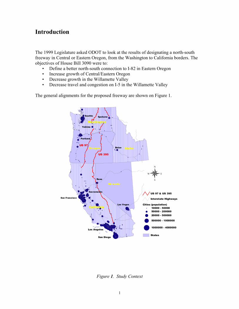
Introduction The 1999 Legislature asked ODOT to look at the results of designating a north-south freeway in Central or Eastern Oregon, from the Washington to California borders. The objectives of House Bill 3090 were to:
• Define a better north-south connection to I-82 in Eastern Oregon • Increase growth of Central/Eastern Oregon • Decrease growth in the Willamette Valley • Decrease travel and congestion on I-5 in the Willamette Valley
The general alignments for the proposed freeway are shown on Figure 1.
##
##
# ########## #### ### ### #
## ######## ######## ## ########### ## ## ######
##
# ##
##
# # #####
#
## #### #### ####### ####### ##
##
####
## #
####
# ##
#
#
##
#
##
###
## #
#
##
##
####
# ## ##
# ####### ### ## ######## ##
### #### ####
######## # #### # ## ### ## ## ### #### # ### ## ##### ## ## # ##### # ###### #### ##
########### ### #####
##### ##
# ######## ## #
##########
# ## ##
#
# ##
# #
## # #
##
# #
## # ##
# ## ### #### # #
#
# ### ###### ### # # ### ## ## ## #### ### # ## ## ### # ## ## ####### ### ## # ## ### ### ## # #### ## ## # ###### #### ### #### ### #### ###### ##### ###### ##### ### ##### # ### # #
### # ## ### #### ######### #### ####
######### ## #
#
##### #
#### #####
California
Idaho
Nevada
Oregon
Washington
Boise
Yakima
SpokaneSeattle
Portland
San Francisco
Las Vegas
Reno
Sacramento
Los Angeles
San Diego
N
EW
S
States
Cities (population)# 10000 - 50000# 50000 - 200000
# 20000 - 500000
# 500000 - 1000000
# 1000000 - 4000000
Interstate Highways
US 97 & US 395
#
US 395
US 97
Figure 1. Study Context
1
Methodology Approach The basic approach of this study was to use the new statewide transportation and land use model to evaluate several alternative freeway scenarios and a base case scenario. A technical advisory committee helped to develop the study alternatives and to review the modeling results. The committee was composed of ODOT staff who are familiar with the legislature’s intent for HB3090, the regions where the freeway might be constructed, and the methods for modeling and evaluating the freeway’s effects. The starting point for modeling was determining the features of the base case scenario. The purpose of the base case scenario is to serve as a reference or control for comparison with the freeway scenarios. Since all modeling of future conditions incorporates a number of assumptions which are more or less certain (such as economic growth, land availability, etc.), it is important that all alternatives be built off of a common base of assumptions. The base case assumptions for the study include the Oregon Department of Administrative Services long-range statewide projections for population and employment1, assumed expansion of highway and public transportation systems in the Willamette Valley2, and urban expansion at historic rates (since the inception of the state land use program). All of the alternative freeway scenarios are variations of a ‘base case’ scenario. They are described in more detail later. The alternative scenarios were modeled over a long time horizon because of the amount of time required to build such a freeway and the time would take for land use effects to occur afterward. For the purposes of this study, completion of the freeway 2020 and 2025. Since significant land use effects of major transportation changes take decades to occur, the modeling time horizon was established as 2050. Data for several evaluation measures were extracted from the model outputs in order to determine whether the objectives of the freeway would be accomplished. The objectives and measures are summarized in Table 1. 1 The DAS projections only go to 2040. They were extended to 2050 for this study. The study only used the statewide level projections, not the county level projections. The statewide model allocates growth between the counties in reponse to the study alternatives. 2 The transportation system improvements assumed for the Willamette Valley were developed for another modeling study now nearing completion. They include major freeway, arterial and major transit expansions similar to those that have build in other areas around the country as those areas have grown.
2
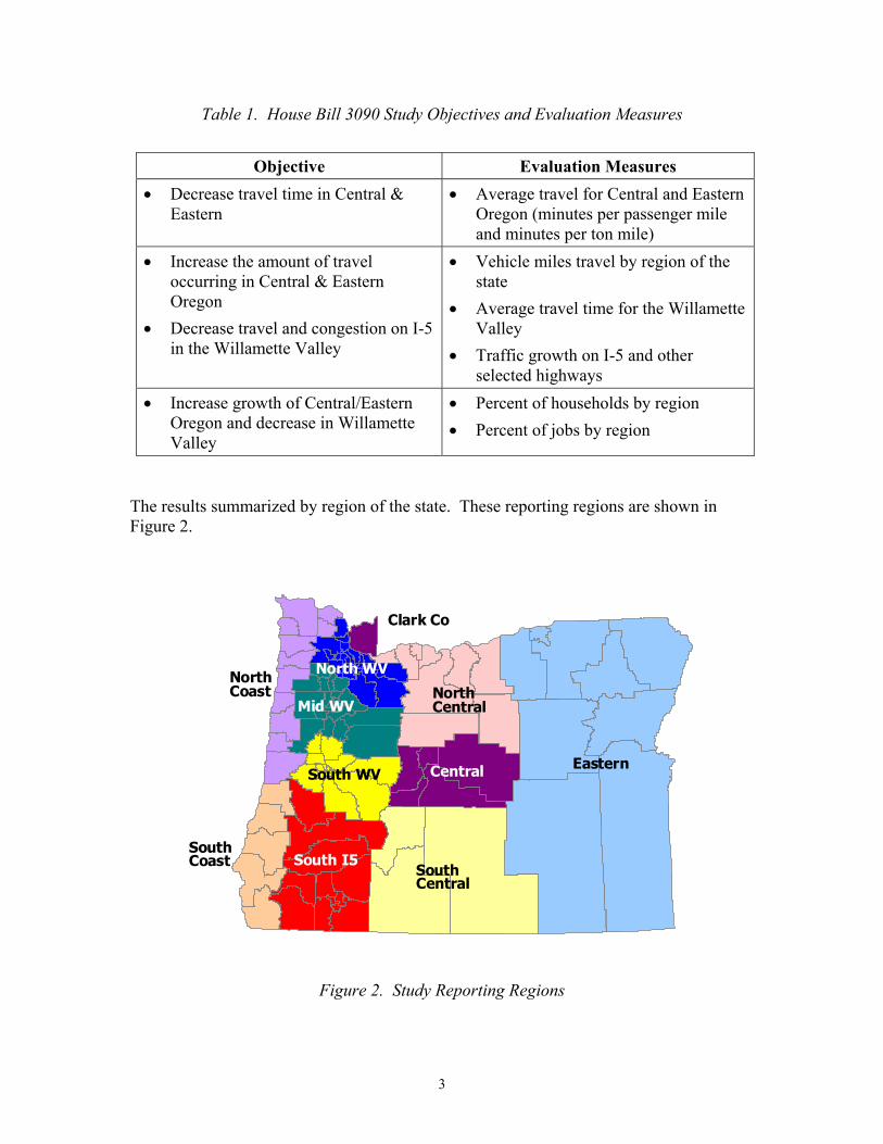
Table 1. House Bill 3090 Study Objectives and Evaluation Measures
Objective Evaluation Measures
• Decrease travel time in Central & Eastern
• Average travel for Central and Eastern Oregon (minutes per passenger mile and minutes per ton mile)
• Increase the amount of travel occurring in Central & Eastern Oregon
• Decrease travel and congestion on I-5 in the Willamette Valley
• Vehicle miles travel by region of the state
• Average travel time for the Willamette Valley
• Traffic growth on I-5 and other selected highways
• Increase growth of Central/Eastern Oregon and decrease in Willamette Valley
• Percent of households by region • Percent of jobs by region
The results summarized by region of the state. These reporting regions are shown in Figure 2.
Clark Co
North WV
Mid WV
South WV
NorthCoast
South I5
NorthCentral
Central
SouthCoast South
Central
Eastern
Figure 2. Study Reporting Regions
3

Statewide Model The statewide model is a set of computer programs and data that describe the relationships between Oregon’s economy, land use patterns and transportation system. This is the only operating model of it’s kind in the United States which integrates economic, land use and transport elements and covers an entire state. Figure 3 a general illustration of interactions of these components in the model.
POLICY
Figure 3. Schematic Representation of Statewide Model The statewide model incorporates a model of the state’s economy. This model describes the relationships between the various sectors of the state’s economy; what they export, what they import, and what they purchase from one-another. The economic model groups business activities into 12 sectors and households into 3 sectors (grouped by income). Growth of exports or other final demand (such as tourism) drives overall economic growth. As these industries grow, they purchase other goods and services to meet their production needs. This fuels additional growth whose effects ripple throughout the economy. The economic model calculates the additional growth of each economic sector in response to th growth of exports and other final demand. The land use part of the model allocates the growth of each sector to various parts of the state (and Clark County, Washington). This allocation is based on the costs of transporting production inputs and outputs and the cost of land. Land costs are adjusted continuously in response to the supply and demand for land in each area. Transportation costs are adjusted in response to congestion and other factors as described below.
4
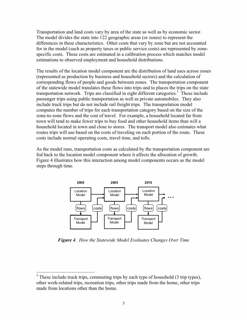
Transportation and land costs vary by area of the state as well as by economic sector. The model divides the state into 122 geographic areas (or zones) to represent the differences in these characteristics. Other costs that vary by zone but are not accounted for in the model (such as property taxes or public service costs) are represented by zone-specific costs. These costs are estimated in a calibration process which matches model estimations to observed employment and household distributions. The results of the location model component are the distribution of land uses across zones (represented as production by business and household sectors) and the calculation of corresponding flows of people and goods between zones. The transportation component of the statewide model translates these flows into trips and to places the trips on the state transportation network. Trips are classified in eight different categories.3 These include passenger trips using public transportation as well as private automobiles. They also include truck trips but do not include rail freight trips. The transportation model computes the number of trips for each transportation category based on the size of the zone-to-zone flows and the cost of travel. For example, a household located far from town will tend to make fewer trips to buy food and other household items than will a household located in town and close to stores. The transport model also estimates what routes trips will use based on the costs of traveling on each portion of the route. These costs include normal operating costs, travel time, and tolls. As the model runs, transportation costs as calculated by the transportation component are fed back to the location model component where it affects the allocation of growth. Figure 4 illustrates how this interaction among model components occurs as the model steps through time.
LocationModel
TransportModel
20052000 2010
LocationModel
costs costs costsflows flows flows
LocationModel
TransportModel
TransportModel
...
Figure 4. How the Statewide Model Evaluates Changes Over Time
3 These include truck trips, commuting trips by each type of household (3 trip types), other work-related trips, recreation trips, other trips made from the home, other trips made from locations other than the home.
5
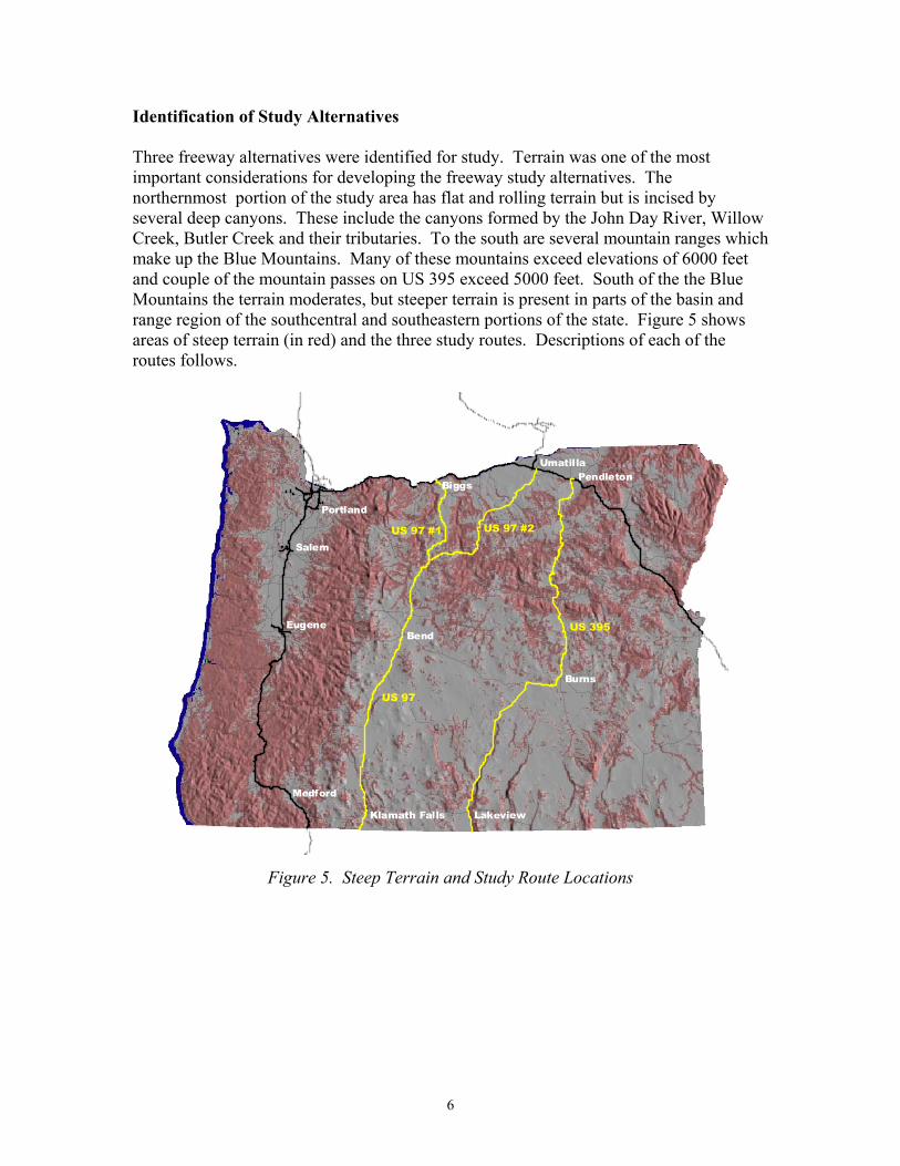
Identification of Study Alternatives Three freeway alternatives were identified for study. Terrain was one of the most important considerations for developing the freeway study alternatives. The northernmost portion of the study area has flat and rolling terrain but is incised by several deep canyons. These include the canyons formed by the John Day River, Willow Creek, Butler Creek and their tributaries. To the south are several mountain ranges which make up the Blue Mountains. Many of these mountains exceed elevations of 6000 feet and couple of the mountain passes on US 395 exceed 5000 feet. South of the the Blue Mountains the terrain moderates, but steeper terrain is present in parts of the basin and range region of the southcentral and southeastern portions of the state. Figure 5 shows areas of steep terrain (in red) and the three study routes. Descriptions of each of the routes follows.
Portland
Salem
Eugene
Medford
Klamath Falls Lakeview
Bend
Burns
PendletonUmatilla
Biggs
US 395
US 97 #2US 97 #1
US 97
Figure 5. Steep Terrain and Study Route Locations
6

The first study route follows the existing alignment of US 97 (referred to as US 97 #1 on the map and in following tables). It connects to I-82 via I-84. As can be seen from Figure 5, this is the line of least resistance between the Columbia River and the California border. Most of the route is on a good alignment and can be traveled at fairly high speeds. Most of the rural portions could be converted into freeway sections with frontage roads being built to serve adjacent farms and developments. It avoids the most difficult terrain in the north by following the plateau between the Deschutes River and John Day River canyons. Realignment would still be necessary in this area because of hilly terrain. Relocations would also be required to bypass several cities and towns along the route. This route would provide Central and Northeastern Oregon with improved access to California markets. (US 97 at the California border is only about 50 miles from the junction with I-5 in Northern California.) The route would also provide Central Oregon with better connections to Central and Eastern Washington and an additional route to the Puget Sound area via I-82 and I-90. (The distance from I-84 to I-82 near Yakima is about 70 miles.) This route, would do little to improve northbound connections for Eastern Oregon’s major population centers since these are already served by I-82 and I-84. A second study alternative also uses US 97, but makes a more direct connection to I-82 rather than relying on I-84 for the connection (referred to as US 97 #2 on the map and in following tables). The route of this connection starts at the junction of ORE 207 with I-84, close to I-82, and ends at the junction of ORE 293 with US 97, about 20 miles north of Madras. The route would follow US 97 to the south from that point. The construction of a connection between I-82 and US 97 would be by mountains and canyons, particularly canyons of the John Day River and its tributaries. Because of these constraints, the scenario mostly follows existing highways, particularly to the south and west of Condon where Oregon Route 218 crosses the John Day River at Clarno. However, the scenario does include a new section of highway between Lexington and Condon. This scenario would provide similar accessibility to California for Central Oregon as the previous scenario and would provide better accessibility for Northeastern Oregon to California as well. The third study scenario generally follows the route of US 395. Few major relocations of the likely because of the terrain. It was assumed, however, that the freeway would follow a more direct alignment south from Mt. Vernon rather than jogging east along US 26 to John Day. This route would provide Eastern Oregon with improved connections to California but more work would be required on the California side of the border to connect to an interstate highway than would be the case with the US 97 scenarios. The distance from the California border to I-80, in Reno, is about 220 miles. This route, as with the other routes, would do little to improve connections from Eastern Oregon’s major population centers to the north since these are already served by I-84 and I-82. Conversion of US 395 to a freeway in Eastern Washington, though, would improve connections between Spokane and I-82.
7
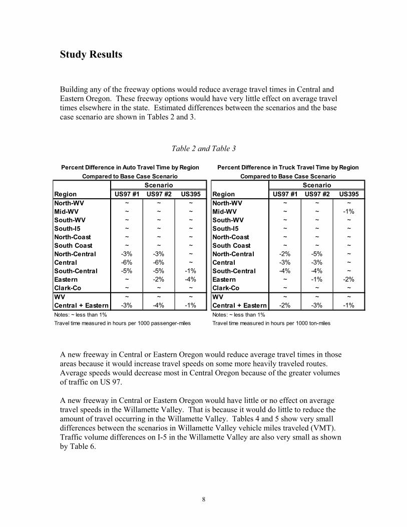
Study Results Building any of the freeway options would reduce average travel times in Central and Eastern Oregon. These freeway options would have very little effect on average travel times elsewhere in the state. Estimated differences between the scenarios and the base case scenario are shown in Tables 2 and 3.
Table 2 and Table 3
Region US97 #1 US97 #2 US395North-WV ~ ~ ~Mid-WV ~ ~ ~South-WV ~ ~ ~South-I5 ~ ~ ~North-Coast ~ ~ ~South Coast ~ ~ ~North-Central -3% -3% ~Central -6% -6% ~South-Central -5% -5% -1%Eastern ~ -2% -4%Clark-Co ~ ~ ~WV ~ ~ ~Central + Eastern -3% -4% -1%Notes: ~ less than 1%Travel time measured in hours per 1000 passenger-miles
Percent Difference in Auto Travel Time by RegionCompared to Base Case Scenario
ScenarioRegion US97 #1 US97 #2 US395North-WV ~ ~ ~Mid-WV ~ ~ -1%South-WV ~ ~ ~South-I5 ~ ~ ~North-Coast ~ ~ ~South Coast ~ ~ ~North-Central -2% -5% ~Central -3% -3% ~South-Central -4% -4% ~Eastern ~ -1% -2%Clark-Co ~ ~ ~WV ~ ~ ~Central + Eastern -2% -3% -1%Notes: ~ less than 1%Travel time measured in hours per 1000 ton-miles
Compared to Base Case ScenarioScenario
Percent Difference in Truck Travel Time by Region
A new freeway in Central or Eastern Oregon would reduce average travel times in those areas because it would increase travel speeds on some more heavily traveled routes. Average speeds would decrease most in Central Oregon because of the greater volumes of traffic on US 97. A new freeway in Central or Eastern Oregon would have little or no effect on average travel speeds in the Willamette Valley. That is because it would do little to reduce the amount of travel occurring in the Willamette Valley. Tables 4 and 5 show very small differences between the scenarios in Willamette Valley vehicle miles traveled (VMT). Traffic volume differences on I-5 in the Willamette Valley are also very small as shown by Table 6.
8

Table 4. Percent Difference in Auto VMT by Region Table 5. Percent Difference in Truck VMT by Region
Region US97 #1 US97 #2 US395North-WV ~ ~ ~Mid-WV ~ ~ -1%South-WV 1% 1% -2%South-I5 ~ 1% ~North-Coast 1% 1% ~South Coast ~ ~ -1%North-Central 1% 3% -1%Central 2% 3% ~South-Central 3% 5% ~Eastern 1% 1% 1%Clark-Co ~ ~ ~WV ~ ~ -1%Central + Eastern 2% 3% ~Note: ~ less than 1%
Scenario
Percent Difference in Auto VMT by RegionCompared to Base Case Scenario
Region US97 #1 US97 #2 US395North-WV ~ ~ ~Mid-WV ~ 1% ~South-WV ~ 1% ~South-I5 -1% ~ ~North-Coast ~ 1% ~South Coast ~ ~ ~North-Central ~ -2% ~Central ~ -1% ~South-Central ~ ~ ~Eastern ~ 1% ~Clark-Co ~ ~ ~WV ~ 1% ~Central + Eastern ~ ~ ~Note: ~ less than 1%
Percent Difference in Truck VMT by RegionCompared to Base Case Scenario
Scenario
Table 6. 2050 Average Daily Traffic
US97 #1 US97 #2 US395 US97 #1 US97 #2 US395I-5 at Columbia River Bridge 500 300 300 ~ ~ ~I-5 between Woodburn and Gervais 400 600 -800 ~ ~ ~I-5 near North Jefferson Interchange ~ 200 -600 ~ ~ ~I-5 north of Anlauf Junction 100 300 -200 ~ ~ ~I-5 at California border -200 -200 ~ ~ ~ ~I-84 near Cascade Locks ~ 300 ~ ~ ~ ~US 26 Wasco - Jefferson County Line ~ 500 ~ 1% 7% ~US 20 Linn - Jefferson County Line ~ ~ ~ ~ ~ ~OR 58, 138, 62 & 140 over South Oregon Cascades 500 700 ~ 4% 6% ~US 97 Wasco - Jefferson County Line 200 900 ~ 4% 20% ~US 97 Jefferson-Deschutes County Line 500 700 ~ 3% 4% ~US 97 0.1 mile south of Paulina Lake Road 1300 1500 ~ 10% 12% ~US 97 Chemult ATR Sta. 18-006 300 400 ~ 4% 6% ~US 97 Oregon - California state line ~ ~ ~ ~ ~ ~I-84 Sherman - Gilliam County Line 200 ~ -100 ~ ~ ~OR 218 Wasco - Wheeler County Line ~ 200 ~ 1% 69% ~US 26 Crook - Wheeler County Line ~ ~ ~ 2% ~ 2%US 20 Lake - Harney County Line ~ -200 ~ ~ -7% ~OR 140 Klamath - Lake County Line ~ 100 ~ -1% 6% 3%US 395 Long Creek ATR Sta. 12-006 ~ -200 600 3% -23% 61%US 395 Grant - Harney County Line ~ -100 400 2% -12% 41%US 395 Lake - Harney County Line ~ ~ ~ -1% ~ -2%US 395 New Pine Creek ATR Sta. 19-008 ~ ~ ~ ~ -1% ~US 26 Prarie City ATR Sta. 12-009 ~ ~ -200 ~ ~ -9%US 20 Harney - Malheur County Line ~ -100 100 ~ -4% 5%Note: ~ less than 100
Pecent Difference
2050 Average Daily Traffic on Various Highways in OregonComparisons of Freeway Scenarios with Base Case Scenario
Highway Route and Location ADT Difference
9
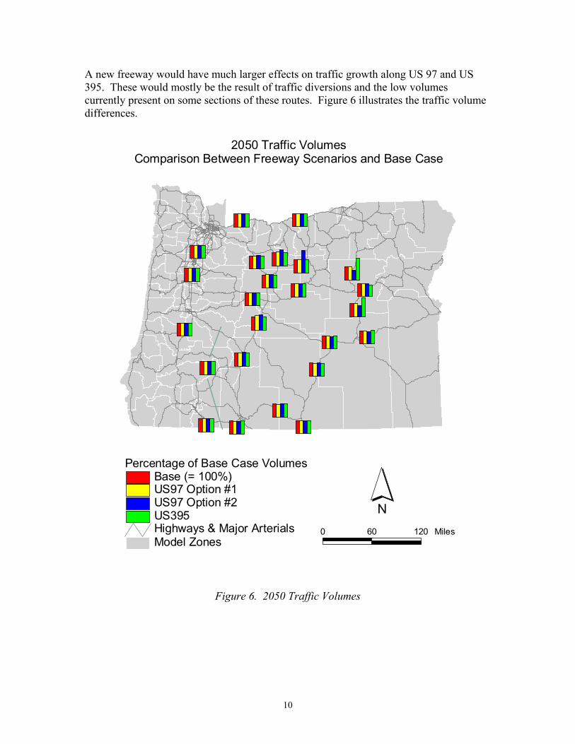
A new freeway would have much larger effects on traffic growth along US 97 and US 395. These would mostly be the result of traffic diversions and the low volumes currently present on some sections of these routes. Figure 6 illustrates the traffic volume differences.
N0 60 120 Miles
2050 Traffic VolumesComparison Between Freeway Scenarios and Base Case
Model ZonesHighways & Major Arterials
Percentage of Base Case VolumesBase (= 100%)US97 Option #1US97 Option #2US395
Figure 6. 2050 Traffic Volumes
10

The location effects of a new freeway would be even less than the transportation effects. This can be seen from tables 7 & 8 which show the modeled distributions of households and employment in 2050.
Table 7. Distribution of Households
Area Base US97 #1 US97 #2 US395North-WV 36.3% 36.4% 36.3% 36.4%Mid-WV 22.0% 22.1% 22.0% 22.0%South-WV 13.2% 13.2% 13.2% 13.1%South-I5 5.6% 5.5% 5.5% 5.6%North-Coast 5.0% 5.0% 5.0% 5.0%South Coast 2.4% 2.4% 2.4% 2.4%North-Central 1.8% 1.8% 1.8% 1.8%Central 3.9% 3.9% 3.9% 3.9%South-Central 1.0% 1.0% 1.0% 1.0%Eastern 2.0% 2.0% 2.0% 2.0%Clark-Co 6.7% 6.8% 6.8% 6.8%WV 71.5% 71.7% 71.6% 71.5%Central + Eastern 8.8% 8.7% 8.7% 8.8%Note: Clark County is included in the total.
Percentage of All Households in 2050
Table 8. Distribution of Employment
Area Base US97 #1 US97 #2 US395North-WV 37.6% 37.7% 37.6% 37.6%Mid-WV 22.9% 23.0% 23.0% 22.9%South-WV 11.7% 11.7% 11.8% 11.7%South-I5 5.7% 5.6% 5.7% 5.7%North-Coast 4.8% 4.9% 4.9% 4.8%South Coast 2.3% 2.2% 2.2% 2.3%North-Central 2.0% 2.0% 2.0% 2.0%Central 4.5% 4.4% 4.4% 4.5%South-Central 1.0% 0.9% 1.0% 1.0%Eastern 1.8% 1.8% 1.8% 1.8%Clark-Co 5.7% 5.7% 5.7% 5.7%WV 72.3% 72.4% 72.4% 72.3%Central + Eastern 9.2% 9.2% 9.1% 9.2%Note: Clark County is included in the total.
Percentage of All Employment in 2050
It can be seen from the tables that the differences in the distribution of population and employment are miniscule. The only observable difference is the very slight tendency for the US 97 scenarios to increase the proportion of development in the Willamette Valley. These findings, that a new freeway in Central or Eastern Oregon would not shift growth there and could very slightly shift growth to the Willamette Valley, might be surprising to
11
some, given the widely held believe that “if you build it, they will come”. That is probably because most of the attention to the relationship between freeway building and growth has centered on the nations most populated areas where the distribution of metropolitan population has clearly been affected by the interstate highway system. But there are many thousands of miles of interstate highways crossing less populated areas which have had little effect on the growth of these areas. Highways don’t cause development by simply being present. Rather, they affect the economy and growth by affecting the cost of transporting people and goods to and from markets. Transportation improvements in a less populated region will have smaller economic effects than improvements in a more populated region because the the market area, in economic terms, would be expanded by a smaller amount in the less populated region and because the more populated region can get more benefits through agglomeration economies. One can look at the distribution of population in Oregon before and since the construction of the interstate highway system as an example. Since the 1950’s, Interstate 5 was built across the state from north and south, and Interstate 84 was built across the state from east and west. Most of the mileage of these highways crosses primarily rural, sparsely populated areas. In 1950, the population of Willamette Valley counties4 was 66% of the state’s total. The population of counties south of the Willamette Valley along the route of I-55 was 9% of the state’s total. Central and Eastern Oregon counties along the route of I-846 also contained 9% of the state’s population. Although all three of these regions grew over the rest of the century, the percentage of the state’s population in Willamette Valley counties grew by 4% to become 70% of the total, the share of South I-5 counties grew by 2% to become 11% of the total7, and the share of the Central and Eastern I-84 counties fell by 3% to become 6% of the total. Although I-5 and I-84 improved the connections of all of these areas to regional and national markets, the Willamette Valley grew the most and acquired an increased share of the state’s population and economy. Although none of the study scenarios would directly connect to the Willamette Valley, unlike I-5 or I-84, the US 97 scenarios would increase the accessibility of the Willamette Valley a little bit. US 97 parallels I-5 and there are several highways which would connect the two freeways. A US 97 freeway would provide an alternate route to the Willamette Valley which would very slightly reduce the average cost of transport to and from there. This, along with the much larger size of the Willamette Valley market (2.3 million in 1999 vs. 209 thousand in Central Oregon) means that the effect on growth could be slightly greater in the Willamette Valley than in Central Oregon.
4 Benton, Clackamas, Lane, Linn, Marion, Multnomah, Polk, Washington, Yamhill 5 Douglas, Jackson, Josephine 6 Baker, Gilliam, Hood River, Malheur, Morrow, Sherman, Umatilla, Union, Wasco 7 It should be noted that 55% of the growth of this region occurred in Jackson County where the Medford metropolitan area is located.
12
13
Conclusions Building a new freeway connecting I-82 with California or Nevada to the south would significantly reduce travel time from border to border, but would have little effect on the growth of Central or Eastern Oregon or the Willamette Valley. It would also have little effect on diverting traffic away from the Willamette Valley. Converting US 97 into a freeway would have the greatest effects on travel and travel delay. These effects would be felt mostly in Central Oregon, as might be expected. It is unlikely, however, that the travel effects would translate into more growth in Central Oregon. Increasing travel speeds on US 97 would not only improve the accessibility of Central Oregon to markets, it would also improve accessibility for the Willamette Valley as well. Since the Willamette Valley is a much bigger market than Central Oregon, building a US 97 freeway may have the effect of slightly increasing the growth of the Willamette Valley instead of Central and Eastern Oregon. Converting US 395 into a freeway would have very little effect on travel and development. It would be unlikely to change the growth of Eastern Oregon unless there were significant changes to US 395 and state economies north and south of the border. Even if there were such changes, it is not guaranteed that building an Eastern Oregon freeway would advantage Oregon more than it would advantage Washington or California. It is possible that the effect would be to pull more development into these states instead of Eastern Oregon. This would require more evaluation with the next generation of the statewide model.