study of deceleration behaviour of … vol2 no3...study of deceleration behaviour of different...

253

International Journal for Traffic and Transport Engineering, 2012, 2(3): 253 – 270

STUDY OF DECELERATION BEHAVIOUR OF DIFFERENT VEHICLE TYPES

Akhilesh Kumar Maurya1, Prashant Shridhar Bokare2

1, 2 Department of Civil Engineering, Indian Institute of Technology, Guwahati, Assam, India – 781039

Received 26 April 2012; accepted 27 July 2012

Abstract: Deceleration characteristics of vehicles are important for intersection design, deceleration lane design, traffic simulation modeling, vehicular emission and fuel consumption modeling, etc. Heterogeneous traffic stream consists of vehicles with wide variation in their physical dimensions, weight to power ratio and dynamic characteristics, which affect their deceleration behaviour. Majority of past studies are restricted to deceleration behaviour study of cars and trucks in homogenous traffic. Present study aims to analyze the deceleration behaviour of different vehicles types (like truck, car, motorized two and three-wheeler) on Nagpur-Mumbai Express Highway at Wardha, India. Drivers were asked to decelerate their vehicles from their maximum speed to zero speed in shortest time and their speed profiles are collected using Global Positioning System. Deceleration behaviour of different vehicle types is significantly different. Vehicles with higher maximum speed have higher deceleration time, deceleration distance, maximum and mean deceleration rates during their deceleration manoeuvre. In deceleration manoeuvre, vehicle’s deceleration rate initially increases, attains the maximum deceleration and decreases afterwards. A dual regime model is developed to describe deceleration behaviour over entire speed range of all vehicle types except car. For car, a second order polynomial is proposed.

Keywords: deceleration, speed, deceleration profiles, dual regime model, Global Positioning System.

1. Introduction

1 Corresponding author: [email protected]

Understanding of the decelerat ion characteristics of vehicle is important for various traffic engineering applications like intersection design, deceleration lane design, traffic simulation modeling, vehicular emission modeling, instantaneous fuel consumption rate modeling, etc. Traffic simulation or emission modeling requires deceleration characteristics of all types of vehicles with wide variation in their physical dimensions, weight to power

ratio and dynamic characteristics. Majority studies carried out in the past are restricted to study of deceleration behaviour of passenger car or truck (Akçelik and Biggs, 1987; Bennett and Dunn, 1995; Bham and Benekohal, 2001; Wang et al., 2005). Deceleration rates of passenger car reported in previous studies are presented in Table 1. A wide variation in deceleration values for car is observed. Studies undertaken by some researchers

UDC: 629.4:531.767

254

Maurya A. K. et al. Study of Deceleration Behaviour of Different Vehicle Types

(Bennett and Dunn, 1995; Wang et al., 2005) show that vehicles employ higher deceleration rate while decelerating from higher desired speed. Deceleration rates proposed/observed by most of the researchers are less or equal to deceleration rate proposed by Institution of Transportation Engineers (1999), (recommended deceleration rate is 3.0 m/s2) and by AASHTO (2004), (comfortable deceleration rate is 3.4 m/s2).

Literature review yields a variety of deceleration models. Samuels and Jarvis (1978) proposed the simplest and constant deceleration model that assumes constant deceleration over entire deceleration manoeuvre that is not realistic (Akçelik and Biggs, 1987; Bham and Benekohal, 2001; Wang et al., 2005). Deceleration characteristics of vehicles are observed to be non-uniform and lower deceleration values are used during starting and finishing of deceleration manoeuvre. Bennett and Dunn (1995) suggested polynomial models for speed-time relationship in deceleration manoeuvre with different approach speeds as given in Eq. (1):

where, S is speed (km/h), a0, a1 and a2 are model coefficients and t is deceleration time in seconds.

Later they proposed other regression model depicting the relation between approach speed and deceleration time of vehicles. This model suggests that drivers decelerate over same distance and time irrespective of their approach speed. According to this model, driver attains the maximum deceleration rate at the end of the deceleration manoeuvre that contradicts to observed behaviour (Bennett and Dunn, 1995).

Akçelik and Biggs (1987) suggested non-uniform deceleration rate depicting a polynomial behaviour between acceleration and speed. According to this, vehicles with higher approach speed decelerate over a longer distance that is similar to the observation made by Akçelik and Besley (2001).

(1)

Author Year Speed range (km/h) Deceleration Rate (m/s2)Gazis et al. 1960 72 4.9

St. John and Kobbet 1978 1.07Parsonson and Santiagio 1980 3

Bester 1981 0.6-1.9Lee et al. 1984 0.28-0.96

Wortman and Fox 1994 48.3-80.5 2.1-4.2Wortman and Matthias 1983 57.6-76.4 2.5-4

Brodin and Carlsson 1986 0.5Watanatada et al. 1987 0.4-0.6

McLean 1991 0.5-1.47

Bennett and Dunn 1995

60-7070-8080-90

90-100

1.391.782.222.34

Akçelik and Besley 2001 60 3.09

Wang et al. 2005

40-5050-6060-7070-8080-90

2.42.392.672.522.55

Table 1Deceleration Rates Observed by Various Researchers

255


In most of previous studies, speed data is collected using detectors or radar guns that limit their scope to get complete deceleration profiles of vehicle. Wang et al. (2005) used vehicles equipped with Global Positioning System (GPS) accelerometers and break sensor system to get speed data at 1 second interval. Following relation (Eq. (2)) between current speed and deceleration time was proposed by Wang et al. (2005):

where, v is speed (km/h), va is approach speed (km/h) and t is relative deceleration time (0 ≤ t ≤ 1).

Relative deceleration time is ratio of deceleration time of trip to total deceleration time. No clear relationship between average and maximum deceleration rates and approach speed were observed. However, drivers with high approach speed decelerate over a longer time and distance (Akçelik and Biggs, 1987; Akçelik and Besley, 2001).

Recently, Warren et al. (2011) reported deceleration of vehicles in through lane prior to right turn based on vehicles’ speed profiles and position data collected using Lidar gun. It was observed that rate of deceleration changes continuously at various points during advance on driveway. This poses a question on constant deceleration rate assumption throughout the deceleration manoeuvre in through lane prior to right turn. Three relationships (between speed and deceleration distance) like linear, second and third order polynomial were proposed for speed ranges 61-67 km/h, 67-74 km/h and ≥74 km/h respectively. This study suggests maximum deceleration rate at the end of deceleration manoeuvre that contradicts the assumption that drivers actually experience

zero jerk (rate of change of deceleration with time) at the end of deceleration manoeuvre.

Most of previous studies were confined to modeling deceleration characteristics of passenger car and truck only. However, deceleration behaviour of other vehicles like motorized three and two wheelers, which are predominantly present in Asian countries, have not been explored. Further, deceleration characteristics of vehicles are also influenced by driver behaviour, available vehicle technologies, traffic stream behaviour, etc. Therefore, observed deceleration behaviour in other continent may differ from Asian countries. Literature review yields no deceleration study conducted in Asian country.

Therefore, in the present study, deceleration behaviour of different type of vehicles (like truck, car, motorized three-wheeler and motorized two-wheeler) have been studied. Influence of maximum (desired) speed on deceleration rate, deceleration time and deceleration distance have been analyzed. Change in deceleration rate over speed is also investigated.

2. Data Collection and Analysis

An assessment of vehicle behaviour can be well estimated by observing it in actual traffic conditions. However, this is often financially and operationally difficult and impossible. In Indian conditions, traffic stream being heterogeneous and weak lane disciplined it is difficult to observe a consistent acceleration/deceleration behaviour at intersections.

Further, heterogeneous traffic stream consist of vehicles with wide variation in their acceleration/deceleration capabilities

(2)

256


influencing their actual acceleration/deceleration behaviour. The data obtained in such studies is sometimes inconsistent and difficult to analyze. An alternative is to observe vehicle behaviour over short stretch and under controlled conditions as an acceptable surrogate for actual behaviour (Mehmood, 2009). Accordingly the data collection in present work is undertaken in controlled manner and efforts are made to ensure that vehicles’ deceleration are not constrained by external factors like surrounding traffic, intersections, etc. (Snare, 2002). Further, the driver deceleration behaviour depends on various factors such as road condition, road geometry, driver behaviour, vehicle age, etc. To minimize the variability of such factors, same road stretch is used for this study during dry weather conditions. Vehicles used in this study are chosen randomly from the real traffic stream plying on the road that represents a real world mix of vehicular and driver characteristics.

2.1. Data Collection

The study was conducted on 1.5 km stretch of a four lane Nagpur-Mumbai Express Highway on outskirts of Wardha Town, about 70 km from Nagpur (India). The geometry of the road was fairly straight and level. Being a newly build facility, asphalt road surface was in good condition and traffic was relatively low. Being an express highway, road was free from intersection, side encroachment, pedestrian movements, etc. All kinds of vehicles (like truck, car, motorized three-wheeler and motorized two-wheeler) are generally observed over this facility. The male drivers are selected for the purpose of this study. GPS was installed in the vehicles before conducting the experiment to collect speed data at 1 second logging interval.

All drivers were asked to speed up their vehicles from stop condition to achieve their desired speed (maximum speed at which driver feel safe for a given road geometry and environmental condition; hereafter referred as maximum speed) as early as possible and they were allowed to drive at their maximum speed for some time (Snare, 2002). Further drivers were asked to decelerate to stop condition in shortest possible time. Drivers were told that collected data will be used only for study and research purpose and not for enforcement purpose. This reduced the possible bias in driver speeding and deceleration attitude. Free flow speeds of uninterrupted vehicles/drivers (who were playing on study stretch) were also measured using radar gun. Measured free flow speeds of uninterrupted vehicles were found comparable to maximum speed of vehicles (recorded using GPS) which are used in the present study. This indicates that data obtained in this study was close to real traffic stream.

All trips were made during free flow traffic condition and vehicles used in this study were randomly sampled within vehicles of real traffic stream plying on that road. A total of 297 trips of vehicles (61 truck, 110 car, 67 motorized three wheeler and 59 motorized two wheeler) are recorded in this study. The car trips are more in number since the composition of cars in traffic stream is 36.5% (Dey et al., 2008). Since vehicles and drivers are chosen randomly, the populations are assumed to follow normal distribution. For normally distributed sample, a size of 10 or more is sufficient to analyze population (Freund and Wilson, 2003). Deceleration data were computed from the second by second speed data obtained from GPS using following formula (Eq. (3)) (Wang et al., 2005):

257


where, d(t2) is deceleration (m/s2) at time t2 , v1 and v2 are the speeds (m/s) at time t1 and t2 (sec) respectively.

Starting of deceleration process is defined from the time onwards where deceleration values calculated from Eq. (3) are greater or equal to 0.1 m/s2continuously for next five seconds. At the end of deceleration process vehicle’s speed become zero. This algorithm is used to separate deceleration profile of all types of vehicles form the combined acceleration/deceleration speed profiles. A typical deceleration profile obtained from GPS data is presented in Fig. 1.

2.2. Data Analysis

All collected deceleration speed profiles are grouped as per their maximum speed range of trips for all categories of vehicles. The speed ranges are different with vehicle types since maximum speeding capacity of different vehicle types are different (Bennett and Dunn, 1995). For example, motorized three-wheeler and truck have lesser speeding capacity as compared to car and motorized two-wheeler. The deceleration speed profile data are analyzed for various parameters like maximum and mean speed of trip, deceleration time and distance, maximum and mean deceleration rates and speed at maximum deceleration (referred hereafter as critical speed). Table 2 presents these parameters for all vehicle types.

(3)

Vehicle Category

Max. Speed Range

(km/h)

Max. Speed (m/s)

Mean Speed (m/s)

Decel. Time (sec)

Decel. Distance

(m)

Speed at Max. Decel.

(m/s)

Max. De-cel. Rate(m/s2)

Mean Decel.Rate

(m/s2)

Truck 20-3030-4040-5050-60

7.5410.4613.2614.55

4.335.847.327.92

1621.3

20.3330.75

70.88124.39148.81243.54

3.7483.823.853.93

0.7190.7530.8760.88

0.4740.4570.5180.512

Car 92-9494-9696-98

98-100

25.8326.3827.1227.67

10.3212.7713.1414.61

8.088.328.608.78

83.38108.8

113.04129.59

10.2816.1723.2824.24

1.5321.56

1.6081.625

1.1511.1241.2081.335

Motor-ized Three-Wheeler

27-3131-3535-3939-43

8.29.19

10.2411.37

5.495.826.547.07

19.8527.3326.4528.42

107.52159.33172.31201.05

3.1543.213.633.21

0.8451.121.14

1.059

0.3530.3060.3570.364

Motor-ized Two-Wheeler

40-5050-6060-65

12.7514.9016.95

8.2210.2812.73

18.3021.2123.00

152.01214.82292.79

7.527.279.65

1.6031.3270.59

0.5810.4730.411

Max. – Maximum, Decel.– Deceleration

Table 2 Various Parameters of Deceleration Manoeuvre

258


Fig. 2.Variation of Deceleration Distance with Maximum Speed of Vehicle

Fig. 3.Variation of Deceleration Time with Maximum Speed of Vehicle

Fig. 1.A Typical Speed Profile of Vehicle Recorded Using GPS during Deceleration Manoeuvre

259


Following observations can be made from the analysis of data presented in Table 2.

2.2.1. Deceleration Distance

Deceleration distance increases with increase in maximum (desired) speed in most of the speed ranges of all vehicle types. This implies that during deceleration manoeuvre from higher speed to stop condition drivers traverse more distance as compared to deceleration manoeuvre from lower speed ranges. Further, vehicle with lower deceleration capability (like motorized three-wheeler who has lower mean deceleration rate, refer Table 2) requires more distance to decelerate in comparison to other vehicles with higher deceleration capability (like car, truck, etc.). Similar observations can also be made from Fig. 2 presenting the variation in deceleration distance with maximum speed of different vehicle types. These observations are in agreement with the observations made by some researchers (Wang et al., 2005; Akçelik and Biggs, 1987) but contradict with the findings of Bennett and Dunn (1995).

2.2.2. Deceleration Time

Similar to deceleration distance behaviour, deceleration time of vehicles also increases with their maximum speed. Further lower deceleration capability vehicles (like motorized three-wheeler) require higher deceleration time than vehicles with higher deceleration capability like car (Table 2 and Fig. 3). For similar maximum speed, lowest deceleration time is observed for car and highest for truck and motorized three-wheeler. The deceleration time of car at maximum speed 60 km/h is comparable with observations reported by Wang et al. (2005). However, higher deceleration time is observed for other speed ranges of all vehicle types.

2.2.3. Critical Speed

For vehicle types which employ higher deceleration rates (like car and motorized two-wheeler), critical speed (i.e. speed at which maximum deceleration rate occurs) increases with their maximum speed range. For other vehicle types, maximum speed ranges don’t have considerable impact on critical speed. Further, it can be observed that car drivers decelerate harder during initial phase of deceleration manoeuvre as compared to later phase. This observation contradicts with the findings for other vehicle types and with Wang et al. (2005) where higher deceleration rate is observed in later phase of deceleration manoeuvre. This highlights the distinctive characteristic observed during this study about car drivers.

2.2.4. Maximum Deceleration Rate

Maximum deceleration rate generally increases with increase in maximum speed of all vehicle types. Car employ highest deceleration rates while truck use the lowest among the vehicle types considered in this study. Maximum deceleration rate observed for car is lower than reported by ITE’s Handbook (1999) and AASHTO (2004). Possible reason behind lower deceleration rate is the nature of the experiment which reflects driver’s normal deceleration rate frequently used in car-following situations. However, above referred deceleration rates from literatures were observed on signalized intersection where drivers have to decelerate hastily resulting in higher rate of deceleration. Deceleration rates reported by Bennett and Dunn (1995) for vehicles on free motor way in New Zealand are similar to the maximum deceleration values observed at speed range 60-70 km/h in present study.

260


3. Evaluation of Existing Models

Literature review yields several deceleration models to describe the relationship between various parameters such as deceleration rate, deceleration distance, maximum (approach) speed, etc. As mentioned earlier that most of the proposed models were based on old data sets and speed data were collected using detector and laser guns (Long, 2000). Later in 2005, Wang et al. (2005) proposed a model based on relationship between approach speed and relative deceleration time as discussed in Section 1 (refer Eq. (2)). This model was developed based on speed profile of vehicles collected by GPS similar to present study. Therefore, Wang et al. (2005) model is evaluated with present study data set. First, this model is calibrated form the present data and speed values are computed using observed deceleration times of present study. The speed values observed are then compared with computed speed values from Wang’s model. A two-sample Kolmogorov-Smirnov test is applied to check whether observed and predicted values of speeds are from same continuous distribution (Freund and Wilson, 2003). h value of 1 indicates that two sets are from different distribution. This implies that Wang et al. (2005) model is not sufficient to describe the present dataset. One of the possible reasons for this lie in difference in nature of experiment conducted to study the deceleration manoeuvre. Wang et al. (2005) studied deceleration processes at a stop sign controlled intersection while the present study is conducted on mid block section with free flow traffic.

Polynomial model proposed by Bennett and Dunn (1995) depicts speed as a function of time during deceleration manoeuvre (refer Eq. (1)). The speed values are predicted using

this model and comparison of predicted and observed speed values are carried out using two samples Kolmogorov-Smirnov test. The evaluation yielded h value of ’0’ indicating that deceleration computed from observed value of speed and computed from second order speed-time model of Bennet and Dunn (1995) come from the identical cumulative distributions and matches with respect to location, dispersion or skewness ( Johnson, 2000).

4. Model Development

Scatter plot of deceleration-speed data points of various vehicle types are presented in Fig. 4. Idealized plots of deceleration versus speed are obtained from their scatter plots for all vehicle types where deceleration values are averaged over every 1 m/s speed interval and presented in Fig. 5a and Fig. 5b. The nature of data in idealized plot presented in Fig. 5 indicates a strong relationship between deceleration rate and speed. Initially deceleration increases with decrease in speed and after achieving a maximum value deceleration starts decreasing with further decrease in vehicle’s speed. Hence, it is more logical to model deceleration as a function of speed rather than as a function of time. This view is also supported by Bham and Benekohal’s (2001) model and Long’s (2000) model. Therefore, in the present work, deceleration rate is modeled as a function of vehicle’s speed.

Fig. 5 shows idealized plots of deceleration versus speed for all vehicle types obtained from trajectories recorded using GPS. It can be observed that critical speed (where deceleration is maximum) depends on vehicle type. Critical speed is highest for car and lowest for motorized three-wheeler that has lower deceleration capability in comparison

261


to other vehicle types. The nature of idealized deceleration-speed curve (more specifically slope) is opposite before and after the critical speed.

Although single regime model (Samuels and Jarvis, 1978), which assumes constant rate of deceleration throughout deceleration

manoeuvre, is the simplest model that can be used for describing deceleration-speed relationship. However, variation of deceleration with speed (as can be observed from Fig. 5) strongly suggest duel regime models as deceleration behaviour changes before and after critical speed, where deceleration is maximum. Hence, it is assumed

Fig. 4.Scatter Plots of Deceleration-Speed Data Points for Various Vehicle Types

Fig. 5.Idealized Plots of Deceleration-Speed for Various Vehicle Types

262


that critical speed will act as divider between both regimes – Regime I for speed higher than critical speed and Regime II for speed lower or equal to critical speed (Fig. 4).

The dual regime model of deceleration-speed offers simplicity requiring less computation work than polynomial models (Bham and Benekohal, 2001; Wang et al., 2005). This results in reduction in simulation time. Only one point of discontinuity lies at critical speed unlike several points in single regime models in the form of step function of deceleration (Bham and Benekohal, 2001). In order to decide the form of proposed model, Pearson Correlation Coefficients are calculated for Regime I and Regime II for all vehicle type. The results are presented in Table 3.

It is observed from Table 3 that Pearson correlation values are very close to either +1 or -1 for both regimes of all vehicle types except car. This suggests strong linear relationship between deceleration-speed data

in both regimes for all vehicle types except car. Pearson correlation values for car suggest that linear relationship between deceleration speed data is not strong. Therefore, a non-linear relationship between deceleration-speed data for car can be explored for both regimes.

Further Residual Sum of Squares (RSS) are calculated for various deceleration-speed model like linear, second order polynomial and exponential in both regimes for all vehicle types. The appropriate model is one which yields minimum value of RSS. The RSS is calculated using following formula (Eq. (4)) (Freund and Wilson, 2003):

where, RSS is Residual Sum of Squares, yi is observed value of response, yˆ is estimated value of response.

The RSS values for different model are shown in Table 4.

It is observed from Table 4 that for all vehicle types (except for car) negative exponential model for Regime I and linear model for Regime II are found suitable. General forms of these models are as follows (Eq. (5) and Eq. (6)):

Vehicle Category Regime I Regime IITruck -0.92 +0.95Car -0.87 +0.88Motorized Three-Wheeler -0.97 +0.97Motorized Two-Wheeler -0.97 +0.94

Table 3 Pearson Correlation Coefficients for Proposed Models

Vehicle Category Regime I Regime ILinear Exponential Second Order

PolynomialLinear Exponential Second Order

PolynomialTruck 0.066 0.031 0.038 0.006 0.1 0.036Car 0.348 0.516 0.106 0.191 0.423 0.024Motorized Three-Wheeler 0.007 0.004 0.005 4.5x10-6 0.006 0.002Motorized Two-Wheeler 0.021 0.016 0.09 0.017 0.028 0.19

Table 4 Residual Sum of Square (RSS) Values forDifferent Models

(4)

(5)(6)

263


where, d1 and d2 are deceleration rates (m/s2) in Regime I and Regime II respectively, k1 and k2 are model parameters for Regime I, α is minimum deceleration rate (m/s2) when speed is zero for Regime II and β is rate of change of deceleration with speed v (m/s) for Regime II.

However, for car, it is observed from Table 4 that for both regimes the RSS values are minimum for second order polynomial. Therefore, both the regimes are combined for car and deceleration-speed relationship is modeled using a single regime second order polynomial model with following general form (Eq. (7)):

where, dc is deceleration rate of car in m/s2

at speed v, m/s and k3, k4 and k5 are model parameters to be determined from field data.

4.1. Model Parameters

Above proposed models for both regimes (single regime in case of car) are fitted with observed deceleration-speed data (given in Fig. 5) for all vehicle type and their

calibration parameters are presented in Table 5. The parameters k3, k4 and k5 (refer Eq. (7)) are obtained as 0.005, 0.154 and 0.493 respectively for car deceleration-speed model.

The coefficient of determination r2 for car is evaluated as 0.927. It can be observed from Table 5 that k1 value is highest for truck (among all vehicle types except car) and lowest for motorized three-wheeler. This is due to higher deceleration capability of truck than motorized two-wheeler and motorized three-wheeler. This is consistent with observations presented in Table 2. The β values (i.e. rate of change of deceleration with speed in Regime II) are highest for trucks and lowest for motorized two wheelers.

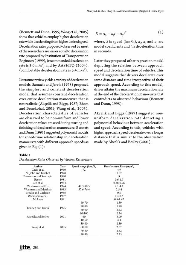
Calibrated models don’t provide zero deceleration values at zero speed (as α and k5 are non zero). This may be due to the reason that observed data cannot provide the exact deceleration rate at every moment since vehicle may have decelerated at any time within initial 1 second period. This can also be observed from modeled deceleration-speed relationship plotted in Fig. 6. The critical speed for motorized two-wheeler is higher than other vehicles.

(7)

Table 5 Calibrated Parameter Values for Models for Both Regimes of All Vehicle Types

Vehicle Category Calibrated parameter values Critical Speed (m/s)

Regime I Regime II

k1 k2 r2 α β r2

Truck 1.587 0.017 0.834 0.104 0.225 0.92 3.49Motorized Three-Wheeler 0.806 0.13 0.912 0.163 0.152 0.928 2.09Motorized Two-Wheeler 1.106 0.08 0.994 0.342 0.087 0.86 11.46

264


4.1. Model Diagnostics

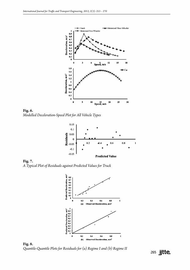
Residues are the difference between observed and predicted values. Residual analysis is carried to check the statistical correctness of models. Plot of residuals against predicted values, for trucks, is presented in Fig. 7. This shows that residuals are uniformly distributed against predicted values depicting uniform variance of errors for trucks. Similar plots are obtained for other vehicle types and it is found that error terms are uniformly distributed against predicted values. The quantile-quantile plot for observed versus predicted values of deceleration in both regimes for trucks are obtained and presented in Fig. 8. The plots show that residuals are approximately normally distributed. Plot of residuals versus time depicted that the residuals are independent over time. Similar test were conducted for other vehicle types also and found residuals are approximately normally distributed and are independent over time. Paired t-test is used to test the means of deceleration computed from observed speed and deceleration obtained from models for Regime I and Regime II in Eq. (5) and Eq. (6). In case of car, model from Eq. (7) is used for Paired t-test. Two hypothesis are tested (i) null hypothesis: µ = µo − µm = 0, where µo and µm are mean of deceleration computed from observed speed and mean of deceleration obtained from model in Eq. (5) and Eq. (6) and (ii) alternate hypothesis: µ = 0. The test statistic is calculated as follows (Eq. (8)) (Freund and Wilson, 2003):

where, µ is mean of the difference between deceleration computed from observed speed, sd is standard deviation of difference in paired data, n is number of data points.

The hypothesis is tested for 95% confidence interval (α = 0.05), where α is significance level. One can reject null hypothesis if |t| ≥ tα/2 (= t0.025). The test statistic is computed for both Regime I and Regime II (single regime in case of cars) using Eq. (8) for all vehicle types and presented in Table 6.

It is seen from Table 6 that for all vehicle types the test statistic |t| ≤ tα/2 (= t0.025). Hence, the null hypothesis that μ = μ0 - μm = 0 cannot be rejected.

Further, a comparison of observed and modeled trajectories and speed profiles of all vehicle types are carried out and presented in Fig. 9 and Fig. 10. Observed trajectory of a vehicle type is the idealized plot where position values of vehicles of same type (obtained from their trajectories recorded using GPS) are averaged over every 1 second time interval. Similarly, observed speed profiles of all vehicle types are also obtained by averaging speed of vehicles of similar types over every 1 second time interval and presented in Fig. 10. Modeled position and speed profiles for all vehicle types are obtained from the proposed models as given in Eqs. (5-7) and model parameters in Table 5.

Vehicle Category Regime I Regime II

t tα/2 t tα/2

Truck 0.045 2.17 0.034 2.57

Motorized Three-Wheeler 1.76 2.17 0.31 2.57

Motorized Two-Wheeler 0.065 2.03 0.06 2.26

Car* 2.05 8.06 -- --

*-Single Regime Model for Cars

Table 6 Test Statistic and tα/2Values for All Vehicle Types

(8)

265


Fig. 6.Modelled Deceleration-Speed Plot for All Vehicle Types

Fig. 8.Quantile-Quantile Plots for Residuals for (a) Regime I and (b) Regime II

Fig. 7.A Typical Plot of Residuals against Predicted Values for Truck

266


Paired t-test is used to compare the means of observed and modeled trajectories and speed profiles. Two hypothesis are tested for 95% confidence interval (α = 0.05) – (i) null hypothesis µ = µo − µm = 0, where µo and µm are mean of observed and modeled values, (ii) alternate hypothesis: μ=0. From the test

results it is observed that for all vehicle types the test statistic |t| ≤ tα/2 (= t0.025) (Table 7). Hence, the null hypothesis cannot be rejected. This indicates that proposed models for various vehicle types estimate the vehicle’s trajectory and speed with fair accuracy.

Vehicle Category Regime I Regime IIt tα/2 t tα/2

Truck 1.93 2.14 1.78 2.14Motorized Three-Wheeler 1.01 2.16 1.82 2.16Motorized Two-Wheeler 1.93 2.11 2.01 2.14

Car 1.49 2.01 1.98 2.01

Fig. 9.Observed and Modelled Trajectories for (a) Truck (b) Car (c) Motorized Three-Wheeler (d) Motorized Two-Wheeler

Table 7 Test Statistic and tα/2 Values Trajectories and Speed Profiles for All Vehicle Types

267


All above diagnostic tests show that the proposed models presented in Eqs. (5-7) are suitable for present data set.

5. Conclusions

This study presents deceleration behaviour of various vehicle types (like truck, car, motorized three wheelers and motorized two wheelers) commonly plying on Indian highways. Deceleration behaviour was studied in free flow condition on a highway where drivers were asked to decelerate from their maximum (desired) speed to zero speed in the shortest possible time. Following conclusions are drawn from the analysis of collected data:

Significant difference exists in deceleration behaviour of different vehicle types.

In a deceleration manoeuvre, vehicle’s deceleration rate initially increases and achieve maximum deceleration rate and later it deceases towards end of deceleration manoeuvre. The speed at which maximum deceleration rate occurred (referred here as critical speed) depends on vehicle type and its maximum speed. Critical speed of all vehicle types increases with the increase in maximum speed of the trip.

Vehicles with higher maximum speed have higher deceleration time, deceleration distance, maximum and mean deceleration rates for all vehicle types.

Maximum deceleration rates observed for truck, car, motorized three-wheelers and motorized two-wheelers are 0.88, 1.71, 1.16,

Fig. 10.Observed and Modelled Speed for (a) Truck (b) Car (c) Motorized Three-Wheeler (d) Motorized Two-Wheeler

268


and 1.59 m/s2 respectively. These values of maximum deceleration rates are lower than deceleration limits reported by ITE’s handbook (1999) and AASHTO (2004). The possible reason for lower deceleration rates is the nature of experiment that has conducted to collect deceleration data. The present study measures normal deceleration rates of driver that they employ in traffic streams generally under car-following situations while the reported deceleration limits in literature were observed on signalized intersections where driver has to decelerate hastily. However, these deceleration values are comparable (for car only) with Bennett and Dunn’s study (1995) conducted on free motor ways in New Zealand. Among all vehicle types, cars have maximum deceleration rate while motorized three wheelers have lowest.

Dual regime models (negative exponential for speed higher than critical speed and linear model otherwise) is found suitable for trucks, motorized three wheelers and motorized two wheelers while a second order polynomial model is proposed for cars.

Results of this study imply that deceleration characteristics of different vehicle types are different. Therefore, simulation model used for heterogeneous traffic should consider the deceleration characteristics of different vehicles accordingly. This study also helps in deriving a more accurate emission model through use of instantaneous emission models that require both, speed and deceleration as an input. Incorporating effect of vehicle types on deceleration in emission models can increase the robustness of emission models. Authors are in process of conducting similar study at signalized intersection to observe the behavioural difference in deceleration manoeuvre of vehicles in both cases.

References

AASHTO. American Association of State Highway and Transportation Officials. Washington, DC. 2004. A policy on geometric design of highways and streets. 896 p.

Akçelik, R.; Besley, M. 2001. Acceleration and deceleration models. In Proceedings of 23rd Conference of Australian Institute of Transport Research. Monash University Melbourne, Australia.

Akçelik, R.; Biggs, D.C. 1987. Acceleration profile models for vehicles in road traffic, Transport Science. DOI: http://dx.doi.org/10.1287/trsc.21.1.36, 21(1): 36-54.

Bennett, C.; Dunn, R.C.M. 1995. Driver deceleration behaviour on a freeway in New Zealand, Transportation Research Record, 1510: 70-75.

Bester, C.J. 1981. Fuel Consumption of Highway Traffic. Ph.D. Thesis, University of Pretoria. 102 p.

Bham, G.; Benekohal, R. 2001. Development, Evaluation, and Comparison of Acceleration Models. Presented at 81st Annual Meeting of the Transportation Research Board, Washington D.C. Paper No. 02-3767. 1-42.

Brodin, A.; Carlsson, A. 1986. The VTI Traffic Simulation Model. VTI Meddelande 321A, Swedish Road and Traffic Research Institute, Linkping. 121 p.

Dey, P.P.; Chandra, S.; Gangopadhyay, S. 2008. Speed studies on two lane Indian Highways, Indian Highways, 36(6): 9-20.

Freund, R.J.; Wilson, W.J. 2003. Statistical Methods. 2nd

Edition. Academic Press, California, USA. 673 p.

Gazis, D.R.; Herman, R.; Maradudin, A. 1960. The Problem of the Amber Signal Light in Traffic Flow, Operations Research. DOI: http://dx.doi.org/10.1287/opre.8.1.112, 8(1): 112-132.

269


Institute of Transportation Engineers. 1999. Traffic Engineering Handbook. 5th Edition, Prentice Hall. 434 and 532 p.

St. John, A.D.; Kobett, D.R. 1978. Grade Effects on Traffic Flow Stability and Capacity. NCHRP Report 185, Transportation Research Board, Washington, D.C. 110 p.

Johnson, R. 2000. Probability and Statistics for Engineers. 6th

Edition, Pearson Education Asia. 622 p.

Lee, K.C.; Balchandran, G.W.; Rosser, M.S. 1984. Driving Patterns of Private Vehicles in New Zealand, Applied Research Office Report No. ARO/1529, University of Auckland, Auckland. New Zealand. 69 p.

Long, G. 2000. Acceleration characteristics of starting vehicles. In Proceedings of the Transportation Research Board, 79th Annual Meeting, Washington, D.C. Paper No. 00-0980. 46 p.

McLean, J.R. 1991. Adapting the HDM-III Vehicle Speed Prediction Models for Australian Rural Highways. Working Document TE 91/014. Australian Road Research Board, Nunawading. 196 p.

Mehmood, A. 2009. Determinants of speeding behaviour of drivers in Al Ain (United Arab Emirates), Journal of Transportation Engineering. DOI: http://dx.doi.org/10.1061/(ASCE)TE.1943-5436.0000049, 135(10): 721-729.

Parsonson, P.S.; Santiago, A. 1980. Traffic Signal Change Interval Must Be Improved. Public Works. 9 p.

Samuels, S.E.; Jarvis, J.R. 1978. Acceleration and deceleration of modern vehicles. Australian Road Research Board, Research Report No. 86. 22 p.

Snare, M. 2002. Dynamics model for predicting maximum and typical acceleration rates of passenger vehicles. Master of Science thesis submitted to Virginia Polytechnic Institute and State University. 124 p.

Wang, J.; Dixon, K.; Li, H.; Ogle, J. 2005. Normal deceleration behaviour of passenger vehicles starting from rest at all way stop controlled intersections, Transportation Research Record. DOI: http://dx.doi.org/10.3141/1883-18, 1883: 158-166.

Warren, A.J.; Gattis, J.L.; Duncan, L.K.; Costello, T.A. 2011. Analysis of Deceleration in Through Lane Prior to Right Turn. Transportation Research Record, DOI: http://dx.doi.org/10.3141/2223-14, 2223/2011: 113-119.

Watanatada, T.; Dhareshwar, A.; Lima, R. 1987. Vehicle Speeds and Operating Costs: Models for Road Planning and Management. Johns Hopkins Press, Baltimore. 470 p.

Wortman, R.H.; Fox, T.C. 1994. An Evaluation of Vehicle Deceleration Profiles, Journal of Advanced Transportation. DOI: http://dx.doi.org/10.1002/atr.5670280303, 28(3): 203-215.

Wortman, R.H.; Matthias, J.S. 1983. Evaluation of Driver Behaviour at Signalized Intersections, Transportation Research Record, 904: 10-20.

270


STUDIJA O KARAKTERU USPORENJA RAZLIČITIH KATEGORIJA VOZILA

Akhilesh Kumar Maurya, Prashant Shridhar Bokare

Sažetak: Karakteristike usporenja vozila su važne za projektovanje raskrsnica, projektovanje traka za usporavanje, simulaciju saobraćaja, modeliranje emisije štetnih gasova vozila i potrošnje goriva, itd. Heterogeni saobraćajni tok sastoji se od vozila sa širokim odstupanjima u pogledu gabaritnih dimenzija, odnosa težine i snage i dinamičkih karakteristika, koje utiču na karakter usporenja. Većina prethodnih studija su ograničene na ispitivanje karaktera usporenja automobila i kamiona u homogenom saobraćajnom toku. Predstavljena studija ima za cilj da analizira karakter usporenja različitih kategorija vozila (kao što su kamioni, automobili, motorizovani dvotočkaši i trotočkaši) na autoputu Nagpur-Mumbai Express u Vardi, Indija. Od vozača je traženo da uspore svoja vozila sa maksimalne brzine do zaustavljanja u najkraćem vremenu, nakon čega su prikupljeni profili njihovih brzina korišćenjem globalnog pozicionog sistema. Istraživanjem je utvrđeno da se karakter usporenja različitih kategorija vozila značajno razlikuje. Vozila sa većom maksimalnom brzinom imaju duže vreme usporavanja, veće rastojanje usporavanja, veće maksimalne i srednje vrednosti usporenja prilikom usporavanja. U toku usporavanja, vrednost usporenja se u početku povećava, dostiže maksimalnu vrednost, a potom opada. U radu je razvijen model dvostrukog režima u cilju modeliranja karaktera usporenja svih vrsta vozila, izezev automobila, u celom opsegu njihovih raspoloživih brzina. Za automobile, predložen je polinom drugog stepena.

Ključne reči: usporenje, brzina, profili usporenja, model dvostrukog režima, globalni pozicioni sistem.

study of deceleration behaviour of … vol2 no3...study of deceleration behaviour of different...

Documents