study of coupled transport and its effect on …
TRANSCRIPT

STUDY OF COUPLED TRANSPORT AND ITS EFFECT ON DIFFERENT
ELECTROCHEMICAL SYSTEMS: IMPLICATIONS IN HIGH
TEMPERATURE ENERGY STORAGE BATTERIES AND
PROTON EXCHANGE MEMBRANE FUEL CELLS
by
Preethy Parthasarathy
A dissertation submitted to the faculty of The University of Utah
in partial fulfillment of the requirements for the degree of
Doctor of Philosophy
Department of Materials Science and Engineering
The University o f Utah
May 2013

Copyright © Preethy Parthasarathy 2013
All Rights Reserved

The U n i v e r s i t y of Utah G r a d u a t e S c h o o l
STATEMENT OF DISSERTATION APPROVAL
The dissertation of Preethy Parthasarathy
has been approved by the following supervisory committee members:
Anil V. Virkar Chair 10/29/2012
Date Approved
Dinesh K. Shetty Member 10/29/2012
Date Approved
Feng Liu Member 10/29/2012
Date Approved
Jules J. Magda Member 10/29/2012
Date Approved
Florian Solzbacher Member 10/29/2012
Date Approved
and by Feng Liu Chair of
the Department of Materials Science and Engineering
and by Charles A. Wight, Dean of The Graduate School.

ABSTRACT
Coupled transport is studied on two electrochemical systems: Na-ZnCl2 batteries
and Proton Exchange Membrane Fuel Cells (PEMFC). The energy storage system of
interest here is based on sodium P”-alumina solid electrolyte (BASE): Na/BASE/ZnCl2.
BASE is an excellent Na+ conductor with a very high conductivity at 300oC. Its high Na+
ion conductivity and high stability are the principal reasons for its application in
electrochemical storage systems. A novel vapor phase process was invented facilitating
the fabrication of high strength and moisture/CO2 resistant BASE. A two-phase
composite of alumina+YSZ is formed by sintering and exposed to Na2O vapor, keeping
the activity of Na2O lower than that in NaAlO2. This prevents the formation of
hygroscopic NaAlO2 at the grain boundaries. A thin layer of P”-alumina is formed on the
surface upon exposure. Further reaction occurs by transporting Na+ ions through the
formed P”-alumina and a parallel transport of O - ions through YSZ. This occurs by a
coupled transport of Na through P”-alumina and O - ions through YSZ, thus expediting
the process.
The second electrochemical system of interest is PEMFC. The degradation
mechanism of catalysts is studied using inexpensive copper particles. The mechanism of
2+growth involves a coupled transport of Cu2+ through the aqueous medium and an electron
transport through the direct particle-to-particle contact. Effect of applied stress on
coarsening of platinum was also investigated. Two platinum wires/foils were immersed in
a PtCl4+DMSO (Dimethyl sulfoxide) solution. A tensile load was applied to one wire/foil

and the other one was left load-free. The wire/foil subjected to a tensile load became
cathodic with respect to the unstressed wire/foil. Thus, under a tensile stress, the chemical
potential of Pt decreases. This result suggests design strategies for core-shell catalysts
used in PEMFCs: stable core-shell catalysts for PEMFC with Pt shell should be designed
such that the shell is under a tensile stress.
Specific surface energies (y) of f.c.c. metals as a function of shape and size were
investigated using the broken-bond model. y decreased with increasing particle size and
approached asymptotic values beyond an equivalent diameter of ~5 nm. Octahedral
shaped particles were the most stable.
iv

For my Amma, Appa, Akka, Athimber, and Nannu

ABSTRACT.................................................................................................................. iii
LIST OF TABLES........................................................................................................ viii
LIST OF FIGURES...................................................................................................... ix
ACKNOWLEDGEMENTS.......................................................................................... xv
Chapter
1. INTRODUCTION.................................................................................................. 1
1.1 Sodium P”-Alumina Solid Electrolyte....................................................... 11.2 Catalyst Degradation in PEM Fuel Cells.................................................. 61.3 Specific Surface Energy and Shape Stability of Metals.......................... 111.4 Scope of the Thesis..................................................................................... 121.5 References................................................................................................... 15
2. HIGH TEMPERATURE SODIUM - ZINC CHLORIDE BATTERIES WITH SODIUM BETA” - ALUMINA SOLID ELECTROLYTE (BASE)................. 18
2.1 Introduction................................................................................................. 182.2 Experimental Procedure.............................................................................. 242.3 Results and Discussions.............................................................................. 282.4 Conclusion................................................................................................... 332.5 Acknowledgements..................................................................................... 342.6 References................................................................................................... 34
3. A STUDY OF THE KINETICS OF CONVERSION OF ALPHA-ALUMINA+ ZIRCONIA INTO SODIUM BETA” - ALUMINA + ZIRCONIA............... 36
3.1 Introduction........................................................................................... 363.2 Theoretical Model................................................................................. 413.3 Experimental Procedure......................................................................... 503.4 Results and Discussion......................................................................... 513.5 Summary................................................................................................. 653.6 Acknowledgements.............................................................................. 663.7 References............................................................................................. 66
TABLE OF CONTENTS
4. ELECTROCHEMICAL COARSENING OF COPPER POWDER IN

AQUEOUS MEDIA............................................................................................... 68
4.1 Introduction........................................................................................... 684.2 Experimental Procedure....................................................................... 714.3 Results and Discussion....................................................................... 734.4 Summary............................................................................................... 894.5 Acknowledgements.............................................................................. 914.6 References............................................................................................. 91
5. EFFECT OF STRESS ON DISSOLUTION/PRECIPITATION OF PLATINUM: IMPLICATIONS CONCERNING CORE-SHELL CATALYSTS AND CATHODE DEGRADATION IN PEM FUELCELLS................................................................................................................... 93
5.1 Introduction.............................................................................................. 935.2 Theory........................................................................................................ 985.3 Experimental Procedure.......................................................................... 1015.4 Results and Discussion............................................................................. 1025.5 Implications Concerning Core-Shell Catalysts for PEMFC.................. 1125.6 Summary................................................................................................... 1185.7 Acknowledgements.................................................................................. 1195.8 References................................................................................................. 120
6. SPECIFIC SURFACE ENERGY AND SHAPE STABILITY OF FACE CENTERED CUBIC METALS AS A FUNCTION OF SIZE........................ 124
6.1 Introduction............................................................................................. 1246.2 Theory....................................................................................................... 1286.3 Discussion................................................................................................. 1406.4 Summary................................................................................................... 1506.5 Acknowledgements................................................................................. 1516.6 References............................................................................................... 151
7. CONCLUSIONS................................................................................................. 154
7.1 Sodium P”-Alumina Solid Electrolyte................................................... 1547.2 Coarsening of Copper Particles in Aqueous Media............................. 1557.3 Electrochemical Coarsening due to Applied Stress............................. 1577.4 Surface Energy and Shape Stability of Metals.................................... 158
APPENDIX.............................................................................................................. 160
vii

LIST OF TABLES
Table Page
3.1 Grain size as a function of sintering conditions.............................................. 53
4.1 Comparison of average particle sizes after various treatments and the corresponding copper ion concentration in the filtrates after the tests in selected cases...................................................................................................... 74
4.2 Comparison of average particle sizes after conducting the experiments for various durations at room temperature............................................................. 84
6.1 Specific surface energies of f.c.c. metal particles of various shapes as a function of size: (a) The smallest possible cluster, (b) Very large crystals (asymptotic limit)............................................................................................... 139
6.2 Lattice parameters, heats of sublimation, and calculated (asymptotic) valuesof specific surface energies for (111) surfaces of various f.c.c. metals.......... 141
A.1 Dependence of specific surface energy with the equivalent particle size for acube-shaped particle in f.c.c.............................................................................. 166
A.2 Dependence of specific surface energy with the equivalent particle size for acubo-octahedron shaped particle in f.c.c......................................................... 167
A.3 Dependence of specific surface energy with the equivalent particle size for atetrahedron-shaped particle in f.c.c.................................................................. 168
A.4 Dependence of specific surface energy with the equivalent particle size for aoctahedron-shaped particle in f.c.c.................................................................. 169
A.5 Dependence of specific surface energy with the equivalent particle size for atruncated octahedron-shaped particle in f.c.c................................................. 170

LIST OF FIGURES
Figure Page
1.1 Schematic of 2-block and 3-block structures of P and P”-alumina, respectively....................................................................................................... 2
2.1 Power demand as a function of time of day................................................. 19
2.2 Crystal structure of Na-P”-alumina.................................................................. 23
2.3 XRD patterns of as-sintered a-alumina/YSZ sample and converted P”- alumina/YSZ sample....................................................................................... 29
2.4 Chemical line scan of P”-alumina tube after 50 hours cycling...................... 30
2.5 Voltage response of the tubular cell, T = 350oC, Time ~5.5 hours.............. 30
2.6 Voltage responses of planar cell after initial run and five freeze - thaw cycles.................................................................................................................. 31
2.7 Chemical line scan of the planar cell electrolyte showing no trace ofzinc..................................................................................................................... 32
2.8 Planar cell stack and the voltage response of the two-cell stack operated ata temperature of 400oC..................................................................................... 33
2.9 Five-cell planar stack arrangement.................................................................. 34
3.1 Mechanism of conversion of a - alumina to BASE. Oxygen ions are transported through YSZ and sodium ions are transported through P”- alumina. It also shows the three different paths through which O2- ions can diffuse at the reaction front to form BASE.................................................... 42
3.2 A schematic showing the variation of the chemical potential of Na2O across the converted BASE with a thickness x. The process involves two interfacial steps and one diffusive (coupled) step.......................................... 44
3.3 Microstructures of a-alumina + 3YSZ samples sintered at (a) 1500oC for 1 hour, (b) 1600oC for 1 hour, (c) 1700oC for 1 hour, and (d) 1800oC for 1hour.................................................................................................................... 51

3.4 Analysis of the interface of partially converted sample. (a) Micrograph of the interface of the partially converted a-alumina + 3YSZ sample which shows the unconverted portion in the top and the interface band in the middle and the converted portion in the bottom. The interface band has the structure of P”-alumina + YSZ but with porosity. (b) Chemical line scan shows the weight percent of sodium present across the cross-section of the sample. The concentration of sodium in the unconverted portion (a- alumina + YSZ) is negligible as compared to that in the interface band the converted portion (P”-alumina + YSZ), which is an order of magnitude higher................................................................................................................. 54
3.5 Schematic of three-phase boundaries (gas phase, a or P”-alumina, and YSZ)- smaller grain size and larger grain size................................................ 58
3.6 Conversion Thickness as a function of hold time for the samples with varying grain sizes, Conversion Temperature: 1250oC. The dependence was fitted to the general kinetic equation modeled for conversion:
(x 2 ~ x02) + ( x z x ) = t ..................................................................................... 60Deff
3.7 Conversion Thickness as a function of hold time for the samples with varying grain sizes, Conversion Temperature: 1450oC. The dependence was fitted to the general kinetic equation modeled for conversion:
(x 2 ~ x02) | (x ~ x0) = t .............................................................................. 60Def
3.8 Effective diffusion and interfacial rate constants as a function of grain size for a conversion temperature of 1250oC. Dependence of diffusion coefficients with respect to grain size is negligible as compared to that of interfacial rate constants................................................................................... 62
3.9 Effective diffusion and interfacial rate constants as a function of grain size for a conversion temperature of 1450oC. Dependence of diffusion coefficients with respect to grain size is negligible as compared to that of interfacial rate constants. The effective interfacial rate constant decreases slightly as grain size increases......................................................................... 62
3.10 Arrhenius plot of interfacial rate constants for different grain sizes of the P” - alumina samples. As grain size decreases, the activation energy of interfacial reactions also decreases. It suggests that interfacial kinetics is dependent on grain size variation.................................................................... 64
3.11 Arrhenius plot of diffusion constants for different grain sizes of the P” - alumina samples. As grain size decreases, the activation energy of diffusion reactions remains constant. This suggests that the diffusion kinetics is independent of grain size variation................................................ 64
x

3.12 Variation of activation energies of interfacial rate constants and diffusion coefficients with grain size. Activation energy for interfacial reaction increases with increase in grain size, whereas activation energies of diffusion coefficient is independent of grain size variation........................... 65
4.1 Mechanism of coarsening in copper particles. (a) A schematic of two isolated copper particles in an aqueous solution containing copper ions. Transport of copper ions occurs from the smaller particle to the larger particle. Once the electrochemical potential of copper ions is the same in both particles, further transport shuts down. The smaller particle is then negatively charged and the larger one is positively charged. (b) If the particles are sitting on an electronically conducting support, a path for transport of electrons exists, thus causing coarsening (Ostwald ripening).(c) If the particles are in contact with each other, electron transport occurs directly with copper ions transporting through the liquid (agglomeration).................................................................................................. 70
4.2 A schematic showing the experimental arrangement.................................... 72
4.3 SEM micrographs of copper powder subjected to various treatments at room temperature: (a) As-received, (b) DI water for 48 h, (c) DI water with hydrogen bubbling for 48 h, and (d) 1 M Cu(NO3 ) 2 solution for 48 h. Significant growth occurred in DI water and even greater growth occurredin 1 M solution................................................................................................... 74
4.4 SEM micrographs of copper powder subjected to various treatments at 80oC: (a) As-received, (b) DI water for 48 h, (c) DI water with hydrogen bubbling for 48 h, and (d) 1 M Cu(NO3 ) 2 solution for 48 h. Detectable growth occurred in DI water with hydrogen bubbling. Growth occurred to a greater extent in DI water. Surface of copper powder treated in 1 M solution appears rough due to the formation of copperoxide.................................................................................................................. 78
4.5 X-ray diffraction patterns of copper powder after various tests and comparison with the as-received powder. (a) Experiments at room temperature. All XRD patterns show only the metallic copper peaks. (b) Experiments at 80oC. All XRD patterns show only metallic copper peaks, except the sample treated in 1 M Cu(NO3 ) 2 solution which also shows peaks corresponding to copper oxide (CuO).................................................. 80
4.6 Particle size distributions of samples subjected to various treatments at room temperature for 48 h ................................................................................ 81
4.7 Particle size distributions of samples subjected to various treatments at80oC for 48 h ..................................................................................................... 81
4.8 SEM micrographs of copper powder treated in DI water at room
xi

temperature for various periods o f time: (a) As-received and washed, (b)12 h, (c) 72 h, and (d) 144 h .............................................................................. 83
4.9 SEM micrographs of copper powder treated in 0.01M copper nitrate solution at room temperature for various periods of time: (a) As-receivedand washed, (b) 12 h, (c) 72 h, (d) 144 h ......................................................... 84
4.10 Particle size distributions of samples treated in DI water at room temperature for various periods of time........................................................... 86
4.11 Particle size distributions of samples treated in 0.01M copper nitrate solution at room temperature for various periods of time.............................. 86
4.12 Kinetics o f coarsening of copper particles under different testing conditions at room temperature....................................................................... 88
5.1 Mechanisms of cathode degradation in PEMFC: (a) Detachment from carbon support, (b) Agglomeration and sintering, (c) Ostwald ripening, and (d) Dissolution at the cathode, transport and precipitation into the membrane........................................................................................................... 94
5.2 Mechanism of particle growth by (a) Ostwald ripening, (b) agglomeration/ sintering. Both occur by a coupled transport of Pt2+ (or Pt4+) ions through ionomer/aqueous media and electron transport through the carbon support (or through direct particle-to-particle contact). Net Pt transport occursfrom smaller particles to larger particles......................................................... 96
5.3 A schematic of the experimental setup used................................................... 99
5.4 Variation of the voltage between the stressed (positive) and the unstressed Pt wires immersed in 0.1 M PtCl4/DMSO solution for different applied loads................................................................................................................... 103
5.5 Variation of the current between the stressed and the unstressed platinum wires immersed in 0.1M PtCl4+DMSO solution for different applied loads................................................................................................................... 103
5.6 Variation of the current between the stressed and the unstressed Pt foils immersed in 0.1 M PtCl4+DMSO solution for different applied loads................................................................................................................... 104
5.7 Voltage between the stressed (positive) and the unstressed wires as a function of the applied tensile stress for varying wire diameters. The intercept is ideally zero. In the fitting of the experimental data, the very small nonzero intercept was neglected in the voltage vs. stress equations given in the inset. Slopes give voltage coefficients per unit stress............... 105
5.8 Variation of the voltage coefficient per unit stress as a function of the
xii
diameter o f platinum wire 108
5.9 SEM micrographs of: (a) Unstressed platinum wire immersed in 0.1 M PtCl4+DMSO electrolyte for 144 hours. The wire diameter shrank to ~120 p,m. (b) Stressed platinum wire: The portion of platinum wire outside the electrolyte (no growth) - 126 p,m, and stressed platinum wire immersed in electrolyte - 135 p,m (wire diameter grew to 135 p,m).................................. 110
5.10 SEM micrographs of foils immersed in 0.1 M PtCl4+DMSO electrolyte for 144 hours. (a) Cross-section of the interface of the unstressed platinum foil where the top portion of the foil was outside the electrolyte (no change) and the bottom portion was immersed in the electrolyte (where dissolution occurred). The thickness reduced to ~116 p,m. (b) Cross-section of stressed platinum foil immersed in the electrolyte. The thickness grew to~136 p,m............................................................................................................. 110
5.11 Schematics of monolithic and core-shell catalyst with an incoherent interface. Compressive stress in the shell is higher than the compressive stress in a monolithic catalyst particle. Such a catalyst should be less stable against dissolution compared to monolithic particle........................... 113
5.12 Schematic of a core-shell catalyst with a coherent interface. Compressive stress in the shell is lower than the compressive stress in a monolithic catalyst particle. Such a catalyst should be more stable against dissolution compared to monolithic particle...................................................................... 114
6.1 The smallest crystal of the size of a unit cell with a face centered cubic structure and lattice parameter ‘a’.................................................................... 129
6.2 A cube-shaped particle of side length L = 2a................................................. ...... 131
6.3 A cubo-octahedron of side length L = 2 a ............................................................. 132
6.4 A tetrahedron of side length L = 2 a ................................................................ ......134
6.5 Octahedra of side lengths L = a, and L = 2a................................................... ......136
6.6 Truncated octahedra with side lengths L = 3a and L = 6a............................. ......137
6.7 Specific surface energy as a function of equivalent diameter for a f.c.c. structure for different shapes: cube, cubo-octahedron, tetrahedron, octahedron, and truncated octahedron. The inset shows the variation of surface energy with equivalent diameter below ~ 1 0 a , where a is the lattice parameter................................................................................................. 139
6.8 Specific surface energy of octahedral particles as a function of equivalent
xiii

diameter for various f.c.c. metals. The inset shows the variation of surface energy with equivalent diameter below 8nm.................................................. 141
6.9 Lattice parameter contraction as a function of particle size for various crystal shapes for platinum (f.c.c.). Figure in the inset shows the lattice parameter contraction as a function of particle size studied by Chepulskii and Curtarolo. In their study, the dependence of lattice contraction on particle size is greater than the dependence showed by broken-bond model.................................................................................................................. 144
6.10 Specific surface energy as a function of equivalent diameter for clusters of an octahedral shape. The inset shows the variation of specific surface energy as a function of size when the number of atoms varies between one complete octahedron ( n = 2 ) and the next complete octahedron ( n = 3 ).The specific surface energy increases to a point and then decreases until it reaches that corresponding to the next complete octahedral structure.............................................................................................................. 150
xiv

ACKNOWLEDGEMENTS
I would like to thank Dr. Anil Virkar for his mentoring, support, enthusiasm, and
belief in hard work. The work presented in this dissertation is as much a result of many
interesting and instructive discussions with him as it is of hours spent in the lab.
I would also like to thank my thesis advisory committee: Dr. Dinesh Shetty, Dr.
Feng Liu, Dr. Jules J. Magda, and Dr. Florian Solzbacher. Their time and effort in
guiding my research and being a part of my committee is greatly appreciated.
This work was made possible through the financial support from the U.S.
Department of Energy under Grant Number DE-FG02-03ER46086, and the National
Science Foundation under Grant Number CBET-0931080, and the Department of
Energy-EFRC under Grant Number DE-SC0001061 as a flow through from the
University of South Carolina.
I would like to express a special word of thanks to Dr. Neill Weber, who was
abundantly helpful and offered invaluable assistance, support, and guidance throughout
my Ph.D. research. Thanks to all my friends and colleagues in the research lab and at the
University of Utah, both past and present, for their support and friendship.
Finally, I would like to thank my family for their constant support and love.
Thank you!

CHAPTER 1
INTRODUCTION
1.1 Sodium P”-Alumina Solid Electrolyte
Sodium P and P”-alumina are known for their excellent conductivity of sodium
ions. Both are highly refractory compounds of stoichiometry Na2O.11Al2O3 and
Na2O.~6.2 Al2O3 in the Na2O-Al2O3 system [1]. The crystal structure of Na P-alumina is
hexagonal and that of Na P”-alumina is rhombohedral, which can be indexed as
hexagonal. Figure 1.1 shows the schematic of 2-block and 3-block structures of P-
alumina and P”-alumina, respectively. Crystal structures of P and P”-alumina consist of
Al-O spinel blocks, separated by conduction planes perpendicular to the c-axis of the unit
cell. Mobility of sodium ions in the conduction plane is very high, whereas the mobility
along the c-axis is negligible. In a polycrystalline body, Na+ ion conduction is isotropic
due to its random orientation of grains. At 300oC, resistivity of P is ~15Qcm and
resistivity of P” is ~3Qcm. Due to the exceptional conductivity of Na+ ions, Na P”-
alumina is used as a solid electrolyte (otherwise known as BASE) in several
electrochemical storage devices. Some of the major applications of BASE are in sodium
sulfur batteries, Zebra batteries, and alkali-metal thermal-to-electric converters
(AMTECs). BASE was first developed by researchers at the Ford Motor Company while
conducting a study on energy storage devices for electric vehicles. They developed the
concept of a sodium sulfur battery, which consists of sulfur at the positive electrode and

2
Figure 1.1 Schematic of 2-block and 3-block structures of P and P”-alumina, respectively
sodium at the negative electrode as active materials, and sodium-conducting beta-alumina
ceramic as the electrolyte. At 300oC, both electrodes are liquid, which leads to a faster
reaction kinetics. While discharging, Na+ ions transport through BASE into the sulfur
electrode with electrons transporting in the external circuit to form sodium polysulfides.
During the charging part of the cycle, Na+ ions transport from the sulfur electrode
through the BASE to the Na anode, with electrons transporting in the external circuit. The
batteries use one end closed BASE tubes, and stainless steel or Ebrite containers with a

protective chromium coating to prevent corrosion induced by sulfur and sodium
polysulfides. Several cells are configured in a module with series and parallel
connections for optimum performance and reliability. Sodium sulfur batteries are
commercialized by NGK Insulators, Ltd., in Japan mainly for stationary applications such
as a load leveling, integrated system with a wind generator and DC power source. Several
other companies like American Electric Power (AEP) and Xcel Energy started utilizing
sodium sulfur batteries for stationary applications. These are no longer used for mobile
applications due to the safety issues concerning the accidental reaction between sodium
and sulfur in the event of a short circuit, which produces highly corrosive sodium
polysulfides.
Another important application of BASE is in ZEBRA batteries (Zeolite Battery
Research Africa Project or Zero Emissions Batteries Research Activity) [2]. ZEBRA
batteries use sodium as anode and NiCl2 as cathode, the electrolyte/ separator being
BASE [3]. The operational temperature of ZEBRA batteries has been chosen in the
range of 270 to 350oC. During charging, sodium is ionized. Na+ ions conduct through
solid electrolyte and electrons through the outer circuit to the higher potential of the
anode, where it recombines with the sodium ions. While discharging, sodium ions
conduct back through the electrolyte to the cathode and electrons via the outer circuit.
BASE is also used in alkali-metal thermal-to-electric converters (AMTECs). An
AMTEC is a highly efficient device with efficiency up to 40% (typical efficiency of
thermoelectrics are in the range of 15 - 20%) for directly converting heat to electricity.
An AMTEC operates as a thermally regenerative electrochemical cell by expanding
sodium through the pressure differential across the (BASE) membrane. It is characterized
by high potential efficiencies and no moving parts, which make it a candidate for space
3

power applications. In this device, sodium is cycled around a closed thermodynamic
cycle between two heat reservoirs at different temperatures. It is a sodium concentration
cell, which uses BASE as a separator between a high pressure region containing sodium
vapor at 600 - 1000oC and a low pressure region containing a condenser for liquid
sodium at 120-420oC. BASE electrolytes have also been used in some molten-carbonate
fuel cells, as well as other liquid electrode/solid electrolyte fuel cell designs. BASE has
demonstrated outstanding stability under high pressure, high temperature, or corrosive
environments far superior than other solid electrolytes currently available, making it an
ideal candidate for electrochemical storage devices.
BASE is conventionally processed by the calcination of a mixture of Na2CO3,
Al2O3 and LiNO3 in air, at ~1250oC, followed by sintering at a temperature of ~1550oC
[4, 5]. Finally, the sintered samples are annealed to ensure the complete conversion of a -
alumina to sodium beta”-alumina. There are several limitations to the traditional method
of fabrication. High sintering temperature enhances soda loss from the samples, which
could be avoided only by using an expensive encapsulation of samples using Pt bags or
MgO crucibles. Remnant sodium aluminate (NaAlO2) is present at the grain boundaries,
which is hygroscopic in nature. Thus, beta”-alumina formed by this process is prone to
moisture and CO2 attack from the atmosphere and is stored in vacuum chambers in order
to avoid degradation. In addition, the strength of conventional beta”-alumina is low,
typically on the order of 200 MPa or less due to exaggerated grain growth. A novel
patented vapor phase process is used for the conversion of sodium beta”-alumina in order
to eliminate the limitations mentioned above [6]. In the vapor phase process, a- alumina
is exposed to a source of Na2O, forming a thin layer of sodium P”-alumina on the surface
of the exposed a- alumina. Since P”-alumina is a good conductor of Na+ ions, the
4

diffusion of sodium ions through the same will be fast. Once the surface layer is formed,
further conversion of alumina to P”-Al2 O3 practically shuts off due to the sluggish
diffusion of O2- ions through sodium beta”-alumina. The rate of diffusion of Na2 O
(formation of P”-alumina) will be dictated by the rate of diffusion of O - ions through P”-
alumina. In fact, Nicholson et al. [7, 8] used the same approach as described above to
form a thin layer of P”-alumina on sapphire crystals and the rate of film growth was very
slow due to the low diffusion rate of oxygen ions. The phenomenon of coupled transport
is utilized to enhance the rate of the conversion process. An alternate rapid path is
provided for the diffusion of O -ions [6] by incorporating an oxygen ion conductor, yttria
stabilized zirconia (YSZ), in the starting material. Thus, a coupled diffusion of Na+ and
O2- ions will occur, leading to a faster conversion of alumina to sodium beta”-alumina.
Once the thin layer of beta”-alumina is formed on the surface, Na+ ions will diffuse
through the formed beta”-alumina and O - ions through the YSZ present in the material.
This process leads to the formation of a two-phase composite of BASE and zirconia. By
choosing the composition of YSZ with low yttria content, typically 3 mol.%, a two-phase
composite can be fabricated with strength of the order of ~900 MPa, which is more than
four times that of the conventional BASE. In the vapor phase process, no encapsulation is
needed as the conversion temperature is relatively low (1450oC), resulting in negligible
soda loss. Moreover, the process is carried out in such a way that the thermodynamic
activity of Na2O is significantly lower than the activity of NaAlO2, preventing the
formation of hygroscopic NaAlO2 at the grain boundaries. This is achieved by controlling
the conversion temperature and the composition of Na2O in the mixture. The BASE thus
formed will be resistant to atmospheric moisture and CO2 , and can even be boiled in
water without any degradation. The first part of this work studies the role of coupled
5

6
transport in the fabrication of Na P”-alumina by vapor phase conversion.
1.2 Catalyst Degradation in PEM Fuel Cells
A proton exchange membrane fuel cell is a low temperature fuel cell that
transforms chemical energy liberated during the electrochemical reaction of hydrogen
and oxygen to electrical energy. Proton Exchange Membrane Fuel Cells (PEMFCs) have
applications in transportation, distributed power, and portable power. Considerable
progress has been made over the past two decades in PEMFC. However, it is well known
that degradation in performance occurs over time, which in part has limited the
commercialization of PEMFC. There are many factors which influence PEMFC
degradation, which include the materials used in PEMFC and the operating conditions.
Much of the current research is on catalyst degradation for PEM fuel cells with additional
objectives of either obtaining higher catalytic activity than the standard carbon-supported
platinum particle catalysts used in current PEM fuel cells or reducing the poisoning of
PEM fuel cell catalysts by impurity gases. Typical catalysts used in PEM fuel cells are
platinum/ platinum alloy nanoparticles embedded in carbon support. One of the reasons
for alloying Pt with non-noble metals is to reduce the Pt loading and thus lower the cost
[9-13]. Catalyst degradation occurs on both cathode and anode sides of PEMFC. Anode
catalyst degradation is low because of the reducing atmosphere due to the presence of
hydrogen. Several mechanisms of cathode degradation have been reported [14-20]
including: (a) detachment of catalyst particles from carbon support, thus rendering them
electro-catalytically inactive; (b) Ostwald ripening of particles; (c) agglomeration and
associated growth (sintering) of particles; (d) dissolution of the catalyst at the cathode, its
transport and precipitation into the membrane. All of these phenomena lead to a decrease

in the catalyst surface area, decrease in catalytic activity, and thus loss in performance.
Studies have shown that greater degradation occurs at open circuit than when the fuel cell
is under load. It is also known that negligible degradation occurs at the anode even when
its composition is substantially the same as the cathode.
In the second part of the dissertation, the main focus is to study the role of
coupled transport in catalyst/ nanoparticle degradation mechanisms. Out of the different
degradation mechanisms mentioned above, this work studies mainly the effect of Ostwald
ripening or agglomeration in nanoparticles. Ostwald ripening or coarsening is a process
in which larger particles grow at the expense of smaller particles. Numerous theoretical
and experimental studies on Ostwald ripening have been conducted over the past several
decades [21-25]. Electrochemical Ostwald ripening is a process in which larger particles
grow at the expense of the smaller ones as ion transport occurs through the ionomer/ion
conducting medium and electron transport occurs via a conductive support. A few reports
on electrochemical Ostwald ripening are also available in the literature [26-31]. In
conventional solid state Ostwald ripening, metal particles grow by bulk or grain boundary
diffusion. In electrochemical Ostwald ripening, growth occurs by a coupled transport of
electrically charged species, for example, metal ions and electrons via parallel paths:
metal ions through the liquid/ionomer and electrons through the metal or supporting
carbon in PEMFC. Coarsening of ionic compounds dissolved in a solvent also occurs by
electrochemical Ostwald ripening. An example is a super-saturated solution of NaCl in
water; coarsening of particles occurs by a coupled transport of Na+ and Cl- through the
solution. If two metal particles are isolated in an ion conducting medium, initially the
smaller particles will tend to dissolve and precipitate on larger particles as the chemical
potential of smaller particles is higher than that of the larger particles. Thus, for isolated
7

8
metal particles in an ion conducting medium (no or negligible electron concentration),
particle growth is not expected. However, this process will occur if the particles are
soluble as neutral species in the conducting medium. Assuming the presence of only ions
in the ion conducting medium (little electronic conduction), ions will be transported
through the conducting medium from smaller to larger particles leaving behind electrons.
Thus, smaller particles will become negatively charged and the larger particles become
positively charged. Once the electrochemical potential o f ions in the particles is
equilibrated, further ion transport will be shut down. However, the coarsening will occur
i f there is an alternate path for electrons. Coarsening will thus occur by a coupled
transport of ions and electrons.
When two metal particles are in contact with each other in an ion conducting
medium, the ions transport through the ion conducting medium and electrons through the
metal particles in contact. This process is known as coalescence/agglomeration. The
driving force is the same as for Ostwald ripening, and bulk diffusion and/or grain
boundary diffusion determines the kinetics of growth in the solid state. The kinetics of
this process is expected to be much faster compared to the typical solid state diffusion
when the ion conducting medium is a liquid (such as an aqueous solution). In order to
investigate the role o f coupled transport in particle coarsening, initial research was
conducted with copper particles treated under various test conditions. Copper powder was
placed in DI water and in different solutions containing various concentrations of
Cu(NO3 )2 . Copper particles in contact with each other are expected to grow at the
expense of smaller particles while isolated copper particles should not grow. Analysis of
the results obtained from these experiments gave insight into the mechanisms of particle
coarsening by electrochemical Ostwald ripening/agglomeration.

9
The study of the mechanism of copper particle coarsening has direct implications
to the cathode catalyst degradation in PEM fuel cells. The thermodynamic driving force
for agglomeration/sintering and Ostwald ripening is the reduction in surface energy
accompanying particle growth, which leads to dissolution of smaller particles and growth
of larger particles. In PEMFC, transport of electrically neutral Pt occurs via a coupled
process involving the transport of ions (Pt2+ and/or Pt4+) through an ionomer or aqueous
medium and a parallel (coupled) transport of electrons through the carbon support [31].
In agglomeration/sintering, a similar process occurs where ions transport through
ionomer/aqueous medium and electrons transport through a direct particle-to-particle
contact. The fundamental physical parameter which dictates degradation kinetics is the
electrochemical potential of Pt ions, which depends upon the chemical potential of Pt. All
those factors which lower the chemical potential of Pt should generally decrease the
kinetics of degradation, and all those factors which increase the chemical potential of Pt
should increase the kinetics of degradation.
The chemical potential of a species depends on composition, temperature, and
pressure. Alloying Pt with other metals lowers the chemical potential of Pt. Hydrostatic
stress (pressure) also affects the chemical potential, which is the basis of the Gibbs-
Kelvin equation and is the reason for the occurrence of Ostwald ripening/agglomeration
[32]. The dependence of chemical potential of Pt, /uPt, on temperature, composition, and
on pressure is given by [32]
VPt = rfPt + RT ln aPt + pVm (11)
owhere ^ Pt is the standard state chemical potential of Pt, apt is the activity of Pt, Vm

is the partial molar volume of Pt, and P is the pressure. If the material is pure Pt, then
apt is unity. For nanosize particles, the pressure is given by 2^ / r where r is the particle
radius and ? is the surface energy. Thus, the smaller the particle size, the higher is the
pressure inside the particle, the higher is the chemical potential, and the greater is the
tendency for its dissolution and deposition on larger particles.
Equation (1.1) shows that the sign of pressure determines whether it will increase
or decrease the chemical potential. Thus, if the pressure is positive (compressive), the
chemical potential will be higher compared to a stress-free material. If the pressure is
negative (tensile), however, the chemical potential should be lower compared to a stress-
free material. Flood [33] demonstrated that the dominant term in chemical potential is
linearly related to pressure (consistent with equation (1.1)), and thus electrode potential is
expected to exhibit a reversal in sign upon a reversal in the sign of stress (tensile or
compressive), in accord with the general thermodynamic theory of Gibbs. This analysis is
important in the role of surface stress on catalyst stability and specifically on the design
of core-shell catalysts. Core-shell catalysts typically consist of a core and a shell of
different materials but generally of the same crystal structure, and with an epitaxially
matched interface. The lattice parameters of the core and the shell determine the
magnitude (and possibly the sign) of the stress in the shell of a core-shell catalyst. If the
Pt shell is under greater compression than a pure Pt catalyst particle of the same diameter,
the chemical potential of Pt will be higher in the shell of the core-shell catalyst than the
monolithic Pt catalyst. Such a catalyst may exhibit increased tendency for dissolution. If
the Pt shell is under reduced compression (or even possibly in tension) than a pure Pt
catalyst of the same diameter, the chemical potential of Pt in the shell will be lower in the
10
core-shell catalyst than the monolithic Pt catalyst. Such a catalyst should exhibit
decreased tendency for dissolution and thus should exhibit increased stability. An
example is a core-shell catalyst with Pt shell and Ag or Au core. Such core-shell catalysts
should be inherently more stable compared to pure Pt catalysts of the same outer
diameter. This work studies the role of stress on the chemical potential of Pt using an
electrochemical technique. Implications of the results for the design of core-shell
catalysts for PEMFC are discussed. The implications for core-shell catalysts are further
compared with recent literature atomistic level (DFT) calculations.
1.3 Specific Surface Energy and Shape Stability of Crystals
In order to successfully characterize nanoparticles and their coarsening, it is very
important to analyze the properties of the surfaces or interfaces of the materials in use,
rather than rely on bulk properties. One such aspect of materials is the specific surface
energy. Surface energy quantifies the disruption of intermolecular bonds that occurs
when a surface is created. Thus, it depends on the number of unsatisfied bonds on the
surface of a particle. Specific surface energy is generally considered as a physical
property of a material and is defined as a constant, specific to the material. Specific
surface energy of a solid can be thought of as the work required to create a new surface of
unit area at constant temperature, volume, and composition. The surface energy of a
metal can be calculated from the bond energy, and the lattice constants of the metal. This
approach is known as the broken-bond model or the cleaved-bond model of surface
energy [34]. This method has been successfully used for many years to calculate the
surface energies of solids from atomization energies, which takes into account only the
nearest neighbor interactions. In order to determine the surface energies of solids, the
11

experiments are conducted at high temperature where the surface tension of the liquid is
measured and is extrapolated to 0 K [35, 36]. Both theoretical and experimental works
have been conducted to calculate the surface energy of solids [37-41].
In the case o f bulk particles, the specific surface energy can be considered
constant as the change in number o f surface atoms (unsatisfied bonds)/ unit area with
surface area is negligible with increasing size. When particle size is in the nano range, the
number of unsatisfied bonds per unit surface area can be very high. For instance, consider
a cubic crystal of the size of a unit cell has 14 atoms arranged in a face centered cubic
structure. In this case, all o f the atoms are on the surface, which leads to a very high
specific surface energy for the particle. Samsonov et al. [42] studied the size dependence
of the surface tension in nano-crystals using a thermodynamic perturbation method for Al
and Xe. They found that surface tension decreases with increase in particle size and
reaches a constant value for bulk materials. In this work, we are using a mathematical
model to study the effect o f particle size on specific surface energy and its shape stability
in the case o f nano and sub-nano particles o f different shapes: cube, cubo-octahedron,
tetrahedron, octahedron, and truncated octahedron.
1.4 Scope of the Thesis
The work presented in this thesis is the result of six years of research on different
projects, which comes under the broad area of the role of coupled transport in materials
and its effect in different applications - high temperature batteries and PEM fuel cells.
The research was mainly focused on the effect of coupled transport in the fabrication of
Na P”-alumina solid electrolyte used in electrochemical storage devices and catalyst
degradation in proton exchange membrane fuel cells.
12

Chapter 2 presents the design, fabrication, and testing of sodium zinc chloride
batteries. Electrochemical tubular and planar cells of configuration, Na/BASE/ZnCl2,
were constructed and tested. The analyses of the results implied that zinc chloride is a
viable cathode. Several freeze-thaw cycles were conducted on the planar cell with a
stable performance output. A three-cell stack was designed, constructed, and
electrochemically tested. A five-cell stack was designed and constructed. In Chapter 3,
the kinetics of fabrication of P”-alumina was studied using a novel patented vapor phase
method [6] for
the conversion of a-alumina to P”-alumina. A rapid parallel path was provided for O -
ions by incorporating yttria-stabilized zirconia (YSZ) to the starting material, thus
making the diffusivities of both Na ions and O - ions comparable. Several a-
alumina+YSZ discs were fabricated with different grain sizes ranging from 0.52pm to
4.1p.m. The effect of grain size on the rate of conversion was studied by converting these
discs to Na P”-alumina+YSZ and the results were analyzed.
Chapter 4 deals with the study of the role of coupled transport in copper particle
coarsening. Experiments on the growth of copper particles in aqueous media containing
various concentrations of copper ions (by dissolving copper nitrate) were conducted at
room temperature and at 80oC. In order to obtain as low a concentration of copper ions as
possible, experiments were also conducted in DI water with hydrogen bubbling. For
determining the kinetics of particle growth, experiments were conducted for different
time periods varying between 12 h and 144 h at room temperature in DI water, in DI
water with hydrogen bubbling, and in 0.01 M Cu(NO3)2 solution. Analyses were done on
the results obtained in this work which has direct implications to the catalyst degradation
in fuel cells.
13

In Chapter 5, the effect of applied stress on the chemical potential of Pt was
measured using an electrochemical cell. Two platinum wires/foils were immersed in a
PtCl4+DMSO solution. One of the wires/foils was subjected to a tensile stress while the
other one was left load-free. It was observed that the wire/foil subjected to a tensile stress
developed a positive electric potential compared to the unstressed one, indicating that the
application of a tensile stress decreases the chemical potential of platinum. When the
wires/foils were connected externally, the diameter/thickness of the one under tensile
stress grew while the diameter/thickness of the unstressed one shrank. These results thus
suggest an approach for the development of stable cathode catalysts for PEMFC. The
present work shows that core-shell catalysts consisting of a core and Pt shell having the
same crystal structures, the Pt shell having a smaller lattice parameter than the core, and
the Pt shell epitaxially matched to the core will result in a tensile stress (or reduced
compression) in the Pt shell. Such core-shell catalysts should be inherently more stable as
the tensile stress in the Pt shell will lower its chemical potential and decrease its tendency
for dissolution. These results thus also show the usefulness of continuum thermodynamic
modeling in the design of nanoscale materials. Chapter 6 presents the simple broken-
bond model that was used to investigate the specific surface energy of f.c.c. metals as a
function of shape and size. It also discusses the results of continuum thermodynamic
modeling that is comparable to DFT calculations in the literature for determining the
surface energy and shape stability of nano particles. Higher specific surface energy of
small particles is due to a greater proportion of atoms at the edges and corners, which
exhibit greater number of unsatisfied bonds. Beyond an equivalent diameter of ~5 nm,
the specific surface energy was nearly constant for each shape investigated. Thus,
specific surface energy may be considered independent of size beyond ~5 nm. Beyond
14

this critical size, octahedral and tetrahedral shapes were the most stable, truncated
octahedron was the second most stable, cubo-octahedron was the third most stable, and
cube was the least stable. A summary of important conclusions and recommendations for
future research in high temperature energy storage devices and efficient cathode catalysts
for PEM fuel cells is presented at the end of this thesis.
1.5 References
1. P.T. Mosley, The solid electrolyte: properties and characteristics, p. 19, in The sodium-sulfur battery, J. L. Sudworth and A. R. Tilley, Editors, Chapman and Hall, London (1985).
2. J. Coetzer, J. Power Sources, 18, 377 (1986).
3. C-H. Dustmann, J. Power Sources, 127, 85 (2004).
4. G. E. Youngblood, A. V. Virkar, W. R. Cannon and R. S. Gordon, Bull. Amer. Ceram. Soc, 56 (2), 206 (1977).
5. A. V. Virkar, M. L. Miller, J. B. Cutler and R. S. Gordon, U.S. Patent, 3 113 928 (1978)
6. A. V. Virkar, J-F. Jue, and K-Z Fung, U.S. Patent No. 6,117,807. (2000).
7. C. K. Kuo and P.S. Nicholson, Solid State Ionics, 67, 157 (1993).
8. C. K. Kuo and P.S. Nicholson, Solid State Ionics, 82, 173 (1995).
9. M. S. Wilson, F. H. Garzon, K. E. Sickhaus and S. Gottesfeld, J. Electrochem. Soc., 140, 2872 (1993).
10. R. Ornelas, A. Stassi, E. Modica, A. S. Arico, and V. Antonucci, ECS Trans., 3(1) 633 (2006).
11. X. Wang, R. Kumar, and D. Meyers, Electrochem. Solid State Lett. 9, A225 (2006).
12. J. Xie, D. L. Wood, III, K. L. More, P. Atanassov, and R. L. Borup, J. Electrochem. Soc., 152, A1011 (2005).
13. P. J. Ferreira, G. J. Lao, Y. Shao-Horn, D. Morgan, R. Makharia, S. Kocha and H. A. Gasteiger, J. Electrochem. Soc., 152, A2256 (2005).
15

14. W. Bi, G. E. Gray and T. F. Fuller, Electrochem. Solid-State Lett., 10, B101 (2007).
15. K. Yasuda, A. Taniguchi, T. Akita, and Z. Siroma, Phys. Chem. Chem. Phys., 8, 746 (2006).
16. A. Ohma, S. Suga, S. Yamamoto, and K. Shinohara, ECS Trans., 3(1), 519 (2006).
17. H. Liu, J. Zhang, F. D. Coms, W. Gu, B. Litteer, and H. A. Gasteiger, ECS Trans., 3(1), 493 (2006).
18. A. Laconti, H. Liu, C. Mittelsteadt, and R. McDonald, ECS Trans., 1(8), 199 (2005).
19. B. Merzougui and S. Swathirajan, J. Electrochem. Soc., 153(12), A2220 (2006).
20. K. L. More, R. Borup, and K. S. Reeves, ECS Trans., 3(1), 717 (2006).
21. P. W. Voorhees, J. Stat. Phys, 38, 231 (1985).
22. S. P. Marsh, M. E. Glicksman, ActaMaterialia, 44, 3761 (1996).
23. H. Gratz, J. Mater. Sci. Lett., 18, 1637 (1999).
24. P. Streitenberger, Scripta Mater., 39, 1719 (1998).
25. G. Madras, B. J. McCoy, Powder Tech., 143, 297 (2004).
26. W.H. Mulder, J.H. Sluyters, J. Electroanal. Chem., 468, 127 (1999).
27. P. L. Redmond, A. J. Hallock, L. E. Brus, Nano Lett., 5, 131 (2005).
28. A. Schroeder, J. Fleig, D. Gryaznov, J. Maier, W. Sitte, J. Phys. Chem. B, 110, 12274 (2006).
29. A. Schroeder, J. Fleig, H. Drings, R. Wuerschum, J. Maier, W. Sitte, Solid State Ionics, 173, 95 (2004).
30. A. Schroeder, J. Fleig, J. Maier, W. Sitte, Electrochimica Acta, 51, 4176 (2006).
31. A.V. Virkar, Y. Zhou, J. Electrochem. Soc., 154, B540 (2007).
32. O.F. Devereux, Topics in Metallurgical Thermodynamics , John Wiley- Interscience, New York (1983).
33. E. A. Flood, Can J. Chem, 36, 1332 (1958).
16

17
34. G.A. Somorjai, Introduction to Surface Chemistry and Catalysis, John Wiley & Sons, New York (1994).
35. L.E. Murr, Interfacial Phenomena in Metals and Alloys, p. 122, Addison - Wesley Publishing Co., Pennsylvania (1975)
36. I.S. Grigoriev, E.Z. Meilikhov, Editors. Handbook o f Physical Quantities, p. 417, CRC Press, Florida (1997).
37. J.M. Blakely, Introduction to the properties o f Crystal Surfaces, Pergamon, (1973).
38. R.G. Linford, Quart. Rev. Chem. Soc., 1, 445 (1972).
39. H. Mykura, Solid Surfaces and Interfaces, Dover, New York (1966).
40. J.G. Eberhart, S. Horner, J. Chem. Ed., 87, 6 (2010).
41. W. R. Tyson, W. A. Miller, Surf Sci. 62, 267 (1977).
42. V.M. Samsonov, N.Y. Sdobnyakov, A.N. Bazulev, Colloids and Surfaces A: Physicochem. Eng. Aspects 239, 113 (2004).

CHAPTER 2
HIGH TEMPERATURE SODIUM - ZINC CHLORIDE BATTERIES
WITH SODIUM BETA”- ALUMINA SOLID ELECTROLYTE
(BASE)
2.1 Introduction
In the present day scenario, electricity is one of the most important forms of
energy that needs to be conserved. It is well known that the demand for electricity varies
depending upon the time of day; low demand during night and high demand during day.
Figure 2.1 shows a typical load curve over the time of day [1]. Since virtually all power
plants are designed for peak power, there is excess capacity during off-peak periods,
which is underutilized. This was one of the main reasons for the emergence of
electrochemical energy storage devices such as batteries. Thus, power plants can be
designed for average demand with the excess energy during off-peak periods stored for
use during high peak demands. This will considerably augment the capacity of power
plants and lower the capital cost. Considerable research is going on in producing
electricity from nonconventional energy resources like tapping tidal, wind, or solar
energies. The main disadvantage of such renewable resources is their inconsistency in
availability as it depends on the geographical locations, climatic conditions etc.
Consequently, the electrochemical energy storage devices can be used to store the energy
produced while the resources are available and use the stored energy while they are not.
The methodology of storing the excess energy produced during night can be

19
Load Curve Ener9y S YPf>ly
Power Generation
Energy Storage
Daytime
15 18 21
Time of Day
Figure 2.1 Power demand as a function of time of day
effectively materialized if the energy storage system has a round-trip efficiency above
90%. While R & D on many of the storage battery concepts have not been actively
pursued in the United States for the past decade or so, a major effort is underway around
the world, with commercialization of load leveling batteries well on its way in Japan. The
fundamental concept and early developments of such electrochemical energy storage
systems, nevertheless, have their origins in the United States. One such technology is
based on a solid electrolyte, much in the same manner as SOFC. [2-4] The most
advanced concept is the Na-S battery, which has now been developed to a point where it
can be subjected to over 4500 cycles (at 80% Depth of Discharge), has a demonstrated
life of greater than 13 years in a 500 kW size, and 9 years in a 8MW size and projected
life of over 15 years [5, 6]. The principal developer of Na-S battery is NGK in Nagoya,
Japan, with a factory at Kamacki, near Nagoya, built jointly by NGK and Tokyo Electric

Power Company (TEPCO). Currently, sodium sulfur batteries are being used for energy
storage by NGK in Nagoya, Japan. In the US, American Electric Power (AEP) and Xcel
Energy have started utilizing sodium sulfur batteries for large-scale energy storage. In
2010, a small city in West Texas installed a medium sized sodium sulfur battery that can
power the entire town and serve as emergency backup.
The Na-S battery comprises liquid sodium anode, solid BASE, and liquid sulfur
cathode impregnated in graphite felt [1, 4, 7, 8]. The discharge part of the cycle
comprises passing Na+ ions through BASE into the sulfur electrode with electrons
transporting in the external circuit to form sodium polysulfides. During the charging part
of the cycle, Na+ ions transport from the sulfur electrode through the BASE to the Na
anode, with electrons transporting in the external circuit. The batteries use one end closed
BASE tubes, and stainless steel or Ebrite containers with a protective chromium coating
to prevent corrosion induced by sulfur and sodium polysulfides. Several cells are
configured in a module with series and parallel connections for optimum performance
and reliability.
The cell reaction is
Na + xS ^ Na2 Sx (EMF: 2.08 ~ 1.78V) T = 300oC (2.1)
A sodium sulfur battery has demonstrated a round trip efficiency of > 90% and
has five times peak power capacity and thermal cycling. Moreover, it has a potential for
projected low cost. However, the sodium sulfur batteries have low volumetric power
density due to their tubular design and the module size cannot be made sufficiently
compact. In these batteries, it is necessary to use graphite felt in the cathode since sulfur
or polysulfides are electrical insulators. The use of graphite increases cost and volume.
20
The use of stainless steels or other inexpensive materials is not possible due to corrosion.
When a Na-S battery fails, its resistance increases, thereby rendering the entire series leg
inoperative - it becomes open circuit. To minimize the probability of failure, the charging
current density is maintained lower than desired. Also, due to corrosion-related issues, a
protective coating is required on the cathode side of the container.
Another approach is to use a Zebra battery which uses NiCl2 + NaCl as the
cathode, wherein during the discharge cycle, Na reacts with NiCl2 to form NaCl,
releasing metallic Ni [9, 10]. The cell reaction is
2Na + NiCl2 ^2N aCl + Ni (EMF~2.57V, 300oC) (2.2)
One of the advantages of the Zebra batteries as compared to Na-S batteries is that
the battery fails with a low resistance. That is if one cell in the series leg fails, it acts as a
short, and the other cells can be used with this failed cell in series. The lowest melting
liquid in the NaCl-NiCl2 system occurs at ~575oC. Thus, to impart sufficient sodium ion
conductivity to the cathode, some low melting NaAlCl4 is also added to the cathode. Due
to corrosion-related problems, an inverted design is used with the cathode placed inside
the BASE tube. Unfortunately, this design is not preferred since it increases the volume
and lowers the specific energy and specific power. In order to overcome the above
mentioned limitations of both Na-S and Zebra batteries, an alternative battery concept is
investigated here: sodium zinc chloride batteries.
2.1.1 Sodium Zinc Chloride Battery
Sodium zinc chloride batteries have liquid sodium as anode and zinc chloride as
cathode with sodium P”-alumina solid electrolyte. Compared to Na-S batteries and Zebra
21

batteries, sodium zinc chloride batteries have some positive attributes. Zinc chloride does
not corrode any of the materials of construction, such as steels, which makes it possible
to use inexpensive materials. Hence, graphite is not required in the cathode. Instead, steel
wool can be used to help enhance the cathode conductivity. Unlike Na-S batteries, the
cathode of sodium zinc chloride batteries has high electrical conductivity due to the
formation of metallic Zn, which implies that a low resistance shunt forms if a cell fails.
Thus, if one cell fails, the rest of the cells in a series leg continue to function normally
and deliver power. The cathode is liquid over a wide temperature range as zinc chloride is
a low melting salt.
The cell reaction is
2Na + ZnCl2 ^2N aCl + Zn (EMF ~ 2.4V, 350oC) (2.3)
During discharge, Na+ ions pass through Na P”-alumina electrolyte to the cathode,
forming NaCl and Zn metal and the electrons pass through the external circuit. During
charge, metallic sodium is formed in the anode side with electrons passing through the
external circuit. Sodium P”-alumina is the common candidate for these high temperature
energy storage systems. Figure 2.2 shows the crystal structure of sodium P”-alumina [1].
It has a rhombohedral structure which can be indexed as hexagonal. It is very refractory
with melting temperatures well above 1650oC. It exhibits excellent sodium ion
conductivity at relatively low temperatures (300oC) in the basal plane of the hexagonal
structure. By virtue of the presence of Al2O3 as the main constituent in Na P”-alumina, its
stability in oxidizing and reducing environments is far superior to that for other known
ion conductors. Thus, devices based on Na P”-alumina can withstand well over 4.0V
without electrolyte reduction or decomposition.
22

23
Figure 2.2 Crystal structure of Na P”-alumina
There are two types of fabrication methods: conventional method and vapor phase
method. In the conventional process, a mixture of Na2 CO3 , Al2 O3, and LiNO3 is calcined
at 1250oC. Tubes are formed and encapsulated in MgO crucibles or platinum bags for
liquid phase sintering at 1550oC. It is then followed by annealing for complete conversion
to P”. There are some limitations for the conventional process. As sintering is done at
relatively high temperature, soda loss can occur. To prevent soda loss, expensive
encapsulation of the samples is required. Moreover, sintering occurs by a transient liquid
phase containing NaAlO2.
Even after annealing, there is remnant NaAlO2 along the grain boundaries
rendering the sample moisture sensitive. In the case of the vapor phase process, the

conversion temperature is lower than the conventional process. Thus, it does not require
expensive encapsulation, unlike the conventional method. Also, the process never
produces NaAlO2 at the grain boundaries, which makes the P”-alumina fully resistant to
moisture attack and it can be boiled in water without any degradation [11].
2.2 Experimental Procedure
2.2.1 Fabrication of Na P”-alumina Discs and Tubes
In order to fabricate P”-alumina discs by the vapor phase process, the starting
materials used were CR 30 (Baikowski International Corporation, high purity a - Al2O3)
and TZ - 3Y (Tosoh corporation, 3 mol.% Y2O3- partially stabilized tetragonal zirconia).
Seventy percent by volume of CR 30 and thirty percent by volume of TZ - 3Y were
dispersed in the pH 10 solution and dried. It was then ball milled with ethanol for 8
hours. The dried powder was ground, sieved, and compacted to form circular discs by die
- pressing uniaxially at 10,000 psi. The discs were then isostatically pressed at 30,000
psi. The samples were heated at 4oC/min in air to 1600oC and maintained at temperature
for 1 hour and subsequently cooled at the same rate. The density of the sintered samples
was > 99% of the theoretical density. In order to convert the a-Al2O3+TZ-3Y discs to P”-
alumina (BASE), the samples were packed in a BASE packing powder in a ceramic 4-
YSZ crucible and heat treated at elevated temperatures, typically 1450oC. XRD was
conducted on the samples to make sure the conversion occurred from a-alumina to P”-
alumina. Na P”-alumina one end closed tubes were also made for electrochemical tests.
These tubes were subsequently used for electrochemical tests on symmetric (same both
electrodes) and asymmetric Na/BASE/ZnCl2 cells. The tubular samples were further
analyzed after conducting several electrochemical tests.
24

2.2.2 Conductivity Measurement of P”-alumina Tubes
The first experiment performed was to determine the conductivity of the BASE
tube. For this experiment, a symmetric cell was used. From the phase diagram of NaCl -
ZnCl2, it is found that a eutectic is present at 262oC with 71 mol. % ZnCl2 [12]. The
experimental set up was placed inside an argon filled glove box with the configuration
given below.
Z n| ZnCl2 + NaCl (eutectic) | BASE| ZnCl2 + NaCl (eutectic) |Zn (2.4)
The BASE tube was placed in a glass test tube. A eutectic mixture of NaCl and
ZnCl2 with Zn metal turnings was melted. Since the melting point of zinc is 419.6oC, it
will remain solid in the mixture. The inside and outside of the BASE tube were filled
with a eutectic mixture of NaCl and ZnCl2 (eutectic temperature ~ 252oC) and zinc
electrodes were placed in the molten salt. The cell was placed within a small tube furnace
and heated to 350oC. The temperature was controlled using a thermocouple placed
outside the glass tube. Voltage and current leads were connected to the Zn electrodes, the
negative terminal to the electrode inside the BASE tube. The cell was then cycled at
constant current mode supplying 500 mA for 50 hours. The test was terminated after the
contact to the outer zinc electrode accidentally broke.
2.2.3 Planar Cell Design and Construction
To construct a planar cell, a tape cast BASE disc of diameter 2” and thickness
1.1mm was used. The first planar cell was assembled in the partially charged state at
eutectic composition. The advantage of this method is that the eutectic composition melts
at the lowest possible temperature (262oC). It is easy to melt and there is no problem of
25

segregation. However, in this construction, both metallic sodium and zinc need to be
incorporated in the cell. Steel end plates with cavities were used for containing cathode
and anode. On the lower end plate, a mixture of sodium chloride and zinc chloride (1:3
by weight) was added with a small amount of zinc metal. This is the positive electrode
side. On the upper end plate, sodium metal was added, which is the anode side. This was
done by impregnating the salt mixture in a ‘0’ grade steel wool. The BASE disc was
placed inbetween the two end plates. The anode and cathode compartments were sealed
with the help of copper gaskets. The steel end plates have a groove with knife edges to
form a good seal. Thin stainless steel sheets were attached by spot welding on both ends
of the steel plates, which act as positive and negative electrode contacts. The author
wishes to express her gratitude to her mentor, Dr. Neill Weber, who was abundantly
helpful and offered invaluable assistance, support, and guidance while doing this project,
especially with the design and construction of cells and cell stacks.
2.2.4 Electrochemical Testing of Tubular and Planar Cells
The tubular cell was assembled in the fully charged state. The electrochemical
cell was constructed by placing a cylindrical electrode of stainless steel into a glass test
tube of outer diameter 25 mm. Zinc sheet rolled into a cylinder was placed inside and in
contact with the cylindrical steel electrode. An aluminum pin of approximately the same
dimensions (slightly smaller) as that of the BASE tube was inserted and “0” grade steel
wool was wedged into the annulus. This steel wool was degreased and cleaned before
inserting into the tube. After removing the metal pin, the required quantities of salts of
previously fused and ground salt of sodium chloride and zinc chloride (eutectic
composition) was added to the glass tube. The bottom of the tube was heated in a furnace
26

after evacuation and back filling with Argon. The temperature was raised to ~420oC. The
sealed tube was then cooled, transferred to the glove box, and reheated up to 375oC to
insert the BASE tube sealed to the alumina tube through the hole in the steel wool and
into the molten salt. A safety tube made of steel was filled with molten sodium and
inserted into the BASE tube. This safety tube was made in such a way that there was a
little hole on the bottom to facilitate flow of sodium in and out of the tube. Copper wire
was inserted into the safety tube as the negative electrode. The open end of the alumina
tube was sealed with a silicone rubber cork. Voltage and current leads were connected to
the electrodes with negative terminal connected to the copper wire and the cell was
operated in the constant current mode.
A planar cell was assembled in the partially charged state at eutectic composition.
This setup was then placed in a tube furnace inside a glove box. The effective cell area
was about 11.3 cm . The amount of sodium in the anode compartment was 2ml. Voltage
and current leads were connected to the stainless steel electrodes with negative terminal
connected to the end plate containing metallic sodium. The cell was operated in the
constant current mode at a temperature of 400oC. After several charging and discharging
cycles, the testing was stopped and the furnace was turned off. The test setup was
allowed to freeze. Then, it was heated and tested again to determine the differences in
performance of the planar cell. This freeze - thawing was done five times followed by
several charge-discharge cycles under the same test conditions as above.
2.2.5 Cell Stack Design and Construction
Three planar cells were assembled in the completely discharged state. Each cell
was assembled separately and connected in series with the help of a stainless steel
27

cylindrical block of diameter 1.5” and length about 1 inch. If these spacers were not used,
the area of contact between the cells would have been lower, resulting in an increase in
resistance, thereby increasing the voltage loss associated with it. The three-cell stack was
then placed in a tube furnace inside a glove box. The effective cell area of each cell was
about 11.3 cm2. The cathode of each cell contained 5.85g NaCl, 6.82g ZnCl2, and 2g Zn.
The choice of the proportion of NaCl to ZnCl2 was based on the available information on
the phase diagram [12]. Voltage and current leads were connected to the stainless steel
electrodes with negative terminal connected to the upper end plate of the top cell and
positive terminal connected to the lower end plate of the bottom cell. The cell stack was
charged in a constant current mode at a temperature of 400oC.
2.3 Results and Discussion
X-ray diffraction patterns of the as-sintered and converted samples were analyzed.
Figure 2.3 shows the identified peaks of the as-sintered a-alumina/YSZ sample and the
converted P”-alumina/YSZ sample. In the second XRD pattern, all the YSZ peaks remain
the same as that in the first XRD pattern while the a-alumina peaks in the as-sintered
sample were fully converted to P”-alumina peaks.
2.3.1 Conductivity of the BASE Tube
There was no evidence of increase in resistance with time. From the values of
voltage and current obtained from the experiment, the resistance of the overall cell was
calculated to be 0.15 Q with effective cell area 25 cm . This includes the resistance of the
BASE tube, molten salts, and the polarization resistances. The estimation of resistivity of
the BASE tube from this test requires knowledge of the resistivity of the eutectic salt.
Analysis of the beta”-alumina tube was done using a Scanning Electron Microscope
28
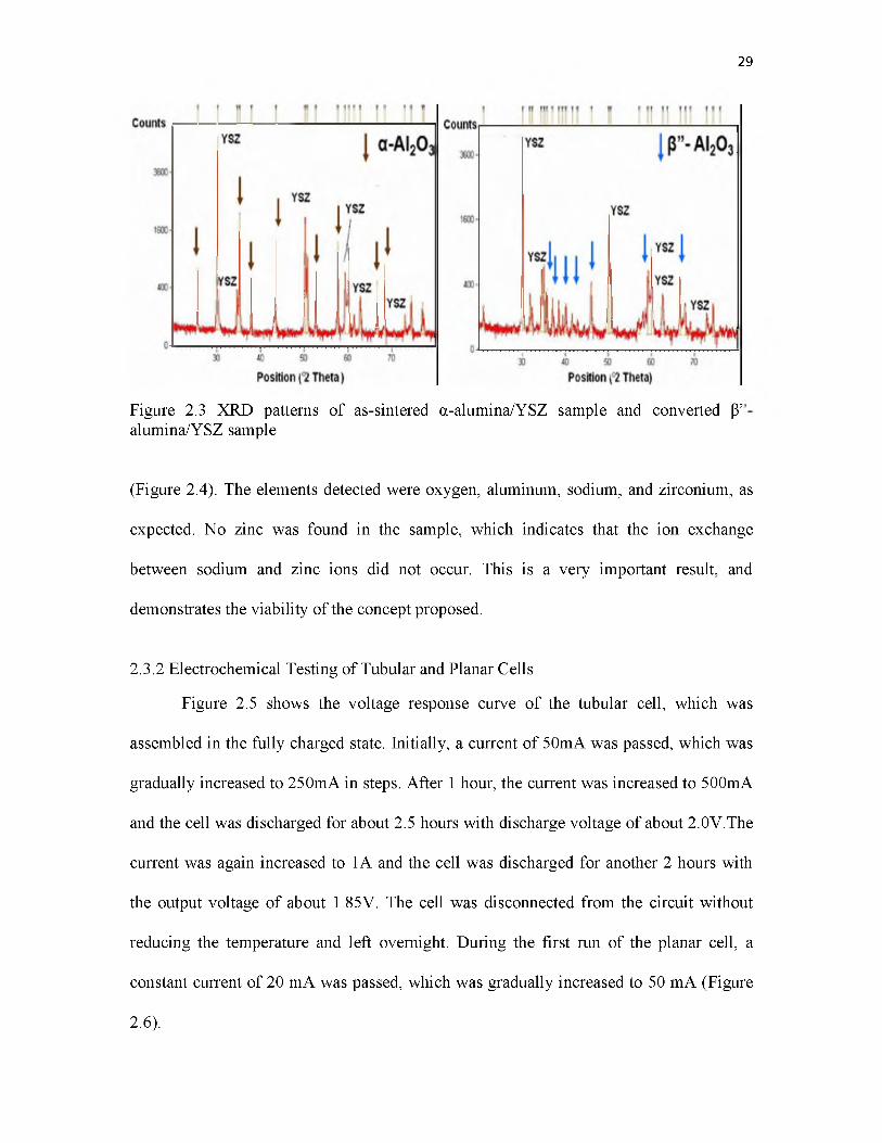
29
Figure 2.3 XRD patterns of as-sintered a-alumina/YSZ sample and converted pr alumina/YSZ sample
(Figure 2.4). The elements detected were oxygen, aluminum, sodium, and zirconium, as
expected. No zinc was found in the sample, which indicates that the ion exchange
between sodium and zinc ions did not occur. This is a very important result, and
demonstrates the viability of the concept proposed.
2.3.2 Electrochemical Testing of Tubular and Planar Cells
Figure 2.5 shows the voltage response curve of the tubular cell, which was
assembled in the fully charged state. Initially, a current of 50mA was passed, which was
gradually increased to 250mA in steps. After 1 hour, the current was increased to 500mA
and the cell was discharged for about 2.5 hours with discharge voltage of about 2.0V.The
current was again increased to 1A and the cell was discharged for another 2 hours with
the output voltage of about 1.85 V. The cell was disconnected from the circuit without
reducing the temperature and left overnight. During the first run of the planar cell, a
constant current of 20 mA was passed, which was gradually increased to 50 mA (Figure
2.6).

30
90
SO
70
100
o O O o o O O o C i o oO O O O S P O O C O O O
Distance
Figure 2.4 Chemical line scan of P”-alumina tube after 50 hours cycling
0)ci(0o>
Figure 2.5 Voltage response of the tubular cell, T = 350oC, Time ~ 5.5 hours

31
»l --------- ' 3'
H5 ltiiit(I — I.......... 0 ...................................................................................... .
0 0.25 0.5 0.75 I 1.25 1.5 0 0.5 1 1.5 2
Time (hours) Time (hours)
Figure 2.6 Voltage responses of planar cell after initial run and five freeze-thaw cycles
It was operated for about 4 hours and it showed no electrolyte failure or any other
type of short. After the first freeze-thaw cycle, the cell was operated for about 2 hours at
50 mA. The cell was run for 3 hours after three freeze-thaw cycles at a constant current of
100 mA. The performance of the cell improved after each freeze-thaw cycle. After the
fifth freeze-thaw cycle, the cell was operated for 1.5 hours at a constant current of 1A
(Figure 2.6). The variation of voltage with time in a given cycle is due to very small
amounts of materials in the electrodes in these experimental cells. It has already been
shown that in the tubular cells with larger amounts of materials, the voltage vs. time plots
are essentially flat (Figure 2.5).
After five freeze-thaw cycles, the planar cell was disassembled and analyzed
under a scanning electron microscopy (Figure 2.7). Even after 5 freeze-thaw cycles, the
electrolyte survived with no cracks. No ion exchange occurred, showing that zinc
chloride is a viable cathode material for the rechargeable battery.

32
Chem ical Lin e S ca n of B A S E after 5 Freeze thaw C y c le s18
16
14
12
£ 10
3Oo 8
6
4
2
00 ' 5 - f iQ ' ^ - C D r ^ C T ) m o j c ir) ' ^ - c £ j i ^ c j > o o f N f in u n c D r ^ ( j ) r ^ c N r Q u n ^ ( D C N C £ ) C N ^ o ^,q ; r a ( N C D q ^ f N fr ) N r - L r i m c o l n f N t D q ^ ; C D ( N (3 0 r - m a ) 0 ( : : i T : r . T - - r s j
□ □ r - o i f N r n r o n t ^ u i c a c d n n n c ri * - •<
Distance
Figure 2.7 Chemical line scan of the planar cell electrolyte showing no trace of zinc
2.3.3 Testing of Three-cell Stack
The charging was done at a temperature of 400oC. To ensure efficient charging,
each cell was charged separately by passing equal amount of charge. Charging was
started with a constant current of 10mA, which was gradually increased to 40mA. It was
started as a three-cell stack. However, the top cell was found short circuited due to the
misalignment of the electrolyte, and thus tested as a two-cell stack. Even though one of
the cells in the cell stack was inoperable, the other two cells in the stack were tested. This
is due to the fact that unlike sodium sulfur batteries, Na - ZnCl2 batteries have high
electrical conductivity due to the formation of metallic Zn in the cathode, which implies
that a low resistant shunt forms when the cell fails.
The voltage response of the three-cell stack (with one failed cell) was analyzed

33
(Figure 2.8). A stable voltage is obtained, unlike the single planar cell response. This is
due to the fact that the cathode and the anode compartment volumes are larger compared
to the previous planar cell. A five-cell planar stack was designed and constructed (Figure
2.9). In the future, the constructed five-cell stack will be electrochemically tested and a
ten-cell planar stack will be designed and tested followed by a full electrochemical
characterization.
2.4 Conclusion
In conclusion, electrochemical tubular and planar cells of configuration,
Na/BASE/ZnCl2, were constructed and tested. There was no evidence of Zn ion exchange
found in BASE. This implies that zinc chloride is a viable cathode. Several freeze-thaw
cycles were conducted on the planar cell with a stable performance output. A three-cell
stack was designed, constructed, and electrochemically tested.
Time (hours)
Figure 2.8 Planar cell stack and the voltage response of the two-cell stack operated at a temperature of 400oC

34
Figure 2.9 Five-cell planar stack arrangement
During the electrochemical testing, one of the cells became inoperable due to the
misalignment of the electrolyte. As the electrode materials are highly conductive due to
the presence of metallic Zn in cathode, the cell got short circuited with low resistance.
The whole stack was tested as a two-cell stack. The stack gave a stable charging voltage
of ~ 4.0 V. A five-cell stack was designed and constructed.
2.5 Acknowledgments
This work is supported by the U. S. Department of Energy under ‘High
Temperature Electrochemistry Center (HiTEC) Advanced Research Program’ DOE
Contract Number: DE-PS26-05NT42470-1A
2.6 References
1. M. McNamee, Sodium-Sulfur Batteries, Modern Battery Technology, p. 458, Ellis Horwood, Ltd, New York and London (1991).
2. R.S. Gordon, W. Fischer, A.V. Virkar, Ceramic Transactions, p. 203, American

35
Ceramic Society, Westerville, Ohio (1996).
3. J. L. Sudworth, Modern Batteries: An Introduction to Electrochemical Power Sources, Colin A. Vincent and Bruno Scrosati, Editors., p. 243, Arnold (Hodder Headline Group), London and John Wiley & Sons, New York (1997).
4. J.L. Sudworth and A. R. Tilley, The Sodium Sulfur Battery, Chapman and Hall, London (1985).
5. M. Kamibayashi and K. Furuta, High Charge and Discharge Cycle Durability o f the Sodium Sulfur (NAS) Battery, Tokyo Electric Power Company and NKG Insulators, Ltd., presented at EESAT (2002).
6. T. Oshima and K. Furuta, Performance Enhancements and Expanded Manufacturing Capacity for Commercial NAS Batteries, NGK Insulators, LTD, presented at ESA (2003).
7. W. Fischer, ABB NaS Battery Review and Preview, Electrochemical Society Fall Meeting, Toronto (1992).
8. W. Fischer, Status and Prospects o f NaS High Energy Batteries, 26th Annual IECEC Proceedings, VI, p. 80 Boston (1991).
9. J. Coetzer, J. Power Sources, 18, 377 (1987)
10. C.-H. Dustmann, ZEBRA Batteries Set to Take on the World”, Batteries International, July (1994)
11. A. V. Virkar, T. J. Armstrong, N. Weber, K-Z Fung and J-F Jue, in High Temperature M aterial, S. C. Singhal, Editor, PV 2002-5, The Electrochemical Society, Inc., Pennington, NJ (2002)
12. Phase Diagrams for Ceramists: Volume II, the American Ceramic Society, Westerville, OH (1969).

CHAPTER 3
A STUDY OF THE KINETICS OF CONVERSION OF ALPHA-
ALUMINA + ZIRCONIA INTO SODIUM BETA” -
ALUMINA + ZIRCONIA
3.1 Introduction
Sodium beta”-alumina is a nonstoichiometric sodium aluminate with an
approximate composition - Na2O.~6Al2O3, known for its excellent conductivity for
sodium ions [1]. Even though the solid electrolyte is generally known as beta-alumina,
there are two different crystal structures: beta-alumina and beta”-alumina. Both structures
have a plane of sodium ions located between spinel blocks. Beta-alumina exists as a two-
block structure and beta”-alumina as a three-block structure. The main difference in
properties of beta and beta”-alumina is in the electrical resistivity, which is considerably
lower for beta”-alumina compared to beta-alumina. The lower resistivity of beta”-
alumina is attributed to differences in Na2 O content between beta” and beta-alumina
(Na2O. ~6Al2O3 and Na2O.~11Al2O3) since the former has a slightly higher soda content,
and also differences in structure [2]. P”-alumina exhibits excellent conductivity at a
relatively low temperature of 300oC compared to other known ion conductors as well: at
300oC the ionic resistivity (conductivity) of Na P”-alumina is ~3 Qcm (~0.33 S/cm). By
comparison, the ionic resistivity (conductivity) of YSZ at 800oC is ~30 Qcm (~0.033
S/cm). At 300oC, the ionic conductivity of YSZ is orders of magnitude lower. The crystal

structure of sodium beta”-alumina provides a rigid framework with channels along which
the mobile ionic species in the solid can migrate [3]. The rhombohedral structure of beta”
is usually represented as a hexagonal unit cell with three times the volume of the
rhombohedral cell. As mentioned earlier, the crystal structure consists of Al-O-Al spinel
blocks, separated by conduction planes perpendicular to the c-axis (which is 1.5 times
larger than beta-alumina) of the hexagonal unit cell [4]. The spinel blocks exhibit
rotational symmetry about the c-axis and are held together by oxygen ions. Sodium ions
are present in the conduction plane and ion transport involves hopping from site to site
along these channels. Weber [5] furthered his studies on beta”-alumina and showed that
small amounts of MgO or Li2 O can stabilize this phase so that it can be sintered into
polycrystalline compacts. Because of its high Na+ ion conductivity, sodium beta”-
alumina is used as a solid electrolyte in electrochemical energy storage systems. As
described in the previous chapter, one of the most advanced energy storage systems is
based on Na P”-alumina solid electrolyte (BASE). The high temperature sodium sulfur
battery, invented at Ford Motor Company during the nineteen sixties, has attractive
features for such applications. The important features include low materials cost, good
durability, high depth of discharge, and potentially low cost. Additionally, the
thermodynamic stability of BASE against reduction or development of electronic
conduction is far greater than that of oxygen ion conductors such as yttria-stabilized
zirconia (YSZ). This presents an excellent opportunity to explore electrochemical energy
conversion or storage devices using BASE.
The traditional method for the fabrication of sodium P”-alumina solid electrolyte
(BASE) is by the calcination of a mixture of Na2CO3, Al2O3 and LiNO3 in air, at
~1250oC [6]. The calcined mixture is then compacted to form desired shapes and they are
37

sintered at a temperature of ~1600oC. Sintering occurs by a transient liquid phase
mechanism between beta-alumina and NaAlO2 . For sintering, the samples are
encapsulated in either MgO crucibles or platinum bags in order to prevent the loss of
Na2O by evaporation. Finally, the sintered samples are annealed to ensure the complete
conversion of P - alumina to sodium P”-alumina. There are several limitations to the
traditional method of fabrication. Higher sintering temperature enhances soda loss from
the samples, which can be avoided only by providing an expensive encapsulation of
samples using Pt bags or MgO crucibles. Remnant sodium aluminate (NaAlO2) which is
hygroscopic in nature is present at the grain boundaries. Thus, beta”-alumina formed by
this process is prone to moisture and CO2 attack from the atmosphere and must be stored
in vacuum chambers in order to avoid degradation. In addition, the strength of
conventional beta”-alumina is low, typically on the order of 200 MPa or less due to the
occurrence of exaggerated grain growth. A novel patented vapor phase process has been
developed for the conversion of a-alumina into sodium beta”-alumina in order to
circumvent the limitations mentioned above [7].
In the vapor phase process, a- alumina is exposed to a source of Na2O, forming a
thin layer of sodium P”-alumina on the surface of the exposed a- alumina. Since P”-
alumina is a good conductor of Na+ ions, diffusion of sodium ions through P”-alumina is
fast. However, to form P”-alumina, it is necessary to incorporate Na2O in the structure.
Therefore, both sodium ions and oxygen ions must have reasonable diffusivities through
the BASE for a vapor phase process. Once a surface layer of P” is formed, further
conversion of alumina to P”-alumina practically shuts down due to the sluggish diffusion
of O2- ions through sodium beta”-alumina. The rate of diffusion of Na2 O (formation of
2-P”-alumina) is dictated by the rate of diffusion of O - ions through P”-alumina. In fact,
38

Nicholson et al. [9,10] used the same approach as described above to form a thin layer of
P”-alumina on sapphire crystals and the rate of film growth was very slow due to the slow
diffusion rate of oxygen ions.
The process can be described as follows. The condition of electroneutrality must
be met, which requires that the fluxes of Na+ and O2- be coupled. From the coupling of
fluxes, the chemical diffusion coefficient of Na2O through P”-alumina is given by,
39
DD P'' D P" (P" _ Na+ O
Na2O~ DP+ + D -i +
5 ln Yn
5 ln X A (3.1)a2O J
where D P"+ and D P2_ are self-diffusivities of Na+ and O2- ions in P”-alumina,Na Ol r ’
r i + 5 ln YNa2O ^5 ln X h
is the thermodynamic factor with YNao and X NaQ being, respectively32° J
2activity coefficient and mole fraction of Na2O in P”-alumina. Since O - ion diffusion is
sluggish in P”-alumina, we can assume that D p"+ >> DP_. Thus, the above equationNa+ ">2-
becomes,
D P" « D P"NaO Dn2^ | 5 ln YnuqO ^
V 5 ln X NaO J(3.2)
If the thermodynamic factor is assumed to be unity, the chemical diffusion coefficient of
Na2 O is the same as the self diffusion coefficient of O2- ions.
D P" « D P"DNa2O ~ DO2- (3.3)
At a temperature of ~1400oC, if the diffusivity of O2- ions in P”-alumina ( D PP-_) is on the

40
10 2order of 10- cm /sec, then the thickness of a-alumina that is converted to P”-alumina in
two days will be ~50 microns. The slow kinetics is due to the slow transport of O - ions
through P”-alumina.
In order to expedite the conversion process, a different approach is used wherein a
rapid path is provided for the diffusion of O -ions [7]. This is done by incorporating an
oxygen ion conductor, yttria stabilized zirconia (YSZ), in the starting material. Thus, a
_i_ 2coupled diffusion of Na+ and O2- ions transport can occur in two phases, leading to a
faster conversion of alumina to sodium beta”-alumina. Once a thin layer of beta”-alumina
_i_ 2 is formed on the surface, Na+ ions diffuse through the formed beta”-alumina and O2- ions
through the YSZ present in the material. This process leads to the formation of a two-
phase composite of BASE and zirconia.
From the condition of local electroneutrality and the coupling of fluxes, the
chemical diffusion coefficient of Na2O through P”-alumina /YSZ is given by,
V V C yszD yszD p"~ P"/ YSZ _ V yszV p "C Q2- D c?- D Ng+_______ ^ 4 ^
n^ o c p" v d p" + 4 D c yszv D ysz ( .C Na+ V P "D Na+ + 4 D C Q2- V YSZD q2-
where D™2 and D P"+ are, respectively, the chemical diffusion coefficients of O2- ions in
YSZ and Na+ ions in B”-alumina, CP + is the concentration of Na+ ions in B”-alumina,1 Na 1
CYS2 is the concentration of O2- ions in YSZ, and V and VYSZ are, respectively, the
volume fractions of P”-alumina and YSZ. In the above equation, the concentration
gradient of Na2 O corresponds to that in the BASE. If the thermodynamic factors are
assumed to be unity, the chemical diffusion coefficients can be replaced by self-
diffusivities of the corresponding ions. That is,

41
V V c yszd yszD p"~ P "/YSZ _ VYSZV P"C O2- D O2- D Na+ /o ^D NaO ^ p -T7- .^v sz -rt- -r^rxv (3 .5)aO C P V D P + 4 C V D YC Na+ V P"D Na+ + 4 C O2- V YSZD o2-
2 +Here, the diffusivities of O - ions in YSZ and Na ions in Na P”-alumina are relatively
comparable (a few orders of magnitude different). The above equations are derived under
the assumptions that both phases are contiguous and parallel transport of oxygen through
Na P”-alumina is negligible. Thus, the chemical diffusion coefficient of Na2O through
P”-alumina/YSZ is much greater than that through single phase P”-alumina. At a
temperature of 1400oC, the thickness of a-alumina that is converted to P”-alumina in ~16
hours was ~1000 microns [8].
By choosing the composition of YSZ with a low yttria content, typically 3%, the
two-phase composite can be fabricated with strength on the order of ~900 MPa, which is
more than four times that of the conventional BASE. In the vapor phase process, no
encapsulation is needed as the conversion temperature is relatively low (1450oC),
resulting in negligible soda loss. Moreover, the process is carried out in such a way that
the thermodynamic activity of Na2 O is significantly lower than the activity of Na2 O in
NaAlO2, preventing the formation of hygroscopic NaAlO2 at the grain boundaries. The
activity of Na2O is controlled by the conversion temperature and composition. The BASE
thus formed is resistant to atmospheric moisture and CO2 , and can even be boiled in
water without any degradation.
3.2 Theoretical Model
Figure 3.1 shows a schematic of the conversion mechanism of a two-phase,
contiguous compact of a -alumina + YSZ into a Na-P”-alumina + YSZ compact. The

42
N a’O
N a:0 Source (Vapor)
2dI
Three phase Boundary
/
faster O2transport^
------- >faster T'fa+transport
¥2
P" a
YSZ
P" alumina
a- alumina
'Reaction Front
Figure 3.1 Mechanism of conversion of a - alumina to BASE. Oxygen ions are transported through YSZ and sodium ions are transported through P”-alumina. It also shows the three different paths through which O2- ions can diffuse at the reaction front to form BASE.
schematic is depicted as alternate layers of alumina and YSZ for the sake of simplicity.
This assumption is reasonable because, in the actual microstructure of the two-
phase material, both phases are contiguous. A theoretical model describing the
conversion kinetics of a - alumina/3YSZ samples to sodium P” - alumina/3YSZ samples
is given in what follows. The conversion was achieved using the patented vapor phase
method [7] and the chemical reaction is as follows:
Na2O + ~6.2Al2O3 ^Na2O.~6.2 AhOs (3.6)
For conversion, a composite of a -alumina + YSZ is exposed to a vapor of Na2O source
at elevated temperatures. A surface layer is converted to Na P”-alumina + YSZ upon the
incorporation of Na2O. Subsequent conversion occurs by the coupled transport of Na+
9ions and O - ions through the ceramic. Sodium ions are transported through the already

formed layer of P”-alumina and oxygen ions are transported through YSZ.
The kinetics of conversion may be either interface controlled or diffusion
controlled or a combination of both. Let x be the thickness converted to P”-alumina at
time t. When the thickness converted is small, the kinetics should be linear (interface
control) and when the thickness converted is large, the kinetics should be parabolic
(diffusion control). The process of conversion to sodium P”-alumina can be broken down
into three steps: interface reaction at the three-phase boundary (YSZ, Na P”-alumina, and
gas phase), transport of ions across the bulk, and the formation of BASE at the reaction
interface. Figure 3.2 shows a schematic of the variation of the chemical potential of Na2O
across the converted (P”-alumina + YSZ) thickness (x). During the conversion process,
2 +0 - ions need to diffuse through BASE/a-alumina to combine with Na ions to form
BASE, which is a slow kinetic step. This can occur along three different paths: through
the P”-alumina phase, along the interface, or through the a-alumina phase, as shown in
Figure 3.1. It is expected to depend on the grain size of the sample as the diffusion
distance of O - ions is half the grain size (d/2) of the sample, as shown in the schematic.
Na2O is dissociated at the three-phase boundary (gas phase, P”-alumina, and
YSZ) and Na ions are transported through P”-alumina and O - ions are transported
through YSZ, as shown in the schematic - Figure 3.1. The condition of electroneutrality
must be satisfied, thus resulting in the fluxes of Na and O - ions being coupled.
Assuming a quasi-steady state:
Na2 O — ► 2Na+ (P”) + O2- (YSZ) (3.7)
Let the interface between the gas phase (Na2O) and P”-alumina+YSZ layer be denoted by
1 and the interface between the reaction front (P”-alumina+YSZ) and a-alumina+YSZ be
43

At the gas
solid interface
(I) and reaction
front (II), the flux
of Na20
is defined by
Assum
ing electroneutrality
and a
quasi-steady state, the
fluxes of sodium
ions and

Figure 3.2
A schem
atic showing
the variation
of the
chemical
potential of
Na20
across the
converted BASE
with a
thickness x. The
process involves
two interfacial
steps and
one diffusive
(coupled) step.

the corresponding interfacial parameters. Across the converted thickness of P”-alumina
+YSZ, flux of Na2 O is a function of the chemical diffusion coefficient and the
concentration of Na2 O in P”-alumina and the gradient in chemical potential of Na2 O
across the thickness.
T — V "{ " 11 \ — 1S'( 1 ^ ^ Nalu “ K'" ~ 1n\Na o ~ K yn ~HN(ho ) - K ynNa20 - n j - — — - , T “ (3-10)
45
where K’ and K” are the interfacial reaction coefficients at the gas-solid interface
(interface I) and the reaction front (interface II), respectively. n’ is the chemical potential
of Na2O in P”-alumina/YSZ, close to the gas phase (Na2O vapor) near interface I and |T’
is the chemical potential of Na2O in P”-alumina/YSZ, close to the reaction front (a-
alumina/YSZ) near interface II.
Vm - Molar volume of BASE
i v „ ,, - Chemical diffusion coefficient ofNa20n a^Q
C - Concentration of Na2O in BASE
x - Thickness converted to P”-alumina at time t
kB - Boltzmann constant
T - Temperature
Since the chemical potentials n’ and |T’ are not measurable parameters, we need to
eliminate them from the equations. From equation (3.10) we know that,
K MNa2Q K U K U K UNa2Q
, K " (UN.,,0-M") i ( 3 1 1 )
: 'U ---- ~ K ' ------- +
We can eliminate |i’ by substituting p’ in equation (3.10)

46
K " « o - M " ) = - K " ( m " - m 1 2o ) =1 ,
k ^ T x
,, K " - m ")m -
K 'MNa0t (3.12)
orL
Rearranging,
■K'K”kBTxii”+ K 'K " k BTxi4a20 = L Nai<J~ v
(3.13)
(3.14)
or
1 i\a7u ~ r - n c u u ' ~ ~ r-Na,u J ' - « ------- r-Na2u ~ Na2u ~ v
(3.15)
Equation (3.15) can be further rearranged to obtain in terms of measurable (in
principle) parameters. Therefore,
' V" It tv , ,nm =
NaO
Lpia,u~\— + K") + K ' K ' kBTx(3.16)
Now, the flux of Na2O is given by
V„ dt(3.17)
Substituting equation (3.16) into equation (3.17) and eliminating and gives,
K " M2i /C ,o + * " /C ,o ) + K ' K "k„TxKl Na2O
+K") + K 'K " kBTx1 dx
V dt(3.18)
/ r
47
Simplifying equation (3.18),
I 1 /7r(3.19)
LNa.u~ v— + K") + K 'K " kBTx Vm dt
or
K 'K "L»a2u~,r-Na2u r-Naiu , m- ------:"kBTx\dx (3.20)
or
l NoAj- , - + k ") , K 'K " k nTx. +----------------- --------- ---------dx = dt (3.21)K 'K " L Na yr.Nai0 -ju L 2oWm K'K"D C(ju“a20
On integration,
x ( K '+ K ") , x k B T r t ,J — ;— -— jj------- -j---------d x + \-~ —-------------- x d x = \d t (3.22)()K K { Na20 ~ Na2oWm Q ^ Na2u ~ \r-Na2Q ~ f Na20 ^ m Q
(3-23)K K (/.lN(liQ 2L Na2u~ \r-Na20 Na2C)) n
The general equation is
kRT 2 (K '+ K ")—~ 1--------7--------x -----;—~— ~j--------1
Na2u~ \r-Na20 ~ Na2o)^m K K (/JNa20 ~ Na2o)^nx2 + ... -------^ r r x = t (3.24)
This general equation describes the kinetics of conversion in terms of measurable
(in principle) parameters. Here, time t is defined as the hold time at the conversion
temperature. So at t = 0, there will be an initial thickness converted (xo) as some
conversion takes place during the heating up process. On integrating from x0 to x instead

48
of 0 to x, the general equation is
kBT , 2 2, (K '+ K ")- ------ ---------(jc - x , ) + --------- ^ -------—j--------( x - x 0) = t (3.25)) — / / \ V K ' K " ( n — / / W^ Na2U~ \r~Na20 ^N a 20 ) V m \H'Na20 H'Na1o ) Vm
Consider a case where the conversion thickness x is very small. In a typical
experiment, the initial thickness xo may not be negligible due to the occurrence of
conversion during the heating up process. If we assume xo to be negligible and if the
diffusion distance of the coupled transport of sodium and oxygen ions across the P”-
alumina layer is very small, then,
(K '+ K ") kBT 2 --------- - x » —~B - 2K ' K " 2 L Na2U ~
We have
(K '+ K ") xv J = t (3.26)
K 'K " ( M l , O - v l , O V
x -M'„a,a)V, ‘ (327)
x = Krnt {MNaO - MNoOO ) Vmt (3.28)
K 1K "where Kint = -------- which includes both interfacial reactions at the gas phase interface
K '+K "
(I) and reaction front interface (II). The kinetics is thus interface controlled.
Effective interfacial coefficient can be defined as,

K f = K,J.MNa,_o - mL,o) V , = K 'K ’ (mL o - v L ,oWm (3.29)( K + K )
Then,
X « K eft (3 .3 0)
Here, the conversion process is controlled by the two interface reactions at gas phase (I)
and reaction front (II) since the diffusion distance is very small for the diffusion across
P”-alumina. Thus, the process follows linear kinetics or it is interface controlled.
Consider a case where the conversion thickness x is large. In this case, the
diffusion distance of sodium and oxygen ions across the P”-alumina/YSZ converted layer
is large. That is,
49
(K '+ K ") kBT 2 , ^ ---------------- - x « — ~ B ~ 2 ’
K ' K " 2 L Na2U ~
Thus,
k„Tx2
^2 _ Na2u~ \t iwa20 f'Na2o'Wm 22.)
x ~ ITT ( . )
Effective diffusion coefficient can be defined as
iwa2u ~ \ t iwa20 ^ W a 20 3 3 ^ )
eff ~ I TThus,

50
x - D f (3.34)
In this case, the conversion process is controlled by the diffusion step since the diffusion
distance is large and the two interface reactions are relatively fast. Thus, the process
follows parabolic kinetics or it is diffusion controlled.
The general form of the equation derived can be written in terms of effective
coefficients of diffusion and interfacial reactions as follows.
x 2D fTV eff J
+ x
V K f J
-------h -V D f f K eff J
x0 = t (3.35)
3.3 Experimental Procedure
A mixture of 70 vol. % a-AhO3 and 30 vol. % 3-YSZ (Baikowski CR-30 and
Tosoh TZ-3Y, respectively) was prepared by planetary milling to ensure a well-mixed,
fine starting powder. Several a-alumina+3YSZ discs were prepared by die-pressing
followed by isostatic pressing. These samples were then sintered at different temperatures
and for different durations: temperatures ranging from 1500oC to 1800oC and durations
from 1 hour to 4 hours. The densities of the samples were determined. The samples
sintered at different temperatures were fine-polished, thermally etched, and analyzed
under a Scanning Electron Microscope to determine the grain sizes of the samples. These
samples were then converted to sodium P” - alumina+3YSZ by heat treating them at
different temperatures ranging between 1250oC and 1450oC and durations ranging from 1
hour to 15 hours. The converted samples were cross-sectioned, coarsely polished, and
examined again under a Scanning Electron Microscope to measure the thickness of the
sample converted and for calculating the corresponding conversion rates. Some of the

partially converted samples were cross-sectioned, finely polished, and analyzed under the
microscope to study the microstructure of the reaction interface between the converted
and the unconverted regions of the samples. The kinetics of conversion at various
conversion temperatures ranging between 1250oC and 1450oC was studied and the
theoretical model proposed was fitted to the experimental data to determine the various
parameters.
3.4 Results and Discussion
The a-alumina+YSZ samples, sintered at different temperatures ranging from
1500oC/1 hour to 1800oC/3 hours, were examined using a Scanning Electron Microscope.
Figures 3.3 (a) through (d) show the microstructures of sintered samples with widely
differing grain sizes: a-alumina + 3YSZ samples sintered at 1500oC, 1600oC, 1700oC,
and 1800oC, respectively. The grey areas are alumina and the white areas are YSZ.
51
Figure 3.3 Microstructures of a-alumina + 3YSZ samples sintered at (a) 1500oC for 1 hour, (b) 1600oC for 1 hour, (c) 1700oC for 1 hour, and (d) 1800oC for 1 hour.

The grain size is considerably greater in the samples sintered at higher
temperatures and for longer times. The average grain sizes of the samples were
determined using Schwartz - Saltykov diameter analysis [11]
Table 3.1 lists the grain size as a function of sintering conditions. The grain size
(average of alumina and zirconia) of the sample sintered at 1500oC/1 hour was 0.53 pm
and that of the sample sintered at 1800oC/3 hours was 4.15 pm. The growth in grain size
was about 8 times when the temperature/time were increased from 1500oC/1 hour to
1800oC/3 hours. This result is consistent with the expectations since the sample sintered
at higher temperature and for longer time exhibits a larger grain size. Figure 3.4 (a)
shows a micrograph of the cross-section of a partially converted P”-alumina sample. In
the figure, interface A shows the actual chemical interface where a-alumina/YSZ changes
to P”-alumina+YSZ and interface B shows the structural interface where damaged P”-
alumina+YSZ changes to a dense P”-alumina+YSZ structure. At the chemical interface
(A), the microstructure of the sample changes abruptly from a-alumina+YSZ to P”-
alumina+YSZ. Even though the actual chemical interface is at A, there is an interface
band between A and B which has the same structure as that of P”-alumina+YSZ with the
exception of porosity/cracks. When a-alumina+YSZ sample is converted to P”-
alumina+YSZ, there will be a volume change due to differences in their densities (density
of a-alumina: 3.97 g/ml and that of beta”-alumina: 3.28 g/ml) and due to the
incorporation of Na2O in the structure.
Consider 1 mole of a-alumina converted to 1 mole of Na P”-alumina.
Volume of 1 mole of a-Al2O3 = (102g/3.97 g/ml) = 25.69 ml
Volume of 1 mole of P”-alumina, (1/6.2) Na2O.Al2O3 = (112g/3.28) =34.15 ml
The net volume change is
52

53
Table 3.1: Grain size as a function of sintering conditions
Sintering Temperature (oC) Hold time (hours) Grain Size (um)
1500 1 0.53 + 0.03
1500 2 0.57 + 0.04
1500 4 0.61 + 0.05
1550 1 0.67 + 0.01
1550 2 0.74 + 0.05
1550 4 0.86 + 0.07
1600 1 0.95 + 0.01
1600 2 1.14 + 0.03
1600 4 1.32 + 0.03
1700 1 1.80 + 0 .0 2
1700 3 2.40 + 0.04
1800 1 3.70 + 0.06
1800 3 4.15 + 0.05
34 15 - 25 69 x 100 = 32.93%25.69
This volume change needs to be accommodated in the material. Figure 3.4 (a)
shows that significant cracking/porosity occur in the structural interface band. The
reaction front undergoes a change in microstructure by repairing the pores formed and
densifying beta”-alumina+YSZ. This is evident from Figure 3.4 (b), which is a chemical
line scan profile across the cross-section of the partially converted sample which shows
the weight percent of sodium with distance. Concentration of sodium in the unconverted
portion is negligible, whereas the concentration of sodium in the converted portion (P”-

54
(a) (b)
Figure 3.4 Analysis of the interface of partially converted sample. (a) Micrograph of the interface of the partially converted a - alumina+3YSZ sample which shows the unconverted portion in the top and the interface band in the middle and the converted portion in the bottom. The interface band has the structure of P”-alumina + YSZ but with porosity. (b) Chemical line scan shows the weight percent of sodium present across the cross-section of the sample. The concentration of sodium in the unconverted portion (a- alumina+YSZ) is negligible as compared to that in the interface band and the converted portion (P”-alumina+YSZ), which is an order of magnitude higher.
alumina+YSZ) is ~3.7 (wt) %.
At the chemical interface A, there is a sharp change in the concentration of
sodium (0.5% to 2.5%), which is consistent with the change in structure from a-
alumina+YSZ to P”-alumina+YSZ. However, across the interface band (between A and
B), right after the sharp increase in sodium concentration, the sodium concentration
further increases gradually as it nears the fully densified P”-alumina+YSZ at interface B.
This may be attributed to the presence of porosity in the interface band. When the
structure changes from a-alumina to P”-alumina, the incorporation of Na2O in the
structure is accompanied by structural damage, which creates pores. As the structure
rearranges and repairs itself to form a dense P” -alumina, the porosity gradually decreases
through the interface band as the sample becomes dense P”- alumina. An order of

magnitude analysis of the concentration profile through the interface band is given below.
Let V'p, Vz , and Vp be the volume fractions of P”-alumina, YSZ, and porosity,
respectively, at the chemical interface and V", V'z , and V'p be the volume fractions of P”-
alumina, YSZ, and porosity, respectively, at the dense P”-alumina (B interface).
Then we have,
v ; + v: + vp = 1 (3.36)
V" + V" + VP = 1 (3.37)
Since the sample is considered fully dense at the structural interface, v "is essentially
zero.
i.e., V'p + V" = 1 (3.38)
The starting composition of the sample before conversion was 70 vol.% of a-alumina and
30 vol.% of YSZ. During conversion, YSZ remains unchanged. Thus, the volumes of
fully converted sample are 75.77 vol.% P”-alumina and 24.23 vol.% YSZ. Thus,
55
V , = V . = 0.7577 = 3 2 7
V' V" .2423z z
i.e. V'p = 3.127* V' (3.39)
Substituting equation (3.39) into equation (3.36)
3.127 V" + V:+ VP = 1 (3.40)

56
From Figure 3.4(b), the ratio of sodium concentrations at the chemical interface and
2 5converted B”-alumina is —— = 0.714.
3.5
V'i.e., - 4 = 0.714 :.Vp = 0 .7 1 4 * ^ = 0.714*0.7577 = 0.541 (3.41)
V P
From equation (3.39), we can determine Vz
V = 0541 = 0.173 (3.42)Z 3 .1 2 7
Therefore, the porosity in the structural interface band can be calculated from equation
(3.40) as
V'p = 1 - 0.541 - 0.173 = 0.286 (3.43)
Thus, the porosity at the chemical interface is calculated to be 28.6%. No separate
measurements of porosity in the interface band have been made. The net volume change
of the sample when converted from a-alumina+YSZ to P”-alumina+YSZ was calculated
to be 32.93%. From the microstructure of the sample cross-section, it is hard to determine
the variation of porosity from interface A to B. The porosity is expected to decrease from
interface A to B as the structure repairs itself to form a dense P”-alumina+YSZ.
As mentioned earlier in this chapter, the conversion to P”-alumina involves three
kinetic steps: two interface reactions and one diffusion step. Interface reaction kinetics is
expected to depend upon the average grain size of the sample. At the reaction front (K”),
O - ions must transport through either the BASE formed, or through the a-alumina, or
along the a-alumina+BASE interface (see schematic in Figure 3.1). The diffusion

distance is about half the grain size of a-alumina (or BASE). Since the grain size in a
given sample is constant, this diffusion distance is fixed. Thus, diffusion distance parallel
to a + YSZ/ P” + YSZ remains fixed throughout the conversion. This reflects as an
interfacial step. The three paths for diffusion are in parallel, and the phenomenon is very
similar to the formation of pearlitic steel by a cellular decomposition of austenite in the
iron-carbon system. Thus, the local diffusion distance at the reaction front is larger for
coarse grained samples and is smaller for fine grained samples. Thus, the interface kinetic
parameter K” is expected to be an inverse function of grain size.
At the gas phase-solid interface (K’) as well, the kinetics depends upon the grain
size of the sample. At this interface, Na2O dissociates to form Na+ and O2- where the
three phases (gas phase, P”-alumina, and YSZ) meet. 2Na+ ions transport through P”-
alumina and O - transport through YSZ. Figure 3.5 shows a schematic representation of
the three phase boundaries of samples with small average grain size and large average
grain size for comparison. The stars in the schematic show the number of three-phase
boundaries with gas phase (Na2O vapor), a or P”-alumina, and YSZ. Since the reaction
occurs only at the three-phase boundaries, the kinetics of this interface reaction is
proportional to the number of points where all the three phases meet. The smaller the
average grain size, the larger the number of three-phase boundaries. Thus, the interfacial
kinetics at the three-phase boundaries is also expected to be an inverse function of grain
size.
The effect of grain size on diffusion coefficient can be hypothesized using the
Brick-Layer model [12]. According to the Brick-Layer model, it can be shown that the
ionic conductivity of BASE is a function of grain size; the larger the grain size, the higher
the conductivity. The resistivity of a P”-alumina sample depends on the resistivity of
57
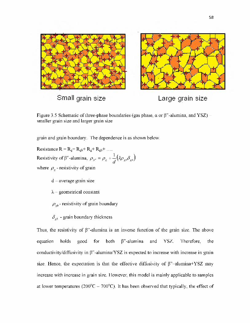
58
Sm all grain size Large grain size
Figure 3.5 Schematic of three-phase boundaries (gas phase, a or P”-alumina, and YSZ) - smaller grain size and larger grain size
grain and grain boundary. The dependence is as shown below.
Resistance R = Rg+ Rgb+ Rg+ Rgb+ ....
Resistivity of P”-alumina, Pp" = P S + 1 W Sb5gb)d
where p - resistivity of grain
d - average grain size
X - geometrical constant
p b - resistivity of grain boundary
Sgb - grain boundary thickness
Thus, the resistivity of P”-alumina is an inverse function of the grain size. The above
equation holds good for both P”-alumina and YSZ. Therefore, the
conductivity/diffusivity in P”-alumina/YSZ is expected to increase with increase in grain
size. Hence, the expectation is that the effective diffusivity of P”-alumina+YSZ may
increase with increase in grain size. However, this model is mainly applicable to samples
at lower temperatures (200oC - 700oC). It has been observed that typically, the effect of

grain size on conductivity is negligible at higher (>700oC) temperatures. The temperature
range studied here was between 1250oC and 1450oC. Thus, the effect of grain boundary
resistance in the current study is negligible. Therefore, the diffusion coefficient is
expected to be independent of the grain size of the sample.
In the vapor phase conversion process, the approach to making samples of
varying grain sizes involved the fabrication of a-alumina+YSZ samples by sintering at
different temperatures and times. This was achieved by sintering a-alumina+YSZ
samples at different temperatures ranging from 1500oC to 1800oC for various durations
ranging between 1 hour and 4 hours. These samples were then converted to sodium
beta”-alumina+YSZ at different temperatures ranging between 1250oC and 1450oC and
hold times varying from 1 hour to 15 hours. The samples were cross-sectioned and
analyzed to determine the rate of conversion from a-alumina to P”-alumina. The
experimental data obtained were fitted to the general kinetics equation given in equation
(3.35) using MATLAB software. Figure 3.6 shows the thickness of conversion of
samples with varying grain sizes as a function of hold time at a conversion temperature of
1250oC. Figure 3.7 shows the conversion kinetics of samples with varying grain sizes as a
function of hold time at a conversion temperature of 1450oC. The dependence of
conversion thickness on time was fitted using the general
(x — x a ) (x — x )equation: ----------- + -------- - = t . In both sets of plots (Figures 3.6 and 3.7), non-zero y-D eff K eff
intercepts (x0) exist, which indicate that some conversion of a-alumina+YSZ to P”-
alumina+YSZ occurs during the initial heat up. x0 depends on the conversion temperature
and grain size of the samples. For higher temperatures and smaller grain sizes, x0 is large
and for lower temperatures and larger grain sizes, x0 is small. This is as expected because
59

60
Figure 3.6 Conversion Thickness as a function of hold time for the samples with varying grain sizes, Conversion Temperature - 1250oC. The dependence was fitted to the general
kinetic equation modeled for conversion:: (x2 - ) (x - x0 )D,eff K,
= teff
Tim e (hr)
Figure 3.7 Conversion Thickness as a function of hold time for the samples with varying grain sizes, Conversion Temperature - 1450oC. The dependence was fitted to the general
kinetic equation modeled for conversion: — x°LJ_.(x—xL)Deff K
■ = t .eff

as the grain size increases, the rate of conversion decreases at a constant conversion
temperature, whereas the rate of conversion increases with increase in the conversion
temperature. At the conversion temperature of 1450oC, it was found that for the 1500oC/1
hour sample (average grain size - 0.53 p,m), the rate of formation of P”-alumina was
about 0.23p,m/sec, whereas for the 1800oC/1 hour sample (average grain size - 3.7 p,m),
the rate of formation of P”-alumina was about 0.06p,m/sec. Therefore, a sample of
thickness 1mm, sintered at 1500oC for 1 hour will require ~35 minutes to convert
completely to beta”-alumina at a temperature of 1450oC. For a 1mm thick sample
sintered at 1800oC for 1 hour, the time required for complete conversion to P” - alumina
will be about 140 minutes (~ 2 hours 20 minutes) when heat treated at 1450oC. This
result indicates that the rate of conversion is higher for the samples having a smaller grain
size. It was observed that the kinetics of conversion was linear (interface controlled)
when the conversion thickness x is small and the conversion kinetics exhibited inverse
dependence on grain size - the smaller the grain size, the faster the conversion rate.
These results can be explained in terms of transport mechanisms.
Over the range of conversion thicknesses studied, which are well over 1 mm, it is
observed that the kinetics is nearly linear when x is small. The observation that the
kinetics is linear at small x implies the kinetics is not controlled by the parallel diffusion
of Na through the BASE formed and O - through the zirconia phase to the reaction front,
even though conversion requires coupled transport of Na+ and O2-. That is, the diffusion
step is relatively fast. With the available experimental data and the best fit obtained using
the theoretical model, the effective diffusion and interfacial rate constants were
determined. Figures 3.8 and 3.9 show the dependence of both interfacial rate constants
and diffusion coefficients as a function of grain size for conversion temperatures of
61
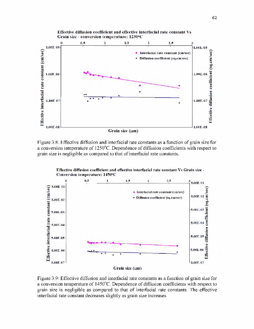
62
Effective diffusion coefficient and effective interfacial rate constant Vs Grain size - conversion temperature: 1250°C
0 0.5 1 1.5 2 2.5 31.00E-05-I ' ' ' ' ' 1-1.00E-05
oa>
Srtiflaou
1.00E-06
ut-l0>a0>ufaw
1.00E-07-
1.00E-08
■ Interfacial rate constant (cm/sec) ♦ Diffusion coefficient (sq.cm/sec)
♦ ♦ ♦
■ " --------------- -♦
♦ ♦ ♦ •♦ ♦
1.00E-06
1.00E-07
QJc/iau
aa#c-»sQO0S3O(/51 ■— ■oCL>
o,4JSsw
Grain size (jim)1.00E-08
Figure 3.8: Effective diffusion and interfacial rate constants as a function of grain size for a conversion temperature of 1250oC. Dependence of diffusion coefficients with respect to grain size is negligible as compared to that of interfacial rate constants.
Effective diffusion coefficient and effective interfacial rate constant Vs Grain size - Conversion temperature: 1450°C
0 0.5 1 1.5 2 2.5 3
<L*</5--su
5.00E-01 -
5.00E-02
5.00E-03 -
£ 5.00E-04
up«0>+-»a
5.00E-05
' £ 5.00E 06 ] ufaW
5.00E-07
■ Interfacia l rate constant (cm/sec)
* D iffusion coefficient (sq.cm/sec)
■— ■— . — .
**♦ ♦ ,■ --------------------
* * * * ♦ ----1 -----
5.00E-01
u
5.00E-02 SUIX!
h5.00E-03 fl
*(-> s
[-5.00E 04 O stO
bS.OOE-OS §2■5
5.00E-0S
5.00E-07
Grain size (urn)
Figure 3.9: Effective diffusion and interfacial rate constants as a function of grain size for a conversion temperature of 1450oC. Dependence of diffusion coefficients with respect to grain size is negligible as compared to that of interfacial rate constants. The effective interfacial rate constant decreases slightly as grain size increases.

1250oC and 1450oC, respectively. At 1250oC, the effective interfacial rate constant (Keff)
decreases with increase in grain size, whereas the effective diffusion coefficient (Deff) is
essentially independent of grain size. Similarly at 1450oC, Keff decreases slightly with
increase in grain size and dependence of Def with grain size is negligible. According to
the Brick-Layer model [12], Deff is expected to increase with increase in grain size, as
discussed earlier. However, the effect of grain boundary resistance is more prominent
only at lower temperatures and is negligible at higher temperatures. In the present study,
since the conversion temperatures are high, it may not affect the diffusion coefficients of
the sample. At 1250oC, the ratio of diffusion coefficients between smallest and largest
grain size is 1.49 and at 1450oC, the corresponding ratio is 1.2. However, the variation of
interfacial rate constants with grain sizes is significant for both conversion temperatures.
The ratio of interfacial rate constants between smallest and largest grain size at 1250oC is
3.3 and at 1450oC is 2.0. In both cases, the dependence at higher conversion temperature
is less prominent than that at lower temperature. This is evident from Figures 3.10 and
3.11, which show the Arrhenius plots of interfacial and diffusion rate constants,
respectively, of the samples with different grain sizes.
The activation energies corresponding to each of the grain sizes were calculated.
The activation energies for diffusion varied between 328 kJ/mol and 340 kJ/mol, whereas
the activation energies for interfacial reaction varied between about ~290 kJ/mol and
~350 kJ/mol with increasing grain sizes. That is, for smaller grain size samples, the
activation energy for interfacial reactions is smaller and vice versa. Thus, the interface
kinetics tends to be more sluggish for large grain size samples.
Figure 3.12 shows the dependence of activation energies corresponding to interface
63

64
l/T [1/K]
Figure 3.10 Arrhenius plot of interfacial rate constants for different grain sizes of the P” - alumina samples. As grain size decreases, the activation energy of interfacial reactions also decreases. It suggests that interfacial kinetics is dependent on grain size variation.
Figure 3.11 Arrhenius plots of diffusion constants for different grain sizes of the P” - alumina samples. As grain size decreases, the activation energy of diffusion reactions remains constant. This suggests that the diffusion kinetics is independent of grain size variation.

65
increase in grain size, whereas activation energies of diffusion coefficient is independent of grain size variations.
reaction and diffusion for various grain size samples. Activation energies for interface
reaction increase with increase in grain size, whereas activation energies for diffusion
step are independent of the grain size variation. The dependence of diffusion constants on
the grain sizes was not very substantial as compared to the dependence of interfacial rate
constants on the grain sizes of the samples.
3.5 Summary
The kinetics of conversion of a-alumina/YSZ to Na P”-alumina/YSZ was studied.
A novel patented vapor phase method was used to fabricate Na P”-alumina samples. In

order to expedite the diffusion of Na2O through the samples, an oxygen ion conductor
was incorporated in the starting a-alumina samples. This provided a rapid parallel path
for the transport of O2- ions as P”-alumina is a poor conductor of oxygen ions. A
theoretical model was proposed and a general kinetic equation for conversion was
formulated with diffusion and interfacial parameters. Several samples of various grain
sizes from 0.53 p,m to 4.15 p,m were fabricated. These samples were converted to P”-
alumina at several temperatures and for various times ranging from 1250oC to 1450oC
and 1 hour to 15 hours. The effective diffusion and interfacial rate constants were
determined from the experimental data and the proposed theoretical model. It showed
that when the thickness converted is small, the kinetics is linear (interface controlled) and
when the thickness converted is large, the kinetics is parabolic (diffusion controlled). The
results also indicated that the smaller the grain size, the faster the rate of conversion.
Arrhenius plots of interfacial and diffusion reactions showed that interfacial reactions at
the three-phase boundaries and reaction front depended more on grain size than the actual
diffusion of Na2O through the sample (Na through P”-alumina and O - through YSZ).
3.6 Acknowledgements
This work is supported by the US Department of Energy under Grant Number
DE-FG02-06ER46086.
3.7 References
1. P. T. Mosley, The solid electrolyte: properties and characteristics, p. 19, in ‘The sodium-sulfur battery’, J. L. Sudworth and A. R. Tilley,Editors, Chapman and Hall, London (1985).
2. J. T. Kummer, “f-alumina electrolytes'”, p. 141, in ‘The sodium-sulfur battery’, J. L, Sudworth and A. R. Tilley, Editors, Chapman and Hall, London (1985).
3. G. Yamaguchi, and K. Suzuki, Bull. Chem. Soc. Japan, 41, 93 (1968).
66

67
4. G. Yamaguchi, J. Japan Electrochem. Soc. 11, 260 (1943).
5. N. Weber and A. Venero, 72nd Annual meeting of Am. Ceramic Soc., May 1970, Philadelphia, unpublished work.
6 . G. E. Youngblood, A. V. Virkar, W. R. Cannon and R. S. Gordon, Bull. Amer. Ceram. Soc., 56, 206 (1977).
7. A. V. Virkar, J-F. Jue, And K-Z. Fung, U. S. Patent No. 6,117,807, (2000).
8 . A.V. Virkar, T.J. Armstrong, N. Weber, K-Z. Fung and J-F. Jue, Electrochem. Sco. Proc, PV 2002-5, 200 (2002)
9. C. K. Kuo, P.S. Nicholson, Solid State Ionics, 67, 157 (1993)
10. C. K. Kuo, P.S. Nicholson, Solid State Ionics, 82, 173 (1995).
11. S. A. Saltykov, in Proceedings of the Second International Congress for Stereology, p.163, H. Elias, Editor, National Science Foundation, New York (1967).
12. T. Van Dijk, A. J. Burggraaf, Phys. Stat. Sol. A, 63, 229 (1981).

CHAPTER 4
ELECTROCHEMICAL COARSENING OF COPPER POWDER
IN AQUEOUS MEDIA
4.1 Introduction
A process in which larger particles grow at the expense of smaller particles is
known as Ostwald ripening or coarsening. Numerous theoretical and experimental studies
on Ostwald ripening have been conducted over the past several decades [1-3]. The first
systematic study of coarsening was by Ostwald in 1900. Lifshitz and Slyozov [2], and
Wagner [3] developed the basic theory of particle coarsening sixty years later. The theory
states that coarsening follows a temporal power law d f <x t with exponent n = 3 for a
diffusion-controlled process and n = 2 for an interface-controlled process, where d™ is
the expectation value of the nth moment of the particle size. Following the work of
Lifshitz and Slyozov [2], many theoretical studies on the Ostwald ripening process have
been reported [4-8]. Recently, Voorhees et al. have conducted an extensive study on the
simulations of classical Ostwald ripening in elastically stressed solids [9].
A few reports on electrochemical Ostwald ripening are also available in the
literature: Mulder et al. conducted a coarsening study on two mercury drops placed on a
2+Pt - plate in an aqueous Hg electrolyte [10]. Even though the droplets were apart (not in
physical contact), the larger droplet grew at the expense of the smaller one as ion
transport occurred through the bulk electrolyte and electron transport occurred via the

69
platinum metal support [10]. Redmond et al. observed that Ag films reformed
electrochemically when exposed to water containing Ag+ ions [11]. This was attributed to
a negative shift in standard electrode potential of silver which causes differences in the
equilibrium silver ion concentration around each particle [12]. Schroeder et al. have done
an extensive study on electrochemical Ostwald ripening using a solid electrolyte cell [13
15]. They observed that the open circuit voltage of the electrochemical cell Ag (nano)|
solid silver electrolyte| Ag (bulk) was unstable due to the coarsening of nano crystalline
silver. The coarsening was attributed to the migration of Ag+ via the electrolyte and e-
through the metal [13-15].
In conventional solid state Ostwald ripening, metal particles grow by bulk or
grain boundary diffusion. In electrochemical Ostwald ripening, growth occurs by a
coupled transport of electrically charged species, for example, metal ions and electrons
via parallel paths: metal ions through the liquid/ionomer and electrons through the metal
or supporting carbon in PEMFC. Coarsening of ionic compounds dissolved in a solvent
also occurs by electrochemical Ostwald ripening. An example is a super-saturated
solution of NaCl in water; coarsening of particles occurs by a coupled transport of Na+
and Cl- through the solution.
Figure 4.1 shows a schematic of the particle coarsening process of metal particles
by electrochemical Ostwald ripening [16]. If the two metal particles are isolated in an ion
conducting medium, initially, the smaller particles will tend to dissolve and precipitate on
larger particles as the chemical potential of smaller particles is higher than that of the
larger particles. Thus, for isolated metal particles in an ion conducting medium (no or
negligible electron concentration), particle growth is not expected. However, this process
will occur if the particles are soluble as neutral species in the conducting medium.

70
Solu t ion
(a) (b)
C u2+
C u2+
(C)
Figure 4.1 Mechanism of coarsening in copper particles. (a) A schematic of two isolated copper particles in an aqueous solution containing copper ions. Transport of copper ions occurs from the smaller particle to the larger particle. Once the electrochemical potential of copper ions is the same in both particles, further transport shuts down. The smaller particle is then negatively charged and the larger one is positively charged. (b) If the particles are sitting on an electronically conducting support, a path for transport of electrons exists, thus causing coarsening (Ostwald ripening). (c) If the particles are in contact with each other, electron transport occurs directly with copper ions transporting through the liquid (agglomeration).
Assuming the presence of only ions in the ion conducting medium (negligible
electronic conduction), ions will be transported through the conducting medium from
smaller to larger particles, leaving behind electrons. Thus, the smaller particles will
become negatively charged and the larger particles become positively charged. Once the
electrochemical potential of ions in the particles is equilibrated, further ion transport will
be shut down (Figure 4.1(a)). However, the coarsening will occur if there is an alternate
path for electrons, as shown in Figure 4.1(b). Coarsening thus will occur by a coupled

transport of ions and electrons.
Coalescence/agglomeration as a mechanism of growth has also been widely
discussed in the literature [17, 18]. The driving force is the same as for Ostwald ripening,
and bulk diffusion and/or grain boundary diffusion determines the kinetics of growth in
the solid state. Figure 4.1(c) shows two metal particles in contact with each other in an
ion conducting medium. Here, the ions are transported through the ion conducting
medium and electrons through the metal particles in contact. The kinetics of this process
is expected to be much faster compared to the typical solid state diffusion when the ion
conducting medium is a liquid (such as an aqueous solution). This paper investigates the
mechanism of electrochemical Ostwald ripening/agglomeration in copper particles
treated under various test conditions. Copper powder was placed in DI water and in
different solutions containing various concentrations of Cu(NO3)2. Copper particles in
contact with each other are expected to grow at the expense of smaller particles while
isolated copper particles should not grow. Analysis of the results obtained from these
experiments should give insight into the mechanisms of particle coarsening by
electrochemical Ostwald ripening/agglomeration.
4.2 Experimental Procedure
Commercial copper powder from MCB reagents was used. Copper powder was
ultrasonically treated in ethanol for 30 minutes. The sample was filtered and dried. Four
different solutions of copper nitrate were prepared in test tubes: 0.001M, 0.01M, 0.1M,
and 1M. Five grams of copper powder was added to each of the copper nitrate solutions.
Additionally, 5 g of powder each was added to two test tubes containing DI water.
Hydrogen gas was bubbled through one of the test tubes with DI water. Figure 4.2 shows
71

72
RubberStopper
TestTube
AqueousMedium
CopperPowder
Figure 4.2: A schematic showing the experimental arrangement.
a schematic of the experimental setup. After 48 h at room temperature, the copper powder
was filtered, washed in DI water to remove the salt, and dried. The dried samples were
analyzed using X-ray diffraction (XRD) and scanning electron microscopy (SEM).
Four different filtrates - DI water sample, DI water sample bubbled with
hydrogen, 0.001M copper nitrate solution, and 0.01M copper nitrate solution - were
saved from the experiments for further analysis. These filtrate samples were analyzed for
the presence of trace elements using Particle Induced X-ray Emission (PIXE). In order to
determine the effect of temperature, similar experiments were also conducted at 80oC in
DI water, DI water with H2 bubbling, 0.001M, and 1M Cu(NO3) 2 solutions.
In order to determine the kinetics of coarsening of copper powder, experiments
were also conducted in DI water and 0.01M Cu(NO3)2 solutions for various time periods:
12h, 24h, 48h, 72h, 96h, and 144h. One sample was treated in DI water for 144 h with
hydrogen bubbling. The samples were washed in DI water, filtered, and dried. These
samples were analyzed using scanning electron microscopy.

The as-received copper powder was also washed in DI water, filtered, and dried
and analyzed using SEM. Powders were filtered using a Grade 1 Whatman filter paper.
The filtered and dried copper powder samples were analyzed by XRD and SEM. The
filtrates of the samples treated 144 h were analyzed for the presence of trace elements
using PIXE.
The average particle size distributions of the samples were estimated using the
Schwartz-Saltykov diameter analysis [19]. Assuming particles to be spherical, particle
volume density is calculated for a particular volume. The different particle sizes were
broken down into a number of groups up to 15, depending upon the desired accuracy.
With the help of the table of coefficients for the Schwartz-Saltykov method, the particle
size distributions were calculated [19]. The coefficients were used in such a way that the
volume density of the particles in each size range was obtained by multiplying the
number fraction with the given multiplying factor according to the respective
contributions to the distribution.
4.3 Results and Discussion
4.3.1 Experiments Conducted at 25oC for 48 h
Figures 4.3(a) through 4.3(d) show scanning electron micrographs (SEM) of
copper powder treated at different conditions. Figure 4.3(a) is an SEM of the as-received
copper powder. Figures 4.3(b) and Figure 4.3(c) are SEM micrographs of copper powder
treated for 48 h in DI water and DI water bubbled with hydrogen, respectively. Figure
4.3(d) shows an SEM image of copper powder treated for 48 h in 1M Cu(NO3)2 solution.
Table 4.1 lists the average particle sizes measured after various tests conducted
for 48 h. The particle size of the copper powder generally increases with increasing
73

74
Figure 4.3: SEM micrographs of copper powder subjected to various treatments at room temperature: (a) As-received, (b) DI water for 48 h, (c) DI water with hydrogen bubbling for 48 h, and (d) 1 M Cu(NO3) 2 solution for 48 h. Significant growth occurred in DI water and even greater growth occurred in 1 M solution.
Table 4.1: Comparison of average particle sizes after various treatments and the corresponding copper ion concentration in the filtrates after the tests in selected cases.
Test Condition (Duration - 48 hrs)
Average Particle Size at 25oC (48 h)
Average Particle Size at 80oC (48 h)
Concentration of copper ions present in the filtrate in ppm (25oC)
As-received copper 2 2 p,m + 10 - -
DI water treated 33 p,m + 21 41 p,m + 31 6 .8 + 0 .6
DI water + H2 2 2 p,m + 11 28 p,m + 16 0 .0
0.001M Cu(NO3)2 29 p,m + 17 38 p,m + 26 46.1 + 1.4
0.01M Cu(NO3)2 33 p,m + 14 - 530.9 + 5.3
0.1M Cu(NO3)2 48 p,m + 28 - -
1M Cu(NO3)2 67 p,m + 30 71 p,m + 35 -

copper nitrate concentration. Considerable particle growth occurred in the copper powder
treated with 1M copper nitrate solution with an average particle size of 67 pm as
compared to the particle size of the as-received copper powder (22 pm). As the copper
ion concentration is much higher in 1 M Cu(NO3) 2 solution than in 0.001 M Cu(NO3)2
solution, the kinetics of coarsening is expected to be more rapid in the solution with
higher copper nitrate concentration, as observed. Significant particle growth also
occurred in copper powder treated in DI water. The average particle size of the copper
powder treated in DI water with hydrogen bubbling is essentially the same as that of the
as-received copper powder. Thus, it can be concluded that significant particle coarsening
did not occur when hydrogen was bubbled in the DI water. The expectation is that copper
ion concentration will be suppressed when hydrogen is bubbled through the liquid. The
observed minimal growth is thus consistent with expectations.
In order to determine concentrations of copper ions in the filtrates, samples were
analyzed using the Particle Induced X-ray Emission (PIXE) technique. Table 4.1 shows
the measured concentration of copper in each of the filtrate samples. The energy of the
major X-ray line used for the quantification of copper is 8.048 keV and the standard
detection limit is 0.533 ppm. The concentration of copper in the filtrate of copper powder
treated with DI water for 48 h was 6 .8 ppm. No copper, however, was detected in the
filtrate sample with hydrogen bubbling. The measured concentrations of copper ions in
0.001M, and 0.01M copper nitrate solutions were, respectively, 46.1 ppm and 530.9 ppm.
However, the average particle size did not seem to vary in proportion to the concentration
of copper ions. Also, the coarsening rate was almost the same for copper particles treated
in DI water and those treated in 0.01M copper nitrate solution. This may be explained
assuming that the local concentration of copper ions near the metal particles probably
75

was about the same in de-ionized water, 0.001M, and 0.01M copper nitrate solutions
since the samples were stagnant during the experiments. Typical diffusion coefficients in
liquids are on the order of 10-6cm2s-1. Thus, any concentration nonuniformities
established near the particles will not be easily dissipated during the course of a typical
experiment. For example, the typical diffusion distance in 144 h, the maximum duration
of experiments in the present work, will be ~0.5 cm. The water (solution) column height
over the powder was ~3 cm. When the filtrate was analyzed, it was not possible to
measure the local copper ion concentration as the whole liquid had to be analyzed.
From the literature [20], it is known that pH of the solution plays an important
role in the solubility of metals. The solubility of copper in neutral water (pH ~7) is
negligible [20]. The pH of the DI water used in the experiment, however, was measured
to be ~5.5. This may be due to the CO2 present in the atmosphere. As soon as the DI
water is exposed to atmospheric air, carbon dioxide present in the atmosphere may
dissolve in DI water, forming carbonic acid. The solubility of carbon dioxide in water is
1.8g/l. In order to account for the change in pH from 7 to 5.5, the required hydrogen ion
concentration is only 3.2 x 10⁻⁶M. As the DI water used was acidic, the copper ion
concentration is expected to be higher than at pH 7, which may explain the higher rate of
coarsening in DI water than initially anticipated. Furthermore, the measured pH of 0.01M
copper nitrate solution was also ~5.5, which is almost the same as that of DI water. Even
though the experimentally detected copper concentration present in the filtrate of copper
powder treated with DI water for 48 hours was only 6 .8 ppm, as stated earlier, the local
copper ion concentration close to the particles may be high and comparable to that of
0.01M copper nitrate solution. The measured pH of 0.001M copper nitrate solution was
~6 , which is slightly less acidic compared to 0.01M copper nitrate solution, resulting in a
76

slightly slower rate of coarsening. Copper nitrate tends to act as a buffer in a solution as it
is formed by a strong acid and its conjugate base. Because of the presence of copper
nitrate in the solution, addition of any reagent which tends to change the pH of the
original solution may not be as effective and the pH changes by less than it would do if
the solution were not buffered.
The pH of the DI water filtrate after treating copper particles for 48 hours at room
temperature was measured to be ~6.5. This indicates that after the test, the filtrate has
turned slightly basic compared to the initial DI water. The pH of a saturated solution of
copper hydroxide was also measured to be ~6.5. Thus, one of the possible chemical
reactions that may occur when copper powder is placed in water is
Cu + 2 H2O ^ Cu (OH)2 + H2
20The equilibrium concentration of hydrogen for the above reaction is ~10- bar,
nwhile the actual concentration of hydrogen in air is 5 x 10- bar [21]. If copper corrosion
is presumed to involve the formation of copper oxide, the corresponding equilibrium pH2
is ~ 10-16 bar at 20oC [22]. If sufficient hydrogen concentration exists, copper particles
will not coarsen when treated in DI water, as the above reaction will shift to the left.
Comparison of the micrographs given in Figures 4.3(a) and 4.3(c) shows that only very
few copper particles coarsened with hydrogen bubbling. The observation that a few
particles coarsened even with hydrogen bubbling suggests that the hydrogen
concentration might have been insufficient near the particles. This is attributed to slow
bubbling of hydrogen on purpose to ensure particles were not stirred during the
experiments. If the particles are stirred, the coarsening phenomenon will be entirely
different from what is studied in this research.
77

4.3.2 Experiments Conducted at 80oC
Figures 4.4(a), 4.4(b), 4.4(c), and 4.4(d) show SEM micrographs of the as-
received powder, treated in DI water, in DI water with H2 bubbling, and in 0.001M
Cu(NO3) 2 solution, respectively, for 48 hours at 80oC. The particle sizes of the three
treated samples are given in Table 4.1. A comparison shows an average growth of around
35 - 40% with respect to the particle size of copper powder treated in DI water and
0.001M Cu(NO3) 2 solution at room temperature. Copper powder treated in DI water with
hydrogen bubbling exhibited significant growth as compared to that at room temperature.
The concentration of copper ions in the liquid in close proximity to the particles must be
higher due to higher temperature, stagnant medium, and partial pressure/concentration of
78
Figure 4.4: SEM micrographs of copper powder subjected to various treatments at 80oC: (a) As-received, (b) DI water for 48 h, (c) DI water with hydrogen bubbling for 48 h, and (d) 1 M Cu(NO3)2 solution for 48 h. Detectable growth occurred in DI water with hydrogen bubbling. Growth occurred to a greater extent in DI water. Surface of copper powder treated in 1 M solution appears rough due to the formation of copper oxide

the bubbling hydrogen close to the particles being lower than a similar experiment
conducted at room temperature. The solubility of H2 in DI water at 25oC is 156p,g/100g
of water, whereas the solubility at 80oC is 0.000079g/100g of water [24]. Thus, the
solubility at 80oC is lower by a factor of about 2. Significant growth of particle size at
80oC even with hydrogen bubbling thus can in part be attributed to the lower solubility of
hydrogen.
In order to determine the possible formation of an oxide layer on copper powders,
the samples were analyzed by XRD. Figure 4.5 shows XRD patterns of copper samples
treated in different solutions for 48 h: (a) at room temperature, and (b) at 80oC. Peaks
corresponding to copper are identified in all samples. The sample treated in 1 M solution
at 80oC contained additional peaks. These extraneous peaks were identified as belonging
to copper oxide. The powder also exhibited dull dark red color as opposed to bright
metallic luster, consistent with surface oxide formation. Miller and Lawless [23]
observed that the formation of oxide on copper crystals when immersed in a copper salt
solution is dependent on the pH of the solution. They conducted experiments with copper
sulfate solution and determined that oxide formation occurred in solutions with pH below
3.8. The pH of copper nitrate solutions of various concentrations used in this study was
measured. The pH of DI water and 0.01M copper nitrate solutions were about the same
(~5.5). The pH of 0.1M copper nitrate solution was ~4.5 and that of 1M copper nitrate
solution was ~3.6, which explains the formation of copper oxide when treated with 1M
copper nitrate solution. Thus, for the current study, copper samples treated with 1M
copper nitrate solution at 80oC are not considered in further analysis. Figures 4.6 and 4.7
show the particle size distributions of copper particles subjected to various test conditions
for 48 h.
79

80
C u (lll)DI water + H2bubbled
Cll(200)
Cu(220) Cu(311)
_____________J C11(222)
i. *
C u ( ll l )
Cu(200)
DI water + H2 bubbled
C n(220) Cu(311)
Cu(222)
(a) Room temperaturePosition [°2Theta]
(b) 80oC
Figure 4.5: X-ray diffraction patterns of copper powder after various tests and comparison with the as-received powder. (a) Experiments at room temperature. All XRD patterns show only the metallic copper peaks. (b) Experiments at 80oC. All XRD patterns show only metallic copper peaks, except the sample treated in 1 M Cu(NO3)2 solution which also shows peaks corresponding to copper oxide (CuO).

81
Figure 4.6: Particle size distributions of samples subjected to various treatments at room temperature for 48 h.
Particle Size Distributions of Copper particles treated under various test conditions at 80C
Figure 4.7: Particle size distributions of samples subjected to various treatments at 80oC for 48 h.

Schwartz-Saltykov diameter analysis was used to determine the distribution and
was fitted log normally with the help of MATLAB software. Figure 4.6 shows the
particle size distributions of copper particles treated in different solutions at room
temperature as compared to the as-received copper powder sample. From the distribution,
it is clear that the particle size distribution of copper particles treated in DI water bubbled
with hydrogen is essentially the same as the as-received sample. Growth of particles and
broadening of the distribution is seen in the samples treated in DI water, 0.001 M
solution, and 0.01 M solution. These three distributions appear to be about the same
within the experimental scatter. As stated earlier, this may well be related to possibly
having about the same concentration of copper ions in close proximity to particles due to
the stagnant medium. Distributions for the samples treated in 0.1 M and 1 M solutions are
broader and have shifted to the right, as expected.
Figure 4.7 compares the particle size distributions of copper particles treated in
various solutions at 80oC with the as-received sample. At 80oC, even with hydrogen
bubbling, there is significant growth of particle size and broadening of the distribution.
As mentioned earlier, the lower solubility of hydrogen in water can be the reason for the
increased growth of copper particles at the higher temperature. At other concentrations
also, the effect of temperature is to broaden the distribution in relation to the
corresponding experiments at room temperature. Also shown in the figure is the
distribution for treatment in 1 M solution.
4.3.3. Experiments Conducted at 25oC for up to 144 h
Figures 4.8(a), 4.8(b), 4.8(c), and 4.8(d) show SEM micrographs of the as-
received and washed powder, treated in DI water at room temperature for 12 h, 72 h, and
82

83
Figure 4.8: SEM micrographs of copper powder treated in DI water at room temperature for various periods of time: (a) As-received and washed, (b) 12 h, (c) 72 h, and (d) 144 h.
144 h, respectively.
Figures 4.9(a), 4.9(b), 4.9(c), and 4.9(d) show SEM micrographs of the as-
received and washed powder, and treated in 0.01M Cu(NO3)2 solution at room
temperature for 12 h, 72 h, and 144 h, respectively. The average particle size of the
samples measured is given in Table 4.2. Coarsening occurred in both sets of samples. The
average particle size of copper powder treated in 0.01M copper nitrate solution for 144 h
is larger than the as-received copper by a factor of ~3. This shows that considerable
growth occurred. The average particle sizes of copper powder treated in DI water and
0.01 M copper nitrate solutions for 144 h appear to be almost the same. As stated earlier,

84
Figure 4.9: SEM micrographs of copper powder treated in 0.01M copper nitrate solution at room temperature for various periods of time: (a) As-received and washed, (b) 12 h, (c) 72 h, (d) 144 h.
Table 4.2: Comparison of average particle sizes after conducting the experiments for various durations at room temperature
Duration (hr) As-received and washed - Average Particle Size
DI water treated - Average Particle Size
0.01 M Cu(NO3)2 - Average Particle Size
- 22.4 p,m + 11 - -
12 - 25 p,m + 14 27 p,m + 19
24 - 30 p,m + 21 31 p,m + 21
48 - 33 p,m + 23 36 p,m + 20
72 - 39 p,m + 21 42 p,m + 24
96 - 48 p,m + 18 49 p,m + 25
144 - 59 p,m + 23 64 p,m + 30

the pH of both DI water and 0.01M copper nitrate solutions were about the same (~5.5)
before conducting the experiment. The concentration of copper ions in the samples
treated for 144 h were determined by PIXE analysis. The concentration of copper in the
filtrate of copper powder treated with DI water for 144 h was 2.9 ppm as compared to 6 .8
ppm for 48 h. This difference in the measured concentrations may be due to the dilution
of the local concentration of copper ions when the whole liquid was analyzed. The
measured concentration of copper ions in 0.01M copper nitrate solution for 144 h was
567 ppm as compared to 530 ppm for 48 h. Even though the copper ion concentration of
0.01M Cu(NO3)2 is vastly different from that of the DI water, the average particle size
was comparable. This suggests that the local concentration of copper ions near the metal
particles may be similar to that in de-ionized water and 0.01M copper nitrate solutions
since the samples were stagnant during the experiments. Since the whole liquid was
analyzed, determining the local concentration where the growth occurred was not
possible. Figures 4.10 and 4.11 show the particle size distributions of the copper particles
treated at room temperature in DI water and in 0.01M copper nitrate solution,
respectively, for various times ranging between 12 h and 144 h. With increase in the time
of treatment, the distributions for the samples treated in both DI water and in 0.01M
copper nitrate solution are broader and have shifted towards the right, as expected.
Copper powder was also treated in DI water with hydrogen bubbling for 144 h. It
was observed that the average particle was virtually unchanged (~23 microns) when
compared to the starting powder size (~22 micron). This observation is again in accord
with expectations - negligible copper ion concentration with hydrogen bubbling leading
to negligible transport and negligible particle growth. This is due to the reducing nature
of hydrogen.
85

86
Particle Size Distribution o f C o m e r Powder treated with DI water at room temoerature tor various time durations
Particle Diameter (urn)
Figure 4.10: Particle size distributions of samples treated in DI water at room temperature for various periods of time.
Particle Size Distribution o f C opper Powder treated with 0.01 M Copper Nitrate Solution for various tim e durations
Particle Diameter (uni)
Figure 4.11: Particle size distributions of samples treated in 0.01M copper nitrate solution at room temperature for various periods of time.

87
4.3.4 Kinetics of Coarsening
The kinetics of particle coarsening or Ostwald ripening can be typically described
by relations of the following type, depending upon whether the process is diffusion-
controlled or interface-controlled. For diffusion-controlled coarsening,
d t — d o = kDt (41)
— -5 --5where d o3 is the average of the third moment of the initial particle size, d t3 is the average
of the third moment of the particle size after time t , and kD is the rate constant for
diffusion-controlled growth (cm /s). If the kinetics is interface-controlled,
d? — d o = kSt (42)
2 1where kS is the rate constant for interface-controlled growth (cm2s-1). The above
equations describe growth kinetics of isolated particles in many metallic and ceramic
systems
Figure 4.12 shows plots of the particle size vs. time for copper particles treated
with DI water and 0.01M Cu(NO3) 2 solution at room temperature for up to 144 h. Also
shown in Figure 4.10 is the data point corresponding to the particle size of the sample
treated in DI water for 144 h with hydrogen bubbling. As is evident, negligible growth
occurred consistent with negligible concentration of copper ions with hydrogen bubbling.
As seen in the figure, the kinetics exhibit linear dependence on time, that is
d t — d o = k L t (43)
The rate constant, kL, is 7.07 x 10⁻⁹ cms-1 for powder treated in DI water and

88
Figure 4.12: Kinetics of coarsening of copper particles under different testing conditions at room temperature.
7.7x10⁻⁹ cms-1 for powder treated in 0.01 M Cu(NO3) 2 solution. The authors are not aware
of any systems exhibiting linear dependence of coarsening. In most studies on particle
coarsening, such as in many metallic systems, particles are physically separate (isolated).
Also, particle growth in PEMFC cathodes involves transport between particles that are
mostly physically isolated although in contact with carbon support. In such a case,
particle growth occurs by electrochemical Ostwald ripening with ion transport through
aqueous medium/Nafion and electron transport occurs through carbon support [16]. In
both of these cases, conventional Ostwald ripening of physically separate metallic
particles (e.g., in a two-phase alloy) or catalyst degradation in PEMFC, the diffusion
distance remains the same.
In the present case, growth of agglomerated particles occurs with ion transport

through the liquid and electron transport through direct particle to particle contact. Thus,
as one particle grows at the expense of another in contact, the center-to-center distance
decreases. A decrease in center-to-center distance would mean an even greater increase in
the driving force - beyond that due to increasing difference in particle sizes of
neighboring particles. The observed linear kinetics may be related to this aspect. Thus,
the kinetics appears to be interface-controlled with the added feature of decreasing inter
particle distance between contacting particles. With hydrogen bubbling, negligible
growth occurred. It is thus the expectation that at very low copper ion concentrations, the
kinetics may be diffusion-controlled.
4.4 Summary
Experiments on the growth of copper particles in aqueous media containing
various concentrations of copper ions (by dissolving copper nitrate) were conducted. The
samples were placed in test tubes in stagnant conditions. Experiments were conducted at
room temperature and at 80oC. In order to obtain as low a concentration of copper ions as
possible, experiments were also conducted in DI water with hydrogen bubbling. For
determining the kinetics of particle growth, experiments were conducted for different
time periods varying between 12 h and 144 h at room temperature in DI water, in DI
water with hydrogen bubbling, and in 0.01 M Cu(NO3) 2 solution. Negligible growth
occurred in samples treated at room temperature with hydrogen bubbling, which was
attributed to very low copper ion concentration. It was also observed that the kinetics was
faster at higher temperature. Since electron concentration in an aqueous medium is
negligible, it is expected that no growth would have occurred in isolated particles.
However, as particles were placed in test tubes, the vast majority of particles were not
89

90
isolated (were in contact with the neighboring particles). The growth of particles occurred
by a coupled transport - that of copper ions through the liquid and that of electrons
through direct contact. Solid state transport is all but ruled out given the very low
diffusion coefficient of copper in the solid state at such a low temperature. Indeed, a
comparison of the present results with Ostwald ripening in metallic alloys shows orders
of magnitude difference in kinetics. Since the diffusion coefficient of ions through
aqueous media is typically 10"6 to 10"5 cm2s-1, which is several orders of magnitude
higher than that in the solid-state, the kinetics of electrochemical Ostwald
ripening/agglomeration is expected to be much faster compared to solid state Ostwald
ripening, as observed in the present work.
The kinetics of particle growth exhibited linear dependence. For physically
separated particles in most studies, kinetics of growth is typically cubic (diffusion-
controlled - equation (4.1)) or parabolic (interface-controlled - equation (4.2)). The
observation that the kinetics is linear (equation (4.3)) is attributed to interface-controlled
growth with the additional feature of increased driving force due to decreased transport
(diffusion) distance as the center-to-center distance between particles decreases with the
occurrence of growth. Since negligible solid state transport is expected, the difference
between Ostwald ripening of physically separate particles (yet sitting on an electronically
conducting support) and those in direct contact with each other (often referred to as
agglomeration) is only the relative difference in diffusion distances. Agglomeration in
such a case may be referred to as electrochemical agglomeration. Since the diffusion
distance is shorter in electrochemical agglomeration, its kinetics is expected to be much
faster than Ostwald ripening of physically separate (yet sitting on an electronically
conducting support) particles. This has important implications to catalyst growth in

91
PEMFC. The present work suggests that catalyst growth of particles in direct physical
contact (agglomerated) may be much faster than physically separate (yet sitting on
carbon) particles. Thus, special care should be taken to avoid agglomeration in PEMFC
electrodes, especially the cathode.
4.5 Acknowledgements
This work was supported by the US Department of Energy under the Grant
Number DE-FG02-06ER46086.
4.6 References
1. G. W. Greenwood, ActaMetallurgica, 4, 243 (1956).
2. I. M. Lifshitz, V. V. Slyozov, Phys. Chem. Solids, 19, 35 (1961).
3. C. Wagner, Z. Elektrochem., 65, 581 (1961).
4. P. W. Voorhees, J. Stat. Phys., 38, 231 (1985).
5. S. P. Marsh, M. E. Glicksman, ActaMaterialia, 44, 3761 (1996).
6 . H. Gratz, J. Mater. Sci. Lett., 18, 1637 (1999).
7. P. Streitenberger, Scripta Mater., 39, 1719 (1998).
8 . G. Madras, B. J. McCoy, Powder Tech., 143, 297 (2004).
9. K. Thornton, N. Akaiwa, P. W. Voorhees, Acta Materialia, 52, 1353 (2004).
10. W.H. Mulder, J.H. Sluyters, J. Electroanal. Chem., 468, 127 (1999).
11. P. L. Redmond, A. J. Hallock, L. E. Brus, Nano Lett., 5, 131 (2005).
12. W. J. Plieth, J. Phys. Chem, 8 6 , 3166 (1982).
13. A. Schroeder, J. Fleig, D. Gryaznov, J. Maier, W. Sitte, J. Phys. Chem. B, 110, 12274 (2006).
14. A. Schroeder, J. Fleig, H. Drings, R. Wuerschum, J. Maier, W. Sitte, Solid State Ionics, 173, 95 (2004).

15. A. Schroeder, J. Fleig, J. Maier, W. Sitte, ElectrochimicaActa, 51, 4176 (2006).
16. A.V. Virkar, Y. Zhou, J. Electrochem. Soc., 154, B540 (2007).
17. X. Wang, C. Somsen, G. Grundmeier, Acta Materialia, 56, 762 (2008).
18. J. D. Porter, T. O. Robinson, J. Phys. Chem., 97, 6696 (1993).
19. S. A. Saltykov, Stereology, p. 163, H. Elias,Editor, Proc. Second Int. Cong. For Stereology, Springer-Verlag, New York (1967).
20. J. A. Dyer, N.C. Scrivner, S.K. Dentel, Environ. Progress, 17, 1 (1998).
21. G. Hultquist and P. Szakalos, J. Atmos. Chem., 55, 131 (2006).
22. B. Beverskog and I. Puigdomenech, J. Electrochem. Soc., 144, 3476 (1997).
23. G. T. Miller, Jr., K. R. Lawless, J. Electrochem. Soc., 106, 854 (1959).
24. A. Seidell, Solubilities o f Inorganic and Metalorganic Compounds, Vol. I., Van Nostrand: New Jersey (1958).
92

CHAPTER 5
EFFECT OF STRESS ON DISSOLUTION/PRECIPITATION OF
PLATINUM: IMPLICATIONS CONCERNING CORE-SHELL
CATALYSTS AND CATHODE DEGRADATION IN
PEM FUEL CELLS
5.1 Introduction
Proton Exchange Membrane Fuel Cells (PEMFCs) have applications in
transportation, distributed power, and portable power. Considerable progress has been
made over the past two decades in PEMFC. However, it is well known that degradation
in performance occurs over time, which in part has limited the commercial exploitation of
PEMFC. There are many factors which influence PEMFC degradation. These include the
materials used in PEMFC and the operating conditions. Typically, both the cathode and
the anode of a PEMFC contain nanosize noble metal (Pt) or noble metal alloy particles
supported on high surface area carbon. One of the reasons for alloying Pt with non-noble
metals is to reduce the Pt loading and thus lower the cost [1-8]. The lowering of Pt
loading can also be achieved by making core-shell catalysts with core made of a non
noble metal or a Pt alloyed with a non-noble metal and shell of Pt. Considerable work has
been reported on core-shell catalysts [9-34].
Several mechanisms of cathode degradation have been reported [35-46]. They
include: (a) detachment of catalyst particles from carbon support, thus rendering them
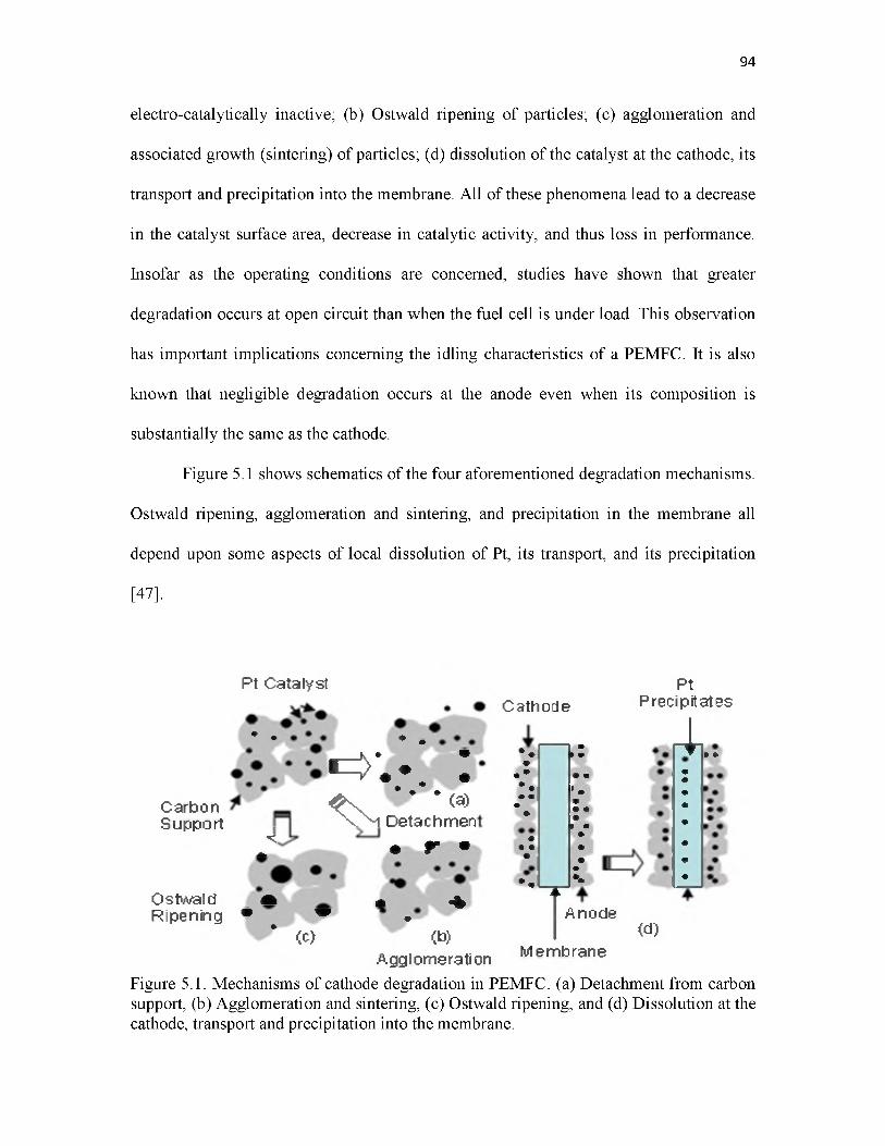
94
electro-catalytically inactive; (b) Ostwald ripening of particles; (c) agglomeration and
associated growth (sintering) of particles; (d) dissolution of the catalyst at the cathode, its
transport and precipitation into the membrane. All of these phenomena lead to a decrease
in the catalyst surface area, decrease in catalytic activity, and thus loss in performance.
Insofar as the operating conditions are concerned, studies have shown that greater
degradation occurs at open circuit than when the fuel cell is under load. This observation
has important implications concerning the idling characteristics of a PEMFC. It is also
known that negligible degradation occurs at the anode even when its composition is
substantially the same as the cathode.
Figure 5.1 shows schematics of the four aforementioned degradation mechanisms.
Ostwald ripening, agglomeration and sintering, and precipitation in the membrane all
depend upon some aspects of local dissolution of Pt, its transport, and its precipitation
[47].
Pt CatalystCathode
• . • *
CarbonSupport
^>>in:^ W* * (a)X /N Detachmen
J m r •
s*•» *
** * •*•mm**
p*#* * **
» **• • ** *•** **
PtPrecipitates
T
r i i * *
Anode<d)
Memb rane
Ostwald m * *Ripening * v ,
* (c) (b) Agglomgrati on
Figure 5.1: Mechanisms of cathode degradation in PEMFC: (a) Detachment from carbon support, (b) Agglomeration and sintering, (c) Ostwald ripening, and (d) Dissolution at the cathode, transport and precipitation into the membrane.

95
The thermodynamic driving force for agglomeration/sintering and Ostwald
ripening is the reduction in surface energy accompanying particle growth. This
phenomenon leads to dissolution of smaller particles and growth of larger particles.
Ostwald ripening occurs by the dissolution of particles into a medium, transport through
the medium, and deposition on larger particles. In PEMFC, transport of electrically
neutral Pt occurs via a coupled process involving the transport of ions (Pt2+ and/or Pt4+)
through an ionomer/aqueous medium and a parallel (coupled) transport of electrons
through the carbon support [48]. In agglomeration/sintering, a similar process occurs
where ions transport through an ionomer/aqueous medium and electrons transport
through a direct particle-to-particle contact. Figure 5.2 shows schematics of the growth of
Pt particles by dissolution/precipitation of isolated particles (supported on high surface
area carbon) and of particles in direct physical contact with each other
(agglomeration/sintering). The fundamental physical parameter which dictates
degradation kinetics is the electrochemical potential of Pt ions, which depends upon the
chemical potential of Pt. All those factors which lower the chemical potential of Pt
should generally decrease the kinetics of degradation, and all those factors which increase
the chemical potential of Pt should increase the kinetics of degradation.
The chemical potential of a species depends on composition, temperature, and
pressure. Alloying Pt with other metals lowers the chemical potential of Pt. Many alloys
of Pt are currently being explored for application as PEMFC catalysts [1-8]. Hydrostatic
stress (pressure) also affects the chemical potential. This of course is well known and is
the basis of the Gibbs-Kelvin equation and is the reason for the occurrence of Ostwald
ripening/agglomeration [49].
The dependence of chemical potential of Pt, on temperature, composition,

96
Figure 5.2: Mechanism of particle growth by (a) Ostwald ripening, (b) Agglomeration/ sintering. Both occur by a coupled transport of Pt2+ (or Pt4+) ions through ionomer/aqueous media and electron transport through the carbon support (or through direct particle-to-particle contact). Net Pt transport occurs from smaller particles to larger particles.
and on pressure is given by [49]
Mpt =M°Pt + RT ln apt + P Vm (51)
where jj is the standard state chemical potential of Pt, apt is the activity of Pt, v is
the partial molar volume of Pt, and p is the pressure. If the material is pure Pt, then apt
is unity. For spherical particles, the pressure is given by 2/ / r where r is the particle
radius and y is the surface energy. Thus, the smaller the particle size, the higher is the
pressure inside the particle, the higher is the chemical potential, and the greater is the
tendency for its dissolution and deposition on larger particles.
Equation (5.1) is very general in that the sign of pressure determines whether it
will increase or decrease the chemical potential. On a sample of any general geometric
shape, positive or negative pressure can be created by the application of external forces.
If the pressure is positive (compressive), the chemical potential will be higher compared

to a stress-free material. If the pressure is negative (tensile), however, the chemical
potential should be lower compared to a stress-free material. The effect of stress on
electrode potentials of metals was investigated during the 1950s and 1960s, primarily to
determine the effect of stress on corrosion. Several authors had assumed that the
dominant stress-related term in chemical potential is the strain energy, which is
proportional to the square of stress (or the square of pressure). The expectation under this
assumption was that the electrode potential should be the same in both tension and
compression for a given magnitude of stress. However, many experimental results were
found to be inconsistent with this expectation [50,51]. It was in fact observed that the
sign of electrode potential depended upon whether the applied load was tensile or
compressive [50,51]. Flood [52], in a classic paper, demonstrated that the dominant term
in chemical potential is in fact linearly related to pressure (consistent with equation
(5.1)), and thus, electrode potential is expected to exhibit a reversal in sign upon a
reversal in the sign of stress (tensile or compressive), in accord with the general
thermodynamic theory of Gibbs. This result is actually not surprising. Indeed, it is well
known in theories of creep that matter movement occurs from regions of compression to
regions of tension.
The analysis by Flood [52] has a significant bearing on the role of stress on
catalyst stability and specifically on the design of core-shell catalysts. Core-shell catalysts
typically consist of a core and a shell of different materials but generally of the same
crystal structure, and with an epitaxially matched interface. The lattice parameters of the
core and the shell determine the magnitude (and possibly the sign) of the stress in the
shell of a core-shell catalyst. If the Pt shell is under greater compression than a pure Pt
catalyst particle of the same diameter, the chemical potential of Pt will be higher in the
97

shell of the core-shell catalyst than the monolithic Pt catalyst. Such a catalyst may exhibit
increased tendency for dissolution. If the Pt shell is under reduced compression (or even
possibly in tension) than a pure Pt catalyst of the same diameter, the chemical potential of
Pt in the shell will be lower in the core-shell catalyst than the monolithic Pt catalyst. Such
a catalyst should exhibit decreased tendency for dissolution and thus should exhibit
increased stability. An example is a core-shell catalyst with Pt shell and Ag or Au core.
Such core-shell catalysts should be inherently more stable compared to pure Pt catalysts
of the same outer diameter.
The objective of the present work was to investigate the role of stress on the
chemical potential of Pt using an electrochemical technique. This was achieved using Pt
wires/foils of macroscopic dimensions as electrodes. Implications of the results for the
design of core-shell catalysts for PEMFC are discussed. The implications for core-shell
catalysts are further compared with recent literature on atomistic level (DFT)
calculations.
5.2 Theory
Figure 5.3 shows a schematic of the experimental setup used. Platinum (IV)
chloride dissolved in DMSO (dimethyl sulfoxide) was used as the electrolyte to
investigate the effect of tensile stress on Pt transport. When Pt wire/foil is immersed in
PtCl4+DMSO solution, the following chemical reaction (locally) is expected to take place
Pt + PtCl4 ^ 2 PtCl2 (5.2)
since the standard Gibbs free energy change at room temperature for the above reaction is
-23.02 kJmol-1 [53]. The solubility of PtCl2 in DMSO is very small. The electrolyte will
98

99
Pt ^ Pt2+ + 2e’ Pt2+ + 2e’ ^ Pt
Figure 5.3: A schematic of the experimental setup used.
thus mainly contain Pt4+ ions with a small concentration of Pt2+. When a tensile load is
applied to one of the wires/foils, the chemical potential of Pt in the stressed wire/foil will
decrease and platinum ions will initially transport from the unstressed platinum wire/foil
to the stressed platinum wire/foil through the electrolyte. Negligible transport of electrons
occurs under open circuit conditions since the electronic conductivity of the electrolyte is
2_|_negligible. The transport of Pt ions shuts down as soon as the electrochemical potentials
2+of Pt ions in both the stressed and the unstressed wires become equal, that is
unstressed stressed
~ = w (53)
2+where ~ 2+ 2+ + 2FO is the electrochemical potential of Pt , jupt 2+ is the chemical
potential of Pt2+, F is the Faraday constant, and ^ is the local electrostatic potential.
Now, within platinum metal, the reaction Pt ^ Pt2+ + 2e’ is at equilibrium. Thus,
Vn = Up, 2+ + 2Ue = ~p 2+ + 2~ = ~p 2+ - 2F p (5.4)
where,

100
in which pe is the chemical potential of electrons, pe is the electrochemical potential of
electrons, and ^ is the experimentally measurable electric potential. Thus, the
electrochemical potential of platinum ions in terms of the chemical potential of Pt and the
measurable electric potential is given by
J~pt2+ = ^ p ~ 2 = ^ t + 2FV (5 6)
2+The electrochemical potentials of Pt2+ in the unstressed and the stressed Pt wires
are given respectively by
r--yun stressed o unstressed
■+ = J “ p t + 2 F ^ (57)
and
jUpt 2+ = ^ pt + P V m + 2FP = M pt + 2FP (5.8)
Substituting equations (5.7) and (5.8) into equation (5.3) gives
stressed unstressed ( \
2F (ty ) = - p V m = - i“pt- pP t) (5.9)
and
stressed unstressed p 1 / 1/ /^ — / / o )
( ^ — <p ) = ^ = — P V r = —v‘Pi p U p t ’ (5 .1 0 )

That is, when a tensile load is applied, the hydrostatic pressure will be negative,
which makes the stressed platinum wire positive (cathodic) - a sort of stress-induced
cathodic protection.
5.3. Experimental Procedure
Figure 5.3 shows the experimental setup used. Two identical platinum wires of
diameter 127 |im were partially immersed in 0.1 M platinum chloride (PtCl4)+DMSO
solution. The distance between the two wires was 1 mm. A tensile load was applied to
one of the platinum wires using a pan tied to it and the other one was maintained stress-
free. The wire attached to the pan was passed over a pulley. The load on the stressed wire
was varied by adding several standard weights to the pan. The corresponding stress was
varied between ~0 MPa and ~210 MPa. Any voltage created between the wires was
measured using an electrometer (Keithley 6514) with a high input impedance (200
TeraQ). In another experiment, an ammeter, capable of measuring current in the pA
range, was connected between the two wires (effectively externally shorting the two
wires) and the current passing through the external circuit was measured as a function of
the applied mechanical load. The corresponding stress was varied between ~0 MPa and
~195 MPa. Similar experiments were also conducted using two identical platinum foils of
thickness 127 |im and width 0.5 cm placed 1 mm apart, partially immersed in 0.1 M
PtCl4+DMSO solution. Voltage (open circuit) and current (short circuit) were measured
as a function of the applied stress ranging between 0 and 9 MPa.
In order to investigate the effect of stress on the kinetics of transport of platinum
between the unstressed and the stressed wires/foils over a period of time, the same setup
was used as above. Two identical platinum wires were partially immersed in the PtCl4
101

electrolyte solution, separated by a distance of 1 mm. A constant tensile stress of 153
MPa was applied to one of the wires. The wires were electrically shorted externally to
provide a path for electrons. The expectation was that platinum will dissolve at the
unstressed wire and will deposit on the stressed wire. After 144 hours, the platinum wires
were cleaned and examined under a scanning electron microscope (SEM). A similar
experiment was also conducted using platinum foils of thickness 127 |im and width 0.5
cm. A tensile stress of 4.5 MPa was applied for 144 hours. The platinum foils were then
cleaned and examined under an SEM.
Another set of experiments was conducted in which platinum wires ranging in
diameters between 0.01 mm and 0.6 mm were used. In each experiment in this set, the
two electrodes were of identical diameters. For a given wire diameter, the voltage
between the stressed and the unstressed wires was measured as a function of the applied
tensile stress. These experiments were conducted in order to determine the possible effect
of the wire diameter on the dependence of voltage on the applied tensile stress.
5.4. Results and Discussion
5.4.1 Effect of Stress on Electrode Potential
Figures 5.4 and 5.5 show voltage (open circuit) and current (short circuit) vs. time
plots for the experiments conducted on platinum wires under various applied tensile loads
(stress ranging from 0 to 210 MPa). Under no applied load, the voltage across the two
wires was near zero and it increased to ~3 mV as the applied stress was increased to 195
MPa. The wire under (tensile) stress became cathodic (positive). Similarly, the current
(when shorted externally) varied between zero and ~2 nA when the applied tensile stress
was varied between zero and ~210 MPa. In both experiments, as soon as the applied load
102

103
Figure 5.4: Variation of the voltage between the stressed (positive) and the unstressed Pt wires immersed in 0.1 M PtCl4/DMSO solution for different applied loads.
Figure 5.5: Variation of the current between the stressed and the unstressed platinum wires immersed in 0.1M PtCl4/DMSO solution for different applied loads.

was changed, the voltage/current changed sharply and equilibrated almost
instantaneously. Figure 5.6 shows the variation of the current between the stressed and
the unstressed platinum foils as a function of time for different applied loads. The figure
shows a discontinuity in the plot which is due to a temporary failure of the recording
software. The higher measured current (as high as 170 nA) in the platinum foil
experiment is attributed to the larger effective area of the foils as compared to the wires.
It is also possible that the exchange current density on the wire surfaces was different
than on foil surfaces due to possible differences in surface features/characteristics. Note
that in this experiment also, the current stabilized instantaneously and remained stable for
the duration over which the stress was maintained constant.
104
Figure 5.6: Variation of the current between the stressed and the unstressed Pt foils immersed in 0.1 M PtCl4/DMSO solution for different applied loads.

Figure 5.7 shows plots of the measured voltage across the wires as a function of
the applied tensile stress for various wire diameters. In each case, the measured voltage
varies linearly with the applied stress. However, the voltage difference, A^, at a given
stress is higher for wires of larger diameters. This observation can be explained on the
basis of the linear elasticity theory [54]. For an elastic body under stress, the three
principal stresses are jx x , , and j z z . The corresponding hydrostatic pressure is
given by [54]
105
P =( J x x + j y y + j J
(5.11)
The corresponding principal strains are related to principal stresses by [54]
Figure 5.7: Voltage between the stressed (positive) and the unstressed wires as a function of the applied tensile stress for varying wire diameters. The intercept is ideally zero. In the fitting of the experimental data, the very small nonzero intercept was neglected in the voltage vs. stress equations given in the inset. Slopes give voltage coefficients per unit stress.
3

106
s = — - - f + f ) (512)C* zz HL./ xx yyf v '
S = — xx ---------f + _ ) (5.13)C* xx £ HL./ yy KS zzf v '
and
s = — - - — + f ) (5.14)yy E j*, xx ^ zz* v y
where — is the Poisson’s ratio and E is the Young’s modulus of elasticity. The two
limiting cases in elasticity are of plane strain and plane stress [54] . Let us consider the
application of a uniaxial load along the z direction. The corresponding stress is
—zz = a (5.15)
If plane strain conditions prevail,
S = S = 0 and — = — (516)O yy O xx yy xx v '
Thus,
s f - - — + a - ) = — - — f + —) (5.17)yy C* xx 'KS yy ' E J7 xx / v 'S y y = S x = 0 = ^ x x - - — + —) = ^ - - — + —
which gives
a = a = i — \ (5 1 8 )ys XX ys yy —1 - —)
Substituting equations (5.15) and (5.18) into equation (5.11) and rearranging, the
hydrostatic pressure is given by
- = - ( r - J f (5 .1 9 )

107
If plane stress conditions are assumed, however, — = = 0, and the
corresponding hydrostatic pressure in the wire is given by [54]
P = — — (5.20)
It is well known in the theory of elasticity that for very thin foils/wires, plane
stress conditions prevail, and for very thick plates/rods, plane strain conditions prevail
[54]. From equations (5.1), (5.10), and (5.20), the difference in the voltage between the
stressed and the unstressed wires/foils under plane stress is given by
(vp —ppt) = p j j \ pfo)= Ap = V m — = ^ j (5.21)2F 2F 3 6 F
where Ap is the voltage developed between the stressed and the unstressed wires/foils.
Here, platinum ions are assumed to be in +2 oxidation state even when the salt used was
2+PtCl4, since locally a reaction between PtCl4 and Pt is expected to form Pt2+. The
theoretically calculated slope of Ap vs. — from equation (5.21) is 1.57 x 10⁻¹¹ VPa-1.
For very thick wires, the prevailing state of stress will be that corresponding to plane
strain. In such a case, the measured voltage will be given by
V, (1 + V— _ Vmp —j ) — p(0) = Ap = - ^ -----= - ^ ----------— (5.22)
2F (1 — v)3 6F1 + V1 — V
For Pt, the Poisson’s ratio is V « 0.39. The estimated slope for plane strain from equation
(5.22) is 3.57 x 10⁻¹¹ VPa-1. The measured slopes of the plots in Figure 5.7 range between
~1.59 x 10⁻¹¹ VPa-1 for a 10 micron wire diameter, which is close to the plane stress case,

108
and ~1.98 x 10"11 VPa-1 for a 0.6 mm wire diameter. Figure 5.8 shows the variation of the
measured slopes or voltage coefficients per unit stress as a function of wire diameter. The
increase in slope with increasing diameter is in accord with the predictions of the linear
elasticity theory. The present results also show that a wire diameter of 0.6 mm is far
below that required for plane strain conditions to prevail. It will be necessary to use rods
of much larger diameters to reach plane strain conditions. This was beyond the practical
range of the current experiments.
The present results also show that the dominant electrode reactions are Pt -> Pt2+
+ 2e’ (anodic) at the unstressed wire/foil and Pt2+ + 2e’ Pt (cathodic) at the (tensile)
stressed wire/foil even though the salt was PtCl4.
o.oi o.iDiameter of Platinum wire (mm)
Figure 5.8: Variation of the voltage coefficient per unit stress as a function of the diameter of platinum wire.

109
If the dominant reactions had been Pt -> Pt4+ + 4e’ and Pt4+ + 4e’ Pt, the
measured Am would have been
VAm = —— a (5.23)12F
or half the observed values. If both reactions had occurred to a comparable extent, the
magnitude of the measured potential, Am, would have been between the values given by
equation (5.23) and equation (5.21), resulting in mixed potential. The observation that the
measurements are in agreement with equation (5.21) suggests that the present results
were not influenced by any mixed potential effect.
5.4.2 SEM Observations of Wires and Foils
Figures 5.9(a) and 5.9(b) respectively show SEM micrographs of the unstressed
and stressed platinum wires (externally shorted) after 144 hours of treatment in 0.1M
PtCl4+DMSO solution. The diameter of the unstressed platinum wire immersed in the
solution shrank from 127 |im to 122 |im and that of the stressed wire increased from 127
|im to 134 |im. Figure 5.9(b) shows part of the stressed wire that was not immersed in the
electrolyte; it exhibited no change in diameter. Figures 5.10(a) and 5.10(b) respectively
show SEM micrographs of the cross-sections of the unstressed and the stressed platinum
foils (externally shorted) after 144 hours of treatment in 0.1M PtCl4+DMSO solution.
The thickness of the unstressed foil shrank from 127 |im to 116 |im and that of the
stressed foil increased from 127 |im to about 138 |im. Figure 5.10(a) shows the interface
region where the top portion of the unstressed foil was outside the electrolyte and the
bottom portion was immersed in the electrolyte. The volume of platinum deposited on the
stressed wire/foil will be the same as the volume of platinum dissolved at the unstressed

110
(a) (b)Figure 5.9: SEM micrographs of: (a) Unstressed Pt wire immersed in 0.1 M PtCl4+DMSO electrolyte for 144 hours. The wire diameter shrank to ~120p,m. (b) Stressed Pt wire: The portion of Pt wire outside the electrolyte (no growth) and stressed Pt wire immersed in electrolyte - 135 p,m (wire diameter grew to 135 p,m).
(a) (b)Figure 5.10; SEM micrographs of foils immersed in 0.1 M PtCl4/DMSO electrolyte for 144 hours. (a) Cross-section of the interface of the unstressed platinum foil where the top portion of the foil was outside the electrolyte (no change) and the bottom portion was immersed in the electrolyte (where dissolution occurred). The thickness reduced to ~116 p,m. (b) Cross-section of stressed platinum foil immersed in the electrolyte. The thickness grew to ~136 p,m.

wire/foil. In the experimental data, it seemed that the decrease in the unstressed wire
diameter is less than the increase in the diameter of the stressed wire. Since the volume of
Pt is conserved, this observation is attributed to the fact that the lengths of the wires
immersed in the solution were not the same for the two wires.
5.4.3 The Sign of Stress/Potential and Chemical Potential
According to equation (5.21), the application of a tensile load/stress (leading to
negative pressure) to a platinum wire/foil lowers the chemical potential of Pt compared to
the unstressed wire/foil. In some of the literature, it has often been assumed (incorrectly)
that applied stress always increases the chemical potential through the strain energy term
[55]. This, however, is incorrect. Excellent discussion of this point has been given by
Flood several decades ago [52]. The analysis by Flood [52] is in agreement with the
original analysis by Gibbs which has often been ignored in more recent literature [55].
Also, experiments conducted on pure metals over 60 years ago are in accord with Flood’s
analysis [50,51] and in accord with predictions of thermodynamics. Thus, platinum ions
2 +tend to move from higher chemical potential of both neutral Pt and Pt2+ (unstressed
2 +wire/foil) to lower chemical potential of both neutral Pt and Pt (wire/foil under a tensile
stress). As the electron concentration is negligible in the electrolyte, no net transport of Pt
takes place when no external path for electrons exists. The wire subjected to a tensile
stress develops a positive potential (becomes cathodic) with respect to the unstressed
wire. The equilibrium electric potential difference corresponds to the difference in
chemical potentials of Pt and is given by equation (5.21) for plane stress (thin wire/foil)
or equation (5.22) for plane strain (thick wire/foil). When an external path is provided for
electrons by shorting the wires/foils, the circuit is completed; Pt ions move from the
111

112
unstressed wire/foil to the stressed (tensile) wire/foil through the electrolyte and electrons
transport from the unstressed to the stressed (tensile) wire/foil in the external circuit. In
this manner, net transport of neutral Pt occurs from the unstressed wire/foil to the stressed
(tensile) wire/foil. This results in the thickening of the stressed (tensile) wire/foil and
shrinking of the unstressed wire/foil, as observed in the present experiments. If the
wire/foil had been stressed compressively (it would be more convenient to use a bar
instead of wire/foil to prevent buckling), then the sign of the voltage developed would
have been opposite; the compressively stressed one would have been negative (anodic).
When connected externally, Pt transport would occur from the compressively stressed to
the unstressed wire/foil.
5.5. Implications Concerning Core-Shell Catalysts for PEMFC
In PEMFC electrodes, catalyst particles are supported on an electronically
conducting carbon support, which provides an electronic short. Particle growth occurs by
a coupled transport of Pt ions through the liquid/ionomer and of electrons through the
carbon support [48]. The present results and the preceding discussion suggest an
approach for the synthesis of durable core-shell catalysts. Much of the reported work on
core-shell catalysts has been primarily conducted with the objective of decreasing the Pt
loading and also enhancing the catalyst activity [1,9,12,13]. While stability is well
recognized as an important consideration, clear design strategies had not been defined
until recently. Many recent studies have addressed stability of core-shell catalysts [16
19,22,25,28,34]. The majority of the studies are either experimental, in which catalyst
performance is investigated using cyclic voltammetry, or theoretical, in which stability is
inferred on the basis of DFT calculations [34]. The present results suggest that if a tensile

113
stress exists in the Pt shell (or a reduced compression as compared to a pure Pt particle),
its chemical potential will be lowered and its stability against dissolution will be
increased. In some core-shell catalyst studies, the nature of the core-shell interface has
not been discussed in the literature. For example, in some studies, the Pt shell was
deposited on cores of different crystal structure, leading to an incoherent interface. Figure
5.11 compares a monolithic Pt catalyst with core-shell catalyst having an incoherent
interface. In such a case, the compressive stress in the Pt shell will be higher than in a
monolithic Pt catalyst. The pressure is given by
where rc is the core radius, r is the outer radius, and Y mt is the interfacial energy
between the core and the shell. If, however, the core-shell interface is perfectly coherent,
Y mt is negligible, and if the lattice parameter of the core is larger than the Pt shell, such as
Figure 5.11: Schematics of monolithic and core-shell catalyst with an incoherent interface. Compressive stress in the shell is higher than the compressive stress in a monolithic catalyst particle. Such a catalyst should be less stable against dissolution compared to monolithic particle.
2r r(5.24)
InterfaceHigher Surface Compression

with Ag or Au core, the corresponding comparison between a monolithic Pt particle and a
core-shell catalyst is shown in Figure 5.12. The corresponding stress state in the shell is
given by
114
p ( r ) = f 2 7 - j . ) (5.25)V r 3 J
where j ee = are principal (angular) stresses in the shell [54]. At the surface , the
state of stress is symmetric bi-axial (with the radial stress, a rr, on the surface of the shell
being zero). The corresponding chemical potential of Pt in the shell is
n„ (r) = < + f 7 (5. 26)ee
r 3
Note that if the shell is under a tension, j ee = > 0 . Thus, the chemical potential of Pt
in the shell of such a core-shell catalyst is lower than the corresponding monolithic Pt
catalyst particle of the same radius. The difference in chemical potential between the
shell of a core-shell catalyst and a monolithic Pt catalyst is
v
Core Shell
7
Lattice Matching
Surface in Tension
7
BiaxialFigure 5.12: Scolh.ermiLSi.ticr of a core-shell catalyst with a coherent interface. Compressive stress in the shell is lower than the compressive stress in a monolithic catalyst particle. Such a catalyst should be more stable against dissolution compared to monolithic particle.

115
Afip, (r) = - f a SS—, (5.27)m\
If the core and the shell are of the same crystal structure, a coherent interface
between the core and the shell is expected. Pt is f. c. c. (A1 structure). Other metals
belonging to the same structure are Ag, Au, Cu, Pd, Ni, etc. Lattice parameters of Cu, Ni
are smaller than that of Pt. Thus, core-shell catalyst made with these metals as the core
will have the Pt shell in compression. This compressive stress will be in addition to the
2/ / r pressure created by the surface energy term. The prediction thus is that core-shell
catalysts made with Cu or Ni as the core will tend to be less stable compared to pure Pt
catalyst. If, however, core-shell catalysts are made with Ag or Au as the core which have
larger lattice parameters than Pt, the Pt shell will be under a tensile stress (or reduced
compression). Such core-shell catalysts will be more stable against dissolution compared
to monolithic Pt catalysts.
The magnitude of the tensile stress in the Pt shell depends upon the difference in
the lattice parameters, the elastic properties, and particle/shell dimensions. The lattice
parameter of Pt is 0.3923 nm and that of Ag is 0.4086 nm. The corresponding strain in
the shell of the core-shell catalyst is on the order of ~4%. The Young’s modulus of Pt is
168 GPa. A hydrostatic tensile stress on the order of ~4 GPa can be expected in the shell
of Pt. Such a high stress is possible if the interface is perfectly coherent with no
dislocations. The corresponding EMF is given by Am = ah—m or ~190 mV as compared2F
to a monolithic Pt catalyst. This means a cathodic protection of core-shell catalysts by
~190 mV. This is a very significant effect. It implies that the stability of the Pt-shell Ag-
core catalyst may be enhanced by ~190 mV in comparison to monolithic Pt catalysts.
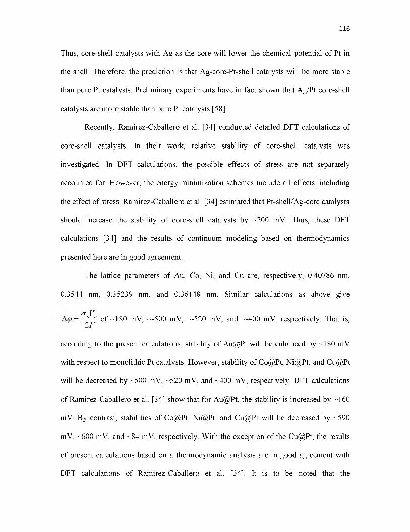
Thus, core-shell catalysts with Ag as the core will lower the chemical potential of Pt in
the shell. Therefore, the prediction is that Ag-core-Pt-shell catalysts will be more stable
than pure Pt catalysts. Preliminary experiments have in fact shown that Ag/Pt core-shell
catalysts are more stable than pure Pt catalysts [58].
Recently, Ramirez-Caballero et al. [34] conducted detailed DFT calculations of
core-shell catalysts. In their work, relative stability of core-shell catalysts was
investigated. In DFT calculations, the possible effects of stress are not separately
accounted for. However, the energy minimization schemes include all effects, including
the effect of stress. Ramirez-Caballero et al. [34] estimated that Pt-shell/Ag-core catalysts
should increase the stability of core-shell catalysts by ~200 mV. Thus, these DFT
calculations [34] and the results of continuum modeling based on thermodynamics
presented here are in good agreement.
The lattice parameters of Au, Co, Ni, and Cu are, respectively, 0.40786 nm,
0.3544 nm, 0.35239 nm, and 0.36148 nm. Similar calculations as above give
= ftVm of ~180 mV, ~-500 mV, ~-520 mV, and ~-400 mV, respectively. That is, 2F
according to the present calculations, stability of Au@Pt will be enhanced by ~180 mV
with respect to monolithic Pt catalysts. However, stability of Co@Pt, Ni@Pt, and Cu@Pt
will be decreased by ~500 mV, ~520 mV, and ~400 mV, respectively. DFT calculations
of Ramirez-Caballero et al. [34] show that for Au@Pt, the stability is increased by ~160
mV. By contrast, stabilities of Co@Pt, Ni@Pt, and Cu@Pt will be decreased by ~590
mV, ~600 mV, and ~84 mV, respectively. With the exception of the Cu@Pt, the results
of present calculations based on a thermodynamic analysis are in good agreement with
DFT calculations of Ramirez-Caballero et al. [34]. It is to be noted that the
116

117
thermodynamic analysis presented here can only address the effect of stress. It cannot,
however, address possible chemical/electronic interactions between the shell and the
core, which are included in the DFT calculations [34]. The comparison between the
present work and the results o f Ramirez-Caballero et al. [34] shows the probably the
stress effect is more dominant. These results also show that thermodynamic modeling
based on continuum modeling is useful for the design of materials and catalysts in the
nanoscale range.
One of the factors which could affect the stability of core-shell catalysts with very
thin shells is the possible diffusion of core atoms through the shell and reacting with the
medium (e.g., water). This is an important factor in the possible degradation o f most of
the core-shell catalysts. An accurate estimate o f the time required for diffusion through
the shell is difficult to obtain for lack of diffusion data at the low operating temperatures
of a typical PEMFC. However, a crude estimate may be made using high temperature
data extrapolated to the PEMFC operating temperature o f ~80oC. Rein et al. [59] have
given self diffusion coefficients of Pt and of Au in Pt at relatively low temperatures.
According to Rein et al. [59], the diffusion coefficients are given by
D Ft = 0.05 x exp2.67eV
cm2s-1 and D Au = 0.13 x exp2.61eV 2 -1cm2s . At 80oC,
the estimated values o f the diffusion coefficients are D Pt = 3 .9 x10 40cm2s-1 and
D a = 7.2 x 10 39 cm2s-1. These are exceptionally small values. Assuming parabolic
dependence between diffusion distance, x , and time ( x 2 ~ D t ), the estimated time for
diffusion to occur through a shell of 1 nm thickness is very long indeed. Thus, if the shell
fully covers the core, it appears unlikely that core-shell catalysts will degrade due to
diffusion o f metals through the shell. It is possible, however, that often the shell may not

completely cover the core or the core may dissolve. Under such conditions, degradation
would be likely. If, however, Au is the core, degradation will likely not occur even when
exposed to the liquid environment due to the stability of gold.
In the present work, a simple relation for the pressure generated due to surface
energy, 2y / r , was assumed for nanosize particles. Many recent studies have used
equations of state which incorporate crystallographic orientation dependence of surface
energies. This is especially important for very small atom clusters, which display various
shapes depending upon the number of atoms in the cluster [60-62]. However, there are
also numerous studies on nanosize particles which assume an isotropic surface energy.
This simple assumption is found to be quite reasonable for particles 2 nm and larger, as
evidenced by their near spherical shape, typical of PEMFC catalysts. A more refined
estimate, while still assuming isotropic surface energy, is the inclusion of the size
dependence of the surface energy itself. For example, several studies have shown that for
very small particles, y itself is a function of the particle size , r , that is Y(r) [63-65].
Then, the pressure created by the surface energy term is 2y (t) / r .
5.6. Summary
The effect of applied stress on the chemical potential of Pt was measured using an
electrochemical cell. Two platinum wires/foils were immersed in a PtCl4+DMSO
solution. One of the wires/foils was subjected to a tensile stress while the other one was
left load-free. It was observed that the wire/foil subjected to a tensile stress developed a
positive electric potential compared to the unstressed one, indicating that the application
of a tensile stress decreases the chemical potential of platinum. This result is in accord
with the thermodynamic theory of Gibbs and the analysis given by Flood [52]. The
118

measured voltage coefficient per unit stress increased with increasing wire diameter. For
wires of the smallest diameter used, the voltage coefficient per unit stress corresponded to
the state of plane stress. The voltage developed per unit stress increased with increasing
wire diameter. Increasing voltage coefficient per unit stress with increasing diameter is in
accord with the predictions of linear elasticity that a transition from plane stress to plane
strain should occur when using rods of a sufficiently large diameter. When the wires/foils
were connected externally, the diameter/thickness of the one under tensile stress grew
while the diameter/thickness of the unstressed one shrank.
These results suggest an approach for the development of stable cathode catalysts
for PEMFC [66]. The present work shows that core-shell catalysts consisting of a core
and Pt shell having the same crystal structures, the Pt shell having a smaller lattice
parameter than the core, and the Pt shell epitaxially matched to the core will result in a
tensile stress (or reduced compression) in the Pt shell. Such core-shell catalysts should be
inherently more stable as the tensile stress in the Pt shell will lower its chemical potential
and decrease its tendency for dissolution. The predictions of the stability of Ag@Pt core
shell catalysts based on the effect of tensile stress in the shell in the present work are
consistent with DFT calculations reported in the literature [34]. Both the DFT
calculations [34] and the present thermodynamic analysis predict a stability of Ag@Pt
against dissolution by about ~190 mV. These results thus also show the usefulness of
continuum thermodynamic modeling in the design of nanoscale materials.
5.7 Acknowledgements
This work was supported by the National Science Foundation under Grant
Number CBET-0931080.
119

120
5.8 References
1. Y. Xu, A. V. Ruban and M. Mavrikakis, J. Am. Chem. Soc., 126 (14) 4717 (2004).
2. R. Srivastava, P. Mani, N. Hanh, and P. Strasser, Angewandte Chemie Int. Edition, 46(47), 8988 (2007).
3. T. Toda, H. Igarashi, M. Watnabe, J. Electroanal. Chem., 460(1,2) 258 (1999).
4. S. Mukerjee, S. Srinivasan, M. P. Soriaga, J. McBreen, J. Electrochem. Soc., 142(5) 1409 (1995).
5. K. Kinoshita, Electrochemical Oxygen Technology, p. 133, Wiley, New York (1992).
6 . V. Jalan and E. J. Taylor, J. Electrochem. Soc., 130(11) 2299 (1983).
7. U. Koponen, H. Kumpulainen, M. Bergelin, J. Keskinen, T. Peltonen, M. Valkianen, and M. Wasberg, J. Power Sources, 118(1-2) 325 (2003).
8 . B. Gurau, R. Viswanathan, R. Liu, T. J. Lafrenz, K. L. Ley, E. S. Smotkin, E. Reddington, A. Sapienza, B. C. Chan, T. E. Mallouk, S. Sarangpani, J. Phys. Chem. B, 102(49) 9997 (1998).
9. J. Zhang, F. Lima, M. Shao, K. Sasaki, J. Wang, J. Hanson, and R. Adzic, J. Phys. Chem. B, 109 22701 (2005).
10. J. Zhai, M. Huang and S. Dong, Electroanalysis 19(4), 506 (2007).
11. ‘Electrode Catalyst for fuel cell and method for production thereof’ , S. Yamamoto, US Patent 7205255, Date of Issue: April 17, 2007.
12. W. Zhou and J. Y. Lee, Electrochem. Comm., 9(7), 1725 (2007).
13. P. Strasser, ‘Platinum-rich shell, platinum poor core’ Public release date: October23, 2007, http://www.rsc.org/chemistryworld/News/2007/Qctober/30100701.asp.
14. Z. D. Wei, Y. C. feng, L. Li, M. J. Liao, Y. Fu, C. X. Sun, Z. G. Shao, and P. K. Shen, J. Power Sources, 180, 84 (2008).
15. S. Ball, S. L. Burton, E. Christian, A. Davies, R. O’Malley, S. Passot, B. Tessier, B. R. C. Theobald, and D. Thompsett, ECS Trans., 25(1) 1011 (2009).
16. R. R. Adzic, J. Zhang, K. Sasaki, M. B. Vukmirovic, M. Shao, J. X. Wang, A. U. Nilekar, M. Mavrikakis, J. A. Valerio, and F. Uribe, Top Catal., 46, 249 (2007).
17. W. Zhou and J. Y. Lee, Electrochem. Comm., 9 1725 (2007).

121
18. B. Fang, B. N. Wanjala, X. Hu, J. last, R. Loukrapam, J. Yin, J. Luo, and C-J. Zhong, J. Power Sources, 196, 659 (2011).
19. P. Hirunsit and P. B. Balbuena, J. Phys. Chem. C, 114, 13055 (2010).
20. J. K. Norskov, T. Bligaard, J. Rossmeisl, and C. H. Christensen, Nature Chem., 1 37 (2009).
21. J. Zhai, M. Huang and S. Dong, Electroanal., 19, 506 (2007).
22. Y. Ma and P. B. Balbuena, J. Electrochem. Soc., 157(6), B959 (2010).
23. S. Zhou, G. S. Jackson, and B. Eichhorn, Adv. Funct. Mater., 17, 3099 (2007).
24. Z. Peng and H. Yang, Nano Res 2, 406 (2009).
25. Y. Xing, Y. Cai, M. B. Vukmirovic, W-P. Zhou, H. Karan, J. X. Wang and R. A. Adzic, J. Phys. Chem. Lett., 1, 3238 (2010).
26. Y. Chen, F. Yang, Y. Dai, W. Wang, and S. Chen, J. Phys. Chem. C, 112, 1645 (2008).
27. Z. Yang, J. Y. Yang, Q. Zhang, W. Zhou, and Z. Liu, J. Electrochem. Soc., 155(7), B776 (2008).
28. R. Srivastava, P. Mani, N. Hahn, and P. Strasser, Angew. Chem. Int. Ed., 46, 8988 (2007).
29. Y. Ma, H. Zhang, H. Zhing, T. Xu, H. Jin and X. Geng, Catal. Comm., 11, 434 (2010).
30. B. C. Tessier, A. E. Russell, B. Theobald, and D. Thompsett, ECS Trans., 16(37), 1 (2009).
31. P. P. Wells, E. M. Crabb, C. R. King, R. Wiltshire, B. Billsborrow, D. Thompsett, and A. E. Russell, Phys. Chem. Chem. Phys., 11, 5773 (2009).
32. Z. Liu, G. S. Jackson, and B. W. Eichhorn, Angew. Chem. 122, 3241 (2010).
33. S. Koh, J. Leisch, M. F. Toney and P. Strasser, J. Phys. Chem. C, 111, 3744 (2007).
34. G. E. Ramirez-Caballero, Y. Ma, R. Callejas-Tovar, and P. B. Balbuena, Phys. Chem. Chem. Phys., 12, 2209 (2010).
35. M. S. Wilson, F. H. Garzon, K. E. Sickhaus and S. Gottesfeld, J. Electrochem. Soc., 140(10), 2872 (1993)

122
36. R. Ornelas, A. Stassi, E. Modica, A. S. Arico, and V. Antonucci, ECS Trans., 3(1), 633 (2006).
37. X. Wang, R. Kumar, and D. Meyers, J. Electrochem. Solid State Lett. 9(5), A225 (2006).
38. J. Xie, D. L. Wood, III, K. L. More, P. Atanassov, and R. L. Borup, J. Electrochem. Soc., 152(5), A1011 (2005).
39. P. J. Ferreira, G. J. Lao, Y. Shao-Horn, D. Morgan, R. Makharia, S. Kocha and H. A. Gasteiger, J. Electrochem. Soc., 152(11), A2256 (2005).
40. W. Bi, G. E. Gray and T. F. Fuller, Electrochem and Solid-State Lett., 10(5), B101 (2007).
41. K. Yasuda, A. Taniguchi, T. Akita, and Z. Siroma, Phys. Chem. Chem. Phys., 8, 746 (2006).
42. A. Ohma, S. Suga, S. Yamamoto, and K. Shinohara, ECS Trans., 3(1), 519 (2006).
43. H. Liu, J. Zhang, F. D. Coms, W. Gu, B. Litteer, and H. A. Gasteiger, ECS Trans., 3(1), 493 (2006).
44. A. Laconti, H. Liu, C. Mittelsteadt, and R. McDonald, ECS Trans., 1(8), 199 (2005).
45. B. Merzougui and S. Swathirajan, J. Electrochem. Soc., 153(12), A2220 (2006).
46. K. L. More, R. Borup, and K. S. Reeves, ECS Trans., 3(1), 717 (2006).
47. R. Darling and J. Meyers, J. Electrochem. Soc., 150(11), A1523 (2003).
48. A. V. Virkar and Y. Zhou, J. Electrochem. Soc., 154(6), B540 (2007).
49. O. F. Devereux, Topics in Metallurgical Thermodynamics, John Wiley-Interscience, New York (1983).
50. R. E. Fryxell and N. H. Nachtrieb, J. Electrochem. Soc., 99, 495 (1952).
51. S. Tan and K. Nobe, Can. J. Chem., 41, 495 (1963).
52. E. A. Flood, Can J. Chem, 36, 1332 (1958).
53. I. Barin, Thermochemical Data o f Pure Substances. Part II, VCH Publication, Germany (1993).

54. S. P. Timoshenko and J. N. Goodier, Theory o f Elasticity, McGraw-Hill, New York (1970).
55. A. Horvath and R. Schiller, Phys. Chem. Chem. Phys., 3, 2662 (2001).
56. S. Yamamoto, ‘Electrode Catalyst for fuel cell and method for production thereof, US Patent 7205255, Date of Issue: April 17, 2007.
57. S. Yamamoto, ‘Electrode Catalyst for fuel cell and method for production thereof, US Patent 7205255, Date of Issue: April 17, 2007.
58. J-H. Koh, R. Abbaraju, N. Dasgupta, and A. V. Virkar, unpublished work (2009).
59. G. Rein, H. Mehrer, Mater, Phys. Sta. Sol., 45, 253 (1978).
60. R. V. Chepulski and S. Curtarolo, ACS Nano, 5(1), 247 (2011).
61. S-P. Huang and P. B. Balbuena, Molecular Physics, 100(13), 2165 (2002).
62. X. Shao, X. Wu, and W. Cai, J. Phys. Chem. A, 114, 12813 (2010).
63. A. N. Goldstein, C. M. Echer, and A. P. Alivisatos, Science, 256, 1425 (1992).
64. H. Hofmeister, S. Thiel, M. Dubiel and E. Schurig, Appl. Phys. Lett., 70, 1694 (1997).
65. K.K. Nanda, A. Maisels, F. E. Kruis, H. Fissan and S. Stappert, Phys. Rev. Letters, 91(10), 106102-1 (2003).
66 . A. V. Virkar, ‘Core-Shell Patent’, US. Patent Application No. 20100062929 (filed 2008).
123

CHAPTER 6
SPECIFIC SURFACE ENERGY AND SHAPE STABILITY OF
FACE CENTERED CUBIC METALS AS
A FUNCTION OF SIZE
6.1 Introduction
Many properties of materials are known to depend upon the size for particles in
the sub-nano to nano size range. Beyond some sizes, properties approach those
corresponding to bulk materials. One such property of materials which depends on size in
the sub-nano to nano size range is the specific surface energy ( y ), which represents the
work done in breaking bonds and creating new surfaces. Thus, specific surface energy
depends on the number of unsatisfied bonds/unit area on the surface of a particle. For
sufficiently large particles, specific surface energy is a constant and is considered a
material property. The specific surface energy of a metal can be estimated from the bond
energy and the lattice constants. This approach is known as the broken-bond model or the
cleaved-bond model of specific surface energy [1]. This method has been used for many
years for estimating surface energies of solids from atomization (sublimation) energies.
Such an approach is considered reasonably accurate as long as bonding can be adequately
described in terms of the nearest neighbor interactions. Experimental measurement of
specific surface energies of solids is generally difficult. The typical approach consists of
conducting experiments at a high temperature in which the surface tension of a liquid is

measured and is extrapolated to 0K [2, 3]. Both theoretical and experimental approaches
have been used over the years to estimate specific surface energies of solids [4-8].
Considerable research is underway on the calculation of specific surface energies
of metals using either ab initio techniques [9-12] or empirical methods [13]. These
calculations have primarily been conducted for body centered cubic and face centered
cubic metals. Methfessel et al. [9] studied transition metals using the full-potential (FP)
linear muffin-tin orbital (LMTO) method, taking into account the local spin density.
Another technique employed is the Density Functional Theory (DFT) using Green’s
function within the LMTO method [10, 11, 14, 15]. More recent studies have been
conducted using a DFT technique in the Generalized Gradient Approximation (GGA).
This technique has been used for large sets of data and has been applied to about 60
elements in the periodic table [16-23]. Many researchers have also estimated specific
surface energies of several crystallographic facets of transition metals and noble metals
using the traditional broken-bond model [24-27]. Galanakis et al. have shown that precise
ab initio calculations lead to the conclusion that specific surface energies of noble metals
can be accurately described in terms of the broken-bond model [26]. Specifically, these
authors have shown that the anisotropy ratio (ratio of specific surface energies of
crystallographically different planes such as (111) and (100)) depends upon the number
of unsatisfied bonds on the surfaces.
Even though atomistic modeling or first principles methods are used to investigate
structure, surface properties, and thermodynamics of various systems, often the
calculations are restricted to a small cluster of atoms to minimize computational times.
Additionally, in most studies, reliance on experimental parameters has been necessary in
ab initio calculations. For example, Galanakis [26] used the experimentally measured
125

lattice parameters. Recent work by Chepulskii and Curtarolo [28] examined stability of
very small clusters of Pt. In their work, ab initio calculations were performed on very
small atom clusters and a variational, continuum approach was used for larger particles.
Some particle shapes, e.g., tetrahexahedron with {730} facets, were not amenable to ab
initio calculations as even the smallest tetrahexahedral particle contains more atoms than
can be treated by the ab initio method [28]. The variational approach used by Chepulskii
and Curtarolo [28] for large crystals was also extended down in the very small size range
to afford a comparison between the ab initio and the variational approaches. In the study
by Chepulskii and Curtarolo [28], entropy effects as well as zero point vibration energy
were ignored in their ab initio calculations. Also, in their variational approach, edges and
corners were ignored.
The observation in the study by Galanakis et al. [26] that ab initio calculations
confirm the validity of the simple broken-bond model has important implications
concerning the study of specific surface energies of small particles and their shape
stability. It suggests that the traditional broken-bond model may in fact be applicable over
a very wide range of particle sizes - from very small all the way up to very large (bulk)
crystals. The experimentally measured parameters that can be used in the broken-bond
model are the enthalpy of sublimation and the lattice parameter.
The objective of the present work was to explore the applicability of the broken-
bond model to the investigation of the effect of size on the specific surface energy of face
centered cubic metals. Using the broken-bond model, various particle shapes are
investigated from the smallest possible size to infinitely large size (bulk materials). The
shapes investigated in the present work are: cube, cubo-octahedron, tetrahedron,
octahedron, and truncated octahedron. Thus, all shapes examined here have {111} and/or
126

{100} planes as the crystal facets. Based on these calculations, relative stabilities of
various shapes as a function of size are examined. The results of the present calculations
are then compared with recent literature in which ab initio and variational approaches
were used [28]. The present results are also compared with computational work by Vitos
et al. [16].
In all cases (but one), calculations are made for particles of any given complete
shape. Thus, in the very small size range, a direct comparison between specific surface
energies of two different shapes cannot be made due to differing numbers of atoms
necessary to form the corresponding complete shapes. For example, the smallest
octahedron contains 6 atoms, but the smallest cube requires 14 atoms. In one case,
specific surface energy is evaluated between two successive sizes of particles of a given
shape by sequentially adding atoms on the smaller sized particle. These calculations give
insight into the variation of specific surface energy as a function of size when the
particles do not form complete shapes, such as would be expected during growth.
On the basis of a continuum thermodynamic model, Tolman [29] had predicted
the existence of a critical length above which surface tension is a constant. Below this
critical radius, it was predicted that surface tension varies with size. On the basis of the
number of unsatisfied bonds/unit surface area, one would expect specific surface energy
to increase with decreasing size, in accord with the considerable literature on this topic.
There is also literature which suggests a decrease in surface energy with decreasing size
[30]. Koga et al. [31] have examined the validity of Tolman’s critical length using DFT.
However, as indicated by Koga et al. [31], the sign of the critical length has not been
unequivocally determined. Reference to Tolman’s work is made here for completeness.
The present calculations are based on the broken-bond model (with the possible
127

6.2 Theory
In the broken-bond model discussed here, only the nearest neighbor interactions
are taken into account. The model assumes an elemental solid of a face centered cubic
structure. Thus, each atom is assumed to have 12 bonds (coordination number - 12). An
atom in the bulk has all 12 bonds satisfied. An atom on {100} surfaces of a particle has 4
unsatisfied bonds.
The smallest cube-shaped crystal has the size of a unit cell and contains 14 atoms
arranged in a face centered cubic structure (Figure 6.1) having a lattice parameter ‘a’. All
schematics of crystals shown in this work were drawn using the Crystal Maker Software.
An important assumption in the broken-bond model is the assignment of discrete bonds
with the nearest neighbors; for example, 12 for a bulk atom in an f.c.c. metal. Atoms on
surfaces, edges, and corners have a number of bonds unsatisfied. This number is
approximately related to the solid angle subtended by the surrounding unfilled sites
(vacuum). The present calculations also ignore the possible redistribution of electrons
that may occur when particles are small. If a redistribution of electrons does occur at
small sizes, one would also expect redistribution of bonds. Recent calculations by
Methfessel et al. [32], however, have shown that electron density distribution is slightly
different only in the exposed part of the first layer of a crystal. Below the first layer, the
electron density distribution is essentially the same as in the bulk of the crystal. Thus, it is
the expectation that the effect related to redistribution of electrons is likely to be rather
small. Let s be the bond energy of one unsatisfied bond. As-defined, when a bond forms
128
redistribution o f bonding electrons ignored) and thus the expectation is that for very small
particles, the specific surface energy should be greater than for large particles.

129
L = a
Face Atoms
Corner Atoms
Figure 6.1: The smallest crystal of the size of a unit cell with a face centered cubic structure and lattice parameter, ‘a’
between two atoms, the corresponding energy released in bond formation is 2 s . Each
atom in the bulk forms 12 bonds with its neighbors. Thus, in this notation, the molar heat
of sublimation is given by
AH subl = 12N As where N is the Avogadro number.
The total number of unsatisfied bonds on a cube-shaped crystal of the size of a
unit cell as shown in Figure 6.1 is 96.
Total energy of unsatisfied bonds = 96s
The total surface area of the cube = 6a2
Thus, the specific surface energy of a cube of the size of a unit cell is given by
a 2 12N a 3 N Aa16 AHsub± = 4 AHsub„ 2 1 O AT "3 A T „ 2 (6 .1)
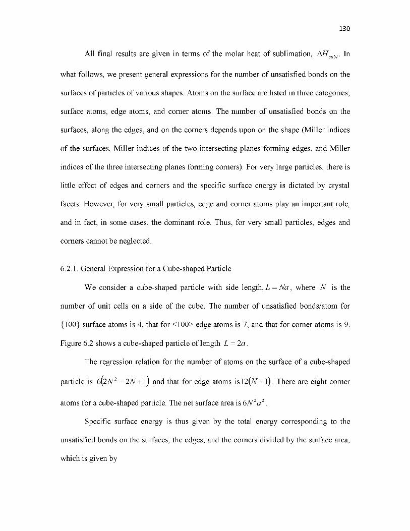
All final results are given in terms o f the molar heat o f sublimation, AHsubv In
what follows, we present general expressions for the number o f unsatisfied bonds on the
surfaces o f particles o f various shapes. Atoms on the surface are listed in three categories;
surface atoms, edge atoms, and corner atoms. The number o f unsatisfied bonds on the
surfaces, along the edges, and on the corners depends upon on the shape (Miller indices
of the surfaces, Miller indices o f the two intersecting planes forming edges, and Miller
indices o f the three intersecting planes forming corners). For very large particles, there is
little effect o f edges and corners and the specific surface energy is dictated by crystal
facets. However, for very small particles, edge and corner atoms play an important role,
and in fact, in some cases, the dominant role. Thus, for very small particles, edges and
corners cannot be neglected.
6.2.1. General Expression for a Cube-shaped Particle
We consider a cube-shaped particle with side length, L = N a , where N is the
number o f unit cells on a side o f the cube. The number o f unsatisfied bonds/atom for
{100} surface atoms is 4, that for <100> edge atoms is 7, and that for corner atoms is 9.
Figure 6.2 shows a cube-shaped particle o f length L = 2 a .
The regression relation for the number o f atoms on the surface o f a cube-shaped
particle is 6—2 N 2 - 2 N + 1) and that for edge atoms is12—N - 1 ) . There are eight corner
atoms for a cube-shaped particle. The net surface area is 6 N 2 a 2 .
Specific surface energy is thus given by the total energy corresponding to the
unsatisfied bonds on the surfaces, the edges, and the corners divided by the surface area,
which is given by
130

131
Figure 6.2: A cube-shaped particle of side length L = 2a
r(N) = 24 N2 + 3N +1}?12 N2 + 3N +1? = 2?l ± + ±_ I 2AHsubi L + _^ + _ I 1a2 I N N2 J 3NAa2 1 4N 4N2
(6 .2)
For very large particles ( N ^ m ), the specific surface energy is given by
r =2AH ,, AH ,,subi _ 0 6667 subi3NAa
(6.3)
Thus, the specific surface energy decreases as the particle size increases. The largest
value of the specific surface energy is 1.33 , corresponding to a cube containing 14NA a
atoms, while the smallest value is 0.667AHsub- . That is, y of the smallest cube-shaped
particle is two times the specific surface energy of very large cube-shaped crystals.
N Aa
1 Details o f calculations are given in the Appendix.

6.2.2 General Expression for a Cubo-octahedron Shaped Particle
We consider a particle in the shape of a cubo-octahedron, which is a truncated
cube. Figure 6.3 shows a cubo-octahedron formed by truncating a cube of length L = 2 a .
Note that this is the smallest possible cubo-octahedron. Also note that N must be
an even number. In this case, there are four different types of surface atoms: atoms on
square {100} surfaces with 4 unsatisfied bonds/atom, atoms on triangular {111} surfaces
with 3 unsatisfied bonds/atom, < 110 > edge atoms with 5 unsatisfied bonds/atom, and
finally, corner atoms with 7 unsatisfied bonds/atom. The volume of a cubo-octahedron
carved out of a cube of edge length L is (5/6)L3. Following the same procedure as
before (Appendix), the specific surface energy is given by
132
^ Corner Atoms Face Atoms
r Edge Atoms Bulk Atoms
Figure 6.3: A cubo-octahedron of side length L = 2a

133
1 2s f 3 1 1 3 A f f„ w f 1 1 1
^ t ) ? ] 3+N + N 2 } = (3 + i k « 2 l ‘ N + 3 N 2 } (65)
The smallest value of N is 2. The corresponding smallest number of atoms is 55.
Thus, the specific surface energy of a cubo-octahedron of the smallest possible size is
y(N = 2) = ^ 1 ) ^ {1 2 } (6 6 )
The specific surface energy of a cubo-octahedron of a very large size ( N ^ m) is given
by
y = ( — = 0.634 (6.7)(3 + V3 )NAa 2 N Aa 2 V '
Thus, the ratio of the specific surface energy of a cubo-octahedron of the smallest
size to that of a very large particle is 19/12. A comparison of equations (6.3) and (6.7)
shows that we expect a cubo-octahedron to be more stable than a cube when the particle
size is sufficiently large. In fact, this is true over the entire range. However, if a cluster
contains fewer than 55 atoms, a comparison of particles of incomplete shapes with other
shapes will need to be made to determine stability, since a complete cubo-octahedron
cannot be formed with fewer than 55 atoms.
6.2.3 General Expression for a Tetrahedron-shaped Particle
We consider a particle in the shape of a tetrahedron cut out of a cube. Figure 6.4
shows a tetrahedron cut out of a cube of length L = 2 a . The smallest tetrahedron can be

134
Figure 6.4: A tetrahedron o f side length L = 2a
created with L = 1a . A tetrahedron is formed by four {111} triangular faces having 3
unsatisfied bonds/atom, edge atoms with 6 unsatisfied bonds/atom, and corner atoms with
9 unsatisfied bonds/atom. The volume o f a tetrahedron o f length L is. L3
3
Following the same procedure as before (Appendix), the specific surface energy is
given by
e I 2 4 N 2 + 3 6 N + 1 2 I2 2 [ S ) n 2
(6 .8)
-t-^e— 12 + — + — \ = -AHsubl- \ \ + — + — J (6.9)[S)a 2 1 N N 2 J S N Aa2 1 2 N 2 N 2 '
For very large particles, N , the specific surface energy is given by

135
AH AH7 = ^ _ _ subi_ = 0.5774-----u i (6.10)V 3 N X NAa2 V '
which is the specific surface energy o f a large tetrahedron. The smallest value o f N = 1.
The corresponding number o f atoms is 10. Thus, according to equation (6.9)
7 (N = 1) = 3 A_ subl = y A_ subl (6.11)S N Aa 2 N Aa 2 V '
That is, the smallest tetrahedron has 3 times the specific surface energy o f a large
tetrahedron. A comparison o f equations (6.7) and (6.10) shows that for large particles, the
stable shape is a tetrahedron and the intuitively expected cubo-octahedron (which is
closer to a spherical shape) exhibits higher specific surface energy.
6.2.4 General Expression for an Octahedron-shaped Particle
We consider a particle in the shape o f an octahedron cut out o f a cube. Figure 6.5
shows an octahedron cut out o f a cube o f length L = a , and an octahedron cut out o f a
cube o f L = 2 a . An octahedron is formed by eight {111} triangular faces with 3
unsatisfied bonds/atom, edge atoms with 5 unsatisfied bonds/atom, and corner atoms with
L38 unsatisfied bonds/atom. The volume o f an octahedron o f length L is — .
Following the same procedure as before (Appendix), the specific surface energy
of an octahedron is given by
7 < N )-= S ]f l S ^ \ (6 ' 2)

136
Figure 6.5: Octahedra o f side lengths L = a, and L = 2a
For very large particles, N ^ m , the specific surface energy is given by
r =A—subl _ q A— subl
S n , a N Aa a(6.14)
which is the same as for particles o f a tetrahedral shape. This is to be expected since both
particles are bounded by {111} faces, and for large particles, there is negligible
contribution from edges and corners. For the smallest value o f N = 1, the specific surface
energy is given by
4A — AHN = 1) = — —— = 2.3094 - subl
V 3 N a N Aa a(6.15)
Note that the specific surface energy o f the smallest octahedron is 4 times that of
a large octahedron. The smallest octahedron has 6 atoms, all o f which are at the corners.

6.2.5 General Expression for a Truncated Octahedron-shaped Particle for N = 3m (Where m Is a Positive Integer with the
Smallest Value of 1)
We consider a particle in the shape of a truncated octahedron. Figure 6.6 shows
truncated octahedra of length L = 3a and L = 6 a . In this case, there are four different
types of surface atoms: atoms on square {100} surfaces with 4 unsatisfied bonds/atom,
atoms on hexagonal {111} surfaces with 3 unsatisfied bonds/atom, edge atoms with 5
unsatisfied bonds/atom, and corner atoms with 7 unsatisfied bonds/atom. The volume of a
137
truncated-octahedron of length L is4L327
Following the same procedure as before (Appendix), the specific surface energy is
given by
Figure 6 .6 : Truncated-octahedra of side lengths L = 3a and L = 6a

138
(6.16)
(1+ 2V 3 a 2
4s8 N 8 N 2
(6.17)
For very large particles, N ^ m , the specific surface energy is given by
(6.18)
For the smallest complete truncated octahedron ( N = 3 ), the specific surface energy is
The smallest truncated octahedron contains 38 atoms. Calculations were
conducted for five different shapes in this work; cube, cubo-octahedron, tetrahedron,
octahedron, and truncated octahedron. Many other shapes can be easily examined.
Table 6.1 shows the specific surface energies o f particles o f various shapes in the
two size limits: the smallest cluster size for a complete given shape and infinitely large
( N ^ m ) size. Figure 6.7 shows the calculated specific surface energies for particles o f
various shapes as a function o f size (equivalent sphere diameter, d , given by
Particle Volume = ■ ). The points shown in the figure thus represent discrete
points corresponding to particles o f any given complete shape. In the bulk limit
( N ^ m ), note that the most stable shapes are tetrahedron and octahedron, and the least
(6.19)

139
Table 6.1: Specific surface energies of f.c.c. metal particles of various shapes as a function of size: (a) The smallest possible cluster, (b) Very large crystals (asymptotic limit).
Shape of an f.c.c. cluster
AHY(N) in terms o f ---- ^ for the
N Aasmallest possible cluster
AHy(N) in terms o f ---- u - forN Aa
large (bulk) clusters
Cube 1.33 0.667
Cubo-octahedron 1.04 0.634
Tetrahedron 1.73 0.577
Octahedron 2.31 0.577
TruncatedOctahedron
1.05 0.597
Figure 6.7: Specific surface energy as a function of equivalent diameter for a f.c.c. structure of different shapes: cube, cubo-octahedron, tetrahedron, octahedron, and truncated octahedron. The inset shows the variation of specific surface energy with equivalent diameter below ~ 10a, where a is the lattice parameter.
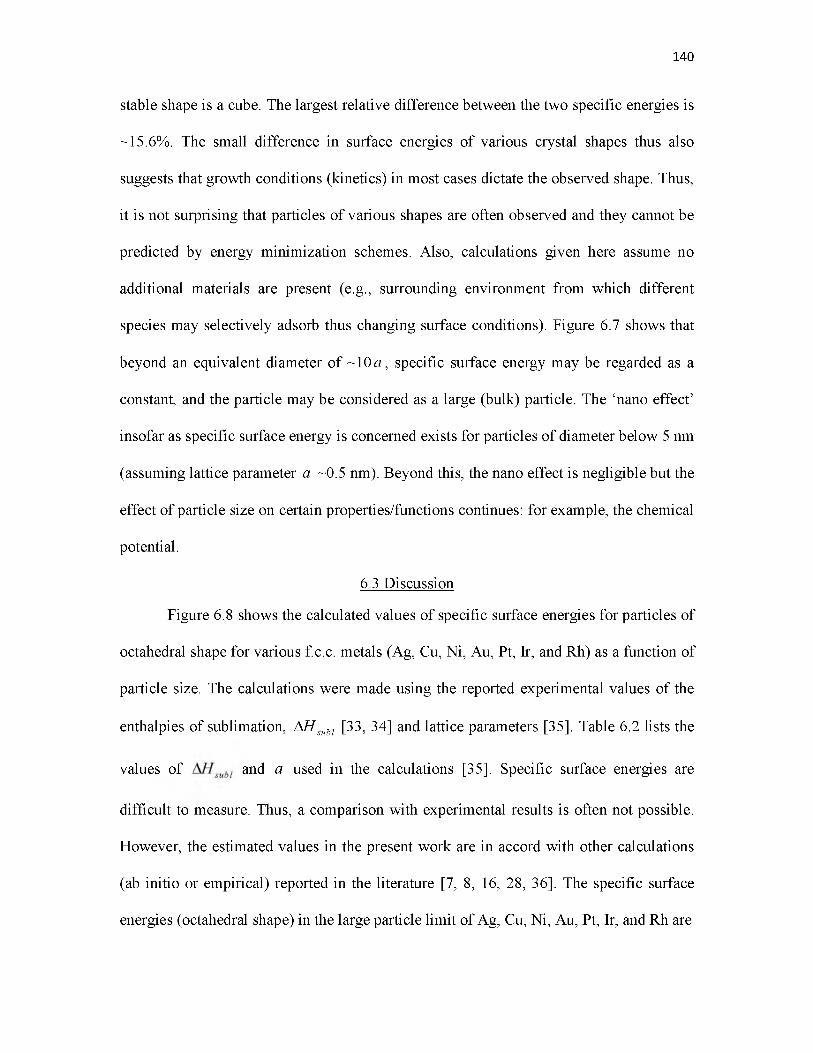
stable shape is a cube. The largest relative difference between the two specific energies is
~15.6%. The small difference in surface energies of various crystal shapes thus also
suggests that growth conditions (kinetics) in most cases dictate the observed shape. Thus,
it is not surprising that particles of various shapes are often observed and they cannot be
predicted by energy minimization schemes. Also, calculations given here assume no
additional materials are present (e.g., surrounding environment from which different
species may selectively adsorb thus changing surface conditions). Figure 6.7 shows that
beyond an equivalent diameter of ~10 a , specific surface energy may be regarded as a
constant, and the particle may be considered as a large (bulk) particle. The ‘nano effect’
insofar as specific surface energy is concerned exists for particles of diameter below 5 nm
(assuming lattice parameter a ~0.5 nm). Beyond this, the nano effect is negligible but the
effect of particle size on certain properties/functions continues: for example, the chemical
potential.
6.3 Discussion
Figure 6.8 shows the calculated values of specific surface energies for particles of
octahedral shape for various f.c.c. metals (Ag, Cu, Ni, Au, Pt, Ir, and Rh) as a function of
particle size. The calculations were made using the reported experimental values of the
enthalpies of sublimation, AHsubl [33, 34] and lattice parameters [35]. Table 6.2 lists the
values of and a used in the calculations [35]. Specific surface energies are
difficult to measure. Thus, a comparison with experimental results is often not possible.
However, the estimated values in the present work are in accord with other calculations
(ab initio or empirical) reported in the literature [7, 8, 16, 28, 36]. The specific surface
energies (octahedral shape) in the large particle limit of Ag, Cu, Ni, Au, Pt, Ir, and Rh are
140

141
20 30 40Equivalent Diameter (nm)
Figure 6 .8 : Specific surface energy of octahedral particles as a function of equivalent diameter for various f.c.c. metals. The inset shows the variation of surface energy with equivalent diameter below 8nm.
Table 6.2: Lattice parameters, heats of sublimation, and calculated (asymptotic) values of specific surface energies for (111) surfaces of various f.c.c. metals.
f.c.c. Metals Lattice Parameter 35 in nm
Heat of Sublimation,
A — subi in k t a d -1
Asymptotic values of specific surface
energy in Jm-2
Silver (Ag) 0.409 160.3133 0.919
Gold (Au) 0.408 224.733 1.29
Copper (Cu) 0.361 338.934 2.49
Iridium (Ir) 0.384 671.034 4.36
Nickel (Ni) 0.352 377.534 2.92
Platinum (Pt) 0.392 357.333 2.23
Rhodium (Rh) 0.380 495.034 3.29

determined to be, respectively,0.919 Jm-2, 2.49 Jm-2, 2.92 Jm-2, 1.29 Jm-2, 2.23 Jm-2, 4.36
2 2Jm- , and 3.29 Jm- . These are comparable to the values reported in the literature [7, 8, 16,
36]. For example, Eberhart et al. [7] used the broken-bond model to calculate the specific
surface energies of b.c.c., f.c.c., and h.c.p structures.
The calculations given in the present work agree well with those in the work by
Eberhart et al. [7]. For instance, the specific surface energy of f.c.c. Cu was determined
by Eberhart et al. [7] to be 2.46 Jm- as compared to the specific surface energy of 2.49
Jm- presented in Figure 6 .8 . The slight difference is related to different values of AHshW
used in the two studies. Using the full charge density model, Vitos et al. [16] estimated
2 2specific surface energies for (111) planes for Ag (1.21 Jm- ), Cu (1.94 Jm- ), Ni (2.01 Jm-
2), Au (1.283 Jm-2), Pt (2.299 Jm-2), Ir (2.971 Jm-2), and Rh (2.43 Jm-2). The values
estimated in the present work are generally comparable to those given by Vitos et al. [16].
It is to be noted, however, that for the estimation of accurate values of specific surface
energies, reliable values of sublimation energies are required.
An indirect method to assess the validity of any theoretical model is to measure
properties which directly depend on the values of the specific surface energies. One such
property is the lattice parameter as a function of particle size. For very small particles,
because of the pressure caused by the specific surface energy (Gibbs-Thompson effect),
the lattice parameter is smaller than for large (bulk) particles. Thus, the measurement of
the lattice parameter as a function of particle size affords an indirect method of model
validation (assuming there is no redistribution of electrons). An approximate estimate of
the effect of pressure on lattice parameter is given below. The calculation is approximate
as it does not account for relaxation (redistribution).
142

143
For a spherical particle of a diameter d , the pressure within the particle is given
by
P = 7 ^ (6.20)d
At small particle sizes, the specific surface energy itself is a function of particle
size, where d is the equivalent diameter. Thus, 7 (d) is a function of particle size. The
change in volume is given by
A’' - P (6 .21)V bulk B
where B is the bulk modulus. Now,
Av 3Aa (6 .22)V bulk a bulk
Thus, the lattice contraction is given by
Aa p 47 (d)
a bulk 3 B 3 B d
(6.23)
Figure 6.9 shows the dependence of the calculated lattice parameter contraction of
platinum on particle size for various crystal shapes: cube, cubo-octahedron, tetrahedron,
octahedron, and truncated octahedron. The lattice parameter contraction was calculated
from the experimental value of bulk modulus of platinum, which is ~278 GPa [37]. The
x-axis in Figure 6.9 is the inverse equivalent diameter, d 1, for any given shape. Note

144
oo 8.0 4.0 Equivalent Diameter, d (nm)
0 0.5 1 1.5 2 2.5 31/Diameter (nm 1)
Figure 6.9: Lattice parameter contraction as a function of particle size for various crystal shapes for platinum (f.c.c.). Figure in the inset shows the lattice parameter contraction as a function of particle size studied by Chepulskii [28]. In their study, the dependence of lattice contraction on particle size is greater than the dependence showed by broken-bond model.
that the lattice parameter for a given equivalent diameter is a function of particle shape
since the specific surface energy is a function of the particle shape. For very small
particles of an octahedral shape of diameter about 0.5 nm, the lattice parameter
contraction was calculated to be about 6%. For a particle of 1 nm in diameter, the
estimated lattice contraction is ~ 1.8%.
The estimated lattice contraction for a 1 nm diameter particle in the work by
Chepulskii and Curtarolo [28] ranged between ~4% and ~6%, depending upon the
particle shape. Solliard et al. [38] experimentally determined lattice parameter
contractions for platinum and gold at 300K using (220) and (422) reflections. For a

platinum particle of diameter ~4 nm, the lattice parameter measured by Solliard et al. [38]
was 3.902 nm, whereas the calculated lattice parameter based on the present work is
3.909 nm. Within the experimental errors and the assumptions made in the model, this
agreement is quite reasonable. However, in order to validate this model, or others in the
literature, it would be necessary to obtain experimental measurements on much smaller
particles, on the order of ~0.5 nm in diameter.
Figure 6.9 shows that the lattice contraction exhibits a convex up curvature when
plotted as an inverse function of the particle diameter. This is due to increasing specific
surface energy with decreasing size. In the work by Chepulskii and Curtarolo [28] also,
the estimated lattice contraction exhibits a convex up curvature, suggesting that in their
work too, specific surface energy increased with decreasing particle size in the sub-nano
to nanosize range.
Chepulskii and Curtarolo [28] also examined the shape stability of nanosize Pt
particles. In the small cluster size range (below 300-400 atoms in the cluster), Chepulskii
and Curtarolo [28] used ab initio calculations. For larger sizes, due to the large
computational time required, Chepulskii and Curtarolo [28] used a variational approach,
which was extended down to the very small size range as well. Many interesting results
from their study will be compared with the present results. Chepulskii and Curtarolo [28]
observed that shape stability depends on the size of the particles. For relatively large
clusters (139 atoms or more), truncated octahedron was determined to be the most stable
shape, with cube-shaped particles being the least stable. In the present work also, cube
shaped particles were found to be the least stable. In the work by Chepulskii and
Curtarolo [28], an octahedron was determined to be almost as stable as a truncated
octahedron. At larger sizes, a truncated octahedron became more stable. Chepulskii and
145

Curtarolo [28] in their ab initio calculations determined that for very small clusters less
than ~1 nm, a tetrahedron is more stable than an octahedron. When the particle diameter
lies between 1 nm and 2 nm, the trend calculated in the present work generally follows
the same trend as discussed by Chepulskii and Curtarolo [28].
In the work by Chepulskii and Curtarolo [28], the most stable shape at the
smallest size (below ~100 atoms) was determined to be a tetrahexahedron with {730}
facets. Chepulskii and Curtarolo [28] were unable to make ab initio calculations on
crystals of a tetrahexahedral shape as the number of atoms was too large, making
computational time too long. Their ab initio calculations were limited to clusters
containing about 300 to 400 atoms. However, extrapolations of the variational
calculations were made down to tetrahexahedral clusters containing as few as 15 atoms.
On the basis of these extrapolations, Chepulskii and Curtarolo [28] determined that for
clusters containing fewer than 139 atoms, tetrahexahedron is the most stable shape. The
extrapolations made down to 15 atoms also indicated that the most stable shape is a
tetrahexahedron. It is to be noted, however, that since even the smallest tetrahexahedron
contains far more than 15 atoms, extrapolations made in their study down to such a small
size are not physically realizable. Yu-Hua et al. [39] have examined specific surface
energies of crystals of tetrahexahedral shapes formed by various crystal facets ({210},
{310}, {410}, {520}, and {730}) as a function of particle size using molecular static
computational methods. It was observed that the specific surface energy decreases with
increasing size and eventually reaches asymptotic limits. These authors investigated
stability of various tetrahexhedral shapes, but did not compare them with any other
crystal shapes. However, Yu-Hua et al. [39] found that within the tetrahexhedral shapes
they examined, {730} planes exhibited higher specific surface energy than {310}, {410},
146

and {510} planes, demonstrating that even within the tetrahexahedral shapes, a
tetrahexahedron with {730} is not the most stable shape.
We have not examined the tetrahexahedral shape. Of the shapes examined in the
present work, an octahedron was determined to be the most stable shape over the entire
size range - from the smallest to very large (bulk) sizes. At the large size range, a
tetrahedron was also found to be as stable as an octahedron. This is not surprising since
both shapes are bounded by {111} planes. However, at the small size range, an
octahedron was found to be more stable than a tetrahedron. This is consistent with
expectations since both corner and edge atoms of a tetrahedron have more unsatisfied
bonds (6 and 9) compared to an octahedron (5 and 8). When particles are small, edge and
corner atoms make larger contribution to the specific surface energy than face atoms. In
the work by Chepulskii and Curtarolo [28], however, calculations made using the
variational approach did not account for edge and corner atoms. As stated earlier, in the
very small size range, based on ab initio calculations, Chepulskii and Curtarolo [28]
found a tetrahedron to be more stable than an octahedron. Our results do not agree with
this result of Chepulskii and Curtarolo [28].
According to the present calculations, an octahedron and a tetrahedron are more
stable than any of the other shapes. In most experimental studies, however, various
shapes are observed, including near spherical. There are several reasons for this. First, the
present calculations (and most other calculations reported in the literature) assume that
particles are surrounded by vacuum. In almost all experiments, many other species are
typically present (in solution or in gas phase from which the particles are formed).
Second, the calculations presented here are equilibrium calculations (and also in the
reported studies). In most experimental work, however, kinetic factors determine the
147

observed shapes. Thus, equilibrium calculations (energy minimization) cannot be
compared with experimentally observed shapes, as in most experimental studies, growth
conditions determine shape. For example, any given shape observed in a low temperature
synthesis process is ‘frozen in’, as solid state diffusion is much too slow, which prevents
particles from achieving their true equilibrium shapes in a reasonable period of time.
One possible method of determining if indeed even large single crystal particles
exhibit tetrahedral or octahedral as the most stable shapes would be to thermally treat
isolated particles in vacuum (or in an inert atmosphere such as Ar) in a suspended state
(without contact with furnace walls). At high temperatures in an inert atmosphere,
surfaces would likely be clean (without any adsorbed species). Also, at high
temperatures, single crystal particles will tend to achieve thermodynamically stable
equilibrium shapes regardless of the starting shapes, as long as particles are sufficiently
far apart so that there is little interparticle flux of atoms, which can cause Ostwald
ripening. The approximate time necessary for a particle to achieve the most stable shape
d 2will be on the order of t --------where D is the self diffusion coefficient. The self
4DS s
diffusion coefficient of silver at 900oC is ~10-9 cm2s-1[40]. For a single crystal particle of
silver of diameter of 0.2 micron (200 nm) at 900oC, the estimated time will be ~0.1 s and
thus should be easily achievable (for example in a free fall through a furnace of sufficient
height). In principle, experimental procedures can be devised to test this on various f.c.c.
metals, such as Ag, Au, Cu, Pt, etc. In all of these metals near the melting temperature,
9 2 1the self diffusion coefficient in the solid state is ~10- cm s- [40-42]. The prediction
therefore is that at a sufficiently high temperature, single crystal particles on the order of
200 nm (which are rather large particles, Figure 6 .8) will achieve equilibrium shapes
148

(octahedron or tetrahedron) in a reasonable time. Within the approximations of the
broken-bond model, the equilibrium shape of particles should be independent of
temperature, since the relative values of specific surface energies of various crystal facets
determined using bond energies are weakly dependent of temperature. Also, all f.c.c.
metals would be expected to exhibit similar shapes. In the computational work by Vitos
et al. [16], it was determined that relative values of specific surface energies of different
crystal facets (anisotropic ratios) were different for different metals, depending upon their
electronic structures. If this is the case, one would expect different shapes for crystals of
different metals after high temperature thermal treatments of the type described here.
Equilibrium calculations such as those given here and in many other studies need to be
compared with such experimental results. To the authors’ knowledge, no such data are
available.
Figure 6.10 shows a plot of the specific surface energy for particles of an octahedral
shape as a function of size. In addition to full octahedra, calculations were also made for
the intermediate range corresponding to N = 2 and N = 3 . Over this range, calculations
of specific surface energy were made by incrementally adding atoms on an octahedron
with N = 2. Initially, atoms were added on {111} surfaces and later on edges and
corners, until ultimately, a full octahedron was again formed corresponding to N = 3 . In
the intermediate range, surfaces contain atoms with more unsatisfied bonds as compared
to a complete octahedron.
Once these atoms are coordinated with other atoms while forming the next
octahedral configuration, the specific surface energy decreases and reaches the value
corresponding to the next larger complete octahedron. Thus, the specific surface energy
initially increases as the size (equivalent diameter) increases and then decreases as the
149

150
Figure 6.10: Specific surface energy as a function o f equivalent diameter for clusters o f an octahedral shape. The inset shows the variation o f specific surface energy as a function o f size when the number o f atoms varies between one complete octahedron (N = 2) and the next complete octahedron (N = 3). The specific surface energy increases to a point and then decreases until it reaches that corresponding to the next complete octahedral structure.
shape approaches a full octahedron corresponding to N = 3.
It is thus expected that whenever clusters are formed that do not correspond to any
complete shape, the specific surface energy will be higher due to the presence o f more
unsatisfied bonds. This would also suggest that catalytic activity will likely be higher for
particles that do not form any complete shape. This o f course is well known as catalytic
activity is generally higher at atomic steps and ledges.
6.4. Summary
In the present work, the simple broken bond model was used to investigate the
specific surface energy o f f.c.c. metals as a function o f shape and size. For all shapes

investigated, the specific surface energy decreased with increasing particle size. Higher
specific surface energy of small particles is due to a greater proportion of atoms at edges
and corners, which exhibit a greater number of unsatisfied bonds. Beyond an equivalent
diameter of ~5 nm, the specific surface energy was nearly constant for each shape
investigated. Thus, specific surface energy may be considered independent of size
beyond ~5 nm. Beyond this critical size, octahedral and tetrahedral shapes were the most
stable, truncated octahedron was the second most stable, cubo-octahedron was the third
most stable, and cube was the least stable. Relative stability of a given shape is thus
directly related to the relative areas of {111} faces and {100} faces; the higher the
percent of {111} surfaces, the greater is the stability. At the smallest size, octahedron was
found to be more stable than tetrahedron. This is attributed to a greater number of
unsatisfied bonds on the corners and the edges of a tetrahedron compared to an
octahedron.
6.5 Acknowledgements
This work was supported by the National Science Foundation under the Grant
Number CBET-0931080.
6.6 References
1. G.A. Somorjai, Introduction to Surface Chemistry and Catalysis, John Wiley & Sons., New York (1994).
2. L.E. Murr, Interfacial Phenomena in Metals and Alloys, Addison - Wesley Publishing Co., Pennsylvania (1975).
3. I.S. Grigoriev, E.Z. Meilikhov, Handbook o f Physical Quantities, CRC Press, Florida (1997).
4. J.M. Blakely, Introduction to the Properties o f Crystal Surfaces, Pergamon, (1973).
151

5. R.G. Linford, Chem.Soc.Rev., 1, 445 (1972).
6 . H. Mykura, Solid Surfaces and Interfaces, Dover, New York (1966).
7. J.G. Eberhart, S. Horner, J. Chem. Ed. 87, 608 (2010).
8 . W. R. Tyson, W. A. Miller, Surf Sci., 62, 267 (1977).
9. M. Methfessel, C. O. Rodriguez, O. K. Andersen, Phys. Rev. B 1989, 40, 20092012 .
10. H.L. Skriver, N.M. Rosengaard, Phys. Rev. B, 46, 7157 (1992).
11. J. Koll'ar, J. Vitos, H.L. Skriver, Phys. Rev. B, 49, 11288 (1994).
12. M.J. Mehl, D.A. Papaconstantopoulos, Phys. Rev. B, 54, 4519 (1996).
13. A.M. Rodriguez, G. Bozzolo, J. Ferrante, Surf. Sci., 289, 100 (1993).
14. H.L. Skriver, N.M. Rosengaard, Phys. Rev. B, 43, 9538 (1991).
15. M. Alden, H.L. Skriver, S. Mirbt, B. Johansson, Phys. Rev. Lett., 69, 2296 (1992).
16. L. Vitos, A.V. Ruban, H.L. Skriver, J. Koll'ar, Surf. Sci., 411, 186 (1998).
17. L. Vitos, J. Koll'ar, H.L. Skriver, Phys. Rev. B, 55, 13521 (1997).
18. O.K. Andersen, O. Jepsen, Phys. Rev. Lett., 53, 2571 (1984).
19. W.R.L. Lambrecht, O.K. Andersen, Phys. Rev. B., 34, 2439 (1986).
20. J.P. Perdew, K. Burke, M. Ernzerhof, Phys. Rev. Lett., 77, 3865 (1996).
21. L. Vitos, J. Koll'ar, H.L. Skriver, Phys. Rev. B., 49, 16694 (1994).
22. J.A. Moriarty, R. Phillips, Phys. Rev. Lett., 66, 3036 (1991).
23. L. Vitos, H.L. Skriver, J. Koll'ar, Surf. Sci, 425, 212 (1999).
24. I. Galanakis, N. Papanikolaou, P.H. Dederichs, Surf. Sci., 511, 1 (2002).
25. M.C. Desjonqu eres, D. Spanjaard, Concepts in Surface Physics, Springer Series in Surface, Springer Berlin (1993).
26. I. Galanakis, G. Bihlmayer, V. Bellini, N. Papanikolaou, R. Zeller, S. Blugel, P.H. Dederichs, Europhys.Lett., 58, 751 (2002).
152

153
27. V.M. Samsonov, N.Y. Sdobnyakov, A.N. Bazulev, Colloids and Surfaces A: Physicochem. Eng. Aspects, 239, 113 (2004).
28. R.V. Chepulskii, S. Curtarolo, ACS Nano, 5, 247 (2011).
29. R. C. Tolman, J. Chem. Phys, 17, 333 (1949).
30. H. M. Lu, Q. Jiang, J. Phys. Chem. B, 108, 5617 (2004).
31. K. Koga, X. C. Zeng, A. K. Shchekin, J. Chem. Phys., 109, 4063 (1998).
32. M. Methfessel, D. Hennig, M. Scheffler, Phys. Rev. B, 46, 4816 (1992).
33. J. A. Kerr, CRC Handbook o f Chemistry and Physics 1999-2000: A Ready- Reference Book o f Chemical and Physical Data (CRC Handbook o f Chemistry and Physics), 81st ed. CRC Press, Florida (2000).
34. A. M. James, M. P. Lord, Macmillan’s Chemical and Physical Data, Macmillan: London (1992).
35. D. Lange, Lange's Handbook o f Chemistry, 8th ed.; Handbook Publishers Inc.: 1952.
36. A.R. Miedema, Philips tech. Rev., 38, 257 (1978).
37. N. C. Holmes, J. A. Moriarty, G. R. Gathers, W. J. Nellis, J. App. Phys., 66, 2962 (1989).
38. C. Solliard, M. Flueli, Surf Sci, 156, 487 (1985).
39. C. T. Tomizuka, E. Sonder, Phys. Rev., 103, 1182 (1956).
40. B. Okkerse, Phys. Rev., 103, 1246 (1956).
41. A. Kuper, H. Letaw, Jr., L. Slifkin, E. Sonder, C. T. Tomizuka, Phys. Rev., 96, 1224 (1954).

CHAPTER 7
CONCLUSIONS
The focus of this thesis was on the study of coupled transport and its effect on
different electrochemical systems and the implications in sodium metal chloride batteries
and Proton Exchange Membrane Fuel Cells.
7.1 Sodium P”-Alumina Solid Electrolyte
A sodium zinc chloride battery was designed using sodium P”-alumina (BASE) as
the solid electrolyte and sodium and ZnCl2 as the electrode materials. Several
electrochemical tubular and planar cells of configuration, Na/BASE/ZnCl2, were
constructed and tested. During charge-discharge and cycling experiments, there was no
evidence of zinc ion exchange found in BASE. This implies that zinc chloride is a viable
cathode. Several freeze-thaw cycles were conducted on the planar cell with a stable
performance output. A three-cell stack was designed, constructed, and electrochemically
tested. During the electrochemical testing, one of the cells became inoperable due to the
misalignment of the electrolyte. As the electrode materials are highly conductive due to
the presence of metallic Zn in cathode, the cell got short circuited with low resistance.
The whole stack was tested as a two-cell stack. The stack gave a stable charging voltage
of ~ 4.0 V. A five-cell stack was designed and constructed.
The kinetics of conversion of a-alumina+YSZ to Na P”-alumina+YSZ was
studied. A patented vapor phase method was used to fabricate Na P”- alumina samples.

In order to expedite the diffusion of Na2O through the samples, an oxygen ion conductor
was incorporated in the starting a-alumina samples. This provided a rapid parallel path
for the transport of Q - ions as P”-alumina is a poor conductor of oxygen ions. A
theoretical model was proposed and a general kinetic equation for conversion was
formulated with diffusion and interfacial parameters. Several samples of various grain
sizes from 0.53 p,m to 4.15 p,m were fabricated. These samples were converted to P”-
alumina at several temperatures and for various times ranging from 1250oC to 1450oC
and 1 hour to 15 hours. The effective diffusion and interfacial rate constants were
determined from the experimental data and the proposed theoretical model. It showed
that when the thickness converted is small, the kinetics is linear (interface controlled) and
when the thickness converted is large, the kinetics is parabolic (diffusion controlled). The
results also indicated that the smaller the grain size, the faster the rate of conversion.
Arrhenius plots of interfacial and diffusion reactions showed that interfacial reactions at
the three-phase boundaries and reaction front depended more on grain size than the actual
diffusion of Na2O through the sample (Na through P”-alumina and Q - through YSZ).
7.2 Coarsening of Copper Particles in Aqueous Media
Experiments on the growth of copper particles in aqueous media containing
various concentrations of copper ions (by dissolving copper nitrate) were conducted. The
samples were placed in test tubes in stagnant conditions. Experiments were conducted at
room temperature and at 80oC. In order to obtain as low a concentration of copper ions as
possible, experiments were also conducted in DI water with hydrogen bubbling. For
determining the kinetics of particle growth, experiments were conducted for different
time periods, varying between 12 h and 144 h at room temperature in DI water, in DI
155

water with hydrogen bubbling, and in 0.01 M Cu(NO3)2 solution. Negligible growth
occurred in samples treated at room temperature with hydrogen bubbling, which was
attributed to very low copper ion concentration. It was also observed that the kinetics was
faster at higher temperature. Since electron concentration in an aqueous medium is
negligible, it is expected that no growth would have occurred in isolated particles.
However, as particles were placed in test tubes, the vast majority of particles were not
isolated (were in contact with the neighboring particles). The growth of particles occurred
by a coupled transport - that of copper ions through the liquid and that of electrons
through direct contact. Solid state transport is all but ruled out given the very low
diffusion coefficient of copper in the solid state at such a low temperature. Indeed, a
comparison of the present results with Ostwald ripening in metallic alloys shows orders
of magnitude difference in kinetics. Since the diffusion coefficient of ions through
aqueous media is typically 10-6 to 10-5 cm2s-1, which is several orders of magnitude
higher than that in the solid-state, the kinetics of electrochemical Ostwald
ripening/agglomeration is expected to be much faster compared to solid state Ostwald
ripening, as observed in the present work.
The kinetics of particle growth exhibited linear dependence. For physically
separated particles in most studies, kinetics of growth is typically cubic (diffusion-
controlled) or parabolic (interface-controlled). The observation that the kinetics is linear
is attributed to interface-controlled growth with the additional feature of increased
driving force due to decreased transport (diffusion) distance as the center-to-center
distance between particles decreases with the occurrence of growth. Since negligible
solid state transport is expected, the difference between Ostwald ripening of physically
separate particles (yet sitting on an electronically conducting support) and those in direct
156

157
contact with each other (often referred to as agglomeration) is only the relative difference
in diffusion distances. Agglomeration in such a case may be referred to as
electrochemical agglomeration. Since the diffusion distance is shorter in electrochemical
agglomeration, its kinetics is expected to be much faster than Ostwald ripening of
physically separate (yet sitting on an electronically conducting support) particles. This
has important implications to catalyst growth in PEMFC. The present work suggests that
catalyst growth of particles in direct physical contact (agglomerated) may be much faster
than physically separate (yet sitting on carbon) particles. Thus, special care should be
taken to avoid agglomeration in PEMFC electrodes, especially the cathode.
7.3 Electrochemical Coarsening due to Applied Stress
The effect of applied stress on the chemical potential of Pt was measured using an
electrochemical cell. Two platinum wires/foils were immersed in a PtCl4+DMSO
solution. One of the wires/foils was subjected to a tensile stress while the other one was
left load-free. It was observed that the wire/foil subjected to a tensile stress developed a
positive electric potential compared to the unstressed one, indicating that the application
of a tensile stress decreases the chemical potential of platinum. The measured voltage
coefficient per unit stress increased with increasing wire diameter. For wires of the
smallest diameter used, the voltage coefficient per unit stress corresponded to the state of
plane stress. The voltage developed per unit stress increased with increasing wire
diameter. Increasing voltage coefficient per unit stress with increasing diameter is in
accord with the predictions of linear elasticity that a transition from plane stress to plane
strain should occur when using rods of a sufficiently large diameter. When the wires/foils
were connected externally, the diameter/thickness of the one under tensile stress grew

158
7.3.1 Core Shell Catalysts
The results obtained from the study of stress effect on the chemical potential of
materials suggest an approach for the development of stable cathode catalysts for
PEMFC. This work shows that core-shell catalysts consisting of a core and Pt shell
having the same crystal structures, the Pt shell having a smaller lattice parameter than the
core, and the Pt shell epitaxially matched to the core will result in a tensile stress (or
reduced compression) in the Pt shell. Such core-shell catalysts should be inherently more
stable as the tensile stress in the Pt shell will lower its chemical potential and decrease its
tendency for dissolution. The predictions of the stability of Ag@Pt core-shell catalysts
based on the effect of tensile stress in the shell in the present work are consistent with
DFT calculations reported in the literature. Both the DFT calculations and the present
thermodynamic analysis predict a stability of Ag@Pt against dissolution by about ~190
mV. These results thus also show the usefulness of continuum thermodynamic modeling
in the design of nanoscale materials.
7.4 Surface Energy and Shape Stability of Metals
A simple broken-bond model was used to investigate the specific surface energy
of f.c.c. metals as a function of shape and size. For all shapes investigated, the specific
surface energy decreased with increasing particle size. Higher specific surface energy of
small particles is due to a greater proportion of atoms at edges and corners, which exhibit
a greater number of unsatisfied bonds. Beyond an equivalent diameter of ~5 nm, the
specific surface energy was nearly constant for each shape investigated. Thus, specific
surface energy may be considered independent of size beyond ~5 nm. Beyond this critical
while the diameter/thickness o f the unstressed one shrank.

size, octahedral and tetrahedral shapes were the most stable, truncated octahedron was the
second most stable, cubo-octahedron was the third most stable, and cube was the least
stable. Relative stability of a given shape is thus directly related to the relative areas of
{111} faces and {100} faces; the higher the percent of {111} surfaces, the greater is the
stability. At the smallest size, octahedron was found to be more stable than tetrahedron.
This is attributed to a greater number of unsatisfied bonds on the corners and the edges of
a tetrahedron compared to an octahedron.
159

APPENDIX
A.1 General Expression for Specific Surface Energy o f a Cube-shaped Particle Valid for N>1
Energy o f unsatisfied bonds
= 6(2N 2 - 2 N + 1)x 4 s + 12(N - 1)x 7 s + 8 x 9 s (A.1)
: {48N 2 - 48N + 24 + 84N - 84 + 72}?
{48N2 + 36 N + 12S (A.2)
: 12{4N2 + 3N + 1}s = {4 N 2 + 3N + 1}-N A
Surface area o f each face = L = N a (A.3)
• r (N) = {4N + 3N + 1} Hsubl = 2^ Hsubl |1 + + _ ^ j ( a 4)) 6 N 2a 2 N^ 3N Aa 2 [ 4N 4 N 2 j )
2 a h AHAs N ^ ™ , y ( N ) ^ -------sub- = 0 .667-----s-^ (A.5)
3N Aa N Aa
A.2 General Expression for Specific Surface Energy o f a Cubo-octahedron Shaped Particle Valid for N/2 >1
In order to form a complete cubo-octahedron, N must be an even, positive
integer. Let us write n = N / 2
• Number o f atoms on the triangular {111} faces o f a cubo-octahedron = (2n - 1)(n -1 )

161
Number o f atoms on the square {100} faces o f a cubo-octahedron = 4n2 - 4n +1
Number o f atoms per edge = (2n -1 )
Number o f atoms at the corners = 12
For a cubo-octahedron, there are 6 square {100} faces, 8 triangular {111} faces, 24
edges, and 12 corners.
Energy o f unsatisfied bonds
= 6(4n2 - 4n +1) x 4s + 8(n - 1)(2n -1 ) x 3s + 24(2n -1 ) x 5s +12 x 7s
= {96n2 - 96n + 24 + 48n2 - 72n + 24 + 240n -1 2 0 + 84^
= {l44n2 + 72n + 1 2 ^
N 2 N= I 144 x -----+ 72 x — +12 >s
I 4 2 |
{36 N 2 + 36 N + 12^
12s{3N2 + 3N + 1} (A 6)
Surface area of each square =
( Na 2 _ N 2 a 2
vV2 j 2 (A.7)
Surface area of each triangle =
Total surface area
42 2N 2a
(A 8)
6 x }N-2 a— + 8 x — N 2a 22
3N 2 a 2 +V 3N
(3 + V3) N 2 a 2
2 2 a (A.9)
8

162
Specific surface energy
H N) = 212e I 3N 2 + 3N +1a 2 | (3 + S )n 2
12s L , ± 1 1 = 3AHsubi f1 + 1 1 (3 + V 3 ja2 1 N N 2 J (3 + V 3 j N a 2 1 N 3N 2
3AH ,, AH ,,As N ^ < n , y ( N ) ^ — = 0.634- subl
(3 + s N o J = 0 6 3 ^ " N ^
A.3 General Expression for Specific Surface Energy of a Tetrahedron-shaped Particle Valid for N>1
Number of atoms on the triangular {111} faces of a tetrahedron = (2N -
Number of atoms per edge = (2N -1)
Number of atoms at the corners = 4
For a tetrahedron, there are 4 triangular {111} faces, 6 edges, and 4 corners.
Energy of unsatisfied bonds
= 4(2N 2 - 3N + 1) x 3s + 6(2N - 1) x 6s + 4 x 9s
= {24N2 - 36N +12 + 72N - 36 + 36^
= {24 N 2 + 36 N + 12S
= 12{2N2 + 3N + 1S
Total surface area = 2 ^ N 2 a 2
Specific surface energy
^ s 124N 2 + 36N +121K N) = 0 2 1 2(T5>2 J
(A10)
(A11)
(A12)
1)(N -1)
(A13)
(A14)
(A 15)

163
6s J _3 1
p j j b 2 ! + N + N 2
AH ibl
y[3NAa,1 + - L + _ ! _
2 1 2N 2 N 2(A 16)
AsAH
N ^ < x , y ( N ) ^ sublV3N, a
AH ,, = 0.5774-----U 1
N Aa 2(A.17)
A.4 General Expression for Specific Surface Energy o f an Octahedron-shaped Particle Valid for N>1
Number o f atoms on the triangular {111} faces o f an octahedron =
1 ( N - 2)( N - 1)
Number o f atoms per edge = (N - 1)
Number o f atoms at the corners = 6
For an octahedron, there are 8 triangular {111} faces, 12 edges, and 6 corners.
Energy o f unsatisfied bonds
= 4(N 2 - 3N + 2) x 3s + 12(N - 1) x 5s + 6 x 8s
= {l2N2 - 36N + 24 + 60N - 60 + 48^ (A.18)
= {l2 N 2 + 24 N + 12^
Total surface area = V 3N 2 a 2 (A.19)
Specific surface energy is given by
K N ) = S J 12N 2 1-^4 N + 12 i (A.20)a 2 ( S f t 2
+ - + V t = 4 H ^ ,1 + 2 + ^ j (A.21)ja2 I N N 2 J S N Aa 2 I N N 2 J V '

164
AsAH
N ^ ^ r- subI = 0.5774S N Aa 2
(A.22)
A.5 General Expression for Specific Surface Energy o f a Truncated Octahedron-shaped Particle Valid
for N/3 >1
To form a complete truncated octahedron from a cube, we must have n be a
multiple o f 3.
Let m = N /3
Number o f atoms per edge = (m -1 )
Number o f atoms at the corners = 24
For a truncated-octahedron, there are 6 square faces, 8 hexagonal faces, 36 edges, and 24
corners.
Energy o f unsatisfied bonds
= 8(3m2 - 3m +1) x 3s + 6(m - 1)2 x 4s + 36(m -1 ) x 5s + 24 x 6s
= {72m2 - 72m + 24 + 24m2 - 48m + 24 + 180m -1 8 0 + 144^
= {96m2 + 60m + 1 2 ^
Number o f atoms on the {111} hexagonal faces o f a truncated-octahedron = 3m2 - 3m +1
Number o f atoms on the {100} square faces o f a truncated-octahedron = (m - 1)2
(A.23)
Surface area o f each square2 2 2 2m a N a (A.24)2 18
Surface area o f each hexagon = ------(ma)2 = — N 2 a 24 v 12
(A.25)
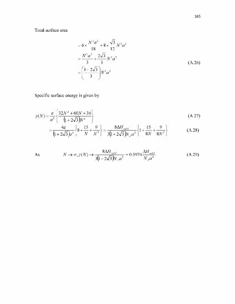
165
Total surface area
. N 2 a 2= 6 x ---------+ 8x — N a
18 12
N 2a 2 . 2V3 , r 2 2
1 + 2V3 2 2N 2a
3 3
3
Specific surface energy is given by
s I 32N 2 + 60N + 36 Ia (1 + 2V3 )n 2
4 s
(1+ 2V 3 Ja
0 15 91-8 +-------1---- T"
2 1 N N 28A H
3(1 + 2V3 JN
9
a
(A.26)
(A.27)
(A.28)
8 a h AH As N ^ ™ , y ( N ) ----- = 0.5974------^ (A.29)
3(1 + 2yf3 )NAa 2 NAa2 V '

166
Table A.1: Dependence o f specific surface energy with the equivalent particle size for acube-shaped particle in f.c.c
N Ncube v = n V S = 6N2a2 EquivalentRadius
Y(N) in terms of^ H sublNAa2
1 14 a3 2a6 0.62 a 1.33
2 63 8 a3 24 a2 1.24 a 0.958
3 172 27 a3 54 a2 1.86 a 0.852
4 365 64 a3 96 a2 2.48 a 0.802
5 666 125 a3 150 a2 3.1 a 0.773
6 1099 216 a3 216 a2 3.72 a 0.755
7 1688 343 a3 294 a2 4.34 a 0.741
8 2457 512 a3 384 a2 4.96 a 0.732
9 3430 729 a3 486 a2 5.58 a 0.724
10 4631 1000 a3 600 a2 6.2 a 0.718
11 6084 1331 a3 726 a2 6.83 a 0.713
12 7813 1728 a3 864 a2 7.45 a 0.71
13 9842 2197 a3 1014 a2 8.07 a 0.706
14 12195 2744 a3 1176 a2 8.69 a 0.703
15 14896 3375 a3 1350 a2 9.31 a 0.701
16 17969 4096 a3 1536 a2 9.93 a 0.699
17 21438 4913 a3 1734 a2 10.55 a 0.697
18 25327 5832 a3 1944 a2 11.17 a 0.695
19 29660 6859 a3 2166 a2 11.79 a 0.693
20 34461 8000 a3 2400 a2 12.41 a 0.692
50 515151 125000 a3 15000 a2 31.02 a 0.677
100 4060301 1000000 a3 60000 a2 62.05 a 0.672

167
Table A.2: Dependence o f specific surface energy and energy density with the equivalentparticle size for a cubo-octahedron shaped particle in f.c.c
N Ncubo-octahedron Volume Surface area Equivalent Radius Y(N) in terms ofAHsublNAa2
2 55 6.67 a3 18.93 a2 1.17 a 1.003793
4 309 53.33 a3 75.71 a2 2.34 a 0.805676
6 923 180 a3 170.35a2 3.5 a 0.745507
8 2057 426.67 a3 302.85 a2 4.67 a 0.716523
10 3871 833.33 a3 473.21 a2 5.84 a 0.699485
12 6525 1440 a3 681.42 a2 7 a 0.688273
14 10179 2286.67 a3 927.48 a2 8.17 a 0.680337
16 14993 3413.33 a3 1211.41 a2 9.34 a 0.674423
18 21127 4860 a3 1533.18 a2 10.51 a 0.669848
20 28741 6666.67 a3 1892.82 a2 11.68a 0.666202
50 429351 104166.7 a3 11830.13 a2 29.19 a 0.646739
100 3383701 833333.3 a3 47320.51 a2 58.39 a 0.640335
oo

168
Table A.3: Dependence o f specific surface energy with the equivalent particle size for atetrahedron-shaped particle in f.c.c
N Ntetrahedron Volume SurfaceArea
Equivalent Radius Y(N) in terms ofAHsublN Aa 2
1 10 0.33 a3 3.464 a2 0.6828 a 1.732
2 35 2.67 a3 13.86 a2 1.3656 a 1.082
3 96 3a9 31.177 a2 2.0484 a 0.898
4 217 21.33 a3 55.426 a2 2.7312 a 0.811
5 422 41.67 a3 86.603 a2 3.414 a 0.762
6 735 72 a3 124.71 a2 4.0968 a 0.729
7 1180 114.33 a3 169.74 a2 4.7796 a 0.706
8 1781 170.67 a3 221.70 a2 5.4624 a 0.690
9 2562 243 a3 280.59 a2 6.1452 a 0.677
10 3547 333.33 a3 346.41 a2 6.828 a 0.666
11 4760 443.67 a3 419.16 a2 7.5108 a 0.658
12 6225 576 a3 498.83 a2 8.1936 a 0.651
13 7966 732.33 a3 585.43 a2 8.8764 a 0.645
14 10007 914.67 a3 678.96 a2 9.5592 a 0.640
15 12372 1125 a3 779.42 a2 10.242 a 0.636
16 15085 1365.33 a3 886.81 a2 10.9248 a 0.632
17 18170 1637.67 a3 1001.1 a2 11.6076 a 0.629
18 21651 1944 a3 1122.4 a2 12.2904 a 0.626
19 25552 2286.33 a3 1250.5 a2 12.9732 a 0.623
20 29897 2666.67 a3 1385.6 a2 13.656 a 0.621
50 485747 41666.67 a3 8660.3 a2 34.14 a 0.594
100 3941497 333333.3 a3 34641 a2 68.28 a 0.586

169
Table A.4: Dependence o f specific surface energy with the equivalent particle size for anoctahedron-shaped particle in f.c.c
N Noctahedron Volume SurfaceArea
EquivalentRadius
n f
in o
) su
aN
r H
1 6 0.166667 a3 1.732051 a2 0.492377 a 2.3094
2 19 1.333333 a3 6.928203 a2 0.984755 a 1.05848
3 44 4.5 a3 15.58846 a2 1.477132 a 0.81257
4 85 10.66667 a3 27.71281 a2 1.969509 a 0.72169
5 146 20.83333 a3 43.30127 a2 2.461887 a 0.67742
6 231 36 a3 62.35383 a2 2.954264 a 0.65219
7 344 57.16667 a3 84.87049 a2 3.446641 a 0.63626
8 489 85.33333 a3 110.8513 a2 3.939019 a 0.62546
9 670 121.5 a3 140.2961 a2 4.431396 a 0.61774
10 891 166.6667 a3 173.2051 a2 4.923774 a 0.61199
11 1156 221.8333 a3 209.5781 a2 5.416151 a 0.60757
12 1469 288 a3 249.4153 a2 5.908528 a 0.60408
13 1834 366.1667 a3 292.7166 a2 6.400906 a 0.60126
14 2255 457.3333 a3 339.482 a2 6.893283 a 0.59895
15 2736 562.5 a3 389.7114 a2 7.38566 a 0.59702
16 3281 682.666 a3 443.405 a2 7.878038 a 0.59539
17 3894 818.8333 a3 500.5627 a2 8.370415 a 0.594
18 4579 972 a3 561.1845 a2 8.862792 a 0.59279
19 5340 1143.167 a3 625.2703 a2 9.35517 a 0.59174
20 6181 1333.333 a3 692.8203 a2 9.847547 a 0.59082
50 88451 20833.33 a3 4330.127 a2 24.61887 a 0.58182
100 686901 16666.7 a3 17320.51 a2 49.23774 a 0.57943ro

170
Table A.5: Dependence o f specific surface energy with the equivalent particle size for atruncated octahedron-shaped particle in f.c.c
N Ntruncated octahedron Volume Surface Area Equivalent Radius Y(N) in terms ofA H sublN A a 2
3 38 4 13.3923 4.1778 a 1.04538
6 201 32 53.56922 8.3556 a 0.8027
9 586 108 120.5307 12.5334 a 0.7301
12 1289 256 214.2769 16.7112 a 0.69536
15 2406 500 334.8076 20.889 a 0.67501
18 4033 864 482.123 25.0668 a 0.66166
21 6266 1372 656.2229 29.2446 a 0.65222
24 9201 2048 857.1075 33.4224 a 0.64519
27 12934 2916 1084.777 37.6002 a 0.63976
30 17561 4000 1339.23 41.778 a 0.63544
33 23178 5324 1620.469 45.9558 a 0.63192
36 29881 6912 1928.492 50.1336 a 0.62899
39 37766 8788 2263.3 54.3114 a 0.62652
42 46929 10976 2624.892 58.4892 a 0.62441
45 57466 13500 3013.269 62.667 a 0.62258
48 69473 16384 3428.43 66.8448 a 0.62098
51 83046 19652 3870.376 71.0226 a 0.61958
99 591526 143748 14584.22 137.8674 a 0.6084