study of common stochastic trend and co-integration in the emerging markets a case ... · ·...

1

Study of Common Stochastic Trend and Co-Integration in the Emerging Markets A Case Study of India, Singapore and Taiwan

Golaka C Nath & Sunil Verma

Abstract The relationship between the stock markets of the developed countries has been

examined extensively in the literature. This study examines the interdependence of the

three major stock markets in South Asia. Using daily stock market data from January

1994 to November 2002, we examine the stock market indices of India (NSE NIFTY),

Singapore (STI) and Taiwan (Taiex). The index level series are non-stationary and so we

employ bi-variate and multivariate cointegration analysis to model the linkages among

these stock markets. We found no cointegration between the stock market indices for the

entire period and hence no long run equilibrium. We found mild causality for some years in

the study though most of the time these markets have not been interlinked. The study has

used. It should be borne in mind that the tests carried out only tests for presence or absence

of linear relationships.

June 2003

2

Introduction Financial literature has presented a strong emphasis on the interaction amongst international

financial markets. Since the October 1987 stock market crash a large empirical literature

has emerged testing interdependence among national equity markets. Portfolio

diversification models (Markowitz, 1952; Sharpe, 1964; Lintner, 1965) have been

developed on the premise of strong interdependence of various markets. If stock markets

move together then investing in various markets would not generate any long-term gain

to portfolio diversification. Therefore, it is important for both investors and academicians

to know whether stock markets are interlinked. The issue is also important for policy

makers for the following reason; if stock markets are found to be closely linked then

there is a danger that shocks in one market may spill over to other markets. The interest

on study of interlinkages of various markets has increased considerably following the

abolition of foreign exchange controls in both mature and emerging markets during last 15

years, the technological developments in communications and trading systems and attaining

such technology at cheaper costs, and the introduction of innovative financial products in

markets giving market participants opportunity to hedge their risk, increasing cross-border

movement of funds, issuers raising funds through American Depository Receipts and Global

Depository Receipts, which have created more opportunities for global international

investments. The gradual dismantling of regulatory barriers and the introduction of more

advanced technology, have called for new market structures and practices, keeping in mind

the move to reach a global standardization. In particular, the new attractive emerging equity

markets have attracted the attention of international fund managers as an opportunity for

portfolio diversification and have also intensified the curiosity of academics in exploring

international market linkages.

Over the past fifteen years, financial markets have become increasingly global. In the

globalised financial markets, the main challenge for both investors and policy makers is to

take advantage of and promote efficiency enhancing aspects of market interaction, while

containing and controlling the undesirable destabilising effects. The early literature, however,

merely showed whether or not there were benefits from international portfolio

3

diversification, ignoring the issue of how the degree of capital market integration may

actually affect these diversification benefits.

Emerging equity markets have continued to grow and have seen the relaxation of foreign

investment restrictions, especially during the last 15 years, primarily through country

deregulation. India, one of the major emerging markets in Asia initiated the financial sector

reforms by way of adopting international practices in its financial market. Indian compamies

have raised funds from abroad through issuance of American Depository Receipts (ADR’s)

or General Depository Receipts (GDR’s) that allow trade of foreign securities on the NYSE,

NASDAQ or on non-American exchanges.

International economic integration is, in general, a trend that is well worth promoting. The

case for capital mobility requires a few more nuances than does the case for trade in goods

and services. Some believe that there are possible market failures in financial markets -

arising, for example, from the presence of speculative overshooting and from the absence of

an international debtors' bankruptcy court -- and that these have contributed to difficulties in

emerging markets. But overall, the advantages of open financial markets dominate. Equities

are a particularly attractive mode for international cross border capital flows. In the event of

adverse economic outcomes, equity prices automatically fall, eliminating the need for lengthy

and costly negotiations between borrower and creditor countries.

Regional integration of equity markets has two distinct facets. First, issuers and investors

expand their activities more widely across the region. Here the point is that the abolition of

barriers to cross-border equity holdings allows borrowers to raise capital more cheaply and

allows investors to earn better returns. Such integration of capital markets also helps

promote integration along other lines as well, such as integration of money markets and of

markets in goods and services. Second, equities are increasingly traded on exchanges outside

the home country. Trading in equities is a financial service. Much like other goods and

services, comparative advantage may dictate that it is more efficient to undertake the trading

in a foreign financial center than domestic.

4

We intend to explicitly characterize the dynamic interactions among these emerging markets

in Asia to study their level of integration. The objective of the paper is to understand the

dynamic inter-linkages between three important emerging equity markets in Asia viz. India,

Taiwan and Singapore and to understand whether the stock markets in these Asian are

interlinked. If these markets are independent then investors in these countries can invest

in different markets of the region to diversify their portfolio and the authorities in the

region need not worry about any contagious effects if one market experiences any

turmoil. The present study will help in understanding portfolio diversification strategy of

international investors who operates in these markets.

The plan of this paper is as follows, in Section 2 we deal with the existing literature survey,

section 3 deals with theory and methodological issues behind this paper followed by the

Section 4 deals in stationarity of data used in the study while Section 5 deals with the data

and section 6 deals with the results followed by Section 7 where we conclude.

Literature Survey:

The most of the existing literature on the study of inter linkages among markets have

followed the approach that involves testing the interdependence directly using

cointegration (or VAR) techniques and these studies have been done concerning markets

of developed and emerging countries. According to this approach if stock prices indices

of two or more countries are found to be cointegrated then this implies that stock markets

of these countries are interdependent. Our study has also been designed on the basis of

this approach and we have reviewed the literature pertaining to the same.

Taylor and Tonks (1989) studies the market integration concerning markets of U.S.,

Germany, Netherlands and Japan using monthly data on stock price indices for the sub-

periods, April1973 – September 1979 and October 1979 – June 1986 and employed is a

bivariate cointegration technique (Engle and Granger, 1987). They found stock price

index of the U.K. was cointegrated with the stock price index of the U.S., Germany,

Netherlands and that of Japan for the later period but not for the former period. Based on

these results they suggested that there is no long-term gain from diversification for the

U.K investors after the abolition of exchange control. Kasa (1992) also explored common

5

stochastic trends in the stock markets of the U.S., the U.K., Japan, Germany and Canada

using monthly and quarterly data from 1974 to 1990 and found that a single common

stochastic trend driving these countries stock markets. Byers and Peel (1993) examined

the interdependence between stock price indices of the U.S., the U.K., Japan, Germany

and the Netherlands using bivariate and multivariate cointegration (Johansen, 1988)

techniques for the period October 1979 – October 1989 but unlike Taylor and Tonks they

did not find any cointegration either for the group as a whole or for the pairs of markets.

Kanas (1998) explored the linkages between the U.S. and European stock markets using

the daily data and found that the U.S. stock market was not pairwise cointegrated with

any of the six European stock markets. Roca (1999) investigated the price linkages

between the equity markets of Australia and that of the U.S., U.K., Japan, Hong Kong,

Singapore, Taiwan and Korea using weekly stock market and found that no cointegration

between Australia and other markets. But he found that the Granger causality tests

revealed that Australia is significantly linked with the U.S. and the U.K.

The literature review shows that there is conflicting evidence on the issue of international

stock market linkages and hence the issue needs further investigation. In this paper we

examine the linkages among the three emerging Asian markets which have introduced

substantial reforms during last one decade and these markets have some common trading

time zone which can help investors to move from one market to another if the need arises

unlike a market like US which has a no common time zone when these markets are open.

Methodological Issues

The dynamic linkage may simply be examined using the concept of Granger’s (1969, 1988)

causality. Formally, a time series Xt Granger-causes another time series Yt if series Yt can be

predicted with better accuracy by using past values of Xt rather than by not doing so, other

information being identical. In other words, variable Xt fails to Granger-cause Yt if

)|YPr()|Pr( mt ttmtY Ω=Ψ ++ (1) where Pr(•) denotes conditional probability, ψ t is the set of all information available at time t

and Ω t is the information set obtained by excluding all information on Xt from ψ t. .

6

Testing causal relations between two stationary series Xt and Yt (in bivariate case) can be

based on the following two equations

∑=

++∑+= −=

p

k-tk1

0

1k X tuYatY kt

p

kk βα (2)

t

p

k

p

kktkktkt vXYX ∑ ∑

= =−− +Φ++=

1 10 ϕϕ (3)

where p is a suitably chosen positive integer; ak’s and ßk’s, k = 0,1, … ..,p are constants; and

ut and vt usual disturbance terms with zero means and finite variances. The null hypothesis

that Xt does not Granger-cause Yt is not accepted if the ßk’s, k>0 in equation (2) are jointly

significantly different from zero using a standard joint test (e.g., an F test). Similarly, Yt

Granger-causes Xt if the f k’s, k>0 coefficients in equation (3) are jointly different from zero.

It may be mentioned that the above test is applicable to stationary series. In reality, however,

underlying series may be non-stationary. In such cases, one has to transform the original

series into stationary series and causality tests would be performed based on transformed-

stationary series. A special class of non-stationary process is the I(1) process (i.e. the process

possessing a unit root). An I(1) process may be transformed to a stationary one by taking

first order differencing. Thus, while dealing with two I(1) process for causality, equations (2)

and (3) must be expressed in terms of differenced-series. However, if underlying I(1)

processes are cointegrated, the specifications so obtained must be modified by inserting the

lagged-value of the cointegration relation (i.e. error-correction term) as an additional

explanatory variable (Engle and Granger, 1987). In other words, equations (2) and (3) should

be modified as

t

p

k

p

kktkktkt uXYY ++∆+∆+=∆ ∑ ∑

= =−− 1-t

1 10 ECTδβαα

(4)

tvECTXYkX t

p

k

p

kktkktt +∑ ∑ +∆Φ+∆+=∆ −

= =−− 1

1 10 ηφφ (5)

where ∆ is the difference operator and ECTt-1 represents an error correction term derived

from the long-run cointegrating relationship between the I(1) processes Xt and Yt. This term

7

can be estimated by using the residual from a cointegrating regression. Clearly, if Xt and Yt

are I(1) but not cointegrated, the term ECTt-1 would be absent from equations (4) and (5).

However the deficiencies as brought forward by a number of researchers (Johansen, 1998

and Phillips and Durlauf, 1986) are:

• Finite sample problems of lack of power in unit roots and cointegration tests,

• Asymmetrical treatment of variables as endogenous and exogenous as there is

simultaneous equation bias of bi-directional causality, and

• Lack of possibilities for running hypothesis tests on cointegrating relationship.

The first two problems are taken care of by the use of large sample size and all of them are

overcome by Johansen’s methodology, 1988. In particular, the Johansen methodology

provides estimates of all the cointegrating vectors that exist within a vector of variables, fully

captures the underlying time series properties of the data, and offers a test statistic for the

number of cointegrating vectors with an exact limiting distribution. This test may therefore

be viewed as more discerning in its ability to reject a false null hypothesis.

Johansen’s Methodology (1988): Johansen's method can be illustrated by considering the

following general autoregressive representation for the vector Y, which contains n

variables, all of which are I(1),

tktkttt YYYY εααα ++++= −−− ....2211 (6)

where k is the maximum lag, εt is assumed to be a (n x1) vector of Gaussian error terms,

and α is a (n x n) matrix of coefficients.

In order to use Johansen’s test, the above vector autoregressive process can be reparametarized and turned into a vector error correction model of the form as:

tktktkt YYYYt ε+∆Γ++∆Γ+Π=∆ −−−−− )1(1111 .... (7) where

g

k

ji I−=Π ∑

=1

)( β and g

i

jji I−=Γ ∑

=1

)( β

The issue of potential cointegration is investigated when we compare both sides of

equation 7. As Yt ~ I(1), ∆ Yt ~ I(0), so are ∆Yt-i. This gives the left-hand side of

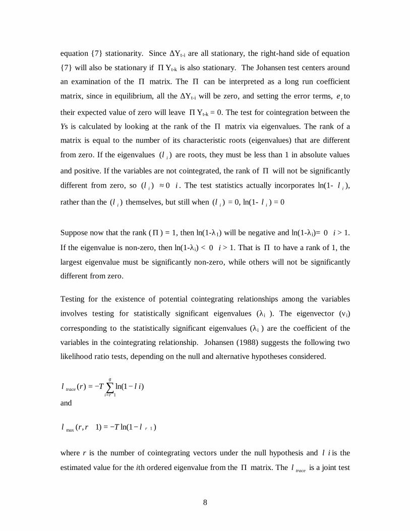
8

equation 7 stationarity. Since ∆Yt-i are all stationary, the right-hand side of equation

7 will also be stationary if Π Yt-k is also stationary. The Johansen test centers around

an examination of the Π matrix. The Π can be interpreted as a long run coefficient

matrix, since in equilibrium, all the ∆Yt-i will be zero, and setting the error terms, tε to

their expected value of zero will leave Π Yt-k = 0. The test for cointegration between the

Ys is calculated by looking at the rank of the Π matrix via eigenvalues. The rank of a

matrix is equal to the number of its characteristic roots (eigenvalues) that are different

from zero. If the eigenvalues )( iλ are roots, they must be less than 1 in absolute values

and positive. If the variables are not cointegrated, the rank of Π will not be significantly

different from zero, so )( iλ i∀≈0 . The test statistics actually incorporates ln(1- iλ ),

rather than the )( iλ themselves, but still when )( iλ = 0, ln(1- iλ ) = 0

Suppose now that the rank (Π ) = 1, then ln(1-λ1) will be negative and ln(1-λi)= i∀0 > 1.

If the eigenvalue is non-zero, then ln(1-λi) < i∀0 > 1. That is Π to have a rank of 1, the

largest eigenvalue must be significantly non-zero, while others will not be significantly

different from zero.

Testing for the existence of potential cointegrating relationships among the variables

involves testing for statistically significant eigenvalues (λi ). The eigenvector (νi)

corresponding to the statistically significant eigenvalues (λi ) are the coefficient of the

variables in the cointegrating relationship. Johansen (1988) suggests the following two

likelihood ratio tests, depending on the null and alternative hypotheses considered.

)1ln()(1

iTrg

ritrace ∑

+=

∧−−= λλ

and

1max 1ln()1,( +∧

−−=+ rTrr λλ )

where r is the number of cointegrating vectors under the null hypothesis and i∧λ is the

estimated value for the ith ordered eigenvalue from the Π matrix. The traceλ is a joint test

9

where the null is that the number of cointegrating vectors is less than or equal to r against

an unspecified or general alternative that there are more than r. The maxλ conducts

separate tests on each eigenvalue, and has as its null hypothesis that the number of

cointegrating vectors is r against an alternative of r+1.

Between Johansen’s two likelihood ratio tests for cointegration, the trace test shows more

robustness to both skewness and kurtosis (i.e., normality) in residuals than the maximum

eigenvalue test (see Cheung and Lai 1993, for details): therefore we employ the trace test

to perform the cointegration tests.

Theory of Stationarity Following are different ways of thinking about whether a time series variable Xt is stationary

or has a unit root:

• In the AR(1) model, if Φ =1, then X has a unit root. If |Φ | <1 then X is stationary.

• If X has a unit root, then its autocorrelations will be near one and will not drop

much as a lag length increases.

• If X has a unit root, then it will have a long memory. Stationary time series do not

have long memory.

• If X has a unit root then the series will exhibit trend behavior.

• If X has a unit root, then ∆X will be stationary. For this reason, series with unit root

are often referred to as difference stationary series.

The stationarity condition of the data series used in the study has been tested using

Augmented Dickey Fuller Test. Consider a simple general AR(p) process given by

tptpttt YYYY εφφφµ +++++= −−− *....** 2211 (14)

If this is the process generating the data but an AR(1) model is fitted, say

10

ttt YY νφµ ++= − 11 * (15)

then tptptt YY εφφν +++= −− *....* 22 (16)

and the auto correlations of vt and vt-k for k> 1 will be nonzero, because of the presence of

the lagged Y terms. Thus an indication of whether it is appropriate to fit an AR(1) model can

be aided by considering the autocorrelations of the residual from the fitted models. To

illiustate how the DF test can be extended to autoregressive process of order greater than 1,

consider the simple AR(2) process below

tttt YYY εφφµ +++= −− 2211 ** (17)

and the above is same as

ttttt YYYY εφφφµ +−−−++= −−− )(**)( 212121 (18)

and subtracting Yt-1 from both the sides give

tttt YYY εαβµ +∆−+=∆ −− 111* (19)

where the following have been defined

121 −+= φφβ

and α1= -φ2

This means that if the appropriate order of the AR process is 2 rather than 1, the term ∆Yt-1

should be added to the regression model. A test of whether there is a unit root can be carried

out in the same way as for the DF test, with the test statistics provided by the ‘t’ statistics of

the β coefficient. If β = 0 then there is a unit root. The same reasoning can be extended for

a generic AR(p) process. Therefore to perform an Unit Root test on a AR(p) model the

following regression should be estimated.

t

p

jjtjt YYYt εαβµ ∑

=−− +∆−+=∆

11 (20)

11

Here the standard Dickey-Fuller model has been augmented by ∆Yt-j. In this case the

regression model and the t test are referred as ADF test.

Data The first hand primary data was collected from the web sites of respective Stock Exchanges

and via written communication from them. The data collected was the closing index values

for the Nifty (India), TAIEX (Taiwan) and STI (Singapore). India is located at the time zone

(GMT + 5.30) while the other two are located at the same time zone. The data is from

January 1994 to November 2002. The cointegration analysis was done for the entire data

from January 1994 to November 2002 as well as for the period from January 1995 to

November 2002 when the stock market reforms took shape in Indian market and National

Stock Exchange came into being, for the period from January 1997 to November 2002 when

further institutional reforms took shape in India and from 2000-2002 when major reforms

like compulsory rolling settlement with electronic book entry form, shortening of settlement

cycle, etc.. The period has been split into the above time buckets, as we understand

substantial market reforms were introduced after the onset of National Stock exchange of

India.

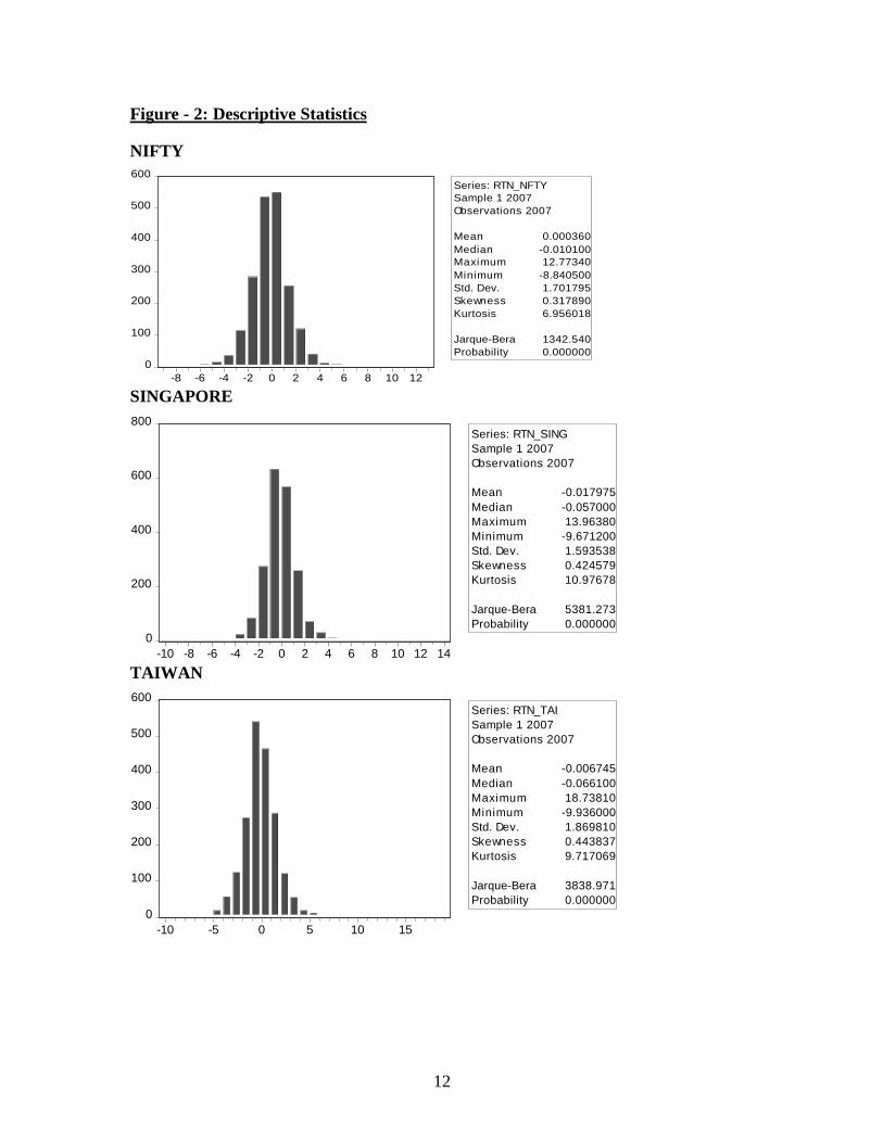
The simple correlation of these markets as well as the descriptive statistics of the three

markets are given in Table 1, Table – 2 respectively and the returns, market movement as

well as the market volatility are plotted in Chart 1, Chart 2 and Chart 3. The volatility

estimates have been calculated using the formula (σt)2 = λ (σt-1)2 + (1 - λ ) (rt)2 where σt is

the standard deviation, λ is assigned 0.94 and rt is the daily logarithmic return. This

formula has been used for calculation of volatility as the same is being used in the Indian

market as given by Securities Exchnage Board of India. (Source www.sebi.gov.in). The

above methodology is widely used in academic literature and has been put forward by

RiskMetrics. (see RiskMetrics Technical Document for details)

Table 1 Correlation of Markets

RET_NIFTY RET_SING RET_TAI RET_NIFTY 1 0.198405 0.112699 RET_SING 1 0.298679 RET_TAI 1

12

Figure - 2: Descriptive Statistics

NIFTY

0

100

200

300

400

500

600

-8 -6 -4 -2 0 2 4 6 8 10 12

Series: RTN_NFTYSample 1 2007Observations 2007

Mean 0.000360Median -0.010100Maximum 12.77340Minimum -8.840500Std. Dev. 1.701795Skewness 0.317890Kurtosis 6.956018

Jarque-Bera 1342.540Probability 0.000000

SINGAPORE

0

200

400

600

800

-10 -8 -6 -4 -2 0 2 4 6 8 10 12 14

Series: RTN_SINGSample 1 2007Observations 2007

Mean -0.017975Median -0.057000Maximum 13.96380Minimum -9.671200Std. Dev. 1.593538Skewness 0.424579Kurtosis 10.97678


TAIWAN

0

100

200

300

400

500

600

-10 -5 0 5 10 15

Series: RTN_TAISample 1 2007Observations 2007

Mean -0.006745Median -0.066100Maximum 18.73810Minimum -9.936000Std. Dev. 1.869810Skewness 0.443837Kurtosis 9.717069


13

Chart 1: Movement of Returns

-10

-5

0

5

10

15

500 1000 1500 2000

RTN_NFTY

-10

-5

0

5

10

15

500 1000 1500 2000

RTN_SING

-15

-10

-5

0

5

10

15

20

500 1000 1500 2000

RTN_TAI

Chart 2: Movement of Markets Indices (1994-2002)

Movement of Markets (1994-2002)

020406080

100120140160180

1/5/

1994

7/5/

1994

1/5/

1995

7/5/

1995

1/5/

1996

7/5/

1996

1/5/

1997

7/5/

1997

1/5/

1998

7/5/

1998

1/5/

1999

7/5/

1999

1/5/

2000

7/5/

2000

1/5/

2001

7/5/

2001

1/5/

2002

7/5/

2002

Period

Inde

x

NIFTYSINGTAI

14

Chart 3: Volatility of markets

Volatility of Markets (1994-2002)

0102030405060708090

1/6/

94

7/6/

94

1/6/

95

7/6/

95

1/6/

96

7/6/

96

1/6/

97

7/6/

97

1/6/

98

7/6/

98

1/6/

99

7/6/

99

1/6/

00

7/6/

00

1/6/

01

7/6/

01

1/6/

02

7/6/

02

Period

Var

ianc

e (A

nnua

lised

)NIFTY

SING

TAIEX

Empirical Study& Results Initially we tried to find out the relationship through a linear equation as follows to see

the significance of the relationship suing the log values of the indices for three countries.

For 1994-2002, the relationship looks as LNIFTY = 1.851281 + 0.432838*LSING + 0.219829*LTAI (0.13221)# (0.01376)# (0.01164)# For 2000-2002, the relationship looks as LNIFTY = 0.040849+ 0.717465*LSING + 0.192962*LTAI (0.1123) (0.02734)# (0.01519)# # indicates significant at 1% and (figures in bracket gives the standard error) From the above we see the signs of the coefficients have not undergone change. The time series properties of the models need to be studied first such as presence of unit

roots, visual properties of the charts, cyclicity, trends etc. Unit root tests were run for

each series. As can be studied from the above graphs there is a presence of trend and

hence the test results from the ADF test are evaluated only where a trend and intercept

are included. The order for Augmented Dickey Fuller (ADF) tests were ascertained on

minimum Schwarz Information Criterion (SC). Table 3 gives the results of the unit root

test.

15

Table 3: Results of ADF Test for Unit Root

Variable Optimal P@ Test Statistics# NIFTY 1 -2.7789

SING 1 -1.8516 TAIEX 1 -1.8424 ∆NIFTY 13 -12.3676* ∆SING 18 -10.9020* ∆TAIEX 21 -10.6717*

@ Optimal P is selected based on minimum Schwarz Information Criterion # Critical values of ADF test statistics for 1%, 5% and 10% level of significance are –3.9676, 3.4144 and –3.1290, respectively * Significance at 1% level Having satisfied with the results of ADF test, we proceed to conduct the Johansen’s

cointegration test for the variables. Though lag of 1 would have been sufficient for testing the

cointegration as given by minimum AIC criteria as shown in the Table - 4, we have tested for

various lags upto 5 and reported the results for lag 5 as the results are not significantly

different.

Table 4: Lag Length Criteria Selection

Lag LogL LR FPE AIC SC HQ 0 -11534.60 NA 20.811 11.549 11.557* 11.552 1 -11503.33 62.419 20.352* 11.526* 11.560 11.539* 2 -11496.08 14.443 20.388 11.528 11.587 11.550 3 -11491.65 8.8261 20.482 11.533 11.617 11.5640 4 -11485.24 12.727 20.535 11.535 11.645 11.575 5 -11481.18 8.0516 20.637 11.540 11.675 11.590 6 -11473.60 15.021 20.666 11.542 11.701 11.600 7 -11470.01 7.1093 20.778 11.547 11.732 11.615 8 -11461.11 17.569* 20.780 11.547 11.757 11.624

LR: sequential modified LR test statistic (each test at 5% level), FPE: Final prediction error, AIC: Akaike information Criterion, SC: Schwarz information criterion, HQ: Hannan-Quinn information criterion and * indicates significant at 5% Level.

We now employ Johansen’s (1991) maximum likelihood method to examine whether or not

the logarithms of indices in question are cointegrated. The same has been performed with a

lag of 5 as we feel that the same is sufficient to transmit all relevant information among the

markets. The Table – 5 reports the relevant results. As can be seen in the table, there is no

cointegration vector between the underlying series and hence no long run equilibrium

16

relationship. Consequently an error term need not be included in the Granger Causality test

equation.

Table 5: Johansen’s Cointegration Test Results with lag of 5

Period Eigen Values

(Descending Order) Null Hypothesis# Trace Statistics* Critical Value 5% 1%

1994 - 2002 0.009194 r=0 26.54633 29.68 35.65

0.002846 r=<1 8.064138 15.41 20.04

0.001179 r=<2 2.361089 3.76 6.65

1995-2002 0.009490 r=0 24.10111 29.68 35.65

0.002852 r=<1 7.013508 15.41 20.04

0.001057 r=<2 1.895299 3.76 6.65

1997-2002 0.018695 r=0 28.38088 29.68 35.65

0.002503 r=<1 4.790431 15.41 20.04

0.001326 r=<2 1.65818 3.76 6.65

2000-2002 0.027086 r=0 26.81349 29.68 35.65

0.009066 r=<1 8.086340 15.41 20.04

0.002746 r=<2 1.875193 3.76 6.65 # - ‘r’ indicates number of cointegrating relationship.

The next step was to examine whether three markets are pair wise cointegrated with each

other for the later period (1997-2002). As mentioned above, we have employed Johansen

cointegration approach to test for the interdependence among these stock markets. The

Table - 6 presents the results of the pair wise cointegration tests for the entire sample period.

We also find that these markets are not cointegrated.

Table 6: Pairwise Cointegration Tests based on Johansen approach (Trace test with

Lag 5)

Period Eigen Values

(Descending Order) Null Hypothesis# Trace Statistics* Critical Value NIFTY-SING 5% 1%

1997 - 2002 0.009194 r=0 14.82720 15.41 20.04 0.002622 r=<1 3.281924 3.76 6.65

1997 - 2002 NIFTY-TAIEX 0.004946 r=0 7.924787 15.41 20.04 0.001381 r=<1 1.727287 3.76 6.65

1997-2002 SING-TAIEX 0.004239 r=0 8.314969 15.41 20.04 0.002401 r=<1 3.005104 3.76 6.65

17

# - ‘r’ indicates number of cointegrating relationship.

Linear Granger Causality Test Results The test results of Granger Causality between various markets are presented in Table-7. We

experimented with a lag of 5-days from the consideration that 5 days period would be

adequate to get effects of one market to another under the assumption of substantial

informational efficiency.

Table 7: Pairwise Granger Causality Tests between ∆Log(NIFTY), ∆Log SING and ∆Log TAIEX

Period Null Hypothesis F-Statistics# Probability 1997-2002 RTN_SING NOT=> RTN_NFTY 0.71354 0.61328

RTN_NFTY NOT=> RTN_SING 1.45541 0.20163 RTN_TAI NOT=> RTN_NFTY 0.87945 0.49406 RTN_NFTY NOT=> RTN_TAI 3.85043 0.00181* RTN_TAI NOT=> RTN_SING 1.84829 0.1006 RTN_SING NOT=> RTN_TAI 4.67467 0.00031*

1997 RTN_SING NOT=> RTN_NFTY 1.28481 0.27164 RTN_NFTY NOT=> RTN_SING 0.76903 0.57305 RTN_TAI NOT=> RTN_NFTY 2.33361 0.04341** RTN_NFTY NOT=> RTN_TAI 0.21478 0.95596 RTN_TAI NOT=> RTN_SING 2.16289 0.05948*** RTN_SING NOT=> RTN_TAI 1.74846 0.12497

1998 RTN_SING NOT=> RTN_NFTY 0.42105 0.83377 RTN_NFTY NOT=> RTN_SING 1.09778 0.3627 RTN_TAI NOT=> RTN_NFTY 0.54265 0.74381 RTN_NFTY NOT=> RTN_TAI 1.77426 0.11943 RTN_TAI NOT=> RTN_SING 2.88083 0.01542** RTN_SING NOT=> RTN_TAI 0.79678 0.55307

1999 RTN_SING NOT=> RTN_NFTY 2.4957 0.03202** RTN_NFTY NOT=> RTN_SING 0.8847 0.49217 RTN_TAI NOT=> RTN_NFTY 1.42402 0.21677 RTN_NFTY NOT=> RTN_TAI 1.2231 0.29933 RTN_TAI NOT=> RTN_SING 0.93257 0.46074 RTN_SING NOT=> RTN_TAI 1.97854 0.08305

2000 RTN_SING NOT=> RTN_NFTY 1.60297 0.16047 RTN_NFTY NOT=> RTN_SING 0.19356 0.96477 RTN_TAI NOT=> RTN_NFTY 0.42663 0.82983 RTN_NFTY NOT=> RTN_TAI 2.48295 0.03273** RTN_TAI NOT=> RTN_SING 0.21336 0.95659 RTN_SING NOT=> RTN_TAI 1.40449 0.22375

2001 RTN_SING NOT=> RTN_NFTY 1.81333 0.11139 RTN_NFTY NOT=> RTN_SING 1.1135 0.35414 RTN_TAI NOT=> RTN_NFTY 1.79851 0.11433

18

RTN_NFTY NOT=> RTN_TAI 0.53704 0.74809 RTN_TAI NOT=> RTN_SING 0.33258 0.8929 RTN_SING NOT=> RTN_TAI 2.13763 0.06217***

2002 RTN_SING NOT=> RTN_NFTY 0.33535 0.89114 RTN_NFTY NOT=> RTN_SING 0.6491 0.6625 RTN_TAI NOT=> RTN_NFTY 1.33219 0.25192 RTN_NFTY NOT=> RTN_TAI 1.54306 0.17794 RTN_TAI NOT=> RTN_SING 0.9024 0.48049 RTN_SING NOT=> RTN_TAI 0.98097 0.43042 # - F values have been derived using lag 5 in the related equation without error correction term and *,**, *** indicates significant at 1%, 5% and 10% level and NOT => means does not Granger Cause.

Now we move to the estimate VAR for the dataset for various time periods and finally proceed to forecast error decomposition using VAR. For the full period, the error variances for each variable are explained by their own innovations. The VAR equation for 1994-2002 and 2000-2002 are given below (Figures in the bracket gives the t-statistics)

DLNFTY= 0.0077*DLSING(-1) + 0.0126*DLSING(-2) - 0.0184*DLTAI(-1) + 0.0478*DLTAI(-2) +

[ 0.30278] [ 0.49689] [-0.84455] [ 2.25190]

0.0884*DLNFTY(-1) - 0.0365DLNFTY(-2) - 0.0017

[ 3.88096] [-1.59946] [-0.04465]

DLSING = 0.1066*DLSING(-1) - 0.0189*DLSING(-2) - 0.0202*DLTAI(-1) + 0.0209*DLTAI(-2) + [ 4.52008] [-0.79649] [-0.99549] [ 1.05602] 0.0403*DLNFTY(-1) + 0.0279*DLNFTY(-2) - 0.0177 [ 1.90040] [ 1.31080] [-0.50374]

DLTAI = 0.1218*DLSING(-1) + 0.0327*DLSING(-2) - 0.0277*DLTAI(-1) + 0.00317*DLTAI(-2) + [ 4.50806] [ 1.20546] [-1.19012] [ 0.14011] 0.08219*DLNFTY(-1) + 0.0304*DLNFTY(-2) - 0.0138 [ 3.38313] [ 1.24717] [-0.34255] The VAR equation for 2000-2002: DLSING = 0.0509*DLSING(-1) + 0.0107*DLSING(-2) - 0.0278*DLTAI(-1) + 0.0178*DLTAI(-2) + [ 1.20218] [ 0.25116] [-0.98626] [ 0.63938] 0.0247*DLNFTY(-1) + 0.0204*DLNFTY(-2) - 0.0751 [ 0.72479] [ 0.59858] [-1.35605] DLTAI = 0.1548*DLSING(-1) + 0.0752*DLSING(-2) - 0.0367*DLTAI(-1) + 0.0043*DLTAI(-2) + [ 2.52823] [ 1.21994] [-0.89914] [ 0.10720] 0.1380*DLNFTY(-1) + 0.0518*DLNFTY(-2) - 0.0634 [ 2.80434] [ 1.05310] [-0.79074] DLNFTY = 0.1204*DLSING(-1) + 0.0262*DLSING(-2) - 0.0013*DLTAI(-1) + 0.0262*DLTAI(-2) + [ 2.36921] [ 0.51256] [-0.03695] [ 0.78525] 0.0509*DLNFTY(-1) - 0.0821*DLNFTY(-2) - 0.0340 [ 1.24637] [-2.00803] [-0.51210]

19

Table-8 gives the decomposition of forecast error variance for the variables.

Table – 8 Variance Decomposition (1994-2002 & 2000-02)

Variance Decomposition of DLSING: Variance Decomposition of DLSING: 1994-2002 2000-2002

Period S.E. DLSING DLTAI DLNFTY Period S.E. DLSING DLTAI DLNFTY 2 1.5872 99.7819 0.0406 0.1776 2 1.4442 99.8012 0.1219 0.0769 3 1.5886 99.6074 0.0887 0.3040 3 1.4456 99.6876 0.1898 0.1226 4 1.5886 99.6033 0.0900 0.3067 4 1.4456 99.6873 0.1899 0.1228 5 1.5886 99.6031 0.0902 0.3067 5 1.4456 99.6873 0.1900 0.1228

10 1.5886 99.6031 0.0902 0.3067 10 1.4456 99.6873 0.1900 0.1228 Variance Decomposition of DLTAI: Variance Decomposition of DLTAI:


10 1.8263 8.8253 90.4806 0.6940 10 2.1245 12.2962 86.3947 1.3091 Variance Decomposition of DLNFTY: Variance Decomposition of DLNFTY:


10 1.7031 3.7334 0.4454 95.8213 10 1.7484 11.8387 1.1038 87.0575 It can be seen that variation in NIFTY and STI have greatly explanative by themselves

for 1994-2002 while TAIWAN is explained by other markets. But in the later period of

2000-02 we see that there has been changed with respect to NIFTY while STI has

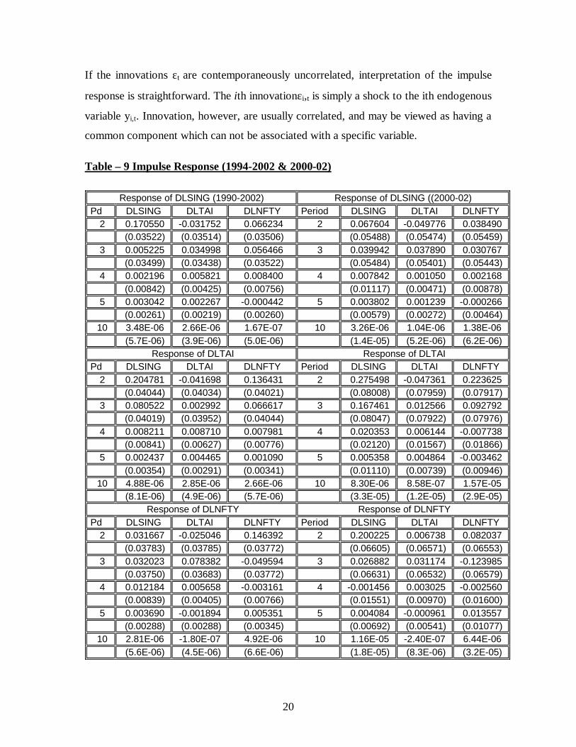
remained more or less unaffected and explains itself. To further investigate the dynamic

responses between the variables we also calculated the impulse response of the VAR

system and results are given in Table-9. An impulse response function traces the effect of

a one time shock to one of the innovations on current and further values of the

endogenous variables. Innovations are usually correlated and may be viewed as having a

common component that can not be associated with a specific variable in order to

interpret the results. A shock to the ith variable not only directly affects the ith variable

but is also transmitted to all of the other endogenous variables through the dynamic (lag)

structure of the VAR. An important response function traces the effect of a one-time

shock to one of the innovations on current and future values of the endogenous variables.

20

If the innovations εt are contemporaneously uncorrelated, interpretation of the impulse

response is straightforward. The ith innovationεi,t is simply a shock to the ith endogenous

variable yi,t. Innovation, however, are usually correlated, and may be viewed as having a

common component which can not be associated with a specific variable.

Table – 9 Impulse Response (1994-2002 & 2000-02)

Response of DLSING (1990-2002) Response of DLSING ((2000-02) Pd DLSING DLTAI DLNFTY Period DLSING DLTAI DLNFTY

2 0.170550 -0.031752 0.066234 2 0.067604 -0.049776 0.038490 (0.03522) (0.03514) (0.03506) (0.05488) (0.05474) (0.05459)

3 0.005225 0.034998 0.056466 3 0.039942 0.037890 0.030767 (0.03499) (0.03438) (0.03522) (0.05484) (0.05401) (0.05443)

4 0.002196 0.005821 0.008400 4 0.007842 0.001050 0.002168 (0.00842) (0.00425) (0.00756) (0.01117) (0.00471) (0.00878)

5 0.003042 0.002267 -0.000442 5 0.003802 0.001239 -0.000266 (0.00261) (0.00219) (0.00260) (0.00579) (0.00272) (0.00464)

10 3.48E-06 2.66E-06 1.67E-07 10 3.26E-06 1.04E-06 1.38E-06 (5.7E-06) (3.9E-06) (5.0E-06) (1.4E-05) (5.2E-06) (6.2E-06)

Response of DLTAI Response of DLTAI Pd DLSING DLTAI DLNFTY Period DLSING DLTAI DLNFTY

2 0.204781 -0.041698 0.136431 2 0.275498 -0.047361 0.223625 (0.04044) (0.04034) (0.04021) (0.08008) (0.07959) (0.07917)

3 0.080522 0.002992 0.066617 3 0.167461 0.012566 0.092792 (0.04019) (0.03952) (0.04044) (0.08047) (0.07922) (0.07976)

4 0.008211 0.008710 0.007981 4 0.020353 0.006144 -0.007738 (0.00841) (0.00627) (0.00776) (0.02120) (0.01567) (0.01866)

5 0.002437 0.004465 0.001090 5 0.005358 0.004864 -0.003462 (0.00354) (0.00291) (0.00341) (0.01110) (0.00739) (0.00946)

10 4.88E-06 2.85E-06 2.66E-06 10 8.30E-06 8.58E-07 1.57E-05 (8.1E-06) (4.9E-06) (5.7E-06) (3.3E-05) (1.2E-05) (2.9E-05)

Response of DLNFTY Response of DLNFTY Pd DLSING DLTAI DLNFTY Period DLSING DLTAI DLNFTY

2 0.031667 -0.025046 0.146392 2 0.200225 0.006738 0.082037 (0.03783) (0.03785) (0.03772) (0.06605) (0.06571) (0.06553)

3 0.032023 0.078382 -0.049594 3 0.026882 0.031174 -0.123985 (0.03750) (0.03683) (0.03772) (0.06631) (0.06532) (0.06579)

4 0.012184 0.005658 -0.003161 4 -0.001456 0.003025 -0.002560 (0.00839) (0.00405) (0.00766) (0.01551) (0.00970) (0.01600)

5 0.003690 -0.001894 0.005351 5 0.004084 -0.000961 0.013557 (0.00288) (0.00288) (0.00345) (0.00692) (0.00541) (0.01077)

10 2.81E-06 -1.80E-07 4.92E-06 10 1.16E-05 -2.40E-07 6.44E-06 (5.6E-06) (4.5E-06) (6.6E-06) (1.8E-05) (8.3E-06) (3.2E-05)

21

The following charts shows the impulse response of one of the variables on other variables.

Chart (1994-2002)

-0.5

0.0

0.5

1.0

1.5

2.0

1 2 3 4 5 6 7 8 9 10

DLSING DLTAI DLNFTY

Response of DLSING to One S.D. Innovations

-0.5

0.0

0.5

1.0

1.5

2.0

1 2 3 4 5 6 7 8 9 10

DLSING DLTAI DLNFTY

Response of DLTAI to One S.D. Innovations

-0.5

0.0

0.5

1.0

1.5

2.0

1 2 3 4 5 6 7 8 9 10

DLSING DLTAI DLNFTY

Response of DLNFTY to One S.D. Innovations

22

Chart (2000-2002)

-0.4

0.0

0.4

0.8

1.2

1.6

1 2 3 4 5 6 7 8 9 10

DLSING DLTAI DLNFTY

Response of DLSING to One S.D. Innovations

-0.5

0.0

0.5

1.0

1.5

2.0

1 2 3 4 5 6 7 8 9 10

DLSING DLTAI DLNFTY

Response of DLTAI to One S.D. Innovations

-0.5

0.0

0.5

1.0

1.5

2.0

1 2 3 4 5 6 7 8 9 10

DLSING DLTAI DLNFTY

Response of DLNFTY to One S.D. Innovations

Conclusions: In this paper, we have analyzed the level of capital market integration by

examining the transmission of market movements among three major stock

markets in Asian region and during the period from 1994 to 2002. We have studied three

important capital markets in Asian region which have attracted significant portfolio capital flows

during last one decade. While the literature suggests the existence of significant interactions

between the various equity markets, our empirical results show that generally returns in these

three markets are not inter-related and there is no long term equilibrium, though in few cases the

23

return in one stock market had causal influence on return in other stock markets though in very

mild form (short-term influences). We have used a time lag of 5 for doing the analysis as we

considered 5 days to be sufficient for any adjustment to take place considering significant

informational efficiency. Our results suggest that international investors can achieve long

term gains by investing in the stock markets as the market under study have been

generally independent.

References:

1. Basu & Morey: Stock Market Prices in India after Economic Liberalization, EPW February 14, 1998

2. Campbell, J.Y., A. W. Lo and A. C. MacKinlay, 1997, “The Econometrics of Financial Markets”, Princeton University Press, Princeton, NJ.

3. Engle, R.F., and C.W.J. Granger. 1987. Co-Integration, error correction: Representation, estimation and testing. Econometrica 55:1251-1276.

4. Engle, R.F., and C.W.J. Granger. 1991. Long-run economic relationships. New York: Oxford University Press.

5. Fuller, W.A. 1976. Introduction to Statistical Time Series. New York: John Wiley.

6. Gujrati, Damodar N.,: “Basic Econometrics”, McGRAW – HILL International Edition, 1995.

7. Geert Bekaerta, Campbell R. Harvey, Robin L. Lumsdaine, Dating the integration of world equity markets, Journal of Financial Economics 00 (2002)

8. Granger, C.W. 1986. Developemnts in the study of co-integrated economic variables. Oxford Bulletin of Economics and Statistics 48:213-228.

9. Granger, C.W.J. 1988. Some recent developments in a concept of causality. Journal of Econometrics 39 (1/2):199-211.

10. Johansen, S. 1988. Statistical analysis of cointegrating vectors. Journal of Economic Dynamic and Control 12:231-254.

11. Johansen, S. 1991. Estimation and hypothesis testing of cointegrating vectors in Gaussian vector autoregressive models. Econometrica 59 (November):1551-1580.

12. Johansen, S. 1992. Determination of cointegration rank in the presence of a linear trend. Oxford Bulletin of Economics and Statistics 54 (3):383-397.

13. Johansen, S., and K. Juselius. 1990. Maximum likelihood estimation and inference on cointegration with application to the demand for money. Oxford Bulletin of Economics and Statistics 52:169-209.

24

14. Johansen, S., and K. Juselius. 1994. Indentification of the long-run and the short-run structure: An application to the ISLM model. Journal of Econometrics 63:7-36.

15. Kanas, A. 1998. Linkages between the US and European equity markets: further evidence from cointegration tests. Applied Financial Economics. 8: 607 - 614.

16. Kasa K, (1992) Common Stochastic trends in International Stock Markets, Journal of Monetary Economics, 29, 95-124

17. Lo A & A Mac Kinlay (1988) Stock Market Prices do not Follow Random Walk: Evidence from a simple specification Test, review of Financial Studies. Vol I, No. 1, (41-66)

18. Nath, G C and Samanta, G P (2003) Dynamic Relation between Exchnage Rate and Stock Prices – A Case for India, 39th Annual Conference paper of Indian Econometric Society also published in NSE News February 2003

19. Nelson, Charles R.: “Applied time series analysis for managerial forecasting”; Holden Day Inc.; 1973

20. Osborne, M.F.M., 1964, “Brownian Motion in the Stock Market”, in P.Cootner, ed., The Random Character of Stock Market Prices, Cambridge: MIT Press.

21. Risk Metrics – Technical Document (1996), 4th Edition, (www.riskmetrics.com)

22. Rocca E.D. 1999. Short-term and long-term price linkages between the equity markets of Australia and its major trading partners. Applied Financial Economics. 9: 501-511

23. Taylor, M.P. and Tonks, I. 1989. The internationalization of stock markets and abolition of UK exchange control, The Review of Economics and Statistics 71: 332 - 336.

study of common stochastic trend and co-integration in the emerging markets a case ... · ·...

Documents