Sample Complexity Bounds for Iterative StochasticPolicy Optimization

Marin KobilarovDepartment of Mechanical Engineering

Johns Hopkins UniversityBaltimore, MD 21218marin@jhu.edu

Abstract

This paper is concerned with robustness analysis of decision making under un-certainty. We consider a class of iterative stochastic policy optimization problemsand analyze the resulting expected performance for each newly updated policyat each iteration. In particular, we employ concentration-of-measure inequali-ties to compute future expected cost and probability of constraint violation usingempirical runs. A novel inequality bound is derived that accounts for the possi-bly unbounded change-of-measure likelihood ratio resulting from iterative policyadaptation. The bound serves as a high-confidence certificate for providing futureperformance or safety guarantees. The approach is illustrated with a simple robotcontrol scenario and initial steps towards applications to challenging aerial vehiclenavigation problems are presented.

1 Introduction

We consider a general class of stochastic optimization problems formulated as

ξ∗ = arg minξ

Eτ∼p(·|ξ)[J(τ)], (1)

where ξ defines a vector of decision variables, τ represents the system response defined throughthe density p(τ |ξ), and J(τ) defines a positive cost function which can be non-smooth and non-convex. It is assumed that p(τ |ξ) is either known or can be sampled from, e.g. in a black-boxmanner. The objective is to obtain high-confidence sample complexity bounds on the expected costfor a given decision strategy by observing past realizations of possibly different strategies. Suchbounds are useful for two reasons: 1) for providing robustness guarantees for future executions, and2) for designing new algorithms that directly minimize the bound and therefore are expected to havebuilt-in robustness.

Our primary motivation arises from applications in robotics, for instance when a robot executescontrol policies to achieve a given task such as navigating to a desired state while perceiving theenvironment and avoiding obstacles. Such problems are traditionally considered in the frameworkof reinforcement learning and addressed using policy search algorithms, e.g. [1, 2] (see also [3] for acomprehensive overview with a focus on robotic applications [4]). When an uncertain system modelis available the problem is equivalent to robust model-predictive control (MPC) [5].

Our specific focus is on providing formal guarantees on future executions of control algorithms interms of maximum expected cost (quantifying performance) and maximum probability of constraintviolation (quantifying safety). Such bounds determine the reliability of control in the presence ofprocess, measurement and parameter uncertainties, and contextual changes in the task. In this workwe make no assumptions about nature of the system structure, such as linearity, convexity, or Gaus-sianity. In addition, the proposed approach applies either to a physical system without an available

1

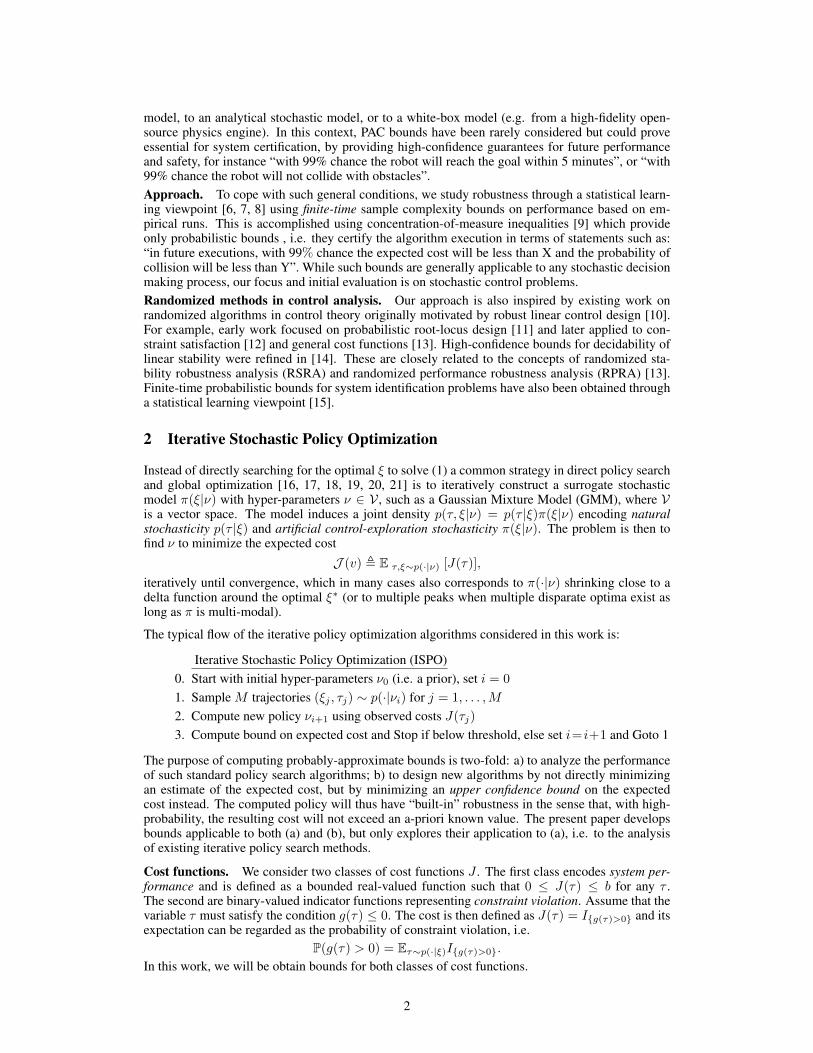
model, to an analytical stochastic model, or to a white-box model (e.g. from a high-fidelity open-source physics engine). In this context, PAC bounds have been rarely considered but could proveessential for system certification, by providing high-confidence guarantees for future performanceand safety, for instance “with 99% chance the robot will reach the goal within 5 minutes”, or “with99% chance the robot will not collide with obstacles”.Approach. To cope with such general conditions, we study robustness through a statistical learn-ing viewpoint [6, 7, 8] using finite-time sample complexity bounds on performance based on em-pirical runs. This is accomplished using concentration-of-measure inequalities [9] which provideonly probabilistic bounds , i.e. they certify the algorithm execution in terms of statements such as:“in future executions, with 99% chance the expected cost will be less than X and the probability ofcollision will be less than Y”. While such bounds are generally applicable to any stochastic decisionmaking process, our focus and initial evaluation is on stochastic control problems.Randomized methods in control analysis. Our approach is also inspired by existing work onrandomized algorithms in control theory originally motivated by robust linear control design [10].For example, early work focused on probabilistic root-locus design [11] and later applied to con-straint satisfaction [12] and general cost functions [13]. High-confidence bounds for decidability oflinear stability were refined in [14]. These are closely related to the concepts of randomized sta-bility robustness analysis (RSRA) and randomized performance robustness analysis (RPRA) [13].Finite-time probabilistic bounds for system identification problems have also been obtained througha statistical learning viewpoint [15].

2 Iterative Stochastic Policy Optimization

Instead of directly searching for the optimal ξ to solve (1) a common strategy in direct policy searchand global optimization [16, 17, 18, 19, 20, 21] is to iteratively construct a surrogate stochasticmodel π(ξ|ν) with hyper-parameters ν ∈ V , such as a Gaussian Mixture Model (GMM), where Vis a vector space. The model induces a joint density p(τ, ξ|ν) = p(τ |ξ)π(ξ|ν) encoding naturalstochasticity p(τ |ξ) and artificial control-exploration stochasticity π(ξ|ν). The problem is then tofind ν to minimize the expected cost

J (v) , E τ,ξ∼p(·|ν) [J(τ)],

iteratively until convergence, which in many cases also corresponds to π(·|ν) shrinking close to adelta function around the optimal ξ∗ (or to multiple peaks when multiple disparate optima exist aslong as π is multi-modal).

The typical flow of the iterative policy optimization algorithms considered in this work is:

Iterative Stochastic Policy Optimization (ISPO)0. Start with initial hyper-parameters ν0 (i.e. a prior), set i = 0

1. Sample M trajectories (ξj , τj) ∼ p(·|νi) for j = 1, . . . ,M

2. Compute new policy νi+1 using observed costs J(τj)

3. Compute bound on expected cost and Stop if below threshold, else set i= i+1 and Goto 1

The purpose of computing probably-approximate bounds is two-fold: a) to analyze the performanceof such standard policy search algorithms; b) to design new algorithms by not directly minimizingan estimate of the expected cost, but by minimizing an upper confidence bound on the expectedcost instead. The computed policy will thus have “built-in” robustness in the sense that, with high-probability, the resulting cost will not exceed an a-priori known value. The present paper developsbounds applicable to both (a) and (b), but only explores their application to (a), i.e. to the analysisof existing iterative policy search methods.

Cost functions. We consider two classes of cost functions J . The first class encodes system per-formance and is defined as a bounded real-valued function such that 0 ≤ J(τ) ≤ b for any τ .The second are binary-valued indicator functions representing constraint violation. Assume that thevariable τ must satisfy the condition g(τ) ≤ 0. The cost is then defined as J(τ) = I{g(τ)>0} and itsexpectation can be regarded as the probability of constraint violation, i.e.

P(g(τ) > 0) = Eτ∼p(·|ξ)I{g(τ)>0}.

In this work, we will be obtain bounds for both classes of cost functions.

2

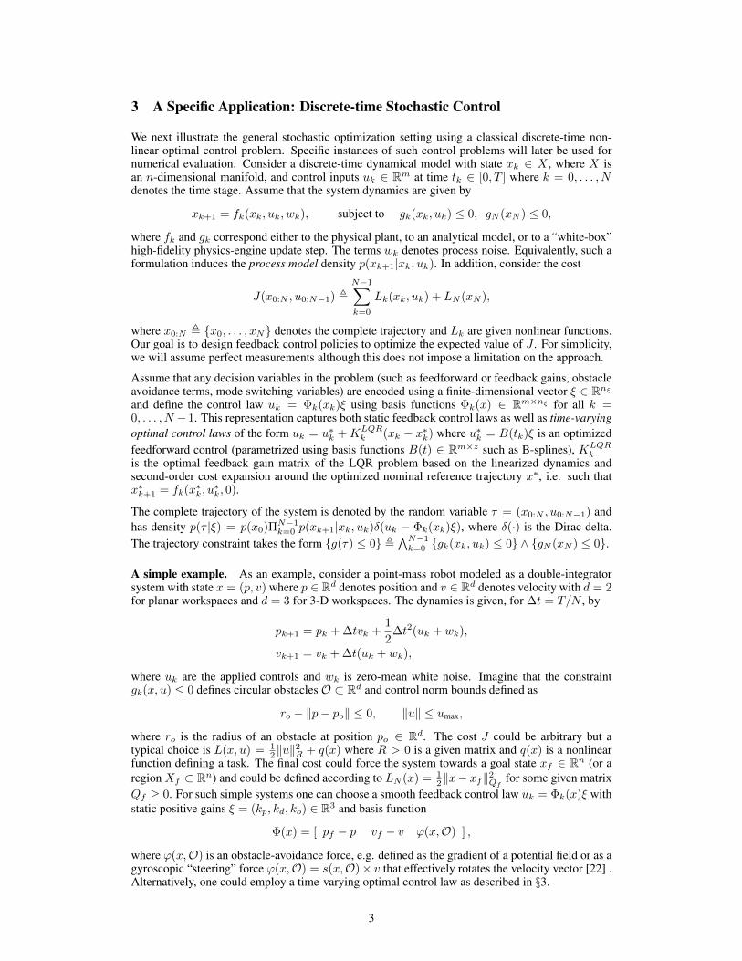
3 A Specific Application: Discrete-time Stochastic Control

We next illustrate the general stochastic optimization setting using a classical discrete-time non-linear optimal control problem. Specific instances of such control problems will later be used fornumerical evaluation. Consider a discrete-time dynamical model with state xk ∈ X , where X isan n-dimensional manifold, and control inputs uk ∈ Rm at time tk ∈ [0, T ] where k = 0, . . . , Ndenotes the time stage. Assume that the system dynamics are given by

xk+1 = fk(xk, uk, wk), subject to gk(xk, uk) ≤ 0, gN (xN ) ≤ 0,

where fk and gk correspond either to the physical plant, to an analytical model, or to a “white-box”high-fidelity physics-engine update step. The terms wk denotes process noise. Equivalently, such aformulation induces the process model density p(xk+1|xk, uk). In addition, consider the cost

J(x0:N , u0:N−1) ,N−1∑k=0

Lk(xk, uk) + LN (xN ),

where x0:N , {x0, . . . , xN} denotes the complete trajectory and Lk are given nonlinear functions.Our goal is to design feedback control policies to optimize the expected value of J . For simplicity,we will assume perfect measurements although this does not impose a limitation on the approach.

Assume that any decision variables in the problem (such as feedforward or feedback gains, obstacleavoidance terms, mode switching variables) are encoded using a finite-dimensional vector ξ ∈ Rnξand define the control law uk = Φk(xk)ξ using basis functions Φk(x) ∈ Rm×nξ for all k =0, . . . , N − 1. This representation captures both static feedback control laws as well as time-varyingoptimal control laws of the form uk = u∗k + KLQR

k (xk − x∗k) where u∗k = B(tk)ξ is an optimizedfeedforward control (parametrized using basis functions B(t) ∈ Rm×z such as B-splines), KLQR

kis the optimal feedback gain matrix of the LQR problem based on the linearized dynamics andsecond-order cost expansion around the optimized nominal reference trajectory x∗, i.e. such thatx∗k+1 = fk(x∗k, u

∗k, 0).

The complete trajectory of the system is denoted by the random variable τ = (x0:N , u0:N−1) andhas density p(τ |ξ) = p(x0)ΠN−1

k=0 p(xk+1|xk, uk)δ(uk − Φk(xk)ξ), where δ(·) is the Dirac delta.The trajectory constraint takes the form {g(τ) ≤ 0} ,

∧N−1k=0 {gk(xk, uk) ≤ 0} ∧ {gN (xN ) ≤ 0}.

A simple example. As an example, consider a point-mass robot modeled as a double-integratorsystem with state x = (p, v) where p ∈ Rd denotes position and v ∈ Rd denotes velocity with d = 2for planar workspaces and d = 3 for 3-D workspaces. The dynamics is given, for ∆t = T/N , by

pk+1 = pk + ∆tvk +1

2∆t2(uk + wk),

vk+1 = vk + ∆t(uk + wk),

where uk are the applied controls and wk is zero-mean white noise. Imagine that the constraintgk(x, u) ≤ 0 defines circular obstacles O ⊂ Rd and control norm bounds defined as

ro − ‖p− po‖ ≤ 0, ‖u‖ ≤ umax,

where ro is the radius of an obstacle at position po ∈ Rd. The cost J could be arbitrary but atypical choice is L(x, u) = 1

2‖u‖2R + q(x) where R > 0 is a given matrix and q(x) is a nonlinear

function defining a task. The final cost could force the system towards a goal state xf ∈ Rn (or aregion Xf ⊂ Rn) and could be defined according to LN (x) = 1

2‖x− xf‖2Qf

for some given matrixQf ≥ 0. For such simple systems one can choose a smooth feedback control law uk = Φk(x)ξ withstatic positive gains ξ = (kp, kd, ko) ∈ R3 and basis function

Φ(x) = [ pf − p vf − v ϕ(x,O) ] ,

where ϕ(x,O) is an obstacle-avoidance force, e.g. defined as the gradient of a potential field or as agyroscopic “steering” force ϕ(x,O) = s(x,O)× v that effectively rotates the velocity vector [22] .Alternatively, one could employ a time-varying optimal control law as described in §3.

3

4 PAC Bounds for Iterative Policy Adaptation

We next compute probabilistic bounds on the expected cost J (ν) resulting from the execution ofa new stochastic policy with hyper-parameters ν using observed samples from previous policiesν0, ν1, . . . . The bound is agnostic to how the policy is updated (i.e. Step 2 in the ISPO algorithm).

4.1 A concentration-of-measure inequality for policy adaptation

The stochastic optimization setting naturally allows the use of a prior belief ξ ∼ π(·|ν0) on whatgood control laws could be, for some known ν0 ∈ V . After observing M executions based on suchprior, we wish to find a new improved policy π(·|ν) which optimizes the cost

J (ν) , Eτ,ξ∼p(·|ν)[J(τ)] = Eτ,ξ∼p(·|ν0)

[J(τ)

π(ξ|ν)

π(ξ|ν0)

], (2)

which can be approximated using samples ξj ∼ π(ξ|ν0) and τj ∼ p(τ |ξj) by the empirical cost

1

M

M∑j=1

[J(τj)

π(ξj |ν)

π(ξj |ν0)

]. (3)

The goal is to compute the parameters ν using the sampled decision variables ξj and the corre-sponding observed costs J(τj). Obtaining practical bounds for J (ν) becomes challenging since thechange-of-measure likelihood ratio π(ξ|ν)

π(ξ|ν0) can be unbounded (or have very large values) [23] and astandard bound, e.g. such as Hoeffding’s or Bernstein’s becomes impractical or impossible to apply.To cope with this we will employ a recently proposed robust estimation [24] technique stipulatingthat instead of estimating the expectation m = E[X] of a random variable X ∈ [0,∞) using itsempirical mean m = 1

M

∑Mj=1Xj , a more robust estimate can be obtained by truncating its higher

moments, i.e. using mα , 1αM

∑Mj=1 ψ(αXj) for some α > 0 where

ψ(x) = log(1 + x+1

2x2). (4)

What makes this possible is the key assumption that the (possibly unbounded) random variable musthave bounded second moment. We employ this idea to deal with the unboundedness of the policyadaptation ratio by showing that in fact its second moment can be bounded and corresponds to aninformation distance between the current and previous stochastic policies.

To obtain sharp bounds though it is useful to employ samples over multiple iterations of the ISPOalgorithm, i.e. from policies ν0, ν1, . . . , νL−1 computed in previous iterations. To simplify notationlet z = (τ, ξ) and define `i(z, ν) , J(τ) π(ξ|ν)

π(ξ|νi) . The cost (2) of executing ν can now be equivalentlyexpressed as

J (ν) ≡ 1

L

L−1∑i=0

Ez∼p(·|νi)`i(z, ν)

using the computed policies in previous iterations i = 0, . . . , L− 1. We next state the main result:Proposition 1. With probability 1 − δ the expected cost of executing a stochastic policy with pa-rameters ξ ∼ π(·|ν) is bounded according to:

J (ν) ≤ infα>0

{Jα(ν) +

α

2L

L−1∑i=0

b2i eD2(π(·|ν)||π(·|νi)) +

1

αLMlog

1

δ

}, (5)

where Jα(ν) denotes a robust estimator defined by

Jα(ν) ,1

αLM

L−1∑i=0

M∑j=1

ψ (α`(zij , ν)) ,

computed after L iterations, with M samples zi1, . . . , ziM ∼ p(·|νi) obtained at iterations i =0, . . . , L− 1, where Dβ(p||q) denotes the Renyii divergence between p and q defined by

Dβ(p||q) =1

β − 1log

∫pβ(x)

qβ−1(x)dx.

The constants bi are such that 0 ≤ J(τ) ≤ bi at each iteration i = 0, . . . , L− 1.

4

Proof. The bound is obtained by relating the mean to its robust estimate according to

P(LM(J (ν)− Jα(ν)) ≥ t

)= P

(eαLM(J (ν)−Jα(ν)) ≥ eαt

),

≤ E[eαLM(J (ν)−Jα(ν))

]e−αt, (6)

= e−αt+αLMJ (ν)E[e∑L−1i=0

∑Mj=1−ψ(α`i(zij ,ν))

]= e−αt+αLMJE

L−1∏i=0

M∏j=1

e−ψ(α`i(zij ,ν))

= e−αt+αLMJ

L−1∏i=0

M∏j=1

E z∼p(·|νi)

[1− α`i(z, ν) +

α2

2`i(z, ν)2

](7)

= e−αt+αLMJ (ν)L−1∏i=0

M∏j=1

(1− αJ (ν) +

α2

2E z∼p(·|νi)[`i(z, ν)2]

)

≤ e−αt+αLMJ (ν)L−1∏i=0

M∏j=1

e−αJ (ν)+α2

2 Ez∼p(·|νi)[`i(z,ν)2] (8)

≤ e−αt+M α2

2

∑L−1i=0 Ez∼p(·|νi)[`i(z,ν)2],

using Markov’s inequality to obtain (6), the identities ψ(x) ≥ − log(1 − x + 12x

2) in (7) and1 + x ≤ ex in (8). Here, we adapted the moment-truncation technique proposed by Catoni [24] forgeneral unbounded losses to our policy adaptation setting in order to handle the possibly unboundedlikelihood ratio. These results are then combined with

E [`i(z, ν)2] ≤ b2iEπ(·|νi)

[π(ξ|ν)2

π(ξ|νi)2

]= b2i e

D2(π||πi),

where the relationship between the likelihood ratio variance and the Renyii divergence was estab-lished in [23].

Note that the Renyii divergence can be regarded as a distance between two distribution and can becomputed in closed bounded form for various distributions such as the exponential families; it isalso closely related to the Kullback-Liebler (KL) divergence, i.e. D1(p||q) = KL(p||q).

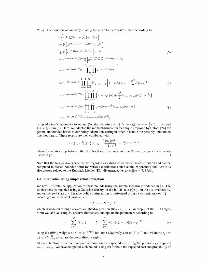
4.2 Illustration using simple robot navigation

We next illustrate the application of these bounds using the simple scenario introduced in §3. Thestochasticity is modeled using a Gaussian density on the initial state p(x0), on the disturbances wkand on the goal state xf . Iterative policy optimization is performed using a stochastic model π(ξ|ν)encoding a multivariate Gaussian, i.e.

π(ξ|ν) = N (ξ|µ,Σ)

which is updated through reward-weighted-regression (RWR) [3], i.e. in Step 2 of the ISPO algo-rithm we take M samples, observe their costs, and update the parameters according to

µ =

M∑j=1

w(τj)ξj , Σ =

M∑j=1

w(τj)(ξj − µ)(ξj − µ)T , (9)

using the tilting weights w(τ) = e−βJ(τ) for some adaptively chosen β > 0 and where w(τj) ,w(τj)/

∑M`=1 w(τ`) are the normalized weights.

At each iteration i one can compute a bound on the expected cost using the previously computedν0, . . . , νi−1. We have computed such bounds using (5) for both the expected cost and probability of

5

-15 -10 -5 0 5

-15

-10

-5

0

5

-15 -10 -5 0 5

-15

-10

-5

0

5

-15 -10 -5 0 5

-15

-10

-5

0

5

obstacles

goal

sampled start states

obstacles

iteration #1 iteration #4 iteration #9 iteration #28

iterations

0 5 10 15 20 25 300

1

2

3

4

5

6

7

8

Expected Cost

empirical J

robust JαPAC bound J

+

iterations

0 5 10 15 20 25 300

0.1

0.2

0.3

0.4

0.5

0.6

0.7

Probability of Collision

empirical P

robust Pα

PAC bound P+

a) b) c)Figure 1: Robot navigation scenario based on iterative policy improvement and resulting predicted perfor-mance: a) evolution of the density p(ξ|ν) over the decision variables (in this case the control gains); b) costfunction J and its computed upper bound J+ for future executions; c) analogous bounds on probability-of-collision P ; snapshots of sampled trajectories (top). Note that the initial policy results in ≈ 30% collisions.Surprisingly, the standard empirical and robust estimates are nearly identical.

collision, denoted respectively by J + and P+ using M = 200 samples (Figure 1) at each iteration.We used a window of maximum L = 10 previous iterations to compute the bounds, i.e. to computeνi+1 all samples from densities νi−L+1, νi−L+2, . . . , νi were used. Remarkably, using our robuststatistics approach the resulting bound eventually becomes close to the standard empirical estimateJ . The collision probability bound P+ decreses to less than 10% which could be further improvedby employing more samples and more iterations. The significance of these bounds is that one canstop the optimization (regarded as training) at any time and be able to predict expected performancein future executions using the newly updated policy before actually executing the policy, i.e. usingthe samples from the previous iteration.

Finally, the Renyii divergence term used in these computations takes the simple form

Dβ (N (·|µ0,Σ0)‖N (·|µ1,Σ1)) =β

2‖µ1 − µ0‖2Σ−1

β

+1

2(1− β)log

|Σβ ||Σ0|1−β |Σ1|β

,

where Σβ = (1− β)Σ0 + βΣ1.

4.3 Policy Optimization Methods

We do not impose any restrictions on the specific method used for optimizing the policy π(ξ|ν).When complex constraints are present such computation will involve a global motion planning stepcombined with local feedback control laws (we show such an example in §5). The approach canbe used to either analyze such policies computed using any method of choice or to derive newalgorithms based on minimizing the right-hand side of the bound. The method also applies to model-free learning. For instance, related to recent methods in robotics one could use reward-weighted-regression (RWR) or policy learning by weighted samples with returns (PoWeR) [3], stochasticoptimization methods such as [25, 26], or using the related cross-entropy optimization [16, 27].

6

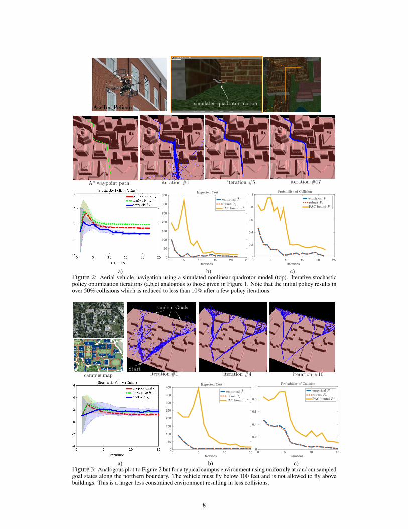
5 Application to Aerial Vehicle NavigationConsider an aerial vehicle such as a quadrotor navigating at high speed through a cluttered environ-ment. We are interested in minimizing a cost metric related to the total time taken and control effortrequired to reach a desired goal state, while maintaining low probability of collision. We employ anexperimentally identified model of an AscTec quadrotor (Figure 2) with 12-dimensional state spaceX = SE(3) × R6 with state x = (p,R, p, ω) where p ∈ R3 is the position, R ∈ SO(3) is therotation matrix, and ω ∈ R3 is the body-fixed angular velocity. The vehicle is controlled with inputsu = (F,M) ∈ R4 including the lift force F ≥ 0 and torque moments M ∈ R3. The dynamics is

mp = Re3F +mg + δ(p, p), (10)

R = Rω, (11)Jω = Jω × ω +M, (12)

where m is the mass, J–the inertia tensor, e3 = (0, 0, 1) and the matrix ω is such that ωη = ω × ηfor any η ∈ R3. The system is subject to initial localization errors and also to random disturbances,e.g. due to wind gusts and wall effects, defined as stochastic forces δ(p, p) ∈ R3. Each componentin δ is zero-mean and has standard deviation of 3 Newtons, for a vehicle with mass m ≈ 1 kg.

The objective is to navigate through a given urban environment at high speed to a desired goalstate. We employ a two-stage approach consisting of an A*-based global planner which producesa sequence of local sub-goals that the vehicle must pass through. A standard nonlinear feedbackbackstepping controller based on a “slow” position control loop and a “fast” attitude control isemployed [28, 29] for local control. In addition, and obstacle avoidance controller is added to avoidcollisions since the vehicle is not expected to exactly follow the A* path. At each iterationM = 200samples are taken with 1 − δ = 0.95 confidence level. A window of L = 5 past iterations wereused for the bounds. The control density π(ξ|ν) is a single Gaussian as specified in §4.2. The mostsensitive gains in the controller are the position proporitional and derivative terms, and the obstaclegains, denoted by kp, kd, and ko, which we examine in the following scenarios:a) fixed goal, wind gusts disturbances, virtual environment: the system is first tested in a cluttered

simulated environment (Figure 2). The simulated vehicle travels at an average velocity of 20m/s (see video in Supplement) and initially experiences more than 50% collisions. After a fewiterations the total cost stabilizes and the probability of collision reduces to around 15%. Thebound is close to the empirical estimate which indicates that it can be tight if more samples aretaken. The collision probability bound is still too high to be practical but our goal was onlyto illustrate the bound behavior. It is also likely that our chosen control strategy is in fact notsuitable for high-speed traversal of such tight environments.

b) sparser campus-like environment, randomly sampled goals: a more general evaluation was per-formed by adding the goal location to the stochastic problem parameters so that the bound willapply to any future desired goal in that environment (Figure 3). The algorithm converges tosimilar values as before, but this time the collision probability is smaller due to more expan-sive environment. In both cases, the bounds could be reduced further by employing more thanM = 200 samples or by reusing more samples from previous runs according to Proposition 1.

6 ConclusionThis paper considered stochastic decision problems and focused on a probably-approximate boundson robustness of the computed decision variables. We showed how to derive bounds for fixed poli-cies in order to predict future performance and/or constraint violation. These results could then beemployed for obtaining generalization PAC bounds, e.g. through a PAC-Bayesian approach whichcould be consistent with the proposed notion of policy priors and policy adaptation. Future workwill develop concrete algorithms by directly optimizing such PAC bounds, which are expected tohave built-in robustness properties.

References[1] Richard S. Sutton, David A. McAllester, Satinder P. Singh, and Yishay Mansour. Policy gradient methods

for reinforcement learning with function approximation. In NIPS, pages 1057–1063, 1999.[2] Csaba Szepesvari. Algorithms for Reinforcement Learning. Morgan and Claypool Publishers, 2010.[3] M. P. Deisenroth, G. Neumann, and J. Peters. A survey on policy search for robotics. pages 388–403,

2013.

7

iteration #1 iteration #5 iteration #17A* waypoint path

simulated quadrotor motionAscTec Pelican

iterations

0 5 10 15 20 250

50

100

150

200

250

300

350

Expected Cost

empirical J

robust JαPAC bound J

+

iterations

0 5 10 15 20 250

0.2

0.4

0.6

0.8

1

Probability of Collision

empirical P

robust Pα

PAC bound P+

a) b) c)Figure 2: Aerial vehicle navigation using a simulated nonlinear quadrotor model (top). Iterative stochasticpolicy optimization iterations (a,b,c) analogous to those given in Figure 1. Note that the initial policy results inover 50% collisions which is reduced to less than 10% after a few policy iterations.

iteration #1 iteration #4 iteration #10campus mapStart

random Goals

iterations

0 5 10 150

50

100

150

200

250

300

350

400

Expected Cost

empirical J

robust JαPAC bound J

+

iterations

0 5 10 150

0.2

0.4

0.6

0.8

1

Probability of Collision

empirical P

robust Pα

PAC bound P+

a) b) c)Figure 3: Analogous plot to Figure 2 but for a typical campus environment using uniformly at random sampledgoal states along the northern boundary. The vehicle must fly below 100 feet and is not allowed to fly abovebuildings. This is a larger less constrained environment resulting in less collisions.

8

[4] S. Schaal and C. Atkeson. Learning control in robotics. Robotics Automation Magazine, IEEE, 17(2):20–29, june 2010.

[5] Alberto Bemporad and Manfred Morari. Robust model predictive control: A survey. In A. Garulli andA. Tesi, editors, Robustness in identification and control, volume 245 of Lecture Notes in Control andInformation Sciences, pages 207–226. Springer London, 1999.

[6] Vladimir N. Vapnik. The nature of statistical learning theory. Springer-Verlag New York, Inc., New York,NY, USA, 1995.

[7] David A. McAllester. Pac-bayesian stochastic model selection. Mach. Learn., 51:5–21, April 2003.

[8] J Langford. Tutorial on practical prediction theory for classification. Journal of Machine Learning Re-search, 6(1):273–306, 2005.

[9] Stphane Boucheron, Gbor Lugosi, Pascal Massart, and Michel Ledoux. Concentration inequalities : anonasymptotic theory of independence. Oxford university press, Oxford, 2013.

[10] M. Vidyasagar. Randomized algorithms for robust controller synthesis using statistical learning theory.Automatica, 37(10):1515–1528, October 2001.

[11] Laura Ryan Ray and Robert F. Stengel. A monte carlo approach to the analysis of control system robust-ness. Automatica, 29(1):229–236, January 1993.

[12] Qian Wang and RobertF. Stengel. Probabilistic control of nonlinear uncertain systems. In GiuseppeCalafiore and Fabrizio Dabbene, editors, Probabilistic and Randomized Methods for Design under Un-certainty, pages 381–414. Springer London, 2006.

[13] R. Tempo, G. Calafiore, and F. Dabbene. Randomized algorithms for analysis and control of uncertainsystems. Springer, 2004.

[14] V. Koltchinskii, C.T. Abdallah, M. Ariola, and P. Dorato. Statistical learning control of uncertain systems:theory and algorithms. Applied Mathematics and Computation, 120(13):31 – 43, 2001. ¡ce:title¿TheBellman Continuum¡/ce:title¿.

[15] M. Vidyasagar and Rajeeva L. Karandikar. A learning theory approach to system identification andstochastic adaptive control. Journal of Process Control, 18(34):421 – 430, 2008. Festschrift honour-ing Professor Dale Seborg.

[16] Reuven Y. Rubinstein and Dirk P. Kroese. The cross-entropy method: a unified approach to combinatorialoptimization. Springer, 2004.

[17] Anatoly Zhigljavsky and Antanasz Zilinskas. Stochastic Global Optimization. Spri, 2008.

[18] Philipp Hennig and Christian J. Schuler. Entropy search for information-efficient global optimization. J.Mach. Learn. Res., 98888:1809–1837, June 2012.

[19] Christian Igel, Nikolaus Hansen, and Stefan Roth. Covariance matrix adaptation for multi-objectiveoptimization. Evol. Comput., 15(1):1–28, March 2007.

[20] Pedro Larraaga and Jose A. Lozano, editors. Estimation of distribution algorithms: A new tool for evolu-tionary computation. Kluwer Academic Publishers, 2002.

[21] Martin Pelikan, David E. Goldberg, and Fernando G. Lobo. A survey of optimization by building andusing probabilistic models. Comput. Optim. Appl., 21:5–20, January 2002.

[22] Howie Choset, Kevin M. Lynch, Seth Hutchinson, George A Kantor, Wolfram Burgard, Lydia E. Kavraki,and Sebastian Thrun. Principles of Robot Motion: Theory, Algorithms, and Implementations. MIT Press,June 2005.

[23] Corinna Cortes, Yishay Mansour, and Mehryar Mohri. Learning Bounds for Importance Weighting. InAdvances in Neural Information Processing Systems 23, 2010.

[24] Olivier Catoni. Challenging the empirical mean and empirical variance: A deviation study. Ann. Inst. H.Poincar Probab. Statist., 48(4):1148–1185, 11 2012.

[25] E. Theodorou, J. Buchli, and S. Schaal. A generalized path integral control approach to reinforcementlearning. Journal of Machine Learning Research, (11):3137–3181, 2010.

[26] Sergey Levine and Pieter Abbeel. Learning neural network policies with guided policy search underunknown dynamics. In Neural Information Processing Systems (NIPS), 2014.

[27] M. Kobilarov. Cross-entropy motion planning. International Journal of Robotics Research, 31(7):855–871, 2012.

[28] Robert Mahony and Tarek Hamel. Robust trajectory tracking for a scale model autonomous helicopter.International Journal of Robust and Nonlinear Control, 14(12):1035–1059, 2004.

[29] Marin Kobilarov. Trajectory tracking of a class of underactuated systems with external disturbances. InAmerican Control Conference, pages 1044–1049, 2013.

9