COO-1199-64

State Water Survey Division ATMOSPHERIC CHEMISTRY SECTION

AT THE UNIVERSITY OF ILLINOIS

Illinois Department of Energy and Natural Resources

SWS Contract Report 347

STUDY OF ATMOSPHERIC POLLUTION SCAVENGING

Twentieth Progress Report Contract Number DE - AC02 - 76EV01199

September 1984

Authors: Richard G. Semonin Gary J. Stensland Van C. Bowersox Mark E. Peden Jacqueline M. Lockard Kevin G. Doty Donald F. Gatz Lih-C. Chu Susan R. Bachman Randall K. Stahlhut

Sponsored by: United States Department of Energy

Pollutant Characterization and Safety Research Division Office of Health and Environmental Research

Washington, DC

Richard G. Semonin Principal Investigator

COO-1199-64

SWS Contract Report 347

STUDY OF ATMOSPHERIC POLLUTION

SCAVENGING

Twentieth Progress Report Contract Number DE-AC02-76E701199

September 1984

Authors: Richard G. Semonin Gary J. Stensland Van C. Bowersox Mark E. Peden Jacqueline M. Lockard Kevin G. Doty-Donald F. Gatz Lih-Ch. Chu Susan R. Backman Randall K. Stahlhut

Sponsored by: United States Department of Energy

Office of Health and Environmental Research Washington, D.C.

Richard G. Semonin Principal Investigator

TABLE OF CONTENTS

Page

CHAPTER 1. 1982-1984 Research Summary and Related Contract Activities Richard G. Semonin 1

CHAPTER 2. Acid Rain Data Collection, Handling, Analysis and Interpretation Richard G. Semonin 7

CHAPTER 3. A Comparison of Four Methods of Computing Precipita­tion pH Averages Gary J. Stensland and Van C. Bowersox 45

CHAPTER 4. Regional Characterization of Rain Acidity Utilizing Gran's Plot Titrations Mark E. Peden and Jacqueline M. Lockard 75

CHAPTER 5. The Chemistry and Meteorology of Extreme pH Departures in Precipitation on the Regional Scale Kevin G. Doty and Richard G. Semonin 85

CHAPTER 6. Dry Bucket Analysis of the NADP Network Richard G. Semonin 137

CHAPTER 7. Metal Solubility in Atmospheric Deposition Donald F. Gatz and Lih-Ching Chu 151

CHAPTER 8. Source Apportionment of Rain Water Impurities in Central Illinois Donald F. Gatz 171

CHAPTER 9. A Few Preliminary Precipitation Chemistry Statistics Richard G. Semonin 193

CHAPTER 10. Results of the World Meteorological Organization (WMO) Interlaboratory Comparison of Reference Pre­cipitation Samples Mark E. Peden 219

CHAPTER 11. Microcomputer Based Data Acquisition and Reduction System for. Ion Chromatography Susan R. Bachman and Randall K. Stahlhut 225

CHAPTER 12. Determination of Organic Acids in Bondville, Illinois Precipitation Samples by Ion Chromatography Exclusion (Ice) Susan R. Bachman, Jacqueline M. Lockard, and Mark E. Peden 233

CHAPTER 13. Feasibility Study to Assess the Impact of Precipita­tion Quality on Soil Water Quality Van C. Bowersox 251

CHAPTER 14. Precipitation, Chemical Depositions and Water Resource Issues Richard G. Semonin 277

CHAPTER 15. A Review of Particle Tracers of Atmospheric Processes Donald F. Gatz 317

CHAPTER 16. Tracer Applications for the Study of Precipitation Processes Richard G. Semonin 339

CHAPTER 1

1982-1984 RESEARCH SUMMARY AND RELATED CONTRACT ACTIVITIES

Richard G. Semonin

INTRODUCTION

The research performed during the past 3 years under this contract can be summarized most easily by 5 subdivisions of the on-going effort. All of the work is directed toward providing information for assessment of the acidic deposition issue in this country. The first four categories all relate to acidic deposition and the progress report has been organized to move through each of the topics in order. The first of these topics is the description and interpretation of acidic deposition, followed by a fe"w statistical analyses of precipitation chemistry with application to acidic deposition. The last two categories are analytical method development for acidic deposition, and finally a few effects and research method develop­ment topics are addressed.

The final section of this chapter will describe some of the related contract activities resulting from the research performed during these three years. These activities range from testimony before congressional committees to participation in review workshops of the National Acid Precipitation Assessment Plan.

RESEARCH SUMMARY

Some of the complexities of sampling precipitation for chemical analysis are discussed in Chapter 2 with emphasis on the care and skill required to insure high quality data. Past and current efforts on this contract have supported the development of laboratory expertise that culminated in the selection of this laboratory to perform the analytical services for the nation's acid precipitation monitoring network. From this experience, a number of potential problems that will diminish the quality of precipitation chemistry data are pointed out in this chapter. These are documented so that those who attempt to establish new monitoring efforts will have the benefit of past experience. In addition, some recent data are shown for pH to illustrate its great spatial variability in the United States. These data show that the lowest values exist in the Northeast while the Great Plains show the highest pH values. The ratios of hydrogen, ammonium, and calcium ions to the sum of sulfate and nitrate reveal that maximum values occur in the Northeast, central Great Plains, and the intermountain basin, respectively. Finally, a brief account of reinterpreting the older data show that the previously perceived rapidly worsening precipitation acidity problem is not true. When account is taken of different sampling procedures, analytical methods, and, most importantly, meteorological sampling conditions, the early chemistry was proven to be inadequate sample as an initiating point to determine a trend in the United States.

-2-

The question of Che calculation and presentation of pH data is one of importance to the determination of acidic precipitation trends owing to the fact that different numbers can be obtained even from the same data set. In Chapter 3, examples are shown for the calculation of various climatological values of pH. These range from the precipitation-weighted average pH, the sample median pH, the arithmetic mean pH, and finally the average pH calculated from the weighted average conservative ion concen­trations. Since all of these methods have appeared in one or more publi­cations dealing with the spatial distribution and the trend of precipita­tion acidity across the U.S., it is important to consider which of these methods is most appropriate for an assessment of the acid rain issue. In summary, this study shows there is no "correct" answer to provide the best value of pH. However, a clearly stated purpose for which the average or central tendency value is needed will help to determine which method will give the most representative value.

In addition to the major anions (sulfate and nitrate) contributing to the acidity of precipitation, it is now recognized that organic acids also contribute to the total acidity. In Chapter 4, some preliminary work is reported on the regional characterization of rain acidity through the use of Grans plot titrations. It was found that the ratio of strong to weak acids decreases from east to west as a result of both decreased strong acidities and increased ammonium concentrations. Due to sampling problems, no evidence of a significant contribution of organic acids was found in samples from any of the sites used in the study. Considerable additional work is needed in this area.

In their recent paper, Stensland and Semonin (1982) suggested that airborne surficial material may have biased the precipitation chemistry of the mid-1950's. To explore this possibility further, statistical methods wer employed on NADP network data sets selected from recent years, and described in Chapter 5. A case was selected from 1981 with relatively high pH values over the Northeast and an additional case was chosen with relatively low pH values in the same area. Using these data, a meteoro­logical explanation was than sought related to suspended airborne mate­rial. Trajectory analyses in one case in the Spring of 1981 provided evidence for the potential transport of crustal dust aerosol from the southern Great Plains and incorporated in precipitation at sites in the Midwest. The more acid case of July 1981 revealed high concentrations of most ions in comparison with adjacent weeks. These high concentrations appeared to be related to the smaller average sample volume across the Midwest and Northeast and the relatively long dry period that was observed prior to the main rainfall event. Additional case studies will be pursued to assist in understanding the natural variability of precipitation acidity.

The MAP3S and NADP networks both use a sampler with a collector for wet-only samples and a collector exposed to dry deposition during non-precipitating periods. The analysis of the dry bucket samples collected from the NADP are presented in Chapter 6. Lack of agreement over a dry deposition measurement method has resulted in a lack of data for a full assessment of the impact of acidic deposition. The dry bucket data may be questioned by the "purist." This is a first attempt to describe the regional dry deposition using readily available data. While more work is needed, these results show between station consistency within large areas

-3-

of the eastern half of the United States. The absolute magnitude of the dry deposition values may be questioned, but the data do give a first glimpse of the areal distribution that is expected with implementation of more sophisticated equipment in the future.

The assessment of the effects of acidic deposition can not be inde­pendently achieved without due consideration given to other coincident and potentially important precipitation chemistry. A contribution in this area is made in Chapter 7 where a set of atmospheric deposition samples in wet, dry, and bulk precipitation were analyzed for metal solubility. The samples were analyzed for zinc, aluminum, copper, iron, cadmium, and lead. The percent soluble metals show zinc is about equal to cadmium and both are greater than copper which is greater than lead. In general, the wet-only samples showed more solubility than bulk and dry which were nearly equal. These results have important implications for precipitation sampling for metal analysis as well as for the understanding metal chemis­try in precipitation, airborne metal scavenging processes, metals as tracers for sources of acidity, and the effects of acidic precipitation on ecosystems.

The identity and relative contributions of various sources of impuri­ties in precipitation are needed to understand the acidic precipitation phenomenon. Factor analyses were used in Chapter 8 to identify, and chemical element balance calculations were performed to apportion, possi­ble sources of impurities in event precipitation samples from central Illinois collected over a two year period. Although factor analyses could group elements or ions that occurred together for chemical, meteorologi­cal, or microphysical reasons, as well as that of having a common source, the following likely sources were identified: crustal dust, sea and/or road salt, and possibly strong acids. In addition, a gaseous precursor factor was identified. The smallest contribution appears to be sea and/or road salt with the greatest contribution in the acids and the gaseous precursors. The contribution of crustal dust is sizable and certainly warrants further investigation. Extensions of this work should include plotting the factor scores against the date of the sample collection as a means to relate the source term to meteorological conditions.

The NADP network data were used to examine the correlation coeffi­cients between the various ions that are commonly analyzed. In Chapter 9, the relationships between these various ions are described and maps are presented indicating areas of relatively high correlations between spe­cific ions. These maps indicate that the Northeast United States experi­ences very high correlations between the acid-forming ions, and high correlations of acid neutralizing materials over the interior continent. The coastal regions show correlations which are equal or greater than either the acid or base ions between sea salt components

The research results presented in this report are given with full confidence in the quality of the analytical values that form the basis for interpretation and subsequent conclusions concerning acidic deposition. To sustain high quality analytical methodology the laboratory continues to participate in various interlaboratory comparisons for low concentration water samples. The most recent World Meteorological Organization compari­son results are presented in Chapter 10. Throughout the past 4 years, the laboratory results have consistantly yielded mean percent deviations of 3

-4-

to 5% from the test sample input. These activities will be continued to insure the highest level of accuracy for reported numbers from precipita­tion samples to insure the user that the data are meaningful and can be interpreted and reported with confidence.

The dependability of analyses is only one essential part of the laboratory performance. The other part is the rapidity with which samples can be analyzed and made available to the research community. A micro­computer based data acquisition and reduction system for ion chromatogra­phy is described in Chapter 11. A microcomputer is connected on-line to an ion chromatograph forming an analytical system of proven accuracy and efficiency for data acquisition and reduction of precipitation sample ion determinations. The most important aspect of this automation is that the analyst time devoted to data reduction tasks has been reduced by an estimated 25%. Another way of viewing this automation is that the through-put in the laboratory has been increased by a comparable percent.

Acidic precipitation samples are generally thought to be composed of a mixture of the strong acids sulfuric and nitric. The potential contri­bution of other components, such as weak acids that are only partially disassociated, can not be over looked. In Chapter 12 some preliminary work on the determination of organic acids in central Illinois precipita­tion is described. The results show that nationwide, the contribution of weak organic acids to the chemistry of rainfall can be quite varied. The weak to strong acid ratio for Illinois precipitation is similar to that of sites in the northeastern United States. Based on the data accumulated thus far for central Illinois, the findings are in agreement with those reported for the Northeast U.S. that strong acids control the pH of rainfall but weak acids are important to the total chemistry of precipita­tion. Since this preliminary data base is limited to samples collected during the spring months, however, additional work needs to be carried out to examine seasonal differences in weak acid concentrations and weak to strong acid relationships.

The acidity of precipitation over the eastern half of the cash grain belt across Iowa, Illinois, Indiana, Ohio, and north and south of those states is of the same value as the much publicized Adirondack lake area of New York state. One of the early concerns in assessment of the acidic deposition problem was the short or long-term damage to soil productivity. Because of this concern and the fact that Illinois represents much of the corn belt (from a climatological point of view), a small effort was devoted to estimating the effects of precipitation quality on soil water quality. The results from this preliminary and limited effort are found in Chapter 13. With the data available using lysimeters to sample soil water, a few results indicate that the precipitation pH is clearly less than the soil water pH for the soils of central Illinois and that neu­tralization of the precipitation occurs in the top most layer of the soil for even the most acidic rainfalls observed (pH of 3.82). These data also indicate that a weak relationship exists between soil water pH and free hydrogen ion deposition with the soil water pH slightly depressed with increased hydrogen ion input. However, much additional research effort is needed to clarify this relationship and to further estimate the impact of acidic deposition on the soils of the Midwest.

-5-

Drawing upon the extensive literature on the various presumed effects of acidic deposition on water resources, Chapter 14 describes some of the knowns and unknowns concerning this aspect of a total assessment. The material presented was collected together for presentation before an international conference, but the material bears repeating in this Pro­gress Report as it addresses a topic of some national interest. The final conclusion of this chapter is that little is known concerning the effects of acidic deposition on the chemical quality of surface and ground water supplies.

A review of particle tracers of atmospheric processes is presented in Chapter 15. This paper was presented at the Department of Energy Workshop on Atmospheric Tracers held in the spring of 1984, but is relevant to the entire subject of acidic deposition assessment since it reviews one of the possible research techniques available to investigators.

In a similar vein, Chapter 16 attempts to address the application of tracers to the study of precipitation processes with specific application to the acidic deposition question. The precipitation process is described as beginning with the availability of water vapor and condensation nuclei, and then moves through the requirement for motions in the atmosphere to produce clouds and precipitation. There is a clear need for tracers in the study of all of these atmospheric attributes leading to precipitation production. However, the presently available suite of gaseous and parti­cle tracers each have inadequacies which inhibit their direct application to resolving acidic precipitation research problems. There is a need for the development of a new tracer which can be freely used in the atmosphere and will have a direct bearing on the conversion and scavenging of acidic deposition precursors.

In general, the research results presented in this Progress Report are directed toward improvement of the quality of the wet acidic deposi­tion data base so that the research results will withstand the closest scrutiny. The interpretation of numbers available to this contract from the various networks suggest: 1) that there is little trend toward increasing acidity, 2) there is little effect of the acidity on waters and soil materials, and 3) the sources of those atmospheric components con­tributing to precipitation quality have not been fully quantified. The future research under this contract will continue to explore the various elements of precipitation chemistry that are necessary for a full assess­ment of the effects of acidic deposition in the United States.

RELATED CONTRACT ACTIVITIES

The publications, reports, and public and scientific lectures result­ing from the research on this contract have led to several related activi­ties. The Principal Investigator presented testimony before a Senate Subcommittee and subsequently before a House Subcommittee on the subject of trends in acidic deposition. Several of the research staff on this contract have also participated in the formulation of statements from austere scientific bodies as well as in reviews of the National Acid Precipitation Assessment Plan.

-6-

The contract effort has also brought to some staff recognition of their expertise resulting in additional resources for additional research. The National Science Foundation is funding a soil dust charac­terization study, the National Oceanic and Atmospheric Administration is supporting research to quantify the natural source of alkaline materials, and the National Park Service (Department of Interior) is supporting a small effort on the effects of acidic deposition on national monuments. All of these efforts are the result of work initially performed under this contract.

In addition to these activities, some staff have been called upon to participate in various Department of Energy discussions and meetings. For example, the 1982 Precipitation Scavenging, Dry Deposition, and Resus-pension Symposium Proceedings were final-edited and processed under the auspicious of this contract. Staff were involved in the initial arrange­ments for the 1984 Tracer Workshop held in Santa Fe, New Mexico in early 1984. Other activities included reviewing certain portions of the U.S.­Canada Memorandum of Intent Work Group Two activities and provided com­ments for the Department of Energy.

While these related activities do not produce measurable research results, they are instrumental in providing contact with research investi­gators across the United States and in other countries. These opportuni­ties, provided to the staff, keep this contract research in the mainstream of important research issues dealing with the assessment of acidic deposi­tion.

REFERENCES

Stensland, G. J. , and R. G. Semonin, 1982: Another interpretation of the pH trend in the United States. Bull. Am. Meteor. Soc. , 63, 1277-1284.

-7-

CHAPTER 2

ACID RAIN DATA COLLECTION, HANDLING,1 ANALYSIS AND INTERPRETATION

Richard 6. Semonin

SUMMARY

Some of the complexities of sampling precipitation for chemical analysis are discussed emphasizing topics requiring care and skill to insure high quality data. This brief discussion includes sampling equipment, sample handling, and sample analysis. Brief descriptions are given of the some interpretive analyses using data from the NADP, MAP3S, and CANSAP data bases.

The national picture of pH is shown to illustrate the spatial variability in the U.S. The northeast shows the lowest pH values while the Great Plains show the highest. The mountain and intermountain West shows great spatial variability influenced by the orography of the region. The distributions of the total ion concentration, and the chloride, calcium, sulfate, nitrate, and hydrogen ions is also shown and discussed. These distributions are used to characterize the precipitation chemistry over the eastern U.S. using only four ions. The ratios of hydrogen, ammonium, and calcium to the sum of sulfate and nitrate reveal the maximums (≥ 0.6) occur in the northeast, central plains, and intermountain basin, respectively. Finally, a brief account of reinterpreting 1955-1956 data suggest that the trend toward increasing and spreading acidity in the northeast may not be as alarming as previously considered.

INTRODUCTION

The chemistry of precipitation has been a scientific curiosity dating back many many years. The first serious work, available in some librar­ies, by Robert Angus Smith, is entitled "Air and Rain: The beginnings of a chemical climatology" (see Fig. 1). This book focused on measurements taken in England with some reports from western Europe taken in the 1850's. Smith in addition to introducing the term acid rain, showed that precipitation chemistry is quite variable and that there are differences

1Prepared for the Proceedings of the Symposium on Air Pollution and the Productivity of the Forest, Washington, D.C., 4-5 October, 1983.

Figure 1. The cover page from the earliest comprehensive report on precipitation chemistry by R.A. Smith in 1872. Smith used the term "acid rain" in this work.

- 8 -

THE BEGINNINGS

OF

A CHEMICAL CLIMATOLOGY.

BY

ROBERT ANGUS SMITH,

PH.D. F.R.S. F.C.S.

LONDON: LONGMANS, GREEN, AND CO.

(G??AL) INSPALTON OF ALKALI WORKS FOR THE GOVERN NEXT.

1872.

AIR AND RAIN. Baturncu by Do?? ??st

-9-

between industrial-urban, rural, and sea coastal regions. Owing to the little documentation of the analytical methods employed, the data presented in this publication are difficult to compare with current values.

In the 1940's, meteorologists became very interested in precipitation chemistry with a view toward explaining the origin of the atmospheric particles used to form raindrops and snowflakes. This major effort to monitor the chemistry of rain and snow was undertaken in the Scandinavian countries as a joint research program between meteorologists and agricul­turalists. In the 1950's a network was established in this country with resources from the U.S. Air Force, but for only one fiscal year. The data from this sample collection effort between July 1955 and June 1956 are often refered to as the "Junge" data after the principle scientist, Dr. Chris Junge. The network shown in Figure 2 was comprised of sites largely located at weather observing stations of the U.S. Weather Bureau. The first description of the nation's precipitation chemistry characterization were obtained from this data set.

Subsequently, a national network was initiated by the U.S. Public Health Service (and the National Center for Atmospheric Research). This somewhat smaller national network was operated between 1960 and 1966. As shown in Figure 3, some of the same stations used for the 1955-1956 network also served this network, but important new stations were added near urban centers. These data are suspect owing to a lack of confidence that the cover over the wet-only collector sealed adequately against wind-blown local dust and other contamination.

Throughout the time frame from the 1800's through the late 1900's, sporadic measurements of precipitation chemistry have been undertaken at individual sites as well as certain network operations for specific purposes. Much of the sporadic sampling was conducted in agricultural research stations for purposes of assessing the value of the precipitation chemistry for crop development. Two examples of such activities are the sulfur analyses for 1913 to 1919 reported by the University of Illinois Agricultural Experiment Station in 1920, and the St. Louis Metropolitan Meteorological Experiment network data for 1971 to 1975.

The 1920's data shown in Figure 4 gave an average annual sulfur deposition of 50.5 kg ha-1 (45.1 lbs acre-1) and this value compares with the current annual average of 23.3 kg ha-1. These values for Illinois are representative of the region encompassing the eastern U.S. as we will see later.

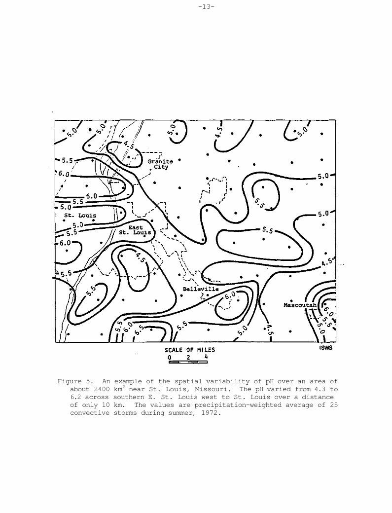
The St. Louis study showed great variability within a 2400 km2 area over and downwind of the city. Values of acidity ranged from less than 4.5 pH near industrialized areas to greater than 6.0 pH at many urban and rural sites (Figure 5).

-10-

Figure 2. The 1955-1956 network of precipitation samplers used by Dr. C.E. Junge and sponsored by the U.S. Air Force. These sites were largely located at first-order weather stations.

i

- 1 1 -

Figure 3. The 1960-1966 Network of precipitation samplers operated by the U.S. Public Health Service and later in the period by the National Center for Atmospheric Research. The closed circles are stations previously used in the Junge network (figure 2) and the stars repre­sent new stations initiated for this network.

- 1 2 -

SULFUR ADDED TO THE SOIL BY RAINFALL: ILLINOIS EXPERIMENTS (Amounts expressed in pounds per acre)

Month 1913 1914 1915 1916 1917 1918 1919 Avg

JAN 4.3 2.9 5.8 7.5 3.7 3.5 4.2 4.6 FEB 2.7 6.9 3.4 2.7 3.3 6.0 5.1 4.3 MAR 4.5 4.0 4.0 4.7 5.1 3.7 (1) 4.3 APR 4.1 4.2 3.0 4.6 5.0 6.0 3.2 4.3 MAY 1.6 2.2 5.1 8.6 5.6 4.8 5.8 4.8 JUN 2.6 2.7 3.3 5.2 4.6 4.3 4.5 3.9 JUL 2.0 2.0 4.4 1.9 3.1 2.2 1.8 2.5 AUG 2.0 5.7 4.1 2.0 4.3 4.7 4.7 3.9 SEP 3.3 3.0 3.0 2.3 2.5 3.4 3.0 2.9 OCT 5.1 3.0 1.6 5.0 4.9 5.8 2.9 4.0 NOV 4.4 2.4 2.5 3.1 3.9 2.4 3.0 3.1 DEC 3.4 1.6 5.4 3.3 1.7 0.7 1.6 2.5

Total 40.0 40.5 45.5 51.0 47.7 47.6 39.81 45.1 Average 3.3 3.4 3.8 4.3 4.0 4.0 3.6 3.8

(1)No record of March rainfall

Figure 4. The deposition of sulfur at Champaign, Illinois by month for the period 1913 through 1919. The average annual value of 45.1 lbs acre-1 (50.5 kg ha-1)is about twice the current average value of 23.3 kg ha-1

obtained for the years 1979 through 1981. These data are from Bulletin 227, University of Illinois Agricultural Experiment Station, Urbana, June 1920.

-13-

Figure 5. An example of the spatial variability of pH over an area of about 2400 km2 near St. Louis, Missouri. The pH varied from 4.3 to 6.2 across southern E. St. Louis west to St. Louis over a distance of only 10 km. The values are precipitation-weighted average of 25 convective storms during summer, 1972.

-14-

The single longest continuing record in this country is the Hubbard Brook site in New Hamsphire which has been in operation since 1963.

Network Operations

This leads me to a brief recounting of the networks that are currently in operation. At last count about 71 recent-past and current monitoring efforts have been identified in Canada, Mexico, and the United States. The largest of these is the network operated by the National Atmospheric Deposition Program which currently includes 116 stations shown in Figure 6. The network was initiated in 1978 with 16 stations and now extends from American Samoa to Maine and from Alaska to Florida. A cooperative effort with Canada involves operation of three of these stations across the border. This network will form the core of the National Trends Network being implemented by the USGS as a task set forth by the federal Interagency Task Force on Acidic Precipitation.

A longer operating network is the Multi-state Atmospheric Power Production Pollution Study (MAP3S) network begun by the Department of Energy and currently is a cooperative effort with EPA. This network also seen in Figure 6 began with 4 stations in 1976 with 4 added in 1978. The MAP3S network is different from the NADP in that event samples are collected as opposed to the weekly samples of the much larger national NADP/NTN.

I do not intend to describe for you all of the various monitoring networks that either were recently operated or are currently in use. I encourage you to read Wisniewski and Kinsman (Bulletin American Meteoro­logical Society, Vol. 63, 598-618, 1982) for further information.

SAMPLE, COLLECTION, HANDLING, AND ANALYSIS

Sample Collection

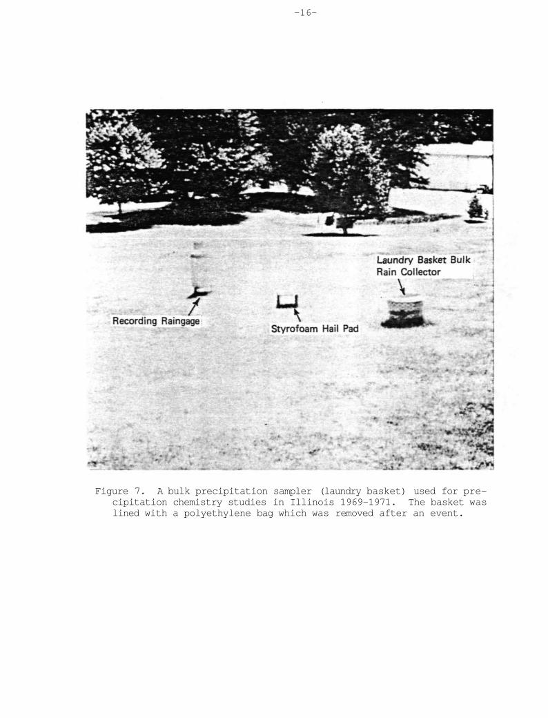
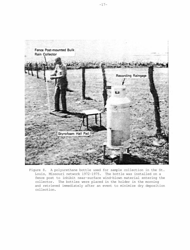
Scientists collecting precipitation samples have used almost anything that one can imagine. This "anything" covers the range from glass bottles (both clear and darkened) to baby bottle plastic liners. In Figure 7 a laundry basket is shown staked to the ground and supplied with a clean polyethylene liner for precipitation collection. The nearness of the opening to the ground invites contamination of samples from wind-blown material. An improvement of this concept is shown in Figure 8. The lower half of a polyethylene bottle is secured by means of hose clamps to a common fence post about 1 m above ground. Prior to a precipitation event, a slightly smaller diameter, clean bottle with a fitted polyethylene liner is placed in the holder. The entire bottle with liner and sample is transported to the laboratory. The sample is removed, a new liner inserted, and the bottle is returned for re-use in the field. For analyses that require very large samples, an entire roof top shown in

-15-

Figure 6. The currently operating National Atmospheric Deposition Program/National Trends Network/Multistate Atmospheric Power Production Pollution Study precipitation sampling sites. The solid circles are the MAP3S event sampler locations. The star indicates a site where both event and weekly samples are collected. The map is correct as of July 1983.

-16-

Figure 7. A bulk precipitation sampler (laundry basket) used for pre­cipitation chemistry studies in Illinois 1969-1971. The basket was lined with a polyethylene bag which was removed after an event.

-17-

Figure 8. A polyurethane bottle used for sample collection in the St. Louis, Missouri network 1972-1975. The bottle was installed on a fence post to inhibit near-surface wind-blown material entering the collector. The bottles were placed in the holder in the morning and retrieved immediately after an event to minimize dry deposition collection.

-18-

Figure 9 was carefully covered with polyethylene and used as the collec­tion surface. Such a large area also increases contamination risk from dry deposition, wind-raised foreign material, and birds. An example of a sequential collector is shown in Figure 10. A number of such devices have been built, but all of them are directed toward acquiring one sample after another during a single rain event. There are means to control the sample collection by either the volume or time interval and some devices incorporate both features. The most widely deployed sample collection equipment is shown in Figure 11. A precipitation sensitive switch is used to activate a motor to uncover and cover the wet-side bucket collector. The dry-side bucket is exposed to dry deposition during non-precipitating periods. This type of collector is currently used for the NADP/NTN and MAP3S networks. Obviously, the quality of the chemical analysis is highly dependent upon the quality of the sample collecting vessel. I recall a project in which the investigator thought it would be cost-saving to use the existing weighing-bucket raingage network to collect samples for trace metal analysis. Unfortunately, zinc was one of the metals of great interest for this particular project and most weighing-bucket raingages use a zinc-coated pail. As a result the entire effort was wasted, but a valuable lesson was learned. The type of collecting vessel is somewhat determined by the goal of a particular sampling program.

Anyone wishing to collect rain or snow samples for chemical analysis are cautioned to first check the collection vessel for the chemicals of interest, to see if, in fact, the analysis will be contaminated.

A second serious consideration is whether one wishes to collect a bulk sample as opposed to a wet-only sample. A bulk sample is one which is directly exposed to the atmosphere and remains open throughout a pre­scribed interval of time. This is not a very satisfactory way of collecting precipitation samples because of the natural tendency of birds to light on the rim of the collector always facing outward contributing to the debris deposited inside of the container. In addition, dust, leaves and other natural materials are likely to enter the sampler and contami­nate the precipitation in an unknown way.

The interval between the collection of samples is also largely determined by the goals for the sampling program. If one wants to study the effects of precipitation chemistry on the forest, for example, it is highly unlikely that it is necessary to collect samples on intervals of anything less than a one week period and perhaps even one month may suffice for the majority of biological effects studies. On the other hand, if one wants to study the variability of precipitation chemistry in convective storms during the warm season, a sequential sampler may be necessary to obtain samples as frequently as one or more per minute. So in establishing a sampling program it is most important to carefully consider the goal of that program and then determine the need for event as opposed to less costly, longer period sampling to achieve that goal. The

-19-

Figure 9. A roof top lined with polyethylene to collect large volumes of water for sensitive analyses of radioactive materials. This form of collection is nearly useless for pollutant wet deposition studies because of the large area exposed to dry deposition.

-20-

Figure 10. A sequential sampler designed to collect a given volume of precipitation in individual bottles. The rate of bottle usage was determined by the precipitation rate. Later versions allow the op­erator to specify time intervals between bottle collections.

-21-

Figure 11. The currently used wet/dry sampler considered standard equipment for the NADP/NTN and MAP3S networks. The covered bucket collector minimizes deposition of dry material between precipitation events. A precipitation-activated motor uncovers the wet side and covers the otherwise exposed dry bucket collector. After a precip­itation event the cover returns to seal the sample in the wet bucket collector.

-22-

NADP/NTN weekly collection network is an arbitration between event samples and monthly samples with the program goals to determine the long-term trend of precipitation chemistry and atmospheric deposition effects on the environment.

Sample Handling

Once a sample has been confined within the collecting vessel the safest thing is to then immediately seal that vessel and carry it or ship it to the analytical laboratory. However, it is a practice in some operations to allow prior handling of the sample such as withdrawal of aliquots for the local determination of a particular parameter. For example, the NADP allows extraction of a few milliliters for the field determination of pH and conductivity. Immediately after the aliquot has been withdrawn, the sample is sealed and then shipped to a central laboratory for further chemical analysis. Shipment of the sample is an important consideration for any type of sampling program since one must be sure that the collecting vessel does not leak in transit.

Sample Analysis

Written documentation of everything concerning the sample up to this point should be provided for the laboratory staff as the analysis of precipitation chemistry proceeds. Certainly, any laboratory, whether it is adjacent to the sampling site or several thousands of kilometers distant, should have certain analytical capabilities for the determination of trace materials in precipitation. The analysts must be trained to recognize the expected concentrations in precipitation and detect contamination in a sample. Contamination can originate either from natural causes or handling of the sample.

And finally, one must be alert that even though a determination may be perfectly accurate and within statistically allowable errors of the instrumentation, the value may, in fact, be excluded from a data set for other reasons. For example, a loose covering over the collection vessel can allow crustal dust to enter into the collector during non-precipitat­ing intervals and can artifically raise the concentrations of those materials. A "leaky" seal results in values that are not representative of precipitation but are more representative of a bulk sample. The major point is that the sample quality control does not begin or end in the laboratory but must be extended to include everything from the sample collection in the field to the point of preparing the data for dissemina­tion or further interpretation and archiving.

Concern has been expressed about the chemical integrity of samples collected less frequently than the duration of a single storm. There is reason for some scientific inquiry on this matter, but the available data suggest that any chemical changes in a sample will occur in a relatively brief period after the precipitation has ended. However, event samples

-23-

may not be any more stable than weekly samples if the delay between the collection of the sample and its analysis is of the order of one or more days. Consequently, until real-time chemical analysis can be performed in the field, all currently available data contain a largely unknown contribution from this effect.

SELECTED INTERPRETIVE ANALYSES

Precipitation-Weighted Average pH

And now having said all of this, I would like to share with you some analyses of the NADP network data that are currently archived in the EPA data files. The first series of maps illustrates the changing pattern of pH distribution as additional stations were added to the network during 1979 to 1981. Figure 12 shows the first set of data for 1979 from the NADP network and Figure 15 indicates the most recently available pH map showing how the variability has apparently increased in the western states due to the siting of additional stations. The gradual increase of the number of samples at each site used to obtain the precipitation-weighted average has produced little change in the northeast U.S. pH pattern. This is easily seen by comparing Figures 12, 13, 14, and 15. A graphical differential analysis of the patterns shown in Figures 12 and 15 reveal only random differences of ±0.1 pH units in the region from Illinois eastward and from Tennessee northward.

Total and Specific Ion Concentrations

An attempt has been made to identify those cations and anions that contribute most to the total ion loading in precipitation over the United States. The dominating feature of the average monthly total ion concen­tration shown in Figure 16 is a relative high located over southern Ontario north of Lakes Erie and Ontario and extending northeast along the St. Lawrence valley. Across Illinois, along the Ohio River Valley, and extending into New England, typical values are 200 yeq L-1 with a slight increase toward Nova Scotia. The Great Plains and the front range of the Rocky Mountains in the U.S. show values of about 150 yeq L-1, and there is a relative minimum over Idaho, Washington, and Oregon.

It is interesting to note that the maximum concentrations are displaced slightly to the northeast of the commonly perceived maximum emissions region of the industrialized Ohio River Valley. The immediate inclination is to interpret this pattern as a downwind displacement due to the mean flow pattern. However, the distribution seems to suggest that wet deposition maximums occur in close proximity to source regions.

The average chloride concentrations show the largest values along the eastern and western coastal areas (Figure 17). These concentrations appear to maximize along those respective coast-line areas where major synoptic storm systems frequently enter the continent from the west or

-24-

Figure 12. The precipitation-weighted average pH obtained from all available samples in the NADP network through May 29, 1979. The closed circles in this map and on those that follow indicate stations where samples were included to define the isopleths. Note the position of the pH = 4.4 isopleth and the absence of a pattern in the west.

-25-

Figure 13. The same as figure 12, but includes samples through Sep­tember 19, 1979 and additional stations. More pattern definition is achieved with additional stations in the west. The pH = 4.4 isopleth has shifted slightly through Illinois in response to more data in western lower Michigan and southern Illinois.

Figure 14. The same as figure 12, but includes samples through Sep­tember 2, 1980 and additional stations. Minor changes of the pattern in the northeast U.S. can be seen as well as in the north-central Great Plains where values of pH > 6.0 are observed.

-26-

-27-

Figure 15. The same as figure 12, but includes samples through January 5, 1982 and additional stations. Note the relative stability of the northeast U.S. pattern and that of the north-central Great Plains (see text).

-28-

Figure 16. The precipitation-weighted average total ion concentration (µeq L-1) as determined from measurements of H+, Na+, Ca2+, NH4

+, NO3-, C1-, and SO42-. Samples through 1981 were used in this analysis.

-29-

Figure 17. The precipitation-weighted chloride concentration (µeq L-1) for all samples available through 1981. The solid line depicts the concentration and the dashed line the percentage of the total ion concentration shown in figure 16. Note the expected coastline maximums.

-30-

move northward along the eastern seaboard. Whether this observation can be borne out by relating seasonal patterns in coastal storm tracks to chloride concentrations has yet to be determined. Minimum values of chloride are observed through the central, south, and western United States, as well as most of Canada. The sodium ion shows an identical pattern to chloride emphasizing the oceanic influence on the concentration pattern for these ions. The dashed lines in Figure 17-22 indicate the percentage of the total ion concentration attributed to the individual ions.

The calcium ion concentration distribution in Figure 18 shows minimum values along the coasts and maximum values over the continent. A maximum in the western provinces of Canada extends through the Great Plains into a second maximum in west Texas, southern Arizona, and New Mexico. The Great Plains maximum appears to be associated with the semi-arid agricultural practices of that area.

Stations in South Dakota, Nebraska, and southern Minnesota show ammonium concentrations of greater than 40 yeq L-1, and equally high values were also observed over extreme southern Ontario (Figure 19). The relative contribution of the ammonium to the ion total shows a clearly distinguishable maximum in excess of 35% over South Dakota and Nebraska.

It is speculated that the observed maximum ammonium concentration values can be attributed to certain types of farming activities, such as cattle feed lot operations. In certain other areas, perhaps ammo­nium-bearing fertilizers may contribute during certain seasons of the year. It is important to extend this analysis to individual seasons to explore possible explanations for these observations.

The nitrate concentration distribution in Figure 20 shows the interesting fact that values greater than 20 yeq L-1 extend along an axis from the extreme southwestern U.S. toward the northeast across the entire continent. Within that broad area of relatively high concentrations, two maximums are observed. The first is over south-central California and the second and larger maximum, extends northeastward over lower Ontario. The Gulf Coast region from Texas to Florida shows very little nitrate in precipitation.

Sulfate ion concentration distribution is dominated by a large maximum over the entire eastern U.S. and southeastern Canada (Figure 21). The high center is located over southern Ontario, and extends to the northeast along the St. Lawrence Valley. Concentrations in excess of 40 yeq L-1 occur from lower James Bay to Minnesota, southward to Oklahoma, southeastward to central Georgia, and then off the Carolina coast. Two other areas with 40 yeq L-1 are observed, one over the western provinces of Canada including British Columbia and one over southern Arizona. In an analysis not presented in this paper, it was found that sulfate was the largest contributor to the total ion concentration over nearly all of North America, and where it was not largest, it was either second or third largest.

-31-

Figure 18. The same as figure 17, but for calcium. This ion associated with crustal dust maximizes in the continental interior.

-32-

Figure 19. The same as figure 17, but for ammonium. The maximum in the Great Plains may be influenced by the extensive feed-lot industry in that area.

-33-

Figure 20. The same as figure 17, but for nitrate. Values in excess of 20 µeq L-1 dominate nearly two-thirds of the U.S. and extend between the east and west coasts.

-34-

Figure 21. The same as figure 17, but for sulfate. This ion accounts for more than one-third of the total ion concentration in the U.S. from the Mississippi River eastward and from Tennessee and North Carolina northward.

-35-

Finally, the hydrogen ion concentrations obtained from measurements of precipitation pH show maximum values over the Ohio River Valley and northeastward into northern New York and Vermont (Figure 22). Values in excess of 25 µeq L-1 (i.e., pH < 4.6) are observed in an area bounded by a line extending southwestward from Newfoundland to Lake Superior, south to northeast Arkansas, and southeastward to the Atlantic Ocean. The maximum concentrations of nitrate and sulfate are located in southern Ontario, and north of Lakes Erie and Ontario, but the maximum hydrogen concentrations are nearly totally confined to the U.S. from Indiana through Ohio, Pennsylvania and New York.

Among the principal features of the several distributions are (1) the sea salt constituents, sodium and chloride, exhibited relative maximums along the east and west coastal regions of North America; (2) elements commonly associated with crustal dust, that is, calcium and magnesium, maximized in the continental interior; (3) a relative ammonium maximum seen in the central Great Plains may be associated with particular agricultural practices in that area; and (4) those ions of most concern to air quality and acidic precipitation considerations maximize in the industrialized east with the sulfate and nitrate maximums in southern Ontario paralleling the St. Lawrence Valley and the hydrogen maximum over the Ohio River Valley.

Precipitation Chemistry Characterization

In an effort to further simplify the characterization of precipitati­on chemistry over the eastern U.S., the four ions contributing the greatest percentage to the total ion concentration were selected from each station. In general, the top four ions at any one station accounted for about 90% of the total. From the previously presented data, it is readily seen that sulfate and hydrogen together account for 60 to 70% of the total ion concentration in the eastern states. If nitrate is added to these two, the total is raised to about 75% over much of the northeast. The addition of a fourth ion depends on the region under consideration and is quite variable. The regional characterization of precipitation chemistry by 4 ions is shown in Figure 23. The largest area of the eastern U.S. is characterized by hydrogen ion, sulfate, nitrate, and ammonium, in that order. This area encompasses Wisconsin, most of Michigan, Illinois, Indiana, Ohio, western Pennsylvania, most of New York, and into the southern states of Kentucky, western Tennessee, and parts of Mississippi and Alabama. If ammonium is replaced with calcium, an additional area encompassing Ontario, southern Quebec, and a small portion of eastern Tennessee is included. Through Vermont, New Hampshire, western Maine, a small portion of the Carolinas, northern Georgia, and the Gulf coastal states of Mississippi, Alabama, and Florida the calcium or ammonium is replaced with sodium. In this region, hydrogen, sulfate, nitrate, and sodium account for nearly 90% of the total ion concentration. Finally, sodium, chloride, hydrogen, and sulfate ions dominate the east coastal areas.

-36-

Figure 22. The same as figure 17, but for hydrogen determined from pH determinations. This ion accounts for about one-third of the total ion concentration along the Ohio River Valley northeastward to east­ern New York.

-37-

Figure 23. The four ions that contribute ≥90% of the total ion concen­tration in the eastern U.S. Note that H+, SO42-, and NO3- dominate except along the east coast. The fourth ion varies regionally. The data through 1981 do not permit a similar analysis of the western U.S.

-38-

Ion Ratio Analysis

The ratio of hydrogen to the sum of sulfate and nitrate (all expressed in microequivalents per liter) is indicative of possible chemical forms responsible for the observed concentrations. For example, if all of the hydrogen ion came from the presence of sulfuric and nitric acids the ratio would be one. The maximum ratio of about 0.6 shown in Figure 24 extends along the Ohio River Valley northeastward into southern Maine. The distribution of this ratio suggests a large fraction of the total sulfate and nitrate concentration is associated with non-acidic compounds.

Application of the same calculation with ammonium as the numerator suggests a relative abundance of ammonium sulfate and/or ammonium nitrate in the Great Plains (Figure 25). Ratios in excess of 0.4 are observed in central California northward to central Washington. Most of the northeast U.S. is characterized by ratios less than 0.2.

The ratio of calcium to the sulfate and nitrate sum is shown in Figure 26. Similar to the ammonium ratios, values less than 0.2 dominate in the northeastern states. A relative maximum is observed over the central Great Plains with ratios exceeding 0.8 seen over the Great Basin.

These three ratio maps suggest the following: 1) the east is dominated by high ratios of hydrogen to the sum of sulfate and nitrate possibly related to fossil fuel consumption; 2) the Great Plains are dominated by large ammonium to the sum of sulfate and nitrate ratios, perhaps associated with agricultural practices; and 3) the Great Basin and secondarily the Great Plains show high ratios of calcium to the sum of sulfate and nitrate likely associated with crustal dust material. Further research into ratios may lead to a better understanding of sources for the observed precipitation chemistry.

Trend of pH

A final word about trends of the chemical components in precipitati­on. As mentioned earlier in this presentation, there are no long-term continuous measurements available to determine a regional trend. The Hubbard Brook, New Hamsphire station shows a rather steady decline of sulfate since measurements began in the early 1960's with little detect­able trend in nitrate. To translate these data to discuss trends over a region is very misleading and should be avoided.

Much concern has been expressed over a perceived trend toward increasing acidity based on data obtained in 1955-1956, 1960-1966, and 1972-1973. Unfortunately, the key data that determines the trend, the 1955-1956 period, were modified by crustal dust associated with a large scale drought.

-39-

Figure 24. The average ratio of hydrogen to the sum of sulfate and nitrate. A ratio of one would suggest that the hydrogen ion arises from sulfuric and nitric acid in precipitation. Note the maximum value of ≥0.6 extends along the Ohio River Valley northeastward to Maine.

-40-

Figure 25. The same as figure 24, but for ammonium to the sum of sulfate and nitrate. The Great Plains maximum of ≥0.6 suggests the presence of ammonium sulfate and/or ammonium nitrate.

-41-

Figure 26. The same as figure 24, but for calcium to the sum of sulfate and nitrate. The Great Basin maximum of ≥0.8 suggests the presence of calcium sulfate and/or calcium nitrate.

-42-

The measurement of pH was not considered in the analysis protocol of this early data set, but estimated values were calculated by means of an ion-balance equation. The calculated distribution of pH for 1955-1956 is shown in Figure 27.

When reasonable mathematical adjustments to the crustal dust contami­nated chemistry are made, the acidity increases to values comparable to currently observed values. Selected isopleths of the recalculated pH are shown as dashed lines in Figure 28. The solid lines represent the precipitation-weighted average pH for samples from the NADP network through June, 1980. Focusing on the pH = 4.4 isopleth in the northeast U.S. one can readily observe reasonable agreement between the adjusted 1955-1956 data and the currently obtained average values. Therefore, there does not appear to be a discernible increase of acidity of precipi­tation in the eastern U.S. within the limitations of available data.

SUMMARY

In summary, I have tried to emphasize the complexity of sampling and analyzing precipitation samples and I believe many of the problems have been overcome with present-day technology. The problems enumerated cast doubt on the utility of past data for shedding light on current acidic precipitation research.

I have also emphasized the nearly complete lack of a precipitation chemistry data base prior to 1979. Any determination of a trend using sporadically obtained data prior to 1979 becomes speculation and is subject to additional interpretation.

Lastly, I have tried to share with you some recent findings from the rapidly increasing national data base. The length of record is still inadequate to describe the precipitation chemistry from a climatological point of view. The natural variability of air motions, pollutant loading, and precipitation is continuing to influence the stabilization of mean acid deposition values. The monitoring program the U.S. has initiated is critical to a better understanding of the acid deposition phenomenon and, by 1989, the 10-year data base will permit a much firmer assessment of the issues surrounding changing precipitation chemical quality and its environmental consequences.

-43-

Figure 27. The pH distribution calculated from the analyses of monthly samples collected by Junge during 1955-1956.

-44-

Figure 28. The dashed line represents recalculated values of pH after adjustment for anomously high concentrations of calcium and magnesium. The solid line represents the measured precipitation-weighted pH values from NADP samples through July 1980. The agreement in the northeast U.S. is striking.

-45-

CHAPTER 3

A Comparison of Four Methods of Computing Precipitation pH Averages

Gary J. Stensland and

Van C. Bowersox

ABSTRACT

Precipitation chemistry data for sites in the National Atmospheric Deposition Program (NADP) network were used to compare four methods of computing pH averages. From 15 to 140 weekly precipitation pH values were available for the 54 sites included in this study. The following four pH averages were examined: mean, median, sample volume weighted average pH, and the average pH calculated from the weighted average conservative ion concentrations. The weighted average pH varied from 4.10 for an Ohio site to 5.50 for an Oregon site and is the type of average generally reported in the literature. When the mean, median, or calculated average pH values were subtracted from the weighted average pH, the differences were from -0.05 to 0.27 for sites east of the Mississippi River. The differences frequently had larger magnitudes for sites west of the Mississippi River. In the extreme, for two Northern Great Plains sites with weighted average pH values of 5.11 and 5.21, the other three types of averages resulted in values that were 0.76 to 1.11 pH units higher. With such large differences at some sites, it is important to select the type of average most appropriate for the particular application being considered.

Introduction

The spatial and temporal patterns of the major inorganic ions in rain and snow have been and are being actively studied by scientists in many countries. The pattern for precipitation acidity in the United States during the last 30 years has been analyzed by several investigators and conflicting results have been reported (Likens and Butler, 1981; Stensland and Semonin, 1982; Hansen and Hidy, 1982). Problems in the interpretation of the time trends of pH have resulted from such things as changes in sampling methods and the fact that the samples were not collected at the same locations over the time periods under investigation. Another complicating factor is that different averaging techniques were used to produce the pH maps in the different studies. The purpose of this paper is to compare four different average pH maps for the United States for one large data set. The results show that indeed there are significant differences between the four approaches for certain regions of the United States. Finally there is some discussion as to which approach might be the most appropriate for various applications.

-46-

Methods

General Description of the Database

Data through 1981 from the National Atmospheric Deposition Program (NADP) were used for this study (NADP, 1978-1981). This data set was chosen because it includes sites from across the United States, and thus a broad range of acidity levels was encountered. The first NADP sites began operation in 1978. By the end of 1978, about 20 sites were in operation; almost 100 were in operation by the end of 1981; and about 140 were in operation by the end of 1983. During the early years of the project, the sites were concentrated in the eastern U.S.

All sites are equipped with the same automatic wet/dry precipitation chemistry sampler. Each week, on Tuesday, the sample bucket on the wet deposition side of the sampler is removed and sent to the Central Analytical Laboratory (CAL). All NADP samples are analyzed at a single laboratory at the Illinois State Water Survey, the CAL of NADP. At the CAL, the sample volume, pH, and solution conductance are measured, along with concentrations of the following soluble ions: sulfate, nitrate, chloride, ammonium, calcium, magnesium, sodium, potassium, and phosphate (which is usually below the analytical detection limit and is not considered in this paper).

At each site the sampling period precipitation and the volume of sample caught in the wet deposition bucket are reported. Most sites employ a recording (weighing-bucket) raingage, which has been modified to include an "event marker"to record periods when the wet-side bucket was exposed to precipitation. This record is evaluated to ascertain that the wet/dry sampler operated correctly to collect a wet-deposition-only sample. Even when no precipitation occurs, the wet-side bucket is sent to the CAL. The contents of these dry wet-side buckets are analyzed as (quality assurance) system blank samples (Stensland, Peden, and Bowersox, 1983).

Data for each wet deposition sample, along with pertinent information from communications with site operators, are reviewed by CAL data management staff to assess a) whether a wet-deposition-only sample was collected, b) whether the proper sample handling and measurement procedures were followed, and c) whether visible organic or other extraneous contamination in the sample had produced a sample unrepresentative for the site. Along with the various physical and chemical measurements of each sample, a record is generated in a computerized database to document the results of this data validation process.

Data Selection Procedures

Since the NADP computerized database contains wet deposition chemical data as well as other supplemental and qualifying information for each sample, the user community is afforded the opportunity of selecting data appropriate to its research objectives. For example, if the volume of water in the bucket received at the CAL was ≤10 mL, then only pH or pH and conductance measurements are available and a user must decide whether or

-47-

not to include samples with this limited data in his/ her study. As another example, if for a given year of data at a site there were 30 weeks with precipitation, but 1/2 of these were not wet-deposition-only samples, data users must decide whether the 15 weeks of data reported are sufficient to represent the site for the year under consideration.

With the objective of this study to compare 4 different scientifically valid pH averages for as many NADP sites as possible, certain data selection criteria were opted. Factors considered in obtaining a representative data set included:

1. Climate averages of precipitation amount and frequency of occurrence vary with the season of the year over much of the country. The largest and most regular seasonal variations occur in the western U.S., particularly in the Northern Plains, the desert Southwest, and California, and along the coastal southeastern U.S., for example Florida (U.S. Dept. of Interior, Geological Survey, 1970).

2. It has been shown that the concentations of the major inorganic constituents of precipitation exhibit seasonal excursions at eastern U.S. sampling locations. Summertime minima and wintertime maxima in the record of precipitation pH were reported in New York and New Hampshire (Likens and Borman, 1974). Examination of the data from the MAP3S network (MAP3S PCN, 1977) at Whiteface and Ithaca, NY, and State College, PA, and Charlottesville, VA, has suggested that precipitation sulfate maximizes throughout most of the northeastern U.S. in summer, as does hydrogen ion (Pack, 1978; Bowersox and dePena, 1980). A comparison of aerosol and precipitation sulfate throughout much of the eastern U.S. showed that May through September concentrations were more than 20% higher than November through March concentrations, and that seasonal differences could be as much as 60% higher in the warm period. In addition, NADP wet deposition data support a south to north gradient in warm versus cold period variations in precipitation nitrate. May through September nitrate concentrations were 30% to 60% higher than November through March values in the south, but the seasonal differences were insignificant at northern latitudes (Bowersox and Stensland, 1981).

To mitigate against the potential for biases due to these seasonal variations or other intra-annual variations, the analysis was limited to whole (site) years of data. For a site year to be considered as "representative," there must have been available data for 3/4 or more of the wet deposition weeks that occurred throughout the year. This somewhat arbitrary criterion has been used by others for selecting data to represent annual ion concentration and deposition statistics from the NADP data set.

-48-

Next, it was necessary to define a wet deposition week, given the attributes of the NADP sampling and analytical scheme. At the CAL, samples of nominally 50 mL or more liquid precipitation are analyzed at the concentration received, that is, without further dilution. This volume of 50 mL, normalized by the collection cross section (bucket radius = 14.7 cm), translates to a liquid precipitation depth of 0.03 inches or 0.76 mm. Smaller volumes require an initial dilution step in order to satisfy the liquid volume requirement of each analytical procedure (Stensland, et al., 1980). This dilution step adds uncertainties to the reported data, due to the extra handling and due to the propagation of errors from the calculation of a dilution factor. To avoid these uncertainties, a wet deposition week was defined as any week during which the precipitation equalled or exceeded 0.76 mm, i.e., a week during which a sample of 50 mL or more liquid volume might have been realized. Weekly precipitation amounts were estimated as the greater of the (wet bucket) sample depth and the precipitation depth reported from precipitation gage measurements.

To assess the number of wet deposition weeks with available precipitation chemistry data for any site year, some additional constraints were considered:

(1) Inasmuch as the standard NADP sample is a 1-week sample, the duration of sampling had to be no less than 6.5 and no more than 7.5 days.

(2) A complete set of ion concentration measurements for a sample to which no diluting water was added must have been reported.

(3) It was necessary that the sample collection bucket be exposed to atmospheric deposition only during precipitation (and minimally for handling). In other words, only data for wet-deposition-only samples were used.

(4) Sample collection, handling, and custody had to follow NADP specified procedures (National Atmospheric Deposition Program, 1982). These procedures are intended to provide a uniformity of collection and storage containers, and a uniformity of protocol for handling and analyzing the samples.

(5) If insect or other animal debris or plant debris or other contaminant introduced through handling or vandalism was noted by sample collection or CAL personnel, then the ion composition of that sample must not have been anomalous when compared to the available historical record of valid NADP precipitation chemistry for that site.

Finally the ratio of the number of wet deposition weeks of available data satisfying the above criteria and the total number of wet deposition weeks (defined earlier) was formed. When this ratio was 0.75 or more, the site year of available data was statistically summarized for this paper. Table 1 summarizes the sites with 1, 2 or 3 years of data used in this study. The location of these sites is shown in Figure 1.

-49-

Figure 1. Location and identification number of NADP sites used in the pH averaging comparisons. (American Samoa not shown.)

-50-

Description of pH Averages

For this study, the precipitation pH values obtained at the CAL were used in calculating the various pH averages. Due to an incomplete quality assurance evaluation of field laboratory performance, these were taken in lieu of the pH measurements reported at field sites. The methodology in Table 2 describes how the median, mean, and weighted average pH were determined for each site listed in Table 1. Recall that the weighted average pH has been the one most frequently reported in the literature in recent years.

The calculated average pH is typically reported only when measured pH data are not available. The measured ion concentrations in microequivalents per liter are used in the charge balance equation

to calculate [H+], and from [H+], pH. Samples are assumed to be in equillibrium with atmospheric carbon dioxide, which leads to

and

At 25°C, KH = 0.0342 X 106 ueq L-1 atm-1 and K1 = 4.5 X 10-1 ueq L-1, K2 = 9.4 X 10-5 ueq L-1, and KW = 10-2 (ueq L - 1 ) 2 (see Harned and Davis, 1943; Harned and Scholes, 1941; Robinson and Stokes, 1959). The partial pressure of CO2 used in these calculations was 335 ppm. For samples with pH <8.0, [HCO3 ]>106[CO32-]. Therefore, the term for [CO32-] in Eq. (1) can be neglected for precipitation samples, producing an equation that is quadratic in [H ].

If we define

(Net Ions) =

then equation (1) becomes

which can be rewritten as

The solution of this quadratic equation with physical meaning is

where the +6 term results from using ion concentrations in microequivalents per liter. Some additional details of this calculational procedure are given by Stensland (1983).

-51-

Table 1. Results by site and by year from the data selection and evaluation process. The ratio is the number of weeks of available data meeting all criteria (see text) divided by the total number of wet deposition weeks.

Whole Total No. NADP Ratio (x 100) No. Samples Data Qualifying Site 1979 1980 1981 1979 1980 1981 Years Samples AR27 NOa NAb 91 NO NA 40 1 40 AZ06 NO NA 94 NO NA 15 1 15 CA45 NA 89 86 NA 24 25 2 49 COOO NO NA 87 NO NA 27 1 27 C015 NA 79 95 NA 30 37 2 67 C019 NO NA 85 NO NA 34 1 34 C021 40 48 81 17 16 29 1 29 C022 NA 84 79 NA 21 27 2 48 FL03 83 40 71 35 19 24 1 35 GA41 91 84 82 41 36 33 3 110 ID03 NO NA 75 NO NA 27 1 27 IL11 NA 90 87 NA 38 39 2 77 IL19 NO NA 89 NO NA 40 1 40 IL35 NA 85 83 NA 33 38 2 71 IL63 NA 82 80 NA 32 37 2 69 IN34 NO NA 87 NO NA 41 1 41 ME00 NO NA 76 NO NA 37 1 37 ME02 NO NA 93 NO NA 43 1 43 ME09 NA NA 90 NA NA 45 1 45 M126 NA 83 90 NA 38 37 2 75 MN16 85 72 89 39 31 39 2 78 MN27 81 79 85 34 30 33 3 97 MS14 NO NA 90 NO NA 36 1 36 NC03 83 77 91 39 33 40 3 112 NC25 91 88 80 43 42 35 3 120 NC34 77 86 95 37 36 39 3 112 NC35 93 98 95 42 43 40 3 125 NC41 84 87 82 37 39 32 3 108 NE15 78 76 83 31 25 29 3 85 NH02 90 81 92 43 39 45 3 127 NY08 NA 88 76 NA 42 39 2 81 NY10 NO NA 94 NO NA 46 1 46 NY12 NO 57 88 NO 28 44 1 44 NY20 92 75 73 45 36 38 2 81 NY51 NA 89 84 NA 39 42 2 81 0H17 92 94 98 44 44 39 3 127 0H49 89 86 98 41 42 45 3 128 0H71 91 85 90 43 41 38 3 122 OR02 NA 86 87 NA 36 34 2 70 OR08 NO NA 78 NO NA 28 1 28 0R10 NO NA 97 NO NA 37 1 37

-52-

Table 1 (continued)

a Site was Not in Operation during this year. b Ratio is Not Available because it was not rigorously calculated; due to the limited data available for this site year, an estimate showed that the ratio was much less than 75.

Whole Total No. NADP Ratio (x 100) No. Samples Data Qualifying Site 1979 1980 1981 1979 1980 1981 Years Samples 0R17 NO NA 82 NO NA 28 1 28 0R99 NA 71 89 NA 29 34 1 34 PA42 NA 90 92 NA 43 44 2 87 SC18 NA 95 95 NA 38 35 2 73 TN00 NO NA 94 NO NA 44 1 44 TN11 NO NA 75 NO NA 36 1 36 TX04 NO NA 89 NO NA 25 1 25 TX53 NO NA 77 NO NA 30 1 30 VA13 87 72 57 34 33 24 1 34 WA14 NO NA 87 NO NA 40 1 40 WI36 NO 93 82 NO 39 37 2 76 WV18 88 94 94 44 49 47 3 140 AS01 NO, NA 77 NO NA 40 1 40

-53-

Table 2. Description of pH averaging procedures.

1. Median pH: All the measured pH values for a site were put in ascending or decending order and the median pH was then identified.

2. Mean pH: A simple arithmetic average of all measured pH values for a site was calculated. This is equivalent to the pH value for the geometric average of the measured hydrogen ion concentrations for a site, i.e.,

Mean pH = -log10[(H1,H2,...HN)1/N],

where N is the total number of samples.

3. Weighted: This pH value corresponds to the sample volume weighted average of the measured hydrogen ion concentrations for a site, i.e.,

Weighted pH = -log10[Sum(HiVi)/Sum(Vi)]

4. Calculated This pH value was calculated for a site from the sample Average pH: volume weighted average concentrations of the

conservative ions (such as sulfate, calcium, etc., but not hydrogen, hydroxide, and bicarbonate). This is analogous to compositing all the precipitation for the entire time period into one large container that is in equillibrium with atmospheric carbon dioxide.

-54-

The example in Table 3 demonstrates the approach to calculating the various pH averages considered in this paper, and it serves to illustrate the differences observed in real data. The median, mean, and calculated average pH are the same, while the weighted average is biased in the more acid (lower pH) direction. It can be shown that the concentration of HCO3

-, the important ion in precipitation from the gas/aqueous phase CO2 equilibrium system, is about 5% or less of the concentration of H when the precipitation pH <5. (Note that HCO3- is not measured in rain samples at the CAL but is calculated from the measured H .) If the three samples in Table 3 were poured together, the masses of H and HCO3- would not be con served. The concentrations of these ions would adjust to a new chemical equillibrium with PCO2, while maintaining a net total ion charge of zero for the composite sample.

Results

Results of the four precipitation pH averages computed by site are presented in Table 4. Also shown are the minimum, maximum, standard errors of the median and mean, and the standard deviations to give some measure of the scatter in the data. Figures referenced in this section display, in various ways, the pH data listed in the table.

Spatial Pattern of Weighted Average pH

The weighted average pH data for the 53 NADP sites with data from 197y to 1981 are shown in Figure 2. The three lowest pH values were 4.10, 4.11, and 4.14 for sites in Ohio, New York, and Pennsylvania, respectively. All pH values east of the Mississippi River were less than 5.0. The highest pH values were for sites in the Northwest, with the three highest values, 5.48, 5.48, and 5.56, for sites in Oregon, two near the coast and one in the semi-arid eastern portion of the state. Contour lines in the western U.S. were dashed to reflect the greater variability and increased uncertainty in the spatial patterns there. There were two reasons for this: (a) low site density and (b) inhomogeneous terrain, which contributes to highly variable precipitation patterns. The problem of low site density will be substantially alleviated when subsequent years of NADP data are available.

Spatial Pattern of Median pH

The median pH data are shown in Figure 3. The pattern in the East was similar to the weighted average pH pattern. The four lowest values of 4.11, 4.12, 4.15 and 4.15 were again for sites in New York, Pennsylvania, and Ohio. In contrast to Figure 2, however, the highest values occurred in the Plains and Rocky Mountains. The four highest values were 5.87, 5.95, 5.96, and 6.19 for sites in Colorado, Arizona, Nebraska, and Minnesota, respectively.

Differences between the median and weighted average pH are shown in Figure 4. Sites in the eastern U.S. generally had differences less than 0.15 pH units, and most values were between +0.08 and -0.04. Differences

-55-

Table 3. Illustrative example of the different pH "averages" for three rain samples collected in different weeks at the same site.

Calculations

1. Median pH = 5.64

2. Mean pH = (4.64 + 5.64 + 6.64)/3 = 5.64

or = -log10([(22.9)(2.29)(.229)]1/3 [10-6]) = 5.64

3. Weighted average pH =

-log10([(22.9)(l) + (2.29X1) + (.229)(l)][10-6][l/3]) = 5.07

4. Calculated average pH:

If the three samples were poured into one container, the masses of sulfate and calcium would be conserved, but the mass of free hydrogen ion would not. In the composite sample, the conservative ions would be at their respective weighted average concentrations, and the pH would be the calculated average pH from equation (2). For the composite sample:

(Net Ions) = (weighted average SO42-) - (weighted average Ca2+).,

where (weighted average SO42-) - [(22.5)(1) + (2.25)(1)][l/3]ueq/L

and (weighted average SO42-) = (weighted average Ca 2 +).

Thus (Net Ions) = 0 and the calculated average pH from eq. (2) is

5.64.

-56-

Table 4. Statistical summary of pH by site.

(

1. AR27 40 4.57 6.89 5.00 5.19 .12 5.34 .10 .64 5.27 2. AZ06 15 4.27 6.95 4.94 5.96 .20 5.70 .20 .76 5.82 3. CA45 49 4.96 7.01 5.44 5.61 .07 5.65 .07 .47 5.58 4. CO00 27 4.56 6.87 5.23 5.87 .18 5.75 .13 .65 5.83 5 . CO15 67 4.30 7.08 4.93 5.06 .03 5.27 .08 .62 5.08 6 . CO 19 34 4.27 6.52 4.98 5.18 .14 5.31 .10 .56 4.95 7. C021 29 4.37 6.90 4.80 5.12 .16 5.31 .13 .68 4.75 8. C022 48 4.43 7.03 5.29 5.73 .13 5.66 .10 .66 6.07 9. FL03 35 4.35 6.47 4.98 5.01 .08 5.10 .08 .47 4.99

1 0 . GA41 110 3.51 7.56 4.54 4.67 .04 4.77 .06 .67 4.55 1 1 . ID03 27 4.49 7.29 5.18 6.07 .18 6.03 .13 .68 5.94 12. IL11 77 3.54 6.97 4.21 4.30 .05 4.43 .07 .61 4.20 13 . IL19 40 3.86 6.57 4.24 4.35 .07 4.41 .07 .47 4.23 14. IL35 71 3.70 7.03 4.39 4.39 .04 4.48 .06 .53 4.36 15. IL63 69 3.58 5.15 4.30 4.31 .03 4.31 .03 .28 4.28 16. IN34 41 3.61 6.99 4.31 4.34 .10 4.58 .11 .74 4.29 1 7 . ME00 37 3.86 5.76 4.46 4.51 .10 4.63 .07 .45 4.41 18. ME02 43 3.83 6.09 4.37 4.37 .07 4.49 .07 .47 4.35 19. ME09 45 4.06 5.68 4.59 4.63 .09 4.66 .05 .35 4.53 20. MI26 75 3.75 6.24 4.32 4.36 .05 4.46 .06 .49 4.29 2 1 . MN16 78 4.36 6.62 4.98 5.22 .08 5.32 .07 .62 5.07 2 2 . MN27 97 4.04 7.53 5.21 6.19 .11 6.02 .08 .76 6.32 23 . MS14 36 4.06 6.44 4.72 4.66 .08 4.74 .07 .41 4.69 24. NC03 112 3.63 6.31 4.54 4.50 .05 4.58 .04 .46 4.50 25 . NC25 120 3.53 6.83 4.58 4.58 .04 4.60 .04 .44 4.53 26. NC34 112 3.26 7.47 4.35 4.37 .04 4.42 .05 .54 4.33 27. NC35 125 3.89 7.00 4.56 4.54 .03 4.67 .05 .57 4.51 28 . NC41 108 3.37 6.52 4.55 4.54 .04 4.60 .05 .51 4 .53 29. NE15 85 4.30 7.31 5.11 5.95 .19 5.87 .09 .79 6.01 30. NH02 127 3.73 6.68 4.34 4.35 .02 4.41 .04 .43 4.30 3 1 . NY08 81 3.65 5.19 4.11 4.11 .04 4.19 .03 .31 4.09 32. NY10 46 3.16 5.35 4.16 4.24 .03 4.26 .05 .34 4 .13 33 . NY12 44 3.76 6.78 4.24 4.25 .09 4.49 .10 .68 4.23 34. NY20 81 3.85 6.06 4.31 4.30 .05 4.40 .05 .45 4.27 35 . NY51 81 3.48 5.26 4.22 4.15 .05 4.19 .04 .33 4.20 36. OH17 127 3.69 6.89 4.18 4.22 .03 4.27 .03 .36 4.16 37. OH49 128 3.61 6.53 4.10 4.15 .02 4.19 .03 .36 4.06 38 . OH71 122 3.81 6.35 4.21 4.27 .02 4.34 .04 .41 4.18 39. OR02 70 4.51 6.72 5.48 5.59 .05 5.65 .05 .40 5.54 40. OR08 28 4.42 6.49 5.42 5.53 .05 5.46 .07 .36 5.53 4 1 . OR10 37 5.02 7.10 5.43 5.44 .04 5.56 .07 .41 5.34 42 . OR17 28 4.83 6.63 5.48 5.80 .08 5.74 .07 .40 5.64 4 3 . OR99 34 4.95 6.63 5.56 5.63 .11 5.74 .07 .43 5.76

-57-

Table 4. (continued)

44. PA42 87 3.68 5.98 4.14 4.12 .05 4.17 .04 .34 4.13 45. SC18 73 3.78 5.63 4.41 4.33 .05 4.38 .04 .31 4.37 46. TNOO 44 3.88 6.68 4.27 4.26 .05 4.38 .08 .53 4.23 47. TN11 36 3.77 5.30 4.44 4.46 .07 4.51 .06 .34 4.41 48. TX04 25 4.62 6.70 5.39 5.61 .10 5.57 .11 .53 5.45 49. TX53 30 3.92 7.16 4.96 5.09 .08 5.20 .14 .76 4.95 50. VA13 34 3.60 6.39 4.56 4.71 .09 4.79 .10 .57 4.57 51. WA14 40 4.57 6.40 5.38 5.40 .05 5.42 .05 .34 5.31 52. WI36 76 4.01 6.75 4.67 4.85 .09 4.94 .07 .58 4.64 53. WV18 140 3.49 5.46 4.19 4.24 .03 4.27 .03 .30 4.14 54. AS012 40 4.87 6.33 5.47 5.52 .04 5.52 .04 .23 5.21 1The standard error of the median is that given in the output of the statistical program BMDP2D. 2The American Samoa site is not shown on the maps but is included on the four scatterplots.

-58-

Figure 2. Weighted average pH for NADP sites, where the pH was calculated from the sample volume weighted average hydrogen ion concentration. "Whole" years of data were used for 1979, 1980 and 1981. (American Samoa not shown.)

-59-

Figure 3. Median pH for NADP sites. "Whole" years of data were used for 1979, 1980 and 1981. (American Samoa not shown.)

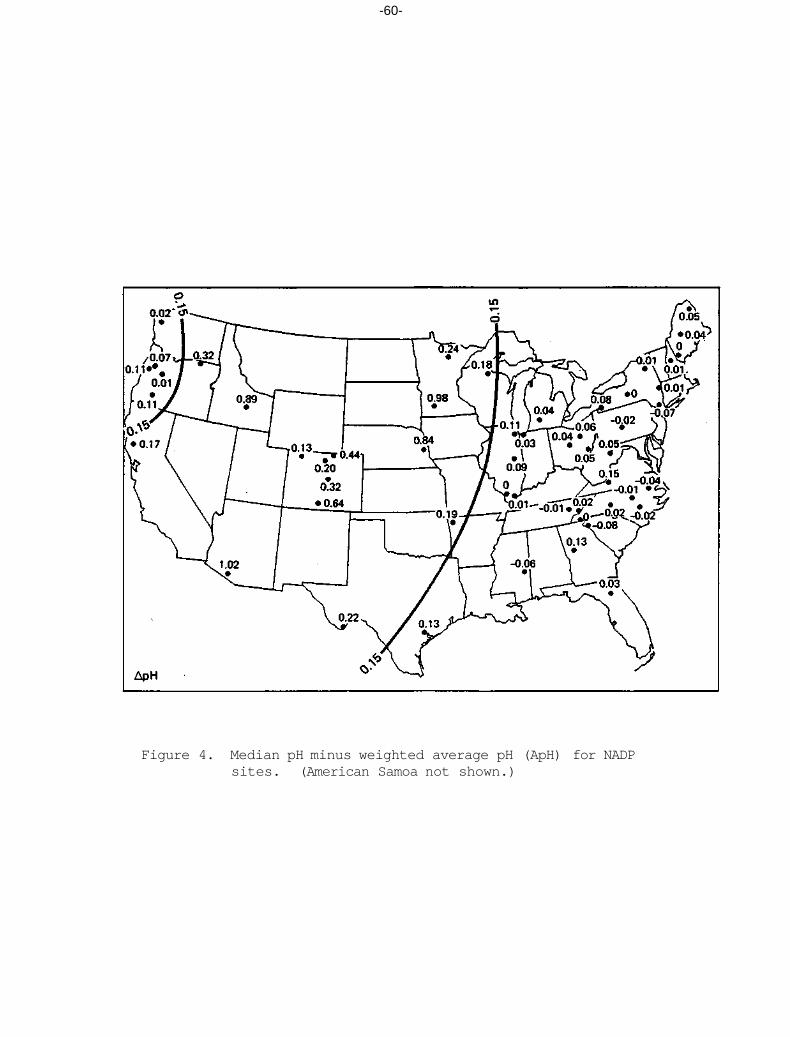
Figure 4. Median pH minus weighted average pH (ApH) for NADP sites. (American Samoa not shown.)

-60-

-61-

were also less than 0.15 in the coastal Northwest. Without exception, the median pH exceeded the weighted average pH for sites west of the Mississippi River.

Spatial Pattern of Mean pH

Figure 5 shows the spatial distribution of pH differences calculated as mean pH minus weighted average pH. To the extent this pattern matches that in Figure 4, it indicates that the spatial patterns of median pH and mean pH are similar, with the highest values in the Plains and Rocky Mountains. Except for a site in southeastern New York and one in western South Carolina, the mean pH was everywhere higher than the weighted average pH.

Spatial Pattern of Calculated Average pH

In Figure 6, pH differences equal to the calculated average pH minus the weighted average pH are plotted. The single contour line of 0 on this figure draws attention to the fact that at almost all sites in the East, the calculated average pH values were slightly smaller than the corresponding weighted average pH values.

Other Comparisons of pH Averages

Scatterplots of the four pH averages are shown in Figures 7-10. Points in these figures have been isolated into four groups:

Group I - sites that are east of the Mississippi River and that had all (East) pH averages less than 5.00. Only two sites, MN16 and FL03,

in that part of the country did not meet the pH criterion. Points lie near and along the 1:1 line in Figures 7, 8, 9, and 10, although the scatter in Figure 10 is somewhat larger than in the other Figures. Linear regressions of the four combinations of ions in these Figures are presented in Table 5. These regressions can be used to empirically estimate one average when only the other is available. As an example, for a data set consisting of conservative ion measurements but no pH measurements, calculated average pH values can be deter­mined; using the appropriate regression equation, these calculated averages can then be "corrected" to the corre­sponding weighted averages for comparison with a data set where pH measurements were reported. A statistical summary of the differences, or relative biases, between all of the pH averages for Group I sites is both listed and displayed sche­matically in Table 6. For sites in the East, the calculated average pH is lowest and the mean pH highest. Biases are smallest between median and weighted average pH values and between weighted average and calculated average pH values. Although all of the biases are small in pH unit differences, recall that 0.04 corresponds to about a 10% H ion increase,

-62-

0.08 to about a 20% H ion increase, 0.15 to about a 40% H ion increase, and 0.30 to about a 100% increase.

Group II - sites generally along the western and southern edges of the Group I area. Only MN16 and FL03 are east of the Mississippi River. The sites in Group II are listed in the order of the highest calculated average pH to the lowest in Figure 7. Average pH values at these sites are typically higher than those in Group I. With only 7 points, the mean pH is clearly the highest statistical average and the largest bias is between the mean and the weighted average pH.

Group III - sites west of the Mississippi River that have a relatively large difference between the weighted average pH and all the other averages (See Figures 7, 9, and 10). Sites in this group are listed from highest to lowest calculated average pH in Figure 7. Points in Figure 8 lie closer to the 1:1 line than in Figures 7, 9, and 10. With 6 sites in this set, the mean, median, and calculated average pH values agree most closely. Median differences in the (mean-median), (mean-calculated average), and (median-calculated average) are -.07, -.11, and -.07, respectively. In contrast, the smallest differences between the weighted average pH and the other averages is .37.

Group IV - sites west of the Mississippi River that have marine area sources in the predominant upwind direction from which storms track. The 9 sites in this group are listed from highest to lowest calculated average pH in Figure 7. For this set, as for all the others, the mean pH is the highest statistical average; and as for Groups II and III, the weighted average pH is the lowest. In contrast to Group III, however, points lie near the 1:1 line in each of Figures 7-10.

Table 5. Linear regressions of the pH averages for the 32 NADP sites in Group I, the East.

-63-

Table 6. A comparison of pH averages for the 32 NADP sites in Group I, the East.1

1This includes all sites in Figure 1 east of the Mississippi River, except MN16 and FL03. 2The mean pH differences are all statistically different from 0 at the .1% level, except (median-weighted), which is different from 0 at the 5% level.

Example: If for three years of weekly samples at IL11 the calculated average pH = 4.30, then the above would suggest the following values: weighted average pH = 4.33; median pH = 4.35; and mean pH = 4.43.

-64-

Figure 5. Mean pH minus weighted average pH (ApH) for NADP sites. (American Samoa not shown.)

-65-

Figure 6. Calculated average pH minus weighted average pH (ApH) for NADP sites. (American Samoa not shown.)

-66-

Figure 8. Scatterplot of calculated average pH and median pH. Groups I-IV are identified in Figure 7.

i

Figure 7. Scatterplot of calculated average pH and weighted average pH at the 54 NADP sites xn this study.

-67-

Figure 9. Scatterplot of median pH and weighted average pH. Groups I-IV are identified in Figure 7.

Figure 10. Scatterplot of mean pH and weighted average pH. Groups I-IV are identified in Figure 7.

-68-

Although the magnitudes differ slightly, differences in the pH averages, plotted in Figures 4, 5, and 6, exhibit spatial patterns which suggest that the median, mean, and calculated average pH values are similar. Scatterplots of pH averages in Figures 7-10 are consistent with this suggestion. By comparison of Figures 7, 9, and 10 with Figures 6, 4, and 5, respectively, it is clear that the weighted average pH is a statis­tic much different than the other three. This difference is manifested in the regions where the precipitation pH is generally above 5.0, in particu­lar at sites in Group III. The similarity between the calculated average and the median pH is reinforced, even at Group III sites, in Figure 3. Regression of the calculated average pH on the median pH at all sites yields the equation:

with a coefficient of determination (r2) equal to 0.97. Ranked in order of occurrence over all sites In this study, the mean pH is the highest, then the median, calculated average, and weighted average. Only in the subset of sites in Group I (the East) is the order different; the calculated average pH is typically .03 units below the weighted average there (see Table 6).

Since the differences between the weighted average pH and the other three pH averages are largest where the pH is generally above 5.0, the question arises: to what extent are the differences affected by the pH scale [i.e., -log(H )]? Hydrogen ion differences for the (median pH -weighted average pH) are shown in Figure 11 for the 54 NADP sites in this study. Groups II, III, and IV sites have again been sequestered for comparison with Group I. In Group III, where the pH differences were 0.44 to 1.02 units, the H ion differences are no greater than in Group I. At sites where the precipitation chemistry is strongly influenced by marine area sources (Group IV), the H ion differences are smallest. Although the pH unit differences only range from -.07 to .18, the H ion differences in Group I exhibit the largest scatter. To a large extent, then, differences in the computed pH averages are sensitive to the pH scale; however, precipitation (free) acidity is most frequently measured and reported in pH units. Recall, too, that differences on the pH scale represent relative differences in H ion concentrations, e.g., pH2 - pH1 = -log[(H2)/(H1).

Discussion

Where rain samples combined physically or mathematically have a pH <5.00, (HCO3-) is insignificant. Provided there are no unmeasured anions or cations of significant concentrations and provided there are no resultant biases in the measurement of pH or any other ion, this condition (pH <5) would result in the calculated average pH being theoretically equal to the weighted average pH. This is essentially confirmed by the data in Figure 6 for sites in the East. As yet, there is no known scheme to identify sites that will have weighted average pH values much lower than the other three pH averages. However, the data in Figures 2-6 do indicate a) that sites with a strong marine influence are unlikely to have a weighted average pH that is greatly different from the other 3 averages,

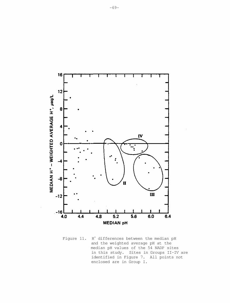
-69-

Figure 11. H+ differences between the median pH and the weighted average pH at the median pH values of the 54 NADP sites in this study. Sites in Groups II-IV are identified in Figure 7. All points not enclosed are in Group I.

-70-

and b) that non-marine influenced sites that frequently encounter pH values above 5 may have large differences between the weighted average and the other three pH averages.

Figure 12 shows the pH histograms for the weekly samples from three NADP sites representing groups I, II, and III. Notice that the tail of the distribution extends to the right for MN16 and IL11 and to the left for MN27, and recall that MN27 is in Group III, where the weighted average pH is much different from the other averages. Although we have not checked this feature thoroughly for all 54 sites, we think the "tail to the left" may be a way to qualitatively identify those sites that will have a weighted pH much lower than the other three pH averages.

Finally it seems useful to point out situations where a particular pH average seems most appropriate. Of course if the four types give essentially the same result, the choice is of little consequence.

1) At a site such as NE15, it may be deceptive to convey an "average pH" of 5.11, the weighted average value, when most of the weekly precipitation pH measurements are above that value (median = 5.95).

2) If the H concentration distribution is log-normal, then the geometric average H concentration, or mean pH, may be the best measure of central tendency for that site.

3) If one wishes to mathematically combine weekly sample data to compare to monthly sample data, then the calculated average pH (i.e., from Net Ions) of the combined weekly samples should be compared one to one with the monthly values.

4) In the East or wherever the pH is consistently below 5, the weighted average pH is convenient to use as a basis for deposition calculations (since [weighted average H+][total volume] = deposition). Table 6 indicates how this value would be biased compared to the three other average values.

5) The median pH best characterizes the "typical" pH at sites where the data sets are small, because the other pH averages are more sensitive to bias from "outlier" values.

6) When using precipitation chemistry data to study effects on plants, lakes, etc., the type of average pH which is most appropriate may depend on the details of the mechanism of the effect.

-71-

Figure 12. Histograms of the measured pH values of the valid 1-week, wet-deposition-only samples at IL11 (Group I), MN16 (Group II), and MN27 (Group III).

-72-

Conclusion

It has been clearly demonstrated that the pH "average" at some sites is very sensitive to the procedure used to calculate that "average". In the extreme, the median, mean, and calculated average pH (which generally are in agreement) can be more than one pH unit larger than the weighted average pH, which is the value most often reported in the literature in recent years.

In determining a time trend of acidity and in comparing different precipitation chemistry data sets, either the same calculational approach to determine the "average" pH should be used throughout the study or else an assessment of the effect of using different "types" of pH averages should be made.

-73-

References

Bowersox, V. C., and R. G. dePena, "Analysis of precipitation chemistry at a central Pennsylvania site," J. Geophys. Res., 85, 5614-5620 (1980).

Bowersox, V. C. and G. J. Stensland, "Seasonal patterns of sulfate and nitrate in precipitation in the United States," Paper 81-6.1, 74th Annual APCA Meeting, Philadelphia, PA, 16 pp (1981).

Hansen, D. A. and G. M. Hidy, "Review of questions regarding rain acidity data," Atmos. Environ., 16, 2107-2126 (1982).

Harned, H. S. and R. Davis, Jr., "The ionization constant of carbonic acid in water and the solubility of carbon dioxide in water and aqueous salt solutions from 0°C to 50°C," J. Am. Chem. Soc, 65, 2030-2037, (1943).

Harned, H. S. and S. R. Scholes, Jr., "The ionization constant of HCO3-. from 0°C to 50°C," J. Am. Chem. Soc, 63, 1706-1709 (1941).

Likens, G. E., and F. H. Borman, "Acid rain: a serious regional environmental problem," Science, 184, 1176-1179 (1974).

Likens, G. E. and T. J. Butler, "Recent acidification of precipitation in North America," Atmos. Environ., 15, 1103-1109 (1981).

MAP3S PCN, "The MAP3S precipitation chemistry network: first periodic summary report (September 1976-June 1977)," Battelle Pacific Northwest Laboratories, Richland, WA, 173 pp (1977).

National Atmospheric Deposition Program," NADP Data Report: Precipitation Chemistry," Vol. 1, 2, 3 and 4, Natural Resource Ecology Laboratory, Fort Collins, CO (1978, 1979, 1980, 1981).

National Atmospheric Deposition Program, "NADP instruction manual for site operation," Natural Resource Ecology Laboratory, Ft. Collins, CO (1982).

Pack, D. W., "Sulfate behavior in eastern U.S. precipitation," Geophys. Res. Letters, 5_, 673-674 (1978).

Robinson, R. A. and R. H. Stokes, "Electrolyte Solutions," Butterworths Publishing Co., London, England, 571 pp. (1959).

Stensland, G. J., "Acid rain," Encyl. Environ. Sci. and Engin., J. R. Pfafflin and E. N. Ziegler, Eds., Gorden and Breach, New York, NY, Vol. 1, pp. 1-9 (1983).

Stensland, G. J. and R. G. Semonin, "Another interpretation of the pH trend in the United States." Bull. Am. Meteorol. Soc, 63, 1277- 1284 (1982).

Stensland, G. J., M. E. Peden and V. C. Bowersox, "NADP quality control procedures for wet deposition sample collection and field measurements," Paper 83-32.2, 76th. Annual APCA Meeting, Atlanta, GA, 20 pp (1983).

Stensland, G. J., R. G. Semonin, M. E. Peden, V. C. Bowersox, F. M. McGurk, L. M. Skowron, M. J. Slater, and R. K. Stahlhut, "NADP Quality Assurance Report, Central Analytical Laboratory, 1 January 1979 to 31 December 1979," Natural Resource Ecology Laboratory, Ft. Collins, CO (1980).

U.S. Dept. of Interior, Geological Survey, "The National Atlas of the United States of America, Washington, DC, p. 98 (1970).

-75-

CHAPTER 4 REGIONAL CHARACTERIZATION OF RAIN ACIDITY

UTILIZING GRAN'S PLOT TITRATIONS

Mark E. Peden and Jacqueline M. Lockard

INTRODUCTION

The acidity of precipitation can be due to a variety of proton sources including strong mineral acids (H2SO4, H N O 3 ) , volatile weak acids (H 2CO 3), non-volatile weak acids (organic acids) and hydrolyzable metals (Fe(H2O)6, A K H 2 O ) 6 ) , (Galloway, Likens, and Cosby, 19797. Galloway et al. (1976) concluded from their studies that the primary sources of H ions that result in acid precipitation in widespread areas of the northeastern United' States are the strong mineral acids H.SO, and HNO3. They also discovered the varying presence of weak acids ranging in concentrations from 1.1 to 15.6 uequivalents per liter. Although the weak acids did not appreciably affect the pH of these samples, they did account for 20 to 50 per cent of the total acid content.

The pH of precipitation is a measure of the free acidity only. This acidity can be influenced by factors other than strong mineral acids, including basic cations and weak acids. To investigate the relationships affecting the free and total acidities at various locations throughout the U.S., we have performed acidity titrations on selected samples from four National Atmospheric Deposition Program (NADP) collection sites.

EXPERIMENTAL METHODS

Site and Sample Selection The sites selected for this study included Bondville, IL

(IL11), Parsons, WV (WV18), Yellowstone, WY (WY08), and Corvallis, OR (OR02). These locations were chosen for their geographical differences and the range of pH values that was characteristic of each area. Twenty weekly wet-only samples from each site were selected for acidity titrations after all routine cation and anion analyses had been completed and the data verified by ion balance calculations. Samples were selected that represented different seasons and varying sample volumes in order to relate the acidity results to meteorological factors as well as location. Whenever possible, the ion balance data obtained

-76-

from the routine analyses were used to include samples that showed a significant deviation from the expected agreement between cation and anion measurements (±15%). A deficit of measured anions, for instance, could be an indication of the presence of a weak organic acid that contributed to the free acidity (pH). Since the associated organic acid anion would not be detected during routine analysis, an anion deficit would appear in the ion balance calculation.

Titration Procedures The pH meter and combination electrode were calibrated using

pH 4.00 and 7.00 National Bureau of Standards (NBS) certified buffers. Forty mL of a rain sample were then pipetted into a borosilicate glass titration vessel. The initial pH of the sample was measured after an equilibration time of 4-5 minutes. A small fritted glass disc, submerged in the rainwater sample, was used to purge the sample with nitrogen for a period of 15-20 minutes prior to the start of each titration. This purging step was necessary to remove any dissolved volatile weak acids (H2CO3) present in the samples. The titration vessel itself was closed to the atmosphere with the exception of a small vent to allow the release of the N2 and CO2 gases. After a 20 minute period, the fritted glass disc was raised to a level just above the rainwater's surface and the nitrogen flow adjusted to maintain a positive pressure within the titration vessel. This prevented the dissolution of CO- back into the sample as the titration progressed.

A piston-driven one mL burette, capable of one uL additions, was used to dispense the 0.02 N NaOH titrant. A magnetic stirring bar turning at approximately four revolutions per second was used to mix the rainwater solution after each titrant addition. The complete titration system is shown in Fig. 1. The titrant was dispensed in 1-10 uL increments depending on the rate of pH change that was being observed. The pH values associated with each addition were recorded up to a pH of 10.3. At this pH all of the acids with a pKa less than 9.5 have been titrated.

The data obtained from each titration were tabulated

according to the procedure developed by Gran (1952) to minimize the uncertainty involved in detecting accurate equivalence points. The Gran's plot principle is based on the theory that OH ions added from the titrant will react preferentially with H ions in solution rather than with the H still undissociated from any weak acid present. The result is a linear transformation of a standard acid-base titration curve that allows for precise equivalence point determinations.

Figure 2 illustrates the application of Gran's technique to the determination of strong, weak, and total acids in a synthetic control sample developed to assess the bias and precision of our titration procedure. Also shown in Fig. 2 is the standard

-77-

Figure 1. Rain titration apparatus with (1. to r.) automatic 1.0 mL burette, glass titration vessel with magnetic stirrer, and pH/millivolt meter.

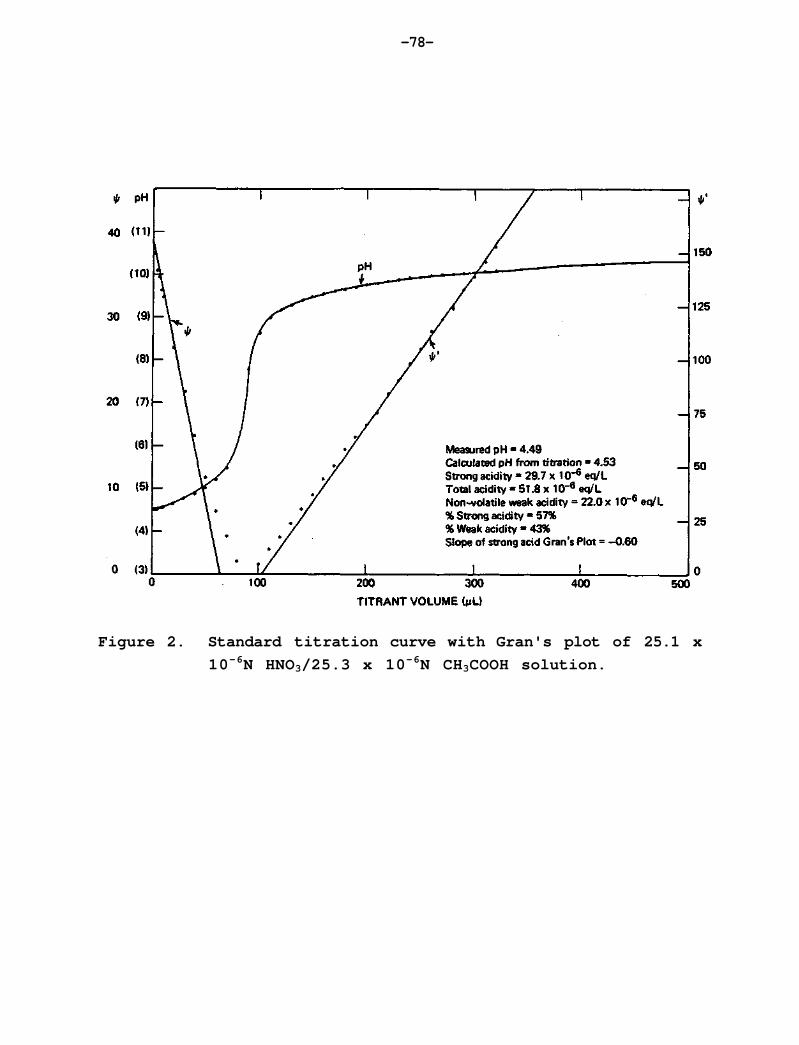
-78-

Figure 2. Standard titration curve with Gran's plot of 25.1 x 10-6N HNO3/25.3 x 10-6N CH3COOH solution.

-79-

titration curve produced by plotting the additions of NaOH versus the resultant measured pH. The first x-intercept of the Gran's plot corresponds to the strong acid content, the second corresponds to the total acidity. Weak acidity is calculated by subtracting the strong acid component from the total acicidy. The example shown in Fig. 2 contains approximately equimolar amounts of the strong acid HNO3, (nitric) and the weak acid CH3COOH (acetic). The accuracy of this procedure, obtained from replicate analyses of this control sample, was +.4 ueq/L.

RESULTS AND DISCUSSION

A compilation of the standard titration curves and Gran's plot data for each of the four sites examined revealed a consistent pattern for all of the samples analyzed. The variability between samples from the same site in terms of strong to weak acid concentration ratios and absolute acidity measured was small. This may be due in part to the fact that all of the samples selected for acidity analyses had relatively large volumes. The use of samples with higher volumes was necessitated by the additional analyses that were to be performed. The results obtained in this study, therefore, reflect the acidity relationships in samples with rainfall amounts greater than 0.5 cm.

Figure 3 summarizes the results obtained from each of the four study sites. The plots shown reflect the median acidities measured from each location. The similarities between the IL11 and the WV18 site are apparent with virtually identical strong acid composition. Differences in the total acidity concentrations and the strong to weak acid ratios are a result of the higher weak acid concentrations measured from ILll. Since these titrations were carried out to a pH of 10.3, the weak acid component will also include any NH, that is present. Comparing these results to the NH, values measured at each of the two sites revealed that the higher ammonium values measured at Bondville, Illinois account for the increased weak acidity reported.

The results shown for the OR02 and the WY08 sites are also similar to each other. Both sites exhibit strong acidity values that are a factor of 15-50 below the ILll and WV18 measurements. The weak acidity concentrations are also much lower, consistent with the lower ammonium values reported for these sites. The average weak acid component found in the OR02 and WY08 samples was 60%, with the average in the samples from ILll and WVl8 being only 30%. This is due to both the higher pH and lower ammonium values measured at the western sites.

The pH values that have been calculated from the intercept of the strong acidity plots show good agreement with the measured pH for all four sites (±4 ueq/L). This is an indication that

-80-

Figure 3. Sample titration curves with Gran's plots for the four sampling sites.

-81-

Figure 3. (contintued)

-82-

the pH electrode measurments are accurately reflecting the free acidity of solutions of varying ionic strengths and acidity levels.

In order to examine the relationships that may exist between the acidity measurements described here and various other factors such as meteorological conditions and major ion chemistry, a correlation matrix was developed using data obtained from the anion/cation results, Gran's plots, and sample volume record. Preliminary plots of seasonal trends in total or weak acid content at each site revealed no discernible patterns so they will not be presented here.

Table 1 is a summary of the various correlation coefficients that were calculated from these data. Both the WV18 and IL11 sites show strong correlations between the measured H (pH) and the strong acid concentration determined from the titration data. This is in agreement with the sample titration data shown in Fig. 3. A correlation between the measured ammonium (NH4) concentration and the weak acid content of these samples is also significant suggesting that the weak acid component is dominated by the NH, in these samples. No correlation is apparent between sample volume and either strong or weak acid contents for any of the four locations.

If the ammonium contribution to the weak acid content is subtracted from the total weak acid measured, the remaining concentration of weak acid may be attributable to either the presence of organic acids or hydrolyzable metals. Since these samples were analyzed from two to six months after collection, it is unlikely that any organic acids would still be present. The titration results, therefore, reflect primarily strong acids, ammonium, and the hydrolyzable metals.

The lack of significant correlations between ammonium and the weak acid concentration for the WY08 and the OR02 sites indicate that the weak acid component is not dominated by the presence of ammonium as was the case for the two eastern sites, ILll and WV18. The low level of weak acids present in samples collected at the western sites makes any further interpretation speculative. The samples from these two sites also showed a strong correlation between the measured pH and and the strong acidity value derived from the Gran's plot data, again indicating that the pH measurements are a reliable indicator of the true free acidity of these samples.

CONCLUSIONS

The data presented have quantitatively characterized the precipitation at four different geographic locations by combining information obtained from routine anion and cation analyses with data derived from total acidity titrations. Similarities are

-83-

Table 1. Correlation coefficient (r) matrix for measured chemical and physical parameters.

-84-

apparent between the two sites located east of the Mississippi River and the two western collection sites. The ratios of strong to weak acids decrease from east to west as a result of both decreased strong acidities and increased ammonium concentrations. No evidence of a significant contribution of organic acids was found in samples from any of these sites, presumably due to the time lag between collection and analysis. Data on the potential contributions of the organic acids to both the free and total acidities at these sites are still needed to completely characterize the acidity relationships presented here.

REFERENCES

Galloway, J. N., G. E. Likens, and E. S. Edgerton, 1976: Acid precipitation in the northeastern United States: pH and acidity. Science. 194. 722-724.

Galloway, J. N., G. E. Likens, and B. T. Cosby, 1979: Acid precipitation: Measurement of pH and acidity. Limnology and Oceanography. 24, 1161-1165.

Gran, G., 1952: Determination of the equivalence point in potentiometric titrations. Analyst, 77. 661.

-85-

CHAPTER 5

THE CHEMISTRY AND METEOROLOGY OF EXTREME PH DEPARTURES IN PRECIPITATION ON THE REGIONAL SCALE

Kevin G. Doty and Richard G. Semonin

INTRODUCTION

Stensland and Semonin (1982) reevaluted the precipitation chemistry data of 1955-56 of Junge (1958) and Junge and Werby (1958), which had been used by Cogbill and Likens (1974) in conjunction with the data of 1965-66 of Lodge et al. (1968), Gambell and Fisher (1966), and Pearson and Fisher (1971) to show an apparent increase in the areal extent and degree of acidity across eastern North America. The reevaluation of the 1955-56 data revealed median concentrations of calcium and magnesium up to six times greater than more current levels (as determined from the National Atmospheric Deposition Program (NADP) network) at sites in the Midwest and East. Stensland and Semonin (1982) hypothesized that the source of the alkaline materials was soil related, since large parts of the Great Plains and Southeast experienced significant drought in the mid 1950's with numerous reports of dust storm events. When the precipitation chemistry data of 1955-56 were adjusted for current concentrations of calcium and magnesium, no apparent change in acidity was seen in the eastern United States.

This hypothesis of soil particulates being transported from source regions and raising the pH of precipitation over a large area in and away from these regions led to the idea of confirming such phenomena in the more current NADP network data. This was especially true for the period from the fall of 1980 through the spring of 1981, when widespread moderate to severe drought occurred throughout many parts of the country, including the Great Plains, Southeast, and East.

The previous hypothesis led to a study by Doty and Semonin (1984), which sought to determine the meteorological and chemical characteristics of extreme pH departures, both in the alkaline and acidic directions, for weekly NADP samples on a regional basis for parts of the Midwest and East. The report had three main sections. The first section discussed the general characteristics of the test group of NADP sites used in the study and the seasonal trends for concentrations as revealed by the data through the end of 1981. The test group included the 15 NADP sites in the states of Ohio, Tennessee, West Virginia, Pennsylvania, and New York. The second section dealt with the general seasonal and chemical patterns of weeks where a sufficient number of sites in the test group met the criterion for extreme pH departures. The third major section, and the largest, discussed the meteorology and chemistry for a select number of weeks for both the acidic and alkaline departure groups. This chapter, which is a summary of that study, will focus primarily on the latter section.

-86-

STATISTICAL ANALYSIS OF SEASONAL CONCENTRATION PATTERNS

Fig. 1 shows the location and site identifiers for all NADP sites in the eastern half of the United States, with the test group including the sites 0H17, 0H49, OH71, TNOO, TN11, WV18, PA29, PA42, NY08, NY10, NY12, NY20, NY51, NY52, and NY65. Before searching for weeks where extreme chemical patterns were displayed, it was decided to investigate the nature of the entire chemical distributions on a seasonal basis for each site. Seasons were defined in the following manner: December through February-winter, March through May-spring, June through August-summer, and September through November-fall. Two statistical tests were used in investigating seasonal changes. One was the nonparametric Wilcoxon test (e.g., see Pratt and Gibbons, 1981), which depends on the relative rank of the pooled data of the two groups under consideration, and a two-sample t test with the number of degrees of freedom adjusted for differences in population variances, as described in Brownlee (1960). Tests were performed on the six possible seasonal combinations (winter-spring, winter-summer, winter-fall, spring-summer, spring-fall, and summer-fall) for the 15 sites and for the nine ions measured in NADP samples: H+, SO4

2-, NO3-, C1-, NH4

+, Ca2+, Mg2+, Na+, and K+. Thus, for each ion there were 90 season-site categories to test. Mathematically, the hypotheses could be stated in the following manner. If u1 is the "central tendency" or location (for the purpose of this discussion, this could be the mean or median) for an ion for one season at a site, and U2 is the location for another season, then the null hypothesis is that u1 - U2 = 0 , against the alternative hypothesis of u1 - u2 ≠ 0. The level of significance of a statistical test, as described by Walpole and Myers (1972), is the probability of rejecting the null hypothesis when in fact it is true. A level of significance of .05 is called "significant" whereas a level of .01 is called "highly significant".

Two analyses were performed. In the first analysis, only the Wilcoxon test was used on the 90 season-site categories for the nine ions. In the second analysis, outliers were removed, a logarithm transformation was applied, and then both the Wilcoxon and t tests were used. Details of this process are given in Doty and Semonin (1984). The purpose of the second analysis was to test the stability of the results of the first analysis. The difficult issue was then how to incorporate the results of the two analyses in a logical manner. It was decided that if the first analysis showed a statistical difference (at either the .05 or .01 levels) and if either test also showed a difference in the second analysis, then the results of the second analysis would be accepted. If the Wilcoxon and t tests showed a difference at different significance levels, then the results of the t test were chosen. Results of this composite analysis are shown in Table 1.

With respect to the total number of differences (at either the .05 or .01 levels) across the seasonal comparisons for the 15 sites, the most variable to least variable ions were SO4

2-, H+, C1-, NH4+, Mg2+, K+,

Ca2+, Na+, and NO3-. Statistical differences for SO42- were concentrated in the winter-spring, winter-summer, and summer-fall comparisons due to the typical sulfate maximum in the warm season. The differences for H+

-87-

Figure 1. National Atmospheric Deposition Program (NADP) site locations and codes.

-88-

Table 1. Summary of composite statistical analyses performed on the 15 NADP sites in Ohio, Tennessee, West Virginia, Pennsylvania, and New York for seasonal differences of nine ions. Each column represents the number of sites having statistical differences between the stated seasons for an ion. Numbers in parentheses are the number of differences at the .01 level. See the text for additional details.

-89-

were similar except for the winter-spring category, where only three sites displayed differences. The largest number of differences for C1-were in the winter-summer and winter-fall categories. This was primarily due to the winter chloride maximum observed at many of the sites in the test group. Possible sources of C1- include sea salt aerosol, road salt (in the form of NaC1 or CaC12), and others. If road salt was a dominant source, one would expect to see significant differences between winter and spring coincident with decreasing snowfall, and yet these were not observed. The ammonium ion was the next in rank, with differences mainly in the winter-spring and winter-summer columns. This was due to the NH4+ maximum observed in the warm season, which is probably the result of increased biogenic production of NH3 with warmer temperatures. Most of the pronounced differences for Ca2+, Mg 2 +, and K+ were in the winter-summer category. For most of the sites, the maxima for these three ions was during the summer season. Na+ and NO3- were relatively constant across the seasons.

At least three conclusions can be drawn from these statistical analyses. The first is that whereas 11 sites showed differences in SO42-between winter and spring, only three sites showed differences in H . A partial explanation may be related to the NH4+ behavior, as seven sites displayed differences in the winter-spring comparison. Increased spring levels of NH3 could react with H2SO4 and other products to form ammonium compounds in aerosol or precipitation. The second major observation is that Na and Cl~ displayed very different seasonal patterns. Na was relatively constant across the seasons, but C1- displayed a winter maximum at most sites. This would seem to imply that these ions have at least one source not in common. The last conclusion is in regard to the ions Ca2+, Mg 2 +, and K+. Evans and Cooper (1980) concluded that on a national basis for 1976 data the four largest open sources of particulate material, in decreasing magnitude, were unpaved roads, wind erosion of soil, agricultural tilling, and construction activity. Gatz (1983) and Gatz et al. (1981) have related unpaved roads and local soil to concentrations of Ca 2 +, Mg2+, and K+ in aerosol and precipitation samples. If soil aerosol from cropland was the only contributor to crustal elements, one would expect to detect differences between spring and summer levels, as most cropland is protected by a vegetative cover during the summer. Yet very few statistical differences were observed in the spring-summer category for Ca 2 +, Mg 2 +, and K+. Thus other sources, such as unpaved roads, may be responsible for maintaining high levels of crustal elements in the spring, summer, and fall seasons.

SELECTION OF WEEKS MEETING DEPARTURE CRITERIA

To examine weeks where acidity was predominantly either very high or very low across the large area defined by the 15 NADP sites in the test group, the following criterion was chosen. Decisions were based with respect to the site median pH values as based on all available data through the end of 1981. For the acidic (alkaline) category, if seven or more of the 15 sites in the test area had pH's .25 units below (above) or

-90-

more than the respective site median pH values, then that week was chosen. This rule was used to insure that the weeks chosen displayed regional chemical and meterological patterns and not merely local variations. Unless otherwise stated, when the median for pH or any other ion is subsequently mentioned, it refers to the site median of all available data from the beginning of a site through 1981. For constituents with a pronounced seasonal cycle, the site median can differ substantially from a seasonal median. Although the selection of the case study weeks was based on site median pH values, the process still located the desired weeks.

For the high pH class, 13 weeks met the established criteria, with 10 of the weeks having an average sample volume of 1000 mL or more. All the samples except for two in September were in cool to cold seasons of late fall, winter, or early spring. SO4

2-, NO3-, and NH4+ were typically

below site median values, whereas roughly half of the weeks had above median values of Na and C1- and half below median values. Most weeks also had below median values of Ca2+ and Mg2+, but 3-5 weeks had one or both of the latter ions at above median values. Initial inspection of these results apart from any meteorological analyses would seem to indicate simply the dilution effect of large precipitation events reducing the concentrations of all ions. However, before any final conclusions could be made, these concentrations would need to be compared with other samples of similar sample volume to determine their relative rank. The week of 17-24 March 1981 was especially interesting in that it had average departures above median values for NO3-, C1-, NH4+ , Ca , Mg2+, Na+ , and K+ but below median values of SO42-. Although the average sample volume was small at 355 mL, this week was chosen as the central week to study because of the apparent strong crustal contributions. Weeks adjacent to 17-24 March did not meet the selection criteria, but still had merit in illustrating regional departures outside the test area. Thus the alkaline period selected for intense study in Doty and Semonin (1984) included the period 10 March through 7 April of 1981. The weeks of 17-24 March and 31 March-7 April will be summarized later in this chapter.

Because of the logarithmic pH scale, not as many weeks were expected to meet the criterion for the acidic category. Indeed this was the case as only four cases met the qualifications. All the weeks were from summer and early fall, which was no surprise based on the sulfate maximum observed during the summer and its high correlation with H . Above median concentrations were observed on the average for S O 4

2 - , NO3-, C1-,

NH 4+, and Ca2+. Average sample volumes for all sites in the test area

for each week were over 1000 mL, which was very similar to the alkaline case departures. There exists a rather strong negative correlation between any single ion (other than H ) and sample volume, but a much weaker relationship between H and sample volume. This seems to be the result of high intercorrelations between cations and anions such that high cation and anion concentrations offset each other. The selection of a week for intense study was not as clear as in the alkaline category, but 21-28 July 1981 was chosen as the central week because of its temporal proximity to the selected alkaline cases and because it too had average concentrations above median values for Ca2 , Mg , and K . The total period of study in Doty and Semonin (1984) for the acidic category

-91-

became 14 July-4 August 1981. Only the central week of 21-28 July will be considered in this summary.

WEEKLY CASE STUDIES

Analysis Tools and Philosophy

In Doty and Semonin (1984), three major data sets were used. These were meteorological data, including surface and upper air analyses, hourly radar summaries, and precipitation amounts; NADP wet chemistry samples, including measurements of pH, SO42-, NO3

-, C1-, NH4+, Ca2+,

Mg2+, Na+, and K+; and measurements of the bulk composition of surficial materials, as given by Boerngen and Shacklette (1981). Since the NADP sampling period ends on Tuesday mornings, the weekly precipitation maps shown in the subsequent discussions are based on the summation of daily amounts with midnight on Monday as the breakpoint. Precipitation data were taken from the publication Climatological Data. For this study raingauge amounts from National Weather Service, Federal Aviation Administration, and some cooperative sites were used. The data of Boerngen and Shacklette (1981) were used in conjunction with a chemical element balance (CEB) model in an attempt to relate concentrations of Ca , Mg , and K to sources such as soil aerosol and unpaved road dust. The CEB results will not be discussed in this summary. Trajectory analyses were used for the week of 31 March-7 April to determine the potential path of a dust cloud created by a dust storm in the southern Plains.

For the 17-24 March case, interpretation will focus not only on sites in the test area but also on some southern sites. For 31 March-7 April, the emphasis will be on sites in the Plains and Midwest. For the acidic case of 21-28 July, the test group will be the prime area of consideration.

17-24 March 1981 Case

Fig. 2 shows the weekly precipitation for 17-23 March. It was similar to the pattern for the previous week except that heavy precipitation covered much of the South. This week was characterized by several storm systems, but with the major storm track across the southern states as Canadian air held sway for much of the week in the Midwest and Northeast, making average temperatures as much as 12°F below weekly normals in the Appalachians from Pennsylvania to West Virginia. Most sites in the test group had several days of precipitation, with daily amounts ranging from .01 to .05 inches, but with much higher values locally. Nine of the NADP sites in the test area had weekly raingauge totals equal to or below .25 inches. Considerable snow cover was evident over the Appalachians and portions of New York and Pennsylvania by the end of the week.

-92-

Figure 2. Precipitation (inches) for the period of 17-23 March 1981.

-93-

Fig. 3 shows the synoptic situation for 2100 GMT 17 March. A strong cold front across New York and Pennsylvania in cooperation with a very intense low off the coast of Maine produced widespread average northwesterly winds of 20 knots over New York and Pennsylvania. Although winds subsided considerably by the next day, snow shower activity continued for much of the week in the cold, unstable flow around the intense low pressure system off the coast. Fig. 3 also shows another intense system over Kansas which produced a large area of blowing and suspended dust over portions of New Mexico, Texas, and Oklahoma behind a cold front. Dramatic surface dew point depressions were observed over eastern New Mexico and western Texas, with temperatures near 60°F and dewpoints as low as -5°F. Surface windspeeds ranged from 30 to 45 knots over the same area. The potential for this dust cloud to affect precipitation chemistry was limited to the southern states, as the upper-air flow traveled southward from Canada around the low over southern Kansas and then basically eastward to the Atlantic.

Fig. 4 illustrates the synoptic system at 0000 GMT 22 March which eventually brought heavy snowfall to the southern Appalachians. It too created a large area of blowing and suspended dust over the southern Plains, but with a more extensive closed circulation aloft. However, the closed circulation remained in the southern states as the storm moved eastward, and therefore any potential impacts of transported dust should again have been in the southern states.

Fig. 5 shows the the laboratory sample pH at each site for the NADP sampling period of 17-24 March 1981. This week was the central week chosen for study in the alkaline category, having eight of the 15 sites in the test area with pH's above normal values by .35 to 2.50 units. The SO42- and NO3

- concentrations in Figs. 6 and 7 show an interesting deviation from the previous week's pattern. SO42- concentrations were 16 to 65 μeq/L below normal throughout Ohio, Pennsylvania, and New York in contrast to the above normal values the previous week, whereas NO3

-

concentrations remained above median values but not as consistently or to the magnitude of the previous week. Part of this reversal may be due to the colder temperatures of this week, but how SO42- and NO3- would be affected in contrasting ways is not readily clear. NH4+ concentrations (Fig. 8) were generally near or below normal, except at WV18 where the weekly sample was about 43 μeq/L above median values. The Ca2+ concentrations in Fig. 9 were 15 to 70 μeq/L above normal values at most sites. The map of K concentrations reveals another interesting pattern. While Ca2+ and Mg2+ concentrations were high, most sites had below normal values of K in the test area.

Although the two blowing dust events in the Texas area this week did not have an upper level flow pattern which allowed any substantial transport northeastward, they did have the potential to effect sites to the south. The highest Ca2+ concentrations outside of the test area in Fig. 9 are seen to be at AR27, IL35, and GA41. The dust event illustrated in Fig. 3 definitely affected the AR27 site, as newspaper reports and comments by the site operator described the deposition of reddish Plains soil by the storm's precipitation. Laboratory personnel also observed reddish dust in the GA41 sample for this week, but this could have been from a local sources. Other than the NE15 site, the

-94-

Figure 3. Surface analysis for 2100 GMT 17 March 1981. Isobaric analysis is incomplete off the coast of Maine. Only the major radar echoes in the test area are shown. Area with blowing dust is indicated by dashed lines.

-95-

Figure 4. Surface analysis for 0000 GMT 22 March 1981. Only major radar echoes are shown near the storm system. Area with blowing dust is indicated by dashed lines.

-96-

Figure 5. Laboratory pH for the NADP sampling period 17-24 March 1981.

-97-

Figure 6. SO42- concentrations (μeq/L) for the NADP sampling period 17-24 March 1981.

-98-

Figure 7. NO3- concentrations (μeq/L) for the NADP sampling period 17-24 March 1981.

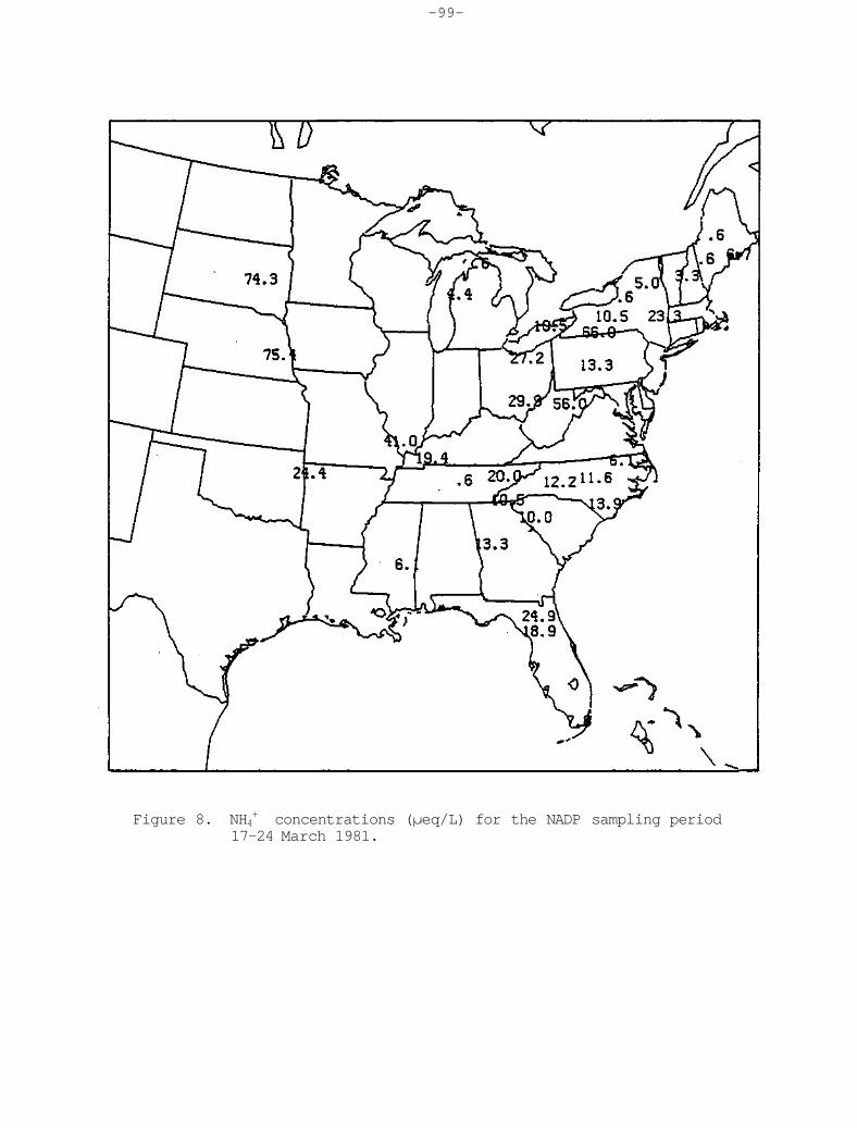
-99-

Figure 8. NH4+ concentrations (μeq/L) for the NADP sampling period 17-24 March 1981.

-100-

Figure 9. Ca2+ concentrations (μeq/L) for the NADP sampling period 17-24 March 1981.

-101-

Figure 10. K concentrations (μeq/L) for the NADP sampling period 17-24 March 1981.

-102-

highest K+ concentrations were also observed at AR27 and GA41. This again weighs the evidence for the influence of the dust storm aerosol, as the typical bulk concentrations of calcium and potassium in southern Plains soils are substantially higher than those of Arkansas and Georgia (Boerngen and Shacklette, 1981).

The elevated concentrations of Ca2+ in the test area for the period 17-24 March seemed to be the net result of light precipitation, relatively dry surfaces in relation to long-term moisture deficits, little extensive snow cover, and high surface winds coincident with precipitation events. More case studies would be needed to determine the relative importance of these factors. Substantial evidence was available to suggest that dust storm aerosol affected the weekly samples at sites AR27 and GA41. This evidence included high levels of Ca2+ and K+, meteorological analyses, and the color of sediment in the sample.

31 March-7 April 1981 Case

Fig. 11 shows the weekly precipitation for the NADP sampling period of 31 March through 6 April. An extensive band of 1 inch or greater totals extended from Ohio to the Gulf coast. Another broad area of 1-2 inch totals existed in the upper Plains and Great Lakes region. The other predominant feature of interest is the belt of lighter precipitation, typically in the .25-.50 inch range, which extended from the southern Plains to the lower Great Lakes area. Two major weather systems dominated the synoptic patterns for the eastern United States during this week. The first moved across the Midwest on 1 April. It involved a cold front which extended southward along the Appalachians from a deep low pressure center over southern Ontario. The cold front produced shower activity along it, with the heaviest precipitation in the Southeast and East. Strong winds to the rear of the front produced observations of blowing dust at West Lafayette and Fort Wayne. This was a reflection of the condition of much of the cropland in the Midwest as a result of a dry spring, extensive field work, and strong winds. Changnon (1982) documented this for Illinois for the period of February through May of 1981. An investigation of state climatic records indicated a drought in the region, but not a severe one. Changnon (1982) attributed the record number of days with blowing dust not only to the dry and windy conditions but also the practice of fall plowing and early fieldwork which provided soil surfaces suitable for wind erosion.

Fig. 12 shows the second major synoptic event for the week with a very intense low pressure center over northern Kansas at 0000 GMT 4 April. Average surface winds of 20-35 knots over eastern New Mexico, northern Texas, and Oklahoma created a large area of blowing and suspended dust. Descent of mid-tropospheric air to the surface was revealed by temperatures of 60-80°F and by dewpoints of 10-20°F. Other areas of blowing dust were also observed over portions of Arkansas and Illinois. Based on the surface maps available every 3 h, the dust storm began at 1800 GMT and lasted approximately 6 h over the original area described above. Many severe thunderstorms and tornadoes were reported ahead of this system, which was an indication of the intrusion of dry air

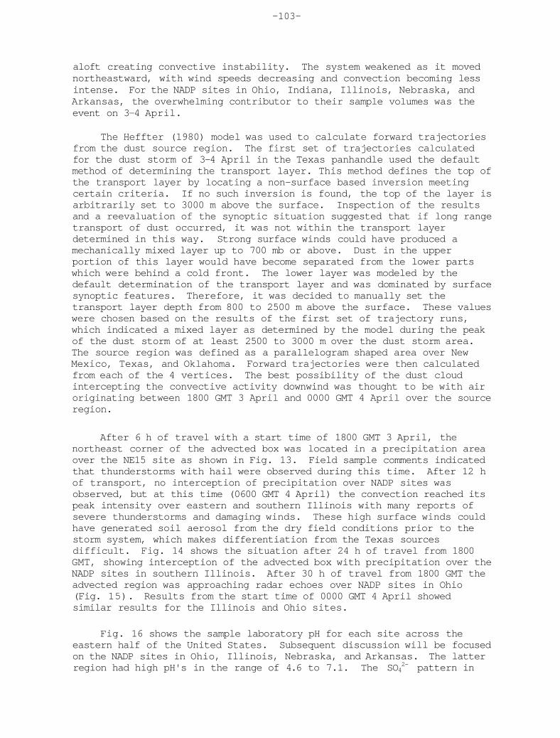
-103-

aloft creating convective instability. The system weakened as it moved northeastward, with wind speeds decreasing and convection becoming less intense. For the NADP sites in Ohio, Indiana, Illinois, Nebraska, and Arkansas, the overwhelming contributor to their sample volumes was the event on 3-4 April.

The Heffter (1980) model was used to calculate forward trajectories from the dust source region. The first set of trajectories calculated for the dust storm of 3-4 April in the Texas panhandle used the default method of determining the transport layer. This method defines the top of the transport layer by locating a non-surface based inversion meeting certain criteria. If no such inversion is found, the top of the layer is arbitrarily set to 3000 m above the surface. Inspection of the results and a reevaluation of the synoptic situation suggested that if long range transport of dust occurred, it was not within the transport layer determined in this way. Strong surface winds could have produced a mechanically mixed layer up to 700 mb or above. Dust in the upper portion of this layer would have become separated from the lower parts which were behind a cold front. The lower layer was modeled by the default determination of the transport layer and was dominated by surface synoptic features. Therefore, it was decided to manually set the transport layer depth from 800 to 2500 m above the surface. These values were chosen based on the results of the first set of trajectory runs, which indicated a mixed layer as determined by the model during the peak of the dust storm of at least 2500 to 3000 m over the dust storm area. The source region was defined as a parallelogram shaped area over New Mexico, Texas, and Oklahoma. Forward trajectories were then calculated from each of the 4 vertices. The best possibility of the dust cloud intercepting the convective activity downwind was thought to be with air originating between 1800 GMT 3 April and 0000 GMT 4 April over the source region.

After 6 h of travel with a start time of 1800 GMT 3 April, the northeast corner of the advected box was located in a precipitation area over the NE15 site as shown in Fig. 13. Field sample comments indicated that thunderstorms with hail were observed during this time. After 12 h of transport, no interception of precipitation over NADP sites was observed, but at this time (0600 GMT 4 April) the convection reached its peak intensity over eastern and southern Illinois with many reports of severe thunderstorms and damaging winds. These high surface winds could have generated soil aerosol from the dry field conditions prior to the storm system, which makes differentiation from the Texas sources difficult. Fig. 14 shows the situation after 24 h of travel from 1800 GMT, showing interception of the advected box with precipitation over the NADP sites in southern Illinois. After 30 h of travel from 1800 GMT the advected region was approaching radar echoes over NADP sites in Ohio (Fig. 15). Results from the start time of 0000 GMT 4 April showed similar results for the Illinois and Ohio sites.

Fig. 16 shows the sample laboratory pH for each site across the eastern half of the United States. Subsequent discussion will be focused on the NADP sites in Ohio, Illinois, Nebraska, and Arkansas. The latter region had high pH's in the range of 4.6 to 7.1. The SO42- pattern in

-104-

Figure 11. Precipitation (inches) for the period 31 March-6 April 1981,

-105-

Figure 12. Surface analysis for 0000 GMT 4 April 1981. Areas with blowing or suspended dust are indicated by dashed lines.

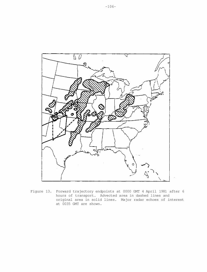
-106-

Figure 13. Forward trajectory endpoints at 0000 GMT 4 April 1981 after 6 hours of transport. Advected area in dashed lines and original area in solid lines. Major radar echoes of interest at 0035 GMT are shown.

-107-

Figure 14. Forward trajectory endpoints at 1800 GMT 4 April 1981 after 24 hours of transport. Advected area in dashed lines and original area in solid lines. Major radar echoes of interest at 1835 GMT are shown.

-108-

Figure 15. Forward trajectory endpoints at 0000 GMT 5 April 1981 after 30 hours of transport. Advected area in dashed lines and original area in solid lines. Major radar echoes of interest at 0035 GMT are shown. Northeastern corner of advected box was outside trajectory model's domain.

-109-

Fig. 17 showed no consistent pattern across the region, with values 10-50 μeq/L above spring median values (spring being defined as all samples for a given site for the months of March-May through 1981) in Nebraska and Arkansas, but near or below spring median values at most sites in Illinois and Ohio. The NO3- pattern in Fig. 18 was generally characterized by below normal values in the region. The NH4+ concentrations in Fig. 19 again showed no consistent features across the region, except in Ohio, where sites 0H17 and OH49 had values 20-30 μeq/L above spring median values. The Ca2+ concentrations in Fig. 20 had the highest values at NE15, IL35, and AR27, with concentrations of 131, 144, and 95 μeq/L, respectively. The high values of Ca2+ and K+ at the IN34 site can probably be attributed to the sand dunes in the area and will not be discussed further. Smaller calcium concentrations, but still relatively high, of 19 to 50 μeq/L were observed at other sites in Illinois and Ohio. The K+ pattern in Fig. 21 showed that NE15 and IL35 again had the largest values, but with concentrations at AR27 below normal values. Other sites in Illinois and Ohio had concentrations of 1.0 to 3.0 μeq/L.

The most distinctive feature for the chemistry of this week was the extremely high concentrations of Ca2+ at the NE15, IL35, and AR27 sites and the high concentrations of K at the NE15 and IL35 sites. The small rainfall (.07 inches) at site AR27 probably played a large role in determining the high concentrations there, but at NE15 and IL35 other factors appear to be involved. Attempts were made by Doty and Semonin (1984) to relate the chemical composition of the dust storm aerosol to the chemistry at NE15 and IL35, but information was insufficient to make any conclusions. Nevertheless, trajectory calculations and the high concentrations of Ca2+ and K+ at NE15 and IL35 again suggest the influence of the calcerous soils of the southern Plains. Laboratory personnel observed large quantities of red dust in the IL35 sample, and communication with site officials provided no local sources of such color. Even if the dust cloud actually became incorporated in the precipitation system, it is likely that its deposition pattern would be difficult to detect given the the spacing of the NADP network. Gatz (1977), in a review of chemical-tracer experiments on precipitation systems, most of which were convective in nature, found that deposition patterns of the tracers were frequently irregular in space and time. Interpretation is made further difficult by the strong synoptic scale winds previous to the system and the locally strong winds in thunderstorms thoughout the Plains and Midwest. These winds could have generated soil aerosol of a more local nature than that produced over the Texas-New Mexico area.

21-28 July 1981 Case

Fig. 22 shows the weekly rainfall for 21-27 July 1981. Amounts over the test area were in general smaller than adjacent weeks, with only scattered areas having totals of more than 1 inch. Relatively dry areas with less than .50 inches for the week existed in eastern Tennessee and northern sections of Ohio, Pennsylvania, and New York. The average weekly temperatures were up to 6°F below normal for the northern half of the country and above normal values for the southern half of the country.

-110-

Figure 16. Laboratory pH for the NADP sampling period 31 March-7 April 1981.

-111-

Figure 17. SO42- concentrations (μeq/L) for the NADP sampling period 31 March-7 April 1981.

-112-

Figure 18. NO3- concentrations (μeq/L) for the NADP sampling period 31 March-7 April 1981.

-113-

Figure 19. NH4+ concentrations (μeq/L) for the NADP sampling period 31 March-7 April 1981.

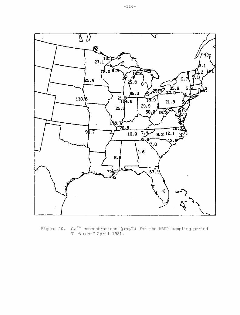
-114-

Figure 20. Ca2+ concentrations (μeq/L) for the NADP sampling period 31 March-7 April 1981.

-115-

Figure 21. K+ concentrations (μeq/L) for the NADP sampling period 31 March-7 April 1981.

-116-

Several weather systems contributed to the weekly precipitation totals at most sites, but one system still dominated. All daily totals for all sites in the test area were under 1 inch. The previous sampling week ended as a cold front moved through the test area. Fig. 23 shows the synoptic situation for 2100 GMT 21 July. This system was the largest producer of rain for NY08, NY12, and PA29, which received .53, .50, and .95 inches, respectively, in association with rain ahead and behind the cold front. The 1019 mb high over southwestern Ontario continued to move southeastward and dominated the weather over the test area for 22-23 July with light winds and cool temperatures. As the high moved off the east coast, scattered areas of showers developed over the Appalachians and Tennessee Valley, as shown in Fig. 24 for 2100 GMT 24 July. A weak low pressure center along the stationary front produced showers over Kentucky, Tennessee, and Mississippi, while the showers over the Appalachians appeared to be in a zone of wind convergence, with weak westerly flow over the Ohio valley and moist southeasterly flow from the Atlantic. TN00, TN11, and WV18 received rain from this system, with amounts of .12, .19, and .41 inches, respectively. This was the largest event for TN00 and the second largest for WV18 in terms of precipitation amount. The major system of the week which brought the most widespread rainfall is illustated in Fig. 25 for 2100 GMT 26 July. It shows a low pressure center over western New York and an associated cold front from southeastern Quebec southwestward to Oklahoma. A seasonally strong high pressure center of 1025 mb was located over North Dakota. For eight sites in the test area, this was the only or largest precipitation event of the week, with amounts ranging from .13 to .82 inches. Intense convection occurred in the warm sector over eastern Pennsylvania with severe thunderstorms and tornadoes reported. Substantial precipitation occured ahead of the system in advance of the warm front as well. Fig. 26 shows the situation for 1800 GMT 27 July, with the high pressure center now over the Great Lakes. Overrunning precipitation in association with the stationary front through the Ohio valley was falling over Ohio and West Virginia and with convection along the front near the Tennessee sites. WV18 and TN11 received their largest weekly amounts with .50 and .88 inches, respectively. The last system of the week developed and moved quickly from the Plains, as shown in Fig. 27 for 1200 GMT 28 July. Ohio sites 0H49 and 0H71 were affected the most with .29 and .64 inches, the latter value the largest amount for 0H71 during the week.

Fig. 28 shows the laboratory pH for the NADP sampling period of 21-28 July. This central week of the acid category had seven (sites with samples passing quality control criteria) of the 15 test sites with pH's below 4.00. In a previous section of this summary, it may be recalled that the central weeks were chosen with respect to the site median pH and not the seasonal median pH. If the pH's of the test sites for this week are compared with summer median values, ten of the sites are still below normal values, but only by a mean of .16 pH units, since the summer medians are all below the site median values. Thus, the sample pH for any one site for this week is not unusual, but the regional scale departure is atypical. Mean concentrations of all ions in the test area were higher this week than the sampling periods before and after it.

The SO42- concentrations shown in Fig. 29 range from 70 to 253 μeq/L

-117-

across the test area, with nine of the sites having concentrations above summer median values. NO3

- concentrations (Fig. 30) ranged from 15 to 76 μeq/L, with eight sites above summer median values. NH4+ continued the same trend, with nine sites above summer median values (Fig. 31). Ca2+ concentrations (Fig. 32) ranged from 7 to 85 μeq/L, with nine sites again having values above summer medians. Two sites, NY51 and NY65, had very high values of 85 and 68 μeq/L, respectively. The two latter sites also had the smallest sample volumes of all those in the test area. K+ concentrations, shown in Fig. 33, did not follow the trend of the other ions, as ten of the sites had concentrations below summer median values.

Inspection of the daily rainfall data in Tables 2-4 gives at least two reasons on possibly why concentrations were enhanced and in this case, acidity as well. As previously mentioned, the average rainfall for the test area for the 21-28 July period was less than either the 14-21 July or 28 July-7 August periods. The latter two periods had several sites with daily rainfall amounts of 1 inch or more, but the central week of 21-28 July had no such events. The central week also had a different distribution of rainfall events across the week in comparison to the other two. Tables 2 and 4 show that the 14-21 July and 28 July-7 August periods had numerous sites with consecutive days of rainfall, whereas the central week had few sites with any substantial rainfall a day before or after the main event on 26 July. Interpretation of this pattern at this time is conjecture, but the dry period before the storm system on 26 July could have allowed additional accumulation of aerosol in the atmosphere.

This sampling period was characterized by an extension of the Bermuda high across the southern states while frontal activity remained to the north. No long term stagnation periods existed over the test area, as two high pressure ridges moved through the Northeast during the week. The main event on 26 July did produce locally intense convection in the warm sector over Ohio and Pennsylvania. The smaller average rainfall and dry period before the 26 July event seem to distinguish the meteorological characteristics in relation to the surrounding weeks, and may have contributed to the higher concentrations of most ions.

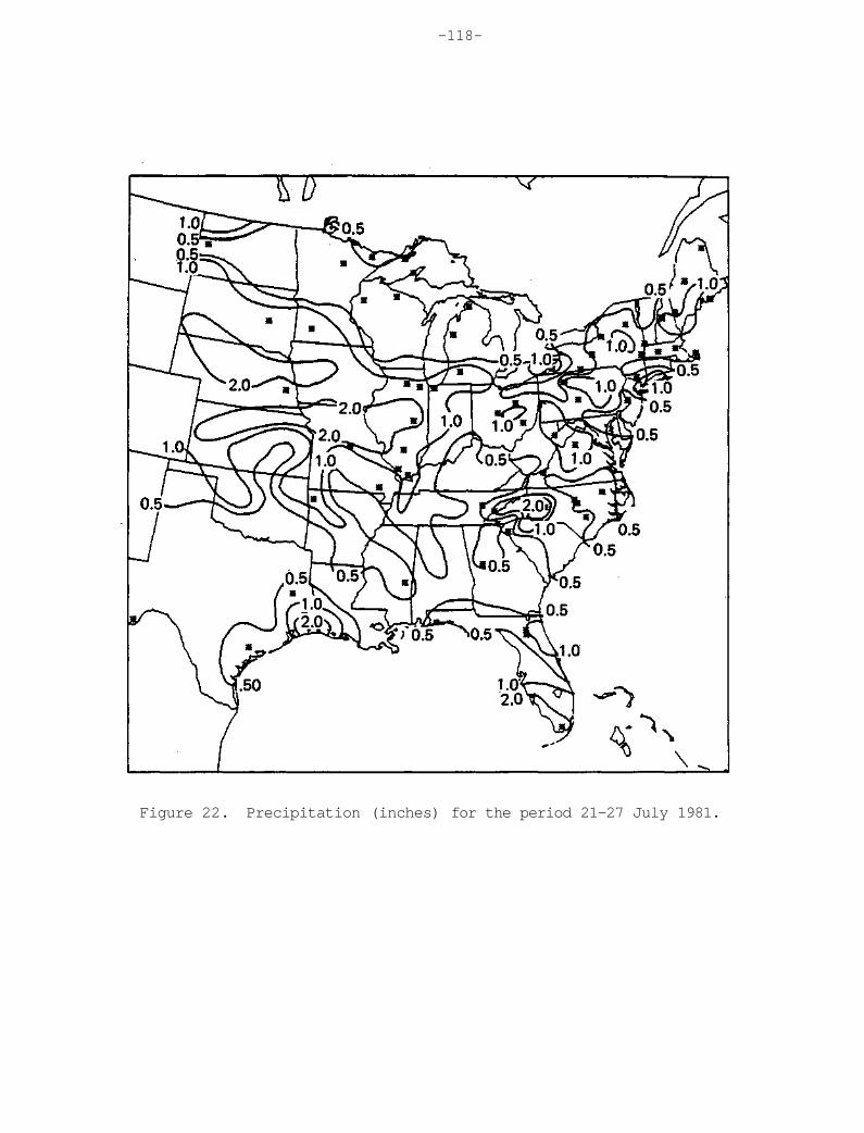
-118-

Figure 22. Precipitation (inches) for the period 21-27 July 1981.

-119-

Figure 23. Surface analysis for 2100 GMT 21 July 1981. Only major radar echoes in test area are shown.

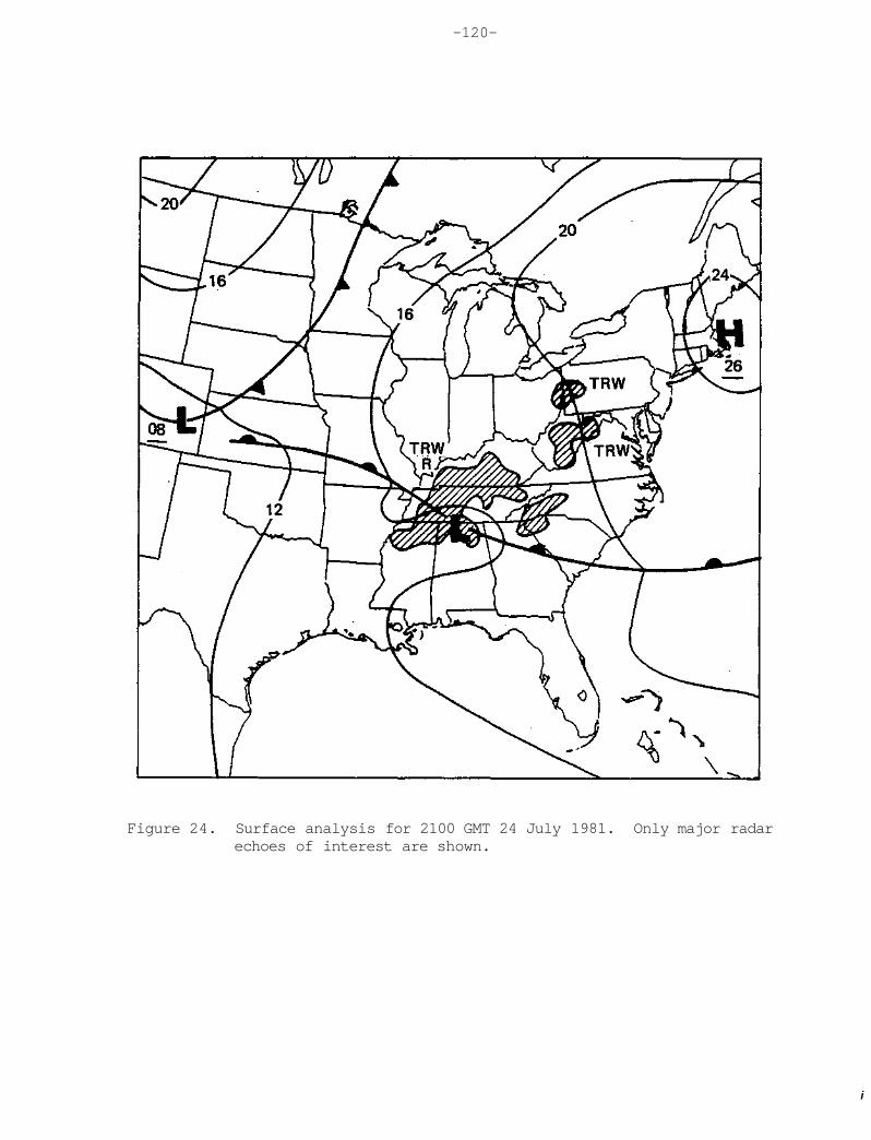
-120-

Figure 24. Surface analysis for 2100 GMT 24 July 1981. Only major radar echoes of interest are shown.

i

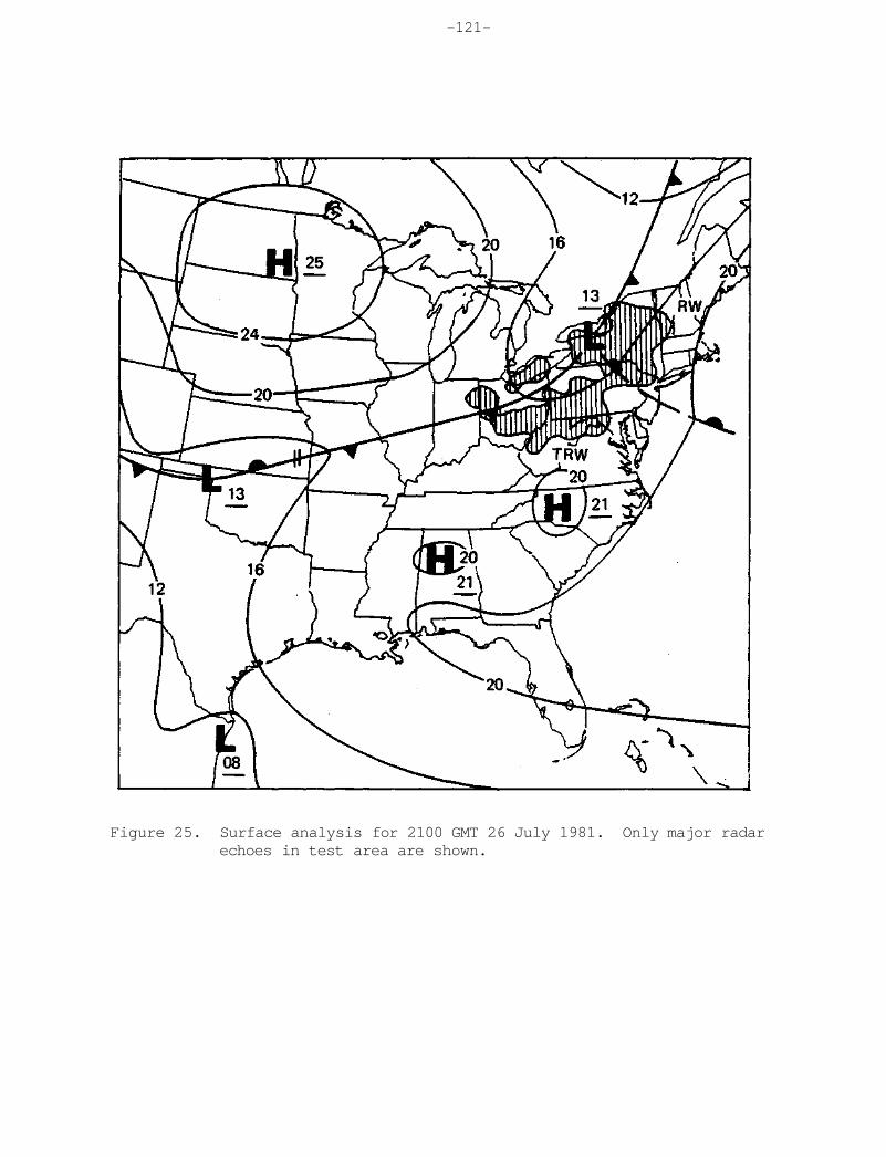
-121-

Figure 25. Surface analysis for 2100 GMT 26 July 1981. Only major radar echoes in test area are shown.

-122-

Figure 26. Surface analysis for 1800 GMT 27 July 1981. Only major radar echoes of interest are shown.

-123-

Figure 27. Surface analysis for 1200 GMT 28 July 1981. Only major radar echoes of interest are shown.

-124-

Figure 28. Laboratory pH for the NADP sampling period 21-28 July 1981.

-125-

Figure 29. SO42- concentrations (μeq/L) for the NADP sampling period 21-28 July 1981.

-126-

Figure 30. NO3- concentrations (μeq/L) for the NADP sampling period

*21-28 July 1981.

-127-

Figure 31. NH4+ concentrations (μeq/L) for the NADP sampling period 21-28 July 1981.

-128-

Figure 32. Ca2+ concentrations (μeq/L) for the NADP sampling period 21-28 July 1981.

-129-

Figure 33. K concentrations (μeq/L) for the NADP sampling period 21-28 July 1981.

-130-

Table 2. Daily rainfall (inches) and laboratory pH for the NADP sampling period 14-21 July 1981 for the 15 sites in the test area. Sites with a "*" are those whose chemical analyses were rejected because of field or laboratory problems.

-131-

Table 3. Daily rainfall (inches) and laboratory pH for the NADP sampling period 21-28 July 1981 for the 15 sites in the test area. Sites with a "*" are those whose chemical analyses were rejected because of field or laboratory problems.

-132-

Table 4. Daily rainfall (inches) and laboratory pH for the NADP sampling period 28 July-4 August 1981 for the 15 sites in the test area. Sites with a "*" are those whose chemical analyses were rejected because of field or laboratory problems.

-133-

CONCLUSIONS

In the statistical analysis of the seasonal distributions of several ions, the results showed that the H+ and SO42- ions were the most variable and the Na+ and NO3- ions were the least variable. The H+ and SO42- ion patterns were very similar except for the winter-spring comparison, where 11 sites showed differences for SO42- but only three sites showed differences for H+. This emphasizes the fact that to predict seasonal changes in precipitation acidity one must consider the total cation-anion balance and not the typical acidic source related ions of SO42- and NO3- alone. Few seasonal differences were observed for the C1-, NH4

+, Ca2+, Mg2 + , and K+ ions for the spring through fall period. High concentrations of Ca2+, Mg2+, and K+ during the period of 17-24

March 1981 across the test area occured in conjunction with weekly precipitation amounts generally less than .25 inches accompanied by high winds over dry land surfaces with little extensive snow cover. Trajectory analyses for 3-4 April 1981 provided evidence for the potential transport of dust storm aerosol from the southern Plains and incorporation with precipitation for NE15, sites in southern Illinois, and possibly sites in Ohio. The acidic departure case study period of 21-28 July 1981 revealed high concentrations of most ions in comparison with adjacent weeks, and appeared to be related with the smaller average sample volume across the test domain and the relatively long dry period before the main rainfall event.

ACKNOWLEDGEMENTS

Major Jerre Wilson, formerly of the Science Research Laboratory of the United States Military Academy, kindly provided the trajectories used in this study.

REFERENCES

Boerngen, J. G., and H. T. Shacklette, 1981: Chemical analyses of soils and other surficial materials of the conterminous United States. U.S. Geological Survey Open File Report 81-197.

Brownlee, K. A., 1960: Statistical theory and methodology in science and engineering, New York, John Wiley & Sons, Inc., 570 pp.

Changnon, S. A., 1982: Causes and implications of record windblown dust conditions during 1981 in Illinois, Circular 151, Illinois State Water Survey, 23 pp.

-134-

Climatological Data, National Oceanic and Atmospheric Administration; National Environmental Satellite, Data, and Information Service; National Climatic Data Center; Asheville, NC.

Cogbill, C. V., and G. E. Likens, 1974: Acid precipitation in the northeastern United States. Water Resour. Res., 10, 1133-1137.

Doty, K. G., and R. G. Semonin, 1984: The chemistry and meteorology of extreme pH departures in precipitation on the regional scale. (to be published), Research report to the U.S. Department of Energy, Pollutant Characterization and Safety Research Division, Office of Health and Environmental Res. by the Illinois State Water Survey, Contract DE-AC02-76EV01199.

Evans, J. S., and D. W. Cooper, 1980: An inventory of particulate emissions from open sources. J. Air Pollut. Control Assoc, 30, 1298-1303.

Gambell, A. W., and D. W. Fisher, 1966: Chemical composition of rainfall in eastern North Carolina and southeastern Virginia. U.S. Geological Survey Water Supply Paper 1535-K, 1-41.

Gatz, D. F., 1983: Source apportionment of rain water impurities in Central Illinois. Proc. 76th Annual Meeting of the Air Poll. Cont. Assoc, Atlanta, GA, June 19-24, 16 pp.

-----, G. J. Stensland, M. V. Miller, and A. C. D. Leslie, 1981: Sources of airborne calcium in rural central Illionois. In: Macias, E. S., and P. K. Hopke, Editors, Atmospheric Aerosol-Source/Air Quality Relationships. ACS Symposium Series 167, Washington D.C., American Chemical Society, 303-326.

-----, 1977: Review of chemical-tracer experiments on precipitation systems. In: Semonin, R. G., and R. W. Beadle, Editors, Precipitation Scavenging (1974), Symposium sponsored by the Illinois State Water Survey and the Division of Biomedical and Environmental Research of the U.S. Atomic Energy Commission, Champaign, IL, October 14-18, 1974, 321-361.

Heffter, J. L., 1980: Air Resources Laboratories Atmospheric Transport and Dispersion Model (ARL-ATAD), Technical Memo ERL-ARL-81, Air Resources Laboratories, National Oceanic and Atmospheric Administration, Silver Spring, MD, 17 pp.

Junge, C. E., 1958: The distribution of ammonia and nitrate in rain water over the United States. Trans. Am. Geophys. Union, 39, 241-248.

, and R. T. Werby, 1958: The concentration of chloride, sodium, potassium, calcium, and sulfate in rain water over the United States. J. Meteorol., 15, 417-425.

-135-

Lodge, J. P., Jr., J. B. Pate, W. Basbergill, G. W. Swanson, K. C. Hill, E. Lorange, and A. L. Lazrus, 1968: Chemistry of United States Precipitation. Final report on the National Precipitation Sampling Network, National Center for Atmospheric Research, Boulder, CO, 66 pp.

Pearson, F. J., and D. W. Fisher, 1971: Chemical composition of atmospheric precipitation in the northeastern United States. U.S. Geological Survey Water Supply Paper 1535-P, 1-23.

Pratt, J. W., and J. D. Gibbons, 1981: Concepts in nonparametric theory. New York, Springer-Verlag, 462 pp.

Stensland, G. J., and R. G. Semonin, 1982: Another interpretation of the pH trend in the United States. Bull. Am. Meteorol. Soc., 63, 1277-1284.

Walpole, R. E., and R. H. Myers, 1972: Probability and statistics for engineers and scientists, New York, Macmillan Publishing Co., Inc., 506 pp.

-137-

CHAPTER 6

DRY BUCKET ANALYSIS OF THE NADP NETWORK

Richard 6. Semonin

INTRODUCTION

The initial deliberations for the design of a national precipitation monitoring network called for the use of a wet/dry sampler. It was early recommended that the sampler available from AeroChem Metrics, Incorp­orated, based on the HASL design, would satisfy needs for the sampling of precipitation and provide an estimate of dry deposition. The question was controversial in the early stages and remains so today concerning the analysis of the dry side of this two bucket instrument.

Research results by others suggested that approximately 1/2 of the total deposition could be attributed to dry processes and therefore dry deposition became an important issue in the national program of monitor­ing. A variety of techniques have been utilized for dry deposition estima­tion ranging from highly sophisticated instruments to simple open buckets exposed to the atmosphere.

Arguments continued to abound concerning the inadequacies of the open bucket system. These arguments centered on questions concerning the mechanical design of the sampler posing an obstacle to the surface layer wind, the scouring action of the wind removing material from the bucket container, and the adsorption of materials on the wall of the bucket making it difficult to obtain a quantitative chemical assessment of the contents. Throughout all of these arguments, however, no data have been presented in a systematic way to show that, in fact, the dry bucket does not represent some relative measure of dry material depositing at the surface of the earth from the atmosphere.

In spite of this lack of evidence to negate the utility of the dry bucket collections, it is now a policy of the national network that the dry- side bucket will be voluntarily submitted to the Central Analytical Laboratory for analysis. This is an unfortunate turn of events since data have continued to be compiled since the initiation of the network and without a suitable replacement for the dry deposition estimate the moni­toring of this "half" of the total deposition will continue to remain a question for some time to come.

In this chapter some preliminary descriptive material are presented showing the dry deposition of selected ions over the United States as estimated from the dry bucket contents.

-138-

SAMPLE COLLECTION AND HANDLING

Early in the NADP program the dry side buckets were collected on the first Tuesday of the even-numbered months throughout the year. This protocol provided six samples for analysis in each year. In 1982 a new policy was adopted to ship the dry bucket each eight weeks for analysis so that in effect the same period of exposure was approximated under both of these sampling schemes.

Owing to the gradual buildup of the NADP/NTN network, some stations have a greater number of dry bucket analyses because they received equip­ment and initiated sampling earlier than others. In fact, because of the gradual buildup of the National Trends Network (NTN) some projected sites are not as yet in operation at the time of this writing.

A dry bucket is collected in the field by simply pounding a lid on the bucket and placing it in a shipping container for transport to the Central Analytical Laboratory. Upon receipt at the CAL, the bucket is opened and qualitatively inspected by laboratory personnel for decaying vegetative matter, decaying insects, and bird droppings. If any of these items are observed in the bucket the sample is discarded.

If the sample is accepted for further treatment, 250 ml of deionized distilled water is placed in the bucket and it is vigorously shaken by hand and then allowed to equilibrate by standing overnight. The sample is then treated the same as a precipitation sample.

DATA ANALYSIS

The laboratory concentrations are converted to depositions and each site sample is compiled into a history of dry deposition. The display of the computer-stored site history presents a median value as well as the extremes and quartile values for each ion at each site. The data to be discussed are median values for the entire length of record at available sites. In addition, two case study examples are shown from the warm, season of 1981 with calculated deposition values obtained directly from two consecutive bucket collections.

DATA DISCUSSION

Median Value Data

Five ions were chosen to exemplify the recognizable pattern of dry deposition estimated from the dry side bucket of the AeroChem Metrics sampler. These five are calcium, chloride, ammonium, nitrate, and sul­fate.

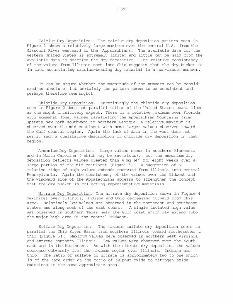
-139-

Calcium Dry Deposition. The calcium dry deposition pattern seen in Figure 1 shows a relatively large maximum over the central U.S. from the Missouri River eastward to the Appalachians. The available data for the western United States is extremely limited and little can be said from the available data to describe the dry deposition. The relative consistency of the values from Illinois east into Ohio suggests that the dry bucket is in fact accumulating calcium-bearing dry material in a non-random manner.

It can be argued whether the magnitude of the numbers can be consid­ered as absolute, but certainly the pattern seems to be consistent and perhaps therefore meaningful.

Chloride Dry Deposition. Surprisingly the chloride dry deposition seen in Figure 2 does not parallel either of the United States coast lines as one might intuitively expect. There is a relative maximum over Florida with somewhat lower values paralleling the Appalachian Mountains from upstate New York southward to northern Georgia. A relative maximum is observed over the mid-continent with some larger values observed toward the Gulf coastal region. Again the lack of data in the west does not permit such a qualitative description of chloride dry deposition in that region.

Ammonium Dry Deposition. Large values occur in southern Minnesota and in North Carolina ( which may be anomalous), but the ammonium dry deposition reflects values greater than 4 mg M-2 for eight weeks over a large portion of the mid-continent (Figure 3). A suggestion of a relative ridge of high values extends eastward from Illinois into central Pennsylvania. Again the consistency of the values over the Midwest and the windward side of the Appalachians appears to strengthen the concept that the dry bucket is collecting representative materials.

Nitrate Dry Deposition. The nitrate dry deposition shown in Figure 4 maximizes over Illinois, Indiana and Ohio decreasing outward from this area. Relatively low values are observed in the northeast and southeast states and along most of the east coast. A single isolated high value was observed in southern Texas near the Gulf coast which may extend into the major high area in the central Midwest.

Sulfate Dry Deposition. The maximum sulfate dry deposition seems to parallel the Ohio River Basin from southern Illinois toward southeastern „ Ohio (Figure 5). Maximum values were observed in northern West Virginia and extreme southern Illinois. Low values were observed over the South-east and in the Northeast. As with the nitrate dry deposition the values decrease outwardly from the maximum region over Illinois, Indiana and Ohio. The ratio of sulfate to nitrate is approximately two to one which is of the same order as the ratio of sulphur oxide to nitrogen oxide emissions in the same approximate area.

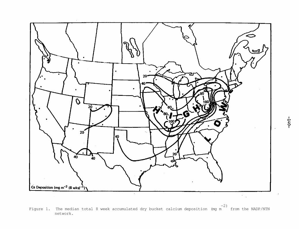
-2) Figure 1. The median total 8 week accumulated dry bucket calcium deposition (mg m from the NADP/NTN network.

Figure 2. The same as Figure 1 for chloride.

Figure 3. The same as Figure 1 for ammonium.

Figure 4. The same as Figure 1 for nitrate.

Figure 5. The same as Figure 1 for sulfate.

-145-

Case Study Analysis

Two consecutive dry bucket collections were analyzed and the data are presented in Figures 6-9. Only calcium and sulfate are presented although nitrate was analysed, but is not discussed here. These data represent the deposition normalized by the number of weeks in the sampling interval and are therefore presented in units of milligrams per square meter per week. To compare the values with the previously presented figures these numbers should be multiplied by approximately 8.

Calcium Dry Deposition. The dry bucket calcium deposition for the period May 19 through July 14 1981 shows a maximum through the central part of the United States as seen in Figure 6. This maximum corresponds quite well to the maximum shown in Figure 1 although shifted somewhat to the north due largely to a single station incorporated in this study but not included in the overall median presentation in northwestern Indiana. The pattern shown in Figure 7 for the period July 14 through September 8, 1981 is remarkably similar to the distribution in Figure 6. The same relatively large maximum is observed over northern Illinois, northern Indiana, and extending into central Ohio with relatively low values along the entire east coast.

As with the median data shown in Figures 1-5 there are not adequate numbers of stations available for a meaningful analysis west of the Missouri River.

The only noteworthy point in comparing these two sample periods is that the dry deposition of calcium for the eastern portion of the country seems to be rather consistent with values ranging up to 10 mg M-2 wk-1 and typical values on the order of 4. When one compares the data in Figures 6 and 7 with Figure 1 and adjusts for the factor of 8 difference in data presentation, we see that we have about the same order of magnitude of dry deposition in each of the case studies as indicated by the eight week accumulated median values.

Sulfate Dry Deposition. The sulfate deposition pattern is extremely similar to that for calcium in both periods as seen in Figures 8 and 9. The maximum value again is over Illinois with a general area extending eastward to Ohio. It is noteworthy to mention that the values of dry sulfate deposition decreased somewhat between the first and second sample periods.

The distribution of dry sulfate deposition is not unlike the median presentation as shown in Figure 5. The general maximum occurs over the Illinois, Indiana, Ohio and western Pennsylvania area and decreasing values are found outward from that general area. As mentioned previously, the general shift of the central maximum value in the case studies to northwestern Indiana is largely a result of a single station in that location that was not included in the median values analyzed in Figure 5 because of a lack of sufficient data.

Figure 6. The measured dry bucket calcium deposition for the period 19 May 1981 to 14 July 1981. The units are mg m-2 wk-1.

Figure 7. The same as Figure 6 for the period 14 July 1981 to 8 September 1981.

Figure 8. The measured dry bucket sulfate deposition for the period 19 May 1981 to 14 July 1981. The units are mg m-2 wk-1.

Figure 9. The same as Figure 8 for the period 14 July 1981 to 8 September 1981.

-150-

SUMMARY

As stated at the outset the purpose of this study was to determine whether some information is contained in the dry bucket samples acquired from an AeroChem Metrics wet-dry sampler. It is contended that the data shown are consistent and not random excursions, and may, in fact, repre­sent some portion of dry deposition for those ions discussed. It should be emphasized that dry deposition has different meanings to different in­vestigators and to the national program. The definition of dry deposition itself needs to be clarified to provide a common foundation for future research endeavors. For example, the dry deposition of sulphur dioxide on a surface of vegetation is largely determined not by atmospheric forces distributing the gas, but rather upon the biological structure of the impinged material. Certain vegetation openly accepts sulphur dioxide through the stomata of the plants whereas others resist gaseous uptake at the same concentration. However, the dry deposition of aerosol is largely determined by mechanical factors in the atmosphere and by the collecting surface. In this case no particular biological effect is responsible, but rather the mechanical attachment of an aerosol particle to whatever collecting surface is impacted. Thus the data presented in Figures 1-9 are likely a realistic assessment of dry deposition to an exposed polyeth­ylene bucket. If one wanted to use these values to estimate the dry deposition to a forest or to a flat grassland or to some other surface, one would have to do research to compare the deposition in a bucket to the particular surface of interest.

It should be stressed that there is a sizable data base existing in the NADP/NTN on the dry bucket chemistry and these data should be more carefully screened and studied to guide future efforts to develop a dry deposition monitoring network.

-151-

CHAPTER 7

METAL SOLUBILITY IN ATMOSPHERIC DEPOSITION*

Donald F. Gatz Lih-Ching Chu

INTRODUCTION

Concern over potential toxicity of heavy metals has led to measurements of their input to terrestrial and aquatic ecosystems via atmospheric deposition (Andren and Lindberg, 1977; Eisenreich, 1980; Jeffries and Snyder, 1981; Lindberg et al., 1980; Schlesinger et al., 1974; Swanson and Johnson, 1980; Wiener, 1979). Effects of metals in ecosystems depend in part on their mobility and bioavailability (Hardy and Crecelius, 1981; Lindberg and Harriss, 1980). Mobility and bio­availability of metals have been characterized in terms of metal solubilities in water and various stronger extractants in samples of aerosols (Lindberg and Harrison, 1980), street dusts (Harrison et al., 1981), and roadside soils (Harrison, et al., 1981). Since atmospheric deposition is a major mechanism by which airborne metals reach ecosystems, it is also important that we understand metal solubility in wet and dry deposition. Further, the mesoscale spatial distributions of soluble and insoluble forms of the same elements appear to be clues to the sources of the elements and/or the scavenging processes by which they are removed from the atmosphere by precipitation (Gatz, 1980).

Solubility of metals in many natural aqueous systems can be influenced by organic materials (Harrison et al., 1981; Slavek and Pickering, 1981; Wilber and Hunter, 1979), clay minerals (Slavek and Pickering, 1981; Wilber and Hunter, 1979), metal hydroxides (Harrison et al., 1981; Wilber and Hunter, 1979), pH (Cavallaro and McBride, 1978; Farrah and Pickering, 1977; Sadiq and Zardi, 1981; Slavek and Pickering, 1981), and divalent ions (Garcia-Miragaya and Page, 1977; Griffin and Au, 1977; McBride, 1976). Of these, clay minerals and metal hydroxides would be part of the insoluble matter in precipitation samples. There have been pleas for separate analyses of soluble and insoluble impurities in precipitation (Lewis and Grant, 1978; Rattonetti, 1976), but the insoluble fraction is still rarely analyzed, and it appears from a recent review of literature on toxic substances in atmospheric precipitation (Galloway et al., 1980), that precipitation has not yet been systematically examined for the influence of insoluble materials on metal solubility.

Of ten recent papers reporting heavy metal concentrations in precipitation, (Andren and Lindberg, 1977; Betson, 1978; Dethier, 1979; Eisenreich, 1980; Hendry and Brezonik, 1980; Jeffries and Snyder, 1981; Navarre et al., 1980; Schlesinger et al., 1974; Swanson and Johnson 1980; Wiener, 1979) none reported soluble and insoluble metals

Submitted to Davidson, C. I., Ed., Metals in the Air, Advances in Environmental Science and Technology Series, 1 November 1983.

-152-

separately. None of these authors separated soluble from insoluble materials before analysis. In one case (Swanson and Johnson, 1980) separation by filtration was tested, but comparison of metal concentra­tions in 20 pairs of filtered and unfiltered subsamples showed no effect on measured concentrations, and filtration was abandoned. In other cases, separation of soluble and insoluble fractions was pre­cluded by preacidification of the collection vessel for the purpose of avoiding wall losses from the precipitation samples. Depending on the specific analytical procedures used, these papers reported metal con­centrations variously as "soluble," "total," or "total acid leachable," or simply did not indicate what their measurements represented.

As pointed out by Rattonetti (1976), proper storage and treatment of natural water samples are necessary for accurate analyses, as well as to enable proper interpretations of the measurments. Rattonetti analyzed soluble and insoluble fractions of stream waters and rain and found that acidification of unfiltered samples artifically released metals from insoluble particles in the samples. Wall losses of dissolved metals were minimal in samples containing insoluble particles. Filtration was recommended to stabilize the distribution of metals between soluble and insoluble fractions. Acidification of the filtrate was recommended to avoid wall losses following filtration.

To help improve our knowledge in this area, we examined a set of atmospheric deposition samples for distributions of metal solubility in wet, dry, and bulk (wet + dry) precipitation, and for their relationship to concentrations of insoluble materials and sample pH.

EXPERIMENTAL METHODS

Sampling Methods Both bulk and separate wet and dry samples were collected weekly

(Tuesdays) except for a few 2- or 3-week periods. The wet and dry samples were collected in 29.4 cm diameter white high density polyethylene buckets using an Aerochem Metrics sampler. The bulk sample, open to the atmosphere continuously, was collected in the same type of bucket.

The collectors were located at a Commonwealth Edison Co. electric power substation in a residential area of Glen Ellyn, Illinois, 42 km west of the Lake Michigan shoreline. The collector openings were positioned about 1.5 m above a grass surface, a few meters south of a seldom used crushed limestone parking lot. The site was bordered to the east and south by the asphalt parking lot of a three-story apartment building located 25 m to the east of the samplers. No obstacles were located higher than 45 degrees from the horizontal.

Rainfall was measured in a standard weighing bucket recording raingage with a 30.5 cm (12-inch) diameter top. In winter the raingage collector bucket was charged with an antifreeze solution to prevent freezing of the accumulated sample. The antifreeze solution was covered

-153-

with a thin layer of motor oil to prevent evaporation. An Alter-type wind shield surrounded the raingage to lessen the effect of the wind on the catch. Openings and closings of the wet/dry collector were recorded on the raingage chart with an event pen.

The pre-weighed sample containers were re-weighed to the nearest gram to measure sample mass before shipment to our laboratory in Champaign, Illinois, for analysis.

Laboratory Procedures

In the laboratory, sample processing was begun immediately upon arrival of the samples to minimize internal chemical changes. The first step was to weigh the containers as a check on possible leaks during shipment. Then, a 16 mL portion of the sample was removed and used for measuring pH and specific conductance. A volume of 250 mL of deionized water was added to the dry-side buckets and 50 mL to those wet and bulk collectors that were exposed during weeks when no precipitation fell. Samples to which water was added were allowed 24 hr to equilibrate before mass, pH, and specific conductance were measured.

To separate the "soluble" (i.e., filterable) and "insoluble" (i.e., non-filterable) materials, samples were filtered through preweighed 47 mm diameter 0.4 μm pore diameter polycarbonate membranes. The portion of the filtrate designated for trace metals analysis was acidified to pH 2 with nitric acid to stabilize the metals in solution (U.S. EPA, 1979).

The filters containing the insoluble impurities were placed in a chamber maintained at a constant 47% relative humidity by a saturated lithium nitrate solution and were allowed to equilibrate for one week before being reweighed to determine insoluble mass. The filters were digested in small amounts of concentrated nitric acid and 30% stabilized hydrogen peroxide in Teflona-lined stainless steel pressure vessels. Following digestion, the sample solutions were diluted to a 1.28 N (8%) nitric acid concentration and stored in acid-washed linear polyethylene bottles. A reagent blank and filter blank were processed concurrently and analyzed with each batch of seven filters.

Flame atomic absorption spectrophotometry (AAS) was used to analyze the acidified portion of the filtrate for Zn and the insoluble portion of the sample for A1, Cu, Fe, and Zn. Flameless AAS was used for the analysis of soluble Cd, Cu, and Pb, and insoluble Cd and Pb. EPA Trace Metals Reference Samples of known concentrations were analyzed with the precipitation samples. Results showed accuracies mostly within 5% and precisions (two standard deviations) mostly less than 15% of the mean values, at concentrations of ten times detection limits.

aDuPont trademark

-154-

Laboratory Equipment

An Oriona model 811 pH meter with a Beckmana Futura microcombination electrode and a Metrohma model 103 pH meter with microcombination electrode were used for pH measurements. Specific conductance was measured with a Yellow Springs Instrument Co.a manually balanced AC bridge with glass microelectrode. Instrumentation Laboratorya models 353 and 951 atomic absorption spectrophotometers were used for all flame atomic absorption measurements. Flameless AAS analyses were carried out on an Instrumentation Laboratory model 151 AAS fitted with Instrumentation Laboratory model 455 and Variana model 63 carbon rod atomizers.

Reagents

All metal standard solutions were prepared from either a reagent grade soluble salt or metal dissolved in the minimum amount of acid and diluted to the desired concentration with polished deionized water. All other chemicals were reagent grade.

RESULTS

Data Summaries

Tables 1 and 2 give a partial summary of analytical results. Minimum and maximum concentrations, as well as median concentrations and standard errors are given for both soluble and insoluble fractions of all metals measured. Results for total insoluble mass (TIM) concentrations and for sample pH are given also. Examination of normal plots of log concentrations indicated that all concentrations were approximately lognormally distributed.

Partition coefficients, which describe the partitioning of metals between solid and liquid phase in atmospheric precipitation, were calculated using the definition of Eisenreich et al., (1981). Thus, the partition coefficient, k , is given by kp = (μg metal/g solids)/(μg metal/g water). The results are summarized in terms of observed median values in wet-only and bulk precipitation in Table 3. The table also gives observed values of kp for the same four metals in lake water from Saginaw Bay, Lake Huron, for comparison. It appears that kp is higher in Saginaw Bay, indicating a greater tendency for metals to adsorb onto solids in lake water than in precipitation. The available data do not permit a clear explanation of these differences, but the composition of suspended solids in lake water is no doubt different from those in precipitation, especially with regard to organic materials, and thus metal sorption characteristics can also be expected to differ. a0rion Research Inc., Cambridge, MA 02139 Beckman Instruments, Inc., Irvine, CA 92713 Brinkman Instruments, Inc., Westbury, NY 11590 (Metrohm) Yellow Springs Instrument Co., Yellow Springs, OH 45387 Instrumentation Laboratory, Inc., Wilmington, MA 01887 Varian Associates, Palo Alto, CA

-155-

Partition coefficients appear to be greater in wet-only than in bulk samples (Table 3), except for Pb. The reasons for these differences are not immediately apparent either, but again suggest a systematic difference in the composition of the solid materials between the two types of atmospheric deposition samples.

Table 1. Summary of analytical results for wet samples.

pH units

Distributions of Percent Soluble Metals

Frequency distributions of soluble fractions of Zn and Pb in wet, dry and bulk samples from weekly sampling periods between December 1979 and March 1981 are shown in Figures 1 and 2, respectively. Zn was almost always very soluble in wet samples, but a wide range of solubilities occurred in the dry and bulk samples. Pb was also quite soluble in wet samples, but somewhat less than Zn. Most of the dry samples, however, had less than 10% soluble Pb.

Distributions of Cu and Cd solubilities (not shown) were inter­mediate between those of Zn and Pb. Table 4 shows that the median solubilities of Cd were very similar to those of Zn in wet, dry, and bulk samples, respectively. The corresponding median solubilities for Cu were intermediate between those of Zn and Pb.

Thus, all four metals examined were mostly soluble in wet samples, but exhibited a wide range of solubility in dry and bulk samples. The solubility distributions in the bulk samples were much more like those of the dry than the wet samples.

-156-

Table 2. Summary of analytical results for bulk samples.

Table 3. Observed partition coefficients in wet-only and bulk precipitation samples.

-157-

Figure 1. Frequency distributions of percent soluble Zn in wet, dry and bulk samples.

-158-

Figure 2. Frequency distributions of percent soluble Pb in wet, dry and bulk samples.

-159-

Metal Solubility as a Function of TIM Concentrations

To examine the possible influence of insoluble materials on metal solubility in atmospheric deposition, the soluble fractions of Zn and Pb were plotted against the concentration of total insoluble mass (TIM) (Fig. 3). For both metals, the wet and bulk samples show a consistent pattern with respect to TIM, with the wet samples on the whole having smaller TIM concentrations and greater solubilities. There were noticeable differences between Zn and Pb in their relationships to TIM concentrations. Both show a general tendency for solubility to decrease as TIM concentrations increase, but Zn was generally more soluble than Pb, at least at higher TIM concentrations. More specifically, for TIM concentrations below 50 mg/L, Zn was likely to be > 80% soluble. For TIM concentrations > 50 mg/L, Zn solubility was rather uniformly distributed between 20 and 90%. Pb, on the other hand, was likely to be > 80% soluble only for TIM concentrations < 3 mg/L. For TIM concentrations between 3 and 30 mg/L, Pb solubility was rather uniformly distributed between 0 and 90%. For TIM concentrations > 30 mg/L, Pb was likely to be < 20% soluble.

Results are not plotted for Cd and Cu, but examination of similar plots for these two metals showed that Cd behaved very similarly to Zn and Cu similarly to Pb. Results for Cd and Cu are included in the summary of median metal solubilities and TIM concentrations given in Table 4. For each sample type, the median percent solubilities of Zn and Cd were very similar, and Cu was intermediate between those elements and Pb. Further, Table 4 shows that solubility varied inversely to TIM among the three types of samples. TIM was lowest in the wet samples, in which metal solubilities were greatest, and highest in dry samples, where solubilities were least.

Table 4. Median values for total and Fe insoluble concentrations in wet, dry, and bulk samples, with corresponding median metal solubilities.

aConcentration measured in diluted samples.

-160-

Figure 3. Metal solubility as a function of total insoluble mass concentration for wet and bulk samples.

-161-

Metal Solubility as a Function of Insoluble Fe Concentrations

One of the specific agents for removal of metal ions from solution, either by sorption at the surface or by inclusion in the metal hydroxide precipitate, is metal hydroxides. As an indication of the possible effect of hydroxides on metal solubility, we plotted solubilities versus concentrations of insoluble Fe. Results for both Zn and Pb are shown in Figure 4. Both Zn and Pb behaved similarly with respect to in­soluble Fe concentrations as they did with respect to TIM concentra­tions. That is, considering wet and bulk samples combined, there were only a few samples having Zn < 50% soluble, while for Pb about half the samples had < 50% of their Pb in soluble form. For both metals, the wet samples had generally higher solubilities than the bulk samples.

More specifically, for insoluble Fe concentrations < 1 mg/L, Zn was likely to be > 80% soluble, while above 1 mg/L Zn solubility was quite uniformly distirbuted between 20 and 90%.

Pb was likely to be > 80% soluble only for insoluble Fe concentrations < 0.1 mg/L, while the range of uniform solubility distribution was 0.1 to 1 mg/L. Above an insoluble Fe concentration of 1 mg/L, Pb was likely to be < 10% soluble.

Again, the results for Cd and Cu are not plotted, but in this case also, the Cd results were very similar to those of Zn and Cu results to those of Pb. As in the case of TIM, Table 4 shows an inverse relationship between median values of metal solubilities and insoluble Fe concentrations.

Metal Solubility as a Function of pH

Results for Zn and Pb are shown in Figure 5. At first glance, Figure 5 appears to show almost random variability of metal solubility with pH, but differences between sample types may be discerned with study of the data. Zn in wet samples was almost all > 80% soluble, regardless of pH. In the bulk samples, however, solubility was quite variable at pH > 4.5, but Zn was mostly > 70% soluble at pH < 4.5.

Pb in wet samples showed quite a strong tendency to increase in solubility with decreasing pH. The same general pattern occurred in the bulk samples, but again pH 4.5 was the dividing line between regimes. At pH > 4.5, Pb was mostly < 20% soluble, but between pH 4.0 and 4.5 the distribution of solubility was again more or less uniform from very low to very high values.

The Sample Volume Effect

The effect of rainfall amount, or sample volume, on concentrations of most any material in precipitation is well known. Concentrations tend to decrease, often exponentially (Hales and Dana, 1979), with rainfall amount. There is also an effect of sample volume on pH, as shown in Figure 6. Two separate regimes appear. For rainfall > 1 cm, the pH values were predominantly between 4 and 5. On the other hand,

-162-

Figure 4. Metal solubility as a function of insoluble Fe concentration for wet and bulk samples.

-163-

Figure 5. Metal solubility as a function of sample pH.

-164-

Figure 6. Variation of sample pH with rainfall.

-165-

for rainfall < 1 cm, the pH was relatively uniformly distributed between pH 4 and 7, for both wet and bulk samples. The reasons for this result are not known, but could be related to differing removal mechanisms for alkaline and acidic materials from the atmosphere.

DISCUSSION

The systematic differences in metal solubility between wet, dry, and bulk samples need an explanation. Figures 1 and 2 and Table 4 demonstrate, first, the metals were generally very soluble in wet samples, but that solubility was distributed more uniformly in the dry and bulk samples, and secondly, that, in a given type of sample, Zn and Cd were the most soluble, followed in order by Cu and Pb.

The reason for the systematic differences in metal solubility between wet and dry or bulk samples appears to lie in the enhanced concentrations of insoluble materials in the dry and bulk samples and the fact that insoluble materials tend to remove ions from solution through some sort of sorption process. As was shown in Figure 3, metal solubility decreased with increasing concentrations of TIM.

One component of the insoluble material that may sorb metal ions on its surface or incorporate them by co-precipitation is the hydrous metal oxides, such as hydrous Fe oxide. The similarity of the metal solubility relationships to TIM and insoluble Fe concentrations in Figures 3 and 4, respectively, indicates that sorption or co-precipitation involving hydrous metal oxides is very likely to be involved in determining metal solubility in atmospheric precipitation.

Another component of the insoluble material that may sorb metal ions is aluminosilicate clay minerals. Indeed, the observed order of solubility (Zn ~ Cd > Cu > Pb, Table 3) is opposite to observed metal ion affinities for montmorillonite, kaolinite, and illite, as reported by Farrah and Pickering (1977).

Local soils contain the clay minerals montmorillonite, kaolinite, and illite in mass fractions totaling about 30%. Thus, the clays are the dominant Al-bearing minerals, and the insoluble Al concentration in precipitation should be a good index of the clay mineral concentration. However, plots (not shown) of the insoluble Al concentration in 25 randomly-chosen samples from the sample set, versus soluble fractions of Zn and Pb, showed only a weak tendency for lower solubilities with higher concentrations of insoluble Al.

The results also illustrate the key role of meteorological factors in precipitation chemistry. It is well known that concentrations of most materials in rain vary inversely with rainfall amount (Hales and Dana, 1979). The variation of pH with rainfall is not so well known, but Figure 6 shows a rather strong relationship for our site in which pH was rather uniformly distributed in rainfall < 1 cm, but confined to a rather narrow range of pH, between pH 4 and 5, with heavy rains. Thus, heavy rains tend to have low concentrations of insoluble materials, and

-166-

low pH, both of which tend to enhance metal solubility. This suggests that two sites having equal total metal deposition but different distributions of rainfall amount could have different amounts of soluble metals deposited. The site with the greater frequency of heavy rains would tend to have a higher soluble metal deposition.

These results also have important implications regarding sample collection methods. If one wants to measure the soluble metal composition of the rain as it hits the ground, it is clear that only a

wet-only sample will give the proper result, because the insoluble materials that accumulate in a bulk sample during dry periods will very likely remove some portion of the soluble metals from solution before they can be measured.

These results also have important implications of the methods used to prepare precipitation samples for metal analyses. Measurements of total metal content of precipitation are the most appropriate for comparison of metal concentrations in precipitation against those in air, or in mass budgets where comparison is made to emissions, since both airborne concentrations and emissions are generally given in terms of total (i.e., not just soluble) metals. To measure total metal concentrations in precipitation, the analyst must be certain that both soluble and insoluble fractions of the metal in question are being measured. Some methods, e.g. neutron activation analysis of liquid samples or of residue left after evaporation of a precipitation sample, can measure totals, but analytical methods that require solids to be dissolved before measurement, such as flame AAS, should be used on separate samples of the soluble and insoluble fractions of precipitation samples. The soluble metals may be determined directly in the sample filtrate, but the insoluble metals must be determined in an appropriately dissolved portion of the insoluble materials.

These results are also important in other areas of precipitation chemistry. For example, to understand the chemistry of metals in precipitation, one clearly needs a complete picture of the distribution of the metal between soluble and insoluble phases, as well as measurements of other species that affect metal solubility in both soluble and insoluble fractions. A similarly complete picture is also needed for other studies involving metals in precipitation, such as scavenging of airborne metals by precipitation, the use of metals in precipitation as source tracers, and effects of increased precpitation acidity on metal mobility and bioavailability in ecosystems.

The results given here do not agree with those of Swanson and John­son (1980), which found no differences in metal concentrations between pairs of filtered and unfiltered samples. No explanation of the earlier results is apparent, unless the samples were collected in a location where insoluble particles did not reach the sampler. The present results show that one cannot assume that there will be no insoluble matter in precipitation samples.

-167-

SUMMARY AND CONCLUSIONS

Both soluble and insoluble metals were measured in weekly wet, dry, and bulk precipitation samples collected in suburban Chicago during 59 sampling periods from December, 1979, to March, 1981.

Distributions of percent soluble metals show differences in solubility between metals, Zn = Cd > Cu > Pb, and differences for all metals between sample types, wet > bulk = dry.

Metal solubility in precipiation is similar to that of other natural waters with respect to the effects of pH and insoluble materials. Solubility decreases as pH and the concentrations of total mass and insoluble Fe increase. Thus, metals are less soluble in dry and bulk samples than in wet-only samples because dry and bulk samples contain more insoluble matter. Only a weak relationship was found between concentrations of insoluble Al (as an idex of clay mineral concentrations) and soluble fractions of Zn and Pb.

These results have important implications for precipitation sampling and sample preparation methodology, as well as for the understanding of metal chemistry in precipitation, airborne metals scavenging processes, metals as tracers for sources of acidity, and effects of acid precipitation on ecosystems.

ACKNOWLEDGEMENTS

Collection and analysis of the samples used in this study was funded by the U.S. EPA Nationwide Urban Runoff Program, through a subcontract with the Northeastern Illinois Planning Commission (NIPC). Donald L. Hey was Principal Investigator and Gary C. Schaefer was Project Coordinator for NIPC. Samples were analyzed using equipment obtained under Contract DEAS0276EVA01199, with the U.S. Department of Energy. Data analysis and interpretation were funded in part by Grants ATM 77-24294 and ATM 80-14893 from the National Science Foundation, Atmospheric Chemistry Program. The Commonwealth Edison Co. and Glenbard West High School allowed us the use of their facilities for sampling and sample shipping, respectively. Samples were collected by Jerry Dudgeon of the DuPage County Regional Planning Commission, and by John Hudson and Laura Streitberger, students at Glenbard West High School. At the Water Survey, Michael Slater was responsible for sample preparation, the samples were analyzed by Barbara Keller under the general direction of Mark Peden; Randall K. Stahlhut and Stacy Craft provided assistance with programming and data processing, and Jean Dennison typed the manuscript.

-168-

REFERENCES

Andren, A.W., and Lindberg, S.E. (1977). "Atmospheric input and origin of selected elements in Walker Branch Watershed, Oak Ridge, Tennessee." Water, Air, Soil Pollut., 8: 199-215.

Betson, R.P. (1978). "Bulk precipitation and streamflow quality relationships in an urban area." Water Resour. Res., 14: 1165-1169.

Cavallaro, N., and McBride, M.B. (1978). "Copper and cadmium adsorption characteristics of selected acid and calcareous soils." Soil Sci. Soc. Am. J., 42: 550-556.

Dethier, D.P. (1979). "Atmospheric contributions to stream water chemistry in the North Cascade Range, Washington." Water Resour. Res., 15: 787-794.

Dolan, D.M., and Bierman, V.J. (1982). "Mass balance modeling of heavy metals in Saginaw Bay, Lake Huron." J. Great Lakes Res., 8 (4): 676-694.

Eisenreich, S.J. (1980). "Atmospheric input of trace metals to Lake Michigan." Water, Air, Soil Pollut., 13: 287-301.

Eisenreich, S.J., Looney, B.B., and Thornton, J.D. (1981). "Airborne organic contaminants in the Great Lakes ecosystem." Environ. Sci. Technol., 15: 30-38.

Emmel, R.H., Sotera, J.J., and Stux, R.L. (1977). "Atomic absorption methods manual, Vol. 1, standard conditions for flame operation." (Lexington, MA: Instrumentation Laboratory).

Farrah, H., and Pickering, W.F. (1977). "Influence of clay-solute interactions on aqueous heavy metal ion levels." Water, Air Soil Pollut., 8: 189-197.

Galloway, J.N., Eisenreigh, S.J., and Scott, B.C., Eds., (1980). Toxic Substances in Atmospheric Deposition, A Review and Assessment. Workshop Report, Jekyll Island, Georgia, November 1979. Published by the National Atmospheric Deposition Program, Colorado State University, Fort Collins, 146 pp.

Garcia-Miragaya, J., and Page, A.L. (1977). "Influence of exchangeable cation on the sorption of trace amounts of Cd by montmorillonite." Soil Sci. Am. J., 41: 718-721.

Gatz, D.F. (1980). "Associations and mesoscale spatial relationships among rainwater constituents." J. Geophys. Res., 85: 5588-5598.

-169-

Griffin, R.A., and Au, A.K. (1977). "Lead adsorption by montmorillonite using a competitive Langmuir equation." Soil Sci. Soc. Am. J., 41: 880-882.

Hales, J.M., and Dana, M.T. (1979). "Precipitation scavenging of urban pollutants by convective storm systems." J. Appl. Meteorol., 36: 294-316.

Hardy, J.T., and Creccelius, E.A. (1981). "Is atmospheric particulate matter inhibiting marine primary productivity?" Environ. Sci. Technol., 15: 1103-1105.

Harrison, R.M., Laxen, D.P.H., and Wilson, S.J. (1981). "Chemical associations of lead, cadmium, copper, and zinc in street dusts and roadside soils." Environ. Sci. Technol., 15: 1378-1383.

Hendry, CD., and Brezonik, P.L. (1980). "Chemistry of precipitation at Gainesville, Florida." Environ. Sci. Technol., 14: 843-849.

Jeffries, D.S., and Snyder, W.R. (1981). "Atmospheric deposition of heavy metals in central Ontario." Water, Air, Soil Pollut., 15: 127-152.

Lewis, M.W., and Grant, M.C. (1978). "Sampling and interpretation of precipitation for mass balance studies." J. Geophys. Res., 14: 1098-1104.

Lindberg, S.E., and Harriss, R.C. (1980). "Trace metal solubility in aerosols produced by coal combustion." an Environmental and Climatic Impact of Coal Utilization, J. J. Singh and A. Deepak, Eds. (New York: Academic Press), pp. 589-608.

Lindberg, S.E., Harriss, R.C, and Turner, R.L.' (1982). "Atmospheric deposition of metals to forest vegetation." Science, 215: 1609-1611.

McBride, M.B. (1976). "Exchange and hydration properties of Cu2+ on mixed-ion Na+-Cu2+ smectites." Soil Sci. Soc. Am. J., 40: 452-456.

Navarre, J.-L., Ronneau, C, and Priest, P. (1980). "Deposition of heavy elements on Belgian agricultural soils." Water, Air, Soil Pollut., 14: 207-213.

Peden, M.E., Skowron, L.M., and McGurk, F.F. (1979). "Precipitation sample handling, analysis and storage procedures. " Research Report 4 to U.S. Dept. of Energy, Contract No. EY-76-S-02-1199. Illinois State Water Survey, Champaign.

Rattonetti, A. (1976). "Stability of metal ions in aqueous environ­mental samples." in Accuracy in Trace Analysis: Sampling, Sample Handling and Analysis, Proceedings of the 7th IMR Symposium (National Bureau of Standards Special Publication 422, Gaithersburg, Maryland).

-170-

Sadiq, M., and Zaidi, T.H. (1981). "The adsorption characteristics of soils and removal of cadmium and nickel from wastewaters," Water, Air, Soil Pollut., 16: 293-299.

Schlesinger, W.H., Reiners, W.A., and Knopman, D.S. (1974). "Heavy metal concentrations and deposition in bulk precipitation in montane ecosystems of New Hampshire, USA." Environ. Pollut., 6: 39-47.

Slavek, J., and Pickering, W.F. (1981). "The Effect of pH on the retention of Cu, Pb, Cd, and Zn by clay-fluvic acid mixtures." Water, Air, Soil Pollut., 16: 209-221.

Sotera, J.J., Bancroft, M.F., Smith, S.B., and Corum, T.L. (1981). "Atomic absorption methods manual, vol. 2, flameless operations." (Lexington, MA: Instrumentaton Laboratory).

Swanson, K.A., and Johnson, A.H. (1980). "Trace metal budgets for a forested watershed in the New Jersey pine barrens." Water Resour. Res., 16: 373-376.

U.S. EPA. (1979). "Methods for chemical analysis of water and wastes." USEPA Report EPA-600/4-79-020 (Cincinnati, OH: Environmental Monitoring and Support Laboratory).

Wiener, J.G. (1979). "Aerial inputs of cadmium, copper, lead, and manganese into a freshwater pond in the vicinity of a coal-fired power plant." Water, Air, Soil Pollut., 12: 343-353.

Wilber, W.G., and Hunter, J.V. (1979). "Distribution of metals in street sweepings, stormwater solids, and urban aquatic sediments." J. Water Pollut. Control Fed., 51: 2810-2822.

-171-

CHAPTER 8

SOURCE APPORTIONMENT OF RAIN WATER IMPURITIES IN CENTRAL ILLINOIS*

Donald F. Gatz

ABSTRACT

The identity and relative contributions of various sources of im­purities in precipitation are needed to understand the acidic precipi­tation phenomenon. This paper reports results of using factor analysis and a chemical element balance (CEB) to apportion sources of impurities in a series of 191 wet-only event precipitation samples collected near Champaign, IL. Factor analysis showed that four major groups of con­stituents accounted for 86% of the variance in the data: crustal dust, pollutants with gaseous precursors, sea salt, and possibly strong acids. Apportionment of plausible sources by CEB yielded estimates of a 2% con­tribution of sea salt to the total mass of impurities, a 32% contribu­tion by ammonium and sulfates (including sulfuric acid), and a 16% con­tribution from nitrates. Calculated results were more sensitive to spatial variations in crustal source composition than to differences in composition between bulk materials and "source aerosols." Without taking account of insoluble materials, the probable contributions of soil dust and road dust were 7% and 12%, respectively, with outside limits of 3-8% and 8-24%, respectively. A reasonable assumption regarding Ca and K solubility increased the likely soil contribution from 7% to 15%, but had little effect on the road dust contribution. The use of extracted source material compositions as input to the CEB analyses to compensate for analysis of only the soluble portion of the precipitation samples was not successful.

INTRODUCTION

Knowing the sources of the impurities in precipitation, and their relative contributions, is important in understanding the acidic pre­cipitation phenomenon. Most efforts to identify sources of substances in precipitation have concentrated on the sources of acidity. However, the acidity of precipitation is the net result of interactions between both acidic and alkaline substances. A general goal of our group in the last few years has been to identify the sources of alkaline aerosols and their role in the chemistry of precipitation.

Source identification and source apportionment methods have been applied successfully to aerosols in recent years. Gordon (1980a,b) has reviewed recent work in receptor modeling, a collective term that in­cludes both qualitative aspects (simply identifying the kinds of sources

*Accepted for publication in Atmospheric Environment, June, 1984.

-172-

contributing to the total aerosol at a receptor) and quantitative aspects (estimating the fractional contribution of each contributing source type).

Chemical element balance (CEB) techniques attempt to estimate the relative contributions of each assumed source to the aerosol at a receptor location. Such estimates have been published for Pasadena (Miller et al., 1972; Friedlander, 1973), Chicago (Gatz, 1975), St. Louis (Dzubay, 1980), and Washington, D.C. (Kowalczyk et al., 1978, 1982).

Factor analyses to identify the types of sources present have been carried out for Tucson (Gaarenstroom et al., 1977), Boston (Hopke et al., 1976) and St. Louis (Gatz, 1978). Alpert and Hopke (1980) rean­alyzed the Boston data using target transformation factor analysis, a method that can yield estimates both of the important sources and their relative contributions to the total aerosol at the receptor site.

Application of the same methods to impurities in precipitation is more problematic, because:

1) ambient precipitation data are usually limited to concentrations of elements or ions that were soluble in the precipitation — what is the appropriate comparable source composition to use?

2) there is the strong likelihood of chemical reactions and other processes (e.g., variable dissolution rates for different elements or ions) affecting the composition of precipitation, so the element groupings that factor analysis might identify could reflect these processes in addition to the original source compositions.

Nevertheless, receptor modeling methods have also been applied to the identification of the sources of impurities in precipitation. CEB methods have been used by Liljestrand and Morgan (1978, 1979, 1981) and factor analyses by Baker et al. (1981).

Our group has collected precipitation samples in a wet/dry collector on an event basis at a rural central Illinois site since 1978 and has recently investigated sources of airborne alkaline materials (Gatz et al., 1981) and the composition of these crustal aerosols (Chu et al., 1982). My purposes in this paper are:

1) to identify potential sources of impurities in precipitation using factor analysis,

2) to estimate the relative contributions of potential sources to the total mass of impurities in precipitation, using CEB analyses, and

-173-

3) to investigate the sensitivity of the CEB results to assumptions concerning source composition and source material solubility in precipitation.

EXPERIMENTAL METHODS

Field and Laboratory Methods

Precipitation samples were collected at a Water Survey atmospheric chemistry sampling site about 10 km southwest of Champaign, Illinois, using a wet/dry collector of the "HASL" design (Volchok and Graveson, 1975). The collector opening was located at a height of 1 m above the ground in a 2.5 ha grass field, surrounded by agricultural land used for growing corn and soybeans. Samples were removed from the collector on an event basis, not later than the day following the end of the precipitation. In the laboratory, sample bottles were weighed with and without the water sample to determine sample mass and volume. The samples were measured for pH and conductance and then filtered through leached and tared 0.45 μm pore diameter Millipore type HA or 0.4μm Nuclepore polycarbonate membranes to remove particulate matter. The filtrate was stored in polyethyene bottles at 4 C. The filters were dried, and allowed to come to moisture equilibrium in a constant humidity chamber at 47% relative humidity before weighing to determine the mass of solids. After weighing, the filters were folded and stored in plastic vials.

Filtrates were analyzed for Na, Mg, K, and Ca using atomic absorption spectrophotometry, and for SO4, NO3, NH4, and C1 using standard automated wet chemistry methods on an AutoAnalyzer II system or an ion chromatograph. (For convenience, ionic charge is omitted throughout this paper.) Complete details of sample collection, handling, and analysis were given by Peden et al. (1979) and Stensland et al. (1980).

Data Analysis Methods

Factor analysis (Harman, 1967; Rummel, 1970) of the precipitation chemistry data was used in an exploratory sense to search for possible unexpected sources to include in the planned CEB analyses. Computations were carried out using the factor analysis program from the BMDP Biomedical Computer Programs (Dixon, 1975). Initial factors were extracted from a matrix of correlations about variable means, or alternatively, from a covariance matrix (about the origin), using a principal components model. The data were arranged in a matrix such that columns represented variables (impurity concentrations or abundances) and the rows represented individual samples. With a data matrix of this form, the resulting loadings table shows which impurities had similar patterns of concentration or abundance, i.e., those with high loadings on the same factor. The number of factors kept for rotation to a final

-174-

solution were chosen from a plot of the variance explained by each factor (its eigenvalue) versus its ordinal number. The factors kept for rotation usually had eigenvalues greater than about 1.0. Varimax rotations were performed.

The chemical element balance method used in this work was described by Dzubay et al. (1981), and uses the weighting factor described by Watson (1979). Watson's weighting factor has the advantage that it includes uncertainties in both precipitation impurity concentrations and the composition of the source aerosol. The method assumes that the precipitation composition can be described by:

where Pk is the predicted concentration of element k (mg/L), Cjk is the fractional abundance of element k in source j , and Mj is the concentration of total mass (mg/L) in the precipitation contributed by source j, and the sum is over all sources j. An "other elements" category was included among the elemental abundances for each component j , so that their sum in any source was unity. The source concentra­tions Mj were obtained by linear least squares, in which X2 is mini­mized in the expression

where ok is the observed concentration of element k and σk is Watson's weighting factor, given by

where ak represents the uncertainties in precipitation impurity concentrations and bjk the uncertainties in the source compositions. The solution to equations (2) and (3) was reached after three iterations. The first iteration calculated the weights k using Mj = 0. The next two iterations calculated the weights using the values of Mj from the previous iteration. The sum in Equation (2) included only those elements used in the least squares fit. The sources assumed for the CEB analysis, and their compositions are given in Tables 1, 4, and 5.

Table 1 shows the six sources considered, and the constant compositions used for four of them. The inclusion of both ammonium sulfate and H2SO4 sources in Table 1 was suggested by the factor analysis results. However, it is only one of the possible combinations of forms in which the sulfur could have existed in air before incorporation into the precipitation. The source materials for ammonium sulfate, sea salt, sulfuric acid, and nitric acid would be expected to dissolve essentially completely in rain. This is not true of the other two sources—unpaved road dust and soil dust. For these crustal materials, the proper composition to use is, presumably, that portion of the aerosol soluble in rain. However, this is still not an adequate

-175-

statement, because for a given element, "solubility" varies with such conditions as the pH of the extractant, the nature of the crustal material (i.e., bulk sample vs. crustal aerosol), the extraction time, and the dilution ratio (mass of solid:mass of extractant).

Table 1. Source (fractional) compositions for CEB analyses.

We have not been able to investigate all these relationships to the extent that we can predict quantitatively the solubility of specific crustal materials in rain. The main thrusts of this portion of the paper are to:

1) evaluate the importance of knowing the crustal aerosol composition, by comparing results of CEB analyses using compositions of bulk source materials with those of resuspended source samples, and

2) to investigate possible approaches to the problem of source material solubility by comparing results from a) "soluble" source compositions obtained by analyzing simulated-rain extractions of source materials, and b) a series of assumptions regarding element solubility in precipitation.

RESULTS AND DISCUSSION

A summary of the concentrations of elements, ions, and insoluble matter in precipitation is presented in Table 2. Medians and volume-weighted means are shown along with maximum and minimum values. The

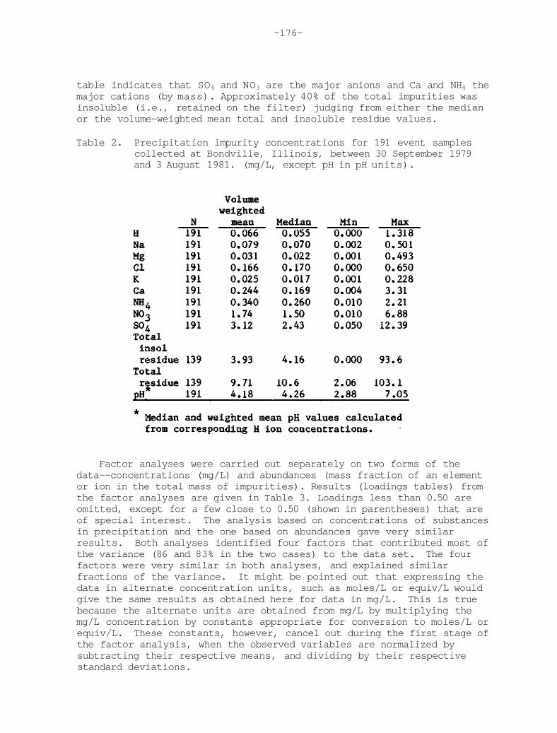
-176-

table indicates that SO4 and NO3 are the major anions and Ca and NH4 the major cations (by mass). Approximately 40% of the total impurities was insoluble (i.e., retained on the filter) judging from either the median or the volume-weighted mean total and insoluble residue values.

Table 2. Precipitation impurity concentrations for 191 event samples collected at Bondville, Illinois, between 30 September 1979 and 3 August 1981. (mg/L, except pH in pH units).

Factor analyses were carried out separately on two forms of the data--concentrations (mg/L) and abundances (mass fraction of an element or ion in the total mass of impurities). Results (loadings tables) from the factor analyses are given in Table 3. Loadings less than 0.50 are omitted, except for a few close to 0.50 (shown in parentheses) that are of special interest. The analysis based on concentrations of substances in precipitation and the one based on abundances gave very similar results. Both analyses identified four factors that contributed most of the variance (86 and 83% in the two cases) to the data set. The four factors were very similar in both analyses, and explained similar fractions of the variance. It might be pointed out that expressing the data in alternate concentration units, such as moles/L or equiv/L would give the same results as obtained here for data in mg/L. This is true because the alternate units are obtained from mg/L by multiplying the mg/L concentration by constants appropriate for conversion to moles/L or equiv/L. These constants, however, cancel out during the first stage of the factor analysis, when the observed variables are normalized by subtracting their respective means, and dividing by their respective standard deviations.

-177-

Table 3. Loadings tables from factor analysis on event precipitation samples, using correlation about the mean.

Factor 1 in both cases was clearly crustal dust, showing high loadings for Ca, Mg, K, and, in the case where the data were concentrations, also for total insoluble residue. Factor 2 in both cases was made up of "gaseous precursors," having high loadings on NH4, NO3, and SO4. Factor 3 in both cases might be labeled sea salt, having high loadings for Na and C1, although road deicing salt is also a plausible source in winter. Facror 4 in both cases was dominated, in terms of the magnitude of the loadings, by hydrogen ion, but in both cases there was a hint, with a loading near 0.50, of an associated SO4 ion. The loadings table based on abundances also hints very slightly at a nitric acid influence on factor 4, with a NO3 loading of 0.43. A previous factor analysis of MAP3S precipitation data by Baker et al. (1981) also found crustal dust and H-SO4-NO3 factors, but not the other two found here.

Based on the factor analysis results, the sources assumed for the CEB analyses include crustal dust, sea salt, and a combination of sulfate, nitrate, and ammonium sources. These last three are not really "sources" in the same sense as crustal dust or sea salt. They were included simply to show what proportion of the precipitation impurity mass was made up of NH4, NO3, and SO4 . The choice of ammonium sulfate, sulfuric acid, and nitric acid was arbitrary, but somewhat consistent with the factor analysis results. Two crustal sources were included, consistent with observations (Gatz et al., 1981) that dust from both unpaved roads and soil contribute to the local aerosol.

-178-

Once the sources were chosen, it was necessary to specify the com­position of their "emissions." This was an easy task for the pure com­pounds, which are not really "emitted" in the same sense as the other sources, especially since all of these are completely soluble in water. Sea salt also has a well-known composition (Junge, 1963) and should be essentially completely soluble in water. The choice of the compositions for the crustal dust sources was not trivial, however, since both soils and road dust have compositions that will vary from place to place, that may have different compositions as aerosols than in their bulk form, and which have relatively unknown solubility characteristics with respect to atmospheric precipitation.

The issue of large scale spatial variability of dust composition is not addressed in this paper. The various compositions used as input to the CEB calculations were all based on measurements of materials collected within several km of the sampling site. I used local soil and road dust compositions because they were one of the few suitable data sets available, and because these source compositions are considered to be reasonably representative of regions within 10-20 km of our site. Thermals that provide the input of moisture and particles to convective precipitation systems that produced rain at our site are likely to originate at such distances from the sampling site. Sources of crustal materials in stratified precipitation systems are likely to be much more distant, of course, and the overall mix of local and distant source contributions cannot be specified. One purpose of varying the assumed source compositions used as input to the CEB calculation was to explore the effect of possible spatial variations of source composition on the results. Still, the two main issues that were addressed in this work were 1) the sensitivity of the results to differences in composition between bulk and resuspended source materials, and 2) source materials solubility.

Table 4 shows input data and results addressing the first of these issues. Trials 1A - 1C are based on total element measurements (complete sample dissolution by fusion, followed by atomic absorption spectrophotometry) of seven samples of dust from local unpaved rural roads, and six soil samples from the square kilometer surrounding the precipitation sampling site. The road surfaces sampled included five of crushed limestone, one of a glacially-derived gravel, and one of a mix­ed limestone and soil composition. This relative distribution is ap-proximatly that of the various surface materials on local unpaved rural roads.

To investigate the sensitivity of the results to local variability in composition, CEB analyses were performed under three different combinations of measured values. The first of these (Trial 1A) used the mean abundances of Ca and K in both soils and road dust. The second (Trial 1B) used the maximum Ca and K abundances measured in the soil samples and the minimum abundances measured in the road samples. Trial 1C used minimum soil abundances and maximum road abundances. The results, in Table 4, show minor differences between trials for all

-179-

sources other than the unpaved roads. The total contribution of all the non-crustal sources to the volume-weighted mean precipitation impurity mass (Trial 1A) was about 50%, with the two sulfate "sources" accounting for about 32%, nitrate 16%, and sea salt 2%.

Table 4. Comparison of results for minimum, mean, and maximum element abundances (%) in bulk and (fine) resuspended source emissions samples, based on mean observed precipitation composition, and assuming 100% element solubility in precipitation.

The unpaved road contributions varied from 7.9 to 21.8%, depending on the composition used as input. The computed contributions varied approximately inversely with the assumed road dust Ca abundance used as input. This is reasonable since road dust is the dominant source of Ca in the precipitation, and since a proportionately greater contribution of the source material is required to account for the observed mean Ca in precipitation as the mass fraction of Ca assumed to be in the source decreases. In other words, it takes more of a low-Ca source than a high-Ca source to produce a given Ca concentration in precipitation.

-180-

To investigate further the sensitivity of results to local variations in source composition, and to compare against results of bulk sample composition, an additional three trials (2A, B, and C) were carried out using measured compositions of four samples of resuspended road dust (three limestone and one mixed limestone/soil samples) and five resuspended soil samples. Sieved (<53 µm) dust samples were resuspended in a chamber and collected in fine (<2.5 µm) and coarse (2.5 - 15 µm) size classes (50% cut points) using a dichotomous virtual impactor, by NEA, Inc., Beaverton, Oregon. NEA also carried out the

analysis of the samples, using X-ray fluorescence techniques. A comparison (not shown) of results from the fine and coarse size classes showed minimal differences in results of CEB analyses. Thus, only one size class (fine) was used here for the comparison against results based on bulk compositions.

Computed contributions of the non-crustal sources were virtually unchanged, since input variations were confined to the crustal sources. The use of resuspended sample compositions resulted in slightly in­creased contributions of unpaved roads, and somewhat decreased soil contributions, compared to the bulk composition.

Results thus far show that unpaved roads could have contributed 8-24% and soils 3-8% of precipitation impurities at our central Illinois site, depending on the source compositions assumed, and assuming complete solubility of contaminants. The effects of assuming less than complete solubility are presented next.

Table 5 presents results of a comparison of approaches to accounting for less than complete solubility. The first approach (Trial 3) was to measure a "soluble" source composition that could be used as input to a CEB analysis. Trial 3 used mean abundances of Ca and K extracted from four dried, sieved (<53 µm) unpaved road samples (2 limestone, 2 mixed limestone and soil), and 34 dried sieved (<53 µm) soil samples using the following procedures. For the road dust, 25 mg samples of dried, sieved (<53 µm) dust were shaken for 20 min on a wrist-action shaker in 25 ml of pH 3 simulated rain water. This was a solids:water dilution of 1:1000. For the soils, 100 mg samples of dried, sieved (<53 µm) dust were shaken for 20 min in the same way in 100 ml of the same extractant. This dilution was also 1:1000. K was not measured in the extracted soil samples; the value of K used was 20% of the mean total K measured in the fused bulk soil samples (from Trial 1). For comparison, the mean extractable Ca and Mg in the soil samples were 38% and 14% of the mean totals (Trial 1), respectively.

The results of Trial 3 for the non-crustal sources, were, of course, very similar to those obtained earlier, since the changes in crustal source composition have little, if any effect on their contributions. The greatly decreased Ca and K concentrations obtained by extraction of source materials produced CEB results showing a nearly 65% contribution of road dust, and a 42% contribution from soil dust. Together with the

-181-

Table 5. Comparison of results of two approaches to the problem of source material solubility in CEB analysis of precipitation composition.

A. Input data for CEB.

B. Results of CEB.

Contribution to total mass (%) Unpaved Ammonium Sea H2SO4 HNO3

Trial roads Soil Sulfate salt _ _ _ _ Total 3 64.6 42.1 12.1 2.4 19.4 16.0 156.6

4A 11.6 6.6 12.1 2.4 19.4 16.0 68.1 4B 23.5 -0.3 11.8 2.4 19.0 15.7 72.1 4C 10.8 21.5 12.1 2.4 19.4 16.0 82.2 4D 22.7 14.3 11.8 2.4 18.9 15.6 85.7 5A 12.0 14.7 12.1 2.4 19.4 16.0 76.6 5B 24.7 10.9 12.1 2.4 19.4 16.0 85.5 5C 9.5 14.8 12.1 2.4 19.4 16.0 74.2

No assumption necessary, since source composition is based on analyses of samples extracted from source materials.

Value for K assumed.

-182-

contributions from the non-crustal sources, this gave a total contribu­tion of about 161%, which indicates, of course, that one or more of the input source compositions were too low. Undoubtedly, the low "soluble" Ca and K abundances of both the road dust and the soil samples were the cause, since the computed contributions of these sources in Trial 3 were much higher than those of previous trials.

These results indicate that in nature dust particles from soil and unpaved road dissolve much more readily in precipitation than they did under the conditions of our extraction procedure. Why this happened is not at all clear, but since the pH of the extractant was as low or lower than most rain samples, the reasons may include the time period of the extraction (20 min), the dilution ratio (1:1000 is probably at least one

hundred times more concentrated than that of a typical precipitation sample), or the size of the particles in the samples extracted (particles collected by cloud or rain droplets in the atmosphere are probably mostly smaller than those in the samples extracted). In any case, the use of extracted source material compositions gave unreasonable results.

An alternative approach was tried in Trial 4A-4D. The same total element source compositions used previously (Trial 2 — resuspended, fine particles) were used, but the observed (soluble) precipitation composition was adjusted to correspond to a total element concentration by making a series of assumptions regarding the solubility of the Ca and K in the precipitation samples. Solubilities of 100% and 50% represent likely upper and lower limits for the solubility of Ca and K in precipitation (Muhlbaier, 1978; Cawse, 1974). Thus, Trials 4A-4D represent the four possible combinations of two elements and two limiting solubilities.

Again, the results of these varied assumptions impacted the results primarily in the two crustal source contributions. Table 5B shows that assuming various combinations of probable limiting solubilities for Ca and K in precipitation gave road dust contributions of up to about double that obtained under the assumption of complete solubility, while the computed soil contributions varied from near zero (probably unreasonable) to about three times that with complete solubility. In all cases, the total source contribution remained less than 100%, a necessary condition for a reasonable result.

Few data are available in the literature on element solubility in precipitation, but one set of such data was given by Muhlbaier (1978) for a small set of samples collected in Maryland. Muhlbaier's results agree substantially with those of Cawse (1974) in the United Kingdom, and with some unpublished data of the author. Thus, in a final set of Trials (5A-5C), we examine the effect of assuming Muhlbaier's mean Ca and K solubilities (94% and 64%, respectively), on a previous set of results (Trials 2A-2C). These results are also shown in Table 5.

-183-

The results show that assuming Muhlbaier's measured Ca and K solubilities had little effect on the computed contribution of unpaved roads, but a substantial effect on the contribution of soils. This is the expected result, since Ca, which strongly indicates the road dust contribution, would be increased in total only slightly by assuming 94% solubility, while K, which strongly indicates the soil contribution, would be increased in total by a greater amount, if only 64% were soluble.

Note that vegetative sources of K have been ignored in this analysis. If vegetation contributes to the K in the measured precipitation, the estimated soil contributions are too high.

Since local compositions of the two alkaline dust sources were used as input, there could be a concern that the CEB results, especially for the two crustal sources, are significant only at one location. However, there are three reasons why these results have at least regional significance. First, local precipitation composition is similar to that at surrounding NAOP sites. Second, comparison of regional soil and precipitation compositions suggests a large non-soil contribution to the alkaline elements in precipitation. Third, my results for the contributions of soil dust are similar to previous results at other locations.

Table 6A lists volume-weighted mean concentrations of three cations at a variety of sampling sites. Values are listed for both the event samples used in the CEB analysis and the weekly National Atmospheric Deposition Program (NADP) samples collected at our Bondville field site (NADP, 1980a-1980e, 1981a, 1981b, 1982, 1983a-1983d). Also listed are the maximum, minimum and median volume-weighted means for the 9 NADP sites within 500 km, and the 22 NADP sites within 750 km of the Bondville site. The ratios Ca/Mg and Ca/K are also shown for all data groups.

Comparison of respective concentrations for the two Bondville data sets indicates higher concentrations for the weekly samples, consistent with the idea that crustal dust particles gradually dissolve while in contact with rain water (Peden and Skowron, 1978). Both ratios are smaller for the weekly samples, showing greater leaching of Mg and K, relative to Ca.

Comparison of the Bondville results with those from the two groups of surrounding sites shows that for each element both event and weekly concentrations fell between the maxima and minima of the 9- and 22-site groups. The same is also true for the ratios, except that Ca/Mg for the Bondville event samples exceeded the maximum of the 9-site group. However, Ca/Mg for the Bondville weekly samples was well within the range of both groups of surrounding sites. Thus, it is clear that Bondville precipitation is not anomalous with respect to alkaline element concentrations at surrounding sites. This makes it unlikely that crustal source contributions to precipiation at Bondville are markedly different from those at the surrounding sites.

-184-

Table 6. Comparison of local precipitation composition with that in surrounding areas, and with regional soil composition.

A. Precipitation Composition

B. Soil Composition in Illinois and Adjacent States.

N = No. of samples. NADP = National Atmospheric Deposition Program. The 9 sites (and respective numbers of samples) are: IL.18(24), IL.19(74), IL35(91), IL47(39), 1L63(111), IN34(61), MI26(94), MI53(103), and 0H17(142). The additional 12 sites in the set of 22 are: AR27(63), MI09(86), MN27(100), NC25(144), NE15(97), OH49(146), OH7K139), TN00(75), TN1K49), VA13(104), WI36(76), WI37(47), and WV18(173). For site names and locations, see NADP references.

-185-

Table 6B lists median abundances for Ca, Mg, and K in the soils of Illinois and adjacent states, based on U.S. Geological Survey data (Boerngen and Schacklette, 1981). There is good agreement from state to state in median abundances as well as their ratios. Further, there is a clear difference in the respective element ratios between soil and precipitation (Table 6A). Even after increasing these ratios by a factor or 2 to account for observed solubility differences in rain (Cawse, 1974; Muhlbaier, 1978) the adjusted Ca/K ratio would still be less than 1.0, whereas the minimum observed ratio in precipitation for the 9- and 22-site groups was 2.99. After adjustment to simulate solubility (x2) the soil Ca/Mg ratios for the several states range from 1.86 to 5.8, and are rather similar to observed ratios in precipitation. These comparisons suggest a major role for Ca-rich (limestone) or Ca and Mg-rich (dolomite) road surfaces as sources of impurities in precipitation.

Finally, the source contributions estimated for the volume-weighted mean composition at Bondville, Illinois, (Trial 5A) may be compared to those estimated for other locations. A comparison to Pasadena, California (Liljestrand and Morgan, 1978) is given in Table 7. The total contribution of both sulfate "sources" was somewhat higher in Illinois. The nitrate contribution, on the other hand, was almost three times higher at Pasadena, as might be expected from a comparison of source strengths at the respective sites. The sea salt contribution was considerably higher in California, as would be expected in comparison to a site far inland. Somewhat surprisingly, the soil dust contribution in Pasadena was slightly more than that of the agricultural midwest. This may reflect nearby construction or other disturbances of the earth's surface by man in Pasadena. It may also include a contribution from paved or unpaved road dust since this source was not specifically listed in the Pasadena results, although the finding of a minimal contribution for "cement" in Pasadena would seem to preclude this possibility.

Table 7. Comparison of results for precipitation impurity source apportionment at Pasadena, California (Liljestrand and Morgan, 1978) and Bondville, Illinois.

-186-

These results may also be compared with some obtained for three sites in Texas by Feeley and Liljestrand (1983). Their results are not directly comparable, because they are expressed in different units (µ eq/L). (Thus, I have not included them in Table 7.) However, Feeley and Liljestrand found "soil dust" contributions of 14%, 16%, and 19% of total eq/L in precipitation at Highlands, Prairie View, and Austin, Texas, respectively, using least-squares chemical mass balance calculations. These values are very similar to both soil dust (mass) contributions shown in Table 7, but less than the combined soil and road dust (mass) contributions at Bondville (27%).

SUMMARY AND CONCLUSIONS

Factor analyses were carried out to identify, and chemical element balance calculations were performed to apportion, possible sources of impurities in event precipitation samples from central Illinois collected between 30 September 1979 and 3 August 1981.

Although factor analysis could group elements or ions that occur together for chemical, meteorological, or microphysical (scavenging) reasons, as well as that of having a common source, the following likely sources were identified: crustal dust (Ca, Mg, K), sea and/or road salt (Na, C1), and possibly strong acids (H2SO4, HNO3). In addition, a "gaseous precursors" factor (NH4, NO3, SO4) was identified.

Apportionment of plausible sources by CEB yielded estimates of a 2% contribution of sea salt to the total mass of precipitation impurities, a 32% contribution by ammonium and sulfates (including H2SO4), and a 16% contribution from nitrates.

An investigation of the effect of varying the assumed source compo­sition of soil and road dust (Trials 1, 2, and 4) suggested that mean values (and reasonable limits) on the contributions of these two crus­tal materials might be 11.6% (8-24%) for road dust and 6.6% (3-8%) for soil, assuming complete solubility. Possible spatial variations in crustal source composition were more important than differences between bulk and "source aerosol" composition in determining source contribu­tions.

The use of source material extractions to estimate the source composition of soluble materials in precipitation was unsuccessful. The best way to deal with the problem of limited solubility of crustal source materials would be to measure the insoluble portion of the precipitation impurities, and then to use total element concentrations in both source compositions and precipitation. Investigations of the sensitivity of CEB results to assumptions about the soluble fraction of Ca and K in the samples used in this work indicated that unpaved road contributions could vary by a factor of about 2, and soil contributions by a larger amount, for Ca and K solubilities between 50 and 100%. The

-187-

use of Mulbaier's (1978) measured mean solubility values from the liter­ature of 94% for Ca and 64% for K approximately doubled the soil contri­bution, but had little effect on the road dust contribution, relative to the results based on the 100% solubility assumption.

Although derived from compositions of local source materials, the estimated crustal contributions to precipitation composition were shown to be regionally significant and similar to previous results for Texas and California.

Further work on this data set should include plotting the factor scores against date of sample collection, so that sources might be examined for possible relation to meteorological conditions.

ACKNOWLEDGEMENTS

I thank Tom Dzubay for supplying the computer program used to perform the CEB analyses, Stacy Craft for data analysis, Van Bowersox for data screening and a careful review of the manuscript, Lih-Ching Chu and Gary Stensland for helpful discussions, Mark Peden and the staff of the Water Survey's Analytical Chemistry Unit for sample analysis, and Bruce Komadina for sample collection.

This material is based on work supported by the U.S. Department of Energy under Contract No. DE-AC02-76EVO1199, and by the National Science Foundation under Grant No. ATM 80-14893.

-188-

REFERENCES

Alpert, D. J., and P. K. Hopke, 1980: A quantitative determination of sources in the Boston urban aerosol. Atmos. Environ., 14, 1134-1146.

Baker, M. B., D. Caniparoli, and H. Harrison, 1981: An analysis of the first year of MAP3S rain chemistry measurements. Atmos. Environ., 15, 43-55.

Boerngen, J. G., and H. T. Schacklette, 1981: Chemical analyses of soils and other surficial materials of the conterminous United States. U.S. Geological Survey, Open-File Report 81-197.

Cawse, P. A., 1974: A survey of atmospheric trace elements in the U.K., 1972-1973. AERE-R7669, H.M.S.O., London.

Chu, L.-C., D. F. Gatz, M. V. Miller, and G. J. Stensland, 1982: The design and application of a soil-blowing wind tunnel for the measurement of crustal aerosol composition and comparison to other Conference on Precipitation Scavenging, Dry Deposition, and Resuspension, Santa Monica, California, November 29 - December 3, 1982.

Dixon, W. J., Editor, 1975: BMDP Biomedical Computer Programs., University of California Press, Berkeley, 792 pp.

Dzubay, T. G., 1980: Chemical element balance method applied to dichotomous sampler data. Ann. New York Acad. Sci., 338, 126-144.

Dzubay, T. G., R. K. Stevens, W. J. Courtney, and E. A. Drane, 1981: Chemical element balance analysis of Denver aerosol. In: Russell, P. A., Editor, Electron Microscopy and X-Ray Applications to Environmental and Occupational Health Analysis, Vol. 2, Ann Arbor Science, Ann Arbor, Michigan, pp. 23-42.

Feeley, J. A., and H. M. Liljestrand, 1983: Source contributions to acid precipitation in Texas. Atmos. Environ., 17, 807-814.

Friedlander, S. K., 1973: Chemical element balances and identification of air pollution sources. Environ. Sci. Technol., 7, 235-240.

Gaarenstroom, P. D., S. P. Perone, and J. L. Moyers, 1977: Application of pattern recognition and factor analysis for characterization of atmospheric particulate composition in southwest desert atmosphere. Environ. Sci. Technol., 11, 795-800.

Gatz, D. F., 1975: Relative contributions of different sources of urban aerosols: application of a new estimation method to multiple sites in Chicago. Atmos. Environ., 9, 1-18.

-189-

Gatz, D. F., 1978: Identification of aerosol sources in the St. Louis area using factor analysis. J. Appl. Meteorol., 17, 600-608.

Gatz, D. F., G. J. Stensland, M. V. Miller, and A. C. D. Leslie,, 1981: Sources of airborne calcium in rural central Illinois. In: Macias, E. S., and P. K. Hopke, Editors, Atmospheric Aerosols: Source/Air Quality Relationships, American Chemical Society Symposium Series 167, American Chemical Society, Washington, D.C., pp. 303-325.

Gordon, G. E., 1980a: Techniques for treating multielement particulate data to obtain information on sources: an overview. Ann. New York. Acad. Sci., 338, 93-102.

Gordon, G. E., 1980b: Receptor models. Environ. Sci. Technol., 14, 792-800.

Harman, H. H., 1967: Modern Factor Analysis, 2nd Edition, University of Chicago Press, Chicago, 474 pp.

Hopke, P. K., E. S. Gladney, G. E. Gordon, W. H. Zoller, and A. G. Jones, 1976: The use of multivariate analysis to identify sources of selected elements in the Boston urban aerosol. Atmos. Environ., 10, 1015-1025.

Junge, C. E., 1963: Air Chemistry and Radioactivity, Academic Press, New York, 382 pp.

Kowalczyk, G. S., C. E. Choquette, and G. E. Gordon, 1978: Chemical element balances and identification of air pollution sources in Washington, D.C, Atmos. Environ., 12, 1143-1153.

Kowalczyk, G. S., G. E. Gordon, and S. W. Rheingrover, 1982: Identification of atmospheric particulate sources in Washington, D.C, using chemical element balances. Environ. Sci. Technol., 16, 79-90.

Liljestrand, H. M., and J. J. Morgan, 1978: Chemical composition of acid precipitation in Pasadena, Calif., Environ. Sci. Technol. 12, 1271-1273.

Liljestrand, H. M., and J. J. Morgan, 1979: Error analysis applied to indirect methods for precipitation acidity. Tellus, 31, 421-431.

Liljestrand, H. M., and J. J. Morgan, 1981: Spatial variations of acid precipitation in Southern California, Environ. Sci. Technol., 15,

333-339.

Miller, M. S., S. K. Friedlander, and G. M. Hidy, 1972: A chemical element balance for the Pasadena aerosol. J. Colloid Interface Sci., 39, 165-176.

-190-

Muhlbaier, J., 1978: The chemistry of precipitation near the Chalk Point Power Plant. Ph.D. Thesis, Department of Chemistry, University of Maryland, pp. 182-190.

National Atmospheric Deposition Program, 1980a: NADP Data Report: Precipitation Chemistry, Third and Fourth Quarters, 1978. Natural Resources Ecology Laboratory, Colorado State University, Fort Collins, CO.

National Atmospheric Deposition Program, 1980b: NADP Data Report: Precipitation Chemistry, First and Second Quarters, 1979. Natural Resources Ecology Laboratory, Colorado State University, Fort Collins, CO. National Atmospheric Deposition Program, 1980c: NADP Data Report: Precipitation Chemistry, Third Quarter, 1979. Natural Resources Ecology Laboratory, Colorado State University, Fort Collins, CO.

National Atmospheric Deposition Program, 1980d: NADP Data Report: Precipitation Chemistry, Fourth Quarter, 1979. Natural Resources Ecology Laboratory, Colorado State University, Fort Collins, CO, 160 pp.

National Atmospheric Deposition Program, 1980e: NADP Data Report: Precipitation Chemistry, First Quarter, 1980. Natural Resources Ecology Laboratory, Colorado State University, Fort Collins, CO, 184 pp.

National Atmospheric Deposition Program, 1981a: NADP Data Report: Precipitation Chemistry, Second Quarter, 1980. Natural Resources Ecology Laboratory, Colorado State University, Fort Collins, CO, 281 pp.

National Atmospheric Deposition Program, 1981b: NADP Data Report: Precipitation Chemistry, Third Quarter, 1980. Natural Resources Ecology Laboratory, Colorado State University, Fort Collins, CO, 314 pp.

National Atmospheric Deposition Program, 1982: NADP Data Report: Precipitation Chemistry, Fourth Quarter, 1980. Natural Resources Ecology Laboratory, Colorado State University, Fort Collins, CO, 342 pp.

National Atmospheric Deposition Program, 1983a: NADP Data Report: Precipitation Chemistry, First Quarter, 1981. Natural Resources Ecology Laboratory, Colorado State University, Fort Collins, CO, 169 pp.

National Atmospheric Deposition Program, 1983b: NADP Data Report: Precipitation Chemistry, Second Quarter, 1981. Natural Resources Ecology Laboratory, Colorado State University, Fort Collins, CO, 184 pp.

-191-

National Atmospheric Deposition Program, 1983c: NADP Data Report: Precipitation Chemistry, Third Quarter, 1981. Natural Resources Ecology Laboratory, Colorado State University, Fort Collins, CO, 189 pp.

National Atmospheric Deposition Program, 1983d: NADP Data Report: Precipitation Chemistry, Fourth Quarter, 1981. Natural Resources Ecology Laboratory, Colorado State University, Fort Collins, CO, 197 pp.

Peden, M. E., and L. M. Skowron, 1978: Ionic stability of precipitation samples. Atmos. Environ., 12, 2343-2349.

Peden, M. E., L. M. Skowron, and F. M. McGurk, 1979: Precipitation sample handling, analysis, and storage procedures. Research Report 4, Contract No. EY-76-S-02-1199, U.S. Department of Energy, Illinois State Water Survey, Champaign.

Rummel, R. J., 1970: Applied Factor Analysis, Northwestern University Press, Evanston, Illinois, 617 pp.

Stensland, G. J., and D. F. Gatz, 1981: Comparison ot total versus soluble data for ambient aerosol filter samples. In: Semonin, R. G., V. C. Bowersox, D. F. Gatz, M. E. Peden, and G. J. Stensland, Study of Atmospheric Pollution Scavenging, Nineteenth Progress Report, Contract No. DE-AC02-76EV01199, U.S. Dept. of Energy, Illinois State Water Survey Contract Report 252, pp 24-29.

Stensland, G. J., R. G. Semonin, M. E. Peden, V. C. Bowersox, F. M. McGurk, L. M. Skowron, M. J. Slater, and R. K. Stahlhut, 1980: NADP Quality Assurance Report, Central Analytical Laboratory, Naional Atmospheric Deposition Program, Natural Resource Ecology Laboratory, Colorado State University, Fort Collins, CO 80523.

Volchok, H. L., and R. T. Graveson, 1975: Wet/dry fallout collection. Proceedings of the Second Federal Conference on the Great Lakes, Interagency Committee on Marine Science and Engineering of the Federal Council for Science and Technology, Agronne National Laboratory, March 25-27, 1975.

Watson, J. G., 1979: Chemical element balance receptor model methodology for assessing the sources of fine and total suspended particulate matter in Portland, Oregon. Ph.D. Thesis, Environmental Science, Oregon Graduate Center, Portland, Oregon.

-193-

CHAPTER 9

A FEW PRELIMINARY PRECIPITATION CHEMISTRY STATISTICS

Richard 6. Semonin

INTRODUCTION

The MAP3S and NADP/NTN precipitation sampling networks have now been in operation for more than one-half decade and a sizable data base is ac­cumulating. The NADP/NTN alone has acquired nearly 25,000 samples since its inaugeration in 1978. Unfortunately, each network site did not initiate sampling at the same time causing disparities in station sample size particularly between the eastern and western states. None the less, some simple statistics can be calculated and used to guide future work and as indicators of relationships between chemical species. In this chapter, a few statistical relationships between ions found in precipitation will be explored to aid in interpretation of the chemical quality of wet deposition across the United States.

There were two basic approaches made in this exploratory research utilizing existing statistical computer software to provide numbers for interpretation. The first of these is the use of a correlation matrix be­tween the ions species and sample volume to examine possible relationships between the various constituents of precipitation chemistry. The second approach was to use factor analysis to examine the concurrent relation­ships among the various species to characterize the components in the chemistry of precipitation in various regions. These results are pre­sented and will be further explored and more fully researched as the data base continues to increase.

ION CORRELATION ANALYSIS

Data

The sample analyses from 87 NADP/NTN network sites were used for this analysis. The number of samples ranged between 34 and 217 at each of the sites with primary emphasis on those sites with 50 or more samples. This would approximate one year of sampling at each site although it would not indicate the length of site operation since many weeks would go by without precipitation. The analysis included samples obtained from the beginning of operation at an individual site through September of 1982

-194-

The correlation matrix was developed from analysis of calcium, magnesium, potassium, sodium, ammonium, hydrogen, nitrate, chloride, sul­fate, calculated bicarbonate, and sample volume. The correlations between pairs of these 11 variables were calculated for the entire data set. A sample correlation matrix for the IL 11 site at Bondville, Illinois is shown in table 1.

Data Analysis

The correlation matrix was developed by standard methods for the 11 species described above. From this matrix only those ion pairs with a correlation coefficient ≥ 0.7 were plotted on a map at each station loca­tion. Isopleths of the correlation coefficient were then hand-drawn to depict the area cohesiveness of a particular correlation value.

The following figures include maps for the ion pairs that either covered a significant area of the United States or have some bearing on the acid rain issue. These data and their interpretation must be consid­ered preliminary and only suggest possible compounds that are involved in the chemistry quality of precipitation. At this time it is difficult to interpret the patterns from a source point of view since many of the cor­related ions occur both in nature and as a result of man's activities.

Potassium:Chloride. While a quick examination of Figure 1 reveals that most of the United States experiences less than 0.7 correlation be­tween potassium and chloride, it must be pointed out that over the area extending through the middle third of the United States from coast to coast the correlation is approximately 0.5 or greater. The areas of interest, of course, are the relatively high correlations along the Gulf and northeast Atlantic coasts with two major isolated high areas in the western intermountain region and across the upper Great Plains and Mid­west.

The relative maximum values along the coastal regions might possibly reflect the dominance of the sea salt component contributing to chloride whereas the continental maximum may reflect a relatively high value of po­tassium associated with particular soil types.

It is clear that the correlation between these two ions is not easily identified with the industrial northeastern United States.

Sodium:Sulfate. There does not seem to be a simply interpreted pattern of sodium-sulfate correlation as seen in Figure 2. Since both of these ions are contained in sea water, one might expect a relative maximum of this correlation to extend along all ocean coastal regions. However this is obviously not the case and as a matter of fact the correlation co­efficients for the northeastern Atlantic coast was very small being less than 0.2 at most sites.

-195-

Table 1. The correlation matrix for ions measured in 145 precipitation samples collected at the NADP IL 11 site at Bondville in east-central Illinois

Figure 1. The correlation coefficient (x100) between potassium and chloride using all available NADP/NTN station data through September 1982. A minimum of 50 samples at a station was required to be included in the analysis.

Figure 2. Same as Figure 1 for sodium and sulfate.

-198-

In general, examination of all available data show that the western half of the United States had the highest correlation values, typically ≥ 0.5. East of the Mississippi River, the correlation values with the exception of the Florida maximum of 0.88, were much less than 0.5 and fre­quently less than 0.3.

Sodium:Chloride. The Atlantic and Gulf coastal areas reflect the sea salt source for the sodium chloride correlation seen in Figure 3. The northern interior states, extending from Montana east to Maine and south to the Ohio River valley and the Southwest, was dominated by low values of correlation as would be expected. However, this general low correlation area was interrupted by two maxima one located in North Dakota and the other in Upper Michigan and Ontario. It is only speculation, but it is possible that these two maxima could be related to non-sea salt sources. In particular, the Upper Great Plains high correlation may be due to the soil in the region. The intermountain maxima are not as easy to explain nor is the low observed over most of California. It is a reasonable assumption that the precipitation in California and other southwestern states would be associated with flow from the Pacific Ocean, and the expected correlation between sodium and chloride would be as high as found on the east coast. The data shown in Figure 3 do not reflect this simplistic view and other reasons must be found to explain the relatively low correlation of these sea salt ions on the west coast. However the low correlations in California are countered by higher values along the Oregon and Washington coasts where numerous cyclones enter the United States. Again this relative maximum in opposition to the low in California raises some interesting questions about the sea salt component of precipitation along the entire west coast.

Ammonium:Nitrate. The highest correlations between ammonium and nitrate were observed along the central Atlantic coast and in southern Arizona (Figure 4). A general maximum occurred along the eastern seaboard and the southwest United States. Additional high values were observed through the upper Great Basin region of western Oregon and southern Idaho and through the northern and central Great Plains states extending from North Dakota through Kansas. A third smaller maximum is centered in the eastern Great Lakes region in northern Ohio, western New York, and western Pennsylvania.

The low areas show <0.5 correlation coefficient between these two ions over much of the country. Values consistently >0.5 but <0.7, were observed through the New England states and in Oregon with a few similar values through Illinois to eastern Tennessee and western North Carolina.

Ammonium:Sulfate. Figure 5 shows correlations >0.9 were observed along the central and northeast Atlantic coast with values decreasing to 0.7 inland to central Pennsylvania. A secondary maximum extended from Texas northeastward with values of > 0.8 from Missouri into Wisconsin. A

Figure 3. Same as Figure 1 for sodium and chloride.

Figure 4. Same as Figure 1 for ammonium and nitrate.

Figure 5. Same as Figure 1 for ammonium and sulfate.

-202-

smaller area of values >0.8 was observed parallel to the Ohio River valley, and a similar area >0.7 was also seen in eastern Oregon and western Montana.

The sources of sulfate, of course, can be from soils, the oceans, and from the burning of fossil fuels. One could perceive that the ob­served pattern reflects each of these sources with the western-most maxi­mum correlation areas associated with soils, the central maximum associated with fossil fuels, and the east coast associated with the sea water contribution.

Calcium;Bicarbonate. The correlation coefficient between these two ions over most of the United States was >0.5 and even becomes negative in the Carolinas (Figure 6). Maximum values of the correlation coeffi­cient were observed in the Great Basin with values >0.8 in western Colorado. A region of high correlations extended from the Rio Grande valley northward with >0.9 observed at the Mexican border. The isolated maximum in the Montana and North Dakota area is also the area where maximum pH values are observed in the NADF/NTN network.

Magnesium:Nitrate. Areas of greater than 0.7 correlation extended from east Texas northeastward to western New York state as seen in Figure 7. The Ohio and western New York maximum may be a combination of natural resources of magnesium and some contribution of anthropogenic nitrate from the industrialized Ohio River valley. Additional values >0.7 were ob­served in the Great Basin and in the Wisconsin and northern Illinois areas. A single station in Canada was observed with > 0.8 correlation between these two ions. The remainder of the country had values of between 0.4 and 0.6 with the lowest correlations observed through the eastern Colorado and Wyoming area.

Calcium: Nitrate. The first interesting noteworthy observation about the correlations in Figure 8 was the relative maximum along the entire east coast and along the United States-Mexican border. In the continental interior, a maximum with values >0.7 was observed in nearly the same location as the magnesium:nitrate correlations shown in Figure 7. An area with > 0.7 correlation through the lower Great Plains into Wisconsin and northern Minnesota is also quite evident in Figure 8. Somewhat interesting were the low values of approximately 0.5 extending along the Appalachian mountains into northern Georgia. A comparable low covering most of Illinois, Indiana and western Michigan was also observed. The northern Great Plains states, entire Great Basin, and the west coast showed low correlations between these two ions.

Magnesium:Chloride. The correlation between these two ions was greater than 0.7 over the entire extent of the Great Plains from the Texas to the Canadian borders and westward into the central Great Basin area. Values greater than 0.9, as seen in Figure 9, were observed in South Dakota and in southern Alberta, Canada. In the eastern United States most of the values of the correlation coefficient were about 0.5 with a few higher values in the central Appalachians, the Florida pennisula, and New England.

Figure 6. Same as Figure 1 for calcium and bicarbonate.

Figure 7. Same as Figure 1 for magnesium and nitrate.

Figure 8. Same as Figure 1 for calcium and nitrate.

Figure 9. Same as Figure 1 for magnesium and chloride.

-207-

Calcium:Chloride. The greatest values of correlation between these two ions extends through the Great Plains region with the highest values over North Dakota and Idaho as seen in Figure 10. Similar to the corre­lation coefficient for magnesium:chloride there were isolated maximum values in northern Florida, western Virginia, and western New York.

Magnesium:Sulfate. The maximum values of the correlation between magnesium and sulfate seen in Figure 11 were observed from the Louisiana coast northward into Illinois, Indiana, Michigan and northern Wisconsin. Low values of about 0.5 extended from Florida along the East coast into New England. A second area of maximum correlation extended over the northern western states including North and South Dakota into Idaho and Washington and Oregon. Low values of the order of 0.5 cover most of the central and southern Great Plains in the southwest as well as the extreme northwest coast.

Calcium:Sulfate; The correlation between calcium and sulfate is very similar to that for magnesium and sulfate shown in Figure 11. In Figure 12, we see a maximum over the western states extending through the Great Basin and a maximum through Indiana, Ohio, and into northern Wisconsin. However, there is a maximum along the Gulf coast and along much of the east coast of the United States which was not apparent in the correlation between magnesium and sulfate.

Low values were observed in New England southwestward into West Virginia and northern North Carolina. In addition, a large area of low correlation values, but still very close to 0.6, extended over the southern and central Great Plains into the western and upper Midwest.

Calcium;Magnesium. Figure 13 shows the correlation between these two cations. This map is presented to show where these two ions may co-exist suggesting a common source. While examination of Figures 11, 12, and 13 might suggest the role of the anions and their possible sources, this correlation shows very high values over the western Great Lakes extending into Indiana and central Illinois. It is interesting to note that most of the United States showed ≥0.7 correlations between these two ions with the low areas confined to the southwestern and central mountain states.

Hydrogen:Ammonium. Owing to the suspected contribution of ammonium to the weak acids in precipitation, the correlation between these two ions is shown in Figure 14. The two maximums in western New York and in central Maine represent the only areas with values ≥0.7 while the remainder of the United States contains a mixed set of correlation values. There were numerous sites, particularly in the West, where negative correlations were found, but over most of the United States the correla­tions were ≤0.3.

Hydrogen:Chloride. The single value of ≥0.7 correlation coefficient between these two ions was found in western New York (Figure 15). The remainder of the United States exhibited very low correlation values with some negative values over parts of the West and extreme Southeast. The

Figure 10. Same as Figure 1 for calcium and chloride.

Figure 11. Same as Figure 1 for magnesium and sulfate.

Figure 12. Same as Figure 1 for calcium and sulfate.

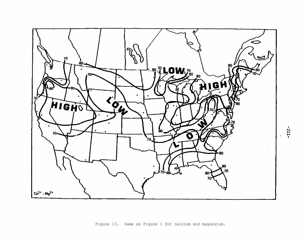
Figure 13. Same as Figure 1 for calcium and magnesium.

Figure 14. Same as Figure 1 for hydrogen and ammonium.

Figure 15. Same as Figure 1 for hydrogen and chloride.

-214-

lack of correlation between these two ions suggests that hydrochloric acid is not a major contributor to the strong acid composition of precipitation samples. It was mildly surprising that no high correlation values were found along the coast lines. As a matter of fact, most of the coast line showed negative correlation values from Florida to Maine and over parts of the west coast as well. The negative coastal values, however, were not very strong being of the order of -0.2 or less.

Hydrogen:Nitrate. The correlation between these two ions, suggestive of a nitric acid contribution in the precipitation, maximized primarily in the East as seen in Figure 16. Only isolated stations in the upper Midwest, the central Rocky Mountains, and in Oregon were seen elsewhere. The maximum values of 0.7 or greater correlation were observed through Virginia, North Carolina and into Georgia in the Southeast with a secon­dary maximum along the border between Canada and the New England states. The remainder of the country was characterized by correlations, both positive and negative, of 0.2. or less.

Hydrogen:Sulfate. This correlation is, of course, one of great interest to many people in acidic precipitation research. As seen in Figure 17 the maximum value of correlation extends along the Appalachians to the northeast from Mississippi to Maine and slightly to the windward or west side of the Appalachians. However, the area encompassed is not extremely large nor does it show a very close association with the pre­sumed emissions maximum along the Ohio River valley in the Midwest. The remainder of the country had mixed correlation values both positive and negative ranging from -0.2 to +0.3.

SUMMARY

This preliminary statistical analysis of the relationship between the primary ions found in precipitation suggests some of the possible combina­tions of ions originally present in the atmosphere and subsequently scavenged by the precipitation. As can be noted in a cursory examination of the figures, the area of the United States encompassed within a corre­lation coefficient of 0.7 or greater is largest for those ion pairs that are commonly associated with natural sources. An example of this is Figure 3 showing the distribution of correlation coefficients between sodium and chloride. As the correlation distributions of ion pairs are examined, progressing from assumed natural resources toward those assumed to be primarily of anthropogenic source, the area of correlation ≥0.7 decreased.

In particular, viewing the acids that are of concern in the National Acid Precipitation Assessment Program, high correlations between hydrogen ion and chloride, nitrate, and sulfate encompass only a small area con­fined to the eastern United States. While the area of the ≥0.7 correla­tion between hydrogen and sulfate can be loosely tied to emissions from

Figure 16. Same as Figure 1 for hydrogen and nitrate.

Figure 17. Same as Figure 1 for hydrogen and sulfate.

-217-

the industrialized Northeast, the extension of this high correlation toward Mississippi seems to also suggest a parallelism with the forested areas of the Appalachians as well.

Future statistical analyses will be directed toward more complex in­terpretations of these data to address more specifically the potential source terms or associations between various of these suggested materials.

-219-

CHAPTER 10 RESULTS OF THE WORLD METEOROLOGICAL ORGANIZATION (WMO)

INTERLABORATORY COMPARISON OF REFERENCE PRECIPITATION SAMPLES Mark E. Peden

The analytical chemistry laboratory has continued its participation in the interlaboratory comparisons of precipitation chemical analyses sponsored by the World Meteorological Organization (WMO). Since 1977, the Illinois State Water Survey (ISWS) laboratory has been receiving synthetic precipitation concentrates in glass ampoules from the U.S. Environmental Protection Agency - Precipitation Reference Laboratory (PRL) at Research Triangle Park, North Carolina. This facility is operated within the framework of the WMO Background Air Pollution Monitoring Network.

The concentrates, when mixed with deionized water to a final volume of 500 mL, contain eighteen chemical constituents at levels normally found in precipitation samples. Laboratories receiving the concentrates are asked to perform chemical analyses for as many parameters as they are capable of measuring. The methods used are left to the discretion of each laboratory. The chemical results are forwarded to the PRL with methods documentation for each parameter measured.

To date, the results of five such intercomparisons have been published. The Water Survey results from the intercomparison conducted in 1980-81, are presented in Table 1. In addition to the ISWS and expected values, the mean and standard deviation from all reporting laboratories are listed. The high and low reported results are also listed to provide an estimate of the range of values encountered. Outliers were removed using the following criteria (Lampe and Puzak, 1981).

1. A mean and standard deviation were determined for all available data.

2. All data more than one standard deviation away from the first mean were rejected and a new mean and standard deviation determined.

3. If less than 67% of the data remained after step 2, the limits of acceptance were increased by 0.1 standard deviation until 67% of the data were included.

Of the four samples tested, the 93 and 94 series were formulated for pH, conductance, and acidity only. All eighteen constituents were determined on the series 91 and 92 samples.

Table 1. - Analysis of reported values with outliers removed

Table 1. (Cont.)

-222-

The participating institutions included four U.S. laboratories and 23 designated WMO laboratories from around the world.

Examination of Table 1 indicates that the ISWS determinations were, without exception, in good agreement with both the expected and the reported mean values. For the first time, an attempt was made by the WMO to rank individual laboratory performance based on their overall accuracy and precision. The relative percent deviations from the expected values were determined for each parameter measured by an individual laboratory. The mean deviation was then calculated. To provide a numerical estimate of the consistency of deviation from the expected values, the standard deviation was calculated using all of the relative deviations for each parameter.

A ranking of the laboratory mean percent deviations using the data obtained from the parameters Ca, Mg, Na, K, SO4, NO3, C1, NH4, pH, and specific conductance revealed that the Water Survey results were closest to the expected values. The Water Survey average deviation was 4.38% +/- 3.32, the lowest of all 27 reporting laboratories. The percent deviations of all the laboratories averaged 17.67% with the highest reported mean deviation being 51.08%.

Continued participation in inter laboratory comparisons such as this is an overall part of our analytical laboratory's quality assurance program. The reputation of our laboratory facility is based in part on it performance on inter laboratory cooperative efforts such as this.

The ISWS has participated in three additional interlaboratory comparisons sponsored by the WMO in the last two years. Although the results from these reference precipitation sample analyses are not yet published, a summary of our performance relative to the expected values and to the other participating laboratories is presented in Table 2. The mean percent deviations have been calculated in an analogous manner to the WMO report of Lampe and Puzak (1981) for ease of comparison.

Examination of Table 2 indicates that our laboratory has continued to provide high quality analytical determinations as an integral part of our overall research effort. Throughout the past four years, the ISWS results have consistently yielded mean percent deviations of 3-5%. At the same time, however, the performance of the laboratories as a group, as indicated by the average percent deviation values listed in Table 2, has declined. The average percent deviation of 17.67% reported in 1980 has risen to 39.53% for the most recently completed intercomparison. A possible explanation for the significantly poorer performance shown by the laboratories as a group in the last intercomparison is the constituent levels used. The cations Ca, Mg, Na, and K had recommended values that were an order of magnitude lower than in the previous two intercomparisons. Although these levels more closely approximated the concentrations actually observed in

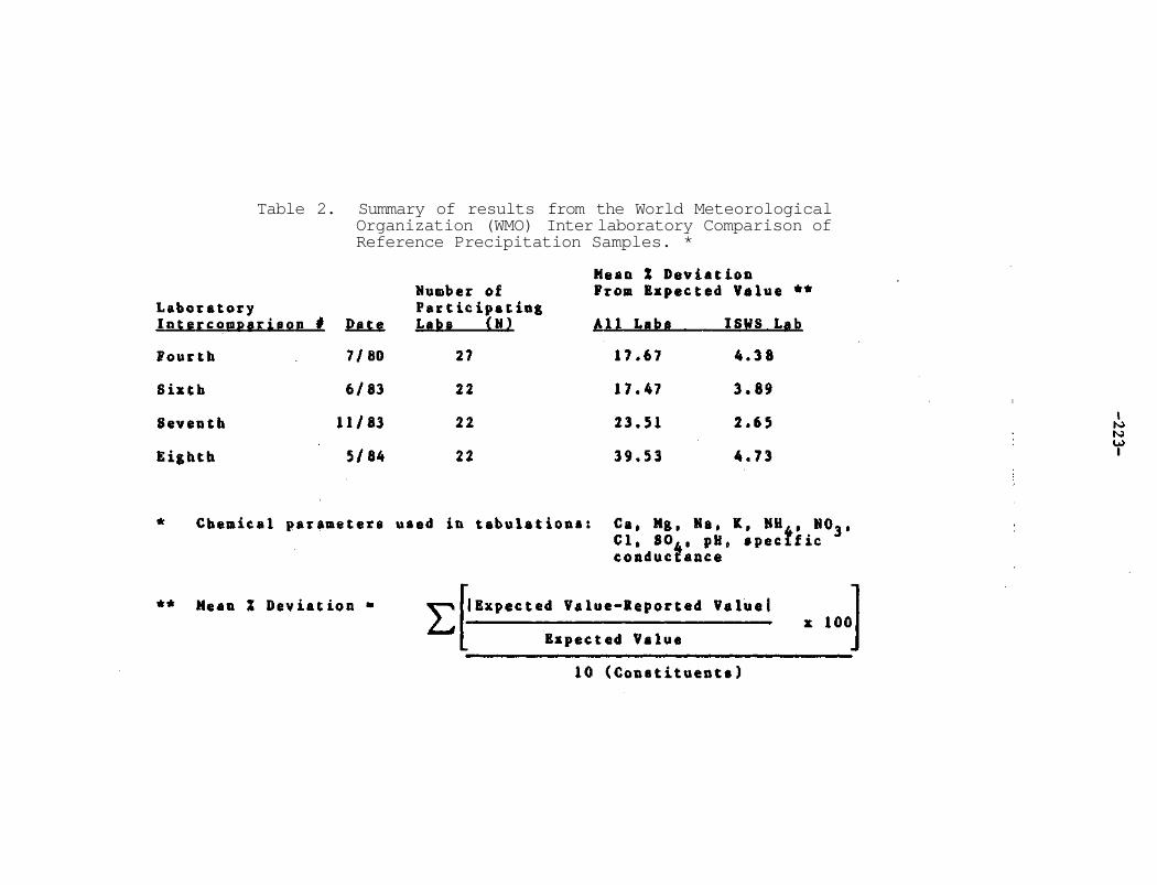
Table 2. Summary of results from the World Meteorological Organization (WMO) Inter laboratory Comparison of Reference Precipitation Samples. *

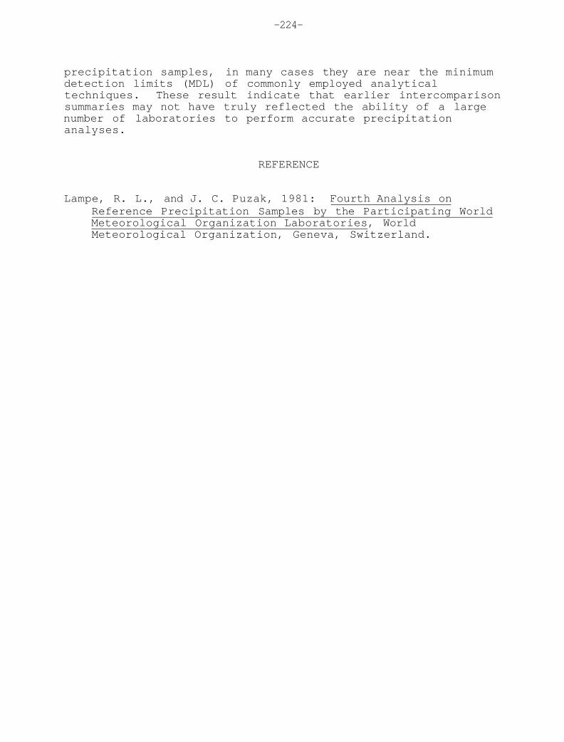
-224-

precipitation samples, in many cases they are near the minimum detection limits (MDL) of commonly employed analytical techniques. These result indicate that earlier intercomparison summaries may not have truly reflected the ability of a large number of laboratories to perform accurate precipitation analyses.

REFERENCE

Lampe, R. L., and J. C. Puzak, 1981: Fourth Analysis on Reference Precipitation Samples by the Participating World Meteorological Organization Laboratories, World Meteorological Organization, Geneva, Switzerland.

-225-

CHAPTER 11 MICROCOMPUTER BASED DATA ACQUISITION AND REDUCTION SYSTEM FOR ION CHROMATOGRAPHY

Susan R. Bachman and Randall K. Stahlhut

INTRODUCTION

Precipitation samples received and processed at the Illinois State Water Survey (ISWS) total over 6,000 anually. Individual analyses per sample increase that number easily ten fold. Laboratory analysts have traditionally used manual data reduction procedures in deriving chemical concentration data. These procedures are no longer cost effective, practical, or efficient. To increase sample throughput and improve accuracy, data acquisition and reduction utilizing a microcomputer based system were implemented.

SYSTEM CONFIGURATION

Ion Chromatograph (IC) A Dionex Model 12 ion chromatograph equipped with an

autosampler, pump, and strip chart recorder has been programmed to routinely analyze precipitation samples received at the ISWS. From sample introduction to computer printout, ion separation and detection are achieved in less than fouteen minutes per sample.

The anion system that is described here utilizes the standard recommended eluent (0.003 M NaHCO3/0.0024 M Na2CO3). Separation of the anions of interest is achieved by utilizing a precolumn (3x50 mm), a fast run anion exchange separator (3x250 mm), and a suppressor (cation exchanger - 6x60 mm). Electrical conductivity is the mode of detection with a full scale detector reading set at 10 umhos. A pump flow rate of 40% (184 mL/hr) is used for mobile phase transport. Good anion separation and detection are achieved in a relatively short span of time. A sample of unknown content can be analyzed and interpreted as to its parameters in 14 minutes or less. Figure 1 is a representative chromatogram of a precipitation sample showing the ions detected and their peak heights in centimeters. The IC system is fitted with a 1.00 mL sample loop, the large size providing increased sensitivity. A three pen strip chart recorder set at 50 mV, 500 mV, and 5000 mV full scale ranges with a chart drive speed of 30 cm/hr is also employed as a backup to

-226-

Figure 1. IC chromatogram of a typical precipitation sample.

-227-

the Apple II system. When the analytical system is "on-line", the pumping pressure is approximately 600 psi.

Calibration standards are prepared weekly from a 1000 mg/L stock solution made from Baker analyzed reagent grade salts. The stock solution is then diluted with polished deionized water to concentrations of 0.05, 0.50, 1.00, 2.50, and 5.00 mg/L for use as working standards. U.S. EPA standard water reference samples and deionized water blanks are also analyzed as daily quality control checks. The Gilson autosampler is prepared by prerinsing all sample cups with deionized water. A programmed sampling time is set at 100 seconds, allowing a 4 mL sample to rinse and fill the 1.00 mL sample loop before injection. After initial set up and baseline equilibration, analysis can usually begin within 20 minutes.

Hardware All data acquisition functions are controlled by an Apple II

microcomputer system. Connected to the microcomputer are a dot matrix printer, a color monitor, and a precision analog to digital (A/D) converter. The A/D converter translates the analog signal from the IC into a 12 bit digital value that can be used by the Apple II. A voltage divider/buffer is placed between the IC and the A/D converter in order to scale the voltage to the suitable level and also to split the signal into two components for input into the A/D converter. One component is 10% of the original voltage, allowing the system to accommodate the higher voltages that accompany concentrated samples without saturating the system. The second signal is unattenuated allowing low concentration samples to be accurately determined.

Software

The data acquistion and reduction software was written specifically for our system at the ISWS. These programs were written in Applesoft Basic (computations and user interaction) and machine language (data collection and graphics). After the program is loaded from the system disk, the analyst is prompted for the project name. This name is used to access a disk file containing the operating parameters (program length, retention times, and sampling rate) for the application. Once these values have been loaded, the number of standards and their associated concentrations are requested, as are the number of samples to be processed, sample identification numbers, and dilution factors. Next, the program requests the IC system parameters for that day's operation. These data are stored on disk and sent to the printer. The analyst then replaces the system disk with a data disk and the analysis can begin.

-228-

Once sampling has begun, peak height data for the standard solutions are collected and stored. When the last standard has been processed, the calibration curves are generated. Figure 2 shows actual calibration curves that have been drawn from data that were generated by the IC software. Both linear least squares and power fits of the concentrations as a function of peak height are computed. The curve with the best regression coefficient is selected by the computer on an ion by ion basis for the calculation of concentrations in the precipitation samples. The results of the regression are listed on the printer. From this point, peak heights are determined for each sample according to the retention times associated with the specific ions being analyzed, and a concentration is computed. The resultant concentrations are recorded on the printer. Table 1 displays a typical printout showing standard curves and sample values. Also shown are the peak heights of each sample in A/D units and the retention times. Retention times recorded by the Apple are determined from the initial sampling point and not the point of injection. This added length of time allows for a longer period of calculation between each sample.

RESULTS

The analytical results from our study indicate that the integrated IC system is providing accurate data in a 'near' real time situation. The precision of this method was determined by replicate analyses of several levels of known standard concentrations and precipitation samples. As shown by the precision Table 2, standard deviations and resultant detection limits have been calculated from 34 replicate analyses of the least concentrated standard performed over several days. Detection limits for this system are calculated as three times the standard deviation of our lowest standard (99% confidence level). Accuracy was also determined and is shown in the figures displaying percent recovery of spiked samples (Fig. 3). The average percent recovery for all samples spiked was 101%.

CONCLUSION The system described has proven to be an accurate and

efficient method of data acquisition and reduction for ion chromatographic determinations of anions in precipitation samples. The software is easily adaptable to cationic as well as organic acid determinations. Errors inherent in manual transcription and data reduction procedures have been eliminated as a result of the implementation of this microcomputer based system. In addition, analyst time devoted to data reduction tasks has been reduced by an estimated 25%. The cost of the computer hardware and software necessary for this sytem totalled less than $3,000, making it a cost effective addition to the atmospheric chemistry laboratory facility.

-229-

3-Figure 2. Computer generated calibration curves for PO4 and NO. using both linear and exponential curve fitting algorithms. Peak height values are in analog to digital converter units.

-230-

Table 1. Data printout from automated ion chromatographic system.

DATE: 7/13/84 SYSTEM: IC PRESSURE: 300 SEPARATOR NUMBER 1 SUPPRESSOR NUMBER 1 ELUENT: El FLOW RATE: 40 CONDUCTIVITY: 10 MICROSIEMENS/CM CHLORIDE REGRESSIONS CHAN1 CHAN2 LINEAR R= .99942 1 POWER R= .9989 1 REGRESSION USED: LINEAR POWER PHOSPHATE REGRESSIONS CHAN1 CHAN2 LINEAR R= .99968 .99934 POWER R= .9997 .99973 REGRESSION USED: POWER POWER

NITRATE REGRESSIONS CHAN1 CHAN2 LINEAR R= .99919 .99685 POWER R= .99947 .99911 REGRESSION USED: POWER POWER

SULFATE REGRESSIONS CHAN1 CHAN2 LINEAR R= .99943 .99974 POWER R= .99982 .99996 REGRESSION USED: POWER POWER

SAMPLE S1

CHLORIDE CHAN1 CHAN2 CONCENTRATION (MG/D= 1.099 OFF SCALE RETENTION TIME (SEC)= 264.3 261 PEAK HEIGHT= 624.224 99999 PHOSPHATE CHAN1 CHAN2 CONCENTRATION (MG/L)= 1.115 1.094 RETENTION TIME (SEC)= 339.3 360 PEAK HEIGHT= 101.397 1127.865 NITRATE CHAN1 CHAN2 CONCENTRATION (MG/D= 4.339 OFF SCALE RETENTION TIME (SEC)= 433 430 PEAK HEIGHT= 423.098 99999 SULFATE CHAN1 CHAN2 CONCENTRATION (MG/D= 3.73 OFF SCALE RETENTION TIME (SEC)= 333 322 PEAK HEIGHT= 779.452 99999

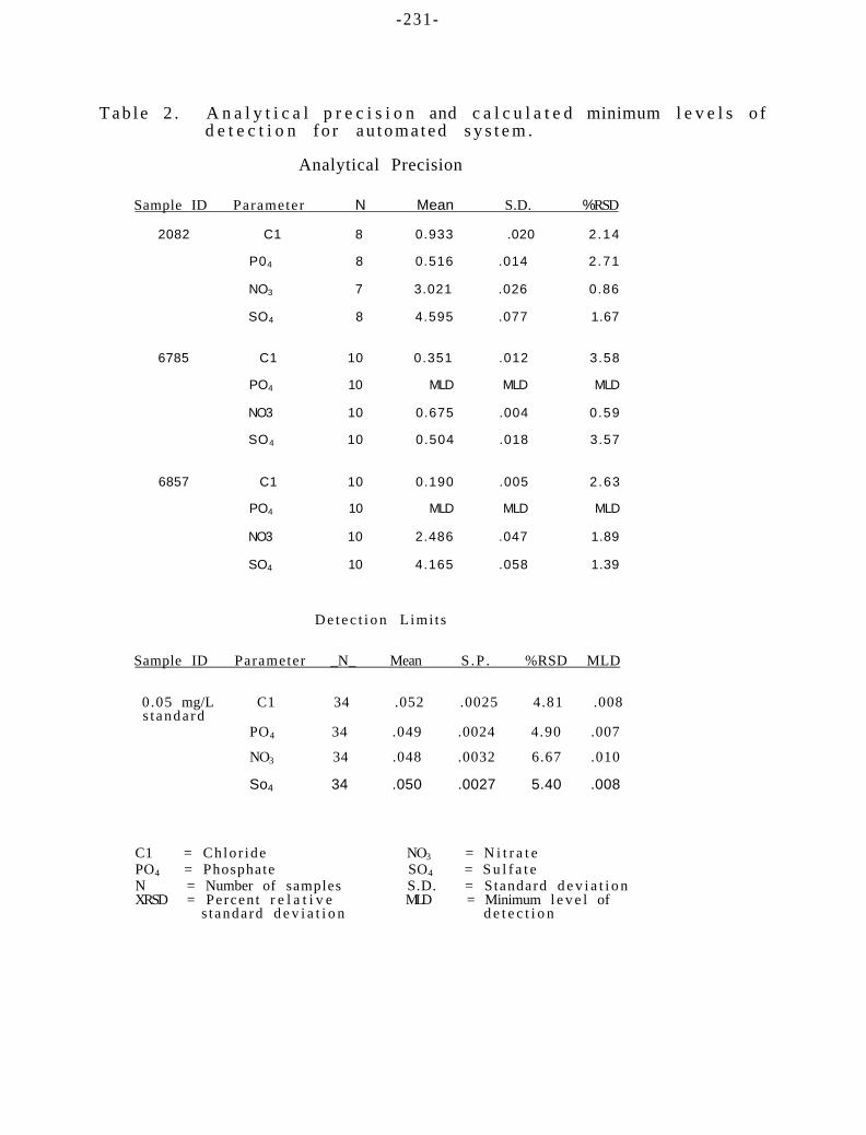
-231-

T a b l e 2 . A n a l y t i c a l p r e c i s i o n and c a l c u l a t e d minimum l e v e l s o f d e t e c t i o n f o r a u t o m a t e d s y s t e m .

Analytical Precision

D e t e c t i o n L imi t s

Sample ID Parameter N Mean S.D. %RSD

2082 C1 8 0.933 .020 2 .14

P04 8 0.516 .014 2 .71

NO3 7 3.021 .026 0.86

SO4 8 4.595 .077 1.67

6785 C1 10 0.351 .012 3.58

PO4 10 MLD MLD MLD

NO3 10 0.675 .004 0.59

SO4 10 0.504 .018 3.57

6857 C1 10 0.190 .005 2 .63

PO4 10 MLD MLD MLD

NO3 10 2.486 .047 1.89

SO4 10 4.165 .058 1.39

Sample ID Parameter _N_ Mean S.P . %RSD MLD

0.05 mg/L C1 34 .052 .0025 4.81 .008 s t anda rd

PO4 34 .049 .0024 4.90 .007

NO3 34 .048 .0032 6.67 .010

So4 34 .050 .0027 5.40 .008

C1 = Ch lo r ide NO3 = N i t r a t e PO4 = Phosphate SO4 = S u l f a t e N = Number of samples S.D. = Standard d e v i a t i o n XRSD = Percen t r e l a t i v e MLD = Minimum l e v e l of

s t anda rd d e v i a t i o n d e t e c t i o n

-232-

Figure 3. Accuracy of anion analyses as percent recovery of spiked precipitation samples.

-233-

CHAPTER 12 DETERMINATION OF ORGANIC ACIDS IN BONDVILLE, ILLINOIS

PRECIPITATION SAMPLES BY ION CHROMATOGRAPHY EXCLUSION (ICE) Susan R. Bachman, Jacqueline M. Lockard, and Mark E. Peden

INTRODUCTION

Acidic precipitation samples are generally thought to be composed of a mixture of the strong acids sulfuric and nitric. The potential contribution of other components such as weak acids that are only partially dissociated, metal compounds, and alkaline paticulates to the free acidity of precipitation cannot, however, be overlooked. Galloway and Likens (1976) reported on the effects of the weak acids, particularly the organic acids, in precipitation samples in the northeastern United States. In order to investigate the importance of weak acid contributions to the rain chemistry of central Illinois, our laboratory has analyzed event precipitation samples by ion chromatography exclusion, looking primarily for the organic acid anions of citrate, formate, and acetate. In addition to confirming the presence of these organic acids, we have also determined the effect of these acids on the free acidity (pH) of rain samples.

EXPERIMENTAL METHODS

HASL design wet/dry sample collectors are located at the Bondville, Illinois field site. At this site there are collectors for event, weekly, and monthly sampling. Samples from the event collector were used for this study. The samples are collected in deionized water washed linear polyethylene buckets, then brought to the laboratory for processing and analysis.

Sample Processing and Analysis

Incoming samples with volumes greater than 200 mL are divided into three portions. First, 8 mL are removed and used for pH and specific conductance measurements. The remaining sample is filtered through a 0.4 micrometer Nuclepore filter. Sixty milliliters are collected in a linear polethylene bottle for routine anion and cation determinations and an additional 125-250 mL are collected for the organic acid and acidity titration analyses.

-234-

The anions (SO4-2, NO 3

-, C1-, PO4-3) and

ammonium (NH4+) are determined colorimetrically using

Technicon AutoAnalyzers. The remaining cations (Ca+2, Mg+2, Na+, and K+) are determined by atomic absorption spectrophotometry. As part of the routine quality control procedures, these ion concentrations, combined with the initial pH and conductance measurements, are used to calculate an ion balance.

The remaining 125-250 mL sample is split into two portions in the chromatography laboratory. Chloroform (250 pL CHC13/125 mL sample) is added to only one of these splits, then both are refrigerated until analysis by ion exclusion chromatography and acidity titration.

Ion Chromatography Procedures

A Dionex Model 12 ion chromatograph with a 250 µL sample loop was used to determine the organic acid content of these precipitation samples. Previous research by Keene et al. (1983) has shown that the dominant organic acids present in precipitation in the northeastern United States and in remote sites throughout the world are citric, formic, and acetic. We therefore focused our initial efforts on the identification and quantitation of these three acids.

The technique of ion chromatography exclusion (ICE) was employed for these analyses. The ICE procedure utilizes a series of columns designed to separate the strongly acidic anions such as nitrate, sulfate, and chloride from weakly acidic anions by the principle of Donnan exclusion. The highly charged density of the interior resin beads of the ICE separator column prevents the retention of completely dissociated species such as sulfate and nitrate. These anions that are not retained by the separator are eluted early in each of the chromatograms. The weak organic acids are retained within the separator column and are eluted sequentially based on their pKa values.

The separator column is connected to a cation exchange suppressor column in the Ag form. This column removes the C1 from the 0.002 M HC1 eluent by the formation of a AgC1 precipitate and the remaining hydrogen ions combine with the organic acid anions to form the corresponding acids. The exhausted portion of the suppressor column, indicated by a dark band of AgCl precipitate, is excised from the column periodically to prevent peak tailing, drifting, and broadening.

The conductimetric detector is set at 3 µmhos full scale to obtain the sensitivity required for trace analysis. A two channel strip chart recorder with full scale ranges set at 20 mV and 200 mV is used to record the output from the detector. The two channel recorder provides an extension of the working range

-235-

up to approximately 5-8 mg/L for each of the organic acids citric, formic, and acetic.

Sample concentrations are determined from calibration curves of standard sample peak heights plotted against their known concentrations. The specific ICE parameters and instrument settings used in this study are listed in Table 1. Figure 1 is a representative chromatogram showing the ion separation using these parameters and instrument settings.

Standard solutions containing the three anions of interest at levels ranging from 0.10 mg/L to 1.00 mg/L were used to generate the standard curve shown in Fig. 2. The coefficient of correlation for each of these curves is 0.999 with standard errors of estimate reflecting less than a 2% dispersion from the regression line. Using the results from repeated analyses of the 0.10 mg/L standard, a minimum detection level (MDL) calculated as three times the standard deviation was determined for each ion. These MDLs are 0.025 mg/L for citrate, 0.027 mg/L for formate, and 0.028 mg/L for acetate. Table 2 shows the analytical precision achieved for these standards.

An assessment of analytical bias was made by spiking precipitation samples with known concentrations of acetate and formate and calculating the percent recovery after analysis. Only those samples that had been preserved with CHC1, were spiked. At this point in our research, it was clear that citrate would not be present in appreciable quantities in the samples we were analyzing, so citrate was not included in the percent recovery study. Spike A contained 0.13 mg/L formate and 0.11 mg/L acetate. Spike B contained 0.45 mg/L of both formate and acetate. Figure 3 shows a representative sampling of the analytical results for these spikes. The mean percent recovery for all of the spikes was 99.4% indicating no statistically significant biases in any of the organic acid determinations.

Both the original sample and the sample with CHC13 added were analyzed by ion chromatography within 24 hours of receipt and then reanalyzed after a three week period to investigate the stability of the organic acids in solution. Figure 4 shows the dramatic losses that occurred in the unpreserved aliquots for both formate and acetate ions. The use of CHC13 as a preservative was successful in retaining these ions at their original concentrations.

Titration Procedures

An acid base titration, following the procedure of Galloway, et al. (1979), is performed on each sample as soon as possible after receipt. The strong, weak, and total acid contents are then calculated using the Gran's analysis technique (Gran, 1952). The Metrohm/Brinkman automatic titrator used for these titrations

-236-

Table 1. ICE Parameters.

Table 2. Analytical precision for ICE system.

-237-

Figure 1. Chromatogram for 1.0 mg/L organic acids standard.

-238-

Figure 2. ICE generated standard calibration curves.

-239-

Figure 3. Representative ICE percent recovery results for precipitation samples spiked with known concentrations of formate and acetate.

-240-

Figure 4. Percentages of original organic anion concentrations remaining after 3 weeks storage comparing preserved (CHCL3 added) and unpreserved samples.

-241-

allows additions of titrant in increments as small as 1.0 µL and provides a closed vessel facilitating titration in a nitrogen atmosphere. Before titration, each sample is purged with N2 for 10-15 minutes to remove all volatile species, predominantly CO 2. The titrant (0.02 N NaOH) is then added to a 10 mL sample in increments of 1-10 µL and the pH recorded after each titrant addition. The titration is continued until a pH greater than 10.3 is reached to make certain that all of the NH, present in the sample has been titrated as well. Figure 5 is a representative pH curve and Gran's plot for a sample containing a large percentage of weak acids. Figure 6 shows the ICE chromatogram for that same sample with the organic acids appearing as well defined and measureable peaks.

Bias and precision checks for this method are performed by several titrations of a strong acid standard (5.05 x 10 N HNO3) and a strong/weak acid mixture (2.53 x 10-5 N H N O 3

+

2.52 x 10-5 N HC 2H 3O 2). Figures 7 and 8 are representative plots of these samples. The calculated (theoretical) values for the acid content of these two standards and the mean acidity values derived from the titrations of them can also be seen in these figures.

Two potential problems that could affect the usefulness of the titration results were also considered. The first concerns the accurate titration of NH, . A mixture of the strong acid standard plus a known concentration of ammonium was titrated to a pH of 10.3-10.5. This was done to confirm our supposition that all of the ammonuim ion present in the sample would have dissociated and been titrated at a pH of 10.2. By titrating to pH 10.3, we consistently titrated 99.8% of the ammonium in our test sample.

The second potential problem was the probability of biased results from the strong acid titration because of the decomposition of the CHCL3 used for preservation. A product of this CHCL3 breakdown is HC1 which, if present, would be titrated as part of the strong acid content of each preserved sample. To be sure this did not occur, 250 µL of CHC13 was added to 125 mL of the strong acid standard (5.05 x 10-5 N HNO3) and this preserved standard titrated periodically over a four week period. There was no increase in the strong acid content of this control sample nor was there any difference in the strong acid content of the preserved and unpreserved precipitation sample pairs. The decomposition of CHC1,, therefore, did not influence the results obtained in this study.

RESULTS AND DISCUSSION

Before summarizing the results obtained, a comment about sample preservation should be made. While it is true that both filtration and refrigeration are accepted methods of sample

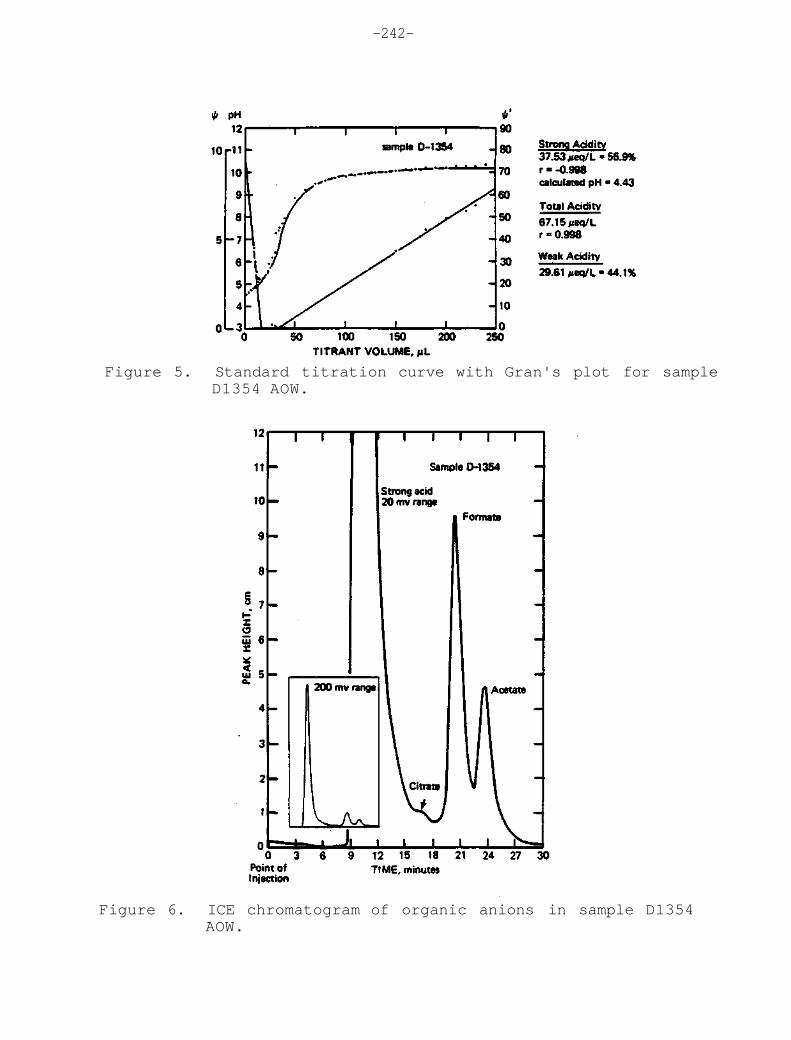
-242-

Figure 6. ICE chromatogram of organic anions in sample D1354 AOW.

Figure 5. Standard titration curve with Gran's plot for sample D1354 AOW.

-243-

Figure 7. Standard titration curve with Gran's plot for 5.05 z 10-5N HNO3.

Figure 8. Standard titration curve with Gran's plot for 2 53 -10-5N HNO3/2.52 x 10-5NH3 COOH.

-244-

preservation, our initial research has indicated that the addition of CHC13 would be necessary to maintain the levels of organic acids present in the original precipitation samples. Figure 4 gives an indication of just how much change in concentration can occur with time. After only three weeks, for example, the organic acids may completely disappear. Degradation and loss of organic constituents is thought to be due to microbial activity. This activity seems to be somewhat inhibited by refrigeration, but is apparently halted by the addition of an effective biocide such as CHC13. This additional preservation step then becomes necessary for all studies of organic acids where immediate chemical analysis is not possible.

Our analyses showed these precipitation samples to be composed of an average of 69% strong acid and 31% weak acid. Approximately 80% of the weak acid content can be accounted for by the measured ammonium concentration, leaving only 20% due to the organic acids. It should by noted that these samples were all collected in early spring (March, 1984 - May, 1984) from a site surrounded by tilled fields. Both the time of year with its associated agricultural activities and the sampler location in the center of these activites are likely reasons for the high concentrations of NH, we report. Figure 9 gives a representative sampling of the total weak acid component measured by titration compared to the total measured by Technicon AutoAnalyzer and ion chromatography exclusion.

Weak acid values obtained by ICE range from 0.026 mg/L (0.55 yeq/L) to 0.43 mg/L (9.10 yeq/L) for formate with a mean value of 0.210 mg/L (4.5 yeq/L). The acetate values range from 0.022 mg/L (0.37 yeq/L) to 0.44 mg/L (7.38 µeq/L) with a mean of 0.205 mg/L (3.48 yeq/L). The combined mean organic acid concentration measured by ICE is 7.34 yeq/L. By subtracting the measured concentration of NH, from the weak acid content found by titration, another measure of the total organic acid concentration for each sample can be determined. The mean organic acid concentration measured by titration after using this procedure was 5.8 yeq/L. Figure 10 shows the correlation between these two measured values. Four outliers have been removed from this plot because the total organic concentration for each is less than the accuracy of the methods used (particularly the titration). This concentration level of 7.34 yeq/L of organic acids corresponds to a maximum of 0.04 pH units contribution to the pH for the rain samples used in this study.

Throughout this work we used three different methods to derive a pH value for each sample. These methods are: measurement of pH using a pH meter and combination electrode, calculation of pH using the ion balance data, and calculation of pH using the acid-base titration results. A pH value calculated from ion balance data greater than that derived using either of the other two methods would be an indication that routine analyses did not measure all of the ions that contribute to the free acidity of the samples. Figure 11 is a graphic display

-245-

Figure 9. Sampling of measured weak acid concentrations, comparing total weak acidity value from titration to the sum of NH4+ (Technicon) plus organic anions (ICE).

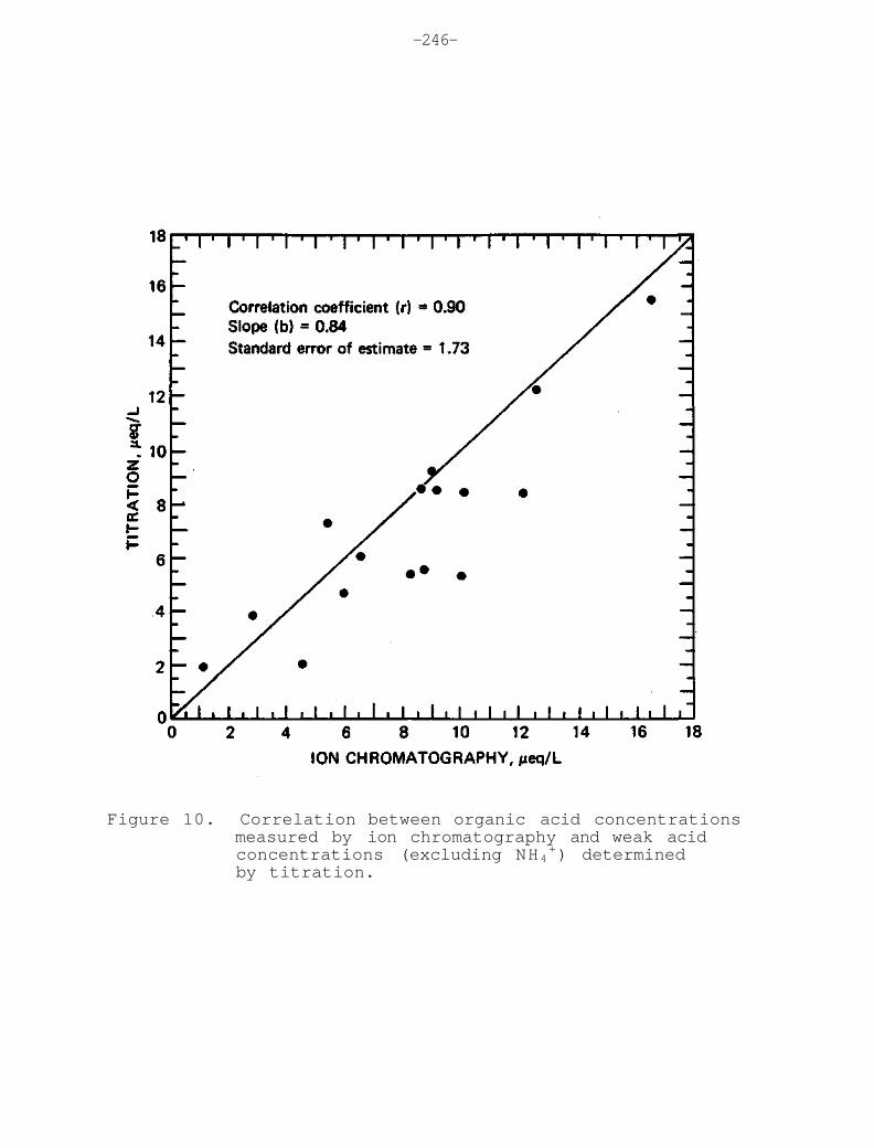
-246-

Figure 10. Correlation between organic acid concentrations measured by ion chromatography and weak acid concentrations (excluding NH4

+) determined by titration.

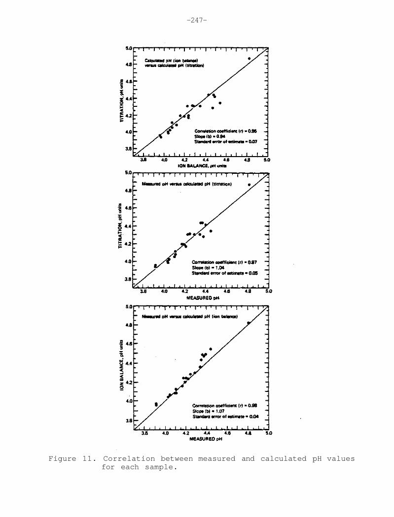
-247-

Figure 11. Correlation between measured and calculated pH values for each sample.

-248-

of the correlation between the pH values found using these three methods. The correlation coefficients of 0.95 - 0.98 show that the pH values derived using the three different methods are in good agreement for all samples analyzed. The slopes of 1.07 -0.94 are an indication that the major ions being routinely measured ( S O 4

- 2 , N O 3 , etc.) typically account for all of the free acidity in these samples and that the weak acid contribution is small.

The findings obtained in this study have been compared to weak acid concentrations measured at other locations in the United States. Recent work by Liljestrand and Morgan (1981) reported values from several different geographical areas of the U.S. comparing the weak acid versus the strong acid contribution in rainfall. Figure 12 shows how central Illinois' stong to weak acidity ratio compares to other U.S. locations. The contributions of ammonium ions to the weak acid concentrations reported for the Illinois data have been subtracted for this comparison since the other sites, with the exception of the two California locations, did not include ammonium in their weak acid results.

Nationwide, the contribution of weak organic acids to the chemistry of rainfall can be quite varied. As Fig. 12 indicates, the weak to strong acid ratio for Illinois precipitation is similar to that of sites in the northeastern United States. This similarity is consistent with the reported values of strong acid components at these locations, as well as the concentrations of weak organic acids measured. An analysis by Galloway et al. (1976) concluded that strong acids control the pH of rainfall in the northeastern U.S. but that weak acids are important to the total chemistry of precipitation and should not be overlooked. Based on the data accumulated thus far for the Bondville, Illinois site, our findings are in agreement with those of Galloway et al. Since our data base is limited to samples collected during the spring months, however, additional work needs to be carried out to examine seasonal differences in weak acid concentrations and weak to strong acid relationships.

REFERENCES

Galloway, J.N., B.T. Cosby and G.E. Likens, 1979: Acid Precipitation: Measurement of pH and Acidity, Limnology and Oceanography. 24. 6, 1161-1165.

, G.E. Likens and E.S. Edgerton, 1976: Acid Precipitation in the Northeastern United States: pH and Acidity, Science. 194. 722-724.

-249-

Figure 12. Strong versus weak acidities at selected U.S. locations.

-250-

Gran, G. 1952: Determination of the Equivalence Point in Potentionmetric Titrations, Analyst. 77, 661.

Keene, W.C., J.N. Galloway, and J.D. Holden Jr., 1983: Measurement of Weak Organic Acids in Precipitation from Remote Areas of the World, Journal of Geophysical Research. 88, C9, 5122-5130.

Liljestrand, H.M. and J.J. Morgan, 1981: Spatial Variation of Acid Precipitation in Southern California, Environmental Science and Technology. 15, 3, 333-338.

-251-

CHAPTER 13

FEASIBILITY STUDY TO ASSESS THE IMPACT OF PRECIPITATION QUALITY ON SOIL WATER QUALITY

Van C. Bowersox

INTRODUCTION

Two years of weekly rain and snow samples from the air and precipita­tion chemistry site (operated under this contract) near Bondville, Illinois, have resulted in pH measurements ranging from 3.5 to 7.0, with a median of 4.31. Eighty percent of these samples have a pH between 4.0 and 4.6. Except for Wisconsin, Florida, and the Gulf Coast areas, the annual median pH for states east of the Mississippi River is less than about 4.6 (Semonin, 1981). In the eastern U.S. this relatively acidic precipitation is primarily an expression of unneutralized sulfates and nitrates in solution (Bowersox and dePena, 1980).

The effects of the acidic inputs, sulfates, nitrates, and hydrogen ions, on the chemical weathering of soils has been little measured. Regions most likely to be sensitive to soil acidification, because of low buffering capacity or low base saturation, however, have been identified (McFee, 1980). Although the soils of east central Illinois have a high organic content, a correspondingly high cation exchange capacity, and a high base saturation, and hence are "not sensitive," these soils comprise an irreplaceable wealth of agricultural productivity. It is with a sense of greater understanding and preservation of this wealth that makes an investigation of the impacts of precipitation quality on the soils of central Illinois apropos.

The measured media in this impact assessment are precipitation chemistry and soil water chemistry. It is presumed that the relationship between these quantities will render some indication of the effect of the input (precipitation) on the throughput (soil water). There are three distinguishable fates of acid precipitation that has infiltrated the soils and been collected as soil water (McFee, Kelly, and Beck, 1977):

(1) it may have been unaffected (2) it may have been neutralized by soluble bases such as,

CaCO3 or Na2CO3 (physical/chemical processes), and/or (3) it may have reacted with the soil complex (chemical

processes). In the first instance, precipitation may percolate relatively unimpeded and unaffected through sandy soils that have little or no humic matter. Fate two typically follows the application of lime to agricultural soils of whatever type. Finally for clay and other soils with a high organic content (as in Illinois), fate three is virtually inescapable. These soils have a large reservoir of exchangeable cations, often alkali or alkaline earth metals that are reactive in nature. Relating the chemistry of the soil water from a wetting front associated with a rain event to the chemistry of that rainfall should provide insight into the chemical processes at work.

-252-

In the simplest sense one could calculate the potential effect of acidic precipitation on soils by utilizing existing information. From the reported concentrations of exchangeable cations, the bulk density of soils, the average acidity of precipitation, and the typical amounts of precipita­tion per year, an estimate could be made of how long it would take to shift the pH by some arbitrary amount (McFee, Kelly, and Beck, 1977). This would be a worst case estimate, though, since it presupposes that the cation input is only H and that all of this H would completely exchange with basic soil cations, neither of which is true. Perhaps of even more con­sequence , however, is that such a treatment conceptualizes the soil as a reactive medium in a container, abstracting it from its very active bio-geochemical setting in nature. Counteracting processes such as nutrient recycling and mineral decomposition would tend to mitigate and may even halt the acidification process. For example, the increased mobilization of most soil elements and the increased flux of nutrients that would be expected from acidic precipitation (Norton, 1977) would likely enhance plant growth, increasing the plant litter returned to the soil. Decomposed organic matter from this litter would enhance the cation exchange capacity of the soil, thereby increasing its buffer capacity and fertility. One researcher has speculated that a possible result of acidic precipitation might even be to increase the cation exchange capacity of soils in certain situations (Norton, 1977).

Given the widespread occurrence of acidic precipitation and given the uncertainty in its effects on soils, this study was initiated to establish a protocol for investigating the impacts of precipitation quality on soils and soil water quality. The focus of the research is on soil water extracted from the unsaturated zone (i.e., generally above the water table) and on tracing the contribution of the major inorganic ions in precipita­tion to the chemistry of the soil water.

SAMPLING OBJECTIVES

Objective 1. to evaluate the feasibility of associating a pulse of water as it percolates downward through a soil column with the precipitation event from which it originates.

Objective 2. to establish a protocol for recovering chemically and volumetrically representative (i.e., unbiased) samples of soil water from a soil column.

Objective 3. to assess the uncertainty and variability of measurements related to objectives (1) and (2).

Objective 4. to intercompare the chemistry of precipitation and soil water; and by integrating data for the chemistry of soils with these results, to ascertain whether the impacts of precipitation quality on soils can be reliably measured using these techniques.

-253-

SAMPLING SITE

Measurements of two time or event dependent quantities, precipitation chemistry and soil water chemistry, are required according to the experimental design (Bowersox, 1981). Both of these measurements are to some extent site specific, if for no other reason than because of the high degree of spatial variability of rainfall and rainfall chemistry (Naiman and Gatz, 1980; Stensland, 1980). Due to this constraint, the soil water samplers (P/V lysimeters) were installed in proximity with the precipitation samplers at the Bondville research site, located some 15 kilometers southwest of residential Champaign. Figure 1 displays the relative locations of the sampling devices currently being operated there. The P/V lysimeter array is nearly 31 meters east of the 'BGDE' wet/dry sampler used to collect daily precipitation samples for chemical analysis. This area is intensively cultivated for cash crop (corn and soybean) purposes, as is much of east-central Illinois within at least a 200 km radius. The site itself is a 2.5 ha (230m x 110m) grass-covered plot surrounded by actively tilled fields. Samples were recovered daily, Monday through Friday, from the lysimeters and from the 'BGDE' sampler (Monday through Friday) when precipitation occurred since the preceding sample.

The soils of Champaign County are largely windblown silts (loess) that cover glacial drift to depths of as much as 1.5m. All of the area was covered by repeated Pleistocene glaciations that dissected the area into gently undulating moraines and nearly level till or outwash plains. Elevation differentials between plain and moraine are of the order of 15 meters. The Bondville site is on an outwash plain about 6.5 km west of the Tolono Moraine. Natural drainage in the area is unconsolidated, i.e., with no clear downward direction along the surface. As a result, the land was wet and marshy and generally unsuitable for tillage until the late 1800's, when drainage districts were formed, ditches were dredged, and the fields were tiled. Grazed prairie grasses gave way to the plow and the area emerged as some of the most highly productive cropland in the nation.

The soils on site are in the Elburn series, a somewhat poorly drained, very dark gray, friable silt loam formed on slight swells (0 to 3 percent) above the more poorly drained Drummer series. In spring, a seasonally high water table can be as shallow as 30 to 90 centimeters from the surface. Although drainage is somewhat limited by the lay of the land, water can move down through these soils when saturated at the moderate rate of 0.6 to 2.0 inches per hour. (This is called permeability.) Only an occasional thundershower may have hourly rates exceeding that range. The clay content of the surface soils ranges from 22 to 27 percent and the organic content is high (4 to 8 percent). These materials contribute to fertility and to a high cation exchange capacity. Despite the large reservoir of cations, the pH varies from a mildly acidic 5.6 to a neutral 7.8. Table 1 summarizes some properties of the Elburn soils with depth (source: Soil Survey of Champaign County, 1982).

Figure 1. Bondvllle Research Site

-255-

Table 1. Some Physical and Chemical Properties of Elburn Soils.

Moist Bulk Available Depth Clay Density Permeability Water Capacity Soil (in) (Pct) (G/CM3) (in/hr) (in./in.soil) pH 0-16 22-27 1.1-1.3 0.6-2.0 0.22-0.24 5.6-7.8

16-46 27-35 1.2-1.4 0.6-2.0 0.18-0.20 5.6-7.8 46-60 15-25 1.5-1.7 0.6-6.0 0.12-0.18 6.1-8.4

SAMPLING INSTRUMENTATION

Above the water table in unsaturated soils, water is held in retention by molecular and capillary forces. During the infiltration of precipitation into the soil, water in excess of that held by those forces (at field capacity) percolates downward toward the water table. A wetting front associated with a precipitation event percolates through the soil at a rate characterized by the soil permeability, the higher the permeability the faster the rate. Any of the chemical interactions of the water with the soils discussed earlier, such as dissolution, adsorption, ion exchange, redox reactions, etc., may, of course, occur. Most, if not all, of these interactions are time dependent; and so percolating water is generally undergoing dynamic changes toward a new equilibrium chemistry. Sampling water for analysis at various stages of its passage through the soil requires an instrument that can extract water against the retaining forces, yet leave the collected sample unchanged. The instrument chosen was a pressure-vacuum lysimeter (Bowersox, 1981). Applications of a vacuum to such a device implanted in the soil effects a flow of moisture toward and through a porous ceramic cup into the evacuated chamber. The 1-2 micron pore size of the cup material prevents entrainment of soil particles or other debris (except colloids smaller than about 1 micron) that may affect the chemistry. Removal of the captured sample is by release of the vacuum and application of pressure to the chamber to force the water to the surface. Figure 2 pictorially represents the field installation of a pressure-vacuum lysimeter at the Bondville site. (For a more detailed description of the P/V lysimeter see Johnson and Cartwright, 1980, or Leonard, Meyer and Wilkinson, 1979.)

Past field and laboratory tests of the validity of soil moisture samples taken with ceramic cup lysimeters have yielded mixed results. Some investigators found that the ceramic cups contribute Ca, Na, and K to soil moisture (Grover and Lamborn, 1977), and screen or adsorb phosphate and nitrate, biasing these constituents low. Other research indicated that the concentration of Ca, Mg, and phosphate are unaltered (Levin and Jackson, 1977). The ceramic cups are fired from a mixture of kaolin and ball clays and alumina. Although these materials are relatively stable and inert, CaO, MgO, Na2O, and K2O are present (Leonard, Meyer, and Wilkinson, 1979). Thus for soil moisture having low solute concentrations, it's

-256-

Figure 2. Field Installation of Pressure-Vacuum Lysimeter at the Bondville Site,

-257-

likely that the reported biasing could significantly affect the results. Leaching of the cups with dilute HC1 has been recommended to reduce Na and K contamination and phosphate adsorption. Reduction of biasing from these ions, however, may be replaced by a pH bias in samples retained in acid-washed containers. If soil moisture samples are to represent actual soil moisture quality, the potential for bias due to the sampling instrumen­tation must be evaluated.

To establish a protocol for sampling soil water that yields repeatable and representative results, two lysimeters were acid washed and two were de-ionized water washed. The acid washed units were immersed for about 2 weeks in a 0.1N HC1 bath that covered the ceramic cups. Acid was flushed through the cups and into the collection tubes on 4 occasions during the 2-week period. A rinse with copious amounts of de-ionized water followed the wash period, and the final rinse had a pH of about 5.3. The water washed units were repeatedly flushed with de-ionized H2O, though no measurements of pH and/or conductance were taken to monitor the progress or effectiveness of the procedure.

To assess the potential for a positive bias in the major inorganic ion concentrations, a blank series was taken from each (washed) lysimeter prior to field installation. The blank determinations proceeded as follows:

Step (1) 13 liter polyethylene bucket washed with de-ionized H2O (for details see Stensland, et al., 1980);

Step (2) bucket was charged with about 8 liters of de-ionized H2O;

Step (3) approx. 40 ml aliquot for analysis removed with clean syringe (This is the water blank sample.);

Step (4) lysimeter suspended in water to depth of several centimeters above ceramic cup;

Step (5) lysimeter evacuated to 50 centibars (about 1/2 atmosphere) reduced pressure and left to collect water overnight;

Step (6) approx. 50 ml aliquot for analysis removed from lysimeter by application of pressure (This is the lysimeter blank sample.);

Step (7) water discarded, bucket rinsed with de-ionized H2O, and steps (2) through (6) repeated until all units were blank tested.

This procedure amounts to an aqueous leach at room temperature of the ceramic cup and internal walls of the PVC tube of the lysimeter. As such, the results indicate a contamination potential from these sources. If the soil water chemistry is reactive (e.g., due to organic acid/base content) with the ceramic matrix or PVC, additional biases may be introduced in sampling. Evaluation of the adsorption and screening potential of the lysimeter system remains a requirement for future efforts.

-258-

Table 2 presents a summary of chemical analyses of the blank series. Lysimeters designated 'A' and 'B' were acid washed and 'C' and 'D' were de-ionized water washed. From the table it is obvious that the water blanks taken during step (3) are relatively free of significant contamina­tion. Only sodium is consistently above the analytical detection limit; the highest value reported, .018 ppm, is within the "range of detection" (<10 X detection limit) and, therefore, subject to a large relative uncer­tainty. In addition, for ammonium, sulfate, nitrate, and chloride there is apparently little to no positive bias, irrespective of the washing techni­que (acid vs. water). The value of 0.40 mg/1 for sulfate from lysimeter C is of limited significance due to its large relative uncertainty, and prob­able extraneous source. Apparently the rinse procedures following the acid wash were adequate, since there is no strong signature for either residual chloride or free acid from blanks A and B. Solution conductance, pH, cal­cium, and magnesium for A and B were virtually unaffected, as well. The alkali metals, sodium and potassium, were significantly elevated to .12 and .02 ppm, respectively. Lysimeters C and D exhibited some spiking in both alkali and earth metals. Levels for sodium and potassium were between 3.5 and 10 times higher than for the acid washed instruments. Calcium and mag­nesium were also significantly affected. Changes in the solution conduc­tance and pH were consistent with dissolution of these cations as bases (e.g., Ca(OH)2). These findings are not inconsistant with those of earlier researchers (Grover and Lamborn, 1970). It is necessary to intercompare actual soil moisture concentrations with these blank level determinations to place the positive contamination potential in perspective. It is of special interest that even acid washing with 0.1N HC1 does not preclude some blank level aliasing. Perhaps a more thorough and rigorous procedure could reduce the blank levels of the deionized water washed lysimeters.

Table 2. Results of the Chemical Analyses of the Blank Series for the Acid Washed (A & B) and De-ionized Water Washed (C & D) Lysimeters.

Note: < symbols designate measurements below the limit of detection. For analytical techniques see Peden, Skowron, and McGurk, 1979.

-259-

SAMPLING AND INSTALLATION PROCEDURES

Four pressure-vacuum lysimeters were implanted at "plow layer" depth in the soils at the Bondville site: 2 were acid washed (A&B), 2 were de-ionized water washed (C&D), and 2 were bedded in an envelope of silt-sized "silica sand" (A&D), 2 were simply bedded in back-filled soil (B&C). (See Fig. 2 for sketch of lysimeter tube installation.) The use of the "silica sand" has been recommended to improve the soil/ceramic cup contact and thereby to improve the efficiency of the catch (Leonard, Meyer, and Wilkinson, 1979). In principal it should facilitate sampling because of its relatively low retention (high conductivity) for water. Its use and the two lysimeter pre-cleaning alternatives are being simultaneously evaluated. To eliminate the depth variable and to minimize the differences that may accrue from lateral separation, each unit was installed at the same depth in a square array 3 meters on a side, according to the arrangement:

The plow layer was chosen since it interfaces with the atmosphere and would, therefore, presumably be the least difficult in which to correlate rain and soil water, both physically and chemically.

Installation was by lowering the lysimeters into 7.6 cm (3 inch) diameter boreholes, augured to depths of 18 centimeters. A bucket type augur, which enabled the removal of soil from the boreholes in a layerwise fashion, was used. Five such layers were removed from each hole and, upon inserting the lysimeters, were returned in reverse order to preserve, so far as practical, the profile through the layer. For lysimeters A and D, "silica sand" was first emplaced around and to the depth of the cup (about 6cm) prior to backfilling with soil. The backfilling sequence was adjusted accordingly. As the gap between the 5 cm diameter lysimeter tube and borehole was filled, the returned soil was lightly tamped. In addition, to prevent channeling of water along th PVC tube from the surface, special care was taken at the topmost layer to adequately compress the soil against the tube. Portions of the excess soil after backfill were sealed in de-ionized water rinsed glass jars. These were frozen for future soil

-260-

assay work. Some 47 centimeters of tube remained above ground. The exposed tubes were supported in an upright position with nylon guylines that also prevented vehicular approach to the grid. Each lysimeter was outfitted with a 2m long rubber presure-vacuum line and a 0.75 meter Tygon discharge line. Screw type compression clamps were used on the P/V and discharge lines to seal the system. As leaks were identified and eliminated from the respective lysimeters, the P/V lines were inter-connected so that a single pump station could evolve. An important advantage of a fully inter-connected system is to assure that all lysimeters have identical sampling vacuums. Installation of the lysimeters was completed on 22 Mar 82, at which time sampling was begun.

To suction the collection chamber and to discharge samples therefrom, a portable hand pump that could produce both positive and negative pressures was used. If present, samples were discharged daily from the lysimeters (Monday through Friday, only) and the systems were re-evacuated (typically) to an 80 centibar vacuum. The recovered samples were stored in sealed LPE containers, which were weighed so that daily collected volumes could be reported. As volume permitted, an aliquot was taken from a daily sample for pH and solution conductance measurements. Seven-day composites, representing a Tuesday-to-Tuesday extended period, were prepared from the daily samples. These composites were submitted to the laboratory for complete cation/anion analyses. Samples received the same care and handling as precipitation samples (Peden, Skowron, and McGurk, 1979).

SAMPLING RESULTS

A. Collected Soil Water Volume - Re; Table 3 and Figure 3.

Daily measurements of the weight of the collected soil water samples and the residual vacuum in the lysimeter tube at collection time were used to determine sample volumes and system leakage. Together these parameters were compiled to deduce whether the collected volumes might have been significantly reduced due to leakage. The capacity or internal volume of each lysimeter is fixed at about 900 cm , therefore the collected sample proportionately affects the internal pressure by reducing the airspace according to the ideal gas law expression, P1V1 = P2V2. With this informa­tion, any leaks in lysimeter systems A, C, and D had been confirmed and repaired by 4 May 82. The P/V lines for these 3 lysimeters were inter­connected then, and sample volume data for 5 May and thereafter were com­pletely intercomparable. An intermittent leak in lysimeter B was not isolated by that time so this lysimeter was left to operate independently. Collected sample volumes have been tabulated in Table 3, along with precip­itation dates and amounts. Total volumes for lysimeters A and D were 2443 ml and 2600 ml, respectively, a 6% difference. For B and C the totals were 511 ml and 706 ml, or 28% less for B than C. Due to the relatively large volume discrepancy between B and C and the known leakage problem, sample volume statistics for B were omitted from further comparisons. Blank spaces in Table 3 appear (usually on weekends) when no samples were re­covered and the system was left to collect soil water for more than 1 day.

-261-

Figure 3 depicts the precipitation and soil water volumes that were accumulated in the initial 3-month period of sampling. Two intervals of time were marked by little to no sample accumulation. First, freezing conditions of 5 to 13 April prevented collection and removal of any sample, although .57 inches of precipitation (snow, rain, and mixed) were recorded in that interval. Second, the onset of rapid growth and greening of the grasses at the Bondville site, coupled with an interval of little precipitation (about 20 April to 20 May), coincided with a 13-day period (7-20 May) of virtually no sample. Vegetation, of course, taps the soil water for growth and sustenance and contributes to the forces with which water is retained by the soils. It is not known to what extent this growth spurt may have inhibited soil water migration toward the internal (approx. 80cb) vacuum of the lysimeter system. A comparison of the pre- versus post-growth response of the collected volumes to precipitation occurrences, however, shows a marked difference. Over half of the accumulated sample was collected before 30 April (vis. A&D), yet less than 1/4 of the total precipitation had occurred prior to that date. After 20 May collected volumes were much reduced and more clearly accompanied large rainfalls. Lysimeters A and D, both bedded in silica sand, exhibited very similar response features; and although much less water was captured by the soil bedded instrument (C), its response profile appeared as a damped version of that for A and D. Clearly the instruments responded to the same phenomena but at different amplitudes.

For the soils at the Bondville site, the use of silica sand facilitates the catch of soil water by some 3.5 to 3.7 times (e.g., ratio of accumulated volume from A or D to C). The sand improves the soil/ceramic cup contact and has a higher conductivity for water than the soil itself. Conceptually the presence of the sand effectively increases the area of the collection surface of the cup. In other words, the collection area for the soil bedded lysimeters is simply the outside surface area of the ceramic cup, while for the sand bedded lysimeters it is the area of the volume filled by the sand (see Fig. 2). Assuming the bottom of the augured hole is a hemisphere of 3.8 cm (1.5 in.) radius and the ceramic cup is covered at all points by at least 1 cm of sand, top and bottom, the collection area for the sand bedded lysimeters is approx. 272 cm . The area of the cup is the sum of the area of a cylinder (r = 2.54 cm, 1 = 4.5 cm) and the area of that part of a (r =) 2.90 cm sphere that exactly fills the end of the cylinder, or a total of 99 cm . The ratio of the areas is 2.7. More careful measurements of the volume occupied by the silica sand are necessary to determine the accuracy of this ratio and whether the above concept is correct. If the silica sand does not influence the chemistry of the soil water, then it indeed enhances the collection efficiency of ceramic cup lysimeters in the silt loams of central Illinois.

-262-

Table 3. Soil Water and Precipitation Data.

Col l ec t ed Volume P r e c i p i t a t i o n (ML) ( i n c h e s ) S o i l Water

-S ince Previous Sample- -S ince Previous P r e c i p . pH A B C D Sample- pH A D

31 Mar 82 127.5 5.6 7.9 62.4 .01 6.71 5.24 7.21 1 Apr 82 157.9 9.6 14.2 108.1 0.00 5.46 6.89 2 Apr 82 95.4 4 . 3 0 .0 0 .0 t r a c e ISA 6.19 3 Apr 82 4 Apr 82 133.4 55.9 46.4 352.6 0.40 ACC NM NM 5 Apr 82 23.0 8.3 4 .7 23.6 t r a c e 6.58 5.78 6.93 6 Apr 82 0 .0 0 .0 0 .0 0 .0 0.38 (snow) 4 .53

weekly t o t a l s 409.7 78.1 65 .3 484.3 0.79

7 Apr 82 0 .0 0 .0 0 .0 0 .0 0 .0 8 Apr 82 0 .0 0 .0 0 .0 0.0 0.02 ACC 9 Apr 82 0 .0 0 .0 0 .0 0 .0 0.08 4.22

10 Apr 82 0 .0 0 .0 0 .0 0 .0 0.02 ACC 11 Apr 82 0.0 0 .0 0 .0 0.0 0.03 ACC 12 Apr 82 0 .0 0.0 0 .0 0.0 0.02 4.07 13 Apr 82 0 .0 0 .0 0 .0 0 .0 0.02 ISA

weekly t o t a l s 0 .0 0 .0 0 .0 0.0 0.19

14 Apr 82 117.9 3.2 9 .8 77.0 0 .0 6.32 7.23 15 Apr 82 163.2 1.7 16.8 168.0 0 .0 6.06 6.61 16 Apr 82 67.4 1.0 12.2 55 .3 0.18 4.50 5.90 6.61 17 Apr 82 18 Apr 82 19 Apr 82 223.5 59.4 23.1 332.9 0.50 4.68 6.23 6.76 20 Apr 82 111.5 16.0 22.8 74.0 0.15 4.24 5.75 6.30

weekly t o t a l s 683.5 91 .3 84.7 707.2 0.83

21 Apr 82 81.6 7.2 18.5 68.8 0.0 6.31 7.14 22 Apr 82 69.8 4.8 14.7 59.0 0.0 6.45 7.10 23 Apr 82 61.2 6.7 14.4 47.7 trace ACC 6.31 6.99 24 Apr 82 34.7 0.0 13.5 42.9 0.0 ACC 5.91 6.90 25 Apr 82 0.0 ACC 26 Apr 82 3.6 17.0 0.0 0.0 trace 4.26 27 Apr 82 83.6 8.2 8.5 68.2 0.07 4.58 5.95 6.23 weekly totals 834.5 44.9 69.6 286.6 0.07

ISA : Insufficient sample for analysis ACC : pH measured on sample accumulated for more than 1 day NM : No measurement on available sample

-263-

Table 3 (continued)

NM : No measurement on available sample

C o l l e c t e d Volume P r e c i p i t a t i o n (ML) ( i nches ) S o i l Water

Since Previous Sample- -S ince Previous P r e c i p . pH A B C D Sample- pH A D_

28 Apr 82 62.6 7.4 10.3 35.4 0.0 5.97 6.24 29 Apr 82 38.4 6.5 7.4 16.8 0.0 6.34 6.94 30 Apr 82 33.1 7.8 8.2 17.3 0.0 6.25 6.98

1 May 82 2 May 82 3 May 82 71.3 16.2 22.7 32.6 0 .0 NM NM 4 May 82 53 .3 5 .3 4 . 3 14.7 0.0 NM NM

weekly t o t a l s 258.7 43 .2 52 .9 116.8 0.0

5 May 82 5.5 5.0 4 .6 .8 0 .0 NM NM 6 May 82 5.8 4 .5 3.4 0 .0 0.0 NM 7 May 82 2.4 9.7 4 .1 .2 .31 4.79 NM NM 8 May 82 9 May 82

10 May 82 2.6 7.0 1.9 2 .1 0.0 NM NM 11 May 82 0.6 . 1 .2 0 .0 0.0 NM

weekly t o t a l s 16.9 26 .3 14.2 3 .1 .31

12 May 82 0.0 0 .0 0.0 0 .0 0.0 13 May 82 0.0 0 .0 0.0 0 .0 0.0 14 May 82 0.0 0 .0 0.0 0 .0 0.0 15 May 82

16 May 82 17 May 82 0.0 0 .0 0.0 0 .0 0.19 4.27

18 May 82 0.0 0 .0 0 .0 0 .0 0.0

weekly t o t a l s 0 .0 0 .0 0 .0 0 .0 0.19

19 May 82 0.0 0 .0 0 .0 0 .0 0.0 20 May 82 0.0 0 .0 0 .0 0 .0 0.0 21 May 82 5.0 6.5 19.9 32 .8 0.73 4.13 NM NM 22 May 82 10.0 2 .5 .6 1.6 0.0 NM NM 23 May 82 24 May 82 0.0 0 .0 0 .0 0.0 0.0 25 May 82 0.0 0 .0 0.0 0.0 0.0

weekly t o t a l s 15.0 9.0 20.5 34.4 0.73

-264-

Table 3 (continued)

ISA : Insufficient sample for analysis ACC : pH measurement on sample accumulated for more than 1 day NM : No measurement on available sample

Collected Volume Precipitation (ML) (inches) Soil Water

-Since Previous Sample- -Since Previous Precip. pH A B C D Sample- pH A D_

26 May 82 1.2 .2 0.0 2.0 0.29 ACC NM NM 27 May 82 1.0 13.0 23.2 85.0 0.53 4.56 NM NM 28 May 82 10.8 3.7 2.9 17.9 trace ISA NM NM 29 May 82 30 May 82 15.1 4.2 8.4 13.3 0.27 4.35 NM NM 31 May 82 1 Jun 82 141.8 59.5 146.5 303.3 1.60 4.35 NM NM

weekly totals 169.9 80.6 181.0 421.5 2.69

2 Jun 82 18.7 2.6 4.6 20.7 0.0 6.58 6.77 3 Jun 82 45.3 2.7 6.0 41.2 0.0 6.56 6.67 4 Jun 82 36.3 4.2 6.7 28.9 0.0 6.60 6.73 5 Jun 82 6 Jun 82 7 Jun 82 81.0 7.1 15.8 47.3 0.0 NM NM 8 Jun 82 21.9 4.1 5.3 9.6 0.13 3.84 6.16 6.65

weekly totals 203.2 20.7 38.4 147.7 0.13

9 Jun 82 23.7 3.3 4.9 7.6 0.11 3.82 NM NM 10 Jun 82 8.0 1.7 3.3 4.4 0.0 NM NM 11 Jun 82 10.0 1.6 3.3 4.4 0.0 NM NM 12 Jun 82 13 Jun 82 14 Jun 82 11.5 2.5 4.9 1.6 0.03 4.02 NM NM 15 Jun 82 .7 .7 0.0 0.0 0.08 4.14 NM NM weekly totals 53.9 9.8 16.4 18.0 0.22

16 Jun 82 1.1 18.0 33.6 12.8 0.76 4.07 NM NM 17 Jun 82 .4 1.8 2.3 1.6 0.08 ACC NM NM 18 Jun 82 .8 2.8 1.9 2.2 0.0 ACC NM NM 19 Jun 82 20 Jun 82 21 Jun 82 199.3 61.3 101.0 283.1 1.23 3.99 6.30 6.63 22 Jun 82 35.5 5.4 6.4 29.5 0.03 5.45 6.02 6.15 weekly t o t a l s 237.1 89.3 145.2 329.2 2.03

-265-

Table 3 (continued)

ACC : pH measurement on sample accumulated for more than 1 day NM : No measurement on available sample

Collected Volume Precipitation (ML) (inches) Soil Water

-Since Previous Sample- -Since Previous Precip. pH A B C D Sample- pH A D

23 Jun 82 30.9 2.1 5.2 17.3 0.0 6.45 6.74 24 Jun 82 14.9 2.4 3.9 17.3 0.0 NM NM 25 Jun 82 8.3 3.0 2.6 5.0 0.0 NM NM 26 Jun 82 27 Jun 82 28 Jun 82 6.4 6.4 6.3 6.0 0.11 ACC NM NM 29 Jun 82 0.0 0.0 0.0 0.0 0.0 3.96 30 Jun 82 0.0 4.1 0.1 5.3 0.06 5.84 NM weekly totals 60.5 18.0 18.1 50.9 0.17

-266-

Figure 3. Accumulated Precipitation and Soil Water Volume Collected 1 Apr to 30 Jun 82.

-267-

B. Soil Water pH, Comparison of Dally Measurements for Lysimeters A and D - Re: Table 3, Figure 4, and Figure 5.

As sufficient volume was available, aliquots of the daily soil water samples were taken for pH measurements. Only samples from lysimeters A and D (silica/sand bedded) were so treated, because volume yields from B and C were generally too small to subdivide. Results of these measurements are listed in Table 3, as are the precipitation pH values for comparison. These pH results are graphically summarized in Figure 4, as well.

Without exception for the 1 April to 30 June period depicted in Figure 4, daily pH values for samples from lysimeter D were higher than from A. These paired samples exhibited a high degree of covariance, though little relationship to precipitation pH values. This evidence suggests that:

(1) The pH of rainfall has little obvious effect on the pH of soil water at plow depth.

(2) Lysimeter pre-cleaning techniques have a manifest impact on blank levels of cations and pH, as well as on soil water pH. De-ionized water washed instruments impart alkali and alkaline earth metals to a pure water leachate and accordingly raise its pH; acid washed lysimeters apparently do not. For soil water samples, the pH from a de-ionized water washed lysimeter is higher than from an acid washed one. It is possible that these differences could be the result of preferential screening or adsorption of cations in the acid washed instruments, as well as blank contamination or biasing from the de-ionized water washed ones. To conclude to what extent these processes are at work and which dominates, further laboratory tests are needed.

Careful examination of Figure 4 reveals a general upward trend in the daily measurements from lysimeter A. This trend is made more evident when the differences in pH values from A and D are shown against time, as in Figure 5. Should this trend continue, the measured values will converge. It is necessary to recall that only about 2.5 liters of soil water have passed through the ceramic cups. It is expected that as more water contacts and interacts with the instruments, differences due to cleaning may vanish.

-268-

Figure 4. Precipitation and Soil Water pH Measurements for the 1 Apr to 30 Jun 82 Time Period.

-269-

Figure 5. Differences in Soil Water pH Measurements for Lysimeter D Versus Lysimeter A (1 Apr to 30 Jun 82).

-270-

C. Soil Water pH, Comparison of Weekly Measurements for All Lysimeters -Re: Table 4 and Figure 6.

A weekly composite sample for each lysimeter is submitted to the laboratory for analysis (usually) every Tuesday. Laboratory pH and solution conductance measurements of these samples along with those for the Tuesday-to-Tuesday precipitation samples are given in Table 4. A mean and range is also included for each parameter except precipitation volume.

From the computed means and the time series plots of Figure 6, it is apparent that none of the lysimeters gives identical results. For pH,

C > D > B > A,

though not without exception. In several instances the differences among the laboratory pH measurements for B, C, and D are within the expected measurement error, and one would conclude that these values were essentially the same. Comparisons of solution conductance measurements, however, suggest that these same samples have a quite different chemical loading. For conductance measurements after 5/25/82,

D > A > C > B.

With the data available some preliminary observations are in order:

(1) Precipitation pH is clearly below soil water pH for the silt loams of central Illinois. Since precipitation can be characterized as a dilute strong acid solution of sulfuric and nitric acids, this increase in pH is tantamount to neutralization of these acids.

Neutralization occurs in the topmost (plow) layer, even for the most acidic (pH of 3.82) rainfalls observed. Further, the values observed for soil water pH are within the range reported for Elburn silt loams in Table 1 (5.6 to 7.8).

(2) Soil water pH measurements for lysimeters A and B are less than for C and D; therefore, lysimeter pre-cleaning techniques have an effect on the results and require further evaluation (see previous section).

(3) Although bedding ceramic cup lysimeters with silica sand has been recommended to enhance the catch, there are differences in the chemistry of samples from sand bedded versus soil bedded devices. In particular, the solution conductance from lysimeter D samples exceeds by 34% to 81% those from lysimeter C, even when both samples have similar pH values. The results of further chemical analyses should fix the source and identity of the contaminants in the sand. Perhaps a cleaning procedure can be developed to purge the sand prior to installation.

-271-

(4) The time series plots of pH in Figure 6 suggest that prior to 11 May the lysimeter/sand/soil systems were in a process of equilibration or adjustment. This process is ongoing as more water interacts with the respective systems. After 11 May, lysimeters B, C, and D have apparently neared stabilization, as evidenced by the covarying pH values, whereas A appears to be yielding measurements that are uncorrelated with the others. Trends indicated in the daily pH measurements of Figure 4 suggest that it, too, will approach stabilization. Only future measurements will elucidate to what extent all the lysimeter results will vary in the same way.

D. Relationship Between Acidic Input and Throughput pH at Plow Layer Depth - Re; Table 4, Figure 4, Figure 6, and Figure 7.

As to the relationship between precipitation pH and soil water pH at the plow layer depth, Figures 4 and 6 suggest little to no correlative behavior between the two. The input function, a quantity of acid of a certain strength is measured not by pH but by the deposition of total acidic hydrogen onto the soil surface. Perhaps this is why no relationship is evident. Total acid deposition was estimated by multiplying sample volume (per unit area) by 10-pH. For central Illinois rains, 10-pH approximately equals the acid hydrogen content. The sample volumes used were those reported in Table 4. (These volumes are for wet-deposition-only samples collected in LPE buckets with a collection cross-section of 825.5cm2. A relationship between soil water pH (throughput) and free hydrogen ion deposition (input) is indicated in Figure 7. As the input increases, the soil water pH tends to be slightly depressed. Future research efforts are needed to clarify this relationship.

-272-

Table 4. Soil Water and Precipitation pH and Solution Conductance Data for 1-Week Samples.

Mean 4.38 42 6.50 6.93 7.31 7.20 117 78 95 110

Min 3.85 13 5.78 6.23 6.96 6.87 82 55 64 71*

Max 5.61 89 7.01 7.20 7.77 7.57 221 120 157 194

NA : None Available NSC : No Sample Collected

Soil Water Precipitation pH Conductance (us/cl)

Sample Volume Conductance Period (ml) pH (us/cm) A B C D A B C D

3/31-4/6 610 5.61 13 5.78 6.23 7.21 7.13 110 57 85 74 4/6-4/13 81 4.04 59 NSC NSC NSC NSC NSC NSC NSC NSC 4/13-4/20 785 4.47 23 6.49 6.72 7.38 7.10 92 64 93 71 4/20-4/27 80 4.46 59 6.87 7.00 7.40 7.22 88 79 98 73 4/27-5/4 0 6.64 7.15 7.77 7.42 92 82 111 86 5/4-5/11 283 4.78 14 7.01 7.20 7.57 7.57 151 110 157 NA 5/11-5/18 180 4.21 40 NSC NSC NSC NSC NSC NSC NSC NSC 5/18-5/25 643 4.22 37 6.63 7.07 7.18 7.24 221 120 83 138 5/25-6/1 2075 4.44 20 6.44 6.78 7.02 7.01 99 58 69 104 6/1-6/8 163 3.85 89 6.96 7.08 7.14 7.04 106 61 71 115 6/8-6/15 215 3.96 61 5.98 7.11 7.31 7.20 127 89 107 194 6/15-6/22 1687 4.12 42 6.35 6.73 6.96 6.87 82 55 64 111 6/22-6/30 NA NA NA 6.40 7.15 7.45 7.41 123 85 103 138

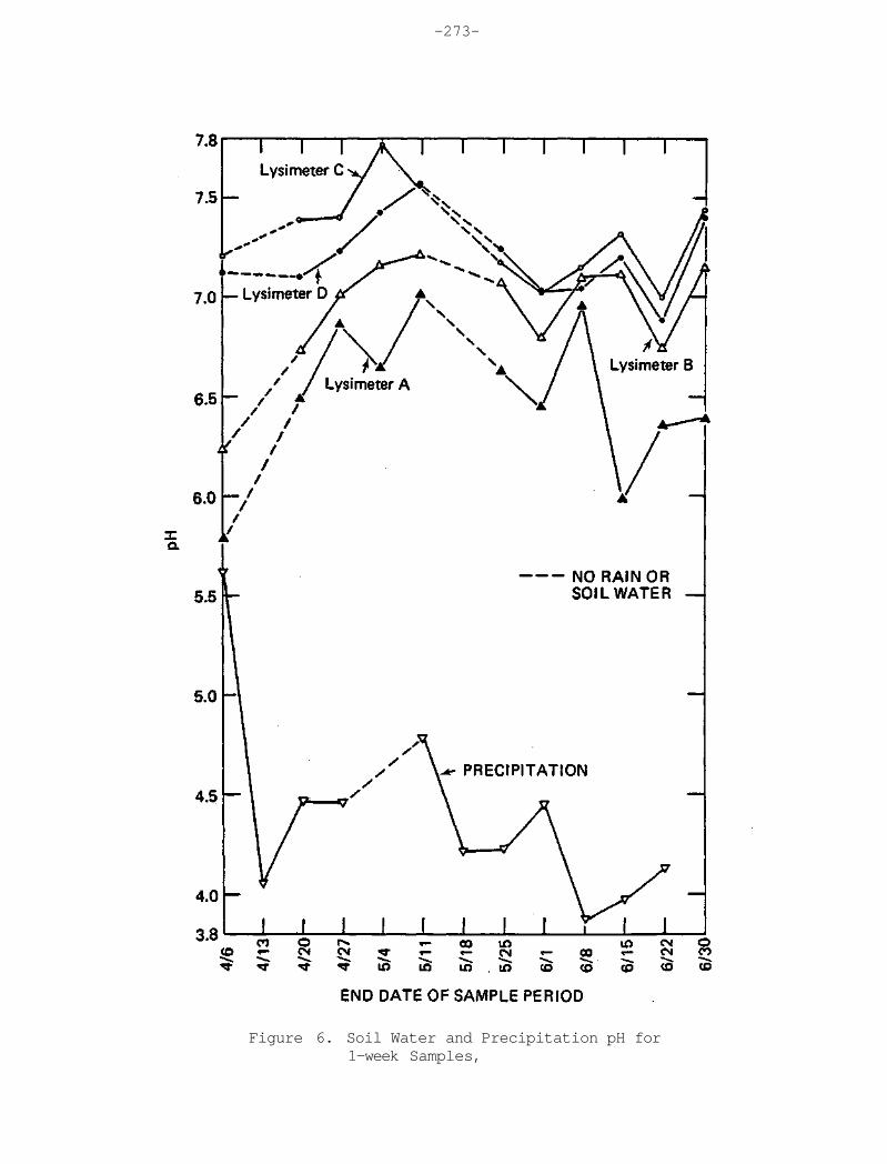
-273-

Figure 6. Soil Water and Precipitation pH for 1-week Samples,

-274-

Figure 7. Soil Water pHlysimeterC Versus Free Hydrogen Ion Deposited by Precipitation.

-275-

REFERENCES

Bowersox, V., 1981: Design of a Feasibility Study to Assess the Impact of Precipitation Quality on Soil Water Quality. Chapter 6 of the Nineteenth Progress Report to the U.S. DOE Pollutant Characterization and Safety Research Division, contract DE-AC02-76EV01199, pp. 49-53.

Bowerox, V., and R. dePena, 1980: Analysis of Precipitation Chemistry at a Central Pennsylvania Site. Journ. Geo. Res., 85, 5614-5620.

Grover, B., and R. Lamborn, 1970: Preparation of Porous Ceramic Cups to be Used for Extraction of Soil Water Having Low Solute Concentrations. Soil Sci. Soc. Am. Proc, v. 34, no. 4, 706-708.

Johnson, T., and K. Cartwright, 1980: Monitoring of Leachate Migration in the Unsaturated Zone in the Vicinity of Sanitary Landfills. IL Institute of Natural Resources, State Geological Survey Division, Urbana, IL, Circular 514, 82 pp.

Leonard, R., A. Meyer, and M. Wilkinson, 1979: Soil Water Quality Studies with Ceramic Cup Lysimeters. Report No. KS-5824-M-1, Calspan Corp., P.O. Box 400, Buffalo, NY 14225, 37 pp.

Levin, M., and D. Jackson, 1977: A Comparison of in Situ Extractors for Sampling Soil Water. Soil Sci. Soc. of Am. Journ., 41, 535-536.

McFee, W., 1980: Sensitivity of Soil Regions to Acid Precipitation. Report No. B0531NAEX to the U.S. EPA, Corvallis Env. Lab. by the Dept. of Agronomy, Purdue Univ., West Lafayette, IN, 179 pp.

McFee, W., J. Kelly, and R. Beck, 1977: Acid Precipitation Effects on Soil pH and Base Saturation of Exchange Sites. Water, Air, Soil Pollution, 7, 401-408.

Naiman, D., and D. Gatz, 1980: Spatial Variability of Rain Water Impurities in Mesoscale Events. Chapter 7 of the Eighteenth Progress Report to the U.S. DOE Pollutant Characterization and Safety Research Division, contract EY-76-S-02-1199, pp. 59-68.

Norton, S., 1977: Changes in Chemical Processes in Soils Caused by Acid Precipitation. Water, Air, Soil Pollution, 7, 389-499.

Peden, M., L. Skowron, and F. McGurk, 1979: Precipitation Sample Handling, Analysis, and Storage Procedures. Research Report 4 to the U.S. DOE Pollutant Characterization and Safety Research Division by the Illinois State Water Survey, Univ. of Illinois, Urbana, IL, 71 pp.

Semonin, R., 1981: Seasonal Precipitation Concentrations and Depositions for North America from the CANSAP/NADP Networks. Chapter 8 of the Nineteenth Progress Report to the U.S. DOE Pollutant Characterization and Safety Research Division, contract DE-AC02-76EV01199, pp. 56-119.

-276-

Stensland, G., 1980: SCORE-78 Case Study for July 2, 1978. Chapter 3 of the Eighteenth Progress Report to the U.S. DOE Pollutant Characterization and Safety Research Division, contract EY-76-S-02-1199, pp. 35-45.

Stensland, G., et al., 1980: NADP Quality Assurance Report, Central Analytical Laboratory, 1 Jan 79 to 31 Dec 79. Illinois Institute of Natural Resources, State Water Survey Division, Champaign, IL, 56 pp.

1982: Soil Survey of Champaign County. USDA Soil Conservation Service in cooperation with Illinois Agricultural Experiment Station, 328 pp.

-277-

CHAPTER 14

PRECIPITATION, CHEMICAL DEPOSITIONS AND WATER RESOURCE ISSUES1

Richard G. Semonin

BACKGROUND

The recent flurry of written material on the subject of acid rain

must be carefully assessed to clearly distinguish fact from fiction. Most

of the attention has been focused on the perceived deleterious effects in

Pennsylvania, New York, and the southeastern Canadian provinces with

increasing emphasis on the perceived problem source along the Ohio Valley

and Midwest. It is time to place in perspective this entire issue and

examine a few major questions related to acid rain.

What are the nearly unquestioned and unchallenged points known at

this time? First, the measured emissions of fossil-fuel consumers are

well documented. The emission inventories are reasonably up-to-date and

provide a means to quantify (within about 20%) the sulfur dioxide burden

entering the atmosphere. Owing to the greater number of different sources

for nitrogen oxides (transportation, home heating, etc.) the total burden

to the atmosphere is less precisely known but can be estimated suffi­

ciently to offer a trend. As pointed out in a recent article in Chemical

and Engineering News (September 21, 1981), there are also a multitude of

other pollutants entering the atmosphere from the same sources. A large

number of these interact synergistically to produce the final environment­

al insult.

1Prepared for presentation at the Water Pollution Control Federation 55th Conference, St. Louis, MO, Oct. 3-8, 1982.

-278-

Second, the currently operating National Atmospheric Deposition

Program sampling network is providing a high quality description of the

chemical quality of precipitation in the United States. The Water Survey

is under contract with the NADP to provide the analytical services for

this network. This service and research contract places us in a unique

position to examine the nation's major measurement program data first

hand. The measurements of the precipitation chemistry, including its

acidity, from this network form the basis for current research on trends

of acid precipitation and its effects.

To recap, the unquestioned knows are emissions of the primary sus­

pected acid rain precursors, and the distribution of wet-deposited chemi­

cals. We must understand that once material is emitted to the atmosphere

it undergoes chemical transformation and is mixed with other substances

from both anthropogenic and natural sources. The material is transported

by atmospheric motions and eventually deposited at a receptor location.

Further transformations by clouds and precipitation occur during transport

and even more complex transformations take place on forests, soils, and in

waters after deposition. Few of these processes are understood.

TWO KEY SCIENTIFIC ISSUES

Two of the key scientific issues can be simply stated in the form of

questions as follows:

1. Is the acidic precipitation observed today a recent and

increasing problem?

-279-

2. Is acidic precipitation responsible for the degradation of

aquatic and terrestrial systems, water resources, human health,

and materials?

I will attempt to touch on each of these and provide some background

information.

THE TREND AND CURRENT STATUS OF ACID PRECIPITATION IN NORTH AMERICA

First, I would like to define acidic precipitation. It has been

widely acclaimed that "natural" precipitation would have a pH of 5.6 which

corresponds to the solution of carbon dioxide from the standard atmosphere

into pure water. However, it is nearly impossible to have precipitation

with only CO2 and water vapor in the atmosphere. It is a necessary

requirement to also have particles around which the water vapor can

condense to form the snow and/or cloud particles that eventually become

precipitation. The incorporation of these particles into either a frozen

or liquid water particle alters its chemistry at the chemistry at the

outset.

With this in mind, the natural pH of precipitation is controversial

since the particles which form clouds can originate from either natural or

anthropogenic sources. Many scientists, including those involved with the

U.S./Canada Memorandum of Intent working groups, are beginning to realize

that the pH value delineating areas impacted by acidic precipitation and

areas that are not should be lowered from 5.6 to a value of no greater

than 5.0. This becomes a real numbers game and one might argue that it

should even be lower. Some evidence is now beginning to appear (although

not in the published literature) showing that in the most remote parts of

-280-

the world such as the Indian Ocean, and the Amazon jungle, precipitation

has a pH of somewhere between 4 and 5. As a matter of passing information

the precipitation pH in central Illinois is 4.3 which corresponds to a

similar value in the Adirondack lake region of upstate New York.

With this definition of acidity of precipitation in mind, the ques­

tions are whether it is increasing and whether the area encompassed is

spreading. Recent research indicates that neither of these is taking

place within the detection limits of existing and past precipitation

chemical data. In a paper soon to appear (Stensland and Semonin, 1982), a

case is made that no trend can be observed in the records (Figure 1). If

there is an acidic precipitation component due to man's activities, it

predates our ability to detect it's beginning because the precipitation

chemistry records are not sufficiently long to discern a measurable

change.

Part of the problem of determining a trend of precipitation chemistry

is that the earliest United States monitoring effort dates back to a

national network operated for one fiscal year (1955-1956) (Junge and

Gustafson, 1956). These data were used to describe the calculated pH

distribution in the United States for that period. This pattern of

calculated acidity was subsequently compared with more recent observed

values by Cogbill and Likens (1974). The original analysis of Drs.

Cogbill and Likens in 1974 showed a trend toward increased acidity in the

east and spreading of the problem to the west and southeast.

In the Stensland and Semonin 1982 paper, it is argued that in fact

the 1950's data were probably heavily biased by the extensive drought of

that period. Most precipitation samples throughout the Midwest and into

parts of the east contained large quantities of alkaline materials because

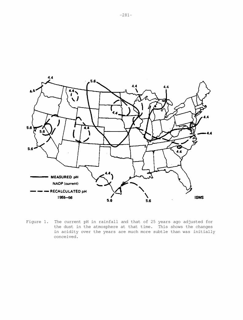
-281-

Figure 1. The current pH in rainfall and that of 25 years ago adjusted for the dust in the atmosphere at that time. This shows the changes in acidity over the years are much more subtle than was initially conceived.

-282-

of high values of crustal dust materials suspended in the atmosphere after

a prolonged period without precipitation. When these 1955-56 data were

adjusted to conform to more recently observed values of crustal dust, the

emerging picture shows nearly the same pH distribution for 1955 as in 1980

over the eastern half of the United States (Figure 1). The impact of this

reanalysis and interpretation of the older chemistry data on the area

encompassed by acid rain is shown in Figure 2. If the original interpre­

tation of the data by Cogbill and Likens stands, then clearly the area

under an acid rain regime has increased during the recent 25 years.

However, if the hypothesis of Stensland and Semonin is correct, the little

areal spreading has occurred and the acidity of precipitation has not

changed significantly. This analysis leads to the conclusion that the

current fear of rapidly increasing acidity of precipitation in the East

and spreading of the problem to the west is unfounded.

POTENTIAL EFFECTS

In the September 14, 1981 Chem and Engineering News there is a quote

on page 27 that I would like to leave with you. "One Canadian scientist

facetiously suggests that forests may be stressed more by the demand for

paper and reports and articles than by acid from the sky." This somewhat

summarizes my opinion as the state of knowledge of impacts from precipita­

tion quality. The effects research efforts are usually categorized into

those dealing with aquatic systems, terrestrial systems (including agri­

culture, forests, and soils), water resources, human health, and materi­

als. Of course, the ones that seem to receive the most notoriety with

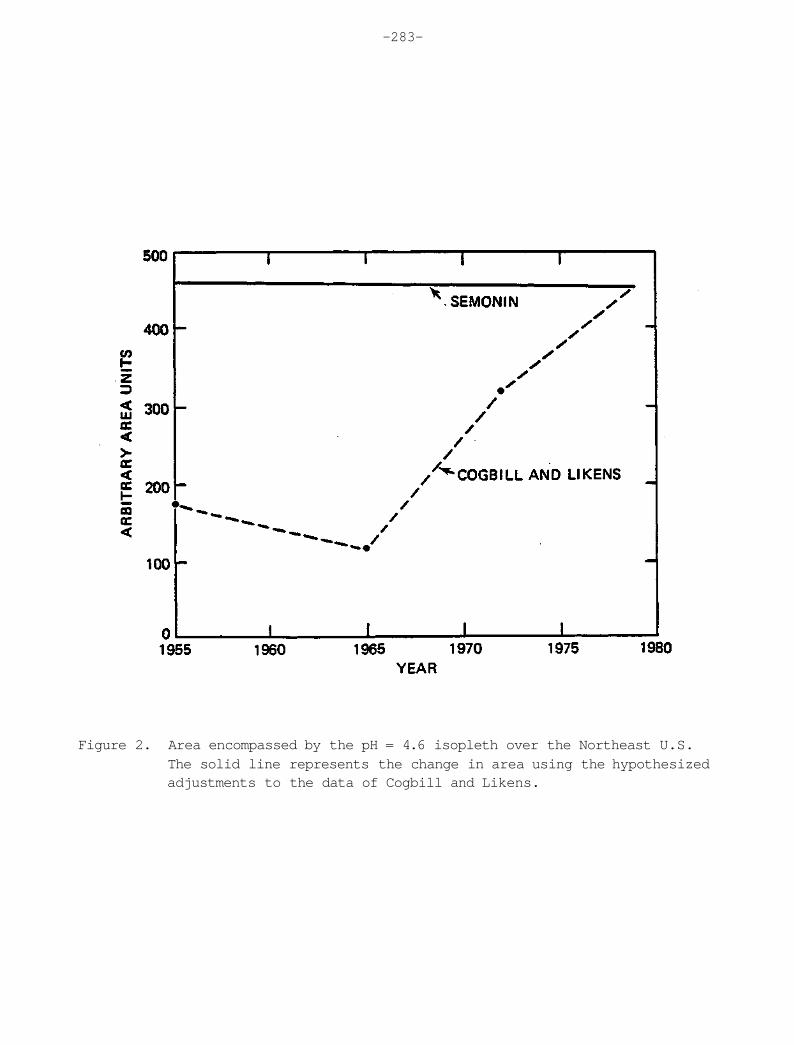
-283-

Figure 2. Area encompassed by the pH = 4.6 isopleth over the Northeast U.S. The solid line represents the change in area using the hypothesized adjustments to the data of Cogbill and Likens.

-284-

regards to international relationships with Canada are the potential

damages to aquatic systems and forests.

I will quote some of the results from the extensive program carried

out as a part of the SNSF project conducted in Norway (Overrein et al.,

1980). This was a major project to examine the effects of acidic precipi­

tation on forests and fish. It is well recognized as one of the major

research programs trying to identify the true impacts in geographical

region claimed worldwide as under the influence of acidic precipitation.

In the following comments, I will refer to the "SNSF" results as published

in the 1980 final report of the 8-year project.

Aquatic Systems c

Anyone that has at one time or another had a home aquarium realizes

that the pH of the tank water must be maintained appropriately or a loss

of fish will occur. This is also true of our fresh waters and research

has identified various levels of toxicity to various species of fish.

More and more evidence, however, is pointing to a perceived secondary

impact of acid precipitation rather than a direct effect. That is, the

release of aluminum into the fresh water system by precipitation on the

surrounding watershed. The aluminum is toxic, at certain concentration

levels, to fish and may be responsible for the demise of some fish species

over a period of time in specific lakes. It must be remembered, though,

from the concept that a trend cannot be observed, many lakes have been

inhospitable to some fish for many years and whether they are becoming

increasingly acidified causing a decrease in fish population is still a

research question. In my opinion, there is little direct evidence to show

-285-

that the acidity or the chemical composition of individual lakes is

changing in a regular manner so as to be responsible for the decline of

aquatic life.

Quoting from the SNSF final report (Overrein et al., 1980): "Massive

fish sills of adult fish during acid episodes is well documented, and is

caused by physiological stress from toxic combinations of water acidity

and aqueous aluminum. The aluminum toxicity depends on water pH and seems

to have a maximum around pH 5." The final paragraph in this summary of

the final results is also worthy of quoting. "The fish in acid waters do

not disappear from lack of food. Fewer food species survive, however, and

those with a particular advantage in acid water, like the water-boatman,

may come to dominate." This suggests that certain acid water tolerant

fish may survive although they may not be desirable game or food fish.

Some definitive experiments are underway in Canada and in the U.S. on this

unresolved question of impact and preliminary results should be forthcom­

ing in early 1983.

Terrestrial Systems

In the June-July, 1981 Crops and Soils Magazine, the Executive Vice

President of the Council for Agricultural Science and Technology (CAST),

Dr. Charles A. Black, assesses some important facts that should be known

about acidic precipitation. Quoting from the summary that appears on page

5, the following points are made:

"1. The sulfur and nitrogen in acidic rain are plant nutrients.

2. Soils and lakes become acid from natural causes as well as from

rain.

-286-

3. The amount of acidity produced in agricultural soils by acidic

rain is small in relation to the acidity produced there by other

causes.

4. Lake that have become acid and fishless because of acidic rain

can be neutralized and be made suitable for fish, should the

presence of fish justify the investment."

I will not attempt to discuss the fourth point because more recent

evidence (unpublished) suggests that even some of the mitigating schemes

cause other problems to occur in lakes. It becomes a case that perhaps

the cure is worse than the ill and, again, is a demonstration of our

ignorance in this entire area.

I would like to quote from page 9 of the SNSF project report where it

states that "At present it is difficult, however, to draw any definite

conclusions on the time required for the reactions and their intensities,"

in the context of the effects of acid precipitation on the properties of

soils. A part of this problem can be attributed to "The great variation

in soil types and in their susceptibility to acid precipitation make

detection of possible effects at an early stage even more difficult."

Little evidence has been presented in this country or in Canada, to my

knowledge, that would counter this vague conclusion of the Norwegians.

A relatively extensive geographic assessment of soils that may be

susceptible to change has been presented in an EPA report but whether

these soils ever will change is another matter. It is a very complex

problem to detect a change of soil composition due to precipitation

chemistry as opposed to the many influences that man has produced in the

tillable soils and managed forest lands in the United States and Canada.

-287-

Research should be initiated to study areas where man has not impressed

his will and determine whether a trend in soil fertility and chemical

composition can be discerned over the next few years. Again, our lack of

specific knowledge demonstrates our ignorance as to an acid precipitation

impact on the terrestrial system.

Water Resources

The surface waters are little impacted by precipitation chemistry

over a large part of North America. The reason for this is that the

watersheds with deep soils surrounding most lakes provides a chemical

treatment to whatever is deposited by precipitation. The chemical quality

of surface waters is largely dominated by so many factors that the quality

of precipitation is relatively unseen in the end product. The management

of the surrounding watershed soils determines much of the chemistry of the

water in a lake or stream. Natural forces are also major contributors in

unmanaged lands exemplified by forested areas where the surface litter

produces a high concentration of acidic materials required for the mainte­

nance of the tree species. The runoff from such areas can contribute

significantly to the chemistry of lakes and streams.

It might be useful for you to have a more quantitative view of the

deposition of some of the ions measured in precipitation.

There are two major North American precipitation chemistry networks

currently in operation with a total of about 160 stations. The first of

these is the CAnadian Network for SAmpling Precipitation CCANSAP) which

began operations in the spring of 1977 and currently has about 50 stations

with 3 in the U.S. The second is the National Atmospheric Deposition

Program (NADP) network which began operations in later summer 1978 and

-288-

currently has 110 stations with 3 in Canada providing samples for analy­

sis. There are other networks for specific research purposes, notably the

DOE MAP3S (Multi-State Atmospheric Power Production Pollution Study), SURE

(Sulfate Regional Experiment), and others that have varying sampling

protocols, different sampling equipment, and separate analytical facili­

ties for analysis. In addition, these research networks are localized in

a regional as opposed to the national CANSAP and NADP networks.

The monthly Canadian data were obtained on magnetic tape and con­

verted to map coordinates for eventual objective plotting by computer

methods. In other to blend the United States and Canadian data together,

the weekly NADP samples had to be composited on a monthly basis to simu­

late the Canadian data. The very simple approach was taken to accumulate

4 weeks (occasionally 5) of NADP data corresponding to individual months

through precipitation weighing of the samples collected in that interval.

The result of this calculation produced a data set of monthly data (plus

or minus 2 days) which corresponds to the monthly data in Canada.

The next step to perform the same calculation using the monthly or

simulated monthly data to acquire a seasonal average. The seasons are the

climatologically defined periods of December-January-February for winter,

March-April-May for spring, June-July-August for summer, and September-

October-November for fall. The three monthly values were combined through

precipitation weighting and then divided by three to get a monthly mean

representative of each of the seasons.

The fall sulfate deposition shown in Figure 3 shows a relative

maximum over southern Ontario with a secondary maximum in Manitoba. There

is a relative minimum in sulfate deposition over north-central

Pennsylvania on the New York state line.

-289-

Figure 3. The North American average sulfate deposition (mg/m2) distribution for the Fall season obtained from the CANSAP and NADP networks.

-290-

The winter deposition pattern of sulfate shown in Figure 4 shows a

maximum extending from southwest Canada toward the southern states with

isolated centers in Alabama and over southern Ontario. Again a minimum is

noted over north-central Pennsylvania.

A spring season deposition maximum appears over Ohio, Pennsylvania

and southward into northern Georgia and Alabama (Figure 5). Again,

similar to the winter season there seems to be an overall maximum over the

eastern states with a north-south orientation.

In the summer season shown in Figure 6, the deposition pattern is

rather simple with a major maximum over the area from Illinois to the East

coast and from West Virginia northward into lower Ontario and Quebec

provinces with decreasing values outward in all directions.

The fall season nitrate deposition (Figure 7) maximizes over lower

Ontario and is generally high over the northeastern states. In the winter

season the deposition pattern shows a strong maximum deposition over the

western sections of Pennsylvania, northeast Ohio and lower Ontario (Figure

8). There is a minor low deposition area shown for both fall and winter

in north-central Pennsylvania reflecting lower precipitation in that

particular area.

The spring nitrate deposition in Figure 9 shows a clear maximum over

eastern Ohio, lower Ontario and western New York and Pennsylvania.

Similarly, there is an increasing deposition gradient oriented north-south

through the Great Plains extending toward the northeast maximum.

The summer season shows the maximum deposition of nitrate (Figure 10)

centered on central Ohio with an orientation into New York state in the

-291-

Figure 4. Same as Figure 3 for the Winter season.

-292-

Figure 5. Same as Figure 3 for the Spring season.

-293-

Figure 6. Same as Figure 3 for the Summer season.

-294-

Figure 7. The North American average nitrate deposition (mg/m2) distribution for the Fall season obtained from the CANSAP and NADP networks.

-295-

Figure 8. The same as Figure 7 for the Winter season.

-296-

Figure 9. The same as Figure 7 for the Spring season.

-297-

Figure 10. The same as Figure 7 for the Summer season.

-298-

east and Illinois in the west. In fact, this maximum dominates the North

American distribution with values decreasing southwest and north from the

Ohio maximum.

The greatest hydrogen ion deposition in the fall season (Figure 11)

occurs over the northeast United States with a maximum over lower Ontario

extending southward into Ohio and Pennsylvania. A small minimum occurs in

north-central Pennyslvania. The relative maximum hydrogen ion deposition

in the east likely occurs from the relatively high concentrations of

nitrate and sulfate observed in that area.

The winter deposition shown in Figure 12 shows a fairly strong

gradient of hydrogen ion deposition oriented northeast-southwest through

the western Midwest into the lower eastern Canadian provinces. The

deposition maximizes in southeastern Ohio and the central Atlantic coast

states.

The spring and summer patterns shown in Figures 13 and 14 are simi­

lar, but with the greatest deposition occurring in the summer months

corresponding to the heavier rainfall observed in that season. Generally

there is a strong east-west gradient through the Great Plains in spring

(Figure 13). The gradient extends east toward lower Hudson's Bay. To the

east and south of this maximum gradient, the hydrogen ion deposition

maximizes through central Ohio and along the southern Pennsylvania-

Maryland state line. During the summer season (Figure 14), the very

strong gradient through the High Plains is still present in almost the

same location as during spring, but the maximum deposition area is greater

in magnitude and covers an area with an east-west orientation from

Illinois to New Jersey encompassing parts of New York, West Virginia, and

northern Kentucky.

-299-

Figure 11. The North American average hydrogen deposition (µg/m2) distribution for the Fall season obtained from the CANSAP and NADP networks.

-300-

Figure -12. The same as Figure 11 for the Winter season.

-301-

Figure 13. The same as Figure 11 for the Spring season.

-302-

Figure 14 . The same as Figure 11 for the Summer season.

-303-

The fall season calcium deposition shows two major maxima, one

located in Saskatchewan and a secondary maximum deposition in lower

Ontario province (Figure 15). This secondary maximum although nearly of

the same magnitude as the western maximum is associated with heavier

precipitation in that area. The middlewest, west, and eastern parts of

the United States are relatively featureless.

The winter deposition pattern in Figure 16 shows the greatest deposi­

tion in the eastern Canadian provinces, again reflecting higher precipita­

tion amounts. The spring season deposition in Figure 17 is almost reflec­

tion of the winter season. The values are generally higher everywhere

indicating a climate change to warm season, greater intensity precipitati­

on systems.

The summer distribution of calcium deposition shown in Figure 18

illustrates a gradual increase in calcium deposition from west to east

across North America. Again the maxima are located in the western

provinces of Canada and along the U.S.-Canadian border in the east with

generally high values extending across the Midwest.

A first order effect of precipitation chemistry on surface waters has

been voiced on numerous occasions. In a recent widely distributed pam­

phlet, the National Wildlife Federation (Reaburn, 1982) stated, "It has

been estimated that acid rain may be slowly poisoning 100,000 miles of

streams and 20,000 lakes." Statements such as these are pure conjecture

and based on fragmentary information frequently relying on qualitative

reporting by the public. Countering this alarmist view, the United States

Geological Survey recently reported to the Senate on analysis of the

chemical trends at a number of stream and river sampling sites throughout

the U.S. (Cohen, 1982). The hydrogen ion concentration trends shown in

-304-

Figure 15. The North American average calcium deposition (mg/m2) distribution for the Fall season obtained from the CANSAP and NADP networks.

-305-

Figure 16. The same as Figure 15 for the Winter season.

-306-

Figure 17. The same as Figure 15 for the Spring season.

-307-

Figure 18. The same as Figure 15 for the Summer season.

-308-

Figure 19 is increasing at only a few somewhat isolated sites. Most

importantly, over the eastern states the majority of sites show no change

over the past 13 years. The alkalinity, on the other hand, shows a trend

upward or no trend over the same region (Figure 20).

These observational data and their interpretive analysis do not

support the concept of a spreading and worsening surface water response to

precipitation chemistry. The trends of sulfate and nitrate-nitrite

(Figures 21 and 22) in the surface waters reveal some additional interest­

ing information. The sulfate levels in the upper northeast show little

change and even isolated decreases. Areas of an upward trend include the

southwest states, the upper Great Plains, the northern Rocky Mountains and

along the front range in Colorado and Wyoming.

The nitrate-nitrite trends upward are observed in a band northward

from lower Mississippi to Tennessee and then northeast to Pennsylvania,

and then southeast to North Carolina. The remainder of the United States

shows no trend of nitrate-nitrite in surface waters.

To try and estimate the impact of precipitation quality on surface

water resources is a very difficult undertaking as are all such impact

assessments. There have been some concerns expressed about the effects of

acidic precipitation on groundwater but these have been undocumented in

the scientific or engineering literature. Some purported evidence is that

groundwaters in some New England states are of such low pH due to acidic

precipitation that the release of cooper and/or lead in water distribution

systems is above the safe drinking water levels. Admittedly, concentra­

tions of these particular metals in excess of the safe drinking water

guidelines have been observed. However, these excesses have been observed

Figure 19. The hydrogen ion concentration trend in streamwater. The number indicates the first year of record. (After Cohen, 1982).

Figure 20. The total alkalinity trend is streamwater. (After Cohen, 1982).

Figure 21. The sulfate concentration trend in streamwater. The numbers indicate the first year of record. (After Cohen, 1982).

Figure 22. The nitrate-nitrite concentration trend in streamwater. (After Cohen, 1982).

-313-

in places where the acidity content of the groundwater supply is practi­

cally nonexistent and therefore we should look to other sources of the

problem. The proclaimed effect on groundwater is even more shrouded in

the complexities of the overlying soils and geological structure of an

aquifer. To demonstrate a direct link between chemicals deposited by

precipitation and the chemical quality of groundwater is almost beyond

experimentation.

Summary

The chemical quality of precipitation is related to many different

compounds found in nature and produced by man's activities. To understand

acidic deposition and its response to nature and man, we must include all

chemical constituents in monitoring and research efforts. The uncertainty

surrounding quantification of natural sources and the non-acid industrial

emissions, their transformation rates in the atmosphere, and their ulti­

mate deposition by precipitation precludes a simple one-to-one relation­

ship between emissions and acidic deposition.

A great deal of the scientific uncertainty surrounding this issue is

whether or not the chemical quality of precipitation is degrading with

time and spreading over a larger area. It is clear at this time, that

neither of these questions can be answered affirmatively. Monitoring of

precipitation chemistry is essential to determine the trend of acidic

precipitation! With a sufficient data base the need for regulatory action

will be much easier to deal with. Since ecosystem processes respond

relatively slowly to gradual environmental changes, including the contin­

ued effects of man through land use management, long-term research and

monitoring of such systems is also essential. It should be clear that

-314-

assessment of the benefits should be measured if any regulations are

invoked. We should no longer impose environmental regulations without

evaluation of their effectiveness in ameliorating the original problem.

The United States has embarked on a path of critical research in all

of the important scientific areas that I mentioned. Within 10 years or

less we should have many more answers than are available today - and then

we can better assess the issues surrounding precipitation chemical quality

and its environmental consequences.

Acknowledgement

The research reported in this paper was partially supported by the

U.S. Department of Energy under Contract Number DE-AC-02-76EVO1199.

-315-

REFERENCES

Black, C. A., 1981: Additional facts you should know about "acid rain."

Crops and Soils Magazine, June-July, 5-9.

Cogbill, X. V., and G. E. Likens, 1974: Acid precipitation in the north-

eastern United States. Water Resources Research, 10, 1133-1137.

Cohen, P., 1982: Testimony before the U.S. Senate Committee on Energy

and Natural Resources, August 19, 1982.

Ember, L. R., 1981: Acid pollutants: hitchhikers ride the wind.

C and EN, Sept. 14, 20-31.

Junge, C. E., and P. E. Gustafson, 1956: Precipitation sampling for

chemical analysis. Bull. Amer. Meteor. Soc, 37, 244.

Overrein, L. N., H. M. Seip, and A. Tollan, 1980: Acid Precipitation -

Effects on Forest and Fish. Final Report of the SNSF-Project 1972-

1980, Oslo, Norway.

Reaburn, R., 1982: Acid Rain: What It Is - How You Can Help! National

Wildlife Federation, Washington, D..C, 12 pp.

Stensland, G. J., and R. G. Semonin, 1982: Another interpretation of the

pH trend in the U.S. To be published, Bull. Amer. Meteor. Society,

63(11).

-317-

CHAPTER 15

A REVIEW OF PARTICLE TRACERS OF ATMOSPHERIC PROCESSES*

Donald F. Gatz

ABSTRACT

This review is limited to particle tracers deliberately released for use in investigations of atmospheric processes, including transport, dispersion, wet and dry deposition, resuspension, and others. Particle tracers have been used in atmospheric research since the early 1950's. There use is currently declining in favor of gaseous tracers useful over longer distances. Publications reporting applications to transport and dispersion peaked in the late 1960's, those giving results of precipitation scavenging and wet deposition experiments peaked in the early 1970's, and those devoted to dry deposition and resuspension peaked in the late 1970's and early 1980's. Many different materials have been used as tracers. The materials generally fall into one of four groups: pollen and spores, organic materials, inorganic materials, and radioisotopes. This review describes the individual materials used as particle tracers, and also the methods used to generate an aerosol of them, to sample them, and to analyze for them. A bibliography of over 100 papers is included.

INTRODUCTION

This paper reviews particulate materials deliberately released for use as tracers of atmospheric processes. This includes releases of natural materials, such as pollen, where the placement or timing of the release has been manipulated by the experimenter. Other papers in this workshop cover gaseous tracers released deliberately and both gas and particle tracers of opportunity.

Since some of the keynote papers focus on tracer materials, and others focus on atmospheric processes for which tracer techniques may be appropriate tools for investigation, this paper may overlap to some extent the papers that address the use of tracers in investigations of atmospheric processes.

Several major reviews of tracer applications have been published. Dumbauld1 provided an early review of fluorescent particle techniques for measuring atmospheric dispersion. Islitzer and Slade2 extensively reviewed results of transport and dispersion experiments up to the mid-60's. Gatz3 reviewed tracer experiments on precipitation systems. Sehmel's4 review of dry deposition includes results of many tracer experiments. Very recently, Johnson5 reviewed tracer techniques for investigation of atmospheric transport and dispersion. A paper on tracer theory with applications in geosciences has also appeared .

Submitted for Proceedings, Dept. of Energy Workshop on Atmospheric Tracers, Santa Fe, New Mexico, 21-25 May 1984.

-318-

As indicated by the subjects of these reviews, particle tracers have been used to investigate atmospheric transport and dispersion2,7-37, precipitation scavenging and convective storm circulations38-70, and dry deposition9-13,17,71-89. Other stated objectives of atmospheric tracer experiments include investigations of stratospheric circulation and mixing90-92, atmospheric residence times of particles93, cooling tower mist interception by plants94, evaluation of cloud seeding effectiveness61,62,64,95,96, and particle resuspension84,97-102 from the earth's surface, roads, or the leaves of plants.

Figure 1 shows a distribution of the number of published papers and reports on particle tracers located in my literature review, by year of publication (in 5-yr blocks), for some major tracer applications. It appears that publications on particle tracers used in transport and dispersion experiments peaked in the late 60's, those used in precipitation scavenging, wet deposition, and storm circulation experiments peaked in the early 70,s, and those used in dry deposition and resuspension experiments are at, or just past, their peak. Overall, use of particle tracers in atmospheric research appear to be declining in recent years.

MATERIALS USED AS PARTICLE TRACERS

A wide variety of materials have been used as particle tracers. Johnson5 listed the key requirements for an effective atmospheric tracer, as follows: 1) Background concentrations of the tracer material in the atmosphere from natural and artificial sources must be small. 2) The tracer must follow air motions faithfully (or, if the tracer is simulating particles, as in a dry deposition experiment, rather than an air parcel, its motions must be those of the particles it is simulating). 3) Transformations and/or removal (deposition) must be small, or at least well known and predictable (unless used in a deposition experiment). 4) The tracer must be easily handled and dispersed, at measureable rates. 5) Sensitive analytical techniques must be available to enable very low concentrations of the tracer to be measured. 6) The tracer must be non-toxic and free from other adverse environmental effects. 7) The cost of the tracer and its sampling and analysis methods must be reasonable (at least, reasonable in terms of the benefits to be gained from the experiment).

For purposes of discussion, it seems reasonable to group the known tracer materials into four general categories: pollen and spores, organic materials, inorganic materials, and radionuclides. The following four subsections of the paper are each devoted to one of these categories. Information on individual tracer materials, generation methods, particle sizes, sampling methods, and analysis methods are presented primarily in tables.

-319-

Figure 1. Time-frequency distribution of publication date (in 5-yr blocks) of papers and reports located in this literature search, by major application category.

-320-

Pollen and Spores

Table I lists 10 species of pollen and spores that have been used as atmospheric tracers. The table also gives information on the shape of the pollen grain or spore, as well as its surface characteristics and size. Many of those listed are spheroidal, including two that may collapse, but other shapes are represented as well. The surfaces range from smooth to spiny, and the diameters from 1 µm to 18 x 58 µm. One advantage of pollen and spores as tracer materials is the rather uniform size of the grains within a given species. Pollen and spores have also been stained various colors and tagged with radioactivity to facilitate the identification of particles of the same size released at different times or different locations.

Methods for generating an aerosol of pollen or spores, and for sampling and analyzing the grains, are listed in Table II. A variety of methods have been used. Atomization methods usually involve suspending the particles in a liquid and spraying them through a nozzle or jet, or using a spinnning disk103 to atomize the liquid into droplets containing at the most a single grain. Other methods involve dispensing single dry grains by jets of air or vibration of the dispenser. Pollen have also been released naturally from plants grown in a specific location, or in pots moved to the test site, or from plants treated to pollenate before their usual season. Bacillus subtilis spores were also sprayed on desert soil and mobilized by vehicle traffic or by marching or crawling men.

Sampling of airborne concentrations (Table II) has been accomplished with filters of various kinds, impactors, by wet and dry moss bags, grass, and trays, and by a number of devices that rely on wind impaction of the grains on to a sticky surface. Sampling of any large particles, including pollen, is difficult because their mass is large enough to keep them from closely following air motions, thus frequently resulting in anisokinetic sampling. The Rotoslide sampler, in which the pollen are sampled on the edge of a microscope slide rotated at high speed, is one way to overcome the wind speed effect. Even so, collection efficiencies generally do not approach 1.0.

Sampling pollen and spore deposition has usually been done using greased microscope slides11-14, although B. subtilis scavenged by snow flakes have also been sampled at the bottom of a chamber by ordinary laboratory beakers and by velvet paper42.

Organic Materials

Organic materials used as atmospheric tracers include one of the earliest—oil fog—as well as a number of fluorescent dyes and a chemiluminescent material. Information on these materials and their generation, sampling, and analysis methods, is given in Table III.

Again, a wide variety of aerosol generation methods have been used. Smoke generators have been used to produce oil fog, having droplets with diameters of 0.3 µm. Other organic tracer aerosols have been produced using various pneumatic spray nozzles or nebulizers to produce liquid

-321-

TABLE I. CHARACTERISTICS OF POLLEN AND SPORES (modified from Ref. 10)

Type Shape Surface Diameter, um

Bacillus subtilis 1

Paper Mulberry Spheroidal Smooth 14 (Broussonetra) (may collapse)

Ragweed Spheroidal Spiny 18-20 (Ambrosia)

Timothy Spheroidal Smooth 30-35 (Phleum) (may collapse)

Summer Cypress Spheroidal Smooth 30 (Kochia scoparia)

Club Moss Modified Slightly 32-33 (Lycopodium) pyramidal rough

Fern Spheroidal Smooth 54 (Osmunda)

Fungus Pyriform Smooth 18x58 (Cronartium) acuminate

Castor Bean Ellipsoidal Smooth 24x38 (Ricinus communis)

Fern Ovoidal Slightly 33x45 (Drvopteris) rough

-322-

TABLE II. GENERATION, SAMPLING, AND ANALYSIS METHODS FOR POLLEN AND SPORES

A. Bacillus subtilis

Generation: Pneumatic atomizer Spinning disk generator Truck traffic (from soil) Men marching and crawling (soil)

Sampling:

Concentration: Filters with pre-impinger Impactor

Deposition: Velvet paper Beaker

Analysis: Counting by microscope

B. All other pollen and spores.

Generation: Pneumatic or atomizing nozzle Dry aerosol generator Air jet Aspirated, vibrated, dispensing bottle Natural, from specially grown or potted plants Natural, from plants treated to pollenate early

Sampling:

Concentration: Slide-edge-cylinder Rotoslide sampler Sticky cylinders Wet and dry moss bags, grass, trays

Deposition: Greased microscope slide

Analysis: Counting by microscope

-323-

TABLE III. TRACES MATERIALS SUMMARY — ORGANIC MATERIALS

Generation Particle Sampling Analysis Material method diameter. um method methoda Remarksb

Fluoresceinc Pneumatic norzle Filter Fluorescence D.L.=2xl0-10 g

Glycerol*' String bean plants Counting of Na-22 R.A. used to tag particles

Oil foge or Smoke generator 0.3 Photography Photography smoke Photometric densi- Densitometer

tometer Opacity method Asbestos filter Fluorescence Nephelometer Lidar

Oleic acidf LaMer generator 0.5 Wet and dry moss Counting of bags, grass, and R.A used to trays tag particles

Polystyreneg Alcohol spray 3 Wet and dry moss Counting of spheres bags, grass, and R.A. used to

trays tag particles

Rhodamineg Jet atomization 0.4-6 Filter Fluorescence D.L.=10-10 g/mL 0.8 HMD Bulk snow by shovel Lee (Ref. 67) re-

Precipitation commends against samplers Rhodamine for

scavenging ex­periments due to high natural background.

TMAEh Bomblets 0.1-4 Film and video Photography photography

Dranine dye1 Nebulizer 0.7 Filter (isokinetic) Fluorescence Hygroscopic Collison generator <1 Membrane filter Pneumatic nozzle 2-10 (5.4 MMD) Glass fiber filter D.L.=10-11 g/mL Spinning disk >2 Precipitation Dry dust dispenser 7.5 sampler Modified commercial 17 Plant leaves paint sprayer (sunflower, (rotating bell) tulip poplar)

Fluid atomizing Lidar generator Vibrating orifice

aR.A. = radioactivity bD.L. = detection limit cReference 22 dReference 81 eReferences 5,16,24,25,31 fReference 78 gReferences 47,55,66,67,77 hReferences 7,21 iReferences 5,23,26,47,72-74,76,79,86

-324-

droplets, which quickly evaporate, leaving as residue the desired particles. With soluble tracers, such as uranine dye, the concentration of the tracer in the sprayed liquid can be varied to control the size of the resulting particles. In general, higher concentrations produce larger particles.

Sampling methods often reflect the objectives of the experiment. The use of plants or precipitation collectors as sampling media shows experimental objectives related to dry and wet deposition, respectively. Methods for "sampling" oil fog include both qualitative and quantitative photographic techniques, as well as filter sampling and subsequent analysis by fluorescence measurements. In addition, oil fog provides a direct visual impression of transport and diffusion at a given site that can be extremely valuable to a researcher, especially early in the investigation of an unfamiliar location. TMAE, a chemiluminescent tracer, would appear to be capable of providing the same visual impression in nighttime situations.

Analysis methods for the organic materials were mostly fluorescence measurements. There were also some measurements of radioactivity, where tagged organic particles were used.

Inorganic Materials This group, listed in Table IV, includes over 15 elements used as

tracers. Often several different compounds of the same element have been used in the same, or associated experiments, where the different compounds were chosen for their contrasting chemical behavior (soluble vs insoluble) or surface characteristics (wettable vs non-wettable).

Aerosol generation methods include spray nozzles, nebulizers, and dry particle dispensers, as described previously, to dispense ZnS and ZnCdS fluorescent particles. The list of methods in Table IV also includes propane and acetone burners and pyrotechnic flares, all of which are also used to generate cloud seeding materials. Some early experiments in the USSR used exploding artillery shells to inject tracer materials into convective storms.

The propane and acetone burners and the pyrotechnic flares often produce tracer particles with diameters near, or less than, 1 um. The fluorescent particles are typically near 2 µm, but smaller and larger particles of this type have also been produced. In a case where a Na2CrO4 tracer was used to simulate cooling tower drift, a much larger size, typical of mist droplets, was produced by a spray nozzle.

A wide range of sampling methods has been used for the inorganic tracer materials, again reflecting diverse experimental objectives, including wet and dry deposition, resuspension, and dispersion measurements. Sampling media include precipitation samplers, filters, impactors, and also a real-time sampler for Li particles, utilizing flame ionization measurements.

-325-

TABLE IV. TRACES MATERIALS SUMMARY — INORGANIC MATERIALS

Generation Particle Sampling Analysis Material method diameter. um method methoda Remarks

AgNO3b Propane AgI burner Precipitation NAA D.L. 10-11 molar samplers

AgIc Propane burner Precipitation Acetone burner sampler network NAA

Agd Propane AgI burner 0.05-0.1 Snow collector NAA Pyrotechnic flare 0.03 (mean) Sequential precip-Droppable pyrotech- itation collector, nic flare mobile collector

CuSe Rocket shell explo- Precipitation sion samplers

CuSO4f 3-7 Paper, metal, soil, plants

CaMoO4g Wind erosion Cascade impactor XRF (Mo)

Csh Pyrotechnic flare Precipitation AAS sampler network

CSNO3, Propane AgI burner Precipitation NAA Sc(NO3)3 samplers Sr(NO3)2

i

FeOOH (beta)J Atomizer Filter sampler R.A. counting array (Fe-59)

Fe2O3k Wind erosion 2 and 5 Filters R.A. counting

Fe(OH)3k Wind erosion Filters R.A. counting

In2O31 Acetone burner 0.05-0.35 Non-hygroscopic

Inm Pyrotechnic flare <1 Precipitation col- NAA Non-wettable lectors AAS

Acetone burner Mobile precipitation ASV collector

LiCln Acetone burner 0.27-0.63, Soluble mean = 0.45

Li2CO3o Sonic atomizing 0.5-1.5 Flame ionization Flame Low solubility nozzle detector (real ionization Modified commercial 1.6 time) paint sprayer Filters ICAP (rotating bell) Spray nozzle 0.7

-326-

TABLE IV. TRACER MATERIALS SUMMARY -- INORGANIC MATERIALS (continued)

Generation Particle Sampling Analysis Material method diameter, um method method Remarks

Li stearatep Acetone burner Precipitation NAA Non-wet table Mechanical dispenser sampler

Lit Acetone burner 0.4 Precipitation NAA Soluble pyrotechnic flare sampler network AAS

Na2CrO4r Pneumatic nozzle 100-1300, SSZ 2-yr grass, pine, Radioactiv-

between 500-800 poplar plants, ity count-filter disks ing (Cr-51)

ing (NH3)2SO48 Dltraaonic 0.7 Conc: filter, Liquid scin-

nebulizer impactor. Depos: filiation filter, funnels, counting bucket (S-35)

Irt Acetone burner Precipitation NAA Non-wettable sampler network

Ta, Re, Au Acetone burner Precipitation NAA Eu, Ru, 0su sampler network

ZnS, Pneumatic atomizer 1 -2 Rotorod sampler Manual count- D.L. 2xl0-10 g ZnCdSv Smoke generator 2.3 Filters ing (by mi-

Dry particle 2.7 Real-time sampler croscope) dispenser Velvet paper. Real-time (Unspecified) 1-10 (mean 3.2) beaker (snow crys- sampler Air jet S tals) Radioactivity Exploding cannister <10 Impactor counting Vehicle traffic <25 Wet and dry moss (tagged par-Modified commercial bags, grass, trays ticles) paint sprayer Drum impactor

Dry duster Venturi tube

aAAS - atomic absorption spectrophotometry; ASV « anodic stripping voltammetry; ICAP = inductively coupled

argon plasma; NAA ■ neutron activation analysis; XRF - X-ray fluorescence. "Reference 41 cReferences 55,58,

59,66 dReferences 61,62,64,70,93,95,104 eReference 63 fReference 105 gReference 99 hReference 54 iReference 41 iReference 89 kReference 84 1Reference 106 mReferences 40,46,49,55,57,58,64-66 nReference

106 oReferences 17,73-75,85 PReferencea 55,66 qReferences 53,55,58-60,65,66 rReference 94 sReference 71 tReference 66 uReferences 43-45,65 vReferences 8,18,20,22,27,28,30,32,42,74,77,78,83,92,100,107-112.

-327-

Several analytical methods have been used, typically those used for metal analyses, including NAA, AAS, ASV, XRF, and ICAP (acronyms explained in Table IV).

Radioisotope Materials

Table V lists several radioisotopes used as tracers. Others were listed on earlier tables when they were used for the purpose of tagging the primary tracer particle to enable more convenient analysis (such as radioactive tagging of pollen or fluorescent particles, which would otherwise have to be counted manually).

We can divide the list in Table V into three separate groups. The first group includes radioisotopes produced specifically as tracers for particles injected into the stratosphere by nuclear test explosions (Rh-102 and W-185). The second group includes several nuclides injected into precipitation systems by artillery shells (P-32, Te-131, and Po-210). The third group is composed of two radionuclides used in dry deposition experiments (Cu-64, Au-198) and a cloud circulation experiment in Australia (Cu-64).

Sampling again reflects the purpose of the various experiments, and analyses were by radioactivity counting methods.

CONCLUDING REMARKS

Over 100 papers on tracer experiments in atmospheric research were reviewed. A wide variety of tracer materials have been applied to such atmospheric processes as transport, dispersion, wet and dry deposition, resuspension, and others. This paper gives a general description of the tracers and their applications. For more details on specific applications, please consult the original papers, listed in Section IV.

Particle tracers are frequently used as one component of dual-tracer experiments. Two or more different tracers with different particle sizes may be used together to measure deposition relative to one another. Or, a particle tracer may be used with an inert gas tracer. In this case, the inert gas is used to correct the particle concentrations for the effects of turbulent diffusion, so that particle deposition may be estimated.

Particle tracers are ordinarily useful only to distances of a few 10's of kilometers. Interest is now turning to transport and dispersion over much greater distances, which require some of the new gaseous tracers useful at distances of 100 - 1000 km. Thus, the use of particle tracers appears to be declining, although they are still being used for short range transport and dispersion, for dry deposition, and for resuspension studies

-328-

TABLE V. TRACER HATERIALS SUMMARY — RADIOISOTOPES

Generation Particle Sampling Analysis Material method diameter, um method methoda Remarks

Au-198b 0.78 AMADC String bean plants R.A. counting

Pneumatic nozzle 9.5 Conc: Rotoslide, R.A. counting Depos: greased microscope slides Airborne gamma counter

P-32e Rocket shell Precipitation R.A. counting Hygroscopic explosion sampling network

Te-131f Rocket shell Precipitation R.A. counting Non-hygroscopic explosion sampler network

Po-210g Rocket shell Precipitation R.A. counting explosion sampler network

Pu-238h Pneumatic Bean plants, mem- R.A. counting nebulizer brane filters,

cascade impactors, thermal precipita­tors

Rh-102i Nuclear Filter R.A. counting explosion

W-185i Nuclear Filter R.A. counting explosion

aR.A. - radioactivity bReference 81 CAMAD - activity mean aerodynamic diameter dReferences 113-115 eReferences 51,52 fReference 51 gReference 52 hReference 82 iReference 91

-329-

Oil fog, although one of the earliest tracer materials, can provide a clear visual impression of transport and dispersion at an unfamiliar site, and is thus extremely useful in guiding further experiments.

REFERENCES

1. Dumbauld, R. K., 1962: Meteorological tracer technique for atmospheric diffusion studies. J. Appl. Meteorol., 1 (4): 437-443.

2. Islitzer, N. F. and D. H. Slade, 1968: Diffusion and transport experiments. Chapter 4, In: D. H. Slade, Meteorology and Atomic Energy-1968. U.S. Atomic Energy Commission, Division of Technical Information.

3. Gatz, D. F., 1977: A review of chemical tracer experiments on precipitation systems. Atmos. Environ., 11: 945-953.

4. Sehmel, G. A., 1980: Particle and gas dry deposition: a review. Atmos. Environ., 14: 983-1012.

5. Johnson, W. B., 1983: Meteorological tracer techniques for parameterizing atmospheric dispersion. Journal of Climate and Meteorology, 22: 931-946.

6. Nir, A. and B. L. Kirk, 1982: Tracer theory with applications in geosciences, Part 1, Oak Ridge National Lab report ORNL-5695/P1, Environ. Sci. Div., Publication No. 1964, 93 pp.

7. Elrick, R. M. and R. E. Smith, 1967: Investigation of TMAE as a chemiluminescent atmospheric tracer. Sandia Corp., Albuquerque, NM, 53 pp.

8. Leighton, P. A., W. A. Perkins, S. W. Grinnell, and F. X. Webster, 1965: The fluorescent particle atmospheric tracer. J. Appl. Meteorol., 4: 334-348.

9. Raynor, G. S., J. V. Hayes, and E. C. Ogden, 1974: Particulate dispersion into and within a forest. Boundary-Layer Meterol., 7_: 429-456.

10. Raynor, G. S., J. V. Hayes, and E. C. Ogden, 1975: Particulate dispersion from sources within a forest. Boundary Layer Meteorol., 9 (3): 257-277.

11. Raynor, G. S., E. C. Ogden, and J. V. Hayes, 1970: Dispersion and deposition of ragweed pollen from experimental sources. J. Appl. Meteorol., 9 (6): 885-895.

12. Raynor, G. S., E. C. Ogden, and J. V. Hayes, 1972: Disperson and deposition of timothy pollen from experimental sources. Agricultural Meteorology, 9, (1971/1972): 347-366.

-330-

13. Raynor, G. S., E. C. Ogden, and J. V. Hayes, 1972: Dispersion and deposition of corn pollen from experimental sources. Agronomy Journal, 64: July-August, 1972, 420-427.

14. Raynor, G. S, E. C. Ogden, and J. V. Hayes, 1973: Dispersion of pollens from low-level, crosswind line sources. Agricultural Meteorology, 9, (1971/1972): 347-366.

15. Raynor, G. S., E. C. Ogden, and J. V. Hayes, 1976: Dispersion of fern spores into and within a forest. Rhodora, 78, 815: 473-487.

16. Raynor, G. S., P. Michael, R. M. Brown, and S. SethuRaman, 1975: Studies of atmospheric diffusion from a nearshore oceanic site. J. Appl. Meteorol., 14 (6): 1080-1094.

17. Sehmel, G. A., 1981: A dual-tracer experiment to investigate pollutant transport, dispersion, and particle dry deposition at the Rio Blanco oil shale site in Colorado, Preprint from Second Conf. on Mountain Meteorology, Nov. 9-12, 1981, Steamboat Springs, CO, pp 137-146.

18. Hilst, G. R. and N. E. Bowne, 1971: Diffusion of aerosols released upwind of an urban complex. Environ. Sci. Technol., 5 (4): 327-332.

19. Webster, F. X., 1963: Collection efficiency of the Rotorod FP Sampler. Tech. Report No. 98, Aerosol Lab., Metronics Assoc, Inc., Stanford Industrial Park, Palo Alto, CA.

20. Dotson, W. L., P. W. Nickola, and M. A. Wolf, 1968: Real time sampling of zinc sulfide tracer in diffusion studies. In: Mawson, C. A., Ed., Proceedings, U.S. Atomic Energy Commission Meteorological Information Meeting, Sept. 11-14, 1967, Chalk River, Ontario, Canada, 277-291.

21. Smith, R. E. and R. M. Elrick, 1968: Investigation of TMAE (tetrakis dimethylamino ethylene), a chemiluminescent material, as an atmospheric tracer. In: C. A. Mawson, Ed., Proceedings, U.S. Atomic Energy Commission Meteorological Information Meeting, Sept. 11-14, 1967, Chalk River, Ontario, Canada, 334-346.

22. Ludwick, J. D., 1966: Atmospheric diffusion studies with fluorescein and zinc sulfide particles as dual tracers. J. Geophys. Res., 71 (6): 1553-1558.

23. Gussman, R. A. and A. M. Sacco, 1964: Notes on a method of establishing a size distribution of meteorological tracer aerosols. J. Appl. Meteorol., 3 (5): 638-640.

24. Smith, M. E., et al, 1958: The variations of effluent concentrations during temperature inversions. J. Air Poll. Control Assoc, 7: 194-197.

-331-

25. Barad, M. L. and B. Shorr, 1954: Field studies in diffusion of aerosols. Amer. Ind. Hyg. Assn. Quart. 15: 136-140.

26. Robinson, E., J. A. McLeod, and C. E. Lapple, 1959: A meteorological technique using uranine dye. J. Meteorol., 16: 63-67.

27. Crozier, W. D. and B. K. Seely, 1955: Concentration distributions in aerosol plumes three to twenty-two miles from a point source. Trans. Amer. Geophys. Union, 36, 42-52.

28. Wedin, B., N. Frossling, and B. Aurivillius, 1959: Comparison of concentration measurements of sulphur dioxide and flourescent pigment. Advances in Geophysics, 6: New York, Academic Press, 425-427.

29. Hay, J. S. and F. Pasquill, 1957: Diffusion experiments from a fixed source at a height of a few hundred feet in the atmosphere. J. Fluid Mech., 2.

30. Braham, R. R., B. K. Seely, and W. D. Crozier, 1952: A technique for tagging and tracing air parcels. Trans. Amer. Geophys. Union, 33: 825-833.

31. Gifford, F. A., 1980: Smoke as a quantitative atmospheric diffusion tracer. Atmos. Environ., 14: 1119-1121.

32. Bierly, E. W. and G. C. Gill, 1963: A technique for measuring atmospheric diffusion. J. Appl. Meteorol., 2 145-150.

33. McElroy, J. L., 1969: A comparative study of urban and rural dispersions. J. Appl. Meteorol., 8: 19-31.

34. Goodman, J. K. and A. Miller, 1977: Mass transport across a temperature inversion. J. Geophys. Res., 82: 3463-3471.

35. Fritschen, L. K., R. Edmonds, 1976: Dispersion of fluorescent particles into and within a Douglas fir forest. Atmos-Surf. Exc, Partic. Gaseous Pollut.(1974), ERDA Symposium Series 38, R. J. Engelmann and G. A. Sehmel, Coordinators, Proc. of Conf., Richland, WA, pp 280-301.

36. Islitzer, N. F., 1961: Short-range atmospheric-dispersion measurements from an elevated source. J. Meteorol., 18 (4): 443-450.

37. Raynor, G. S., L. A. Cohen, J. V. Hayes, and E. C. Ogden, 1966: Dyed pollens and other spores as tracers in dispersion and deposition studies. J. Appl. Meteorol., 5: 728-729.

38. May, F. G., 1958: The washout of Lycopodium spores by rain. Quart. J. Roy. Meteorol. Soc, 84: 451.

-332-

39. Dingle, A. N. and K. S. Bhatki, 1970: Tracer indium determination in rain samples by neutron activation and radiochemical analysis. Radiochem. Radioanal. Letters, 3 (1): 71-79.

40. Bhatki, K. S. and A. N. Dingle, 1969: The measurement of tracer indium in rain samples. J. Appl. Meteorol., 9 (2): 276-282.

41. Haller, W. A., 1967: Evaluation of elemental tracers and neutron activation analyses in atmospheric precipitation studies. In: Pacific Northwest Laboratory Annual Report for 1966 to the USAEC Div. of Biology & Medicine, Vol. II, Physical Sciences. Part I, Atmospheric Sciences, BNWL-481, pp 82-84.

42. Sood, S. K. and M. R. Jackson, 1969: Scavenging study of snow and ice crystals. Final Report No. IITRI-C6105-9 of IIT Research Institute Technology Center.

43. Young, J. A., T. M. Tanner, C. W. Thomas, and N. A. Wogman, 1975: The entrainment of tracers near the sides of convective clouds. Pacific Northwest Laboratory Annual Report for 1974 to the USAEC Division of Biomedical and Environmental Research, BNWL-1950 PT3, UC-11, pp 140-142.

44. Young, J. A., T. M. Tanner, C. W. Thomas, and N. A. Wogman, 1976: The entrainment of tracers near the sides of convective clouds. BNWL-2000, PT 3,Pacific Northwest Laboratory Annual Report for 1975. Battelle, Pacific Northwest Laboratory, Richland WA, pp 179-184.

45. Young, J. A., T. M. Tanner, C. W. Thomas, and N. A. Wogman, 1976: The entrainment of tracers into convective clouds at 10,000 to 13,500 feet near St. Louis. Proceedings of Precipitation Scavenging Symposium (1974), Champaign, IL, Oct. 14-18, 1974. U.S. Energy Research and Development Administration.

46. Davis, W. E., 1976: An estimate of in-cloud scavenging of a tracer injected into two frontal storms. BNWL-2000, PT 3, Pacific Northwest Laboratory Annual Report for 1975, Battelle, Pacific Northwest Laboratory, Richland WA, pp 160-165.

47. Dana, M. T., 1970: Scavenging of soluble dye particles by rain. In: Engelmann, R J, and W G N Slinn, Coords., Precipitation Scavenging (1970), Proc. Sympos., Richland WA, June, 1970. U.S. Atomic Energy Commission, Division of Technical Information, pp 137-147.

48. Engelmann, R. J., R. W. Perkins, D. I. Hagen, and W. A. Haller, 1966: Washout coefficients for selected gases and particles. Report BNWL-SA-657, Battelle Pacific Northwest Laboratory, Richland, WA.

49. Dingle A. N., D. F. Gatz, and J. W. Winchester, 1969: A pilot experiment using indium as tracer in a convective storm. J. Appl. Meteorol., 8 (2): 236-240.

-333-

50. Dana, M. T. and J. M. Hales, 1976: Statistical aspects of the washout of polydisperse aerosols. Atmos. Environ., 10; 45-50.

51. Burtsev, I. E., L. V. Burtseva, and S. G. Malakhov, 1970: Washout characteristics of a P aerosol injected into a cloud. In: Atmospheric Scavenging of Radioisotopes, Symposium Proceedings, Palanga, USSR, June 7-9, 1966, pp 242-250. Published for Env. Sci. Serv. Admin., US Dept. of Commerce and NSF by Israel Program for Sci. Translation, Jerusalem.

52. Shopauskas, K., B. Styra, E. Verba B. K. Vebrene, et al, 1970: Washout of radioisotopes injected into a cloud from data of ground observations. In: Atmospheric Scavenging of Radioisotopes, Symposium Proceedings, Palanga, USSR, June 7-9, 1966, pp 233-241. Published for Env. Sci. Serv. Admin., US Dept. of Commerce and NSF by Israel Program for Sci. Translation, Jerusalem.

53. Gatz, D. F., 1974: METROMEX: air and rain chemistry analyses. Bull. Amer. Meteor. Soc, 55: 92-93.

54. Staff, Illinois State Water Survey, 1975: Projects of the Illinois State Water Survey, In: Auer, A. H., Compiler, 1975 Operational Report for METROMEX, University of Wyoming, Laramie, WY, pp 13-18.

55. Slinn, W. G. N., 1973: In-cloud scavenging studies. Annual Report to the U.S. Atomic Energy Commission, Division of Biomedical and Environmental Research, Vol. II, Part 1, pp 76-79, Battelle Pacific Northwest Laboratory, BNWL-1751 PT1.

56. Thomas, C. W., R. G. Rieck, J. A. Young, and N. A. Wogman, 1973: An aerosol generator system for sequential tracer releases. Pacific Northwest Laboratory Annual Report for 1972. Battelle Pacific Northwest Laboratory, Richland, WA. BNWL-1751, PT1, pp 101-103.

57. Dingle, A. N., 1976: Scavenging and dispersal of tracer by a self-propagating convective shower system. Proceedings, Precipitation Scavenging Symposium (1974), Champaign, IL, Oct. 14-18, 1974. U.S. Energy Research and Development Admin.

58. Atkinson, D. G., W. E. Davis, L. F. Radke, B. C. Scott, et al., 1972: Precipitation scavenging of tracers released into frontal storms. Annual Report to U.S. Atomic Energy Commission, Division of Biology and Medicine, Battelle Pacific Northwest Laboratory, BNWL-1651, PT1, pp. 1-16.

59. Smith, M. D., D. H. Steffe., and T. J. Henderson, 1969: Chadron tracer experiment. Report 69-2 to National Science Foundation, Chadron Atmospheric Research Institute, Chadron State College, Chadron, Neb.

-334-

60. Semonin, R. G., 1972: Tracer chemical experiments in midwest convective clouds. Symposium Proceedings, Rapid City, SD, June 26-29, 1972, pp 83-87, Third Conf. on Weather Modification, Amer. Meteorol. Soc, Boston.

61. Summers, P. W., 1972: The silver fallout patterns in precipitation from seeded convective storms. Symposium Proceedings, Rapid City, SD, June 26-29, 1972, pp 279- 286, Third Conf. on Weather Modification, Amer. Meteoro. Soc, Boston.

62. Renick, J. H. , A. J. Chisholm, and P. W. Summers, 1972: The seedability of multicell and supercell hailstorms using droppable pyrotechnic flares. Symposium Proceedings, Rapid City, SD, June 26-29, 1972, pp 272- 278, Third Conf. on Weather Modification, Amer. Meteoro. Soc, Boston.

63. Preobrazhenskaia, E. V., 1968: Detection of copper traces in precipitation in cases of cuprous sulfide modification of convective clouds. Glavnia Geofisicheskaia Observatoriia, Trudy, No. 224:169-175.

64. Warburton, J. A., 1973: The distribution of silver in precipitation from two seeded Alberta hailstorms. J. Appl. Meteor., 12: 677-682.

65. Davis, W. E., J. A. Young, and J. M. Thorp, 1974: Progress report on in-cloud scavenging in frontal storms. Annual Report to U.S. Atomic Energy Commission, Division of Biomedical and Environmental Research, Part 3, pp 109-111 Battelle Pacific Northwest Laboratory, BNWL-1850 PT3.

66. Davis, W. E. and J. A. Young, 1976: Results of in-cloud tracer releases in frontal storms. Proceedings of Precipitation Scavenging Symposium, 1974, Champaign, IL, Oct. 14-18, 1974. U.S. Energy Research and Development Administration.

67. Lee, R. N., 1975: A reevaluation of the use of Rhodamine for in-cloud scavenging studies. Pacific Northwest Laboratory Annual Report for 1974. Battelle Pacific Northwest Laboratory, Richland, WA, BNWL-1950 PT3, pp 134 -136.

68. Engelmann, R. J., 1963: Rain scavenging of particulates. General Electric Co., Richland, WA, Hanford Atomic Products Operation, 227 pp.

69. Engelmann, R. J., 1965: Rain scavenging of zinc sulphide particles. J. Atmos. Sci., 22: 719-724.

70. Engelmann, R. J., D. I. Hagen, W. A. Haller, and R. W. Perkins, 1966: Washout coefficients for silver iodide. Report, BNWL-SA-798, Battelle Pacific Northwest Laboratory, Richland, WA.

-335-

71. Ibrahim, M., L. A. Barrie, and F. Fanaki, 1983: An experimental and theoretical investigation of the dry deposition of particles to snow, pine trees and artificial collectors. Atmos. Environ., 17, No. 4: 781-788.

72. Sehmel, G. A. and S. L. Sutter, 1974: Particle deposition rates on a water surface as a function of particle diameter and air velocity. J. Rech. Atmos., 911-919.

73. Sehmel, G. A. and W. H. Hodgson, 1984: Generation of nearly monodispersed particles for dry deposition field experiments. PNL Annual Report for 1983 to the DOE Office of Energy Research, Part 3, Atmospheric Sciences, pp 41-42.

74. Sehmel, G. A., 1984: Dry deposition experiments using multiple tracers on the Hanford diffusion grid. Pacific Northwest Laboratory Annual Report for 1983. PNL-5000 Pt 3. Battelle, Pacific Northwest Laboratory, Richland, WA.

75. Sehmel, G. A., 1982: Plume depletion by particle dry deposition in a forested canyon. Pacific Northwest Laboratory Annual Report for 1981. PNL-4100 Pt 3. Battelle, Pacific Northwest Laboratory, Richland, WA.

76. Sehmel, G. A. and W. H. Hodgson, 1975: Penetration of depositing particles through crushed gravel. Pacific Northwest Laboratory Annual Report for 1974, BNWL-1950, Part 3, Battelle Pacific Northwest Laboratory, Richland, WA 181-183.

77. Nickola, P. W. and R. N. Lee, 1975: Direct measurements of particulate deposition on a snow surface. Pacific Northwest Laboratory Annual Report for 1974, BNWL-1950, Part 3, Battelle Pacific Northwest Laboratory, Richland, WA pp 181-183.

78. Clough, W. S., 1975: The deposition of particles on moss and grass surfaces. Atmos. Environ, 9: 1113-1119.

79. Sehmel, G. A. and W. H. Hodgson, 1976: Field deposition velocity measurements to a sagebrush canopy. Pacific Northwest Laboratory Annual Report for 1975: Atmos. Sciences, BNWL-2000-3. Battelle, Pacific Northwest Laboratory, Richland, WA, 89-91.

80. Raynor, G. S., 1976: Experimental studies of pollen deposition to vegetated surfaces. Atmos-Surf. Exch., Partic. Gaseous Pollut. (1974). ERDA Symposium Series 38, R. J. Engelmann and G. A. Sehmel, Coordinators, Proc. of Conf., Richland, WA. pp 264-279.

81. Vaughn, B. E., 1976: Suspended particle interactions and uptake in terrestrial plants. Atmos.-Surf. Exch. Partic. Gaseous Pollut. (1974). ERDA Symposium Series 38, R. J. Engelmann and G. A. Sehmel, Coordinators, Proc. of Conf., Richland, WA. pp 228-243.

-336-

82. Craig, D. K., B. L. Klepper, and R. L. Buschbom, 1976: Deposition of various plutonium-compound aerosols on to plant foilage at very low wind velocities. Atmos.-Surf. Exch., Partic. Gaseous Pollut. (1974). ERDA Symposium Series 38, R. J. Engelmann and G. A. Sehmel, Coordinators, Proc. of Conf., Richland, WA. pp 244-263.

83. Nickola, P. W. and G. H. Clark, 1976: Field measurement of particulate plume depletion by comparison with an inert gas plume. Atmos.-Surf. Exch., Partic. Gaseous Pollut. (1974). ERDA Symposium Series 38, R. J. Engelmann and G. A. Sehmel, Coordinators, Proc. of Conf., Richland, WA. pp 74-86.

84. Garland, J. A., 1983: Some recent studies of the resuspension of deposited material from soil and grass. Precipitation Scavenging, Dry Deposition, Resuspension, Elsevier, New York, pp 1087-1097.

85. Sehmel, G. A., 1983: Particle dry deposition measurements with dual tracers in field experiments. Precipitation Scavenging, D.D., Resus., pp 1013-1025.

86. Wedding, J. B., R. W. Carlson, J. J. Stukel, and F. A. Bazzazz, 1975: Aerosol deposition on plant leaves. Environ. Sci. Technol., 9: 151-153.

87. Chamberlain, A. C., 1960: Aspects of the deposition of radioactive and other gases and particles. Int. J. Air Pollut., 3: 63-88.

88. Chamberlain, A. C., 1966: Transport of Lycopodium spores and other small particles to rough surfaces. Proc. R. Soc, 296, 45-70.

89. Garland, J. A., 1983: Dry deposition of small particles to grass in field conditions. Precipitation Scavenging, Dry Deposition, Resuspension, Elsevier, New York, pp 849-858.

90. Feely, H. W. and J. Spar, 1960: Tungsten-185 from nuclear bomb tests as a tracer for stratospheric meteorology. Nature, 188 (4756): 1062-1064.

91. Kalkstein, M. I., 1962: Rhodium 102 high-altitude tracer experiment. Science, 137: 645.

92. Droessler, E. G., K. J. Heffernan, and E. K. Bigg, 1967: A stratospheric air tracer experiment using zinc sulfide. J. Appl. Meteorol., 6: 373-379.

93. LaCaux, J. P. and J. A. Warburton, 1983: Precipitation scavenging of submicron particles released by rockets into convective storms. Precipitation Scavenging, Dry Deposition, and Resuspension, Elsevier, New York, pp 303-313.

94. Taylor, F. G., Jr., P. D. Parr, and F. Ball, 1980: Interception and retention of simulated cooling tower drift (100-1300 urn diameter) by vegetation. Atmos. Environ., 14: 19-25.

95. Parungo, F. P., and C. E. Robertson, 1969: Silver analysis of seeded snow by atomic absorption spectrophotometry. J. of Appl. Meteorol., 8 (3): 315-321.

-337-

94. Taylor, F. G., Jr., P. D. Parr, and F. Ball, 1980: Interception and retention of simulated cooling tower drift (100-1300 urn diameter) by vegetation. Atmos. Environ., 14: 19-25.

95. Parungo, F. P., and C. E. Robertson, 1969: Silver analysis of seeded snow by atomic absorption spectrophotometry. J. of Appl. Meteorol., 8 (3): 315-321.

96. de Pena, R. G., and E. A. Caimi, 1967: Hygroscopicity and chemical composition of silver iodide smoke used in cloud seeding experiments. J. Appl. Meteorol., 24: 383-386.

97. Aylor, D. E., 1976: Resuspension of particles from plant surfaces by wind. Atmos.-Surf. Exch., Partic. Gaseous Pollut. (1974). ERDA Symposium Series 38, R. J. Engelmann and G. A. Sehmel, Coordinators, Proc. of Conf., Richland, WA. pp 791-812.

98. Hereim, A. T. and B. Richie, 1976: Resuspended bacteria from desert soil. Atmos.-Surf. Exch., Partic. Gaseous Pollut. (1974). ERDA Symposium Series 38, R. J. Engelmann and G. A. Sehmel, Coordinators, Proc. of Conf., Richland, WA. pp 835-845.

99. Sehmel, G. A., 1983: Resuspension rates from aged inert-tracer sources. In: H. R. Pruppacher, R. G. Semonin, and W. G. N. Slinn, Eds., Precipitation Scavenging, Dry Deposition, and Resuspension, Elsevier, New York, pp 1073-1086.

100. Sehmel, G. A., 1976: Particle resuspension from an asphalt road caused by car and truck traffic. Atmos.-Surf. Exch., Partic. Gaseous Pollut. (1974). ERDA Symposium Series 38, R. J. Engelmann and G. A. Sehmel, Coordinators, Proc. of Conf., Richland, WA. pp 859-882.

101. Sehmel, G. A., F. D. Lloyd, 1974: Particle resuspension rates Atmos.-Surf. Exch., Partic. Gaseous Pollut. (1974). ERDA Symposium Series 38, R. J. Engelmann and G. A. Sehmel, Coordinators, Proc. of Conf., Richland, WA. pp 846-858.

102. Sehmel, G. .A., 1973: Particle resuspension from an asphalt road caused by car and truck traffic. Atmos. Environ., 7_ (3): 291-309.

103. Harstad, J. B., M. E. Filler, W. T. Hushen, and H. M. Decker, 1970: Homogeneous bacterial aerosols produced with a spinning-disc generator. Appl. Microbiol., 20, (1): 94-97.

104. Warburton, J. A., L. G. Young, 1972: Determination of silver in precipitation down to 10-11 m concentrations by ion exchange and neutron activation analysis. Anal. Chem., 44 (12): 2043-2045.

105. Herbert, M., K. J. Vost, and L. Angeletti, 1976: Studies on the deposition of aerosols on vegetation and other surfaces. Report, ORNL tr-4314, Oak Ridge National Lab, Oak Ridge, TN.

-338-

106. Finnegan, W. G., L. A.Burkhardt, and P. St. Amand, 1971: Generation of atmospheric tracer materials. Proc, Int. Conf. Weather Modification, Canberra, Australia. Australian Academy of Science and American Meteorological Society Boston, MA. 355 pp.

107. Nickola, P. W., 1964: Sampler for recording the concentration of airborne zinc sulfide on a real time scale. U.S. Atomic Energy Comm., BNWL-36, Sec. 1, Battelle Pacific NW Lab., Richland, WA. pp 59-64. 108. Nickola, P. W., 1966: Instrumentation of the Queen Air Aircraft for sampling of a zinc sulfide atmospheric tracer. In: PNL annual report for 1965, Vol. I: Atmos. Sci.) Battelle Pacific Northwest Lab, p 11.

109. Orgill, M. M. and P. W. Nickola, 1974: Evaluation of an airborne fluorescent particle counter for atmospheric tracer studies. Pacific NW Lab Annual Rept. for 1973, Part 3. Atmospheric Sciences. Battelle Memorial Inst., Richland, WA. pp 75-79.

110. Perkins, W. A., P. A. Leighton, S. W. Grinnell, F. X. Webster, 1952: A fluorescent atmospheric tracer technique for mesometeorological research. Proc. Natl. Air Poll. Symp., 2nd., Pasadena, CA, pp 42-6.

111. Perkins, W. A. and R. W. McMullen, 1962: The change in particle size distribution of fluorescent particle tracer during city wide travel. Metronics Assoc, Inc. Palo Alto, CA, Aerosol Lab., Contract CWB 10313, TR-95, 15 pp.

112. Murray, J. A. and L. M. Vaughan, 1970: Measuring pesticide drift at distances to four miles. J. Appl. Meteorol., 9 (1): pp 79-85.

113. Fookes, R. A., J. S. Watt, and J. A. Warburton, 1962: A radioisotope technique for tracing air movement in clear air and in clouds. Nature, 196: 328-329.

114. Raynor, G. S. and M. E. Smith, 1964: A diffusion-deposition tracer system. Brookhaven National Lab, Upton, NY, BNL 859 (T-343), 17 pp.

115. Raynor, G. S., 1964: Radioactive copper as an atmospheric tracer. Preprint, Am. Soc. of Agricultural Engr., Saint Joseph, MI, 33. pp. (Presented at Am. Soc. of Ag. Engrs., Winter Meeting, New Orleans, LA, Dec. 8-11, 1964, paper 64-823).

-339-

CHAPTER 16

TRACER APPLICATIONS FOR THE STUDY OF PRECIPITATION PROCESSES1

Richard G. Semonin

INTRODUCTION

Before embarking on the use of tracers to improve our knowledge of precipitation processes, I believe it is essential to attempt to touch on some of the unknowns about these processes and then pose some thoughts as to how tracers might be used to improve our knowl­edge. At the risk of oversimplifying the precipitation process, we should remember that there are three necessary and sufficient condi­tions for precipitation. The first is an adequate supply of water vapor to the process. Second, an appropriate supply of either cloud condensation or ice forming nuclei or both, and third, the presence of appropriate atmospheric motions conducive to the interaction of the first and second in the formation of either liquid or solid cloud particles, the precursors to precipitation.

WATER VAPOR AVAILABILITY

Viewing the precipitation reaching the ground as a condensed form of a gas, one is left to question the source or sources of the original water vapor later observed as either liquid or solid. We know that water vapor is a minor constituent of the atmosphere and is highly variable in both space and time. We further know it enters the atmosphere in its lowest layers by evaporation from oceans, lakes, and land surfaces, and by evapotranspiration from vegetation. The flux of water vapor from the earth's surface is seasonally and latitudinally dependent. The return of the vapor in the form of precipitation, frost, and dew completes a major part of the general hydrologic cycle. Precipitation is the primary removal process of atmospheric water vapor with frost and dew only minor contributors.

Obvious to the experience of many, precipitation is zero most of the time with very large values occurring in relatively short time periods at a point. It is this very nature of precipitation, its

1Submitted for Proceedings, Dept. of Energy Workshop on Atmospheric Tracers, Santa Fe, New Mexico, 21-14, May 1984.

-340-

relatively infrequent occurrence, that is one of the obstacles to progress toward greater knowledge of precipitation processes.

Equally obvious, the upward flux of water vapor and the downward flux of precipitation must be equal over the globe when measured over an appropriate time scale, but owing to large local variability the water vapor transport remains very complex on all motion scales including the general circulation of the atmosphere. The transport of water vapor is important even in times of no precipitation. It has been estimated that the daily horizontal transport of water vapor across the state of Illinois, expressed as grams of available precip­itation, is 7.6 x 1015g1. Of this immense value only 5% reaches the surface as precipitation. While this percentage is small, the amount of water is still tremendous, being 3.8 x 1014g. These numbers are given to impress all investigators of the scope of the problem and the relative inefficiency of the atmosphere in processing the availa­ble water vapor. While to some this assessment may appear of trival interest, it must be also remembered that due to its high latent heat of condensation, water vapor is important to the transport of energy. The release of the latent energy in cyclonic as well as localized convective storms is a major factor in developing the character and intensity of precipitation.

The application of information regarding source apportionment of water vapor relates to: 1) differentiating between the role of the Pacific Ocean, Gulf of Mexico, Atlantic Ocean, and various local sources for the development of precipitation. This problem is analogous to following a pollutant from a source through transport and transformation processes to its deposition. To achieve a higher level of knowledge for these equivalent water vapor processes, it is first advantageous to be knowledgeable about the source or relative contributions from multiple sources.

An example of the diversity of the source term for water vapor in the upper Midwest and Great Lakes is shown in Fig. 1. The most striking feature in Fig. 1 is the very dry air through the lower Mississippi valley associated with a strong anticyclone over the central U.S. This pattern was the major contributing factor to the drought of the mid-1930's. However, in the midst of this drought, the upper Great Lakes states received above normal precipitation as shown by the shading in the small inset map in Fig. 1. It is some­what obvious that the water vapor source for this above normal precipitation is the Pacific Ocean feeding across the mountain barriers of Mexico and the U.S. This case study is a very good example of source knowledge, but the usual precipitation systems are much more difficult to evaluate. Clearly, there is a need to iden­tify and separate the long distance sources as opposed to the contri­bution from local evaporation and vegetative transpiration.

-341-

Figure 1. Isentropic chart for the 315°A surface for August 1936. Solid lines are isopleths of mixing ratio in grams per kilogram, broken lines represent in meters the height of the isentropic surface, moist and dry tongues are labeled M and D, respec­tively. The insert shows departure from normal of precipita­tion for the month in inches, shaded areas showing excess, and unshaded areas deficit (Ref. 3).

-342-

WATER AND ICE NUCLEI

The combination of water vapor and the presence of nuclei are necessary conditions for the formation of clouds - the precursors to precipitation. The upward movement of air in the free atmosphere causing expansion and cooling and transporting vapor and nuclei is the final condition required for cloud formation and will be dis­cussed in the next section.

The process of condensation is not one that occurs readily in an environment free of impurities. Some of the earliest laboratory ex­periments confirmed that in the absence of nuclei super saturation of 400% may be necessary before condensed droplets become visible by light scattering3. Fortunately, the real atmosphere contains numer­ous particle, crystals, and even solution droplets that stand ready to serve as condensation centers at very low supersaturations. The supersaturation during cloud initiation range between a few hundreths of a percent up to perhaps a few tens of percent. Obviously, there is competition for the available supply of water vapor between the various nuclei. Those that require less supersaturation remove some water vapor, reducing the supersaturation and decreasing the opportu­nity for nuclei requiring greater supersaturation from becoming active in the process.

The chemical and physical properties of the nuclei determine their effectiveness in forming water droplets or ice crystals. In relatively pure form, the effectiveness of various nuclei to form water or ice particles can be determined. However, the atmospheric aerosol is thought to arise from three primary ways none of which will yield chemically homogeneous nuclei. These three means of nuclei production are: 1) the condensation and sublimation of vapors in the formation of smokes and in gaseous reactions; 2) the formation of dust and spray by mechanical disruption and dispersion of matter, and 3) the coagulation of existing nuclei leading to larger particles of even greater mixed constitution . The inhomogeneity of the atmospheric aerosol results in great difficulty identifying individ­ual sources.

A generalized picture of the atmospheric aerosol size distribu­tion is shown in Fig. 2. In this figure, the size of the aerosol extends from nanometers in radius for small ions to micrometers for giant nuclei, that is, a range of greater than four orders of magni­tude. However, as mentioned previously, the competition for water vapor precludes activation of most of the aerosol. Cloud condensa­tion nuclei (CCN) are usually considered as that portion of the size distribution shown in Fig. 2 classified as large and giant particles. The chemical speciation of that fraction of the CCN population that become cloud particles is not documented well and only alluded to by a qualitative judgment of the source in notes 8, 9, and 10 of Fig. 2.

-343-

Figure 2. The size range of atmospheric condensation nuclei taken from many sources. For details see Ref. 5. The meaning of the numbers along the ordinate are: 1. Classification of nuclei into size groups 2. Classification of atmospheric ions. 3. Percent distribution of total ions in country air. 4. Percent distribution of total ions at Frankfort-on-Main. 5. Size range of newly formed gas-flame ions. 6. Size range of Aitken nuclei by electromicrographs. 7. Percent distribution of haze droplets in country air. 8. Size distribution of atmospheric dust. 9. Size distribution of continental aerosol at Frankfort. 10. Size distribution of sea-salt nuclei over oceans.

-344-

AD additional complexity is the fact that evaporated cloud "releases" used nuclei into the atmosphere for repeating the cloud process. The number of times that an original nuclei particle undergoes condensation and evaporation prior to its deposition by precipitation is largely unknown although it has been estimated as greater than 10 times6. Each time the "wet" process occurs followed by evaporation, the microphysical cloud processes including droplet or crystal pair interactions lead to a chemical reformulation of the evaporated aerosol.

Since the period of time between the appearance of a nucleus to its deposition in precipitation may be many hours, and perhaps even days, the task of identifying particular sources from the viewpoint of a particular receptor becomes immense. The complexities of this problem are underlined by the various factors touched on in the above and the result is the development of great inhomogeneities of nuclei chemistry during transport and transformation.

ATMOSPHERIC MOTIONS

The final, and sufficient, condition for the formation of clouds and eventually precipitation is the appropriate movement of the water vapor and nuclei in the free atmosphere. A parcel of air rising in the atmosphere undergoes cooling and a reduction in the partial pressure of water vapor. While the dewpoint temperature cools in an ascending parcel, it does so at a slower rate than the temperature. Eventually the temperature overtakes the dewpoint in a continuously rising parcel and condensation begins. A further contribution to the upward speed arises due to the release of latent heat to the parcel during the change of phase of the water vapor.

The atmospheric motions important to the cloud formation process can be categorized into four compartments. These four categories of motion are: 1) the relatively slow movement of air constrained to gently sloping isentropic surfaces, including certain fronts; 2) the mechanically induced motion caused by terrain barriers; 3) convective motion largely in response to differential surface heating but also influenced by sharply defined fronts; and 4) the turbulence resulting from ground friction resulting in random stirring of the atmosphere below an inversion'. The first three of these motions influence the formation of clouds and precipitation profoundly while the relative role of the fourth category is little understood at this time.

At first glance, these categories of motion appear independent while, in fact, they are dependent upon one another to varying degrees adding further to our incomprehension of the precipitation process. The clouds associated with upglide motion on fronts and other baroclinic disturbances are similar to the frequently observed

-345-

clouds formed by mountain barriers, and both are occasionally associ­ated with embedded convective elements. The stratiform clouds at mid-and upper-levels of the atmosphere directly resulting from strong convection further exemplify the less than independent character of the motion categories.

The relatively gentle upglide motion is usually correlated to specific patterns of large scale convergence which, in turn, pre-disposes the atmosphere to organized convection on the meso scale. Similarly, organized convection systems can modify the larger scale flow in ways not yet fully appreciated.

Figures 3 and 4 serve as illustrations of two concepts of motion associated with convective storms. In Fig. 3°, a schematic of the motions in the environment and inside a convective storm are shown in simple form. Even this simple picture was used to explain the growth of flanking clouds and thus propagating the storm8. A more compli­cated model of air motion in proximity to a front is shown in Fig. 49. Both of these models show the mutual interaction between the atmospheric environment and the storm. Figure 4 was not constructed from measurements, but represents a concept based on the surface measured variables of pressure, temperature, humidity, wind speed, and wind direction. The verticality of the picture is inferred from remote measures of radar reflectivity and a scattering of aircraft probes. What is needed is a means of validating this model as well as other forms of convective cloud systems. Knowledge of the par­titioning between these motions and the role of turbulence in the precipitation process remain fruitful research topics.

PRECIPITATION FORMATION AND DURATION

The two primary forms of precipitation, rain and snow, are to many people the most common form of experienced weather and are the final product of the coexistence of the three conditions briefly described in the foregoing material. Soon after these conditions are satisfied and a size spectrum of liquid or solid water particles is formed, microphysical processes begin to deform the initial spectrum by continued condensation and aggregation.

To illustrate this point, consider the information shown in Table 1 . The nucleation process is seen to vary markedly with the time required to grow a 5 μm radius droplet extending from as lows as 30s to as high as 2,450s. There are several points implicitly expressed in this table, but two are immediately noteworthy. The first is the general indication of a decrease in the time of appear­ance of 5 μm radius droplets with increasing parcel rate of ascent. Second, the spread within a fixed ascent rate column indicates the efficiency of the CCN size spectrum at producing 5 μm droplets.

-346-

Figure 3. Ambient and in-cloud winds associated with a model convective rainstorm imbedded in a shearing current. The model suggests relative inflow and outflow on the downshear side giving rise to new turret development. (After Ref. 8).

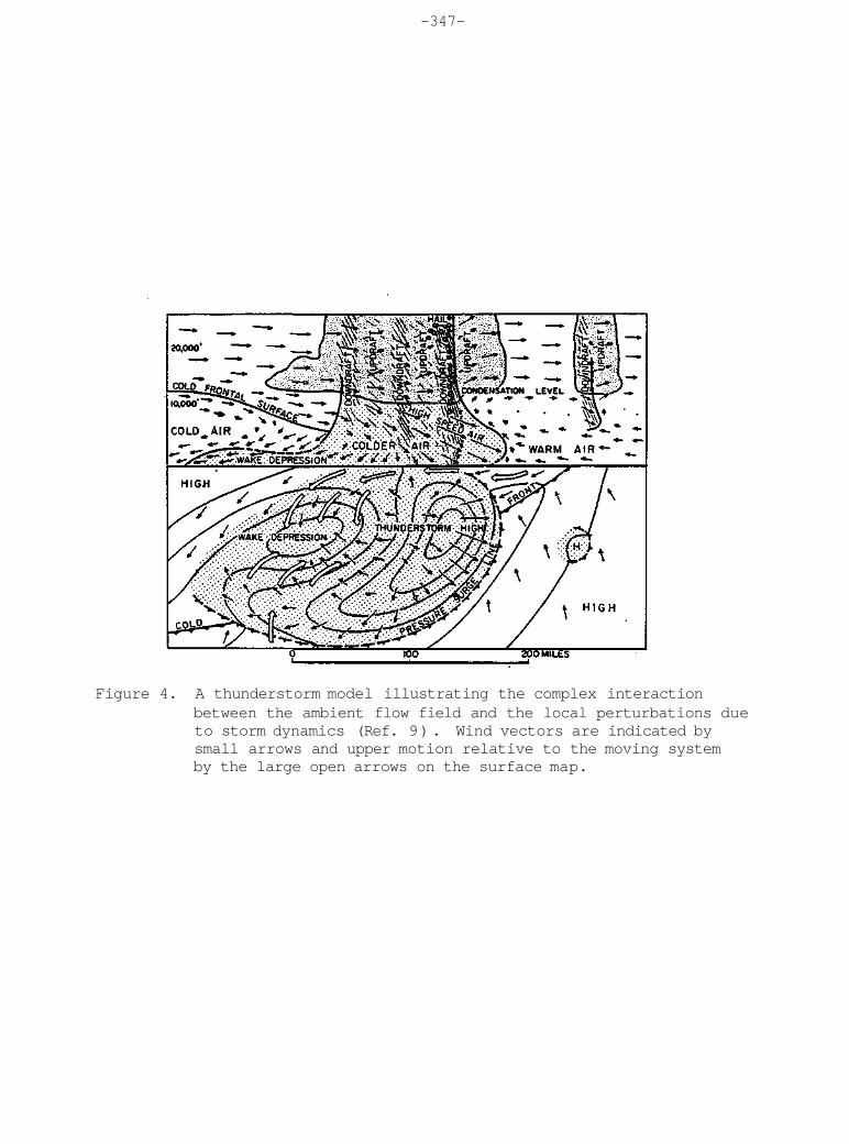
-347-

Figure 4. A thunderstorm model illustrating the complex interaction between the ambient flow field and the local perturbations due to storm dynamics (Ref. 9). Wind vectors are indicated by small arrows and upper motion relative to the moving system by the large open arrows on the surface map.

-348-

TABLE I. THE GROWTH OF NON-UNIFORM GROUPS OF NUCLEI UNDER VARIOUS ATMOSPHERIC CONDITIONS (REF. 4).

† m = √(2σ/rn) where rn = median-volume radius and σ = standard deviation of drop volumes. A small value of m denotes a more nearly uniform spectrum.

-349-

Another way of viewing this problem is shown in Fig. 510. These calculations assumed the total aerosol was composed of soluble ammonium sulfate and other insoluble material. The size distribution was prescribed but various percentages from 0 to 100 of ammonium sulfate were considered. The size distribution of the simulated cloud was calculated and developed as a result of condensation and collection. A uniform ascent rate was imposed but the supersatura-tion varied in response to the condensation process. The calculation was terminated when a minimum detectable radar signal (MDS) level was achieved. The time required to reach the MDS ranged from 1,410s to 1,680s for the 0 to 100 percent soluble CCN spectrum, respectively.

At this point lets return to the concepts of motion leading to cloud formation very briefly and focus on only the relatively slow, upglide motion and the more vigorous convective motion producing stratiform and cumuliform clouds. In the former, the sustaining upward motion would be measured in centimeters per second while for the latter upward speeds are measured in meters per second. The horizontal motion of a cloudy air parcel in a stratiform cloud is typically the same as the wind determined primarily by the pressure gradient at cloud level. The movement of a cloudy element of a cumuliform cloud is influenced considerably by the strong upward speed in addition to the cloud environment horizontal wind.

These dynamic differences between the two major cloud types lead to differences in time scales for the microphysical processes leading to differences in the release of precipitation. Consideration of these concepts is cause to admit to the relative chemical differences expected between clouds and precipitation embedded in the horizontal long-range transport layers (stratiform clouds) and those that penetrate vertically through such layers. The vertical transport of boundary layer pollutants into stratiform clouds is a slow process and will draw upon many sources as the cloud system is advected over great distances. Contrasting this process, cumuliform clouds quickly inhale the boundary layer air and subject that air to the in-cloud microphysics very rapidly.

No two cyclonic systems are identical, but all are characterized by associated cold and warm fronts in the middle latitudes. The relatively wide-spread and slow vertical speeds are schematically inferred from Fig. 611. This figure also illustrates the difficul­ties is following the general atmospheric motion to and through the clouds and precipitation associated with such an extratropical cyclone. The gentle slope of the warm frontal surface gives rise to upward speeds of centimeters per second and the subsiding atmosphere in the cold air mass provides downward speeds of the same magnitude. Of course in the cloud and precipitating regions, these speeds are locally increased as determined by the system thermodynamics and microphysics. The smooth streamlines depicted in Fig. 6 indicate the

-350-

Figure 5. Computed raindrop size distributions at a constant radar reflectivity value for initial CCN properties ranging from totally insoluble to 100% soluble ammonium sulfate (Ref. 10)

-351-

Figure 6. A schematic diagram showing the general relationship between air masses, fronts, relative circulation and cloudiness. Note the scale of such a system is nearly continental. (Ref. 11).

-352-

general horizontal motion associated with such a large system, but whether any property of an air parcel survives the long-range trans­port along such a streamline while subjected to gentle and severe upward and downward motions is in need of experimentation.

The growth of cloud particles leading to precipitation develop­ment is accomplished by either prolonged condensation (deposition) of vapor to previously nucleated droplets (ice crystals) or by the aggregation of water or ice particles. The rate at which these two broad mechanisms proceed is greatly influenced by the dynamics of the cloud system, the available vapor supply, and the chemical makeup of the cloud nuclei size spectrum. The complexities of the system preclude quantitative predictions of either the quality or quantity of precipitation deposited from a specific storm event. The relative sizes of the particles comprising a precipitating cloud are shown in Fig. 712 . xhe sizes of particles range over four orders of magnitude while the number of concentrations extend over six. From a cloud chemistry point of view, the interaction between these particles and interstitial gases is not well described. The drops may undergo evaporation altering their original chemical character, they may also absorb gases, and they may serve as a solvent for captured aerosol. In addition, the long acknowledged, but still little understood, role of entrainment in altering the cloud dynamics and chemistry must be quantified as a contribution to the total picture of the precipita­tion process.

TRACER NEEDS

The development and application of suitable tracers must be con­sidered carefully in attempting to address the development of precip­itation. The many intermediate, and usually isolated, steps involved in cloud and precipitation initiation involve gases and particles and are not unlike the steps taken to study atmospheric pollution.

As stated earlier, it is clear that tracers are needed to identify water vapor sources. At the very least, a means of par­titioning observed water vapor into either oceanic or continental sources would be very helpful. The source identification can be used to infer the transport and dispersion that occurred prior to the observed deposition. If the tracer is sufficiently unique, it may also lead to clarification of some of the questions embedded in our crude image of precipitating storm dynamics.

A cloud system can be conceptually thought of as a filter operating on both particles and gases. Like all filters certain amounts of the particles and gases pass through the filter depending on the particle size spectrum and their chemical composition, and on the absorption - desorption properties of pollutant gases. The cloud

Figure 7. The relative size of particles involved in the development of clouds and precipitation (Ref. 12). Note the disparity between the size of a typical cloud droplet (bearing the initial chemistry) and the typical raindrop (the contributor to wet deposition). The 10° difference in volume suggests that the rain is an amalgamation of much cloud chemistry.

-353-

-354-

general horizontal motion associated with such a large system, but whether any property of an air parcel survives the long-range trans­port along such a streamline while subjected to gentle and severe upward and downward motions is in need of experimentation.

The growth of cloud particles leading to precipitation develop­ment is accomplished by either prolonged condensation (deposition) of vapor to previously nucleated droplets (ice crystals) or by the aggregation of water or ice particles. The rate at which these two broad mechanisms proceed is greatly influenced by the dynamics of the cloud system, the available vapor supply, and the chemical makeup of the cloud nuclei size spectrum. The complexities of the system preclude quantitative predictions of either the quality or quantity of precipitation deposited from a specific storm event. The relative sizes of the particles comprising a precipitating cloud are shown in Fig. 7 1 2. The sizes of particles range over four orders of magnitude while the number of concentrations extend over six. From a cloud chemistry point of view, the interaction between these particles and interstitial gases is not well described. The drops may undergo evaporation altering their original chemical character, they may also absorb gases, and they may serve as a solvent for captured aerosol. In addition, the long acknowledged, but still little understood, role of entrainment in altering the cloud dynamics and chemistry must be quantified as a contribution to the total picture of the precipita­tion process.

TRACER NEEDS

The development and application of suitable tracers must be con­sidered carefully in attempting to address the development of precip­itation. The many intermediate, and usually isolated, steps involved in cloud and precipitation initiation involve gases and particles and are not unlike the steps taken to study atmospheric pollution.

As stated earlier, it is clear that tracers are needed to identify water vapor sources. At the very least, a means of par­titioning observed water vapor into either oceanic or continental sources would be very helpful. The source identification can be used to infer the transport and dispersion that occurred prior to the observed deposition. If the tracer is sufficiently unique, it may also lead to clarification of some of the questions embedded in our crude image of precipitating storm dynamics.

A cloud system can be conceptually thought of as a filter operating on both particles and gases. Like all filters certain amounts of the particles and gases pass through the filter depending on the particle size spectrum and their chemical composition, and on the absorption - desorption properties of pollutant gases. The cloud

-355-

system by its very nature is a powerful transport vehicle for pollut­ants into upper atmospheric layers and not all material is scavenged in the process. Anyone that has observed the anvil on a thunderstorm can readily appreciate that the cirrus cloud represents the high level injection and transport of water vapor originating mostly in the sub-cloud layer. To place the importance of cloud systems, especially convective storms, in the context of a vertical transport medium, some relative scales are shown in Fig. 811. Even this picture is not quite accurate as it is now thought that buoyant elements of large thunderstorms may penetrate the tropopause and release material into the stratosphere.

The tracer simulation of both cloud condensation and ice nuclei will add the final technique for quantifying the precipitation processes. A note of caution must be expressed, however, since the entire field of weather modification has been intentionally placing a "tracer" into clouds for more than 35 years. The problem is that the "tracer" presumably influences the cloud microphysics and, in turn, the cloud dynamics. This feedback leads to a paradox. If a suitable tracer is inert to the in-cloud physical and chemical processes then it is not a reliable tracer of the very processes needing quantifica­tion. On the other hand, if the tracer enters fully into the thermo­dynamic system that is the cloud, the result may be an inadvertent modification of the cloud itself.

SUMMARY

The major points brought out are enumerated as follows:

A. Water Vapor Availability

1. Quantify the source apportionment between evaporation from water surfaces and transpiration from land sur­faces.

B. Water and Ice Nuclei

1. Quantify source differences between natural and anthropogenic.

2. Ascertain the chemical evolution of nuclei from their source to their ultimate deposition.

3. Quantify the nucleating efficiency of aging aerosol.

C. Atmospheric Motions

1. Determine the filter efficiency of cloudy air for both particles and gases.

STRATOSPHERE

Figure 8. A relative vertical scale of clouds, prominent land features and important strata of the atmosphere (Ref. 11). The similarity between the moderate thunderstorm extending into the boundary layer and a rising plume from an emission source is important to consider for understanding the distribution of gases and aerosol in the troposphere (and, perhaps, the stratosphere).

-357-

There are numerous additional problems that could be concep­tualized here, for example the influence of cloud electrification on nucleating efficiency, on cloud dynamics, and on cloud chemistry, but these few general points are enough to set the framework for in-depth development of the subject.

Many of these points are not new to the atmospheric sciences community. Listed here are some additional fruitful areas of re­search :

1. "It is therefore essential that flight measurements be made to determine which precipitation process operates under various conditions and to obtain a quantitative verification of the operation of the assumed processes13."

2. "The growth of nuclei, especially at humidities of less than 70 percent, and the associated problem concerning the physical structure of nuclei (mixed nuclei, supersaturation of solution, and crystallization) ."

3. "The chemical composition of the aerosol. Parallel measure­ments of the tracers of substances and of the number of nuclei, dust particles, and haze droplets should be made. The proportion of traces of gaseous materials should be determined5."

This list could go on and on, but the point is that the early post-World War II understanding of precipitation processes has not advanced significantly in spite of the technological advances through the years. One of the major impediments to a new level of learning is the necessary instruments for critical measurements on a time and space scale appropriate to the precipitation process. As examples, radar is extensively used to estimate internal cloud motions, but the measurements in three dimensions require periods of time that pre­clude simultaneity of observations of whole-cloud dynamics. In contrast to this remote sensing, aircraft measurements of particle size distribution only sample a microscopic volume of the cloud under scrutiny, and to generalize such measurements to the whole cloud can lead to serious misinformation about the chemical-thermodynamic forces at work in the system.

Without question, tracers are much needed to inquire quantita­tively into the physical precipitation process and its importance to atmospheric chemistry.

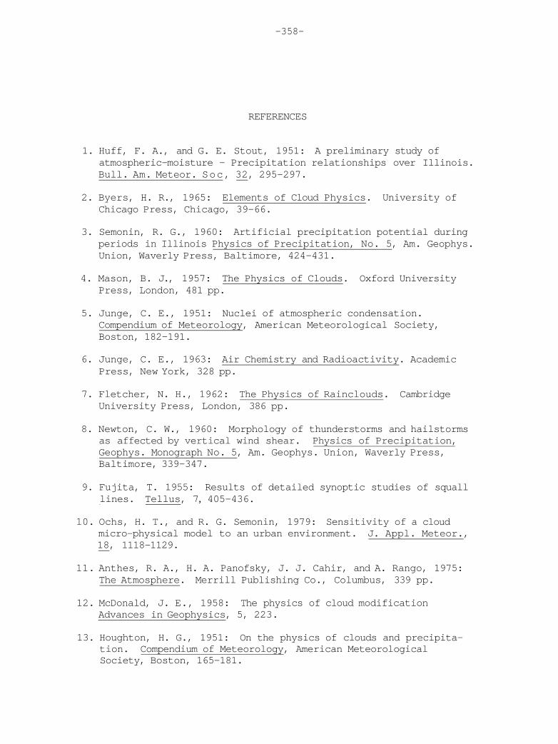
-358-

REFERENCES

1. Huff, F. A., and G. E. Stout, 1951: A preliminary study of atmospheric-moisture - Precipitation relationships over Illinois. Bull. Am. Meteor. Soc, 32, 295-297.

2. Byers, H. R., 1965: Elements of Cloud Physics. University of Chicago Press, Chicago, 39-66.

3. Semonin, R. G., 1960: Artificial precipitation potential during periods in Illinois Physics of Precipitation, No. 5, Am. Geophys. Union, Waverly Press, Baltimore, 424-431.

4. Mason, B. J., 1957: The Physics of Clouds. Oxford University Press, London, 481 pp.

5. Junge, C. E., 1951: Nuclei of atmospheric condensation. Compendium of Meteorology, American Meteorological Society, Boston, 182-191.

6. Junge, C. E., 1963: Air Chemistry and Radioactivity. Academic Press, New York, 328 pp.

7. Fletcher, N. H., 1962: The Physics of Rainclouds. Cambridge University Press, London, 386 pp.

8. Newton, C. W., 1960: Morphology of thunderstorms and hailstorms as affected by vertical wind shear. Physics of Precipitation, Geophys. Monograph No. 5, Am. Geophys. Union, Waverly Press, Baltimore, 339-347.

9. Fujita, T. 1955: Results of detailed synoptic studies of squall lines. Tellus, 7, 405-436.

10. Ochs, H. T., and R. G. Semonin, 1979: Sensitivity of a cloud micro-physical model to an urban environment. J. Appl. Meteor., 18, 1118-1129.

11. Anthes, R. A., H. A. Panofsky, J. J. Cahir, and A. Rango, 1975: The Atmosphere. Merrill Publishing Co., Columbus, 339 pp.

12. McDonald, J. E., 1958: The physics of cloud modification Advances in Geophysics, 5, 223.

13. Houghton, H. G., 1951: On the physics of clouds and precipita­tion. Compendium of Meteorology, American Meteorological Society, Boston, 165-181.