studies of ruminant digestion, ecology, and evolution
TRANSCRIPT

STUDIES OF RUMINANT DIGESTION,
ECOLOGY, AND EVOLUTION
_______________________________________
A Thesis
presented to
the Faculty of the Graduate School
at the University of Missouri-Columbia
_______________________________________________________
In Partial Fulfillment
of the Requirements for the Degree
Master of Science
_____________________________________________________
by
TIMOTHY HACKMANN
Dr. James Spain, Thesis Supervisor
DECEMBER 2008

© Copyright by Timothy Hackmann 2008
All Rights Reserved

The undersigned, appointed by the dean of the Graduate School, have examined the
thesis entitled
STUDIES OF RUMINANT DIGESTION,
ECOLOGY AND EVOLUTION
presented by Timothy Hackmann,
a candidate for the degree of Master of Science,
and hereby certify that, in their opinion, it is worthy of acceptance.
Professor James Spain
Professor Monty Kerley
Professor Joshua Millspaugh

ii
ACKNOWLEDGEMENTS
The author is indebted to
Dr. James Spain, Julie Sampson, and Benjamin Nielson, for varied support
and insight that turned the impossible into the possible
Lucas Warnke, Chad McNeal, Eric Meyer, Zach Brockman, Reagan Bluel,
Ruthie Dietrich, Marin Summers, Asa Spain, and Denise Frietag, for
additional assistance in the lab and the field
Dr. Joshua Millspaugh, for his ecological perspective and reaffirming the
value of mathematical modeling
Dr. Monty Kerley, for additional review and teaching me the importance of
originality
Drs. William Lamberson and John Fresen, for introducing me to much of
the statistical analysis used herein
Drs. James Williams, Ronald Belyea, and Deke Alkire, for additional
critical review
Matthew Brooks, Illana Barasch, and Nicole Barkley, for academic and
non-academic conversations alike
My parents, other family, and friends, for listening to me during the joys
and frustrations of research
Kate Kocyba, for being special
Father God for orchestrating it all.
This thesis belongs to them as much as it does to me.

iii
TABLE OF CONTENTS
ACKNOWLEDGEMENTS ............................................................................................ ii
LIST OF FIGURES ......................................................................................................... x
LIST OF TABLES ........................................................................................................xii
ABSTRACT .................................................................................................................. xv
CHAPTER
1. LITERATURE REVIEW ........................................................................................ 1
Introduction ............................................................................................................ 1
Ecology and Evolutionary History of Wild Ruminants ............................................ 1
Ruminant Families ...................................................................................... 1
Phylogeny and Evolution ............................................................................. 3
Distribution, Abundance, BW, and Dietary Preferences of Living Ruminants
.................................................................................................................... 5
Domestication of Ruminant Species ........................................................................ 7
Details of Domestication ............................................................................. 7
Characteristics of Domestic Species ............................................................ 8
Summary and Experimental Objectives ................................................................... 8
Appendix .............................................................................................................. 10
2. COMPARING RELATIVE FEED VALUE WITH DEGRADATION
PARAMETERS OF GRASS AND LEGUME FORAGES ................................. 29
Abstract ................................................................................................................ 29
Introduction .......................................................................................................... 30
Materials and Methods .......................................................................................... 31
Hay Types and Sampling Procedures ......................................................... 31
In Situ and Chemical Analysis ................................................................... 31

iv
Calculations and Statistical Analysis ......................................................... 34
Comparison with Data of Mertens (1973) .................................................. 39
Results and Discussion.......................................................................................... 40
Chemical Composition .............................................................................. 40
Model Selection ........................................................................................ 40
Influence of Incubation Times on Model Selection and Parameter Estimates
.................................................................................................................. 44
Degradation Parameter Estimate Means..................................................... 46
Correlation between RFV and Degradation Parameter Values ................... 46
Assumption in Correlation Analysis .......................................................... 47
Comparison with Data of Mertens (1973) .................................................. 48
Shortcomings of the conceptual structure of RFV ...................................... 49
3. VARIABILITY IN RUMINAL DEGRADATION PARAMETERS CAUSES
IMPRECISION IN ESTIMATED RUMINAL DIGESTIBILITY ....................... 64
Abstract ................................................................................................................ 64
Introduction .......................................................................................................... 65
Experimental Methods .......................................................................................... 66
Hay Types and Sampling Procedures ......................................................... 66
In Situ and Chemical Analysis ................................................................... 66
Calculations and Statistical Analysis of In Situ Data .................................. 67
Statistical Analysis with Other Previously Published Degradation Data ..... 69
Calculation of Ruminal Digestibility and 95% Confidence Limits ............. 70
Results .................................................................................................................. 74
Discussion ............................................................................................................ 77
Chemical Composition and Degradation Parameter Means ........................ 77

v
Variation in Degradation Parameter Estimates ........................................... 77
Calculated Digestibilities and Their 95% Confidence Limits ..................... 79
Analysis Where a and b are Known with Certainty .................................... 81
Appendix .............................................................................................................. 83
4. USING YTTERBIUM-LABELED FORAGE TO INVESTIGATE PARTICLE
FLOW KINETICS ACROSS SITES IN THE BOVINE RETICULORUMEN ... 89
Abstract ................................................................................................................ 89
Introduction .......................................................................................................... 90
Materials and Methods .......................................................................................... 91
Animals and Diets ..................................................................................... 91
Marker Preparation .................................................................................... 92
Passage Trial ............................................................................................. 92
Chemical Analyses .................................................................................... 94
Regression with Yb Profile Data ............................................................... 94
Calculation of Mean Residence Time ........................................................ 96
Peak Marker Concentration ....................................................................... 97
ANOVA and Other Statistical Procedures ................................................. 97
Results .................................................................................................................. 98
Forage Composition and Intake ................................................................. 98
General Shape of Yb Marker Profiles ........................................................ 99
Comparison of Methods Used to Calculate Mean Residence Time ............ 99
Differences in MRT by Cow, Diet, Period, and Site................................. 100
Differences in Marker Concentration Peak by Cow, Diet, Period, and Site ....
................................................................................................................ 101
Discussion .......................................................................................................... 101

vi
Forage Composition and Intake ............................................................... 101
Stochastic Variation in Yb Marker Profiles .............................................. 102
Regression Models to Visualize Marker Profiles ..................................... 102
Differences in Yb Marker Profiles by Cow, Diet, Period, and Site ........... 106
Difference between Dosing and Sampling Sites within the Dorsal Sac..... 107
Particle Flow Kinetics in the Reticulorumen ............................................ 108
Limitations of our Analysis ..................................................................... 112
Conclusion .......................................................................................................... 113
5. A MECHANISTIC MODEL FOR PREDICTING INTAKE OF FORAGE DIETS
BY RUMINANTS ........................................................................................... 121
Abstract .............................................................................................................. 121
Introduction ........................................................................................................ 122
Materials and Methods ........................................................................................ 123
General Structure .................................................................................... 123
Model Equations ..................................................................................... 125
Feedback Signals and Prediction of voluntary feed intake ........................ 125
Other Notes on Model Structure .............................................................. 128
Model Parameters .................................................................................... 129
Model Validation .................................................................................... 130
Results and Discussion........................................................................................ 131
Validation Results ................................................................................... 131
Comparison with Prior Mechanistic Models ............................................ 133
Model Limitations ................................................................................... 134
Potential Model Applications .................................................................. 134
Appendix 1 ......................................................................................................... 136

vii
Units ....................................................................................................... 136
Abbreviations .......................................................................................... 136
Symbols and Notation ............................................................................. 138
Appendix 2 ......................................................................................................... 141
Conversion Factors .................................................................................. 141
Protein Feedback Signal that Affects Degradation Rates .......................... 142
Absorption, Hydrolysis, and Passage Rates ............................................. 142
Endogenous Protein and PU .................................................................... 144
MICRO Submodel................................................................................... 145
Heat of Combustion and Heat Increment ................................................. 146
Yield Parameters for Diet Composition ................................................... 147
Miscellaneous Yield and Other Parameters. ............................................. 147
6. PRESSURE FOR LARGE BODY MASS IN THE RUMINANTIA: THE ROLE
OF NUTRITIONAL RESOURCE LIMITATIONS .......................................... 171
Abstract .............................................................................................................. 171
Introduction ........................................................................................................ 171
Methods .............................................................................................................. 174
Scaling of PPDMI and DDM with BW .................................................... 174
Allometric Equations for Scaling of RR Parameters with BW ................. 177
Calculation of FMR and Other Parameters when RR Size Scales with
BW0.75
vs. BW1 .................................................................................... 178
Investigating PPDMI Scaling with a Mechanistic Model of Ruminant
Digestion .............................................................................................. 183
Body Mass Distributions of Fossil and Extant Ruminants ........................ 184
Results ................................................................................................................ 185
Scaling of PPDMI with BW .................................................................... 185
viii
Scaling of DDM with BW ....................................................................... 185
Scaling Results of the Mechanistic Model ............................................... 186
Value of Physiological Parameters when RR Size Scales with BW0.75
vs.
BW1 ..................................................................................................... 186
Body Mass of Fossil Ruminants over the North American Tertiary.......... 187
Discussion .......................................................................................................... 188
Scaling of PDDMI and DDM with BW ................................................... 188
Scaling Results of the Mechanistic Model ............................................... 190
Adaptive Costs and Benefits of RR Size Scaling with BW0.75
vs. BW1..... 191
Nutritional Resource Limitations and Evolution of Body Size in the
Ruminantia ........................................................................................... 193
Implications for Non-Ruminant Species .................................................. 195
Appendix 1 ......................................................................................................... 196
Appendix 2 ......................................................................................................... 199
7. PERSPECTIVES FROM RUMINANT ECOLOGY AND EVOLUTION USEFUL
TO RUMINANT LIVESTOCK RESEARCH AND PRODUCTION ............... 210
Abstract .............................................................................................................. 210
Introduction ........................................................................................................ 211
Ecology, Evolution, and Domestication of Ruminants ......................................... 212
Ruminant Families .................................................................................. 212
Evolution................................................................................................. 213
Ecological Characteristics ....................................................................... 214
Details of Domestication ......................................................................... 215
Characteristics of Domestic Species ........................................................ 215
Perspectives Relevant to Modern Production Systems ......................................... 215
Predicting Values of Physiological Parameters from BW......................... 216

ix
Role of Physical and Metabolic Factors in Regulation Intake ................... 218
Primary Function of the Omasum ............................................................ 220
Dietary Niche Separation and Mixed-Species Grazing ............................. 223
Extended Lactation .................................................................................. 225
Conclusions ........................................................................................................ 227
References ................................................................................................................... 233
Vita ............................................................................................................................. 259
x
LIST OF FIGURES
Figure Page
1.1 A greater Malay chevrotain ................................................................................... 23
1.2 A member of the family Moschidae ...................................................................... 24
1.3 Restoration of Archaeomeryx optatus .................................................................... 25
1.4 Restoration of Dromomeryx borealis..................................................................... 26
1.5 A phylogeny of ruminant families ......................................................................... 27
1.6 Increase in BW of ruminants over evolutionary time ............................................. 28
2.1 Examples of bag observations that were identified as aberrant and removed ......... 61
2.2 An example of a 0 h bag pair that criteria for bag removal but from which the
aberrant bag of the pair could not be identified ................................................... 62
2.3 Fit of several models to DM disappearance data of one 2003 late-cut alfalfa sample .
.......................................................................................................................... 63
3.1 Graphical explanation of how increasing uncertainty in degradation parameters
increases uncertainty in digestibility ................................................................... 88
4.1 Location of dosing and sampling sites within the reticulorumen .......................... 116
4.2 Yb marker profile in mid-dorsal sac, mid-ventral sac, caudo-ventral blind sac, and
ventral reticulum for cows during period 1 ....................................................... 117
4.3 Comparison of mean residence time values calculated using raw observations and
local regression model...................................................................................... 118
4.4 Comparison of mean residence time values calculated using raw observations and
the numerical method with those of the G2→G1→O model ............................ 119
4.5 Proposed kinetics of particle flow across sampling sites in the reticulorumen ...... 120
5.1 Empirical relationship between chemostatic and distention feedbacks derived from
Bernal-Santos (1989) and Bosch et al. (1992a,b) .............................................. 168
5.2 Comparison between actual and model-predicted voluntary feed intake of forage
diets by ruminant species of various physiological states .................................. 169

xi
5.3 Comparison between actual voluntary feed intake and that predicted by our
mechanistic model and the empirical equations of the NRC (2000) for cattle ... 170
6.1 Relationship between model-predicted physiologically potential DMI and BW
under three scenarios ........................................................................................ 209
7.1 Graph of the allometric relationship between BW and wet mass of reticulorumen
tissue. ............................................................................................................... 229
7.2 The isthmus in the stomach of the lesser mouse deer ........................................... 230
7.3 Botanical composition of diets chosen by goat, sheep, and cattle on pasture ........ 231
7.4 Milk production of extended vs. conventional lactations of multiparous Muriciano-
Granadina goats milked once daily ................................................................... 232

xii
LIST OF TABLES
Table Page
1.1 Description of extant ruminant families................................................................. 12
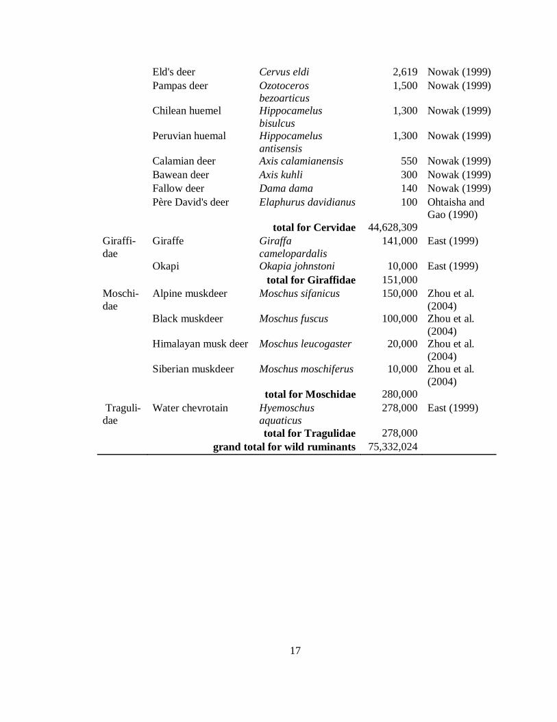
1.2 Estimated global population sizes of wild ruminant species................................... 13
1.3 Native distribution of species across continents and habitat and climate types ....... 18
1.4 Body mass of wild ruminant species by family...................................................... 19
1.5 Dietary preferences of species, according to their assignment as browser,
intermediate feeder, or grazer ............................................................................. 20
1.6 Domesticated ruminant species and details of their domestication ......................... 21
1.7 Characteristics of domestic species ....................................................................... 22
2.1 Description of hays used for in situ analysis .......................................................... 52
2.2 Degradation models considered for describing in situ data .................................... 53
2.3 Chemical composition and RFV of forages ........................................................... 54
2.4 Values of model selection criteria obtained when fitting DM, CP, and NDF
degradation data to models ................................................................................. 55
2.5 Relative ranking of degradation models according to average values of model
selection criteria ................................................................................................. 56
2.6 Degradation parameter estimates of forages by forage class and chemical fraction
.......................................................................................................................... 57
2.7 Significant correlations between degradation parameter estimates of forages and
relative feed value .............................................................................................. 59
2.8 Significant correlations between NDF degradation parameters and digestible DMI
for a subsample of alfalfa and grass forages in data of Mertens (1973) ............... 60
3.1 Standard deviation and CV of degradation parameter estimates, averaged by
chemical fraction ................................................................................................ 85
3.2 Calculated digestibility of chemical fractions by forage class and upper and lower
95% confidence limits, using uncertainty values of degradation parameters equal
to their SD.......................................................................................................... 86
xiii
3.3 Calculated digestibility of chemical fractions by forage class and upper and lower
95% confidence limits, using uncertainty values of digestion rate equal to its SD ...
............................................................................................................................. 87
4.1 Chemical composition of high-quality alfalfa, low-quality alfalfa, and bromegrass
forage diets fed to cows during passage trial..................................................... 114
4.2 Voluntary intake of bromegrass, high-quality alfalfa, and low-quality alfalfa diets
fed to cows during passage trial ........................................................................ 115
5.1 Studies and species used in model validation ...................................................... 149
5.2 Descriptive statistics of studies used in model validation ..................................... 150
5.3 Performance of mechanistic models used to predict feed intake of ruminants ...... 151
5.4 Main system of differential equations used in the mechanistic model to represent
digestive events in the reticulorumen, small intestine, large intestine, and plasma ..
........................................................................................................................... 152
5.5 Auxiliary equations for the main system of differential equations of the mechanistic
model ............................................................................................................... 156
5.6 Equations for microbial submodel of the mechanistic model ............................... 158
5.7 Miscellaneous equations in the mechanistic model .............................................. 160
5.8 Estimated parameter values for absorption rates .................................................. 161
5.9 Estimated parameter values for age-dependent hydrolysis rates ........................... 162
5.10 Estimated parameter values for endogenous protein and plasma urea secretion ... 163
5.11 Estimated parameter values for microbial uptake of ammonia and soluble protein ....
........................................................................................................................... 164
5.12 Estimated parameter values for heat of combustion and heat increment parameter
values............................................................................................................... 165
5.13 Estimated yield parameter values for diet composition ........................................ 166
5.14 Estimated miscellaneous parameter values .......................................................... 167
6.1 Species used to derive allometric equations relating several physiological
parameters to BW ............................................................................................ 203

xiv
6.2 Descriptive statistics of studies used to determine empirical relationship between
BW and physiologically potential DMI and digestible DM............................... 204
6.3 Allometric equations which relate reticulorumen and energetic parameters with BW
........................................................................................................................... 205
6.4 Expected values of some digestive, energetic, and other parameters when
reticulorumen size scales with BW1 ................................................................. 206
6.5 Expected values of some digestive, energetic, and other parameters when
reticulorumen size scales with BW0.75
.............................................................. 207
6.6 Change in some digestive, energetic, and other parameters when reticulorumen size
scaling is changed from BW1 to BW
0.75 ............................................................ 208
7.1 Some allometric equations useful for values predicting physiological parameter
values from BW ............................................................................................... 228

xv
STUDIES OF RUMINANT DIGESTION,
ECOLOGY, AND EVOLUTION
Timothy Hackmann
Dr. James Spain, Thesis Supervisor
ABSTRACT
This thesis examines ruminant digestion, ecology, and evolution, particularly where they
can improve livestock production systems. We performed an experiment that estimated
ruminal in situ degradation parameter values of grass and legume forages. In one
analysis, we showed the relative feed value system did not explain variation in these
parameter estimates, underscoring a biological limitation of this system. In a subsequent
analysis, we found that ruminal digestibility estimated from mean parameter estimates
had large 95% confidence limits (81% of digestibility means), suggesting digestibility
values so estimated have little meaning.
We performed another experiment that monitored concentrations of labeled
forage particles within the reticulorumen. We inferred that once a particle escapes from
the dorsal sac for the final time, it must escape from ventral regions soon after entry.
We also developed a mechanistic model of ruminant gastrointestinal tract function
(based on chemical reactor theory) that predicted feed intake of wild and domestic
ruminants precisely (generally R2
> 0.9, root mean square prediction error < 1.4 kg∙d-1
).
We then used this mechanistic model, along with allometric equations and the fossil
record, to demonstrate the pattern of large BW within the Ruminantia is a response to
nutritional resource limitations.

xvi
Our final study recapitulates key points in the ecology and evolution of wild
ruminants, then discusses how these points and others presented in the thesis offer insight
to improving livestock production systems.

1
CHAPTER 1
LITERATURE REVIEW
INTRODUCTION
Owing to ruminants’ ability to digest fiber, ruminant livestock production systems
convert low-quality fibrous and other feedstuffs into highly-nutritious meat and milk. In
total, these systems produce nearly 30 and 100% of the world’s supply of these meat and
milk products (FAO, 2008a). Because these systems play a keystone role in the world’s
food supply, it is crucial to understand the ruminant animal underlying their operation.
This review examines the evolution, ecology, and domestication of the ruminant to give a
comprehensive overview of this animal.
ECOLOGY AND EVOLUTIONARY HISTORY OF WILD RUMINANTS
For the purpose of this review, a ruminant includes any artiodactyl (member of
the mammalian order Artiodactyla) possessing a rumen, reticulum, omasum or isthmus
homologous to the omasum, and abomasum. Ruminants also possess certain skeletal
features—such as loss of upper incisors, presence of incisiform lower canines, and fusion
of cubiod and navicular bones in the tarsus—that are useful in fossil identification (e.g.,
Gentry, 2000) but not of primary consideration here.
Ruminant Families
The six extant (i.e., non-extinct) ruminant families include the Tragulidae,
Moschidae, Bovidae, Giraffidae, Antilocapridae, and Cervidae. Table 1.1 provides a

2
description of these families, including the number of species and genera (from Nowak
[1999]).
The Tragulidae (chevrotains) (4 sp.) are small, reclusive, forest-dwelling, deer-
like ruminants (Figure 1.1). They are the most primitive of all living families and have
changed little morphologically over evolutionary history—this has led them to being
called ―living fossils‖ (Janis, 1984). Their primitiveness is demonstrated by (1) their very
simple social behavior, (2) retention of a gallbladder and appendix (Janis, 1984), (3) lack
of a true omasum (Langer, 1988), and (4) possession of many skeletal characters (e.g.,
short, unfused metapodials) considered ancestral (Webb and Taylor, 1980). While still
considered ruminants, the Tragulidae are not included in the same infraorder (Pecora) as
other ruminant families (Moschidae, Bovidae, Giraffidae, Antilocapridae, Cervidae)
because of these ancestral features.
The Moschidae (musk deer) (5 sp.) are small tropical Asiatic deer whose males
possess a musk gland anterior to the genitals. Like tragulids, the moschids are hornless
(other families possess horns or antlers) and the males have large upper canines instead
(Figure 1.2). The remaining families, the Bovidae (e.g., cattle, sheep, goats, antelope;
140 sp.), Giraffidae (giraffe and okapi), Cervidae (true deer; e.g., white-tailed deer,
caribou, moose; 41 sp.), and Antilocapridae (pronghorn), include species familiar to most
readers. Standard mammalogy textbooks (e.g., Feldhamer et al., 2007) and
encyclopedias (e.g., Nowak, 1999) provide additional information for all these families.
There are 5 additional extinct families that are generally recognized (Carroll,
1988), the Hypertragulidae, Leptomerycidae, Gelocidae, Palaeomerycidae, and
Dromomerycidae. The Hypertragulidae and Leptomerycidae were small, hornless
3
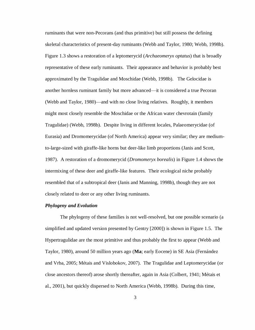
ruminants that were non-Pecorans (and thus primitive) but still possess the defining
skeletal characteristics of present-day ruminants (Webb and Taylor, 1980; Webb, 1998b).
Figure 1.3 shows a restoration of a leptomerycid (Archaeomeryx optatus) that is broadly
representative of these early ruminants. Their appearance and behavior is probably best
approximated by the Tragulidae and Moschidae (Webb, 1998b). The Gelocidae is
another hornless ruminant family but more advanced—it is considered a true Pecoran
(Webb and Taylor, 1980)—and with no close living relatives. Roughly, it members
might most closely resemble the Moschidae or the African water chevrotain (family
Tragulidae) (Webb, 1998b). Despite living in different locales, Palaeomerycidae (of
Eurasia) and Dromomerycidae (of North America) appear very similar; they are medium-
to-large-sized with giraffe-like horns but deer-like limb proportions (Janis and Scott,
1987). A restoration of a dromomerycid (Dromomeryx borealis) in Figure 1.4 shows the
intermixing of these deer and giraffe-like features. Their ecological niche probably
resembled that of a subtropical deer (Janis and Manning, 1998b), though they are not
closely related to deer or any other living ruminants.
Phylogeny and Evolution
The phylogeny of these families is not well-resolved, but one possible scenario (a
simplified and updated version presented by Gentry [2000]) is shown in Figure 1.5. The
Hypertragulidae are the most primitive and thus probably the first to appear (Webb and
Taylor, 1980), around 50 million years ago (Ma; early Eocene) in SE Asia (Fernández
and Vrba, 2005; Métais and Vislobokov, 2007). The Tragulidae and Leptomerycidae (or
close ancestors thereof) arose shortly thereafter, again in Asia (Colbert, 1941; Métais et
al., 2001), but quickly dispersed to North America (Webb, 1998b). During this time,

4
tropical, closed-canopy forests were widespread (Janis, 1993) and temperatures were very
warm (near their highest point in the last 65 million years; Zachos et al., 2001). The
Gelocidae appeared at approximately 40 million years ago (middle Eocene), when the
climate had already cooled (about 5C relative to 50 Ma; Zachos et al., 2001) and
temperate woodlands appeared (Janis, 1993).
When these first ruminant groups emerged, they were rabbit-sized (<5 kg; Métais
and Vislobokov, 2007), but as demonstrated in the North American fossil record, their
size progressively increased over time (Figure 1.6). Their skull and dental morphology
(low-crowned teeth, small incisors, long and narrow skulls) was optimal for consuming
fruits, shoots, and insects (Webb, 1998b). This evidence in addition to the observed
habitat and diet of living tragulid and moschid species (which are taken as rough
analogues for these first groups) suggests the first ruminants were small, reclusive, forest-
dwelling omnivores (Webb, 1998b). Foregut fermentation and rumination was not
extensive when these first ruminants emerged but developed by approximately 40 Ma, as
indicated by dental morphology (Janis, 1976) and molecular techniques (Jermann et al.,
1995).
The remaining families evolved about 18 to 23 Ma (early Miocene) during a
second radiation (Janis, 1982) in Eurasia (Antilocapridae, Cervidae, Moschidae,
Dromomerycidae, Bovidae, Palaeomerycidae) and Africa (Giraffidae) (Gentry, 2000).
Many of these families (Moschidae, Dromomerycidae, Antilocapridae) dispersed to
North America shortly after their emergence (Janis and Manning, 1998a,b; Webb,
1998b). By this time, the climate was drier (Janis, 1993) and cooled substantially (first
Antarctic ice sheets formed; Zachos et al., 2001) and open, temperate woodlands were the

5
dominant flora (Janis, 1982, 1993). Dental wear patterns and craniodental morphology
suggests these groups ate primarily leaves (Janis, 1982; Solounias and Meolleken, 1992)
or grass and leaves (Solounias et al., 2000; Semprebon et al., 2004; Semprebon and
Rivals, 2007; DeMiguel et al., 2008). Body mass of these groups was larger (20-40 kg;
Janis, 1982) and increased over time, continuing the prior trend (Figure 1.6).
By about 5 to 11 Ma (Late Miocene), grasslands expanded (Jacobs et al., 1999),
and some species began including more grass in their diets, again suggested by dental
wear patterns and craniodental morphology (Semprebon et al., 2004; Semprebon and
Rivals, 2007). At the end of this period (5 Ma), bovids and cervids migrated to North
America (Webb, 1998a, 2000). Later (2 Ma; Latest Pliocene) deer would migrate to SA
(Webb, 2000).
Distribution, Abundance, BW, and Dietary Preferences of Living Ruminants
Today there exist nearly 200 ruminant wild species (Nowak, 1999), most of which
are Bovidae and Cervidae (Table 1.1). A conservative estimate places the world
population of wild ruminants at 75.3 million, with 0.28 million tragulids, 0.28 million
moschids, 44.6 million cervids, 29.1 million bovids, 0.15 million giraffids, and 0.88
million antilocaprids (Table 1.2). The majority of wild ruminants, in terms of species and
population numbers, are thus bovids and cervids.
Following their distribution in the fossil record, living ruminants are natively
found on all continents except Antarctica and Australia, though most species are found in
Africa and Eurasia (Table 1.3, constructed from data in van Wieren [1996]). The Bovidae
and Cervidae both enjoy an almost world-wide distribution, while the range of the

6
remaining families is much more restricted (Table 1.3). Only the Cervidae are found in
South America (Table 1.3).
Ruminants not only have a wide geographic distribution but are also found across
many climates and habitats. Though the classification system of habitats and climates
used in this review (adopted from van Wieren [1996]) is admittedly crude, it still gives a
general sense of this distribution. As a whole, ruminant species are evenly spread across
open, ecotone, and forested habitats, but they prefer warm to other types of climates
(Table 1.3). The distribution of the Bovidae and Cervidae is generally representative of
this overall pattern, whereas other families individually inhabit a more restricted range of
habitats and climates (Table 1.3).
As reported in Table 1.4 (data from van Wieren [1996]), median BW of modern
ruminants is 45 kg, near that expected from the historical trend (Figure 1.6). Body mass
ranges greatly, from approximately 2 kg (Salt’s dik to dik [Madoqua saltiana], royal
antelope [Neotragus pygmaeus], lesser Malay mouse deer [Tragulus javanicus]) to 800
kg (American bison [Bison bison], wisent [Bison bonasus], gaur [Bos gaurus], Asian
water buffalo [Bubalus bubalis], kouprey [Bos sauveli]; van Wieren, 1996). Though not
shown in Table 1.4, some individuals from the largest species achieve BW ≥1,000 kg,
with maximum size of male reticulated giraffe (Giraffa camelopardalis) reaching 1,400
kg (Clauss et al., 2003). By family, the Giraffidae are the largest; Antilocapridae,
Bovidae, Cervidae intermediate; and Moschidae and Tragulidae smallest (Table 1.4).
The Bovidae and Cervidae have species at or near these BW extremes, while the other
families display a much more restricted range in BW (Table 1.4).
7
Ruminant species display innate dietary preferences, and these differ greatly
across species. A concise way of classifying these preferences is with the feeding class
system (first proposed by Hoffman and Stewart [1972]), which categorizes species as
either (1) browsers, which innately prefer browse like fruits, shoots, and leaves (typically
from shrubs, forbs, and trees), (2) grazers, which innately prefer grasses and other
roughage, or (3) intermediate feeders, which switch between browse and grass, usually
depending on their seasonal availability. For most of their evolutionary history, ruminant
species were predominately or exclusively browsers. Today, a plurality of ruminant
species is still classified as browsers (Table 1.5), and only about a quarter are grazers.
The Bovidae and Cervidae have species represented in all three feeding classes; the other
families are exclusively browsers.
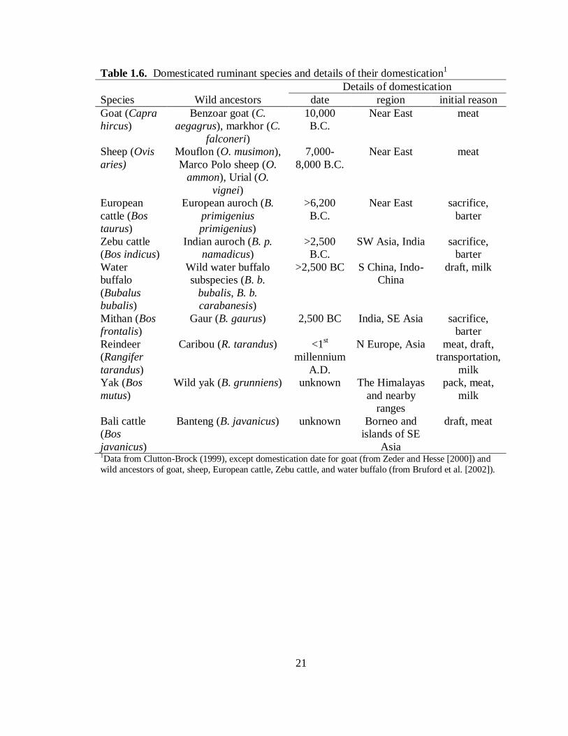
DOMESTICATION OF RUMINANT SPECIES
Details of Domestication
The following details of domestication are from Clutton-Brock (1999) (except
where noted) and summarized in Table 1.6. The first livestock species to be
domesticated (ruminant or non-ruminant) was the goat at approximately 10 000 B.C. in
the Fertile Crescent of the Near East (Zeder and Hesse, 2000). The goat was initially
domesticated to supply meat to burgeoning, congested human populations whose hunting
had depleted large prey populations in the wild (Clutton-Brock, 1999; Diamond, 2002).
Most of the other 8 domesticated ruminant species (sheep, European and Zebu cattle,
water buffalo, mithan, reindeer, yak, Bali cattle) were brought under human control by
2500 B.C. in either the Near East or southern Asia. Some of these species were initially

8
domesticated for meat, like the goat, but reasons for domestication varied greatly,
including for milk, draft, transportation, sacrifice, and barter.
Molecular approaches (Bruford et al., 2003) have determined each domestic
species is probably derived from several wild species; at least 12 species can claim
ancestry to the 9 domesticated species. Of the multitude of available wild species, these
twelve were chosen for domestication because they were gregarious, submissive to
human captors, unexcitable, and easy to breed (Clutton-Brock, 1999; Diamond, 2002).
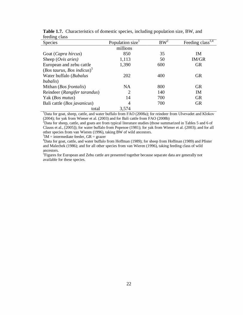
Characteristics of Domestic Species
Except where noted, points in the discussion below are summarized in Table 1.7.
The total population size of domestic species is 3.57 billion, nearly 50-fold larger than
that of wild ruminants. As might be anticipated, cattle, sheep, and goats comprise most
(about 95%) of the domestic ruminant population. All but reindeer belong to the family
Bovidae.
Most species are grazers, with goats and reindeer the notable exceptions. Sheep
were classified by Hoffman (1989) as grazers, though others (e.g., Pfister and Malechek,
1986) argue that they are instead intermediate feeders.
Though BW varies greatly by sex and across breeds, the rough averages in Figure
1.7 demonstrates that BW of domestic ruminants is large in comparison to many wild
ruminants. The smallest species (sheep, goat) are near the median BW of wild ruminants
(45 kg) and many species (cattle, mithan, Bali cattle) approach the maximum observed in
the wild (800 kg; Table 1.4).

9
SUMMARY AND EXPERIMENTAL OBJECTIVES
The first ruminants evolved approximately 50 million years ago and were small (<5 kg)
forest-dwelling omnivores. Today there are almost 200 living ruminant species in 6
families. Wild ruminants number about 75 million, range from about 2 to more than 800
kg, and generally prefer at least some browse in their diet. Eight species have been
domesticated within the last 12,000 years, currently numbering 3.6 billion. In contrast to
wild ruminants, domestic species naturally prefer at least some grass in their diets, are of
large BW (roughly from 35 to 800 kg), and, excepting reindeer, belong to one family
(Bovidae).
The goal of the following work is to enhance our understanding of ruminant
digestive function, ecology, and evolution, particularly where they intersect with and thus
can improve livestock production systems. A myriad of approaches are used herein.
Chapters 2 and 3 both discuss an experiment that measured the ruminal in situ
degradation of a large number of grass and legume forages. Chapter 2 uses the
degradation data collected in this experiment to identify (1) the mathematical model that
optimally fits these data and should be used estimate values of degradation parameters
(e.g., rate and extent of digestion) from them, (2) the relationship between the
degradation parameter values so estimated and relative feed value system (RFV), in order
identify biological reasons for RFV’s poor performance. Many feed evaluation systems
use mean degradation parameter values to estimate in vivo ruminal digestibility, and
Chapter 3 shows how variability around these mean values can lead to gross imprecision
in this estimation.
10
Chapter 4 summarizes an experiment that monitored concentrations of labeled
forage across sites in the bovine reticulorumen to infer general patterns of digesta particle
flow therein. Chapter 5 presents a holistic mechanistic model of the ruminant
gastrointestinal tract function. This chapter emphasizes the model as a practical tool to
predict intake, though it has other uses (as Chapters 6 and 7 will show).
The focus of Chapters 6 and 7 is ruminant ecology and evolution. Chapter 6
attempts to demonstrate the pattern of large BW in ruminants (whose median BW is 500-
fold greater than mammals as a whole) is evolutionary strategy adopted by ruminants to
overcome nutritional resource limitations. The mechanistic model of Chapter 5,
allometric equations of digestive parameters, and the ruminant fossil record are used as
supporting evidence for the chapter’s arguments. Chapter 7 briefly recapitulates the
summary of ruminant ecology and evolution first presented in the literature review. It
then attempts to show how points from Chapter 6, among others in ruminant ecology and
evolutionary research, can offer insight into livestock research and production.
APPENDIX
Global population estimates of wild ruminants were compiled from several sources
(Whitehead, 1971; Ohtaishi and Gao, 1990; East, 1999; Nowak, 1999; Wiener, 2003;
Ulvevadet and Klokov, 2004; IUCN, 2008), many of which are compilations themselves.
We excluded from our estimates domesticated, feral, captive, and non-natively
introduced populations or species. We also excluded species for which estimates were
judged very fragmentary (included only a few isolated or subspecies populations) and
were unlikely to approach anything of a global estimate.
11
In all, we obtained estimates for 150 species (78% of total). This includes 1
species from Antilocapridae (100% of family total), 116 from Bovidae (83% of total), 26
from Cervidae (63% of total), 2 from Giraffidae (100% of total), 4 from Moschidae (80%
of total), and 1 from Tragulidae (25% of total). Poor or non-existent census data
accounts for missing species. Also note that estimates for many Asian species include
numbers only in China, again due to poor census data.
The population sizes reported here are clear underestimates. In total they are still
more comprehensive and up-to-date than the last apparent global census (McDowell,
1977), which estimated population numbers for only 11 species (excluding feral and
currently unrecognized species) in two families (Bovidae, Cervidae), for a total of 27
million ruminants overall.

12
Table 1.1. Description of extant ruminant families, including number of genera and
species and example species.1
family Number of genera Number of species Example species
Antilocapridae 1 1 Pronghorn
Bovidae 49 140 Cattle, sheep, goats, antelope
Cervidae 17 41 White-tailed deer, caribou,
moose
Giraffidae 2 2 Giraffe, okapi
Moschidae 1 5 Muskdeer
Tragulidae 3 4 Chevrotains
total 73 193 1Data from Nowak (1999)

13
Table 1.2. Estimated global population sizes of wild ruminant species.
species name
family common scientific population source
Antilo-
capridae
Pronghorn Antilocapra
americana
875,000 Nowak (1999)
total for Antilocapridae 875,000
Bovidae blue duiker Cephalophus
monticola
7,000,000 East (1999)
Maxwell's duiker Cephalophus
maxwelli
2,137,000 East (1999)
Impala Aepyceros melampus 1,990,000 East (1999)
Grey duiker Sylvicapra grimmia 1,660,000 East (1999)
Bushbuck Tragelaphus scriptus 1,340,000 East (1999)
Common wildebeest Connochaetes
taurinus
1,200,000 East (1999)
Kirk's dik-dik Madoqua kirki 971,000 East (1999)
Oribi Ourebia ourebi 750,000 East (1999)
Bay duiker Cephalophus dorsalis 725,000 East (1999)
African buffalo Syncerus caffer 687,000 East (1999)
Steenbok Raphiceros
campestris
663,000 East (1999)
Thomson's gazelle Gazella thomsoni 650,000 East (1999)
Peter's duiker Cephalophus
callipygus
570,000 East (1999)
Gunther's dik-dik Madoqua guentheri 511,000 East (1999)
Salt's dik-dik Madoquo saltiana 485,600 East (1999)
Alpine chamois Rupicapra rupicapra 400,000 Nowak (1999)
Sable antelope Hippotragus niger 373,000 East (1999)
Suni Neotragus moschatus 365,000 East (1999)
Greater kudu Tragelaphus
strepsiceros
352,000 East (1999)
Black-fronted duiker Cephalophus
nigrifons
300,000 East (1999)
Mongolian gazelle Procapra gutturosa 300,000 Nowak (1999)
Topi Damaliscus lunatus 300,000 East (1999)
Kob Kobus kob 295,000 East (1999)
White-bellied duiker Cephalophus
leucogaster
287,000 East (1999)
Common hartebeest Alcelaphus
buselaphus
280,000 East (1999)
Bontebok Damaliscus dorcas 237,500 East (1999)
Pygmy antelope Neotragus batesi 219,000 East (1999)
Lechwe Kobus lechwe 212,000 East (1999)

14
Bison Bison bison 202,500 Nowak (1999)
Waterbuck Kobus ellipsiprymnus 200,000 East (1999)
Red-flanked duiker Cephalophus
rufilatus
170,000 East (1999)
Sitatunga Tragelaphus spekei 170,000 East (1999)
Yellow-backed
duiker
Cephalophus
sylvicultor
160,000 East (1999)
Grant's gazelle Gazella granti 140,000 East (1999)
Comon eland Tragelaphus oryx 136,000 East (1999)
puku Kobus vardoni 130,000 East (1999)
Muskox Ovibos moschatus 122,600 Nowak (1999)
Lesser kudu Tragelaphus imberbis 118,000 East (1999)
Dall sheep Ovis dalli 112,000 Nowak (1999)
Bohor reedbuck Redunca fulvorufula 101,000 East (1999)
Black duiker Cephalophus adersi 100,000 East (1999)
Goitred gazelle Gazella subgutturosa 100,000 Nowak (1999)
Serow Capricornis crispis 100,000 Nowak (1999)
Tibetan antelope Pantholops hodgsoni 100,000 Nowak (1999)
Gerenuk Litocranius walleri 95,000 East (1999)
Sharpe's grysbok Raphiceros sharpei 95,000 East (1999)
Argali Ovis ammon 80,000 Nowak (1999)
Roan antelope Hippotragus equinus 76,000 East (1999)
Mountain goat Oreamnos
americanus
75,000 Nowak (1999)
Southern reedbuck Redunca arundinum 73,000 East (1999)
Oryx Oryx beisa 67,000 East (1999)
Royal antelope Neotragus pygmaeus 62,000 East (1999)
Bighorn sheep Ovis canadensis 58,000 Nowak (1999)
Iberian wild goat Capra pyrenaica 50,000 IUCN (2008)
Saiga Saiga tatarica 50,000 IUCN (2008)
Speke's gazelle Gazella spekei 50,000 East (1999)
Klipspringer Oreotragus
oreotragus
42,000 East (1999)
Red forest duiker Cephalophus
natalensis
42,000 East (1999)
Urial Ovis vignei 40,000 Nowak (1999)
Dorcas gazelle Gazella dorcas 37,500 East (1999)
Mountain reedbuck Redunca redunca 36,350 East (1999)
Blackbuck Antilope cervicapra 36,000 Nowak (1999)
Lichtenstein's
hartebeest
Alcelaphus
lichtensteini
36,000 East (1999)
Nile lechwe Kobus megaceros 36,000 East (1999)
Ogilby's duiker Cephalophus ogilbyi 35,000 East (1999)

15
Nyala Tragelaphus angasi 32,000 East (1999)
Ibex Capra ibex 31,670 IUCN (2008)
Cape grysbok Raphiceros melanotis 30,500 East (1999)
Piacentinis's dik-dik Madoquo piacentinii 30,000 East (1999)
Bongo Tragelaphus
eurycerus
28,000 East (1999)
Zebra duiker Cephalophus zebra 28,000 East (1999)
Blue sheep Pseuodois nayaur 25,000 Nowak (1999)
East Caucasian tur Capra caucasica 25,000 Nowak (1999)
Red-fronted gazelle Gazella rufifrons 25,000 East (1999)
Springbok Antidorcas
marsupialis
24,000 East (1999)
Harvey's red duiker Cephalophus 20,000 East (1999)
Black wildebeest Connochaetes gnou 18,000 East (1999)
gray rhebuck Pelea capreolus 18,000 East (1999)
Grey rhebok Pelea capreolus 18,000 East (1999)
Giant Eland Tragelaphus
derbianus
17,650 East (1999)
Pyrenean chamois Rupicapra pyrenaica 15,000 IUCN (2008)
Yak Bos grunniens 15,000 Wiener et al.
(2003)
Soemmering's gazelle Gazella Soemmerring 14,000 East (1999)
Mountain gazelle Gazella gazella 12,000 Nowak (1999)
Indian gazelle Gazella bennetti 10,000 Nowak (1999)
Nilgai Boselaphus
tragocamelus
10,000 Nowak (1999)
Tibetan gazelle Procapra
picticaudata
10,000 Nowak (1999)
West Caucasian tur Capra caucasica 10,000 Nowak (1999)
Mouflon Ovis aries 7,500 IUCN (2008)
Beira Dorcatragus
megalotis
7,000 East (1999)
Four-horned antelope Tetracerus
quadricornis
5,500 Nowak (1999)
Markhor Capra falconeri 5,200 Nowak (1999)
Jentink's duiker Cephalophus jentinki 3,500 East (1999)
Water buffalo Bubalus bubalis 3,500 Nowak (1999)
Abbott's duiker Cephalophus spadix 2,500 East (1999)
Dama gazelle Gazella dama 2,500 East (1999)
Dibatag Ammodorcas clarkei 2,500 East (1999)
Mountain nyala Tragelaphus buxtoni 2,500 East (1999)
European wild goat Capra hircus 2,335 IUCN (2008)
Nilgiri tahr Hemitragus hylocrius 2,200 Nowak (1999)

16
Nilgiri tahr Hemitragus jayakari 2,000 Nowak (1999)
Wisent Bison bonasus 1,800 IUCN (2008)
Zanzibar duiker Cephalophus adersi 1,400 East (1999)
Banteng Bos javanicus 1,000 Nowak (1999)
Gaur Bos gaurus 1,000 Nowak (1999)
hirola Betragus hunteri 1,000 East (1999)
Slender-horned
gazelle
Gazella leptoceros 1,000 East (1999)
Cuvier's gazelle Gazella cuvieri 560 Nowak (1999)
Arabian oryx leucoryx 500 Nowak (1999)
Walia ibex Walia ibex 400 Nowak (1999)
Addax Addax nasomaculatus 350 East (1999)
Saola Pseudoryx
nghetinhensis
350 Nowak (1999)
Tamaraw Anoa mindorensis 350 Nowak (1999)
Przewalskii's gazelle Procapra przewalskii 200 Nowak (1999)
Scimitar-horned oryx Oryx dammah 200 Nowak (1999)
total for Bovidae 29,119,715
Cervidae Roe deer Capreolus capreolus 15,000,000 IUCN (2008)
White-tailed deer Odocoileus
virginianus
14,000,000 Nowak (1999)
Mule deer Odocoileus hemionus 5,500,000 Nowak (1999)
Caribou Rangifer tarandus 4,421,500 Ulvevadet and
Klokov
(2004)
Moose Alces alces 1,500,000 IUCN (2008)
Elk/red deer Cervus elaphus 1,000,000 Nowak (1999)
Siberian roe deer Capreolus pygargus 1,000,000 Nowak (1999)
Wapiti Cervus canadensis 782,500 Nowak (1999)
Reeves muntjac Muntiacus reevesi 650,000 Nowak (1999)
Tufted deer Elaphodus
cephalophus
500,000 Nowak (1999)
red muntjac Muntiacus muntjac 145,000 Nowak (1999)
White-lipped deer Cervus albirostris 75,000 Nowak (1999)
Black muntjac Muntiacus crinifrons 10,000 Nowak (1999)
Javan rusa Cervus timorensis 10,000 Whitehead
(1971)
Water deer Hydropotes inermis 10,000 Nowak (1999)
Marsh deer Blastoceros
dichotomus
7,000 Nowak (1999)
Sika deer Cervus nippon 5,935 Ohtaisha and
Gao (1990)
Barasingha Cervus duvaucelii 3,565 Nowak (1999)
17
Eld's deer Cervus eldi 2,619 Nowak (1999)
Pampas deer Ozotoceros
bezoarticus
1,500 Nowak (1999)
Chilean huemel Hippocamelus
bisulcus
1,300 Nowak (1999)
Peruvian huemal Hippocamelus
antisensis
1,300 Nowak (1999)
Calamian deer Axis calamianensis 550 Nowak (1999)
Bawean deer Axis kuhli 300 Nowak (1999)
Fallow deer Dama dama 140 Nowak (1999)
Père David's deer Elaphurus davidianus 100 Ohtaisha and
Gao (1990)
total for Cervidae 44,628,309
Giraffi-
dae
Giraffe Giraffa
camelopardalis
141,000 East (1999)
Okapi Okapia johnstoni 10,000 East (1999)
total for Giraffidae 151,000
Moschi-
dae
Alpine muskdeer Moschus sifanicus 150,000 Zhou et al.
(2004)
Black muskdeer Moschus fuscus 100,000 Zhou et al.
(2004)
Himalayan musk deer Moschus leucogaster 20,000 Zhou et al.
(2004)
Siberian muskdeer Moschus moschiferus 10,000 Zhou et al.
(2004)
total for Moschidae 280,000
Traguli-
dae
Water chevrotain Hyemoschus
aquaticus
278,000 East (1999)
total for Tragulidae 278,000
grand total for wild ruminants 75,332,024

Table 1.3. Native distribution of species (% of total within family) across continents and habitat and climate types1
Continent2,3
Habitat Climate
family EA AF NA SA forest ecotone open warm temperate cold
-------------------------------------------------------% of total within family-------------------------------------------------------
Antilo-
capridae
0 0 100 0 0 0 100 0 100 0
Bovidae
28.4 67.6 4.9 0 25.4 32.4 42.2 74.5 16.7 8.8
Cervidae 63.3 04
13.3 30.0 50.0 30.0 20.0 46.7 46.7 6.7
Giraffidae 0 100 0 0 50.0 50.0 0 100 0 0
Moschidae 100 0 0 0 0 100 0 0 0 100
Tragulidae 75.0 25.0 0 0 100 0 0 100 0 0
total 37.6 51.1 7.1 6.4 32.6 31.9 35.5 68.8 22.0 9.2 1Data from van Wieren (1996) 2EA = Eurasia, AF = Africa, NA = North America, SA = South America 3Percentages for continent may not sum to 100 within family because some species may be located on multiple continents.
4Does not include species which have a limited range in Africa.
18

19
Table 1.4. Body mass of wild ruminant species by family1
Body mass (kg)
Family Median Min Max
Antilocapridae 40 40 40
Bovidae 52.5 2 800
Cervidae 47.5 6 550
Giraffidae 475 250 700
Moschidae 11.5 11 12
Tragulidae 2 2 8
total 45 2 800 1Data from van Wieren (1996)

20
Table 1.5. Dietary preferences of species (% of total within family), according to their
assignment as browser (BR), intermediate feeder (IM), or grazer (GR)1
Feeding class
Family BR IM GR
--------------------% of total species within family--------------------
Antilocapridae 100 0 0
Bovidae
35.3 26.5 39.2
Cervidae 46.7 36.7 16.7
Giraffidae 100 0 0
Moschidae 100 0 0
Tragulidae 100 0 0
total 41.1 31.9 27.0 1Data from van Wieren (1996)
21
Table 1.6. Domesticated ruminant species and details of their domestication1
Details of domestication
Species Wild ancestors date region initial reason
Goat (Capra
hircus)
Benzoar goat (C.
aegagrus), markhor (C.
falconeri)
10,000
B.C.
Near East meat
Sheep (Ovis
aries)
Mouflon (O. musimon),
Marco Polo sheep (O.
ammon), Urial (O.
vignei)
7,000-
8,000 B.C.
Near East meat
European
cattle (Bos
taurus)
European auroch (B.
primigenius
primigenius)
>6,200
B.C.
Near East sacrifice,
barter
Zebu cattle
(Bos indicus)
Indian auroch (B. p.
namadicus)
>2,500
B.C.
SW Asia, India sacrifice,
barter
Water
buffalo
(Bubalus
bubalis)
Wild water buffalo
subspecies (B. b.
bubalis, B. b.
carabanesis)
>2,500 BC S China, Indo-
China
draft, milk
Mithan (Bos
frontalis)
Gaur (B. gaurus) 2,500 BC India, SE Asia sacrifice,
barter
Reindeer
(Rangifer
tarandus)
Caribou (R. tarandus) <1st
millennium
A.D.
N Europe, Asia meat, draft,
transportation,
milk
Yak (Bos
mutus)
Wild yak (B. grunniens) unknown The Himalayas
and nearby
ranges
pack, meat,
milk
Bali cattle
(Bos
javanicus)
Banteng (B. javanicus) unknown Borneo and
islands of SE
Asia
draft, meat
1Data from Clutton-Brock (1999), except domestication date for goat (from Zeder and Hesse [2000]) and
wild ancestors of goat, sheep, European cattle, Zebu cattle, and water buffalo (from Bruford et al. [2002]).
22
Table 1.7. Characteristics of domestic species, including population size, BW, and
feeding class
Species Population size1
BW2 Feeding class
3,4
millions
Goat (Capra hircus) 850 35 IM
Sheep (Ovis aries) 1,113 50 IM/GR
European and zebu cattle
(Bos taurus, Bos indicus)5
1,390 600
GR
Water buffalo (Bubalus
bubalis)
202 400 GR
Mithan (Bos frontalis) NA 800 GR
Reindeer (Rangifer tarandus) 2 140 IM
Yak (Bos mutus) 14 700 GR
Bali cattle (Bos javanicus) 4 700 GR
total 3,574 1Data for goat, sheep, cattle, and water buffalo from FAO (2008a); for reindeer from Ulvevadet and Klokov
(2004); for yak from Wiener et al. (2003) and for Bali cattle from FAO (2008b) 2Data for sheep, cattle, and goats are from typical literature studies (those summarized in Tables 5 and 6 of Clauss et al., [2005]); for water buffalo from Popenoe (1981); for yak from Wiener et al. (2003); and for all
other species from van Wieren (1996), taking BW of wild ancestors. 3IM = intermediate feeder, GR = grazer 4Data for goat, cattle, and water buffalo from Hoffman (1989); for sheep from Hoffman (1989) and Pfister
and Malechek (1986); and for all other species from van Wieren (1996), taking feeding class of wild
ancestors. 5Figures for European and Zebu cattle are presented together because separate data are generally not
available for these species.

23
Figure 1.1. A greater Malay chevrotain (Tragulus napu), a member of the family
Tragulidae and one of the most primitive ruminants. Note small size (approximately 3
kg), short limbs, and absence of horns, all of which are characteristic of early ruminants.
Enlarged upper canines are absent because this specimen is a female. Photo courtesy of
Dr. Ellen S. Dierenfeld.

24
Image removed for electronic publication because copyright permission could not be
obtained. Reader is referred to Figure 3 of source (Colbert, 1941) for original
image.
Figure 1.2. A member of the family Moschidae, probably Alpine musk deer (Moschus
chrysogaster). Note large upper canines and absence of horns. Reproduced from
Wemmer (1998).

25
Image removed for electronic publication because copyright permission could not be
obtained. Reader is referred to Figure 3 of source (Colbert, 1941) for original
image.
Figure 1.3. Restoration of Archaeomeryx optatus, one of the earliest ruminants.
Archaeomeryx belonged to the Hypertragulidae, but aspects of its appearance (small size,
short front legs, absence of horns) are representative of other early ruminant families
(Tragulidae, Leptomerycidae). Reproduced from Colbert (1941).

26
Figure 1.4. Restoration of Dromomeryx borealis (from Scott 1913). Dromomeryx
belonged to the Dromomerycidae, but its size and giraffe-like horns are also
characteristic of Palaeomerycidae. Reproduced from Scott (1913).

27
Hypertragulidae
Leptomerycidae
Tragulidae
Gelocidae
Moschidae
Dromomerycidae
Palaeomerycidae
Antilocapridae
Cervidae
Bovidae
Giraffidae
50 40 30 20 10 0
Millions of years before present
Figure 1.5. A phylogeny of ruminant families. Families included are the
Hypertragulidae, Tragulidae, Leptomerycidae, Gelocidae, Moschidae, Dromomerycidae,
Palaeomerycidae, Antilocapridae, Giraffidae, Cervidae, and Bovidae—i.e., those
recognized by Carroll (1988). Solid lines indicate age ranges documented in the fossil
record (adapted from Métais et al. [2001] for Tragulidae; Webb [1998] and Gentry [2000]
for Gelocidae; and Gentry [2000] for all other families, assuming Archaeomeryx belongs
to Leptomerycidae [Webb and Taylor 1980]); stippled lines indicate inferred age ranges
and family relationships (adapted from Gentry [2000]).

28
Est
imate
d B
W, k
g
Millions of years ago
Figure 1.6. Increase in BW of ruminants over evolutionary time (millions of years), as
shown in fossil record of the North American Tertiary (2 to 65 million years ago). Each
point represents the appearance date of a single genus within the Hypertragulidae (■),
Leptomerycidae (▲), Antilocapridae (●), Dromomerycidae (□), Moschidae (○),
Gelocidae (+), or an indeterminate hornless ruminant family (*). Masses were estimated
from lengths of fossilized molars. For comparison, BW of all extant ruminant species (-)
are included. Note plot is semi-logarithmic for BW. Chapter 6 describes the
methodology used in constructing this figure in more detail.
0.1
1
10
100
1000
-50 -40 -30 -20 -10 0

29
CHAPTER 2
COMPARING RFV TO DEGRADATION PARAMETERS OF GRASS AND
LEGUME FORAGES
ABSTRACT
Relative feed value (RFV) was evaluated relative to in situ degradation parameters of
grass and legume forages. Early-cut alfalfa (n = 20), late-cut alfalfa (n = 26), cool season
grass (n = 11), warm season grass (n = 4), and grass/legume (n = 20) samples were
collected from duplicate hay bales submitted to the 2002 and 2003 MO State Fair Hay
Contests. Sub-samples were incubated in the rumen of 2 lactating Holstein cows for 0, 6
or 8, 12, 24, and 48 h to determine in situ degradation of DM, ADF, NDF, CP, and
hemicellulose over time. Degradation data were fit to a variety of candidate models to
estimate degradation parameters. Correlation coefficients were determined between
degradation parameter estimates (sorted according to forage [early-cut alfalfa, late-cut
alfalfa, grass/legume, grass]) and RFV. For further comparison, correlations between
NDF degradation parameter estimates and digestible DMI were determined with data
from a previous study. Degradation data were best fit to a single, gamma 2-distributed
pool model without a lag phase. Relative feed value was significantly correlated (P <
0.05) to potentially digestible DM and CP for early-cut alfalfa, potentially digestible DM
for late-cut alfalfa, and potentially digestible DM, NDF, and hemicellulose for
grass/legume. The percentage of significant correlations (10.7%) across the entire dataset

30
was low and no correlations were significant for grass. Relative feed value did not
account for variation in degradation parameters, especially for grasses. A further
correlation analysis, which compared digestible DMI with degradation parameter
estimates reported by another dataset, revealed that digestible DMI and degradation
parameter estimates were related for grass but not alfalfa forages. These results suggest
that RFV is limited by its failure to include degradation parameters.
INTRODUCTION
Numerous systems have been developed to predict quality of forages fed to ruminants
(Moore, 1994). Relative feed value (RFV; Rohweder et al., 1978) is the most widely
employed. Relative feed value grades forages according to their predicted digestible
DMI (DDMI), the product of DMI and percentage digestible DM (DDM). Predicted
DDMI is divided by a base DDMI to establish an index with a typical full bloom legume
hay scoring 100. To parameterize the RFV system, the National Forage Testing
Association selected equations that relate forage NDF and ADF to DMI and DDM, with a
base DDMI of 1.29% (Linn and Martin, 1989).
Despite the extensive use of the RFV system parameterized according to the
National Forage Testing Association recommendations, RFV has been criticized. In their
summary, Moore and Undersander (2002) demonstrated NDF and ADF are inconsistent
and poor predictors of DDMI. Sanson and Kercher (1996) found that RFV prediction
equations accounted for less than 1% of total variation in DDMI for 20 alfalfa hays fed to
lambs.

31
Whereas RFV’s poor performance has been identified statistically, further work
needs to ascertain the underlying biological reasons for this performance. One area that
deserves attention is degradation characteristics. Degradation characteristics, such as
degradation rate and extent, are linked to DMI and DDM (Mertens, 1973), the two factors
on which RFV is based. Many studies have measured degradation characteristics but
only for a limited number of forages or chemical fractions. Furthermore, degradation
characteristics have rarely been collected to evaluate RFV; only Canbolat et al. (2006)
has done so, finding variable correlations between in vitro gas production characteristics
and RFV for 1 alfalfa sample collected over 3 maturities.
To further evaluate RFV, this study was designed to determine degradation
characteristics of legume and grass hays that are representative of those graded by the
RFV system.
MATERIALS AND METHODS
Hay Types and Sampling Procedures
Hay samples were obtained from entries submitted to the Missouri State Fair Hay
Contest in 2002 and 2003. The entries came from across the state of Missouri and
included early-cut alfalfa (ECA), late-cut alfalfa (LCA), cool season grass (CSG), warm
season grass (WSG), and grass/legume (GL) samples. A detailed description of the
forages, including number of samples collected by year of harvest, class, variety, and
cutting within year is reported in Table 2.1.
Each entry was submitted as duplicate hay bales. Each bale was cored with a hay
probe (Penn State Forage Sampler; Nasco, Ft. Atkinson, CO), and the core samples of
32
duplicate bales were combined to give a representative sample of each entry. Samples
were ground in a Wiley mill (Arthur H. Thomas Company, Philadelphia, PA) to pass
through a 2-mm screen. Ground samples were placed in sealed plastic bags and stored at
room temperature for further analysis.
In Situ and Chemical Analysis
In situ degradation characteristics were determined for all samples. The samples
were analyzed over 3 different 2-d time periods, two 2-d periods for 2002 samples and
one 2-d period for 2003 samples (as discussed below). Air-dry dacron bags (10 x 20 cm;
50 ± 15μm pore size; ANKOM Technology, Macedon, NY) were filled with 5 ± 0.1 g of
air-dry sample for 2002 hay samples and 4 ± 0.1 g of sample for 2003 hay samples;
sample mass to surface area ratio was approximately 12.5 mg∙cm-2
and 10 mg∙cm-2
for
2002 and 2003 samples, respectively, which are within those suggested by Nocek (1988).
Duplicate bags were prepared for insertion into 2 cows, giving a total of 4 bags per
sample at each incubation time. Bags were heat sealed (AIE-200; American International
Electric, Wittier, CA), secured to plastic cable ties, and tied in bundles to nylon retrieval
cords according to their incubation time.
Two ruminally cannulated, multiparous Holstein cows housed in free-stall
facilities at the University of Missouri-Columbia Foremost Dairy Center were selected
for in situ procedures. All procedures involving the animals were approved by the
Animal Care and Use Committee, University of Missouri-Columbia. Each animal was
provided ad libitum access to a standard lactation diet. The diet was a corn silage, alfalfa
hay, alfalfa haylage-based diet (240 g corn silage, 123 g alfalfa hay, 150 g alfalfa

33
haylage, 467 g concentrate and 190 g CP, 240 g ADF and 410 g NDF∙kg DM-1
) fed as a
total mixed ration. Bags were inserted into the ventral rumen of the cows in reverse
order. Incubation times chosen were 0, 8, 12, 24, and 48 h for 2002 hay samples (for
original run; see below) and 0, 6, 12, 24, and 48h for 2003 hay samples. All samples
within year (2002 or 2003) were to be incubated during a single 2-d period, giving two 2-
d periods total. However, one of the cows used to incubate the 2002 samples stopped
ruminating during the 2-d period sampling period, and the samples from this cow for that
period were discarded. New subsamples of the 2002 hay samples were incubated in this
cow for an additional 2-d period, with incubation times of 0, 6, 12, 24, and 48 h. Samples
from 2003 were incubated during a single 2-d period as originally planned, giving a total
of three 2-d periods during which the forages were incubated. A standard forage was not
used to correct for differences between runs because all samples within a cow∙period
were incubated in one run, and any systematic differences between cow∙periods could be
detected by comparing degradation parameter values across cow∙periods with an
ANOVA (see below). During all runs, 0h bags were exposed to rumen fluid briefly
(approximately 5 min) to allow hydration. All bags were removed simultaneously, as
suggested by Nocek (1988).
After removal from the rumen, the bags were doused with cold (approximately
15°C) water to halt fermentation and were rinsed until the wash water ran relatively clear.
Bags were then washed in a domestic washing machine until the wash water ran
completely clear, as suggested by Cherney et al. (1990b). Samples were airdried in a
55°C convection oven to a constant mass and then were completely dried in a 105°C

34
oven. Bags were then air-equilibrated and weighed to determine their residue mass.
Residues were then removed, composited by duplicates within cow, and stored at <0°C
for further analysis.
Bag residue and original forage samples were ground with a Wiley mill to pass
through a 1-mm screen. All material was subsequently analyzed for DM by drying at
105C for 24 h; NDF and ADF using an ANKOM200
Fiber Analyzer (ANKOM
Technology); and total N by combustion analysis (LECO FP-428; LECO Corporation, St.
Joseph, MI). Hemicellulose (HEM) was calculated by difference between NDF and
ADF. No assay to determine microbial contamination was made; previous work where
bags were washed in a similar manner reported negligible microbial contamination of
residues (Coblentz et al., 1997).
Calculations and Statistical Analysis
All degradation data were expressed as fractional disappearance (g∙g-1
). Using a
variant of an equation from Weisbjerg et al. (1990; as cited by Stensig et al., 1994), NDF,
HEM, and ADF degradation data at each incubation time were corrected for insoluble
material washed from the bag. Because NDF, ADF, and HEM are insoluble entities, it
was assumed that the truly soluble fraction, W, was 0, and so the equation of Weisbjerg et
al., (1990) was simplified and applied as follows:
)1
)(1()()(
P
PtMPtMtK i
ii
where K(ti) = corrected degradation at time ti (g∙g-1
), M(ti) = measured (uncorrected)
degradation at time ti (g∙g-1
), and P = insoluble fraction washed from 0h bag (total
fraction washed from 0h bag; g∙g-1
).

35
A method was developed to eliminate aberrant bag observations, which might be
caused by undetected bag rupture or other errors. Whereas such observations can be
identified and eliminated using conventional statistical methods (e.g., studentized
residuals and Cook’s distance [Kaps and Lamberson, 2004]), such methods require the
data to be fit to a pre-determined model. However, because several models were under
consideration, conventional methods could not be applied, and an alternative method for
removing outliers was formulated. Bag observations that satisfied any one of the
following conditions were considered for removal, as described below:
(1) Those whose disappearance values were 20% greater than the mean disappearance
value of the next incubation time of the same cow;
(2) Those whose disappearance values were 20% less than the mean disappearance value
of the prior incubation time of the same cow;
(3) Those which created >15% replicate error relative to duplicate bag at the same
incubation time and cow.
Condition 1 is based on the premise that degradation increases monotonically; those that
fulfill condition 1 violate that premise. For illustration, Figure 2.1A shows a 6 h bag
observation from a 2002 GL sample that fulfilled condition 1 and was removed. If a bag
observation had an aberrantly low disappearance value, it could cause the bag at the next
incubation time to fulfill condition 1, even if the bag at the next incubation time was not
aberrant. For this reason, condition 2 was enacted to identify such bags with aberrantly
low disappearance values and prevent non-aberrant bags from being removed. Figure
2.1B shows a 12 h bag observation from a 2002 CSG sample that fulfilled condition 2

36
and was removed. Condition 3 was designed to remove bag observations that failed to
fulfill conditions 1 and 2 yet were still grossly aberrant; most duplicate bag pairs repeated
well (median replicate error was 2.4% after removing bags that fulfilled conditions 1 and
2), and a large replicate error (>15%) indicated that 1 of 2 bags in a duplicate pair was
aberrant. If condition 3 was fulfilled by a duplicate bag pair, the aberrant bag of the pair
was identified visually as an outlier from the degradation curve and removed. Though a
subjective selection, the offending bag of the duplicate pair was usually identified easily;
Figure 2.1C illustrates an example where a bag from a poorly replicated (16.55%
replicate error) 48 h bag pair (2002 LCA sample) was identified as aberrant because its
disappearance (0.990 g∙g-1
) was abnormally high, both absolutely and relative to the
asymptotic disappearance value suggested by observations prior to 48 h.
However, for some 0 h bags, the aberrant bag could not be identified because
disappearance values of both bags were reasonable based on the behavior of the
degradation curve >6 h; Figure 2.2 gives an example of a 0 h bag pair from which an
aberrant bag could not be identified for removal despite poor repeatability (30.56%
replicate error) of disappearance values within the pair. In this case, no correction could
be made, and both bag observations were retained.
Models based on the gamma distribution (Pond et al., 1988; Ellis et al., 1994;
Ellis et al., 2005) were considered for describing the in situ degradation data. Due to the
limited number of incubation times, only single pool models reported in Table 2.2 could
be considered. The G1 and G1L models are equivalent to the commonly used first-order
kinetics models of rskov and McDonald (1979) and McDonald (1981), respectively,

37
and were considered with less frequently used age-dependent G2, G2L, G3, and G3L
models.
The PROC NLIN procedure of SAS (SAS Institute, Inc., Cary, NC) was used to
estimate parameters in the models for DM, NDF, ADF, HEM, and CP degradation data.
Parameters estimated include the age-dependent degradation rate, λd (h-1
); fraction
degraded at t = 0, a (g∙g-1
); potential extent of degradation, (a + b) (g∙g-1
); fraction not
degraded at t = 0 that is potentially degradable, b (g∙g-1
); and discrete lag time before
onset of degradation, τ (h).
Note that most degradation rates reported in the literature are age-independent
rates—that is, refer to specific degradation rates (g substrate degraded ∙ g total substrate-1
∙ h-1
) that remain constant over time. The specific degradation rate associated with λd (an
age-dependent rate) increases asymptotically to λd (Pond et al., 1988; Ellis et al., 1994).
For this reason, comparison between age-independent rates reported by most literature
and the age-dependent rate λd is not commensurate and leads to the finding that age-
dependent rates are greater than age-independent ones. To allow more commensurate
comparison, the mean degradation rate of λd , k, was calculated as 0.59635 ∙ λd (Pond et
al., 1988). This mean rate is the specific degradation rate associated with λd averaged
over time. It is effectively an age-independent equivalent of an age-dependent rate and
can be compared to age-independent rates commonly reported in the literature.
Because NDF, ADF, and HEM degradation data had been corrected to make
disappearance 0 at t = 0, the value of a was constrained to 0 for fitting procedures for
38
these fractions. For all fractions, the value of (a + b) was bounded between 0 and 1 g∙g-1
,
the theoretical limits of degradation.
Using the criteria for eliminating aberrant bag observations, nearly all NDF, ADF,
and HEM bag observations had to be eliminated for one 2003 ECA sample. So few bag
observations were left after this elimination that NDF, ADF, and HEM degradation data
could not be fit to a model for this forage sample.
At first, degradation data of each cow were kept separate for the fitting procedure.
However, after a preliminary ANOVA indicated that degradation parameter values did
not consistently differ across cow∙periods, cow∙period data were pooled by year of forage
(2002 or 2003), entailing that data of 2 cows (n = 2, 2002 and n = 2, 2003) were used to
construct each degradation curve. The results of model fit using this pooled data set were
employed in all subsequent statistical analysis.
Models were evaluated using residual sums of squares (SSRES), residual mean
square (MSRES), and Akaike information criterion (AIC) values for DM, CP, and NDF
degradation data. The model with the lowest numerical value for each test was
considered best (Kaps and Lamberson, 2004).
Relative feed value and forage degradation parameter estimates (λd, k, a, b, and [a
+ b]) were sorted according to forage class (ECA, LCA, grass, or GL). The PROC
CORR procedure of SAS was used to determine correlation coefficients between RFV
and degradation parameter estimates. Correlations with P < 0.05 were considered
significant.
39
Comparison with Data of Mertens (1973)
For comparison, correlations between RFV, NDF degradation parameters, and
DDMI reported by Mertens (1973) were determined. Data for 15 grass (11 CSG and 4
WSG) and 15 alfalfa forages were selected to create a dataset with similar forage
varieties and chemical composition (mean and SD) as the forage populations examined in
this study. Cutting of alfalfa was not reported by Mertens (1973), and thus alfalfa
samples were pooled under a common alfalfa class. A GL class was not examined
because only 4 GL samples were appropriate for correlation analysis; the other 8 GL
samples in Mertens (1973) included birdsfoot trefoil, which was not examined in this
study. Digestible DM intake was reported for sheep or cattle or both; if DDMI was
reported for both animals, then average DDMI was calculated and used.
Mertens (1973) fit degradation data to a model similar to the G1L model (Table
2.2), which includes degradation parameters kd and η but not λd.. The parameter λd. was
estimated from mean lifetime (Ellis et al., 2005), which is related to kd , η ,and n as
follows:
mean lifetime = n/(λd / 100) = 1/(kd / 100)+ η
and hence
λd = n kd /(1+ kd /100 τ)
where n = order of the gamma distribution associated with λd.
Relative feed value, DDMI, and forage degradation parameter estimates, (λd, kd, a,
b, [a + b], and τ), were sorted according to forage class (alfalfa or grass). The PROC

40
CORR procedure of SAS was used to determine correlation coefficients between RFV
and degradation parameters. Correlations with P < 0.05 were considered significant.
RESULTS AND DISCUSSION
Chemical Composition
The chemical composition and RFV of the forages is reported in Table 2.3. The
mean and SD of the chemical composition data were generally similar to those
summarized by the Dairy NRC (2001), indicating a representative range of forages were
included in this study. However, WSG generally had lower NDF, ADF, and HEM as
well as greater CP than bermudagrass reported in the NRC (2001). Warm season grasses
in this study were generally of better quality than those summarized by the NRC. This
difference is related to contestants of MO State Fair Hay Contest submitting only higher
quality WSG.
Model Selection
Table 2.4 illustrates values of SSRES, MSRES, and AIC values obtained when
fitting G1, G1L, G2, G2L, G3, and G3L models to DM, CP, and NDF degradation data of
all forages. These values were used as criteria for model fit, with lower values for a
given model indicating better fit (Kaps and Lamberson, 2004). On this basis, models
(G1, G1L, G2, G2L, G3, and G3L) were assigned a rank of model fit (1 to 6, where 1
indicates best fit and 6 the worst) relative to other models within each chemical fraction
(DM, CP, and NDF). Table 2.5 reports the mean and range of these rankings across
fractions (DM, CP, and NDF).

41
Across chemical fractions, values of SSRES are lowest for the G1L model, and
values of SSRES were lower for lagged (G1L, GL2, GL3) models than their non-lagged
counterparts (G1, G2, G3; Table 2.4). As such, the G1L model was ranked best and
lagged models ranked better than non-lagged according to the SSRES criterion (Table 2.5).
However, the use of SSRES as a model selection criterion is not commensurate in this case
because SSRES decreases with increasing parameters, and the lagged models contain 1
more parameter than the non-lagged models.
As the ratio of SSRES to error degrees of freedom, MSRES accounts for the number
of parameters in the model and is a more appropriate selection criterion than SSRES where
the number of parameters varies across models, as is in the case in the present study.
However, MSRES still tends to decrease with increasing number of parameters (Kaps and
Lamberson, 2004), and thus one risks bias towards selection of larger models when
employing MSRES as a selection criterion. The expression for AIC (n log [SSRES / n] + 2p,
where n = number of observations and p = number of parameters) penalizes for excessive
parameters in a given model to avoid such biased selection, and, for this reason, AIC is
the most preferable model selection criterion in this study.
Values of both MSRES and AIC were lowest for the G2 models and, with the
exception of the MSRES for the G1 model, were lower for non-lagged (G1, G2, G3)
models than their lagged counterparts (G1L, G2L, G3L; Table 2.4). Consequently, the
G2 model was ranked best and non-lagged models ranked better than their lagged
counterparts. These results indicate the G2 model is optimal. They also suggest that the
42
decrease in total error (SSRES) by the inclusion of a lag term is not justified by the
addition of a model parameter in so doing.
The above discussion refers to mean SSRES, MSRES, and AIC values and rankings.
Values of SSRES, MSRES, and AIC values differed by chemical fraction and so did the
rankings in some cases (Tables 4 and 5). Still, the rankings based on AIC, the most
preferred criterion, showed unequivocally that the G2 model was best, as it was ranked 1
across all chemical fractions.
Difference in performance among models may be understood by considering
model shapes. Figure 2.3 shows the fit of G2 vs. G1 (A), G1L (B), and G3 (C) models to
DM disappearance data of a 2003 LCA sample (where the 2 observations at each
incubation time represent mean values from each of the 2 cows) to illustrate these shapes.
The G2 and other age-dependent models represent degradation as following a sigmoidal
curve, with an increasingly more protracted sigmoidal shape as the order increases from
G2 to GN (where N represents the order of the model; see Figure 2.3C; Pond et al., 1988;
and Ellis et al., 1994). The G1 model, by contrast, represents degradation as an abrupt
first-order decay process lacking the smooth sigmoidal shape of the age-dependent
models (Figure 2.3A). A lag phase is often added to the G1 model, yielding the G1L
model (Figure 2.3B), because degradation does not begin instantaneously but rather
shows a phase of slow degradation at early time points followed by more rapid
degradation later (see Figure 2.3 of Van Milgen et al., 1991); this lag phase may also be
added to the age-dependent models, as done in this study for comparative purposes, as
discussed below.
43
In this study, the sigmoidal shape of the G2 model appears to accommodate the
transition between these slow and fast degradation phases better than a G1 model, as
indicated by better fit to degradation data between 6 to 12 h (Figure 2.3A) and the lower
error (SSRES) for the G2 model relative to the G1 model. A similar analysis suggests that
the G3 model (and higher order models) appears to possess too protracted of a sigmoidal
shape to properly model degradation data (Figure 2.3C).
Though the addition of a lag phase in the G1L model decreased total error
(SSRES) relative to the G1 model, it did not improve fit to match the parsimony of the G2
model, as indicated by lower values of MSRES and AIC for the G2 model. Figure 2.3B
shows a typical example where error of the G1L model fit (SSRES = 8.2910-2
) is indeed
lower than that of the G2 model (SSRES = 8.3610-2
) but is so marginal the increased
complexity of the G1L model (where model complexity is measured in terms of number
of parameters) is not justified. The addition of a lag term in the G2L and G3L models
did not appreciably lower total error relative to non-lagged counterparts and caused
MSRES and AIC values to rise; the sigmoidal shape of the age-dependent curves already
represented the transition between slow and fast degradation phases, and thus the addition
of a lag phase was redundant and reduced parsimony. Often, as in the case of the LCA
sample shown in Figure 2.3, the estimated value of the lag phase for G2L and G3L
models was 0 h, yielding a model shape identical those of the G2 and G3 models and
demonstrating that the lag term was an superfluous addition.
The conclusion that a two-compartmental model such as the G2 model performs
better than the G1L agrees with Van Milgen et al. (1991). This report along with Ellis et

44
al. (2005) suggest that multi-compartmental age-dependent models often perform better
than the oft-used G1 and G1L models and should be considered in future in situ and in
vitro degradation experiments.
Influence of Incubation Times on Model Selection and Parameter Estimates
To maximize the number of forages that could be analyzed, the number of
degradation observations was limited to only five (0, 6 or 8, 12, 24, and 48h), with
relatively few observations at early and late time points. Some may suggest including
more early degradation observations would have led to better performance of lagged vs.
non-lagged models, particularly when considering the first non-0h observation (6 or 8h)
falls beyond most values of lag phase (typical values ranging from 1 to 6 h; Mertens,
1973; von Keyserlink et al., 1996). If there indeed exists a discrete lag phase before
onset of degradation, as represented by the lagged models, the omission of early
degradation observations would have artificially improved fit of non-lagged models.
However, if degradation follows a more sigmoidal response as represented by the G2 and
G3 models, fit of lagged models would have been artificially improved. Thus, the limited
number of observations at early incubation times makes the selection of the G2 more
uncertain but does not inherently support that the G1L or other lagged model is more
appropriate. For the present purposes, the statistical procedures identify the G2 model as
the best for use with this dataset, and thus all degradation parameter estimates presented
hereon pertain to the G2 model.
Conversely, the terminal observation is less than the time required to approach
asymptotic degradation (approximately 24 to 60h for high and 48 to 72h for poor-quality
45
forages; Ørskov et al., 1980). Asymptotic degradation was probably not approached by
the 48h terminal observation for some samples, particularly for the poorer-quality WSG.
At first consideration, the use of a 48h terminal observation may seem to greatly
underestimate (a + b), the estimate of asymptotic degradation, but note that (a + b) was
not measured as the value of the 48h terminal observation but was rather estimated during
the model fitting procedure. Using nonlinear regression to estimate (a + b), in
comparison to employing a log-linear transformation, decreases the sensitivity of (a + b)
to the value of the terminal observation and appears to report more realistic values of (a +
b) when terminal observations of 48h or less are used (Van Milgen et al., 1991).
The G1 and G1L models estimated the value of (a + b) as 1 g∙g-1
, the upper bound
set during fitting procedures for 16 and 4 of the 402 total degradation curves,
respectively; these represent a small number of instances where (a + b) was clearly
overestimated, despite the use of non-linear regression. These cases of overestimation
may be due more to poor model fit than the relatively early terminal incubation time per
se; as Figure 2.3A shows, the G1 model (and G1L model to a lesser extent) was often
forced to overestimate degradation values of later incubation times in order to better fit
the sigmoidal shape of the degradation profile at early time points, which led to
overestimation of (a + b) in some cases. The G2 and other higher-order models did not
appear to display this overestimating property (c.f., Figures 3A,B,C) and did not reach the
1 g∙g-1
bound of (a + b) in any case. Because the G2 model was ultimately adopted to
estimate all degradation parameters, because non-linear regression has been shown to
deliver more realistic estimates of (a + b; Van Milgen et al., 1991), and because values of
46
(a + b) are similar to those in published reports (Mertens, 1973; Brown and Pitman,
1991; von Keyserlingk et al., 1996), one may infer overall that (a + b) was
underestimated minimally if at all by using a 48 h terminal incubation.
Degradation Parameter Estimate Means
Table 2.6 reports means of degradation parameter estimates λd, k, a, b, and (a + b)
using the G2 model. These means, with the exception of λd, (see below), are similar to
those presented by other reports (Smith et al., 1971; Mertens, 1973; von Keyserlingk,
1996), indicating they are suitable for the subsequent correlation analysis comparing
degradation parameter estimates with RFV. As discussed in Materials and Methods,
values of λd generated in this study are numerically greater than degradation rate values
reported by other investigators because λd is a rate-dependent degradation rate whereas
most degradation rates reported in the literature are age-independent rates. For
commensurate comparison between degradation rates in this and prior studies, the mean
degradation rate k should be used for reference (Materials and Methods).
Correlation between RFV and Degradation Parameter Values
Results of the correlation analysis between degradation parameter estimates and
RFV scores are listed in Table 2.7. Six of the 56, or 10.7%, of tested correlations were
significant. This percentage only slightly exceeds that which is expected by random
chance (5%) due to incidence of type I error with α = 0.05. Furthermore, no correlations
were significant for grasses. Correlations were thus poor overall. Statistically, this is
likely because the relationship between NDF degradation characteristics and NDF
concentration is fair to poor: with 275 legume and CSG forages, Mertens (1973) found
47
the correlation coefficient between NDF and NDF degradation rate, extent, and lag to be
0.59, -0.28, and 0.22, respectively. Because RFV is essentially a reexpression of NDF
(Weiss, 2002), only fair to poor correlations would be expected between RFV and
degradation characteristics. Biological reasons for this poor relationship are discussed in
the Shortcomings of the Conceptual Structure of RFV section below.
Despite the general lack of correlations, a few patterns were observed in the
correlation analysis. The parameter DM(a + b), the potential extent of degradation of DM
(g∙g-1
), was consistently significant with RFV scores of ECA, LCA, and GL. The value
of the correlation coefficient, r, for these correlations and all significant correlations was
always positive. Though it is not apparent why DM(a + b) alone was consistently
significant with RFV, the positive values of r for this and other correlations indicate that
RFV accounts for the correct, positive relationship between degradation parameter
values and RFV scores.
Whereas a few patterns were observed in the correlation analysis, it must be
emphasized that degradation parameter values were poorly correlated to RFV overall.
Given that degradation parameters are often linked to DMI and DDM (Mertens, 1973),
the factors on which RFV is based, it may be concluded tentatively that RFV is
inadequate because of weak correlations between it and degradation parameters.
Assumption in Correlation Analysis
This tentative conclusion rests on an assumption that degradation characteristics
are related to DDMI. Because RFV is an index of DDMI, the most direct evaluation of
RFV would involve a comparison between DDMI and RFV. Still, if degradation

48
characteristics are related to DDMI, as assumed, RFV can be compared to degradation
characteristics as if it is being directly compared to DDMI. The assumption is supported
by the observation that DMI, DDM, and degradation parameters are related (Mertens,
1973). Still, it has not been tested directly because it has not been shown whether a
simple linear relationship exists between DDMI and degradation values for an extensive
forage dataset.
Comparison with Data of Mertens (1973)
To test this assumption directly, the data of Mertens (1973) were used to
determine the correlation between NDF degradation parameters and in vivo DDMI,
which were reported for a wide range and number of grass and alfalfa forages. Table 2.8
reports correlations found between DDMI and NDF degradation parameter values
reported by Mertens (1973). Correlations between DDMI and NDF degradation
parameters were consistently significant for grass; correlations involving kd, λd, and η
were all significant (P < 0.001, P < 0.001, and P = 0.048, respectively), and the
correlation involving b showed a statistical trend (P = 0.065; data not shown). Curiously,
NDFb alone was significantly correlated with DDMI for alfalfa. These findings support
that DDMI is linearly related to degradation parameters of grass but not alfalfa, and thus
our assumption that degradation characteristics are related to DDMI was not supported
for alfalfa.
Because degradation parameter values were not strongly correlated with DDMI
for alfalfa, one might infer that correlations measured in this study cannot be used to
demonstrate RFV is inadequate for alfalfa. However, there are several limitations in the
49
analysis with the data of Mertens (1973) that should caution the drawing of this
inference. First, cutting time of alfalfa could not be considered because it was not
reported by Mertens (1973). Because alfalfa degradation parameter values differ by
cutting time (Hackmann, T.J., Sampson, J.D., and Spain, J.N., unpublished data), the
relationships between degradation parameter values, DDMI, and RFV may differ by
cutting time, as well. Hence, examining these relationships as they pertain to a general
alfalfa class only, as done in the analysis involving the dataset of Mertens (1973), ignores
potential differences between ECA and LCA that may significantly impact the correlation
results. For example, degradation parameter values and DDMI were poorly correlated for
the alfalfa class from Mertens (1973), but it is possible that stronger correlations exist for
ECA and LCA when each cutting is considered separately, and these stronger
correlations were simply masked in the analysis of Mertens (1973) by pooling cutting
times. The analysis is also limited because degradation parameters of non-NDF chemical
fractions could not be considered, as the necessary data were lacking in Mertens (1973).
As such, the conclusions drawn from the analysis involving Merten's data do not
necessarily apply to specific cuttings times of alfalfa or to non-NDF degradation
parameter values.
Shortcomings of the Conceptual Structure of RFV
Noting the limitations in the analysis involving the dataset of Mertens (1973), and
considering other studies that find RFV inadequate (Sanson and Kercher, 1996; Moore
and Undersander, 2002; Weiss, 2002), the findings of this study suggest RFV may be
limited by its poor relationship with degradation parameter values. Because degradation

50
parameters are related to DMI and DDM (Mertens, 1973), the lack of relationship
between RFV and degradation parameters potentially limits the accuracy of RFV
equations.
The lack of a relationship between degradation parameters and RFV indicates a
pivotal, but not isolated, shortcoming in the conceptual structure of RFV. Relative feed
value is a simple empirical prediction system which fundamentally relies on linear
equations to predict DMI from NDF and DDM from ADF. It does not explicitly include
terms for degradation parameters or any other factors.
In representing DMI and DDM as functions of NDF and ADF alone, RFV does
not explicitly consider plant-related factors that impact DMI and DDM. A multitude of
non-mutually exclusive plant-related factors affect DMI and DDM, including forage
species, growth conditions (soil type, fertilization, climate), maturity, cutting date,
morphology (proportion of leaf and stem), physical properties (density, resistance to
breakdown), disease, and processing method (chopping, pelleting; Van Soest et al., 1978;
Minson, 1990; Van Soest, 1994). At least in some cases, these factors may change DMI
and DDM independently of NDF and ADF concentrations, contrary to the conceptual
structure of RFV. For example, Cherney et al. (1990a) found that intake and DDM of
twelve grass hays by sheep changed with plant morphology—intake increased with
increasing proportion of leaf blade, and intake and DDM decreased with increasing
proportion of stem—despite similar concentrations of NDF (658 ± 7 g∙kg DM-1
; mean ±
SEM) and ADF (289 ± 8 g∙kg DM-1
) across the hays.

51
Note that most plant-related factors not accounted by RFV affect degradation
characteristics (forage species, growth conditions, maturity, cutting date, morphology;
review by Mertens, 1993). We suggest that variation in degradation characteristics may
capture some variation in plant-related factors that affect DMI and DDM, such that
incorporation of degradation characteristics in a forage quality prediction system may
improve prediction accuracy of specific forage classes and cuttings. Incorporating
degradation parameters into a forage quality prediction system is unlikely to account for
all factors influencing forage quality, such as animal-related factors that interact with
forage quality (Minson, 1990), but it is a suitable first step in improving forage quality
prediction systems.
Whether such a forage quality system should employ an empirical approach (such
as RFV) or a more mechanistic approach (sensu Baldwin, 1995) is subject to results of
future study. If incorporating degradation characteristics into a forage quality prediction
system shows further promise, it must be determined how degradation characteristics
should be estimated or measured, for conventional in situ/in vitro procedures are too
laborious for routine analysis.

52
Table 2.1. Description of hays used for in situ analysis
Year Class1 n Variety
2002 ECA 15 alfalfa 2nd
cutting
LCA 16 alfalfa 3rd
cutting
CSG 4 brome 1st cutting
orchard 1st cutting (n=1)
timothy 1st cutting (n=1)
canary grass 2nd
cutting (n=1)
WSG 1 unspecified 1st cutting
GL 16 alfalfa/orchardgrass 2nd
cutting (n=4)
alfalfa/canary grass 2nd
cutting (n=2)
alfalfa/orchardgrass 3rd
cutting (n=2)
alfalfa/timothy 2nd
cutting (n=1)
alfalfa/bromegrass 2nd
cutting (n=1)
alfalfa/unspecified grass 1st cutting (n=1)
alfalfa/unspecified grass 2nd
cutting (n=1)
alfalfa/unspecified grass 3rd
cutting (n=1)
red clover/fescue 2nd
cutting (n=1)
red clover/timothy 1st cutting (n=1)
unspecified grass/legume 2nd
cutting (n=1)
2003 ECA 5 alfalfa 2nd
cutting
LCA 10 alfalfa 3rd
cutting
CSG 7 orchardgrass 2nd
cutting (n=2)
brome/orchardgrass 1st cutting (n=1)
orchardgrass 1st cutting (n=1)
orchardgrass hay 2nd
cutting (n=1)
reed canary grass 2nd
cutting (n=1)
rye grass hay 3rd
cutting (n=1)
WSG 3 bermudagrass hay 2nd
cutting (n=2)
bermudagrass hay 3rd
cutting (n=1)
GL 4 alfalfa/orchardgrass hay 3rd
cutting (n=2)
alfalfa/timothy hay 1st cutting (n=1)
unspecified grass/legume 2nd
cutting (n=1) 1ECA = early cutting alfalfa, LCA = late cutting alfalfa, CSG = cool season grass, WSG = warm season
grass, GL = grass/legume mix
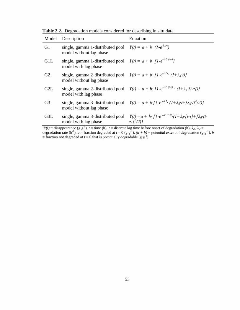
53
Table 2.2. Degradation models considered for describing in situ data
Model Description Equation1
G1 single, gamma 1-distributed pool
model without lag phase
Y(t) = a + b∙ (1-e-kd∙t
)
G1L single, gamma 1-distributed pool
model with lag phase
Y(t) = a + b∙ [1-e-kd∙ (t-η)
]
G2 single, gamma 2-distributed pool
model without lag phase
Y(t) = a + b∙ [1-e-λd∙t
∙ (1+λd∙t)]
G2L single, gamma 2-distributed pool
model with lag phase
Y(t) = a + b∙ [1-e-λd∙ (t-η)
∙ (1+λd∙[t-η])]
G3 single, gamma 3-distributed pool
model without lag phase
Y(t) = a + b∙[1-e-λd∙t
∙ (1+λd∙t+[λd∙t]2/2)]
G3L single, gamma 3-distributed pool
model with lag phase
Y(t) =a + b∙ [1-e-λd∙ (t-η)
∙(1+λd∙[t-η]+[λd∙(t-
η)]2/2)]
1Y(t) = disappearance (g∙g-1), t = time (h), η = discrete lag time before onset of degradation (h), kd , λd =
degradation rate (h-1), a = fraction degraded at t = 0 (g∙g-1), (a + b) = potential extent of degradation (g∙g-1), b
= fraction not degraded at t = 0 that is potentially degradable (g∙g-1)

54
Table 2.3. Chemical composition and RFV1 of forages
n Mean Minimum Maximum SD
--------------------------g∙kg DM-1
---------------------------
ECA
DM 20 870 842 896 14
NDF 20 431 329 502 45
ADF 20 304 218 369 45
HEM3
20 127 95 184 28
CP 20 208 150 293 38
RFV 20 143 119 203 23
LCA
DM 26 859 825 880 15
NDF 26 384 268 463 51
ADF 26 265 195 354 43
HEM3
26 119 66 185 37
CP 26 222 194 260 20
RFV 26 169 125 254 30
CSG
DM 11 876 867 892 7
NDF 11 658 452 772 81
ADF 11 338 299 380 28
HEM3
11 320 123 392 73
CP 11 123 60 174 33
WSG
DM 4 867 845 886 17
NDF 4 623 395 732 155
ADF 4 266 233 343 52
HEM3
4 357 155 484 154
CP 4 180 104 233 54
RFV 11 90 71.5 130 15
GL
DM 20 868 819 890 18
NDF 20 453 355 613 52
ADF 20 304 241 384 36
HEM3
20 149 101 272 41
CP 20 204 124 308 40
RFV 20 136 95 184 20 1RFV = relative feed value 2ECA = early cutting alfalfa, LCA = late cutting alfalfa, CSG = cool season grass, WSG = warm season
grass, GL = grass/legume mix
3HEM = hemicellulose

55
Table 2.4. Values of model selection criteria (SSRES, MSRES, and AIC) obtained when
fitting DM, CP, and NDF degradation data to models
Model1,2
Item3 G1 G1L G2 G2L G3 G3L
SSRES4,5
DM 1.80 1.61 1.57 1.43 1.67 1.32
CP 4.41 3.50 3.96 3.82 4.15 3.69
NDF 7.31 6.20 6.79 6.22 6.95 6.93
mean 4.41 3.77 4.11 3.82 4.26 3.98
MSRES4,6
DM 2.58 2.69 2.25 2.38 2.38 2.19
CP 5.88 5.83 5.66 6.36 5.93 6.15
NDF 9.13 8.86 8.49 8.89 8.69 9.91
mean 5.87 5.79 5.46 5.88 5.67 6.08
AIC4
DM -8.21 -6.99 -8.54 -6.97 -8.46 -7.06
CP -6.40 -4.90 -6.57 -4.74 -6.51 -4.79
NDF -7.28 -5.74 -7.50 -5.78 -7.44 -5.45
mean -7.30 -5.88 -7.54 -5.83 -7.47 -5.77 1G1= single, gamma 1-distributed pool model without lag phase, G1L= single, gamma 1-distributed pool
model with lag phase, G2 = single, gamma 2-distributed pool model without lag phase, G2L = single,
gamma 2-distributed pool model with lag phase, G3 = single, gamma 3-distributed pool model without lag
phase, G3L = single, gamma 3-distributed pool model with lag phase 2See Table 2.2 for model equations. 3SSRE S= residual sums of squares, MSRES=residual mean square, AIC = Akaike information criterion 4Values of SSRES, MSRES, and AIC by chemical fractions (DM, CP, and NDF), and the mean value across
chemical fractions 5Values listed are actual values102 6Values listed are actual values103

56
Table 2.5. Relative ranking (1-6) of degradation models according to average values of
model selection criteria (SSRES, MSRES, and AIC)1
Model2
Item3,4
G1 G1L G2 G2L G3 G3L
SSRES rank
mean 5.67 2.00 3.33 2.33 5.33 2.33
range 5-6 1-4 3-4 2-3 5-6 1-4
MSRES rank
mean 4.33 3.67 1.33 4.67 3.00 4.00
range 3-5 2-6 1-2 4-6 2-4 1-6
AIC rank
mean 3.67 4.33 1.00 5.33 2.00 4.67
range 3-5 3-5 1 4-6 2 4-6 1See Table 2.2 for model equations.
2G1 = single, gamma 1-distributed pool model without lag phase, G1L = single, gamma 1-distributed pool
model with lag phase, G2 = single, gamma 2-distributed pool model without lag phase, G2L = single,
gamma 2-distributed pool model with lag phase, G3=single, gamma 3-distributed pool model without lag
phase, G3L = single, gamma 3-distributed pool model with lag phase 3SSRES = residual sums of squares, MSRES = residual mean square, AIC = Akaike information criterion 4Mean and range ranks refer to rankings across fractions (DM, CP, and NDF).

57
57
Table 2.6. Degradation parameter estimates of forages by forage class and chemical fraction
Chemical fraction1
DM NDF ADF
HEM1
CP
Item2,3,4
mean SEM mean SEM mean SEM mean SEM mean SEM
ECA (n=20)5
λd , h-1
0·198 0·008 0·155 0·012 0·147 0·014 0·208 0·019 0·231 0·010
k , h-1
0·118 0·005 0·093 0·007 0·088 0·008 0·124 0·011 0·138 0·006
a, g∙g-1
0·341 0·023 ----- ----- ----- ----- ----- ----- 0·412 0·030
b, g∙g-1
0·419 0·021 0·554 0·019 0·535 0·018 0·626 0·026 0·483 0·027
(a+ b), g∙g-1
0·760 0·011 0·554 0·019 0·535 0·018 0·626 0·026 0·894 0·009
LCA (n=26)
λd , h-1
0·229 0·008 0·173 0·009 0·154 0·010 0·234 0·017 0·263 0·008
k , h-1
0·136 0·005 0·103 0·005 0·092 0·006 0·140 0·010 0·157 0·005
a, g∙g-1
0·387 0·022 ----- ----- ----- ----- ----- ----- 0·442 0·025
b, g∙g-1
0·407 0·018 0·537 0·016 0·514 0·015 0·584 0·025 0·481 0·022
(a+ b), g∙g-1
0·794 0·008 0·537 0·016 0·514 0·015 0·584 0·025 0·924 0·005
CSG (n=11)
λd , h-1
0·109 0·007 0·098 0·005 0·098 0·006 0·104 0·011 0·130 0·010
k , h-1
0·065 0·004 0·058 0·003 0·058 0·004 0·062 0·007 0·078 0·006
a, g∙g-1
0·246 0·018 ----- ----- ----- ----- ----- ----- 0·341 0·037
b, g∙g-1
0·451 0·020 0·583 0·026 0·589 0·032 0·576 0·035 0·507 0·032
(a+ b), g∙g-1
0·697 0·018 0·583 0·026 0·589 0·032 0·576 0·035 0·848 0·035
WSG (n=4)
λd , h-1
0·093 0·022 0·071 0·003 0·058 0·006 0·071 0·019 0·091 0·009
k , h-1
0·056 0·013 0·043 0·002 0·035 0·004 0·042 0·011 0·054 0·005
a, g∙g-1
0·250 0·016 ----- ----- ----- ----- ----- ----- 0·359 0·068
b, g∙g-1
0·421 0·018 0·567 0·017 0·535 0·029 0·515 0·039 0·424 0·055
(a+ b), g∙g-1
0·670 0·008 0·567 0·017 0·535 0·029 0·515 0·039 0·783 0·016
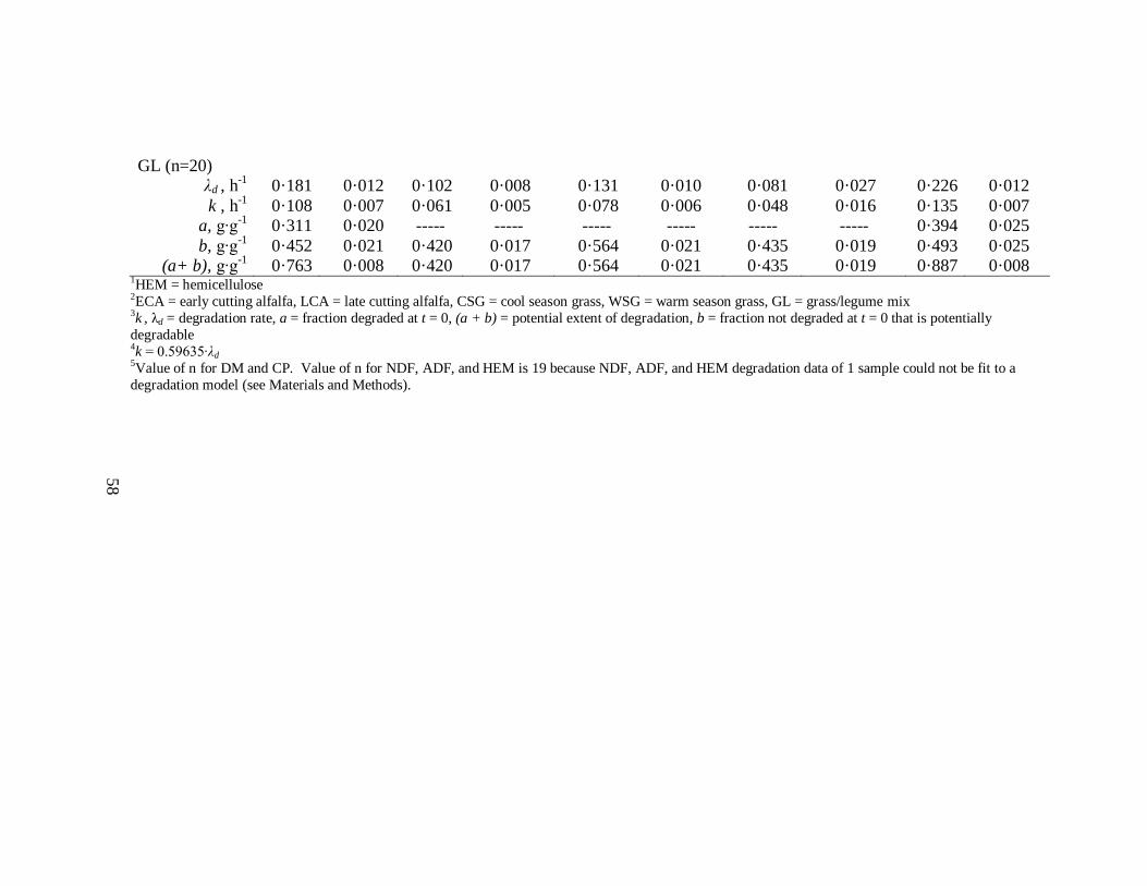
58
58
GL (n=20)
λd , h-1
0·181 0·012 0·102 0·008 0·131 0·010 0·081 0·027 0·226 0·012
k , h-1
0·108 0·007 0·061 0·005 0·078 0·006 0·048 0·016 0·135 0·007
a, g∙g-1
0·311 0·020 ----- ----- ----- ----- ----- ----- 0·394 0·025
b, g∙g-1
0·452 0·021 0·420 0·017 0·564 0·021 0·435 0·019 0·493 0·025
(a+ b), g∙g-1
0·763 0·008 0·420 0·017 0·564 0·021 0·435 0·019 0·887 0·008 1HEM = hemicellulose 2ECA = early cutting alfalfa, LCA = late cutting alfalfa, CSG = cool season grass, WSG = warm season grass, GL = grass/legume mix 3k , λd = degradation rate, a = fraction degraded at t = 0, (a + b) = potential extent of degradation, b = fraction not degraded at t = 0 that is potentially
degradable 4k = 0.59635∙λd 5Value of n for DM and CP. Value of n for NDF, ADF, and HEM is 19 because NDF, ADF, and HEM degradation data of 1 sample could not be fit to a
degradation model (see Materials and Methods).
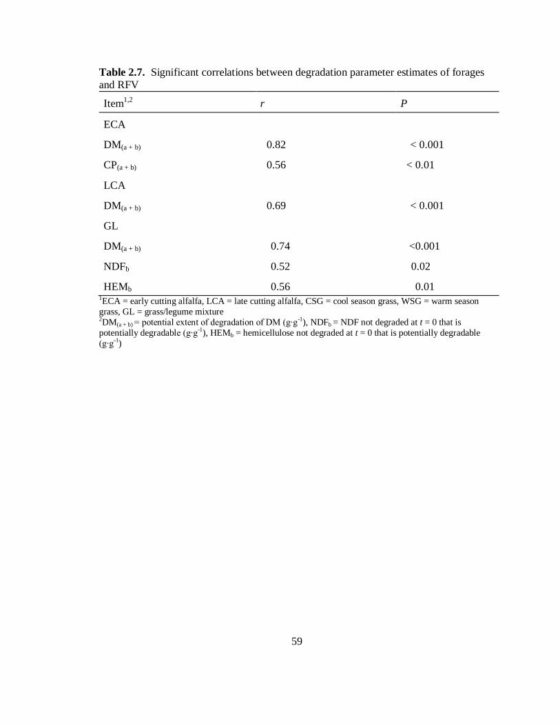
59
Table 2.7. Significant correlations between degradation parameter estimates of forages
and RFV
Item1,2
r P
ECA
DM(a + b) 0.82 < 0.001
CP(a + b) 0.56 < 0.01
LCA
DM(a + b) 0.69 < 0.001
GL
DM(a + b) 0.74 <0.001
NDFb 0.52 0.02
HEMb 0.56 0.01 1ECA = early cutting alfalfa, LCA = late cutting alfalfa, CSG = cool season grass, WSG = warm season
grass, GL = grass/legume mixture 2DM(a + b) = potential extent of degradation of DM (g∙g-1), NDFb = NDF not degraded at t = 0 that is
potentially degradable (g∙g-1), HEMb = hemicellulose not degraded at t = 0 that is potentially degradable
(g∙g-1)
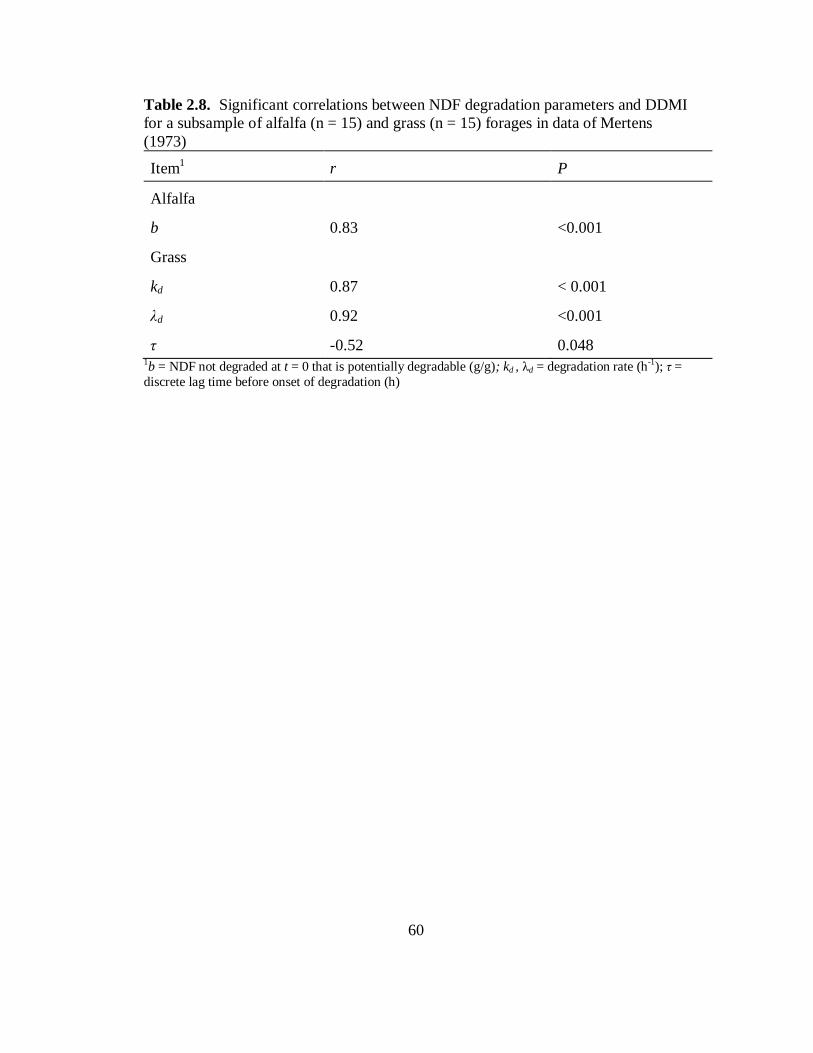
60
Table 2.8. Significant correlations between NDF degradation parameters and DDMI
for a subsample of alfalfa (n = 15) and grass (n = 15) forages in data of Mertens
(1973)
Item1 r P
Alfalfa
b 0.83 <0.001
Grass
kd 0.87 < 0.001
λd 0.92 <0.001
η -0.52 0.048 1b = NDF not degraded at t = 0 that is potentially degradable (g/g); kd , λd = degradation rate (h
-1); η =
discrete lag time before onset of degradation (h)

61
Dis
ap
pea
ran
ce o
f D
M,
g∙g
-1
A
B
C
Incubation time, h
Figure 2.1. Examples of bag observations that were identified as aberrant and
removed because they fulfilled one of the three conditions for bag removal described
in Materials and Methods. Each of the 2 points at each incubation time represents
one bag observation. (A) A 6 h bag observation (circled) from a 2002 GL sample
removed because it fulfilled condition 1; its disappearance value was 34.1% greater
than the mean disappearance of the 12 h bag observations (B) A 12 h observation
(circled) from a 2002 CSG removed because it fulfilled condition 2; its disappearance
value was 85.1% lower than the mean disappearance of the 6 h bag observations. (C)
A 48 h observation (circled) from a 2002 LCA bag pair that fulfilled condition 3; the
replicate error was 16.6%. The circled observation was judged to be the aberrant one
of the pair because its disappearance was abnormally high (0.990 g∙g-1
), both
absolutely and relative to the asymptotic disappearance value suggested by
observations prior to 48 h.
0.2
0.4
0.6
0.8
0 6 12 18 24 30 36 42 48
0.0
0.2
0.4
0.6
0.8
0 6 12 18 24 30 36 42 48
0.2
0.4
0.6
0.8
1.0
0 6 12 18 24 30 36 42 48

62
Dis
ap
pea
ran
ce o
f D
M,
g∙g
-1
Incubation time, h
Figure 2.2. An example of a 0 h bag pair that fulfilled condition 3 of the criteria for
bag removal (see Materials and Methods) but from which the aberrant bag of the pair
could not be identified for removal. The 0 h observations (bracketed for emphasis)
had poor repeatability (30.56% replicate error), but disappearance values of both
observations were reasonable according to behavior of the curve after 6 h, and thus
neither bag could be identified as aberrant and removed.
0.3
0.5
0.7
0.9
0 6 12 18 24 30 36 42 48
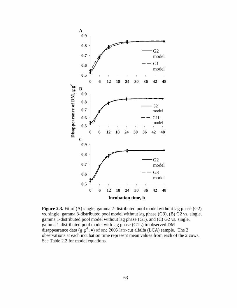
63
Dis
ap
pea
ran
ce o
f D
M,
g∙g
-1
A
B
C
Incubation time, h
Figure 2.3. Fit of (A) single, gamma 2-distributed pool model without lag phase (G2)
vs. single, gamma 3-distributed pool model without lag phase (G3), (B) G2 vs. single,
gamma 1-distributed pool model without lag phase (G1), and (C) G2 vs. single,
gamma 1-distributed pool model with lag phase (G1L) to observed DM
disappearance data (g∙g-1
; ♦) of one 2003 late-cut alfalfa (LCA) sample. The 2
observations at each incubation time represent mean values from each of the 2 cows.
See Table 2.2 for model equations.
0.5
0.6
0.7
0.8
0.9
0 6 12 18 24 30 36 42 48
G2
model
G1
model
0.5
0.6
0.7
0.8
0.9
0 6 12 18 24 30 36 42 48
G2 model
G1L model
0.5
0.6
0.7
0.8
0.9
0 6 12 18 24 30 36 42 48
G2
model
G3
model
64
CHAPTER 3
VARIABILITY IN RUMINAL DEGRADATION PARAMETERS CAUSES
IMPRECISION IN ESTIMATED RUMINAL DIGESTIBILITY
ABSTRACT
Ruminal digestibility of dietary ingredients is frequently estimated with degradation
parameters. Mean degradation parameters (e.g., those in a feed library) are often used,
but limited data suggests considerable variation around these means, potentially leading
to imprecise digestibility estimates. This experiment quantified degradation parameter
variation for forage hays and determined this variation’s impact on precision of ruminal
digestibility estimates. Degradation data were those previously published by our lab and
included degradation rate, λd (h-1
), fraction instantly degraded, a (g∙g-1
), degradation
extent, (a + b) (g∙g-1
), and fraction not instantly degraded that is degradable, b (g∙g-1
) of
alfalfa, grass, grass-legume hays. Ruminal digestibilities of chemical fractions (DM,
NDF, ADF, hemicellulose, CP) were estimated using these data. Ninety-five percent
confidence limits of digestibility were determined using propagation of uncertainty with
measured SD of degradation parameters. Values of CV for degradation parameters were
large; averaged across chemical fractions, they were 24.8, 28.6, 20.7, and 12.6% for λd ,
a, b, and (a + b). Ninety-five percent confidence limits of digestibility were large (80.5%
of digestibility means) and often overlapped each other, even where digestibility means
greatly differed numerically. Consequently, digestibility values computed with mean
degradation parameters may have little biological and practical significance. When

65
uncertainty in all parameters but λd was set to zero (λd alone had uncertainty), 95%
confidence limits still encompassed 54.5% of digestibility means. Thus, uncertainty in λd
alone causes considerable imprecision in estimated digestibility. These results caution
using mean degradation parameters to estimate digestibility.
INTRODUCTION
Grass and legume forages are key components of ruminant diets. Quality of these
forages and of other components of ruminant diets is largely influenced by their
digestibility (Minson, 1990), making a measure of digestibility useful in diet formulation.
Because measurement of digestibility in vivo is laborious and requires large amounts of
forage, digestibility is frequently estimated. Many current feed evaluation systems (e.g.,
Cornell Net Carbohydrate and Protein System [Sniffen et al., 1992]; Molly [Baldwin,
1995]; Beef NRC (2000); Dairy NRC [2001]) use ruminal degradation parameters (such
as rate and extent of digestion) to estimate ruminal digestibility, which in turn is used
with estimated post-ruminal digestion to calculate total tract digestibility. These feeding
systems use simple averages of degradation parameters, such as those compiled in a feed
library, to estimate ruminal digestibility. However, a limited number of sources suggest
considerable variability exists for these mean values for forages and other feeds (von
Keyserlingk et al., 1996; NRC, 2001; Hvelplund and Weisbjerg, 2000). This variability
raises questions about the precision of using simple averages to calculate digestibility.
More work needs to determine the actual variability in degradation parameters of forages
and to ascertain whether use of average values is valid.

66
The objectives of this study were to (1) determine the variability in ruminal
degradation parameters within and across hay forages, and (2) assess the impact of this
variability on the precision of digestibility calculations.
MATERIALS AND METHODS
Hay Types and Sampling Procedures
Hay samples were obtained from entries submitted to the Missouri State Fair Hay
Contest in 2002 and 2003. The entries came from across the state of Missouri and
included early-cut alfalfa (ECA; n = 20), late-cut alfalfa (LCA; n = 26), cool season grass
(CSG; n = 11), warm season grass (WSG; n = 4), and grass-legume (GL; n = 20)
samples. A detailed description of the species composition of the forages has been
reported in Chapter 2. Samples were collected from hay bales using a hay probe (Penn
State Forage Sampler; Nasco, Ft. Atkinson, CO), ground through a 2 mm screen with a
Wiley mill (Arthur H. Thomas Company, Philadelphia, PA), and stored in sealed plastic
bags at room temperature for further analysis.
In Situ and Chemical Analysis
In situ degradation characteristics were determined for all samples. Dacron bags
(10 x 20 cm; 50 ± 15μm pore size; ANKOM Technology, Macedon, NY) were filled with
5 ± 0·1 g (2003 samples) or 4 ± 0.1 g (2002 samples) of sample. Duplicate bags were
prepared for insertion into two cows, giving a total of four bags per sample at each
incubation time.
Two ruminally cannulated, multiparous Holstein cows housed in free-stall
facilities at the University of Missouri-Columbia Foremost Dairy Center were selected
for in situ procedures. All procedures involving the animals were approved by the

67
Animal Care and Use Committee, University of Missouri-Columbia. Each animal was
provided ad libitum access to a lactation diet (240 g corn silage, 123 g alfalfa hay, 150 g
alfalfa haylage, 467 g concentrate and190 g CP, 240 g ADF and 410 g NDF/kg DM)
formulated to meet their requirements (NRC, 2001). Bags containing 2003 hay samples
were inserted into 2 cows for 0, 6, 12, 24, and 48 h during one 2-d period. Bags
containing 2002 hay samples were inserted into 2 cows for 0, 8, 12, 24, and 48 h during
another 2-d period. However, one of the cows used to incubate 2002 samples stopped
ruminating during the sampling period, and the samples from this cow for that period
were discarded. New subsamples of the 2002 hay samples were incubated in this cow for
an additional 2-d period, with incubation times of 0, 6, 12, 24, and 48 h. Zero hour bags
were exposed to rumen fluid briefly (approximately 5 min) to allow hydration. All bags
were removed simultaneously, as suggested by Nocek (1988).
After removal from the rumen, bags were doused with cold water (approximately
15C) to halt fermentation and were rinsed until wash water ran relatively clear. Bags
were stored at <0C to await further processing. Once removed from storage, bags were
thawed to room temperature and washed in a domestic washing machine until the wash
water ran completely clear, as suggested by Cherney et al. (1990b). Samples were air-
dried in a 55C convection oven to a constant mass, then air-equilibrated and weighed to
determine residue mass. Residues were then removed and composited by duplicates
within cow. Bag residue and original forage samples were ground to pass through a 1-
mm screen and subsequently analyzed for DM, NDF, ADF, HEM, and CP as described in
Chapter 2.

68
Calculations and Statistical Analysis of In Situ Data
All degradation data were expressed as fractional disappearance. Using an
equation from Weisbjerg et al. (1990) (cited by Stensig et al. [1994]), NDF, HEM, and
ADF degradation data at each incubation time were corrected for insoluble material
washed out of the bag. Since NDF, ADF, and HEM are insoluble entities, it was assumed
that the truly soluble fraction was zero when applying the equation.
Aberrant bag observations were identified and eliminated using a method reported
in Chapter 2. Using the criteria for eliminating aberrant bag observations, nearly all
NDF, ADF, and HEM bag observations had to be eliminated for one 2003 ECA sample.
So few bag observations were left after this elimination that NDF, ADF, and HEM
degradation data could not be fit to a model for this forage sample.
In situ data were described using a single, gamma 2-distributed pool model
without lag phase (G2) model from Pond et al. (1988) and Ellis et al. (1994) as follows:
)]1()exp(1[)( ttbatY dd
where Y(t) is fractional disappearance (g∙g-1
), λd is degradation rate (h-1
), a is fraction
degraded at t = 0 (g∙g-1
), (a + b) is potential extent of degradation (g∙g-1
), b is fraction not
degraded at t = 0 that is potentially degradable (g∙g-1
), and t is time (h). The age-
dependent, G2 model was chosen over oft-used age-independent models (Ørskov and
McDonald, 1979) because the G2 model yielded lower values of Akaike information
criterion relative to age-independent models, indicating the G2 model provided fit
superior to that of first-order kinetic models for this dataset (see Chapter 2).
The PROC NLIN procedure of SAS (SAS Institute, Inc., Cary, NC) was used to
estimate parameters in the models for DM, NDF, ADF, HEM, and CP degradation data.
69
Because NDF, ADF, and HEM degradation data had been corrected to make
disappearance zero at t = 0, the value of a was constrained to zero for fitting procedures
for these fractions.
Most degradation rates reported in the literature are age-independent whereas λd is
an age-dependent rate (Pond et al., 1988; Ellis et al., 1994). Comparison between an age-
independent rate, kd (h-1
), and the age-dependent rate λd is not commensurate; an age-
independent rate is less than an age-dependent one when describing the same degradation
data. To allow more commensurate comparison, the mean degradation rate of λd , k, was
calculated as 0.5964 ∙ λd (Pond et al., 1988). This mean rate is effectively an age-
independent equivalent of an age-dependent rate and can be compared to age-
independent rates commonly reported in the literature.
At first, degradation data of each cow were kept separate for the fitting procedure.
However, after a preliminary ANOVA indicated that degradation parameter values did
not consistently differ across cow∙periods, cow∙period data were pooled by year of forage
(2002 or 2003), entailing that data of 2 cows (n = 2, 2002 and n = 2, 2003) were used to
construct each degradation curve.
Values of SD and CV of degradation parameter estimates were calculated for each
chemical fraction within forage class. Because values of SD and CV were similar across
forage classes, values were averaged across forage classes before they were tabulated.
These tabulated values should not be mistaken as SD and CV of data pooled by forage
class; data were separated by forage class when values of SD and CV were calculated,
and only thereafter were values of SD and CV averaged.

70
Statistical Analysis with Other Previously Published Degradation Data
The data of Mertens (1973), von Keyserlingk et al. (1996), NRC (2001), and
Hvelplund and Weisbjerg (2000) were used to calculate CV of degradation parameter
estimates for comparison with our own results. Values of CV for (a + b) and kd in
Mertens (1973) were calculated by compiling data in the appendix, which listed estimates
of (a + b) and kd individually for each experimental forage. When not reported in the
original publication, values of CV for a, b, and kd in von Keyserlingk et al. (1996) were
calculated directly using reported mean and SD pooled by forage class.
Because Hvelplund and Weisbjerg (2000) reported SD by forage species and not
forage class, SD for forage class was calculated by pooling variances of degradation
parameter estimates across forage species within a class. Similarly, because the NRC
(2001) reported SD by forage maturity and not forage class, SD for forage class was
calculated by pooling variances of degradation parameter estimates across forage
maturities within a class. Once values of SD were calculated in this way, values of CV
were then computed as with the data of von Keyserlingk et al. (1996).
Calculation of Ruminal Digestibility and 95% Confidence Limits
Predicted ruminal digestibilities of DM, ADF, HEM, and CP by forage class were
calculated using the equation
2
,|
2
,|
,,,)( pjid
jid
jijijik
baitydigestibil
[1]
where digestibilityi,j (g∙g-1
) is the ruminal digestibility of chemical fraction i (DM, ADF,
HEM, CP) and forage class j (ECA, LCA, CSG, WSG, GL); ai,j is a for chemical fraction
i and forage class j; bi,j is b for chemical fraction i and forage class j; λd|i,j is λd for

71
chemical fraction i and forage class j; and kp is the fractional rate of passage from the
rumen (h-1
), set to a constant value of 0·06 h-1
. This equation is conceptually analogous
to the oft-used equation
pd
d
kk
kbaitydigestibil
[2]
developed by Ørskov and McDonald (1979). Eq. 1 and 2 are derived using the same
biological principles and compute the same entity, though their precise mathematical
forms differ because of the use of the age-dependent rate λd in Eq. 1 in place of the
independent-rate kd in Eq. 2. (See Appendix for the derivation of Eq. 1)
Upper and lower 95% confidence limits (CL) of calculated digestibility were
determined using the law of propagation of uncertainty (e.g., Taylor, 1997; Heuvelink,
1998). Frequently used in the physical and quantitative sciences, the law of propagation
of uncertainty is employed to compute the amount of uncertainty (analogous to SD)
expected in a calculated quantity (e.g., digestibility) originating from uncertainty in one
or more measured quantities (e.g., a, b, λd) used in the calculations. In general, using a
first-order Taylor approximation, uncertainty in a dependent variable y that is a function
of independent variables x1, x2, . . . , xn is the following:
2
1 1
)],([lxkxlk
n
k
n
l lk
xxx
y
x
yy
[3]
where kx
y
and
lx
y
are the partial derivatives of y in respect to xk and xl , respectively;
∆xk and ∆xl are the uncertainties of xk and xl, respectively; and lxkx , is the correlation
coefficient between variables xk and xl. When k = l, the term 2
, klxkxlk xxx and
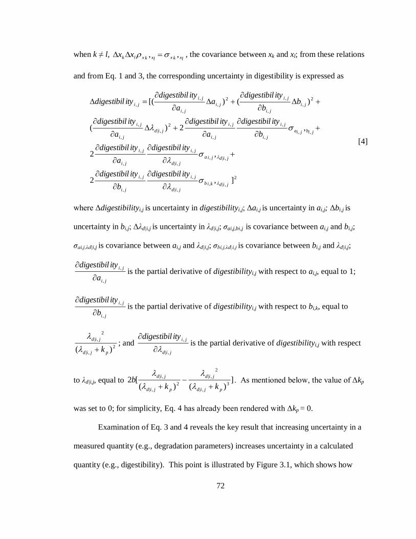
72
when k ≠ l, lxkxlxkxlk xx ,, , the covariance between xk and xl; from these relations
and from Eq. 1 and 3, the corresponding uncertainty in digestibility is expressed as
2
,|,
,|
,
,
,
,|,
,|
,
,
,
,,,
,
,
,2
,|
,
,
2
,
,
,2
,
,
,
,
],2
,2
,2)(
)()[(
jidkib
jid
ji
ji
ji
jidjia
jid
ji
ji
ji
jibjia
ji
ji
ji
ji
jid
ji
ji
ji
ji
ji
ji
ji
ji
ji
itydigestibil
b
itydigestibil
itydigestibil
a
itydigestibil
b
itydigestibil
a
itydigestibil
a
itydigestibil
bb
itydigestibila
a
itydigestibilitydigestibil
[4]
where Δdigestibilityi,j is uncertainty in digestibilityi,j; Δai,j is uncertainty in ai,j; Δbi,j is
uncertainty in bi,j; Δλd|i,j is uncertainty in λd|i,j; ζai,j,bi,j is covariance between ai,j and bi,j;
ζai,j,λd|i,j is covariance between ai,j and λd|i,j; ζbi,j,λd|i,j is covariance between bi,j and λd|i,j;
ji
ji
a
itydigestibil
,
,
is the partial derivative of digestibilityi,j with respect to ai,j, equal to 1;
ji
ji
b
itydigestibil
,
,
is the partial derivative of digestibilityi,j with respect to bi,k, equal to
2
,|
2
,|
)( pjid
jid
k
; and
jid
jiitydigestibil
,|
,
is the partial derivative of digestibilityi,j with respect
to λd|i,j, equal to ])()(
[23
,|
2
,|
2
,|
,|
pjid
jid
pjid
jid
kkb
. As mentioned below, the value of Δkp
was set to 0; for simplicity, Eq. 4 has already been rendered with Δkp = 0.
Examination of Eq. 3 and 4 reveals the key result that increasing uncertainty in a
measured quantity (e.g., degradation parameters) increases uncertainty in a calculated
quantity (e.g., digestibility). This point is illustrated by Figure 3.1, which shows how
73
uncertainty in b translates into uncertainty in digestibility. The solid black line represents
values of digestibility (computed with Eq. 1) when b varies from 0 to 1 (and with a and
d set to 0 and 0·075, values similar to those for NDF of WSG). The value of b is
0·08 and centered around b = 0·60 (values similar to those for NDF of WSG);
covariances and all other uncertainties are set to 0. As shown in Figure 3.1, a vertical line
extending from the lower bound of b on the x-axis intersects with a horizontal line
extending from the lower bound of itydigestibil on the y-axis, where the point of
intersection is a point on the graph of digestibility. A similar relationship is observed
between the upper bounds of b and itydigestibil (Figure 3.1). As such, when b is
increased, itydigestibil increases in kind. Note that the exact relationship between b and
digestibility shown in Figure 3.1 exists only when covariances and all other uncertainties
are equal to 0, but the general principle illustrated ( itydigestibil increases with b )
holds true under all conditions.
Further examination of Eq. 3 and 4 also reveals that increasing the partial
derivative of the measured quantity relative to the calculated quantity (i.e., kx
y
)
increases uncertainty, as does increasing the covariances between the measured quantities
(i.e., kxkx , ).
At first, Δai,j and Δbi,j were set to the standard deviations of ai,j and bi,j measured
in the study, and so too were covariances set to their measured values, in order to
determine the composite effect of Δai,j, Δbi,j, and Δλd|i,j on Δdigestibilityi,j. Next, Δai,j and
Δbi,j were set to zero in order to study the effect of Δλd|i,j on Δdigestibilityi,j in isolation.
In all analyses, the values of Δλd|i,j and Δkp were set to the SD of λd|i,j and 0, respectively.

74
For calculating the composite effect of Δai,j, Δbi,j, and Δλd|i,j on Δdigestibilityi,j,
methods other than law of propagation of uncertainty may be employed; one alternative
is to determine digestibility of each sample using Eq. 1 and then compute the SD of these
digestibility values to yield Δdigestibilityi,j when Δai,j, Δbi,j, and Δλd|i,j are equal to their
SD. However, only the law of propagation of uncertainty can be used for the more
complex analysis in which the effect of Δλd|i,j on Δdigestibilityi,j is studied in isolation.
For this reason, the law of propagation of uncertainty was used for all analyses.
Upper and lower 95% CL were computed as the quantity
1,0250,, njiji titydigestibilitydigestibil
where t0·025,n-1 = critical value of the right tail of the t distribution with α / 2=0·025 and
with n - 1 degrees of freedom (n = number of digestibilityi,j observations).
RESULTS
The chemical composition of the forages is presented in Table 2.3. Numerically, both
alfalfa classes (ECA, LCA) had higher mean concentrations of CP and lower
concentrations of fiber (NDF, ADF, HEM) than for grass classes (CSG, WSG). Within
alfalfa, LCA had a numerically higher mean CP concentration and lower fiber
concentrations than for ECA. Within grasses, CSG had numerically higher mean CP
concentration and lower fiber concentrations than for WSG.
Table 2.6 reports means of degradation parameter estimates λd, k, a, b, and (a +
b). Mean values of (a + b) of DM and CP were numerically higher for alfalfa (ECA,
LCA) than for grass samples (CSG, WSG). Values of (a + b) of fiber (NDF, ADF,
HEM) were similar across classes. Mean values of λd and k were numerically higher for
alfalfa (ECA, LCA) than for grasses (CSG, WSG). Within alfalfa, λd and k were higher

75
for LCA than for ECA, and within grasses, these parameters were higher for CSG than
for WSG. Differences in λd and k were consistently preserved across chemical fractions
(DM, NDF, ADF, HEM, CP).
Table 3.1 reports their SD and CV of degradation parameter estimates (λd, k, a, b,
and [a + b]). Values in Table 3.1 were averaged across forage classes for brevity
because SD and CV did not vary appreciably across classes. Values of SD are large
relative to the mean, illustrated by large values of CV. Values of CV range from 17.3 to
36.2% for λd and k, 24.8 to 32.4% for a, 18.0 to 23.4% for b, and 5.5 to 16.4% for (a +
b). Values of CV for (a + b) were systematically smaller than for any other parameter,
while values of CV for other parameters (λd, k, a, and b) were similar in magnitude.
Similarly, values of CV for HEM were consistently larger than for any other chemical
fraction, and while CV for CP were systematically smaller.
Table 3.2 shows digestibility means and their associated upper and lower 95% CL
when Δλd, Δa, and Δb were set to the SD values of λd, a, and b measured in the study.
The mean digestibilities of CP range from 0.513 to 0.761 g∙g-1
for CP. Numerically,
these are generally higher than those of DM digestibility, with values of 0.406 to 0.642
g∙g-1
. These values are in turn numerically higher than those of NDF, ADF, and HEM,
which are themselves similar, with digestibilities ranging from 0.193 to 0.288 g∙g-1
for
NDF, 0.192 to 0.270 for ADF, and 0.217 to 0.396 g∙g-1
for HEM.
Within ECA, 95% CL of DM and CP are distinct from NDF and ADF, and all
other 95% CL overlap each other. Within LCA, 95% CL of CP digestibility are distinct
from those of HEM, ADF, and NDF digestibility; 95% CL of DM digestibility are
distinct from those of NDF and ADF digestibility; and all other 95% CL overlap each

76
other. Within CSG, the 95% CL of CP are distinct from all other chemical fractions
(DM, NDF, ADF, HEM), and all other 95% CL overlap each other. Within WSG, the
95% CL of DM are distinct from all other chemical fractions (NDF, ADF, HEM, CP),
and all other 95% CL overlap each other. Within GL, 95% CL of DM and CP
digestibility are distinct from those of NDF and ADF, and all other 95% CL overlap each
other.
When compared within the same chemical fraction, mean digestibilities for WSG
and CSG are systematically lower than for other forage classes, which are themselves
similar to each other (Table 3.2). As shown in Table 3.2, 95% CL of DM, NDF, ADF,
HEM, and CP digestibility overlap each other across forage classes, with only one
exception (95% CL of DM digestibility of WSG were distinct those of LCA).
Table 3.3 shows digestibility means and their associated upper and lower 95% CL
when Δλd was set to the SD of λd measured in this study (and Δa and Δb were set to zero).
Mean digestibilities are the same as those reported in Table 3.2. Within ECA, LCA, and
CSG, 95% CL of CP and DM digestibility are distinct from each other and of all other
chemical fractions; and 95% CL of NDF, ADF, and HEM digestibility overlap each
other. A similar pattern is found for WSG, except 95% CL of HEM is not distinct from
that of DM. Within GL, 95% CL of CP digestibility are distinct from those of NDF,
ADF, and HEM digestibility; 95% CL of DM digestibility are distinct from those of NDF
and ADF digestibility; and all other 95% CL overlap each other.
Compared across forages, 95% CL of DM digestibility for CSG and WSG are
distinct from those for ECA, LCA, and GL. Additionally, 95% CL of CP digestibility for
WSG are distinct from those for ECA, LCA, and GL, and 95% CL for CP digestibility

77
for CSG are distinct from those for LCA. All other 95% CL of forage classes overlap
each other.
DISCUSSION
Chemical Composition and Degradation Parameter Means
The mean and SD of the chemical composition data in Table 2.3 were generally
similar to those summarized by the Dairy NRC (2001), though our samples of WSG had
lower NDF, ADF, and HEM and higher CP than reported by the NRC (2001). These
results suggest a representative range of forages was included in this study. With the
exception of λd, (see below), degradation parameter means in Table 2.6 are similar to
those presented by other reports (Smith et al., 1972; Mertens, 1973; von Keyserlingk et
al., 1996), indicating they are suitable for the digestibility analyses below. Values of λd
generated in this study are numerically greater than degradation rate values reported by
other investigators because λd is a age-dependent degradation rate whereas most
degradation rates reported in the literature are age-independent rates. For commensurate
comparison between degradation rates in this and prior studies, the mean degradation rate
k should be used for reference (Materials and Methods).
Variation in Degradation Parameter Estimates
For comparison with values in Table 3.1, we summarize CV values for
degradation parameters estimates from prior studies. In the data of von Keyserlingk et al.
(1996) values of CV for a, b, and kd of CP were 11.4, 20.1, and 35.1% for alfalfa hay and
26.3, 24.1, and 34.9% for grass hay. For DM, values of CV for a, b, and kd were 7.9, 7.4,
and 36.7% for alfalfa hay and 16.3, 25.6, and 36.8% for grass hay. Similarly, in the data
of Hvelplund and Weisbjerg (2000), values of CV of a, b, and kd were 11.1, 16.0, and

78
27.2% for alfalfa CP. In the same dataset, values of CV of a, b, and kd were 21.8, 17.6,
and 24.7% for CSG CP. In the data of NRC (2001), values of CV of a, b, (a + b) and kd
were 34.8, 32.2, 11.2, 46.5% for alfalfa CP. In the same dataset, values of CV of a, b, (a
+ b) and kd were 22.7, 20.4, 4.8, and 35.5% for CSG CP. In Mertens (1973), values of
CV of (a + b) and kd for NDF were 18.1 and 21.5% for alfalfa; 14.8 and 19.6% for
GL;10.9 and 29.3 for CSG; and 12.8 and 25.5% for WSG.
In sum, literature values of CV for a range from 7.9 to 34.8%; those for b range
from 7.4 to 32.2%; those for (a + b) range from 4.8 to 18.1; and those for kd range from
19.6 to 36.5%, with no clearly detectable differences across forage classes (alfalfa, GL,
CSG, WSG) or chemical fractions (DM, CP, NDF). Coefficient of variation values for
DM, CP, and NDF in our own dataset (Table 3.1) generally fall within these ranges. The
large amount of variability we found in degradation parameters values is thus reasonable.
Note that in prior reports, CV for degradation rate were larger than CV of other
parameters, unlike in this experiment.
In general, the reason for variation in degradation parameter estimates is due to a
combination of (1) variation truly attributable to chemical fraction and forage class and
(2) procedural variation. For in situ studies (such as the current), common sources of
procedural variation arise from factors such as bag characteristics (material, size, pore
size, sample size:surface area), sample preparation (grind size), incubation procedure
(presence or absence of pre-incubation, reticuloruminal region in which bags are
incubated, incubation times, order of bag removal and insertion), replications (number of
animal, day, and bag replications), rinsing technique (hand vs. mechanical rinsing), and
animal-related parameters (species, diet, temporal and individual variation in
79
reticulorumen environment) (Nocek, 1988; Vanzant et al., 1998). Most of these factors
(bag characteristics, sample preparation, incubation technique, rinsing technique, animal
species, diet) were controlled in this study by adopting a standardized procedure. Other
sources of variation, such as variation among animals, days, and replicate bags (Mehrez
and Ørskov, 1977; Vanzant et al., 1998) were reduced by use of multiple animals (2 per
forage) and bags (2 per animal).
Though extensive effort was made to minimize procedural error relative to
variation attributable to chemical fraction and forage class, procedural error may have
still been appreciable. In this context, it is difficult to explain systematic differences in
CV across degradation parameters and chemical fractions, for these differences are
confounded by the two sources of variation defined above. For example, the consistently
smaller CV for (a + b) compared to other degradation parameters could be caused by
lower measurement error due to some feature of the procedure, or lower true variation in
this parameter across chemical fractions and forages, or both. Whatever its source,
variation in degradation parameters was substaintial and comparable to studies using a
wide range of in situ and in vitro methodology.
Calculated Digestibilities and Their 95% CL
Many feed analysis systems (e.g., Cornell Net Carbohydrate and Protein System
[Sniffen et al., 1992]; Molly [Baldwin, 1995]; Beef NRC [2000]; Dairy NRC [2001]) use
degradation parameter estimate means to calculate ruminal digestibility or TDN.
Because of the considerable variability in degradation rate and other degradation
parameter estimates, as discussed above, the precision in using simple means may be
questioned. To determine variability in ruminal digestibility calculated using mean

80
values, 95% CL of digestibility was computed using the law of propagation of
uncertainty.
Values in Table 3.2 (where λd , a, and b equal their SD) represent the case in
which digestibility is calculated from estimated a, b, and λd means, such as those from a
feed library. There existed large numerical differences in digestibilities across chemical
fractions, with CP digestibility higher than DM digestibility, which is in turn higher than
NDF, ADF, and HEM digestibilities (which are themselves similar). There existed large
numerical differences across forage classes, also, with digestibilities of ECA, LCA, and
GL systematically higher than those of CSG and WSG (which are themselves similar).
However, these appreciable numerical differences are often not preserved when
comparing 95% CL (Table 3.2). As suggested by their frequent overlapping, 95% CL
span a wide range of values, equal to 80.5% of their associated digestibility means on
average. These findings, together with those discussed above, suggest digestibility values
calculated using mean values of a, b, and λd may have limited practical and biological
meaning.
Note that kp and chemical composition of the forages was assumed to have no
uncertainty–i.e., there is assumed to be no error in their estimation. Because there is
considerable variability in kp and published equations predict kp with low precision (the
best equation for predicting kp of forages in Seo et al. [2006] had a root mean square
prediction error of 0·011 h-1
with R2 = 0·39), 95% CL would be much greater in more
practical cases–in which kp was not known and thus had to be estimated–than in Table 3.2
where it is assumed to be known with certainty. In all likelihood, the 95% CL reported in
81
Table 3.2 are greatly underestimated. This further cautions the use of mean values of a,
b, and λd to calculate digestibility.
Analysis Where a and b are Known with Certainty
Values of a and b may often be measured or estimated readily using solubility and
chemical assays, such as buffer-soluble N (Krishnamoorthy et al., 1983), which is used to
estimate a for CP, and lignin, used to predict b for NDF (Smith et al., 1972; Mertens,
1973; Traxler et al., 1998). To mimic cases in which a and b are measured, 95% CL
were re-calculated assuming that a and b were known with certainty, and λd alone had
uncertainty (Table 3.3).
The 95% CL in Table 3.3 overlap each less frequently than in Table 3.2,
compared both within and across forage classes. However, considerable variation in
calculated digestibility is still present when a and b are known with certainty. On
average, 95% CL encompass values 54.4% of their associated digestibility means. This
percentage is less than that when a and b are uncertain (80.5%), but it is still large enough
to limit the practical and biological meaning of the calculated digestibilities.
As discussed above, kp of the forages were assumed to have no uncertainty, and
thus the 95% CL listed in Table 3.3 are likely to be smaller than realized when kp must be
estimated. Note also that it is unrealistic to assume values of a and b with absolute
certainty, as done in calculating 95% CL reported Table 3.3. At the very least, analytical
error in measuring a and b contributes uncertainty to the values of these parameter.
Further, a and b may not be measured directly but estimated from another chemical or
physical measurement; for example, b of NDF is often estimated from lignin content of
the NDF (Smith et al., 1972; Mertens, 1973; Traxler et al., 1998); errors in this estimation

82
add uncertainty. Overall, due to these sources of uncertainty that were not accounted in
the calculations in this report, the widths of the 95% CL in Table 3.3 are likely
underestimated.
Here and throughout, one may attribute the large 95% CL we found to some
suspected peculiarity in our in situ procedure, kinetic model (Eq. 1), uncertainty analysis
(Eq. 4), or some other aspect of our methodology. We reemphasize that the amount of
variability in degradation parameter values we found is comparable to that of in vitro and
other in situ studies using a wide range of methodology. Though we fully carried out
uncertainty analysis with our parameter values alone, we would expect similarly large
95% CL using values from other reports because of this comparable variability (c.f.,
Figure 3.1 and Materials and Methods). While largely foreign to animal and nutritional
sciences, the uncertainty analysis we used is itself well-accepted in the physical sciences.
The large 95% CL we found are thus not artifacts of the conditions of our study.
These results caution the use of mean degradation parameter values in estimating
digestibility. As a corollary, caution should be exercised when using digestibility values
garnered from feed analysis systems that rely on approaches to calculate digestibility
similar to those used in this report. Because uncertainty in λd contributes appreciable
uncertainty in calculated digestibility, techniques to efficiently measure or effectively
estimate λd should continue to be developed. One promising approach is that of Van
Soest et al. (2000), who developed multiple regression equations that accurately predict
the degradation rate of forage NDF from chemical composition and in vitro digestibility.
The dataset from this study could be used to further validate the equations of Van Soest et
al. (2000) and formulate similar equations for non-NDF chemical fractions.

83
APPENDIX
Digestibility is the sum of ai,j and bi,j that is digested in the rumen:
jijiji baitydigestibil ,,, '
where ai,j’ and bi,j’ are ai,j and bi,j that is digestible (g∙g-1
). The terms ai,j’ and bi,j’ are
explicitly defined as
jijiaji apa ,,, '
and
jijibji bpb ,,, '
where pai,j and pbi,j are the fractions (g∙g-1
ai,j or bi,j) of ai,j and bi,j that is digestible. It is
assumed that the ai,j fraction is completely digestible—i.e. pai,j = 1—following its
definition that it is instantly degraded. For the G2 model used in this report, pbi,j is equal
to
2
,|
2
,|
)(,
pjid
jid
bk
pji
.
This follows from the definition of fractional digestibility as the amount of material (in
this case, bi,j) that disappears by digestion divided by its total disappearance;
mathematically, this is equivalent to the integral (over the interval t = 0 to infinity) of
ri,j(t), the rate function for digestion of bi,j (h-1
), multiplied by Bi,j(t), the amount of bi,j
remaining over time (g∙g-1
bi,j):
2
,|
2
,|
,,)(
)]()([,
pjid
jid
otjijib
kdttBtrp
ji
(For a G2 model, ri,j(t) is (Pond et al., 1988; Ellis et al., 1994)

84
t
ttr
jid
jid
ji
,|
2
,|
,1
)(
,
and the term Bi,j(t)
)](exp[)1()( ,|,|, pjidjidji ktttB
is the solution to the differential equation that describes the change of Bi,j(t) over time by
due digestion and passage:
)(])([)(
,,
,tBktr
dt
tdBjipji
ji .)
Making the appropriate substitutions, the final digestibility equation (Eq. 1 in the text) is
then
2
,|
2
,|
,,,)( pjid
jid
jijijik
baitydigestibil
.

85
Table 3.1. Standard deviation and CV of degradation parameter estimates, averaged by
chemical fraction1,2
Degradation parameter
λd k a b (a + b)
DM
SD 0.031 0.019 0.079 0.077 0.041
CV, % 17.3 17.3 24.8 18.0 5.5
NDF
SD 0.032 0.019 ----- ----- 0.073
CV, % 21.7 21.7 ----- ----- 12.9
ADF
SD 0.038 0.023 ----- ----- 0.088
CV, % 29.1 29.1 ----- ----- 15.7
HEM
SD 0.069 0.041 ----- ----- 0.097
CV, % 36.2 36.2 ----- ----- 16.4
CP
SD 0.037 0.022 0.127 0.111 0.065
CV, % 19.7 19.7 32.4 23.4 10.1 1kd , λd, degradation rate (h-1); a, fraction degraded at t = 0 (g∙g-1); (a + b), potential extent of degradation
(g∙g-1); b, fraction not degraded at t = 0 that is potentially degradable (g∙g-1); HEM, hemicellulose. 2Values of SD and CV are averaged across forage class. Units for SD are h-1 for λd and k and g∙g-1 for a, b,
and (a + b).

86
Table 3.2. Calculated digestibility of chemical fractions by forage class and upper and
lower 95% confidence limits (CL), using uncertainty values of λd , a, and b equal to their
SD1,2
Forage class
ECA LCA CSG WSG GL
------------------------------------g∙g-1
------------------------------------
DM
Digestibility3
0.588a
0.642ab
0.436ab
0.406a
0.570a
Lower 95% CL 0.456 0.508 0.301 0.324 0.434
Upper 95% CL 0.720 0.777 0.571 0.487 0.707
NDF
Digestibility3
0.288b
0.296c
0.225b
0.193b
0.296b
Lower 95% CL 0.157 0.177 0.113 0.123 0.192
Upper 95% CL 0.420 0.415 0.337 0.264 0.401
ADF
Digestibility3
0.270b
0.266c
0.226b
0.192b
0.266b
Lower 95% CL 0.123 0.167 0.114 0.120 0.158
Upper 95% CL 0.417 0.366 0.338 0.263 0.374
HEM
Digestibility3
0.377ab
0.370bc
0.231ab
0.217ab
0.396ab
Lower 95% CL 0.174 0.134 0.107 0.045 0.170
Upper 95% CL 0.581 0.606 0.355 0.389 0.623
CP
Digestibility3
0.716a
0.761a
0.597a
0.513ab
0.702a
Lower 95% CL 0.544 0.640 0.348 0.240 0.573
Upper 95% CL 0.877 0.882 0.847 0.787 0.831 a,b,cMeans with different superscripts within column have non-overlapping 95% CL 1λd, degradation rate (h-1); a, fraction degraded at t = 0 (g∙g-1); b, fraction not degraded at t = 0 that is
potentially degradable (g∙g-1); (a + b), potential extent of degradation; ECA, early-cut alfalfa; LCA, late-
cut alfalfa; CSG, cool season grass; WSG, warm season grass; GL, grass-legume mixture; HEM,
hemicellulose. 2Values calculated using Eq. 1 and 4 in text and passage rate of 0·06 h-1. 3All means within rows have overlapping 95% CL; corresponding superscript symbols omitted for brevity.

87
Table 3.3. Calculated digestibility of chemical fractions by forage class and upper and
lower 95% confidence limits (CL), using uncertainty values of λd equal to its SD1,2
Forage class
ECA LCA CSG WSG GL
------------------------------------g∙g-1
------------------------------------
DM
Digestibility 0.588b,x
0.642b,x
0.436b,y
0.406b,y
0.570ab,x
Lower 95% CL 0.539 0.602 0.391 0.387 0.497
Upper 95% CL 0.636 0.683 0.481 0.424 0.644
NDF
Digestibility 0.288c
0.296c
0.225c
0.193c
0.296c
Lower 95% CL 0.173 0.212 0.175 0.146 0.209
Upper 95% CL 0.404 0.381 0.275 0.241 0.383
ADF
Digestibility 0.270c
0.266c
0.226c
0.192c
0.266c
Lower 95% CL 0.136 0.169 0.143 0.104 0.145
Upper 95% CL 0.404 0.364 0.309 0.280 0.387
HEM
Digestibility 0.377c
0.370c
0.231c
0.217bc
0.396bc
Lower 95% CL 0.239 0.258 0.172 0.011 0.227
Upper 95% CL 0.516 0.483 0.290 0.423 0.566
CP
Digestibility 0.716a,xy
0.761a,x
0.597a,yz
0.513a,z
0.702a,xy
Lower 95% CL 0.664 0.722 0.530 0.436 0.640
Upper 95% CL 0.767 0.801 0.665 0.590 0.763 a,b,cMeans with different superscripts within column have non-overlapping 95% CL x,y,zMeans with different superscripts within row have non-overlapping 95% CL 1λd, degradation rate (h-1); ECA, early-cut alfalfa; LCA, late-cut alfalfa; CSG, cool season grass; WSG,
warm season grass; GL, grass-legume mixture; HEM, hemicellulose.
2Values calculated using Eq. 1 and 4 in text and passage rate of 0·06 h-1.

88
dig
esti
bil
ity,
g∙g
-1
b, g∙g
-1
Figure 3.1. Graphical illustration of how increasing uncertainty in a measured quantity
(e.g., degradation parameters) increases uncertainty in a calculated quantity (e.g.,
digestibility) according to the law of propagation of uncertainty. Digestibility (solid
black line) is computed using Eq. 1 in the text with b (fraction not degraded at t = 0 that
is potentially degradable [g∙g-1
]) varying from 0 to 1 and a (fraction degraded at t = 0
[g∙g-1
]) and d (degradation rate [h-1
]) held constant at 0 and 0·075. The value of b
(uncertainty in b) is 0·08 and is centered around b = 0·60, with covariances and all other
uncertainties set to zero. Dashed lines mark the upper and lower bounds of b and
itydigestibil (uncertainty in digestibility). The point of intersection between horizontal
and vertical lines extending from the lower bounds of b and itydigestibil is a point on
the graph of digestibility; a similar relationship exists between the upper bounds of the
two variables. Increasing b hence increases itydigestibil .
0
0.05
0.1
0.15
0.2
0.25
0.3
0 0.1 0.2 0.3 0.4 0.5 0.6 0.7 0.8 0.9 1
Δb
Δdigestibility

89
CHAPTER 4
USING YTTERBIUM-LABELED FORAGE TO INVESTIGATE PARTICLE
FLOW KINETICS ACROSS SITES IN THE BOVINE RETICULORUMEN
ABSTRACT
To better understand particle flow kinetics across the reticulorumen (RR), we monitored
concentrations of Yb-marked forage across several RR sites over time. We fed three
forages (bromegrass, high-quality alfalfa, low-quality alfalfa) ad libitum to lactating
Holstein dairy cows in an incomplete 3x3 Latin square design. After dosing Yb-marked
forage in the mid-dorsal sac (DS), we determined Yb concentrations of particulate
samples taken from several sites (DS, ventral sac [VS], ventral blind sac [VBS],
reticulum [RT]) from 0 to 72 h. For each site we constructed marker concentration
profiles and applied non-parametric (local quadratic) and parametric (two-
compartmental, G2→G1→O) regression models to these profiles. We determined mean
residence time (MRT) and peak marker concentration using the original profile
observations and regressions. Across forage diets, intake of DM differed (P = 0.022) but
that of other chemical fractions did not (P = 0.125). The local regression fit the data well
visually, and MRT calculated using this model and original observations closely agreed.
This suggests the local regression successfully smoothed the original observations, which
had considerable stochastic variation, without changing the underlying shapes they
implied. Similar considerations showed the G2→G1→O model fit the data poorly.
Visually, marker profiles shapes varied greatly, but we found few differences attributable
90
to diet and site. Mean residence and peak marker concentration times, which reflect
marker profile shape, did not strongly differ by diet (P = 0.434, 0.0824) or site (P =
0.113, 0.0824), though they did by cow (P = 0.036, 0.004). These results further show
differences in profile shapes—and the particle flow kinetics they reflect—are explained
poorly by diet and site but somewhat explained by unidentified animal factors. Based on
studies that demonstrate particles flows through RR in the partial order
DS→VBS↔VS→RT, we expected MRT values to follow the order MRTDS < MRTVS ≈
MRTVBS < MRTRT (where MRTi is MRT of the ith site). Our finding that MRT values
were similar across sites suggests that once a particle escapes from the DS for the final
time, it must escape from ventral regions (VS, VBS, RT) soon after entry. Our attempt to
model these particle flow kinetics more quantitatively failed. Still, the experiment
suggests that feed products designed to initially enter the ventral rumen and resist
regurgitation should pass quickly from the RR.
INTRODUCTION
The kinetics of digesta flow and passage in the reticulorumen (RR) affect many digestive
parameters, namely nutrient digestibility and voluntary feed intake. Digestibility is
nutrient absorption rate divided by total disappearance rate (absorption and passage), and
thus it depends on the precise kinetic pattern of digesta passage (Waldo, 1972; Allen and
Mertens 1988). When steady-state conditions apply, rate of feed intake is equal to
disappearance rate and thus partly a function of particle flow kinetics (Allen and Mertens,
1988).
Pulse-dosing feed particles mordanted with an external marker, then monitoring
marker concentration over time to construct a marker profile, permits particle flow
91
kinetics to be described in detail (Ellis et al., 1979). Such methods have been repeatedly
used to describe flow kinetics across the entire RR or at sites distal to it (duodenum,
ileum, rectum). However, few studies have examined marker profile kinetics at different
sites within the RR. The few studies that have done so examined flow at two sites only
(dorsal and ventral sacs [Ellis et al., 1979; Dixon et al., 1983; Ellis et al., 1994; Poppi et
al., 2001] or dorsal sac and reticulum [Balch, 1950]) or used such infrequent sampling
(every 6 h at most) that identifying differences across sites is difficult (Walz et al., 2004).
Understanding flow kinetics at different sites within the RR and how they integrate
together may explain the overall pattern of particle flow dynamics and passage from the
RR as a whole.
The objective of this study was to determine Yb marker profiles at multiple sites
within the RR (dorsal sac, ventral sac, ventral blind sac, reticulum) when three forage
(bromegrass, low-fiber alfalfa, high-fiber alfalfa) were fed.
MATERIALS AND METHODS
Animals and Diets
Three hays, a bromegrass (BG; Bromus inermis), a low-fiber alfalfa (LFA;
Medicago sativa), and a high-fiber alfalfa (HFA), were fed to one multiparous and three
primiparous lactating Holstein cows (mean BW of 499 ± 50 kg; mean±SD) fitted with a
permanent rumen cannula. Hays were chopped through a TMR mixer (New Direction
Equipment, Sioux Falls, SD) before feeding. All procedures involving the animals were
approved by the Animal Care and Use Committee, University of Missouri-Columbia.
The experimental design was an incomplete 3x3 Latin square, with four cows in the first
period (with two cow replicates for HFA) and three in the second period (one

92
primiparous cow was removed midway during collection phase of the second period due
to illness).
Marker Preparation
Eight kilograms of chopped BG, HFA, and LFA were soaked overnight in
approximately 125 L of distilled H2O to remove soluble material and subsequently dried
to 105°C on 1-mm i.d. wire screens. Dried forage was then soaked overnight in a
distilled H2O solution containing 12.5 mg YbCl3∙6H2O∙g DM-1
with pH adjusted to 3.00
with H2SO4 (to remove Yb from acid-labile binding sites) To remove loosely-bound Yb,
labeled forage was washed on 1-mm i.d. wire screens once per hour for six hours, until
wash water ran clear. Absence of Yb in washwater was confirmed using a phosphate
buffer with pH = 10 (Teeter, 1984).
Passage trial
During an initial adjustment phase, animals were housed in free-stall barns of the
University of Missouri-Columbia Foremost Dairy Center. Adjustment was 9 d during the
first period and 6 d during the second. Length of adjustment was longer during the first
period because animals were fed a total mixed ration (467 g∙kg DM-1
concentrate) prior
to first period and displayed poor intakes during the initial days of adjustment; prior to
the second period, animals were fed the experimental all-forage diets and showed little
initial intake depression. Animals were fed approximately 110% ad libitum intake of
BG, HFA, or LFA diets through electronic feeding gates (American Calan, Inc.,
Northwood, NH). Fresh diet was provided at 06:00, 14:00, and 22:00 and orts removed
at 06:00 the following day.
93
During the following 3-d collection phase, animals were fed 110% of DM intake
established during last 3 d of adjustment. Fresh diet was fed and orts removed at same
times as during adjustment. To facilitate intense sampling on collection day 1, on that
day animals were housed in tie-stall barns of University of Missouri-Columbia Foremost
Dairy Center. Thereafter animals were transferred to free-stall barns for the remaining
collection days. Approximately 100 g of feed and orts were sampled once daily for all
collection days; samples were placed in sealed plastic bags then stored at <0°C to await
chemical analysis.
At 08:00 of collection day one, animals were dosed approximately 350 g Yb-
marked forage (BG, HFA, or LFA, corresponding with diet fed) by placing the marked
forage in the mid-dorsal rumen sac (DS) (Figure 4.1). The marked forage was firmly
embedded in the center of the rumen mat in the DS but not mixed within. Between 100
and 200 mL of digesta contents were sampled from the DS, mid-ventral sac (VS), caudo-
ventral blind sac (VBS), and ventral reticulum (RT) (Figure 4.1) at 0 (predosing), 1, 2, 3,
4, 6, 8, 10, 12, 16, 20, 24, 28, 32, 36, 40, 44, 48, 54, 60, 66, and 72 h relative to dosing
(Figure 4.1). Samples were collected using a 250 mL plastic container. To sample from
sites below the DS (VS, VBS, RT), the container was cupped with one hand (avoiding
inadvertent sampling of the DS) and led down the wall of the rumen (avoiding mixing of
DS with other sample sites). Immediately after sampling, sampled contents were removed
from containers, strained through two layers of cheesecloth, returned to containers, and
stored at <0°C to await further processing.
94
Chemical Analyses
After thawing, orts and feed samples were ground with a Wiley mill (Arthur H.
Thomas Company, Philadelphia, PA) to pass through a 1-mm screen and analyzed for
DM by drying at 105°C for 24 h; neutral detergent fibre (NDF) including residual ash
(using heat-stable α-amylase and sodium sulphite) and acid detergent fibre (ADF)
according to Van Soest et al. (1991) in an ANKOM200
Fiber Analyzer (ANKOM
Technology); and total N by combustion analysis (LECO FP-428; LECO Corporation, St.
Joseph, MI).
After thawing, rumen contents samples were dried to a 55°C oven to a constant
mass. Subsamples were analyzed for DM by drying at 105°C for 24 h. Yb was extracted
from contents using ethylenediaminetetraacetic acid solution and its concentration
analyzed using atomic absorption spectrophotometry (S Series AA Spectrometer; Thermo
Electron Corporation, Beverly, MA), as described by Hart and Polan (1984).
Regression with Yb Profile Data
Examination of the raw marker profiles revealed considerable stochastic variation
(―noise‖) that tended to mask the overall shapes of the profiles. To reduce this variation
and better visualize the underlying shape of the profiles, we applied both parametric and
non-parametric regressions to the original profile observations (hereto referred to as the
raw observations). A non-parametric regression has the advantage of flexibility, as it
does not rely on or assume any structured (i.e., parametric) equation form and can thus fit
a range of curve shapes. While less flexible, a parametric regression (i.e., a regression
that uses a structured equation form) has the advantage of delivering parameter estimates,

95
which can be used for quantitatively summarizing and comparing the results of fitted
curve shapes.
The non-parametric regression was a local regression model (a robust local
averaging procedure) fitted using LOCFIT package of R (Loader, 1999). The model
chosen was a local quadratic model with Gaussian kernel and nearest neighbor bandwidth
of 0.4, parameters which visually provided the smoothest fit while minimizing
underestimation at profile peaks and overestimation at early sampling times. Using the
local regression model, values of marker concentration were predicted at each of the
original sampling times (0 thorugh 72 h) to construct a dataset of smoothed values. The
smoothed dataset was subjected to the following data editing procedures. First, all 0 h
smoothed observations were adjusted to 0 ppm, as the 0 h observation was defined as 0
ppm during spectrometric analysis. Also, all values <0 ppm were raised to 0 ppm, which
was defined as the minimum concentration of marker during spectrometric analysis.
The parametric models included the two-compartmental models of Pond et al.
(1988) and Ellis et al. (1994). These models assume gamma-distributed residences times
in the first compartment and exponentially-distributed times in the second, sequential
compartment. The equation form of these models is the following:
])!(
)([)(
1
n
i
ittkn
in
teeCtY
where Y(t) is the concentration of marker at time t, C is the initial concentration of marker
entering the first compartment, n is the order of the gamma-distribution associated with
the first compartment, λ is the passage rate in the first compartment, k is the passage rate
in the second compartment, and )/( k . The order n can assume integer values
96
≥1, and the optimal value of n is determined during model fitting procedures. We found
a model with n = 2 yielded lowest the value of Akaike’s information criterion (data not
shown) and thus was optimal (see Chapter 2 for use of Akaike’s information criterion for
model selection). Following the convention of Pond et al. (1988) and Ellis et al. (1994),
we refer to this optimal model as G2→G1→O. Fitted concentrations from this model are
constrained to 0 and ≥0 ppm at t = 0 and > 0 h, respectively, and thus it was not necessary
to edit the fitted data in the manner done for the local regression.
Calculation of Mean Residence Time
We calculated mean residence time (MRT) from the raw observations, local
regression, and G2→G1→O model numerically using the equation of Thielemans
(1978):
dtC
dttCMRT
t
t [1]
where t is the sampling time (h), the time between marker administration and the
midpoint of the successive sampling times; Ct is the concentration of Yb in sample taken
at t; and dt is the interval (h) between the successive sampling times. For the
G2→G1→O model, which is a continuous equation (not discrete as required by Eq. 1),
marker concentration values at each of original sampling points (0 to 72 h) were
predicted using the model, and values of Ct thusly calculated from these predicted values.
For the G2→G1→O model, MRT was additionally calculated analytically using
model parameters and the equation
knMRT /1/ [2]
(Pond et al., 1988; Ellis et al, 1994).

97
Eq. 2 is more robust and accurate than Eq. 1 because it is the exact analytical
expression for MRT for the G2→G1→O model, whereas Eq. 1 is only its numerical,
discrete approximation. The main limitation of the numerical method (Eq. 1) is that it
accounts for residence time accumulated only to the last sampling point; it consequently
underestimates MRT if additional residence time accumulates thereafter (usually
indicated by >0 ppm at the last sampling point). The analytical method (Eq. 2) effectively
extrapolates beyond the final sampling time and is not liable to such underestimation.
For raw observations and local regression, we calculated MRT only numerically
(Eq. 2) because appropriate analytical expressions cannot be derived, as this requires
continuous, parametric models. For the G2→G1→O model, we calculated MRT both
analytically (for better potential accuracy) and numerically (for better comparison with
MRT values calculated numerically using raw observations and local regression).
Peak Marker Concentration
We determined the time of peak marker concentration for each marker profile
according to (1) local regression and (2) G2→G1→O models. We did not assess the time
of peak concentration using raw observations because the presence stochastic variation in
these observations entailed that the observation with highest concentration may not
represent a meaningful physiological peak, but rather an observation which was highest
only by chance.
ANOVA and Other Statistical Procedures
Intake of DM, NDF, ADF, and N (kg∙[100 kg BW∙d]-1
) was calculated using mass
and chemical composition of feed and orts as well as BW.
98
Intake (DM, NDF, ADF, N), time of peak marker concentration (determined from
local regression or G2→G1→O models), and MRT (calculated using raw observations,
local regression, or G2→G1→O models in conjunction with Eq. 1 or 2, where
appropriate) were analyzed using PROC GLM of SAS (SAS Institute, Inc., Cary, NC)
with cow, diet, period, and site as fixed effects. Main effects of cow, period, diet, and
site were determined using an F-test. When the F-test was significant (P < 0.05), a
Tukey’s test was used to identify significant differences between the means.
For comparison of approaches to calculate MRT, we linearly regressed (PROC
REG of SAS) MRT values calculated using raw observations (in conjunction with Eq. 1)
against values calculated using local regression (in conjunction with Eq. 1) and
G2→G1→O models (in conjunction with Eq.. 1 or 2), giving 3 regressions in total.
RESULTS
Forage Composition and Intake
Table 4.1 reports chemical composition of LFA, HFA, and BG forage diets.
Concentrations of NDF and ADF increase and N decrease in the order of LFA, HFA, and
BG. There is a large difference in NDF (approximately 150 g∙kg DM-1
) and N
(approximately 15 g∙kg DM-1
) between LFA and BG, with HFA intermediate.
Table 4.2 reports voluntary intake of DM, NDF, ADF, and N of LFA, HFA, and
BG diets. Diet significantly influenced intake of DM (P = 0.022), with intake of HFA
tending to be higher than BG (P = 0.058). Diet did not influence NDF, ADF, or N
intakes (P = 0.259, 0.788, 0.125; Table 4.2). For all chemical fractions, effect of cow
was highly significant (P = 0.012 or lower; Table 4.2). Intakes were not affected by
period for any chemical fraction (P = 0.050 or higher; Table 4.2).

99
General Shape of Yb Marker Profiles
Figure 4.2 shows Yb marker profiles for period 1 (DS, VS, VBS, and RT sites for
cows 270, 957, 963, and 968) to illustrate general profile shapes. Considerable stochastic
variation is present in the raw observations (shown as symbols in Figure 4.2). The non-
parameteric, local regression (producing a set of smooth observations connected by solid,
linear splines in Figure 4.2) reduces this variation. It reveals that for most, but not all,
profiles, marker concentration follows a biphasic curve, ascending steadily to a peak
between 1 and 16 h then declining exponentially thereafter.
Like the local regression, the parameteric regression (the G2→G1→O model;
shown as smooth, dotted lines in Figure 4.2) fits the data as a biphasic curve. In some
cases, the fit is close to the raw observations and similar to the non-parametric, local
regression (e.g., RT of cow 270 in Figure 4.2). In other cases, relative to raw
observations and the local regression, the G2→G1→O model appears to peak too early
(e.g., VBS of cow 968 in Figure 4.1) or too low (DS of cow 270 in Figure 4.2) or decline
too slowly after peak (VS of cow 963 in Figure 4.2).
Visual comparison among profiles revealed that marker concentration peaked in
the DS earliest and more sharply relative to other sites, and latest and least sharply in the
VBS. Few other consistent differences in shape were found attributable to cow, diet,
period, or site.
Comparison of Methods Used to Calculate MRT
Figure 4.3 shows the relationship between MRT values computed with raw
observations vs. local regression. The best-fit line for the relationship (Y =

100
[0.96±0.02]∙X + [1.12±0.38]) has a high R2 (0.993) and low root mean squared error
(RMSE; 0.386).
Figure 4.4A shows the relationship between MRT values computed with raw
observations vs. G2→G1→O model, using the analytical method (Eq. 2). The best-fit
line for the relationship (Y = [1.01±0.26]∙X+[5.29±6.45]) has a low R2 (0.367) and very
high RMSE (6.492). Though neither slope nor intercept are significantly different from 1
or 0 (slope: P = 0.974; intercept: P = 0.420), visually, MRT values calculated using raw
observations are systematically smaller than those calculated from the G2→G1→O
model, with only 3 of 28 total observations falling below the line x = y.
Figure 4.4B shows the relationship between MRT values computed with raw
observations (using the numerical method; Eq. 1) vs. G2→G1→O model (using the
analytical method; Eq. 2). The best-fit line for the relationship (Y =
[0.28±0.018]∙X+[18.8±4.4]) has a very low R2 (0.086) and moderately high RMSE
(4.41). Values of MRT calculated using raw observations are not systematically smaller
than those calculated with the G2→G1→O model and the numerical method (Figure
4.4B).
Differences in MRT by Cow, Diet, Period, and Site
For raw observations, MRT averaged (mean± SEM) 24.4 ± 4.0 h. This value did
not differ by diet (P = 0.434), and there existed only weak to moderate trends for period
(P = 0.187) and site (P = 0.113). Statistics were similar for MRT calculated using local
regression (owing to agreement between MRT values using each of the source data;
Figure 4.3) and are not presented for brevity.

101
For raw observations, there was a significant main effect for cow (P = 0.036).
Mean MRT for cow 963 (27.8 ± 1.9 h; mean ± SEM) tended to be higher than that of cow
968 (20.3 ± 1.9 h) (P = 0.070), but no other pair-wise comparisons between cows
approached significance (P = 0.228 or higher). Statistics were again similar for MRT
calculated using local regression and not presented.
Differences in Marker Concentration Peak by Cow, Diet, Period, and Site
Assessed using local regression, as described in Materials and Methods, peak
concentration time averaged (mean±SEM.) 7.6 ± 2.9 h. This value tended to differ by
site (P = 0.0824). There were no statistical differences between periods (P = 0.354) and
diet (P = 0.5630). The only significant main effect was for cow (P = 0.004), with marker
concentration peaking later for cow 963 (10.8 h) than for cow 270 (5.7 h; P = 0.011) and
968 (4.7 h; P = 0.034).
DISCUSSION
Forage Composition and Intake
The decrease in NDF and ADF and decrease in N in the order of LFA, HFA, and
BG was expected; LFA and HFA so named because of these observed differences in
chemical composition, and legumes typically have lower NDF and ADF but higher N
than grasses (NRC, 2001). The large difference in NDF and N between LFA and BG
(with HFA intermediate) ensures a range of forge qualities were used in this experiment.
Intake of legumes is typically higher than that of grasses on a DM basis (Mertens,
1973). This explains why intake of HFA tended to be higher than BG. It was unexpected
that intake of LFA was not significantly higher than BG, also. Mertens (1985, 1987)
suggested that, when physically restricted, intake should remain constant across diets (1.1

102
to 1.2 kg NDF∙[100 kg BW∙d]-1
). This is within the general range observed in this
experiment (Table 4.2) and explains why diet did not influence NDF intake. Similar
ADF intake across diets is a consequence of similar NDF intakes combined with similar
dietary ratios of ADF to NDF across diets (0.756, 0.690, and 0.648 for LFA, HFA, and
BG). Given large differences in N content across diets, we expected N intake to differ by
diet, though statistically they did not. Despite the absence of a strong statistical
difference, numerical differences were great, with mean N intake of LFA 183% greater
than BG (Table 4.2).
Stochastic Variation in Yb Marker Profiles
The substantial stochastic variation in raw observations (Figure 4.2) is probably
due to violation of two common assumptions in marker analysis (1) uniform,
instantaneous mixing of marked material and (2) steady-state conditions (i.e., constant
influx, efflux, and pool size of unmarked material) (Shipley and Clark, 1972). The thick
digesta consistency encountered with these forage diets (especially in the compact DS)
very likely prevented uniform marker mixing within sampling sites, creating local
sampling regions with highly variable Yb concentrations and stochasticity in sampling
concentration. Intermittent meal consumption (animals fed most heavily near delivery of
fresh feed at 06:00, 14:00, and 22:00) and non-constant digesta passage (Aitchison et al.,
1986) very likely caused fluctuation in digesta pool size (violating steady-state
conditions) and marker concentration in turn. Very frequent feed delivery (e.g., every
hour) would have reduced such fluctuation (c.f., Ulyatt et al., 1984), but we chose not
employ very frequent feeding because it strays far from typical management practice and
might produce unrepresentative physiological responses. The stochastic variation of

103
marker concentration is made more conspicuous by the intense frequency of sample
collection (every 1 h for the first 4 h, then at least every 4 h for first 48 h). In studies with
similar sampling intensity, the level of stochastic variation in dorsal rumen (Balch, 1950;
Ellis et al., 1994) and RT (Balch, 1950) sampling sites was similar.
Regression Models to Visualize Marker Profiles
To reduce stochastic variation and better visualize the underlying shape of the
profiles, we applied both non-parametric (local quadratic) and parametric (G2→G1→O)
regressions to the raw observations. Because it often peaked too early, too low, or
declined too slowly after peak, the parametric regression (G2→G1→O) model visually
appeared to fit the data inconsistently and at times poorly. From this somewhat
subjective assessment, the G2→G1→O model does not appear appropriate to visualize
the data, even though it reduced stochastic variation. By contrast, the non-parameteric,
local regression reduced this variation while visually fitting the peak and other regions of
the marker profiles well. It tentatively appears to be an appropriate tool by which to
smooth the raw data and help detect the underlying shapes they imply.
Mean residence time is the time expected for an average particle to escape from a
sampling site. It is a function of marker concentration over time (Eq. 1) and thus closely
reflects marker profile shape. Consequently, comparing MRT values calculated using
different source data (raw data, local regression model, G2→G1→O model) permits us to
determine whether these source data imply similar or different profile shapes. From this
comparison, we can test our visual finding that the local regression fit accurately reflects
the shape of the raw data, but the G2→G1→O model fit does not.

104
We found close agreement between MRT values computed using raw
observations vs. local regression, as indicated by the high R2 and low RMSE of their
regression (Figure 4.3). This close agreement suggests that the underlying shapes
implied by these source data are indeed similar. Thus, the local regression successfully
reduced stochastic variation in the raw observations without changing the underlying
shapes they formed, further supporting the use of the local regression to visualize marker
profiles.
We found poor agreement between MRT values computed with raw observations
vs. G2→G1→O model. However, the nature of this poor agreement appeared to differ
whether we used analytical (Eq. 2) or numerical methods (Eq. 1) to calculate MRT of
G2→G1→O model. When we used the analytical method, R2 was moderate and RMSE
was high, indicating marginal precision but high total error. When we used the numerical
method, R2 and RMSE were lower, indicating worse precision but less error overall.
Total error is lower because MRT values calculated using raw observations are not
systematically smaller than those calculated with the G2→G1→O model and the
numerical method (Figure 4.4B), unlike in the prior regression where the analytical
method was used throughout. The absence of systematic differences when the numerical
method was used for the G2→G1→O model—but their presence when the analytical
method was used instead—demonstrates that the numerical method can underestimate
MRT relative to the analytical method.
In any event, the poor agreement between MRT values computed with raw
observations vs. G2→G1→O model, regardless of MRT calculation methods used,
suggests that the underlying shapes implied by these source data differ. This suggests the

105
fit of the G2→G1→O model can poorly reflect the raw observations, dovetailing with
earlier visual findings. The G2→G1→O is thus not appropriate to visualize the marker
profile data. This finding also suggests that the kinetic parameters estimated from the
G2→G1→O (which reflect the shape of model fit) might poorly describe marker profiles
in some cases. For these reasons, we will not present or further discuss MRT, parameter
estimates, peak concentration times, or other values associated with the G2→G1→O
model.
In contrast to our findings, Ellis et al. (1979), Dixon et al. (1983) (for large
particles), Poppi et al. (2001), and Walz et al. (2004) reported that two pool-
compartmental models (such as the G2→G1→O model used here) fit RR marker profile
data well. However, for all studies except Dixon et al. (1983), sampling intensity was
relatively low (at most every 3.5 [Ellis et al., 1979], 4 [Poppi et al., 2001], or 6 [Walz et
al., 2004] h), which tends to artificially improve model fit. Ellis et al. (1994), who used a
similar sampling frequency as we did, noted large deviations between observed marker
concentration and that predicted by the G2→G1→τ→O model (the G2→G1→O model
with a time delay) for the dorsal rumen. With fecal excretion data and intense sampling
frequency, Matis et al. (1989) noted that the Gn→G1→O family of models (to which
G2→G1→O belongs) qualitatively displayed poor fit to peak concentration observations,
the principal problem we found with the G2→G1→O model applied to our RR data.
None of these prior reports (whether finding the two-compartmental model adequate or
not) critically appraised two-compartmental models by comparing (1) their fit to a non-
parametric regression or (2) MRT values calculated from them with those calculated from
raw observations. Our more critical appraisal, which used both of these comparisons,

106
strongly suggests that two-compartmental models require improvement in order to
accommodate RR marker profiles.
Differences in Yb Marker Profiles by Cow, Diet, Period, and Site
The local regression reveals the marker profiles have an underlying biphasic
shape. This general finding is consistent with Balch (1950) for the dorsal rumen and RT
when long hay was fed; Ellis et al. (1979) for large particles in the ―upper‖ and ―lower‖
rumen; Ellis et al. (1994) for the ventral rumen; and Poppi et al. (2001) for the raft and
ventral rumen. However, an initial ascending phase was not present in Balch (1950) for
the dorsal rumen and RT when ground hay was fed; Ellis et al. (1979) for small particles
in the ―upper‖ and ―lower‖ rumen; and Walz et al. (2004) for most (9 out of 144) profiles
for five sites in the reticulorumen, though this may be due the limited number of
sampling points (only 2 within first 16 h) in this dataset. The biphasic shape present in
most, but not all, of our profiles and prior studies demonstrates that particle flow from the
RR usually does not follow simple first-order kinetics (which would produce one
monotonically descending phase), despite the common assumption that is does (e.g.,
Waldo, 1972; Ørskov and McDonald, 1979).
The lack of consistent differences in marker profile shape across cow, diet,
period, and site (except in the peak region between DS and VBS) was striking. In some
cases profile shapes from different cows, sites, diets, or all three appeared very similar,
such as DS and VBS profiles of cow 957 as well as DS profiles of cow 270 and 968 in
Figure 4.2. In Walz et al. (2004), few differences may be found visually among the many
sites sampled, but it was not clear whether similarity was due to true physiological

107
differences or due to infrequent (every 6 h at most) sampling scheme (causing low
resolution of profiles).
As explained above, MRT is a quantitative measure that closely reflects
underlying marker profile shape. We compared MRT values by cow, diet, period, and
site to quantitatively test our visual finding that profile shapes were similar across these
factors. Peak marker concentration time is another aspect of marker profile shape that
could be assessed quantitatively, and we compared these values across factors with the
same aim.
Our finding that neither MRT nor peak marker concentration differed by diet or
period suggests these factors did not consistently affect marker profile shape. Site affects
marker profile marginally at most; while peak marker concentration tended to differ by
site, there were no such differences in MRT. Cow, however, significantly affected both
MRT and peak marker concentration. This finding, along with our other statistical and
visual and results, suggests that cow and cow alone exerted a strong and consistent effect
on profile shape.
Difference between Dosing and Sampling Sites within the DS
For two DS profiles (cows 968 and 270 of period 1; Figure 4.2), marker
concentration peaks at the first non-zero hour sampling time (hour 1), whereas it more
gradually ascends (reaching a peak between 4 to 16 h) in the five other DS profiles (as
shown in Figure 4.2 for cows 957 and 963). If sampling and dosing site within the DS
were the same, marker concentration should peak immediately by sampling hour 1 (the
first sampling point after dosing), when the marker dose is undispersed and creates a
region of high Yb concentration (as observed for cows 968 and 270 of period 1). If
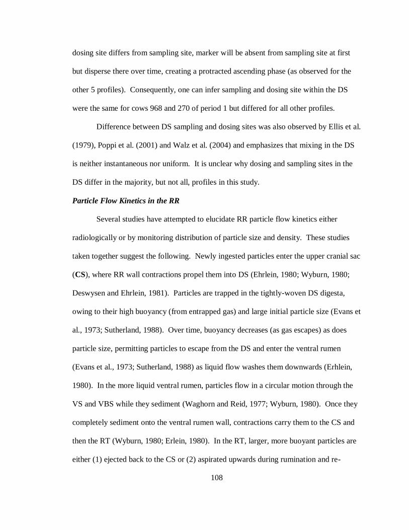
108
dosing site differs from sampling site, marker will be absent from sampling site at first
but disperse there over time, creating a protracted ascending phase (as observed for the
other 5 profiles). Consequently, one can infer sampling and dosing site within the DS
were the same for cows 968 and 270 of period 1 but differed for all other profiles.
Difference between DS sampling and dosing sites was also observed by Ellis et al.
(1979), Poppi et al. (2001) and Walz et al. (2004) and emphasizes that mixing in the DS
is neither instantaneous nor uniform. It is unclear why dosing and sampling sites in the
DS differ in the majority, but not all, profiles in this study.
Particle Flow Kinetics in the RR
Several studies have attempted to elucidate RR particle flow kinetics either
radiologically or by monitoring distribution of particle size and density. These studies
taken together suggest the following. Newly ingested particles enter the upper cranial sac
(CS), where RR wall contractions propel them into DS (Ehrlein, 1980; Wyburn, 1980;
Deswysen and Ehrlein, 1981). Particles are trapped in the tightly-woven DS digesta,
owing to their high buoyancy (from entrapped gas) and large initial particle size (Evans et
al., 1973; Sutherland, 1988). Over time, buoyancy decreases (as gas escapes) as does
particle size, permitting particles to escape from the DS and enter the ventral rumen
(Evans et al., 1973; Sutherland, 1988) as liquid flow washes them downwards (Erhlein,
1980). In the more liquid ventral rumen, particles flow in a circular motion through the
VS and VBS while they sediment (Waghorn and Reid, 1977; Wyburn, 1980). Once they
completely sediment onto the ventral rumen wall, contractions carry them to the CS and
then the RT (Wyburn, 1980; Erlein, 1980). In the RT, larger, more buoyant particles are
either (1) ejected back to the CS or (2) aspirated upwards during rumination and re-

109
deposited into the DS after traveling through the cranial rumen (Ehrlein, 1980; Wyburn,
1980; Sutherland, 1988). Small and dense particles in the RT are trapped by honeycomb
cells of the RT and conveyed to the reticulo-omasal orifice, where they escape into the
omasum (Reid, 1984).
This view suggests particle flow occurs primarily in the sequence CS→DS→VS
→VBS↔VS↔RT↔omasum or CS→DS, which generally follows with the order of RR
wall contractions (RT→CS→DS→VS→VBS) (Erlein, 1980). By endoscopic observation
of dyed particles, Lirette and Milligan (1990) propose circular movement of digesta
following in the opposite direction (DS→RT→CS→VS→VBS→caudo-dorsal blind
sac→DS), but this isolated suggestion is difficult to accept over multi-faceted evidence to
the contrary. According to the probable flow sequence
CS→DS→VS→VBS↔VS↔RT↔omasum or CS→DS, MRT values should be in the
order MRTDS < MRTVS ≈ MRTVBS < MRTRT (where MRTi refers to MRT of the ith
site)
because of the order in which particles enter and exit these sites.
However, in our dataset, there was no significant difference in MRT by site—i.e.,
differences in MRT by site, if any, are so small that they are masked by variability in
MRT across replicates. Similarity in MRT between the dorsal and ventral rumen was
also found in data of Dixon et al. (1983) (compared within particle size class) and Ellis et
al. (1994). Within diet, Walz et al. (2004) also found similarity in MRT across five sites
in the RR (craniodorsal rumen, DS, caudodorsal rumen, VS, RT), though from examining
their data in isolation it is not clear whether this similarity arose simply from difficulty to
discriminate differences with the infrequent sampling interval (every 6 h at most). It is
unclear if MRT differences exist between dorsal and ventral rumen in Poppi et al. (2001)

110
because the authors claim, without presenting statistical test results, that kinetic
parameters (from which MRT is calculated) are similar but MRT differ across sites.
Values in our dataset did not follow the expected MRT order (MRTDS < MRTVS ≈
MRTVBS < MRTRT) even on a numerical basis, with the numerical order MRTVS (21.5 h)
< MRTRT (23.1 h) < MRTVBS (25.0 h) < MRTDS (26.7 h) (SEM = 1.8 h).
Similar MRT values across sites suggests that once a particle escapes from the DS
for the final time (see below), it resides in the ventral regions (VS, VBS, RT) only shortly
before escaping; only under this condition can MRTVS, MRTVBS, and MRTRT not be
appreciably greater than MRTDS, as found in this study. In support of this idea, Poppi et
al. (2001), who modeled flow of Yb-marked stem and leaf through the DS and VF, found
that particle escape from the VS must occur rapidly relative to the DS. Also, Welch
(1982) found plastic particles arrived in the RT quickly (within ~35 min) after original
placement in the VS.
This conclusion does not rule out the possibility that particles to spend
appreciable time in the ventral regions at some point during their residence in the RR.
Indeed, we could envision the following scenario consistent with the MRT results of this
study: after a sojourn in the DS, particles (1) exit the DS and enter the VS, (2) spend
appreciable time in the ventral regions (VS, VBS, RT), (3) are recycled into the DS (via
rumination then re-deposition into the CS), (4) exit the DS and enter the VS once more,
then (5) continue steps 2-4 or quickly escape from the VS, VBS, and finally RT (via
reticulo-omasal orifice). Particles can follow steps 2-4 and still ultimately result in
MRTDS ≈ MRTVS ≈ MRTVBS ≈ MRTRT because the way in which residence time is
accrued by particles. If particles re-enter the DS (via recycling) after residing in the

111
ventral regions (VS, VBS, RT), the residence time they accumulate in the DS will include
that accrued in the VBS, VS, and RT prior to being recycled. This process results in
similar residence times across sites, and consequently MRT (calculated from the
residence time distribution) will also then be similar. However, whether or not recycling
occurs, the order of MRT values found in this experiment again demonstrate that once a
particle escapes from the DS the final time, it must escape from the ventral regions (VS,
VBS, RT) soon after entry. Figure 4.5 illustrates the findings of the above discussion,
assuming the direction of flow between sites follows that delineated beforehand.
The above discussion and Figure 4.5 imply that if appreciable recycling of
particles from the RT to the DS does not occur, escape from the DS is the limiting
process to passage from the RR, consistent with suggestions by Evans et al. (1973),
Fainchey (1986), and Sutherland (1988). If appreciable recycling does occur, escape
from the DS need not be rate-limiting, consistent with the contention by Mathison et al.
(1994) that escape through the reticulo-omasal orifice, not the DS, limits passage.
Determining the extent of such recycling, in conjunction with these results, could hence
demonstrate how strongly the DS acts as a barrier to passage from the RR.
Because the conclusions above (i.e., those illustrated in Figure 4.5) are founded
on a negative finding (i.e., lack of MRT differences across sites), their strength relies on
our experiment’s power to detect MRT differences across sites. According to a power
analysis (Kutner et al. 2004), an F-test could detect a difference of 7.99 h—specifically,
the difference between sites with highest and lowest MRT values—in our data with a
statistical power (1-β) of at least 0.8 and level of significance (α) of 0.05. In other words,
if the true range of MRT values across sites was greater than 8 h, our experiment would

112
have had a reasonable chance (≥80%) to find a significant (P < 0.05) difference in MRT
values across sites. Thus, our experiment is relatively sensitive in detecting differences
in MRT values across sites, our negative finding is meaningful, and the conclusions made
from this finding have merit.
Limitations of our Analysis
The chief limitation of our analysis is our inability to find a suitable model to
deliver kinetic parameter estimates. Because they describe marker profile shape
quantitatively and concisely, kinetic parameter estimates would allow us to compare
particle flow kinetics more thoroughly and rigorously than our analysis above.
We reported some results (MRT values) gathered with the G2→G1→O model
because we could achieve model fit to the data. Our original goal in this study was to
build a more compelx compartmental model that represents bidirectional flow through
each of the sampling sites (DS, VS, VBS, RT). In so doing, we could quantify the net
direction of flow through the sites, determine the flow paths of particles within the RR,
and consequently test view of particle flow kinetics delineated by radiological and
particle analysis studies (Evans et al., 1973; Waghorn and Reid, 1977; Erlein, 1980;
Wyburn, 1980; Deswysen and Ehrlein, 1981; Sutherland, 1988). However, fitting data to
this model (and, later, highly simplified versions thereof) led to failed convergance, very
poor fit (negative R2), parameter values that approached either 0 or infinity, or a
combination of these problems.
We attribute the poor model fit to the stochastic variation in the data (which
violates the ideal compartmental behavior assumed by these models) and difficulty in
estimating sizes of sampling sites (which were not measured in this experiment). We
113
caution future researchers who attempt to build a similarly complex model. Poppi et al.
(2001) were able to build a compartmental model that simulated flow through the DS and
VS alone, though inferring particle flow dynamics through the entire RR from examining
only 2 sites is questionable. Our approach of comparing MRT values, along with
radiological and particle studies, offer the most cohesive picture of particle flow kinetics
in the RR achievable at this time.
CONCLUSION
In our experiment, variability in marker profile shape (indicated by visual assessment and
values of MRT and peak marker concentration time) remains largely unexplained by diet,
site, and period; only cow has a consistent effect on profile shape. Because profile shape
relates to particle flow kinetics and parameters linked to it (e.g., digestibility and
voluntary intake), the source of this variation is important for future efforts to uncover.
Development of a parametric model suitable to quantitatively represent particle
flow in the RR is imperative. Only once such a model is developed can marker data be
quantitatively examined and compared to the fullest extent possible.
Our inference that a particle quickly leaves the RR after escaping the DS the final
time has an important practical implication: designing feed products to immediately
enter the ventral rumen (bypassing the DS) and resist regurgitation guarantees their quick
passage from the RR.
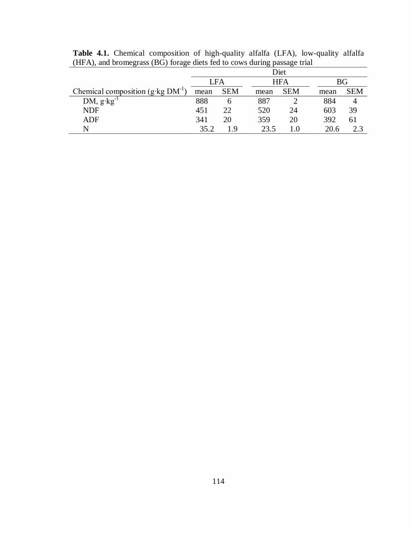
114
Table 4.1. Chemical composition of high-quality alfalfa (LFA), low-quality alfalfa
(HFA), and bromegrass (BG) forage diets fed to cows during passage trial
Diet
LFA HFA BG
Chemical composition (g∙kg DM-1
) mean SEM mean SEM mean SEM
DM, g∙kg-1
888 6 887 2 884 4
NDF
451 22 520 24 603 39
ADF
341 20 359 20 392 61
N
35.2 1.9 23.5 1.0 20.6 2.3

115
Table 4.2. Voluntary intake of bromegrass (BG), high-quality alfalfa (LFA), and low-
quality alfalfa diets (HFA) fed to cows during passage trial
Diet P-values
Intake (kg∙[100 kg BW·d]-1
) BG LFA HFA SEM diet period cow
DM 1.82 2.11 2.32 0.24 0.022 0.050 <0.001
NDF 1.23 0.94 1.16 0.27 0.259 0.385 0.016
ADF 0.89 0.74 0.79 0.22 0.789 0.207 0.012
N 0.038 0.070 0.059 0.10 0.125 0.659 <0.001

116
DS
VS VBS
RT
Figure 4.1. Location of dosing (mid-dorsal sac [DS]) and sampling sites (DS, mid-
ventral sac [VS], caudo-ventral blind sac [VBS], ventral reticulum [RT]) within the
reticulorumen.

117
DS VS VBS RT
Yb
con
cen
trati
on
, p
pm
time after dosing, h
Figure 4.2. Yb marker profile in (from left to right) dorsal sac (DS), mid-ventral sac
(VS), caudo-ventral blind sac (VBS), and ventral reticulum (RT) for cows (from top to
bottom) 270, 957, 963, and 968 during period 1. Raw observations are shown with filled
triangle symbols (▲). Observations given by local regression model (with Gaussian
kernel and nearest neighbor bandwidth of 0.4) are connected by linear splines (solid
lines); symbols are omitted for clarity. Fit of G2→G1→O model is shown by dotted
lines.
0.00
0.50
1.00
1.50
2.00
2.50
3.00
0 20 40 60
0.00
0.10
0.20
0.30
0.40
0.50
0.60
0.70
0.80
0 20 40 60
0.00
0.10
0.20
0.30
0.40
0.50
0.60
0.70
0.80
0.90
0 20 40 60
0
0.2
0.4
0.6
0.8
1
1.2
0 50
0.00
0.10
0.20
0.30
0.40
0.50
0.60
0.70
0.80
0.90
0 20 40 60
0.00
0.10
0.20
0.30
0.40
0.50
0.60
0.70
0 20 40 60
0.00
0.10
0.20
0.30
0.40
0.50
0.60
0.70
0 20 40 60
0.00
0.10
0.20
0.30
0.40
0.50
0.60
0.70
0.80
0 20 40 60
0.00
0.20
0.40
0.60
0.80
1.00
1.20
1.40
1.60
0 20 40 60
0.00
0.10
0.20
0.30
0.40
0.50
0.60
0.70
0 20 40 60
0.00
0.10
0.20
0.30
0.40
0.50
0.60
0.70
0.80
0 20 40 60
0.00
0.10
0.20
0.30
0.40
0.50
0.60
0.70
0.80
0.90
1.00
0 20 40 60
0.00
0.50
1.00
1.50
2.00
2.50
3.00
3.50
4.00
0 20 40 60
0.00
0.20
0.40
0.60
0.80
1.00
1.20
0 20 40 60
0.00
0.20
0.40
0.60
0.80
1.00
1.20
1.40
1.60
0 20 40 60
0.00
0.20
0.40
0.60
0.80
1.00
1.20
0 20 40 60

118
Mea
n r
esid
ence
tim
e (h
) ca
lcu
late
d f
rom
loca
l
regre
ssio
n
Mean residence time (h) calculated from raw observations
Figure 4.3. Comparison of mean retention time values calculated using raw observations
and local regression model. In each case, the numerical method (Eq. 1) was used for
calculation. Dotted and solid lines represent x = y and best-fit regression, respectively.
0
5
10
15
20
25
30
35
0 5 10 15 20 25 30 35
Y = (0.96±0.02)∙X+(1.12±0.38)
R2 = 0.993
n = 28
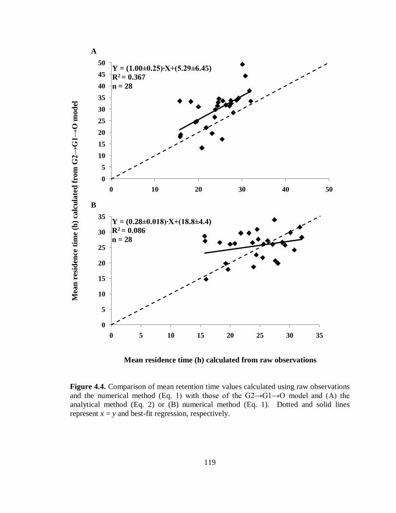
119
Mea
n r
esid
ence
tim
e (h
) ca
lcu
late
d f
rom
G2→
G1→
O m
od
el
A
B
Mean residence time (h) calculated from raw observations
Figure 4.4. Comparison of mean retention time values calculated using raw observations
and the numerical method (Eq. 1) with those of the G2→G1→O model and (A) the
analytical method (Eq. 2) or (B) numerical method (Eq. 1). Dotted and solid lines
represent x = y and best-fit regression, respectively.
0
5
10
15
20
25
30
35
40
45
50
0 10 20 30 40 50
Y = (1.00±0.25)∙X+(5.29±6.45)
R2 = 0.367
n = 28
0
5
10
15
20
25
30
35
0 5 10 15 20 25 30 35
Y = (0.28±0.018)∙X+(18.8±4.4)
R2 = 0.086
n = 28
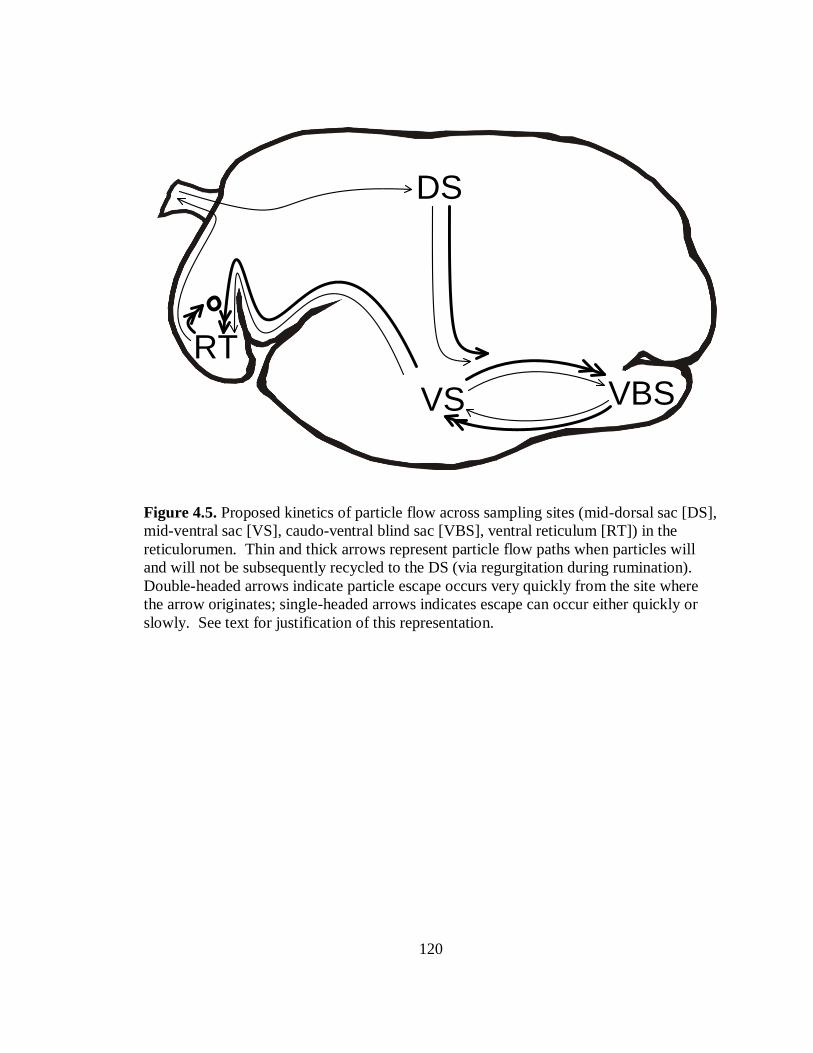
120
DS
VS VBS
RT
Figure 4.5. Proposed kinetics of particle flow across sampling sites (mid-dorsal sac [DS],
mid-ventral sac [VS], caudo-ventral blind sac [VBS], ventral reticulum [RT]) in the
reticulorumen. Thin and thick arrows represent particle flow paths when particles will
and will not be subsequently recycled to the DS (via regurgitation during rumination).
Double-headed arrows indicate particle escape occurs very quickly from the site where
the arrow originates; single-headed arrows indicates escape can occur either quickly or
slowly. See text for justification of this representation.
121
CHAPTER 5
A MECHANISTIC MODEL FOR PREDICTING INTAKE OF FORAGE DIETS
BY RUMINANTS
ABSTRACT
Accurate voluntary feed intake (VFI) prediction is critical to the productivity and
profitability of ruminant livestock production systems. Simple empirical models have
been used to predict VFI for decades but are inflexible, restrictive, and poorly
accommodate many feeding conditions, such as those of developing countries. We have
developed a mechanistic model to predict VFI over a range over a range forage diets
(low- and high-quality grasses and legumes) by wild and domestic ruminants of varying
physiological states (growth, lactation, gestation, non-productive). Based on chemical
reactor theory, the model represents the reticulorumen, large intestine, and blood plasma
as continuous stirred reactors and the small intestine as a plug flow reactor. Predicted
VFI is that which (1) fulfills an empirical relationship between chemostatic and distention
feedbacks observed in the literature, and (2) leads to steady-state conditions. In all model
validations, agreement with observed feed intake was high (R2 > 0.9, root mean square
prediction error < 1.4 kg∙d-1
). Root mean square prediction error for our model was only
67% of that of the Beef NRC model, the leading empirical prediction system for cattle.
These results together demonstrate that our model can predict ruminant VFI more broadly
and accurately than prior methods and, by consequence, serve as a crucial tool to
ruminant livestock production systems.
122
INTRODUCTION
Predicting voluntary feed intake (VFI) is critical to the profitability and productivity of
ruminant livestock production systems (Yearsley et al., 2001). Since their introduction in
the 1960s (Conrad et al., 1964), multiple regression and other simple empirical equations
(Forbes, 2007) have been embraced for VFI prediction. Typically, these equations are
parameterized with data encompassing a narrow range of biological conditions (e.g.,
focusing on only one animal species, physiological state, environment, and dietary type;
Forbes, 2007) because correlations between predictor variables and VFI vary across
conditions. Whereas these equations can have good predictive power within the specific
conditions used for parameterization, extrapolation is not appropriate due to the
equations’ purely empirical basis (Yearsley et al., 2001). Because they have generally
been developed for conventional feeding situations in developed countries (cattle and
sheep fed high-quality temperate forages and grain), these equations can be restrictive,
particularly for novel feeding situations (such as for new or unconventional livestock
species; NRC, 1991, 2007) or in developing countries (where goats, in addition to sheep
and cattle, and poor-quality tropical forages are mainstays; Timon and Hanrahan, 1986;
Chenost and Kayouli, 1997).
In contrast to empirical models, mechanistic models estimate VFI by modeling
underlying intake regulation mechanisms (Illius and Allen, 1994; Illius et al., 2000;
Yearsley et al., 2001). Their broader biological aims and reliance on more than one
dataset for parameterization grants them wider applicability than empirical models.
However, their historically low precision, in addition to more theoretically-focused aims,
has led to little adoption in practice.

123
The objective of this study was to develop and evaluate a mechanistic model that
reliably predicts VFI over a range of forage diets by wild and domestic ruminants of
varying physiological states.
MATERIALS AND METHODS
Our model of VFI represents digestive events within the ruminant gastrointestinal
tract (GIT). It is based on chemical reactor theory (Penry and Jumars, 1987) and
compartmental modeling (Jacquez, 1985) and is mechanistic, dynamic, and deterministic
(Thornley and France, 2007).
General Structure
The model’s representation of digestion begins with feed being consumed and
entering the reticulorumen (RR), modeled as a continuously-stirred reactor (after Penry
and Jumars, 1987; Mertens and Ely, 1979) Nutrients in the food include soluble
carbohydrate (SCHO; low molecular weight carbohydrates, pectins, and fructans),
insoluble, non-fibrous carbohydrate (InNFC; starch and other insoluble non-structural
polysaccharides), digestible hemicellulose (DHEM), indigestible hemicellulose (IHEM),
digestible ADF (DADF), indigestible ADF (IADF), soluble protein (SP; amino acids,
short-chain peptides, hydrophilic proteins), insoluble digestible protein (InDP),
indigestible CP (protein bound to ADF and lignin nitrogen), lipid (FAT), and ash.
Metabolites generated from fermentation of feed include VFA and ammonia (NH3).
Once in the RR, these entities enter into their respective RR compartments (with
the exception of ash and indigestible CP, which are assumed to be inert and not explicitly
represented). Entities exit their RR compartments via (1) microbe (MICRO) mediated
hydrolysis (InNFC, DHEM, DADF, InDP), (2) uptake by MICRO (SCHO, SP, NH3), (3)
124
absorption through the RR wall (VFA, NH3), and (4) passage through the RR-omasal
orifice (all entities). SCHO and SP taken up by MICRO are used for MICRO growth or
fermentation. Growth produces MICRO biomass, comprised of InDP, InNFC, FAT, and
nucleic acids (NcAc). Fermentation of excess SCHO and SP produces VFA and NH3.
Entities that pass through the RR-omasal orifice flow through the omasum are
exposed abomasal acid hydrolysis, which converts a fraction of InDP to SP. They then
enter the small intestine (SI), represented as a plug flow reactor (after Penry and Jumars,
1987). Once entities enter their respective compartments, they can exit via (1) hydrolysis
by SI enzymes (InNFC, InDP), (2) absorption through the SI wall (SCHO, SP, FAT,
NH3, NcAc), and (3) passage through the ileocecal junction (all entities). Entities that
pass through the ileocecal junction enter large intestine (LI) compartments.
The LI is modeled as a continuously-stirred reactor and constructed almost
identically to the RR (after Danfaer, 1990). Entities exit their compartments via routes
similar to those in the RR. For simplicity, the model does not directly simulate MICRO
uptake of NcAc, though it is observed experimentally (Wallace et al., 1997); for this
reason, the model immediately converts NcAc entering the LI to equivalent amounts of
SCHO and NH3 (which MICRO take up) to effectively permit MICRO to take up NcAc.
Passed, undigested material is excreted in the feces.
Absorbed amino nitrogen and NH3 is transferred to a blood plasma urea space
(modeled as a continuously-stirred reactor; after Baldwin, 1995), where they are
converted to urea and excreted into the urine or into the GIT as an endogenous secretion.
Endogenous protein (assumed for simplicity to be entirely SP) is also secreted into the
125
GIT through the saliva or other sources (e.g., sloughing of GIT epithelium, mucin
secretions by goblet cells, enzymatic secretions).
Viscera and other organs outside the GIT are not included explicitly, though some
of their functions that determine intake and digestibility are implicit; for example,
conversion of NH3 to urea is a function of the liver and kidneys, though neither is
represented in the model.
Model Equations
We used a system of differential equations to quantify the fluxes of nutrients,
metabolites, and MICRO across compartments and spaces, as described above. These
equations follow the general format
t compartmen from outflow
t compartmen toinflowt compartmen of size
j
jdt
jd
where t = time and <inflow to compartment j> and <outflow from compartment j> are
the sums of all processes causing entity j to flow into and out of compartment j,
respectively.
Equations describing digestive events in the RR, LI, SI, and plasma are provided
in Table 5.1, and supporting auxiliary equations are presented in Table 5.5. Equations for
a MICRO submodel are presented in Table 5.6. Miscellaneous equations are given in
Table 5.7. All other equations are provided below in the text. Units, abbreviations, and
symbols used in these equations are provided in Appendix 1.
Feedback Signals and Prediction of VFI
In simulating digestion for a given level of VFI (kg DM∙d-1
), the model computes
two key parameters: (1) RR fill with space-occupying NDF (kg∙100 kg BW-1
), (2) the
126
quantity of nutrients and metabolites the gastrointestinal tract absorbs per unit time, with
NE (expressed in units of NEm [Mcal∙100 kg BW-1
∙h-1
]) and protein (kg∙100 kg BW-1
∙h-1
)
of particular importance. Both of parameters have been proposed to regulate intake in the
ruminant (Forbes, 2007). We compared the computed value of these two parameters to
optimal or reference values by taking the ratio between reference and actual parameter
values. We define the ratio of optimal (Cr) to actual (NEI) NE intake as the chemostatic
feedback signal (Cs)—i.e.,
NEI
CC r
s
The value of Cr is equal to the energy required to reach genetic production potential
(defined here as the production level expected from an individual of a given species, BW,
physiological state, production stage, and sex under optimal nutritional, environmental,
and managerial conditions) and computed as described below. We additionally define
the ratio of reference (Dr) to actual (<RR
NDF>) RR fill with NDF as the distention
feedback signal (Ds)—i.e.,
NDF
DD
RR
rs
We define Dr as <RR
NDF> when Cs = 1 and set its value to 1.7 kg∙100 kg BW-1
, a value
found by applying the model to a calibration dataset (Mertens, 1973). We used NDF as a
measure of RR fill following its historic use in the literature (Mertens, 1987) and because
its use led to higher system stability (faster and higher convergence rates during model
solution procedures) relative to other potential measures.
To find an empirical relationship between Cs and Ds, we calculated values of Cs
and Ds from two studies in the literature (Bernal-Santos, 1989; Bosch et al., 1992a,b).

127
We estimated Cs from milk output and BW reported by the two studies in conjunction
with energy requirement equations of the NRC (2000, 2001). Following our definition of
genetic potential, we assume that milk output realized on these high-quality diets
approached the animals’ genetic potential. We estimated Dr from the value of
indigestible NDF (Bernal-Santos, 1989) or lignin (Bosch et al., 1992a,b) when Cs = 1, the
definition of the reference value for RR fill. We used indigestible NDF and lignin instead
of NDF (as in the model) because these measures of RR fill were most consistently
related to Cs across these datasets (though NDF gave greater system stability in the
model). We found that Cs and Ds followed the relationship
ss CD [1]
where α is a shape parameter found by regression (using log-transformed values with
PROC REG of SAS; SAS Institute, Inc., Cary, NC) and equal to (mean±SEM) -
0.78±0.16 (P < 0.001; Figure 5.1).
Eq. 1 was derived under circumstances where the dietary energy:protein ratio was
low, though high ratios strongly reduce intake (Moore and Kunkle, 1995). To
accommodate diets with high ratios, we added a feedback signal for energy:protein, using
an equation form proposed by Fisher (1996)
):(1
PNEeePs
where Ps = energy:protein feedback signal; NE:P = ratio of NE to protein absorption from
the GIT (Mcal∙kg-1
); and γ, δ, and ε = shape parameters (unitless). The value of γ (0.7) is
from Fisher (1996) and δ and ε (6, 0.17) were found by applying the model to a
calibration dataset (Mertens, 1973). This signal describes the fraction of VFI realized

128
when energy:protein feedback occurs relative to the case where no feedback occurs.
After incorporating this signal, the relationship between Ct and Dt can be shown to
become
s
ss
P
CD
[2]
We solved the model’s system of differential equations to find a level of VFI (predicted
VFI) that (1) yields values of Cs, Ds, and Ps that fulfill Eq. 2 and (2) lead to steady-state
conditions. After Fisher (1996), we solved the equations by encoding them into
Microsoft Excel 2007 (Microsoft Corporation, Seattle, WA) and applying Euler’s method
with time step t between 0.001 and 0.01 d. We considered convergence reached when
fractional change in VFI between iterations was less than 1∙10-6
, and the final solution
was insensitive to the time step used.
Other Notes on Model Structure
We have modeled many digestive processes as following simple first-order and
Michaelis-Menten saturation kinetics, as in previous, related models (Penry and Jumars,
1987; Illius and Allen, 1994). However, in accordance with experimental observations
(Hungate, 1966; Chapter 2), we represented passage in the RR with two sequential
passage rates (Blaxter et al., 1956) and hydrolysis in the RR and LI with age-dependent
kinetics (following a second-order Erlang distribution; Matis, 1972). We have devised
―subcompartments‖ (c.f., Table 5.4) as mathematical artifices to represent these complex
kinetic schemes with only simple first-order equations.
We use the term ―compartment‖ loosely when referring to SI entities;
compartments are strictly defined as well-mixed spaces (Jacquez, 1985), but by definition
129
there is no longitudinal mixing in plug flow reactors. We assume that secretion of
endogenous protein into the SI occurs evenly along the SI length.
Given the importance of the microbial ecosystem in the ruminant animal
(Hungate, 1966), we included within the model a submodel of MICRO (Table 5.6).
MICRO, which are represented as one homogenous entity, take up SCHO, SP, and NH3
according to Michaelis-Menten kinetics. After discounting total SCHO uptake for a
MICRO maintenance energy requirement, the first-limiting nutrient (SCHO or N)
determines growth. A portion of SCHO is used as a carbon source for MICRO biomass
synthesis and a portion fermented for energy to drive growth. Any SCHO or SP
remaining (as a result of being non-limiting to growth) is fermented, mirroring the
observation that copious amounts of SCHO (van Kessell and Russell, 1996) and SP
(Russell et al., 1983) are fermented in such cases.
In addition to Ds, Cs, and Ps, which directly modulate VFI, our model includes a
protein feedback (Pd ) that indirectly affects intake by modifying degradation rates of
insoluble nutrients according to ratio of N:SCHO taken up by microbes (Eq. 3a,b, Table
5.7). This feedback follows a Michaelis-Menten relationship. We predict the slow-
passage rate of particles from the RR ( j
p
RR k 2 ) from indigestible NDF fill of the RR,
employing Michaelis-Menten kinetics and assuming all particles pass at the same rate as
INDF (Eq. 19, Table 5.5). The equation for NEI (Eq. 4, Table 5.7) follows standard
conventions, except for the use of the heat increment of eating ( eH ; see Appendix 2).
Model Parameters
Model inputs include forage chemical composition (NDF, ADF, CP, ash) as well
as forage type (early or late-cut alfalfa, C3 grass, C4 grass, grass/legume mixture), which

130
determine dietary degradation characteristics. Cr is calculated by estimating genetic
production potential (by locating a study that reports productive output under optimal
conditions), then NE (expressed in NEm equivalents) required to reach that production
level (referencing Blaxter, 1989; NRC, 2000, 2001, 2007). All other parameters are
constants estimated from 65 publications (Appendix 2, Tables 5.8 – 5.14) and our own
unpublished data. The model currently accommodates one-ingredient diets containing
only forage because of the complexity and number of model equations.
Model Validation
We compared model-predicted VFI with actual values from 15 studies reporting
ad libitum consumption of all-forage diets by 14 bovid, 4 cervid, and 1 giraffid species
during gestation, lactation, growth, or non-productive physiological states. Studies and
species included are given in Table 5.1, and descriptive statistics of these studies are
given in Table 5.2. We focused on all-forage diets because these are the most pervasive
one-ingredient diets (as required by the model), though we included a wide range of
dietary qualities (Table 5.2).
We conducted validations with the full dataset (n = 158) and a subset of domestic
species (cattle, sheep, goats) only (n = 118). We also compared performance of our
model with that of the NRC (2000) using the 43 cattle observations (including growing,
lactating, gestating, and non-productive animals) within our validation dataset to which
we could apply the NRC (2000) equations. We assessed mean and linear biases of model
predictions using residual analysis (St-Pierre, 2003).

131
RESULTS AND DISCUSSION
Validation Results
We found good agreement between model-predicted and actual values of VFI for
the full dataset ( 0.16][0.35VFI predicted0.02][0.99 VFI actual ; R2 = 0.910, root
mean square prediction error [RMSPE], 1.35 kg∙d-1
, n = 158), indicated by high R2 and
low RMSPE (Figure 5.2A). Residual analysis (St-Pierre, 2003) revealed statistically
significant but numerically minor biases in both intercept (-0.28 kg∙d-1
; P = 0.008) and
slope (-0.076; P = 0.001).
The model over-predicted the two giraffe observations in the validation dataset
(from Foose, 1982; circled in Figure 5.2A). Foose (1982) and those who have studied his
work (Owen-Smith, 1988) noted qualitatively that giraffes were reluctant, for unspecified
reasons, to consume hay; our model’s over-prediction of giraffe VFI underscores for
these qualitative behavioral observations. Omitting the giraffe observations increases R2
(0.942) and lowers RMSPE (1.05 kg∙d-1
) and reduces biases in both intercept (-0.19 kg∙d-
1; P = 0.025) and slope (-0.039; P = 0.045).
For livestock species (cattle, sheep, goat) alone, we found marginally higher
agreement ( 0.13][0.17VFI predicted0.02][0.97 VFI actual ; R2 = 0.955, RMSPE
= 0.96 kg/d, n = 118; Figure 5.2B) than for the full dataset with giraffe observations
removed. We attribute this higher agreement to the likely higher precision with which
we could compute Cr for domestic species; energy requirement equations are reasonably
well-established for domestic species (NRC, 2000, 2001, 2007), but equations for cervids
are based on limited data (NRC, 2007), and equations for most other wild species have
not been published (forcing us to use an imprecise interspecific equation; Blaxter, 1989).

132
There were no significant biases in either intercept (P = 0.697) or slope (P = 0.385).
These results demonstrate our model, with few exceptions, predicts VFI reliably across a
wide range of diet qualities, ruminant species, and physiological states.
We compared predictive performance of our model and that of the NRC (2000),
one of the most widely-accepted and general empirical prediction systems for cattle
(particularly in North America). Agreement between model-predicted and actual values
of VFI for our model ( 0.63][1.89VFI predicted0.06][0.81 VFI actual ; R2
=
0.812, RMSPE = 1.55 kg/d) was appreciably better than for the NRC (2000) (
0.50][4.23VFI predicted0.05][0.48 VFI actual ; R2 = 0.700, RMSPE = 2.31
kg/d) in terms of R2 and RMSPE (Figure 5.3A,B). Further, there were no biases in
intercept or slope for our model (intercept: P = 0.674; slope: P = 0.971) but large and
significant biases in intercept (0.783 kg∙d-1
; P = 0.014) and slope (0.462; P = 0.004) for
the NRC (2000). Gestation observations from Stanley et al. (1993) (circled in Figure
5.3A) were moderately over-predicted by our model for indeterminate reasons. These
observations were present in the validations above, but their outlying behavior is more
conspicuous here because comparatively few observations were included in this
validation (n = 43). When these observations were removed, predictive performance of
our model (R2 = 0.958, RMSPE = 1.09 kg/d) was elevated even more highly above that of
the NRC (2000) (R2
= 0.724, RMSPE = 2.45 kg/d) and more consistent with level of
precision in previous validations.
We note that to predict cattle VFI, the NRC (2000) employs four distinct
empirical equations (one each for growing calves, growing yearlings, gestating and non-
lactating, and gestating and lactating cattle). Our model uses the same equation set for all
133
physiological states and animal types. Though not specifically designed for cattle or
certain physiological states, our system predicts cattle VFI of forage diets with
superiority to that of the empirical NRC (2000). This point demonstrates how the
mechanistic model proposed here can exceed both the breadth and precision of an
empirical system.
Comparison with Prior Mechanistic Models.
Our mechanistic model is one of several previously developed (Illius and Allen,
1994; Illius et al., 2000; Yearsley et al., 2001). Table 5.3 summarizes the predictive
performance of models that have been validated, showing that most have low precision,
large slope and intercept biases, or both. For this reason, mechanistic models have been
regarded primarily as research and not predictive tools (Illius et al., 2000; Yearsley et al.,
2001). Only two models, Chilibroste et al. (1997) and our own, display good predictive
power within their validation datasets (Table 5.3). Whereas the model of Chilibroste et al.
(1997) displays a high R2 value (0.949), its practicability as a universal VFI prediction
model is uncertain because its performance was (1) evaluated only with cattle, (2) not
directly compared to other models, (3) likely exaggerated by its small validation dataset
size (n = 18). From this perspective, our model stands uniquely as a reliable, practical,
and universal VFI prediction system.
Though the complexity of mechanistic models makes it difficult to definitively
determine reasons for their predictive performance, we believe that our mechanistic
model performs well because it integrates several intake-regulating mechanisms
according to an empirical relationship (Figure 5.1), capturing a broad number of
mechanisms known the regulate intake (Forbes, 2007) and representing them realistically.

134
Other models may perform poorly because they either focus exclusively on one intake-
regulating mechanism (Illius and Allen, 1994; Illius et al., 2000) or integrate multiple
regulation mechanisms according to a theoretical relationship only (Fisher, 1996).
Model Limitations
Despite good agreement between actual and model-predicted VFI, the model’s
structure is necessarily limited in certain aspects. We model the effects and integration of
feedback signals only at a gross level (Eq. 2) and not the specific means by which such
effects are mediated (e.g., hormonal and neuronal pathways; Forbes, 2007). The effect of
this simplification on VFI-prediction is uncertain, but does prohibit investigation and
further understanding of how VFI is regulated at a fine degree of resolution.
Our model cannot account for VFI-depression occurring under special conditions,
such as deficiency or excess of micronutrients, extreme temperatures, presence of plant
secondary metabolites or other toxins, or endocrinal involvement during estrus and late
pregnancy (Forbes, 2007). The model’s omission of endocrine-mediated VFI depression
may partially explain its systematic over-prediction of gestation observations from
Stanley et al. (1993) (Figure 5.3A), though we note gestation observations from two other
studies (Table 5.1) were well-predicted.
Another limitation of the model is its accommodation of only one dietary
ingredient. Expanding the model to accommodate more complex diets is a goal of future
work.
Potential Model Applications
An important feature of the model is its ability to predict reliably over a wide
range of animal species and forage qualities. The model should serve as an appropriate
135
predictive tool for application to small ruminants and poor-quality forages, which are
mainstays of livestock production in developing countries (Timon and Hanrahan, 1986;
Chenost and Kayouli, 1997) but for which few empirical intake prediction systems
(excepting sheep) have been developed. By the same reasoning, the model may be
suitable to accommodate new or unconventional ruminant livestock species and breeds
(NRC, 1991, 2007); these animals have similarly been ignored by empirical systems
although they have considerable economic promise in developed and developing
countries alike and, in the latter, may help solve the problem of low meat and milk
availability (NRC, 1991). Our model can serve as a valuable tool to livestock production
systems, such as those in developing countries, that animal production research has
largely neglected.
Rook et al. (1991) previously concluded that a universal model of ruminant VFI
prediction is unattainable, and that a battery of empirical equations (each equation
specific to a biological condition) be developed and applied instead. Though animal
scientists have tacitly accepted the conclusions of Rook et al. (1991) (even as developing
such as monumental battery of equations has doubtful practicability), our model’s ability
to predict intake over a wide range of physiological states and dietary qualities illustrates
that a universal model of VFI can indeed be developed. As the model is refined (such as
expansion to accommodate several dietary ingredients) and the world’s population and
demand for animal products climbs (Delgado, 2003), the model’s VFI prediction will
become of crucial value to improving profitability and productivity of ruminant livestock
systems. The model has other useful applications. Because it can consistently deliver
accurate food intake predictions when external constraints (e.g., limited food availability,

136
competition) are absent, our model can provide baseline predictions for VFI capacity that
could be highly valuable to ecological investigations.
APPENDIX 1
Units
Entity (nutrient, metabolite, or microbes; MICRO) compartment size and flow (by
absorption, hydrolysis, intake, passage, or uptake) have units of kg∙100 kg BW-1
and
kg∙100 kg BW-1
∙h-1
. Fractional rate constants have units of h-1
. Affinity, inhibition, and
maximum velocity constants (except for MICRO) are in kg∙100 kg BW-1
, kg∙100 kg BW-
1, and kg∙100 kg BW
-1∙h
-1. MICRO maximum velocity constants are kg∙kg MICRO
-1h
-1.
MICRO growth has units of kg MICRO∙100 kg BW-1
∙h-1
. Heat of combustion and heat
increments are in Mcal∙kg-1
and Mcal-1Mcal
-1.
Miscellaneous units not included above are defined in the text where they are
introduced. Exceptions to the conventions above are also indicated in the text where
appropriate.
Abbreviations
Space abbreviations
AB = abomasum
RR = reticulorumen
OMA = omasum
LI = large intestine
plasma = blood plasma space
SI = small intestine
urine = urinary space

137
Nutrient, MICRO, and metabolite compartment abbreviations
CP = crude protein
DADF = potentially digestible acid detergent fiber
DHEM = potentially digestible hemicellulose
DM = dry matter
IADF = indigestible acid detergent fiber
ICP = indigestible crude protein
IHEM = indigestible hemicellulose
InDP = insoluble potentially digestible protein
InNFC = insoluble non-fibrous carbohydrate
FAT = lipid
MICRO = microbes
NDF = neutral detergent fiber
NH3 = ammonia
DP = potentially digestible protein
PU = plasma urea
SCHO = soluble carbohydrate
SP = soluble protein
Process, k, abbreviations
a = absorption
e = excretion
h = hydrolysis
L = soluble entity passage rate

138
p1 = insoluble entity fast passage rate
p2 = insoluble entity slow passage rate
p = passage rate (no designation as fast or slow nor soluble or insoluble)
u = uptake
Other abbreviations
C3 = C3 grass
C4 = C4 grass
ECA = early-cut alfalfa
GL = grass-legume mixture
LCA = late-cut alfalfa
MRT = mean residence time
Symbols and Notation
Compartment and subcompartment symbols
ji = size of compartment of entity j in space i
e.g., DHEMRR = size of compartment of DHEM in RR
m
ij = size of the subcompartment m of entity j in space i
e.g., A
RRDHEM1 = size of 1A subcompartment of DHEM in RR
21 mm
ij =size of the sum of m1 and m2 subcompartments, where m1 and m2 are any
subcompartments within a parent compartment j
e.g., AA
RRDHEM 21 = size of the sum 1A and 2A subcompartments of DHEM
in RR

139
Rate constant symbols
j
k
ik = age-independent rate for process k pertaining to nutrient j in space i
e.g., DHEM
p
RRk 1 = slow passage rate of DHEM from the RR
j
k
i = age-dependent rate for process k pertaining to nutrient j in space i
*j
k
i =age-dependent rate without the effect of d
i P
MICRO SYMBOLS
microGi = actual MICRO growth in space i
SPmicroGi | = actual MICRO growth supported by SP in space i
3| NHmicroGi = actual MICRO growth supported by NH3 in space i
NpmicroGi | = potential MICRO growth supported by N (from SP and NH3) in space i
SCHOpmicroGi | = potential MICRO growth supported by SCHO in space i
biomassj
lmicroGR |
| = requirement for nutrient j for incorpotation into biomass in MICRO growth
supported by nitrogen source l (NH3,SP) (kg j∙kg MICRO-1
)
fermentj
lmicroGR |
| = requirement for nutrient j for fermentation into biomass in MICRO growth
supported by nitrogen source l (NH3, SP) (kg j∙kg MICRO-1
)
SCHOmicroMR = minimal requirement for SCHO for maintenance (kg SCHO∙kg MICRO
-1∙h
-1)
= shape parameter for SP uptake (unitless)
Other symbols and notation
SPInDPA , =fraction of InDP flowing from RR hydrolyzed to SP in abomasum (kg InDP∙kg
SP-1
)

140
PU
saliva
RR E =endogenous input of PU into the RR from inflow of saliva
SP
s
i E = endogenous input of SP into space i
SP
saliva
RR E = endogenous input of SP into the RR from inflow of saliva
SP
wall
RR E =endogenous input of SP into the RR from epithelial sloughing of RR wall
jf = fraction of nutrient j in diet (kg∙kg DM-1
)
ji ferment = quantity of nutrient j fermented by MICRO in space i
jcH = heat of combustion of nutrient j (Mcal∙Mcal
-1)
jmH = heat increment of metabolism of nutrient j
eH = heat increment of eating
INTAKE = voluntary feed intake
jlk
i J | =inhibition constant for nutrient j in the process k involving nutrient l in space i
e.g.,3
|NHPUe
RRJ = inhibition constant for NH3 in the excretion of PU into the RR
PUe
urinek = excretion of PU through urine (L∙100 kg BW-1
∙h-1
)
j
lk
i K | =affinity constant for nutrient j in the process k involving nutrient l in space i
SPSCHO
dPi K : = affinity constant for Pd
NEI = actual NE intake
NE:P =absorption of NE:absorption of CP (Mcal∙kg-1
)
jiO = outflow of nutrient j from space i by passage
iPd = protein feedback signal that affects degradation rates in space i (unitless)
t = time
141
tt = SI mean residence time
j
u
i v = uptake of entity j by MICRO in space i
j
k
iV = maximum rate of process k for nutrient j into space i
dPiVmax = maximum value of the fraction by which d
i P can increase degradation rates of
insoluble nutrients (unitless)
VFASP=VFA from SP fermentation (kg∙100 kg BW
-1)
VFASCHO=VFA from SCHO fermentation (kg∙100 kg BW
-1)
ljY , = yield of entity l from entity j (kg l∙kg j-1
)
APPENDIX 2
Refer to Appendix 1 for units, abbreviations, and symbols.
Conversion Factors
In order to convert values from literature sources to be consistent with units used
in the model, molecular masses of nutrients were assumed to be 17, 60, 110, 134, 162,
and 675 gmol-1
for NH3, PU, protein, CHO, and FAT (Dijkstra et al., 1992); 60, 74, 88,
and 102 g/mol for acetate, butyrate, propionate, and valerate; and 67.3 and 79.3 gmol-1
for SCHOVFA and SPVFA (calculated using average molar proportions for CHO and
protein fermentation reported by Murphy [1984]). The volume of the RR, SI, LI, and
plasma spaces were assumed to be 11, 1.3, 2.4, and 79.5 L∙100 kg BW-1
, typical of sheep
and cattle (Grovum and Hecker, 1973; Grovum and Williams, 1973; McAllan, 1981;
Dixon and Nolan, 1982; Dixon and Milligan, 1984; Barry et al., 1985; Baldwin, 1995;
Pitt et al., 1996). We also assumed 1.26 mol Nmol SP-1
(Dijkstra et al., 1992).
142
Protein Feedback Signal that Affects Degradation Rates
To estimate parameter values for di P , we used the data of Houser (1970), which
report the effect of adding urea to the in vitro degradation rate of Pangola grass OM, with
the following assumptions: (1) all nutrient disappearance was due to MICRO uptake, (2)
all non-CP OM that disappeared was CHO, (3) 75% of grass CP disappeared, (4) all urea
disappeared, and (5) dPiVmax=1 (so that jh
ijh
id
i
SCHOSPP
*][lim
:). By regression (PROC
NLIN of SAS; SAS Institute, Inc., Cary, NC) we found SCHON
P
i
dK : =31.7 (and dPiVmax=1 by
definition).
Absorption, Hydrolysis, and Passage Rates
Values for SCHO
a
SIV and SCHO
SCHOa
SI K | were set to 8.30∙10-2
and 1.64∙10-4
(Cant et al.,
1996). The value of 3NHRRk is from Baldwin (1995) and
3NHSI k and 3NHLI k are typical
values calculated from the literature for sheep (Hecker, 1971; Grovum and Williams,
1973; Nolan et al., 1976; McAllan, 1981; Dixon and Nolan, 1983, 1984, 1986; Siddons et
al., 1985; Sklan et al., 1985b; Table 5.8). An estimate of 3NHi is required to
calculate 3NHik , and when unavailable in a report, was taken from Hecker (1971)
(assuming 1 kg∙L SI digesta-1
and all non-protein nitrogen is NH3) for the SI and from
Dixon and Nolan (1982) for the LI.
To estimate NcAca
SI k , FATa
SI k , SPa
SI k , and we first constructed curves that relate
nutrient absorption to time spent in the SI. We constructed these curves using data from
McAllan (1981) and Sklan (1985a,b; for nutrient absorption, assuming all nutrient
disappearance is due to absorption) and Grovum and Williams (1973; for segmental
143
MRT). We then applied regression (PROC NLIN of SAS) to estimate SPa
SI k , FATa
SI k ,
and NcAca
SI k . For FAT and SP disappearance curves, we resolved two distinct first-order
rates. We used the slow rates as estimates for ia
SI k , assuming the fast rate was that
associated with rapid resorption of endogenous secretions (Sklan [1985a,b] show that
resorption of many endogenous enzymes is rapid).
We estimated InDPh
SI k as 0.73 with the same technique for estimating SPa
SI k ,
FATa
SI k , and NcAca
SI k , using data from Sklan (1985b; for InDP hydrolysis, assuming all
disappearance is due to hydrolysis) and Grovum and Williams (1973; for segmental
MRT). In absence of sufficient data for direct estimation, InNFCh
SI k was set to 0.50 to
yield starch a digestibility value within the range summarized by Owens et al. (1986) for
an SI MRT of 2h.
Values for i
h
i are from NRC (2000) for InNFC (using the approximate
conversion factor 0.59635∙ i
h
i = j
h
ik ; Pond et al., 1988) and Chapter 2 for all other
parameters (Table 5.9). These parameter values generally vary by diet type (ECA, LCA,
C3, C4, GL).
The value of j
L
RR k is estimated using the following equation (Illius and Gordon,
1991):
BWffffffk DADFDHEMInDPSPInNFCSCHOj
L
RR 51031.2)(145.0)(176.0
.
The value of jp
RRk 1was set to 0.10 (Ellis et al., 2000). The value ofIADFIHEM
jpRRK
|2 was
set to 1 (after Figure 5.16.7(a) from Ellis et al. [2000]), andj
pRRV 2 was set to 0.083,

144
double the maximum INDF outflow rate from Figure 5.16.7(a) in Ellis et al. (2000). We
doubled the outflow rate because calculating passage rate directly from total INDF (or
any other nutrient) outflow yields a passage rate that is the composite of j
p
RR k 1 and j
p
RR k 2
(rather than j
p
RR k 2 alone). We found that doubling INDF outflow rate empirically yielded
values of j
p
RR k 2 that closely matched values calculated from the graph using the direct
numerical method (by partitioning MRT between that associated with j
p
RR k 2 and j
p
RR k 1 ,
assuming j
p
RR k 1 = 0.10), and resulted in a much simpler expression for j
p
RR k 2 compared
with direct MRT partitioning.
Values of tt andjp
LI k were set to 2.00 and 0.065 according to typical values for
sheep, cattle, and goats (tt: Coombe and Kay, 1965; Grovum and Williams, 1973, 1977;
Warner, 1981; Barry et al., 1985; Gregory et al., 1985; Gregory and Miller, 1989; Ellis et
al., 2002; Walz et al., 2004; jp
LI k : Coombe and Kay, 1965; Grovum and Hecker, 1973;
Hecker and Grovum, 1975; Grovum and Williams, 1977; Warner, 1981; Dixon and
Nolan, 1982; Faichney and Boston, 1983; Barry et al., 1985; de Vega et al., 1998; Ellis et
al., 2002; Walz et al., 2004).
Endogenous Protein and PU
Values of SP
saliva
RR E and PU
saliva
RR E are calculated as salivation rate multiplied by
salivary concentration of PU and SP, respectively. Salivation rate is calculated from the
equations of Baldwin (1995), with time spent ruminating estimated from NDF
concentration (Murphy et al., 1983) and the default feed intake (9 kg∙d-1
) in Baldwin
(1995). Salivary concentration of SP and urea were taken to be 1.10∙10-4
kg∙L (Dijkstra

145
et al., 1992) and 0.65 of that in the plasma space (Bailey and Balch, 1961; Somers, 1961;
Doyle et al., 1982; Cirio et al., 2000; Piccione et al., 2006), and thus
BWBW
BWffffE IADFDADFIHEMDHEMSP
saliva
RR
/}0163.0
)](796.0850.0{[1058.4 75.04
BWBWBW
ffffPUE IADFDADFIHEMDHEMplasmaPU
saliva
RR
/}0163.0
)](796.0850.0{[1006.8
75.0
4
.
Values of PU
e
RRV , PU
PUe
RR K | , and 3
|
NH
PUe
RR J were set to 1.32∙10-2
∙BW-0.25
, 1.47∙10-3
, and
8.45∙10-2
(Baldwin, 1995). The value of SP
wall
RR E was set to 9.05∙10-6
, typical for cattle and
sheep (MacRae and Reeds, 1980; Ørskov, 1982; Ørskov and MacLeod, 1982, 1983;
Ørskov et al., 1986). Values for SPi E and PU
e
ik for all other spaces were those typical for
cattle, sheep, and goats ( SPi E : Harrop, 1974; Ørskov and MacLeod, 1982; Dixon and
Milligan, 1984; Dixon and Nolan, 1985; Siddons et al., 1985; Ørskov et al., 1986; Van
Bruchem et al., 1997; Ouellet et al., 2002; PUe
ik :
Nolan et al., 1976; von Engelhardt and Hinderer, 1976; Dixon and Nolan, 1983, 1986;
Dixon and Milligan, 1984; Siddons et al., 1985; Kohn et al., 2005; Table 5.10).
MICRO Submodel
The value for SCHO
u
iV was set to 1.11 (Dijkstra et al., 1992). In absence of
sufficient data for direct estimation, SCHO
SCHOu
RR K | and SCHO
SCHOu
LI K | were set heuristically to
0.20 and 7.58∙10-3
to result in first-order uptake rates within the general range (typically
0.75 to 4∙h-1
) of ―A‖ CHO fraction digestion rates suggested by Sniffen et al. (1992).
Parameter values for MICRO uptake of NH3 and SP were estimated by applying
regression (PROC NLIN of SAS) to data of Atasoglu et al. (1999; Table 5.11). We made

146
the following assumptions: (1) InDPMICROY , = 0.42 (Dijkstra et al., 1992), (2) SCHO
u
i v =1.1 (
SCHO
u
RR v when SCHOi is large; required to calculate average SCHO concentration),
and (3) values of SCHO
SPu
i K | and SCHO
NHu
i K 3| from Dijkstra et al. (1992).
The value of InNFCMICROY , was set to 0.20 (Reichl and Baldwin, 1975) and
InDPMICROY , , FATMICROY , , and NcAcMICROY , were set to 0.42, 0.11, and 0.13 (Dijkstra et al.,
1992). Values for biomassSCHO
NHmicroGR |
3| , fermentSCHO
NHmicroGR |
3| ,
biomassSCHO
SPmicroGR |
| , fermentSCHO
SPmicroGR |
| , 3
3|
NH
NHmicroGR , and
SP
SPmicroGR | were set to were set to 1.13, 1.12, 0.52, 0.88, 0.12, and 0.59 (Dijkstra et al.,
1992) and SCHO
microMR was set to 0.042 (Isaacson et al., 1975).
Heat of Combustion and Heat Increment
Values of j
cH for SCHO, InNFC, HEM, cellulose, lignin, InDP, SP, FAT, and PU
are those reported by Blaxter (1989) for α-D-glucose, xylan, starch, cellulose, lignin,
myosin, grain lipids, and urea (Table 5.12). Values for SCHOVFA
cH and SPVFA
cH were
calculated using j
cH of individual VFA (Blaxter, 1989) and average VFA molar
proportions for CHO and protein fermentation reported by Murphy (1984).
Values of j
mH for all entities but FAT are those reported by Blaxter (1989) for
ruminants ―below maintenance‖ (Table 5.12). Values of SCHOVFA
mH and SPVFA
mH are
calculated using j
mH for individual VFA (Blaxter, 1989) and the average VFA molar
proportions from Murphy (1984). We could not find a literature value of FAT
mH for
ruminants near maintenance, and so we adopted a typical value of FAT
mH for monogastic
species (Blaxter 1989; Table 5.12). Because j
mH are set to values for near or below

147
maintenance, they are most appropriate for calculation of NEm, explaining our convention
to express NE in units of NEm throughout the model (e.g., in calculation of Cr).
Typical literature values of eatH (as reported by Blaxter, 1989) are 0.05.
However, eatH is classically defined as a constant fraction of ME, whereas the model
implicitly defines it as a fraction of total ME less heat losses due to fermentation and
metabolism (c.f. Eq. 4, Table 5.7). Because ME less fermentation and metabolism heat
losses is about 20% smaller than total ME, we set eatH to 0.04, 20% less than the typical
value of 0.05.
Yield Parameters for Diet Composition
Values of ljY , are from Stefanon et al. (1996) for SCHONFCY , ; Chapter 2 for
DHEMHEMY , , DADFADFY , , and DPCPY , ; and T.J. Hackmann, J.D. Sampson, and J.N. Spain
(unpublished results) for SPDPY , (Table 5.13). Parameter values generally differ by diet
type.
Miscellaneous Yield and Other Parameters.
Values for 3,NHNcAcY and SCHONcAcY , were back-calculated from the amount of
SCHO and NH3 for NcAc synthesis reported by (Dijkstra et al., 1992; Table 5.14).
Values for VFASCHOY , and VFASPY , are averages for CHO and protein from Murphy (1984).
All other miscellaneous jiY , values were calculated using conversion factors explained
above.
The value of SPInDPA , was set to 0.50, based on data from Crooker et al. (1982)
reporting the fraction of feed N remaining after in vitro incubation in the AB fluid (after

148
prior incubation in situ in the RR). Values for NFCf and FATf are those reported by
NRC (2001).
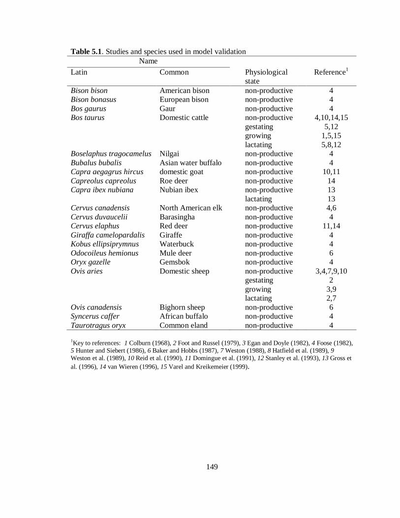
149
Table 5.1. Studies and species used in model validation
Name
Latin Common Physiological
state
Reference1
Bison bison American bison non-productive 4
Bison bonasus European bison non-productive 4
Bos gaurus Gaur non-productive 4
Bos taurus Domestic cattle non-productive 4,10,14,15
gestating 5,12
growing 1,5,15
lactating 5,8,12
Boselaphus tragocamelus Nilgai non-productive 4
Bubalus bubalis Asian water buffalo non-productive 4
Capra aegagrus hircus domestic goat non-productive 10,11
Capreolus capreolus Roe deer non-productive 14
Capra ibex nubiana Nubian ibex non-productive 13
lactating 13
Cervus canadensis North American elk non-productive 4,6
Cervus duvaucelii Barasingha non-productive 4
Cervus elaphus Red deer non-productive 11,14
Giraffa camelopardalis Giraffe non-productive 4
Kobus ellipsiprymnus Waterbuck non-productive 4
Odocoileus hemionus Mule deer non-productive 6
Oryx gazelle Gemsbok non-productive 4
Ovis aries Domestic sheep non-productive 3,4,7,9,10
gestating 2
growing 3,9
lactating 2,7
Ovis canadensis Bighorn sheep non-productive 6
Syncerus caffer African buffalo non-productive 4
Taurotragus oryx Common eland non-productive 4
1Key to references: 1 Colburn (1968), 2 Foot and Russel (1979), 3 Egan and Doyle (1982), 4 Foose (1982),
5 Hunter and Siebert (1986), 6 Baker and Hobbs (1987), 7 Weston (1988), 8 Hatfield et al. (1989), 9
Weston et al. (1989), 10 Reid et al. (1990), 11 Domingue et al. (1991), 12 Stanley et al. (1993), 13 Gross et
al. (1996), 14 van Wieren (1996), 15 Varel and Kreikemeier (1999).

150
150
Table 5.2. Descriptive statistics of studies used in model validation1,2
Dietary composition Digestibility
Item NDF ADF CP NEm3
DM OM NDF ADF CP BW VFI VFI
-----g∙kg DM-1
-----
-
Mcal∙kg
DM-1
g∙g-1
g∙g-1
g∙g-1
g∙g-1
g∙g-1
kg g DM∙100 g
BW-1
kg DM∙d-1
Mean 562 366 147 1.23 0.619 0.606 0.578 0.555 0.806 223 2.44 4.72
Min 351 261 36 0.71 0.460 0.442 0.370 0.392 0.541 16 0.47 0.29
Max 787 551 231 1.77 0.747 0.781 0.834 0.745 0.975 907 4.89 17.2
SD 105 56 52 0.20 0.067 0.092 0.105 0.087 0.124 210 0.81 4.26
N 158 158 158 158 39 53 89 55 51 158 158 158
1Studies include Colburn (1968), Foot and Russel (1979), Egan and Doyle (1982), Foose (1982), Hunter and Siebert (1986), Baker and Hobbs (1987), Weston (1988), Hatfield et al. (1989), Weston et al. (1989), Reid et al. (1990), Domingue et al. (1991), Stanley et al. (1993), Gross et al. (1996), van Wieren
(1996), Varel and Kreikemeier (1999). 2VFI = voluntary feed intake 3Values NEm are estimated using equations of NRC (2001).

151
151
Table 5.3. Performance of mechanistic models used to predict feed intake of ruminants
best-fit line1
model species physiological
state2
feed expression
for VFI3
slope intercept R2 n
Mertens and
Ely (1979,
1982)
Sheep growth (?), non-
productive
C3 and C4 grass,
legume, grass/legume
mixture
kg∙100 kg
BW-1
∙d-1
0.39 1.33 0.262 166
Hyer et al.
(1991a,b)
Cattle growth, non-
productive (?)
C3 and C4 grass,
legume
kg∙d-1
0.794
3.924
NA 42
Illius and
Gordon
(1991)
Sheep,
cattle
growth, non-
productive
C3 and C4 grass g∙kg
BW-0.73
∙d-1
0.98±0.03 NA 0.606 25
Illius and
Gordon
(1992)
Domestic
and wild
ungulates
non-productive C3 grass g∙kg
BW-0.73
∙d-1
0.77±0.03 NA 0.641 27
Fisher (1996) Cattle growth (?) C3 and C4 grass,
legume
kg∙100 kg
BW-1
∙d-1
NA
NA
0.504 38
Chilibroste et
al. (1997)
Cattle lactating,
gestating, growth,
non-productive (?)
C3 grass, C4 grass,
and legume-
concentrate diets
kg∙d-1
1.03±0.065
0.03±0.815
0.9495
18
our model Domestic
and wild
ruminants
gestating, growth,
lactating, non-
productive
C3 and C4 grass,
legume, grass/legume
mixture
kg∙d-1
0.99±0.02
0.35±0.16 0.910 158
1Values line (mean±SE) refer to line actual VFI = slope∙predicted VFI + intercept. 2Model reports and references therein did not always report physiological state; uncertainty in physiological state, where present, is indicated with ―?‖. 3VFI = voluntary feed intake 4Found by digitizing Figure 5.1 of Hyer et al. (1991b). 5Calculated using data in original report of Chilibroste et al. (1997).

152
Table 5.4. Main system of differential equations used in the mechanistic model to represent digestive events in the RR, SI, LI, and
plasma1
Space Compart
ment
Subcom
partment
Equation
RR SCHO
)()
(
2222
22
SCHO
L
RRRRSCHO
u
RRDADF
h
RR
BA
RRDHEM
h
RR
BA
RR
INFC
h
RR
BA
RRSCHORR
kSCHOvDADFDHEM
INFCfINTAKEdt
SCHOd
[1]
InNFC 1A )( 11
1 InNFC
p
RRInNFC
h
RR
A
RRInNFCA
RR
kINFCfINTAKEdt
InNFCd
[2]
2A )( 121
2 InNFC
p
RRInNFC
h
RR
A
RRInNFC
h
RR
A
RRA
RR
kInNFCInNFCdt
InNFCd
[3]
1B )( 2111
1 InNFC
p
RRInNFC
h
RR
B
RRInNFC
p
RR
A
RRB
RR
kInNFCkInNFCdt
InNFCd
[4]
2B
)(
)(
22
112
2
InNFC
p
RRInNFC
h
RR
B
RR
InNFC
h
RR
B
RRInNFC
p
RR
A
RRB
RR
kInNFC
InNFCkInNFCdt
InNFCd
[5]
DHEM 1A Replace ―InNFC‖ in Eq. 2 with ―DHEM‖ throughout [6]
2A Replace ―InNFC‖ in Eq. 3 with ―DHEM‖ throughout [7]
1B Replace ―InNFC‖ in Eq. 4 with ―DHEM‖ throughout [8]
2B Replace ―InNFC‖ in Eq. 5 with ―DHEM‖ throughout [9]
IHEM A IHEMp
RRA
RRIHEMARR
kIHEMfINTAKEdt
IHEMd1
[10]
B IHEMp
RRB
RRIHEMp
RRA
RRBRR
kIHEMkIHEMdt
IHEMd21
[11]
DADF 1A Replace ―InNFC‖ in Eq. 2 with ―DADF‖ throughout [12]
2A Replace ―InNFC‖ in Eq. 3 with ―DADF‖ throughout [13]
1B Replace ―InNFC‖ in Eq. 4 with ―DADF‖ throughout [14]
152
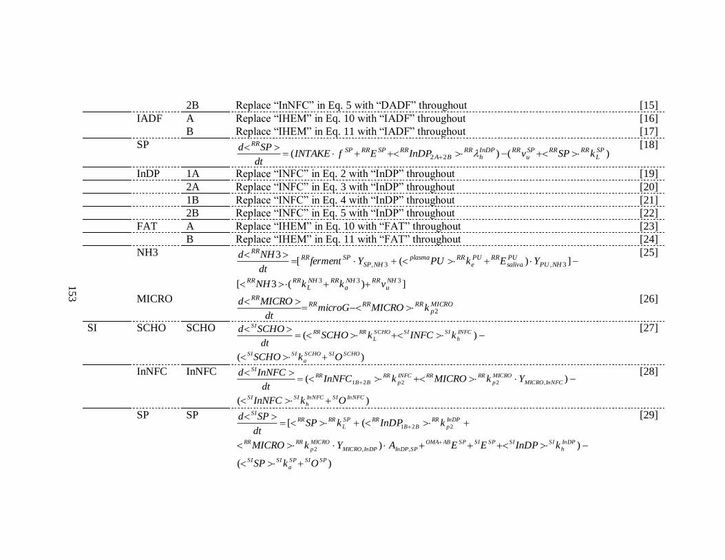
153
2B Replace ―InNFC‖ in Eq. 5 with ―DADF‖ throughout [15]
IADF A Replace ―IHEM‖ in Eq. 10 with ―IADF‖ throughout [16]
B Replace ―IHEM‖ in Eq. 11 with ―IADF‖ throughout [17]
SP )()( 22
SPL
RRRRSPu
RRInDPh
RRBA
RRSPRRSPRR
kSPvInDPEfINTAKEdt
SPd
[18]
InDP 1A Replace ―INFC‖ in Eq. 2 with ―InDP‖ throughout [19]
2A Replace ―INFC‖ in Eq. 3 with ―InDP‖ throughout [20]
1B Replace ―INFC‖ in Eq. 4 with ―InDP‖ throughout [21]
2B Replace ―INFC‖ in Eq. 5 with ―InDP‖ throughout [22]
FAT A Replace ―IHEM‖ in Eq. 10 with ―FAT‖ throughout [23]
B Replace ―IHEM‖ in Eq. 11 with ―FAT‖ throughout [24]
NH3
])(3[
])([3
333
3,3,
NHu
RRNHa
RRNHL
RRRR
NHPUPUsaliva
RRPUe
RRplasmaNHSP
SPRRRR
vkkNH
YEkPUYfermentdt
NHd
[25]
MICRO MICROp
RRRRRRRR
kMICROmicroGdt
MICROd2
[26]
SI SCHO SCHO
)(
)(
SCHOSISCHO
a
SISI
INFC
h
SISISCHO
L
RRRRSI
OkSCHO
kINFCkSCHOdt
SCHOd
[27]
InNFC InNFC
)(
)( ,2221
InNFCSIInNFC
h
SISI
InNFCMICRO
MICRO
p
RRRRINFC
p
RR
BB
RRSI
OkInNFC
YkMICROkInNFCdt
InNFCd
[28]
SP SP
)(
))
([
,,2
221
SPSISP
a
SISI
InDP
h
SISISPSISPABOMA
SPInDPInDPMICRO
MICRO
p
RRRR
InDP
p
RR
BB
RRSP
L
RRRRSI
OkSP
kInDPEEAYkMICRO
kInDPkSPdt
SPd
[29]
153
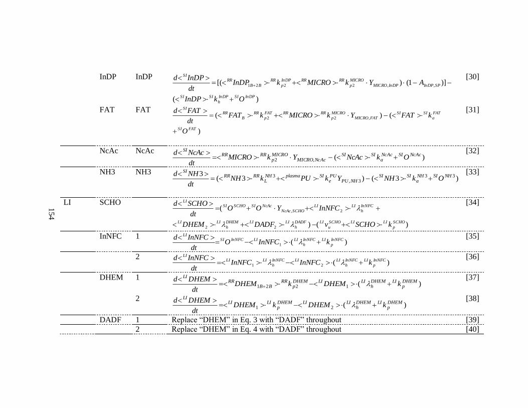
154
InDP InDP
)(
)]1()[( ,,2221
InDPSIInDP
h
SISI
SPInDPInDPMICRO
MICRO
p
RRRRInDP
p
RR
BB
RRSI
OkInDP
AYkMICROkInDPdt
InDPd
[30]
FAT FAT
)
()( ,22
FATSI
FAT
a
SISI
FATMICRO
MICRO
p
RRRRFAT
p
RR
B
RRSI
O
kFATYkMICROkFATdt
FATd
[31]
NcAc NcAc )(,2
NcAcSINcAca
SISINcAcMICRO
MICROp
RRRRSI
OkNcAcYkMICROdt
NcAcd
[32]
NH3 NH3 )3()3(
3 333,
3 NHSINHa
SISINHPU
PUe
SIplasmaNHL
RRRRSI
OkNHYkPUkNHdt
NHd
[33]
LI SCHO
)()
(
22
2,
SCHO
p
LILISCHO
u
LIDADF
h
LILIDHEM
h
LILI
InNFC
h
LILI
SCHONcAc
NcAcSISCHOSILI
kSCHOvDADFDHEM
InNFCYOOdt
SCHOd
[34]
InNFC 1 )(1
InNFC
p
LIInNFC
h
LILIInNFCSILI
kInNFCOdt
InNFCd
[35]
2 )(21
InNFC
p
LIInNFC
h
LILIInNFC
h
LILILI
kInNFCInNFCdt
InNFCd
[36]
DHEM 1 )(1221
DHEMp
LIDHEMh
LILIDHEMp
RRBB
RRLI
kDHEMkDHEMdt
DHEMd
[37]
2 )(21
DHEMp
LIDHEMh
LILIDHEMp
LILILI
kDHEMkDHEMdt
DHEMd
[38]
DADF 1 Replace ―DHEM‖ in Eq. 3 with ―DADF‖ throughout [39]
2 Replace ―DHEM‖ in Eq. 4 with ―DADF‖ throughout [40]
154
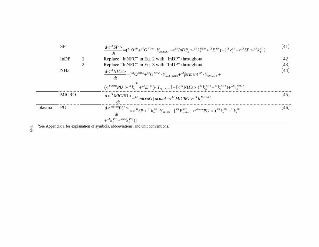
155
SP )()( 2,
SP
p
LILISP
u
LISPLIInDP
h
LILI
SPNcAc
NcAcSISPSILI
kSPvEInDPYOOdt
SPd
[41]
InDP 1 Replace ―InNFC‖ in Eq. 2 with ―InDP‖ throughout [42]
2 Replace ―InNFC‖ in Eq. 3 with ―InDP‖ throughout [43]
NH3
])(3[])(
[3
333
3,
3,3,
3
NH
u
LINH
a
LINH
p
LILI
NHPU
PULIPU
e
LIplasma
NHSP
SPLI
NHNcAc
NcAcSINHSILI
vkkNHYEkPU
YfermentYOOdt
NHd
[44]
MICRO MICROp
LILILILI
kMICROactualmicroGdt
MICROd
|
[45]
plasma PU
)]
([,
PU
e
urinePU
e
LI
PU
e
SIPU
e
RRplasmaPU
saliva
RR
PUSP
SP
a
SISIplasma
kk
kkPUEYkSPdt
PUd
[46]
11See Appendix 1 for explanation of symbols, abbreviations, and unit conventions.
155

156
Table 5.5. Auxiliary equations for the main system of differential equations of the mechanistic model1,2
Category Equation jf
NFC
SCHONFC
SCHO fYf , [1]
NFC
SCHONFC
InNFC fYf )1( , [2]
)(,ADFNDF
DHEMHEMDHEM ffYf [3]
)()1( ,ADFNDF
DHEMHEMIHEM ffYf [4]
ADFDADFADF
DADF fYf , [5]
ADFIADFADF
IADF fYf )1( , [6]
CPSPDPDPCP
SP fYYf ,, [7]
CPSPDPDPCP
InDP fYYf )1( ,, [8]
jSIO
)(
])exp()exp([
)exp(
SCHOa
SIInNFCh
SISCHOa
SI
SCHOa
SISCHOa
SISCHOa
SIInNFCh
SISCHOa
SIInNFCh
SISCHOL
RRRR
SCHOa
SISCHOL
RRRRSCHOSI
kkk
kttkkttkkkkSCHO
ttkkSCHOO
[9]
)exp(221 ttkkInNFCO InNFCa
SIInNFCp
RRBB
RRInNFCSI [10]
)(
)]exp()exp([
)exp()exp(1
SPa
SIInDPh
SISPa
SI
SPa
SISPa
SISPa
SIInDPh
SISPa
SIInDPh
SIInDPSI
SPa
SISPSI
SPa
SI
SPa
SISPSISPSI
kkk
kkkttkkkI
ttkIttk
ttkEO
where SPABOMA
SPInDPInDPMICRO
MICRO
p
RRRRInDP
p
RR
BB
RRSP
L
RRRRSPSI EAYkMICROkInDPkSPI
,,2221 )(
and
[11a]
[11b]
156

157
)1()( ,,2221 SPInDPInDPMICROMICROp
RRRRInDPp
RRBB
RRInDPSI AYkMICROkInDPI [11c]
)exp( ttkIO InDPa
SIInDPSIInDPSI
[12]
)exp()( ,222 ttkYkMICROkFATO FATa
SIFATMICRO
MICROp
RRRRFATp
RRRRFATSI [13]
)exp(,2 ttkYkMICROO FATa
SIFATMICRO
MICROp
RRRRNcAcSI [14]
)exp(3
)exp(1 33
3
3
3,
3 ttkkNHttk
ttkYkPUO NH
a
SINH
L
RRRR
NH
a
SI
NH
a
SI
NHPU
PU
e
SIplasmaNHSI
[15]
miscellaneous d
ijh
ijh
i P * [16]
3|| /3/1 NHPUe
RRRRplasmaPUPUe
RR
plasmaPUe
RRPUe
RR
JNHPUK
PUVk
[17]
SCHOK
SCHOVk
SISCHOSCHOa
SI
SISCHOa
SISCHOa
SI
/1 |
[18]
)/(1
)/(
|2
2
2
IADFIHEMK
IADFIHEMVk
RRRRIADFIHEM
jp
RR
RRRRj
p
RR
j
p
RR
[19]
SPsaliva
RRSPwall
RRSPRR EEE [20]
1See Appendix 1 for explanation of symbols, abbreviations, and unit conventions
.
157

158
Table 5.6. Equations for MICRO submodel of the mechanistic model1
Equation
SCHOK
VMICROv
iSCHO
SCHOu
i
SCHO
u
iiSCHO
u
i
/1 |
[1]
SCHOKSPK
VMICROv
iSCHOSPu
iiSPSPu
i
SPu
iiSPu
i
/)/(1 ||
[2]
SPNHu
iiiSCHONHu
iiNHNHu
i
NHu
iiNHu
i
JSPNHKNHK
VMICROv
3|3|3
3|
33
/3/3/1
[3]
SCHOmicroM
ii RMICROmicroM [4]
)(
)(|
)(
)(3||
|
|
|
|
|
3|
|
3|
fermentSCHO
SPmicroF
biomassSCHO
SPmicroG
i
iSCHO
u
ii
fermentSCHO
NHmicroG
biomassSCHO
NHmicroG
i
iSCHO
u
iii
RRmicroG
microMvSPmicroG
RRmicroG
microMvNHmicroGSCHOpmicroG
[5]
biomassSP
SPmicroG
SP
u
i
biomassNH
NHmicroG
NH
u
ii
R
v
R
vNpmicroG
|
|
|3
3|
3
| [6]
)|,|min( NpmicroGSCHOpmicroGmicroG iii [7]
biomassNH
NHmicroG
NH
u
ii
R
vNHmicroG
|3
3|
3
3| [8]
3|| NHmicroGmicroGSPmicroGi [9]
)|3|( |
|
|
3|
biomassSCHO
SPmicroG
ibiomassSCHO
NHmicroG
iSCHO
u
iSCHOi RSPmicroGRNHmicroGvferment
[10]
biomassSP
SPmicroG
iSP
u
iSPi RSPmicroGvferment |
|| [11]
VFASCHO
SCHOiSCHOi YfermentVFA ,
[12]
VFASP
SPiSPi YfermentVFA ,
[13]
1Refer to Table 5.4 for the main system of differential equations.
158

159
2See Appendix 1 for explanation of symbols, abbreviations, and unit conventions.
159

160
Table 5.7. Miscellaneous equations in the mechanistic model1
Equation Note
IADFDADFIHEMDHEMNDF RRRRRRRRRR [1] c.f.
main
text
SPa
SISI kSP
NEIPNE
:
[2] c.f.
main
text
SCHOSP
P
i
Pi
d
i
d
d
KSCHON
VP
:
max
/:1
where
SCHO
u
i
SPNH
NH
u
iSP
u
i
v
YvvSCHON
)(:
,3
3
[3a]
[3b]
)1(]
)1()1()(
)1()()1(
)1()()1([
e
PU
c
PU
e
urineplasma
NcAc
m
NcAc
c
NcAc
a
SISIVFA
m
VFA
c
SPLISPRR
VFA
m
VFA
c
SCHOLISCHORRSCHO
m
SCHO
c
SCHO
a
SISI
SP
m
SP
c
SPLISPSISPABOMSPRRSP
a
SISIFAT
m
FAT
c
FAT
a
SISI
HHkPU
HHkNcAcHHVFAVFA
HHVFAVFAHHkSCHO
HHEEEEkSPHHkFATNEI
SPSP
SCHOSCHO
[4]
1See Appendix 1 for explanation of symbols, abbreviations, and unit conventions.
160

161
Table 5.8. Estimated parameter values for absorption rates1,2
space i
nutrient j RR SI LI
SCHO ----- c.f. Eq. 18, Table 5.5 -----
InNFC ----- ----- -----
SP ----- 3.75 -----
InDP ----- ----- -----
NH3 0.52 1.50 0.35
FAT ----- 0.91 -----
NcAc ----- 2.80 ----- 1See Appendix 1 for explanation of symbols, abbreviations, and unit conventions. 2See Appendix 2 for literature sources and methods used for parameter estimation.
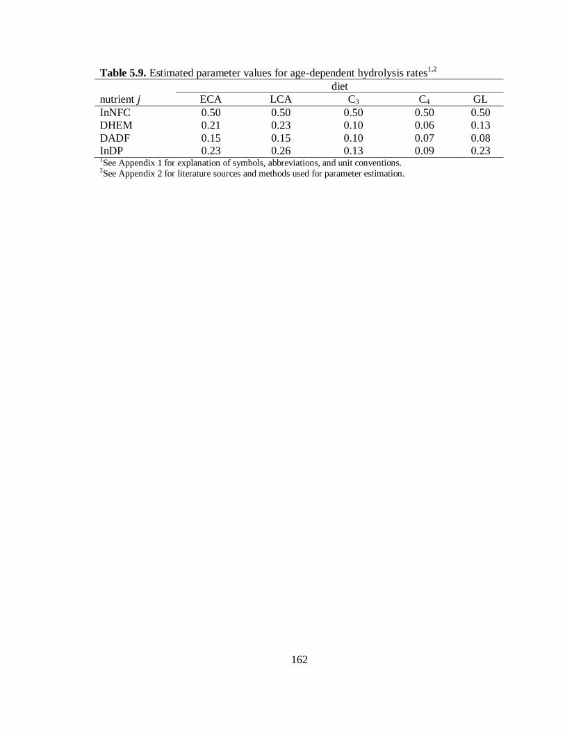
162
Table 5.9. Estimated parameter values for age-dependent hydrolysis rates1,2
diet
nutrient j ECA LCA C3 C4 GL
InNFC 0.50 0.50 0.50 0.50 0.50
DHEM 0.21 0.23 0.10 0.06 0.13
DADF 0.15 0.15 0.10 0.07 0.08
InDP 0.23 0.26 0.13 0.09 0.23 1See Appendix 1 for explanation of symbols, abbreviations, and unit conventions. 2See Appendix 2 for literature sources and methods used for parameter estimation.

163
Table 5.10. Estimated parameter values for endogenous protein and PU secretion1,2
space
parameter RR OM + AB SI LI urine SPi E ----- 3.15∙10
-6 2.10∙10
-5 2.05∙10
-6 -----
PUe
ik c.f. Eq. 17, Table S4 ----- 2.75∙10-2
1.10∙10-2
6.30∙10-2
1See Appendix 1 for explanation of symbols, abbreviations, and unit conventions. 2See Appendix 2 for literature sources and methods used for parameter estimation.
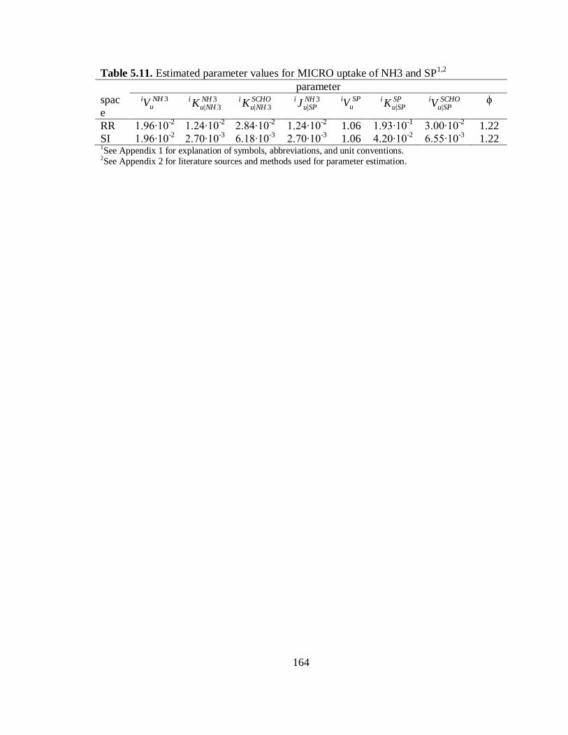
164
Table 5.11. Estimated parameter values for MICRO uptake of NH3 and SP1,2
parameter
spac
e
3NHu
iV 33|
NHNHu
i K SCHO
NHui K 3|
3|
NHSPu
i J SP
uiV SP
SPui K |
SCHOSPu
iV | ϕ
RR 1.96∙10-2
1.24∙10-2
2.84∙10-2
1.24∙10-2
1.06 1.93∙10-1
3.00∙10-2
1.22
SI 1.96∙10-2
2.70∙10-3
6.18∙10-3
2.70∙10-3
1.06 4.20∙10-2
6.55∙10-3
1.22 1See Appendix 1 for explanation of symbols, abbreviations, and unit conventions. 2See Appendix 2 for literature sources and methods used for parameter estimation.

165
Table 5.12. Estimated parameter values for heat of combustion and heat increment
parameter values1,2
nutrient or metabolite j j
cH j
mH
SCHO 4.15 0.00
SP 5.96 0.19
FAT 9.36 0.05 SCHOVFA 2.53 0.14
SPVFA 4.27 0.12 1See Appendix 1 for explanation of symbols, abbreviations, and unit conventions. 2See Appendix 2 for literature sources and methods used for parameter estimation.
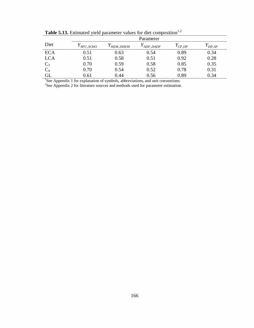
166
Table 5.13. Estimated yield parameter values for diet composition1,2
Parameter
Diet SCHONFCY , DHEMHEMY , DADFADFY , DPCPY , SPDPY ,
ECA 0.51 0.63 0.54 0.89 0.34
LCA 0.51 0.58 0.51 0.92 0.28
C3 0.70 0.59 0.58 0.85 0.35
C4 0.70 0.54 0.52 0.78 0.31
GL 0.61 0.44 0.56 0.89 0.34 1See Appendix 1 for explanation of symbols, abbreviations, and unit conventions. 2See Appendix 2 for literature sources and methods used for parameter estimation.

167
Table 5.14. Estimated miscellaneous parameter values1,2
j and l in ljY ,
j l value
SP NH3 0.20
NH3 SP 5.13
PU NH3 0.58
SP PU 0.34
NcAc NH3 0.22
NcAc SCHO 0.63
SCHO SCHOVFA 0.76
SP SPVFA 0.50 1See Appendix 1 for explanation of symbols, abbreviations, and unit conventions. 2See Appendix 2 for literature sources and methods used for parameter estimation.

168
Ds
Cs
Figure 5.1. Empirical relationship between chemostatic (Cs) and distention (Ds)
feedbacks derived from Bernal-Santos (1989) (□) and Bosch et al. (1992a,b) (♦). We
estimated Cs and Ds according to methods described in the text. The dotted line is the
regression line. The plot is semi-logarithmic.
0.3
3
0.3 3
Ds = Cs-0.78±0.16
P < 0.001

169
Pre
dic
ted
volu
nta
ry f
eed
in
tak
e, k
gd
-1
A
B
Actual voluntary feed intake, kgd
-1
Figure 5.2. Comparison between actual and model-predicted voluntary feed intake (VFI;
kg∙d-1
) of forage diets by ruminant species of various physiological states (growth [■],
gestation [+], lactation [x], non-productive [○]). (A) All species (14 bovids, 4 cervids,
and 1 giraffid). (B) Livestock species only. Circled in (A) are giraffe observations from
Foose (1982) that our model systematically over-predicted. Dotted and solid lines
represent x = y and the best-fit linear regression, respectively.
0
5
10
15
20
0 5 10 15 20
actual VFI = (0.99±0.02)∙predicted VFI+(0.35±0.16)
R2 = 0.910
RMSPE = 1.35 kg∙d-1
n = 158
0
5
10
15
20
0 5 10 15 20
actual VFI = (0.97±0.02)∙predicted VFI+(0.17±0.13)
R2 = 0.955
RMSPE = 0.96 kg∙d-1
n = 118

170
Pre
dic
ted
volu
nta
ry f
eed
in
tak
e, k
gd
-1
A
B
Actual voluntary feed intake, kgd
-1
Figure 5.3. Comparison between actual voluntary feed intake (VFI; kg∙d-1
) and that
predicted by (A) our mechanistic model and (B) the empirical equations of the NRC
(2000) for cattle of various physiological states (growth [■], gestation [+], lactation [x],
non-productive [○]). Circled in (A) are gestation observations from Stanley et al. (1993)
that our model moderately over-predicted. Dotted and solid lines represent x = y and the
best-fit linear regression, respectively.
0
5
10
15
20
0 5 10 15 20
actual VFI = (0.81±0.06)∙predicted VFI+(1.89±0.63)
R2 = 0.812
RMSPE = 1.55 kg∙d-1
n = 43
0
5
10
15
20
0 5 10 15 20
actual VFI = (0.48±0.05)∙predicted VFI+(4.23±0.50)
R2 = 0.700
RMSPE = 2.31 kg∙d-1
n = 43

171
CHAPTER 6
PRESSURE FOR LARGE BODY MASS IN THE RUMINANTIA: THE ROLE OF
NUTRITIONAL RESOURCE LIMITATIONS
ABSTRACT
Explaining determinants of BW is a critical because BW accounts for 75% of variation in
mammalian life history traits. Our objective was to determine whether nutritional
resource limitations could exert pressure for large BW. We focus on the Ruminantia
because there has been a clear pressure for large BW within this clade (median body BW
is approximately 45 kg) and because we developed a ruminant food intake model key to
this analysis. We found that increasing BW increases physiologically potential nutrient
intake relative to metabolic requirements. The adaptive costs of increasing relative
nutrient intake with increased BW (e.g., 20% increase in metabolic rate) underscore the
impact of nutritional resource limitations on ruminant fitness. Tendency towards large
BW, as evidenced by extant and fossil ruminants, is an evolutionary strategy adopted by
the Ruminantia to overcome these nutritional resource limitations. Similar principles
may partially explain BW evolution in other mammals.
INTRODUCTION
Body mass is highly correlated to a range of physiological variables (Peters, 1983) and
overall accounts for 75% of variation in mammalian and avian life history traits (Calder,
1984). As such, BW is a crucial biological parameter and elucidating evolutionary
pressures determining BW is important. The Ruminantia, an herbivorous mammalian

172
clade, is a suitable group with which to study pressures for large BW. Whereas the
median BW of all extant mammals is approximately 90 g (Smith et al., 2003), the median
BW of extant ruminant species is approximately 45 kg (van Wieren, 1996; Smith et al.,
2003), with no species less than approximately 2 kg (van Wieren, 1996; Smith et al.,
2003) and several extant and extinct species that have exceeded 1000 kg (Clauss et al.,
2003).
There are a number of general advantages of large BW that may have selected for
large BW within the Ruminantia. As discussed in part by Clauss et al. (2003) and
Capellini and Gosling (2007), increasing BW increases daily travelling distance (Garland,
1983) and locomotory velocity (Peters 1983), increasing home range (Harested and
Bunnell, 1979; Peters, 1983; Owen-Smith, 1988), foraging range, and ability to flee from
predators (Altman, 1987). Large BW enhances the ability to stand defensively against
predators (megaherbivores act indifferently or aggressively towards encroaching
predators whereas small herbivores flee; Owen-Smith, 1988). It can provide better access
to resources difficult spatially to reach, as for the giraffe in the African browsing ungulate
guild (Woolnough and du Toit, 2001). Success in contests for mates also increases with
increasing BW (Andersson, 1994). The difference between lower critical temperature
and normal body temperature increases with increasing BW (Peters, 1983), permitting
greater tolerance to cold. Further, with increasing BW, energy storage (in the form of
adipose deposits) increases relative to metabolic requirements (Calder, 1984).
Whereas these advantages are well-documented and perhaps contributed to the
pattern of large BW within Ruminantia, the advantage of large BW emphasized most
frequently is embodied by the Bell-Jarman principle (Geist, 1974). This principle asserts

173
that increased BW grants an advantage in resource acquisition because metabolic
requirements scale with BW0.75
whereas physiologically potential intake of digestible
nutrients (i.e., intake that is determined only by the internal physiological restrictions, not
food availability, competition, or other factors) should scale with BW1 (though this
proposed intake scaling pattern was not tested). Because intake rate increases over
metabolic rate with increasing BW, poorer-quality foods could be selected by larger
ruminants (Bell, 1970; Jarman, 1974), implying a fitness benefit associated with and
pressure for large BW when poor-quality foods predominate.
Demment and Van Soest (1985) proposed a variant of this hypothesis by
suggesting that because gut contents scale with BW1 and metabolic rate scales with
BW0.75
, residence time should increase, permit more extensive digestion of the diet, and
result in higher digestible nutrient intake relative to metabolic requirements with
increasing BW. They used this reasoning to explain the lower BW limit of herbivores.
Illius and Gordon (1991, 1992) and Gordon and Illius (1996) found through mechanistic
modeling that intake scaled approximately with BW0.8-0.9
, again suggesting an advantage
with increasing BW. Neither Demment and Van Soest (1985) or Illius and Gordon
(1991, 1992) presented empirical data that directly support their contentions that
digestible nutrient intake increases with increasing BW.
A major limitation of these hypotheses is their tacit assumption that nutritional
resource limitations have appreciably impacted fitness. The possibility that resource-
acquisition adaptations have exerted pressure for large BW exists, but the probability of
this scenario remains unknown. Further, these hypotheses do not consider the importance
of other resource-acquisition adaptations associated with increasing BW (larger foraging

174
range, better access to resources difficult to reach), making it difficult to assess the true
importance of enhanced physiologically potential digestible nutrient intake. Another
limitation of these hypotheses, as indicated in the discussion above, is their ultimate
conclusions concerning the nutritional advantages with increasing BW often lack critical
comparison with empirical data.
In this study we re-examine the core hypothesis that large BW within Ruminantia
are explained by greater physiologically potential digestible nutrient intake with
increasing BW. We also explore the corollary hypothesis that resource limitations have
impacted the fitness of ruminants and ultimately generated selective pressure for large
BW. We examine these hypotheses by considering how reticulorumen digesta contents
scale with BW and inferring fitness implications of different scaling patterns. Finally, we
apply, to non-ruminants, our finding that ruminants evolved large BW as a likely strategy
to overcome nutritional resource limitations.
METHODS
Scaling of PPDMI and DDM with BW
To empirically test the Bell-Jarman principle and its variants, we compiled
literature data to derive the allometric relationship relating BW to digestible DM (DDM)
and physiologically potential DMI (PPDMI). We define PPDMI as intake determined by
only internal, physiological constraints (gastrointestinal tract [GIT] capacity,
chemostatis, lipostasis, other physiological regulation) and not external constraints like
food availability, competition, or other factors. In order to provide a controlled analysis
and accommodate other factors, we employed the following selection criteria in choosing
literature sources:

175
(1) Diets offered must consist of entirely forage, excepting vitamin and mineral
supplements. Compared to mixed forage-concentrate diets, all-forage diets permit
limited dietary selection by animals. They also allow better comparison between
empirical results and that of our mechanistic model (see below), which accommodates
forage diets only.
(2) Very similar or identical diets must be offered to all species within a study,
permitting the effect of diet on PPDMI to be removed (see below).
(3) Animals must be of mature size and a non-productive physiological state (i.e., non-
lactating, non-gestating), ensuring a uniform animal type across studies.
(4) To fulfill the definition of PPDMI, forage must be made freely available at all times
and other measures taken such that food availability does not limit intake.
(5) Studies must include three or more animal species. This criterion allows regression
outliers within a study to be better detected; because an allometric equation requires two
df (intercept and scaling parameter), at least three species are required to detect outliers
within a study.
Five studies met these criteria and were thus selected. They included 19 species with a
BW range of 17.2 to 907 kg. Table 6.1 lists these studies and species, and Table 6.2
reports descriptive statistics of these studies.
We examined the relationship between PPDMI (kg∙d-1
) and DDM (g∙g DM
-1) with
the following analysis of covariance (ANCOVA) model:
Y = a + diet + b∙BW + diet x BW
where Y = independent variable (DMD or log-transformed PPDMI), diet = diet type
within study, BW = log-transformed BW (the covariate), diet x BW = diet x BW
176
interaction term, a = intercept term, and b = scaling parameter. We did not
logarithmically-transform DMD because doing so did not improve linearity. Because
diet x BW terms were not significant for PPDMI (P = 0.960) or DMD (P = 0.706)
regressions, we dropped the interaction term and re-ran the regressions. We re-expressed
and reported the PPDMI regression equation in the exponential form
Y = a∙BWb
With exception of the DDM regression (inappropriate to express in the exponential form
because we used untransformed values of DDM), all allometric equations subsequently
discussed are reported in this exponential form.
For Foose (1982) and van Weiren (1996), DMD was not reported, and OM
digestibility (OMD) was used a proxy. Its use as a proxy is supported by several reasons
beyond statistical necessity. First, ash comprises a relatively small fraction of DM
relative to other macronutrients (mean concentration ± SD was 0.073±0.031 g∙g-1
),
digestibility of ash was found highly variable (-0.090±0.369) but appeared to have no
apparent relationship with BW (Domingue et al., 1991), and the diet covariate in the
ANCOVA removes any systematic differences between studies that reported DDM and
those that reported OMD. Consequently, differences between DDM and OMD should be
minor and unrelated to BW, and differences across studies that report DDM and OMD
should be removed, justifying the use of OMD as a proxy for DDM.
We identified two giraffe observations in the dataset, those for grass and alfalfa
from Foose (1982), as outliers and subsequently removed them. Each fell far below the
PPDMI regression line, as indicated visually and by the large negative value of their
studentized residuals, -2.467 (alfafa) and -3.389 (grass). Owen-Smith (1988) also
177
identified these giraffe observations as outliers in his own regression analysis of Foose’s
(1982) data.
Allometric Equations for Scaling of RR Parameters with BW
We took allometric equations relating BW with reticulorumen (RR) volume (L),
RR DM contents (kg), basal metabolic rate (BMR; kcal∙d-1
), and field metabolic rate
(FMR; kcal∙d-1
) from van Wieren (1996), Illius and Gordon (1992), Blaxter (1989), and
Nagy et al. (1999), respectively (Table 6.3). The allometric equation for BMR from
Blaxter (1989) is that reported for Artiodactyla, and that for FMR from Nagy et al. (1999)
is for all eutharian mammals. Illius and Gordon (1992) reported that the scaling
parameter for the RR DM contents equation did not differ from 1, and, as done by those
authors, we report a regression with a scaling parameter set to 1.
We derived allometric equations relating BW with RR wet matter (WM) contents
(kg) and RR tissue WM (kg). For the former, we used data from nine studies on 22
species (Table 6.1), with BW ranging from 3.69 to 807.5 kg. For the latter, we used data
from 10 studies on 18 species (Table 6.1), with BW ranging from 20.7 to 807.5 kg. In
order to estimate a and b, we used a simple linear regression model with log-transformed
RR tissue mass and log-transformed BW as dependent and independent variables. We
could not use an ANCOVA because too few studies listed multiple species.
Though the scaling parameters of RR-related parameters differ from 1
numerically, all approach 1 and parameters for two equations (RR DM contents, RR
tissue mass) do not differ statistically. For brevity they will be referenced as scaling to 1
precisely.
178
For comparison, we determined values of RR-related parameters for the
hypothetical case where they scale with BW0.75
. To compute these values, values of b in
the RR-parameter prediction equations (Table 6.3) were changed to 0.75, while the
original values of a were retained. Where we refer to parameter values when RR size
scales with BW0.75
, we refer to parameter values calculated with b = 0.75 (and a equal to
original values). By the same token, where we refers to RR size scaling with BW1, we
refer to parameter values calculated with original values of b (which approach 1) and a—
i.e., with prediction equations in Table 6.3.
Calculation of FMR and Other Parameters when RR Size Scales with BW0.75
vs. BW1
Using the following methods, we calculated FMR and other parameters when the
RR size scales with BW1
vs. a hypothetical case where it scales with BW0.75
.
Total BW can be partitioned into (1) RR tissue WM and contents and (2) remaining
tissue as follows:
BW = RR tissue WM and WM contents + RR-free BW [1]
Here and throughout this analysis, we impose the condition that individuals with RR
size∝BW0.75
and RR size∝BW1 are identical in all ways except those immediately
impacted by RR size. We recognize that parameters even distantly related to RR size
could change over evolutionary time if RR size scaling changed, but we assume general
similarity between scaling cases in order to study the impact of changing RR size scaling
in isolation. Following this assumption, parameter values when RR size∝BW0.75
vs.
BW1 are identical when expressed on a RR-free basis—e.g., RR-free BW is identical
when RR size∝BW0.75
vs. BW1. Here and throughout we assign subscripts to the RR-
dependent parameters to designate their value when RR∝BW0.75
vs. BW1; let ―1‖

179
designate the case when scaling is with BW1
and ―2‖ when scaling is with BW0.75
—e.g.,
BW2 is BW when RR size∝BW0.75
. Additionally, we append the subscript ―0‖ to BW
and other parameters to indicate their value when the RR is absent—e.g., BW0 is RR-free
BW. For BW, we thus have
BWi = BW0 + [RR tissue and WM contents]i [2]
where i = 1 or 2 in order to designate whether parameters pertain to the case where RR
parameters∝BW1 or BW
0.75, respectively.
Acceleration is given by the general formula
a = (P∙t)/(mass∙d) [3]
where a = acceleration (m∙s-2
), P = power (W), t = time (s), mass = mass (kg), d =
distance (m). Because RR size does not immediately affect muscle size or strength, we
assume that power delivered by the muscles, P, is identical in each case (i.e., P1 = P2).
With massi = BWi and for identical t and d, the ratio of a1 to a2 is
a1/a2 = BW1/BW2 [4]
To give an index of the absorptive and secretive capacity of the RR, we define the
term relative absorptive/secretive capacity (RASC):
RASC = RR SA/RR volume [5]
where SA = surface area (m2). The use of this ratio as an index reflects that (1)
metabolite absorption (such as that of short-chain fatty acids and NH3) and secretion
(such as that of urea) rates from the RR are proportional to RR epithelial SA, and (2) the
load of metabolites required to be absorbed and secreted should increase with RR volume
(because size of fermentation contents directly increase with RR volume and so too will
acid and NH3 production and microbial urea-N requirement). Thus, with increasing

180
RASC, requirements for absorption and secretion are more fully met, making larger
values of RASC potentially more advantageous. Under the case of geometric similarity,
SA increases with V2/3
. Setting V to the volume of the RR, RASCi is
RASCi = Vi2/3
/Vi1 =Vi
-1/3 [6]
In his classic investigation of the stomach structure of 27 African ruminant
species, Hoffman (1973) remarks that the RR ―occupies almost three-quarters of the
peritoneal cavity‖ (p. 23). Following this observation, it is assumed that fraction of space
not occupied by the RR is 0.3 when RR∝BW1. To calculate the value of this fraction
when RR size∝BW0.75
, first, the total volume of peritoneal space (L) when RR∝BW1
is
calculated as
[volume of peritoneal space]1 = [RR volume]1 / 0.7 [7]
where 0.7 represents the fraction of peritoneal space occupied by the RR when RR
size∝BW1. For this analysis, the volume of the peritoneal space when RR∝BW
0.75 is the
same as that when RR∝BW1 (i.e., there is geometric similarity for peritoneal cavity size
and architecture). The fraction of peritoneal space not occupied by the RR when
RR∝BW0.75
is then
[fraction of peritoneal space not occupied by the RR]2 = [RR volume]2 /
[volume of peritoneal space]1 [8]
As mentioned above, FMR when RR size∝BW1 (FMR1) is estimated from an
equation from Nagy et al. (1999). After accounting for several changes that occur when
RR size changes scaling from BW1 to BW
0.75, we can calculated FMR2 from FMR1. This
section discusses the scaling-related changes that impact FMR, including changes in RR
181
metabolic rate, activity costs, and heat increment (HI). Because of its detail, the precise
calculation of FMR2 is relegated to Appendix 1.
A large component of BMR (and thus FMR) is the metabolism of the GIT
(McBride and Kelly, 1990), which includes the RR. To calculate the metabolic rate of
RR tissue (kcal∙d-1
) when RR size∝BW0.75
and BW1, we multiple estimated RR tissue
WM (Table 6.2) by the mass-specific metabolic rate of RR tissue, 929 kcal∙kg RR tissue
DM-1
∙d-1
(average cattle values summarized by Cant et al. [1996]). Further assuming RR
tissue WM is 0.825 g water∙g tissue WM-1
(Smith and Baldwin 1974), we have
RR metabolic rate = 929∙RR tissue WM∙(1-0.825). [9]
We reason that changing RR size scaling affects FMR also by changing activity
expenditures. This reasoning is fundamentally based on the work of Taylor et al. (1980),
which demonstrated with rats, dogs, humans, and horses that carrying a load increases O2
production during movement relative to the case where no load is carried. Specifically,
they found that the relationship
O2 production of loaded animal during movement / O2 production of loaded
animal during movement = 1.01 mass of animal, loaded / mass of animal,
unloaded
[10]
Because the relationship found by Taylor et al. (1980) was independent of locomotion
speed and gait, we reason that O2 production during standing (locomotion speed = 0) is
increased by carrying a load in the same manner as when locomotion speed >0. We
assume that O2 production is directly proportional to heat production so that ratio of heat
production for the loaded and unloaded animal follows the mass relationship given in Eq.
10. We also envision the RR tissue WM and WM contents as a ―load‖ carried by the

182
ruminant similar in effect as external loads applied by Taylor et al. (1980). Finally, we
define activity to consist of either standing or movement. (Some may consider eating as
an activity, but we classify and account for it as a component of HI, as discussed later.)
Applying the above logic and assumptions to Eq. 10 yields the following relationship
[heat release during activity]i / [heat release during activity]0 = BWi / BW0 [11]
The HI component of FMR is the increase in heat production following
consumption of a meal and primarily includes heat released from microbial fermentation,
eating (mastication, rumination, and other digestive processes), and nutrient metabolism
(arising from the inherent inefficiency of assimilating absorbed nutrients) (Blaxter, 1989).
It is often expressed as a fraction of metabolizable energy intake (MEI)—i.e.,
HI = MEI∙(1-k) [12]
where k = efficiency of use of ME (Mcal NE∙Mcal ME-1
).
Under conditions of energy stasis, carrying a load (e.g., that of the RR contents
and tissue) increases the HI. Carrying a load increases energetic expenditures, as
indicated by the effect carrying a load on heat production (Eq. 11). To maintain energy
stasis, carrying a load necessitates that MEI must be increased, which, by Eq. 12,
increases heat increment. From Eq. 11 and 12, as well as calculated RR metabolic rate,
FMR2 we calculate FMR1, as detailed in the appendix.
The allometric equation for PPDMI (see Results) was used to estimate PPDMI1.
As discussed below, we found PPDMI would scale with BW0.75
if RR hypothetically
scaled with BW0.75
. To estimate PPDMI2, the value of b was changed to 0.75 while
original value of the coefficient a was unchanged.

183
To help illustrate the change in FMR and other parameters when RR scales with
BW0.75
vs. BW1, parameter values were calculated at discrete values of BW. Body
weight values chosen were 2, 50, 100, 500, 1000, 1500, and 3000 kg. These values range
from the smallest (Madoqua saltiana swaynei, Neotragus pygmaeus, Tragulus javanicus)
to largest (the extinct Sivatheriinae) ruminants and included the largest extant bovid
(Bison bison, Bos gaurus, Bubalus bubalis) and giraffid (Giraffa camelopardalis) along
with several intermediate points for comparison. Body weights for smallest and largest
extant ruminants were from those summarized by van Weiren (1996) and Clauss et al.
(2003), respectively, and that for the largest extinct ruminant in the upper end of the
range estimated by Clauss et al. (2003). To help illustrate change in parameter values
when RR size scales with BW0.75
vs. BW1, we calculated the ratio of parameters values
when RR size∝BW0.75
vs. BW1.
Investigating PPDMI Scaling with a Mechanistic Model of Ruminant Digestion
We hypothesized that PPDMI scales with BW0.875
because RR DM contents scale
with BW1 and metabolic rate scales with BW
0.75. We further hypothesized that PPDMI
would scale with BW0.75
if RR DM contents were to hypothetically scale with BW0.75
.
To test these hypotheses, we used a mechanistic model of ruminant digestion developed
in Chapter 6. A brief description of the model is provided in Appendix 2.
In the model, we set RR DM contents and metabolic rate (more precisely, optimal
RR fill and energetic demands, respectively; see appendix) to scale with BW1 and
BW0.75
, respectively (their empirical patterns). With these scaling patterns, the model
was used to predict PPDMI of a high-quality C3 grass (500 g NDF, 300 g ADF, 150 g CP,
90 g ashkg DM-1
) by an ox (maintenance energetic demands of 65 kcal∙kg BW0.75
; NRC
184
2000, assuming empty BW = 0.85 full BW). We varied mature BW of the ox in
increments from 1 to 2000 kg and predicted-PPDMI at each increment recorded. Scaling
of model-predicted PPDMI with BW was determined using a one-way ANOVA, with
BW as the factor. Different forage types and qualities, as well as ruminant species (with
corresponding metabolic rates), were later used. It was found that the scaling of
predicted-PPDMI with BW was insensitive to forage and animal species, and thus results
for the alfalfa and ox alone are subsequently presented.
Next, we set RR DM contents and metabolic rate both set to scale with (1) BW0.75
or (2) BW1. For these two scaling patterns, we used the model to determine PPDMI over
a wide range of BW, and determined scaling of model-predicted PPDMI with BW with
an ANOVA. Again, final scaling results were insensitive to forage and animal types
selected.
Body Mass Distributions of Fossil and Extant Ruminants
We estimated and compared BW of fossil ruminants to those of extant ruminants
to determine the change in BW of ruminants over evolutionary time. Our approach in
summarizing and estimating BW of fossil species largely follows that of Janis (2000).
We took data for fossil ruminants from chapters of Janis et al. (1998), a comprehensive
and standardized source for the North American (NA) Tertiary fossil record. We
included all genera of NA Tertiary ruminant families (Hypertragulidae, Leptomerycidae,
Antilocapridae, Dromomerycidae, Moschidae) except those of the Bovidae and Cervidae.
We excluded these groups because they represent rare and recent migrants (late Miocene)
in the NA Tertiary (Webb, 1998a). We estimated BW using reported dental
measurements (average m2 or, when unavailable, average M2 lengths) with prediction
185
equations of Janis (1990). Appearance dates were those reported in chapters of Janis et
al. (1998). We took BW for extant ruminants from van Wieren (1996).
We examined relationship between estimated BW (kg) of fossil ruminants and
date of appearance (millions of years relative to present) with the ANCOVA model:
log BW = a + family + b∙ time + family x time
where log BW = log-transformed BW, family = taxonomic family (Hypertragulidae,
Leptomerycidae, Antilocapridae, Dromomerycidae, Moschidae), time = date of
appearance, family x time = family x time interaction, a = intercept term, and b = slope
term.
RESULTS
Scaling of PPDMI with BW
The allometric equation relating BW with PPDMI for 18 species (BW range 17.2
– 817 kg)
PPDMI = 10(-1.36±0.0756 + diet)
∙BW(0.875±0.0324)
where values presented are parameter means±SE (n = 51, root mean square prediction
error [RMSPE] = 1.20 kg∙d-1
, R2
= 0.967). Lower and upper ninety-five percent
confidence limits for b are 0.810 and 0.941. The BW term and overall regression and
were highly significant (P < 0.001 for each), as was the diet term (P < 0.001), which, for
brevity, is not given numerical values in the equation above but ranged from -0.205 to
0.094 across diets.
Scaling of DDM with BW
The allometric equation relating BW with DDM for 19 species (BW range 17.2 –
907 kg) of ruminants is
186
DDM = (0.524±0.049) + (0.0152±0.0206 + diet)∙log(BW)
where parameter means±SE are given parenthetically (n = 53, RMSPE = 0.0102 g∙ g-1
,
R2 = 0.944). The overall regression was highly significant (P < 0.001), as was the diet
term (P < 0.001), which, for brevity, is not given numerical values in the equation above
but ranged from -3.806 to 19.000 across diets. In contrast, the BW term did not approach
significance (P = 0.465).
Scaling Results of the Mechanistic Model
We used a mechanistic model to predict PPDMI under three scenarios: (1)
metabolic rate and RR DM contents scale with BW0.75
and BW1, respectively, (2)
metabolic rate and RR DM contents each scale with BW1, and (3) metabolic rate and RR
DM contents each scale with BW0.75
. Figure 6.1 shows model-predicted PPDMI under
these three scenarios for a hypothetical ox (ranging in BW from 1 to 2000 kg) consuming
a C3 grass; results are similar for different forage and animal types, and only those of the
ox and grass are presented for brevity.
Under scenario #1, in which metabolic rate and RR DM contents scale according
to their observed patterns, PPDMI scales with BW0.901±0.0005
(mean±SE). Under scenario
#2, when we set RR DM contents to artificially scale with BW0.75
, PPDMI only scales
with BW0.76±0.002
. Under scenario #3, where metabolic rate was artificially set to scale
with BW1, PPDMI scales with BW
1±0.00001.
Value of Physiological Parameters when RR Size Scales With BW0.75
vs. BW1
Table 6.4 and 6.5 reports the value of RR volume RR WM contents, RR tissue
WM, FMR, RASC, and fraction of peritoneal space not occupied by the RR when RR
size∝BW0.75
vs. BW1, respectively. In Table 6.5, BW when RR size∝BW
1 is reported
187
alongside BW when RR size∝BW0.75
to facilitate comparison between Tables 4 and 5.
The values of RR volume RR WM contents, RR tissue WM, and FMR increase with
increasing BW when RR size∝BW0.75
and BW1, but increase more rapidly when RR
size∝BW1. The value of RASC decreases with increasing BW because SA increases
more slowly than does volume with increasing RR size. It decreases more rapidly when
RR size∝BW1. The fraction of peritoneal space not occupied by the RR remains constant
for RR size∝BW1, as defined in Methods, but it increases with RR size∝BW
0.75.
To further facilitate comparison between the cases where RR size∝BW0.75
vs.
BW1, Table 6.6 reports the fraction of parameter values expected when RR size∝BW
0.75
vs. BW1. Values of the most important parameters (FMR, fraction of peritoneal space
not occupied by the RR, RASC, maximum locomotory acceleration, and PPDMI) only
are included for brevity (the importance of other parameters is solely for calculation of
FMR2). Maximum locomotory acceleration and PPDMI are not included in previous
tables, where absolute values of parameters are reported, because calculation of absolute
values for locomotory acceleration require parameter values not estimated in this study
and calculation of absolute values of PPDMI depends on dietary quality, which varies
considerably. In Table 6.6, values for FMR and PPDMI are less than unity for all BW
and decrease with increasing BW. The fraction of peritoneal space, RASC, and
maximum locomotory acceleration are greater than unity at all BW and increase with
increasing BW.
BW of Fossil Ruminants over the NA Tertiary
Figure 1.6 shows estimated BW of fossil ruminants over the NA Tertiary.
Visually, there is a consistent and approximately log-linear increase in BW manifested
188
across all families, except Gelocidae (which is relatively small for its appearance date).
Formally, the ANCOVA indicates that BW increased, on average, 9.11% per million
years; this rate of increase is both highly significant (P < 0.001 for time) and invariant
across families (P = 0.142 for time x family interaction).
DISCUSSION
Scaling of PDDMI and DDM with BW
The mean and 95% confidence limits of b for the allometric equation relating BW
with PPDM suggest that scaling of potential PPDMI is less than isometric but higher than
metabolic rate. By contrast, most reviews in animal ecology find that PPDMI scales
with BW0.75
for ruminants and other herbivores (review by Clauss et al. [2007]). For
ruminants, at least, this BW0.75
scaling is likely artificially low. Across feeding trials, low
BW species are typically provided higher-quality diets than those of high BW (c.f.,
supplement to Clauss et al. [2007]). Because consumption of higher-quality diets should
be greater than that of low-quality diets, PPDMI by low-BW animals is artificially
inflated and PPDMI of high-BW animals artificially lowered when compared
concurrently. This leads the value of b to be underestimated when data across
experiments are compiled and diet-related variation not removed, as in most reviews.
The value of b in this investigation would not be susceptible to such
underestimation because diet effects are removed by employing an ANCOVA,
supporting the validity of our value of b. Additional support for our finding of b comes
from Reid et al. (1990), who summarized ruminant livestock feeding trials (involving
domestic cattle, sheep, and goats) in which diet attributes were kept constant across BW,

189
and thus diet-related variation was controlled. They found PPDMI scaled approximately
with BW0.9
, similar to the scaling found in this study.
In its allometric equation for DDM, DDM did not scale significantly with BW (P
= 0.465). This finding, along with a highly-significant term for diet (P < 0.001), suggests
that DDM is affected primarily by dietary factors and not BW. Demment and Van Soest
(1985), Illius and Gordon (1991, 1992), and Gordon and Illius (1994), among others,
have argued that digesta retention time should increase with increasing BW, permit more
extensive digestion of DM, and lead to higher DDM. Our results suggest that either (1)
retention time does not appreciably increase with increasing BW, as supported by an
extensive review by Clauss et al. (2007), or (2) retention time does not appreciably limit
DDM.
The allometric equations relating PPDMI and DDM demonstrate that digestible
nutrient intake scales with BW0.875
; digestible nutrient intake is the product of PPDMI,
which scales with BW0.875
, and DDM, which scales with BW0. The scaling for
digestible nutrient intake is thus higher than that for metabolic requirements, revealing a
mechanism for the Bell-Jarman principle. The Bell-Jarman principle suggests increasing
BW grants greater tolerance to poor-quality food, and was developed to explain patterns
of dietary selection across BW in ruminants and other ungulates (Geist, 1974) and has
since been applied to a wide range of mammals, including primates (Gaulin, 1979) and
sciurids (Tyser and Moermond, 1983). Despite extensive observational data and
conceptual arguments (Demment and Van Soest, 1985; Illius and Gordon, 1991, 1992;
Gordon and Illius, 1996) consistent with the hypothesis, to our knowledge no study has
directly verified a possible underlying mechanism of the principle. Importantly, the

190
results of this study show that for ruminants, the large-BW advantages described by the
Bell-Jarman principle arise from an advantage in PPDMI (not DDM), in contrast to the
oft-cited argument of Demment and Van Soest (1985) but in general agreement with
Illius and Gordon (1991, 1992) and Gordon and Illius (1996).
Expanding upon the Bell-Jarman principle, these results suggest that because of
their PPDMI-advantage, large ruminants can select a poorer-quality diet than small
ruminants and still meet basal requirements. Further, they suggest large ruminants can
more greatly exceed their basal requirements than small ruminants when selecting the
same diet, permitting a higher production level (e.g., of milk, conceptus, and other body
tissue). This might be one route by which selective pressure for larger BW is exerted.
The likelihood of this scenario is determined by the probability that intake of digestible
nutrients is a limiting factor to fitness and is determined appreciably by the PPDMI-
advantaged mechanism described here (i.e., in comparison to other mechanisms by which
large BW may increase nutrient consumption, as discussed in the introduction).
Scaling Results of the Mechanistic Model
When we set both RR DM contents and metabolic rate to their empirically-
observed scaling patterns, the mechanistic model predicted a PPDMI scaling pattern
(BW0.901
) very close to the empirical pattern found in this dataset (BW
0.875) and that found
by Reid et al. (1990) (BW0.9
). By contrast, when we changed either RR DM and
metabolic rate scaling from its empirically observed pattern to an artificial one (BW0.75
for RR DM, BW1 for metabolic rate), PPDMI scaling shifted dramatically from BW
0.9 to
either BW0.76
(when RR DM∝BW0.75
) or BW1 (when metabolic rate ∝BW
1). These
results together suggest PPDMI scales with BW0.875
as the result of metabolic rate scaling

191
with BW0.75
and RR DM contents scaling with BW1. Similarly, they show that the BW-
related advantage in PPDMI arises from RR DM size scaling with BW>0.75
(BW1
specifically).
In their models, Illius and Gordon (1991, 1992) and Gordon and Illius (1996)
found that PPDMI scaled approximately with BW0.8-0.9
, as well. However, they
explained the scaling pattern as resulting from an interaction between scaling of retention
time (which they contend scales with BW0.27
) and digestion rate (which scales with BW0;
see Illius and Gordon [1991]). Their explanation also predicts that intake scaling should
change with diet quality, but comparison with empirical data show this not be the case
(diet x BW term in the allometric analysis was not significant; P = 0.960), suggesting that
their scaling explanation is incorrect.
These model findings suggest the consequences of RR scaling with BW1 vs.
BW0.75
be further examined: why should RR size scale with BW1
if scaling with BW0.75
causes no disadvantage in PPDMI with increasing BW?
Adaptive Costs and Benefits of RR Size Scaling with BW0.75
vs. BW1
Results in Tables 4, 5, and 6 imply a ruminant with RR size∝BW0.75
has several
major advantages over a similarly-sized individual with RR size∝BW1. The individual
with RR size∝BW0.75
is expected to have lower heat production and energetic
requirements, indicated by values of FMR. Such an individual would also have greater
space for fat storage and organ differentiation, indicated by values of fraction of
peritoneal space unoccupied by RR; ability to absorb and secrete necessary nutrients and
metabolites from the RR, indicated by RASC; and ability to flee from predators,
indicated by values of maximum locomotory acceleration. Furthermore, these relative

192
advantages increase with increasing BW, becoming considerable at high BW. By
changing RR size scaling from BW1 to BW
0.75 for the largest extant ruminant (1500 kg),
we expect FMR to decrease by nearly 20% while the fraction of peritoneal space, RASC,
and locomotory acceleration to increase more than 250, 150, and 120%. The composite
impact of these advantages on fitness are difficult to quantitate precisely but must be
great.
In the midst of these advantages, scaling RR size with BW0.75
vs. BW1
brings one
key disadvantage. From Table 6.6, there exists a clear disadvantage in PPDMI, with
PPDMI of the largest extant ruminant only about 0.4 when RR size∝BW0.75
vs. BW1.
According to the Bell-Jarman principle and the discussion above, this would cause an
animal with RR size∝BW0.75
to be less tolerant of poor-quality food or maintain a lower
production level than an individual with RR size∝BW1.
There are a few related disadvantages associated with RR size∝BW0.75
vs. RR
size∝BW1. Decreased RR size would lower RR storage capacity, both long- and short-
term. Decreased long-term storage of food and water would decrease long-term capacity
for intake (effectively PPDMI), and thus render no different disadvantages than discussed
above. Decreased short-term storage would lower short-term intake capacity as the RR
would be filled more quickly during feeding. Among other effects, this could increase
predation risk. Lower short-term intake capacity would decrease the amount of nutrients
that could be acquired in one foraging bout, increase the number of foraging bouts
required to meet daily nutrient requirements, increase the required foraging frequency,
and hence could force animals to forage during times of day when predation risk is
higher. Note that this disadvantage is still fundamentally related to physiological intake

193
limitations, which PPDMI reflects (albeit more so on the long- than short-term
timescale).
In sum, there exist a number of potential adaptive benefits to scaling RR size with
BW0.75
vs. BW1 whereas there exists only one core disadvantage, decreased PPDMI.
However, despite the severity of the relative costs of RR size∝BW1, RR size is observed
to scale with BW1. This suggests that advantage gained from increasing PPDMI with
increasing BW must be great. For the fitness benefit of PPDMI to be considerable,
nutritional resources must have been limiting. This, in turn, demonstrates that nutritional
resource limitations, at root, have generated selective force for large BW. In sum, this
analysis suggests that fitness of ruminants is limited by acquisition of nutritional
resources, and development of large BW is a key strategy of coping with these
limitations.
Note that the approach above does not directly assess the importance of other
resource-acquisition adaptations associated with increasing BW (larger foraging range,
better access to resources difficult to reach). These other adaptations may well exert
selective pressure, but we emphasize that PPDMI still has appreciable, if predominant,
importance relative to these adaptations. Again, if PPDMI were not appreciable, RR size
would scale with BW0.75
instead of BW1 due to the myriad adaptive costs of RR
size∝BW1.
Nutritional Resource Limitations and Evolution of Body Size in the Ruminantia
The principles demonstrated above strongly suggest that nutritional resource
limitations are largely, if not predominantly, responsible for the pattern of large body
sizes in the Ruminantia. It is tempting to speculate that nutritional resource limitations

194
are not just presently responsible for large BW but, mediated by foregut fermentation,
have contributed to the evolution of large BW in the Ruminantia.
At their emergence in the NA fossil record during the middle Eocene, the
primitive Hypertragulidae were small (<4 kg; Figure 1.6), as was their likely ancestor, the
rabbit-sized Diacodexis (Rose, 1982). As observed in Figure 1.6, ruminant BW
progressively increased with the rise Leptomerycidae during the middle Eocene and
Antilocapridae, Dromomerycidae, and Moschidae in the Early to Late Miocene, though
the Gelocidae of the Late Miocene is curiously small (approximately 1.3 kg). The results
of the ANCOVA, indicating a steady BW increase of 9.11% per million years,
statistically verify the visually apparent trend in Figure 1.6.
Increase in body size over evolutionary time has been noted for many mammals
(Alroy, 1998), and several explanations for increase in body size exist (e.g., sexual
selection [Andersson, 1994]). We posit that, at least for the ruminants, this increase in
BW may have been actuated by nutritional resource limitations. We suggest that the
evolution of foregut fermentation and rumination (occurring approximately 40 million
years before present; Janis, 1976; Jermann et al., 1995) provided a means for PPDMI to
increase with increasing BW (via scaling of RR with BW>0.75
), and that resource
limitations pressured for increasing BW because of this advantage gained in PPDMI.
Further support for this argument depends on testing the evolution of many specific
features (e.g., forestomach scaling with BW>0.75
) that currently have not been tested.

195
Implications for Non-Ruminant Species
Because the mechanistic model used in this analysis accommodates only ruminant
species, the analysis cannot be extended quantitatively beyond ruminants. Qualitatively,
however, some links can be made to non-ruminant species.
The analysis suggests the fitness of any mammal with a large GIT is impacted by
nutritional resource limitations. Ruminants are renowned for large RR size, but other
herbivores have similar mass of fermentation contents in their total GIT as ruminants
(Parra, 1978; Clauss et al., 2007). Even some non-herbivores have large GIT sizes, with
Mustela erminea having a GIT tissue WM of 27 g∙100 g BW-1
(Chivers and Hladik,
1980). Computational results in Tables 4, 5, and 6 demonstrate that a reduction in GIT
size causes dramatic decreases in FMR while increases in RASC, acceleration, and
peritoneal space unoccupied by the GIT. This shows several potential adaptive benefits
of small GIT size. If we assume enlarged GIT size enhances nutrient extraction and
storage with few other benefits, as demonstrated for ruminants and might be expected
intuitively, we conclude that nutrient extraction and storage must be highly important to
any mammal with a large GIT, such that these benefits exceed the benefits of a small
GIT. For nutrient extraction and storage to be of such importance, it follows that
nutritional resource limitations impact the fitness of these species. This in some ways
may seem like an intuitive point, but the calculations here underscore the depth of this
impact on fitness.
Concluding whether increased BW is a strategy adopted by non-ruminants to
overcome these limitations (as in the ruminant) is more speculative. To firmly advance
nutritional resource limitations as an ecological and evolutionary force increasing BW in

196
non-ruminants, digestible nutrient intake scaling with BW needs to be precisely
quantified (avoiding the biased approach of a simple compilation technique) and
explained mechanistically, as we have done for ruminants. At the present time, our
preliminary analysis with ruminants suggests that increased nutrient extraction with
increased BW may be an important force driving evolution of large BW.
APPENDIX 1
We partition FMR into the following components
FMRi = [heat released during activity, excluding HI]i + [heat released
during rest, excluding HI]i + HIi [1]
To calculate FMR2, we calculate the value of these components for FMR1, convert these
values to ones independent of RR-scaling patterns (i.e., where i = 0), and use these RR-
independent values to calculate components of FMR2.
We define
[heat released during rest, excluding HI]1 = BMR1∙(1-activity) [2]
where activity = fraction of day spent lying (not standing or moving) (d∙d-1
). The value of
activity is set equal to 0.533, the average value for 18 ruminant species compiled by
Mysterud (1998). Eq. 2 assumes that when heat increment is excluded, metabolic rate
during rest is equal to BMR—i.e., there is no activity during rest.
We additionally define
HI1 = FMR1∙(1-k). [3]
This equation assumes that animals eat to maintain energy stasis, which requires MEI
equal FMR (which has units of ME). It also assumes that the same k value can be applied
all maintenance and activity functions associated FMR, which is supported by the
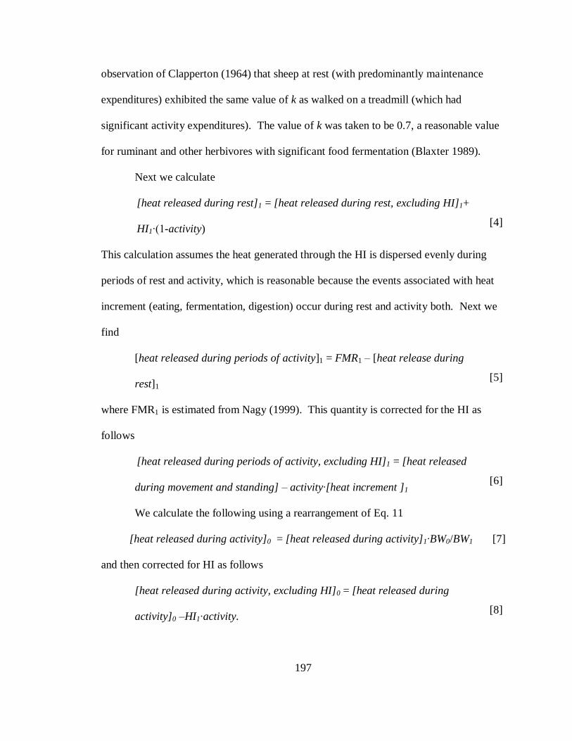
197
observation of Clapperton (1964) that sheep at rest (with predominantly maintenance
expenditures) exhibited the same value of k as walked on a treadmill (which had
significant activity expenditures). The value of k was taken to be 0.7, a reasonable value
for ruminant and other herbivores with significant food fermentation (Blaxter 1989).
Next we calculate
[heat released during rest]1 = [heat released during rest, excluding HI]1+
HI1∙(1-activity) [4]
This calculation assumes the heat generated through the HI is dispersed evenly during
periods of rest and activity, which is reasonable because the events associated with heat
increment (eating, fermentation, digestion) occur during rest and activity both. Next we
find
[heat released during periods of activity]1 = FMR1 – [heat release during
rest]1 [5]
where FMR1 is estimated from Nagy (1999). This quantity is corrected for the HI as
follows
[heat released during periods of activity, excluding HI]1 = [heat released
during movement and standing] – activity∙[heat increment ]1 [6]
We calculate the following using a rearrangement of Eq. 11
[heat released during activity]0 = [heat released during activity]1∙BW0/BW1 [7]
and then corrected for HI as follows
[heat released during activity, excluding HI]0 = [heat released during
activity]0 –HI1∙activity. [8]
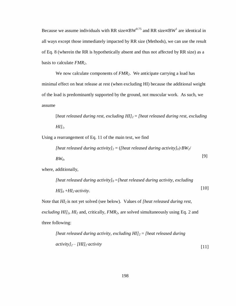
198
Because we assume individuals with RR size∝BW0.75
and RR size∝BW1 are identical in
all ways except those immediately impacted by RR size (Methods), we can use the result
of Eq. 8 (wherein the RR is hypothetically absent and thus not affected by RR size) as a
basis to calculate FMR2.
We now calculate components of FMR2. We anticipate carrying a load has
minimal effect on heat release at rest (when excluding HI) because the additional weight
of the load is predominantly supported by the ground, not muscular work. As such, we
assume
[heat released during rest, excluding HI]2 = [heat released during rest, excluding
HI]1.
Using a rearrangement of Eq. 11 of the main text, we find
[heat released during activity]2 = ([heat released during activity]0)∙BW2/
BW0. [9]
where, additionally,
[heat released during activity]0 =[heat released during activity, excluding
HI]0 +HI2∙activity. [10]
Note that HI2 is not yet solved (see below). Values of [heat released during rest,
excluding HI]2, HI2 and, critically, FMR2, are solved simultaneously using Eq. 2 and
three following:
[heat released during activity, excluding HI]2 = [heat released during
activity]2 – [HI]2∙activity
[11]

199
FMR2= [heat released during rest, excluding heat increment]2 + [heat
released during activity, excluding HI]2 + HI2 [12]
HI2 = FMR2∙(1-k). [13]
The forms of these equations, and the assumptions used in formulating them, are
analogous to those used when RR size∝BW1.
APPENDIX 2
The mechanistic model of ruminant digestion employed in this study was formulated in
Chapter 5. The model is based on chemical reactor theory (Penry and Jumars 1986,
1987) and represents the RR, large intestine, and blood as continuously-stirred reactors
and the small intestine as a plug flow reactor. To simulate digestion, it uses a system of
differential equations to represent flows of nutrients (indigestible NDF; digestible NDF;
indigestible ADF; digestible ADF; soluble non-structural carbohydrate; and insoluble
non-structural carbohydrates; soluble protein; insoluble, indigestible protein; insoluble,
digestible protein; lipid), metabolites (NH3, urea, SCFA), and microbes within and across
these reactors.
In simulating digestion for a given level of PPDMI, the model computes two key
parameters: (1) RR fill with space-occupying NDF (kg∙100 kg BW-1
), (2) the quantity of
nutrients and metabolites the gastrointestinal tract absorbs per unit time, with NE
(expressed in units of NEm [Mcal∙100 kg BW-1
∙h-1
]) and protein (kg∙100 kg BW-1
∙h-1
) of
particular importance. Both of parameters have been proposed to regulate intake in the
ruminant (Forbes, 2007). We compared the computed value of these two parameters to
optimal or reference values by taking the ratio between reference and actual parameter

200
values. We define the ratio of optimal (Cr) to actual (NEI) NE intake as the chemostatic
feedback signal (Cs)—i.e.,
NEI
CC r
s
The value of Cr is equal to the energy required to reach genetic production potential
(defined here as the production level expected from an individual of a given species, BW,
physiological state, production stage, and sex under optimal nutritional, environmental,
and managerial conditions) and computed as described below. We additionally define
the ratio of reference (Dr) to actual (<RR
NDF>) RR fill with NDF as the distention
feedback signal (Ds)—i.e.,
NDF
DD
RR
rs
We define Dr as <RR
NDF> when Cs = 1 and set its value to 1.7 kg∙100 kg BW-1
, a value
found by applying the model to a calibration dataset (Mertens, 1973). We used NDF as a
measure of RR fill following its historic use in the literature (Mertens, 1987) and because
its use led to higher system stability (faster and higher convergence rates during model
solution procedures) relative to other potential measures.
We found an empirical relationship between chemostatic and distention feedbacks
from two studies in the literature (Bernal Santos, 1989; Bosch et al., 1992a,b),
summarized by the equation
ss CD [3]
where α is a shape parameters found by regression (using log-transformed values of
variables) and equal to (mean±SE) -0.78±0.16 (MSE = 0.16, P < 0.001).

201
Eq. 1 was derived under circumstances where the dietary energy:protein ratio was
low, though high ratios strongly reduce intake (Moore and Kunkle, 1995). To
accommodate diets with high ratios, we added a feedback signal for energy:protein, using
an equation form proposed by Fisher (1996)
):(1
PNEeePs
where Ps = energy:protein feedback signal; NE:P = ratio of NE to protein absorption from
the GIT (Mcal∙kg-1
); and γ, δ, and ε = shape parameters (unitless). The value of γ (0.7) is
from Fisher (1996) and δ and ε (6, 0.17) were found by applying the model to a
calibration dataset (Mertens, 1973). This signal describes the fraction of PPDMI realized
when energy:protein feedback occurs relative to the case where no feedback occurs.
After incorporating this signal, the relationship between Ct and Dt can be shown to
become
s
ss
P
CD
[2]
We solved the model’s system of differential equations to find a level of PPDMI
(predicted PPDMI) that (1) yields values of Cs, Ds, and Ps that fulfill Eq. 2 and (2) lead to
steady-state conditions.
We assumed that the energetic demands of an animal at the maintenance, non-
productive state (as in the validation studies) are equal to maintenance metabolic rate;
that is, the animal ―seeks‖ to maintain energy stasis. We predicted maintenance
metabolic rate and thus Cr with Blaxter (1989) and NRC (2000, 2001, 2007) in
conjunction with species and BW data given in the published report. Other inputs for the
model include chemical composition of the forage (NDF, ADF, CP, ash) as well as

202
forage type (alfalfa [including cutting, if available], C3 grass, C4 grass, grass/legume
mixture), which determine the degradation characteristics of the diet. All other
parameters were constants estimated from 65 published reports and our own unpublished
data (Hackmann, T.J., Sampson, J.D., and Spain, J.N., unpublished). Because of the
complexity and number of equations used in the model, the model currently
accommodates diets with only one ingredient (including more than one dietary ingredient
would require multiplicity of equations).
In discussing the model in Methods and elsewhere, we use the terms metabolic
rate and RR DM contents and as synonyms for energetic demands and RR NDF fill,
respectively. Given the definition of energetic demands as maintenance metabolic rate
above, the use of metabolic rate as a synonym for energetic demands is ensuant. The
high correlation between RR DM and NDF contents (r = 0.975; Hackmann, T.J.,
unpublished summary of 20 cattle studies) suggests that the two can be used
synonymously, also.
As discussed in Chapter 5, good agreement between model-predicted and actual
values of PPDMI was found in a validation with 15 studies (including the 5 studies used
in determining the empirical relationship between PPDMI and BW) reporting ad libitum
consumption of all-forage diets by 14 bovid, 4 cervid, and 1 giraffid species during
gestation, lactation, growth, or non-productive physiological states (R2 = 0.910, root
mean square prediction = 1.35 kg∙d-1
). The good agreement circumstantially suggests
that the underlying mechanisms in the model are represented correctly and in accordance
with real biological phenomena, making the model appropriate for mechanistic analysis
of PPDMI scaling with BW.

203
Table 6.1 Species used to derive allometric equations relating several physiological
parameters (PPDMI, DDM, RR WM contents, RR tissue WM) to BW
Species name Equations2
binomial common PPDMI RR WM
contents
RR tissue
WM
Aepyceros melampus Impala X X
Alces alces North American moose X X
Antidorcas marsupialis Springbok X X
Bison bison American bison X
Bison bonasus European bison X
Bos gaurus Gaur X
Bos taurus Domestic cattle X X
Boselaphus tragocamelus Nilgai X
Bubalus bubalis Asian water buffalo X
Capra aegagrus hircus Domestic goat X
Capreolus capreolus Roe deer X X X
Cervus canadensis North American elk X X
Cervus duvaucelii Barasingha X
Cervus elaphus Red deer X X X
Cervus nippon Sika deer X X
Connochaetes taurinus Blue wildebeest X X
Dama dama Fallow deer X X
Gazella granti Grant’s gazelle X
Gazella thomsoni Thomson’s gazelle X
Giraffa camelopardalis Giraffe X X
Hemitragus jemlahicus Himalayan Tahr X X
Kobus ellipsiprymnus Waterbuck X X
Litocranius walleri Gerenuk X
Neotragus moschatus Suni X
Odocoileus hemionus Mule deer X
Odocoileus virginianus White-tailed deer X X
Oryx gazelle Gemsbok X X X
Ovibos moschatus Muskoxen X X
Ovis aries Domestic sheep X X
Ovis canadensis Bighorn sheep X
Rangifer tarandus Reindeer X X
Syncerus caffer African buffalo X X X
Taurotragus oryx Common eland X X
Tragelaphus strepsiceros Greater kudu X X PPDMI = physiologically potential DMI, RR = reticulorumen, WM = wet mass 2An ―X‖ below indicates that the species in the corresponding row was used in the derivation of the
allometric equation in the corresponding column.

204
Table 6.2. Descriptive statistics of studies used to determine empirical relationship
between BW and PPDMI and DDM1,2
Item3 n mean min max SD
Diet
NDF, g∙kg-1
DM 52 575 351 787 147
ADF, g∙kg-1
DM 52 388 261 501 60
CP, g∙kg-1
DM 52 13.3 36 231 69
NEm, Mcal∙
kg DM-1 4
52 1.23 0.71 1.77 0.304
Animal
BW, kg 52 275.3 17.2 907 232
DDM, g∙g-1
DM 18 0.566 0.460 0.687 0.568
DOM, g∙g-1
OM 41 0.613 0.445 0.781 0.117
PPDMI, kg∙(100 kg
BW∙d)-1
52 1.90 0.467 3.86 0.67
PPDMI, kg∙d-1
52 4.37 0.458 12.81 3.41 1Studies include Foose (1982), Baker and Hobbs (1987), Reid et al. (1990), Domingue et al. (1991), and
van Weiren (1996). 2PPDMI = physiologically potential DMI, DDM = digestible DM 3OMD = digestible OM 4NEm estimated using equations of NRC (2001)
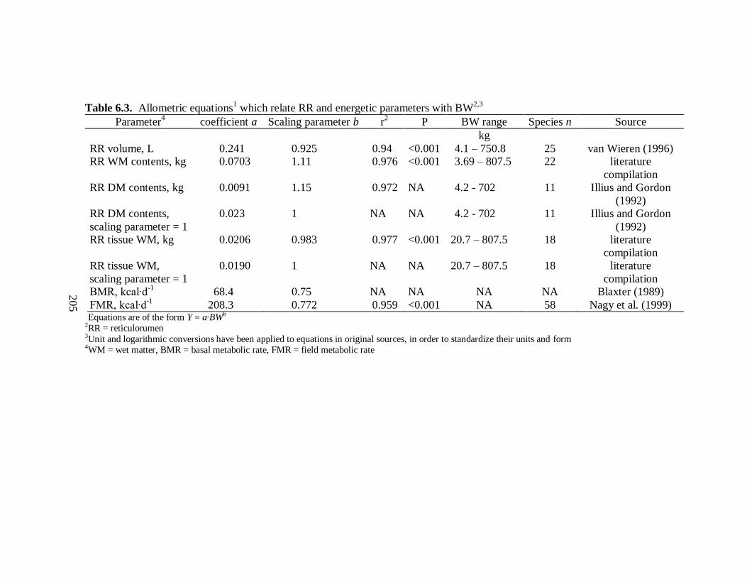
205
Table 6.3. Allometric equations1 which relate RR and energetic parameters with BW
2,3
Parameter4 coefficient a
Scaling parameter b
r
2 P BW range
Species n Source
kg
RR volume, L 0.241 0.925 0.94 <0.001 4.1 – 750.8 25 van Wieren (1996)
RR WM contents, kg 0.0703 1.11 0.976 <0.001 3.69 – 807.5 22 literature
compilation
RR DM contents, kg 0.0091 1.15 0.972 NA 4.2 - 702 11 Illius and Gordon
(1992)
RR DM contents,
scaling parameter = 1
0.023 1 NA NA 4.2 - 702 11 Illius and Gordon
(1992)
RR tissue WM, kg 0.0206 0.983 0.977 <0.001 20.7 – 807.5 18 literature
compilation
RR tissue WM,
scaling parameter = 1
0.0190 1 NA NA 20.7 – 807.5 18 literature
compilation
BMR, kcal∙d-1
68.4 0.75 NA NA NA NA Blaxter (1989)
FMR, kcal∙d-1
208.3 0.772 0.959 <0.001 NA 58 Nagy et al. (1999) 1Equations are of the form Y = a∙BWb
2RR = reticulorumen 3Unit and logarithmic conversions have been applied to equations in original sources, in order to standardize their units and form 4WM = wet matter, BMR = basal metabolic rate, FMR = field metabolic rate
205

206
Table 6.4. Expected values of some digestive, energetic, and other parameters when RR size scales with BW1 1,2
BW Remark RR
volume
RR WM
contents3
RR tissue
WM3
FMR4
RASC5 Fraction of peritoneal
space not occupied by
RR
kg L kg kg kcal∙d-1
m-1
L∙L-1
2 Smallest ruminant 0.459 0.151 0.0407 356 1.30 0.3
50 9.00 5.32 0.963 4270 0.491 0.3
100 17.1 11.4 1.90 7290 0.388 0.3
500 75.8 67.9 9.26 25200 0.236 0.3
1000 Largest bovid 144 146 18.3 43100 0.191 0.3
1500 Largest giraffid 209 229 27.3 59000 0.168 0.3
3000 Largest extinct ruminant 397 492 53.9 101000 0.136 0.3 1RR = reticulorumen, BW = body weight 2Values calculated using regression equations in Methods (shown partially in Table 6.2) 3WM = wet mass 4FMR = field metabolic rate 5RASC = relative absorptive/secretive capacity
206

207
Table 6.5. Expected values of some digestive, energetic, and other parameters when RR size scales with BW0.75 1,2
BW when
RR∝BW1
BW when
RR∝BW0.75
Remark RR
volume
RR WM
contents3
RR tissue
WM3
FMR4
RASC5 Fraction of peritoneal
space not occupied by
RR
kg kg L kg kg kcal∙d-1 m-1
L∙L-1
2 1.96 Smallest
ruminant
0.406 0.118 0.0346 349 1.35 1.35
50 45.4 4.54 1.32 0.387 3860 0.604 0.604
100 89.5 7.64 2.22 0.651 6500 0.508 0.508
500 432 25.5 7.43 2.18 21700 0.340 0.340
1000 851 Largest bovid 42.9 12.5 3.66 36400 0.286 0.286
1500 1270 Largest giraffid 58.2 16.9 4.96 49300 0.258 0.258
3000 2490 Largest extinct
ruminant
97.9 28.5 8.34 82800 0.217 0.217
1RR = reticulorumen, BW = body weight 2Values calculated using regression equations in Methods (shown partially in Table 6.2) 3WM = wet mass 4FMR = field metabolic rate 5RASC = relative absorptive/secretive capacity
207
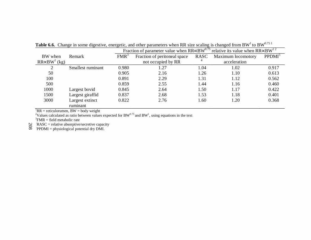
208
Table 6.6. Change in some digestive, energetic, and other parameters when RR size scaling is changed from BW1 to BW
0.75 1
Fraction of parameter value when RR∝BW0.75
relative its value when RR∝BW1 2
BW when
RR∝BW1 (kg)
Remark FMR3 Fraction of peritoneal space
not occupied by RR
RASC4
Maximum locomotory
acceleration
PPDMI5
2 Smallest ruminant 0.980 1.27 1.04 1.02 0.917
50 0.905 2.16 1.26 1.10 0.613
100 0.891 2.29 1.31 1.12 0.562
500 0.859 2.55 1.44 1.16 0.460
1000 Largest bovid 0.845 2.64 1.50 1.17 0.422
1500 Largest giraffid 0.837 2.68 1.53 1.18 0.401
3000 Largest extinct
ruminant
0.822 2.76 1.60 1.20 0.368
1RR = reticulorumen, BW = body weight 2Values calculated as ratio between values expected for BW0.75 and BW1, using equations in the text 3FMR = field metabolic rate 4RASC = relative absorptive/secretive capacity 5PPDMI = physiological potential dry DMI.
208
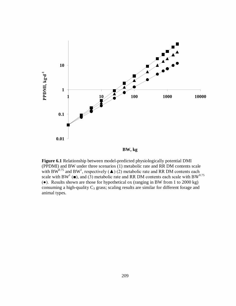
209
PP
DM
I, k
g∙d
-1
BW, kg
Figure 6.1 Relationship between model-predicted physiologically potential DMI
(PPDMI) and BW under three scenarios (1) metabolic rate and RR DM contents scale
with BW0.75
and BW1, respectively (▲) (2) metabolic rate and RR DM contents each
scale with BW1 (■), and (3) metabolic rate and RR DM contents each scale with BW
0.75
(●). Results shown are those for hypothetical ox (ranging in BW from 1 to 2000 kg)
consuming a high-quality C3 grass; scaling results are similar for different forage and
animal types.
0.01
0.1
1
10
1 10 100 1000 10000

210
CHAPTER 7
PERSPECTIVES FROM RUMINANT ECOLOGY AND EVOLUTION USEFUL
TO RUMINANT LIVESTOCK RESEARCH AND PRODUCTION
ABSTRACT
This chapter presents insights ruminant ecology and evolution that can be utilized in
livestock research. The first ruminants evolved about 50 million years ago and were
small (<5 kg) forest-dwelling omnivores. Today there are almost 200 living ruminant
species in 6 families. Wild ruminants number about 75 million, range from about 2 to
more than 800 kg, and generally prefer at least some browse in their diet. Eight species
have been domesticated within the last 12,000 years. Their combined population
currently numbers 3.6 billion. In contrast to wild ruminants, domestic species naturally
prefer at least some grass in their diets, are of larger BW (roughly from 35 to 800 kg),
and, excepting reindeer, belong to one family (Bovidae). Wild ruminants thus have a
comparatively rich ecological diversity and long evolutionary history. Studying them
gives a broad perspective that can augment ruminant research and production.
Allometric equations, often used in ecology, relate BW to physiological measurements
from several species (typically both wild and domestic). Their utility is to predict or
explain values of physiological parameters from BW alone. Voluntary feed intake is
proportional to BW0.9
across wild and domestic ruminant species. This proportionality
suggests that physical and metabolic factors regulate intake simultaneously, not mutually
exclusively as often presumed. Studying the omasum in wild species suggests it

211
functions primarily in particle separation and retention and only secondarily in absorption
and other roles. Studies on the African Serengeti show that multiple species, when
grazed together, feed such that they use grasslands more completely. They support use of
mixed-species grazing systems in production agriculture. When under metabolic stress,
wild species will not rebreed but rather extend lactation (to nourish their current
offspring). This bolsters the suggestion that lactation length be extended in dairy
operations. Cooperation between animal scientists and ecologists could generate
valuable insight.
INTRODUCTION
As an applied field, animal science borrows variously from classical physiology,
endocrinology, biochemistry, genetics, and nutrition, among other disciplines. Seldom
though does it draw from ecological and evolutionary research. For ruminant research, at
least, this is not because of a dearth of excellent material on the subject, with classic
works such as Hoffman (1973), Clutton-Brock et al. (1982), Foose (1982), and Owen-
Smith (1988) and more recent material compilations as Vbra and Schaller (2000) and
Prothero and Foss (2008).
In his general ruminant nutrition text, Van Soest (1994) presents a fairly
comprehensive account of ruminant ecology and evolution—perhaps the most
comprehensive in an animal science work. However, as may be expected from a general
text, Van Soest’s (1994) account lacks detail and syntheses few explicit connections
between ruminant ecology and evolution and applied livestock research. Some individual
manuscripts (e.g., Walker 1994, Knight 2001) have drawn more detailed and direct
212
connections. While valuable in their own right, these manuscripts have a limited scope
and lack a thorough introduction to ruminant ecology and evolution.
Chapter 1 has reviewed key points of ruminant ecology and evolution. This
chapter briefly recapitulates these points then shows where they offer insight into
livestock research and production. We draw on both our original ideas and some
presented previously. The focus on nutrition and physiology in this review reflects our
own expertise, not a lack of importance of other fields (e.g., reproduction, behavior,
genetics).
ECOLOGY, EVOLUTION, AND DOMESTICATION OF RUMINANTS
Details of the discussion below are found in Chapter 1. A ruminant is any artiodactyl that
possesses a rumen, reticulum, omasum or isthmus homologous to the omasum, and
abomasum. Ruminants also possess certain skeletal features—e.g., fusion of cubiod and
navicular bones in the tarsus—that are useful in fossil identification.
Ruminant Families
Except where noted, details of the discussion below are from Nowak (1999) and
Feldhamer et al. (2007). The six extant (i.e., non-extinct) ruminant families include the
Tragulidae, Moschidae, Bovidae, Giraffidae, Antilocapridae, and Cervidae. The
Tragulidae (chevrotains) and Moschidae (musk deer) are small forest-dwelling, deer-like
ruminants. Members of both families are hornless, and males have large upper canines
instead. The Tragulidae are phylogenetically and morphologically primitive—they have
even been called ―living fossils‖ (Janis, 1984))—and lack a true omasum (Langer, 1988).
The remaining families, the Bovidae (e.g., cattle, sheep, goats, antelope), Giraffidae

213
(giraffe and okapi), Cervidae (true deer; e.g., white-tailed deer, caribou, moose), and
Antilocapridae (pronghorn), include species familiar to most readers.
There are 5 additional extinct families, the Hypertragulidae, Leptomerycidae,
Gelocidae, Palaeomerycidae, and Dromomerycidae (Carroll, 1988). The
Hypertragulidae, Leptomerycidae, and Gelocidae were small, hornless ruminants that
probably most closely resembled moschids or tragulids (Webb and Taylor, 1980; Webb,
1998b). The Palaeomerycidae and Dromomerycidae are medium-to-large-sized with
giraffe-like horns but deer-like limb proportions (Janis and Scott, 1987). Their ecological
niche probably resembled that of a subtropical deer (Jannis and Manning, 1998b).
Evolution
The Hypertragulidae first appeared about 50 million years ago in SE Asia (Métais
and Vislobokov, 2007) and were soon followed by the Tragulidae and Leptomerycidae
(Colbert, 1941; Métais et al., 2001). The Gelocidae appeared at approximately 40 million
years ago (Ma) (Genry, 2000). All but the Tragulidae eventually migrated to North
America (Webb, 1998b). These groups were rabbit-sized at first, though their size
increased progressively over time (Chapter 6). They probably were reclusive, forest-
dwelling omnivores (Webb, 1998b). They did not have extensive foregut fermentation or
rumination until about 40 Ma (Jermann et al., 1995).
The remaining families evolved around 18 to 23 Ma in Eurasia (Antilocapridae,
Cervidae, Moschidae, Dromomerycidae, Bovidae, Palaeomerycidae) and Africa
(Giraffidae) (Gentry, 2000). Many (Bovidae, Cervidae, Moschidae, Dromomerycidae,
Antilocapridae) migated to North America (Janis and Manning, 1998a,b; Webb, 1998b),
though the Bovidae and Cervidae did not migrate until relatively late (5 Ma) (Webb,
214
1998a, 2000). By 2 Ma, Cervidae migrated to South America (Webb, 2000). Body mass
of these groups was larger (20 to 40 kg; Janis, 1982) and increased over time. The first of
these groups lived in open woodlands and ate primarily grass and leaves (Janis, 1982;
DeMiguel et al., 2008). When grasslands expanded about 5 to 11 Ma, some species
began including more grass in their diets (Semprebon et al., 2004; Semprebon and Rivals,
2007).
Ecological Characteristics
Except where noted, details of the discussion below are from van Wieren (1996).
Today there exist nearly 200 ruminant wild species (Nowak, 1999), most of which are
Bovidae and Cervidae. A conservative estimate places the world population of wild
ruminants at 75.3 million, with 0.28 million tragulids, 0.28 million moschids, 44.6
million cervids, 29.1 million bovids, 0.15 million giraffids, and 0.88 million antilocaprids
(Chapter 1). Living ruminants are natively found on all continents except Antarctica and
Australia, with most species are found in Africa and Eurasia. As a whole, ruminant
species are evenly spread across open, ecotone, and forested habitats, but they prefer
warm to other types of climates. Median BW of modern ruminants is 45 kg, near that
expected from the historical trend. Species BW ranges greatly, from approximately 2 kg
to 800 kg or more. For most of their evolutionary history, ruminant species were
predominately or exclusively browsers (consume fruits, shoots, and leaves) (see above).
Today, a plurality of ruminant species is still classified as browsers, and only about a
quarter are grazers (consume grass and roughage).
215
Details of Domestication
Except where noted, details of the discussion below are from Clutton-Brock
(1999). The goat was domesticated at approximately 10,000 B.C. in the Fertile Crescent
of the Near East (Zeder and Hesse, 2000). Most of the other 8 domesticated ruminant
species (sheep, European and Zebu cattle, water buffalo, mithan, reindeer, yak, Bali
cattle) were brought under human control by 2,500 B.C. in either the Near East or
southern Asia. The goat and other species were initially domesticated for meat, but
reasons for domesticating other species included milk, draft, transportation, sacrifice, and
barter. Each domestic species is probably derived from several wild species; at least 12
species can claim ancestry to the 9 domesticated species (Bruford et al., 2003). These 12
and possibly others were chosen for domestication because they were gregarious,
submissive to human captors, unexcitable, and easy to breed.
Characteristics of Domestic Species
The total population size of domestic species is 3.57 billion (Chapter 1), nearly
50-fold larger than that of wild ruminants. All but reindeer belong to the family Bovidae.
Most species are grazers, though goats, reindeer, and possibly sheep are intermediate
feeders (consume either browse and grass) (Chapter 1). Body mass of domestic
ruminants is larger than most wild ruminants. The smallest species (sheep, goat) are near
the median BW of wild ruminants (45 kg) and many species (cattle, mithan, Bali cattle)
approach the maximum observed in the wild (800 kg) (Chapter 1).
PERSPECTIVES REVELANT TO MODERN PRODUCTION SYSTEMS
Wild ruminants, past and present, prove much more diverse (in terms of phylogeny,
behavior, diet, and otherwise) than domestic ruminants. Further, the 50 million year
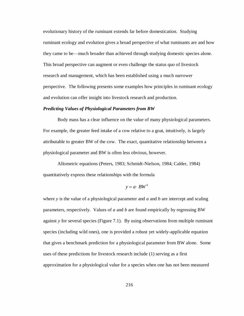
216
evolutionary history of the ruminant extends far before domestication. Studying
ruminant ecology and evolution gives a broad perspective of what ruminants are and how
they came to be—much broader than achieved through studying domestic species alone.
This broad perspective can augment or even challenge the status quo of livestock
research and management, which has been established using a much narrower
perspective. The following presents some examples how principles in ruminant ecology
and evolution can offer insight into livestock research and production.
Predicting Values of Physiological Parameters from BW
Body mass has a clear influence on the value of many physiological parameters.
For example, the greater feed intake of a cow relative to a goat, intuitively, is largely
attributable to greater BW of the cow. The exact, quantitative relationship between a
physiological parameter and BW is often less obvious, however.
Allometric equations (Peters, 1983; Schmidt-Nielson, 1984; Calder, 1984)
quantitatively express these relationships with the formula
bBWay
where y is the value of a physiological parameter and a and b are intercept and scaling
parameters, respectively. Values of a and b are found empirically by regressing BW
against y for several species (Figure 7.1). By using observations from multiple ruminant
species (including wild ones), one is provided a robust yet widely-applicable equation
that gives a benchmark prediction for a physiological parameter from BW alone. Some
uses of these predictions for livestock research include (1) serving as a first
approximation for a physiological value for a species when one has not been measured
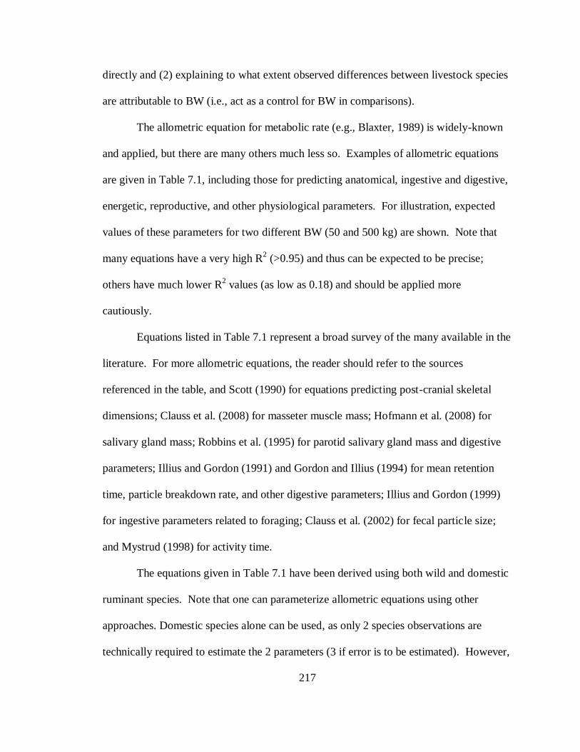
217
directly and (2) explaining to what extent observed differences between livestock species
are attributable to BW (i.e., act as a control for BW in comparisons).
The allometric equation for metabolic rate (e.g., Blaxter, 1989) is widely-known
and applied, but there are many others much less so. Examples of allometric equations
are given in Table 7.1, including those for predicting anatomical, ingestive and digestive,
energetic, reproductive, and other physiological parameters. For illustration, expected
values of these parameters for two different BW (50 and 500 kg) are shown. Note that
many equations have a very high R2 (>0.95) and thus can be expected to be precise;
others have much lower R2 values (as low as 0.18) and should be applied more
cautiously.
Equations listed in Table 7.1 represent a broad survey of the many available in the
literature. For more allometric equations, the reader should refer to the sources
referenced in the table, and Scott (1990) for equations predicting post-cranial skeletal
dimensions; Clauss et al. (2008) for masseter muscle mass; Hofmann et al. (2008) for
salivary gland mass; Robbins et al. (1995) for parotid salivary gland mass and digestive
parameters; Illius and Gordon (1991) and Gordon and Illius (1994) for mean retention
time, particle breakdown rate, and other digestive parameters; Illius and Gordon (1999)
for ingestive parameters related to foraging; Clauss et al. (2002) for fecal particle size;
and Mystrud (1998) for activity time.
The equations given in Table 7.1 have been derived using both wild and domestic
ruminant species. Note that one can parameterize allometric equations using other
approaches. Domestic species alone can be used, as only 2 species observations are
technically required to estimate the 2 parameters (3 if error is to be estimated). However,

218
with so few species observations, an outlier from any one species can unduly affect
parameter estimates. Wild species should thus be included to increase the number of
observations and the robustness of parameter estimates. At the opposite end, non-
ruminant species (wild or domestic) can be included in addition to ruminants. In this
case, phylogenetic differences across the wide range of species, if not controlled for
statistically, may make the resultant equation very general but also very imprecise and
potentially biased. For example, adding marsupials to the allometric equation for
metabolic rate would make the equation more widely applicable (viz., for marsupials) but
would skew the regression because marsupials have characteristically low metabolic rates
(Dawson and Hulbert, 1970). A good balance between precision, generality, and
robustness is thus found by including domestic and wild ruminant species and these
alone.
Role of Physical and Metabolic Factors in Regulating Feed Intake
Besides the two general uses of allometric equations explained above, some
allometric equations can be applied to draw deeper, more complex inferences. For
example, the allometric equation for feed intake demonstrates that forage intake is
regulated by physical and metabolic factors simultaneously.
Physiological regulation of feed intake is important to livestock production
systems because feed intake impacts animal performance and operation costs. Of the
many proposed regulation mechanisms (Forbes, 2007), physical (Allen, 1996) and
metabolic regulation (Illius and Jessop, 1996) are often suggested to predominate.
Generally these two regulation mechanisms (physical, metabolic) are typically considered
operate on a mutually exclusive basis, with intake of low-energy, bulky diets (usually

219
forages) regulated only physically and high-energy, highly-degradable diets regulated
only metabolically (Conrad et al., 1964; Baumgardt, 1970).
Theoretical arguments have suggested that these two and more regulation
mechanisms operate simultaneously (Fisher et al., 1987; Fisher, 1996), as do experiments
in which VFA is infused and physical ballast is placed in the rumen simultaneously
(Forbes, 1996). A recent examination of feed intake behavior of wild and domestic
ruminants (Chapter 6) considerably strengthens the case for simultaneous regulation.
Because reticulorumen digesta contents and volume are nearly proportional to BW1 (i.e.,
proportionally do not change with BW; Table 7.1), one would expect feed intake be
proportional to BW1, also, if physical regulation only were operating. On other hand,
because metabolic rate is proportional to BW0.75
(Table 7.1), one would expect feed
intake be proportional to BW0.75
, also, if metabolic regulation acted alone. However, in a
summary 19 species from 5 studies, we (Chapter 6) found that intake of forage is
proportional to BW0.875±0.032
(Table 7.1), with lower and upper 95% percent confidence
limits of BW0.810
and BW0.941
. This agrees with the finding that for livestock species
(cattle, sheep, goats) intake scales with BW0.9
(Minson 1990, Reid et al., 1990).
The mean value of the scaling parameter (~0.9) and its 95% confidence limits fall
in between values expected if intake were regulated only physically (1) and metabolically
(0.75). Intuitively, this suggests that physical and metabolic regulation operate
simultaneously for forage diets, contrary to the classical suggestion physical regulation
alone should occur; mechanistic modeling described in Chapter 6 confirmed this
suggestion. Though lack of controlled data disallowed a similar examination with non-all
forage diets, the wide range in quality of the forage diets (predicted NEm ranged from

220
0.71 to 1.77 Mcal∙kg DM-1
) suggests the results are not simply constrained to a narrow
range of forages. Because this simultaneous regulation is apparent across wild and
domestic species alike, it can be inferred that it is highly conserved evolutionarily and
deeply-seated.
Conrad et al. (1964), who originally proposed that metabolic and physical
regulation are mutually exclusive, also used allometry to support their arguments. They
concluded that for high-producing dairy cows, intake scaled with BW0.73
for low-
digestibility (>66.7% DDM) and BW1 for high-digestibility (<66.7% DDM) diets,
consistent with mutually exclusive regulation. This conclusion is, at the very least,
oversimplified. For high-digestibility diets, scaling parameter values were ~0.73 for only
2 of their 5 regressions; all others were lower (≤0.62). The upper 95% confidence limits
of these 2 favorable regressions (0.962 and 1.03) do not rule out intake scaling with
BW0.9
or even possibly BW1. This, and considering that intake was only poorly related to
BW (R2 = 0.074 or lower), indicates that this dataset is poor for discriminating intake
scaling patterns. Detailed results are not presented for low digestibility diets, but the
above suggests one should remain skeptical of their conclusion that intake scales with
BW1
for these diets. While intriguing for their time, the allometric analysis of Conrad et
al. (1964) and conclusions based thereon must be rejected over our more discriminating
analysis.
Primary Function of the Omasum
Whereas functions of the rumen, reticulum, and abomasum are well-delineated,
the chief function of the omasum remains somewhat a mystery. It may help retain and
separate particles, as (1) large particles tend to become trapped between the omasal

221
laminae while small particles and liquid pass through quickly (Bost, 1970; Langer, 1988),
and (2) large particles can be ejected from the omasum back into the reticulum (via the
reticuloomasal orifice) (Ehrlein, 1980). It may more generally serve as a suction-pump
that regulates flow of digesta (both liquid and particles) from the reticulum to the
abomasum (Stevens et al., 1960), though some question this purported ability (Bost,
1970; Langer, 1988). It may also be an absorptive organ; the omasum absorbs
approximately 12.5, 50, 35, 25, 10, and 50% of water, VFA, ammonia, sodium,
potassium, and CO2 that enter (Engelhardt and Hauffe, 1975). Some fiber digestion (7 to
9% of total tract; Ahvenjärvi et al., 2000, 2001) also occurs in the omasum. Finally,
some claim the omasum reduces particle size (via purported grinding of digesta between
laminae), though evidence for this function is at best circumstantial (Bost, 1970).
To establish the primary function of the omasum, we will review the omasal form
and function of several wild species and suggest how and why the omasum evolved. In
tragulids, a true omasum is not present at all; where it should be found there exists only
an isthmus instead (Langer, 1988). As shown in Figure 7.2, this isthmus (also called a
transisiton zone by some) is short, narrow, and with only small, subtle longitudinal folds
(Agungpriyono et al., 1992). Though it does not form a distinct compartment like a true
omasum, it is still histologically distinct from the reticulum and abomasum
(Agungpriyono et al., 1995). Considering this evidence and that the Tragulidae are
otherwise primitive (Figure 1.5), this isthmus probably resembles a very early form of
omasum, as concluded by other authors (see Langer [1988]). Because the isthmus lacks
structures to retain digesta within it, its contribution to absorption, fiber fermentation,
absorption, and particle size reduction must be minimal. Its poor structural development

222
also precludes it from acting as a suction-pump to regulate digesta flow. However, the
isthmus likely helps retain particles as its small aperture should allow only fine particles
to pass into the abomasum and subsequently through the rest of the tract (Langer, 1988).
In small browsing Pecoran species, which are more advanced than the tragulids,
the omasum forms a distinct compartment, but it still tends to be small and has few
laminae (Hoffman, 1973; Langer, 1988, Hoffman, 1989; van Wieren, 1996). Hoffman
(1989) concluded that its simple structure permits it to serve little more than a ―sieving
screen‖ that prevents large particles from entering the abomasum. In large, grazing
ruminants (such as cattle), the omasum is large and with many laminae (Hoffman, 1973;
Langer, 1988; Hoffman, 1989; van Wieren, 1996). Whereas the omasum in these species
still helps retain particles (Langer, 1988), its large surface area may additionally
contribute to absorption (Hoffman, 1973; Hoffman, 1989) and presumably other more
advanced functions (e.g., fiber fermentation).
We thus find a progression in omasal form and function from the tragulids to
browsing then grazing Pecoran ruminants. This progression suggests the omasum
originally evolved as a simple isthmus that acted as a ―flood-gate‖ (Bost, 1970) to retain
particles. Compartmentalization, well-developed laminae, and complex motor activity
subsequently evolved to support absorption, fiber fermentation, and suction-based digesta
flow control. These more derived functions indeed have some adaptive benefit,
particularly for grazers, where they may help process large amounts of refractory fiber
(Hoffman 1973, 1989; Van Soest 1994). Still, considering that the particle retention
function is pervasive across all species and the impetus for the omasum’s evolution, this
function is almost certainly of primary importance.
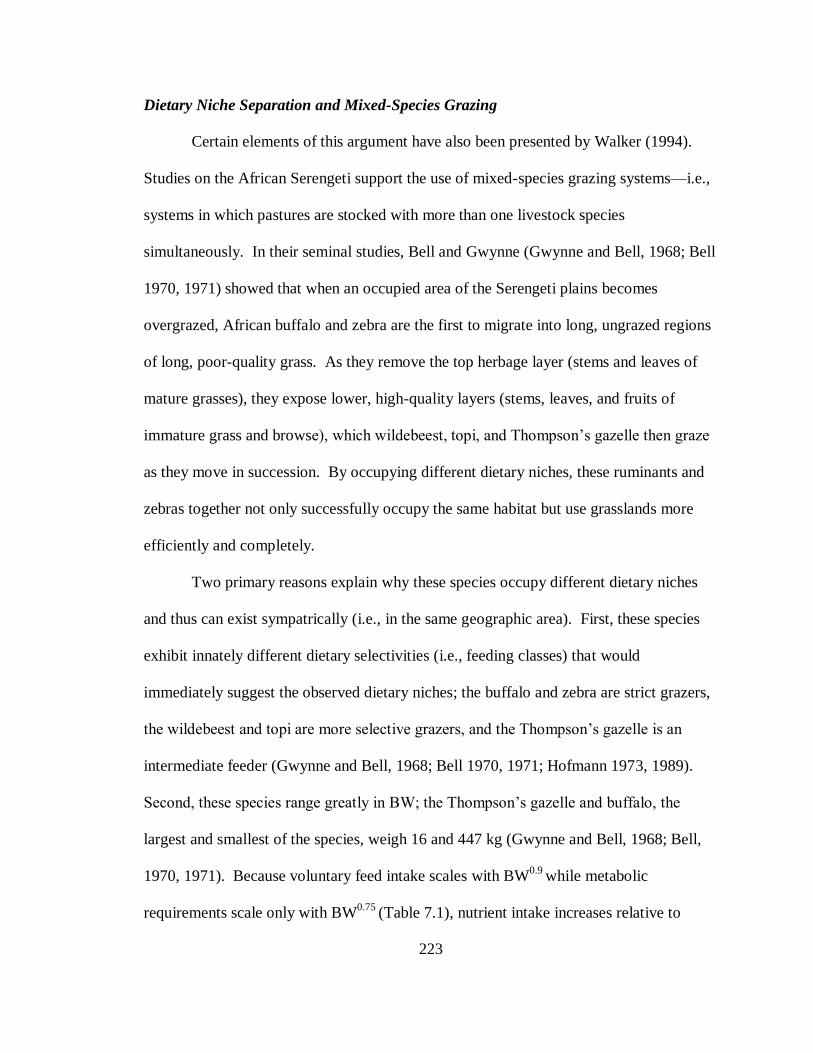
223
Dietary Niche Separation and Mixed-Species Grazing
Certain elements of this argument have also been presented by Walker (1994).
Studies on the African Serengeti support the use of mixed-species grazing systems—i.e.,
systems in which pastures are stocked with more than one livestock species
simultaneously. In their seminal studies, Bell and Gwynne (Gwynne and Bell, 1968; Bell
1970, 1971) showed that when an occupied area of the Serengeti plains becomes
overgrazed, African buffalo and zebra are the first to migrate into long, ungrazed regions
of long, poor-quality grass. As they remove the top herbage layer (stems and leaves of
mature grasses), they expose lower, high-quality layers (stems, leaves, and fruits of
immature grass and browse), which wildebeest, topi, and Thompson’s gazelle then graze
as they move in succession. By occupying different dietary niches, these ruminants and
zebras together not only successfully occupy the same habitat but use grasslands more
efficiently and completely.
Two primary reasons explain why these species occupy different dietary niches
and thus can exist sympatrically (i.e., in the same geographic area). First, these species
exhibit innately different dietary selectivities (i.e., feeding classes) that would
immediately suggest the observed dietary niches; the buffalo and zebra are strict grazers,
the wildebeest and topi are more selective grazers, and the Thompson’s gazelle is an
intermediate feeder (Gwynne and Bell, 1968; Bell 1970, 1971; Hofmann 1973, 1989).
Second, these species range greatly in BW; the Thompson’s gazelle and buffalo, the
largest and smallest of the species, weigh 16 and 447 kg (Gwynne and Bell, 1968; Bell,
1970, 1971). Because voluntary feed intake scales with BW0.9
while metabolic
requirements scale only with BW0.75
(Table 7.1), nutrient intake increases relative to

224
metabolic requirements with increasing BW. Consequently, large species can adapt to
poor-quality material because they can consume relatively large amounts to meet their
metabolic requirements, while smaller species are constrained to higher-quality material
because they can eat relatively little (Bell, 1970, 1971, Jarman, 1974; Chapter 6). This
principle (the Bell-Jarman principle; Geist, 1974) further reinforces innate selectivity
differences to establish different dietary niches.
Significantly, major livestock species (goat, sheep, cattle) differ greatly in feeding
class or BW or both (Table 1.5). Probably as a combination of these factors, species
choose diets that overlap incompletely: goats choose more browse, cattle choose more
grass, and sheep are intermediate (Figure 7.3). Diets should be even less similar than
Figure 7.3 might suggest because (1) Figure 7.3 shows ranges that apply to single-species
grazing, and cattle shift to poorer-quality diets in their range when grazing with sheep
(Walker, 1994), (2) sheep eat plant biomass soiled by cattle feces, which cattle
themselves avoid (Nolan and Connolly, 1989), and (3) the rough expression of botanical
composition shown in Figure 7.3 ignores other ways diets can differ (e.g., by plant
species or part). Livestock species thus have ample opportunity to separate their dietary
niches when grazed concurrently.
Given this probable dietary niche separation, one might expect mixed-grazing
systems to lead more complete utilization of pasture and higher combined level of animal
productivity (as more pasture is transformed into animal tissue). In support, Vallentine
(1990) observed that extent of pasture use can be increased by 25% by using multi- vs.
single-species grazing, and Walker (1994) found that multi-species grazing increased

225
animal gain by 9 and 24% per unit area compared to sheep- and cattle-only systems,
respectively.
There exist some legitimate, practical limitations to mixed-species grazing, such
as elevated facility costs and predation risk of sheep and goats (Vallentine, 1990).
However, most barriers are social, based on tradition and prejudice towards species
(Walker, 1994). The enhanced production and efficiency of the systems vs. conventional
ones—as expected from the archetypal mixed-grazing system on the Serengeti—
challenges these barriers.
Extended Lactation
Elements of this discussion are derived from Knight (2001). The aim of many
dairy cow operations is a 305-d lactation with a 12 to 14 month calving interval. This
requires cattle be rebred by 100 d following parturition, soon after peak lactation, when
they experience a negative energy balance (Bauman and Currie, 1980) and other
metabolic stress that severely reduces fertility (Chagas et al., 2007). With pregnancy
rates of U.S. breeds averaging about 25% (Animal Improvement Programs Laboratory,
2008), this management strategy is largely untenable.
An alternative management approach, forwarded by Knight (1984) and others, is
to purposely extend lactation as long as possible and thus avoid early rebreeding. This
approach, compared to current practice, indeed appears better supported by ecological
observations. When in severe metabolic stress (poor body condition or nutritional plane)
during lactation, many wild species (muskoxen [Adamczewski et al., 1998], red deer
[Loudon et al., 1983; Albon et al. 1986], caribou [Gerhardt et al., 1997]) will not rebreed
or do so only at low rates. Instead of rebreeding, they may extend lactation and thus

226
invest in their current young (caribou: White and Luick, 1984; muskoxen: Knight, 2001).
In muskoxen, this extended lactation can exceed 1 year (Adamczewski et al. 1997). As
explained by Knight (2001), extending lactation is presumably a maternal strategy to
maximize fitness (the most important biological drive of organisms); investing in current
offspring by extending lactation is safer and, in the long-term, more profitable than
producing new offspring when necessary nutritional resources are inadequate.
These observations of wild species suggest that when under metabolic stress, the
ruminant animal is evolutionary entrained to continue lactation rather than rebreed.
Attempting to rebreed the high-producing dairy cow soon after parturition is a direct fight
against this entrained response. If producing replacement heifers is not a major
production goal, it might make more sense to rebreed less frequently and exploit the
physiological capacity and drive for extended lactation shown in wild ruminants.
Though this argument for extended lactation is largely conceptual, growing
experimental evidence suggests practicing extended lactation is viable and profitable.
Lactation has been maintained naturally in goats for 4 years (Linzell, 1973) and in cattle
nearly 2 years (Auldist et al., 2007); with bovine somatropin supplementation, it has been
maintained for more 2 years in cattle (van Amburgh et al., 1997). Milk production far
into an extended lactation is less than around peak, but it is more than production of a
rebred animal during late pregnancy and its dry period (Figure 7.4). Pre-designed
experiments have demonstrated that, over the long term, extending lactation up to 16
months (and sometimes longer) does not decrease daily production (van Amburgh et al.,
1997; Rehn et al., 2000; Arbel et al., 2001; Österman and Bertilsson, 2003; Salama et al.,
2005; Auldist et al., 2007). In some cases, extending lactation has increased either total

227
milk (second lactation of primiparous cows; Arbel et al., 2001) or component (protein
and fat of goats; Salama et al., 2005) yields. The economic advantage of extended
lactation ranged from $0.12 to 0.21∙(d calving interval)-1 among treatment groups in
Arbel et al. (2001) and $0.75∙(d productive life)-1 in van Amburgh et al. (1997). (Note
that earlier studies claiming no positive economic response [e.g., Holmann et al., 1984]
were observational or theoretical, not experimental.) Though more research is clearly
needed, these preliminary results suggest that the biological principles of extended
lactation, as illuminated by wild ruminants, may be of great service to livestock
production systems.
CONCLUSIONS
By offering a comparative vantage point, ruminant ecological and evolutionary research
can offer great insight into livestock research. This research can reinforce and augment
some conventional livestock practices, and if we allow, challenge and help revise others.
With further dialogue and cooperation between animal scientists and ecologists, the
insights that ruminant ecology and evolution have to offer should grow in number and
usefulness.

228
Table 7.1. Some allometric equations useful for predicting physiological parameter values from BW1,2
Equation
parameters
Predicted value for BW
of
Category Physiological parameter a
b
r2 50 kg 500 kg Source
3
Anatomical Reticulorumen volume, L 0.241 0.925 0.940 8.99 75.61 van Wieren (1996)
Skull length, cm 6.18 0.337 0.960 23.1 50.2 Janis (1990)
Ingestive and
digestive
Voluntary feed intake at
maintenance, kg DM∙d-1
0.04374
0.875 0.967 1.34 10.05 Chapter 6
Maximum intake rate, g
WM∙min-1
5
0.738 0.621 0.754 8.37 34.96 data from Shipley et al.
(1994)
Chewing rate during
rumination, s-1
2.53 -0.141 0.660 1.46 1.05 data from Langer
(1988)
Reticulorumen DM contents,
kg
0.0091 1.15 0.972 0.82 11.56 Illius and Gordon
(1992)
Energetic Basal metabolic rate, kcal∙d-1
68.4 0.75 NA 1,286 7,232 Blaxter (1989)
Reproductive Age at sexual maturity,
months
8.86 0.156 0.250 16.3 23.4 van Wieren (1996)
Reproductive output,
youngyr-1
2.54 -0.167 0.180 1.32 0.90 van Wieren (1996)
Gestation length, d 129 0.125 0.556 210 280 data from Peréz-
Barbería and Gordon
(2005)
Other Respiratory frequency, s-1
1.27 -0.221 0.215 0.54 0.32 data from Mortola and
Lanthier (2005) 1Equations are of the form Y = a∙BWb
2Unit, logarithmic, and other conversions have been applied to equations in original sources, in order to standardize their units and form 3The phrase ―data from‖ preceding a source, where present, indicates that we performed the allometric regression using ruminant data (averaged by species)
originally reported by that source. 4b and predicted values reported in this table are for the 58% NDF, 19% CP mature alfalfa hay of van Wieren (1996); in the original equation, b is adjusted
by a fixed-effect term for diet, which allows intake to be predicted for other diet types, but this term was omitted here for simplicity. 5WM = wet matter.
228
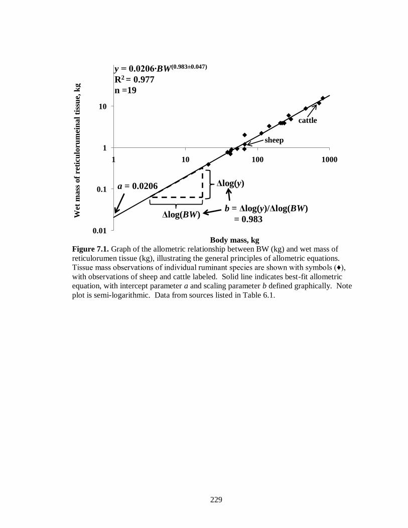
229
Wet
mass
of
reti
culo
rum
ein
al
tiss
ue,
kg
Body mass, kg
Figure 7.1. Graph of the allometric relationship between BW (kg) and wet mass of
reticulorumen tissue (kg), illustrating the general principles of allometric equations.
Tissue mass observations of individual ruminant species are shown with symbols (♦),
with observations of sheep and cattle labeled. Solid line indicates best-fit allometric
equation, with intercept parameter a and scaling parameter b defined graphically. Note
plot is semi-logarithmic. Data from sources listed in Table 6.1.
0.01
0.1
1
10
1 10 100 1000
sheep
cattle
b = Δlog(y)/Δlog(BW)
= 0.983Δlog(BW)
Δlog(y)a = 0.0206
y = 0.0206∙BW(0.983±0.047)
R2 = 0.977
n =19

230
Images removed for electronic publication because copyright permission
could not be obtained. Reader is referred to Figures 5A and 2 of source
(Agungpriyono et al., 1992) for original images.
Figure 7.2. The isthmus in the stomach of the lesser mouse deer (Tragulus javanicus), a
member of the family Tragulidae. (A) The isthmus (arrow) in relation to the reticulum
(―R‖) and abomasum (―1‖). Note its narrow aperture and subtle longitudinal folds. (B)
The isthmus in relation to the entire stomach, showing its small size. 1 = reticulum, 2 =
rumen, 3 = abomasum, 4 = reticular groove, 5 = isthmus. Scale bar in (A) and (B) is 5
mm. Reproduced from Agungpriyono et al. (1992).

231
Bro
wse
, %
Grass, %
Figure 7.3. Botanical composition (% grass and browse) of diets chosen by goat (n = 13),
sheep (n = 105), and cattle (n = 121) on pasture. Bars delineate mean ± SD. Data from
Van Dyne et al. (1980).
0
10
20
30
40
50
60
70
80
90
100
0 10 20 30 40 50 60 70 80 90 100
Goat
Sheep
Cattle

232
Image removed for electronic publication because copyright permission could not be
obtained. Reader is referred to Figure 1 of source (Salama et al., 2005) for original
image.
Figure 7.4. Milk production of extended vs. conventional lactations of multiparous
Muriciano-Granadina goats milked once daily. Open (○) and closed (●) symbols
represent production of goats managed for kidding intervals of 12-months (K12) and 24-
months (K24), respectively. Arrows labeled (a) and (b) highlight where milk production
of extended lactation is greater (during pregnancy and dry period of K12 goats) and less
(during peak lactation of K12 goats) than conventional lactation. First and second
asterisks near x-axis indicate times that K12 and all goats were rebred, respectively.
Figure modified from Salama et al. (2005).

233
REFERENCES
Adamczewski, J. Z., P. F. Flood, and A. Gunn. 1997. Seasonal patterns in body
composition and reproduction of female muskoxen (Ovibos moschatus). J. Zool.
241: 245-269.
Adamczewski, J. Z., P. J. Fargey, B. Laarveld, A. Gunn, and P.F. Flood. 1998. The
influence of fatness on the likelihood of early-winter pregnancy in muskoxen
(Ovibos moschatus). Theriogenology 50:605–614.
Agungpriyono, S, Y. Yamamoto, N. Kitamura, J. Yamada, K. Sigit, and T. Yamashita.
1992. Morphological study on the stomach of the lesser mouse deer (Tragulus
javanicus) with special reference to the internal surface. J. Vet. Med. Sci.
54:1063-1069.
Agungpriyono, S., J. Yamada, N. Kitamura, K. Sigit, Y. Yamamoto, A. Winarto, and T.
Yamashita. 1995. Light microscopic studies of the stomach of the lesser mouse
deer (Tragulus javanicus). Eur. J. Morphol. 33:59-70.
Ahvenjärvi, S., A. Vanhatalo, P. Huhtanen, and T. Varvikko. 2000. Determination of
reticulo-rumen and whole-stomach digestion in lactating cows by omasal canal or
duodenal sampling. Br. J. Nutr. 83:67–77.
Ahvenjärvi, S., B. Skiba, and P. Huhtanen. 2001. Effect of heterogeneous digesta
chemical composition on the accuracy of measurements of fiber flow in dairy
cows. J Anim Sci. 79:1611-1620.
Aitchison, E. M., M. Gill, M. S. Dhanoa, and D. F. Osbourn. 1986. The effect of
digestibility and forage species on the removal of digesta from the rumen and the
voluntary intake of hay by sheep. Br. J. Nutr. 56:463-476.
Albon, S.D., B. Mitchell, B.J. Huby, and D. Brown. 1986. Fertility in female red deer
(Cervus elaphus) : the effects of body composition, age and reproductive status. J.
Zool. 209:447–460.
Allen, M. S., and D. R. Mertens. 1988. Evaluating constraints on fiber digestion by
rumen microbes. J. Nutr. 118:261-270.
Allen, M.S. 1996. Physical constraints on voluntary intake of forages by ruminants. J.
Anim. Sci. 74:3063-3075.
Alory, J. 1998. Cope’s rule and the dynamics of body mass evolution in North American
fossil mammals. Science 280:731-734.
234
Altman, S. A. 1987. The impact of locomotor energetic on mammalian foraging. J. Zool.
Lond. 211: 215-225.
Andersson, M. 1994. Sexual Selection. Princeton University Press, Princeton, NJ.
Animal Improvement Programs Laboratory. 2008. Cow genetic trends. United States
Department of Agriculture, Beltsville, MD.
http://aipl.arsusda.gov/eval/summary/trend.cfm Accessed Oct. 13, 2008.
Arbel, R., Y. Bigun, E. Ezra, H. Sturman, D. Hojman. 2001. The effect of extended
calving intervals in high lactating cows on milk production and profitability. J.
Dairy Sci. 84:600-608.
Atasoglu, C., and C. Valdés, C. J. Newbold, and R. J. Wallace. 1999. Influence of
peptides and amino acids on fermentation rate and de novo synthesis of amino
acids by mixed micro-organisms from the sheep rumen. Br. J. Nutr. 81:307-314.
Auldist, M. J., G. O'Brien, D. Cole, K. L. Macmillan, and C. Grainger. 2007. Effects of
varying lactation length on milk production capacity of cows in pasture-based
dairying systems. J. Dairy Sci. 90:3234-3241.
Bailey, C. B., and C. C. Balch. 1961. Saliva secretion and its relation to feeding in cattle.
2. The composition and rate of secretion of mixed saliva in the cow during rest.
Br. J. Nutr. 15:383-402.
Baker, D. L., and N. T. Hobbs. 1987. Strategies of digestion: digestion efficiency and
retention time of forage diets in montane ungulates. Can. J. Zool. 65:1978-1984.
Balch, C. C. 1950. Factors affecting the utilization of food by dairy cows; the rate of
passage of food through the digestive tract. Br. J. Nutr. 4:361-388.
Baldwin, R. L. 1995. Modeling ruminant digestion and metabolism. Chapman and Hall,
London, UK.
Barry, T. N., G. J. Faichney, and C. Redekopp. 1985. Gastro-intestinal tract function in
sheep infused with somatostatin. Aust. J. Biol. Sci. 38:393-403.
Bauman, D. E., and W. B. Currie. 1980. Partitioning of nutrients during pregnancy and
lactation: a review of mechanisms involving homeostasis and homeorhesis. J.
Dairy Sci. 63:1514-1529.
Baumgardt, B. R. 1970. Regulation of feed intake and energy balance. Pages 235-253 in
Physiology of Digestion and Metabolism in the Ruminant. A. T Phillipson, ed.
Oriel Press, Newcastle upon Tyne, UK.

235
Bell, R. H. V. 1970. The use of the herb layer by grazing ungulates in the Serengeti.
Pages 111-123 in Animal Population in Relation to Their Food Resources. A.
Watson, ed. Blackwell Scientific, New York.
Bell, R. H. V. 1971. A grazing ecosystem in the Serengeti. Sci. Am. 224:86-93.
Bernal-Santos, M. G. 1989. Dynamics of rumen turnover in cows at various stages of
lactation. PhD Diss. Cornell Univ., Ithica, NY.
Blaxter, K. L. 1989. Energy Metabolism in Animals and Man. Cambridge Univ. Press,
Cambridge, UK.
Blaxter, K. L., N. M. McGraham, and F. W. Wainman. 1956. Some observations on the
digestibility of food by sheep and on related problems. Br. J. Nutr. 10:69-91.
Boda, J. M., P. Riley, and T. Wegner. 1962. Tissue glycogen levels in relation to age and
some parameters of rumen development in lambs. J. Anim. Sci. 21:252-257.
Bosch, M. W., S. Tamminga, G. Pos, C. P. Leffering, and J. M. Muylaert. 1992a.
Influence of stage of maturity of grass silages on digestion processes in dairy
cows. 1. Composition, nylon bag degradation rates, fermentation characteristics,
digestibility and intake. Livestock Prod. Sci. 32:245-264.
Bosch, M. W., S. Tamminga, G. Post, C. P. Leffering, and J. M. Muylaert. 1992b.
Influence of stage of maturity of grass silages on digestion processes in dairy
cows. 2. Rumen contents, passage rates, distribution of rumen and faecal particles
and mastication activity. Livestock Prod. Sci. 32:265-281.
Bost, J. 1970. Omasal physiology. Pages 52-65 in Physiology of Digestion and
Metabolism in Ruminants. A. T. Phillipson, ed. Oriel Press, Newcastle upon
Tyne, UK.
Brown, W. F., and Pitman, W.D. 1991. Concentration and degradability of nitrogen and
fibre fractions in selected tropical grasses and legumes. Trop. Grass. 25:305-312.
Bruford, M. W., D. G. Bradley, and G. Luikart. 2003. DNA markers reveal the
complexity of livestock domestication. Nat Rev. Genet. 2003 4:900-910.
Calder, W. A., III. 1984. Size, Function, and Life History. Harvard Univ. Press,
Cambridge, MA.
Canbolat, O., Kamalak, A., Ozkan, C. O., Erol, A., Sahin, M., Karakas, E., and E.
Ozkose. 2006. Prediction of relative feed value of alfalfa hays harvested at
different maturity stages using in vitro gas production. Livestock Res. Rural Dev.
http://www.cipav.org.co/lrrd/lrrd18/2/canb18027.htm Accessed March 23, 2007.

236
Cant, J. P., B. W. McBride, and W. J. Croom, Jr. 1996. The regulation of intestinal
metabolism and its impact on whole animal energetics. J. Anim. Sci. 74:2541-
2553.
Capellini, I., and L. M. Gosling. 2007. Habitat primary production and the evolution of
body size within the hartebeest clade. Biol. J. Linn. Soc. 92:431-440.
Carroll, R. L. 1988. Vertebrate Paleontology and Evolution. W.H. Freeman & Co., New
York, NY.
Chagas, L. M., J. J. Bass, D. Blache, C. R. Burke, J. K. Kay, D. R. Lindsay, M. C. Lucy,
G. B. Martin, S. Meier, F. M. Rhodes, J. R. Roche, W. W. Thatcher, and R.
Webb. 2007. New perspectives on the roles of nutrition and metabolic priorities in
the subfertility of high-producing dairy cows. J. Dairy Sci. 90:4022-4032.
Chenost, M., and C. Kayouli. 1997. Roughage Utilization in Warm Climates. FAO
Animal Production and Health Paper no. 135. Food and Agriculture Organization
of the United Nations, Rome, IT.
Cherney, D. J. R., Patterson, J. A., and R. P. Lemenager. 1990b. Influence of in situ bag
rinsing technique on determination of dry matter disappearance. J. Dairy Sci.
73:391-397.
Cherney, D. J., Mertens, D. R., and J. E. Moore. 1990a. Intake and digestibility by
wethers as influenced by forage morphology at three levels of forage offering. J.
Anim. Sci. 68:4387-4399.
Chilibroste, P., C. Aguilar, and F. García. 1997. Nutritional evaluation of diets.
Simulation model of digestion and passage of nutrients through the rumen-
reticulum. Anim. Feed Sci. Tech. 68:259-275.
Chivers, D.J., and C. M. Hladik. 1980. Morphology of the gastrointestinal tract in
primates: comparisons with other mammals in relation to diet. J. Morphol.
166:337–386.
Church, D. C., and W. H. Hines. 1978. Ruminoreticular characteristics of elk. J. Wildl.
Manage. 42:654-659.
Cirio, A., F. Méot, M. L. Delignette-Muller, and R. Biovin. 2000. Determination of
parotid urea secretion in sheep by means of ultrasonic flow probes and a
multifactorial regression analysis. J. Anim. Sci. 78:471-476.
Clapperton, J. L. 1964. The effect of walking upon the utilization of food by sheep. Br. J.
Nutr. 18: 39-46.
237
Clauss, M., A. Schwarm, S. Ortmann, W. J. Streich, and J. Hummel. 2007 A case of non-
scaling in mammalian physiology? Body size, digestive capacity, food intake, and
ingesta passage in mammalian herbivores. Comp. Biochem. Physiol. A. 148:249–
265.
Clauss, M., J. Hummel, F. Vercammen, and W. J. Streich. 2005. Observations on the
macroscopic digestive anatomy of the Himalayan tahr (Hemitragus jemlahicus).
Anat. Histol Embryol. 34:276-8.
Clauss, M., M. Lechner-Doll, and W. J. Striech. 2002. Faecal particle size distribution in
captive wild ruminants: an approach to the browser/grazer dichotomy from the
other end. Oecologia. 131:343-349.
Clauss, M., R. Frey, B. Kiefer, M. Lechner-Doll, W. Loehlein, C. Polster, G. E. Rössner,
and W. J. Streich. 2003. The maximum attainable body size of herbivorous
mammals: morphophysiological constraints on foregut, and adaptations of
hindgut fermenters. Oecologia 136: 14–27.
Clauss, M., R. R. Hofmann, J. Hummel, J. Adamczewski, K. Nygren, C. Pitra, W. J.
Streich, and S. Reese. 2006. Macroscopic anatomy of the omasum of free-ranging
moose (Alces alces) and muskoxen (Ovibos moschatus) and a comparison of the
omasal laminal surface area in 34 ruminant species. J. Zool. 270:346-358.
Clauss, M., R. R. Hofmann, W. J. Streich, J. Fickel, and J. Hummel. 2008. Higher
masseter muscle mass in grazing than in browsing ruminants. Oecologia.
157:377-385.
Clutton-Brock, J. 1999. A Natural History of Domesticated Mammals. 2nd ed.
Cambridge Univ. Press, Cambridge, UK.
Clutton-Brock, T. H., F. E. Guinness, and S. D. Albon. 1982. Red Deer: The Behaviour
and Ecology of Two Sexes. University of Chicago Press, Chicago.
Coblentz, W. K., Fritz, J. O., Cochran, R. C., Rooney, W. L., and K. K. Bolsen. 1997.
Protein degradation in response to spontaneous heating in alfalfa hay by in situ
and ficin methods. J. Dairy Sci. 80:700-713.
Colbert, E. H. 1941. The osteology and relationships of Archaeomeryx, an ancestral
ruminant. Am. Mus. Novit. 1135:1–24.
Colburn, M. W. 1968. Ingestion control, protein and energy requirements for
maintenance, and metabolic size of growing ruminant animals. PhD Diss. Rutgers
University, New Brunswick, NJ.

238
Conrad, H. D., J. W. Hibbs, and A. D. Pratt. 1964. Regulation of feed intake in dairy
cows. I. Change in importance of physical and physiological factors with
increasing digestibility. J. Dairy Sci. 47:54-62.
Conrad, H. R., A. D. Pratt, and J. W. Hibbs. 1964. Regulation of feed intake in dairy
cows. I. Change in importance of physical and physiological factors with
increasing digestibility. J. Dairy Sci. 47:54-62.
Coombe, J. B., and R. N. Kay. 1965. Passage of digesta through the intestines of the
sheep: retention times in the small and large intestines. Br. J. Nutr. 19:325-338.
Crooker, B. A., J. H. Clark, and R. D. Shanks. 1982. Rare earth elements as markers for
rate of passage measurements of individual feedstuffs through the digestive tract
of ruminants. J. Nutr. 112:1353-1361.
Danfaer, A. 1990. A dynamic model of nutrient digestion and metabolism in lactating
dairy cows. PhD Diss. National Institute of Animal Science, Foulam, DK.
Dawson, T.J., and A.J. Hulbert. 1970. Standard metabolism, body temperature, and
surface area of Australian marsupials. Am. J. Physiol. 218:1233-1238.
de Vega, A., J. Gasa, C. Castrillo, and J. A. Guada. 1998. Passage through the rumen and
the large intestine of sheep estimated from faecal marker excretion curves and
slaughter trials. Br. J. Nutr. 80:381-389.
Delgado, C. L. 2003. Rising consumption of meat and milk in developing countries has
created a new food revolution. J. Nutr. 133:3907S-3910S.
DeMiguel, D., M. Fortelius, B. Azanza, and J. Morales. 2008. Ancestral feeding state of
ruminants reconsidered: earliest grazing adaptation claims a mixed condition for
Cervidae. BMC Evol. Biol. 8:13
Demment, M.W., and P. J. Van Soest. 1985. A nutritional explanation for body-size
patterns of ruminant and nonruminant herbivores. Am. Nat. 125: 641-672.
Deswysen, A.G., and H. J. Ehrlein. 1981. Silage intake, rumination and pseudo-
rumination activity in sheep studied by radiography and jaw movement
recordings. Br. J. Nutr. 46:327-335
Diamond J. 2002. Evolution, consequences and future of plant and animal domestication.
Nature 418:700-707.
Dijkstra, J., H. D. Neal, D. E. Beever, and J. France. 1992. Simulation of nutrient
digestion, absorption and outflow in the rumen: model description. J. Nutr.
122:2239-2256.

239
Dixon, R. M., and J. V. Nolan. 1982. Studies of the large intestine in sheep. 1.
Fermentation and absorption in sections of the large intestine. Br. J. Nutr. 47:289-
300.
Dixon, R. M., and J. V. Nolan. 1986. Nitrogen and carbon flows between the caecum,
blood and rumen in sheep given chopped lucerne (Medicago sativa) hay. Br. J.
Nutr. 55:313-332.
Dixon, R. M., and L. P. Milligan. 1984. Nitrogen kinetics in the large intestine of sheep
given bromegrass pellets. Can. J. Anim. Sci. 64:103-111.
Dixon, R. M., J. J. Kennelly, and L. P. Milligan. 1983. Kinetics of
[103Ru]phenanthroline and dysprosium particulate markers in the rumen of
steers. Br. J. Nutr. 49:463-473.
Dixon, R.M., and J. V. Nolan. 1983. Studies of the large intestine in sheep. 3. Nitrogen
kinetics in sheep given chopped lucerne (Medicago sativa) hay. Br. J. Nutr.
50:757-768.
Domingue, B. M. F., D. W. Dellow, P. R. Wilson, and T. N. Barry. 1991. Comparative
digestion in deer, goats, and sheep. N.Z. J. Agric. Res. 34:45–53.
Doyle, P.T., J. K. Egan, and A. J. Thalen. 1982. Parotid saliva of sheep. I. Effects of level
of intake and type of roughage. Aust. J. Agric. Res. 33:573-584.
East, R. 1999. African Antelope Database 1998. IUCN/SSC Antelope Specialist Group,
Gland, CH
Egan, J. K., and P. T. Doyle. 1982. The effect of stage of maturity in sheep upon intake
and digestion of roughage diets. Aust. J. Agric. Res. 33:1099-1105.
Ehrlein, H.J. 1980. Forestomach motility in ruminants. Film C 1328 des IWF,
Goettingen, W. German. Publikationen zu Wissenschagtlichen Filmen, Sektion
Medizin, Serie 5, No. 9/C 1328.
Ellis, W. C., J. H. Matis, and C. Lascano. 1979. Quantitating ruminal turnover. Fed Proc.
38:2702-6.
Ellis, W. C., J. H. Matis, T. M. Hill, and M. R. Murphy. 1994. Methodology for
estimating digestion and passage kinetics of forages. Pages 682-753 in Forage
Quality, Evaluation, and Utilization. G. C. Fahey, Jr, M. Collins, D. R. Mertens,
and L. E. Moser, ed. American Society of Agronomy, Crop Science of America,
Soil Science Society of America, Madison, WI.

240
Ellis, W. C., Mahlooji, M., and J. H. Matis. 2005. Models for estimating parameters of
neutral detergent fiber digestion by ruminal microorganisms. J. Anim. Sci.
83:1591-1601.
Ellis, W.C., D. Poppi, and J. H. Matis. 2000. Feed intake in ruminants: kinetic aspects.
Pages 335-363 in Farm Animal Metabolism and Nutrition. J. P. F. D’Mello, ed.
CABI, Wallingford, UK.
Engelhardt, W. V., and R. Hauffe. 1975. Role of the omasum in absorption an secretion
of water and electrolytes in sheep and goats. Pages 216–230 in Digestion and
Metabolism in the Ruminant. I. W. McDonald and A. C. I. Warner, ed. University
of New England Publishing Unit, Armidale, AU.
Evans, E. W., G. R. Pearce, J. Burnett, and S. L. Pillinger. 1973. Changes in some
physical characteristics of the digesta in the reticulo-rumen of cows fed once
daily. Br. J. Nutr. 29:357-376.
Faichney, G. J. 1986. The kinetics of particulate matter in the rumen. Pages 173-195 in
Control of Digestion and Metabolism in Ruminants. L. P. Milligan, W. L.
Grovum, and A. Dobson, ed. Prentice-Hall, Englewood Cliffs, NJ.
Faichney, G. J., and R. C. Boston. 1983. Interpretation of faecal excretion patterns of
solute and particle markers introduced into the rumen of sheep. J. Agric. Sci
(Camb). 101:575-581.
FAO. 2008a. Domestic Animal Diversity Information System. Food and Agriculture
Organization of the United Nations, Rome, IT. http://lprdad.fao.org/ Accessed
Sep. 9, 2008.
FAO. 2008b. FAO Statistical Databases. Food and Agriculture Organization of the
United Nations, Rome, IT. http://faostat.fao.org/ Accessed Sep. 9, 2008.
Feldhamer, G. A., L. C. Drickamer, S. H. Vessey, J. F. Merrit, and C. Krajewski. 2007.
Mammalogy: Adaptation, Diversity, Ecology. 3rd ed. The John Hopkins Univ.
Press, Baltimore, MD.
Fernández, M. H, and E. S. Vrba. 2005. A complete estimate of the phylogenetic
relationships in Ruminantia: a dated species-level supertree of the extant
ruminants. Biol Rev. 80:269-302.
Fisher, D. S. 1996. Modeling ruminant feed intake with protein, chemostatic, and
distention feedbacks. J. Anim. Sci. 74:3076-3081.
241
Fisher, D. S., J. C. Burns, and K. R. Pond. 1987. Modeling ad libitum dry matter intake
by ruminants as regulated by distension and chemostatic feedbacks. J. Theor.
Biol. 126:407-418.
Foose, T. J. 1982. Trophic strategies of ruminant versus nonruminant ungulates. PhD
Diss. University of Chicago, Chicago, IL.
Foot, J. Z., and A. J. F. Russel. 1979. The relationship in ewes between voluntary food
intake during pregnancy and forage intake during lactation and after weaning.
Anim. Prod. 28:25-39.
Forbes, J. M. 1996. Integration of regulatory signals controlling forage intake in
ruminants. J Anim Sci. 74:3029-3035.
Forbes, J. M. 2007. Voluntary Food Intake and Diet Selection in Farm Animals. 2nd ed.
CABI, Wallingford, UK.
Garland, T., Jr. 1983. Scaling the ecological cost of transport to body mass in terrestrial
mammals. Am. Nat. 121:571-87.
Gaulin, S. J.C. 1979. A Bell/Jarman model of primate feeding niches. Hum. Ecol. 7:1-20.
Geist, V. 1974. On the relationship of ecology and behavior in the evolution of ungulates:
theoretical considerations. Pages 235-246 in The Behavior of Ungulates and Its
Relation to Management. V. Geist and F. R. Walther, ed. IUCN Publications,
New Series no. 24. IUCN, Morges, Switzerland.
Gentry, A. W. 2000. The ruminant radiation. Pages 11-25 in Antelopes, Deer, and
Relatives: Fossil Record, Behavioral Ecology, Systematics, and Conservation. E.
Vbra and G. B. Schaller. Yale Univ. Press, New Haven, CT.
Gerhart, K.L., D.E. Russell, D. van de Wetering, R.G. White, and R.D. Cameron. 1997.
Pregnancy of adult caribou (Rangifer tarandus): evidence for lactational
infertility. J. Zool. 242:17-30.
Giesecke, D., and N. O. Van Gylswyk. 1975 A study of feeding types and certain rumen
functions in six species of South African wild ruminants. J. Agric. Sci. 85:75–83.
Gordon, I. J., and A. W. Illius. 1994. The functional significance of the browser-grazer
dichotomy in African ruminants. Oecologia 98: 167-175.
Gordon, I. J., and A. W. Illius. 1996. The nutritional ecology of African ruminants: A
reinterpretation. J. Anim. Ecol. 65:18-28.

242
Gregory, P. C., and S. J. Miller. 1989. Influence of duodenal digesta composition on
abomasal outflow, motility and small intestinal transit time in sheep. J. Physiol.
413:415-431.
Gregory, P. C., S. J. Miller, and A. C. Brewer. 1985. The relation between food intake
and abomasal emptying and small intestinal transit time in sheep. Br. J. Nutr.
53:373-380.
Gross, J. E., P. U. Alkon, and M. W. Demment. 1996. Nutritional ecology of dimorphic
herbivores: digestion and passage rates in Nubian ibex. Oecologia. 107:170-178.
Grovum, W. L., and J. F. Hecker. 1973. Rate of passage of digesta in sheep. 2. The effect
of level of food intake on digesta retention times and on water and electrolyte
absorption in the large intestine. Br. J. Nutr. 30:221-230.
Grovum, W. L., and V. J. Williams. 1973. Rate of passage of digesta in sheep. 1. The
effect of level of food intake on marker retention times along the small intestine
and on apparent water absorption in the small and large intestines. Br. J. Nut.
29:13-21.
Grovum, W. L., and V. J. Williams. 1977. Rate of passage of digesta in sheep. 6. The
effect of level of food intake on mathematical predictions of the kinetics of
digesta in the reticulorumen and intestines. Br. J. Nutr. 38:425-36.
Gwynne, M. D., and R. H. V. Bell. 1968. Selection of vegetation components by grazing
ungulates in the Serengeti National Park. Nature 220:390-393.
Harested, A. S. and F. L. Bunnell. 1979. Home range and body weight: a reevaluation.
Ecology 60:389-402.
Harrop, C. J. F. 1974. Nitrogen metabolism in the ovine stomach. 4. Nitrogenous
components of the abomasal secretions. J. Agric. Sci. 83:249-257.
Hatfield, P. G., D. C. Clanton, K. M. Eskridge, and D. W. Sanson. 1989. Forage intake by
lactating beef cows differing in potential for milk production. J. Anim. Sci.
67:3018-3027.
Hecker, J. F. 1971. Ammonia in the large intestine of herbivores. Br. J. Nutr. 26:135-145.
Hecker, J. F., and W. L. Grovum. 1975. Rates of passage of digesta and water absorption
along the larg intestines of sheep, cows and pigs. Aust. J. Biol. Sci. 28:161-167.
Heuvelink, G. B. M. 1998. Error Propagation in Environmental Modelling with GIS.
Taylor & Francis, Bristo, PA.

243
Hoffman, R. R, and D. R. M. Stewart. 1972. Grazer or browser: a classification based on
the stomach-structure and feeding habits of East African ruminants. Mammalia.
36:226-240.
Hoffman, R. R. 1989. Evolutionary steps of ecophysiological adaptation and
diversification of ruminants: a comparative view of their digestive system.
Oecologia 78:443–457.
Hofmann, R. R. 1973. The Ruminant Stomach: Stomach Structure and Feeding Habits of
East African Game Ruminants. East African Literature Bureau, Nairobi, Kenya.
Hofmann, R. R., W. J. Streich, J. Fickel, J. Hummel, and M. Clauss. 2008. Convergent
evolution in feeding types: salivary gland mass differences in wild ruminant
species. J. Morphol. 269:240-257.
Holmann, F. J., C. R. Shumway, R. W. Blake, R. B. Schwart, and E. M. Sudweeks. 1984.
Economic value of days open for Holstein cows of alternative milk yields with
varying calving intervals. J. Dairy. Sci. 67:636-643.
Houser, R. H. 1970. Physiological effects of supplemental nitrogen and energy in sheep
feed low-quality roughage. PhD Diss. U. Florida, Gainesville.
Hummel, J., M. Clauss, W. Zimmerman, K. Johanson, C. Nørgaard, Pfeffer E. 2005.
Fluid and particle retention in captive okapi (Okapia johnstoni). Comp. Biochem.
Phys. A. 140:426-446
Hungate, R. E. 1966. The rumen and its microbes. Academic Press, New York.
Hungate, R. E., G. D. Phillips, A. McGregor, D. P. Hungate, and H. K. Buechner. 1959.
Microbial fermentation in certain mammals. Science 130:1192-1194.
Hunter, R. A, and B. D. Siebert. 1986. The effects of genotype, age, pregnancy, lactation
and rumen characteristics on voluntary intake of roughage diets by cattle. Aust. J.
Agric. Res. 37:549-560.
Hvelplund, T., and M. R. Weisbjerg. 2000. In situ techniques for the estimation of protein
degradability and postrumen availability. Pages 233-258 in Forage Evaluation in
Ruminant Nutrition. D. I. Givens, E. Owen, R. F. E. Axford, and H. M Omed, ed.
CABI, Wallingford, UK.
Hyer, J. C., J. W. Oltjen, and M. L. Galyean. 1991a. Development of a model to predict
forage intake by grazing cattle. J. Anim. Sci. 69:827-835.
Hyer, J. C., J. W. Oltjen, and M. L. Galyean. 1991b. Evaluation of a feed intake model
for the grazing beef steer. J. Anim. Sci. 69:836-842.

244
Illius, A. W, and I. J. Gordon. 1991. Prediction of intake and digestion n ruminants and
by a model of rumen kinetics integrating animal size and plant characteristics. J.
Agric. Sci. (Camb). 116:145-157.
Illius, A. W, and N. S. Jessop. 1996. Metabolic constraints on voluntary intake in
ruminants. J Anim Sci. 74:3052-3062.
Illius, A. W, N. S. Jessop, and M. Gill. 2000. Mathematical models of food intake and
metabolism in ruminants. Pages 21-40 in Ruminant Physiology: Digestion,
Metabolism, Growth and Reproduction. P. B. Cronjé, ed. CABI, Wallingford,
UK.
Illius, A. W. and I. J. Gordon. 1991. Prediction of intake and digestion in ruminants by a
model of rumen kinetics integrating animal size and plant characteristics. J. Agric.
Sci. (Camb.) 116:145-157.
Illius, A. W., and I. J. Gordon. 1992. Modelling the nutritional ecology of ungulate
herbivores: evolution of body size and competitive interactions. Oecologia.
89:428-434.
Illius, A. W., and M. S. Allen. 1994. Assessing forage quality using integrated models of
intake and digestion by ruminants. Pages 969-890 In Forage Quality, Evaluation,
and Utilization. G. C. Fahey, Jr., M. Collines, D. R. Mertens, and L. E. Moser, ed.
ASA-CSSA-SSA, Madison, WI.
Illius, A.W., and I. J. Gordon, I.J. 1999. Physiological ecology of mammalian herbivory.
Pages 71-96 in Vth International Symposium on the Nutrition of Herbivores. H.-J.
G. Jung and G. C. Fahey, Jr., ed. American Society of Animal Science, Savoy,
IL,
Isaacson, H. R., F. C. Hinds, M. P. Bryant, and F. N. Owens. 1975. Efficiency of energy
utilization by mixed rumen bacteria in continuous culture. J. Dairy Sci. 58:1645-
1659.
IUCN. 2008. European Mammal Assessment.
http://ec.europa.eu/environment/nature/conservation/species/ema/species/all.htm
Accessed Sep. 9, Cited 2008.
Jacobs, B. F., J. D. Kingston, and L. J. Jacobs. 1999. The origin of grass-dominated
ecosystems. Ann. Mo. Bot. Gard. 86:590-643.
Jacquez, J. A. 1985. Compartmental Analysis in Biology and Medicine. University of
Michigan Press, Ann Arbor, MI.

245
Janis, C. M. 2000. Patterns in the evolution of herbivory in large terrestrial mammals:
the Paleogene in North America. Pages 168-222 in Evolution of Herbivory in
Terrestrial Herbivores: Perspectives from the Fossil Record. H.-D. Sues, ed.
Cambridge University Press, New York.
Janis, C. M. 1976. The evolutionary strategy of the Equidae and the origins of rumen and
cecal digestion. Evolution 30: 757-774.
Janis, C. M. 1982. Evolution of horns in ungulates: ecology and paleoecology. Biol. Rev.
57:261-318.
Janis, C. M. 1984. Tragulids as living fossils. Pages 87-94 in Living Fossils. N. Eldredge
and S. Stanley, ed. Springer-Verlag, New York.
Janis, C. M. 1990. Correlation of cranial and dental variables with body size in ungulates
and macropodoids. Pages 255-300 in Body Size in Mammalian Paleobiology:
Estimation and Biological Implications. J. Damuth and B.J . MacFadden, ed.
Cambridge University Press, Cambridge.
Janis, C. M. 1993. Tertiary mammal evolution in the context of changing climates,
vegetation, and tectonic events. Annu. Rev. Ecol. Syst. 24:467-500.
Janis, C. M., and E. Manning. 1998a. Antilocapridae. Pages 491- 507 in Evolution of
Tertiary Mammals of North America: Volume 1, Terrestrial Carnivores,
Ungulates, and Ungulatelike Mammals. C. M. Janis, K. M. Scott, L. L. Jacobs, ed.
Cambridge Univ. Press: Cambridge, UK.
Janis, C. M., and E. Manning. 1998b. Dromomerycidae. Pages 477- 90 in Evolution of
Tertiary Mammals of North America: Volume 1, Terrestrial Carnivores,
Ungulates, and Ungulatelike Mammals. C. M. Janis, K. M. Scott, and L. L.
Jacobs, ed. Cambridge Univ. Press: Cambridge, UK.
Janis, C. M., and K. M. Scott. 1987. The interrelationships of higher ruminant families
with special emphasis on the members of the Cervoidea. Am. Mus. Novit.
2893:1-85.
Janis, C.M., K. M. Scott, and L. L. Jacobs, ed. 1998. Evolution of Tertiary Mammals of
North America. Volume 1: Terrestrial Carnivores, Ungulates, and Ungulatelike
Mammals. Cambridge University Press, Cambridge.
Jarman, P. J. 1974. The social organization of antelope in relation to their ecology.
Behaviour 48: 215-266.
246
Jermann, T. M., J. G. Opitz, J. Stackhouse, and S. A. Benner. 1995. Reconstructing the
evolutionary history of the artiodactyl ribonuclease superfamily. Nature 374:57-
59.
Kaps, M., and W. Lamberson. 2004. Biostatistics for Animal Science. CABI Publishing,
Cambridge, MA.
Knight, C. H. 1984. Mammary growth and development: strategies of animals and
investigators. Symp. Zool. Soc. Lond. 51:147-170.
Knight, C. H., 2001. Lactation and gestation in dairy cows: flexibility avoids nutritional
extremes. Proc. Nutr. Soc. 60:527–537.
Kohn, R. A., M. M. Dinneen, and E. Russek-Cohen. 2005. Using blood urea nitrogen to
predict nitrogen excretion and efficiency of nitrogen utilization in cattle, sheep,
goats, horses, pigs, and rats. J. Anim. Sci. 83:879-889.
Krishnamoorthy, U., C. J. Sniffen, M. D. Stern, and P. J. Van Soest. 1983. Evaluation of
a mathematical model of rumen digestion and an in vitro simulation of rumen
proteolysis to estimate the rumen-undegraded nitrogen content of feedstuffs. Br. J.
Nutr. 50:555-568.
Kutner, M. H., C. J. Nachtsheim, J. Neter, and W. Li. 2004. Applied Linear Statistical
Models. 5th ed.McGraw-Hill: New York.
Langer, P. 1988. The Mammalian Herbivore Stomach: Comparative Anatomy, Function
and Evolution. Gustav Fischer Verlag, New York.
Linn, J. G., and N. P. Martin. 1989. Forage quality tests and interpretation. Univ. of
Minnesota Ext. Ser. Publ. AG-FO-2637.
Linzell, J. L. 1973. Innate seasonal oscillations in the rate of milk secretion in goats. J.
Physiol. 230:225–233.
Lirette, A., and L. P. Milligan. 1990. Endoscopic technique to follow the mixing and
breakdown of colored forage particles in the rumino-reticulum of cattle. Can. J.
Anim. Sci. 70:219-226.
Loader, C., 1999. Local Regression and Likelihood. Springer, New York.
Loudon, A.S.I., A. S. McNeilly, and J. A. Milne. 1983. Nutrition and. lactational control
of fertility in red deer. Nature 302:145–147.

247
MacRae, J. C., and P. J. Reeds. 1980. Prediction of protein deposition in ruminants.
Pages 225-249 in Protein Deposition in Animals. P. J. Buttery, and D. B. Lindsay,
ed. Buttersworths, London.
Maloiy, G.M.O., E. T. Clemens, and J. M. Z. Kamau, 1982. Aspects of digestion and in
vitro rumen fermentation rate in six species of East African wild ruminants J.
Zoo. Lond. 197:345-353.
Mathison, G. W., E. K. Okine, A. S. Vaage, M. Kaske, and L. P. Milligan. 1995. Current
understanding of the contribution of the propulsive activities in the forestomach to
the flow of digesta. Pages 23-41 in Ruminant Physiology: Digestion, Metabolism,
Growth, and Reproduction. Proceedings of the VIII International Symposium of
Ruminant Physiology. W. von Engelhardt, S. Leonhard-Marek, G. Breves, and D.
Giesecke, ed. Delmar Publ., Albany, NY, pp. 23-41.
Matis, J. H. 1972. Gamma time-dependency in Blaxter’s compartmental model.
Biometrics. 28:597–602.
Matis, J. H., T. E. Wehrly, and W. C. Ellis. 1989. Some generalized stochastic
compartment models for digesta flow. Biometrics 45:703-720.
McAllan, A. B. 1981. Changes in the composition of digesta during passage through the
small intestines of steers. Br. J. Nutr. 46:431-440.
McBride, B.W., and J. M. Kelly. 1990. Energy cost of absorption and metabolism in the
ruminant gastrointestinal tract and liver: a review. J. Anim. Sci. 68:2997-3010.
McDonald, I. 1981. A revised model for the estimation of protein degradability in the
rumen. J. Agric. Sci. 96:251–252.
McDowell, R. E. 1977. Ruminant Products: More than Meat and Milk. Winrock
International Livestock Research and Training Center, Morrilton, AR
Mehrez, A. Z., and E. R. Ørskov. 1977. A study of the artificial fibre bag technique for
determining the digestibility of feeds in the rumen. J. Agric. Sci. 88:645-650.
Mertens, D. R. 1973. Application of theoretical mathematical models to cell wall
digestion and forage intake in ruminants. PhD Diss. Cornell Univ., Ithica, NY.
Mertens, D. R. 1985. Factors influencing feed intake in lactating cows: from theory to
application using neutral detergent fiber. Pages 1-18 in Proceedings of the
Georgia Nutrition Conference, Atlanta, GA. University of Georgia Press, Athens.
Mertens, D. R. 1987. Predicting intake and digestibility using mathematical models of
ruminal function. J. Anim. Sci. 64:1548-1558.

248
Mertens, D. R. 1993. Kinetics of cell wall digestion and passage in ruminants. Pages 535-
570 in Forage Cell Wall Structure and Digestibility. H. G. Jung, D. R. Buxton, R.
D. Hatfield, and J. Ralph, eds. ASA-CSSA-SSSA, Madison, WI.
Mertens, D. R., and L. O. Ely. 1979. A dynamic model of fiber digestion and passage in
the ruminant for evaluating forage quality. J. Anim. Sci. 49:1085–1095.
Mertens, D. R., and L. O. Ely. 1982. Relationship of rate and extent of digestion to forage
utilization- dynamic model evaluation. J. Anim. Sci. 54:895-905.
Métais, G, and I. Vislobokova. 2007. Basal ruminants. Pages 189 – 212 in The Evolution
of the Artiodactyls. D. R. Prothero and S. E. Foss, ed. The John Hopkins Univ.
Press, Baltimore MD.
Métais, G., Y. Chaimanee, J. J. Jaeger, and S. Ducrocq. 2001. New remains of primitive
ruminants from Thailand: evidence of the early evolution of the Ruminantia in
Asia. Zool. Scr. 30:231-248.
Minson, D. J. 1990. Forage in Ruminant Nutrition. Academic Press, London, UK.
Moore, J. E, and W. E. Kunkle. 1995. Meeting energy requirements of beef cattle with
forages and concentrates—a mathematical approach to supplementation and
economic evaluation of forages of different qualities. Pages 190-197 in Proc. 50th
Southern Pasture and Forage Crop Improvement Conf., Knoxville, TN.
Moore, J. E. 1994. Forage quality indices: Development and application. Pages 967-998
in Forage Cell Wall Structure and Digestibility. H. G. Jung, D. R. Buxton, R. D.
Hatfield, and J. Ralph, eds. ASA-CSSA-SSSA, Madison, WI.
Moore, J. E., and D. J. Undersander. 2002. Relative forage quality: An alternative to
relative feed value and quality index. Pages 16-32 in Proc. 13th Annual Florida
Ruminant Nutr. Symp., Gainesville, FL.
Mortola, J. P., and C. Lathier. 2005. Breathing frequency in ruminants: a comparative
analysis with non-ruminant mammals. Respir. Physiol. Neurobiol. 145:265-77.
Murphy, M. R. 1984. Modeling production of volatile fatty acids in ruminants. Pages 59-
62 in Modeling Ruminant Digestion and Metabolism, Proc. of the 2nd Int.
Workshop, Davis, CA.
Murphy, M. R., R. L. Baldwin, M. J. Ulyatt, and L. J. Koong. 1983. A quantitative
analysis of rumination patterns. J. Anim. Sci. 56:1236-1240.
Mystrud, A. 1998. The relative roles of body size and feeding type on activity time of
temperate ruminants. Oecologia 113:442-446.
249
Nagy, J. G., and W. L. Regelin. 1975. Comparison of digestive organ size of three deer
species. J. Wildl. Manage. 39:621-624.
Nagy, K. A., I. A. Girard, and T. K. Brown. 1999. Energetics of free-ranging mammals,
reptiles, and birds. Annu. Rev. Nutr. 19:247–277.
Nocek, J. E. 1988. In situ and other methods to estimate ruminal protein and energy
digestibility: a review. J. Dairy Sci. 71:2051-2069.
Nolan, J. V., B. W. Norton, and R. A. Leng. 1976. Further studies of the dynamics of
nitrogen metabolism in sheep. Br. J. Nutr. 35:127-147.
Nolan, T., and J. Connolly. 1989. Mixed versus mono grazing of steers and sheep. Anim.
Prod. 48:519-533.
Nowak, R. M. 1999. Walker’s Mammals of the World. Vol 2. 6th ed. John Hopkins
Univ. Press: Baltimore, MD.
NRC. 1991. Microlivestock: Little-Known small Animals with a Promising Economic
Future. Natl. Acad. Press, Washington, DC.
NRC. 2000. Nutrient Requirements of Beef Cattle. 7th updated ed. Natl. Acad. Press,
Washington, DC.
NRC. 2001. Nutrient Requirements of Dairy Cattle, 7th rev. edn. Natl. Acad. Press,
Washington, DC.
NRC. 2007. Nutrient Requirements of Small Ruminants: Sheep, Goats, Cervids, and New
World Camelids. Natl. Acad. Press, Washington, DC.
Ohtaishi, N., and Y. Gao. 1990. A review of the distribution of all species of deer
(Tragulidae, Moschidae and Cervidae) in China. Mamm. Rev. 20:125-144.
Oltjen, J. W., and J. L. Beckett. 1996. Role of ruminant livestock in sustainable
agricultural systems. J. Anim. Sci. 74:1406-1409.
Ørskov, E. R. 1982. Protein Nutrition in Ruminants. Academic Press, New York.
Ørskov, E. R., and I. McDonald. 1979. The estimation of protein degradability in the
rumen from incubation measurements weighted according to the rate of passage.
J. Agric. Sci. 92:499-503.
Ørskov, E. R., and N. A. MacLeod. 1982. The flow of N from the rumen of cows and
steers maintained by intraruminal infusion of volatile fatty acids. Proc. Nutr. Soc.
41:76A.

250
Ørskov, E. R., and N. A. MacLeod. 1983. Flow of endogenous N from the rumen and
abomasum of cattle given protein-free nutrients. Proc. Nutr. Soc. 42:61A.
Ørskov, E. R., Hovell, F. D. DeB., and Mould, F. 1980. The use of the nylon bag
technique for the evaluation of feedstuffs. Trop. Anim. Prod. 5:195–213.
Ørskov, E. R., N. A. MacLeod, and D. J. Kyle. 1986. Flow of nitrogen from the rumen
and abomasum in cattle and sheep given protein-free nutrients by intragastric
infusion. Br. J. Nutr. 56:241-248.
Österman, S., and J. Bertilsson. 2003. Extended calving interval in combination with
milking two or three times per day: effects on milk production and milk
composition. Livestock Prod. Sci. 82:139-149.
Ouellet, D. R., M. Demers, G. Zuur, G. E. Lobley, J. R. Seoane, J. V. Nolan, and H.
Lapierre. 2002. Effect of dietary fiber on endogenous nitrogen flows in lactating
dairy cows. J. Dairy Sci. 85:3013-3025.
Owens, F. N., R. A. Zinn, and Y. K. Kim. 1986. Limits to starch digestion in the
ruminant small intestine. J. Anim. Sci. 63:1634-1648.
Owen-Smith, N. 1988. Megaherbivores: The Influence of Very Large Body Size on
Ecology. Cambridge University Press, Cambridge.
Parra, R., 1978. Comparison of foregut and hindgut fermentation in herbivores. Pages
205-229 in The Ecology of Arboreal Folivores. G. G. Montgomery, ed.
Smithsonian Institution Press, Washington, DC.
Penry, D. L, and P. A. Jumars. 1987. Modeling animal guts as chemical reactors. Am.
Nat. 129:69-96.
Peréz-Barbería, J.F., and I. J. Gordon. 2005. Gregariousness increases brain size in
ungulates. Oecologia 145:41-52.
Peters, R. H. 1983. The Ecological Implications of Body Size. Cambridge University
Press, Cambridge.
Pfister, J. A., and J. C. Malechek.1986. Dietary selection by goats and sheep in a
deciduous woodland of northeastern Brazil. J. Range Manage. 39:24–28.
Popenoe, H. 1981. The water buffalo: new prospects for an underutilized animal.
Natl. Acad. Press, Washington, D.C.
Piccione, G., A. Foà, C. Bertolucci, and G. Coala. 2006. Daily rhythm of salivary and
serum urea concentration in sheep. J. Circadian Rhythms. 4:16
251
Pitt, R. E., J. S. Van Kessel, D. G. Fox, A. N. Pell, M. C. Barry, and P. J. Van Soest.
1996. Prediction of ruminal volatile fatty acids and pH within the net
carbohydrate and protein system. J. Anim. Sci. 74:226-244.
Pond, K. R., Ellis, W. C., Matis, J. H., Ferreiro, H. M., and J. D. Sutton. 1988.
Compartment models for estimating attributes of digesta flow in cattle. Br. J.
Nutr. 60:571-95.
Poppi, D. P., W. C. Ellis, J. H. Matis, and C. E. Lascano. 2001. Marker concentration
patterns of labelled leaf and stem particles in the rumen of cattle grazing bermuda
grass (Cynodon dactylon) analysed by reference to a raft model. Br. J. Nutr.
85:553-563.
Prothero, D. R, and S. E. Foss, ed. 2007. The Evolution of the Artiodactyls. The John
Hopkins Univ. Press, Baltimore MD.
Rehn, H., B. Berglund, U. Emanuelson, G. Tengroth, and J. Philipsson. 2000. Milk
production in Swedish dairy cows managed for calving intervals of 12 and 15
months. Acta Agric. Scand. Sect. A. Anim. Sci. 50:263-271.
Reichl, J. R., and R. L. Baldwin. 1975. Rumen modeling: rumen input-output balance
models. J. Dairy Sci. 58:879-890.
Reid, C.S.W. 1984. The progress of solid feed residues through the ruminoreticulum: the
ins and outs of particles. Pages 79-84 in Ruminant Physiology: Concepts and
Consequences. S. K. Baker, J. M. Gawthorne, J. B. McIntosh, and D. B. Purser,
ed. School of Agriculture, University of Western Australia, Perth..
Reid, R. L., G. A. Jung, J. M. Cox-Ganser, B. F. Rybeck, and E. C. Townsend. 1990.
Comparative utilization of warm-and cool-season forages by cattle, sheep and
goats. J. Anim. Sci. 68:2986-2994.
Robbins, C. T., D. E. Spalinger, and W. van Hoven. 1995. Adaptation of ruminants to
browse and grass diets: are anatomical-based browser-grazer interpretations
valid? Oecologia 103:208-213.
Rohweder, D. A., Barnes, R. F., and N. Jorgeson. 1978. Proposed hay grading standards
based on laboratory analyses for evaluating quality. J. Anim. Sci. 47:747-759.
Rook, A. J., M. Gill, R. D. Willink, and S. J. Lister. 1991. Prediction of voluntary intake
of grass silages by lactating cows offered concentrates at a flat rate. Anim. Prod.
52:407-420.
Rose, K. D. 1982. Skeleton of Diacodexis, oldest known artiodactyl. Science 216:621-
623.

252
Russell, J. B., C. J. Sniffen, and P. J. Van Soest. 1983. Effect of carbohydrate limitation
on degradation and utilization of casein by mixed rumen bacteria. J. Dairy Sci.
66:763-775.
Salama, A. A. K., G. Caja, X. Such, R. Casals, and E. Albanell. 2005. Effect of
pregnancy and extended lactation on milk production in dairy goats milked once
daily. J. Dairy Sci. 88:3894-3904
Sanson, D. W., and C. J. Kercher. 1996. Validation of equations used to estimate relative
feed value of alfalfa hay. Prof. Anim. Sci. 12:162-166.
Schmidt-Neilson, K. 1984. Scaling, why is animal size so important? Cambridge
University Press: Cambridge.
Scott, K. M. 1990. Postcranial dimensions of ungulates as predictos of body mass. Pages
301-36 in Body Size in Mammalian Paleobiology. J. Damuth and B. J.
MacFadden, ed. Cambridge Univ. Press, Cambridge.
Scott, W. B. 1913. A History of Land Mammals of the Western Hemisphere. Macmillan,
New York.
Semprebon, G., C. M. Janis, and N. Solounias. 2004. The diets of the Dromomerycidae
(Mammalia: Artiodactyla) and their response to Miocene vegetational change. J.
Vertebr. Paleontol. 24:427–444.
Semprebon, G.M., and F. Rivals. 2007. Was grass more prevalent in the pronghorn past?
an assessment of the dietary adaptations of Miocene to recent Antilocapridae
(Mammalia: Artiodactyla). Palaeogeogr. Palaeoclimatol. Palaeoecol. 253:332–
347.
Seo, S., L. O. Tedeschi, C. G. Schwab, C. Lanzas, and D. G. Fox. 2006. Development
and evaluation of empirical equations to predict feed passage rate in cattle. Anim.
Feed Sci. Tech. 128:67-83.
Shipley, L. A., J. E. Gross, D. E. Spalinger, N. T. Hobbs, and B. A. Wunder. 1994. The
scaling of intake rate in mammalian herbivores. Am. Nat. 143:1055-1082.
Shipley, R. A., and R. E. Clark. 1972. Tracer Methods for In Vivo Kinetics: Theory and
Application. Academic Press, New York.
Short, H. L. 1964. Postnatal stomach development of white-tailed deer. J. Wildl. Manage.
28:445-458.
253
Siddons, R. C., J. V. Nolan, D. E. Beever, and J. C. MacRae. 1985. Nitrogen digestion
and metabolism in sheep consuming diets containing contrasting forms and levels
of N. Br. J. Nutr. 54:175-187.
Sklan, D., A. Arieli, W. Chalupa, and D. S. Kronfeld. 1985a. Digestion and absorption of
lipids and bile acids in sheep fed stearic acid, oleic acid, or tristearin. J. Dairy Sci.
68:1667-1675.
Sklan, D., A. Arieli, W. Chalupa, and D. S. Kronfeld. 1985b. Digestion and absorption of
protein along ovine gastrointestinal tract. J. Dairy Sci. 68:1676-1681.
Smith, F. A., S. K. Lyons, S. K. Morgan Ernest, K. E. Jones, D. M. Kaufman, T. Dayan,
P. A. Marquet, J. H. Brown, and J. P. Haskell. 2003. Body mass of late quaternary
mammals. Ecology 84:3403.
Smith, L. W., Goering, H. K., Waldo, D. R., and C. H. Gordon. 1971. In vitro digestion
rate of forage cell wall components. J. Dairy Sci. 54:71-76.
Smith, L. W., H. K. Goering, and C. H. Gordon. 1972. Relationships of forage
compositions with rates of cell wall digestion and indigestibility of cell walls. J.
Dairy Sci. 55:1140-1147.
Smith, N. E., and R. L. Baldwin. 1974. Effects of breed, pregnancy, and lactation on
weight of organs and tissues in dairy cattle. J. Dairy Sci. 57:1055-1060.
Sniffen, C. J., J. D. O'Connor, P. J. Van Soest, D. G. Fox, and J. B. Russell. 1992. A net
carbohydrate and protein system for evaluating cattle diets: II. Carbohydrate and
protein availability. J. Anim. Sci. 70:3562-3577.
Solounias, N. and S. M. C. Moelleken. 1992. Tooth microwear analysis of Eotragus
sansaniensis (Mammalia: Ruminantia), one of the oldest known bovids. J.
Vertebr. Paleontol. 12:113-121.
Solounias, N., W. S. McGraw, L-A. C. Hayek and L. Werdelin. 2000. The paleodiet of
the Giraffidae. Pages 84-95 in Antelopes, Deer, and Relatives: Fossil Record,
Behavioral Ecology, Systematics, and Conservation. E. Vbra and G. B. Schaller,
ed. Yale Univ. Press, New Haven, CT.
Somers, M. 1961. Factors influencing the secretion of nitrogen in sheep saliva. 3. Factors
affecting nitrogen fractions in the parotid saliva of sheep with special reference to
the influence of ammonia production in the rumen and fluctuations in fluctuations
in level of blood urea. Aust. J. Exp. Biol. 39:133-144.
Staaland, H., E. Jacobsen, and R. G. White. 1979. Comparison of the digestive tract in
Svalbard and Norwegian reindeer. Arctic Alpine Res. 11:457-466.

254
Stanley, T. A., R. C. Cochran, E. S. Vanzant, D. L. Harmon, and L. R. Corah. 1993.
Periparturient changes in intake, ruminal capacity, and digestive characteristics in
beef cows consuming alfalfa hay. J. Anim. Sci. 71:788-795.
Stefanon, B, A. N. Pell, and P. Schofield. 1996. Effect of maturity on digestion kinetics
of water-soluble and water-insoluble fractions of alfalfa and brome hay. J. Anim.
Sci. 74:1104-1115.
Stensig, T., M. R. Weisbjerg, and T. Hvelplund. 1994. Estimation of ruminal digestibility
of NDF from in sacco degradation and rumen outflow rate. Acta. Agric. Scand.
Sect. A Anim. Sci. 44:96-109.
Stevens, C. E., A. F. Sellers, and F. A. Spurrell. 1960. Function of the bovine omasum in
ingesta transfer. Am. J. Physiol. 198:449–455.
St-Pierre, N. R. 2003. Reassessment of biases in predicted nitrogen to the duodenum by
NRC 2001. J Dairy Sci. 86:344-350.
Sutherland, T. M. 1988. Particle separation in the forestomach of sheep. Pages 43-73 in
Aspects of Digestive Physiology in Ruminants. A. Dobson, and M. J. Dobson, ed.
Comstock Publishing Associates, Ithaca, NY.
Takatsuki, S. 1988. The weight contributions of stomach compartments of sika deer. J.
Wildl. Manage. 52:313-316.
Taylor, C. R., N. C. Heglund, T. A. McMahon, and T. R. Looney. 1980. Energetic cost of
generating muscular force during running. J. Exp. Biol. 86:9-18.
Taylor, J. R. 1997. An Introduction to Error Analysis: The Study of Uncertainties in
Physical Measurements. 2nd ed. University Science Books, Sausalito, CA.
Teeter, R. G, F. N. Owens, and T. L. Mader. 1984. Ytterbium chloride as a marker for
particulate matter in the rumen. J. Anim. Sci. 58:465-473.
Thielemans, R. F., E. Francois, C. Bodart, and A. Thewis. 1978. Mesure du transit
gastrointestinal chez le porc à l'aide des radiolanthanides. Comparaison avec le
mouton. Ann. Biol. Anim. Biochim. Biophys. 18:237-247.
Thornley, J. H. M, and J. France. 2007. Mathematical Models in Agriculture. 2nd ed.
CABI, Wallingford, UK.
Timon, V. M., and J. P. Hanrahan, ed. 1986. Small Ruminant Production in the
Developing Countries. FAO Animal Production and Health Paper no. 54. Food
and Agriculture Organization of the United Nations, Rome, IT.
255
Traxler, M. J., D. G. Fox, P. J. Van Soest, A. N. Pell, C. E. Lascano, D. P. Lanna, J. E.
Moore, R. P. Lana, M. Vélez, and A. Flores. 1988. Predicting forage indigestible
NDF from lignin concentration. J. Anim. Sci. 76:1469-1480.
Tyser, R.W. and T. C. Moermond. 1983. Foraging behavior in two species of different-
sized sciurids. Am. Midland. Nat. 109:240-245.
Ulvevadet, B., and K. Klokov, eds. 2004. Family-Based Reindeer Herding and Hunting
Economies and the Status and Management of Wild Reindeer/Caribou
Populations. Centre for Saami Studies, Univ of Tromsø, Tromsø, Norway.
Ulyatt, M. J., G. C. Waghorn, A. John, C. S. W. Reid, and J. Monro. 1984. Effect of
intake and feeding frequency on feeding behaviour and quantitative aspects of
digestion in sheep fed chaffed lucerne hay. J. Agric. Sci. 102:645-657.
Vallentine, J. F. 1990. Grazing Management. Academic Press, San Diego, CA.
van Amburgh, M. E., D. M. Galton, D. E. Bauman, and R. W. Everett. 1997.
Management and economics of extended calving intervals with use of bovine
somatotropin. Livestock. Prod. Sci. 50:15-28.
Van Bruchem, J., J. Voigt, T. S. Lammers-Wienhoven, U. Schonhusen, J. J. Ketelaars,
and S. Tamminga. 1997. Secretion and reabsorption of endogenous protein along
the small intestine of sheep: estimates derived from 15N dilution of plasma non-
protein-N. Br. J. Nutr. 77:273-286.
Van Dyne, G. M., N. R. Brockington, Z. Szocs, J. Duek, and C. A. Ribic. Large herbivore
subsystem. Pages 269-537 in Grasslands, Systems Analysis and Man. A. I.
Breymeyer and G. M. Van Dyne, ed. Cambridge Univ. Press, Cambridge, UK.
van Kessell, J. S., and J. B. Russell. 1996. The effect of amino nitrogen on the energetics
of ruminal bacteria and its impact on energy spilling. J Dairy Sci. 79:1237-1243.
Van Milgen, J., M. R. Murphy, and L. L. Berger. 1991. A compartmental model to
analyze ruminal degradation. J. Dairy Sci.74:2515–2529.
Van Soest, P. J. 1994. Nutritional Ecology of the Ruminant. 2nd ed. Cornell Univ. Press:
Ithica, NY.
Van Soest, P. J. 1994. Nutritional Ecology of the Ruminant. 2nd ed. Cornell University
Press, Ithaca, NY.
Van Soest, P. J., J. B. Robertson, and B. A. Lewis. 1991. Methods for dietary fiber,
neutral detergent fiber and non-starch polysaccharides in relation to animal
nutrition, J. Dairy Sci. 74:3568–3597.
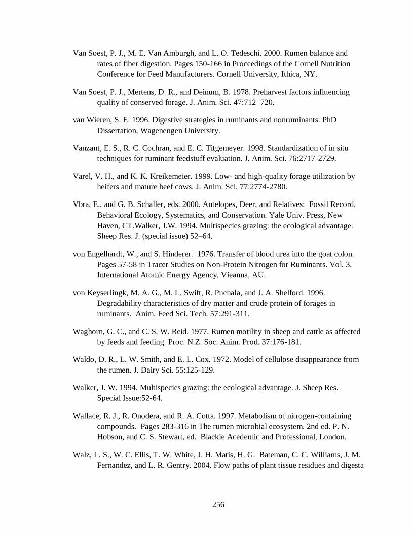
256
Van Soest, P. J., M. E. Van Amburgh, and L. O. Tedeschi. 2000. Rumen balance and
rates of fiber digestion. Pages 150-166 in Proceedings of the Cornell Nutrition
Conference for Feed Manufacturers. Cornell University, Ithica, NY.
Van Soest, P. J., Mertens, D. R., and Deinum, B. 1978. Preharvest factors influencing
quality of conserved forage. J. Anim. Sci. 47:712–720.
van Wieren, S. E. 1996. Digestive strategies in ruminants and nonruminants. PhD
Dissertation, Wagenengen University.
Vanzant, E. S., R. C. Cochran, and E. C. Titgemeyer. 1998. Standardization of in situ
techniques for ruminant feedstuff evaluation. J. Anim. Sci. 76:2717-2729.
Varel, V. H., and K. K. Kreikemeier. 1999. Low- and high-quality forage utilization by
heifers and mature beef cows. J. Anim. Sci. 77:2774-2780.
Vbra, E., and G. B. Schaller, eds. 2000. Antelopes, Deer, and Relatives: Fossil Record,
Behavioral Ecology, Systematics, and Conservation. Yale Univ. Press, New
Haven, CT.Walker, J.W. 1994. Multispecies grazing: the ecological advantage.
Sheep Res. J. (special issue) 52–64.
von Engelhardt, W., and S. Hinderer. 1976. Transfer of blood urea into the goat colon.
Pages 57-58 in Tracer Studies on Non-Protein Nitrogen for Ruminants. Vol. 3.
International Atomic Energy Agency, Vieanna, AU.
von Keyserlingk, M. A. G., M. L. Swift, R. Puchala, and J. A. Shelford. 1996.
Degradability characteristics of dry matter and crude protein of forages in
ruminants. Anim. Feed Sci. Tech. 57:291-311.
Waghorn, G. C., and C. S. W. Reid. 1977. Rumen motility in sheep and cattle as affected
by feeds and feeding. Proc. N.Z. Soc. Anim. Prod. 37:176-181.
Waldo, D. R., L. W. Smith, and E. L. Cox. 1972. Model of cellulose disappearance from
the rumen. J. Dairy Sci. 55:125-129.
Walker, J. W. 1994. Multispecies grazing: the ecological advantage. J. Sheep Res.
Special Issue:52-64.
Wallace, R. J., R. Onodera, and R. A. Cotta. 1997. Metabolism of nitrogen-containing
compounds. Pages 283-316 in The rumen microbial ecosystem. 2nd ed. P. N.
Hobson, and C. S. Stewart, ed. Blackie Acedemic and Professional, London.
Walz, L. S., W. C. Ellis, T. W. White, J. H. Matis, H. G. Bateman, C. C. Williams, J. M.
Fernandez, and L. R. Gentry. 2004. Flow paths of plant tissue residues and digesta
257
through gastrointestinal segments in Spanish goats and methodological
considerations. J. Anim. Sci. 82:508-520.
Warner, A. C. I. 1981. Rate of passage of digesta through the gut of mammals and birds.
Nutr. Abrst. Rev. B. 51:789-820.
Webb, S. D. 1998a. Cervidae and bovidae. Pages 508 - 10 in Evolution of Tertiary
Mammals of North America: Volume 1, Terrestrial Carnivores, Ungulates, and
Ungulate like Mammals. C. M. Janis, K. M. Scott, L. L. Jacobs, ed. Cambridge
Univ. Press: Cambridge, UK.
Webb, S. D. 1998b. Hornless ruminants. Pages 463- 76 in Evolution of Tertiary
Mammals of North America: Volume 1, Terrestrial Carnivores, Ungulates, and
Ungulate like Mammals. C. M. Janis, K. M. Scott, L. L. Jacobs, ed. Cambridge
Univ. Press: Cambridge, UK.
Webb, S. D. 2000. Evolutionary history of new world Cervidae. Pages 38 – 64 in
Antelopes, Deer, and Relatives: Fossil Record, Behavioral Ecology, Systematics,
and Conservation. E. Vbra and G. B. Schaller, ed. Yale Univ. Press, New Haven,
CT.
Webb, S. D., and B.E. Taylor. 1980. The phylogeny of hornless ruminants and a
description of the cranium of Archaeomeryx. Bull. Am. Mus. Nat. Hist. 167:120–
157.
Weisbjerg, M. R., P. K. Bhargava, T. Hvelplund, and J. Madsen. 1990. Anvendelse af
nedbrydningsprofiler i fodermiddelvurderingen. Beretning fra Statens
Husdyrbrugsforsøg 679:33.
Weiss, W. P. 2002. Relative feed value of forage and dairy cows: A critical appraisal.
Pages 127-140 in Proc. Tri-State Dairy Nutr. Conf., Ft. Wayne, IN.
Welch, J. G. 1982. Rumination, particle size and passage from the rumen. J. Anim. Sci.
54:885-894.
Wemmer, C. 1998. Deer: Status Survey and Conservation Action Plan. IUCN/SSC
Antelope Specialist Group, Gland, CH.
Weston, R. H. 1988. Factors limiting the intake of feed by sheep. 12. Digesta load and
chewing activities in relation to lactation and its attendant increase in voluntary
roughage consumption. Aust. J. Agric. Res. 39:671-677.
Weston, R. H., J. R. Lindsay, D. W. Peter, and D. J. Buscall. 1989. Factors limiting the
intake of feed by sheep. 14. Comparisons of voluntary feed consumption and

258
various transactions in the alimentary tract between lambs and sheep fed roughage
diets. Aust. J. Agric. Res. 40:625-642.
White, R.G., and J.R. Luick. 1984. Plasticity and constraints in the lactational strategy of
reindeer and caribou. Symp. Zool. Soc. Lond. 51:215-232.
Whitehead, G. K. 1972. Deer of the World. Constable, London.
Wiener, G., H. Jianlin, and L. Ruijun. 2003. The Yak. 2nd ed. Food and Agriculture
Organization of the United Nations, Bangkok, TH.
Wiener, G., H. Jianlin, and L. Ruijun. 2003. The Yak. 2nd ed. Food and Agriculture
Organization of the United Nations, Bangkok, TH.
Woolnough, A. P. and J. P. du Toit. 2001. Vertical zonation of browse quality in tree
canopies exposed to a size-structured guild of African browsing ungulates.
Oecologia 129: 585-590.
Wyburn, R. S. 1980. The mixing and propulsion of the stomach contents of ruminants.
Pages 35-51 in Digestive Physiology and Metabolism in Ruminants. Y.
Ruckebusch and P. Thivend, ed. AVI Publishing, Westport, CT.
Yearsley, J., B. J. Tolkamp BJ, and A. W. Illius. 2001. Theoretical development in the
study and prediction of food intake. Proc. Nutr. Soc. 60:145-156.
Zachos, J., M. Pagani, L. Sloan, E. Thomas, and K. Billups. 2001. Trends, rhythms, and
aberrations in global climate 65 Ma to present. Science. 292:686-693.
Zeder, M. A., and B. Hesse. The initial domestication of goats (Capra hircus) in the
Zagros Mountains 10,000 years ago. Science. 287:2254-2257.

259
VITA
Timothy John Hackmann was born to Donald and Dianne Hackmann on 13
October, 1984 in St. Louis, MO. During his youth, he enjoyed the company of many
pets—cats, dogs, fish, gerbils, toads, and turtles—but had no contact with livestock
animals.
After graduating from Lindbergh High School, Timothy matriculated the
University of Missouri-Columbia to study biology with the intention of entering
veterinary school. He became aware of the existence of animal science after taking an
introductory class there with Dr. James ―Jimmy‖ Spain. He milked a cow for his first
time (at age 20) in a subsequent class with Dr. Spain. During this time, Dr. Spain offered
Timothy an opportunity in undergraduate research then convinced him to pursue a career
as a researcher. After graduating summa cum laude with a B.S. (Hons.) in Biology,
Timothy entered the M.S. program in Animal Sciences at the University of Missouri-
Columbia under Dr. Spain’s direction.
After 2 years of hard work, excitement, frustration, and sleep deprivation, Timothy
earned a M.S. in December 2008. He will pursue a Ph.D. in Nutrition at The Ohio State
University in 2009.