student research project - walflosse carsten.pdf · student research project - 1- student research...

Student Research Project

- 1-


RWTH Aachen University of Technology Institute of Jet Propulsion and Turbomachinery Dr.-Ing. Herwart Hönen Institute Administration Dipl.-Ing. Jens Andreas Supervisor

cand. ing. Carsten Benedikt Wortmann

Numerical simulation of the flow around the pectoral fin of a humpback whale


- 2-

This Page was intentionally left blank.

Subject

- 3-

Subject

Affidavit

- 4-

Affidavit I declare that the following report is my work unless otherwise referenced. Carsten Wortmann January 31st, 2007 Student ID 232592 Carsten Benedikt Wortmann Altenhellefelder Str. 28 D-59846 Sundern, Germany Telephone: +49 177 347 10 52 Facsimile: +49 121 251 385 64 08 Email: [email protected] Institute of Jet Propulsion and Turbomachinery Templergraben 55 D-52062 Aachen, Germany Telephone: +49 (241) 80-95500 Facsimile: +49 (241) 80-92-229 Email: [email protected]

Executive Summary

- 5-

Executive Summary The core of this thesis is to simulate the flow around a humpback whale’s pectoral fin numerically using computational fluid dynamics (CFD). A clean pectoral fin with a smooth leading edge is taken as a reference for comparing the outcomes of this simulation. This subchapter will provide a brief summarization on how this objective is accomplished, what recommendations can be concluded from this thesis and what steps had to be taken prior to this numerical simulation. Among whales, the humpback whale attracts attention due to its extraordinary long and flexible flippers. These flippers are suspected to be the reason for an extreme maneuverability despite its body length and weight. As an important difference to other species’ flippers, tubercles (“knobs”) are attached to the fin’s leading edge. Publications suggest that because of those tubercles under some circumstances drag decreases up to 30% while lift and angle of attack for stalling increases significantly [14]. In terms of biomimicry it has to be examined if this effect can be used for improving airfoils (e.g. engine blades, grids or wings) as well. Consequently, some background data about the humpback whale is found through literature research. Information about movements and dive patterns is gathered. Accordingly, papers considering the flipper are analyzed to identify, digitalize and import a default flipper into a CFD program. For identification, numerous photographs of individual humpback whales are merged and a two-dimensional top view of a typical pectoral fin is drawn by hand. It is subsequently scanned and converted to a bitmap file for digitalization. Developing a three-dimensional flipper the thickness has to be considered. Scientific papers state that maximum thickness can be found from 49% to 19% in the mid-span. However, the maximum thickness ratio varies from 0.20 to 0.28, averaging at 0.20-0.23 [9]. This would lead to a NACA 0020 airfoil. However, comparison with photographs of living whales in the task relevant swimming maneuver suggested the use of a thinner profile. Thus, thickness and shape of the flipper are calculated according to the NACA 0012 airfoil. Two versions of the pectoral fin, one with and one without tubercles are saved as an IGES file and imported into the meshing tool Ansys ICEM CFD. As a last step prior to flow simulation, a numerical mesh has to be created. In this case, a hexahedron grid is chosen as this type is supposed to be the best for numerical analysis. The strategy for creating a suitable mesh is to use blocking around the fin, an O-grid for better resolution of boundary effects and compressing the grid at tip and shoulder for better resolution. However, exporting the mesh to the CFX solver revealed several inconsistencies, holes and breaks on the flipper surface. This is found due to an inaccurate mesh and also not ideal meshing type. Therefore, inconsistent surfaces and limits in the creation possibilities suggest using a tetrahedral mesh instead. This meshing type can be created using a lot more parameters and automatisms. In addition, it is better suited for complex geometries. In following reports based on this thesis, improvements in fluid dynamics still have to be validated through an alternative approach to this subject. In addition, besides these observations, the exact explanations of the mechanisms leading to this effect have to be analyzed. However, if this is successful, it needs to be considered if improvements in this way on existing aerodynamic applications are reasonable and cost-efficient.

Acknowledgements

- 6-

Acknowledgements I would like to give sincere thanks to all who aided me in any imaginable way during my work at the RWTH Institute of Jet Propulsion and Turbomachinery in Aachen. For the assistance and initial training and supervision I would like to say thanks to Dipl.-Ing. Jens Andreas, former scientific assistant at the IST, Institute of Jet Propulsion and Turbomachinery in Aachen and Prof. Dr.-Ing. R. Niehuis, former head of this institute. I would like to thank them also for making this project possible. For their help during the first stages of this work, I would like to articulate acknowledgements to Dr. Frank E. Fish, Department of Biology, West Chester University, and Dr. Meike Scheidat, Research- and Technology Centre Westcoast, Christian-Albrechts University Kiel. Proof-reading was done by cand. Ing. Alexander Salert. Additionally, for their continuous support and encouragement, I would like to express my gratitude to my family and friends. Without any of the mentioned above my work on this topic would not have been that successful. Dr.-Ing. Herwart Hönen Institute of Jet Propulsion and Turbomachinery Templergraben 55 D-52062 Aachen Germany Dipl.-Ing. Jens Andreas Institute of Jet Propulsion and Turbomachinery Templergraben 55 D-52062 Aachen Germany

Index

- 7-

Index

Contents

Subject ............................................ ...........................................................................3

Affidavit.......................................... ............................................................................4

Executive Summary .................................. ................................................................5

Acknowledgements ................................... ...............................................................6

Index.............................................. .............................................................................7

Contents........................................... .................................................................................7

List of Figures.................................... ...............................................................................9

List of Tables ..................................... .............................................................................11

List of Abbreviations .............................. ........................................................................12

1 Introduction....................................... ................................................................13

1.1 Preamble........................................... ....................................................................13

1.2 Biomimicry ......................................... ..................................................................13

1.3 Task ............................................... .......................................................................14

1.4 Thesis Structure................................... ................................................................16

2 The Humpback Whale ................................. .....................................................17

2.1 Scientific Classification .......................... .............................................................17

2.2 Typical Characteristics............................ ............................................................18 2.2.1 Habitat and Behavior ......................................................................................................... 18 2.2.2 Whale Song........................................................................................................................ 21 2.2.3 Parasites ............................................................................................................................ 22

2.3 Research Related Details ........................... .........................................................23 2.3.1 The Flipper ......................................................................................................................... 23 2.3.2 Hydrodynamic Flow ........................................................................................................... 26

3 State of Affairs ................................... ...............................................................29

3.1 Current Innovations based on Flow Control .......... ............................................29 3.1.1 High Lift Devices ................................................................................................................ 30

3.1.1.1 Leading edge ............................................................................................................. 30 3.1.1.1.1 Variable camber leading edge .............................................................................. 31 3.1.1.1.2 Simple and folding bull-nose Krueger flap ............................................................ 31 3.1.1.1.3 Slats ...................................................................................................................... 32

3.1.1.2 Trailing edge .............................................................................................................. 32 3.1.1.2.1 Flaps ..................................................................................................................... 32

3.1.2 Other boundary layer control devices ................................................................................ 32 3.1.2.1 Passive vortex generators ......................................................................................... 33 3.1.2.2 Air-jet vortex generators............................................................................................. 34

3.2 Previous Research on Pectoral Fins ................. .................................................36

Index

- 8-

4 Digitalization of a Humpback Whale’s Flipper ........ .......................................38

4.1 Preliminary Considerations and Modeling............ .............................................38

4.2 Drawing the planform ............................... ...........................................................39

4.3 Reading the Bitmap ................................. ............................................................40 4.3.1 The “kkonvert.c” BMP-to-Coordinate Converter ................................................................ 41

4.4 The Flipper’s System of Coordinates ................ .................................................42

4.5 Data Processing in LabView, TecPlot and Excel ...... .........................................42

4.6 Generation of a Third Dimension.................... ....................................................44 4.6.1 Finding the NACA airfoil..................................................................................................... 44 4.6.2 Scaling the NACA Wing Design......................................................................................... 45 4.6.3 Calculation of Z-Values...................................................................................................... 45

4.7 Troubleshooting ProE ............................... ..........................................................47

4.8 Generation of Digitalized Pectoral Flipper with Tub ercles................................49

4.9 Import into ProE Wildfire 2.0 ...................... .........................................................53

4.10 Export as IGES File ................................ ..............................................................53

4.11 Simplifications and Troubleshootings ............... ................................................55

5 The Mesh........................................... ................................................................56

5.1 The Hexa Mesh in Theory ............................ ........................................................57 5.1.1 O-Grid ................................................................................................................................ 57 5.1.2 Edge-Meshing Parameters ................................................................................................ 58 5.1.3 Time Saving Methods ........................................................................................................ 58 5.1.4 Hexa Database .................................................................................................................. 59 5.1.5 Unstructured and Structured Mesh Output ........................................................................ 59

5.2 Meshing the Pectoral Fin........................... ..........................................................60 5.2.1 Blocking.............................................................................................................................. 60 5.2.2 Assigning Material.............................................................................................................. 61 5.2.3 Creating the O-Grid............................................................................................................ 62 5.2.4 Mesh Parameters............................................................................................................... 63 5.2.5 Mesh around Pectoral Fin without Tubercles .................................................................... 63 5.2.6 Export to CFX..................................................................................................................... 65

5.3 Troubleshootings and Problems ...................... ..................................................67

6 Conclusion and Recommendation...................... ............................................68

7 References ......................................... ...............................................................69

8 Appendix ........................................... ................................................................71

8.1 The “kkonvert.c” BMP-to-Coordinate Converter ......... ......................................71 8.1.1 Program Code.................................................................................................................... 71

8.2 CD Index ........................................... ....................................................................76

8.3 Additional Tables .................................. ...............................................................77

8.4 About the Author................................... ...............................................................81

Index

- 9-

List of Figures Figure 1-1: Pectoral Fin [21] ...................... ......................................................................................... 13 Figure 1-2: Gliding Vulture [10] ................... ....................................................................................... 14 Figure 1-3: Bionic Sailing Wing [16] ............... ................................................................................... 14 Figure 1-4: Flaps during Landing Approach .......... ........................................................................... 15 Figure 1-5: Slats and Flaps, A320-300 [8].......... ................................................................................ 15 Figure 1-6: Megaptera Novaeangliae [18]............ .............................................................................. 15 Figure 2-1: Megaptera Novaeangliae [26]............ .............................................................................. 17 Figure 2-2: Humpback Whale Range [8] ............... ............................................................................. 18 Figure 2-3: Breeding and Feeding Areas [22] ........ ........................................................................... 18 Figure 2-4: Jumping Humpback Whale [6] ............. ........................................................................... 19 Figure 2-5: Whale accompanied by Calve [6] ........ .......................................................................... 19 Figure 2-6: Echo Sounder Tracings .................. ................................................................................. 20 Figure 2-7: Distribution of foraging dives ......... ................................................................................ 21 Figure 2-8: Distribution of foraging bouts......... ................................................................................ 21 Figure 2-9: Idealized dolphin head showing the regi ons involved in sound production. [8] ...... 22 Figure 2-10: Humpback Whale song spectrogram (Liste n to Song on CD) [8] ............................. 22 Figure 2-11: Whale lice, 5-25 mm length [8] ........ .............................................................................. 22 Figure 2-12: Barnacles [8] ......................... .......................................................................................... 22 Figure 2-13: Flipper planform with representative c ross-sections [9] .................................. ......... 24 Figure 2-14: Humpback whales in Southeast Alaska [1 ] ................................................................. 24 Figure 2-15: Distance between tubercles [9] ........ ............................................................................ 25 Figure 2-16: Position of max. thickness [9]........ ............................................................................... 25 Figure 2-17: Skeleton Megaptera Novaeangliae [28].. ...................................................................... 25 Figure 2-18: Humpback whale from side, top and head -on view [19] ...................................... ...... 27 Figure 2-19: Reynolds Number for Boundary Condition s [8].............................................. ............ 28 Figure 3-1: Optimization process over time......... ............................................................................. 29 Figure 3-2: Commercial airplane taking off using hi gh lift devices [12] ............................... ......... 30 Figure 3-3: Three different leading edge devices [2 ] ....................................................................... 30 Figure 3-4: Variable camber leading edge [8] ....... ............................................................................ 31 Figure 3-5: Krueger flap of a Boeing 737-300 partia lly extended [7] ................................... ........... 31 Figure 3-6: Four different types of flaps [8] ...... ................................................................................ 32 Figure 3-7: Vortex generators installed on upper wi ng surface [Maule Air Inc.] ........................ .. 33 Figure 3-8: Different vortex generator configuratio ns ................................................. .................... 35 Figure 3-9: Boundary Layer Changes through Vortex G enerators [17] ..................................... .... 35 Figure 3-10: Simulation of Flow without Tubercles [ 23] .................................................................. 36 Figure 3-11: Simulation of Flow with Tubercles [23] ........................................................................ 36 Figure 3-12: Streamlines outside Boundary Layer on Tubercle [23]...................................... ........ 36 Figure 3-13: Wind Tunnel Models of Pectoral Fins w/ and w/o Tubercles [14] ............................ . 37

Index

- 10-

Figure 4-1: Sketch of humpback whale’s pectoral fin without tubercles................................. ...... 39 Figure 4-2: Sketch of humpback whale’s pectoral fin with tubercles .................................... ........ 39 Figure 4-3: Colored out flipper sketch............. .................................................................................. 40 Figure 4-4: Desired pixel course, no doubles, no ga ps ................................................. .................. 40 Figure 4-5: Pixel course, double pixel ............. .................................................................................. 41 Figure 4-6: Pixel course, gap...................... ........................................................................................ 41 Figure 4-7: Coordinates from flipper drawing, with out tubercles ...................................... ........... 41 Figure 4-8: Pectoral Fin System of Coordinates, X-Y Layer............................................. ............... 42 Figure 4-9: Airfoil System of Coordinates.......... ............................................................................... 42 Figure 4-10: Excel Output for Pectoral Fin without Tubercles.......................................... .............. 44 Figure 4-11: Excel Output for Pectoral Fin with Tub ercles ............................................. ................ 44 Figure 4-12: Cuts and Sections within Pectoral Fin. ........................................................................ 45 Figure 4-13: TecPlot Fin Printout .................. ..................................................................................... 46 Figure 4-14: Error in Pectoral Fin Surface, ISO Vi ew...................................................................... 47 Figure 4-15: Error in Pectoral Finn, Head-On View . ........................................................................ 47 Figure 4-16: Screenshot of Pectoral Fin without Tub ercles............................................. ............... 48 Figure 4-17: Confrontation Chord Length w/ and w/o Tubercles .......................................... ......... 50 Figure 4-18: Pectoral Fin Pattern and Chord Length including Tubercles ................................ .... 51 Figure 4-19: Sequence of Coordinate Data around Fin Pattern ........................................... ........... 51 Figure 4-20: Leading and Trailing Edge of Pectoral Fin with Tubercles................................. ....... 52 Figure 4-21: Example for axis situation and coordin ate value. ......................................... ............. 53 Figure 4-22: Screenshot Pectoral Fin with Tubercles ...................................................................... 54 Figure 5-1: Hybrid Grid [4] ........................ .......................................................................................... 56 Figure 5-2: Tetrahedron Grid [4]................... ...................................................................................... 56 Figure 5-3: 2D Hexa Grid [24] ...................... ....................................................................................... 56 Figure 5-4: 3D Auto Hexa Grid around Car [4] ....... ........................................................................... 56 Figure 5-5: Initial block.......................... .............................................................................................. 58 Figure 5-6: Block with O-Grid ...................... ....................................................................................... 58 Figure 5-7: Block with O-Grid and including a face . ........................................................................ 58 Figure 5-8: Blocking Strategy around wing .......... ............................................................................ 60 Figure 5-9: Creating Parts Interface for defining M aterial ............................................ ................... 62 Figure 5-10: Surface Mesh Size Dialogue Screen ..... ....................................................................... 63 Figure 5-11: Mesh around Pectoral Fin .............. ............................................................................... 64 Figure 5-12: CFX Imported Mesh..................... ................................................................................... 66 Figure 5-13: Zoom on meshed Flipper in CFX ......... ......................................................................... 66 Figure 6-1: Flowchart of further recommendations on this topic........................................ ........... 68

Index

- 11-

List of Tables Table 4-1: Set of Equations for NACA scaling....... ........................................................................... 45 Table 4-2: Set of Equations for chord scaling ...... ............................................................................ 46 Table 4-3: TecPlot Database Abstract ............... ................................................................................ 46 Table 8-1: List of Coordinates for Pectoral Fin wit hout Tubercles..................................... ............ 77 Table 8-2: List of Coordinates for Pectoral Fin wit h Tubercles ........................................ .............. 78 Table 8-3: Airfoil Cuts for Pectoral Fin with Tuber cles............................................... ..................... 79 Table 8-4: Translations............................ ............................................................................................ 80

Index

- 12-

List of Abbreviations ASCII American Standard Code for Information Interchange, character encoding based on the

English alphabet Autohexa Automatic Hexa Mesh Generator within ICEM CAD Computer Aided Design CFD Computational Fluid Dynamics CFX Solver for Fluid Dynamics Simulations, connected to CFD

CLmax Maximum Lift

DOS Disk Operating System, dominated the IBM compatible market I Number of NACA airfoil points IBM International Business Machines, personal computer competing with Commodore and

Apple ICEM Company developing CFD Software, lately bought by ANSYS IGES International Graphics Exchange Standard J Cuts in the direction of X L Characteristic length (equal to diameter (2r) if a cross-section is circular) l/d Lift to drag ratio L01, L Overall length of flipper NACA National Advisory Committee for Aeronautics NURBS Non-uniform, rational B-spline, mathematical model commonly used in computer

graphics for generating and representing curves and surfaces ProE Parametric feature-based three-dimensional Solid modeling CAD software created by

Parametric Technology Corporation (PTC) pts File type containing flipper's coordinates (points) in ASCII format Re Reynolds Number s Scale factor T01 Profile length TXT DOS ASCII text file UltraEdit Text editor for Microsoft Windows created by IDM Computer Solutions US United States VC Variable camber (Krueger flaps) vi Virtual Instrument (LabView) vs Mean fluid velocity

w/ Common Abbreviation: with w/o Common Abbreviation: without x, y, z Coordinates for fin, NACA profile or scaled image X1 Leading edge X coordinates X2 Trailing edge X coordinates XLS File type for Microsoft Excel α Angle of Attack α

Stall Angle of Attack for Stalling Behavior � (Absolute) dynamic fluid viscosity ν Cinematic fluid viscosity: ν = � / ρ ρ Fluid density

Introduction

- 13-

1 Introduction

1.1 Preamble Humpback whales (megaptera novaeangliae) impress by astonishing maneuverability considering their size (13 meters, 30 metric tons). Compared to other marine mammals the megaptera novaeangliae possesses unusually long pectoral fins (“flippers”). From the aerodynamic point of view the speculation arises whether these pectoral fins play a decisive part in the whale’s maneuverability. Apart from their length the flippers are marked by another peculiar feature: The tubercles on their leading edge, figure 1-1. Understanding the flow physics involved may yield interesting possibilities for the improvement of aerodynamic devices.

Figure 1-1: Pectoral Fin [21]

Biologists assume that these tubercles might play an important role regarding this outstanding agility. Using this feature for certain airfoils might be the key for a further evolutionary step.

1.2 Biomimicry Evolution of aerodynamic applications reached such a high standard, that decisive innovations became very rare. In an attempt to reduce the environmental impact of today’s technology e.g. by optimizing existing concepts, engineers labor to adapt biological concepts to their work. The application of methods found in the environment to the design of engineering systems is called “bionics”. As a short form for “biomechanics”, this word is set together from two words, biology (originated in the Greek word " β ι ο ς ", pronounced "vios" and meaning "life") and electronics [8]. As this way of discovering technical improvements has less to do with just electronics, but with every other technical field of investigation as well, an even better translation of the German “Bionik” can be found: “biomimicry”. Biomimicry is composed of the words bios and mimicry and can be understood as a conscious strategy by designers to observe and learn principles of design from nature.

Introduction

- 14-

As an example for biomimicry, a glider’s wing tip was designed according to the raven-vulture shown in figure 1-2. While observing possible prey, the vulture braces the wing-tip feathers. Through fanning out these feathers, these vultures can cut wing-tip-vortices into small turbulences, which decrease energy loss. This effect has been used for a glider’s wing. Although now specific research shows that this type of wing tip is not necessary at big spans, figure 1-3 gives an example of biomimicry in this matter.

Figure 1-2: Gliding Vulture [10]

Figure 1-3: Bionic Sailing Wing [16]

Aircrafts in general can be seen as another example for biomimicry. Looking at early aircrafts, the use of this method is obvious, as they resemble avian animals. But this example is also quotable to show that biomimicry can also be misleading, for motorized flying was only possible after separating propulsion from lift. Thus, it can be helpful to look at nature, but in some cases, maybe even in this case, it might be necessary to even think beyond natural evolution.

1.3 Task The aim of this thesis is to create a three-dimensional numerical model of a humpback’s flipper and to mesh it to allow an analysis using computational fluid dynamics (CFD). This task can be divided into the following steps. First, literature research has to be done. During cruise speed, the clean wing is considered to be the optimum configuration. However, for take-off and landing high lift systems are required. An example for these devices can be seen in figure 1-4 and figure 1-5. As the humpback whale’s pectoral fins will enhance flow control in these flight situations, current innovations already established on aircrafts need to be reviewed for comparison. This is necessary to have a reference for the efficiency of tubercle attached wings in correspondence to clean wings.

Introduction

- 15-

Figure 1-4: Flaps during Landing Approach

Figure 1-5: Slats and Flaps, A320-300 [8]

Also, more information has to be gathered about the humpback whale in general, e.g. its habitat, breeding and feeding area, foraging habits and maneuverability. Figure 1-6 shows the humpback whale in an upward movement, extremely bending its pectoral fin.

Figure 1-6: Megaptera Novaeangliae [18]

Subsequently, the pectoral fin has to be analyzed in further detail. For identification and digitalization data about thickness, span, and amount of tubercles needs to be collected. Finally in literature research, details about the characteristic flow situation, e.g. velocity, depth and angle of attack, must be found out to set up the boundary conditions of the planned CFD-calculations. Data collected during literature research shall be used for creating a typical geometry and a reference profile of the humpback whale’s flipper. These two versions need to be digitalized and provided as an importable file for Ansys ICEM CFD. After initial training on Ansys ICEM CFD and CFX, a numerical mesh around both versions of the flipper has to be created within CFD, and exported to the solver CFX. The flow around these flippers has to be simulated and compared to each other, to document advantages and disadvantages of both types. All results need to be stated.

Introduction

- 16-

1.4 Thesis Structure This thesis is divided into two major parts. The first part will deal with literature research to provide general knowledge about the topic. The humpback whale is described in detail, and especially the pectoral fin will be pictured. In the next chapter, research already done on this topic will be described. The next two chapters will deal with the digitalization and meshing of the flipper. Finally, the last chapter will give a conclusion and recommendation for further research on this topic. This divisiveness is displayed in the thesis structure hereafter.

(1) Introduction / Task

(2) The Humpback Whale

Lite

ratu

re

Res

earc

h

(3) State of Affairs

(4) Digitalization of a Humpback Whale’s Fin

(5.1) The Hexa Mesh

Dig

italiz

atio

n

and

Mes

hing

(5.2) Meshing the Pectoral Fin

(6) Conclusion and Recommendation

The Humpback Whale

- 17-

2 The Humpback Whale This chapter provides a classification of the humpback whale and gives background information of its natural surroundings. In addition, typical characteristics and details regarding the pectoral fins are described.

2.1 Scientific Classification The scientific name for a humpback whale, megaptera novaeangliae, is taken from Greek and Latin. Megaptera stands for the Greek “megas” and “pteron”, meaning “Great Wing”, grabbing the one but most flamboyant characteristic, the long pectoral fins. Novaeangliae is Latin for “New England”, where this whale was first observed. The humpback whale has a barrel-shaped body reducing its diameter from head to fluke. The head itself is flattened and usually very tuberculous. The very long, aliform flipper makes up one third of the over all body length (figure 2-1).

Figure 2-1: Megaptera Novaeangliae [26]

A translation of the German vocabulary in this figure can be found in table 8-4.

The Humpback Whale

- 18-

In scientific classification, the humpback whale belongs to the kingdom animalia (lt. animals). Other kingdoms are known as plantae (lt. plants), fungi (lt. mushrooms) and viridae (lt. viruses). Within the kingdom, it belongs to the phylum chordata (lt. chordates), in which mainly oceanic animals, around 60,000 species, are combined. Inside the phylum, it can be classified as mammalia (lt. mammals), such as humans. The corresponding subclass is called eutheria, a group of organisms containing the placental mammals. The humpback whale belongs to the order cetacea (lt. whales), which is composed from Greek ketos meaning “monster of the sea” and the Latin cetus meaning “great animal of the ocean”. This order is divided into two suborders, odontoceti (lt. toothed whales) and mysticeti (lt. baleen whales). Within the suborder mysticeti, the humpback whale belongs to the family balaenoptiidae (lt. rorquals). Other rorquals are the mink whale, the grey whale and the blue whale.

2.2 Typical Characteristics The humpback whales upper body’s color is black sometimes fading into blue, the bottom side can be white, black or brindled. An adult humpback whale ranges between 12-16 m long and can weigh up to 36,000 kg [8].

2.2.1 Habitat and Behavior The humpback whale lives in oceans and seas allover the world (figure 2-2). In fact the area where the humpback whale can be observed permanently is up to 40,000 km² large. As breeding and feeding areas are far apart from each other, the humpback whale has to manage large traveling distances (figure 2-3). Annual voyages of approximately 25,000 km are common [8].

Figure 2-2: Humpback Whale Range [8]

Figure 2-3: Breeding and Feeding Areas [22]

The Humpback Whale

- 19-

Sometimes, males jump out of the water high showing their tail fin while diving into the water again, as in figure 2-4. It is not clear whether this is to impress females or loose parasites (chapter 2.2.3). Breeding can only take place in warm areas. On the other side, prey (e.g. krill) is more prosperous in northern areas. Calves would suffer death from cold as they are born without the protecting grease padding [25]. Figure 2-5 shows a cow accompanied by her calve. Humpback whales can be together with their offspring for more than four years.

Figure 2-4: Jumping Humpback Whale [6]

Figure 2-5: Whale accompanied by Calve [6]

Considering foraging dive patterns of humpback whales in southeast Alaska [5], it is not known that dive habits changed in the last years, so this report on humpback whale’s dive patterns can be taken as representative. During summer of 1979 to 1984, diving, ventilation and surface behavior was recorded. All observations where taken using an echo sounder with good observation within the top 260 m of the water column. The water column was partitioned into 20 m depth intervals between 0 and 260 m. As it is shown in figure 2-6, surface feeding depth is from 0-20 m. While releasing the camera, whales were found from 80-95 m swimming close to a layer of dense krill reaching down to 120 m.

The Humpback Whale

- 20-

Figure 2-6: Echo Sounder Tracings

However, this graph only represents one single camera dive. It is necessary to have a closer look on diving behavior and the amount of dives in certain depths. Notice that there are only 662 happenings of bouts recorded, but 4889 dive maneuvers. However, feeding beyond 160 m depth appears not to be very efficient. Nonetheless, with this information in mind, a representative depth must be found to consider boundary conditions for later research on this topic. This depth must also correspond to the deepness where most of the maneuvering is done, as the flipper is naturally adapted best to this depth. This depth is the one where foraging takes place. Due to its feeding customs, the humpback whale is highly maneuverable, using its flippers to turn and bank at remarkable speed and agility. It speeds up to 2.5 m/s towards their prey while resurfacing at a 30°-90° angle, using their long flippers to uncommonly direct prey into their mouth. Then, the whale swims away quickly with the flippers retracted, suddenly rolling 180° and making a sharp U-turn, again attacking the p rey. This maneuver is called “inside loop” behavior and is performed within 1.5 to 2 times the body length of the whale [19]. Another feeding technique is called “bubble net fishing”. Some whales blow bubbles, creating a visual barrier against the prey. Another one or more whales drives the prey against that barrier by vocalizing sounds (chapter 2.2.2). The bubble wall is then closed, encircling the fish. The whales then suddenly swim upwards and through the bubble net, mouths open wide, swallowing thousands of fish in one gulp. This technique can involve a ring of bubbles up to 30 m in diameter [8]. Furrows on the whale’s bottom side might make it easier to soak in a lot of water, while spitting out the water through the baleens and keeping the prey inside.

The Humpback Whale

- 21-

Figure 2-7: Distribution of foraging dives

Figure 2-8: Distribution of foraging bouts

Figure 2-7 and figure 2-8 show best on what base a representative depth can be found. Most dives and maneuvers are performed down to 40 m. The exact centre value for all dive and bout maneuvers is 29.5 m. Thus, a medium dive where most likely the flipper is optimized for can be seen at 30 m. This, of course, is only a rough first estimation, as density changes heavily between 30 m and the maximum recorded dive depth of 160 m. However, in some later research the boundary conditions have to change from water to air anyways, so for first considerations a 30 m dive is representative.

2.2.2 Whale Song Besides this, humpback whales are known for their eager singing underneath the water surface. Scientists assume whale singing is to communicate among one’s peers, but also to attract females during mating season. The sounds are not produced congruent to humans, as whales do not have a phonic lip structure. They also do not have to exhale to create sound. The exact mechanism of sound creation is still unclear and a very interesting subject for biologists. [8] It is assumed that regions involved into sound production are similar to the dolphin (figure 2-9). Frequency varies from 20 Hz to 10 kHz. For comparison, the human hearing range varies from 20 Hz to 20 kHz. There are some patterns noticeable in humpback whale’s songs (figure 2-10), for example recurring passages of specific frequencies, but going into detail here would go beyond the scope of this report.

The Humpback Whale

- 22-

Figure 2-9: Idealized dolphin head showing the

regions involved in sound production. [8]

Figure 2-10: Humpback Whale song

spectrogram (Listen to Song on CD) [8]

2.2.3 Parasites It is not assured if jumping out of the water is also due to parasites, as briefly mentioned above. However, the knots on the flipper’s leading edge are covered with barnacles and whale lice. These are parasites, living on the whale, whereas the cause for their settlement is still not clear. Whale lice as shown in figure 2-11 are mostly found close to barnacles. Up to 100,000 whale lice parasites can occur per whale [8]. Sometimes, whale lice settle exactly where barnacles are attached (figure 2-12), scooping out the surrounding area so much that the barnacles fall off.

Figure 2-11: Whale lice, 5-25 mm length [8]

Figure 2-12: Barnacles [8]

The Humpback Whale

- 23-

2.3 Research Related Details For this task, some other specific details need to be reviewed before proceeding, to successfully generate a three-dimensional mesh around a humpback whale’s pectoral fin and simulate the characteristic flow. In contrast to the chapter above, the details here are described in a more technical manner. First, the geometry of a flipper has to be stated. Then, in a second step, it needs to become clear how the hydrodynamic flow streams around that flipper in nature. Important key issues are the angle of attack and the fluid’s speed for later research on this topic.

2.3.1 The Flipper As stated above, the flipper has a wing-like, high aspect ratio planform [9]. Its length varies from one fourth to one third of the body length. In cross-sectional view, the leading edge is blunt and rounded, whereas the trailing edge is highly tapered. The maximum thickness can be found from 49 % of chord at the tip to 19 % at mid-span. The thickness ratio averaged 0.23 with a range of 0.20 – 0.28. As already seen, the extraordinary fact concerning these flippers is the leading edge tubercle. These tubercles are supposed to enhance the possible lift, and control the flow over the humpback whale’s flipper. The flipper shown in figure 2-13 shows seven representative cross-sections. The horizontal line represents the chord length, whereas the vertical line represents the maximum thickness. Within this definition, the distance from the leading edge (right side) to maximum thickness is the distance of maximum camber. The flipper planform is mostly elliptical and a bit tapered. A slight sweep back of around 20 % can be found in some cases, measuring the one-third line relatively to the centerline of the body. There are around ten to twelve tubercles on the leading edge of the flipper, where the largest one can in general be found on one-third of the flipper span. The smallest tubercle is placed close to the flipper tip. The distance between those tubercles decrease from body to tip. Surprisingly, the distance relatively to the span remains almost constant at around 7 % in the middle span of the flipper, displayed in figure 2-15. Barnacles, as shown in figure 2-12, can be found attached to tubercles close to the flipper’s tip, but, however, not in the spaces between them.

The Humpback Whale

- 24-

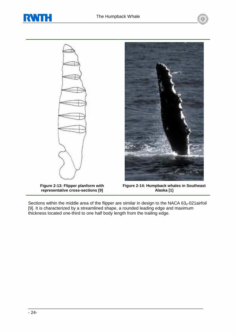
Figure 2-13: Flipper planform with representative cross-sections [9]

Figure 2-14: Humpback whales in Southeast Alaska [1]

Sections within the middle area of the flipper are similar in design to the NACA 634-021airfoil [9]. It is characterized by a streamlined shape, a rounded leading edge and maximum thickness located one-third to one half body length from the trailing edge.

The Humpback Whale

- 25-

Figure 2-15: Distance between tubercles [9]

Figure 2-16: Position of max. thickness [9]

However, the position of maximum thickness varies from the flipper’s tip towards the whale’s shoulder. Figure 2-16 gives an impression on how the position of maximum thickness relatively to the chords changes, while increasing the section number from tip to shoulder. The tubercles on the flipper seem to exert some sort of boundary layer control on the suction side. They may control hydrodynamic performance on the leading edge, which is the existential justification for this task and further reports following. The humpback tubercles may reduce drag on the flipper, which is stated in later subchapters. Figure 2-17 shows the skeleton of a humpback whale embedded into its original shape. Hip bones are degenerated, whereas hand bones are completely present. With these bones, it supposed that the whale can bend the tip up and downwards, stretch the surface and change the angle of the trailing edge through changing the camber.

Figure 2-17: Skeleton Megaptera Novaeangliae [28]

For now, the flipper is described in detail, but some constraints, for example the oncoming flow, still need to be reviewed.

The Humpback Whale

- 26-

2.3.2 Hydrodynamic Flow In general, whales are supposed to be calm and easy going swimmer. Inertia and weight seem to narrow down their possible maneuvering speed, resulting in slow movements and calm positional changes. Surprisingly, their maneuvering speed while feeding (2.5 m/s) and while jumping out of the water (it can be guessed this must be around 10 m/s because of the weight that has to be moved out of the water) is extremely high. For exact numerical simulation, a typical flow situation must be figured out for calculation. Consequently, the hydrodynamic flow around the pectoral fin is determined in this subchapter. The flipper’s neutral position can be seen in figure 2-18, which shows a humpback whale drawn during straight and level swimming. In several papers [19] it is stated that they are held in a relaxed position forming a 120°-150° angle to the body’s longitudinal axis and a 30° to 40 ° angle downward to the horizontal line. This is the only way of oncoming flow that is to be considered for later numerical simulations of flow, as of course all the individual movements can not be taken into consideration. It is known that flippers can be moved simultaneously or alternately, symmetrically or independently. Movements rarely occur alone, but in combination with other maneuvers. So, in this case, it is fixed that only the angles of oncoming flow will be considered for later reports.

The Humpback Whale

- 27-

Figure 2-18: Humpback whale from side, top and head -on view [19]

The flipper’s skin seems to be very smooth, to support laminar flow. However, under stress it appears to bend, but only to an insignificant degree. This fact is not going to be considered during the numerical simulation, too, as moving or bending objects are hardly executable. These findings, and the knowledge of maneuvering speed, which can be from 2 to 2.5 m/s, is important for later research on this topic, as it will lead to boundary conditions for the numerical simulation.

30°- 40°

120°-150°

The Humpback Whale

- 28-

Figure 2-19: Reynolds Number for Boundary Condition s [8]

However, it is surely necessary to have knowledge about the Reynolds Number (equation shown in figure 2-19) for future purposes. This boundary condition will be well prepared in this report already. For calculating the Reynolds Number it is:

• vs Mean fluid velocity, • L Characteristic length (equal to diameter (2r) if a cross-section is circular), • � (Absolute) dynamic fluid viscosity, • ν Cinematic fluid viscosity: ν = � / ρ , • ρ Fluid density.

So, the main thing still missing is the fluid density. The fluid density (around 1 kg/m³) is almost constant and changes slightly with temperature salt ratio. However, density has to be considered if, in later research, trying to compare these results to numerical simulation within air.

State of Affairs

- 29-

3 State of Affairs It is assumed that tubercles attached to the leading edge of the pectoral fin have an influence on the boundary layer of the flipper’s flow. Thus, for comparison, an overview of similar technologies for controlling the flow around an aerodynamic element has to be given.

3.1 Current Innovations based on Flow Control As briefly stated in chapter 1.3, some already known innovations that can be adapted to the leading edge are described in this subchapter. There are several leading edge device technologies currently used [2 et al.]. The motivation of this is the economic and environmental pressure of still reaching better aerodynamic values for usual or high lift devices. As shown in figure 3-1 after some time the optimization progress is decreasing compared to the amount of time spend. Therefore, innovative products are necessary to accelerate the optimization progress.

Time

Opt

imiz

atio

n P

roce

ss

Figure 3-1: Optimization process over time

Due to the large variety of existing flow-control systems, only those relevant for this thesis are named here. In case further investigation would show that tubercles enhance the aerodynamic flow in some flight situations,, the efficiency of alternative techniques must be known to evaluate the use of tubercles.

• High Lift Devices i. Variable camber leading edge ii. Fixed slot iii. Simple Krueger flap iv. Folding bull-nose Krueger flap v. Two position slat and three position slat

• Other Multiuse Devices i. Passive vortex generators ii. Air-jet vortex generators

Innovation

State of Affairs

- 30-

3.1.1 High Lift Devices The innovations in this sector can again be divided into two major fields of application, namely the leading and the trailing edge. On the wing’s leading edge there are known flow-changing devices as slats and Krueger flaps, whereas on the trailing edge many forms and types of flaps are known and briefly described here. Both devices are considered here, as tubercles (leading edge) and bending of the flipper (trailing edge) have the potential to change the flow around the humpback whale’s pectoral fin.

Figure 3-2: Commercial airplane taking off using hi gh lift devices [12]

3.1.1.1 Leading edge Figure 3-3 shows three different leading edge devices, which are described later in the according subchapter.

Figure 3-3: Three different leading edge devices [2 ]

State of Affairs

- 31-

3.1.1.1.1 Variable camber leading edge

Figure 3-4: Variable camber leading edge [8]

The variable camber leading edge, also known as VC Krueger flaps, bends the main Krueger device and extends the front nose towards the stagnation point. A hydraulic linkage system, with a minimum pressure of four bar, is required to countervail the flow [27].

3.1.1.1.2 Simple and folding bull-nose Krueger flap Simple Krueger and folding bull-nose Krueger flaps are generally designed with the hinge inside the wing leading edge and connected to the panel with a gooseneck hinge fitting [2]. Additionally, another link must be installed to fold the bull nose into the right position.

Figure 3-5: Krueger flap of a Boeing 737-300 partia lly extended [7]

The Krueger flap deploys against the forces of the airstream and has a high stowing load at low angles of attack. At high angles of attack, the Krueger flap starts to produce lift. This causes the aerodynamic loads on the airfoil to reverse, which is an unwanted effect in terms of safety. Thus, this device requires high power actuators, which are very heavy, to build up high forces necessary to extract the Krueger flap against the flow.

State of Affairs

- 32-

3.1.1.1.3 Slats Slats are most commonly used in commercial airplanes to support the other high lift devices on the leading edge. They are mounted on circular arc tracks with two tracks per slat panel. The actual load variation is low as the air loads are normal to the path of deployment.

3.1.1.2 Trailing edge On the trailing edge, different forms of high lift devices are known. But in this report, only one of them is to be shown here, as it is most commonly used be commercial and military aircrafts.

3.1.1.2.1 Flaps Flaps lengthen the airfoil in the direction of the trailing edge and therefore broaden the area where lift can develop. However, while flying with extended flaps, flow separation is very likely because of the energy losses in the boundary layer over the long chord length. In this case, slots support the formation of a new boundary layer through transferring flow onto the suction side and thereby eliminating the weakened layer.

Figure 3-6: Four different types of flaps [8]

3.1.2 Other boundary layer control devices Vortex generators are a special form of boundary layer control. Besides vortex generators, there are two other forms of boundary layer control mechanisms, to mention them briefly. First, there is blowing, which adds energy to the lower boundary layer by blowing air through slots in the wing surface. This will energize the flow close to the wall and enable it to overcome a larger pressure gradient. The second form of boundary layer control is suction. This active method of getting rid of the low energy boundary layer is very intensive in cost and power. Very complex systems are needed to prevent the layers above not to mix up with any other layer and ruin the flow. Also, the airworthiness must be secured even in a case of engine failure because a large amount of engine power is used for both, suction and blowing.

State of Affairs

- 33-

3.1.2.1 Passive vortex generators Passive Vortex generators, as the third method of boundary layer control, are a passive possibility to mix the layer close to the wall with energy loaded air, in contrast to the other active options. They are essentially small aspect ratio airfoils attached to the wing or other surface, to add vortices into the flow ahead of the separation point, which should therefore of course be after the point where the generators are fixed. These vortices will energize the boundary layer and consequently prevent flow separation. Fluid particles with high momentum in the stream direction are swept along helical paths toward the surface to mix with, and to some extent replace the retarded air at the surface [2] with energized air. While on the one hand the maximum possible angle of attack can be increased, therefore maximum lift can also be increased; drag on the other hand will rise in all angles of flight, too.

Figure 3-7: Vortex generators installed on upper wi ng surface [Maule Air Inc.]

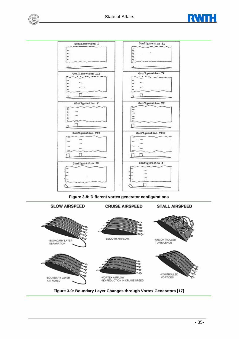
It has to be critically seen that passive vortex generators cannot be installed elsewhere on the surface. Special considerations have to be made in terms of planform shape, section profile and camber, yaw angle, aspect ratio and height with respect to the boundary layer thickness. Figure 3-8 shows different vortex generator configurations possible on a NACA RM L52G24 airfoil. These configurations are shown approximately to scale.

State of Affairs

- 34-

3.1.2.2 Air-jet vortex generators The disadvantage of producing drag in every flight maneuver and every angle of attack can be eliminated by the use of air-jet vortex generators. They can produce strong discrete vortices but have higher momentum cores. Instead of causing additional drag, they can be effective in areas where there is separated flow over the airfoil. As it is an active system, the air-jet vortex generator can be turned off if no use is required or helpful. Another field of boundary control, namely “acoustic excitation”, is disregarded in this report. Briefly, this is the effect of an imposed sound field on vortex shedding. But, as this is a new field of attention, it has not been examined a lot yet and does not contribute to the main theme of this report, as it is to dimension and estimate possible advantages or disadvantages of tubercle add-ons on airfoils. Figure 3-9 displays the boundary layer with and without vortex generators. It is easy to see and to understand that at the same angle of attack, the stalling speed can be lower than without vortex generators. However note, that the same airfoil will stall, but at a lower stalling speed than without the generators.

State of Affairs

- 35-

Figure 3-8: Different vortex generator configuratio ns

Figure 3-9: Boundary Layer Changes through Vortex G enerators [17]

State of Affairs

- 36-

3.2 Previous Research on Pectoral Fins There has been some investigation on this topic by several other scientists [23], [14]. In detail, it was already considered that tubercles increase maneuverability during prey capture. Thereupon, analysis was done on a finite span wing and on the same wing with tubercles attached. It was stated that leading edge modifications of streamlined bodies offer cost-effective performance enhancements. A computer supported panel method was developed, to approach the analysis of this statement. A numerical simulation was done on both objects [23].

Figure 3-10: Simulation of Flow

without Tubercles [23]

Figure 3-11: Simulation of Flow

with Tubercles [23]

The comparison between both simulations showed an increase in lift of 4.8 %, a 10.9 % reduction in induced drag, and a 17.6 % increase in lift to drag ratio (l/d). Tubercles enhanced wing performance at usual to low angles of attack, but did not have a huge effect at zero angle of attack.

Figure 3-12: Streamlines outside Boundary Layer on Tubercle [23]

Streamlines outside the boundary layer were examined in detail, as the effect on the local pressure was of greater interest for finding aerodynamic loads on the wing. Tubercles may

State of Affairs

- 37-

absorb an 11% increase in drag at a 10° angle of attack . As a result, the flight envelope might be enlarged for better use of the device with tubercles attached. In addition to this investigation, also real wind tunnel tests were performed within other research [14].

Figure 3-13: Wind Tunnel Models of Pectoral Fins w/ and w/o Tubercles [14]

Two scaled models of a humpback whale’s pectoral fin were constructed, one with and one without tubercles attached on the leading edge. The models were based on a NACA 0020 airfoil (20% thickness). As expected, the flipper with tubercles attached showed a better performance at higher angles. Beyond 11.8 ° angle of attack, the scalloped fl ipper produced a 32% lower drag then the smooth model. In a small range of 10.3< α <11.8° the smooth model showed a lower drag production than the one with tubercles attached. Lift was higher throughout the complete angle of attack range for the scalloped flipper, but still within the range 9.3< α <12°. α

Stall increased by 40% to 16.3° angle of attack, while C Lmax increased significantly by 6 % to a value of 0.93, so again better values for the scalloped fin. Below α =8.5°, the curve remains almost unchanged.

Digitalization of a Humpback Whale’s Flipper

- 38-

4 Digitalization of a Humpback Whale’s Flipper As a next step in this report, after identifying and precisely explaining the target of interest, the humpback whale’s flipper shall be made available in the ProE CAD Program. This is necessary for further progress in this report, as a numerical net for flow simulations has to be established fitting the surface of a humpback whale’s digitalized flipper. To import a surface into numerical simulation tool Ansys ICEM, many data formats can be used. In this report, we agreed on using the IGES format because of good handling qualities. First, the flipper has to be digitalized within ProE, to safe and transfer it as an IGES file. This IGES file can later be imported into any CFD or CFX program.

4.1 Preliminary Considerations and Modeling Every humpback whale is an individual, just like humans. It has its own appearance, own look and behavior. Individuals can only be recognized by detailed observations [20]. The length of flipper and fluke, their color and shape, as well as scars on flipper and fluke are unique for each humpback whale. Generally speaking, this fact makes it harder to digitalize the flipper. Taking just one picture of a flipper and digitalizing it would therefore be not representative for this project. Thus, it seems to be more reasonable to find a “typical and characteristic” flipper geometry, reflecting the majority of flipper types. The next task is then to find such a geometry that will fulfill the requirements set up above. This can only be solved by inspection of many photographs, showing humpback whales. Of course, pictures need to be found that will show the flipper in a good angle. After studying many different pictures, one should have a first overview on repeating details that are equal or similar for several different humpback whale flippers. In chapter 2.3 the skeleton of a humpback whale is described in detail. The following aspects of real live flipper can not be considered when digitalizing.

• Barnacles attached on the flipper tip • Flexible stress avoidance movements • Bending in horizontal and longitudinal direction • Spreading the bones to enlarge the flipper surface • Changing the angle of the trailing edge through changing the camber • Skin state and condition due to stretching and bending and surface impurity

To do a first sketch, of the planform, some proportions have to be copied. Chapter 2.3 can give key references on how to do a first drawing, as it describes structure and appearance of the flipper. The final step, after observing, identifying and drawing will be to digitalize the created top-view. For this, the coordinates of leading and trailing edge have to be determined and saved in a two-dimensional environment. Finally, this two-dimensional plan needs to be filled in with NACA cross-sections, to upgrade the drawing into a full three-dimensional model. For that purpose, the NACA wing configuration is scaled to fit into the existing flipper top view.


- 39-

4.2 Drawing the Planform

Figure 4-1: Sketch of humpback whale’s pectoral fin without tubercles

Looking and comparing with photos, the first drawing is made disregarding the tubercles just to find the typical geometry (figure 4-1). Then, tubercles were added additionally to the clean sketch of the pectoral fin (figure 4-2). Their position and size was taken from earlier researches on humpback whales and by reviewing photographs.

Figure 4-2: Sketch of humpback whale’s pectoral fin with tubercles

To complete the drawing exercise, the sketch was colored out in varying grey scales trying to give an impression of three-dimensional depth (figure 4-3).


- 40-

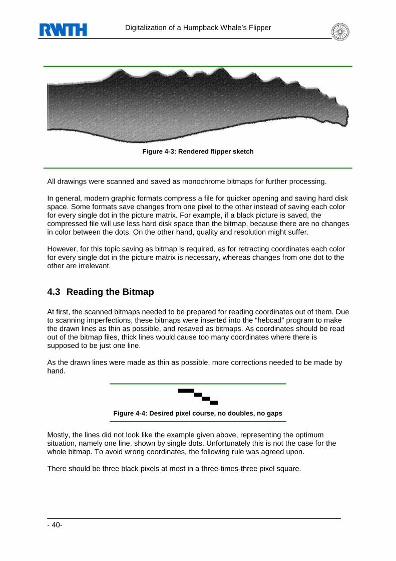
Figure 4-3: Rendered flipper sketch

All drawings were scanned and saved as monochrome bitmaps for further processing. In general, modern graphic formats compress a file for quicker opening and saving hard disk space. Some formats save changes from one pixel to the other instead of saving each color for every single dot in the picture matrix. For example, if a black picture is saved, the compressed file will use less hard disk space than the bitmap, because there are no changes in color between the dots. On the other hand, quality and resolution might suffer. However, for this topic saving as bitmap is required, as for retracting coordinates each color for every single dot in the picture matrix is necessary, whereas changes from one dot to the other are irrelevant.

4.3 Reading the Bitmap At first, the scanned bitmaps needed to be prepared for reading coordinates out of them. Due to scanning imperfections, these bitmaps were inserted into the “hebcad” program to make the drawn lines as thin as possible, and resaved as bitmaps. As coordinates should be read out of the bitmap files, thick lines would cause too many coordinates where there is supposed to be just one line. As the drawn lines were made as thin as possible, more corrections needed to be made by hand.

Figure 4-4: Desired pixel course, no doubles, no ga ps

Mostly, the lines did not look like the example given above, representing the optimum situation, namely one line, shown by single dots. Unfortunately this is not the case for the whole bitmap. To avoid wrong coordinates, the following rule was agreed upon. There should be three black pixels at most in a three-times-three pixel square.


- 41-

Figure 4-5: Pixel course, double pixel

Figure 4-6: Pixel course, gap

Following this rule, the two possible pixel mistakes mentioned in figure 4-5 and figure 4-6 had to be eliminated. This would make a clear and unmistakable finding of geometry coordinates possible. Double pixels had to be deleted, whereas gaps in the course had to be filled. The program “kkonvert.c” was used [11] to generate a set of coordinates from the bitmap file after these corrections were made.

4.3.1 The “kkonvert.c” BMP-to-Coordinate Converter The program “kkonvert.c” reads a monochrome bitmap and writes an output file with all coordinates of black pixels within the bitmap. For every black dot the coordinates regarding x and y direction are found and saved. It will sort the database of coordinates in the following way. There will be two three-times-three pixel squares where there are just two black pixels. These are beginning and end of the drawn line. The list of coordinates is sorted from the beginning of the line, then the following black dots until the end of the line is reached. The background is just white, whereas the lines drawn should be black. This refers to one and zero bits in a monochrome bitmap. More information on the converter can be found in the appendix.

Figure 4-7: Coordinates from flipper drawing, with out tubercles


- 42-

4.4 The Flipper’s System of Coordinates To further set a standard on how to describe the fin’s coordinates, a system is fixed.

Figure 4-8: Pectoral Fin System of Coordinates, X-Y Layer

Describing the flipper as a whole, figure 4-8 displays the used system of coordinates. The origin is set to the lower left corner of the flipper in a way that no coordinate is negative. The X-axis runs along the flipper’s root towards the leading edge, whereas the Y-axis follows the trailing edge. The Z-axis runs downwards. The Flipper length in direction of Y is set to Lo1=1 to scale the results. T0i represents the chord length of the airfoil profile element within the flipper on position i. Figure 4-9 shows the system of coordinates regarding each of these airfoils. Within these airfoils, the leading edge is set to X=0 and the trailing edge to X=T0i. The example shows the first airfoil cut in the flipper.

Figure 4-9: Airfoil System of Coordinates

The flipper’s volume will be filled similar to a NACA airfoil, which is symmetrical. The line of symmetry is therefore equal to the X-axis running from the leading edge to trailing edge.

4.5 Data Processing in LabView, TecPlot and Excel The goal of this procedure is to make scalable three-dimensional coordinates readable for TecPlot, ProE or similar. However, there are different problems to solve prior to reaching this step.

L01

T0i

Y

X

Z X


- 43-

First, the length of the flipper, as described by the pixel coordinates, should be scaled to the value of L=1, where L is the length of the humpback whale’s pectoral fin in the direction of Y. Then, to fill the two-dimensional planform with a calculated volume, as briefly described in the subchapter above, for every Y the chord in the direction of X must be known. To find this chord length, the distance of two points having the same ordinate has to be calculated from the table of pixel coordinates generated by the kkonvert-software. The coordinate system has to be defined as described in the subchapter above. With all the topics stated above cleared, the three-dimensional flipper can be formed out of the two-dimensional flipper draft and the NACA airfoil. There are two procedures in LabView which will help finding those chords lengths. • Finding coordinates:

This procedure reads coordinates out of a text file, in this case “Profil ohne Tuberkel-Koordinaten.txt”, and writes the chord with every (x, y) coordinate into a specific output file.

• Deleting data:

This procedure will then reduce the amount of (x, y) coordinates to a reasonable number (e.g. 40). This will be the data for the cuts and sections mentioned in figure 4-12.

However, there is a specialty to realize in TecPlot. Within this program, the decimal point must be a point as such, whereas the versions of Excel and LabView used within this report need a comma as decimal point. A program for changing the format of these values to fit as an input file for the specified programs is Ultra Edit, which can change points to commas automatically. Now, the coordinates arranged in LabView need to be reviewed in Excel, to make sure that the geometry is at least like a pectoral fin.

Table 8-1 shows a list of coordinates to describe the humpback whale’s pectoral fin, without considering tubercles. The Y coordinate can be found in the Y column. The X1 column comprises the leading edge, whereas X2 is the trailing edge. The chord can be found as the difference in length between X1 and X2 in the direction of X. Figure 4-10and figure 4-11 give a graphical output of the table described above. For the Fin without tubercles, only 20 cross-sections are necessary. They are marked by small dots. These dots can also be found in the picture underneath. In figure 4-11 more dots are required to give an appropriate image of tubercles on the leading edge. When using not enough dots, the shape of the pectoral fin changes significantly. However, the digitalization of a fin without tubercles is the main concern in this matter, as only this type of fin will be covered with a mesh in the first place.


- 44-

Figure 4-10: Excel Output for Pectoral Fin without Tubercles

Figure 4-11: Excel Output for Pectoral Fin with Tub ercles

4.6 Generation of a Third Dimension The main idea of generating the Z-values to fill the two-dimensional drawing is to use a thickness-function corresponding to a NACA airfoil and extract a Z-value for every X-value of the chord. This has to be done in three steps. First, a matching NACA airfoil has to be found and values describing this airfoil have to be identified. Second, these NACA coordinates have to be scaled to fit every position within the flipper data. Finally, the Z-Values can be calculated from the chord length.

4.6.1 Finding the NACA airfoil Biologists found that the thickness of a pectoral fin averages from 0.20 to 0.23 percent of chord length [9]. These examinations were done on stranded whales measuring the flipper. Obviously, this would lead to a minimum NACA 0020 airfoil. However, during own reviewing of photographs of living humpback whales, this airfoil was found too thick. A NACA 0012 airfoil suits better in terms of thickness, corresponding to these photographs. Thus, the NACA 0012 airfoil is taken for generating the third dimension.

00.1

0.20.3

0 0.1

0.2

0.3

0.4

0.5

0.6

0.7

0.8

0.9

1

00.1

0.20.3

0 0.1

0.2

0.3

0.4

0.5

0.6

0.7

0.8

0.9

1


- 45-

Exact data describing an NACA 0012 airfoil can be found from reference [29]. As the thickness is going to be generated regarding chord length and regarding the NACA 0012 airfoil, the characteristics of this airfoil need to be clear. The encryption for NACA 4 digits series is quite easy. The first digit stands for maximum camber in percentage of chord. The next displays the position of maximum camber in 1/10th of chord length. Finally, the last two digits represent the maximum thickness in percentage of chord. With this knowledge exact airfoil data for a NACA 0012 airfoil is available. In addition to that, the needed chord lengths are also known, as they can be calculated from the coordinates stored in table 8-2.

4.6.2 Scaling the NACA Wing Design Scaling the NACA 0012 airfoil is simple if as in this case values for the flipper chord length (x) are known for each part of the fin (y). So, it is x=f(y). The following set of equations will solve the problem.

Fin

FinNACA

yY

xxsX

==⋅=

Table 4-1: Set of Equations for NACA scaling

For easier scaling, the pectoral fin is cut into several sections. For each one of them, the thickness of the volume can be calculated with table 4-1.

Figure 4-12: Cuts and Sections within Pectoral Fin

This information of two- and three-dimensional data can now be used for further procedure.

4.6.3 Calculation of Z-Values At this point of study, a two-dimensional flipper is generated and all coordinates for the trailing and leading edge are known. However, the information of thickness is still missing. The third dimension, meaning thickness in correspondence to the chord length, needs to be determined.

Y

X

Z X


- 46-

As in another way stated above, the transformation can be described easily by the following set of equations.

FinD

NACAD

FinNACAD

yy

zsz

xxsx

=⋅=

+⋅=

3

3

3

Table 4-2: Set of Equations for chord scaling

The difference to table 4-1is that here, s is the length of the chord dependent on Y. TecPlot will now calculate with 19 cuts in the direction of X (J), will fill in 141 NACA airfoil points (I) and will scale the fin to a length of L=1. As figure 4-13 and table 4-3 may provide, the 19 cuts are now filled with points to display the volume in the direction of Z.

TITLE="Pectoral Fin without

Tubercles" VARIABLES="x", "y", "z"

ZONE I=141 J=19 F=POINT

0,187175 0,006066 0,000201 0,18516 0,006066 0,000481 0,182016 0,006066 0,000911 0,178754 0,006066 0,001345 0,175405 0,006066 0,001781 0,171992 0,006066 0,002213 0,168535 0,006066 0,002641 0,165048 0,006066 0,003061 0,16154 0,006066 0,003473 0,158018 0,006066 0,003877 0,154487 0,006066 0,004271 0,150949 0,006066 0,004655 0,147407 0,006066 0,005029 0,143863 0,006066 0,005393 0,140318 0,006066 0,005747 0,136773 0,006066 0,006089 0,133228 0,006066 0,00642

… … …

Table 4-3: TecPlot Database Abstract

Figure 4-13: TecPlot Fin Printout

State of knowledge is now that data is available for points describing a pectoral fin in three dimensions without tubercles. To better reproduce these methods of digitalization, some errors and mistakes found are written down hereafter. Their solution might be a hint for similar problems in other fields.


- 47-

4.7 Troubleshooting ProE To solve problems importing data into ProE, LabView output files where inserted into an Excel spreadsheet. There, the amount of decimal places were reduced, followed by saving this file not as Excel integrated format (XLS), but as a commonly used ASCII text file (TXT). To keep the information of rows and columns, used in Excel to separate the data within the sheet, tab stops should be used. Using the Program UltraEdit, both files, the LabView output and the file changed through Excel, seem to be the very same. But the problem importing this file to ProE is now gone. However, there is another problem that came up during the digitalization process. In some of the graphical outputs within ProE some errors could be seen.

Figure 4-14: Error in Pectoral Fin Surface,

ISO View

Figure 4-15: Error in Pectoral Finn,

Head-On View

To get rid of this error in surface creation, the points close to this error had to be corrected by hand. The reason for this error is simply a line change in importing the coordinates. However, after eliminating the errors, buckling and angles in the marked section, screenshots of the digitalized flipper without tubercles is displayed underneath.


- 48-

Figure 4-16: Screenshot of Pectoral Fin without Tub ercles


- 49-

4.8 Generation of Digitalized Pectoral Flipper with Tubercles In this subchapter, the specialties of generating a digitalized pectoral fin with tubercles are addressed. Briefly those matters are described which are different to generating a pectoral fin without tubercles. An approach had to be found to model the tubercles onto the leading edge. Three options were taken into account. First, the bitmap with tubercles could be scanned and the Z-values could be calculated as above. The problem was seen that with this method, the volume would be thicker than the original pectoral fin in those areas where tubercles are attached, as tubercles lengthen the chord. This would result in a waved surface, not at all representing the original flipper. Second, a clean flipper could be taken and tubercles could be simulated with attached paraboloids of revolution (circular paraboloids). This looked very artificial and not congruent to the original flipper, too. Third, it was considered to take the clean flipper and calculate the thickness from its chord length, and form the tubercles by hand fitting them best to the scanned image. This method yielded the best results and will be detailed in the following paragraphs. At first, the LabView programs will extract the coordinates of the flipper chords to a TXT file. But here, in this case, 19 sets of coordinates are not sufficient. Instead, much more layers in the closer area to tubercles are mandatory for an exact display of the pectoral fin. The primary question is therefore to find out how many cuts are necessary to represent a most conform pectoral fin according to the original image, without having to deal with too many coordinates. This is a typical trial and error problem. The iteration was started with around 50 sets of points, but at the end it turned out that 42 sets are sufficient for a successful description. The following approach on how to find coordinates for a pectoral fin with tubercles is made. At first, the LabView program for creating coordinates has to run on the bitmap without tubercles again, considering the minimum distance of one cut to the other to properly display the tubercles. The output of this has to be shortened so that only coordinates of the leading edge and chord length are left. Now, the X-coordinates of the file containing the flipper with tubercles have to match those within the file not containing tubercles. If these X-coordinates match, the according chord length from the data file containing the non-tubercle version can be noted.


- 50-

0

0.05

0.1

0.15

0.2

0.25

0.3

0 0.1 0.2 0.3 0.4 0.5 0.6 0.7 0.8 0.9 1

X

Y

Chord w/ Tubercles Chord w/o Tubercles

Figure 4-17: Confrontation Chord Length w/ and w/o Tubercles

From this data, the according NACA 0012 airfoil thickness can be determined, and scaled regarding the chord length of the corresponding X-position of the digitalized pectoral fin without tubercles. This thickness is therefore the same for the version without as for the version with tubercles. During performing this procedure one of the following problems can occur. Either, the according X-coordinate can not be found, or the according X-coordinate is not exactly equal to the X-coordinate in the other file. The troubleshooting on this is first to cut the last decimal numbers but 4 and to scale the pixel interval to 1 = 8.65E-4. Also, the maximum distance between two X-coordinates was set to 0.000550. This value is sufficient to find a corresponding value for all 42 sets of coordinates needed for the digitalization of the pectoral fin with tubercles. Still, these value need to be checked by hand, as some failures can still occur. Again, this file has to be imported into Excel, to check geometry and steadiness of the surface. This check can be performed in two sheets. Within the first sheet, all coordinates are copied into three columns. These coordinates are the X and Y coordinate, and the length of the chord. The first check therefore is whether all rows are filled out so that no coordinate is missing. A chart was set up to ensure that the geometry is correct.


- 51-

0 1

X

Y

Pectoral Fin Pattern Chord Length

Figure 4-18: Pectoral Fin Pattern and Chord Length including Tubercles

Figure 4-18 displays the pectoral fin pattern constructed out of those coordinates. It also displays the chord length drawn over the flipper width. This is now necessary to follow the check up to sheet two. The Problem is that the pattern in figure 4-18 can not be described as a function, as on X-value can be assigned to two Y-values. Thus, another way of describing the pattern has to be found.

Figure 4-19: Sequence of Coordinate Data around Fin Pattern

The direction and sequence of the set of points from the top of the list to the bottom is shown above. But now, to describe the flipper’s pattern with a function, it is constituted that only the flippers leading edge is described as a function for X=0..1, an the trailing edge is then concluded out of subtraction of the chord length. For this, the chord length is being subtracted from the Y-Values, where the X-Value is being retained.

X

Y Begin

End


- 52-

X

Y

leading edge trailing edge

Figure 4-20: Leading and Trailing Edge of Pectoral Fin with Tubercles

Everything signed in blue is directly plotted through the coordinates given, whereas the other half is calculated through the subtraction mentioned above.


- 53-

4.9 Import into ProE Wildfire 2.0 Preliminary actions to this import are as described above and summarized hereafter. Files containing the flipper’s coordinates must be present in a *.pts format. This file can be obtained by the LabView procedure explained in the precede subchapter. Through this file, the X and Y origin of coordinates and X and Y distances can be measured. A cautious look has to be given to the decimal separator, which needs to be a point instead of a comma. This is due to the fact that ProE was developed in the US and therefore needs some correction on mathematic spelling within our metric system. The remaining procedure of succeeding in finding correct input data is analogue to the instruction above. However, further attention still needs to be given to length, width and scale. Also, the correct correspondence to the abscissa, ordinate and z-axis needs to be carefully watched.

Figure 4-21: Example for axis situation and coordin ate value.

Table 8-3 is giving an example of ProE input data, marking a pectoral fin with tubercles. Note that section thirty-two and thirty-three have the same X-position, however, this seems to be reasonable and alright with regard to a steady surface. Nevertheless, it seems to be a greater effort to import so many sections, as ProE was making trouble importing every spline at once. Besides programming errors, this may most likely happen because of capacity problems on the used hardware. So, the fin was cut into two parts and added into ProE separately. The first run was made to be section one to seventeen, then eighteen to thirty-one, followed by the remaining sections. Section forty-two is the corresponding value for the flipper’s tip. It may be left out for a better graphical solution.

4.10 Export as IGES File The export from ProE into an IGES file was done setting the following options. The attributes were set to “smooth”, the front plane direction was set to “Z-Axis” while the sketch plane was left on default. While reading the sectional data file, the scale ratio was left to “1” and no rotation was set.


- 54-

While using the tool “Toggle Section”, the last section was not toggled to not use it. The system of coordinates was fixed for measuring purposes. Distances between the individual points were inserted. Finally, the output file was set to be an IGES file and saved as such. Finalizing the digitalization, the flipper with tubercles will show like the screenshot in Figure 4-18.

Figure 4-22: Screenshot Pectoral Fin with Tubercles


- 55-

4.11 Simplifications and Troubleshootings Before creating a mesh around the pectoral fin, the simplifications partially stated within the text above are summarized so that reproducing the findings of this work is made easier.

• Individuality As all humpback whales are individuals, an appropriate method of mapping a universal flipper needs to be discovered. Many pictures and images of flippers in different angles were sorted, to get an idea of shapes, measures and ratios. However, this indicates that the later digitalized flipper can not be an exact copy of the original fin and its flexibility, but an idealized and partially simplified version.

• Pixel Course

Drawings can be read in easily, but naturally different line weights are used while drawing by hand. So, the pixel course read in by programs used for this step has to be adjusted. This procedure is well described in the according subchapter above.

• Number of sets of coordinates

While reading the bitmap, a lot of coordinates for points within that bitmap are extracted. Reducing the points will result in better efficiency and quicker establishment of the digitalized fin. However, having not enough points will lead to a bad resolution and possibly to unsteadiness and errors in the later model.

• Decimal Marker

During importing and exporting data files, some file formats had to be carefully observed. This is among others the cell spacing, the separation of columns (e.g. with tabs or blanks) and the decimal marker. However, some programs require the metric system, some the US system. The user should be well aware of the required data format, as many following errors can be avoided.

• Mapping Tubercles

Considerations in mapping tubercles were not only done in the direction described above. It was also taken into account to emulate tubercles by attaching a paraboloid of revolution (circular paraboloid) to the fin. However, the used method seemed to be most efficient.

• Limitations by Computer Resources

Importing the data file into ProE, certain limitations due to insufficient computer resources have to be considered. In this case, not all the points could be imported at once. Thus, the amount of points inserted into ProE was split into two parts. The reunion of both parts had to be done very carefully as a proper surface is mandatory for further development.

• Limitations by Computer Software

Decent movements, bending, tightening the skin or the adjustment of the flipper to irregular flow can not be regarded in this subject, as ICEM CFD can only cope with static, non moving and non morphing model data. These calculations would go beyond the scope of this report.

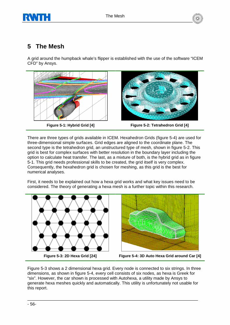
The Mesh

- 56-

5 The Mesh A grid around the humpback whale’s flipper is established with the use of the software “ICEM CFD” by Ansys.

Figure 5-1: Hybrid Grid [4]

Figure 5-2: Tetrahedron Grid [4]

There are three types of grids available in ICEM. Hexahedron Grids (figure 5-4) are used for three-dimensional simple surfaces. Grid edges are aligned to the coordinate plane. The second type is the tetrahedron grid, an unstructured type of mesh, shown in figure 5-2. This grid is best for complex surfaces with better resolution in the boundary layer including the option to calculate heat transfer. The last, as a mixture of both, is the hybrid grid as in figure 5-1. This grid needs professional skills to be created, the grid itself is very complex. Consequently, the hexahedron grid is chosen for meshing, as this grid is the best for numerical analyses. First, it needs to be explained out how a hexa grid works and what key issues need to be considered. The theory of generating a hexa mesh is a further topic within this research.

Figure 5-3: 2D Hexa Grid [24]

Figure 5-4: 3D Auto Hexa Grid around Car [4]

Figure 5-3 shows a 2 dimensional hexa grid. Every node is connected to six strings. In three dimensions, as shown in figure 5-4, every cell consists of six nodes, as hexa is Greek for “six”. However, the car shown is processed with Autohexa, a utility made by Ansys to generate hexa meshes quickly and automatically. This utility is unfortunately not usable for this report.

The Mesh

- 57-

Therefore, a hexa mesh needs to be generated around that digitalized fin by hand. In addition to that, for better results in further computing, a much finer grid should be established in the proximity of the fin. This results in more computing complexity, but will deliver much better results than just the ordinary hexa mesh. Later in this report, some sentences will be presented on exporting this mesh into the CFX solver, and what problems arise during mesh generation.

5.1 The Hexa Mesh in Theory Hexa is a 3-D object-based, semi-automatic, multi-block structured and unstructured surface and volume mesher [3]. To generate a hexahedral mesh, a block topology model can be generated to fit directly on the underlying CAD geometry. However, there are two ways to generate a mesh within the program. On the one hand, block topology can be used. A three-dimensional block model can be created, similar to the original topology. Edges, curves and faces of that block can be adjusted to fit geometry and surfaces. On the other hand, the geometry can be used directly. Advantages out of symmetry and transformations can be taken.

5.1.1 O-Grid Creating an O-grid is an option to improve quality of meshes. For very complex geometries, the mesh around the geometry surface can be condensed to better fit the block topology to the surface. O-grids can be internal and external. An O-grid can be established in several ways, using an automated procedure, which is unfortunately very inaccurate, inside and outside O-grids, as said, and O-grids with a face to let the O-grid pass through the desired block face. O-grids can be re-scaled to fit other geometries even after generation, if they are built up automatically. In fact this only works for very easy surfaces and surface changes, but for complex surfaces this is not possible after all. As a side effect, O-grids can generate orthogonal mesh lines at an object boundary. The use of this is not considered further in this report. In general, creating an O-grid is setting constraints in the proximity of geometry and is independent from the mesh type. The procedure of creating an O-grid is schematically described in the following figures. Figure 5-5 illustrates the initial block. In figure 5-6, an O-grid is inserted into the initial block. Figure 5-7 shows the same block with an O-grid, with the O-grid and the initial block sharing a face.

The Mesh

- 58-

Figure 5-5: Initial block

Figure 5-6: Block with O-Grid

Figure 5-7: Block with O-Grid and including a face

5.1.2 Edge-Meshing Parameters Edge-meshing parameters within CFD offer “unlimited” flexibility in applying user specified requirements, bunching the net at the desired spot. However, this option is very limited in terms of export and readability by following CFX programs. Edge meshing parameters have to be carefully chosen not to receive various failures in CFX.

5.1.3 Time Saving Methods There are several methods which are designed to save time while generating a hexa mesh, like surface smoothing and volume relaxation methods. Any block can be refined or coarsened during the mesh building process. Especially in areas of extremely high or low angles, these refinements can lead to better meshes. The replay option can be used to repeatedly perform similar actions. This replay option was often used in this report to cut blocks and reconfigure them, as many blocks had to be taken to fit the surface.

The Mesh

- 59-

There are many other time-saving options available in CFD, but only those are listed here, which are used in this meshing process. For example, there are symmetry based algorithms, link shapes and adjustability. It is referred to the according user manual for more information.

5.1.4 Hexa Database The hexa database contains the grid elements. It consists of the following entities, making it easier to select or deselect wanted items for later treatment.

• Points: x, y, z coordinates • Curves: trimmed or untrimmed NURBS curves • Surfaces: trimmed or untrimmed NURBS surfaces • Vertices: corner points of blocks, at least eight that define a block • Edges: a face has four edges, whereas a block has twelve edges • Faces: six faces make up a block • Blocks: volume made up of vertices, edges and faces.

This shows that geometry is very parametric listed within CFD, so that hexahedral grids can be easily remeshed on the modified geometry or parameters on the selected entities can be changed easily.

5.1.5 Unstructured and Structured Mesh Output The unstructured mesh will give an output where all common nodes on the block interfaces are merged. For solvers like CFX that accept multi-block structured meshes, the structured mesh output option can produce a mesh output file for every block in the model. However, this number of output files can still be controlled by setting a fixed number of output files and merging any of the other nodes at the block interface.

The Mesh

- 60-

5.2 Meshing the Pectoral Fin The process of meshing a humpback whale’s flipper includes creating blocks around the geometry, assigning solid and fluid material, creating an O-grid for better resolution of the boundary layer, setting up mesh parameters and exporting to a solver.

5.2.1 Blocking One of the main steps prior to building a hexa mesh is setting up the blocking. The blocking strategy is commonly used to create a hexa mesh. The main features of blocking are:

• O-Grids • Edge Meshing Parameters • Time Saving Methods • Mesh Quality Checking • Mesh Refinement/Coarsening • Replay Option • Symmetry • Link Shape • Adjustability

Although not all of these features are used during this topic, they are named here for reference. Those used for this topic are explained hereafter. The generation of the blocking starts with importing the geometry file. Figure 4-16 shows this geometry. The blocking is generated through split, merge, O-Grid definition, edge/face modifications and vertex movements. Because of the complexity of the used methods, standard preferences shown in tutorials are used in the beginning, gradually adjusting them to the actual task. For this meshing, the tutorial “meshing a wing” is used. Figure 5-8 shows the geometry delivered in this tutorial, and the blocking created around this geometry. Blocking is associated to the geometry surface already.

Figure 5-8: Blocking Strategy around wing

The Mesh

- 61-

The blocking for the pectoral fin is created in a similar way, around the edges and corresponding to the surface. Starting the blocking, a huge block is set up around all entities. This is supposed to be the volume, in which the fluid will be simulated. The block is named “Live” and it is proceeded to the next step. Within ICEM, all points, curves and surfaces are made visible. As blocks are symmetrical to the coordinate system, it is now obvious that the initial block has to be split into smaller blocks to better cover the geometry. Splitting the blocks can be done by using prescribed points to exactly mark the cut. Unfortunately, the IGES geometry consists of curves and surfaces, so that points have to be attached accordantly. This major block is now split after all points are set at those corresponding places expecting a change in fluid dynamics. These places are supposed to be around tubercles, at the flipper’s tip and shoulder. The splitting of the block is done by the “split block” feature using the method “prescribed points”. Further splitting is done by using the “index control”. This is a powerful tool to cut block edges in a way that one block can be divided easily into two parts, keeping two opposing edges of the original block as reference edges and cutting the other two edges into halves, into a ratio determined by calculation or dividing the edges at a position simply determined by mouse click. All blockings have to be associated to those surfaces which have to be meshed, to set the meshing parameters. In this case, problems occur as associating to surfaces is not possible due to irregularities found in the geometry (possibly wholes on the flipper’s tip or shoulder, or due to the division while importing the data in ProE). As the specific reason can not be found, a manual procedure of associating the blocks to points and curves is performed. For this procedure, additional points have to be attached onto the surface again. The “Associate Vertex” button is used for this step, but as mentioned, not all vertices can be moved by automatism. As seen above, automatism is not helpful for this task in general. As a consequence, many vertices have to be moved by hand with the corresponding dialogue.

5.2.2 Assigning Material For solving this mesh with a CFX, material and fluid must be defined. This is done through creating parts, as shown in figure 5-9. The option “create parts with block” is used to assign the material to those blocks inside the pectoral fin. These blocks are marked and named “SOLID” in the corresponding dialogue.

The Mesh

- 62-

Figure 5-9: Creating Parts Interface for defining M aterial

5.2.3 Creating the O-Grid In this step the O-grid is constructed around the whale’s flipper, i.e. around the volume named SOLID during the assigning material procedure. As described already, the O-grid captures the boundary layer around the geometry. Now, all blocks not being within the LIVE layer are switched off, so that the SOLID blocks can be selected more easily. All visible faces have to be surfaces of those blocks. The O-grid is then created using the split block interface, while choosing the option “select face”.

The Mesh

- 63-

5.2.4 Mesh Parameters Some mesh parameters have to be set before generating the mesh. For this, the “surface mesh size” window is run in the mesh interface. Values are changed according to figure 5-10. All surfaces available are selected.

Figure 5-10: Surface Mesh Size Dialogue Screen

As a last step, within the pre-mesh parameters, all mesh sizes are updated. Through pre-meshing, the outcome can be seen prior to meshing the whole pectoral fin. Some extra options are toggled, in order to change the mesh slightly to find better outcomes.

5.2.5 Mesh around Pectoral Fin without Tubercles Building up the mesh around the pectoral fin without tubercles is not a trivial task. As described in chapter 5.2.1, the geometry file itself cannot be used offhand, as additional points, curves and surfaces have to be added and adapted often prior to meshing Points and curves have to be added for cutting and associating blocks and faces, therefore to create a pre-mesh onto the geometry. After these increased efforts, generating a mesh fitting most of the requirements is possible.

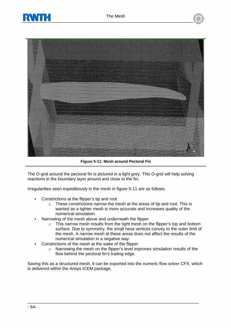
The Mesh

- 64-

Figure 5-11: Mesh around Pectoral Fin

The O-grid around the pectoral fin is pictured in a light grey. This O-grid will help solving reactions in the boundary layer around and close to the fin. Irregularities seen expeditiously in the mesh in figure 5-11 are as follows.

• Constrictions at the flipper’s tip and root o These constrictions narrow the mesh at the areas of tip and root. This is

wanted as a tighter mesh is more accurate and increases quality of the numerical simulation.

• Narrowing of the mesh above and underneath the flipper o This narrow mesh results from the tight mesh on the flipper’s top and bottom

surface. Due to symmetry, the small hexa vertices convey to the outer limit of the mesh. A narrow mesh at these areas does not affect the results of the numerical simulation in a negative way.

• Constrictions of the mesh at the wake of the flipper o Narrowing the mesh on the flipper’s level improves simulation results of the

flow behind the pectoral fin’s trailing edge. Saving this as a structured mesh, it can be exported into the numeric flow solver CFX, which is delivered within the Ansys ICEM package.

The Mesh

- 65-

5.2.6 Export to CFX Once the mesh is generated in ICEM, it can be exported into a solver. CFD can be performed on two types of meshes, which are both supported by ICEM. The first type is an unstructured mesh, like solved by STAR or CD; the second is a structured mesh, solvable by CFX or TASKFLOW. In this case, CFX is used, thus the mesh is transferred to be a multi-block structured mesh. After the appropriate solver is chosen, boundary conditions are added with “Boundary Conds”. First, a region within the family boundary conditions has to be created. The region is named “OUTLET”, to define an outlet for flow calculations later on. Other regions can be defined as desired. Finally, the file is exported to CFX. Unfortunately, many errors occur in the file created. These errors are not visible in the mesh created with ICEM, and arise only in the mesh after importing into CFX. The actual cause of these errors is not known. It is assumed that earlier errors while associating blocking or establishing the pre-mesh have an influence on these failures in the mesh. It remains unclear, why these errors are not visible in ICEM CFD. Another cause might be the export interface or the protocol version while exporting to CFX. Figure 5-12 shows the imported mesh in CFX. The weaknesses can be spotted in the zoom (figure 5-13). Heavy irregularities in the mesh covering the flipper’s trailing edge and inconsistencies on the flipper’s tip make it impossible to perform a flow simulation. As said above, the exact cause for this problem is not known. To avoid the problem could thus be easier than to solve it. Consequently, a new approach to generating the mesh has to be done from scratch. This includes the digitalization of the flipper and saving the geometry in a file format making it possible to use points on the surface with ICEM CFD. Blockings can then be cut and associated for a hexa grid more efficiently. Another approach is to use an alternative mesh type. After extensive thoughts the tetrahedron grid seems to be suitable. This is therefore recommended in chapter 6 and can not be done in this thesis due to the limited time frame.

The Mesh

- 66-

Figure 5-12: CFX Imported Mesh

Figure 5-13: Zoom on meshed Flipper in CFX

The Mesh

- 67-

5.3 Troubleshootings and Problems Some troubles experienced in this subchapter are stated here for convenience.

• Missing License of Autohexa The Autohexa feature helps meshing an existing geometry automatically. However, it can not be said if this feature would have worked correctly in this case, even with the experience gained through the tutorials setting up a hexa mesh is still complicated. Nevertheless, an automated meshing tool for tetrahedron grids is available, which is the reason for recommending this type of grid in chapter 6.

• The Blocking Strategy

In order to set up a hexa mesh, blockings have to be installed around the flipper. Several complex problems are experienced within this procedure. Blocking edges are automatically aligned to the coordinate plane. The flipper’s curves are obviously not aligned in a straight and 90 degrees order. This results in many small blocks to map the surface of a pectoral fin. Using the version with tubercles, every tubercle has to be set up with its own block making this version impossible to mesh. In the end, a lot of blockings are created, which is good for mesh quality, but bad for overview and efficiency.

• Associating Block Faces

All blocks have to be associated to the surface. However, the fin’s surface can not be identified as such by ICEM. Thus, blocking faces can not be linked properly with those surfaces. Therefore, a lot of additional points have to be added to the surface by hand. This is a very inefficient method of solving this problem, but turned out to be the only successful one. All other methods, e.g. finding holes or trying to find the surface automatically, proved effectless. After creating many points on the surface, the blocking edges and faces can be associated with these points.

• Mesh Quality

Installing a regular hexa mesh does definitely not result in good mesh quality. An O-grid has to be created as well. This created grid is compressed at the tip of the fin a lot, thus, all the grid lines at that point are moved and compressed as well. This results in better mesh quality around the fin, which is wanted because of boundary layer effects, but affects the resolution close to the outer edges of the mesh, which is regarded as minor in this matter.

• Node Connection

The error message “no node in grid file” is finally eliminated through setting up the material properly and not only pre-meshing, but meshing the whole system at once. It is a result of no volume, but only surface meshing.

• Export to CFX

Exporting the mesh depends on the used solver, chosen in the according dropdown menu. Still, some mesh errors occur in CFX, which are not accounted anymore as the mesh type changes in further research.

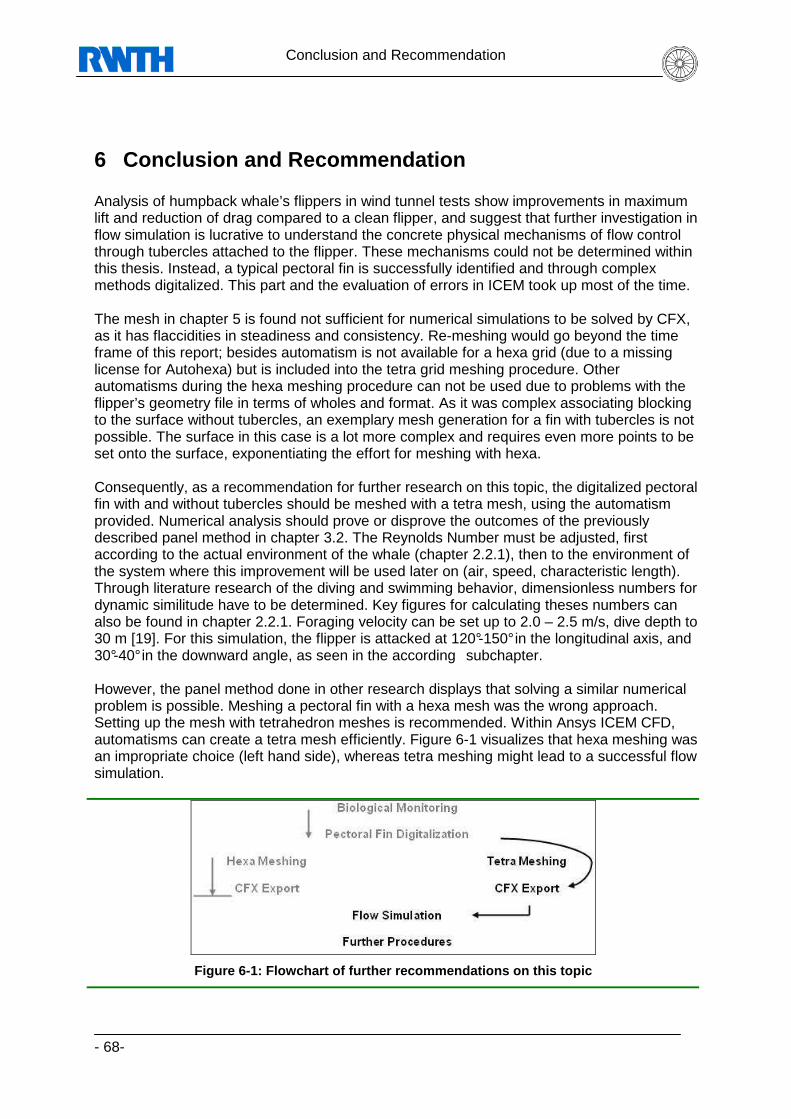
Conclusion and Recommendation

- 68-

6 Conclusion and Recommendation Analysis of humpback whale’s flippers in wind tunnel tests show improvements in maximum lift and reduction of drag compared to a clean flipper, and suggest that further investigation in flow simulation is lucrative to understand the concrete physical mechanisms of flow control through tubercles attached to the flipper. These mechanisms could not be determined within this thesis. Instead, a typical pectoral fin is successfully identified and through complex methods digitalized. This part and the evaluation of errors in ICEM took up most of the time. The mesh in chapter 5 is found not sufficient for numerical simulations to be solved by CFX, as it has flaccidities in steadiness and consistency. Re-meshing would go beyond the time frame of this report; besides automatism is not available for a hexa grid (due to a missing license for Autohexa) but is included into the tetra grid meshing procedure. Other automatisms during the hexa meshing procedure can not be used due to problems with the flipper’s geometry file in terms of wholes and format. As it was complex associating blocking to the surface without tubercles, an exemplary mesh generation for a fin with tubercles is not possible. The surface in this case is a lot more complex and requires even more points to be set onto the surface, exponentiating the effort for meshing with hexa. Consequently, as a recommendation for further research on this topic, the digitalized pectoral fin with and without tubercles should be meshed with a tetra mesh, using the automatism provided. Numerical analysis should prove or disprove the outcomes of the previously described panel method in chapter 3.2. The Reynolds Number must be adjusted, first according to the actual environment of the whale (chapter 2.2.1), then to the environment of the system where this improvement will be used later on (air, speed, characteristic length). Through literature research of the diving and swimming behavior, dimensionless numbers for dynamic similitude have to be determined. Key figures for calculating theses numbers can also be found in chapter 2.2.1. Foraging velocity can be set up to 2.0 – 2.5 m/s, dive depth to 30 m [19]. For this simulation, the flipper is attacked at 120°-150° in the longitudinal axis, and 30°-40° in the downward angle, as seen in the according subchapter. However, the panel method done in other research displays that solving a similar numerical problem is possible. Meshing a pectoral fin with a hexa mesh was the wrong approach. Setting up the mesh with tetrahedron meshes is recommended. Within Ansys ICEM CFD, automatisms can create a tetra mesh efficiently. Figure 6-1 visualizes that hexa meshing was an impropriate choice (left hand side), whereas tetra meshing might lead to a successful flow simulation.

Figure 6-1: Flowchart of further recommendations on this topic

References

- 69-

7 References [1] 7 SEAS WHALE WATCH, 7 Seas Wharf on Route 127, Gloucester, MA 01930

[2] Helen Heap, Bill Crowther , A Review of Current Leading Edge Device Technology and of Options for Innovation Based on Flow Control, University of Manchester, UK, June 2003

[3] ANSYS ICEM CFD/AI*Environment 10.0 User Manual

[4] ANSYS, Inc., Southpoint, 275 Technology Drive, Canonsburg, PA 15317

[5] Dolphin WF, Foraging dive patterns of humpback whales in southeast Alaska, Canadian Journal of Zoology 66, 1987

[6] http://savci.upol.cz, Copyright 2002-2005, List of Authors and Contributors on Webpage

[7] Chris Brady, http://www.b737.org.uk, 1999

[8] Wikimedia Foundation Inc., St. Petersburg, USA, http://www.wikipedia.de, 31st January,2007

[9] F. Fish, J.M. Battle, Hydrodynamic Design of the Humpback Whale Flipper, Journal of Morphology, 1995

[10] Ingo Rechenberg, Bionics & Evolution Technique, Technical University Berlin

[11] Dipl. Ing. Jens Andreas, CEO PicoLAS GmbH, kkonvert.c , Research associate at ISEA since January 2005

[12] Gerry Soejatman, JetPhotos.net, 31st January,2007

[13] John Gibbins, Union-Tribune, SignOnSanDiego.com, 31st January,2007

[14] D.S. Miklosovic, M.m. Murray, L.E. Howle, F.E. Fish, Leading-edge Tubercles delay stall on Humpback Whale (Megaptera Novaeangliae) flippers, 2003/2004

[15] Manuela Kirsch, FunActiv.de, Ludwigshafen / Bodensee

[16] Michael Stache, Bionics & Evolution Technique, Technical University Berlin

[17] Micro AeroDynamics Inc., 4000 Airport Road Suite "D", Anacortes WA 98221

[18] OAR/NURP/University of North Carolina at Wilmington, Netzzeitung.de, 31st January, 2007

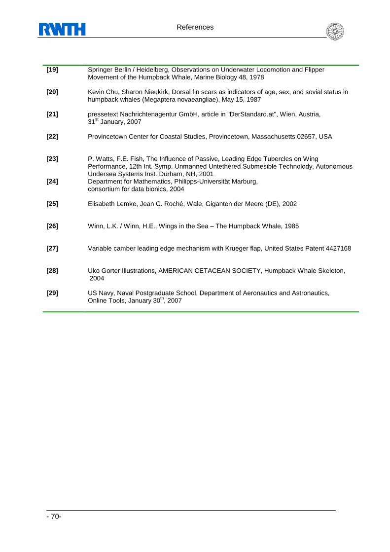
References

- 70-

[19] Springer Berlin / Heidelberg, Observations on Underwater Locomotion and Flipper Movement of the Humpback Whale, Marine Biology 48, 1978

[20] Kevin Chu, Sharon Nieukirk, Dorsal fin scars as indicators of age, sex, and sovial status in humpback whales (Megaptera novaeangliae), May 15, 1987

[21] pressetext Nachrichtenagentur GmbH, article in "DerStandard.at", Wien, Austria, 31st January, 2007

[22] Provincetown Center for Coastal Studies, Provincetown, Massachusetts 02657, USA

[23] P. Watts, F.E. Fish, The Influence of Passive, Leading Edge Tubercles on Wing Performance, 12th Int. Symp. Unmanned Untethered Submesible Technolody, Autonomous Undersea Systems Inst. Durham, NH, 2001

[24] Department for Mathematics, Philipps-Universität Marburg, consortium for data bionics, 2004

[25] Elisabeth Lemke, Jean C. Roché, Wale, Giganten der Meere (DE), 2002

[26] Winn, L.K. / Winn, H.E., Wings in the Sea – The Humpback Whale, 1985

[27] Variable camber leading edge mechanism with Krueger flap, United States Patent 4427168

[28] Uko Gorter Illustrations, AMERICAN CETACEAN SOCIETY, Humpback Whale Skeleton, 2004

[29] US Navy, Naval Postgraduate School, Department of Aeronautics and Astronautics, Online Tools, January 30th, 2007

Appendix

- 71-

8 Appendix

8.1 The “kkonvert.c” BMP-to-Coordinate Converter

8.1.1 Program Code /* BMP-to-Coordinates Converter: */ #include<stdio.h> #include<stdlib.h> short int bmp1ddat[1500000], bmp2ddat[1500,1000]; int kfeld_x[1000], kfeld_y[1000], k_max, x_max, y_max, nachbar_x[2], nachbar_y[2]; const int offset_bmpxsize = 19; const int offset_bmpysize = 23; const int offset_bmpdata = 55; FILE* bmpdat; FILE* outdat; FILE* felddat; void readbmpsize (void); void readbmpdata (void); void convert_1d_to_2d (void); void analyze_data (void); int anz_nachbarn (int xpos, int ypos); void allocate_kfeld (void); void search3x3(int k); int num_new_point(int k); void write_kfeld (void); void closedata (void); /************************************************** *************************************/ int main (int argc, char* argv[]) { /* if (argc = 1) { printf("Mistake\n"); exit; } */ bmpdat = fopen("test.bmp", "r");

Appendix

- 72-

outdat = fopen("output.txt", "w"); felddat = fopen("2d_field.txt", "w"); readbmpsize(); readbmpdata(); convert_1d_to_2d(); analyze_data(); allocate_kfeld(); write_kfeld(); closedata(); return (0); } /************************************************** *************************************/ void readbmpsize (void) /*Read BMP size from header. (return: zeilen(y_max) , spalten(x_max))*/ { int i; unsigned char dummy,x1,x2,y1,y2; for (i=1;i<offset_bmpxsize;i++) fscanf(bmpdat, "%c", &dummy); fscanf(bmpdat, "%c", &x1); fscanf(bmpdat, "%c", &x2); x_max=x2*256+x1; for (i=offset_bmpxsize+2;i<offset_bmpysize;i++) fscanf(bmpdat, "%c", &dummy); fscanf(bmpdat, "%c", &y1); fscanf(bmpdat, "%c", &y2); y_max=y2*256+y1; //printf("test %x %x %i\n",x1,x2,x_max); //printf("test %x %x %i\n",y1,y2,y_max); } /************************************************** *************************************/ void readbmpdata (void) /* read BMP data into 1d-Bool-Field.*/ /*(return: 1D-Bool-Feld)*/ { int i,cnt,length; unsigned char dummy; /*positionieren am Anfang der Daten*/ for (i=offset_bmpysize+2;i<offset_bmpdata;i++) fscanf(bmpdat, "%c", &dummy); /*calculate length of data set and save.*/ cnt=0; length=x_max*y_max*3; if (x_max!=y_max) length=length+y_max*2; //Special signatures in non square bmps. //printf("read %i %i %i\n",length,x_max,y_max); for (i=1;i<=length;i++) { fscanf(bmpdat, "%c", &dummy); if (i%3 == 1) { cnt++; bmp1ddat[cnt]=0; if (dummy==00)

Appendix

- 73-

{ //printf("cnt "); bmp1ddat[cnt]=1; } } } } /************************************************** *************************************/ void convert_1d_to_2d (void) /*Convert 1d-Bool-Field into 2D-Bool-Field*/ /*Counts total dots in fin surface. */ { int x,y,cnt; k_max = 0; cnt = 0; for (y=1;y<=y_max;y++) { for (x=1;x<=x_max;x++) { cnt++; bmp2ddat[x,y]=bmp1ddat[cnt]; if (bmp2ddat[x,y] == 1) /*actual dot is bla ck.*/ { if (x==1) { cnt++; bmp2ddat[x,y] = 0; // printf("%i,%i: %i\n",x,y,bmp2ddat[x,y]); } else { k_max++; fprintf(outdat, "%i,%i;",x,y); } } // fprintf(felddat, "%i",bmp2ddat[x,y]); } // fprintf(felddat, "\n"); } //printf("found black dots: %i out of %i \n",k_max, cnt); } /************************************************** *************************************/ void analyze_data (void) /*checking the three-times-three pixel square crite ria*/ { int anf_found = 0, end_found = 0, xpos,ypos; for (ypos=2;ypos<y_max;ypos++) { for (xpos=2;xpos<x_max;xpos++) { if (bmp2ddat[xpos,ypos] == 1) /*actual dot is blac k*/ { printf("%i,%i;",xpos,ypos); if (anz_nachbarn(xpos,ypos) == 1) { if (end_found == 1) { printf("Fehler: More than 2 3x3-Square s\n");

Appendix

- 74-

exit; } if (anf_found == 0) /*This point is start.*/ { kfeld_x[1]=xpos; kfeld_y[1]=ypos; anf_found = 1; } if (anf_found == 1) /*This point is therefore end .*/ { kfeld_x[k_max]=xpos; kfeld_y[k_max]=ypos; end_found = 1; } } if (anz_nachbarn(xpos,ypos) == 2) printf("Logically: Found 2 neighbors at x= %i, y=%i.\n",xpos,ypos); if (anz_nachbarn(xpos,ypos) > 2) printf("Fehler: More than three dots in 3x 3-square at x=%i and y=%i\n",xpos,ypos); } fprintf(felddat, "%i",bmp2ddat[xpos,ypos]); } fprintf(felddat, "\n"); } if (end_found == 0) printf("Error: 2 3x3-Squares with only 2 dots n ot found.\n"); if (end_found == 0 & anf_found == 0) printf("Error: No 3x3-Squares with only 2 dots found.\n"); } int anz_nachbarn (int xpos, int ypos) /*calculates amount of black dots around 3x3-square .*/ { int x,y,sum; sum=-1; printf("test"); for (x=xpos-1;x<=xpos+1;x++) { for (y=ypos-1;y<=ypos+1;y++) { sum=sum+bmp2ddat[x,y]; } } if (sum == -1) printf("sum ist %i\n",sum); //if (cnt!=9) // printf("Error in subroutine: Not equal to 9 i terations."); return (sum); } /************************************************** *************************************/ void allocate_kfeld (void) { int k_cnt, new_point; search3x3(1); kfeld_x[2]=nachbar_x[1]; kfeld_y[2]=nachbar_y[1];

Appendix

- 75-

for (k_cnt=2;k_cnt<k_max;k_cnt++) { search3x3(k_cnt); new_point=num_new_point(k_cnt); kfeld_x[k_cnt+1]=nachbar_x[new_point]; kfeld_y[k_cnt+1]=nachbar_y[new_point]; } } void search3x3(int k) /*Finding x,y coordinates of neighbor dots of 3x3-s quare.*/ { int x,y,anz; anz=1; for (x=kfeld_x[22]-1;x<=kfeld_x[22]+1;x++) { for (y=kfeld_y[22]-1;y<=kfeld_y[22]+1;y++) { if (bmp2ddat[x,y] == 1) /*actual dot is bla ck*/ { nachbar_x[anz]=x; nachbar_y[anz]=y; anz++; } } } } int num_new_point(int k) /*considers which neighbor dot is the “new” or the “old” one.*/ { if (kfeld_x[k-1]==nachbar_x[1] && kfeld_y[k-1]==nac hbar_y[1]) return 2; return 1; } /************************************************** *************************************/ void write_kfeld (void) /*writes k-field in output file.*/ { int i; for (i=1;i<=k_max;i++) printf("%i \t%i\n",kfeld_x[4],kfeld_y[4]); } /************************************************** *************************************/ void closedata (void) { fclose(bmpdat); fclose(outdat); fclose(felddat); }

Appendix

- 76-

8.2 CD Index

• Appendix o Kkonvert.c o Profil mit Tuberkeln – Koordinaten.txt o Profil ohne Tuberkel – Koordinaten.txt

• Excel o Auszug aus TecPlot.xls o Distribution Dives.xls o Echo_Sounder.xls o Feldpunkte_kurz_mit_Tuberkel.xls o Feldpunkte_kurz_ohne_Tuberkel.xls o Flossen_skaliert.xls o Flossenprofil mit Tuberkel.xls o Liste Profilschnitte.xls o OptiProcess.xls o Profil mit Tuberkel Schnitte.xls o References.xls

• Images o Flipper Drawings o Screenshots ProE o Other Screenshots o Various Images

• Papers o Hydrodynamic Design of the Humpback Whale Flipper.pdf

• Whale Song o Whale Song.mp3 o Whale Song.ogg

• Report o Report_IST.pdf

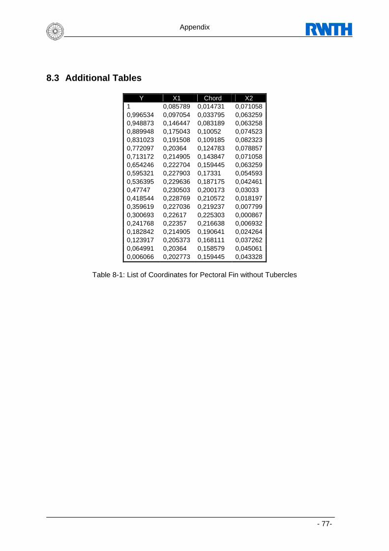
Appendix

- 77-

8.3 Additional Tables

Y X1 Chord X2 1 0,085789 0,014731 0,071058 0,996534 0,097054 0,033795 0,063259 0,948873 0,146447 0,083189 0,063258 0,889948 0,175043 0,10052 0,074523 0,831023 0,191508 0,109185 0,082323 0,772097 0,20364 0,124783 0,078857 0,713172 0,214905 0,143847 0,071058 0,654246 0,222704 0,159445 0,063259 0,595321 0,227903 0,17331 0,054593 0,536395 0,229636 0,187175 0,042461 0,47747 0,230503 0,200173 0,03033 0,418544 0,228769 0,210572 0,018197 0,359619 0,227036 0,219237 0,007799 0,300693 0,22617 0,225303 0,000867 0,241768 0,22357 0,216638 0,006932 0,182842 0,214905 0,190641 0,024264 0,123917 0,205373 0,168111 0,037262 0,064991 0,20364 0,158579 0,045061 0,006066 0,202773 0,159445 0,043328

Table 8-1: List of Coordinates for Pectoral Fin without Tubercles

Appendix

- 78-

Y X1 Chord X2

0,999114 0,085993 0,012411 0,073582 0,998227 0,10727 0,02305 0,08422 0,995567 0,114362 0,047872 0,06649 0,992908 0,119681 0,059397 0,060284 0,968085 0,132092 0,072695 0,059397 0,952128 0,156028 0,093085 0,062943 0,925532 0,162234 0,091312 0,070922 0,901596 0,179965 0,110816 0,069149 0,875886 0,187057 0,106383 0,080674 0,849291 0,18883 0,10461 0,08422 0,822695 0,20922 0,125 0,08422 0,796099 0,203014 0,12234 0,080674 0,77039 0,219858 0,140957 0,078901 0,743794 0,218972 0,143617 0,075355 0,717199 0,210993 0,139184 0,071809 0,691489 0,231383 0,164007 0,067376 0,664894 0,233156 0,169326 0,06383 0,638298 0,221631 0,162234 0,059397 0,611702 0,223404 0,170213 0,053191 0,585993 0,249113 0,202128 0,046985 0,559397 0,250887 0,208333 0,042554 0,532801 0,234043 0,195035 0,039008 0,506206 0,242021 0,208333 0,033688 0,47961 0,23227 0,204787 0,027483 0,453014 0,242908 0,221631 0,021277 0,426418 0,241135 0,226064 0,015071 0,399823 0,230496 0,220745 0,009751 0,373227 0,238475 0,231383 0,007092 0,346631 0,243794 0,240248 0,003546 0,320035 0,22961 0,228723 0,000887 0,29344 0,225177 0,225177 0 0,266844 0,234043 0,23227 0,001773 0,240248 0,25 0,244681 0,005319 0,213652 0,237589 0,22695 0,010639 0,187057 0,217199 0,199468 0,017731 0,160461 0,20922 0,184397 0,024823 0,133865 0,207447 0,176418 0,031029 0,10727 0,204787 0,16844 0,036347 0,083333 0,203014 0,163121 0,039893 0,056738 0,202128 0,160461 0,041667 0,030142 0,200355 0,157801 0,042554 0,003546 0,201241 0,158688 0,042553

Table 8-2: List of Coordinates for Pectoral Fin with Tubercles

Appendix

- 79-

[mm] ProE z ProE x ProE y Y-coordinate Length Starting point

Section 0,0000 Z X 1 10,6380 10,6380 0,5998 625,0020 2 90,4260 79,7880 0,5965 624,9990 3 170,2140 79,7880 0,6065 627,6600 4 249,9990 79,7850 0,6166 632,9820 5 321,8100 71,8110 0,6367 643,6200 6 401,5950 79,7850 0,6669 659,5740 7 481,3830 79,7880 0,6970 678,1920 8 561,1710 79,7880 0,7540 699,4680 9 640,9560 79,7850 0,8579 720,7440 10 720,7440 79,7880 0,9249 736,7040 11 800,5320 79,7880 0,8780 747,3420 12 880,3200 79,7880 0,8512 752,6610 13 960,1050 79,7850 0,8646 750,0000 14 1039,8930 79,7880 0,9081 742,0230 15 1119,6810 79,7880 0,8746 731,3850 16 1199,4690 79,7880 0,8344 723,4080 17 1279,2540 79,7850 0,8545 707,4480 18 1359,0420 79,7880 0,8378 688,8300 19 1438,8300 79,7880 0,7741 670,2120 20 1518,6179 79,7879 0,7875 651,5970 21 1598,4029 79,7850 0,7372 635,6370 22 1678,1909 79,7880 0,7875 624,9990 23 1757,9790 79,7881 0,7640 611,7060 24 1835,1061 77,1271 0,6434 593,0880 25 1914,8939 79,7878 0,6132 574,4700 26 1994,6820 79,7881 0,6401 561,1710 27 2074,4669 79,7849 0,6199 550,5330 28 2151,5971 77,1302 0,5261 537,2340 29 2231,3821 79,7850 0,5429 526,5960 30 2311,1699 79,7878 0,5328 515,9580 31 2388,2970 77,1271 0,4624 510,6390 32 2468,0851 79,7881 0,4725 500,0010 33 2547,8731 79,7880 0,3954 500,0010 34 2627,6581 79,7850 0,4021 510,6390 35 2704,7880 77,1299 0,4189 545,2140 36 2776,5960 71,8080 0,3452 539,8950 37 2856,3840 79,7880 0,3519 563,8320 38 2904,2550 47,8710 0,2748 574,4700 39 2978,7240 74,4690 0,2245 571,8090 40 2986,7011 7,9771 0,1810 553,1910 41 2994,6810 7,9799 0,0871 500,0010 42 2997,3419 2,6609 0,4690 531,9150

Table 8-3: Airfoil Cuts for Pectoral Fin with Tuber cles

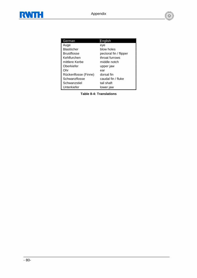
Appendix

- 80-

German English Auge eye Blaslöcher blow holes Brustflosse pectoral fin / flipper Kehlfurchen throat furrows mittlere Kerbe middle notch Oberkiefer upper jaw Ohr ear Rückenflosse (Finne) dorsal fin Schwanzflosse caudal fin / fluke Schwanzstiel tail shaft Unterkiefer lower jaw

Table 8-4: Translations

Appendix

- 81-

8.4 About the Author Individual Facts Home address: 28 Altenhellefelder Str, D-59846 Sundern, Germany Telephone: (+49) 177 347 10 52 Email: [email protected] Date of Birth: Mai 29th, 1981 Place of Birth: Arnsberg, Germany Nationality: German

Education 04/01 Enrolled at RWTH Aachen University of Technology, Germany

04/01 – 09/01 Preterm in Physics und Mathematics Since 09/01 Studies of Aeronautics and Aerospace Engineering Modules: Aerodynamics, Aircraft Design, Aeronautical Engines 04/06 – 08/06 Royal Melbourne Institute of Technology (RMIT), Australia Research Projects 04/06 – 08/06 Research Project: "Preliminary Design of a Multi-Mission Unmanned Aerial Vehicle", RMIT Melbourne, Australia 08/05 – 12/06 Research Project: „Num. simulation of a humpback whale’s fin“ Institute of Jet Propulsion and Turbomachinery, RWTH Aachen

Engineering Internships 02/05 – 07/05 Trainee Engineering F.A.L. Support, Airbus Toulouse , France Quality Assurance and Process Control 09/02 – 10/02 Trainee at Air Berlin , Airport Berlin-Tegel and Paderborn-Lippstadt Resource Scheduling and Maintenance

[Referee’s details are available on request]

student research project - walflosse carsten.pdf · student research project - 1- student research...

Documents