Grobner Bases

with DERIVE

Alessandro Perotti

Universita degli Studi di Trento

Trento, March 2004

Page: 1

Groebner6.dfw - a DfW Utility File for computing Gröbner Bases in DERIVE 6

(Version 1.2 for DERIVE 6.00, February 2004)Alessandro Perotti, Dept. of Mathematics, University of Trento, Italy

perotti@science.unitn.itwww.science.unitn.it/~perotti/groebner.htm

This DfW utility file contains a function that computes Gröbner bases of a set of polynomials with respect to a monomial ordering and other related functions. DERIVE 6 contains the new internal function GROEBNER_BASIS to construct the Gröbner basis for a collection of polynomials based on lexicographic ordering of the variables. We introduce new functionalities giving the possibility of choosing the monomial ordering. Besides allowing the explicit computation of Gröbner bases and normal forms, the new functions can be used, for example, to eliminate some variables between the equations and to perform the gaussian reduction of a system depending on parameters. We wish to thank V. Anisiu for his useful suggestions.

• • • • 1. Functions Groebner(f,v,ord) reduced Gröbner basis for a set of polynomials Eliminate(f,v1,v2) elimination of a set of variables in equations f=0 TotalDegree(f, v) total degree of a polynomial OrdMatrix(ord, n) matrices inducing relevant monomial orderings ElOrd(k, n) matrices inducing elimination orderings LeadingTerm(f, v, ord) leading term of a polynomial NF(f, ff, v, ord) normal form of a polynomial with respect to a

set of polynomials Buchberger(f, v, ord) (non reduced) Gröbner basis for a set of

polynomials System(e, v, k) gaussian reduction of a system depending on

parameters Eigensystem(a, ord, v, w) reduction of the eigensystem Ax=¿x RREF(a, k) row-reduction of a matrix depending on

parameters RREF(a, b, k) row-reduction of augmented matrix depending

on parameters LagrangeMultipliers(f,g,v) computation of min-max points using Lagrange

multipliers

• • • • 2. Description of the functions • 2.1 Computation of Gröbner Bases

Groebner([f1,...,fm], [x1,...,xn], ord)computes the reduced Gröbner basis for the set of polynomials generated by f1,...,fm with respect to the ordered variables x1,...,xn and to the monomial ordering described by ord.

Page: 2

The argument ord that defines the monomial ordering can be:- an integer between 1 and 4 (or the variables lex, grlex, grevlex, invlex), corresponding to lexicographic, graded lexicographic, graded reverse lexicographic, inverse lexicographic- a non-singular matrix with non-negative integral entries that induces the ordering (see [1] and 2.2 for more information).• • • • The default ordering is lexicographic with respect to the variables x1>x2>...>xn.• • • • If also the second argument is omitted, the ordering is lexicographic with respect to the variables appearing in f1,...,fm ordered by internal Derive ordering.

• Examples

#1: 2 2 2 2 2 2 2 3 3 Groebner(x + y + z + w , x + 2�y - y�z - w , x + z - w ,

[x, y, z, w], grevlex)

#2: 2 2 2 2 2 2 3 3y - y�z - z - 2�w , x + y�z + 2�z + 3�w , x + z - w

#3: 2 2 2 2 2 2 2 3 3 Groebner(x + y + z + w , x + 2�y - y�z - w , x + z - w , w

- 1)

#4: 12 9 8 6 5 4 3 2 w - 1, z - 4�z + 5�z + 12�z - 10�z + 5�z - 16�z + 18�z +

11 8 7 5 4 3 2 16, 4�y - z + 4�z - 5�z - 8�z + 10�z - 5�z + 8�z - 10�z,

3 x + z - 1

#5: 2 2 2 2 2 2 2 3 GROEBNER_BASIS(x + y + z + w , x + 2�y - y�z - w , x + z -

3 w , w - 1, [x, y, z, w])

#6: 12 9 8 6 5 4 3 2 w - 1, z - 4�z + 5�z + 12�z - 10�z + 5�z - 16�z + 18�z +

11 8 7 5 4 3 2 16, 4�y - z + 4�z - 5�z - 8�z + 10�z - 5�z + 8�z - 10�z,

3 x + z - 1

#7: 2 3 2 4 1 3 Groebnerx �y - x�y , x �y - x, [x, y], 3 0

Page: 3

#8: 3 x - x, x�(y - x)

Eliminate([f1,...,fm], [x1,...,xh], [y1,...,yk])constructs equations in which some variables have been eliminated. It eliminates the first set of variables x1,...,xh between the polynomial equations f1=0,...,fm=0 in the variables x1,...,xh,y1,...,yk.

• • • • If the third argument is omitted, the equations are considered with respect to all the variables appearing in f1,...,fm.

• • • • As it is shown in the examples of section 3, the function can be used in some cases also when the equations are not polynomial.

• Examples

#9: 2 2 2 2 2 2 2 3 3 Eliminate(x + y + z + w , x + 2�y - y�z - w , x + z - w , w

- 1, [x, w])

#10: 2 2 6 3 2 y - y�z - z - 2, y�z + z - 2�z + 2�z + 4

#11: 2 3 2 4 Eliminate(x �y - x�y , x �y - x, [x])

#12: []

• • • • 2.2 Other functions related to Gröbner Bases

TotalDegree(f, [x1,...,xn])computes the total degree of a multivariate polynomial f in the variables x1,...,xn.

#13: 5 7 5 TotalDegree(2�x �y - 3�x�y�z )

#14: 12

OrdMatrix(ord, n)gives an integer square matrix of order n that induces the rational monomial ordering ord, which can be lex or 1, grlex or 2, grevlex or 3, invlex or 4. See [1] for more details.

#15: MAP_LIST(OrdMatrix(ord, 3), ord, [1, ..., 4])

#16:

1 0 0 1 1 0 1 1 1 0 0 1 0 1 0 , 1 0 1 , 1 1 0 , 0 1 0 0 0 1 1 0 0 1 0 0 1 0 0

ElOrd(k, n)

Page: 4

gives an integer square matrix of order n that induces an elimination ordering with respect to which the first k variables always precede the others.

#17: ElOrd(2, 4)

#18:

1 0 0 1 1 0 0 0 0 1 1 0 0 1 0 0

LeadingTerm(f, [x1,...,xn], ord)computes the leading term of the polynomial f with respect to the ordering ord in the variables x1>x2>...>xn.

• The default ordering is lexicographic with respect to all the variables appearing in f.

#19: 2 3 2 2 2 5 MAP_LIST(LeadingTerm(2�x �y + 3�x �y �z - x�y , [x, y, z], ord),

ord, [lex, grlex, grevlex, invlex])

#20: 2 3 2 2 2 5 2 2 22�x �y , 3�x �y �z , - x�y , 3�x �y �z

NF(f, [f1,...,fk], [x1,...xn], ord)returns the remainder of the polynomial f on division by f1,...,fk with respect to the ordering ord. If [f1,...,fk] is a Gröbner basis, the remainder does not depend on the ordering of the polynomials and is called Normal Form of the polynomial f with respect to [f1,...,fk]. It is zero if and only if f is a polynomial combination of f1,...,fk.

• The default ordering is lexicographic with respect to all the variables appearing in f.

#21: 2 3 3 2 2 2 2 2 NF(3�x �y, x + z - w , x + y�z + 2�z + 3�w , y - y�z - z -

2 2�w , [x, y, z, w], grlex)

#22: 2 2 2 33�x - 9�y�(z + w ) - 6�w �z - 3�w

#23: 2 3 3 2 2 2 2 2 NF(3�x �y, x + z - w , x + y�z + 2�z + 3�w , y - y�z - z -

2 2�w )

#24: 6 3 3 6 y�(3�z - 6�w �z + 3�w )

Buchberger([f1,...,fm], [x1,...,xn], ord)

Page: 5

implements the Buchberger algorithm for the computation of a (non-reduced) Gröbner basis for the set of polynomials generated by f1,...,fm with respect to the ordered variables x1,...,xn and to the monomial ordering described by ord. The basis obtained always containes the generators f1,...,fm.

• • • • The function Groebner(f,v,ord) uses an improved version of Buchberger algorithm for the computation of the reduced basis.

• The default ordering is lexicographic with respect to all the variables appearing in f.

#25: 2 2 2 2 2 2 2 3 3 Buchberger(x + y + z + w , x + 2�y - y�z - w , x + z - w ,

[x, y, z, w], grevlex)

#26: 2 2 2 2 2 2 2 3 3 2 x + y + z + w , x + 2�y - y�z - w , x + z - w , - y + y�z

2 2+ z + 2�w

#27: 2 2 2 2 2 2 2 3 3 Buchberger(x + y + z + w , x + 2�y - y�z - w , x + z - w )

#28: 2 2 2 2 2 2 2 3 3 2 x + y + z + w , x + 2�y - y�z - w , x + z - w , - y + y�z

2 2 6 3 3 2 6 2 2 4 + z + 2�w , y�z + z - 2�w �z + 2�z + w + 3�w , - w �y�(w +

11 3 8 7 5 6 2 3 4 3 3) + z - 4�w �z + 5�z + z �(5�w + 3�w ) - 10�w �z + 5�z -

5 2 4 6 2 17 3 14 13 2�w �z �(w + 3) + z�(3�w + 7�w ), z - 6�w �z + 5�z +

11 6 2 3 10 9 5 8 4 z �(14�w + 6�w ) - 20�w �z + 5�z - 8�w �z �(2�w + 3) +

7 6 2 3 6 5 12 8 4 z �(25�w + 13�w ) - 10�w �z + z �(9�w + 30�w + 9�w ) -

5 4 4 7 2 8 4 14 3 11 2�w �z �(5�w + 13) - 2�w �z �(w + 6�w + 9), - z + 4�w �z

10 2 8 4 3 7 6 5 9 5 - 5�z - 6�w �z �(w + 1) + 10�w �z - 5�z + z �(4�w + 12�w )

2 4 4 4 2 8 4 3 13 12 - w �z �(5�w + 13) - w �z �(w + 6�w + 9), 2�w �z - 2�z -

6 10 3 9 8 7 9 5 2 6 4 8�w �z + 18�w �z - 10�z + z �(12�w + 12�w ) - 4�w �z �(8�w

3 5 4 12 8 3 9 5 + 3) + 30�w �z - 2�z �(4�w + 12�w + 5) + z �(18�w + 50�w )

Page: 6

2 2 4 15 11 7 12 - 2�w �z �(5�w + 13) + z�(2�w + 12�w + 18�w ) - 2�w -

8 4 12 3 9 8 6 6 2 12�w - 18�w , z - 4�w �z + 5�z + z �(6�w + 6�w ) -

3 5 4 5 3 4 2 6 2 12 10�w �z + 5�z - 4�w �z �(w + 3) + z �(5�w + 13�w ) + w +

8 46�w + 9�w

• 2.3 Elementary applications to linear systems and m atrices

System([e1,...,em], [x1,...,xn], [k1,...,ks]) performs the gaussian reduction of the system of linear equations e1=0,...,em=0 in the variables x1,...,xn depending polynomially on parameters k1,...,ks. If the vector of parameters is omitted, then in the resulting equations may appear rational functions of the parameters and they may be not equivalent to the given equations for some values of the parameters.

#29: 2 System(x + y + z - 1, k �x + 4�y + 9�z + 11, k�x + 2�y + 3�z +

1, [x, y, z], [k])

#30: [(k - 3)�(z + 3), (k - 2)�(y - 4), y�(z + 3) - 4�z - 12, x + y + z

- 1]

From the reduced system we get that if k=3 the system has infinite solutions x = -3-t, y = 4, z = t (t any real), if k=2 the system has infinite solutions x = 4-t, y = t, z = -3 (t any real), else it has a unique solution x = 0, y = 4, z = -3.

#31: 2 System(x + y + z - 1, k �x + 4�y + 9�z + 11, k�x + 2�y + 3�z +

1, [x, y, z])

#32: 2 3�k�(3 - k)�(z + 3), (k - 4)�(y - 4), k�x

Eigensystem(a, ord, [x1,...,xn], w)performs the gaussian reduction of the eigenvalues system Ax=¿x associated to a square matrix a. The default ordering is lex, with default linear variables x1,...,xn and eigenvalue variable w.

Page: 7

#33:

2 1 0 Eigensystem 1 3 4 0 0 2

#34: 2 x3�(w - 2), x2�(w - 5�w + 5), x2�x3, - w�x2 + x1 + 3�x2 + 4�x3

#35:

2 1 0 Eigensystem 1 3 4 , grlex, [x, y, z], t 0 0 2

#36: 2 z�(t - 2), -x + y�(t - 3) - 4�z, y�z, x�(t - 2) - y, x�z + 4�z ,

2 2 2x + x�y - y - 16�z

RREF(a, [k1,...,ks])tries to compute a Row Reduced Echelon Form of a matrix a depending on parameters k1,...,ks. RREF(a, b, [k1,...,ks])computes the Row Reduced Echelon Form of the augmented matrix [a,b] depending on parameters k1,...,ks. The second argument b can be a vector or a matrix. Any null row is deleted.If the parameters are omitted, then the internal function ROW_REDUCE is called for a more efficient computation. In this case, the reduced matrix may contain rational functions of the parameters and the reduction may be not valid for some values of the parameters.

#37:

2 3 4�h RREF 3 2�h 1 , [h] 0 2 1

#38:

28 0 5 0 2 1 0 0 28�h - 13

The RREF shows that the matrix has rank 2 for h=13/28, rank 3 otherwise.

#39:

2 3 4�h RREF 3 2�h 1 , [2, 1, 1], [h] 0 2 1

Page: 8

#40:

28 0 5 9 - 8�h 0 2 1 1 0 0 28�h - 13 4�h - 1

#41:

2 3 4�h RREF 3 2�h 1 0 2 1

#42:

1 0 0 0 1 0 0 0 1

• 2.4 Another application: the Lagrange multipliers

LagrangeMultipliers(f,[g1,...,gk],[x1,...,xn])applies the method of Lagrange multipliers for the computation of critical points of a polynomial function f(x1,...xn) subject to k polynomial constraints g1=0,...,gk=0. It returns a system of equations reduced with respect to lexicographic ordering, whose solutions are the coordinates of the critical points.

#43: 2 2 2 LagrangeMultipliers(z - x�y�z + x, x + y - 1, y�z - 2)

#44: 8 6 5 2 2 2 z - 4�z - 4, 2�y - z �(z - 4), 2�x - z �(z - 4)

#45: 2 LagrangeMultipliers(z - x�y�z + x, [y�z - 2])

#46: [1]

If the constant polynomial 1 is returned, the function has no critical points subject to the constraints.

• 3 Other examples

In the univariate case, the Gröbner basis contains only the GCD of the polynomials.

#47: 9 8 7 6 5 4 3 2 Groebner(x - 3�x + x - 3�x - 3�x + 6�x + 17�x - 22�x -

7 6 5 4 3 2 11�x + 15, 3�x - 9�x + 5�x - 15�x - 4�x + 3�x + 48�x - 63)

#48: [x - 3]

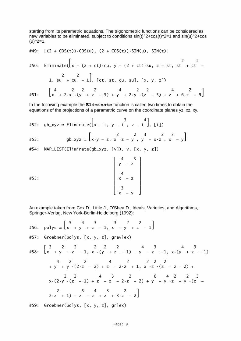
The function Eliminate can be applied to find the fourth degree equation of a torus

Page: 9

starting from its parametric equations. The trigonometric functions can be considered as new variables to be eliminated, subject to conditions sin(t)^2+cos(t)^2=1 and sin(u)^2+cos(u)^2=1.

#49: [(2 + COS(t))�COS(u), (2 + COS(t))�SIN(u), SIN(t)]

#50: 2 2 Eliminate(x - (2 + ct)�cu, y - (2 + ct)�su, z - st, st + ct -

2 2 1, su + cu - 1, [ct, st, cu, su], [x, y, z])

#51: 4 2 2 2 4 2 2 4 2 x + 2�x �(y + z - 5) + y + 2�y �(z - 5) + z + 6�z + 9

In the following example the Eliminate function is called two times to obtain the equations of the projections of a parametric curve on the coordinate planes yz, xz, xy.

#52: 3 4 gb_xyz ≔ Eliminate(x - t, y - t , z - t , [t])

#53: 2 2 3 2 3 gb_xyz ≔ x�y - z, x �z - y , y - x�z , x - y

#54: MAP_LIST(Eliminate(gb_xyz, [v]), v, [x, y, z])

#55:

4 3 y - z 4 x - z 3 x - y

An example taken from Cox,D., Little,J., O’Shea,D., Ideals, Varieties, and Algorithms, Springer-Verlag, New York-Berlin-Heidelberg (1992):

#56: 5 4 3 3 2 2 polys ≔ x + y + z - 1, x + y + z - 1

#57: Groebner(polys, [x, y, z], grevlex)

#58: 3 2 2 2 2 2 4 3 4 3 x + y + z - 1, x �(y + z - 1) - y - z + 1, x�(y + z - 1)

4 2 2 4 2 2 2 2 + y + y �(2�z - 2) + z - 2�z + 1, x �z �(z + z - 2) +

2 2 4 3 2 6 4 2 2 3 x�(2�y �(z - 1) + z - z - 2�z + 2) + y - y �z + y �(z -

2 5 4 3 2 2�z + 1) - z - z + z + 3�z - 2

#59: Groebner(polys, [x, y, z], grlex)

Page: 10

#60: 3 2 2 2 2 2 4 3 4 3 x + y + z - 1, x �(y + z - 1) - y - z + 1, x�(y + z - 1)

4 2 2 4 2 2 2 2 + y + y �(2�z - 2) + z - 2�z + 1, x �z �(z + z - 2) +

2 2 4 3 2 6 4 2 2 3 x�(2�y �(z - 1) + z - z - 2�z + 2) + y - y �z + y �(z -

2 5 4 3 2 2 4 3 2 2�z + 1) - z - z + z + 3�z - 2, x�(y �(3�z - z - 6�z +

6 5 4 3 2 8 6 4 3 4) + z - 3�z - 3�z + 3�z + 6�z - 4) + y - y + y �(2�z -

2 2 4 2 6 4 3 2 5�z + 3) - 7�y �(z - 2�z + 1) - 2�z + 9�z - 2�z - 9�z + 4

An assignment to a variable is a convenient way for using a lengthy result in other computations:

#61: PROG(gb ≔ Groebner(polys, [x, y, z], lex),

MAP_LIST(LeadingTerm(f), f, gb))

#62: 12 11 2 4 2 4 2 2 3y , x�z , 24�x�y �z, x�y , 12�x �z , x �y , x

This means that the lex Gröbner basis contains 7 polynomials...

#63: MAP_LIST(DIM(TERMS(EXPAND(f))), f, gb)

#64: [25, 49, 53, 9, 49, 6, 4]

...and that these polynomials contain up to 53 terms...

#65: MAP_LIST(TotalDegree(f), f, gb)

#66: [12, 13, 12, 5, 12, 4, 3]

...and their maximum total degree is 13.

#67: 10 3 3 NF(x �y �z , gb)

#68: 11 3 7 6 3 3 9 6 3 y �z + y �(2�z - 2�z ) + y �(z - 2�z + z )

#69:

2 3 4�h 2 1 RREF 3 2�h 1 , 1 1 , [h] 0 2 1 1 1

Page: 11

#70:

28 0 5 9 - 8�h 7 - 8�h 0 2 1 1 1 0 0 28�h - 13 4�h - 1 4�h - 7

#71: 2 2 2 LagrangeMultipliers(z - x�y�z + x, x + y - 1)

#72: 6 4 2 4 2 z�(256�z - 32�z + 17�z + 3), y + z�(32�z - 2�z + 1), z�(2�x

4 2 2 4 2 + 16�z - 9�z + 1), x - 16�z + z - 1

• References

[1] A. Perotti, Gröbner Bases with DERIVE , International DERIVE Journal, Vol.3,n.2, 83-98 (1996)

Appendix: Grobner Bases

1. NOTATION AND DEFINITIONS

Let k be the coefficient field and k[x1, . . . , xn] the polynomial ring in n indeterminates x1, . . . , xn.Every polynomial f is a sum

∑α∈A aαxα of terms aαxα (aα 6= 0), where A is a finite subset of

n-tuples of nonnegative integers α1, . . . , αn. A term is a product of a nonzero coefficient aα and amonomial xα = xα1

1 · · ·xαnn . The sum |α| = α1 + . . . + αn of the exponents in a monomial is called

the total degree of the monomial.Once the order of the variables has been fixed, every monomial is uniquely determined by the

n-tuple α1, . . . , αn of its exponents in Zn≥0. A monomial ordering is a total ordering on Zn

≥0 (orequivalently, on the set of monomials) which is a well-ordering, compatible with the sum of theexponents in Zn

≥0: if α > β, then α + γ > β + γ for any γ ∈ Zn≥0.

Examples: the lexicographic order lex , defined by xα >lex xβ if the first non-zero component ofthe vector α − β is positive, is a monomial ordering. Another example is the graded (or total)lexicographic order grlex , defined by xα >grlex xβ if |α| > |β| , or |α| = |β| and α >lex β.

Let f =∑

α∈A aαxα be a non-zero polynomial and let > be a fixed monomial ordering. The mul-tidegree of f is the n-tuple MDEG(f) = max{α ∈ Zn

≥0 such that aα 6= 0}. The leading coefficientof f is LC(f) = aMDEG(f), the leading monomial is LM(f) = xMDEG(f) and the leading term isLT(f) = LC(f) LM(f).

Examples: with respect to the lex order with x > y, the polynomial 2x2y3 + 5xy5 − 3xy − 2y + 4has multidegree (2, 3) and leading term 2x2y3; with respect to the grlex order, the multidegree is(1, 5) and the leading term is 5xy5.

2. THE DIVISION ALGORITHM

The choice of a monomial ordering makes it possible to extend the well-known division algorithm forunivariate polynomials. Let F = (f1, . . . , fs) be an ordered s-tuple of polynomials in k[x1, . . . , xn].Every polynomial f can be written as

f = q1f1 + q2f2 + · · ·+ qsfs + r

where MDEG(f) > MDEG(qifi) for any i such that qifi 6= 0 and the remainder r is a sum ofterms, none of which is divisible by a LT(fi).

Remark: the quotients q1, . . . , qs and the remainder r depend on the choice of the monomialordering and, in general, also on the ordering of the divisors f1, . . . , fs.

The following algorithm gives q1, . . . , qs and the remainder r:

q1 := 0; . . . ; qs := 0; r := 0p := fWHILE p 6= 0 DO

IF there exists a first index i such that LT(fi) divides LT(p) THENqi := qi + LT(p)

LT(fi)

p := p− LT(p)LT(fi)

fi

ELSEr := r + LT(p)p := p− LT(p)

1

3. GROBNER BASES AND BUCHBERGER’S ALGORITHM

Let I be an ideal of polynomials. The subset {g1, . . . , gs} of I is a Grobner basis of I with respectto a fixed monomial ordering if the monomials LT(g1), . . . , LT(gs) generate the initial ideal 〈LT(I)〉generated by all the leading terms of elements in I. The set G = {g1, . . . , gs} is a reduced Grobnerbasis for I if it is a Grobner basis such that every element has leading coefficient 1 and for everygi ∈ G, no monomial of gi is generated by the leading terms of the other elements of G. Thiscondition guarantees the uniqueness of the reduced Grobner basis of an ideal.

If G = {g1, . . . , gs} is a Grobner basis of an ideal I, then the ambiguity in the definition of aremainder of f on division by g1, . . . , gs disappears. In this case, the remainder r is also called thenormal form of f with respect to G, and denoted by NF(f, G). Otherwise, it is called the normalform of f with respect to the ordered set (g1, . . . , gs).

The division algorithm gives the following useful characterization of Grobner bases. In partic-ular, it provides a membership criterion for the ideal.Proposition 1: the subset {g1, . . . , gs} of I is a Grobner basis of I if and only if for every f ∈ Ithe normal form of f with respect to g1, . . . , gs is zero.

Buchberger’s algorithm is based on a stronger version of the last result. We recall the definitionof the S-polynomial of f and g:

S(f, g) =xγ

LT(f)f − xγ

LT(g)g

where the monomial xγ is the least common multiple of LM(f) and LM(g).Proposition 2: the subset G = {g1, . . . , gs} of I is a Grobner basis of I if and only if for everypair (i, j), i 6= j, the normal form of S(gi, gj) with respect to G is zero.

Buchberger’s algorithm

Let F = (f1, . . . , fs) be a set of generators of the ideal I. A Grobner basis G = (g1, . . . , gt) of I isobtained by the following algorithm:B := {(i, j)|1 ≤ i < j ≤ s}G := Ft := sWHILE B 6= ∅ DO

select (i, j) ∈ Bg := NF(S(gi, gj), G)IF g 6= 0 THEN

t := t + 1G := G ∪ {g}B := B ∪ {(i, t)|1 ≤ i ≤ t− 1}

B := B − {(i, j)}This algorithm can be made more efficient by giving conditions to know in advance if the

normal form of S(gi, gj) does not need to be included in the new generating set. We refer thereader to section 2.9 of Cox et al, 1992 for a complete treatment.

4. ORDERINGS ON Zn

Definition 1: we call an ordering on Zn any total ordering compatible with addition in Zn.Every monomial ordering > extends to a unique ordering on Zn. To see this, given α, β ∈ Zn,

let γ(α, β) be the smallest element (with respect to the well-ordering >) of the non-empty set

2

{γ′ ∈ Zn≥0|α− β + γ′ ∈ Zn

≥0}. Then we say α > β if and only if α− β + γ(α, β) > γ(α, β) in Zn≥0.

Since γ(α + δ, β + δ) = γ(α, β) for every α, β, δ ∈ Zn, this induced ordering is compatible with theaddition in Zn.

Definition 2: a matrix A in GL(n,Z) induces an ordering >A on Zn by defining

α >A β if and only if αA >lex βA

Examples: the lex order is induced by the identity matrix In; the grlex order, the graded inverselex order (grevlex ) and the inverse lex order (invlex ) (see Cox et al, 1992 section 2.2) are inducedby the matrices

Agrlex =

1 1 0 · · · 01 0 1 · · · 0...

......

. . ....

1 0 0 · · · 11 0 0 · · · 0

Agrevlex =

1 1 · · · 11 · · · 1 0...

...1 0 · · · 0

Ainvlex =

0 · · · 0 10 · · · 1 0...

......

1 0 · · · 0

In the following, we shall show that a large class of monomial orderings can be obtained in such away.

Robbiano (1985 and 1986) has proved that every total ordering on Zn is induced (in the sensegiven above) by a real nonsingular matrix. In fact, every such ordering extends to a (not necessarilyunique) continuous ordering on Rn (with the euclidean topology). Then it is shown possible to findan orthogonal basis of Rn whose elements are positive with respect to the ordering. The matrixwhose columns are the vectors of the basis in decreasing order induces the ordering on Rn.

The following result, whose easy proof we omit, gives the relation existing between matriceswhich induce the same ordering.

Proposition 3: two matrices A,B ∈ GL(n,R) induce the same ordering on Rn if and only if theydefine the same right lateral modulo the (non-normal) subgroup T+ of upper triangular matriceswith positive diagonal. In particular, A,B ∈ GL(n,Z) induce the same ordering on Zn if and onlyif B = AU , where U is an upper triangular, integer matrix with only 1 on the diagonal.

Definition 3: an ordering > on Zn will be called rational if there exists a nonsingular rationalmatrix which induces >.

Examples: all the orderings shown above are rational; the following is an example of a non-rationalordering on Z2: α > β if and only if

√2α1 + α2 >

√2β1 + β2.

Other rational orderings are product orders constructed from two (or more) rational orders (seesection 2.4 of Cox et al, 1992): in this case an inducing matrix is the direct sum of the matricesof the given orderings. Another class of rational orderings on Zn is given by the eliminationorders >k (Bayer and Stillman, 1987): α >k β if and only if α1 + · · · + αk > β1 + · · · + βk, orα1 + · · ·+ αk = β1 + · · ·+ βk and α >grevlex β. A matrix corresponding to >k is the following

A>k=

1... O Ak − 1

11 0 · · · 0 0 · · · 00... An− k O0

3

where Ai denote the square matrix of order i associated to grevlex .

Proposition 4: every rational ordering > is induced by a matrix A ∈ GL(n,Z).

Proof: let B be a rational matrix inducing >. By means of elementary column operations, thetranspose matrix BT can be transformed into its Hermite form H, which is a non-negative, lowertriangular matrix. Then H = BT K, where K ∈ GL(n,Z). Set U = HT and A = (KT )−1 and getAU = B.

Now we return to monomial orderings. They are characterized by the following condition (seeCorollary 2.4.6 in Cox et al, 1992):

Proposition 5: an ordering on Zn restricts to a monomial ordering if and only if every non-zerovector in Zn

≥0 is positive with respect to the ordering.

Proposition 6: every rational monomial ordering > is induced by a non-negative matrix inGL(n,Z).

Proof: let A ∈ GL(n,Z) a matrix which induces >. For every element ej of the standard basis ofZn, we get from Proposition 5 that ejA >lex 0. This means that the rows of A are positive withrespect to the lex order. By adding to every column an integral linear combination of the precedingcolumns, A can be transformed into a non-negative matrix.

This result gives an easy method to compute the leading term with respect to any rationalmonomial ordering. Let f ∈ k[x1, . . . , xn] be a polynomial and A = (aij) ∈ GL(n,Z) a non-negativematrix corresponding to the ordering >. Consider the following change of variables

xi =n∏

j=1

yaij

j

Then the leading term of f(x1, . . . , xn) with respect to > is the monomial obtained by applying theinverse transformation (in general, a rational transformation) to the leading term of f(y1, . . . , yn) ∈k[y1, . . . , yn] with respect to the lex order.

Remark: in order to construct Grobner bases, it is sufficient to consider rational monomial order-ings, since any real matrix can be approximated by a rational one.

5. THE REDUCED GROBNER BASIS

Given a Grobner basis F = {f1, . . . , fs}, a reduced Grobner basis G can be obtained by thefollowing algorithm:

G := FFOR all g ∈ G DO

IF there exists h ∈ G, h 6= g, such that LT(h) divides LT(g) THENG := G− {g}

ELSEg := NF(g, G− {g})

FOR all g ∈ G DOg := g

LC(g)

REFERENCES

Bayer, D. and Stillman, M. (1987). A theorem on refining division orders by the reverse lexicographicorder. Duke J.Math., 55, 321–328

4

Becker, T. and Weispfenning, V. (1993). Grobner bases, Springer-Verlag, New York-Berlin-Heidel-bergCarra Ferro, G. and Sit, W. (1994). On Term-Orderings and Rankings. In Fischer, K., Loustaunau,P., Shapiro, K., Green, E., Farkas, D. (eds.). Computational algebra, Lecture Notes in Pure andApplied Mathematics Vol.151, 31–77.Cox, D., Little, J., O’Shea, D. (1992). Ideals, Varieties, and Algorithms, Springer-Verlag, NewYork-Berlin-HeidelbergPerotti, A., (1996) Grobner Bases with DERIVE, International DERIVE Journal, Vol.3,n.2, 83–98Robbiano, L. (1985). Term orderings on the polynomial ring. Proceedings EUROCAL 1985, LNCS204, 513–517Robbiano, L. (1986). On the theory of graded structures. J.Symb.Comp., 2, 139–170

5