Structure Learning of Probabilistic Graphical

Models: A Comprehensive Survey

Yang Zhou

Michigan State University

Nov 2007

Contents

1 Graphical Models 3

1.1 Introduction . . . . . . . . . . . . . . . . . . . . . . . . . . . . . . 31.2 Preliminaries . . . . . . . . . . . . . . . . . . . . . . . . . . . . . 31.3 Undirected Graphical Models . . . . . . . . . . . . . . . . . . . . 5

1.3.1 Markov Random Field . . . . . . . . . . . . . . . . . . . . 51.3.2 Gaussian Graphical Model . . . . . . . . . . . . . . . . . . 6

1.4 Directed Graphical Models . . . . . . . . . . . . . . . . . . . . . 61.4.1 Conditional Probability Distribution . . . . . . . . . . . . 7

1.5 Other Graphical Models . . . . . . . . . . . . . . . . . . . . . . . 91.6 Network Topology . . . . . . . . . . . . . . . . . . . . . . . . . . 101.7 Structure Learning of Graphical Models . . . . . . . . . . . . . . 11

2 Constraint-based Algorithms 12

2.1 The SGS Algorithm . . . . . . . . . . . . . . . . . . . . . . . . . 122.2 The PC Algorithm . . . . . . . . . . . . . . . . . . . . . . . . . . 132.3 The GS Algorithm . . . . . . . . . . . . . . . . . . . . . . . . . . 14

3 Score-based Algorithms 16

3.1 Score Metrics . . . . . . . . . . . . . . . . . . . . . . . . . . . . . 173.1.1 The MDL Score . . . . . . . . . . . . . . . . . . . . . . . 173.1.2 The BDe Score . . . . . . . . . . . . . . . . . . . . . . . . 183.1.3 Bayesian Information Criterion (BIC) . . . . . . . . . . . 19

3.2 Search for the Optimal Structure . . . . . . . . . . . . . . . . . . 213.2.1 Search over Structure Space . . . . . . . . . . . . . . . . . 213.2.2 Search over Ordering Space . . . . . . . . . . . . . . . . . 25

4 Regression-based Algorithms 27

4.1 Regression Model . . . . . . . . . . . . . . . . . . . . . . . . . . . 274.2 Structure Learning through Regression . . . . . . . . . . . . . . . 30

4.2.1 Likelihood Objective . . . . . . . . . . . . . . . . . . . . . 304.2.2 Dependency Objective . . . . . . . . . . . . . . . . . . . . 314.2.3 System-identification Objective . . . . . . . . . . . . . . . 334.2.4 Precision Matrix Objective . . . . . . . . . . . . . . . . . 344.2.5 MDL Objective . . . . . . . . . . . . . . . . . . . . . . . . 35

1

5 Hybrid Algorithms and Others 36

5.1 Hybrid Algorithms . . . . . . . . . . . . . . . . . . . . . . . . . . 365.2 Other Algorithms . . . . . . . . . . . . . . . . . . . . . . . . . . . 37

5.2.1 Clustering Approaches . . . . . . . . . . . . . . . . . . . . 375.2.2 Boolean Models . . . . . . . . . . . . . . . . . . . . . . . . 375.2.3 Information Theoretic Based Approach . . . . . . . . . . 375.2.4 Matrix Factorization Based Approach . . . . . . . . . . . 37

2

Chapter 1

Graphical Models

1.1 Introduction

Probabilistic graphical models combine the graph theory and probability theoryto give a multivariate statistical modeling. They provide a unified descriptionof uncertainty using probability and complexity using the graphical model. Es-pecially, graphical models provide the following several useful properties:

• Graphical models provide a simple and intuitive interpretation of thestructures of probabilistic models. On the other hand, they can be usedto design and motivate new models.

• Graphical models provide additional insights into the properties of themodel, including the conditional independence properties.

• Complex computations which are required to perform inference and learn-ing in sophisticated models can be expressed in terms of graphical manip-ulations, in which the underlying mathematical expressions are carriedalong implicitly.

The graphical models have been applied to a large number of fields, includ-ing bioinformatics, social science, control theory, image processing, marketinganalysis, among others. However, structure learning for graphical models re-mains an open challenge, since one must cope with a combinatorial search overthe space of all possible structures.

In this paper, we present a comprehensive survey of the existing structurelearning algorithms.

1.2 Preliminaries

We will first define a set of notations which will be used throughout this paper.We represent a graph as G = 〈V,E〉 where V = vi is the set of nodes in thegraph and each node corresponds to a random variable xi ∈ X . E = (vi, vj) :

3

i 6= j is the set of edges. In a directed graph, if there is an edge Ei,j from vi tovj , then vi is a parent of node vj and vj is a child of node vi. If there is no cyclein a directed graph, we call it a Directed Acyclic Graph (DAG). The number ofnodes and number of edges in a graph are denoted by |V | and |E| respectively.π(i) is used to represent all the parents of node vi in a graph. U = x1, · · · , xndenotes the finite set of discrete random variables where each variable xi maytake on values from a finite domain. V al(xi) denotes the set of values thatvariable xi may attain, and |xi| = |V al(xi)| denotes the cardinality of this set.In probabilistic graphical network, the Markov blanket ∂vi [Pearl, 1988] of anode vi is defined to be the set of nodes in which each has an edge to vi, i.e., allvj such that (vi, vj) ∈ E. The Markov assumption states that in a probabilisticgraphical network, every set of nodes in the network is conditionally independentof vi when conditioned on its Markov blanket ∂vi. Formally, for distinct nodesvi and vk,

P (vi|∂vi ∩ vk) = P (vi|∂vi)

The Markov blanket of a node gives a localized probabilistic interpretation ofthe node since it identifies all the variables that shield off the node from therest of the network, which means that the Markov blanket of a node is theonly information necessary to predict the behavior of that node. A DAG G isan I-Map of a distribution P if all the Markov assumptions implied by G aresatisfied by P .

Theorem 1.2.1. (Factorization Theorem) If G is an I-Map of P , then

P (x1, · · · , xn) =∏

i

P (xi|xπ(i))

According to this theorem, we can represent P in a compact way when Gis sparse such that the number of parameter needed is linear in the number ofvariables. This theorem is true in the reverse direction.

The set X is d-separated from set Y given set Z if all paths from a node inX to a node in Y are blocked given Z.

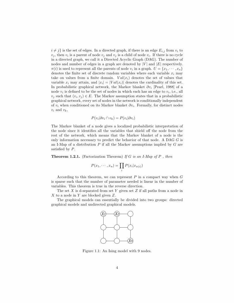
The graphical models can essentially be divided into two groups: directedgraphical models and undirected graphical models.

X2

X9

X1

Figure 1.1: An Ising model with 9 nodes.

4

1.3 Undirected Graphical Models

1.3.1 Markov Random Field

A Markov Random Field (MRF) is defined as a pair M = 〈G,Φ〉. Here G =〈V,E〉 represents an undirected graph, where V = Vi is the set of nodes,each of which corresponds to a random variable in X ; E = (Vi, Vj) : i 6= jrepresents the set of undirected edges. The existence of an edge u, v indicatesthe dependency of the random variable u and v. Φ is a set of potential functions(also called factors or clique potentials) associated with the maximal cliques inthe graph G. Each potential function φc(·) has the domain of some clique cin G, and is a mapping from possible joint assignments (to the elements of c)to non-negative real values. A maximal clique of a graph is a fully connectedsub-graph that can not be further extended. We use C to represent the setof maximal cliques in the graph. φc is the potential function for a maximalclique c ∈ C. The joint probability of a configuration x of the variables V canbe calculated as the normalized product of the potential function over all themaximal cliques in G:

P (x) =

∏

c∈C φc(xc)∑

x′

c

∏

c∈C φc(xc)

where xc represents the current configuration of variables in the maximal cliquec, x′

c represents any possible configuration of variable in the maximal clique c.In practice, a Markov network is often conveniently expressed as a log-linearmodel, given by

P (x) =exp

(∑

c∈C wcφc(xc))

∑

x∈X exp(∑

c∈C wcφc(xc))

In the above equation, φc are feature functions from some subset of X to realvalues, wc are weights which are to be determined from training samples. A log-linear model can provide more compact representations for any distributions,especially when the variables have large domains. This representation is alsoconvenient in analysis because its negative log likelihood is convex. However,evaluating the likelihood or gradient of the likelihood of a model requires in-ference in the model, which is generally computationally intractable due to thedifficulty in calculating the partitioning function.

The Ising model is a special case of Markov Random Field. It comes fromstatistical physics, where each node represents the spin of a particle. In anIsing model, the graph is a grid, so each edge is a clique. Each node in theIsing model takes binary values 0, 1. The parameters are θi representing theexternal field on particle i, and θij representing the attraction between particles

5

i and j. θij = 0 if i and j are not adjacent. The probability distribution is:

p(x|θ) = exp

∑

i<j

θijxixj +∑

i

θixi = −A(θ)

=1

Z(θ)exp

∑

i<j

θijxixj +∑

i

θixi

where Z(θ) is the partition function.

1.3.2 Gaussian Graphical Model

A Gaussian Graphical Model (GGM) models the Gaussian property of multi-variate in an undirected graphical topology. Assuming that there are n variablesand all variables are normalized so that each of them follows a standard Gaus-sian distribution. We use X = (x1, · · · ,xn) to represent the n × 1 columnmatrix. In a GGM, the variables X are assumed to follow a multivariate Gaus-sian distribution with covariance matrix Σ,

P (X) =1

(2π)n2 |Σ| 12

exp

(

−1

2X⊤Σ−1X

)

In a Gaussian Graphical Model, the existence of an edge between two nodesindicates that these two nodes are not conditionally independent given othernodes. Matrix Ω = Σ−1 is called the precision matrix. The non-zeros elementsin the precision matrix correspond to the edges in the Gaussian GraphicalModel.

1.4 Directed Graphical Models

The most commonly used directed probabilistic graphical model is BayesianNetwork [Pearl, 1988], which is a compact graphical representation of jointdistributions. A Bayesian Network exploits the underlying conditional inde-pendencies in the domain, and compactly represent a joint distribution overvariables by taking advantages of the local conditional independence structures.A Bayesian network B = 〈G,P 〉 is made of two components: a directed acyclicgraph (DAG) G whose nodes correspond to the random variables, and a setof conditional probabilistic distributions (CPD), P (xi|xπ(i)), which describe thestatistical relationship between each node i and its parents π(i). In a CPD, forany specific configuration of xπ(i), the sum over all possible values of xi is 1,

∑

xi∈V al(xi)

P (xi|xπ(i)) = 1.

In the continuous case,∫

xi∈V al(xi)

P (xi|xπ(i))dxi = 1

6

where P (xi|xπ(i)) is the conditional density function. The conditional in-dependence assumptions together with the CPDs uniquely determine a jointprobability distribution via the chain rule:

P (x1, · · · , xn) =n∏

i=1

P (xi|xπ(i))

Figure 1.2: A Bayesian network for detecting credit-card fraud. Arcs indicatethe causal relationship. The local conditional probability distributions associ-ated with a node are shown next to the node. The asterisk indicates any valuefor that variable. Figure excerpted from [Heckerman et al., 1995].

1.4.1 Conditional Probability Distribution

The CPDs may be represented in different ways. The choice of the represen-tation is critical because it specifies the intrinsic nature of the conditional de-pendencies as well as the number of parameters needed for this representation.Here we describe some different types of CPDs.

Table CPDs

In the discrete case, the CPDs can be simply represented as a table in whicheach row corresponds to a specific configuration of a node and its parents, as wellas the corresponding conditional probability of this configuration [Heckermanet al., 1995]. The table CPDs are advantageous in that they are simple andclear, but the size of the table CPDs will grow exponentially with the increasein the number of parents and the number of values that each node can take.

7

Tree CPDs

The tree CPDs try to exploit the context specific information (CSI), i.e., thedistribution over the values of a node does not depend on the value of somesubset of its parents given the value of the other parents [Boutilier et al., 1996].In a tree CPD, each interior vertex represents the splits on the value of someparent vertices, and each leaf represents a probability conditioned on a specificconfiguration along the path originated from the root. The tree CPDs usuallyrequire a substantially smaller number of parameters than table CPDs whenCSI holds in many places of the Bayesian network.

Softmax CPDs

The softmax CPDs approximates the dependency of a discrete variable xi on itsparents xπ(i) by a linear threshold function Segal [2004]. In this case, the valueof each node is determined based on the sum of the contributions of the valuesof all its parents, i.e., the effect of π(i) on node i taking on a value xi can besummarized via a linear function:

fxi(xπ(i) =

|π(i)|∑

j=1

wxi,jxπ(i)(j)

In the above equation, each weight wxi,j represents the contribution of thejth parent to the value of the target node i. Given the contribution function f,acommon choice of how the probability of xi depends on fxi

(xπ(i)) is the softmaxdistribution, which is the standard extension of the binary logistic conditionaldistribution to the multi-class case:

P (xi|xπ(i)) =exp(fxi

(xπ(i)))∑

xi∈V al(xi)exp(fxi

(xπ(i)))

Gaussian CPDs

In many cases the random variables are continuous with associated densityfunctions. A common choice of the density function is Gaussian distribution orNormal distribution t ∼ N(µ, σ2):

P (xi = t) = N(µ, σ2) =1√2πσ

exp

(

(t− µ)22σ2

)

The Gaussian CPDs are often incorporated in the table or tree CPDs, inwhich the parameters mu and σ of the Gaussian distribution are determined bythe configuration of node is parents.

8

Sigmoid CPDs

The Sigmoid Belief Networks (SBN) [Neal, 1992, Titov and Henderson, 2007]has the CPD in the form:

P (xi = 1|xπ(i)) = σ(∑

j∈π(i)

Jijxj)

where σ(·) denotes the logistic sigmoid function, and Jij is the weight from j toi.

Probability Formulas CPDs

In a Relational Bayesian Network (RBN) [Jaeger, 1997, 2001], all variables takebinary values. Each root node i has probability θi ∈ [0, 1] to be 1. For eachnon-root node, the probability to taking value 1 is a combination function of thevalues of all its parents. A commonly used combination function is the noisy-orfunction which is defined as noisy-or(I) = 1− πp∈I(1− p) where I is a multisetof probabilities.

1.5 Other Graphical Models

• Dependency Networks : In [Heckerman et al., 2000], the authors proposed aprobabilistic graphical model named Dependency Networks, which can beconsidered as combination of Bayesian network and Markov network. Thegraph of a dependency network, unlike a Bayesian network, can be cyclic.The probability component of a dependency network, like a Bayesian net-work, is a set of conditional distributions, one for each node given itsparents.

A dependency network is a pair 〈G,P 〉 where G is a cyclic directed graphand P is a set of conditional probability distributions. The parents ofnodes π(i) of node i correspond to those variables that satisfy

p(xi|xπ(i)) = p(xi|xV \i)

In other words, a dependency network is simply a collection of conditionaldistributions that are defined and built separately. In a specific contextof sparse normal models, these would define a set of separate conditionallinear regressions in which xi is regressed to a small selected subset ofother variables, each being determined separately.

The independencies in a dependency network are the same as those ofa Markov network with the same adjacencies. The authors proved thatthe Gibbs sampler applied to the dependency network will yield a jointdistribution for the domain. The applications of dependency network in-clude probabilistic inference, collaborative filtering and the visualizationof causal predictive relationships.

9

• Module Networks : In [Segal et al., 2003], the authors proposed a mod-ule networks model for gene regulatory network construction. The basicstructure is a Bayesian network. Each regulatory module is a set of genesthat are regulated in concert by a shared regulation program that governstheir behavior. A regulation program specifies the behavior of the genesin the module as a function of the expression level of a small set of regula-tors. By employing the Bayesian structure learning to the modules insteadof genes, this algorithm is able to reduce the computational complexitysignificantly.

In [Toh and Horimoto, 2002] the authors proposed a model with the sim-ilar idea, yet they built a Gaussian Graphical Model instead of Bayesiannetworks, of module networks. In their study of the yeast (Saccharomycescerevisiae) genes measured under 79 different conditions, the 2467 genesare first classified into 34 clusters by a hierarchical clustering analysis [Ho-rimoto and Toh, 2001]. Then the expression levels of the genes in eachcluster are averaged for each condition. The averaged expression profiledata of 34 clusters were subjected to GGM, and a partial correlation co-efficient matrix was obtained as a model of the genetic network.

• Probabilistic Relational Models : A probabilistic relational model [Fried-man et al., 1999a] is a probabilistic description of the relational models,like the models in relational databases. A relational model consists of a setof classes and a set of relations. Each entity type is associated with a set ofattributes. Each attribute takes on values in some fixed domain of values.Each relation is typed. The probabilistic relational model describes therelationships between entities and the properties of entities. The modelconsists of two components: the qualitative dependency structure whichis a DAG, and the parameters associated with it. The dependency struc-ture is defined by associating with each attribute and its parents, whichis modeled as conditional probabilities.

1.6 Network Topology

Two classes of network architectures are of special interest to system biology [Ki-tano, 2002]: the small world networks [Watts and Strogatz, 1998] and scall-freepower law networks [Barabasi and Albert, 1999]. Small world networks arecharacterized by high clustering coefficients and small diameters. The clus-tering coefficient C(p) is defined as follows. Suppose that a vertex v has kvneighbors; then at most kv(kv − 1)/2 edges can exist between them (this occurswhen every neighbor of v is connected to every other neighbor of v). Let Cv de-note the fraction of these allowable edges that actually exist, then the clusteringcoefficient C is defined as the average of Cv over all v.

These properties reflect the existence of local building blocks together withlong-range connectivity. Most nodes in small world networks have approxi-mately the same number of links, and the degree distribution P (k) decays ex-

10

ponentially for large k. Compared to small world networks, the scale-free powerlaw networks have smaller clustering coefficients and large diameters. Mostnodes in the scale-free networks are connected to a few neighbors, and only asmall number of nodes, which is often called “hubs”, are connected to a largenumber of nodes. This property is reflected by the power law for the degreedistribution P (k) ∼ k−v.

Previous studies have found that a number of network structures appear tohave structures between the small-world network and the scale-free network. Infact, these networks behave more like hierarchical scale-free [Han et al., 2004,Jeong et al., 2000, Lukashin et al., 2003, Basso et al., 2005, Bhan et al., 2002,Ravasz et al., 2002]. Nodes within the networks are first grouped into modules,whose connectivity is more like the small worlds network. The grouped modulesare then connected into a large network, which follows the degree distributionthat is similar to that of the scale-free network.

1.7 Structure Learning of Graphical Models

There are three major approaches of existing structure learning methods: constraint-based approaches, score-based approaches and regression-based approaches.

Constraint-based approaches first attempt to identify a set of conditionalindependence properties, and then attempt to identify the network structurethat best satisfies these constraints. The drawback with the constraints basedapproaches is that it is difficult to reliably identify the conditional independenceproperties and to optimize the network structure [Margaritis, 2003]. Plus, theconstraints-based approaches lack an explicit objective function and they donot try to directly find the globally optimal structure. So they do not fit in theprobabilistic framework.

Score-based approaches first define a score function indicating how well thenetwork fits the data, then search through the space of all possible structuresto find the one that has the optimal value for the score function. Problem withthis approach is that it is intractable to evaluate the score for all structures, sousually heuristics, like greedy search, are used to find the sub-optimal structures.Regression-based approaches are gaining popularity in recent years. Algorithmsin this category are essentially optimization problems which guarantees globaloptimum for the objective function, and have better scalability.

Regression-based approaches are gaining popularity in recent years. Algo-rithms in this category are essentially optimization problems which guaranteesglobal optimum for the objective function, and have better scalability.

11

Chapter 2

Constraint-basedAlgorithms

The constraint-based approaches [Tsamardinos et al., 2006, Juliane and Ko-rbinian, 2005, Spirtes et al., 2000, Wille et al., 2004, Margaritis, 2003, Margari-tis and Thrun, 1999] employ the conditional independence tests to first identifya set of conditional independence properties, and then attempts to identify thenetwork structure that best satisfies these constraints. The two most popularconstraint-based algorithm are the SGS algorithm and PC algorithm [Tsamardi-nos et al., 2006], both of which tries to d-separate all the variable pairs with allthe possible conditional sets whose sizes are lower than a given threshold.

One problem with constraint-based approaches is that they are difficult toreliably identify the conditional independence properties and to optimize thenetwork structure [Margaritis, 2003]. The constraint-based approaches lack anexplicit objective function and they do not try to directly find the global struc-ture with maximum likelihood. So they do not fit in the probabilistic framework.

2.1 The SGS Algorithm

The SGS algorithm (named after Spirtes, Glymour and Scheines) is the moststraightforward constraint-based approach for Bayesian network structure learn-ing. It determines the existence of an edge between every two node variables byconducting a number of independence tests between them conditioned on all thepossible subsets of other node variables. The pseudo code of the SGS algorithmis listed in Algorithm 1. After slight modification, SGS algorithm can be usedto learn the structure of undirected graphical models (Markov random fields).

The SGS algorithm requires that for each pair of variables adjacent in G,all possible subsets of the remaining variables should be conditioned. Thus thisalgorithm is super-exponential in the graph size (number of vertices) and thusunscalable. The SGS algorithm rapidly becomes infeasible with the increaseof the vertices even for sparse graphs. Besides the computational issue, the

12

Algorithm 1 SGS Algorithm

1: Build a complete undirected graph H on the vertex set V .2: For each pair of vertices i and j, if there exists a subset S of V \ i, j such

that i and j are d-separated given S, remove the edge between i and j fromG.

3: Let G′ be the undirected graph resulting from step 2. For each triple ofvertices i, j and k such that the pair i and j and the pair j and k are eachadjacent in G′ (written as i − j − k) but the pair i and k are not adjacentin G′, orient i − j − k as i → j ← k if and only if there is no subset S ofj ∪ V \ i, j that d-separate i and k.

4: repeat

5: If i → j, j and k are adjacent, i and k are not adjacent, and there is noarrowhead at j, then orient j − k as j → k.

6: If there is a directed path from i to j, and an edge between i and j, thenorient i− j as i→ j.

7: until no more edges can be oriented.

SGS algorithm has problems of reliability when applied to sample data, becausedetermination of higher order conditional independence relations from sampledistribution is generally less reliable than is the determination of lower orderindependence relations.

2.2 The PC Algorithm

The PC algorithm (named after Peter Spirtes and Clark Glymour) is a moreefficient constraint-based algorithm. It conducts independence tests between allthe variable pairs conditioned on the subsets of other node variables that aresorted by their sizes, from small to large. The subsets whose sizes are largerthan a given threshold are not considered. The pseudo-code of the PC algorithmis given in Algorithm 2. We use N (i) to denote the adjacent vertices to vertexi in a directed acyclic graph G.

The complexity of the PC algorithm for a graph G is bounded by the largestdegree in G. Suppose d is the maximal degree of any vertex and n is thenumber of vertices. In the worst case the number of conditional independencetests required by the PC algorithm is bounded by

2

(

n

2

) d∑

i=1

(

n− 1

i

)

The PC algorithm can be applied on graphs with hundreds of nodes. How-ever, it is not scalable if the number of nodes gets even larger.

13

Algorithm 2 PC Algorithm

1: Build a complete undirected graph G on the vertex set V .2: n = 0.3: repeat

4: repeat

5: Select an ordered pair of vertices i and j that are adjacent in G suchthat N (i) \ j has cardinality greater than or equal to n, and a subsetS of N (i) \ j of cardinality n, and if i and j are d-separated given Sdelete edge i− j from G and record S in Sepset(i, j) and Sepset(j, i).

6: until all ordered pairs of adjacent variables i and j such that N (i)\jhascardinality greater than or equal to n and all subsets S of N (i) \ jofcardinality n have been tested for d-separation.

7: n = n + 1.8: until for each ordered pair of adjacent vertices i and j, N (i) \ j is of

cardinality less than n.9: For each triple of vertices i, j and k such that the pair i, j and the pairj, k are each adjacent in G but the pair i, k are not adjacent in G, orienti− j − k as i→ j ← k if and only if j is not in Sepset(i, k).

10: repeat

11: If i → j, j and k are adjacent, i and k are not adjacent, and there is noarrowhead at j, then orient j − k as j → k.

12: If there is a directed path from i to j, and an edge between i and j, thenorient i− j as i→ j.

13: until no more edges can be oriented.

2.3 The GS Algorithm

Both the SGS and PC algorithm start from a complete graph. When the numberof nodes in the graph becomes very large, even PC algorithm will be intractabledue to the large combinatorial space.

In Margaritis and Thrun [1999], the authors proposed a Grow-Shrinkage(GS) algorithm to address the large scale network structure learning problemby exploring the sparseness of the graph. The GS algorithm use two phases toestimate a superset of the Markov blanket ∂(j) for node j as in Algorithm 3. Inthe pseudo code, i ↔S j denotes that node i and j are dependent conditionedon set S.

Algorithm 3 includes two phases to estimate the Markov blanket. In the“grow” phase, variables are added to the Markov blanket ∂(j) sequentially usinga forward feature selection procedure, which often results in a superset of the realMarkov blanket. In the “shrinkage” phase, variables are deleted from the ∂(j) ifthey are independent from the target variable conditioned on the subset of othervariables in ∂(j). Given the estimated Markov blanket, the algorithm then triesto identify both the parents and children for each variable as in Algorithm 4.

In [Margaritis and Thrun, 1999], the authors further developed a randomizedversion of the GS algorithm to handle the situation when 1) the Markov blanket

14

Algorithm 3 GS: Estimating the Markov Blanket

1: S ← Φ.2: while ∃j ∈ V \ i such that j ↔S i do

3: S ← S ∪ j.4: end while

5: while ∃j ∈ S such that j =S\i i do6: S ← S \ j.7: end while

8: ∂(i)← S

Algorithm 4 GS Algorithm

1: Compute Markov Blankets : for each vertex i ∈ V compute the Markovblanket ∂(i).

2: Compute Graph Structure: for all i ∈ V and j ∈ ∂(i), determine j to be adirect neighbor of i if i and j are dependent given S for all S ⊆ T where Tis the smaller of ∂(i) \ j and ∂(j) \ i.

3: Orient Edges : for all i ∈ V and j ∈ ∂(i), orient j → i if there exists avariable k ∈ ∂(i) \ ∂(j) ∪ j such that j and k are dependent givenS ∪ i for all S ⊆ U where U is the smaller of ∂(j) \ k and ∂(k) \ j.

4: repeat

5: Compute the set of edges C = i→ jsuch thati→ j is part of a cycle.6: Remove the edge in C that is part of the greatest number of cycles, and

put it in R.7: until there is no cycle exists in the graph.8: Reverse Edges : Insert each edge from R in the graph, reversed.9: Propagate Directions : for all i ∈ V and j ∈ ∂(i) such that neither j → i nori→ j, execute the following rule until it no longer applies: if there exists adirected path from i to j, orient i→ j.

is relatively large, 2) the number of training samples is small compared to thenumber of variables, or there are noises in the data.

In a sparse network in which the Markov blankets are small, the complexityof GS algorithm is O(n2) where n is the number of nodes in the graph. Notethat GS algorithm can be used to learn undirected graphical structures (MarkovRandom Fields) after some minor modifications.

15

Chapter 3

Score-based Algorithms

Score-based approaches [Heckerman et al., 1995, Friedman et al., 1999b, Harteminket al., 2001] first posit a criterion by which a given Bayesian network structurecan be evaluated on a given dataset, then search through the space of all possi-ble structures and tries to identify the graph with the highest score. Most of thescore-based approaches enforce sparsity on the learned structure by penalizingthe number of edges in the graph, which leads to a non-convex optimizationproblem. Score-based approaches are typically based on well established statis-tical principles such as minimum description length (MDL) [Lam and Bacchus,1994, Friedman and Goldszmidt, 1996, Allen and Greiner, 2000] or the Bayesianscore. The Bayesian scoring approaches was first developed in [Cooper andHerskovits, 1992], and then refined by the BDe score [Heckerman et al., 1995],which is now one the of best known standards. These scores offer sound and wellmotivated model selection criteria for Bayesian network structure. The mainproblem with score based approaches is that their associated optimization prob-lems are intractable. That is, it is NP-hard to compute the optimal Bayesiannetwork structure using Bayesian scores [Chickering, 1996]. Recent researcheshave shown that for large samples, optimizing Bayesian network structure is NP-hard for all consistent scoring criteria including MDL, BIC and the Bayesianscores [Chickering et al., 2004]. Since the score-based approaches are not scal-able for large graphs, they perform searches for the locally optimal solutions inthe combinatorial space of structures, and the local optimal solutions they findcould be far away from the global optimal solutions, especially in the case whenthe number of sample configurations is small compared to the number of nodes.

The space of candidate structures in scoring based approaches is typicallyrestricted to directed models (Bayesian networks) since the computation of typi-cal score metrics involves computing the normalization constant of the graphicalmodel distribution, which is intractable for general undirected models [Pollard,1984]. Estimation of graph structures in undirected models has thus largelybeen restricted to simple graph classes such as trees [Chow et al., 1968], poly-trees [Chow et al., 1968] and hypertrees [Srebro, 2001].

16

3.1 Score Metrics

3.1.1 The MDL Score

The Minimum Description Length (MDL) principle [Rissanen, 1989] aims tominimize the space used to store a model and the data to be encoded in themodel. In the case of learning Bayesian network B which is composed of a graphG and the associated conditional probabilities PB, the MDL criterion requireschoosing a network that minimizes the total description length of the networkstructure and the encoded data, which implies that the learning procedure bal-ances the complexity of the induced network with the degree of accuracy withwhich the network represents the data.

Since the MDL score of a network is defined as the total description length,it needs to describe the data U , the graph structure G and the conditionalprobability P for a Bayesian network B = 〈G,P 〉.

To describe U , we need to store the number of variables n and the cardinalityof each variable xi. We can ignore the description length of U in the totaldescription length since U is the same for all candidate networks.

To describe the DAG G, we need to store the parents π(i) of each variablexi. This description includes the number of parents |π(i)| and the index of theset π(i) in some enumeration of all

(

n|π(i)|

)

sets of this cardinality. Since the

number of parents |π(i)| can be encoded in log n bits, and the indices of allparents of node i can be encoded in log

(

nπ(i)

)

bits, the description length of the

graph structure G is

DLgraph(G) =∑

i

(

log n+ log

(

n

|π(i)|

))

(3.1)

To describe the conditional probability P in the form of CPD, we need to storethe parameters in each conditional probability table. The number of param-eters used for the table associated with xi is |π(i)|(|xi| − 1). The descriptionlength of these parameters depends on the number of bits used for each numericparameter. A usual choice is 1/2 logN [Friedman and Goldszmidt, 1996]. Sothe description length for xi’s CPD is

DLtab(xi) =1

2|π(i)| (|xi| − 1) logN

To describe the encoding of the training data, we use the probability measuredefined by the network B to construct a Huffman code for the instances in D.In this code, the length of each codeword depends on the probability of thatinstance. According to [Cover and Thomas, 1991], the optimal encoding lengthfor instance xi can be approximated as − logPxi

. So the description length of

17

the data is

DLdata(D|B) = −N∑

i=1

logP (xi)

= −∑

i

∑

xi,xπ(i)

#(xi,xπ(i)) logP (xi|xπ(i)).

In the above equation, (xi,xπ(i)) is a local configuration of variable xi andits parents, #(xi,xπ(i)) is the number of the occurrence of this configurationin the training data. Thus the encoding of the data can be decomposed as thesum of terms that are “local” to each CPD, and each term only depends on thecounts #(xi,xπ(i)).

If P (xi|xπ(i)) is represented as a table, then the parameter values that mini-

mize DLdata(D|B) are θxi|xπ(i)= P (xi|xπ(i)) [Friedman and Goldszmidt, 1998].

If we assign parameters accordingly, thenDLdata(D|B) can be rewritten in termsof conditional entropy as N

∑

iH(xi|xπ(i)), where

H(X|Y ) = −∑

x,y

P (x, y) log P (x|y)

is the conditional entropy ofX given Y . The new formula provides an information-theoretic interpretation to the representation of the data: it measures how manybits are necessary to encode the values of xi once we know xπ(i).

Finally, by combining the description lengths above, we get the total de-scription length of a Bayesian network as

DL(G,D) = DLgraph(G) +∑

i

DLtab(xi) +N∑

i

H(xi|xπ(i)) (3.2)

3.1.2 The BDe Score

The Bayesian score for learning Bayesian networks can be derived from methodsof Bayesian statistics, one important example of which is BDe score [Cooper andHerskovits, 1992, Heckerman et al., 1995]. The BDe score is proportional to theposterior probability of the network structure given the data. Let Gh denote thehypothesis that the underlying distribution satisfies the independence relationsencoded in G. Let ΘG represent the parameters for the CPDs qualifying G. ByBayes rule, the posterior probability P (Gh|D) is

P (Gh|D) =P (D|Gh)P (Gh)

P (D)

In the above equation, 1/P (D) is the same for all hypothesis, and thus wedenote this constant as α. The term P (D|Gh) is the probability given thenetwork structure, and P (Gh) is the prior probability of the network structure.They are computed as follows.

18

The prior over the network structures is addressed in several literatures.In [Heckerman et al., 1995], this prior is chosen as P (Gh) ∝ α∆(G,G′), where∆(G,G′) is the difference in edges between G and a prior network structure G′,and 0 < a < 1 is the penalty for each edge. In [Friedman and Goldszmidt, 1998],this prior is set as P (Gh) ∝ 2−DLgraph(G), where DLgraph(G) is the descriptionlength of the network structure G, defined in Equation 3.1.

The evaluation of P (D|Gh) needs to consider all possible parameter assign-ments to G, namely

P (D|Gh) =

∫

P (D|ΘG, Gh)P (ΘG|Gh)dΘG, (3.3)

where P (D|ΘG, Gh) is the probability of the data given the network structure

and parameters. P (ΘG|Gh) is the prior probability of the parameters. Underthe assumption that each distribution P (xi|xπ(i)) can be learned independentlyof all other distributions [Heckerman et al., 1995], Equation 3.3 can be writtenas

P (D|Gh) =∏

i

∏

π(i)

∫

∏

xi

θN(xi,xπ(i))

i,π(i) P (Θi,π(i)|Gh)dΘi,π(i).

Note that this decomposition is analogous to the decomposition in Equation 3.2.In [Heckerman et al., 1995], the author suggested that each multinomial distri-bution Θi,π(i) takes a Dirichlet prior, such that

P (ΘX) = β∏

x

θN ′

xx

where N ′x : x ∈ V al(X) is a set of hyper parameters, β is a normalization

constant. Thus, the probability of observing a sequence of values of X withcounts N(x) is∫

∏

x

θN(x)x P (ΘX |Gh)dΘX =

Γ(∑

xN′(x))

Γ(∑

x(N′x +N(x)))

∏

x

Γ(N ′x +N(x))

Γ(N ′x)

where Γ(x) is the Gamma function defined as

Γ(x) =

∫ ∞

0

tx−te−tdt

The Gamma function has the following properties:

Γ(1) = 1

Γ(x+ 1) = xΓ(x)

If we assign each Θi,π(i) a Dirichlet prior with hyperparameters N then

P (D|Gh) =∏

i

∏

π(i)

Γ(∑

iN′i,π(i))

Γ(∑

iN′i,π(i) +N(π(i)))

∏

xi

Γ(N ′i,π(i)+N(i,π(i)))

Γ(N ′i,π(i))

19

3.1.3 Bayesian Information Criterion (BIC)

A natural criterion that can be used for model selection is the logarithm of therelative posterior probability:

logP (D,G) = logP (G) + logP (D|G) (3.4)

Here the logarithm is used for mathematical convenience. An equivalentcriterion that is often used is:

log

(

P (G|D)

P (G0|D)

)

= log

(

P (G)

P (G0)

)

+ log

(

P (D|G)P (D|G0)

)

The ratio P (D|G)/P (D|G0) in the above equation is called Bayes factor [Kassand Raftery, 1995]. Equation 3.4 consists of two components: the log prior ofthe structure and the log posterior probability of the structure given the data.In the large-sample approximation we drop the first term.

Let us examine the second term. It can be expressed by marginalizing allthe assignments of the parameters Θ of the network:

logP (D|G) = log

∫

Θ

P (D|G,Θ)P (Θ|G)dΘ (3.5)

In [Kass and Raftery, 1995], the authors proposed a Gaussian approximationfor P (Θ|D,G) ∝ P (D|Θ, G)P (Θ|G) for large amounts of data. Let

g(Θ) ≡ log(P (D|Θ, G)P (Θ|G))

We assume that Θ is the maximum a posteriori (MAP) configuration of Θfor P (Θ|D,G), which also maximizes g(Θ). Using the second degree Taylorseries approximation of g(Θ) at Θ:

g(Θ) ≈ g(Θ)− 1

2(Θ− Θ)A(Θ− Θ)⊤

Where A is the negative Hessian of g(Θ) at Θ. Thus we get

P (Θ|D,G) ∝ P (D|Θ, G)P (Θ, G)

≈ P (D|Θ, S)P (Θ|S) exp(

1

2(Θ− Θ)A(Θ− Θ)⊤

)

(3.6)

So we approximate P (Θ|D,G) as a multivariate Gaussian distribution. PluggingEquation 3.6 into Equation 3.5 and we get:

logP (D|G) ≈ logP (D|Θ, G) + logP (Θ|G) + d

2log(2π)− 1

2log |A| (3.7)

where d is the dimension of g(Θ). In our case it is the number of free parameters.Equation 3.7 is called a Laplace approximation, which is a very accurate

approximation with relative error O(1/N) where N is the number of samples inD [Kass and Raftery, 1995].

20

However, the computation of |A| is a problem for large-dimension models.We can approximate it using only the diagonal elements of the Hessian A, inwhich case we assume independencies among the parameters.

In asymptotic analysis, we get a simpler approximation of the Laplace ap-proximation in Equation 3.7 by retaining only the terms that increase withthe number of samples N : logP (D|Θ, G) increases linearly with N ; log |A| in-creases as d logN . And Θ can be approximated by the maximum likelihoodconfiguration Θ. Thus we get

logP (D|G) ≈ P (D|Θ, S)− d

2logN (3.8)

This approximation is called the Bayesian Information Criterion (BIC) [Schwarz,1978]. Note that the BIC does not depend on the prior, which means we canuse the approximation without assessing a prior. The BIC approximation canbe intuitively explained: in Equation 3.8 , logP (D|Θ, G) measures how well theparameterized structure predicts the data, and (d/2 logN) penalizes the com-plexity of the structure. Compared to the Minimum Description Length scoredefined in Equation 3.2, the BIC score is equivalent to the MDL except term ofthe description length of the structure.

3.2 Search for the Optimal Structure

Once the score is defined, the next task is to search in the structure spaceand find the structure with the highest score. In general, this is an NP-hardproblem [Chickering, 1996].

Note that one important property of the MDL score or the Bayesian score(when used with a certain class of factorized priors such as the BDe priors) isthe decomposability in presence of complete data, i.e., the scoring functions wediscussed earlier can be decomposed in the following way:

Score(G : D) =∑

i

Score(xi|xπ(i) : Nxi,xπ(i))

where Nxi,xπ(i)is the number of occurrences of the configuration xi,xπ(i).

The decomposability of the scores is crucial for score-based learning of struc-tures. When searching the possible structures, whenever we make a modifica-tion in a local structure, we can readily get the score of the new structure byre-evaluating the score at the modified local structure, while the scores of therest part of the structure remain unchanged.

Due to the large space of candidate structures, simple search would in-evitably leads to local maxima. To deal with this problem, many algorithmswere proposed to constrain the candidate structure space. Here they are listedas follows.

21

Algorithm 5 Hill-climbing search for structure learning

1: Initialize a structure G′.2: repeat

3: Set G = G′.4: Generate the acyclic graph set Neighbor(G) by adding, removing or re-

versing an edge in graph G.5: Choose from Neighbor(G) the one with the highest score and assign to

G′.6: until Convergence.

3.2.1 Search over Structure Space

The simplest search algorithm over the structure is the greedy hill-climbingsearch [Heckerman et al., 1995]. During the hill-climbing search, a series ofmodifications of the local structures by adding, removing or reversing an edge aremade, and the score of the new structure is reevaluated after each modification.The modifications that increase the score in each step is accepted. The pseudo-code of the hill-climbing search for Bayesian network structure learning is listedin Algorithm 5.

Besides the hill-climbing search, many other heuristic searching methodshave also been used to learn the structures of Bayesian networks, including thesimulated annealing [Chickering and Boutilier, 1996], best-first search [Russeland Norvig, 1995] and genetic search [Larranaga et al., 1996].

A problem with the generic search procedures is that they do not exploit theknowledge about the expected structure to be learned. As a result, they need tosearch through a large space of candidate structures. For example, in the hill-climbing structure search in Algorithm 5, the size ofNeighbor(G) isO(n2) wheren is the number of nodes in the structure. So the algorithm needs to compute thescores of O(n2) candidate structures in each update (the algorithm also needto check acyclicity of each candidate structure), which renders the algorithmunscalable for large structures.

In [Friedman et al., 1999b], the authors proposed a Sparse Candidate HillClimbing (SCHC) algorithm to solve this problem. The SCHC algorithm firstestimates the possible candidate parent set for each variable and then use hill-climbing to search in the constrained space. The structure returned by thesearch can be used in turn to estimate the possible candidate parent set foreach variable in the next step.

The key in SCHC is to estimate the possible parents for each node. Earlyworks [Chow et al., 1968, Sahami, 1996] use mutual information to determineif there is an edge between two nodes:

I(X;Y ) =∑

x,y

P (x, y) logP (x, y)

P (x)P (y)

where P (·) is the observed frequencies in the dataset. A higher mutual in-

22

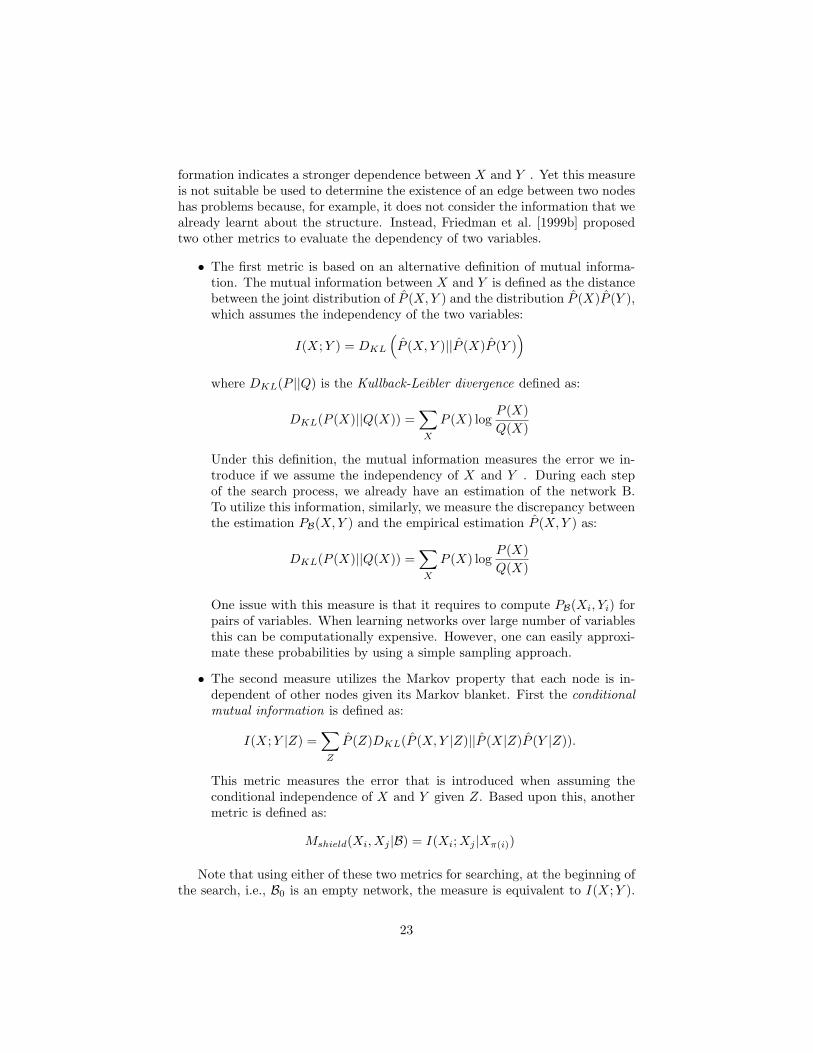
formation indicates a stronger dependence between X and Y . Yet this measureis not suitable be used to determine the existence of an edge between two nodeshas problems because, for example, it does not consider the information that wealready learnt about the structure. Instead, Friedman et al. [1999b] proposedtwo other metrics to evaluate the dependency of two variables.

• The first metric is based on an alternative definition of mutual informa-tion. The mutual information between X and Y is defined as the distancebetween the joint distribution of P (X,Y ) and the distribution P (X)P (Y ),which assumes the independency of the two variables:

I(X;Y ) = DKL

(

P (X,Y )||P (X)P (Y ))

where DKL(P ||Q) is the Kullback-Leibler divergence defined as:

DKL(P (X)||Q(X)) =∑

X

P (X) logP (X)

Q(X)

Under this definition, the mutual information measures the error we in-troduce if we assume the independency of X and Y . During each stepof the search process, we already have an estimation of the network B.To utilize this information, similarly, we measure the discrepancy betweenthe estimation PB(X,Y ) and the empirical estimation P (X,Y ) as:

DKL(P (X)||Q(X)) =∑

X

P (X) logP (X)

Q(X)

One issue with this measure is that it requires to compute PB(Xi, Yi) forpairs of variables. When learning networks over large number of variablesthis can be computationally expensive. However, one can easily approxi-mate these probabilities by using a simple sampling approach.

• The second measure utilizes the Markov property that each node is in-dependent of other nodes given its Markov blanket. First the conditionalmutual information is defined as:

I(X;Y |Z) =∑

Z

P (Z)DKL(P (X,Y |Z)||P (X|Z)P (Y |Z)).

This metric measures the error that is introduced when assuming theconditional independence of X and Y given Z. Based upon this, anothermetric is defined as:

Mshield(Xi, Xj |B) = I(Xi;Xj |Xπ(i))

Note that using either of these two metrics for searching, at the beginning ofthe search, i.e., B0 is an empty network, the measure is equivalent to I(X;Y ).

23

Later iterations will incorporate the already estimated network structure inchoosing the candidate parents.

Another problem with the hill-climbing algorithm is the stopping criteria forthe search. There are usually two types of stopping criteria:

• Score-based criterion: the search process terminates when Score(Bt) =Score(Bt−1). In other words, the score of the network can no longer beincreased by updating the network from candidate network space.

• Candidate-based criterion: the search process terminates when Cti = Ct−1

i

for all i, that is, the candidate space of the network remains unchanged.

Since the score is a monotonically increasing bounded function, the score-based criterion is guaranteed to stop. The candidate-based criterion might entera loop with no ending, in which case certain heuristics are needed to stop thesearch.

There are four problems with the SCHC algorithm. First, the estimation ofthe candidate sets is not sound (i.e., may not identify the true set of parents),and it may take a number of iterations to converge to an acceptable approx-imation of the true set of parents. Second, the algorithm needs a pre-definedparameter k, the maximum number of parents allowed for any node in the net-work. If k is underestimated, there is a risk of discovering a suboptimal network.On the other hand, if k is overestimated, the algorithm will include unnecessaryparents in the search space, thus jeopardizing the efficiency of the algorithm.Third, as already implied above, the parameter k imposes a uniform sparsenessconstraint on the network, thus may sacrifice either efficiency or quality of thealgorithm. A more efficient way to constrain the search space is the Max-MinHill-Climbing (MMHC) algorithm [Tsamardinos et al., 2006], a hybrid algorithmwhich will be explained in Section 5.1. The last problem is that the constraintof the maximum number of parents k will conflict with the scale-free networksdue to the existence of hubs (this problem exists for any algorithm that imposesthis constraint).

Using the SCHC search, the number of candidate structures in each updateis reduced from O(n2) to O(n) where n is the number of nodes in the structure.Thus, the algorithm is capable to learn large-scale structures with hundreds ofnodes.

The hill-climbing search is usually applied with multiple restarts and tabulist [Cvijovicacute and Klinowski, 1995]. Multiple restarts are used to avoidlocal optima, and the tabu list is used to record the path of the search so as toavoid loops and local minima.

To solve the problem of large candidate structure space and local optima,some other algorithms are proposed as listed in the following.

• In [Moore and keen Wong, 2003], the authors proposed a search strategybased on a more complex search operator called optimal reinsertion. Ineach optimal reinsertion, a target node in the graph is picked and all arcsentering or exiting the target are deleted. Then a globally optimal com-bination of in-arcs and out-arcs are found and reinserted into the graph

24

subject to some constraints. With the optimal reinsertion operation de-fined, the search algorithm generates a random ordering of the nodes andapplies the operation to each node in the ordering in turn. This proce-dure is iterated, each with a newly randomized ordering, until no changeis made in a full pass. Finally, a conventional hill-climbing is performed torelax the constraint of max number of parents in the optimal reinsertionoperator.

• In [Xiang et al., 1997], the authors state that with a class of domainmodels of probabilistic dependency network, the optimal structure can notbe learned through the search procedures that modify a network structureone link at a time. For example, given theXOR nodes there is no benefit inadding any one parent individually without the others and so single-linkhill-climbing can make no meaningful progress. They propose a multi-link lookahead search for finding decomposable Markov Networks (DMN).This algorithm iterates over a number of levels where at level i, the currentnetwork is continually modified by the best set of i links until the entropydecrement fails to be significant.

• Some algorithms identify the Markov blanket or parent sets by eitherusing conditional independency test, mutual information or regression,then use hill-climbing search over this constrained candidate structurespace [Tsamardinos et al., 2006, Schmidt and Murphy, 2007]. These al-gorithms belong to the hybrid methods. Some of them are listed in Sec-tion 5.1.

3.2.2 Search over Ordering Space

The acyclicity of the Bayesian network implies an ordering property of the struc-ture such that if we order the variables as 〈x1, · · · , xn〉, each node xi would haveparents only from the set x1, · · · , xi−1. Fundamental observations [Buntine,1991, Cooper and Herskovits, 1992] have shown that given an ordering on thevariables in the network, finding the highest-scoring network consistent with theordering is not NP-hard. Indeed, if the in-degree of each node is bounded to kand all structures are assumed to have equal probability, then this task can beaccomplished in time O(nk) where n is the number of nodes in the structure.

Search over the ordering space has some useful properties. First, the order-ing space is significantly smaller than the structure space: 2O(n logn) orderingsversus 2Ω(n2) structures where n is the number of nodes in the structure [Robin-son, 1973]. Second, each update in the ordering search makes a more globalmodification to the current hypothesis and thus has more chance to avoid localminima. Third, since the acyclicity is already implied in the ordering, there isno need to perform acyclicity checks, which is potentially a costly operation forlarge networks.

The main disadvantage of ordering-based search is the need to compute alarge set of sufficient statistics ahead of time for each variable and each possibleparent set. In the discrete case, these statistics are simply the frequency counts

25

of instantiations: #(xi,xπ(i)) for each xi ∈ V al(xi) and xπ(i) ∈ V al(xπ(i)). Thiscost would be very high if the number of samples in the dataset is large. How-ever, the cost can be reduced by using AD-tree data structure [Moore and Lee,1998], or by pruning out possible parents for each node using SCHC [Friedmanet al., 1999b], or by sampling a subset of the dataset randomly.

Here some algorithms that search through the ordering space are listed:

• The ordering-based search was first proposed in [Larranaga et al., 1996]which uses a genetic algorithm search over the structures, and thus is verycomplex and not applicable in practice.

• In [Friedman and Koller, 2003], the authors proposed to estimate theprobability of a structural feature (i.e., an edge) over the set of all orderingsby using a Markov Chain Monte Carlo (MCMC) algorithm to sample overthe possible orderings. The authors asserts that in the empirical study,different runs of MCMC over network structure typically lead to verydifferent estimates in the posterior probabilities over network structurefeatures, illustrating poor convergence to the stationary distribution. Bycontrast, different runs of MCMC over orderings converge reliably to thesame estimates.

• In [Teyssier and Koller, 2005], the authors proposed a simple greedy localhill-climbing with random restarts and a tabu list. First the score of anordering is defined as the score of the best network consistent with it.The algorithm starts with a random ordering of the variables. In eachiteration, a swap operation is performed on any two adjacent variablesin the ordering. Thus the branching factor for this swap operation isO(n). The search stops at a local maximum when the ordering with thehighest score is found. The tabu list is used to prevent the algorithmfrom reversing a swap that was executed recently in the search. Given anordering, the algorithm then tries to find the best set of parents for eachnode using the Sparse Candidate algorithm followed by exhaustive search.

• In [Koivisto, 2004, Singh and Moore, 2005], the authors proposed to useDynamic Programming to search for the optimal structure. The key inthe dynamic programming approach is the ordering ≺, and the marginalposterior probability of the feature f

p(f | ≺) =∑

≺

p(≺ |x)p(f |x,≺)

Unlike [Friedman and Koller, 2003] which uses MCMC to approximatethe above value, the dynamic programming approach does exact summa-tion using the permutation tree. Although this approach may find theexactly best structure, the complexity is O(n2n + nk+1C(m)) where n isthe number of variables, k is a constant in-degree, and C(m) is the cost

26

of computing a single local marginal conditional likelihood for m data in-stances. The authors acknowledge that the algorithm is feasible only forn ≤ 26.

27

Chapter 4

Regression-basedAlgorithms

4.1 Regression Model

Given N sample data points as (xi, yi) and pre-defined basis functions φ(·), thetask of regression is to find a set of weights w such that the basis functionsgive the best prediction of the label yi from the input xi. The performanceof the prediction is given by an loss function ED(w). For example, in a linearregression,

ED(w) =1

2

N∑

i=1

(

yi −w⊤φ(xi))2

(4.1)

To avoid over-fitting, a regularizer is usually added to penalize the weights w.So the regularized loss function is:

E(w) = ED(w) + λEW (w) (4.2)

The regularizer penalizes each element of w:

EW (w) =

M∑

j=1

αi‖wj‖q

When all αi’s are the same, then

EW (w) = ‖wj‖q

where ‖ · ‖q is the Lq norm, λ is the regularization coefficient that controlsthe relative importance of the data-dependent error and the regularization term.With different values of q, the regularization term may give different results:

28

1. When q = 2, the regularizer is in the form of sum-of-squares

EW (w) =1

2w⊤w

This particular choice of regularizer is known in machine learning liter-ature as weight decay [Bishop, 2006] because in sequential learning al-gorithm, it encourages weight values to decay towards zeros, unless sup-ported by the data. In statistics, it provides an example of a parametershrinkage method because it shrinks parameter values towards zero.

One advantage of the L2 regularizer is that it is rotationally invariant inthe feature space. To be specific, given a deterministic learning algorithmL, it is rotationally invariant if, for any training set S, rotational matrixM and test example x, there is L[S](x) = L[MS](Mx). More generally, ifL is a stochastic learning algorithm so that its predictions are random, itis rotationally invariant if, for any S, M and x, the prediction L[S](x) andL[MS](Mx) have the same distribution. A complete proof in the case oflogistic regression is given in [Ng, 2004].

This quadratic (L2) regularizer is convex, so if the loss function beingoptimized is also a convex function of the weights, then the regularizedloss has a single global optimum. Moreover, if the loss function ED(w)is in quadratic form, then the minimizer of the total error function hasa closed form solution. Specifically, if the data-dependent error ED(w)is the sum-of-squares error as in Equation 4.2, then setting the gradientwith respect to w to zero, then the solution is

w = (λI+Φ⊤Φ)−1Φ⊤t

This regularizer is seen in ridge regression [Hoerl and Kennard, 2000], thesupport vector machine [Hoerl and Kennard, 2000, Schlkopf and Smola,2002] and regularization networks [Girosi et al., 1995].

2. q = 1 is called lasso regression in statistics [Tibshirani, 1996]. It has theproperty that if λ is sufficiently large, then some of the coefficients wi aredriven to zero, which leads to a sparse model in which the correspondingbasis functions play no role. To see this, note that the minimization ofEquation 4.2 is equivalent to minimizing the unregularized sum-of-squareserror subject to the constraint over the parameters:

argminw

1

2

N∑

i=1

(

yi −w⊤φ(xi))2

(4.3)

s. t.

M∑

j=1

‖wj‖q ≤ η (4.4)

29

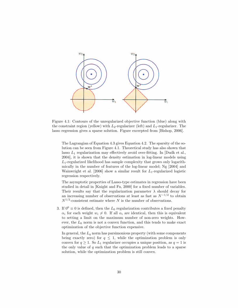
Figure 4.1: Contours of the unregularized objective function (blue) along withthe constraint region (yellow) with L2-regularizer (left) and L1-regularizer. Thelasso regression gives a sparse solution. Figure excerpted from [Bishop, 2006].

The Lagrangian of Equation 4.3 gives Equation 4.2. The sparsity of the so-lution can be seen from Figure 4.1. Theoretical study has also shown thatlasso L1 regularization may effectively avoid over-fitting. In [Dudk et al.,2004], it is shown that the density estimation in log-linear models usingL1-regularized likelihood has sample complexity that grows only logarith-mically in the number of features of the log-linear model; Ng [2004] andWainwright et al. [2006] show a similar result for L1-regularized logisticregression respectively.

The asymptotic properties of Lasso-type estimates in regression have beenstudied in detail in [Knight and Fu, 2000] for a fixed number of variables.Their results say that the regularization parameter λ should decay foran increasing number of observations at least as fast as N−1/2 to obtainN1/2-consistent estimate where N is the number of observations.

3. If 00 ≡ 0 is defined, then the L0 regularization contributes a fixed penaltyαi for each weight wi 6= 0. If all αi are identical, then this is equivalentto setting a limit on the maximum number of non-zero weights. How-ever, the L0 norm is not a convex function, and this tends to make exactoptimization of the objective function expensive.

In general, the Lq norm has parsimonious property (with some componentsbeing exactly zero) for q ≤ 1, while the optimization problem is onlyconvex for q ≥ 1. So L1 regularizer occupies a unique position, as q = 1 isthe only value of q such that the optimization problem leads to a sparsesolution, while the optimization problem is still convex.

30

4.2 Structure Learning through Regression

Learning a graphical structure by regression is gaining popularity in recentyears. The algorithms proposed mainly differ in the choice of the objective lossfunctions. They are listed in the following according to the different objectivesthey use.

4.2.1 Likelihood Objective

Methods in this category use the negative likelihood or log-likelihood of the datagiven the parameters of the model as the objective loss function ED(·).

• In [in Lee et al., 2006], the authors proposed a L1-regularized structurelearning algorithm for Markov Random Field, specifically, in the frame-work of log-linear models. Given a variable set X = x1, · · · ,xn, a log-linear model is defined in terms of a set of feature functions fk(xk), eachof which is a function that defines a numerical value for each assignmentxk to some subset xk ⊂ X . Given a set of feature functions F = fk,the parameters of the log-linear model are weights θ = θk : fk ∈ F. Theoverall distribution is defined as:

Pθ(x) =1

Z(θ)exp

∑

fk∈F

θkfk(x)

where Z(θ) is a normalizer called partition function. Given an iid trainingdataset D, the log-likelihood function is:

L(M,D) =∑

fk∈F

θkfk(D −M logZ(θ) = θ⊤f(D)−M logZ(θ)

where fk(D) =∑M

m=1 fk(xk[m]) is the sum of the feature values over theentire data set, f(D) is the vector where all of these aggregate features havebeen arranged in the same order as the parameter vector, and θ⊤f(D) is avector dot-product operation. To get a sparse MAP approximation of theparameters, a Laplacian parameter prior for each feature fk is introducedsuch that

P (θk) =βk2

exp(−βk|θk|)

And finally the objective function is:

maxθ

θ⊤f(D)−M logZ(θ)−∑

k

βk|θk|

31

Before solving this optimization problem to get the parameters, featuresshould be included into the model. Instead of including all features inadvance, the authors use grafting procedure [Perkins et al., 2003] andgain-based method [Pietra et al., 1997] to introduce features into the modelincrementally.

• In [Wainwright et al., 2006], the authors restricted to the Ising model, aspecial family of MRF, defined as

p(x, θ) = exp

∑

s∈V

θsxs +∑

(s,t)∈E

θstxsxt −Ψ(θ)

The logistic regression with L1-regularization that minimizing the negativelog likelihood is achieved by optimizing:

θs,λ = argminθ∈Rp

(

1

n

n∑

i=1

(

log(1 + exp(θ⊤z(i,s)))− x(i)s θ⊤z(i,s))

+ λn‖θ\s‖1)

4.2.2 Dependency Objective

Algorithms in this category use linear regression to estimate the Markov blanketof each node in a graph. Each node is considered dependent on nodes withnonzero weights in the regression.

• In [Meinshausen and Buhlmann, 2006], the authors used linear regressionwith L1 regularization to estimate the neighbors of each node in a Gaussiangraphical model:

θi,λ = argminθ:θi=0

1

n‖xi − θ⊤x‖22 + λ‖θ‖1

The authors discussed in detail the choice of regularizer weight λ, for whichthe cross-validation choice is not the best under certain circumstances. Forthe solution, the authors proposed an optimal choice of λ under certainassumptions with full proof.

• In [Fan, 2006], the authors proposed to learn GGM from directed graphicalmodels using modified Lasso regression, which seems a promising method.The algorithm is listed here in detail.

Given a GGM with variables x = [x1, · · · , xp]⊤ and the multivariate Gaus-sian distribution with covariance matrix Σ:

P (x) =1

(2π)p/2|Σ|1/2 exp

(

−1

2x⊤Σ−1x

)

This joint probability can always be decomposed into the product of mul-tiple conditional probabilities:

P (x) =

p∏

i=1

P (xi|xi+1,··· ,p)

32

Since the joint probability in the GGM is a multivariate Gaussian dis-tribution, each conditional probability also follows Gaussian distribution.This implies that for any GGM there is at least one DAG with the samejoint distribution.

Suppose that for a DAG there is a specific ordering of variables as 1, 2, · · · , p.Each variable xi only has parents with indices larger than i. Let β de-note the regression coefficients and D denote the data. The posteriorprobability given the DAG parameter β is

P (D|β) =p∏

i=1

P (xi|x(i+1):p, β)

Suppose linear regression xi =∑p

j=i+1 βjixj+ǫi where the error ǫi followsnormal distribution ǫi ∼ N(0, ψi), then

x = Γx+ ǫ

ǫ ∼ Np(0,Ψ)

Where Γ is an upper triangular matrix, Γij = βji, i < j, ǫ = (ǫ1, · · · , ǫp)⊤and Ψ = diag(ψ1, · · · , ψp). Thus

x = (I − Γ)−1ǫ

So x follows a joint multivariate Gaussian distribution with covariancematrix and precision matrix as:

Σ = (I − Γ)−1Ψ((I − Γ)−1)⊤

Ω = (I − Γ)⊤Ψ−1(I − Γ)

Wishart prior is assigned to the precision matrix Ω such that Ω ∼Wp(δ, T )with δ degrees of freedom and diagonal scale matrix T = diag(θ1, · · · , θp).Each θi is a positive hyper prior and satisfies

P (θi) =λ

2exp(

−λθi2

)

Let βi = (β(i+1)i, · · · , βpi)⊤, and Ti represents the sub-matrix of T corre-sponding to variables x(i+1):p. Then the associated prior for βi is P (βi|ψi, θ(i+1):p) =Np−1(0, Tiψi) [Geiger and Heckerman, 2002], thus:

P (βji|ψi, θj) = N(0, θjψi)

And the associated prior for ψi is

P (ψ−1i |θi) = Γ

(

δ + p− 1

2,θ−1i

2

)

33

where Γ(·) is the Gamma distribution. Like in [Figueiredo and Jain, 2001],the hyper prior θ can be integrated out from prior distribution of βji andthus

P (βji|ψi) =

∫ ∞

0

P (βji|ψi, θj)P (θj)

=1

2

(

λ

ψi

)

exp

(

−( λ

ψi

)12 |βji|

)

Suppose there are K samples in the data D and xki is the ith variable inthe kth sample, then

P (βi|ψi, D) ∝ P (xix(i+1):p, βi, ψi)P (βi|ψi)

∝ exp

(

∑

k(xki −∑p

j=i+1 βjixkj)2 +√λψi

∑pj=i+1 |βji|

−ψi

)

and

P (ψ−1i |θi, βi, D) = Γ

(

δ + p− i+K

2,θ−1i +

∑

k(xki −∑p

j=i+1 βjixkj)2

2

)

The MAP estimation of βi is:

βi = argmin∑

k

xki −p∑

j=i+1

βjixkj

2

+√

λψi

p∑

j=i+1

|βji|

βi is the solution of a Lasso regression.

The authors further proposed a Feature Vector Machine (FVM) which isan advance to the the generalized Lasso regression (GLR) [Roth, 2004]which incorporates kernels, to learn the structure of undirected graphicalmodels. The optimization problem is:

argminβ

1

2

∑

p,q

βpβqK(fp, fq)

s.t.

∣

∣

∣

∣

∣

∑

p

βpK(fq, fp)−K(fq, y)

∣

∣

∣

∣

∣

≤ λ

2, ∀q

where K(fi, fj) = φ(fi)⊤φ(fj) is the kernel function, φ(·) is the mapping,

either linear or non-linear, from original space to a higher dimensionalspace; fk is the k-th feature vector, and y is the response vector from thetraining dataset.

34

4.2.3 System-identification Objective

Algorithms in this category [Arkin et al., 1998, Gardner et al., 2003, Glass andKauffman, 1973, Gustafsson et al., 2003, McAdams and Arkin, 1998] get ideasfrom network identification by multiple regression (NIR), which is derived froma branch of engineering called system identification [Ljung, 1999], in which amodel of the connections and functional relations between elements in a networkis inferred from measurements of system dynamics. The whole system is mod-eled using a differential equation, then regression algorithms are used to fit thisequation. This approach has been used to identify gene regulatory networks.Here the key idea of this type of approaches is illustrated by using the algorithmin [Gustafsson et al., 2003] as an example.

Near a steady-state point (e.g., when gene expression does not change sub-stantially over time), the nonlinear system of the genes may be approximatedto the first order by a linear differential equation as:

dxtidt

=

n∑

j=1

wijxtj + ǫi

where xti is the expression of gene i at time t. The network of the interactioncan be inferred by minimizing the residual sum of squares with constraints onthe coefficients:

argminwij

∑

t

n∑

j=1

wijxtj −

dxtidt

2

s.t.

n∑

j=1

|wij | ≤ µi

Note that this is essentially a Lasso regression problem since the constraintsadded to the Lagrangian is equivalent to L1 regularizers. Finally the adjancencymatrix A of the network is identified from the coefficients by

Aij =

0 if wji = 0

1 otherwise

One problem with this approach is when the number of samples is less than thenumber of variables, the linear equation is undetermined. To solve this prob-lem, D’haeseleer et al. [1999] use non-linear interpolation to generate more datapoints to make the equation determined; Yeung et al. [2002] use singular valuedecomposition (SVD) to first decompose the training data, and then constrainthe interaction matrix by exploring the sparseness of the interactions.

4.2.4 Precision Matrix Objective

In [Banerjee et al., 2006], the authors proposed a convex optimization algorithmfor fitting sparse Gaussian Graphical Model from precision matrix. Given a

35

large-scale empirical dense covariance matrix S of multivariate Gaussian data,the objective is to find a sparse approximation of the precision matrix. AssumingX is the estimate of the precision matrix (the inverse of the variance matrix).The optimization of the penalized maximum likelihood (ML) is:

maxX≻0

log det(X)− Tr(SX)− ρ‖X‖1

The problem can be efficiently solved by Nesterovs method [Nesterov, 2005].

4.2.5 MDL Objective

Methods in this category encode the parameters into the Minimum DescriptionLength (MDL) criterion, and tries to minimize the MDL with respect to theregularization or constraints.

• In [Schmidt and Murphy, 2007], the authors proposed a structure learningapproach which uses the L1 penalized regression with MDL as loss functionto find the parents/neighbors for each node, and then apply the score-based search. The first step is the L1 regularized variable selection to findthe parents/neighbors set of a node by solving the following equation:

θL1j (U) = argmin

θNLL(j, U, θ) + λ‖θ‖1 (4.5)

where λ is the regularization parameter for the L1 norm of the parametervector. NLL(j, U, θ) is the negative log-likelihood of node j with parentsπ(j) and parameters θ:

MDL(G) =

d∑

j=1

NLL(j, πj , θmlej +

|θmlej |2

log n (4.6)

NLL(j, π(j), θ) = −N∑

i=1

logP (Xij |Xi,π(j), θ) (4.7)

where N is the number of samples in the dataset.

The L1 regularization will generate a sparse solution with many parame-ters being zero. The set of variables with non-zero values are set as theparents of each node. This hybrid structure learning algorithm is furtherdiscussed in Section 5.1.

In general, this regression method is the same as the likelihood objectedapproaches, since the term of the description length of model in Equa-tion 4.7 is incorporated into the regularization term in Equation 4.5.

• In [Guo and Schuurmans, 2006], the authors proposed an interesting struc-ture learning algorithm for Bayesian Networks, which incorporates pa-rameter estimation, feature selection and variable ordering into one single

36

convex optimization problem, which is essentially a constrained regressionproblem. The parameters of the Bayesian network and the feature selec-tor variables are encoded in the MDL objective function which is to beminimized. The topological properties of the Bayesian network (antisym-metricity, transitivity and reflexivity) are encoded as constraints to theoptimization problem.

37

Chapter 5

Hybrid Algorithms andOthers

5.1 Hybrid Algorithms

Some algorithms perform the structure learning in a hybrid manner to utilizethe advantages of constraint-based, score-based or regression-based algorithms.Here we list some of them.

• Max-min Hill-climbing (MMHC): In [Tsamardinos et al., 2006], the au-thors proposed a Max-min Hill-climbing (MMHC) algorithm for structurelearning of Bayesian networks. The MMHC algorithm shares the simi-lar idea as the Sparse Candidate Hill Climbing (SCHC) algorithm. TheMMHC algorithm works in two steps. In the first step, the skeleton of thenetwork is learned using a local discovery algorithm called Max-Min Par-ents and Children (MMPC) to identify the parents and children of eachnode through the conditional independency test, where the conditionalsets are grown in a greedy way. In this process, the Max-Min heuristicis used to select the variables that maximize the minimum associationwith the target variable relative to the candidate parents and children.In the second step, the greedy hill-climbing search is performed withinthe constraint of the skeleton learned in the first step. Unlike the SCHCalgorithm, MMHC does not impose a maximum in-degree for each node.

• In [Schmidt and Murphy, 2007], the authors proposed a structure learn-ing approach which uses the L1 penalized regression to find the par-ents/neighbors for each node, and then apply the score-based search. Thefirst step is the L1 variable selection to find the parents/neighbors set ofa node. The regression algorithm is discussed in Section 4.2.5.

After the parent sets of all node are identified, a skeleton of the structure iscreated using the ‘OR’ strategy [Meinshausen and Buhlmann, 2006]. Thisprocedure is called L1MB (L1-regularized Markov blanket). The L1MB is

38

plugged into structure search (MMHC) or ordering search [Teyssier andKoller, 2005]. In the application to MMHC, L1MB replaces the SparseCandidate procedure to identify potential parents. In the application toordering search in [Teyssier and Koller, 2005], given the ordering, L1MBreplaces the SC and exhaustive search.

5.2 Other Algorithms

Besides the structure learning algorithms mentioned before, there are some otherapproaches. They are listed here.

5.2.1 Clustering Approaches

The simplest structure learning method is through clustering. First the similar-ities of any two variables are estimated, then any two variables with similarityhigher than a threshold are connected by an edge [Lukashin et al., 2003]. Herethe similarity may take different measures, including correlation [Eisen et al.,1998, Spellman et al., 1998, Iyer et al., 1999, Alizadeh et al., 2000], Euclideandistance [Wen et al., 1998, Tamayo et al., 1999, Tavazoie et al., 1999] and mutualinformation [Butte and Kohane, 2000]. Using hierarchical clustering [Manninget al., 2008], the hierarchy structure may be presented at different scales.

5.2.2 Boolean Models

Some algorithms employed the Boolean models for structure learning in generegulatory network reconstruction [Thomas, 1973, Akutsu et al., 1999, Lianget al., 1998]. These approaches assume the boolean relationship between regu-lators and regulated genes, and tried to identify appropriate logic relationshipamong gene based on the observed gene expression profiles.

5.2.3 Information Theoretic Based Approach

In [Basso et al., 2005], the authors employ the information theoretic approachesfor reconstructing gene regulatory network. It first identify pairs of correlatedgenes based on the measurement of mutual information. It then eliminatesindirect interaction among genes by applying the well-known staple of datatransimission theory, the “data processing inequality” (DPI). There are twothings unclear about this approaches: 1) Since the results could be sensitiveto the order of elimination, it is important to provide a justification about theorder of edges to be eliminated. 2) Most of the discussion within the paper islimited to loops with three edges. It is important to know how to address thecycles with more than three genes.

39

5.2.4 Matrix Factorization Based Approach

Methods in this category use matrix factorization techniques to identify theinteractions between variables. The matrix factorization algorithms used in-cludes singular value decomposition [Alter et al., 2000, D’haeseleer et al., 1999,Raychaudhuri et al., 2000], max-margin matrix factorization [DeCoste, 2006,Rennie and Srebro, 2005, Srebro et al., 2005] and non-negative matrix factor-ization [Badea and Tilivea, 2005, Paatero and Tapper, 1994, Hoyer and Dayan,2004, Lee and Seung, 2001, Shahnaz et al., 2006, Weinberger et al., 2005], net-work component analysis (NCA) [Liao et al., 2003]. Readers are referred to reada technical report [Jin and Zhou, 2006] for more details of this method.

40

Bibliography

Tatsuya Akutsu, Satoru Miyano, and Satoru Kuhara. Identification of geneticnetworks from a small number of gene expression patterns under the booleannetwork model. In Pacific Symposium on Biocomputing, pages 17–28, 1999.

Ash A. Alizadeh, Michael B. Eisen, R. Eric Davis, Chi Ma, Izidore S. Lossos,Andreas Rosenwald, Jennifer C. Boldrick, Hajeer Sabet, Truc Tran, Xin Yu,John I. Powell, Liming Yang, Gerald E. Marti, Troy Moore, James Hudson,Lisheng Lu, David B. Lewis, Robert Tibshirani, Gavin Sherlock, Wing C.Chan, Timothy C. Greiner, Dennis D. Weisenburger, James O. Armitage,Roger Warnke, Ronald Levi, Wyndham Wilson, Michael R. Grever, John C.Byrd, David Botstein, Patrick O. Brown, and Louis M. Staudt. Distincttypes of diffuse large b-cell lymphoma identified by gene expression profiling.Nature, 403(6769):503–511, 2000.

Tim Van Allen and Russell Greiner. Model selection criteria for learning beliefnets: An empirical comparison. In ICML ’00: Proceedings of the Seven-teenth International Conference on Machine Learning, pages 1047–1054, SanFrancisco, CA, USA, 2000. Morgan Kaufmann Publishers Inc. ISBN 1-55860-707-2.

Orly Alter, Patrick O. Brown, and David Botstein. Singular value decompositionfor genome-wide expression data processing and modeling. Proceedings of theNational Academy of Sciences of the United States of America, 97(18):10101–10106, 2000. URL http://www.pnas.org/content/97/18/10101.abstract.

Adam Arkin, John Ross, and Harley H. McAdams. Stochastic ki-netic analysis of developmental pathway bifurcation in phage λ-infectedescherichia coli cells. Genetics, 149(4):1633–1648, 1998. URLhttp://www.genetics.org/cgi/content/abstract/149/4/1633.

Liviu Badea and Doina Tilivea. Sparse factorizations of gene expression dataguided by binding data. In PSB, 2005.

Onureena Banerjee, Laurent El Ghaoui, Alexandre d’Aspremont, and GeorgesNatsoulis. Convex optimization techniques for fitting sparse gaussian graph-ical models. In ICML ’06: Proceedings of the 23rd international conference

41

on Machine learning, pages 89–96, New York, NY, USA, 2006. ACM. ISBN1-59593-383-2. doi: http://doi.acm.org/10.1145/1143844.1143856.

Albert-Laszlo Barabasi and Reka Albert. Emergence of scal-ing in random networks. Science, 286:509, 1999. URLhttp://www.citebase.org/abstract?id=oai:arXiv.org:cond-mat/9910332.

Katia Basso, Adam A. Margolin, Gustavo Stolovitzky, Ulf Klein, RiccardoDalla-Favera, and Andrea Califano. Reverse engineering of regulatory net-works in human b cells. Nature Genetics, 37(4):382–390, 2005.

Ashish Bhan, David J. Galas, and Gregory T. Dewey. Aduplication growth model of gene expression networks.Bioinformatics, 18(11):1486–1493, November 2002. URLhttp://bioinformatics.oxfordjournals.org/cgi/content/abstract/18/11/1486.

Christopher M. Bishop. Pattern Recognition and Machine Learning (Informa-tion Science and Statistics). Springer-Verlag New York, Inc., Secaucus, NJ,USA, 2006. ISBN 0387310738.

C. Boutilier, N. Friedman, M. Goldszmidt, and D. Koller. Context-specificindependence in Bayesian networks. In Proceedings of the Twelfth Conferenceon Uncertainty in Artificial Intelligence, pages 115–123, 1996.

Wray Buntine. Theory refinement on bayesian networks. In UAI, pages 52–60.Morgan Kaufmann, 1991.

A. J. Butte and I. S. Kohane. Mutual information relevance net-works: functional genomic clustering using pairwise entropy measure-ments. In Pacific Symposium of Biocomputing, pages 418–429, Children’sHospital Informatics Program, Boston, MA 02115, USA., 2000. URLhttp://view.ncbi.nlm.nih.gov/pubmed/10902190.

David M. Chickering, David Heckerman, and Christopher Meek.Large-sample learning of bayesian networks is np-hard. J.Mach. Learn. Res., 5:1287–1330, 2004. ISSN 1533-7928. URLhttp://portal.acm.org/citation.cfm?id=1044703.

David Maxwell Chickering. Learning bayesian networks is np-complete. InLearning from Data: Artificial Intelligence and Statistics V, pages 121–130.Springer-Verlag, 1996.

David Maxwell Chickering and Craig Boutilier. Learning equivalence classes ofbayesian-network structures. In Journal of Machine Learning Research, pages150–157. Morgan Kaufmann, 1996.

C. I. Chow, Sexior Member, and C. N. Liu. Approximating discrete probabil-ity distributions with dependence trees. IEEE Transactions on InformationTheory, 14:462–467, 1968.

42

Gregory F. Cooper and Edward Herskovits. A bayesian method for the in-duction of probabilistic networks from data. Machine Learning, 9(4):309–347, October 1992. doi: http://dx.doi.org/10.1007/BF00994110. URLhttp://dx.doi.org/10.1007/BF00994110.

Thomas M. Cover and Joy A. Thomas. Elements of Information The-ory. Wiley-Interscience, August 1991. ISBN 0471062596. URLhttp://www.amazon.ca/exec/obidos/redirect?tag=citeulike09-20&amp;path=ASIN/0471062596.

Djurdje Cvijovicacute and Jacek Klinowski. Taboo search: An approachto the multiple minima problem. Science, 267(5198):664–666, Febru-ary 1995. doi: http://dx.doi.org/10.1126/science.267.5198.664. URLhttp://dx.doi.org/10.1126/science.267.5198.664.

Dennis DeCoste. Collaborative prediction using ensembles of maxi-mum margin matrix factorizations. In ICML ’06: Proceedings ofthe 23rd international conference on Machine learning, pages 249–256, New York, NY, USA, 2006. ACM. ISBN 1-59593-383-2. doi:http://doi.acm.org/10.1145/1143844.1143876.

P. D’haeseleer, X. Wen, S. Fuhrman, and R. Somogyi. Linear modeling of mrnaexpression levels during cns development and injury. In Pacific Symposiumon Biocomputing. Pacific Symposium on Biocomputing, page 41, 1999.

Miroslav Dudk, Steven J. Phillips, and Robert E. Schapire. Performance guar-antees for regularized maximum entropy density estimation. In Proceedingsof the 17th Annual Conference on Computational Learning Theory, pages472–486. Springer Verlag, 2004.

M. B. Eisen, P. T. Spellman, P. O. Brown, and D. Botstein. Clus-ter analysis and display of genome-wide expression patterns. ProcNatl Acad Sci, 95(25):14863–14868, December 1998. ISSN 0027-8424. doi: http://dx.doi.org/10.1073/pnas.95.25.14863. URLhttp://dx.doi.org/10.1073/pnas.95.25.14863.

Liming Fan. Structure learning with large sparse undirected graphs and itsapplications. Technical report, Carnegie Mellon University, 2006.

Mario A. T. Figueiredo and Anil K. Jain. Bayesian learning of sparse classifiers.In In 2001 Conference on Computer Vision and Pattern Recognition (CVPR2001, pages 35–41. IEEE Press, 2001.

N. Friedman and M. Goldszmidt. Learning bayesian networks with local struc-ture. Learning in Graphical Models, pages 421–460, 1998.

Nir Friedman and Moises Goldszmidt. Learning in Graph-ical Models, chapter Learning Bayesian networks with lo-cal structure, pages 252–262. MIT Press, 1996. URLhttp://citeseerx.ist.psu.edu/viewdoc/summary?doi=10.1.1.30.573.

43

Nir Friedman and Daphne Koller. Being bayesian about network struc-ture. a bayesian approach to structure discovery in bayesian networks.Machine Learning, 50(1-2):95–125, January 2003. ISSN 0885-6125. URLhttp://www.ingentaconnect.com/content/klu/mach/2003/00000050/F0020001/05096739.

Nir Friedman, Lise Getoor, Daphne Koller, and Avi Pfeffer. Learning proba-bilistic relational models. In IJCAI, pages 1300–1309. Springer-Verlag, 1999a.

Nir Friedman, Iftach Nachman, and Dana Pe’er. Learning bayesian networkstructure from massive datasets: The “sparse candidate” algorithm. In UAI,pages 206–215, 1999b. URL http://citeseer.ist.psu.edu/218089.html.

T. S. Gardner, D. di Bernardo, D. Lorenz, and J. J. Collins. In-ferring genetic networks and identifying compound mode of action viaexpression profiling. Science, 301(5629):102–105, July 2003. ISSN1095-9203. doi: http://dx.doi.org/10.1126/science.1081900. URLhttp://dx.doi.org/10.1126/science.1081900.

Dan Geiger and David Heckerman. Parameter priors for directed acyclicgraphical models and the characterization of several probability dis-tributions. The Annals of Statistics, 30(5):1412–1440, 2002. URLhttp://www.jstor.org/stable/1558719.

Federico Girosi, Michael Jones, and Tomaso Poggio. Regularization theory andneural networks architectures. Neural Computation, 7:219–269, 1995.

L. Glass and SA Kauffman. The logical analysis of continuous, non-linear bio-chemical control networks. Journal of Theoretical Biology, 39(1):103, 1973.

Yuhong Guo and Dale Schuurmans. Convex structure learning for bayesiannetworks: polynomial feature selection and approximate ordering. In UAI,2006.

Mika Gustafsson, Michael Hornquist, and Anna Lombardi. Large-scale reverse engineering by the lasso. In ICSB, 2003. URLhttp://www.citebase.org/abstract?id=oai:arXiv.org:q-bio/0403012.

Jing-Dong J. Han, Nicolas Bertin, Tong Hao, Debra S. Goldberg, Gabriel F.Berriz, Lan V. Zhang, Denis Dupuy, Albertha J. Walhout, Michael E. Cu-sick, Frederick P. Roth, and Marc Vidal. Evidence for dynamically orga-nized modularity in the yeast protein-protein interaction network. Nature, 430(6995):88–93, July 2004. doi: http://dx.doi.org/10.1038/nature02555. URLhttp://dx.doi.org/10.1038/nature02555.

A. J. Hartemink, D. K. Gifford, T. S. Jaakkola, and R. A. Young. Using graph-ical models and genomic expression data to statistically validate models ofgenetic regulatory networks. Pac Symp Biocomput, pages 422–433, 2001.URL http://view.ncbi.nlm.nih.gov/pubmed/11262961.

44

D. Heckerman, D. Geiger, and D. M. Chickering. Learning bayesiannetworks: The combination of knowledge and statistical data. Ma-chine Learning, 20(3):197–243, September 1995. ISSN 0885-6125. URLhttp://www.ingentaconnect.com/content/klu/mach/1995/00000020/00000003/00422402.

David Heckerman, David M. Chickering, Christopher Meek, RobertRounthwaite, and Carl Kadie. Dependency networks for in-ference, collaborative filtering, and data visualization. Jour-nal of Machine Learning Research, 1:49–75, October 2000. URLhttp://www.jmlr.org/papers/volume1/heckerman00a/heckerman00a.pdf.

A. E. Hoerl and R. W. Kennard. Ridge regression: Biased estimation fornonorthogonal problems. Technometrics, 42(1):80–86, 2000.

Katsuhisa Horimoto and Hiroyuki Toh. Statistical estimation of cluster bound-aries in gene expression profile data. Bioinformatics, 17(12):1143–1151,December 2001. doi: http://dx.doi.org/10.1093/bioinformatics/17.12.1143.URL http://dx.doi.org/10.1093/bioinformatics/17.12.1143.

Patrik O. Hoyer and Peter Dayan. Non-negative matrix factorization withsparseness constraints. Journal of Machine Learning Research, 5:1457–1469,2004.

Su in Lee, Varun Ganapathi, and Daphne Koller. Efficient structure learning ofmarkov networks using ℓ1-regularization. In NIPS, 2006.

V. R. Iyer, M. B. Eisen, D. T. Ross, G. Schuler, T. Moore, J. C. Lee, J. M.Trent, L. M. Staudt, J. Hudson, M. S. Boguski, D. Lashkari, D. Shalon,D. Botstein, and P. O. Brown. The transcriptional program in the responseof human fibroblasts to serum. Science, 283(5398):83–87, January 1999. ISSN0036-8075. URL http://view.ncbi.nlm.nih.gov/pubmed/99102697.

Manfred Jaeger. Relational bayesian networks. In UAI, pages 266–273. MorganKaufmann, 1997.

Manfred Jaeger. Complex probabilistic modeling with recursive re-lational bayesian networks. Annals of Mathematics and Artifi-cial Intelligence, 32(1-4):179–220, 2001. ISSN 1012-2443. URLhttp://portal.acm.org/citation.cfm?id=590425.590441.

H. Jeong, B. Tombor, R. Albert, Z. N. Oltvai, and A. L. Barabasi. The large-scale organization of metabolic networks. Nature, 407(6804):651–654, Octo-ber 2000. ISSN 0028-0836. doi: http://dx.doi.org/10.1038/35036627. URLhttp://dx.doi.org/10.1038/35036627.

Rong Jin and Yang Zhou. Gene regulatory network reconstruction by matrixfactorization. Technical Report MSU-CSE-06-33, Department of ComputerScience and Engineering, Michigan State University, 2006.

45

Schafer Juliane and Strimmer Korbinian. An empirical bayesapproach to inferring large-scale gene association networks.Bioinformatics, 21(6):754–764, March 2005. ISSN 1367-4803.doi: http://dx.doi.org/10.1093/bioinformatics/bti062. URLhttp://dx.doi.org/10.1093/bioinformatics/bti062.

Robert E. Kass and Adrian E. Raftery. Bayes factors. Jour-nal of the American Statistical Association, 90(430):773–795, 1995. doi: http://dx.doi.org/10.2307/2291091. URLhttp://dx.doi.org/10.2307/2291091.

H. Kitano. Computational system biology. Nature, 420:206–210, 2002.

Keith Knight and Wenjiang Fu. Asymptotics for lasso-type esti-mators. The Annals of Statistics, 28(5):1356–1378, 2000. URLhttp://www.jstor.org/stable/2674097.

Mikko Koivisto. Exact bayesian structure discovery in bayesian networks. J. ofMachine Learning Research, 5:2004, 2004.

Wai Lam and Fahiem Bacchus. Learning bayesian belief networks: An approachbased on the mdl principle. Computational Intelligence, 10:269–293, 1994.

P. Larranaga, M. Poza, Y. Yurramendi, R. H. Murga, and C. M. H.Kuijpers. Structure learning of bayesian networks by genetic al-gorithms: a performance analysis of control parameters. Pat-tern Analysis and Machine Intelligence, IEEE Transactions on, 18(9):912–926, 1996. doi: http://dx.doi.org/10.1109/34.537345. URLhttp://dx.doi.org/10.1109/34.537345.

Daniel D. Lee and H. Sebastian Seung. Algorithms for non-negative matrixfactorization. In NIPS, pages 556–562. MIT Press, 2001.

Shoudan Liang, Stefanie Fuhrman, and Roland Somogyi. Reveal: A generalreverse engineering algorithm for inference of genetic network architectures.In PSB, 1998.

James C. Liao, Riccardo Boscolo, Young-Lyeol Yang, Linh M. Tran, ChiaraSabatti, and Vwani P. Roychowdhury. Network component analysis: Recon-struction of regulatory signals in biological systems. Proceedings of the Na-tional Academy of Sciences of the United States of America, 100(26):15522–15527, 2003. URL http://www.jstor.org/stable/3149038.

L. Ljung. System identication: Theory for the user. Prentice-Hall, 1999.

A. V. Lukashin, M. E. Lukashev, and R. Fuchs. Topology ofgene expression networks as revealed by data mining and model-ing. Bioinformatics, 19(15):1909–1916, October 2003. ISSN 1367-4803. doi: http://dx.doi.org/10.1093/bioinformatics/btg333. URLhttp://dx.doi.org/10.1093/bioinformatics/btg333.

46

Christopher D. Manning, Prabhakar Raghavan, and Hin-rich Schutze. Introduction to Information Retrieval. Cam-bridge University Press, July 2008. ISBN 0521865719. URLhttp://www.amazon.ca/exec/obidos/redirect?tag=citeulike09-20&amp;path=ASIN/0521865719.

D. Margaritis. Learning bayesian networks model structure from data. PhDthesis, CMU, 2003.

Dimitris Margaritis and Sebastian Thrun. Bayesian network induction via localneighborhoods. In Advances in Neural Information Processing Systems 12,pages 505–511. MIT Press, 1999.

H. H. McAdams and A. Arkin. Simulation of prokaryotic genetic cir-cuits. Annu Rev Biophys Biomol Struct, 27:199–224, 1998. ISSN 1056-8700. doi: http://dx.doi.org/10.1146/annurev.biophys.27.1.199. URLhttp://dx.doi.org/10.1146/annurev.biophys.27.1.199.

Nicolai Meinshausen and Peter Buhlmann. High-dimensional graphsand variable selection with the lasso. Ann. Statist., 34(3):1436–1462, 2006. doi: http://dx.doi.org/10.1214/009053606000000281. URLhttp://dx.doi.org/10.1214/009053606000000281.

Andrew Moore and Weng keen Wong. Optimal reinsertion: A new search oper-ator for accelerated and more accurate bayesian network structure learning.In In Proceedings of the 20th International Conference on Machine Learning(ICML 03, pages 552–559. AAAI Press, 2003.

Andrew W. Moore and Mary S. Lee. Cached sufficient statistics for efficient ma-chine learning with large datasets. Journal of Artificial Intelligence Research,8:67–91, 1998. URL http://citeseer.ist.psu.edu/moore97cached.html.

Radford M. Neal. Connectionist learning of belief networks. Artif. Intell.,56(1):71–113, 1992. ISSN 0004-3702. doi: http://dx.doi.org/10.1016/0004-3702(92)90065-6.

Yu Nesterov. Smooth minimization of non-smooth functions.Math. Program., 103(1):127–152, 2005. ISSN 0025-5610. doi:http://dx.doi.org/10.1007/s10107-004-0552-5.

Andrew Y. Ng. Feature selection, l1 vs. l2 regularization, and rotational invari-ance. In ICML ’04: Proceedings of the twenty-first international conferenceon Machine learning, page 78, New York, NY, USA, 2004. ACM. ISBN 1-58113-828-5. doi: http://doi.acm.org/10.1145/1015330.1015435.

Pentti Paatero and Unto Tapper. Positive matrix factoriza-tion: A non-negative factor model with optimal utilization oferror estimates of data values. Environmetrics, 5(2):111–126,1994. doi: http://dx.doi.org/10.1002/env.3170050203. URLhttp://dx.doi.org/10.1002/env.3170050203.

47

Judea Pearl. Probabilistic Reasoning in Intelligent Systems : Networks of Plau-sible Inference. Morgan Kaufmann, September 1988. ISBN 1558604790. URLhttp://www.amazon.ca/exec/obidos/redirect?tag=citeulike09-20&amp;path=ASIN/1558604790.

Simon Perkins, Kevin Lacker, and James Theiler. Grafting: fast, incrementalfeature selection by gradient descent in function space. J. Mach. Learn. Res.,3:1333–1356, 2003. ISSN 1533-7928.

Stephen Della Pietra, Vincent Della Pietra, and John Lafferty. Inducing fea-tures of random fields. IEEE Transactions on Pattern Analysis and MachineIntelligence, 19:380–393, 1997.

David Pollard. Convergence of stochastic process. Springer-Verlag, 1984.

E. Ravasz, A. L. Somera, D. A. Mongru, Z. N. Oltvai, and A. L. Barabasi. Hier-archical organization of modularity in metabolic networks. Science, 297(5586):1551–1555, August 2002. doi: http://dx.doi.org/10.1126/science.1073374.URL http://dx.doi.org/10.1126/science.1073374.

S. Raychaudhuri, J. M. Stuart, and R. B. Altman. Principal componentsanalysis to summarize microarray experiments: application to sporula-tion time series. Pacific Symposium on Biocomputing. Pacific Sympo-sium on Biocomputing, pages 455–466, 2000. ISSN 1793-5091. URLhttp://view.ncbi.nlm.nih.gov/pubmed/10902193.

Jasson D. M. Rennie and Nathan Srebro. Fast maximum margin ma-trix factorization for collaborative prediction. In ICML ’05: Proceed-ings of the 22nd international conference on Machine learning, pages 713–719, New York, NY, USA, 2005. ACM. ISBN 1-59593-180-5. doi:http://doi.acm.org/10.1145/1102351.1102441.

Jorma Rissanen. Stochastic Complexity in Statistical Inquiry Theory. WorldScientific Publishing Co., Inc., River Edge, NJ, USA, 1989. ISBN 981020311X.

R. W. Robinson. Counting labeled acyclic digraphs. In F. Harary, editor, NewDirections in Graph Theory. New York: Academic Press, 1973.

V. Roth. The generalized lasso. IEEE Transactions on Neural Networks, 15:16–28, 2004.

S. Russel and P. Norvig. Articial ingelligence. Prentice-Hall., 1995.

Mehran Sahami. Learning limited dependence bayesian classifiers. In In KDD-96: Proceedings of the Second International Conference on Knowledge Dis-covery and Data Mining, pages 335–338. AAAI Press, 1996.

M. Niculescu-Mizil Schmidt and K. A. Murphy. Learning graphical model struc-ture using l1-regularization paths. In AAAI, 2007.

Gideon Schwarz. Estimating the dimension of a model. The Annals of Statistics,6(2):461–464, 1978. URL http://www.jstor.org/stable/2958889.

48

Bernhard Schlkopf and Alex Smola. Learning with Kernels. MIT Press, 2002.

E. Segal, M. Shapira, A. Regev, D. Pe’er, D. Botstein, D. Koller, and N. Fried-man. Module networks: identifying regulatory modules and their condition-specific regulators from gene expression data. Nat Genet, 34(2):166–176,June 2003. ISSN 1061-4036. doi: http://dx.doi.org/10.1038/ng1165. URLhttp://dx.doi.org/10.1038/ng1165.

Eran Segal. Rich probabilistic models for genomic data. PhD thesis, StanfordUniversity, 2004.

Farial Shahnaz, Michael W. Berry, V. Paul Pauca, and Robert J. Plem-mons. Document clustering using nonnegative matrix factorization.Inf. Process. Manage., 42(2):373–386, 2006. ISSN 0306-4573. doi:http://dx.doi.org/10.1016/j.ipm.2004.11.005.

Ajit Singh and Andrew Moore. Finding optimal bayesian networks by dynamicprogramming. Technical Report CMU-CALD-05-106, Carnegie Mellon Uni-versity, 2005.

P. T. Spellman, G. Sherlock, M. Q. Zhang, V. R. Iyer, K. Anders, M. B. Eisen,P. O. Brown, D. Botstein, and B. Futcher. Comprehensive identification of cellcycle-regulated genes of the yeast saccharomyces cerevisiae by microarray hy-bridization. Mol Biol Cell, 9(12):3273–3297, December 1998. ISSN 1059-1524.URL http://www.molbiolcell.org/cgi/content/abstract/9/12/3273.

P. Spirtes, C. Glymour, and R. Scheines. Causation, prediction, and search.MIT press, 2000.

Nathan Srebro. Maximum likelihood bounded tree-width markov networks. InArtificial Intelligence, pages 504–511, 2001.

Nathan Srebro, Jason D. M. Rennie, and Tommi S. Jaakkola. Maximum-marginmatrix factorization. In Advances in Neural Information Processing Systems17, pages 1329–1336. MIT Press, 2005.

Pablo Tamayo, Donna Slonim, Jill Mesirov, Qing Zhu, Sutisak Kitareewan,Ethan Dmitrovsky, Eric S Lander, and Todd R Golub. Interpreting patternsof gene expression with self-organizing maps: Methods and application tohematopoietic differentiation. PNAS, 96(6):2907–2912, 1999.

S. Tavazoie, J. D. Hughes, M. J. Campbell, R. J. Cho, and G. M. Church.Systematic determination of genetic network architecture. Nat Genet, 22(3):281–285, July 1999. ISSN 1061-4036. doi: http://dx.doi.org/10.1038/10343.URL http://dx.doi.org/10.1038/10343.

Marc Teyssier and Daphne Koller. Ordering-based search: A simple andeffective algorithm for learning bayesian networks. In Proceedings ofthe Conference on Uncertainty in Artificial Intelligence, 2005. URLhttp://robotics.stanford.edu/~koller/Papers/Teyssier+Koller:UAI05.pdf.

49

Rene Thomas. Boolean formalization of genetic control cir-cuits. Journal of Theoretical Biology, 42(3):563–585, December1973. doi: http://dx.doi.org/10.1016/0022-5193(73)90247-6. URLhttp://dx.doi.org/10.1016/0022-5193(73)90247-6.

Robert Tibshirani. Regression shrinkage and selection via the lasso. Journal ofthe Royal Statistical Society, Series B, 58:267–288, 1996.

Ivan Titov and James Henderson. Incremental bayesian networks for structureprediction. In ICML ’07: Proceedings of the 24th international conference onMachine learning, pages 887–894, New York, NY, USA, 2007. ACM. ISBN978-1-59593-793-3. doi: http://doi.acm.org/10.1145/1273496.1273608.

Hiroyuki Toh and Katsuhisa Horimoto. Inference of a genetic network by a com-bined approach of cluster analysis and graphical gaussian modeling. Bioin-formatics, 18(2):287–297, 2002.

Ioannis Tsamardinos, Laura E. Brown, and Constantin F. Aliferis. The max-minhill-climbing bayesian network structure learning algorithm. Mach. Learn.,65(1):31–78, 2006. ISSN 0885-6125. doi: http://dx.doi.org/10.1007/s10994-006-6889-7.

Martin J. Wainwright, Pradeep Ravikumar, and John D. Lafferty. High-dimensional graphical model selection using l1-regularized logistic regression.In NIPS, pages 1465–1472. MIT Press, 2006. ISBN 0-262-19568-2. URLhttp://dblp.uni-trier.de/rec/bibtex/conf/nips/WainwrightRL06.

D. J. Watts and S. H. Strogatz. Collective dynamics of small-world networks. Nature, 393(6684):440–442, June 1998. ISSN0028-0836. doi: http://dx.doi.org/10.1038/30918. URLhttp://dx.doi.org/10.1038/30918.

Kilian Q. Weinberger, Benjamin D. Packer, and Lawrence K. Saul. Nonlin-ear dimensionality reduction by semidefinite programming and kernel matrixfactorization. In In Proceedings of the Tenth International Workshop on Ar-tificial Intelligence and Statistics, pages 381–388, 2005.

Xiling Wen, Stefanie Fuhrman, George S. Michaels, Daniel B. Carr,Susan Smith, Jeffery L. Barker, and Roland Somogyi. Large-scaletemporal gene expression mapping of central nervous system develop-ment. Proceedings of the National Academy of Sciences, 95(1):334–339, January 1998. doi: http://dx.doi.org/10.1073/pnas.95.1.334. URLhttp://dx.doi.org/10.1073/pnas.95.1.334.

A. Wille, P. Zimmermann, E. Vranova, A. Furholz, O. Laule, S. Bleuler,L. Hennig, A. Prelic, P. von Rohr, L. Thiele, E. Zitzler, W. Gruis-sem, and P. Buhlmann. Sparse graphical gaussian modeling of the iso-prenoid gene network in arabidopsis thaliana. Genome Biol, 5(11), 2004.ISSN 1465-6914. doi: http://dx.doi.org/10.1186/gb-2004-5-11-r92. URLhttp://dx.doi.org/10.1186/gb-2004-5-11-r92.

50

Y. Xiang, S. K. M. Wong, and N. Cercone. A “microscopic” studyof minimum entropy search in learning decomposable markov net-works. Mach. Learn., 26(1):65–92, 1997. ISSN 0885-6125. doi:http://dx.doi.org/10.1023/A:1007324100110.

M. K. Yeung, J. Tegner, and J. J. Collins. Reverse engineeringgene networks using singular value decomposition and robust regres-sion. Proc Natl Acad Sci U S A, 99(9):6163–6168, April 2002.ISSN 0027-8424. doi: http://dx.doi.org/10.1073/pnas.092576199. URLhttp://dx.doi.org/10.1073/pnas.092576199.

51