structured prediction, dual extragradient and bregman projections

Journal of Machine Learning Research 7 (2006) 1627–1653 Submitted 10/05; Published 7/06

Structured Prediction, Dual Extragradient and Bregman Projections

Ben Taskar [email protected]

Simon Lacoste-Julien [email protected]

Computer ScienceUniversity of CaliforniaBerkeley, CA 94720, USA

Michael I. Jordan [email protected]

Computer Science and StatisticsUniversity of CaliforniaBerkeley, CA 94720, USA

Editors: Kristin P. Bennett and Emilio Parrado-Hernandez

AbstractWe present a simple and scalable algorithm for maximum-margin estimation of structured outputmodels, including an important class of Markov networks andcombinatorial models. We formulatethe estimation problem as a convex-concave saddle-point problem that allows us to use simpleprojection methods based on the dual extragradient algorithm (Nesterov, 2003). The projectionstep can be solved using dynamic programming or combinatorial algorithms for min-cost convexflow, depending on the structure of the problem. We show that this approach provides a memory-efficient alternative to formulations based on reductions to a quadratic program (QP). We analyzethe convergence of the method and present experiments on twovery different structured predictiontasks: 3D image segmentation and word alignment, illustrating the favorable scaling properties ofour algorithm.1

Keywords: Markov networks, large-margin methods, structured prediction, extragradient, Breg-man projections

1. Introduction

Structured prediction problems are classification or regression problems inwhich the output vari-ables (the class labels or regression responses) are interdependent.These dependencies may reflectsequential, spatial, recursive or combinatorial structure in the problem domain, and capturing thesedependencies is often as important for the purposes of prediction as capturing input-output depen-dencies. In addition to modeling output correlations, we may wish to incorporate hard constraintsbetween variables. For example, we may seek a model that maps descriptionsof pairs of structuredobjects (shapes, strings, trees, etc.) into alignments of those objects. Real-life examples of suchproblems include bipartite matchings in alignment of 2D shapes (Belongie et al., 2002) and wordalignment of sentences from a source language to a target language in machine translation (Ma-tusov et al., 2004) or non-bipartite matchings of residues in disulfide connectivity prediction forproteins (Baldi et al., 2005). In these examples, the output variables encode presence of edges in thematching and may obey hard one-to-one matching constraints. The predictionproblem in such situ-

1. Preliminary versions of some of this work appeared in the proceedings of Advances in Neural Information ProcessingSystems 19, 2006 and Empirical Methods in Natural Language Processing, 2005.

c©2006 Ben Taskar, Simon Lacoste-Julien and Michael I. Jordan.

TASKAR, LACOSTE-JULIEN AND JORDAN

ations is often solved via efficient combinatorial optimization such as finding the maximum weightmatching, where the model provides the appropriate edge weights.

Thus in this paper we define the termstructured output modelvery broadly, as a compact scor-ing scheme over a (possibly very large) set of combinatorial structures and a method for findingthe highest scoring structure. For example, when a probabilistic graphical model is used to capturedependencies in a structured output model, the scoring scheme is specifiedvia a factorized proba-bility distribution for the output variables conditional on the input variables, and the search involvessome form of generalized Viterbi algorithm. More broadly, in models based on combinatorial prob-lems, the scoring scheme is usually a simple sum of weights associated with vertices, edges, orother components of a structure; these weights are often represented asparametric functions of theinputs. Given training data consisting of instances labeled by desired structured outputs and a setof features that parameterize the scoring function, the (discriminative) learning problem is to findparameters such that the highest scoring outputs are as close as possibleto the desired outputs.

In the case of structured prediction based on graphical models, which encompasses most work todate on structured prediction, two major approaches to discriminative learning have been explored:(1) maximum conditional likelihood (Lafferty et al., 2001, 2004) and (2) maximum margin (Collins,2002; Altun et al., 2003; Taskar et al., 2004b). Both approaches are viable computationally for re-stricted classes of graphical models. In the broader context of the current paper, however, only themaximum-margin approach appears to be viable. In particular, it has been shown that maximum-margin estimation can be formulated as a tractable convex problem — a polynomial-size quadraticprogram (QP) — in several cases of interest (Taskar et al., 2004a, 2005a); such results are not avail-able for conditional likelihood. Moreover, it is possible to find interesting subfamilies of graphicalmodels for which maximum-margin methods are provably tractable whereas likelihood-based meth-ods are not. For example, for the Markov random fields that arise in object segmentation problemsin vision (Kumar and Hebert, 2004; Anguelov et al., 2005) the task of finding the most likely as-signment reduces to a min-cut problem. In these prediction tasks, the problem of finding the highestscoring structure is tractable, while computing the partition function is #P-complete. Essentially,maximum-likelihood estimation requires the partition function, while maximum-margin estimationdoes not, and thus remains tractable. Polynomial-time sampling algorithms for approximating thepartition function for some models do exist (Jerrum and Sinclair, 1993), but have high-degree poly-nomial complexity and have not yet been shown to be effective for conditional likelihood estimation.

While the reduction to a tractable convex program such as a QP is a significant step forward, itis unfortunately not the case that off-the-shelf QP solvers necessarilyprovide practical solutions tostructured prediction problems. Indeed, despite the reduction to a polynomial number of variables,off-the-shelf QP solvers tend to scale poorly with problem and training sample size for these models.The number of variables is still large and the memory needed to maintain second-order information(for example, the inverse Hessian) is a serious practical bottleneck.

To solve the largest-scale machine learning problems, researchers haveoften found it expedientto consider simple gradient-based algorithms, in which each individual step ischeap in terms ofcomputation and memory (Platt, 1999; LeCun et al., 1998). Examples of this approach in the struc-tured prediction setting include the Structured Sequential Minimal Optimization algorithm (Taskaret al., 2004b; Taskar, 2004) and the Structured Exponentiated Gradient algorithm (Bartlett et al.,2005). These algorithms are first-order methods for solving QPs arising from low-treewidth Markovrandom fields and other decomposable models. In these restricted settings these methods can beused to solve significantly larger problems than can be solved with off-the-shelf QP solvers. These

1628

STRUCTUREDPREDICTION, DUAL EXTRAGRADIENT AND BREGMAN PROJECTIONS

methods are, however, limited in scope in that they rely on dynamic programming tocompute es-sential quantities such as gradients. They do not extend to models where dynamic programming isnot applicable, for example, to problems such as matchings and min-cuts. Another line of work inlearning structured prediction models aims to approximate the arising QPs via constraint genera-tion (Altun et al., 2003; Tsochantaridis et al., 2004). This approach only requires finding the highestscoring structure in the inner loop and incrementally solving a growing QP as constraints are added.

In this paper, we present a solution methodology for structured predictionthat encompasses abroad range of combinatorial optimization problems, including matchings, min-cutsand other net-work flow problems. There are two key aspects to our methodology. The first is that we take anovel approach to the formulation of structured prediction problems, formulating them as saddle-point problems. This allows us to exploit recent developments in the optimization literature, wheresimple gradient-based methods have been developed for solving saddle-point problems (Nesterov,2003). Moreover, we show that the key computational step in these methods—a certain projectionoperation—inherits the favorable computational complexity of the underlying optimization prob-lem. This important result makes our approach viable computationally. In particular, for decompos-able graphical models, the projection step is solvable via dynamic programming.For matchings andmin-cuts, projection involves a min-cost quadratic flow computation, a problemfor which efficient,highly-specialized algorithms are available.

The paper is organized as follows. In Section 2 we present an overviewof structured prediction,focusing on three classes of tractable optimization problems. Section 3 showshow to formulate themaximum-margin estimation problem for these models as a saddle-point problem. InSection 4 wediscuss the dual extragradient method for solving saddle-point problemsand show how it specializesto our setting. We derive a memory-efficient version of the algorithm that requires storage propor-tional to the number of parameters in the model and is independent of the number of examples inSection 5. In Section 6 we illustrate the effectiveness of our approach ontwo very different large-scale structured prediction tasks: 3D image segmentation and word alignment innatural languagetranslation. Finally, Section 7 presents our conclusions.

2. Structured Output Models

We begin by discussing three special cases of the general framework that we present subsequently:(1) tree-structured Markov networks, (2) Markov networks with submodular potentials, and (3)a bipartite matching model. Despite significant differences in the formal specification of thesemodels, they share the property that in all cases the problem of finding the highest-scoring outputcan be formulated as a linear program (LP).

2.1 Tree-Structured Markov Networks

For simplicity of notation, we focus on tree networks, noting in passing that theextension to hy-pertrees is straightforward. GivenN variables,y = {y1, . . . ,yN}, with discrete domainsy j ∈ D j ={α1, . . . ,α|D j |}, we define a joint distribution overY = D 1× . . .×DN via

P(y) ∝ ∏j∈V

φ j(y j) ∏jk∈E

φ jk(y j ,yk),

where(V = {1, . . . ,N},E ⊂{ jk : j < k, j ∈V ,k∈V }) is an undirected graph, and where{φ j(y j), j ∈V } are the node potentials and{φ jk(y j ,yk), jk ∈ E } are the edge potentials. We can find the most

1629


likely assignment, argmaxy P(y), using the Viterbi dynamic programming algorithm for trees. Wecan also find it using a standard linear programming formulation as follows. Weintroduce variableszjα to denote indicators1(y j = α) for all variablesj ∈ V and their valuesα ∈ D j . Similarly, weintroduce variableszjkαβ to denote indicators1(y j = α,yk = β) for all edgesjk ∈ E and the valuesof their nodes,α ∈ D j ,β ∈ D k. We can formulate the problem of finding the maximal probabilityconfiguration as follows:

max0≤z≤1

∑j∈V

∑α∈D j

zjα logφ j(α) + ∑jk∈E

∑α∈D j ,β∈D k

zjkαβ logφ jk(α,β) (1)

s.t. ∑α∈D j

zjα = 1, ∀ j ∈ V ; ∑α∈D j ,β∈D k

zjkαβ = 1, ∀ jk ∈ E ; (2)

∑α∈D j

zjkαβ = zkβ, ∀ jk ∈ E ,β ∈ D k; ∑β∈D k

zjkαβ = zjα, ∀ jk ∈ E ,α ∈ D j , (3)

where (2) expresses normalization constraints and (3) captures marginalization constraints. This LPhas integral optimal solutions ifE is a forest (Chekuri et al., 2001; Wainwright et al., 2002; Chekuriet al., 2005). In networks of general topology, however, the optimal solution can be fractional(as expected, since the problem is NP-hard). Other important exceptionscan be found, however,specifically by focusing on constraints on the potentials rather than constraints on the topology. Wediscuss one such example in the following section.

2.2 Markov Networks with Submodular Potentials

We consider a special class of Markov networks, common in vision applications, in which inferencereduces to a tractable min-cut problem (Greig et al., 1989; Kolmogorov andZabih, 2004). Weassume that (1) all variables are binary (D j = {0,1}), and (2) all edge potentials are “regular” (i.e.,submodular):

logφ jk(0,0)+ logφ jk(1,1) ≥ logφ jk(1,0)+ logφ jk(0,1), ∀ jk ∈ E . (4)

Such potentials prefer assignments where connected nodes have the samelabel, that is,y j = yk.This notion of regularity can be extended to potentials over more than two variables (Kolmogorovand Zabih, 2004). These assumptions ensure that the LP in Eq. (1) has integral optimal solu-tions (Chekuri et al., 2001; Kolmogorov and Wainwright, 2005; Chekuriet al., 2005). Similarkinds of networks (defined also for non-binary variables and non-pairwise potentials) were called“associative Markov networks” by Taskar et al. (2004a) and Anguelov et al. (2005), who used themfor object segmentation and hypertext classification.

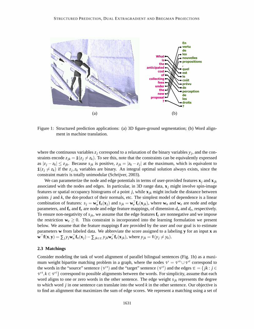
In figure-ground segmentation (see Fig. 1a), the node potentials capturelocal evidence aboutthe label of a pixel or range scan point. Edges usually connect nearbypixels in an image, and serveto correlate their labels. Assuming that such correlations tend to bepositive(connected nodes tendto have the same label) leads us to consider simplified edge potentials of the formφ jk(y j ,yk) =exp{−sjk1(y j 6= yk)}, wheresjk is a nonnegative penalty for assigningy j andyk different labels.Note that such potentials are regular ifsjk ≥ 0. Expressing node potentials asφ j(y j) = exp{sjy j},we haveP(y) ∝ exp

{∑ j∈V sjy j −∑ jk∈E sjk1(y j 6= yk)

}. Under this restriction on the potentials, we

can obtain the following (simpler) LP:

max0≤z≤1

∑j∈V

sjzj − ∑jk∈E

sjkzjk (5)

s.t. zj −zk ≤ zjk, zk−zj ≤ zjk, ∀ jk ∈ E ,

1630


Whatis

theanticipated

costof

collecting fees

under the

new proposal

?

En vertudelesnouvellespropositions, quelestle coûtprévude perception de les droits?

(a) (b)

Figure 1: Structured prediction applications: (a) 3D figure-ground segmentation; (b) Word align-ment in machine translation.

where the continuous variableszj correspond to a relaxation of the binary variablesy j , and the con-straints encodezjk = 1(zj 6= zk). To see this, note that the constraints can be equivalently expressedas |zj − zk| ≤ zjk. Becausesjk is positive,zjk = |zk − zj | at the maximum, which is equivalent to1(zj 6= zk) if the zj ,zk variables are binary. An integral optimal solution always exists, since theconstraint matrix is totally unimodular (Schrijver, 2003).

We can parameterize the node and edge potentials in terms of user-providedfeaturesx j andx jk

associated with the nodes and edges. In particular, in 3D range data,x j might involve spin-imagefeatures or spatial occupancy histograms of a pointj, while x jk might include the distance betweenpoints j andk, the dot-product of their normals, etc. The simplest model of dependenceis a linearcombination of features:sj = w⊤

n fn(x j) andsjk = w⊤e fe(x jk), wherewn andwe are node and edge

parameters, andfn andfe are node and edge feature mappings, of dimensiondn andde, respectively.To ensure non-negativity ofsjk, we assume that the edge featuresfe are nonnegative and we imposethe restrictionwe ≥ 0. This constraint is incorporated into the learning formulation we presentbelow. We assume that the feature mappingsf are provided by the user and our goal is to estimateparametersw from labeled data. We abbreviate the score assigned to a labelingy for an inputx asw⊤f(x,y) = ∑ j y jw⊤

n fn(x j)−∑ jk∈E y jkw⊤e fe(x jk), wherey jk = 1(y j 6= yk).

2.3 Matchings

Consider modeling the task of word alignment of parallel bilingual sentences(Fig. 1b) as a maxi-mum weight bipartite matching problem in a graph, where the nodesV = V s∪V t correspond tothe words in the “source” sentence(V s) and the “target” sentence(V t) and the edgesE = { jk : j ∈V s,k∈ V t} correspond to possible alignments between the words. For simplicity, assume that eachword aligns to one or zero words in the other sentence. The edge weightsjk represents the degreeto which word j in one sentence can translate into the wordk in the other sentence. Our objective isto find an alignment that maximizes the sum of edge scores. We represent a matching using a set of

1631


binary variablesy jk that are set to 1 if wordj is assigned to wordk in the other sentence, and 0 oth-erwise. The score of an assignment is the sum of edge scores:s(y) = ∑ jk∈E sjky jk. The maximumweight bipartite matching problem, argmaxy∈Y s(y), can be found by solving the following LP:

max0≤z≤1

∑jk∈E

sjkzjk (6)

s.t. ∑j∈V s

zjk ≤ 1, ∀k∈ V t ; ∑k∈V t

zjk ≤ 1, ∀ j ∈ V s.

where again the continuous variableszjk correspond to the relaxation of the binary variablesy jk.As in the min-cut problem, this LP is guaranteed to have integral solutions for any scoring functions(y) (Schrijver, 2003).

For word alignment, the scoressjk can be defined in terms of the word pairjk and input featuresassociated withx jk. We can include the identity of the two words, the relative position in the re-spective sentences, the part-of-speech tags, the string similarity (for detecting cognates), etc. We letsjk = w⊤f(x jk) for a user-provided feature mappingf and abbreviatew⊤f(x,y) = ∑ jk y jkw⊤f(x jk).

2.4 General Structure

More generally, we consider prediction problems in which the inputx ∈ X is an arbitrary structuredobject and the output is a vector of valuesy = (y1, . . . ,yLx) encoding, for example, a matching or acut in the graph. We assume that the lengthLx and the structure encoded byy depend determinis-tically on the inputx. In our word alignment example, the output space is defined by the length ofthe two sentences. Denote the output space for a given inputx asY (x) and the entire output spaceasY =

S

x∈X Y (x).Consider the class of structured prediction modelsH defined by the linear family:

hw(x) = argmaxy∈Y (x)

w⊤f(x,y), (7)

wheref(x,y) is a vector of functionsf : X × Y 7→ IRn. This formulation is very general. Indeed,it is too general for our purposes—for many(f,Y ) pairs, finding the optimaly is intractable. Wespecialize to the class of models in which the optimization problem in Eq. (7) can besolved in poly-nomial time via convex optimization; this is still a very large class of models. Beyond the examplesdiscussed here, it includes weighted context-free grammars and dependency grammars (Manningand Schutze, 1999) and string edit distance models for sequence alignment (Durbinet al., 1998).

3. Large Margin Estimation

We assume a set of training instancesS= {(xi ,yi)}mi=1, where each instance consists of a structured

objectxi (such as a graph) and a target solutionyi (such as a matching). Consider learning theparametersw in the conditional likelihood setting. We can definePw(y | x) = 1

Zw(x) exp{w⊤f(x,y)},

whereZw(x) = ∑y′∈Y (x) exp{w⊤f(x,y′)}, and maximize the conditional log-likelihood∑i logPw(yi |xi), perhaps with additional regularization of the parametersw. As we have noted earlier, however,the problem of computing the partition functionZw(x) is computationally intractable for many of theproblems we are interested in. In particular, it is #P-complete for matchings andmin-cuts (Valiant,1979; Jerrum and Sinclair, 1993).

1632


We thus retreat from conditional likelihood and consider the max-margin formulation developedin several recent papers (Collins, 2002; Altun et al., 2003; Taskar etal., 2004b). In this formulation,we seek to find parametersw such that:

yi = argmaxy′i∈Y i

w⊤f(xi ,y′i), ∀i,

whereY i = Y (xi). The solution spaceY i depends on the structured objectxi ; for example, the spaceof possible matchings depends on the precise set of nodes and edges in the graph.

As in univariate prediction, we measure the error of prediction using a lossfunction ℓ(yi ,y′i).To obtain a convex formulation, we upper bound the lossℓ(yi ,hw(xi)) using the hinge function:maxy′i∈Y i

[w⊤f i(y′i) + ℓi(y′i)−w⊤f i(yi)], whereℓi(y′i) = ℓ(yi ,y′i), andf i(y′i) = f(xi ,y′i). Minimizingthis upper bound will force the true structureyi to be optimal with respect tow for each instancei:

minw∈W

∑i

maxy′i∈Y i

[w⊤f i(y′i)+ ℓi(y′i)]−w⊤f i(yi), (8)

whereW is the set of allowed parametersw. We assume that the parameter spaceW is a convexset, typically a norm ball{w : ||w||p ≤ γ} with p= 1,2 and a regularization parameterγ. In the casethatW = {w : ||w||2 ≤ γ}, this formulation is equivalent to the standard large margin formulationusing slack variablesξ and slack penaltyC (cf. Taskar et al., 2004b), for some suitable values ofCdepending onγ. The correspondence can be seen as follows: letw∗(C) be a solution to the optimiza-tion problem with slack penaltyC and defineγ(C) = ||w∗(C)||. Thenw∗ is also a solution to Eq. (8).Conversely, we can invert the mappingγ(·) to find those values ofC (possibly non-unique) that giverise to the same solution as Eq. (8) for a specificγ. In the case of submodular potentials, there areadditional linear constraints on the edge potentials. In the setting of Eq. (5),we simply constrainwe ≥ 0. For general submodular potentials, we can parameterize the log of the edge potential usingfour sets of edge parameters,we00,we01,we10,we11, as follows: logφ jk(α,β) = w⊤

eαβf(x jk). Assum-ing, as before, that the edge features are nonnegative, the regularityof the potentials can be enforcedvia a linear constraint:we00+we11 ≥ we10+we01, where the inequality should be interpreted com-ponentwise.

The key to solving Eq. (8) efficiently is theloss-augmented inference problem,

maxy′i∈Y i

[w⊤f i(y′i)+ ℓi(y′i)]. (9)

This optimization problem has precisely the same form as the prediction problemwhose parameterswe are trying to learn—maxy′i∈Y i

w⊤f i(y′i)—but with an additional term corresponding to the lossfunction. Tractability of the loss-augmented inference thus depends not only on the tractability ofmaxy′i∈Y i

w⊤f i(y′i), but also on the form of the loss termℓi(y′i). A natural choice in this regard is theHamming distance, which simply counts the number of variables in which a candidate solutiony′idiffers from the target outputyi . In general, we need only assume that the loss function decomposesover the variables inyi .

In particular, for word alignment, we use weighted Hamming distance, which counts the numberof variables in which a candidate matchingy′i differs from the target alignmentyi , with different costfor false positives(c+) and false negatives(c-):

ℓ(yi ,y′i) = ∑jk∈E i

[c-yi, jk(1−y′i, jk)+c+ y′i, jk(1−yi, jk)

](10)

= ∑jk∈E i

c-yi, jk + ∑jk∈E i

[c+ − (c- +c+)yi, jk]y′i, jk,

1633


whereyi, jk indicates the presence of edgejk in examplei andE i is the set of edges in examplei.The loss-augmented matching problem can then be written as an LP similar to Eq. (6) (without theconstant term∑ jk c-yi, jk):

max0≤zi≤1

∑jk∈E i

zi, jk[w⊤f(xi, jk)+c+ − (c- +c+)yi, jk]

s.t. ∑j∈V s

i

zi, jk ≤ 1, ∀k∈ V ti ; ∑

k∈V ti

zi, jk ≤ 1, ∀ j ∈ V si ,

wheref(xi, jk) is the vector of features of the edgejk in examplei andV si andV t

i are the nodes inexamplei. As before, the continuous variableszi, jk correspond to the binary valuesy′i, jk.

Generally, suppose we can express the prediction problem as an LP:

maxy′i∈Y i

w⊤f i(y′i) = maxzi∈Z i

w⊤Fizi ,

whereZ i = {zi : A izi ≤ bi , 0≤ zi ≤ 1}, (11)

for appropriately definedFi ,A i andbi . Then we have a similar LP for the loss-augmented inferencefor each examplei:

maxy′i∈Y i

w⊤f i(y′i)+ ℓi(y′i) = di +maxzi∈Z i

(F⊤i w+ci)

⊤zi , (12)

for appropriately defineddi andci . For the matching case,di = ∑ jk c-yi, jk is the constant term,Fi isa matrix that has a column of featuresf(xi, jk) for each edgejk in examplei, andci is the vector ofthe loss termsc+−(c- +c+)yi, jk. Letz= {z1, . . . ,zm} andZ = Z1× . . .×Zm. With these definitions,we have the following saddle-point problem:

minw∈W

maxz∈Z

∑i

(w⊤Fizi +c⊤i zi −w⊤f i(yi)

). (13)

where we have omitted the constant term∑i di . The only difference between this formulation andour initial formulation in Eq. (8) is that we have created a concise continuous optimization problemby replacing the discretey′i ’s with continuouszi ’s.

When the prediction problem is intractable (for example, in general Markovnetworks or tripar-tite matchings), we can use a convex relaxation (for example, a linear or semidefinite program) toupper bound maxy′i∈Y i

w⊤f i(y′i) and obtain an approximate maximum-margin formulation. This isthe approach taken in Taskar et al. (2004b) for general Markov networks using the LP in Eq. (1).

To solve (13), we could proceed by making use of Lagrangian duality. This approach, exploredin Taskar et al. (2004a, 2005a), yields a joint convex optimization problem.If the parameter spaceW is described by linear and convex quadratic constraints, the result is a convex quadratic programwhich can be solved using a generic QP solver.

We briefly outline this approach below, but in this paper, we take a different tack, solving theproblem in its natural saddle-point form. As we discuss in the following section, this approachallows us to exploit the structure ofW andZ separately, allowing for efficient solutions for a widerrange of parameterizations and structures. It also opens up alternatives with respect to numericalalgorithms.

1634


Before moving on to solution of the saddle-point problem, we consider the joint convex formwhen the feasible set has the form of (11) and the loss-augmented inference problem is a LP, asin (12). Using commercial convex optimization solvers for this formulation will provide us with acomparison point for our saddle-point solver. We now proceed to present this alternative form.

To transform the saddle-point form of (13) into a standard convex optimization form, we takethe dual of the individual loss-augmented LPs (12):

maxzi∈Z i

(F⊤i w+ci)

⊤zi = min(λi ,µi)∈Λi(w)

b⊤i λi +1⊤µi (14)

whereΛi(w)= {(λi ,µi)≥ 0 : F⊤i w+ci ≤A⊤

i λi +µi} defines the feasible space for the dual variablesλi andµi . Substituting back in equation (13) and writingλ = (λ1, . . . ,λm), µ = (µ1, . . . ,µm), weobtain (omitting the constant∑i di):

minw∈W ,(λ,µ)≥0

∑i

(b⊤

i λi +1⊤µi −w⊤f i(yi))

(15)

s.t. F⊤i w+ci ≤ A⊤

i λi +µi i = 1, . . . ,m.

If W is defined by linear and convex quadratic constraints, the above optimizationproblem can besolved using standard commercial solvers. The number of variables and constraints in this problemis linear in the number of the parametersand the training data (for example nodes and edges).

4. Saddle-Point Problems and the Dual Extragradient Method

We begin by establishing some notation and definitions. Denote the objective ofthe saddle-pointproblem in (13) by:

L (w,z) ≡ ∑i

w⊤Fizi +c⊤i zi −w⊤f i(yi).

L (w,z) is bilinear inw andz, with gradient given by:∇wL (w,z) = ∑i Fizi − f i(yi) and∇ziL (w,z) =F⊤

i w+ci .We can view this problem as a zero-sum game between two players,w andz. Consider a simple

iterative improvement method based on gradient projections:

wt+1 = πW (wt −η∇wL (wt ,zt)); zt+1i = πZ i (z

ti +η∇ziL (w

t ,zt)), (16)

whereη is a step size andπV (v) = argminv′∈V ||v− v′||2 denotes the Euclidean projection of avectorv onto a convex setV . In this simple iteration, each player makes a small best-responseimprovement without taking into account the effect of the change on the opponent’s strategy. Thisusually leads to oscillations, and indeed, this method is generally not guaranteed to converge forbilinear objectives for any step size (Korpelevich, 1976; He and Liao, 2002). One way forward isto attempt to average the points(wt ,zt) to reduce oscillation. We pursue a different approach thatis based on the dual extragradient method of Nesterov (2003). In our previous work (Taskar et al.,2006), we used a related method, the extragradient method due to Korpelevich (1976). The dualextragradient is, however, a more flexible and general method, in terms ofthe types of projectionsand feasible sets that can be used, allowing a broader range of structured problems and parameterregularization schemes. Before we present the algorithm, we introduce some notation which will beuseful for its description.

1635


Let us combinew and z into a single vector,u = (w,z), and define the joint feasible spaceU =W ×Z . Note thatU is convex since it is a direct product of convex sets.

We denote the (affine) gradient operator on this joint space as

∇wL (w,z)−∇z1L (w,z)

...−∇zmL (w,z)

=

0 F1 · · · Fm

−F⊤1

... 0−F⊤

m

︸︷︷︸

wz1...

zm

︸︷︷︸

−

∑i f i(yi)c1...

cm

︸︷︷︸

= Fu−a.

F u a

4.1 Dual Extragradient

We first present the dual extragradient algorithm of Nesterov (2003)using the Euclidean geometryinduced by the standard 2-norm, and consider a non-Euclidean setup in Sec. 4.2.

As shown in Fig. 2, the dual extragradient algorithm proceeds using very simple gradient andprojection calculations.

Initialize: Chooseu ∈ U , sets−1 = 0.Iterationt, 0≤ t ≤ τ:

v = πU (u+ηst−1);

ut = πU (v−η(Fv−a)); (17)

st = st−1− (Fut −a).

Output: uτ = 1τ+1 ∑τ

t=0ut .

Figure 2: Euclidean dual extragradient.

To relate this generic algorithm to our setting, recall thatu is composed of subvectorsw andz; this induces a commensurate decomposition of thev and s vectors into subvectors. To referto these subvectors we will abuse notation and use the symbolsw and zi as indices. Thus, wewrite v = (vw,vz1, . . . ,vzm), and similarly foru ands. Using this notation, the generic algorithmin Eq. (17) expands into the following dual extragradient algorithm for structured prediction (wherethe brackets represent gradient vectors):

vw = πW (uw +ηst−1w ); vzi = πZ i (uzi +ηst−1

zi), ∀i;

utw = πW (vw −η

[

∑i

Fivzi − f i(yi)

]); ut

zi= πZ i (vzi +η

[F⊤

i vw +ci

]), ∀i;

stw = st−1

w −

[

∑i

Fiutzi− f i(yi)

]; st

zi= st−1

zi+

[F⊤

i utw +ci

], ∀i.

In the convergence analysis of dual extragradient (Nesterov, 2003), the stepsizeη is set to theinverse of the Lipschitz constant (with respect to the 2-norm) of the gradient operator:

1/η = L ≡ maxu,u′∈U

||F(u−u′)||2||u−u′||2

≤ ||F||2,

1636


where||F||2 is the largest singular value of the matrixF. In practice, various simple heuristics can beconsidered for setting the stepsize, including search procedures based on optimizing the gap meritfunction (see, e.g., He and Liao, 2002).

4.1.1 CONVERGENCE

One measure of quality of a saddle-point solution is via the gap function:

G (w,z) =

[maxz′∈ZL (w,z′)−L ∗

]+

[L ∗− min

w′∈WL (w′,z)

], (18)

where the optimal loss is denotedL ∗ = minw′∈W maxz∈Z L (w,z). For non-optimal points(w,z),the gapG (w,z) is positive and serves as a useful merit function, a measure of accuracy of a solutionfound by the extragradient algorithm. At an optimum we have

G (w∗,z∗) = maxz′∈ZL (w∗,z′)− min

w′∈WL (w′,z∗) = 0.

Define the Euclidean divergence function as

d(v,v′) =12||v−v′||22,

and define a restricted gap function parameterized by positive divergence radiiDw andDz

GDw,Dz(w,z) = maxz′∈Z

[L (w,z′) : d(z,z′) ≤ Dz

]− min

w′∈W

[L (w′,z) : d(w,w′) ≤ Dw

],

where the pointu = (uw, uz) ∈ U is an arbitrary point that can be thought of as the “center” ofU .Assuming there exists a solutionw∗,z∗ such thatd(w,w∗) ≤ Dw andd(z,z∗) ≤ Dz, this restrictedgap function coincides with the unrestricted function defined in Eq. (18). The choice of the centerpoint u should reflect an expectation of where the “average” solution lies, as willbe evident from theconvergence guarantees presented below. For example, we can takeuw = 0 and letuzi correspondto the encoding of the targetyi .

By Theorem 2 of Nesterov (2003), afterτ iterations, the gap of(wτ, zτ) = uτ is upper boundedby:

GDw,Dz(wτ, zτ) ≤

(Dw +Dz)Lτ+1

. (19)

This implies thatO (1ε ) steps are required to achieve a desired accuracy of solutionε as measured by

the gap function. Note that the exponentiated gradient algorithm (Bartlett etal., 2005) has the sameO (1

ε ) convergence rate. This sublinear convergence rate is slow compared tointerior point methods,which enjoy superlinear convergence (Boyd and Vandenberghe, 2004). However, the simplicityof each iteration, the locality of key operations (projections), and the linearmemory requirementsmake this a practical algorithm when the desired accuracyε is not too small, and, in particular, theseproperties align well with the desiderata of large-scale machine learning algorithms. We illustratethese properties experimentally in Section 6.

1637


j

s t

k

Figure 3: Euclidean projection onto the matching polytope using min-cost quadratic flow. Sources is connected to all the “source” nodes and targett connected to all the “target” nodes,using edges of capacity 1 and cost 0. The original edgesjk have a quadratic cost1

2(z′jk −

zjk)2 and capacity 1.

4.1.2 PROJECTIONS

The efficiency of the algorithm hinges on the computational complexity of the Euclidean projectiononto the feasible setsW andZ i . In the case ofW , projections are cheap when we have a 2-normball {w : ||w||2 ≤ γ}: πW (w) = γw/max(γ, ||w||2). Additional non-negativity constraints on theparameters (e.g.,we ≥ 0) can also be easily incorporated by clipping negative values. Projectionsonto the 1-norm ball are not expensive either (Boyd and Vandenberghe, 2004), but may be betterhandled by the non-Euclidean setup we discuss below.

We turn to the consideration of the projections ontoZ i . The complexity of these projectionsis the key issue determining the viability of the extragradient approach for our class of problems.In fact, for both alignment and matchings these projections turn out to reduce to classical networkflow problems for which efficient solutions exist. In case of alignment,Z i is the convex hull of thebipartite matching polytope and the projections ontoZ i reduce to the much-studied minimum costquadratic flow problem (Bertsekas, 1998). In particular, the projectionproblemz = πZ i (z

′i) can be

computed by solving

min0≤zi≤1

∑jk∈E i

12(z′i, jk −zi, jk)

2

s.t. ∑j∈V s

i

zi, jk ≤ 1, ∀ j ∈ V ti ; ∑

k∈V ti

zi, jk ≤ 1, ∀k∈ V si .

We use a standard reduction of bipartite matching to min-cost flow (see Fig. 3)by introducing asource nodesconnected to all the words in the “source” sentence,V s

i , and a target nodet connectedto all the words in the “target” sentence,V t

i , using edges of capacity 1 and cost 0. The originaledgesjk have a quadratic cost1

2(z′i, jk − zi, jk)2 and capacity 1. Since the edge capacities are 1, the

flow conservation constraints at each original node ensure that the (possibly fractional) degree ofeach node in a valid flow is at most 1. Now the minimum cost flow from the sources to the targettcomputes projection ofz′i ontoZ i .

1638


The reduction of the min-cut polytope projection to a convex network flow problem is morecomplicated; we present this reduction in Appendix A. Algorithms for solving convex networkflow problems (see, for example, Bertsekas et al., 1997) are nearly as efficient as those for solvinglinear min-cost flow problems, bipartite matchings and min-cuts. In case of word alignment, therunning time scales with the cube of the sentence length. We use standard, publicly-available codefor solving this problem (Guerriero and Tseng, 2002).2

4.2 Non-Euclidean Dual Extragradient

Euclidean projections may not be easy to compute for many structured prediction problems or pa-rameter spaces. The non-Euclidean version of the algorithm of Nesterov(2003) affords flexibilityto use other types of (Bregman) projections. The basic idea is as follows. Let d(u,u′) denote asuitable divergence function (see below for a definition) and define a proximal step operator:

Tη(u,s) ≡ argmaxu′∈U

[s⊤(u′−u)−1η

d(u,u′)].

Intuitively, the operator tries to make a large step fromu in the direction ofs but not too large asmeasured byd(·, ·). Then the only change to the algorithm is to switch from using a Euclideanprojection of a gradient stepπU (u + 1

ηs) to a proximal step in a direction of the gradientTη(u,s)(see Fig. 4):

Initialize: Chooseu ∈ U , sets−1 = 0.Iterationt, 0≤ t ≤ τ:

vw = Tη(uw,st−1w ); vzi = Tη(uzi ,s

t−1zi

), ∀i;

utw = Tη(vw,−

[

∑i

Fivzi − f i(yi)

]); ut

zi= Tη(vzi ,

[F⊤

i vw +ci

]), ∀i;

stw = st−1

w −

[

∑i

Fiutzi− f i(yi)

]; st

zi= st−1

zi+

[F⊤

i utw +ci

], ∀i.

Output: uτ = 1τ+1 ∑τ

t=0ut .

Figure 4: Non-Euclidean dual extragradient.

To define the range of possible divergence functions and to state convergence properties of thealgorithm, we will need some more definitions. We follow the development of Nesterov (2003).Given a norm|| · ||W onW and norms|| · ||Z i onZ i , we combine them into a norm onU as

||u|| = max(||w||W , ||z1||Z1, . . . , ||zm||

Zm).

We denote the dual ofU (the vector space of linear functions onU ) asU ∗. The norm|| · || on thespaceU induces the dual norm|| · ||∗ for all s∈ U ∗:

||s||∗ ≡ maxu∈U ,||u||≤1

s⊤u.

2. Available from http://www.math.washington.edu/∼tseng/netflowgnl/.

1639


The Lipschitz constant with respect to this norm (used to setη = 1/L) is

L ≡ maxu,u′∈U

||F(u−u′)||∗||u−u′||

.

The dual extragradient algorithm adjusts to the geometry induced by the norm by making useof Bregman divergences. We assume a strongly convex functionh(u):

h(αu+(1−α)u′) ≤ αh(u)+(1−α)h(u′)−α(1−α)σ2||u−u′||2, ∀u,u′,α ∈ [0,1],

for someσ > 0, the convexity parameter ofh(·). This function is constructed from strongly convexfunctions on each of the spacesW andZ i by a simple sum:h(u) = h(w)+ ∑i h(zi). Its conjugateis defined as:

h∗(s) ≡ maxu∈U

[s⊤u−h(u)].

Sinceh(·) is strongly convex,h∗(u) is well-defined and differentiable at anys∈ U ∗. We define

U ≡ {∇h∗(s) : s∈ U ∗}.

We further assume thath(·) is differentiable at anyu ∈ U ; since it is also strongly convex, for anytwo pointsu ∈ U andu′ ∈ U we have

h(u′) ≥ h(u)+∇h(u)⊤(u′−u)+σ2||u′−u||2,

and we can define the Bregman divergence:

d(u,u′) = h(u′)−h(u)−∇h(u)⊤(u′−u).

Note that when|| · || is the 2-norm, we can useh(u) = 12||u||

22, which has convexity parameterσ = 1,

and induces the usual squared Euclidean distanced(u,u′) = 12||u−u′||22. When|| · || is the 1-norm,

we can use the negative entropyh(u) = −H(u) (say ifU is a simplex), which also hasσ = 1 andrecovers the Kullback-Leibler divergenced(u,u′) = KL(u′||u).

With these definitions, the convergence bound in Eq. (19) applies to the non-Euclidean setup,but now the divergence radii are measured using Bregman divergence and the Lipschitz constant iscomputed with respect to a different norm.

EXAMPLE 1: L1 REGULARIZATION

SupposeW = {w : ||w||1 ≤ γ}. We can transform this constraint set into a simplex constraint by thefollowing variable transformation. Letw = w+−w−, v0 = 1−||w||1/γ, andv ≡ (v0,w+/γ,w−/γ).ThenV = {v : v ≥ 0;1⊤v = 1} corresponds toW . We defineh(v) as the negative entropy ofv:

h(v) = ∑d

vd logvd.

The resulting conjugate function and its gradient are given by

h∗(s) = log∑d

esd ;∂h∗(s)

∂sd=

esd

∑d esd.

1640


Hence, the gradient space ofh∗(s) is the interior of the simplex,V = {v : v > 0;1⊤v = 1}. Thecorresponding Bregman divergence is the standard Kullback-Leibler divergence

d(v,v′) = ∑d

v′d logv′dvd

, ∀v ∈ V ,v′ ∈ V ,

and the Bregman proximal step or projection,v = Tη(v,s) = argmaxv′∈v[s⊤v′− 1

ηd(v,v′)] is givenby a multiplicative update:

vd =vdeηsd

∑d vdeηsd.

Note that we cannot chooseuv = (1,0,0) as the center ofV —given that the updates are multi-plicative the algorithm will not make any progress in this case. In fact, this choice is precluded by

the constraint thatuv ∈ V , not justuv ∈ V . A reasonable choice is to setuv to be the center of thesimplexV , uvd = 1

|V |= 1

2|W |+1.

EXAMPLE 2: TREE-STRUCTURED MARGINALS

Consider the case in which each examplei corresponds to a tree-structured Markov network, andZ i

is defined by the normalization and marginalization constraints in Eq. (2) and Eq. (3) respectively.These constraints define the space of valid marginals. For simplicity of notation, we assume thatwe are dealing with a single examplei and drop the explicit indexi. Let us use a more suggestivenotation for the components ofz: zj(α) = zjα andzjk(α,β) = zjkαβ. We can construct a natural jointprobability distribution via

Pz(y) = ∏jk∈E

zjk(y j ,yk) ∏j∈V

(zj(y j))1−q j ,

whereq j is the number of neighbors of nodej. Now z defines a point on the simplex of jointdistributions overY , which has dimension|Y |. One natural measure of complexity in this enlargedspace is the 1-norm. We defineh(z) as the negative entropy of the distribution represented byz:

h(z) = ∑jk∈E

∑α∈D j ,β∈D k

zjk(α,β) logzjk(α,β)+(1−q j) ∑j∈V

∑α∈D j

zj(α) logzj(α).

The resultingd(z,z′) is the Kullback-Leibler divergence KL(Pz′ ||Pz). The corresponding Breg-man step or projection operator,z = Tη(z,s) = argmaxz′∈Z [s

⊤z′− 1ηKL(Pz′ ||Pz)] is given by a mul-

tiplicative update on the space of distributions:

Pz(y) =1Z

Pz(y)eη[∑ jk sjk(y j ,yk)+∑ j sj (y j )] =1Z ∏

jk

zjk(y j ,yk)eηsjk(y j ,yk) ∏

j(zj(y j))

1−q j eηsj (y j ),

where we use the same indexing for the dual space vectorsas forz andZ is a normalization constant.Hence, to obtain the projectionz, we compute the node and edge marginals of the distributionPz(y)via the standard sum-product dynamic programming algorithm using the node and edge potentialsdefined above. Note that the form of the multiplicative update of the projectionresembles that ofexponentiated gradient. As in the example above, we cannot letuz be a corner (or any boundarypoint) of the simplex sinceZ does not include it. A reasonable choice foruz would be either thecenter of the simplex or a point near the target structure but in the interior ofthe simplex.

1641


5. Memory-Efficient Formulation

Consider the memory requirements of the algorithm. The algorithm maintains the vector sτ as wellas the running average,uτ, a total dimensionality of|W |+ |Z |. Note, however, that these vectorsare related very simply by:

sτ = −τ

∑t=0

(Fut −a) = −(τ+1)(Fuτ −a).

So it suffices to only maintain the running averageuτ and reconstructs as needed.In problems in which the number of examples,m, is large we can take advantage of the fact

that the memory needed to store the target structureyi is often much smaller than the correspondingvectorzi . For example, for word alignment, we needO (|V s

i | log|V ti |) bits to encode a matchingyi

by using roughly logV ti bits per node inV s

i to identify its match. By contrast, we need|V si ||V

ti |

floating numbers to maintainzi . The situation is worse in context-free parsing, where a parse treeyi requires space linear in the sentence length and logarithmic in grammar size, while |Z i | is theproduct of the grammar size and the cube of the sentence length.

Note that fromuτ = (uτw, uτ

z), we only care aboutuτw, the parameters of the model, while the

other component,uτz, maintains the state of the algorithm. Fortunately, we can eliminate the need

to storeuz by maintaining it implicitly, at the cost of storing a vector of size|W |. This allows us toessentially have the same small memory footprint of online-type learning methods, where a singleexample is processed at a time and only a vector of parameters is maintained. Inparticular, insteadof maintaining the entire vectorut and reconstructingst from ut , we can instead store onlyut

w andstw between iterations, since

stzi

= (t +1)(F⊤i ut

w +ci).

The diagram in Fig. 5 illustrates the process and the algorithm is summarized in Fig. 6. Weuse two “temporary” variablesvw and rw of size |W | to maintain intermediate quantities. Theadditional vectorqw shown in Fig. 5 is introduced only to allow the diagram to be drawn in asimplified manner; it can be eliminated by usingsw to accumulate the gradients as shown in Fig. 6.The total amount of memory needed is thus four times the number of parameters plus memory fora single example(vzi ,uzi ). We assume that we do not need to storeuzi explicitly but can constructit efficiently from (xi ,yi).

Note that in case the dimensionality of the parameter space is much larger than thedimen-sionality of Z , we can use a similar trick to only store variables of the size ofz. In fact, ifW = {w : ||w||2 ≤ γ} and we use Euclidean projections ontoW , we can exploit kernels to de-fine infinite-dimensional feature spaces and derive a kernelized version of the algorithm.

6. Experiments

In this section we describe experiments focusing on two of the structured models we describedearlier: bipartite matchings for word alignments and restricted potential Markov nets for 3D seg-mentation.3 We compared three algorithms: the dual extragradient (dual-ex ), the averaged pro-jected gradient (proj-grad ) defined in Eq. (16), and the averaged perceptron (Collins, 2002). For

3. Software implementing our dual extragradient algorithm can be foundathttp://www.cs.berkeley.edu/ ∼slacoste/research/dualex .

1642


Figure 5: Dependency diagram for memory-efficient dual extragradient. The dotted box representsthe computations of an iteration of the algorithm. Onlyut

w andstw are kept between itera-

tions. Each example is processed one by one and the intermediate results areaccumulatedasrw = rw −Fivzi + f i(yi) andqw = qw −Fiuzi + f i(yi). Details shown in Fig. 6, exceptthat intermediate variablesuw andqw are only used here for pictorial clarity.

Initialize: Chooseu ∈ U , sw = 0, uw = 0, η = 1/L.Iterationt, 0≤ t ≤ τ:

vw = Tη(uw,sw); rw = 0.Examplei, 1≤ i ≤ m:

vzi = Tη(uzi , t(F⊤i uw +ci)); rw = rw −Fivzi + f i(yi);

uzi = Tη(vzi ,F⊤i vw +ci); sw = sw −Fiuzi + f i(yi).

uw =tuw+Tη(vw,rw)

t+1 .Outputw = uw.

Figure 6: Memory-efficient dual extragradient.

dual-ex and proj-grad , we used Euclidean projections, which can be formulated as min-costquadratic flow problems. We usedw = 0 andzi corresponding toyi as the centroidu in dual-exand as the starting point ofproj-grad .

In our experiments, we consider standardL2 regularization,{||w||2 ≤ γ}. A question whicharises in practice is how to choose the regularization parameterγ. The typical approach is to run thealgorithm for several values of the regularization parameter and pick the best model using a valida-tion set. This can be quite expensive, though, and several recent papers have explored techniquesfor obtaining the whole regularization path, either exactly (Hastie et al., 2004), or approximately us-ing path following techniques (Rosset, 2004). Instead, we run the algorithm without regularization(γ = ∞) and track its performance on the validation set, selecting the model with best performance.For comparison, whenever feasible with the available memory, we used commercial software tocompute points on the regularization path. As we discuss below, the dual extragradient algorithmapproximately follows the regularization path in our experiments (in terms of the training objective

1643


and test error) in the beginning and the end of the range ofγ and often performs better in terms ofgeneralization error in the mid-range.

6.1 Object Segmentation

We tested our algorithm on a 3D scan segmentation problem using the class of Markov networkswith regular potentials that were described above. The dataset is a challenging collection of clutteredscenes containing articulated wooden puppets (Anguelov et al., 2005). It contains eleven differentsingle-view scans of three puppets of varying sizes and positions, with clutter and occluding objectssuch as rope, sticks and rings. Each scan consists of around 7,000 points. Our goal was to segmentthe scenes into two classes—puppet andbackground. We use five of the scenes for our trainingdata, three for validation and three for testing. Sample scans from the training and test set can beseen athttp://www.cs.berkeley.edu/˜taskar/3DSegment/ . We computed spin images of size 10× 5bins at two different resolutions, then scaled the values and performed PCA to obtain 45 principalcomponents, which comprised our node features. We used the surface links output by the scanner asedges between points and for each edge only used a single feature, setto a constant value of 1 for alledges. This results in all edges having the same potential. The training data contains approximately37,000 nodes and 88,000 edges. We used standard Hamming distance for our loss functionℓ(yi ,y′i).

We compared the performance of the dual extragradient algorithm along itsunregularized pathto solutions of the regularized problems for different settings of the norm.4 For dual extragradient,the stepsize is set toη = 1/||F||2 ≈ 0.005. We also compared to a variant of the averaged perceptronalgorithm (Collins, 2002), where we use the batch updates to stabilize the algorithm, since we onlyhave five training examples. We set the learning rate to 0.0007 by trying several values and pickingthe best value based on the validation data.

In Fig. 7(a) we track the hinge loss on the training data:

∑i

maxy′i∈Y i

[w⊤f i(y′i)+ ℓi(y′i)]−w⊤f i(yi). (20)

The hinge loss of the regularization path (reg-path ) is the minimum loss for a given norm, andhence is always lower than the hinge loss of the other algorithms. However,as the norm increasesand the model approaches the unregularized solution,dual-ex loss tends towards that ofreg-path .Note thatproj-grad behaves quite erratically in the range of the norms shown. Fig. 7(b) showsthe growth of the norm as a function of iteration number fordual-ex andave-perc . The unreg-ularized dual extragradient seems to explore the range of models (in terms on their norm) on theregularization path more thoroughly than the averaged perceptron and eventually asymptotes to theunregularized solution, whileproj-grad quickly achieves very large norm.

Fig. 7(c) and Fig. 7(d) show validation and test error for the three algorithms. The best valida-tion and test error achieved by thedual-ex andave-perc algorithms as well asreg-path are fairlyclose, however, this error level is reached at very different norms.Since the number of scenes in thevalidation and test data is very small (three), because of variance, the best norm on validation is notvery close to the best norm on the test set. Selecting the best model on the validation set leads totest errors of 3.4% for dual-ex , 3.5% for ave-perc , 3.6% for reg-path and 3.8% for proj-grad

4. We used CPLEX to solve the regularized problems and also to find the projections onto the min-cut polytope, sincethe min-cost quadratic flow code we used (Guerriero and Tseng, 2002) does not support negative flows on edges,which are needed in the formulation presented in Appendix A.

1644


0 10 20 30 40 50 60 700

0.5

1

1.5

2x 10

4

||w||2

loss

proj−gradave−percdual−exreg−path

0 200 400 600 800 10000

50

100

150

200

250

300

350

400

iteration

||w|| 2

proj−gradave−percdual−ex

(a) (b)

0 10 20 30 40 50 60 700

0.02

0.04

0.06

0.08

0.1

0.12

0.14

0.16

||w||2

erro

r

proj−gradave−percdual−exreg−path

0 10 20 30 40 50 60 700

0.02

0.04

0.06

0.08

0.1

0.12

0.14

0.16

||w||2

erro

rproj−gradave−percdual−exreg−path

(c) (d)

Figure 7: Object segmentation results: (a) Training hinge loss for the regularization path(reg-path ), the averaged projected gradient (proj-grad ), the averaged perceptron(ave-perc ) and unregularized dual extragradient (dual-ex ) vs. the norm of the pa-rameters. (b) Norm of the parameters vs. iteration number for the three algorithms.(c) Validation error vs. the norm of the parameters. (d) Test error vs.the norm of theparameters.

(proj-grad actually improves performance after the model norm is larger than 500, which is notshown in the graphs).

6.2 Word Alignment

We also tested our algorithm on word-level alignment using a data set from the 2003 NAACLset (Mihalcea and Pedersen, 2003), the English-French Hansards task. This corpus consists of1.1M pairs of sentences, and comes with a validation set of 37 sentence pairs and a test set of 447word-aligned sentences. The validation and test sentences have been hand-aligned (see Och andNey, 2003) and are marked with bothsureandpossiblealignments. Using these alignments, thealignment error rate(AER) is calculated as:

AER(A,S,P) = 1−|A∩S|+ |A∩P|

|A|+ |S|,

1645


whereA is a set of proposed alignment pairs,S is the set of sure gold pairs, andP is the set ofpossible gold pairs (whereS⊆ P).

We experimented with two different training settings. In the first one, we splitthe original testset into 100 training examples and 347 test examples—this dataset is called the ‘Gold’ dataset. Inthe second setting, we used GIZA++ (Och and Ney, 2003) to produce IBM Model 4 alignments forthe unlabeled sentence pairs. We took the intersection of the predictions of the English-to-Frenchand French-to-English Model 4 alignments on the first 5000 sentence pairs from the 1.1M sentencesin order to experiment with the scaling of our algorithm (training on 500, 1000and 5000 sentences).The number of edges for 500, 1000 and 5000 sentences of GIZA++ were about 31,000, 99,000 and555,000 respectively. We still tested on the 347 Gold test examples, and used the validation setto select the stopping point. The stepsize for the dual extragradient algorithm was chosen to be1/||F||2.

We used statistics computed on the 1.1M sentence pairs as the edge features for our model. Adetailed analysis of the constructed features and corresponding erroranalysis is presented in Taskaret al. (2005b). Example features include: a measure of mutual information between the two wordscomputed from their co-occurrence in the aligned sentences (Dice coefficient); the difference be-tween word positions; character-based similarity features designed to capture cognate (and exactmatch) information; and identity of the top five most frequently occurring words. We used thestructured lossℓ(yi ,y′i) defined in Eq. (10) with(c+,c-) = (1,3) (where 3 was selected by testingseveral values on the validation set). We obtained low recall when using equal cost for both typeof errors because the number of positive edges is significantly smaller thanthe number of negativeedges, and so it is safe (precision-wise) for the model to predict feweredges, hurting the recall.Increasing the cost for false negatives solves this problem.

Fig. 8(a) and Fig. 8(e) compare the hinge loss of the regularization path withthe evolution ofthe objective for the unregularized dual extragradient, averaged projected gradient and averagedperceptron algorithms when trained on the Gold data set, 500 sentences and1000 sentences of theGIZA++ output respectively.5 The dual extragradient path appears to follow the regularization pathclosely for ||w|| ≤ 2 and||w|| ≥ 12. Fig. 8(b) compares the AER on the test set along the dualextragradient path trained on the Gold dataset versus the regularization path AER. The results onthe validation set for each path are also shown. On the Gold data set, the minimumAER wasreached roughly after 200 iterations.

Interestingly, the unregularized dual extragradient path seems to give better performance on thetest set than that obtained by optimizing along the regularization path. The dominance of the dualextragradient path over the regularization path is more salient in figure 8(f) for the case where bothare trained on 1000 sentences from the GIZA++ output. We conjecture that the dual extragradi-ent method provides additional statistical regularization (compensating for the noisier labels of theGIZA++ output) by enforcing local smoothness of the path in parameter space.

The averaged projected gradient performed much better for this task thansegmentation, gettingsomewhat close to the dual extragradient path as is shown in Fig. 8(c). The online version of theaveraged perceptron algorithm varied significantly with the order of presentation of examples (up tofive points of difference in AER between two orders). To alleviate this, we randomize the order ofthe points at each pass over the data. Fig. 8(d) shows that a typical run of averaged perceptron doessomewhat worse than dual extragradient. The variance of the averaged perceptron performance for

5. The regularization path is obtained by using the commercial optimization software Mosek with the QCQP formulationof Eq. (15). We did not obtain the path in the case of 5000 sentences, as Mosek runs out of memory.

1646


0 5 10 15 201000

1500

2000

2500

3000

3500

||w||2

loss

ave−percproj−graddual−exreg−path

0 5 10 15 200.05

0.055

0.06

0.065

0.07

0.075

0.08

0.085

0.09

||w||2

AE

R

reg−path valid.dual−ex valid.reg−path testdual−ex test

(a) (b)

0 5 10 15 200.05

0.055

0.06

0.065

0.07

0.075

0.08

0.085

0.09

||w||2

AE

R

proj−grad valid.dual−ex valid.proj−grad testdual−ex test

0 5 10 15 200.05

0.06

0.07

0.08

0.09

0.1

0.11

||w||2

AE

R

ave−perc valid.dual−ex valid.ave−perc testdual−ex test

(c) (d)

0 5 10 15 20 25 300

0.5

1

1.5

2

2.5

3x 10

4

||w||2

loss

dual−ex 1kreg−path 1kdual−ex 500reg−path 500

0 5 10 15 20 25 300.1

0.105

0.11

0.115

0.12

0.125

0.13

||w||2

AE

R

reg−path 1kdual−ex 1kdual−ex 5k

(e) (f)

Figure 8: Word alignment results: (a) Training hinge loss for the three different algorithms and the regularization pathon the Gold dataset. (b) AER for the unregularized dual extragradient (dual-ex ) and the regularization path(reg-path ) on the 347 Gold sentences (test ) and the validation set (valid ) when trained on the 100 Goldsentences; (c) Same setting as in (b), comparingdual-ex with the averaged projected-gradient (proj-grad );(d) Same setting as in (b), comparingproj-grad with the averaged perceptron (ave-perc ); (e) Traininghinge loss fordual-ex andreg-path on 500 and 1000 GIZA++ labeled sentences. (f) AER fordual-exandreg-path tested on the Gold test set and trained on 1000 and 5000 GIZA++ sentences. The graph for500 sentences is omitted for clarity.

1647


different datasets and learning rate choices was also significantly higherthan for dual extragradient,which is more stable numerically. The online version of the averaged perceptron converged veryquickly to its minimum AER score; converging in as few as five iterations for the Gold training set.Selecting the best model on the validation set leads to test errors of 5.6% for dual-ex , 5.6% forreg-path , 5.8% for proj-grad and 6.1% for ave-perc on the Gold data training set.

The running time for 500 iterations of dual extragradient on a 3.4 Ghz IntelXeon CPU with4G of memory was roughly 10 minutes, 30 minutes and 3 hours for 500, 1000 and 5000 sentences,respectively, showing the favorable linear scaling of the algorithm (linearin the number of edges).Note, by way of comparison, that Mosek ran out of memory for more than 1500 training sentences.

The framework we have presented here supports much richer models forword alignment; forexample, allowing finer-grained, feature-based fertility control (numberof aligned words for eachword) as well as inclusion of positive correlations between adjacent edges in alignments. Theseextensions are developed in Lacoste-Julien et al. (2006).

7. Conclusions

We have presented a general and simple solution strategy for large-scalestructured prediction prob-lems. Using a saddle-point formulation of the problem, we exploit the dual extragradient algorithm,a simple gradient-based algorithm for saddle-point problems (Nesterov, 2003). The factoring ofthe problem into optimization over the feasible parameter spaceW and feasible structured out-put spaceZ allows easy integration of complex parameter constraints that arise in estimation ofrestricted classes of Markov networks and other models.

Key to our approach is the recognition that the projection step in the extragradient algorithm canbe solved by network flow algorithms for matchings and min-cuts (and dynamic programming fordecomposable models). Network flow algorithms are among the most well-developed algorithms inthe field of combinatorial optimization, and yield stable, efficient algorithmic platforms.

One of the key bottlenecks of large learning problems is the memory requirement of the algo-rithm. We have derived a version of the algorithm that only uses storage proportional to the numberof parameters in the model, and is independent of the number of examples. Wehave exhibited thefavorable scaling of this overall approach in two concrete, large-scalelearning problems. It is alsoimportant to note that the general approach extends and adopts to a much broader class of problemsby allowing the use of Bregman projections suitable to particular problem classes.

Acknowledgments

We would like to thank Paul Tseng for kindly answering our questions about the minimum costquadratic flow implementation. We also wish to acknowledge support from the Defense AdvancedResearch projects Agency under contract NBCHD030010, and grants from Google and MicrosoftResearch.

1648


Appendix A. Min-Cut Polytope Projections

Consider projection for a single examplei:

minz ∑

j∈V

12(z′j −zj)

2 + ∑jk∈E

12(z′jk −zjk)

2 (21)

s.t. 0≤ zj ≤ 1, ∀ j ∈ V ; zj −zk ≤ zjk, zk−zj ≤ zjk, ∀ jk ∈ E .

Let h+j (zj) = 1

2(z′j − zj)2 if 0 ≤ zj , else∞. We introduce non-negative Lagrangian variables

λ jk,λk j for the two constraints for each edgejk andλ j0 for the constraintzj ≤ 1 each nodej.The Lagrangian is given by:

L(z,λ) = ∑j∈V

h+j (zj)+ ∑

jk∈E

12(z′jk −zjk)

2− ∑j∈V

(1−zj)λ j0

− ∑jk∈E

(zjk −zj +zk)λ jk − ∑jk∈E

(zjk −zk +zj)λk j

Letting λ0 j = λ j0 +∑k: jk∈E (λ jk −λk j)+∑k:k j∈E (λ jk −λk j), note that

∑j∈V

zjλ0 j = ∑j∈V

zjλ j0 + ∑jk∈E

(zj −zk)λ jk + ∑jk∈E

(zk−zj)λk j.

So the Lagrangian becomes:

L(z,λ) = ∑j∈V

[h+

j (zj)+zjλ0 j −λ j0

]+ ∑

jk∈E

[12(z′jk −zjk)

2−zjk(λ jk +λk j)

].

Now, minimizingL(z,λ) with respect toz, we have

minz

L(z,λ) = ∑jk∈E

q jk(λ jk +λk j)+ ∑j∈V

[q0 j(λ0 j)−λ j0],

whereq jk(λ jk +λk j) = minzjk

[12(z′jk −zjk)

2−zjk(λ jk +λk j)]

andq0 j(λ0 j) = minzj [h+j (zj)+zjλ0 j ].

The minimizing values ofz are:

z∗j = argminzj

[h+

j (zj)+zjλ0 j

]=

{0 λ0 j ≥ z′j ;z′j −λ0 j λ0 j ≤ z′j ;

z∗jk = argminzjk

[12(z′jk −zjk)

2−zjk(λ jk +λk j)

]= z′jk +λ jk +λk j.

Hence, we have:

q jk(λ jk +λk j) = −z′jk(λ jk +λk j)−12(λ jk +λk j)

2

q0 j(λ0 j) =

{12z′j

2 λ0 j ≥ z′j ;z′jλ0 j −

12λ2

0 j λ0 j ≤ z′j .

1649


The dual of the projection problem is thus:

maxλ

∑j∈V

[q0 j(λ0 j)−λ j0]+ ∑jk∈E

[−z′jk(λ jk +λk j)−

12(λ jk +λk j)

2]

(22)

s.t. λ j0−λ0 j + ∑jk∈E

(λ jk −λk j) = 0, ∀ j ∈ V ;

λ jk,λk j ≥ 0, ∀ jk ∈ E ; λ j0 ≥ 0, ∀ j ∈ V .

Interpretingλ jk as flow from nodej to nodek, andλk j as flow fromk to j andλ j0,λ0 j as flowfrom and to a special node 0, we can identify the constraints of Eq. (22) as conservation of flowconstraints. The last transformation we need is to address the presence of cross-termsλ jkλk j inthe objective. Note that in the flow conservation constraints,λ jk, λk j always appear together asλ jk −λk j. Since we are minimizing(λ jk + λk j)

2 subject to constraints onλ jk −λk j, at least one ofλ jk, λk j will be zero at the optimum and the cross-terms can be ignored. Note that allλ variablesare non-negative except forλ0 j ’s. Many standard flow packages support this problem form, but wecan also transform the problem to have all non-negative flows by introducing extra variables. Thefinal form has a convex quadratic cost for each edge:

minλ

∑j∈V

[−q0 j(λ0 j)+λ j0]+ ∑jk∈E

[z′jkλ jk +

12

λ2jk

]+ ∑

jk∈E

[z′jkλk j +

12

λ2k j

](23)

s.t. λ j0−λ0 j + ∑jk∈E

(λ jk −λk j) = 0, ∀ j ∈ V ;

λ jk,λk j ≥ 0, ∀ jk ∈ E ; λ j0 ≥ 0, ∀ j ∈ V .

References

Yasemin Altun, Ioannis Tsochantaridis, and Thomas Hofmann. Hidden Markov support vectormachines. InInternational Conference on Machine Learning. ACM Press, New York, 2003.

Drago Anguelov, Ben Taskar, Vassil Chatalbashev, Daphne Koller, Dinkar Gupta, Geremey Heitz,and Andrew Y. Ng. Discriminative learning of Markov random fields for segmentation of 3D scandata. InInternational Conference on Computer Vision and Pattern Recognition. IEEE ComputerSociety, Washington, DC, 2005.

Pierre Baldi, Jianlin Cheng, and Alessandro Vullo. Large-scale prediction of disulphide bond con-nectivity. In Advances in Neural Information Processing Systems. MIT Press, Cambridge, MA,2005.

Peter L. Bartlett, Michael Collins, Ben Taskar, and David McAllester. Exponentiated gradient algo-rithms for large-margin structured classification. InAdvances in Neural Information ProcessingSystems. MIT Press, Cambridge, MA, 2005.

Serge Belongie, Jitendra Malik, and Jan Puzicha. Shape matching and object recognition usingshape contexts.IEEE Transactions on Pattern Analysis and Machince Intelligence, 24:509–522,2002.

Dimitri P. Bertsekas.Network Optimization: Continuous and Discrete Models. Athena Scientific,Belmont, MA, 1998.

1650


Dimitri P. Bertsekas, Lazaros C. Polymenakos, and Paul Tseng. Anε-relaxation method for separa-ble convex cost network flow problems.SIAM Journal on Optimization, 7(3):853–870, 1997.

Stephen Boyd and Lieven Vandenberghe.Convex Optimization. Cambridge University Press, 2004.

Chandra Chekuri, Sanjeev Khanna, Joseph Naor, and Leonid Zosin.Approximation algorithms forthe metric labeling problem via a new linear programming formulation. InProceedings of the12th Annual ACM-SIAM Symposium on Discrete Algorithms, Washington, DC, 2001.

Chandra Chekuri, Sanjeev Khanna, Joseph Naor, and Leonid Zosin.A linear programming formu-lation and approximation algorithms for the metric labeling problem.SIAM Journal on DiscreteMathematics, 18(3):606–635, 2005.

Michael Collins. Discriminative training methods for hidden Markov models: Theory and exper-iments with perceptron algorithms. InProceedings of the Conference on Empirical Methods inNatural Language Processing, Philadelphia, PA, 2002.

Richard Durbin, Sean Eddy, Anders Krogh, and Graeme Mitchison.Biological Sequence Analysis.Cambridge University Press, UK, 1998.

D. M. Greig, B. T. Porteous, and A. H. Seheult. Exact maximum a posteriori estimation for binaryimages.Journal of the Royal Statistical Society B, 51:271–279, 1989.

Francesca Guerriero and Paul Tseng. Implementation and test of auctionmethods for solving gen-eralized network flow problems with separable convex cost.Journal of Optimization Theory andApplications, 115:113–144, 2002.

Trevor Hastie, Saharon Rosset, Robert Tibshirani, and J. Zhu. The entire regularization path for thesupport vector machine.Journal of Machine Learning Research, 5:1391–1415, 2004.

Bingsheng He and Li-Zhi Liao. Improvements of some projection methods for monotone nonlinearvariational inequalities.Journal of Optimization Theory and Applications, 112:111–128, 2002.

Mark Jerrum and Alistair Sinclair. Polynomial-time approximation algorithms for theIsing model.SIAM Journal on Computing, 22:1087–1116, 1993.

Vladimir Kolmogorov and Martin Wainwright. On the optimality of tree-reweighted max-productmessage passing. InUncertainty in Artificial Intelligence: Proceedings of the Twenty-First Con-ference. Morgan Kaufmann, San Mateo, CA, 2005.

Vladimir Kolmogorov and Ramin Zabih. What energy functions can be minimized using graphcuts? IEEE Transactions on Pattern Analysis and Machince Intelligence, 26:147–159, 2004.

G. M. Korpelevich. The extragradient method for finding saddle points and other problems.Ekonomika i Matematicheskie Metody, 12:747–756, 1976.

Sanjiv Kumar and Martial Hebert. Discriminative fields for modeling spatial dependencies in naturalimages. InAdvances in Neural Information Processing Systems. MIT Press, Cambridge, MA,2004.

1651


Simon Lacoste-Julien, Ben Taskar, Dan Klein, and Michael I. Jordan. Word alignment via quadraticassignment. InHuman Language Technology–North American Association for ComputationalLinguistics, New York, NY, 2006.

John Lafferty, Andrew McCallum, and Fernando Pereira. Conditional random fields: Probabilisticmodels for segmenting and labeling sequence data. InInternational Conference on MachineLearning. Morgan Kaufmann, San Mateo, CA, 2001.

John Lafferty, Xiaojin Zhu, and Yan Liu. Kernel conditional random fields: Representation andclique selection. InInternational Conference on Machine Learning. ACM Press, New York,2004.

Yan LeCun, Leon Bottou, Yoshua Bengio, and Patrick Haffner. Gradient-based learning applied todocument recognition.Proceedings of the IEEE, 86:2278–2324, 1998.

Christopher Manning and Hinrich Schutze. Foundations of Statistical Natural Language Process-ing. MIT Press, Cambridge, MA, 1999.

Evgeny Matusov, Richard Zens, and Herman Ney. Symmetric word alignmentsfor statistical ma-chine translation. InProceedings of the Twentieth International Conference on ComputationalLinguistics, Geneva, Switzerland, 2004.

Rada Mihalcea and Ted Pedersen. An evaluation exercise for word alignment. InHuman LanguageTechnology–North American Association for Computational Linguistics, Edmonton, Canada,2003.

Yurii Nesterov. Dual extrapolation and its application for solving variational inequalites and relatedproblems. Technical report, CORE, Catholic University of Louvain, 2003.

Franz Och and Herman Ney. A systematic comparison of various statistical alignment models.Computational Linguistics, 29(1):19–52, 2003.

John C. Platt. Fast training of support vector machines using sequential minimal optimization. InB. Schlkopf, C. Burges, and A. Smola, editors,Advances in Kernel Methods—Support VectorLearning, pages 185–208. MIT Press, Cambridge, MA, 1999.

Saharon Rosset. Tracking curved regularized optimization solution paths.In Advances in NeuralInformation Processing Systems. MIT Press, Cambridge, MA, 2004.

Alexander Schrijver. Combinatorial Optimization: Polyhedra and Efficiency. Springer, Berlin,2003.

Ben Taskar. Learning Structured Prediction Models: A Large Margin Approach. PhD thesis,Stanford University, 2004.

Ben Taskar, Vassil Chatalbashev, and Daphne Koller. Learning associative Markov networks. InInternational Conference on Machine Learning. ACM Press, New York, 2004a.

Ben Taskar, Carlos Guestrin, and Daphne Koller. Max margin Markov networks. InAdvances inNeural Information Processing Systems. MIT Press, Cambridge, MA, 2004b.

1652


Ben Taskar, Vassil Chatalbashev, Daphne Koller, and Carlos Guestrin. Learning structured predic-tion models: a large margin approach. InInternational Conference on Machine Learning. ACMPress, New York, 2005a.

Ben Taskar, Simon Lacoste-Julien, and Dan Klein. A discriminative matching approach to wordalignment. InProceedings of the Conference on Empirical Methods in Natural Language Pro-cessing, Vancouver, CA, 2005b.

Ben Taskar, Simon Lacoste-Julien, and Michael I. Jordan. Structuredprediction via the extragra-dient method. InAdvances in Neural Information Processing Systems. MIT Press, Cambridge,MA, 2006.

Ioannis Tsochantaridis, Thomas Hofmann, Thorsten Joachims, and Yasemin Altun. Support vectormachine learning for interdependent and structured output spaces. InInternational Conferenceon Machine Learning. ACM Press, New York, 2004.

Leslie G. Valiant. The complexity of computing the permanent.Theoretical Computer Science, 8:189–201, 1979.

Martin Wainwright, Tommi Jaakkola, and Alan Willsky. Map estimation via agreement on (hy-per)trees: Message-passing and linear programming approaches. InProceedings of the AllertonConference on Communication, Control and Computing, Allerton, IL, 2002.

1653

structured prediction, dual extragradient and bregman projections

Documents