Schrödinger Workshop 2013

Structure Based Virtual Screening- Various Approaches

Jas BhachooSchrodinger Senior Applications Scientist

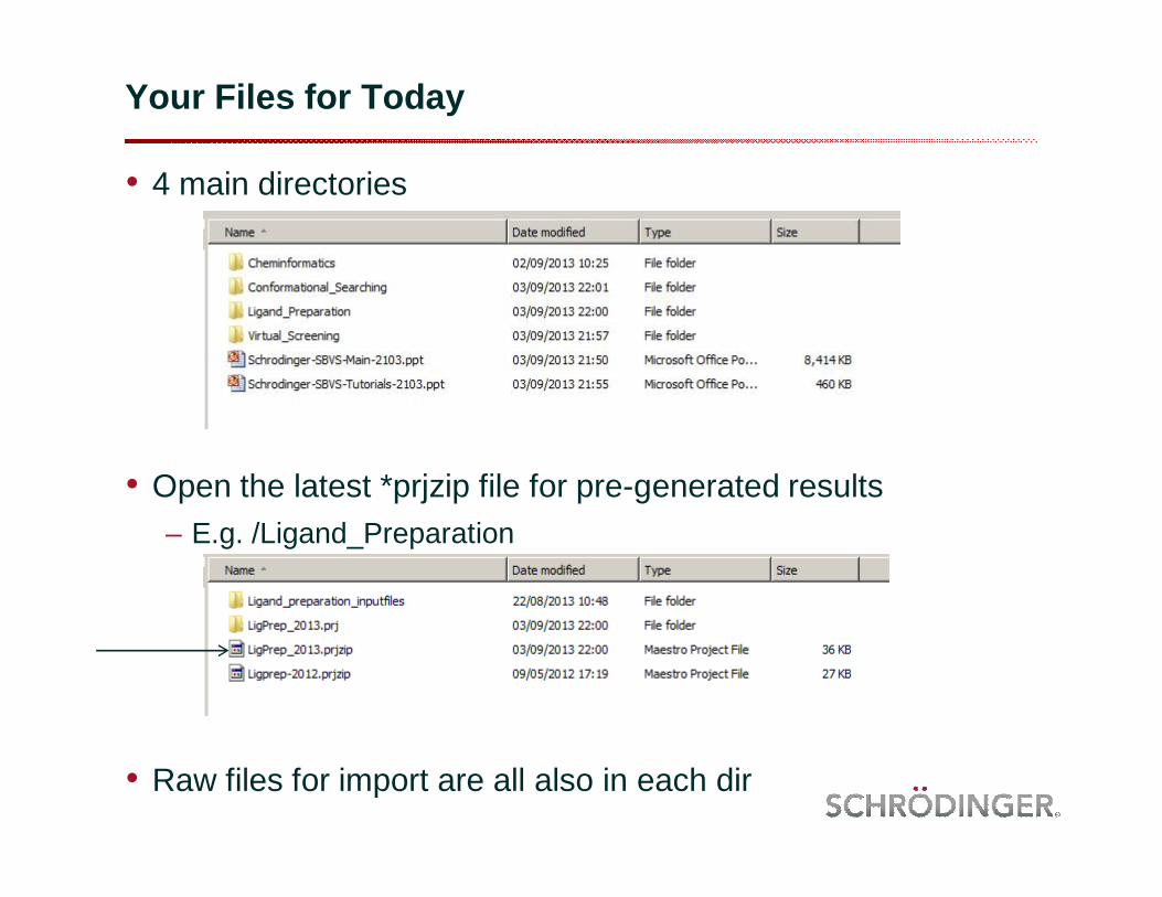
Your Files for Today

• 4 main directories

• Open the latest *prjzip file for pre-generated results– E.g. /Ligand_Preparation

• Raw files for import are all also in each dir

Structure Based Virtual Screening

• Virtual screening is a cost-effective early stage lead generation method

• How do we design a successful structure based virtual screening campaign?

The road to success : What we have found

Based on experiences from our Drug Design Team who are dedicated to working with Customers on new projects....

• Careful protein preparation – Know your target• Careful ligand preparation – Enumerate states and

conformations• Pilot screening – Know the best combination of constraints

and scores• Screening• Post-screening processing• Purchase and assay

Questions we will be Asking Today

•Do we have a crystal structure or an homology model?

•Is the target drug-able?

•What is the quality of the model - electron density?•Understanding the binding site: big small buried pockets general-properties?

•Are there known ligands for this target, and how can we

use that information?

•How to screen compounds

•How to improve the quality of screened outputs?

•How to filter and cluster the output from screen to manageable numbers for synthesis or purchase

Putting everything together– Tailored Protocols for XYZ Protein

v Databases v ABCDE pocket of XYZ

v Glide SP*

1. CACDB2010 lead/drug-like set.2. Phase mining, with multiple hypotheses, of CACDB phase

database using ABCDE as queries (shape similarity > 0.6 or top 0.5%).*

3. Fingerprint-based similarity search of whole CACDB using HTS hits as queries (Tanimoto >= 0.6 or top 0.5%).*

1. Receptor of ABCDE site with HB to Res123 (-C=O and –NH) and/or Res 122 (-NH) on chain A.

2. Receptor of ABCDE site with HB to Res123 (-C=O and –NH) and/or Res 122 (-NH) on chain B.

3. Receptor of ABCDE site with HB to Res123 (-C=O and –NH) on both chain A and B

v Glide XP*

1. Mine for poses with desirable interactions, i.e., hydrogen bonding.2. Rescore with Epik state and strain penalties3. Take top scoring 5000 to next step for visualization4. Select molecules for sourcing with help of clustering tools

*: Combined structures taken directly to XP

(25 % top scoring)

•Three conformations of ligands for XP docking•ConfGen/MM/multiple FFs

v Glide HTVS

(15 % top scoring)

(post-processing of ensemble)

•Two conformations of ligands for SP docking•Glide shows dependency on input conformations

Target structure preparation, prediction and characterization

Problems with PDB structures

Lys58 rotamer χ1 = -73.5 χ2 = +179.2 χ3 = +154.2 χ4 = +85.4

Extremely rareLys rotamer

XP GlideScore = -6.9 kcal/mol

Crystallographic refinement (PrimeX)

Lys58 rotamer χ1 = -69.8 χ2 = -178.4 χ3 = +178.2 χ4 = -179.9

Most commonLys rotamer

XP GlideScore = -8.7 kcal/mol

Challenges in homology modeling

• Accurate alignment– High sequence identity is straight forward and can produce high

quality structures– Low sequence identity requires assistance and manual editing– Depends on human intervention, experimental data

• Model refinement– Side chain conformation– Loop conformation– Binding site conformation– Depends strongly on the quality of the force field

High Resolution Protein Structure Prediction:Comparative Modeling

Query sequence Blast/PSI-BlastBlast/PSI-Blast

Template(s), PSI-Blast Profile (PSSM), Query Secondary Structure Predictions, Multiple

Structure Alignment Profile

AlignAlign

Protein ReportValidateValidateRefined protein structure

RefineRefine

BuildBuildQuery/Template Alignment

Homology model

Alignments of GPCRs: Example

• Sequence alignment between human β2-adrenergic and human Melanin-concentrating hormone-1 sequences using the ‘Align GPCR’ mode– ‘Align GPCR’ mode correctly aligned all helices, including the challenging helix 5,

without any user intervention. All gaps in the alignment are located in the intracellular and extracellular loop regions, and not in TM regions

Representation of loops - Variable Dielectric Constants

( ) ( )

1 1 1 1( )2 2

i j i jes

i j ijij in ij in ij sol GB

q q q qG

r fε ε ε<

= − −∑ ∑

( ) ( ) ( )max( , )in ij in i in jε ε ε=

Reparametrization of internal dielectric constants for charged side chains:Lys = 4Glu = 3Asp = 2Arg = 2His = 2Others = 1

continuum solventε=80

ε=2 ε=1

ε=4

Number of Cases

Uniform Dielectric

Variable Dielectric

Uniform + Hydrophobic

Variable + Hydrophobic

6 residue 99 0.48 0.40 0.46 0.41

8 residue 65 0.84 0.79 0.76 0.74

10 residue 41 1.27 0.73 1.05 0.76

13 residue 35 2.73 1.62 1.29 1.08

Improvement of solvation model impacts on loop prediction accuracy

RMSD (Å)

Tips and tricks

• Induced fit docking to generate bioactive conformations• Prime side chain predictions, Macromodel side chain

conformation search and hand tweaks if needed• Molecular dynamics simulations to measure the stability of

your protein model

Screening 1

• Ligand Based Methods

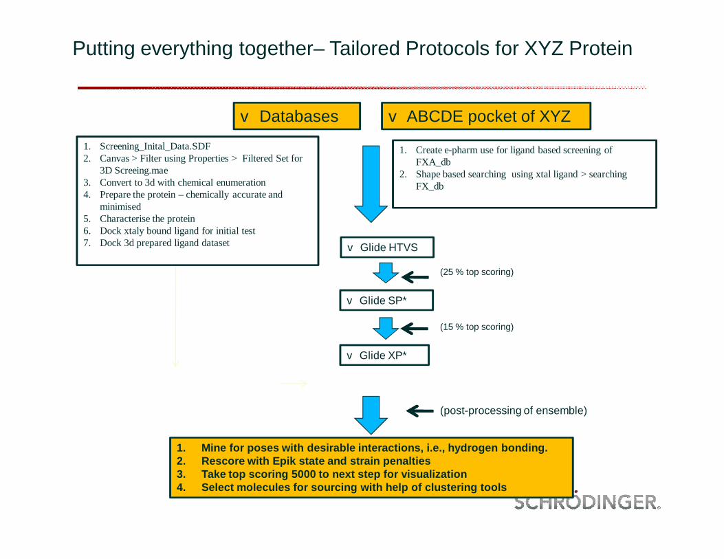
Putting everything together– Tailored Protocols for XYZ Protein

v Databases v ABCDE pocket of XYZ

v Glide SP*

1. Create e-pharm use for ligand based screening of FXA_db

2. Shape based searching using xtal ligand > searching FX_db

v Glide XP*

1. Mine for poses with desirable interactions, i.e., hydrogen bonding.2. Rescore with Epik state and strain penalties3. Take top scoring 5000 to next step for visualization4. Select molecules for sourcing with help of clustering tools

(25 % top scoring)

v Glide HTVS

(15 % top scoring)

(post-processing of ensemble)

1. Screening_Inital_Data.SDF2. Canvas > Filter using Properties > Filtered Set for

3D Screeing.mae3. Convert to 3d with chemical enumeration4. Prepare the protein – chemically accurate and

minimised5. Characterise the protein6. Dock xtaly bound ligand for initial test7. Dock 3d prepared ligand dataset

Ligand preparation

2D Perspective• Smart filtering of your screening deck for optimal druglike and

leadlike properties (REOS, Ligparse, Ligfilter)

3D Perspective• Chemically accurate ligand structures (tautomers, ionization

states, stereoisomers..)• Multiple input ligand conformations

– Confgen and MacroModel • Estimate state penalties

Fingerprints in Canvas

• Fingerprints are defined by fragments used• Rules of making fragment are different

– how you define the path through the molecule, linearly or via torsions, or through pre-defined libraries like MACCS

• Available

MACCS and Custom MACCS & Custom are fragment based

TorsionPairwise Triplet Linear (default) ‘Daylight’ Others are based on topology (exhaustive)Dendritic Molprint2D Radial ‘Circular SciTegic’

Mor

e

sp

ecifi

c

• Structures/properties retrieved from SQLite database as needed

• Scroll smoothly through 106

compounds, hundreds of columns

• Create custom views from sorting, filtering, and chart selections

High Performance Chemical Spreadsheet

Fingerprints in Canvas

• Linear• Dendritic• Radial• MOLPRINT2D• Pairwise• Triplet• Torsion

• MACCS keys

Exercise 1Fast Screening Using 2D Approaches (.../Cheminformatics)

• Create a Canvas project and import ’FXA_all_initial_data.sdf’ / *ligprep.out

– Note you may want to start from different points• 2D filtering > 3D preparation > 2D Filtering ........• 3D preparation > Shape filtering > 2D Filtering ........

• Generate molecular properties– Applications -> Molecular properties

• Incorporate the results• Filter by properties using

– Data -> Property Filter– Scatter plots

• Similarity Searches if you have data on known ligands• Clustering data with different Clustering methods

Path dependent fingerprint methods

• Linear fingerprint – codes for all linear path up to

7 bonds – codes up to 14 bonds for ring

closures • Dendritic fingerprint

– codes for branches up to 5 bonds

Circular fingerprint methods

• Radial fingerprint (Extended Connectivity fingerprint)– generated by fragmenting a

structure into pieces that grow radially from each heavy atom over a series of iterations (4 by default)

– Each atom identified by its atom type and connecting bond types.

• MOLPRINT2D fingerprint– each heavy atom in a structure

is characterized by an environment that consists of all other heavy atoms within a distance of two bonds

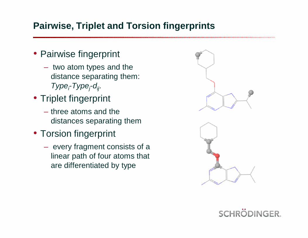
Pairwise, Triplet and Torsion fingerprints

• Pairwise fingerprint– two atom types and the

distance separating them: Typei-Typej-dij.

• Triplet fingerprint– three atoms and the

distances separating them

• Torsion fingerprint– every fragment consists of a

linear path of four atoms that are differentiated by type

What are the recommendations?

• There is no single best setting for all targets and query molecules.

• Pairwise and Triplet methods exhibit size dependency.• Without prior knowledge about the performance of fingerprint

methods for a target, the best choice can be– MOLPRINT2D, Dendritic– Fingerprint combination– Fingerprint averaging: modal fingerprint

• More specific atom typing schemes (Daylight, Mol2, Carhart) are best but probably less suited for lead hopping

Sastry, M.; Lowrie, J.F.; Dixon, S.L.; Sherman, W., "Large-Scale Systematic Analysis of 2D Fingerprint Methods and Parameters to Improve Virtual Screening Enrichments," J. Chem. Inf. Model., 2010, 50, 771–784

Exercise 2Preparing 3D Ligands for 3D Screening (.../Ligand preparation)

• In Maestro import a simple example of starting ligands– Import 2D_variations.sdf – In the first structure note, it has two ionisable groups, an ammonium

counter ion and there are three chiral centres (two marked)• Run LigPrep

– Default options– Start and Append new entries as a new group

• Observe results in Maestro– Tile and label the structures to see them individually– In the first structure note, carboxylate is unprotonated, pyridine is both

protonated and unprotonated, the variety of R/S chiralities

• In Maestro import FXA_ligprep-out.mae– Only import the first few ligands using the Advanced options. We do not

need to see the entire file as it is very large.

Conformer Generation

• Accurate and efficient bioactive conformational searching– It is important to reproduce bioactive ligand geometries in minimally

sized conformer sets, and still obtain accuracy and coverage.– Imatinib shown colored according to how ConfGen treats various parts

of the molecule. Rotatable torsions are rendered in yellow, templated rings in green carbon atoms, and rigid rings/bonds are in cyan.

http://www.schrodinger.com/productpage/14/26/

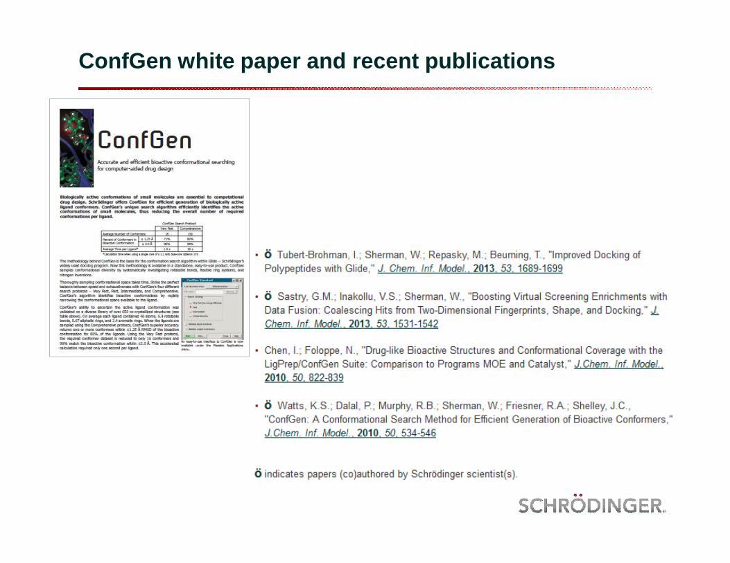
ConfGen white paper and recent publications

Screening 2Structure Based Methods

Background to Xtalographically obtained PDB files

• Most protein structures solved by X-ray crystallography have a drawback that becomes apparent as soon as the structure is used for molecular simulations and related applications: the electron density traces the shape of the molecules, but does not really permit to identify hydrogen atoms or distinguish the heavier elements C, N and O. Consequently ambiguities arise if groups of atoms can be rotated without affecting the overall shape.

• If a molecular simulation is run with incorrectly oriented or protonated side-chains, the protein stability can be reduced significantly, in the worst case the protein may even fall apart. The only way to resolve the issue is to infer the correct orientations and protonation patterns from the chemical environment, most importantly the hydrogen bonding possibilities. Since several of the critical side-chains are often found in close contact, a choice made for one side-chain immediately influences others, giving rise to a hydrogen bonding network that must be optimized in one shot.

http://www.yasara.org/hbondnet.htm

ASN, GLN, ASP, GLU, HIS residues• Typical examples in proteins are the

side-chains of asparagine and glutamine, whose terminal amide group can be rotated by 180 degrees with almost no impact on the electron density.

• The same applies to the imidazolering of histidine, which can additionally adopt three different pH dependent protonation patterns, giving rise to six different states, that can hardly be distinguished based on the electron density alone.

• Aspartates and glutamates can adopt three different states (negatively charged or neutral with the hydrogen on either of the two terminal side-chain oxygens), with the neutral states being mostly important for buried residues with strongly shifted pKa values.

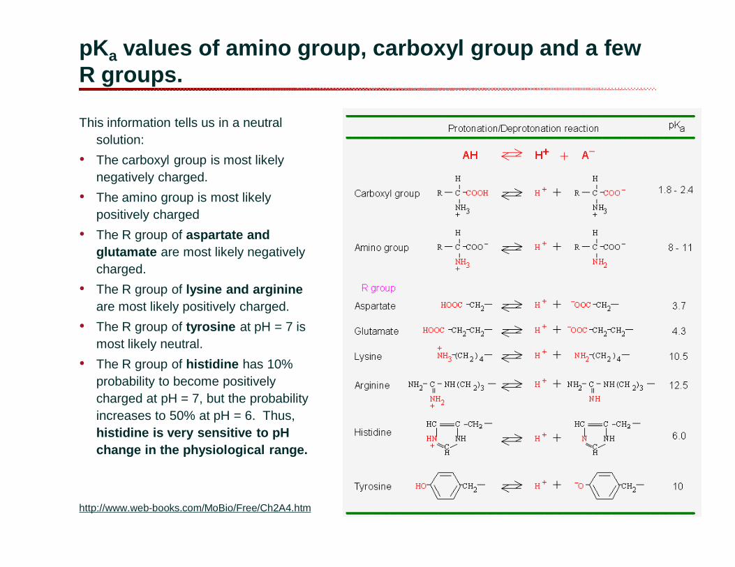
pKa values of amino group, carboxyl group and a few R groups.

This information tells us in a neutral solution:

• The carboxyl group is most likely negatively charged.

• The amino group is most likely positively charged

• The R group of aspartate and glutamate are most likely negatively charged.

• The R group of lysine and arginine are most likely positively charged.

• The R group of tyrosine at pH = 7 is most likely neutral.

• The R group of histidine has 10% probability to become positively charged at pH = 7, but the probability increases to 50% at pH = 6. Thus, histidine is very sensitive to pH change in the physiological range.

http://www.web-books.com/MoBio/Free/Ch2A4.htm

The Importance Of Protein Preparation

• Almost all protein structures require some sort of remediation before they can be used in drug-design.

– Protonation.• Most structures come from X-ray crystallography. As protons don’t show up well in X-ray experiments

they are normally missing from structures and need to be added.– Missing side-chains.

• Any side-chain which is too mobile will not diffract well and will not be visible in the electron density. Simply ignoring this side-chain may not be a good idea as any ligand may well interact with the side-chain and cause it to adopt a fixed position.

– Missing loops.• Similar to the above situation. However in this case whole residues can be missing from the final

structure.– Counterions/random small molecules/waters.

• The crystallisation media will often contain other counterions and small molecules along with water. These frequently show up in the final structure. Sometimes these species reveal important information (particularly water molecules), but in many cases they need to be removed.

– Bonding/ionisation/tautomerisation.• Crystallography only provides the atomic coordinates of the structure. The bonding information needs to

be added manually. For standard amino-acids this is trivial, however other species such as ligands and cofactors will need to be edited manually. Related to this the ionisation state and tautomerisation state of any non-standard species present will need to be assigned.

Protein preparation wizard:Prepare and repair PDB structures

The preparation wizard (under Applications >) helps us through this process of…

• Cleaning up raw PDB files– Assign bond order – Add hydrogen atoms– Delete unwanted part of the system– Optimize the hydrogen bond networks (flip of residues like ASN, GLN, tautomer

determination: HIE, HID or protonation state HIP…)– Remove putative clashes in your structure (ideally with diffraction data)

• Dealing with missing information – Important side-chains are missing– Important loops are missing

• Download 1FJS structures in Protein preparation wizard. – Extra: go to EDS (http://eds.bmc.uu.se/eds/) and download the

CNS format map (2mFo-DFc) for 1FJS; Examine the electron density

– Notes on electron density: do the residues ligand protein water sit in the electron density or is there an anomoloy? ...

• Prepare 1FJS• Set up Glide grids (Applications -> Glide -> Receptor grid

generation)

Exercise 3 (.../Virtual Screening)

Preparing a PDB Structure for Virtual Screening

Understanding Sigma values

• The sigma level of an electron density map refers to the standard deviation.

After taking a fourier transform of your data and refining it through a variety of methods to find the phases, you're left with an electron density map ρ(x,y,z), which describes the intensity of the electron density at each point in real space. This reflects the fact that regions in space with a higher electron density will scatter more X-rays, although this is not what you measure directly. Once the mean and the standard deviation (σ) of the intensity across the entire map are calculated, the intensity of every point in ρ(x,y,z) can be described in standard deviation (σ) units away from the mean.

• The "sigma level" is the contour level or cut-off point in the intensity of any particular 3D representation of the electron density represented in standard deviation units. For example a sigma level of 1 would show density only for values in ρ(x,y,z) which have intensities greater than one standard deviation unit above the mean. Lowering the sigma level will give you a 3D map with more density, but if it's too low you won't be certain that what you're seeing is real electron density and not noise and it will be harder to fit your molecule into it. Raising the sigma level will reduce the noise, but if you raise it too high you will eliminate some of your real data and see gaps in the density at positions where actual atoms happened to have measured intensities lower than the sigma level. Flexible portions of the protein, even when crystallized, will be the first regions of the electron density to go as the sigma level is raised. Of course, the sigma level just reflects cosmetic changes to what you see on the screen; your full dataset with the intensities for every point is unaffected. Contour levels are just a convenient way of representing an extra dimension of intensity in the three dimensional space.

http://www.quora.com/What-does-the-sigma-level-refer-to-in-electron-density-mapping#

Different Sigma Levels in RNase A

• Here is the electron density for the RNase A unit cell at four different contour levels in standard deviation units above the mean: 0.5σ, 1σ, 2σ, and 3σ.

Raising the sigma level will reduce the noise

Lowering the sigma level will increase the noise

(visualized in Coot) http://www.quora.com/What-does-the-sigma-level-refer-to-in-electron-density-mapping#

Characterize the binding pocket - Sitemap

• Early stage analysis tool– Summarises key parts of the protein structure

• Find potential binding sites • Characterize known binding sites• Is the binding site drug-able?

• Potential binding sites characterized by– Hydrophobic, hydrophilic, hbond donor/acceptor isosurfaces, volume etc– Scoring used to determine drug-ability– Site points can be used to define Glide grids (treat as ligand entry)

• Validated for site “druggability” – Halgren, T., "New Method for Fast and Accurate Binding-site Identification and Analysis",

Chem. Biol. Drug Des., 2007, 69, 146–148.– Halgren, T., "Identifying and Characterizing Binding Sites and Assessing Druggability”, J.

Chem. Inf. Model., 2009, 49, 377–389.

SiteMap Feature Detection

Thrombin (1ett)

Sites identified by SiteMap can easily be used to set up Glide grids for virtual screening experiments.

Druggability Dataset

Druggable Prodrug/transporterUndruggable

ACE-1 Acetylcholinesterase Cathepsin KAldose reductase Thrombin PTP-1BcAbl kinase Neuraminidase Caspase 1 (ICE-1)CDK2 IMPDH HIV integraseCyclooxygenase 2 Penicillin binding proteinDNA gyrase B HIV RT (nucleotide site)EGFR kinaseEnoyl reductaseFactor XFungal Cyp51HIV RT (NNRTI site)HIV-1 ProteaseHMG CoA reductaseMDM2P38 kinasePDE 4DPDE 5AThrombin

-diverse set of pharmaceutically relevant targets

-widely used in benchmark studies to study the properties of binding sites

SiteMap Druggability Results

UndruggableDifficult

MAPPOD is from Cheng et al.

Rule of thumb

Exercise 4 (.../Virtual Screening)

Property Mapping the Xtal Structure

• Run Sitemap for 1FJS– Try ”Evaluate...” Tasks.

• Analyse the results. Where are the hydrophobic areas and polar areas? * Is the target druggable?

• Sitemap has been parameterized such that :

SiteMap of IFJS

• The active site of factor Xa is divided into four sub pockets as S1, S2, S3 and S4.

The S1 subpocket determines the major component of selectivity and binding. The S2 sub-pocket is small, shallow and not well defined. It merges with the S4

subpocket. The S3 sub-pocket is located on the rim of the S1 pocket and is quite exposed to

solvent. The S4 sub-pocket has 3 ligand binding domains, namely the “hydrophobic box”, the

“cationic hole” and the water site.

• Factor Xa inhibitors generally bind in an L-shaped Conformation. One group of the ligand occupiesthe anionic S1 pocket lined by residues Asp189, Ser195, and Tyr228, and another group of the ligand occupies the aromatic-S4 pocket lined by residues Tyr99, Phe174, & Trp228.

• Typically, a fairly rigid linker group bridges these two interaction sites.

Tips and tricks

• Make sure your structure is chemically accurate!• Use multiple structures, even different chains from same PDB• Induced fit docking to generate bioactive conformations• Prime side chain predictions, Macromodel side chain

conformation search and hand tweaks if needed• Molecular dynamics simulations to understand flexibility of the

structure• Molecular dynamics simulations to measure the stability of

your protein model

Pre-screen

• Pilot screens to evaluate performance of different combinations of constraints (EFs; GlideScores; Chemical matter ‘eyeballing for a motif’).

• Check if co-crystallised ligand can be docked with Standard Docking. If large RMS to native. Find out why:– Are there any crystal mates?– Constraints, multiple protein input conformations (see VSW GUI

for Glide), QPLD• Screen your database!

Glide Overview

• The conformations then enter the ‘Glide Filter’– This is a series of hierarchical filters which are used to rapidly

eliminate poses of the ligand which cannot correspond to a well-docked solution.

Diameter Test/Subset Test

Greedy Score

Refinement

Site-point Search

Minimisation

Final Score

Ligand conformations

Top hits

diametercentercore O

N

OO-

H sidechaingroup

sidechaingroup

SN

• Protein & ligand preparation• Calculate Coulomb & vdW grids• Docking algorithm• 3 Modes:

• HTVS 3-5 secs/lig• SP 30-50secs/lig• XP 3-5mins/lig

Additional Information: Glide Implementation Details

• The value of GlideScore is determined as follows:

• The PBuryP is a penalty term for burying polar functionality in a hydrophobic environment.

• The PRotB is a penalty term for freezing rotatable bonds. • The Site term rewards polar, but non-hydrogen bonding

interactions in the site.

SitePPEEEEE

GlideScoreRotBBuryPMetal

HBondLipovdWcoul

+++++++

=130.0065.0

Glide SP: Enrichment Summary

• Glide: A New Approach for Rapid, Accurate Docking and Scoring. 1. Method and Assessment of Docking Accuracy. R. A. Friesner, J. L. Banks, R. B. Murphy, T. A. Halgren, J. J. Klicic, D. T. Mainz, M. P. Repasky, E. H. Knoll, M. Shelley, J. K. Perry, D. E. Shaw, P. Francis, and P. S. Shenkin. J. Med. Chem. 2004, 47, 1739-1749

• Glide: A New Approach for Rapid, Accurate Docking and Scoring. 2. Enrichment Factors in Database Screening. T. A. Halgren, R. B. Murphy, R. A. Friesner, H. S. Beard, L. L. Frye, W. T. Pollard, and J. L. Banks. J. Med. Chem. 2004, 47,1750-1759

• Extra Precision Glide: Docking and Scoring Incorporating a Model of Hydrophobic Enclosure for Protein-Ligand Complexes. Friesner, R. A.; Murphy, R. B.; Repasky, M. P.; Frye, L. L.; Greenwood, J. R.; Halgren,T. A.; Sanschagrin, P. C.; Mainz, D. T., J. Med. Chem., 2006, 49, 6177–6196.

• Comparative Performance of Several Flexible Docking Programs and Scoring Functions: Enrichment Studies for a Diverse Set of Pharmaceutically Relevant Targets. Zhou, Z.; Felts, A. K.; Friesner, R. A.; Levy, R. M., J. Chem. Inf. Model., 2007, 47, 1599–1608.

EF(1%)

Average enrichment in recovering actives in top 1% of decoys(Average of 65 systems)

Exercise 5Virtual Screening: Docking and Visualising Poses

• Generate the Glide Grid for 1fjs– Use the fully prepared protein and co-crystralised ligand as starting point

for Glide > Receptor Grid Generation– Define the ligand inside the Grid panel– Start the job (1-2 minutes)– ’1fjs-grid-2013.zip’ is the pre-generated output

• Dock the 1fjs ligand using this Grid file– In Glide > Ligand Docking, Settings tab > browse for the 1fjs grid file,

choose SP mode– In Ligands tab > choose selected entry and ensure the ’1fjs ligand only’

is highlited in the Project Table– Start the job– ’Selfdock-1fjs-sp-pv.mae’ is the pre-generated output

• Use Maestro to view the result(s)... Overlay Sitemap result!

VSW Interface for automated Glide docking

• Docking the xtal ligand is the first step to running a full docking study which may begin with millions of molecules or a few thousand.

• Glide Virtual Screening Workflow is powerful interface for setting up a series of screens that iteratively run through the various precision-levels of docking (HTVS>SP>XP) and the interface is especially useful for including an ensemble of receptor structures.

• Applications > Glide > VSW

Post processing methods:What do I do with 1000s hits?

• Pose Filter based on known interactions (Script menu)

• Filter poses based on pharmacophore (Phase)

More Post-processing

• Filter based on Strain Rescore (Script menu)

• Calculating Prime MM-GBSA or Macromodel Embrace

Du, J.; Sun, H.; Xi, L.; Li, J.; Yang, Y.; Liu, H.; Yao, X., "Molecular modeling study of checkpoint kinase 1 inhibitors by multiple docking strategies and Prime/MM-GBSA calculation," J. Comp. Chem., 2011, 32(13), 2800-2809

Lyne, P. D.; Lamb, M. L.; Saeh, J. C., "Accurate Prediction of the Relative Potencies of Members of a Series of Kinase Inhibitors Using Molecular Docking and MM-GBSA Scoring," J. Med. Chem., 2006, 49, 4805-4808

Selection of Hits

• If resources are limited, only the most diverse ligands are selected for experimental measurements– Upcoming Exercise: Run this script on VSW results output (96 - VSW

1FOR results)• Use fingerprints to cluster hits and choose cluster representatives

– Scripts> Cheminformatics > Canvas Similarity & Clustering…

Structural Interaction Fingerprints

• Original publication: Chuaqui et al., J. Med. Chem. 47 (2005) 121-133 (Biogen)

• Basic algorithm– Begin with pre-docked poses– For each ligand, generate fingerprint based on types of contact with the receptor

• The bit string is translated into a matrix/plot where the ‘1’s’ and ‘0’s’ can be easily interpreted (next slide)

– Use the fingerprints for filtering, similarity searching, and clustering

Structural Interaction Fingerprints

bit1 = contact

bit2 = backbone

bit3 = side chain

bit4 = polar

bit5 = hydrophobic

bit6 = HB acceptor

bit7 = HB donor

bit8 = aromatic (addition to paper)

bit9 = charge (addition to paper)

1 1 0 0 1 1 0 1 00 0 0 0 1 0 0 1 01 1 0 1 0 1 0 1 0

1 1 0 0 1 1 0 1 00 0 0 0 1 0 0 1 01 1 0 1 0 1 0 1 0

0 1 1 0 0 1 1 0 00 0 0 0 1 0 0 1 01 1 0 1 0 0 0 0 0

1 0 0 0 1 1 0 1 0 1 0 0 0 1 1 0 1 00 1 0 0 0 1 0 1 0

0.8 0.6 0 0.1 0.2 0.5 0 1 0.1 0.8 0.6 0 0.1 0.2 0.5 0 1 0.10.2 0.4 0.1 0.1 0.2 0.3 0.1 0.2 0

…

……

… …compound 1compound 2compound 3

compound n

pSIFt

Residue 1 Residue 2 Residue N

Structural Interaction Fingerprints (Demo or Exercise)

• Calculate Fingerprints• Visualize contacts with Interaction Matrix

Interactive Analysis of Contacts

• Picking in the matrix displays the residue and the interaction

Interactive Distance Matrix

Exercise 6Post-Docking Analysis; SIFTs and Clustering

Using the Workspace Style toolbar is an easy way to visualize the docked poses, along with ’view poses’ option with a ’right click’ to the Group in the PT. While eye-balling is crucial, the SiFTS interface makes identifying key interactions easy

• Run the script on VSW results output (96 - VSW 1FOR results) and analyse the interaction pattern– Scripts->Cheminformatics->Interaction fingerprints

• Perform Clustering, chosing the number of ’desired clusters’

Visual Inspection

• The different filtering methods reduce the number of hits• The final selection should be done by human visual inspection

of the protein ligand interactions.• Possible selection criterias:

– Does the ligand have strange docked conformations? – Do the protein-ligand interactions fit SiteMap results?– Does the ligand have good ligand efficiencies?

Post-screen

• Pose filter (Scripts -> Docking post-processing-> Pose filter)• Filter based on Interaction fingerprints, ligand strain energy,

ligand efficiency• Reserve slots for compounds with somewhat lower

GlideScores that came via ligand based methods (show high similiarity using techniques we’ve seen here)

• Visualize 5-10x the number of compounds to be wet-screened by several people; balance leadlike vs. druglike; tabulate votes

• Cluster results by chemotype (e.g. spectral clustering) and only order up to 2-4 best examples from each cluster for testing

Glide XP and beyond

• Empirical scoring functions tell us the propensity of binding between two things

• The ability to decompose the scoring function in more detail can tell us more about the reasons for good binging and help to distinguish between close-binding ligands– If we know which tiny factors contribute better to binding, this in

turn helps us design better ligands

• The topic of structure based pharmacophores leads on from this concept, but let’s look at Glide XP first...

Glide XP Visualiser

You can read in your pv file here

Exercise 7Understanding Extra Precision Docking, XPVisuliaser

• Do Glide ’Score in Place’ with the co-crystalized ligand IFJS using XP and toggle on ”Write XP descriptor information”

• Examine the XP descriptors in Applications-> Glide -> XP Visualizer (read in your *xp pv file)– A pre-generated file can be used

”ScoreInPlace_1FJS_XP_pv.maegz”• Use ’Help...’ To understand the terms in the scoring function• ...• Leads to Exercise 4b

Structure based pharmacophorehttps://www.schrodinger.com/productpage/14/41

“Novel Method for Generating Structure-Based Pharmacophores Using Energetic Analysis”

N. K. Salam, R. Nuti, W. ShermanJ. Chem. Inf. Model. 2009, 49, 2356-2368

"Energetic analysis of fragment docking and application to structure-based pharmacophore hypothesis generation,“

K. Loving, N. K. Salam, W. ShermanJ. Comput. Aided Mol. Des. 2009, 23, 541–554.

Introduction to Energetic-Pharmacophores

• By capturing the power of XP to de-convolute the scoring function we are able to use those components to rank the most important features of binding

• The binding interactions are translated into ‘pharmacophore features’ and presented to the user– Only the highest ranked feature will make up the final

pharmacophore– We can use this PH4 to screen for similar compounds that will

also exhibit these “key features for binding”

Which are the important features?

--2.22.2 --1.21.2

--2.42.4

--1.21.2

0.00.0

0.00.0

0.00.0

0.00.00.00.0

0.00.0

0.00.0

0.00.0

--0.30.3

--0.40.4

0.00.0

0.00.00.00.0

0.00.0

0.00.00.00.0

0.00.0

0.00.0

This is an example of using fragments, but the same concept holds true for single ligand as seen in the previous slide

Which are the important features?

Which are the important features?

--2.22.2 --1.21.2

--2.42.4

--1.21.2

0.00.0

0.00.0

0.00.0

0.00.0

0.00.0

0.00.0

0.00.0

0.00.0

--0.30.3

--0.40.4

0.00.0

0.00.00.00.0

0.00.0

0.00.00.00.0

0.00.0

0.00.0

Optimal Site Selection

--2.22.2 --1.21.2

--2.42.4

--1.21.2

--2.22.2 --1.21.2

--2.42.4

--1.21.2

Methods

• Protein PDB structure preparation• Fragments ionization/tautomer states generated• Glide XP modified settings

• Increase number of poses generated for initial docking stage• Wider scoring window for filtration on initial poses• Increase number of poses per ligand for energy minimization

– Write XP Descriptor Information• Writes atom-level energy terms

– H-bond – Electrostatic and vdw– Hydrophobic enclosure– π-π and π-cation

Exercise 8Generating a Structure Based Pharmacophore for Screening

• ... In the PT Group **** E-PH4s*****, the XP ligand can be used to generate e-Pharmacophore with Scripts->Post-docking processing-> e-Pharmacophore (< 1 min)– Single ligand option– Create hypothesis

• Note, the input is a ’glide-dock-XP-SIP-2013-pv.maegz’ pose-viewer file normally.

• Search the Phase database using Applications -> Phase -> Advanced Pharmacophore Screening(< 1 min for search)– Database: /Conf_database/FXA_db.phdb (latest 2013 format)– Choose hypothesis in workspace (or selected entry)– Use existing conformations

• View results in Maestro – Fitness is the output column– Use ’right click fix’ on highlited row to fix the original

pharmacophore in the workspace. Arrow-through results.

Use all possible known information

• Use all available information about target and its ligand preferences– 2D similarity – Pharmacophore – Shape based

Shape in Phase (latest seminar: http://www.schrodinger.com/seminarprior/19/39/)

• Shape based methods are widely used in industry– Literature > especially for virtual screening– Fast, easy, sound-physical justification

• Based on principal of rapid initial alignments using atom triplets followed by refinement and volume overlap scoring – Different to Gaussian-based methods in their output– Speed roughly 500 confs/sec on opteron 2.4GHz– A number of publications

http://www.schrodinger.com/productpublications/14/13/

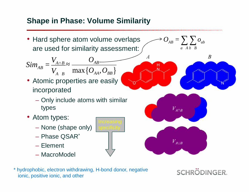
Shape in Phase: Volume Similarity

• Hard sphere atom volume overlaps are used for similarity assessment:

• Atomic properties are easily incorporated– Only include atoms with similar

types• Atom types:

– None (shape only)– Phase QSAR*

– Element– MacroModel

SimAB = VA∩B

VA∪B

Increasing specificity

* hydrophobic, electron withdrawing, H-bond donor, negative ionic, positive ionic, and other

≈ OAB

max OAA,OBB{ }

OAB = oabb∈B∑

a∈A∑

Additional Pharmacophore Mode

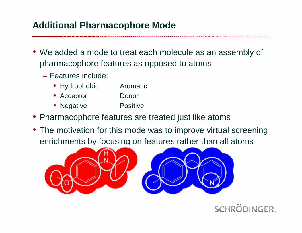
• We added a mode to treat each molecule as an assembly of pharmacophore features as opposed to atoms– Features include:

• Hydrophobic ü Aromatic• Acceptor ü Donor• Negative ü Positive

• Pharmacophore features are treated just like atoms• The motivation for this mode was to improve virtual screening

enrichments by focusing on features rather than all atoms

Atoms for Alignment

• Assessing all possible atomic alignments is computationally intractable

• We simplify the problem by focusing on local atom environments1. Compute a distance profile for

each atom2. Compare atom profiles between

different molecules3. Align top scoring triplets4. Refine alignment by adding

more atoms• Triangular area and binning is

used to eliminate edge effects• Atom types can be easily

incorporated

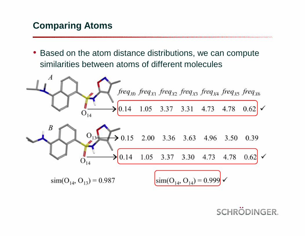
Comparing Atoms

• Based on the atom distance distributions, we can compute similarities between atoms of different molecules

Alignment of 3 Points

• Triad from structure B can be rapidly aligned to a triad in structure A1. Shift A & B to a common centroid2. Rotate them to the xy plane3. Determine the angle θB that

minimizes the sum of squared distances between the pairs of atoms (a1, b1), (a2, b2) and (a3, b3)

• ~3x faster than standard 3D least-squares alignment– Results in significant speedup due

to the number of alignments being considered

• Refinement of top alignments by considering atoms within 0.5 Å from each other

Exercise 9 (if you have energy!)Shape Based Searching

• Use the VDW shape of a ligand to search for molecules of a similar shape. The 1FJS xtal ligand is the template.

• Applications > Shape Screening...– Use Shape query from workspace– Generate conformations during search– Drop-down options give you more stringency in addition to shape– “Shape sim” is the output column– View results in Maestro as before

Putting everything together– Tailored Protocols for XYZ Protein

v Databases v ABCDE pocket of XYZ

v Glide SP*

1. CACDB2010 lead/drug-like set.2. Phase mining, with multiple hypotheses, of CACDB phase

database using half and whole of ABCDE as queries (shape similarity > 0.6 or top 0.5%).*

3. Fingerprint-based similarity search of whole CACDB using HTS hits as queries (Tanimoto >= 0.6 or top 0.5%).*

1. Receptor of ABCDE site with HB to Res123 (-C=O and –NH) and/or Res 122 (-NH) on chain A.

2. Receptor of ABCDE site with HB to Res123 (-C=O and –NH) and/or Res 122 (-NH) on chain B.

3. Receptor of ABCDE site with HB to Res123 (-C=O and –NH) on both chain A and B

v Glide XP*

1. Mine for poses with desirable interactions, i.e., hydrogen bonding.2. Rescore with Epik state and strain penalties3. Take top scoring 5000 to next step for visualization4. Select molecules for sourcing with help of clustering tools

*: Combined structures taken directly to XP

(25 % top scoring)

* Three conformations of ligands for XP docking

v Glide HTVS

(15 % top scoring)

(post-processing of ensemble)

* Two conformations of ligands for XP docking

Summary

• Virtual screening needs careful planning and preparation• Post-process the results using different tools and re-score, re-

rank• Products and tools that have been discussed today:

– PrimeX, Prime, Macromodel, Sitemap, Glide, Epik, Canvas, Phase, Prime MM-GBSA, Interaction fingerprint, Spectral clustering, Strain rescore, Pose filter, e-Pharmacophore

Thanks Audience for your attention !