structure analysis of the perseus and the cepheus b...
TRANSCRIPT
Structure analysis of the Perseus and theCepheus B molecular clouds
Inaugural-Dissertationzur
Erlangung des Doktorgradesder Mathematisch-Naturwissenschaftlichen Fakultat
der Universitat zu Koln
vorgelegt von
Kefeng Sunaus VR China
Koln, 2008

Berichterstatter : Prof. Dr. Jurgen StutzkiProf. Dr. Andreas Zilges
Tag der letzten mundlichen Prufung : 26.06.2008

To my parents and Jiayu

Contents
Abstract i
Zusammenfassung v
1 Introduction 11.1 Overview of the interstellar medium . . . . . . . . . . . . . . . . 1
1.1.1 Historical studies of the interstellar medium . . . . . .. . 11.1.2 The phases of the ISM . . . . . . . . . . . . . . . . . . . 21.1.3 Carbon monoxide molecular clouds . . . . . . . . . . . . 3
1.2 Diagnostics of turbulence in the dense ISM . . . . . . . . . . . .41.2.1 The∆-variance method . . . . . . . . . . . . . . . . . . . 61.2.2 Gaussclumps. . . . . . . . . . . . . . . . . . . . . . . . 8
1.3 Photon dominated regions . . . . . . . . . . . . . . . . . . . . . 91.3.1 PDR models . . . . . . . . . . . . . . . . . . . . . . . . 12
1.4 Outline . . . . . . . . . . . . . . . . . . . . . . . . . . . . . . . 12
2 Previous studies 142.1 The Perseus molecular cloud . . . . . . . . . . . . . . . . . . . . 142.2 The Cepheus B molecular cloud . . . . . . . . . . . . . . . . . . 16
3 Large scale low -J CO survey of the Perseus cloud 183.1 Observations . . . . . . . . . . . . . . . . . . . . . . . . . . . . 183.2 Data Sets . . . . . . . . . . . . . . . . . . . . . . . . . . . . . . 21
3.2.1 Integrated intensity maps . . . . . . . . . . . . . . . . . . 213.2.2 Velocity structure . . . . . . . . . . . . . . . . . . . . . . 24
3.3 The∆-variance analysis . . . . . . . . . . . . . . . . . . . . . . . 243.3.1 Integrated intensity maps . . . . . . . . . . . . . . . . . . 273.3.2 Velocity channel maps . . . . . . . . . . . . . . . . . . . 30
3.4 Discussion . . . . . . . . . . . . . . . . . . . . . . . . . . . . . . 343.4.1 Integrated intensity maps . . . . . . . . . . . . . . . . . . 343.4.2 Velocity channel maps . . . . . . . . . . . . . . . . . . . 34
I

II CONTENTS
3.5 Summary . . . . . . . . . . . . . . . . . . . . . . . . . . . . . . 38
4 The Gaussclumps analysis in the Perseus cloud 404.1 Results and discussions . . . . . . . . . . . . . . . . . . . . . . . 40
4.1.1 Clump mass . . . . . . . . . . . . . . . . . . . . . . . . . 414.1.2 Clump mass spectra . . . . . . . . . . . . . . . . . . . . 424.1.3 Relations of clump size with line width and mass . . . . . 464.1.4 Equilibrium state of the clumps . . . . . . . . . . . . . . 49
4.2 Summary . . . . . . . . . . . . . . . . . . . . . . . . . . . . . . 53
5 Study of the photon dominated region in the IC 348 cloud 555.1 Datasets . . . . . . . . . . . . . . . . . . . . . . . . . . . . . . . 56
5.1.1 [CI] and12CO 4–3 observations with KOSMA . . . . . . 565.1.2 Complementary data sets . . . . . . . . . . . . . . . . . . 57
5.2 Observational results . . . . . . . . . . . . . . . . . . . . . . . . 575.3 LTE Analysis . . . . . . . . . . . . . . . . . . . . . . . . . . . . 635.4 PDR Model . . . . . . . . . . . . . . . . . . . . . . . . . . . . . 67
5.4.1 FUV intensity . . . . . . . . . . . . . . . . . . . . . . . . 675.4.2 Clumpy PDR scenarios . . . . . . . . . . . . . . . . . . . 68
5.5 Summary and Conclusions . . . . . . . . . . . . . . . . . . . . . 78
6 Multi-line study of the Cepheus B cloud 806.1 The IRAM 30m telescope observations . . . . . . . . . . . . . . . 816.2 Chemical tracers at the PDR interfaces . . . . . . . . . . . . . . .816.3 Two observed cuts . . . . . . . . . . . . . . . . . . . . . . . . . . 836.4 Results . . . . . . . . . . . . . . . . . . . . . . . . . . . . . . . . 85
6.4.1 Spectra at the two interface positions . . . . . . . . . . . 856.4.2 Integrated intensities along the two cuts . . . . . . . . . .916.4.3 LTE analysis . . . . . . . . . . . . . . . . . . . . . . . . 91
6.5 Summary and outlook . . . . . . . . . . . . . . . . . . . . . . . . 95
7 Summary and future prospects 977.1 Summary of results . . . . . . . . . . . . . . . . . . . . . . . . . 977.2 Future prospects . . . . . . . . . . . . . . . . . . . . . . . . . . . 99
A Local thermodynamic equilibrium analysis 101A.1 Opacity . . . . . . . . . . . . . . . . . . . . . . . . . . . . . . . 101A.2 Excitation temperature . . . . . . . . . . . . . . . . . . . . . . . 102A.3 Column density . . . . . . . . . . . . . . . . . . . . . . . . . . . 102A.4 Mass . . . . . . . . . . . . . . . . . . . . . . . . . . . . . . . . . 103

CONTENTS III
B A new atmospheric calibration method 104B.1 Introduction . . . . . . . . . . . . . . . . . . . . . . . . . . . . . 104
B.1.1 Atmospheric model . . . . . . . . . . . . . . . . . . . . . 105B.2 The previous calibration (Hiyama’s) . . . . . . . . . . . . . . . .106B.3 The new calibration scheme . . . . . . . . . . . . . . . . . . . . 107B.4 Testing the new calibration . . . . . . . . . . . . . . . . . . . . . 108
B.4.1 How to useKalibrate . . . . . . . . . . . . . . . . . . . . 108B.4.2 On simulations . . . . . . . . . . . . . . . . . . . . . . . 112B.4.3 On real data . . . . . . . . . . . . . . . . . . . . . . . . . 116
B.5 Conclusion . . . . . . . . . . . . . . . . . . . . . . . . . . . . . 116
C A uniform observing script 118
Reference 121
List of Figures 136
List of Tables 144
Acknowledgments 147
Publications 151
Lebenslauf 152

Abstract
Astronomical observations have shown that molecular clouds are the birth placesof new stars and planets. As molecular clouds are massive objects with a massvarying from∼ 106 to a few solar masses, a mechanism is needed to break upthe molecular clouds into stellar size fragments. Star formation occurs when indi-vidual fragments become gravitationally dominated, whichcan occur either spon-taneously or triggered by external forces. Molecular clouds are observed to beturbulent. Turbulence plays a dual role in star formation. It creates density fluc-tuations to initiate gravitational collapse; on the other hand, it can counter localcollapse. Hence, the cloud structure and dynamics control important properties ofstar formation.
In the first part of this work, I study the structural properties of Galactic molec-ular clouds. To determine cloud properties, observable quantities, such as (inte-grated) intensities, spectral line profiles of the standardtracers are used. The car-bon monoxide, CO, molecule is the second most abundant molecule in the Uni-verse after H2 and because of its low rotational excitation energy, it is the principalmolecule to study the molecular gas in galactic and extragalactic sources. Its iso-topomer13CO is often optically thin, and is a good tracer of column density. Inthis work, four rotational transitions of12CO and13CO are employed:12CO 1–0and 3–2, and13CO 1–0 and 2–1.
For both dust continuum maps and integrated line intensity maps, it has beenshown that the observed intensities follow a power law scalerelation. The spatialstructure of the emission has been quantified in terms of its power spectrum thatis the Fourier transform of the autocorrelation function. For a given observablequantity, the power spectrum gives a plot of the portion of power falling withingiven unit bins. When fitting the azimuthally averaged powerspectrum with apower law, the fitted slopeβ provides information on the relative amount of struc-ture at the linear scales resolved in the image. I apply the∆-variance method toquantitatively characterize the observed cloud structures. The∆-variance methodmeasures the relative amount of structure on a given scale byfiltering an ob-served map by a radially symmetric wavelet with a characteristic length scaleLand computing the total variance in the convolved map. Within the typical range
i

of spectral indices measured in interstellar clouds, the fitted exponent from the∆-variance method can be related to the exponent of the power spectrum. Theadvantage of the∆-variance method is that it allows clear discrimination againstthe noise and other systematic effects (finite size, beam smearing) in the observedmaps.
There is a different approach to quantify the observed cloudstructure, which isthe decomposition of the observed emission into discrete entities clumps in orderto establish scaling relations for the clumps e.g. mass-size relation and clumpmass spectra. For this purpose, I use the method,Gaussclumps. This methodidentifies a clump as a Gaussian shaped least square fit to the surroundings of thepresent map maximum, and successively subtracts one clump after the other untilthe complete intensity has been assigned to clumps.Gaussclumpscan identifyefficiently small clumps near the resolution limit of the observations, and thus it isvery helpful to obtain a complete clump mass spectrum that measures the numberof clumps of a given mass.
The Perseus molecular cloud has been selected for these studies. Since it is oneof the best examples of the nearby active low- to intermediate-mass star formingregions.
The ∆-variance method is applied to both the CO integrated intensity mapsand the velocity channel maps that present spatial distribution of line intensitiesat each successive velocity interval. The spectral indexβ of the correspondingpower spectrum is determined. Its variation across the cloud and across the linesis studied. It is found that the power spectra of all CO line integrated maps ofthe whole complex show the same index,β ≈ 3.1, for scales between about 0.2and 3 pc, independent of isotopomer and rotational transition. However, the COmaps of individual subregions show a variation ofβ . The12CO 3–2 data providea spread of indices between 2.9 in L 1455 and 3.5 in NGC 1333. In general, activestar forming regions show a larger power-law exponent. I usethe velocity channelanalysis to study the statistical relation between the neighboring channel maps.Some theory predicts systematic increase of the spectral index with channel width.Such systematic increase is only detected in the blue line wings for the CO data.
I apply Gaussclumpsto the whole observed Perseus cloud and seven sub-regions, and to derive the clump properties as traced in13CO 1–0 and 2–1. Withthe individual clumps identified, their properties such as mass, size, velocity widthare derived. The clumps identified have a power law mass spectrum, and a powerlaw index∼ 1.9 of clump mass spectra. The virial parameter, which is theratiobetween virial mass and the mass estimated from the Local Thermodynamic Equi-librium (LTE) analysis, is used to characterize the equilibrium state of a clump.The LTE assumes that all distribution functions characterizing the material andits interaction with the radiation field at one position are given by thermodynamicequilibrium relations at local values of the temperature and density. Virial mass
ii
here is the mass of a clump in statistical equilibrium derived by using the virialtheorem. All clumps identified in both NGC 1333 and L 1455 are found with avirial parameter above 1. The external pressure needed to bind the clumps fallswithin 103 K cm−3 and 106 K cm−3 for the whole observed Perseus cloud, whileit varies between active star formation regions and quiescent dark clouds.
After stars form, they provide important feedback mechanisms for regulat-ing star formation: ultraviolet (UV) radiation dissociates molecules, ionizes, andheats the gas and the dust in photon dominated regions (PDRs). Outflows, radia-tion driven bubbles, and supernova (SN) shells provide mechanical energy input.All effects lead to the dispersion of molecular clouds and tothe compression ofcores possibly triggering further star formation. The study of photon dominatedregions is to understand the effects of stellar far-ultraviolet photons on the struc-ture, chemistry, thermal balance, and evolution of the neutral interstellar mediumof galaxies.
The second part of this thesis is to study the physical properties of the transi-tion layers on the surface of molecular clouds, i.e. Galactic photon dominated re-gions. Two clouds are selected for the study: IC 348 and Cepheus B. Both cloudsare close to the radiation field of the bright stars that are part of the youngestgeneration. Hence, they are ideal places to study the properties of PDRs.
The KOSMA - τ PDR model is used to interpret the observed line intensi-ties. It is a spherical PDR model, which computes the chemical and temperaturestructure of a spherical clump illuminated by an isotropic FUV radiation field andcosmic rays. The form of carbon changes with increasing depth from the surfaceof the PDR from C+ through C0 to CO. Therefore emission from [CII ], [C I] andthe rotational lines of CO can be used as probes of temperature, density and col-umn density in the PDRs. I use the data of12CO 1–0, 4–3,13CO 1–0 and [CI]3P1 – 3P0 to study physical and chemical properties of the PDRs in IC 348.
New observations of maps in [CI] at 492 GHz and12CO 4–3 with a resolutionof ∼ 1′ are combined with the FCRAO data of12CO 1–0,13CO 1–0 and far-infrared continuum data. To derive the physical parametersof the region, threeindependent line ratios are analyzed using the following: asimple LTE analysis;KOSMA - τ PDR model considering an ensemble of PDR clumps. Detailed fits toobservations are presented at seven representative positions in the cloud revealingclump densities between about 4.4 104 cm−3 and 4.3 105 cm−3, and C/CO columndensity ratios between 0.02 and 0.26. The FUV flux obtained from the model fitis consistent with that derived from FIR continuum data, varying between 2 to100 Draine units across the cloud. An ensemble of a few tens PDR clumps with atotal mass of a few solar masses and a beam filling close to unity reproduces theobserved line intensities and intensity ratios.
A multi-line study in the Cepheus B molecular clouds is presented. Two5′ long cuts have been observed for up to three transitions of the CS, HCO+,
iii

HCN, HNC, CN, and C2H molecules. The integrated intensity distribution alongthe cuts have been calculated and a least square fit is used to the observed hy-perfine structure of C2H, CN and HCN for deriving the opacities. At the two in-terface positions, column densities of H2, 12CO, 13CO, C18O, CS, C34S, HCO+,H13CO+, HCN, HNC, HCS+ and HCO are estimated under the LTE assumption.
The thesis presents the comparison of the structural properties for entire sur-veys and sub-sets, as well as the velocity channel analysis,provide additional,significant characteristics of the ISM in observed CO spectral line maps. Thesequantities are useful for a comparison of the structure observed in different clouds,possibly providing a diagnostic tool to characterize the star-formation activity andproviding additional constraints for numerical simulations of the ISM structure.The thesis also studies different PDRs subject to low and intermediate FUV fieldsusing the clumpy KOSMA -τ PDR model. Future observations will be usefulto constrain the models and to judge the importance of different input parame-ters used. A better knowledge of these conditions in IC 348 and Cepheus B willprovide a template for future studies of Galactic PDRs and the ISM in externalgalaxies.
iv
Zusammenfassung
Astronomische Beobachtungen haben gezeigt, dass in Molek¨ulwolken die Enste-hungsbebiete neuer Sterne und Planeten liegen. Da Molekulwolken massive Ob-jekte mit Massen im Bereich von einigen Sonnenmassen bis 106 Sonnenmassensind, gibt es einen Mechanismus zur Enstehung stellarer Massen-Fragmente. DieSternentstehung beginnt, wenn einzelne Fragmente von der Gravitationskraft do-miniert werden, was entweder spontan oder durch externe Kr¨afte initialisiert wer-den kann. Beobachtungen zeigen, dass Molekulwolken turbulent sind. Die Tur-bulenz spielen dabei eine duale Rolle in der Sternentstehung: einerseits werdenDichtefluktuationen erzeugt die Kollaps durch Gravitationerzeugen; zum An-deren verhindert die Turbulenz lokalen Kollaps. In diesem Sinne bestimmenraumliche Struktur und Dynamik der Molekulwolken wichtige Eigenschaften derSternentstehung.
Im ersten Teil dieser Arbeit werden die strukturellen Eigenschaften galaktis-cher Molekulwolken untersucht. Um die Eigenschaften der Molekulwolken zubestimmen, benutzen wir Beobachtungsgroßen wie (integrierte) Intensitaten undspektrale Linienprofile von ublichen Linienubergangen. Das Karbonmonoxid-Molekul, CO, ist das nach dem H2 zweithaufigste Molekul im Universum. Durchseine niedrige Rotationsanregungsenergie ist es das meiststudierte Molekul ingalaktischen und extragalaktischen Quellen. Das13CO Isotop ist haufig optischdunn und eignet sich deshalb als Indikator fur Saulendichten. In dieser Arbeitbenutzen wir 4 Rotationsubergange von12CO und13CO: 12CO 1–0 und 3–2, und13CO 1–0 und13CO 2–1.
Um die Struktur der Molekulwolken zu quantifizieren, benutzen wir die∆−Var-ianz Methode undGAUSSCLUMPS. Die ∆−Varianz Methode ermoglicht dieIdentifizierung von Rauschen und anderen systematischen Effekten (begrenzteGroße, Beam-Verschmierung) in den beobachteten Karten.GAUSSCLUMPSkanneffizient kleine Klumpen nahe des Auflosungslimits der jeweiligen Beobachtun-gen identifizieren und ist deshalb sehr hilfreich fur die Bestimmung eines kom-pletten Klumpen-Massen Spektrums, welches die Zahl der Klumpen in einemMassenintervall angibt.
Die Molekulwolke Perseus wurde fur diese Beobachtungen ausgewahlt, da Sie
v
eine der besten Beispiele fur eine nahegelegene aktive Sternentstehungsregion imniegrigen und mittleren Massenbereich darstellt.
Wir haben das Power-Spektrum der Fourier-Transformiertender Autokorre-lationsfunktion der raumlichen Struktur der Emission bestimmt. Fur eine bes-timmte Beobachtungsgroße quantifiziert das Powerspektrum die Energie die inbestimmten raumlichen Einheiten auftritt. Durch Anfitteneines Power-Laws mitSteigungβ an das Power-Spektrum, konnen wir studieren, welcher Anteil derStruktur auf verschiedenen linearen Skalen in der Region aufgeloste wurde. Die∆−Varianz Methode wurde sowohl auf die integrierten CO Intensitaskarten alsauch auf die Geschwindigkeitskanalkarten angewandt, die die raumliche Verteilungder Linienintensitaten in unterschiedlichen Geschwindigkeitsbereichen quantifizier-en. Der spektrale Indexβ der korrespondierenden Power-Spektra wird bestimmt.Wir finden, dass auf Skalen von 0.2-3pc die integrierten Karten des gesamtenPerseus-Komplexes unabhangig von Isotopomer und Rotationsubergang einen Spek-tral Indexβ = 3.1 haben. Die CO-Karten individueller Teilregionen zeigen Vari-ation inβ . 12CO 3–2 Daten zeigen einenβ -Bereich von 2.9 in L 1455 bis 3.5 inNGC 1333. Im Allgemeinen findet man großere Power-Indizes in aktiven Ster-nenstehungsgebieten. Die Abhangigkeit der Powerspektrader Kanalkarten vonder Breite der Geschwindikeitskanale zeigt sich nur in derZunahme der Spek-tralindizes im blauen Linienflugel.
GAUSSCLUMPSidentifiziert einen Klumpen als gaußformigen least-squareFit zum aktuellen Maximum der Karte und subtrahiert iterativ Klumpen von derKarte bis die komplette Intensitat in Klumpen aufgeteilt wurde. Ich benutze dieseMethode in der gesamten Perseus Wolke und in sieben Sub-Regionen, um dieKlumpeneigenschaften in13CO 1–0 und 2–1 zu studieren. Fur die einzelnenidentifizierten Klumpen untersuchen wir Masse, Große und Geschwindigkeits-breite des jeweiligen Klumpens. Die identifizierten Klumpen zeigen ein Power-law mit einem Index∼ 1.9 des Klumpen-Massen Spektrums. Der Virialparame-ter, das Verhaltnis aus Virialmasse und Masse berechnet unter Annahme lokalenthermischen Gleichgewichtes (LTE), beschreibt den Gleichgewichtszustand derKlumpen. Die LTE-Annahme impliziert, dass sich alle Verteilungsfunktionen,die Materie und seine Interarktion mit dem Strahlungsfeld beschreiben, durchlokale Werte fur Temperatur und Dichte im thermodynamischen Gleichgewichtbeschreiben lassen. Mit Virialmasse bezeichnen wir hier die Gleichgewichtsmasseeines Klumpen hergeleitet unter Annahme des Virialtheorems. Alle Klumpen inden Regionen NGC 1333 und L1455 haben Virialparameter großer als 1. Derexterne Druck, der benotigt wird um einen Klumpen zu binden, ist zwischen103Kcm−3 und 106Kcm−3 im gesamten Perseus-Gebiet. Zwischen aktiven Ster-nentstehungsgebieten und Dunkelwolken finden wir Variationen in den Virialpa-rametern.
Nach der Entstehung von Sternen sind diese ein wichtiger Teil der Regulierung
vi

neuer Sternentstehung: ultraviolett (UV) Strahlung dissoziert Molekule, ionisiertund heizt Gas und Staub in Photonen dominierten Regionen (PDRs). DurchAusflusse, durch Strahlungsblasen und Supernovaschalen wird mechanische En-ergie abgegeben. Alle Effekte fuhren zur Dispersion der Molekulwolken undmoglichen neuen Sternentstehung in neuen komprimierten Kernen. Die StudienPhotonen dominierten Regionen helfen dabei, die Effekte der stellaren UV-Strahlu-ng auf Struktur, Chemie, thermisches Gleichgewicht und dieEntwicklung desneutralen interstellaren Mediums in Galaxien zu verstehen.
Im zweiten Teil dieser Arbeit werden die physikalischen Eigenschaften derUbergangsschichten an der Oberflache von Molekulwolken studiert, d.h. Galak-tische PDRs. Dafur werden zwei Regionen betrachtet:IC348und CepheusB. BeideWolken liegen im Strahlungsfeld heller junger Sterne und damit ideal um dieEigenschaften von PDRs zu untersuchen.
Das KOSMA-τ PDR-Model wird benutzt um die beobachteten Linieninten-sitaten zu interpretieren. Das Model ist ein spharischesPDR-Model und berechnetdie chemische Struktur und Temperaturverteilung eines Klumpens, der in einemisotropen FUV- und kosmischen Strahlungsfeld liegt. Die Form in der Kohlenstoffvorliegt andert sich im Klumpen mit zunehmenden Abstand von der Oberflachevon C+ uber C zu CO. Deshalb konnen [CII ], [C I] und die Rotationsubergangevon CO benutzen, um Temperatur, DIchte und Saulendichte inPDRs zu bestim-men. In dieser Arbeit werden12CO 1–0, 4–3,13CO 1–0 und [CI] 1–0 um diechemischen und physikalischen Eigenschaften der PDRs in IC348 zu studieren.
Dazu werden neu beobachtete Karten in [CI] bei 492 GHz und12CO 4–3bei ca. 1’ Auflosung mit FCRAO-Daten der Linien12CO 1–0,13CO 1–0 undFern-Infrarot (FUV) Kontinuum-Daten kombiniert. Um die physikalischen Pa-rameter dieser Region zu bestimmen, analysieren wir wie folgt drei unabhangigeLinienverhaltnisse: mit einer einfachen LTE-Analyse undmit Hilfe des KOSMA-τ PDR-Models und einem Ensemble von Klumpen. An sieben reprasentativen Po-sitionen der Wolke diskutieren wir detaillierte Fits an dieBeobachtungen, welcheKlumpen-Dichten zwischen 4.4 104 und 4.3 105 cm−3 ergeben. Die Fits furden FUV-Fluss aus dem PDR-Model sind konsistent mit Ergebnissen aus denFUV Kontinuum-Daten und varieren zwischen 2 und 100 Draine-Einheiten inder Wolke. Ein Ensemble einigen zehn PDR Klumpen mit einer totalen Massevon einigen zehn Sonnenmassen und einem Fullfaktor nahe 1 reproduziert diebeobachteten integrierten Intensitaten und Linienverh¨altnisse.
Eine Studie in verschieden Linien in der CepheusB-Molekulwolke wird vorges-tellt. In zwei 5’ langen Schnitten wurden bis zu drei Linien¨ubergange der CS,,HCO+, HCN, HNC, CN, und C2H Molekule beobachtet. Es wurden die inte-grierten Intensitaten berechnet und ein least-square Fitwurde benutzt um aus denbeobachteten Hyperfeinstrukturubergangen von C2H,CN und HCN die Opazitatenzu bestimmen. An zwei Interface-Positionen werden H2,112CO,13CO,, C18O, CS,
vii
C34S, HCO+, H13CO+, HCN, HNC, HCS+ und HCO Saulendichten unter derAnnahme von LTE bestimmt.
Diese Arbeit prasentiert den Vergleich der strukturellenEigenschaften kom-pletter Studien und Untermengen, ebenso wie die Analyse vonGeschwindigkeit-skanalkarten. Diese zeigen zusatzliche, wichtige Eigenschaften des interstellarenMediums in den beobachteten CO-Karten. Diese Großen sind nutzlich um einenVergleich der Struktur in verschiedenen Wolken zu studieren um damit eine moglic-he Diagnostik zur Charakterisierung der SternentstehungsAktivitat zu erhaltenund weitere Einschrankungen fur numerische Simulationen der Struktur des ISM.Außerdem werden in dieser Arbeit mit Hilfe des klumpigen KOSMA-τ PDR-Models verschiedene PDR-Regionen in niedriger und mittlerer FUV-Strahlungstudiert. Zukunftige Beobachtungen werden helfen, die Modelle weiter einzuschra-nken und die Wichtigkeit verschiedener Parameter zu bestimmen. Ein besseresVerstandnis der Bedingungen in IC 348 und Cepheus B wird eine nutzliche Ref-erenz fur zukunftige Studien in galaktischen PDRs und desISM in externen Galax-ien darstellen.
viii

Chapter 1
Introduction
1.1 Overview of the interstellar medium
1.1.1 Historical studies of the interstellar medium
In 1811, William Herschel created a catalog of bright patches on the sky andcalled themnebulae. In 1904, Johannes Hartmann discovered stationary [CaII ]lines in the spectrum of the spectroscopic binary,δ Orionis, and he came to theconclusion that the gas responsible for the absorption was not present in the at-mosphere ofδ Orionis, but was instead located within an isolated cloud ofmatterresiding somewhere along the line-of-sight to this star. This discovery startedthe study of the interstellar medium (ISM). Barnard (1919) catalogued 182 darknebulae in the sky using photographs. Those dark places wereconsidered to bepossible holes in stellar distribution or obscuring matter. Heger (1922) observed anumber of line-like absorption features which seemed to be interstellar in origin,which is the discovery of diffuse interstellar bands (DIBs). In 1944, van de Hulstpredicted the existence of the 21 cm hyperfine line of neutralinterstellar hydro-gen. And the 21 cm emission was detected by Ewen & Purcell (1951); Muller& Oort (1951). The first interstellar molecules (CH, CH+, CN) were detectedby Swings & Rosenfeld (1937); McKellar (1940); Adams (1941). Weinreb etal. (1963) discovered interstellar OH masers. And NH3 was first detected in theISM by Cheung et al. (1968). Wilson et al. (1970) detected12CO 1–0 emissionat 115 GHz, which later becomes the principal molecule to study the moleculargas in galactic and extragalactic sources. As of January 2008, there are more than140 molecules listed as detected in the interstellar mediumor circumstellar shells(CDMS, http://www.astro.uni-koeln.de/vorhersagen/).
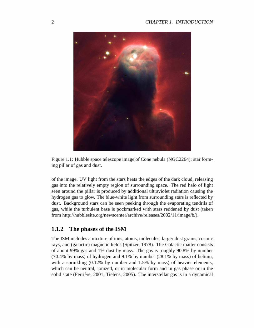
Fig. 1.1 presents the Cone Nebula observed by the Hubble space telescope(HST). The Cone Nebula lies at a distance of about 770 pc. Fig.1.1 shows theupper∼ 0.8 pc of the nebula. There are hot, young stars located beyond the top
1
2 CHAPTER 1. INTRODUCTION
Figure 1.1: Hubble space telescope image of Cone nebula (NGC2264): star form-ing pillar of gas and dust.
of the image. UV light from the stars heats the edges of the dark cloud, releasinggas into the relatively empty region of surrounding space. The red halo of lightseen around the pillar is produced by additional ultraviolet radiation causing thehydrogen gas to glow. The blue-white light from surroundingstars is reflected bydust. Background stars can be seen peeking through the evaporating tendrils ofgas, while the turbulent base is pockmarked with stars reddened by dust (takenfrom http://hubblesite.org/newscenter/archive/releases/2002/11/image/b/).
1.1.2 The phases of the ISM
The ISM includes a mixture of ions, atoms, molecules, largerdust grains, cosmicrays, and (galactic) magnetic fields (Spitzer, 1978). The Galactic matter consistsof about 99% gas and 1% dust by mass. The gas is roughly 90.8% bynumber(70.4% by mass) of hydrogen and 9.1% by number (28.1% by mass)of helium,with a sprinkling (0.12% by number and 1.5% by mass) of heavier elements,which can be neutral, ionized, or in molecular form and in gasphase or in thesolid state (Ferriere, 2001; Tielens, 2005). The interstellar gas is in a dynamical

1.1. OVERVIEW OF THE INTERSTELLAR MEDIUM 3
state of constant change, driven by ultraviolet (UV) heating where stars are form-ing, by supersonic expansion of supernova explosions, and subject to dynamicalinstabilities on varies scales from a small fraction of a parsec to thousands of par-secs (Burke & Graham-Smith, 2002). A wide span of densities and temperaturesof the ISM has been found.
Ranges of densities and temperatures are usually indicatedas components orphases. The term′′phases′′ is used to denote components that may exist in ther-mal pressure equilibrium, withP/k = nT ∼ 3×103 cm−3 K in the solar vicinity(Jenkins et al., 1983). In the three-phase model, those phases often include thefollowing (McKee & Ostriker, 1977; Hollenbach & Tielens, 1999; Cox, 2005):the low-density hot ionized medium (HIM) with temperaturesin excess of 105 Kand densities below about 0.01 cm−3; the warm neutral medium (WNM) and thewarm ionized medium (WIM) with densities in the range 0.1 to 1cm−3 and tem-peratures of several thousand Kelvin; and the dense cold neutral medium (CNM)with densities above about 10 cm−3 and temperatures below 100 K (McKee &Ostriker, 1977; Kulkarni & Heiles, 1987).
The CNM itself contains a variety of cloud types, spanning a wide range ofphysical and chemical conditions. The densest clouds that are most protected fromUV radiation from stars are referred to as dense clouds, darkclouds, or molecularclouds, which may be thought of as a short-term product of theISM leading tostar formation (Cox, 2005). The most tenuous clouds, fully exposed to starlight,are usually called diffuse clouds. Clouds that fall in between these two extremesare often referred to as translucent clouds (Snow & McCall, 2006). This thesiswork mainly deals with molecular clouds, particularly carbon monoxide (CO)molecular clouds.
1.1.3 Carbon monoxide molecular clouds
Molecular clouds are composed of dust and molecular gas thatis molecular hy-drogen (H2) and helium, with small amounts of heavier elements. They make upfor about 50 to 75% of the dense interstellar medium in the Milky Way. Typically,molecular clouds are cold (10 - 50 K) and dense (102 - 106 cm−3). Because oftheir dusty content, visible light can not penetrate into a molecular cloud. Hence,infrared and (sub)millimeter observations are needed.
Molecular hydrogen is the most abundant molecule in ISM and it plays a fun-damental role in star formation. However, the first excitation state of the hydrogenmolecule is about a few hundred Kelvin. And the hydrogen molecule is homo-nuclear, it does not have a permanent dipole moment and vibrational or rotationaltransitions do not occur in electric dipole transition. These transitions are allowedin electric quadrupole transition and therefore have very low probabilities. Thus,cold molecular hydrogen is very hard to observe. Fortunately, there are other

4 CHAPTER 1. INTRODUCTION
molecules mixed with the hydrogen and dust. The most abundant of these is car-bon monoxide. CO is a very stable molecule and the first rotational excited statelies only 5 Kelvin above the ground state, and therefore is readily excited by theambient cosmic microwave background radiation or collisions with neighboringmolecules (usually H2). CO is the principal molecule to study the molecular gasin galactic and extragalactic sources. The main rotationallines of CO are oftenoptically thick. Thus it is also important to observe its isotopomers,13CO orC18O. The abundance ratio between12CO and13CO is about 65 and it is about470 between12CO and C18O (Langer et al., 1990).
1.2 Diagnostics of turbulence in the dense ISM
Turbulence is extremely important for many physical processes that take placein the ISM, including star formation, cosmic ray and dust dynamics, magneticfield formation and evolution, and heat transport (Vazquez-Semadeni, 2000). Forthose reasons there is an increasing interest in the astronomical community on tur-bulence (Esquivel et al., 2007). Understanding the role andnature of interstellarturbulence has been the subject of intensive studies for about half a century now,but many aspects still remain open (Elmegreen & Scalo, 2004). Turbulence causesthe formation of structures of many different length scales. The large scale struc-tures contain most of the energy of the turbulent motion. Theenergy cascadesfrom the large scale structures to smaller scale structures. This process continuesand creates smaller and smaller structures which produces ahierarchy of struc-tures. Major questions concern the mechanisms by which turbulent motions aredriven and the role of the strong compressibility of the interstellar medium for thestructure of the turbulent energy cascade.
Various methods (Scalo, 1984; Klein & Dickman, 1984; Perault et al., 1986;Miesch & Bally, 1994; Stutzki et al., 1998; Rosolowsky et al., 1999) have beenused to quantitatively characterize the interstellar turbulence. They study the two-point correlation function or directly the power spectrum of the observed emis-sion. There are methods like autocorrelation, structure function and power spectra(Scalo, 1984; Klein & Dickman, 1984; Perault et al., 1986; Miesch & Bally, 1994;Rosolowsky et al., 1999). Here I will only give details on themethod used in thethesis, which is the∆-variance method introduced by Stutzki et al. (1998). Thismethod has proven to be particularly useful. It allows for a better separation ofthe intrinsic cloud structure from contributions resulting from the finite signal-to-noise in the data, the telescope beam and limited map size. Inaddition, problemsrelated to the discrete sampling of the data can be avoided (Stutzki et al., 1998;Bensch et al., 2001). The detailed introduction of the∆-variance method will begiven in the following subsection.
1.2. DIAGNOSTICS OF TURBULENCE IN THE DENSE ISM 5
One thing to be noted is that the astronomically observed maps are two di-mensional projection of the structure. However, Stutzki etal. (1998) have shownthat the spectral indexβ of the power spectrum for an spatially isotropic structureremains constant on projection, which means that the projected map of three di-mensional density structures shows the sameβ as the original structure assumingthat the astronomical structure is on the average isotropic.
Interstellar turbulence has also been characterized by a different approach toquantify the structure. That is the decomposition of the observed emission intodiscrete entities (′′clumps′′) in order to establish scaling relations for the clumpse.g. mass-size relation and clump mass spectra (cf. Stutzki& Gusten, 1990;Williams et al., 1994; Kramer et al., 1998b; Heyer & Terebey,1998). With anindividual clump identified, its mass, size, line width, andother parameters canbe determined. One of the more fundamental parameters of a clump is its mass.The mass is generally derived via the integrated intensity of an optically thin line.Hence, the clump mass is a very robust parameter and does not depend on theactual spatial or velocity resolution (unless small size clumps blend into a largerclump).
Several different methods (e.g. eye inspection,ClumpfindandGaussclumps,etc.) have been developed to characterize the clumpy structure. There are studiesreporting clump mass spectra by eye inspection (Carr, 1987;Loren, 1989; Nozawaet al., 1991; Lada et al., 1996; Blitz, 1993; Dobashi et al., 1996). But eye inspec-tion is obviously limited to uncrowded fields and to the identification of only thelarger clumps. Two computerized clump decomposition algorithms are widelyused:ClumpfindandGaussclumps. Clumpfindhas been developed by Williamset al. (1994), which decomposes an observed image into a number of clumps byassigning each volume element of the three dimensional datacube to one of thelocal maxima identified in the observed intensity distribution. In this method thenumber of clumps is limited exactly to the number of local maxima in the observeddata cube. TheClumpfindmethod allows the clumps to have arbitrarily complexshapes, while it fails to identify weaker clumps partially overlapping with largerones.Gaussclumps, developed by Stutzki & Gusten (1990), is used in this thesiswork. The detailed introduction ofGaussclumpswill be given in the followingsubsection.
In the cases where clump masses have been derived for a significantly largenumber of clumps, the different methods agree in showing a clump mass spectraldistribution following a power law mass spectrum of the formdN/dM ∝ M−α
with α of 1.7 - 1.9 for large well-sampled maps (Blitz, 1993; Krameret al.,1998b).

6 CHAPTER 1. INTRODUCTION
Figure 1.2: Example of the filter function used in the∆-variance analysis
1.2.1 The∆-variance method
The ∆-variance method is a means to quantify the relative amount of structuralvariation at a particular scale in a two dimensional map or a three dimensional dataset. It follows the concept of the Allan-variance, originally introduced by Allan(1966) to study the stability of atomic clocks. The∆-variance analysis providesan extension to functions in higher dimensions and can be applied to images andthree dimensional structures. Consider a two dimensional scalar function s = s(x,y) with x and y representing continuous Cartesian coordinates. Because we aremainly interested in spatial intensity distributions we refer to s(x, y) as an′′image′′.For the sake of simplicity we assume a vanishing average,〈s〉x,y ≡ 0. This is noessential restriction and can always be achieved by adding aconstant. The∆-variance is defined as the variance of an images(~r) convolved with a normalizedspherically symmetric wavelet of sizeL
σ2∆ = 〈[s(~r)∗L(~r)]2〉~r , (1.1)
where the asterix denotes the spatial convolution (Stutzkiet al., 1998; Bensch etal., 2001) and is defined as below (see also Fig. 1.2):
L(~r) =
1π(L/2)2 , r ≤ L
2−1
8π(L/2)2 ,L2 < L ≤ 3L
2 ,
0, r > 3L2
(1.2)
For structures characterized by a power-law spectrum,P(|~k|) ∝ |~k|−β wherek = (k2
x + k2y)
1/2, the∆-variance follows as well a power law, with the exponent
1.2. DIAGNOSTICS OF TURBULENCE IN THE DENSE ISM 7
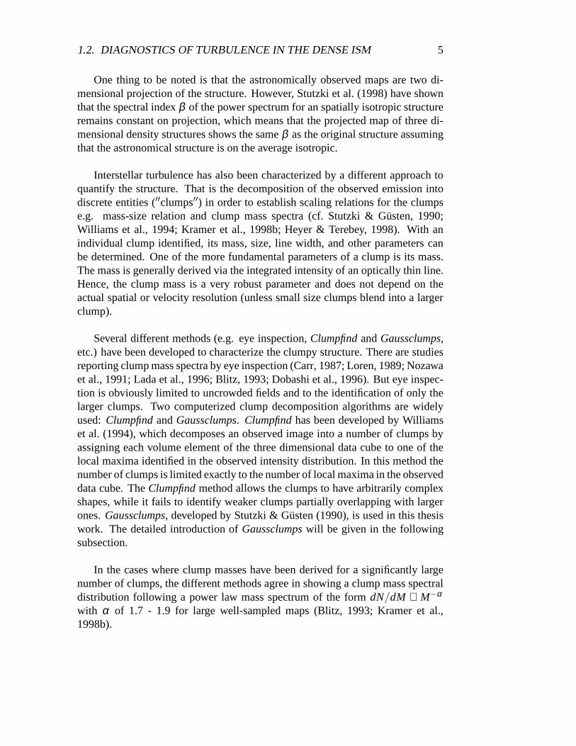
Figure 1.3: An example of a typical∆-variance spectrum for a subset of theFCRAO outer galaxy survey (13CO 1–0). This subset has a very large scale (384by 128 pixels; 50′′per pixel). The x axis is the lag and the y axis is the value ofthe variance. The black line indicates the power-law fits to the data. The turnoverat the smallest angular scales shows the effect from the white noise behavior (forpure white noise,σ2
∆(L) ∝ L−2); the turnover at the large angular scales is dueto the influence of the typical size of main structures in the image. The figure isadapted from the Fig. 3 in the paper by Stutzki et al. (1998).
d∆ = β − 2 in the range 0≤ β ≤ 6 (Stutzki et al., 1998). Fig. 1.3 presents anexample of a∆-variance spectrum.
Several studies have been performed using the∆-variance method. Stutzkiet al. (1998) used this method to study the structure of molecular cloud images(the Polaris Flare and subset of the Five College Radio Astronomy Observatory(FCRAO) outer galaxy survey). Their application to the observed CO maps showsthe power spectrum has a power law shape and the power law index is close toβ =2.8 in clouds. Plume et al. (2000) employed the∆-variance analysis for a quanti-tative comparison of the structure visible in the line-integrated maps of13CO 1–0and [CI] 3P1 – 3P0 and found a typicalβ of ∼ 2.6. Bensch et al. (2001) presenteda detailed study of the∆-variance method as a tool to determine the power lawpower spectral indexβ of two dimensional intensity distributions. They appliedthe ∆-variance method to several observed CO maps, including surveys of giantmolecular clouds made with the Bell Labs 7 m telescope and observations towardthe Polaris Flare/MCLD 123.5+24.9. And they found that for linear scales≥ 0.5pc, the spectral index is remarkably uniform (2.5< β < 2.8) for different clouds(quiescent/star forming) and tracers with different optical depths (12CO and13COJ = 1–0). Significantly larger indices (β >3) are found for the13CO 1–0 mapof Perseus/NGC 1333 and observations made at higher spatialresolution towardMCLD 123.5+24.9. The indexβ found by Bensch et al. (2001) steepens in thePolaris Flare from 2.5 to 3.3 for maps with a linear resolution increasing from
8 CHAPTER 1. INTRODUCTION
>∼ 1 pc to<∼ 0.1 pc.
1.2.2 Gaussclumps
Gaussclumps, developed by Stutzki & Gusten (1990), is a modified least squarefitting procedure to decompose the observed three dimensional data cubes (twospatial coordinates, one spectral coordinate) into a series of clumps, which areassumed to have Gaussian shape (details on this algorithm can be found in Krameret al., 1998b). Stutzki & Gusten (1990) tested the reliability of the Gaussian clumpdecomposition algorithm with artificially generated clumpensembles. The powerlaw index of artificially created clump ensembles was reproduced by the algorithmto within less than 0.1 in the rangeα = 1.1 to 1.75.
The clump decomposition provides the positions, LSR centervelocities, ori-entations of the individual clumps, the clump sizes, brightness temperatures, andFWHM line widths. The intrinsic sizes of the clumps (i.e. de-convolved from theresolution) are calculated by:
xins =√
∆x2−d2beam;yins =
√
∆y2−d2beam;vins =
√
∆v2−v2res. (1.3)
Wherexins, yins andvins are the three dimensional intrinsic sizes of a clump,∆x,∆y and∆v are clump parameters obtained fromGaussclumps, dbeam is the beamsize, andvres is the spectral resolution.
One advantage ofGaussclumpsis that it can principally find clumps blendingin position and velocity by a priori assuming a Gaussian shaped clump profile.While usually only clumps fulfilling the following criteriawill be used to deriveclump mass spectra, which is that the three dimensional intrinsic sizes of a clump,xins, yins andvins, are larger than 50% of the resolution. The criteria can be writtenas:
xins > 0.5 ·dbeam;yins > 0.5 ·dbeam;vins > 0.5 ·vres. (1.4)
The criteria will exclude a large number of small-size clumps. However, thepower law index of clump mass spectrum will not be changed by this (Kramer etal., 1998b).
Stutzki & Gusten (1990) used the method for an analysis of a C18O 2–1 mapof the M17 SW cloud core and decomposed it into about 170 clumps. The methodhas been applied to different molecules and transitions by anumber of other au-thors (Hobson, 1992; Johnen, 1992; Herbertz, 1992; Zimmermann, 1993; Hobsonet al., 1994; Corneliussen, 1996; Kramer et al., 1996; Rohrig, 1996; Wiesemeyeret al., 1997; Heithausen et al., 1998; Kramer et al., 1998b; Simon et al., 2001;
1.3. PHOTON DOMINATED REGIONS 9
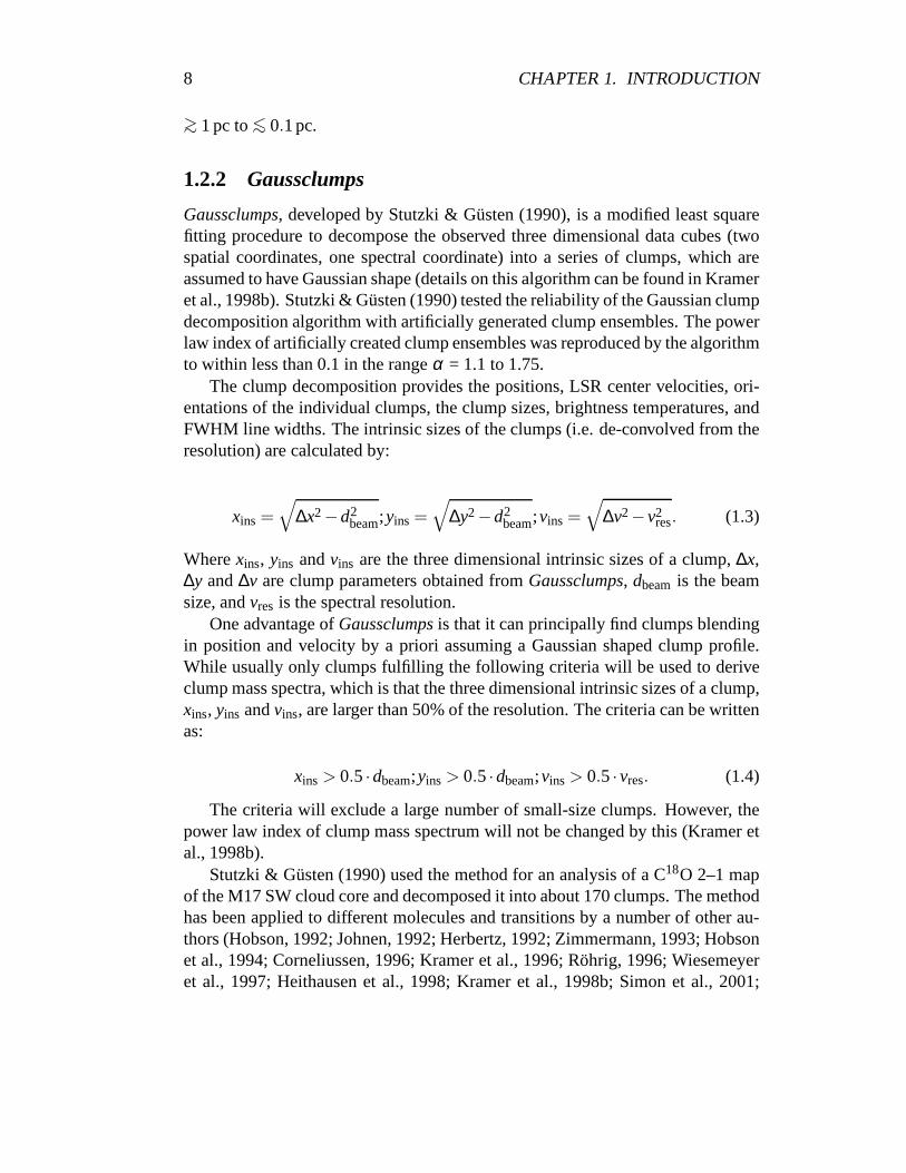
Figure 1.4: An example of a clump mass spectrum for clump massspectra ofNGC 7538. All spectra are fitted by a power law functiondN = dM ∝ M−α . Thestraight line represents the best linear fit over the range ofmasses spanned by theline. The resulting indicesα is 1.79 in this case. The dashed line denotes theminimum possible mass limit, which is estimated by the resolution limits and therms noise. The figure is adapted from the Fig. 6 in the paper by Kramer et al.(1998b).
Mookerjea et al., 2004). Below I will summarize some previous studies usingGaussclumps.
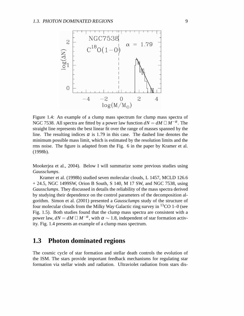
Kramer et al. (1998b) studied seven molecular clouds, L 1457, MCLD 126.6+ 24.5, NGC 1499SW, Orion B South, S 140, M 17 SW, and NGC 7538, usingGaussclumps. They discussed in details the reliability of the mass spectra derivedby studying their dependence on the control parameters of the decomposition al-gorithm. Simon et al. (2001) presented aGaussclumpsstudy of the structure offour molecular clouds from the Milky Way Galactic ring survey in 13CO 1–0 (seeFig. 1.5). Both studies found that the clump mass spectra areconsistent with apower law,dN = dM ∝ M−α , with α ∼ 1.8, independent of star formation activ-ity. Fig. 1.4 presents an example of a clump mass spectrum.
1.3 Photon dominated regions
The cosmic cycle of star formation and stellar death controls the evolution ofthe ISM. The stars provide important feedback mechanisms for regulating starformation via stellar winds and radiation. Ultraviolet radiation from stars dis-
10 CHAPTER 1. INTRODUCTION
Figure 1.5: The GRS13CO intensity integrated over the velocity range relevantfor emission from the individual cloud complexes. The beam size is indicated as afilled circle in the lower left corner of each panel. Top panels : Quiescent clouds;Bottom: Star-forming clouds. The figure is adapted from the Fig. 2 in the paperby Simon et al. (2001).
sociates molecules, ionizes, and heats the gas and the dust in photon dominatedregions (PDRs). PDRs are the interface between the hot ionized medium and cold,dense molecular clouds. They are predominantly neutral, atomic and molecularregions where the physical and chemical processes are dominated by Far Ultra-violet (FUV) (6.0 eV< hν < 13.6 eV) radiation (Hollenbach & Tielens, 1997).Due to the clumpy nature of molecular clouds, PDRs are not strictly confined tothe surface of the molecular clouds. For example, the extended [CII ] and [CI]emission observed from all over the molecular clouds suggest formation of PDRsdeep inside the molecular clouds, at the surfaces of clumps inundated with FUVphotons escaping into the cloud (Mookerjea et al., 2006).
The study of photon dominated regions is the study of the effects of stellarfar-ultraviolet photons on the structure, chemistry, thermal balance, and evolutionof the neutral interstellar medium of galaxies.
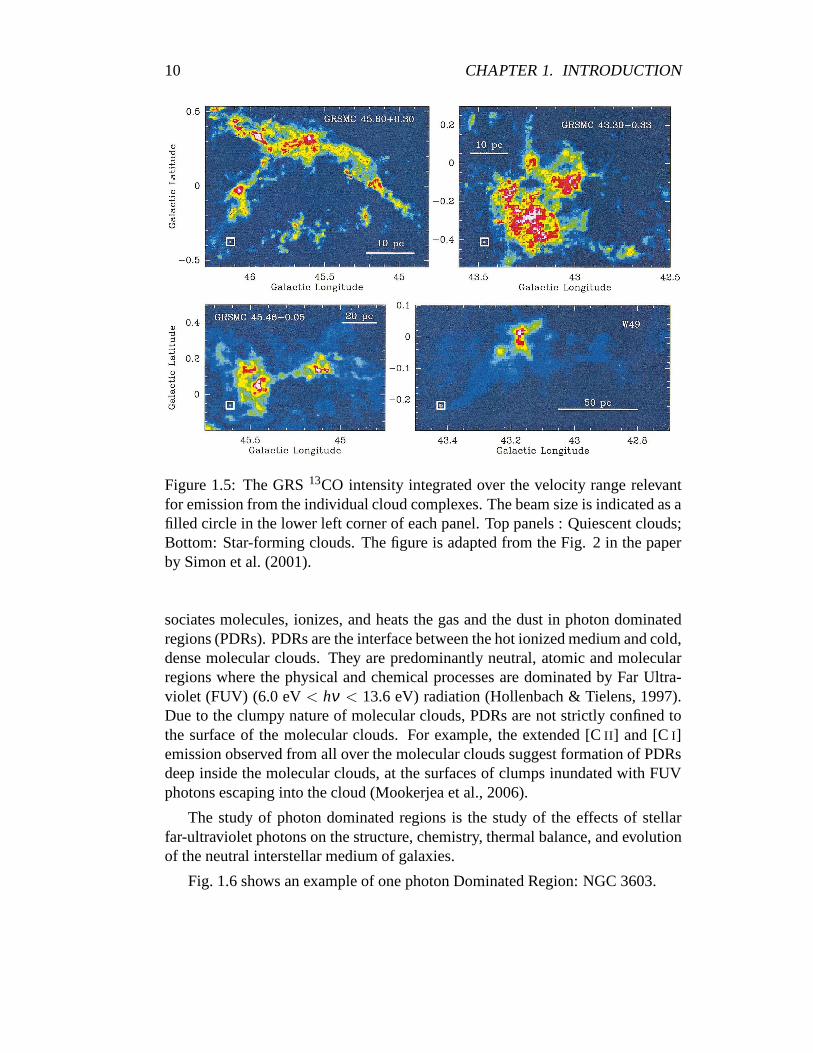
Fig. 1.6 shows an example of one photon Dominated Region: NGC3603.

1.3. PHOTON DOMINATED REGIONS 11
Figure 1.6: One example of galactic photon dominated region: NGC 3603 ob-served by HST. Sher 25, the evolved blue supergiant, is to theupper right ofcenter. The star has a unique circumstellar ring of glowing gas. A starburst clus-ter is near the center. A torrent of ionizing radiation and fast stellar winds fromthese massive stars has blown a large cavity around the cluster. The giant gaseouspillars to the right and lower left of the cluster are the evidence of the interactionof ionizing radiation with cold molecular-hydrogen cloud material.(http://hubblesite.org/newscenter/archive/releases/1999/20/image/a/).

12 CHAPTER 1. INTRODUCTION
1.3.1 PDR models
To study the chemical and physical structure of PDRs, this thesis uses the KOSMA- τ PDR model, a spherical PDR model developed by Storzer et al.(1996). De-tailed description has been given by Storzer et al. (1996);Rollig et al. (2006,2007). This model solves the coupled equations of energy balance (heating andcooling), chemical equilibrium, and radiative transfer, considering spherical cloudsilluminated by an isotropic FUV field and cosmic rays. It computes the chemicaland temperature structure of a spherical clump illuminatedby an isotropic FUVradiation field and cosmic rays.
The PDR clumps are characterized by the incident FUV field intensityχ , givenin units of the mean interstellar radiation field of Draine (Draine, 1978); the clumpmass; and the average density of the clump. The emission fromthe models iscalculated as a function of the hydrogen volume density, FUVradiation field andmass of the clumps (implicitly specifying the clump size). The model clump isassumed to have a power-law density profile ofn(r) ∼ r−1.5 for 0.2≤ r/rcl ≤ 1andn(r) = const. forr/rcl ≤ 0.2. The surface density is about half of the meanclump density.
The PDR models are available on a regular grid with equidistant logarith-mic steps. The FUV field covers the range from 100,100.5, ...,105.5,106.0 G0;The clump surface densities range from 102.0,102.5, ...,105.5,106.0 cm−3; and theclump masses cover 10−3.0,10−2.5, ...,101.5,102.0 M.
1.4 Outline
This investigation of turbulence in dense interstellar medium and photon domi-nated regions unfolds over six chapters.
Chapter 2 summarizes the previous studies in the Perseus andCepheus Bmolecular clouds. In Chapter 3 and Chapter 4, a structure analysis of maps oflow -J CO lines (12CO 1–0, 3–2 and13CO 1–0 and 2–1) in the Perseus cloud ispresented. The analysis uses both the∆-variance method andGaussclumps. Thespatial structures of both line-integrated maps and velocity channel maps are stud-ied. The spectral indexβ of the corresponding power spectrum is determined andits variation across the cloud and across the lines is also studied. I also use a threedimensional Gaussian clump decomposition,Gaussclumps, to identify clumps inthe clouds and to investigate their properties.
Chapter 5 and 6 contain a photon dominated region study in IC 348, a subsetof the Perseus cloud, and in Cepheus B. In Chapter 5, I presentmaps in [CI] at492 GHz and12CO 4–3 combined with the FCRAO data of12CO 1–0,13CO 1–0and far-infrared continuum data observed by HIRES/IRAS. Toderive the physi-
1.4. OUTLINE 13
cal parameters of the region, I analyze the line ratios of [CI] 3P1–3P0/12CO 4–3,
[C I]3P1–3P0/13CO 1–0, and12CO 4–3/12CO 1–0 using the following: a simple
LTE analysis; analysis using the KOSMA -τ PDR model considering (a) a singlespherical clump and (b) an ensemble of PDR clumps. The singlespherical PDRmodel constrains the clump density and FUV field well, although it fails to ex-plain the observed absolute line integrated intensities. The clumpy PDR modelsproduce model line intensities which are in good agreement to within a factor of∼ 2 with the observed intensities. In Chapter 6, I study two cuts running throughthe interfaces into the main cloud and thus allow to trace several interface regionsin Cepheus B. Particularly, we select two positions at the interfaces for a more de-tailed study. The studied frequency covers from 85 GHz to 272GHz and includes21 transitions of 11 molecules, such as HCN, HCO+, CN, CS and CCH. The aimof this study is to resolve the temperature, chemical, and excitation structure ofthe transition zone from the HII region to the dense molecular cloud in a PDRwhich is subject only to moderately strong UV fields.
A summary of all the results and an outlook of possible futurework are pre-sented in Chapter 7.
There are three appendices in this thesis work. Appendix A summarizes thebasic of the LTE analysis. Appendix B is about a new atmospheric calibrationroutine. Different to the traditional calibration approach that determines the atmo-spheric transmission as an average over a representative section of each receiverband individually, that new atmospheric calibration scheme uses a single, freeparameter, the precipitable water vapor (pwv) which is fitted to the observed at-mospheric emission spectrum derived from HOT/COLD/SKY-measurements inthe standard calibration cycle. Appendix C presents the introduction of a uniformobserving script used at both the KOSMA and the NANTEN 2 observatories.

Chapter 2
Previous studies
To investigate turbulence in dense interstellar medium andthe properties of pho-ton dominated regions, I select two nearby star forming regions: the Perseus andCepheus B molecular clouds. In this chapter, I present a brief summary of theprevious studies in those two molecular clouds.
The Perseus molecular cloud is one of the best examples of thenearby activelow- to intermediate-mass star forming regions and about 10 away from Taurus.It lies at a distance of 350 pc (Borgman & Blaauw, 1964; Herbig& Jones, 1983;Bachiller & Cernicharo, 1986) and is known to be related to the Perseus OB2 as-sociation (Bachiller & Cernicharo, 1986; Ungerechts & Thaddeus, 1987). Thereare an active star-forming region (NGC 1333), a young cluster (IC 348) and sev-eral dark clouds (L 1448, L 1445, Barnard 1, Barnard 1 EAST, Barnard 3 andBarnard 5) in this region.
The Cepheus molecular cloud is at a distance of 730 pc from theSun (Blaauw,1964). Cepheus B is the hottest12CO component in the CO maps (Sargent, 1979)and is located to the northwestern edge of the Cepheus molecular complex, nearthe Cepheus OB 3 association. The interface between the molecular cloud andthe OB stars is clearly delineated by the optically visible HII region S 155, whosevery sharp edges clearly indicate the presence of ionization fronts bounding thedust/molecular cloud. The OB association itself seems to becomposed of twosubgroups of different ages, with the youngest lying closerto the molecular cloud(Sargent, 1979). There are also indications that the younger subgroup has itsorigin near the Cepheus B cloud (Testi et al., 1995).
2.1 The Perseus molecular cloud
Ungerechts & Thaddeus (1987) carried a CO survey of the dark nebulae in Perseus,and they obtained the morphology and mass of the clouds. Bachiller & Cer-
14

2.1. THE PERSEUS MOLECULAR CLOUD 15
Figure 2.1: Map of the integrated intensity of the13CO 1–0 in the Perseus cloud(Bachiller & Cernicharo, 1986).
nicharo (1986) studied the relation between CO emission andvisual extinctionin the Perseus dark cloud (see Fig.2.1) and they determined the regression line ofN(13CO) on Av for the range 1 mag< Av < 5 mag N(13CO)=(2.5±0.5)1015(Av-0.8±0.4), where N(13CO) is the LTE column density measured in cm−2 and Av
is the visual extinction in mag. From a extensive survey of the Perseus cloud inseveral molecular lines and star counts, Bachiller (1985) showed that the molecu-lar cores in Perseus have densities and temperatures similar to those of the Taurusclumps (Bachiller & Cernicharo, 1984, 1986). 91 protostarsand pre-stellar coreshave been identified in a 3 square degree survey of the dust continuum at 850 and450 µm made with the James Clerk Maxwell Telescope, JCMT (Hatchell et al.,2005). Imaging observations of the Perseus complex in molecular cloud tracersexhibit a wealth of substructure, such as cores, shells, filaments, outflows, jets,and a large-scale velocity gradient (Padoan et al., 1999). Padoan et al. (1999)compared the structure traced by13CO 1–0 observations to synthetic spectra andfind that the motions in the cloud must be super-Alfvenic, with the exception ofthe B1 core, where Goodman et al. (1989) and Crutcher et al. (1993) detected astrong magnetic field. Padoan et al. (2003a) find that the structure function ofthe line-integrated13CO 1–0 map follows a power law for linear scales between0.3–3 pc, and Padoan et al. (2003b) compared the velocity structure of Perseus toMHD simulations.

16 CHAPTER 2. PREVIOUS STUDIES
2.2 The Cepheus B molecular cloud
Sargent (1979) carried out a large-scale CO survey in Cepheus and found a clumpyand irregular structure, with several components having sizes of a few parsecs.The observations of these condensations imply that most arepossible sites of re-cent star formation. The radio emission in the Cepheus B molecular cloud exhibitsan extended arc-shaped structure (Felli et al., 1978) whichsurrounds the molec-ular cloud and smoothly decreases away from the molecular cloud. The physicalassociation between the Cepheus B molecular cloud and the S 155 H II region wasalso confirmed by the H2CO and recombination lines observations of Panagia &Thum (1981)). They deduced that the ionization front is moving into the molec-ular cloud at a velocity of about 2 km s−1, while the ionized material is flowingaway at∼ 11 km s−1.
In a first study with the KOSMA 3 m telescope, Beuther et al. (2000) mappedthe Cepheus B cloud in 2–1 and 3–2 transitions of12CO, 13CO, and C18O at2′resolution and used PDR models (Storzer et al., 2000) to explain the emissionat four selected positions. The hotspot emission indicatedthe presence of shocks.Beuther et al. (2000) derived local volume densities of∼ 2×104 cm−3, and aver-age volume density less than 103 cm−3 and they drove an conclusion that CepheusB is highly clumped with clumps filling only 2% to 4% by volume of the cloud.Then Mookerjea et al. (2006) observed fully-sampled maps of[C I] at 492 GHzand12CO 4–3 in the Cepheus B cloud at resolution of∼ 1′with the KOSMA 3 mtelescope. They found an anti-correlation between C/CO andN(H2) which can beexplained by considering an ensemble of clumps.
Fig 2.2 is a12CO 1–0 map in the Cepheus molecular cloud to indicate the lo-cation of the Cepheus B cloud in that cloud complex.
In the following chapters, I will present results of the structure analysis in thePerseus molecular cloud (Chapter 3 and Chapter 4) and PDR analysis in the IC348 cloud (Chapter 5 and in the Cepheus B cloud (Chapter 6).

2.2. THE CEPHEUS B MOLECULAR CLOUD 17
Figure 2.2: Integrated intensity map of12CO 1–0 in Cepheus (Masur, 2005).Cepheus A to Cepeheus F are marked. The white stars donate thestars in CepheusOB3 association.

Chapter 3
Large scale low -J CO survey of thePerseus cloud
In this chapter, I will present the results on the∆-variance analysis in the Perseusmolecular cloud. Mainly, the12CO 3–2 and13CO 2–1 data are used for the anal-ysis. Optical extinction data from 2mass,12CO 1–0 and13CO 1–0 from FCRAOare also used as complementary data in the analysis.
Section 3.1 presents the details on the data observations. The general prop-erties of the CO data sets are discussed in Section 3.2. Section 3.3 presents theresults of the∆-variance analysis in both integrated intensity maps and velocitychannel maps. The discussion of the results and a summary of the ∆-varianceanalysis are given in Section 3.4 and 3.5, respectively. Part of this chapter hasbeen publish on Astronomy and Astrophysics in 2006 (Sun et al., 2006).
3.1 Observations
The observations were made from February to April, 2004 using the KOSMA3m submillimeter telescope on Gornergrat, Switzerland, equipped with a dual-channel SIS receiver (Graf et al., 1998) and acousto opticalspectrometers (Schiederet al., 1989). Main beam efficiencies and half power beamwidths (HPBWs) are68%, 130′′ at 220 GHz and 70%, 82′′ at 345 GHz. The HPBWs correspond tolinear resolutions of 0.22 pc and 0.14 pc, where I adopted a distance of 350 pc(Borgman & Blaauw, 1964; Herbig & Jones, 1983; Bachiller & Cernicharo, 1986).All temperatures quoted in this paper are given on the main beam temperaturescale.
The whole observation target is about 7.1 deg2 that was divided into 10′×10′fields.Each map was observed using the on-the-fly (OTF) mode (Krameret al., 1999)with a scanning speed of 7.5′′/s, a sampling rate of 4s, and a distance between
18

3.1. OBSERVATIONS 19
Figure 3.1: The12CO 3–2 spectra in one 10′×10′ field.
successive scanning lines of 30′′, which results in an evenly sampled map of 21× 21 points with a grid spacing of 30′′(see Fig. 3.1). All the maps had the samecenter (03:26:00 +31:10:00 B1950) and I selected 3 emission-free off positionsaccording to the13CO 1-0 map from the COMPLETE website.
The pointing was accurate to within 10′′by regularly checking the standardpointing sources and planets. The channel spacing∆vch and the average baselinenoise rms of the spectra is 0.22 km s−1, 0.48 K for 13CO 2–1 and 0.29 km s−1,1.02 K for12CO 3–2.
Atmospheric calibration was done by measuring the atmospheric emission atthe off position to derive the opacity (Hiyama, 1998). Spectra of the two frequencybands were calibrated separately. Sideband imbalances were corrected by usingstandard atmospheric models (Cernicharo, 1985). During the whole observation,I used DR 21, W3(OH) and the center of NGC 1333 as the calibration sourcesand the accuracy of the absolute intensity calibration is better than 15%. Thebasic observational parameters are listed in Table 3.1 and the dynamic range is inTable 3.2.

20CHAPTER 3. LARGE SCALE LOW -J CO SURVEY OF THE PERSEUS CLOUD
Table 3.1: Basic observation parameters. The first two columns indicate the lineand transition frequency, followed by the main beam efficiency, Be f f. The tele-scope Half Power Beam Width (HPBW) (considering a distance of 350 pc, I con-verted the angle distance to distance) is listed in Column four. Column five is theobserving grid and Column six is the number of observation points. ∆v denotesthe velocity resolution and Trms is the average rms noise temperature per channelon a Tmb scale.
line Frequency Be f f HPBW Grid Position ∆v Trms
[GHz] [′′]/pc [′′] [kms−1] [K]13CO 2–1 220 0.68 130/0.22 30 96451 0.23 0.4812CO 3–2 345 0.70 82/0.14 30 96451 0.29 1.02
Table 3.2: Dynamic range. Column one and two indicate the line and mapped area(I adopted the 350 pc as the distance) followed by the ratios of mapped area overbeam size, the peak temperature over the average rms noise temperature and theσ . Theσ is defined:σ =
√N∆VresTrms. And the velocity range is from 0kms−1
to 16kms−1.Dynamic range
line Mapped area Mapped area/Beam2 Peak temp./rms σ[degree2]/[pc2] [Kkms−1]
13CO 2–1 7.10/264.67 5445 28.6 0.712CO 3–2 7.10/264.67 13685 41.6 1.7

3.2. DATA SETS 21
Figure 3.2: The spectra of12CO 3–2 (black) and13CO 2–1 (red or grey in blackand white) at the center of the observed map.
3.2 Data Sets
3.2.1 Integrated intensity maps
Fig. 3.2 presents the12CO 3–2 and13CO 2–1 spectra of the center (0,0) position inmain beam scales. The emission of the12CO 3–2 ranges from∼ 0 to 14 km s−1;and it is about from 4 to 12 km s−1 for 13CO 2–1 spectra. The peak temperature isabout 18 and 9 K for the12CO 3–2 and13CO 2–1 spectra, respectively. A dip inthe12CO 3–2 spectrum lies at the peak of the13CO 2–1 spectrum. This indicatesself-absorption for the12CO 3–2 spectrum.
The maps of velocity integrated13CO 2–1 and12CO 3–2 emission (Figs. 3.3,3.4)show the Perseus region, viz. the well known string of molecular clouds runningover∼ 30 pc projected distance from NGC 1333 and L 1455 in the west toB 1,B 1 East, and B 3 in the center, and to IC 348 and B ,5 in the east (cf. Bachiller& Cernicharo, 1986; Ungerechts & Thaddeus, 1987). Generally, there is a goodcorrelation between12CO 3–2 and13CO 2–1 integrated intensities.
Two major molecular clouds dominate the map: NGC 1333 and IC 348. Theintegrated intensity is strongest in NGC 1333 in12CO 3–2 and there are two peaksin it: one is around (0′,0′), the other lies about (5′,5′). The peak intensity of IC 348is around (195′,45′) and the emission extends in the north-east direction followingthe filament. There are weaker peaks in B 1, B 1 EAST, B 3 and B 5, while the

22CHAPTER 3. LARGE SCALE LOW -J CO SURVEY OF THE PERSEUS CLOUD
Figure 3.3: The Perseus molecular cloud complex. KOSMA mapsof integratedintensities of13CO 2–1 (colors) and12CO 3–2 (contours) at 150′′ resolution.The integration interval is 0–16 km s−1. Colors run from 1 Kkms−1 (∼ 1σ ) to32 Kkms−1. Contours range from 6.6 Kkms−1 (∼ 3σ ) to 83 Kkms−1 in stepsof 9 Kkms−1. The (0,0) position corresponds to RA=03:26:00, DEC=+31:10:00(B1950). Seven sub-regions are marked by dotted square boxes of 50′×50′.
weakest emissions are in L 1448 and L 1455.
In the next section, I compare the statistical properties ofthe structure seen inthe entire Perseus map with the structure seen in individualregions. For this, I de-fined seven boxes of 50′×50′ which roughly coincide with the known molecularclouds (cf. Fig. 3.3).
Figure 3.4 shows an overlay of integrated13CO 2–1 intensities and a map ofoptical extinctions (Goodman, 2004; Alves et al., 2005), at2.5′ and 5′ resolution,respectively. The13CO map covers all regions above 7 mag and∼ 70% of theregions above 3 mag. A linear least squares fit to a plot of Av vs. 13CO 2–1 resultsin a correlation coefficient of 0.76. The region mapped in13CO has a mass of 1.7× 10⁴ M using theAV data and the canonical conversion factor [H2]/[AV] = 9.36× 1020 cm−2 mag−1 (Bohlin et al., 1978).

3.2. DATA SETS 23
Figure 3.4: Overlay of13CO 2–1 integrated intensities (contours) with a map ofoptical extinctions in colors (Goodman, 2004; Alves et al.,2005). Contours rangefrom 2.7 Kkms−1 (3σ ) to 32 Kkms−1 by 3 Kkms−1. Colors range from Av =1 mag to 11 mag. Resolutions are 2.5′ for 13CO and 5′ for AV. A polygon marksthe boundary of the13CO map.

24CHAPTER 3. LARGE SCALE LOW -J CO SURVEY OF THE PERSEUS CLOUD
3.2.2 Velocity structure
Maps of13CO 2–1 emission integrated over small velocity intervals (Fig. 3.5) il-lustrate the filamentary structure of the Perseus clouds. The channel maps showthe well-known velocity gradient between the western sources, e.g. NGC 1333 at∼ 7 km s−1, and the eastern sources, e.g. IC 348 at∼ 9 km s−1. The channel mapintegrated between 5 and 6 km s−1 exhibits two filaments originating at L 1455,one runs north to NGC 1333, the second runs north-east to B 1. Iwill discuss thestructural properties of individual velocity channel mapsin the next sections.
To study the statistics of the velocity field, I start with thedistribution of theline widths across the map. Since many spectra show deviations from a Gaus-sian line shape, I use the equivalent line width∆veq =
∫
Tdv/Tpeak as a measureof the velocity dispersion along individual lines of sight.Figure 3.6 shows themean equivalent line widths and their scatter for the seven sub-regions shown inFigure 3.3.
The mean12CO widths vary significantly between 2.2 km s−1 in the quiescentdark cloud L 1455 and 3.8 km s−1 in the active star forming region NGC 1333.In contrast, the13CO widths are smaller and show only a weak trend around∼2 km s−1.
Several positions in L 1455, but also in e.g. IC 348, show small line widths of∼1 km s−1, only a factor of∼ 8–11 larger than the CO thermal line width, whichis ≈ 0.16 km s−1 for a kinetic temperature of 10 K as was found for the bulk ofthe gas in Perseus by Bachiller & Cernicharo (1986).
3.3 The∆-variance analysis
In this section, I statistically quantify the spatial structure observed in the maps,both for the overall structure and for the structure of individual regions withinthe Perseus molecular cloud. I measure the spectral index ofthe power spectrumusing the∆-variance analysis, a wavelet convolution technique. I analyze the newCO data and compare the results with an equivalent analysis of the FCRAO12CO1–0,13CO 1–0 maps and theAV Perseus map obtained from 2MASS (Two MicronAll Sky Survey) by the COMPLETE team (Goodman, 2004; Alves etal., 2005).
In the KOSMA data I noticed that the noise does not follow a pure white noisebehaviour, but it is′′colored′′ due to artifacts from instrumental drifts, baselineripples, OTF stripes etc. This has to be taken into account when deriving thecloud spectral indexβ from the∆-variance spectra.
Thus I measured the spectral index of the colored noisednoise by analyzingmaps created from velocity channels which do not see any lineemission but whichcover the same velocity width as the actual molecular line maps. The result is

3.3. THE∆-VARIANCE ANALYSIS 25
Figure 3.5:13CO 2–1 velocity channel maps of the Perseus region. The velocityrange runs from 3 km s−1 to 11 km s−1 with an interval of 1 km s−1 which is in-dicated on the top of each plot. The intensities are plotted from 0.7 Kkm s−1 (∼1σ ) to 15 Kkm s−1.

26CHAPTER 3. LARGE SCALE LOW -J CO SURVEY OF THE PERSEUS CLOUD
Figure 3.6: Mean and rms of the equivalent line widths∆veq of the12CO 3–2 and13CO 2–1 spectra for the observed positions of the seven 50′× 50′ sub regions(Fig. 3.3). The dashed line delineates equal widths in12CO and13CO. The errorbars indicate the difference between the minimum/maximum and the mean values.

3.3. THE∆-VARIANCE ANALYSIS 27
shown in Fig. 3.7. I find a nearly constant indexdnoise≈ −1.5 for all off-linechannels at scales between about 1 and 6′. At larger lags, the noise deviates fromtheβ = 0.5 behaviour, but this does not affect the structure analysis as the absolutenoise contribution is negligible there.
For the FCRAO data and the COMPLETEAV map I have no emission-freechannels available so that I cannot perform an equivalent noise fit there. The∆-variance at small lags shows however no indications for a deviation from the purewhite noise behaviour, so that I stick todnoise= −2 for the fit of these data.
3.3.1 Integrated intensity maps
Figure 3.8 compares the∆-variance spectra of the different integrated intensitymaps for the entire region mapped with KOSMA (see Fig. 3.3)1. When correctedfor the observational noise, the∆-variance spectra of all maps follow power lawsbetween the linear resolution of the surveys and about 3 pc (Table 3.3). The goodagreement of the spectral indices obtained from the different CO data is remark-able. They cover only the narrow range between 3.03±0.14 and 3.15±0.04. Incontrast, the extinction data result in a significantly lower index. This indicatesa more filamentary structure inAV. When I actually compare theAV map with13CO 2–1 data smoothed to the same resolution, it is also noticeable by eye thattheAV map looks more clumpy or filamentary than the13CO map. This indicatesthat13CO does not trace all details of the cloud structure, but rather measures themore extended, and thus more smoothly distributed gas.
All ∆-variance spectra show a turnover at about 3 pc. To test whether this peakmeasures the real width of the Perseus cloud or whether it is produced by theelongated shape of the CO maps, I have repeated the∆-variance analysis for theAV data of the entire region shown in Figure 3.4. In this case I find almost thesame spectrum below 3 pc, but instead of a turnover only a slight decrease of theslope at larger lags. Thus I have to conclude that the∆-variance spectra of the COmaps at scales beyond 3 pc are dominated by edge effects, due to the shape of themaps, so that these scales should be excluded from the analysis. In Figure 3.8 Icompare only spectra for the same region, i.e. the∆-variance spectra of theAVdata of the region also mapped with KOSMA.
As it is not guaranteed that the structure of the overall region is representa-tive for individual components, I have also applied the∆-variance analysis to theKOSMA data of the individual clouds contained in the seven 50′×50′ subregionsshown in Fig. 3.3. The results of the power-law fits to the∆-variance spectraare listed in Table 3.4. They differ significantly between the individual regions.The active star-forming region NGC 1333 shows the highest spectral indices in
1Note that the area covered by the FCRAO is slightly smaller than that observed with KOSMA.
28CHAPTER 3. LARGE SCALE LOW -J CO SURVEY OF THE PERSEUS CLOUD
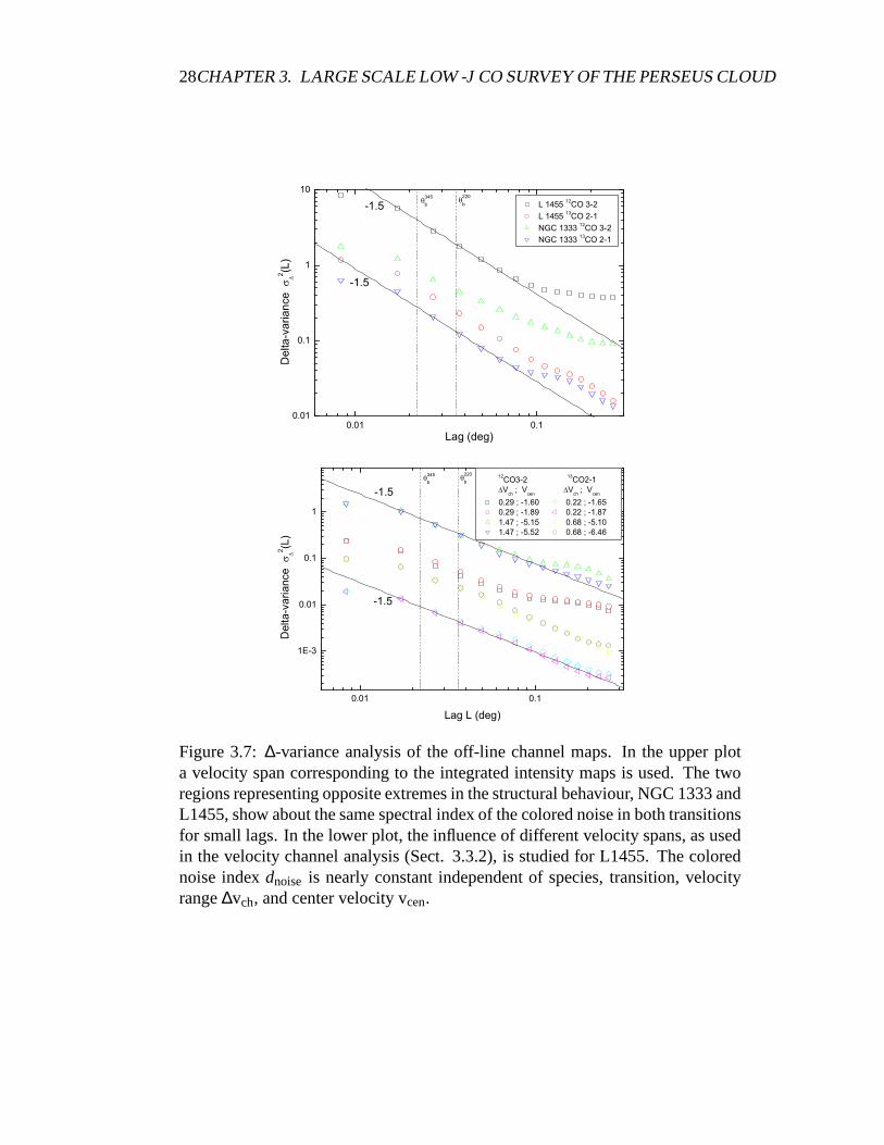
Figure 3.7:∆-variance analysis of the off-line channel maps. In the upper plota velocity span corresponding to the integrated intensity maps is used. The tworegions representing opposite extremes in the structural behaviour, NGC 1333 andL1455, show about the same spectral index of the colored noise in both transitionsfor small lags. In the lower plot, the influence of different velocity spans, as usedin the velocity channel analysis (Sect. 3.3.2), is studied for L1455. The colorednoise indexdnoise is nearly constant independent of species, transition, velocityrange∆vch, and center velocity vcen.

3.3. THE∆-VARIANCE ANALYSIS 29
Figure 3.8:∆-variance spectra of integrated intensities.a) Spectra obtained fromthe CO maps and theAV data of the region mapped with the KOSMA telescope.b) Spectra of integrated intensity maps of two 50′× 50′sub-regions: NGC 1333and L 1455. Power-law fits to the data corrected for noise and beam-blurring areindicated as solid lines.

30CHAPTER 3. LARGE SCALE LOW -J CO SURVEY OF THE PERSEUS CLOUD
Table 3.3: Results of the∆-variance analysis of the integrated CO maps and theAV data for the region mapped with KOSMA (Fig. 3.3).
Transition Telescope resol. Fit Range β[′] [ ′]
AV 2MASS 5 5.0-28 2.55± 0.0213CO 1–0 FCRAO 0.77 0.8-28 3.09± 0.0912CO 1–0 FCRAO 0.77 0.8-28 3.08± 0.0413CO 2–1 KOSMA 2.17 2.2-28 3.03± 0.1412CO 3–2 KOSMA 1.37 1.4-28 3.15± 0.04
Table 3.4: Results of the∆-variance analysis of the KOSMA data for seven 50′×50′sub-regions of the cloud (Figure 3.3). The spectral indicesβ were fitted in thesize range 2.2-14′ for the13CO 2–1 and in the size range 1.4-14′ for the12CO 3–2data.
Region β (13CO2−1) β (12CO3−2)L 1448 2.96± 0.42 3.41± 0.16L 1455 2.86± 0.09 2.85± 0.30NGC 1333 3.76± 0.48 3.52± 0.11B 1 3.14± 0.29 3.00± 0.20B 1 EAST 3.16± 0.09 3.39± 0.09B 3 3.36± 0.09 3.14± 0.06IC 348 2.71± 0.42 3.06± 0.24
both transitions. The low end of the spectral index range is formed by the darkcloud L 1455 together with the environment of the young cluster IC 348. The∆-variance spectra of the two extreme examples NGC 1333 and L 1455 are shownin Fig. 3.8b. Starting from the same noise values at small scales the spectra of thetwo regions show an increasing difference in the relative amount of structure atlarge scales reflected by the strongly deviating spectral indices. Altogether, I findhigh indices as characteristics of large condensations forthe regions with activestar formation and lower indices quantifying more filamentary structure for darkclouds, but IC 348 as an exception to this rule, showing also avery filamentarystructure.
3.3.2 Velocity channel maps
When performing the∆-variance analysis not only for maps of integrated intensi-ties, but for individual channel maps I obtain additional information on the veloc-ity structure of the cloud. In the velocity channel analysis(VCA), introduced by

3.3. THE∆-VARIANCE ANALYSIS 31
Lazarian & Pogosyan (2000), the change of the spectral indexof channel maps asa function of the channel width was used to simultaneously determine the scalingbehavior of the density and the velocity fields from a single data cube of line data.Here I conduct such a study for the KOSMA CO data.
I start with the analysis of individual channel maps as they are provided bythe channel spacing∆vch of the backends (cf.§3.1). For all channel maps I per-form the∆-variance analysis and fit power laws to the measured structure for alllags between the telescope beam size and the maximum scale resolved by the∆-variance (about 1/4 of the map size). As a result I get the power-law index as afunction of the channel velocity, a curve which I callindex spectrum. As an exam-ple I show the index spectrum obtained for the13CO 2–1 data in the L 1455 regionin Fig. 3.9. The spectrum is always truncated at velocities where the average linetemperature is lower than the noise rms.
The overall structure of the index spectrum is similar to theline profile. Thelargest spectral indices are found at velocities close to the average line peak. Thismay implicate that extended smooth structure provides the major contribution tothe overall emission, while the velocity tail of this structure is formed by small-scale features. However, the indices show an asymmetric behavior with respect tothe blue and the red wing. The indices drop steeply to a noise-dominated value atthe red wing, while the blue wing shows only a very shallow decay. Even at thenoise limit, noticeable structure is detected in the channel maps there.
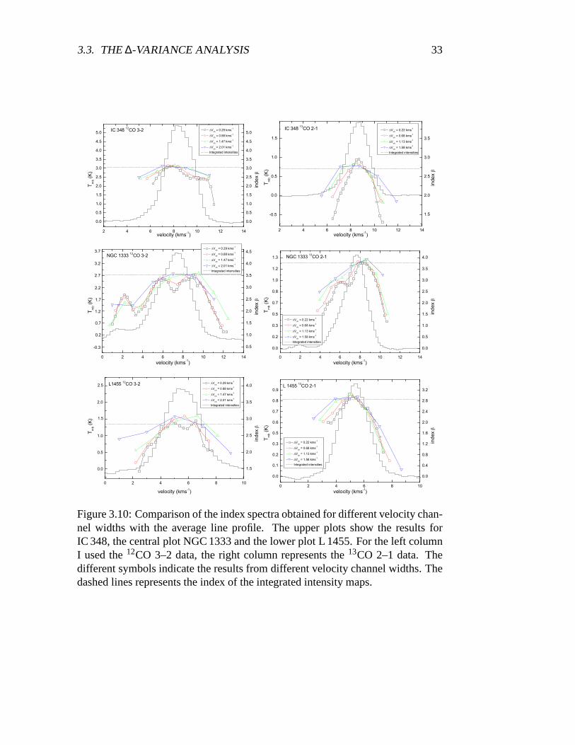
For the full velocity channel analysis, the index spectrum has to be computedfor different velocity channel widths (Lazarian & Pogosyan, 2000). Thus I havebinned the data to averages of three, five, and seven velocitychannels and com-puted the index spectra for these binned channel maps. In Fig. 3.10 I show theresults for three examples: IC 348, NGC 1333 and L 1455. For the sake of claritythe error bars of the index spectra were omitted in these plots.
The overall structure of the index spectra is similar to Fig.3.9 for all sources,transitions and channel widths. In most cases I find the asymmetry of a shallowerblue wing relative to the red wing. When looking at narrow velocity channels, Ifind a dip in the centre of the index spectrum for the12CO 3–2 data of NGC 1333and L 1455. A slight indication of such a dip is also present inthe12CO 3–2 dataif IC348 and in the13CO 2–1 data of NGC 1333. This could be due to opticaldepth effects. Because I see self-absorption in quite a few positions, when I checkindividual spectra in those regions. This leads to a more filamentary appearanceof the central channel maps reflected by this dip in the index spectra. It is inter-esting to notice that the VCA is more sensitive to self-absorption than the averagespectrum.
When increasing the channel width by binning, the self-absorption dip is smoothedout, so that the resulting index spectra peak again close to the peak velocity of theline temperature. In all situations where the self absorption is negligible, the in-

32CHAPTER 3. LARGE SCALE LOW -J CO SURVEY OF THE PERSEUS CLOUD
Figure 3.9: Comparison of the index spectrum of the13CO 2–1 data in L 1455with the average line profile. The index spectrum is created by power-law fits tothe ∆-variance spectrum of individual channel maps (∆vch = 0.22 km s−1). Thevertical error bars represent the uncertainty of the fit. Thehorizontal error barsindicate the velocity channel width.
dices for the line core channels are almost independent fromthe channel width.The indices for the line integrated intensities always fallslightly below the peakindices, as they represent an average which is typically dominated by the linecores.
In the red line wings, most indices remain approximately constant when in-creasing the velocity width, except for the largest bin width where the contribu-tion from the core leads to an observable increase. In the blue wing, I find amonotonic growth of the spectral indices with the channel width for both tracersin all three regions. The additional peak at 2 km s−1 visible in the12CO 3–2 dataof NGC 1333 stems from a separate dark cloud which is also contained in theNGC 1333 map.
Figure 3.11 summarizes the relation between the spectral indices and the ve-locity channel width. In Fig. 3.11a I plot the average spectral index over the lineas a function of the channel width for the six data sets presented in Fig. 3.10. Fig-ure 3.11b contains the analysis when restricted to a 2 km s−1 window in the blueline wings. The error bars contain the standard deviation ofthe index variationacross the line and the fit errors. They are necessarily largebecause of the system-atic variation of indices over the velocity range. In contrast to similar analysis byDickey et al. (2001); Stanimirovic & Lazarian (2001) I find no significant system-atic variation of the mean line index as a function of channelwidth (Figure 3.11a).
3.3. THE∆-VARIANCE ANALYSIS 33
Figure 3.10: Comparison of the index spectra obtained for different velocity chan-nel widths with the average line profile. The upper plots showthe results forIC 348, the central plot NGC 1333 and the lower plot L 1455. Forthe left columnI used the12CO 3–2 data, the right column represents the13CO 2–1 data. Thedifferent symbols indicate the results from different velocity channel widths. Thedashed lines represents the index of the integrated intensity maps.

34CHAPTER 3. LARGE SCALE LOW -J CO SURVEY OF THE PERSEUS CLOUD
In contrast to the average of the index spectrum I find a continuous increase of thespectral index with the channel width when restricting the analysis to the bluewing (Figure 3.11b). The average index steepens from about 2.8 to about 3.1 inthe 12CO 3–2 maps and from about 2.4 to about 2.8 in the13CO 2–1 maps. Asdiscussed above I find no systematic trend in the red wings. This indicates that theaverage spectral index taken over the full line profile provides no measure for thevelocity structure in the CO maps while the peculiar behaviour in the blue wingsneeds further investigation.
3.4 Discussion
3.4.1 Integrated intensity maps
Besides the∆-variance, other tools have been used to characterize interstellarcloud structure. The second-order structure function for an observables(~r) isS2 = 〈|s(~r)−s(~r +δ~r)|2〉~r which is treated as a function of the absolute value ofthe increment|δ~r| (Elmegreen & Scalo, 2004). Padoan et al. (2003a) computedthe structure function of the integrated intensity map of13CO 1–0 in Perseus. Apower-law fit to S2 ∝ δ rζ over a range of 0.3 to 3 pc provided an indexζ of0.83. The index of the structure function is related to the power spectral index byζ = β −2 for 2< β < 4 (Stutzki et al., 1998) resulting inβ = 2.83. This resultof Padoan et al. (2003a) agrees within the error bars with theindices found by the∆-variance analysis of the Perseus maps of integrated CO intensities over almostthe same linear range (see Table 3.3).
However, the∆-variance spectra of individual regions show significant vari-ations of the spectral index as discussed above. For13CO 2–1, these span therange betweenβ = 2.86 in L1455 and 3.76 in NGC 1333 (Table 3.4). The anal-ysis of different sub-sets in molecular cloud complexes thus provides additionaland complementary information on the structure of the cloudcomplex.
3.4.2 Velocity channel maps
The velocity channel analysis, was used previously by Dickey et al. (2001) tostudy HI maps of two regions in the 4th Galactic quadrant. One of the regions isrich in warm HI gas, the other is rich in cool HI gas. For the warm gas, Dickeyet al. (2001) find a systematic increase of the mean index withvelocity channelwidth. The cold gas at lower latitudes behaves differently and shows rather con-stant indices of 2.7–3.1.
The latter results resemble the outcome of the VCA of the12CO and13COchannel maps in Perseus presented above. I find similar indices for the velocity

3.4. DISCUSSION 35
Figure 3.11: Average spectral indices of the channel maps asa function of thechannel width.a) shows the average over the full line width.b) represents onlythe indices in the blue ling wings. The line wing components are centered at5 km s−1 for NGC 1333, at 4 km s−1 for L 1455, and at 7 km s−1 for IC 348. Theerror bars contain the fit error and the standard deviation ofthe indices withinthe considered velocity range. To avoid overlapping error bars in the plot, I haveshifted the points for IC 348 and NGC 1333 by±0.02 km s−1 relative to theiractual position.

36CHAPTER 3. LARGE SCALE LOW -J CO SURVEY OF THE PERSEUS CLOUD
integrated maps of the full region (cf. Table 3.3) and the CO data show no signif-icant variation of the index with velocity channel width when averaged over allvelocity bins (Figure 3.11a). The indices stay relatively constant. Since the bulkof the molecular gas traced by CO is even colder than cold HI gas, these resultssuggest a sequence of a reduced dependence of the spectral index of the channelmaps on the bin widths from the warm to the cold ISM. The constancy of the av-erage spectral index could also be explained by optical depth effects. Lazarian &Pogosyan (2004) have shown that absorption can lead to an effective slice broad-ening, which leads in extreme cases to slice indices that become independent fromthe actual channel width.
Studying the spectral index of individual velocity bins of the CO data acrossthe line profile (Fig. 3.10), I find that the power-law indicesincrease with the ve-locity channel width in the blue wing (Fig. 3.11b) while staying rather constant inthe red wing. No corresponding analysis was conducted for the H I data by Dickeyet al. (2001). One possibility to explain the asymmetry between the blue and redwings might be a shock expansion of the CO gas in Perseus. Sancisi (1974) foundan expanding shell of neutral hydrogen which was created by asupernova in thePer OB2 association a few 106 years ago. At the location of the molecular cloudcomplex, the expansion is directed away from the Sun. Most ofthe associatedmolecular gas has been swept up by the shock, but pillar-likefilaments have beenleft at the backside of the shock. They are visible in the channel maps (Fig. 3.5)and produce the velocity dependence seen in the VCA of the blue line wings,i.e. the increase of indices with size of the velocity bin because of a gradual in-crease of large scale contributions across the line wing. I illustrate this scenario inFig. 3.12.
The quantitative results from the velocity channel analysis can be interpretedin terms of the power spectrum of the velocity structure. Lazarian & Pogosyan(2000) showed that the spectrum of velocity slices as a function of the velocitychannel width is determined by the power spectral indices ofthe density structureβ and the velocity structurem. They obtain different regimes for shallow (β < 3)and steep (β > 3) density power spectra:
P(k) ∝
k−β+m−32 , thin slices,
k−β , thick slices,k−β , very thick slices;
(β < 3)
P(k) ∝
k−9−m
2 , thin slices,
k−3+m
2 , thick slices,k−β , very thick slices.
(β > 3)
Thin slices have a velocity width less than the local velocity dispersion at the stud-ied scale; thick slices have a width larger than the velocitydispersion and very

3.4. DISCUSSION 37
Perseus Molecular Cloud
9 kms-1
12 kms-1
104M
to Sun (350pc)
20pc
7 kms-1
IC 348
NGC 1333
Figure 3.12: Sketch adopted from Fig. 3 of Sancisi (1974) illustrating the spatialarrangement and motion of the Perseus cloud complex. The gasis swept up by ashock expansion with 12 km s−1. Due to the overall curvature, the line-of-sightvelocity is 9 km s−1 for IC 348, but only 7 km s−1 for NGC1333. The diameter ofthe cloud is∼ 20 pc. Pillar-like structures are left at lower velocities as remaindersof high-density regions which were not accelerated to the same velocity.

38CHAPTER 3. LARGE SCALE LOW -J CO SURVEY OF THE PERSEUS CLOUD
thick slices essentially correspond to the integrated maps(Lazarian & Pogosyan, 2000). I can assume that a single channel of the data corresponds to thin slicesas they are much narrower than any observed line width. I useβ from the in-tegrated maps and the index measured in the single channels to derivem. Fromthe indices obtained by averaging over the full line profile (Fig. 3.11a), I obtainm values of 3.9±1.6, 3.9±1.9 and 3.8±1.7 for 12CO 3–2 in IC 348, NGC 1333and L 1455, respectively; whilem is 3.9±2.0, 3.5±2.5 and 4.1±1.8 for13CO 2–1in the same three regions. In the blue wings (Fig. 3.11b), I obtain m values of3.2±1.6, 3.4±1.4 and 3.6±1.5 for 12CO 3–2; whilem is 4.3±1.9, 4.3±1.7 and4.1±1.5 for 13CO 2–1 in the three regions. These values have large error bars,so that they are not directly suited to discriminate betweendifferent turbulencemodels. At least, I find that all values are consistent with Kolmogorov turbulencethat givesm∼ 3.7 (Kolmogorov, 1941).
3.5 Summary
1. I present KOSMA maps of the13CO 2–1 and12CO 3–2 emission of thePerseus molecular cloud covering 7.1 deg2. These data are combined withFCRAO maps of integrated12CO and13CO 1–0 intensities and with a2MASS map of optical extinctions.
2. To characterize the cloud density structure, I applied the∆-variance analysisto integrated intensity maps. The∆-variance spectra of the overall regionfollow a power law with an index ofβ = 2.9−3.0 for scales between 0.2and 3 pc. This agrees with results obtained by Padoan et al. (2003a) studyingstructure functions of a13CO 1–0 map of Perseus.
3. I also applied the∆-variance method to seven sub-regions of Perseus. Theresulting power spectral indices vary significantly between the individualregions. The active star-forming region NGC 1333 shows highspectral in-dices (β = 3.5−3.8) while the dark cloud L 1455 shows low indices of 2.9in both transitions.
4. Additional information is obtained from the∆-variance spectra of individualvelocity channel maps. They are very sensitive to optical depth effects,indicating self-absorption in the densest regions. The asymmetry of thechannel map indices relative to the line centrum is a hint towards a peculiarvelocity structure of the Perseus cloud complex.
5. When analyzing the spectral indices as a function of the velocity channelwidth I find almost constant indices when averaging over the total line pro-file. A continuous increase of the index with varying velocity channel width

3.5. SUMMARY 39
is, however, observed in the blue wings. This behavior can beexplained bya shock running through the region creating a filamentary structure prefer-entially at low velocities.
I find that the comparison of the structural properties for entire surveys andsub-sets, as well as the velocity channel analysis (VCA), provide additional, sig-nificant characteristics of the ISM in observed CO spectral line maps. These quan-tities are useful for a comparison of the structure observedin different clouds,possibly providing a diagnostic tool to characterize the star-formation activity andproviding additional constraints for numerical simulations of the ISM structure.
In the next chapter (Chapter 4), I will use a different approach to quantify thestructure with decomposing the observed emission into discrete entities (′′clumps′′).For this purpose,Gaussclumpsis used in that analysis.

Chapter 4
The Gaussclumps analysis in thePerseus cloud
Visual inspection of position-velocity cuts and of channelmaps of molecularclouds, indicate a large number of structures; all these maps exhibit a complex,inhomogeneous, nested, filamentary, or clumpy structure onall scales down to theresolution limits. These maps appear self-similar: the structure looks the sameindependent of the scales. The derivation of clump mass spectra leads to a betterquantification of this description. Another motivation to analyze the distributionof clump masses is, that it possibly determines the stellar initial mass function,which in turn determines all stellar evolution, and its links with star formationefficiency (Zinnecker et al., 1993).
In this chapter, I useGaussclumps(Stutzki & Gusten, 1990) to identify clumpsin the Perseus molecular cloud and to investigate its properties. The aim of theanalysis is to identify clumps in clouds and to derive their basic properties, suchas sizes, line widths and masses. Here I study mainly the13CO 2–1 data from theKOSMA 3m telescope and the13CO 1–0 data from the FCRAO 14m telescope.
This chapter is organized as the following: Section 1 presents the results anddiscussions on clump mass spectra, the relations of clump size with line width andmass and the equilibrium state of the clumps; a summary is given in Section 2.
4.1 Results and discussions
Using the KOSMA13CO 2–1 data, there are 341 clumps found, the mass rangeof which is between 0.54 M and 87.98 M. And I find 737 clumps using theFCRAO 13CO 1–0 data and the clump mass ranges from 0.28 M and 140.90M.
Fig. 4.1 presents the clump center velocity and peak temperature for the clumps
40

4.1. RESULTS AND DISCUSSIONS 41
Figure 4.1: Velocity (v0) of the clumps found in NGC 1333 versus peak intensity(amp.). The average spectrum of13CO 2-1 in NGC1333 is also presented.
found in NGC 1333. The averaged spectrum of13CO 2–1 emission is also pre-sented in the figure. The peak temperatures of all clumps are significantly abovethe general noise level. Furthermore, the center velocities of those clumps liewithin the velocity range of emission. This is one additional proof, that almost allclumps are decomposed from the emission.
4.1.1 Clump mass
Under the assumption of local thermodynamic equilibrium and optically thin emis-sion of 13CO 2–1, I calculate the13CO clump column density using13CO 2–1clump brightness temperaturesTmb in K and the FWHM line widths∆v in kms−1. To derive the clump mass, I assume that the excitation temperature is fixed tobe 10 K. In the active star forming regions like NGC 1333, the excitation temper-ature must be higher. However,13CO column densities are only weakly sensitiveto the exact choice of the excitation temperature. If excitation temperature ischanged to 20 K or to 30 K, the derived column densities increases only by 40%and 92%, respectively. So theTex assumption of 10 K will be good estimation.Then taken the canonical abundance factors of[12CO/13CO] = 65 (Langer et al.,
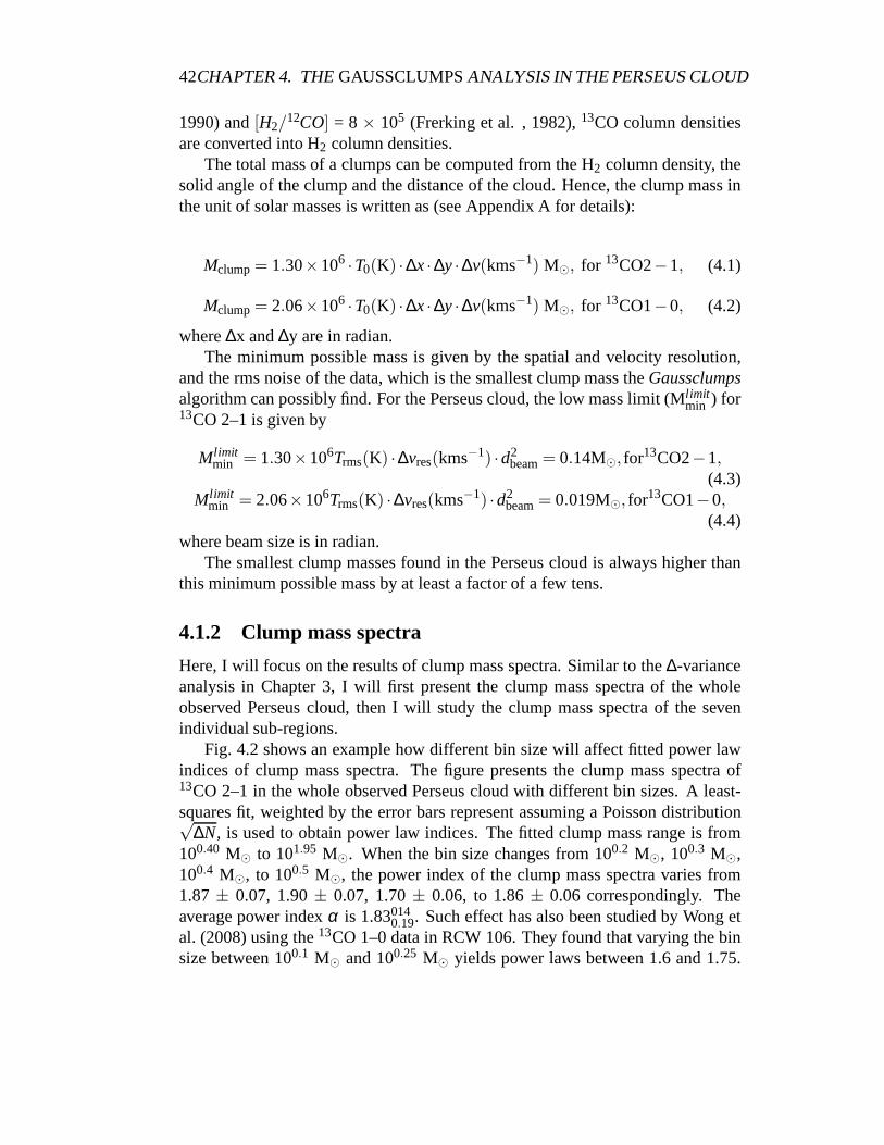
42CHAPTER 4. THEGAUSSCLUMPSANALYSIS IN THE PERSEUS CLOUD
1990) and[H2/12CO] = 8 × 10⁵ (Frerking et al. , 1982),13CO column densities
are converted into H2 column densities.The total mass of a clumps can be computed from the H2 column density, the
solid angle of the clump and the distance of the cloud. Hence,the clump mass inthe unit of solar masses is written as (see Appendix A for details):
Mclump= 1.30×10⁶ ·T0(K) ·∆x·∆y·∆v(kms−1) M, for 13CO2−1, (4.1)
Mclump= 2.06×10⁶ ·T0(K) ·∆x·∆y·∆v(kms−1) M, for 13CO1−0, (4.2)
where∆x and∆y are in radian.The minimum possible mass is given by the spatial and velocity resolution,
and the rms noise of the data, which is the smallest clump masstheGaussclumpsalgorithm can possibly find. For the Perseus cloud, the low mass limit (Mlimit
min ) for13CO 2–1 is given by
Mlimitmin = 1.30×10⁶Trms(K) ·∆vres(kms−1) ·d2
beam= 0.14M, for13CO2−1,(4.3)
Mlimitmin = 2.06×10⁶Trms(K) ·∆vres(kms−1) ·d2
beam= 0.019M, for13CO1−0,(4.4)
where beam size is in radian.The smallest clump masses found in the Perseus cloud is always higher than
this minimum possible mass by at least a factor of a few tens.
4.1.2 Clump mass spectra
Here, I will focus on the results of clump mass spectra. Similar to the∆-varianceanalysis in Chapter 3, I will first present the clump mass spectra of the wholeobserved Perseus cloud, then I will study the clump mass spectra of the sevenindividual sub-regions.
Fig. 4.2 shows an example how different bin size will affect fitted power lawindices of clump mass spectra. The figure presents the clump mass spectra of13CO 2–1 in the whole observed Perseus cloud with different binsizes. A least-squares fit, weighted by the error bars represent assuming a Poisson distribution√
∆N, is used to obtain power law indices. The fitted clump mass range is from100.40 M to 101.95 M. When the bin size changes from 100.2 M, 100.3 M,100.4 M, to 100.5 M, the power index of the clump mass spectra varies from1.87± 0.07, 1.90± 0.07, 1.70± 0.06, to 1.86± 0.06 correspondingly. Theaverage power indexα is 1.83014
0.19. Such effect has also been studied by Wong etal. (2008) using the13CO 1–0 data in RCW 106. They found that varying the binsize between 100.1 M and 100.25 M yields power laws between 1.6 and 1.75.

4.1. RESULTS AND DISCUSSIONS 43
Figure 4.2: An example of the effect of different clump mass binning sizes. Thebin size changes from 100.2 M, 100.3 M, 100.4 M, to 100.5 M. Error barsrepresent the standard deviation of a Poisson distribution
√∆N. The dashed line
denotes the lower clump mass limit (10*Mlimitmin ).
The derivation of the power indices is small, which indicates that bin size has nobig effect on the results. In the following, I will choose a bin size of 100.2 M forall the analysis.
4.1.2.1 The whole observed Perseus cloud
I firstly derive the power indice of clump mass spectra of the whole observedPerseus cloud for the KOSMA13CO 2–1 data and the FCRAO13CO 1–0 data(see Fig. 4.3). Due to the much smaller beam of the FCRAO telescope (∼ 46′′),there are much more clumps identified, especially small clumps, using the13CO1–0 data. A lease-squares fit is used to obtain the power law index. The fittedclump mass ranges are from 100.4 M to 101.9 M for 13CO 2–1 data and from100.7 M to 101.9 M for 13CO 1–0 data. The minimum clump massMcl
min, foundfrom the FCRAO13CO 1–0 data, is much larger than 10 times of the lower masslimit Mlimit
min (0.019 M for 13CO 1–0, 1.42 M for 13CO 2–1).For both13CO 1–0 and13CO 2–1, the fitted power law indices are close to
1.9, which is consistent with the results from other clouds (Kramer et al., 1998b;Simon et al., 2001; Mookerjea et al., 2004; Wong et al., 2008).
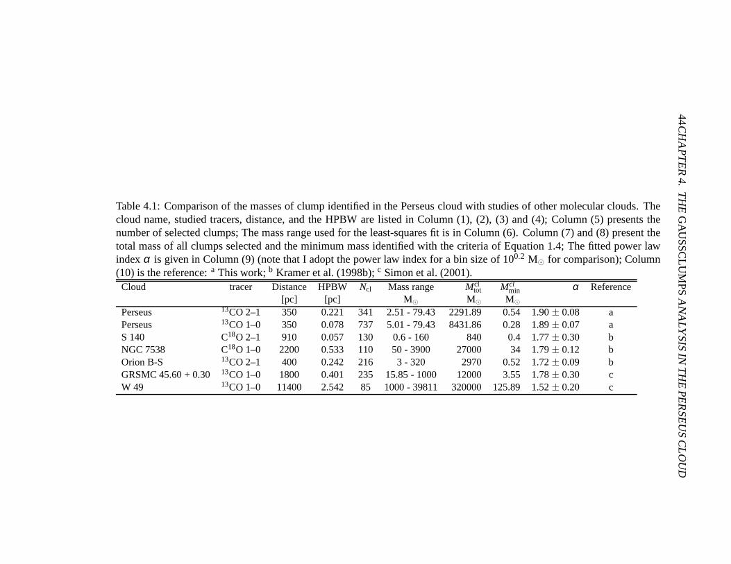
44C
HA
PT
ER
4.T
HE
GA
US
SC
LUM
PSA
NA
LYS
ISIN
TH
EP
ER
SE
US
CLO
UD
Table 4.1: Comparison of the masses of clump identified in thePerseus cloud with studies of other molecular clouds. Thecloud name, studied tracers, distance, and the HPBW are listed in Column (1), (2), (3) and (4); Column (5) presents thenumber of selected clumps; The mass range used for the least-squares fit is in Column (6). Column (7) and (8) present thetotal mass of all clumps selected and the minimum mass identified with the criteria of Equation 1.4; The fitted power lawindexα is given in Column (9) (note that I adopt the power law index for a bin size of 100.2 M for comparison); Column(10) is the reference:a This work;b Kramer et al. (1998b);c Simon et al. (2001).Cloud tracer Distance HPBW Ncl Mass range Mcl
tot Mclmin α Reference
[pc] [pc] M M MPerseus 13CO 2–1 350 0.221 341 2.51 - 79.43 2291.89 0.54 1.90± 0.08 aPerseus 13CO 1–0 350 0.078 737 5.01 - 79.43 8431.86 0.28 1.89± 0.07 aS 140 C18O 2–1 910 0.057 130 0.6 - 160 840 0.4 1.77± 0.30 bNGC 7538 C18O 1–0 2200 0.533 110 50 - 3900 27000 34 1.79± 0.12 bOrion B-S 13CO 2–1 400 0.242 216 3 - 320 2970 0.52 1.72± 0.09 bGRSMC 45.60 + 0.30 13CO 1–0 1800 0.401 235 15.85 - 1000 12000 3.55 1.78± 0.30 cW 49 13CO 1–0 11400 2.542 85 1000 - 39811 320000 125.89 1.52± 0.20 c

4.1. RESULTS AND DISCUSSIONS 45
Figure 4.3: Clump mass spectra of the Perseus molecular cloud from both theFCRAO 13CO 1–0 data and the KOSMA13CO 2–1 data. Both spectra are fittedby a power law functiondN = dM/M−α . The straight line represents the bestlinear fit over the range of masses spanned by the line. The resulting indicesα forboth datasets are very similar,∼ 1.9. The two vertical dashed lines show the 10times of the lower mass limits for both tracers.
4.1.2.2 The seven sub-regions in the Perseus cloud
To study the behavior of the power indices of clump mass spectra for different re-gions (quiescent or star forming), I divide the Perseus molecular cloud into sevensub-regions as the same as the∆-variance analysis in Chapter 3. Then using theKOSMA 13CO 2–1 data, I derive the power law indices of the clump mass spectra.The results of the seven sub-regions are presented in Fig. 4.4 and Table 4.2. Theclump identification works on the way that the maximum clump masses found re-flect the peak temperatures, maximum line widths, and largest spatial clump sizesfound in an observed region. Molecular clouds with ongoing star formation likeNGC 1333, exhibit massive clumps of up to∼ 100 M, whereas quiescent, coldclouds like L 1455 and L 1448, only show clumps of less than 30 M.
I also perform a least-squares fit to the data. The lower mass limit of the fitis fixed to all the seven sub-regions to 100.5 M and the upper mass limit is themaximum clump mass of each sub-region. The upper limit of each sub-region isdifferent. The biggest up limit is∼ 101.02 M in NGC 1333, while the smallestone is∼ 19.40 M in L 1455. The power law indices of the seven regions showslightly variation, changing from 1.65 in IC 348 and 1.85 in B1 EAST. The activestar forming region, NGC 1333, does not have the largest power law index. whilethe quiescent clouds like L 1455, B1 and B1 EAST have the largest power lawindex. It seems that the power law index of clump mass spectrais not directlyrelated to star forming activities. The average power law index of those seven

46CHAPTER 4. THEGAUSSCLUMPSANALYSIS IN THE PERSEUS CLOUD
Table 4.2: The results of the seven sub-regions. The cloud name is listed in Col-umn (1); Column (2) presents the number of selected clumps; The mass rangeused for the least-squares fit is in Column (3). Column (4) and(5) present the to-tal mass of all clumps selected and the minimum mass identified with the criteriaof Equation 1.4; The fitted power law indexα is given in Column (6).
Cloud Ncl Mass range Mcltot Mcl
min αLog(M) M M
L 1448 28 0.5 - 1.5 156.92 0.62 1.72± 0.24L 1455 39 0.5 - 1.1 179.45 0.65 1.81± 0.27NGC 1333 76 0.5 - 2.1 547.77 0.56 1.78± 0.17B 1 58 0.5 - 1.7 333.12 0.54 1.83± 0.19B 1 East 43 0.5 - 1.5 270.82 0.59 1.85± 0.18B 3 70 0.5 - 1.5 377.71 0.55 1.76± 0.20IC 348 65 0.5 - 1.9 611.23 0.66 1.65± 0.13
regions is 1.80, which is a typical value found in the previous studies of clumpmass spectra. It may show a trend that clump mass spectra havea common powerlaw index, independent of star formation activity, which have als0 been pointedout by Kramer et al. (1998b); Simon et al. (2001).
The power law index of clump mass spectra found using the molecular linedata ( mainly CO) is also often smaller than that using the (sub)millimeter contin-uum (Mookerjea et al., 2004; Kirk et al., 2006). The different power law indicesbetween CO and (sub)millimeter continuum may be due to different methods ofobservations, in the definition of structure, the effects ofchemistry such as freeze-out, or real differences in the structures at the large and small scales (Kirk et al.,2006).
4.1.3 Relations of clump size with line width and mass
In this subsection, I will study the relations of clump size with line width, and withmass in the Perseus cloud and two typical sub-regions: NGC 1333 and L 1455.NGC 1333 is an active star forming region and L 1455 is a quiescent dark cloud.Hence, those two sub-regions are typical examples in the Perseus cloud.
Fig. 4.5 and Fig. 4.6 present the relations between line width and mass as afunction of size of all clumps in the three regions mentionedbefore. The clumpradius is defined as the geometric mean of the major and minor half-axes identifiedfrom Gaussclumps.
The contribution from the thermal line width to the observedline width maybe considerable and could flatten the power index of a size-line width relation(Myers & Goodman , 1988). For13CO, the thermal line width can be given as
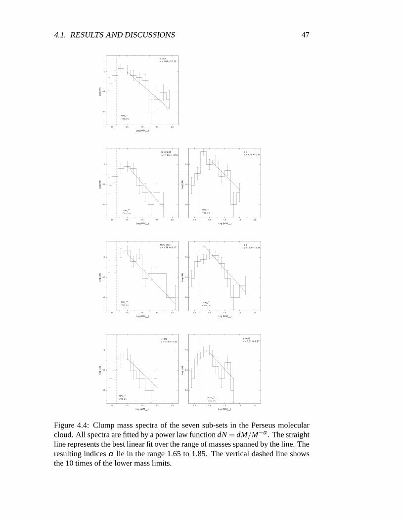
4.1. RESULTS AND DISCUSSIONS 47
Figure 4.4: Clump mass spectra of the seven sub-sets in the Perseus molecularcloud. All spectra are fitted by a power law functiondN= dM/M−α . The straightline represents the best linear fit over the range of masses spanned by the line. Theresulting indicesα lie in the range 1.65 to 1.85. The vertical dashed line showsthe 10 times of the lower mass limits.

48CHAPTER 4. THEGAUSSCLUMPSANALYSIS IN THE PERSEUS CLOUD
Figure 4.5: Size-line width (top panel) and size-mass (bottom panel) relationsfor the Perseus cloud using13CO 2–1 data. Least-squares fits to∆v ∝ Rαlw , andMLTE ∝ Rαm are presented by the solid lines. The dashed lines show fit with fixedpower law indices ofαlw = 0.5 andαm = 2, which correspond the conventionalLarson relations (Larson, 1981).
∆vth = 2(ln2)12
√
kTkinu = 0.13
√
Tkin10 km s−1, wherek is the Boltzmann constant,
Tkin is the kinetic temperature in K, andu is the mean molecular weight. Fora kinetic temperature of 10 K, each clump identified has highly supersonic linewidths.
Least-squares fits to∆v ∝ Rαlw , andMLTE ∝ Rαm are presented in Fig. 4.5 andFig. 4.6. For the whole Perseus cloud, we obtainαlw of 0.47± 0.05 andαm of2.19± 0.17. For NGC 1333 and L 1455, the fittedαlw is 0.51± 0.17 and 0.78± 0.10, respectively; the fittedαm is 1.96± 0.18 and 2.45± 0.13 for NGC 1333and L 1455, respectively. Previous studies yield power law indices that coverwide ranges:αlw between 0.15 and 0.7, andαm between 1.7 and 2.5 (Larson,1981; Leung et al., 1983; Myers, 1983; Sanders et al., 1985; Dame et al., 1986;Solomon et al., 1987; Heithausen, 1996; Kramer et al., 1996;Heyer & Schloerb,1997; Williams et al., 2000; Simon et al., 2001). The fitted indices from this workare consistent with those studies.
The assumption of gravitational virial equilibriumGM/R∝ ∆v2 implies scal-ing relation of the formαlw = (αm − 1)/2 (Simon et al., 2001). Values of thedifferent power-law indices were empirically determined from giant molecular
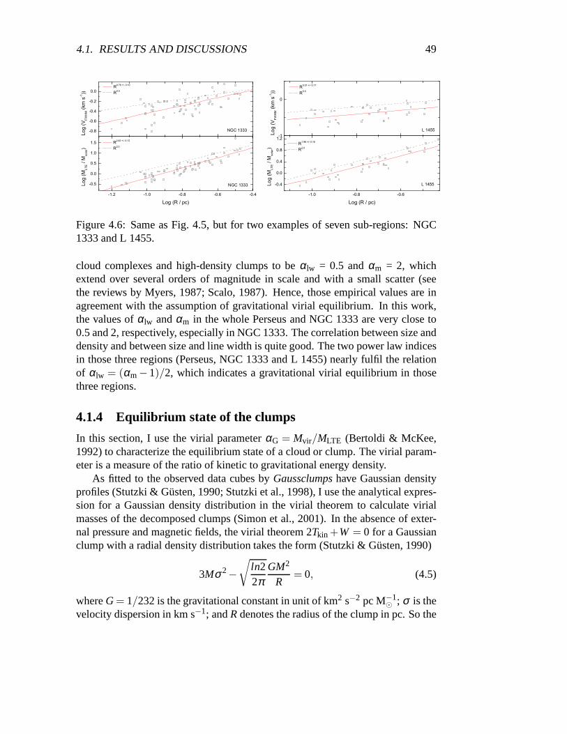
4.1. RESULTS AND DISCUSSIONS 49
Figure 4.6: Same as Fig. 4.5, but for two examples of seven sub-regions: NGC1333 and L 1455.
cloud complexes and high-density clumps to beαlw = 0.5 andαm = 2, whichextend over several orders of magnitude in scale and with a small scatter (seethe reviews by Myers, 1987; Scalo, 1987). Hence, those empirical values are inagreement with the assumption of gravitational virial equilibrium. In this work,the values ofαlw andαm in the whole Perseus and NGC 1333 are very close to0.5 and 2, respectively, especially in NGC 1333. The correlation between size anddensity and between size and line width is quite good. The twopower law indicesin those three regions (Perseus, NGC 1333 and L 1455) nearly fulfil the relationof αlw = (αm−1)/2, which indicates a gravitational virial equilibrium in thosethree regions.
4.1.4 Equilibrium state of the clumps
In this section, I use the virial parameterαG = Mvir/MLTE (Bertoldi & McKee,1992) to characterize the equilibrium state of a cloud or clump. The virial param-eter is a measure of the ratio of kinetic to gravitational energy density.
As fitted to the observed data cubes byGaussclumpshave Gaussian densityprofiles (Stutzki & Gusten, 1990; Stutzki et al., 1998), I use the analytical expres-sion for a Gaussian density distribution in the virial theorem to calculate virialmasses of the decomposed clumps (Simon et al., 2001). In the absence of exter-nal pressure and magnetic fields, the virial theorem 2Tkin +W = 0 for a Gaussianclump with a radial density distribution takes the form (Stutzki & Gusten, 1990)
3Mσ2−√
ln22π
GM2
R= 0, (4.5)
whereG= 1/232 is the gravitational constant in unit of km2 s−2 pc M−1 ; σ is the
velocity dispersion in km s−1; andRdenotes the radius of the clump in pc. So the

50CHAPTER 4. THEGAUSSCLUMPSANALYSIS IN THE PERSEUS CLOUD
viral mass of a clump with Gaussian density distribution canbe given by (Simonet al., 2001)
Mvir
M= 378R∆v2, (4.6)
where∆v is the FWHM line width (∆v = σ(8ln2)).The ratio of virial to LTE clump mass as a function of LTE clumpmass in the
Perseus cloud and in the two sub-regions (NGC 1333 and L 1455)is presented inFig. 4.7 and Fig. 4.8, respectively. In the two sub-regions,all clumps identifiedare found aboveMvir/MLTE = 1; in the Perseus cloud, only one clump is belowMvir/MLTE = 1 and the rest are above that. The ratios of the virial to LTE mass forthe Perseus cloud are between 0.77 (only 1 clump) and 13.61. And the same ratiosare between 2.43 and 14.38 for NGC 1333, and from 1.94 to 11.98for L 1455.This means that those clumps are not gravitationally bound.This results showthe same trend as those found in the previous studies that clumps typically haveratios of virial to LTE mass well above the limit of virialization, Mvir/MLTE ' 1(Bertoldi & McKee, 1992; Williams et al., 1995; Heyer et al.,2001; Simon et al.,2001).
There is a tight correlation of the virial parameter with clump mass accordingto αG = (M0/MLTE)
23 found by Bertoldi & McKee (1992); Williams et al. (1995);
Heyer et al. (2001). Such correlation is theoretically expected for gravitationallyunbound, pressure-confined clumps (Bertoldi & McKee, 1992). While in thiswork, the distributions of the virial parameter with clump mass for the clumpsidentified in both the whole Perseus cloud and in NGC 1333 and L1455 show notrend of following this correlation as the also found by Kramer et al. (1996); Simonet al. (2001). However, for large values ofαG and masses above the completenesslimit, the virial parameters for the clumps seem to follow the correlation. I alsoplot the power law index of−2
3 in Fig. 4.7 and Fig. 4.8 (solid lines in the figures).The external pressures (Pex) can be evaluated by adding the surface term 4πR3Pex
to the equation of viral equilibrium. So the binding pressure of a clump is writtenas
Pex
k= 0.56
MR2(378
∆v2
R− M
R2)Kcm−3, (4.7)
and it can also be given by
σ2
R∝
Pex
k1
N(H2)+N(H2). (4.8)
The balance between the external pressure and the turbulentgas pressure isdescribed by that equation. Clumps withPex ' 0 K cm−3 are gravitationallybound. Histograms of required external pressure were developed from the datain Fig. 4.9 for the Perseus cloud and Fig. 4.10 for NGC 1333 andL 1455. The

4.1. RESULTS AND DISCUSSIONS 51
Figure 4.7: Ratio of virial to LTE mass as a function of LTE mass for the clumpsin the Perseus cloud. The dotted line corresponds toMvir = MLTE; The dashed lineshows the 10 times of the lower mass limits forMLTE. The solid line presents apower law index of−2
3.
Figure 4.8: Same as Fig. 4.7, but for two examples of seven sub-regions: NGC1333 and L 1455.
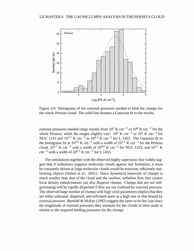
52CHAPTER 4. THEGAUSSCLUMPSANALYSIS IN THE PERSEUS CLOUD
Figure 4.9: Histograms of the external pressures needed to bind the clumps forthe whole Perseus cloud. The solid line donates a Gaussian fitto the results.
external pressures needed range mainly from 103 K cm−3 to 106 K cm−3 for thewhole Perseus, while the ranges slightly vary: 103 K cm−3 to 105 K cm−3 forNGC 1333 and 102.5 K cm−3 to 104.2 K cm−3 for L 1455. The Gaussian fit tothe histograms lie at 104.6 K cm−3 with a width of 101.1 K cm−3 for the Perseuscloud, 103.7 K cm−3 with a width of 100.8 K cm−3 for NGC 1333, and 103.7 Kcm−3 with a width of 100.3 K cm−3 for L 1455.
The simulations together with the observed highly supersonic line widths sug-gest that if turbulence supports molecular clouds against star formation, it mustbe constantly driven or large molecular clouds would be transient, efficiently star-forming objects (Simon et al., 2001). Since dynamical timescale of clumps ismuch smaller than that of the cloud and the random, turbulentflow that createslocal density enhancements can also disperse clumps. Clumps that are not self-gravitating will be rapidly dispersed if they are not confined by external pressure.The observed large number of clumps with high virial parameters implies that theyare either unbound, dispersed, and reformed anew at a high rate or else bound byexternal pressure. Bertoldi & McKee (1992) suggest the latter to be the case sincethe magnitude of external pressures they estimate for the clouds in their study issimilar to the required binding pressures for the clumps.

4.2. SUMMARY 53
Figure 4.10: Same as Fig. 4.9, but for two examples of seven sub-regions: NGC1333 and L 1455.
4.2 Summary
A three-dimensional Gaussian decomposition algorithm (Gaussclumps) has beenused to identify clumps inside each cloud and to derive the clump properties astraced in13CO 1–0 and 2–1 in the Perseus cloud. A power law index of∼ 1.9has been found for the whole observed Perseus cloud. When studying the sevensub-regions in the Perseus cloud, an common power law index of ∼ 1.80 hasbeen found, which may show a trend that clump mass spectra have a commonpower law index, independent of star formation activity, which have been foundby Kramer et al. (1998b); Simon et al. (2001).
Relations of clump size with line width and mass have been studied. Theobtainedαlw andαm follow the relation ofαlw = (αm−1)/2 for both the Perseuscloud and the two examples of the seven sub-regions (NGC 1333and L 1455),which implies that those clouds is gravitational virial equilibrium. The values ofαlw andαm confirm the standard Larson relations, especially of the Perseus cloudand NGC 1333.
I have used the virial parameterαG = Mvir/MLTE (Bertoldi & McKee, 1992)to characterize the equilibrium state of a cloud or clump. All clumps identified inNGC 1333 and L 1455 are found aboveMvir/MLTE = 1; And in the Perseus cloud,All except one clump is aboveMvir/MLTE = 1. The ratios of the virial to LTEmass for the Perseus cloud are between 0.77 (only 1 clump) and13.61. And thesame ratios are between 2.43 and 14.38 for NGC 1333, and from 1.94 to 11.98 forL 1455. It confirms the previous studies that clumps typically have ratios of virialto LTE mass well above the limit of virialization,Mvir/MLTE ' 1.
As found by Kramer et al. (1996); Simon et al. (2001), this work does not

54CHAPTER 4. THEGAUSSCLUMPSANALYSIS IN THE PERSEUS CLOUD
find a tight correlation of the virial parameter with clump mass according toαG =
(M0/MLTE)23 found by Bertoldi & McKee (1992); Williams et al. (1995); Heyer
et al. (2001). However, for large values ofαG and masses above the completenesslimit, the virial parameters for the clumps seem to follow the correlation.
The external pressures needed to bind the clumps range mainly from 103 Kcm−3 to 106 K cm−3 for the whole Perseus. In NGC 1333, the range varies from103 K cm−3 to 105 K cm−3 and it is between 102.5 K cm−3 to 104.2 K cm−3 in L1455.
In Chapter 3 and Chapter 4, I have presented the structure analysis using both∆-variance andGaussclumps. In the next two chapters, I will zoom into a par-ticular part of the Perseus cloud (IC 348) and the Cepheus B cloud and study thestructure and properties of those two clouds using an alternative method, the PDRanalysis.

Chapter 5
Study of the photon dominatedregion in the IC 348 cloud
In this chapter, I will zoom into a particular sub-region in the Perseus cloud, IC348 to study the photon dominated region in that sub-region.Here, I presentlarge-scale (20′× 20′) fully-sampled maps of the [CI] 3P1 – 3P0 (hereafter [CI])and12CO 4–3 emission from the IC 348 molecular cloud. The map coordinatesin IC 348 refer to the (0,0) center position atα = 03h44m10s, δ = 3206′(J2000).At a common resolution of 70′′, I combine the data with the12CO 1–0,13CO1–0 data from the Five College Radio Astronomy Observatory (FCRAO), andFIR continuum data from HIRES/IRAS. The goal of the analysispresented is tounderstand to what degree the observed line emission can be understood in theframework of a photon dominated region. The upper level energy of [C I] 1–0is 24 K and the critical density is 103 cm−3 for collisions with H2 (H) (Beutheret al., 2000). Hence this level is easily excited under standard molecular cloudconditions. Although chemical models predicted that neutral carbon occurs onlyin a thin layer between ionized carbon and molecular CO, many[C I] observationshave indicated extended emission well correlated with low–J CO (see a review byPreibish et al., 1996; Schneider et al., 2003; Mookerjea et al., 2006).
Section 5.1 describes the KOSMA observations and the complementary datasetsused for analysis. Section 5.2 discusses the general observational results. A Lo-cal Thermodynamic Equilibrium (LTE) analysis of the observed line intensities ispresented in Section 5.3. Comparison of the observed line intensities and ratioswith clumpy PDR models is in Section 5.4. Section 5.5 summarizes the results.
55

56CHAPTER 5. STUDY OF THE PHOTON DOMINATED REGION IN THE IC 348 CLOUD
5.1 Datasets
5.1.1 [CI] and 12CO 4–3 observations with KOSMA
I have used the Kolner Observatorium fur Sub-Millimeter Astronomie (KOSMA)3-m sub-millimeter telescope on Gornergrat, Switzerland (Winnewisser et al.,1986; Kramer et al., 1998a) to observe the emission of the finestructure lineof neutral carbon at 492 GHz and12CO 4–3 at 461 GHz. I have used the Sub-Millimeter Array Receiver for Two frequencies (SMART) on KOSMA for theseobservations (Graf et al., 2002). SMART is an eight-pixel dual-frequency SIS-heterodyne receiver capable of observing in the 650 and 350µm atmosphericwindows (Graf et al., 2002). The IF signals were analyzed with two 4×1 GHzarray-acousto-optical spectrometers with a spectral resolution of 1.5 MHz (Hornet al., 1999). The typical double side band receiver noise temperature at 492 GHzis about 150 K. The observations were performed in position-switched On-The-Fly (OTF) between December 2004 and February 2005. Owing to technical diffi-culties the higher frequency channel of SMART could not be used at the time ofthese observations.
I observed a fully sampled map of the IC 348 molecular cloud centered atα= 03h44m10s, δ = 3206′(J2000), extending over 20′× 20′. For the observations,I used the position-switched on-the-fly (OTF) mode (Beutheret al., 2000) with asampling of 29′′. The emission-free off position was selected from the13CO 1–0FCRAO map, which is (-8′,10′) relative to the map center. I estimate the pointingaccuracy to be better than 10′′. The half power beam width (HPBW) and themain beam efficiency (Beff) were derived from continuum scans of the Sun andthe Jupiter. The HPBW at both frequencies is 60′′and the main beam efficiencyis 50%. The forward efficiencyFeff of the telescope is∼ 90%. Atmosphericcalibration was done by measuring the atmospheric emissionat the OFF-positionand using a standard atmospheric model to fit the opacity taking into account thesideband imbalance (Cernicharo, 1985; Hiyama, 1998).
All data presented in this paper are in units of main beam temperatureTmb,calculated from the observed calibrated antenna temperatureT∗
A using the derivedbeam and forward efficiencies,Tmb = T∗
A (Feff/Beff). Based on observations ofreference sources such as W 3 and DR 21 I estimate the accuracyof the absoluteintensity calibration to be better than 15%. The data reduction was carried outusing the GILDAS1 software package.
1http://www.iram.fr/IRAMFR/GILDAS/
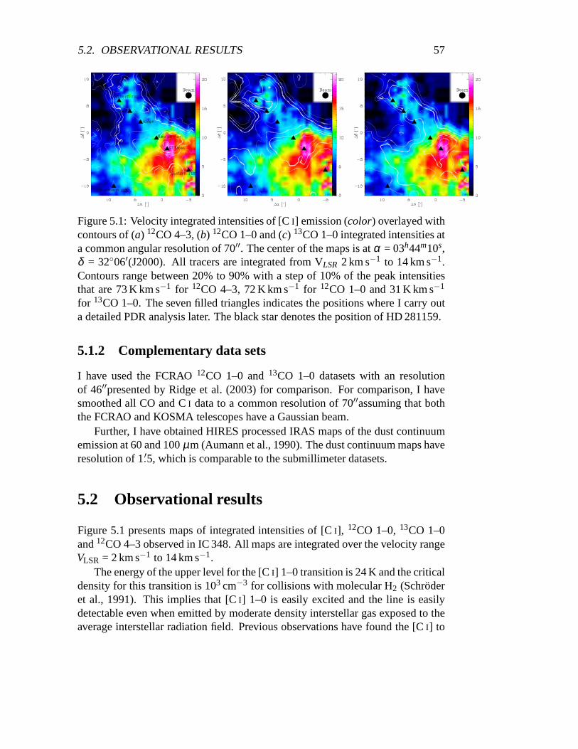
5.2. OBSERVATIONAL RESULTS 57
Figure 5.1: Velocity integrated intensities of [CI] emission (color) overlayed withcontours of (a) 12CO 4–3, (b) 12CO 1–0 and (c) 13CO 1–0 integrated intensities ata common angular resolution of 70′′. The center of the maps is atα = 03h44m10s,δ = 3206′(J2000). All tracers are integrated from VLSR 2 km s−1 to 14 km s−1.Contours range between 20% to 90% with a step of 10% of the peakintensitiesthat are 73 K km s−1 for 12CO 4–3, 72 K km s−1 for 12CO 1–0 and 31 K km s−1
for 13CO 1–0. The seven filled triangles indicates the positions where I carry outa detailed PDR analysis later. The black star denotes the position of HD 281159.
5.1.2 Complementary data sets
I have used the FCRAO12CO 1–0 and13CO 1–0 datasets with an resolutionof 46′′presented by Ridge et al. (2003) for comparison. For comparison, I havesmoothed all CO and CI data to a common resolution of 70′′assuming that boththe FCRAO and KOSMA telescopes have a Gaussian beam.
Further, I have obtained HIRES processed IRAS maps of the dust continuumemission at 60 and 100µm (Aumann et al., 1990). The dust continuum maps haveresolution of 1.′5, which is comparable to the submillimeter datasets.
5.2 Observational results
Figure 5.1 presents maps of integrated intensities of [CI], 12CO 1–0,13CO 1–0and12CO 4–3 observed in IC 348. All maps are integrated over the velocity rangeVLSR = 2 km s−1 to 14 km s−1.
The energy of the upper level for the [CI] 1–0 transition is 24 K and the criticaldensity for this transition is 103 cm−3 for collisions with molecular H2 (Schroderet al., 1991). This implies that [CI] 1–0 is easily excited and the line is easilydetectable even when emitted by moderate density interstellar gas exposed to theaverage interstellar radiation field. Previous observations have found the [CI] to

58CHAPTER 5. STUDY OF THE PHOTON DOMINATED REGION IN THE IC 348 CLOUD
be extended and well correlated with the low-J CO emission (see a review byPreibish et al., 1996; Schneider et al., 2003; Mookerjea et al., 2006). In IC 348the [CI] emission peaks to the south-west of the mapped region with avalue of24 K km s−1 and I detect [CI] emission over a large region with a homogeneousintensity distribution at a level of 65% of the peak intensity. The [CI] emission isextended towards the east and north-east of the mapped region. This is consistentwith the clumpy UV irradiated cloud scenario.
Globally the12CO 4–3 emission peaks at almost the same position as [CI]with an intensity of∼ 66 K km s−1. However, the12CO 4–3 emission shows twoadditional peaks, with intensities of about two-thirds of the global peak, whichlie to the north of HD 281159 (a B 5 V star) and elongated along the north-southdirection. The distribution of the12CO 4–3 emission agrees very well with that of12CO 3–2 (Sun et al., 2006). I attribute the difference in the intensity distributionsof [C I] and 12CO 4–3 to the fact that12CO 4–3 emission arises from regions ofhigher temperature and density, while [CI] emission can arise also from moderateto low density embedded PDR surfaces within the molecular clouds.
The12CO 1–0 emission is similar to that of12CO 4–3, with two similar inten-sity peaks. The12CO 1–0 emission is more extended than the12CO 4–3 emissionand this is consistent with the fact that12CO 1–0 traces lower temperature anddensity. The morphologies of [CI] and 13CO 1–0 appear to be very similar, im-plying that they trace the same material and both lines are effectively columndensity tracers.
I selected seven positions within IC 348 for a more detailed study. Six of theseven positions are oriented along a cut from the northern edge of the cloud, pastHD 281159 and into the clouds. The seventh position is at the south-east edgeof the cloud. Though emission at the seventh position (southern rim) is weak,it is clearly detected. The selected positions vary in theirphysical and chemicalconditions. Spectra of [CI], 12CO 4–3,12CO 1–0 and13CO 1–0 at those sevenpositions are displayed in Fig. 5.2.
The [CI] emission is centered at a velocity of∼ 8 km s−1. The lowest [CI]main beam brightness temperature (∼ 2 K) occurs at the southern rim (9′,-10′),while the highest temperatures of 7.0 K and 6.7 K are observedat the position ofthe [CI] peak (-1′,-3′) and the western rim (-5′,-7′), respectively. The line widthsof [C I] spectra at the seven positions range between 2.0 km s−1 and 2.6 km s−1.
The 12CO 4–3 main beam brightness temperature varies between∼ 3.6 K atsouthern rim and 16.4 K at [CI] peak. The line width of the12CO 4–3 spectraranges between 2.0 km s−1 and 2.7 km s−1.
Both the12CO 1–0 and13CO 1–0 spectra consist of two velocity components:one is at∼ 7 km s−1 and the other lies at∼ 8 km s−1. The two components aremost prominently visible at the southern rim, map center andthe [CI] peak. Forthe 8 km s−1 component at the [CI] peak, the13CO 1–0 spectrum peaks at the

5.2. OBSERVATIONAL RESULTS 59
dip of the12CO 1–0 spectrum, which may indicate self-absorption effectfor thiscomponent.
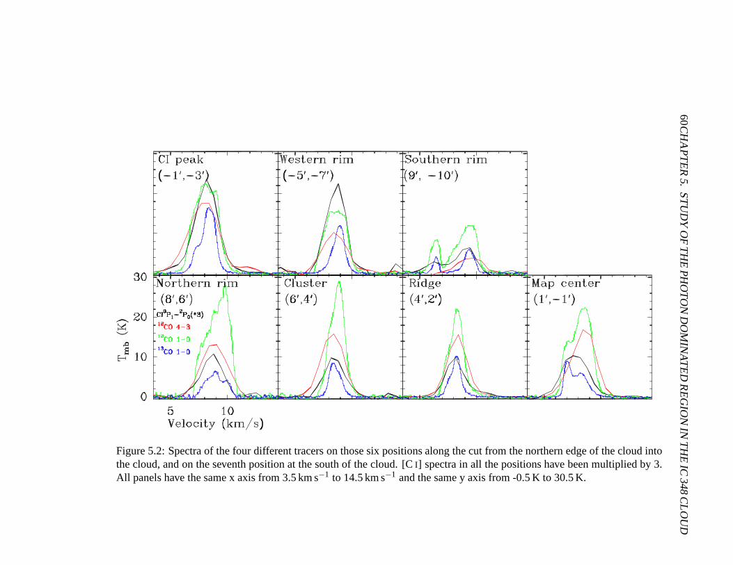
60C
HA
PT
ER
5.S
TU
DY
OF
TH
EP
HO
TO
ND
OM
INAT
ED
RE
GIO
NIN
TH
EIC
348CLO
UD
Figure 5.2: Spectra of the four different tracers on those six positions along the cut from the northern edge of the cloud intothe cloud, and on the seventh position at the south of the cloud. [C I] spectra in all the positions have been multiplied by 3.All panels have the same x axis from 3.5 km s−1 to 14.5 km s−1 and the same y axis from -0.5 K to 30.5 K.

5.2. OBSERVATIONAL RESULTS 61
Table 5.1 presents the integrated intensities and line ratios at the seven selectedpositions. Figure 5.3 shows the variation of the integratedintensities and theirratios at these seven positions.
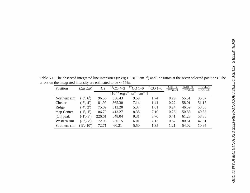
62C
HA
PT
ER
5.S
TU
DY
OF
TH
EP
HO
TO
ND
OM
INAT
ED
RE
GIO
NIN
TH
EIC
348CLO
UD
Table 5.1: The observed integrated line intensities (in ergs−1 sr−1 cm−2) and line ratios at the seven selected positions. Theerrors on the integrated intensity are estimated to be∼ 15%.
Position (∆α,∆δ ) [C I] 12CO 4–3 12CO 1–0 13CO 1–0 [Ci]1−012CO4−3
[Ci]1−013CO1−0
12CO4−312CO1−0
[10−8 erg s−1 sr−1 cm−2]Northern rim ( 8′, 6′) 96.56 336.43 9.59 1.74 0.29 55.51 35.07Cluster ( 6′, 4′) 81.99 365.30 7.14 1.41 0.22 58.01 51.15Ridge ( 4′, 2′) 75.09 313.20 5.37 1.61 0.24 46.59 58.38map Center ( 1′,-1′) 106.79 413.27 8.38 2.10 0.26 50.85 49.33[Ci] peak (-1′,-3′) 226.61 548.04 9.31 3.70 0.41 61.23 58.85Western rim (-5′,-7′) 172.05 256.15 6.01 2.13 0.67 80.61 42.61Southern rim ( 9′,-10′) 72.71 60.21 5.50 1.35 1.21 54.02 10.95
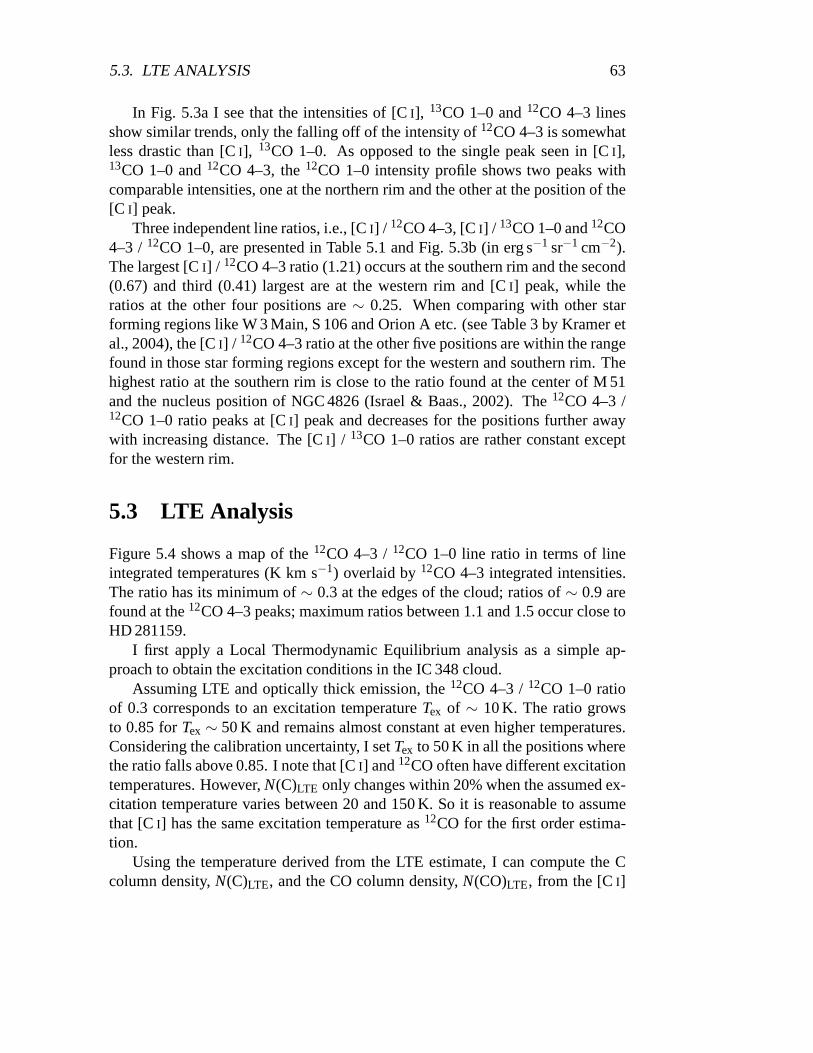
5.3. LTE ANALYSIS 63
In Fig. 5.3a I see that the intensities of [CI], 13CO 1–0 and12CO 4–3 linesshow similar trends, only the falling off of the intensity of12CO 4–3 is somewhatless drastic than [CI], 13CO 1–0. As opposed to the single peak seen in [CI],13CO 1–0 and12CO 4–3, the12CO 1–0 intensity profile shows two peaks withcomparable intensities, one at the northern rim and the other at the position of the[C I] peak.
Three independent line ratios, i.e., [CI] / 12CO 4–3, [CI] / 13CO 1–0 and12CO4–3 / 12CO 1–0, are presented in Table 5.1 and Fig. 5.3b (in erg s−1 sr−1 cm−2).The largest [CI] / 12CO 4–3 ratio (1.21) occurs at the southern rim and the second(0.67) and third (0.41) largest are at the western rim and [CI] peak, while theratios at the other four positions are∼ 0.25. When comparing with other starforming regions like W 3 Main, S 106 and Orion A etc. (see Table3 by Kramer etal., 2004), the [CI] / 12CO 4–3 ratio at the other five positions are within the rangefound in those star forming regions except for the western and southern rim. Thehighest ratio at the southern rim is close to the ratio found at the center of M 51and the nucleus position of NGC 4826 (Israel & Baas., 2002). The 12CO 4–3 /12CO 1–0 ratio peaks at [CI] peak and decreases for the positions further awaywith increasing distance. The [CI] / 13CO 1–0 ratios are rather constant exceptfor the western rim.
5.3 LTE Analysis
Figure 5.4 shows a map of the12CO 4–3 /12CO 1–0 line ratio in terms of lineintegrated temperatures (K km s−1) overlaid by12CO 4–3 integrated intensities.The ratio has its minimum of∼ 0.3 at the edges of the cloud; ratios of∼ 0.9 arefound at the12CO 4–3 peaks; maximum ratios between 1.1 and 1.5 occur close toHD 281159.
I first apply a Local Thermodynamic Equilibrium analysis as asimple ap-proach to obtain the excitation conditions in the IC 348 cloud.
Assuming LTE and optically thick emission, the12CO 4–3 /12CO 1–0 ratioof 0.3 corresponds to an excitation temperatureTex of ∼ 10 K. The ratio growsto 0.85 forTex ∼ 50 K and remains almost constant at even higher temperatures.Considering the calibration uncertainty, I setTex to 50 K in all the positions wherethe ratio falls above 0.85. I note that [CI] and12CO often have different excitationtemperatures. However,N(C)LTE only changes within 20% when the assumed ex-citation temperature varies between 20 and 150 K. So it is reasonable to assumethat [CI] has the same excitation temperature as12CO for the first order estima-tion.
Using the temperature derived from the LTE estimate, I can compute the Ccolumn density,N(C)LTE, and the CO column density,N(CO)LTE, from the [CI]
64CHAPTER 5. STUDY OF THE PHOTON DOMINATED REGION IN THE IC 348 CLOUD
Figure 5.3: The top panel(a) presents the normalized integrated intensities of[C I], 12CO 4–3,12CO 1–0 and13CO 1–0 in the seven selected positions. Thetypical errors of the intensities are about 15%;(b) displays integrated line intensityratios. The x axes of all panels are the relative distance to the northern rim (8′,6′)position. The southern rim is plotted in a separate box.
and13CO 1–0 line intensities assuming that both lines have the same excitationtemperature as12CO and that they are optically thin.
I apply the relative abundance ratio [12CO]/[13CO] of 65 (Langer et al., 1990)to translate13CO column densities into CO column densities. From the relativeabundance ratio [CO]/[H2] of 8 × 10⁻⁵ (Frerking et al. , 1982), I also derive theH2 column density (see Table 5.2).
The resulting map of C/CO column density ratios is presentedin Fig. 5.5. Inmost of the cloud, the C/CO ratio falls below 0.1. Higher values (up to 1.5) occurat the rim of the cloud where the13CO 1–0 emission is more diffuse. Values aslow as 0.02 are found at the south-west of the cloud and along the ridge to thenorth-east. As13CO 1–0 roughly traces the H2 column density, this plot indicatesan anti-correlation between the C/CO ratio and the H2 column density. The resultsare consistent with the conclusion of Mookerjea et al. (2006) that the [CI] line isnot a tracer of optical extinction, total H2 column density or total mass in thebeam.
The seven positions, for which I will perform a detailed analysis within thecontext of a PDR model, exhibit C/CO column density ratios between about 0.05and 0.5, i.e. they cover a relatively wide range (see Table 5.2).

5.3. LTE ANALYSIS 65
Figure 5.4: The color plot represents the12CO 4–3 /12CO 1–0 line intensity ratio(in units of K km s−1) observed in the IC 348 cloud. The contours show the12CO4–3 line intensity spaced at 10% intervals from 20% to 90% relative to the peakintensity of 73 K km s−1. For line ratios, I only calculate for the positions wherethe line intensities of both tracer are larger than each 3 sigma value.
Table 5.2: Results of the LTE analysis. The excitation temperatureTex is listed inColumn (2); Column (3) - (5) present C, CO and H2 column densities; the C/COratio is listed in Column (6). The uncertainties of the column densities are derivedby varying the integrated intensities by±15%.
number Tex N(C)LTE N(CO)LTE N(H2)LTE C/COLTE
K 1016[cm−2] 1017[cm−2] 1021[cm−2]Northern rim 1847
15 12.0819.719.27 9.5622.84
7.16 12.5028.558.95 0.130.28
0.04Cluster 5020 9.6111.17
7.77 16.9919.547.33 21.2424.43
9.16 0.060.150.04
Ridge 5028 9.0410.467.32 19.3723.03
10.43 24.2128.7813.04 0.050.10
0.03Map center 4850
18 13.0916.0010.68 24.3929.03
10.25 30.4936.2912.82 0.050.16
0.04[Ci] peak 5029 26.8530.88
21.71 44.4751.1424.56 55.5963.93
30.70 0.060.130.04
Western rim 285015 19.7228.30
17.61 16.2529.999.52 20.3137.49
11.90 0.120.300.06
Southern rim 786 37.5072.5721.96 6.668.54
5.40 8.3210.676.76 0.561.34
0.26

66CHAPTER 5. STUDY OF THE PHOTON DOMINATED REGION IN THE IC 348 CLOUD
Figure 5.5: The C/CO column density ratio overlaid by13CO 1–0 integrated in-tensities contours. The contour levels are spaced at 10% intervals from 20% to90% relative to the peak intensity of 31 K km s−1. For column density ratios, Ionly calculate for the positions where the line intensitiesof 13CO 1–0 are abovethe 3 sigma value.

5.4. PDR MODEL 67
5.4 PDR Model
I use the KOSMA -τ PDR model (Storzer et al., 1996; Rollig et al., 2006, 2007)toderive the physical conditions from the observed molecularand atomic emissionlines in IC 348.
In the following, I first estimate the FUV field in IC 348 using the FIR con-tinuum and the stellar radiation; then I compare the emission from an ensembleof PDR model clumps with the observed line intensity ratios to reproduce the ob-served absolute intensity. In the clumpy PDR scenarios, twoclump ensemblesare used: an ensemble of identical clumps and an ensemble with a distribution ofclumps over a range of masses and sizes.
5.4.1 FUV intensity
5.4.1.1 Estimate from the FIR continuum
I use HIRES processed 60 and 100µm IRAS data (Aumann et al., 1990) to gen-erate a far-infrared intensity mapIFIR in IC 348. It represents the far-infraredintensity between 42.5µm and 122.5µm as measured by the two IRAS data sets(Nakagawa et al., 1998). Following Kaufman et al. (1999), I assume that the totalFUV flux, χFIR, absorbed by the dust grains is re-radiated in the far-infrared. Inthis way I estimate the FUV field from the far-infrared field (cf. Kramer et al.,2005): χFIR/χ0 = 4π IFIR, whereχ0 = 2.7×10⁻³ erg s−1 cm−2 (Draine, 1978;Draine & Bertoldi, 1996). The derived spatial distributionof the FUV intensity ispresented in Fig. 5.6. In the mapped region, the FUV fieldχFIR varies betweenabout 1 and 100 Draine units. For the seven selected positions χFIR is listed inTable 5.3.
5.4.1.2 Estimate from the stellar radiation
The primary source of UV radiation in the cloud is HD 281159. Assuming that thestar is a black body at an effective temperatureTeff corresponding to its spectraltype, I can estimate the FUV flux independently (Kramer et al., 1996; Beuther etal., 2000). A B 5 V star has an effective temperature log(Teff) = 4.182 and a totalluminosity L of log(L/L) = 2.681 (de Jager & Nieuwenhuijzen, 1987). TheFUV luminosityLFUV and the FUV fluxχFUV are defined as
LFUV = L · ΦUV
Φtotal, and χFUV =
LFUV
4πd2 , (5.1)
whereΦUV is the FUV flux between 6 eV and 13.6 eV,Φtotal is the total flux, andd is the distance to the UV source. I compute the distanced in two ways: for the
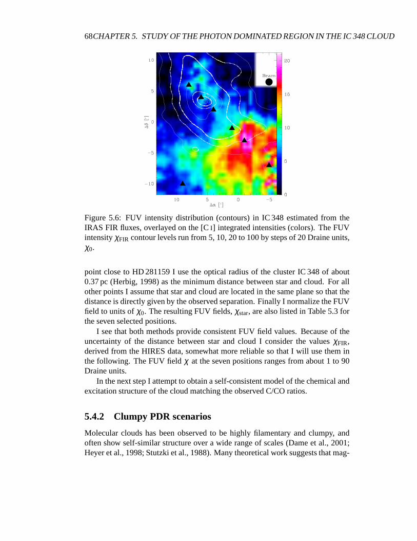
68CHAPTER 5. STUDY OF THE PHOTON DOMINATED REGION IN THE IC 348 CLOUD
Figure 5.6: FUV intensity distribution (contours) in IC 348estimated from theIRAS FIR fluxes, overlayed on the [CI] integrated intensities (colors). The FUVintensityχFIR contour levels run from 5, 10, 20 to 100 by steps of 20 Draine units,χ0.
point close to HD 281159 I use the optical radius of the cluster IC 348 of about0.37 pc (Herbig, 1998) as the minimum distance between star and cloud. For allother points I assume that star and cloud are located in the same plane so that thedistance is directly given by the observed separation. Finally I normalize the FUVfield to units ofχ0. The resulting FUV fields,χstar, are also listed in Table 5.3 forthe seven selected positions.
I see that both methods provide consistent FUV field values. Because of theuncertainty of the distance between star and cloud I consider the valuesχFIR,derived from the HIRES data, somewhat more reliable so that Iwill use them inthe following. The FUV fieldχ at the seven positions ranges from about 1 to 90Draine units.
In the next step I attempt to obtain a self-consistent model of the chemical andexcitation structure of the cloud matching the observed C/CO ratios.
5.4.2 Clumpy PDR scenarios
Molecular clouds has been observed to be highly filamentary and clumpy, andoften show self-similar structure over a wide range of scales (Dame et al., 2001;Heyer et al., 1998; Stutzki et al., 1988). Many theoretical work suggests that mag-

5.4. PDR MODEL 69
netic fields and/or turbulence can be proposed to influence the formation of molec-ular cloud filaments (Gehman et al., 1996; Nakajima & Hanawa,1996; Padoan etal., 1998; Fiege & Pudritz, 2000; Klessen & Burkert, 2000; Ostriker et al., 2001).Furthermore, the observed structure further breaks up intosubstructures with in-creasing spatial resolution (Falgarone & Phillips, 1996; Bensch et al., 2001). Somolecular clouds are filled with internal surfaces (Ossenkopf et al., 2007). Thisexplains that [CI] acts as a molecular cloud volume tracer rather than a surfacetracer, and [CII ] emission extends far into molecular clouds which could notbeexplained by assuming a homogeneous cloud. The [CII ] emission distribution canbe well modelled within a clumpy cloud scenario (Stutzki et al., 1988; Howe etal., 1991; Stacey et al., 1993; Meixner & Tielens, 1993). In aclumpy cloud, theUV field can penetrate deep into the cloud and forms PDRs on thesurface of theclumps. It is necessary to consider a clumpy molecular cloudstructure.
I here apply two different clump ensembles to reproduce the observed lineintensity ratios and absolute line intensities.
5.4.2.1 Ensemble of identical clumps
In the following, I first compare the emission from individual PDR model clumpsto the observed line intensity ratios, then expand the analysis to an ensemble ofidentical clumps, to also reproduce the observed absolute intensity.
Single spherical PDR model.I perform aχ2 fitting of the three line intensityratios given in Table 5.1, using a single spherical PDR model, to determine thedensities, FUV fields, and clump masses. Figure 5.7 presentsan example of theχ2 fitting for the map center (1′, −1′). The left panel shows the fitting of clumpmass Mcl and clump densityn0 and the right panel presents the fitting to obtainthe FUV fieldχ and the clump densityn0. It shows that all line ratios are gooddensity tracers, but do not constrain the clump masses. The clump density is wellconstrained within 2.5 - 5.0 105 cm−3. But the reducedχ2 changes only upto 2.5when the clump mass varies from 10−2.0 to 101.0 M, when the clump density iskept at 105.6 cm−3 (see the left panel of Fig. 5.7).
The results from the single spherical PDR clump model analysis are presentedin Table 5.3. The fitted FUV fluxχPDR agrees withχFIR derived from the FIRcontinuum. The largest deviations differ by a factor of only3.
The clump densities at the seven positions vary between 4.4 104 to 4.3 105 cm−3
and the highest clump density occurs at positions of the ridge and the map center.Though the clump masses are not well constrained, the best fitting clump masseslie between 0.1 and 0.4 M.

70CHAPTER 5. STUDY OF THE PHOTON DOMINATED REGION IN THE IC 348 CLOUD
Figure 5.7: Comparison of the observed line intensity ratios [C I]/12CO 4–3,[C I]/13CO 1–0 and12CO 4–3/12CO 1–0 at (1′, −1′) with the single clumpKOSMA - τ PDR model calculations. The left figure shows the fitting of a clumpmass and densities; the right one presents the fitting of the FUV field and clumpdensities. The middle drawn contours are the observed intensity ratios, and theouter two are those for the 20% uncertainty. The grey-scale images indicate thereducedχ2 of the fit. The position of the minimum reducedχ2 is marked using awhite cross. The horizontal light blue line in the right panel shows the FUV fluxχFIR from the HIRES data.

5.4.P
DR
MO
DE
L7
1
Table 5.3: Physical parameters at selected positions in Fig5.1, obtained by fitting the observed intensity ratios to thesingleclump KOSMA - τ PDR models. Columns (2) - (5) list the fitted clump densities,clump mass, clump radius and FUV field;the derived FUV field from the HIRES data and from the star are are in Column (6) and (7); The distance to HD 281159used for the calculation ofχstaris listed in Column (8); Column (9) is the minimum chi square of the PDR fit.
Position n Mcl Rcl χPDR χFIR χstar d χ2min
[105cm−3] M pc pcNorthern rim 1.91 0.2 0.01 15 39 40 0.37 1.38
Cluster 2.75 0.1 0.01 98 84 40 0.37 1.05Ridge 4.25 0.4 0.01 38 46 40 0.37 1.23
Map center 3.98 0.1 0.01 23 23 13 0.64 1.04[Ci] peak 1.91 0.1 0.02 23 11 7 0.90 1.96
Western rim 0.63 0.2 0.02 20 6 3 1.42 2.00Southern rim 0.44 0.4 0.02 2 1 3 1.29 2.31
72CHAPTER 5. STUDY OF THE PHOTON DOMINATED REGION IN THE IC 348 CLOUD
The clump masses of the best fit vary between 0.1 M and 0.4 M (Table 5.3),while the LTE analysis indicates that the total mass in the beam is a few solarmasses. After correcting for beam and velocity filling, the absolute line intensitiesfrom the single spherical PDR model are much smaller than theobservations. Thesingle spherical PDR model constrains the clump density andFUV field well,but fails to explain the observed absolute line integrated intensities. An ensembleof clumps within the beam is needed, the intensities of whichaccumulate to theobserved absolute intensity within the beam.
Ensemble of identical clumps. I consider an ensemble of identical clumps(hereafter Ensemble case 1). The total number of clumps in the beamNens iscalculated from the comparison of the absolute line integrated intensities fromthe observations and models, correcting for both the velocity filling factor andthe beam filling factor. The observed [CI] full width at half maximum (FWHM)∆vobs varies from 2.0 to 2.6 km s−1. The velocity dispersion of the gas of theKOSMA - τ model clump has a Gaussian FWHM of∆vmod = 1.7 km s−1. Thevelocity filling factor is automatically taken into accountby using line integratedintensities. A 70′′ beam corresponds to a diameter of 0.10 pc at the distance ofIC 348. The clump size obtained from the best fit models found in the previoussection ranges from 0.01 to 0.02 pc. The beam filling factorηbf,i of each clumpis calculated asηbf,i = Ωcl/Ωbeam, whereΩcl andΩbeam are the solid angles ofa clump and the beam.Ωcl = πR2
cl/d2 is the solid angle of the individual clumpand is the quantity to which the model output intensities arereferred. d is thedistance of the cloud; assuming a Gaussian beam shape,Ωbeam is computed asΩbeam= πθ2
beam/4ln2, whereθbeam is the FWHM of the beam. The intensitycorrection for a single clump isI ′i = Imb,i/ηbf,i , whereImb,i is the beam averagedline intensity for that single clump. Since [CI] is the most optically thin oneamong the four tracers, I use its line intensity to derive thenumber of clumps inthe beamNens (see Table 5.4) by dividing the observed intensitiesI[Ci]obs by theintensities for a single clumpI[Ci]mod,i , corrected for both the velocity and beamfilling, i.e.,
Nens=I[Ci]obs
I[Ci]mod,i ∗ηbf,i=
I[Ci]obs
I[Ci]mod,i× Ωbeam
Ωcl. (5.2)

5.4.P
DR
MO
DE
L7
3
Table 5.4: Results of ensemble of identical clumps,Ensemble case 1. The mass and FUV field for each single clump arelisted in Column (2) and (3); Column (4) - (6) present the lineintensity ratios between the ensemble models and observationsof 12CO 4–3,12CO 1–0 and13CO 1–0; The C, CO and H2 column densities from the ensembles are presented in Column(7), (8) and (9); Column (10) is the C/CO ratios. The total number of the clumps in the ensemble and ensemble mass arelisted in Column (11) and (12)The total ensemble massMens listed in the table is computed asMens= Nens×Mcl, whereMclis the mass of a clump.Position Mcl χcl R12CO4−3 R12CO1−0 R13CO1−0 N(C)ens N(CO)ens N(H2)ens C/COens Nens Mens
M 1016[cm−2] 1017[cm−2] 1021[cm−2] MNorthern rim 0.32 10 0.63 0.67 0.87 13.97 18.58 7.72 0.075 4.59 1.47Cluster 0.10 100 1.07 0.99 1.13 10.02 21.56 8.90 0.046 16.75 1.68Ridge 0.32 32 0.95 1.13 0.95 8.90 29.49 11.29 0.030 6.72 2.15Map center 0.10 32 0.94 1.05 0.97 13.25 34.24 13.05 0.039 24.56 2.46[Ci] peak 0.10 32 0.94 1.59 0.83 31.54 29.88 13.14 0.106 24.74 2.47Western rim 0.10 10 0.78 1.43 0.71 24.52 9.33 6.10 0.263 11.511.15Southern rim 0.32 1 0.84 0.81 0.74 14.62 6.28 3.03 0.233 5.70 1.82
74CHAPTER 5. STUDY OF THE PHOTON DOMINATED REGION IN THE IC 348 CLOUD
Then I useNens to calculate the ratiosR of line intensities between modelensemble and observations for the four tracers, whereR is defined as follows:
R=Nens· Imod,i
Iobs. (5.3)
This allows easy judgment of the quality of the model fit, as aR value unitymeans that the model predicts exactly the observed intensity. I list the ratios ofthe remaining three tracers in Table 5.4. Considering the calibration uncertainty, aperfectly fitting model will yield a ratioR of 1±0.15. All three remaining tracersfrom Ensemble case 1 have a good agreement between the modelled and observedabsolute line intensities.
5.4.2.2 Ensemble of power law clump mass distribution
Large-scale CO maps present the clumpy structure of the ISM with a mass distri-bution following a power lawdN/dM ∝ M−α , whereN is the number of clumpsandα has a value around 1.8 (Kramer et al., 1998b). Furthermore, the observa-tions also show that there is a strong correlation of the density and mass of theclumps corresponding a mass-size relationr ∝ Mγ with γ ≈ 2.3 (Heithausen et al.,1998). For an ensemble of randomly positioned clumps with a power law massspectrum, there is a relation among the power law spectral indexβ of the powerspectrum,α andγ: β = γ(3−α) (Stutzki et al., 1998). Using theα andγ valuesabove,β = 2.76, which is close to the power law indexβ = 2.71 of 13CO 2–1 inIC 348 found by Sun et al. (2006).
I assume these characteristics to be universal and model theemission by en-semble averaging the PDR single clump results over such a clump distribution(Cubick, 2005; Cubick et al., 2008) (hereafter Ensemble case 2) to reproduce theobserved line intensities. The mean solid angleΩi of each clump size at the givendistance is evaluated to calculate the total fluxF of the clump ensemble by usingF = ∑i ΩiIi , whereIi are the clump integrated intensities. The mean intensity ofthe ensemble results inI = F/Ωbeam, whereΩbeamis the beam solid angle.
The input parameters for the ensemble routines are the totalmass within thebeamMens; the mean clump ensemble densitynmean; the FUV field inputχensandthe minimum and maximum clump mass,mmin
cl andmmaxcl .
The total mass within the beam is initially set to be half of the total mass es-timated from Ensemble case 1. at last, I obtain the total masswithin the beam bycomparing the observed absolute line intensity of [CI]. The upper mass limit,mmax
cl , is set close to the initial total mass. I set the lower mass limit, mmincl ,
to 10−2 M. Considering that clumps have a FWHM of∆vmod = 1.7 km s−1
in the KOSMA - τ model, I calculate the virial mass of the smallest clump,Mvir ∝ R∆v2
mod. The resulting virial mass is a factor of 400 larger than the smallest

5.4. PDR MODEL 75
clump. Such large ratio indicates that these small clumps can only exist transientlyand evaporate on a time scale of∼ 5000 yrs Kramer et al. (2008).
The model output is insensitive to the value assumed for the lower and uppermass limits of the ensemble. Cubick et al. (2008) studied thedependencies ofthe clump model output from the upper and lower clump mass limits. They havefound that some tracers, such as the high -J CO (like 12CO 8–7), [CII ] and [OI],are sensitive to the upper and lower clump mass limits. However, for the fivetracers that I studied here, the modelled intensities change only by less than afactor of∼ 2 relative to the best fitting solution when varying one of themasslimits by one order of magnitude (Kramer et al., 2008; Cubicket al., 2008).
Similar to the single clump PDR analysis, I compare the observed line ratioswith the results of Ensemble case 2 to fit the mean clump ensemble density andthe FUV field. I compute the line intensities of all the remaining tracers with thesame model (see Table 5.5). The beam averaged H2, C and CO column densitiescan be calculated as:
N(X)ens= ∑Ni ·ηbf,i ·N(X)i; (5.4)
whereNi andN(X)i are the number of clumps in each clump mass bin and thecolumn density of tracer X of a single clump, respectively.ηbf,i is the beam fillingfactor for each clump. The results are presented in Table 5.5.

76C
HA
PT
ER
5.S
TU
DY
OF
TH
EP
HO
TO
ND
OM
INAT
ED
RE
GIO
NIN
TH
EIC
348CLO
UD
Table 5.5: Results of ensembles with a clump mass distribution and mass-size distribution,Ensemble case 2. Column (2) -(4) present the ratios (in erg s−1 sr−1 cm−2) of the modelled and observed line intensities for12CO 4–3,12CO 1–0 and13CO1–0; The mean clump ensemble densitynmeanand the fitted FUV fieldχensare presented in Column (5) and (6). The C, COand H2 column densities from the ensembles are presented in Column(7), (8) and (9); Column (10) is the C/CO ratios. Thetotal masses are listed in Column (11).Position R12CO4−3 R12CO1−0 R13CO1−0 nmean χens N(C)ens N(CO)ens N(H2)ens C/COens Mens
[105cm−3] 1016[cm−2] 1017[cm−2] 1021[cm−2] MNorthern rim 1.00 1.04 1.44 3.2 3 14.36 51.82 19.28 0.028 3.84Cluster 1.06 1.03 1.13 3.2 100 9.88 25.58 9.93 0.039 1.97Ridge 1.13 1.26 0.91 3.2 32 9.05 23.43 9.10 0.039 1.83Map center 1.08 1.19 1.08 3.2 10 13.78 40.71 15.39 0.034 3.07[Ci] peak 1.13 1.73 0.86 1.0 10 31.24 40.16 16.61 0.078 2.88Western rim 1.83 2.03 1.13 1.0 10 30.49 23.72 12.61 0.078 2.19Southern rim 1.06 0.84 0.66 0.3 1 13.58 5.24 2.62 0.259 0.53

5.4. PDR MODEL 77
Figure 5.8: Observed (filled symbols) and modelled (drawn lines with open sym-bols) line intensities of12CO,13CO, and [CI] from Ensemble case 2 at the north-ern rim (left panel) and the southern rim (right panel). To better display the data,I artificially shift the [CI] frequency by +40 GHz for the observed intensity.
Table 5.5 shows a reasonable agreement between the modelledline intensitiesfrom Ensemble case 2 and the observed ones. The intensity ratios between En-semble case 2 and observations range between 0.7 and 2.0. Thefit is not betterthan for an ensemble of identical clumps (Ensemble case 1).
To compare the observed absolute line intensities with the model predictionfrom Ensemble case 2, I show two examples of observed and modelled integratedintensities versus frequency, i.e. the cooling curves of12CO, 13CO (uptoJ = 9–8) and [CI] for the best-fit Ensemble case 2 model at the northern rim andthesouthern rim (see Fig. 5.8). At those two positions the modelled and observed lineintensities agree very well. Fig. 5.8 also provides a predication for line intensitiesof [C I] 3P2 – 3P1, 12CO 7–6,13CO 8–7 and etc.
Based on the CO and H2 column densities from the PDR analysis, I find theaveraged CO relative abundance [CO]/[H2] is ∼ 2.4 10−4, which is 3 times largerthan than the canonical ratio [CO]/[H2] of 8 × 10⁻⁵ (Frerking et al. , 1982) that Iused in the LTE analysis.
The beam averaged C/CO abundance ratio (Table 5.5) varies bya factor 10between 0.03 at the northern rim, which shows the highest column density of allstudied positions of 21021 cm−2, and 0.26 at the southern rim, which shows thelowest H2 column density of 31021 cm−2. The observed anti-correlation betweenC/CO and N(H2) and also the absolute values resemble those found in many otherGalactic molecular clouds as compiled recently by Mookerjea et al. (2006). Theyused the KOSMA-τ model to interpret data taken in the Cepheus B star formingregion. They suggested that the emission of high column density peaks is domi-nated by massive clumps exhibiting low C/CO ratios, while positions of low col-

78CHAPTER 5. STUDY OF THE PHOTON DOMINATED REGION IN THE IC 348 CLOUD
umn densities are dominated by smaller clumps, exhibiting higher C/CO ratios.This scenario is confirmed in IC 348 by a more complete analysis using clumpmass ensembles following the canonical mass and size distributions. However,the scatter of the present data is large. Observations of an optical thin tracer likeC18O and observations of the higher lying transitions of [CI] and CO are neededto further improve the analysis.
5.5 Summary and Conclusions
I have presented fully sampled [CI] and12CO 4–3 maps of the IC 348 molecularcloud, covering a region of 20′× 20′. The observed12CO 4–3/12CO 1–0 ratiosvary between 0.2 and 1.5. High12CO 4–3/12CO 1–0 ratios occur near the B 5 star,at the cloud center and northern edge of the cloud.
I have estimated the FUV field from the FIR continuum intensities obtainedfrom the 60 and 100µm HIRES/IRAS images. The FUV field in the whole ob-served region ranges between 1 and 100 Draine unites. I also used HD 281159,the primary source of UV radiation in this region, to estimate the FUV field forthe seven studied regions and the FUV field varies between 3 to40 Draine units.
I applied the KOSMA -τ PDR model at seven selected positions by exam-ining the three independent line ratios: [CI] / 12CO 4–3, [CI] / 13CO 1–0 and12CO 4–3 /12CO 1–0 to derive the local physical condition. First I comparedthe emission from individual PDR model clumps to the observed line intensityratios. The clump density in those seven positions falls between 4.4 104 cm−3 and4.3 105 cm−3. The FUV field fitted from the model is between 2 to 100 Draineunits, consistent within a factor of 3 with independent estimates for the FUV fieldderived from the FIR continuum maps by IRAS and from the stellar radiation.
The single spherical PDR model constrains the clump densityand FUV fieldwell, although it fails to explain the observed absolute line integrated intensities.Hence I expanded the analysis to an ensemble of identical clumps (Ensemble case1) and furthermore I considered a distribution of clumps over a range of massesand sizes (Ensemble case 2). Both Ensemble case 1 and Ensemble case 2 producemodel line intensities which are in good agreement to withina factor of∼ 2 withthe observed intensities. I also predicted the line intensities for [CI] 3P2 – 3P1,12CO 7–6,13CO 8–7 and etc., which can be confirmed by the future observations.
By using a more complete analysis of clump mass ensembles following thecanonical mass and size distributions, I confirmed the anti-correlation betweenC/CO abundance ratio and hydrogen column density found in many regions andexplained by Mookerjea et al. (2006).

5.5. SUMMARY AND CONCLUSIONS 79
In the next chapter, I will present the results on a multi-line study in anothernearby star forming region: Cepheus B.

Chapter 6
Multi-line study of the Cepheus Bcloud
The Cepheus B cloud, at a distance of 730 pc (Blaauw, 1964) is atypical examplefor triggered star formation. To the north-west lie the [HII ] region S 155 and theCepheus OB3 association. The primary sources of UV radiation are an O7 starat a distance of∼1.2 pc to the north-west of the hot core position, and a B1 starat a projected distance of 0.7 pc to the west. Based on the FIR continuum, theFUV radiation field varies between 1500 Draine units at the interface and∼ 25Draine units in the inner core (Mookerjea et al., 2006). The proximity of CepheusB allows to spatially resolve the PDR: 10′′ correspond to 0.035 pc. Hence, theCepheus B cloud represents the class of PDRs with moderatelystrong UV field.
Following up on the previous low-resolution (∼ 1′) studies of low -J CO, [CII ]and far-infrared continuum (Beuther et al., 2000; Mookerjea et al., 2006), I try tounderstand photo-induced chemistry of the photon dominated regions using thehigher resolution (∼ 20′′) molecular line data at 3 mm and 1 mm data observedwith the IRAM 30m telescope at Pico Veleta. The aim of the study is to resolvethe temperature, chemical, and excitation structure of thetransition zone fromthe [H II ] region to the dense molecular cloud in a PDR which is subjectonly tomoderately strong UV fields.
In this chapter, I study two cuts through the interfaces intothe main cloud.Particularly, I select two positions at the interface for more detailed studies (seeFig. 6.1). The study covers the frequency range from 85 GHz to272 GHz and in-cludes 21 transitions of 13 molecules and their isotopomers: HCN, H13CN, HNC,HCO+, H13CO+, HCO, CN, CS, C34S, C2H, C2S, HCS+ and c-C3H2. Combinedwith low - J CO maps of this region (Ungerechts et al., 2000), I calculatethe inte-grated intensity distribution along the cuts and line ratios between different tracersand transitions. The H2 column density along the cuts has been estimated underthe Local Thermodynamic Equilibrium assumption. The integrated line intensi-
80

6.1. THE IRAM 30M TELESCOPE OBSERVATIONS 81
ties shows a clear change from the [HII ] region into the molecular clouds. Thereis an intensity enhancement of all the tracers at the two interface positions.
Observations are presented in Section 1; Section 2 describes the diagnosticvalues of the observed tracers; The selection of the two cutsis presented in Section3; The spectral results and a basic LTE analysis are presented in Section 4. Section5 is the summary and an outlook for future studies.
6.1 The IRAM 30m telescope observations
I carried out a molecular line survey with the IRAM 30m telescope at Pico Veleta(Spain) in one week during July and August 2006. I observed two cuts runningthrough the interfaces (between S 155 and the Cepheus B cloud) into the maincloud and thus allow to trace several interface regions. Particularly, I select twopositions at the interface for a more detailed study. The studied frequency coversfrom 85 GHz to 272 GHz and includes 21 transitions of 11 molecules, such asHCN, HCO+, CN, CS and CCH (See Table 6.1).
I used all the eight receivers for the observations and a maximum of four het-erodyne receivers can be used simultaneously. Those eight receivers are A 100, B100, C 150, D 150, A 230, B 230, C 270 and D 270. The numbers indicate the typ-ical frequency for each receiver. During the observations,I used both the 1 MHzbackends (resolution 1 MHz) with an effective total bandwidth of 512 MHz andVESPA with a resolution of 3.3 kHz - 1.25 MHz and bandwidth of 10 - 512 MHz.The HPBW of each frequency can be well fit by: by: HPBW(′′) = 2460/freq(GHz).The beam efficiencyBeff can be calculated byBeff = 0.828exp[−(0.28π/λ )2]. Theforward efficiencyFeff is 0.95 for receiver A 100 and B 100, 0.93 for receiver C150 and D 150, 0.91 for receiver A 230 and B 230, and 0.88 for receiver C 270and D 270. Using the beam efficiency and the forward efficiencyFeff, I convertthe data to main beam temperature scales.
6.2 Chemical tracers at the PDR interfaces
Recent observations of photon dominated regions have revealed an unexpectedrichness in chemical species. The CF+ ion (Neufeld et al., 2006) and DCN(Leurini et al., 2006) have been detected in the Orion Bar region. Moreover, anumber of carbon chain molecules and other carbon-rich species, such as C2H,C4H and c-C3H2 have been detected toward several spots in IC 63, L 1688-W andthe Horsehead nebula with abundances that are often close tothose in the TMC-1dark cloud. HC3N was only observed toward the Hydrocarbon peak of the lat-ter while both C3H isomers have been seen only toward the IR peak (Teyssier et

82 CHAPTER 6. MULTI-LINE STUDY OF THE CEPHEUS B CLOUD
Table 6.1: Rest frequencies of observed spectral linesMolecule Transition Rest frequecncy
[GHz]HCN J=1–0 88.6316
J=2–1 177.2611J=3–2 265.8864
H13CN J=1–0 86.3399HNC J=1–0 90.6636
J=2–1 181.3248HCO+ J=1–0 89.1885
J=2–1 178.3750J=3–2 267.5575
H13CO+ J=1–0 86.7543CS J=2–1 97.9810
J=3–2 146.9690J=5–4 244.9356
C34S J=2–1 96.4129J=3–2 144.6171
CN N(J,F)=1(12, 12)−−0(1
2, 32) 113.1442
N(J,F)=1(12, 32)−−0(1
2, 12) 113.1705
N(J,F)=1(12, 32)−−0(1
2, 32) 113.1913
N(J,F)=1(32, 32)−−0(1
2, 12) 113.4881
N(J,F)=1(32, 52)−−0(1
2, 32) 113.4910
N(J,F)=1(32, 12)−−0(1
2, 12) 113.4996
N(J,F)=1(32, 32)−−0(1
2, 32) 113.5089
N(J,F)=2(32, 52)−−1(3
2, 52) 226.3600
N(J,F)=2(32, 52)−−1(1
2, 32) 226.6595
N(J,F)=2(32, 12)−−1(1
2, 12) 226.6337
N(J,F)=2(52, 52)−−1(3
2, 32) 226.8748
CCH N(J,F)=1(32,2)−−0(12,1) 87.3169
N(J,F)=1(32,1)−−0(12,0) 87.3286
N(J,F)=1(12,1)−−0(12,1) 87.4020
N(J,F)=1(12,0)−−0(12,1) 87.4072
N(J,F)=2(52,3)−−1(32,2) 174.6637
N(J,F)=2(52,2)−−1(32,1) 174.6881
N(J,F)=2(32,2)−−1(12,1) 174.7222
N(J,F)=2(32,1)−−1(12,0) 174.7285
N(J,F)=3(72,4)−−2(52,3) 262.0045
N(J,F)=3(72,3)−−2(52,2) 262.0068
N(J,F)=3(52,3)−−2(32,2) 262.0651
N(J,F)=3(52,2)−−2(32,1) 262.0658
HCS+ J=2–1 85.3479c-C3H2 N(J,F)=2(1,2)–1(0,1) 85.3389
6.3. TWO OBSERVED CUTS 83
al., 2004). These findings warrant detailed investigationsinto the chemical com-plexity of a representative ensemble of PDRs in order to testand improve PDRmodels and thus facilitate the understanding of this important part of the interstel-lar medium.
HCN and HCO+ are sensitive tracers of the chemistry and the ionization frac-tion in photon dominated regions (Boger & Sternberg, 2005).The ion fraction hasa very strong impact on the abundances of these species (and others like HOC+).
The CN/HCN line ratio has been identified as an important indicator of thephysics of dense PDRs (Boger & Sternberg, 2005; Meijerink & Spaans, 2005).High ratios are observed in PDRs near the illuminated surfaces (e.g. Fuente etal., 1993). However, different scenarios are suggested to explain the observations.New observations of higher excited lines and of more speciesare needed to im-prove on this analysis.
Chemical stratification of CN and CS sub-millimeter emission have been ob-served in Orion Bar (Simon et al., 1997).
C2H abundance could probe the low density envelop interclump medium wheregrains are fragmented (Fuente et al., 1993; Pety et al., 2005). At present its highobscured abundance can not be reproduced by PDR models.
The high spatial resolution achieved by the 30m is essentialfor this project.Data will be interpreted using the KOSMA-τ model (Rollig et al., 2006).
6.3 Two observed cuts
Cepheus B exhibits PDRs which are subject to only moderatelystrong UV fieldof χ ≈ 103 in contrast to most of the classical PDRs like the Orion Bar, MonR2,M17SW which are subject to much strong UV fields. Moreover, the western PDRof Cepheus B allows to study the stratification of chemical abundances expectedfrom PDR models. A recent detailed comparison of various PDRmodels (Rolliget al., 2006) showed that observations of specific tracer molecules are needed totest the models.
Two cuts through different environments of 5′ length each have been observedin the Cepheus B cloud (see Fig. 6.1). The map coordinates in the Cepheus Bcloud refer to the (0,0) center position atα = 22h57m07s, δ = 6237′33′′(J2000).Both cuts run through the interfaces into the main cloud and thus allow to traceseveral interface regions where I expect to trace the stratified structure of the PDRas a function of the distance from the illuminating sources.To focus on the effectof the combination of density structure and radiation field,I avoid the hot coreregion, where the gas is affected by shocks and the interaction with the newlyborn IR cluster. I also pick up two interface positions for a more detailed study.Those two positions are (60′′, -185′′) and (20′′, -50′′), which lie on the two cuts.

84 CHAPTER 6. MULTI-LINE STUDY OF THE CEPHEUS B CLOUD
Figure 6.1: The MSX 8 micron PAH map of the Cepheus B PDRs overlayed byC18O 1–0 (thick black contours),12CO 1–0 (dashed black contours), radio contin-uum (white contours) and FUV field (dotted white contours). The two sets of threedashed lines in a raw indicate the cuts I observed; the two white crosses show thetwo interface positions. The B 1 star, HD 217061 is donated asan open triangle.The center (0,0) is corresponding toα = 22h57m07s, δ = 6237′33′′(J2000).

6.4. RESULTS 85
6.4 Results
6.4.1 Spectra at the two interface positions
Spectra of the observed lines at the two observed positions are shown in Fig. 6.2- Fig. 6.4. The rest frequencies of those lines are presentedin Table 6.1. All thespectra presented here are all in main beam temperature scales. The velocity rangeis fixed from -25 km s−1 to 0 km s−1 and the main beam temperature is fixed from-0.5 K to 3 K. All tracers have been detected at (60′′, -185′′). The weakest lineis HCS+ 2–1, which is about 80 mK. Both C34S 2–1 and 3–2 are around 200mK. As seen from those figures, the strongest line is12CO 1–0:∼ 45 K at (60′′,-185′′) and∼ 41 K at (20′′, -50′′). Besides for CO and its isotopes, strong lineswere observed for all these species with Tmb peaking near∼ 10 K. Except for COlines, the strongest emission is HCN 1–0. The ratios of CN 1–0/ HCN 1–0 andCN 2–1 / HCN 2–1 are 0.92 and 1.16, respectively. Fairly strong (∼ 0.5 K) lineshave been seen for the ubiquitous c-C3H2 while weak lines have been detected forHCO, HC3N, and HCS+. The line intensities are also list in Table 6.2.
The observed hyperfine spectra depend on the total optical depth, the linewidth, the Doppler velocity of the source ad the amplitude factor. All those pa-rameters can be derived by a least square fit to the observed spectrum using theCLASS software (http://www.iram.es/IRAMFR/GILDAS/). The results of suchleast square fit for HCN, CN and C2H at the two interface positions are shown inFig. 6.3 and Fig. 6.4, respectively. To fit the line profile I assumed optical depthratios between individual hyperfine components that are consistent with the rela-tive intensities. The results of the fit are listed in Table 6.3. Due to bad signal tonoise ratios for C2H 3–2 and CN 2–1 at (20′′, -50′′), the opacity derived there isnot very reliable.
I have detected four strongest ones of six hyperfine transitions of C2H 1–0(Ziurys et al., 1982) and five of eleven hyperfine transitionsof C2H 2–1 (Ziurys etal., 1982) at both positions. And four of eleven hyperfine transitions of C2H 3–2(Ziurys et al., 1982) are detected at (60′′, -185′′), while the C2H 3–2 transition isvery weak at (20′′, -50′′). C2H lines are believed to be optically thin, as suggestedby their hyperfine-split intensity ratios and line-widths (Tucker et al., 1974). Fromthe hyperfine structure fit, the obtained opacities of C2H 1–0 at (60′′, -185′′) and(20′′, -50′′) are 0.65 and 0.69, respectively. And the opacities of C2H 2–1 arearound 1. So C2H lines are not really optically thin.
The hyperfine structure upto the J = 3–2 transition of HCN has been wellresolved at (60′′, -185′′). While only the hyperfine structure of the J = 1–0 tran-sition of HCN is resolved at (20′′, -50′′). HCN 1–0 at both positions are opti-cally thin, the opacities are 0.43 at (60′′, -185′′) and 0.1 at 20′′, -50′′). Whilethe HCN 2–1 transitions are optically thick at both positions, especially at (60′′,

86 CHAPTER 6. MULTI-LINE STUDY OF THE CEPHEUS B CLOUD
Figure 6.2: The spectra of HCS+ 2–1, HNC 1–0, HNC 3–2,12CO 1–0,13CO 1–0, 13CO 2–1, C18O 1–0, C18O 2–1, HCO+ 1–0, HCO+ 2–1, HCO+ 3–2, c-C3H221,2–10,1, H13CN 1–0, H13C+ 1–0, HC3N 1–0, HCO 1–0, C34S 2–1, C34S 3–2,CS 2–1, CS 3–2, CS 5–4, HCN 1–0, HCN 2–1 and HCN 3–2 at the two interfacepositions.

6.4. RESULTS 87
Table 6.2: Line Parameters on the two interface positions besides for CO and itsisotopes. ND is indicates non-detection.Molecule Transition (60′′,-185′′) Imb (K km s−1) (20′′,-50′′) Imb K km s−1)
C34S 2–1 0.452 0.503C34S 3–2 0.584 0.630
c-C3H2 21,2–10,1 1.213 1.757C2H 1–0 7.140 5.048C2H 2–1 6.950 4.794C2H 3–2 6.981 1.850CN 1–0 11.076 9.811CN 2–0 8.045 6.249CS 2–1 4.973 2.471CS 3–2 4.193 2.076CS 5–4 3.539 0.428
H13CN 1–0 0.679 0.194H13CO+ 1–0 0.578 0.177HC3N 10–9 0.260 NDHCN 1–0 12.125 11.044HCN 2–1 6.860 6.506HCN 3–2 6.463 2.276HCO 1–0 0.384 0.163
HCO+ 1–0 6.772 7.240HCO+ 2–1 8.315 7.251HCO+ 3–2 7.344 3.269HCS+ 2–1 0.105 0.123HNC 1–0 3.875 2.850HNC 1–0 1.498 0.141

88 CHAPTER 6. MULTI-LINE STUDY OF THE CEPHEUS B CLOUD
Table 6.3: The results of hyperfine transition fitting for C2H, CN and HCN.(60′′, -185′′) (20′′, -50′′)
Tmb∗ τtot τtot Tmb∗ τtot τtot
C2H 1–0 4.252± 0.133 0.653± 0.191 2.524± 0.089 0.690± 0.221C2H 2–1 5.583± 0.663 1.825± 1.004 2.327± 0.161 0.100± 1.157C2H 3–2 3.536± 0.494 0.402± 1.060 3.507± 3.890 7.245± 8.857CN 1–0 11.570± 0.517 4.581± 0.454 5.809± 0.075 0.100± 0.045CN 2–1 10.215± 0.735 7.912± 1.031 3.220± 0.450 0.100± 0.707HCN 1–0 5.295± 0.104 0.434± 0.087 4.471± 0.031 0.100± 0.007HCN 2–1 10.919± 0.917 12.163± 1.284 4.648± 0.864 2.877± 0.763HCN 3–2 1.259± 0.041 0.100± 0.090 1.761± 1.061 1.437± 1.762
-185′′) where the opacity for HCN 2–1 is 12.16. However, the opacityof HCN3–2 is again optically thin at (60′′, -185′′). Fig. 6.3 and Fig. 6.4 indicate that theLTE intensities can not reproduce the observed HCN line intensities, especiallyat (60′′, -185′′). For example, the ratiosR1 12 = I(F = 1−1)/I(F = 2−1) andR1 02 = I(F = 0−1)/I(F = 2−1) for HCN J = 1–0 are 0.54 and 0.40 at (60′′,-185′′), respectively. And the ratios at (20′′, -50′′) are R1 12 = 0.49 andR1 02
= 0.20. The LTE ratios areR1 12 = 0.6 andR1 02 = 0.2 (Baudry et al., 1980).These anomalous ratios of hyperfine components can not be interpreted in termsof a single excitation temperature. Rapidly collapsing or expanding cloud modelshave previously been utilized to explain anomalies in the ratiosR1 12 = andR1 02
(Gottlieb et al., 1975; Baudry et al., 1980).
At both positions, the peak temperatures of CN 1–0 are higherthan those ofCN 2–1. Both observed CN transitions are optically thick (4.58 and 7.91 forCN 1–0 and 2–1, respectively) at (60′′, -185′′), while they are optically thin at(20′′, -50′′). There is no deviation from LTE for the CN lines at (60′′, -185′′),especially for CN 1–0. Although the intensity of N(J,F) = 2(3/2, 3/2)–1(1/2, 1/2)is higher than the LTE prediction (∼ 20%) at (60′′, -185′′), which was also foundfor Orion A by Greaves & White (1992). And they attributed their finding tonon-LTE effects affecting the CN 2–1 line fine structure levels. But consideringthe observational uncertainties, it is not confirmed in thiscase. For CN N 1–0 at (20′′, -50′′), there are some evidence of self-absorption for N(J,F) = 1(3/2,3/2)–0(1/2, 1/2), 1(3/2, 1/2)–0(1/2, 1/2), and 1(3/2, 3/2)–0(1/2, 3/2). The self-absorption effects were also found in TMC-1 andρ Ophiuchus by Crutcher et al.(1984); Simon et al. (1997).

6.4. RESULTS 89
Figure 6.3: Spectra at the interface (60′′, -185′′). In the sequence of left to rightand top to bottom, there are C2H 1–0, 2–1, 3–2, HCN 1–0, 2–1, 3–2 and part ofCN 1–0 and 2–1. The green lines are the results from the hyperfine structure fit.

90 CHAPTER 6. MULTI-LINE STUDY OF THE CEPHEUS B CLOUD
Figure 6.4: Spectra at the interface (20′′, -50′′). In the sequence of left to right andtop to bottom, there are C2H 1–0, 2–1, 3–2, HCN 1–0, 2–1, 3–2 and part of CN1–0 and 2–1. The green lines are the results from the hyperfinestructure fit.

6.4. RESULTS 91
6.4.2 Integrated intensities along the two cuts
Fig. 6.5 presents the distribution of integrated intensities along the two cuts. Forsome positions where there is no detection, I take the 3-sigma values as upperlimits. For all the tracers, line intensities behave very similar: they increase fromthe HII region to the interface position, then decrease when going into the clouds.The strongest intensity of each tracers occurs at the interfacer positions. Amongall tracers, the strongest is HCN 1–0 and the second strongest tracer is CN 1–0.The ratio of CN 1–0 / HCN 1–0 is rather constant along both cuts. The CN/HCNline ratio has been identified as an important indicator of the physics of densePDRs (Meijerink & Spaans, 2005). The weakest transitions are C34S 2–1 and 3–2. They only show up at the two interface positions with an integrated intensifyof ∼ 300 mK km s−1. For cut1, the line intensities drop fast after the interfaceposition; while for cut2, the intensities extend into the cloud.
6.4.3 LTE analysis
In this subsection, I present the results from a LTE analysisat the two interfacepositions. The results include opacity and excitation temperature estimations andcolumn density calculations.
Opacity of each tracers is calculated from the line intensity ratios betweenisotopomers except for HCN. The opacities of HCN is derived from the hyperfinestructure fit.
To derive the excitation temperatureTex, the line intensity ratios of two transi-tions of each molecules are used. I also assume that12CO, 13CO and C18O havethe same excitation temperature. And this assumption also applied to CS andC34S, HCO+ and H13CO+. For those molecules observed only one transition likeHCS+ and HCO, I assume an excitation temperature of 10 K.
I use Equation A.11 in Appendix A to calculate column densities for12CO,13CO, C18O, CS, C34S, HCO+, H13CO+, HCN, HNC, HCS+ and HCO at thetwo interface positions. A optical thick correction for allthe column densities(except for HNC, HCS+ and HCO) is the factor of τ
1−exp(−τ) . The permanentdipole momentµ and the rotational constantB of each tracer used in the columndensity calculations are list in Table 6.4.
The details on opacity, excitation temperature and column density calculationscan be found in Appendix A. All the results are listed in Table6.5.
The line intensity ratio of12CO 1–0 and13CO 1–0 is used to derive the opticaldepth (opacity) for those two transitions, taking account of the [12CO]/[13CO] of65 (Langer et al., 1990). Then I use the intensity ratio of13CO 1–0 and C18O 1–0and the13CO 1–0 opacity to estimate the opacity of C18O 1–0. As expected,12CO1–0 transition is optically thick, while13CO 1–0 and C18O 1–0 are optically thin,

92 CHAPTER 6. MULTI-LINE STUDY OF THE CEPHEUS B CLOUD
Figure 6.5: The distribution of integrated intensities along the two cuts. The x axisindicates the relative distance to those two interface positions. Negative and pos-itive distances are assigned to the west and east of those twointerface positions,respectively.
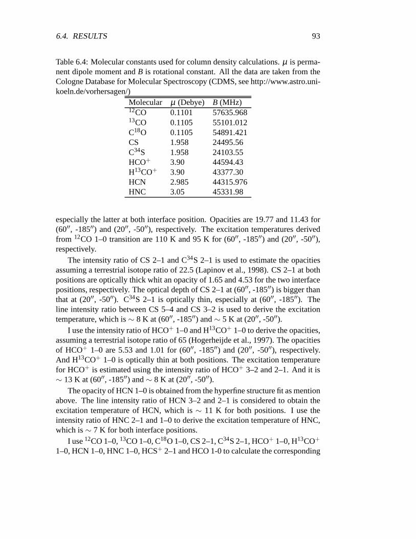
6.4. RESULTS 93
Table 6.4: Molecular constants used for column density calculations.µ is perma-nent dipole moment andB is rotational constant. All the data are taken from theCologne Database for Molecular Spectroscopy (CDMS, see http://www.astro.uni-koeln.de/vorhersagen/)
Molecular µ (Debye) B (MHz)12CO 0.1101 57635.96813CO 0.1105 55101.012C18O 0.1105 54891.421CS 1.958 24495.56C34S 1.958 24103.55HCO+ 3.90 44594.43H13CO+ 3.90 43377.30HCN 2.985 44315.976HNC 3.05 45331.98
especially the latter at both interface position. Opacities are 19.77 and 11.43 for(60′′, -185′′) and (20′′, -50′′), respectively. The excitation temperatures derivedfrom 12CO 1–0 transition are 110 K and 95 K for (60′′, -185′′) and (20′′, -50′′),respectively.
The intensity ratio of CS 2–1 and C34S 2–1 is used to estimate the opacitiesassuming a terrestrial isotope ratio of 22.5 (Lapinov et al., 1998). CS 2–1 at bothpositions are optically thick whit an opacity of 1.65 and 4.53 for the two interfacepositions, respectively. The optical depth of CS 2–1 at (60′′, -185′′) is bigger thanthat at (20′′, -50′′). C34S 2–1 is optically thin, especially at (60′′, -185′′). Theline intensity ratio between CS 5–4 and CS 3–2 is used to derive the excitationtemperature, which is∼ 8 K at (60′′, -185′′) and∼ 5 K at (20′′, -50′′).
I use the intensity ratio of HCO+ 1–0 and H13CO+ 1–0 to derive the opacities,assuming a terrestrial isotope ratio of 65 (Hogerheijde et al., 1997). The opacitiesof HCO+ 1–0 are 5.53 and 1.01 for (60′′, -185′′) and (20′′, -50′′), respectively.And H13CO+ 1–0 is optically thin at both positions. The excitation temperaturefor HCO+ is estimated using the intensity ratio of HCO+ 3–2 and 2–1. And it is∼ 13 K at (60′′, -185′′) and∼ 8 K at (20′′, -50′′).
The opacity of HCN 1–0 is obtained from the hyperfine structure fit as mentionabove. The line intensity ratio of HCN 3–2 and 2–1 is considered to obtain theexcitation temperature of HCN, which is∼ 11 K for both positions. I use theintensity ratio of HNC 2–1 and 1–0 to derive the excitation temperature of HNC,which is∼ 7 K for both interface positions.
I use12CO 1–0,13CO 1–0, C18O 1–0, CS 2–1, C34S 2–1, HCO+ 1–0, H13CO+
1–0, HCN 1–0, HNC 1–0, HCS+ 2–1 and HCO 1-0 to calculate the corresponding
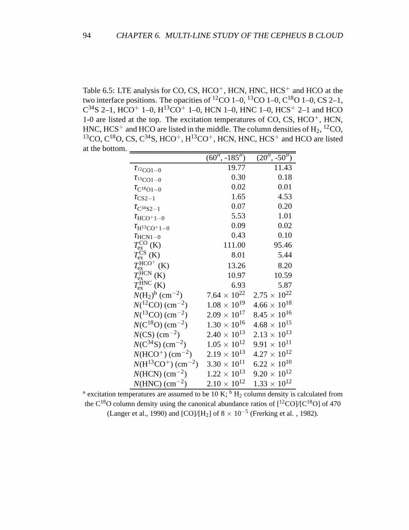
94 CHAPTER 6. MULTI-LINE STUDY OF THE CEPHEUS B CLOUD
Table 6.5: LTE analysis for CO, CS, HCO+, HCN, HNC, HCS+ and HCO at thetwo interface positions. The opacities of12CO 1–0,13CO 1–0, C18O 1–0, CS 2–1,C34S 2–1, HCO+ 1–0, H13CO+ 1–0, HCN 1–0, HNC 1–0, HCS+ 2–1 and HCO1-0 are listed at the top. The excitation temperatures of CO,CS, HCO+, HCN,HNC, HCS+ and HCO are listed in the middle. The column densities of H2, 12CO,13CO, C18O, CS, C34S, HCO+, H13CO+, HCN, HNC, HCS+ and HCO are listedat the bottom.
(60′′, -185′′) (20′′, -50′′)τ12CO1−0 19.77 11.43τ13CO1−0 0.30 0.18τC18O1−0 0.02 0.01τCS2−1 1.65 4.53τC34S2−1 0.07 0.20τHCO+1−0 5.53 1.01τH13CO+1−0 0.09 0.02τHCN1−0 0.43 0.10TCO
ex (K) 111.00 95.46TCS
ex (K) 8.01 5.44THCO+
ex (K) 13.26 8.20THCN
ex (K) 10.97 10.59THNC
ex (K) 6.93 5.87N(H2)b (cm−2) 7.64× 10²² 2.75× 10²²
N(12CO) (cm−2) 1.08× 10¹⁹ 4.66× 10¹⁸
N(13CO) (cm−2) 2.09× 10¹⁷ 8.45× 10¹⁶
N(C18O) (cm−2) 1.30× 10¹⁶ 4.68× 10¹⁵
N(CS) (cm−2) 2.40× 10¹³ 2.13× 10¹³
N(C34S) (cm−2) 1.05× 10¹² 9.91× 10¹¹
N(HCO+) (cm−2) 2.19× 10¹³ 4.27× 10¹²
N(H13CO+) (cm−2) 3.30× 10¹¹ 6.22× 10¹⁰
N(HCN) (cm−2) 1.22× 10¹³ 9.20× 10¹²
N(HNC) (cm−2) 2.10× 10¹² 1.33× 10¹²
a excitation temperatures are assumed to be 10 K;b H2 column density is calculated fromthe C18O column density using the canonical abundance ratios of [12CO]/[C18O] of 470
(Langer et al., 1990) and [CO]/[H2] of 8 × 10⁻⁵ (Frerking et al. , 1982).

6.5. SUMMARY AND OUTLOOK 95
Table 6.6: Results of the relative column densities to H2 column density at twointerface positions. X(Y) is the fractional abundance of tracer Y relative to H2:N(Y)/N(H2).
(60′′, -185′′) (20′′, -50′′)X(12CO) 1.41× 10⁻⁴ 1.69× 10−4
X(13CO) 2.74× 10⁻⁶ 3.07× 10⁻⁶
X(C18O) 1.70× 10⁻⁷ 1.70× 10⁻⁷
X(CS) 3.14× 10⁻¹⁰ 7.75× 10⁻¹⁰
X(C34S) 1.37× 10⁻¹¹ 3.60× 10⁻¹¹
X(HCO+) 2.87× 10⁻¹⁰ 1.55× 10⁻¹⁰
X(H13CO+) 4.32× 10⁻¹² 2.26× 10⁻¹²
X(HCN) 1.60× 10⁻¹⁰ 3.35× 10⁻¹⁰
X(HNC) 2.75× 10⁻¹¹ 4.84× 10⁻¹¹
column densities of each molecule. I also estimate the H2 from the C18O columndensity using the canonical abundance ratios of [12CO]/[C18O] of 470 (Langer etal., 1990) and [CO]/[H2] of 8 × 10⁻⁵ (Frerking et al. , 1982). The H2 columndensities I obtain are 7.64× 10²² at (60′′, -185′′) and 2.75× 10²² at (20′′, -50′′),which are at the same order of the H2 column densities in Cepheus B calculatedby Beuther et al. (2000).
The column densities ofN(CS),N(C34S), N(HCO+), N(H13CO+), N(HCN)(cm−2), N(HNC) (cm−2) are very similar with those found in N 159W, but biggerthan those in N 159S, N 160, 30 Dor-10, 30 Dor-27, N 27 in Magellanic clouds(Heikkila et al., 1999).
I also calculate the fractional abundance of each moleculesrelative to H2 col-umn density (see Table 6.6). I find the X(HCO+) ∼ 10−10, which is smallerto previous studies (Hogerheijde et al., 1997). Hogerheijde et al. (1997) foundX(HCO+) of 1.2× 10⁻⁸ in L 1489 IRS, T Tau, Haro 6-10, L 1551 IRS 5, L 1535IRS, TMR 1, TMC 1A, L 1527 IRS and TMC 1.
6.5 Summary and outlook
I have presented the first results of a multi-line study in theCepheus B molecu-lar clouds. I have recorded two 5′long cuts for up to three transitions of the CS,HCO+, HCN, HNC, CN, and C2H molecules. Strong lines were observed for allthese species withTmb peaking∼ 10 K range. I calculate the integrated inten-sity distribution along the cuts. I use a least square fit to the observed hyperfinestructure of C2H, CN and HCN to derive the opacities.
At the two interface positions, column densities of H2, 12CO, 13CO, C18O,

96 CHAPTER 6. MULTI-LINE STUDY OF THE CEPHEUS B CLOUD
CS, C34S, HCO+, H13CO+, HCN, HNC, HCS+ and HCO are estimated underthe LTE assumption. The fractional abundance of each molecules relative to H2column density is also calculated.
The study in Cepheus B cloud has not been finished yet. The column densitiesof C2H and CN are needed to be estimated. A more detailed comparison withliterature is also needed. And follow-up study will be a radiative transfer analysisusing large velocity gradient codes and a detailed PDR modelanalysis.
Chapter 7
Summary and future prospects
7.1 Summary of results
This thesis work is on the structure of the interstellar medium. I have studiedtwo topics: a.) use large scale surveys of Galactic molecular clouds (the Perseusmolecular cloud) to study their structural properties; b.)study the physical prop-erties of the transition layers on the surface of molecular clouds as traced by emis-sion from [CII ], [C I], and CO, which reflects the structure of molecular clouds.The aim is to understand the energy balance of photon dominated regions, photo-induced chemistry, and PDR dynamics and kinematics.
To study large scale structural properties, I mapped the nearby low-mass star-forming regions Perseus in12CO 3–2 and13CO 2–1 with the KOSMA 3m tele-scope. The∆ - variance method was used to study the spatial structure of line-integrated and velocity channel maps in Perseus. I estimated the spectral indexβ of the corresponding power spectrum and studied its variation across the cloudand across the lines. I found that the overall mapped region follows a power lawwith an index ofβ = 2.9 - 3.0 for scales between 0.2 and 3 pc. This agrees withthe results obtained by Padoan et al. (2003b) who studied structure functions ofa 13CO 1–0 map of Perseus. While for the individual sub-regions,the result-ing power spectral indices vary significantly: the active star-forming region NGC1333 shows high spectral indices (β = 3.5 - 3.8), while the dark cloud L 1455shows low indices of 2.9. Then I applied the same method to individual velocitychannel maps. I found an asymmetry of the power law indices ofthe channel mapsrelative to the line centrum, which is a hint towards a peculiar velocity structure ofthe Perseus cloud complex. The indices with increasing velocity width are almostconstant. A continuous increase of the index with varying velocity channel widthis observed in the blue wings, which can be explained by a shock running throughthe region creating a filamentary structure preferentiallyat low velocities. And it
97

98 CHAPTER 7. SUMMARY AND FUTURE PROSPECTS
is coincident with an expanding shell of neutral hydrogen which was created by asupernova in the Per OB2 association a few 106 years ago (Sancisi, 1974).
GAUSSCLUMPSis used to identify clumps for the whole observed Perseuscloud and seven sub-regions as the same as in the∆ - variance method analysis,and to derive the clump properties as traced in13CO 1–0 and 2–1. Using theKOSMA 13CO 2–1 data, there are 341 clumps found, the mass range of which isbetween 0.54 M and 87.98 M. And I find 737 clumps using the FCRAO13CO1–0 data and the clump mass ranges from 0.28 M and 140.90 M. A power lawindex∼ 1.9 of clump mass spectra is found. Studies of the relations of clump sizeswith line widths and clump masses confirm the standard Larsonrelations. Thevirial parameter, which is the ratio between virial mass andthe mass estimatedfrom the Local Thermodynamic Equilibrium analysis, is usedto characterize theequilibrium state of a clump. All clumps identified in both NGC 1333 and L 1455are found with a virial parameter above 1. The external pressures needed to bindthe clumps fall within 103 K cm−3 and 106 K cm−3 for the whole observed Perseuscloud.
I applied the KOSMA -τ photon dominated region model at seven selectedpositions in IC 348 by examining the three independent line ratios to derive thelocal physical condition. The clump density in those seven positions falls between4.4 104 cm−3 and 4.3 105 cm−3. The FUV field fitted from the model is consistentwith independent estimates for the FUV field derived from theFIR continuummaps by IRAS and from the stellar radiation. Then I expanded the analysis to aclumpy PDR scenario with a distribution of clumps over a range of masses andsizes. This clumpy PDR model produces model line intensities which are in goodagreement within a factor of∼ 2 with the observed intensities. I also predicted theline intensities for [C I]3P2 – 3P1, 12CO 7–6,13CO 8–7 which can be confirmedby future observations. Finally, I confirmed the anti-correlation between C/COabundance ratio and hydrogen column density. This anti-correlation has beenfound in many regions and has been explained by Mookerjea et al. (2006).
To understand photo-induced chemistry of the photon dominated regions, Icarried out a multi-line study of two cuts in the nearby star forming region CepheusB using the IRAM 30m telescope at Pico Veleta. Cepheus B is particularly wellsuited as a PDR candidate because it is relatively close (730pc) and fairly ex-tended (more than 5′ × 5′) thus permitting the PDR to be resolved spatially. Tothe north-west lie the HII region S 155 and the Cepheus OB3 association. Basedon the FIR continuum, the FUV radiation field varies between 1500 G0 at the in-terface and∼ 25 G0 in the inner core (Mookerjea et al., 2006). Thus, Cepheus Brepresents a class of PDRs with moderately strong UV field. I have recorded two5′ long cuts for up to three transitions of the CS, HCO+, HCN, HNC, CN, andC2H molecules. Strong lines were observed for all these species with T∗
A peakingin the 1−3 K range. Other species were searched for in two positions atthe in-
7.2. FUTURE PROSPECTS 99
terfaces. Fairly strong (∼ 0.5 K) lines were seen for the ubiquitous c-C3H2 whileweak lines were detected for HCO, HC3N, and HCS+ along with some isotopicspecies of the molecules seen very strongly. Data at the two cuts were combinedwith low - J 12CO, 13CO, and C18O IRAM-30m maps of Cepheus B (Ungerechtset al., 2000). In the first step, I estimated the relative abundance of each moleculealong the cuts assuming Local Thermodynamic Equilibrium (LTE). The follow-upstudy will be a detailed PDR model analysis.
7.2 Future prospects
More follow-up studies are needed on the velocity channel analysis using CO data.As CO is an optical thick and cold tracer (compared with HI clouds), the velocitychannel analysis (VCA) in CO data provides complementary information on theVCA theory (Lazarian & Pogosyan , 2000), which only deals with optical thintracers and the line center.
Another study is to determine the cross correlation betweendifferent tracersand different regions (as different sub-regions in the Perseus molecular cloud).Such studies will provide the comparison between star formation regions and qui-escent dark clouds, and also the structure between different tracers.
Future observations will be useful to test the results and assess the importanceof different parameters used in the clumpy PDR models. The tracers such as12CO 7–6,13CO 8–7 and [CI] 3P2 – 3P1 are essential to constrain the models.This needs further NANTEN 2 telescope observations. SOFIA and Herschel willprovide observations in the Terahertz regime of the electromagnetic spectrum suchas the [CII ] fine structure transitions. The [CII ] emission is important to studythe physical properties of the transition layers on the surface of molecular clouds.Velocity-resolved observations of this transition are important to distinguish itsemission from that emerging from the ambient WIM.
There are more studies which can be carried out in the CepheusB molecu-lar cloud. Cepheus B exhibits PDRs which are subject to only moderately strongUV field of ∼103 G0 in contrast to most of the classical PDRs like the OrionBar, MonR2, M17SW which are subject to much strong UV fields. Moreover,the western PDR of Cepheus B is seen almost edge-on, thus allowing to studythe stratification of chemical abundances expected from PDRmodels. So studythe PDRs in Cepheus B can be a complementary sample to the Herschel Guar-anteed Time Key Project, the warm and dense ISM. Furthermore, some tracersobserved in the Cepheuse B cloud like C2H, could probe the low density envelop-interclump medium where grains are fragmented. At present its high obscuredabundance can not be reproduced by PDR models. So further studies on CepheusB can test current PDR models and may also provide information to implement

100 CHAPTER 7. SUMMARY AND FUTURE PROSPECTS
them.
The thesis presents the comparison of the structural properties for entire sur-veys and sub-sets of the Perseus molecular cloud, as well as the velocity channelanalysis, provide additional, significant characteristics of the ISM in observed COspectral line maps. These quantities are useful for a comparison of the structureobserved in different clouds, possibly providing a diagnostic tool to characterizethe star-formation activity and providing additional constraints for numerical sim-ulations of the ISM structure. The thesis also studies different PDRs subject to lowand intermediate FUV fields using the clumpy KOSMA -τ PDR model. Futureobservations will be useful to constrain the models and to judge the importance ofdifferent input parameters used. A better knowledge of these conditions in IC 348and Cepheus B will provide a template for future studies of Galactic PDRs andthe ISM in external galaxies.

Appendix A
Local thermodynamic equilibriumanalysis
I have used the local thermodynamic equilibrium (LTE) analysis in Chapter 4,Chapter 5, and Chapter 6. To present more details in LTE, I will here presentthe basic analysis of opacity, excitation temperature, column densities and massesunder the local thermodynamic equilibrium assumption.
A.1 Opacity
If one considers the coupling of the telescope beam to the source via couplingefficiencyηc, the detection equation is written as
T∗R = ηc[Jν(Tex)−Jν(Tbg)][1−exp(−τ)], with Jν(T) =
hνk
1exp(hν/kT)−1
(A.1)whereJν(T) is the normalized Plank intensity, ,Tex is the excitation temperature,k is the Boltzmann constant,Tbg is the 2.74 K black body radiation of the Cosmicback ground,τ is the opacity andT∗
R is the antenna temperature.Under the LTE assumption, the opacityτ of a tracer X can be obtained when
comparing the line intensity ratio of X and its isotopomer Y.It can be written as
T∗R(X)
T∗R(Y)
≈ 1−exp(−τX)
1−exp(−τY)=
1−exp(−τX)
1−exp(−τX/Ifac), (A.2)
whereτX andτY are the opacity for X and Y, andIfac is the isotopic abundanceratio of [X/Y]. In the above equation, the assumption is thatboth X and Y arecharacterized by the same excitation temperature.
101

102 APPENDIX A. LOCAL THERMODYNAMIC EQUILIBRIUM ANALYSIS
A.2 Excitation temperature
The excitation temperatureTex for tracer X can be derived using the intensity ratioRc of different transitions of tracer X with frequencies ofν1 andν2.
Rc =[Jν1(Tex)−Jν1(Tbg)][1−exp(−τ1)]
[Jν2(Tex)−Jν2(Tbg)][1−exp(−τ2)]≈ Jν1(Tex)−Jν1(Tbg)
Jν2(Tex)−Jν2(Tbg), (A.3)
whereτ1 and τ2 are the opacity of the transitions corresponding toν1 and ν2.There is an assumption that both transitions are optically thick.
If both transitions are optically thin, then the Equation A.3 can be written as
Rc ≈[Jν1(Tex)−Jν1(Tbg)]τ1
[Jν2(Tex)−Jν2(Tbg)]τ2, (A.4)
If there is only one transition with frequencyν measured for tracer X, then theexcitation temperature can be estimated from the peak brightness temperatureTmbassuming this transition is optically thick and the beam filling factor f of 1. Theequation is written as
Tmb = f [Jν(Tex)−Jν(Tbg)][1−exp(−τ)] ≈ Jν(Tex)−Jν(Tbg). (A.5)
If this transition is optically thin, then the Equation A.5 can be expressed as
Tmb≈ [Jν(Tex)−Jν(Tbg)]τ. (A.6)
In Chapter 5, I used Equation A.3 to derive CO excitation temperatures. InChapter 6, I used both Equation A.3 and A.4 depending on the opacity of thetracers, and I also used Equation A.5 when there is no one transition observed.
A.3 Column density
For a molecule Y in LTE, the line opacityτν , and excitation temperatureTex,the column density of tracer Y, can be estimated using the expression for columndensity in a single rotational level (Scoville et al., 1986):
NJ(Y) =8πν3
c3AJ+1,J
gJ
gJ+1[1−exp(− hν
kTex)]
∫
τνdv, (A.7)
whereNJ is the total column density of the lower level,c is the velocity of light,his the Planck constant,J is the rotational quantum number of the lower state,gJ(=2J + 1),gJ+1(= 2J + 3) are the statistical weights of the lower and upper rotational
103
levels andAJ+1,J is the Einstein coefficient for spontaneous transitions from upperlevels to the lower level, andv is the velocity (noting that dν/ν = dv/v).
The Einstein coefficient for a spontaneous electric dipole transition is
AJ+1,J =64π4ν3
3hc3 µ2J+1gJ+1
, (A.8)
whereµ is the permanent dipole moment of the molecule. The column densityNJis related to the total column densityNtot summed over all levels (Garden et al.,1991)
NJ(Y) =gJ
Q(Tex)Ntotexp[−hBJ(J+1)
kTex], (A.9)
whereB is the rotational constant of the molecular andQ(Tex) is the partitionfunction, which can be expressed as
Q(Tex) =∞
∑J=0
gJexp[−hBJ(J+1)
kTex] ≈ k(Tex+hB)
3hkB, (A.10)
,Finally, the total column densityNtot can be written as (Scoville et al., 1986;
Garden et al., 1991)
Ntot(Y) =3k
8π3Bµ2
ehBJ(J+1)/kTex
J+1Tex+hB/3k
1−e−hν/kTex
∫
τdv, (A.11)
A.4 Mass
Then the total mass of gas in the source is given by (Scoville et al., 1986)
M = Ntot(Y)[H2
Y]µGmH2
πθ2
4d2, (A.12)
where[H2Y ] is the H2 to Y abundance ratio,µG is the mean atomic weight of the
gas,mH2 is the mass of a H2 molecule,θ is the angular diameter of the source andd is the distance of the source.

Appendix B
A new atmospheric calibrationmethod
B.1 Introduction
Astronomical instruments have been developed rapidly (KOSMA, NANTEN 2,SOFIA and etc.). Stratospheric Observatory for Infrared Astronomy (SOFIA)is one of them. SOFIA is an airborne observatory that will study the universein the infrared spectrum, which will fly at around 13 km high. At such highaltitude, the air contains only about 20% of the molecules present at sea level.All those current/new observatories demand a new and more precise atmosphericcalibration routine.
Different to the traditional calibration approach that determines the atmo-spheric transmission as an average over a representative section of each receiverband individually, this new atmospheric calibration scheme uses a single, freeparameter, the precipitable water vapor (pwv) which is fitted to the observed at-mospheric emission spectrum derived from HOT/COLD/SKY-measurements inthe standard calibration cycle.
Currently there are two programs to convert raw fits data intoCLASS data, oneis calledOfflinecaland the other isKalibrate. In other word, those two programswill transform backend counts (raw fits data) to antenna temperatures (CLASSdata). InOfflinecal, the traditional (Hiyama calibration) atmospheric calibrationroutines are used, and InKalibrate, the new atmospheric calibration routines areused. Here I compared bothKalibrate and Offlinecal to test the two differentatmospheric calibration methods on both simulation and real observed data.Notethat all the tests here are based on the observational data from the NANTEN 2telescope in 2006 and the simulation data that are based on the similar setting asthe NANTEN 2 observatory.
104

105
Here are the terms that will be used later.
C counts; a subscript indicates for ZERO, COLD, HOT, SKY or OFF
T temperature; a subscript indicates for COLD, HOT, AMBIENT or SKY
ηfe,mb forward efficiency or main beam efficiency
Tcal calibration factor
famb fraction of ambient material in main beam
Gs,i receiver gain in the signal and image sidebandGs+Gi = 1⇒ Gs =1
1+Gi/Gs
xs,i response in signal (image) band to sky port
bs,i ,cs,i b and c coefficients from the atm lookup table
pwv water vapor
τν opacity,τν = bs,i ∗ pwv+cs,i
tas,i,ν atmospheric transmission,tas,i,ν = exp(−τν)
A airmass, A = 1 / sin(elevation)
A term with a variable A withA indicates a channel averaged value; a termwith a subscripti indicates a value for a single channel.
B.1.1 Atmospheric model
In our calibration, Atmospheric Transmission at Microwaves (ATM) model (Pardoet al., 2001, 2005) is used.
The ATM model is based on recent broadband measurements and calculations.Its primary goal is to simulate the atmospheric spectrum in the millimeter andsub-millimeter regions of the electromagnetic spectrum under a wide range ofconditions and geometries. The model is fully applicable from 0 to 2 THz whileincluding lines up to 10 THz (Pardo et al., 2001). for high anddry mountain sitesby means of ground-based Fourier Transform Spectroscopy measurements.
Line-by-line calculations of the absorption are performedusing a line database generated from the latest available spectroscopic constants for all relevant at-mospheric species. The line widths have been obtained from published laboratorydata. The excess of absorption in the long-wave range that cannot be explainedby the resonant spectrum is modelled by introducing two different (dry and wet)continuum-like terms that have been precisely quantified byour measurement andthat are theoretically explainable. Phase delays near H2O, O2 and O3 resonancesup to 10 THz are also described in the model since they affect the interferometricphase. The frequency-dependent (resonant) phase delay function is formally re-lated to the absorption line shape via the Kramers-Kronig dispersion theory, andthis relation has been used for modelling them (Pardo et al.,2001).

106 APPENDIX B. A NEW ATMOSPHERIC CALIBRATION METHOD
Especial effects involving polarization, such as the Zeeman Effect, reflec-tion on the oceanic surface, or scattering by aerosols or hydrometeors (rain, ice,snow...), can also be simulated (Pardo et al., 2001).
B.2 The previous calibration (Hiyama’s)
The previous calibration method used in the KOSMA and NANTEN2 is calledHiyama calibration. It was developed by Hiyama (1998) as a diploma thesis inUniversitat zu Koln. Hiyama calibration works as the following:
• For each connected backend,Offlinecalreads the ZERO, COLD, HOT andSKY (or OFF) counts from the raw fits data ; then it does the average overthe whole channels after zero substraction;
• Hiyama’s calibration calculates a mean atmospheric transmission by
ta = (Chot−Cmeansky )/(γ ∗Aeff ∗ (1− famb)∗Thot,eff)− (1−Aeff)/Aeff,
(B.1)whereγ is defined as
γ =Chot−Ccold
Thot−Tcold; (B.2)
Thot,eff is the effective HOT load temperature, which is defined as
Thot,eff =Thot− famb∗Tamb
1− famb; (B.3)
Aeff is defined as
Aeff =Tsky
Thot,eff. (B.4)
• Then it does an iteration (maximum 300 times) on theα function to derivethe water vapor with an initial value of 1 forα. Theα function is definedas following:
α =1+ Gixi
Gsxs
1+taitas
GixiGsxs
(B.5)
wheretas andtai are
ta = exp(−A∗ (bi ∗ pwv+ci)) (B.6)
and water vaporpwv is defined
pwv=− 1
A ln tas−cs
bs(B.7)

107
• Then it calculates a constant calibration factor for each connected backend,which is computed as
Tcal = (1+Z)∗ Thot−Tcold
η ∗ ta,s; (B.8)
to convert toT∗A scales,η is the forward efficiency; to convert to main beam
scales,η is the beam efficiency. Z is defined asGi∗xiGs∗xs
.
• At the end this constantTcal is applied to each spectral channel to convertthe counts to Kelvin scales.
• For common calibration,Offlinecalwill carry it out after single calibration.Then it weights the individual water vapor from each connected backend bysystem temperature to calculate a common water vapor. At last it appliesthis common water vapor for calculatingTcal of each connected backend.
B.3 The new calibration scheme
The new atmospheric calibration is carried out as following:
• the new calibration fits all the input channels simultaneously by using theformulae below:
f (pwv) = TA,sky−TA,hot = (1− frmamb) (B.9)
[(1− tas)Gsxs+(1− tai)Gixi ] (B.10)
Tsky+ famb(Gsxs+Gixi)Thot (B.11)
−(Gsxs+Gixi)Thot
= −Aeff
αThot(1− famb)(Gsxs+Gixi)(B.12)
(
tas +α1−Aeff
Aeff
)
(B.13)
= −Aeff
αThot(1− famb)Gsxs (B.14)
(
1+Gixi
Gsxs
)(
tas +α1−Aeff
Aeff
)
(B.15)
f (pwv) = TA,sky−TA,hot =1γ(Csky−Chot)(Gsxs+Gixi) (B.16)
with
108 APPENDIX B. A NEW ATMOSPHERIC CALIBRATION METHOD
tas,i = exp(
−A[b(νs,i)pwv+c(νs,i)])
(B.17)
By using the f(pwv) formulae in the equation (10) and (11) andweightedby receiver temperatures, one can fit the water vapor value.
• Then it uses the same calibration factor formula as the Hiyama calibra-tion but calculates the calibration factor for each channel(each frequency),Tcal,ν ; then for each channel, it converts the counts to Kelvin scales by ap-plying the correspondingTcal,ν .
• The new calibration supports both single and common calibration modesand treat both modes same. For a single calibration, the input channelsare from each connected receiver band separately; for a common, the inputchannels are from all the connected receiver bands simultaneously.
Below is theFlow chart of CALIBRATIONFACTOR.f which is the maincalibration routine and sends back an array ofTcal,ν to Kalibrate.
B.4 Testing the new calibration
To verify the new calibration routines, I did the comparisonwith the Hiyamacalibration both on the simulation and real observational data. The observationaldata are from the NANTEN 2 telescope in 2006 and the simulation data are basedon the similar setting as the NANTEN 2 observatory.
B.4.1 How to useKalibrate
Here I first give a brief introduction on how to useKalibrate.
1. By typingkalibrate -h, one can list all the options forkalibrate.
Usage: kalibrate [OPTIONS] offlinecal program Options:-h, --help this help text-o, --outputformat <f> output to class,
fits format or none-O, --offlinemode Set Offline mode
(with KOSMA_file_io)Hint:-OO will skip allnot yet written scansand wait for new

109
Subroutine
Call frq_range.f
Obtain the number of connect spectrometers and the frequency range
of each spectrometer: high_frq and low_frq
Call subroutine binning
to bin each spectrometer according to input bin size
Mode (1 means only calculate Trec;
0 means a normal fit; 2 means
users gives a water vapor value)
Return
Calculate opacity by using the pwv
given by users.
First time call the
calibration routine?
0
1
2
Y
Call lookup_coeff_from_disk;
Store lookup table into a
temporary memory (stored_frq,
stored_b and stored_c)
High_frq(i) and
low_frq(i) fall
within stored_frq
N
N
Call lookup_coeff_from_disk;
Store lookup table into a temporary
memory (stored_frq, stored_b and
stored_c)
Call get_coeff_b_c
Return
Calculate Tobs and initial guess (call
initial_cal) for pwv. Fit pwv value by using
least square fit, then calculate opacity.
Calclate Tcal, Tsys for each bin.
0
2Mode
Calculate airmass, Rayleigh-Jeans correction for all
temperatures, inner variables and receiver temperature (Trec).
Y

110 APPENDIX B. A NEW ATMOSPHERIC CALIBRATION METHOD
-S, --start-channel Start Channel (default:700)-E, --end-channel End Channel (default:1300)-s, --scan start[,end] Scan-Range (default:10000,
10008)-c, --classfile <name> Set default output file name
red-a, --atmfile <name> Set default atm file name
Default is :/opt/kosma_control/share/atm-table.dat
-d, --datapath <name> Set default input data pathof FITS RAW dataDefault is :/data1/kosma_control/tmp
-m, --method <name> Set calibration method (-m helpfor a list)
-v, --verbose Increase Verbose level-G, --guimode Open display window
(offlinecalplot)
Send bugs to <[email protected]>
The import ones are option-d to set input raw data path, option-a to givethe atm look-up table path;
2. Option-m provides interaction between users and the program. By usingkalibrate -m help, one can list all the available sub-options as shown below:
Help for option -m:
prefetch=<n> Prefetch n Scans to catchfollowing load scans(default:1)
interpolate=-1/0/1/2 Allow interpolation betweentwo scans (mode 1)
If mode is -1 no interpolation isdone and last scans will be usedIn mode 0 no interpolation is done,but use closest scans
In mode 2 extrapolation isalso allowed
common=0/1 Common calibration

111
(default:single)dsb=0/1 0 - singesideband, 1 -
doublesidebandusequality=0/1 If set (default 1)
flag output qualitycalfactors=0/1 Write out the calibration
factors usedtau=0/1 Write out the signal and
image band zenit tauskyhotobs=0/1 Wrtie observed SKY-HOT
(default:0)skyhotfit=0/1 Write fitted SKY-HOT
(default:0)write_loadscans=0/1 Write Trec-Load scans
(default:1)write_combscans=0/1 Write Comb scans
(default:1)write_offscans=0/1 Write Ref scans
(default:1)atmcode=hiyama/kefeng Choose Fitting code
(default:hiyama)airmass=0/1 Correct airmass between
ON and REFdoppler=0/1 Correct doppler velocity
for each scanotfoff=0/1 Create difference scans
between two OFFsexpandotf=0/1 Create and calibrate
individual spectra foreach OTF ON position
pvotf=0/1 Write OTF data in 2dim formatallowskip=<n> Allows to override n missing
subscans (default:5)tcold=<t> Override cold load temperaturethot=<t> Override hot load temperaturetamb=<t> Override ambient temperaturetsky=<t> Override sky temperature.
If negative, then substractfrom tamb
forweff=default e.g. b0=0.9:b1=0.87feff=0..1 Override forward efficiency
112 APPENDIX B. A NEW ATMOSPHERIC CALIBRATION METHOD
pwv=(>0) Use this water vapor valueweight= Weight parameter for individual
backends/channelse.g. b0=0.4:b1=1:b2:s0:e2047=0Some global keywords are none/trec/tsys
*azoff=<offset in arcsec>*eloff=<offset in arcsec>
help This help text
Sub-optionatmcod(hiyama or kefeng) gives a possibility to switch betweenthe Hiyama atmospheric calibration method nd the new atmospheric cal-ibration method. Sub-optioncommon(0/1 for single or common calibra-tion). One important option under-m is interpolate, which allow interpola-tion between two OFF scans (mode 1) and mode -1 means no interpolationand last OFF scan will be used; mode 0 means no interpolation and theclosest OFF scan in time serial will be used; in mode 2 extrapolation isalso allowed. For the new calibration, it is also possible towrite Tcal andTA,sky−TA,hot from observations and fitting out to a CLASS file by settingcalfactors, skyhotobs, skyhotfitto 1. Forward efficiency, cold, hot, sky andambient temperature etc. are also possible to be overwritten via -moptions;
3. Here I give an example of runningKalibrate by giving a raw data path, aatm look-up table, specifying atmcode, overwriting the forward efficiency,and writing Tcal, andTA,sky−TA,hot from observations and fitting out to aCLASS file.
kalibrate -s 2995,3021 -a /home/kontrol/nanten2_recalibration/offlinecal_feoff/atmfeb05_nanten.dat-d /kosmadaten/raw/kosma_control/nanten2_thotproblem/complete_data/sep06-m feff=0.86-m atmcode=kefeng -m interpolate=-1
B.4.2 On simulations
I have tested on several sets of simulation data under different conditions mainlybased on the similar setting as the NANTEN 2 observatory. Foreach simulationdata, the input water vapor always varies from 0.2 mm to 2 mm with a step of 0.2mm. Then I ranOfflinecalandKalibrate in both single and common calibrationon output raw data and used the same atm look-up table.

113
Figure B.1: The the water vapor comparison between the inputand calibrated val-ues for low and normal receiver temperatures. The left panelshows the compari-son for single calibration and the right panel presents the comparison for commoncalibration.
In the simulations, one can set ambient temperature Tamb and sky tempera-ture Tsky using the commandKset dummyatm. In the raw data fits header thereis no item for sky temperature. So the sky temperature is taken as the ambienttemperature in data calibration.
The following cases I have tested are a.) different receivertemperature andb.) different ambient temperature Tamband sky temperature Tsky relationship withTamb = Tsky, Tamb> Tsky and Tamb< Tsky.
B.4.2.1 Different receiver temperature
I used the simulation to test the effect from different receiver temperature on datacalibration.
I compared the output water vapor values for both low (∼ 40 K for both 810GHz and 492 GHz) and normal (∼ 441 K for 492 GHz and∼ 1336 K for 810GHz) receiver temperature by using bothOfflinecalandKalibrate. The resultsare presented in Figure B.1. For both low and normal receivertemperature, thereis no difference in the output water vapor from bothOfflinecalandKalibrate insingle and common calibration modes. And low receiver temperature has no effecton output water vapors, because it has the same output water vapors as normalreceiver temperature for both single and calibration modes.
B.4.2.2 Different ambient temperature Tamb and sky temperature Tsky
As mentioned before, one can set both ambient temperature Tamband sky temper-ature Tsky in the simulations, but sky temperature in the calibration is always set
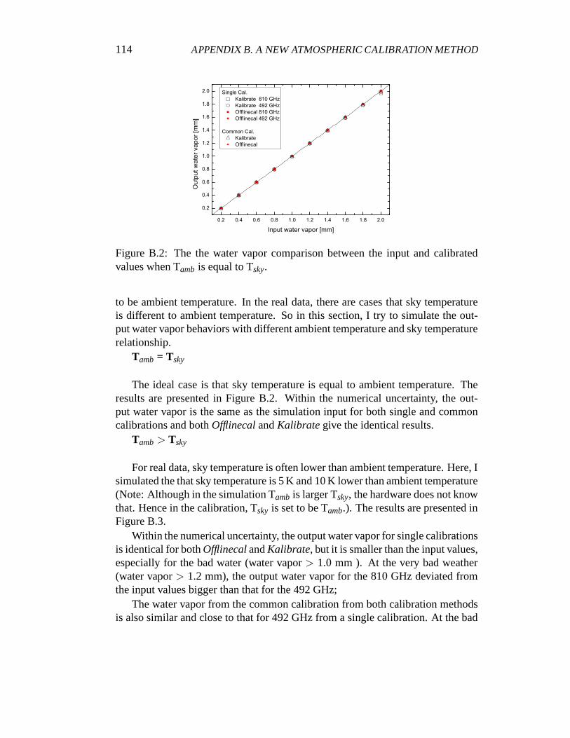
114 APPENDIX B. A NEW ATMOSPHERIC CALIBRATION METHOD
Figure B.2: The the water vapor comparison between the inputand calibratedvalues when Tamb is equal to Tsky.
to be ambient temperature. In the real data, there are cases that sky temperatureis different to ambient temperature. So in this section, I try to simulate the out-put water vapor behaviors with different ambient temperature and sky temperaturerelationship.
Tamb = Tsky
The ideal case is that sky temperature is equal to ambient temperature. Theresults are presented in Figure B.2. Within the numerical uncertainty, the out-put water vapor is the same as the simulation input for both single and commoncalibrations and bothOfflinecalandKalibrategive the identical results.
Tamb> Tsky
For real data, sky temperature is often lower than ambient temperature. Here, Isimulated the that sky temperature is 5 K and 10 K lower than ambient temperature(Note: Although in the simulation Tamb is larger Tsky, the hardware does not knowthat. Hence in the calibration, Tsky is set to be Tamb.). The results are presented inFigure B.3.
Within the numerical uncertainty, the output water vapor for single calibrationsis identical for bothOfflinecalandKalibrate, but it is smaller than the input values,especially for the bad water (water vapor> 1.0 mm ). At the very bad weather(water vapor> 1.2 mm), the output water vapor for the 810 GHz deviated fromthe input values bigger than that for the 492 GHz;
The water vapor from the common calibration from both calibration methodsis also similar and close to that for 492 GHz from a single calibration. At the bad

115
Figure B.3: The the water vapor comparison between the inputand calibratedvalues for sky temperature lower than ambient temperature.The left panel showsthe comparison for single calibration and the right panel presents the comparisonfor common calibration.
weather (water vapor> 1.2 mm) in common calibration, the output water vaporfrom Kalibrate is closer to the input values than that fromOfflinecal.
For both single and common calibration modes, the lower sky temperature isthan ambient temperature, the lower output water vapor is than the input value.
Tamb < Tsky
For comparison, I simulated the that sky temperature is 5 K and 10 K greaterthan ambient temperature (Note: Although in the simulationTamb is lower Tsky,the hardware does not know that. Hence in the calibration, Tsky is set to be Tamb.).The results are presented in Figure B.4.
Within the numerical uncertainty, the output water vapor for single calibrationsis identical for bothOfflinecalandKalibrate, but it is greater than the input values,especially for the bad water. At the very bad weather (water vapor≥ 1.4 mm forthe case that Tsky is 5 K greater than Tamb and water vapor≥ 1.2 mm for the casethat Tsky is 10 K greater than Tamb), there is no solution of output water vapor forthe 810 GHz for bothKalibrateandOfflinecal;
The water vapor from the common calibration from both calibration methodsis also similar and close to that for 492 GHz from a single calibration. Whilethe output water vapor fromKalibrate is closer to the input values than that fromOfflinecal. In the common calibration,Offlinecal takes the water vapor for 492GHz from a single calibration as the common water vapor valuewhen there is nosolution for 810 GHz from a single calibration, whileKalibrate treats differentlyby using a receiver temperature weighted method.
For both single and common calibration modes, the greater sky temperature is
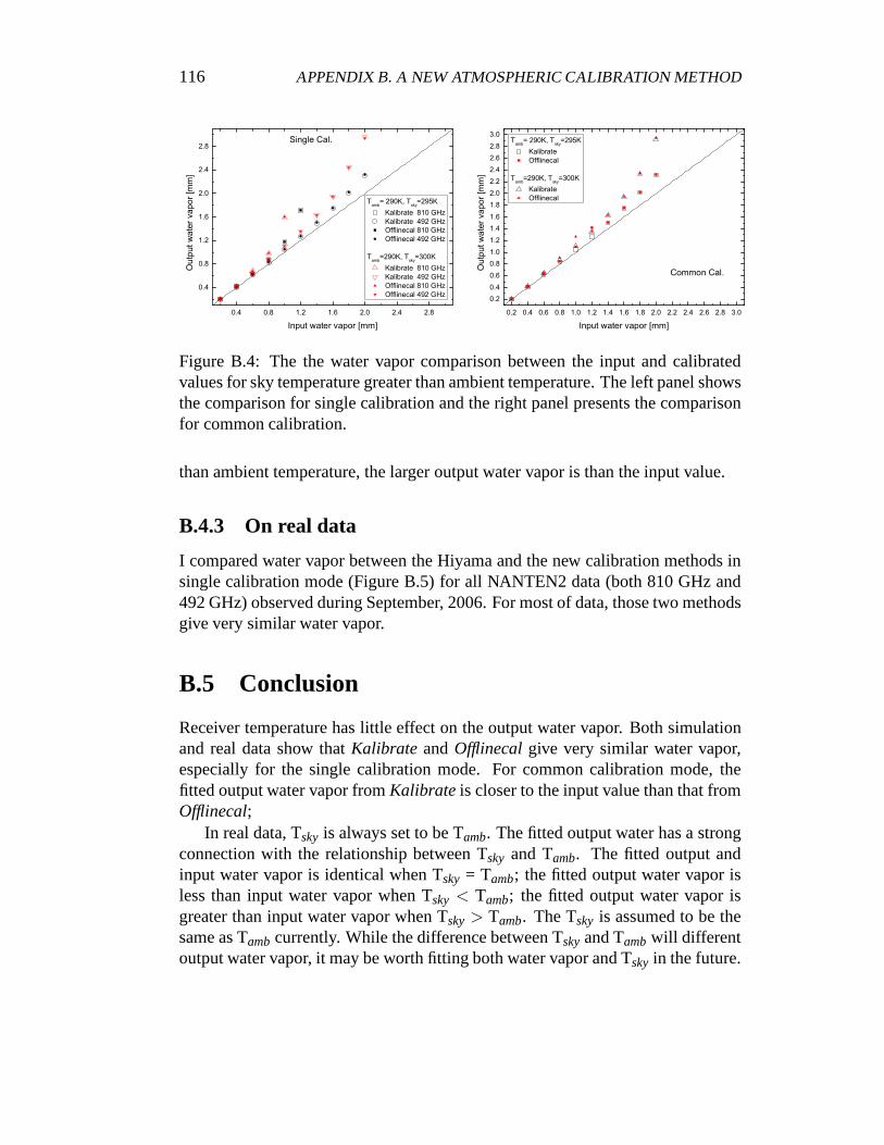
116 APPENDIX B. A NEW ATMOSPHERIC CALIBRATION METHOD
Figure B.4: The the water vapor comparison between the inputand calibratedvalues for sky temperature greater than ambient temperature. The left panel showsthe comparison for single calibration and the right panel presents the comparisonfor common calibration.
than ambient temperature, the larger output water vapor is than the input value.
B.4.3 On real data
I compared water vapor between the Hiyama and the new calibration methods insingle calibration mode (Figure B.5) for all NANTEN2 data (both 810 GHz and492 GHz) observed during September, 2006. For most of data, those two methodsgive very similar water vapor.
B.5 Conclusion
Receiver temperature has little effect on the output water vapor. Both simulationand real data show thatKalibrate andOfflinecalgive very similar water vapor,especially for the single calibration mode. For common calibration mode, thefitted output water vapor fromKalibrate is closer to the input value than that fromOfflinecal;
In real data, Tsky is always set to be Tamb. The fitted output water has a strongconnection with the relationship between Tsky and Tamb. The fitted output andinput water vapor is identical when Tsky = Tamb; the fitted output water vapor isless than input water vapor when Tsky < Tamb; the fitted output water vapor isgreater than input water vapor when Tsky > Tamb. The Tsky is assumed to be thesame as Tambcurrently. While the difference between Tskyand Tambwill differentoutput water vapor, it may be worth fitting both water vapor and Tsky in the future.

117
Figure B.5: The water vapor comparison between the Hiyama and the new cali-bration methods. The drawn lines are where the two methods give the same watervapor.
Generally, common calibration give a more reliable output water vapor.
Appendix C
A uniform observing script
In this appendix, I will describe a uniform observing scriptfor the KOSMA con-trol software, which is a state of art telescope control software developed in I.Physikalisches Institut, Universitat zu Koln. Currently this observing script isused in the NANTEN 2 observatory.
The NANTEN 2 Observatory (NANTEN is japanese for southern sky) is acollaboration between research institutes in Japan (Nagoya and Osaka Univer-sity), South Korea (Seoul National University), Germany (KOSMA, Universitatzu Koln, Argelander-Institut Universitat Bonn), and Chile (Universidad de Chile).The observatory is located at 4900 m altitude on Pampa la Bolain the Atacamadesert, Chile. Equipped with a 4 m submillimeter telescope,NANTEN 2 will beused to survey the southern sky in molecular and atomic spectral lines between110 and 880 GHz (http://www.astro.uni-koeln.de//nanten2/).
At the beginning of observing with the NANTEN 2 telescope, every observerhas to write his own observing script for each of his project,even for each differentobserving mode: position switch mode, on-the-fly mode and etc.. So it is difficultfor a fresh observer to start his observation immediately. Furthermore, becauseeach observer uses his own script, it is hard to track the observation history suchas the ON time, the map size and so on.
Under such condition, a uniform and easily-used observing script is essen-tially needed. I created a uniform observing script using Linux shell language,which works as an interface between observers and telescopecontrol software(the KOSMA control software). It has been installed and usedat the NANTEN 2observatory since 2006.
This observing script contains two parts: one is the main program in linuxshell scripts and the other is a simple ASCI input file that canbe modified todifferent observations. In addition, the script also supports the input parametersusing command lines.
Observing.shis a uniform observing script now and it is in/home/observer/bin
118

119
of thekosmapc at the NANTEN2 site. So there is no need to copy it into differentsource directories.
To set up observing parameters, one can use input file, command line or both.The basic usage is below.
• observing.sh -h; give the help;
• observing.sh -N n; disable display of the input parameters (the default op-tion isyes);
• observing.sh; the script will take the default input parameter filein par inthe directory where the script is running.
• observing.sh -f filename (or path+filename); the script will take the giveninput file;
• observing.sh -GhfmSRlbtMOgLBadcnoCse values; give the options via com-mand line. For example:
– observing.sh -S sourcename -R refname -l mapcenterlam -b mapcen-terbet; in this case, the script will take the source name, referencename, map center (or desired position for psw) in lam and map center(or desired position for psw) in bet from the command line andthe restparameters from the default input filein par.
– observing.sh -S sourcename -R refname -f inputfile; in this case, thescript will take the source name and reference name from the com-mand line and the rest parameters from the give input file
Parameters given from command line have a higher priority. It meansif one sets the same parameter both in the input file and via command line,only the one from the command line will be taken.
If option -N is yes, the script will first display the parameters again in thescreen before starting an observation. One has to typey(Y) + Enter to continueand typen(N) + Enterto quit.
The default log file is stored in a file calledobservinglogsin the same directorywhere one runs the script. One can use the option-G logfile (or path+logfile)toset up a log file.
Below are some examples for carrying out different observing modes (the ex-amples here are using the input parameter file, one can also carry out the sameobservations by using the proper options via command line).

120 APPENDIX C. A UNIFORM OBSERVING SCRIPT
• absolute or relative reference positions. to use an absolute reference, justgive the ref name inrefname; to use a relative reference, one need to dothe following: setrefnameto NAN; then give the relative offsets (arcsec) inrefoffl andrefoffb.
• otf map. set mode tootfl or otfb (otfl means otf scans in +l direction; otfbmeans otf scans in +b direction. The otf mode used in the former version ofthe script will be automatically set to otfl); give source name and ref namein sourceandrefname; give the center of the map inlam andbet; give theON time in ton (this is the ON time per dump! The OFF time is calculatedfrom ON time); set map step instep(for the test receiver, 10′′is used for afully sampled map); set map size inmapsizelandmapsizeb; set the map andref cood. system incormapandcorref.
• psw observation. set mode topsw; give source name and ref name insourceandrefname; give the observed position inlam andbet; give the ON timein ton (OFF time is the same as ON time); set how many cycles and scansin ncycleandnscans(In each cycle, there is a calibration comb/sky.) set themap and ref cood. system incormapandcorref.
• pswcross. set mode topswcross; give source name and ref name insourceandrefname; give the center of the cross inlamandbet; give the integrationtime in ton (OFF time is the same as ON time); set cross step instep(forthe test receiver, 10′′is used for a fully sampled map); if one wants to do a3×3 cross, then set thecrossnumas 3; set the map and ref cood. system incormapandcorref.
• pswrast map. set mode topswrast; give source name and ref name insourceandrefname; give the center of the map inlam andbet; give the ON timein ton; set theonsperoffvalue (it will calculate OFF time means how manyONs after one OFF); set map step instep; set map size inmapsizelandmapsizeb; set the map and ref cood. system incormapandcorref.
• pswmap. set mode topswmap; give source name and ref name insourceandrefname; give the center of the map inlamandbet; give the ON time inton (OFF time is the same as ON time); set map step instep; set map sizein mapsizelandmapsizeb; set the map and ref cood. system incormapandcorref.
• dbs observations (the same for swa and swb observations). set mode todbs(or swaor swb) give source name insource; give the observed position inlam andbet; give the beam switch time inton; map and ref cood. systemare alwaysHORIZON no matter what is set incormapandcorref; wobbler

121
amplitude (chopamp) and frequency (chop frq) are fixed to be 82′′in Az and1.01 Hz, respectively for the NANTEN2, unless there will be new measure-ments to indicate a different value. for dbs mode, one can usedbsnumtoset numbers of dbs cycle; to observe a single position, a cross or a map, therest parameters are the same as for psw mode.
Bibliography
Adams, W. S. 1941, ApJ, 98, 11
Allan, D. W. 1966, Proc. IEEE, 54, 221
Alten, V. P., Bally, J., Devine, D. & Miller, G. J. 1997, in IAUSymp. 182 PosterProc., Low Mass Star Formation Infall to Outflow, ed. F. Malbet & A. Castets(Grenoble, Obs. Grenoble) 51
Alves et al. 2005 in preparation
Aspin, C., Sandell, G. & Russel, A. P. G. 1994, A&AS, 106,165
Aumann, H. H., Fowler, J. W., & Melnyk, M. 1990, AJ, 99, 1674
Bachiller, R. 1985, Ph.D Thesis, Universite de Grenoble
Bachiller, R. & Cernicharo, J. 1984, A&A, 140, 414
Bachiller, R. & Cernicharo, J. 1986, A&A, 168, 262
Bachiller, R.; Martin-Pintado, J. & Planesas,P. 1991, A&A,251,639
Bachiller, R., Menten, K. M. & del Rio-Alvarez, S. 1990, A&A,236,461
Bally, J.; Devine, D.; Alten, V. & Sutherland, R. S. 1999, AJ,478,603
Bally, J., Devine, D. & Reipurth, B. 1996, ApJ, 473,L49
Bally, J.; Stark, A. A.; Wilson, R. W. & Langer, W. D. 1987,ApJ, 312, 45
Barnard, E. E. 1919, AJ, 49, 1
Baudry, A., Combes, F., Perault, M. & Dickman, R. 1980, A&A, 85, 244
Beech, M. 1986, Astrophys. Space Sci., 133, 193
122

BIBLIOGRAPHY 123
Bell, T. A., Viti, S., Williams, D. A., Crawford, I. A. & Price, R. J. 2005, MNRAS,357, 961
Bensch, F. & Simon, R. Poster in Star Formation Workshop, July 14-19, 2001,Santa Cruz, CA, USA
Bensch, F., Stutzki, J. & Ossenkopf, V. 2001, A&A, 366, 636
Bergin, E. A., Kaufman, M. J., Melnick, G. J. et al. 2003, ApJ,582,830
Bertoldi, F. & Draine, B. T 1996, ApJ, 458, 222
Bertoldi, F. & McKee, C. F. 1992, ApJ, 395, 140
Beuther, H. 1999, On The Fly Kartierung und Multilinienanalyse der interstellarenMolekulwolke Cepheus B, Diploma thesis, Universitat zu Koln
Beuther, H., Kramer, C., Deiss, B. & Stutzki, J. 2000, A&A, 362, 1109
Blaauw, A. 1964, ARA&A, 2, 213
Blake, G. A.; Sutton, E. C.; Masson, C. R. & Phillips, T. G. 1987, ApJ, 315, 621
Blitz, L. 1993, Giant Molecular Clouds. In: Levy E.H., Lunine J.I. (eds.), Proto-stars and Planets III. The University of Arizona Press, Tuscon & London
Boger, G. I. & Sternberg, A. 2005, ApJ, 632, 302
Bohlin, R. C., Savage, B. D. & Drake, J. F. 1978, ApJ, 224, 132
Borgman, J. & Blaauw, A. J. 1964, Bull. Astron. Inst. Netherlands, 17, 358
Boulares, A. & Cox, D. P. 1990, ApJ, 365, 544
Burke, B. F. & Graham-Smith, F. 2002, An introduction to Radio Astronomy,second edition, Cambridge University press
Carr, J. S. 1987, ApJ, 323, 170
Cazaux, S. & Tielens, A. G. G. M. 2004, ApJ, 604, 222
Ceccarelli, C., Caux, E., Tielens, A. G. G. M., Kemper, F., Waters, L. B. F. M. &Phillips, T 2002, A&A, 395,L29
Cermis, K. 1990, ApJS166,315
Cernicharo, J. 1985, ATM: A program to compute theoretical atmospheric opacityfor frequencies ¡ 1000GHz, Tech. rep., IRAM

124 BIBLIOGRAPHY
Cheung, A. C., Rank, D. M., Townes, C. H., Thornton, D. D. & Welch, W. J.1968, Phys. Rev. Lett., 21, 1701
Combes, F. 2001, ApSSS, 277, 29
Corneliussen, U., 1996, Ph.D. thesis, University of Cologne
Cox, D. P. 2005, ARA&A, 43, 337
Crovisier, J. & Dickey, M. 1983, A&A, 122, 282
Crutcher, R. M., Churchwell, E. & Ziurys, L. M. 1984, ApJ, 321, 516
Crutcher, R. M., Troland, T. H., Goodman, A. A., Heiles, C., I., Kazes, & Myers,P. C. 1993, ApJ, 407, 175
Cubick, M. 2005, The contribution of photon dominated regions to the far-infraredemission of the Milky Way: construction of PDR models, Diploma thesis, Uni-versitat zu Koln
Cubick, M., Rollig, M., Ossenkopf, V., Kramer, C., & Stutzki, J. 2008, submitedto A&A,
Cubick M., Roellig M., Ossenkopf V., Kramer C., Stutzki J. 2007, A&A, in prep.
Dame, T., Elmegreen, B. G., Cohen, R. & Thaddeus, P. 1986, ApJ, 305, 892
Dame, T. M., Hartmann, D., & Thaddeus, P. 2001, ApJ, 547, 792
de Boisanger, C. B., Chieze, J. P. & Meltz, B. 1992, ApJ, 401, 182
de Jager, C. & Nieuwenhuijzen, H. 1987, A&A, 177, 217
de Jong, T., Boland, W. & Dalgarno, A. 1980, A&A, 91, 68
di Francesco, J., Myers, P. C., Wilner, D. J., Ohashi, N. & Mardones, D. 2002, HotStar Workshop III: The Earliest Stages of Massive Star Birth. ASP ConferenceProceedings, Vol. 267. Edited by Paul A. Crowther. ISBN: 1-58381-107-9. SanFrancisco, Astronomical Society of the Pacific, p.365
Dickey, J. M., McClure-Griffiths, N. M., Stanimirovic, S.,Gaensler, B. M. &Green, A. J. 2001, ApJ, 561, 264
Dobashi, K., Bernard, J. P. & Fukui, Y. 1996, ApJ, 466, 282
Draine, B. T. 1978, ApJS, 36, 595
BIBLIOGRAPHY 125
Draine, B. T. & Bertoldi, F. 1996, ApJ, 468, 269
Eisloeffel, J., Froebrich, D.; Stanke, T. & McCaughrean, M.J. 2003, ApJ, 595,259
Elmegreen, B. G. 1991, In The Physics of Star Formation and Early Stellar Evo-lution, ed. CJ Lada, ND Kylafis, pp. 35C60. Dordrecht: Kluwer
Elmegreen, B. G. 1999, ApJ, 527, 266
Elmegreen, B. G. & Falgarone, E. 1996, ApJ, 471, 816
Elmegreen, B. G., Kim, S. & Staveley-Smith, L. 2001, ApJ, 548, 749
Elmegreen, B. G. & Scalo, J. 2004, ARA&A, 42, 211
Esquivel, A., Lazarian, A., Pogosyan, D., Cho, J. 2003, MNRAS, 342, 325
Esquivel, A., Lazarian, A., Horibe, S. et al. 2007, MNRAS, 381, 1733
Evans II, N. J., Allen, L. E., Blake, G. A. et al. 2003, PASP, 115, 965
Ewen, H. & Purcel, E. 1951, Nature 168, 356
Falgarone, E., Hily-Blant, P., Levrier, F. 2004, Ap&SS, 292, 89
Falgarone, E., & Phillips, T. G. 1996, ApJ, 472, 191
Falgarone, E., Phillips, T. G. & Walker, C. K. 1991, ApJ, 378,186
Felli, M., Tofani, G., Harten, R. H. & Panagia, N. 1978, A&A, 69, 199
Ferriere, K. M. 2001, Rev. of Mod. Phy., 73, 1031
Fiege, J. D., & Pudritz, R. E. 2000, MNRAS, 311, 105
Field, G. B., Somerville, W. B. & Dressler, K. 1966, ARA&A, 4,207
Flannery, B.P., Roberge, W. & Rybicki, G.B. 1980, ApJ, 236, 598
Frerking, M. A., Langer, W. D. & Wilson, R. W. 1982, ApJ, 262, 590
Fuente, A., Martın-Pintado, J., Cernicharo, J. & Bachiller, R. 1993, A&A, 276,473
Garcıa-Burillo, S., Martın-Pintado, J., Fuente, A., Usero, A. & Neri, R. 2002,ApJ, 575, L55

126 BIBLIOGRAPHY
Garden, R. P., Hayashi, M., Gatley, I., Hasegawa, T. & Kaifu,N. 1991, ApJ, 374,540
Gehman, C. S., Adams, F. C., & Watkins, R. 1996, ApJ, 472, 673
Getman, K., Feigelson, E., Townsley, L., Bally, J., Lada, C.& Reipurth, B. 2002,ApJ, 575,354
Glada, G. & Rodrıguez, L. F. 2002, Revista Mexicana de Astronomıa y AstrofısicaVol. 38, pp. 13-21
Glassgold, A. E. & Langer, W. D. 1975, ApJ, 197, 347
Goodman, A. A. 2004, ASP Conference Series, 323, 171
Goodman, A. A., Crutcher, R. M., Heiles, C., Meyers, P. C., & Troland, T. H.1989, ApJ, 338, L61
Gottlieb, C. A., Lada, C. J. Gottlieb, E. W., Lilley, A. E. & Litvak, M. M. 1975,ApJ, 202, 655
Graf, U.U., Honingh, C. E., Jacobs, K., Schieder, R., Stutzki, J. 1998, In As-tronomische Gesellschaft Meeting Abstracts, 14, 120
Graf, U. U., Heyminck, S., Michael, E. A., et al. 2002, in Millimeter and Sub-millimeter Detectors for Astronomy, ed. T. G. Phillips, & J.Zmuidzinas, Proc.SPIE, Hawaii/USA, 4855, 99, 167
Greaves, J. S. & White, G.J. 1992, MNRAS, 259, 457
Green, D. A. 1993, MNRAS, 262, 327
Habing, H. J. 1968, Bull. Astron. Inst. Netherlands 19, 421.
Hatchell, J.; Richer, J. S.; Fuller, G. A.; Qualtrough, C. J.; Ladd, E. F. & Chandler,C. J. 2005, A&A, 440, 151
Heger, M. L. 1922, Further study of the sodium lines in class Bstars ; The spectraof certain class B stars in the regions 5630A-6680A and 3280A-3380A ; Noteon the spectrum of [gamma] Cassiopeiae between 5860A and 6600A. Lick Ob-servatory bulletin ; no. 337; Lick Observatory bulletins ; no. 337., Berkeley :University of California Press, [1922], p. 141-148
Hegmann, M. & Kegel, W. H. 1996, MNRAS, 283, 167
Heikkila, A., Johansson, L. E. B. & Olofsson, H. 1999, A&A, 344, 817
BIBLIOGRAPHY 127
Heithausen, A. 1996, A&A, 314, 251
Heithausen, A.; Bensch, F.; Stutzki, J.; Falgarone, E. & Panis, J. F. 1998, A&A,331, 65
Heitsch, F., Mac Low M. M., Klessen, R. S. 2001, ApJ, 547, 280
Herbertz, R., 1992, Ph.D. thesis, University of Cologne
Herbig, G. H. 1974, Draft catalog of Herbig-Haro object No.1, IBVS, no.832
Herbig, G. H. 1998, AJ, 497, 736
Herbig, G. H. & Jones, B. F. 1983, AJ, 88, 1040
Herbst, W., Maley, J. A. & Williams, E. C. 2000, AJ, 120,349
Heyer, M. H., Brunt, C., Snell, R. L., Howe, J. E., Schloerb, F. P. & Carpenter, J.M. 1998, ApJS, 115, 241
Heyer, M. H., Carpenter, J. M. & Snell, R. L. 2001, ApJ, 551, 852
Heyer, M. H. & Schloerb, F. P. 1997, ApJ, 475, 173
Heyer, M. H. & Terebey, S. 1998, ApJ, 502, 265
Hill, J. K. & Hollenbach, D. J. 1978, ApJ, 225, 390
Hiltner, W. A. 1949, ApJ, 109, 471
Hiyama, S. 1998, Seitenbandkalibration radioastronomischer Linienbeobachtun-gen, Diploma thesis, Universitat zu Koln
Hirano, N., Kamazaki, T., Mikami, H., Saito, S., Umemoto, T.& Yamamoto, S.1999, ApJ, 478,631
Hobson, M.P., 1992, MNRAS, 256, 457
Hobson, M.P., Jenness, T., Padman, R. & Scott, P.F., 1994, MNRAS, 266, 972
Hodapp, K. W. & Ladd, E. F. 1995, ApJ, 453,715
Hogerheijde, M. R., van Dishoeck, E. F., Blake, G. A. & van Langevelde, H. J.1997, ApJ, 489, 293
Hollenbach, D. & Salpeter, E. E. 1971, ApJ, 163, 155
Hollenbach, D. J. & Tielens, A. G. G. M. 1997, ARA&A, 35, 179

128 BIBLIOGRAPHY
Hollenbach, D. J. & Tielens, A. G. G. M. 1999, Rev of Mod. Phhys., 71, 173
Horn, J., Siebertz, O., Schmulling, F., et al. 1999, Exp. Astron., 9, 17
Hollenbach, D., Werner, M. W. & Salpeter, E. E. 1971, ApJ, 163, 165
Hossack, W. R. & Hogg, F. S. 1949, AJ, 54, R189
Howe, J. E., Jaffe, D. T., Genzel, R. & Stacey, G. J. 1991, ApJ,373, 158
Israel, F. P., & Baas, F. 2002, A&A, 383, 82
Itoh, M., Fukunaga, H., Sekimoto, Y., Tatematsu, K. & Koyama, K. 1999, sf99.proc 100
Jenkins, E. B., Jura, M. & Loewenstein, M. 1983, ApJ, 270, 88.
Jennings, R. E., Cameron, D. H. M., Cudlip, W. & Hirst, C. J. 1987, MNRAS,226,461
Johnen, C., 1992, Diplom thesis, University of Cologne
Johnstone, D. & Bally, J. 2006, ApJ, 653, 383
Johnstone, D., Wilson, C, D., Moriarty-Schieven, G. et al. 2000, ApJ, 545, 327
Juan, J., Bachiller, R., Koempe, C. & Martin-Pintado, J. 2000, A&A, 270,432
Jura, M. 1974, ApJ, 191, 375
Jura, M. 1976, AJ, 204, 12.
Kaufman, M., Wolfire, M., Hollenbach, D., & Luhman, M. 1999, ApJ, 527, 795
Kirk, H., Johnstone, D. & Di Francesco, J. 2006, ApJ, 646, 1009
Klein, S. C. & Dickman, R. L. 1984, ApJ, 286, 255
Klein, S. C. & Dickman, R. L. 1987, ApJ, 312, 837
Klessen, R. S., & Burkert, A. 2000, ApJS, 128, 287
Kolmogorov AN. 1941. Proc. R. Soc. London Ser. A 434:9C13. Reprinted in 1991
Kramer, C., Beuther, H., Simon, R., Stutzki, J., & Winnewisser, G. 1999, Imag-ing at radio through submillimetre wavelength, ed. J. G. Mangum, & S. J. E.Radford, Astronomical Society of the Pacific, CF-217

BIBLIOGRAPHY 129
Kramer, C., Cubick, M., Rollig, M., et al. 2008, A&A, 477, 547
Kramer, C., Degiacomi, C., Graf, U., et al. 1998, in AdvancedTechnol-ogy MMV, Radiao, and Terahertz Telescopes, ed. T. Phillips,Proc. SPIE,Kona/Hawaii/USA, 3357, 71
Kramer, C., Jakob, H., Mookerjea, B., Schneider., N., Brull, M. & Stutzki., J.2004, A&A, 424, 887
Kramer C., Mookerjea B., Bayet E., Garcia-Burillo S., GerinM., Israel F. P.,Stutzki J. & Wouterloot J.G.A, 2005, A&A, 441, 961
Kramer, C., Stutzki, J., Rohrig, R. & Corneliussen, U. 1998, A&A, 329, 249
Kramer C., Stutzki J. & Winnewisser, G. 1996, A&A, 307, 915
Kulkarni, S. R. & Heiles, C. 1987, in Interstellar Processes, edited by D. J. Hol-lenbach and H. A. Thronson (Reidel, Dordrecht), p. 87
Langer, W. D. & Penzias, A. A. 1990, ApJ, 357, 477
Larson, R. B. 1981, MNRAS, 194,809
Lazarian, A. & Pogosyan, D. 2000, ApJ, 537, 720
Lazarian, A. & Pogosyan, D. 2004, ApJ, 616, 943
Lada, C. J., Alves, A. & Lada, E. A. 1996, AJ, 111,1964
Lada, E.A., Bally, J. & Stark, A. A. 1991, ApJ, 368, 432
Lada, E. A., & Lada, C. J. 1995, AJ, 109, 1682
Ladd, E. F., Lada, E.A. & Myers, P. C. 1993, ApJ, 410,168
Langer, W. D. & Penzias, A. A. 1990, ApJ, 357, 477
Langer, W. D., Wilson, R.W. & Anderson, C. H. 1993, ApJ, 408, L45
Lapinov, A. V., Schilke, P., Juvela, M. & Zinchenko, I. I. 1998, A&A, 336, 1007
Lazarian, A. & Pogosyan, D. 2000, ApJ, 537, 720
Lazarian, A. & Pogosyan, D. 2004, ApJ, 616, 943
Lazarian, A.; Pogosyan, D.; Vazquez-Semadeni, E. & Pichardo, B. 2001, ApJ,555, 130

130 BIBLIOGRAPHY
Le Bourlot, J., Pineau Des Forets, G., Roueff, E. & Flower, D. R. 1993, A&A,267, 233
Leung, C. M., Kutner, M. L. & Mead, K. N. 1983, ApJ, 262, 583
Leurini, S., Rolffs, R., Thorwirth, S. et al. 2006, A&A, 454,L47
Little, L. T & Matheson, D. N. 1973, MNRAS, 162, 329C38
Lis, D. C., Roueff, E., Gerin, M., Phillips, T. G., Coudert, L. H., van der Tak, F. F.S. & Schilke, P 2001, ApJ, 571,L55
Liseau, R., Sandell, G. & Knee, L. B. G. 1988, A&A, 192,153
Loren, R. B. 1989, ApJ, 338, 902
Luhman, K. L., Lada, E. A., Muench, A. A, & Elston, R. J. 2005, ApJ, 618, 810
Luhman, K. L., Rieke, G. H., Lada, C. J, & Lada, E. A. 1998, ApJ,508, 347
Luhman, K. L., Stauffer, J. R. & Muench, A. A, et al. 2003, ApJ,593, 1093
Maron, J. & Goldreich, P. 2001, ApJ, 554,1175
Masur, M. 2005, Diploma thesis, Universitat zu Koln
Matthews, B. C. & Wilson, C. D 2003, ApJ, 574,822
McKee, C. F.& Ostriker, E. C. 2007, ARA&A, 45, 565
McKee, C. F. & Ostriker, J. P. 1977, ApJ, 218, 148
McKellar, A. 1940, PASP, 52, 187
Meijerink, R. & Spaans, M. 2005, A&A, 436, 397
Meixner, M., & Tielens, A. G. G. M. 1993, ApJ, 405, 216
Miesch, M. S. & Bally, J. 1994, ApJ, 429, 645
Minchin, N. R., Ward-Thompson, D. & White, G. J. 1992, A&A, 265, 733
Minkowski, R. 1955. In Gas Dynamics of Cosmic Clouds, ed. J. M. Burgers, H.C. van de Hulst, pp. 3C12. Amsterdam: North Holland
Mookerjea, B., Kramer, C., Nielbock, M. & Nyman, L. A&A, 2004, A&A, 426,119
BIBLIOGRAPHY 131
Mookerjea, B., Kramer, C., Rollig, M. & Masur, M. 2006, A&A,456, 235
Moreno-Corral, M., Chavarria, K.C., Lara, E. & Wagner, S. 1993, A&A, 98, 295
Nozawa, S., Mizuno, A., Teshima, Y., et al. 1991, ApJS, 77, 647
Muller, C. A. & Oort, J. H. 1951, Nature, 168,357
Myers, P. C. 1983, ApJ, 270,105
Myers, P. C. 1987, in Interstellar Processes, ed. D. J. Hollenbach & H. A. Thron-son (Dordrecht: Reidel), 71
Myers, P. C. & Goodman, A. A. 1988, ApJ, 329, 392
Najita, J. R., Tiede, G. P. & Carr, J. S. 2000, ApJ, 541, 977
Nakagawa, T., Yui, Y. Y., & Doi, et al. 1998, ApJS, 115, 259
Nakajima, Y., & Hanawa, T. 1996, ApJ, 467, 321
Nejad, L. A. M. & Wagenblast, R. 1999, A&A, 350, 204
Neufeld, D. A., Schilke, P., Menten, K. M. et al. 2006, A&A, 454, L37
Oka, T., Iwata, M., Maezawa, H., Ikeda, M., Ito, T., Kamegai,K., Sakai, T. &Yamamoto, S. 2004, ApJ, 602,803
Ossenkopf, V., Esquivel, A., Lazarian, A. & Stutzki, J. 2006, A&A, 452, 223
Ossenkopf, V., Klessen, R. S. & Heitsch, F. 2001, A&A, 379, 1005
Ossenkopf, V. & Mac Low, M. M. 2002, A&A, 390, 307
Ossenkopf, V., Rollig, M., Cubick, M., & Stutzki, J. 2007, Molecules in Space &Laboratory, Paris, ed. J. L. Lemaire & F. Combes, 950
Ostriker, E. C, Stone, J. M., Gammie, C. F. 2001, ApJ, 546, 980
Padoan, P., Boldyrev, S., Langer, W. & Nordlund,A, 2003a, ApJ, 583, 308
Padoan, P., Bally, J., Billawala, Y., Juvela, M. & Nordlund,A. 1999, ApJ, 525,318
Padoan, P., Goodman, A. A. & Juvela, M. 2003b, ApJ, 588, 881
Padoan, P., Juvela, M., Bally, J., & Nordlund,A. 1998, ApJ, 504, 300

132 BIBLIOGRAPHY
Panagia, N. & Thum, C. 1981, A&A, 98, 295
Pardo, J. R., Cernicharo, J & Serabyn, E. 2001, IEEE Trans. onAntennas andPropagation, 49/12, 1683
Pardo, Serabyn, E., Wiedner, M. C. & J. R., Cernicharo, J, 2005, J. Quant. Spec.and Radiat. Transfer 96/3-4, 537
Patrikeev, I., Fletcher, A., Stepanov, R. et al. 2006, A&A, 458, 441
Pety, J., Teyssier, D., Fosse, D., Gerin, M., Roueff, E. et al. 2005, A&A, 435, 885
Perault, M., Falgarone, E. & Puget, J. L. 1986, A&A, 157, 139
Plume, R., Bensch, F., Howe, J. E. et al. 2000, ApJ, 539, L133
Plume, R., Jaffe, D., Tatematsu, K., et al. 1999, ApJ, 512, 768
Preibisch, T. 2003, A&A, 401,543
Preibisch, T. & Zinnecker, H. 2001, AJ, 122, 866
Preibisch, T. & Zinnecker, H. 2002, AJ, 123,1613
Preibisch, T., Zinnecker, H. & Herbig, G. H. 1996, A&A, 310, 456
Rebull, L. M., Cole, D. M., Stapelfeldt, K. R. & Werner, M. W. 2003, AJ,125,2568
Rickett, B. J. 1970, MNRAS, 150,67
Ridge, N. A., Wilson, T. L., Megeath, S. T., Allen, L. E., & Myers, P. C. 2003,AJ, 126, 286
Rosolowsky, E. W., Goodman, A. A., Wilner, D. J. & Williams, J. P. 1999, ApJ,524, 887
Rohrig, R., 1996, Ph.D. thesis, University of Cologne
Rollig, M., Abel, N. P., Bell, T. et al. 2007, A&A, 467, 187
Rollig, M., Hegmann, M., Kegel, W. H. 2002, A&A, 392, 1081
Rollig, M., Ossenkopf, V., Jeyakumar, S. & Stutzki, J. 2006, A&A, 451, 917
Rudolph, A. L., Bachiller, R., Rieu, N. Q., Trune, D. V., Palmer, P. & Welch, W.J. 2001, ApJ, 558,204

BIBLIOGRAPHY 133
Salpeter, E. E. 1955, ApJ, 121, 161
Sancisi, R. 1974, IAUS, 60, 115
Sandell, G., Aspin, C., Duncan, W. D., Russell, A. P. G. & Robson, E. I. 1991,ApJ, 376,L17
Sandell, G., Knee, L. B. G., Aspin, C., Robson, I. E. & Russell, A. P. G. 1994,A&A, 285,L1
Sanders, D. B., Scoville, N. Z. & Solomon, P. M. 1985, ApJ, 289, 373
Sargent, A. I. 1979, ApJ, 233, 163
Scalo, J. M. 1984. ApJ, 277,556
Scalo, J. M. 1987, in Plasma Turbulence and Energetic Particles, ed. M. Ostrowski& R. Schlickeiser (Krakow: Univ. Jagiellonski Astro. Obs.), 1
Scalo, J. & Elmegreen, B. G. 2004, ARA&A, 42, 275
Schieder, R., Tolls, V., Winnewisser, G. 1989, Exp. Astron., 1, 101
Schneider, N., Simon, R., Kramer, C., Kraemer, K., Stutzki,J. & Mookerje, B.2003, A&A, 406, 915
Schroder, K., Staemmler, V., Smith, M. D., Flower, D. R., & Jaquet, R. 1991, J.Phys. B, 24, 2487
Scoville, N. Z., Sargent, A. I., Sanders, D. B., Claussen, M.J. et al. 1986, ApJ,303, 416
Sharpless, S. 1959, ApJS, 4, 257
Simon, R. 1997, Ph.D. thesis, University of Cologne
Simon, R., Jackson, J. M., Clemens, D. P., Bania, T. M. & Heyer, M. H. 2001,ApJ, 551, 747
Simon, R., Stutzki, J., Sternberg A. & Winnewisser, G. 1997,A&A, 327, 9
Snow, T. P. & McCall, B. J. 2006, ARA&A, 44, 367
Solomon, P. M., Rivolo, A. R., Barrett, J. & Yahil, A. 1987, ApJ, 319, 730
Spaans, M. 1996, A&A, 307, 271

134 BIBLIOGRAPHY
Spitzer, L. 1978, Physical Processes in the Interstellar Medium, Wiley
Stacey, G. J., Jaffe, D. T., Geis, N., et al. 1993, ApJ, 404, 219
Stanimirovic, S. & Lazarian, A. 2001, ApJ, 551, L53
Stanimirovic, S., Staveley-Smith, L., Dickey, J. M., Sault, R. J. & Snowden, S. L.1999, MNRAS, 302, 417
Stenholm, L. G. 1984, A&A, 137, 133
Sternberg, A. & Dalgarno, A. 1989, ApJ, 338, 197
Sternberg, A. & Dalgarno, A. 1995, ApJS, 99, 565
Stutzki, J., Bensch, F., Heithausen, A., Ossenkopf, V. & Zielinsky, M. 1998, A&A,336, 697
Stutzki, J. & Gusten, R. 1990, ApJ, 356, 513
Stutzki, J., Stacey, G. J., Genzel, R., Harris, A. I., Jaffe,D. T. & Lugten, J. B.1988, ApJ, 332, 379
Storzer H. & Hollenbach, D. 1998, ApJ, 495, 853
Storzer, H., Stutzki, J. & Sternberg, A. 1996, A&A, 310, 592
Storzer, H., Zielinsky, M., Stutzki, J., & Sternberg, A. 2000, A&A, 358, 682
Sun, K., Kramer, C., Ossenkopf, V., Bensch, F., Stutzki, J & Miller, M. 2006,A&A, 451, 539
Swings, P. & Rosenfeld, L. 1937, ApJ, 86, 483
Tielens, A. G. G. M. 2005, The physics and chemistry of the interstellar medium
Tielens, A. G. G. M. & Hollenbach, D. 1985, ApJ, 291, 722
Testi, L., Olmi, L. & Hunt, L. et al. 1995, A&A, 303, 881
Teyssier, D., Fosse, D., Gerin, M., Pety, J., Abergel, A. & Roueff, E. 2004, A&A,417, 135
Trullols, E. & Jordi, C. 1999, A&A, 324,549
Trumpler, R. J. 1930, PASP, 42, 214
Tucker, K. D, Kutner, M. L. Thaddeus, P. 1974, ApJ, 193, L115
BIBLIOGRAPHY 135
Ungerechts, H., Brunswing, W., Kramer, C. et al. 2000, ASPC,217, 190
Ungerechts, H. & Thaddeus, P. 1987, ApJS, 63, 645
van der Tak, F. F. S., Schilke, P., Muller, H. S. P., Lis, D. C., Phillips, T. G., Gerin,M. & Roueff, E 2002, A&A, 388,L53
van Dishoeck, E. F. 2006, The lecture’s notes of Interstellar Medium course
van Dishoeck, E. F., Black, J. H. 1988, ApJ, 334, 771
Vazquez-Semadeni, E., Ostriker, E. C., Passot, T., Gammie, C. F. & Stone, J. M.2000, in Mannings V., Boss A. P., Russell S. S., eds, Protostars and Planets IV.University of Arizona Press, Tucson, p. 3
Viti, S., Roueff, E., Hartquist, T. W., Pineau des Forets, G. & Williams, D. A.2001, A&A, 370, 557
Vogelaar, M. G. R. & Wakker, B. P. 1994, A&A, 291, 557
Von Weizsacker, C. F. 1951. ApJ, 114,165
Wagenblast, R. & Hartquist, T. W. 1988, MNRAS, 230, 363
Walsh, A. J., Myers, P. C., di Francesco, J., Wilner, D. J. & Bourke, T. L. 2003,International Astronomical Union. Symposium no. 221, held22-25 July, 2003in Sydney, Australia
Wang, H. 2003, Doctoral thesis of Purple Mountain Observatory
Watson, W. D. 1972, AJ, 176, 103.
Warin, S., Castets, A., Langer, W. D., Wilson, R. W. & Pagani,L. 1996, A&A,306, 935
Weinreb, S., Barrett, A. H., Meeks, M. L. & Henry, J. C. 1963, Nature, 200, 829
Wiesemeyer, H., Guesten, R., Wink, J. E. & Yorke, H. W. 1997, A&A, 320,287
Williams, J. P., Blitz, L. & McKee, C. F. 2000, in Protostars and Planets IV, ed. V.Mannings, A. P. Boss, & S. S. Russell (Tucson: Univ. Arizona Press), 97
Williams, J. P., Blitz, L. & Stark, A. A. 1995, ApJ, 451, 252
Williams, J. P., de Geus, E. J. & Blitz, L. 1994, ApJ, 428, 693
Wilson, R. W., Jefferts, K. B. & Penzias, A. A. 1970, ApJ, 161,43

136 BIBLIOGRAPHY
Winnewisser, G., Bester, M., & Ewald, R. 1986, A&A, 167, 207
Wong, T., Ladd, E. F., Brisbin, D. et al. 2008, submitted to MNRAS
Yu, K. C., Billawala, Y. & Bally, J. 1999, AJ, 118, 2940
Zimmermann, T., 1993, Ph.D. thesis, University of Cologne
Zimmermann, T. & Stutzki, J. 1993, Fractals, 1, 930
Zinnecker, H., McCaughrean, M.J. & Wilking, B.A. 1993, The initial stellar pop-ulation. In: Levy E.H., Lunine J.I. (eds.), Protostars and Planets III. The Uni-versity of Arizona Press, Tuscon & London
Ziurys, L. M. Saykally, R. J., Plambeck, R. L. & Erickson, N. R. 1982, ApJ, 254,94
List of Figures
1.1 Hubble space telescope image of Cone nebula (NGC2264): starforming pillar of gas and dust. . . . . . . . . . . . . . . . . . . . 2
1.2 Example of the filter function used in the∆-variance analysis . . . 6
1.3 An example of a typical∆-variance spectrum for a subset of theFCRAO outer galaxy survey (13CO 1–0). This subset has a verylarge scale (384 by 128 pixels; 50′′per pixel). The x axis is the lagand the y axis is the value of the variance. The black line indicatesthe power-law fits to the data. The turnover at the smallest angularscales shows the effect from the white noise behavior (for purewhite noise,σ2
∆(L) ∝ L−2); the turnover at the large angular scalesis due to the influence of the typical size of main structures in theimage. The figure is adapted from the Fig. 3 in the paper byStutzki et al. (1998). . . . . . . . . . . . . . . . . . . . . . . . . . 7
1.4 An example of a clump mass spectrum for clump mass spectraofNGC 7538. All spectra are fitted by a power law functiondN =dM ∝ M−α . The straight line represents the best linear fit over therange of masses spanned by the line. The resulting indicesα is1.79 in this case. The dashed line denotes the minimum possiblemass limit, which is estimated by the resolution limits and therms noise. The figure is adapted from the Fig. 6 in the paper byKramer et al. (1998b). . . . . . . . . . . . . . . . . . . . . . . . . 9
1.5 The GRS13CO intensity integrated over the velocity range rel-evant for emission from the individual cloud complexes. Thebeam size is indicated as a filled circle in the lower left corner ofeach panel. Top panels : Quiescent clouds; Bottom: Star-formingclouds. The figure is adapted from the Fig. 2 in the paper bySimon et al. (2001). . . . . . . . . . . . . . . . . . . . . . . . . . 10
137
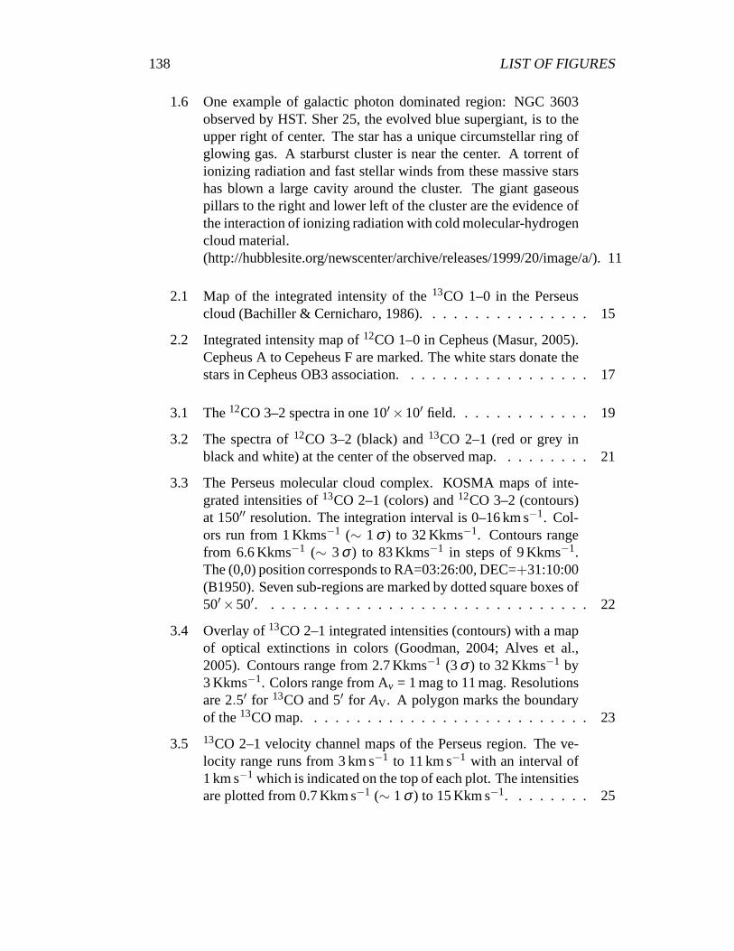
138 LIST OF FIGURES
1.6 One example of galactic photon dominated region: NGC 3603observed by HST. Sher 25, the evolved blue supergiant, is to theupper right of center. The star has a unique circumstellar ring ofglowing gas. A starburst cluster is near the center. A torrent ofionizing radiation and fast stellar winds from these massive starshas blown a large cavity around the cluster. The giant gaseouspillars to the right and lower left of the cluster are the evidence ofthe interaction of ionizing radiation with cold molecular-hydrogencloud material.(http://hubblesite.org/newscenter/archive/releases/1999/20/image/a/). 11
2.1 Map of the integrated intensity of the13CO 1–0 in the Perseuscloud (Bachiller & Cernicharo, 1986). . . . . . . . . . . . . . . . 15
2.2 Integrated intensity map of12CO 1–0 in Cepheus (Masur, 2005).Cepheus A to Cepeheus F are marked. The white stars donate thestars in Cepheus OB3 association. . . . . . . . . . . . . . . . . . 17
3.1 The12CO 3–2 spectra in one 10′×10′ field. . . . . . . . . . . . . 19
3.2 The spectra of12CO 3–2 (black) and13CO 2–1 (red or grey inblack and white) at the center of the observed map. . . . . . . . . 21
3.3 The Perseus molecular cloud complex. KOSMA maps of inte-grated intensities of13CO 2–1 (colors) and12CO 3–2 (contours)at 150′′ resolution. The integration interval is 0–16 km s−1. Col-ors run from 1 Kkms−1 (∼ 1σ ) to 32 Kkms−1. Contours rangefrom 6.6 Kkms−1 (∼ 3σ ) to 83 Kkms−1 in steps of 9 Kkms−1.The (0,0) position corresponds to RA=03:26:00, DEC=+31:10:00(B1950). Seven sub-regions are marked by dotted square boxes of50′×50′. . . . . . . . . . . . . . . . . . . . . . . . . . . . . . . 22
3.4 Overlay of13CO 2–1 integrated intensities (contours) with a mapof optical extinctions in colors (Goodman, 2004; Alves et al.,2005). Contours range from 2.7 Kkms−1 (3σ ) to 32 Kkms−1 by3 Kkms−1. Colors range from Av = 1 mag to 11 mag. Resolutionsare 2.5′ for 13CO and 5′ for AV. A polygon marks the boundaryof the13CO map. . . . . . . . . . . . . . . . . . . . . . . . . . . 23
3.5 13CO 2–1 velocity channel maps of the Perseus region. The ve-locity range runs from 3 km s−1 to 11 km s−1 with an interval of1 km s−1 which is indicated on the top of each plot. The intensitiesare plotted from 0.7 Kkm s−1 (∼ 1σ ) to 15 Kkm s−1. . . . . . . . 25

LIST OF FIGURES 139
3.6 Mean and rms of the equivalent line widths∆veq of the12CO 3–2 and13CO 2–1 spectra for the observed positions of the seven50′×50′ sub regions (Fig. 3.3). The dashed line delineates equalwidths in 12CO and13CO. The error bars indicate the differencebetween the minimum/maximum and the mean values. . . . . . . 26
3.7 ∆-variance analysis of the off-line channel maps. In the upper plota velocity span corresponding to the integrated intensity maps isused. The two regions representing opposite extremes in thestruc-tural behaviour, NGC 1333 and L1455, show about the same spec-tral index of the colored noise in both transitions for smalllags. Inthe lower plot, the influence of different velocity spans, asused inthe velocity channel analysis (Sect. 3.3.2), is studied forL1455.The colored noise indexdnoise is nearly constant independent ofspecies, transition, velocity range∆vch, and center velocity vcen. . 28
3.8 ∆-variance spectra of integrated intensities.a) Spectra obtainedfrom the CO maps and theAV data of the region mapped withthe KOSMA telescope.b) Spectra of integrated intensity maps oftwo 50′× 50′sub-regions: NGC 1333 and L 1455. Power-law fitsto the data corrected for noise and beam-blurring are indicated assolid lines. . . . . . . . . . . . . . . . . . . . . . . . . . . . . . . 29
3.9 Comparison of the index spectrum of the13CO 2–1 data in L 1455with the average line profile. The index spectrum is created bypower-law fits to the∆-variance spectrum of individual channelmaps (∆vch = 0.22 km s−1). The vertical error bars represent theuncertainty of the fit. The horizontal error bars indicate the veloc-ity channel width. . . . . . . . . . . . . . . . . . . . . . . . . . . 32
3.10 Comparison of the index spectra obtained for differentvelocitychannel widths with the average line profile. The upper plotsshowthe results for IC 348, the central plot NGC 1333 and the lowerplot L 1455. For the left column I used the12CO 3–2 data, theright column represents the13CO 2–1 data. The different symbolsindicate the results from different velocity channel widths. Thedashed lines represents the index of the integrated intensity maps. 33
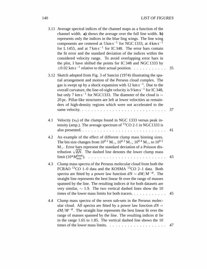
140 LIST OF FIGURES
3.11 Average spectral indices of the channel maps as a function of thechannel width.a) shows the average over the full line width.b)represents only the indices in the blue ling wings. The line wingcomponents are centered at 5 km s−1 for NGC 1333, at 4 km s−1
for L 1455, and at 7 km s−1 for IC 348. The error bars containthe fit error and the standard deviation of the indices withintheconsidered velocity range. To avoid overlapping error barsinthe plot, I have shifted the points for IC 348 and NGC 1333 by±0.02 km s−1 relative to their actual position. . . . . . . . . . . . 35
3.12 Sketch adopted from Fig. 3 of Sancisi (1974) illustrating the spa-tial arrangement and motion of the Perseus cloud complex. Thegas is swept up by a shock expansion with 12 km s−1. Due to theoverall curvature, the line-of-sight velocity is 9 km s−1 for IC 348,but only 7 km s−1 for NGC1333. The diameter of the cloud is∼20 pc. Pillar-like structures are left at lower velocities as remain-ders of high-density regions which were not accelerated to thesame velocity. . . . . . . . . . . . . . . . . . . . . . . . . . . . . 37
4.1 Velocity (v0) of the clumps found in NGC 1333 versus peak in-tensity (amp.). The average spectrum of13CO 2-1 in NGC1333 isalso presented. . . . . . . . . . . . . . . . . . . . . . . . . . . . . 41
4.2 An example of the effect of different clump mass binning sizes.The bin size changes from 100.2 M, 100.3 M, 100.4 M, to 100.5
M. Error bars represent the standard deviation of a Poisson dis-tribution
√∆N. The dashed line denotes the lower clump mass
limit (10*Mlimitmin ). . . . . . . . . . . . . . . . . . . . . . . . . . . 43
4.3 Clump mass spectra of the Perseus molecular cloud from both theFCRAO 13CO 1–0 data and the KOSMA13CO 2–1 data. Bothspectra are fitted by a power law functiondN = dM/M−α . Thestraight line represents the best linear fit over the range ofmassesspanned by the line. The resulting indicesα for both datasets arevery similar,∼ 1.9. The two vertical dashed lines show the 10times of the lower mass limits for both tracers. . . . . . . . . . . .45
4.4 Clump mass spectra of the seven sub-sets in the Perseus molec-ular cloud. All spectra are fitted by a power law functiondN =dM/M−α . The straight line represents the best linear fit over therange of masses spanned by the line. The resulting indicesα liein the range 1.65 to 1.85. The vertical dashed line shows the 10times of the lower mass limits. . . . . . . . . . . . . . . . . . . . 47
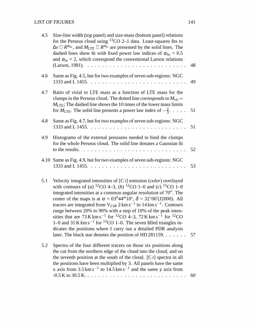
LIST OF FIGURES 141
4.5 Size-line width (top panel) and size-mass (bottom panel) relationsfor the Perseus cloud using13CO 2–1 data. Least-squares fits to∆v ∝ Rαlw , andMLTE ∝ Rαm are presented by the solid lines. Thedashed lines show fit with fixed power law indices ofαlw = 0.5andαm = 2, which correspond the conventional Larson relations(Larson, 1981). . . . . . . . . . . . . . . . . . . . . . . . . . . . 48
4.6 Same as Fig. 4.5, but for two examples of seven sub-regions: NGC1333 and L 1455. . . . . . . . . . . . . . . . . . . . . . . . . . . 49
4.7 Ratio of virial to LTE mass as a function of LTE mass for theclumps in the Perseus cloud. The dotted line corresponds toMvir =MLTE; The dashed line shows the 10 times of the lower mass limitsfor MLTE. The solid line presents a power law index of−2
3. . . . . 51
4.8 Same as Fig. 4.7, but for two examples of seven sub-regions: NGC1333 and L 1455. . . . . . . . . . . . . . . . . . . . . . . . . . . 51
4.9 Histograms of the external pressures needed to bind the clumpsfor the whole Perseus cloud. The solid line donates a Gaussian fitto the results. . . . . . . . . . . . . . . . . . . . . . . . . . . . . 52
4.10 Same as Fig. 4.9, but for two examples of seven sub-regions: NGC1333 and L 1455. . . . . . . . . . . . . . . . . . . . . . . . . . . 53
5.1 Velocity integrated intensities of [CI] emission (color) overlayedwith contours of (a) 12CO 4–3, (b) 12CO 1–0 and (c) 13CO 1–0integrated intensities at a common angular resolution of 70′′. Thecenter of the maps is atα = 03h44m10s, δ = 3206′(J2000). Alltracers are integrated from VLSR2 km s−1 to 14 km s−1. Contoursrange between 20% to 90% with a step of 10% of the peak inten-sities that are 73 K km s−1 for 12CO 4–3, 72 K km s−1 for 12CO1–0 and 31 K km s−1 for 13CO 1–0. The seven filled triangles in-dicates the positions where I carry out a detailed PDR analysislater. The black star denotes the position of HD 281159. . . . .. . 57
5.2 Spectra of the four different tracers on those six positions alongthe cut from the northern edge of the cloud into the cloud, andonthe seventh position at the south of the cloud. [CI] spectra in allthe positions have been multiplied by 3. All panels have the samex axis from 3.5 km s−1 to 14.5 km s−1 and the same y axis from-0.5 K to 30.5 K. . . . . . . . . . . . . . . . . . . . . . . . . . . . 60

142 LIST OF FIGURES
5.3 The top panel(a) presents the normalized integrated intensities of[C I], 12CO 4–3,12CO 1–0 and13CO 1–0 in the seven selectedpositions. The typical errors of the intensities are about 15%; (b)displays integrated line intensity ratios. The x axes of allpanelsare the relative distance to the northern rim (8′,6′) position. Thesouthern rim is plotted in a separate box. . . . . . . . . . . . . . . 64
5.4 The color plot represents the12CO 4–3 /12CO 1–0 line intensityratio (in units of K km s−1) observed in the IC 348 cloud. Thecontours show the12CO 4–3 line intensity spaced at 10% intervalsfrom 20% to 90% relative to the peak intensity of 73 K km s−1.For line ratios, I only calculate for the positions where thelineintensities of both tracer are larger than each 3 sigma value. . . . . 65
5.5 The C/CO column density ratio overlaid by13CO 1–0 integratedintensities contours. The contour levels are spaced at 10% inter-vals from 20% to 90% relative to the peak intensity of 31 K km s−1.For column density ratios, I only calculate for the positions wherethe line intensities of13CO 1–0 are above the 3 sigma value. . . . 66
5.6 FUV intensity distribution (contours) in IC 348 estimated fromthe IRAS FIR fluxes, overlayed on the [CI] integrated intensities(colors). The FUV intensityχFIR contour levels run from 5, 10,20 to 100 by steps of 20 Draine units,χ0. . . . . . . . . . . . . . 68
5.7 Comparison of the observed line intensity ratios [CI]/12CO 4–3, [C I]/13CO 1–0 and12CO 4–3/12CO 1–0 at (1′, −1′) with thesingle clump KOSMA -τ PDR model calculations. The left fig-ure shows the fitting of a clump mass and densities; the right onepresents the fitting of the FUV field and clump densities. The mid-dle drawn contours are the observed intensity ratios, and the outertwo are those for the 20% uncertainty. The grey-scale imagesin-dicate the reducedχ2 of the fit. The position of the minimum re-ducedχ2 is marked using a white cross. The horizontal light blueline in the right panel shows the FUV fluxχFIR from the HIRESdata. . . . . . . . . . . . . . . . . . . . . . . . . . . . . . . . . . 70
5.8 Observed (filled symbols) and modelled (drawn lines withopensymbols) line intensities of12CO, 13CO, and [CI] from Ensem-ble case 2 at the northern rim (left panel) and the southern rim(right panel). To better display the data, I artificially shift the [C I]frequency by +40 GHz for the observed intensity. . . . . . . . . . 77
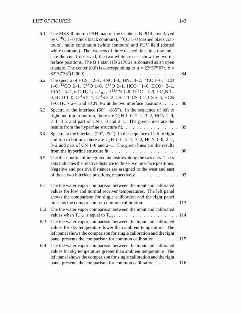
LIST OF FIGURES 143
6.1 The MSX 8 micron PAH map of the Cepheus B PDRs overlayedby C18O 1–0 (thick black contours),12CO 1–0 (dashed black con-tours), radio continuum (white contours) and FUV field (dottedwhite contours). The two sets of three dashed lines in a raw indi-cate the cuts I observed; the two white crosses show the two in-terface positions. The B 1 star, HD 217061 is donated as an opentriangle. The center (0,0) is corresponding toα = 22h57m07s, δ =6237′33′′(J2000). . . . . . . . . . . . . . . . . . . . . . . . . . . 84
6.2 The spectra of HCS+ 2–1, HNC 1–0, HNC 3–2,12CO 1–0,13CO1–0, 13CO 2–1, C18O 1–0, C18O 2–1, HCO+ 1–0, HCO+ 2–1,HCO+ 3–2, c-C3H2 21,2–10,1, H13CN 1–0, H13C+ 1–0, HC3N 1–0, HCO 1–0, C34S 2–1, C34S 3–2, CS 2–1, CS 3–2, CS 5–4, HCN1–0, HCN 2–1 and HCN 3–2 at the two interface positions. . . . . 86
6.3 Spectra at the interface (60′′, -185′′). In the sequence of left toright and top to bottom, there are C2H 1–0, 2–1, 3–2, HCN 1–0,2–1, 3–2 and part of CN 1–0 and 2–1. The green lines are theresults from the hyperfine structure fit. . . . . . . . . . . . . . . . 89
6.4 Spectra at the interface (20′′, -50′′). In the sequence of left to rightand top to bottom, there are C2H 1–0, 2–1, 3–2, HCN 1–0, 2–1,3–2 and part of CN 1–0 and 2–1. The green lines are the resultsfrom the hyperfine structure fit. . . . . . . . . . . . . . . . . . . . 90
6.5 The distribution of integrated intensities along the two cuts. The xaxis indicates the relative distance to those two interfacepositions.Negative and positive distances are assigned to the west andeastof those two interface positions, respectively. . . . . . . . . .. . 92
B.1 The the water vapor comparison between the input and calibratedvalues for low and normal receiver temperatures. The left panelshows the comparison for single calibration and the right panelpresents the comparison for common calibration. . . . . . . . . .113
B.2 The the water vapor comparison between the input and calibratedvalues when Tamb is equal to Tsky. . . . . . . . . . . . . . . . . . 114
B.3 The the water vapor comparison between the input and calibratedvalues for sky temperature lower than ambient temperature.Theleft panel shows the comparison for single calibration and the rightpanel presents the comparison for common calibration. . . . .. . 115
B.4 The the water vapor comparison between the input and calibratedvalues for sky temperature greater than ambient temperature. Theleft panel shows the comparison for single calibration and the rightpanel presents the comparison for common calibration. . . . .. . 116

144 LIST OF FIGURES
B.5 The water vapor comparison between the Hiyama and the newcalibration methods. The drawn lines are where the two methodsgive the same water vapor. . . . . . . . . . . . . . . . . . . . . . 117
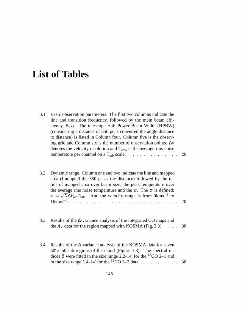
List of Tables
3.1 Basic observation parameters. The first two columns indicate theline and transition frequency, followed by the main beam effi-ciency, Be f f. The telescope Half Power Beam Width (HPBW)(considering a distance of 350 pc, I converted the angle distanceto distance) is listed in Column four. Column five is the observ-ing grid and Column six is the number of observation points.∆vdenotes the velocity resolution and Trms is the average rms noisetemperature per channel on a Tmb scale. . . . . . . . . . . . . . . 20
3.2 Dynamic range. Column one and two indicate the line and mappedarea (I adopted the 350 pc as the distance) followed by the ra-tios of mapped area over beam size, the peak temperature overthe average rms noise temperature and theσ . Theσ is defined:σ =
√N∆VresTrms. And the velocity range is from 0kms−1 to
16kms−1. . . . . . . . . . . . . . . . . . . . . . . . . . . . . . . 20
3.3 Results of the∆-variance analysis of the integrated CO maps andtheAV data for the region mapped with KOSMA (Fig. 3.3). . . . 30
3.4 Results of the∆-variance analysis of the KOSMA data for seven50′× 50′sub-regions of the cloud (Figure 3.3). The spectral in-dicesβ were fitted in the size range 2.2-14′ for the13CO 2–1 andin the size range 1.4-14′ for the12CO 3–2 data. . . . . . . . . . . 30
145

146 LIST OF TABLES
4.1 Comparison of the masses of clump identified in the Perseus cloudwith studies of other molecular clouds. The cloud name, studiedtracers, distance, and the HPBW are listed in Column (1), (2), (3)and (4); Column (5) presents the number of selected clumps; Themass range used for the least-squares fit is in Column (6). Col-umn (7) and (8) present the total mass of all clumps selected andthe minimum mass identified with the criteria of Equation 1.4;The fitted power law indexα is given in Column (9) (note that Iadopt the power law index for a bin size of 100.2 M for compar-ison); Column (10) is the reference:a This work; b Kramer et al.(1998b);c Simon et al. (2001). . . . . . . . . . . . . . . . . . . . 44
4.2 The results of the seven sub-regions. The cloud name is listed inColumn (1); Column (2) presents the number of selected clumps;The mass range used for the least-squares fit is in Column (3).Column (4) and (5) present the total mass of all clumps selectedand the minimum mass identified with the criteria of Equation1.4;The fitted power law indexα is given in Column (6). . . . . . . . 46
5.1 The observed integrated line intensities (in erg s−1 sr−1 cm−2) andline ratios at the seven selected positions. The errors on the inte-grated intensity are estimated to be∼ 15%. . . . . . . . . . . . . 62
5.2 Results of the LTE analysis. The excitation temperatureTex islisted in Column (2); Column (3) - (5) present C, CO and H2
column densities; the C/CO ratio is listed in Column (6). Theuncertainties of the column densities are derived by varying theintegrated intensities by±15%. . . . . . . . . . . . . . . . . . . . 65
5.3 Physical parameters at selected positions in Fig 5.1, obtained byfitting the observed intensity ratios to thesingle clumpKOSMA- τ PDR models. Columns (2) - (5) list the fitted clump densities,clump mass, clump radius and FUV field; the derived FUV fieldfrom the HIRES data and from the star are are in Column (6) and(7); The distance to HD 281159 used for the calculation ofχstarislisted in Column (8); Column (9) is the minimum chi square ofthe PDR fit. . . . . . . . . . . . . . . . . . . . . . . . . . . . . . 71
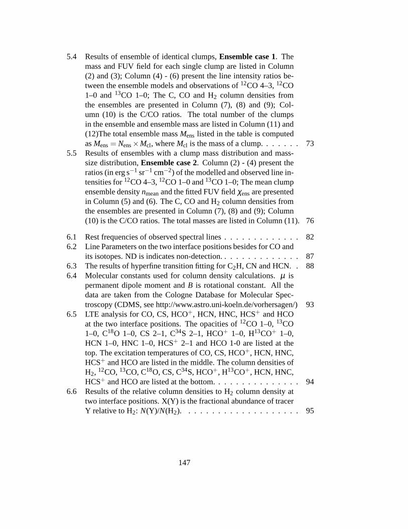
5.4 Results of ensemble of identical clumps,Ensemble case 1. Themass and FUV field for each single clump are listed in Column(2) and (3); Column (4) - (6) present the line intensity ratios be-tween the ensemble models and observations of12CO 4–3,12CO1–0 and13CO 1–0; The C, CO and H2 column densities fromthe ensembles are presented in Column (7), (8) and (9); Col-umn (10) is the C/CO ratios. The total number of the clumpsin the ensemble and ensemble mass are listed in Column (11) and(12)The total ensemble massMens listed in the table is computedasMens= Nens×Mcl, whereMcl is the mass of a clump. . . . . . . 73
5.5 Results of ensembles with a clump mass distribution and mass-size distribution,Ensemble case 2. Column (2) - (4) present theratios (in erg s−1 sr−1 cm−2) of the modelled and observed line in-tensities for12CO 4–3,12CO 1–0 and13CO 1–0; The mean clumpensemble densitynmeanand the fitted FUV fieldχensare presentedin Column (5) and (6). The C, CO and H2 column densities fromthe ensembles are presented in Column (7), (8) and (9); Column(10) is the C/CO ratios. The total masses are listed in Column(11). 76
6.1 Rest frequencies of observed spectral lines . . . . . . . . . .. . . 826.2 Line Parameters on the two interface positions besides for CO and
its isotopes. ND is indicates non-detection. . . . . . . . . . . . .. 876.3 The results of hyperfine transition fitting for C2H, CN and HCN. . 886.4 Molecular constants used for column density calculations. µ is
permanent dipole moment andB is rotational constant. All thedata are taken from the Cologne Database for Molecular Spec-troscopy (CDMS, see http://www.astro.uni-koeln.de/vorhersagen/) 93
6.5 LTE analysis for CO, CS, HCO+, HCN, HNC, HCS+ and HCOat the two interface positions. The opacities of12CO 1–0,13CO1–0, C18O 1–0, CS 2–1, C34S 2–1, HCO+ 1–0, H13CO+ 1–0,HCN 1–0, HNC 1–0, HCS+ 2–1 and HCO 1-0 are listed at thetop. The excitation temperatures of CO, CS, HCO+, HCN, HNC,HCS+ and HCO are listed in the middle. The column densities ofH2, 12CO,13CO, C18O, CS, C34S, HCO+, H13CO+, HCN, HNC,HCS+ and HCO are listed at the bottom. . . . . . . . . . . . . . . 94
6.6 Results of the relative column densities to H2 column density attwo interface positions. X(Y) is the fractional abundance of tracerY relative to H2: N(Y)/N(H2). . . . . . . . . . . . . . . . . . . . 95
147
Acknowledgments
Foremost, my deepest gratitude goes first to my advisors Prof. Jurgen Stutzki andCarsten Kramer for their constant encouragement and advise. I am very gratefulfor their patience, enthusiasm, and immense knowledge in astrophysics. They arealways willing to answer my questions. Their penetrating and insightful com-ments afford me with inspiring source. I also thank their suggestions and cor-rections on this thesis. Without their consistent and illuminating instruction, thisthesis could not have reached its present form.
I also like to thank Prof. Andreas Zilges for co-refereeing this thesis.I would also like to extend my sincere thanks to all members inA1 and A6
groups of SFB 494 from I. Physikalisches Institut for providing a very friendlyand inspiring working atmosphere. I specially thank MartinMiller for helping meadapt to a new country. It would be much harder without his help on all thosethings like opening a bank account, first-time registrationin the university and soon. I thank him for introducing me to get familiar with the KOSMA 3m telescopeobservations. I also thank him and his wife for providing me aplace to stay at thebeginning of my study in Koln.
I thank Bhaswati Mookerjea who not only gave me the fruitful scientific dis-cussions on the PDR analysis in IC 348, but also passed me her tips on living inGermany. I also thank Volker Ossenkopf for helping me with the ∆-variance andPDR analysis and also for letting me using his IDL codes for the∆-variance anal-ysis. I am greatly indebted to him for those very useful and inspiring discussions.I appreciate the help from Markus Rollig on the PDR analysis. I also thank FrankBensch for his great help on the∆-variance analysis and for letting me use hisFortran codes on the∆-variance analysis. Once more, I thank all those people Ihave mentioned for their great and patient help on the language corrections of thepublished papers.
I am indebted to Robert Simon for his great help on using GILDAS software.He is such an expert on GILDAS. Whenever I encountered the difficulties on datareduction, he is always the first one I would ask for help and tips. I would likealso to thank Nikolaus Volgenau for his patience with my English. I thank MartinaWiedner for her help, as it is very nice to chat with someone who can speak a little
148

Chinese.I also thank Marc Hitschfeld, Martin Emprechtinger, MarkusCubick and Oliver
Baum for their help and chats and for their skills in spreading happiness. I reallyappreciate their help with my German translations, especially Marc’s. BecauseI often bothered him with my German letters, and with asking him to help mecontact with people who only speak German. I thank Holger Jakob and MartinBrull for their help on the data reduction. Some of the startup scripts I used arefrom them. I also appreciate the help from Bettina Krause, Stefanie Kramer andMarlies Selt.
I also thank those Japanese colleagues for their supports during my NANTEN2observations. I thank the staff at the IRAM 30m telescope fortheir support duringmy observations. I really like the environment at the 30m telescope, especially thefood there.
I am very grateful to helpful discussions with Alex Lazarianand Doug John-stone on the∆-variance analysis. I also thank Joao Alves for providing usthe2MASS extinction data. I thank Naomi Ridge for allowing us touse the FCRAOlow-J CO data in IC 348. I thank Hans Ungerechts for letting me use the low-JCO data in Cepheus B. In this work, I used the NASA/IPAC/IRAS/HIRES datareduction facilities.
I thank to all the friends I made in Koln for giving me the opportunity to spenda great time during my PhD study. I am grateful to my parents for their supportduring all these years. They always have faith in me. I also thank Jiayu for herpatience and encouragement since we met during our undergraduate studies.
I acknowledge the financial support from the grant SFB494 of the DeutscheForschungsgemeinschaft during my PhD study.
149

Erkl arung
Ich versichere, dass ich die von mir vorgelegte Dissertation selbstandig angefer-tigt, die benutzten Quellen und Hilfsmittel vollstandig angegeben und die Stellender Arbeit einschlieslich Tabellen, Karten und Abbildungen, die anderen Werkenim Wortlaut oder dem Sinn nach entnommen sind, in jedem Einzelfall als Entlehnungkenntlich gemacht habe; dass diese Dissertation noch keiner anderen Fakultat oderUniversitat zur Prufung vorgelegen hat; dass sie abgesehen von unten angegebe-nen Teilpublikationen noch nicht ver”offentlicht worden ist sowie, dass ich einesolche Veroffentlichung vor Abschluss des Promotionsverfahrens nicht vornehmenwerde. Die Bestimmungen der Promotionsordnung sind mir bekannt. Die von mirvorgelegte Dissertation ist von Herrn Prof. Dr. Jurgen Stutzki betreut worden.
150

Publications
[1.] K. Sun, V. Ossenkopf, C. Kramer, B. Mookerjea, M. Rollig, M. Cubick, M.,and J. Stutzki, J.,The Photon Dominated Region in the IC 348 molecular cloud,2008, accepted by Astronomy & Astrophysics[2.] J.L. Pineda N. Mizuno, J. Stutzki, M. Cubick, et al.Submillimeter line emis-sion from LMC N159W: a dense and clumpy PDR in a low metallicity environ-ment, 2008, accepted by Astronomy & Astrophysics, (arXiv:0802.1929)[3.]M. Hitschfeld, M. Aravena, C. Kramer, F. Bertoldi, et al., CO 4–3 and [C I]1–0 in the centers of NGC4945 and Circinus, 2008, Astronomy & Astrophysics,in press, (arXiv:0712.1924)[4.] C. Kramer, M. Cubick, M. Rollig, K. Sun, K., et al.,Photon-dominatedregions in the Carina nebula. I. Maps of atomic carbon and mid-J CO lines withNANTEN2, 2008, Astronomy & Astrophysics, 477, 547[5.] K. Sun, C. Kramer, V. Ossenkopf, F. Bensch, J. Stutzki, and M. Miller, AKOSMA 7 deg2 13CO 2–1 and12CO 3–2 survey of the Perseus cloud I. Structureanalysis, 2006, Astronomy & Astrophysics, 451, 539[6.] Y. Wu, Q. Zhang, W. Yu, M. Miller, R. Mao, K. Sun, and Y. Wang, Ammoniacores in high mass star formation regions, 2006, Astronomy & Astrophysics, 450,607[7.] K. Sun, J. Yang, S. Luo, M. Wang, L. Deng, X. Zhou, and J. Chen,Large-Scale Distribution of Herbig-Haro Objects in Taurus, 2003, Chinese Journal ofAstronomy and Astrophysics, 3, 458[8.] K. Sun, Y. Wu, and L. Wang,High-velocity Gas near S106, 2003, ActaAstronomica Sinica, 44, 94[9.] K. Sun, and Y. Wu,A new high-velocity molecular outflow of IRAS 19282+1814,2003, Chinese Astronomy and Astrophysics, 27, 73
151

Lebenslauf
Name : Kefeng SunAnschrift : Bachemer str. 46
50931 KolnGeburtsdatum : 19.03.1978Geburtsort : Wuxi, Jiangsu, ChinaStaatsangehorigkeit : ChinesischEMail : [email protected]
Schule09. 1984 - 07. 1990 Luoshe-Zentral-Grundschule der Stadt Wuxi, Jiangsu, China09. 1990 - 07. 1993 Luoshe-Mittelschule der Stadt Wuxi, Jiangsu, China09. 1993 - 07. 1996 Obere Mittelschule Tianyi, Wuxi, Jiangsu, China
Universitat09. 1996 - 07. 2000 Peking Universitat, Beijing, China
Bachelor of Science, Astrophysik09. 2000 - 07. 2003 Peking Universitat, Beijing, China
Master of Science, Astrophysik01. 2004 I. Physikalisches Institut, Universitat zu Koln, Deutschland
Beginn der Dissertation
Berufserfahrung09. 2001 - 07. 2003 Wissenschaftliche Hilfskraft, Peking Universitat
Beijing, China10. 2001 - 11. 2001 Gastwissenschaftler, Purple Mountain Observatory
Nanjing, China02. 2002 - 07. 2002 Tutor fur Thermodynamics, Peking Universitat, Beijing, China09. 2003 - 11. 2003 Gastwissenschaftler, I. PhysikalischesInstitut
Universitat zu Koln, Deutschlandseit 01. 2004 Wissenschaftlicher Mitarbeiter, I. Physikalisches Institut
Universitat zu Koln, Deutschland
152

153