Structural Change in a Multi-Sector Model of

Growth∗

L Rachel Ngai

Centre for Economic Performance

London School of Economics

Christopher A Pissarides

Centre for Economic Performance

London School of Economics, CEPR and IZA

November 2004

Abstract

We study a multi-sector model of growth with differences in TFP growth

rates across sectors and derive sufficient conditions for the coexistence of struc-

tural change, characterized by sectoral labor reallocation, and constant ag-

gregate growth path. The conditions are weak restrictions on the utility and

production functions commonly applied by macroeconomists. We present evi-

dence from US two-digit industries that is consistent with our predictions about

structural change and successfully calibrate the historical shift from agriculture

to manufacturing and services. We show quantitatively that reasonable devi-

ations from our conditions do not have a big impact on the properties of the

model.

∗This paper previously circulated under the title "Balanced Growth with Structural Change" andpresented at the CEPR ESSIM 2004 meetings, the SED 2004 annual conference, the NBER 2004Summer Institute, the 2004 Canadian Macroeconomic Study Group and elsewhere. The presentversion has benefited from comments received at these meetings and from the comments and discus-sions that we have had with Francesco Caselli, Nobu Kiyotaki, Nick Oulton and Jaume Ventura (ourdiscussant at ESSIM). Evangelia Vourvachaki worked for us as research assistant. Funding from theCEP, a designated ESRC Research Centre, is gratefully acknowledged.

1

JEL Classification: O41, O14

Keywords: multi-sector growth, structural change, unbalanced growth, bal-

anced growth, sectoral employment.

1 Introduction

Economic growth takes place at uneven rates across different sectors of the economy.

This paper has two objectives related to this fact, (a) to derive the implications of

uneven sectoral growth for structural change, the name given to the shifts in industrial

employment shares that take place over long periods of time, and (b) to show that

even with different sectoral rates of total factor productivity growth, there can still be

growth at constant or near-constant rate in the aggregate economy. The restrictions

needed to yield structural change consistent with the facts and constant growth are

weak restrictions on functional forms that are frequently imposed by economists in

related contexts.

Pioneering work on the connections between growth and structural change was

done by Baumol (1967; Baumol et al., 1985). Baumol divided the economy into two

sectors, a “progressive” one that uses capital and new technology and grows at some

constant rate and a “stagnant” one that uses labor as the only input and produces

services as final output (as for example in the arts or the legal profession). He then

claimed that because of factor mobility, the production costs and prices of the stagnant

sector should rise indefinitely, a process known as “Baumol’s cost disease.” Over time,

the stagnant sector should attract more labor to satisfy demand if demand is either

income elastic or price inelastic, but should vanish otherwise. Baumol controversially

also claimed that if the stagnant sector does not vanish, the economy’s growth rate

will be on a declining trend, as more weight is shifted to the stagnant sector.

We confirm Baumol’s claim about structural change but also show that his con-

clusion about growth was overly pessimistic. Although costs rise and resources shift

into low-growth sectors during structural change, the growth rate of the aggregate

economy is bounded from below by a positive rate that depends on the growth rate of

Baumol’s progressive sector.1 Our economy satisfies Kaldor’s stylized facts of constant

1Ironically, we get our result because we include capital in our analysis, a factor left out of theanalysis by Baumol “for ease of exposition ... that is [in]essential to the argument”. We show thatthe inclusion of capital is essential for the more optimistic growth results, though not for structuralchange.

2

capital-output ratio, even before it gets to the limiting state of no further structural

change.

We obtain our results in a baseline model by assuming that capital goods are

supplied by only one sector, which we label manufacturing, and which produces also

a consumption good. We show, however, that they are consistent with the existence

of many capital goods and many intermediate goods under some reasonable restric-

tions. Production functions in our model are identical in all sectors except for their

rates of TFP growth and each sector produces a differentiated good that enters a

constant elasticity of substitution (CES) utility function. We show that a low (below

one) elasticity of substitution across goods leads to shifts of employment shares to

sectors with low TFP growth. In the limit the employment share used to produce

consumption goods vanishes from all sectors except for the slowest-growing one, but

the employment shares used to produce the capital good in manufacturing and any

intermediate goods in other sectors converge to non-trivial stationary values.

At the aggregate level our economy exhibits constant or near-constant growth. If

the utility function has unit inter-temporal elasticity of substitution, during structural

change the capital-output ratio is constant and the aggregate economy is on a steady-

state growth path.2 We calibrate the dynamic model when the intertemporal elasticity

is not unity and find that with reasonable values the aggregate growth rate converges

much faster to its steady state value than do the employment shares. Consequently,

even without unit intertemporal elasticity, the economy exhibits nontrivial structural

change and near-constant aggregate growth over long periods of time.

Our results contrast with the results of Echevarria (1997), who assumed non-

homothetic preferences to derive structural change from different rates of sectoral

TFP growth. In her economy balanced aggregate growth exists only in the limit,

when preferences reduce to homotheticity with unit elasticity of substitution and

structural change ceases. In the transition to the limiting state the aggregate growth

rate first rises and then falls, in contrast to ours, which is either constant or con-

verges fast. Our results also contrast with the results of Kongsamut et al. (2001)

and Foellmi and Zweimuller (2002), who derive simultaneously constant aggregate

growth and structural change. Kongsamut et al. obtain their results by imposing a

2In contrast to one-sector models, a constant capital-output ratio in our model does not implythat the rate of return to capital in consumption units is constant. It may be constant, decreasingor increasing over time. Under our set of restrictions it is mildly decreasing during structural changeand converging to a lower bound.

3

restriction that maps some of the parameters of their Stone-Geary utility function

on to the parameters of the production functions, violating one of the most useful

conventions of modern macroeconomics, the complete independence of preferences

and technologies. Foellmi and Zweimuller (2002) obtain their results by assuming

endogenous growth driven by the introduction of new goods into a hierarchic utility

function. Our restrictions are quantitative restrictions on a conventional CES util-

ity function that maintains the independence of the parameters of preferences and

technologies.

In the empirical literature two competing explanations (which can coexist) have

been put forward for structural change. Our explanation, which is sometimes termed

“technological” because it attributes structural change to different rates of sectoral

TFP growth, and a utility-based explanation, which requires different income elastic-

ities for different goods and can yield structural change even with equal TFP growth

in all sectors.3 Kravis et al. (1983) present evidence that favours the technological

explanation, at least when the comparison is between manufacturing and services.

Two features of their data that are satisfied by the technological explanation are

(a) relative prices reflect differences in TFP growth rates and (b) real consumption

shares are fairly constant. Our model has both these implications provided there is

low substitutability in the CES utility function across goods. We use multi-sector

data for the United States for the post-war period to show that changes in employ-

ment shares and prices are also consistent with our model’s predictions under the

same low substitutability requirement. Under low substitutability our model is also

consistent with the historical OECD evidence presented by Kuznets (1966) and Mad-

dison (1980), which shows a falling share of agriculture, a rising share of services and

a hump-shaped share of manufacturing. In a quantitative exercise with the model’s

equations we evaluate the model’s performance in the explanation for the long-run

shifts between agriculture, manufacturing and services in the United States. We

show that the model tracks the trends well, although it predicts a slower decline of

agriculture than is observed in the data. This leads us to conclude that although

for manufacturing and services the technological explanation may be sufficient to ex-

plain structural change, the explanation for the fast decline of agriculture may require

something additional, such as a below-unity income elasticity.

Section 2 describes our model of growth with many sectors and sections 3 and 4

3Some other explanations have also been forward to explain, in particular, the fast decline ofagricultural employment. See section 8 for more discussion of this topic and some references.

4

respectively derive the conditions for structural change and the conditions for bal-

anced aggregate growth equilibrium. In sections 5 and 6 we study two extensions

of our benchmark model, one where there are many capital goods and one where

consumption goods can also be used as intermediate inputs. In section 7 we show

evidence from two-digit US industries for 1977-2001 that supports our results. In sec-

tion 8 we focus on the long-run structural change between manufacturing, agriculture

and services and show both analytically and with computations that our predictions

match reasonably well the experience of the United States.

2 An economy with many sectors

The benchmark economy consists of an arbitrary number of m sectors. Sectors i =

1, ...,m − 1 produce only consumption goods. The last sector, which is denoted

by m and labeled manufacturing, produces both a final consumption good and the

economy’s capital stock. Manufacturing is the numeraire.4

We derive the equilibrium as the solution to a social planning problem. The

objective function is

U =

Z ∞

0

e−ρtv (c1, .., cm) dt, (1)

where ρ > 0, ci ≥ 0 are per-capita consumption levels and the instantaneous utilityfunction v (.) is concave and satisfies the Inada conditions. The constraints of the

problem are as follows.

The labor force is exogenous and growing at rate ν and the aggregate capital stock

is endogenous and defines the state of the economy. Sectoral allocations are controls

that satisfymPi=1

ni = 1;mPi=1

niki = k, (2)

where ni ≥ 0 is the employment share of sector i, ki ≥ 0 is the capital-labor ratioin sector i and k ≥ 0 is the aggregate capital-labor ratio. Mobility costs are zero forboth factors.

4The label manufacturing is used for convenience. Although in the standard industrial classi-fications our capital-goods producing sector belongs to manufacturing, some sectors classified asmanufacturing in the data (e.g. food and clothing) fall into the consumption category of our model.See below for more discussion of the empirical interpretation of our model.

5

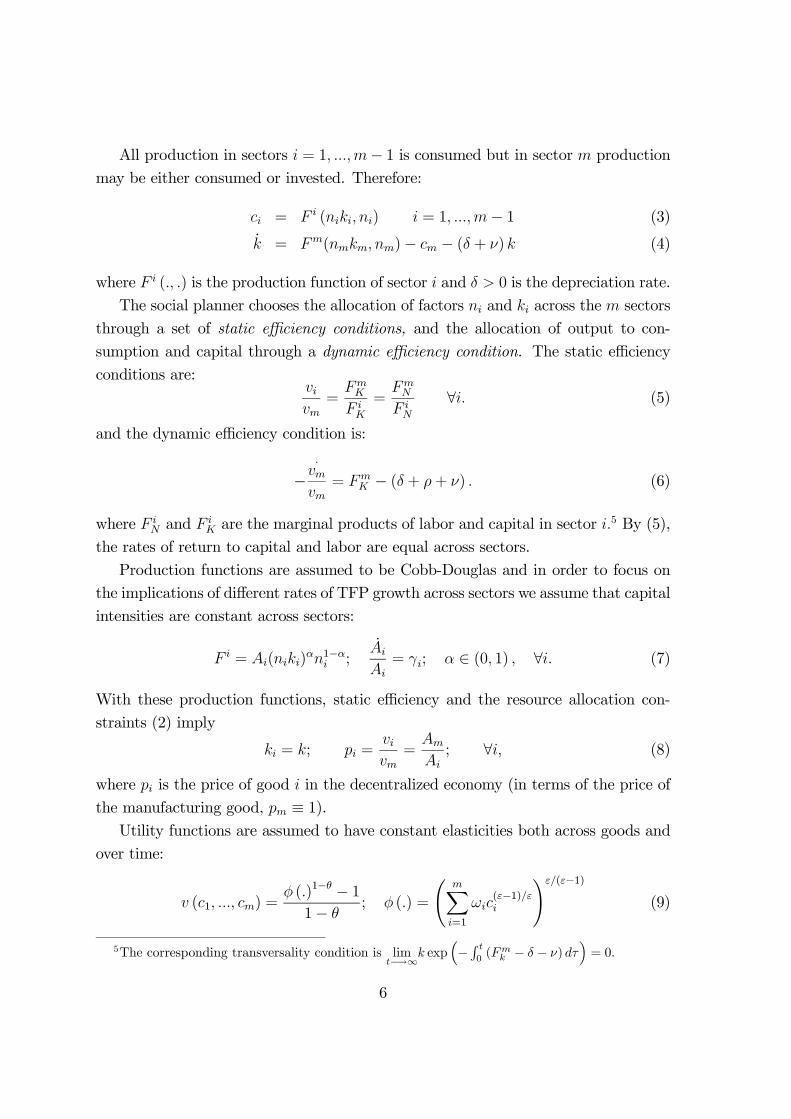
All production in sectors i = 1, ...,m− 1 is consumed but in sector m production

may be either consumed or invested. Therefore:

ci = F i (niki, ni) i = 1, ...,m− 1 (3)

k = Fm(nmkm, nm)− cm − (δ + ν) k (4)

where F i (., .) is the production function of sector i and δ > 0 is the depreciation rate.

The social planner chooses the allocation of factors ni and ki across the m sectors

through a set of static efficiency conditions, and the allocation of output to con-

sumption and capital through a dynamic efficiency condition. The static efficiency

conditions are:vivm

=FmK

F iK

=FmN

F iN

∀i. (5)

and the dynamic efficiency condition is:

−·vmvm

= FmK − (δ + ρ+ ν) . (6)

where F iN and F

iK are the marginal products of labor and capital in sector i.

5 By (5),

the rates of return to capital and labor are equal across sectors.

Production functions are assumed to be Cobb-Douglas and in order to focus on

the implications of different rates of TFP growth across sectors we assume that capital

intensities are constant across sectors:

F i = Ai(niki)αn1−αi ;

Ai

Ai= γi; α ∈ (0, 1) , ∀i. (7)

With these production functions, static efficiency and the resource allocation con-

straints (2) imply

ki = k; pi =vivm

=Am

Ai; ∀i, (8)

where pi is the price of good i in the decentralized economy (in terms of the price of

the manufacturing good, pm ≡ 1).Utility functions are assumed to have constant elasticities both across goods and

over time:

v (c1, ..., cm) =φ (.)1−θ − 11− θ

; φ (.) =

ÃmXi=1

ωic(ε−1)/εi

!ε/(ε−1)

(9)

5The corresponding transversality condition is limt−→∞k exp

³− R t

0(Fm

k − δ − ν) dτ´= 0.

6

where θ, ε, ωi > 0 andPm

i=1 ωi = 1. Of course, if θ = 1, v(.) = lnφ(.) and if ε = 1,

lnφ(.) =Pm

i=1 ωi ln ci. The utility function is strictly concave and satisfies the Inada

conditions,6 so if prices are finite there is a non-trivial demand for all consumption

goods. In the decentralized economy demand functions have constant price elasticity

−ε and unit income elasticity.With the iso-elastic utility function, equation (8) yields:

picicm

=

µωi

ωm

¶εµAm

Ai

¶1−ε≡ xi ∀i. (10)

The new variable xi is the ratio of consumption expenditure on good i to consumption

expenditure on the manufacturing good. We also define consumption expenditure and

output per capita in terms of the numeraire:

c ≡mXi=1

pici; y ≡mXi=1

piFi (11)

Following these definitions, and using static efficiency, we can rewrite per capita

consumption and output as:

c = cmX; y = Amkα (12)

where X ≡Pmi=1 xi.We note that although k is the ratio of the economy-wide capital

stock to the labor force, the technology parameter for output is TFP in manufacturing

and not an average of all sectors’ TFP.

3 Structural change

We define structural change as the state in which at least some of the labor shares

change over time, i.e., ni 6= 0 for at least some i.We derive in Appendix 1 (Lemma 6) the time path of employment shares. For

the consumption goods sectors, the employment shares satisfy:

ni =xiX

µc

y

¶i = 1, ..m− 1, (13)

and for the capital-producing sector:

nm =xmX

µc

y

¶+

µ1− c

y

¶. (14)

6Note that although φ (.) does not satisfy the Inada conditions, the utility function v (.) doessatisfy them.

7

The first term in the right side of (14) parallels the term in (13) and so represents the

employment needed to satisfy the consumption demand for manufacturing goods. The

second bracketed term is equal to the savings rate and represents the manufacturing

employment needed to satisfy investment demand.

Condition (13) implies that the ratio of employment in sector i to employment in

sector j is equal to the ratio xi/xj (for i, j 6= m). By differentiation we obtain that

the growth rate of relative employment depends only on the difference between the

sectors’ TFP growth rates and the elasticity of substitution between goods:

nini− nj

nj= (1− ε)

¡γj − γi

¢ ∀i, j 6= m. (15)

But (8) implies that the growth rate of the relative price of good i is:

pipi= γm − γi i = 1, ...,m− 1 (16)

and so,nini− nj

nj= (1− ε)

µpipi− pj

pj

¶∀i, j 6= m (17)

Proposition 1 The rate of change of the relative price of good i to good j is equal

to the difference between the TFP growth rates of sector j and sector i. In sectors

producing only consumption goods, relative employment shares grow in proportion to

relative prices, with the factor of proportionality given by one minus the elasticity of

substitution across goods.7

The dynamics of the individual employment shares satisfy:

nini

=

·c/y

c/y+ (1− ε) (γ − γi) ; i = 1, ...m− 1 (18)

nmnm

=

·c/y

c/y+ (1− ε) (γ − γm)

(c/y) (xm/X)nm

+

·(1− c/y)

(1− c/y)

µ1− c/y

nm

¶(19)

where γ ≡Pmi=1 (xi/X) γi is the weighted average of TFP growth rates.

Equation (18) gives the growth rate in the employment share of each consumption

sector as a linear function of its own TFP growth rate. The intercept and slope of this

function are common across sectors but although the slope is a constant, the intercept

7All derivations and proofs, unless trivial, are collected in Appendix 1.

8

is in general a function of time because both c/y and γ are in general functions of

time. Manufacturing, however, does not conform to this rule, because its employment

share is made up of two components, one for the production of the consumption good

(which behaves similarly to the employment share of consumption sectors) and one

for the production of capital goods, which behaves differently. These are key results

about structural change which are compared with US data in section 7.

The properties of structural change follow immediately from (18) and (19). Con-

sider first the case of equality in sectoral TFP growth rates, i.e., let γi = γm ∀i. Oureconomy in this case is one of balanced TFP growth, with relative prices remaining

constant but with many differentiated goods. Because of the constancy of relative

prices all consumption goods can be aggregated into one, so we effectively have a two-

sector economy, one sector producing consumption goods and one producing capital

goods. Structural change can still take place in this economy but only between the

aggregate of the consumption sectors and the capital sector, and only if c/y changes

over time. If c/y is increasing over time, the savings and investment rate are falling

and labor is moving out of the manufacturing sector and into the consumption sectors.

Conversely, if c/y is falling over time labor is moving out of the consumption sectors

and into manufacturing. In both cases, however, the relative employment shares in

consumption sectors are constant.

If c/y is constant over time, structural change requires ε 6= 1 and different ratesof sectoral TFP growth rates. It follows immediately from (16), (18) and (19) that

if c/y = 0, ε = 1 implies constant employment shares but changing prices. With

constant employment shares faster-growing sectors produce relatively more output

over time. Price changes in this case are such that consumption demands exactly

absorb all the output changes that are due to the higher TFP growth rates. But if

ε 6= 1, prices still change as before and consumption demands are either too inelastic(in the case ε < 1) to absorb all the output change, or are too elastic (ε > 1)

to be satisfied merely by the increase in output due to TFP growth. So if ε < 1

employment has to move into the slow-growing sectors and if ε > 1 it has to move

into the fast-growing sectors.

Proposition 2 If γi = γm ∀i = 1, ...,m− 1, a necessary and sufficient condition forstructural change is c/c 6= y/y. The structural change in this case is between the ag-

gregate of consumption sectors and the manufacturing sector. If c/c = y/y, necessary

and sufficient conditions for structural change are ε 6= 1 and ∃i ∈ {1, ..,m− 1} s.t.

γi 6= γm. The structural change in this case is between all sector pairs with different

9

TFP growth rates.

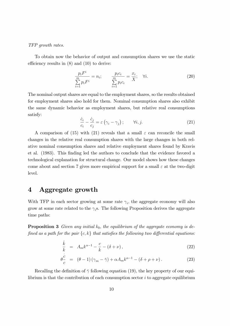
To obtain now the behavior of output and consumption shares we use the static

efficiency results in (8) and (10) to derive:

piFi

mPi=1

piF i

= ni;pici

mPi=1

pici

=xiX; ∀i. (20)

The nominal output shares are equal to the employment shares, so the results obtained

for employment shares also hold for them. Nominal consumption shares also exhibit

the same dynamic behavior as employment shares, but relative real consumptions

satisfy:cici− cj

cj= ε

¡γi − γj

¢; ∀i, j. (21)

A comparison of (15) with (21) reveals that a small ε can reconcile the small

changes in the relative real consumption shares with the large changes in both rel-

ative nominal consumption shares and relative employment shares found by Kravis

et al. (1983). This finding led the authors to conclude that the evidence favored a

technological explanation for structural change. Our model shows how these changes

come about and section 7 gives more empirical support for a small ε at the two-digit

level.

4 Aggregate growth

With TFP in each sector growing at some rate γi, the aggregate economy will also

grow at some rate related to the γis. The following Proposition derives the aggregate

time paths:

Proposition 3 Given any initial k0, the equilibrium of the aggregate economy is de-fined as a path for the pair {c, k} that satisfies the following two differential equations:

k

k= Amk

α−1 − c

k− (δ + ν) , (22)

θ

·c

c= (θ − 1) (γm − γ) + αAmk

α−1 − (δ + ρ+ ν) . (23)

Recalling the definition of γ following equation (19), the key property of our equi-

librium is that the contribution of each consumption sector i to aggregate equilibrium

10

is through its weight xi in γ. Note that because each xi depends on the sector’s relative

TFP level (Ai/Am), the weights here are functions of time.

We characterize the aggregate equilibrium by investigating whether there is an

equilibrium path that satisfies Kaldor’s fact of constant capital-output ratio k/y.

From the aggregation in (12) constant k/y requires Amkα−1 to be constant, i.e., k

to grow at rate γm/(1 − α). The state equation (22) implies that c/k must also be

a constant, so in this steady state, if it exists, aggregate output and consumption

grow at the same rate as the capital-labor ratio with all aggregates defined in units of

the manufacturing numeraire. We define this steady state as the aggregate balanced

growth path.

We note that if all the γs are equal, relative prices are constant and the economy’s

average TFP growth rate is also the common γ. Our definition of aggregate consump-

tion and output then correspond to the conventional definitions of real consumption

and output, and our dynamic equations in Proposition 3 reduce to the conventional

dynamic equations of the one-sector Ramsey economy. Given our results in Propo-

sition 2, structural change takes place in the transition to the steady state of this

economy, when c/y is changing, but not on the aggregate balanced growth path.

The more interesting case arises when at least some of the γs are different. In

this case relative prices change and our definition of aggregate output and consump-

tion are different from the conventional definitions, because they are deflated by the

manufacturing price and not by an average of all prices. However, we can still talk

of a aggregate balanced growth path defined as the state consistent with a constant

capital-output ratio. We established in the preceding paragraph that on this path

c/y is constant and so, by Proposition 2, structural change requires, in addition to

the different γs, ε 6= 1.We now investigate whether such a aggregate balanced growthpath exists.

It follows trivially from (23) that a necessary condition for a aggregate balanced

growth path is that the expression (θ − 1) (γm − γ) be a constant. Let for now:

(θ − 1)(γm − γ) ≡ ψ constant. (24)

Define aggregate consumption and the aggregate capital-labor ratio in terms of

efficiency units

ce ≡ cA−1/(1−α)m ; ke ≡ kA−1/(1−α)m .

11

The dynamic equations become

cece

=αkα−1e − (δ + ν + ρ) + ψ

θ− γm1− α

(25)

keke

= kα−1e − ceke−µ

γm1− α

+ δ + ν

¶. (26)

Equations (25) and (26) parallel the two differential equations in the control and

state of the one-sector Ramsey model, making the aggregate equilibrium of our many-

sector economy identical to the equilibrium of the one-sector Ramsey economy (when

ψ = 0) and trivially different from it otherwise. Both models have a saddlepath

equilibrium and stationary solutions³ce, ke

´that imply balanced growth in the three

aggregates. As anticipated in the aggregate production function (12), a key result

is that in our economy the rate of growth of our aggregates in the steady state is

equal to the rate of growth of labor-augmenting technological progress in the sector

that produces capital goods: the ratio of capital to employment in each sector and

aggregate capital per worker grow at rate γm/(1−α).When nominal output is deflatedby the price of manufacturing goods, output per worker and aggregate consumption

per worker also grow at the same rate.

Proposition 2 and the results just derived give the important result:

Proposition 4 Necessary and sufficient conditions for the existence of an aggregatebalanced growth path with structural change are:

θ = 1, (27)

ε 6= 1; and ∃i ∈ {1, .., n} s.t. γi 6= γm.

Under the conditions of Proposition 4, ψ = 0, and our aggregate economy becomes

formally identical to the one-sector Ramsey economy. ψ is constant under two other

(alternative) conditions, which give balanced aggregate growth: γi = γm ∀i and ε = 1.But as we showed in connection to Proposition 2, neither condition permits structural

change.

Proposition 4 requires the utility function to be logarithmic in the consumption

composite φ, which implies an intertemporal elasticity of substitution equal to one,

but be non-logarithmic across goods, which implies non-unit price elasticities. A

noteworthy implication of Proposition 4 is that balanced aggregate growth does not

require constant rates of growth of TFP in any sector other than manufacturing.

Because both capital and labor are perfectly mobile across sectors, changes in the

12

TFP growth rates of consumption-producing sectors are reflected in immediate price

changes and reallocations of capital and labor across sectors, without effect on the

aggregate growth path.

To give some intuition for the logarithmic intertemporal utility function we note

that balanced aggregate growth requires that aggregate consumption be a constant

fraction of aggregate wealth. With our homothetic utility function this can be satisfied

either when the interest rate is constant or when consumption is independent of

the interest rate. The relevant interest rate here is the rate of return to capital in

consumption units, which is given by the net marginal product of capital in terms of

the manufacturing numeraire, αy/k− δ, minus the change in the relative price of the

consumption composite, γm− γ. The latter is not constant during structural change.

In the case ε < 1, γ is falling over time, and so the real interest rate is also falling and

converging to αy/k − δ. With a non-constant interest rate the consumption-wealth

ratio is constant only if consumption is independent of the interest rate, which requires

a logarithmic utility function.

Proposition 4 confirms Baumol’s (1967) claims about structural change. When

demand is price inelastic (ε < 1), the sectors with the low productivity growth rate

attract a bigger share of labor, despite the rise in their price. The lower the elasticity

of demand, the less the fall in demand that accompanies the price rise, and so the

bigger the shift in employment needed to maintain high relative consumption. But

in contrast to Baumol’s claims, the economy’s growth rate is not on an indefinitely

declining trend because of the existence of capital goods. The economy-wide TFP

growth rate γ is however falling over time when ε < 1.

Next, we characterize the set of expanding sectors (ni ≥ 0) , denoted Et, and the

set of contracting sectors (ni ≤ 0) , denoted Dt, at any time t. We establish

Proposition 5 Both in the aggregate balanced growth path and in the transition froma low initial capital stock, the set of expanding sectors is contracting over time and

the set of contracting sectors is expanding over time:

Et0 ⊆ Et and Dt ⊆ Dt0 ∀t0 > t

Asymptotically, the economy converges to an economy with

n∗m = σ = α

µδ + ν + γm/ (1− α)

δ + ν + ρ+ γm/ (1− α)

¶; n∗l = 1− σ

13

σ is the investment rate along the aggregate balanced growth path and sector l denotes

the sector with the smallest (largest) TFP growth rate if and only if goods are poor

(good) substitutes.

In order to give some intuition for the proof (which is in the Appendix), consider

the dynamics of sectors on the aggregate balanced growth path. Along this path, the

set of expanding and contracting sectors satisfy:

Et = {i ∈ {1, ...,m} : (1− ε) (γ − γi) ≥ 0} ; (28)

Dt = {i ∈ {1, ...,m} : (1− ε) (γ − γi) ≤ 0} .If goods are poor substitutes (ε < 1), sector i expands if and only if its TFP growth

rate is smaller than the weighted average of all sectors’ TFP growth rates, and con-

tracts if and only if its growth rate exceeds their weighted average. But if ε < 1, the

weighted average γ is decreasing over time (see Lemma 7 in the Appendix). There-

fore, the set of expanding sectors is shrinking over time, as more sectors’ TFP growth

rates exceed γ. If goods are good substitutes (ε > 1), sector i expands if and only if its

TFP growth rate is greater than γ, and contracts otherwise. But ε > 1 implies that

γ is also increasing over time, so, as before, the set of expanding sectors is shrinking

over time.8

In contrast to each sector’s employment share, once the economy is on the aggre-

gate balanced growth path output and consumption in each consumption sector (as

a ratio to the total labor force) grows according to

F i

F i=

Ai

Ai+ α

kik+

nini

(29)

= εγi +α

1− αγm + (1− ε) γ

Thus, if ε 6 1 the rate of growth of consumption and output in each sector is positive,and so sectors never vanish, even though their employment shares in the limit may

vanish. If ε > 1 the rate of growth of output may be negative in some low-growth

sectors, and since by Lemma 7 γ is rising over time in this case, their rate of growth

remains indefinitely negative until they vanish.

Having shown the properties of the aggregate growth path for θ = 1, we now

examine briefly the implications of θ 6= 1. When θ 6= 1 balanced aggregate growth

8We can also see from (14) that on the balanced growth path, because c/y is constant, theasymptotic employment share in manufacturing is smaller than its employment share along thebalanced growth path at any point in time.

14

cannot coexist with structural change, because the term ψ = (θ − 1) (γm − γ) in the

Euler condition (25) is a function of time given γ is a function of time. But as shown

in lemma 7 γ is monotonic. As t→∞, ψ converges to the constant (θ − 1) (γm − γl),

where γl is the TFP growth rate in the limiting sector (the slowest or fastest growing

consumption sector depending on whether ε < or > 1). Therefore, the economy with

θ 6= 1 converges to an asymptotic steady state with the same growth rate as the

economy with θ = 1.

What characterizes the dynamic path of the aggregate economy when θ 6= 1? Bydifferentiation and a straightforward application of the result in Appendix Lemma 7,

we obtain

ψ = (θ − 1)(1− ε)Pm

i=1 (xi/X) (γi − γ)2 (30)

so ψ does not change much during the transition to the asymptotic steady state if the

‘variance’ of the TFP growth rates is small. But from (15), employment shares can

still change a lot during the transition if individual TFP growth rates differ. Moreover,

ψ converges to zero over time but changes in the relative employment shares are more

persistent. We show in section 8 that observed TFP growth rates are such that for

plausible θ changes in ψ are very small yet structural change is large.

5 Many capital goods

Our baseline model has only one sector producing capital goods and no intermediate

inputs. We now generalize it to allow for more capital-producing sectors and (in the

next section) introduce intermediate inputs. The motivation for many capital goods

is obvious: more than one manufacturing sector produces capital goods and we wish

to study the implications of different TFP growth rates for each of these sectors.

We suppose that there are κ different capital-producing sectors, each supplying

the inputs into a production function G, which produces a capital aggregate that can

be either consumed or used as an input in all production functions F i. Thus, the

model is the same as before, except that now the capital input ki is not the output of

a single sector but of the production function G. Appendix 1 derives the equilibrium

for the case of a CES function with elasticity µ, i.e., when

G =

"κX

j=1

ξmj(Fmj)(µ−1)/µ

#µ/(µ−1)(31)

15

where µ > 0, ξmj≥ 0 and Fmj is the output of each capital goods sector mj. G now

replaces the output of the “manufacturing” sector in our baseline model, Fm.

It follows immediately that the structural change results derived for the m − 1consumption sectors remain intact, as we have made no changes to that part of

the model. But there are new results to derive concerning structural change within

the capital-producing sectors. The relative employment shares across the capital-

producing sectors satisfy:

nmj

nmi

=

µξmj

ξmi

¶µµAmi

Amj

¶1−µ; ∀i, j = 1, .., κ (32)

·nmj/nmi

nmj/nmi

= (1− µ)³γmi− γmj

´; ∀i, j = 1, .., κ

If µ = 1 (G is Cobb-Douglas), then the relative employment shares across capital-

producing sectors remain constant over time. If µ > 1 (< 1) , then more productive

capital-producing sectors increase (decrease) their employment share over time.

Comparing the new results to the results derived for consumption sectors in the

baseline model, the Am of the baseline model is replaced by GmjAmj , where Gmj

denotes the marginal product and Amj denotes TFP of capital good mj. This term

measures the rate of return to capital in the jth capital-producing sector, which is

equal across all κ sectors because of the free mobility of capital. Defining Am ≡Gm1Am1 we derive the growth rate:

γm =κX

j=1

ζjγmj; ζj ≡ ξµmj

A(µ−1)mj/

ÃκX

j=1

ξµmjA(µ−1)mj

!, (33)

which is a weighted average of TFP growth rates in all capital-producing sectors. The

dynamic equations for c and k are the same as in the baseline model.

If TFP growth rates are equal across all capital-producing sectors, c and k grow

at a common rate in the steady state. But then all capital producing sectors can be

aggregated into one, and the model reduces to one with a single capital-producing

sector.

If TFP growth rates are different across the capital-producing sectors and µ 6= 1,there is structural change within the capital-producing sectors along the transition

to the asymptotic state. Asymptotically, only one capital-producing sector remains.

In the asymptotic state, c and k again grow at common rate, so there exists an

asymptotic aggregate balanced growth path with only one capital-producing sector.

16

A necessary and sufficient condition for the coexistence of an aggregate balanced

growth path and multiple capital-producing sectors with different TFP growth rates

is µ = 1. The aggregate growth rate in this case is γm/ (1− α) and (33) implies

γm =Pκ

j=1 ξmjγmj

. Using (32), the relative employment shares across capital-

producing sectors are equal to their relative input shares in G. There is no structural

change within the capital producing sectors, their relative employment shares remain-

ing constant independently of their TFP growth rates.

The extended model with ε < 1 and µ = 1 predicts that along the aggregate

balanced growth path there is reallocation from high TFP growth consumption sectors

to low TFP growth sectors but no relation between TFP growth rates and changes

in employment shares across the capital-producing sectors.

6 Intermediate goods

In our second extension we allow all sectors to produce intermediate goods which

can be used as an input in production by other sectors. The key difference between

intermediate goods and capital goods is that capital goods are re-usable while inter-

mediate goods depreciate fully after one usage. The motivation for the introduction

of intermediate inputs is that many of the sectors that may be classified as consump-

tion sectors produce in fact for businesses. Business services is one obvious example.

Input-output tables show that a large fraction of output in virtually all sectors of the

economy is sold to businesses.9

As in the baseline model, sectors are of two types. The first type, which consists of

sectors such as food and services, produces perishable goods that are either consumed

by households or used as intermediate inputs by firms. We continue referring to these

sectors as consumption sectors for short. The second type of sector consists of sectors

such as engineering and metals and produces goods that can be used as capital. For

generality’s sake, we assume that the outputs of capital-producing sectors can also

be processed into both consumption goods and intermediate inputs. As before, we

assume that there are i = 1, ...,m − 1 consumption sectors and there is only onecapital-goods sector.

9According to input-output tables for the United States, in 1990 the percentage distribution ofthe output of two-digit sectors across three types of usage, final consumption demand, intermediategoods and capital goods was 43, 48 and 9 respectively. In virtually all sectors, however, a largefraction of the intermediate goods produced are consumed by the same sector.

17

As in the case of many capital goods, we assume the existence of an aggregate

intermediate production function Φ(h1, ..., hm) that produces a single intermediate

good Φ. The output of consumption sector i is ci + hi, where hi is the output that is

used as an input in the production of the intermediate good. Manufacturing output

can be consumed, cm, used as an intermediate input, hm, or used as new capital, k.

The production functions are modified to F i ≡ Ainikαi q

βi , ∀i, where qi is the ratio

of the intermediate good to employment in sector i and β is its input share, with

α, β > 0 and α + β < 1. When β = 0, we return to our baseline model. Restricting

Φ(.) to the CES class with elasticity η > 0, we show in Appendix 1 that a necessary

and sufficient condition for an aggregate balanced growth path with structural change

requires η = 1, i.e. Φ(.) to be Cobb-Douglas.10 When Φ(.) is Cobb-Douglas, all our

results from the baseline model remain essentially the same, except for the results for

relative employment shares, (13) and (14), which require modification.

The aggregate equilibrium is similar to the baseline model:

·c

c= αAk(α+β−1)/(1−β) − (δ + ρ+ ν) , (34)

k

k= (1− β)Ak(α+β−1)/(1−β) − c

k− (δ + ν) (35)

where A ≡hAm (βΦm)

βi1/(1−β)

and Φm is the marginal product of the manufacturing

good inΦ.The growth rate ofA is constant and equal to γ = γm+(βPm

i=1 ϕiγi) / (1− β) ,

where ϕi is the input share of sector i in Φ. Therefore, we can define aggregate con-

sumption and the aggregate capital-labor ratio in terms of efficiency units and obtain

an aggregate balanced growth path where the common growth rate is (γm + βPm

i=1 ϕiγi) / (1− α− β) .

Recall the aggregate growth rate in the baseline model depended only on the TFP

growth rate in manufacturing. In the extended model with intermediate goods, the

TFP growth rates in all sectors contribute to aggregate growth. Note that if β = 0

the model collapses to the baseline case.

10This result is related to the result in Oulton (2001). Oulton claimed that if the slow-growingsectors that attract employment produce intermediate goods, and if the elasticity of substitutionbetween the intermediate goods and labor in the sectors that lose labor is bigger than 1, the growthrate of the latter sectors rises over time and Baumol’s stagnationist results could be overturned(as in Baumol, capital goods are absent from Oulton’s model). No such possibility arises withCobb-Douglas production functions.

18

The employment shares are now:

ni =

µc

y

¶³xiX

´+ ϕiβ; i = 1, ...,m− 1 (36)

nm =

·µc

y

¶³xmX

´+ ϕmβ

¸+

·1− β − c

y

¸(37)

which are intuitive compared to (13) and (14). For the consumption sectors, the

extra term in (36) is ϕiβ, which captures the employment required for producing

intermediate goods. ϕi is the share of sector i’s output used for intermediate pur-

poses and β is the share of the aggregate intermediate input in aggregate output.

For the manufacturing sector, the terms in the first bracket parallel those of the con-

sumption sectors. The second term captures the employment share for investment

purposes. The relative employment shares across consumption sectors are no longer

equal to xi/xj (as in the baseline model) because of the presence of intermediate

goods. Therefore, Proposition 1 only holds for relative prices, but not for relative

employment. The modification, however, is straightforward because ϕiβ is constant,

and the results about the direction of structural change hold as in the baseline model.

The asymptotic results in Proposition 5 are, however, modified. Asymptotically, the

employment share used for the production of consumption goods still vanishes in all

sectors except for the slowest growing one (when ε < 1), but the employment share

used to produce intermediate goods, ϕiβ, survives in all sectors.

7 Multi-sector evidence

A full empirical test of our model will need to take into account barriers to factor mo-

bility, which slow down the adjustment to the aggregate balanced growth equilibrium.

We postpone this topic for future work. Here we show some facts about structural

change in the United States, as the country least likely to suffer from barriers to

inter-sectoral allocations. Our objective is to pick up underlying trends characteriz-

ing structural change, so we take five-year averages of the relevant variables to smooth

temporary fluctuations.11

Because of the difficulties of measuring TFP for individual sectors, we focus on the

implications of our model for prices and employment shares across sectors. Relative

11Nickell et al. (2004) recently estimated the pattern of “deindustrialization” across the OECDby using annual data since 1970 and concluded, consistent with our model, that TFP differences area major source of differences in the speed of deindustrialization observed in OECD countries.

19

prices in our model change according to differences in TFP growth rates, as in (16).

The employment share of consumption sector i is given either by (36) if the sector

produces intermediate goods or by (13) if it does not. We differentiate the more

general (36) to obtain

nini − φiβ

=

·c/y

c/y+ (1− ε) γ

− (1− ε)γi; i = 1, ...m− 1. (38)

We note that the right-hand side is made up of a term that is a function of time

but is common to all sectors and a second term that is proportional to the sector’s

own TFP growth rate. When the sector’s share of intermediate good production is

small the left-hand side is approximately equal to the percentage rate of growth of the

sector’s employment share. Combining (16) and (38) we obtain the following relation

between employment growth and prices

nini − φiβ

=

·c/y

c/y+ (1− ε) γ − γm

+ (1− ε)pipi; i = 1, ...m− 1. (39)

We plot five-year averages of employment growth (measured in hours or number

of persons employed) against prices for three sets of two-digit sectors, on the basis

of the type of output that they produce (the construction of the data is described in

Appendix 3). There are three sectors that produce large amounts of capital goods

(more than 25 percent of total output) and two other sectors that produce only

intermediate goods and sell their output to a capital producing sector. We call these

five sectors the capital sectors. Next, we group together all the remaining sectors for

which the production of goods for final consumption is at least 50 percent of output

(12 sectors) and agriculture, which, although it produces mainly intermediate goods

it supplies mostly itself and the foods industry, which is itself a consumption sector.

The remaining 9 sectors produce a range of intermediate goods and supply a large

number of sectors, and they are grouped together into an intermediate category.

The 13 consumption sectors have small φi in equation (39). Our model says

that the relation between their percent employment change and percent price change

should be approximately linear but the intercept may change from one five-year period

to the next. Our sample covers 1977-2001, so there are five five-year periods. Figure

1 shows the scattergram of the growth in the sector share of hours against the growth

in the sector’s value-added price for the five five-year periods. A positive relationship

is clearly discernible. However, our model says that the 13 points for each five-year

20

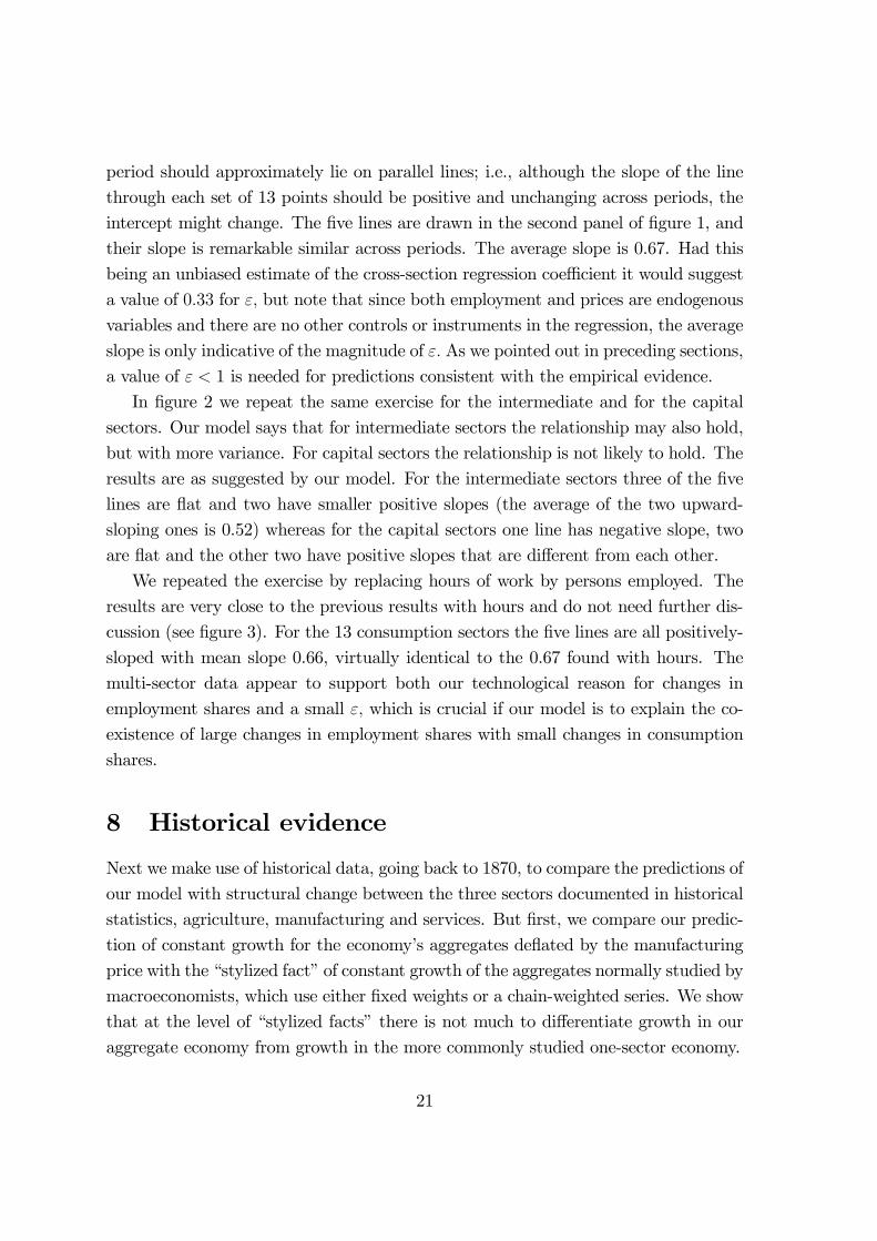
period should approximately lie on parallel lines; i.e., although the slope of the line

through each set of 13 points should be positive and unchanging across periods, the

intercept might change. The five lines are drawn in the second panel of figure 1, and

their slope is remarkable similar across periods. The average slope is 0.67. Had this

being an unbiased estimate of the cross-section regression coefficient it would suggest

a value of 0.33 for ε, but note that since both employment and prices are endogenous

variables and there are no other controls or instruments in the regression, the average

slope is only indicative of the magnitude of ε. As we pointed out in preceding sections,

a value of ε < 1 is needed for predictions consistent with the empirical evidence.

In figure 2 we repeat the same exercise for the intermediate and for the capital

sectors. Our model says that for intermediate sectors the relationship may also hold,

but with more variance. For capital sectors the relationship is not likely to hold. The

results are as suggested by our model. For the intermediate sectors three of the five

lines are flat and two have smaller positive slopes (the average of the two upward-

sloping ones is 0.52) whereas for the capital sectors one line has negative slope, two

are flat and the other two have positive slopes that are different from each other.

We repeated the exercise by replacing hours of work by persons employed. The

results are very close to the previous results with hours and do not need further dis-

cussion (see figure 3). For the 13 consumption sectors the five lines are all positively-

sloped with mean slope 0.66, virtually identical to the 0.67 found with hours. The

multi-sector data appear to support both our technological reason for changes in

employment shares and a small ε, which is crucial if our model is to explain the co-

existence of large changes in employment shares with small changes in consumption

shares.

8 Historical evidence

Next we make use of historical data, going back to 1870, to compare the predictions of

our model with structural change between the three sectors documented in historical

statistics, agriculture, manufacturing and services. But first, we compare our predic-

tion of constant growth for the economy’s aggregates deflated by the manufacturing

price with the “stylized fact” of constant growth of the aggregates normally studied by

macroeconomists, which use either fixed weights or a chain-weighted series. We show

that at the level of “stylized facts” there is not much to differentiate growth in our

aggregate economy from growth in the more commonly studied one-sector economy.

21

Our aggregate per capita income in (11) is, in nominal terms, pmy, with the

normalization pm ≡ 1. So, if national statistics report real incomes deflated by someother implicit or explicit index p, reported real income in our notation is pmy/p. The

difference between our aggregate y and the reported one is the ratio of the price of our

manufacturing good to the deflator, pm/p.When Kaldor and others concluded that a

constant rate of growth of per capita GDP is a “stylized fact” that could be imposed

on aggregative models, they were looking at the rate of growth of pmy/p.12 In our

model, the average relative manufacturing price does not grow at constant rate, even

on our aggregate balanced growth path, because the relative sector shares that are

used to calculate p are changing during structural change. So it is not possible to have

a precisely constant rate of growth of both our y and another aggregate pmy deflated

by a weighted average of sector prices. But because sector shares do not change

rapidly over time, at least visually, there is nothing to distinguish the “stylized fact”

of constant growth in the chain-weighted (or fixed-weights) per capita GDP and in

our per capita output variable. The two series for the United States are shown in

Figure 4 for 1929-2000 (data before 1929 are not available for the chain-weighted

series). The growth rates of the chain-weighted and our series are, respectively, 2.46

and 2.44 percent, and at least at the level of “stylized facts” they look comparable.13

Turning now to the long-term shifts between agriculture, manufacturing and ser-

vices, we note that if empirically the relative price of services in terms of manufactur-

ing goods is rising while the relative price of agriculture goods is falling, the model

implies the ranking of their TFP growth rates is such that γa > γm > γs. Then the

TFP growth rate for agriculture is always above the weighted average of TFP growth

rates while the TFP growth rate for services is always below it, i.e. γa > γt > γs for

all t. Therefore, the model predicts that if the three goods are poor substitutes, the

agricultural employment share should decline indefinitely and the service sector em-

ployment share should rise. The manufacturing employment share may rise before it

starts to decline if its TFP growth rate is lower than the initial economy-wide weighted

average of TFP growth rates. But even if the share of manufacturing increases at first,

eventually it should decline, as the weighted average of the TFP growth rates falls

12More specifically, Kaldor was looking at a “steady trend rate” of growth of the “aggregatevolume of production.” See Kaldor (1961, p.178)13Another “stylized fact” suggested by Kaldor was a constant rate of return to capital. Barro and

Sala-i-Martin (2004, p.13) recently suggested that perhaps this should be replaced by falling rates

of return over some range as the economy develops, which is consistent with our claims made abovefor ε < 1.

22

over time. Asymptotically, employment shares in the three-sector economy converge

to manufacturing and services, with the employment share of manufacturing equal to

the investment to output ratio.

From (13), the employment shares at any time t obey

nit = (1− σ)xitXt

i = a, s (40)

nmt = 1− nat − nst,

with the notation i = a for agriculture, i = m for manufacturing and i = s for ser-

vices. Therefore, given any initial distribution of employment shares (na0, ns0, nm0) ,

we have xa0 = na0/ (nm0 − σ) and xs0 = ns0/ (nm0 − σ). With information on the

parameter ε and the growth rate of relative prices (or differences in their TFP growth

rates), the model implies that the growth rate of xit is equal to (1− ε) (pi/pi) (or

(1− ε) (γm − γs)). The distribution of employment shares over time can then be

derived from (40). As shown previously, our model implies that the time path of

employment in manufacturing is hump-shape if its TFP growth rate is less than the

initial weighted average of all TFP growth rates. Therefore, by matching the initial

employment distribution and growth rates of relative prices, this condition reduces

to ns0 (ps/ps) < na0 (−pa/pa) or equivalently ns0 (γm − γs) < na0 (γa − γm) .

To evaluate the quantitative implications of our model for the long-term histori-

cal shifts, we calibrate our aggregate balanced growth path to the US economy from

1869 to 1998. We describe how we conducted the calibration in Appendix 2. Our

model makes predictions about the aggregate economy, relative prices and employ-

ment shares. The strategy is to choose parameters to match the first two and let the

model determine the dynamics of employment shares. In brief, we set σ to match

the aggregate investment rate and (γm − γa, γm − γs) to match the average growth

rate for the relative prices of agriculture and services in terms of manufacturing. The

calibrated parameters are: σ = 0.2, γm − γs = 0.01 and γa − γm = 0.01.We use

two values for ε, a baseline one of 0.3 and a smaller one of 0.1. We then match the

employment shares in 1869, and examine how the predictions of the model compare

with the employment shares in the data, on the assumption the economy has been

on our aggregate balanced growth path throughout the period.

Figure 5, panel (a), reports the results for ε = 0.3 and panel (b) for ε = 0.1. The

model captures the general features of the data, especially for the lower value of ε. The

hump shape for manufacturing employment is a feature of the data in both the US

23

and other OECD countries and as a prediction is, we believe, unique to our model.14.

For ε = 0.1 the model predicts a decline in the share of agriculture of 38 percentage

points between 1870 and 2000 (for ε = 0.3 the decline is 32 points). The actual

fall was 46 points. This suggests productivity growth alone may not be sufficient

to account for the decline in agriculture, but the model predicts well the allocations

of non-agricultural employment between manufacturing and services. If the surplus

predicted share in agriculture is redistributed to manufacturing and services according

to their existing share proportions, we obtain a share of manufacturing and services

which are very close to their respective actual shares.15

In the calibration we imposed the restriction θ = 1 and examined steady-state

growth only, on the premise that growth in the US economy has been approximately

constant. It is interesting to check, however, the quantitative implications of a differ-

ent value of θ, when growth is exactly constant only in the asymptotic steady state,

but (as we argued in section 4) it may be near-constant on the transition to the as-

ymptotic state. We compute the equilibrium for the commonly-used value of θ = 2

by making use of the initial capital and calibrated parameters that we used for θ = 1.

As previously shown, the economy will converge to an asymptotic aggregate balanced

growth path where both the investment rate and the growth rate are constant. The

growth rate is the same as in the economy with θ = 1.

The results of the calibration are shown in figure 6. The most noticeable feature of

figure 6 is that although the growth rate converges quickly to its asymptotic steady-

state value of 2 percent, structural change is taking place at about the same rate as

for θ = 1. The most striking new feature of structural change is that now the “bell

shape” predicted for manufacturing employment is less shallow, which is a feature

of the data. with θ = 2 agricultural employment declines slightly faster and service

14Kuznets (1966) documented structural change for 13 OECD countries and the USSR between1800 and 1960 and Maddison (1980) documented the same pattern for 16 OECD countries from

1870 to 1987. They both found a pattern with the same general features as our predictions. The“shallow bell shape” for manufacturing was found by Maddison (1980, p. 48) for each of the 16OECD countries.

15A number of authors have made alternative assumptions to match the decline of agriculturalemployment. Laitner (2000) and Gollin et al. (2002) use a utility function which implies bothan income elasticity less than one and a zero elasticity of substitution after a subsistence level of

agricultural consumption has been reached. In contrast Caselli and Coleman (2002), assume a unitelasticity of substitution but match the fast decline of agricultural employment by arguing that thecost of moving out of agriculture fell because of the increase of educational attainment in rural areas.

24

employment rises more slowly but the differences are small.

9 Conclusion

We have shown that predicted sectoral change that is consistent with the facts re-

quires low substitutability between the final goods produced by each sector. Balanced

aggregate growth requires in addition a logarithmic intertemporal utility function.

Underlying the balanced aggregate growth there is a shift of employment away from

sectors with high rate of technological progress towards sectors with low growth, and

eventually, in the limit, all employment converges to only two sectors, the sector pro-

ducing capital goods and the sector with the lowest rate of productivity growth. If

the economy also produces intermediate goods the sectors that produce these goods

also retain some employment in the limit, for similar reasons. Reasonable deviations

form the restriction required for balanced aggregate growth have only a small im-

pact on structural change and the aggregate economy converges fast to a state with

near-constant growth rate.

An examination of two-digit industrial data for the United States has shown that

our predictions are consistent with the facts. In an examination of historical evidence

since 1869 we found that focusing on uneven sectoral growth and abstracting from all

other causes of structural change (such as different capital intensities and non-unit

income elasticities) can explain a large fraction of the observed long-term employment

shifts. More specifically, it can explain large parts of the shift of employment from

agriculture to manufacturing and services and subsequently from manufacturing to

services, albeit at a somewhat lower rate than is observed in the data. Of course,

enriching the model with different capital intensities and non-unit income elasticities

may improve the predictions. Future empirical work also needs to deal with inter-

mediate goods and frictions in factor mobility. Intermediate goods alter some of our

conclusions although not the important ones about structural change.

Finally, our model has implications for studies that take structural change as a

fact and calculate its contribution to overall growth (Broadberry, 1998, Temple, 2001).

For example, Broadberry and others calculate an economy’s growth rate under the

counterfactual of no structural change. They then attribute the difference between

the actual growth rate and their hypothetical rate to structural change. Our model

shows that structural change is a necessary part of aggregate growth and should be

taken into account when designing accounting exercises of this kind.

25

References

[1] Barro, R. J. and X. Sala-i-Martin (2004). Economic Growth. Second edition.

Cambridge, Mass., MIT Press.

[2] Baumol, W. (1967). ‘Macroeconomics of Unbalanced Growth: The Anatomy of

Urban Crisis,’ American Economic Review 57: 415-26.

[3] Baumol, W., S. Blackman and E. Wolff (1985). ‘Unbalanced Growth Revisited:

Asymptotic Stagnancy and New Evidence,’ American Economic Review 75: 806-

817.

[4] Broadberry, S. N. (1998). ‘How did the United States and Germany Overtake

Britain? A Sectoral Analysis of Comparable Productivity Levels, 1870-1990’.

Journal of Economic History, 58(2), 375-407.

[5] Caselli, F. and W.J. Coleman II (2001). ‘The U.S. Structural Transformation

and Regional Convergence: A Reinterpretation,’ Journal of Political Economy

109: 584-616.

[6] Echevarria, C. (1997). ‘Changes in Sectoral Composition Associated with Eco-

nomic Growth.’ International Economic Review 38 (2): 431-452.

[7] Gollin, D., S. Parente, and R. Rogerson (2002). ‘Structural Transformation and

Cross-Country Income Differences.’ Working Paper.

[8] Foellmi, R. and Zweimuller, J. (2002). “Structural Change and Kaldor’s Facts

of Economic Growth.” Discussion Paper No. 472 (April), IZA (Institute for the

Study of Labor), Bonn.

[9] Kaldor, N (1961). “Capital Accumulation and Economic Growth.” InThe Theory

of Capital, ed. F.A. Kutz and D.C. Hague. New York: St. Martins.

[10] Kongsamut, P., S. Rebelo and D. Xie (2001). ‘Beyond Balanced Growth,’ Review

of Economic Studies 68: 869-882.

[11] Kravis, I., A. Heston and R. Summers (1983). ‘The Share of Service in Economic

Growth’. Global Econometrics: Essays in Honor of Lawrence R. Klein, Edited

by F. Gerard Adams and Bert G. Hickman

26

[12] Kuznets, S.Modern Economic Growth: Rate, Structure, and Spread. New Haven,

Conn.: Yale University Press, 1966.

[13] Laitner, J. (2000). ‘Structural Change and Economic Growth’. Review of Eco-

nomic Studies 67: 545-561.

[14] Maddison, A., (1980). “Economic Growth and Structural Change in the Ad-

vanced Countries,” in Western Economies in Transition. Eds.: I. Leveson and

W. Wheeler. London: Croom Helm.

[15] Maddison, A., (1992). A long-run perspective on saving, Scandinavian Journal

of Economics, 84: 181-196.

[16] Nickell, S., S. Redding and J. Swaffield, (2004). “The Uneven Pace of Deindus-

trialization in the OECD.” London School of Economics mimeo.

[17] Oulton, N. (2001). ‘Must the Growth Rate Decline? Baumol’s Unbalanced

Growth Revisited.’ Oxford Economic Papers 53: 605-627.

[18] Temple, J. (2001). ‘Structural Change and Europe’s Golden Age’. Working paper.

University of Bristol.

[19] US Bureau of the Census (1975). Historical Statistics of the United States, Colo-

nial Times to 1970 ; Bicentennial Edition, Part 1 and Part 2. US Government

Printing Office, Washington, DC.

27

10 Appendix 1: Proofs

Lemma 6 The employment shares satisfy:

ni =³xiX

´µ c

y

¶,

nini=

·c/y

c/y+ (1− ε) (γ − γi) ; i = 1, ...m− 1,

nm =

µc/y

X

¶+ 1− c

y, nm =

·c/y

c/y+ (1− ε) (γ − γm)

µc/yX

¶−

·c/y

where γ ≡Pmi=1 (xi/X) γi is the weighted average of TFP growth rates.

Proof. ni follows from substituting F i into (10) , and nm is derived from (2) . Given

xi/xi = (1− ε) (γm − γi) and X =Pm

i=1 xi = (1− ε) (γm − γ)X, we have

nini=

·c/y

c/y+

·xi/X

xi/X=

·c/y

c/y+ (1− ε) (γ − γi) i = 1, ..m− 1

and by (2) ,

nm = −m−1Pi=1

ni = −·

c/y

c/y(1− nm)− (1− ε)

µc/y

X

¶m−1Pi=1

xi (γ − γi)

=

·c/y

c/y

µc/y

X− c

y

¶+ (1− ε)

µc/y

X

¶(γ − γm)

=

·c/y

c/y+ (1− ε) (γ − γm)

µc/yX

¶−

·c/y.

Proof of Proposition 3. Use (2) and (8) to rewrite (4) as:

k/k = Amkα−1(1−Pm−1

i=1 ni)− cm/k − (δ + ν) .

But pi = Am/Ai and by the definition of c, this is equivalent to:

k/k = Amkα−1 − c/k − (δ + ν) .

Next, φ is homogenous of degree one: φ =Pm

i=1 φici =Pm

i=1 piciφm = φmc. But

φm = ωm (φ/cm)1/ε and c = cmX, thus φm = ω

ε/(ε−1)m X1/(ε−1) and vm = φ−θφm =³

ωε/(ε−1)m X1/(ε−1)

´1−θc−θ, so (6) becomes

θc/c = (θ − 1) (γm − γ) + αAmkα−1 − (δ + ρ+ ν) .

28

Lemma 7 dγ/dt ≶ 0⇔ ε ≶ 1.

Proof. Totally differentiating γ as defined in Proposition 3 we obtain

dγ/dt =Pm

i=1 (xi/X) γi (xi/xi −Pm

i=1 xj/X)

= (1− ε)Pm

i=1 (xi/X) γi¡γm − γi −

Pmi=1 (xi/X) (γm − γj

¢= (1− ε)

¡γ2 −Pm

i=1 (xi/X) γ2i

¢= −(1− ε)

Pmi=1 (xi/X) (γi − γ)2

Since the summation term is always positive the result follows.

Proof of Proposition 5

Lemma 8 Along the aggregate balanced growth path, if ε ≶ 1, ∀i = 1, ..,m − 1, ni isnon-monotonic if and only if γ0 ≷ γi. The non-monotonic ni first increases at a decreasing

rate for t < ti, then decreases and converges to constant n∗i asymptotically, where ti is suchthat γti = γi. The monotonic ni are decreasing and converge to zero asymptotically.

Proof. ∀i = 1, ..,m− 1, Lemma 6 implies that along the aggregate balanced growthpath, ni/ni = (1− ε) (γt − γi) > 0⇔ γt > γi. Lemma 7 implies ni eventually decreases.

Therefore, ni is non-monotonic if and only if γ0 > γi.

Corollary 9 If ε < 1, ts → ∞ where s is such that γs = min {γi}i=1,.,m . If ε > 1,

tf →∞ where f is such that γf = max {γi}i=1,..,m.

To establish now the claims in Proposition 5, assume, without loss of generality, ε < 1,

γ1 > ... > γm−1 and γm < γh = γ0 where 1 < h < m− 1. Then, Lemma 8 implies ti = 0∀i ≤ h, and i ∈ E0 ∀i ≥ h, moreover, Eth+1 ∪ {h+ 1} = E0 and Dth+1 = D0 ∪ {h+ 1} ,thus Eth+1 ⊆ E0 and D0 ⊆ Dth+1.The result follows for any arbitrary t > 0. Next, we

prove that the economy converges to a two-sector economy. Without loss of generality,

consider ε < 1. Given X/xi =Pm

i=1 (ωj/ωi)ε (Ai/Aj)

1−ε , and Ai/Aj → 0 ⇔ γi < γj,

we have X/xi → 1 ⇔ γi = min©γjªj=1,.,m

. Therefore, asymptotically, n∗l = cek−αe and

n∗m = 1− n∗l , where γl = min {γi}i=1,.,m .

We now prove these results hold also in the transition to the steady state from any small

k0. Let z ≡ ce/ke, (25) and (26) (with ψ = 0 and θ = 1) imply:

z/z = (α− 1) kα−1e + z − ρ, ke/ke = kα−1e − z − [γm/ (1− α) + δ + ν] .

A phase diagram can be drawn with z < 0 along the transition. For c/y, we have:

·c/y

c/y=

cece− α

keke= αz − ρ− (1− α)

µγm1− α

+ δ + ν

¶.

29

Since·

c/y = 0 in the steady state but z < 0 in the transition, thus·

c/y > 0 and··c/y < 0

along the transition. Also, ∀t,∀i = 1, ..,m− 1, we have:

ni/ni = αz − ρ− (1− α) [γm/ (1− α) + δ + ν] + (1− ε) (γ − γi) ,

which decreases along the transition given lemma 7 and z < 0. Thus, starting from any

small k0, if i ∈ E0 then ni > 0, ni < 0, and if i 6= l, i ∈ Et ∀t < ti, and i ∈ Dt ∀t ≥ ti,

where ti is defined in Lemma 8. If i ∈ D0, then i ∈ Dt ∀t. Therefore, Lemma 8 holds alongthe transition.

Many capital-producing sectors ∀j = 1, .., κ, Fmj ≡ Amjnmj

kαmj, which together

produce good m through G =hPκ

j=1 ξmj(Fmj)(µ−1)/µ

iµ/(µ−1), ξmj

> 0, µ > 0, andPκj=1 ξmj

= 1. The planner’s problem is similar to before with k = G − cm − (δ + ν) k

replacing (4), and¡kmj , nmj

¢j=1,.,κ

as additional control variables.

The static efficiency conditions are F iK/F

iN = F

mj

K /Fmj

N , ∀i = 1, ..m− 1, ∀j = 1, ., κ,so ki = kmj = k. Also Gmj/Gmi = Fmi

K /Fmj

K = Ami/Amj , ∀i, j = 1, ..κ, which impliesnmj/nmi =

³ξmj

/ξmi

´µ ¡Ami/Amj

¢1−µand grows at (1− µ)

¡γmi− γmj

¢. Let nm ≡Pκ

j=1 nmj , we have nm = nm1

Pκj=1

³ξmj

/ξm1

´µ ¡Am1/Amj

¢1−µ. Next, ∀i = 1, ..m− 1,

pi = vi/vm = Am/Ai, where Am ≡ Gm1Am1. Thus, ni/nj and pi/pj are the same

as in the baseline model. For the aggregate equilibrium, note G =Pκ

j=1 FmjGmj

=

Amkαnm, so c/c and k/k become the same as in the baseline model. Thus, we obtain

the same equilibrium if Am/Am is constant. Note Gm1 = ξm1(G/Fm1)1/µ and G/Fm1 =hPκ

j=1 ξmj

¡Amj

nmj/ (Am1nm1)

¢(µ−1)/µiµ/(µ−1), then use the result on nmj

/nm1, we have

G/Fm1 =

·Pκj=1 ξ

µmj

³ξm1

Am1

´1−µA(µ−1)mj

¸µ/(µ−1), thus we have

Am = Gm1Am1 =

"κX

j=1

ξµmjA(µ−1)mj

#1/(µ−1)and its growth rate is

γm =κX

j=1

ζjγmj; ζj ≡ ξµmj

A(µ−1)mj/

ÃκX

j=1

ξµmjA(µ−1)mj

!.

So γm is constant if (µ− 1)Pκ

j=1 ζj

³γmj− γm

´2= 0, i.e. if (1) γmi

= γmj∀i, j = 1, ., κ

or (2) µ = 1. If (1) is true, the capital-producing sectors can be aggregated into one and the

30

model reduces to one with only one capital-producing sector. Thus, coexistence of multiple

capital-producing sectors with different TFP growth rates and an aggregate balanced growth

path requires (2), i.e., G =Qκ

j=1 (Fmj)ξj and γm =

Pκj=1 ξmj

γmj.

Intermediate goods The production functions are, F i ≡ Ainikiαqβi , ∀i, α, β ∈ (0, 1)

and α + β < 1. For i = 1, ..,m − 1, F i is either bought by consumers (ci) or by busi-

nesses (hi) . But Fm can also be used as investment. Intermediate goods are produced by

Φ (h1, .., hm), which satisfies Φi > 0,Φii < 0, and constant return to scale. The planner’s

problem is similar to before with k = Fm−hm−cm−(δ + ν) k replacing (4),Pm

i=1 niqi = Φ

as an additional resource constraint and the additional controls are {hi, ci, qi}i=1,..,m.The static efficiency conditions are:

vivm

=FmK

F iN

=FmN

F iN

=FmQ

F iQ

=Φi

Φm; ∀i,

which implies ki = k, qi = Φ, pi = Am/Ai, ∀i, and y = AmkαΦβ. Define aggregate

intermediate inputs h ≡ Pmi=1 pihi. To solve for h, use the planner’s optimal conditions

for hm and qm to obtain 1 = βΦmAmkαΦβ−1. But Φ is homogenous of degree one: Φ =Pm

i=1Φihi =Pm

i=1Φmpihi = Φmh, we have h = βy, together with static efficiency,

k = AmkαΦβ

³1−

Xm−1i=1

ni´− hm − cm − (δ + ν) k = h (1− β) /β − c− (δ + ν) k.

The dynamic efficiency condition is −vm/vm = αAmkα−1Φβ − (δ + ρ+ ν) , so

c/c = αh/ (βk)− (δ + ρ+ ν) , k/k = (1− β)h/ (βk)− c/k − (δ + ν) .

Constant c/c requires constant h/k and constant k/k requires constant c/k. Thus, h/h

must be constant, i.e. Φ/Φm must be growing at a constant rate. Suppose Φ is a

CES function, Φ =³Pm

i=1 ϕih(η−1)/ηi

´η/(η−1), then the static efficiency conditions im-

ply ∀i, pihi/hm = (ϕi/ϕm)η (Am/Ai)

1−η ≡ zi, h = Zhm, where Z ≡ Pmi=1 zi, so

Φm = ϕη/(η−1)m Z1/(η−1) and Φ =

³βAmk

αϕη/(η−1)m Z1/(η−1)

´1/(1−β). Hence,

h = Φ/Φm = (βAmkα)1/(1−β)

¡ϕη/(η−1)m Z1/(η−1)

¢β/(1−β)=⇒ (1− β) h/h =

³γm + αk/k

´+ β

³Xm

i=1(zi/Z) γi − γm

´which is constant only if

Pmi=1 ziγi is constant. From the definition of zi and given that the

γi are not the same across all i, constancy requires η = 1, and soΦ =Qm

i=1 hϕii , Z = 1/ϕm,

31

and zi = ϕi/ϕm, ∀i. The static efficiency conditions imply Φ = hmQm

i=1 (ziAi/Am)ϕi and

so Φm = ϕmΦ/hm =Qm

i=1 (ϕiAi/Am)ϕi . But Φ = [βAmk

αΦm]1/(1−β) , so h = Φ/Φm =

(βAmkα)1/(1−β)Φβ/(1−β)

m . The dynamic equations become:

c

c+ δ + ρ+ ν =

α

βk

£(βAmk

α)Φβm

¤ 11−β = α

hkα+β−1Am (βΦm)

βi 11−β

,

k

k+

c

k+ δ + ν =

(1− β)

βk

£(βAmk

α)Φβm

¤ 11−β = (1− β)

hkα+β−1Am (βΦm)

βi 11−β

.

Define ce ≡ cA−(1−β)/(1−α−β) and ke ≡ kA−(1−β)/(1−α−β), whereA ≡hAm (βΦm)

βi1/(1−β)

,

and γ ≡ A/A = [γm + βPm

i=1 ϕi (γi − γm)] / (1− β) = γm + (βPm

i=1 ϕiγi) / (1− β) ,

ce/ce = αk(α+β−1)/(1−β)e − [δ + ρ+ ν + (1− β) γ/ (1− α− β)] ,

ke/ke = (1− β) k(α+β−1)/(1−β)e − ce/ke − [δ + ν + (1− β) γ/ (1− α− β)] ,

which imply existence and uniqueness of an aggregate balanced growth path. ∀i = 1, ..m−1, we obtain ni using F i = ci + hi, i.e. Ainik

αΦβpi = pi (ci + hi) = xicm + zihm =

cxi/X + ϕih. Substitute pi and h to obtain niy = cxi/X + ϕiβy, finally

ni = (c/y) (xi/X) + ϕiβ; ∀i, nm = [(c/y) (xm/X) + ϕmβ] + [1− β − c/y] .

11 Appendix 2: Calibration and sources of historical evidence

Sources of historical evidence (1) Historical Statistic of the United States: Colonial

Times to 1970, Part 1 and 2: for employment (series F250-258), for prices (series E17, E23-

25, E42, E52-E53) and index of manufacturing production (series P13-17); (2) Economic

Report of the President: for prices and index of manufacturing production; and (3) Bureau

of Economic Analysis (BEA): for investment rate and capital-output ratio.

Model in discrete time The Euler condition (25) and the feasibility condition (26) are:

ce (t+ 1)

ce (t)=

"Ã1− δ + αkα−1e (t+ 1)

(1 + g)θ (1 + ν) /β

!µX (t+ 1)

X (t)

¶(1−θ)/(ε−1)#1/θ(41)

ke (t+ 1)

ke (t)=

[ke (t)]α−1 − ce/ke + (1− δ)

(1 + g) (1 + ν)(42)

where g =(1 + γm)1/(1−α)−1 is the aggregate growth rate. The variables in our model are

matched to US annual data.

32

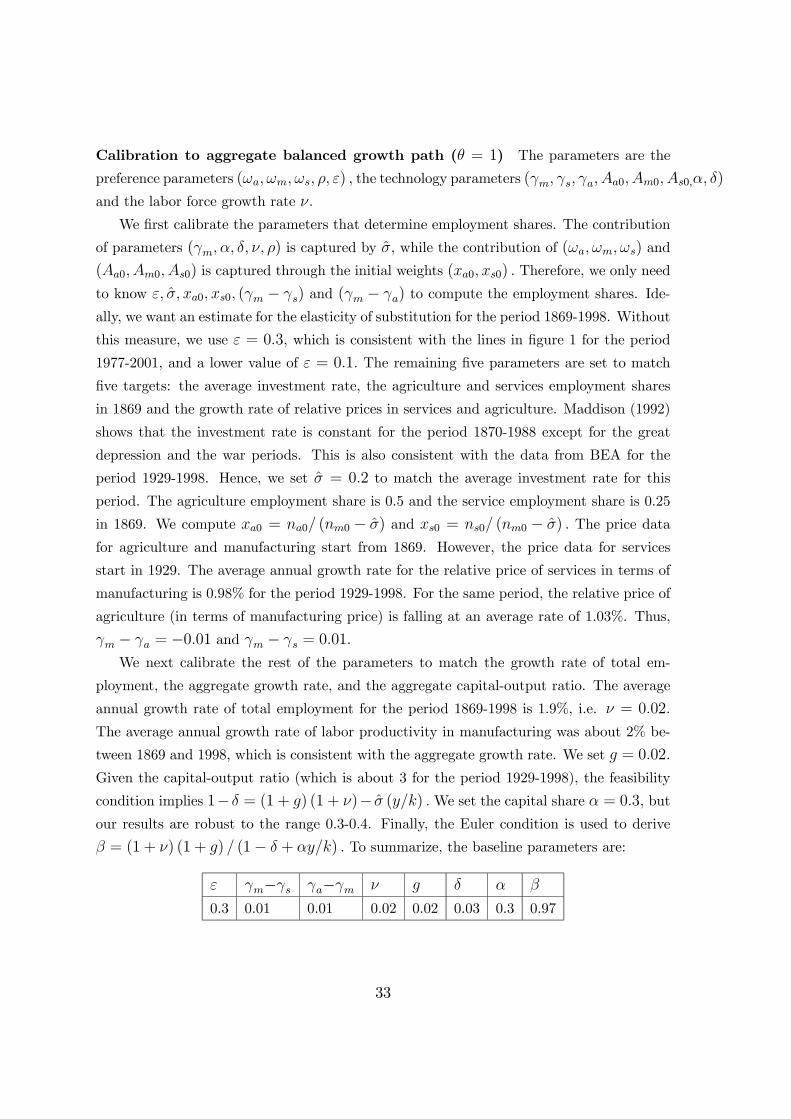
Calibration to aggregate balanced growth path (θ = 1) The parameters are the

preference parameters (ωa, ωm, ωs, ρ, ε) , the technology parameters (γm, γs, γa, Aa0, Am0, As0,α, δ)

and the labor force growth rate ν.

We first calibrate the parameters that determine employment shares. The contribution

of parameters (γm, α, δ, ν, ρ) is captured by σ, while the contribution of (ωa, ωm, ωs) and

(Aa0, Am0, As0) is captured through the initial weights (xa0, xs0) . Therefore, we only need

to know ε, σ, xa0, xs0, (γm − γs) and (γm − γa) to compute the employment shares. Ide-

ally, we want an estimate for the elasticity of substitution for the period 1869-1998. Without

this measure, we use ε = 0.3, which is consistent with the lines in figure 1 for the period

1977-2001, and a lower value of ε = 0.1. The remaining five parameters are set to match

five targets: the average investment rate, the agriculture and services employment shares

in 1869 and the growth rate of relative prices in services and agriculture. Maddison (1992)

shows that the investment rate is constant for the period 1870-1988 except for the great

depression and the war periods. This is also consistent with the data from BEA for the

period 1929-1998. Hence, we set σ = 0.2 to match the average investment rate for this

period. The agriculture employment share is 0.5 and the service employment share is 0.25

in 1869. We compute xa0 = na0/ (nm0 − σ) and xs0 = ns0/ (nm0 − σ) . The price data

for agriculture and manufacturing start from 1869. However, the price data for services

start in 1929. The average annual growth rate for the relative price of services in terms of

manufacturing is 0.98% for the period 1929-1998. For the same period, the relative price of

agriculture (in terms of manufacturing price) is falling at an average rate of 1.03%. Thus,

γm − γa = −0.01 and γm − γs = 0.01.

We next calibrate the rest of the parameters to match the growth rate of total em-

ployment, the aggregate growth rate, and the aggregate capital-output ratio. The average

annual growth rate of total employment for the period 1869-1998 is 1.9%, i.e. ν = 0.02.

The average annual growth rate of labor productivity in manufacturing was about 2% be-

tween 1869 and 1998, which is consistent with the aggregate growth rate. We set g = 0.02.

Given the capital-output ratio (which is about 3 for the period 1929-1998), the feasibility

condition implies 1−δ = (1 + g) (1 + ν)− σ (y/k) .We set the capital share α = 0.3, butour results are robust to the range 0.3-0.4. Finally, the Euler condition is used to derive

β = (1 + ν) (1 + g) / (1− δ + αy/k) . To summarize, the baseline parameters are:

ε γm−γs γa−γm ν g δ α β

0.3 0.01 0.01 0.02 0.02 0.03 0.3 0.97

33

Computation for economy with θ 6= 1 We use the baseline parameters to compute

the transition path for the economy with θ 6= 1. We start with the same initial income andinitial employment distribution. The initial income is matched by choosing the same ke (1)

as in the benchmark. To match the initial employment we need to adjust xa0 and xs0.

These two parameters were previously calibrated to match the initial employment shares

under the assumption that the investment rate is σ. When θ 6= 1, the initial employmentshares depend on the initial investment rate, which is different from σ.

We rewrite (41) and (42) in terms of z ≡ c/k:

z (t+ 1)

z (t)=

µke (t)

ke (t+ 1)

¶"Ã1− δ + αkα−1e (t+ 1)

(1 + g)θ (1 + ν) /β

!µX (t+ 1)

X (t)

¶(1−θ)/(ε−1)#1/θke (t+ 1)

ke (t)=

[ke (t)]α−1 − z (t) + (1− δ)

(1 + g) (1 + ν).

Given ke (1) , if we know z (1) , the equilibrium is derived by iteration. We use a shooting

algorithm to look for z (1) . As t −→∞, X (t+ 1) /X (t) converges to a constant, so this

economy converges to an asymptotic steady state with αkα−1e − δ − ν = ρ− ψ + θg and

k/k = g. First note that the transversality condition holds if ρ > (1− θ) (g − (γm − γs)) ,

which is satisfied under the calibrated parameters at all positive θ. Let z∗ be the asymptoticsteady state value. Thus, for sufficiently large T, z (T ) ≈ z∗. The shooting algorithm is

as follows: given an initial ke (1) , guess a z (1) . For any t, if ke (t) < 0, decrease z (1) .

Since X is a function independent of z and ke, z (T ) is increasing in z (1) . Therefore, if

z (T ) < (>) z∗, increase (decrease) z (1) .

12 Appendix 3: Sectorial Data sources and construction

We make use of two data sources, both of which are available online at www.oecd.org:

1. OECD Structural Analysis Database for Industrial Analysis (STAN ), which is en-

tirely based on national US sources, and covers the period 1977-2001.

2. OECD input-output database (I/O database).

We extract from STAN data for total hours of work, total employment and prices

(obtained as the ratio of the sector’s value added at current prices to the volume measure

of value added). There is a complete annual data set for 1977-2001 for 27 groupings of

two-digit industries, shown in Table 1. Our sectors cover about 98 percent of employment

34

in the Unites States. The table also shows the sample mean of the share of each sector in

total hours and also whether the sector is classified as consumption, intermediate or capital.

In order to classify sectors we used information from the 1990 input-output tables.

The tables can be used to calculate the share of output of each sector that is capital

formation (column headed “Private GFCF”), intermediate inputs (column headed “Total”)

and private consumption (column headed “Private Domestic Consumption”). We defined

a sector’s output as the sum of the three columns and calculated the shares of each. There

are 3 sectors where production of capital goods amount to more than 28% of total output.

The next highest capital-producing sector is wholesale and retail trade whose production

of capital goods amount to 6% of total output. We classify the first three sectors as capital

(or manufacturing) sectors.16 In addition, we include two other sectors which respectively

produced 94% and 100% intermediate goods but supplied almost exclusively one capital

sector each: 93% of the output of non-mineral manufacturing consisted of intermediate

goods, and 70% of it was bought either by itself or by the construction sector; and 80% of

the output of the combined basic metals and fabricated metals sectors (which produce only

intermediate goods) is bought by the machinery and equipment sector.

Of the remaining sectors, those that supply more than 50% of output to final consump-

tion use are classified as consumption sectors. In addition, agriculture produces almost

exclusively intermediate goods for the food industries, which are a consumption sector, and

is classified as a consumption sector. The remaining sectors produce more than 50% of their

output for a range of other sectors and are classified as intermediate sectors.

16The 1990 tables appear to have an aberration that we ignored: 9.7% of the output ofmining is reported as capital goods. In 1977,1982 and 1985 (all the other years that tablesare available) capital goods are less than 1% of the output of this sector. The percentagedistribution for other sectors is virtually unchanged between years.

35

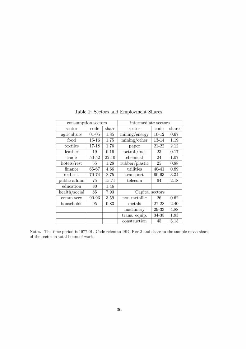
Table 1: Sectors and Employment Shares

consumption sectors intermediate sectorssector code share sector code share

agriculture 01-05 1.85 mining/energy 10-12 0.67food 15-16 1.75 mining/other 13-14 1.19textiles 17-18 1.76 paper 21-22 2.12leather 19 0.16 petrol./fuel 23 0.17trade 50-52 22.10 chemical 24 1.07

hotels/rest 55 1.28 rubber/plastic 25 0.88finance 65-67 4.66 utilities 40-41 0.89real est. 70-74 8.75 transport 60-63 3.34

public admin 75 15.71 telecom 64 2.18education 80 1.46health/social 85 7.93 Capital sectorscomm serv 90-93 3.59 non metallic 26 0.62households 95 0.83 metals 27-28 2.40

machinery 29-33 4.88trans. equip. 34-35 1.93construction 45 5.15

Notes. The time period is 1977-01. Code refers to ISIC Rev 3 and share to the sample mean shareof the sector in total hours of work

36

-12-10-8-6-4-20246810

-5 0 5 10 15

percent change in price

perc

ent c

hang

e in

hou

rs

-12-10-8-6-4-20246810

-5 0 5 10 15

percent change in prices

perc

ent c

hang

e in

hou

rs

Figure 1Changes in hours of work and prices, 13 consumption sectors

five-year averages 1977-2001

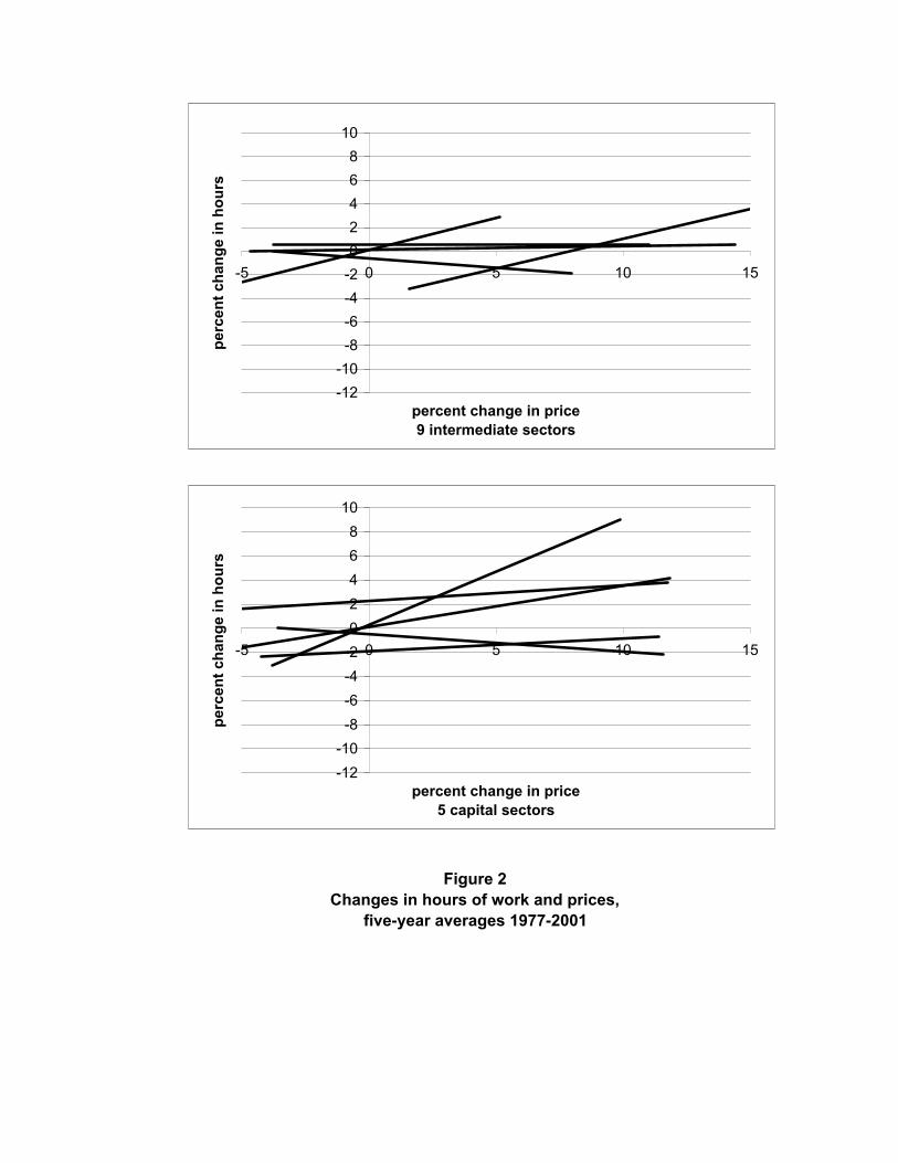
Figure 2Changes in hours of work and prices,

five-year averages 1977-2001

-12-10-8-6-4-20246810

-5 0 5 10 15

percent change in price5 capital sectors

perc

ent c

hang

e in

hou

rs

-12-10-8-6-4-20246810

-5 0 5 10 15

percent change in price 9 intermediate sectors

perc

ent c

hang

e in

hou

rs

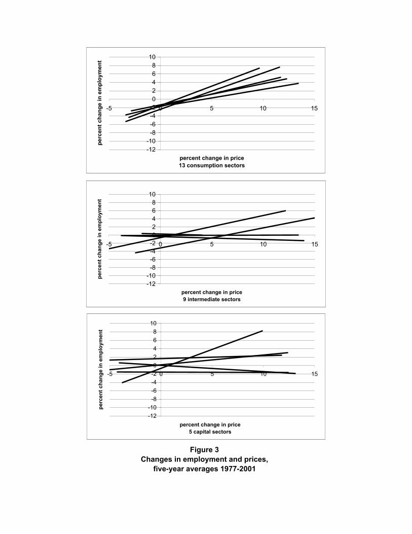
-12-10-8-6-4-20246810

-5 0 5 10 15

percent change in price13 consumption sectors

perc

ent c

hang

e in

em

ploy

men

t

Figure 3Changes in employment and prices,

five-year averages 1977-2001

-12-10-8-6-4-20246810

-5 0 5 10 15

percent change in price5 capital sectors

perc

ent c

hang

e in

em

ploy

men

t

-12-10-8-6-4-20246810

-5 0 5 10 15

percent change in price9 intermediate sectors

perc

ent c

hang

e in

em

ploy

men

t

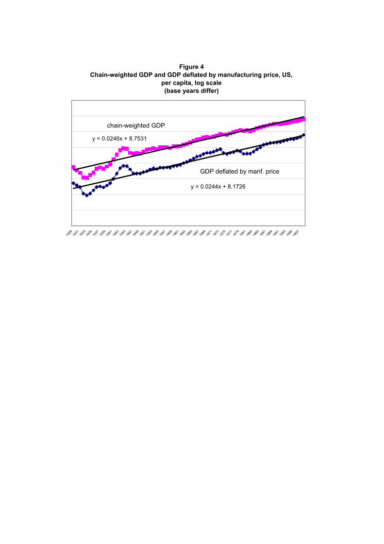
Figure 4Chain-weighted GDP and GDP deflated by manufacturing price, US,

per capita, log scale(base years differ)

y = 0.0246x + 8.7531

y = 0.0244x + 8.1726

1929

1931

1933

1935

1937

1939

1941

1943

1945

1947

1949

1951

1953

1955

1957

1959

1961

1963

1965

1967

1969

1971

1973

1975

1977

1979

1981

1983

1985

1987

1989

1991

1993

1995

1997

chain-weighted GDP

GDP deflated by manf. price

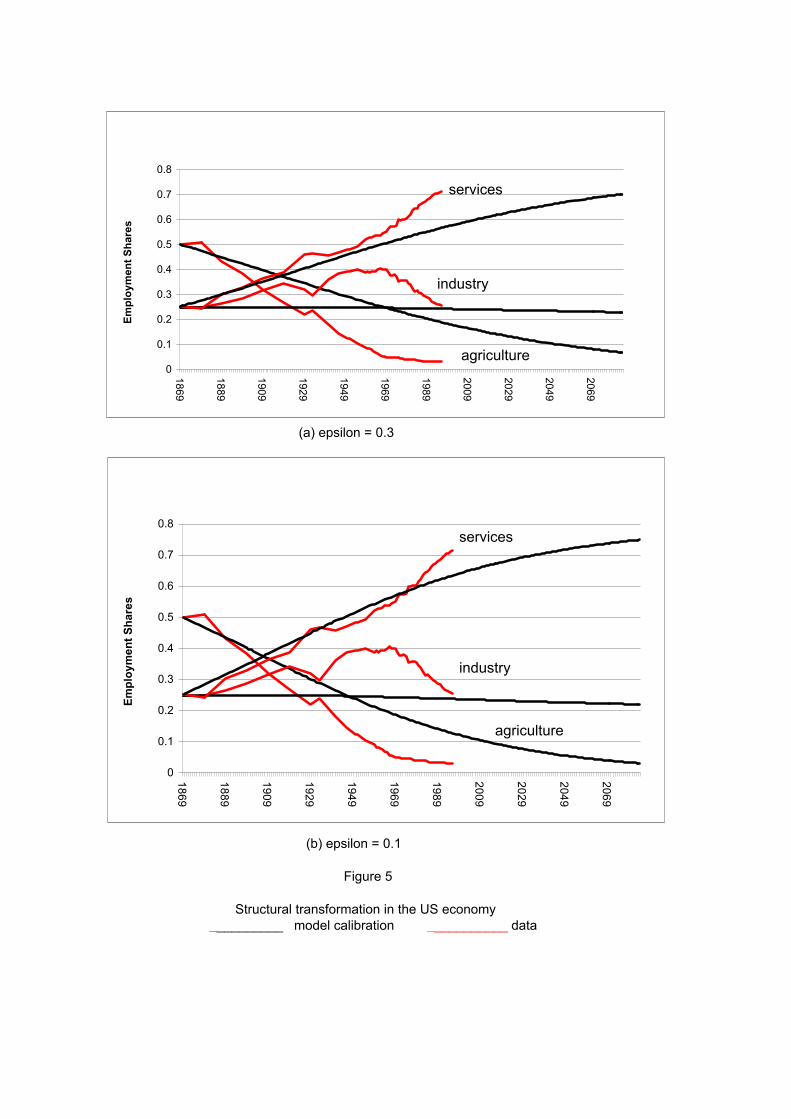
(a) epsilon = 0.3

(b) epsilon = 0.1

Figure 5

Structural transformation in the US economy__________ model calibration ___________ data

0

0.1

0.2

0.3

0.4

0.5

0.6

0.7

0.8

1869

1889

1909

1929

1949

1969

1989

2009

2029

2049

2069

Empl

oym

ent S

hare

s

services

industry

agriculture

0

0.1

0.2

0.3

0.4

0.5

0.6

0.7

0.8

1869

1889

1909

1929

1949

1969

1989

2009

2029

2049

2069

Empl

oym

ent S

hare

s

services

industry

agriculture

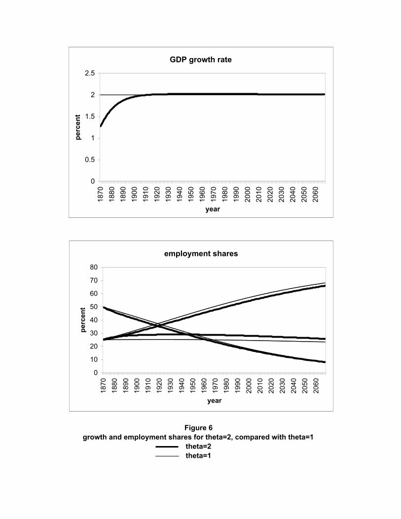
GDP growth rate

0

0.5

1

1.5

2

2.5

1870

1880

1890

1900

1910

1920

1930

1940

1950

1960

1970

1980

1990

2000

2010

2020

2030

2040

2050

2060

year

perc

ent

employment shares

0

10

20

30

40

50

60

70

80

1870

1880

1890

1900

1910

1920

1930

1940

1950

1960

1970

1980

1990

2000

2010

2020

2030

2040

2050

2060

year

perc

ent

Figure 6growth and employment shares for theta=2, compared with theta=1

theta=2theta=1